Commissioning dose computation models for spot scanning proton beamsin water for a commercially available treatment planning system

X. R. Zhu,a) F. Poenisch, M. Lii, G. O. Sawakuchi, U. Titt, M. Bues, X. Song, X. Zhang, Y. Li,G. Ciangaru, H. Li, M. B. Taylor, K. Suzuki, R. Mohan, M. T. Gillin, and N. SahooDepartment of Radiation Physics, The University of Texas MD Anderson Cancer Center, Houston, Texas 77030

(Received 10 September 2011; revised 11 March 2013; accepted for publication 12 March 2013;published 2 April 2013)

Purpose: To present our method and experience in commissioning dose models in water for spotscanning proton therapy in a commercial treatment planning system (TPS).Methods: The input data required by the TPS included in-air transverse profiles and integral depthdoses (IDDs). All input data were obtained from Monte Carlo (MC) simulations that had been vali-dated by measurements. MC-generated IDDs were converted to units of Gy mm2/MU using the mea-sured IDDs at a depth of 2 cm employing the largest commercially available parallel-plate ionizationchamber. The sensitive area of the chamber was insufficient to fully encompass the entire lateral dosedeposited at depth by a pencil beam (spot). To correct for the detector size, correction factors as afunction of proton energy were defined and determined using MC. The fluence of individual spotswas initially modeled as a single Gaussian (SG) function and later as a double Gaussian (DG) func-tion. The DG fluence model was introduced to account for the spot fluence due to contributions oflarge angle scattering from the devices within the scanning nozzle, especially from the spot profilemonitor. To validate the DG fluence model, we compared calculations and measurements, includingdoses at the center of spread out Bragg peaks (SOBPs) as a function of nominal field size, range, andSOBP width, lateral dose profiles, and depth doses for different widths of SOBP. Dose models werevalidated extensively with patient treatment field-specific measurements.Results: We demonstrated that the DG fluence model is necessary for predicting the field size depen-dence of dose distributions. With this model, the calculated doses at the center of SOBPs as a functionof nominal field size, range, and SOBP width, lateral dose profiles and depth doses for rectangulartarget volumes agreed well with respective measured values. With the DG fluence model for ourscanning proton beam line, we successfully treated more than 500 patients from March 2010 throughJune 2012 with acceptable agreement between TPS calculated and measured dose distributions. How-ever, the current dose model still has limitations in predicting field size dependence of doses at someintermediate depths of proton beams with high energies.Conclusions: We have commissioned a DG fluence model for clinical use. It is demonstrated thatthe DG fluence model is significantly more accurate than the SG fluence model. However, somedeficiencies in modeling the low-dose envelope in the current dose algorithm still exist. Further im-provements to the current dose algorithm are needed. The method presented here should be useful forcommissioning pencil beam dose algorithms in new versions of TPS in the future. © 2013 AmericanAssociation of Physicists in Medicine. [http://dx.doi.org/10.1118/1.4798229]

Key words: spot scanning, proton beam, convolution dose algorithms

I. INTRODUCTION

There has been increased interest in proton therapy in recentyears, primarily due to its ability to spare healthy tissues be-yond the range of the proton beam. Several approaches todeliver proton therapy are available, including double scat-tering, uniform scanning, and spot scanning.1, 2 In spot scan-ning delivery, a proton pencil beam (spot) is magneticallyscanned in lateral directions, creating a large field without re-quiring scattering elements into the beam path.3, 4 Monoen-ergetic pencil beams with different energies from an accel-erator can be stacked to create the desired dose distributionalong the beam direction. Neither an aperture nor a compen-sator is necessary for spot scanning proton therapy (SSPT)delivery.4

At The University of Texas MD Anderson Cancer Cen-ter, the delivery system for SSPT has been commissioned5

and used for treating patients since May 2008. The first groupof patients treated were prostate patients.6 The scanning noz-zle delivers the discrete spot scanning “spot-by-spot” and en-ergy “layer-by-layer.”5, 7 The energy, spot position, and num-ber of monitor units (MUs) of each spot are determined bya treatment planning system (TPS). That is, absolute dosesmust be calculated by the TPS for spot scanning delivery.The TPS used in this work employs the same fluence-dosecalculation method used for double scattering, uniform scan-ning, and spot scanning beam. The difference between differ-ent delivery methods is accounted by different in-air fluencemodeling.8–10 Previous dose algorithms for SSPT normallyused a single Gaussian (SG) function to describe the shape of

041723-1 Med. Phys. 40 (4), April 2013 © 2013 Am. Assoc. Phys. Med. 041723-10094-2405/2013/40(4)/041723/15/$30.00

041723-2 Zhu et al.: Commissioning dose models for spot scanning proton beams 041723-2

an in-air lateral profile of an individual pencil beam.4, 11 How-ever, our recent works have demonstrated that a SG functioncould not describe in-air lateral profiles well for an individ-ual pencil beam from our scanning nozzle.12–15 The TPS ven-dor, therefore, implemented a double Gaussian (DG) fluencemodel to account for the spot fluence due to contributions oflarge angle scattering from the devices within the scanningnozzle. In this work, we present our method and experienceof commissioning a pencil beam algorithm with DG fluencemodel. All optional devices in the scanning nozzle,7 includingscatter device, energy filter, energy absorber, and treatmentaperture, are not considered.

II. MATERIALS AND METHODS

II.A. Discrete spot scanning beam delivery system

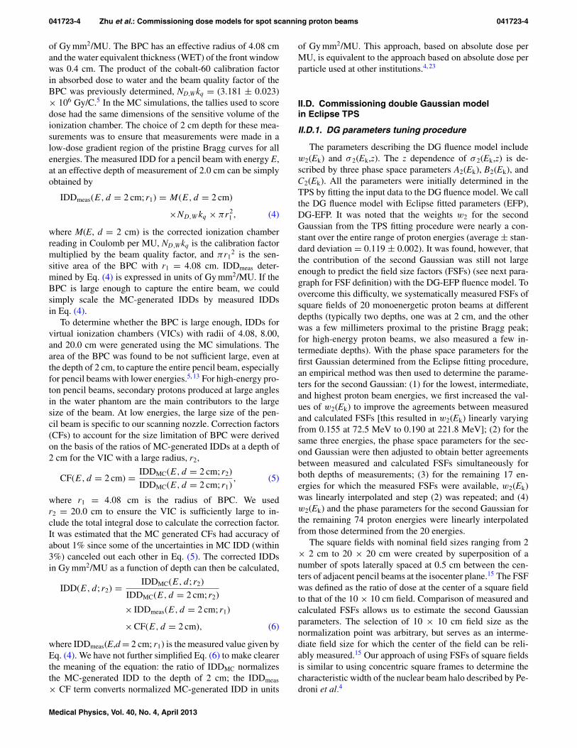
The details of our delivery system have been described inRefs. 5 and 7. Only a brief description is provided here. Thereare 94 energies between 72.5 and 221.8 MeV, correspondingto proton ranges of 4.0–30.6 g/cm2 in water, available fromour synchrotron in the proton therapy facility (PROBEATProton Beam Therapy System, Hitachi America, Ltd., Tarry-town, NY) at MD Anderson Cancer Center. The maximumfield size is 30 × 30 cm at isocenter. A schematic of thescanning nozzle is shown in Fig. 1. Briefly, after entering thenozzle, a pencil beam goes through the profile monitor first.Then the X and Y scanning magnets direct the beam to thedesired lateral position. The main dose monitor determineshow long the spot will remain in the position, and the spotposition monitor checks the position of the spot. For the scan-ning nozzle, a MU is defined on the basis of a fixed amount ofcharge collected in the main dose monitor ionization cham-ber, corresponding to a physical dose to water of 1 cGy,which was determined using the International Atomic EnergyAgency (IAEA) TRS 398 protocol16 under a specific refer-ence condition.5 The minimum and maximum MU values fordelivering each spot are 0.005 and 0.04, respectively.5, 7, 17 Theresolution is 0.0001 MU, which is 1/50 of the minimum MU.5

Absorbed doses at the Bragg peak irradiated by a single spotwith 0.04 MU varies from 1.6 to 4.4 cGy, depending on theenergy of the pencil beam. The proton beam with the energyof approximate 160 MeV has the maximum Bragg peak ab-sorbed dose.5

Iso-center

Spot position monitor

Dosemonitor

Y scanning magnet

X scanningmagnet

Profilemonitor

Protonbeam

FIG. 1. Schematic of the scanning nozzle illustrating its major components.

II.B. Treatment planning system

The TPS used in this work was Eclipse version 8.120 and8.917 (Varian Medical Systems, Palo Alto, CA) with a protonmodule for double scattering and spot scanning delivery. Apencil beam algorithm is used by the TPS,8–10, 18, 19 which isbriefly described in Sec. II.B.1. The input data required for thespot scanning beam are integral depth doses (IDDs) and in-airlateral profiles (see Sec. II.B.3). The SG fluence model wasonly used by Eclipse version 8.120.6 The DG fluence modelhas been available since version 8.908.

II.B.1. Pencil beam algorithm

The dose is calculated using a pencil beam algorithm, indi-vidual proton beamlets, DBeamlet

Ek(x, y, d(z), ), convolved with

the fluence, �Ek(x, y, z), at the position of the beamlet for

the kth energy layer, Ek. A beamlet is the 3D dose distri-bution of an infinitesimal pencil beam of protons in a wa-ter phantom.9 Let the beam central axis be the z-axis, theisocenter plane be defined at z = 0 cm, the positive z towardthe proton source, and x and y axes be the transverse coor-dinates. The general 3D dose distribution can be written asfollows:8–10, 18, 19

D(x, y, z) =∑Ek

∑Beamletj

�Ek(xj , yj , z)DBeamlet

Ek

× (x − xj , y − yj , d(z)), (1)

where d(z) is the water equivalent depth of position z alongthe beamlet direction. Particles contributing to the protonbeam absorbed dose include primary protons and secondaryparticles. Primary protons include protons that only undergoelastic interactions with electrons and elastic proton-nucleusscatterings in the medium. Secondary particles are generatedthrough nonelastic nuclear interactions and include secondaryprotons and other fragments (deuterons, tritons, alphas, neu-trons, etc.).14 The beamlet dose distribution is assumed tohave radial symmetry and can be written as10, 18, 19

DBeamletEk

(r, d(z)) = 1

ρH2O[Spp(d(z))Klat,pp(r, d(z))

+ Ssp(d(z))Klat,sp(r, d(z))], (2)

where r is the radial coordinate in the transverse plane,r =

√x2 + y2, ρH2O is the density of water and S(d) is the

weighted stopping power at the position of the z-axis witha water equivalent depth of d; subscript pp stands for pri-mary protons, and sp represents secondary particles; Klat,pp

describes the lateral dose distribution of the primary protonsfor the beamlet. This lateral distribution is mainly causedby multiple Coulomb scattering of protons off nuclei, in-cluding protons of hydrogen, which can be described by thewell-known Molière theory.20 The Molière theory is approxi-mated by the sum of two Gaussian functions representing the

Medical Physics, Vol. 40, No. 4, April 2013

041723-3 Zhu et al.: Commissioning dose models for spot scanning proton beams 041723-3

scattering angles probability; the second Gaussian describesthe tail of the scattering distribution due to large angle scat-tering, which accounts for only 4% of the contributions.10, 19

Klat,sp describes the lateral dose distribution of the secondaryparticles for the beamlet and is represented by the third Gaus-sian function in Eq. (2).19

The secondary particles deposit energy outside the primaryproton beam; therefore, the low-dose envelope from these sec-ondary products, also known as a nuclear “halo” dose, is ex-pected to have a broad lateral distribution.4, 14, 15 It should benoted that the parameters in Eq. (2) are not adjustable for thepurpose of commissioning the TPS. Pencil beam algorithmssimilar to Eq. (2) have been reported,4, 11 although normallyonly two Gaussians are used, one for multiple Coulomb scat-tering and the other for nuclear interactions, accounting forthe “halo” dose.

II.B.2. Single and double Gaussian fluence models

The fluence (protons/mm2) for the kth energy layeris calculated as the sum of fluence over all spots inthis layer, �Ek

(x, y, z) = ∑m φEk

(x, y; xm, ym, z), whereφEk

(x, y; xm, ym, z) is the fluence at position (x, y, z) con-tributed by the spot centered at (xm, ym) and could be de-scribed by Eq. (3) for the double Gaussian fluence model,

φEk(x, y; xm, ym, z)

= φmEk

(z)

⎡⎢⎣

w1(Ek )2πσ 2

1 (Ek,z)exp

(− (x−xm)2+(y−ym)2

2σ 21 (Ek,z)

)+

w2(Ek )2πσ 2

2 (Ek,z)exp

(− (x−xm)2+(y−ym)2

2σ 22 (Ek,z)

)

⎤⎥⎦ , (3)

where φmEk

(z) is the maximum fluence of the spot centeredat (xm, ym), w1(Ek) and w2(Ek) are the weights of the firstand second Gaussian function and satisfies w1(Ek) + w2(Ek)

= 1, and σi(Ek, z) =√

(Ai (Ek)2 + Bi(Ek)z + Ci (Ek)

2 z2) is thespot size for the first (i = 1) or second (i = 2) Gaussians,Ai(Ek), Bi(Ek), and Ci(Ek) are phase space parameters as afunction of energy. It is common to use a SG to describe thespot fluence, i.e., w2(Ek) = 0. Recently, we have demonstratedthat the SG fluence model is not accurate enough because ofthe contributions of large angle scattering from the deviceswithin the Hitachi scanning nozzle.14, 15 In general, σ i in the xand y directions are different due to the elliptical shape of theinitial beam. For the first Gaussian, the values of σ 1 in the xand y directions change with the gantry angle due to changesin the magnetic fields of steering and focusing magnets withthe treatment gantry rotation.21 However, the Eclipse TPS hasnot modeled this change with the gantry angle. The differ-ence of σ 1 in the x and y directions was small,5 the averagevalues in the x and y directions was used as σ 1. For the secondGaussian caused by large angle scattering in the materials in-side the scanning nozzle, we assumed that σ 2 is independentof the x and y directions.

When the DG fluence model was first introduced (Eclipseversion 8.908), w2 was assumed to be constant for all pro-

ton energies and σ 2 was a linear function of z. In the currentversion of DG fluence model (Eclipse version 8.917), w2 canvary with proton energy and σ 2 is described by phase spaceparameters, as defined in Eq. (3). In this work, the DG fluencemodel refers to the current model in Eclipse version 8.917, un-less otherwise specified. The SG fluence model in Eclipse ver-sion 8.120 was used only for creating plans for targets in dis-ease sites where tumor sizes and depths were similar to thosein prostate cancer.6 After the release of the version 8.908 ofEclipse in March 2010, the SG fluence model was removedfrom clinical use.

II.B.3. Required input data

The TPS system requires in-air profiles at three to five po-sitions from the isocenter (e.g., Z = 0, ±10, ±20 cm, i.e.,at the isocenter plane, 10 and 20 cm above and below theisocenter plane) for every 10–20 MeV in both the x and ydirections for each beam energy. If range shifting devices areused, the profile data sets for different thicknesses of the de-vices are required. In this work, range shifting devices are notconsidered.

The required depth doses are IDDs for single pencil beamfor each of the available proton energies. The IDD is definedas the integral of dose for a single spot over a very large planenormal to the beam direction (the total dose deposited at adepth), which is the well-known Bragg curve.22 The IDDsshould be measured with a parallel plate ionization chamberlarge enough to ostensibly capture the entire beam and be ex-pressed in units of Gy/MU multiplied by the active area ofthe ionization chamber in mm2, i.e., Gy mm2/MU. This leadsto values of IDDs in Gy/MU as if all of the doses were ap-plied to a water column of 1 mm2. The input data must be asaccurate as possible because they define the parameters thatthe dose algorithm uses for calculation of absorbed dose dis-tribution in the patient’s computed tomography (CT) volume.Such measurements are very time-consuming and require anextensive amount of beam time and well-trained personnel.Moreover, the area of the largest commercially available ion-ization chamber is insufficient to capture the entire beam,5, 13

as discussed in Sec. II.C. Considering these limitations in per-forming accurate measurements, we used Monte Carlo (MC)simulations to generate the input data. A limited number ofmeasurements of in-air profiles and IDDs were performedto validate a MC model of the scanning nozzle. The agree-ments between MC generated data and measurements usinga large area ionization chamber were within 3% in the prox-imal region of the pristine Bragg curves. The MC generatedranges agreed with measurements within 0.13 cm. Details ofthe MC model’s validation of the scanning nozzle have beenpublished in Ref. 13.

II.C. Conversion of MC-generated IDDs

We used a Bragg peak chamber (BPC) (model 34070,PTW-Freiburg, Freiburg, Germany) to perform the absolutedose measurements at an effective depth of 2 cm to convertMC-generated IDDs in units of MeV cm−3 per history to units

Medical Physics, Vol. 40, No. 4, April 2013

041723-4 Zhu et al.: Commissioning dose models for spot scanning proton beams 041723-4

of Gy mm2/MU. The BPC has an effective radius of 4.08 cmand the water equivalent thickness (WET) of the front windowwas 0.4 cm. The product of the cobalt-60 calibration factorin absorbed dose to water and the beam quality factor of theBPC was previously determined, ND,Wkq = (3.181 ± 0.023)× 106 Gy/C.5 In the MC simulations, the tallies used to scoredose had the same dimensions of the sensitive volume of theionization chamber. The choice of 2 cm depth for these mea-surements was to ensure that measurements were made in alow-dose gradient region of the pristine Bragg curves for allenergies. The measured IDD for a pencil beam with energy E,at an effective depth of measurement of 2.0 cm can be simplyobtained by

IDDmeas(E, d = 2 cm; r1) = M(E, d = 2 cm)

×ND,Wkq × πr21 , (4)

where M(E, d = 2 cm) is the corrected ionization chamberreading in Coulomb per MU, ND,Wkq is the calibration factormultiplied by the beam quality factor, and πr1

2 is the sen-sitive area of the BPC with r1 = 4.08 cm. IDDmeas deter-mined by Eq. (4) is expressed in units of Gy mm2/MU. If theBPC is large enough to capture the entire beam, we couldsimply scale the MC-generated IDDs by measured IDDsin Eq. (4).

To determine whether the BPC is large enough, IDDs forvirtual ionization chambers (VICs) with radii of 4.08, 8.00,and 20.0 cm were generated using the MC simulations. Thearea of the BPC was found to be not sufficient large, even atthe depth of 2 cm, to capture the entire pencil beam, especiallyfor pencil beams with lower energies.5, 13 For high-energy pro-ton pencil beams, secondary protons produced at large anglesin the water phantom are the main contributors to the largesize of the beam. At low energies, the large size of the pen-cil beam is specific to our scanning nozzle. Correction factors(CFs) to account for the size limitation of BPC were derivedon the basis of the ratios of MC-generated IDDs at a depth of2 cm for the VIC with a large radius, r2,

CF(E, d = 2 cm) = IDDMC(E, d = 2 cm; r2)

IDDMC(E, d = 2 cm; r1), (5)

where r1 = 4.08 cm is the radius of BPC. We usedr2 = 20.0 cm to ensure the VIC is sufficiently large to in-clude the total integral dose to calculate the correction factor.It was estimated that the MC generated CFs had accuracy ofabout 1% since some of the uncertainties in MC IDD (within3%) canceled out each other in Eq. (5). The corrected IDDsin Gy mm2/MU as a function of depth can then be calculated,

IDD(E, d; r2) = IDDMC(E, d; r2)

IDDMC(E, d = 2 cm; r2)

× IDDmeas(E, d = 2 cm; r1)

× CF(E, d = 2 cm), (6)

where IDDmeas(E,d = 2 cm; r1) is the measured value given byEq. (4). We have not further simplified Eq. (6) to make clearerthe meaning of the equation: the ratio of IDDMC normalizesthe MC-generated IDD to the depth of 2 cm; the IDDmeas

× CF term converts normalized MC-generated IDD in units

of Gy mm2/MU. This approach, based on absolute dose perMU, is equivalent to the approach based on absolute dose perparticle used at other institutions.4, 23

II.D. Commissioning double Gaussian modelin Eclipse TPS

II.D.1. DG parameters tuning procedure

The parameters describing the DG fluence model includew2(Ek) and σ 2(Ek,z). The z dependence of σ 2(Ek,z) is de-scribed by three phase space parameters A2(Ek), B2(Ek), andC2(Ek). All the parameters were initially determined in theTPS by fitting the input data to the DG fluence model. We callthe DG fluence model with Eclipse fitted parameters (EFP),DG-EFP. It was noted that the weights w2 for the secondGaussian from the TPS fitting procedure were nearly a con-stant over the entire range of proton energies (average ± stan-dard deviation = 0.119 ± 0.002). It was found, however, thatthe contribution of the second Gaussian was still not largeenough to predict the field size factors (FSFs) (see next para-graph for FSF definition) with the DG-EFP fluence model. Toovercome this difficulty, we systematically measured FSFs ofsquare fields of 20 monoenergetic proton beams at differentdepths (typically two depths, one was at 2 cm, and the otherwas a few millimeters proximal to the pristine Bragg peak;for high-energy proton beams, we also measured a few in-termediate depths). With the phase space parameters for thefirst Gaussian determined from the Eclipse fitting procedure,an empirical method was then used to determine the parame-ters for the second Gaussian: (1) for the lowest, intermediate,and highest proton beam energies, we first increased the val-ues of w2(Ek) to improve the agreements between measuredand calculated FSFs [this resulted in w2(Ek) linearly varyingfrom 0.155 at 72.5 MeV to 0.190 at 221.8 MeV]; (2) for thesame three energies, the phase space parameters for the sec-ond Gaussian were then adjusted to obtain better agreementsbetween measured and calculated FSFs simultaneously forboth depths of measurements; (3) for the remaining 17 en-ergies for which the measured FSFs were available, w2(Ek)was linearly interpolated and step (2) was repeated; and (4)w2(Ek) and the phase parameters for the second Gaussian forthe remaining 74 proton energies were linearly interpolatedfrom those determined from the 20 energies.

The square fields with nominal field sizes ranging from 2× 2 cm to 20 × 20 cm were created by superposition of anumber of spots laterally spaced at 0.5 cm between the cen-ters of adjacent pencil beams at the isocenter plane.15 The FSFwas defined as the ratio of dose at the center of a square fieldto that of the 10 × 10 cm field. Comparison of measured andcalculated FSFs allows us to estimate the second Gaussianparameters. The selection of 10 × 10 cm field size as thenormalization point was arbitrary, but serves as an interme-diate field size for which the center of the field can be reli-ably measured.15 Our approach of using FSFs of square fieldsis similar to using concentric square frames to determine thecharacteristic width of the nuclear beam halo described by Pe-droni et al.4

Medical Physics, Vol. 40, No. 4, April 2013

041723-5 Zhu et al.: Commissioning dose models for spot scanning proton beams 041723-5

II.D.2. Verification measurements for TPScommissioning

Eclipse input data verification (selected IDDs and in-air lateral profiles) were measured for monoenergetic pen-cil beams for several different energies.13 IDDs were mea-sured point-by-point with the BPC.5 In-air lateral profileswere measured with a “Pinpoint chamber” (model 31014,PTW-Freiburg), and another chamber with similar sensitivevolume as the reference chamber. The data acquisition sys-tem included a large water phantom (MP3 Phantom Tank,model 981010, PTW-Freiburg) and dual-channel electrometer(TANDEM, PTW-Freiburg). The in-air lateral profiles weremeasured by scanning the Pinpoint chamber with a dwell timeof 4 s and step sizes of 0.1–1 cm. The details of the measure-ments has recently been reported.15

FSFs of square fields of monoenergetic proton beams inwater were measured by an “Advanced Markus” ionizationchamber (model 34045, PTW-Freiburg) in a small rectangularwater phantom. Volumetric dose distributions were gener-ated by stacking multiple layers of square fields of pencilbeams. Verification measurements in the volumetric dosedistributions included point doses in the center of SOBP andfield, depth doses along the central axis, lateral dose profilesalong the center of the SOBP, and two-dimensional (2D)dose distributions in selected plans perpendicular to the beamincident direction for selected SOBPs. All point doses at thecenter of the fields, including depth doses, were measured asa function of nominal field size (ranging from 2 × 2 to 20× 20 cm), the width of the SOBP (from 2 to 20 cm), andthe range of the highest proton energies (from 6 to 30.6 cm)in the same way as the FSF measurements. For all fieldscreated by superposition of pencil beams measured withan ionization chamber, the chamber was positioned at eachselected location when the entire field was delivered. Aftercompleting each position, the chamber was remotely movedto the next location by a computer. A Pinpoint ionizationchamber was also used to verify the results of the AdvancedMarkus chamber measurements for the small fields. Lateraldose profiles were measured with a Pinpoint ionizationchamber and radiochromic film (Gafchromic EBT Film,International Specialty Products, Wayne, NJ) in a water phan-tom. Isodose distributions were measured with radiochromicfilms and a 2D ionization chamber array detector (MatriXX,IBA Dosimetry, Schwarzenbruck, Germany). Radiochromicfilms were used for relative measurements in the planesperpendicular to the incident beam, therefore, their LETdependences are not considered.

II.D.3. Correction table for the absolute doses

The Eclipse TPS provided a depth dose normalization table(DDNT) to allow the user, if necessary, to scale the calculatedabsolute doses in order to obtain better agreement with mea-sured absolute doses. This is a 2D table, which is a function ofthe proton range and of the width of the SOBP. If the model isperfect, it would be unnecessary to use the DDNT. In the cur-rent clinical implementation, the DDNT entries are a slowly

varying function of proton range (energy) but not of SOBPwidth. We expanded the use of this table to have doses fortreatment planning expressed as biological doses of a constantRBE. We expressed the input IDDs in physical dose (Gy), notin biological dose [Gy (RBE)]. If no scaling is required, thevalues of the DDNT table would be equal to 1/RBE = 1/1.1∼= 0.9091, not RBE = 1.1. This is purely due to how theDDNT is defined within the TPS. Thus, while the input com-missioning data are in physical dose Gy, the treatment plandose distributions are in biological dose Gy (RBE). We com-pared all measured absolute doses, in the center of fields andSOBPs, with the calculated doses to obtain scaling factors.The decision to use physical dose for IDDs and to use DDNTto convert them to biological doses for treatment planning wasarbitrary but believed to be more convenient. Alternatively,one could certainly convert IDDs into biological doses beforeinputting them into the TPS.

II.E. Measurements for patient-specificquality assurance

Before treating the first patient, we replanned using scan-ning beam several patients previously treated with passivescattering proton beams to evaluate the entire planning,dose validation, and delivery process. The details of patient-specific measurements for prostate cancer patients receiv-ing single field uniform dose (SFUD) have recently beenreported.6 Patient-specific measurements included point dosefor each plan, depth dose for each field, and 2D measurementsin the planes perpendicular to the beam incident direction foreach field at multiple depths. Comparison of calculated (bythe DG and SG fluence models) and measured dose distribu-tions for two patient plans obtained with a SFUD techniquewill be presented in Sec. III.E.4, as examples.

III. RESULTS

III.A. TPS input data generated by MC

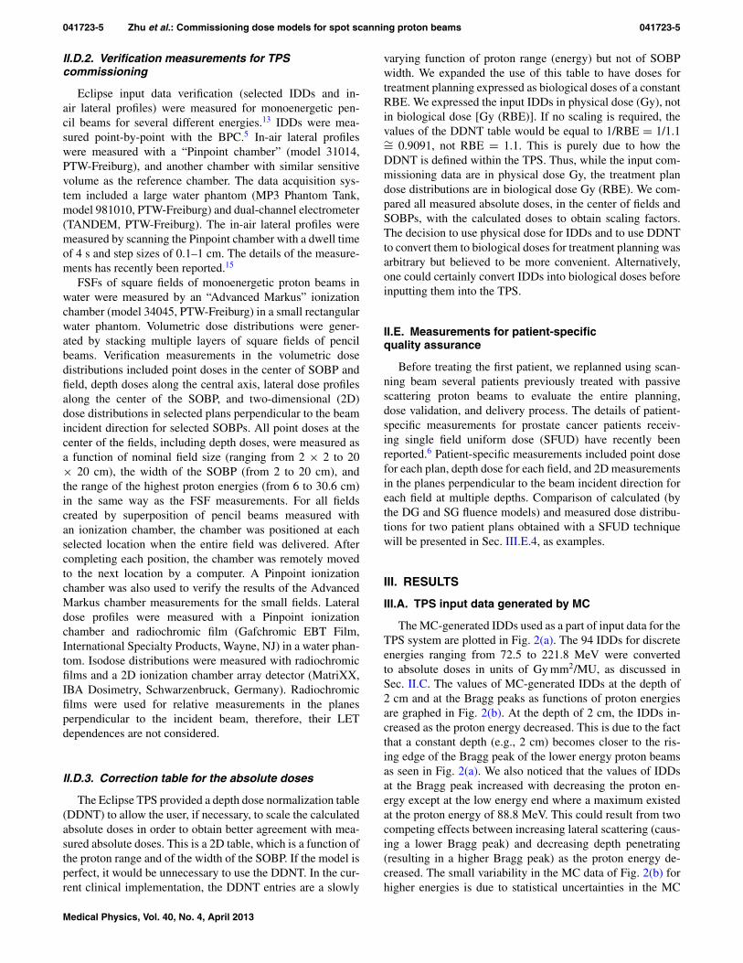
The MC-generated IDDs used as a part of input data for theTPS system are plotted in Fig. 2(a). The 94 IDDs for discreteenergies ranging from 72.5 to 221.8 MeV were convertedto absolute doses in units of Gy mm2/MU, as discussed inSec. II.C. The values of MC-generated IDDs at the depth of2 cm and at the Bragg peaks as functions of proton energiesare graphed in Fig. 2(b). At the depth of 2 cm, the IDDs in-creased as the proton energy decreased. This is due to the factthat a constant depth (e.g., 2 cm) becomes closer to the ris-ing edge of the Bragg peak of the lower energy proton beamsas seen in Fig. 2(a). We also noticed that the values of IDDsat the Bragg peak increased with decreasing the proton en-ergy except at the low energy end where a maximum existedat the proton energy of 88.8 MeV. This could result from twocompeting effects between increasing lateral scattering (caus-ing a lower Bragg peak) and decreasing depth penetrating(resulting in a higher Bragg peak) as the proton energy de-creased. The small variability in the MC data of Fig. 2(b) forhigher energies is due to statistical uncertainties in the MC

Medical Physics, Vol. 40, No. 4, April 2013

041723-6 Zhu et al.: Commissioning dose models for spot scanning proton beams 041723-6

(a)

(b) (c)

FIG. 2. (a) IDDs for all 94 energies in units of Gy mm2/MU generated using MC simulations; (b) IDDs values at a depth of 2 cm (MC and measurement) andat the Bragg peak (MC) as a function of proton energy; the inset is MC-generated CFs at a depth of 2 cm; and (c) FWHM of Bragg peaks (MC) in the depthdirection as a function of proton energy.

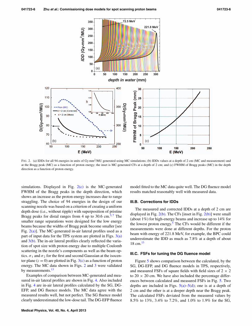
simulations. Displayed in Fig. 2(c) is the MC-generatedFWHM of the Bragg peaks in the depth direction, whichshows an increase as the proton energy increases due to rangestraggling. The choice of 94 energies in the design of ourscanning nozzle was based on a criterion of creating a uniformdepth dose (i.e., without ripple) with superposition of pristineBragg peaks for distal ranges from 4 up to 30.6 cm.5, 7 Thesmaller range separations were designed for the low energybeams because the widths of Bragg peak become smaller [seeFig. 2(a)]. The MC-generated in-air lateral profiles used as apart of input data for the TPS system are plotted in Figs. 3(a)and 3(b). The in-air lateral profiles clearly reflected the varia-tion of spot size with proton energy due to multiple Coulombscattering in the nozzle’s components as well as the beam op-tics. σ 1 and σ 2 for the first and second Gaussian at the isocen-ter plane (z = 0) are plotted in Fig. 3(c) as a function of protonenergy. The MC data shown in Figs. 2 and 3 were validatedby measurements.13

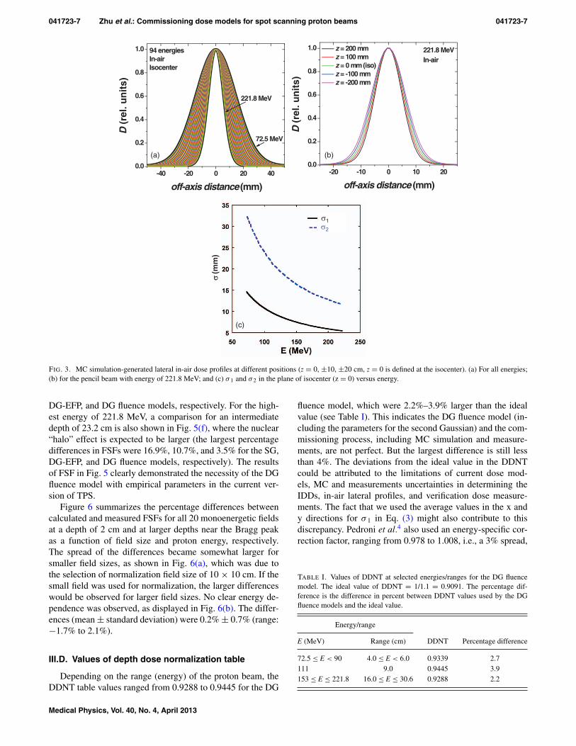
Examples of comparison between MC-generated and mea-sured in-air lateral profiles are shown in Fig. 4. Also includedin Fig. 4 are in-air lateral profiles calculated by the SG, DG-EFP, and DG fluence models. The MC data agree with themeasured results well, but not perfect. The SG fluence modelclearly underestimated the low-dose tail. The DG-EFP fluence

model fitted to the MC data quite well. The DG fluence modelresults matched reasonably well with measured data.

III.B. Corrections for IDDs

The measured and corrected IDDs at a depth of 2 cm aredisplayed in Fig. 2(b). The CFs [inset in Fig. 2(b)] were small(about 1%) for high-energy beams and increase up to 14% forthe lowest proton energy.5 The CFs would be different if themeasurements were done at different depths. For the protonbeam with energy of 221.8 MeV, for example, the BPC couldunderestimate the IDD as much as 7.8% at a depth of about18 cm.13

III.C. FSFs for tuning the DG fluence model

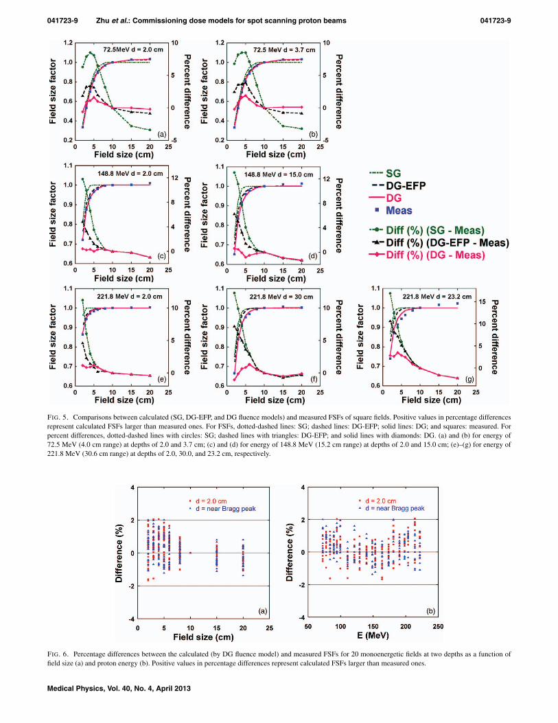
Figure 5 shows comparison between the calculated, by theSG, DG-EFP, and DG fluence models in TPS, respectively,and measured FSFs of square fields with field sizes of 2 × 2to 20 × 20 cm. We have also included the percentage differ-ences between calculated and measured FSFs in Fig. 5. Twodepths are included in Figs. 5(a)–5(d); one is at a depth of2 cm and the other is at a deeper depth near the Bragg peak.The calculated FSFs deviated from the measured values by8.5% to 13%, 3.4% to 7.2%, and 1.0% to 1.9% for the SG,

Medical Physics, Vol. 40, No. 4, April 2013

041723-7 Zhu et al.: Commissioning dose models for spot scanning proton beams 041723-7

-20 -10 0 10 200.0

0.2

0.4

0.6

0.8

1.0

D (

rel.

un

its)

off-axis distance (mm)

z = 200 mmz = 100 mmz = 0 mm (iso)z = -100 mmz = -200 mm

221.8 MeVIn-air

-40 -20 0 20 400.0

0.2

0.4

0.6

0.8

1.0

D (

rel.

un

its)

off-axis distance (mm)

221.8 MeV

72.5 MeV

94 energiesIn-airIsocenter

(a)

(c)

(b)

FIG. 3. MC simulation-generated lateral in-air dose profiles at different positions (z = 0, ±10, ±20 cm, z = 0 is defined at the isocenter). (a) For all energies;(b) for the pencil beam with energy of 221.8 MeV; and (c) σ 1 and σ 2 in the plane of isocenter (z = 0) versus energy.

DG-EFP, and DG fluence models, respectively. For the high-est energy of 221.8 MeV, a comparison for an intermediatedepth of 23.2 cm is also shown in Fig. 5(f), where the nuclear“halo” effect is expected to be larger (the largest percentagedifferences in FSFs were 16.9%, 10.7%, and 3.5% for the SG,DG-EFP, and DG fluence models, respectively). The resultsof FSF in Fig. 5 clearly demonstrated the necessity of the DGfluence model with empirical parameters in the current ver-sion of TPS.

Figure 6 summarizes the percentage differences betweencalculated and measured FSFs for all 20 monoenergetic fieldsat a depth of 2 cm and at larger depths near the Bragg peakas a function of field size and proton energy, respectively.The spread of the differences became somewhat larger forsmaller field sizes, as shown in Fig. 6(a), which was due tothe selection of normalization field size of 10 × 10 cm. If thesmall field was used for normalization, the larger differenceswould be observed for larger field sizes. No clear energy de-pendence was observed, as displayed in Fig. 6(b). The differ-ences (mean ± standard deviation) were 0.2% ± 0.7% (range:−1.7% to 2.1%).

III.D. Values of depth dose normalization table

Depending on the range (energy) of the proton beam, theDDNT table values ranged from 0.9288 to 0.9445 for the DG

fluence model, which were 2.2%–3.9% larger than the idealvalue (see Table I). This indicates the DG fluence model (in-cluding the parameters for the second Gaussian) and the com-missioning process, including MC simulation and measure-ments, are not perfect. But the largest difference is still lessthan 4%. The deviations from the ideal value in the DDNTcould be attributed to the limitations of current dose mod-els, MC and measurements uncertainties in determining theIDDs, in-air lateral profiles, and verification dose measure-ments. The fact that we used the average values in the x andy directions for σ 1 in Eq. (3) might also contribute to thisdiscrepancy. Pedroni et al.4 also used an energy-specific cor-rection factor, ranging from 0.978 to 1.008, i.e., a 3% spread,

TABLE I. Values of DDNT at selected energies/ranges for the DG fluencemodel. The ideal value of DDNT = 1/1.1 = 0.9091. The percentage dif-ference is the difference in percent between DDNT values used by the DGfluence models and the ideal value.

Energy/range

E (MeV) Range (cm) DDNT Percentage difference

72.5 ≤ E < 90 4.0 ≤ E < 6.0 0.9339 2.7111 9.0 0.9445 3.9153 ≤ E ≤ 221.8 16.0 ≤ E ≤ 30.6 0.9288 2.2

Medical Physics, Vol. 40, No. 4, April 2013

041723-8 Zhu et al.: Commissioning dose models for spot scanning proton beams 041723-8

FIG. 4. In-air lateral profiles for pencil beams with three different energies. Solid lines: MC; dots: measured data; dashed lines: calculated bySG fluence model; dashed-dotted lines: calculated by DG fluence model with empirical parameters; and dashed lines: calculated by DG-EFP.(a) 72.5, (b) 148.8, and (c) 221.8 MeV.

to fine-tune the agreement between measurements and calcu-lations for the absolute doses.

III.E. Dose verification

III.E.1. Absolute doses in the center of the SOBP

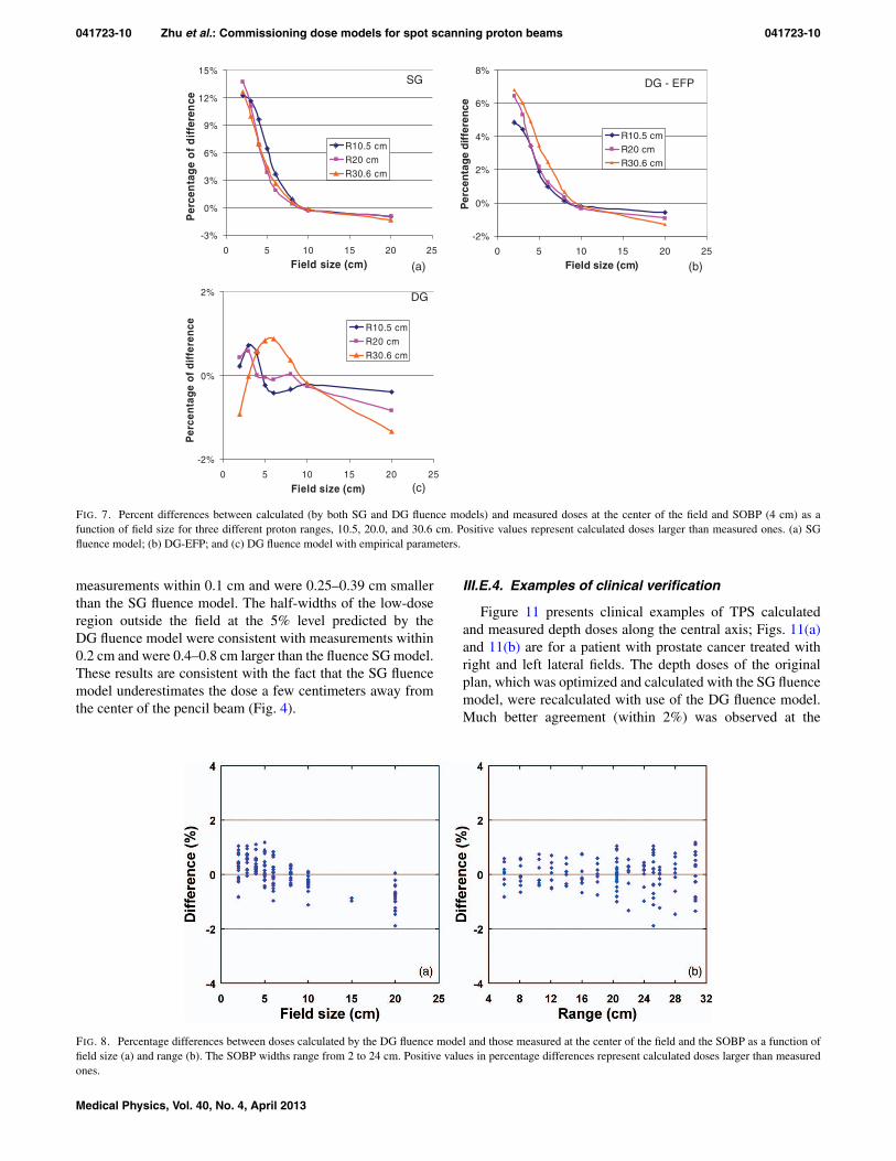
Figure 7 shows percentage differences between dosescalculated by the SG and DG fluence models and measured atthe center of the field and at the depths of the center of SOBP(4 cm wide) as a function of field size for three differentproton ranges, 10.5, 20.0, and 30.6 cm, corresponding to max-imum energies of 121.2, 173.7, and 221.8 MeV, respectively.The maximum differences were 13.8%, 6.8%, and 1.3%for the SG, DG-EFP, and DG fluence models, respectively.Figure 8 summarizes the percentage differences betweenthe doses calculated by the DG fluence model and thosemeasured at the center of the field and the SOBP as a functionof field size and range, with SOBP widths ranging from 2 to24 cm. The differences (mean ± standard deviation) are 0.0%± 0.6% (range: −1.9% to 1.2%) for the data included inFig. 8.

III.E.2. Absolute depth doses along the central axis

The measured and calculated depth doses, along the centralaxis of proton fields with a nominal field size of 10 × 10 cm

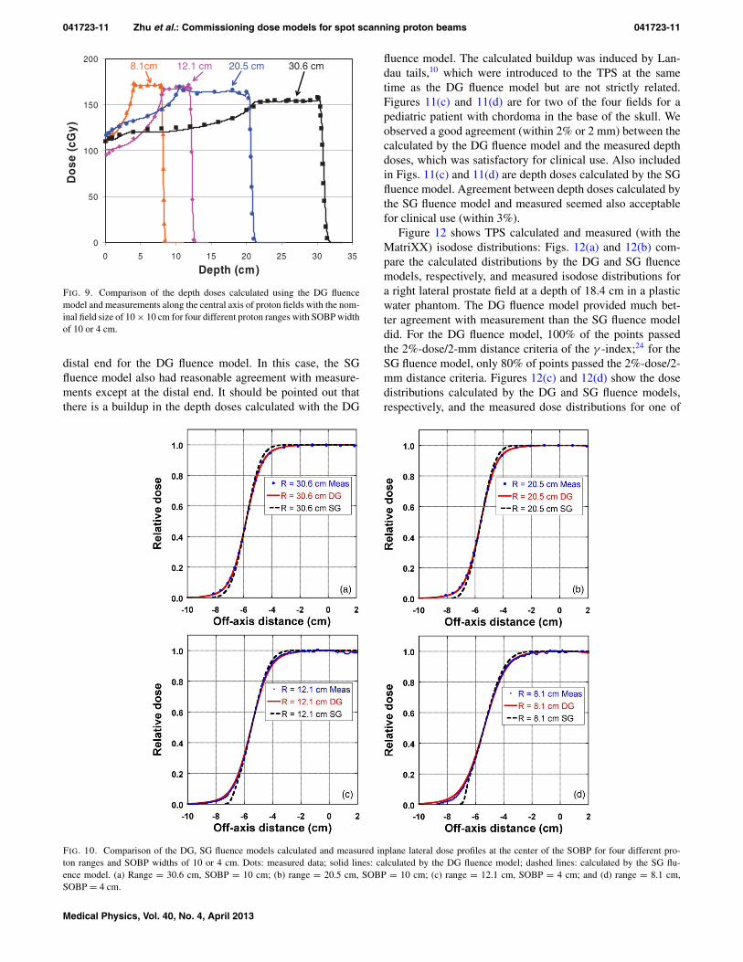
are compared in Fig. 9. The SOBP width was 4 cm for fieldswith ranges 8.1 and 12.1 cm, and was 10 cm for fields withranges 20.5 and 30.6 cm. The corresponding maximum ener-gies were 105.2, 131.0, 176.2, and 221.8 MeV, respectively.Figure 9 demonstrates that the depth doses calculated by theDG fluence model are in excellent agreement with measureddata.

III.E.3. In-water lateral dose profiles

Figure 10 compares doses calculated by both SG and DGfluence models with measured inplane lateral dose profiles atthe center of a 4 cm wide SOBP for proton ranges of 8.1and 12.1 cm (measured with EBT film) and a 10 cm wideSOBP for proton ranges of 20.5 and 30.6 cm (measured witha Pinpoint ionization chamber). The results from DG fluencemodel clearly demonstrated a better agreement with the mea-surements than the SG fluence model, especially in the areasof the shoulder and outside the field. Both SG and DG flu-ence models predicted the 50%–50% field size within 1 mmof the measured ones. Table II lists other dosimetric param-eters for the lateral profiles presented in Fig. 10. The 20%–80% penumbras predicted by the DG model agreed with themeasurements within 0.1 cm and were 0.15–0.2 cm largerthan the SG model. The half-widths of the shoulder at the95% level calculated by the DG fluence model agreed with

Medical Physics, Vol. 40, No. 4, April 2013

041723-9 Zhu et al.: Commissioning dose models for spot scanning proton beams 041723-9

FIG. 5. Comparisons between calculated (SG, DG-EFP, and DG fluence models) and measured FSFs of square fields. Positive values in percentage differencesrepresent calculated FSFs larger than measured ones. For FSFs, dotted-dashed lines: SG; dashed lines: DG-EFP; solid lines: DG; and squares: measured. Forpercent differences, dotted-dashed lines with circles: SG; dashed lines with triangles: DG-EFP; and solid lines with diamonds: DG. (a) and (b) for energy of72.5 MeV (4.0 cm range) at depths of 2.0 and 3.7 cm; (c) and (d) for energy of 148.8 MeV (15.2 cm range) at depths of 2.0 and 15.0 cm; (e)–(g) for energy of221.8 MeV (30.6 cm range) at depths of 2.0, 30.0, and 23.2 cm, respectively.

FIG. 6. Percentage differences between the calculated (by DG fluence model) and measured FSFs for 20 monoenergetic fields at two depths as a function offield size (a) and proton energy (b). Positive values in percentage differences represent calculated FSFs larger than measured ones.

Medical Physics, Vol. 40, No. 4, April 2013

041723-10 Zhu et al.: Commissioning dose models for spot scanning proton beams 041723-10

-2%

0%

2%

4%

6%

8%

0 5 10 15 20 25

Field size (cm)

Per

cen

tag

e d

iffe

ren

ce

R10.5 cmR20 cmR30.6 cm

-2%

0%

2%

0 5 10 15 20 25

Field size (cm)

Per

cen

tag

e o

f d

iffe

ren

ce R10.5 cmR20 cmR30.6 cm

-3%

0%

3%

6%

9%

12%

15%

0 5 10 15 20 25

Field size (cm)

Per

cen

tag

e o

f d

iffe

ren

ce

R10.5 cmR20 cmR30.6 cm

SG

DG

(a)

(c)

(b)

DG - EFP

FIG. 7. Percent differences between calculated (by both SG and DG fluence models) and measured doses at the center of the field and SOBP (4 cm) as afunction of field size for three different proton ranges, 10.5, 20.0, and 30.6 cm. Positive values represent calculated doses larger than measured ones. (a) SGfluence model; (b) DG-EFP; and (c) DG fluence model with empirical parameters.

measurements within 0.1 cm and were 0.25–0.39 cm smallerthan the SG fluence model. The half-widths of the low-doseregion outside the field at the 5% level predicted by theDG fluence model were consistent with measurements within0.2 cm and were 0.4–0.8 cm larger than the fluence SG model.These results are consistent with the fact that the SG fluencemodel underestimates the dose a few centimeters away fromthe center of the pencil beam (Fig. 4).

III.E.4. Examples of clinical verification

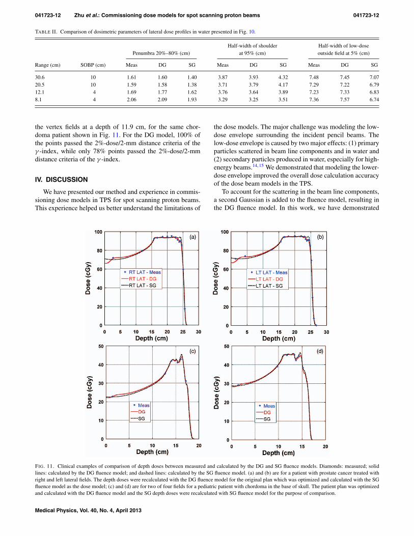
Figure 11 presents clinical examples of TPS calculatedand measured depth doses along the central axis; Figs. 11(a)and 11(b) are for a patient with prostate cancer treated withright and left lateral fields. The depth doses of the originalplan, which was optimized and calculated with the SG fluencemodel, were recalculated with use of the DG fluence model.Much better agreement (within 2%) was observed at the

FIG. 8. Percentage differences between doses calculated by the DG fluence model and those measured at the center of the field and the SOBP as a function offield size (a) and range (b). The SOBP widths range from 2 to 24 cm. Positive values in percentage differences represent calculated doses larger than measuredones.

Medical Physics, Vol. 40, No. 4, April 2013

041723-11 Zhu et al.: Commissioning dose models for spot scanning proton beams 041723-11

0

50

100

150

200

0 5 10 15 20 25 30 35

Depth (cm)

Do

se (

cGy)

30.6 cm8.1cm 12.1 cm 20.5 cm

FIG. 9. Comparison of the depth doses calculated using the DG fluencemodel and measurements along the central axis of proton fields with the nom-inal field size of 10 × 10 cm for four different proton ranges with SOBP widthof 10 or 4 cm.

distal end for the DG fluence model. In this case, the SGfluence model also had reasonable agreement with measure-ments except at the distal end. It should be pointed out thatthere is a buildup in the depth doses calculated with the DG

fluence model. The calculated buildup was induced by Lan-dau tails,10 which were introduced to the TPS at the sametime as the DG fluence model but are not strictly related.Figures 11(c) and 11(d) are for two of the four fields for apediatric patient with chordoma in the base of the skull. Weobserved a good agreement (within 2% or 2 mm) between thecalculated by the DG fluence model and the measured depthdoses, which was satisfactory for clinical use. Also includedin Figs. 11(c) and 11(d) are depth doses calculated by the SGfluence model. Agreement between depth doses calculated bythe SG fluence model and measured seemed also acceptablefor clinical use (within 3%).

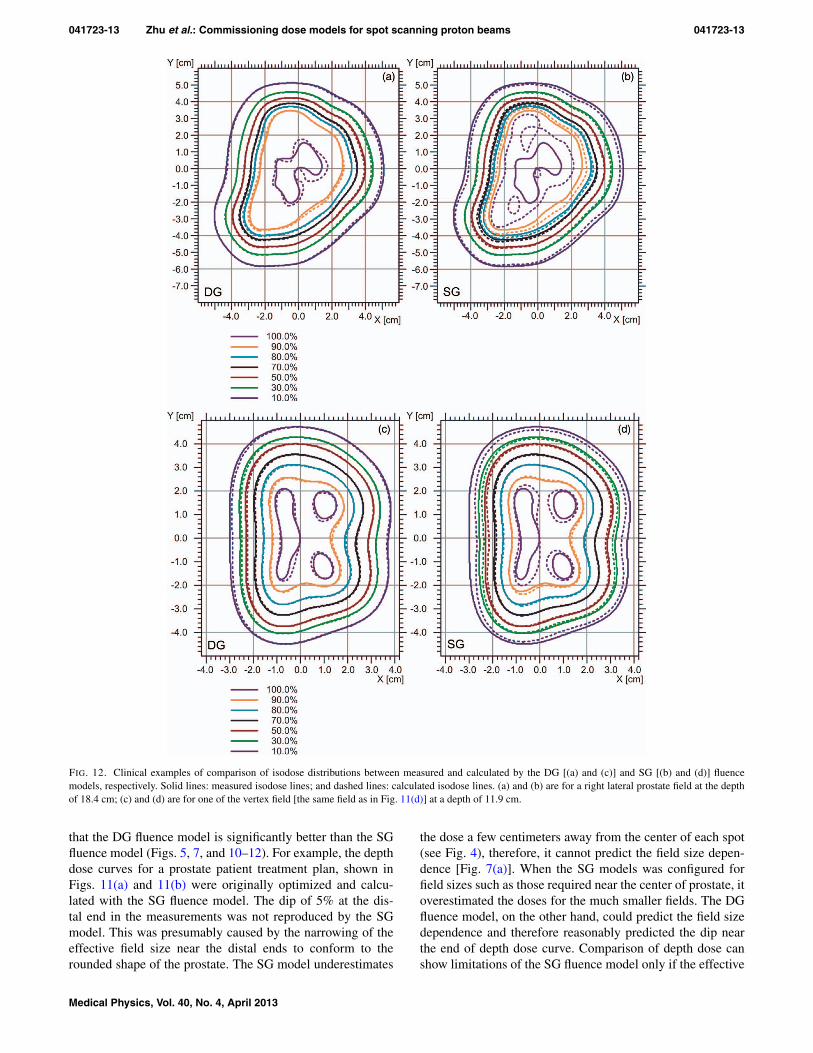
Figure 12 shows TPS calculated and measured (with theMatriXX) isodose distributions: Figs. 12(a) and 12(b) com-pare the calculated distributions by the DG and SG fluencemodels, respectively, and measured isodose distributions fora right lateral prostate field at a depth of 18.4 cm in a plasticwater phantom. The DG fluence model provided much bet-ter agreement with measurement than the SG fluence modeldid. For the DG fluence model, 100% of the points passedthe 2%-dose/2-mm distance criteria of the γ -index;24 for theSG fluence model, only 80% of points passed the 2%-dose/2-mm distance criteria. Figures 12(c) and 12(d) show the dosedistributions calculated by the DG and SG fluence models,respectively, and the measured dose distributions for one of

FIG. 10. Comparison of the DG, SG fluence models calculated and measured inplane lateral dose profiles at the center of the SOBP for four different pro-ton ranges and SOBP widths of 10 or 4 cm. Dots: measured data; solid lines: calculated by the DG fluence model; dashed lines: calculated by the SG flu-ence model. (a) Range = 30.6 cm, SOBP = 10 cm; (b) range = 20.5 cm, SOBP = 10 cm; (c) range = 12.1 cm, SOBP = 4 cm; and (d) range = 8.1 cm,SOBP = 4 cm.

Medical Physics, Vol. 40, No. 4, April 2013

041723-12 Zhu et al.: Commissioning dose models for spot scanning proton beams 041723-12

TABLE II. Comparison of dosimetric parameters of lateral dose profiles in water presented in Fig. 10.

Half-width of shoulder Half-width of low-dosePenumbra 20%–80% (cm) at 95% (cm) outside field at 5% (cm)

Range (cm) SOBP (cm) Meas DG SG Meas DG SG Meas DG SG

30.6 10 1.61 1.60 1.40 3.87 3.93 4.32 7.48 7.45 7.0720.5 10 1.59 1.58 1.38 3.71 3.79 4.17 7.29 7.22 6.7912.1 4 1.69 1.77 1.62 3.76 3.64 3.89 7.23 7.33 6.838.1 4 2.06 2.09 1.93 3.29 3.25 3.51 7.36 7.57 6.74

the vertex fields at a depth of 11.9 cm, for the same chor-doma patient shown in Fig. 11. For the DG model, 100% ofthe points passed the 2%-dose/2-mm distance criteria of theγ -index, while only 78% points passed the 2%-dose/2-mmdistance criteria of the γ -index.

IV. DISCUSSION

We have presented our method and experience in commis-sioning dose models in TPS for spot scanning proton beams.This experience helped us better understand the limitations of

the dose models. The major challenge was modeling the low-dose envelope surrounding the incident pencil beams. Thelow-dose envelope is caused by two major effects: (1) primaryparticles scattered in beam line components and in water and(2) secondary particles produced in water, especially for high-energy beams.14, 15 We demonstrated that modeling the lower-dose envelope improved the overall dose calculation accuracyof the dose beam models in the TPS.

To account for the scattering in the beam line components,a second Gaussian is added to the fluence model, resulting inthe DG fluence model. In this work, we have demonstrated

FIG. 11. Clinical examples of comparison of depth doses between measured and calculated by the DG and SG fluence models. Diamonds: measured; solidlines: calculated by the DG fluence model; and dashed lines: calculated by the SG fluence model. (a) and (b) are for a patient with prostate cancer treated withright and left lateral fields. The depth doses were recalculated with the DG fluence model for the original plan which was optimized and calculated with the SGfluence model as the dose model; (c) and (d) are for two of four fields for a pediatric patient with chordoma in the base of skull. The patient plan was optimizedand calculated with the DG fluence model and the SG depth doses were recalculated with SG fluence model for the purpose of comparison.

Medical Physics, Vol. 40, No. 4, April 2013

041723-13 Zhu et al.: Commissioning dose models for spot scanning proton beams 041723-13

FIG. 12. Clinical examples of comparison of isodose distributions between measured and calculated by the DG [(a) and (c)] and SG [(b) and (d)] fluencemodels, respectively. Solid lines: measured isodose lines; and dashed lines: calculated isodose lines. (a) and (b) are for a right lateral prostate field at the depthof 18.4 cm; (c) and (d) are for one of the vertex field [the same field as in Fig. 11(d)] at a depth of 11.9 cm.

that the DG fluence model is significantly better than the SGfluence model (Figs. 5, 7, and 10–12). For example, the depthdose curves for a prostate patient treatment plan, shown inFigs. 11(a) and 11(b) were originally optimized and calcu-lated with the SG fluence model. The dip of 5% at the dis-tal end in the measurements was not reproduced by the SGmodel. This was presumably caused by the narrowing of theeffective field size near the distal ends to conform to therounded shape of the prostate. The SG model underestimates

the dose a few centimeters away from the center of each spot(see Fig. 4), therefore, it cannot predict the field size depen-dence [Fig. 7(a)]. When the SG models was configured forfield sizes such as those required near the center of prostate, itoverestimated the doses for the much smaller fields. The DGfluence model, on the other hand, could predict the field sizedependence and therefore reasonably predicted the dip nearthe end of depth dose curve. Comparison of depth dose canshow limitations of the SG fluence model only if the effective

Medical Physics, Vol. 40, No. 4, April 2013

041723-14 Zhu et al.: Commissioning dose models for spot scanning proton beams 041723-14

field size of the beam changes significantly along the depth[see Figs. 11(c) and 11(d)]. On the other hand, comparison ofisodose distribution in the planes perpendicular to the incidentbeam is more effective at revealing the limitations of the SGfluence model. For example, in Fig. 12, the isodose lines cal-culated by the SG and DG fluence models show a pattern con-sistent with the results of lateral profiles displayed in Fig. 10;that is, the SG fluence model overestimates the dose in theshoulder region and underestimates the dose outside the field.

The results in Figs. 4, 5, 7(b), and 7(c) demonstrate thechallenges in configuring the DG fluence model. First, inFig. 4, the DG-EFP fluence model calculated lateral in-airprofiles agree with MC simulated data well; and the MCdata match with the measured data also well. However, DG-EFP fluence did poorly in predicting field size dependence[Figs. 5 and 7(b)]. One could argue that MC simulated in-air lateral profiles might not be accurate enough compared tomeasured data [i.e., MC data are somewhat lower than mea-sured ones, see Figs. 4(a) and 4(b), at distances near 5 and2.5 cm, respectively, away from the center of the spot]. Butfurther improvement of MC data might be limited by statisti-cal noises and measurement uncertainties. On the other hand,the DG fluence model calculated in-air lateral profiles agreewith measured data well, except in some regions, such as atthe distances near 3.5 and 2.5 cm [see Figs. 4(b) and 4(c)],where the DG data are higher than measured. All these differ-ences are small and within experimental uncertainties.15 Butthe data in Figs. 5 and 7(c) suggest that DG fluence model hassignificantly improved the field size dependence. The data inFigs. 4, 5, and 7 demonstrate that direct comparison of in-airlateral profiles, which may not be accurately known, would bedifficult to properly tune the DG parameters. Therefore, weused FSFs of square fields of monoenergetic fields to deter-mine the empirical DG parameters. Pedroni et al.4 used con-centric frames to carry out similar tasks.

The empirical parameters determined for the second Gaus-sian should be considered as the current “best-estimated” pa-rameters for the DG fluence model. The physical meanings ofthese parameters might not be straight forward. The secondGaussian in the fluence model was intended for describingthe low-dose envelope due to the scattering from the beamline components in the nozzle. One would expect larger scat-tering angles for protons with lower energies. However, theempirical values of w2(Ek) increase linearly from 0.155 to0.190 with increasing proton beam energy. One of possibleexplanations might be that the TPS inadequately modeled in-phantom interactions, including multiple-Coulomb scatteringand secondary particles originated from nuclear interactions,and the second Gaussian of the DG fluence model used non-physically larger weights to compensate the deficiency of themodel for proton beams with high energies.

Nuclear interactions are more important for the high-energy proton beams in water. The secondary particles pro-duced in water for the high-energy beams are challengingto model. The low-dose envelope due to nuclear interactionschanges with depth for a given proton energy, building upand reaching the maximum at an intermediate depth, and thenreceding.11, 14, 15 The TPS must accurately model this varia-

tion. The observed larger differences at some intermediatedepths for high proton energies (e.g., 23.2 cm for 221.8 MeV,as shown in Fig. 5) suggests that the current dose model in theTPS may need to be further improved. Within the frameworkof current pencil beam dose algorithm, a simple and straightforward approach might be to fix (not using empirical tun-ing) the parameters of the second Gaussian in the DG fluencemodel after the TPS fitting process. Then, better agreementbetween calculated and measured FSFs of all depths can beachieved by adjusting some of the parameters for the dose dis-tribution of secondary particles found in Eq. (2). For furtherimprovements, the TPS vendor could implement functionsother than Gaussian to describe the lateral dose distributionof the secondary particles. In fact, we have recently demon-strated that a modified Cauchy–Lorentz distribution functionis a better choice for modeling the low-dose envelopes in thewater phantom.25

Between March 2010 and June 2012, we treated more than500 patients with scanning proton beams using the DG flu-ence model, including approximately more than 150 patientswith central nerve system, head and neck, and other cancers.We used SFUD, single field integrated boost, and IMPT forthese treatments. From patient treatment field-specific qualityassurance measurements, we have found that the TPS calcu-lated and measured absolute doses normally agree within 3%or 2 mm [an example shown in Figs. 11(c) and 11(d)]. For rel-ative 2D dose distributions in the planes perpendicular to theincident beam direction, usually more than 90% of the pixelspassed the 2% dose/2 mm distance agreement criteria of theγ -index [an example shown in Figs. 12(a) and 12(c)].

V. CONCLUSIONS

In this work, we have presented our method and experiencein commissioning dose models for SSPT. Input data requiredby the TPS were generated by measurement-validated MC.A method for correcting the effect of finite detector size forIDDs was derived from MC-generated data. One of the mostchallenging and highly laborious tasks was to determine theempirical parameters for the second Gaussian function in theDG fluence model. We have demonstrated that the DG flu-ence model is significantly better than the SG fluence model.However, our results suggest that there are still limitations inmodeling the low-dose envelope, especially for in-phantominteractions of high-energy proton beams. Dose algorithmsfor proton beam therapy will continue to improve as moreand more institutions start to offer proton therapy to cancerpatients worldwide. Medical physicists face the challengingtask of commissioning and recommissioning the new and im-proved dose models as they become available. The authorshope that the method and experience presented here would beuseful for commissioning the dose models.

ACKNOWLEDGMENTS

The authors thank many members of the Department ofRadiation Physics at MD Anderson Cancer Center who con-tributed to the commissioning measurements and Tamara

Medical Physics, Vol. 40, No. 4, April 2013

041723-15 Zhu et al.: Commissioning dose models for spot scanning proton beams 041723-15

Locke from MD Anderson’s Department of Scientific Pub-lications for her editorial review of this paper. Helpful dis-cussions with Barbara Schaffner, Ph.D. and Sami Siljamaki,Ph.D. of Varian Medical Systems are greatly appreciated.This work was supported in part by the NCI P01 CA021239and MD Anderson’s cancer center support grant CA016672.The authors report no conflicts of interest in conducting theresearch.

a)Author to whom correspondence should be addressed. Electronic mail:xrzhu@mdanderson.org; Telephone: (713) 563-2553; Fax: (713) 563-1521.

1T. F. Delaney and H. M. Kooy, Proton and Charged Particle Radiotherapy(Lippincott, Philadelphia, 2008).

2ICRU, “Prescribing, recording, and reporting proton-beam therapy,” ICRUReport No. 78 (International Commission on Radiation Units and Measure-ments, Bethesda, MD, 2007).

3T. Haberer, W. Becher, D. Schardt, and G. Kraft, “Magnetic scanning sys-tem for heavy ion therapy,” Nucl. Instrum. Methods Phys. Res. A 330, 296–305 (1993).

4E. Pedroni et al., “The 200-MeV proton therapy project at the Paul ScherrerInstitute: Conceptual design and practical realization,” Med. Phys. 22, 37–53 (1995).

5M. T. Gillin, N. Sahoo, M. Bues, G. Ciangaru, G. Sawakuchi, F. Poenisch,B. Arjomandy, C. Martin, U. Titt, K. Suzuki, A. R. Smith, and X. R. Zhu,“Commissioning of the discrete spot scanning proton beam delivery systemat the University of Texas M. D. Anderson Cancer Center, Proton TherapyCenter, Houston,” Med. Phys. 37, 154–163 (2010).

6X. R. Zhu, F. Poenisch, X. Song, J. L. Johnson, G. Ciangaru, M. B. Tay-lor, M. Lii, C. Martin, B. Arjomandy, A. K. Lee, S. Choi, Q. N. Nguyen,M. T. Gillin, and N. Sahoo, “Patient-specific quality assurance for prostatecancer patients receiving spot scanning proton therapy using single-fielduniform dose,” Int. J. Radiat. Oncol., Biol., Phys. 81, 552–559 (2011).

7A. Smith, M. Gillin, M. Bues, X. R. Zhu, K. Suzuki, R. Mohan, S. Woo,A. Lee, R. Komaki, J. Cox, K. Hiramoto, H. Akiyama, T. Ishida, T. Sasaki,and K. Matsuda, “The M. D. Anderson proton therapy system,” Med. Phys.36, 4068–4083 (2009).

8B. Schaffner, E. Pedroni, and A. Lomax, “Dose calculation models for pro-ton treatment planning using a dynamic beam delivery system: An attemptto include density heterogeneity effects in the analytical dose calculation,”Phys. Med. Biol. 44, 27–41 (1999).

9B. Schaffner, “Proton dose calculation based on in-air fluence measure-ments,” Phys. Med. Biol. 53, 1545–1562 (2008).

10W. Ulmer and E. Matsinos, “Theoretical methods for the calculation ofBragg curves and 3D distributions of proton beams,” Eur. Phys. J. Spec.Top. 190, 1–81 (2010).

11M. Soukup, M. Fippel, and M. Alber, “A pencil beam algorithm for in-tensity modulated proton therapy derived from Monte Carlo simulations,”Phys. Med. Biol. 50, 5089–5104 (2005).

12G. Ciangaru, N. Sahoo, X. R. Zhu, G. O. Sawakuchi, and M. T. Gillin,“Computation of doses for large-angle Coulomb scattering of proton pencilbeams,” Phys. Med. Biol. 54, 7285–7300 (2009).

13G. O. Sawakuchi, D. Mirkovic, L. A. Perles, N. Sahoo, X. R. Zhu, G. Cian-garu, K. Suzuki, M. T. Gillin, R. Mohan, and U. Titt, “An MCNPX MonteCarlo model of a discrete spot scanning proton beam therapy nozzle,” Med.Phys. 37, 4960–4970 (2010).

14G. O. Sawakuchi, U. Titt, D. Mirkovic, G. Ciangaru, X. R. Zhu, N. Sahoo,M. T. Gillin, and R. Mohan, “Monte Carlo investigation of the low-doseenvelope from scanned proton pencil beams,” Phys. Med. Biol. 55, 711–721 (2010).

15G. O. Sawakuchi, X. R. Zhu, F. Poenisch, K. Suzuki, G. Ciangaru, U. Titt,A. Anand, R. Mohan, M. T. Gillin, and N. Sahoo, “Experimental charac-terization of the low-dose envelope of spot scanning proton beams,” Phys.Med. Biol. 55, 3467–3478 (2010).

16IAEA, “Absorbed dose determination in external beam radiotherapy: Aninternational code of practice for dosimetry based on standards of absorbeddose to water,” Technical Reports Series No. 398 (International AtomicEnergy Agency, Vienna, Austria, 2000).

17X. R. Zhu, N. Sahoo, X. Zhang, D. Robertson, H. Li, S. Choi, A. K. Lee,and M. T. Gillin, “Intensity modulated proton therapy treatment planningusing single-field optimization: The impact of monitor unit constraints onplan quality,” Med. Phys. 37, 1210–1219 (2010).

18W. Ulmer and B. Schaffner, “Foundation of an analytical proton beamletmodel for inclusion in a general proton dose calculation system,” Radiat.Phys. Chem. 80, 378–389 (2011).

19Varian, Proton Algorithm Reference Guide (Varian Medical Systems, PaloAlto, CA, 2009).

20H. A. Bethe, “Molière’s theory of multiple scattering,” Phys. Rev. 89,1256–1266 (1953).

21J. C. Polf, M. C. Harvey, and A. R. Smith, “Initial beam size study forpassive scatter proton therapy. II. Changes in delivered depth dose profiles,”Med. Phys. 34, 4219–4222 (2007).

22S. Scheib and E. Pedroni, “Dose calculation and optimization for 3Dconformal voxel scanning,” Radiat. Environ. Biophys. 31, 251–256(1992).

23S. Lorin, E. Grusell, N. Tilly, J. Medin, P. Kimstrand, and B. Glimelius,“Reference dosimetry in a scanned pulsed proton beam using ionisa-tion chambers and a Faraday cup,” Phys. Med. Biol. 53, 3519–3529(2008).

24D. A. Low, W. B. Harms, S. Mutic, and J. A. Purdy, “A technique forthe quantitative evaluation of dose distributions,” Med. Phys. 25, 656–661(1998).

25Y. Li, X. R. Zhu, N. Sahoo, A. Anand, and X. Zhang, “Beyond Gaussians:A study of single-spot modeling for scanning proton dose calculation,”Phys. Med. Biol. 57, 983–997 (2012).

Medical Physics, Vol. 40, No. 4, April 2013