combining heuristic procedures and simulation models for

Combining heuristic procedures and simulation models for

balancing a PC camera assembly line*

Ana R. Mendes, Ana L. Ramos, Ana S. Simaria, Pedro M. Vilarinho*

Departamento de Economia, Gestao e Engenharia Indusrial, Universidade de Aveiro, Campo Universitario de Santiago,

3810-193 Aveiro, Portugal

Received 18 March 2004; revised 26 April 2005; accepted 28 July 2005

Available online 23 September 2005

Abstract

In this paper, a mixed-model PC camera assembly line balancing case study is presented. The aim of the study is

to establish different line configurations, for varying levels of demand. In the first stage of the study, a heuristic

procedure previously developed by some of the authors, based on the simulated annealing meta-heuristic, is used

to derive line configurations with a minimum number of workstations and a smooth workload balance between and

within the workstations. In the second stage, the solutions provided by the heuristic are used as an input to discrete

event simulation models in which certain manufacturing parameters that analytical procedures have difficulty to

accommodate, namely, stochastic times, machine breakdowns, rework, etc. are introduced. These simulation

models derive different performance measures (e.g. flow times and resources utilization) that provide operational

support and help fine-tune the line configurations.

This paper reports on the collaborative study between the Department of Economics, Management and

Industrial Engineering of University of Aveiro and a major manufacturer of electronic consumer goods.

q 2005 Elsevier Ltd. All rights reserved.

Keywords: Simulation; Simulated annealing; Assembly line balancing; Hybrid simulation/analytic modeling

1. Introduction

The case study reported in this paper is the outcome of the business internship program sponsored by

the University of Aveiro for the students in the Industrial Management and Engineering program.

Computers & Industrial Engineering 49 (2005) 413–431
www.elsevier.com/locate/dsw
0360-8352/$ - see front matter q 2005 Elsevier Ltd. All rights reserved.

doi:10.1016/j.cie.2005.07.003

* Processed by Area Editor Gary L. Hogg* Corresponding author. Tel.: C351 234 370 025; fax: C351 234 370215.

E-mail address: [email protected] (P.M. Vilarinho).

http://www.elsevier.com/locate/dsw

A.R. Mendes et al. / Computers & Industrial Engineering 49 (2005) 413–431414

The company in which the study took place is a major manufacturer of consumer electronic goods and

the system analyzed is the PC camera assembly line.

The assembly line under analysis is used to assemble three different versions of a PC camera with

some dissimilar technical specifications. This type of line, which allows for the simultaneous assembly

of a set of similar models of a product, is called mixed-model assembly line and is steadily replacing the

traditional single-model assembly line in companies who want to compete in markets characterized by a

growing trend for higher product variety.

To configure this type of line one looks for a feasible assignment of the tasks to the workstations in

such a way that the number of workstations is minimized for pre-specified levels of demand of the

different products to be assembled and the constraints of the assembly process are satisfied. This line

configuration problem is termed type-I mixed-model assembly line balancing problem.

In the line under consideration most of the tasks required to complete the assembly of the models are

manual and only the final tasks require equipment for testing the assemblies. So, the line employs low

skilled labor, which is cross-trained to perform all the operations and, as a result, it is relatively easy to

rebalance the line and change its configuration. However, there is a high level of absenteeism among the

workforce, typical of assembly lines that rely on a low skill workforce, and consequently the line

managers’ need to rebalance the line on a daily base.

On the other hand, the great variability and uncertainty associated with the product demand levels is a

major problem that the company has to deal with, requiring frequent changes in the line configuration.

The ability to quickly manage the assembly line to compensate for changes in both the labor workforce

and market demand is becoming an important competitive factor. Consequently, the company must be

agile to implement changes in a quick and effective manner.

The proposed approach combines analytical and simulation models to support the operational

decisions that the line managers have to carry out in light of the issues stated above. The main goal of the

study was to produce a set of different assembly line configurations that the line managers can select in

light of the different levels of demand they face in a specific planning horizon.

The proposed approach uses a heuristic procedure to solve the mixed-model assembly line balancing

problem and derive rough-cut line configurations, with a minimum number of workstations and a smooth

workload balance between and within the workstations. In the second stage of the study, the solutions

provided by the heuristic procedure are used as an input to discrete event simulation models in order to

test the robustness of these solutions when variability was introduced in some of the design parameters

(e.g. stochastic task times). Different performance measures (e.g. flow times and resources utilization)

were derived from the simulation models in order to help the decision maker to fine-tune the suggested

line configurations. Stochastic task times are characteristic of this type of line in which workers’

performance is highly variable. This approach in which a simulation model is used in a subordinate way

for an analytical model of the system is classified by Shanthikumar and Sargent (1983) as a class III

hybrid simulation and analytical model.

The use of a hybrid simulation and analytical approaches has been previously reported in the literature

for dealing with single-model assembly line problems. McMullen and Frazier (1999) use simulation and

data envelopment analysis to compare assembly line balancing solutions. Lee et al. (2000) use

simulation and genetic algorithms to analyze assembly lines, through the optimization of line

throughput, machine utilization and tardiness. Hsieh (2002) present a case study in which a hybrid

analytic and simulation approach is used in designing a multi-stage, multi-buffer electronic device

assembly line.

A.R. Mendes et al. / Computers & Industrial Engineering 49 (2005) 413–431 415

2. The PC camera assembly line

The assembly line under analysis is used to assemble three different versions of a PC camera (model

A, model B and model C), with some dissimilar technical specifications. Fig. 1 shows an exploded view

of the PC camera. The PCB (printed circuit board) is the only camera part that is manufactured in the

facility, while all the other components are outsourced.

The assembly system is composed of a sequence of workstations performing manual operations and

an automated conveyor that transports the sub-assemblies along the process. The main tasks for the PC

camera assembly are the following:

(a) cutting of collective PCBs;

(b) soldering of microphone pins;

(c) cleaning, inspecting and soldering of electronic components;

(d) functional testing;

(e) soldering of cable connector;

(f) attaching lens into front cover part;

(g) placing and screwing individual PCB at front cover;

(h) attaching back cover part and screwing closing part;

(i) final testing;

(j) encasing lens ring, putting foot into camera and placing sticker on the cable.

After task (j) the cameras proceed to the packaging table where some other tasks are performed,

namely cleaning and packaging the camera into its individual box with software and documentation,

placing the closing sticker and the bar code and packing several individual boxes into a collective one.

These collective boxes are then grouped in pallets and transported to the finished products warehouse.

The assembly process for each model defines: (i) the task time, i.e. the time required to perform each

task and (ii) a set of precedence relationships, which determine the sequence in which the tasks can be

performed. Although each model has its own set of precedence relationships, there is a large subset of

tasks common to all models. Hence, the precedence diagrams for all the models can be combined and the

resulting one accounts for all the tasks required for assembling all the models. For each task in

Fig. 1. Exploded view of the PC camera.

23

5

4

1

14

3

9

19

2

6

7

15

13

11

10

8 12 16 17 18 21

20 22 24 25 26 27

28

29 30 31 32

33

34

35

37

36 38 39

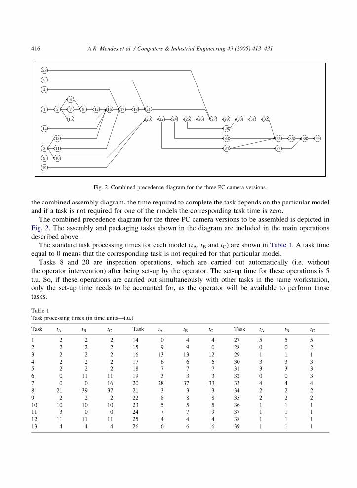
Fig. 2. Combined precedence diagram for the three PC camera versions.


the combined assembly diagram, the time required to complete the task depends on the particular model

and if a task is not required for one of the models the corresponding task time is zero.

The combined precedence diagram for the three PC camera versions to be assembled is depicted in

Fig. 2. The assembly and packaging tasks shown in the diagram are included in the main operations

described above.

The standard task processing times for each model (tA, tB and tC) are shown in Table 1. A task time

equal to 0 means that the corresponding task is not required for that particular model.

Tasks 8 and 20 are inspection operations, which are carried out automatically (i.e. without

the operator intervention) after being set-up by the operator. The set-up time for these operations is 5

t.u. So, if these operations are carried out simultaneously with other tasks in the same workstation,

only the set-up time needs to be accounted for, as the operator will be available to perform those

tasks.

Table 1

Task processing times (in time units—t.u.)

Task tA tB tC Task tA tB tC Task tA tB tC

1 2 2 2 14 0 4 4 27 5 5 5

2 2 2 2 15 9 9 0 28 0 0 2

3 2 2 2 16 13 13 12 29 1 1 1

4 2 2 2 17 6 6 6 30 3 3 3

5 2 2 2 18 7 7 7 31 3 3 3

6 0 11 11 19 3 3 3 32 0 0 3

7 0 0 16 20 28 37 33 33 4 4 4

8 21 39 37 21 3 3 3 34 2 2 2

9 2 2 2 22 8 8 8 35 2 2 2

10 10 10 10 23 5 5 5 36 1 1 1

11 3 0 0 24 7 7 9 37 1 1 1

12 11 11 11 25 4 4 4 38 1 1 1

13 4 4 4 26 6 6 6 39 1 1 1

Table 2

Set of pairs of incompatible tasks

Pair 1 2 3 4 5 6 7 8 9 10

Task 1 6 7 7 8 8 10 18 19 20 20

Task 2 8 8 20 12 20 20 20 20 24 34


Some tasks cannot be performed in the same workstation (incompatible tasks) due to physical or

process related constraints. For example, soldering and packaging tasks are incompatible due to

ergonomic issues: soldering requires the operator to be seated, while packaging requires the operator to

be standing. The set of pairs of incompatible tasks is presented in Table 2.

3. Mixed-model assembly line balancing using a heuristic procedure

The mathematical formulation of the assembly line balancing problem (ALBP) for single-model

assembly lines was first stated by Salveson (1955) and since then extensive research has been done in the

area. Comprehensive literature reviews on this subject are provided in Becker and Scholl (2005); Ghosh

and Gagnon (1989); Scholl (1999). Recent trends in the demand for customized products increased the

pressure for assembly flexibility, resulting in the replacement of single-model assembly lines by mixed-

model ones. So, techniques to solve the mixed-model ALBP have been recently reported in the literature

on the ALBP, namely by Erel and Gocken (1999); Gocken and Erel (1997, 1998), Jin and Wu (2003);

McMullen and Frazier (1997, 1998), Merengo et al. (1999).

The heuristic procedure for the mixed-model assembly line balancing problem, used in the first stage

of the study to derive line configurations for the relevant levels of demand, is based on the one proposed

by Vilarinho and Simaria (2002) and its main goal is to minimize the number of workstations, for a given

cycle time (or equivalently, for a given production rate).

A secondary goal of the procedure is to balance the workload between workstations (i.e. for each

model the idle time is distributed across the workstations as equally as possible) and within workstations

(i.e. the overall idle time for each workstation is distributed across models as evenly as possible), thus

assuring that all the workers across the line perform approximately the same amount of work on each

model being assembled and that a constant amount of work is carried out in each workstation regardless

of the model being assembled.

The procedure accounts for some relevant issues that reflect the operating conditions of real-world

assembly lines, like zoning constraints and parallel workstations. The decision maker can control the

generation of parallel workstations by defining a limit on the maximum number of replicas of a

workstation and the conditions under which a workstation can be replicated. The heuristic procedure

proposed by Vilarinho and Simaria (2002) is briefly described, together with an application example.

In addition to the combined precedence diagram, the mixed-model assembly line balancing heuristic

requires the following data set to be defined:

(i) the task processing times for each model mKtm (shown in Table 1);

(ii) the forecasted demand for each model (Dm) over the planning horizon (P), used to compute the

cycle time of the line CZP=PMmZ1

Dm

� �and each model production share qmZDm=

PMkZ1

Dk

� �—

Table 3

Demand values and cycle time for the different production scenarios.

Product demand

DA DB DC C

Scenario 1 (LLL) 1610 390 1670 36.2

Scenario 2 (MMM) 3150 1330 3130 17.5

Scenario 3 (HHH) 5230 2720 6580 9.1

Scenario 4 (MLM) 3150 390 3130 19.9

Scenario 5 (MMH) 3150 1330 6580 12.0


the different demand scenarios analyzed, for a planning horizon of PZ132.900 t.u., are presented

in Table 3, which also includes the required cycle time for each scenario;

(iii) the set of incompatible tasks (shown in Table 2);

(iv) the maximum number of replicas allowed for a workstation—MAXP;

(v) the minimum task time (expressed as a percentage of the cycle time: aC) that triggers the

‘parallelization’ of the workstation performing that task (this time will be termed minimum

‘parallelization’ time—MPT).

The demand for the different scenarios was provided by the line manager and represents the typical lot

sizes of the production runs for the demand levels, for each model, used to operate the line (Low,

Medium and High).

In order to allow for cycle times shorter than the longest task processing times, and thus, increase

production rate, assembly lines must operate with parallel workstations. This feature is included in the

heuristic, in which the maximum number of replicas of a workstation (MAXP) must be defined. The

replication of a workstation is only possible when it performs one or more tasks with processing time

higher than a user defined percentage of the cycle time (a% of the cycle time) for, at least, one of the

models being assembled.

The procedure works in two stages and is depicted in Fig. 3. The first stage looks for a near-optimal

solution for the problem’s primary goal, the minimization of the number of workstations. The second

stage is concerned with balancing the workloads between workstations (Bb), to ensure that

approximately the same amount of work is carried out in each workstation regardless of the model

being assembled, and within workstations (Bw), thus ensuring that operators perform approximately the

same amount of work on each model being assembled. Both Bb and Bw are within the value range [0,1],

where a balance value of 0 is the optimal case and a balance value of 1 is the worst case (Vilarinho &

Simaria, 2002).

The first stage of the heuristic starts with a solution built using a version of the well-known ranked

positional weight heuristic (Helgeson & Birnie, 1961), specially adapted for the mixed-model case with

parallel workstations. The positional weight of a task in a mixed-model assembly line is the cumulative

average task time associated with itself and its successors in the precedence diagram. The average task

time is the sum of the processing times of that task for each model weighted by the respective production

share. Tasks are assigned to the lowest numbered feasible workstation by decreasing order of their

positional weight. If a workstation performs a task with a processing time higher than MPT for, at least,

one model, than its capacity is C!MAXP, otherwise is C. The heuristic also forbids incompatible tasks

from being assigned to the same workstation.

1st stageBest solution

2nd stage Initial solution

Obj: MINUnba lance betweenand within sta tions

STOP?

2nd stageBest solution

Heur isticBest solution

InitialsolutionModified

RPW heuristic

Obj: MINIdle timeSTOP?

Neighbouringsolution

Current solution

Swap orTransfer

Solution intaboo list?

Verifyconstraints?(precedence,

zoning,capacity)

Y

Y

N

N

Y Y

Neighbouringsolution

Current solution

Swap orTransfer

Solution intaboo list?

Verifyconstraints?(precedence,

zoning,capacity, first

stage)Y

Y

N

N

N N

FIRST STAGE SECOND STAGE

Fig. 3. The heuristic procedure for the mixed-model ALBP.


For the demand scenario 1, the initial solution is depicted in Table 4, where the first column represents

the workstation index, the second column shows the set of tasks assigned to each workstation and the

third column shows the number of replicas of each workstation (parallel workstations have more than

one replica of the workstation). In this case study, there were special task related conditions that had to

be taken into account when applying the heuristic: tasks 8 and 20 are related to testing operations and

while the test program is running the assigned operator can execute other tasks simultaneously. The

heuristic was, therefore, modified to reproduce, as closely as possible, this issue.

After the initial solution is computed, the procedure tries to improve its number of workstations

through a simulated annealing approach, in which the neighboring solutions are generated by one of the

following actions: (i) swapping two tasks in different workstations or (ii) transferring a task to another

workstation. The tasks and workstations involved in these movements are randomly chosen. Only

transfer movements may contribute to reduce the number of workstations, nevertheless, swap procedures

are also required to ease the generation of successful transfer movements. So, the probability of

performing a transfer must be higher than for a swap and, by default, probabilities of 75 and 25% were,

respectively, set. At the end of this stage, the best solution has the lowest number of workstations. For the

demand scenario 1 the heuristic could not improve the number of workstations of the initial solution.

Table 4

Initial solution for the demand scenario 1

Workstation Tasks assigned Replicas

1 1,2,3,4,6,7,11,15 1

2 5,8,9,10,13,14,19,23 2

3 12,16,17 1

4 18,21 1

5 20,22 2

6 24,25,26,27,28,29,30,31,34,37 1

7 32,33,35,36,38,39 1


The initial solution of the second stage, which aims to balance the workloads between and within the

workstations, is the best solution found at the end of the first stage. For the demand scenario 1 this solution

has 9 workstations (including parallel workstations), a workload balance between workstations of BbZ0.15 and a workload balance within workstations of BwZ0.38. At the second stage the initial number of

workstations cannot be exceeded and, if possible, may be improved. A simulated annealing based

procedure is also used and swap and transfer movements are performed, but the tasks and workstations

involved in these movements are selected to foster improving solutions. As the main goal is to balance the

workloads, swap movements are more likely to contribute towards this end (probabilities of 75% for swap

and 25% for transfer moves are set). At the end of this stage, the best solution found has the minimum

number of workstations and the best workload balance between and within workstations. In each iteration,

the procedure verifies precedence, incompatibility and capacity constraints, in order to always generate

feasible solutions. The best solution found for the demand Scenario 1 has workload balances of BbZ0.06

and BwZ0.13, which shows an improvement of 50% on objective function BbCBw.

The described heuristic was used as an input for the simulation models of the PC camera mixed-model

assembly line. In the present study, five different combinations (the demand scenarios with an higher

occurrence probability within the real context) were tested corresponding to the different demand

scenarios already presented in Table 3. The final solutions provided by the heuristic for these demand

scenarios are depicted in Table 5 The cycle times for each scenario were recomputed taking into account

the task assignments provided by the heuristic and are shown in Table 5.

In order to evaluate these solutions, the lower bound for the mixed-model assembly line balancing

problem with parallel workstations, proposed by Vilarinho and Simaria (2002), was adapted to take into

account a maximum of five replicas of one workstation (in their paper, those authors considered a

maximum of two replicas). The details of the computation of this lower bound are given in Appendix A.

As one can observe from Table 6, the solutions obtained from the heuristic are optimal for four of the

scenarios.

4. Development of the simulation models

The set of line configurations produced by the heuristic procedure presented in the previous section

were based on various operational parameters that do not mimic exactly the real system, mainly because

the solutions obtained do not reflect the operational variability and randomness induced to the system by

the manual operations and by other factors, like rework, which affect the regular system operation.

So, simulation models for the different line configurations suggested by the heuristic procedure were

developed in order to check the dynamic behavior of the different line configurations in the presence of

modeling parameters that describe the system dynamics and which the heuristic does not consider. The

modeling scope embraced the complete assembly system: the assembly line, the packaging table and the

material handling equipments.

The different models were analyzed taking into account the following significant performance

measures of the system:

(i) throughput (number of cameras assembled for the planning period analyzed);

(ii) flow time (for each product);

(iii) utilization of resources (labor).

Table 5

Final line configurations for the different production scenarios.

SCENARIO 1 (LLL)/CZ31 t.u SCENARIO 2 (MMM)/CZ17 t.u.

Workstation Tasks assigned Replicas Workstation Tasks assigned Replicas

1 1,2,6,7 1 1 1,2,6 1

2 3,4,8,9,10,14,15,

19

2 2 7,15 1

3 12,13 1 3 3,4,8,9,10,11,13,

14,19,23

3

4 11,16,17,18 1 4 12 1

5 5,20,21,22,23 2 5 5,16 1

6 24,25,33 1 6 17,18 1

7 26,27,28,29,30,

31,32,34,35,36,

37,38,39

1 7 20,21,22 3

8 24,25,34,37 1

9 26,27,28,29,30 1

10 31,32,33,35,36,

38,39

1

SCENARIO 3 (HHH)/CZ9 t.u. SCENARIO 4 (MLM)/CZ18 t.u.

Workstation Tasks assigned Replicas Workstation Tasks assigned Replicas

1 1,2,6 2 1 1,2,6 1

2 7,15 2 2 7,15 1

3 3,4,8,9,10,13,14,

19,23

5 3 3,8,9,10,13,14,19 2

4 12 2 4 11,12 1

5 11,16 2 5 4,16 1

6 17 1 6 17,18 1

7 5,18 1 7 5,20,22,23 2

8 20,22 5 8 21,24,25,28 1

9 24 1 9 26,27,29,33,34 1

10 25,28,34 1 10 30,31,32,35,36,

37,38,39

1

11 21,26 1

12 27,29,30 1

13 31,33 1

14 32,35,36,37,38,39 1

SCENARIO 5 (MMH)/CZ12 t.u.


1 1,2,7 2

2 6 1

3 3,8,9,10,13,14,15,19,23 4

4 12 1

5 11,16 2

(continued on next page)


Table 5 (continued)

SCENARIO 5 (MMH)/CZ12 t.u.


6 4,17 1

7 18 1

8 5,20,21,22 4

9 24,34,37 1

10 25,26,28 1

11 27,29,30,31 1

12 32,33,35,36,38,39 1


Successful input modeling requires a close match between the input model and the true underlying

probabilistic mechanism allied with the system (Leemis, 1999). The sufficient quality and quantity input

data to perform a reasonable output analysis is often, difficult to gather.

In this particular case study, one of the members involved in the project worked fulltime on the

facility, thus the process of input data collection and analysis was easily accomplished. Her presence on

site was also crucial in obtaining the clear definition of control and decision rules used in the daily

operation of the assembly line. In addition, there were large amounts of historical data related to

processing times of all the assembly and packaging tasks for each version of the product, enabling the fit

of proper distributions to this data. The Arena simulation software package contains the Input Analyzer

module (Swets & Drake, 2001) that allows the modeler to fit a statistical distribution from the raw data,

which can be incorporated directly into the models.

Neither the maintenance procedures nor the equipment breakdowns were modeled, since the sole

equipments in the line are the ones used for material handling and inspection operations, which are rarely

faulty. Conveyor details (e.g. length, speed) were set as specified in technical documentation and

accordingly to the cycle time. The number of units rejected at the inspecting and testing operations was

modeled as a percentage of the cameras processed. There was also a wide availability of historical data

to figure out the reject rates related to those operations. It was assumed that some of those rejected

products could be repaired, re-entering the assembly process at fixed points.

The workforce consists of one shift working 8.5 h a day, 5 days a week. The shift has fixed daily

breaks for meals and work meetings. The production scheduling is made on a weekly basis and it is

conveyed to the assembly line supervisor. The printed circuit boards are manufactured on the facility

and, usually, they are ready to enter the assembly line when required. The other materials are outsourced

Table 6

Comparison of the solutions against the lower bounds (Lbpmix), for each scenario

Number of operators

Scenario Solution LBpmix

1 9 8

2 14 14

3 26 26

4 12 12

5 20 20


and are located near the corresponding assembly/packaging station and can be picked from stock when

needed.

The simulation models were implemented in the Arenaw simulation software (Kelton, Sadowski, &

Sadowski, 2002). This software has a high capability to model manufacturing systems and embedded

key technology for desktop application integration, enabling the use of existing enterprise models. In

addition, the software version employed includes tools to analyse input and output data.

The simulation model logic can be described as follows:

† the collective PCBs for the different camera models are the first entities that are created in the model;

these collective PCBs arrive at the line in boards, each containing several PCBs. As only one PCB is

mounted in each camera printed circuit board, the collective boards need to be cut into single PCBs

(the new entities in the simulation model);

† the single PCB is checked to verify its corresponding camera model (A, B or C) and it is assigned a

pre-defined assembly sequence (workstations set) and the task times required for that particular

model;

† the PCB follows its sequence through the different workstations and the corresponding resources

(mainly, human resources) perform the assembly operations (e.g. soldering, screwing). The task

times can differ from model to model;

† through the assembly line there are inspecting/testing tasks and, for each model, there are some reject

rates. The items to be repaired re-enter the line at some pre-defined locations. The scrap is sent out of

the process;

† between workstations, the product is handled by an automated conveyor of constant speed and with

different segment lengths;

† after the final assembly tasks, the cameras are conveyed to a packaging table where the individual

boxes are settled and batched into a collective one. These boxes are also grouped in pallets (the last

entities in the model) and transported to the finished products warehouse.

These major steps illustrate the simulation models main logic that was implemented with different

modules from the simulation software libraries (e.g. Create, Decide, Assign, Process, Convey, Batch,

Transport modules).

The verification and validation process is extremely important for successful completion of

simulation modeling efforts (Balci, 1998). Model verification deals with building the model right and

ensures that the computer program of the computerized model and its implementation are correct.

Model validation deals with building the right model and confirms that the simulation model behaves

with satisfactory accuracy consistent with the modeling objectives, within its domains of

applicability.

The models were verified and validated using different techniques advised by several authors (Maria,

1997; Sargent, 2001). The verification techniques used were: examination of model traces, structured

walkthroughs, varying input parameters and checking the output and animation. The validation

techniques used were: predictive validation, event validity, internal and face validity and historical data

validation.

The animation played an important role on the results presentation phase. With this technique, the

operational behavior of the assembly line is displayed graphically as the model evolves through time.


Fig. 4 shows two snap shots of the three-dimensional animation model developed for the actual assembly

line operation.

Once again, the team member who accompanied the project on site was crucial on the verification and

validation process, as she combined the knowledge of the simulation tool being used with the perception

gained on the assembly process details.

5. Simulation experiment and results

Once the experiments were designed and all the assumptions were verified, statistical analysis

was performed to determine the number of replications needed to yield statistically valid results. In

order to get valid and precise (with small variance) estimates of the performance measures (Law &

Kelton, 2000) the replications were performed with the same initial conditions and using non-

overlapping streams of random numbers, ensuring the desired independence. The amount of

variation across replications was not too high and consequently, 10 replications of one work week

(the planning horizon) each were adequate to get tight confidence intervals for the different

performance measures.

Previously to the development of the simulation models for the line configurations suggested by the

heuristic, a simulation model of the actual assembly system was built. This model allowed: (i) to better

understand the actual assembly system operation, (ii) to validate the assumptions used to build it

Fig. 4. Outline of the simulation models logic.


and later included in the different models and (iii) to gain the confidence of the decision makers

regarding the used methodology.

The outcome of this simulation study showed that the estimates obtained for the selected performance

measures were very similar to the real system measures and no major deviances between the simulation

results and reality were found. The results also emphasized the actual line was clearly unbalanced. Given

these results, it was decided to go on to the second phase of the study.

As mentioned in Section 4, the main goal of the second phase was to build simulation models for the

set of configurations, for the different levels of demand, generated by the heuristic procedure. Regarding

the throughput performance measures settled before, the simulation results for these models showed

that:

(i) the levels of demand considered at scenarios 1 and 5 could be easily satisfied with the line

configurations proposed by the heuristic procedure;

(ii) the forecasted demand for scenarios 2, 3 and 4 was not satisfied with the configurations proposed

by the heuristic procedure.

The line bottlenecks were identified as being workstation 8 for scenario 2 and workstation 7 for

scenarios 3 and 4.

Several experimental tests were carried out in order to eliminate the bottlenecks, which included

adjustments of the demand levels for the different models and replication of the bottleneck

workstations. The demand levels for the different scenarios were provided by the line manager as a

guideline for typical production runs. Small adjustment (up to 5%) to these demand levels was

allowed when leading to a reduction in the number of workers in the line. The adjustment of the

demand levels was carried out in order to figure out the number units of each model that could be

produced with the configuration suggested by the heuristic procedure. As a significant reduction in

the number of units to be assembled, for some of the models, was required, this course of action

was abandoned.

On the other hand, the replication of the bottleneck stations led to the desired production levels

and, in some of the scenarios, some slack capacity was left available in the workstation if needed

to increase production. The performance measurements for the actual assembly system and for the

line configurations for each scenario (with the replicated bottleneck workstations in scenarios 2, 3

and 4) are shown in Table 7 (average flow time) and Fig. 5 (average usage rate). When the average

flow time (i.e. the average time required to completely assemble a unit of model A) of the actual

system is compared to the different scenarios one can notice that for model A the average flow

time is reduced by 30–40% and for models B and C is more or less the same. As can be observed

in Fig. 6 for scenario 1, for example, when the demand is met there is still a slack capacity of

around 20% in the most loaded workstation (workstation 4), so it is possible to increase production

if required.

Table 8 shows the average usage rate and the standard deviation of this rate over the

workstations for the actual system for each of the scenarios. The average usage rate shows a

reduction in the overall idle time for all of the scenarios, except scenario 1, in comparison to the

actual system performance. The poorer performance in scenario 1 is justified by the fact that

the line was simulated to produce 3.670 cameras (CZ36.2 t.u., as shown in Table 3) when the

configuration provided by the heuristic could increase the output to 4.287 cameras (CZ31 t.u., as

Table 7

Simulation results for average flow time (actual system, scenarios 1–5)

Actual system Scenario 1 Scenario 2

Flow time (time units) Flow time (time units) Flow time (time units)

Model A 352.4 Model A 207.6 Model A 237.5

Model B 453.2 Model B 437.4 Model B 456.3

Model C 416.4 Model C 401.3 Model C 418.9

Scenario 3 Scenario 4 Scenario 5

Flow time (time units) Flow time (time units) Flow time (time units)

Model A 227.9 Model A 217.6 Model A 220.3

Model B 483.9 Model B 442.6 Model B 487.3

Model C 407.6 Model C 422.9 Model C 438.9


shown in Table 5). The standard deviation explains how evenly split the workload is distributed

across the workstations and, as can be observed from Table 8, all of the scenarios show an

improvement over the actual system.

As one can see from the results presented, the configurations proposed by the heuristic procedure were

suitable when the stochastic behavior of the assembly system was contemplated in simulation models. In

fact, with some adjustments to the solutions obtained for scenarios 2, 3 and 4:

the desired levels of demand were satisfied;

(ii) the flow times for the three PC camera models and for the different scenarios were at acceptable

levels and, for a particular case (Model A) were significantly reduced relatively to the actual

system;

(iii) the assembly line operation for the proposed configurations is smoother, that is, the workload is

more evenly distributed.

The results showed that the analytical method employed provided good quality results that were

easily fine-tuned using simulation. On the other hand, simulation allowed to gain the confidence of the

decision makers on the techniques employed and to test different options to fine-tune the line

Fig. 5. Animation of the actual assembly line operation.

ACTUAL SYTEM

0%10%20%30%40%50%60%70%80%90%

100%

1 2 3 4 5_1 5_2 5_3 6_1 6_2 7_1 7_2 8_1 8_2 9_1 9_2 9_3 9_4 10 11 12 13 14 15 16 17

Workstation

Ave

rage

usa

ge r

ate

SCENARIO 1 SCENARIO 1

0%20%40%60%80%

100%

1 2_1 2_2 3 4 5_1 5_2 6 7

Workstation

Ave

rage

usa

ge r

ate

0%20%40%60%80%

100%

1 2 3_1 3_2 3_3 4 5 6 7_1 7_2 7_3 8_1 8_2 9 10

Workstation

Ave

rage

usa

ge r

ate

SCENARIO 3

0%

20%

40%

60%

80%

100%

11_

1 22_

1 33_

13_

23_

33_

4 44_

1 55_

1 6 77_

1 88_

18_

28_

38_

4 9 10 11 12 13 14

Workstation

Ave

rage

usa

ge r

ate

SCENARIO 4

0%

20%

40%

60%

80%

100%

1 2 3 3_1 4 5 6 7 7_1 7_2 8 9 10

Workstation

SCENARIO 5

Workstation

Ave

rage

usa

ge r

ate

0%

10%

20%

30%

40%

50%

60%

70%

80%

90%

100%

1 1_1 2 3 3_1 3_2 3_3 4 5 5_1 6 7 8 8_1 8_2 8_3 9 10 11 12

Ave

rage

usa

ge r

ate

Fig. 6. Simulation results for average usage rate (actual system, scenarios 1–5).


Table 8

Average usage rate and standard deviation

Usage rate Actual system Scenario 1 Scenario 2 Scenario 3 Scenario 4 Scenario 5

Average 67% 57% 76% 73% 70% 75%

Std. Deviation 0.19 0.12 0.08 0.13 0.11 0.15


configurations suggested by the heuristic when more realistic parameters and operational details are

introduced.

6. Conclusions

The results of the study reported in this paper were very useful for the line manager to define the line

configurations for different demand scenarios by providing him production run figures that maximize the

use of the assembly line for these different scenarios. From the study carried out it is evident that the

integrated approach used to design and analyze assembly line configurations is promising for this type of

line.

From an academic perspective, the methodology described here makes a contribution to the

literature because it: (i) focuses attention on the joint use of analytical and simulation models to

provide operational decision support for assembly line balancing and (ii) demonstrates that when

dealing with real-world problems, effective communication channels and company involvement are

critical factors on the attainment of meaningful and in-depth results. In fact the team member who

worked fulltime within the company throughout the duration of the project has established

privileged communication channels between the university and the company and has directed

management and staff attention to the project.

Appendix A

Computation of the lower bound for the number of workstations

The lower bound for the mixed-model assembly line balancing problem with parallel workstations,

LBpmix, proposed by Vilarinho and Simaria (2002) was adapted to take into account the following set of

assumptions:

(i) the maximum number of replicas of each workstation is given by MAXPkZ(tmax/c(, where tmax

is the processing time of the longest task assigned to workstation k,

(ii) a workstation can be replicated only if the task time of one of the tasks assigned to it exceeds the

cycle time (aZ100%, MPTZC), and

(iii) the task time of the longest task does not exceed five times the cycle time (tmax%5C).

LBpmix is computed as follows:


Step 1: For each model, the tasks are classified according to the corresponding task time, as shown in

Table A1.

Step 2: For each model, compute LB’(m).

LB00ðmÞ Z 5ðnA CnB CnCÞC4ðnD CnE CnFÞC3ðnG CnH CnIÞC2ðnJ CnK

CnLÞCyðnMKnCKnFKnIKnLÞC ð1=2ÞwðnNKnBKnEKnHKnKÞ

C ð14=3ÞnO C ð13=3ÞnP C ð11=3ÞnQ C ð10=3ÞnR C ð8=3ÞnS C ð7=3ÞnT

C ð5=3ÞnU C ð4=3ÞnV C ð2=3ÞnW C ð1=3ÞnX (1)

LB0ðmÞ Z ðLB00ðmÞÞd e (2)

where nX is the number of tasks of type i (iZA,.,X), y equals 1 if nM–nC–nF–nI–nLO0 or zero

otherwise and w equals 1 if nN–nB–nE–nH–nKO0 or zero otherwise. The reasoning for this computation

is as follows.

The workstations performing tasks whose processing time is longer than the cycle time (tasks of

types A to L) need to be replicated. As two tasks of any of these types cannot share the same

workstation, because the value of MAXPk would be exceeded, a lower bound for the overall

number of workstations (including replicas) is the number of tasks of each type multiplied by the

number of replicas created in a workstation by the assignment of each task (for instance, each task

of type A, B, and C will create a workstation with 5 replicas, because they have processing times

between 4C and 5C). Each task of type M can be combined with a task of type C, F, J or L in a

replicated workstation, however, if there are not enough replicated workstations to accommodate

the tasks of type M, each of these remaining tasks will require a workstation. The same reasoning

applies to tasks of type N, that is, two tasks of type N require a single workstation, but they can

also be combined with a replicated workstation performing tasks of type B, E, H or K. Finally, the

tasks of types O to X have a fixed task time and so they occupy a fraction of a workstation

corresponding to the ratio between their task time and the cycle time.

Step 3: For each model, compute Z(m).

Z(m) adds up the number of workstations needed to process tasks of type Y. Because

these tasks can easily be included in workstations that perform tasks of the other types, it

is necessary to verify if, after filling up these workstations, there are tasks of type Y

remaining to create new workstations. The minimum number of workstations required to

perform tasks of type Y, after filling up the remaining capacity of the workstation

assigned to other task types is then given by:

ZðmÞ ZXiZY

tiK LB0ðmÞ$CKXisJ

ti

!" #.C

& ’(3)

Step 4: For each model, compute LBpmix(m)ZLB’(m)CZ(m).

Step 5: Select LBpmix for the problem: LBpmixZmaxm[LBpmix(m)].


Table A1 Classification of the tasks to compute LBpmix

Task type Task time Task type Task time Task type Task time

A 14/3C!tA %5C I 2C!tI %7/3C R tRZ10/3C

B 13/3C!tB%14/

3C

J 5/3C!tJ%2C S tSZ8/3C

C 4C!tC%13/3C K 4/3C!tK%5/3C T tTZ7/3C

D 11/3C!tD%4C L C!tL%4/3C U tUZ5/3C

E 10/3C!tE%11/

3C

M 2/3C!tM%C V tVZ4/3C

F 3C!tF%10/3C N 1/3C!tN%2/3C W tWZ2/3C

G 8/3C!tG%3C O tOZ14/3C X tXZ1/3C

H 7/3C!tH%8/3C P tP!13/3C Y tY!1/3C

I 2C!tI%7/3C Q tQZ11/3C

References

Balci, O. (1998). Verification, validation and accreditation. In D. J. Medeiros, E. F. Watson, J. S. Carson, & M. S. Manivannan

(Eds.), Proceedings of the 1998 Winter Simulation Conference, 41–48.

Becker, C., & Scholl, A. (2005). A survey on problems and methods in generalized assembly line balancing. European Journal

of Operational Research.

Erel, E., & Gocken, H. (1999). Shortest-route formulation of mixed-model assembly line balancing problem. European Journal

of Operational Research, 116, 194–204.

Ghosh, S., & Gagnon, R. J. (1989). A comprehensive literature review and analysis of the design, balancing and scheduling of

assembly systems. International Journal of Production Research, 27, 637–670.

Gocken, H., & Erel, E. (1997). A goal programming approach to mixed-model assembly line balancing problem. International

Journal of Production Economics, 48, 177–185.

Gocken, H., & Erel, E. (1998). Binary integer formulation for mixed-model assembly line balancing problem. Computers and

Industrial Engineering, 23, 451–461.

Helgeson, W. B., & Birnie, D. P. (1961). Assembly line balancing using the ranked positional weight technique. Journal of


Hsieh, S. J. (2002). In which a hybrid analytic and simulation modeling approach is used in designing a multi-stage, multi-buffer

electronic device assembly line. Simulation Modelling Practice and Theory, 10, 87–108.

Jin, M. Z., & Wu, S. D. (2003). A new heuristic method for mixed model assembly line balancing problem. Computers and


Kelton, W. D., Sadowski, R. P., & Sadowski, D. A. (2002). Simulation with arena (2nd ed.). New York: WCB McGraw-Hill.

Law, A. M., & Kelton, W. D. (2000). Simulation modelling and analysis (3rd ed.). New York: McGraw-Hill.

Lee, S. G., Khoo, L. P., & Yin, X. F. (2000). Optimising an assembly line through simulation augmented by genetic algorithms.

International Journal of Advanced Manufacturing Technology, 16, 220–228.

Leemis, L. (1999). Simulation input modelling. In P. A. Farrington, H. B. Nembhard, D. T. Sturrock, & G. W. Evans (Eds.),

Proceedings of the 1999 Winter Simulation Conference, 14–23.

Maria, A. (1997). Introduction to modelling and simulation. In S. Andradottir, K. J. Healy, D. H. Withers, & B. L. Nelson

(Eds.), Proceedings of the 1997 Winter Simulation Conference, 7–13.

McMullen, P. R., & Frazier, G. V. (1997). A heuristic for solving mixed-model line balancing problems with stochastic task

durations and parallel workstations. International Journal of Production Economics, 51, 177–190.

McMullen, P. R., & Frazier, G. V. (1998). Using simulated annealing to solve a multiobjective line balancing problem with

parallel workstations. International Journal of Production Research, 36, 2717–2741.


McMullen, P. R., & Frazier, G. V. (1999). Using simulation and data envelopment analysis to compare assembly line balancing

solutions. Journal of Productivity Analysis, 11, 149–168.

Merengo, C., Nava, F., & Pozzetti, A. (1999). Balancing and sequencing manual mixed-model assembly lines. International

Journal of Production Research, 37, 2835–2860.

Salveson, M. E. (1955). The assembly line balancing problem. Journal of Industrial Engineering, 6, 18–25.

Sargent, R. G. (2001). Some approaches and paradigms for verifying and validating simulation models. In B. A. Peters, J. S.

Smith, D. J. Medeiros, & M. W. Rohrer (Eds.), Proceedings of the 2001 Winter Simulation Conference, 106–114.

Scholl, A. (1999). Balancing and sequencing of assembly lines. Heidelberg: Physica-Verlag.

Shanthikumar, J. G., & Sargent, R. G. (1983). Unifying view of hybrid simulation/analytic models and modeling. Operations

Research, 31, 1030–1052.

Swets, R. J., & Drake, G. R. (2001). The arena product family: Enterprise modeling solutions. In B. A. Peters, J. S. Smith, D. J.

Medeiros, & M. W. Rohrer (Eds.), Proceedings of the 2001 Winter Simulation Conference, 201–208.

Vilarinho, P. M., & Simaria, A. S. (2002). A two-stage heuristic method for balancing mixed-model assembly lines with parallel

workstations. International Journal of Production Research, 40(6), 1405–1420.

combining heuristic procedures and simulation models for

Documents