collision analysis of vehicle following operations in automated highway systems
TRANSCRIPT
eScholarship provides open access, scholarly publishingservices to the University of California and delivers a dynamicresearch platform to scholars worldwide.
California Partners for AdvancedTransportation Technology
UC Berkeley
Title:Collision Analysis Of Vehicle Following Operations By Two-dimensional Simulation Model: Part II-Vehicle Trajectories With Follow-up Maneuvers
Author:Chan, Ching-Yao
Publication Date:01-01-1997
Series:Research Reports
Permalink:http://escholarship.org/uc/item/8t03g51k
Keywords:Automobiles--Automatic control--Simulation methods, Automobile driving--Braking--Automation,Express highways--Automation--Simulation methods, Automobiles--Dynamics
Abstract:This paper discusses the effects of collisions in vehicle-following operations, especially for short-spacing scenarios. The collision analysis is conducted with a two-dimensional simulation programby which the translational and rotational movements of vehicles can be fully represented. Alsopresented are simulation scenarios where control actions are taken in post-impact conditions.The potential implications and the effects of these maneuvers on the vehicle trajectories areinvestigated. The studies of these post-impact maneuvers offer a perspective on the possibleactions for vehicles in automated modes. The current and future work of this study should provideinsights for the evaluation of the safety hazards and control strategies in Automated HighwaySystems.
Copyright Information:All rights reserved unless otherwise indicated. Contact the author or original publisher for anynecessary permissions. eScholarship is not the copyright owner for deposited works. Learn moreat http://www.escholarship.org/help_copyright.html#reuse
ISSN 1055-1425
January 1997
This work was performed as part of the California PATH Program of theUniversity of California, in cooperation with the State of California Business,Transportation, and Housing Agency, Department of Transportation; and theUnited States Department of Transportation, Federal Highway Administration.
The contents of this report reflect the views of the authors who are responsiblefor the facts and the accuracy of the data presented herein. The contents do notnecessarily reflect the official views or policies of the State of California. Thisreport does not constitute a standard, specification, or regulation.
Report for MOU 252
CALIFORNIA PATH PROGRAMINSTITUTE OF TRANSPORTATION STUDIESUNIVERSITY OF CALIFORNIA, BERKELEY
Collision Analysis of Vehicle FollowingOperations by Two-Dimensional SimulationModel: Part II – Vehicle Trajectories withFollow-Up Maneuvers
UCB-ITS-PRR-97-5California PATH Research Report
Ching-Yao Chan
CALIFORNIA PARTNERS FOR ADVANCED TRANSIT AND HIGHWAYS
Collision Analysis of Vehicle Following Operationsby Two-Dimensional Simulation Model
IIVehicle Trajectories with Follow-Up Maneuvers
Project Progress ReportMOU 252
Ching-Yao ChanCalifornia PATH, Headquarters
University of California, BerkeleyRichmond Field Station, Bldg. 452, 1357 S. 46th Street, Richmond, CA 94804-4698, USA
Phone 510-231-5663, Fax 510-231-5600, [email protected]
EXECUTIVE SUMMARY
The work discussed in this report is a continuation of the studies in MOU 252 and the discussions in a precedingreport, UCB-ITS-PRR-97-4.
In operations of automated vehicles or Automated Highway Systems (AHS), vehicles may be designed orcommanded to travel with a small spacing between them. The automated vehicles should travel safely in normaloperating conditions. If collisions occur as a result of failures or malfunctions, it is necessary to minimize theconsequences of the collisions. This report presents work conducted to understand the effects of operational variableson the outcome of collision in vehicle-following operations and the feasibility of controlling vehicle motions incollisions.
A two-dimensional simulation model is used in this study. The model allows translational movement on ahorizontal plane and the rotational motion (yaw) about the vertical axis of a vehicle. A hard-braking failure scenariois simulated in this study with the leading vehicle decelerating while the following vehicle fails to brakeaccordingly. By using this model with a variety of initial conditions and vehicle parameters, the effects of offset,vehicle size, spacing and vehicle speed on the outcome of collisions are evaluated.
Several follow-up maneuvers by applying steering or braking inputs on the vehicles to respond to the failure eventare also simulated to investigate the feasibility of control actions. Different approaches of follow-up actions areexamined to discuss the hazards and benefits of these maneuvers. The work discussed in this paper represent acontinuation of safety evaluation for automated vehicles in various operating conditions and an initiation of acomprehensive model of collision analysis for future studies.
2
INTRODUCTION
In Automated Highway Systems (AHS), vehicles are equipped with automatic control systems to govern theaccelerating, steering and braking functions in order to maintain an appropriate speed and spacing from thesurrounding vehicles. One concept of AHS suggests the implementation of vehicle platoons with small spacingbetween vehicles. (1,2) If implemented successfully, the density of vehicles on the roadway is higher and thereforethe throughput can be increased. Furthermore, in the events of malfunctions or failures that lead to collisionsbetween a leading vehicle and a following vehicle, the relative speed difference (delta-V) at impact is smaller becausethe spacing is small.
With vehicles moving closely together in platoons, the hazards of Òchain-reactionÓ collisions become a concern.The benefits of small delta-V need to be weighed against the number of collisions in such feared Òchain-collisionÓscenarios. Hitchcock created a probabilistic model in which he included the statistical distribution of spacing,numbers of vehicle on a highway, vehicle weight, and the roadway friction coefficient to estimate the severity ofcollision and the probable Abbreviated Injury Scale (AIS) levels of the occupants. (3) His collision model is one-dimensional and plastic thus the vehicle masses are aggregated together once they are involved in collisions.
Tongue and Young examined the consequences and effects of different control schemes in platoon collisiondynamics in non-nominal conditions. (4,5,6) Vehicle bumper models were built into a one-dimensional platooncollision model. The effects of selected platoon parameter variations on the platoon response under various controlalgorithms were investigated. The control algorithms included forward and backward schemes, in which the controlof individual vehicle depends on the dynamic information of the vehicles ahead and behind.
This paper discusses the effects of collisions in vehicle-following operations, especially for short-spacing scenarios.In this study, the collision analysis is conducted with a two-dimensional simulation program by which thetranslational and rotational movements of vehicles can be fully represented. Some earlier work presented by theauthor has identified certain parameters that are most influential on the post-impact vehicle trajectories. (7,8) Forexample, a greater delta-V of the initial collisions or a larger lateral offset between the vehicles can cause the greatestdeviations from the specified path. Some of the findings will be reviewed in a following section.
Also presented in this paper are simulation scenarios where control actions are taken in post-impact conditions.Vehicle maneuvers in these simulations include steering and braking inputs to perform lane-following and lanechanging. The potential implications and the effects of these maneuvers on the vehicle trajectories are investigated.The studies of these post-impact maneuvers offer a perspective on the possible actions for vehicles in automatedmodes. The current and future work of this study should provide insights for the evaluation of the safety hazardsand control strategies in AHS.
SIMULATION MODEL
The analysis of vehicle collisions in this work is conducted with a simulation program developed by EngineeringDynamics Corporation (EDC). The software package, EDSMAC (Engineering Dynamics Corporation SimulationModel of Automobile Collisions), is used for the analysis of a single or two-vehicle accident. It is based on aprogram called SMAC (9-11) initially developed and validated by Calspan Corporation and subsequently improvedby EDC (12-15). EDSMAC uses a set of assumed or estimated initial conditions, including positions andvelocities, and predicts the outcome of a collision. Engineers and accident reconstructionists have been using thissimulation program to analyze vehicle dynamics and the damage resulting from crashes. Researchers have found thatthe program yields reasonable results with sound input data (16-21).
In its vehicle model, EDSMAC allows the longitudinal and lateral movements as well as the rotational motionabout the vertical axis of vehicles on a horizontal plane. If a contact between vehicles is detected, the collision phaseis analyzed. The external forces can be applied either at the tire/road interface or between the vehicles. The vehicleexterior is assumed to have homogeneous stiffness.
In the simulation model, a force proportional to the amount of crush is exerted as the body of a vehicle is crushed.This is accomplished by dividing the vehicleÕs perimeter into equally spaced intervals. Each of these intervalsforms a pie-shaped wedge having its focus at the center of gravity of the vehicle. By knowing where the vehiclesare with respect to each other, EDSMAC locates the wedges which are in contact and equalize the force between
3
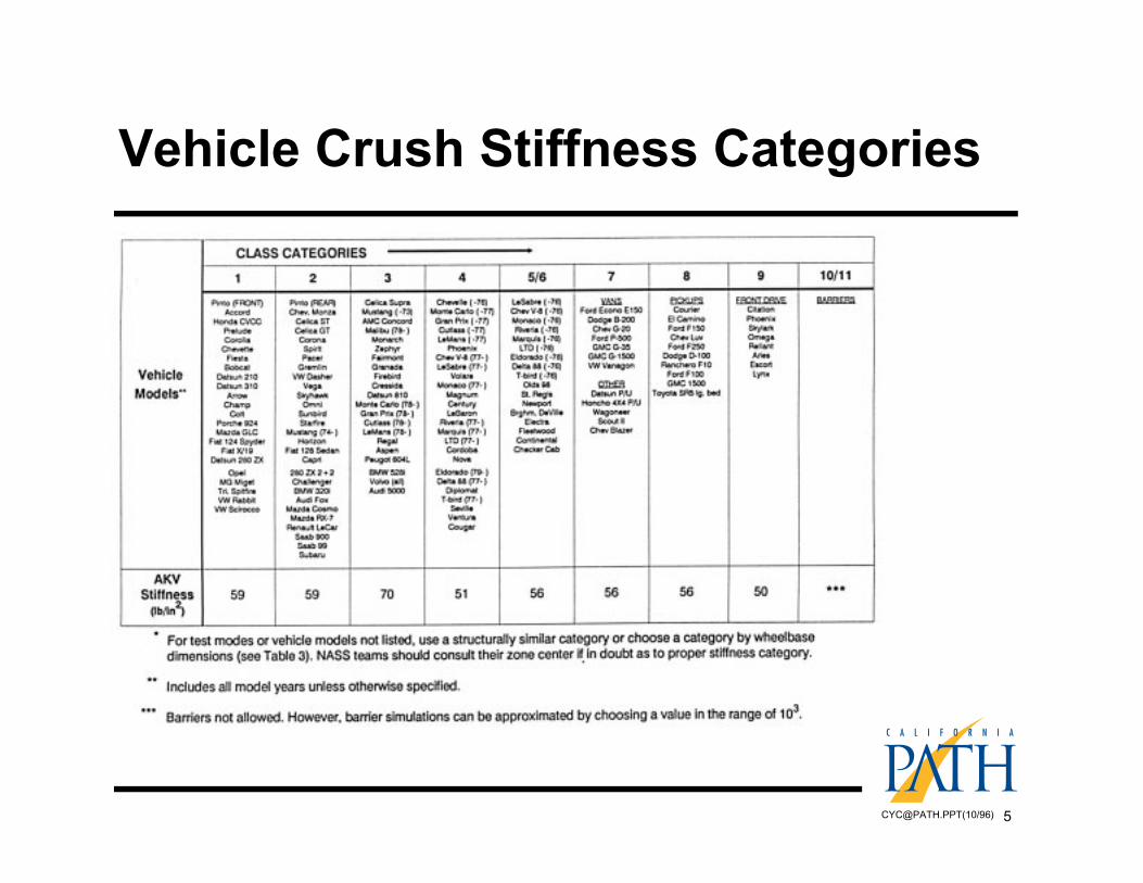
them. The resulting summation of forces dictates the motion of each vehicle due to the collision. This processcontinues for each collision time increment until the vehicles are no longer in contact. Default values of the crushstiffness data according to vehicle class category are used in the simulation.
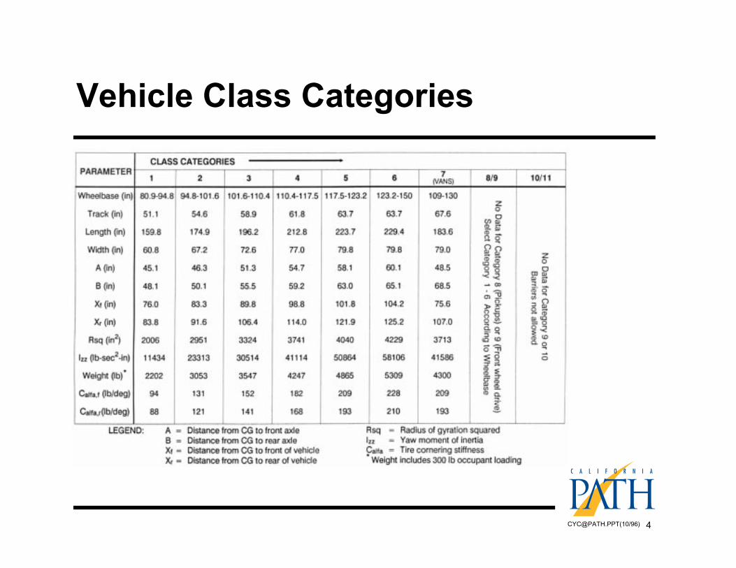
EDSMAC allows the direct entry of vehicle data by users or the selection of default values. The vehicles arecategorized by their wheelbase into several classes. Classes I and II are small passenger cars while Classes III to Vare medium to large cars. In this paper, default values provided by EDSMAC are used in the simulation. (15)
Appendix A contains exemplar pages of the program EDSMAC and tables showing the default values of differentvehicle classes.
Due to the limitations of the simulation models, the problem is formulated to analyze two-vehicle collisions only.The existing software does not allow a third vehicle or object to be involved in the collision process. The motionsof the vehicles are restricted on a horizontal plane. In the discussion of simulation results shown in this paper, thesimulation is terminated four seconds after the initial collision.
SIMULATION SCENARIOS, ASSUMPTIONS, AND PARAMETERS
In earlier publications (7, 8), simulation results were discussed for the following scenario:(1) The two vehicles are proceeding straight and no steering inputs are entered before, during, or after the impact;(2) The leading vehicle at time zero began braking with a constant 0.7 g deceleration and the following vehicleapplied no acceleration or deceleration until collisions occur; Throughout the simulation duration, the braking ofthe leading vehicle remains applied;(3) No other objects or vehicles come into contact or collisions with the two vehicles in question.
The simulation scenario was chosen to reflect one of the most critical failure conditions that might occur to causecollisions. Such scenarios might result from malfunctions or failures by:(1) a miscommunication from the leading vehicle to the following vehicle, and a failure in the range and range ratesensor on the following vehicle, or(2) a failure in brake actuation on the second vehicle.
The scenario above was simulated with a range of initial spacing, lateral offset between the longitudinal axes, initialspeed and vehicle sizes. The outcomes of the simulations were evaluated by examining the vehicle trajectories, suchas lateral displacement, angular rotation, and time to depart from a specified path. Other critical variables that maycause complications include the yaw angle and the vehicle speed at time of lane departure, but they are notdiscussed. Although the outcome of each collision case depended a great deal on the specific conditions, certainparameters proved to be critical.
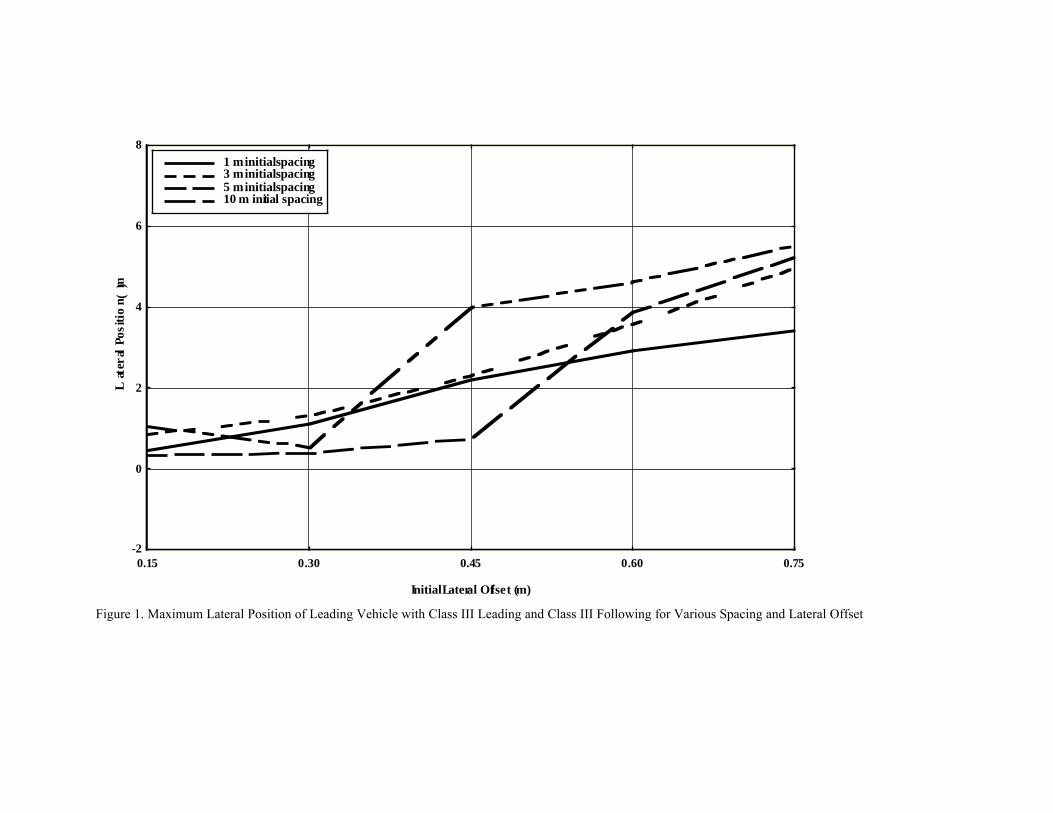
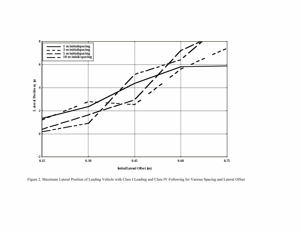
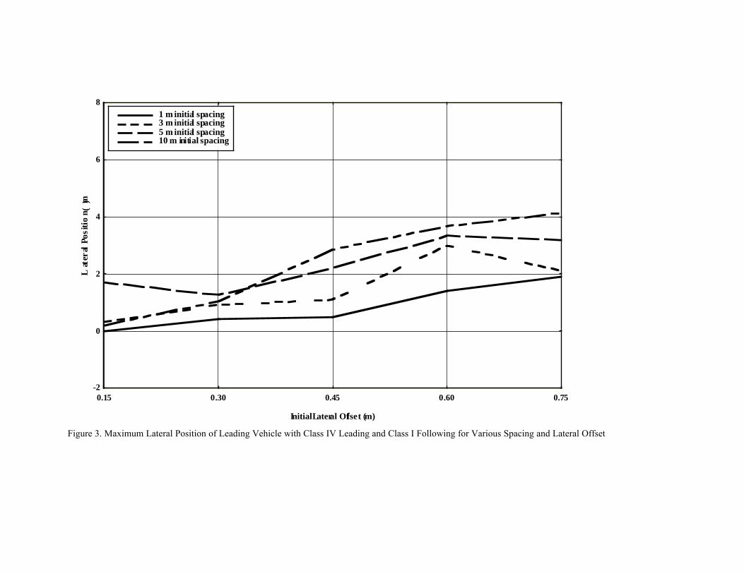
For example, large delta-V and lateral offset can cause greater deviations of trajectories. Figures 1-3 show themaximum lateral movement of the leading vehicle in a series of simulations with different formations. The threeformations are Formation I with two Class III vehicles, Formation II with a small vehicle leading a large vehicle(Class I & IV), and Formation III with a large vehicle leading a small vehicle (Class IV & I). The lateral offset isvaried from 0.15 m to 0.75 m for two vehicles of the same size traveling initially at 105 kmph with an initialspacing of 1, 3, 5, or 10 m. In all cases, the lateral movement increase with the lateral offset.
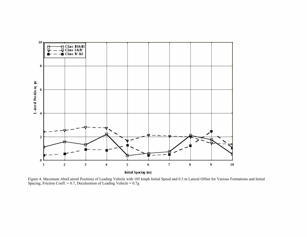
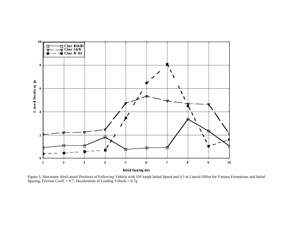
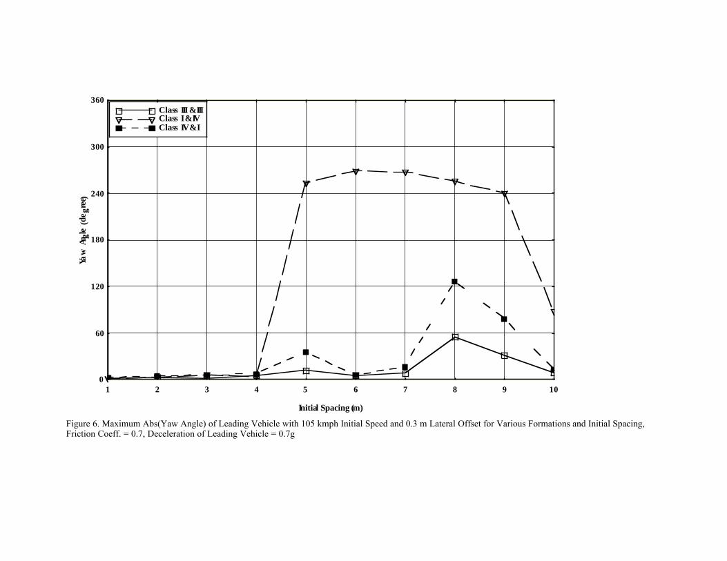
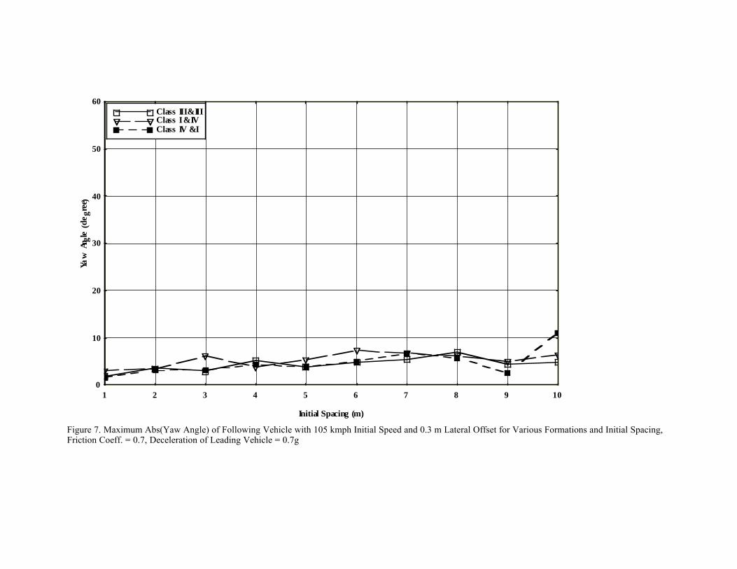
Figures 4 and 5 shows the effects of the initial spacing on the lateral deviation of the leading and following vehiclein three formations of different vehicle. Figure 6 and 7 shows the yaw rotation of the leading vehicle sizes that alsoreflects the effect of large spacing. The initial spacing is varied from 1 to 10 m for two vehicles initially traveling at105 kmph with a lateral offset of 0.3 m. In all three formations, the angular motion becomes erratic as the initialspacing increases. Further details and explanations of the simulation results can be found in previous papers by theauthor. (7,8)
One of the factor that should be mentioned here is the tire-roadway interaction issue. If the tire is skidding due tofull braking (and without anti-lock braking capability), the directional stability of vehicle motion control is injeopardy. When braking is not used (as in the failure vehicle) or only partially used, the steering function can beexecuted more effectively. Two series with different degrees of brake utilization are simulated to examine the effectsof this factor.
4
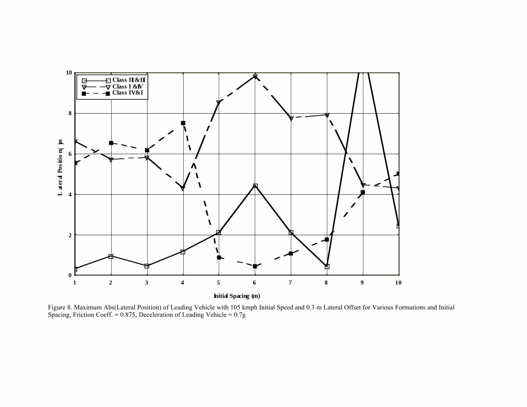
In the simulation results shown in Figures 4-7, the tire-roadway friction coefficient is assumed to be 0.7 and theleading vehicle is braking with a deceleration of 0.7 g. Since the vehicle is utilizing the full deceleration capability,the directional stability is lost. As a result, the leading vehicle, upon impact, has a tendency to spin. This can beobserved from the large values of yaw angle in Figure 6. A separate series of cases is simulated with an assumedtire-roadway friction coefficient of 0.875 while the leading vehicle is braking at 80% capacity, resulting also a 0.7 gdeceleration. Figure 8-11 are counterparts of Figures 4-7 depicting the simulation results in the second series. Asillustrated, the yaw angle is somehow smaller in the large spacing cases but the lateral deviation is much greater.This is because the leading vehicle will spin less but move more in the translational mode. Although the Ònon-locking brakeÓ case shows more lateral deviations in Figure 9, these results represent the cases when no follow-upactions are taken. If control actions taken after the collision involve steering inputs, then the Ònon-locking brakeÓbecomes significant because it allows directional control, while the ÒlockingÓ case will not permit meaningfulsteering input.
POST-COLLISION VEHICLE MANEUVERS
The simulation results from previous studies demonstrated that control actions are necessary to correct or maintainthe vehicle motion in its intended path. Without corrective actions, the vehicles can either travel out of its path tocollide with other traffic or lose control with excessive translation and rotation. To examine the feasibility of suchactions, several types of vehicle maneuvers are simulated to follow up the scenario described in the previous section:(1) After the initial collision, the following vehicle makes a lane-change maneuver with steering input to avoidfurther impacts;(2) After failing to activate braking, the following vehicle initiates a lane-change attempt with steering input toavoid impacts or to minimize the collision magnitude;(3) After the initial failure, the following vehicle activates an emergency braking actuator with a delay to reduce itsspeed and to mitigate collision magnitude;(4) After the initial collision, the following vehicle uses steering input to maintain its own path in the original lane.All of these scenarios assume that the vehicles are operable after the initial collision to the extent that the requiredactuation, braking or steering, are still functional. The implications and consequences of these scenarios areexplained below.
In the previous section, the simulated scenario assumes two possible types of failure conditions. One involves afailure event in which the following vehicle fails to activate the braking function. If the event represents a totalbreakdown of the braking system, the following vehicle will continue to lack the braking ability in the followingperiod. Therefore, the first two follow-on actions given above make an attempt to steer away from the deceleratingleading vehicle before or after the first collision. Obviously the second maneuver scenario is a better alternative thanthe first if the collision can be avoided at all. However, both of these actions require a decision making process withthe following considerations: 1) The steering function needs to be operable; 2) There is an adjacent lane that is opento accept the lane changing vehicle; and 3) the vehicle has the ability to detect or learn about such availability. Keepin mind that the lane-changing vehicle has a brake failure and will continue to move at a considerable speed evenafter a successful maneuver. Some further follow-up actions or procedures, such as energy-absorbing soft barriers tostop the vehicle, are required.
The third follow-up maneuver scenario suggests that an ÒemergencyÓ brake be applied after the initial collision witha time delay. This action represents a condition where the Òphysical capability of brakingÓ is not lost but thedecision making process has failed to activate. It can also imply a system in which a separate ÒswitchÓ for thebraking system is built into the vehicle. This switch is activated by a collision sensor. Again, the basic assumptionis that the braking system is still ÒphysicallyÓ intact and functional in the collision process.
The fourth follow-up maneuver scenario utilizes the steering input of the following vehicle to perform its ÒlanekeepingÓ function. Further collisions with the leading vehicle are likely to occur but the magnitude of impact willconitnue to decrease as both vehicles slow down. This action can be explained as an alternative to utilize thestopping capability of the leading vehicle to stop the motions of both vehicles. This action avoids the difficulty ofdecision making for lane changing but it still requires the ability of both vehicles to perform lane tracking in acollision process involving multiple impacts.
The risks of vehicle damage and occupant injuries in these follow-up actions should be evaluated on a case-by-casebasis and require further studies. However, the follow-up actions involve the emergency handling logistics
5
embedded in the design process of automated vehicles and they should be weighed carefully. For example, withManeuvers One and Two, the attempt is made to move the failure vehicle away from the other vehicle and to bringit to a stop through other methods. On the other hand, Maneuver Four sacrifices the leading vehicle by utilizing itsstopping capability to decelerate the failure vehicle. Such ÒunselfishÓ approach may be acceptable if the collisionmagnitude can be determined to be small.
While proposing vehicle maneuvers, we are hoping to resolve answer the following main questions or concerns:(1) the feasibility of conducting steering functions for lane tracking or lane changing in a collision process;(2) the type of steering inputs needed to perform such functions;(3) the effectiveness of delayed emergency braking on the vehicle motions;(4) the comparison of vehicle trajectories and vehicle status in different follow-up scenarios.
SIMULATION RESULTS
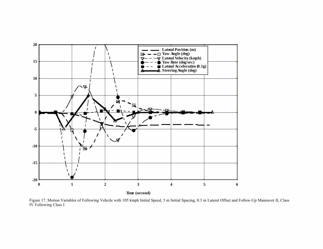
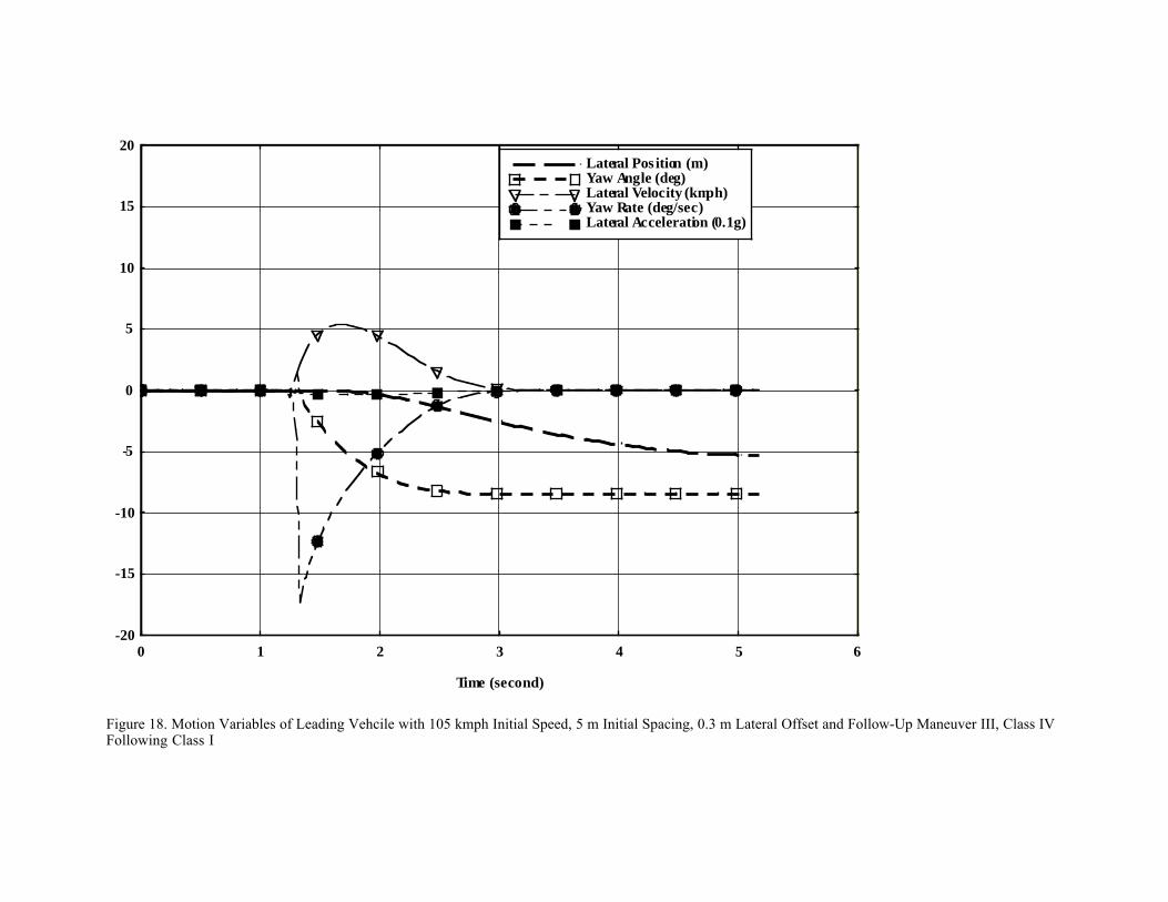
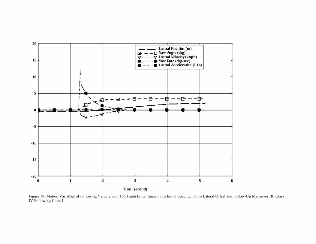
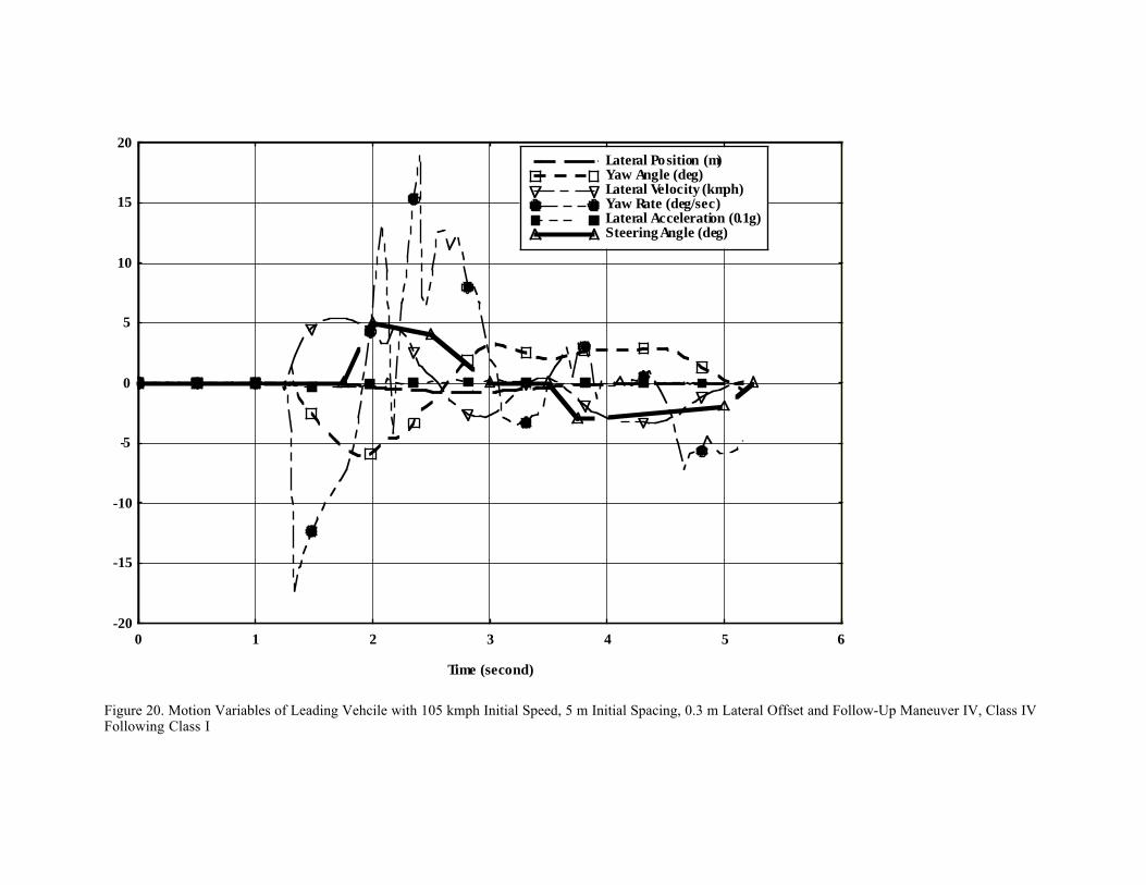
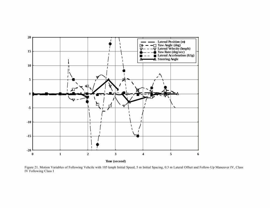
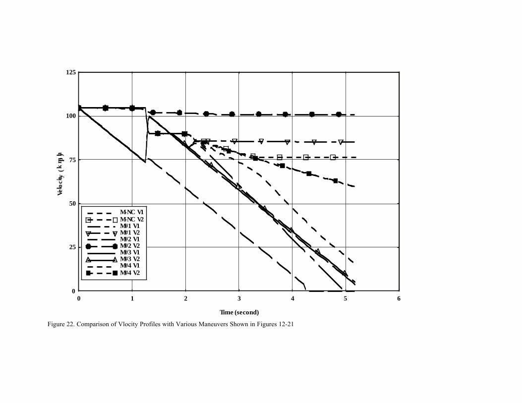
In the simulation of Maneuver One, the steering input to change lanes for the following vehicle is initiated at 1.71seconds, about 0.5 seconds after the initial impact. In Maneuver Two, the steering action is activated at 0.5 seconds.Both of these scenarios assume that a time period of 0.5 seconds is needed for the decision making process to startthe action. The steering angle inputs are selected to complete a 3.6 m (12 ft) lane change. During the lane change,subsequent contacts between vehicles continue to occur, therefore causing the steering inputs to be different fromtypical lane change maneuvers. In Maneuver Three, a deceleration of 0.7 g on the following vehicle is assumed to beinitiated at 0.5 seconds, representing an emergency braking capability activated after the collision. No steeringinputs are used in this scenario. In Maneuver Four, steering inputs are applied on both vehicles to maintain bothvehicles in the lane but no braking is applied to the following vehicle. In all maneuver scenarios, the braking on theleading vehicle remains at 0.7 g throughout the simulation.
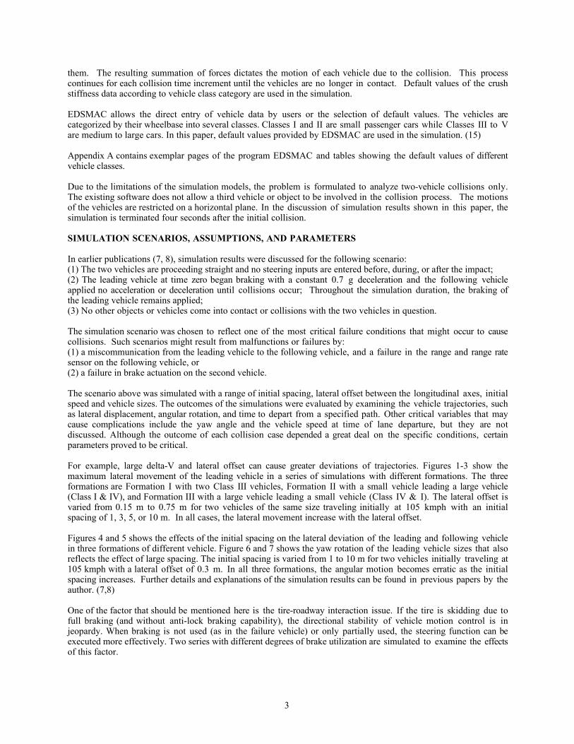
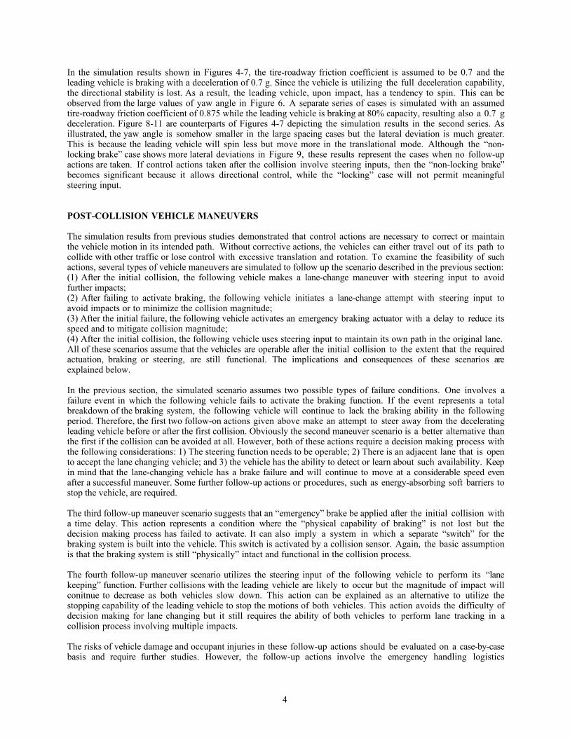
Table 1 and 2 show the vehicle status and positions of the leading and the following vehicles in differentmaneuvers. Table 1 contains the results from a case of a large vehicle following a small vehicle, and Table 2 from acase of a small vehicle following a large vehicle. It should be noted that although in Maneuver 2 the followingvehicle makes a lane-change attempt, a collision still occurs before the lane change is completed. This collisioninvolves a front corner of the following vehicle and a rear corner of the leading vehicle and results in a lowest delta-V impact among all maneuvers. As a result, the following vehicle has the highest speed and travels the longestdistance at the termination of the simulation, as indicated in both tables. Maneuver 4, with steering inputs fromboth vehicles, is most efficient in keeping both vehicles in the original lane. If the braking capability in thefollowing vehicle is lost (as in Maneuvers 1, 2, and 4), Maneuver 4 appears to be a reasonable approach to slowdown both vehicles while maintaining vehicles in the original lane. With an emergency braking capability,Maneuver 3 is able to bring the speeds of both vehicles to a much lower level.
Table 1 Class I v. Class IV, v1= v2= 105 kmph, a1= -0.7 g, f = 0.875Leading Vehicle
Lateral PositionRange (m)
Yaw Angle Range(deg)
Final TotalSpeed (kmph)
Final YawAngle (deg)
Final Position (m)
No Action -8.55, 0.06 -192.29, 0.00 15.372 -192.29 98.91, -8.55Maneuver 1 -4.12, 0.06 -142.99, 0.00 0.08 -142.78 87.42, -4.12Maneuver 2 -0.00, 0.47 0.00, 0.88 0.00 0.27 64.70, 0.46Maneuver 3 -5.29, 0.06 -8.47, 0.00 3.89 -8.47 87.80, -5.29Maneuver 4 -0.74, 0.06 -6.04, 3.20 59.71 -0.58 114.33, -0.02
Following Vehicle with an intial offset of 0.30 mLateral PositionRange (m)
Yaw Angle Range(deg)
Final TotalSpeed (m/sec)
Final YawAngle (deg)
Final Position (m)
No Action -6.75, 0.25 -9.39, 2.92 76.30 -7.92 114.91, -6.75Maneuver 1 -0.32, 3.76 -1.69, 7.97 85.23 0.32 120.57, 3.60Maneuver 2 -4.19, -0.31 -10.89, 3.39 101.01 -0.23 136.70, -3.72Maneuver 3 -0.32, 2.09 0.00, 3.33 5.16 3.33 84.57, 2.09Maneuver 4 -0.32, 0.40 -6.20, 5.41 60.00 0.42 110.21, 0.40
6
Table 2 Class IV v. Class I, v1= v2= 105 kmph, a1= -0.7 g, f = 0.875Leading Vehicle
Lateral PositionRange (m)
Yaw Angle Range(deg)
Final TotalSpeed (kmph)
Final YawAngle (deg)
Final Position (m)
No Action 0.00, 0.88 0.00, 1.48 0.00 1.21 75.46, 0.88Maneuver 1 0.00, 0.95 0.00, 1.60 0.00 1.60 74.64, 0.94Maneuver 2 -0.63, 0.02 -1.75, 0.00 0.00 -1.75 62.54, -0.63Maneuver 3 0.00, 0.91 0.00, 1.47 3.68 1.47 74.50, 0.91Maneuver 4 0.00, 0.98 -5.01, 4.48 19.40 4.48 87.20, 0.82
Following Vehicle with an intial offset of 0.30 mLateral PositionRange (m)
Yaw Angle Range(deg)
Final TotalSpeed (m/sec)
Final YawAngle (deg)
Final Position (m)
No Action -5.64, -0.31 -4.41, 0.01 74.26 -4.41 107.77, -5.64Maneuver 1 -3.57, -0.31 -8.39, 0.01 75.90 -0.04 109.86, -3.57Maneuver 2 -3.81, -0.31 -9.92, 0.76 100.95 0.13 136.35, -3.66Maneuver 3 -1.39, -0.31 -6.10, 0.01 0.00 -6.10 63.63, -1.39Maneuver 4 -0.98, 0.41 -3.32, 11.14 19.53 1.29 82.97, -0.15
Figure 12 and 13 depicts several variables representing the motion of the leading and following vehicles in asimulation with no follow-up actions in Table 1. Figures 14-21 are the corresponding plots for maneuvers 1-4. Inthese figures, the lateral position and speed, yaw angle and yaw rate, lateral acceleration and steering angle at thefront wheel are plotted. In these cases, a leading small vehicle and a following large vehicle are both traveling at105 kmph with an initial spacing of 5 m and a lateral offset of 0.3 m. At time 0, the leading vehicle begins brakingat a deceleration of 0.7 g and at 1.21 seconds the first collision occurs. In Maneuver 1, roughly 0.5 seconds after thefirst impact, steering actions are taken on the following vehicle in an attempt to change lanes. In Maneuver 2, attime = 0.5 seconds (0.5 seconds after the initial failure), steering actions are taken on the following vehicle in anattempt to change lanes. In Maneuver 3, at time = 0.5 seconds (0.5 seconds after the initial failure), emergencybraking is applied on the following vehicle, but no steering actions are taken on both vehicles. In Maneuver 4,roughly 0.5 seconds after the first impact, steering actions are taken on both vehicles to maintain both vehicles inthe original lane.
Figure 22 compares the velocity profiles of both vehicles in the four different maneuvers and the original simulationwhere no actions are taken In Table 1. It can be seen that Maneuver 3 brings the final speeds down to the lowestlevels because the braking of the following vehicle is activated after the first impact. Maneuver 2 yields the highestspeed of the following vehicle because the lane change maneuver is initiated before the first collision occurs. It isnoteworthy that delta-V in subsequent collisions in Maneuver 4 gradually decreases. This is significant because thestrategy deployed in Maneuver 4 is only sensible when the subsequent collisions cause less severe damage tovehicles and injuries to occupants in subsequent impacts.
Using the initial and final speeds of both vehicles for calculation, the ÒequivalentÓ stopping deceleration are 0.25gand 0.46g respectively for Maneuver 4 in Tables 1 and 2. This ÒequivalentÓ deceleration represents the effectivebraking capability of both vehicles without braking power in the following vehicle. The difference in thedeceleration in both cases is caused by the vehicle weight differential. In the simulation program, a Class I vehiclehas a default weight of 1000 kgs (2202 lbs) and Class IV a weight of 1928 kgs (4247 lbs).
The magnitude of steering angle and the timing of steering and braking inputs in these maneuvers are determinedafter a few iterations of simulation by an ad hoc approach. Since the maneuver objectives are well defined, theselection of steering inputs is accomplished in a few iterations. The values selected in these simulations arereasonable but they will ultimately depend on the design specifications of automated vehicles and controlalgorithms.
One issue that is not discussed in this paper is the effects of operational variables and vehicle maneuvers on vehicledamage. It should be noted that vehicle damage or structural deformation is not linear or additive in multiplecollisions. For example, two collisions of 10 kmph delta-V on the same region of a vehicle are not likely togenerate the same degree of damage when compared to a single 20 kmph collision. Sophisticated modeling and
7
reliable crush measurement data are needed for accurate estimates of vehicle damage in multiple collisions. Athorough investigation into this problem may lead to certain guidelines of structural requirements and the effects ofcollisions on the integrity of control systems and vehicle operability.
SUMMARY
This report reviews the effects of certain operational parameters on the post-impact vehicle trajectories. Simulationsof vehicle-following collisions show that large lateral offset and large initial spacing can result in significant pathdeviations or vehicle rotation and cause quick departure from the original traveling lane. The speed-differential ordelta-V in collision appears to be a significant factor of the collision outcome in typical highway operations, asreflected in the large initial-spacing cases. The results also indicate that without control actions, the vehiclesinvolved in a collision can be out of their lanes within 1 to 3 seconds.
Several maneuvers are proposed to examine the feasibility of controlling vehicle motions during or after collisions.These maneuvers involve the use of steering and/or braking inputs on one or both vehicles. The results demonstratelane-change or lane-keeping functions can be accomplished in the representative scenarios. An emergency brakingfunction, if implemented, will be desirable to reduce the vehicle speed and their traveling distance.
The understanding of vehicle motions in collisions is an important element in evaluating the safety hazards andbenefits of automated vehicles. The use of two-dimensional crash models allows the examination of lateral androtational movement. These simulations enable the assessment of operational parameters as well as the controlinputs in crash conditions. A continuation of this work should include the implementation of a closed-loop controlmodel with the crash and dynamic models. Efforts in developing a model with similar features for multiple vehiclecollisions are also considered.
ACKNOWLEDGMENTS
This work was performed as part of the California PATH Program of the University of California in cooperationwith the state of California Business, Transportation, and Housing Agency, Department of Transportation; and theUnited States Department of Transportation, Federal Highway Administration.
The contents of this paper reflect the views of the author who is responsible for the facts and the accuracy of the datapresented herein. The contents do not necessarily reflect the official views or policies of the State of California.This report does not constitute a standard, specification, or regulation.
The author would like to thank Engineering Dynamics Corporation for providing a library version of the simulationprogram. The program was used extensively in this study.
8
REFERENCES1. Shladover, S.E., ÒDynamic Entrainment of Automated Guideway Transit VehiclesÓ, High Speed Ground
Transportation Journal, Vol. 12, No. 3, pp 87-113, 1978.2. Shladover, S.E., ÒLongitudinal Control of Automotive Vehicles in Close-Formation Platoons,Ó ASME Journal
of Dynamic Systems, Measurement and Control, Vol. 113, pp. 231-241, 1991.3. Hitchcock, A., ÒIntelligent Vehicle Highway System Safety: Multiple Collisions in Automated Highway
Systems,Ó California PATH Research Report, UCB-ITS-PRR-95-10.4. Tongue, B.H., Yang, Y-T, ÒPlatoon Collision Dynamics and Emergency Maneuvering II: Platoon Simulations
for Small Disturbances,Ó California PATH Research Report, UCB-ITS-PRR-94-04.5. Tongue B. H., Yang, Y-T, ÒPlatoon Collision Dynamics and Emergency Maneuvering III: Collision Models
and Simulations,Ó California PATH Research Report, UCB-ITS-PRR-94-02.6. Tongue, B.H., Yang, Y-T., ÒPlatoon Collision Dynamics and Emergency Maneuvering IV: Intraplatoon
Collision Behavior and A New Control Approach for Platoon Operation During Vehicle Exit/Entry,Ó PATHResearch Report, UCB-ITS-PRR-94-25.
7. Chan, C., ÒStudies of Collisions in Vehicle Following Operations by Two-Dimensional Impact Simulations,ÓITS American, Sixth Annual Meeting, Houston, April 1996.
8. Chan, C., ÒCollision Analysis of Vehicle Following Operations in Automated Highway Systems,Ó ThirdWorld Congress on Intelligent Transport Systems, Orlando, October 1996.
9. McHenry, R.R., ÒDevelopment of a Computer Program to Aid the Investigation of Highway Accidents,ÓCalspan Report No. VJ-2979-V-1, DOT HS 800 821, December 1971.
10. Solomon, P.L., ÒThe Simulation Model of Automobile Collisions (SMAC) OperatorÕs Manual,Ó US DOT,NHTSA, Accident Investigation Division, 1974.
11. Noga, T., Oppenheim, T., ÒCRASH3 UserÕs Guide and Technical Manual,Ó U.S. DOT, January, 1981.12. Day, T., R.L. Hargens, ÒDifferences between EDCRASH and CRASH3,Ó SAE Paper No. 850253.13. Day, T., Hargens, R., ÒAn Overview of the Way EDSMAC Computes Delta-V,Ó SAE Paper No. 880069,
Society of Automotive Engineers, 1988.14. Engineering Dynamics Corporation, EDCRASH, ÒReconstruction of Accident Speeds on the Highway,Ó
Version 4.5, June 1989.15. Engineering Dynamics Corporation, EDSMAC, ÒSimulation Model of Automobile Collisions,Ó Version 2.4,
May 1989.16. Jones, I.S., ÒResults of Selected Applications to Actual Highway Accidents of the SMAC Reconstruction
Program, Ò SAE Paper No. 741179, 1974.17. Jones, I.S., ÒThe Application of the SMAC Accident Reconstruction Program to Actual Highway Accidents,Ó
Proceedings of the Eighteenth Conference of the American Association of Automotive Medicine, 1974.18. Smith, R.S., Noga, J.T., ÒAccuracy and Sensitivity of CRASH,Ó National Center for Statistics and Analysis,
NHTSA, January 1982.19. Prasad, A.K., ÒCRASH3 Damage Algorithm Reformulation for Front and Rear Collisions,Ó SAE Paper No.
900098.20. ÒCollision Deformation Classification,Ó SAE Technical Report J224 MAR80, March 1980.21. Day, T., Hargens, R., ÒApplication and Misapplication of Computer Programs for Accident Reconstructions,Ó
SAE Paper No. 890738, 1989.
APPENDIX A
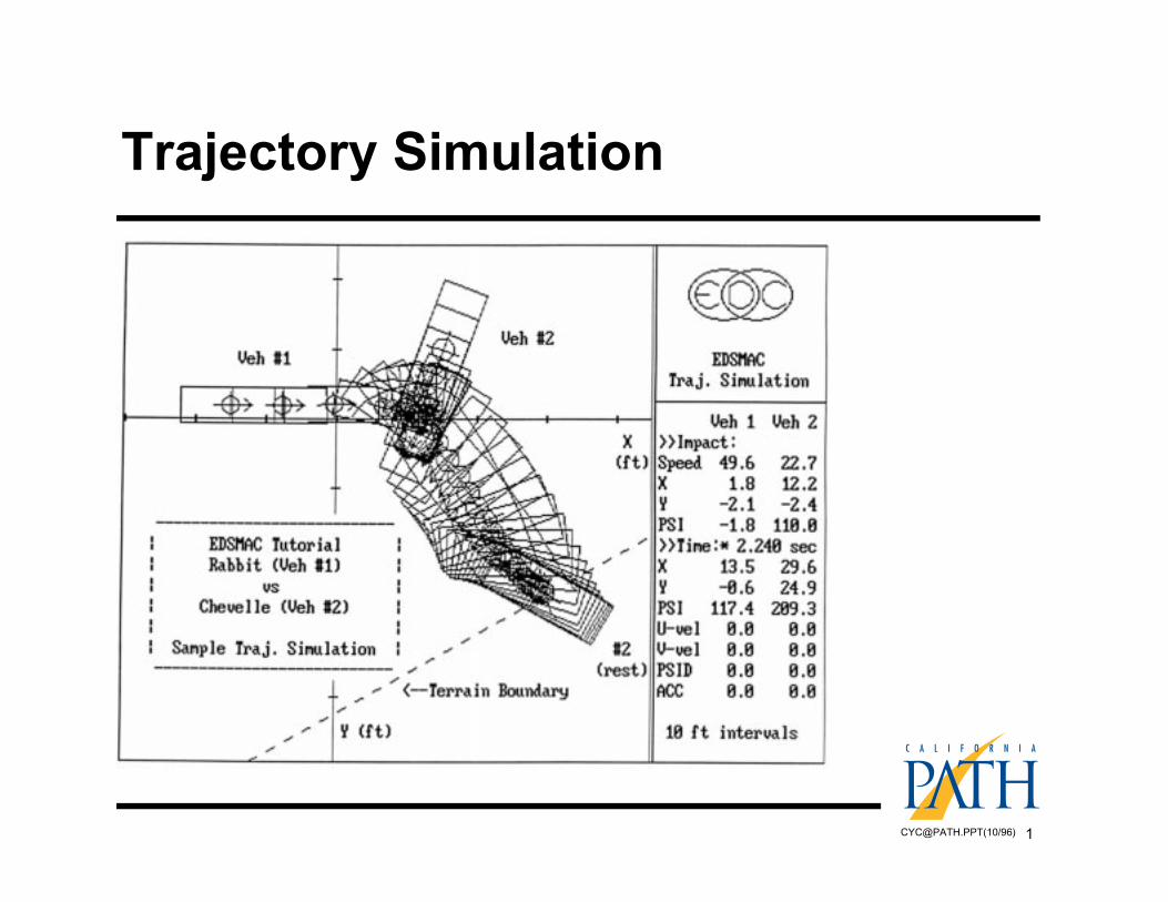
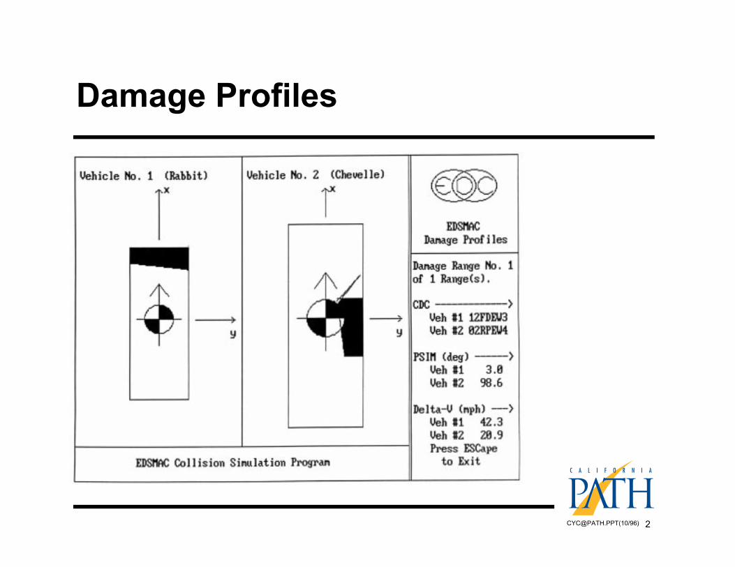
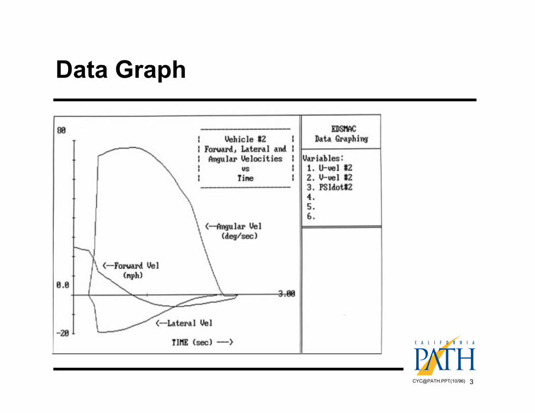
The following figures are pages from the userÕs manual of EDSMAC. (13)
No. Title of Figures1. A typical screen display of an EDSMAC simulation.2. A post-simulation display of vehicle damage.3. A graphic illustration of selected variables of an EDSMAC simulation.4. The classification of vehicle sizes by their wheel base and the default values of vehicle parameters.5. Different classes of vehicle stiffness and exemplar vehicles.
9
LIST OF FIGURES
No. Title of Figures1. Maximum Lateral Position of Leading Vehicle with Class III Leading and Class III Following for Various
Spacing and Lateral Offset2. Maximum Lateral Position of Leading Vehicle with Class I Leading and Class IV Following for Various
Spacing and Lateral Offset3. Maximum Lateral Position of Leading Vehicle with Class IV Leading and Class I Following for Various
Spacing and Lateral Offset4. Maximum Abs(Lateral Position) of Leading Vehicle with 105 kmph Initial Speed and 0.3 m Lateral Offset for
Various Formations and Initial Spacing, Friction Coeff. = 0.7, Deceleration of Leading Vehicle = 0.7g5. Maximum Abs(Lateral Position) of Following Vehicle with 105 kmph Initial Speed and 0.3 m Lateral Offset
for Various Formations and Initial Spacing, Friction Coeff. = 0.7, Deceleration of Leading Vehicle = 0.7g6. Maximum Abs(Yaw Angle) of Leading Vehicle with 105 kmph Initial Speed and 0.3 m Lateral Offset for
Various Formations and Initial Spacing, Friction Coeff. = 0.7, Deceleration of Leading Vehicle = 0.7g7. Maximum Abs(Yaw Angle) of Following Vehicle with 105 kmph Initial Speed and 0.3 m Lateral Offset for
Various Formations and Initial Spacing, Friction Coeff. = 0.7, Deceleration of Leading Vehicle = 0.7g8. Maximum Abs(Lateral Position) of Leading Vehicle with 105 kmph Initial Speed and 0.3 m Lateral Offset for
Various Formations and Initial Spacing, Friction Coeff. = 0.875, Deceleration of Leading Vehicle = 0.7g9. Maximum Abs(Lateral Position) of Following Vehicle with 105 kmph Initial Speed and 0.3 m Lateral Offset
for Various Formations and Initial Spacing, Friction Coeff. = 0. 875, Deceleration of Leading Vehicle = 0.7g10. Maximum Abs(Yaw Angle) of Leading Vehicle with 105 kmph Initial Speed and 0.3 m Lateral Offset for
Various Formations and Initial Spacing, Friction Coeff. = 0. 875, Deceleration of Leading Vehicle = 0.7g11. Maximum Abs(Yaw Angle) of Following Vehicle with 105 kmph Initial Speed and 0.3 m Lateral Offset for
Various Formations and Initial Spacing, Friction Coeff. = 0. 875, Deceleration of Leading Vehicle = 0.7g12. Motion Variables of Leading Vehcile with 105 kmph Initial Speed, 5 m Initial Spacing, 0.3 m Lateral Offset
and No Follow-Up Maneuvers, Class IV Following Class I13. Motion Variables of Following Vehcile with 105 kmph Initial Speed, 5 m Initial Spacing, 0.3 m Lateral Offset
and No Follow-Up Maneuvers, Class IV Following Class I14. Motion Variables of Leading Vehcile with 105 kmph Initial Speed, 5 m Initial Spacing, 0.3 m Lateral Offset
and Follow-Up Maneuver I, Class IV Following Class I15. Motion Variables of Following Vehcile with 105 kmph Initial Speed, 5 m Initial Spacing, 0.3 m Lateral Offset
and Follow-Up Maneuver I, Class IV Following Class I16. Motion Variables of Leading Vehcile with 105 kmph Initial Speed, 5 m Initial Spacing, 0.3 m Lateral Offset
and Follow-Up Maneuver II, Class IV Following Class I17. Motion Variables of Following Vehcile with 105 kmph Initial Speed, 5 m Initial Spacing, 0.3 m Lateral Offset
and Follow-Up Maneuver II, Class IV Following Class I18. Motion Variables of Leading Vehcile with 105 kmph Initial Speed, 5 m Initial Spacing, 0.3 m Lateral Offset
and Follow-Up Maneuver III, Class IV Following Class I19. Motion Variables of Following Vehcile with 105 kmph Initial Speed, 5 m Initial Spacing, 0.3 m Lateral Offset
and Follow-Up Maneuver III, Class IV Following Class I20. Motion Variables of Leading Vehcile with 105 kmph Initial Speed, 5 m Initial Spacing, 0.3 m Lateral Offset
and Follow-Up Maneuver IV, Class IV Following Class I21. Motion Variables of Following Vehcile with 105 kmph Initial Speed, 5 m Initial Spacing, 0.3 m Lateral Offset
and Follow-Up Maneuver IV, Class IV Following Class I22. Comparison of Vlocity Profiles with Various Maneuvers Shown in Figures 12-21
-2
0
2
4
6
8
0.15 0.30 0.45 0.60 0.75
1 m initial spacing3 m initial spacing5 m initial spacing10 m initial spacing
Initial Lateral Offset (m)
Lat
eral
Po
siti
on (
m )
Figure 1. Maximum Lateral Position of Leading Vehicle with Class III Leading and Class III Following for Various Spacing and Lateral Offset
-2
0
2
4
6
8
0.15 0.30 0.45 0.60 0.75
1 m initial spacing3 m initial spacing5 m initial spacing10 m initial spacing
Initial Lateral Offset (m)
Lat
eral
Po
siti
on (
m )
Figure 2. Maximum Lateral Position of Leading Vehicle with Class I Leading and Class IV Following for Various Spacing and Lateral Offset
-2
0
2
4
6
8
0.15 0.30 0.45 0.60 0.75
1 m initial spacing3 m initial spacing5 m initial spacing10 m initial spacing
Initial Lateral Offset (m)
Lat
eral
Po
siti
on (
m )
Figure 3. Maximum Lateral Position of Leading Vehicle with Class IV Leading and Class I Following for Various Spacing and Lateral Offset
0
2
4
6
8
10
1 2 3 4 5 6 7 8 9 10
Class III & IIIClass I & IVClass IV & I
Initial Spacing (m)
Lat
eral
Po
siti
on (
m )
Figure 4. Maximum Abs(Lateral Position) of Leading Vehicle with 105 kmph Initial Speed and 0.3 m Lateral Offset for Various Formations and InitialSpacing, Friction Coeff. = 0.7, Deceleration of Leading Vehicle = 0.7g
0
2
4
6
8
10
1 2 3 4 5 6 7 8 9 10
Class III & IIIClass I & IVClass IV & I
Initial Spacing (m)
Lat
eral
Po
siti
on (
m )
Figure 5. Maximum Abs(Lateral Position) of Following Vehicle with 105 kmph Initial Speed and 0.3 m Lateral Offset for Various Formations and InitialSpacing, Friction Coeff. = 0.7, Deceleration of Leading Vehicle = 0.7g
0
60
120
180
240
300
360
1 2 3 4 5 6 7 8 9 10
Class III & IIIClass I & IVClass IV & I
Initial Spacing (m)
Yaw
Angl
e (d
e gre
e )
Figure 6. Maximum Abs(Yaw Angle) of Leading Vehicle with 105 kmph Initial Speed and 0.3 m Lateral Offset for Various Formations and Initial Spacing,Friction Coeff. = 0.7, Deceleration of Leading Vehicle = 0.7g
0
10
20
30
40
50
60
1 2 3 4 5 6 7 8 9 10
Class III & IIIClass I & IVClass IV & I
Initial Spacing (m)
Yaw
Angl
e (d
e gre
e )
Figure 7. Maximum Abs(Yaw Angle) of Following Vehicle with 105 kmph Initial Speed and 0.3 m Lateral Offset for Various Formations and Initial Spacing,Friction Coeff. = 0.7, Deceleration of Leading Vehicle = 0.7g
0
2
4
6
8
10
1 2 3 4 5 6 7 8 9 10
Class III & II IClass I & IVClass IV & I
Initial Spacing (m)
Lat
eral
Po
siti
on (
m )
Figure 8. Maximum Abs(Lateral Position) of Leading Vehicle with 105 kmph Initial Speed and 0.3 m Lateral Offset for Various Formations and InitialSpacing, Friction Coeff. = 0.875, Deceleration of Leading Vehicle = 0.7g
0
2
4
6
8
10
1 2 3 4 5 6 7 8 9 10
Class III & IIIClass I & IVClass IV & I
Initial Spacing (m)
Lat
eral
Po
siti
on (
m )
Figure 9. Maximum Abs(Lateral Position) of Following Vehicle with 105 kmph Initial Speed and 0.3 m Lateral Offset for Various Formations and InitialSpacing, Friction Coeff. = 0. 875, Deceleration of Leading Vehicle = 0.7g
0
60
120
180
240
300
360
1 2 3 4 5 6 7 8 9 10
Class III & IIIClass I & IVClass IV & I
Initial Spacing (m)
Yaw
Angl
e (d
e gre
e )
Figure 10. Maximum Abs(Yaw Angle) of Leading Vehicle with 105 kmph Initial Speed and 0.3 m Lateral Offset for Various Formations and Initial Spacing,Friction Coeff. = 0. 875, Deceleration of Leading Vehicle = 0.7g
0
60
120
180
240
300
360
1 2 3 4 5 6 7 8 9 10
Class III & IIIClass I & IVClass IV & I
Initial Spacing (m)
Yaw
Angl
e (d
e gre
e )
Figure 11. Maximum Abs(Yaw Angle) of Following Vehicle with 105 kmph Initial Speed and 0.3 m Lateral Offset for Various Formations and Initial Spacing,Friction Coeff. = 0. 875, Deceleration of Leading Vehicle = 0.7g
-20
-15
-10
-5
0
5
10
15
20
0 1 2 3 4 5 6
Lateral Position (m)Yaw Angle (deg)Lateral Velocity (kmph)Yaw Rate (deg/sec)Lateral Acceleration (0.1g)
Time (second)
Figure 12. Motion Variables of Leading Vehcile with 105 kmph Initial Speed, 5 m Initial Spacing, 0.3 m Lateral Offset and No Follow-Up Maneuvers, ClassIV Following Class I
-20
-15
-10
-5
0
5
10
15
20
0 1 2 3 4 5 6
Lateral Pos ition (m)Yaw Angle (deg)Lateral Velocity (kmph)Yaw Rate (deg/sec)Lateral Acceleration (0.1g)
Time (second)
Figure 13. Motion Variables of Following Vehcile with 105 kmph Initial Speed, 5 m Initial Spacing, 0.3 m Lateral Offset and No Follow-Up Maneuvers, ClassIV Following Class I
-20
-15
-10
-5
0
5
10
15
20
0 1 2 3 4 5 6
Lateral Pos ition (m)Yaw Angle (deg)Lateral Velocity (kmph)Yaw Rate (deg/sec)Lateral Acceleration (0.1g)
Time (second)
Figure 14. Motion Variables of Leading Vehcile with 105 kmph Initial Speed, 5 m Initial Spacing, 0.3 m Lateral Offset and Follow-Up Maneuver I, Class IVFollowing Class I
-20
-15
-10
-5
0
5
10
15
20
0 1 2 3 4 5 6
Lateral Pos ition (m)Yaw Angle (deg)Lateral Velocity (kmph)Yaw Rate (deg/sec)Lateral Acceleration (0.1g)Steering Angle (deg)
Time (second)
Figure 15. Motion Variables of Following Vehcile with 105 kmph Initial Speed, 5 m Initial Spacing, 0.3 m Lateral Offset and Follow-Up Maneuver I, Class IVFollowing Class I
-20
-15
-10
-5
0
5
10
15
20
0 1 2 3 4 5 6
Lateral Pos ition (m)Yaw Angle (deg)Lateral Velocity (kmph)Yaw Rate (deg/sec)Lateral Acceleration (0.1g)
Time (second)
Figure 16. Motion Variables of Leading Vehcile with 105 kmph Initial Speed, 5 m Initial Spacing, 0.3 m Lateral Offset and Follow-Up Maneuver II, Class IVFollowing Class I
-20
-15
-10
-5
0
5
10
15
20
0 1 2 3 4 5 6
Lateral Pos ition (m)Yaw Angle (deg)Lateral Velocity (kmph)Yaw Rate (deg/sec)Lateral Acceleration (0.1g)Steering Angle (deg)
Time (second)
Figure 17. Motion Variables of Following Vehcile with 105 kmph Initial Speed, 5 m Initial Spacing, 0.3 m Lateral Offset and Follow-Up Maneuver II, ClassIV Following Class I
-20
-15
-10
-5
0
5
10
15
20
0 1 2 3 4 5 6
Lateral Pos ition (m)Yaw Angle (deg)Lateral Velocity (kmph)Yaw Rate (deg/sec)Lateral Acceleration (0.1g)
Time (second)
Figure 18. Motion Variables of Leading Vehcile with 105 kmph Initial Speed, 5 m Initial Spacing, 0.3 m Lateral Offset and Follow-Up Maneuver III, Class IVFollowing Class I
-20
-15
-10
-5
0
5
10
15
20
0 1 2 3 4 5 6
Lateral Pos ition (m)Yaw Angle (deg)Lateral Velocity (kmph)Yaw Rate (deg/sec)Lateral Acceleration (0.1g)
Time (second)
Figure 19. Motion Variables of Following Vehcile with 105 kmph Initial Speed, 5 m Initial Spacing, 0.3 m Lateral Offset and Follow-Up Maneuver III, ClassIV Following Class I
-20
-15
-10
-5
0
5
10
15
20
0 1 2 3 4 5 6
Lateral Position (m)Yaw Angle (deg)Lateral Velocity (kmph)Yaw Rate (deg/sec)Lateral Acceleration (0.1g)Steering Angle (deg)
Time (second)
Figure 20. Motion Variables of Leading Vehcile with 105 kmph Initial Speed, 5 m Initial Spacing, 0.3 m Lateral Offset and Follow-Up Maneuver IV, Class IVFollowing Class I
-20
-15
-10
-5
0
5
10
15
20
0 1 2 3 4 5 6
Lateral Position (m)Yaw Angle (deg)Lateral Velocity (kmph)Yaw Rate (deg/sec)Lateral Acceleration (0.1g)Steering Angle
Time (second)
Figure 21. Motion Variables of Following Vehcile with 105 kmph Initial Speed, 5 m Initial Spacing, 0.3 m Lateral Offset and Follow-Up Maneuver IV, ClassIV Following Class I
0
25
50
75
100
125
0 1 2 3 4 5 6
M-NC V1M-NC V2M#1 V1M#1 V2M#2 V1M#2 V2M#3 V1M#3 V2M#4 V1M#4 V2
Time (second)
Vel o
cit y
(km p
h )
Figure 22. Comparison of Vlocity Profiles with Various Maneuvers Shown in Figures 12-21