arX

iv:h

ep-t

h/96

1115

6v1

20

Nov

199

6

Coarse grainings and irreversibility in

quantum field theory

C. AnastopoulosTheoretical Physics Group, The Blackett Lab.

Imperial CollegeE-mail : can@tp.ph.ic.ac.uk

October 1996

Abstract

In this paper we are interested in the studying coarse-graining infield theories using the language of quantum open systems. Motivatedby the ideas of Calzetta and Hu [1] on correlation histories we employthe Zwanzig projection technique to obtain evolution equations for rel-evant observables in self-interacting scalar field theories. Our coarse-graining operation consists in concentrating solely on the evolutionof the correlation functions of degree less than n, a treatment whichcorresponds to the familiar from statistical mechanics truncation ofthe BBKGY hierarchy at the n-th level. We derive the equationsgoverning the evolution of mean field and two-point functions thusidentifying the terms corresponding to dissipation and noise. We dis-cuss possible applications of our formalism, the emergence of classicalbehaviour and the connection to the decoherent histories framework.

1

1 Introduction

Motivation Quantum field theory has a rich structure, which manifests it-self in the possibility of describing the same field system from diverse pointsof view. Hence, depending on the problem of interest one could focus forinstance on the Hamiltonian, the statistical or the particle aspects of thequantum field. This potentiality for description within different frameworks,inherent in quantum field theory is the cause of its large domain of applica-tions, but is also a source of interesting questions.

The more important one is to identify the level of observation in a fieldtheory or, putting it another way, what an actual observer measures in aquantum field. The answer to this question is not easy and it is clear thatthe level of observation cannot be fixed uniquely. Unlike non-relativisticquantum mechanics where one is essentially measuring phase space quanti-ties for a particle system spatially localized, in quantum field theory localmeasurements contain only a very small portion of information about thestate of the field. A local observer, will for instance be able to record onlythe mean field and the higher order correlation functions are inaccessible tohim. Therefore, for most of the possible configurations, he might lose allsense of predictability for the field observables.

This is closely connected with the problem of the classical limit of fieldtheories. In the context of the decoherent histories approach to quantummechanics, the classical domain corresponds to a set of coarse-grained andnon-interfering histories, from which one can obtain almost deterministicequations for a class of observables [15]. In our case there is a large number ofsuch classes. At low energies one might consider the particle-like behaviourof the fields and obtain in the classical limit a theory of interacting non-relativistic particles. Or one could concentrate on phase space histories,to see the extent to which QFT behaves as a Hamiltonian system. Or evenconsider histories of quantities like energy and momentum density and obtaina classical hydrodynamics description.

The above issues are also of value for early Universe cosmology. Thetransition from quantum to classical is of great importance in models ofinflation since many of its predictions are based on the fact that the longwavelength modes of the inflaton exhibit classical behaviour. When consid-ering the non-equilibrium dynamics of fields (mainly for the study of phasetransitions) the first point needed to be settled is what are the variables we

2

should concentrate, that contain the relevant information for the problem inhand.

The notion of natural coarse-graining in field theories is also important inthe context of field theories in curved spacetime. For it is only one quantitythat actually governs the backreaction dynamics of spacetime: the expecta-tion value of the field energy-momentum tensor (essentially constructed fromthe two-point correlation functions in the case of free fields).

To address these problems a number of techniques from non-equilibriumstatistical mechanics has been employed with varying degree of success: theFeynman-Vernon influence functional technique [7, 8, 9] and the close timepath formalism [13, 12]. It is the aim of this paper to exhibit the use of an-other powerful technique of statistical mechanics in a field theoretic context:the Zwanzig projection method (for a review see [14, 3, 10]). The great ad-vantage of this method lies in its wide range of possible applications: for anychoice of coarse-graining it can be applied once we are able to identify thecoarse graining operation with an indempotent map on the space of states.Our choice of coarse-graining is motivated by the ideas of Calzetta and Hu[1] on the truncation of the Schwinger-Dyson hierarchy of n-point functions.

But before discussing the approach we adopt at this paper, we find mean-ingful to give a short discussion on possible choices for coarse graining.

Coarse grainings There are two important constraints one might imposeon our possible choices for coarse-graining: naturality and Lorentz covariance.To see what we mean by naturality, let us consider cases of typical coarsegrainings in standard non-equilibrium statistical mechanics. A typical situa-tion is to separate relevant and irrelevant observables according to the orderof magnitude of some physical parameter characterizing them. Hence we canfor instance average out the effect of “fast” variables (evolving within veryshort timescales) or trace out the contribution of particles with the smallermasses (as is the case in quantum Brownian motion). Such a separation ofscales, while quite common in non-relativistic many particle systems is rarein relativistic quantum field theory. If possible it would involve a fine tuningof the the coupling constants and masses of the field systems as well as theimposition of a particular initial condition. In a generic systems it is unlikelythat such “autocratic ” coarse grainings can emerge naturally [1].

The requirement of Lorentz covariance, though it can be relaxed in a

3

number of situations (like for instance when non-relativistic matter is present[11]) is of great importance both for the cosmological applications and theemergence of classical behaviour for the field variables. For when we try tostudy a field system for first principles, there is no natural way a non-Lorentzinvariant quantity can be introduced in our schemes. Hence, for instance, acoarse graining taking the form of a high momentum cut-off for the fieldmodes should not be considered as fundamental but rather as emerging fromthe full dynamics of the theory under particular circumstances.

Besides those two a priori criteria for our choice of coarse graining, thereis an equally important one that can be considered only a posteriori, thatis after we have identified the dynamics of the relevant variables. This isthe requirement of persistent predictability for the evolution equations. Inthe language of the decoherent histories approach it states that histories ofrelevant observables ought to form a quasiclassical domain. This means thatthe evolution equations have to be approximately dynamically autonomous[3] (even though we cannot expect to obtain Markovian behaviour). Thisagain implies that the noise due to the irrelevant part of the field, thoughsufficient to decohere the histories of relevant observables is weak enough toallow a degree of predictability [15]. In general, this is expected to be possibleonly for a small class of initial states of our system (or the Universe forcosmological applications). This is a fact that we will verify in our analysis.

Truncation of the Schwinger-Dyson hierarchy The coarse-grainingoperation we shall examine, is one proposed by Calzeta and Hu [1]. They re-marked on the similarity of the chain of Dyson equations linking each Greenfunction to others of higher order with the BBKGY hierarchy of correlationfunctions in classical statistical mechanics. Since the set of expectation val-ues of field products contains all information about the state of the field, atruncation in the chain of Green function will form a natural coarse-grainingoperation and the lower order n-point functions will be our relevant observ-ables. The authors then proceed to compute the effective equations of motionfrom a master effective action using a generalizaion of the close time-pathformalism. The important feature of these equations is the presence of cor-relation noise, which under particular conditions may guarantee decoherenceof the “correlation histories”.

The truncation of the Schwinger-Dyson hierarchy does satisfy the condi-

4

tions of Lorentz covariance and naturality for the choice of the coarse grain-ing operation. First, this choice of coarse graining is closer to actual mea-surements of the quantum field since any finite measurement device cannotobtain information about arbitrarily high orders of correlation. Actually,a local observer might be expected to monitor only the mean field values.Second, being an intrinsically justifiable division between relevant and irrel-evant observables it can be applied to a wide variety of systems, withoutthe need to recourse to special arguments for each particular case. Third, itseems promising when trying to consider evolution of hydrodynamic quan-tities since quantities like energy and momentum density can be obtainedthrough the knowledge of low order correlation functions. In particular,when dealing with the backreaction problem in curved spacetime, trunca-tion of the hierarchy at the level n = 2 might give interesting results sincethe energy-momentum tensor determining backreaction can be determinedthrough the knowledge of 2-point functions.

As far as the third requirement of predictability is concerned, we needto have a detailed calculation of the dynamical evolution of the relevantobservables. Still, it is important to note, that the classical behaviour of thetwo point correlations observed at later stages, gives us at least a hint forthe possibility of an initial condition such that the dynamics of observablesobtained from a truncation at the level n = 2 are approximately autonomous.

The Zwanzig method To obtain the evolution equations for the relevantobservables, we are going to utilize, as mentioned earlier, the Zwanzig projec-tion technique. There is a number of reasons for believing that this providesan important calculational tool when dealing with the above isssues:1. It allows us to use a canonical formalism, hence gaining intuition bycomparison with well studied systems in non-relativistic quantum statisticalmechanics. Our results are still covariantly, though not manifestly, since wehave restricted ourselves to an invariant choice of coarse-graining.2. To perform a perturbation expansion for the equations of motion it issufficent to construct perturbatively the field propagator e−iHt. This is bestcarried out in the Fock representation [2], which turns out to be particularlyuseful for implementing our choice of coarse graining.3. We are allowed a certain degree of flexibility since the choice of the pro-jector onto the level of description is not unique [14]. Hence, depending on

5

the details of our problem (mainly the initial condition) we can choose aprojector so as to reduce the strength of the noise terms.4. It provides a straightforward relation between the initial state of the ir-relevant variables and the noise terms in the evolution equations.5. It does not depend on the particular dynamics of the full system, that isone can apply it even when the field evolution is non-unitary, non-Markovianor non-autonomous . Therefore, it might be used in conjunction with othermethods (in particular the influence functional technique) in order to reducethe amount of calculations needed for a particular problem.6. The Zwanzig method, is essentially algebraic, in the sense that it dependssolely on the properties of the space of observables and not on any particularrealization in some Hilbert space. This means that, at least in principle, onecan employ it in systems where quantum are coupled to classical variables asis the case of the field theory in curved spacetime.

This paper It is the aim of this paper to apply the above ideas in thesimplest of field systems, first to exhibit the technique and understand theinsight it can offer in particular for the case of quantum to classical transition.Hence, we concentrate on a single self-interacting scalar field in Minkowskispacetime and consider coarse-grainings corresponding to truncation at thelevels n = 1 and n = 2.

We mainly focus on two issues: the derivation of the effectiver equationfor the relevant variables and the estimation of strength of the noise term,which determines the degree of predictability of our preferred set of variables.

The paper is then organized as follows: In section 2 we give a brief re-view of the Zwanzig projection formalism, and construct the indempotentoperators that implement the coarse-graining operation in the space of ob-servables. In section 3, we derive the mean field dynamics ina λφ4 scalar fieldtheory and give a general discussion on the relation of correlation noise withthe initial condition. In section 4 we perform the same analysis for a gφ3

theory for the case of truncation at the level of two point functions. Finallyin section 5, we give a discussion of our results, on the possibility of obtainingMarkovin behaviour and on future applications of the formalism.

We have found more convenient to implement the coarse-graining on thenormal-ordered form of the observables. The expressions we obtain are sim-plified significantly if we use an index notation to denote products of creation

6

and annihilation operators a(x) and a†(x). The conventions of this notationare found in Appendix 1. Finally, some useful formulas concerning the Fockrepresentation and the normal form of operators are to be found in Appendix2.

2 The method

2.1 The Zwanzig technique

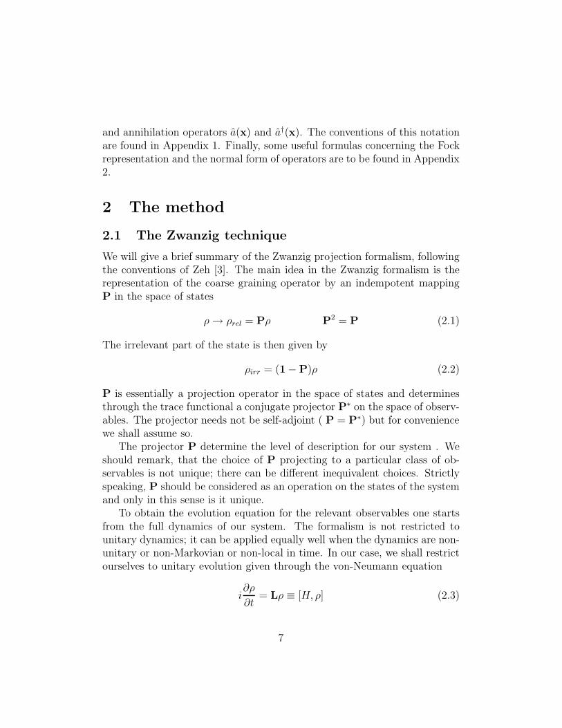
We will give a brief summary of the Zwanzig projection formalism, followingthe conventions of Zeh [3]. The main idea in the Zwanzig formalism is therepresentation of the coarse graining operator by an indempotent mappingP in the space of states

ρ → ρrel = Pρ P2 = P (2.1)

The irrelevant part of the state is then given by

ρirr = (1 − P)ρ (2.2)

P is essentially a projection operator in the space of states and determinesthrough the trace functional a conjugate projector P∗ on the space of observ-ables. The projector needs not be self-adjoint ( P = P∗) but for conveniencewe shall assume so.

The projector P determine the level of description for our system . Weshould remark, that the choice of P projecting to a particular class of ob-servables is not unique; there can be different inequivalent choices. Strictlyspeaking, P should be considered as an operation on the states of the systemand only in this sense is it unique.

To obtain the evolution equation for the relevant observables one startsfrom the full dynamics of our system. The formalism is not restricted tounitary dynamics; it can be applied equally well when the dynamics are non-unitary or non-Markovian or non-local in time. In our case, we shall restrictourselves to unitary evolution given through the von-Neumann equation

i∂ρ

∂t= Lρ ≡ [H, ρ] (2.3)

7

from which we obtain the following system of coupled differential equationsfor ρrel and ρirr

i∂ρrel

∂t= PLρrel + PLρirr (2.4)

i∂ρirr

∂t= (1 − P)Lρrel + (1 −P)Lρirr (2.5)

We can solve equation (2.5) by treationg the ρrel term as an external force

ρirr(t) = e−i(1−P)Ltρirr(0) − i∫ t

0dτe−i(1−P)Lτ (1 −P)Lρrel(t − τ) (2.6)

Here we have denoted by e−i(1−P)Lt = (1−P)e−iLt the evolution operator ofthe equation

i∂ρ

∂t= (1 −P)Lρ (2.7)

and no actual exponentiation is implied. Substituting (2.6) into (2.4) we getthe Zwanzig pre-master equation

i∂ρrel(t)

∂t= PLρrel(t) + PLe−i(1−P)Ltρirr(0) − i

∫ t

0dτG(τ)ρrel(t − τ) (2.8)

Here G stands for the kernel

G(τ) = PLe−i(1−P)Lτ (1 − P)LP (2.9)

Given then a relevant observable A, i.e. one such that PA = A, we obtainfor the evolution of its expectation value 〈A〉

i∂

∂t〈A〉(t) − 〈PLA〉(t)

+i∫ t

0dτ〈PL(1 −P)eiLτ (1 − P)LPA〉(t − τ) = FA(t) (2.10)

FA(t) is “driving force” term, essentially stochastic in nature, since it dependson the irrelevant components of the initial state that are inaccesible from ourlevel of description. It reads

FA(t) = −Tr(

ρ(0)[(1 − P)ei(1−P)LtLA])

(2.11)

Note, that in general the evolution of the relevant observables is non-localin time.

8

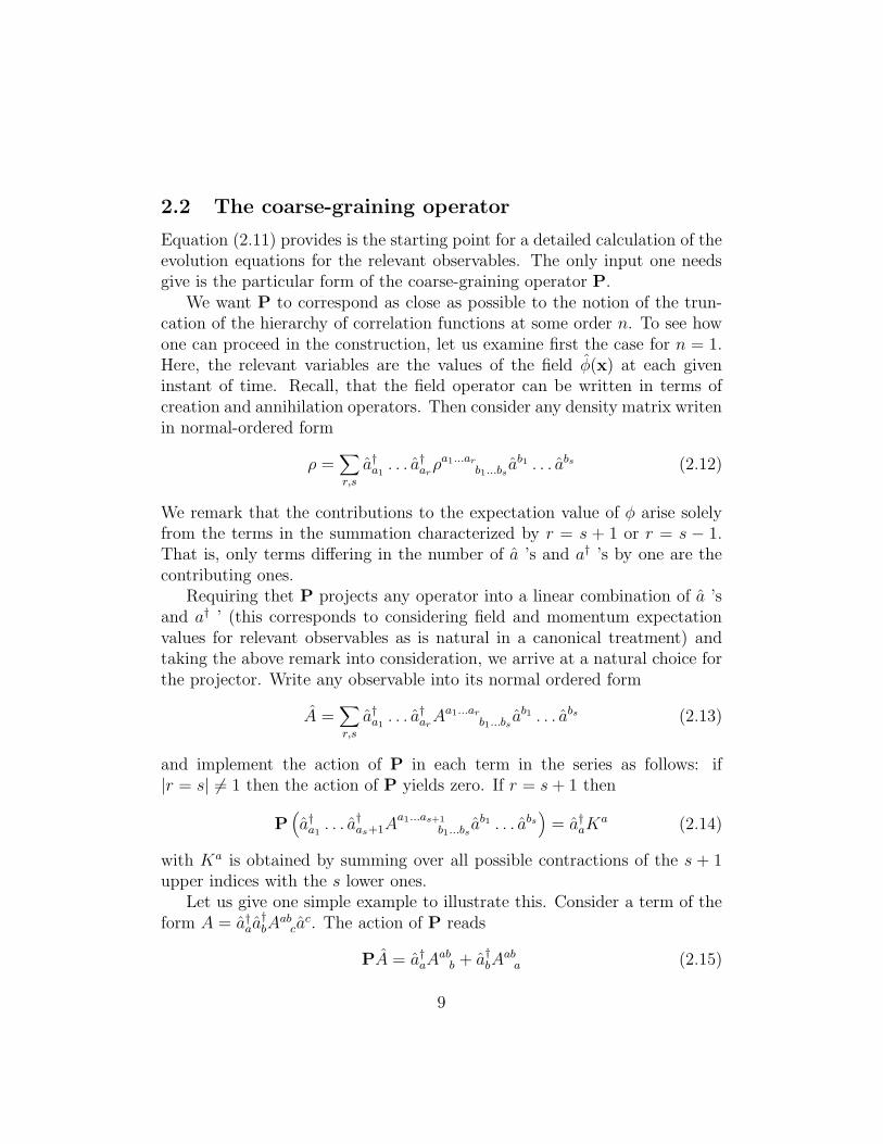
2.2 The coarse-graining operator

Equation (2.11) provides is the starting point for a detailed calculation of theevolution equations for the relevant observables. The only input one needsgive is the particular form of the coarse-graining operator P.

We want P to correspond as close as possible to the notion of the trun-cation of the hierarchy of correlation functions at some order n. To see howone can proceed in the construction, let us examine first the case for n = 1.Here, the relevant variables are the values of the field φ(x) at each giveninstant of time. Recall, that the field operator can be written in terms ofcreation and annihilation operators. Then consider any density matrix writenin normal-ordered form

ρ =∑

r,s

a†a1

. . . a†ar

ρa1...arb1...bs

ab1 . . . abs (2.12)

We remark that the contributions to the expectation value of φ arise solelyfrom the terms in the summation characterized by r = s + 1 or r = s − 1.That is, only terms differing in the number of a ’s and a† ’s by one are thecontributing ones.

Requiring thet P projects any operator into a linear combination of a ’sand a† ’ (this corresponds to considering field and momentum expectationvalues for relevant observables as is natural in a canonical treatment) andtaking the above remark into consideration, we arrive at a natural choice forthe projector. Write any observable into its normal ordered form

A =∑

r,s

a†a1

. . . a†ar

Aa1...arb1...bs

ab1 . . . abs (2.13)

and implement the action of P in each term in the series as follows: if|r = s| 6= 1 then the action of P yields zero. If r = s + 1 then

P(

a†a1

. . . a†as+1A

a1...as+1

b1...bsab1 . . . abs

)

= a†aK

a (2.14)

with Ka is obtained by summing over all possible contractions of the s + 1upper indices with the s lower ones.

Let us give one simple example to illustrate this. Consider a term of theform A = a†

aa†bA

abca

c. The action of P reads

PA = a†aA

abb + a†

bAab

a (2.15)

9

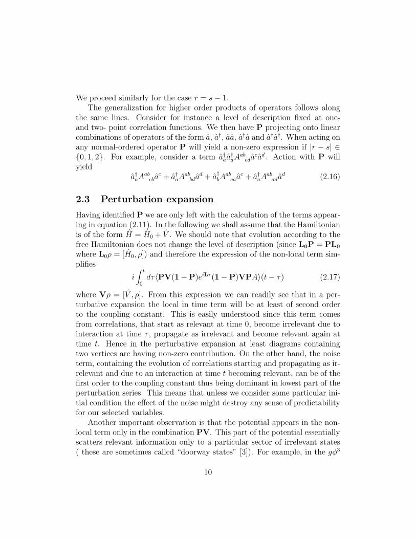
We proceed similarly for the case r = s − 1.The generalization for higher order products of operators follows along

the same lines. Consider for instance a level of description fixed at one-and two- point correlation functions. We then have P projecting onto linearcombinations of operators of the form a, a†, aa, a†a and a†a†. When acting onany normal-ordered operator P will yield a non-zero expression if |r − s| ∈{0, 1, 2}. For example, consider a term a†

aa†aA

abcda

cad. Action with P willyield

a†aA

abcba

c + a†aA

abbda

d + a†bA

abcaa

c + a†aA

abada

d (2.16)

2.3 Perturbation expansion

Having identified P we are only left with the calculation of the terms appear-ing in equation (2.11). In the following we shall assume that the Hamiltonianis of the form H = H0 + V . We should note that evolution according to thefree Hamiltonian does not change the level of description (since L0P = PL0

where L0ρ = [H0, ρ]) and therefore the expression of the non-local term sim-plifies

i∫ t

0dτ〈PV(1 −P)eiLτ (1 − P)VPA〉(t − τ) (2.17)

where Vρ = [V , ρ]. From this expression we can readily see that in a per-turbative expansion the local in time term will be at least of second orderto the coupling constant. This is easily understood since this term comesfrom correlations, that start as relevant at time 0, become irrelevant due tointeraction at time τ , propagate as irrelevant and become relevant again attime t. Hence in the perturbative expansion at least diagrams containingtwo vertices are having non-zero contribution. On the other hand, the noiseterm, containing the evolution of correlations starting and propagating as ir-relevant and due to an interaction at time t becoming relevant, can be of thefirst order to the coupling constant thus being dominant in lowest part of theperturbation series. This means that unless we consider some particular ini-tial condition the effect of the noise might destroy any sense of predictabilityfor our selected variables.

Another important observation is that the potential appears in the non-local term only in the combination PV. This part of the potential essentiallyscatters relevant information only to a particular sector of irrelevant states( these are sometimes called “doorway states” [3]). For example, in the gφ3

10

theory with truncation at the level of n = 2, we shall examine in the followingsections, the doorway states are the ones supporting third order correlations.Further propagation is needed to reach states with higher order correlations.

When considering the lowest order term in the perturbation expansionthe expression of the non-local terms is significantly simplified. To see this,note that these can be writen in the form

i∫ t

0dτ(

P[V , (1 − P)(

e−iH0τ [V , ρrel(t − τ)]eiH0τ)

], A)

(2.18)

where (, ) refers to the Hilbert-Schmidt inner product. Now since ||e−iH0τρ(t−τ)eiH0τ − ρ(t)|| = O(g) we can easily verify that within the second order tothe coupling constant we get

i〈P(

[(1 − P)(

[A, V ])

, W ])

〉(t) (2.19)

where

W (t) =∫ t

0dτe−iH0τ V eiH0τ (2.20)

Hence to the lowest order in the perturbative expansion the non-unitary termbecomes local in time. This is due to the fact that the free propagation cannot remove correlations from the doorway states into the more deeply lyingstates of the irrelevant sector. Evolution within the sector of doorway statesmakes the correlations lose fast the memory of the initial condition (withina time interval proportional to the coupling constant) and hence when theyreappear in the relevant channel they do not impose a time correlation in therelevant dynamics.

We are going to carry our calculation in the lowest order of perturbationtheory. We should remark though, that apart from the technical compli-cation, the computation of higher order corrections is not difficult. It issufficient to have a perturbation expansion in the propagator e−iHt. This isbest carried in the Fock representation [2], which is a desirable feature giventhe connection of our coarse-graining projector with the normal-ordered formof the observables.

3 Evolution of mean field in λφ4 theory

Let us apply now the above construction to the case of a λφ4 theory fortruncation at the level n = 1. The operator for the potential is given by

11

equations (B.14- B.19), while the operator W is easily computed

W =λ

4!

(

Wabcdaaabacad + 4a†

aWabcda

bacad

+6a†aa

†bW

abcda

cad + 4a†aa

†ba

†cW

abcda

d + a†aa

†ba

†ca

†dW

abcd)

(3.1)

with

Wabcd ❀

∫ 4∏

i=1

dki

(2ωki)1/2

e−i(k1x1+k2x2+k3x3+k4x4) (2π)3δ(k1 + k2 + k3 + k4)

×e−i(ωk1

+ωk2+ωk3

+ωk4)t − 1

−i(ωk1+ ωk2

+ ωk3) + ωk4

(3.2)

W abcd ❀

∫ 4∏

i=1

dki

(2ωki)1/2

e−i(−k1x1+k2x2+k3x3+k4x4) (2π)3δ(k1 + k2 + k3 + k4)

×e−i(−ωk1

+ωk2+ωk3

+ωk4)t − 1

−i(−ωk1+ ωk2

+ ωk3) + ωk4

(3.3)

W abcd ❀

∫ 4∏

i=1

dki

(2ωki)1/2

e−i(−k1x1−k2x2+k3x3+k4x4) (2π)3δ(k1 + k2 + k3 + k4)

×e−i(−ωk1

−ωk2+ωk3

+ωk4)t − 1

−i(−ωk1− ωk2

+ ωk3) + ωk4

(3.4)

W abcd ❀

∫ 4∏

i=1

dki

(2ωki)1/2

e−i(−k1x1−k2x2−k3x3+k4x4) (2π)3δ(k1 + k2 + k3 + k4)

×e−i(−ωk1

−ωk2−ωk3

+ωk4)t − 1

−i(−ωk1− ωk2

− ωk3) + ωk4

(3.5)

W abcd❀

∫ 4∏

i=1

dki

(2ωki)1/2

ei(k1x1+k2x2+k3x3+k4x4) (2π)3δ(k1 + k2 + k3 + k4)

×ei(ωk1

+ωk2+ωk3

+ωk4)t − 1

i(ωk1+ ωk2

+ ωk3) + ωk4

(3.6)

Having the expression for W one can use in a straightforward way equa-tion (2.19) to compute the dissipative terms in the evolution equation. Letus perform the calculations step by step.

12

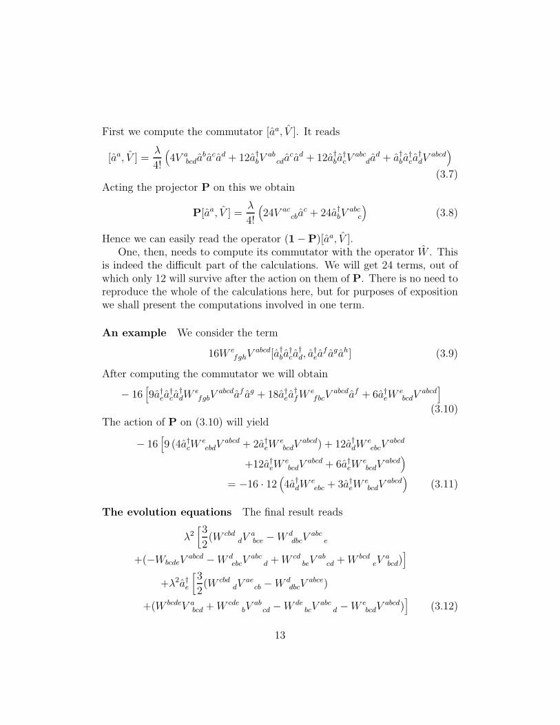
First we compute the commutator [aa, V ]. It reads

[aa, V ] =λ

4!

(

4V abcda

bacad + 12a†bV

abcda

cad + 12a†ba

†cV

abcda

d + a†ba

†ca

†dV

abcd)

(3.7)Acting the projector P on this we obtain

P[aa, V ] =λ

4!

(

24V accba

c + 24a†bV

abcc

)

(3.8)

Hence we can easily read the operator (1 − P)[aa, V ].One, then, needs to compute its commutator with the operator W . This

is indeed the difficult part of the calculations. We will get 24 terms, out ofwhich only 12 will survive after the action on them of P. There is no need toreproduce the whole of the calculations here, but for purposes of expositionwe shall present the computations involved in one term.

An example We consider the term

16W efghV

abcd[a†ba

†ca

†d, a

†ea

f agah] (3.9)

After computing the commutator we will obtain

− 16[

9a†ea

†ca

†dW

efgbV

abcdaf ag + 18a†ea

†fW

efbcV

abcdaf + 6a†eW

ebcdV

abcd]

(3.10)The action of P on (3.10) will yield

− 16[

9 (4a†cW

eebdV

abcd + 2a†eW

ebcdV

abcd) + 12a†dW

eebcV

abcd

+12a†eW

ebcdV

abcd + 6a†eW

ebcdV

abcd)

= −16 · 12(

4a†dW

eebc + 3a†

eWebcdV

abcd)

(3.11)

The evolution equations The final result reads

λ2[

3

2(W cbd

dVabce − W d

dbcVabc

e

+(−WbcdeVabcd − W d

ebcVabc

d + W cdbeV

abcd + W bcd

eVabcd)

]

+λ2a†e

[

3

2(W cbd

dVae

cb − W ddbcV

abce)

+(W bcdeV abcd + W cde

bVab

cd − W debcV

abcd − W e

bcdVabcd)

]

(3.12)

13

Note, the symmetry between the terms contracting ae and a†e.

We can therefore write down the evolution equation for a(x) = 〈a(x)〉and a∗(x) = 〈a†(x)〉:

i∂

∂ta(x) −

∫

dx′h(x,x′)a(x′) − λ∫

dx (V (x,x′)a(x′) + V (x,−x′)a∗(x′))

−iλ2∫

dx′ (A(x,x′)a(x′) + A∗(x,−x′)a∗(x′))

+λ2∫

dx′ (B(x,x′)a(x′) + B(x,−x′)a∗(x′)) = Fa(x)(t) (3.13)

where h(x,x’) is given by equation (B.2), V (x,x′) (essentially V accb) reads

V (x,x′) =∫

dk1

(2ωk1)1/2

dk2

(2ωk2)1/2

1

2ω(k1+k2)/2

e−ik1x+ik2x′

(3.14)

while

A(x,x′) =∫ 4∏

i=1

dki

2ωki

e−ik1(x−x′) (2π)3δ(k1 + k2 + k3 + k4)∆(k1,k2,k3,k4; t) (3.15)

B(x,x′) = 3∫

dk1

(2ωk1)1/2

dk2

(2ωk2)1/2

eik1x−ik2x′

×

(

∫ dk1

2ωk3

dk1

2ωk4

(2π)3δ(k1 + k2 + k3 + k4)E(k3,k4; t)

)

(3.16)

∆ and E contain the time dependence of the kernels A and B and read

∆(k1,k2,k3,k4; t) =∫ t

0dτe−iωk1

τ(

−e−i(ωk2+ωk3

+ωk4)τ

−e−i(ωk2+ωk3

−ωk4)τ + e−i(ωk2

−ωk3−ωk4

)τ + ei(ωk2+ωk3

+ωk4)τ)

(3.17)

E(k,k′; t) =cos(ωk + ωk′)t − 1

ωk + ωk′

(3.18)

Note that for times t << m−1 we have ∆(k1,k2,k3,k4; t) ≈ t.A more transparent form is given when calculating the expectation values

of creation and annihilation operators in momentum space.

∂

∂ta(k) + iωka(k) + i

∫

dk′ [V (k,k′) − λB(k,k′)] [a(k′) + a∗(k′)]

14

(3.19)

−λ2 [A(k; t)a(k) + A∗(k; t)a∗(k)] = −iFa(k)(t) (3.20)

∂

∂ta∗(k) − iωka

∗(k) − i∫

dk′ [V (k,k′) − λB(k,k′)] [a(k′) + a∗(k′)]

−λ2 [A(k, t)a(k) + A∗(k; t)a∗(k)] = −iFa∗(k)(t) (3.21)

with

A(k) =1

2ωk

∫

dk1

2ωk1

dk2

2ωk2

1

2ωk+k1+k2

∆(k,k1,k2,k + k1 + k2; t) (3.22)

B(k,k′) =3

16ωk+k′ωk′

∫

dk1

ωk1ωk+k′+k1

E(k1,k + k′ + k1; t) (3.23)

V (k,k′) =1

4ωk′ω(k+k′)/2

(3.24)

Renormalization The function A(k; t) is actually divergent. We can per-form a Taylor expansion of A around k = 0 and verify that the term A(0; t)is divergent, the terms containing first derivatives vanish while the ones con-taining the second order derivatives are finite. Hence, as could be expected,it is the zero modes of the field that give a divergent contribution. This canbe removed by a redefinition

Aren(k; t) = A(k; t) − A(0; t) (3.25)

and by absorbing A(0; t) in a field renormalization. To see this, note that

∂

∂t

(

a(k)a∗(k)

)

= finite terms + λ2

(

A(0; t) A∗(0; t)A(0; t) A∗(0; t)

) (

a(k)a∗(k)

)

(3.26)

Hence the divergencies can be absorbed through a redefinition of the Heisen-berg picture operators a(k, t), a†(k, t)

(

a(k, t)a†(k, t)

)

→ exp

[

λ2∫ t

0dτ

(

A(0; t) A∗(0; t)A(0; t) A∗(0; t)

)](

a(k, t)a†(k, t)

)

(3.27)

It is easy to interpret the terms in (3.19) and (3.20). The term V contains thelowest order contribution from the potential to our coarse-grained dynam-ics. Its form is better understood by observing that the mean field theory

15

approximation amounts to substituting four-point vartices (say with incom-ing momenta k1 and k2 and outcoming k3 and k4) with free propagationof a mode with momentum the average of the incoming (or the outcoming)modes’ momenta: (k1 + k2)/2.

The term B is a higher order, time dependent correction to the contri-bution of the potential, while the term A corresponds to dissipation. This iseasily verified when we take the time-reverse of equations (3.19) and (3.20).The terms containing A are the only non-invariant terms.

The noise terms Most important, from the point of view of the classicalbehaviour and predictability of the mean field is the noise term. As we said itis at least of first order to the coupling constant and in principle can dominateboth the potential and the dissipation terms.

Starting from equation (2.11) it is straightforward to calculate the leading(first order to λ) contribution to the noise. It reads (we switch back to theindex notation)

Faa(t) =λ

4!Tr

(

ρ(0)A(t))

(3.28)

where

A(t) = 4V abcda

b(t)ac(t)ad(t) + 12a†b(t)V

abcda

c(t)ad(t)

+12a†b(t)a

†c(t)V

abcda

d(t) + 4a†b(t)a

†c(t)a

†d(t)V

abcd

−24V accba

b(t) − 24a†bV

abcc (3.29)

where with a(t) and a†(t) we denote the Heisenberg picture operators evolvingaccording to the free Hamiltonian.

In order for our coarse-grained description to satisfy the predictabilitycriterion, the noise term should be sufficiently weak (though strong enoughto cause decoherence of the mean field histories). This, as we see, cannot betrue for a generic initial state of the system. We can nevertheless observe thatthe noise terms vanishes when the initial state is the vacuum ρvac = |0〉〈0|.This means that for states ρ(0) sufficiently close to the vacuum the noiseterm becomes smaller and smaller. This means that for any state ρ(0) suchthat ||ρ(0) − ρvac||HS < ǫ the noise term will be of order O(ǫ).

Consider for instance that the initial state of the system is some coher-ent state |α(x)〉, determined by a square-integrable function α(x). Coherent

16

states are eigenstates of the annihilation operators, hence the trace in equa-tion (3.) is easily performed. Now if we assume that ||α(x)|| < ǫ it is easy toestablish that ||ρ(0)− ρvac||HS = O(ǫ). Hence to leading order in ǫ the noiseterm reads

Faa(t) = −λǫ(

V accbζ

b(t) + ζ∗b (t)V

abcc

)

(3.30)

where we wrote α(t) = ǫζ(t). This is an example of an initial conditionthat renders the noise term sufficiently weak to allow for predictability. Thisparticular condition, we believe, is realistic when considering cosmologicalscenaria.

Finally we should remark that it is straightforward to obtain evolutionequations for the mean field and momentum by using the equations

a(k) =∫

dxeikx(

ωkφ(x) + iπ(x))

(3.31)

a†(k) =∫

dxe−ikx(

ωkφ(x) − iπ(x))

(3.32)

4 Two point functions in gφ3 theory

In this section we are going to give the results for the truncation of thehierarchy at the level n = 2 for a gφ3 scalar field theory.

The mean field equations For completeness we will give very brieflythe results of the mean field analysis for the gφ3 case. The expectation valueof the operator a(k) evolves according to an equation similar to (3.19)

∂

∂ta(k) + iωka(k) − iλ2

∫

B(k,k′) (a(k′) + a∗(k′))

−λ2 [A(k; t)a(k) + A∗(k; t)a∗(k)] = Fa(k)(t) (4.1)

where here the functions A and B are given by

A(k; t) =3

16ωk

∫

dk1

ωk3+kωk3

∆(k,k + k3,k3; t) (4.2)

B(k,k′; t) =1

2ωk′ωk+k′

cos ωk+k′t − 1

ωk+k′

(4.3)

17

with

∆(k1,k2,k3; t) = − 2i∫ t

0e−iωk1

τ sin (ωk2+ ωk3

) (4.4)

As is well known, the potential does not contribute in the lowest order equa-tion for the mean field theory, and the quantities A and B again characterizedissipation and time-dependent correction to the potential.

Evolution equations for two-point functions Let us now give theresults for the case of truncation at the n = 2 level. We prefer to give themin terms of the functions G(k) and Z(k) defined by

〈a(x)a(x′)〉 =∫ dk

2ωk

e−ik(x+x′)G(k) (4.5)

〈a†(x)a(x′)〉 =∫

dk

2ωk

e−ik(x−x′)Z(k) (4.6)

We will skip all calculations and present straightforwardly the results, sincethe way to proceed is exactly as previously and the only difficulty is a com-putational one. Thus, we get for a final result

∂

∂ta(k) + iωka(k) = −iFa(k) (4.7)

(4.8)

∂

∂tZ(k) −

λ

4

(

2

ωk

+1

(ωkωk/2)1/2

)

[a(k) + a∗(k)]

+iλ2∫

dk′ [r(k,k′; t)G(k′) + r∗(k,k′; t)G∗(k′) + s(k,k′; t)Z(k′)]

+iλ2 [D1(k; t)G(k) + D2(k; t)G∗(k) + D3(k; t)Z(k)] = −iFZ(k)(t) (4.9)

(4.10)

∂

∂tG(k) + 2iωkG(k) −

λ

4

(

2

ωk

+1

(ωkωk/2)1/2

)

[a(k) + a∗(k)]

+iλ2∫

dk′ [K1(k,k′; t)G(k′) + K2(k,k′; t)G∗(k′) + K3(k,k′; t)Z(k′)]

+iλ2 [L1(k; t)G(k) + L2(k; t)Z(k)] = −iFG(k)(t)(4.11)

The form of the functions appearing in these equations can be found inAppendix C.

18

This equation is not very inspiring as it stands. But when we try tocompute the noise in first order to perturbation theory according to equation(2.11) we can verify that

P[A, V ] = [A, V ] (4.12)

which means that the lowest order term in the perturbation expansion of thenoise term is vanishing. Hence in a weak coupling regime one can consideronly the first order to λ which gives an autonomous and time-independent setof equations, for our relevant variables. The one-point functions evolve freelyand drive the corrsponding values of the two-point correlation dunctions.

∂

∂ta(k) + iωka(k) = 0 (4.13)

∂

∂tZ(k) =

λ

4

(

2

ωk

+1

(ωkωk/2)1/2

)

[a(k) + a∗(k)] (4.14)

∂

∂tG(k) = −2iωkG(k) +

λ

4

(

2

ωk

+1

(ωkωk/2)1/2

)

[a(k) + a∗(k)] (4.15)

5 Conclusions and remarks

The techniques we have employed in this paper have given as a picture for theevolution of relevant variables, when the coarse-graining operation consistsin the truncation of the Schwinger-Dyson hierarchy of n-point functions.

One of the great difficulties in such considerations is the complicated ex-pressions we get for our equations in the end. It seems that it is very difficultto find a regime in a field theory where the dynamics would be Marko-vian. This essentially means that noise should be with good aproximation“white” and in the autonomous part of the dynamics one should have notime-dependent coefficents. It seems unlikely that we can obtain Markovianevolution for a generic state of the system. In any case we should expect itwhen the field is in a state of partial (local) equilibrium [3]. This regime canstill be studied using our techniques, but it might be that a different choiceof coarse-graining projector might be more of use. The Kawasaki-Guntonand the Mori projector [14] might prove more convenient when dealing withthis regime.

Another avenue to explore towards obtaining Markovian equations is toconsider non-unitary dynamics for the evolution of the total system. This

19

might come from a contact with a heat bath or through the interaction withother ignored degrees of freedom (a supermassive field or gravitons for thecase of cosmology).

As far as the noise is concerned, we should stress that the Zwanzig methodallows to derive the noise term in the evolution equations solely from theknowledge of the initial state of the system. The comparison of its strengthwith the size of the terms entering the evolution equations offers a goodcriterion ( though rather heuristic) for the classicalization of the variablesunder study. Remember, that noise should be strong enough to decohere butweak enough to allow for predictability and not covering up the effects of thepotential. Only a particular class of initial states offers this possibility.

Finally, we should make some remarks concerning the classical domain ingeneric field theories. The techniques developed in this paper do provide auseful tool for dealing with the emergence of classical behaviour. Still, it ismy belief, that concrete understanding of the quantum to classical transitionrequires in addition, employment of the conceptual technical tools of thedecoherent histories approach to quantum mechanics. To obtain a completeand rigorous characterization of the classical domain ( like for instance [4,5, 6]) one needs to construct the decoherence functional for coarse grainedcorrelation histories in a manageable computationally form. This is currentlyunder investigation.

6 Aknowledgements

I would like to thank B. L. Hu for a stimulating discussion on relevant issues.

References

[1] B. L. Hu and E. Calzetta, “Decoherence of correlation histories”, in Di-

rections in General Relativity, vol II: Brill Festschrift,edited by B.L Huand T. A. Jacobson (Cambridge University Press, Cambridge UniversityPress, Cambridge 1994). 9302013 9501040; “ Correlations, Decoherence,Dissipation and Noise in Quantum Field Theory”, in Heat Kernel Tech-

niques and Quantum Gravity, edited by S. A. Fulling (Texas AM Press,College Station 1995) gr-qc 9501040.

20

[2] F. A. Berezin, The Method of Second Quantization, (Academic Press,New York, 1966).

[3] H. D. Zeh, The Physical Basis of the Direction of Time (Springer Verlag,Berlin, 1989).

[4] C. Anastopoulos, Phys. Rev. E53, 4711 (1996).

[5] R. Omnes, J. Stat. Phys. 57, 357 (1989); The Interpretation of Quantum

Mechanics ( Princeton University Press, Princeton, 1994)

[6] H. F. Dowker and J. J. Halliwell, Phys. Rev. D46, 1580 (1992).

[7] R. P. Feynman and A. R. Hibbs, Quantum Mechanics and path integrals(McGraw-Hill, New York, 1965) ; R. P. Feynman and F. L. Vernon, Annals

of Physics 24, 118 (1963).

[8] A. O. Caldeira and A. J. Leggett, Physica A121, 587 (1983).

[9] B. L. Hu and A. Matacz, Phys. Rev. D49, 6612 (1994).

[10] K. Lindenberg and B. J. West, The non-equilibrium statistical mechanics

of open and closed systems,(VHC Publishers, New York 1990)

[11] J. R. Anglin and W. H¿ Zurek, Decoherence of quantum fields: Pointer

states and Predictability, gr-qc 9510021.

[12] B. L. Hu and E. Calzetta, Phys. Rev. D52, 6770(1995).

[13] B. L. Hu and E. Calzetta, Phys. Rev.D35, 495 (1987); Phys. Rev D 40,656 (1989).

[14] J. Rau and B. Muller, From reversible quantum microdynamics to irre-

versible quantum transport, nucl-th 9505009.

[15] M. Gell-Mann and J. B. Hartle, in Complexity, Entropy and the Physics

of Information, edited by W. Zurek, (Addison Wesley,Reading (1990));Phys. Rev. D47, 3345 (1993).

21

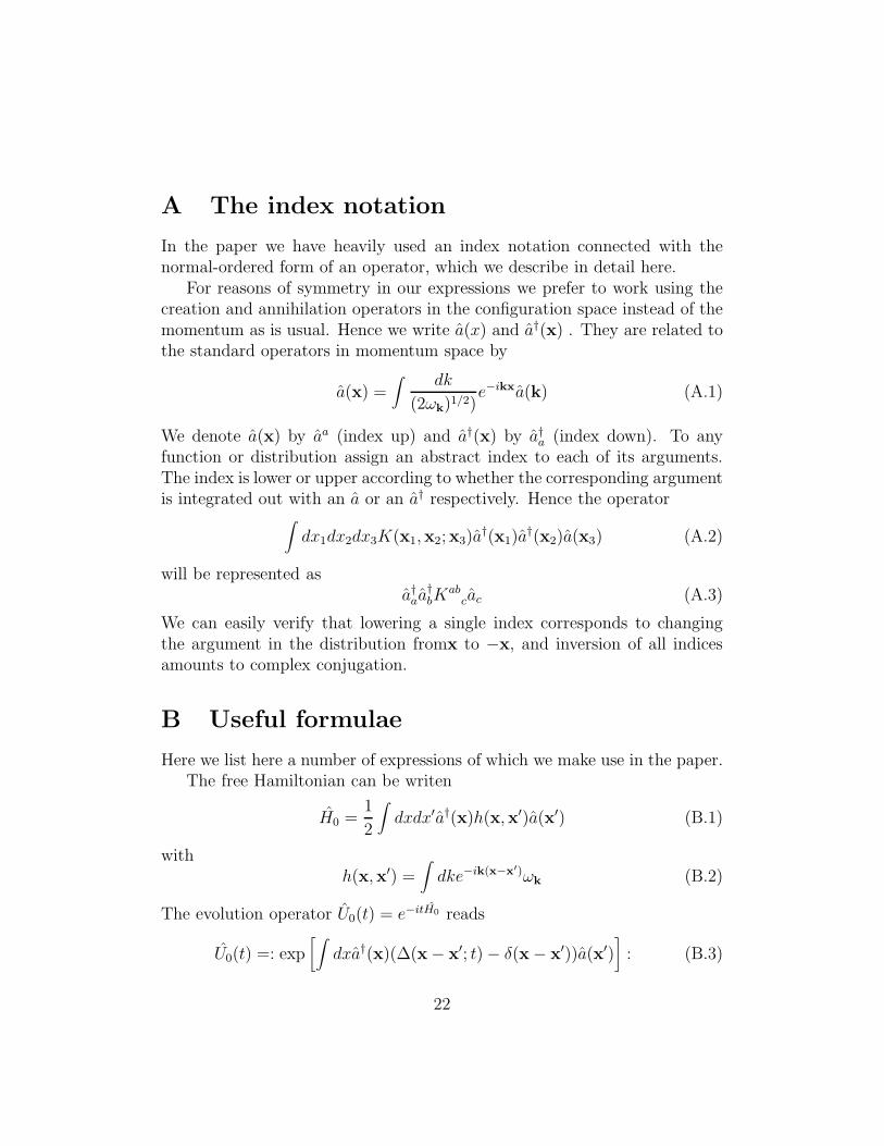
A The index notation

In the paper we have heavily used an index notation connected with thenormal-ordered form of an operator, which we describe in detail here.

For reasons of symmetry in our expressions we prefer to work using thecreation and annihilation operators in the configuration space instead of themomentum as is usual. Hence we write a(x) and a†(x) . They are related tothe standard operators in momentum space by

a(x) =∫ dk

(2ωk)1/2)e−ikxa(k) (A.1)

We denote a(x) by aa (index up) and a†(x) by a†a (index down). To any

function or distribution assign an abstract index to each of its arguments.The index is lower or upper according to whether the corresponding argumentis integrated out with an a or an a† respectively. Hence the operator

∫

dx1dx2dx3K(x1,x2;x3)a†(x1)a

†(x2)a(x3) (A.2)

will be represented asa†

aa†bK

abcac (A.3)

We can easily verify that lowering a single index corresponds to changingthe argument in the distribution fromx to −x, and inversion of all indicesamounts to complex conjugation.

B Useful formulae

Here we list here a number of expressions of which we make use in the paper.The free Hamiltonian can be writen

H0 =1

2

∫

dxdx′a†(x)h(x,x′)a(x′) (B.1)

withh(x,x′) =

∫

dke−ik(x−x′)ωk (B.2)

The evolution operator U0(t) = e−itH0 reads

U0(t) =: exp[∫

dxa†(x)(∆(x − x′; t) − δ(x − x′))a(x′)]

: (B.3)

22

where∆(x − x′; t) =

∫

dke−ik(x−x′)e−iωkt (B.4)

A coherent state is characterized by the square integrable function α(x) andis an eigenstate of the annihilation operator a(x). Under evolution of thefree Hamiltonian we have

U0(t)|α(x)〉 = |α(x, t)〉 (B.5)

whereα(x, t) =

∫

dx′∆(x − x′; t)α(x′) (B.6)

The operator

V =:∫

dxg

3!φ3 : (B.7)

reads in the index notation

V (α∗, α) =g

3!

(

Vabcaaabac + 3a†

aVabca

bac + 3a†aa

†bV

abca

c + a†aa

†ba

†cV

abc)

(B.8)

with the correspondence

Vabc ❀

∫∏3

i=1dki

(2ωki)1//2 e

−i(k1x1+k2x2+k3x3)(2π)3δ(k1 + k2 + k3) (B.9)

V abc ❀

∫∏3

i=1dki

(2ω1/2

ki)e−i(−k1x1+k2x2+k3x3)(2π)3δ(k1 + k2 + k3) (B.10)

V abc ❀

∫∏3

i=1dki

(2ωki)1/2 e

−i(−k1x1−k2x2+k3x3)(2π)3δ(k1 + k2 + k3) (B.11)

Vabc ❀

∫∏3

i=1dki

(2ωki)1/2 e

i(k1x1+k2x2+k3x3)(2π)3δ(k1 + k2 + k3) (B.12)

while the operator

V =:∫

dxλ

4!φ4 : (B.13)

reads

V =λ

4!

(

Vabcdaaabacad + 4a†

aVabcda

bacad

+6a†aa

†bV

abcda

cad + 4a†aa

†ba

†cV

abcda

d + a†aa

†ba

†ca

†d

)

(B.14)

23

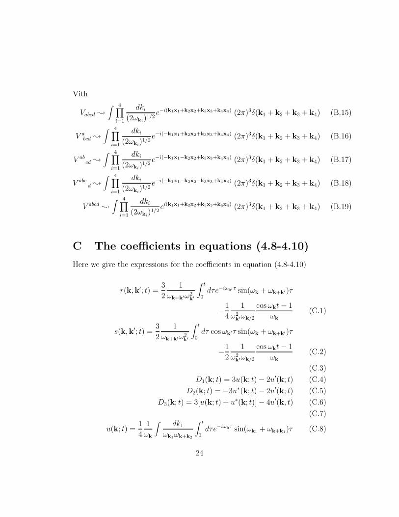
Vith

Vabcd ❀

∫ 4∏

i=1

dki

(2ωki)1/2

e−i(k1x1+k2x2+k3x3+k4x4) (2π)3δ(k1 + k2 + k3 + k4) (B.15)

V abcd ❀

∫ 4∏

i=1

dki

(2ωki)1/2

e−i(−k1x1+k2x2+k3x3+k4x4) (2π)3δ(k1 + k2 + k3 + k4) (B.16)

V abcd ❀

∫ 4∏

i=1

dki

(2ωki)1/2

e−i(−k1x1−k2x2+k3x3+k4x4) (2π)3δ(k1 + k2 + k3 + k4) (B.17)

V abcd ❀

∫ 4∏

i=1

dki

(2ωki)1/2

e−i(−k1x1−k2x2−k3x3+k4x4) (2π)3δ(k1 + k2 + k3 + k4) (B.18)

V abcd❀

∫ 4∏

i=1

dki

(2ωki)1/2

ei(k1x1+k2x2+k3x3+k4x4) (2π)3δ(k1 + k2 + k3 + k4) (B.19)

C The coefficients in equations (4.8-4.10)

Here we give the expressions for the coefficients in equation (4.8-4.10)

r(k,k′; t) =3

2

1

ωk+k′ω2k′

∫ t

0dτe−iω

k′τ sin(ωk + ωk+k′)τ

−1

4

1

ω2k′ωk/2

cos ωkt − 1

ωk

(C.1)

s(k,k′; t) =3

2

1

ωk+k′ω2k′

∫ t

0dτ cos ωk′τ sin(ωk + ωk+k′)τ

−1

2

1

ω2k′ωk/2

cos ωkt − 1

ωk

(C.2)

(C.3)

D1(k; t) = 3u(k; t) − 2u′(k; t) (C.4)

D2(k; t) = −3u∗(k; t) − 2u′(k; t) (C.5)

D3(k; t) = 3[u(k; t) + u∗(k; t)] − 4u′(k, t) (C.6)

(C.7)

u(k; t) =1

4

1

ωk

∫

dk1

ωk1ωk+k2

∫ t

0dτe−iωkτ sin(ωk1

+ ωk+k1)τ (C.8)

24

u′(k; t) =1

2

1

ω3kωk/2

(cos ωkt − 1) (C.9)

(C.10)

K1(bfk,k′; t) =3

4

1

ωk+k′ω2k′

cos(ωk + ωk+k′ − ωk′)t − 1

ωk + ωk+k′ − ωk′

−1

2

1

ω2k′ωk/2

e−iωkt − 1

ωk

(C.11)

K2(k,k′; t) =3

2

1

ωk+k′ω2k′

∫ t

0e−i(ωk+ω

k′)τ cos(ω

k+k′τ

−1

2

1

ω2k′ωk/2

e−iωkt − 1

ωk

(C.12)

K3(k,k′; t) =1

2

1

ωk+k′ω2k′

cos(ωk + ωk+k′ + ωk′)t − 1

ωk + ωk+k′ + ωk′

(C.13)

(C.14)

L1(k; t) = −3i

4

1

ωk

∫

dk1

ωk1ωk+k2

∫ t

0dτe−iωkτ cos(ωk1

+ ωk+k1)τ

−1

ω2k′ωk/2ωk

(cos ωkt − 1) (C.15)

L2(k; t) = −1

ω3kωk/2

(cos ωkt − 1)

+3

4

1

ωk

∫

dk1

ωk1ωk+k1

∫ t

0dτeiωkτ sin ωk2+kτ (C.16)

25