Technological Diffusion, Uncertainty and Irreversibility:

The International Diffusion of Industrial Robots*

By

Paul Stoneman and Otto Toivanen

Warwick Business School and the Helsinki School of Economics

June 2000

PRELIMINARY AND INCOMPLETE; PLEASE DO NOT CITE

WITHOUT PERMISSION

Abstract

The impact of uncertainty on the diffusion of new technology is explored. A probit type model of

technological diffusion based upon a model of irreversible investment is constructed and tested on data

relating to international differences in the diffusion of robot technology. The model provides a rigorous

theoretical foundation for widely used empirical diffusion models. It predicts and the preliminary empirical

estimates confirm that uncertainty, as measured by the volatility of several macroeconomic indicators,

impacts significantly on the diffusion process. However, we find that volatility of several of our variables

actually increases the adoption hazard.

Key words: Technological diffusion, uncertainty, risk, robots

JEL Classification:

* The authors would like to thank Ricardo Caballero for helpful discussions. The second author thanksAcademy of Finland and Yrjö Jahnsson Foundation for generous financial support, and MIT economicsdepartment and NBER for hospitality during the early phases of this research. The usual caveat applies.Correspondence either to Paul Stoneman, Warwick Business School, CV4 7AL Coventry, UK,wbsrbps@wbs.warwick.ac.uk, or Otto Toivanen, economics department, Helsinki School of economics, POBox 1210, FIN-00101 Helsinki, FINLAND, toivanen@hkkk.fi.

1

1. INTRODUCTION

Investment in general, and the adoption of new technology in particular, is a process

inherently characterized by risk and uncertainty on both the cost and the demand side. At

the same time, such investments would seem to be irreversible to at least the same extent

as traditional investments. A new technology requires almost by definition additional

investments in complementary human capital. Such investments are by their nature sunk

and irreversible. The fact that the technology is new could mean that no, or only a

limited, second hand market exists for such goods, increasing the degree of irreversibility

further.

The investment literature, both theoretical and empirical, has made good use of

the potential of models that make uncertainty and irreversibility the corner stones of

analysis (for a recent example, see Caballero and Engel, 1999), although the empirical

literature has placed little emphasis on analyzing the effects of uncertainty directly (but

see Driver and Morton, 1991, Pindyck and Solimano, 1993, and Leahy and Whited,

1996). It is therefore somewhat surprising that the literature on the diffusion of

technology has made little use of such models. The objective of this paper is to partly fill

this gap by doing two things. First, by building a model of technology diffusion that is

based on an optimizing firm (project holder) facing an irreversible investment choice in a

world of uncertainty, and aggregating up to get an economy level expression for the

diffusion of technology. We use a continuous time approach as that allows a relatively

direct way of incorporating well-defined measures of uncertainty into the estimation

equation. Second, by estimating the model using inter-country data on the diffusion of

industrial robots, placing special emphasis on the effects of macro-level uncertainty on

2

the adoption hazard. On the way, we provide a rigorous theoretical foundation for some

widely used empirical models of technology diffusion, and show that these can be

thought of as aggregate models of individual optimizing behavior, where an ad hoc

structure has been placed on the adoption hazard. One would think that new technologies

provide a good case for studying the effects of uncertainty, as the level of technological

uncertainty is almost by definition greater than in investments in “old” technologies. As a

consequence, any “environmental” uncertainty, such as that at the macro level, should

have a greater impact as long as it is uncorrelated with the technological uncertainty of

the new technology.

In the next section of this paper we develop a model of technology choice in a

world of irreversibility and uncertainty. From that model we then construct an aggregate

diffusion curve for an economy. In section 3 we discuss the nature of robot technology

and the data on robot diffusion used to test the model. We demonstrate that investments

in robots are more volatile than aggregate manufacturing investment. In section 4 we

discuss econometric issues. In section 5 we present the results of the estimation and

discuss their implications. We then use the estimated parameters in Section 6 to conduct

policy experiments, in particular, to explore the effects of changing the volatility of the

environment in which investment decisions are made. Section 7 contains the conclusions.

2. THE MODELING FRAMEWORK

We define a project (indexed by i) as an investment in a unit of robot technology.1 At any

time (indexed by t) in a country (indexed by j) we define Njt as the total number of

1 This approach via projects can be contrasted with a more standard diffusion approach via firms. The latter

approach however usually necessitates assumptions guaranteeing that intra firm diffusion is instantaneous.

3

projects that could be undertaken, or the total number of robots that could be used. We

discuss Njt in more detail below. We assume that the returns to individual projects are

independent of each other. We further define Mjt as the number of robots installed, or the

number of projects initiated at or before time t in country j. It is assumed that the

adoption of a robot is an irreversible decision and robot technology has an infinite

(physical) life.

2.1 The adoption timing decision

The model that we employ is adapted from a model by Dixit and Pindyck (1994, pp. 207

-211), first studied by McDonald and Siegel (1986). Defining Pjt as the cost of a unit of

robot technology in country j in time t, assumed the same for all projects i, and Rijt as the

annual gross profit increase generated by project i in country j in time t, we assume that

both Pjt and Rijt are uncertain but exhibit geometric Brownian motion such that,

(1) dRijt/Rijt = αRijdt + σRijdz

and that

(2) dPjt/Pjt = αPjdt + σPjdz

where dz is the increment of a standard Wiener Process. Note that the α ’s measure the

expected rates of growth or drift of the variables over time while the σ ’s show the

volatility or uncertainty attached to the variable. It is the impact of the σ terms that in this

paper measure the effects of uncertainty on the diffusion process.

For ease of exposition, we assume here that Pjt and Rijt are independent covariates

with zero covariance (but allow for nonzero covariance in the empirical model). We also

The former approach does not. As we do not actually have any firm level data no information is being lost

by taking the project rather than the firm as the basic unit of analysis.

4

assume that Pjt and Rijt are independent of the (existing) number of robots in use and

actual dates of adoption. In terms of the diffusion literature this is the same as assuming

that there are no stock and order effects in the diffusion process (see Karshenas and

Stoneman, 1993). The resulting model thus falls within the class of probit or rank models

of diffusion whereby different rates of adoption across countries will reflect the different

characteristics of those countries, the characteristics being exogenous to the diffusion

process.

Defining rjt as the riskless real interest rate in country j in time t, a project, which

has not previously been undertaken, will be undertaken (started) in time t if and only if

(3) Rijt/Pjt ≥ ρijt ≡ βij(rjt - αRij)/ (βij – 1)

where ρijt is the threshold ratio of profit gains relative to the cost of acquisition above

which project i will be undertaken in time t and below which it will not (this being

allowed to be time dependent for generality), and βij is the larger root of the quadratic

equation

(4) 0.5.(σRij2

+ σPj2 ). βij.(βij - 1) + (αRij - αPj).βij + (αPj - rjt) = 0

enabling us to write (3) more generally as (5).

(5) Rijt/Pjt ≥ ρijt ≡ F(rjt, σRij2

, σPj2 , αRij , αPj )

Following Dixit and Pindyck we assume that rjt - αRij > 0 and rjt - αPj > 0 which implies

that βij > 1, and then using (3) and (4) we may deduce that F2 >0, F3>0, F5<0 but the signs

of F1 and F4 are indeterminate. Thus increases in uncertainty (σRij2

, σPj2) will lead to

increases in the threshold value of ρijt and an increase in the drift rate of increase of robot

prices will reduce the threshold, however the impact of an increase in the interest rate and

the drift (rate of increase) of profit gains are indeterminate. Basically, although the direct

5

impact of increases in the latter two parameters on (rjt - αRij) is clear, their impact on βij

βij – 1) is of the opposite sign. If there is no uncertainty so that σRij = σPj = 0 then (3)

collapses to

(6) Rijt/Pjt ≥ ρijt = rjt - αPj

which is the standard intertemporal arbitrage condition for adoption of a new technology

in time t (see Ireland and Stoneman, 1986 ). In this case the impact of changes in rjt and

αRij can be clearly signed as positive and zero respectively.

2.2 The aggregate diffusion curve

In this part we derive the aggregate diffusion curve, and relate it to the project level

model of adoption presented above. This is undertaken at least partly with one eye upon

the kind of inter-country data that is available to us.

A. The generalized diffusion curve

The data available to us upon the diffusion of robots indicates the number of robots

owned in each country at each point of time. To generate a suitable variant of the

modeling framework relevant for such data we define hjt as the probability that a project

that has not been previously undertaken will be started in country j in time t. In the

absence of any scrapping of the existing robot stock (a consequence of our assumption

that R follows a geometric Brownian motion is that it is bounded below to be nonnegative

and a robot will be operated forever),2 one may then immediately write (7) as the

expression for the increase in the stock of robots in country j in time t.

(7) Mjt - Mjt-1 = hjt(Njt - Mjt-1)

2 One could allow for exit of robots by defining R=0 as an absorbing barrier.

6

Equation (7) is a logistic diffusion curve with the rate of diffusion given by the

hazard rate, hjt and would be the same as the standard curve often used in diffusion

analysis if hjt were a constant. A useful variant on (7) can be obtained using the

approximation that (x – y)/y ≅ logx – logy which yields a Gompertz diffusion curve

(8) logMjt – logMjt-1 = hjtlogNjt – logMjt-1.

Diffusion curves such as (7) and (8) are usually based upon information spreading or

epidemic arguments (see Stoneman, 2001) but in this case that is not so. When they are

so based the lagged stock usually appears on the on the right hand side as a proxy for

current stock. In the current model the lagged stock appears in its own right.

One should note that in (7) and (8) Njt plays a somewhat different role than is

often assumed in diffusion analysis. It is often assumed that as t tends to infinity the stock

of new technology (in this case robots) tends to Njt. Here however that is not necessarily

so. Here, the diffusion process will continue only as long as hjt is positive and hjt may

tend to zero well before Mjt = Njt.

B. Modeling the returns to adoption

We do not have data upon the gross returns to robot adoption at either the project

level, Rijt, or macro level. To model Rijt we assume that

(9) Rijt = exp(aijt + ΣkbkXkjt)

The term aijt reflects the heterogeneity of returns to different projects in country j, and we

will be more precise about its nature below. It is reasonable to expect that different

projects, even in a given country, will offer different returns. Determining factors, for

example, might be the industry in which they are located and the demand conditions and

factor prices in those industries. Alternatively it may be that projects are specific to firms

7

and different firms face different returns to potential robot investment because of, for

example, scale economies or different managerial efficiencies.

The term ΣkbkXkjt in (9) is a weighted sum of a number, k, of macroeconomic

variables that are determinants of the returns to the adoption of robots. If the Xkjt all

follow an absolute, then Rijt follows a geometric Brownian motion so that (10) and (11)

hold

(10) αRij = ΣkbkαXkj

(11) σ2Rij = Σkb2

kσ2Xkj.

This approach ensures that ρijt is the same for all i for a given j and t and thus we may

write, using (5), that

(12) ρijt = ρjt = F(rjt, Σkb2kσXkj

2, σPj

2 , ΣkbkαXkj, αPj )

where F2 > 0 for all k.

In essence therefore (9) assumes that different projects in a given country yield

different levels of gross returns from the use of the new technology (determined by macro

economic factors and project specific effects) but the drift and volatility of the returns is

the same for all projects in that country (but may differ across countries).

C. Generating the hazard rate

From (5), the condition for undertaking project i in time t may be written as

(13) lnRijt - lnPjt ≥ lnρjt

and after substitution from (10) and (11) this yields the adoption condition

(14) aij + ΣkbkXkjt - lnPjt- lnρjt ≥ 0

where ρjt is given by (12). From the above it is clear that the way we model aij will

determine how hjt, the hazard rate is to be specified.

8

Our model needs to be able – a priori – to explain within country heterogeneity in

robot adoption. This naturally means that the returns to different projects within a country

have to differ. One way of approaching this is to specify ait (we drop the country subscript

j as superfluous for the moment) as:

(15) itiit dda εη 1211 +−= .

In (15), iη is a project specific time-invariant (unobservable) term. We further assume

that iη is distributed N( 211,0 d− ). The term itε is distributed N( 2

1,0 d ) with

cov( 1,, −tiit εε )=0 and cov( iit ηε , )=0. Utilizing the distributional assumption of ε, the

adoption probability in the first period for projects with the same project specific

unobservable η can then be written as

(16) Prob(adopting in t=1|η=η) =

max0, [ ])lnln1( 1121

21 ∑ −+−−Φ −

k kkiPXbdd ρη .

Equation (16) necessitates the assumption d1>0. It is clear from (16) that the effects of the

determinants of the adoption threshold on the adoption probability are opposite to their

effects on the threshold. As our data shows that robot adoption is always strictly positive,

we will make the simplifying assumption that the adoption probabilities are always

strictly positive. Then, to get the population adoption probability, we need to integrate

over η, yielding

(17) Prob(adopting in t=1)=

[ ] iik kkidPXbdd ηηφρη )()lnln1( 11

21

21∫ ∑

∞

∞−

− −+−−Φ .

9

To derive the hazard rate of adoption for period t, first fix the value of the project specific

unobservable to η. Subtract all those projects that have already adopted. This yields the

(discrete version of the) hazard rate of adoption conditional on the project specific

unobservable as

(18) Prob(adoption in t|no adoption by end of period t-1, η))(1

)()(

1

1

ηηη

−

−

Φ−Φ−Φ

=t

tt .

All the values of the cdf functions are now functions of η. To get the population hazard,

we again need to integrate over η. This yields

(19) Prob(adoption in t|no adoption by end of period t-1)

jtt

tt hd =Φ−

Φ−Φ= ∫∞

∞− −

− ηηφη

ηη)(

)(1)()(

1

1 .

Equation (19) provides the expression for the hazard rate in (8).

The formulation above has the attractive feature that it allows us to capture what most

likely is an essential feature of the real world; not all projects that could technically utilise

robots have equal expected revenues, and some differences could well be time-invariant.

As an example, it is well documented that adoption decisions depend positively on

firm size (e.g. Rose and Joskow 1990, Karshenas and Stoneman, 1993). Consider that

projects are distributed across firms in proportion to firm size, and that project returns

increase with firm size and that firm size follows (approximately) a log-normal

distribution in many countries. One could then interpret iti εη + to measure the firm size

realization of different projects and the above model would square nicely with the

observed firm size – adoption correlation. As the model also has a time varying, zero

auto-correlation error term, it also allows for the possibility that not all projects of the

10

same size behave identically. In addition, it is possible that the smallest adopter is smaller

than the largest non-adopter.

D. Modeling the total number of projects

What remains to fully specify the model is to consider how the total number of projects is

to be determined. We have defined Njt as the number of projects where, technically,

robots could be used, constituting thereby the total set of potential adoptions. Njt will be

related to the nature of products produced in the economy and also the general type of

production processes in place but has the important characteristic that it is independent of

the costs or returns to the use of robot technology. It is worth repeating again, as stated

above, that in this framework the diffusion process will continue only as long as hjt is

positive and hjt may tend to zero well before Mjt = Njt thus it is not the case that as t tends

to infinity the stock of new technology (robots) will necessarily (or be even expected to)

tend to Njt.

In Section 3 we discuss the nature of robot technology. It is clear that to some

considerable extent robot technology is largely applicable in the manufacturing sector

alone and thus a simple approach is to argue that the prime determinant of Njt is

manufacturing output. In a first approach therefore it is assumed that Njt is related to

manufacturing output INDjt, in country j such that

(20) λjtjt INDN =

3. ROBOT TECHNOLOGY AND DATA

3.1 Robot Technology

11

International statistics3 on industrial robots are compiled by the UN and the International

Federation of Robotics (IFR). These statistics cover 28 countries, 16 of which were included

in our sample4 although due to gaps in the data our panel is unbalanced, yielding a total of

161 observations. The sixteen countries are listed together with summary statistics in Table

1; the table also reports the observation period for each country. IFR has created an

international standard (ISO TR 8373) that was used in compiling the statistics. Robots are

customarily classified into standard and advanced robots and by the application area.

However for the period 1981-1993 only aggregate data is available. It is estimated (the

statistics are not water-tight) that there were some 610 000 robots in use worldwide at the

end of 1993. The rate of growth of this stock has been fast, ranging from the 16-23% p.a.

recorded at the turn of the decade to current levels of 6-8% p.a.. . The average yearly change

in the robot stock varies between almost 30,000 in Japan to 41 in Norway.

As evidence that robot adoption is significant, but different from aggregate

manufacturing investment, in 1993 robot investment amounted to 12% of total machine tool

investments in the US, to 11% in both Germany and the UK and to 6% in France. Japan is

by far the largest user of robots whether measured by absolute (some 60% of world stock) or

relative numbers (in 1993 Japan had 264 advanced robots per 10 000 employees in

manufacturing when the country with the second highest density (Singapore) had 61).

3 Our discussion on robots and robot statistics relies heavily on World Industrial Robots 1994, Geneva,

United Nations.

4 12 countries were excluded for a variety of reasons, for example, for Russia and Hungary there was no

reliable data on macrovariables (and even the robot data is suspicious) and the Benelux countries

(Netherlands, Belgium and Luxembourg) were summed together in the robot statistics.

12

Robots are used in several industries, and perform a variety of tasks. World-wide, the

traditional "vehicle" for diffusion of robots has been the transport equipment industry

(especially the motor vehicle industry), but lately e.g. in Japan, the electrical machinery

industry has adopted more robots. The major application areas are welding, machining and

assembly, with the leading application area varying over countries. Although it would

certainly be beneficial to have more detailed country level data on the composition of the

robot stock, and its use, such country-level idiosyncrasies are to a great extent constant over

time, and can be captured by country-level controls in the econometrics model.

Intuition suggests that investments into a new technology such as robots may be

more volatile than aggregate manufacturing investment. The reason is that as the degree of

technological uncertainty is greater (leading to a greater variance of future revenue streams),

such investments are more sensitive to changes in other variables (such as prices, and

interest rates) that affect investment decisions. To check whether this is the case, we

compared manufacturing investment volatility to that of robot diffusion volatility in the

OECD countries of our sample (thereby excluding Singapore, Switzerland and Taiwan, for

which it proved difficult to obtain a comparable investment series at this point). To be able

to compare two different forms of investment that are measured differently (manufacturing

investment in monetary terms, robots in units), we employed the coefficient of variation.

Comparing for each of the 13 countries the two series over the robot observation period (see

Table 1) we found that for all countries, the coefficient of variation of robot diffusion was

larger than that of aggregate manufacturing investment (which includes robots, thereby

biasing these figures upwards). The mean ratio of robot coefficient of variation to that of

manufacturing investment was 3.60, with a minimum of 1.26 (Sweden) and a maximum of

13

5.74 (France). We read this as evidence that robot diffusion indeed is more volatile than

aggregate manufacturing investment.

TABLE 1 SOMEWHERE HERE

Robot price data were not available on an individual country basis, but we located

such data for Germany (and Italy). The results that we present are based on the German data.

The prices were converted into real U.S. dollars using the respective consumer price index

and the yearly (average) exchange rates as reported in IMF's International Financial

Statistics Yearbook.

3.2 Macro data

The data on macrovariables comes mainly (but not solely, see the Data Appendix) from

Penn World Tables Mark 6 (Summers and Heston, 1991). The relevant variables (see

Section 4 below) are GDP, the investment share of GDP, the real interest rate (taken from

IFS statistics) and the rate of inflation measured using the Penn World Tables’ index on

consumer prices.

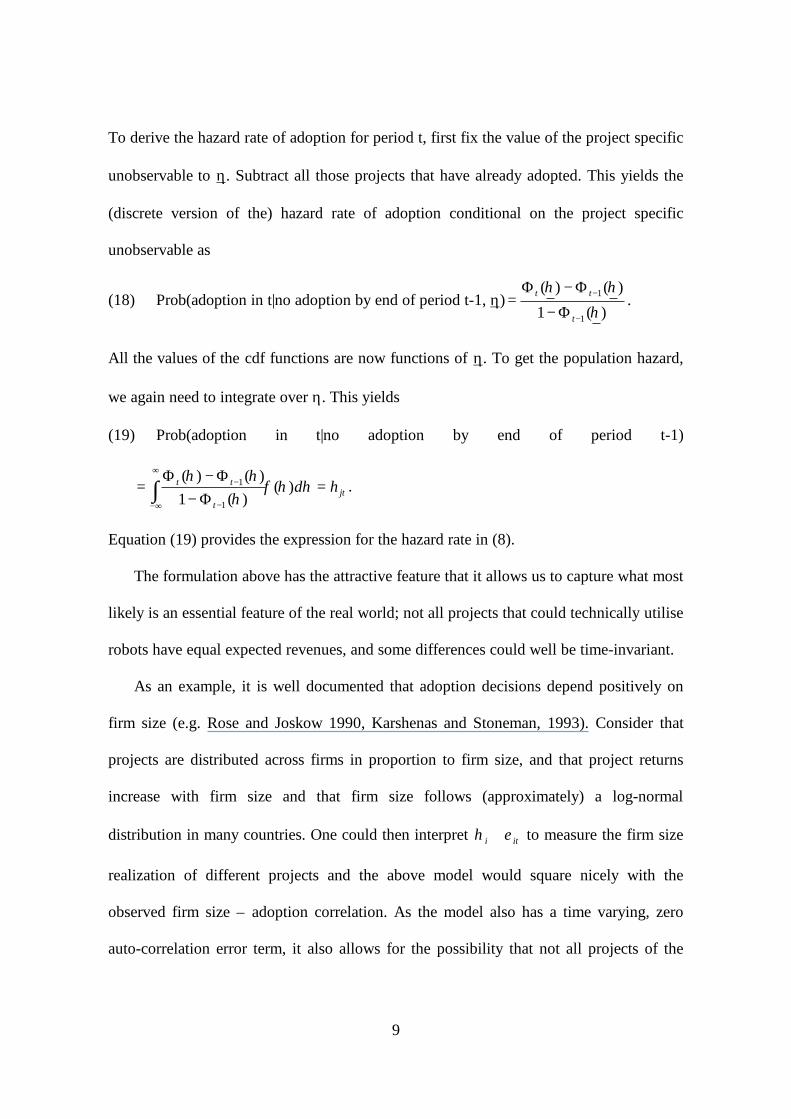
TABLE 2 SOMEWHERE HERE

Table 2 reveals that there is considerable variation in the macrovariables over countries. The

mean of GDP growth varies between 11.72% (Taiwan) and 4.4% (Norway). The mean of

the real interest rate varies between 0.69% (Switzerland) and 7.45% (Taiwan) whereas the

lowest mean inflation rate is found in USA (1.3%) and the highest in Spain (11.1%). There

are also considerable inter-country differences in the volatility measures, but the different

measures do not necessarily move in parallel.

For the drift and volatility of these variables, we use the ML estimates of average

annual growth and its standard deviation, calculated over the period 1975-1992. In the

appendix we report Dickey-Fuller unit root tests employing all the data available in the Penn

14

world tables (usually but not uniformly from 1940 to 1991); for none of the series can we

reject the Null of a random walk. As noted e.g. by Dixit and Pindyck, (1994), it is very much

possible that these results would change had we more data available. As this is not the case,

we proceed on the assumption that the macro level time series are well approximated by

random walks with drift.

4. ECONOMETRIC ISSUES

There are several econometric modeling issues that need to be tackled:

Specification of the model. We proceed by assuming that the potential profit gain from

installing robots is driven by three main macroeconomic indicators, viz. real gross domestic

product GDP, the share of investment in GDP, I/GDP, and the general price level, PI. In

other words, these three variables constitute the vector Xjt. The logic for the variables

included is that demand conditions as measured by GDP and the general price level will be a

main determinant of profit gains from adoption, whereas I/GDP will reflect the general

investment climate and thus also the profitability of robot adoption. One may note that no

cost indicators e.g. factor prices appear in this formulation. Although such cost indicators

will affect the profitability of adoption, the I/GDP variable is a reduced form variable that

will pick up such influences (as well as many others e.g. the buoyancy of expectations). One

might argue that I/GDP could also be said to pick up the influence of the general price level.

We have however included this separately because so much of the literature on investment

and uncertainty stresses the potential impact of the drift and volatility of the price level

(inflation and changes therein). It is important to note that strictly speaking, inflation is a

drift variable, not a volatility variable. Although the popular view is that inflation impedes

investment, one can build an argument for exactly the opposite by noting that the level of

15

consumer prices could measure the price of outputs of robot adopters, rather than the cost of

inputs. In that case increases in the drift of the consumer prices would mean higher expected

prices in the future, thereby increasing discounted profits, and lowering the adoption

threshold. We find (empirically) that GDP, I/GDP and the price level each follow an

absolute Brownian motion and thus their weighed sum will also do so.

Given our limited sample size, we have mainly chosen to parameterize the model to

gain efficiency. We therefore maintain the assumption that both unobservables in R are

normally distributed. Our specific theoretical model does yield an explicit (but

complicated) expression for ρ. Instead of using that, we approximate lnρ with a low order

polynomial, restricting some cross terms to have zero coefficients (to reduce the number

of parameters to be estimated), thereby estimating it semi-parametrically.

We employ the Gompertz specification of the aggregate diffusion curve (equation (8))

as previous work with the same data suggests that this fits the data considerably better

than the logistic (equation (7)).

Error structure. An important issue relating to the error structure rises from the cross-

country nature of our data. It is very likely that e.g. the potential number of robots varies

over countries in a manner that is country specific, time-invariant, and unobservable to

us. This suggests the use of a random effects specification. We could write

(20’) jeINDN jtjtχτθ=

where τ is distributed N(0,χ2), and the country specific time-invariant error term is (after

taking logs; see equation (14)) multiplied by hjt. This creates a random coefficients – type

(equi-correlated) model that cannot be estimated with standard methods.

16

Initial conditions. It is well known that initial conditions (we do not observe robot

diffusion from T=0) may be correlated with time-invariant unobservables (Heckman,

1981). Note however that we do observe country-wise robot stocks “almost” from the

beginning (essentially apart from France): this is likely to reduce the problem

considerably. As can be seen from Table 3, for twelve out of sixteen countries, the first

observed stock accounts for less than 13% of final observed stock and for some,

substantially less. For four countries, the first observed stock is over 20% of the final

observed stock. These countries are Australia (29,97%, 1st observation year 1984), France

(40.44%, 1987), Norway (26.04%, 1982), and Sweden 24.73%, 1982). Together, these

countries account for 4% of sample robot stock at the end of 1992. It would therefore

seem that initial conditions do not pose a serious problem in our data.

TABLE 3 SOMEWHERE HERE

Endogeneity of price terms. Although it may be plausible to think that individual firms

take prices as given when contemplating the adoption of robots, it is less plausible to

assume that the price of robots is exogenous at the country level. This would seem to be

the case at least for the countries with higher adoption rates (Japan being the prime

example). We therefore test for the exogeneity of robot prices in the future.

Aggregation. Our current framework assumes that there is no connection between the

unobservables in Rjt, and the number of potential robots, Njt. In future work we plan to

exploit the knowledge that i) large firms usually adopt earlier (e.g. Rose and Joskow,

1990, Karshenas and Stoneman, 1993) and ii) the firm size distribution is (close to) log-

normal. By assuming that industrial output is the sum of iti εη + over all firms in country

j, we can connect the hazard rate to Njt.

17

Estimation methods. We use a generalized method of moments estimator (GMM) and a

method of simulated moments estimator (MSM) respectively, for models with and

without a time-invariant error term. Both estimators minimize the difference between the

first moments of the data and the model. Currently we use S=40, where S is the number

of simulations, for the MSM estimator. We use simulation to estimate the hazard rate, and

the country specific unobservable τ. We simulate them by drawing pseudo random

numbers from a standard normal with zero mean and unit variance. As the variance of η

is 211 d− , and the coefficient 2

11 d− , we utilize the fact that for )1

()(2

1d−= ηφηφ to

hold (where η is the draw from the standard normal), 211ˆ d−=ηη . That is, to

transform the distribution from a standard normal to N(0, 211 d− ), we insert the η ’s into

the objective function and impose a unit coefficient onto them.

Instruments. Both estimators require instruments. Berndt et al. (1974) show that optimal

instruments are of the form

(21) 1* )'()( −Ω= jtjt xDGxA o

where γ is a vector of parameters, xjt is a data vector,

(22) [ ]jtjtjt xExD |/)( γϕ ∂∂=

where ijtϕ is the distance between data and model moments, and

(23) [ ]jtjtjt xE |'ϕϕ=Ω .

These, however, suffer from reliance on functional form assumptions: if there is

functional form misspecification, the resulting estimator is consistent but inefficient

(Newey, 1990). Newey (1990) has proposed instruments that are asymptotically optimal

18

even under functional form misspecification. Currently we use (untransformed)

explanatory variables as instruments.

Generated regressors. Our drift and volatility variables are generated, leading to biased

standard errors. The problem is exacerbated in our model as the generated regressors

appear in a (highly) nonlinear context. Currently, we are not making this correction.

5. RESULTS (VERY PRELIMINARY)

The estimation results are presented in Table 4. Looking first at the levels variables, we

find that I/GDP and (log of) robot prices affect the hazard rate negatively, GDP and the

real interest rate positively. Of these, the I/GDP sign is contrary to expectations, the

others either as expected, or (in the case of the real interest rate) theoretically

undetermined. Our estimates suggest that the (log of the) number of potential adopters is

0.02 times that industrial output. We inserted a full vector of time dummies into the

hazard rate specification to control for period specific unobservables such as changes in

the quality of robots (normalizing the coefficient of year 1981 to zero). We find that all

time dummies’ coefficients up to and including 1987 are positive and significant, those

for later years negative and significant.

TABLE 4 SOMEWHERE HERE

Turning then to the drift variables, we find that the drift of I/GDP has a positive

impact, and its square a negative one. Within sample values the effect is negative and in

line with the negative coefficient on the levels term. For robot prices, the signs are

reversed, but again within sample values the effect is negative and this time contrary to

expectation. For GDP, the combined effect is positive as predicted, even though the

second order term carries a negative coefficient. Finally, we find that the drift of the price

19

level, i.e., inflation, obtains negative coefficients for both the linear and the second order

terms. This is in line with the popular view that inflation has a negative impact on

investment.

Theory predicts that volatility increases the adoption threshold. In our semi-

parametric specification of the investment threshold, we allowed for interaction terms

between the different volatility variables and have therefore calculated the marginal

effects of volatility on the adoption threshold by its source, holding other types of

volatility at their sample means. These calculations reveal that if one ignores the

interaction terms, the “direct” effect of all types of volatility, but that of the volatility of

I/GDP, are negative. Taking the highly significant interaction terms into account changes

the picture in that now only the volatility of the price level has a positive effect on the

adoption threshold. In other words, the interaction terms change the signs of the partial

derivatives of the (log of) the adoption threshold with respect to the volatility of I/GDP

and price level.

Finally, our set up allows potentially for the estimation of the variance shares of

the time-invariant and time varying components of the unobservable in R. However, the

estimated values rarely diverge from their starting values by much. We have therefore

done limited robustness experiments and found that the results presented are remarkably

robust to large changes in the (starting) value of this parameter.

6. POLICY EXPERIMENTS

TO BE WRITTEN

7. CONCLUSIONS

20

In this paper, we have built an economy level model of technology diffusion that is based

on micro-level optimizing behavior. We show that the traditionally used empirical

models can be cast in this framework, the difference being that the parameter, which has

been called “the adjustment speed” previously, is actually the adoption hazard.

Our model allows for project specific permanent unobservables, as well as time-

varying unobservable differences in project returns. The project level model also shows

how to incorporate measures of uncertainty into the diffusion model, and what measures

of uncertainty to use. We estimate the model using a data set on the international

diffusion of industrial robots.

Our current estimates suggest that uncertainty plays an important role in

determining the adoption speed of industrial robots, but in a way that is to a large extent

incompatible with theory. Of our five identified sources of volatility, namely the

volatility of I/GDP, GDP, robot prices, inflation (drift of the price level), and the

volatility of the price level, only the last two have the predicted negative impact on the

speed of adoption. The other three sources of volatility increase adoption hazard.

21

REFERENCES

Berndt, E. R., B. H. Hall, R. E. Hall, and J. A. Hausman, (1974), “Estimation and Inference in Nonlinear

Structural Models”, Analysis of Economic and Social Measurement, 3, 653-666.

Caballero R- J. and Engel E. M. R. A., (1999), “Explaining investment dynamics in US manufacturing: A

generalized (S,s) approach”, Econometrica,

Dixit A., and R. Pindyck (1994), Investment Under Uncertainty, Princeton, Princeton University Press.

Driver C., and D. Moreton (1991), “The Influence of Uncertainty on UK Manufacturing Investment”,

Economic Journal, 101, 1452 - 59

Heckman J., (1981), “The Incidental Parameters Problem and the Problem of Initial Conditions in

Estimating a Discrete Time-Discrete Data Stochastic Process”, in Manski and McFadden (eds.)

Structural Analysis of Discrete Data with Econometric Applications, MIT Press

Karshenas K., and P. Stoneman (1993), "Rank, Stock, Order and Epidemic Effects in the Diffusion of New

Process Technology", Rand Journal of Economics, 24, 4, 503-528, Winter 1993.

Leahy, J., and Whited. T., (1996), “The Effect of Uncertainty on Investment: Some Stylized Facts”, Journal

of Money, Credit and Banking, 28, 64-83.

Mansfield E., (1968), Industrial Research and Technological Innovation, New York, Norton.

McDonald, R., and Siegel, D., (1986), “The value of waiting to invest”, Quarterly Journal of Economics,

101, 707-727.

Newey, W. K., (1990), “Efficient Instrumental Variables Estimation of Nonlinear Models”, Econometrica,

58, 4, 809-837.

Pagan A. R., (1984). “Econometric Issues in the Analysis of Regressions with Generated Regressors”,

International Economic-Review; 25(1), 221-47.

Pindyck R. S , and A. Solimano (1993), “Economic Instability and Aggregate Investment”, NBER

Macroeconomics Annual, 259 – 303.

Rose, N. and P. Joskow (1990), “The Diffusion of New Technologies: Evidence from the Electricity Utility

Industry”, Rand Journal of Economics, 21, 354 – 373.

Stoneman, P. (1983), The Economic Analysis of Technological Change, London, Oxford University Press

Stoneman, P., (2001), The Economic Analysis of Technological Diffusion, Blackwell. Oxford,

22

forthcoming.

Summers, R. and Heston, A., (1991), “The Penn World Table (Mark 5): An Expanded Set of International

Comparisons, 1950-1988”, Quarterly-Journal-of-Economics; 106(2), 327-68.

Toivanen, O., P. Stoneman and P. Diederen (1999),“Uncertainty, Macroeconomic Volatility and

Investment in New Technology”, in C Driver (ed.), Investment, Growth and Employment:

Perspectives for Policy, 136 – 160, 1999, London, Routledge

23

DATA APPENDIX

1. Data sources and variable definitions

- robot and robot price data: World industrial robots 1994, United Nations. For robot

prices, we use the German prices on the unit value of robot production. Prices for

1979 and 1978 were calculated using the results of a regression of prices on a

constant, years and squared years. The price series was deflated using the consumer

price index reported in the IFS statistics (the only price series available for all

countries). We use prices in constant 1985 US dollars for all countries in the

regressions. To calculate drift and volatility for robot prices we use the whole series.

- GDP, from Penn World Tables Mark 5.6. Defined as GDP = real GDP per capita

(series name CGDP) times population in 000’s (POP)/1000 000. To calculate drift

and volatility for GDP, we use 1960-1992 data, as this was the longest series

available to all countries.

- Manufacturing output. Manufacturing in 1986 defined as Man. = index of

manufacturing times GDP (defined as above) times the manufacturing share of GDP.

For other years, the level of manufacturing is calculated from the 1986 (1992 for

Taiwan, see below) figure using the index of manufacturing. The index is from

International Financial Statistics (for Taiwan from Financial Statistics, Taiwan

District Republic of China: these are designed to conform to the IFS statistics) and

GDP is derived from Penn World Tables as described above. The share of

manufacturing as a per cent of GDP in1986 is from the UN Statistical Yearbook 1995

for all other countries but Italy and Taiwan (not available for these two). For Italy, the

manufacturing share of GDP was calculated as the ratio between figures “industria in

24

senso stretto” (total industry output) and “totale” in Table “Tavola 10 – Produzione al

costo dei fattori – Valori a prezzi 1995” (Table 10 – Production at factor cost – 1995

values”). The table can be found on the web page of the National Institute of Statistics

of Italy (http://www.istat.it/) as file TAVOLE-PRODUZIONE.XLS. The

manufacturing share of GDP was calculated for 1986. For Taiwan, the source is the

file VIGNOF4D.XLS to be found on the web page of the Directorate General of

Budget, Accounting and Statistics of Taiwan (http://www.dgbasey.gov.tw/). The file

contains Table H-2 Structure of Domestic Production, in which the manufacturing

share of GDP is reported for 1992-1995. We used the 1992 figure.

- Investment share of GDP: Penn world tables (CI). Drift and volatility calculations as

with GDP.

- Consumer price level, Penn World Tables (PI). Inflation in country i in year t defined

as inflit = ln(PIit)-ln(PIit-1).

- real interest rate. Defined as the difference between the nominal interest rate and

inflation, both calculated from indexes from the IFS. Inflation is calculated from the

consumer price index as reported in IFS (it is the only price index available for all

sample countries in IFS). We use the money market rate from IFS statistics as the

nominal interest rate.

25

2. Testing the assumption of a random walk

(PRELIMINARY: MORE TESTING TO BE DONE)

Our theoretical model assumes that the relevant (country-level) time-series are random

walks (with drift). In the estimations, we use as explanatory variables ML estimates of

the drift (growth rate) and standard error of GDP, investment share of GDP, and of robot

prices. To test that our time-series are random walks, we regressed the difference in the

series on a constant, time trend, and lagged level using data from the period 1960-1992

(we also estimated the model with out the time trend, with similar results). We then

calculated a Dickey-Fuller test. Table A.1 below summarises our findings, presenting the

D-F test value (p-value) of the GDP and I/GDP estimations for each country separately

(32 degrees of freedom), and finally the robot price tests.

26

TABLE A.1DICKEY FULLER TESTS

Country GDP I/GDPAustralia 1.3640

(1.0000)4.4769

(1.0000)Austria 0.0234

(1.0000)2.3260

(1.0000)Denmark 1.1187

(1.0000)2.5019

(1.0000)Finland 2.0427

(1.0000)2.8554

(1.0000)France 1.0780

(1.0000)2.2507

(1.0000)Germany 1.5006

(1.0000)2.9139

(1.0000)Italy 0.9978

(1.0000)3.0360

(1.0000)Japan 1.1567

(1.0000)2.0718

(1.0000)Norway 1.9845

(1.0000)1.9929

(1.0000)Singapore 2.8244

(1.0000)1.6285

(1.0000)Spain 0.8829

(1.0000)1.8924

(1.0000)Sweden 2.0859

(1.0000)2.9694

(1.0000)Switzerland 0.5560

(1.0000)2.2222

(1.0000)Taiwan 4.6409

(1.0000)1.3666

(1.0000)UK 1.8332

(1.0000)2.5871

(1.0000)USA 1.3868

(1.0000)4.3405

(1.0000)

27

TABLE 1VOLATILITY OF ROBOT ADOPTION INCOMPARISON TO MANUFACTURING

INVESTMENTCountry Ratio of robot diffusion coefficient of

variation to manufacturing investmentcoefficient of variation

Australia 4.15677Austria 5.43715Denmark 3.340727Finland 1.91579France 5.724699Germany 2.729275Italy 4.548866Japan 1.73117Norway 2.944321Spain 2.780212Sweden 1.256557UK 1.422169USA 5.592314

28

TABLE 2COUNTRY-LEVEL DESCRIPTIVE STATISTICS

COUNTRY GDPMillions of1985 USdollars

GDPgrowth %

GDPgrowth

GDPgrowths.d.

Investmentshare ofGDP(I/GDP) percent

%-changein I/GDP

I/GDPgrowth

I/GDPgrowth s.d.

Inflation

Australia1985-1991

271.738241.1980

0.05940.0310

0.0812 0.0347 25.63752.2772

-0.01830.0757

-0.0064 0.0802 -0.00080.09607

Austria1982-1992

98.665521.5569

0.06440.0163

0.0822 0.0279 24.79091.7335

0.00350.0540

0.0073 0.0641 0.03000.1273

Denmark1982-1992

74.667414.6161

0.06330.0191

0.0749 0.0242 21.29092.0364

-0.00150.0843

-0.0096 0.0914 0.02170.1299

Finland1982-1992

67.562213.2520

0.05350.0506

0.0785 0.0467 30.51823.4713

-0.03150.0959

-0.0127 0.0976 0.00500.1073

France1988-1992

948.400786.0395

0.06220.0191

0.0821 0.0226 26.82001.0208

0.00400.0512

0.0021 0.0549 0.02130.0920

Germany1982-1992

933.3297228.9880

0.06850.0196

0.0801 0.0258 23.97270.8855

-0.00110.0332

-0.0077 0.0522 0.02210.1256

Italy1982-1992

729.1065158.3957

0.06290.0141

0.0843 0.0291 24.13640.6772

-0.00290.0341

-0.0083 0.0655 0.04010.1144

Japan1982-1992

1739.0154468.7260

0.07870.0166

0.1080 0.0319 34.42733.3142

0.00940.0443

0.0155 0.0591 0.03090.1297

Norway1983-1992

61.63307.7665

0.04610.0391

0.0802 0.0457 27.70003.7205

-0.02470.1011

-0.0114 0.0965 0.03210.1014

Singapore1982-1992

28.998410.4600

0.10640.0460

0.1284 0.0595 35.80003.6927

-0.00490.0808

0.0121 0.0811 0.00420.0489

Spain1984-1992

387.243087.2258

0.07370.0242

0.0922 0.0262 25.37783.5643

0.02400.0607

0.0117 0.0546 0.07470.1023

Sweden1982-1992

128.596924.3775

0.05450.0210

0.0705 0.0273 21.49092.1741

0.00450.0771

-0.0036 0.0833 0.02240.1184

Switzerland1983-1992

117.101923.1568

0.06060.0190

0.0750 0.0242 30.98002.6599

0.00640.0542

0.0035 0.0800 0.03630.1372

Taiwan1982-1990

130.625844.1117

0.11720.0302

0.1306 0.0349 22.56672.1575

-0.02050.0947

0.0214 0.0955 0.02640.0814

UK1982-1992

742.3100153.1283

0.06050.0227

0.0699 0.0252 17.87271.6298

0.01890.0642

0.0027 0.0771 0.00480.1041

USA1982-1992

4250.05721370.0140

0.05770.0224

0.07490.0016

0.0251 22.08331.8004

-0.00380.0706

-0.00230.0016

0.06380.0042

0.00580.0062

NOTES: First column gives the country name and period used in estimation (which is due to differencing one year less than theobservation period). In most cases, robot data limits the observation period. Each column gives the country level mean and s.d. of therespective variable. Note that e.g. the GDP growth % and GDP growth differ because the former is calculated over the robot stockobservation period only, the latter over a longer period (defined in the data appendix ). For the drift (growth) and volatility variables, nos.d.’s are reported as they are by definition zero.

29

TABLE 2COUNTRY-LEVEL DESCRIPTIVE STATISTICS

COUNTRY Robot stock# robots

Change inrobot stock

%-change Robot priceRP1985 USdollars

RP drift RP s.d. Real interestratePercentagepoints

IndustrialproductionMillions of1985 USdollars

Australia1985-1991

1229.3750402.7757

154.250050.1960

0.15060.0683

98.951031.0942

0.0832 0.2139 6.32381.3662

59.62612.1126

Austria1982-1992

667.6364566.1875

150.0909101.2496

0.30910.0808

90.467629.8562

0.0497 0.2007 4.66290.9528

13.97984.4845

Denmark1982-1992

301.4545193.6958

48.454529.7098

0.22160.1095

90.467629.8562

0.0760 0.2102 7.09891.4206

11.41561.0931

Finland1982-1992

494.2727342.9624

92.363637.4039

0.30930.1797

90.467629.8562

0.0756 0.2182 6.12853.0889

13.83561.1285

France1988-1992

8380.20002071.8759

1289.0000180.4896

0.18110.0638

114.112629.4699

0.0810 0.2144 6.03770.4904

176.15893.8855

Germany1982-1992

17533.181812165.3533

3371.81821782.6613

0.25820.0856

90.467629.8562

0.0516 0.2016 3.81561.1037

282.742830.7243

Italy1982-1992

7573.36365451.8190

1513.3636685.0799

0.33070.1996

90.467629.8562

0.0962 0.2194 4.66621.8523

2.52760.2000

Japan1982-1992

167296.6364111333.3099

29859.818214306.0971

0.25560.1040

90.467629.8562

0.0333 0.2238 3.72690.7464

472.775865.7128

Norway1983-1992

422.4000128.8825

42.600019.0916

0.13450.0970

93.019130.1806

0.0817 0.2150 5.58711.4845

9.10561.2137

Singapore1982-1992

807.4545798.0270

189.5455238.4023

0.54870.4845

90.467629.8562

0.0457 0.3636 5.74925.6178

7.04262.9696

Spain1984-1992

1642.11111006.8790

342.2222217.3671

0.23260.0287

96.027230.3798

0.0902 0.2308 6.46932.7346

85.65905.5779

Sweden1982-1992

2781.27271106.0298

311.363689.7700

0.12700.0318

90.467629.8562

0.0877 0.2199 5.83303.9539

26.02121.6903

Switzerland1983-1992

868.5000695.1109

197.7000132.3976

0.33350.1330

93.019130.1806

0.0524 0.1924 0.69641.0631

28.31992.8359

Taiwan1982-1990

462.4444435.5362

143.5556111.3217

0.79610.8907

88.044532.7886

0.0422 0.2668 7.44581.8341

53.477110.2842

UK1982-1992

4301.54552150.9057

625.9091127.8870

0.21510.1345

90.467629.8562

0.0576 0.2045 4.66911.4663

146.14189.3619

USA1982-1992

25849.833314659.5393

3468.66671890.8775

0.17870.1376

91.656128.7630

0.06860.0035

0.24470.0127

4.88611.6758

800.3874221.5590

NOTES: First column gives the country name and period used in estimation (which is due to differencing one year less than theobservation period). In most cases, robot data limits the observation period. Each column gives the country level mean and s.d. of therespective variable. Note that e.g. the GDP growth % and GDP growth differ because the former is calculated over the robot stockobservation period only, the latter over a longer period (defined in the data appendix ). For the drift (growth) and volatility variables, nos.d.’s are reported as they are by definition zero.

30

TABLE 3COUNTRY LEVEL INITIAL STOCKS AND FINAL

STOCKS OF ROBOTSCountry Initial

stock ofrobots

Final stockof robots

Ratio ofinitial to

final stockof robots

1st year ofobservation/

# obs.

Australia 528 1762 0.2997 1984/7Austria 57 1708 0.0334 1981/11Denmark 51 584 0.0873 1981/11Finland 35 1051 0.0333 1981/11France 4376 10821 0.4044 1987/5Germany 2300 39390 0.0584 1981/11Italy 450 17097 0.0263 1981/11Japan 21000 349458 0.0601 1981/11Norway 150 576 0.2604 1982/10Singapore 5 2090 0.0024 1981/11Spain 433 3513 0.1233 1983/9Sweden 1125 4550 0.2473 1981/11Switzerland 73 2050 0.0356 1982/10Taiwan 1 2217 0.0005 1981/9UK 713 7598 0.0938 1981/11USA 6000 47000 0.1277 1981/11

31

TABLE 4ESTIMATION RESULTS

Variable/parameter (1)GMM

Baseline hazardConstant/β0 -

GDP/β1 0.000206 0.000000

αGDP/β11 4.968712 0.00869

α2GDP/β12 -3.451337

0.025332σGDP/β13 -0.397163

0.008947σ2

GDP/β14 -3.121666 0.117557

I/GDP/β2 -0.00120.0001

αIGDP/β21 0.061762 0.025885

α2IGDP/β22 -1.049791

0.608599σIGDP/β23 3.976006

0.010012σ2

IGDP/β24 0.078959 0.006117

lnP/β3 -0.024560 0.000086

αP/β31 -5.236258 0.009672

α2P/β32 0.651282

0.034230σP/β33 3.513657

0.000600σ2

P/β34 12.192355 0.007358

r/β4 0.021415 0.000064

i/β51 -14.852534 0.035978

i2/β52 -1.948580 0.469109

σi/β53 0.033383 0.006828

σ2i/β53 0.198876

0.073622σI/GDPσP /β53 4.557470

0.022868σI/GDPσi/β53 -0.952449

0.078442σI/GDPσGDP/β53 1.271087

0.139501σPσi/β53 -0.027212

0.039015σPσGDP/β53 4.848620

0.055216σiσGDP/β53 0.387525

0.138850d1 0.500000

0.000001Frictionless robot stock

lnIND/λ 0.018992 0.010878

NOTES: S=40 (S = # simulation draws). *** = sign. at the 1% level., ** = sign. at the 5% level., * = sign. atthe 10% level.. A full set of time dummies is included into the probability ofadoption function

32