characterisation of dystrophic skeletal muscle using
TRANSCRIPT
Characterisation of dystrophic skeletal muscle using polarisation-sensitive and needle-based
optical coherence tomography
Xiaojie Yang
Master of Biomedical Engineering
This thesis is presented for the degree of Doctor of Philosophy of The
University of Western Australia
School of Electrical, Electronic & Computer Engineering
October, 2014

Abstract
i
Abstract Characterisation and assessment of skeletal muscle damage resulting from Duchenne muscular
dystrophy is essential for the pharmaceutical and nutritional interventions being investigated as
potential treatments for this disease. The conventional method of examining tissue by
histological analysis requires excision, preservation, sectioning, staining, and evaluation by light
microscopy and is, therefore, time-consuming and laborious. Moreover, preclinical and clinical
research, respectively, require sacrifice of animals, which is costly, and biopsy from human
patients, which is invasive. As importantly, it is not possible to perform a longitudinal study of
the same animal or human tissue over an extended period of time. Biomedical imaging
modalities, such as ultrasound, X-ray computed tomography, magnetic resonance imaging, and
light microscopy, have been extensively studied and applied to muscle imaging. The spatial
resolution provided by these clinical volumetric imaging modalities is typically not fine enough
to resolve the ultrastructure of skeletal muscle, such as individual myofibres, that is required for
full characterisation. Moreover, high radiation dose and low contrast in soft tissues remain
issues for X-ray computed tomography and magnetic resonance imaging requires long
acquisition times and is costly.
Optical coherence tomography (OCT) potentially overcomes many of these limitations. OCT is
a noninvasive, low-cost imaging modality providing volumetric data with spatial resolution of
approximately 10 µm. OCT has been applied to imaging skeletal muscle tissue and has
demonstrated potential for characterising muscle damage within dystrophic muscle in mouse
models. However, OCT does not readily lend itself to automatic quantification of the proportion
of muscle damage within a muscle sample, mainly because of its low contrast. This hampers the
inter-scan or inter-sample comparison of the myopathology of the muscle, which is often
required in assessment of skeletal muscle damage. Moreover, the penetration depth of OCT is
limited to approximately 2 mm beneath the surface of skeletal muscle tissue. Visualisation of
the internal structures of tissue ideally requires a greater penetration depth.
In this thesis, two advancements in imaging skeletal muscle using OCT are presented. The
application of an extension of OCT, polarisation-sensitive OCT (PS-OCT), for characterising
and quantitatively assessing muscle damage within dystrophic mouse muscle is presented.
Birefringence of the muscle samples detected by PS-OCT provides a more objective and
reliable indicator of muscle damage. Two-dimensional parametric images, readily indicating the
volumetric proportion of damage within imaged regions of muscle samples, were automatically
generated by a custom computational algorithm applied to the acquired volumetric PS-OCT
data. The volumetric proportion of muscle damage calculated from the parametric images is in
good agreement with the volumetric values manually assessed by conventional stereology of the
Abstract
ii
corresponding histological sections. This method may provide an efficient and accurate
alternative to conventional approaches to damage assessment in the future.
The second advancement presented in this thesis is the development, fabrication and application
of an ultrathin side-viewing needle-based OCT probe. The probe is the smallest side-viewing
OCT volumetric imaging needle probe to be developed in the world, and is reported here along
with two alternative designs for achieving an extended depth of focus. The ultrathin side-
viewing OCT needle probe was first applied in imaging internal ultrastructures of lung tissue.
The results demonstrated the capability of the needle probe in imaging the internal ultrastructure
of opaque tissue. Subsequently, the ultrathin needle probe was applied to imaging internal
ultrastructures of skeletal muscle. Individual myofibres and other internal structures, such as
connective tissues, that were ~1 cm below the tissue surface were clearly visualised within the
acquired volumetric data. This demonstration of an ultrathin needle probe for muscle imaging
extends the utility of OCT to deep in tissue well beyond the conventional few-millimetre limits.
Contents
iii
Contents
Abstract ........................................................................................................................................... i
Contents ....................................................................................................................................... iii
Acknowledgements ..................................................................................................................... vii
Statement of contribution .............................................................................................................. ix
List of publication ....................................................................................................................... xii
List of figures .............................................................................................................................. xvi
List of tables ................................................................................................................................ xxi
List of abbreviations ................................................................................................................. xxii
Chapter 1 Introduction ........................................................................................................ 1
1.1 Research motivation.......................................................................................................... 1
1.2 Outline of thesis ................................................................................................................ 3
Chapter 2 Background ........................................................................................................ 6
2.1 Preface .............................................................................................................................. 6
2.2 Overview of the structure and function of muscles .......................................................... 6
2.3 Skeletal muscle ................................................................................................................. 8
2.3.1 Myofibres in skeletal muscle ............................................................................... 8
2.3.2 ECM in skeletal muscle ..................................................................................... 13
2.3.3 Contraction of skeletal muscle ........................................................................... 16
2.4 DMD ............................................................................................................................... 18
2.4.1 Phenotype of DMD ............................................................................................ 18
2.4.2 Pathological changes of DMD ........................................................................... 20
2.4.3 The mdx mouse model ....................................................................................... 22
2.5 Techniques for imaging skeletal muscle and muscle damage ........................................ 23
2.5.1 Ultrasonography ................................................................................................. 24
2.5.2 CT ...................................................................................................................... 27
2.5.3 MRI .................................................................................................................... 29
2.5.4 Light microscopy ............................................................................................... 31
Contents
iv
2.6 OCT ................................................................................................................................ 33
2.6.1 Working principle .............................................................................................. 34
2.6.2 Application of OCT in imaging skeletal muscle and muscle damage ............... 37
2.6.3 Challenges of using OCT for assessment of muscle damage and in vivo imaging
of skeletal muscle .............................................................................................. 39
2.7 Chapter summary............................................................................................................ 40
Chapter 3 Characterisation of skeletal muscle damage using PS-OCT ....................... 42
3.1 Preface ............................................................................................................................ 42
3.2 Optical birefringence and polarisation ........................................................................... 42
3.3 Representation of the SoP .............................................................................................. 46
3.4 PS-OCT .......................................................................................................................... 49
3.5 Birefringence of skeletal muscle .................................................................................... 52
3.6 En face parametric imaging of tissue birefringence using polarization-sensitive optical
coherence tomography .................................................................................................... 56
3.6.1 Introduction ....................................................................................................... 56
3.6.2 Method............................................................................................................... 57
3.6.3 Experiment ........................................................................................................ 59
3.6.4 Results ............................................................................................................... 61
3.6.5 Discussion ......................................................................................................... 63
3.6.6 Conclusion ......................................................................................................... 64
3.6.7 Acknowledgements ........................................................................................... 65
3.6.8 References ......................................................................................................... 65
3.7 Quantitative assessment of muscle damage in the mdx mouse model of Duchenne
muscular dystrophy using polarization-sensitive optical coherence tomography .......... 68
3.7.1 Introduction ....................................................................................................... 68
3.7.2 Materials and methods ....................................................................................... 71
3.7.3 Results ............................................................................................................... 76
3.7.4 Discussion ......................................................................................................... 79
3.7.5 Conclusion ......................................................................................................... 82
3.7.6 Acknowledgements ........................................................................................... 82

Contents
v
3.7.7 References .......................................................................................................... 82
3.8 Related works ................................................................................................................. 87
3.8.1 The injected EBD does not significantly affect the detected birefringence ....... 87
3.8.2 Manual estimation of percentage necrosis within histological sections ............ 88
3.9 Chapter summary ............................................................................................................ 92
Chapter 4 Needle probes for OCT .................................................................................... 94
4.1 Preface ............................................................................................................................ 94
4.2 Review of endoscopic OCT probes ................................................................................ 94
4.2.1 Catheter-based OCT probes ............................................................................... 94
4.2.2 Needle-based OCT probes ................................................................................. 95
4.3 Development of ultrathin needle probes for OCT imaging ............................................ 96
4.3.1 Preface ............................................................................................................... 96
4.3.2 Ultra-thin side-viewing needle probe for optical coherence tomography .......... 96
4.3.3 Static and dynamic imaging of alveoli using optical coherence tomography
needle probes ................................................................................................... 102
4.4 Alternative designs of OCT fibre probes for extended depth of focus with maintained
lateral resolution and sensitivity ................................................................................... 118
4.4.1 Preface ............................................................................................................. 118
4.4.2 Ultrathin fiber probes with extended depth of focus for optical coherence
tomography ...................................................................................................... 119
4.4.3 Accurate modeling and design of graded-index fiber probes for optical
coherence tomography using the beam propagation method ........................... 124
4.5 Chapter summary .......................................................................................................... 145
Chapter 5 Imaging skeletal muscle using an ultrathin side-viewing OCT needle probe
......................................................................................................................... 148
5.1 Preface .......................................................................................................................... 148
5.2 Imaging data of mouse skeletal muscle obtained using the 840-nm OCT needle probe
............................................................................................................................................... 149
5.3 Imaging deep skeletal muscle structure using a high-sensitivity ultrathin side-viewing
optical coherence tomography needle probe ................................................................. 152
5.3.1 Introduction ...................................................................................................... 152

Contents
vi
5.3.2 Materials and methods ..................................................................................... 154
5.3.3 Results ............................................................................................................. 160
5.3.4 Discussion ....................................................................................................... 163
5.3.5 Conclusion ....................................................................................................... 164
5.3.6 Acknowledgements ......................................................................................... 164
5.3.7 References ....................................................................................................... 165
5.4 Effect of the relative orientation of the needle insertion and myofibres ...................... 169
5.5 Chapter summary .......................................................................................................... 171
Chapter 6 Conclusion ...................................................................................................... 172
6.1 Significance of the research outcomes ......................................................................... 172
6.2 Research limitations and future work ........................................................................... 174
6.3 Summary of contributions ............................................................................................ 176
Appendix I Theoretical description of OCT ................................................................... 177
Preface ................................................................................................................................... 177
Introduction ........................................................................................................................... 177
A1.1 The incident light .......................................................................................................... 177
A1.2 The reflected and back-scattered light .......................................................................... 178
A1.3 Detection of the signal .................................................................................................. 179
A1.4 Analysis of the signal ................................................................................................... 182
References ................................................................................................................................ 185

Acknowledgements
vii
Acknowledgements First of all, I would like to thank God for helping me to have the chance to pursue an
engineering PhD in a world-class university overseas, which has been a dream since my
childhood. I presume that God has been witnessing me standing on the top of the hill behind my
apartment in Qingdao (Tsingtao) (Shandong, China) and praying towards the sky with the Bible
in early 2009.
I would like to thank my mother, my father, and my grandparents. They are either teachers in
primary and middle schools, or professors in colleges and universities. Therefore, great
demands are required to be their child due to their extremely high expectations for me. As their
only child, I am supposed to be better than any other children that they know, especially in
terms of studying. Whether or not these requirements are acceptable in western culture, I am
propelled to pull through any hardships to pursue the highest qualification. My grandmother on
my mother’s side, unfortunately, passed away in 2010. I hope she has been able to see my
progress from heaven. Special gratitude should be conferred to my mother’s father, my
grandfather. Although he has been probably deprived of the right of seeing my progress because
of Alzheimer’s disease, I will never forget his encouragement to me whilst I was growing up.
It is my real honour to be included in this world-class research group, Optical + Biomedical
Engineering Laboratory (OBEL), and to be admitted to the University of Western Australia
(UWA). My first thanks go to Winthrop Professor David D. Sampson for mentoring me in
2009. David’s warm reply to my inquiry emails in 2008 gave me the most brilliant and glittering
light of hope, when almost all of other universities relentlessly ignored my inquiries about PhD
studies at that time. Associate Professor Robert A. McLaughlin’s very warm welcome and
detailed guidance permeated not only into my research but also into my life. It was my luck to
be supervised by and work with Assistant Professor Dirk Lorenser during my PhD years. Dr.
Lorenser is the best supervisor I have ever met. His patient and considerate guidance helped me
to overcome numerous practical problems during experiments. Winthrop Professor Miranda D.
Grounds is another supervisor for whom I should show my sincere respect. Her comfort and
encouragement rebuilt my confidence constantly. Thus, I could keep walking forward along this
long journey.
Moreover, I would like to thank Dr. Joanne Edmondston, who always provided me with
substantial help and significant support during my whole PhD candidature; thanks to Dr.
Timothy R. Hillman, who was the first friendly colleague in OBEL explaining the principle of
spectral-domain optical coherence tomography (SD-OCT) to me; thanks to Mr. Bryden C.
Quirk, who generously gave me professional guidance in practical operations; thanks to Mr.
Lixin Chin, who came to OBEL perfectly in time to provide me with help in computational
Acknowledgements
viii
programming; thanks to Dr. Yih M. Liew and Mr. Peijun Gong, who were the only people
speaking Mandarin to me in OBEL.
I have suffered many trials and tribulations during my five years of PhD study. I was suffering
from bed bugs in early 2011. Numerous clusters of red bumps covered my body and brought me
unbearable itching. In the middle of 2011, my short-sightedness became worse. The most
serious issue happened in the middle of 2012 when I became a victim of internet violence from
Qingdao (Tsingtao) (Shandong, China). My private information was illegally released and
abused by several lawbreakers in Qingdao. Libel and insult were levelled at me and,
unavoidably, caused me psychological trauma. However, I have overcome all of these
difficulties. For those who expect to see my failure, I will try my best to keep disappointing
you! For those who have plagued me, my payback time will definitely come, sooner or later!
I have been in Australia for almost seven years. I have finished my master’s degree in
Melbourne, and I am finishing my PhD in Perth. I determined to study overseas to pursue my
honour of life, although it is clearer than crystal that this way is deemed to be tough from its
beginning to the end. I am not as lucky as those Chinese students who are sponsored by the
Chinese government (specifically, the Chinese Scholarship Council). Instead, I was self-funding
in Melbourne and then successfully applied for the scholarships from UWA by myself. I am not
a born genius, so I have to devote more time and effort compared with those intelligent or lucky
people. It is true that I am not young anymore at the last stage of my PhD. Thirty, is no longer a
proud age for submitting a PhD thesis. According to Chinese tradition, a 30-year-old man
should already have his own career and family. From this perspective, I am not yet successful.
However, I will go on following my way towards my aim, no matter what dangers and obstacles
are in store for me in the future. I will try my best to raise me up!
Statement of contribution
ix
Statement of contribution This thesis contains seven published journal articles. The candidate, Xiaojie Yang (XY), is the
first author of two of these journal articles and the second author of five other journal articles.
Xiaojie Yang is the sole author for the remainder of this thesis. The journal articles are
presented in the form in which they were published, except the formatting has been adapted to
match the style of the thesis, according to The University of Western Australia’s guidelines on
“Thesis as a series of papers” (http://www.postgraduate.uwa.edu.au/students/thesis/series.
Accessed: 22 March, 2014). The bibliographical details of these articles, the locations where
they appear and the contribution by XY are outlined below. Acronyms for other authors’ names
are BCQ (Bryden C. Quirk), BRK (Blake R. Klyen), DDS (David D. Sampson), DL (Dirk
Lorenser), LC (Lixin Chin), MCS (M. Cather Simpson), ME (Matthew Edmond), MDG
(Miranda D. Grounds), PBN (Peter B. Noble), RAM (Robert A. McLaughlin), RWK (Rodney
W. Kirk), and TS (Tea Shavlakadze).
Lixin Chin, Xiaojie Yang, Robert A. McLaughlin, Peter B. Noble, and David D. Sampson,
“En face parametric imaging of tissue birefringence using polarization-sensitive optical
coherence tomography”, Journal of Biomedical Optics, 18(6), art.066005, 2013.
This publication is presented in Chapter 3, Section 3.6. XY prepared the tissue (tendon) samples
for PS-OCT imaging and provided assistance for the operation of the imaging system. The
sample preparation included excision and cutting of the tendon samples. XY provided assistance
in the experiment for the thermal damage of the samples. The estimated percentage contribution
from XY is 20%.
X. Yang, L. Chin, B. R. Klyen, T. Shavlakadze, R. A. McLaughlin, M. D. Grounds, and D.
D. Sampson, "Quantitative assessment of muscle damage in the mdx mouse model of
Duchenne muscular dystrophy using polarization-sensitive optical coherence
tomography," Journal of Applied Physiology 115(9), pp. 1393-1401, 2013.
This publication is presented in Chapter 3, Section 3.7. XY, under the supervision of RAM,
MDG, and DDS, conducted all the imaging experiments presented in this article, to acquire the
PS-OCT volumetric data and photographs of all the imaged muscle samples. Moreover, XY
conducted the fixation of the samples after imaging in preparation for histology. The
histological sections were imaged by XY. The image coregistration and colocated comparison
between the images of histological sections and the corresponding PS-OCT images were
performed by XY. The manual estimation of the percentage necrosis within the histological
sections was performed by XY. XY provided assistance in the sacrifice of the mice and excision
Statement of contribution
x
of the muscle samples. XY drafted the journal article, which has been comprehensively
reviewed and edited by all co-authors. The estimated percentage contribution from XY is 40%.
D. Lorenser, X. Yang, R. W. Kirk, B. C. Quirk, R. A. McLaughlin, and D. D. Sampson,
“Ultrathin side-viewing needle probe for optical coherence tomography”, Optics Letters,
36(19), pp. 3894-3896, 2011.
This publication is presented in Chapter 4, Section 4.3.2. XY fabricated the ultrathin side-
viewing OCT needle probe under the detailed supervision by DL. The fabrication included
cleaving, and splicing that were for the fabrication of the optical fibre elements following the
specific design; angle-polishing and fibre probe with accurate control of the removed fibre
lengths; taking microphotograph of the fabricated fibre probe. All of these steps of fabrication
were conducted by XY. XY provided assistance in the metal coating of the fibre probe and the
assembling of the completed needle probe. XY, under the supervision of BCQ, conducted the
electro-chemical etching of the side opening on the employed hypodermic needles.
Furthermore, the beam profiles of the fabricated fibre probes and assembled needle probes were
measured by XY. The estimated percentage contribution from XY is 30%.
R. A. McLaughlin, X. Yang, B. C. Quirk, D. Lorenser, R. W. Kirk, P. B. Noble, and D. D.
Sampson, “Static and dynamic imaging of alveoli using optical coherence tomography
needle probes”, Journal of Applied Physiology, 113(6), pp. 967-974, 2012.
This publication is presented in Chapter 4, Section 4.3.3. XY fabricated the ultrathin OCT
needle probe (the probe presented in the previous journal article by Lorenser et al. published in
2011) used in the experiments that was presented in this article. XY provided assistance in the
imaging experiment. The estimated percentage contribution from XY is 20%.
D. Lorenser, X. Yang, and D. D. Sampson, "Ultrathin fiber probes with extended depth of
focus for optical coherence tomography", Optics Letters, 37(10), pp. 1616-1618, 2012.
This publication is presented in Chapter 4, Section 4.4.2. XY fabricated the designed fibre
probes. This fabrication included cleaving and splicing of the sections of optical fibres with
accurate control of their lengths. The hemispherical refractive lens was generated and appended
by XY to the end of the fibre probe, using optical adhesive and the ultraviolet lamp. The beam
profiles of the fabricated fibre probes were measured by XY. The estimated percentage
contribution from XY is 40%.
Statement of contribution
xi
D. Lorenser, X. Yang, and D. D. Sampson, "Accurate modeling and design of graded-
index fiber probes for optical coherence tomography using the beam propagation
method", IEEE Photonics Journal, 5(2), art.3900015, 2013.
This publication is presented in Chapter 4, Section 4.4.3. XY fabricated the fibre probes, which
were for the validation of the simulated results, following the design by DL. The beam profiles
of the fabricated fibre probes were measured by XY. The estimated percentage contribution
from XY is 15%.
X. Yang, D. Lorenser, R. A. McLaughlin, R. W. Kirk, M. Edmond, M. C. Simpson, M. D.
Grounds, and D. D. Sampson, "Imaging deep skeletal muscle structure using a high-
sensitivity ultrathin side-viewing optical coherence tomography needle probe," Biomedical
Optics Express, 5(1), pp. 136-148, 2014.
This publication is presented in Chapter 5, Section 5.2. XY fabricated the improved ultrathin
side-viewing OCT needle probes that were presented in the article. The fabrication included
cleaving, and splicing that were for the fabrication of the optical fibre elements following the
specific design; angle-polishing and fibre probe with accurate control of the removed fibre
lengths; and taking a microphotograph of the fabricated fibre probe. All of these steps of
fabrication were conducted by XY. The beam profiles of the fabricated fibre probes and
assembled needle probes were measured by XY. XY operated the customised imaging system
and achieved the imaging experiments under the detailed supervision of DL. The imaged muscle
samples were prepared by XY. After imaging, the acquired OCT data were processed by XY,
using the customised software developed by RWK. The imaged muscle samples were fixed by
XY in preparation for histology. The histological sections were imaged by XY. The colocated
comparison and image coregistration between the images of histological sections and the OCT
data were subsequently performed by XY. The journal article was drafted by XY based on the
analysis of the OCT data. The article draft was comprehensively reviewed and edited by all co-
authors. The estimated percentage contribution from XY is 40%.
Student’s signature: Date:
Co-ordinating supervisor’s signature: Date:
List of publication
xii
List of publication Peer-reviewed journal articles:
1. D. Lorenser, X. Yang, R. W. Kirk, B. C. Quirk, R. A. McLaughlin, and D. D. Sampson,
“Ultrathin side-viewing needle probe for optical coherence tomography”, Optics Letters,
36(19), pp. 3894-3896, 2011.
2. D. Lorenser, X. Yang, and D. D. Sampson, "Ultrathin fiber probes with extended depth of
focus for optical coherence tomography", Optics Letters, 37(10), pp. 1616-1618, 2012.
3. R. A. McLaughlin, X. Yang, B. C. Quirk, D. Lorenser, R. W. Kirk, P. B. Noble, and D. D.
Sampson, “Static and dynamic imaging of alveoli using optical coherence tomography
needle probes”, Journal of Applied Physiology, 113(6), pp. 967-974, 2012.
4. X. Yang, L. Chin, B. R. Klyen, T. Shavlakadze, R. A. McLaughlin, M. D. Grounds, and D.
D. Sampson, "Quantitative assessment of muscle damage in the mdx mouse model of
Duchenne muscular dystrophy using polarization-sensitive optical coherence tomography,"
Journal of Applied Physiology 115(9), pp. 1393-1401, 2013.
5. D. Lorenser, X. Yang, and D. D. Sampson, "Accurate modeling and design of graded-index
fiber probes for optical coherence tomography using the beam propagation method", IEEE
Photonics Journal, 5(2), art.3900015, 2013.
6. L. Chin, X. Yang, R. A. McLaughlin, P. B. Noble, and D. D. Sampson, “En face parametric
imaging of tissue birefringence using polarization-sensitive optical coherence tomography”,
Journal of Biomedical Optics, 18(6), art.066005, 2013.
7. X. Yang, D. Lorenser, R. A. McLaughlin, R. W. Kirk, M. Edmond, M. C. Simpson, M. D.
Grounds, and D. D. Sampson, "Imaging deep skeletal muscle structure using a high-
sensitivity ultrathin side-viewing optical coherence tomography needle probe," Biomedical
Optics Express, 5(1), pp. 136-148, 2014.
Conference proceedings:
Keys: § Domestic; ‡ International; † poster presentation; ¡ oral presentation
1. §† X. Yang, L. Chin, R. A. McLaughlin, B. R. Klyen, H. G. Radley-Crabb, G. J. Pinniger,
M. D. Grounds, and D. D. Sampson, "Quantitative identification of muscle necrosis in an
mdx mouse using high-resolution optical birefringence imaging," presented at Combined
Biological Sciences Meeting (CBSM), Perth, WA, Australia, 2011.
2. ‡¡ X. Yang, R. A. McLaughlin, D. Lorenser, R. W. Kirk, P. B. Noble, and D. D. Sampson,
"In situ 3D imaging of alveoli with a 30 gauge side-facing optical needle probe," presented at

List of publication
xiii
International Conference on Intelligent Sensors, Sensor Networks and Information
Processing (ISSNIP), Adelaide, SA, Australia, 2011.
3. §† L. Chin, X. Yang, R. A. McLaughlin, and D. D. Sampson, "A novel image processing
algorithm for high resolution assessment of tissue damage using polarisation sensitive optical
coherence tomography," presented at Combined Biological Sciences Meeting (CBSM), Perth,
WA, Australia, 2011.
4. ‡¡ X. Yang, D. Lorenser, R. W. Kirk, B. C. Quirk, P. B. Noble, R. A. McLaughlin, and D. D.
Sampson, "In situ 3D imaging of alveoli with a 30-gauge side-facing OCT needle probe,"
presented at BiOS, San Francisco, CA, US, 2012.
5. ‡¡ X. Yang, D. Lorenser, G. J. Pinniger, R. W. Kirk, R. A. McLaughlin, and D. D. Sampson,
“In situ 3D imaging of internal structures of skeletal muscle with a 30-gauge optical needle
probe”, presented at International Conference of APMC-ICONN-ACMM, Perth, WA,
Australia, 2012.
6. ‡† X. Yang, D. Lorenser, R. W. Kirk, G. J. Pinniger, M. D. Grounds, R. A. McLaughlin, and
D. D. Sampson, “3D imaging of internal structures of skeletal muscle with an ultrathin side-
viewing optical needle probe”, presented at International Congress of World Muscle Society
(WMS), Perth, WA, Australia, 2012.
7. §† X. Yang, R. A. McLaughlin, D. Lorenser, B. C. Quirk, R. W. Kirk, P. B. Noble, G. J.
Pinniger, M. D. Grounds, and D. D. Sampson, “3D imaging of biological tissue using a 30-
gauge side-facing OCT needle probe”, presented at Combined Biological Sciences Meeting
(CBSM), Perth, WA, Australia, 2012.
8. §† X. Yang, R. A. McLaughlin, D. Lorenser, B. C. Quirk, R. W. Kirk, P. B. Noble, G. J.
Pinniger, M. D. Grounds, and D. D. Sampson, "3D imaging of biological tissue using a 30-
gauge side-viewing optical needle probe," presented at Postgraduate Electrical Engineering
and Computing Symposium (PEECS), Perth, WA, Australia, 2012.
9. ‡¡ D. Lorenser, X. Yang, R. W. Kirk, B. C. Quirk, R. A. McLaughlin, and D. D. Sampson,
"Ultra-thin 30-gauge needle probe for minimally invasive 3D optical coherence
tomography," presented at BiOS, San Francisco, CA, US, 2012.
10. §† L. Chin, X. Yang, B. R. Klyen, R. A. McLaughlin, T. Shavlakadze, M. D. Grounds, and
D. D. Sampson, “Automated assessment and quantification of muscle necrosis in the mdx
mouse model of Duchenne muscular dystrophy”, presented at Combined Biological Sciences
Meeting (CBSM), Perth, WA, Australia, 2012.
11. ‡¡ L. Chin, X. Yang, R. A. McLaughlin, H. G. Radley-Crabb, M. D. Grounds, and D. D.
Sampson, “Parametric imaging of birefringence in muscle using polarisation-sensitive
optical coherence tomography using polarisation-sensitive optical coherence tomography”,
List of publication
xiv
presented at International Conference of APMC-ICONN-ACMM, Perth, WA, Australia,
2012.
12. ‡† L. Chin, X. Yang, R. A. McLaughlin, B. R. Klyen, H. G. Radley-Crabb, G. J. Pinniger, T.
Shavlakadze, M. D. Grounds, and D. D. Sampson, “Identification of muscle necrosis in mdx
mice using optical birefringence imaging”, presented at International Congress of World
Muscle Society (WMS), Perth, WA, Australia, 2012.
13. ‡¡ D. Lorenser, X. Yang, R. W. Kirk, B. C. Quirk, R. A. McLaughlin, and D. D. Sampson,
“Needle probes for optical coherence tomography: recent advances in technology and
applications”, oral presentation in International Conference Series of Focus on Microscopy
(FOM), Singapore, 2012.
14. ‡¡ D. Lorenser, X. Yang, and D. D. Sampson, “Analysis of fiber-optic probes using graded-
index fiber microlenses with non-ideal refractive index profiles”, presented at International
Conference of Optical Fibre Sensors (OFS), Beijing, China, 2012.
15. ‡¡ X. Yang, D. Lorenser, R. A. McLaughlin, R. W. Kirk, M. Edmond, M. C. Simpson, M. D.
Grounds, and D. D. Sampson, "Robust ultrathin needle probe with high sensitivity for
imaging deep skeletal muscle structure with optical coherence tomography," presented at
Australian and New Zealand Conference on Optics and Photonics (ANZCOP), Fremantle,
WA, Australia, 2013.
16. ‡¡ L. Chin, X. Yang, B. R. Klyen, R. A. McLaughlin, T. Shavlakadze, M. D. Grounds, and
D. D. Sampson, “Automated quantification of birefringence for assessment of muscle
necrosis using polarization-sensitive optical coherence tomography”, presented at BiOS, San
Francisco, CA, US, 2013.
17. ‡¡ L. Chin, X. Yang, R. A. McLaughlin, P. B. Noble, and D. D. Sampson, "Birefringence
imaging for optical sensing of tissue damage," presented at International Conference on
Intelligent Sensors, Sensor Networks and Information Processing (ISSNIP), Melbourne,
VIC, Australia, 2013.
18. ‡¡ D. Lorenser, L. Scolaro, X. Yang, B. C. Quirk, R. W. Kirk, M. Auger, W. Madore, N.
Godbout, M. Edmond, M. C. Simpson, C. Boudoux, R. A. McLaughlin, and D. D. Sampson,
"Advancements in performance and capabilities of OCT needle probes," presented at
European Conferences on Biomedical Optics (ECBO), Munich, Germany, 2013.
19. §¡ R. A. McLaughlin, D. Lorenser, B. C. Quirk, L. Scolaro, X. Yang, K. M. Kennedy, and
D. D. Sampson, "A microscope in a needle - new techniques to view disease," presented at
Engineering and the Physical Sciences in Medicine conference (EPSM), Perth, WA,
Australia, 2013.
List of publication
xv
20. ‡¡ X. Yang, D. Lorenser, R. A. McLaughlin, R. W. Kirk, M. Edmond, M. C. Simpson, M. D.
Grounds, and D. D. Sampson, "Demonstration of 3D imaging of skeletal muscle at
centimeter depths using a 30-gauge side-viewing optical coherence tomography needle
probe," presented at BiOS, San Francisco, CA, US, 2014.
List of figures
xvi
List of figures
2.1 Light microscopic images of the H&E-stained histological sections of mouse skeletal
muscle, smooth muscle and cardiac muscle ..................................................................... 7
2.2 Diagram to illustrate myogenesis and the formation of skeletal myofibres, with
comparison to cell sizes .................................................................................................... 9
2.3 Structural hierarchy of skeletal muscle .......................................................................... 10
2.4 Different architectures of skeletal muscle ...................................................................... 10
2.5 Distribution of nuclei in mature and regenerated myofibres .......................................... 11
2.6 The interdigitating arrangement of myosin and actin filaments ..................................... 12
2.7 The structure of sarcomeres at the cellular and molecular levels, including the
definitions of A-band, I-band, H-zone, M-line, and Z-line ............................................ 12
2.8 The ECM structure of skeletal muscle ........................................................................... 14
2.9 Tendons attach the ends of skeletal muscle to bones ..................................................... 15
2.10 Schematic representation of the ECM surrounding skeletal muscle .............................. 15
2.11 The arrangement of myofilaments, as well as the definitions of A-band, I-band, H-zone,
M-line, Z-line, within one individual sarcomere when the muscle is stretched, resting
and contracted ................................................................................................................. 17
2.12 Schematic and TEM images revealing that cross-bridges are formed when the state of
muscle changes from resting to contracted..................................................................... 17
2.13 H&E-stained transverse sections of dystrophic mouse quadriceps muscle containing
normal-appearing, necrotic, and regenerated myofibres revealing the changes in
geometry and the locations of nuclei .............................................................................. 19
2.14 TEM image revealing Delta lesion ................................................................................. 21
2.15 Summary of pathological event sequence of DMD ........................................................ 22
2.16 Transverse US images of a normal and a DMD left quadriceps muscle of human
patients ............................................................................................................................ 26
2.17 CT scan of skeletal muscle of a human patient at the lumbar level ............................... 29
2.18 MRI images of dystrophic muscle from mdx mice with and without the contrast agent
M-325 ............................................................................................................................. 31
2.19 SHG images of normal and mdx mouse muscle ............................................................. 32
2.20 Schematic of a generic fibre-optic OCT system ............................................................. 34
List of figures
xvii
2.21 Illustration of the A-scan, B-scan, and C-scan performed by OCT scanning mechanism
........................................................................................................................................ 35
2.22 OCT image of mouse muscle from the whole-muscle autograft model ......................... 38
2.23 OCT image of exercised mdx mouse muscle .................................................................. 39
3.1 Schematic of linear SoP oriented vertical, linear SoP oriented 45˚, and right-hand
circular SoP ..................................................................................................................... 44
3.2 Differential phase retardation between the two orthogonal polarisation components is
introduced by the medium with SoP-dependent refractive index ................................... 45
3.3 Schematic of double refraction within a crystal medium................................................ 46
3.4 Schematic of the Poincaré sphere ................................................................................... 49
3.5 Schematic of a bulk-optic PS-OCT system ..................................................................... 52
3.6 The direction of optic axis within skeletal muscle .......................................................... 54
3.7 Schematic of the employed PS-OCT system .................................................................. 60
3.8 Quadrature demodulation and phase unwrapping applied to a single representative A-
scan ................................................................................................................................. 60
3.9 The mean birefringence of porcine tendon samples after thermal stress ........................ 61
3.10 Phase retardation B-scans of a porcine tendon sample after partial immersion into 69˚C
Krebs solution for 5 min ................................................................................................. 62
3.11 En face OCT intensity images, the corresponding en face parametric PS-OCT images,
and H&E-stained histological section of the same porcine tendon sample depicted in
Fig. 3.10 before and after the partial immersion into 69˚C Krebs solution for 5 min .... 63
3.12 Schematic of PS-OCT imaging system and experimental setup ..................................... 73
3.13 Representative H&E-stained histological sections of mdx muscles revealing normal-
appearing region, necrotic region with fragmentation of sarcoplasm and minimal
evidence of inflammation, and necrotic region with inflammation ................................ 74
3.14 Colocated EBD photograph, H&E-stained histological section, OCT log-scaled en face
intensity image, and parametric birefringence image of dystrophic triceps muscle from a
treadmill-exercised mdx mouse ....................................................................................... 77
3.15 Second representative set of colocated EBD photograph, H&E-stained histological
section, OCT log-scaled en face intensity image, and parametric birefringence image of
dystrophic triceps muscle from a second treadmill-exercised mdx mouse ..................... 78
List of figures
xviii
3.16 Colocated EBD photograph, H&E-stained histological section, OCT log-scaled en face
intensity image, and parametric birefringence image of quadriceps muscle from a C57
wild-type mouse ............................................................................................................. 78
3.17 Comparison of percentage necrosis evaluated using histology and PS-OCT for 11 scans
of selected 4 × 4 mm regions within 7 muscle samples from 5 mdx mice ..................... 79
3.18 Colocated EBD photograph and EBD auto-fluorescence image revealing necrosis
within dystrophic mouse muscle .................................................................................... 88
3.19 Colocated H&E-stained histological section and en face parametric PS-OCT image of
the EBD-free treadmill-exercised mdx mouse muscle.................................................... 88
3.20 Representative histological sections with manual identification and measurement of the
necrosis areas and sample areas inside the images ......................................................... 89
4.1 Side-viewing OCT needle probes with different deflection mechanisms ...................... 96
4.2 Schematic of the ultrathin side-viewing needle probe design, the corresponding
micrographs of the angle-polished fibre probe with the deposition of the metal coating,
and the micrograph of the completed needle probe ........................................................ 98
4.3 Output beam characteristics of the fabricated 30G needle probe ................................... 99
4.4 Schematic of the 840 nm SD-OCT system, and the SNR measurement of the 30G
needle probe immersed in water at 2-µs exposure time ............................................... 100
4.5 OCT images of a lamb lung obtained with the 30G needle probe ................................ 101
4.6 Schematic of OCT needle imaging system................................................................... 105
4.7 Illustration of the functionality of the 2 types of OCT needle probes used in the imaging
of lung tissue ................................................................................................................ 106
4.8 Static OCT images and the colocated H&E-stained histological section of a rat lung
sample ........................................................................................................................... 108
4.9 Static OCT images and the colocated H&E-stained histological section of a fetal lamb
lung sample ................................................................................................................... 108
4.10 Three-dimensional visualisation of fetal lamb lung ..................................................... 109
4.11 Screen shots from animation acquired with the dynamic OCT needle probe .............. 110
4.12 EDOF probe using a GRIN fibre lens and a GRIN fibre phase mask .......................... 120
4.13 EDOF probe using a refractive lens and a GRIN fibre phase mask ............................. 121
4.14 Results for the fabricated EDOF probe ........................................................................ 122
4.15 Results for the fabricated normal refractive-lens probe ............................................... 123
List of figures
xix
4.16 Schematics of a fibre-optic OCT needle probe and the same probe but with an
additional GRIN phase mask ........................................................................................ 125
4.17 Schematic of the BPM simulation geometry ................................................................ 127
4.18 Power-law refractive index profile with central dip and ripple, illustration of the effect
of the power-law exponent α on the profile shape, and the measured index profiles and
power-law fits of several commercial fibres ................................................................. 131
4.19 BPM simulation results of a lensed fibre probe using a GRIN fibre lens with an ideal
parabolic profile but finite core diameter, illustrating the effects of aperture diffraction
on the output beam as function of the fill factor w/a .................................................... 135
4.20 BPM simulation of a GRIN-lensed fibre with α = 2.15 ................................................ 136
4.21 BPM simulation of a GRIN-lensed fibre with α = 1.85 ................................................ 136
4.22 BPM simulation of a GRIN-lensed fibre with α = 2.0 and central index dip with wdip =
1.5 μm and hdip = 0.5 ..................................................................................................... 137
4.23 BPM simulation of a GRIN-lensed fibre with α = 2.0 and ripple with hrip = 0.03 and prip
= 5 μm ........................................................................................................................... 139
4.24 Comparison of BPM simulation to the measured beam profile of a lensed fibre using the
GRIN MMF with the index profile shown in Fig. 4.18(c) ............................................ 140
4.25 BPM simulation of a GRIN fibre probe using a phase mask to increase the DOF ....... 141
5.1 OCT image acquired from the first-generation ultrathin OCT needle probe, showing the
transverse view of a healthy left TA mouse muscle, and the colocated histological
section ........................................................................................................................... 150
5.2 OCT image acquired from the first-generation ultrathin OCT needle probe, showing the
longitudinal view of a healthy right TA mouse muscle, and the colocated histological
section ........................................................................................................................... 151
5.3 A 3D-rendered volumetric OCT image of the healthy right TA mouse muscle ........... 151
5.4 Schematic of the ultrathin OCT needle probe, microscope image of the angle-polished
fiber probe before metallisation, SEM image of the laser-drilled side opening, fully
assembled needle probe showing the laser-drilled side opening .................................. 156
5.5 Beam profile and sensitivity characterisation of the probe, illustration of the
astigmatism introduced by the fibre, resulting in different working distances WDx and
WDy in the x- and y-directions, measured, simulated and fitted FWHM output beam
diameters in water, and calculated normalised on-axis intensity, transverse intensity
profile of the beam in water at the focus of the x-direction, at a distance of 330 µm from
List of figures
xx
the fibre, averaged OCT A-scan of a silica/water interface located at the distance of
maximum SNR ............................................................................................................. 158
5.6 Schematic of the 1300-nm SSOCT needle imaging system ......................................... 159
5.7 Representative images of normal mouse skeletal muscle and the corresponding H&E-
stained histology ........................................................................................................... 161
5.8 Representative images of dystrophic mouse skeletal muscle and the corresponding
H&E-stained histology ................................................................................................ 162
5.9 A 3D-rendered volumetric OCT dataset of normal mouse muscle and three orthogonal
cross sections ................................................................................................................ 162
5.10 Schematic of 3D view of longitudinal and transverse needle insertion; schematic of the
radial B-scans of longitudinal and transverse needle insertion (according to the green
dash lines); schematic of the en face 2D view of longitudinal and transverse needle
insertion (according to the purple dash lines); the corresponding OCT images of the en
face 2D view of longitudinal and transverse needle insertion ...................................... 170
A1-1 Schematic of the field quantities in a typical OCT system ........................................... 179
A1-2 Spectral interferogram of a single reflector and multiple reflectors ............................. 182
A1-3 Fourier transform relationship between the coherence function and the spectrum of the
OCT light source .......................................................................................................... 183
A1-4 Illustration of the spatial-domain A-scan calculated based on the IFT ........................ 184

List of tables
xxi
List of tables
2.1 A summary of dimensions, shape, and nucleus arrangement of skeletal, smooth, and
cardiac muscle cells .......................................................................................................... 8
2.2 A summary of US technical properties corresponding to different incident frequencies
........................................................................................................................................ 25
3.1 Reference values of birefringence in skeletal muscles ................................................... 53
3.2 Changes of muscle birefringence caused by muscle contraction .................................... 55
3.3 A summary of imaged muscles ....................................................................................... 72
3.4 The manually measured and calculated percentage values of each histological section
and histology stack. ......................................................................................................... 91

List of abbreviations
xxii
List of abbreviations 1D one-dimensional
2D two-dimensional
3D three-dimensional
BPM beam propagation method
BWF bound water fraction
CCD charge-coupled device
CT X-ray computed tomography
CW continuous-wave
DMD Duchenne muscular dystrophy
DOF depth of focus
EBA Evans blue dye-albumin conjugate
EBD Evans blue dye
ECM extracellular matrix
EDL extensor digitorum longus
EDOF extended depth of focus
FFT fast Fourier transform
FoV field of view
FS fused-silica
FWHM full-width at half-maximum
G gauge
GRIN graded-index
H&E haematoxylin and eosin
HRCT high-resolution computed tomography
IFT inverse Fourier transform
MCVD modified chemical vapor deposition
MEMS microelectromechanical system
MFD mode field diameter
List of abbreviations
xxiii
MMF multimode fibre
MPM multiphoton microscopy
MRI magnetic resonance tomography
MZI Mach-Zehnder interferometer
NA numerical aperture
NCF no-core fibre
NIR near infrared
OCS optical coherence system
OCT optical coherence tomography
OD outer diameter
PBS phosphate-buffered saline
PM phase mask
PMF polarisation-maintaining fibre
PS-OCT polarisation-sensitive optical coherence tomography
RI refractive index
RDOF relative depth-of-focus
RMS root mean square
SA spherical aberration
SD standard deviation
SD-OCT spectral-domain optical coherence tomography
SHG second harmonic generation
SMF single-mode fibre
SNR signal-to-noise ratio
SoP state of polarisation
SS-OCT swept-source (spectral-domain) optical coherence tomography
TA tibialis anterior
TD-OCT time-domain optical coherence tomography
TEM transmission electron microscope
TPM two-photon microscopy

List of abbreviations
xxiv
US ultrasound
WD working distance
WDM wavelength-division multiplexer

Chapter 1 - Introduction
1
Chapter 1
Introduction
1.1 Research motivation
One of the most severe modes of human muscular dystrophy, Duchenne muscular dystrophy
(DMD), occurs at a rate of 1 in 3600 to 6000 male births worldwide [1]. Duchenne muscular
dystrophy is characterised by the progressive degeneration of skeletal and cardiac muscle tissue,
eventually resulting in death from respiratory or cardiac failure [1, 2]. Duchenne muscular
dystrophy is caused by a mutation of a recessive gene located on the X-chromosome that codes
for dystrophin. Dystrophin is a sub-sarcolemmal protein that is vital for preserving mechanical
integrity of the muscle fibres (i.e., myofibres) [3]. Absence of dystrophin results in a fragile
membrane that is easily damaged, activating an inflammatory response that leads to degradation
and fragmentation of myofibres [4-6]. Although there is regeneration of new muscle tissue in
DMD, repeated cycles of muscle damage result in the progressive replacement of functional
tissue with fibrous and fatty connective tissue [7].
To treat the inflammatory response that precedes the loss of functional muscle tissue in DMD,
pharmaceutical and nutritional interventions are currently being investigated as potential DMD
treatments [8-11]. To determine the effectiveness of these potential treatments, it is important to
assess the progression of the disease pathology by morphological analysis of the internal
structure of skeletal muscle at the microscopic level. The conventional method is the visual
analysis of haematoxylin and eosin (H&E)-stained histology sections of tissue samples under
light microscopy [12]. The preparation of H&E histology sections requires excision of tissue,
which has a number of disadvantages. For preclinical research using animal models, H&E
histology requires sacrifice of animals, which is costly. For humans, biopsy samples are
required, which may cause further loss of functional muscle tissue in patients with an already
reduced amount of functioning muscle tissue. Moreover, the method does not allow the
longitudinal study of the same animal or same human tissue over multiple times points.
Furthermore, the preservation, sectioning, staining, and the microscopic evaluation of tissues are
time-consuming and laborious.
Numerous biomedical imaging modalities have been investigated as alternatives or adjuncts to
H&E histology, including ultrasound (US) [13-17], X-ray computed tomography (CT) [18-22],
magnetic resonance imaging (MRI) [23-27], and light microscopy [28-31]. These imaging
modalities have been applied to muscle imaging in preclinical research with animals or routine
clinical use, or both. As a noninvasive imaging modality, US has been widely used in routine
clinical practice because of its low cost and short acquisition time. This methodology is able to

Chapter 1 - Introduction
2
differentiate dystrophic from healthy skeletal muscle [15, 32], measure the response of tissue to
pharmacological treatment in vivo [33], and discriminate in longitudinal in vivo studies between
mouse models of DMD with varying severity of dystropathology. Ultrasonography has been
used for the quantitative assessment of skeletal muscle tissue from mouse models of muscular
dystrophy [34]. Conventional US has a large penetration depth [35] and moderate spatial
resolution that is typically coarser than 80 µm [36, 37]. This resolution is usually not enough for
resolving ultrastructure within skeletal muscle, such as individual myofibres. However, the
resolution of micro-US is fine enough (~20 µm) to resolve ultrastructures within skeletal
muscles [13].
X-ray computed tomography generates three-dimensional (3D) images using computer-based
scanning and processing. The spatial resolution of conventional CT is coarser than 100 µm [38],
whilst micro-CT can provide 3D images with ~20-µm resolution [22, 39, 40]. However,
although CT possesses the advantages of simple operability and fast scanning protocols, it is
limited by the high radiation patients are exposed to and relatively low contrast in soft tissues.
Micro-CT has not been applied on clinical imaging, because of the high radiation dose.
Magnetic resonance imaging is able to provide 3D volumetric imaging data noninvasively.
Imaging of canine [41, 42] and murine [27, 43-45] models have demonstrated that MRI is
capable of discriminating between dystrophic and healthy muscle tissue. However, the spatial
resolution (20 to 50 µm) of conventional MRI is still not fine enough to resolve individual
myofibres [46, 47]. Although the resolution of some micro-MRI systems can be as fine as 20
µm [48-50], the long acquisition time and high cost of MRI remain as disadvantages.
Optical coherence tomography (OCT), is an optical imaging technique that offers the potential
for high-resolution (~10 µm), non-invasive 3D imaging [51]. Optical coherence tomography is a
reflectance-mode optical imaging modality which uses low-coherence interferometry to produce
3D images of tissue [52, 53]. Optical coherence tomography operates by detecting depth-
resolved backscattered near-infrared light (typical wavelengths lie in the range 800 nm to 1300
nm) in a way that is analogous to ultrasonic pulse-echo imaging. Several studies have reported
the application of OCT to imaging muscular dystrophy [54, 55]. These studies have
demonstrated that OCT is capable of differentiating damaged muscle tissue from undamaged
tissue. Polarisation-sensitive OCT (PS-OCT), an extension of OCT, has been applied to muscle
imaging [56]. Polarisation-sensitive OCT detects an optical property, birefringence, of the
imaged tissue [57] and, thus, introduces new contrast mechanism to differentiate damaged from
undamaged muscle tissue.
One of the limitations of OCT is that it does not lend itself to automated quantification of the
areas of muscle damage. This is because OCT detects the intensity of the reflected or
backscattered signal. This intensity is dependent on not only the reflectivity of the imaged
reflector inside the tissue, but also the intensity of the incident light, the sensitivity of the system
Chapter 1 - Introduction
3
used to detect the light signal, and the position of the imaged tissue. As a result, the inter-scan
comparison of the detected signal intensity is difficult. Another limitation of OCT is its
moderate penetration depth. The penetration depth of the incident light from a free-space OCT
probe is typically less than 2 mm from the surface of opaque tissues. This penetration depth is
not usually adequate to image structures deep inside biological tissues.
The aim of this thesis is to further develop the application of optical imaging techniques to
muscle imaging. As OCT does not lend itself to automated quantification of the areas of
necrosis, PS-OCT is applied to the imaging of muscle damage within dystrophic murine muscle.
Pasquesi et al. did preliminary work by applying PS-OCT to characterising the change of
birefringence in dystrophic muscle and, furthermore, demonstrating the correlation between
remarkably reduced birefringence and the exercised dystrophic muscle (mdx mouse muscle)
[56]. We have presented an extension of this study by correlating low-birefringence regions
with the muscle damage in dystrophic muscles from the acquired 3D PS-OCT data volumes and
the corresponding histological analysis. Moreover, the implementation of a fully automated
algorithm for the quantitative analysis of muscle birefringence and assessment of muscle
damage is another extension. In this thesis, a computational algorithm that enables automated
quantitative analysis and assessment of muscle damage within the imaged dystrophic muscle is
developed for PS-OCT imaging. For each one-dimensional (1D) scan in depth, a birefringence
value is automatically calculated based on the measured PS-OCT data. The two-dimensional
(2D) collection of these birefringence values in the en face plane (the surface perpendicular to
optical beam direction) defines a parametric image of birefringence. Areas with damaged
muscle are, therefore, quantitatively differentiated from the areas with undamaged muscle,
based on variations in the birefringence. Hence, the automatically generated 2D parametric map,
which contains 3D information, illustrates the percentage and distribution of areas with muscle
damage.
To overcome the penetration limitations of OCT, an ultrathin side-viewing OCT needle probe
was developed and applied to imaging internal structures deep inside skeletal muscle. Since the
needle probe can be inserted into tissue, 3D scans can be performed deep inside (tens of
millimetres from the tissue surface) the tissue. As the ultrathin needle probe is the smallest
reported side-viewing OCT needle probe (outer diameter 0.31 mm), the damage caused by
needle insertion is minimised.
1.2 Outline of thesis
Chapter 2 – Background. In Chapter 2 of this thesis, an overview of the background relevant
to the physiology of skeletal muscle, the pathology of DMD, the mdx mouse model, and the
imaging modalities applied to muscular dystrophy are provided. The chapter begins with a
review of skeletal muscle ultrastructure, including myofibres, myofibrils, sarcomeres, myosin

Chapter 1 - Introduction
4
filaments, and actin filaments. The genetic basis and pathological effects of DMD in altering
these ultrastructures are subsequently described. The mdx mouse model, as the most widely
used animal model in the preclinical research of DMD, is described. Imaging modalities for the
characterisation of muscular dystrophy, such as US, CT, MRI, and microscopy, are reviewed.
The focus of this thesis, OCT, is then discussed in relation to its physical principles and reported
application to muscle imaging.
Chapter 3 – Characterisation of skeletal muscle damage using PS-OCT. In Chapter 3 of this
thesis, the physical basis of birefringence is described, followed by the working principles of
PS-OCT. This is followed by the application of PS-OCT to quantitative characterisation of
muscle damage in the mdx mouse model of DMD based on the measurement of muscle
birefringence. To our knowledge, this is the first time that PS-OCT has been applied to 3D,
automated characterisation and assessment of muscle damage within DMD muscle. This
research was published in Journal of Applied Physiology. The development of the
computational algorithm that is employed in the automated generation of parametric images and
analysis of tissue damage is described. This research was published in Journal of Biomedical
Optics.
Chapter 4 – Needle probes for optical coherence tomography. In Chapter 4 of this thesis, the
development of an ultrathin side-viewing OCT needle probe is described, followed by the
application of this probe to biological tissue imaging and probe optimisation. Four published
journal papers are presented in this chapter, following a brief review of endoscopic OCT probes
(both catheter-based and needle-based). The first paper (published in Optics Letters) in this
chapter describes the design, fabrication, and validation of the probe. The second paper
(published in the Journal of Applied Physiology) demonstrates the application of the probe to
imaging ultrastructures within biological tissue in situ. The other two journal papers (published
in Optics Letters and IEEE Photonics Journal) describe the depth-of-focus (DOF) optimisation
of a fibre-based OCT probe (which is encased in the OCT needle probe) by accurately modeling
focus optics using computational simulation.
Chapter 5 – Imaging skeletal muscle suing an ultrathin side-viewing OCT needle probe. In
Chapter 5 of this thesis, the application of the improved ultrathin side-view OCT needle probe
to imaging internal structures, such as myofibres and connective tissues, deep inside (tens of
millimetres from the tissue surface) skeletal muscle is described. The use of the improved
needle probe to overcome the limitations of OCT in penetration depth is described. The probe is
shown to offer high-resolution 3D imaging data volumes with minimum invasive tissue damage.
The visualisation of individual myofibres and differentiation of damaged from undamaged
muscle tissue demonstrate the potential of the OCT needle probe to characterise muscular
dystrophy and other myopathies. This research was published in Biomedical Optics Express.
Chapter 1 - Introduction
5
Chapter 6 – Conclusions and future research. In the final chapter of this thesis, Chapter 6,
the research findings are summarised and synthesised. Polarisation-sensitive OCT, with the
developed computational algorithm, is shown to quantitatively characterise muscle damage
within dystrophic muscle based on the measurement of tissue birefringence, providing
automated assessment of muscular dystrophy. The developed ultrathin side-facing OCT needle
probe is able to provide high-resolution 3D imaging data showing individual myofibres deep
inside the skeletal muscle tissue up to tens of millimetres from the tissue surface. This suggests
that further development of ultrathin side-viewing PS-OCT needle probes is warranted and may
lead to an automated method for the quantitative assessment of muscular dystrophy inside
skeletal muscle tissue with minimum damage to the muscle.

Chapter 2 - Background
6
Chapter 2
Background
2.1 Preface
This chapter provides some background to the motivation and aims of the presented research.
Moreover, the description of the employed imaging technology, as well as the comparison of
this technology to other available imaging modalities, is given. After an overview of the
structure and function of muscles, the anatomy and physiology of skeletal muscle is described.
An introduction of the targeted myodiseases and the available imaging modalities for the
detection of these myodiseases is subsequently provided, followed by the technical description
of our employed imaging technology, OCT. Previous studies in imaging skeletal muscle using
this technology and their reported challenges, which have led to the research presented here, are
discussed in the final part of this chapter.
2.2 Overview of the structure and function of muscles
Three types of muscles, namely skeletal, smooth, and cardiac muscle, exist within human bodies
and most animals (Fig. 2.1). Skeletal muscles contribute approximately 40% of the human body
weight and the force generated by skeletal muscle contraction causes movements of the skeleton
and other parts of the body involved in various physiological functions (e.g., respiration) [58,
59]. Skeletal muscle consists of muscle cells and extracellular matrix (ECM) with many
interstitial cells. Each mature multinucleated muscle cell is referred to as a muscle fibre (or
myofibre), because of its long, rod-like shape with the diameter typically ranging from 30 to 50
µm [60] (Fig. 2.1a). Myofibres are highly organised in a parallel arrangement to provide the
mechanical basis of muscle contraction. The ECM, providing mechanical support and the
surrounding environment of myofibres, comprises membrane and interstitial connective tissue
that contains blood vessels, nerves and lymphatics [61]. As the main focus of this thesis is
skeletal muscle, the structure and function of skeletal muscle will be discussed in detail in
Section 2.3, but smooth and cardiac muscle are first concisely reviewed.

Chapter 2 - Background
7
Fig. 2.1 Light microscopic images of the H&E-stained histological sections of mouse (a) skeletal muscle,
(b) smooth muscle, and (c) cardiac muscle. Scale bar indicates 50 µm (adapted from [62]).
Smooth muscles were first described in the mid-nineteenth century [63, 64] and studied based
on electron microscopy in the 1950s [65-67]. Microscope studies have shown that smooth
muscles are mononucleated cells and form muscle layers in most hollow organs, typically in
visceral tissues, such as the intestine and urinary bladder [68], and they are arranged in a spiral
or helical fashion in the walls of blood vessels [69-71]. The diameter of smooth muscle cells in
their nuclear regions ranges from 2 to 12 µm. This variety in diameter is due to the various
shapes (e.g., polyhedral, triangular, ribbon-like, or rod-like) of the smooth muscle cells [64].
Smooth muscle cells in both muscle layers [65, 72-77] and media of blood vessels [78] have
been shown to be arranged in bundles, with the bundles’ diameters of ~100 μm or slightly less
[73, 74, 77, 79-81]. The separation of neighbouring smooth muscle cells is from 50 to 80 μm in
most organs [74, 75, 82]. The extracellular space is filled with basement membrane and other
ECM molecules, including collagens, mucopolysaccharides and elastic tissue, plus blood
vessels, nerves, macrophages, fibroblasts, and Schwann cells [83]. The length of smooth muscle
cells ranges from 30 to 1200 μm [64]. However, this size varies by hundreds of microns
dependent on the specific tissue in which the smooth muscle is located and the degree of muscle
contraction. Tightly packed contractile myofilaments lying approximately parallel to the long
axes of the smooth muscle cells occupy the entire cell area except the terminal zones [67, 83-
87]. The dominant components of these myofilaments are actin filaments (i.e., thin filaments),
which are 3 to 8 nm in diameter and form distinct bundles [74, 86]. Myosin filaments (i.e., thick
filaments) are reported to be present but dispersed as single molecules, with their diameters of 7
to 20 nm (Fig. 2.1b).
Cardiac muscle provides the structural basis of most cardio-vascular functions in heart. In
mammals, ~75% of the total volume of the heart is made up of cardiac myocytes
(cardiomyocytes), which are the mature contractile cells of cardiac muscle (Fig. 2.1c). These

Chapter 2 - Background
8
cardiomyocytes usually have one or two nuclei in most adult mammalian hearts [88]. Data from
left ventricular myocytes show that the mean length of individual cardiac myocytes is 120 to
150 μm [89]. The mean value of the diameter of individual cardiac myocytes in the adult heart
of mammals ranges from 10 to 25 μm [90], with females being in the lower range and males in
the upper range. This diameter, furthermore, varies depending on the wall stress of the
ventricular chamber [91, 92]. The total number of cardiac myocytes per heart, based on data
from rats, appears to be different between males and females. Males tend to have a larger
number of myocytes due to the effect of larger body mass on heart growth [88]. The
architectural arrangement of cardiac myocytes forms helical muscle wrapping around the
ventricular cavities inside the heart [93]. Branching interconnections occur intensively at the
specialised junctions at the ends of cardiomyocytes, to rapidly transmit electrical signal between
the cardiomyocytes to result in coordinated 3D pumping contractions. Light microscopic studies
have revealed that contractile myofibrils occupying more than 50% of the cytoplasm of
cardiomyocytes. These myofibrils are composed primarily of overlapping myosin and actin
myofilaments organised into sarcomeres, visible by the transmission electron microscope
(TEM). When the myosin and actin filaments slide past one another, contraction results to
provide the pumping action of the heart [88]. A summary of the dimensions, shapes, and
nucleus arrangement of the three types of muscles is given in Table 2.1.
Table 2.1 A summary of dimensions, shape, and nucleus arrangement of skeletal, smooth, and cardiac
muscle cells.
Skeletal muscle Smooth muscle Cardiac muscle
Diameter (µm) 30 to 50 2 to 12 (in nuclear region) 10 to 25
Length (µm) 103 to 106 30 to 1200 120 to 150
Cell shape rod-like polyhedral, triangular,
ribbon-like, rod-like
rod-like
Nucleus
arrangement
multinucleated (mature
cells) or mononucleated
(young or regenerated cells)
mononucleated mono- or two-
nucleated
2.3 Skeletal muscle
2.3.1 Myofibres in skeletal muscle
Multinucleated skeletal myofibres are formed by myogenesis that involves the proliferation of
mononucleated myoblasts that differentiate and fuse together to form small multinucleated
myotubes, which mature into innervated myofibres (Fig. 2.2). Mononucleated muscle precursor
cells (myoblasts) are similar in size to fibroblast, macrophages and many other mononucleated

Chapter 2 - Background
9
cells (roughly 10-20 µm in diameter). Myoblasts proliferate and then differentiate and fuse to
form thin, multinucleated, immature muscle cells (myotubes) that subsequently mature into
myofibres. Some myoblasts persist as quiescent muscle precursor cells located on the surface of
myotubes and myofibres, between the sarcolemma (muscle cell membrane) and the overlying
basement membrane: these are called satellite cells and are responsible for generation of new
myoblasts and muscle regeneration in response to necrosis of post-natal myofibres. The
basement membrane is a light microscopy term that refers to the complex layer of specialised
ECM molecules adjacent to the sarcolemma; it includes the basal lamina at the cell surface and
others associated layers that are described by electron microscopy. The myotubes continue to
differentiate and enlarge, become innervated (not shown) and expand dramatically in width
(hypertrophy) and especially length during post-natal growth, until adult myofibres stabilise in
length as bone growth ceases (Fig. 2.2). This huge post-natal growth for almost 20 years in
humans is associated with dynamic expansion of cell membranes, specifically sarcolemma.
Only a portion of a mature myofibre is indicated, since the average adult human myofibre can
reach about 60 µm in width and 40 mm or more in length [94].
Fig. 2.2 Diagram to illustrate myogenesis and the formation of skeletal myofibres, with comparison to
cell sizes [94].
The number of myofibres within various skeletal muscles varies from over a million (e.g.,
medial gastrocnemius muscle) to a few hundred (e.g., tensor tympani) [95]. These myofibres are
organised into bundles called fascicles, with each individual fascicle surrounded by ECM called
perimysium, and multiple fascicles are encapsulated within epimysium to form the completed
muscle (the ECM is discussed in detail in Section 2.3.2, see Fig. 2.3). The myofibres are
Chapter 2 - Background
10
arranged in a parallel style lying obliquely (e.g., pinnate muscle) to, or along, the longitudinal
axis (e.g., strap muscle) of the muscle, depending on the architecture of various skeletal muscle
[95] (Fig. 2.4).
Fig. 2.3 Structural hierarchy of skeletal muscle (adapted from [62]).
Fig. 2.4 Different architectures of skeletal muscle.
The length of an individual myofibre can range from millimetres (mm) to centimetres (cm) in
humans, while the diameter of a myofibre usually ranges from 30 to 50 µm [60]. Each healthy
mature myofibre contains numerous nuclei that are dispersed along its length in a peripheral
location beneath the cell membrane (sarcolemma). When mature muscles are damaged and
undergo necrosis and regeneration, the myonuclei within the newly formed myotubes or
myofibres are initially in a central location. This difference in the distribution of nuclei can be
easily visualised in longitudinal and transverse H&E-stained histological sections of the muscle
sample (Fig. 2.5). This difference is widely used in both pre-clinical and clinical studies for
distinguishing between healthy mature myofibres and recently regenerated myofibres arising
from damage or disease [12].
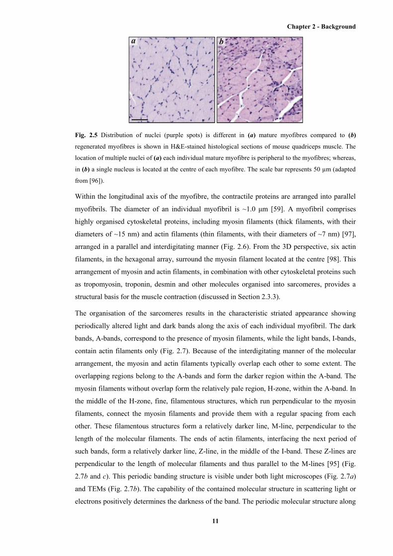
Chapter 2 - Background
11
Fig. 2.5 Distribution of nuclei (purple spots) is different in (a) mature myofibres compared to (b)
regenerated myofibres is shown in H&E-stained histological sections of mouse quadriceps muscle. The
location of multiple nuclei of (a) each individual mature myofibre is peripheral to the myofibres; whereas,
in (b) a single nucleus is located at the centre of each myofibre. The scale bar represents 50 µm (adapted
from [96]).
Within the longitudinal axis of the myofibre, the contractile proteins are arranged into parallel
myofibrils. The diameter of an individual myofibril is ~1.0 μm [59]. A myofibril comprises
highly organised cytoskeletal proteins, including myosin filaments (thick filaments, with their
diameters of ~15 nm) and actin filaments (thin filaments, with their diameters of ~7 nm) [97],
arranged in a parallel and interdigitating manner (Fig. 2.6). From the 3D perspective, six actin
filaments, in the hexagonal array, surround the myosin filament located at the centre [98]. This
arrangement of myosin and actin filaments, in combination with other cytoskeletal proteins such
as tropomyosin, troponin, desmin and other molecules organised into sarcomeres, provides a
structural basis for the muscle contraction (discussed in Section 2.3.3).
The organisation of the sarcomeres results in the characteristic striated appearance showing
periodically altered light and dark bands along the axis of each individual myofibril. The dark
bands, A-bands, correspond to the presence of myosin filaments, while the light bands, I-bands,
contain actin filaments only (Fig. 2.7). Because of the interdigitating manner of the molecular
arrangement, the myosin and actin filaments typically overlap each other to some extent. The
overlapping regions belong to the A-bands and form the darker region within the A-band. The
myosin filaments without overlap form the relatively pale region, H-zone, within the A-band. In
the middle of the H-zone, fine, filamentous structures, which run perpendicular to the myosin
filaments, connect the myosin filaments and provide them with a regular spacing from each
other. These filamentous structures form a relatively darker line, M-line, perpendicular to the
length of the molecular filaments. The ends of actin filaments, interfacing the next period of
such bands, form a relatively darker line, Z-line, in the middle of the I-band. These Z-lines are
perpendicular to the length of molecular filaments and thus parallel to the M-lines [95] (Fig.
2.7b and c). This periodic banding structure is visible under both light microscopes (Fig. 2.7a)
and TEMs (Fig. 2.7b). The capability of the contained molecular structure in scattering light or
electrons positively determines the darkness of the band. The periodic molecular structure along
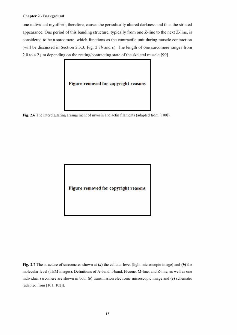
Chapter 2 - Background
12
one individual myofibril, therefore, causes the periodically altered darkness and thus the striated
appearance. One period of this banding structure, typically from one Z-line to the next Z-line, is
considered to be a sarcomere, which functions as the contractile unit during muscle contraction
(will be discussed in Section 2.3.3; Fig. 2.7b and c). The length of one sarcomere ranges from
2.0 to 4.2 μm depending on the resting/contracting state of the skeletal muscle [99].
Fig. 2.6 The interdigitating arrangement of myosin and actin filaments (adapted from [100]).
Fig. 2.7 The structure of sarcomeres shown at (a) the cellular level (light microscopic image) and (b) the
molecular level (TEM images). Definitions of A-band, I-band, H-zone, M-line, and Z-line, as well as one
individual sarcomere are shown in both (b) transmission electronic microscopic image and (c) schematic
(adapted from [101, 102]).
Chapter 2 - Background
13
2.3.2 ECM in skeletal muscle
The material between the myofibres is called the ECM or connective tissue, and accounts for
approximately 1 to 10% of the muscle tissue [103, 104]. The ECM of skeletal muscles is very
important for various reasons: firstly, it serves as a scaffold for myofibre formation during
muscle development and to hold the myofibres together in the gross structure of mature muscle;
secondly, to provide a conduit for the blood vessels and nerves; thirdly, to resist excessive
passive stretching of the muscle and minimise myofibre damage; and fourthly, to transfer the
force (generated by the contractile proteins within the myofibres) to move the parts of the body,
especially via tendons connected to the bones [95].
The connective tissue of the skeletal muscle is organised into: the epimysium, perimysium, and
endomysium [105, 106] (Fig. 2.8). The epimysium that encloses the entire muscle is composed
mainly of tightly woven bundles of collagen fibres (600 to 1800 nm in diameter) and is a
particularly tough coat that separates individual muscles. The perimysium is tough and
relatively thick and composed mainly of collagens. The perimysium surrounds the bundles of
myofibres (fascicles) and contains the blood vessels and nerves. Within the coarse perimysial
sheets, each individual myofibre is surrounded by a more complex ECM, the endomysium. The
endomysium consists of a looser and more delicate interstitial network of collagen fibrils (60 to
120 nm in diameter) run in all directions and connected with the basement membrane
(specialised ECM rich in laminin and glycoproteins) that surrounds, and is in intimate contact
with, the surface of each myofibre. The interstitial spaces separating the myofibres are usually
no wider than 1 μm [95] and some of these collagen fibrils are continuous with the fine fibrillar
mesh of the perimysium. The force generated within each myofibre is transferred laterally
directly through the basement membrane to the interstitial collagens to convey part of the
contractile force to the tendon [95, 107] (Fig. 2.8c and d).
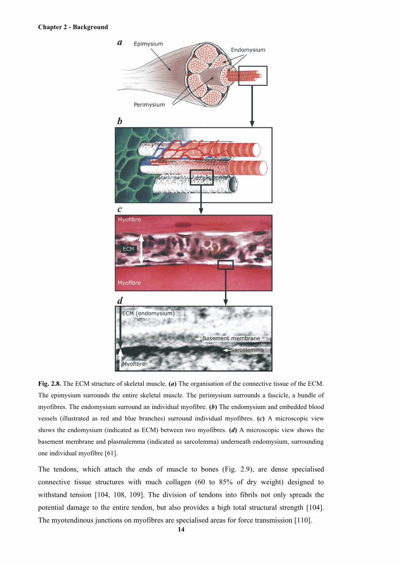
Chapter 2 - Background
14
Fig. 2.8. The ECM structure of skeletal muscle. (a) The organisation of the connective tissue of the ECM.
The epimysium surrounds the entire skeletal muscle. The perimysium surrounds a fascicle, a bundle of
myofibres. The endomysium surround an individual myofibre. (b) The endomysium and embedded blood
vessels (illustrated as red and blue branches) surround individual myofibres. (c) A microscopic view
shows the endomysium (indicated as ECM) between two myofibres. (d) A microscopic view shows the
basement membrane and plasmalemma (indicated as sarcolemma) underneath endomysium, surrounding
one individual myofibre [61].
The tendons, which attach the ends of muscle to bones (Fig. 2.9), are dense specialised
connective tissue structures with much collagen (60 to 85% of dry weight) designed to
withstand tension [104, 108, 109]. The division of tendons into fibrils not only spreads the
potential damage to the entire tendon, but also provides a high total structural strength [104].
The myotendinous junctions on myofibres are specialised areas for force transmission [110].
Chapter 2 - Background
15
Fig. 2.9 Tendons attach the ends of skeletal muscle to bones (adapted from [111]).
The basement membrane, is specialised ECM that anchors the myofibre to collagens in the
interstitial connective tissue: in mature skeletal muscle it is composed largely of laminins,
glycoproteins, collagens IV and VI, and a wealth of other interacting molecules that form a
complex network on the surface of the myofibre and interact with protein complexes that span
the cell membrane (sarcolemma) and connect to various molecules within the myofibre (Fig.
2.10) [61, 95, 112].
Fig. 2.10 Schematic representation of the ECM surrounding skeletal muscle. Individual molecules are
depicted at their approximate location in relation to the sarcolemma. Well-established molecular
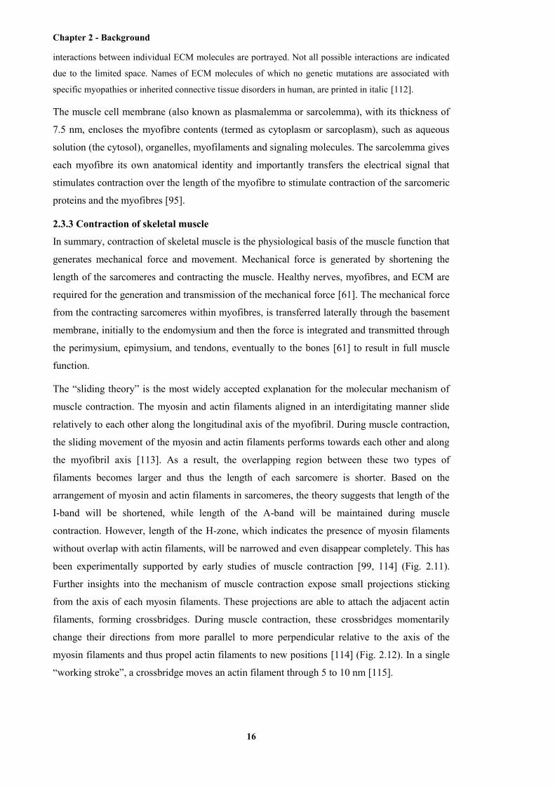
Chapter 2 - Background
16
interactions between individual ECM molecules are portrayed. Not all possible interactions are indicated
due to the limited space. Names of ECM molecules of which no genetic mutations are associated with
specific myopathies or inherited connective tissue disorders in human, are printed in italic [112].
The muscle cell membrane (also known as plasmalemma or sarcolemma), with its thickness of
7.5 nm, encloses the myofibre contents (termed as cytoplasm or sarcoplasm), such as aqueous
solution (the cytosol), organelles, myofilaments and signaling molecules. The sarcolemma gives
each myofibre its own anatomical identity and importantly transfers the electrical signal that
stimulates contraction over the length of the myofibre to stimulate contraction of the sarcomeric
proteins and the myofibres [95].
2.3.3 Contraction of skeletal muscle
In summary, contraction of skeletal muscle is the physiological basis of the muscle function that
generates mechanical force and movement. Mechanical force is generated by shortening the
length of the sarcomeres and contracting the muscle. Healthy nerves, myofibres, and ECM are
required for the generation and transmission of the mechanical force [61]. The mechanical force
from the contracting sarcomeres within myofibres, is transferred laterally through the basement
membrane, initially to the endomysium and then the force is integrated and transmitted through
the perimysium, epimysium, and tendons, eventually to the bones [61] to result in full muscle
function.
The “sliding theory” is the most widely accepted explanation for the molecular mechanism of
muscle contraction. The myosin and actin filaments aligned in an interdigitating manner slide
relatively to each other along the longitudinal axis of the myofibril. During muscle contraction,
the sliding movement of the myosin and actin filaments performs towards each other and along
the myofibril axis [113]. As a result, the overlapping region between these two types of
filaments becomes larger and thus the length of each sarcomere is shorter. Based on the
arrangement of myosin and actin filaments in sarcomeres, the theory suggests that length of the
I-band will be shortened, while length of the A-band will be maintained during muscle
contraction. However, length of the H-zone, which indicates the presence of myosin filaments
without overlap with actin filaments, will be narrowed and even disappear completely. This has
been experimentally supported by early studies of muscle contraction [99, 114] (Fig. 2.11).
Further insights into the mechanism of muscle contraction expose small projections sticking
from the axis of each myosin filaments. These projections are able to attach the adjacent actin
filaments, forming crossbridges. During muscle contraction, these crossbridges momentarily
change their directions from more parallel to more perpendicular relative to the axis of the
myosin filaments and thus propel actin filaments to new positions [114] (Fig. 2.12). In a single
“working stroke”, a crossbridge moves an actin filament through 5 to 10 nm [115].

Chapter 2 - Background
17
Fig. 2.11 The arrangement of myofilaments, as well as the definitions of A-band, I-band, H-zone, M-line,
Z-line, within one individual sarcomere when the muscle is (a) stretched, (b) resting, and (c) contracted
(adapted from [101]).
Fig. 2.12 Cross-bridges are formed when the state of muscle changes from (a) resting to (b) contracted.
TEM reveals the formed cross-bridges during muscle contraction in (c) [116, 117].
Muscle function can be impaired by many forms of injury and a wide range of muscle disorders.
In muscle with Duchenne muscular dystrophy, for instance, the absence of the protein of
dystrophin, which plays a vital part connecting the intracellular filaments with the ECM, could
cause abnormal force transmission and distribution that may injure the plasmalemma and thus
lead to muscular necrosis (discussed in Section 2.5) [12]. The central aim of this thesis is to
develop new imaging techniques that can observe changes in muscle structure that affect muscle
function. Of central interest to this thesis is imaging of skeletal muscles in the inherited lethal
muscle disease DMD that is described below.
Chapter 2 - Background
18
2.4 DMD
2.4.1 Phenotype of DMD
The genetic muscle disease DMD is one of the most severe muscular dystrophies, which was
described by the English physician Edward Meryon in 1851 [118] and affects about 1 in 3600 to
6000 male births worldwide [1]. Muscles of boys with DMD progressively degenerate, leading
to replacement of myofibres by fibrous and fatty connective tissue and dysfunction of the
skeletomuscular system (Fig. 2.13). The pathological loss of muscle mass results in weakness,
loss of function and general locomotion, wheel-chair confinement by 12 years of age. The death
of DMD patients usually occurs in the second to third decade of their life due to respiratory or
cardiac failure. To date, there is no cure for DMD and thus the death from the disease is
inevitable. Current treatment for DMD is administration of steroids (that has variable success)
and interventions to aid quality of life, pain relief, and respiratory assistance [12, 118].

Chapter 2 - Background
19
Fig. 2.13 H&E-stained transverse sections of dystrophic mouse quadriceps muscle containing (a) normal-
appearing myofibres with multiple peripheral nuclei, (b) necrotic myofibres with infiltration of
inflammatory cells and fragmented sarcoplasm, and (c) regenerated myofibres with single central nuclei.
Scale bars indicate 50 µm (adapted from [96]).
Duchenne muscular dystrophy results from mutations in the gene that is mapped to the Xp21.1
band on the human X chromosome: mutations in this gene result in an altered form or complete
absence of the protein dystrophin [119, 120]. Dystrophin is a cell membrane-associated protein,
which plays a vital role in membrane stability and maintenance, and is found in not only skeletal
muscle but also cardiac and smooth muscle, as well as the brain [119, 121]. In skeletal muscle,
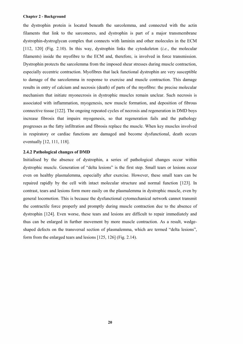
Chapter 2 - Background
20
the dystrophin protein is located beneath the sarcolemma, and connected with the actin
filaments that link to the sarcomeres, and dystrophin is part of a major transmembrane
dystrophin-dystroglycan complex that connects with laminin and other molecules in the ECM
[112, 120] (Fig. 2.10). In this way, dystrophin links the cytoskeleton (i.e., the molecular
filaments) inside the myofibre to the ECM and, therefore, is involved in force transmission.
Dystrophin protects the sarcolemma from the imposed shear stresses during muscle contraction,
especially eccentric contraction. Myofibres that lack functional dystrophin are very susceptible
to damage of the sarcolemma in response to exercise and muscle contraction. This damage
results in entry of calcium and necrosis (death) of parts of the myofibre: the precise molecular
mechanism that initiate myonecrosis in dystrophic muscles remain unclear. Such necrosis is
associated with inflammation, myogenesis, new muscle formation, and deposition of fibrous
connective tissue [122]. The ongoing repeated cycles of necrosis and regeneration in DMD boys
increase fibrosis that impairs myogenesis, so that regeneration fails and the pathology
progresses as the fatty infiltration and fibrosis replace the muscle. When key muscles involved
in respiratory or cardiac functions are damaged and become dysfunctional, death occurs
eventually [12, 111, 118].
2.4.2 Pathological changes of DMD
Initialised by the absence of dystrophin, a series of pathological changes occur within
dystrophic muscle. Generation of “delta lesions” is the first step. Small tears or lesions occur
even on healthy plasmalemma, especially after exercise. However, these small tears can be
repaired rapidly by the cell with intact molecular structure and normal function [123]. In
contrast, tears and lesions form more easily on the plasmalemma in dystrophic muscle, even by
general locomotion. This is because the dysfunctional cytomechanical network cannot transmit
the contractile force properly and promptly during muscle contraction due to the absence of
dystrophin [124]. Even worse, these tears and lesions are difficult to repair immediately and
thus can be enlarged in further movement by more muscle contraction. As a result, wedge-
shaped defects on the transversal section of plasmalemma, which are termed “delta lesions”,
form from the enlarged tears and lesions [125, 126] (Fig. 2.14).
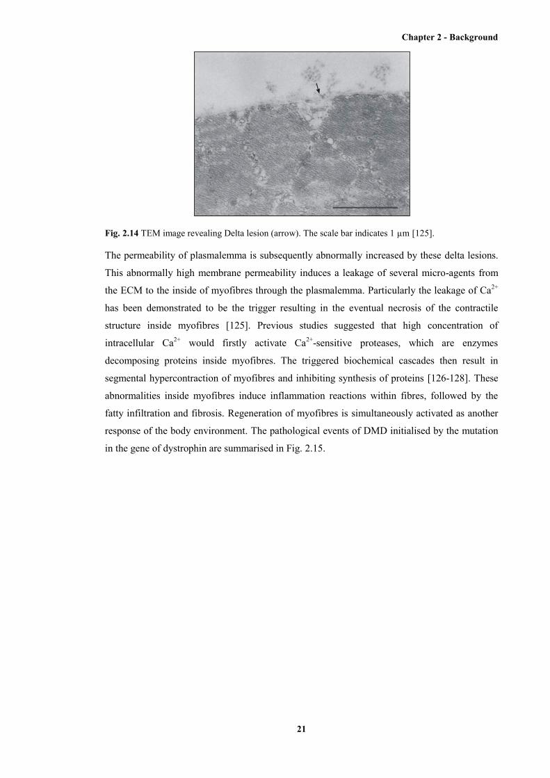
Chapter 2 - Background
21
Fig. 2.14 TEM image revealing Delta lesion (arrow). The scale bar indicates 1 µm [125].
The permeability of plasmalemma is subsequently abnormally increased by these delta lesions.
This abnormally high membrane permeability induces a leakage of several micro-agents from
the ECM to the inside of myofibres through the plasmalemma. Particularly the leakage of Ca2+
has been demonstrated to be the trigger resulting in the eventual necrosis of the contractile
structure inside myofibres [125]. Previous studies suggested that high concentration of
intracellular Ca2+ would firstly activate Ca2+-sensitive proteases, which are enzymes
decomposing proteins inside myofibres. The triggered biochemical cascades then result in
segmental hypercontraction of myofibres and inhibiting synthesis of proteins [126-128]. These
abnormalities inside myofibres induce inflammation reactions within fibres, followed by the
fatty infiltration and fibrosis. Regeneration of myofibres is simultaneously activated as another
response of the body environment. The pathological events of DMD initialised by the mutation
in the gene of dystrophin are summarised in Fig. 2.15.
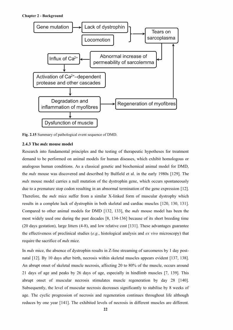
Chapter 2 - Background
22
Fig. 2.15 Summary of pathological event sequence of DMD.
2.4.3 The mdx mouse model
Research into fundamental principles and the testing of therapeutic hypotheses for treatment
demand to be performed on animal models for human diseases, which exhibit homologous or
analogous human conditions. As a classical genetic and biochemical animal model for DMD,
the mdx mouse was discovered and described by Bulfield et al. in the early 1980s [129]. The
mdx mouse model carries a null mutation of the dystrophin gene, which occurs spontaneously
due to a premature stop codon resulting in an abnormal termination of the gene expression [12].
Therefore, the mdx mice suffer from a similar X-linked form of muscular dystrophy which
results in a complete lack of dystrophin in both skeletal and cardiac muscles [120, 130, 131].
Compared to other animal models for DMD [132, 133], the mdx mouse model has been the
most widely used one during the past decades [8, 134-136] because of its short breeding time
(20 days gestation), large litters (4-8), and low relative cost [131]. These advantages guarantee
the effectiveness of preclinical studies (e.g., histological analysis and ex vivo microscopy) that
require the sacrifice of mdx mice.
In mdx mice, the absence of dystrophin results in Z-line streaming of sarcomeres by 1 day post-
natal [12]. By 10 days after birth, necrosis within skeletal muscles appears evident [137, 138].
An abrupt onset of skeletal muscle necrosis, affecting 20 to 80% of the muscle, occurs around
21 days of age and peaks by 26 days of age, especially in hindlimb muscles [7, 139]. This
abrupt onset of muscular necrosis stimulates muscle regeneration by day 28 [140].
Subsequently, the level of muscular necrosis decreases significantly to stabilise by 8 weeks of
age. The cyclic progression of necrosis and regeneration continues throughout life although
reduces by one year [141]. The exhibited levels of necrosis in different muscles are different.

Chapter 2 - Background
23
The hindlimb muscles, including tibialis anterior (TA), gastrocnemius, quadriceps, and extensor
digitorum longus, typically show severe necrosis [142, 143], whereas the necrosis within some
muscles of the head and chest region is very mild [12]. Besides the natural biophysical variety
between these muscles, one another possible reason for this difference in the severity of
pathology is that the hindlimb muscles are more involved in the endurance exercises (e.g.,
forced treadmill running) performed on the mdx mice. The endurance exercises are commonly
employed in preclinical research to enhance the level of muscular necrosis within mdx mice [55,
144-148].
The differences between mdx mice and DMD human patients should be noted. Although both
caused by the null mutation of the dystrophin gene, the muscular dystrophy in the mdx mouse
shows milder phenotypes than in DMD human patients. The mdx mouse has an almost normal
lifespan and exhibits only minor clinical dysfunction for most of time [149]. Although the full
explanation to this difference is yet to be elucidated, this difference is possibly due to the much
larger scale of a human patient compared to the mdx mouse. As a result, the mechanical stress
applied on the muscles, which is postulated to be related to the cube of the linear size of the
body [150, 151], is much larger in a human patient than in the mdx mouse. The damage to the
dystrophic muscle, therefore, is more severe in the human patients [149].
2.5 Techniques for imaging skeletal muscle and muscle damage
A wide range of imaging techniques have been employed for assessing and/or revealing the
extent of muscle disease based on their visualisation of muscle composition and structure at
both the macroscopic and the microscopic levels. Ultrasonography, MRI, and CT are clinical
imaging modalities that are used in both preclinical and clinical imaging of skeletal muscle
because these imaging modalities are capable of serial detection and assessment of living
muscle tissue in a noninvasive manner. Microscopic imaging modalities, such as confocal
microscopy, multiphoton microscopy (MPM), and second harmonic generation (SHG)
microscopy, serve as preclinical imaging modalities only since they typically require excision
and preparation of muscle samples. The applications of these modalities in muscle imaging
include: firstly, the development of image-based biomarkers for muscle damage and/or repair;
secondly, the development of an improved understanding in the pathology of skeletomuscular
diseases, based on the acquired information from structural and functional measurement;
thirdly, the studies of candidate drugs and therapeutic interventions, including the assessment of
drug efficacy and the investigation in the mechanism of drug action [25].
In preclinical studies, the noninvasive or nondestructive nature of clinical imaging modalities
enables their exclusive benefits, such as the longitudinal study of living tissue on the same
animal, reduced animals use, and reduced biological variability [25]. However, those preclinical
imaging modalities are able to provide high-resolution images showing structural and/or
Chapter 2 - Background
24
functional information at the subcellular level. By contrast, the finest spatial resolution that
clinical imaging modalities can reach is tens of microns, which is at the cellular level within
skeletal muscle.
2.5.1 Ultrasonography
After being used in microstructural imaging at the cellular level within biological tissues for the
first time in the 1930s [13] and in medical practice since the early 1950s [152], US has rapidly
developed its widespread use in almost all fields of medicine because of its non-invasiveness
(especially the freedom from ionising radiation), real-time display, low cost, and portability of
equipment [15, 16, 153]. Early US typically provided 2D or B-mode images, until 3D scanning
mechanism was developed and enabled C-mode volumetric images in the mid 1980s [154]. The
physical basis of US is the incident sound waves and their echoes. A sequence of sound-wave
pulses is sent into biological tissues by the pulse transducer. These sound-wave pulses are then
attenuated, due to the reflection, dispersion, and absorption, when transmitting through the
tissue. The reflected sound waves and echoes are received by the same transducer and
computationally analysed for intensity and arrival time. Array transducers have been recently
developed to improve focusing [155] and increase image frame rates [17], compared with the
originally employed single, mechanically scanned transducers. The temporal property of the
echo, that is, the time between sending and receiving the same US pulse, determines the
location of the corresponding reflecting pixel. Moreover, the amplitude of the echo indicates the
acoustic property of the corresponding pixel within the tissue and determines the brightness of
the pixel on the image [156-160]. As the reflection only occurs when the US beam encounters
tissue with different acoustical properties (i.e., acoustical impedance), tissues with small
acoustical impedance (e.g., muscle, fat) show as darker regions on the image and vice versa
(e.g., bone/air interface). Little/no tissue beneath the structure with large acoustical impedance,
as a result, can be detected because of the shadow effect [36, 156, 157].
The axial resolution of US is determined by and proportional to the frequency of the incident
sound, whereas the lateral resolution is limited by the beam width and can be several times
larger than the axial resolution [36]. However, the depth of penetration is inversely correlated
with the frequency [36, 158-160]. The trade-off between the axial resolution and penetration
depth makes the range of 2-20 MHz commonly used for clinical US, mainly including the eye
[14, 161, 162], the skin [163-165], and the intravascular imaging [166-168]. Axial resolution
ranging from 80 to 800 µm can be achieved with adequate depth of penetration (no less than
several mm) [36, 37]. Broadband transducers have been developed recently for combining the
high resolution and deeper penetration using both high and low frequencies. High-frequency
US, which is termed as US biomicroscopy or micro-US, was first demonstrated in the late 1980s
by Sherar et al. [154] in imaging tumour spheroids and mainly for preclinical imaging of small
animals, including developmental biology [169-173], cardiovascular research [174-177], and
cancer imaging [178-182], due to its relatively smaller depth of penetration [183]. Typical

Chapter 2 - Background
25
frequencies employed by micro-US range from 20 to 70 MHz, resulting in axial resolutions in
the range 20-80 µm [13]. Higher frequencies such as 100 MHz or 200 MHz have also been
reported to be used [13, 154, 184, 185]. Besides very high frequencies, higher resolution can be
achieved by using contrast agents, such as gas bubbles [186] or nano-/micro-sized particles [37],
although the diffusion of the intravenously administrated contrast agents out of vasculature that
are injected into blood vessels is a potential disadvantage. The values of spatial resolution and
depth of field, corresponding to three typical frequencies of US or micro-US are listed in Table
2.2 (adapted from [13]).
Table 2.2 A summary of US technical properties corresponding to different incident frequencies.
30 MHz 60 MHz 100 MHz
Lateral resolution 250 µm 75 µm 60 µm
Axial resolution 62 µm 31 µm 19 µm
Depth of field 2.5 mm 1.6 mm 1.6 mm
Ultrasound was demonstrated to be able to differentiate diseased muscles from healthy muscles
first by Heckmatt et al. in 1980 [187]. As a noninvasive and easily accessible method, US is
suitable for muscle imaging in young children even without sedation [153, 188, 189]. Several
following studies subsequently suggested each type of muscular disorder tends to show specific
appearance on muscle US compared not only controls but also other types of muscle disorders
[16, 189-191]. Healthy muscle tissue, because of its highly organised ultrastructure consisting of
cytoplasm and repeating links of identical structural proteins, shows low echo intensity (i.e., a
darker structure), which makes muscle distinct from surrounding structures such as
subcutaneous fat, bone, nerves, and blood vessels [188, 190, 192-197]. A speckled appearance
in the transverse plane of muscle is caused by the echogenic sheets of connective tissue [15]. In
contrast, dystrophic muscle shows higher echo intensity because of the pathological fatty
infiltration within myofibres and intramuscular fibrosis [15, 187, 198]. Although the age [190,
199], proportion of fibrous tissue (determined by the type of the muscle) [200], and even the
imaged location [16, 187] or direction [188, 201, 202] of the muscle could elevate the muscle
echo intensity, the specific extent and distribution of the increase of echo intensity within
muscle with specific disorders (e.g., DMD) give diagnostic information [189, 203, 204]. For
example, DMD results in a severe, homogenous increase of muscle echo intensity (compared
with that of controls) with normal muscle thickness (Fig. 2.16), whereas spinal muscular
atrophy shows an inhomogeneous increase of echo intensity with severe atrophy [15]. A visual
grading scale for manually evaluating muscle echo intensity, giving that grade I represents
normal muscle and grade IV represents the severest diseased muscle, was developed by
Heckmatt et al. [205]. Quantification of muscle echo intensity based on computer-aided

Chapter 2 - Background
26
techniques, which is more objective and allows for statistical analysis, has been introduced in
image interpretation nowadays [34, 190, 198, 199, 204, 206-208]. Although early clinical
studies suggested that US has less capable of detecting pathological changes in early or pre-
symptomatic disease, and in metabolic or mitochondrial myopathies, muscle US was showed to
be capable of discriminating between children with and without a neuromuscular disorder with
high predictive values ~90% in children elder than 3 years old [16, 188, 190, 209], as
inflammatory events in advanced stage of muscular dystrophy show remarkable and specific
changes on US [188, 190]. Furthermore, dynamic imaging of muscle movement using US has
been also operated for evaluating muscle diseases [193, 194].
Fig. 2.16. Transverse US image of a normal left quadriceps muscle (a) and of a patient with DMD (b).
Both are 3.5 years of age. The rectus femoris muscle is encircled. The mean echo intensity is measured
for this region, as shown in the histograms below (scale: black = 0; white = 255). The rectus femoris of
the DMD patient has increased muscle echo intensity, with the corresponding histogram being displaced
to the right. Note the fine granular pattern of echo intensity, homogeneously spread among the muscle
with attenuation of the US beam; that is, the echo intensity in deeper areas of the muscle is decreased
compared to the superficial areas. Fascia within the muscle, such as the central fascia in the anterior part
of the rectus femoris (single arrow), are more difficult to recognise in the DMD patient. VM, vastus
medialis; VL, vastus lateralis; VI, vastus intermedius; F, femur; double arrow, subcutaneous tissue. The
quadriceps muscle was measured halfway along the line from the anterosuperior iliac spine to the patella
[15].
In summary, US has the advantages of non-invasiveness, low cost, portability of equipment, and
easy accessibility, which make US routinely employed in clinical imaging. However, the
primary limitation of US in muscle imaging is the moderate spatial resolution that is typically
coarser than 50 µm. Individual myofibres, typically with their diameter of 20 to 50 µm, cannot
be resolved by US. The resolution of micro-US is as fine as ~20 µm with high-frequency
incident sound. With the penetration depth of ~2 mm inside biological tissues, and this fine
spatial resolution, micro-US is promising in imaging ultrastructures in biological tissues.

Chapter 2 - Background
27
2.5.2 CT
The technology of CT (X-ray CT) produces tomographic X-ray images using computer-based
scanning and processing. Employing digital geometry processing, 3D images showing inside
structure and morphology of the object are generated for diagnostic or therapeutic purposes. The
contrast of CT is typically introduced by attenuation of the incident X-rays in the examined
sample [210]. With lower incident X-ray energy, the attenuation is caused mainly by the
photoelectric effect, which makes the resulting X-ray energy after attenuation anti-proportional
to the 3rd power of the atomic number. With a higher incident X-ray energy, Compton scattering
becomes the dominant cause of the attenuation, leading to an anti-proportional dependency of
attenuated X-ray energy to the atomic number divided by 2 [19]. Some physical methods, such
as K-edge subtraction [211-214], X-ray phase delay contrast [215-217], and X-ray scatter
contrast [218] were employed to further enhance the X-ray contrast. Although widely used in
clinical applications, conventional CT typically provides moderate spatial resolution coarser
than 100 µm, which precludes the capability of conventional CT in visualising microscopic
structures inside biological tissues [38].
Micro-CT is a novel imaging technique which has attracted increasing attention from the early
1980s [219, 220]. Micro-CT is able to provide 3D images with their typical spatial resolution
finer than 50 µm [22, 39] or even 20 µm with contrast-enhanced agents [40]. Recent studies
demonstrated the applications of micro-CT in osseous-structure imaging [221, 222], vascular-
structure imaging [223, 224], cardiothoracic imaging [20, 225], thoracic imaging [226, 227],
cardiac imaging [228, 229], abdominal-organ imaging [21, 230], and cerebral-structure imaging
[231, 232]. However, although micro-CT demonstrates excellent capability in imaging tissue
samples with high atomic number (e.g., bones), the exhibited contrast in soft tissue under micro-
CT is relatively weak. Conventional CT, due to the same contrast mechanism, shows the same
limitation. As a result, the administration of a contrast agent during CT or micro-CT imaging is
desirable or even indispensable when imaging soft tissues [19].
Contrast agents employed in micro-CT imaging are able to transfer in vitro applications to in
vivo ones by elevating soft tissue contrast in preclinical research regarding to the evaluation of
soft tissue structure or morphology. Three types of contrast agents are generally available for in
vivo imaging: first, a conventional iodinated contrast medium; second, a blood-pool contrast
agent; third, a liposome-based contrast agent [19]. Water-soluble, non-ionic, iodine-based
contrast agents are generally used in humans because it can be eliminated from the blood
immediately after injection via the kidneys. Whereas this rapid elimination benefits human
patients, it restricts the use of iodinated contrast agents in small animals such as rodents due to
their very short circulation times [233]. Blood-pool contrast agents consist of molecules that are
able to bind to structural proteins or other macromolecules inside biological tissues. As a result,
longer scanning time lasting up to several hours, or even repeated measurement without
repeated administration of contrast agents, is enabled by blood-pool contrast agents. However,

Chapter 2 - Background
28
the level of contrast provided by blood-pool contrast agents is generally lower than that
provided by conventional iodinated contrast agents [234, 235]. Liposome-based contrast agents
are novel ones allowing for the measurement of hepatic metastasis and delineation of the liver
and spleen [19]. Moreover, liposome-based contrast agents are suitable for imaging vascular
structures [236].
The application of CT in imaging muscular degradation was in 1938 [237, 238], after the initial
radiological study of neuromuscular pathology starting from 1928 [237, 238]. Muscular
dystrophy can be diagnosed based on the morphological imaging of the diseased muscle.
Skeletal muscles with muscular dystrophy appear to be enlarged or pseudohypertrophic [239].
X-ray computed tomography is able to explicitly detect and measure these morphological
changes [38, 239-241]. Furthermore, damaged areas within dystrophic muscle can be
distinguished by CT imaging from those undamaged areas based on tissue composition and thus
tissue density. The detected tissue density of undamaged regions of dystrophic muscle, as well
as normal muscle, appears to be uniformly high, whereas damaged areas are shown as low-
density areas [18, 242]. This altered density of tissue is caused by the replacement of muscle
tissue by the infiltrating fat and connective tissue (fatty infiltration), which is the principal
feature of many muscular dystrophies (e.g., DMD) [38, 243]. It should be noted that the extent
of fatty infiltration and thus the decrease of tissue density vary among different types of
muscles. Density readings of exactly the same area (on the same muscle), however, enable
quantitative longitudinal study of muscular dystrophy, which can monitor the progress in
severity of the pathology. This is based on the plausible positive correlation between the
decrease of tissue density and the severity of the muscular degradation [244, 245]. In some
recent studies, the muscle volume index was measured as a novel indicator for the severity of
DMD using CT scanning [246]. A typical CT scan of skeletal muscle is shown in Fig. 2.17.
Although muscle CT scans, as well as other preclinical or clinical applications of CT and micro-
CT, have the advantages of permitting non-destructive and painless imaging, simple operability,
fast scanning protocols (up to less than 1 min), and fine spatial resolution (for micro-CT), the
high radiation dosage and relatively low contrast in soft tissues remain to be unavoidable
limitations, compared to other clinical imaging modalities [19].
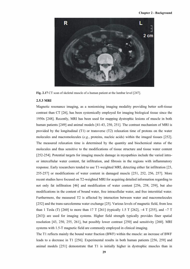
Chapter 2 - Background
29
Fig. 2.17 CT scan of skeletal muscle of a human patient at the lumbar level [247].
2.5.3 MRI
Magnetic resonance imaging, as a nonionising imaging modality providing better soft-tissue
contrast than CT [26], has been systemically employed for imaging biological tissue since the
1950s [248]. Recently, MRI has been used for mapping dystrophic lesions of muscle in both
human patients [249] and animal models [41-43, 250, 251]. The contrast mechanism of MRI is
provided by the longitudinal (T1) or transverse (T2) relaxation time of protons on the water
molecules and macromolecules (e.g., proteins, nucleic acids) within the imaged tissues [252].
The measured relaxation time is determined by the quantity and biochemical status of the
molecules and thus sensitive to the modifications of tissue structure and tissue water content
[252-254]. Potential targets for imaging muscle damage in myopathies include the varied intra-
or intercellular water content, fat infiltration, and fibrosis in the regions with inflammatory
response. Early researchers tended to use T1-weighted MRI, detecting either fat infiltration [23,
255-257] or modifications of water content in damaged muscle [251, 252, 256, 257]. More
recent studies have focused on T2-weighted MRI for acquiring detailed information regarding to
not only fat infiltration [46] and modification of water content [256, 258, 259], but also
modifications in the content of bound water, free intracellular water, and free interstitial water.
Furthermore, the measured T2 is affected by interaction between water and macromolecules
[252] and the trans-sarcolemma water exchange [25]. Various levels of magnetic field, from less
than 1 Tesla (T) [260] to more than 17 T [261] (typically 1.5 T [262], ~4 T [255], and ~7 T
[263]) are used for imaging systems. Higher field strength typically provides finer spatial
resolution [43, 250, 255, 261], but possibly lower contrast [250] and sensitivity [260]. MRI
systems with 1.5-T magnetic field are commonly employed in clinical imaging.
The T1 reflects mainly the bound water fraction (BWF) within the muscle: an increase of BWF
leads to a decrease in T1 [256]. Experimental results in both human patients [256, 259] and
animal models [251] demonstrate that T1 is initially higher in dystrophic muscles than in
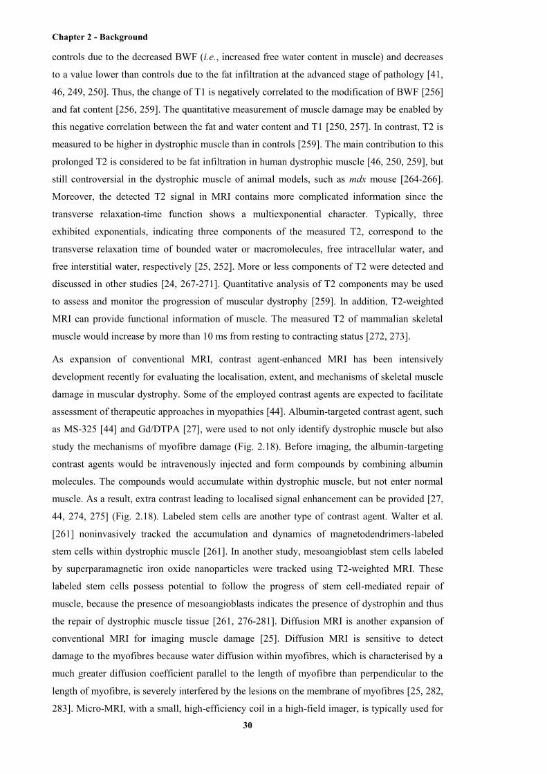
Chapter 2 - Background
30
controls due to the decreased BWF (i.e., increased free water content in muscle) and decreases
to a value lower than controls due to the fat infiltration at the advanced stage of pathology [41,
46, 249, 250]. Thus, the change of T1 is negatively correlated to the modification of BWF [256]
and fat content [256, 259]. The quantitative measurement of muscle damage may be enabled by
this negative correlation between the fat and water content and T1 [250, 257]. In contrast, T2 is
measured to be higher in dystrophic muscle than in controls [259]. The main contribution to this
prolonged T2 is considered to be fat infiltration in human dystrophic muscle [46, 250, 259], but
still controversial in the dystrophic muscle of animal models, such as mdx mouse [264-266].
Moreover, the detected T2 signal in MRI contains more complicated information since the
transverse relaxation-time function shows a multiexponential character. Typically, three
exhibited exponentials, indicating three components of the measured T2, correspond to the
transverse relaxation time of bounded water or macromolecules, free intracellular water, and
free interstitial water, respectively [25, 252]. More or less components of T2 were detected and
discussed in other studies [24, 267-271]. Quantitative analysis of T2 components may be used
to assess and monitor the progression of muscular dystrophy [259]. In addition, T2-weighted
MRI can provide functional information of muscle. The measured T2 of mammalian skeletal
muscle would increase by more than 10 ms from resting to contracting status [272, 273].
As expansion of conventional MRI, contrast agent-enhanced MRI has been intensively
development recently for evaluating the localisation, extent, and mechanisms of skeletal muscle
damage in muscular dystrophy. Some of the employed contrast agents are expected to facilitate
assessment of therapeutic approaches in myopathies [44]. Albumin-targeted contrast agent, such
as MS-325 [44] and Gd/DTPA [27], were used to not only identify dystrophic muscle but also
study the mechanisms of myofibre damage (Fig. 2.18). Before imaging, the albumin-targeting
contrast agents would be intravenously injected and form compounds by combining albumin
molecules. The compounds would accumulate within dystrophic muscle, but not enter normal
muscle. As a result, extra contrast leading to localised signal enhancement can be provided [27,
44, 274, 275] (Fig. 2.18). Labeled stem cells are another type of contrast agent. Walter et al.
[261] noninvasively tracked the accumulation and dynamics of magnetodendrimers-labeled
stem cells within dystrophic muscle [261]. In another study, mesoangioblast stem cells labeled
by superparamagnetic iron oxide nanoparticles were tracked using T2-weighted MRI. These
labeled stem cells possess potential to follow the progress of stem cell-mediated repair of
muscle, because the presence of mesoangioblasts indicates the presence of dystrophin and thus
the repair of dystrophic muscle tissue [261, 276-281]. Diffusion MRI is another expansion of
conventional MRI for imaging muscle damage [25]. Diffusion MRI is sensitive to detect
damage to the myofibres because water diffusion within myofibres, which is characterised by a
much greater diffusion coefficient parallel to the length of myofibre than perpendicular to the
length of myofibre, is severely interfered by the lesions on the membrane of myofibres [25, 282,
283]. Micro-MRI, with a small, high-efficiency coil in a high-field imager, is typically used for
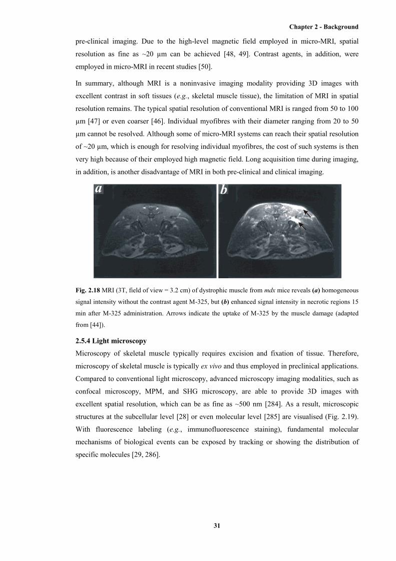
Chapter 2 - Background
31
pre-clinical imaging. Due to the high-level magnetic field employed in micro-MRI, spatial
resolution as fine as ~20 µm can be achieved [48, 49]. Contrast agents, in addition, were
employed in micro-MRI in recent studies [50].
In summary, although MRI is a noninvasive imaging modality providing 3D images with
excellent contrast in soft tissues (e.g., skeletal muscle tissue), the limitation of MRI in spatial
resolution remains. The typical spatial resolution of conventional MRI is ranged from 50 to 100
µm [47] or even coarser [46]. Individual myofibres with their diameter ranging from 20 to 50
µm cannot be resolved. Although some of micro-MRI systems can reach their spatial resolution
of ~20 µm, which is enough for resolving individual myofibres, the cost of such systems is then
very high because of their employed high magnetic field. Long acquisition time during imaging,
in addition, is another disadvantage of MRI in both pre-clinical and clinical imaging.
Fig. 2.18 MRI (3T, field of view = 3.2 cm) of dystrophic muscle from mdx mice reveals (a) homogeneous
signal intensity without the contrast agent M-325, but (b) enhanced signal intensity in necrotic regions 15
min after M-325 administration. Arrows indicate the uptake of M-325 by the muscle damage (adapted
from [44]).
2.5.4 Light microscopy
Microscopy of skeletal muscle typically requires excision and fixation of tissue. Therefore,
microscopy of skeletal muscle is typically ex vivo and thus employed in preclinical applications.
Compared to conventional light microscopy, advanced microscopy imaging modalities, such as
confocal microscopy, MPM, and SHG microscopy, are able to provide 3D images with
excellent spatial resolution, which can be as fine as ~500 nm [284]. As a result, microscopic
structures at the subcellular level [28] or even molecular level [285] are visualised (Fig. 2.19).
With fluorescence labeling (e.g., immunofluorescence staining), fundamental molecular
mechanisms of biological events can be exposed by tracking or showing the distribution of
specific molecules [29, 286].
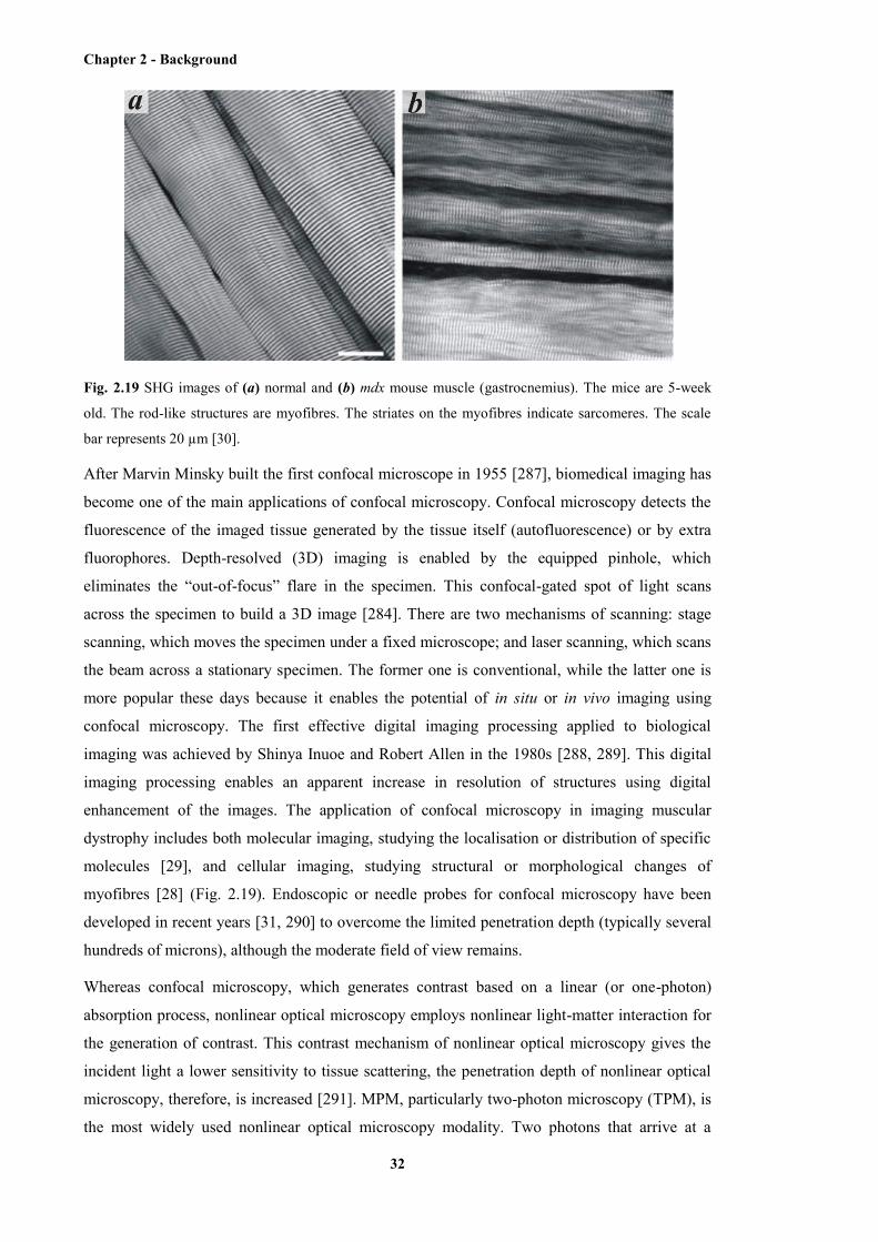
Chapter 2 - Background
32
Fig. 2.19 SHG images of (a) normal and (b) mdx mouse muscle (gastrocnemius). The mice are 5-week
old. The rod-like structures are myofibres. The striates on the myofibres indicate sarcomeres. The scale
bar represents 20 µm [30].
After Marvin Minsky built the first confocal microscope in 1955 [287], biomedical imaging has
become one of the main applications of confocal microscopy. Confocal microscopy detects the
fluorescence of the imaged tissue generated by the tissue itself (autofluorescence) or by extra
fluorophores. Depth-resolved (3D) imaging is enabled by the equipped pinhole, which
eliminates the “out-of-focus” flare in the specimen. This confocal-gated spot of light scans
across the specimen to build a 3D image [284]. There are two mechanisms of scanning: stage
scanning, which moves the specimen under a fixed microscope; and laser scanning, which scans
the beam across a stationary specimen. The former one is conventional, while the latter one is
more popular these days because it enables the potential of in situ or in vivo imaging using
confocal microscopy. The first effective digital imaging processing applied to biological
imaging was achieved by Shinya Inuoe and Robert Allen in the 1980s [288, 289]. This digital
imaging processing enables an apparent increase in resolution of structures using digital
enhancement of the images. The application of confocal microscopy in imaging muscular
dystrophy includes both molecular imaging, studying the localisation or distribution of specific
molecules [29], and cellular imaging, studying structural or morphological changes of
myofibres [28] (Fig. 2.19). Endoscopic or needle probes for confocal microscopy have been
developed in recent years [31, 290] to overcome the limited penetration depth (typically several
hundreds of microns), although the moderate field of view remains.
Whereas confocal microscopy, which generates contrast based on a linear (or one-photon)
absorption process, nonlinear optical microscopy employs nonlinear light-matter interaction for
the generation of contrast. This contrast mechanism of nonlinear optical microscopy gives the
incident light a lower sensitivity to tissue scattering, the penetration depth of nonlinear optical
microscopy, therefore, is increased [291]. MPM, particularly two-photon microscopy (TPM), is
the most widely used nonlinear optical microscopy modality. Two photons that arrive at a
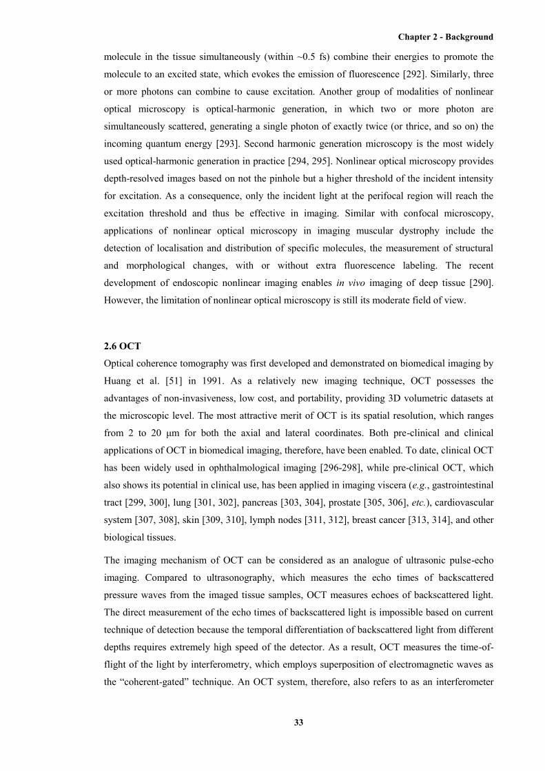
Chapter 2 - Background
33
molecule in the tissue simultaneously (within ~0.5 fs) combine their energies to promote the
molecule to an excited state, which evokes the emission of fluorescence [292]. Similarly, three
or more photons can combine to cause excitation. Another group of modalities of nonlinear
optical microscopy is optical-harmonic generation, in which two or more photon are
simultaneously scattered, generating a single photon of exactly twice (or thrice, and so on) the
incoming quantum energy [293]. Second harmonic generation microscopy is the most widely
used optical-harmonic generation in practice [294, 295]. Nonlinear optical microscopy provides
depth-resolved images based on not the pinhole but a higher threshold of the incident intensity
for excitation. As a consequence, only the incident light at the perifocal region will reach the
excitation threshold and thus be effective in imaging. Similar with confocal microscopy,
applications of nonlinear optical microscopy in imaging muscular dystrophy include the
detection of localisation and distribution of specific molecules, the measurement of structural
and morphological changes, with or without extra fluorescence labeling. The recent
development of endoscopic nonlinear imaging enables in vivo imaging of deep tissue [290].
However, the limitation of nonlinear optical microscopy is still its moderate field of view.
2.6 OCT
Optical coherence tomography was first developed and demonstrated on biomedical imaging by
Huang et al. [51] in 1991. As a relatively new imaging technique, OCT possesses the
advantages of non-invasiveness, low cost, and portability, providing 3D volumetric datasets at
the microscopic level. The most attractive merit of OCT is its spatial resolution, which ranges
from 2 to 20 μm for both the axial and lateral coordinates. Both pre-clinical and clinical
applications of OCT in biomedical imaging, therefore, have been enabled. To date, clinical OCT
has been widely used in ophthalmological imaging [296-298], while pre-clinical OCT, which
also shows its potential in clinical use, has been applied in imaging viscera (e.g., gastrointestinal
tract [299, 300], lung [301, 302], pancreas [303, 304], prostate [305, 306], etc.), cardiovascular
system [307, 308], skin [309, 310], lymph nodes [311, 312], breast cancer [313, 314], and other
biological tissues.
The imaging mechanism of OCT can be considered as an analogue of ultrasonic pulse-echo
imaging. Compared to ultrasonography, which measures the echo times of backscattered
pressure waves from the imaged tissue samples, OCT measures echoes of backscattered light.
The direct measurement of the echo times of backscattered light is impossible based on current
technique of detection because the temporal differentiation of backscattered light from different
depths requires extremely high speed of the detector. As a result, OCT measures the time-of-
flight of the light by interferometry, which employs superposition of electromagnetic waves as
the “coherent-gated” technique. An OCT system, therefore, also refers to as an interferometer
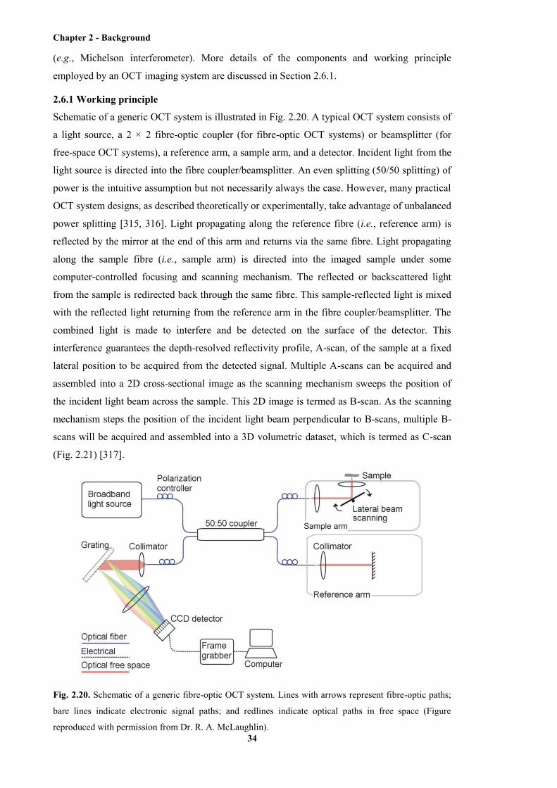
Chapter 2 - Background
34
(e.g., Michelson interferometer). More details of the components and working principle
employed by an OCT imaging system are discussed in Section 2.6.1.
2.6.1 Working principle
Schematic of a generic OCT system is illustrated in Fig. 2.20. A typical OCT system consists of
a light source, a 2 × 2 fibre-optic coupler (for fibre-optic OCT systems) or beamsplitter (for
free-space OCT systems), a reference arm, a sample arm, and a detector. Incident light from the
light source is directed into the fibre coupler/beamsplitter. An even splitting (50/50 splitting) of
power is the intuitive assumption but not necessarily always the case. However, many practical
OCT system designs, as described theoretically or experimentally, take advantage of unbalanced
power splitting [315, 316]. Light propagating along the reference fibre (i.e., reference arm) is
reflected by the mirror at the end of this arm and returns via the same fibre. Light propagating
along the sample fibre (i.e., sample arm) is directed into the imaged sample under some
computer-controlled focusing and scanning mechanism. The reflected or backscattered light
from the sample is redirected back through the same fibre. This sample-reflected light is mixed
with the reflected light returning from the reference arm in the fibre coupler/beamsplitter. The
combined light is made to interfere and be detected on the surface of the detector. This
interference guarantees the depth-resolved reflectivity profile, A-scan, of the sample at a fixed
lateral position to be acquired from the detected signal. Multiple A-scans can be acquired and
assembled into a 2D cross-sectional image as the scanning mechanism sweeps the position of
the incident light beam across the sample. This 2D image is termed as B-scan. As the scanning
mechanism steps the position of the incident light beam perpendicular to B-scans, multiple B-
scans will be acquired and assembled into a 3D volumetric dataset, which is termed as C-scan
(Fig. 2.21) [317].
Fig. 2.20. Schematic of a generic fibre-optic OCT system. Lines with arrows represent fibre-optic paths;
bare lines indicate electronic signal paths; and redlines indicate optical paths in free space (Figure
reproduced with permission from Dr. R. A. McLaughlin).

Chapter 2 - Background
35
Fig. 2.21. Illustration of the A-scan (1D), B-scan (2D), and C-scan (3D) performed by OCT scanning
mechanism (Figure reproduced with permission from Dr. D. Lorenser).
Optical coherence tomography systems are divided into time-domain OCT (TD-OCT) and
spectral-domain OCT (SD-OCT). Spectral-domain OCT systems are further subdivided into
spectrometer-based SD-OCT and swept-source SD-OCT. The latter one is sometimes referred
to as SS-OCT. In addition, SS-OCT is alternatively called optical frequency-domain imaging or
OFDI. The key differences among these OCT systems include their employed light source,
photoreceiver/detector, and the scanning mechanism of their reference arms. In the case of TD-
OCT, the employed light source is a low-coherence one with broadband and continuous-wave
(CW), the reference arm delay is repetitively scanned in length. A single-channel photoreceiver
is employed in a TD-OCT system for detecting the envelope of the detected fringe burst pattern
corresponding to interference between the reference arm light and each successive scattering
site in the sample [318, 319]. In the case of spectrometer-based SD-OCT, the employed light
source is also broadband and CW. However, the reference arm length is fixed at a position
instead of changing in length. An array detector (e.g., a photodiode array or charge-coupled
device, CCD) is employed for simultaneously collecting and dispersing the spectral interference
pattern between the reflected light from the reference arm and all depths in the sample. In the
case of SS-OCT, the light source has narrow instantaneous linewidth but is rapidly swept in
wavelength. The spectral interference pattern is correspondingly detected on a single or small
number of photoreceivers as a function of time, based on a reference arm with fixed-length. In
SD-OCT, inverse Fourier transverse is thus employed to obtain the entire depth-resolved
information of the sample from each A-scan based on the analysis of the detected spectral
interference pattern. Additional signal processing steps (e.g., interpolation) may also be required
in SD-OCT to prepare the spectral interferogram for the inverse Fourier transform.
Chapter 2 - Background
36
A sample under OCT imaging is characterised by its profile of depth-dependent reflectivity,
)( SS zr , where Sz is the sample depth. This reflectivity profile may be defined as a discrete sum
of delta functions spaced arbitrarily closely:
N
nnn zzrzr
1SSSSS )()( (1)
This definition is a discrete approximation of the continuous reflectivity profile in depth in a
practical sample under interrogation. This approximation enables further digital analysis of the
detected signal. The reflected electric fields returning from the sample reflectors, SE , contain
spatial information (i.e., depth-resolved). The interference between this SE and the reflected
field returning from the reference arm, RE , is detected by causing photocurrent response in the
employed detector. Therefore, this photocurrent is proportional to the intensity of interference:
2SRD 2
EEI (2)
Here, DI is the photocurrent. SR EE represents the interference between the two reflected
fields. The intensity of this interference is given by squaring the module of the interference
field. is termed as the responsivity of the detector. The factor of 2 indicates the loss of signal
intensity when passing through the beamsplitter after reflection.
In the case of TD-OCT, the depth of each detected sample reflector is explicitly given by the
corresponding reference pathlength, Rz , since the reflected fields from other sample reflectors
are filtered by the dominated coherent signal intensity (fringe burst) from the sample reflector
located at the depth without pathlength difference compared to the reference pathlength. The
precisely controlled axial change of the reference pathlength over the entire range of imaging
depth guarantees the generation of each depth-resolved reflectivity profile (i.e., A-scan) during
TD-OCT scanning. In the case of SD-OCT, however, the depth of each sample reflector is given
by data analysis. As the spectral signal (spectral interferogram) is acquired by the array detector,
spatial information can be obtained via inverse Fourier transform (IFT) of the spectral
interferogram. Hence, depth-resolved A-scans are generated by an SD-OCT system employing
its reference arm with a fixed pathlength [52, 317-320]. Further theoretical description OCT
(based on SD-OCT) is provided in Appendix I.
The spatial axial resolution of OCT is inversely proportional to the bandwidth of the employed
light source, either the spectral bandwidth of the broadband employed in TD-OCT and
spectrometer-based SD-OCT or the swept range of a narrowband swept source employed in SS-
OCT [319, 321]. A Gaussian-shaped function in spectral domain is a valid approximation of the
source spectrum. This Gaussian-shaped spectrum is characterised by its full-width half-

Chapter 2 - Background
37
maximum (FWHM) value of source bandwidth, , and its central wavelength, 0 (typically
at ~800 nm or ~1300 nm). The spatial axial resolution is then given by
202ln2
cl (3)
Here, cl is the spatial axial resolution. Spatial transverse resolution, which is defined as the spot
size of the light exiting from the lens at the end of sample arm, is inversely proportional to the
numerical aperture (NA) of the objective lens in the sample arm and, thus, decoupled from the
axial resolution. This conclusion is physically reasonable because a larger NA leads to a more
tightly focused light beam with a smaller spot size and thus a smaller transverse resolution. The
transverse resolution is given by
NAx037.0
[317]. (4)
Notably, a trade-off exists between a fine x and a larger DOF, as the DOF is dependent on the
Rayleigh range for a Gaussian beam and proportional to x . In most pre-clinical and clinical
applications of OCT, the employed imaging systems are designed to generate approximately
isotropic voxels by making the transverse and axial resolutions comparable to each other [317,
318].
2.6.2 Application of OCT in imaging skeletal muscle and muscle damage
The application of OCT in imaging skeletal muscle is relatively later compared to other
biological tissues, although macroscopic structure and morphology of skeletal muscle (e.g.,
muscle layers, fascicles) have been visualised in the demonstration of the developed ultrahigh-
resolution OCT systems [322] or OCT needle probes [323]. In contrast to lung tissue filled with
alveoli, which are microscopic structures providing high-contrast air/tissue interface,
ultrastructures within skeletal muscle typically show moderate contrast and, thus, appear almost
homogeneous under imaging modalities with insufficient spatial resolution or sensitivity [324].
However, investigations in imaging another type of striated muscle, cardiac muscle,
experimentally demonstrated the potential of OCT in resolving cellular structures (i.e., muscle
fibres) and their lesions inside striated muscle by visualising tissue lesions and the orientation of
cardiac fibres inside cardiac muscle [325, 326].
The first OCT image showing individual myofibres was reported by Klyen et al. in 2008 [60]. A
whole-muscle autograft mouse model was employed in the ex vivo study. In the acquired 3D
OCT images, the transverse view of individual myofibres, as distinctive high-intensity circular-
shaped structures, was shown within the healthy muscle samples (host tissue). Moreover, the
grafted tissue containing necrotic tissue and inflammatory cells were differentiated from those
healthy host tissues by showing as featureless and low-intensity regions under OCT imaging
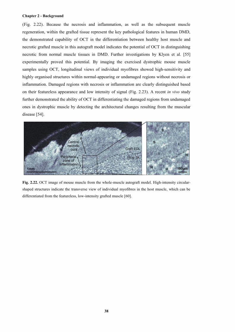
Chapter 2 - Background
38
(Fig. 2.22). Because the necrosis and inflammation, as well as the subsequent muscle
regeneration, within the grafted tissue represent the key pathological features in human DMD,
the demonstrated capability of OCT in the differentiation between healthy host muscle and
necrotic grafted muscle in this autograft model indicates the potential of OCT in distinguishing
necrotic from normal muscle tissues in DMD. Further investigations by Klyen et al. [55]
experimentally proved this potential. By imaging the exercised dystrophic mouse muscle
samples using OCT, longitudinal views of individual myofibres showed high-sensitivity and
highly organised structures within normal-appearing or undamaged regions without necrosis or
inflammation. Damaged regions with necrosis or inflammation are clearly distinguished based
on their featureless appearance and low intensity of signal (Fig. 2.23). A recent in vivo study
further demonstrated the ability of OCT in differentiating the damaged regions from undamaged
ones in dystrophic muscle by detecting the architectural changes resulting from the muscular
disease [54].
Fig. 2.22. OCT image of mouse muscle from the whole-muscle autograft model. High-intensity circular-
shaped structures indicate the transverse view of individual myofibres in the host muscle, which can be
differentiated from the featureless, low-intensity grafted muscle [60].
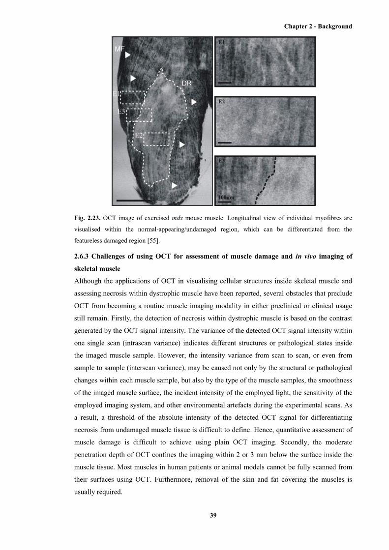
Chapter 2 - Background
39
Fig. 2.23. OCT image of exercised mdx mouse muscle. Longitudinal view of individual myofibres are
visualised within the normal-appearing/undamaged region, which can be differentiated from the
featureless damaged region [55].
2.6.3 Challenges of using OCT for assessment of muscle damage and in vivo imaging of
skeletal muscle
Although the applications of OCT in visualising cellular structures inside skeletal muscle and
assessing necrosis within dystrophic muscle have been reported, several obstacles that preclude
OCT from becoming a routine muscle imaging modality in either preclinical or clinical usage
still remain. Firstly, the detection of necrosis within dystrophic muscle is based on the contrast
generated by the OCT signal intensity. The variance of the detected OCT signal intensity within
one single scan (intrascan variance) indicates different structures or pathological states inside
the imaged muscle sample. However, the intensity variance from scan to scan, or even from
sample to sample (interscan variance), may be caused not only by the structural or pathological
changes within each muscle sample, but also by the type of the muscle samples, the smoothness
of the imaged muscle surface, the incident intensity of the employed light, the sensitivity of the
employed imaging system, and other environmental artefacts during the experimental scans. As
a result, a threshold of the absolute intensity of the detected OCT signal for differentiating
necrosis from undamaged muscle tissue is difficult to define. Hence, quantitative assessment of
muscle damage is difficult to achieve using plain OCT imaging. Secondly, the moderate
penetration depth of OCT confines the imaging within 2 or 3 mm below the surface inside the
muscle tissue. Most muscles in human patients or animal models cannot be fully scanned from
their surfaces using OCT. Furthermore, removal of the skin and fat covering the muscles is
usually required.

Chapter 2 - Background
40
In the following chapters of this thesis, solutions to these obstacles are addressed and discussed.
In Chapter 3, it is reported that an extension of OCT, PS-OCT, has been employed for the
detection of muscle damage within dystrophic muscle samples. The contrast of PS-OCT is
generated based on the pathological change of an optical property, birefringence, inside the
muscle samples. Since birefringence is less affected by the experimental artefacts just described,
quantitative assessment of muscle damage within dystrophic muscles samples is enabled. In
Chapters 4 and 5, the development of an ultrathin OCT needle probe and the application of this
needle probe in visualising cellular structures and pathological changes deep inside muscle
samples are described. The developed OCT needle probe can be inserted into the imaged muscle
and thus overcome the limitation in penetration depth of OCT. A significant step forward to in
vivo OCT imaging of skeletal muscle with minimum invasion is achieved by this development
of the ultrathin OCT needle probe.
2.7 Chapter summary
Skeletal muscle, as one of the three types of muscle tissue within human bodies and most
animals, possesses highly organised structures from the molecular level (i.e., myofilaments) to
the cellular level (i.e., myofibres). Mature myofibres that are developed from myotubes are rod-
like, multinucleated cells, forming bundles termed fascicles. The myofibres are arranged in
parallel styles, which lie obliquely to, or along, the longitudinal axis. These arrangements
perform as structural basis of the various architectures of skeletal muscles. Each myofibre
consists of hundreds of myofibrils; while each myofibril comprises hundreds of myofilaments.
The myofilaments include myosin (i.e., thick) and actin (i.e., thin) filaments. The interdigitating
arrangement of myosin and actin filaments provides the structural basis of muscle contraction,
which is driven by the relative sliding between these two types of myofilaments.
Duchenne muscular dystrophy, as one of the most severe muscular dystrophies, is caused by
mutations in the gene mapped on the human X chromosome. The genetic abnormality results in
an altered form or complete absence of the protein dystrophin, which subsequently reduces the
stability and maintenance of sarcolemma. The myofibres with the lack of functional dystrophin
are dystrophic myofibres, which are very susceptible to the damage of sarcolemma in response
to muscle contraction during exercise (e.g., general locomotion). The entry of calcium through
the damage (e.g., delta lesions) on the sarcolemma triggers enzyme-involved cascades and leads
to muscle necrosis. The respiratory or cardiac failure resulted from the muscle necrosis results
in the death of DMD patients in the second to third decade of their life.
Several imaging techniques, including US, CT, MRI, and light microscopy, have been applied
to the characterisation and analysis of DMD. Ultrasonography, CT, and MRI typically perform
as clinical imaging modalities. Ultrasonography is a non-invasive, low-cost imaging modality
with real-time display and portable equipment. Three-dimensional data volumes, with the

Chapter 2 - Background
41
spatial resolution ranging from 80 to 800 μm and the penetration depth of several millimetres,
can be provided by US. The spatial resolution of micro-US, which is typically used for
preclinical imaging, can be as fine as 20 μm. X-ray computed tomography generates 3D data
volumes with the spatial resolution of ~100 μm, although it has been reported that the spatial
resolution of micro-CT that is used for preclinical imaging can reach 50 μm, or even 20 μm with
the contrast-enhanced agents. However, the high radiation dosage and relatively low contrast in
soft tissues remain to be limitations of CT in clinical imaging. Magnetic resonance imaging
provides better soft-tissue contrast without invasiveness or radiation dosage. The spatial
resolution of MRI ranges from 50 to 100 μm. A finer resolution of ~20 μm can be achieved by
micro-MRI, which is typically used for preclinical imaging. Light microscopic imaging
modalities, including confocal microscopy, MPM, SHG, provide high-resolution (finer than 1
μm) 3D images. However, excision and preparation of tissue samples are typically required.
Hence, light microscopic imaging modalities are typically applied to preclinical imaging.
Optical coherence tomography, including TD-OCT and SD-OCT, is a non-invasive imaging
modality providing 3D data volumes with the spatial resolution of ~10 μm. Klyen et al. first
applied OCT to the characterisation of muscle damage within dystrophic muscle samples. The
capability of OCT in differentiating muscle damage from surrounding normal-appearing tissue
within dystrophic mouse muscle samples has been demonstrated. However, OCT does not lend
itself to automatic quantification of the proportion of muscle damage within a muscle sample.
Moreover, the penetration depth of OCT in opaque tissues, which is no more than 2 mm, is
usually not enough for in vivo muscle imaging. Therefore, two solutions respectively according
to these limitations are presented in this thesis. The application of PS-OCT, with a
computational algorithm, enables fully automatic and quantitative characterisation of muscle
damage within dystrophic muscle samples. The moderate penetration depth of OCT in opaque
tissue can be overcome by OCT needle probes, which is presented in Chapter 3 and 4 in this
thesis.

Chapter 3 - Characterisation of skeletal muscle damage using PS-OCT
42
Chapter 3
Characterisation of skeletal muscle damage using PS-OCT
3.1 Preface
This chapter begins with a detailed theoretical explanation of polarisation and optical
birefringence, given its prominence in this thesis. An extension of OCT, namely PS-OCT,
which can characterise and assess the birefringence of imaged samples, is described.
Subsequently, birefringence within skeletal muscle, in terms of the structural origin of muscle
birefringence and the effect of muscle contraction in muscle birefringence, is discussed. Two
published journal papers (with minor modifications in the first paper) are then presented. The
first paper presents our self-developed automated algorithm for the quantitative assessment of
tissue birefringence based on PS-OCT imaging data. The second paper demonstrates the
application of this developed algorithm for the quantitative characterisation and assessment of
muscle damage in dystrophic muscle (mdx mouse muscle) based on PS-OCT imaging data.
Additional work related to the published papers is presented in the last part of this chapter.
Following Azzam and Bashara [327], in the text, bold face symbols are used to represent both
vector and matrix quantities and these may be distinguished by the context in which they are
used.
3.2 Optical birefringence and polarisation
Light propagating in free space is a transverse wave because the local oscillations of a light
wave can be oriented perpendicular to the direction of wave propagation. Therefore, a light
wave cannot be completely described by the parameters of amplitude, frequency, and phase. An
extra freedom, given by the direction of local oscillations, is called the polarisation state or state
of polarisation (SoP) [328]. A generic monochromatic light wave can be described by its
complex electric field ),(C tzE (hereafter, the letters in bold indicate vectors). This ),(C tzE is
defined as )-i(e ωtkzE , where k is known as the wavenumber. This wavenumber, k, is given by
2 , where λ is the wavelength of the light wave. The symbol of is the angular frequency of
the light wave; and i is the unit of imaginary number. The direction of the local oscillations of
this light wave can be decomposed in terms of a pair of othonormal basis vectors: the horizontal
vector (H) and the vertical vector (V). Thus
VVHH ˆˆ ee EE E , (1)
where

Chapter 3 - Characterisation of skeletal muscle damage using PS-OCT
43
H-iHH e aE , (2)
and
V-iVV e aE . (3)
Here, He and Ve are unit vectors along the horizontal and vertical directions, respectively; Ha
and Va are amplitude components along the horizontal and vertical, respectively. As the local
oscillations are always perpendicular to the z-axis, which is the propagation direction of the
light wave, the SoP is determined by the change of direction in local oscillation in the xy-plane
[328, 329]. The local oscillations can be performed along the x-axis, y-axis, or any arbitrary
combination of the two. Therefore, if z is set to 0 for simplicity, then the curve traced out by the
tip of the electric field, known as the vibrational ellipse, can be obtained [328]. The shape of this
vibrational ellipse determines the SoP of the light wave. Following the definitions and equations
above, the mathematical expression of this vibrational ellipse is given by [328]
VVVHHHvib ˆcosˆcos e e tatatE . (4)
Here, we define the phase retardation between the horizontal and vertical polarisation
components of the light wave as
VH . (5)
When m , where Zm , the vibrational ellipse collapses to a straight line described by
[328]
ee HVVHHvib cos ˆ1ˆ taat mE . (6)
In this particular case, the SoP is said to be linear. The ratio between Ha and Va determines the
orientation of this straight line [328]. If 0H a or 0V a , the straight line will be oriented
vertically (Fig. 3.1a) or horizontally, respectively. If 0VH aa , the straight line will be
oriented at ±45˚ (Fig. 3.1b). In more general cases, the orientation angle can be calculated by
[328]
V
H1tanaa . (7)
When 0VH aa and
n2
(where Zn ), the vibrational ellipse becomes a circle
described by [328]
VHHHHvib ˆsinˆcos e e ttatE . (8)
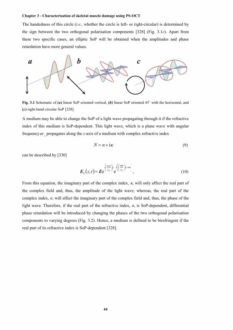
Chapter 3 - Characterisation of skeletal muscle damage using PS-OCT
44
The handedness of this circle (i.e., whether the circle is left- or right-circular) is determined by
the sign between the two orthogonal polarisation components [328] (Fig. 3.1c). Apart from
these two specific cases, an elliptic SoP will be obtained when the amplitudes and phase
retardation have more general values.
Fig. 3.1 Schematic of (a) linear SoP oriented vertical, (b) linear SoP oriented 45˚ with the horizontal, and
(c) right-hand circular SoP [328].
A medium may be able to change the SoP of a light wave propagating through it if the refractive
index of this medium is SoP-dependent. This light wave, which is a plane wave with angular
frequency , propagates along the z-axis of a medium with complex refractive index
i nN (9)
can be described by [330]
tz
cn
zctz
00i-
C ee, EE , (10)
From this equation, the imaginary part of the complex index, , will only affect the real part of
the complex field and, thus, the amplitude of the light wave; whereas, the real part of the
complex index, n, will affect the imaginary part of the complex field and, thus, the phase of the
light wave. Therefore, if the real part of the refractive index, n, is SoP-dependent, differential
phase retardation will be introduced by changing the phases of the two orthogonal polarisation
components to varying degrees (Fig. 3.2). Hence, a medium is defined to be birefringent if the
real part of its refractive index is SoP-dependent [328].
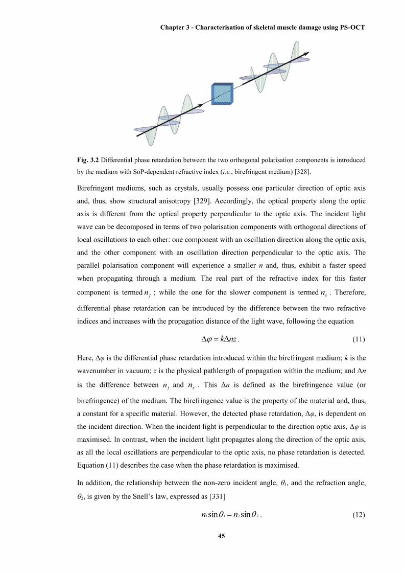
Chapter 3 - Characterisation of skeletal muscle damage using PS-OCT
45
Fig. 3.2 Differential phase retardation between the two orthogonal polarisation components is introduced
by the medium with SoP-dependent refractive index (i.e., birefringent medium) [328].
Birefringent mediums, such as crystals, usually possess one particular direction of optic axis
and, thus, show structural anisotropy [329]. Accordingly, the optical property along the optic
axis is different from the optical property perpendicular to the optic axis. The incident light
wave can be decomposed in terms of two polarisation components with orthogonal directions of
local oscillations to each other: one component with an oscillation direction along the optic axis,
and the other component with an oscillation direction perpendicular to the optic axis. The
parallel polarisation component will experience a smaller n and, thus, exhibit a faster speed
when propagating through a medium. The real part of the refractive index for this faster
component is termed fn ; while the one for the slower component is termed sn . Therefore,
differential phase retardation can be introduced by the difference between the two refractive
indices and increases with the propagation distance of the light wave, following the equation
nzk . (11)
Here, Δφ is the differential phase retardation introduced within the birefringent medium; k is the
wavenumber in vacuum; z is the physical pathlength of propagation within the medium; and Δn
is the difference between fn and sn . This Δn is defined as the birefringence value (or
birefringence) of the medium. The birefringence value is the property of the material and, thus,
a constant for a specific material. However, the detected phase retardation, Δφ, is dependent on
the incident direction. When the incident light is perpendicular to the direction optic axis, Δφ is
maximised. In contrast, when the incident light propagates along the direction of the optic axis,
as all the local oscillations are perpendicular to the optic axis, no phase retardation is detected.
Equation (11) describes the case when the phase retardation is maximised.
In addition, the relationship between the non-zero incident angle, 1, and the refraction angle,
2, is given by the Snell’s law, expressed as [331]
2211 sinsin nn . (12)

Chapter 3 - Characterisation of skeletal muscle damage using PS-OCT
46
Here, n1 and n2 represent the refractive indices of the medium in which the incident light
propagates and the medium in which the refractive light propagates, respectively. If the incident
light is a polarised light beam propagating from the air to a birefringent medium, n1 should be
the refractive index of the air and n2 should be the refractive index of the birefringent medium,
which is SoP-dependent. The two polarisation components of the incident light will, thus,
experience different refractive indices and show different refractive angles. As a result, two
refractive light beams, representing these two polarisation components, can be observed inside
the birefringent medium (Fig. 3.3). This phenomenon is called “double refraction”. Calcite is a
classic example of a birefringent medium that exhibits double refraction [328, 329].
Fig. 3.3 Schematic of double refraction within a crystal medium. The optic axis is horizontal. The
horizontal oscillation component and the vertical oscillation component are divided during the refraction
of the incident light.
3.3 Representation of the SoP
The SoPs of light waves are usually represented using the Jones formalism or the Mueller-
Stokes formalism. Because the decomposition of the electric field of a light wave involves two
orthogonal components, the horizontal and vertical components, this electric field can be
intuitively represented by a two-element vector as
V
H
EE
E . (13)
Here, HE and VE represent the scalar electric fields of the horizontal and vertical components,
respectively. This vector is called the Jones vector [328]. The electric field in the Jones vector is
considered to be time-invariant. Hence, the represented electric field is only dependent on the
amplitudes and exact phases of the components, as
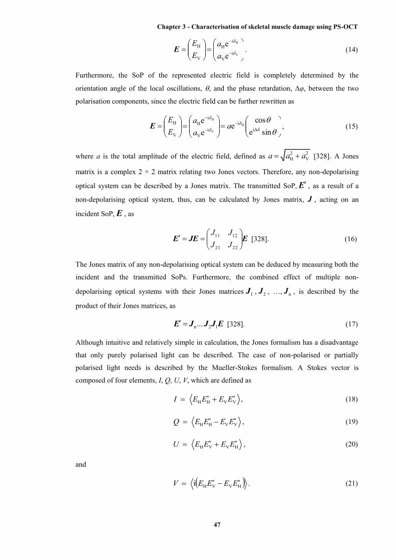
Chapter 3 - Characterisation of skeletal muscle damage using PS-OCT
47
V
H
iV
iH
V
H
ee
aa
EE
E . (14)
Furthermore, the SoP of the represented electric field is completely determined by the
orientation angle of the local oscillations, , and the phase retardation, Δφ, between the two
polarisation components, since the electric field can be further rewritten as
sinecos
eee
ii
iV
iH
V
H H
V
H
aaa
EE
E , (15)
where a is the total amplitude of the electric field, defined as 2V
2H aaa [328]. A Jones
matrix is a complex 2 × 2 matrix relating two Jones vectors. Therefore, any non-depolarising
optical system can be described by a Jones matrix. The transmitted SoP, E , as a result of a
non-depolarising optical system, thus, can be calculated by Jones matrix, J , acting on an
incident SoP, E , as
EJEE
2221
1211
JJJJ
[328]. (16)
The Jones matrix of any non-depolarising optical system can be deduced by measuring both the
incident and the transmitted SoPs. Furthermore, the combined effect of multiple non-
depolarising optical systems with their Jones matrices 1J , 2J , …, nJ , is described by the
product of their Jones matrices, as
EJJJE 12n ... [328]. (17)
Although intuitive and relatively simple in calculation, the Jones formalism has a disadvantage
that only purely polarised light can be described. The case of non-polarised or partially
polarised light needs is described by the Mueller-Stokes formalism. A Stokes vector is
composed of four elements, I, Q, U, V, which are defined as
VVHH EEEE I , (18)
VVHH EEEE Q , (19)
HVVH EEEE U , (20)
and
HVVHi EEEE V . (21)

Chapter 3 - Characterisation of skeletal muscle damage using PS-OCT
48
Here, the angular parentheses indicate an average over a long time interval compared with the
period and E represents the conjugate electric field. The irradiance of the electric field, thus,
can be calculated by EE (The permittivity is omitted for simplicity here) [328]. Therefore, I
and Q intuitively represent the total irradiance and the difference in irradiance between the
horizontal and vertical components, respectively. The elements U and V characterise the phase
and circularity of the components, respectively [328, 332]. The degree of polarisation is
introduced by this Mueller-Stokes formalism, which is described as
2
222
IVUQP
. (22)
This degree of polarisation ranges from 0 for non-polarised light to 1 for purely polarised light
[328]. Corresponding to the four elements involved in a Stokes vector, a Mueller matrix relating
an incident Stokes vector to a transmitted vector is a 4 × 4 matrix. Although more
comprehensive than the Jones matrices, Mueller matrices have the advantage over Jones
matrices of being able to describe depolarisation effects and, thus, depolarising optical systems
[333, 334].
Based on the definition of a Stokes vector, only three elements (Q, U, and V) are adequate to
describe the SoP of the light. The additional element I only provides the degree of polarisation.
Hence, a 3D representation of SoP can be performed by the Poincaré sphere based on the Q-, U-
, and V-coordinates of a 3D space (Fig. 3.4). The centre of the sphere is located at the origin;
and the radius of the sphere can be 1 or I. For any purely polarised light, the SoP corresponds to
a particular point on the surface of the Poincaré sphere [328, 332, 335]. Some particular SoPs
are shown in Fig. 3.4 (the radius here is set as 1): (-1, 0, 0) and (1, 0, 0) represent linear SoPs
with horizontal and vertical oscillations, respectively; (0, -1, 0) and (0, 1, 0) represent linear
SoPs with their oscillations oriented at 45˚ and –45˚, respectively; (0, 0, -1) and (0, 0, 1)
represent left- and right-circular SoPs, respectively. The transition between two SoPs is
represented by a path on the surface of the Poincaré sphere. In addition, when the degree of
polarisation is less than 1 and the light is partially polarised, the SoP of the light can be
represented by a particular point inside the Poincaré sphere. As a result, depolarisation effects
can be represented by a path from the surface to the inside of the Poincaré sphere.
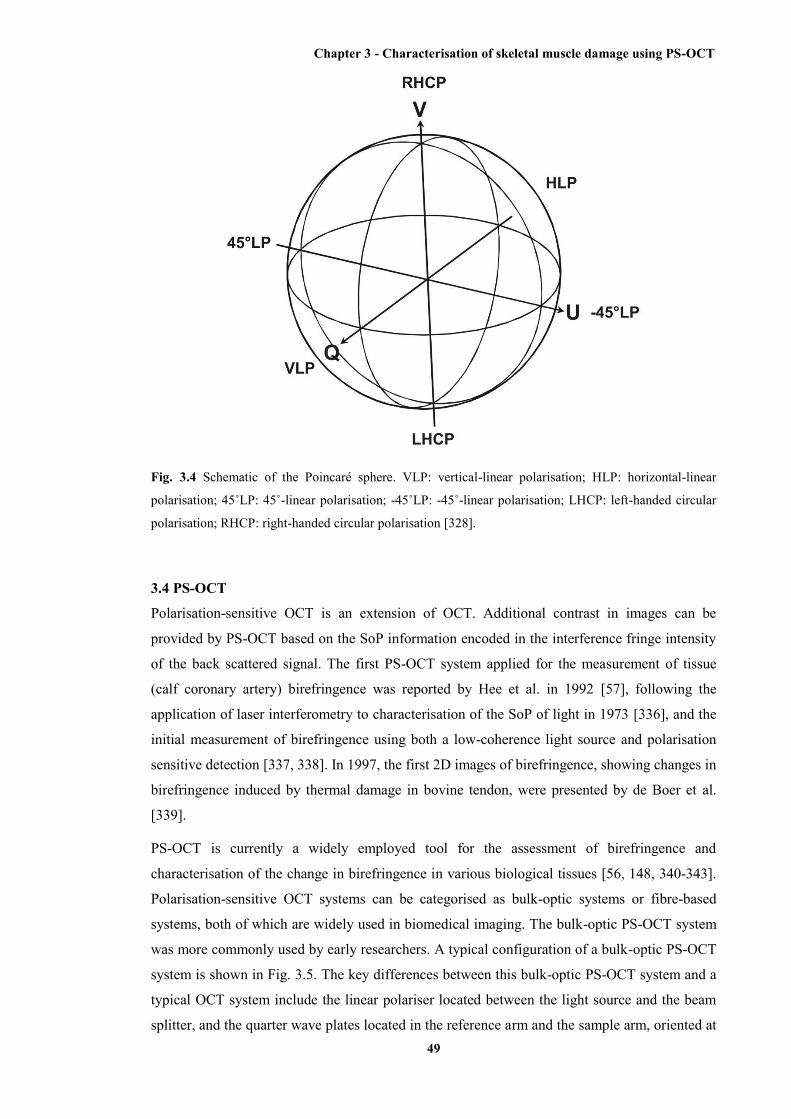
Chapter 3 - Characterisation of skeletal muscle damage using PS-OCT
49
Fig. 3.4 Schematic of the Poincaré sphere. VLP: vertical-linear polarisation; HLP: horizontal-linear
polarisation; 45˚LP: 45˚-linear polarisation; -45˚LP: -45˚-linear polarisation; LHCP: left-handed circular
polarisation; RHCP: right-handed circular polarisation [328].
3.4 PS-OCT
Polarisation-sensitive OCT is an extension of OCT. Additional contrast in images can be
provided by PS-OCT based on the SoP information encoded in the interference fringe intensity
of the back scattered signal. The first PS-OCT system applied for the measurement of tissue
(calf coronary artery) birefringence was reported by Hee et al. in 1992 [57], following the
application of laser interferometry to characterisation of the SoP of light in 1973 [336], and the
initial measurement of birefringence using both a low-coherence light source and polarisation
sensitive detection [337, 338]. In 1997, the first 2D images of birefringence, showing changes in
birefringence induced by thermal damage in bovine tendon, were presented by de Boer et al.
[339].
PS-OCT is currently a widely employed tool for the assessment of birefringence and
characterisation of the change in birefringence in various biological tissues [56, 148, 340-343].
Polarisation-sensitive OCT systems can be categorised as bulk-optic systems or fibre-based
systems, both of which are widely used in biomedical imaging. The bulk-optic PS-OCT system
was more commonly used by early researchers. A typical configuration of a bulk-optic PS-OCT
system is shown in Fig. 3.5. The key differences between this bulk-optic PS-OCT system and a
typical OCT system include the linear polariser located between the light source and the beam
splitter, and the quarter wave plates located in the reference arm and the sample arm, oriented at

Chapter 3 - Characterisation of skeletal muscle damage using PS-OCT
50
22.5˚ and 45˚, respectively [332]. Jones formalism will be employed in the following
description of the bulk-optic PS-OCT system. The light coming from the low coherence light
source becomes a purely polarised one with linear SoP after propagating through the linear
polariser. For simplicity, the local oscillations of this linearly polarised light are assumed to be
horizontal. So the electric field of the incident light arriving at the beam splitter is given by
01
zEzE . (23)
Since the light source has low temporal coherence, i.e., the light is broadband (non-
monochromatic), a complex analytic function is employed for the description of the electric
field amplitude, as
dkkezEkz)i(
e)(~
[344]. (24)
Here, k is the wavenumber of the light and )(~ ke is the field amplitude in k-space. Assume the
beam splitter has a 50/50 splitting ratio and, thus, the incident light is divided evenly by
amplitude between both arms of the interferometer. Since the beam splitter does not change the
SoP of the light, the electric fields of both the sample arm and reference arm are given by
01
2)(
S0R0zEEE . (25)
Here, R0E and S0E represent the electric fields of the incident light to the reference and sample
arms, respectively. The light propagating within the reference arm passes through the quarter
wave plate oriented at 22.5˚to the incident horizontal polarisation. Following the reflection from
a mirror or retroreflector, the light passes through the same quarter wave plate again. The Jones
matrix of the quarter wave plate is given in Equation (26):
QWP =
/4i-
/4i
e00e
, (26)
and the rotation matrix as Equation (27):
cossinsincos
)(R . (27)
Here, φ = 22.5, corresponding to the rotation angle of the optic axis of the quarter wave plate.
Then the reflected light from the reference arm is given by
11
)2(2122.5-22.5 RR0
2RR zEz EE RQWPR [332]. (28)
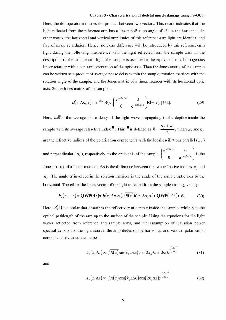
Chapter 3 - Characterisation of skeletal muscle damage using PS-OCT
51
Here, the dot operator indicates dot product between two vectors. This result indicates that the
light reflected from the reference arm has a linear SoP at an angle of 45˚ to the horizontal. In
other words, the horizontal and vertical amplitudes of this reference-arm light are identical and
free of phase retardation. Hence, no extra difference will be introduced by this reference-arm
light during the following interference with the light reflected from the sample arm. In the
description of the sample-arm light, the sample is assumed to be equivalent to a homogenous
linear retarder with a constant orientation of the optic axis. Then the Jones matrix of the sample
can be written as a product of average phase delay within the sample, rotation matrices with the
rotation angle of the sample, and the Jones matrix of a linear retarder with its horizontal optic
axis. So the Jones matrix of the sample is
RR 2/i
2/ii
e00e
e,, nkz
nkznkznzB [332]. (29)
Here, nkz is the average phase delay of the light wave propagating to the depth z inside the
sample with its average refractive index n . This n is defined as 2
sf nnn
, where fn and sn
are the refractive indices of the polarisation components with the local oscillations parallel ( fn )
and perpendicular ( sn ), respectively, to the optic axis of the sample.
2/i
2/i
e00e
nkz
nkz
is the
Jones matrix of a linear retarder. n is the difference between the two refractive indices fn and
sn . The angle involved in the rotation matrices is the angle of the sample optic axis to the
horizontal. Therefore, the Jones vector of the light reflected from the sample arm is given by
sss 45-,,,,45 EBBE QWPQWP nzzRnzzz . (30)
Here, zR is a scalar that describes the reflectivity at depth z inside the sample; while zs is the
optical pathlength of the arm up to the surface of the sample. Using the equations for the light
waves reflected from reference and sample arms, and the assumption of Gaussian power
spectral density for the light source, the amplitudes of the horizontal and vertical polarisation
components are calculated to be
2
-
00H e22cossin,
lz
zknzkzRzzA (31)
and
2
-
00V e2coscos,
lz
zknzkzRzzA , (32)
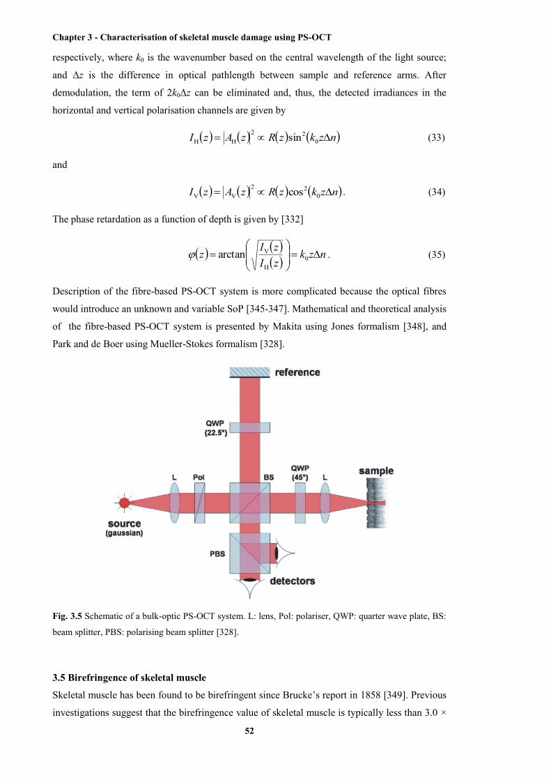
Chapter 3 - Characterisation of skeletal muscle damage using PS-OCT
52
respectively, where k0 is the wavenumber based on the central wavelength of the light source;
and Δz is the difference in optical pathlength between sample and reference arms. After
demodulation, the term of 2k0Δz can be eliminated and, thus, the detected irradiances in the
horizontal and vertical polarisation channels are given by
nzkzRzAzI 022
HH sin (33)
and
nzkzRzAzI 022
VV cos . (34)
The phase retardation as a function of depth is given by [332]
nzkzIzIz
0
H
Varctan . (35)
Description of the fibre-based PS-OCT system is more complicated because the optical fibres
would introduce an unknown and variable SoP [345-347]. Mathematical and theoretical analysis
of the fibre-based PS-OCT system is presented by Makita using Jones formalism [348], and
Park and de Boer using Mueller-Stokes formalism [328].
Fig. 3.5 Schematic of a bulk-optic PS-OCT system. L: lens, Pol: polariser, QWP: quarter wave plate, BS:
beam splitter, PBS: polarising beam splitter [328].
3.5 Birefringence of skeletal muscle
Skeletal muscle has been found to be birefringent since Brucke’s report in 1858 [349]. Previous
investigations suggest that the birefringence value of skeletal muscle is typically less than 3.0 ×
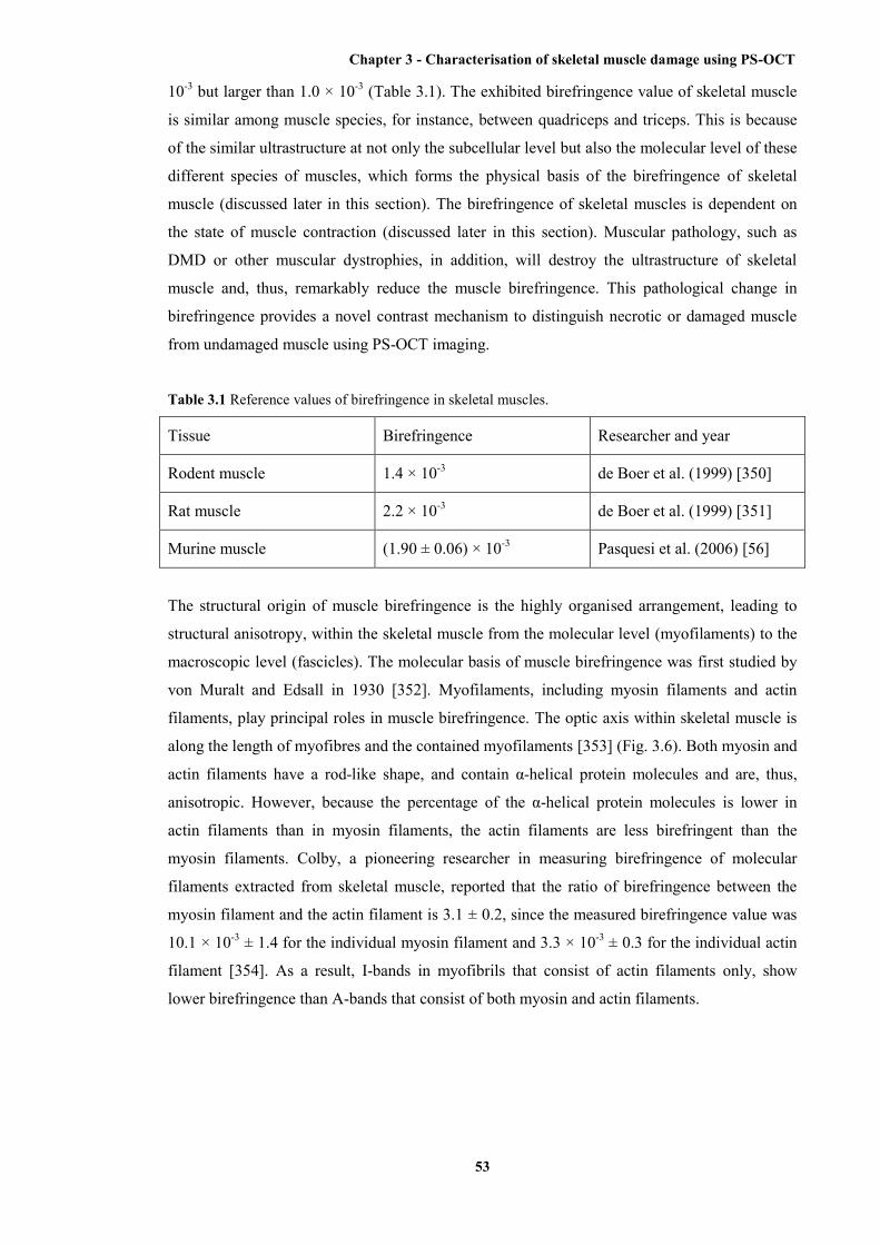
Chapter 3 - Characterisation of skeletal muscle damage using PS-OCT
53
10-3 but larger than 1.0 × 10⁻³ (Table 3.1). The exhibited birefringence value of skeletal muscle
is similar among muscle species, for instance, between quadriceps and triceps. This is because
of the similar ultrastructure at not only the subcellular level but also the molecular level of these
different species of muscles, which forms the physical basis of the birefringence of skeletal
muscle (discussed later in this section). The birefringence of skeletal muscles is dependent on
the state of muscle contraction (discussed later in this section). Muscular pathology, such as
DMD or other muscular dystrophies, in addition, will destroy the ultrastructure of skeletal
muscle and, thus, remarkably reduce the muscle birefringence. This pathological change in
birefringence provides a novel contrast mechanism to distinguish necrotic or damaged muscle
from undamaged muscle using PS-OCT imaging.
Table 3.1 Reference values of birefringence in skeletal muscles.
Tissue Birefringence Researcher and year
Rodent muscle 1.4 × 10⁻³ de Boer et al. (1999) [350]
Rat muscle 2.2 × 10⁻³ de Boer et al. (1999) [351]
Murine muscle (1.90 ± 0.06) × 10-3 Pasquesi et al. (2006) [56]
The structural origin of muscle birefringence is the highly organised arrangement, leading to
structural anisotropy, within the skeletal muscle from the molecular level (myofilaments) to the
macroscopic level (fascicles). The molecular basis of muscle birefringence was first studied by
von Muralt and Edsall in 1930 [352]. Myofilaments, including myosin filaments and actin
filaments, play principal roles in muscle birefringence. The optic axis within skeletal muscle is
along the length of myofibres and the contained myofilaments [353] (Fig. 3.6). Both myosin and
actin filaments have a rod-like shape, and contain α-helical protein molecules and are, thus,
anisotropic. However, because the percentage of the α-helical protein molecules is lower in
actin filaments than in myosin filaments, the actin filaments are less birefringent than the
myosin filaments. Colby, a pioneering researcher in measuring birefringence of molecular
filaments extracted from skeletal muscle, reported that the ratio of birefringence between the
myosin filament and the actin filament is 3.1 ± 0.2, since the measured birefringence value was
10.1 × 10⁻³ ± 1.4 for the individual myosin filament and 3.3 × 10⁻³ ± 0.3 for the individual actin
filament [354]. As a result, I-bands in myofibrils that consist of actin filaments only, show
lower birefringence than A-bands that consist of both myosin and actin filaments.
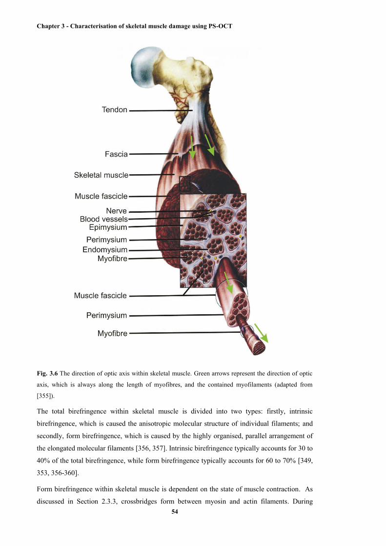
Chapter 3 - Characterisation of skeletal muscle damage using PS-OCT
54
Fig. 3.6 The direction of optic axis within skeletal muscle. Green arrows represent the direction of optic
axis, which is always along the length of myofibres, and the contained myofilaments (adapted from
[355]).
The total birefringence within skeletal muscle is divided into two types: firstly, intrinsic
birefringence, which is caused the anisotropic molecular structure of individual filaments; and
secondly, form birefringence, which is caused by the highly organised, parallel arrangement of
the elongated molecular filaments [356, 357]. Intrinsic birefringence typically accounts for 30 to
40% of the total birefringence, while form birefringence typically accounts for 60 to 70% [349,
353, 356-360].
Form birefringence within skeletal muscle is dependent on the state of muscle contraction. As
discussed in Section 2.3.3, crossbridges form between myosin and actin filaments. During

Chapter 3 - Characterisation of skeletal muscle damage using PS-OCT
55
muscle contraction, these crossbridges momentarily change direction from more parallel to
more perpendicular relative to the axis of the myosin filaments, driving the relative sliding
between myosin and actin filaments. As a result, the angle between each crossbridge and the
myosin filament increases by some degree during muscle contraction (Fig. 2.11). Hence, the
anisotropy provided by the parallel arrangement will be decreased by these perpendicular
crossbridges, which structurally disturb the parallel arrangement and significantly reduce the
birefringence (Table 3.2) [98, 349, 358, 360-363]. Irving has shown that this decrease in
birefringence is roughly proportional to the degree of overlap between the actin and myosin
filament molecules during muscle contraction [364]. This decrease is reversible and
birefringence returns when the skeletal muscle comes to its relaxed state [98, 360]. However,
when muscle contraction is excessive and the crossbridges over rotate, causing the angle
between each crossbridge and the myosin filament to exceed 90˚, the parallel organisation of
myosin molecules is reinstated. In this case, birefringence increases again after reaching the
minima [360, 365].
Table 3.2 Change of muscle birefringence caused by muscle contraction.
Resting birefringence Contracting birefringence Muscle Researcher(s) and year
1.92 ± 0.03 × 10⁻³ 8.2 ± 1.2% lower frog myofibre Eberstein and Rosenfalck
(1963) [366]
1.67 ± 0.05 × 10⁻³ 1.46 ± 0.08 × 10⁻³ rabbit psoas Taylor (1975) [98]
20% lower Fischer (1936) [358]
2.80 ± 0.59 × 10⁻³ 8.4% ± 6.4% lower Burton et al. (1990) [367]
As discussed in Section 2.4.1, muscular dystrophies, such as DMD, introduce structural damage
within diseased muscles by necrosis and inflammation of myofibres. This significantly disorders
the parallel arrangement of myofilaments, myofibrils, and myofibres (Fig. 2.14). Therefore, the
structural anisotropy and, subsequently, the birefringence of the muscle are reduced. Pasquesi et
al. have shown that the birefringence is remarkably reduced in exercised mdx mouse muscle
[56]. The following sections in this chapter present two published papers (with minor
modifications in the first paper) which demonstrate the ability of PS-OCT to quantitatively
assess the damage within dystrophic muscle (mdx mouse muscle) using an automated algorithm
expressly developed for this purpose.
Chapter 3 - Characterisation of skeletal muscle damage using PS-OCT
56
3.6 En face parametric imaging of tissue birefringence using polarization-sensitive optical
coherence tomography
[Lixin Chin, Xiaojie Yang, Robert A. McLaughlin, Peter B. Noble, David D. Sampson; Journal of
Biomedical Optics, 18(6), 066005, 2013]
Abstract We present a technique for generating en face, parametric images of tissue birefringence from scans
acquired using a fiber-based polarization-sensitive optical coherence tomography (PS-OCT) system
utilizing only a single incident polarization state. The value of birefringence is calculated for each A-scan
in the PS-OCT volume using a quadrature demodulation and phase unwrapping algorithm. The algorithm
additionally uses weighted spatial averaging and weighted least squares regression to account for
variation in phase accuracies due to varying OCT signal-to-noise-ratio. The utility of this technique is
demonstrated using a model of thermally induced damage in porcine tendon, and validated against
histology. The resulting en face images of tissue birefringence are more useful than conventional PS-OCT
B-scans in assessing the severity of tissue damage, and in localizing the spatial extent of damage.
3.6.1 Introduction
Many types of tissue exhibit birefringence, such as those of the musculoskeletal system –
muscle, cartilage, ligaments and tendon [1, 2]. Birefringence in biological tissue results from the
presence and arrangement of anisotropic ultrastructures. Disease and other processes can disrupt
these structures and reduce the degree of birefringence. Quantification of birefringence is, thus,
a potential metric for quantifying tissue damage [1, 2]. The shape, extent, and distribution of the
damaged regions are also informative in pathological assessment, and an en face view of
birefringence could provide additional spatial information about the damaged tissue.
Polarization-sensitive optical coherence tomography (PS-OCT) is a noninvasive imaging
modality that can quantify the birefringence in tissue by measuring the changes in the
polarization of back-scattered light [3]. Local estimates of birefringence are calculated from PS-
OCT scans using the rate of change of phase retardation with axial depth [4]. Computing this
parameter for each A-scan in the volume generates a two-dimensional (2-D) map of
birefringence. We refer to this map as a parametric image [5], where the pixel intensity at each
(x, y) location is indicative of an optical parameter, birefringence, calculated from the
underlying PS-OCT data. Such an image gives a visual representation of the changes in
birefringence, and hence the extent of tissue damage.
Sakai et al. presented a method for generating parametric images of birefringence from PS-OCT
scans of human skin [6]. However, skin possesses relatively low levels of birefringence, ≈10%
of the birefringence of tendon, or 20% of that of skeletal muscle [1, 6-8]. Highly birefringent
tissue presents the additional complication of phase wrapping [9].
One method of overcoming the problem of phase wrapping is to calculate the local phase
retardation from cumulative Jones matrix measurements. This requires calculating the local

Chapter 3 - Characterisation of skeletal muscle damage using PS-OCT
57
change in the tissue’s optic axis, which in fiber-based PS-OCT systems is typically
accomplished by sampling the tissue using multiple incident polarization states [9, 10].
Alternatively, Stifter et al. adopted a signal processing technique to unwrap the cumulative
phase retardation based on a 2-D quadrature transformation [11]. They demonstrated its use in
imaging the cross-sectional (B-scan) view of the birefringence of polymer materials under stress
[11]. However, the accuracy of the phase retardation signal is related to the signal-to-noise ratio
(SNR) of the OCT signal (OCT SNR) [4, 12]. Previously reported methods have not accounted
for this reduction in accuracy in areas of low signal, such as in the troughs of OCT speckle, or
with increasing depth into the tissue.
We propose a fully automated signal processing algorithm to quantify the birefringence of a
sample accounting for differing phase accuracies due to varying OCT SNR and utilizing a
quadrature transformation to account for highly birefringent materials. In addition, we extend
the algorithm to generate an en face parametric OCT image of birefringence capable of
highlighting areas of tissue damage in biological samples. This method is usable on scan
volumes acquired with fiber-based PS-OCT systems possessing only a single incident
polarization state. The algorithm is demonstrated on porcine tendon; the degree of measured
birefringence is compared to the degree of thermally induced tissue damage, and validated
against colocated histological sections.
3.6.2 Method
Generating parametric images of birefringence from PS-OCT scan volumes requires separating
the value of birefringence from the other polarization altering properties of both the tissue and
of the PS-OCT system itself. The recorded signal from each voxel in the scan volume can be
expressed as a real-valued Stokes vector, TVUQI ],,,[S , which describes the polarization
state of light [13,14]. PS-OCT detects a fully polarized signal, so the Q, U, and V components
fully describe the polarization state. The normalized, reduced Stokes vector (hereafter, “Stokes
vector”), TVUQ ]ˆ,ˆ,ˆ[ˆ S , is obtained by dividing the Q, U, and V components by
I = (Q2 + U2 + V2)1/2. It is common to treat the polarization changes due to the PS-OCT system
as both lossless and constant during imaging [4]. The birefringence of the tissue sample can,
thus, be extracted from the relative difference between Stokes vectors in an A-scan.
The phase retardation, or phase angle φr(zi), is the angle between the Stokes vectors refS (at the
surface of the tissue) and )(ˆizS (at a depth zi into the tissue. That is, ii zz SS ˆˆ)(cos refr ,
where is the three-dimensional (3-D) vector dot product and the subscript i represents the
discretization of the OCT signal in the z-dimension. The measurement accuracy of φr(zi) is
affected by the OCT SNR, which varies due to speckle, and decreases with depth into the tissue.
In the shot-noise limit, noise can be modeled as a circularly symmetric complex Gaussian
random variable [zero mean, phase uniformly distributed over (-π, π)] added to the complex

Chapter 3 - Characterisation of skeletal muscle damage using PS-OCT
58
electric field describing light backscattered from the sample. With high OCT SNR, this gives
the variance of φr(zi) as approximately twice the inverse OCT SNR at zi, )(SNR/2)(2r ii zz
[4, 12]. The effects of varying OCT SNR due to speckle can be decreased by averaging the
Stokes vectors over distances larger than the coherence length of the source [14-16]. The
relationship between OCT SNR and the accuracy of φr(zi) implies that the Stokes vectors should
be weighted by 2/)(SNR)(/1)( 2r iii zzzw during spatial averaging. The variance of the
angle calculated from the weighted, spatially averaged Stokes vectors is then given by
av2av SNR/2SNR)/(2 K , where denotes the convolution operation, K the kernel
used for spatial averaging, and SNRSNR av K the “spatially averaged” SNR.
In a noise-free model, the angle, φr(zi), between Stokes vectors is a function of the polarization
state of light incident on the tissue (hereafter “incident polarization”), the diattenuation of the
tissue, the birefringence of the tissue, and the orientation of the tissue’s optic axis [16]. If the
tissue’s optic axis changes minimally within an A-scan, its effects on φr(zi) will be limited and
can be modeled as a low-frequency modulation allowing φr(zi) to be measured using a single-
incident polarization state. The incident polarization should ideally be circular or linearly
polarized at 45˚ to the tissue optic axis. Misalignment of the incident polarization away from
these target polarization states degrades the effective SNR of φr(zi) [16].
The effects of incident polarization, diattenuation, and changing optic axis with depth into the
tissue can be modeled as modulations of the amplitude, A(zi), of the cosine-phase signal with
depth [11,16],
)(cosˆˆcinref iiii zzAzCz SS . (1)
This leaves φc(zi), the continuous-phase retardation with depth, as a function of tissue
birefringence. The amplitude modulations, A(zi), can be removed using the quadrature
component, )(sin cquad iii zzAzC , determined using the Hilbert transform, H, to the in-
phase signal Cin(zi). That is, ))(H( inquad ii zCzC [11]. This gives the demodulated, wrapped,
phase retardation,
)()( quadinw iii ziCzCz . (2)
As φw(zi) is discretized in zi, it can be unwrapped by considering the difference between
successive values, 1wwdiff iii zzz . Phase wrapping is considered to occur at the
values of zi for which |φdiff(zi)| exceeds a threshold, and phase unwrapping is performed by
interpolating φdiff(zi) at these locations. Calculating the cumulative sum of φdiff(zi) with depth
gives the unwrapped double-pass phase retardation
i
j ji zz0 diffu )( . The
birefringence, Δn, in each A-scan is then calculated as
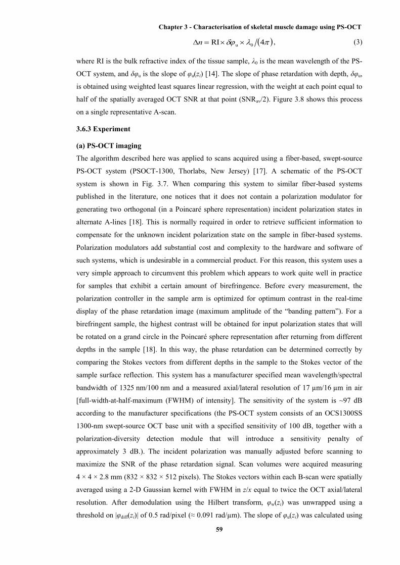
Chapter 3 - Characterisation of skeletal muscle damage using PS-OCT
59
4RI 0u n , (3)
where RI is the bulk refractive index of the tissue sample, λ0 is the mean wavelength of the PS-
OCT system, and δφu is the slope of φu(zi) [14]. The slope of phase retardation with depth, δφu,
is obtained using weighted least squares linear regression, with the weight at each point equal to
half of the spatially averaged OCT SNR at that point (SNRav/2). Figure 3.8 shows this process
on a single representative A-scan.
3.6.3 Experiment
(a) PS-OCT imaging
The algorithm described here was applied to scans acquired using a fiber-based, swept-source
PS-OCT system (PSOCT-1300, Thorlabs, New Jersey) [17]. A schematic of the PS-OCT
system is shown in Fig. 3.7. When comparing this system to similar fiber-based systems
published in the literature, one notices that it does not contain a polarization modulator for
generating two orthogonal (in a Poincaré sphere representation) incident polarization states in
alternate A-lines [18]. This is normally required in order to retrieve sufficient information to
compensate for the unknown incident polarization state on the sample in fiber-based systems.
Polarization modulators add substantial cost and complexity to the hardware and software of
such systems, which is undesirable in a commercial product. For this reason, this system uses a
very simple approach to circumvent this problem which appears to work quite well in practice
for samples that exhibit a certain amount of birefringence. Before every measurement, the
polarization controller in the sample arm is optimized for optimum contrast in the real-time
display of the phase retardation image (maximum amplitude of the “banding pattern”). For a
birefringent sample, the highest contrast will be obtained for input polarization states that will
be rotated on a grand circle in the Poincaré sphere representation after returning from different
depths in the sample [18]. In this way, the phase retardation can be determined correctly by
comparing the Stokes vectors from different depths in the sample to the Stokes vector of the
sample surface reflection. This system has a manufacturer specified mean wavelength/spectral
bandwidth of 1325 nm/100 nm and a measured axial/lateral resolution of 17 µm/16 µm in air
[full-width-at-half-maximum (FWHM) of intensity]. The sensitivity of the system is ~97 dB
according to the manufacturer specifications (the PS-OCT system consists of an OCS1300SS
1300-nm swept-source OCT base unit with a specified sensitivity of 100 dB, together with a
polarization-diversity detection module that will introduce a sensitivity penalty of
approximately 3 dB.). The incident polarization was manually adjusted before scanning to
maximize the SNR of the phase retardation signal. Scan volumes were acquired measuring
4 × 4 × 2.8 mm (832 × 832 × 512 pixels). The Stokes vectors within each B-scan were spatially
averaged using a 2-D Gaussian kernel with FWHM in z/x equal to twice the OCT axial/lateral
resolution. After demodulation using the Hilbert transform, φw(zi) was unwrapped using a
threshold on |φdiff(zi)| of 0.5 rad/pixel (≈ 0.091 rad/µm). The slope of φu(zi) was calculated using
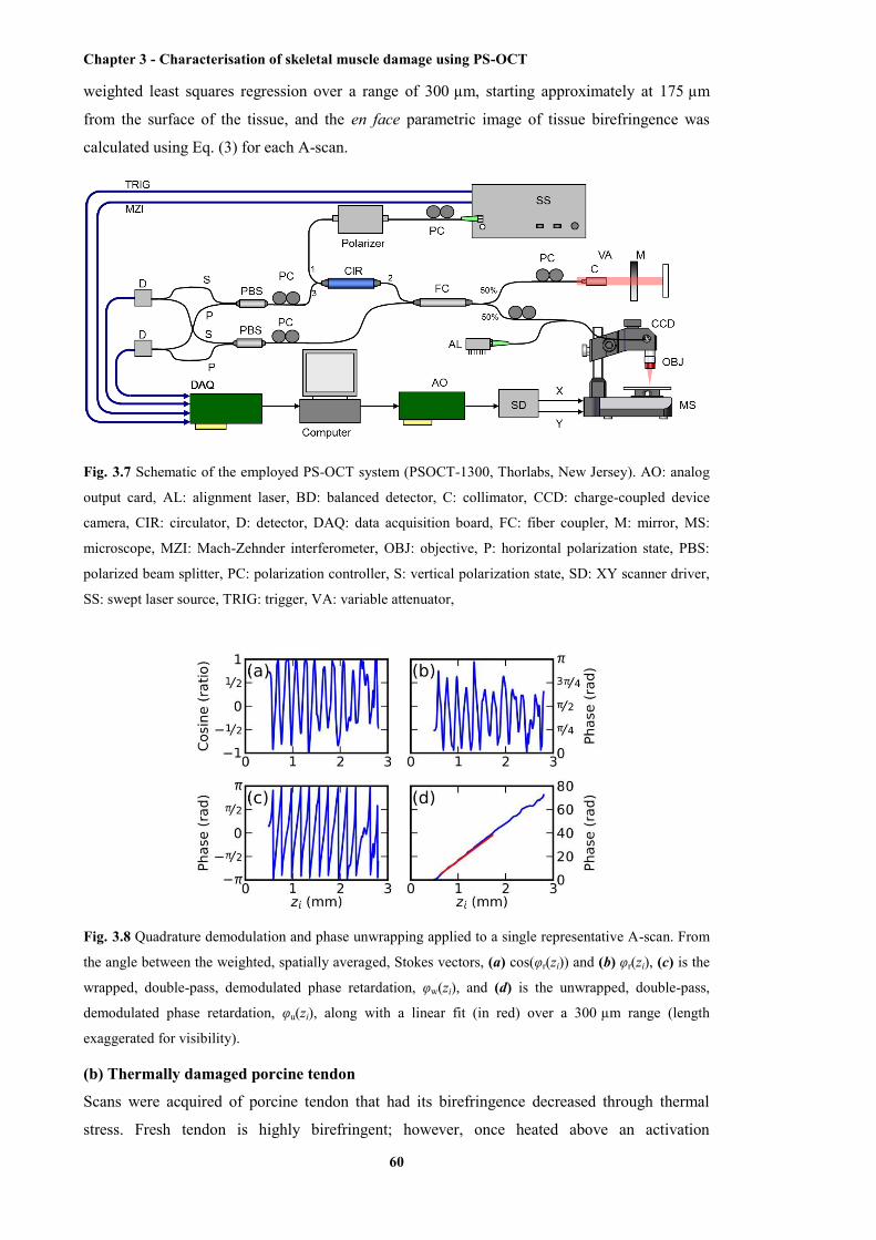
Chapter 3 - Characterisation of skeletal muscle damage using PS-OCT
60
weighted least squares regression over a range of 300 µm, starting approximately at 175 µm
from the surface of the tissue, and the en face parametric image of tissue birefringence was
calculated using Eq. (3) for each A-scan.
Fig. 3.7 Schematic of the employed PS-OCT system (PSOCT-1300, Thorlabs, New Jersey). AO: analog
output card, AL: alignment laser, BD: balanced detector, C: collimator, CCD: charge-coupled device
camera, CIR: circulator, D: detector, DAQ: data acquisition board, FC: fiber coupler, M: mirror, MS:
microscope, MZI: Mach-Zehnder interferometer, OBJ: objective, P: horizontal polarization state, PBS:
polarized beam splitter, PC: polarization controller, S: vertical polarization state, SD: XY scanner driver,
SS: swept laser source, TRIG: trigger, VA: variable attenuator,
Fig. 3.8 Quadrature demodulation and phase unwrapping applied to a single representative A-scan. From
the angle between the weighted, spatially averaged, Stokes vectors, (a) cos(φr(zi)) and (b) φr(zi), (c) is the
wrapped, double-pass, demodulated phase retardation, φw(zi), and (d) is the unwrapped, double-pass,
demodulated phase retardation, φu(zi), along with a linear fit (in red) over a 300 µm range (length
exaggerated for visibility).
(b) Thermally damaged porcine tendon
Scans were acquired of porcine tendon that had its birefringence decreased through thermal
stress. Fresh tendon is highly birefringent; however, once heated above an activation

Chapter 3 - Characterisation of skeletal muscle damage using PS-OCT
61
temperature (≈ 62 °C for these samples), the collagen in the tendon denatures. This leads to a
decrease in birefringence with the rate of decrease being a function of both temperature and
heating time [2, 8]. This model was used to both quantify birefringence and to generate en face
parametric OCT images of birefringence.
Three castrated-male pigs (≈ 8 to 10 weeks, 30 kg) were euthanized by exsanguination under
barbiturate anesthesia in accordance with institutional ethics requirements. Tendons were
extracted from the posterior side of the hind limbs and cut into strips measuring approximately
10 × 10 × 5 mm. The samples were clamped between aluminum blocks and fully immersed in
heated physiological Krebs solution. After 2.5 min, the samples were removed from solution
and imaged on the PS-OCT system. The samples were then replaced in the heated Krebs
solution for a further 2.5 min, and the process repeated until each sample had been heated for a
total of 15 min. En face parametric birefringence images of each sample were generated using
the described algorithm, taking the bulk refractive index of porcine tendon, RI, as 1.4 [8, 19].
3.6.4 Results
Fig. 3.9 shows the mean birefringence for six tendon samples at temperatures ranging from
61 °C to 67 °C. The birefringence of fresh tendon prior to thermal stress (t = 0 min) was
4.0 × 10⁻³ ± 0.4 × 10⁻³ (mean ± standard deviation), comparable with previously reported values
of 4.2 × 10⁻³ ± 0.3 × 10⁻³ [8]. As anticipated, the mean birefringence decreased with time, as the
period of thermal stress increased, and the rate at which the birefringence decreased was
observed to increase with temperature. Tendon birefringence was generally unchanged by
heating at 61°C, but had mostly dissipated after 7.5 min at 67 °C. This agrees with previous
studies, which showed that porcine tendon was unaffected by heating at 60 °C, but rapidly
denatured at 65 °C [20].
Fig. 3.9 The mean birefringence of porcine tendon samples (S1-S6) after thermal stress. Samples were
immersed in heated Krebs solution at the indicated temperatures. Total heating time refers to the duration
of the applied thermal stress.
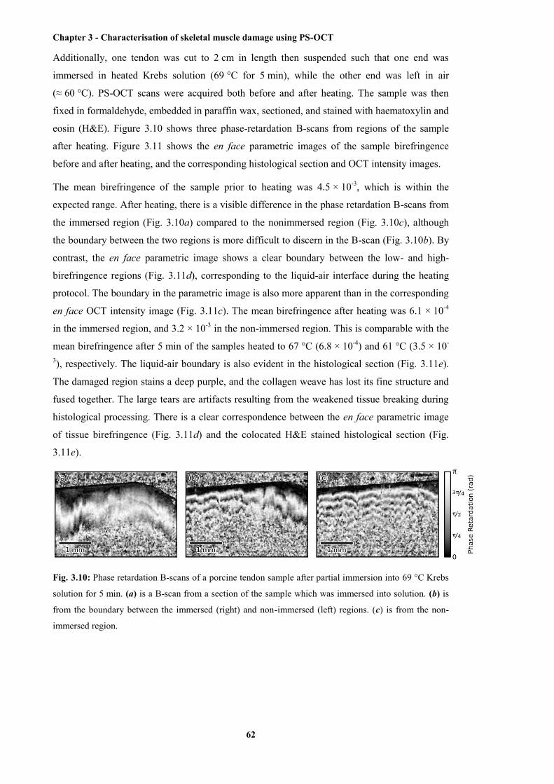
Chapter 3 - Characterisation of skeletal muscle damage using PS-OCT
62
Additionally, one tendon was cut to 2 cm in length then suspended such that one end was
immersed in heated Krebs solution (69 °C for 5 min), while the other end was left in air
(≈ 60 °C). PS-OCT scans were acquired both before and after heating. The sample was then
fixed in formaldehyde, embedded in paraffin wax, sectioned, and stained with haematoxylin and
eosin (H&E). Figure 3.10 shows three phase-retardation B-scans from regions of the sample
after heating. Figure 3.11 shows the en face parametric images of the sample birefringence
before and after heating, and the corresponding histological section and OCT intensity images.
The mean birefringence of the sample prior to heating was 4.5 × 10⁻³, which is within the
expected range. After heating, there is a visible difference in the phase retardation B-scans from
the immersed region (Fig. 3.10a) compared to the nonimmersed region (Fig. 3.10c), although
the boundary between the two regions is more difficult to discern in the B-scan (Fig. 3.10b). By
contrast, the en face parametric image shows a clear boundary between the low- and high-
birefringence regions (Fig. 3.11d), corresponding to the liquid-air interface during the heating
protocol. The boundary in the parametric image is also more apparent than in the corresponding
en face OCT intensity image (Fig. 3.11c). The mean birefringence after heating was 6.1 × 10⁻⁴
in the immersed region, and 3.2 × 10⁻³ in the non-immersed region. This is comparable with the
mean birefringence after 5 min of the samples heated to 67 °C (6.8 × 10⁻⁴) and 61 °C (3.5 × 10-
3), respectively. The liquid-air boundary is also evident in the histological section (Fig. 3.11e).
The damaged region stains a deep purple, and the collagen weave has lost its fine structure and
fused together. The large tears are artifacts resulting from the weakened tissue breaking during
histological processing. There is a clear correspondence between the en face parametric image
of tissue birefringence (Fig. 3.11d) and the colocated H&E stained histological section (Fig.
3.11e).
Fig. 3.10: Phase retardation B-scans of a porcine tendon sample after partial immersion into 69 °C Krebs
solution for 5 min. (a) is a B-scan from a section of the sample which was immersed into solution. (b) is
from the boundary between the immersed (right) and non-immersed (left) regions. (c) is from the non-
immersed region.
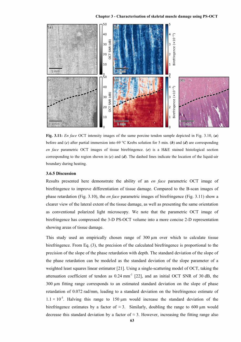
Chapter 3 - Characterisation of skeletal muscle damage using PS-OCT
63
Fig. 3.11: En face OCT intensity images of the same porcine tendon sample depicted in Fig. 3.10, (a)
before and (c) after partial immersion into 69 °C Krebs solution for 5 min. (b) and (d) are corresponding
en face parametric OCT images of tissue birefringence. (e) is a H&E stained histological section
corresponding to the region shown in (c) and (d). The dashed lines indicate the location of the liquid-air
boundary during heating.
3.6.5 Discussion
Results presented here demonstrate the ability of an en face parametric OCT image of
birefringence to improve differentiation of tissue damage. Compared to the B-scan images of
phase retardation (Fig. 3.10), the en face parametric images of birefringence (Fig. 3.11) show a
clearer view of the lateral extent of the tissue damage, as well as presenting the same orientation
as conventional polarized light microscopy. We note that the parametric OCT image of
birefringence has compressed the 3-D PS-OCT volume into a more concise 2-D representation
showing areas of tissue damage.
This study used an empirically chosen range of 300 µm over which to calculate tissue
birefringence. From Eq. (3), the precision of the calculated birefringence is proportional to the
precision of the slope of the phase retardation with depth. The standard deviation of the slope of
the phase retardation can be modeled as the standard deviation of the slope parameter of a
weighted least squares linear estimator [21]. Using a single-scattering model of OCT, taking the
attenuation coefficient of tendon as 0.24 mm-1 [22], and an initial OCT SNR of 30 dB, the
300 µm fitting range corresponds to an estimated standard deviation on the slope of phase
retardation of 0.072 rad/mm, leading to a standard deviation on the birefringence estimate of
1.1 × 10⁻⁵. Halving this range to 150 µm would increase the standard deviation of the
birefringence estimates by a factor of ≈ 3. Similarly, doubling the range to 600 µm would
decrease this standard deviation by a factor of ≈ 3. However, increasing the fitting range also
Chapter 3 - Characterisation of skeletal muscle damage using PS-OCT
64
increases the possibility of errors due to aggregating birefringence over different tissue types.
The optimal fitting length will be application specific, depending on the anticipated
homogeneity of the tissue.
The current implementation assumes tissue homogeneity within the section of the A-scan used
to calculate the birefringence. This is likely to be the case when imaging musculoskeletal tissue,
such as tendon or muscle, which consist mostly of a single tissue type, but may not be the case
in complex biological structures such as airways. In this situation, a segmentation algorithm
(e.g., as shown by van Soest et al. [23]) will be necessary to identify homogenous regions of
tissue, so that the birefringence of each tissue type can be calculated separately.
The presented method has been demonstrated on ex vivo tissue samples. The low penetration
depth of PS-OCT (≈ 1 to 2 mm in tissue) presents a challenge to extending this work to in vivo
imaging. In addition, the method works best if the incident polarization state is manually
optimized before imaging, but such adjustments also complicate potential in vivo imaging
scenarios. To overcome the challenge posed by the low penetration depth of OCT-based
imaging modalities, several groups have shown that OCT imaging probes can be miniaturized
and encased within hypodermic needles [24-27] and endoscopes [23, 28-30]. OCT needle
probes capable of acquiring 3-D scans have been reported to be as small as 30-gauge (outer
diameter 310 µm) [25, 31], significantly smaller than standard biopsy needles. PS-OCT needle
probes could be used interstitially to image birefringent tissues such as tendon, muscle, or
cartilage in situ. OCT endoscopic probes have been demonstrated capable of in vivo imaging of
human airways [28] and arteries [23], and PS-OCT endoscopic probes have been demonstrated
on ex vivo human arteries [29]. Additionally, as one method of addressing the challenge posed
by the optimization of the incident polarization state, it has been shown that fiber-based PS-
OCT systems may be constructed using polarization-maintaining fibers (PMFs) [32, 33]. PMF-
based systems keep the use of a single incident polarization state, but do not require tuning of
the incident polarization before each scan [32]. In combination with the technique presented,
PS-OCT needle and endoscopic probes and PMF-based PS-OCT systems could enable the
generation of parametric OCT images of tissue birefringence in vivo.
3.6.6 Conclusion
In summary, we have demonstrated an automated method to quantify birefringence in PS-OCT
volumes and have used this to define a novel en face parametric image. This method accounts
for variances in phase accuracy due to differing OCT SNR, improving performance compared to
conventional mean filtering, and accounts for highly birefringent tissue by utilizing quadrature
demodulation and phase unwrapping. In addition, this method is useable with fiber-based PS-
OCT systems possessing only a single-incident polarization state. When compared against OCT,
the en face parametric image of birefringence gave clear visualization of the damage in
birefringent tissue and enabled automated quantification of the degree of tissue damage.
Chapter 3 - Characterisation of skeletal muscle damage using PS-OCT
65
3.6.7 Acknowledgments L. Chin is supported by a Robert and Maude Gledden postgraduate research scholarship from the
University of Western Australia. R. A. McLaughlin is supported by a fellowship from the Cancer Council
Western Australia. P. B. Noble is supported by a career development fellowship from the NHMRC of
Australia (1045824).
3.6.8 References
[1] M. S. Islam, M. C. Oliveira, Y. Wang, F. P. Henry, M. A. Randolph, B. H. Park and J. F. de
Boer, "Extracting structural features of rat sciatic nerve using polarization-sensitive spectral
domain optical coherence tomography," Journal of Biomedical Optics 17(5), 056012 (2012)
[2] D. J. Maitland and J. T. Walsh, Jr., "Quantitative measurements of linear birefringence
during heating of native collagen," Lasers in Surgery and Medicine 20(3), 310-318 (1997)
[3] J. F. de Boer, T. E. Milner, M. J. C. van Gemert and J. S. Nelson, "Two-dimensional
birefringence imaging in biological tissue by polarization-sensitive optical coherence
tomography," Optics Letters 22(12), 934-936 (1997)
[4] B. H. Park, M. C. Pierce, B. Cense, S.-H. Yun, M. Mujat, G. J. Tearney, B. E. Bouma and J.
F. de Boer, "Real-time fiber-based multi-functional spectral-domain optical coherence
tomography at 1.3 µm," Optics Express 13(11), 3931-3944 (2005)
[5] R. A. McLaughlin, L. Scolaro, P. Robbins, C. Saunders, S. L. Jacques and D. D. Sampson,
"Parametric imaging of cancer with optical coherence tomography," Journal of Biomedical
Optics 15(4), 046029 (2010)
[6] S. Sakai, N. Nakagawa, M. Yamanari, A. Miyazawa, Y. Yasuno and M. Matsumoto,
"Relationship between dermal birefringence and the skin surface roughness of photoaged human
skin," Journal of Biomedical Optics 14(4), (2009)
[7] K. H. Kim, M. C. Pierce, G. Maguluri, B. H. Park, S. J. Yoon, M. Lydon, R. Sheridan and J.
F. de Boer, "In vivo imaging of human burn injuries with polarization-sensitive optical
coherence tomography," Journal of Biomedical Optics 17(6), 066012 (2012)
[8] S. Jiao and L. V. Wang, "Jones-matrix imaging of biological tissues with quadruple-channel
optical coherence tomography," Journal of Biomedical Optics 7(3), 350-358 (2002)
[9] C. Fan and G. Yao, "Mapping local retardance in birefringent samples using polarization
sensitive optical coherence tomography," Optics Letters 37(9), 1415-1417 (2012)
[10] S. Makita, M. Yamanari and Y. Yasuno, "Generalized Jones matrix optical coherence
tomography: performance and local birefringence imaging," Optics Express 18(2), 854-876
(2010)
[11] D. Stifter, E. Leiss-Holzinger, Z. Major, B. Baumann, M. Pircher, E. Götzinger, C. K.
Hitzenberger and B. Heise, "Dynamic optical studies in materials testing with spectral-domain

Chapter 3 - Characterisation of skeletal muscle damage using PS-OCT
66
polarization-sensitive optical coherence tomography," Optics Express 18(25), 25712-25725
(2010)
[12] B. H. Park, M. C. Pierce, B. Cense and J. F. de Boer, "Optic axis determination accuracy
for fiber-based polarization-sensitive optical coherence tomography," Optics Letters 30(19),
2587-2589 (2005)
[13] N. Ghosh and I. A. Vitkin, "Tissue polarimetry: concepts, challenges, applications, and
outlook," Journal of Biomedical Optics 16(11), 110801 (2011)
[14] J. F. de Boer and T. E. Milner, "Review of polarization sensitive optical coherence
tomography and Stokes vector determination," Journal of Biomedical Optics 7(3), 359-371
(2002)
[15] E. Z. Zhang and B. J. Vakoc, "Polarimetry noise in fiber-based optical coherence
tomography instrumentation," Optics Express 19(18), 16830-16842 (2011)
[16] N. J. Kemp, J. Park, H. N. Zaatari, H. G. Rylander and T. E. Milner, "High-sensitivity
determination of birefringence in turbid media with enhanced polarization-sensitive optical
coherence tomography," Journal of the Optical Society of America, A 22(3), 552-560 (2005)
[17] Y. M. Liew, R. A. McLaughlin, P. Gong, F. M. Wood and D. D. Sampson, "In vivo
assessment of human burn scars through automated quantification of vascularity using optical
coherence tomography," Journal of Biomedical Optics 18(6), 061213 (2013)
[18] B. H. Park and J. F. de Boer, “Polarization-sensitive optical coherence tomography,” in
Optical Coherence Tomography: Technology and Applications (Biological Medical Physics,
Biomedical Engineering), W. Drexler and J. G. Fujimoto, eds., Springer, New York, NY (2008),
pp. 653-695
[19] N. Ugryumova, J. Jacobs, M. Bonesi and S. J. Matcher, "Novel optical imaging technique
to determine the 3-D orientation of collagen fibers in cartilage: variable-incidence angle
polarization-sensitive optical coherence tomography," Osteoarthritis and Cartilage 17(1), 33-42
(2009)
[20] J. C. Wang, J. M. Kabo, P. M. Tsou, L. Halevi and A. N. Shamie, "The effect of uniform
heating on the biomechanical properties of the intervertebral disc in a porcine model," The Spine
Journal 5(1), 64-70 (2005)
[21] W. H. Press, S. A. Teukolsky, W. T. Vetterling and B. P. Flannery, Numerical Recipes:
The Art of Scientific Computing, Cambridge University Press (2007)
[22] M. Todorović, S. Jiao, L. V. Wang and G. Stoica, "Determination of local polarization
properties of biological samples in the presence of diattenuation by use of Mueller optical
coherence tomography," Optics Letters 29(20), 2402-2404 (2004)
Chapter 3 - Characterisation of skeletal muscle damage using PS-OCT
67
[23] G. van Soest, T. Goderie, E. Regar, S. Koljenović, G. L. J. H. van Leenders, N. Gonzalo, S.
van Noorden, T. Okamura, B. E. Bouma, G. J. Tearney, J. W. Oosterhuis, P. W. Serruys and A.
F. W. van der Steen, "Atherosclerotic tissue characterization in vivo by optical coherence
tomography attenuation imaging," Journal of Biomedical Optics 15(1), 011105 (2010)
[24] L. Scolaro, D. Lorenser, R. A. McLaughlin, B. C. Quirk, R. W. Kirk and D. D. Sampson,
"High-sensitivity anastigmatic imaging needle for optical coherence tomography," Optics
Letters 37(24), 5247-5249 (2012)
[25] R. A. McLaughlin, X. Yang, B. C. Quirk, D. Lorenser, R. W. Kirk, P. B. Noble and D. D.
Sampson, "Static and dynamic imaging of alveoli using optical coherence tomography needle
probes," Journal of Applied Physiology 113(6), 967-974 (2012)
[26] B. C. Quirk, R. A. McLaughlin, A. Curatolo, R. W. Kirk, P. B. Noble and D. D. Sampson,
"In situ imaging of lung alveoli with an optical coherence tomography needle probe," Journal of
Biomedical Optics 16(3), 036009 (2011)
[27] Y. Wu, J. Xi, L. Huo, J. Padvorac, E. J. Shin, S. A. Giday, A. A. Lennon, M. I. F. Canto, J.
H. Hwang and X. Li, "Robust High-Resolution Fine OCT Needle for Side-Viewing Interstitial
Tissue Imaging," IEEE Journal of Selected Topics in Quantum Electronics 16(4), 863-869
(2010)
[28] J. P. Williamson, J. J. Armstrong, R. A. McLaughlin, P. B. Noble, A. R. West, S. Becker,
A. Curatolo, W. J. Noffsinger, H. W. Mitchell, M. J. Phillips, D. D. Sampson, D. R. Hillman
and P. R. Eastwood, "Measuring airway dimensions during bronchoscopy using anatomical
optical coherence tomography," European Respiratory Journal 35(1), 34-41 (2010)
[29] S. D. Giattina, B. K. Courtney, P. R. Herz, M. Harman, S. Shortkroff, D. L. Stamper, B.
Liu, J. G. Fujimoto and M. E. Brezinski, "Assessment of coronary plaque collagen with
polarization sensitive optical coherence tomography (PS-OCT)," International Journal of
Cardiology 107(3), 400-409 (2006)
[30] P. B. Noble, A. R. West, R. A. McLaughlin, J. J. Armstrong, S. Becker, P. K. McFawn, J.
P. Williamson, P. R. Eastwood, D. R. Hillman, D. D. Sampson and H. W. Mitchell, "Airway
narrowing assessed by anatomical optical coherence tomography in vitro: dynamic airway wall
morphology and function," Journal of Applied Physiology 108(2), 401-411 (2010)
[31] D. Lorenser, X. Yang, R. W. Kirk, B. C. Quirk, R. A. McLaughlin and D. D. Sampson,
"Ultrathin side-viewing needle probe for optical coherence tomography," Optics Letters 36(19),
3894-3896 (2011)
[32] E. Götzinger, B. Baumann, M. Pircher and C. K. Hitzenberger, "Polarization maintaining
fiber based ultra-high resolution spectral domain polarization sensitive optical coherence
tomography," Optics Express 17(25), 22704-22717 (2009)
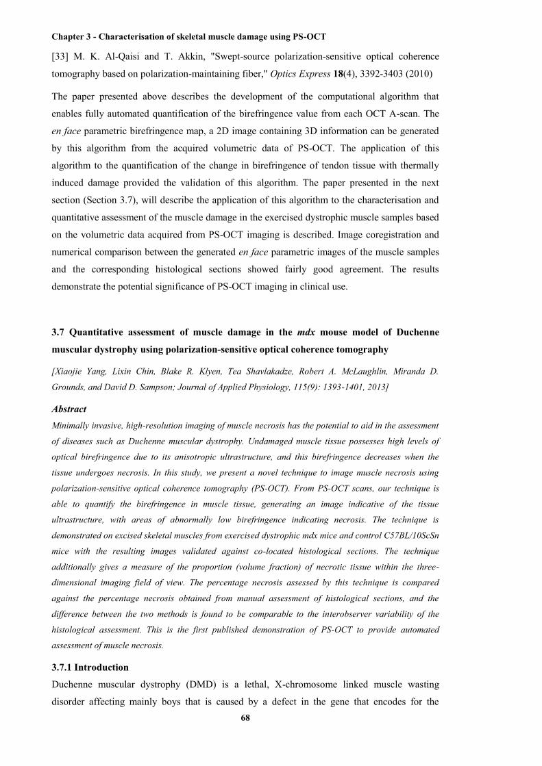
Chapter 3 - Characterisation of skeletal muscle damage using PS-OCT
68
[33] M. K. Al-Qaisi and T. Akkin, "Swept-source polarization-sensitive optical coherence
tomography based on polarization-maintaining fiber," Optics Express 18(4), 3392-3403 (2010)
The paper presented above describes the development of the computational algorithm that
enables fully automated quantification of the birefringence value from each OCT A-scan. The
en face parametric birefringence map, a 2D image containing 3D information can be generated
by this algorithm from the acquired volumetric data of PS-OCT. The application of this
algorithm to the quantification of the change in birefringence of tendon tissue with thermally
induced damage provided the validation of this algorithm. The paper presented in the next
section (Section 3.7), will describe the application of this algorithm to the characterisation and
quantitative assessment of the muscle damage in the exercised dystrophic muscle samples based
on the volumetric data acquired from PS-OCT imaging is described. Image coregistration and
numerical comparison between the generated en face parametric images of the muscle samples
and the corresponding histological sections showed fairly good agreement. The results
demonstrate the potential significance of PS-OCT imaging in clinical use.
3.7 Quantitative assessment of muscle damage in the mdx mouse model of Duchenne
muscular dystrophy using polarization-sensitive optical coherence tomography
[Xiaojie Yang, Lixin Chin, Blake R. Klyen, Tea Shavlakadze, Robert A. McLaughlin, Miranda D.
Grounds, and David D. Sampson; Journal of Applied Physiology, 115(9): 1393-1401, 2013]
Abstract Minimally invasive, high-resolution imaging of muscle necrosis has the potential to aid in the assessment
of diseases such as Duchenne muscular dystrophy. Undamaged muscle tissue possesses high levels of
optical birefringence due to its anisotropic ultrastructure, and this birefringence decreases when the
tissue undergoes necrosis. In this study, we present a novel technique to image muscle necrosis using
polarization-sensitive optical coherence tomography (PS-OCT). From PS-OCT scans, our technique is
able to quantify the birefringence in muscle tissue, generating an image indicative of the tissue
ultrastructure, with areas of abnormally low birefringence indicating necrosis. The technique is
demonstrated on excised skeletal muscles from exercised dystrophic mdx mice and control C57BL/10ScSn
mice with the resulting images validated against co-located histological sections. The technique
additionally gives a measure of the proportion (volume fraction) of necrotic tissue within the three-
dimensional imaging field of view. The percentage necrosis assessed by this technique is compared
against the percentage necrosis obtained from manual assessment of histological sections, and the
difference between the two methods is found to be comparable to the interobserver variability of the
histological assessment. This is the first published demonstration of PS-OCT to provide automated
assessment of muscle necrosis.
3.7.1 Introduction
Duchenne muscular dystrophy (DMD) is a lethal, X-chromosome linked muscle wasting
disorder affecting mainly boys that is caused by a defect in the gene that encodes for the
Chapter 3 - Characterisation of skeletal muscle damage using PS-OCT
69
structural subsarcolemmal protein dystrophin [54]. Initial muscle damage in boys with DMD
can progress to myofiber necrosis, because absence or impaired functioning of the dystrophin
protein leads to increased susceptibility of dystrophic myofibers to contractile damage after
exercise [36]. In DMD, repeated cycles of myofiber necrosis over many years leads to
replacement of muscle tissue with fibrous connective tissue and fat [30, 37], resulting in
progressive loss of muscle mass and function and early death, often due to cardiac or respiratory
failure [4, 12]. The dystrophic mdx mutant mouse (C57BL/10ScSnmdx/mdx) is a model for DMD
that is widely used in preclinical research [15, 16, 50]. Assessment of disease progression in the
mouse typically involves death of the animal for tissue sampling and histological analysis to
identify muscle necrosis [15]. Such analysis is both very time-consuming and its invasive nature
precludes the possibility of longitudinal assessment of disease progression over time in a single
animal, increasing experimental uncertainty and cost.
In whole living animals, noninvasive imaging techniques such as magnetic resonance imaging
(MRI) [2, 25, 26, 31, 43, 47], ultrasonography [11, 42, 46] or X-ray computed tomography (CT)
[39, 40, 44, 53], have shown potential for imaging muscle necrosis in vivo, with the option of
repeated measurements over time on the same subject. MRI is able to provide three-dimensional
(3-D) imaging data from tissue volumes and discriminate between healthy and dystrophic
muscle in canine [25, 26] and murine [2, 31, 43, 47] animal models. Use of MRI contrast agents
enables quantitative assessment of the permeability of dystrophic myofibers and improves
imaging contrast [2, 43]. However, the imaging resolution of MRI is insufficient to visualize
individual myofibers. Furthermore, the cost and long acquisition time of scans remain a
challenge for employing MRI in either clinical imaging or preclinical studies. Ultrasonography,
due to its lower cost and shorter acquisition time, is preferable for routine clinical use. The
imaging resolution of ultrasonography, however, is also not capable of differentiating individual
myofibers [11, 42, 46]. CT is employed in clinical studies of myopathies, and a resolution of 40
to 50 µm can be reached with high-resolution micro-CT imaging of small animals [39, 53].
With iodinated contrast agent, the imaging resolution of micro-CT can be as fine as 16 µm [40]
under ideal conditions. However, the disadvantages of lower soft tissue contrast, and very high
radiation dosage, remain impediments in micro-CT imaging [39]. The challenge is to provide a
minimally invasive imaging technique that can view a wide area of tissue with deep penetration,
combined with high resolution [38], and ideally with the potential to be applied in situ in living
animals.
Recently developed optical imaging techniques, such as optical coherence tomography (OCT),
offer the potential for high-resolution, minimally invasive imaging methodologies [10, 13].
OCT is a reflectance-mode optical imaging modality that uses low-coherence interferometry
combined with point beam scanning to produce 3-D images of tissue structure. OCT operates by
detecting depth-resolved backscattered near-infrared light (typical operating wavelength bands
lie in the vicinity of 800 nm and 1,300 nm) in a way that is analogous to ultrasonic pulse-echo
Chapter 3 - Characterisation of skeletal muscle damage using PS-OCT
70
imaging [21]. OCT imaging has been demonstrated to be capable of displaying the changes in
myofibers due to necrosis in whole ex vivo murine muscles [23, 24]. Although OCT has
demonstrated an ability to display myofibers, it does not lend itself to automatic quantification
of the proportion (volume fraction) of necrotic tissue within a muscle sample [23, 24].
Polarization-sensitive optical coherence tomography (PS-OCT) is an extension of OCT that
measures the optical birefringence of tissue by analyzing the polarization of the backscattered
light [19]. Birefringence is an optical property of an anisotropic material whereby the
propagation speed (and hence refractive index) of light traveling through the material depends
on the polarization state of the light. In linear birefringence, which is the property of interest
here, light polarized linearly parallel to the optic axis of the uniaxial, birefringent material
experiences a different refractive index than light polarized linearly orthogonal to the optic axis.
The difference between these two refractive indices is the amount of linear birefringence of the
material [3]. Healthy skeletal muscle tissue exhibits high linear birefringence (hereafter
“birefringence”), arising from the highly organized anisotropic cellular structure and
arrangement of myofibers. The detected birefringence is a maximum for light incident
orthogonal to the fiber axis, which is the optic axis in this case, and is zero for coaxial
illumination. Previous studies have shown that birefringence in normal skeletal muscle is due
both to the anisotropic arrangement of subcellular structure within myofibers [18], and the
anisotropic molecular structure of the filament molecules contained in the myofibers [6, 52]. By
contrast, damaged or necrotic muscle loses its anisotropic ultrastructure, and possesses
correspondingly low birefringence [22]. Although collagen and other filamentous,
nonmyofibrillar proteins also exhibit birefringence [45], muscle birefringence is mostly a result
of myofiber structures [6, 18]. We therefore postulate that it is possible to use PS-OCT to
identify regions of necrosis within skeletal muscle by calculating the birefringence across the
muscle, and locating the regions of abnormally low birefringence. A previous study suggests
that PS-OCT can detect the damage induced by exercise in dystrophic mdx mouse muscles by
determining the decrease in birefringence. However, the study did not extend to visualization of
the areas of necrosis, nor to quantification of the proportion of necrotic tissue within the mdx
muscles [33].
In this paper, we present a novel imaging and analysis technique that uses PS-OCT to quantify
the proportion of necrotic tissue in fresh (unfixed) skeletal muscle tissue. The technique
quantifies the level of birefringence in muscle tissue, generating an image that is indicative of
the tissue structure. The technique is demonstrated on ex vivo skeletal muscles from both
dystrophic mdx mice, and wild-type C57BL/10ScSn mice. The resulting birefringence images
are validated against colocated histological sections. Automated segmentation of the
birefringence image additionally provides a measure of the proportion (volume fraction) of
necrotic tissue within the imaging field of view (FoV). The proportion of muscle necrosis
Chapter 3 - Characterisation of skeletal muscle damage using PS-OCT
71
assessed by this technique is favorably compared against the proportion of muscle necrosis
obtained from manual assessment of the histological sections.
3.7.2 Materials and methods
(a) Animal handling. All mice were obtained from the Animal Resources Center, Murdoch,
Western Australia. Experiments conformed to the guidelines of the National Health and Medical
Research Council Code of Practice for the Care and Use of Animals for Scientific Purposes
(2004) and the Animal Welfare Act of Western Australia (2002) and were approved by The
University of Western Australia Animal Ethics Committee. Six mdx mice
(C57BL/10ScSnmdx/mdx) (male, 9-10 wk old) were exercised on a horizontal treadmill for 30 min
at a speed of 12 m/min to increase the amount of necrosis in their skeletal muscles [36].
Immediately after exercise, five of the mdx mice were injected with 1% (wt/vol) Evans Blue
Dye (EBD; Sigma, St. Louis, Missouri) in phosphate-buffered saline (PBS) (pH 7.5) by
intraperitoneal injection at a dose of 100 µL per 10 g body wt [17, 41]. The remaining mdx
mouse was imaged without EBD injection as a control sample. EBD has been shown to be a
useful marker for identifying the onset of muscle damage by binding to serum albumin and
readily diffusing only into myofibers with a permeable (damaged) membrane [15]. The
damaged EBD-positive myofibers could be identified macroscopically by their dark blue
staining. This in situ staining was used to guide the subsequent imaging. In addition, four wild-
type normal mice (C57BL/10ScSn) (male, 8-10 wk old) were sampled and imaged without
exercise or EBD injection to provide necrosis-negative control (healthy) muscle samples. The
C57 mice were not exercised because it is well documented that even strenuous exercise does
not induce necrosis in normal wild-type mouse muscles [36].
(b) Sample collection. All mice were anesthetized using 2% (vol/vol) isoflurane (Bomac,
Australia), N2O, and O2 and then killed via cervical dislocation. This occurred in the mdx mice
24 h after completing the treadmill running exercise. Skeletal muscles from both the forelimbs
and hindlimbs were excised and immediately placed in PBS on ice. Muscles were excised by
severing muscle-tendon and muscle-bone attachments; subsequent PS-OCT imaging was
performed away from muscle-tendon junctions and muscle-bone attachment points to avoid any
effect of excision-induced muscle trauma on the PS-OCT images. Muscles were selected for
PS-OCT imaging on the basis of observation of EBD accumulation, indicating leaky myofibers
and an increased likelihood of a necrotic lesion. These muscles were preferentially dissected and
scanned during the time period available. Scanning of the muscle samples began within 2 h of
excision. A total of 11 muscles were imaged from six mdx mice (7 from five mdx mice injected
with EBD; 4 from one mdx mouse that was not injected with EBD), and 15 muscles were
imaged from four C57 wild-type mice (that were not injected with EBD), as shown in Table 3.3.
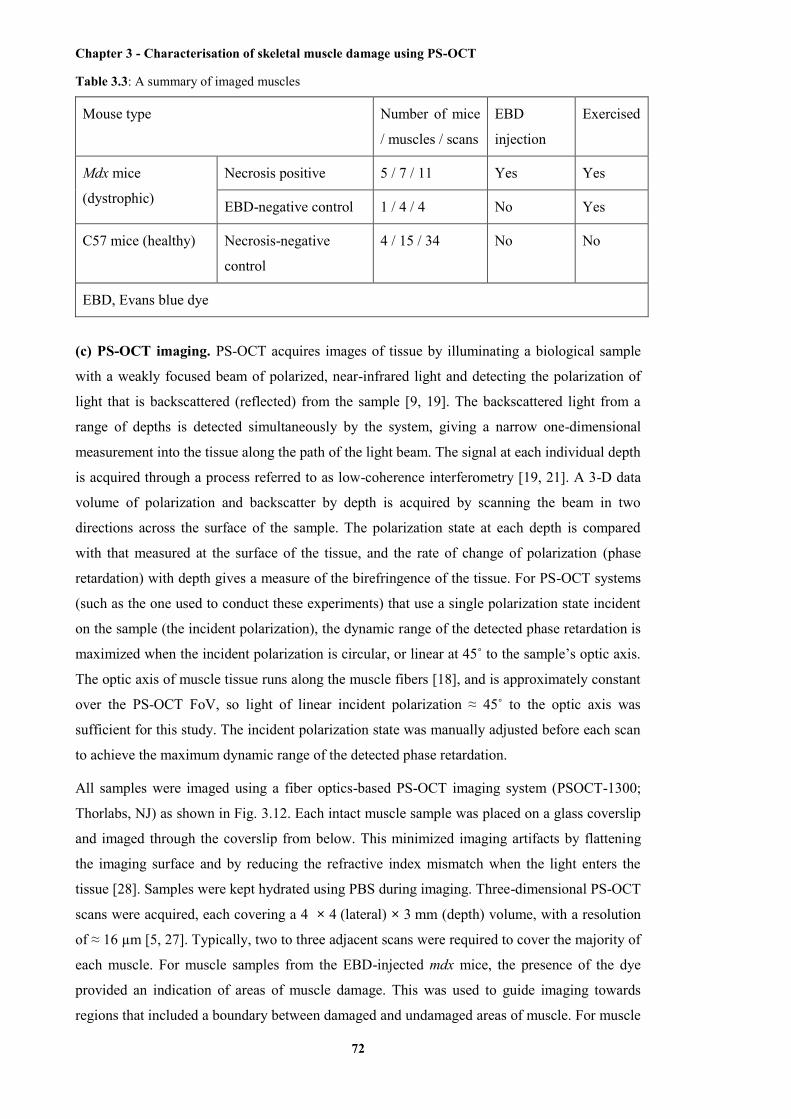
Chapter 3 - Characterisation of skeletal muscle damage using PS-OCT
72
Table 3.3: A summary of imaged muscles
Mouse type Number of mice
/ muscles / scans
EBD
injection
Exercised
Mdx mice
(dystrophic)
Necrosis positive 5 / 7 / 11 Yes Yes
EBD-negative control 1 / 4 / 4 No Yes
C57 mice (healthy) Necrosis-negative
control
4 / 15 / 34 No No
EBD, Evans blue dye
(c) PS-OCT imaging. PS-OCT acquires images of tissue by illuminating a biological sample
with a weakly focused beam of polarized, near-infrared light and detecting the polarization of
light that is backscattered (reflected) from the sample [9, 19]. The backscattered light from a
range of depths is detected simultaneously by the system, giving a narrow one-dimensional
measurement into the tissue along the path of the light beam. The signal at each individual depth
is acquired through a process referred to as low-coherence interferometry [19, 21]. A 3-D data
volume of polarization and backscatter by depth is acquired by scanning the beam in two
directions across the surface of the sample. The polarization state at each depth is compared
with that measured at the surface of the tissue, and the rate of change of polarization (phase
retardation) with depth gives a measure of the birefringence of the tissue. For PS-OCT systems
(such as the one used to conduct these experiments) that use a single polarization state incident
on the sample (the incident polarization), the dynamic range of the detected phase retardation is
maximized when the incident polarization is circular, or linear at 45˚ to the sample’s optic axis.
The optic axis of muscle tissue runs along the muscle fibers [18], and is approximately constant
over the PS-OCT FoV, so light of linear incident polarization ≈ 45˚ to the optic axis was
sufficient for this study. The incident polarization state was manually adjusted before each scan
to achieve the maximum dynamic range of the detected phase retardation.
All samples were imaged using a fiber optics-based PS-OCT imaging system (PSOCT-1300;
Thorlabs, NJ) as shown in Fig. 3.12. Each intact muscle sample was placed on a glass coverslip
and imaged through the coverslip from below. This minimized imaging artifacts by flattening
the imaging surface and by reducing the refractive index mismatch when the light enters the
tissue [28]. Samples were kept hydrated using PBS during imaging. Three-dimensional PS-OCT
scans were acquired, each covering a 4 × 4 (lateral) × 3 mm (depth) volume, with a resolution
of ≈ 16 µm [5, 27]. Typically, two to three adjacent scans were required to cover the majority of
each muscle. For muscle samples from the EBD-injected mdx mice, the presence of the dye
provided an indication of areas of muscle damage. This was used to guide imaging towards
regions that included a boundary between damaged and undamaged areas of muscle. For muscle

Chapter 3 - Characterisation of skeletal muscle damage using PS-OCT
73
samples from the non-EBD-injected mdx mouse, regions for imaging were selected using a real-
time display of the PS-OCT phase retardation signal. For muscle samples from the C57 wild-
type mice, the regions for imaging were selected to cover the whole muscle.
Fig. 3.12. Schematic of PS-OCT imaging system and experimental setup. The imaging beam is weakly
focused into the muscle sample by the objective lens setup to a depth of 300 to 400 µm (depending on the
region of interest) from the coverslip. The beam is raster-scanned over the sample surface by the xy-
galvanometer mirror scanner. The PS-OCT system guides light using a single-mode optical fiber (blue
line in the schematic).
(d) Post PS-OCT imaging histology. Immediately after imaging, the muscle samples were
carefully moved onto cork boards to preserve their orientation. The samples were fixed to the
cork with tragacanth gum or pins to prevent any movement, before being preserved either by
freezing in liquid nitrogen-cooled isopentane, or fixed in formaldehyde solution (Confix Clear
pH 7.0, AB1020.1000C; Australian Biostain) for future histological analyses. This ensured as
much as possible that the subsequent histological sections were obtained parallel to the plane of
the PS-OCT birefringence images. Histologic preparation was carried out on a series of 8-µm-
thick sections that were obtained on a cryomicrotome with 120-µm intervals between adjacent
sections throughout the depth of tissue, and stained with hematoxylin and eosin (H&E).
Histological sections were digitally photographed at 20× magnification (Scanscope XT; Aperio
Technologies, Vista, CA). Muscle regions in H&E-stained histological sections were classified
as either normal-appearing or necrotic, on the basis of visual inspection of the photographed
sections. Examples of normal-appearing muscle histology and two stages of necrotic muscle
histology are shown in Fig. 3.13.
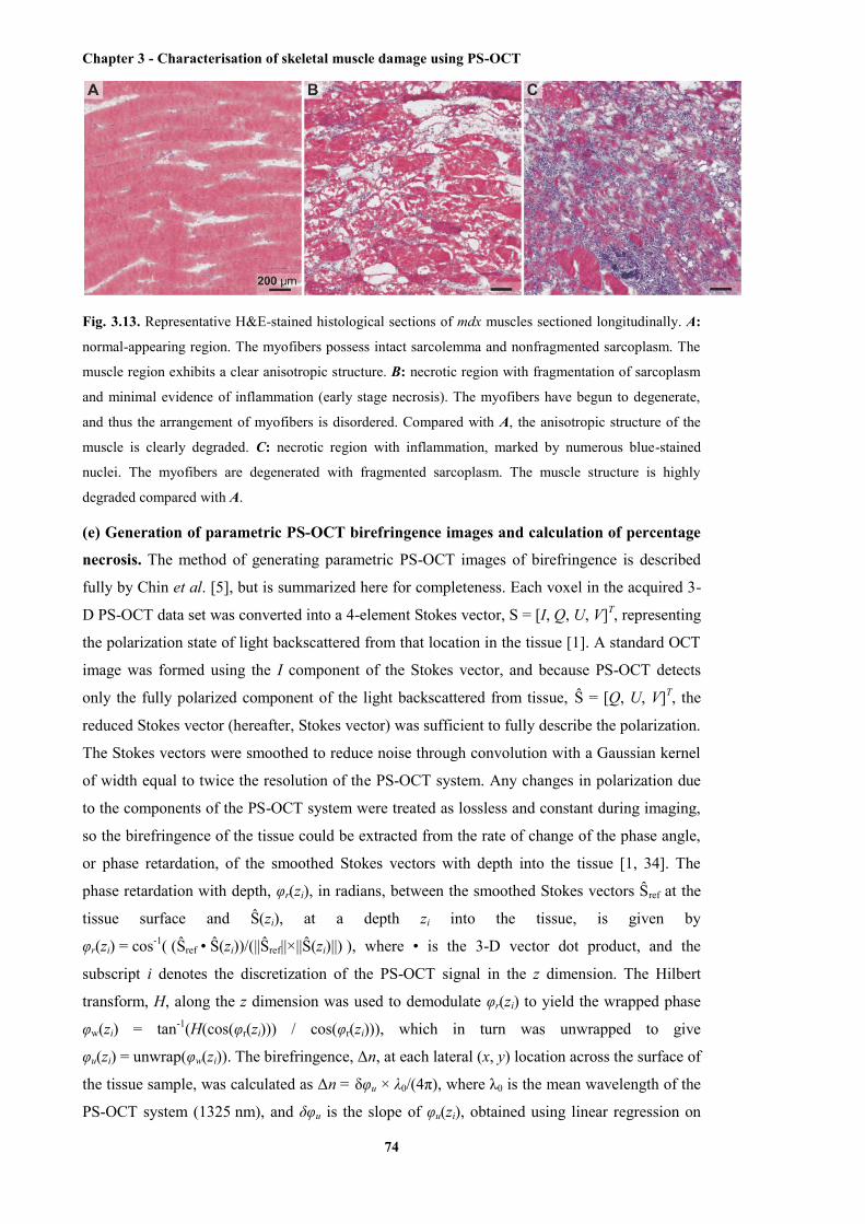
Chapter 3 - Characterisation of skeletal muscle damage using PS-OCT
74
Fig. 3.13. Representative H&E-stained histological sections of mdx muscles sectioned longitudinally. A:
normal-appearing region. The myofibers possess intact sarcolemma and nonfragmented sarcoplasm. The
muscle region exhibits a clear anisotropic structure. B: necrotic region with fragmentation of sarcoplasm
and minimal evidence of inflammation (early stage necrosis). The myofibers have begun to degenerate,
and thus the arrangement of myofibers is disordered. Compared with A, the anisotropic structure of the
muscle is clearly degraded. C: necrotic region with inflammation, marked by numerous blue-stained
nuclei. The myofibers are degenerated with fragmented sarcoplasm. The muscle structure is highly
degraded compared with A.
(e) Generation of parametric PS-OCT birefringence images and calculation of percentage
necrosis. The method of generating parametric PS-OCT images of birefringence is described
fully by Chin et al. [5], but is summarized here for completeness. Each voxel in the acquired 3-
D PS-OCT data set was converted into a 4-element Stokes vector, S = [I, Q, U, V]T, representing
the polarization state of light backscattered from that location in the tissue [1]. A standard OCT
image was formed using the I component of the Stokes vector, and because PS-OCT detects
only the fully polarized component of the light backscattered from tissue, Ŝ = [Q, U, V]T, the
reduced Stokes vector (hereafter, Stokes vector) was sufficient to fully describe the polarization.
The Stokes vectors were smoothed to reduce noise through convolution with a Gaussian kernel
of width equal to twice the resolution of the PS-OCT system. Any changes in polarization due
to the components of the PS-OCT system were treated as lossless and constant during imaging,
so the birefringence of the tissue could be extracted from the rate of change of the phase angle,
or phase retardation, of the smoothed Stokes vectors with depth into the tissue [1, 34]. The
phase retardation with depth, φr(zi), in radians, between the smoothed Stokes vectors Ŝref at the
tissue surface and Ŝ(zi), at a depth zi into the tissue, is given by
φr(zi) = cos-1( (Ŝref • Ŝ(zi))/(||Ŝref||×||Ŝ(zi)||) ), where • is the 3-D vector dot product, and the
subscript i denotes the discretization of the PS-OCT signal in the z dimension. The Hilbert
transform, H, along the z dimension was used to demodulate φr(zi) to yield the wrapped phase
φw(zi) = tan-1(H(cos(φr(zi))) / cos(φr(zi))), which in turn was unwrapped to give
φu(zi) = unwrap(φw(zi)). The birefringence, Δn, at each lateral (x, y) location across the surface of
the tissue sample, was calculated as Δn = δφu × λ0/(4π), where λ0 is the mean wavelength of the
PS-OCT system (1325 nm), and δφu is the slope of φu(zi), obtained using linear regression on
Chapter 3 - Characterisation of skeletal muscle damage using PS-OCT
75
φu(zi) over a physical range of 50 µm to 550 µm from the tissue surface (determined from the
OCT signal by taking the tissue refractive index as 1.4) [9].
The resulting 2-D collection of values was used to define a parametric image of birefringence,
where each value specified the image intensity at a corresponding lateral (x, y) location, and is
represented graphically using a false-color map, as shown in Figs. 3.14D, 3.15D, and 3.16D.
Blue indicates a high birefringence value; red indicates low birefringence. At locations where
there was insufficient signal to calculate the fitting over the full 500-µm range, the
corresponding region in the parametric image is encoded as white. The resulting color-coded
parametric image was then compared against colocated H&E-stained histological sections.
(f) Coregistration of images. As mentioned previously, a 3-D OCT data set was generated
from the I component of the Stokes vector form of the 3-D PS-OCT data set. The two data sets
are thus automatically coregistered. The 3-D PS-OCT data set was used to generate the
corresponding 2-D PS-OCT birefringence image, and on the basis of size, geometry, and
features of interest shown in the birefringence image, the colocated 2-D OCT slice in the x-y
plane with the best correlated features was chosen from the 3-D OCT data set. The OCT data
were presented as log-scaled signal-to-noise-ratio intensity with an approximate dynamic range
of 40 dB.
From the stack of H&E-stained histological sections (8 µm thick, 120 µm apart), a single
representative section was chosen from the first nine sections in the stack. This representative
section was selected on the basis of a visual correlation of features between the histological
sections, photographs of the sample taken during the imaging experiment, the 2-D OCT image,
and the 2-D PS-OCT birefringence image. It should be noted that there are small discrepancies
between the PS-OCT birefringence image and the corresponding OCT image or H&E-stained
histological section because the PS-OCT birefringence image contains 3-D information,
whereas the OCT image and H&E-stained histological section contain only 2-D information.
These 2-D images were used for visual comparison of the discernible features using the
different methods. The calculation of muscle necrosis was performed using multiple histological
sections.
(g) Automated calculation of the percentage of muscle necrosis from PS-OCT
birefringence images. The birefringence measurements were thresholded to automatically
distinguish normal-appearing tissue from necrotic tissue. The threshold was empirically
calculated from four training data sets with matching histology, and then applied to all
remaining PS-OCT data sets, giving an estimate of the percentage of muscle necrosis within
each imaging region. Birefringence values above 0.5 × 10⁻³ were deemed to indicate normal-
appearing/healthy tissue regions, and birefringence values below this threshold were deemed to
indicate necrotic tissue. The relative areas of necrotic muscle and normal-appearing/healthy
muscle were automatically calculated by counting the number of pixels in the birefringence
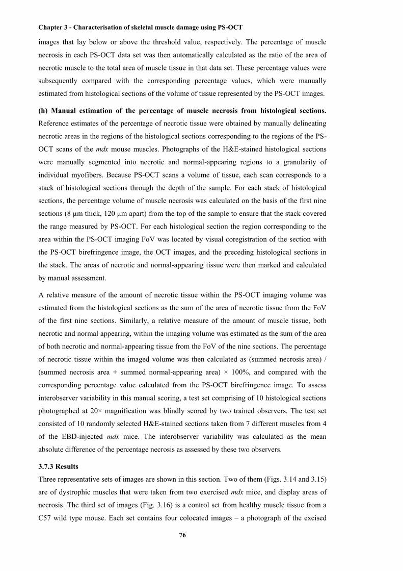
Chapter 3 - Characterisation of skeletal muscle damage using PS-OCT
76
images that lay below or above the threshold value, respectively. The percentage of muscle
necrosis in each PS-OCT data set was then automatically calculated as the ratio of the area of
necrotic muscle to the total area of muscle tissue in that data set. These percentage values were
subsequently compared with the corresponding percentage values, which were manually
estimated from histological sections of the volume of tissue represented by the PS-OCT images.
(h) Manual estimation of the percentage of muscle necrosis from histological sections.
Reference estimates of the percentage of necrotic tissue were obtained by manually delineating
necrotic areas in the regions of the histological sections corresponding to the regions of the PS-
OCT scans of the mdx mouse muscles. Photographs of the H&E-stained histological sections
were manually segmented into necrotic and normal-appearing regions to a granularity of
individual myofibers. Because PS-OCT scans a volume of tissue, each scan corresponds to a
stack of histological sections through the depth of the sample. For each stack of histological
sections, the percentage volume of muscle necrosis was calculated on the basis of the first nine
sections (8 µm thick, 120 µm apart) from the top of the sample to ensure that the stack covered
the range measured by PS-OCT. For each histological section the region corresponding to the
area within the PS-OCT imaging FoV was located by visual coregistration of the section with
the PS-OCT birefringence image, the OCT images, and the preceding histological sections in
the stack. The areas of necrotic and normal-appearing tissue were then marked and calculated
by manual assessment.
A relative measure of the amount of necrotic tissue within the PS-OCT imaging volume was
estimated from the histological sections as the sum of the area of necrotic tissue from the FoV
of the first nine sections. Similarly, a relative measure of the amount of muscle tissue, both
necrotic and normal appearing, within the imaging volume was estimated as the sum of the area
of both necrotic and normal-appearing tissue from the FoV of the nine sections. The percentage
of necrotic tissue within the imaged volume was then calculated as (summed necrosis area) /
(summed necrosis area + summed normal-appearing area) × 100%, and compared with the
corresponding percentage value calculated from the PS-OCT birefringence image. To assess
interobserver variability in this manual scoring, a test set comprising of 10 histological sections
photographed at 20× magnification was blindly scored by two trained observers. The test set
consisted of 10 randomly selected H&E-stained sections taken from 7 different muscles from 4
of the EBD-injected mdx mice. The interobserver variability was calculated as the mean
absolute difference of the percentage necrosis as assessed by these two observers.
3.7.3 Results
Three representative sets of images are shown in this section. Two of them (Figs. 3.14 and 3.15)
are of dystrophic muscles that were taken from two exercised mdx mice, and display areas of
necrosis. The third set of images (Fig. 3.16) is a control set from healthy muscle tissue from a
C57 wild type mouse. Each set contains four colocated images – a photograph of the excised
Chapter 3 - Characterisation of skeletal muscle damage using PS-OCT
77
muscle, an H&E-stained histological section, an OCT image, and the calculated PS-OCT
birefringence image showing corresponding features of interest.
Figure 3.14 A shows a photograph of an EBD-stained, excised, mdx mouse triceps muscle. The
necrotic region is visible by its darker blue staining relative to the rest of the muscle. The
corresponding H&E histology is shown in Fig. 3.14B, with areas of necrosis identified by
fragmented muscle fibers and the appearance of purple-stained, basophilic inflammatory cells
(with examples marked by * symbols). Figure 3.14, C and D shows the colocated OCT image
and the parametric birefringence image computed from the PS-OCT data acquired on the intact,
fresh (prefixation) tissue. The OCT image shows striations corresponding to intact myofibers
and an area of low (dark) signal in the region of necrosis, in agreement with previously
published findings (23, 24). The parametric birefringence image demonstrates a clear distinction
between the high birefringence of the region of undamaged tissue (blue and green) and the
region of necrosis (red). The corresponding values for the birefringence extracted from the PS-
OCT signal are indicated by the color bar to the right of Fig. 3.14D.
Fig. 3.14. Colocated images of dystrophic triceps muscle from a treadmill-exercised mdx mouse. A:
photograph of the whole muscle showing EBD staining. B: H&E histology of a frozen tissue section from
within the tissue volume imaged by PS-OCT. C: OCT log-scaled en face intensity image of intact whole
muscle, 0.73 mm from the top surface of the sample. D: parametric birefringence image. * indicates
necrotic regions with inflammation, which correspond to the low-birefringence regions within the
parametric birefringence image D.
Figure 3.15 shows a large region of necrosis present in a triceps muscle from a different mdx
mouse, enclosed on either side by normal-appearing muscle tissue. There is a clear
correspondence between the region marked by EBD (Fig. 3.15A), areas of inflammatory cells
and degraded myofibers in the histology (Fig. 3.15B), and the region of low birefringence
observed in the PS-OCT image (Fig. 3.15D). These regions are notably less well differentiated
in the standard OCT image (Fig. 3.15C), with faint striations still visible in the area of necrosis.

Chapter 3 - Characterisation of skeletal muscle damage using PS-OCT
78
Fig. 3.15. Second representative set of colocated images of dystrophic triceps muscle from a second
treadmill-exercised mdx mouse. A: photograph of the whole muscle showing EBD staining. B: H&E
histology of a frozen tissue section from within the tissue volume imaged by PS-OCT. C: OCT log-scaled
en face intensity image of intact whole muscle, 0.52 mm from the top surface of the sample. D:
parametric birefringence image. * indicates regions with necrosis, including inflammation and fragmented
myofibers. Both of these regions correspond to the low-birefringence regions within the parametric
birefringence image D.
Figure 3.16 shows colocated images of healthy muscle taken from a C57 wild-type mouse. The
H&E histology (Fig. 3.16B) shows all myofibers to be intact and well organized. The OCT
image (Fig. 3.16C) shows a generally consistent striation pattern over the entire imaging region.
Similarly, the parametric birefringence image of Fig. 3.16D measured a high birefringence
(healthy/normal-appearing muscle) across the entire imaging field (blue and green). Some
localized artifacts of low birefringence are present, due primarily to hairs and surface dirt
obstructing and distorting the imaging light beam. Such small particles proved difficult to
remove from the surface of the fresh tissue without risking damage to the samples.
Fig. 3.16. Quadriceps muscle from a C57 wild-type mouse. A: photograph of the whole muscle showing
Evans blue dye staining. B: H&E histology of a frozen tissue section from within the tissue volume
imaged by PS-OCT. C: OCT log-scaled en face intensity image of intact whole muscle, 0.57 mm from
the top surface of the sample. D: parametric birefringence image. Small patches of unusually low
birefringence are believed to be caused by occasional hairs and small particles of nontissue substances on
the surface of the tissue distorting the PS-OCT measurements.
Figure 3.17 shows the comparison between the manually estimated (from H&E histology) and
automatically calculated (from PS-OCT) percentage of necrotic tissue within corresponding
regions of dystrophic mdx mouse muscle samples. This comparison involves the 11 scans (with
matching histology) from 7 different muscle samples from 5 different EBD-injected mdx mice.

Chapter 3 - Characterisation of skeletal muscle damage using PS-OCT
79
Although histology covers the entire muscle, this comparison is calculated only for the areas of
the muscle samples that lay within the 4 × 4 mm FoV of the PS-OCT scans. The mean
difference between the percentage necrosis calculated from PS-OCT and from histology was ≈
2%. The error bars indicate the calculated interobserver variability for manual scoring of the
H&E histology; 4.1% ± 4.7%, mean ± SD (standard deviation), calculated from the 10 test
sections.
Fig. 3.17. Comparison of percentage necrosis evaluated using histology (white bars) and PS-OCT (black
bars) for 11 scans of selected 4 × 4 mm regions within 7 muscle samples from 5 mdx mice. Scans 1 and 2
are two different regions from the left quadriceps of mdx mouse 1. Scans 3 and 4 are two different regions
from the right triceps of mdx mouse 1. Scans 5, 6, and 7 are three different regions from the right
quadriceps of mdx mouse 2. Scan 8 is a region from the right triceps of mdx mouse 2. Scan 9 is a region
from the right triceps of mdx mouse 3. Scan 10 is a region from the right tibialis anterior of mdx mouse 4.
Scan 11 is a region from the right gluteus of mdx mouse 5. Error bars indicate the calculated interobserver
variability for manual scoring of the H&E histology. The mean difference between the percentage
necrosis calculated from PS-OCT and from histology is ≈ 2%. The interobserver variability for manual
scoring of the H&E histology is 4.1% over all 10 test sections, with an SD of 4.7%.
3.7.4 Discussion
We have presented a new technique for the automated quantification of the amount of necrosis
in fresh (unfixed) muscle tissue on the basis of a method for calculating birefringence from 3-D
PS-OCT scan volumes. Visual assessment of the extent of necrosis may be made by inspection
of the generated parametric birefringence images, and automated quantification of the
proportion of necrotic tissue may be performed by thresholding of the birefringence values. We

Chapter 3 - Characterisation of skeletal muscle damage using PS-OCT
80
suggest that this technique has the potential to complement current histological and imaging
methods.
The optical birefringence of muscle tissue is primarily a result of the anisotropic structural
organization of the myofibrils, and not of their genetic encoding [6, 18]. For this reason, healthy
muscle tissue, regenerated muscle tissue, and regions of normal-appearing tissue in dystrophic
muscle exhibit comparable birefringence, allowing this technique to distinguish between
normal-appearing and necrotic tissue in dystrophic muscle. Similarly, we noted that muscle
tissue loses its birefringence at an early stage of the necrosis process, as seen for example, in the
center right in Fig. 3.15, B and D. The histological section in Fig. 3.15B shows the myofibers in
this region to be still relatively intact, although starting to fragment, but the birefringence in Fig.
3.15D is comparable to the regions in the center left of the image, which consist of highly
fragmented myofibers.
We used systemic injection of EBD to guide imaging toward those muscle regions likely to
contain necrosis. EBD stains necrotic regions dark blue due to the enhanced permeability of
damaged myofibers. Note that whereas EBD was used to aid in the validation, it is not required
in general usage of the technique. The imaging of a control, EBD-free mdx mouse was used to
confirm that PS-OCT imaging is not affected by the presence or absence of EBD (data not
shown). Treadmill exercise of mdx mice is also not required to perform PS-OCT imaging, but
has been used here simply to increase the proportion of necrotic tissue assessed within these
experiments.
Examination of individual histological sections provides a detailed 2-D assessment of the
integrity of individual myofibers; however, the parametric birefringence images provide a more
concise representation of the amount of necrosis within the 3-D volume. Differences in the
estimated percentage (≈ 2%) of necrotic tissue between an observer manually scoring H&E-
stained histological sections and the proposed automated method were found to be comparable
to the interobserver variability (4.1 ± 4.7%, mean ± SD). In general, the parametric
birefringence images show good visual correspondence to the H&E-stained sections. However,
we note small discrepancies between the parametric birefringence images and specific H&E-
stained histological sections. This is due in part to the histological sections being 8 µm thick,
whereas the birefringence image aggregates information over a 500-µm-thick volume of the
tissue. For example, the band of low birefringence to the left of the birefringence image in Fig.
3.14D is not visible in the corresponding histologic image, Fig. 3.14C; however, an examination
of subsequent and preceding histological sections reveals a region of fragmentary myofibers
corresponding to this band of low birefringence. Additionally, tissue is subject to shrinkage and
deformation during freezing and histological staining [20, 48], and this has the potential to
affect both the location and relative size of areas of necrosis and normal-appearing tissue. It is
also extremely difficult in practice to obtain a histological section in precisely the same

Chapter 3 - Characterisation of skeletal muscle damage using PS-OCT
81
orientation as the plane of the birefringence image, and this could further increase the
discrepancy between features visible in the histological sections and in the birefringence
images. We have conservatively attributed features visible in the PS-OCT birefringence images,
but not in the histological sections, to imaging artifacts; for example, the band of higher
birefringence to the right in Fig. 3.14D, or the small regions of low birefringence in Fig. 3.16D.
However, such imaging artifacts make only a small contribution to the estimates of the
proportion of necrotic tissue, accounting for the good correspondence between the manual and
automated estimates of the percentage volume of muscle necrosis.
Furthermore, we note that the measured birefringence of the muscle is dependent upon the
orientation of the myofibers with respect to the optical beam. The maximum birefringence will
be measured when the PS-OCT beam is oriented perpendicular to the longitudinal axis of the
myofibers. In this case, the generated birefringence image will correspond to a histological
section that cuts longitudinally across the myofibers. When the PS-OCT light beam is parallel to
the longitudinal axis of the myofibers, no birefringence will be detected even in healthy or
normal-appearing regions of the muscle sample. If the sample contains myofibers oriented in
multiple directions, then PS-OCT imaging will tend to underestimate the birefringence of
myofibers that are not oriented parallel to the plane of the birefringence image. However, the
expected orientation of the myofibers is typically well understood from the morphology of the
muscle, allowing optimization of the direction of PS-OCT scanning.
Muscle samples often exhibit regional variations in the severity of necrosis, as illustrated by the
range of values for the proportion of necrotic tissue shown in Fig. 3.17 (i.e., for the same muscle
from the same mouse, when acquired over a 4 × 4 mm subset of the muscle). This may cause
difficulties in estimating the overall necrosis within dystrophic muscle when employing a PS-
OCT system with a limited FoV (less than 10 × 10 mm). Within this study, scans were guided
by the use of EBD as a marker of necrosis. In practice, multiple acquisitions across the muscle
would be required during the assessment. However, recent improvements in OCT image
acquisition rates (49) could potentially allow larger scans to be acquired in real time.
One challenge in extending the use of PS-OCT to an in vivo setting is its limited penetration
depth in tissue, typically 1-2 mm. However, it has been shown that an OCT probe may be
miniaturized and encased in a medical needle [8, 32, 35, 51]. OCT needle probes capable of
acquiring 3-D data volumes have been reported down to a size of a 30-gauge needle (outer
diameter 0.31 mm) [29, 32], substantially smaller and less invasive than standard biopsy
needles. Such an imaging probe could be used interstitially to image muscle structure in situ. A
single needle scan, because it can image a greater area of muscle tissue, may be as informative
as tissue removal, sectioning, and histological analysis. Insertion of a fine needle at several
locations within one large muscle is potentially far more informative (and less invasive) than a
single biopsy.

Chapter 3 - Characterisation of skeletal muscle damage using PS-OCT
82
3.7.5 Conclusion
This paper presents a new technique that utilizes PS-OCT to image dystrophic skeletal muscle
in a mouse model to estimate the proportion (volume fraction) of necrosis using a fully
automated algorithm. PS-OCT detects the optical birefringence in skeletal muscle tissues with
high birefringence values (> 0.5 × 10⁻³) indicative of healthy skeletal muscle tissue and normal-
appearing regions in dystrophic muscle tissue. Low birefringence values (< 0.5 × 10⁻³) are
indicative of necrotic (damaged) regions of myofibers (both early and later stage damage
indicated by inflammation) within dystrophic muscle. This report presents the first 3-D PS-OCT
data volumes from both dystrophic and healthy mouse skeletal muscle samples, as well as the
first quantitative color-coded parametric images differentiating normal-appearing from necrotic
regions within skeletal muscle on the basis of calculated optical birefringence values. The
percentage of necrotic tissue within the imaged locations on whole muscles was calculated and
found to correspond well (mean difference of ≈ 2%) to manual assessment of H&E-stained
histological sections. This technique has the potential to provide a complementary, minimally
invasive modality for analyzing and assessing the pathology of muscular dystrophy in situ.
3.7.6 Acknowledgements We thank Dr Gavin J. Pinniger, School of Anatomy, Physiology & Human Biology, The University of
Western Australia, and Dr Hannah Radley-Crabb, Curtin University, for discussions and suggestions
relating to muscle physiology. We thank Ms Leonie Khoo, CELLCentral, The University of Western
Australia, for the preparation of the H&E-stained histological sections. The authors acknowledge the
facilities, and the scientific and technical assistance of the Australian Microscopy & Microanalysis
Research Facility at the Centre for Microscopy, Characterization & Analysis, The University of Western
Australia, a facility funded by the University, State and Commonwealth Governments.
3.7.7 References
[1] Adie SG, Hillman TR, and Sampson DD. Detection of multiple scattering in optical
coherence tomography using the spatial distribution of Stokes vectors. Opt Express 15: 18033-
18049, 2007.
[2] Amthor H, Egelhof T, McKinnell I, Ladd ME, Janssen I, Weber J, Sinn H, Schrenk HH,
Forsting M, Voit T, and Straub V. Albumin targeting of damaged muscle fibres in the mdx
mouse can be monitored by MRI. Neuromuscular Disord 14: 791-796, 2004.
[3] Born M, and Wolf E. Optics of crystals. In: Principles of Optics. Oxford, UK: Pergamon
Press, 1980, p. 665-716.
[4] Bushby K, Finkel R, Birnkrant DJ, Case LE, Clemens PR, Cripe L, Kaul A, Kinnett K,
McDonald C, Pandya S, Poysky J, Shapiro F, Tomezsko J, Constantin C, and Working DCC.
Diagnosis and management of Duchenne muscular dystrophy, part I: diagnosis, and
pharmacological and psychosocial management. Lancet Neurol 9: 77-93, 2010.
Chapter 3 - Characterisation of skeletal muscle damage using PS-OCT
83
[5] Chin L, Yang X, McLaughlin RA, Noble PB, and Sampson DD. Enface parametric imaging
of tissue birefringence using polarization-sensitive optical coherence tomography. J Biomed Opt
18: 066005, 2013.
[6] Colby RH. Intrinsic birefringence of glycerinated myofibrils. J Cell Biol 51: 763-771, 1971.
[7] Coulton GR, Morgan JE, Partridge TA, and Sloper JC. The mdx mouse skeletal-muscle
myopathy: I. a histological, morphometric and biochemical investigation. Neuropath Appl
Neuro 14: 53-70, 1988.
[8] Curatolo A, McLaughlin RA, Quirk BC, Kirk RW, Bourke AG, Wood BA, Robbins PD,
Saunders CM, and Sampson DD. Ultrasound-guided optical coherence tomography needle
probe for the assessment of breast cancer tumor margins. Am J Roentgeno 199: W520-W522,
2012.
[9] De Boer JF, and Milner TE. Review of polarization sensitive optical coherence tomography
and Stokes vector determination. J Biomed Opt 7: 359-371, 2002.
[10] Fercher AF, Drexler W, Hitzenberger CK, and Lasser T. Optical coherence tomography –
principles and applications. Rep Prog Phys 66: 239-303, 2003.
[11] Foster FS, Pavlin CJ, Harasiewicz KA, Christopher DA, and Turnbull DH. Advances in
ultrasound biomicroscopy. Ultrasound Med Biol 26: 1-27, 2000.
[12] Frank M, Beneker J, and Ekkernkamp A. Respiratory failure due to Duchenne muscular
dystrophy. Notarzt 24: 59-60, 2008.
[13] Fujimoto JG. Optical coherence tomography for ultrahigh resolution in vivo imaging. Nat
Biotechnol 21: 1361-1367, 2003.
[14] Gilbert RK, and Hawk WA. The incidence of necrosis of muscle fibers in Duchenne type
muscular dystrophy. Am J Pathol 43: 107-122, 1963.
[15] Grounds MD, Radley HG, Lynch GS, Nagaraju K, and De Luca A. Towards developing
standard operating procedures for pre-clinical testing in the mdx mouse model of Duchenne
muscular dystrophy. Neurobiol Dis 31: 1-19, 2008.
[16] Grounds MD, and Torrisi J. Anti-TNF α (Remicade®) therapy protects dystrophic skeletal
muscle from necrosis. FASEB J 18: 676-682, 2004.
[17] Hamer PW, McGeachie JM, Davies MJ, and Grounds MD. Evans blue dye as an in vivo
marker of myofibre damage: optimising parameters for detecting initial myofibre membrane
permeability. J Anat 200: 69-79, 2002.
[18] Haskell RC, Carlson FD, and Blank PS. Form birefringence of muscle. Biophys J 56: 401-
413, 1989.
Chapter 3 - Characterisation of skeletal muscle damage using PS-OCT
84
[19] Hee MR, Huang D, Swanson EA, and Fujimoto JG. Polarization-sensitive low-coherence
reflectometer for birefringence characterization and ranging. J Opt Soc Am B 9: 903-908, 1992.
[20] Hsiung PL, Nambiar PR, and Fujimoto JG. Effect of tissue preservation on imaging using
ultrahigh resolution optical coherence tomography. J Biomed Opt 10: 064033, 2005.
[21] Huang D, Swanson EA, Lin CP, Schuman JS, Stinson WG, Chang W, Hee MR, Flotte T,
Gregory K, Puliafito CA, and Fujimoto JG. Optical coherence tomography. Science 254: 1178-
1181, 1991.
[22] Jacoby AS, Busch-Nentwich E, Bryson-Richardson RJ, Hall TE, Berger J, Berger S,
Sonntag C, Sachs C, Geisler R, Stemple DL, and Currie PD. The zebrafish dystrophic mutant
softy maintains muscle fibre viability despite basement membrane rupture and muscle
detachment. Development 136: 3367-3376, 2009.
[23] Klyen BR, Armstrong JJ, Adie SG, Radley HG, Grounds MD, and Sampson DD. Three-
dimensional optical coherence tomography of whole-muscle autografts as a precursor to
morphological assessment of muscular dystrophy in mice. J Biomed Opt 13: 2008.
[24] Klyen BR, Shavlakadze T, Radley-Crabb HG, Grounds MD, and Sampson DD.
Identification of muscle necrosis in the mdx mouse model of Duchenne muscular dystrophy
using three-dimensional optical coherence tomography. J Biomed Opt 16: 076013, 2011.
[25] Kobayashi M, Nakamura A, Hasegawa D, Fujita M, Orima H, and Takeda Si. Evaluation
of dystrophic dog pathology by fat-supressed T2-weighted imaging. Muscle Nerve 40: 815-826,
2009.
[26] Korneagay JN, Li J, Bogan JR, Bogan DJ, Chen C, Zheng H, Wang B, Qiao C, Howard JF
Jr., and Xiao X. Widespread muscle expression of an AAV9 human mini-dystrophin vector
after intravenous injection in neonatal dystrophin-deficient dogs. Mol Ther 18: 1501-1508,
2010.
[27] Liew YM, McLaughlin RA, Gong P, Wood FM, and Sampson DD. In vivo assessment of
human burn scars through automated quantification of vascularity using optical coherence
tomography. J Biomed Opt 18: 061213, 2013.
[28] Liew YM, McLaughlin RA, Wood FM, and Sampson DD. Reduction of image artifacts in
three-dimensional optical coherence tomography of skin in vivo. J Biomed Opt 16: 11608, 2011.
[29] Lorenser D, Yang X, Kirk RW, Quirk BC, McLaughlin RA, and Sampson DD. Ultrathin
side-viewing needle probe for optical coherence tomography. Opt Lett 36: 3894-3896, 2011.
[30] Manzur AY, and Muntoni F. Diagnosis and new treatments in muscular dystrophies.
Postgrad Med J 85: 622-630, 2009.
Chapter 3 - Characterisation of skeletal muscle damage using PS-OCT
85
[31] McIntosh LM, Baker BE, and Anderson JE. Magnetic resonance imaging of regenerating
and dystrophic mouse muscle. Biochem Cell Biol 76: 532-541, 1998.
[32] McLaughlin RA, Yang X, Quirk BC, Lorenser D, Kirk RW, Noble PB, and Sampson DD.
Static and dynamic imaging of alveoli using optical coherence tomography needle probes. J
Appl Physiol 113: 967-974, 2012.
[33] Pasquesi JJ, Schlachter SC, Boppart MD, Chaney E, Kaufman SJ, and Boppart SA. In vivo
detection of exercise-induced ultrastructural changes in genetically-altered murine skeletal
muscle using polarization-sensitive optical coherence tomography. Opt Express 14: 1547-1556,
2006.
[34] Pierce MC, Park BH, Cense B, and De Boer JF. Simultaneous intensity, birefringence, and
flow measurements with high-speed fiber-based optical coherence tomography. Opt Lett 27:
1534-1536, 2002.
[35] Quirk BC, McLaughlin RA, Curatolo A, Kirk RW, Noble PB, and Sampson DD. In situ
imaging of lung alveoli with an optical coherence tomography needle probe. J Biomed Opt 16:
036009, 2011.
[36] Radley-Crabb H, Terrill J, Shavlakadze T, Tonkin J, Arthur P, and Grounds M. A single 30
min treadmill exercise session is suitable for “proof-of-concept studies” in adult mdx mice: a
comparison of the early consequences of two different treadmill protocols Neuromuscular
Disord 22: 170-182, 2012.
[37] Radley HG, De Luca A, Lynch GS, and Grounds MD. Duchenne muscular dystrophy:
focus on pharmaceutical and nutritional interventions. Int J Biochem Cell B 39: 469-477, 2007.
[38] Sampson DD. Optical bioimaging 2010: seeing more, deeper, faster. IEEE Photonics J 3:
278-283, 2011.
[39] Schambach SJ, Bag S, Schilling L, Groden C, and Brockmann MA. Application of micro-
CT in small animal imaging. Methods 50: 2-13, 2010.
[40] Schambach SJ, Bag S, Steil V, Isaza C, Schilling L, Groden C, and Brockmann MA.
Ultrafast high-resolution in vivo volume-CTA of mice cerebral vessels. Stroke 40: 1444-1450,
2009.
[41] Shavlakadze T, White J, Hoh JFY, Rosenthal N, and Grounds MD. Targeted Expression of
insulin-like growth factor-I reduces early myofiber necrosis in dystrophic mdx mice. Mol Ther
10: 829-843, 2004.
[42] Sipila S, and Suominen H. Ultrasound imaging of the quadriceps muscle in elderly athletes
and untrained men. Muscle Nerve 14: 527-533, 1991.
Chapter 3 - Characterisation of skeletal muscle damage using PS-OCT
86
[43] Straub V, Donahue KM, Allamand V, Davisson RL, Kim YR, and Campbell KP. Contrast
agent-enhanced magnetic resonance imaging of skeletal muscle damage in animal models of
muscular dystrophy. Magnet Reson Med 44: 655-659, 2000.
[44] Swash M, Brown MM, and Thakkar C. CT muscle imaging and the clinical-assessment of
neuromuscular disease. Muscle Nerve 18: 708-714, 1995.
[45] Van Erp C, Irwin NG, and Hoey AJ. Long-term administration of pirfenidone improces
cardiac function in mdx mice. Muscle Nerve 34: 327-334, 2006.
[46] Wallace KD, Marsh JN, Baldwin SL, Connolly AM, Keeling R, Lanza GM, Wickline SA,
and Hughes MS. Sensitive ultrasonic delineation of steroid treatment in living dystrophic mice
with energy-based and entropy-based radio frequency signal processing. IEEE T Ultrason Ferr
54: 2291-2299, 2007.
[47] Walter G, Cordier L, Bloy D, and Sweeney HL. Noninvasive monitoring of gene correction
in dystrophic muscle. Magnet Reson Med 54: 1369-1376, 2005.
[48] Ward SR, and Lieber RL. Density and hydration of fresh and fixed human skeletal muscle.
J Biomech 38: 2317-2320, 2005.
[49] Wieser W, Biedermann BR, Klein T, Eigenwillig CM, and Huber R. Multi-megahertz
OCT: high quality 3D imaging at 20 million A-scan and 4.5 GVoxels per second. Opt Express
18: 14685-14704, 2010.
[50] Willmann R, De Luca A, Benatar M, Grounds M, Dubach J, Raymackers JM, Nagaraju K,
and Network T-NN. Enhancing translation: guidelines for standard pre-clinical experiments in
mdx mice. Neuromuscular Disord 22: 43-49, 2012.
[51] Wu YC, Xi JF, Huo L, Padvorac J, Shin EJ, Giday SA, Lennon AM, Canto MIF, Hwang
JH, and Li XD. Robust high-resolution fine OCT needle for side-viewing interstitial tissue
imaging. IEEE J Sel Top Quant 16: 863-869, 2010.
[52] Yeh Y, Baskin RJ, Brown RA, and Burton K. Depolarization spectrum of diffracted light
from muscle fiber – the intrinsic anisotropy component. Biophys J 47: 739-742, 1985.
[53] Zhu XY, Rodriguez-Porcel M, Bentley MD, Chade AR, Sica V, Napoli C, Caplice N,
Ritman EL, Lerman A, and Lerman LO. Antioxidant intervention attenuates myocardial
neovascularization in hypercholesterolemia. Circulation 109: 2109-2115, 2004.
[54] Zubrzyckagaarn EF Bulman DE, Karpati G, Burghes AHM, Belfall B, Klamut HJ, Talbot
J, Hodges RS, Ray PN, and Worton RG. The Duchenne muscular dystrophy gene product is
localized in sarcolemma of human skeletal muscle. Nature 333: 466-469, 1988.
Chapter 3 - Characterisation of skeletal muscle damage using PS-OCT
87
3.8 Related works
3.8.1 The injected EBD does not significantly affect the detected birefringence
Evans blue dye has been widely used as a non-toxic in vivo marker of myofibre damage in
muscle imaging [55, 368]. EBD can be administrated via intravenous or intraperitoneal
injection, and specifically binds to serum albumin forming EBD-albumin conjugate (EBA). As
the sarcolemma of a necrotic or damaged myofibre within dystrophic muscle is abnormally
permeable, serum albumin and EBA can penetrate through the abnormal sarcolemma into the
myofibres. This allows damaged myofibres to be macroscopically identified due to EBD’s
striking blue colour [368, 369] (Fig. 3.18a), and microscopically visualised with fluorescence
microscopy due to EBD’s red fluorescence emission [368-371] (Fig. 3.18b). We employed EBD
in the quantitative assessment of muscle damage as an indicator of regions with high potential
for necrosis, which are required for further PS-OCT imaging. We hypothesised that the presence
of EBD, as well as the form of EBA, would not significantly affect the detected birefringence of
the tissue, because both EBD and EBA are small and homogeneous molecules. This hypothesis
can be expressed as followed: the detected low birefringence from the necrotic regions within
exercised dystrophic muscle is caused by the muscle damage instead of the injected EBD or
formed EBA. To test this hypothesis, an mdx mouse (dystrophic) muscle sample that had not
been administered with EBD was imaged using PS-OCT.
The acquired parametric birefringence map from PS-OCT and the colocated H&E histology of a
frozen tissue section from within the same tissue volume are shown in Fig. 3.19 a and b,
respectively. The red regions (labeled with *) in the birefringence map indicate those regions
with low birefringence (< 0.5 × 10⁻³). These regions show fairly good correspondence with the
necrotic regions within the H&E histological section (labeled with *). This suggests that the
absence of EBD hardly affect the loss in birefringence caused by necrosis within the dystrophic
muscle. Loss of birefringence detected under PS-OCT resulted from the disorder of muscle
ultrastructure that was caused by muscle damage or necrosis and, thus, has no large relevance to
the presence or absence of EBD.
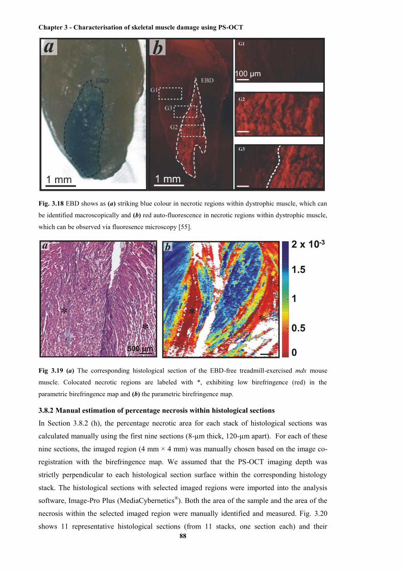
Chapter 3 - Characterisation of skeletal muscle damage using PS-OCT
88
Fig. 3.18 EBD shows as (a) striking blue colour in necrotic regions within dystrophic muscle, which can
be identified macroscopically and (b) red auto-fluorescence in necrotic regions within dystrophic muscle,
which can be observed via fluoresence microscopy [55].
Fig 3.19 (a) The corresponding histological section of the EBD-free treadmill-exercised mdx mouse
muscle. Colocated necrotic regions are labeled with *, exhibiting low birefringence (red) in the
parametric birefringence map and (b) the parametric birefringence map.
3.8.2 Manual estimation of percentage necrosis within histological sections
In Section 3.8.2 (h), the percentage necrotic area for each stack of histological sections was
calculated manually using the first nine sections (8-µm thick, 120-µm apart). For each of these
nine sections, the imaged region (4 mm × 4 mm) was manually chosen based on the image co-
registration with the birefringence map. We assumed that the PS-OCT imaging depth was
strictly perpendicular to each histological section surface within the corresponding histology
stack. The histological sections with selected imaged regions were imported into the analysis
software, Image-Pro Plus (MediaCybernetics®). Both the area of the sample and the area of the
necrosis within the selected imaged region were manually identified and measured. Fig. 3.20
shows 11 representative histological sections (from 11 stacks, one section each) and their
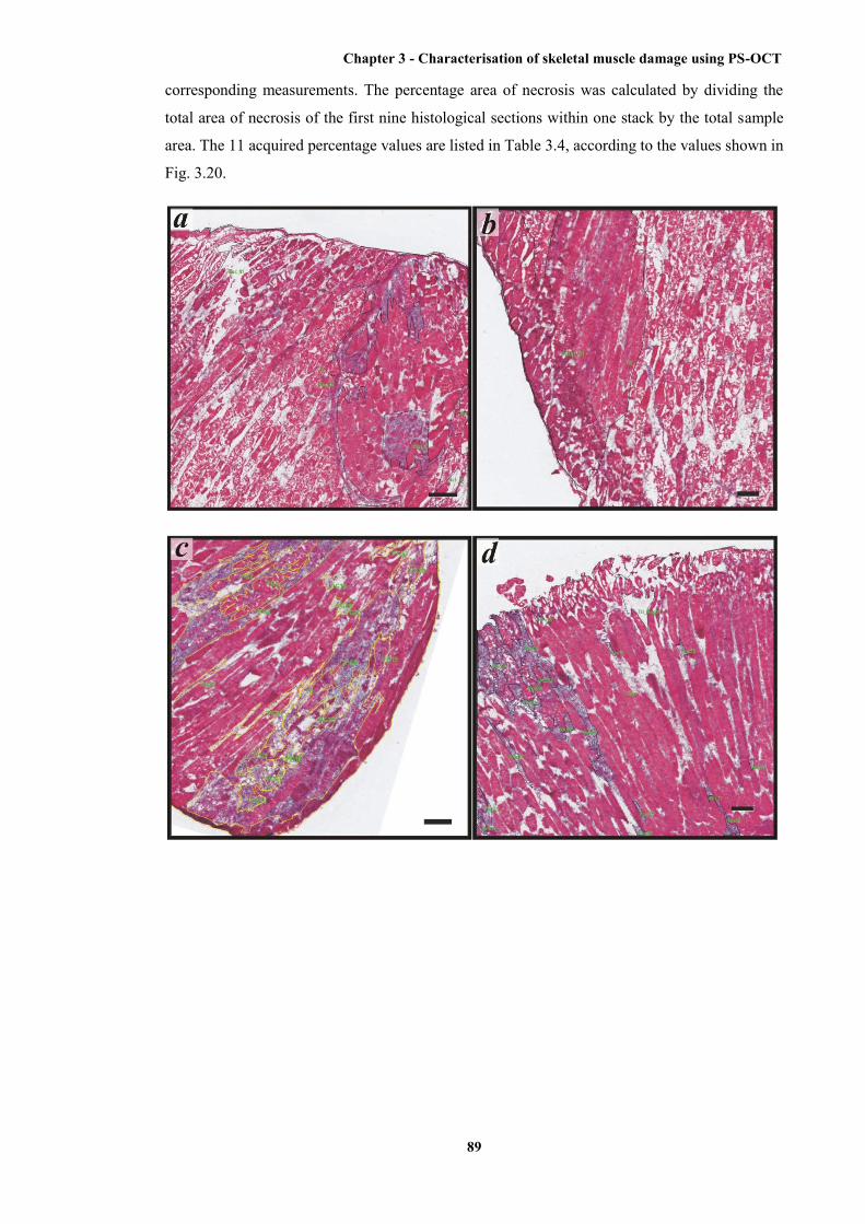
Chapter 3 - Characterisation of skeletal muscle damage using PS-OCT
89
corresponding measurements. The percentage area of necrosis was calculated by dividing the
total area of necrosis of the first nine histological sections within one stack by the total sample
area. The 11 acquired percentage values are listed in Table 3.4, according to the values shown in
Fig. 3.20.
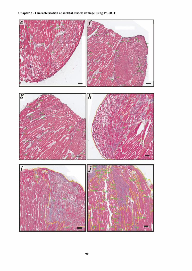
Chapter 3 - Characterisation of skeletal muscle damage using PS-OCT
90

Chapter 3 - Characterisation of skeletal muscle damage using PS-OCT
91
Fig. 3.20 Representative histological sections with manual identification and measurement of the necrosis
areas and sample areas inside the images. The necrotic regions, as well as the region of the sample within
the section, were manually selected and marked by the black or yellow lines. Then the areas of these
regions are automatically measured by the software. The percentage of the necrosis area is calculated by
dividing the sum of the necrosis area by the sample total area. The green words are labels of the selected
regions (e.g., PG11 indicates the 11th polygonal region). Representative sections of (a) to (k) are from the
imaged histology stacks 1 to 11, respectively. Scale bars indicate 100 µm.
Table 3.4 The manually measured and calculated percentage values of each histological section and
histology stack. *Because of the different employed slicing protocol, 8 sections were measured within the
11th stack.
Section level 1 2 3 4 5 6 7 8 9 Average
Stack 1
Stack 2
Stack 3
Stack 4
Stack 5
Stack 6
Stack 7
Stack 8
Stack 9
Stack 10
Stack 11
25.4 31.7 35.3 35.9 16.4 21.5 16.5 14.4 12.4 22.8
2.4 22.2 14.9 12.4 6.8 6.6 5.4 5.8 6.4 8.7
94.7 95.5 77.3 51.2 36.3 34.7 32.7 41.0 29.6 49.9
85.9 95.2 72.5 60.0 61.1 63.6 34.2 38.7 49.8 58.9
6.6 17.2 26.0 30.3 31.2 25.6 29.9 41.2 59.7 31.1
12.6 9.9 10.9 13.8 12.1 19.9 19.1 14.2 16.2 14.6
5.9 8.0 7.8 12.2 5.8 9.9 4.5 7.5 5.4 7.5
60.3 68.5 70.4 69.0 65.7 61.7 65.0 61.5 60.8 64.6
54.7 46.3 35.6 37.5 33.4 38.2 29.5 33.2 23.1 37.1
34.7 31.5 24.9 28.0 27.8 16.5 15.5 26.1 12.0 24.4
37.8 45.3 48.6 55.6 50.5 46.8 38.6 42.4 N/A* 46.16
Chapter 3 - Characterisation of skeletal muscle damage using PS-OCT
92
3.9 Chapter summary
The birefringence of skeletal muscle tissue provides a new contrast mechanism that can be used
for the quantitative analysis and assessment of muscle necrosis within dystrophic muscle. PS-
OCT is able to measure tissue birefringence and, thus, can be used to quantify the amount of
necrosis within exercised mdx mouse muscle.
In this chapter, a theoretical overview and discussion of optical polarisation and birefringence
has been presented. The polarisation of a light beam is specified using the SoP, which can be
described by either the Jones formalism (comprising Jones vectors and Jones matrices) or
Mueller-Stokes formalism (comprising Stokes vectors, Mueller matrices; Stokes vectors can be
additionally represented as points on the Poincaré sphere). A theoretical description of a generic
bulk-optic PS-OCT system has been provided using the Jones formalism in this chapter.
Following the description of polarisation theory in this chapter, birefringence of skeletal muscle
has been discussed. A literature review of the measured birefringence of various skeletal
muscles, as well as a discussion of the physiological basis of muscle birefringence, has been
given. Birefringence in skeletal muscle can be divided into intrinsic birefringence and form
birefringence. Intrinsic birefringence is caused by the anisotropic structure of each individual
myofilament (i.e., a myosin or actin filament), whilst form birefringence is caused by the highly
organised arrangement of these myofilaments. Moreover, previous studies have demonstrated
that the form birefringence is dependent on the state of muscle contraction.
In this chapter, two published journal papers (with minor modifications in the first paper) on the
subject of PS-OCT are presented. The first one, “En face parametric imaging of tissue
birefringence using polarization-sensitive optical coherence tomography”, demonstrates a newly
developed computational algorithm to measure the birefringence in PS-OCT scans, which
generates a 2D parametric image, and maps the birefringence measured at every point on the
surface of a tissue sample. This algorithm was validated by using a model of thermally induced
damage in porcine tendon. The second paper, “Quantitative assessment of muscle damage in the
mdx mouse model of Duchenne muscular dystrophy using polarization-sensitive optical
coherence tomography”, presents the first application of this algorithm on the analysis of PS-
OCT imaging data of dystrophic muscle. This study shows that en face birefringence maps
generated from PS-OCT can be used to identify areas of necrosis, as validated against H&E-
stained histology, and can additionally be used to automatically quantify the amount of muscle
necrosis in mdx mouse muscle samples, to an accuracy of within 2% when compared to manual
quantification using the standard of H&E-stained histology.
In the last part of this chapter, additional work related to the PS-OCT scanning of muscle tissue
has been presented. Additional experimental results showed that EBD, used to visually locate
areas of probable necrosis, had no discernible impact on the measurement of birefringence

Chapter 3 - Characterisation of skeletal muscle damage using PS-OCT
93
within muscle samples using PS-OCT. Finally, the manual procedure for calculating the
percentage necrosis within the imaged muscle samples has been described in detail.

Chapter 4 - Needle probes for OCT
94
Chapter 4
Needle probes for OCT
4.1 Preface
As a high-resolution optical imaging modality, conventional OCT has been restricted in clinical
and in vivo pre-clinical imaging applications due to its limited penetration depth of 2 - 3 mm
within opaque tissue [323, 372]. The limited penetration depth is due to its reliance on the
reflectance measurements using low-power, nonionising near infrared (NIR) light [317, 373],
which is significantly scattered and to a lesser extent absorbed when propagating within opaque
tissue.
The limited penetration depth of OCT can be overcome by using endoscopic OCT probes,
including catheter-based and needle-based probes. Mechanical insertion of these probes allows
them to deliver incident light into hollow tissues, such as the gastrointestinal tract [299, 374-
376] and airways [377-380], and also solid tissues such as the lungs [301, 302] and skeletal
muscle [381]. Mechanical insertion of the needle-based OCT probes into the solid tissue,
however, leads to tissue damage. As a result, there is a demand for highly miniaturised probes
that minimise the damage caused to tissues during scans.
In this chapter, we review endoscopic OCT probes, specifically catheter-based and needle-based
probes. In Section 4.3, two published papers are presented describing the development of an
ultrathin side-viewing OCT needle probe, and the application of this probe to imaging animal
lung tissue in situ. In Section 4.4, two additional published papers are presented. The first
describes the design of two optical-fibre-based OCT probes that have an extended depth of
focus, overcoming a basic restriction of miniaturisation, that the beam depth of focus is limited.
The other paper provides an accurate modeling of the light propagation within the OCT probes
involving graded-index optical fibres.
4.2 Review of endoscopic OCT probes
4.2.1 Catheter-based OCT probes
Catheter-based OCT probes are used to image natural lumens, such as the gastrointestinal tract,
airway, and blood vessels. Hence, almost no trauma will be caused by the insertion of such
probes. A generic catheter-based OCT probe typically consists of core optics assembled with
optical fibres, which are encased in a protective plastic catheter. Focusing optics are involved at
the distal end of the probe, which focus the beam using a length of graded-index fibre [382] or a
small graded-index (GRIN) lens [383]. Most catheter-based OCT probes are side-viewing, and
Chapter 4 - Needle probes for OCT
95
deflect the light beam perpendicular to the length of the probe. Deflection is achieved by either
a micro-prism [384-387] or a mirror [388, 389]. More recently, forward-imaging probes have
been developed to scan using a microelectromechanical system (MEMS) mirror [390, 391], or a
piezoelectric cantilever that deflects the fibre over the scanning range [392].
Catheter-based OCT probes can scan linearly or radially. A linearly scanning probe will use a
translation stage at the proximal end to move the probe back and forth. This allows the
construction of a 2D image based on a sequence of radial A-scans [393]. This linear scanning
mechanism has been employed in imaging the urinary tract (e.g., bladder), larynx and uterine
cervix [394]. Compared to linear scanning, which can only generate 2D images, radial scanning
can generate 3D images by combining a sequence of 2D images generated by rotating the probe
and translating it (usually backwards, termed “pullback”). This allows a more complete view of
the lumen and has been applied to scanning the gastrointestinal tract [374], colon [395], cardiac
blood vessels [396] and airways [377, 397]. Catheter-based OCT probes for imaging large
lumens (e.g., gastrointestinal tract) are often large. The diameter of such probes can be 2 mm
[387] or more [386, 398]. The diameter of intravascular probes, however, is restricted to ~1 mm
[383, 384] or less [382] by the size of blood vessels.
4.2.2 Needle-based OCT probes
Although widely employed in visualising ultrastructures within lumens, catheter-based OCT
probes are not able to image areas deep inside solid tissues. Instead, needle-based OCT probes
(i.e., OCT needle probes) are required. These needle probes consist of focusing optics encased
in a hypodermic needle and can be inserted and positioned deep in the solid tissues to image the
area of interest [372]. However, during the insertion of OCT needle probes, there is often some
trauma caused to the tissue. This trauma can be minimised by miniaturising the probe. The
reported sizes of OCT needle probes, corresponding to the size of the used hypodermic needles,
range from 19 gauge (G) to 31G, with outer diameter ranging from 1.067 mm to 0.254 mm.
These sizes are smaller than the typical size of biopsy needles [399].
A forward-imaging OCT needle probe was used by Iftimia et al. to image biological tissues
[400, 401]. The optics were inserted through the bore of a 23G needle and aspiration of the
tissue during imaging was achieved by the suction created by an attached syringe. However,
because focusing optics were not incorporated into this OCT needle probe, the imaging depth
was limited by the diverging light beam.
A more widely used OCT needle probe is the side-viewing one. The optics of a side-viewing
OCT needle probe consist of a length of single-mode fibre (SMF) that transports light from the
scanner to the probe. Focusing optics, usually involving a length of no-core fibre (NCF) and a
length of GRIN fibre, are spliced to the end of the SMF. A deflection mechanism is employed to
redirect the light beam perpendicular to the axis of the needle tubing (Fig. 4.1), and can include
an angle-polished ball lens [402, 403], microprism [323], or mirror [301, 404] at the proximal
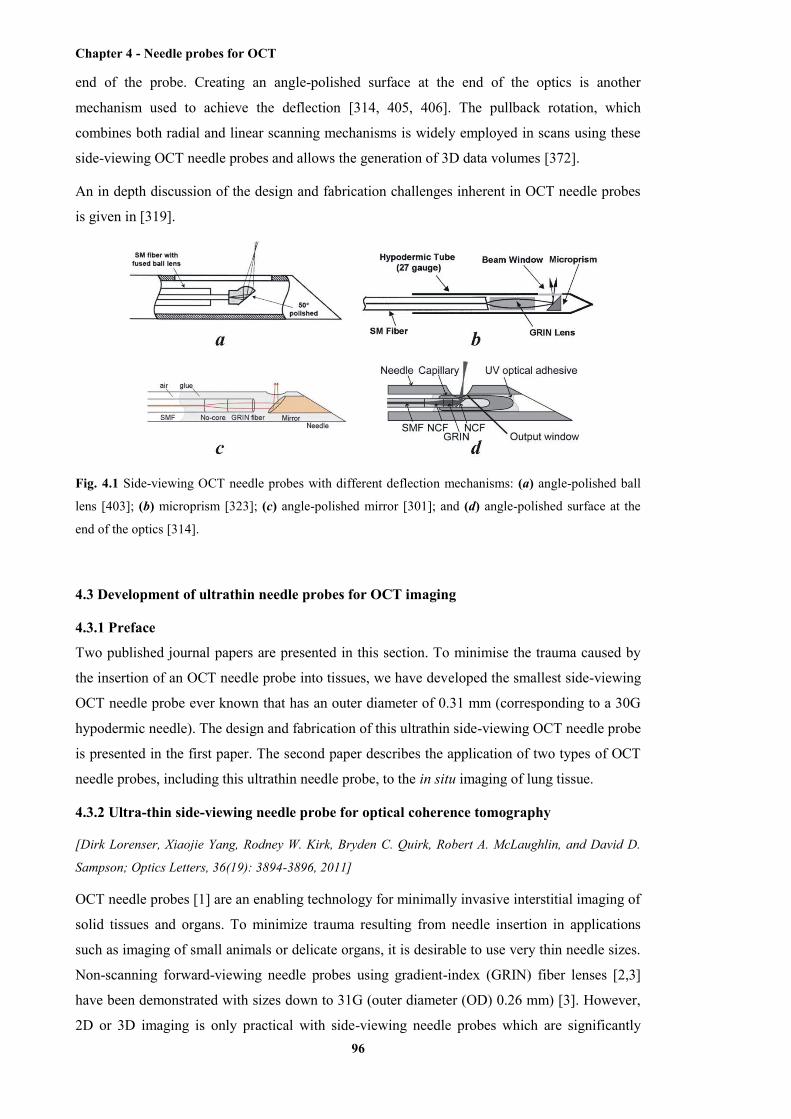
Chapter 4 - Needle probes for OCT
96
end of the probe. Creating an angle-polished surface at the end of the optics is another
mechanism used to achieve the deflection [314, 405, 406]. The pullback rotation, which
combines both radial and linear scanning mechanisms is widely employed in scans using these
side-viewing OCT needle probes and allows the generation of 3D data volumes [372].
An in depth discussion of the design and fabrication challenges inherent in OCT needle probes
is given in [319].
Fig. 4.1 Side-viewing OCT needle probes with different deflection mechanisms: (a) angle-polished ball
lens [403]; (b) microprism [323]; (c) angle-polished mirror [301]; and (d) angle-polished surface at the
end of the optics [314].
4.3 Development of ultrathin needle probes for OCT imaging
4.3.1 Preface
Two published journal papers are presented in this section. To minimise the trauma caused by
the insertion of an OCT needle probe into tissues, we have developed the smallest side-viewing
OCT needle probe ever known that has an outer diameter of 0.31 mm (corresponding to a 30G
hypodermic needle). The design and fabrication of this ultrathin side-viewing OCT needle probe
is presented in the first paper. The second paper describes the application of two types of OCT
needle probes, including this ultrathin needle probe, to the in situ imaging of lung tissue.
4.3.2 Ultra-thin side-viewing needle probe for optical coherence tomography
[Dirk Lorenser, Xiaojie Yang, Rodney W. Kirk, Bryden C. Quirk, Robert A. McLaughlin, and David D.
Sampson; Optics Letters, 36(19): 3894-3896, 2011]
OCT needle probes [1] are an enabling technology for minimally invasive interstitial imaging of
solid tissues and organs. To minimize trauma resulting from needle insertion in applications
such as imaging of small animals or delicate organs, it is desirable to use very thin needle sizes.
Non-scanning forward-viewing needle probes using gradient-index (GRIN) fiber lenses [2,3]
have been demonstrated with sizes down to 31G (outer diameter (OD) 0.26 mm) [3]. However,
2D or 3D imaging is only practical with side-viewing needle probes which are significantly

Chapter 4 - Needle probes for OCT
97
more challenging to miniaturize, as they require a micro-mirror to deflect the beam. The
smallest demonstrated side-viewing needle had a size of 27-gauge (OD 0.41 mm) [1], limited in
size by the necessity to insert and align a micro-prism inside the needle. A higher level of
miniaturization can be achieved with all-fiber designs employing an angle-polished fiber tip as a
beam deflector. Whilst this concept has been partially realized in early work [1-3], no validated
working prototypes of such needle probes with OCT imaging results have been reported. Angle-
polished fiber tip reflectors pose two substantial challenges. Firstly, the output beam acquires
significant astigmatism as it exits the fiber cladding, which acts as a cylindrical lens. Secondly,
the application of a metallic or dielectric reflective coating to the polished end face is
problematic, as the simultaneous coating of the beam output window must be avoided.
Therefore, this concept has only been employed in catheter-type probe assemblies which allow
the use of an uncoated reflector under total internal reflection [4], or the elimination of the
astigmatism with index matching fluid [5]. However, this results in larger probe diameters due
to the enclosing catheter lumen.
In this Letter, we show that all-fiber probes incorporating angle-polished fiber tip reflectors can
be designed to yield probe beams with sufficient depth-of-field and sensitivity for practical
imaging applications. We describe the fabrication and optical characterization of a 30G (OD
0.31 mm) needle probe based on this design, which we believe is the smallest side-viewing
OCT needle probe demonstrated to date, and validate its performance by acquiring 3D OCT
images of lamb lungs. A schematic of our probe is shown in Fig. 4.2a. The distal focusing
optics consist of a 290-µm section of no-core fiber and a 126-µm section of GRIN fiber
(GIF625, Thorlabs, USA) spliced to the end of a single-mode fiber (SM800, Fibercore, UK). An
additional section of no-core fiber is added after the GRIN section, and polished at an angle of
45° using a fiber connector polishing machine (SpecPro 4L, Krelltech, USA). A metal coating
consisting of a 10-nm chrome adhesion layer and a 300-nm gold layer is applied to the angle-
polished fiber tip using a thermal vacuum deposition machine (see Fig. 4.2c). The Cr/Au
combination was chosen because of its good adhesion properties and because it is a reliable and
well-established process in our facility. The coating had a measured reflectivity of ~50%,
indicating that the chrome layer introduces significant losses. A reflector material such as
aluminium (R = 87% at 840 nm), which can be deposited directly without an adhesion layer,
should yield better reflectivities. The thermal vacuum deposition process is ideal since the metal
atoms travel on a line-of-sight trajectory from the source to the sample and therefore the beam
output window of the probe can be protected by orienting it to face away from the source. After
coating, the fiber probe is mounted inside a 30G needle with an output window that is fabricated
via electrochemical etching (see Fig. 4.2d) using a custom-made setup.
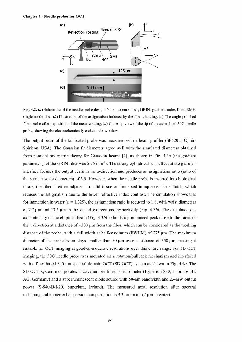
Chapter 4 - Needle probes for OCT
98
Fig. 4.2. (a) Schematic of the needle probe design. NCF: no-core fiber; GRIN: gradient-index fiber; SMF:
single-mode fiber (b) Illustration of the astigmatism induced by the fiber cladding. (c) The angle-polished
fiber probe after deposition of the metal coating. (d) Close-up view of the tip of the assembled 30G needle
probe, showing the electrochemically etched side-window.
The output beam of the fabricated probe was measured with a beam profiler (SP620U, Ophir-
Spiricon, USA). The Gaussian fit diameters agree well with the simulated diameters obtained
from paraxial ray matrix theory for Gaussian beams [2], as shown in Fig. 4.3a (the gradient
parameter g of the GRIN fiber was 5.75 mm-1). The strong cylindrical lens effect at the glass-air
interface focuses the output beam in the x-direction and produces an astigmatism ratio (ratio of
the y and x waist diameters) of 3.9. However, when the needle probe is inserted into biological
tissue, the fiber is either adjacent to solid tissue or immersed in aqueous tissue fluids, which
reduces the astigmatism due to the lower refractive index contrast. The simulation shows that
for immersion in water (n = 1.329), the astigmatism ratio is reduced to 1.8, with waist diameters
of 7.7 µm and 13.6 µm in the x- and y-directions, respectively (Fig. 4.3b). The calculated on-
axis intensity of the elliptical beam (Fig. 4.3b) exhibits a pronounced peak close to the focus of
the x direction at a distance of ~300 µm from the fiber, which can be considered as the working
distance of the probe, with a full width at half-maximum (FWHM) of 275 µm. The maximum
diameter of the probe beam stays smaller than 30 µm over a distance of 550 µm, making it
suitable for OCT imaging at good-to-moderate resolutions over this entire range. For 3D OCT
imaging, the 30G needle probe was mounted on a rotation/pullback mechanism and interfaced
with a fiber-based 840-nm spectral-domain OCT (SD-OCT) system as shown in Fig. 4.4a. The
SD-OCT system incorporates a wavenumber-linear spectrometer (Hyperion 830, Thorlabs HL
AG, Germany) and a superluminescent diode source with 50-nm bandwidth and 23-mW output
power (S-840-B-I-20, Superlum, Ireland). The measured axial resolution after spectral
reshaping and numerical dispersion compensation is 9.3 µm in air (7 µm in water).

Chapter 4 - Needle probes for OCT
99
Fig. 4.3. Output beam characteristics of the fabricated 30G needle probe. (a) Simulated and measured
beam diameters in air. (b) Simulated beam diameters in water (n = 1.329), as well as the calculated on-
axis intensity of the astigmatic probe beam.
The sensitivity of the needle-based SD-OCT system was compared to that of a standard galvo-
scanning sample arm configuration (collimator, x/y galvanometers, scan lens). At 2 µs exposure
time and a reference arm power of 4.7 µW, the galvo-scanning sample arm configuration had a
measured sensitivity of 91 dB, whereas the needle-based configuration had a measured
sensitivity of 84 dB. The theoretical shot-noise-limited sensitivity is 99 dB. For the needle-
based configuration, the sensitivity was determined for the water-immersed needle probe by
measuring the SNR of a reflection from a fused-silica (FS) prism surface (n = 1.453), resulting
in a -27 dB Fresnel reflection (see Fig. 4.4b). The solid line shows the averaged A-scan signal
obtained when the water/FS interface (peak 5) is at a distance of 488 µm from the fiber. Peak 1
is due to backscattering from imperfections of the angle-polished fiber-tip reflector and peak 2
is the backreflection from the fiber/water interface. Peaks 3 and 4 are autocorrelation artifacts of
peak 5 with peaks 1 and 2, respectively, appearing broadened after numerical dispersion
compensation. The maximum SNR of 57 dB, corresponding to a sensitivity of 84 dB, is
obtained at a distance of ~300 µm from the fiber, which is consistent with the output beam
profile simulation in water (Fig. 4.3b).
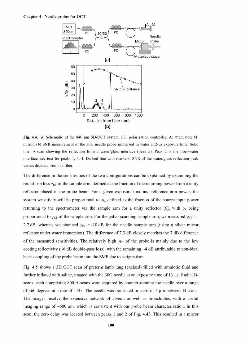
Chapter 4 - Needle probes for OCT
100
Fig. 4.4. (a) Schematic of the 840 nm SD-OCT system. PC: polarization controller; A: attenuator; M:
mirror. (b) SNR measurement of the 30G needle probe immersed in water at 2-μs exposure time. Solid
line: A-scan showing the reflection from a water/glass interface (peak 5). Peak 2 is the fiber/water
interface, see text for peaks 1, 3, 4. Dashed line with markers: SNR of the water/glass reflection peak
versus distance from the fiber.
The difference in the sensitivities of the two configurations can be explained by examining the
round-trip loss RT of the sample arm, defined as the fraction of the returning power from a unity
reflector placed in the probe beam. For a given exposure time and reference arm power, the
system sensitivity will be proportional to S, defined as the fraction of the source input power
returning to the spectrometer via the sample arm for a unity reflector [6], with S being
proportional to RT of the sample arm. For the galvo-scanning sample arm, we measured RT = -
2.7 dB, whereas we obtained RT = -10 dB for the needle sample arm (using a silver mirror
reflector under water immersion). The difference of 7.3 dB closely matches the 7 dB difference
of the measured sensitivities. The relatively high RT of the probe is mainly due to the low
coating reflectivity (~6 dB double-pass loss), with the remaining ~4 dB attributable to non-ideal
back-coupling of the probe beam into the SMF due to astigmatism.
Fig. 4.5 shows a 3D OCT scan of preterm lamb lung (excised) filled with amniotic fluid and
further inflated with saline, imaged with the 30G needle at an exposure time of 13 µs. Radial B-
scans, each comprising 800 A-scans were acquired by counter-rotating the needle over a range
of 360 degrees at a rate of 1 Hz. The needle was translated in steps of 5 µm between B-scans.
The images resolve the extensive network of alveoli as well as bronchioles, with a useful
imaging range of ~600 µm, which is consistent with our probe beam characterization. In this
scan, the zero delay was located between peaks 1 and 2 of Fig. 4.4b. This resulted in a mirror
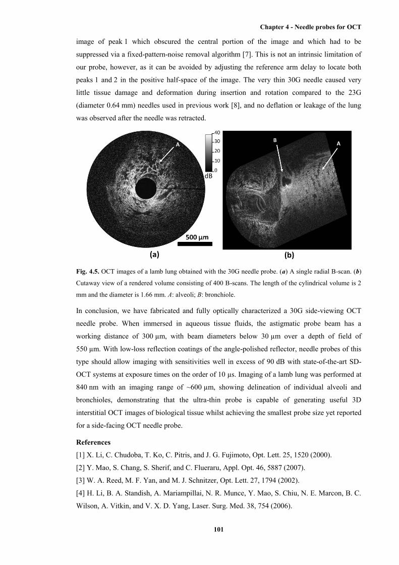
Chapter 4 - Needle probes for OCT
101
image of peak 1 which obscured the central portion of the image and which had to be
suppressed via a fixed-pattern-noise removal algorithm [7]. This is not an intrinsic limitation of
our probe, however, as it can be avoided by adjusting the reference arm delay to locate both
peaks 1 and 2 in the positive half-space of the image. The very thin 30G needle caused very
little tissue damage and deformation during insertion and rotation compared to the 23G
(diameter 0.64 mm) needles used in previous work [8], and no deflation or leakage of the lung
was observed after the needle was retracted.
Fig. 4.5. OCT images of a lamb lung obtained with the 30G needle probe. (a) A single radial B-scan. (b)
Cutaway view of a rendered volume consisting of 400 B-scans. The length of the cylindrical volume is 2
mm and the diameter is 1.66 mm. A: alveoli; B: bronchiole.
In conclusion, we have fabricated and fully optically characterized a 30G side-viewing OCT
needle probe. When immersed in aqueous tissue fluids, the astigmatic probe beam has a
working distance of 300 µm, with beam diameters below 30 µm over a depth of field of
550 µm. With low-loss reflection coatings of the angle-polished reflector, needle probes of this
type should allow imaging with sensitivities well in excess of 90 dB with state-of-the-art SD-
OCT systems at exposure times on the order of 10 µs. Imaging of a lamb lung was performed at
840 nm with an imaging range of ~600 µm, showing delineation of individual alveoli and
bronchioles, demonstrating that the ultra-thin probe is capable of generating useful 3D
interstitial OCT images of biological tissue whilst achieving the smallest probe size yet reported
for a side-facing OCT needle probe.
References
[1] X. Li, C. Chudoba, T. Ko, C. Pitris, and J. G. Fujimoto, Opt. Lett. 25, 1520 (2000).
[2] Y. Mao, S. Chang, S. Sherif, and C. Flueraru, Appl. Opt. 46, 5887 (2007).
[3] W. A. Reed, M. F. Yan, and M. J. Schnitzer, Opt. Lett. 27, 1794 (2002).
[4] H. Li, B. A. Standish, A. Mariampillai, N. R. Munce, Y. Mao, S. Chiu, N. E. Marcon, B. C.
Wilson, A. Vitkin, and V. X. D. Yang, Laser. Surg. Med. 38, 754 (2006).
Chapter 4 - Needle probes for OCT
102
[5] M. S. Jafri, S. Farhang, R. S. Tang, N. Desai, P. S. Fishman, R. G. Rohwer, C. M. Tang, and
J. M. Schmitt, J. Biomed. Opt. 10, 051603 (2005).
[6] R. Leitgeb, C. Hitzenberger, and A. Fercher, Opt. Express 11, 889 (2003).
[7] S. Moon, S. W. Lee, and Z. Chen, Opt. Express 18, 24395 (2010).
The paper presented above describes the design and fabrication of the ultrathin side-viewing
OCT needle probe. The application of this probe in imaging the biological tissue will be
presented in the paper in the following section. In the next paper, two types of OCT needle
probes, the ultrathin side-viewing OCT needle probe and a dynamic OCT probe, were applied to
imaging samples of animal lung tissue. In the ultrathin side-viewing OCT needle probe, the
focusing optics is rigidly encased within the needle, allowing a high degree of miniaturisation.
In the dynamic OCT needle probe, a more complex scanning mechanism is utilised, which
comprises a small OCT needle encased within a larger needle. This reduces the miniaturisation
possible for the larger, enclosing needle. A range of designs were available for the internal OCT
needle. We chose to use the design first published in [301]. Smaller internal needles are feasible.
However, our goal within this chapter is to provide a proof-of-principle of the operation of a
dynamic OCT needle probe, which is achieved using the design from [301]. Microscopic
structures, such as alveoli, were clearly visualised from the acquired imaging data.
4.3.3 Static and dynamic imaging of alveoli using optical coherence tomography needle
probes
[Robert A. McLaughlin; Xiaojie Yang; Bryden C. Quirk; Dirk Lorenser; Rodney W. Kirk; Peter B. Noble;
David D. Sampson; Journal of Applied Physiology, 113(6): 967-974, 2012]
Abstract
Imaging of alveoli in situ has for the most part been infeasible due to the high resolution
required to discern individual alveoli and limited access to alveoli beneath the lung surface. In
this study, we present a novel technique to image alveoli using optical coherence tomography
(OCT). We propose the use of OCT needle probes, where the distal imaging probe has been
miniaturized and encased within a hypodermic needle (as small as 30-gauge, outer diameter
310 µm), allowing insertion deep within the lung tissue with minimal tissue distortion. Such
probes enable imaging at a resolution of ~12 µm within a three-dimensional cylindrical field of
view with diameter ~1.5 mm centered on the needle tip. The imaging technique is demonstrated
on excised lungs from three different species: adult rats, fetal sheep, and adult pigs. OCT needle
probes were used to image alveoli, small bronchioles, and blood vessels, and results were
matched to histological section. We also present the first dynamic OCT images acquired with an
OCT needle probe, allowing tracking of individual alveoli during simulated cyclical lung
inflation and deflation.
Chapter 4 - Needle probes for OCT
103
(a) Introduction
For the study and assessment of lung physiology, both in healthy tissue and in the presence of
respiratory disease, lung imaging is a particularly informative approach. Imaging of lung tissue
has the potential to reveal structural, functional and anatomical abnormalities that may occur in
disease or following acute lung injury. For example, thickening or degradation of alveoli walls
in chronic disease [1, 23], changes in lung elastance [7, 13, 47, 48] and the innate heterogeneity
of disease processes are all properties that can be assessed by an appropriate in vivo imaging
device. The development of new, more effective ways to image the lung is an important area of
respiratory science.
Unlike airway passages (i.e., bronchi) which are accessible by high resolution computed
tomography (HRCT), an approach utilized routinely in clinical research [6, 24, 38, 39], imaging
of alveoli presents particular challenges. The high resolution required to discern individual
alveoli and the depth of the tissue being imaged has, for the most part, prevented real-time
visualization of alveoli. X-ray micro-computed tomography has been used to image fixed lung
samples from mice [43], rats [27], pigs [30] and humans [52]. Such imaging provides exquisite
anatomical detail, but is restricted to ex vivo samples, which are subject to tissue shrinkage and
distortion as a result of the fixation process. Intravital [26] and confocal microscopy [44] have
been used with some success to image alveoli in rats. However, this is restricted to imaging
alveoli at the very surface of the lung due to the limited penetration depth of these imaging
modalities, in the latter case to a depth of 30 µm. Other more indirect approaches have also been
applied, notably 3He diffusion magnetic resonance imaging (MRI) [18] which provides
estimates of alveolar volume and surface area by characterizing the pattern of 3He diffusion
through the lungs and combining this with geometrical models of idealized alveolar ducts.
These techniques are non-invasive and lend themselves to dynamic studies, although the limited
spatial resolution of the underlying MRI acquisitions means that these measurements are not
able to image individual alveoli.
Optical coherence tomography (OCT) is a high-resolution optical imaging modality, based on
reflectance measurements using low power, non-ionizing near-infrared light [11, 12]. It has
been used to quantify airway size in both animal models [41, 42] and in vivo in humans [35, 54-
57]. Ex vivo studies have also shown that OCT may be used to image individual alveoli [4, 19],
and in vivo OCT imaging using a thoracic window has been demonstrated in both mouse and
rabbit models [3, 36, 37]. While conventional OCT has a tissue penetration depth of only 2-
3 mm, this limitation can be overcome by use of OCT needle probes [8, 31, 46, 59], wherein the
optics have been miniaturized and encased within a hypodermic needle. Needle OCT facilitates
access to deeper regions of the target tissue with an acquisition time sufficient to provide
information on dynamic tissue properties.
Chapter 4 - Needle probes for OCT
104
In this paper, we examined the utility of a new lung imaging technique using OCT needle
probes, allowing high-resolution static and dynamic visualization of parenchymal structures
deep within the lung. We present two OCT needle probes designed by our group: the first,
encased within a 30-gauge needle, is designed to minimize tissue distortion and damage; and the
second, encased within a larger 18-gauge needle, is optimized for dynamic imaging and tracking
of individual alveoli. In the present study, the needle probes were used to image ex-vivo lung
lobes from three different species: adult rats, fetal sheep, and adult pigs. Our findings
demonstrate the capacity for OCT needle probes to image alveoli, small peripheral airways and
blood vessels deep within lung tissue. We show the first co-registered OCT-histology image
pairs acquired with a 30-gauge OCT needle probe. This probe is half the size of that used in the
acquisition of previously published comparable lung images [46], resulting in substantially less
trauma-induced artifact. In addition, this paper presents the first published dynamic OCT needle
images of alveoli during lung inflation and deflation.
(b) Materials and methods
(i) Animal Handling
All animal experiments conformed to the American Physiological Society’s Guiding Principles
in the Care and Use of Animals. Animal tissue was obtained from animals sacrificed as part of a
different research project approved by the University of Western Australia Animal Ethics
Committee, and tissue was utilized under institutional tissue sharing protocols. Three different
species were used: rats, sheep and pigs. Adult rats (Wistar, n = 2) were euthanized by CO2
inhalation. One pre-term fetal merino lamb (144 days gestation, term = 150 days) was delivered
by caesarian section and overdosed by pentobarbitone (250 mg/kg IV). Rats and sheep were
exsanguinated prior to removal of lung lobes. One adult White Landrace pig was sedated with
tiletamine/zolazepam (4.4 mg/kg IM) and xylazine (2.2 mg/kg IM) and exsanguinated under
pentobarbital sodium anesthesia (30 mg/kg IV).
(ii) Excised lung lobes
Animals were sacrificed on the day of experiment and dissection was performed immediately
post mortem. Scans were acquired between 1 and 4 hours after dissection. During this period
lungs were kept moist with Krebs solution to prevent tissue dehydration. Rat and sheep lung
lobes were used for static OCT needle imaging, and pig lobes for dynamic OCT needle imaging.
Rat and pig lobes were excised and allowed to deflate passively for 1-2 hr. Following tracheal
cannulation, lungs were inflated by a syringe filled with Krebs solution or isotonic saline. The
pre-term lamb lung containing amniotic fluid was clamped at the trachea prior to excision to
prevent fluid drainage. The trachea was subsequently cannulated and inflated as above. Prior to
scanning, lungs were laid horizontally with the anterior surface facing downwards and cycled
several times between 0 and 30 cmH2O (tracheal pressure) as determined from a fluid-filled
column connected in series with the trachea. Static imaging was performed under a fixed
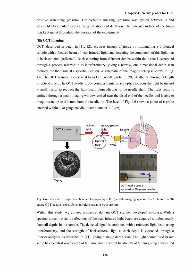
Chapter 4 - Needle probes for OCT
105
positive distending pressure. For dynamic imaging, pressure was cycled between 0 and
20 cmH2O to simulate cyclical lung inflation and deflation. The external surface of the lungs
was kept moist throughout the duration of the experiments.
(iii) OCT imaging
OCT, described in detail in [11, 12], acquires images of tissue by illuminating a biological
sample with a focused beam of near-infrared light, and detecting the component of this light that
is backscattered (reflected). Backscattering from different depths within the tissue is separated
through a process referred to as interferometry, giving a narrow, one-dimensional depth scan
focused into the tissue at a specific location. A schematic of the imaging set-up is shown in Fig.
4.6. The OCT scanner is interfaced to an OCT needle probe [8, 29, 34, 46, 59] through a length
of optical fiber. The OCT needle probe contains miniaturized optics to focus the light beam and
a small mirror to redirect the light beam perpendicular to the needle shaft. The light beam is
emitted through a small imaging window etched near the distal end of the needle, and is able to
image tissue up to 2-3 mm from the needle tip. The inset of Fig. 4.6 shows a photo of a probe
encased within a 30-gauge needle (outer diameter 310 µm).
Fig. 4.6. Schematic of optical coherence tomography (OCT) needle imaging system. Inset: photo of a 30-
gauge OCT needle probe. Units on ruler shown in inset are mm.
Within this study, we utilized a spectral domain OCT scanner developed in-house. With a
spectral domain system, reflections of the near infrared light beam are acquired simultaneously
from all depths in the sample. The detected signal is combined with a reference light beam using
interferometry, and the strength of backscattered light at each depth is extracted through a
Fourier analysis, as described in [11], giving a single depth scan. The light source used in our
setup has a central wavelength of 836 nm, and a spectral bandwidth of 50 nm giving a measured
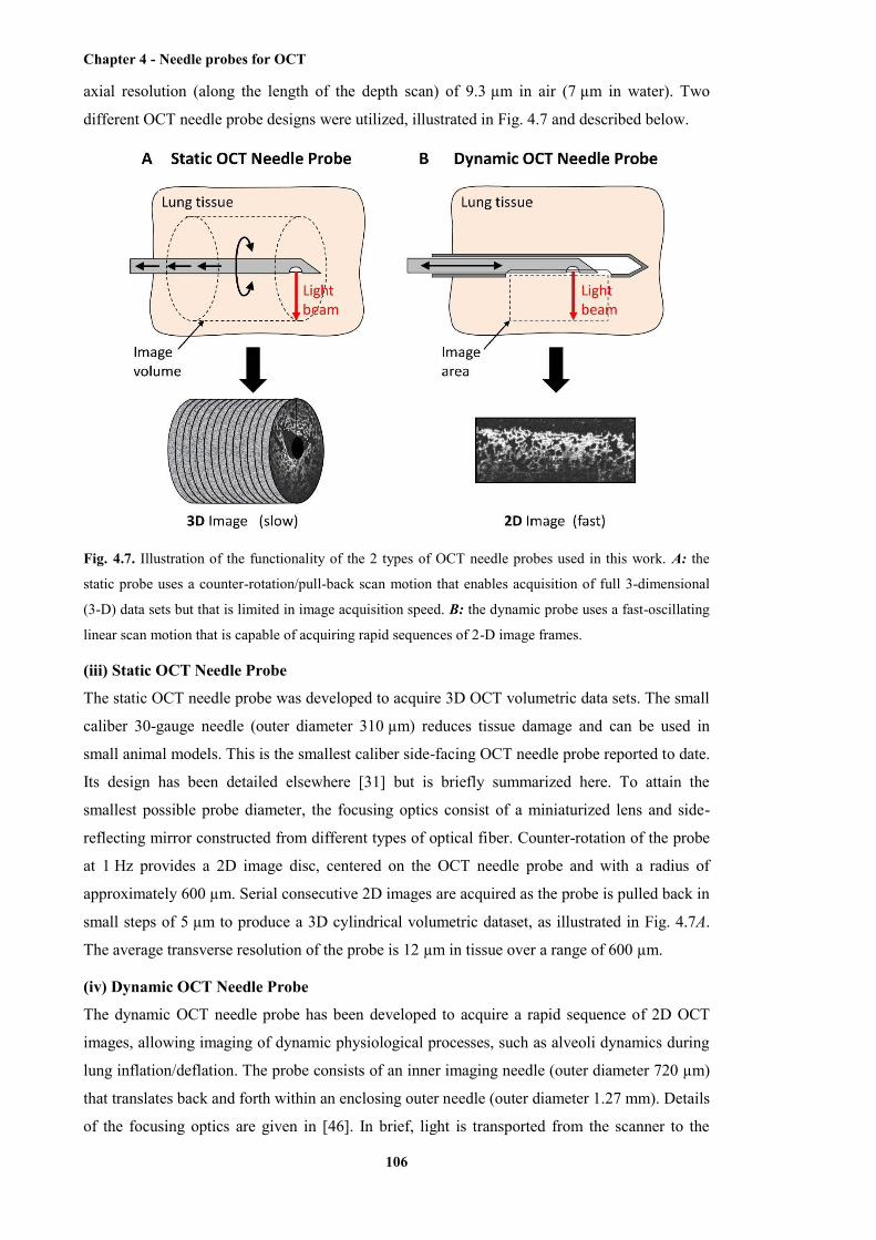
Chapter 4 - Needle probes for OCT
106
axial resolution (along the length of the depth scan) of 9.3 µm in air (7 µm in water). Two
different OCT needle probe designs were utilized, illustrated in Fig. 4.7 and described below.
Fig. 4.7. Illustration of the functionality of the 2 types of OCT needle probes used in this work. A: the
static probe uses a counter-rotation/pull-back scan motion that enables acquisition of full 3-dimensional
(3-D) data sets but that is limited in image acquisition speed. B: the dynamic probe uses a fast-oscillating
linear scan motion that is capable of acquiring rapid sequences of 2-D image frames.
(iii) Static OCT Needle Probe
The static OCT needle probe was developed to acquire 3D OCT volumetric data sets. The small
caliber 30-gauge needle (outer diameter 310 µm) reduces tissue damage and can be used in
small animal models. This is the smallest caliber side-facing OCT needle probe reported to date.
Its design has been detailed elsewhere [31] but is briefly summarized here. To attain the
smallest possible probe diameter, the focusing optics consist of a miniaturized lens and side-
reflecting mirror constructed from different types of optical fiber. Counter-rotation of the probe
at 1 Hz provides a 2D image disc, centered on the OCT needle probe and with a radius of
approximately 600 µm. Serial consecutive 2D images are acquired as the probe is pulled back in
small steps of 5 µm to produce a 3D cylindrical volumetric dataset, as illustrated in Fig. 4.7A.
The average transverse resolution of the probe is 12 µm in tissue over a range of 600 µm.
(iv) Dynamic OCT Needle Probe
The dynamic OCT needle probe has been developed to acquire a rapid sequence of 2D OCT
images, allowing imaging of dynamic physiological processes, such as alveoli dynamics during
lung inflation/deflation. The probe consists of an inner imaging needle (outer diameter 720 µm)
that translates back and forth within an enclosing outer needle (outer diameter 1.27 mm). Details
of the focusing optics are given in [46]. In brief, light is transported from the scanner to the
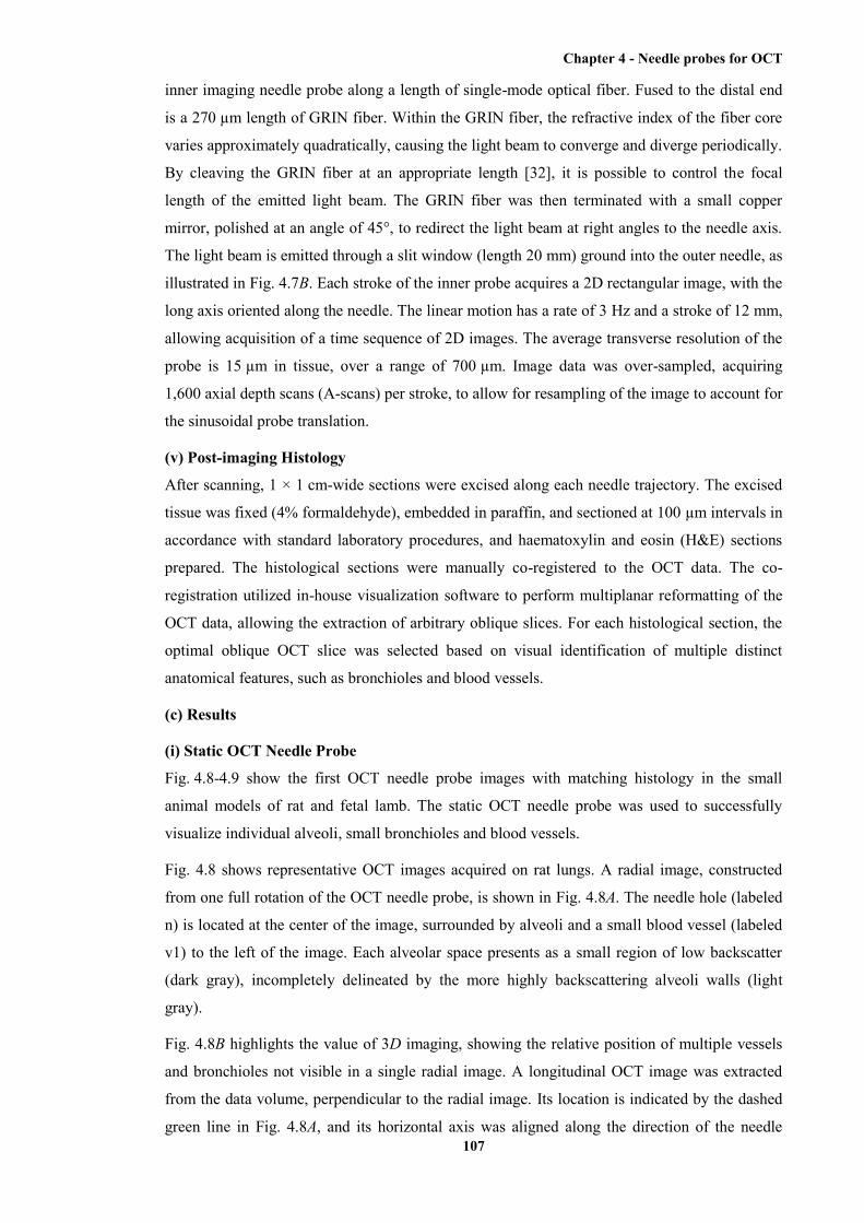
Chapter 4 - Needle probes for OCT
107
inner imaging needle probe along a length of single-mode optical fiber. Fused to the distal end
is a 270 µm length of GRIN fiber. Within the GRIN fiber, the refractive index of the fiber core
varies approximately quadratically, causing the light beam to converge and diverge periodically.
By cleaving the GRIN fiber at an appropriate length [32], it is possible to control the focal
length of the emitted light beam. The GRIN fiber was then terminated with a small copper
mirror, polished at an angle of 45°, to redirect the light beam at right angles to the needle axis.
The light beam is emitted through a slit window (length 20 mm) ground into the outer needle, as
illustrated in Fig. 4.7B. Each stroke of the inner probe acquires a 2D rectangular image, with the
long axis oriented along the needle. The linear motion has a rate of 3 Hz and a stroke of 12 mm,
allowing acquisition of a time sequence of 2D images. The average transverse resolution of the
probe is 15 µm in tissue, over a range of 700 µm. Image data was over-sampled, acquiring
1,600 axial depth scans (A-scans) per stroke, to allow for resampling of the image to account for
the sinusoidal probe translation.
(v) Post-imaging Histology
After scanning, 1 × 1 cm-wide sections were excised along each needle trajectory. The excised
tissue was fixed (4% formaldehyde), embedded in paraffin, and sectioned at 100 µm intervals in
accordance with standard laboratory procedures, and haematoxylin and eosin (H&E) sections
prepared. The histological sections were manually co-registered to the OCT data. The co-
registration utilized in-house visualization software to perform multiplanar reformatting of the
OCT data, allowing the extraction of arbitrary oblique slices. For each histological section, the
optimal oblique OCT slice was selected based on visual identification of multiple distinct
anatomical features, such as bronchioles and blood vessels.
(c) Results
(i) Static OCT Needle Probe
Fig. 4.8-4.9 show the first OCT needle probe images with matching histology in the small
animal models of rat and fetal lamb. The static OCT needle probe was used to successfully
visualize individual alveoli, small bronchioles and blood vessels.
Fig. 4.8 shows representative OCT images acquired on rat lungs. A radial image, constructed
from one full rotation of the OCT needle probe, is shown in Fig. 4.8A. The needle hole (labeled
n) is located at the center of the image, surrounded by alveoli and a small blood vessel (labeled
v1) to the left of the image. Each alveolar space presents as a small region of low backscatter
(dark gray), incompletely delineated by the more highly backscattering alveoli walls (light
gray).
Fig. 4.8B highlights the value of 3D imaging, showing the relative position of multiple vessels
and bronchioles not visible in a single radial image. A longitudinal OCT image was extracted
from the data volume, perpendicular to the radial image. Its location is indicated by the dashed
green line in Fig. 4.8A, and its horizontal axis was aligned along the direction of the needle
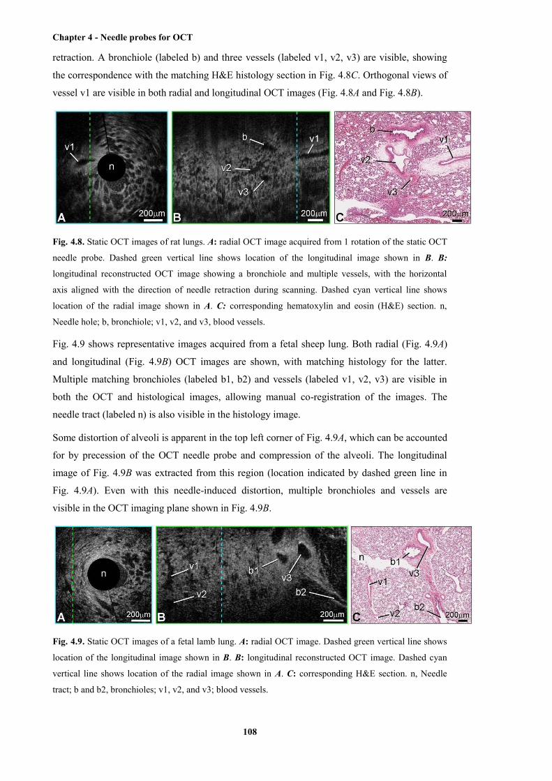
Chapter 4 - Needle probes for OCT
108
retraction. A bronchiole (labeled b) and three vessels (labeled v1, v2, v3) are visible, showing
the correspondence with the matching H&E histology section in Fig. 4.8C. Orthogonal views of
vessel v1 are visible in both radial and longitudinal OCT images (Fig. 4.8A and Fig. 4.8B).
Fig. 4.8. Static OCT images of rat lungs. A: radial OCT image acquired from 1 rotation of the static OCT
needle probe. Dashed green vertical line shows location of the longitudinal image shown in B. B:
longitudinal reconstructed OCT image showing a bronchiole and multiple vessels, with the horizontal
axis aligned with the direction of needle retraction during scanning. Dashed cyan vertical line shows
location of the radial image shown in A. C: corresponding hematoxylin and eosin (H&E) section. n,
Needle hole; b, bronchiole; v1, v2, and v3, blood vessels.
Fig. 4.9 shows representative images acquired from a fetal sheep lung. Both radial (Fig. 4.9A)
and longitudinal (Fig. 4.9B) OCT images are shown, with matching histology for the latter.
Multiple matching bronchioles (labeled b1, b2) and vessels (labeled v1, v2, v3) are visible in
both the OCT and histological images, allowing manual co-registration of the images. The
needle tract (labeled n) is also visible in the histology image.
Some distortion of alveoli is apparent in the top left corner of Fig. 4.9A, which can be accounted
for by precession of the OCT needle probe and compression of the alveoli. The longitudinal
image of Fig. 4.9B was extracted from this region (location indicated by dashed green line in
Fig. 4.9A). Even with this needle-induced distortion, multiple bronchioles and vessels are
visible in the OCT imaging plane shown in Fig. 4.9B.
Fig. 4.9. Static OCT images of a fetal lamb lung. A: radial OCT image. Dashed green vertical line shows
location of the longitudinal image shown in B. B: longitudinal reconstructed OCT image. Dashed cyan
vertical line shows location of the radial image shown in A. C: corresponding H&E section. n, Needle
tract; b and b2, bronchioles; v1, v2, and v3; blood vessels.
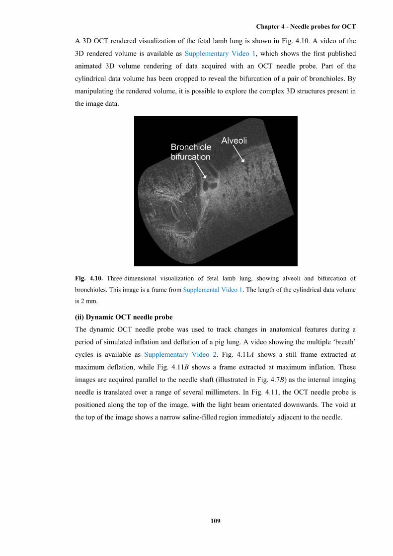
Chapter 4 - Needle probes for OCT
109
A 3D OCT rendered visualization of the fetal lamb lung is shown in Fig. 4.10. A video of the
3D rendered volume is available as Supplementary Video 1, which shows the first published
animated 3D volume rendering of data acquired with an OCT needle probe. Part of the
cylindrical data volume has been cropped to reveal the bifurcation of a pair of bronchioles. By
manipulating the rendered volume, it is possible to explore the complex 3D structures present in
the image data.
Fig. 4.10. Three-dimensional visualization of fetal lamb lung, showing alveoli and bifurcation of
bronchioles. This image is a frame from Supplemental Video 1. The length of the cylindrical data volume
is 2 mm.
(ii) Dynamic OCT needle probe
The dynamic OCT needle probe was used to track changes in anatomical features during a
period of simulated inflation and deflation of a pig lung. A video showing the multiple ‘breath’
cycles is available as Supplementary Video 2. Fig. 4.11A shows a still frame extracted at
maximum deflation, while Fig. 4.11B shows a frame extracted at maximum inflation. These
images are acquired parallel to the needle shaft (illustrated in Fig. 4.7B) as the internal imaging
needle is translated over a range of several millimeters. In Fig. 4.11, the OCT needle probe is
positioned along the top of the image, with the light beam orientated downwards. The void at
the top of the image shows a narrow saline-filled region immediately adjacent to the needle.
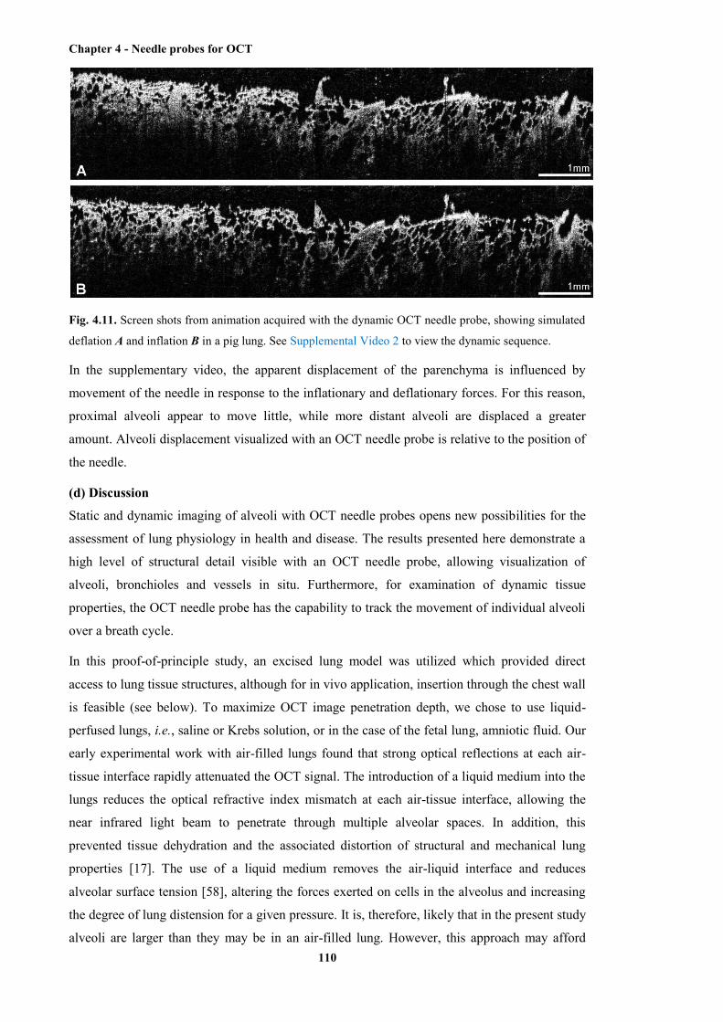
Chapter 4 - Needle probes for OCT
110
Fig. 4.11. Screen shots from animation acquired with the dynamic OCT needle probe, showing simulated
deflation A and inflation B in a pig lung. See Supplemental Video 2 to view the dynamic sequence.
In the supplementary video, the apparent displacement of the parenchyma is influenced by
movement of the needle in response to the inflationary and deflationary forces. For this reason,
proximal alveoli appear to move little, while more distant alveoli are displaced a greater
amount. Alveoli displacement visualized with an OCT needle probe is relative to the position of
the needle.
(d) Discussion
Static and dynamic imaging of alveoli with OCT needle probes opens new possibilities for the
assessment of lung physiology in health and disease. The results presented here demonstrate a
high level of structural detail visible with an OCT needle probe, allowing visualization of
alveoli, bronchioles and vessels in situ. Furthermore, for examination of dynamic tissue
properties, the OCT needle probe has the capability to track the movement of individual alveoli
over a breath cycle.
In this proof-of-principle study, an excised lung model was utilized which provided direct
access to lung tissue structures, although for in vivo application, insertion through the chest wall
is feasible (see below). To maximize OCT image penetration depth, we chose to use liquid-
perfused lungs, i.e., saline or Krebs solution, or in the case of the fetal lung, amniotic fluid. Our
early experimental work with air-filled lungs found that strong optical reflections at each air-
tissue interface rapidly attenuated the OCT signal. The introduction of a liquid medium into the
lungs reduces the optical refractive index mismatch at each air-tissue interface, allowing the
near infrared light beam to penetrate through multiple alveolar spaces. In addition, this
prevented tissue dehydration and the associated distortion of structural and mechanical lung
properties [17]. The use of a liquid medium removes the air-liquid interface and reduces
alveolar surface tension [58], altering the forces exerted on cells in the alveolus and increasing
the degree of lung distension for a given pressure. It is, therefore, likely that in the present study
alveoli are larger than they may be in an air-filled lung. However, this approach may afford

Chapter 4 - Needle probes for OCT
111
some advantage in that tissue displacements measured reflect the intrinsic mechanical properties
of the parenchymal tissue. In vivo extensions of these measurements are feasible through the use
of bronchoalveolar lavage [9, 51] or whole lung lavage [2]. Notably, other exogenous refractive
index-matching liquids are available and could be used to optimize imaging depth. Imaging is
certainly possible in air-filled lungs, although with present probe designs, the imaging depth is
reduced to alveoli immediately adjacent to the OCT needle probe.
Translation from the excised lung model to the in vivo scenario is possible by inserting the
needle probe through the chest wall. As with transthoracic lung biopsies and fine-needle
aspiration biopsies, the use of OCT needle probes carries a risk of pneumothorax, or tissue
trauma due to the relative movement of the lung surface and the chest wall. In the present study,
introduction of the OCT needle probe was found to cause some local trauma to pulmonary
structures. Our development of a small caliber 30-gauge OCT needle probe, which is
significantly smaller than the needles currently used for lung biopsies, is an important step
forward in reducing these complications.
Earlier work [46] has shown the use of static OCT needle probes in larger animal models (pig).
The present study has demonstrated the first use of static OCT needle probes in small animal
models (rat, fetal lamb). Miniaturization of the OCT needle probe (outer diameter 310µm) has
been critical in extending the range of animal models for this imaging technique, with the needle
used in the current studies being less than half the outer diameter of the probe used in [46]. The
reduction in probe size has been possible by redesigning the distal focusing optics. The small
copper mirror present in earlier designs [34, 46], used to redirect the light beam at right angle to
the needle axis, has been replaced in the static probe with a gold-coated angle polished length of
no-core fiber [31].
Correlations were demonstrated between OCT needle probe images and matching H&E
sections. However, some differences were observed, due to imaging artifacts in both the H&E
preparation and the OCT image acquisition. In this study, the tissue adjacent to the OCT needle
probe was excised immediately after imaging, to assist in colocation of histology and OCT. The
difference in inflation between OCT imaging of the fresh tissue, and fixation of the excised
sample will have contributed to discrepancies between the OCT and histology images. Tissue
samples have also been shown to undergo shrinkage and deformation during histological
preparation [20, 33], with different tissues affected to different degrees [60]. Because of such
inhomogeneous distortion, there will be additional disparity between the optimal OCT imaging
plane and each histological section. Rotation of the needle probe during 3D imaging also
resulted in some tissue drag. Alternative OCT needle probe designs have been proposed to
minimize this by enclosing the imaging probe within a stationary catheter [29].
Of further consideration is the impact that breathing movements may have on the positioning of
the probe. During lung inflation and deflation, the needle will move with the surrounding
Chapter 4 - Needle probes for OCT
112
parenchyma. As can be seen in Supplementary Video 2, distant alveoli appear to move more
than alveoli that are adjacent to the needle, as the displacement is visualized relative to the
needle position. However, by tracking the movement of the OCT probe [28, 61], it is possible to
calculate absolute displacement of the alveoli walls.
A feature of the present probe design is the capacity for assessment of lung viscoelastic
properties, which can be achieved by tracking the displacement of individual alveoli in response
to pressure fluctuations. Similar measurements have been performed with ex vivo tissue samples
using light microscopy and multi-photon microscopy [10, 15], and these small-scale
measurements have been correlated against whole lung measurements of elastance [5]. OCT is
capable of performing highly localized measurements of the viscoelastic properties of tissue, a
technique referred to as optical coherence elastography [21, 22, 49]. We note that dynamic OCT
needle probes may present the opportunity to perform such measurements in situ at different
locations and depths within the lung, which may be useful in the scenario of lung disease or
injury that is inherently heterogeneous.
In addition to the possible assessment of lung pathologies by needle OCT, there are number of
physiological questions that could be addressed by use of an OCT needle probe. For instance,
the mechanisms of lung volume expansion have been widely discussed in the literature [14, 47],
yet no established unifying model of alveolar mechanics has been accepted. A key question is
whether alveoli are recruited during respiration, or do they follow some model of expansion.
Different models of expansion include isotropic growth; growth which changes the shape of the
alveoli; or expansion through the folding and unfolding of the alveoli walls [16]. Techniques to
perform dynamic imaging of fresh (not fixed) or in vivo tissue are providing new insights into
these mechanisms. Endoscopic confocal microscopy [50] has been used to track alveolar
expansion in mouse lungs, and has shown evidence of alveolar recruitment driven by airflow
between alveoli via the pores of Kohn (40). 3He diffusion MRI studies of healthy human lungs
suggest inflation occurs primarily through recruitment in conjunction with anisotropic
expansion of the alveolar ducts [18]. We propose that OCT needle probes provide an alternative
imaging modality to explore the specific mechanisms of lung inflation (i.e., alveoli expansion
versus recruitment). In the present study, the excised lung lobe model was subject to alveoli
collapse, not only during the process of dissection but also as a result of deflation to 0 cmH2O
tracheal pressure (0 cmH2O transpulmonary pressure). We note that this is below the normal
physiological lung volume present at functional residual capacity, and that under these
experimental conditions inflation of the excised lung lobe likely involves considerable lung
recruitment. During the inflationary maneuver, alveoli recruitment as well as expansion of
individual alveoli was detected (see Supplementary Video 2). These observations provide proof-
of-concept that OCT needle probes have the potential to discern alveoli expansion and
recruitment. The dynamic OCT probe used in this study has a greater imaging field of view than
is possible in endoscopic confocal microscopy, and higher resolution than can be achieved with

Chapter 4 - Needle probes for OCT
113
MRI. For measurements which require a higher resolution, our group has recently published a
confocal needle probe with a lateral resolution of 700 nm [45].
Methods for analysis of OCT needle probe data need further development; however,
quantification of 2D OCT images could be achieved through the use of stereological methods
for estimation of characteristics such as lung surface density and number of alveoli in a given
region [53]. By defining a number of random test lines spanning the 2D image and recording the
distance between adjacent intercepts with the alveoli walls, it is possible to accumulate an
estimate of the distribution of intra-alveoli chord lengths. The arithmetic mean and other
moments of this distribution provide a quantification of both average alveoli size and size
variation, as described in [25]. The high image contrast between the alveoli walls and the
enclosed airspace visible in the OCT images lends itself to analysis with image processing
techniques to discern the extent of each alveolus and allow automated stereological analysis of
OCT needle probe scans. Static OCT needle probes scans may be acquired in both deflated and
inflated states, provided that a constant lung pressure is maintained during each individual
acquisition. This would allow the use of stereological techniques to contrast lung characteristics
between these states.
(e) Conclusion
This paper describes the use of a new technique for pulmonary imaging using OCT needle
probes. These probes may be optimized for a range of applications, and we have described
specific designs for minimal caliber needle imaging of lung tissue in small animals models, and
for dynamic imaging of alveoli during simulated inflation and deflation. This paper has
presented the first published dynamic images acquired with an OCT needle probe, and the first
co-registered OCT-histology images acquired with a 30-gauge OCT needle probe. Individual
alveoli, bronchioles and blood vessels were visualized, and 3D rendering of the data allowed the
exploration of features such as bronchiole bifurcations. This technique has the potential to offer
new insight into a range of physiological properties, including alveolar mechanics and
morphometric analysis of parenchymal structures.
(f) Acknowledgements
The authors wish to acknowledge Prof. J. Pillow, UWA, Centre for Neonatal Research and
Education, for provision of the lung tissue used in this research.
(g) Grants
R. A. McLaughlin is supported by a fellowship from the Cancer Council Western. P. B. Noble
is supported by an NHMRC of Australia Biomedical Fellowship (513921). This project has
been supported by the Raine Medical Research Foundation and the National Breast Cancer
Foundation, Australia.
(h) Disclosure
The authors have no conflicts of interest.
Chapter 4 - Needle probes for OCT
114
(i) References
[1] Barnes PJ. Chronic obstructive pulmonary disease. New Engl J Med 343: 269-280, 2000.
[2] Beccaria M, Luisetti M, Rodi G, Corsico A, Zoia MC, Colato S, Pochetti P, Braschi A,
Pozzi E, and Cerveri I. Long-term durable benefit after whole lung lavage in pulmonary alveolar
proteinosis. Eur Respir J 23: 526-531, 2004.
[3] Bickenbach J, Dembinski R, Czaplik M, Meissner S, Tabuchi A, Mertens M, Knels L,
Schroeder W, Pelosi P, Koch E, Kuebler WM, Rossaint R, and Kuhlen R. Comparison of two in
vivo microscopy techniques to visualize alveolar mechanics. J Clin Monitor Comp 23: 323-332,
2009.
[4] Boppart SA, Bouma BE, Pitris C, Tearney GJ, and Fujimoto JG. Forward-imaging
instruments for optical coherence tomography. Opt Lett 22: 1618-1620, 1997.
[5] Brewer KK, Sakai H, Alencar AM, Majumdar A, Arold SP, Lutchen KR, Ingenito EP, and
Suki B. Lung and alveolar wall elastic and hysteretic behavior in rats: effects of in vivo elastase
treatment. J Appl Physiol 95: 1926-1936, 2003.
[6] Brown RH, and Mitzner W. Understanding airway pathophysiology with computed
tomograpy. J Appl Physiol 95: 854-862, 2003.
[7] Colebatch HJ, Finucane KE, and Smith MM. Pulmonary conductance and elastic recoil
relationships in asthma and emphysema. J Appl Physiol 34: 143-153, 1973.
[8] Curatolo A, McLaughlin RA, Quirk BC, Kirk RW, Bourke AG, Wood BA, Robbins PD,
Saunders CM, and Sampson DD. Ultrasound-guided optical coherence tomography needle
probe for the assessment of breast cancer tumor margins. Am J Roentgenol 199: 2012.
[9] Daniele RP, Elias JA, Epstein PE, and Rossman MD. Bronchoalveolar lavage: role in the
pathogenesis, diagnosis, and management of interstitial lung disease. Ann Intern Med 102: 93-
108, 1985.
[10] Dassow C, Wiechert L, Martin C, Schumann S, Muller-Newen G, Pack O, Guttmann J,
Wall WA, and Uhlig S. Biaxial distension of precision-cut lung slices. J Appl Physiol 108: 713-
721, 2010.
[11] Drexler W, and Fujimoto JG. Optical Coherence Tomography: Technology and
Applications. Berlin; New York: Springer, 2008.
[12] Fujimoto JG. Optical coherence tomography for ultrahigh resolution in vivo imaging. Nat
Biotechnol 21: 1361-1367, 2003.
[13] Fulmer JD, Roberts WC, von Gal ER, and Crystal RG. Morphologic-physiologic correlates
of the severity of fibrosis and degree of cellularity in idiopathic pulmonary fibrosis. J Clin
Invest 63: 665-676, 1979.
[14] Gatto LA, Fluck RR, Jr., and Nieman GF. Alveolar mechanics in the acutely injured lung:
role of alveolar instability in the pathogenesis of ventilator-induced lung injury. Resp Care 49:
1045-1055, 2004.
Chapter 4 - Needle probes for OCT
115
[15] Gerstmair A, Fois G, Innerbichler S, Dietl P, and Felder E. A device for simultaneous live
cell imaging during uni-axial mechanical strain or compression. J Appl Physiol 107: 613-620,
2009.
[16] Gil J, Bachofen H, Gehr P, and Weibel ER. Alveolar volume-surface area relation in air-
and saline-filled lungs fixed by vascular perfusion. J Appl Physiol 47: 990-1001, 1979.
[17] Glucksberg MR, and Bhattacharya J. Effect of dehydration on interstitial pressures in the
isolated dog lung. J Appl Physiol 67: 839-845, 1989.
[18] Hajari AJ, Yablonskiy DA, Sukstanskii AL, Quirk JD, Conradi MS, and Woods JC.
Morphometric changes in the human pulmonary acinus during inflation. J Appl Physiol 112:
937-943, 2011.
[19] Hanna N, Saltzman D, Mukai D, Chen Z, Sasse S, Milliken J, Guo S, Jung W, Colt H, and
Brenner M. Two-dimensional and 3-dimensional optical coherence tomographic imaging of the
airway, lung, and pleura. J Thorac Cadiov Sur 129: 615-622, 2005.
[20] Hayatdavoudi G, Crapo JD, Miller FJ, and O'Neil JJ. Factors determining degree of
inflation in intratracheally fixed rat lungs. J Appl Physiol 48: 389-393, 1980.
[21] Kennedy BF, Hillman TR, McLaughlin RA, Quirk BC, and Sampson DD. In vivo dynamic
optical coherence elastography using a ring actuator. Opt Express 17: 21762-21772, 2009.
[22] Kennedy KM, Kennedy BF, McLaughlin RA, and Sampson DD. Needle optical coherence
elastography for tissue boundary detection. Opt Lett 37: 2310-2312, 2012.
[23] Khalil N, and O'Connor R. Idiopathic pulmonary fibrosis: current understanding of the
pathogenesis and the status of treatment. Can Med Assoc J 171: 153-160, 2004.
[24] King GG, Carroll JD, Muller NL, Whittall KP, Gao M, Nakano Y, and Pare PD.
Heterogeneity of narrowing in normal and asthmatic airways measured by HRCT. Eur Respir J
24: 211-218, 2004.
[25] Knudsen L, Weibel ER, Gundersen HJG, Weinstein FV, and Ochs M. Assessment of air
space size characteristics by intercept (chord) measurement: an accurate and efficient
stereological approach. J Appl Physiol 108: 412-421, 2010.
[26] Kuebler WM, Parthasarathi K, Lindert J, and Bhattacharya J. Real-time lung microscopy. J
Appl Physiol 102: 1255-1264, 2007.
[27] Langheinrich AC, Leithauser B, Greschus S, von Gerlach S, Breithecker A, Matthias FR,
Rau WS, and Bohle RM. Acute rat lung injury: feasibility of assessment with micro-CT.
Radiology 233: 165-171, 2004.
[28] Lau B, McLaughlin RA, Curatolo A, Kirk RW, Gerstmann DK, and Sampson DD. Imaging
true 3D endoscopic anatomy by incorporating magnetic tracking with optical coherence
tomography: proof-of-principle for airways. Opt Express 18: 27173-27180, 2010.
[29] Li H, Standish BA, Mariampillai A, Munce NR, Mao Y, Chiu S, Marcon NE, Wilson BC,
Vitkin A, and Yang VXD. Feasibility of interstitial Doppler optical coherence tomography for
Chapter 4 - Needle probes for OCT
116
in vivo detection of microvascular changes during photodynamic therapy. Laser Surg Med 38:
754-761, 2006.
[30] Litzlbauer HD, Neuhaeuser C, Moell A, Greschus S, Breithecker A, Franke FE, Kummer
W, and Rau WS. Three-dimensional imaging and morphometric analysis of alveolar tissue from
microfocal X-ray-computed tomography. Am J Physiol - Lung C 291: L535-L545, 2006.
[31] Lorenser D, Yang X, Kirk RW, Quirk BC, McLaughlin RA, and Sampson DD. Ultrathin
side-viewing needle probe for optical coherence tomography. Opt Lett 36: 3894-3896, 2011.
[32] Mao Y, Chang S, Sherif S, and Flueraru C. Graded-index fiber lens proposed for ultrasmall
probes used in biomedical imaging. Appl Optics 46: 5887-5894, 2007.
[33] Mazzone RW, Kornblau S, and Durand CM. Shrinkage of lung after chemical fixation for
analysis of pulmonary structure-function relations. J Appl Physiol 48: 382-385, 1980.
[34] McLaughlin RA, Quirk BC, Curatolo A, Kirk RW, Scolaro L, Lorenser D, Robbins PD,
Wood BA, Saunders CM, and Sampson DD. Imaging of breast cancer with optical coherence
tomography needle probes: feasibility and initial results. IEEE J Sel Top Quant 18: 1184-1191,
2012.
[35] McLaughlin RA, Williamson JP, Phillips MJ, Armstrong JJ, Becker S, Hillman DR,
Eastwood PR, and Sampson DD. Applying anatomical optical coherence tomography to
quantitative 3D imaging of the lower airway. Opt Express 16: 17521-17529, 2008.
[36] Meissner S, Knels L, Schnabel C, Koch T, and Koch E. Three-dimensional Fourier domain
optical coherence tomography in vivo imaging of alveolar tissue in the intact thorax using the
parietal pleura as a window. J Biomed Eng 15: 016030, 2010.
[37] Mertens M, Tabuchi A, Meissner S, Krueger A, Schirrmann K, Kertzscher U, Pries AR,
Slutsky AS, Koch E, and Kuebler WM. Alveolar dynamics in acute lung injury: heterogeneous
distension rather than cyclic opening and collapse. Crit Care Med 37: 2604-2611, 2009.
[38] Mott LS, Park J, Murray CP, Gangell CL, de Klerk NH, Robinson PJ, Robertson CF,
Ranganathan SC, Sly PD, and Stick SM. Progression of early structural lung disease in young
children with cystic fibrosis assessed using CT. Thorax 67: 509-516, 2012.
[39] Nakano Y, Muller NL, King GG, Niimi A, Kalloger SE, Mishima M, and Pare PD.
Quantitative assessment of airway remodeling using high-resolution CT. Chest 122: 271S-275S,
2002.
[40] Namati E, Thiesse J, de Ryk J, and McLennan G. Alveolar dynamics during respiration: are
the pores of Kohn a pathway to recruitment? Am J Resp Cell Mol 38: 572-578, 2008.
[41] Noble PB, McLaughlin RA, West AR, Becker S, Armstrong JJ, McFawn PK, Eastwood
PR, Hillman DR, Sampson DD, and Mitchell HW. Distribution of airway narrowing responses
across generations and at branching points, assessed in vitro by anatomical optical coherence
tomography. Resp Res 11: 2010.
[42] Noble PB, West AR, McLaughlin RA, Armstrong JJ, Becker S, McFawn PK, Williamson
JP, Eastwood PR, Hillman DR, Sampson DD, and Mitchell HW. Airway narrowing assessed by

Chapter 4 - Needle probes for OCT
117
anatomical optical coherence tomography in vitro: dynamic airway wall morphology and
function. J Appl Physiol 108: 401-411, 2010.
[43] Parameswaran H, Bartolak-Suki E, Hamakawa H, Majumdar A, Allen PG, and Suki B.
Three-dimensional measurement of alveolar airspace volumes in normal and emphysematous
lungs using micro-CT. J Appl Physiol 107: 583-592, 2009.
[44] Perlman CE, and Bhattacharya J. Alveolar expansion imaged by optical sectioning
microscopy. J Appl Physiol 103: 1037-1044, 2007.
[45] Pillai RS, Lorenser D, and Sampson DD. Deep-tissue access with confocal fluorescence
microendoscopy through hypodermic needles. Opt Express 19: 7213-7221, 2011.
[46] Quirk BC, McLaughlin RA, Curatolo A, Kirk RW, Noble PB, and Sampson DD. In situ
imaging of lung alveoli with an optical coherence tomography needle probe. J Biomed Eng 16:
036009, 2011.
[47] Roan E, and Waters CM. What do we know about mechanical strain in lung alveoli? Am J
Physiol – Lung C 301: L625-L635, 2011.
[48] Sansores RH, Ramirez-Venegas A, Perez-Padilla R, Montano M, Ramos C, Becerril C,
Gaxiola M, Pare P, and Selman M. Correlation between pulmonary fibrosis and the lung
pressure-volume curve. Lung 174: 315-323, 1996.
[49] Sun C, Standish B, and Yang VX. Optical coherence elastography: current status and future
applications. J Biomed Eng 16: 043001, 2011.
[50] Thiberville L, Salaun M, Lachkar S, Dominique S, Moreno-Swirc S, Vever-Bizet C, and
Bourg-Heckly G. Confocal fluorescence endomicroscopy of the human airways. Proc Am
Thoracic Soc 6: 444-449, 2009.
[51] Walters EH, and Gardiner PV. Bronchoalveolar lavage as a research tool. Thorax 46: 613-
618, 1991.
[52] Watz H, Breithecker A, Rau WS, and Kriete A. Micro-CT of the human lung: imaging of
alveoli and virtual endoscopy of an alveolar duct in a normal lung and in a lung with
centrilobular emphysema--initial observations. Radiology 236: 1053-1058, 2005.
[53] Weibel ER, Hsia CCW, and Ochs M. How much is there really? Why stereology is
essential in lung morphometry. J Appl Physiol 102: 459-467, 2007.
[54] Williamson JP, Armstrong JJ, McLaughlin RA, Noble PB, West AR, Becker S, Curatolo
A, Noffsinger WJ, Mitchell HW, Phillips MJ, Sampson DD, Hillman DR, and Eastwood PR.
Measuring airway dimensions during bronchoscopy using anatomical optical coherence
tomography. Eur Respir J 35: 34-41, 2010.
[55] Williamson JP, McLaughlin RA, Noffsinger WJ, James AL, Baker VA, Curatolo A,
Armstrong JJ, Regli A, Shepherd KL, Marks GB, Sampson DD, Hillman DR, and Eastwood
PR. Elastic properties of the central airways in obstructive lung diseases measured using
anatomical optical coherence tomography. Am J Respir Crit Care 183: 612-619, 2011.
Chapter 4 - Needle probes for OCT
118
[56] Williamson JP, McLaughlin RA, Phillips MJ, Armstrong JJ, Becker S, Walsh JH, Sampson
DD, Hillman DR, and Eastwood PR. Using optical coherence tomography to improve
diagnostic and therapeutic bronchoscopy. Chest 136: 272-276, 2009.
[57] Williamson JP, McLaughlin RA, Phillips MJ, Curatolo A, Armstrong JJ, Maddison KJ,
Sheehan RE, Sampson DD, Hillman DR, and Eastwood PR. Feasibility of applying real-time
optical imaging during bronchoscopic interventions for central airway obstruction. J Bronchol
Intervent Pulmonol 7: 307-316, 2010.
[58] Wilson TA, and Bachofen H. A model for mechanical structure of the alveolar duct. J Appl
Physiol 52: 1064-1070, 1982.
[59] Wu Y, Xi J, Huo L, Padvorac J, Shin EJ, Giday SA, Lennon AM, Canto MIF, Hwang JH,
and Li X. Robust High-Resolution Fine OCT Needle for Side-Viewing Interstitial Tissue
Imaging. IEEE J Sel Top Quant 16: 863-869, 2010.
[60] Yeap BH, Muniandy S, Lee S-K, Sabaratnam S, and Singh M. Specimen shrinkage and its
influence on margin assessment in breast cancer. Asian J Surg 30: 183-187, 2007.
[61] Yeo BY, McLaughlin RA, Kirk R, W., and Sampson DD. Enabling freehand lateral
scanning of optical coherence tomography needle probes with a magnetic tracking system.
Biomed Opt Express 3: 1565-1578, 2012.
4.4 Alternative designs of OCT fiber probes for extended depth of focus with maintained
lateral resolution and sensitivity
4.4.1 Preface
Two published journal papers are presented in this section. In the first paper, two alternative
designs of ultrathin OCT needle probes that have an extended depth of focus (EDOF) whilst
maintaining lateral resolution and sensitivity are presented. Although these two designs are
forward-viewing, they have the potential to be used in side-viewing OCT needle probes if a
deflection mechanism, such as a microprism or mirror, is added. However, as mentioned in this
paper, attempts to fabricate the probe showed that the beam profile is sensitive to deviations of
the refractive index profile of the GRIN lens section from the ideal parabolic shape. We
confirmed this by computational simulation of the beam propagation within the GRIN lens. The
simulation results and the supporting experimental data are presented in the second paper.
All non-Gaussian beams with extended DOF exhibit a certain amount of sidelobe structure as
well as a resulting loss of signal in the main lobe. To illustrate this phenomenon, the relative
sidelobe intensity levels have been quantified in some specific examples presented in the two
papers (in percent of the central lobe peak intensity). Furthermore, the second paper introduces
the Strehl ratio as a quantitative measure of the loss of signal in the central lobe of aberrated and
wavefront-shaped beams.

Chapter 4 - Needle probes for OCT
119
4.4.2 Ultrathin fiber probes with extended depth of focus for optical coherence
tomography
[Dirk Lorenser, Xiaojie Yang, and David D. Sampson; Optics Letters, 37(10): 1616-1618, 2012]
Ultrathin fiber-optic probes delivered via hypodermic needles enable imaging deep within
biological tissue using optical coherence tomography (OCT) [1, 2]. Using state-of-the-art
broadband light sources, such probes can image with high axial resolutions of a few
micrometers. However, it is not straightforward to increase their transverse resolution to similar
values without severely compromising the useful imaging depth range due to the strong
divergence of the tightly focused beam. This problem has been addressed in bulk-optic OCT
scanners by generating focal regions with an extended depth of focus (DOF) using axicons [3,
4] or pupil phase masks [5]. Unfortunately, it is not possible to simply scale down the bulk-optic
solutions to the dimensions of ultrathin fiber probes with diameters on the order of 125 µm, as
in the latter case the formation of the focal region takes place in a regime of Fresnel diffraction
where the optical design methods and approximations used in [3-5] are no longer valid. A first
demonstration of an ultrathin OCT probe using a fiber-tip micro-axicon [6] has shown that
pseudo-Bessel beams can still be generated from such structures at low Fresnel numbers, but
with a very short working distance and reduced DOF gain compared to their bulk-optic
counterparts. Rather than trying to mimic bulk-optic axicons, we have explored the use of phase
mask structures in the regime of low Fresnel numbers using numerical simulations based on the
beam propagation method (BPM). As a result of this, we demonstrate an extended-depth-of-
focus (EDOF) fiber probe design that uses a very simple phase mask consisting of a short
section of overfilled graded-index (GRIN) fiber, which can yield a DOF gain around 2.
The concept is illustrated in Fig. 4.12a. A normal lensed fiber is made by using a section of no-
core fiber (NCF) to expand the beam emitted by the single-mode fiber (SMF), and a section of
GRIN fiber to focus it with the desired NA. In order to make an EDOF probe, a phase mask
consisting of an additional short section of GRIN fiber with a smaller core diameter is appended
to the lensed fiber. The rays traced in Fig. 4.12a show that the effect of this arrangement can be
intuitively understood as a “double-focus” lens, with the small core of the phase mask affecting
only the central portion of the converging wavefront (see Fig. 4.12b). The output beam from
such a probe was simulated at a wavelength of 820 nm using a split-operator BPM algorithm
[7], where the propagation operator is applied in the spatial frequency domain after fast Fourier
transform (FFT) of the transverse field amplitude. The EDOF probe has design lengths of
LNCF = 300 µm, LGRIN = 190 µm and LPM = 14 µm, connected to SMF with a mode-field
diameter of 5.6 µm. The lens section is a 100-µm core diameter GRIN fiber with a gradient
parameter of g = 4.5 mm-1, and the phase mask is a 32-µm core diameter GRIN fiber with
g = 10 mm-1. The simulated output beam intensity in water (refractive index n = 1.33) is shown
in Fig. 4.12c. The full width half maximum (FWHM) beam diameter and the normalized on-
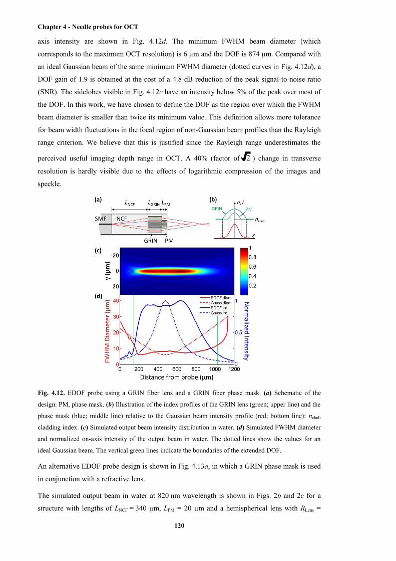
Chapter 4 - Needle probes for OCT
120
axis intensity are shown in Fig. 4.12d. The minimum FWHM beam diameter (which
corresponds to the maximum OCT resolution) is 6 µm and the DOF is 874 µm. Compared with
an ideal Gaussian beam of the same minimum FWHM diameter (dotted curves in Fig. 4.12d), a
DOF gain of 1.9 is obtained at the cost of a 4.8-dB reduction of the peak signal-to-noise ratio
(SNR). The sidelobes visible in Fig. 4.12c have an intensity below 5% of the peak over most of
the DOF. In this work, we have chosen to define the DOF as the region over which the FWHM
beam diameter is smaller than twice its minimum value. This definition allows more tolerance
for beam width fluctuations in the focal region of non-Gaussian beam profiles than the Rayleigh
range criterion. We believe that this is justified since the Rayleigh range underestimates the
perceived useful imaging depth range in OCT. A 40% (factor of 2 ) change in transverse
resolution is hardly visible due to the effects of logarithmic compression of the images and
speckle.
Fig. 4.12. EDOF probe using a GRIN fiber lens and a GRIN fiber phase mask. (a) Schematic of the
design: PM, phase mask. (b) Illustration of the index profiles of the GRIN lens (green; upper line) and the
phase mask (blue; middle line) relative to the Gaussian beam intensity profile (red; bottom line): nclad,
cladding index. (c) Simulated output beam intensity distribution in water. (d) Simulated FWHM diameter
and normalized on-axis intensity of the output beam in water. The dotted lines show the values for an
ideal Gaussian beam. The vertical green lines indicate the boundaries of the extended DOF.
An alternative EDOF probe design is shown in Fig. 4.13a, in which a GRIN phase mask is used
in conjunction with a refractive lens.
The simulated output beam in water at 820 nm wavelength is shown in Figs. 2b and 2c for a
structure with lengths of LNCF = 340 µm, LPM = 20 µm and a hemispherical lens with RLens =

Chapter 4 - Needle probes for OCT
121
80 µm and n = 1.7 (a typical value for photoresist). The GRIN phase mask has a 32-µm core
diameter and g = 10 mm-1. The minimum FWHM beam diameter is 6.5 µm and the DOF is
1060 µm. Compared with an ideal Gaussian beam of the same minimum FWHM diameter
(dotted curves in Fig. 4.13c), a DOF gain of 2 is obtained at the cost of a 5.2-dB reduction of the
peak SNR. The sidelobe intensity is below 5% of the peak over most of the DOF.
Fig. 4.13. EDOF probe using a refractive lens and a GRIN fiber phase mask. (a) Schematic of the design.
(b) Simulated output beam intensity distribution in water. (c) Simulated FWHM diameter and normalized
on-axis intensity of the output beam in water. The dotted lines show the values for an ideal Gaussian
beam. The vertical green lines indicate the boundaries of the extended DOF.
The EDOF probe designs presented in Figs. 4.12 and 4.13 are both tolerant of length errors of
up to ~20% in the GRIN phase mask section, and our fabrication method which uses a
micrometer translation stage mounted to the fiber cleaver can achieve this level of accuracy
(fabricated lengths are validated by inspection under a phase-contrast microscope). However,
attempts to fabricate designs of the type shown in Fig. 4.12 revealed that the beam profile is
sensitive to deviations of the refractive index profile of the GRIN lens section from the ideal
parabolic shape (which is often the case in commercial GRIN fibers [8]), and we were able to
confirm this in simulations (results not shown here). To experimentally validate our EDOF
probe concept, we therefore chose to fabricate a probe of the type shown in Fig. 4.13, which
avoids the use of a GRIN lens section, and we modified the design to use a phase mask
consisting of 50-µm core diameter GRIN fiber (GIF50, Thorlabs, USA) with g = 6.2 mm-1 (g
was obtained from fits of beam profiles of test structures). In order to overfill this GRIN fiber,
the beam from the SMF (SM800, Fibercore, UK) had to be expanded to a relatively large 1/e2
diameter of 52 µm, which resulted in a noticeable degradation of the beam quality due to the
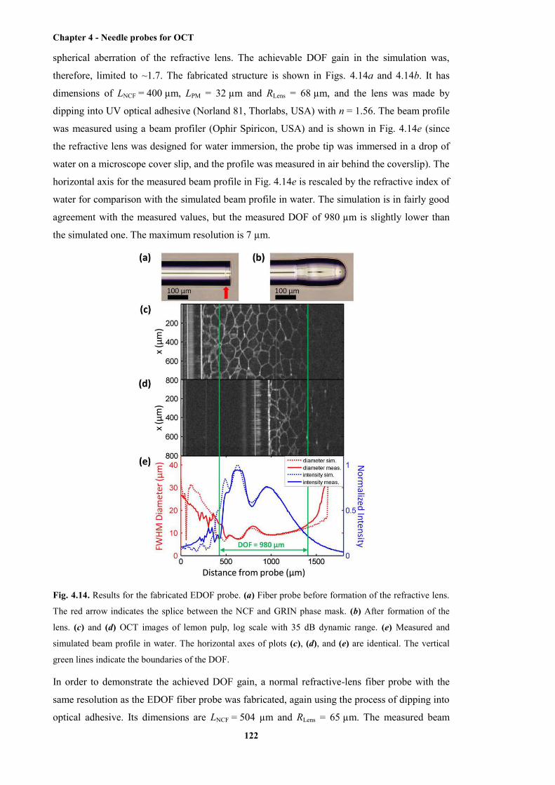
Chapter 4 - Needle probes for OCT
122
spherical aberration of the refractive lens. The achievable DOF gain in the simulation was,
therefore, limited to ~1.7. The fabricated structure is shown in Figs. 4.14a and 4.14b. It has
dimensions of LNCF = 400 µm, LPM = 32 µm and RLens = 68 µm, and the lens was made by
dipping into UV optical adhesive (Norland 81, Thorlabs, USA) with n = 1.56. The beam profile
was measured using a beam profiler (Ophir Spiricon, USA) and is shown in Fig. 4.14e (since
the refractive lens was designed for water immersion, the probe tip was immersed in a drop of
water on a microscope cover slip, and the profile was measured in air behind the coverslip). The
horizontal axis for the measured beam profile in Fig. 4.14e is rescaled by the refractive index of
water for comparison with the simulated beam profile in water. The simulation is in fairly good
agreement with the measured values, but the measured DOF of 980 µm is slightly lower than
the simulated one. The maximum resolution is 7 µm.
Fig. 4.14. Results for the fabricated EDOF probe. (a) Fiber probe before formation of the refractive lens.
The red arrow indicates the splice between the NCF and GRIN phase mask. (b) After formation of the
lens. (c) and (d) OCT images of lemon pulp, log scale with 35 dB dynamic range. (e) Measured and
simulated beam profile in water. The horizontal axes of plots (c), (d), and (e) are identical. The vertical
green lines indicate the boundaries of the DOF.
In order to demonstrate the achieved DOF gain, a normal refractive-lens fiber probe with the
same resolution as the EDOF fiber probe was fabricated, again using the process of dipping into
optical adhesive. Its dimensions are LNCF = 504 µm and RLens = 65 µm. The measured beam
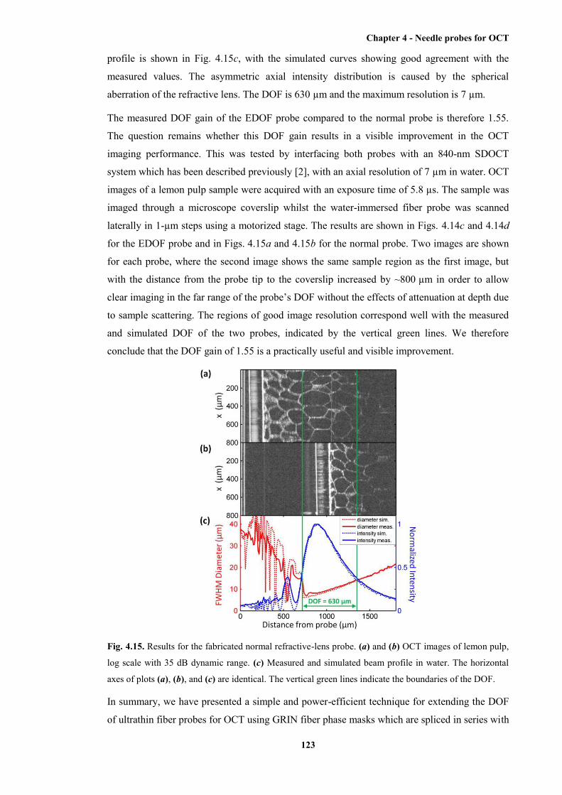
Chapter 4 - Needle probes for OCT
123
profile is shown in Fig. 4.15c, with the simulated curves showing good agreement with the
measured values. The asymmetric axial intensity distribution is caused by the spherical
aberration of the refractive lens. The DOF is 630 µm and the maximum resolution is 7 µm.
The measured DOF gain of the EDOF probe compared to the normal probe is therefore 1.55.
The question remains whether this DOF gain results in a visible improvement in the OCT
imaging performance. This was tested by interfacing both probes with an 840-nm SDOCT
system which has been described previously [2], with an axial resolution of 7 µm in water. OCT
images of a lemon pulp sample were acquired with an exposure time of 5.8 µs. The sample was
imaged through a microscope coverslip whilst the water-immersed fiber probe was scanned
laterally in 1-µm steps using a motorized stage. The results are shown in Figs. 4.14c and 4.14d
for the EDOF probe and in Figs. 4.15a and 4.15b for the normal probe. Two images are shown
for each probe, where the second image shows the same sample region as the first image, but
with the distance from the probe tip to the coverslip increased by ~800 µm in order to allow
clear imaging in the far range of the probe’s DOF without the effects of attenuation at depth due
to sample scattering. The regions of good image resolution correspond well with the measured
and simulated DOF of the two probes, indicated by the vertical green lines. We therefore
conclude that the DOF gain of 1.55 is a practically useful and visible improvement.
Fig. 4.15. Results for the fabricated normal refractive-lens probe. (a) and (b) OCT images of lemon pulp,
log scale with 35 dB dynamic range. (c) Measured and simulated beam profile in water. The horizontal
axes of plots (a), (b), and (c) are identical. The vertical green lines indicate the boundaries of the DOF.
In summary, we have presented a simple and power-efficient technique for extending the DOF
of ultrathin fiber probes for OCT using GRIN fiber phase masks which are spliced in series with

Chapter 4 - Needle probes for OCT
124
the distal focusing optics and thereby require no additional fabrication processes. A DOF gain
of 1.55 compared to a conventional lensed fiber probe was demonstrated in a prototype device
with a lateral resolution of 7 µm. Using GRIN fibers with suitable parameters, our simulations
show that a DOF gain of 2 can be obtained at the cost of a modest reduction in peak SNR of
about 5 dB. Since modern preform fabrication processes can produce custom GRIN fibers with
high optical quality [8], this approach could facilitate the development of high-transverse-
resolution extended-DOF ultrathin needle probes for OCT.
References
[1] X. Li, C. Chudoba, T. Ko, C. Pitris, and J. G. Fujimoto, Opt. Lett. 25, 1520 (2000).
[2] D. Lorenser, X. Yang, R. W. Kirk, B. C. Quirk, R. A. McLaughlin, and D. D. Sampson, Opt.
Lett. 36, 3894 (2011).
[3] Z. Ding, H. Ren, Y. Zhao, J. S. Nelson, and Z. Chen, Opt. Lett. 27, 243 (2002).
[4] R. A. Leitgeb, M. Villiger, A. H. Bachmann, L. Steinmann, and T. Lasser, Opt. Lett. 31,
2450 (2006).
[5] L. Liu, C. Liu, W. C. Howe, C. J. R. Sheppard, and N. Chen, Opt. Lett. 32, 2375 (2007).
[6] K. M. Tan, M. Mazilu, T. H. Chow, W. M. Lee, K. Taguchi, B. K. Ng, W. Sibbett, C. S.
Herrington, C. T. A. Brown, and K. Dholakia, Opt. Express 17, 2375 (2009).
[7] M. D. Feit and J. A. Fleck Jr, Appl. Opt. 17, 3990 (1978).
[8] W. A. Reed, M. F. Yan, and M. J. Schnitzer, Opt. Lett. 27, 1794 (2002).
As mentioned in the paper presented above, for the design using an additional GRIN lens, there
was a discrepancy between the measured beam profile and the simulated one. It was
hypothesised that this discrepancy is due to the deviation of the refractive index profile of the
additional GRIN lens section from the ideal parabolic shape, which occurs in commercial GRIN
fibres fabricated by using modified chemical vapor deposition method. The measured beam
profile is sensitive to this deviation and, thus, interfered. In the paper presented in the next
section, this hypothesis is presented to be validated by accurately simulating the beam
propagation along the designed fibre probe with the additional GRIN lens section by means of
using the beam propagation method instead of ABCD matrix transformations.
4.4.3 Accurate modeling and design of graded-index fiber probes for optical coherence
tomography using the beam propagation method
[D. Lorenser, X. Yang, and D. D. Sampson; IEEE Photonics Journal 5(2): art. 3900015, 2013]
Abstract
Fiber-optic probes for sensing and biomedical imaging applications such as optical coherence
tomography (OCT) frequently employ sections of graded-index (GRIN) fiber to re-focus the
diverging light from the delivery fiber. Such GRIN fiber microlenses often possess aberrations
that cause significant distortions of the focused output beam. Current design methods based on

Chapter 4 - Needle probes for OCT
125
ABCD matrix transformations for Gaussian beams cannot model such effects and are therefore
inadequate for the analysis and design of high-performance probes that require diffraction-
limited output beams. We demonstrate use of the beam propagation method (BPM) to analyze
beam distortion in GRIN-lensed fibers resulting from ripples or a central dip. Furthermore, we
demonstrate the power of this method for exploring novel probe designs that incorporate GRIN
phase masks to generate wavefront-shaped output beams with extended depth-of-focus (DOF).
We present results using our method that are in good agreement with experimental data. The
BPM enables accurate simulation of fiber probes using non-ideal or custom-engineered GRIN
fibers with arbitrary refractive index profile, which is important in the design of high-
performance fiber-based micro-imaging systems for biomedical applications.
(a) Introduction
Miniaturized fiber-optic probes that can be delivered to deep-tissue locations via hypodermic
needles or catheters are an enabling technology that allows minimally invasive optical
biomedical imaging far beyond the normal depth penetration of light into biological tissues
using techniques such as optical coherence tomography (OCT) [1]-[3]. Fig. 4.16(a) shows a
schematic of a fiber-optic OCT imaging probe, consisting of an assembly of a single-mode fiber
(SMF) terminated with focusing optics and a side-deflecting micromirror inside a hypodermic
needle with a side opening, allowing the generation of 3-D images by rotation and pullback of
the needle after its insertion into the tissue region of interest [4]. In order to eliminate the need
for alignment of discrete micro-optical components, there has been a trend toward all-fiber
probe designs using no-core fiber (NCF) spacers for beam expansion and sections of graded-
index (GRIN) fiber that act as microlenses to focus the beam into the biological tissue for
imaging at high resolution [2], [5]-[7]. Such highly miniaturized all-fiber probes are amenable
to fabrication using established fusion-splicing technology, which is reproducible and self-
aligning, and which also ensures minimal losses and back reflections. Furthermore, we have
recently shown that this all-fiber probe concept includes the possibility of adding a GRIN phase
mask section after the GRIN lens section in order to generate a wavefront-shaped output beam
with extended depth-of-focus (DOF) [8], as illustrated in Fig. 4.16(b).
Fig. 4.16. (a) Schematic of a fiber-optic OCT needle probe. The focused output beam has a Gaussian
transverse intensity profile. SMF, single-mode fiber; NCF, no-core fiber; GRIN, graded-index fiber;
DOF, depth-of-focus. (b) Schematic of the same imaging probe as in (a), but with an additional GRIN
Chapter 4 - Needle probes for OCT
126
phase mask (PM), which generates an output beam with a non-Gaussian transverse intensity profile that
has similar transverse resolution but extended DOF compared to (a).
For high-performance OCT imaging, it is important that the probe optics introduces minimal
aberrations since the characteristics of the output beam determine the transverse resolution and
also directly impact on the sensitivity of the system (as the signal level obtained from a point-
like scattering object will depend on the peak intensity of the focused probe beam). One of the
current limitations of fiber-optic OCT probes lies in the optical quality of the GRIN fiber lenses,
as the probe designer is typically forced to choose from a finite range of commercially available
multimode fibers (MMFs), which are optimized for optical telecommunications rather than for
imaging. It was already recognized in early work that the refractive index profiles of such GRIN
MMFs can exhibit significant deviations from the parabolic shape required for them to act as
ideal GRIN lenses, which results in aberrations and sub-optimal optical performance [5], [9].
Improved preform fabrication methods [5], [10] have led to a new generation of high-bandwidth
GRIN MMFs with smooth refractive index profiles, which are free of the central index dip that
plaques legacy GRIN MMFs. However, these modern high-bandwidth GRIN MMFs are only
available with small core diameters of 50 and 62.5 μm, limiting their use to probe designs with
relatively low numerical aperture (NA) and working distance (WD). Furthermore, their index
profiles tend to exhibit a more or less pronounced deviation from the ideal parabolic shape that
is purposely introduced by the manufacturer in order to minimize intermodal pulse broadening
in the targeted operating wavelength band [11], [12]. Thus, large-core-diameter fibers drawn
from preforms of such high-bandwidth GRIN MMFs [5] will not necessarily behave as ideal
GRIN lenses.
The aberrations introduced by index profiles with non-parabolic shapes and central dips cannot
be modeled by current design methods based on ABCD matrix transformations for Gaussian
beams [13], as these assume a perfect square-law refractive index profile of the GRIN fiber.
ABCD matrix modelling has proven to be a useful framework for basic probe design and
analysis [2], [6], [7], [14], [15] and as a simple tool for calculating approximate values for the
GRIN fiber and NCF spacer section lengths, which can then be experimentally optimized to
yield the desired output beam characteristics [7]. However, for the development of next-
generation, high-performance OCT fiber probes, a more sophisticated numerical modeling
technique is required for two reasons. First, in order to achieve diffraction-limited resolution
and maximum sensitivity, it is necessary to quantify how imperfections of the GRIN fiber
profile influence the beam quality and focal spot intensity (Strehl ratio), particularly in probe
designs with high NA or long WD that may require the use of large-core-diameter GRIN fibers
of sub-optimal quality. Secondly, the development of novel probe designs of the type shown in
Fig. 4.16(b), which make use of GRIN fiber phase masks to generate non-Gaussian, wavefront-
shaped output beams with increased DOF, requires a rigorous diffraction modeling method that
can accommodate GRIN elements with arbitrary refractive index profiles.

Chapter 4 - Needle probes for OCT
127
Fig. 4.17. (a) Schematic of our BPM simulation geometry. (b) The N × N simulation grid with dimension
L sampled with increments Δx = Δy = L/N and with an absorbing boundary of radius Rabs. (c) The N × N
simulation grid in the spatial frequency domain sampled with increments Δfx = Δfy = 1/L with a guard
band of radius fguard.
In this paper, we demonstrate the application of advanced numerical modeling based on the
beam propagation method (BPM) [16], [17] to fiber-optic probes using GRIN lenses and phase
masks. The BPM can be used to simulate light propagation through GRIN fibers with arbitrary
refractive index profiles and to calculate the true 3-D diffracted field in the focal region of the
probe, from which the designer can extract a wealth of advanced performance metrics beyond a
rudimentary characterization in terms of WD and “spot size”, including Strehl ratio and DOF.
One of the great strengths of the BPM is its validity for systems of arbitrary Fresnel numbers
(The Fresnel number N = a2/(λL)) determines whether the imaging system operates in the “near
field” or in the “far field” of the diffraction pattern generated by the system aperture of radius a,
where L is the distance of the focal region from the aperture, and λ is the wavelength [18].).
Miniaturized fiber-optic probes for OCT are near-field systems with Fresnel numbers on the
order of unity, and for this reasons, it is difficult to extend their DOF by a straightforward
application of schemes developed for bulk-optic microscopes (e.g., pupil plane phase masks
[19] or axicons [20], [21]) since these are all derived under the assumption of large Fresnel
number. Thus, the BPM is a necessary tool for studying schemes for creating focal regions with
extended DOF in low-Fresnel-number systems such as fiber-optic probes.
The remainder of this paper is divided into three main sections. In Section 2, we describe our
implementation of the BPM algorithm and its application to the problem of GRIN fiber probes,
including a brief discussion of its numerical accuracy. In Section 3, we use the BPM to analyze
beam distortions resulting from index profile aberrations that are common in commercial GRIN
fibers, and we demonstrate good agreement with experimental data. In Section 4, we explore the
performance of a novel probe design incorporating an axicon-like GRIN phase mask to generate
a Bessel-like output beam with extended DOF.
(b) Numerical modeling technique
The general simulation geometry used in this paper is illustrated in Fig. 4.17(a) [22]. The
launched fundamental mode from the SMF is treated as an ideal Gaussian beam with a 1/e2

Chapter 4 - Needle probes for OCT
128
waist diameter equal to the mode field diameter (MFD) of the SMF, and its complex field
amplitude at the location of the NCF/GRIN interface is used as the input to the BPM simulation.
In the GRIN fiber lens, in the (optional) GRIN fiber phase mask, and in the sample medium, the
field is numerically propagated with BPM step sizes Δzlens, Δzpm, and Δzout, respectively (the step
sizes are not necessarily identical as the BPM accuracy constraints differ in the various
sections.). The field is sampled on a N × N Cartesian grid of dimension L, as illustrated in Fig.
4.17(b). As the BPM algorithm switches back and forth between the spatial and spectral
(spatial-frequency) domains, the field is also represented by its discrete Fourier transform on an
N × N spectral grid of dimension N/L, as shown in Fig. 4.17(c). In order to prevent the sampled
wave amplitude from exceeding the boundaries of the spatial and spectral grid during the
numerical propagation, we have implemented two simple but effective measures. First, we
apply an “absorbing boundary” (a 2-D window function) to the field amplitude in the spatial
domain at every BPM step in order to prevent large-angle diffracted light from reaching the
edges of the grid and causing artifacts in the fast Fourier transform (FFT) [see Fig. 4.17(b)]. We
have chosen a Tukey window, which smoothly tapers to zero at the grid boundary for radii
exceeding a radius Rabs, which is chosen to lie within the cladding region of the fiber. During the
simulation, we monitor the integrated beam power and can therefore detect when a significant
amount of light reaches the boundary. Second, in the spectral domain, we define a “guard
band”, which covers all spatial frequencies that exceed a frequency of fquard, which we choose to
be 90% of the spectral grid half-width N/2L. At every BPM step, we compute the relative
integrated spectral power in the guard band to check that it remains negligible (below 10-6).
We closely follow the implementation of the BPM in [17]; therefore, we review it only briefly
here with a view toward some aspects that are important for its application to light propagation
in GRIN fiber lenses and phase masks. Our BPM code is implemented in MATLAB, and the
simulations presented in this paper took between 8-16 s on a basic desktop computer with a 2.4-
GHz CPU and 4 GB of memory.
(i) Beam propagation method
The BPM is a numerical technique for solving the scalar Helmholtz equation in a weakly
inhomogeneous medium with a spatially dependent refractive index n(r) [16]:
022 Uk , (1)
where k = n(r)k0 is the spatially dependent propagation constant, with k0 = 2π/λ0 and λ0 denoting
the vacuum values of the propagation constant and wavelength, respectively. In optical fibers,
the refractive index variation is on the order of a few percent, and therefore, the refractive index
can be expressed as n(r) = yxnn , , where n is a constant background refractive index
(e.g., the index of the silica cladding), and n(x, y) is a small transverse index variation. The
complex scalar wave amplitude U can be written as zkzyxAzyxU -ie,,,, , where 0knk
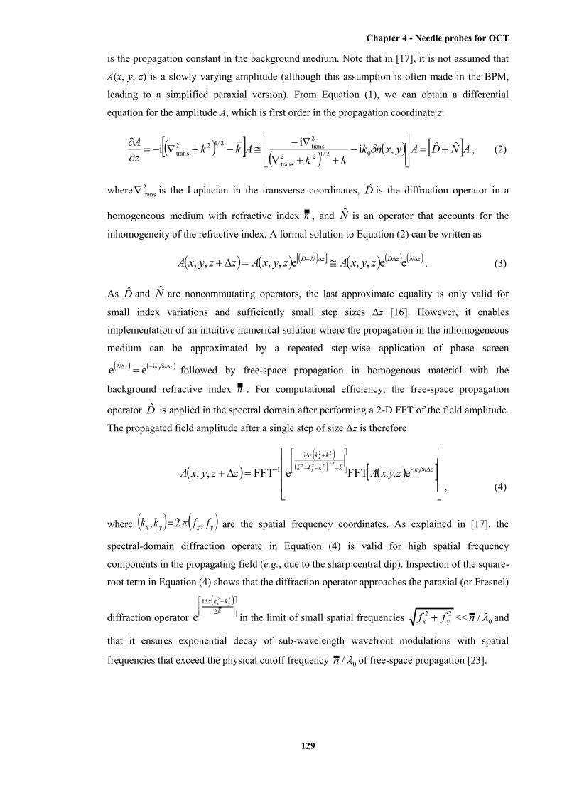
Chapter 4 - Needle probes for OCT
129
is the propagation constant in the background medium. Note that in [17], it is not assumed that
A(x, y, z) is a slowly varying amplitude (although this assumption is often made in the BPM,
leading to a simplified paraxial version). From Equation (1), we can obtain a differential
equation for the amplitude A, which is first order in the propagation coordinate z:
ANDAyxnkkk
AkkzA ˆˆ,iii 02/122
trans
2trans2/122
trans
, (2)
where 2trans is the Laplacian in the transverse coordinates, D is the diffraction operator in a
homogeneous medium with refractive index n , and N is an operator that accounts for the
inhomogeneity of the refractive index. A formal solution to Equation (2) can be written as
zNzDzND zyxAzyxAzzyxA ˆˆˆˆ ee,,e,,,, . (3)
As D and N are noncommutating operators, the last approximate equality is only valid for
small index variations and sufficiently small step sizes Δz [16]. However, it enables
implementation of an intuitive numerical solution where the propagation in the inhomogeneous
medium can be approximated by a repeated step-wise application of phase screen
znkzN 0iˆ ee followed by free-space propagation in homogenous material with the
background refractive index n . For computational efficiency, the free-space propagation
operator D is applied in the spectral domain after performing a 2-D FFT of the field amplitude.
The propagated field amplitude after a single step of size Δz is therefore
znkkkkk
kkz
x,y,zAzzyxA yx
yx
02/1222
22
i-
i
1 eFFTeFFT,,, (4)
where yxyx ffkk , 2 , are the spatial frequency coordinates. As explained in [17], the
spectral-domain diffraction operate in Equation (4) is valid for high spatial frequency
components in the propagating field (e.g., due to the sharp central dip). Inspection of the square-
root term in Equation (4) shows that the diffraction operator approaches the paraxial (or Fresnel)
diffraction operator
kkkz yx
2i 22
e in the limit of small spatial frequencies 22yx ff << 0/n and
that it ensures exponential decay of sub-wavelength wavefront modulations with spatial
frequencies that exceed the physical cutoff frequency 0/n of free-space propagation [23].

Chapter 4 - Needle probes for OCT
130
(ii) Refractive index profile model
For the GRIN fiber lens, we use a power-law profile of the type widely used in the fiber-optic
telecommunications literature, which has been modified to allow for the optional inclusion of a
Gaussian central index dip or a sinusoidal “ripple” term [see Fig. 4.18(a)] [12]
rp
nhharnrn
wr
ripripdip1
2sine21
2
dip
(when ar ) (5)
2112 nnrn (when ar ) (5)
where a is the core radius, and 21
22
21
2nnn
is the relative index difference between the core
and cladding refractive indices n1 and n2 (for small index differences, we can write 1nn
,
where 21 nn ). The central index dip is characterized by its relative depth n
nh
dipdip and
1/e – radius wdip. The sinusoidal ripple is characterized by its relative amplitude n
nh
riprip and
its period prip. The dip and ripple are index profile errors commonly encountered in GRIN fibers
fabricated using the modified chemical vapor deposition (MCVD) method, where the dip results
from “burnoff” of dopant during the high-temperature collapse of the preform, and the ripples
result from the deposition of a finite number of layers of changing composition as well as
gradients within these layers caused by dopant evaporation from the layer surface during
vitrification [24]. The effect of the power-law exponent α on the profile shape is illustrated in
Fig. 4.18(b).
Some example index profiles of commercial GRIN fibers, together with their best-fit power-law
profiles, are shown in Fig. 4.18(c)-(e). Fig. 4.18(c) shows a 100-μm core-diameter GRIN MMF
(100/140 MMF, POFC, Taiwan), which was profile on an EXFO NR-9200 fiber analyzer at a
wave-length of 655 nm. The fiber has an α-parameter of 2.1 and a central index dip with wdip =
1.8 μm and hdip = 0.12. This GRIN fiber produces significant beam distortion, as we will show
in Section 3.3. Fig. 4.18(d) shows a 62.5-μm core-diameter GRIN MMF (GIF625, Thorlabs,
USA), which we have used extensively in our recent work [2], [7] because probes fabricated
using this fiber have exhibited very good Gaussian-like beam quality and shown fairly good
agreement with ABCD matrix calculations. This observation is not surprising when one
considers the index profile, which has no measurable dip in the center, and a near-parabolic
shape with α = 1.96. The 50-μm core-diameter GRIN MMF shown in Fig. 4.18(e) (GIF50,
Thorlabs, USA) also has a very clean index profile with no central dip. However, its profile
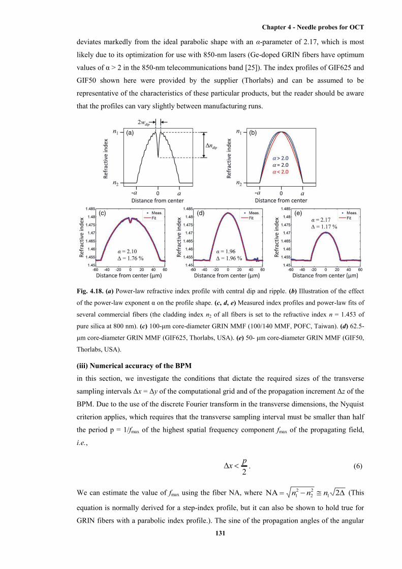
Chapter 4 - Needle probes for OCT
131
deviates markedly from the ideal parabolic shape with an α-parameter of 2.17, which is most
likely due to its optimization for use with 850-nm lasers (Ge-doped GRIN fibers have optimum
values of α > 2 in the 850-nm telecommunications band [25]). The index profiles of GIF625 and
GIF50 shown here were provided by the supplier (Thorlabs) and can be assumed to be
representative of the characteristics of these particular products, but the reader should be aware
that the profiles can vary slightly between manufacturing runs.
Fig. 4.18. (a) Power-law refractive index profile with central dip and ripple. (b) Illustration of the effect
of the power-law exponent α on the profile shape. (c, d, e) Measured index profiles and power-law fits of
several commercial fibers (the cladding index n2 of all fibers is set to the refractive index n = 1.453 of
pure silica at 800 nm). (c) 100-μm core-diameter GRIN MMF (100/140 MMF, POFC, Taiwan). (d) 62.5-
μm core-diameter GRIN MMF (GIF625, Thorlabs, USA). (e) 50- μm core-diameter GRIN MMF (GIF50,
Thorlabs, USA).
(iii) Numerical accuracy of the BPM
in this section, we investigate the conditions that dictate the required sizes of the transverse
sampling intervals Δx = Δy of the computational grid and of the propagation increment Δz of the
BPM. Due to the use of the discrete Fourier transform in the transverse dimensions, the Nyquist
criterion applies, which requires that the transverse sampling interval must be smaller than half
the period p = 1/fmax of the highest spatial frequency component fmax of the propagating field,
i.e.,
2px . (6)
We can estimate the value of fmax using the fiber NA, where 2NA 122
21 nnn (This
equation is normally derived for a step-index profile, but it can also be shown to hold true for
GRIN fibers with a parabolic index profile.). The sine of the propagation angles of the angular
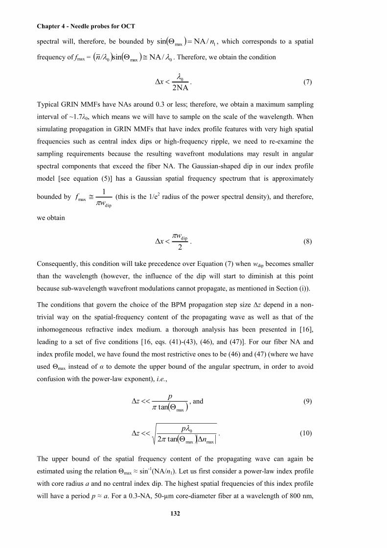
Chapter 4 - Needle probes for OCT
132
spectral will, therefore, be bounded by 1max /NAsin n , which corresponds to a spatial
frequency of fmax = 0max0 /NAsin /n . Therefore, we obtain the condition
NA20x . (7)
Typical GRIN MMFs have NAs around 0.3 or less; therefore, we obtain a maximum sampling
interval of ~1.7λ0, which means we will have to sample on the scale of the wavelength. When
simulating propagation in GRIN MMFs that have index profile features with very high spatial
frequencies such as central index dips or high-frequency ripple, we need to re-examine the
sampling requirements because the resulting wavefront modulations may result in angular
spectral components that exceed the fiber NA. The Gaussian-shaped dip in our index profile
model [see equation (5)] has a Gaussian spatial frequency spectrum that is approximately
bounded by dip
max1w
f
(this is the 1/e2 radius of the power spectral density), and therefore,
we obtain
2dipw
x
. (8)
Consequently, this condition will take precedence over Equation (7) when wdip becomes smaller
than the wavelength (however, the influence of the dip will start to diminish at this point
because sub-wavelength wavefront modulations cannot propagate, as mentioned in Section (i)).
The conditions that govern the choice of the BPM propagation step size Δz depend in a non-
trivial way on the spatial-frequency content of the propagating wave as well as that of the
inhomogeneous refractive index medium. a thorough analysis has been presented in [16],
leading to a set of five conditions [16, eqs. (41)-(43), (46), and (47)]. For our fiber NA and
index profile model, we have found the most restrictive ones to be (46) and (47) (where we have
used Θmax instead of α to demote the upper bound of the angular spectrum, in order to avoid
confusion with the power-law exponent), i.e.,
maxtan
pz , and (9)
maxmax
0
tan2 npz
. (10)
The upper bound of the spatial frequency content of the propagating wave can again be
estimated using the relation Θmax ≈ sin-1(NA/n1). Let us first consider a power-law index profile
with core radius a and no central index dip. The highest spatial frequencies of this index profile
will have a period p ≈ a. For a 0.3-NA, 50-µm core-diameter fiber at a wavelength of 800 nm,

Chapter 4 - Needle probes for OCT
133
Equation (10) turns out to be the most restrictive condition, with a maximum step size of Δz =
23 µm. If this fiber additionally has a central index dip of radius wdip = 1 µm, then Equation (9)
becomes the most restrictive condition, yielding a maximum step size of Δz = 5 µm.
In practice, these numbers can be used as an orientation, and the optimum step size will become
evident by running repeated simulations with decreasing Δz until the results converge to a
steady state. Consistent with [16], we have found that the point of diminishing returns for
decreasing Δz is of the same order as the limits calculated via Equation (9) and (10). Therefore,
in the context of the simulation tasks described in this work, there is no need to stay an order of
magnitude below the calculated limits as the “<<” in Equation (9) and (10) might imply.
We have compared the results of our BPM code with ABCD matrix simulations of simple
NCF/GRIN fiber probes with ideal parabolic refractive index profiles and found the relative
errors of the values of focal spot diameter and ED to be less than 1%.
(c) Analysis of beam distortions caused by index profile aberrations
In this section, we utilize our BPM code to analyze the effects of index profile variations from
the ideal on the output beam of a lensed fiber probe. When we analyze distorted or wavefront-
shaped output beams in the following, we will measure the “quality” of the focal region by two
parameters that are of relevance to the performance of the probe for OCT imaging, namely,
Strehl ratio and relative depth-of-focus (RDOF). The Strehl ratio of an aberrated system is
defined as the ratio of its focal spot peak intensity to that of an equivalent diffraction-limited
system [18]. Similarly, we define the RDOF as the ratio of the DOF of the simulated beam to
that of an equivalent diffraction-limited system. In this context, we represent the equivalent
diffraction-limited system by a suitably defined “reference” Gaussian beam. In the case of the
weakly aberrated power-law profiles considered in this section, we define the reference
Gaussian as the output beam produced by the corresponding aberration-free power-law profile
with α = 2.0 of infinite extent (not truncated at the core radius a, in order to eliminate aperture
diffraction effects). For very strongly aberrated or wavefront-shaped systems, where an
equivalent aberration-free system cannot be inferred in a straightforward manner, we define the
reference Gaussian as the ideal Gaussian beam that has the same full-width at half-maximum
(FWHM) focal spot diameter and integrated power as the simulated beam. We choose to use the
FWHM rather than the more commonly used 1/e2 criterion because the former yields more
meaningful values for the central lobe diameters of non-Gaussian output beams with sidelobes
or pedestals, which often exceed relative levels of 1/e2.
Thus, the Strehl ratio is given by Gaussˆ/ˆ IIS , with I denoting the peak intensity at the focus of
the simulated beam, and GaussI the peak intensity of the reference Gaussian
2FWHM
2Gauss
Gauss)2ln(42ˆ
dP
wPI
, (11)
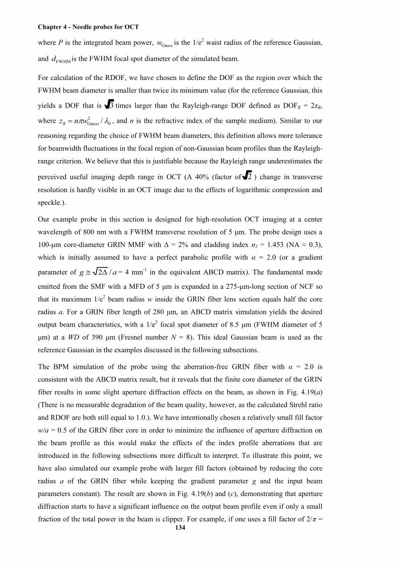
Chapter 4 - Needle probes for OCT
134
where P is the integrated beam power, Gaussw is the 1/e2 waist radius of the reference Gaussian,
and FWHMd is the FWHM focal spot diameter of the simulated beam.
For calculation of the RDOF, we have chosen to define the DOF as the region over which the
FWHM beam diameter is smaller than twice its minimum value (for the reference Gaussian, this
yields a DOF that is 3 times larger than the Rayleigh-range DOF defined as DOFR = 2zR,
where 02Gauss /wnzR , and n is the refractive index of the sample medium). Similar to our
reasoning regarding the choice of FWHM beam diameters, this definition allows more tolerance
for beamwidth fluctuations in the focal region of non-Gaussian beam profiles than the Rayleigh-
range criterion. We believe that this is justifiable because the Rayleigh range underestimates the
perceived useful imaging depth range in OCT (A 40% (factor of 2 ) change in transverse
resolution is hardly visible in an OCT image due to the effects of logarithmic compression and
speckle.).
Our example probe in this section is designed for high-resolution OCT imaging at a center
wavelength of 800 nm with a FWHM transverse resolution of 5 μm. The probe design uses a
100-μm core-diameter GRIN MMF with Δ = 2% and cladding index n2 = 1.453 (NA ≈ 0.3),
which is initially assumed to have a perfect parabolic profile with α = 2.0 (or a gradient
parameter of ag /2 = 4 mm-1 in the equivalent ABCD matrix). The fundamental mode
emitted from the SMF with a MFD of 5 μm is expanded in a 275-μm-long section of NCF so
that its maximum 1/e2 beam radius w inside the GRIN fiber lens section equals half the core
radius a. For a GRIN fiber length of 280 μm, an ABCD matrix simulation yields the desired
output beam characteristics, with a 1/e2 focal spot diameter of 8.5 μm (FWHM diameter of 5
μm) at a WD of 390 μm (Fresnel number N = 8). This ideal Gaussian beam is used as the
reference Gaussian in the examples discussed in the following subsections.
The BPM simulation of the probe using the aberration-free GRIN fiber with α = 2.0 is
consistent with the ABCD matrix result, but it reveals that the finite core diameter of the GRIN
fiber results in some slight aperture diffraction effects on the beam, as shown in Fig. 4.19(a)
(There is no measurable degradation of the beam quality, however, as the calculated Strehl ratio
and RDOF are both still equal to 1.0.). We have intentionally chosen a relatively small fill factor
w/a = 0.5 of the GRIN fiber core in order to minimize the influence of aperture diffraction on
the beam profile as this would make the effects of the index profile aberrations that are
introduced in the following subsections more difficult to interpret. To illustrate this point, we
have also simulated our example probe with larger fill factors (obtained by reducing the core
radius a of the GRIN fiber while keeping the gradient parameter g and the input beam
parameters constant). The result are shown in Fig. 4.19(b) and (c), demonstrating that aperture
diffraction starts to have a significant influence on the output beam profile even if only a small
fraction of the total power in the beam is clipper. For example, if one uses a fill factor of 2/π =
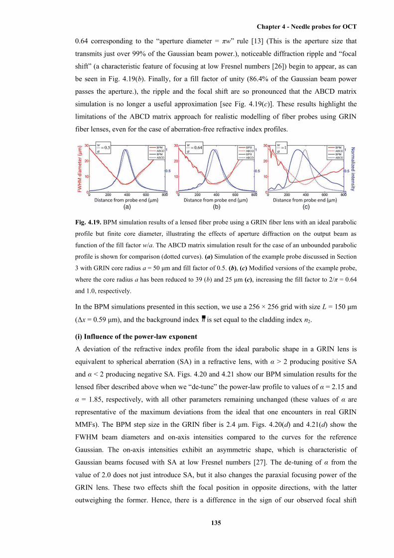
Chapter 4 - Needle probes for OCT
135
0.64 corresponding to the “aperture diameter = πw” rule [13] (This is the aperture size that
transmits just over 99% of the Gaussian beam power.), noticeable diffraction ripple and “focal
shift” (a characteristic feature of focusing at low Fresnel numbers [26]) begin to appear, as can
be seen in Fig. 4.19(b). Finally, for a fill factor of unity (86.4% of the Gaussian beam power
passes the aperture.), the ripple and the focal shift are so pronounced that the ABCD matrix
simulation is no longer a useful approximation [see Fig. 4.19(c)]. These results highlight the
limitations of the ABCD matrix approach for realistic modelling of fiber probes using GRIN
fiber lenses, even for the case of aberration-free refractive index profiles.
Fig. 4.19. BPM simulation results of a lensed fiber probe using a GRIN fiber lens with an ideal parabolic
profile but finite core diameter, illustrating the effects of aperture diffraction on the output beam as
function of the fill factor w/a. The ABCD matrix simulation result for the case of an unbounded parabolic
profile is shown for comparison (dotted curves). (a) Simulation of the example probe discussed in Section
3 with GRIN core radius a = 50 μm and fill factor of 0.5. (b), (c) Modified versions of the example probe,
where the core radius a has been reduced to 39 (b) and 25 μm (c), increasing the fill factor to 2/π = 0.64
and 1.0, respectively.
In the BPM simulations presented in this section, we use a 256 × 256 grid with size L = 150 μm
(Δx = 0.59 μm), and the background index n is set equal to the cladding index n2.
(i) Influence of the power-law exponent
A deviation of the refractive index profile from the ideal parabolic shape in a GRIN lens is
equivalent to spherical aberration (SA) in a refractive lens, with α > 2 producing positive SA
and α < 2 producing negative SA. Figs. 4.20 and 4.21 show our BPM simulation results for the
lensed fiber described above when we “de-tune” the power-law profile to values of α = 2.15 and
α = 1.85, respectively, with all other parameters remaining unchanged (these values of α are
representative of the maximum deviations from the ideal that one encounters in real GRIN
MMFs). The BPM step size in the GRIN fiber is 2.4 μm. Figs. 4.20(d) and 4.21(d) show the
FWHM beam diameters and on-axis intensities compared to the curves for the reference
Gaussian. The on-axis intensities exhibit an asymmetric shape, which is characteristic of
Gaussian beams focused with SA at low Fresnel numbers [27]. The de-tuning of α from the
value of 2.0 does not just introduce SA, but it also changes the paraxial focusing power of the
GRIN lens. These two effects shift the focal position in opposite directions, with the latter
outweighing the former. Hence, there is a difference in the sign of our observed focal shift

Chapter 4 - Needle probes for OCT
136
compared to [27] and other optics texts, where pure primary SA is added to an ideal lens of
fixed focal length.
Fig. 4.20. BPM simulation of a GRIN-lensed fiber with α = 2.15. (a) Index profile of the GRIN fiber
compared to an ideal parabolic profile. (b) E-field amplitude in the entire simulated region. (c) Output
beam intensity. (d) FWHM beam diameter and on-axis intensity of the simulated output beam (solid
lines) compared to the reference Gaussian (dotted lines).
Fig. 4.21. BPM simulation of a GRIN-lensed fiber with α = 1.85. (a) Index profile of the GRIN fiber
compared to an ideal parabolic profile. (b) E-field amplitude in the entire simulated region. (c) Output
beam intensity. (d) FWHM beam diameter and on-axis intensity of the simulated output beam (solid
lines) compared to the reference Gaussian (dotted lines).
For the case of α = 2.15, we obtain a significantly reduced Strehl ratio of S = 0.77 and a slight
increase of the DOF (RDOF = 1.1). In the case of α = 1.85, the index profile begins to approach
a triangular shape [see Fig. 4.21(a)], resulting in an axicon-like effect on the wavefront. As a
result of this, the output beam starts to show features of a Bessel-like profile with sidelobes and
an elongated focal region with RDOF = 1.44 obtained at the cost of a slightly reduced Strehl
ratio of S = 0.96. We exploit this effect in Section 4 to design a GRIN phase mask with axicon-
like properties in order to maximize the RDOF.
(ii) Influence of the central index dip and index ripple
The effects of the central index dip and index ripple on the bandwidth of GRIN MMFs have
been studies extensively in the fiber-optic telecommunications literature from the viewpoint of
modal analysis [12], [24]. However, these studies provide little insight into the wavefront
distortions that result when using short sections of such GRIN MMFs as lenses. Our aim here is
to gain an intuitive understanding of the beam distortions resulting from central index dips and
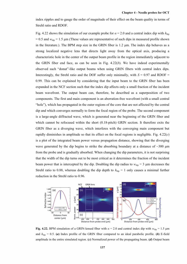
Chapter 4 - Needle probes for OCT
137
index ripples and to gauge the order of magnitude of their effect on the beam quality in terms of
Strehl ratio and RDOF.
Fig. 4.22 shows the simulation of our example probe for α = 2.0 and a central index dip with hdip
= 0.5 and wdip = 1.5 μm (These values are representative of such dips in measured profile shown
in the literature.). The BPM step size in the GRIN fiber is 1.2 μm. The index dip behaves as a
strong localized negative lens that directs light away from the optical axis, producing a
characteristic hole in the center of the output beam profile in the region immediately adjacent to
the GRIN fiber end face, as can be seen in Fig. 4.22(b). We have indeed experimentally
observed such “donut”-like output beams when using GRIN fibers with central index dips.
Interestingly, the Strehl ratio and the DOF suffer only minimally, with S = 0.97 and RDOF =
0.99. This can be explained by considering that the input beam to the GRIN fiber has been
expanded in the NCF section such that the index dip affects only a small fraction of the incident
beam wavefront. The output beam can, therefore, be described as a superposition of two
components. The first and main component is an aberration-free wavefront (with a small central
“hole”), which has propagated in the outer regions of the core that are not affected by the central
dip and which converges normally to form the focal region of the probe. The second component
is a large-angle diffracted wave, which is generated near the beginning of the GRIN fiber and
which cannot be refocused within the short (0.18-pitch) GRIN section. It therefore exits the
GRIN fiber as a diverging wave, which interferes with the converging main component but
rapidly diminishes in amplitude so that its effect on the focal regions is negligible. Fig. 4.22(c)
is a plot of the integrated beam power versus propagation distance, showing that the diverging
wave generated by the dip begins to strike the absorbing boundary at a distance of ~300 μm
from the probe and is gradually absorbed. When changing the dip parameters, it is not surprising
that the width of the dip turns out to be most critical as it determines the fraction of the incident
beam power that is intercepted by the dip. Doubling the dip radius to wdip = 3 μm decreases the
Strehl ratio to 0.88, whereas doubling the dip depth to hdip = 1 only causes a minimal further
reduction in the Strehl ratio to 0.96.
Fig. 4.22. BPM simulation of a GRIN-lensed fiber with α = 2.0 and central index dip with wdip = 1.5 μm
and hdip = 0.5. (a) Index profile of the GRIN fiber compared to an ideal parabolic profile. (b) E-field
amplitude in the entire simulated region. (c) Normalized power of the propagating beam. (d) Output beam
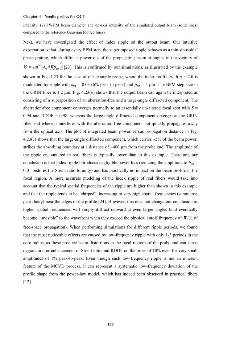
Chapter 4 - Needle probes for OCT
138
intensity. (e) FWHM beam diameter and on-axis intensity of the simulated output beam (solid lines)
compared to the reference Gaussian (dotted lines).
Next, we have investigated the effect of index ripple on the output beam. Our intuitive
expectation is that, during every BPM step, the superimposed ripple behaves as a thin sinusoidal
phase grating, which diffracts power out of the propagating beam at angles in the vicinity of
rip01 /sin pn [23]. This is confirmed by our simulations, as illustrated by the example
shown in Fig. 4.23 for the case of our example probe, where the index profile with α = 2.0 is
modulated by ripple with hrip = 0.03 (6% peak-to-peak) and prip = 5 μm. The BPM step size in
the GRIN fiber is 1.2 μm. Fig. 4.23(b) shows that the output beam can again be interpreted as
consisting of a superposition of an aberration-free and a large-angle diffracted component. The
aberration-free component converges normally to an essentially un-altered focal spot with S =
0.94 and RDOF = 0.98, whereas the large-angle diffracted component diverges at the GRIN
fiber end where it interferes with the aberration-free component but quickly propagates away
from the optical axis. The plot of integrated beam power versus propagation distance in Fig.
4.23(c) shows that the large-angle diffracted component, which carries ~5% of the beam power,
strikes the absorbing boundary at a distance of ~400 μm from the probe end. The amplitude of
the ripple encountered in real fibers is typically lower than in this example. Therefore, our
conclusion is that index ripple introduces negligible power loss (reducing the amplitude to hrip =
0.01 restores the Strehl ratio to unity) and has practically no impact on the beam profile in the
focal region. A more accurate modeling of the index ripple of real fibers would take into
account that the typical spatial frequencies of the ripple are higher than shown in this example
and that the ripple tends to be “chirped”, increasing to very high spatial frequencies (submicron
periodicity) near the edges of the profile [24]. However, this does not change our conclusion as
higher spatial frequencies will simply diffract outward at even larger angles (and eventually
become “invisible” to the wavefront when they exceed the physical cutoff frequency of 0/n of
free-space propagation). When performing simulations for different ripple periods, we found
that the most noticeable effects are caused by low-frequency ripple with only 1-3 periods in the
core radius, as these produce beam distortions in the focal regions of the probe and can cause
degradation or enhancement of Strehl ratio and RDOF on the order of 10% even for very small
amplitudes of 1% peak-to-peak. Even though such low-frequency ripple is not an inherent
feature of the MCVD process, it can represent a systematic low-frequency deviation of the
profile shape from the power-law model, which has indeed been observed in practical fibers
[12].
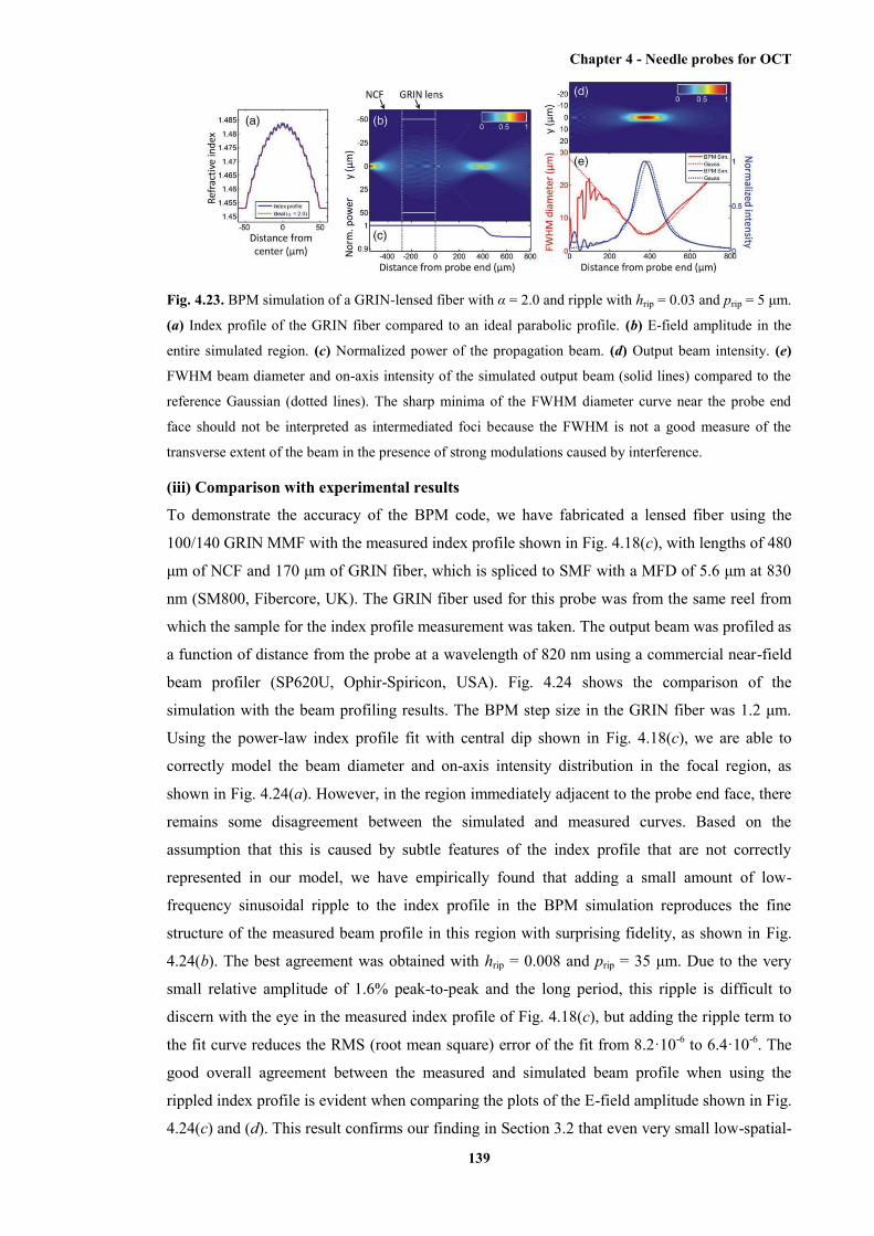
Chapter 4 - Needle probes for OCT
139
Fig. 4.23. BPM simulation of a GRIN-lensed fiber with α = 2.0 and ripple with hrip = 0.03 and prip = 5 μm.
(a) Index profile of the GRIN fiber compared to an ideal parabolic profile. (b) E-field amplitude in the
entire simulated region. (c) Normalized power of the propagation beam. (d) Output beam intensity. (e)
FWHM beam diameter and on-axis intensity of the simulated output beam (solid lines) compared to the
reference Gaussian (dotted lines). The sharp minima of the FWHM diameter curve near the probe end
face should not be interpreted as intermediated foci because the FWHM is not a good measure of the
transverse extent of the beam in the presence of strong modulations caused by interference.
(iii) Comparison with experimental results
To demonstrate the accuracy of the BPM code, we have fabricated a lensed fiber using the
100/140 GRIN MMF with the measured index profile shown in Fig. 4.18(c), with lengths of 480
μm of NCF and 170 μm of GRIN fiber, which is spliced to SMF with a MFD of 5.6 μm at 830
nm (SM800, Fibercore, UK). The GRIN fiber used for this probe was from the same reel from
which the sample for the index profile measurement was taken. The output beam was profiled as
a function of distance from the probe at a wavelength of 820 nm using a commercial near-field
beam profiler (SP620U, Ophir-Spiricon, USA). Fig. 4.24 shows the comparison of the
simulation with the beam profiling results. The BPM step size in the GRIN fiber was 1.2 μm.
Using the power-law index profile fit with central dip shown in Fig. 4.18(c), we are able to
correctly model the beam diameter and on-axis intensity distribution in the focal region, as
shown in Fig. 4.24(a). However, in the region immediately adjacent to the probe end face, there
remains some disagreement between the simulated and measured curves. Based on the
assumption that this is caused by subtle features of the index profile that are not correctly
represented in our model, we have empirically found that adding a small amount of low-
frequency sinusoidal ripple to the index profile in the BPM simulation reproduces the fine
structure of the measured beam profile in this region with surprising fidelity, as shown in Fig.
4.24(b). The best agreement was obtained with hrip = 0.008 and prip = 35 μm. Due to the very
small relative amplitude of 1.6% peak-to-peak and the long period, this ripple is difficult to
discern with the eye in the measured index profile of Fig. 4.18(c), but adding the ripple term to
the fit curve reduces the RMS (root mean square) error of the fit from 8.2·10-6 to 6.4·10-6. The
good overall agreement between the measured and simulated beam profile when using the
rippled index profile is evident when comparing the plots of the E-field amplitude shown in Fig.
4.24(c) and (d). This result confirms our finding in Section 3.2 that even very small low-spatial-
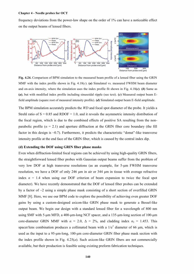
Chapter 4 - Needle probes for OCT
140
frequency deviations from the power-law shape on the order of 1% can have a noticeable effect
on the output beams of lensed fibers.
Fig. 4.24. Comparison of BPM simulation to the measured beam profile of a lensed fiber using the GRIN
MMF with the index profile shown in Fig. 4.18(c). (a) Simulated vs. measured FWHM beam diameter
and on-axis intensity, where the simulation uses the index profile fit shown in Fig. 4.18(c). (b) Same as
(a), but with modified index profile including sinusoidal ripple (see text). (c) Measured output beam E-
field amplitude (square root of measured intensity profile). (d) Simulated output beam E-field amplitude.
The BPM simulation accurately predicts the WD and focal spot diameter of the probe. It yields a
Strehl ratio of S = 0.85 and RDOF = 1.0, and it reveals the asymmetric intensity distribution of
the focal region, which is due to the combined effects of positive SA resulting from the non-
parabolic profile (α = 2.1) and aperture diffraction at the GRIN fiber core boundary (the fill
factor in this design is ~0.7). Furthermore, it predicts the characteristic “donut”-like transverse
intensity profile at the end face of the GRIN fiber, which is caused by the central index dip.
(d) Extending the DOF using GRIN fiber phase masks
Even when diffraction-limited focal regions can be achieved by using high-quality GRIN fibers,
the straightforward lensed fiber probes with Gaussian output beams suffer from the problem of
very low DOF at high transverse resolutions (as an example, for 5-μm FWHM transverse
resolution, we have a DOF of only 246 μm in air or 344 μm in tissue with average refractive
index n = 1.4 when using our DOF criterion of beam expansion to twice the focal spot
diameter). We have recently demonstrated that the DOF of lensed fiber probes can be extended
by a factor of ~2 using a simple phase mask consisting of a short section of overfilled GRIN
MMF [8]. Here, we use our BPM code to explore the possibility of achieving even greater DOF
gains by using a custom-designed axicon-like GRIN phase mask to generate a Bessel-like
output beam. We begin our design with a standard lensed fiber for a wavelength of 800 nm
using SMF with 5-μm MFD, a 400-μm-long NCF spacer, and a 135-μm-long section of 100-μm
core-diameter GRIN MMF with α = 2.0, Δ = 2%, and cladding index n2 = 1.453. This
spacer/lens combination produces a collimated beam with a 1/e2 diameter of 66 μm, which is
used as the input to a 95-μm-long, 100-μm core-diameter GRIN fiber phase mask section with
the index profile shown in Fig. 4.25(a). Such axicon-like GRIN fibers are not commercially
available, but their production is feasible using existing preform fabrication techniques.
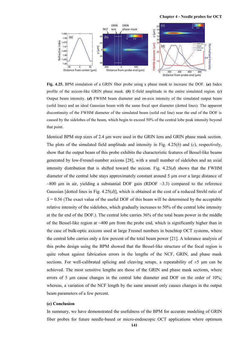
Chapter 4 - Needle probes for OCT
141
Fig. 4.25. BPM simulation of a GRIN fiber probe using a phase mask to increase the DOF. (a) Index
profile of the axicon-like GRIN phase mask. (b) E-field amplitude in the entire simulated region. (c)
Output beam intensity. (d) FWHM beam diameter and on-axis intensity of the simulated output beam
(solid lines) and an ideal Gaussian beam with the same focal spot diameter (dotted lines). The apparent
discontinuity of the FWHM diameter of the simulated beam (solid red line) near the end of the DOF is
caused by the sidelobes of the beam, which begin to exceed 50% of the central lobe peak intensity beyond
that point.
Identical BPM step sizes of 2.4 μm were used in the GRIN lens and GRIN phase mask section.
The plots of the simulated field amplitude and intensity in Fig. 4.25(b) and (c), respectively,
show that the output beam of this probe exhibits the characteristic features of Bessel-like beams
generated by low-Fresnel-number axicons [28], with a small number of sidelobes and an axial
intensity distribution that is shifted toward the axicon. Fig. 4.25(d) shows that the FWHM
diameter of the central lobe stays approximately constant around 5 μm over a large distance of
~800 μm in air, yielding a substantial DOF gain (RDOF ~3.3) compared to the reference
Gaussian [dotted lines in Fig. 4.25(d)], which is obtained at the cost of a reduced Strehl ratio of
S = 0.56 (The exact value of the useful DOF of this beam will be determined by the acceptable
relative intensity of the sidelobes, which gradually increases to 50% of the central lobe intensity
at the far end of the DOF.). The central lobe carries 36% of the total beam power in the middle
of the Bessel-like region at ~400 μm from the probe end, which is significantly higher than in
the case of bulk-optic axicons used at large Fresnel numbers in benchtop OCT systems, where
the central lobe carries only a few percent of the total beam power [21]. A tolerance analysis of
this probe design using the BPM showed that the Bessel-like structure of the focal region is
quite robust against fabrication errors in the lengths of the NCF, GRIN, and phase mask
sections. For well-calibrated splicing and cleaving setups, a repeatability of ±5 μm can be
achieved. The most sensitive lengths are those of the GRIN and phase mask sections, where
errors of 5 μm cause changes in the central lobe diameter and DOF on the order of 10%;
whereas, a variation of the NCF length by the same amount only causes changes in the output
beam parameters of a few percent.
(e) Conclusion
In summary, we have demonstrated the usefulness of the BPM for accurate modeling of GRIN
fiber probes for future needle-based or micro-endoscopic OCT applications where optimum
Chapter 4 - Needle probes for OCT
142
resolution and sensitivity will be crucial for enabling minimally invasive imaging with quality
comparable to state-of-the-art benchtop microscopes.
Our simulations have revealed a number of new insights about GRIN fiber lenses, which cannot
be obtained using established ABCD matrix modeling techniques. The most significant finding
is that low-spatial-frequency features of the index profile (such as deviation of the power-law
exponent α from the ideal value of 2.0 or low-spatial-frequency variations of the profile about
the power-law shape) are much more critical for the output beam quality than high-spatial-
frequency features such as central index dips and short-period ripples, which are often
encountered in fibers drawn from preforms fabricated using the MCVD process. This finding is
important for specifying the fabrication tolerances of customized preforms for high-quality
GRIN fiber lenses. It was also found that the negative SA introduced by profiles with α < 2.0
can be used to enhance the DOF, whereas the positive SA introduced by values of α > 2.0
produces less favourable output beam distortions that result in a significantly reduced Strehl
ratio.
Furthermore, we have demonstrated the power of the BPM for studying advanced probe designs
incorporating novel optical elements such as GRIN phase masks with arbitrary refractive index
profiles to engineer the 3-D diffracted field in the focal region. We would like to point out that
the BPM naturally also includes the possibility of multiplying the propagating wavefront with a
“thin” phase or amplitude mask (which could, for example, represent a diffractive optical
element created by microstructuring the fiber tip). The BPM has also successfully been used to
model refractive surfaces such as waveguide lenses [29] and hemispherical lenses [8]. This
capability is important for studying the effects of enclosing catheters, capillaries, or other
transparent protective sheaths on the output beams of side-facing lensed fiber probes (The
analysis of astigmatism introduced by such cylindrical interfaces is obviously an important
aspect of any realistic side-facing probe design, and it has been studies extensively using ABCD
matrix simulations for the case of probes with Gaussian output beams [2], [7], [14], [15].).
In this paper, we have neglected wavefront distortions that the output beams incur as they
propagate in biological tissue. However, the BPM can be used to study these effects if the tissue
is modelled as an inhomogeneous dielectric medium, and such simulations have provided
important insights regarding optimum beam shapes for microscopy in dense scattering media
[30], [31].
In this paper, we have focused on GRIN fiber probes for OCT imaging, but the methods
described here can also be applied to other imaging systems incorporating GRIN elements, such
as microendoscopes for confocal fluorescence [32] or multiphoton microscopy [33], which use
very thin fiber-like GRIN relay rods and lenses with diameters down to 350 μm at moderate
NAs in the range 0.3-0.5, where scalar diffraction theory (which is the underlying framework of
the BPM) is still very accurate. Some elements of the work presented here could also be useful
Chapter 4 - Needle probes for OCT
143
for non-biomedical applications of GRIN fiber microlenses, such as analysis and design of
fiber-to-freespace or fiber-to-fiber coupling assemblies in photonic devices and interconnects
[9], [34].
(f) References
[1] X. Li, C. Chudoba, T. Ko, C. Pitris, and J. G. Fujimoto, “Imaging needle for optical
coherence tomography,” Opt. Lett., vol. 25, no. 20, pp. 1520–1522, Oct. 2000.
[2] D. Lorenser, X. Yang, R. W. Kirk, B. C. Quirk, R. A. McLaughlin, and D. D. Sampson,
“Ultrathin side-viewing needle probe for optical coherence tomography,” Opt. Lett., vol. 36, no.
19, pp. 3894–3896, Oct. 2011.
[3] R. A. McLaughlin, B. C. Quirk, A. Curatolo, R. W. Kirk, L. Scolaro, D. Lorenser, P. D.
Robbins, B. A. Wood, C. M. Saunders, and D. D. Sampson, “Imaging of breast cancer with
optical coherence tomography needle probes: Feasibility and initial results,” IEEE J. Sel. Topics
Quantum Electron., vol. 18, no. 3, pp. 1184–1191, May/Jun. 2012.
[4] B. C. Quirk, R. A. McLaughlin, A. Curatolo, R. W. Kirk, P. B. Noble, and D. D. Sampson,
“In situ imaging of lung alveoli with an optical coherence tomography needle probe,” J.
Biomed. Opt., vol. 16, no. 3, p. 036009, Mar. 2011.
[5] W. A. Reed, M. F. Yan, and M. J. Schnitzer, “Gradient-index fiber-optic microprobes for
minimally invasive in vivo low-coherence interferometry,” Opt. Lett., vol. 27, no. 20, pp. 1794–
1796, Oct. 2002.
[6] Y. Mao, S. Chang, S. Sherif, and C. Flueraru, “Graded-index fiber lens proposed for
ultrasmall probes used in biomedical imaging,” Appl. Opt., vol. 46, no. 23, pp. 5887–5894, Aug.
2007.
[7] L. Scolaro, D. Lorenser, R. A. McLaughlin, B. C. Quirk, R. W. Kirk, and D. D. Sampson,
“High-sensitivity anastigmatic imaging needle for optical coherence tomography,” Opt. Lett.,
vol. 37, no. 24, pp. 5247–5249, Dec. 2012.
[8] D. Lorenser, X. Yang, and D. D. Sampson, “Ultrathin fiber probes with extended depth of
focus for optical coherence tomography,” Opt. Lett., vol. 37, no. 10, pp. 1616–1618, May 2012.
[9] W. Emkey and C. Jack, “Analysis and evaluation of graded-index fiber lenses,” J. Lightw.
Technol., vol. LT-5, no. 9, pp. 1156–1164, Sep. 1987.
[10] D. Mazzarese, G. E. Oulundsen III, I. T. F. McMahon, and M. T. Owsiany, “Method of
collapsing a tube for an optical fiber preform,” U.S. Patent 6 718 800, Apr. 13, 2004.
[11] R. Olshansky and D. Keck, “Pulse broadening in graded-index optical fibers,” Appl. Opt.,
vol. 15, no. 2, pp. 483–491, Feb. 1976.
Chapter 4 - Needle probes for OCT
144
[12] D. Marcuse, “Calculation of bandwidth from index profiles of optical fibers. 1: Theory,”
Appl. Opt., vol. 18, no. 12, pp. 2073–2080, Jun. 1979.
[13] A. E. Siegman, Lasers. Mill Valley, CA, USA: Univ. Sci. Books, 1986.
[14] W. Jung, W. A. Benalcazar, A. Ahmad, U. Sharma, H. Tu, and S. A. Boppart, “Numerical
analysis of gradient index lens based optical coherence tomography imaging probes,” J.
Biomed. Opt., vol. 15, no. 6, pp. 066027-1–066027-10, Nov./Dec. 2010.
[15] W. A. Benalcazar, W. Jung, and S. A. Boppart, “Aberration characterization for the optimal
design of high-resolution endoscopic optical coherence tomography catheters,” Opt. Lett., vol.
37, no. 6, pp. 1100–1102, Mar. 2012.
[16] J. Van Roey, J. Van der Donk, and P. E. Lagasse, “Beam-propagation method: Analysis
and assessment,” J. Opt. Soc. Amer., vol. 71, no. 7, pp. 803–810, Jul. 1981.
[17] M. D. Feit and J. A. Fleck, Jr., “Light propagation in graded-index optical fibers,” Appl.
Opt., vol. 17, no. 24, pp. 3990–3998, Dec. 1978.
[18] M. Born and E. Wolf, Principles of Optics. Cambridge, U.K.: Cambridge Univ. Press,
1999.
[19] L. Liu, C. Liu, W. C. Howe, C. J. R. Sheppard, and N. Chen, “Binary-phase spatial filter
for real-time swept-source optical coherence microscopy,” Opt. Lett., vol. 32, no. 16, pp. 2375–
2377, Aug. 2007.
[20] Z. Ding, H. Ren, Y. Zhao, J. S. Nelson, and Z. Chen, “High-resolution optical coherence
tomography over a large depth range with an axicon lens,” Opt. Lett., vol. 27, no. 4, pp. 243–
245, Feb. 2002.
[21] R. A. Leitgeb, M. Villiger, A. H. Bachmann, L. Steinmann, and T. Lasser, “Extended focus
depth for Fourier domain optical coherence microscopy,” Opt. Lett., vol. 31, no. 16, pp. 2450–
2452, Aug. 2006.
[22] D. Lorenser, X. Yang, and D. D. Sampson, “Analysis of fiber-optic probes using graded-
index fiber microlenses with non-ideal refractive index profiles,” in Proc. SPIE 22nd Int. Conf.
Opt. Fiber Sens., vol. 8421, Y. Liao, H. Ho, D. D. Sampson, R. Yamauchi, Y. Chung, K.
Nakamura, and Y. Rao, Eds., Bellingham, WA, USA, 2012, 84211W.
[23] J. Goodman, Introduction to Fourier Optics. New York, NY, USA: McGraw-Hill, 1968.
[24] A. Carnevale and U. C. Paek, “Empirical evaluation of profile variations in an MCVD
optical waveguide fiber using modal structure analysis,” Bell Syst. Tech. J., vol. 62, no. 7, pp.
1937–1954, Sep. 1983.
Chapter 4 - Needle probes for OCT
145
[25] G. E. Peterson, A. Carnevale, U. C. Paek, and J. W. Fleming, “Numerical calculation of
optimum alpha for a germania-doped silica lightguide,” Bell Syst. Tech. J., vol. 60, no. 4, pp.
455–470, Apr. 1981.
[26] Y. Li and E. Wolf, “Three-dimensional intensity distribution near the focus in systems of
different Fresnel numbers,” J. Opt. Soc. Amer. A, vol. 1, no. 8, pp. 801–808, Aug. 1984.
[27] J. Pu and H. Zhang, “Intensity distribution of Gaussian beams focused by a lens with
spherical aberration,” Opt. Commun., vol. 151, no. 4–6, pp. 331–338, Jun. 1998.
[28] C. Zapata-Rodriguez and A. Sanchez-Losa, “Three-dimensional field distribution in the
focal region of low-Fresnelnumber axicons,” J. Opt. Soc. Amer. A, vol. 23, no. 12, pp. 3016–
3026, Dec. 2006.
[29] A. Ishikawa, M. Izutsu, and T. Sueta, “Beam propagation method analysis of optical
waveguide lenses,” Appl. Opt., vol. 29, no. 34, pp. 5064–5068, Dec. 1990.
[30] A. Rohrbach, “Artifacts resulting from imaging in scattering media: A theoretical
prediction,” Opt. Lett., vol. 34, no. 19, pp. 3041–3043, Oct. 2009.
[31] F. O. Fahrbach, P. Simon, and A. Rohrbach, “Microscopy with self-reconstructing beams,”
Nat. Photon., vol. 4, no. 11, pp. 780–785, Nov. 2010.
[32] R. S. Pillai, D. Lorenser, and D. D. Sampson, “Deep-tissue access with confocal
fluorescence microendoscopy through hypodermic needles,” Opt. Exp., vol. 19, no. 8, pp. 7213–
7221, Apr. 2011.
[33] J. C. Jung and M. J. Schnitzer, “Multiphoton endoscopy,” Opt. Lett., vol. 28, no. 11, pp.
902–904, Jun. 2003.
[34] P. Hofmann, A. Mafi, C. Jollivet, T. Tiess, N. Peyghambarian, and A. Schulzgen, “Detailed
investigation of mode-field adapters utilizing multimode-interference in graded index fibers,” J.
Lightw. Technol., vol. 30, no. 14, pp. 2289–2298, Jul. 2012.
4.5 Chapter summary
The moderate penetration depth of OCT in opaque tissues can be overcome by the use of
endoscopic OCT probes, which are able to deliver the incident light deep inside the imaged
tissue after the insertion. The endoscopic OCT probes can be divided into catheter-based and
needle-based OCT probes. Catheter-based OCT probes are typically of larger size and are used
to image the lumens (e.g., gastrointestinal tract, cardiac blood vessels, and airways). Catheter-
based OCT probes perform linear or radial scans. In contrast to the linear scans, which only
provide 2D images, the radial scans give a more completed view of the imaged lumen.

Chapter 4 - Needle probes for OCT
146
Needle-based OCT probes, which typically miniaturise focusing optics within hypodermic
needles, are able to scan deep inside solid tissues because they can be inserted into the imaged
tissue. Because the size of needle-based OCT probes is usually small (outer diameter less than 2
mm), the tissue trauma caused by the probe insertion can be minimised. Needle-based OCT
probes can be divided into two categories, forward-viewing and side-viewing ones. Three-
dimensional data volumes can be generated by the side-viewing probes via radial scans (with
pullback rotation). The deflection mechanisms employed by side-viewing probes include angle-
polished ball lens, microprism, angel-polished mirror, and angle-polished surface at the end of
the optics.
The ultrathin side-viewing OCT needle probe developed by us is presented. The deflection
mechanism of angle-polished surface (with the metal coat deposited on the polished surface) at
the end of optics was employed in the design. Therefore, the extremely miniaturised focusing
optics are small enough to be encased in a 30G hypodermic needle, with its outer diameter 0.31
mm. Tissue trauma caused by the insertion, therefore, can be significantly minimised. A side
opening that performs as the output window of the light was fabricated on the needle via
electrochemical etching. This design generates astigmatism because the output beam propagates
through the curved surface on the side of the optical fibre. However, this astigmatism can be
significantly reduced (astigmatism ratio from 3.9 to 1.8) by the aqueous interstitial fluids after
inserted into biological tissues. Interfacing with a fibre-based 840-nm SD-OCT system, the
measured working distance (FWHM) is 275 μm and the beam waist stays smaller than 30 μm
over a distance of 550 μm (in water). The axial resolution and sensitivity measured in water are
7 μm and 84 dB, respectively. Acquired 3D images of lamb lung tissue demonstrate the
capability of this probe in visualising the individual alveoli and bronchioles over a depth of
~600 μm.
A more rigorous application of both this developed ultrathin side-viewing needle probe and a
dynamic OCT needle probe in imaging animal lungs is presented in the second paper. Individual
alveoli and bronchioles are clearly visible in the obtained volumetric OCT data. The dynamic
OCT needle is able to track changes in anatomical features during a period of time. In the
experiment, periodic inflation and deflation of a pig lung simulated the multiple “breath” cycles.
The motion of individual alveoli and bronchioles inside the lung tissue during these cycles was
characterised by the dynamic OCT needle probe.
Two alternative designs of the focusing optics with EDOF, which can be used for making
needle-based OCT probes with EDOF, are presented in the third paper. An additional GRIN
lens section with a smaller core diameter is appended to the end of the focusing optics in the
first design. Based on the computational simulation using the BPM, this design is able to yield a
DOF gain ~2, because the central portion of the converging wavefront is “double focused” by
both the original and the additional GRIN lens sections. With the DOF gain, the transverse
Chapter 4 - Needle probes for OCT
147
resolution of this designed probe is slightly compromised by the generated non-Gaussian beam
profile. However, this compromise in the transverse resolution is hardly visible after the
logarithmic compression of the images and speckle. The fabrication of the probe following this
design was proved to be difficult. We hypothesised that this difficulty was because the
measured beam profile of the fabricated probe is sensitive to the deviation of the refractive
index profile of the additional GRIN lens section from the ideal parabolic shape. The validation
of this hypothesis is presented in the fourth paper. The computational simulation using the
BPM, instead of ABCD matrix transformation, provides an accurate description of the beam
profile generated using the GRIN lens with imperfect parabolic refractive index profile. The
simulating results were supported by the acquired experimental data.
In the second design of the probe with EDOF, the original GRIN lens section with a larger core
diameter is removed. The additional GRIN lens section with a smaller core diameter is directly
appended to the NCF. A hemispherical refractive lens is further added to the additional GRIN
lens section. The DOF gain of this designed probe in the simulation is limited to ~1.7 due to the
degradation of the beam quality caused by the spherical aberration of the refractive lens. The
experimentally measured values of the fabricated probe following this design showed fairly
good agreement with the simulated ones.
Chapter 5 - Imaging skeletal muscle using an ultrathin side-viewing OCT needle probe
148
Chapter 5
Imaging skeletal muscle using an ultrathin side-viewing OCT
needle probe
5.1 Preface
The successful development of ultrathin OCT needle probes enables the application of these
needle probes in the visualisation and characterisation of microscopic structures inside small
animals in a minimally invasive manner. The first-generation 30G side-viewing OCT needle
probe presented in Chapter 4 [407] has been successfully applied in imaging alveolar structures
inside animal lungs [302]. In this chapter, this first-generation 30G side-viewing OCT needle
probe has been applied to imaging skeletal muscle. The acquired results, which are presented in
Section 5.2, reveal information with moderate quality and quantity. This is deemed to be caused
by the low sensitivity of the probe. An improved second-generation 30G side-viewing OCT
needle probe is subsequently presented in Section 5.3. In addition to longer wavelength
operation and better mechanical integrity due to the laser-drilled side-opening, a higher
sensitivity (108 dB) is achieved by this second-generation ultrathin OCT needle probe and its
combined OCT imaging system. The combination of small size and high sensitivity has
benefited the characterisation of ultrastructures deep inside mouse skeletal muscle.
A published journal paper (with minor modifications) is presented in Section 5.3. This paper
demonstrates the first successful application of an ultrathin side-viewing OCT needle probe in
the detection of ultrastructures inside skeletal muscle. The results demonstrate the visualisation
of internal structures, such as individual myofibres and connective tissues, of mouse skeletal
muscle samples. In addition, pathological features, such as the necrotic regions, were
characterised within dystrophic mdx mouse muscle samples.
In addition, we have noted that the needle insertion orientation relative to the myofibre
orientation affects the imaging results. We define the transverse view of the myofibres as the
view showing cross-sections of individual myofibres. The longitudinal view of the skeletal
muscle is defined to be perpendicular to this transverse view. Imaging results revealed that the
longitudinal view contained more resolved ultrastructures than the transverse view. This finding
is presented and we hypothesise possible mechanisms for this in Section 5.4.
The paper presented in Section 5.3 has been published in Biomedical Optics Express vol. 5(1),
pp. 136-148, 2014. All citations in this paper are listed in the chapter bibliography (Section
5.2.7) rather than the thesis bibliography.
Chapter 5 - Imaging skeletal muscle using an ultrathin side-viewing OCT needle probe
149
5.2 Imaging data of mouse skeletal muscle obtained using the 840-nm OCT needle probe
The muscle imaging results acquired from our first-generation 30G OCT needle probe are
presented. As described in Section 4.3.2 in Chapter 4, the sensitivity of the first-generation 30G
OCT (with the 840-nm OCT imaging system) needle probe was measured to be 84 dB. The
results revealed that this sensitivity was barely sufficient to resolve the internal ultrastructure,
such as individual myofibres, of skeletal muscle.
The OCT image acquired using the first-generation ultrathin OCT needle probe, showing the
transverse view of a left tibialis anterior (TA) muscle is shown in Fig. 5.1a. The colocated
histological section is shown in Fig. 5.1b. From the OCT image, the connective tissue is
characterised (indicated by the arrow) due to its different reflectivity and relatively large
dimension. However, circular features representing the cross-sections of individual myofibres
cannot be clearly identified, although a few reflective spots (indicated by the arrow heads) are
occasionally visualised. The OCT image and its colocated histological section illustrating the
longitudinal view of a right TA muscle are shown in Fig. 5.2a and b, respectively. The tendon is
clearly visualised in the OCT image as a reflective structure with a relatively large dimension
(indicated by the arrow). Some striated structures (indicated by the arrow head) following the
running directions of myofibres can be identified. However, these structures are faint.
Moreover, the compacted multiple striated structures in a regular pattern, as shown in the
corresponding region of the histological section, are not observed in the OCT image. A view of
the 3D rendered visualisation of the OCT image of the same right TA muscle is shown in Fig.
5.3. Although the tendon structure is clearly visualised (indicated by the arrow), individual
myofibres cannot be fully resolved. The occasionally appeared striated structures demonstrate
the difficulty in the characterisation of individual myofibres using the first-generation ultrathin
OCT needle probe with low sensitivity.
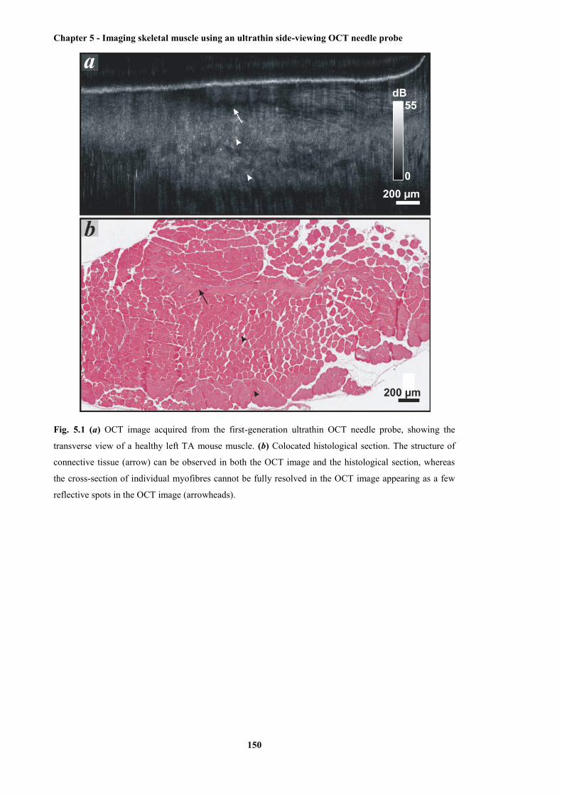
Chapter 5 - Imaging skeletal muscle using an ultrathin side-viewing OCT needle probe
150
Fig. 5.1 (a) OCT image acquired from the first-generation ultrathin OCT needle probe, showing the
transverse view of a healthy left TA mouse muscle. (b) Colocated histological section. The structure of
connective tissue (arrow) can be observed in both the OCT image and the histological section, whereas
the cross-section of individual myofibres cannot be fully resolved in the OCT image appearing as a few
reflective spots in the OCT image (arrowheads).
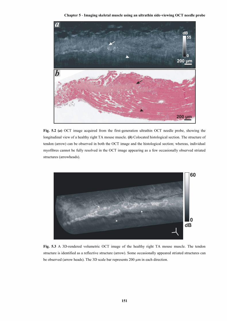
Chapter 5 - Imaging skeletal muscle using an ultrathin side-viewing OCT needle probe
151
Fig. 5.2 (a) OCT image acquired from the first-generation ultrathin OCT needle probe, showing the
longitudinal view of a healthy right TA mouse muscle. (b) Colocated histological section. The structure of
tendon (arrow) can be observed in both the OCT image and the histological section; whereas, individual
myofibres cannot be fully resolved in the OCT image appearing as a few occasionally observed striated
structures (arrowheads).
Fig. 5.3 A 3D-rendered volumetric OCT image of the healthy right TA mouse muscle. The tendon
structure is identified as a reflective structure (arrow). Some occasionally appeared striated structures can
be observed (arrow heads). The 3D scale bar represents 200 µm in each direction.
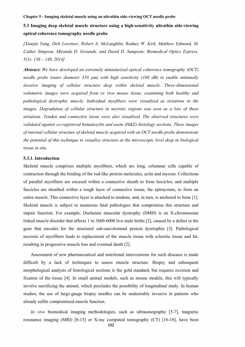
Chapter 5 - Imaging skeletal muscle using an ultrathin side-viewing OCT needle probe
152
5.3 Imaging deep skeletal muscle structure using a high-sensitivity ultrathin side-viewing
optical coherence tomography needle probe
[Xiaojie Yang, Dirk Lorenser, Robert A. McLaughlin, Rodney W. Kirk, Matthew Edmond, M.
Cather Simpson, Miranda D. Grounds, and David D. Sampson; Biomedical Optics Express,
5(1): 136 – 148, 2014]
Abstract: We have developed an extremely miniaturized optical coherence tomography (OCT)
needle probe (outer diameter 310 µm) with high sensitivity (108 dB) to enable minimally
invasive imaging of cellular structure deep within skeletal muscle. Three-dimensional
volumetric images were acquired from ex vivo mouse tissue, examining both healthy and
pathological dystrophic muscle. Individual myofibers were visualized as striations in the
images. Degradation of cellular structure in necrotic regions was seen as a loss of these
striations. Tendon and connective tissue were also visualized. The observed structures were
validated against co-registered hematoxylin and eosin (H&E) histology sections. These images
of internal cellular structure of skeletal muscle acquired with an OCT needle probe demonstrate
the potential of this technique to visualize structure at the microscopic level deep in biological
tissue in situ.
5.3.1. Introduction
Skeletal muscle comprises multiple myofibers, which are long, columnar cells capable of
contraction through the binding of the rod-like protein molecules, actin and myosin. Collections
of parallel myofibers are encased within a connective sheath to form fascicles; and multiple
fascicles are sheathed within a tough layer of connective tissue, the epimysium, to form an
entire muscle. This connective layer is attached to tendons, and, in turn, is anchored to bone [1].
Skeletal muscle is subject to numerous fatal pathologies that compromise this structure and
impair function. For example, Duchenne muscular dystrophy (DMD) is an X-chromosome
linked muscle disorder that affects 1 in 3600-6000 live male births [2], caused by a defect in the
gene that encodes for the structural sub-sarcolemmal protein dystrophin [3]. Pathological
necrosis of myofibers leads to replacement of the muscle tissue with sclerotic tissue and fat,
resulting in progressive muscle loss and eventual death [2].
Assessment of new pharmaceutical and nutritional interventions for such diseases is made
difficult by a lack of techniques to assess muscle structure. Biopsy and subsequent
morphological analysis of histological sections is the gold standard, but requires excision and
fixation of the tissue [4]. In small animal models, such as mouse models, this will typically
involve sacrificing the animal, which precludes the possibility of longitudinal study. In human
studies, the use of large-gauge biopsy needles can be undesirably invasive in patients who
already suffer compromised muscle function.
In vivo biomedical imaging methodologies, such as ultrasonography [5-7], magnetic
resonance imaging (MRI) [8-15] or X-ray computed tomography (CT) [16-18], have been
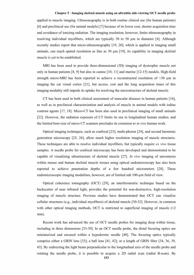
Chapter 5 - Imaging skeletal muscle using an ultrathin side-viewing OCT needle probe
153
applied to muscle imaging. Ultrasonography is in both routine clinical use (for human patients)
[6] and preclinical use (for animal models) [7] because of its lower cost, shorter acquisition time
and avoidance of ionizing radiation. The imaging resolution, however, limits ultrasonography in
resolving individual myofibers, which are typically 30 to 50 µm in diameter [4]. Although
recently studies report that micro-ultrasonography [19, 20], which is applied in imaging small
animals, can reach spatial resolution as fine as 30 µm [19], its capability in imaging skeletal
muscle is yet to be established.
MRI has been used to provide three-dimensional (3D) imaging of dystrophic muscle not
only in human patients [8, 9] but also in canine [10, 11] and murine [12-15] models. High-field
strength micro-MRI has been reported to achieve a reconstructed resolution of ≈30 µm in
imaging the cat visual cortex [21], but access, cost and the long acquisition times of this
imaging modality still impede its uptake for resolving the microstructure of skeletal muscle.
CT has been used in both clinical assessment of muscular diseases in human patients [16],
as well as in preclinical characterization and analysis of muscle in animal models with iodine
contrast agents [17, 18]. Micro-CT has been also used in preclinical imaging of small animals
[22]. However, the radiation exposure of CT limits its use in longitudinal human studies; and
the limited bore-size of micro CT scanners precludes its extension to in vivo human work.
Optical imaging techniques, such as confocal [23], multi-photon [24], and second harmonic
generation microscopy [25, 26], allow much higher resolution imaging of muscle structures.
These techniques are able to resolve individual myofibers, but typically require ex vivo tissue
samples. A needle probe for confocal microscopy has been developed and demonstrated to be
capable of visualizing ultrastructure of skeletal muscle [27]. In vivo imaging of sarcomeres
within mouse and human skeletal muscle tissues using optical endomicroscopy has also been
reported to achieve penetration depths of a few hundred micrometers [28]. These
endomicroscopic imaging modalities, however, are of limited sub 100-µm field of view.
Optical coherence tomography (OCT) [29], an interferometric technique based on the
backscatter of near infrared light, provides the potential for non-destructive, high-resolution
imaging of muscle structure. Previous studies have demonstrated that OCT can visualize
cellular structures (e.g., individual myofibers) of skeletal muscle [30-32]. However, in common
with other optical imaging methods, OCT is restricted to superficial imaging of muscle (≈2
mm).
Recent work has advanced the use of OCT needle probes for imaging deep within tissue,
including in three dimensions [33-39]. In an OCT needle probe, the distal focusing optics are
miniaturized and encased within a hypodermic needle [40]. The focusing optics typically
comprise either a GRIN lens [33]; a ball lens [41, 42]; or a length of GRIN fiber [34, 36, 39,
43]. By redirecting the light beam perpendicular to the longitudinal axis of the needle probe and
rotating the needle probe, it is possible to acquire a 2D radial scan (radial B-scan). By
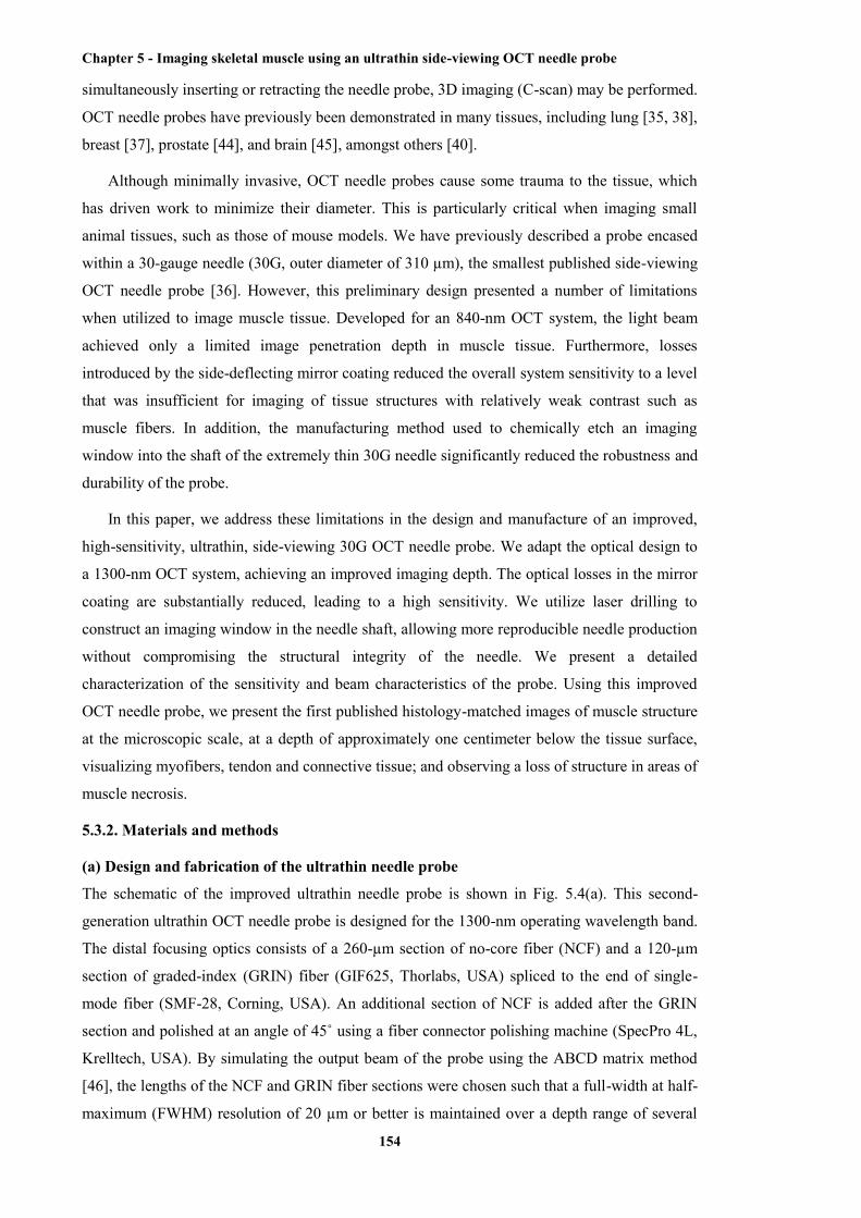
Chapter 5 - Imaging skeletal muscle using an ultrathin side-viewing OCT needle probe
154
simultaneously inserting or retracting the needle probe, 3D imaging (C-scan) may be performed.
OCT needle probes have previously been demonstrated in many tissues, including lung [35, 38],
breast [37], prostate [44], and brain [45], amongst others [40].
Although minimally invasive, OCT needle probes cause some trauma to the tissue, which
has driven work to minimize their diameter. This is particularly critical when imaging small
animal tissues, such as those of mouse models. We have previously described a probe encased
within a 30-gauge needle (30G, outer diameter of 310 µm), the smallest published side-viewing
OCT needle probe [36]. However, this preliminary design presented a number of limitations
when utilized to image muscle tissue. Developed for an 840-nm OCT system, the light beam
achieved only a limited image penetration depth in muscle tissue. Furthermore, losses
introduced by the side-deflecting mirror coating reduced the overall system sensitivity to a level
that was insufficient for imaging of tissue structures with relatively weak contrast such as
muscle fibers. In addition, the manufacturing method used to chemically etch an imaging
window into the shaft of the extremely thin 30G needle significantly reduced the robustness and
durability of the probe.
In this paper, we address these limitations in the design and manufacture of an improved,
high-sensitivity, ultrathin, side-viewing 30G OCT needle probe. We adapt the optical design to
a 1300-nm OCT system, achieving an improved imaging depth. The optical losses in the mirror
coating are substantially reduced, leading to a high sensitivity. We utilize laser drilling to
construct an imaging window in the needle shaft, allowing more reproducible needle production
without compromising the structural integrity of the needle. We present a detailed
characterization of the sensitivity and beam characteristics of the probe. Using this improved
OCT needle probe, we present the first published histology-matched images of muscle structure
at the microscopic scale, at a depth of approximately one centimeter below the tissue surface,
visualizing myofibers, tendon and connective tissue; and observing a loss of structure in areas of
muscle necrosis.
5.3.2. Materials and methods
(a) Design and fabrication of the ultrathin needle probe
The schematic of the improved ultrathin needle probe is shown in Fig. 5.4(a). This second-
generation ultrathin OCT needle probe is designed for the 1300-nm operating wavelength band.
The distal focusing optics consists of a 260-µm section of no-core fiber (NCF) and a 120-µm
section of graded-index (GRIN) fiber (GIF625, Thorlabs, USA) spliced to the end of single-
mode fiber (SMF-28, Corning, USA). An additional section of NCF is added after the GRIN
section and polished at an angle of 45˚ using a fiber connector polishing machine (SpecPro 4L,
Krelltech, USA). By simulating the output beam of the probe using the ABCD matrix method
[46], the lengths of the NCF and GRIN fiber sections were chosen such that a full-width at half-
maximum (FWHM) resolution of 20 µm or better is maintained over a depth range of several

Chapter 5 - Imaging skeletal muscle using an ultrathin side-viewing OCT needle probe
155
100 micrometers in water, taking into account the astigmatism resulting from the cylindrical
output window, as discussed in more detail in the following subsection. The beam propagation
method (BPM) is particularly useful in cases where GRIN fibers with non-parabolic index
profiles are used, or when analyzing the effects of phase masks [47]. In the case of this
particular probe, we used a very high quality GRIN fiber which has a nearly perfect parabolic
profile. Hence, the ABCD method was sufficiently accurate to design the probe and it is faster
and simpler than a rigorous BPM simulation.
A metal reflection coating consisting of a 3-nm chrome adhesion layer and a 300-nm gold
layer is applied to the angle-polished fiber tip using a thermal vacuum deposition machine.
After metallization, the fiber probe is mounted inside a 30G hypodermic needle with a 140-µm
diameter side opening (as shown in Figs. 1(c) and 1(d)). In the first-generation ultrathin OCT
needle probe, the side opening was fabricated via electrochemical etching using a customized
setup [36]. Neither the size nor the geometry of the opening could be precisely controlled and
erosion of the hypodermic needle tubing near the imaging window led to a reduction in
structural integrity of the needle.
In the second-generation ultrathin OCT needle probe, the side opening was fabricated by
laser ablation with a femtosecond laser micromachining system based upon a commercial
Ti:Sapphire amplified femtosecond laser (Mantis (oscillator) and Legend Elite (amplifier),
Coherent Inc., USA). The 800-nm, 100-fs pulsetrain with a repetition rate of 500 Hz was
directed to a micromachining stage (IX-100C, JPSA, Inc. USA). The laser focal spot at the
workpiece had a flat-top intensity profile and a diameter of 50 µm, and pulse energy ranged
from 15 to 40 µJ. The spot was scanned in a circle of radius 45 µm, with 0.5-µm spacing
between successive laser pulses. 20 to 30 passes were required to drill through the needle wall.
As can be seen in the scanning electron microscope (SEM) image of the side opening in Fig.
5.4(c), the non-thermal ablation in the femtosecond regime eliminates problems resulting from a
heat-affected zone surrounding the hole that would otherwise compromise the structural
integrity of the very thin hypodermic needle.
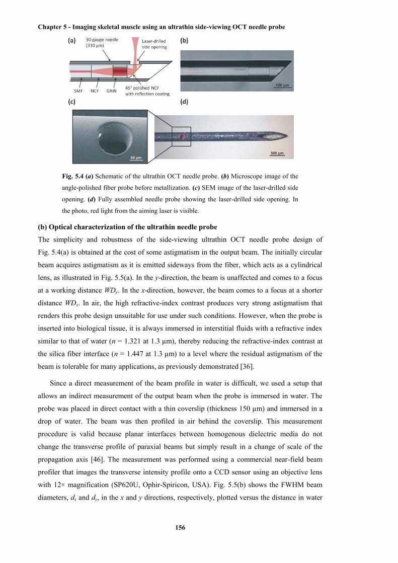
Chapter 5 - Imaging skeletal muscle using an ultrathin side-viewing OCT needle probe
156
Fig. 5.4 (a) Schematic of the ultrathin OCT needle probe. (b) Microscope image of the
angle-polished fiber probe before metallization. (c) SEM image of the laser-drilled side
opening. (d) Fully assembled needle probe showing the laser-drilled side opening. In
the photo, red light from the aiming laser is visible.
(b) Optical characterization of the ultrathin needle probe
The simplicity and robustness of the side-viewing ultrathin OCT needle probe design of
Fig. 5.4(a) is obtained at the cost of some astigmatism in the output beam. The initially circular
beam acquires astigmatism as it is emitted sideways from the fiber, which acts as a cylindrical
lens, as illustrated in Fig. 5.5(a). In the y-direction, the beam is unaffected and comes to a focus
at a working distance WDy. In the x-direction, however, the beam comes to a focus at a shorter
distance WDx. In air, the high refractive-index contrast produces very strong astigmatism that
renders this probe design unsuitable for use under such conditions. However, when the probe is
inserted into biological tissue, it is always immersed in interstitial fluids with a refractive index
similar to that of water (n = 1.321 at 1.3 µm), thereby reducing the refractive-index contrast at
the silica fiber interface (n = 1.447 at 1.3 µm) to a level where the residual astigmatism of the
beam is tolerable for many applications, as previously demonstrated [36].
Since a direct measurement of the beam profile in water is difficult, we used a setup that
allows an indirect measurement of the output beam when the probe is immersed in water. The
probe was placed in direct contact with a thin coverslip (thickness 150 µm) and immersed in a
drop of water. The beam was then profiled in air behind the coverslip. This measurement
procedure is valid because planar interfaces between homogenous dielectric media do not
change the transverse profile of paraxial beams but simply result in a change of scale of the
propagation axis [46]. The measurement was performed using a commercial near-field beam
profiler that images the transverse intensity profile onto a CCD sensor using an objective lens
with 12× magnification (SP620U, Ophir-Spiricon, USA). Fig. 5.5(b) shows the FWHM beam
diameters, dx and dy, in the x and y directions, respectively, plotted versus the distance in water
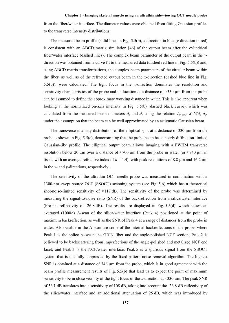
Chapter 5 - Imaging skeletal muscle using an ultrathin side-viewing OCT needle probe
157
from the fiber/water interface. The diameter values were obtained from fitting Gaussian profiles
to the transverse intensity distributions.
The measured beam profile (solid lines in Fig. 5.5(b), x-direction in blue, y-direction in red)
is consistent with an ABCD matrix simulation [46] of the output beam after the cylindrical
fiber/water interface (dashed lines). The complex beam parameter of the output beam in the y-
direction was obtained from a curve fit to the measured data (dashed red line in Fig. 5.5(b)) and,
using ABCD matrix transformations, the complex beam parameters of the circular beam within
the fiber, as well as of the refracted output beam in the x-direction (dashed blue line in Fig.
5.5(b)), were calculated. The tight focus in the x-direction dominates the resolution and
sensitivity characteristics of the probe and its location at a distance of ≈330 µm from the probe
can be assumed to define the approximate working distance in water. This is also apparent when
looking at the normalized on-axis intensity in Fig. 5.5(b) (dashed black curve), which was
calculated from the measured beam diameters dx and dy using the relation Ion-axis ∝ 1/(dx dy)
under the assumption that the beam can be well approximated by an astigmatic Gaussian beam.
The transverse intensity distribution of the elliptical spot at a distance of 330 µm from the
probe is shown in Fig. 5.5(c), demonstrating that the probe beam has a nearly diffraction-limited
Gaussian-like profile. The elliptical output beam allows imaging with a FWHM transverse
resolution below 20 µm over a distance of ≈700 µm from the probe in water (or ≈740 µm in
tissue with an average refractive index of n = 1.4), with peak resolutions of 8.8 µm and 16.2 µm
in the x- and y-directions, respectively.
The sensitivity of the ultrathin OCT needle probe was measured in combination with a
1300-nm swept source OCT (SSOCT) scanning system (see Fig. 5.6) which has a theoretical
shot-noise-limited sensitivity of ≈117 dB. The sensitivity of the probe was determined by
measuring the signal-to-noise ratio (SNR) of the backreflection from a silica/water interface
(Fresnel reflectivity of -26.8 dB). The results are displayed in Fig. 5.5(d), which shows an
averaged (1000×) A-scan of the silica/water interface (Peak 4) positioned at the point of
maximum backreflection, as well as the SNR of Peak 4 at a range of distances from the probe in
water. Also visible in the A-scan are some of the internal backreflections of the probe, where
Peak 1 is the splice between the GRIN fiber and the angle-polished NCF section; Peak 2 is
believed to be backscattering from imperfections of the angle-polished and metalized NCF end
facet; and Peak 3 is the NCF/water interface. Peak 5 is a spurious signal from the SSOCT
system that is not fully suppressed by the fixed-pattern noise removal algorithm. The highest
SNR is obtained at a distance of 346 µm from the probe, which is in good agreement with the
beam profile measurement results of Fig. 5.5(b) that lead us to expect the point of maximum
sensitivity to be in close vicinity of the tight focus of the x-direction at ≈330 µm. The peak SNR
of 56.1 dB translates into a sensitivity of 108 dB, taking into account the -26.8-dB reflectivity of
the silica/water interface and an additional attenuation of 25 dB, which was introduced by
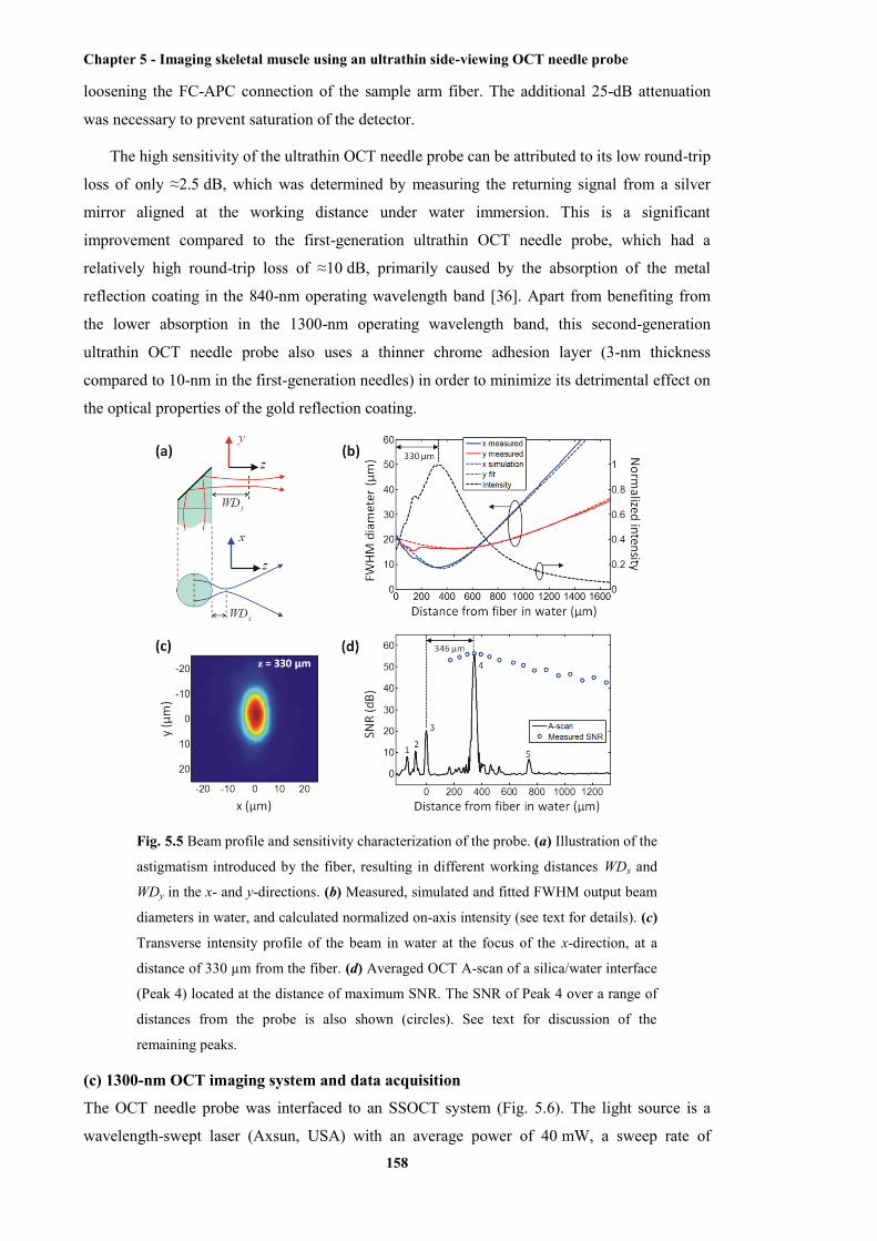
Chapter 5 - Imaging skeletal muscle using an ultrathin side-viewing OCT needle probe
158
loosening the FC-APC connection of the sample arm fiber. The additional 25-dB attenuation
was necessary to prevent saturation of the detector.
The high sensitivity of the ultrathin OCT needle probe can be attributed to its low round-trip
loss of only ≈2.5 dB, which was determined by measuring the returning signal from a silver
mirror aligned at the working distance under water immersion. This is a significant
improvement compared to the first-generation ultrathin OCT needle probe, which had a
relatively high round-trip loss of ≈10 dB, primarily caused by the absorption of the metal
reflection coating in the 840-nm operating wavelength band [36]. Apart from benefiting from
the lower absorption in the 1300-nm operating wavelength band, this second-generation
ultrathin OCT needle probe also uses a thinner chrome adhesion layer (3-nm thickness
compared to 10-nm in the first-generation needles) in order to minimize its detrimental effect on
the optical properties of the gold reflection coating.
Fig. 5.5 Beam profile and sensitivity characterization of the probe. (a) Illustration of the
astigmatism introduced by the fiber, resulting in different working distances WDx and
WDy in the x- and y-directions. (b) Measured, simulated and fitted FWHM output beam
diameters in water, and calculated normalized on-axis intensity (see text for details). (c)
Transverse intensity profile of the beam in water at the focus of the x-direction, at a
distance of 330 µm from the fiber. (d) Averaged OCT A-scan of a silica/water interface
(Peak 4) located at the distance of maximum SNR. The SNR of Peak 4 over a range of
distances from the probe is also shown (circles). See text for discussion of the
remaining peaks.
(c) 1300-nm OCT imaging system and data acquisition
The OCT needle probe was interfaced to an SSOCT system (Fig. 5.6). The light source is a
wavelength-swept laser (Axsun, USA) with an average power of 40 mW, a sweep rate of

Chapter 5 - Imaging skeletal muscle using an ultrathin side-viewing OCT needle probe
159
50 kHz, and a full sweep bandwidth of 100 nm centered at 1310 nm. The source power is
approximately constant within the sweep bandwidth, resulting in a flat-top spectral shape. For
this reason, a Hann window (also known as Hanning window) is applied to the spectral data
prior to the Fourier transform in order to reduce the sidelobes in the axial point spread function.
The resulting FWHM axial resolution in air, after application of the Hann window, is 21 µm.
The source provides a clock output that is generated using a Mach-Zehnder interferometer
(MZI), allowing equidistant sampling in frequency space and eliminating the need for
computationally intensive resampling of the spectral data. The 50-kHz trigger pulses from the
source are gated by a synchronization signal from the needle motion controller which counter-
rotates and retracts the needle during scanning. The motion controller outputs 1600 trigger
pulses per 360 degree rotation of the needle, and it performs a full counter-rotation (360 degrees
clockwise and anticlockwise) every second, resulting in an effective scan rate of ≈3200 A-scans
per second. The OCT signal is sampled with a 12-bit, 500-MS/s digitizer card (ATS9350,
Alazar Technologies, Canada).
The rotation-scanning principle employed acquires A-scans at constant angular intervals,
which inherently results in a circumferential spatial sampling interval that linearly increases as a
function of distance from the needle axis. For this reason, a high angular sampling density of
1600 A-scans per 360 degree rotation was chosen to ensure that, at any given distance from the
needle, the circumferential sampling is always finer than the FWHM transverse resolution of the
beam (see Fig. 5.5(b)). For example, at the maximum expected useful imaging depth in
scattering tissue of 2 mm, the circumferential sampling interval has a size of 8 µm, which is
smaller than the transverse resolution at that depth.
Fig. 5.6 Schematic of the 1300-nm SSOCT needle imaging system. MZI, Mach-
Zehnder interferometer; WDM, wavelength-division multiplexer; VOA, variable optical
attenuator; SYNC, synchronization signal; PC, polarization controller.
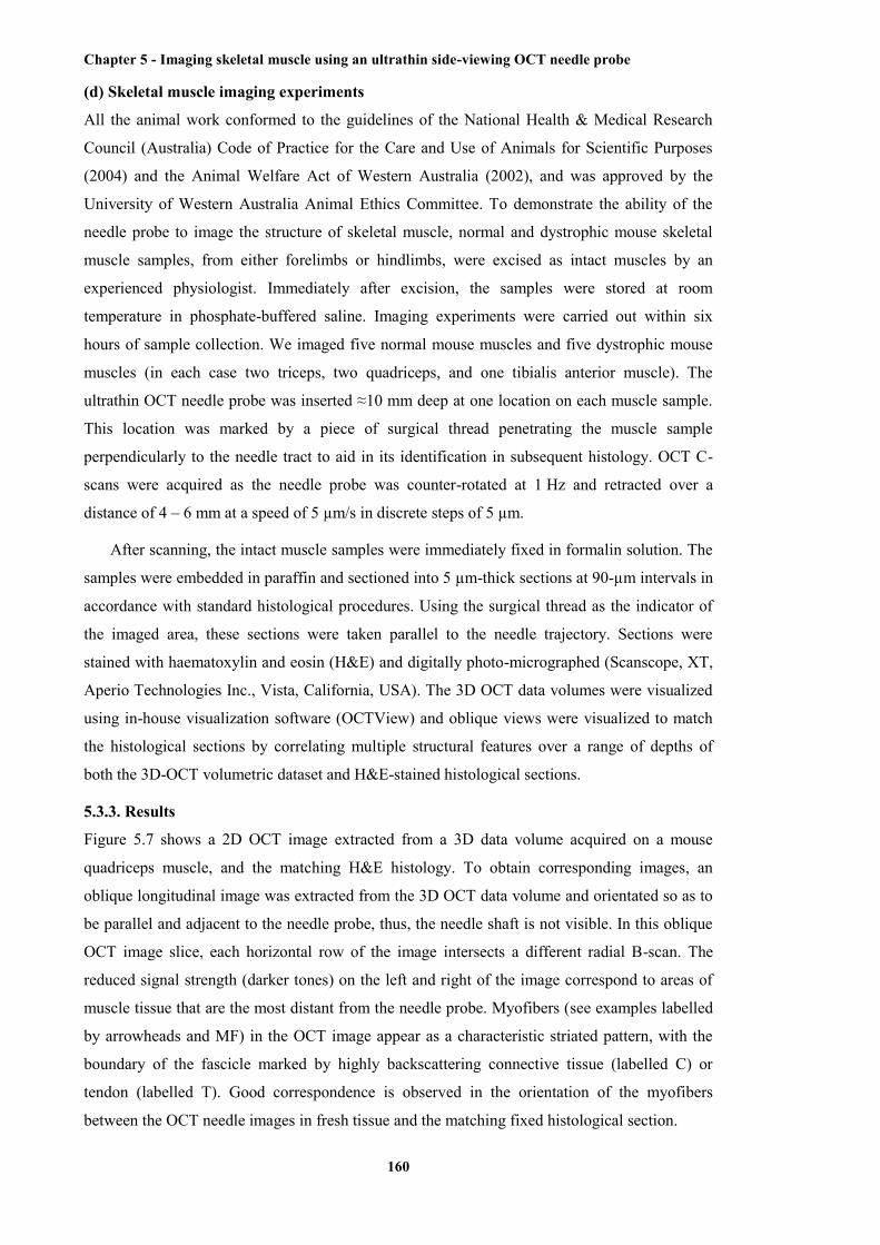
Chapter 5 - Imaging skeletal muscle using an ultrathin side-viewing OCT needle probe
160
(d) Skeletal muscle imaging experiments
All the animal work conformed to the guidelines of the National Health & Medical Research
Council (Australia) Code of Practice for the Care and Use of Animals for Scientific Purposes
(2004) and the Animal Welfare Act of Western Australia (2002), and was approved by the
University of Western Australia Animal Ethics Committee. To demonstrate the ability of the
needle probe to image the structure of skeletal muscle, normal and dystrophic mouse skeletal
muscle samples, from either forelimbs or hindlimbs, were excised as intact muscles by an
experienced physiologist. Immediately after excision, the samples were stored at room
temperature in phosphate-buffered saline. Imaging experiments were carried out within six
hours of sample collection. We imaged five normal mouse muscles and five dystrophic mouse
muscles (in each case two triceps, two quadriceps, and one tibialis anterior muscle). The
ultrathin OCT needle probe was inserted ≈10 mm deep at one location on each muscle sample.
This location was marked by a piece of surgical thread penetrating the muscle sample
perpendicularly to the needle tract to aid in its identification in subsequent histology. OCT C-
scans were acquired as the needle probe was counter-rotated at 1 Hz and retracted over a
distance of 4 – 6 mm at a speed of 5 µm/s in discrete steps of 5 µm.
After scanning, the intact muscle samples were immediately fixed in formalin solution. The
samples were embedded in paraffin and sectioned into 5 µm-thick sections at 90-µm intervals in
accordance with standard histological procedures. Using the surgical thread as the indicator of
the imaged area, these sections were taken parallel to the needle trajectory. Sections were
stained with haematoxylin and eosin (H&E) and digitally photo-micrographed (Scanscope, XT,
Aperio Technologies Inc., Vista, California, USA). The 3D OCT data volumes were visualized
using in-house visualization software (OCTView) and oblique views were visualized to match
the histological sections by correlating multiple structural features over a range of depths of
both the 3D-OCT volumetric dataset and H&E-stained histological sections.
5.3.3. Results
Figure 5.7 shows a 2D OCT image extracted from a 3D data volume acquired on a mouse
quadriceps muscle, and the matching H&E histology. To obtain corresponding images, an
oblique longitudinal image was extracted from the 3D OCT data volume and orientated so as to
be parallel and adjacent to the needle probe, thus, the needle shaft is not visible. In this oblique
OCT image slice, each horizontal row of the image intersects a different radial B-scan. The
reduced signal strength (darker tones) on the left and right of the image correspond to areas of
muscle tissue that are the most distant from the needle probe. Myofibers (see examples labelled
by arrowheads and MF) in the OCT image appear as a characteristic striated pattern, with the
boundary of the fascicle marked by highly backscattering connective tissue (labelled C) or
tendon (labelled T). Good correspondence is observed in the orientation of the myofibers
between the OCT needle images in fresh tissue and the matching fixed histological section.

Chapter 5 - Imaging skeletal muscle using an ultrathin side-viewing OCT needle probe
161
Fig. 5.7 Representative images of normal mouse skeletal muscle. (Left) OCT oblique
slice taken from the 3D OCT volumetric dataset. The striated appearance indicates the
highly organized arrangement of the myofibers (MF and/or arrowhead). Several
structures with higher signal intensity indicate tendon (T) and connective tissue (C).
(Right) Corresponding H&E histology.
Figure 5.8 shows representative images obtained from a dystrophic muscle sample taken
from the quadriceps muscle of an mdx mouse [4]. As with Fig. 5.7, a longitudinal image was
extracted from the 3D OCT volume and matched against histology. The characteristic striated
pattern of myofibers can be seen in the left most area of the image (see examples labelled by
arrowheads and MF), correlating with myofibers visible in the matching histology. An area of
necrosis is visible in the middle section of the histology image, marked by the appearance of
purple-stained, basophilic inflammatory cells, and a “broken” appearance in the adjacent
myofibers. This presents in the OCT image as a loss of striated texture of myofibers (labelled
Necrosis). The normal and necrotic regions are clearly delineated by connective tissue (labelled
C), visible in both images. The appearance of both healthy and necrotic regions of skeletal
muscle imaged with the OCT needle probe are consistent with earlier results obtained with a
standard, external-scanning benchtop OCT system [30, 31]. The OCT image, however, does not
show a structure corresponding to the connective tissue in the right-hand-side of the histological
slide. This is probably because of insufficient signal intensity within that corresponding region
in the OCT image.
Several views of a 3D rendered visualization of the mouse skeletal muscle OCT image are
shown in Fig. 5.9, and the associated video is available as Supplementary Video 3. During each
scan, a 3D cylinder of OCT data is acquired, with the central axis located along the needle
trajectory (labelled N), and the radius of the cylinder corresponding to the image depth from the
needle shaft. Fig. 5.9(a) shows the uncropped data set, with the dashed lines indicating the
different cropping planes used in Fig. 5.9(b)-(d). Note that Fig. 5.9(d) is cropped to show the
imaging plane that was histology matched in Fig. 5.7. Cropping of the 3D data allows
inspection of the 3D structure of the muscle fibers. Connective tissue and tendon are also
visible, labelled C and T, respectively, from different orientations.
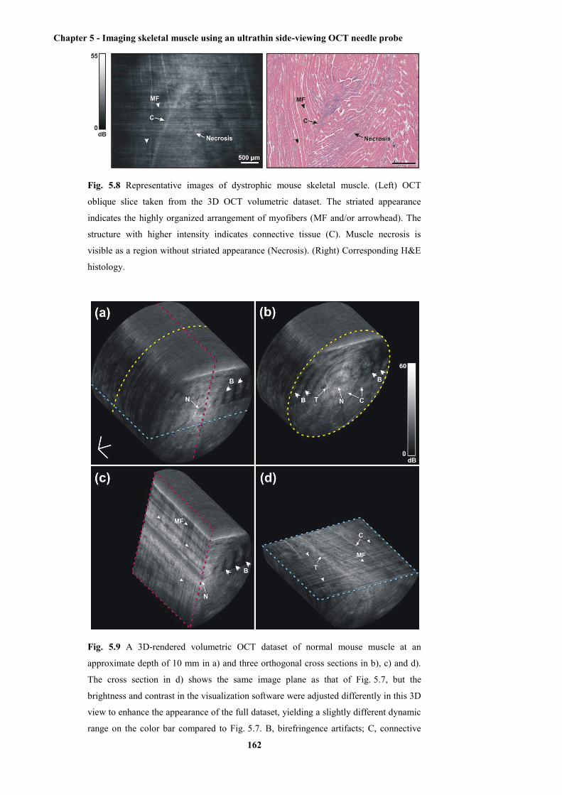
Chapter 5 - Imaging skeletal muscle using an ultrathin side-viewing OCT needle probe
162
Fig. 5.8 Representative images of dystrophic mouse skeletal muscle. (Left) OCT
oblique slice taken from the 3D OCT volumetric dataset. The striated appearance
indicates the highly organized arrangement of myofibers (MF and/or arrowhead). The
structure with higher intensity indicates connective tissue (C). Muscle necrosis is
visible as a region without striated appearance (Necrosis). (Right) Corresponding H&E
histology.
Fig. 5.9 A 3D-rendered volumetric OCT dataset of normal mouse muscle at an
approximate depth of 10 mm in a) and three orthogonal cross sections in b), c) and d).
The cross section in d) shows the same image plane as that of Fig. 5.7, but the
brightness and contrast in the visualization software were adjusted differently in this 3D
view to enhance the appearance of the full dataset, yielding a slightly different dynamic
range on the color bar compared to Fig. 5.7. B, birefringence artifacts; C, connective
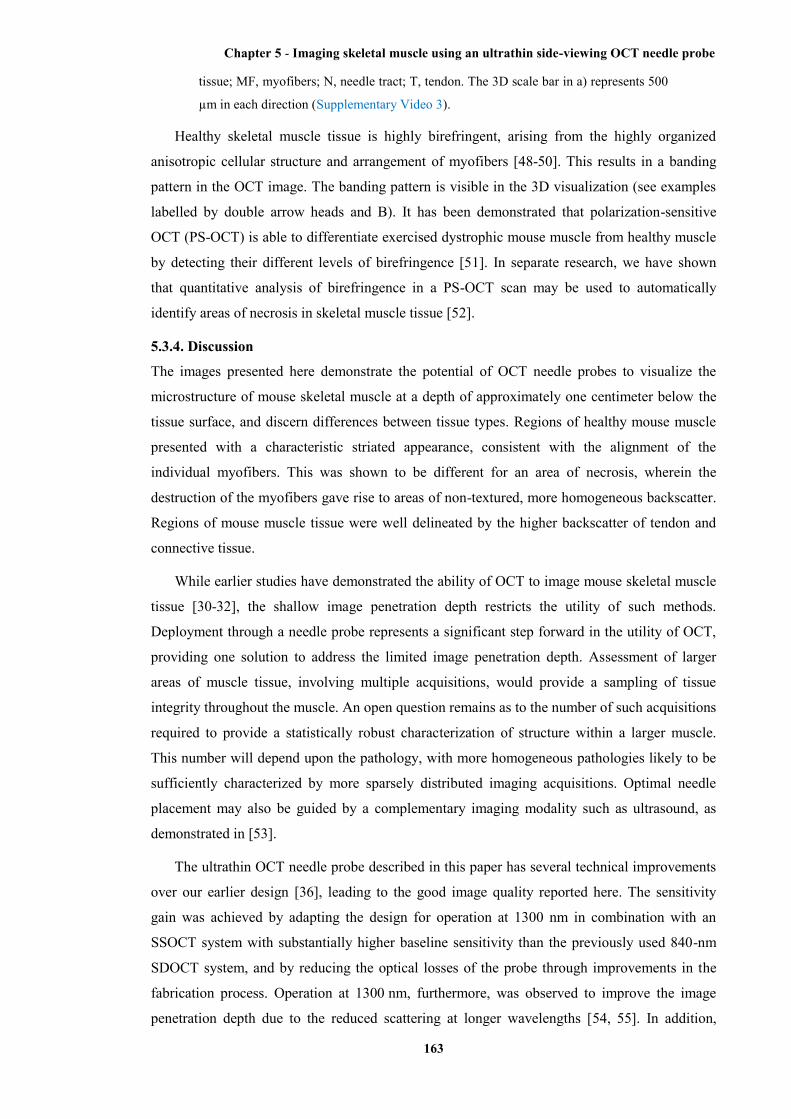
Chapter 5 - Imaging skeletal muscle using an ultrathin side-viewing OCT needle probe
163
tissue; MF, myofibers; N, needle tract; T, tendon. The 3D scale bar in a) represents 500
µm in each direction (Supplementary Video 3).
Healthy skeletal muscle tissue is highly birefringent, arising from the highly organized
anisotropic cellular structure and arrangement of myofibers [48-50]. This results in a banding
pattern in the OCT image. The banding pattern is visible in the 3D visualization (see examples
labelled by double arrow heads and B). It has been demonstrated that polarization-sensitive
OCT (PS-OCT) is able to differentiate exercised dystrophic mouse muscle from healthy muscle
by detecting their different levels of birefringence [51]. In separate research, we have shown
that quantitative analysis of birefringence in a PS-OCT scan may be used to automatically
identify areas of necrosis in skeletal muscle tissue [52].
5.3.4. Discussion
The images presented here demonstrate the potential of OCT needle probes to visualize the
microstructure of mouse skeletal muscle at a depth of approximately one centimeter below the
tissue surface, and discern differences between tissue types. Regions of healthy mouse muscle
presented with a characteristic striated appearance, consistent with the alignment of the
individual myofibers. This was shown to be different for an area of necrosis, wherein the
destruction of the myofibers gave rise to areas of non-textured, more homogeneous backscatter.
Regions of mouse muscle tissue were well delineated by the higher backscatter of tendon and
connective tissue.
While earlier studies have demonstrated the ability of OCT to image mouse skeletal muscle
tissue [30-32], the shallow image penetration depth restricts the utility of such methods.
Deployment through a needle probe represents a significant step forward in the utility of OCT,
providing one solution to address the limited image penetration depth. Assessment of larger
areas of muscle tissue, involving multiple acquisitions, would provide a sampling of tissue
integrity throughout the muscle. An open question remains as to the number of such acquisitions
required to provide a statistically robust characterization of structure within a larger muscle.
This number will depend upon the pathology, with more homogeneous pathologies likely to be
sufficiently characterized by more sparsely distributed imaging acquisitions. Optimal needle
placement may also be guided by a complementary imaging modality such as ultrasound, as
demonstrated in [53].
The ultrathin OCT needle probe described in this paper has several technical improvements
over our earlier design [36], leading to the good image quality reported here. The sensitivity
gain was achieved by adapting the design for operation at 1300 nm in combination with an
SSOCT system with substantially higher baseline sensitivity than the previously used 840-nm
SDOCT system, and by reducing the optical losses of the probe through improvements in the
fabrication process. Operation at 1300 nm, furthermore, was observed to improve the image
penetration depth due to the reduced scattering at longer wavelengths [54, 55]. In addition,

Chapter 5 - Imaging skeletal muscle using an ultrathin side-viewing OCT needle probe
164
improved mechanical robustness was obtained by using non-thermal ablation with femtosecond
laser pulses to fashion the imaging window. This also provided improved control over the
dimensions of the window and improved structural integrity of the adjacent sections of the
needle shaft. Such improvements in the OCT needle manufacturing process are important steps
to transition these probes from an optics research environment to the larger-scale production
required for pre-clinical and clinical usage.
The 2D OCT images of Figs. 4 and 5 exhibit some horizontal striations (perpendicular to
the needle axis), caused by variation in the SNR of individual B-scans. We observed this to be
due to small, isolated pieces of tissue being temporarily lodged in the needle hole through which
imaging occurs. Such tissue debris is typically cleared within one or two rotations of the needle
probe. The effects of such tissue debris could be reduced by increasing the spatial sampling
density in the pullback direction and performing spatial averaging along that axis in post-
processing.
The utility of OCT needle probes in the diagnostic assessment of muscle pathology could be
enhanced by employing quantitative image analysis for identifying regions of diseased tissue.
We note that a range of such techniques is under development, quantifying the distinction
between diseased and healthy tissue using optical properties such as the optical attenuation
coefficient [56, 57] or birefringence [52, 58].
5.3.5. Conclusion
In this paper, a highly optimized, high-sensitivity, ultrathin, side-viewing OCT needle probe has
been presented. With an outer diameter of 310 µm, the needle probe presents a minimally
invasive means of performing OCT imaging deep within tissue. We have presented the first
published 3D OCT data volumes of mouse skeletal muscle obtained by an OCT needle probe of
significantly improved performance and validated against co-registered H&E histology sections.
Results demonstrated the ability of such needle probes to distinguish the appearance of healthy
and necrotic mouse muscle tissue, and differentiate such areas from connective tissue and
tendon. These preliminary findings demonstrate the potential of OCT needle probes to provide a
new way to visualize in situ, deep within the tissue, the structure and integrity of skeletal
muscle.
5.3.6 Acknowledgements
The authors acknowledge Dr. Gavin J. Pinniger for providing the skeletal muscle tissue
samples. The authors acknowledge the facilities, and the scientific and technical assistance of
the Australian Microscopy & Microanalysis Research Facility at the Centre for Microscopy,
Characterisation and Analysis, The University of Western Australia, a facility funded by the
University, State and Commonwealth Governments. We also wish to acknowledge
CELLCentral, University of Western Australia, for the preparation of histological slides. We
acknowledge the support from the Western Australian node of the Australian National
Chapter 5 - Imaging skeletal muscle using an ultrathin side-viewing OCT needle probe
165
Fabrication Facility for vacuum deposition of the metal reflection coatings in the OCT needle
fabrication, and we especially thank Nir Zvison. We also thank Peijun Gong for his help in the
generation of the video. Robert A. McLaughlin is supported by a fellowship from Cancer
Council Western Australia and this research is supported in part by funding from the National
Breast Cancer Foundation, Australia.
5.3.7 References
[1] E. N. Marieb, “Human anatomy & physiology,” in Human anatomy & physiology, K. Ueno,
ed. (Daryl Fox, San Francisco, USA, 2001) p. 324.
[2] K. Bushby, R. Finkel, D. J. Birnkrant, L. E. Case, P. R. Clemens, L. Cripe, A. Kaul, K.
Kinnett, C. McDonald, S. Pandya, J. Poysky, F. Shapiro, J. Tomezsko, C. Constantin, and D. C.
C. Working, "Diagnosis and management of Duchenne muscular dystrophy, Part 1: diagnosis,
and pharmacological and psychosocial management," Lancet Neurol. 9(1), 77-93 (2010).
[3] E. P. Hoffman, K. H. Fischbeck, R. H. Brown, M. Johnson, R. Medori, J. D. Loike, J. B.
Harris, R. Waterston, M. Brooke, and L. Specht, "Characterization of dystrophin in muscle -
biopsy specimens from patients with Duchenne's or Becker's muscular dystrophy," New Engl. J.
Med. 318(21), 1363-1368 (1988).
[4] M. D. Grounds, H. G. Radley, G. S. Lynch, K. Nagaraju, and A. De Luca, "Towards
developing standard operating procedures for pre-clinical testing in the mdx mouse model of
Duchenne muscular dystrophy," Neurobiol. Dis. 31(1), 1-19 (2008).
[5] F. S. Foster, C. J. Pavlin, K. A. Harasiewicz, D. A. Christopher, and D. H. Turnbull,
"Advances in ultrasound biomicroscopy," Ultrasound Med. Biol. 26(1), 1-27 (2000).
[6] S. Sipila, and H. Suominen, "Ultrasound imaging of the quadriceps muscle in elderly
athletes and untrained men," Muscle Nerve 14(6), 527-533 (1991).
[7] K. D. Wallace, J. N. Marsh, S. L. Baldwin, A. M. Connolly, R. Keeling, G. M. Lanza, S. A.
Wickline, and M. S. Hughes, "Sensitive ultrasonic delineation of steroid treatment in living
dystrophic mice with energy-based and entropy-based radio frequency signal processing," IEEE
Trans. Ultrason., Ferroelectr., Freq. Control 54(11), 2291-2299 (2007).
[8] J. Philpot, C. Sewry, J. Pennock, and V. Dubowitz, "Clinical phenotype in congenital
muscular dystrophy - correlation with expression of merosin in skeletal muscle,"
Neuromuscular Disord. 5(4), 301-305 (1995).
[9] J. Phoenix, D. Betal, N. Roberts, T. R. Helliwell, and R. H. T. Edwards, "Objective
quantification of muscle and fat in human dystrophic muscle by magnetic resonance image
analysis," Muscle Nerve 19(3), 302-310 (1996).
[10] M. Kobayashi, A. Nakamura, D. Hasegawa, M. Fujita, H. Orima, and S. Takeda,
"Evaluation of dystrophic dog pathology by fat-suppressed T2-weighted imaging," Muscle
Nerve 40(5), 815-826 (2009).
[11] J. N. Kornegay, J. A. Li, J. R. Bogan, D. J. Bogan, C. L. Chen, H. Zheng, B. Wang, C. P.
Qiao, J. F. Howard, and X. A. Xiao, "Widespread muscle expression of an AAV9 human mini-

Chapter 5 - Imaging skeletal muscle using an ultrathin side-viewing OCT needle probe
166
dystrophin vector after intravenous injection in neonatal dystrophin-deficient dogs," Mol. Ther.
18(8), 1501-1508 (2010).
[12] H. Amthor, T. Egelhof, I. McKinnell, M. E. Ladd, I. Janssen, J. Weber, H. Sinn, H. H.
Schrenk, M. Forsting, T. Voit, and V. Straub, "Albumin targeting of damaged muscle fibres in
the mdx mouse can be monitored by MRI," Neuromuscular Disord. 14(12), 791-796 (2004).
[13] L. M. McIntosh, B. E. Baker, and J. E. Anderson, "Magnetic resonance imaging of
regenerating and dystrophic mouse muscle," Biochem. Cell Biol. 76(2-3), 532-541 (1998).
[14] V. Straub, K. M. Donahue, V. Allamand, R. L. Davisson, Y. R. Kim, and K. P. Campbell,
"Contrast agent-enhanced magnetic resonance imaging of skeletal muscle damage in animal
models of muscular dystrophy," Magnet. Reson. Med. 44(4), 655-659 (2000).
[15] G. Walter, L. Cordier, D. Bloy, and H. L. Sweeney, "Noninvasive monitoring of gene
correction in dystrophic muscle," Magnet. Reson. Med. 54(6), 1369-1376 (2005).
[16] M. Swash, M. M. Brown, and C. Thakkar, "CT muscle imaging and the clinical -
assessment of neuromuscular disease," Muscle Nerve 18(7), 708-714 (1995).
[17] S. J. Schambach, S. Bag, V. Steil, C. Isaza, L. Schilling, C. Groden, and M. A. Brockmann,
"Ultrafast high-resolution in vivo volume-CTA of mice cerebral vessels," Stroke 40(4), 1444-
1450 (2009).
[18] X. Y. Zhu, M. Rodriguez-Porcel, M. D. Bentley, A. R. Chade, V. Sica, C. Napoli, N.
Caplice, E. L. Ritman, A. Lerman, and L. O. Lerman, "Antioxidant intervention attenuates
myocardial neovascularization in hypercholesterolemia," Circulation 109(17), 2109-2115
(2004).
[19] M. Ni, M. Zhang, S. F. Ding, W. Q. Chen, and Y. Zhang, "Micro-ultrasound imaging
assessment of carotid plaque characteristics in apolipoprotein-E knockout mice,"
Atherosclerosis 197(1), 64-71 (2008).
[20] A. R. Patel, E. S. Y. Chan, D. E. Hansel, C. T. Powell, W. D. Heston, and W. A. Larchian,
"Transabdominal micro-ultrasound imaging of bladder cancer in a mouse model: a validation
study," Urology 75(4), 799-804 (2010).
[21] P. J. Bolan, E. Yacoub, M. Garwood, K. Ugurbil, and N. Harel, "In vivo micro-MRI of
intracortical neurovasculature," Neuroimage 32(1), 62-69 (2006).
[22] S. J. Schambach, S. Bag, L. Schilling, C. Groden, and M. A. Brockmann, "Application of
micro-CT in small animal imaging," Methods 50(1), 2-13 (2010).
[23] T. Masuda, N. Fujimaki, E. Ozawa, and H. Ishikawa, "Confocal laser microscopy of
dystrophin localization in guinea pig skeletal muscle fibers," J. Cell Biol. 119(3), 543-548
(1992).
[24] M. Bartoli, N. Bourg, D. Stockholm, F. Raynaud, A. Delevacque, Y. Han, P. Borel, K.
Seddik, N. Armande, and I. Richard, "A mouse model for monitoring calpain activity under
physiological and pathological conditions," J. Biol. Chem. 281(51), 39672-39680 (2006).
Chapter 5 - Imaging skeletal muscle using an ultrathin side-viewing OCT needle probe
167
[25] S. V. Plotnikov, A. M. Kenny, S. J. Walsh, B. Zubrowski, C. Joseph, V. L. Scranton, G. A.
Kuchel, D. Dauser, M. S. Xu, C. C. Pilbeam, D. J. Adams, R. P. Dougherty, P. J. Campagnola,
and W. A. Mohler, "Measurement of muscle disease by quantitative second-harmonic
generation imaging," J. Biomed. Opt. 13(4), 044018 (2008).
[26] O. Friedrich, M. Both, C. Weber, S. Schurmann, M. D. H. Teichmann, F. von Wegner, R.
H. A. Fink, M. Vogel, J. S. Chamberlain, and C. Garbe, "Microarchitecture is severely
compromised but motor protein function is preserved in dystrophic mdx skeletal muscle,"
Biophys. J. 98(4), 606-616 (2010).
[27] R. S. Pillai, D. Lorenser, and D. D. Sampson, "Deep-tissue access with confocal
fluorescence microendoscopy through hypodermic needles," Opt. Express 19(8), 7213-7221
(2011).
[28] M. E. Llewellyn, R. P. J. Barretto, S. L. Delp, and M. J. Schnitzer, "Minimally invasive
high-speed imaging of sarcomere contractile dynamics in mice and humans," Nature 454(7205),
784-788 (2008).
[29] D. Huang, E. A. Swanson, C. P. Lin, J. S. Schuman, W. G. Stinson, W. Chang, M. R. Hee,
T. Flotte, K. Gregory, C. A. Puliafito, and J. G. Fujimoto, "Optical coherence tomography,"
Science 254(5035), 1178-1181 (1991).
[30] B. R. Klyen, J. J. Armstrong, S. G. Adie, H. G. Radley, M. D. Grounds, and D. D.
Sampson, "Three-dimensional optical coherence tomography of whole-muscle autografts as a
precursor to morphological assessment of muscular dystrophy in mice," J. Biomed. Opt. 13(1),
011003 (2008).
[31] B. R. Klyen, T. Shavlakadze, H. G. Radley-Crabb, M. D. Grounds, and D. D. Sampson,
"Identification of muscle necrosis in the mdx mouse model of Duchenne muscular dystrophy
using three-dimensional optical coherence tomography," J. Biomed. Opt. 16(7), 076013 (2011).
[32] R. M. Lovering, S. B. Shah, S. J. P. Pratt, W. Gong, and Y. Chen, "Architecture of healthy
and dystrophic muscles detected by optical coherence tomography," Muscle Nerve 47(4), 588-
590 (2013).
[33] X. D. Li, C. Chudoba, T. Ko, C. Pitris, and J. G. Fujimoto, "Imaging needle for optical
coherence tomography," Opt. Lett. 25(20), 1520-1522 (2000).
[34] Y. C. Wu, J. F. Xi, L. Huo, J. Padvorac, E. J. Shin, S. A. Giday, A. M. Lennon, M. I. F.
Canto, J. H. Hwang, and X. D. Li, "Robust high-resolution fine OCT needle for side-viewing
interstitial tissue imaging," IEEE J. Sel. Topics Quantum Electron. 16(4), 863-869 (2010).
[35] B. C. Quirk, R. A. McLaughlin, A. Curatolo, R. W. Kirk, P. B. Noble, and D. D. Sampson,
"In situ imaging of lung alveoli with an optical coherence tomography needle probe," J.
Biomed. Opt. 16(3), 036009 (2011).
[36] D. Lorenser, X. Yang, R. W. Kirk, B. C. Quirk, R. A. McLaughlin, and D. D. Sampson,
"Ultrathin side-viewing needle probe for optical coherence tomography," Opt. Lett. 36(19),
3894-3896 (2011).
Chapter 5 - Imaging skeletal muscle using an ultrathin side-viewing OCT needle probe
168
[37] R. A. McLaughlin, B. C. Quirk, A. Curatolo, R. W. Kirk, L. Scolaro, D. Lorenser, P. D.
Robbins, B. A. Wood, C. M. Saunders, and D. D. Sampson, "Imaging of breast cancer with
optical coherence tomography needle probes: feasibility and initial results," IEEE J. Sel. Topics
Quantum Electron. 18(3), 1184-1191 (2012).
[38] R. A. McLaughlin, X. Yang, B. C. Quirk, D. Lorenser, R. W. Kirk, P. B. Noble, and D. D.
Sampson, "Static and dynamic imaging of alveoli using optical coherence tomography needle
probes," J. Appl. Physiol. 113(6), 967-974 (2012).
[39] L. Scolaro, D. Lorenser, R. A. McLaughlin, B. C. Quirk, R. W. Kirk, and D. D. Sampson,
"High-sensitivity anastigmatic imaging needle for optical coherence tomography," Opt. Lett.
37(24), 5247-5249 (2012).
[40] R. A. McLaughlin, D. Lorenser, and D. D. Sampson, "Needle probes in optical coherence
tomography," in Handbook of Coherent-Domain Optical Methods: Biomedical Diagnostics,
Environmental Monitoring, and Material Science, V. V. Tuchin, ed. (Springer
Science+Business, New York, USA, 2013), pp. 1065-1102.
[41] V. X. D. Yang, L. Mao, N. Munce, B. Standish, N. E. Marcon, W. Kucharczyk, B. C.
Wilson, and I. A. Vitkin, "Interstitial Doppler optical coherence tomography," Opt. Lett. 30(14),
1791-1793 (2005).
[42] K. M. Tan, M. Shishkov, A. Chee, M. B. Applegate, B. E. Bouma, and M. J. Suter,
"Flexible transbronchial optical frequency domain imaging smart needle for biopsy guidance,"
Biomed. Opt. Express 3(8), 1947-1954 (2012).
[43] W. A. Reed, M. F. Yan, and M. J. Schnitzer, "Gradient-index fiber-optic microprobes for
minimally invasive in vivo low-coherence interferometry," Opt. Lett. 27(20), 1794-1796 (2002).
[44] B. A. Standish, K. K. C. Lee, X. Jin, A. Mariampillai, N. R. Munce, M. F. G. Wood, B. C.
Wilson, I. A. Vitkin, and V. X. D. Yang, "Interstitial Doppler optical coherence tomography as
a local tumor necrosis predictor in photodynamic therapy of prostatic carcinoma: an in vivo
study," Cancer Res. 68(23), 9987-9995 (2008).
[45] M. S. Jafri, R. Tang, and C. M. Tang, "Optical coherence tomography guided neurosurgical
procedures in small rodents," J. Neurosci. Meth. 176(2), 85-95 (2009).
[46] A. E. Siegman, Lasers (University Science Books, CA, USA, 1986).
[47] D. Lorenser, X. Yang, and D. D. Sampson, “Accuate modeling and design of graded-index
fiber probes for optical cohernece tomography using the beam propagation method,” IEEE
Photonics J. 5(2), 3900015 (2013).
[48] R. H. Colby, "Intrinsic birefringence of glycerinated myofibrils," J. Cell Biol. 51(3), 763-
771 (1971).
[49] Y. Yeh, R. J. Baskin, R. A. Brown, and K. Burton, "Depolarization spectrum of diffracted
light from muscle fiber - the intrinsic anisotropy component," Biophys. J. 47(5), 739-742
(1985).

Chapter 5 - Imaging skeletal muscle using an ultrathin side-viewing OCT needle probe
169
[50] R. C. Haskell, F. D. Carlson, and P. S. Blank, "Form birefringence of muscle," Biophys. J.
56(2), 401-413 (1989).
[51] J. J. Pasquesi, S. C. Schlachter, M. D. Boppart, E. Chaney, S. J. Kaufman, and S. A.
Boppart, "In vivo detection of exercise-induced ultrastructural changes in genetically-altered
murine skeletal muscle using polarization-sensitive optical coherence tomography," Opt.
Express 14(4), 1547-1556 (2006).
[52] X. Yang, L. Chin, B. R. Klyen, T. Shavlakadze, R. A. McLaughlin, M. D. Grounds, and D.
D. Sampson, "Quantitative assessment of muscle damage in the mdx mouse model of Duchenne
muscular dystrophy using polarization-sensitive optical coherence tomography," J. Appl.
Physiol. 115(9), 1393-1401 (2013).
[53] A. Curatolo, R. A. McLaughlin, B. C. Quirk, R. W. Kirk, A. G. Bourke, B. A. Wood, P. D.
Robbins, C. M. Saunders, and D. D. Sampson, "Ultrasound-guided optical coherence
tomography needle probe for the assessment of breast cancer tumor margins," Am. J.
Roentgenol. 199(4), W520-W522 (2012).
[54] J. M. Schmitt, A. Knuttel, M. Yadlowsky, and M. A. Eckhaus, "Optical coherence
tomography of a dense tissue - statistics of attenuation and backscattering," Phys. Med. Biol.
39(10), 1705-1720 (1994).
[55] A. W. Sainter, T. A. King, and M. R. Dickinson, "Effect of target biological tissue and
choice of light source," J. Biomed. Opt. 9(1), 193-199 (2004).
[56] L. Scolaro, R. A. McLaughlin, B. R. Klyen, B. A. Wood, P. D. Robbins, C. M. Saunders,
S. L. Jacques, and D. D. Sampson, "Parametric imaging of the local attenuation coefficient in
human axillary lymph nodes assessed using optical coherence tomography," Biomed. Opt.
Express 3(2), 366-379 (2012).
[57] R. A. McLaughlin, L. Scolaro, P. Robbins, C. Saunders, S. L. Jacques, and D. D. Sampson,
"Parametric imaging of cancer with optical coherence tomography," J. Biomed. Opt. 15(4),
046029 (2010).
[58] L. Chin, X. Yang, R. A. McLaughlin, P. B. Noble, and D. D. Sampson, "En face parametric
imaging of tissue birefringence using polarization-sensitive optical coherence tomography," J.
Biomed. Opt. 18(6), 066005 (2013).
5.4 Effect of the relative orientation of the needle insertion and myofibres
The orientation of the imaging needle relative to the direction of the myofibres was observed to
have an effect on the ability to discern the myofibre striations. Two possible orientations are
illustrated in Fig. 5.10. The imaging view (transverse or longitudinal) is constructed by rotating
and retracting the needle, and extracting a 2D image plane that is parallel to the direction of
retraction of the needle. Figure 5.10(a) shows the needle inserted into a section of muscle, with
the needle orientated along the muscle fibres. The radial B-scan (c) is orientated perpendicular
to the myofibres, and the longitudinal view is generated by taking an imaging plane parallel to
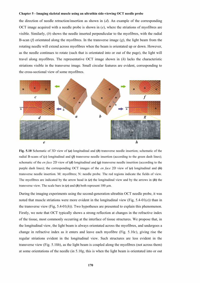
Chapter 5 - Imaging skeletal muscle using an ultrathin side-viewing OCT needle probe
170
the direction of needle retraction/insertion as shown in (d). An example of the corresponding
OCT image acquired with a needle probe is shown in (e), where the striations of myofibres are
visible. Similarly, (b) shows the needle inserted perpendicular to the myofibres, with the radial
B-scan (f) orientated along the myofibres. In the transverse image (g), the light beam from the
rotating needle will extend across myofibres when the beam is orientated up or down. However,
as the needle continues to rotate (such that is orientated into or out of the page), the light will
travel along myofibres. The representative OCT image shown in (h) lacks the characteristic
striations visible in the transverse image. Small circular features are evident, corresponding to
the cross-sectional view of some myofibres.
Fig. 5.10 Schematic of 3D view of (a) longitudinal and (b) transverse needle insertion; schematic of the
radial B-scans of (c) longitudinal and (f) transverse needle insertion (according to the green dash lines);
schematic of the en face 2D view of (d) longitudinal and (g) transverse needle insertion (according to the
purple dash lines); the corresponding OCT images of the en face 2D view of (e) longitudinal and (h)
transverse needle insertion. M: myofibres; N: needle probe. The red regions indicate the fields of view.
The myofibres are indicated by the arrow head in (e) the longitudinal view and by the arrows in (h) the
transverse view. The scale bars in (e) and (h) both represent 100 µm.
During the imaging experiments using the second-generation ultrathin OCT needle probe, it was
noted that muscle striations were more evident in the longitudinal view (Fig, 5.4-01(e)) than in
the transverse view (Fig, 5.4-01(h)). Two hypotheses are presented to explain this phenomenon.
Firstly, we note that OCT typically shows a strong reflection at changes in the refractive index
of the tissue, most commonly occurring at the interface of tissue structures. We propose that, in
the longitudinal view, the light beam is always orientated across the myofibres, and undergoes a
change in refractive index as it enters and leave each myofibre (Fig. 5.10c), giving rise the
regular striations evident in the longitudinal view. Such structures are less evident in the
transverse view (Fig. 5.10h), as the light beam is coupled along the myofibres (not across them)
at some orientations of the needle (in 5.10g, this is when the light beam is orientated into or out
Chapter 5 - Imaging skeletal muscle using an ultrathin side-viewing OCT needle probe
171
of the page). In such orientations, the light does not intersect the boundary of the myofibres,
thus shows less discernible backscatter.
Secondly, we hypothesise that, as the needle is inserted across and through many myofibres to
acquire the transverse view (Fig. 5.10b), it may damage the myofibres. The resulting optical
interface between the needle and adjacent, severed myofibres will present a rough optical
surface which may backscatter light in many directions, only some of which will be detected by
the needle probe.
The relationship between imaging geometry and the detection of anatomical features warrants
additional study, which lies outside of the scope of this thesis. However, our results have
established that the imaging geometry does have an impact of clarity with which features such
as the striations of myofibres may be discerned.
5.5 Chapter summary
The first-generation of ultrathin (30G) side-viewing OCT needle probe was applied to imaging
skeletal muscle. However, the moderate sensitivity (84 dB) makes the needle probe bare enough
to resolve the internal ultrastructure, such as individual myofibres, of skeletal muscle. The
second-generation of ultrathin side-viewing OCT needle probe possesses an improved
mechanical integrity and, more importantly, sensitivity (108 dB). The application of this
second-generation OCT needle probe in imaging skeletal muscle has been successfully
performed on both healthy and dystrophic mouse muscles. Compared with the colocated
histological sections, individual myofibres and other internal structures, such as connective
tissue and tendon, were clearly visualised from the acquired imaging data. From the imaging
data of the dystrophic mouse muscle, muscle damage was differentiated from surrounding
undamaged tissue. This differentiation was validated by the colocated histological sections.
Therefore, the capability of the second-generation ultrathin side-viewing OCT needle probe in
resolving ultrastructure (e.g., individual myofibres) and differentiating pathological muscle
damage deep inside skeletal muscle has been experimental demonstrated.
It was noted from the acquired OCT imaging data that the longitudinal view of skeletal muscle
contained more evident ultrastructures, striated pattern of myofibres, compared to the transverse
view. This phenomenon was hypothesised to be resulted from several mechanisms. One of the
possible mechanisms is that the incident light will experience multiple changes in refractive
index when acquiring the longitudinal view of myofibres. However, such experience will not
occur when acquiring the transverse view of myofibres due to the optical isotropy along the
length of each myofibre. Another possible mechanism is that the irregular interfaces between
the needle and the myofibres, which are created by the disruption and cut of the myofibres
operated by the needle insertion, will reduce the amount of backscattered light. Therefore, the
signal intensity is less in the transverse view of myofibres than in the longitudinal view.

Chapter 6 - Conclusion
172
Chapter 6
Conclusion
6.1 Significance of the research outcomes
This thesis has focused on overcoming the impediments of OCT in skeletal muscle imaging.
Specifically, the imaging modality of PS-OCT, an extension of OCT, was applied to the
measurement of muscle birefringence and quantitative assessment of muscle damage within
dystrophic muscle based on the correlation between muscle damage and low birefringence. This
application was able to overcome the limitation of OCT by automatically quantifying the
proportion of muscle damage within a dystrophic muscle sample, which is important for inter-
scan and inter-sample comparisons of the extent of muscle damage. An ultrathin side-viewing
OCT needle probe was developed for minimally invasive in situ or in vivo imaging of
ultrastructures deep inside skeletal muscle. This OCT needle probe overcame the penetration
depth limitations of OCT when imaging opaque tissue samples.
The birefringence of skeletal muscle is the physical and physiological basis of PS-OCT muscle
imaging. From the cellular level to the molecular level, the highly organised structural
arrangement inside skeletal muscle, as described in Chapters 2 and 3, leads to optical anisotropy
of skeletal muscle. Whilst studies of the muscle birefringence have been performed for several
decades [349-354, 357, 359, 366], measurement of muscle birefringence using PS-OCT only
began in the 1990s [350, 351]. Earlier studies usually employed polarised light microscopy.
The mathematical representation (the Jones or the Mueller-Stokes formalisms) of the SoP of
each reflector in an imaged muscle sample can be obtained from PS-OCT data. Based on the
change of SoP along each A-scan, a specific birefringence value can be automatically calculated
using the computational algorithm developed by Chin et al. [408] (see Chapter 3). Therefore,
each PS-OCT volumetric dataset is collapsed to a single value of birefringence along the depth
or A-scan direction.
The optical anisotropy of dystrophic muscle is disrupted by the structural disorder, induced by
the pathological muscle damage associated with the disease. Exercise of the dystrophic muscle
elevates this muscle damage. As a result, the birefringence of damaged muscle tissue is
significantly reduced due to the loss of optical anisotropy. Using PS-OCT imaging, Pasquesi et
al. in 2006 first demonstrated experimentally that exercised dystrophic muscle from mdx mice
had remarkably lower birefringence compared with healthy muscle samples and non-exercised
mdx muscle [56].
Chapter 6 - Conclusion
173
In Chapter 3, the research by Pasquesi et al. was extended by applying PS-OCT to the
characterisation of the SoP of each voxel in imaged muscle samples. The computational
algorithm was used to generate the 2D en face parametric images from each acquired volumetric
PS-OCT dataset. The volumetric proportion of muscle damage was then automatically assessed
from the generated en face parametric images. The measured and calculated birefringence of
each pixel on the en face parametric image is represented by an absolute value, which is
determined only by the extent of optical anisotropy and, thus, the extent of structural anisotropy
of the corresponding A-scan. This distribution of muscle damage, as well as the calculated
volumetric proportion of muscle damage using this method is, therefore, more objective and
reliable than the characterisation of muscle damage offered by OCT, which is based on signal
intensity that is not only determined by the reflectivity of the tissue reflector but also by the
irradiance of the incident light, the sensitivity of the imaging system, and imaging artefacts
induced by the sample itself. Hence, inter-scan and inter-sample comparison of the distribution
and proportion of muscle damage, which is important in both preclinical and clinical studies of
muscular dystrophy, can be achieved by the characterisation and quantitative assessment of
muscle damage using PS-OCT. Moreover, the 2D en face parametric image generated by PS-
OCT gives a more intuitive visualisation of the volumetric proportion of muscle damage.
The development of an ultrathin side-viewing OCT needle probe and the application of this
probe to the characterisation of structures deep inside skeletal muscle samples are described in
Chapters 4 and 5, respectively. Endoscopic OCT probes, including catheter-based [384, 387,
389, 390, 394] and needle-based ones [301, 314, 323, 372, 403, 404], have been intensively
developed to overcome the limited penetration depth of OCT when imaging opaque biological
tissues. In contrast to the catheter-based OCT probes that are typically used to image cavities or
lumens inside animals or human patients, needle-based OCT probes enable deep imaging inside
solid tissues based on needle insertion. For the side-viewing OCT needle probes, which are able
to provide 3D imaging data from the radial scans achieved by pullback rotation, several designs
have been reported [301, 314, 323, 372, 403]. However, the ball lens, microprism, or mirror in
these designs, hamper the extreme miniaturisation of the optics. Therefore, we chose to design a
probe with an angle-polished surface at the end of the optics, which makes the optics small
enough to be encased in a 30G hypodermic needle (OD 0.31 mm). This is the smallest reported
functional side-viewing OCT needle probes and for this reason, tissue damage as a result of the
needle insertion is minimised.
When this fabricated ultrathin side-viewing OCT needle probe was applied to the in situ
imaging of animal lung tissue, this probe was able to image the internal structures of solid
biological tissues. The ultrastructures inside the lung tissue, such as individual alveoli and
bronchioles, were clearly visualised from the acquired volumetric OCT data. However, further
application of this probe to skeletal muscle imaging revealed that the sensitivity of the
employed probe, which is 84 dB, was not enough to resolve muscle ultrastructures, such as

Chapter 6 - Conclusion
174
individual myofibres. This is probably because the contrast provided from the interface between
air and tissue inside lungs is higher than the contrast provided by the individual myofibres and
their surrounding tissue.
An improved version of the ultrathin side-viewing OCT needle probe, as well as its application
to the characterisation of internal ultrastructures of skeletal muscle, is presented in Chapter 5.
Interfaced to a newly customised 1300-nm SS-OCT system, the sensitivity measured from this
second-generation needle probe was increased to 108 dB. The mechanical integrity of this probe
was improved by including a laser-drilled side opening on the hypodermic needle. The acquired
volumetric data of OCT, which were obtained using this improved probe, were able to visualise
the individual myofibres and differentiate muscle necrosis from the surrounding undamaged
tissue within dystrophic muscle.
By delivering the incident light at a depth of ~1 cm below the tissue surface, the ultrathin side-
viewing OCT needle probe offers a solution to the problem of limited penetration depth of
traditional OCT (with a free-space probe) in imaging opaque biological tissue. In vivo imaging
of the ultrastructures inside solid tissue, especially from small animals, such as mice, can be
achieved with minimal invasion. The capability of the OCT needle probe to characterise the
internal ultrastructures, such as individual myofibres, and differentiate muscle necrosis from the
surrounding undamaged tissue, enables the longitudinal study of animal models and, potentially,
human patients with myopathies, such as muscular dystrophy. This will significantly benefit
pharmaceutical and nutritional intervention studies of myopathies, which require in vivo
monitoring of pathological tissue damage.
In Chapter 4, two alternative designs of the optics are presented that can be potentially
employed in the side-viewing OCT needle probes and extend the DOF. Following one of these
designs, a DOF gain of more than 1.5 was obtained experimentally with acceptable compromise
in the lateral resolution and sensitivity. The other design showed experimental problems in the
demonstration. These problems were hypothesised to be due to the imperfect index refractive
profile of the commercially available GRIN fibre. Further computational simulation based on
BPM validated this hypothesis. Validation of the fabricated probe following one of these
alternative designs demonstrated that the design of the probe was practically useful and
improved the visualisation of tissue.
6.2 Research limitations and future work
The studies presented in this thesis extend the traditional OCT imaging of skeletal muscle in
two ways. The extension of PS-OCT imaging with the automated algorithm offers a more
reliable means for the automatic characterisation and quantitative assessment of muscle damage
within dystrophic muscle tissue. The ultrathin side-viewing OCT needle probe offers access to
the internal structures of solid biological tissues, which enables in vivo imaging of muscle
Chapter 6 - Conclusion
175
damage inside dystrophic muscle with minimal invasion. Future research may combine these
two extensions by developing needle-based PS-OCT probes. These PS-OCT needle probes will
be able to provide 3D PS-OCT images of the internal structures inside biological tissue. Muscle
damage within dystrophic muscle tissue can then be visually characterised and quantitatively
assessed (with the developed automated algorithm), perhaps at multiple locations, due to
minimal trauma induced by needle insertion (as compared with removal of a small segment of
tissue from a single site as occurs in muscle biopsy that is then analysed by conventional
histology).
The automated algorithm for the calculation of birefringence and assessment of muscle damage,
which is presented in Chapter 3, is not able to provide depth-resolved birefringence profiles.
Each birefringence value calculated using this algorithm represents the birefringence of the
corresponding A-scan, which over a physical range of 50 µm to 550 µm from the tissue surface
(determined from the OCT signal by taking the tissue refractive index as 1.4). Therefore, the
current implementation of the developed algorithm hypothesises that the birefringence of the
tissue is a constant along each A-scan. This occurs because the algorithm calculates the
birefringence by evaluating the slope of the unwrapped phase retardation obtained from each A-
scan over some range. The hypothesis of a constant birefringence along each A-scan is usually
valid for the relatively homogeneous tissues, such as tendon. However, complex structures
inside skeletal muscle, such as connective tissue, may introduce change of birefringence along
tissue depth. In this case, segmentation of the tissue into several homogenous regions may be
required to enable the separate calculation of the birefringence of each homogeneous region.
Hence, a segmentation algorithm, such as the algorithm proposed by van Soest et al. [409], is
likely to represent an improvement over the current algorithm.
There are about 600 different skeletal muscles that represent about 40-50% of the mass of the
human body and an overview of the distribution and proportion of muscle damage can be
problematic because the FoV of each generated en face parametric image is relatively small,
typically less than 10 × 10 mm and individual muscles need to be assessed. A PS-OCT system
with a larger FoV or multiple scans will be required if an overview of the muscle damage in the
whole body of a large animal or human patient is needed. Another potential solution to the
problem of larger scale imaging is to operate random partial scans with the current FoV, which
would give an estimation of the total distribution and proportion of muscle damage.
The small FoV, furthermore, limits needle-based OCT imaging. The FoV of the volumetric
datasets acquired using the ultrathin side-viewing OCT needle probe developed in this study is a
cylinder with an approximate radius of 2 mm and a length of 4 to 6 mm. The length is
determined by the pullback distance of the probe during scans and, thus, can be enlarged at the
expense of longer scan duration. In contrast, the radius of the cylindrical dataset is determined
by the penetration depth of OCT and, thus, cannot be readily changed. Therefore, multiple scans
Chapter 6 - Conclusion
176
are still likely to be required for imaging of the muscle damage in several muscles from the
animals or human patients.
The multiple scans require repeated needle insertion in needle-based OCT imaging, which is
challenging to manage. Minimal repetition of needle insertion is always preferred as long as a
statistically robust characterisation of the structure within the imaged tissue can be provided.
Hence, the homogeneity and size of the imaged tissue will determine the required number of
needle insertions. For tissues with homogenous internal structures, a relatively small number of
data acquisitions and, thus, needle insertions will be statistically sufficient for the
characterisation of the structural information of the tissue; whilst a large number of needle
insertions will be required if the tissue contains various structures inside. A distribution of the
needle insertions is required to cover the range of structural variety inside the imaged tissue.
Furthermore, different muscles are affected in the various muscular dystrophies. The
distribution of the needle insertions, therefore, should be focused within the most affected
muscles. This distribution can be optimised by the guidance provided by some complementary
imaging modality with larger FoV, such as US, as demonstrated in [410].
6.3 Summary of contributions
In summary, the contributions of this thesis include:
1. Demonstration of the capability of PS-OCT to characterise and quantitatively assess muscle
damage within dystrophic muscle. This is the first report to describe the generation of the en
face parametric images in this application, illustrating the distribution and proportion of muscle
damage within a region of dystrophic muscle from acquired 3D PS-OCT data using an
automated algorithm.
2. Development of an ultrathin side-viewing OCT needle probe. This probe is the smallest (OD
0.31 mm) reported functional side-viewing OCT needle probe. The capability of this probe to
image internal ultrastructures of solid biological tissue was demonstrated by imaging animal
lung samples in which individual alveoli and bronchioles were clearly visible. Two additional
alternative designs potentially useful for OCT needle probes with an extended depth of focus are
presented.
3. Demonstration of the first application of the improved ultrathin side-viewing OCT needle
probe to imaging internal ultrastructures of skeletal muscle and differentiating muscle necrosis
from surrounding undamaged muscle tissue. Individual myofibres were clearly visible in the
acquired 3D OCT images.
The advances reported in this thesis pave the way for future clinical applications of OCT to the
characterisation and quantitative assessment of muscle damage for muscular dystrophies and
other muscle disorders.

Appendix I - Theoretical description of OCT
177
Appendix I
Theoretical description of OCT
Preface
In this appendix, a theoretical description of OCT principles is provided. Since we employed
spectral domain OCT (SD-OCT) as our imaging technology, this description is based on a
generic SD-OCT system. However, we note that the technical development of SD-OCT was not
the focus of this thesis.
Introduction
For a generic OCT imaging system, the incident light comes from the light source to a
beamsplitter, typically with 50/50 splitting ratio. At the beamsplitter, half of the light intensity is
deflected to the mirror at the end of the reference arm, while the other half propagates through
the beamsplitter and illuminates the sample after exiting from the sample arm. The light in the
reference arm will be back-reflected from the reference mirror, whilst the light in the sample
arm will be back-scattered from the sample. Both of these signals will return to the beamsplitter
via the same paths. The light reflected from the reference arm will mix and, subsequently,
interfere with the light reflected from the sample arm at the beamsplitter. The interference signal
between these two light beams is detected by the detector, and a depth-resolved reflectivity
profile (A-scan) at the illuminated position on the imaged sample can be extracted from the
detected signal using Fourier analysis. By incorporating a beam scanning mechanism, B-scans
and C-scans can be acquired by extracting multiple A-scans.
A1.1 The incident light
We use iE to represent the electric field of the incident light exiting from the light source (Fig.
A1-1). This electric field is characterised by its wave number k and angular frequency ,
according to
)(ii e),( tkzksE
, (1)
where z and t are spatial position and time, respectively. The wave number k is defined as
2k , where is the wavelength of the light; while the angular frequency is defined as

Appendix I - Theoretical description of OCT
178
2 , where is the frequency. The wavelength and frequency are coupled following
the relationship
nc
, (2)
where c and n are vacuum speed of light and refractive index of the medium in which the light
propagates, respectively.
The typically employed 50/50 beamsplitter will deflect half intensity of the incident light to the
reference arm and let the other half intensity of light propagate through (Fig. A1-1). The electric
field intensity is defined as the square modulus of the electric field. As a result, the electric
fields distributed by the beamsplitter to the reference arm and sample arm are both 2iE
.
Because the length of the reference arm is fixed in a typical SD-OCT, we set the optical
pathlength (one way) of the reference arm as Rz (Fig. A1-1). Before hitting the mirror at the end
of the reference arm, the electric field of the incident light propagating through the reference
arm is given by
RiiR e
2kzEE
, (3)
where i in the exponent is the unit of imaginary number. Similarly, the electric field of the
incident light along the sample arm, hitting some reflector inside the imaged sample is
nkzn
EE SiiS e
2
, (4)
where nzS is the total optical pathlength of the incident light from the beamsplitter to the specific
sample reflector [317]. Different sample reflectors at different depths refer to different nES and
nzS (Fig. A1-1).
A1.2 The reflected and back-scattered light
The electric field of the reflected light is dependent on the field reflectivity of the corresponding
reflector. The reflectivity of the mirror at the end of reference arm is fixed, and defined as Rr .
The reflected field from the reference arm at the beamsplitter is given by
R2iR
iR e
2kzrEE
. (5)
The employed factor of 2 indicates the round-trip pathlength of the field (Fig. A1-1).
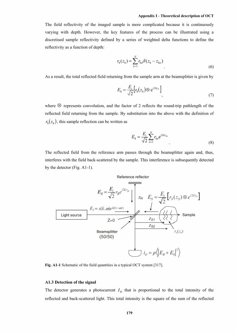
Appendix I - Theoretical description of OCT
179
The field reflectivity of the imaged sample is more complicated because it is continuously
varying with depth. However, the key features of the process can be illustrated using a
discretised sample reflectivity defined by a series of weighted delta functions to define the
reflectivity as a function of depth:
N
nnn zzrzr
1SSSSS )()(
. (6)
As a result, the total reflected field returning from the sample arm at the beamsplitter is given by
S2iSS
iS e
2kzzrEE
, (7)
where represents convolution, and the factor of 2 reflects the round-trip pathlength of the
reflected field returning from the sample. By substitution into the above with the definition of
SS zr , this sample reflection can be written as
nkzN
nnrEE Si2
1S
iS e
2
. (8)
The reflected field from the reference arm passes through the beamsplitter again and, thus,
interferes with the field back-scattered by the sample. This interference is subsequently detected
by the detector (Fig. A1-1).
Fig. A1-1 Schematic of the field quantities in a typical OCT system [317].
A1.3 Detection of the signal
The detector generates a photocurrent DI that is proportional to the total intensity of the
reflected and back-scattered light. This total intensity is the square of the sum of the reflected

Appendix I - Theoretical description of OCT
180
fields. Hence, the photocurrent arising from the reflected fields from both the reference arm and
sample arm is given by
2
2SR
DEE
I
, (9)
where is the responsivity of the detector with units of Amperes/Watt. The factor of 2
indicates the second pass of each field through the beamsplitter. Furthermore, the angular
brackets denote the integration over the response time of the detector. If we replace the reflected
fields with their equivalent expressions involving the incident field, field reflectivities, and the
travelled optical pathlengths, the photocurrent can be rewritten as
2
1
2iS
i2iR
iD
SR e2
e22
N
n
kzn
kz nrErEI
. (10)
With the replacement of iE with )(ii e),( tkzksE , setting 0z at the surface of the
beamsplitter, the detected photocurrent can be fully expressed as
2
1
)2i(S
)2i(RD
SR e2
),(e2
),(2
N
n
tkzn
tkz nrksrksI
. (11)
The expansion of this squared expression eliminates the temporal-dependent terms, which
include 2 . From physical perspective, it is reasonable to eliminate these temporal-
dependent terms because oscillates too fast compared with the response time of any practical
detector. The detected photocurrent, therefore, is only dependent on the temporally invariant
terms:
N
mn
zzkzzkmn
N
n
zzkzzkn
mnmn
nn
RRkS
RRkS
RRRkSI
1
)(2i-)(2iSS
1
)(2i-)(2iSR
S2S1RD
SSSS
SRSR
ee)(4
ee)(4
...))((4
. (12)
Here, )(kS is the substitute of 2),( ks , indicating that the detected photocurrent is
independent of the angular frequency . RR and SR are termed the power reflectivities of the
reference mirror and sample reflector, defined as 2Rr and 2
Sr , respectively. Using Euler’s rule
to rewrite this equation, the detected photocurrent can be expressed as a real function of the
wavenumber, k :
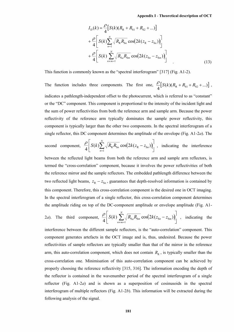
Appendix I - Theoretical description of OCT
181
N
mnmnmn
N
nnn
zzkRRkS
zzkRRkS
RRRkSkI
1SSSS
1SRSR
S2S1RD
)(2cos)(4
)(2cos)(4
...))((4
)(
. (13)
This function is commonly known as the “spectral interferogram” [317] (Fig. A1-2).
The function includes three components. The first one, ...))((4 S2S1R RRRkS ,
indicates a pathlength-independent offset to the photocurrent, which is referred to as “constant”
or the “DC” component. This component is proportional to the intensity of the incident light and
the sum of power reflectivities from both the reference arm and sample arm. Because the power
reflectivity of the reference arm typically dominates the sample power reflectivity, this
component is typically larger than the other two components. In the spectral interferogram of a
single reflector, this DC component determines the amplitude of the envelope (Fig. A1-2a). The
second component,
N
nnn zzkRRkS
1SRSR )(2cos)(
4
, indicating the interference
between the reflected light beams from both the reference arm and sample arm reflectors, is
termed the “cross-correlation” component, because it involves the power reflectivities of both
the reference mirror and the sample reflectors. The embedded pathlength difference between the
two reflected light beams, nzz SR , guarantees that depth-resolved information is contained by
this component. Therefore, this cross-correlation component is the desired one in OCT imaging.
In the spectral interferogram of a single reflector, this cross-correlation component determines
the amplitude riding on top of the DC-component amplitude or envelope amplitude (Fig. A1-
2a). The third component,
N
mnmnmn zzkRRkS
1SSSS )(2cos)(
4
, indicating the
interference between the different sample reflectors, is the “auto-correlation” component. This
component generates artefacts in the OCT image and is, thus, undesired. Because the power
reflectivities of sample reflectors are typically smaller than that of the mirror in the reference
arm, this auto-correlation component, which does not contain RR , is typically smaller than the
cross-correlation one. Minimisation of this auto-correlation component can be achieved by
properly choosing the reference reflectivity [315, 316]. The information encoding the depth of
the reflector is contained in the wavenumber period of the spectral interferogram of a single
reflector (Fig. A1-2a) and is shown as a superposition of cosinusoids in the spectral
interferogram of multiple reflectors (Fig. A1-2b). This information will be extracted during the
following analysis of the signal.
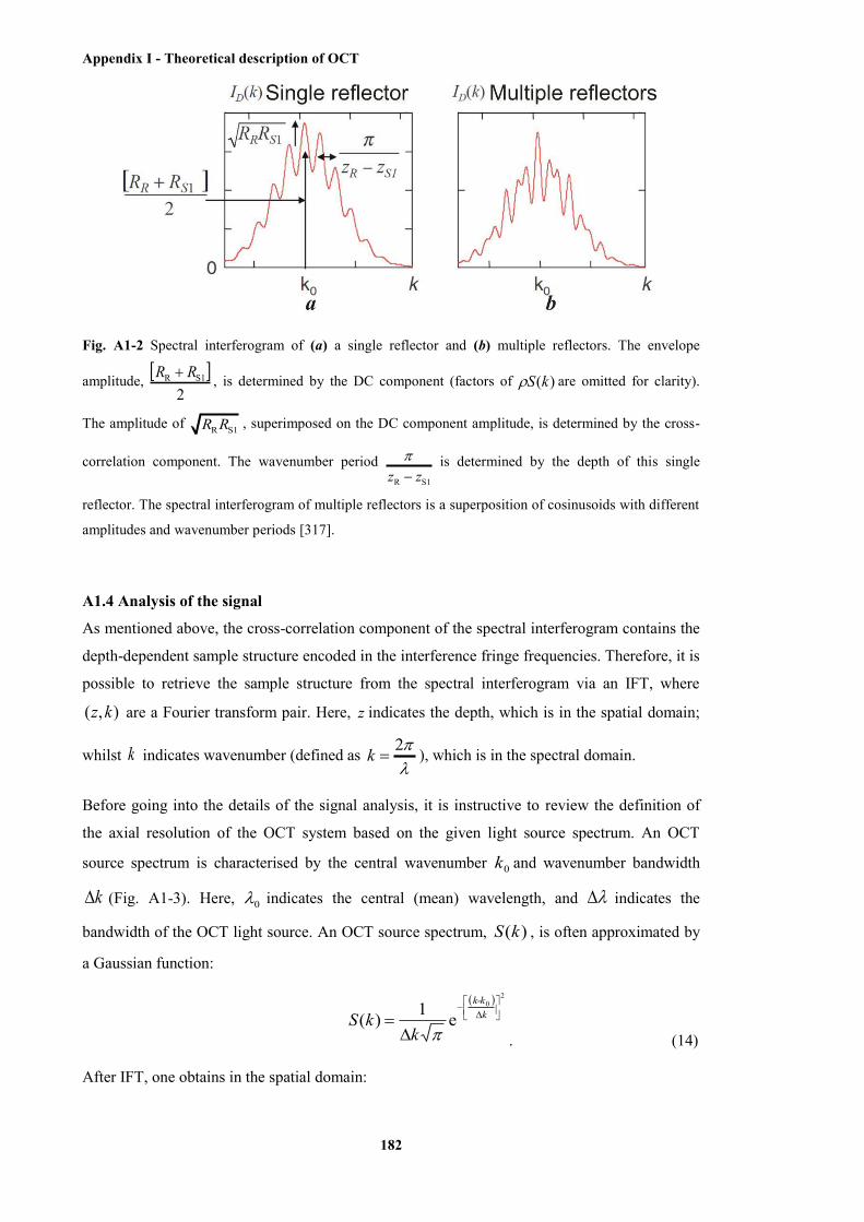
Appendix I - Theoretical description of OCT
182
Fig. A1-2 Spectral interferogram of (a) a single reflector and (b) multiple reflectors. The envelope
amplitude, 2
S1R RR , is determined by the DC component (factors of )(kS are omitted for clarity).
The amplitude of S1RRR , superimposed on the DC component amplitude, is determined by the cross-
correlation component. The wavenumber period S1R zz
is determined by the depth of this single
reflector. The spectral interferogram of multiple reflectors is a superposition of cosinusoids with different
amplitudes and wavenumber periods [317].
A1.4 Analysis of the signal
As mentioned above, the cross-correlation component of the spectral interferogram contains the
depth-dependent sample structure encoded in the interference fringe frequencies. Therefore, it is
possible to retrieve the sample structure from the spectral interferogram via an IFT, where
),( kz are a Fourier transform pair. Here, z indicates the depth, which is in the spatial domain;
whilst k indicates wavenumber (defined as
2k ), which is in the spectral domain.
Before going into the details of the signal analysis, it is instructive to review the definition of
the axial resolution of the OCT system based on the given light source spectrum. An OCT
source spectrum is characterised by the central wavenumber 0k and wavenumber bandwidth
k (Fig. A1-3). Here, 0 indicates the central (mean) wavelength, and indicates the
bandwidth of the OCT light source. An OCT source spectrum, )(kS , is often approximated by
a Gaussian function:
20
e1)(
k
k-k
kkS
. (14)
After IFT, one obtains in the spatial domain:

Appendix I - Theoretical description of OCT
183
22-ze)( kz . (15)
This spatial-domain function is called the “coherence function”. Here, z is the sample depth.
The FWHM of this coherence function, cl (Fig. A1-3), indicating the axial spatial resolution of
the OCT system, is an explicit function of the light source bandwidth:
202ln22ln2
klc
. (16)
This cl is termed the “coherence length” [317]. Hence, a broadband light source or a
monochromatic source that scans over a broad band is typically employed in OCT systems to
achieve a finer axial resolution.
Fig. A1-3 Fourier transform relationship between the coherence function )(z and the spectrum )(kS of the OCT light source [317].
Using the IFT, we can now retrieve the depth-resolved sample structure [317]. Convolution
appears after IFT due to the fact that the product of two original functions will become the
convolution of the two transformed functions. The calculated expression of the acquired spectral
interferogram based on IFT is:
N
mnmnmn
N
nnn
zzzRRz
zzzRRz
RRRzzi
1SSSS
1SRSR
S2S1RD
)(2)(8
)(2)(4
...))((8
)(
. (17)
Taking advantage of the sifting property of the delta function, the convolutions can be carried
out and the function rearranged as:
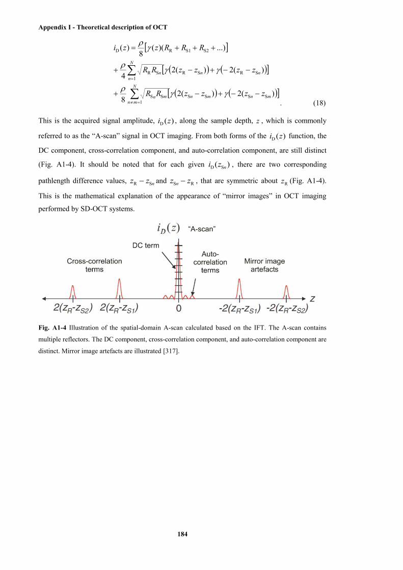
Appendix I - Theoretical description of OCT
184
N
mnmnmnmn
N
nnnn
zzzzRR
zzzzRR
RRRzzi
1SSSSSS
1SRSRSR
S2S1RD
)(2)(28
)(2)(24
...))((8
)(
. (18)
This is the acquired signal amplitude, )(D zi , along the sample depth, z , which is commonly
referred to as the “A-scan” signal in OCT imaging. From both forms of the )(D zi function, the
DC component, cross-correlation component, and auto-correlation component, are still distinct
(Fig. A1-4). It should be noted that for each given )( SD nzi , there are two corresponding
pathlength difference values, nzz SR and RS zz n , that are symmetric about Rz (Fig. A1-4).
This is the mathematical explanation of the appearance of “mirror images” in OCT imaging
performed by SD-OCT systems.
Fig. A1-4 Illustration of the spatial-domain A-scan calculated based on the IFT. The A-scan contains
multiple reflectors. The DC component, cross-correlation component, and auto-correlation component are
distinct. Mirror image artefacts are illustrated [317].
References
185
References
1. K. Bushby, R. Finkel, D. J. Birnkrant, L. E. Case, P. R. Clemens, L. Cripe, A. Kaul, K.
Kinnett, C. McDonald, S. Pandya, J. Poysky, F. Shapiro, J. Tomezsko, C. Constantin, and D.
C. C. Working, "Diagnosis and management of Duchenne muscular dystrophy, part 1:
diagnosis, and pharmacological and psychosocial management," Lancet Neurol. 9(1), 77-93
(2010).
2. A. Y. Manzur and F. Muntoni, "Diagnosis and new treatments in muscular dystrophies," J.
Neurol. Neurosurg. Psychiatr. 80(7), 706-714 (2009).
3. E. Le Rumeur, S. J. Winder, and J. F. Hubert, "Dystrophin: more than just the sum of its
parts," Biochim. Biophys. Acta 1804(9), 1713-1722 (2010).
4. M. J. Spencer and J. G. Tidball, "Do immune cells promote the pathology of dystrophin-
deficient myopathies?" Neuromuscular Disord. 11(6-7), 556-564 (2001).
5. J. G. Tidball and M. Wehling-Henricks, "Damage and inflammation in muscular dystrophy:
potential implications and relationships with autoimmune myositis," Curr. Opin. Rheumatol.
17(6), 707-713 (2005).
6. N. P. Evans, S. A. Misyak, J. L. Robertson, J. Bassaganya-Riera, and R. W. Grange,
"Dysregulated intracellular signaling and inflammatory gene expression during initial disease
onset in Duchenne muscular dystrophy," Am. J. Phys. Med. Rehab. 88(6), 502-522 (2009).
7. T. Shavlakadze, J. White, J. F. Y. Hoh, N. Rosenthal, and M. D. Grounds, "Targeted
expression of insulin-like growth factor-1 reduces early myofiber necrosis in dystrophic mdx
mice," Mol. Ther. 10(5), 829-843 (2004).
8. M. D. Grounds and J. Torrisi, "Anti-TNF α (Remicade®) therapy protects dystrophic skeletal
muscle from necrosis," FASEB J. 18(6), 676-682 (2004).
9. S. Hodgetts, H. Radley, M. Davies, and M. D. Grounds, "Reduced necrosis of dystrophic
muscle by depletion of host neutrophils, or blocking TNF alpha function with Etanercept in
mdx mice," Neuromuscular Disord. 16(9-10), 591-602 (2006).
10. S. Pierno, B. Nico, R. Burdi, A. Liantonio, M. P. Didonna, V. Cippone, B. Fraysse, J. F.
Rolland, D. Mangieri, F. Andreetta, P. Ferro, C. Camerino, A. Zallone, P. Confalonieri, and A.
de Luca, "Role of tumour necrosis factor alpha, but not of cyclo-oxygenase-2-derived
eicosanoids, on functional and morphological indices of dystrophic progression in mdx mice: a
pharmacological approach," Neuropath. Appl. Neuro. 33(3), 344-359 (2007).
11. H. G. Radley, M. J. Davies, and M. D. Grounds, "Reduced muscle necrosis and long-term
benefits in dystrophic mdx mice after cV1q (blockade of TNF) treatment," Neuromuscular
Disord. 18(3), 227-238 (2008).
References
186
12. M. D. Grounds, H. G. Radley, G. S. Lynch, K. Nagaraju, and A. de Luca, "Towards
developing standard operating procedures for pre-clinical testing in the mdx mouse model of
Duchenne muscular dystrophy," Neurobiol. Dis. 31(1), 1-19 (2008).
13. F. S. Foster, C. J. Pavlin, K. A. Harasiewicz, D. A. Christopher, and D. H. Turnbull,
"Advances in ultrasound biomicroscopy," Ultrasound Med. Biol. 26(1), 1-27 (2000).
14. C. J. Pavlin, K. Harasiewicz, M. D. Sherar, and E. S. Foster, "Clinical use of ultrasound
biomicroscopy," Ophthalmology 98(3), 287-295 (1991).
15. S. Pillen, I. M. P. Arts, and M. J. Zwarts, "Muscle ultrasound in neuromuscular disorders,"
Muscle Nerve 37(6), 679-693 (2008).
16. S. M. Zuberi, N. Matta, S. Nawaz, J. B. Stephenson, R. C. McWilliam, and A. Hollman,
"Muscle ultrasound in the assessment of suspected neuromuscular disease in childhood,"
Neuromuscular Disord. 9(4), 203-207 (1999).
17. F. S. Foster, J. Mehi, M. Lukacs, D. Hirson, C. White, C. Chaggares, and A. Needles, "A
new 15-50 MHz array-based micro-ultrasound scanner for preclinical imaging," Ultrasound
Med. Biol. 35(10), 1700-1708 (2009).
18. L. M. Stern, D. J. Caudrey, L. V. Perrett, and D. W. Boldt, "Progression of muscular
dystrophy assessed by computed tomography," Dev. Med. Child Neurol. 26(5), 569-573
(1984).
19. S. J. Schambach, S. Bag, L. Schilling, C. Groden, and M. A. Brockmann, "Application of
micro-CT in small animal imaging," Methods 50(1), 2-13 (2010).
20. V. Persy, A. Postnov, E. Neven, G. Dams, M. de Broe, P. D'Haese, and N. de Clerck,
"High-resolution X-ray microtomography is a sensitive method to detect vascular calcification
in living rats with chronic renal failure," Arterioscl. Throm. Vas. 26(9), 2110-2116 (2006).
21. Y. K. Luu, S. Lublinsky, E. Ozcivici, E. Capilla, J. E. Pessin, C. T. Rubin, and S. Judex,
"In vivo quantification of subcutaneous and visceral adiposity by micro-computed tomography
in a small animal model," Med. Eng. Phys. 31(1), 34-41 (2009).
22. M. Marxen, M. M. Thornton, C. B. Chiarot, G. Klement, J. Koprivnikar, J. G. Sled, and R.
M. Henkelman, "Micro-CT scanner performance and considerations for vascular specimen
imaging," Med. Phys. 31(2), 305-313 (2004).
23. W. A. Murphy, W. G. Totty, and J. E. Carroll, "MRI of normal and pathological skeletal
muscle," Am. J. Roentgenol. 146(3), 565-574 (1986).
24. G. Saab, G. D. Marsh, M. A. Casselman, and R. T. Thompson, "Changes in human muscle
transverse relaxation following short-term creatine supplementation," Exp. Physiol. 87(3), 383-
389 (2002).
References
187
25. B. M. Damon, "MRI in pre-clinical models of muscle disease," in International Society for
Magnetic Resonance in Medicine, Chicago, IL (2011),
26. M. Rudin, N. Beckmann, R. Porszasz, T. Reese, D. Bochelen, and A. Sauter, "In vivo
magnetic resonance methods in pharmaceutical research: current status and perspectives,"
NMR Biomed. 12(2), 69-97 (1999).
27. H. Amthor, T. Egelhof, I. McKinnell, M. E. Ladd, I. Janssen, J. Weber, H. Sinn, H. H.
Schrenk, M. Forsting, T. Voit, and V. Straub, "Albumin targeting of damaged muscle fibres in
the mdx mouse can be monitored by MRI," Neuromuscular Disord. 14(12), 791-796 (2004).
28. S. I. Head, D. A. Williams, and D. G. Stephenson, "Abnormalities in structure and function
of limb skeletal muscle fibers of dystrophic mdx mice," P. Roy. Soc. B-Biol. Sci. 248(1322),
163-169 (1992).
29. T. Masuda, N. Fujimaki, E. Ozawa, and H. Ishikawa, "Confocal laser microscopy of
dystrophin localization in guinea pig skeletal muscle fibers," J. Cell Biol. 119(3), 543-548
(1992).
30. S. V. Plotnikov, A. M. Kenny, S. J. Walsh, B. Zubrowski, C. Joseph, V. L. Scranton, G. A.
Kuchel, D. Dauser, M. S. Xu, C. C. Pilbeam, D. J. Adams, R. P. Dougherty, P. J. Campagnola,
and W. A. Mohler, "Measurement of muscle disease by quantitative second-harmonic
generation imaging," J. Biomed. Opt. 13(4), art.044018 (2008).
31. R. S. Pillai, D. Lorenser, and D. D. Sampson, "Deep-tissue access with confocal
fluorescence microendoscopy through hypodermic needles," Opt. Express 19(8), 7213-7221
(2011).
32. D. Laux, H. Blasco, J. Y. Ferrandis, G. Hugon, G. Despaux, A. Leydier, and D. Mornet,
"In vitro mouse model in Duchenne muscular dystrophy diagnosis using 50-MHz ultrasound
waves," Ultrasonics 50(8), 741-743 (2010).
33. K. D. Wallace, J. N. Marsh, S. L. Baldwin, A. M. Connolly, R. Keeling, G. M. Lanza, S.
A. Wickline, and M. S. Hughes, "Sensitive ultrasonic delineation of steroid treatment in living
dystrophic mice with energy-based and entropy-based radio frequency signal processing,"
IEEE T. Ultrason. Ferr. 54(11), 2291-2299 (2007).
34. J. Heckmatt, E. Rodillo, M. Doherty, K. Willson, and S. Leeman, "Quantitative
sonography of muscle," J. Child Neurol. 4(1), S101-S106 (1989).
35. M. Narici, "Human skeletal muscle architecture studied in vivo by non-invasive imaging
techniques: functional significance and applications," J. Electromyogr. Kines. 9(2), 97-103
(1999).
36. D. Cosgrove, "Ultrasound: general principles," in Diagnostic Radiology, R. G. Grainger
and D. J. Allison, eds. (Churchill Livingstone, Edinburph, UK, 1992), pp. 65-77.
References
188
37. N. Deshpande, A. Needles, and J. K. Willmann, "Molecular ultrasound imaging: current
status and future directions," Clin. Radiol. 65(7), 567-581 (2010).
38. D. A. Jones, J. M. Round, R. H. T. Edwards, S. R. Grindwood, and P. S. Tofts, "Size and
composition of the calf and quadriceps muscles in Duchenne muscular dystrophy: a
tomographic and histochemical study," J. Neurol. Sci. 60(2), 307-322 (1983).
39. O. A. Peters, C. I. Peters, K. Schonenberger, and F. Barbakow, "ProTaper rotary root canal
preparation: effects of canal anatomy on final shape analysed by micro CT," Int. Endod. J.
36(2), 86-92 (2003).
40. S. J. Schambach, S. Bag, V. Steil, C. Isaza, L. Schilling, C. Groden, and M. A. Brockmann,
"Ultrafast high-resolution in vivo volume-CTA of mice cerebral vessels," Stroke 40(4), 1444-
1450 (2009).
41. M. Kobayashi, A. Nakamura, D. Hasegawa, M. Fujita, H. Orima, and S. Takeda,
"Evaluation of dystrophic dog pathology by fat-suppressed T2-weighted imaging," Muscle
Nerve 40(5), 815-826 (2009).
42. J. N. Kornegay, J. Li, J. R. Bogan, D. J. Bogan, C. Chen, H. Zheng, B. Wang, C. Qiao, J. F.
Howard, Jr., and X. Xiao, "Widespread muscle expression of an AAV9 human mini-
dystrophin vector after intravenous injection in neonatal dystrophin-deficient dogs," Mol. Ther.
18(8), 1501-1508 (2010).
43. L. M. McIntosh, B. E. Baker, and J. E. Anderson, "Magnetic resonance imaging of
regenerating and dystrophic mouse muscle," Biochem. Cell Biol. 76(2-3), 532-541 (1998).
44. V. Straub, K. M. Donahue, V. Allamand, R. L. Davisson, Y. R. Kim, and K. P. Campbell,
"Contrast agent-enhanced magnetic resonance imaging of skeletal muscle damage in animal
models of muscular dystrophy," Magnet. Reson. Med. 44(4), 655-659 (2000).
45. G. Walter, L. Cordier, D. Bloy, and H. L. Sweeney, "Noninvasive monitoring of gene
correction in dystrophic muscle," Magnet. Reson. Med. 54(6), 1369-1376 (2005).
46. J. Phoenix, D. Betal, N. Roberts, T. R. Helliwell, and R. H. T. Edwards, "Objective
quantification of muscle and fat in human dystrophic muscle by magnetic resonance image
analysis," Muscle Nerve 19(3), 302-310 (1996).
47. M. A. Cole, J. A. Rafael, D. J. Taylor, R. Lodi, K. E. Davies, and P. Styles, "A quantitative
study of bioenergetics in skeletal muscle lacking utrophin and dystrophin," Neuromuscular
Disord. 12(3), 247-257 (2002).
48. J. A. Hipp, A. Jansujwicz, C. A. Simmons, and B. D. Snyder, "Trabecular bone
morphology from micro-magnetic resonance imaging," J. Bone Miner. Res. 11(2), 286-292
(1996).
References
189
49. I. Koizuka, Y. Seo, M. Murakami, R. Seo, and I. Kato, "Micro-magnetic resonance
imaging of the inner ear in the guinea pig," NMR Biomed. 10(1), 31-34 (1997).
50. H. Kobayashi, S. Kawamoto, P. L. Choyke, N. Sato, M. V. Knopp, R. A. Star, T. A.
Waldmann, Y. Tagaya, and M. W. Brechbiel, "Comparison of dendrimer-based
macromolecular contrast agents for dynamic micro-magnetic resonance lymphangiography,"
Magnet. Reson. Med. 50(4), 758-766 (2003).
51. D. Huang, E. A. Swanson, C. P. Lin, J. S. Schuman, W. G. Stinson, W. Chang, M. R. Hee,
T. Flotte, K. Gregory, C. A. Puliafito, and J. G. Fujimoto, "Optical coherence tomography,"
Science 254(5035), 1178-1181 (1991).
52. A. F. Fercher, W. Drexler, C. K. Hitzenberger, and T. Lasser, "Optical coherence
tomography - principles and applications," Rep. Prog. Phys. 66(2), 239-303 (2003).
53. D. D. Sampson and T. R. Hillman, "Optical coherence tomography," in Lasers and Current
Optical Techniques in Biology, G. Palumbo and R. Pratesi, eds. (Royal Society of Chemistry,
Cambridge, UK, 2004), pp. 481-571.
54. R. M. Lovering, S. B. Shah, S. J. P. Pratt, W. Gong, and Y. Chen, "Architecture of healthy
and dystrophic muscles detected by optical coherence tomography," Muscle Nerve 47(4), 588-
590 (2013).
55. B. R. Klyen, T. Shavlakadze, H. G. Radley-Crabb, M. D. Grounds, and D. D. Sampson,
"Identification of muscle necrosis in the mdx mouse model of Duchenne muscular dystrophy
using three-dimensional optical coherence tomography," J. Biomed. Opt. 16(7), art.076013
(2011).
56. J. J. Pasquesi, S. C. Schlachter, M. D. Boppart, E. Chaney, S. J. Kaufman, and S. A.
Boppart, "In vivo detection of exercise-induced ultrastructural changes in genetically-altered
murine skeletal muscle using polarization-sensitive optical coherence tomography," Opt.
Express 14(4), 1547-1556 (2006).
57. M. R. Hee, D. Huang, E. A. Swanson, and J. G. Fujimoto, "Polarization-sensitive low-
coherence reflectometer for birefringence characterization and ranging," J. Opt. Soc. Am. B
9(6), 903-908 (1992).
58. H. Schmalbruch, Skeletal muscle (Springer-Verlag, Berlin Heidelberg, Germany, 1985).
59. J. Ranasinghesagara and G. Yao, "Effects of inhomogeneous myofibril morphology on
optical diffraction in single muscle fibers," J. Opt. Soc. Am. A 25(12), 3051-3058 (2008).
60. B. R. Klyen, J. J. Armstrong, S. G. Adie, H. G. Radley, M. D. Grounds, and D. D.
Sampson, "Three-dimensional optical coherence tomography of whole-muscle autografts as a
precursor to morphological assessment of muscular dystrophy in mice," J. Biomed. Opt. 13(1),
011003 (2008).

References
190
61. M. D. Grounds, "Complexity of extracellular matrix and skeletal muscle regeneration," in
Skeletal Muscle Repair and Regeneration, S. Schiaffino and T. Partridge, eds. (Springer,
Dordrecht, The Netherlands, 2008), pp. 269-302.
62. M. R. Ross and W. Pawlina, "Muscle tissue," in Histology - A Text and Atlas, 5th ed.
(Lippincott Williams & Wilkins, Baltimore, MD, 2006), pp. 280-317.
63. T. Schwann, Microscopical Researches into the Accordance in the Structure and Growth
of Animals and Plants (Sydenham Society, London, 1847), p. 268.
64. G. Burnstock, "Structure of smooth muscle and its innervation," in Smooth Muscle, E.
Bulbring, A. F. Brading, A. W. Jones, and T. Tomita, eds. (Edward Arnold, London, 1970),
pp. 1-69.
65. A. I. Csapo, "The uterus - model experiments and clinical trials " in The Structure and
Function of Muscle, G. Bourne, ed. (Academic Press, London, 1955).
66. R. A. Bergman, "Intercellular bridges in ureteral smooth muscle," B. Johns Hopkins Hosp.
102(4), 195-202 (1958).
67. J. S. T. Mark, "An electron microscope study of uterine smooth muscle," Anat. Rec.
125(3), 473-493 (1956).
68. G. Burnstock and G. Campbell, "Comparative physiology of the vertebrate autonomic
nervous system II. Innervation of the urinary bladder of the ringtail possum (psudocheirus
peregrinus)," J. Exp. Biol. 40, 421-436 (1963).
69. K. C. Strong, "A study of the structure of the media of the distributing arteries by the
method of microdissection," Anat. Rec. 72(2), 151-167 (1938).
70. D. C. Pease and W. J. Paule, "Electron microscopy of elastic arteries: the thoracic aorta of
the rat," J. Ultra. Mol. Struct. R. 3(4), 469-483 (1960).
71. M. K. Keech, "Electron microscope study of the normal rat aorta," J. Biophys. Biochem.
Cy. 7(3), 533-538 (1960).
72. A. I. Csapo, "Function and regulation of the myometrium," Ann. NY Acad. Sci. 75(2), 790-
808 (1959).
73. A. I. Csapo, "Smooth muscle as a contractile unit," Physiol. Rev. 42(5), 7-33 (1962).
74. C. L. Prosser, G. Burnstock, and J. Kahn, "Conduction in smooth muscle: comparative
structural properties," Am. J. Physiol. 199(3), 545-552 (1960).
75. N. C. R. Merrillees, G. Burnstock, and M. E. Holman, "Correlation of fine structure and
physiology of the innervation of smooth muscle in the guinea pig vas deferens," J. Cell. Biol.
19(3), 529-550 (1963).
References
191
76. D. H. L. Evans and E. M. Evans, "The membrane relationships of smooth muscles: an
electron microscope study," J. Anat. 98(Pt 1), 37-46 (1964).
77. M. R. Bennett and D. C. Rogers, "A study of the innervation of the taenia coli," J. Cell
Biol. 33(3), 573-596 (1967).
78. R. J. Boucek, R. Fojaco, and Takashit.R, "Relation between microanatomy and functional
properties of coronary arteries (dog)," Anat. Rec. 147(2), 199-207 (1963).
79. M. R. Bennett and G. Burnstock, "Electrophysiology of transmission in the intestine," in
The handbook of physiology (American Physiology Society, Washington, D. C., US, 1968).
80. G. Burnstock and C. L. Prosser, "Conduction in smooth muscles: comparative electrical
properties," Am. J. Physiol. 199(3), 553-559 (1960).
81. J. Nagasawa and S. Mito, "Electron microscopic observations on the innervation of the
smooth muscle," Tohoku J. Exp. Med. 91(3), 277-293 (1967).
82. N. C. R. Merrillees, "The nervous environment of individual smooth muscle cells of the
guinea pig vas deferens," J. Cell Biol. 37(3), 794-817 (1968).
83. R. Caesar, G. A. Edwards, and H. Ruska, "Architecture and nerve supply of mammalian
smooth muscle tissue," J. Biophys. Biochem. Cy. 3(6), 867-878 (1957).
84. D. C. Pease and S. Molinari, "Electron microscopy of muscular arteries; pial vessels of the
cat and monkey," J. Ultra. Mol. Struct. R. 3(4), 447-468 (1960).
85. H. E. Karrer, "An electron microscope study of the aorta in young and in aging mice," J.
Ultra. Mol. Struct. R. 5(1), 1-27 (1961).
86. B. P. Lane, "Alterations in the cytologic detail of intestinal smooth muscle cells in various
stages of contraction," J. Cell Biol. 27(1), 199-213 (1965).
87. B. J. Panner and C. R. Honig, "Filament ultrastructure and organization in vertebrate
smooth muscle: contraction hypothesis based on localization of actin and myosin," J. Cell Biol.
35(2), 303-321 (1967).
88. A. M. Gerdes, "Cardiomyocyte ultrastructure," in Muscle - Fundamental Biology and
Mechanisms of Disease, 1 ed., J. A. Hill and E. N. Olson, eds. (Elsevier, San Diego, CA,
2012).
89. A. M. Gerdes, J. A. Moore, J. M. Hines, P. A. Kirkland, and S. P. Bishop, "Regional
differences in myocyte size in normal rat heart," Anat. Rec. 215(4), 420-426 (1986).
90. L. H. Opie, Heart Physiology: from Cell to Circulation, 4 ed. (Lippincott Williams &
Wilkins, Philadelphia, PA, 2003).

References
192
91. S. Goktepe, O. J. Abilez, K. K. Parker, and E. Kuhl, "A multiscale model for eccentric and
concentric cardiac growth through sarcomerogenesis," J. Theor. Biol. 265(3), 433-442 (2010).
92. A. M. Gerdes, "Cardiac myocyte remodeling in hypertrophy and progression to failure," J.
Card. Fail. 8(6), S264-S268 (2002).
93. F. Torrent-Guasp, G. D. Buckberg, C. Clemente, J. L. Cix, H. C. Coghlan, and M. Gharib,
"The structure and function of the helical heart and its buttress wrapping. I. The normal
macroscopic structgure of the heart," Semin. Thorac. Cardiovasc. Surg. 13(4), 301-319 (2001).
94. M. D. Grounds and T. Shavlakadze, "Growing muscle has different sarcolemmal properties
from adult muscle: a proposal with scientific and clinical implications reasons to reassess
skeletal muscle molecular dynamics, cellular responses and suitability of experimental models
of muscle disorders," Bioessays 33(6), 458-468 (2011).
95. B. R. MacIntosh, P. F. Gardiner, and A. J. McComas, Skeletal Muscle: Form and
Function, 2 ed. (Human Kinetics, US, 2006).
96. H. G. Radley, "The role of resident mast cells in the onset of necrosis in dystrophic skeletal
muscle," (The University of Western Australia, WA, Australia, 2005).
97. G. M. Cooper, The Cell: A Molecular Approach, 2 ed. (Sinauer Associates, Sunderland,
MA, 2000).
98. D. L. Taylor, "Birefringence changes in vertebrate striated muscle," J. Supramol. Str. Cell
3(2), 181-191 (1975).
99. A. F. Huxley and R. Niedergerke, "Structural changes in muscle during contraction:
interference microscopy of living muscle fibres," Nature 173(4412), 971-973 (1954).
100. W. D. McArdle, K. F. I., and K. V. L., "Skeletal muscle: structure and function," in
Exercise Physiology, 5th ed. (Lippincott Williams & Wilkins, Baltimore, MD, 2001), pp. 358-
382.
101. R. Craig, "The structure of the contractile filaments," in Myology, A. G. Engel and B. Q.
Banker, eds. (McGraw-Hill Book Company, New York, NY, 1986), pp. 73-124.
102. B. Q. Banker and A. G. Engel, "Basic reactions of muscle," in Myology, A. G. Engel and
B. Q. Banker, eds. (McGraw-Hill Book Company, New York, NY, 1986), pp. 845-908.
103. S. Bortoluzzi, P. Scannapieco, A. Cestaro, G. A. Danieli, and S. Schiaffino,
"Computational reconstruction of the human skeletal muscle secretome," Proteins 62(3), 776-
792 (2006).
104. M. Kjaer, "Role of extracellular matrix in adaptation of tendon and skeletal muscle to
mechanical loading," Physiol. Rev. 84(2), 649-698 (2004).
References
193
105. T. K. Borg and J. B. Caulfield, "Morphology of connective tissue in skeletal muscle,"
Tissue Cell 12(1), 197-207 (1980).
106. R. W. D. Rowe, "Morphology of perimysial and endomysial connective tissue in skeletal
muscle," Tissue Cell 13(4), 681-690 (1981).
107. S. F. Street and R. W. Ramsey, "Sarcolemma: transmitter of active tension in frog skeletal
muscle," Science 149(3690), 1379-1380 (1965).
108. S. Fukashiro, M. Itoh, Y. Ichinose, Y. Kawakami, and T. Fukunaga, "Ultrasonography
gives directly but noninvasively elastic characteristic of human tendon in vivo," Eur. J. Appl.
Physiol. O. 71(6), 555-557 (1995).
109. C. M. Tipton, R. D. Matthes, J. A. Maynard, and R. A. Carey, "The influence of physical
activity on ligaments and tendons," Med. Sci. Sport. 7(3), 165-175 (1975).
110. J. G. Tidball, "Force transmission across muscle cell membranes," J. Biomech. 24(Suppl.
1), 43-52 (1991).
111. E. N. Marieb, "The muscular system," in Human Anatomy and Physiology, 5th ed.
(Benjamin Cummings, an imprint of Addison Wesley Longman, Inc., San Francisco, CA,
2001), pp. 322-285.
112. N. C. Voermans, C. G. Bonnemann, P. A. Huijing, B. C. Hamel, T. H. van Kuppevelt, A.
de Haan, J. Schalkwijk, B. G. van Engelen, and G. J. Jenniskens, "Clinical and molecular
overlap between myopathies and inherited connective tissue diseases," Neuromuscular Disord.
18(11), 843-856 (2008).
113. H. E. Huxley, "The contraction of muscle," Sci. Am. 199(5), 67-72 (1958).
114. H. Huxley and J. Hanson, "Changes in the cross-striations of muscle during contraction
and stretch and their structural interpretation," Nature 173(4412), 973-976 (1954).
115. H. E. Huxley, "Sliding filaments and molecular motile systems," J. Biol. Chem. 265(15),
8347-8350 (1990).
116. D. H. Cormack, "Muscle tissue," in Introduction to Histology (J. B. Lippincott Company,
Philadelphia, PA, 1984), pp. 225-244.
117. H. E. Huxley, "The double array of filaments in cross-striated muscle," J. Biophys.
Biochem. Cy. 3(5), 631-648 (1957).
118. A. E. H. Emery, "The muscular dystrophies," Lancet 359(9307), 687-695 (2002).
119. A. McArdle, R. H. T. Edwards, and M. J. Jackson, "How does dystrophin deficiency lead
to muscle degeneration-evidence from the mdx mouse," Neuromuscular Disord. 5(6), 445-456
(1995).

References
194
120. C. L. Ward and K. E. Davies, "Genetic modelling of muscular dystrophies," Neuropath.
Appl. Neuro. 24(2), 96-100 (1998).
121. V. Straub and K. P. Campbell, "Muscular dystrophies and the dystrophin-glycoprotein
complex," Curr. Opin. Neurol. 10(2), 168-175 (1997).
122. P. Reed and R. J. Bloch, "Postnatal changes in sarcolemmal organization in the mdx
mouse," Neuromuscular Disord. 15(8), 552-561 (2005).
123. P. L. McNeil and M. Terasaki, "Coping with the inevitable: how cells repair a torn
surface membrane," Nat. Cell Biol. 3(5), E124-E129 (2001).
124. B. J. Petrof, J. B. Shrager, H. H. Stedman, A. M. Kelly, and H. L. Sweeney, "Dystrophin
protects the sarcolemma from stresses developed during muscle contraction," P. Natl. Acad.
Sci. USA 90(8), 3710-3714 (1993).
125. T. Yoshimura, M. Tsujihata, A. Satoh, M. Mori, R. Hazama, N. Kinoshita, H. Takashima,
and S. Nagataki, "Ultrastructural study of the effect of calcium ionophore, A23187, on rat
muscle," Acta Neuropathol. 69(3-4), 184-192 (1986).
126. A. Pestronk, I. M. Parhad, D. B. Drachman, and D. L. Price, "Membrane myopathy:
morphological similarities to Duchenne muscular dystrophy," Muscle Nerve 5(3), 209-214
(1982).
127. S. Carpenter and G. Karpati, "Duchenne muscular dystrophy: plasma membrane loss
initiates muscle cell necrosis unless it is repaired," Brain 102(Mar), 147-161 (1979).
128. K. Wrogemann and S. D. J. Pena, "Mitochondrial calcium overload: general mechanism
for cell necrosis in muscle diseases," Lancet 1(7961), 672-674 (1976).
129. G. Bulfield, W. G. Siller, P. A. L. Wight, and K. J. Moore, "X chromosome-linked
muscular dystrophy (mdx) in the mouse," P. Natl. Acad. Sci. USA 81(4), 1189-1192 (1984).
130. T. Yokota, Q. L. Lu, J. E. Morgan, K. E. Davies, R. Fisher, S. Takeda, and T. A.
Partridge, "Expansion of revertant fibers in dystrophic mdx muscles reflects activity of muscle
precursor cells and serves as an index of muscle regeneration," J. Cell Sci. 119(13), 2679-2687
(2006).
131. B. R. Klyen, "Application of optical coherence tomography for muscular dystrophy
imaging," (The University of Western Australia, 2005).
132. S. J. Schatzberg, N. J. Olby, M. Breen, L. V. B. Anderson, C. F. Langford, H. F. Dickens,
S. D. Wilton, C. J. Zeiss, M. M. Binns, J. N. Kornegay, G. E. Morris, and N. J. H. Sharp,
"Molecular analysis of a spontaneous dystrophin 'knockout' dog," Neuromuscular Disord.
9(5), 289-295 (1999).
References
195
133. M. J. Parsons, I. Campos, E. M. A. Hirst, and D. L. Stemple, "Removal of dystroglycan
causes severe muscular dystrophy in zebrafish embryos," Development 129(14), 3505-3512
(2002).
134. T. Shavlakadze and M. D. Grounds, "Therapeutic interventions for age-related muscle
wasting: importance of innervation and exercise for preventing sarcopenia," in Modulating
Aging and Longevity, S. Rattan, ed. (Kluwer Academic Publisher, The Nedlands, 2003), pp.
139-166.
135. H. G. Radley and M. D. Grounds, "Cromolyn administration (to block mast cell
degranulation) reduces necrosis of dystrophic muscle in mdx mice," Neurobiol. Dis. 23(2),
387-397 (2006).
136. N. Stupka, M. A. Tarnopolsky, N. J. Yardley, and S. M. Phillips, "Cellular adaptation to
repeated eccentric exercise-induced muscle damage," J. Appl. Physiol. 91(4), 1669-1678
(2001).
137. L. F. B. Torres and L. W. Duchen, "The mutant mdx: inherited myopathy in the mouse -
morphological studies of nerves, muscles and end-plates," Brain 110(2), 269-299 (1987).
138. G. R. Coulton, J. E. Morgan, T. A. Partridge, and J. C. Sloper, "The mdx mouse skeletal
muscle myopathy: I. a histological, morphometric and biochemical investigation," Neuropath.
Appl. Neuro. 14(1), 53-70 (1988).
139. F. Muntoni, A. Mateddu, F. Marchei, A. Clerk, and G. Serra, "Muscular weakness in the
mdx mouse," J. Neurol. Sci. 120(1), 71-77 (1993).
140. N. P. Whitehead, E. W. Yeung, and D. G. Allen, "Muscle damage in mdx (dystrophic)
mice: role of calcium and reactive oxygen species," Clin. Exp. Pharmacol. P. 33(7), 657-662
(2006).
141. J. K. McGeachie, M. D. Grounds, T. A. Partridge, and J. E. Morgan, "Age-related
changes in replication of myogenic cells in mdx mice: quantitative autoradiographic studies,"
J. Neurol. Sci. 119(2), 169-179 (1993).
142. D. J. Parry and R. S. Wilkinson, "The effect of reinnervation on the distribution of muscle
fiber types in the tibialis anterior muscle of the mouse," Can. J. Physiol. Pharm. 68(5), 596-
602 (1990).
143. L. C. Wang and D. Kernell, "Fibre type regionalisation in lower hindlimb muscles of
rabbit, rat and mouse: a comparative study," J. Anat. 199(6), 631-643 (2001).
144. A. Hayes and D. A. Williams, "Beneficial effects of voluntary wheel running on the
properties of dystrophic mouse muscle," J. Appl. Physiol. 80(2), 670-679 (1996).
References
196
145. J. T. Vilquin, V. Brussee, I. Asselin, I. Kinoshita, M. Gingras, and J. P. Tremblay,
"Evidence of mdx mouse skeletal muscle fragility in vivo by eccentric running exercise,"
Muscle Nerve 21(5), 567-576 (1998).
146. A. de Luca, B. Nico, A. Liantonio, M. P. Didonna, B. Fraysse, S. Pierno, R. Burdi, D.
Mangieri, J. F. Rolland, C. Camerino, A. Zallone, P. Confalonieri, F. Andreetta, E. Arnoldi, I.
Courdier-Fruh, J. P. Magyar, A. Frigeri, M. Pisoni, M. Svelto, and D. C. Camerino, "A
multidisciplinary evaluation of the effectiveness of cyclosporine A in dystrophic mdx mice,"
Am. J. Pathol. 166(2), 477-489 (2005).
147. H. Radley-Crabb, J. Terrill, T. Shavlakadze, J. Tonkin, P. Arthur, and M. Grounds, "A
single 30 min treadmill exercise session is suitable for 'proof-of concept studies' in adult mdx
mice: a comparison of the early consequences of two different treadmill protocols,"
Neuromuscular Disord. 22(2), 170-182 (2012).
148. X. Yang, L. Chin, B. R. Klyen, T. Shavlakadze, R. A. McLaughlin, M. D. Grounds, and
D. D. Sampson, "Quantitative assessment of muscle damage in the mdx mouse model of
Duchenne muscular dystrophy using polarization-sensitive optical coherence tomography," J.
Appl. Physiol. 115(9), 1393-1401 (2013).
149. T. A. Partridge, "The mdx mouse model as a surrogate for Duchenne muscular
dystrophy," FEBS J. 280(17), 4177-4186 (2013).
150. J. B. S. Haldane, "On being the right size," in Possible Worlds and Other Essays (Harper
and Brothers, New York, NY, 1928).
151. D. W. Thompson, On Growth and Form (Cambridge University Press, New York, NY,
1945).
152. J. J. Wild and D. Neal, "Use of high-frequency ultrasonic waves for detecting changes of
texture in living tissues," Lancet 260(24), 655-657 (1951).
153. F. O. Walker, M. S. Cartwright, E. R. Wiesler, and J. Caress, "Ultrasound of nerve and
muscle," Clin. Neurophysiol. 115(3), 495-507 (2004).
154. M. D. Sherar, M. B. Noss, and F. S. Foster, "Ultrasound backscatter microscopy images
the internal structure of living tumor spheroids," Nature 330(6147), 493-495 (1987).
155. O. Aristizabal, J. A. Ketterling, and D. H. Turnbull, "40-MHz annular array imaging of
mouse embryos," Ultrasound Med. Biol. 32(11), 1631-1637 (2006).
156. P. Fish, Physics and Instrumentation of Diagnostic Medical Ultrasound (John Wiley &
Sons, Chichester, UK, 1990).
157. I. M. Shirley, A User's Guide to Diagnostic Ultrasound (Pitman Medical University Park
Press, Tunbridge Wells, UK, 1978).
References
197
158. W. A. Riley, "Physics and principles of ultrasound and instrumentation," in
Neurosonology, 1st ed., C. H. Tegeler, V. L. Babikian, and C. R. Gomez, eds. (Mosby-Year-
Book, New York, NY, 1996), pp. 3-7.
159. W. A. Riley, "Ultrasonic B-mode imaging systems," in Neurosonology, C. H. Tegeler, V.
L. Babikian, and C. R. Gomez, eds. (Mosby-Year-Book, New York, NY, 1996), pp. 14-18.
160. F. W. Kremkau, Diagnostic Ultrasound: Principles, Instruments and Exercises, 6th ed.
(Saunders, Philadelphia, PA, 2002).
161. M. D. Sherar, B. G. Starkoski, W. B. Taylor, and F. S. Foster, "A 100 MHz B-scan
ultrasound backscatter microscope," Ultrasonic Imaging 11(2), 95-105 (1989).
162. C. J. Pavlin, M. D. Sherar, and F. S. Foster, "Subsurface ultrasound microscopic imaging
of the intact eye," Ophthalmology 97(2), 244-250 (1990).
163. F. K. Forster, G. R. Pomajevich, A. W. Holmes, and S. R. Sharar, "High-frequency
ultrasonic imaging and backscatter attenuation techniques for determination of thermal injury
to the skin," in IEEE 1986 Ultrasonics Symposium (1986), pp. 845-848.
164. T. Yano, H. Fukukita, S. Ueno, and A. Fukumoto, "40 HMz ultrasound diagnostic system
for dermatologic examination," in IEEE 1987 Ultrasonic Symposium (1987), pp. 875-878.
165. D. A. Perednia, "What dermatologists should know about digital imaging," J. Am. Acad.
Dermatol. 25(1), 89-108 (1991).
166. M. J. Wiersema, C. R. Reilly, N. T. Sanghvi, R. Hawes, L. Wiersema, and C. Aust,
"Twenty-five MHz gastrointestinal ultrasonography," in IEEE 1989 Ultrasonics Symposium
(1989), pp. 845-848.
167. F. E. Silverstein, R. W. Martin, M. B. Kimmey, G. C. Jiranek, D. W. Franklin, and A.
Proctor, "Experimental evaluation of an endoscopic ultrasound probe: in vitro and in vivo
canine studies," Gastroenterology 96(4), 1058-1062 (1989).
168. N. T. Sanghvi, M. Wiersema, C. R. Reilly, P. E. Smith, and T. D. Franklin, "PC-based
high-resolution, high-frequency ultrasound system for gastroenterology," in IEEE 1990
Ultrasonics Symposium (1990), pp. 1477-1479.
169. C. K. L. Phoon, "Imaging tools for the developmental biologist: ultrasound
biomicroscopy of mouse embryonic development," Pediatr. Res. 60(1), 14-21 (2006).
170. Y. Q. Zhou, F. S. Foster, D. W. Qu, M. Zhang, K. A. Harasiewicz, and S. L. Adamson,
"Applications for multifrequency ultrasound biomicroscopy in mice from implantation to
adulthood," Physiol. Genomics 10(2), 113-126 (2002).
171. B. J. Nieman and D. H. Turnbull, "Ultrasound and magnetic resonance microimaging of
mouse development," Method. Enzymol. 476, 379-400 (2010).
References
198
172. S. Kulandavelu, D. W. Qu, N. Sunn, J. W. Mu, M. Y. Rennie, K. J. Whiteley, J. R. Walls,
N. A. Bock, J. C. H. Sun, A. Covelli, J. G. Sled, and S. L. Adamson, "Embryonic and neonatal
phenotyping of genetically engineered mice," Ilar. J. 47(2), 103-117 (2006).
173. P. Pallares, M. E. Fernandez-Valle, and A. Gonzalez-Bulnes, "In vivo virtual histology of
mouse embryogenesis by ultrasound biomicroscopy and magnetic resonance imaging,"
Reprod. Fert. Develop. 21(2), 283-292 (2009).
174. Y. B. Li, C. D. Garson, Y. Q. Xu, B. A. French, and J. A. Hossack, "High frequency
ultrasound imaging detects cardiac dyssynchrony in noninfarcted regions of the murine left
ventricle late after reperfused myocardial infarction," Ultrasound Med. Biol. 34(7), 1063-1075
(2008).
175. J. Liu, J. F. Du, C. Zhang, J. W. Walker, and X. P. Huang, "Progressive troponin I loss
impairs cardiac relaxation and causes heart failure in mice," Am. J. Physiol-Heart C. 293(2),
H1273-H1281 (2007).
176. Y. Q. Zhou, F. S. Foster, B. J. Nieman, L. Davidson, X. J. Chen, and R. M. Henkelman,
"Comprehensive transthoracic cardiac imaging in mice using ultrasound biomicroscopy with
anatomical confirmation by magnetic resonance imaging," Physiol. Genomics 18(2), 232-244
(2004).
177. Y. Q. Zhou, S. N. Zhu, F. S. Foster, M. I. Cybulsky, and R. M. Henkelman, "Aortic
regurgitation dramatically alters the distribution of atherosclerotic lesions and enhances
atherogenesis in mice," Arterioscl. Throm. Vas. 30(6), 1181-U1239 (2010).
178. A. M. Y. Cheung, A. S. Brown, V. Cucevic, M. Roy, A. Needles, V. Yang, D. J. Hicklin,
R. S. Kerbel, and F. S. Foster, "Detecting vascular changes in tumour xenografts using micro-
ultrasound and micro-CT following treatment with VEGFR-2 blocking antibodies,"
Ultrasound Med. Biol. 33(8), 1259-1268 (2007).
179. W. Goessling, T. E. North, and L. I. Zon, "Ultrasound biomicroscopy permits in vivo
characterization of zebrafish liver tumors," Nat. Methods 4(7), 551-553 (2007).
180. K. C. Graham, L. A. Wirtzfeld, L. T. MacKenzie, C. O. Postenka, A. C. Groom, I. C.
MacDonald, A. Fenster, J. C. Lacefield, and A. F. Chambers, "Three-dimensional high-
frequency ultrasound imaging for longitudinal evaluation of liver metastases in preclinical
models," Cancer Res. 65(12), 5231-5237 (2005).
181. K. P. Olive, M. A. Jacobetz, C. J. Davidson, A. Gopinathan, D. McIntyre, D. Honess, B.
Madhu, M. A. Goldgraben, M. E. Caldwell, D. Allard, K. K. Frese, G. DeNicola, C. Feig, C.
Combs, S. P. Winter, H. Ireland-Zecchini, S. Reichelt, W. J. Howat, A. Chang, M. Dhara, L. F.
Wang, F. Ruckert, R. Grutzmann, C. Pilarsky, K. Izeradjene, S. R. Hingorani, P. Huang, S. E.
Davies, W. Plunkett, M. Egorin, R. H. Hruban, N. Whitebread, K. McGovern, J. Adams, C.
References
199
Iacobuzio-Donahue, J. Griffiths, and D. A. Tuveson, "Inhibition of hedgehog signaling
enhances delivery of chemotherapy in a mouse model of pancreatic cancer," Science
324(5933), 1457-1461 (2009).
182. Y. Shaked, A. Ciarrocchi, M. Franco, C. R. Lee, S. Man, A. M. Cheung, D. J. Hicklin, D.
Chaplin, F. S. Foster, R. Benezra, and R. S. Kerbel, "Therapy-induced acute recruitment of
circulating endothelial progenitor cells to tumors," Science 313(5794), 1785-1787 (2006).
183. F. S. Foster, M. Y. Zhang, Y. Q. Zhou, G. Liu, J. Mehi, E. Cherin, K. A. Harasiewicz, B.
G. Starkoski, L. Zan, D. A. Knapik, and S. L. Adamson, "A new ultrasound instrument for in
vivo microimaging of mice," Ultrasound Med. Biol. 28(9), 1165-1172 (2002).
184. F. S. Foster, C. J. Pavlin, G. R. Lockwood, L. K. Ryan, K. A. Harasiewicz, L. Berube,
and A. M. Rauth, "Principles and applications of ultrasound backscatter microscopy," IEEE T.
Ultrason. Ferr. 40(5), 608-617 (1993).
185. R. Cobbold, Foundations of Biomedical Ultrasound (Oxford University Press, New York,
NY, 2008).
186. M. A. Borden, S. Qin, and K. W. Ferrara, "Ultrasound contrast agents," in Molecular
Imaging, R. Weissleder, ed. (Peoples Medical Publishing House, Shelton, CT, 2010), pp. 425-
444.
187. J. Z. Heckmatt, V. Dubowitz, and S. Leeman, "Detection of pathological change in
dystrophic muscle with B-scan ultrasound imaging," Lancet 1(8183), 1389-1390 (1980).
188. J. Z. Heckmatt, N. Pier, and V. Dubowitz, "Real-time ultrasound imaging of muscles,"
Muscle Nerve 11(1), 56-65 (1988).
189. A. Q. Fischer, D. W. Carpenter, P. L. Hartlage, J. E. Carroll, and S. Stephens, "Muscle
imaging in neuromuscular disease using computerized real-time sonography," Muscle Nerve
11(3), 270-275 (1988).
190. C. D. Reimers, J. L. Fleckenstein, T. N. Witt, W. Mullerfelber, and D. E. Pongratz,
"Muscular ultrasound in idiopathic inflammatory myopathies of adults," J. Neurol. Sci. 116(1),
82-92 (1993).
191. S. Pillen, A. Verrips, N. van Alfen, I. M. P. Arts, L. T. L. Sie, and M. J. Zwarts,
"Quantitative skeletal muscle ultrasound: diagnostic value in childhood neuromuscular
disease," Neuromuscular Disord. 17(7), 509-516 (2007).
192. W. G. Ferrell, N. Crowe, F. O. Walker, P. D. Donofrio, and D. Williams, "Force/diameter
relationships in human muscle: an EMG and sonographic study," Muscle Nerve 12(9), 759-759
(1989).
References
200
193. F. O. Walker, "Normal neuromuscular sonography," in Neurosonology, 1st ed., C. H.
Tegeler, V. L. Babikian, and C. R. Gomez, eds. (Mosby-Year-Book, New York, NY, 1996),
pp. 397-405.
194. F. O. Walker, P. D. Donofrio, G. J. Harpold, and W. G. Ferrell, "Sonographic imaging of
muscle contraction and fasciculations: a correlation with electromyography," Muscle Nerve
13(1), 33-39 (1990).
195. K. Reimers, C. D. Reimers, S. Wagner, I. Paetzke, and D. E. Pongratz, "Skeletal muscle
sonography: a correlative study of echogenicity and morphology," J. Ultras. Med. 12(2), 73-77
(1993).
196. P. Peetrons, "Ultrasound of muscles," Eur. Radiol. 12(1), 35-43 (2002).
197. A. Lamminen, J. Jaaskelainen, J. Rapola, and I. Suramo, "High-frequency
ultrasonography of skeletal muscle in children with neuromuscular disease," J. Ultras. Med.
7(9), 505-509 (1988).
198. S. Pillen, R. R. Scholten, M. J. Zwarts, and A. Verrips, "Quantitative skeletal muscle
ultrasonography in children with suspected neuromuscular disease," Muscle Nerve 27(6), 699-
705 (2003).
199. N. M. Maurits, A. E. Bollen, A. Windhausen, A. E. J. de Jager, and J. H. van der Hoeven,
"Muscle ultrasound analysis: normal values and differentiation between myopathies and
neuropathies," Ultrasound Med. Biol. 29(2), 215-225 (2003).
200. R. R. Scholten, S. Pillen, and A. Verrips, "Quantitative ultrasonography of skeletal
muscles in children: normal values," Muscle Nerve 27(6), 693-698 (2003).
201. E. B. Cady, J. E. Gardener, and R. H. T. Edwards, "Ultrasonic tissue characterization of
skeletal muscle," Eur. J. Clin. Invest. 13, 469-473 (1983).
202. C. D. Reimers and H. Kellner, "Muscle ultrasound," in Muscle Imaging in Health and
Disease, J. L. Fleckenstein, J. V. I. Crues, and C. D. Reimers, eds. (Springer, New York, NY,
1996), pp. 13-20.
203. N. Aydinli, B. Baslo, M. Caliskan, M. Ertas, and M. Ozmen, "Muscle ultrasonography
and electromyography correlation for evaluation of floppy infants," Brain Dev. 25(1), 22-24
(2003).
204. M. Bargfrede, A. Schwennicke, H. Tumani, and C. D. Reimers, "Quantitative
ultrasonography in focal neuropathies as compared to clinical and EMG findings," Eur. J.
Ultrasound 10(1), 21-29 (1999).
205. J. Z. Heckmatt, S. Leeman, and V. Dubowitz, "Ultrasound imaging in the diagnosis of
muscle disease," J. Pediatr. 101(5), 656-660 (1982).
References
201
206. N. M. Maurits, E. A. C. Beenakker, D. E. C. van Schaik, J. M. Fock, and J. H. van der
Hoeven, "Muscle ultrasound in children: normal values and application to neuromuscular
disorders," Ultrasound Med. Biol. 30(8), 1017-1027 (2004).
207. S. Pillen, M. van Keimpema, R. A. J. Nievelstein, A. Verrips, W. van Kruijsbergen-
Raijmann, and M. J. Zwarts, "Skeletal muscle ultrasonography: visual versus quantitative
evaluation," Ultrasound Med. Biol. 32(9), 1315-1321 (2006).
208. R. Pohle, D. Fischer, and L. von Rohden, "Computer-supported tissue characterization in
ultrasound images of neuromuscular diseases.," Ultraschall. Med. 21(6), 245-252 (2000).
209. S. Pillen, E. Morava, M. van Keimperma, H. J. Ter Laak, M. C. de Vries, R. J.
Rodenburg, and M. J. Zwarts, "Skeletal muscle ultrasonography in children with a dysfunction
in the oxidative phosphorylation system," Neuropediatrics 37(3), 142-147 (2006).
210. M. E. Phelps, M. H. Gado, and E. J. Hoffman, "Correlation of effective atomic number
and electron density with attenuation coefficients measured with polychromatic X-rays,"
Radiology 117(3), 585-588 (1975).
211. M. Torikoshi, T. Tsunoo, M. Sasaki, M. Endo, Y. Noda, Y. Ohno, T. Kohno, K. Hyodo,
K. Uesugi, and N. Yagi, "Electron density measurement with dual-energy X-ray CT using
synchrotron radiation," Phys. Med. Biol. 48(5), 673-685 (2003).
212. A. Sarnelli, H. Elleaume, A. Taibi, M. Gambaccini, and A. Bravin, "K-edge digital
subtraction imaging with dichromatic X-ray sources: SNR and dose studies," Phys. Med. Biol.
51(17), 4311-4328 (2006).
213. A. Sarnelli, A. Taibi, A. Tuffanelli, G. Baldazzi, D. Bollini, A. E. C. Rodriguez, M.
Gombia, F. Prino, L. Ramello, E. Tomassi, and M. Gambaccini, "K-edge digital subtraction
imaging based on a dichromatic and compact X-ray source," Phys. Med. Biol. 49(14), 3291-
3305 (2004).
214. B. Bewer, H. L. Zhang, Y. Zhu, L. M. Zhang, G. N. George, I. J. Pickering, and D.
Chapman, "Development of a combined K-edge subtraction and fluorescence subtraction
imaging system for small animals," Rev. Sci. Instrum. 79(8), 085102 (2008).
215. F. Beckmann, U. Bonse, F. Busch, and O. Gunnewig, "X-ray microtomography (µ CT)
using phase contrast for the investigation of organic matter," J. Comput. Assist. Tomo. 21(4),
539-553 (1997).
216. U. Bonse, F. Beckmann, M. Bartscher, T. Biermann, F. Busch, and O. Gunnewig, "Phase
contrast X-ray tomography using synchrotron radiation," Devel. X-Ray Tomo. 3149, 108-119
(1997).
References
202
217. M. Bech, O. Bunk, C. David, R. Ruth, J. Rifkin, R. Loewen, R. Feidenhans'l, and F.
Pfeiffer, "Hard X-ray phase-contrast imaging with the compact light source based on inverse
Compton X-rays," J. Synchrotron. Radiat. 16(Pt. 1), 43-47 (2009).
218. D. L. Batchelar, M. T. M. Davidson, W. Dabrowski, and I. A. Cunningham, "Bone-
composition imaging using coherent-scatter computed tomography: assessing bone health
beyond bone mineral density," Med. Phys. 33(4), 904-915 (2006).
219. M. A. Kujoory, B. J. Hillman, and H. H. Barrett, "High-resolution computed tomography
of the normal rat nephrogram," Invest. Radiol. 15(2), 148-154 (1980).
220. J. C. Elliott and S. D. Dover, "X-ray microtomography," J. Microsc-Oxford 126(May),
211-213 (1982).
221. L. A. Feldkamp, S. A. Goldstein, A. M. Parfitt, G. Jesion, and M. Kleerekoper, "The
direct examination of 3-dimensional bone architecture in vitro by computed tomography," J.
Bone Miner. Res. 4(1), 3-11 (1989).
222. H. Watanabe, E. H. Kislauskis, C. A. Mackay, A. Mason-Savas, and S. C. Marks, "Actin
mRNA isoforms are differentially sorted in normal osteoblasts and sorting is altered in
osteoblasts from a skeletal mutation in the rat," J. Cell Sci. 111, 1287-1292 (1998).
223. C. Wietholt, D. L. Roerig, J. B. Gordon, S. T. Haworth, R. C. Molthen, and A. V. Clough,
"Bronchial circulation angiogenesis in the rat quantified with SPECT and micro-CT," Eur. J.
Nucl. Med. Mol. I. 35(6), 1124-1132 (2008).
224. I. Willekens, T. Lahoutte, N. Buls, C. Vanhove, R. Deklerck, A. Bossuyt, and J. de Mey,
"Time course of contrast enhancement in spleen and liver with exia 160, Fenestra LC, and
VC," Mol. Imaging Biol. 11(2), 128-135 (2009).
225. S. H. Bartling, J. Dinkel, W. Stiller, M. Grasruck, I. Madisch, H. U. Kauczor, W.
Semmler, R. Gupta, and F. Kiessling, "Intrinsic respiratory gating in small-animal CT," Eur.
Radiol. 18(7), 1375-1384 (2008).
226. X. F. Li, P. Zanzonico, C. C. Ling, and J. O'Donoghue, "Visualization of experimental
lung and bone metastases in live nude mice by X-ray micro-computed tomography," Technol.
Cancer Res. T. 5(2), 147-155 (2006).
227. M. F. Fredin, L. Hultin, G. Hyberg, E. Rehnstrom, E. H. Hornquist, S. Melgar, and L.
Jansson, "Predicting and monitoring colitis development in mice by micro-computed
tomography," Inflamm. Bowel. Dis. 14(4), 491-499 (2008).
228. X. Y. Zhu, M. Rodriguez-Porcel, M. D. Bentley, A. R. Chade, V. Sica, C. Napoli, N.
Caplice, E. L. Ritman, A. Lerman, and L. O. Lerman, "Antioxidant intervention attenuates
myocardial neovascularization in hypercholesterolemia," Circulation 109(17), 2109-2115
(2004).

References
203
229. M. Drangova, N. L. Ford, S. A. Detombe, A. R. Wheatley, and D. W. Holdsworth, "Fast
retrospectively gated quantitative four-dimensional (4D) cardiac micro computed tomography
imaging of free-breathing mice," Invest. Radiol. 42(2), 85-94 (2007).
230. L. Desnoyers, R. Pai, R. Ferrando, K. Hotzel, T. Le, J. Ross, R. Carano, A. D'Souza, J.
Qing, I. Mohtashemi, A. Ashkenazi, and D. French, "Targeting FGF19 inhibits tumor growth
in colon cancer xenograft and FGF19 transgenic hepatocellular carcinoma models," Oncogene
27(1), 85-97 (2008).
231. B. P. Chugh, J. P. Lerch, L. X. Yu, M. Pienkowski, R. V. Harrison, R. M. Henkelman,
and J. G. Sled, "Measurement of cerebral blood volume in mouse brain regions using micro-
computed tomography," Neuroimage 47(4), 1312-1318 (2009).
232. D. Balvay, I. Tropres, R. Billet, A. Joubert, M. Peoc'h, C. A. Cuenod, and G. Le Duc,
"Mapping the zonal organization of tumor perfusion and permeability in a rat glioma model by
using dynamic contrast-enhanced synchrotron radiation CT," Radiology 250(3), 692-702
(2009).
233. F. Kiessling, S. Greschus, M. P. Lichy, M. Bock, C. Fink, S. Vosseler, J. Moll, M. M.
Mueller, N. E. Fusenig, H. Traupe, and W. Semmler, "Volumetric computed tomography
(VCT): a new technology for noninvasive, high-resolution monitoring of tumor angiogenesis,"
Nat. Med. 10(10), 1133-1138 (2004).
234. X. Montet, M. Rajopadhye, and R. Weissleder, "An albumin-activated far-red
fluorochrome for in vivo imaging," ChemMedChem. 1(1), 66-69 (2006).
235. T. Barrett, H. Kobayashi, M. Brechbiel, and P. L. Choyke, "Macromolecular MRI
contrast agents for imaging tumor angiogenesis," Eur. J. Radiol. 60(3), 353-366 (2006).
236. X. Montet, C. M. Pastor, J. P. Vallee, C. D. Becker, A. Geissbuhler, D. R. Morel, and P.
Meda, "Improved visualization of vessels and hepatic tumors by micro-computed tomography
(CT) using iodinated liposomes," Invest. Radiol. 42(9), 652-658 (2007).
237. M. Calo, G. Crisi, C. Martinelli, A. Colombo, R. Schoenhuber, and M. Gibertoni, "CT
and the diagnosis of myopathies: preliminary findings in 42 cases," Neuroradiology 28(1), 53-
57 (1986).
238. G. di Chiro and K. B. Nelson, "Soft tissue radiography of extremities in neuromuscular
disease with histological correlations," Acta Radiol. Diagn. 3(1), 65-88 (1965).
239. D. S. O'doherty, D. Schellinger, and V. Raptopoulos, "Computed tomographic patterns of
pseudohypertrophic muscular dystrophy - preliminary results," J. Comput. Assist. Tomo. 1(4),
482-486 (1977).
240. J. A. Bulcke, J. L. Termote, Y. Palmers, and D. Crolla, "Computed tomography of the
human skeletal muscular system," Neuroradiology 17(3), 127-136 (1979).
References
204
241. J. A. Bulcke, D. Crolla, J. L. Termote, A. Baert, Y. Palmers, and R. Vandenbergh,
"Computed tomography of muscle," Muscle Nerve 4(1), 67-72 (1981).
242. T. Haggmark, E. Jansson, and B. Svane, "Cross-sectional area of thigh muscle in man
measured by computed tomography," Scand. J. Clin. Lab. Inv. 38(4), 355-360 (1978).
243. S. Grindrod, P. Tofts, and R. Edwards, "Investigation of human skeletal muscle structure
and composition by X-ray computerized tomography," Eur. J. Clin. Invest. 13(6), 465-468
(1983).
244. D. Rickards, I. Isherwood, R. Hutchinson, A. Gibbs, and W. J. K. Cumming, "Computed
tomography in dystrophia myotonica," Neuroradiology 24(1), 27-31 (1982).
245. Y. Arai, M. Osawa, and Y. Fukuyama, "Muscle CT scans in preclinical cases of
Duchenne and Becker muscular dystrophy," Brain Dev. 17(2), 95-103 (1995).
246. S. Kuru, M. Sakai, N. Tanaka, M. Konagaya, T. Nakayam, and M. Kawai, "Natural
course of muscular involvement assessed by a new computed tomography method in
Duchenne muscular dystrophy," Neurol. Clin. Neurosci. 1(2), 63-68 (2013).
247. M. Swash, M. M. Brown, and C. Thakkar, "CT muscle imaging and the clinical
assessment of neuromuscular disease," Muscle Nerve 18(7), 708-714 (1995).
248. E. Odeblad and G. Lindstrom, "Some preliminary observations on the proton magnetic
resonance in biologic samples," Acta Radiol. [Old Series] 43(6), 469-476 (1955).
249. A. E. Lamminen, "Magnetic resonance imaging of primary skeletal muscle diseases:
patterns of distribution and severity of involvement," Brit. J. Radiol. 63(756), 946-950 (1990).
250. J. F. Dunn and Y. Zaim-Wadghiri, "Quantitative magnetic resonance imaging of the mdx
mouse model of Duchenne muscular dystrophy," Muscle Nerve 22(10), 1367-1371 (1999).
251. P. A. Narayana, W. W. Brey, M. V. Kulkarni, and L. K. Misra, "In vivo proton spin-
lattice relaxation-times of normal and dystrophic muscles," Magnet. Reson. Med. 4(2), 153-
161 (1987).
252. C. F. Hazlewood, D. C. Chang, B. L. Nichols, and D. E. Woessner, "Nuclear magnetic
resonance transverse relaxation times of water protons in skeletal muscle," Biophys. J. 14(8),
583-606 (1974).
253. R. Mathur-de Vre, "Biomedical implications of the relaxation behaviour of water related
to NMR imaging," Brit. J. Radiol. 57(683), 955-976 (1984).
254. E. Le Rumeur, J. D. Certaines, P. Toulouse, and P. Rochongar, "Water phases in rat
striated muscles as determined by T2 proton NMR relaxation times," Magn. Reson. Imaging
5(4), 267-272 (1987).
References
205
255. S. Tardif-de Gery, J. T. Vilquin, P. Carlier, J. S. Raynaud, C. Wary, K. Schwartz, and A.
Leroy-Willig, "Muscular transverse relaxation time measurement by magnetic resonance
imaging at 4 Tesla in normal and dystrophic dy/dy and dy2j/dy2j mice," Neuromuscular Disord.
10(7), 507-513 (2000).
256. K. Matsumura, I. Nakano, N. Fukuda, H. Ikehira, Y. Tateno, and Y. Aoki, "Proton spin-
lattice relaxation time of Duchenne dystrophy skeletal muscle by magnetic resonance
imaging," Muscle Nerve 11(2), 97-102 (1988).
257. K. Matsumura, I. Nakano, N. Fukuda, H. Ikehira, Y. Tateno, and Y. Aoki, "Duchenne
muscular dystrophy carriers - proton spin-lattice relaxation times of skeletal muscles on
magnetic resonance imaging," Neuroradiology 31(5), 373-376 (1989).
258. R. Scelsi, F. Savoldi, L. Borghi, and M. Villa, "Detection of myopathies in children by 1H
nuclear magnetic resonance (NMR) and comparison with histopathological patterns," Ital. J.
Neurol. Sci. 5(4), 381-384 (1984).
259. Y. M. Huang, S. Majumdar, H. K. Genant, W. P. Chan, K. R. Sharma, P. Yu, M.
Mynhier, and R. G. Miller, "Quantitative MR relaxometry study of muscle composition and
function in Duchenne muscular dystrophy," J. Magn. Reson. Imaging 4(1), 59-64 (1994).
260. J. H. Chen, H. E. Avram, L. E. Crooks, M. Arakawa, L. Kaufman, and A. C. Brito, "In
vivo relaxation times and hydrogen density at 0.063-4.85 T in rats with implanted mammary
adenocarcinomas," Radiology 184(2), 427-434 (1992).
261. G. A. Walter, K. S. Cahill, J. Huard, H. S. Feng, T. Douglas, H. L. Sweeney, and J. W. M.
Bulte, "Noninvasive monitoring of stem cell transfer for muscle disorders," Magnet. Reson.
Med. 51(2), 273-277 (2004).
262. E. E. Drakonaki and G. M. Allen, "Magnetic resonance imaging, ultrasound and real-time
ultrasound elastography of the thigh muscles in congenital muscle dystrophy," Skeletal Radiol.
39(4), 391-396 (2010).
263. Y. Cremillieux, S. J. Ding, and J. F. Dunn, "High-resolution in vivo measurements of
transverse relaxation times in rats at 7 Tesla," Magnet. Reson. Med. 39(2), 285-290 (1998).
264. J. W. Carnwath and D. M. Shotton, "Muscular dystrophy in the mdx mouse:
histopathology of the soleus and extensor digitorum longus muscles," J. Neurol. Sci. 80(1), 39-
54 (1987).
265. J. Dangain and G. Vrbova, "Muscle development in mdx mutant mice," Muscle Nerve
7(9), 700-704 (1984).
266. J. F. Dunn, N. Bannister, G. J. Kemp, and S. J. Publicover, "Sodium is elevated in mdx
muscles: ionic interactions in dystrophic cells," J. Neurol. Sci. 114(1), 76-80 (1993).
References
206
267. Z. Ababneh, H. Beloeil, C. B. Berde, G. Gambarota, S. E. Maier, and R. V. Mulkern,
"Biexponential parameterization of diffusion and T2 relaxation decay curves in a rat muscle
edema model: decay curve components and water compartments," Magnet. Reson. Med. 54(3),
524-531 (2005).
268. R. H. Fan and M. D. Does, "Compartmental relaxation and diffusion tensor imaging
measurements in vivo in λ-carrageenan-induced edema in rat skeletal muscle," NMR Biomed.
21(6), 566-573 (2008).
269. L. L. Ploutz-Snyder, S. Nyren, T. G. Cooper, E. J. Potchen, and R. A. Meyer, "Different
effects of exercise and edema on T2 relaxation in skeletal muscle," Magnet. Reson. Med.
37(5), 676-682 (1997).
270. G. Saab, R. T. Thompson, and G. D. Marsh, "Multicomponent T2 relaxation of in vivo
skeletal muscle," Magnet. Reson. Med. 42(1), 150-157 (1999).
271. G. Saab, R. T. Thompson, and G. D. Marsh, "Effects of exercise on muscle transverse
relaxation determined by MR imaging and in vivo relaxometry," J. Appl. Physiol. 88(1), 226-
233 (2000).
272. R. A. Meyer, B. M. Prior, R. I. Siles, and R. W. Wiseman, "Contraction increases the T2
of muscle in fresh water but not in marine invertebrates," NMR Biomed. 14(3), 199-203
(2001).
273. B. M. Prior, L. L. Ploutz-Snyder, T. G. Cooper, and R. A. Meyer, "Fiber type and
metabolic dependence of T2 increases in stimulated rat muscles," J. Appl. Physiol. 90(2), 615-
623 (2001).
274. V. Straub, J. A. Rafael, J. S. Chamberlain, and K. P. Campbell, "Animal models for
muscular dystrophy show different patterns of sarcolemmal disruption," J. Cell Biol. 139(2),
375-385 (1997).
275. F. Cornelio and I. Dones, "Muscle fiber degeneration and necrosis in muscular dystrophy
and other muscle diseases: cytochemical and immunocytochemical data," Ann. Neurol. 16(6),
694-701 (1984).
276. B. Odintsov, J. L. Chun, J. A. Mulligan, and S. E. Berry, "14.1 T whole body MRI for
detection of mesoangioblast stem cells in a murine model of Duchenne muscular dystrophy,"
Magnet. Reson. Med. 66(6), 1704-1714 (2011).
277. A. Stroh, C. Faber, T. Neuberger, P. Lorenz, K. Sieland, P. M. Jakob, A. Webb, H.
Pilgrimm, R. Schober, E. E. Pohl, and C. Zimmer, "In vivo detection limits of magnetically
labeled embryonic stem cells in the rat brain using high-field (17.6 T) magnetic resonance
imaging," Neuroimage 24(3), 635-645 (2005).

References
207
278. R. Guzman, N. Uchida, T. M. Bliss, D. P. He, K. K. Christopherson, D. Stellwagen, A.
Capela, J. Greve, R. C. Malenka, M. E. Moseley, T. D. Palmer, and G. K. Steinberg, "Long-
term monitoring of transplanted human neural stem cells in developmental and pathological
contexts with MRI," P. Natl. Acad. Sci. USA 104(24), 10211-10216 (2007).
279. P. Walczak, J. Zhang, A. A. Gilad, D. A. Kedziorek, J. Ruiz-Cabello, R. G. Young, M. F.
Pittenger, P. C. M. van Zijl, J. Huang, and J. W. M. Bulte, "Dual-modality monitoring of
targeted intraarterial delivery of mesenchymal stem cells after transient ischemia," Stroke
39(5), 1569-1574 (2008).
280. E. Sykova, P. Jendelova, and V. Herynek, "MR tracking of stem cells in living
recipients," in Neural Cell Transplantation, N. J. Scolding and D. Gordon, eds. (Human Press,
2009), pp. 197-215.
281. J. S. Weinstein, C. G. Varallyay, E. Dosa, S. Gahramanov, B. Hamilton, W. D. Rooney,
L. L. Muldoon, and E. A. Neuwelt, "Superparamagnetic iron oxide nanoparticles: diagnostic
magnetic resonance imaging and potential therapeutic applications in neurooncology and
central nervous system inflammatory pathologies, a review," J. Cerebr. Blood F. Met. 30(1),
15-35 (2010).
282. G. G. Cleveland, D. C. Chang, C. F. Hazlewood, and H. E. Rorschach, "Nuclear magnetic
resonance measurement of skeletal muscle: anisotropy of diffusion coefficient of intracellular
water," Biophys. J. 16(9), 1043-1053 (1976).
283. P. J. Basser, J. Mattiello, and D. Lebihan, "MR diffusion tensor spectroscopy and
imaging," Biophys. J. 66(1), 259-267 (1994).
284. S. W. Paddock, "An introduction to confocal imaging," in Confocal Microscopy -
Methods and Protocols, S. W. Paddock, ed. (Humana Press, Totowa, NJ, 1999).
285. A. O. Jorgensen, W. Arnold, A. C. Y. Shen, S. H. Yuan, M. Gaver, and K. P. Campbell,
"Identification of novel proteins unique to either transverse tubules (TS28) or the sarcolemma
(Sl50) in rabbit skeletal muscle," J. Cell Biol. 110(4), 1173-1185 (1990).
286. L. Brocks, P. H. K. Jap, F. C. S. Ramarkers, and A. M. Stadbouders, "Vimentin and
desmin expression in degenerating and regenerating dystrophic murine muscles," Virchows
Archiv. B. Cell Pathology 61(2), 89-96 (1991).
287. M. Minsky, "Memoir on inventing the confocal scanning microscope," Scanning 10(4),
128-138 (1988).
288. R. D. Allen and N. S. Allen, "Video-enhanced microscopy with a computer frame
memory," J. Microscopy 129(1), 3-17 (1983).
289. S. Inoue, "Progress in video microscopy," Cell Motil. Cytoskel. 10(1-2), 13-17 (1988).

References
208
290. P. Kim, M. Puoris'haag, D. Cote, C. P. Lin, and S. H. Yun, "In vivo confocal and
multiphoton microendoscopy," J. Biomed. Opt. 13(1), art.010501 (2008).
291. P. Theer, M. T. Hasan, and W. Denk, "Two-photon imaging to a depth of 1000 mu m in
living brains by use of a Ti : Al2O3 regenerative amplifier," Opt. Lett. 28(12), 1022-1024
(2003).
292. W. Denk, D. W. Piston, and W. W. Webb, "Two-photon molecular excitation in laser-
scanning microscopy," in Handbook of Biological Confocal Microscopy, 2nd ed., J. B. Pawley,
ed. (Plenum Press, New York, NY, 1995), pp. 445-458.
293. P. J. Campagnola and L. M. Loew, "Second-harmonic imaging microscopy for
visualizing biomolecular arrays in cells, tissues and organisms," Nat. Biotechnol. 21(11), 1356-
1360 (2003).
294. J. A. Squier, M. Muller, G. J. Brakenhoff, and K. R. Wilson, "Third harmonic generation
microscopy," Opt. Express 3(9), 315-324 (1998).
295. D. Oron, D. Yelin, E. Tal, S. Raz, R. Fachima, and Y. Silberberg, "Depth-resolved
structural imaging by third-harmonic generation microscopy," J. Struct. Biol. 147(1), 3-11
(2004).
296. M. R. Hee, J. A. Izatt, E. A. Swanson, D. Huang, J. S. Schuman, C. P. Lin, C. A.
Puliafito, and J. G. Fujimoto, "Optical coherence tomography of the human retina," Arch.
Ophthalmol-Chic. 113(3), 325-332 (1995).
297. C. A. Puliafito, M. R. Hee, C. P. Lin, E. Reichel, J. S. Schuman, J. S. Duker, J. A. Izatt, E.
A. Swanson, and J. G. Fujimoto, "Imaging of macular diseases with optical coherence
tomography," Ophthalmology 102(2), 217-229 (1995).
298. J. S. Schuman, C. A. Puliafito, J. G. Fujimoto, and J. S. Duker, Optical Coherence
Tomography of Ocular Diseases, 3rd ed. (Slack Incorporated, Thorofare, NJ, 2012), p. 640.
299. S. Jackle, N. Gladkova, F. Feldchtein, A. Terentieva, B. Brand, G. Gelikonov, V.
Gelikonov, A. Sergeev, A. Fritscher-Ravens, J. Freund, U. Seitz, S. Schroder, and N.
Soehendra, "In vivo endoscopic optical coherence tomography of the human gastrointestinal
tract - toward optical biopsy," Endoscopy 32(10), 743-749 (2000).
300. S. Brand, J. M. Poneros, B. E. Bouma, G. J. Tearney, C. C. Compton, and N. S. Nishioka,
"Optical coherence tomography in the gastrointestinal tract," Endoscopy 32(10), 796-803
(2000).
301. B. C. Quirk, R. A. McLaughlin, A. Curatolo, R. W. Kirk, P. B. Noble, and D. D.
Sampson, "In situ imaging of lung alveoli with an optical coherence tomography needle
probe," J. Biomed. Opt. 16(3), art.036009 (2011).

References
209
302. R. A. McLaughlin, X. Yang, B. C. Quirk, D. Lorenser, R. W. Kirk, P. B. Noble, and D.
D. Sampson, "Static and dynamic imaging of alveoli using optical coherence tomography
needle probes," J. Appl. Physiol. 113(6), 967-974 (2012).
303. G. J. Tearney, M. E. Brezinski, J. F. Southern, B. E. Bouma, S. A. Boppart, and J. G.
Fujimoto, "Optical biopsy in human pancreatobiliary tissue using optical coherence
tomography," Digest. Dis. Sci. 43(6), 1193-1199 (1998).
304. P. Singh, A. Chak, J. E. Willis, A. Rollins, and M. V. Sivak, "In vivo optical coherence
tomography imaging of the pancreatic and biliary ductal system," Gastrointest. Endosc. 62(6),
970-974 (2005).
305. G. J. Tearney, M. E. Brezinski, J. F. Southern, B. E. Bouma, S. A. Boppart, and J. G.
Fujimoto, "Optical biopsy in human urologic tissue using optical coherence tomography," J.
Urology 157(5), 1915-1919 (1997).
306. A. V. D'Amico, M. Weinstein, X. D. Li, J. P. Richie, and J. Fujimoto, "Optical coherence
tomography as a method for identifying benign and malignant microscopic structures in the
prostate gland," Urology 55(5), 783-787 (2000).
307. O. C. Raffel, T. Akasaka, and I. K. Jang, "Cardiac optical coherence tomography," Heart
94(9), 1200-1210 (2008).
308. P. Barlis, E. Regar, P. W. Serruys, K. Dimopoulos, W. J. van der Giessen, R. J. M. van
Geuns, G. Ferrante, S. Wandel, S. Windecker, G. A. van Es, P. Eerdmans, P. Juni, and C. di
Mario, "An optical coherence tomography study of a biodegradable vs. durable polymer-
coated limus-eluting stent: a LEADERS trial sub-study," Eur. Heart J. 31(2), 165-176 (2010).
309. J. Welzel, E. Lankenau, R. Birngruber, and R. Engelhardt, "Optical coherence
tomography of the human skin," J. Am. Acad. Dermatol. 37(6), 958-963 (1997).
310. Y. M. Liew, R. A. McLaughlin, P. J. Gong, F. M. Wood, and D. D. Sampson, "In vivo
assessment of human burn scars through automated quantification of vascularity using optical
coherence tomography," J. Biomed. Opt. 18(6), art.061213 (2013).
311. W. Luo, F. T. Nguyen, A. M. Zysk, T. L. S. Ralston, J. Brockenbrough, D. L. Marks, A.
L. Oldenburg, and S. A. Boppart, "Optical biopsy of lymph node morphology using optical
coherence tomography," Technol. Cancer Res. T. 4(5), 539-547 (2005).
312. R. A. McLaughlin, L. Scolaro, P. Robbins, S. Hamza, C. Saunders, and D. D. Sampson,
"Imaging of human lymph nodes using optical coherence tomography: potential for staging
cancer," Cancer Res. 70(7), 2579-2584 (2010).
313. R. A. McLaughlin, B. C. Quirk, A. Curatolo, R. W. Kirk, L. Scolaro, D. Lorenser, P. D.
Robbins, B. A. Wood, C. M. Saunders, and D. D. Sampson, "Imaging of breast cancer with
References
210
optical coherence tomography needle probes: feasibility and initial results," IEEE J. Sel. Top.
Quant. 18(3), 1184-1191 (2012).
314. L. Scolaro, R. A. McLaughlin, B. R. Klyen, B. A. Wood, P. D. Robbins, C. M. Saunders,
S. L. Jacques, and D. D. Sampson, "Parametric imaging of the local attenuation coefficient in
human axillary lymph nodes assessed using optical coherence tomography," Biomed. Opt.
Express 3(2), 366-379 (2012).
315. A. M. Rollins and J. A. Izatt, "Optimal interferometer designs for optical coherence
tomography," Opt. Lett. 24(21), 1484-1486 (1999).
316. A. G. Podoleanu, "Unbalanced versus balanced operation in an optical coherence
tomography system," Appl. Optics 39(1), 173-182 (2000).
317. J. A. Izatt and M. A. Choma, "Theory of optical coherence tomography," in Optical
Coherence Tomography: Technology and Applications (Biological and Medical Physics,
Biomedical Engineering), 2008 ed., W. Drexler and J. G. Fujimoto, eds. (Springer, New York,
2008), pp. 47-72.
318. Z. Yaqoob, J. Wu, and C. Yang, "Spectral domain optical coherence tomography: a better
OCT imaging strategy," Biotechniques 39(Suppl. 6), S6-S13 (2005).
319. R. A. McLaughlin, D. Lorenser, and D. D. Sampson, "Needle probes in optical coherence
tomography," in Handbook of Coherent-Domain Optical Methods: Biomedical Diagnostics,
Environmental Monitoring, and Material Science, 2nd ed., V. V. Tuchin, ed. (Springer, New
York, NY, 2013), pp. 1065-1102.
320. M. E. Brezinski, "Optical coherence tomography theory," in Optical Coherence
Tomography - Principles and Applications (Elsevier, London, UK, 2006), pp. 97-146.
321. M. E. Brezinski and J. G. Fujimoto, "Optical coherence tomography: high-resolution
imaging in nontransparent tissue," IEEE J. Sel. Top. Quant. 5(4), 1185-1192 (1999).
322. I. Hartl, X. D. Li, C. Chudoba, R. K. Ghanta, T. H. Ko, J. G. Fujimoto, J. K. Ranka, and
R. S. Windeler, "Ultrahigh-resolution optical coherence tomography using continuum
generation in an air-silica microstructure optical fiber," Opt. Lett. 26(9), 608-610 (2001).
323. X. D. Li, C. Chudoba, T. Ko, C. Pitris, and J. G. Fujimoto, "Imaging needle for optical
coherence tomography," Opt. Lett. 25(20), 1520-1522 (2000).
324. C. A. Jesser, S. A. Boppart, C. Pitris, D. L. Stamper, G. P. Nielsen, M. E. Brezinski, and
J. G. Fujimoto, "High resolution imaging of transitional cell carcinoma with optical coherence
tomography: feasibility for the evaluation of bladder pathology," Brit. J. Radiol. 72(864),
1170-1176 (1999).
References
211
325. W. J. Hucker, C. M. Ripplinger, C. P. Fleming, V. V. Fedorov, A. M. Rollins, and I. R.
Efimov, "Bimodal biophotonic imaging of the structure-function relationship in cardiac
tissue," J. Biomed. Opt. 13(5), art. 054012 (2008).
326. C. P. Fleming, C. B. M. Ripplinger, B. Webb, I. R. Efimov, and A. M. Rollins,
"Quantification of cardiac fiber orientation using optical coherence tomography," J. Biomed.
Opt. 13(3), art. 030505 (2008).
327. R. M. A. Azzam and B. N. M. Bashara, Ellipsometry and Polarized Light, 3rd ed., North-
Holland Personal Library (North Holland, Amsterdam, 1992), p. 558.
328. B. H. Park and J. F. de Boer, "Polarization-sensitive optical coherence tomography," in
Optical Coherence Tomography: Technology and Applications (Biological and Medical
Physics, Biomedical Engineering), W. Drexler and J. G. Fujimoto, eds. (Springer, New York,
NY, 2008), pp. 653-695.
329. B. E. A. Saleh and M. C. Teich, "Ploarization and crystal optics," in Fundamentals of
Photonics (John Wiley & Sons, US, 1991), pp. 193-237.
330. C. F. Bohren and D. R. Huffman, Absorption and Scattering of Light by Small Particles
(Wiley-VCH Verlag GmbH & Co. KGaA, Weinheim, Germany, 2004).
331. B. E. A. Saleh and M. C. Teich, "Ray optics," in Fundamentals of Photonics (John Wiley
& Sons, US, 1991), pp. 1-40.
332. J. F. de Boer and T. E. Milner, "Review of polarization sensitive optical coherence
tomography and Stokes vector determination," J. Biomed. Opt. 7(3), 359-371 (2002).
333. G. Yao and L. V. Wang, "Two-dimensional depth-resolved Mueller matrix
characterization of biological tissue by optical coherence tomography," Opt. Lett. 24(8), 537-
539 (1999).
334. S. L. Jiao, G. Yao, and L. H. V. Wang, "Depth-resolved two-dimensional Stokes vectors
of backscattered light and Mueller matrices of biological tissue measured with optical
coherence tomography," Appl. Optics 39(34), 6318-6324 (2000).
335. M. Todorovic, S. L. Jiao, and L. V. Wang, "Determination of local polarization properties
of biological samples in the presence of diattenuation by use of Mueller optical coherence
tomography," Opt. Lett. 29(20), 2402-2404 (2004).
336. H. F. Hazebroek and A. A. Holscher, "Interferometric ellipsometry," J. Phys. E. Sci.
Instrum. 6(9), 822-826 (1973).
337. T. P. Newson, F. Farahi, J. D. C. Jones, and D. A. Jackson, "Combined interferometric
and polarimetric fiber optic temperature sensor with a short coherence length source," Opt.
Commun. 68(3), 161-165 (1988).
References
212
338. M. Kobayashi, H. Hanafusa, K. Takada, and J. Noda, "Polarization-independent
interferometric optical-time-domain reflectometer," J. Lightwave Technol. 9(5), 623-628
(1991).
339. J. F. de Boer, T. E. Milner, M. J. C. van Gemert, and J. S. Nelson, "Two-dimensional
birefringence imaging in biological tissue by polarization-sensitive optical coherence
tomography," Opt. Lett. 22(12), 934-936 (1997).
340. M. J. Everett, K. Schoenenberger, B. W. Colston, and L. B. da Silva, "Birefringence
characterization of biological tissue by use of optical coherence tomography," Opt. Lett. 23(3),
228-230 (1998).
341. S. L. Jiao and L. H. V. Wang, "Two-dimensional depth-resolved Mueller matrix of
biological tissue measured with double-beam polarization-sensitive optical coherence
tomography," Opt. Lett. 27(2), 101-103 (2002).
342. C. E. Saxer, J. F. de Boer, B. H. Park, Y. H. Zhao, Z. P. Chen, and J. S. Nelson, "High-
speed fiber-based polarization-sensitive optical coherence tomography of in vivo human skin,"
Opt. Lett. 25(18), 1355-1357 (2000).
343. M. G. Ducros, J. D. Marsack, H. G. Rylander, S. L. Thomsen, and T. E. Milner, "Primate
retina imaging with polarization-sensitive optical coherence tomography," J. Opt. Soc. Am. A
18(12), 2945-2956 (2001).
344. L. Mandel and E. Wolf, Optical Coherence and Quantum Optics (Cambridge Univevrsity
Press, Cambridge, 1995).
345. E. Z. Zhang and B. J. Vakoc, "Polarimetry noise in fiber-based optical coherence
tomography instrumentation," Opt. Express 19(18), 16830-16842 (2011).
346. N. J. Kemp, J. Park, H. N. Zaatari, H. G. Rylander, and T. E. Milner, "High-sensitivity
determination of birefringence in turbid media with enhanced polarization-sensitive optical
coherence tomography," J. Opt. Soc. Am., A 22(3), 552-560 (2005).
347. D. Stifter, E. Leiss-Holzinger, Z. Major, B. Baumann, M. Pircher, E. Götzinger, C. K.
Hitzenberger, and B. Heise, "Dynamic optical studies in materials testing with spectral-domain
polarization-sensitive optical coherence tomography," Opt. Express 18(25), 25712-25725
(2010).
348. S. Makita, M. Yamanari, and Y. Yasuno, "Generalized Jones matrix optical coherence
tomography: performance and local birefringence imaging," Opt. Express 18(2), 854-876
(2010).
349. E. Fischer, "Birefringence and ultrastructure of muscle," Ann. NY Acad. Sci. 47(6), 783-
797 (1947).
References
213
350. J. F. de Boer, T. E. Milner, and J. S. Nelson, "Determination of the depth-resolved Stokes
parameters of light backscattered from turbid media by use of polarization-sensitive optical
coherence tomography," Opt. Lett. 24(5), 300-302 (1999).
351. J. F. de Boer, S. M. Srinivas, B. H. Park, T. H. Pham, Z. P. Chen, T. E. Milner, and J. S.
Nelson, "Polarization effects in optical coherence tomography of various biological tissues,"
IEEE J. Sel. Top. Quant. 5(4), 1200-1204 (1999).
352. A. L. von Muralt and J. T. Edsall, "Studies in the physical chemistry of muscle globulin.
IV. The anisotropy of myosin and double refraction of flow.," J. Biol. Chem. 89(1), 351-386
(1930).
353. R. C. Haskell, F. D. Carlson, and P. S. Blank, "Form birefringence of muscle," Biophys. J.
56(2), 401-413 (1989).
354. R. H. Colby, "Intrinsic birefrigence of glycerinated myofibrils," J. Cell Biol. 51(3), 763-
771 (1971).
355. R. J. Chai, "The importance of proper neuromuscular innervation in muscle maintenance,
ageing and disease," (The University of Western Australia, 2013).
356. E. Fischer, "The birefringence of striated and smooth mammalian muscles," J. Cell.
Compar. Physiol. 23(3), 113-130 (1944).
357. Y. Maeda, "Birefringence of oriented thin filaments in I-bands of crab striated muscle and
comparison with flow birefringence of reconstituted thin filaments," Eur. J. Biochem. 90(1),
113-121 (1978).
358. E. Fischer, "The submicroscopical structure of muscle and its chagnes during contraction
and stretch," Cold Spring Harb. Sym. Quant. Biol. 4, 214-223 (1936).
359. S. M. Baylor and H. Oetliker, "Optical properties of birefringence signals from single
muscle fibers," J. Physiol.-London 264(1), 163-198 (1977).
360. H. M. Jones, R. J. Baskin, and Y. Yeh, "The molecular origin of birefringence in skeletal
muscle - contribution of myosin subfragment S-1," Biophys. J. 60(5), 1217-1228 (1991).
361. H. E. Huxley and M. Kress, "Crossbridge behavior during muscle contraction," J. Muscle
Res. Cell M. 6(2), 153-161 (1985).
362. M. Cantino and J. Squire, "Resting myosin cross-bridge configuration in frog muscle
thick filaments," J. Cell Biol. 102(2), 610-618 (1986).
363. D. D. Thomas, "Spectroscopic probes of muscle cross-bridge rotation," Annu. Rev.
Physiol. 49, 691-709 (1987).
364. M. Irving, "Birefringence changes associated with isometric contraction and rapid
shortening steps in frog skeletal muscle fibers," J. Physiol.-London 472, 127-156 (1993).
References
214
365. Y. Yeh and R. J. Baskin, "Theory of optical ellipsometric measurements from muscle
diffraction studies," Biophys. J. 54(2), 205-218 (1988).
366. A. Eberstein and A. Rosernfalck, "Birefringence of solated muscle fibres in twitch and
tetanus," Acta Physiol. Scand. 57(1-2), 144-166 (1963).
367. K. Burton, R. J. Baskin, and Y. Yeh, "Crossbridge activity monitored from the state of
polarization of light diffracted by activated frog muscle fibers," J. Muscle Res. Cell M. 11(3),
258-270 (1990).
368. P. W. Hamer, J. M. McGeachie, M. J. Davies, and M. D. Grounds, "Evans blue dye as an
in vivo marker of myofibre damage: optimising parameters for detecting initial myofibre
membrane permeability," J. Anat. 200(1), 69-79 (2002).
369. R. Matsuda, A. Nishikawa, and H. Tanaka, "Visualization of dystrophic muscle fibers in
mdx mouse by vital staining with Evans blue - evidence of apoptosis in dystrophin-deficient
muscle," J. Biochem.-Tokyo 118(5), 959-964 (1995).
370. V. Brussee, F. Tardif, and J. P. Tremblay, "Muscle fibers of mdx mice are more
vulnerable to exercise than those of normal mice," Neuromuscular Disord. 7(8), 487-492
(1997).
371. J. G. Tidball, E. Berchenko, and J. Frenette, "Macrophage invasion does not contribute to
muscle membrane injury during inflammation," J. Leukocyte Biol. 65(4), 492-498 (1999).
372. R. A. McLaughlin and D. D. Sampson, "Clinical applications of fiber-optic probes in
optical coherence tomography," Opt. Fiber Technol. 16(6), 467-475 (2010).
373. J. G. Fujimoto, "Optical coherence tomography for ultrahigh resolution in vivo imaging,"
Nat. Biotechnol. 21(11), 1361-1367 (2003).
374. M. V. Sivak, K. Kobayashi, J. A. Izatt, A. M. Rollins, R. Ung-runyawee, A. Chak, R. C.
K. Wong, G. A. Isenberg, and J. Willis, "High-resolution endoscopic imaging of the GI tract
using optical coherence tomography," Gastrointest. Endosc. 51(4), 474-479 (2000).
375. R. S. Dacosta, B. C. Wilson, and N. E. Marcon, "New optical technologies for earlier
endoscopic diagnosis of premalignant gastrointestinal lesions," J. Gastroen. Hepatol.
17(Suppl. 1), S85-S104 (2002).
376. C. Pitris, C. Jesser, S. A. Boppart, D. Stamper, M. E. Brezinski, and J. G. Fujimoto,
"Feasibility of optical coherence tomography for high-resolution imaging of human
gastrointestinal tract malignancies," J. Gastroenterol. 35(2), 87-92 (2000).
377. H. O. Coxson, B. Quiney, D. D. Sin, L. Xing, A. M. McWilliams, J. R. Mayo, and S.
Lam, "Airway wall thickness assessed using computed tomography and optical coherence
tomography," Am. J. Resp. Crit. Care 177(11), 1201-1206 (2008).

References
215
378. N. Hanna, D. Saltzman, D. Mukai, Z. Chen, S. Sasse, J. Milliken, S. Guo, W. Jung, H.
Colt, and M. Brenner, "Two-dimensional and 3-dimensional optical coherence tomographic
imaging of the airway, lung, and pleura," J. Thorac. Cardiov. Sur. 129(3), 615-622 (2005).
379. J. J. Armstrong, M. S. Leigh, I. D. Walton, A. V. Zvyagin, S. A. Alexandrov, S. Schwer,
D. D. Sampson, D. R. Hillman, and P. R. Eastwood, "In vivo size and shape measurement of
the human upper airway using endoscopic long-range optical coherence tomography," Opt.
Express 11(15), 1817-1826 (2003).
380. R. A. McLaughlin, J. P. Williamson, M. J. Phillips, J. J. Armstrong, S. Becker, D. R.
Hillman, P. R. Eastwood, and D. D. Sampson, "Applying anatomical optical coherence
tomography to quantitative 3D imaging of the lower airway," Opt. Express 16(22), 17521-
17529 (2008).
381. X. Yang, D. Lorenser, R. A. McLaughlin, R. W. Kirk, M. Edmond, M. C. Simpson, M. D.
Grounds, and D. D. Sampson, "Imaging deep skeletal muscle structure using a high-sensitivity
ultrathin side-viewing optical coherence tomography needle probe," Biomed. Opt. Express
5(1), 136-148 (2014).
382. J. Schmitt, D. Kolstad, and C. Petersen, "Intravascular optical coherence tomography
opens a window onto coronary artery disease," Opt. Photonics News 15(2), 20-25 (2004).
383. J. G. Fujimoto, S. A. Boppart, G. J. Tearney, B. E. Bouma, C. Pitris, and M. E. Brezinski,
"High resolution in vivo intra-arterial imaging with optical coherence tomography," Heart
82(2), 128-133 (1999).
384. G. J. Tearney, S. A. Boppart, B. E. Bouma, M. E. Brezinski, N. J. Weissman, J. F.
Southern, and J. G. Fujimoto, "Scanning single-mode fiber optic catheter-endoscope for
optical coherence tomography," Opt. Lett. 21(7), 543-545 (1996).
385. B. E. Bouma and G. J. Tearney, "Power-efficient nonreciprocal interferometer and linear-
scanning fiber-optic catheter for optical coherence tomography," Opt. Lett. 24(8), 531-533
(1999).
386. A. M. Rollins, R. Ung-arunyawee, A. Chak, R. C. K. Wong, K. Kobayashi, M. V. Sivak,
and J. A. Izatt, "Real-time in vivo imaging of human gastrointestinal ultrastructure by use of
endoscopic optical coherence tomography with a novel efficient interferometer design," Opt.
Lett. 24(19), 1358-1360 (1999).
387. A. R. Tumlinson, L. P. Hariri, U. Utzinger, and J. K. Barton, "Miniature endoscope for
simultaneous optical coherence tomography and laser-induced fluorescence measurement,"
Appl. Optics 43(1), 113-121 (2004).

References
216
388. S. G. Guo, R. Hutchison, R. P. Jackson, A. Kohli, T. Sharp, E. Orwin, R. Haskell, Z. P.
Chen, and B. J. F. Wong, "Office-based optical coherence tomographic imaging of human
vocal cords," J. Biomed. Opt. 11(3), art. 030501 (2006).
389. P. Meemon, K. S. Lee, S. Murali, and J. Rolland, "Optical design of a dynamic focus
catheter for high-resolution endoscopic optical coherence tomography," Appl. Optics 47(13),
2452-2457 (2008).
390. Y. T. Pan, H. K. Xie, and G. K. Fedder, "Endoscopic optical coherence tomography based
on a microelectromechanical mirror," Opt. Lett. 26(24), 1966-1968 (2001).
391. T. Q. Xie, H. K. Xie, G. K. Fedder, and Y. T. Pan, "Endoscopic optical coherence
tomography with a modified microelectromechanical systems mirror for detection of bladder
cancers," Appl. Optics 42(31), 6422-6426 (2003).
392. S. A. Boppart, B. E. Bouma, C. Pitris, G. J. Tearney, J. G. Fujimoto, and M. E. Brezinski,
"Forward-imaging instruments for optical coherence tomography," Opt. Lett. 22(21), 1618-
1620 (1997).
393. B. E. Bouma, G. J. Tearney, C. C. Compton, and N. S. Nishioka, "High-resolution
imaging of the human esophagus and stomach in vivo using optical coherence tomography,"
Gastrointest. Endosc. 51(4), 467-474 (2000).
394. F. I. Feldchtein, G. V. Gelikonov, V. M. Gelikonov, R. V. Kuranov, A. M. Sergeev, N. D.
Gladkova, A. V. Shakhov, N. M. Shakhova, L. B. Snopova, A. B. Terent'eva, E. V. Zagainova,
Y. P. Chumakov, and I. A. Kuznetzova, "Endoscopic applications of optical coherence
tomography," Opt. Express 3(6), 257-270 (1998).
395. P. R. Pfau, M. V. Sivak, A. Chak, M. Kinnard, R. C. K. Wong, G. A. Isenberg, J. A. Izatt,
A. Rollins, and V. Westphal, "Criteria for the diagnosis of dysplasia by endoscopic optical
coherence tomography," Gastrointest. Endosc. 58(2), 196-202 (2003).
396. B. E. Bouma, G. J. Tearney, H. Yabushita, M. Shishkov, C. R. Kauffman, D. D. Gauthier,
B. D. MacNeill, S. L. Houser, H. T. Aretz, E. F. Halpern, and I. K. Jang, "Evaluation of
intracoronary stenting by intravascular optical coherence tomography," Heart 89(3), 317-320
(2003).
397. J. P. Williamson, R. A. McLaughlin, M. J. Phillips, J. J. Armstrong, S. Becker, J. H.
Walsh, D. D. Sampson, D. R. Hillman, and P. R. Eastwood, "Using optical coherence
tomography to improve diagnostic and therapeutic bronchoscopy," Chest 136(1), 272-276
(2009).
398. X. M. Liu, M. J. Cobb, Y. C. Chen, M. B. Kimmey, and X. D. Li, "Rapid-scanning
forward-imaging miniature endoscope for real-time optical coherence tomography," Opt. Lett.
29(15), 1763-1765 (2004).
References
217
399. T. H. Helbich, M. Rudas, A. Haitel, P. D. Kohlberger, M. Thurnher, M. Gnant, P.
Wunderbaldinger, G. Wolf, and G. H. Mostbeck, "Evaluation of needle size for breast biopsy:
comparison of 14-, 16-, and 18-gauge biopsy needles," Am. J. Roentgenol. 171(1), 59-63
(1998).
400. N. V. Iftimia, B. E. Bouma, M. B. Pitman, B. Goldberg, J. Bressner, and G. J. Tearney,
"A portable, low coherence interferometry based instrument for fine needle aspiration biopsy
guidance," Rev. Sci. Instrum. 76(6), art. 064301 (2005).
401. N. V. Iftimia, M. Mujat, T. Ustun, R. D. Ferguson, V. Danthu, and D. X. Hammer,
"Spectral-domain low coherence interferometry/optical coherence tomography system for fine
needle breast biopsy guidance," Rev. Sci. Instrum. 80(2), art. 024302 (2009).
402. S. A. Boppart, W. Luo, D. L. Marks, and K. W. Singletary, "Optical coherence
tomography: feasibility for basic research and image-guided surgery of breast cancer," Breast
Cancer Res. Tr. 84(2), 85-97 (2004).
403. V. X. D. Yang, Y. X. Mao, N. Munce, B. Standish, W. Kucharczyk, N. E. Marcon, B. C.
Wilson, and I. A. Vitkin, "Interstitial Doppler optical coherence tomography," Opt. Lett.
30(14), 1791-1793 (2005).
404. Y. C. Wu, J. F. Xi, L. Huo, J. Padvorac, E. J. Shin, S. A. Giday, A. M. Lennon, M. I. F.
Canto, J. H. Hwang, and X. D. Li, "Robust high-resolution fine OCT needle for side-viewing
interstitial tissue imaging," IEEE J. Sel. Top. Quant. 16(4), 863-869 (2010).
405. W. A. Reed, M. F. Yan, and M. J. Schnitzer, "Gradient-index fiber-optic microprobes for
minimally invasive in vivo low-coherence interferometry," Opt. Lett. 27(20), 1794-1796
(2002).
406. Y. X. Mao, S. Chang, S. Sherif, and C. Flueraru, "Graded-index fiber lens proposed for
ultrasmall probes used in biomedical imaging," Appl. Optics 46(23), 5887-5894 (2007).
407. D. Lorenser, X. Yang, R. W. Kirk, B. C. Quirk, R. A. McLaughlin, and D. D. Sampson,
"Ultrathin side-viewing needle probe for optical coherence tomography," Opt. Lett. 36(19),
3894-3896 (2011).
408. L. Chin, X. Yang, R. A. McLaughlin, P. B. Noble, and D. D. Sampson, "En face
parametric imaging of tissue birefringence using polarization-sensitive optical coherence
tomography," J. Biomed. Opt. 18(6), 066005 (2013).
409. G. van Soest, T. Goderie, E. Regar, S. Koljenovic, G. L. J. H. van Leenders, N. Gonzalo,
S. van Noorden, T. Okamura, B. E. Bouma, G. J. Tearney, J. W. Oosterhuis, P. W. Serruys,
and A. F. W. van der Steen, "Atherosclerotic tissue characterization in vivo by optical
coherence tomography attenuation imaging," J. Biomed. Opt. 15(1), art. 011105 (2010).

References
218
410. A. Curatolo, R. A. McLaughlin, B. C. Quirk, R. W. Kirk, A. G. Bourke, B. A. Wood, P.
D. Robbins, C. M. Saunders, and D. D. Sampson, "Ultrasound-guided optical coherence
tomography needle probe for the assessment of breast cancer tumor margins," Am. J.
Roentgenol. 199(4), W520-W522 (2012).