genomic characterisation, polymorphism analysis and
TRANSCRIPT
Wissenschaftszentrum Weihenstephan
für Ernährung, Landnutzung und Umwelt der
Technischen Universität München
Lehrstuhl für Tierzucht
Genomic Characterisation, Polymorphism Analysis and
Association Studies of Candidate Genes
for BSE Susceptibility
Katrin Juling
Vollständiger Abdruck der von der Fakultät Wissenschaftszentrum Weihenstephan
für Ernährung, Landnutzung und Umwelt der Technischen Universität München zur
Erlangung eines akademischen Grades eines
Doktors der Naturwissenschaften
(Dr. rer. nat.)
genehmigten Dissertation.
Vorsitzender: Univ.-Prof. Dr. H. H. D. Meyer
Prüfer der Dissertation: 1. Univ.-Prof. Dr. H.-R. Fries
2. Univ.-Prof. Dr. Th. A. Meitinger
3. Univ.-Prof. Dr. Dr. h.c. J. Bauer
Die Dissertation wurde am 27.02.2007 bei der Technischen Universität München
eingereicht und durch die Fakultät Wissenschaftszentrum Weihenstephan für Ernäh-
rung, Landnutzung und Umwelt am 31.07.2007 angenommen.

ii

iii
Publications arising from this thesis
Juling, K., Schwarzenbacher H., Williams, J.L., Fries R.
A major genetic component of BSE susceptibility; BMC Biology 2006, 4:33
Juling, K., Schwarzenbacher H., Williams, J.L., Fries R.
Characterisation of a 300-kb region containing the HEXA gene on bovine chromosome 10 and
analysis of its association with BSE susceptibility
Manuscript in preparation for submitting to Animal Genetics

iv
Table of Contents
v
Table of Contents
Publications arising from this thesis..................................................................................... iii
Table of Contents ................................................................................................................... v
List of Tables......................................................................................................................... ix
List of Figures ........................................................................................................................ x
Abbreviations .......................................................................................................................xii
1 Introduction and Goals....................................................................................... 1
2 Literature review ................................................................................................ 3
2.1 Bovine Spongiform Encephalopathy (BSE) and Prion Diseases ..........................3
2.1.1 Incidence of BSE and surveillance strategy in the United Kingdom (UK) ......................................... 3
2.1.2 Incidence of BSE and surveillance strategy in Germany ..................................................................... 4
2.1.3 Basics and genetics of prion diseases.................................................................................................... 5
2.1.4 Genetic Background of BSE in cattle.................................................................................................... 8
2.2 Single Nucleotide Polymorphisms.......................................................................9
2.3 Challenge of Association studies.......................................................................10
3 Animals, Methods and Material ....................................................................... 13
3.1 Animals ............................................................................................................13
3.1.1 Animals used for comparing sequencing and SNP detection............................................................. 13
3.1.2 Animals used for genotyping............................................................................................................... 13
3.1.2.1 German Fleckvieh, German Brown and German Holstein ...................................................... 13
3.1.2.2 German BSE-Animals ................................................................................................................ 13
3.1.2.3 German Control Animals........................................................................................................... 14
3.1.2.4 UK Animals ................................................................................................................................ 14
3.2 DNA Handling..................................................................................................15
3.3 The Basic Local Alignment Search Tool (BLAST) ...........................................15
3.4 Excursus: Changes in bovine genomic sequence availability .............................16
3.4.1 Sequence detection by BAC–DNA (Primer walking) ........................................................................ 16
3.4.2 Bovine Expressed Sequence Tags (ESTs) .......................................................................................... 17
3.4.3 Btau 1.0: First genomic cattle sequence.............................................................................................. 19
3.4.4 Btau 2.0: Second assembly of the cow genome.................................................................................. 19
3.4.5 Btau 3.1: Chromosomal assembly of the cow genome....................................................................... 20
3.5 Handling repetitive sequences ...........................................................................20
3.6 Primer design....................................................................................................21
3.7 Screening of BAC Libraries ..............................................................................21
3.8 Preparation of BAC DNA .................................................................................22
Table of Contents
vi
3.9 Polymerase Chain Reaction (PCR)....................................................................23
3.9.1 Standard PCR ....................................................................................................................................... 23
3.9.2 Primer optimisation.............................................................................................................................. 23
3.9.3 Long range PCR................................................................................................................................... 23
3.10 DNA Sequencing ..............................................................................................24
3.11 Analysis of the sequences and SNP detection ....................................................25
3.12 Estimation of allele frequencies in the populations ............................................26
3.13 Selection of SNPs / polymorphisms for genotyping...........................................27
3.13.1 SNPs for the Genomic Control (GC).............................................................................................. 27
3.13.2 SNPs for the Association Study...................................................................................................... 27
3.14 Genotyping SNPs with MALDI-TOF MS .........................................................28
3.14.1 The hME (homogeneous MassExtendTM) method......................................................................... 28
3.14.1.1 PCR reaction for the hME method ............................................................................................ 29
3.14.1.2 SAP-digestion ............................................................................................................................. 30
3.14.1.3 Primer extension reaction for the hME method........................................................................ 31
3.14.2 The iPLEX method ......................................................................................................................... 31
3.14.2.1 PCR reaction for the iPLEX method ......................................................................................... 33
3.14.2.2 Primer extension for the iPLEX method.................................................................................... 33
3.14.3 Processing of the extension products for MALDI-TOF MS ......................................................... 34
3.14.4 MALDI-TOF MS Analysis............................................................................................................. 34
3.15 Processing the genotype data and statistical analysis .........................................34
3.15.1 Data handling .................................................................................................................................. 34
3.15.2 Test for Hardy-Weinberg-Equilibrium........................................................................................... 35
3.15.3 The Armitage Trend test ................................................................................................................. 35
3.15.4 Logistic regression analysis ............................................................................................................ 36
3.15.5 Measuring Linkage Disequilibrium and tagging SNPs ................................................................. 36
3.15.6 Inferring haplotypes ........................................................................................................................ 37
3.15.7 Correction for Multiple Testing...................................................................................................... 37
3.15.8 Inferring the Inflation factor as Genomic Control (GC)................................................................ 38
3.15.9 Inferring Population Attributable Risk (PAR) ............................................................................... 39
3.15.10 Inferring allele and genotype frequencies from half-sibs .............................................................. 40
4 Results ............................................................................................................... 41
4.1 Characterisation of the bovine HEXA gene ........................................................41
4.2 Fine-mapping of the region surrounding HEXA .................................................48
4.2.1 Elucidation of the structure of the region surrounding HEXA. .......................................................... 48
4.2.1.1 Isolation of BAC clones for the bovine HEXA region .............................................................. 48
4.2.1.2 Using Btau 1.0............................................................................................................................ 50
Table of Contents
vii
4.2.1.3 Using Btau 2.0............................................................................................................................ 52
4.2.1.4 Using Btau 3.1............................................................................................................................ 52
4.2.2 Characterisation of HEXA-neighbouring genes .................................................................................. 54
4.2.2.1 Ariadne-1 protein homolog (ARIH1)......................................................................................... 54
4.2.2.2 Bruno-like 6, RNA binding protein (Drosophila) (BRUNOL6)................................................ 57
4.2.2.3 Poly- (ADP-ribose) Polymerase 6 (PARP6) ............................................................................. 61
4.3 Polymorphism Analysis in the HEXA region .....................................................65
4.4 Genomic control (GC).......................................................................................67
4.5 Genotyping of SNP with MALDI-TOF MS.......................................................70
4.6 Association of single markers with BSE............................................................72
4.6.1 SNPs in the extended HEXA region .................................................................................................... 72
4.6.2 SNPs in additional candidate genes..................................................................................................... 76
4.7 Analysis of the HEXA region ............................................................................78
4.7.1 LD in HEXA region among UK animals ............................................................................................. 78
4.7.2 Haplotype analysis and SNP tagging for UK animals........................................................................ 79
4.7.3 Haplotype analysis for the German Holstein animals ........................................................................ 84
4.8 Association of polymorphisms in PRNP promoter with BSE.............................86
4.8.1 Characterisation of the bovine PRNP gene ......................................................................................... 86
4.8.2 Single Marker Analyses....................................................................................................................... 89
4.8.3 Inferring haplotype and diplotype frequencies from half-sibs at the PRNP polymorphisms............ 91
4.8.4 Haplotype analyses............................................................................................................................... 93
4.8.5 Diplotype analyses ............................................................................................................................... 94
4.8.6 Modelling the modes of allelic action and relative contribution of both polymorphisms................. 97
5 Discussion .......................................................................................................... 98
5.1 Characterisation of the extended HEXA region ..................................................98
5.2 SNP analysis .....................................................................................................99
5.2.1 SNP identification and selection.......................................................................................................... 99
5.2.2 SNP genotyping with MALDI-TOF MS........................................................................................... 101
5.3 Genomic control (GC).....................................................................................101
5.4 Association of SNPs in the extended HEXA region with BSE..........................102
5.5 Association of SNPs in the promoter region of PRNP .....................................103
6 Conclusions and Outlook................................................................................ 105
7 Summary ......................................................................................................... 107
8 Zusammenfassung........................................................................................... 109
9 Acknowledgements.......................................................................................... 111
10 Bibliography.................................................................................................... 113
Table of Contents
viii
11 Appendices ...........................................................................................................I
11.1 Buffers................................................................................................................ I
11.2 Primers ............................................................................................................... I
11.3 Polymorphisms identified in the extended HEXA region by re-sequencing ..... XII
11.4 Polymorphisms in additional candidate genes selected for genotyping ...........XVI
11.5 Genotyping results for the null-loci (UK Holstein animals) ...........................XVII
11.6 Genotyping results for the null-loci (German Holstein animals) .................. XVIII
11.7 Genotyping results for the null-loci (Fleckvieh, Brown and Holstein).............XIX
11.8 Genotyping results for the candidate SNPs (UK Holstein animals) .................. XX
11.9 Genotyping results for the candidate SNPs (German Holsteins animals).........XXI
11.10 Genotyping results for the candidate SNPs (Fleckvieh,Brown and Holstein) XXIII
Curriculum vitae .................................................................................................XXV
List of tables and figures
ix
List of Tables
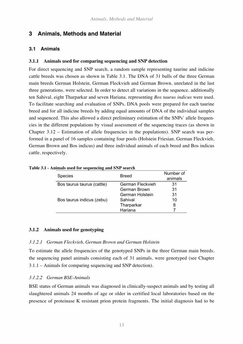
Table 3.1 - Animals used for sequencing and SNP search ......................................................................... 13
Table 3.2 - Characterisation of bovine BAC library................................................................................... 21
Table 3.3 - Master Mix for hME-PCR (single reaction)............................................................................. 30
Table 3.4 - Time-temperature programme for hME-PCR. ......................................................................... 30
Table 3.5 - Mix for SAP-Treatment (single reaction)................................................................................. 30
Table 3.6 - Incubation time-temperature programme for SAP treatment .................................................. 31
Table 3.7 - Master Mix for hME Extension reaction (single reaction). ..................................................... 31
Table 3.8 - Time-temperature programme for hME Extension reaction.................................................... 31
Table 3.9 - Mass differences between iPLEX extension products ............................................................. 33
Table 3.10 - Master Mix for iPLEX-PCR (single reaction). ...................................................................... 33
Table 3.11 - Master Mix for iPLEX-Extension reaction (single reaction)................................................. 34
Table 3.12 - iPLEX Time-temperature programme.................................................................................... 34
Table 3.13 - 2x3 Contingency table for the Armitage Trend test............................................................... 35
Table 3.14 - Calculation of allele frequencies of dams of half-sibs. .......................................................... 40
Table 3.15 - Calculation of the genotype frequencies of the dams of German Holstein half-sibs............ 40
Table 4.1 - Bovine ESTs for the HEXA gene.............................................................................................. 43
Table 4.2 - Exon and intron organisation of bovine HEXA gene. .............................................................. 43
Table 4.3 - Identified BAC clones containing a HEXA specific insert ...................................................... 49
Table 4.4 - Bovine scaffolds for ARIH1, HEXA, BRUNOL6 and PARP6 (Btau 1.0)................................ 51
Table 4.5 - PARP6, BRUNOL6, HEXA, ARIH1 mapped on bovine contig BTA 10.23 (Btau 2.0) .......... 52
Table 4.6 - PARP6, BRUNOL6, HEXA, ARIH1 mapped on BTA10 (Btau 3.1)........................................ 53
Table 4.7 - Exon and intron organisation of bovine ARIH1 gene. ............................................................. 55
Table 4.8 - Exon and intron organisation of bovine BRUNOL6 gene........................................................ 58
Table 4.9 - Exon and intron organisation of bovine PARP6 gene.............................................................. 62
Table 4.10 - SNPs and insertion/deletion (indel) polymorphism found in HEXA region. ........................ 66
Table 4.11 - Results of GC approach in the UK and German Holstein animals........................................ 68
Table 4.12 - Summary of SNP genotyping with MALDI-TOF MS........................................................... 71
Table 4.13 - Results of single marker analyses in the UK Holstein animals. ............................................ 74
Table 4.14 - Results of single marker analyses in the German Holstein animals...................................... 75
Table 4.15 - Analysis of association within haplotype blocks in the UK Holstein animals...................... 84
Table 4.16 - Haplotype analysis in the German Holstein animals. ............................................................ 85
Table 4.17 - Exon and intron organisation of bovine PRNP gene.............................................................. 86
Table 4.18 - Genotype frequencies and association analyses at PRNP promoter polymorphisms ........... 90
Table 4.19 - Allele frequencies and association analyses at PRNP promoter polymorphisms ................. 90
Table 4.20 - Calculation of haplotype frequencies in dams of half-sibs.................................................... 91
Table 4.21 - Calculation of the frequency of maternally inherited haplotypes.......................................... 92
Table 4.22 - Calculation of approximative numbers of diplotypes of German Holstein........................... 92
Table 4.23 - Haplotype frequencies and association analyses at PRNP promoter polymorphisms .......... 94
Table 4.24 - Diplotype frequencies and association analyses at PRNP polymorphisms........................... 96
List of tables and figures
x
List of Figures
Figure 2.1 - Development of the number of BSE-diseased animals in the UK (state 12/05)...................... 3
Figure 2.2 - Development of the number of BSE-diseased animals in Germany (state 11/06) .................. 5
Figure 2.3 - Hypothetical protein structure models for PrPc (left) and PrPsc (right). ................................... 6
Figure 2.4 - Genotype Frequencies at human Prion protein polymorphism (M129V)................................ 7
Figure 2.5 - Effect of Population Stratification at a SNP locus.................................................................. 11
Figure 3.1 - Exemplified EST sequencing approach. ................................................................................. 18
Figure 3.3 - Consed view of aligned sequence traces ................................................................................. 25
Figure 3.4 - Comparison of sequencing traces of a) individual animals and b) pooled DNA................... 26
Figure 3.5 - Principle of the hME method................................................................................................... 29
Figure 3.6 - Principle of the iPLEX method. .............................................................................................. 32
Figure 3.7 - Distribution curve of 105 permutation tests............................................................................. 37
Figure 4.1 - Model for the lysosomal function of HexA ............................................................................ 41
Figure 4.2 - Graphical overview bovine HEXA. ......................................................................................... 44
Figure 4.3 - Alignment of HexA protein sequences from different species. ............................................. 44
Figure 4.4 - Conservation profile of the aligned bovine and human 5’-region of HEXA.......................... 45
Figure 4.5 - Predicted bovine HEXA promoter sequence ........................................................................... 46
Figure 4.6 - Predicted CpG islands in the 5'-end of HEXA from a) man b) cattle and c) mouse. ............. 47
Figure 4.7 - BAC-Contig encompassing the bovine HEXA region. ........................................................... 49
Figure 4.8 - Encompassing region of HEXA in Apollo view (Lewis et al., 2002)..................................... 53
Figure 4.9 - Graphical overview of bovine ARIH1 ..................................................................................... 54
Figure 4.10 - Alignment of protein sequences of ARIH1 of different species. .......................................... 55
Figure 4.11 - Conservation profile of the aligned bovine and human 5'-region of ARIH1 ....................... 56
Figure 4.12 - Predicted CpG islands in the 5'-end of ARIH1 in a) man and b) cattle................................ 57
Figure 4.13 - Graphical overview of bovine BRUNOL6 ............................................................................ 58
Figure 4.14 - Alignment of BRUNOL6 protein sequences of different species......................................... 59
Figure 4.15 - Conservation profile of the aligned bovine and human 5’-region of BRUNOL6. ............... 60
Figure 4.16 - Predicted CpG islands in the 5'-end of BRUNOL6 in a) man and b) cattle. ........................ 60
Figure 4.17 - Graphical overview bovine PARP6....................................................................................... 61
Figure 4.18 - Alignment of PARP6 protein sequences of different species............................................... 63
Figure 4.19 - Prediction of CpG islands in the 5'-end of PARP6 in a) man and b) cattle. ........................ 64
Figure 4.20 - Conservation profile of the aligned bovine and human 5’-region of PARP6 ...................... 64
Figure 4.21 - Minor allele frequencies (MAF) and Trend Values of the null-loci used for calculation
the inflation factors for a) UK Holsteins b) for the German Holsteins................................. 68
Figure 4.22 - MAF of null-loci of UK and German Holsteins and corresponding Trend values.............. 69
Figure 4.23 - SNPs successfully genotyped in the extended HEXA region. .............................................. 71
Figure 4.24 - MAF and Trend values of the SNPs genotyped in (a) the UK and (b) German Holsteins
BSE-cases and controls. ......................................................................................................... 72
Figure 4.25 - MAF in German Fleckvieh, German Brown and German Holsteins bulls.......................... 76
Figure 4.26 - Minor Allele Frequencies (MAF) of eight SNPs in additional candidate genes. ................ 77
Figure 4.27 - LD plot of the extended HEXA region (208 kb) among UK Holsteins................................ 79
Figure 4.28 - Haplotypes in the extended HEXA region including 38 SNPs. ............................................ 80
Figure 4.29 - Haplotype analysis in the extended HEXA region including 18 tagSNPs. .......................... 81
Figure 4.30 - LD plot and haplotype block structure for tagged SNPs...................................................... 82

List of tables and figures
xi
Figure 4.31 - Haplotype blocks for the tagged SNPs of the extended HEXA region ................................ 83
Figure 4.32 - Graphical overview bovine PRNP gene................................................................................ 87
Figure 4.33 - Predicted CpG islands in bovine PRNP. ............................................................................... 87
Figure 4.34 - Allele frequencies of the PRNP polymorphisms .................................................................. 89
Figure 4.35 - Haplotype Frequencies of PRNP polymorphisms ................................................................ 93
Figure 4.36 - Diplotype Frequencies of the PRNP polymorphisms........................................................... 95
Figure 4.37 - Odds Ratios of Diplotypes..................................................................................................... 95
Abbreviations
xii
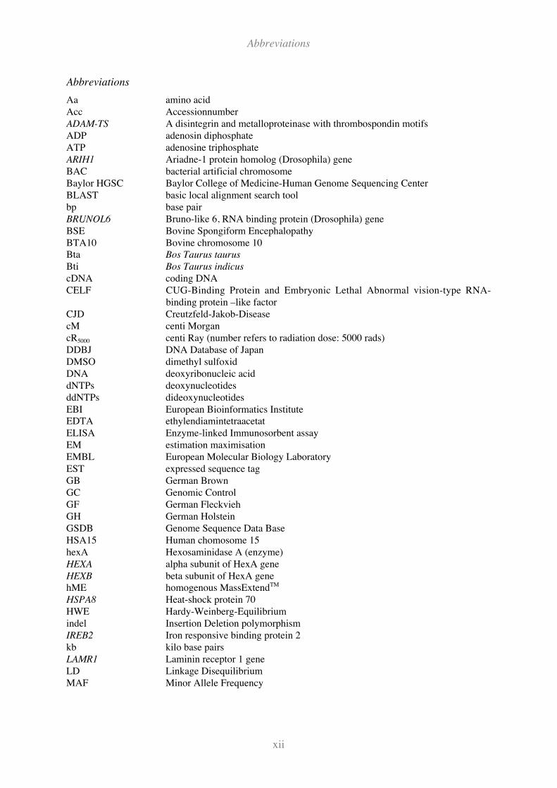
Abbreviations
Aa amino acid
Acc Accessionnumber
ADAM-TS A disintegrin and metalloproteinase with thrombospondin motifs
ADP adenosin diphosphate
ATP adenosine triphosphate
ARIH1 Ariadne-1 protein homolog (Drosophila) gene
BAC bacterial artificial chromosome
Baylor HGSC Baylor College of Medicine-Human Genome Sequencing Center
BLAST basic local alignment search tool
bp base pair
BRUNOL6 Bruno-like 6, RNA binding protein (Drosophila) gene
BSE Bovine Spongiform Encephalopathy
BTA10 Bovine chromosome 10
Bta Bos Taurus taurus
Bti Bos Taurus indicus
cDNA coding DNA
CELF CUG-Binding Protein and Embryonic Lethal Abnormal vision-type RNA-
binding protein –like factor
CJD Creutzfeld-Jakob-Disease
cM centi Morgan
cR5000 centi Ray (number refers to radiation dose: 5000 rads)
DDBJ DNA Database of Japan
DMSO dimethyl sulfoxid
DNA deoxyribonucleic acid
dNTPs deoxynucleotides
ddNTPs dideoxynucleotides
EBI European Bioinformatics Institute
EDTA ethylendiamintetraacetat
ELISA Enzyme-linked Immunosorbent assay
EM estimation maximisation
EMBL European Molecular Biology Laboratory
EST expressed sequence tag
GB German Brown
GC Genomic Control
GF German Fleckvieh
GH German Holstein
GSDB Genome Sequence Data Base
HSA15 Human chomosome 15
hexA Hexosaminidase A (enzyme)
HEXA alpha subunit of HexA gene
HEXB beta subunit of HexA gene
hME homogenous MassExtendTM
HSPA8 Heat-shock protein 70
HWE Hardy-Weinberg-Equilibrium
indel Insertion Deletion polymorphism
IREB2 Iron responsive binding protein 2
kb kilo base pairs
LAMR1 Laminin receptor 1 gene
LD Linkage Disequilibrium
MAF Minor Allele Frequency
Abbreviations
xiii
MALDI-TOF MS Matrix Assisted Laser Desorption Ionisation Time of Flight Mass Spectro-
metry
Mb Mega bases
MIH Maternal Inherited Haplotype
mRNA messenger ribonucleic acid
N A, C, G, T, U
NCBI National Center of Biotechnology Information
OR Odds Ratio
ORF Open Reading Frame
PAR Population Attributable Risk
PARP6 Poly-(ADP-ribose) Polymerase 6 gene
PCR polymerase chain reaction
PLG Plasminogen gene
PRNP prion protein gene
PrPc cellular prion protein
PrPsc scrapie prion protein
QTL quantitative trait loci
RACE rapid amplification of copyDNA ends
RFLP restriction fragment length polymorphism
RH radiation hybrid
Rpm rounds per minute
SAP Shrimp Alkaline Phosphatase
SBE single base extension
SDS sodium dodecylsulfat
SNP Single nucleotide polymorphism
SP1 Stimulating Protein 1 (transcription factor)
SQL Structured Query Language
TBE Tris Borate EDTA buffer
TDT Transmission Disequilibrium Test
TE Tris EDTA buffer
TGF Transforming Growth Factor
THSD4 thrombospondin, type 1, domain containg 4 gene
TNE Tris Natr EDTA buffer
Tris Tris (hydroxymethyl) aminomethane
TSE Transmissible spongiforme encephalopathy
UK United Kingdom
UTR Untranslated Region
vCJD variant CJD
Introduction and Goals
1
1 Introduction and Goals
Bovine Spongiform Encephalopathy (BSE) and its human form, variant Creutzfeld-Jakob
disease (vCJD) belong to a group of fatal neurodegenerative prion diseases that are known as
Transmissible Spongiform Encephalopathies (TSE). Most likely, BSE originates from Scra-
pie, the TSE of sheep, which was transmitted from sheep to cattle via the ingestion of infected
meat and bone meal, a substantial protein source for cattle in the UK. Disease specific iso-
forms of the prion protein (PrPsc) cause BSE by interaction with normal host prions (PrP),
resulting in its conversion to PrPsc. The misfolded PrPsc later accumulates in the brain leading
to neurodegeneration with formation of spongiform vacuoles (Prusiner, 1998a). In the disease
process, the host’s own PrP plays a crucial role: knockout mice experiments showed that mice
lacking the prion protein never develop TSE. A notable feature of TSEs is a varying suscepti-
bility of individuals to succumb to the diseases that is influenced by the genetic make-up and
in particular, their prion protein gene (PRNP) genotype. Only human beings homozygous for
a PRNP variant are currently known to have developed the variant Creutzfeldt-Jakob disease.
In sheep, three codons in PRNP are strongly associated with the resistance or susceptibility to
Scrapie. However to date, the genetic background of BSE in cattle is still unclear. Efforts to
identify variants in the bovine PRNP that influence the susceptibility of cattle to BSE did not
give a clear answer. So far, no convincing association between polymorphisms in the coding
sequence of PRNP gene with the BSE incidence could be demonstrated. Nevertheless, a re-
cent study investigating a small number of diseased animals from different breeds showed
significant association of polymorphisms in the PRNP promoter and BSE (Sander et al.,
2004). It is quite possible that these variants are influencing the expression levels of PRNP
and are so intervening in PrPc procession. The role of PRNP as a functional candidate gene for
BSE susceptibility is remarkable and encourages to investigate the bovine PRNP in more de-
tail by studying the promoter polymorphisms in a large sample of BSE diseased animals and
controls.
In order to identify positional candidates, whole genome marker scans were performed in a
set of BSE diseased and control animals revealing several marker loci that were significantly
associated with BSE (Hernandez-Sanchez et al., 2002) (Zhang et al., 2004). Assuming a con-
tinuous trait, which can be measured (e.g., the individual incubation time), the regions en-
compassing the associated marker loci can be considered as so called Quantitative Trait Loci
(QTL). One of these QTL regions on cattle chromosome 10 contains the gene encoding the
alpha subunit of the lysosomal enzyme beta-hexosaminidase A (hexA), HEXA. Recently, a
QTL study in mice linked the prion incubation time to the homologous region containing
Introduction and Goals
2
Hexa (Stephenson et al., 2000). The enzyme HexA plays a central role in the degradation of
glyco-proteins of nerve cell membrane in the lysosome. In humans, polymorphisms in HEXA
cause the neurodegenerative Tay-Sachs disease with accumulation of glyco-proteins in the
lysosome. Further, HEXA was functionally connected to TSEs by showing that gene expres-
sion is elevated in Scrapie infected brains of mice (Kopacek et al., 2000). Thus, the chromo-
somal region of HEXA was postulated as a potential candidate region for BSE susceptibility.
In this work, genetic factors which influence the susceptibility to BSE in cattle were identified
and assessed by candidate gene analyses and association studies of the coding and promoter
regions of PRNP, HEXA and the adjacent region of HEXA.
The specific goals of this thesis were
1. Characterisation of candidate genes for BSE susceptibility on bovine chromosome 10
• Sequence and structure analysis of the bovine HEXA gene and its promoter
• Elucidation of 300 kb region centred on the HEXA gene
2. Screening for polymorphisms in HEXA and neighbouring genes
3. Investigation of the potential role of candidate genes for BSE susceptibility by asso-
ciation studies in different breeds
• Genotyping of null-loci as Genomic Control to assess putative population stratification.
• Genotyping of polymorphisms in the extended HEXA region in BSE diseased and con-
trol animals.
• Genotyping of polymorphisms in the promoter region of PRNP in BSE diseased and
control animals.
Literature Review
3
2 Literature review
2.1 Bovine Spongiform Encephalopathy (BSE) and Prion Diseases
2.1.1 Incidence of BSE and surveillance strategy in the United Kingdom (UK)
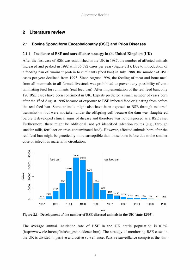
After the first case of BSE was established in the UK in 1987, the number of affected animals
increased and peaked in 1992 with 36 682 cases per year (Figure 2.1). Due to introduction of
a feeding ban of ruminant protein to ruminants (feed ban) in July 1988, the number of BSE
cases per year declined from 1993. Since August 1996, the feeding of meat and bone meal
from all mammals to all farmed livestock was prohibited to prevent any possibility of con-
taminating feed for ruminants (real feed ban). After implementation of the real feed ban, only
120 BSE cases have been confirmed in UK. Experts predicted a small number of cases born
after the 1st of August 1996 because of exposure to BSE infected feed originating from before
the real feed ban. Some animals might also have been exposed to BSE through maternal
transmission, but were not taken under the offspring cull because the dam was slaughtered
before it developed clinical signs of disease and therefore was not diagnosed as a BSE case.
Furthermore, there might be additional, not yet identified infection routes (e.g., through
suckler milk, fertilizer or cross-contaminated feed). However, affected animals born after the
real feed ban might be genetically more susceptible than those born before due to the smaller
dose of infectious material in circulation.
Figure 2.1 - Development of the number of BSE-diseased animals in the UK (state 12/05).
The average annual incidence rate of BSE in the UK cattle population is 0.2%
(http://www.oie.int/eng/info/en_esbincidence.htm). The strategy of monitoring BSE cases in
the UK is divided in passive and active surveillance. Passive surveillance comprises the sim-
Literature Review
4
ple recording of sick animals. This method identified 179 130 BSE positive animals to the end
of 2005. Active surveillance identified 1 678 BSE positive animals by testing brain samples
using EU approved rapid testing procedures based on the presence of proteinase K resistant
prion protein fragments. The following categories of cattle are tested for BSE:
• All cattle destined for human consumption aged over 30 months,
• All fallen stock aged over 24 months,
• All emergency slaughter animals,
• Animals found sick at ante mortem inspection aged over 24 months,
• All cattle born between August 1, 1995 and August 1, 1996 entering the Older Cattle
Disposal System.
The programme results are published regularly on the web page http://www.defra.gov.uk/
animalh/bse/statistics/incidence.html.
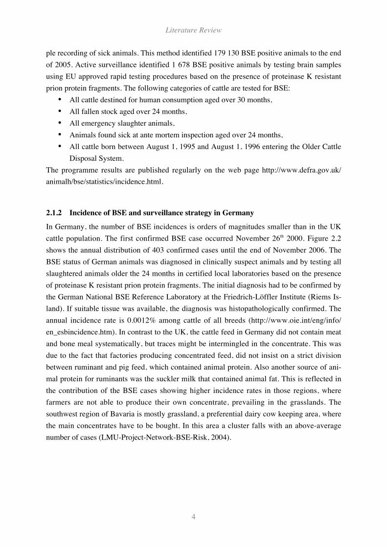
2.1.2 Incidence of BSE and surveillance strategy in Germany
In Germany, the number of BSE incidences is orders of magnitudes smaller than in the UK
cattle population. The first confirmed BSE case occurred November 26th 2000. Figure 2.2
shows the annual distribution of 403 confirmed cases until the end of November 2006. The
BSE status of German animals was diagnosed in clinically suspect animals and by testing all
slaughtered animals older the 24 months in certified local laboratories based on the presence
of proteinase K resistant prion protein fragments. The initial diagnosis had to be confirmed by
the German National BSE Reference Laboratory at the Friedrich-Löffler Institute (Riems Is-
land). If suitable tissue was available, the diagnosis was histopathologically confirmed. The
annual incidence rate is 0.0012% among cattle of all breeds (http://www.oie.int/eng/info/
en_esbincidence.htm). In contrast to the UK, the cattle feed in Germany did not contain meat
and bone meal systematically, but traces might be intermingled in the concentrate. This was
due to the fact that factories producing concentrated feed, did not insist on a strict division
between ruminant and pig feed, which contained animal protein. Also another source of ani-
mal protein for ruminants was the suckler milk that contained animal fat. This is reflected in
the contribution of the BSE cases showing higher incidence rates in those regions, where
farmers are not able to produce their own concentrate, prevailing in the grasslands. The
southwest region of Bavaria is mostly grassland, a preferential dairy cow keeping area, where
the main concentrates have to be bought. In this area a cluster falls with an above-average
number of cases (LMU-Project-Network-BSE-Risk, 2004).
Literature Review
5
Figure 2.2 - Development of the number of BSE-diseased animals in Germany (state 11/06)
2.1.3 Basics and genetics of prion diseases
Transmissible Spongiform Encephalopathies (TSEs) are fatal neurodegenerative disorders in
humans and other mammals that can be experimentally transmitted to individuals of the same
and other species. The morbid agent is the so called Scrapie prion protein (PrPsc); the name
origins from the archetype TSE of sheep (Scrapie) and is used for all TSE pathogens. In con-
trast to other classical pathogens, PrPsc has no own genome and consists of an abnormal con-
formation of the cellular and hosts own prion protein (PrPc) (Prusiner, 1982).
PrPc is a glycoprotein attached by a C-terminally linked glycosyl-phosphat-idylinositol (GPI)
anchor on the plasma membrane of neuronal cells, predominantly on presynaptic membranes
(Herms et al., 1999). Due to copper-binding ability assigned by an octapeptide repeat, possi-
ble copper-specific neuroprotective mechanisms have been proposed (Roucou et al., 2004;
Vassallo and Herms, 2003).
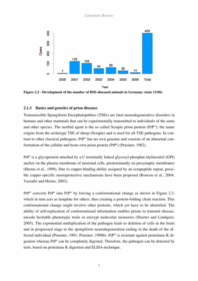
PrPsc converts PrPc into PrPsc by forcing a conformational change as shown in Figure 2.3,
which in turn acts as template for others, thus creating a protein-folding chain reaction. This
conformational change might involve other proteins, which yet have to be identified. The
ability of self-replication of conformational information enables prions to transmit disease,
encode heritable phenotypic traits or encrypt molecular memories (Shorter and Lindquist,
2005). The exponential multiplication of the pathogen leads to deletion of cells in the brain
and in progressed stage to the spongiform neurodegeneration ending in the death of the af-
fected individual (Prusiner, 1991; Prusiner, 1998b). PrPsc is resistant against proteinase K di-
gestion whereas PrPc can be completely digested. Therefore, the pathogen can be detected by
tests, based on proteinase K digestion and ELISA-technique.
Literature Review
6
Figure 2.3 - Hypothetical protein structure models for PrPc (left) and PrPsc (right).
Conversion of !-helices into "-sheet structure by formation of the pathogenous form.
Scrapie, the archetype prion disease, is a natural disease of sheep and goats and its character-
istics include a long incubation or preclinical period, progressive ataxia, astrocytosis, tremor
and death. Scrapie has been recognized in Europe for over 200 years ago and is present in
many countries worldwide. The typical histopathological changes are prior in the brain that
include vacuolation from cell death, neuronal loss and, in some cases amyloid plaque forma-
tions. In sheep, variations at positions 136, 154 and 171 of the prion protein sequence play an
important role for the susceptibility to Scrapie. In dependence of the arrangement of the
genotypes at the three loci, the sheep is more or less liable to come down with Scrapie
(Hunter et al., 1997). Testing the individual Scrapie resistance by genotyping has become an
important issue in the sheep production. In the European Union a breeding programme for
TSE resistance in purebred sheep exists forcing the member states and their sheep flocks to
follow the selection for resistance to TSE (Commission-of-the-European-Union, 2003).
In human beings, several distinctable prion diseases are known (Prusiner, 1991; Prusiner,
1998b) (Collinge, 2001). The sporadic Creutzfeld-Jakob-Disease (CJD), the most frequent
form of human prion diseases affects about one individual per million. In the United King-
dom, there are fifty to sixty deaths per year due to sporadic CJD. In the affected individuals,
the PrPc undergoes a spontaneous conformation change to the abnormal form and leads to the
disease. Kuru, the prion disease among the Fore folk in Papua New Guinea, first recognized
in the 1950s, was transmitted from human to human during cannibalistic feasts (Gajdusek et
al., 1966). Initially misfolded prion proteins were migrating from the dead to the tribesman
alive, consuming the brains of the affected people. A novel form of human TSE, variant CJD
(vCJD), was first reported in the United Kingdom in 1996 (Will et al., 1996) (Collinge and
Rossor, 1996). VCJD is said to be the human form of BSE, transmitted by passing the infec-
Literature Review
7
tious prions from cattle to human in the form of brain tissue contaminated beef.
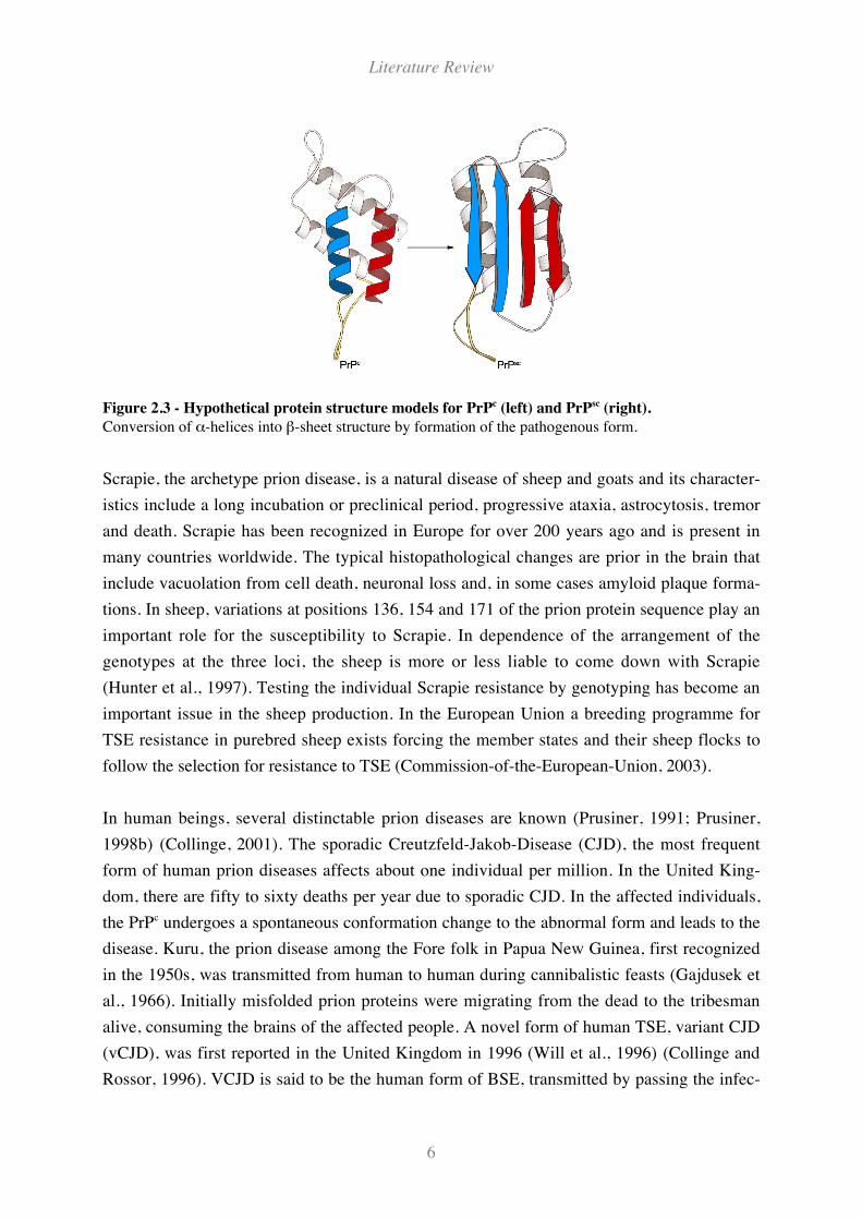
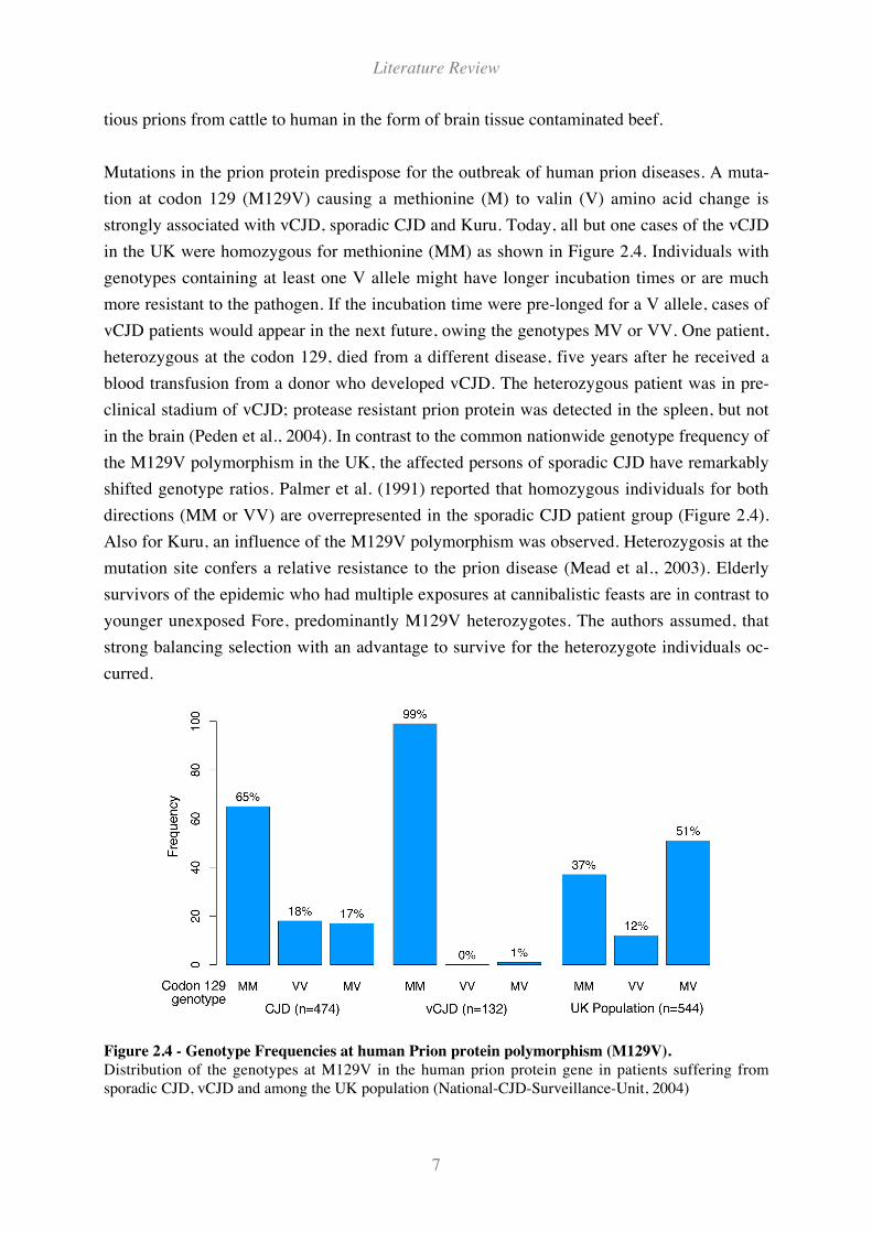
Mutations in the prion protein predispose for the outbreak of human prion diseases. A muta-
tion at codon 129 (M129V) causing a methionine (M) to valin (V) amino acid change is
strongly associated with vCJD, sporadic CJD and Kuru. Today, all but one cases of the vCJD
in the UK were homozygous for methionine (MM) as shown in Figure 2.4. Individuals with
genotypes containing at least one V allele might have longer incubation times or are much
more resistant to the pathogen. If the incubation time were pre-longed for a V allele, cases of
vCJD patients would appear in the next future, owing the genotypes MV or VV. One patient,
heterozygous at the codon 129, died from a different disease, five years after he received a
blood transfusion from a donor who developed vCJD. The heterozygous patient was in pre-
clinical stadium of vCJD; protease resistant prion protein was detected in the spleen, but not
in the brain (Peden et al., 2004). In contrast to the common nationwide genotype frequency of
the M129V polymorphism in the UK, the affected persons of sporadic CJD have remarkably
shifted genotype ratios. Palmer et al. (1991) reported that homozygous individuals for both
directions (MM or VV) are overrepresented in the sporadic CJD patient group (Figure 2.4).
Also for Kuru, an influence of the M129V polymorphism was observed. Heterozygosis at the
mutation site confers a relative resistance to the prion disease (Mead et al., 2003). Elderly
survivors of the epidemic who had multiple exposures at cannibalistic feasts are in contrast to
younger unexposed Fore, predominantly M129V heterozygotes. The authors assumed, that
strong balancing selection with an advantage to survive for the heterozygote individuals oc-
curred.
Figure 2.4 - Genotype Frequencies at human Prion protein polymorphism (M129V).
Distribution of the genotypes at M129V in the human prion protein gene in patients suffering from
sporadic CJD, vCJD and among the UK population (National-CJD-Surveillance-Unit, 2004)
Literature Review
8
2.1.4 Genetic Background of BSE in cattle
In 1990, Wijeratne and Curnow showed by segregation analysis in families with BSE-
members that 73% of the affected animals had first or second degree relatives also affected.
The Mendelian model for an autosomal recessive inheritance could not be excluded. But the
piled occurrence of bulls as ancestors of BSE animals could also arise from the international
breeding strategy. Studies of the progenies of BSE affected cows indicated, that there may be
a genetic influence on the susceptibility in cattle, because of the apparent higher risk of devel-
oping BSE in off-spring of BSE-affected cows compared with uninfected controls (Donnelly
et al., 1997; Ferguson et al., 1997; Wilesmith et al., 1997). The gene encoding the prion pro-
tein, PRNP, has been suggested as a candidate locus for BSE susceptibility. However, no
clear relationships between bovine PRNP polymorphisms and susceptibility to BSE have been
revealed so far. The study of Neibergs et al. (1994) showed that an octapeptide repeat in the
amino acid sequence is associated with BSE, but this was not confirmed in a similar study of
Hunter et al. (1994). Moreover, two insertion / deletion (indel) polymorphisms in the pro-
moter region of PRNP were subject of an association study of Sander et al. (2004), revealing
that both the 23-bp indel (Sander et al., 2004) in the promoter region and the 12-bp indel
(Hills et al., 2001) in intron 1 are tentatively associated with the BSE status. In vitro analysis
showed that both indel sides affect binding sites for transcription factors (RP58 and SP1, re-
spectively), and in vivo and in vitro investigations suggest that the two polymorphisms affect
PRNP expression, albeit with the direction on the effects remaining to be clarified (Sander et
al., 2005).
In order to identify loci responsible for susceptibility to BSE, Hernandez-Sanchez et al.
(2002) performed a genome-wide search for markers associated with BSE, by using a Trans-
mission Disequilibrium Test (TDT). In this study, 358 BSE affected and 172 healthy half-sibs
of four fathers were genotyped at 146 informative microsatellite markers loci. Significant seg-
regation distortion was found on cattle chromosomes 5, 10 and 20. Putative candidates lo-
cated in these regions are e.g. both subunits of the enzyme hexosaminidase A (hexA), HEXA
and HEXB on cattle chromosomes (BTA) 10 and 20, respectively. To map quantitative trait
loci (QTL) for BSE susceptibility, a whole-genome scan was conducted by Zhang et al.
(2004), including 173 microsatellite markers and four half-sib families with affected and un-
affected members. Two genome-wide significant QTL (BTA17 and X/Yps) and four genome-
wide suggestive QTL (BTA 1, 6, 13 and 19) were revealed. A potential candidate for BSE
susceptibility, which falls within the 95% C.I. of the QTL on BTA 19 is the gene encoding
neurofibromin 1 NF1. A microsatellite flanking this gene was genotyped in a panel of BSE-
affected and control animals by Geldermann et al. (2006), revealing significant association in
one of four investigated cattle breeds.
Literature Review
9
2.2 Single Nucleotide Polymorphisms
A Single Nucleotide Polymorphism (SNP) refers to a position in the DNA sequence at which
two alternative bases occur at appreciable frequency (>1%). SNPs are the most common type
of variations found in mammalian genome. In human beings, SNPs occur with a mean fre-
quency of one SNP per kb (Wang et al., 1998). For cattle, Werner et al. (2004) identified on
average one SNP every 180 bp by randomly screening of 91 kb bovine genomic DNA. In this
study, SNP screening was performed in a panel of animals belonging to the taurine breeds
German Holstein, German Brown, German Fleckvieh, Kerry and Angus and to the indicine
breeds Sahiwal and Hariana. Bovine DNA from seven US breeds was used to screen 5.2 kb of
nine loci of the chemokine gene family by Heaton et al. (2001). The authors detected on aver-
age one variable site every 143 bp. First, SNPs were used as genetic markers in analysing
Restriction Fragment Length Polymorphisms (RFLPs) (Botstein et al., 1980). Often without
knowing the sequence data, this was an indirect method of genotyping SNPs, because the
RFLPs were caused by point mutations, which determine the cutting site of an enzyme. How-
ever, this method is still in use and appropriate to genotype few SNPs with known sequence
information. Due to the abundance and distribution of SNPs, the interest of using SNPs as
genetic markers increased in the last decade. As a by-product of the whole genome sequenc-
ing projects, thousands of SNPs were identified in the different species. Nowadays, SNPs are
being genotyped in disease association studies and pharmacogenetics, etc. (Gray et al., 2000)
and the application of SNPs is ranging from forensic fingerprinting where individuals can be
identified by determining the genotypes at a panel of 34 SNPs (Li et al., 2006) to whole ge-
nome association studies where pooled DNA can be genotyped parallel at 500 000 SNPs
(Papassotiropoulos et al., 2006). Other biallelic variation occuring with considerable fre-
quency are insertion-deletion (indel) polymorphisms. At an indel polymorphism the DNA
sequence of one to thousand or more bases are either existent or not. Indels can be genotyped
with the methods of SNP typing if the first base of insertion and first base after insertion are
different nucleotides.
Various methods of genotyping SNPs are established. The appropriate genotyping approach
depends on the number of samples and SNPs. Common SNP typing chemistries currently
available are based on differential hybridisation, allele specific amplification, primer exten-
sion with allele specific nucleotide incorporation and allele specific DNA-cleavage. Each
chemistry has its appropriate detection system. Some of the current technologies of high
throughput genotyping SNPs are fluorescent microarray-based systems (e.g., Gene Chips
from Affymetrix, Santa Clara, CA, USA), fluorescent bead-based technologies (e.g., BeadAr-
ray, Illumina, San Diego, CA, USA), automated enzyme-linked immunosorbent (ELISA) as-
says (SNP-IT, Orchid, Princeton, NJ, USA) and the technique used in context of this thesis,
Literature Review
10
mass spectroscopy detection (e.g., iPlex, Sequenom, San Diego, CA, USA). This technique is
described in detail in Chapter 3.14 - Genotyping SNPs with MALDI-TOF MS.
2.3 Challenge of Association studies
Case-Control-Studies based on the comparison of affected (= cases) and unaffected (= con-
trols) individuals from a population is called a population-based association study. The allele
A at a gene locus is said to be associated with a phenotype, if it occurs with a significantly
higher or lower frequency in the affected group compared to the unaffected (Lander and
Schork, 1994). Mainly, biallelic DNA polymorphisms were used to perform association stud-
ies including SNPs and insertion-deletion polymorphisms with minor allele frequencies of
above 5%. After genotyping of a panel of cases and controls, the statistical analysis include
the Test for Hardy-Weinberg-Equilibrium (as shown in Chapter 3.15.2 – Test for Hardy-
Weinberg-Equilibrium), allele and genotype frequency based calculation of the test statistic
(as shown in Chapter 3.15.3 – The Armitage Trend test) and logistic regression analysis for
risk calculations (as shown in Chapter 3.15.4 – Logistic regression analysis). Afterwards,
Linkage Disequilibrium (LD) and haplotype analysis were performed to elucidate putative
combined effects on the trait (as shown in Chapters 3.15.5 and 3.15.6 – Measuring LD and
tagging SNPs and Inferring haplotypes, respectively). Recent advances of the availability of
many genetic markers, in particular of SNPs and the increasing speed and capacity of geno-
typing machines, faciliate the performance of association studies.
Association of a marker allele with a phenotype might have different origins. First, the SNP is
causal and the individual genotype influences the phenotype (e.g., predisposition to a disease).
In this case, the same direction and effect size of the association would be expected to occur
in different populations. Hence, the association can be replicated in other studies. The in-
volvement of the polymorphism in the phenotype can be confirmed by other approaches like
expression analysis or verification of the function or malfunction in transgenic animal models.
Second, the allele does not cause or change the trait, but is in LD with the causative polymor-
phism. I.e., the associated allele tends to occur on those chromosomes, which carry the causa-
tive/trait changing mutation, due to the haplotype configuration of the ancestor, where the
mutation debuted. Depending on the genetic distance and the age of the mutation, recombina-
tion events reduce the LD between marker and causative mutation. A genetic distance of 1cM
corresponds to a probability of recombination in meiosis of 1%. Here, the results for different
isolated populations (e.g., cattle breeds) can be oppositional. In one population the first allele
can be associated with the trait and in the other population the second allele, due to specific
recombination events in the ancestry of the populations. Consequentially, no allelic associa-
tion can be found if these populations were pooled for the study.
Literature Review
11
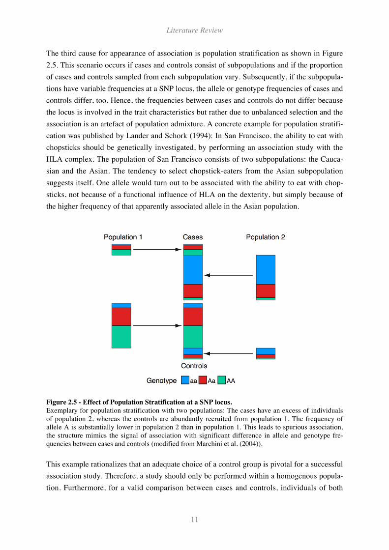
The third cause for appearance of association is population stratification as shown in Figure
2.5. This scenario occurs if cases and controls consist of subpopulations and if the proportion
of cases and controls sampled from each subpopulation vary. Subsequently, if the subpopula-
tions have variable frequencies at a SNP locus, the allele or genotype frequencies of cases and
controls differ, too. Hence, the frequencies between cases and controls do not differ because
the locus is involved in the trait characteristics but rather due to unbalanced selection and the
association is an artefact of population admixture. A concrete example for population stratifi-
cation was published by Lander and Schork (1994): In San Francisco, the ability to eat with
chopsticks should be genetically investigated, by performing an association study with the
HLA complex. The population of San Francisco consists of two subpopulations: the Cauca-
sian and the Asian. The tendency to select chopstick-eaters from the Asian subpopulation
suggests itself. One allele would turn out to be associated with the ability to eat with chop-
sticks, not because of a functional influence of HLA on the dexterity, but simply because of
the higher frequency of that apparently associated allele in the Asian population.
Figure 2.5 - Effect of Population Stratification at a SNP locus.
Exemplary for population stratification with two populations: The cases have an excess of individuals
of population 2, whereas the controls are abundantly recruited from population 1. The frequency of
allele A is substantially lower in population 2 than in population 1. This leads to spurious association,
the structure mimics the signal of association with significant difference in allele and genotype fre-
quencies between cases and controls (modified from Marchini et al. (2004)).
This example rationalizes that an adequate choice of a control group is pivotal for a successful
association study. Therefore, a study should only be performed within a homogenous popula-
tion. Furthermore, for a valid comparison between cases and controls, individuals of both
Literature Review
12
groups should differ preferable only in the investigated attribute. Thus, a comparison of indi-
viduals from different origins (e.g., cattle breeds) in the case and control group is not useful
and must be avoided. If origin, parentage and relatedness of the samples are unknown or
population substructure is expected (e.g., in inbred populations), the population stratification
should be detected and corrected. An appropriate approach is the Genomic Control (GC)
(Devlin and Roeder, 1999). For GC, additional loci to the candidates’ -so called null-loci-
have to be genotyped. The null-loci are unlinked polymorphisms, considered having no effect
on the susceptibility or the value of the trait. By calculating the Armitage Trend test statistic
for the null-loci, the inflation factor # is inferred as the empirical median divided by its ex-
pectation under the $2-distribution. If # > 1, the test statistics of the investigated candidate
loci are divided by #, in order to correct for stratification.
The analysis of multiple polymorphisms in a candidate region inflates the global type 1 error
rate. Adjustment for multiple testing is a basic problem of association studies performed with
many markers. The test wise type 1 error rate (alpha-level) has to be corrected downwards to
consider false positives, if more than one test in a particular study was made. Usually, the
alpha-level is set to 0.05, which denotes that one of twenty tests shows a false positive asso-
ciation. The probability of finding at least one association rises in line with the number of
performed tests. Therefore, a correction for multiple testing is required. Customarily, this can
be performed by order of Bonferroni-Holm correction, False Discovery Rate approach or
permutation procedure.
Animals, Methods and Material
13
3 Animals, Methods and Material
3.1 Animals
3.1.1 Animals used for comparing sequencing and SNP detection
For direct sequencing and SNP search, a random sample representing taurine and indicine
cattle breeds was chosen as shown in Table 3.1. The DNA of 31 bulls of the three German
main breeds German Holstein, German Fleckvieh and German Brown, unrelated in the last
three generations, were selected. In order to detect all variations in the sequence, additionally
ten Sahival, eight Tharparkar and seven Hariana, representing Bos taurus indicus were used.
To facilitate searching and evaluation of SNPs, DNA pools were prepared for each taurine
breed and for all indicine breeds by adding equal amounts of DNA of the individual samples
and sequenced. This also allowed a direct preliminary estimation of the SNPs’ allele frequen-
cies in the different populations by visual assessment of the sequencing traces (as shown in
Chapter 3.12 – Estimation of allele frequencies in the populations). SNP search was per-
formed in a panel of 16 samples containing four pools (Holstein Friesian, German Fleckvieh,
German Brown and Bos indicus) and three individual animals of each breed and Bos indicus
cattle, respectively.
Table 3.1 - Animals used for sequencing and SNP search
Species BreedNumber of
animals
Bos taurus taurus (cattle) German Fleckvieh
German Brown
German Holstein
31
31
31
Bos taurus indicus (zebu) Sahival
TharparkarHariana
10
87
3.1.2 Animals used for genotyping
3.1.2.1 German Fleckvieh, German Brown and German Holstein
To estimate the allele frequencies of the genotyped SNPs in the three German main breeds,
the sequencing panel animals consisting each of 31 animals, were genotyped (see Chapter
3.1.1 – Animals for comparing sequencing and SNP detection).
3.1.2.2 German BSE-Animals
BSE status of German animals was diagnosed in clinically-suspect animals and by testing all
slaughtered animals 24 months of age or older in certified local laboratories based on the
presence of proteinase K resistant prion protein fragments. The initial diagnosis had to be
Animals, Methods and Material
14
confirmed by the German National BSE Reference Laboratory at the Friedrich-Löffler-Institut
of Novel and Emerging Infectious Diseases (FLI-INNT) (Riems Island) formerly known as
Bundesforschungsanstalt für Viruserkrankungen. DNA was extracted using the QiAamp
DNA Mini Kit (Qiagen Valencia, CA) after tissue decontamination with 13.5 M guanidine
chloride and kindly provided by the FLI-INNT. A total number of 276 cases, collected from
November 2000 until the end of 2005, was available. Based on the farmer’s declaration, 127
of these belong to German Holstein, 106 to German Fleckvieh and 43 to German Brown
breed. This separation into different populations is required, because of the genetical differ-
ence due to distinct selection strategies and breeding goals depending on the utilisation. To
date there are 403 BSE cases recorded in Germany, including at least ten different breeds. The
breed information was provided by the Friedrich-Löffler-Institut of Epidemiology in Wuster-
hausen. German Holstein black pied -BSE cases (n=73) with diagnosis in the years 2001 and
2002 were used for further investigations at the HEXA locus. For the association study at the
prion protein polymorphisms, all available BSE cases until the end of 2005 of the main breeds
German Holstein, German Brown and German Fleckvieh were investigated.
3.1.2.3 German Control Animals
Control animals for the German Holstein breed consisted of 627 paternal half-sibs, whose
DNA have been isolated in the framework of a QTL-mapping project by the Institute of Ani-
mal Breeding at the Christian-Albrechts-University of Kiel, by the Department of Animal
Breeding and Genetics at the Justus-Liebig-University of Gießen and by the Research Unit
Molecular Biology at the Research Institute for the Biology of Farm Animals. The half-sib
animals were approximately contemporary with the BSE animals and geographically similarly
distributed. Only the maternally inherited alleles were considered (see Chapter 3.15.10 - In-
ferring allele- and genotype frequencies from half-sibs). For the association study at the
PRNP promoter polymorphisms control animals were selected as follows: German Brown
bulls (n =90) used for artificial insemination were selected so that their pedigree was repre-
sentative for the German Brown population. The German Fleckvieh control (n = 137) con-
sisted of bulls kept at the experimental Station Hirschau of the Technical University of Mu-
nich. They were purchased on markets throughout Bavaria and can be considered to be repre-
sentative for the German Fleckvieh population. DNA was isolated by proteinase K and chlo-
roform-phenol extraction of blood (German Fleckvieh controls) or bull sperm (German
Brown control), provided by several Bavarian insemination stations.
3.1.2.4 UK Animals
Samples of BSE-affected UK animals were collected between 1990 and 1993. Animals were
identified as BSE suspects by veterinary diagnosis of live animals and the initial diagnosis
confirmed by histopathological examination. Blood samples were obtained from a total of 365
Animals, Methods and Material
15
BSE affected and 276 BSE unaffected age-matched paternal half-sib offspring, born on the
same farms as the BSE affected animals. The proportion of affected to unaffected animals was
similar in each of the 37 half-sib groups. None of the controls was recorded in the BSE case
database of the UK-Department for Environment, Food and Rural Affairs (Defra) at a later
date. DNA was obtained from blood via proteinase K digestion and phenol-extraction at the
Veterinary Laboratories Agency in Weybridge, UK.
3.2 DNA Handling
Genomic DNA was extracted from frozen bull semen for the individuals of the sequencing
panel and the German Brown control animals in our laboratory. Further, DNA of the German
Fleckvieh control animals was prepared from blood samples by proteinase K digestion and
chloroform-phenol extraction. DNA samples of German BSE diseased animals, German Hol-
stein control animals and UK animals were obtained from different other laboratories (see
Chapter 3.1.2 – Animals used for genotyping). Depending on further use, different DNA con-
centrations were required. DNA for sequencing was calibrated to a working solution of
25ng/µl, while DNA for genotyping by MALDI-TOF MS was adjusted to 1ng/µl.
To control the quantity and quality of the DNA, 1-2 µl of the solution were tested by gel
electrophoresis on a 0.8% agarose gel in 1/2 TBE buffer together with lambda DNA standard
(SD0011; MBI Fermentas, St. Leon-Rot, Germany) of known concentration. The quantity
was further assessed using fluorometric methods by mixing 2µl of each DNA with 1x TNE
buffer containing fluorescent Hoechst Dye (H33258, Fluka) incorporating into the DNA in a
special cuvette. The solution was measured by a fluorometer (DyNA-quant 200, Hoefer Sci-
entific, San Francisco, CA, USA). The DNA solutions of the samples for genotyping were
measured by PicoGreen dsDNA Quantification Kit (Molecular Probes, Leiden, Netherlands)
with a flourometry plate reader (GeniOS Fluorescence Plate Reader, TECAN, Crailsheim,
Germany). The advantage of this system is the high-throughput analysing of the plate reader,
the favoured binding of the Pico Green to double stranded (ds) DNA and the sensitive detec-
tion of quantities as little as 25pg/ml of ds DNA. After quantification of the DNA solutions,
200 ng of DNA was diluted with TE to 200 µl to aim for a final concentration of 1ng/µl. 5µl
of each DNA dilution (1ng/µl) was dispensed by pipetting station (TECAN, Crailsheim,
Germany) over a 384-sample plate and dried at room temperature.
3.3 The Basic Local Alignment Search Tool (BLAST)
The Basic Local Alignment Search tool (BLAST) (Altschul et al., 1990) is a powerful method
to identify similar and/or homologues sequences. BLAST finds regions of local similarity
Animals, Methods and Material
16
between sequences by comparing nucleotide or protein sequences to sequence databases and
calculates the statistical significance of matches. The tool is available on the web-pages of the
National Center of Biotechnology Information in Rockville Pike, USA (NCBI)
http://www.ncbi.nlm.nih.gov/ or the web-page of the European cooperation of Welcome Trust
Sanger Institute and the European Bioinformatics Institute (EBI) http://www.ensembl.org/.
The programme and sequence databases can be downloaded and installed locally on a desktop
computer to reduce processing times because of independence from the official server.
The tool was used for different purposes:
• Analysis of exon-intron structures by BLAST search of mRNA sequences against ge-
nomic sequences,
• Identifying bovine sequences (genomic or ESTs) by using homologous human se-
quences as query input,
• Newly sequenced bovine sequences were approved and assigned
• Alignment of two sequences with bl2seq (NCBI BLAST).
Sources for human sequences are, e.g. nr (non redundant)-, RefSeq and EST-Division of the
Nucleotide database of NCBI and the cow or human division of Ensembl web-page which
contains sequence data from GenBank (NCBI), EMBL (European Molecular Biological Labo-
ratory in Hinxton Hall, UK), GSDB (Genome Sequence Data Base in Santa Fe, USA) and
DDBJ (DNA Database of Japan in Mishima, Japan).
The gene structure and the neighbouring genes were detected with the tool Ensembl Mart
View, where gene information can be exported (http://www.ensembl.org/Multi/martview).
The region of interest can be chosen, different filters can be applied and various output infor-
mation can be requested (e.g. RefSeq ID, strand, start and end position, external gene ID,
etc.).
3.4 Excursus: Changes in bovine genomic sequence availability
The sources of bovine sequence data have enlarged many-fold over the last four years. The
following excursus should show how the increased sequence yield has changed the working
strategies for analysing candidate genes.
3.4.1 Sequence detection by BAC–DNA (Primer walking)
In case where no bovine sequence is available for the gene of interest, an initial bovine PCR
system and its primers need to be derived from human or mouse sequences. It is especially
advantageous to use coding sequences of the gene for this purpose (e.g. human mRNA) be-
cause exons are more highly conserved between species than are introns. Using the initial
Animals, Methods and Material
17
bovine PCR system, as verified by sequencing and BLAST comparison, a bovine Bacterial
Artificial Chromosome (BAC) library is screened for clones containing gene-inserts. After
BAC-DNA isolation, the insert is used as a template for Primer-Walking, where the BAC-
DNA is sequenced directly without a previous PCR-amplification by e.g., one up-primer or
from a primer of the BAC ends known vector sequence (BAC end sequencing). Initial primers
for BAC end sequencing were derived from T7 and SP6 promoter sites, which were located
on the pBACe3.6 vector flanking the insert. After determination of the sequence, the next up-
primer can be designed from it. This process is repeated iteratively: a direct sequencing step is
applied, the new sequence is determined and this sequence is used for primer design. To
identify SNPs in the newly determined gene sequence, region-specific PCR primers have to
be designed and applied to the DNA of both pooled and individual animals. In summary, the
steps that need to be performed for each part of the gene are, in order, primer walk sequenc-
ing, applying a PCR-system and finally sequencing of individuals to find sequence variations.
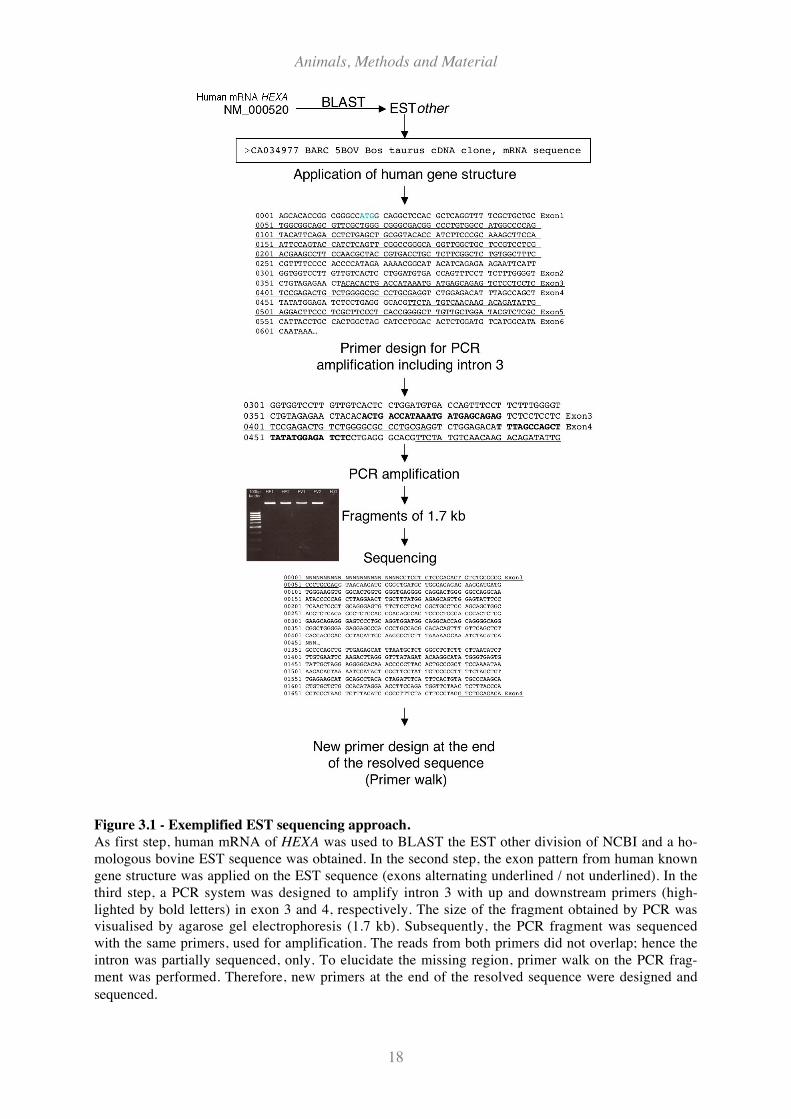
3.4.2 Bovine Expressed Sequence Tags (ESTs)
The first abundant bovine sequences that could be identified by BLAST search were ex-
pressed sequence tags (ESTs). Inserts of cDNA clones were partially sequenced from one or
both ends performing single-pass automated sequencing read. ESTs are characterised by be-
ing short (400 – 600 bases) and relatively inaccurate (around 2% error) (Adams et al., 1991).
In the current context, a human reference sequence (mRNA) was used to blast search the EST-
other division (dbEST) of GenBank to find bovine sequences for the candidate genes of inter-
est. In Figure 3.1, the EST sequencing approach is shown. By comparison of the human exon
structure and the EST sequences, the bovine structure could be inferred and used for primer
design spanning the introns as well. For the obtained PCR fragment, the size could be esti-
mated by agarose gel electrophoresis. Sequencing of the PCR fragments resulted in one up
and one downstream read of around 450 to 500 bases, which were assembled if the sequences
overlapped in the intron. This was the case when the fragment was smaller than 900 bp, for
larger fragments the missing region was elucidated by primer walk on the PCR fragment by
primer design at the end of the resolved region. In summary, a conserved gene structure be-
tween human and cattle was postulated and the human exon pattern was applied on the EST
sequence to identify exon-intron-boundaries. Than PCR systems were designed to amplify the
intron sequence, which were subsequently sequenced.
Animals, Methods and Material
18
Figure 3.1 - Exemplified EST sequencing approach.
As first step, human mRNA of HEXA was used to BLAST the EST other division of NCBI and a ho-
mologous bovine EST sequence was obtained. In the second step, the exon pattern from human known
gene structure was applied on the EST sequence (exons alternating underlined / not underlined). In the
third step, a PCR system was designed to amplify intron 3 with up and downstream primers (high-
lighted by bold letters) in exon 3 and 4, respectively. The size of the fragment obtained by PCR was
visualised by agarose gel electrophoresis (1.7 kb). Subsequently, the PCR fragment was sequenced
with the same primers, used for amplification. The reads from both primers did not overlap; hence the
intron was partially sequenced, only. To elucidate the missing region, primer walk on the PCR frag-
ment was performed. Therefore, new primers at the end of the resolved sequence were designed and
sequenced.
Animals, Methods and Material
19
3.4.3 Btau 1.0: First genomic cattle sequence
In October 2004, the first preliminary genomic sequence for cattle was published and avail-
able at the Ensembl Web-service (www.ensembl.org; Cow v.25, Btau 1.0). A whole
genome shotgun approach was employed and clones containing small DNA inserts of one
Hereford bull were sequenced. About 15 million reads were assembled by the Atlas genome
assembly system (Havlak et al., 2004) at the Baylor College of Medicine Human Genome
Sequencing Center (Baylor HGSC) (http://www.hgsc.bcm.tmc.edu/projects/bovine/). This
sequence represent about 9 Gb and a 3x coverage of the clonable bovine genome. If both end
sequences from one clone did not overlap, a contig was build by filling the missing base pairs
with an appropriate number of Ns as estimated by the insert size. Two contigs were assembled
if they contained partly the same sequence. The total length of the scaffolds was 2.26 Gb and
they ranged in size from 1 kb to 30 kb with an N50 size of 13.5 kb (i.e. 50% of all assembled
scaffolds are greater than or equal to this length). This first assembly of the bovine draft se-
quence was of fragmentary nature with relatively short scaffolds in respect to the estimated
mean gene size of 27 kb (Wong et al., 2001), leading to single genes being distributed across
two or more scaffolds. By BLAST search, the scaffolds containing the candidate gene could
be identified. The availability of these genomic sequences allowed optimisation of primer
design and PCR for sequencing. Moreover, the scaffold sequences simplified primer design
within the genes as well as for the 5'- and 3'- ends and the segments between the genes, e.g.
for selective PCR amplification and sequencing of exons. To obtain the sequence of exons,
primers were placed in intronic sequences, spanning the PCR system over the exon. However
due to the incomplete nature of the scaffolds, gaps still existed not only between genes, but
also within genes.
3.4.4 Btau 2.0: Second assembly of the cow genome
In June 2005, the Baylor HGSC published the second version of the bovine draft sequence
(Btau 2.0). The new chromosomal linear scaffolds were produced by the Atlas genome as-
sembly system (Havlak et al., 2004) with contigs of whole shotgun sequences and BAC end
sequences of one Hereford bull. About 23 million reads were assembled, representing about
17.7 Gb of sequence and about 6.2x coverage of the bovine genome. The total length of all
scaffolds was 2.62 Gb, with the N50 size of the scaffolds being 434.7 kb (i.e. 50% of all as-
sembled scaffolds are greater than or equal to this length). Including the gaps in the scaffolds,
the total length was inflated to 3.1 Gb. Therefore, 0.48 Gb or 15 % of the sequence were gaps
filled with Ns. The scaffolds were composed of contigs that could be ordered and oriented
with respect to one other by sequence accordance and were annotated in a 5'-3' direction from
the centromere to the telomere of the chromosomes. In the cow genome released at the En-
sembl web service (www.ensembl.org; Btau 2.0; v.39, June 2006) the contigs were assembled
chromosome-wise and moreover, genes were annotated based on evidence derived from
Animals, Methods and Material
20
known proteins of cDNA and EST sequences by the Ensembl Automatic Gene Annotation
System (Curwen et al., 2004). Genes, which are not yet annotated in cattle but, e.g. in human
or other species, were identified by orthologous prediction searching for similarity between
the species.
3.4.5 Btau 3.1: Chromosomal assembly of the cow genome
In August 2006, the third draft assembly of the bovine genome (Btau 3.1) was released by the
Baylor HGSC. Produced in combination of the Whole Genome Shotgun approach and the
hierarchical approach using BAC sequences, the release was assembled from BAC shotgun
reads and whole genome shotgun reads from small insert libraries as well as BAC end se-
quences. About 26 million reads were fitted which yields 7.0x sequence coverage. The total
length of the scaffolds was 2.73 Gb with the N50 size being 997.5 kb. Additionally, contigs
not overlapping and therefore not annotated on chromosomes exist with a N50 size of 48.7
kb. However, most of the sequence was annotated chromosome-wise and the number of Ns
has been reduced in respect to the previous version. The total length of the sequence counted
up to 2.73 Gb and including gaps to 2.87 Gb. Hence, 0.14 Gb or 5% of the sequence is filled
with Ns (Btau 2.0 contained 15 % unknown sequence).
3.5 Handling repetitive sequences
Stretches of highly repetitive DNA sequences are uniformly distributed over the bovine ge-
nome. These repetitive sequences might be similary represented in cattle and human, and are
estimated to represent up to 50% of the whole genome. Different repetitive sequences are
known: short simple repeats (e.g., AAAA), tandem repeats (e.g., (CA)N -usable as genetic
markers-), segmental duplications of 10 - 300 bp blocks, processed pseudo-genes (non-
functional re-integrated RNA copies), SINES (Short Interspersed Elements), DNA Transpos-
ons, Retroviral Retrotransposons or LINES (Long Interspersed Elements). Repetitive se-
quences cause technical problems during PCR due to unspecific primer binding (it binds
maybe at more than one locus). Therefore, non-specific amplification could occur, which is
often visible in double bands when the probe runs an agarose gel, followed by ambiguous
sequencing results with highly polymorphic sequences. Variations found in repetitive se-
quences are inappropriate for genotyping because the origin of the different alleles is not
clear. Genotyping in repetitive regions could entail an excess of heterozygous individuals be-
cause of disguising unspecific PCR fragments. Thus, it is important for sequencing and es-
sential for genotyping procedures to check for repetitive sequences before designing primer
assays. A tool to find repetitive sequences is RepeatMasker (Smit et al., 1996-2004). The pro-
gramme identifies repetitive sequences and substitutes the corresponding sequences with Ns.
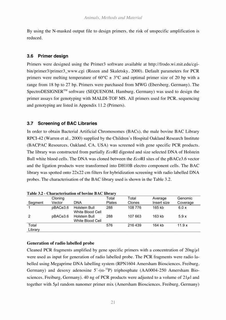
Animals, Methods and Material
21
By using the N-masked output file to design primers, the risk of unspecific amplification is
reduced.
3.6 Primer design
Primers were designed using the Primer3 software available at http://frodo.wi.mit.edu/cgi-
bin/primer3/primer3_www.cgi (Rozen and Skaletsky, 2000). Default parameters for PCR
primers were melting temperature of 60°C ± 3°C and optimal primer size of 20 bp with a
range from 18 bp to 27 bp. Primers were purchased from MWG (Ebersberg, Germany). The
SpectroDESIGNERTM software (SEQUENOM, Hamburg, Germany) was used to design the
primer assays for genotyping with MALDI-TOF MS. All primers used for PCR, sequencing
and genotyping are listed in Appendix 11.2 (Primers).
3.7 Screening of BAC Libraries
In order to obtain Bacterial Artificial Chromosomes (BACs), the male bovine BAC Library
RPCI-42 (Warren et al., 2000) supplied by the Children’s Hospital Oakland Research Institute
(BACPAC Resources, Oakland, CA, USA) was screened with gene specific PCR products.
The library was constructed from partially EcoRI digested and size selected DNA of Holstein
Bull white blood cells. The DNA was cloned between the EcoRI sites of the pBACe3.6 vector
and the ligation products were transformed into DH10B electro component cells. The BAC
library was spotted onto 22x22 cm filters for hybridization screening with radio labelled DNA
probes. The characterisation of the BAC library used is shown in the Table 3.2.
Table 3.2 - Characterisation of bovine BAC library
SegmentCloningVector DNA
TotalPlates
TotalClones
AverageInsert size
GenomicCoverage
1 pBACe3.6 Holstein BullWhite Blood Cell
288 108 776 165 kb 6.0 x
2 pBACe3.6 Holstein BullWhite Blood Cell
288 107 663 163 kb 5.9 x
TotalLibrary
576 216 439 164 kb 11.9 x
Generation of radio labelled probe
Cleaned PCR fragments amplified by gene specific primers with a concentration of 20ng/µl
were used as input for generation of radio labelled probe. The PCR fragments were radio la-
belled using Megaprime DNA labelling system (RPN1604 Amersham Biosciences, Freiburg,
Germany) and desoxy adenosine 5’-(!-32P) triphosphate (AA0004-250 Amersham Bio-
sciences, Freiburg, Germany). 40 ng of PCR products were adjusted to a volume of 21µl and
together with 5µl random nanomer primer mix (Amersham Biosciences, Freiburg, Germany)
Animals, Methods and Material
22
denatured at 95°C for five minutes. The reaction was chilled and the following reagents were
added: 5 µl reaction buffer (10 x), 4µl of dGTP, dCTP and dTTP, 2µl Klenow Enzym and 5µl
dATP32 (1.85 kBq). After incubation for 15 minutes at 37°C, the reaction was stopped by
adding 10µl of 0.2 M EDTA (pH 8.0). The radio labelled probes were denaturised at 95°C for
seven minutes.
Dot-Blot as positive control
Two µl of each, PCR product and its ten- and hundred-fold dilution were blotted onto nylon
membranes (Hybond-N+, PRN303B; Amersham Bioscience Freiburg, Germany), which were
saturated with 0.4N NaOH. After five minutes, the dot-blot was shaken for one minute in 5x
SSC buffer.
Hybridization
Two filters of the BAC library were applied to a roller bottle and pre-hybridised at 67 °C for
30 minutes together with a dot-blot control and 15-20 ml of Church buffer (Church and
Gilbert, 1984). Subsequently, 17 µl of radio labelled probe and 10ml of Church buffer was
added in each bottle and incubated for hybridisation at 67°C overnight (14-16 hours). Filters
were washed for 20 minutes at 63°C twice in 2x SSC and a third time in 0.5x SSC + 0.1%
SDS. Finally, each filter was rinsed in 2x SSC, wrapped in plastic film and placed together
with medical X-ray film NewRX (03E220; FUJIFILM Medical Systems, Stamford, CT, USA)
in cassettes. X-ray films were exposed for eight hours at –80°C. After the development of the
X-ray films, the positive clones could be identified. From the position on the filter the positive
clones can be named by filter number, plate number and position on the plates and ordered. A
colony PCR with the primers used for the screening attested the containing of the right insert
in the clones.
3.8 Preparation of BAC DNA
The starter culture was made from a single colony picked after laying out the clones on a se-
lective lurid broth (LB) agar plate (containing 12.5µg/mL chloramphenicol (CHL) 0634433;
Roche Diagnostics, Mannheim, Germany). The colony was applied in 3ml LB medium
(12.5µg/mL CHL) and strongly shaken with 300rpm for 8 hours at 37°C. For the culture
100ml LB medium (12.5µg/mL CHL) was inoculated with 500µl of the starter culture and
incubated overnight at 37°C with shaking at 300rpm. For BAC DNA preparation, the Qiagen
Plasmid Midi Kit (12462; Qiagen, Hilden, Germany) was used according to manufactures
manual. The DNA pellet was re-dissolved in 500µl 10mM Tris-Cl (pH 8.0) and desalted using
Microcon YM-100 filters (42413, Millipore, Eschborn, Germany). Samples were centrifuged
at 7000rpm for 15 minutes and another 10 minutes after adding 250µl 10 mM Tris-Cl (pH
Animals, Methods and Material
23
8.0). After adding 200µl Tris-Cl (pH 8.0) an upside down centrifugation of the filters for 1
minute at 7000rpm recovered the cleaned BAC DNA. The concentration of the DNA was
measured with a fluorometer (DyNA Quant200; Hoefer Pharmacia BiotechInc, San Francisco,
CA, USA).
3.9 Polymerase Chain Reaction (PCR)
3.9.1 Standard PCR
Standard PCR reaction was made in a volume of 20 µl per sample. Master Mix was prepared
containing 0.5 Units of Qiagen Taq Polymerase (1005476, Qiagen Hilden Germany), 1x
Qiagen PCR buffer (containing 1,5 mM MgCl), 200 µM of each nucleotide and 0.5µM of
forward and reverse primer (MWG) and 50 ng of DNA was amplified in a T-Gradient Ther-
mocycler (Biometra, Göttingen, Germany) under the following conditions: initial denaturation
at 94 °C for three minutes, followed by 30 cycles consisting of 30 seconds at 94°C for denatu-
ration, 60 seconds at 60 °C for primer annealing and 60 seconds at 72 °C for extension. This
was followed by a final extension step for three minutes.
3.9.2 Primer optimisation
Each primer system was tested with bovine DNA with an annealing temperature of 60 °C in
three different reactions: standard PCR reaction without any additives (plain), the standard
PCR reaction with 5% DMSO (dimethyl sulfoxid) and the standard PCR reaction with 1x Q-
solution (Qiagen). The conditions supplying the best amplification results were applied for the
sequencing panel. In case of unspecified amplification a gradient PCR with varying annealing
temperature was performed. PCR products together with a DNA marker (Genruler 100 bp
ladder: SM024; MBI Fermentas, St. Leon-Rot, Germany) were tested by 2 %-agarose gel
electrophoresis.
3.9.3 Long range PCR
In order to amplify fragments larger than 2 kb, a long range PCR protocol was used. In addi-
tion to AmpliTaq Polymerase (201207; Qiagen, Hilden, Germany), ProofStartTaq (202203;
Qiagen, Hilden, Germany) as proofreading polymerase was used for the amplification. Proof-
reading is achieved by a 3' to 5' exonuclease activity where the polymerase recognizes and
removes incorrectly incorporated desoxynucleotides. The exonuclease activity can lead to
primer degradation during PCR setup, which result in unspecific amplification products.
Qiagen ProofStartTaq polymerase has been chemically modified for initial temporally inacti-
vation. The enzyme is activated by the initial denaturing step at 95°C. The reaction was per-
formed in a volume of 25 µl with an input of 50ng DNA, 1x PCR buffer (including MgSO4),
Animals, Methods and Material
24
1µM of each primer, 300µM of each nucleotide, 1 Unit AmpliTaq and 0.1 Unit ProofStartTaq
Polymerase in a T-Gradient Thermocycler (Biometra, Göttingen, Germany) under the fol-
lowing conditions: initial denaturation at 94 °C for three minutes, followed by 35 cycles con-
sisting of 10 seconds at 94°C for denaturation, 60 seconds at 60 °C for primer annealing and
depending on the expected fragment-length 60 seconds per kb at 68 °C for extension. The last
extension step at 68°C for 180 seconds was completing the reaction before cooling.
3.10 DNA Sequencing
The sequencing was performed according to Sanger et al. (1977) (chain-termination-method)
with fluorescent didesoxy-nucleotides. The generated PCR-products were sequenced by Big-
Dye% Terminator Cycling Kit v1.1 (BigDye) (Applied Biosystems, Foster City, CA, USA).
The products were separated by polyacrylamid gel electrophoresis with the help of an auto-
mated sequencer ABI 377 (Applied Biosystems, Foster City, CA, USA).
Sequencing reaction for BAC DNA
Primerwalking on BAC DNA was performed in total 10 µl volume, by adding 150 ng of
BAC-DNA, 4µl BigDye and 2.5 pM of either up or down primer. For BAC-end sequencing,
the initial primers were derived from the T7 and SP6 promoter sites, which were located on
the pBACe3.6 vector flanking the insert. For BAC sequencing the conditions for temperature
cycling was initial denaturation for five minutes at 96°C, followed by 100 cycles being 20
seconds at 96°C, 20 seconds at 58°C and four minutes at 60°C.
Sequencing reaction for PCR products
In order to sequence PCR-fragments, they were purified with Multi-Screen-Filtration-Plates
(MANU03010; Millipore, Eschborn, Germany) under vacuum (MAVM0960R; Millipore,
Eschborn, Germany). Products were eluated with 40µl Tris-HCl (10mM) and quantity was
tested together with a DNA marker (Genruler 100 bp ladder: SM0241; MBI Fermentas, St.
Leon-Rot, Germany) by 2 %-agarose gel electrophoresis. Subsequently, the sequencing reac-
tion was performed in a 10µl volume. 10-20 ng of purified PCR fragment, 2 - 4µl BigDye and
2.5 pM of either up or down primer was added. Initial denaturation for 15 seconds at 96°C,
followed by 35 cycles of 10 seconds at 96°C, 5 seconds at 50°C and 4 minutes at 60°C was
applied to the reactions.
Cleaning of sequencing reactions
Sequencing reactions were cleaned from unincorporated dye terminators by gel filtration. The
purifying step was done with MultiScreen filtration plates (MAHVN4510; Millipore, Esch-
born, Germany), which were loaded with 45 µL of Sephadex G-50 Fine (G-50-50; Sigma-
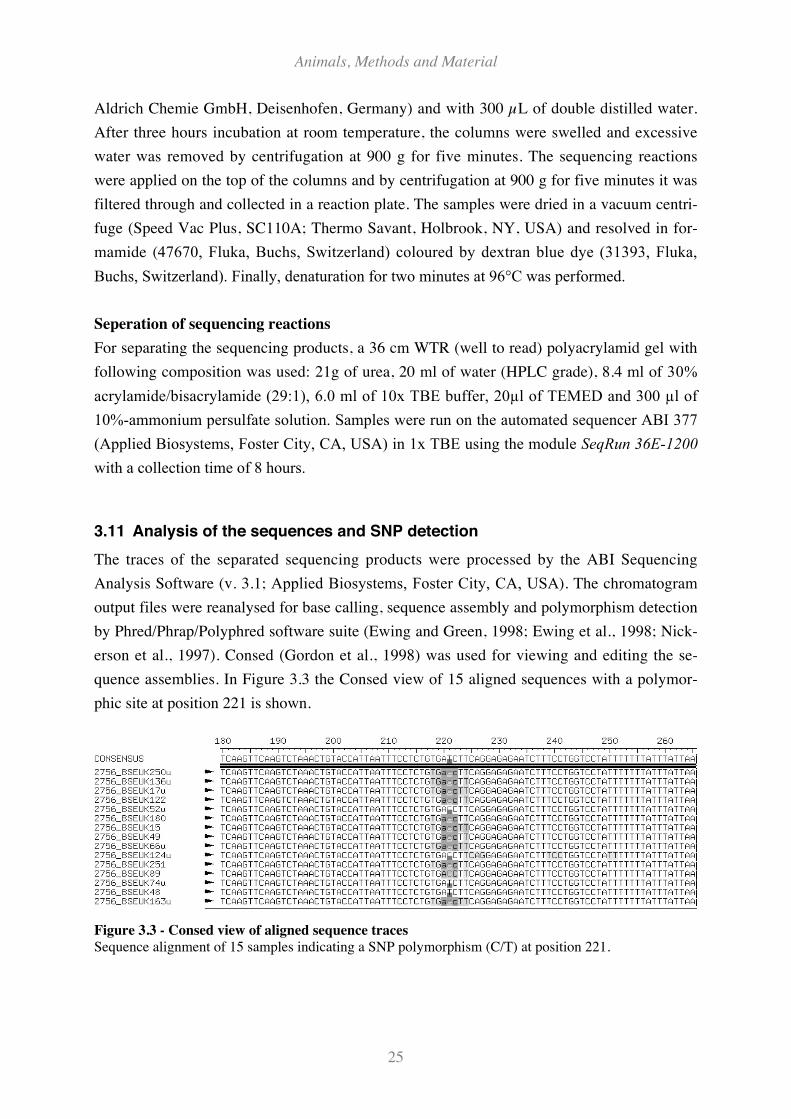
Animals, Methods and Material
25
Aldrich Chemie GmbH, Deisenhofen, Germany) and with 300 µL of double distilled water.
After three hours incubation at room temperature, the columns were swelled and excessive
water was removed by centrifugation at 900 g for five minutes. The sequencing reactions
were applied on the top of the columns and by centrifugation at 900 g for five minutes it was
filtered through and collected in a reaction plate. The samples were dried in a vacuum centri-
fuge (Speed Vac Plus, SC110A; Thermo Savant, Holbrook, NY, USA) and resolved in for-
mamide (47670, Fluka, Buchs, Switzerland) coloured by dextran blue dye (31393, Fluka,
Buchs, Switzerland). Finally, denaturation for two minutes at 96°C was performed.
Seperation of sequencing reactions
For separating the sequencing products, a 36 cm WTR (well to read) polyacrylamid gel with
following composition was used: 21g of urea, 20 ml of water (HPLC grade), 8.4 ml of 30%
acrylamide/bisacrylamide (29:1), 6.0 ml of 10x TBE buffer, 20!l of TEMED and 300 !l of
10%-ammonium persulfate solution. Samples were run on the automated sequencer ABI 377
(Applied Biosystems, Foster City, CA, USA) in 1x TBE using the module SeqRun 36E-1200
with a collection time of 8 hours.
3.11 Analysis of the sequences and SNP detection
The traces of the separated sequencing products were processed by the ABI Sequencing
Analysis Software (v. 3.1; Applied Biosystems, Foster City, CA, USA). The chromatogram
output files were reanalysed for base calling, sequence assembly and polymorphism detection
by Phred/Phrap/Polyphred software suite (Ewing and Green, 1998; Ewing et al., 1998; Nick-
erson et al., 1997). Consed (Gordon et al., 1998) was used for viewing and editing the se-
quence assemblies. In Figure 3.3 the Consed view of 15 aligned sequences with a polymor-
phic site at position 221 is shown.
Figure 3.3 - Consed view of aligned sequence traces
Sequence alignment of 15 samples indicating a SNP polymorphism (C/T) at position 221.
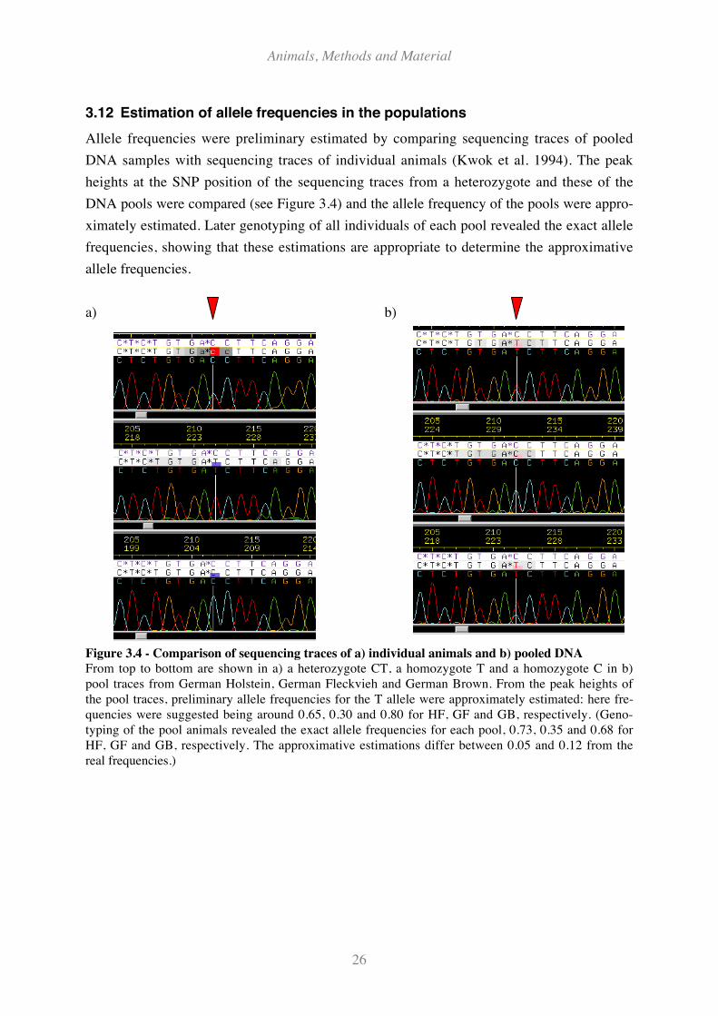
Animals, Methods and Material
26
3.12 Estimation of allele frequencies in the populations
Allele frequencies were preliminary estimated by comparing sequencing traces of pooled
DNA samples with sequencing traces of individual animals (Kwok et al. 1994). The peak
heights at the SNP position of the sequencing traces from a heterozygote and these of the
DNA pools were compared (see Figure 3.4) and the allele frequency of the pools were appro-
ximately estimated. Later genotyping of all individuals of each pool revealed the exact allele
frequencies, showing that these estimations are appropriate to determine the approximative
allele frequencies.
a) b)
Figure 3.4 - Comparison of sequencing traces of a) individual animals and b) pooled DNA
From top to bottom are shown in a) a heterozygote CT, a homozygote T and a homozygote C in b)
pool traces from German Holstein, German Fleckvieh and German Brown. From the peak heights of
the pool traces, preliminary allele frequencies for the T allele were approximately estimated: here fre-
quencies were suggested being around 0.65, 0.30 and 0.80 for HF, GF and GB, respectively. (Geno-
typing of the pool animals revealed the exact allele frequencies for each pool, 0.73, 0.35 and 0.68 for
HF, GF and GB, respectively. The approximative estimations differ between 0.05 and 0.12 from the
real frequencies.)
Animals, Methods and Material
27
3.13 Selection of SNPs / polymorphisms for genotyping
3.13.1 SNPs for the Genomic Control (GC)
For the GC approach a SNP panel initially developed for paternal testing and identity control
(Werner et al., 2004) was used. The panel consists of 37 SNP markers, which were allocated
over the whole genome and are considered as being polymorphic in the European cattle
breeds Holstein Friesian, German Fleckvieh and German Brown.
3.13.2 SNPs for the Association Study
SNPs in the candidate genes ARIH1, HEXA, BRUNOL6 and PARP6 were selected for geno-
typing in BSE diseased and control animals. The SNPs were derived by comparing sequenc-
ing of DNA pools and individual animals of different breeds.
SNPs were selected for genotyping considering the following criteria:
• SNP is not located in repetitive sequence.
• Exonic SNPs and SNPs in regulatory regions (Splice sites, 5'-UTRs, promoter regions)
were preferentially chosen, subsequently intronic SNPs.
• Pre-estimated allele frequency of the rare allele is >10% in German Fleckvieh, Ger-
man Holstein and UK Holstein animals.
• SNPs are evenly distributed over the gene.
• Extension primer region (up to 50 bases around the SNP) is free of variation.
Additionally, two insertion/deletion polymorphisms (indel) in the regulatory region of the
prion protein gene (PRNP) were selected because it has been shown in a small case-control
study (Sander et al., 2004) that these variants were tentatively associated with BSE. The indel
polymorphisms were genotyped with the first base of the insertion and the first base after the
insertion representing the insertion and deletion alleles, respectively.
Futhermore, eight SNPs in four additional candidate genes have been selected because the
genes encoding Plasminogen (PLG), Heat-shock protein 70 (HSPA8), Iron-responsive binding
element (IREB2) and the Laminin Receptor (LAMR1) have been postulated as candidate genes
for BSE susceptibility in Juling (2002).
Animals, Methods and Material
28
3.14 Genotyping SNPs with MALDI-TOF MS
Matrix Assisted Laser Desorption/Ionisation (MALDI) is a pulsing technique, which can
analyse molecule mass with the help of a Time of Flight (TOF) analysator. The probe is co-
crystallised with an excess of suitable matrix, most frequently an organic acid (e.g. 3-
hydroxypicolinic acid) and is hit by a very short laser pulse in the mass spectrometer under
high vacuum. The laser ionizes the analyt, consisting of DNA molecules and matrix, and in-
troduces it into the flight tube. The role of the matrix is to absorb the laser energy during sub-
sequent collisions with the DNA molecules resulting in the formation of DNA ions. Further-
more it secures the probe from photolytic damages and from interaction of the analytes among
each other. The generated ions are all accelerated to the same potential in an electric field
causing them to fly through a field - free drift region, also known as flight tube, to the detec-
tor, where they are separated according to their mass-over-charge ratio. Ions with a higher
mass-over-charge ratio pass slower through the flight tube and achieve the detector later than
ions with a small mass-over-charge ratio. Lighter ions (smaller DNA fragments) travel faster,
than heavier (larger DNA fragments), leading to a separation of the fragments based on their
mass difference. The electric measurement of the time of flight from the start of the ions to
the arrival at the detector is a Time Of Flight Mass Spectrometer (TOF MS).
3.14.1 The hME (homogeneous MassExtendTM) method
The principle of the hME method (homogenous MassExtendTM, Sequenom, Hamburg, Ger-
many) is shown in Figure 3.5. In order to genotype SNPs with this method, first, the genomic
sequence in a scope of 200 to 500 bp around the SNP locus has to be amplified. The PCR
assays can be multiplexed up to ten PCR primer systems. The PCR primers are modified at
the 5'- end by adding a ten base pair tag in order that they are not disturbing the measurement
of the MALDI-TOF analysis by being out of the range of the extension primers. Excessive
and unbound nucleotides were degraded by incubation with SAP (Shrimp Alkaline Phospha-
tase) since they could be built in the extension products and falsify the results. During the
hME reaction, the extension primers anneal adjacent to the SNP and the addition of a DNA
polymerase along with a mixture of nucleotides and a terminator nucleotide allows extension
through the polymorphic site and generates allele specific extension-products, each having a
unique molecular mass. As shown in Figure 3.5, hME uses 1 base in conjunction with 2-3
bases extension products for genotyping in order to create large mass differences between the
allelic specific products. Before the extension products can be spotted on a microchip (Spec-
troChipTM, Sequenom, Hamburg, Germany) by a nano-dispenser (SpectroPointTM Nanoliter
Pipetting System, Sequenom, Hamburg, Germany), the conditioning of the products by treat-
ing with a special ion exchanger resin (SpectroCleanTM, Sequenom, Hamburg, Germany) is
necessary.
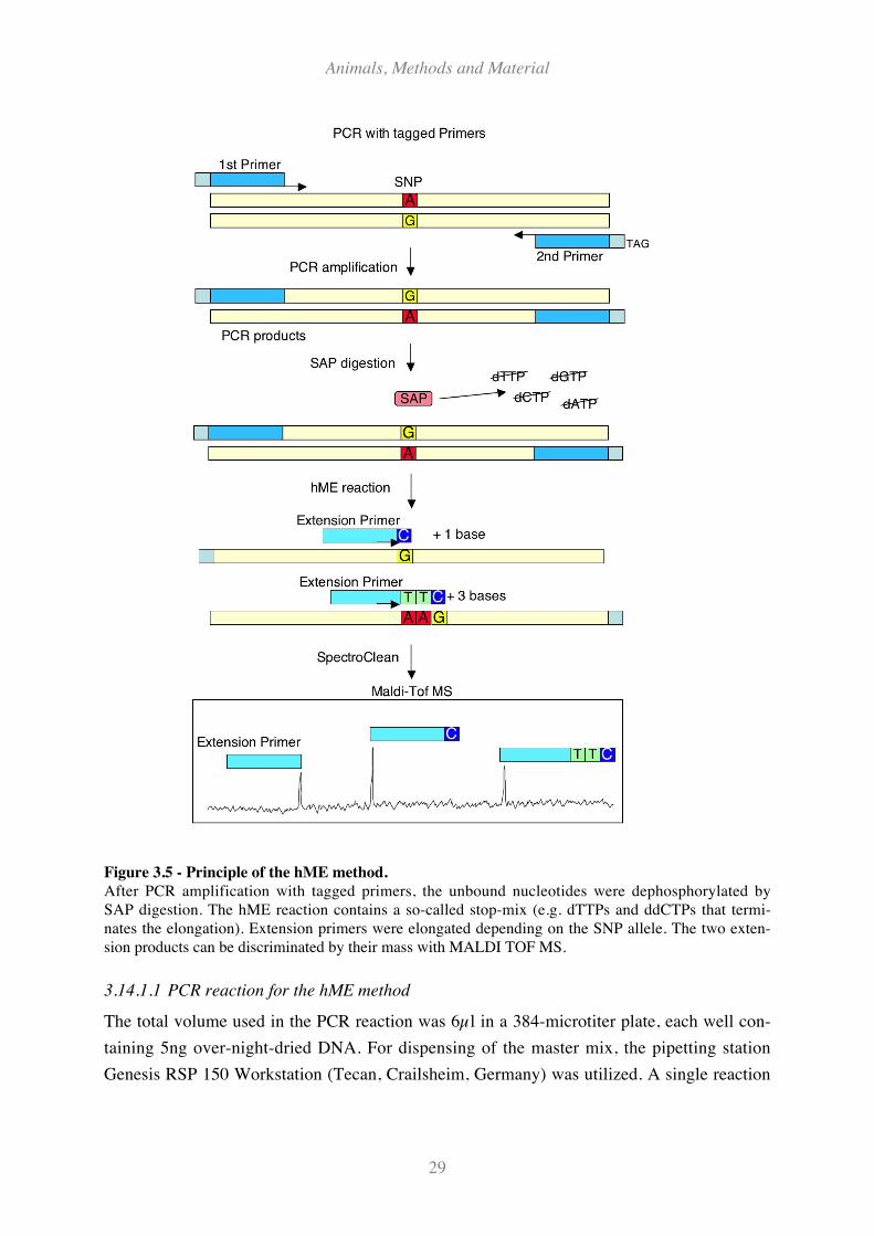
Animals, Methods and Material
29
Figure 3.5 - Principle of the hME method.
After PCR amplification with tagged primers, the unbound nucleotides were dephosphorylated by
SAP digestion. The hME reaction contains a so-called stop-mix (e.g. dTTPs and ddCTPs that termi-
nates the elongation). Extension primers were elongated depending on the SNP allele. The two exten-
sion products can be discriminated by their mass with MALDI TOF MS.
3.14.1.1 PCR reaction for the hME method
The total volume used in the PCR reaction was 6µl in a 384-microtiter plate, each well con-
taining 5ng over-night-dried DNA. For dispensing of the master mix, the pipetting station
Genesis RSP 150 Workstation (Tecan, Crailsheim, Germany) was utilized. A single reaction
Animals, Methods and Material
30
included the PCR reagents (HotStar Taq&, buffer and MgCL2 from Abgene, Hamburg, Ger-
many) as shown in Table 3.3.
Table 3.3 - Master Mix for hME-PCR (single reaction).
Volume (!l) Reagent Concentration
0.60 PCR-Buffer 10 x
0.60 dNTPs 2mM0.60 MgCl2 25mM0.01 Primer up 100pmol/!l0.01 Primer dn 100pmol/!l0.02 HotStar Taq&-Polymerase 5U/!l
4.16 H2O
6.00
For thermo cycling, a PCR PTC 225 Tetrad, Peltier Thermal Cycler of MJ Research (Boston,
USA) was used with the time-temperature-programme as shown in Table 3.4 with 45 cycles.
Table 3.4 - Time-temperature programme for hME-PCR.
Step Temperature Time
1 Initial denaturation 94°C 15 min2 Denaturation 94°C 20 sec3 Annealing 56°C 30 sec Go 44-times to step 24 Extension 72°C 60 sec5 Final Extension 72°C 10 min6 Final cooling 20°C 1 sec
3.14.1.2 SAP-digestion
For the Shrimp Alkaline Phosphatase (SAP, Amersham Biosciences, Freiburg, Germany)
treatment to dephosphorylate unincorporated dNTPs, one reaction with a total volume of 2µl
contained reagents as shown in Table 3.5.
Table 3.5 - Mix for SAP-Treatment (single reaction).
Volume (!l) Reagent
0.17 hME buffer0.30 SAP1.53 H2O
2.00
2µl of the solution was dispersed in the wells over the plates with a Multimek96 Automated
96-Channelpipettor (Beckmann Coulter, Fullerton, USA) and the incubation and SAP-
deactivation was done in a PCR PTC 225 Tetrad Peltier Thermal Cycler of MJ Research
(Boston, USA) as shown in Table 3.6.
Animals, Methods and Material
31
Table 3.6 - Incubation time-temperature programme for SAP treatment
Step Temperature Time
1 Incubation 37°C 20 min2 Deactivation of SAP 85°C 5 min3 Final Cooling 20°C 1 sec
3.14.1.3 Primer extension reaction for the hME method
Primer extension was performed with the MassExtend enzyme (Sequenom, Hamburg, Ger-
many) which is a Thermosequenase and the hME Extend Mix, which contains Buffer and
dideoxy-nucleotides and deoxynucleotides, respectively) 2µl of the hME-Mix Cocktail (see
Table 3.7) was dispersed with a Multimek96 Automated 96-Channelpipettor (Beckmann
Coulter, Fullerton, USA) into the wells of the 384 well plate. The time-temperature pro-
gramme as used for the Primer-extension reaction in a PCR PTC 225 Tetrad Peltier Thermal
Cycler of MJ Research (Boston, USA) is shown in Table 3.8.
Table 3.7 - Master Mix for hME Extension reaction (single reaction).
Volume (2!l) Reagent Concentration
0.200 hME Extend Mix 10 x Buffer + 2.25 mM of each d/ddNTP0.054 hME Primers 100 pmol/!l0.018 MassExtend enzyme 32U/!l1.728 H2O
2.000
Table 3.8 - Time-temperature programme for hME Extension reaction.
Step Temperature Time
1 Initial denaturation 94°C 2 min2 Denaturation 94°C 5 sec3 Annealing 52°C 5 sec Go 55-times to step 24 Extension 72°C 10 sec6 Final cooling 20°C 1 sec
3.14.2 The iPLEX method
The iPLEX method (Sequenom, Hamburg, Germany) is shown in Figure 3.6. Similar to the
hME procedure (see Chapter 3.14.1 – The hME method), the first step is the PCR amplifica-
tion of the region around the SNP with tagged primers. IPLEX allows multiplexing the PCR
reaction up to 29 different SNP loci. Than, unbound nucleotides were dephosphorylated by
incubation with SAP since they could be built in the extension products and falsify the results.
The most significant difference relative to the hME method is that all reactions for the iPLEX
assay are terminated by a single base extension (SBE), meaning that the differences between
the two allelic specific products arise only from the different mass of the modified nucleo-
tides. Table 3.9 shows the mass differences between the SBE products of the iPLEX assay.
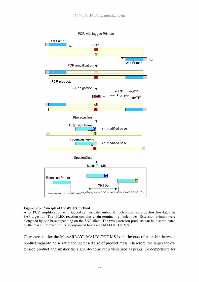
Animals, Methods and Material
32
Figure 3.6 - Principle of the iPLEX method.
After PCR amplification with tagged primers, the unbound nucleotides were dephosphorylated by
SAP digestion. The iPLEX reaction contains chain terminating nucleotides. Extension primers were
elongated by one base depending on the SNP allele. The two extension products can be discriminated
by the mass differences of the incorporated bases with MALDI TOF MS.
Characteristic for the MassARRAY% MALDI-TOF MS is the inverse relationship between
product signal-to noise ratio and increased size of product mass. Therefore, the larger the ex-
tension product, the smaller the signal-to-noise ratio visualised as peaks. To compensate for
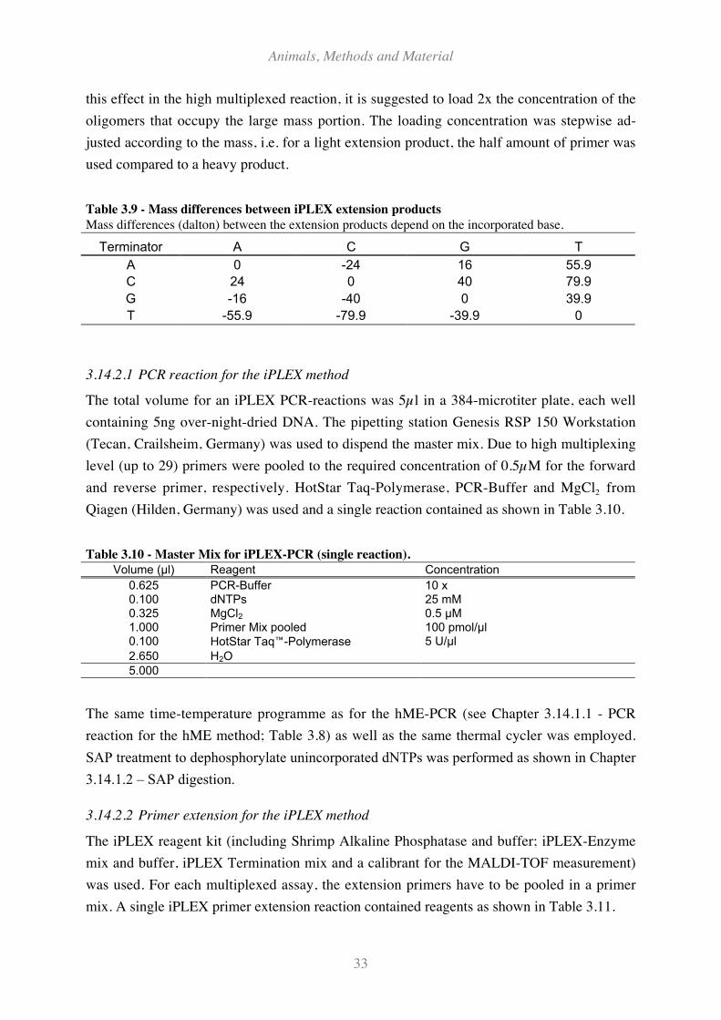
Animals, Methods and Material
33
this effect in the high multiplexed reaction, it is suggested to load 2x the concentration of the
oligomers that occupy the large mass portion. The loading concentration was stepwise ad-
justed according to the mass, i.e. for a light extension product, the half amount of primer was
used compared to a heavy product.
Table 3.9 - Mass differences between iPLEX extension products
Mass differences (dalton) between the extension products depend on the incorporated base.
Terminator A C G T
A 0 -24 16 55.9
C 24 0 40 79.9
G -16 -40 0 39.9
T -55.9 -79.9 -39.9 0
3.14.2.1 PCR reaction for the iPLEX method
The total volume for an iPLEX PCR-reactions was 5µl in a 384-microtiter plate, each well
containing 5ng over-night-dried DNA. The pipetting station Genesis RSP 150 Workstation
(Tecan, Crailsheim, Germany) was used to dispend the master mix. Due to high multiplexing
level (up to 29) primers were pooled to the required concentration of 0.5µM for the forward
and reverse primer, respectively. HotStar Taq-Polymerase, PCR-Buffer and MgCl2 from
Qiagen (Hilden, Germany) was used and a single reaction contained as shown in Table 3.10.
Table 3.10 - Master Mix for iPLEX-PCR (single reaction).
Volume (!l) Reagent Concentration
0.625 PCR-Buffer 10 x0.100 dNTPs 25 mM0.325 MgCl2 0.5 !M1.000 Primer Mix pooled 100 pmol/!l0.100 HotStar Taq&-Polymerase 5 U/!l
2.650 H2O
5.000
The same time-temperature programme as for the hME-PCR (see Chapter 3.14.1.1 - PCR
reaction for the hME method; Table 3.8) as well as the same thermal cycler was employed.
SAP treatment to dephosphorylate unincorporated dNTPs was performed as shown in Chapter
3.14.1.2 – SAP digestion.
3.14.2.2 Primer extension for the iPLEX method
The iPLEX reagent kit (including Shrimp Alkaline Phosphatase and buffer; iPLEX-Enzyme
mix and buffer, iPLEX Termination mix and a calibrant for the MALDI-TOF measurement)
was used. For each multiplexed assay, the extension primers have to be pooled in a primer
mix. A single iPLEX primer extension reaction contained reagents as shown in Table 3.11.
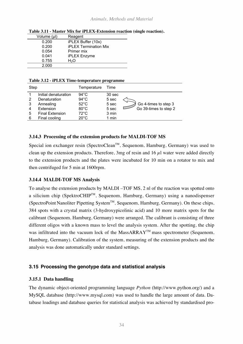
Animals, Methods and Material
34
Table 3.11 - Master Mix for iPLEX-Extension reaction (single reaction).
Volume (!l) Reagent
0.200 iPLEX Buffer (10x)
0.200 iPLEX Termination Mix0.054 Primer mix0.041 iPLEX Enzyme0.755 H2O
2.000
Table 3.12 - iPLEX Time-temperature programme
3.14.3 Processing of the extension products for MALDI-TOF MS
Special ion exchanger resin (SpectroCleanTM, Sequenom, Hamburg, Germany) was used to
clean up the extension products. Therefore, 3mg of resin and 16 µl water were added directly
to the extension products and the plates were incubated for 10 min on a rotator to mix and
then centrifuged for 5 min at 1600rpm.
3.14.4 MALDI-TOF MS Analysis
To analyse the extension products by MALDI –TOF MS, 2 nl of the reaction was spotted onto
a silicium chip (SpektroCHIPTM, Sequenom, Hamburg, Germany) using a nanodispenser
(SpectroPoint Nanoliter Pipetting SystemTM, Sequenom, Hamburg, Germany). On these chips,
384 spots with a crystal matrix (3-hydroxypicolinic acid) and 10 more matrix spots for the
calibrant (Sequenom, Hamburg, Germany) were arranged. The calibrant is consisting of three
different oligos with a known mass to level the analysis system. After the spotting, the chip
was infiltrated into the vacuum lock of the MassARRAYTM mass spectrometer (Sequenom,
Hamburg, Germany). Calibration of the system, measuring of the extension products and the
analysis was done automatically under standard settings.
3.15 Processing the genotype data and statistical analysis
3.15.1 Data handling
The dynamic object-oriented programming language Python (http://www.python.org/) and a
MySQL database (http://www.mysql.com) was used to handle the large amount of data. Da-
tabase loadings and database queries for statistical analysis was achieved by standardised pro-
Step Temperature Time
1 Initial denaturation 94°C 30 sec2 Denaturation 94°C 5 sec3 Annealing 52°C 5 sec Go 4-times to step 34 Extension 80°C 5 sec Go 39-times to step 25 Final Extension 72°C 3 min6 Final cooling 20°C 1 min
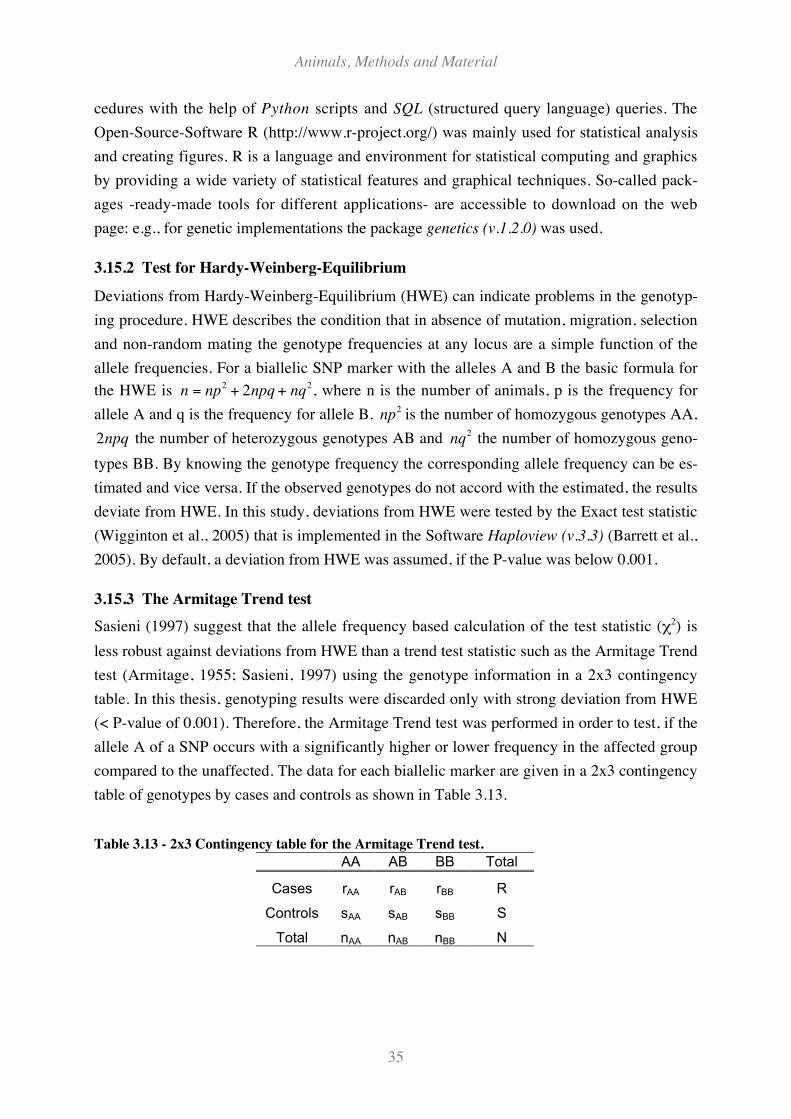
Animals, Methods and Material
35
cedures with the help of Python scripts and SQL (structured query language) queries. The
Open-Source-Software R (http://www.r-project.org/) was mainly used for statistical analysis
and creating figures. R is a language and environment for statistical computing and graphics
by providing a wide variety of statistical features and graphical techniques. So-called pack-
ages -ready-made tools for different applications- are accessible to download on the web
page: e.g., for genetic implementations the package genetics (v.1.2.0) was used.
3.15.2 Test for Hardy-Weinberg-Equilibrium
Deviations from Hardy-Weinberg-Equilibrium (HWE) can indicate problems in the genotyp-
ing procedure. HWE describes the condition that in absence of mutation, migration, selection
and non-random mating the genotype frequencies at any locus are a simple function of the
allele frequencies. For a biallelic SNP marker with the alleles A and B the basic formula for
the HWE is
!
n = np2
+ 2npq + nq2, where n is the number of animals, p is the frequency for
allele A and q is the frequency for allele B.
!
np2 is the number of homozygous genotypes AA,
!
2npq the number of heterozygous genotypes AB and
!
nq2 the number of homozygous geno-
types BB. By knowing the genotype frequency the corresponding allele frequency can be es-
timated and vice versa. If the observed genotypes do not accord with the estimated, the results
deviate from HWE. In this study, deviations from HWE were tested by the Exact test statistic
(Wigginton et al., 2005) that is implemented in the Software Haploview (v.3.3) (Barrett et al.,
2005). By default, a deviation from HWE was assumed, if the P-value was below 0.001.
3.15.3 The Armitage Trend test
Sasieni (1997) suggest that the allele frequency based calculation of the test statistic ($2) is
less robust against deviations from HWE than a trend test statistic such as the Armitage Trend
test (Armitage, 1955; Sasieni, 1997) using the genotype information in a 2x3 contingency
table. In this thesis, genotyping results were discarded only with strong deviation from HWE
(< P-value of 0.001). Therefore, the Armitage Trend test was performed in order to test, if the
allele A of a SNP occurs with a significantly higher or lower frequency in the affected group
compared to the unaffected. The data for each biallelic marker are given in a 2x3 contingency
table of genotypes by cases and controls as shown in Table 3.13.
Table 3.13 - 2x3 Contingency table for the Armitage Trend test.
AA AB BB Total
Cases rAA rAB rBB R
Controls sAA sAB sBB S
Total nAA nAB nBB N
Animals, Methods and Material
36
Thus, the chi-square test for no association between disease and genotype, calculated under an
additive genetic model, is
!
Ytrend
2 =N N{ (r
AB+ 2r
BB) " R(n
AB+ 2n
BB)}2
R(N " R) N(nAB
+ 4nBB) " (n
AB+ 2n
BB)2{ }
.
The trend values (Y2) follow the chi-square distribution with one degree of freedom. The sig-
nificance thresholds for 5% and 1% type 1 error rate are 3.84 and 6.62, respectively. The Ar-
mitage Trend test statistic was implemented in the R package association created by R.Fries.
3.15.4 Logistic regression analysis
Logistic regression is part of a category of statistical models called generalized linear models
and is used to model dichotomous (0 or 1) outcomes, such as the case-control status. This
technique models the log odds of an outcome defined by the values of covariates in the
model. For logistic regression, the R package ‘logistf’, version 1.05 (Heinze and Ploner, 2004)
was applied, which fits parameters based on penalized maximum likelihood estimation. Like-
lihood ratio test were applied as proposed by North et al. (2005) to investigate both the mode
of allelic action (additive vs. dominance effects) and for possible epistatic effects (additive by
additive, additive by dominance, dominance by dominance interactions) for the PRNP poly-
morphism data.
3.15.5 Measuring Linkage Disequilibrium and tagging SNPs
Pairwise Linkage Disequilibrium (LD) is a non-random association between two loci. LD
represents a condition in which some combinations of marker alleles occur more or less fre-
quently in a population than would be expected from a random arrangement of haplotypes
from the allele frequencies. The two most common measures of LD are the Lewontin’s stan-
dardized disequilibrium coefficient D' (Lewontin, 1964) and the square of correlation coeffi-
cient r2 (Hill and Robertson, 1968). Both methods are implemented in Haploview (v3.3)
(Barrett et al., 2005).
Measuring the LD between SNPs is of particular importance in preliminary studies which aim
at selecting a marker set that represents all existent haplotypes. SNPs which are in strong LD
are redundant, i.e. genotyping of one of these SNPs is enough to determine the genotypes of
the other SNPs. From the redundant SNPs, those are chosen for further genotyping which
cover all known variation. This selection is called tagging SNPs and the SNPs are called tag
SNPs. By genotyping these tag SNPs the haplotype can be uniquely determined. In this study,
SNPs were tagged by using the software Tagger (de Bakker et al., 2005) that combines a
pairwise r2 method with a multi-marker haplotype approach and is implemented in Haploview
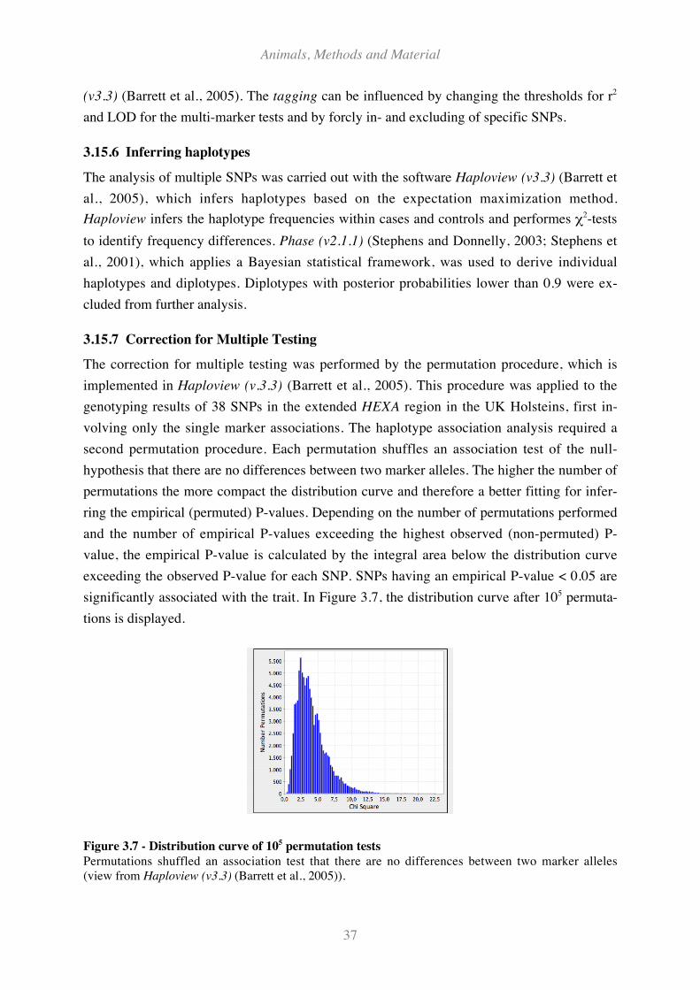
Animals, Methods and Material
37
(v3.3) (Barrett et al., 2005). The tagging can be influenced by changing the thresholds for r2
and LOD for the multi-marker tests and by forcly in- and excluding of specific SNPs.
3.15.6 Inferring haplotypes
The analysis of multiple SNPs was carried out with the software Haploview (v3.3) (Barrett et
al., 2005), which infers haplotypes based on the expectation maximization method.
Haploview infers the haplotype frequencies within cases and controls and performes $2-tests
to identify frequency differences. Phase (v2.1.1) (Stephens and Donnelly, 2003; Stephens et
al., 2001), which applies a Bayesian statistical framework, was used to derive individual
haplotypes and diplotypes. Diplotypes with posterior probabilities lower than 0.9 were ex-
cluded from further analysis.
3.15.7 Correction for Multiple Testing
The correction for multiple testing was performed by the permutation procedure, which is
implemented in Haploview (v.3.3) (Barrett et al., 2005). This procedure was applied to the
genotyping results of 38 SNPs in the extended HEXA region in the UK Holsteins, first in-
volving only the single marker associations. The haplotype association analysis required a
second permutation procedure. Each permutation shuffles an association test of the null-
hypothesis that there are no differences between two marker alleles. The higher the number of
permutations the more compact the distribution curve and therefore a better fitting for infer-
ring the empirical (permuted) P-values. Depending on the number of permutations performed
and the number of empirical P-values exceeding the highest observed (non-permuted) P-
value, the empirical P-value is calculated by the integral area below the distribution curve
exceeding the observed P-value for each SNP. SNPs having an empirical P-value < 0.05 are
significantly associated with the trait. In Figure 3.7, the distribution curve after 105 permuta-
tions is displayed.
Figure 3.7 - Distribution curve of 105 permutation tests
Permutations shuffled an association test that there are no differences between two marker alleles
(view from Haploview (v3.3) (Barrett et al., 2005)).
Animals, Methods and Material
38
For the German Holstein association study, the permutation procedure of Haploview could
not be used. The German control animals consists of paternal half-sibs and the maternal in-
herited alleles were inferred and genotype data for the maternal population estimated. Hence,
the single genotype data, all used for the controls were not assigned to individuals, but used as
maternal population genotype frequency (see Chapter 3.15.10 – Inferring allele and genotype
frequencies from half-sibs). Therefore, Bonferroni- Holm correction for multiple comparisons
was applied to the German Holstein data or else when required: For this approach, the global
alpha-value (alphag) is normally set to 0.05 and the p-values of n comparison were sorted
from the lowest to the highest. The alpha value for the lowest p-value is set equal to alphag/n.
For the 2nd lowest p-value, the alpha value is set equal to alphag/(n-1). For the next p-value,
alpha value is set equal to alphag/(n-2), etc.
3.15.8 Inferring the Inflation factor as Genomic Control (GC)
GC (Devlin and Roeder, 1999) was performed to identify population stratification. A GC ap-
proach attempts to find an inflation factor # that, approximately,
!
Ytest
2
"~ #
1
2(0)
where
!
"1
2(0) is the central chi-square distribution with 1 degree of freedom. # considers the
excess of variance in the chi-square distributed test statistic. To infer #, GC uses a panel of
unlinked null-loci, which were regarded as having no effect. By inferring the median of the
null-loci trend statistic between the cases and controls, # of the population is calculated ex-
pressing the value for population stratification. For # Devlin and Roeder (1999) propose the
robust estimator
!
ˆ " =median(Y1
2,Y2
2,...,Y
L
2)
0.456,
where
!
Y1
2,Y2
2,...,Y
L
2 denote the calculated values of the Armitage Trend statistic at the null-loci
and 0.456 is the median of the
!
" 2(0)- distribution. For correction of the test-statistic at the
candidate loci, the trend test statistic has to be divided by #.
Animals, Methods and Material
39
3.15.9 Inferring Population Attributable Risk (PAR)
PAR is calculated after Greenland (1998) and Greenland and Rothman (1998) by substracting
the incidence rate among non-carriers of the risk allele (Iu) from the total incidence rate of the
population (Ip) divided by the total incidence rate (Ip):
!
PAR =Ip " Iu
Ip,
where
!
Iu =p(AAcases) " Ip
p(AAcases) " Ip + p(AAcontrols) " (1# Ip )
and
!
p(AAcases) = genotype frequency no risk allele " carriers among cases
!
p(AAcontrols) = genotype frequency no risk allele " carriers among controls
!
Ip (UK) = 0.002
!
Ip (Germany) = 0.000012
(Incidence rates after World-Organisation-of-Animal-Health (2006))
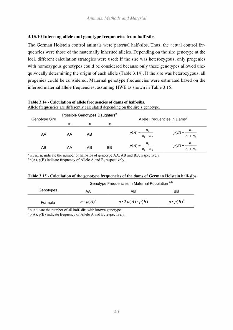
Animals, Methods and Material
40
3.15.10 Inferring allele and genotype frequencies from half-sibs
The German Holstein control animals were paternal half-sibs. Thus, the actual control fre-
quencies were those of the maternally inherited alleles. Depending on the sire genotype at the
loci, different calculation strategies were used: If the sire was heterozygous, only progenies
with homozygous genotypes could be considered because only these genotypes allowed une-
quivocally determining the origin of each allele (Table 3.14). If the sire was heterozygous, all
progenies could be considered. Maternal genotype frequencies were estimated based on the
inferred maternal allele frequencies, assuming HWE as shown in Table 3.15.
Table 3.14 - Calculation of allele frequencies of dams of half-sibs.
Allele frequencies are differently calculated depending on the sire’s genotype.
Possible Genotypes Daughtersa
Genotype Siren1 n2 n3
Allele Frequencies in Damsb
AA AA AB
!
p(A) =n1
n1
+ n2
!
p(B) =n2
n1
+ n2
AB AA AB BB
!
p(A) =n1
n1
+ n3
!
p(B) =n3
n1
+ n3
a n1, n2, n3 indicate the number of half-sibs of genotype AA, AB and BB, respectively.b p(A), p(B) indicate frequency of Allele A and B, respectively.
Table 3.15 - Calculation of the genotype frequencies of the dams of German Holstein half-sibs.
Genotype Frequencies in Maternal Population a,b
Genotypes AA AB BB
Formula
!
n " p(A)2
!
n " 2p(A) " p(B)
!
n " p(B)2
a n indicate the number of all half-sibs with known genotypeb p(A), p(B) indicate frequency of Allele A and B, respectively.
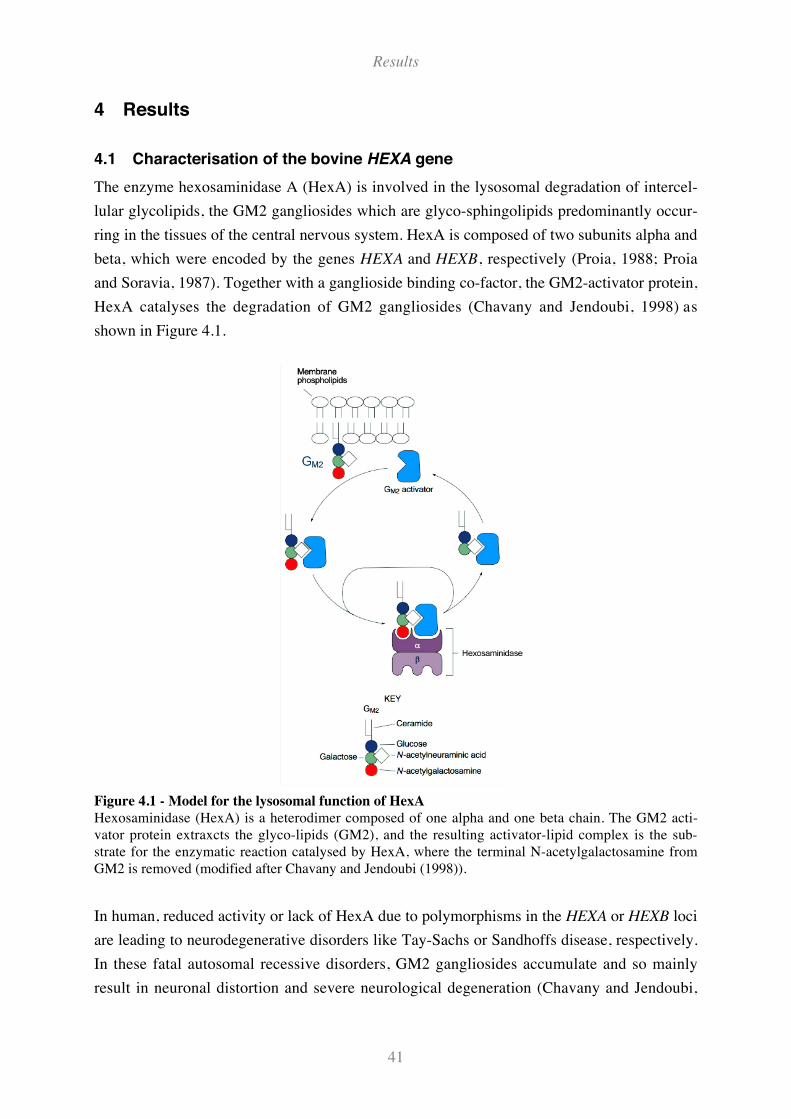
Results
41
4 Results
4.1 Characterisation of the bovine HEXA gene
The enzyme hexosaminidase A (HexA) is involved in the lysosomal degradation of intercel-
lular glycolipids, the GM2 gangliosides which are glyco-sphingolipids predominantly occur-
ring in the tissues of the central nervous system. HexA is composed of two subunits alpha and
beta, which were encoded by the genes HEXA and HEXB, respectively (Proia, 1988; Proia
and Soravia, 1987). Together with a ganglioside binding co-factor, the GM2-activator protein,
HexA catalyses the degradation of GM2 gangliosides (Chavany and Jendoubi, 1998) as
shown in Figure 4.1.
Figure 4.1 - Model for the lysosomal function of HexA
Hexosaminidase (HexA) is a heterodimer composed of one alpha and one beta chain. The GM2 acti-
vator protein extraxcts the glyco-lipids (GM2), and the resulting activator-lipid complex is the sub-
strate for the enzymatic reaction catalysed by HexA, where the terminal N-acetylgalactosamine from
GM2 is removed (modified after Chavany and Jendoubi (1998)).
In human, reduced activity or lack of HexA due to polymorphisms in the HEXA or HEXB loci
are leading to neurodegenerative disorders like Tay-Sachs or Sandhoffs disease, respectively.
In these fatal autosomal recessive disorders, GM2 gangliosides accumulate and so mainly
result in neuronal distortion and severe neurological degeneration (Chavany and Jendoubi,
Results
42
1998). Tay-Sachs and Sandhoffs disease have almost the same clinical symptoms, which in-
clude onset in infancy, rapid progression, and death usually before age of 4 years. Over 50
different types of Tay-Sachs disease are described, all caused by different sequence variants
in HEXA resulting in defected or inefficient enzyme. In animals, the disorders are called Gan-
gliosidoses, occurring naturally in cats (Cork et al., 1978) and dogs (Singer and Cork, 1989).
The human and animal diseases are also called Lysosomal Storage Diseases, because of the
accumulation of intercellular components in the lysosome. The storage of ‚waste’ in the
lysosome of nerve cells can be observed in prion diseases, too. The turnover of PrPc to PrPSc
generates protease-resistant components, which are indigestible for the lysosomal enzymes.
Therefore, lysosomal enzyme efficiency could influence BSE development.
Furthermore, Kopacek et al. (2000) showed an increased expression of HEXA - mRNA in
PrPSc infected brains of mice as well as an increasing expression of HEXB - mRNA during the
infection. The up-regulation of both, HEXA and HEXB correlated well with the spongiform
degeneration in the brain after infection. Similar results were obtained in a study using gene
expression array technology. Xiang et al. (2004) identified an emerged expression of HEXB in
Scrapie- infected brains of mice compared to uninfected. This leads to the assumption that
prion diseases either directly or indirectly influence HexA.
In cattle, the HEXA gene is located close to a marker on BTA 10 that showed significant seg-
regation distortion in BSE affected animals analysed by Transmission-Disequilibrium Tests
(TDTs) (Hernandez-Sanchez et al., 2002). Moreover, the homologous region in mice located
on chromosome 9 seems to affect the incubation time after experimental challenge with Scra-
pie (Stephenson et al., 2000). Thus, both functional and positional data made HEXA a prom-
ising candidate gene for BSE susceptibility in cattle.
For investigation of potential linkage of the HEXA gene and BSE, first the homologues bo-
vine region was identified and the structure compared with the human and mouse HEXA lo-
cus. In order to obtain sequences of bovine HEXA, the human reference mRNA of HEXA
(Acc NM_000520, NCBI) was subject to a BLAST search of the ESTother database division
of NCBI. Three bovine Expressed Sequence Tags (ESTs) could be identified and are listed in
Table 4.1. The corresponding sequences are covering the translated region of the HEXA gene,
except for a gap of 35 basepairs in exon 6. The EST sequencing approach is shown in Figure
3.1 of Animal, Material and Methods section. The re-sequenced DNA and the derived exonic
sequence are almost identical to the EST sequences and all discrepancies are located at the
ends of the sequences and were presumably caused by poor sequence quality of the EST se-
quences.
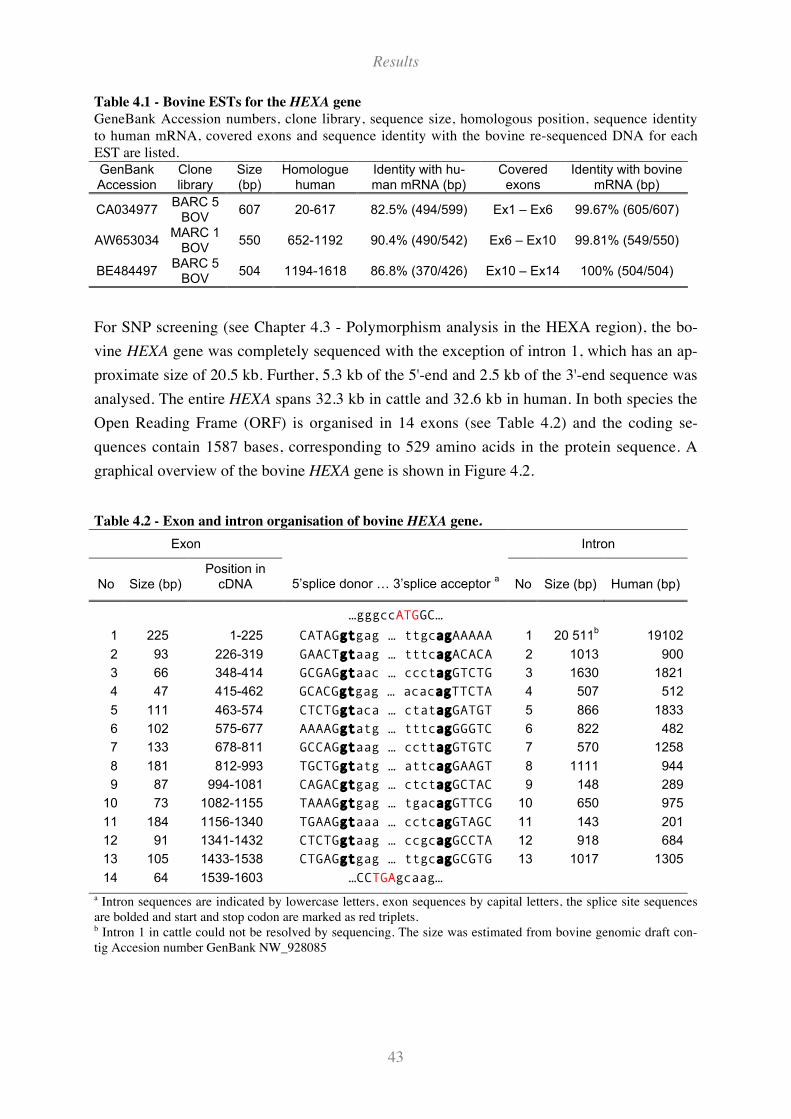
Results
43
Table 4.1 - Bovine ESTs for the HEXA gene
GeneBank Accession numbers, clone library, sequence size, homologous position, sequence identity
to human mRNA, covered exons and sequence identity with the bovine re-sequenced DNA for each
EST are listed.
GenBankAccession
Clonelibrary
Size(bp)
Homologuehuman
Identity with hu-man mRNA (bp)
Coveredexons
Identity with bovinemRNA (bp)
CA034977BARC 5
BOV607 20-617 82.5% (494/599) Ex1 – Ex6 99.67% (605/607)
AW653034MARC 1
BOV550 652-1192 90.4% (490/542) Ex6 – Ex10 99.81% (549/550)
BE484497BARC 5
BOV504 1194-1618 86.8% (370/426) Ex10 – Ex14 100% (504/504)
For SNP screening (see Chapter 4.3 - Polymorphism analysis in the HEXA region), the bo-
vine HEXA gene was completely sequenced with the exception of intron 1, which has an ap-
proximate size of 20.5 kb. Further, 5.3 kb of the 5'-end and 2.5 kb of the 3'-end sequence was
analysed. The entire HEXA spans 32.3 kb in cattle and 32.6 kb in human. In both species the
Open Reading Frame (ORF) is organised in 14 exons (see Table 4.2) and the coding se-
quences contain 1587 bases, corresponding to 529 amino acids in the protein sequence. A
graphical overview of the bovine HEXA gene is shown in Figure 4.2.
Table 4.2 - Exon and intron organisation of bovine HEXA gene.
Exon Intron
No Size (bp)Position in
cDNA 5’splice donor … 3’splice acceptor a
No Size (bp) Human (bp)
…gggccATGGC…
1 225 1-225 CATAGgtgag … ttgcagAAAAA 1 20 511b
19102
2 93 226-319 GAACTgtaag … tttcagACACA 2 1013 900
3 66 348-414 GCGAGgtaac … ccctagGTCTG 3 1630 1821
4 47 415-462 GCACGgtgag … acacagTTCTA 4 507 512
5 111 463-574 CTCTGgtaca … ctatagGATGT 5 866 1833
6 102 575-677 AAAAGgtatg … tttcagGGGTC 6 822 482
7 133 678-811 GCCAGgtaag … ccttagGTGTC 7 570 1258
8 181 812-993 TGCTGgtatg … attcagGAAGT 8 1111 944
9 87 994-1081 CAGACgtgag … ctctagGCTAC 9 148 289
10 73 1082-1155 TAAAGgtgag … tgacagGTTCG 10 650 975
11 184 1156-1340 TGAAGgtaaa … cctcagGTAGC 11 143 201
12 91 1341-1432 CTCTGgtaag … ccgcagGCCTA 12 918 684
13 105 1433-1538 CTGAGgtgag … ttgcagGCGTG 13 1017 1305
14 64 1539-1603 …CCTGAgcaag…
a Intron sequences are indicated by lowercase letters, exon sequences by capital letters, the splice site sequences
are bolded and start and stop codon are marked as red triplets.b Intron 1 in cattle could not be resolved by sequencing. The size was estimated from bovine genomic draft con-
tig Accesion number GenBank NW_928085
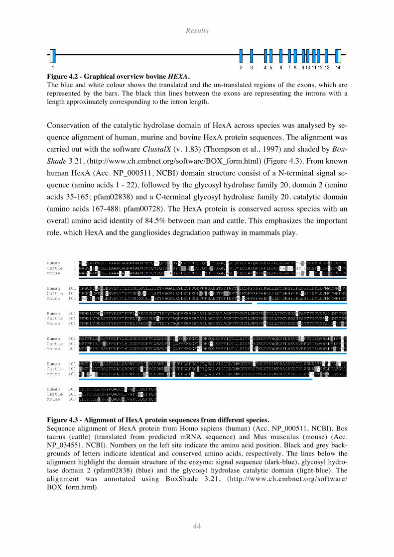
Results
44
Figure 4.2 - Graphical overview bovine HEXA.
The blue and white colour shows the translated and the un-translated regions of the exons, which are
represented by the bars. The black thin lines between the exons are representing the introns with a
length approximately corresponding to the intron length.
Conservation of the catalytic hydrolase domain of HexA across species was analysed by se-
quence alignment of human, murine and bovine HexA protein sequences. The alignment was
carried out with the software ClustalX (v. 1.83) (Thompson et al., 1997) and shaded by Box-
Shade 3.21, (http://www.ch.embnet.org/software/BOX_form.html) (Figure 4.3). From known
human HexA (Acc. NP_000511, NCBI) domain structure consist of a N-terminal signal se-
quence (amino acids 1 - 22), followed by the glycosyl hydrolase family 20, domain 2 (amino
acids 35-165; pfam02838) and a C-terminal glycosyl hydrolase family 20, catalytic domain
(amino acids 167-488; pfam00728). The HexA protein is conserved across species with an
overall amino acid identity of 84.5% between man and cattle. This emphasizes the important
role, which HexA and the gangliosides degradation pathway in mammals play.
Figure 4.3 - Alignment of HexA protein sequences from different species.
Sequence alignment of HexA protein from Homo sapiens (human) (Acc. NP_000511, NCBI), Bos
taurus (cattle) (translated from predicted mRNA sequence) and Mus musculus (mouse) (Acc.
NP_034551, NCBI). Numbers on the left site indicate the amino acid position. Black and grey back-
grounds of letters indicate identical and conserved amino acids, respectively. The lines below the
alignment highlight the domain structure of the enzyme: signal sequence (dark-blue), glycosyl hydro-
lase domain 2 (pfam02838) (blue) and the glycosyl hydrolase catalytic domain (light-blue). The
alignment was annotated using BoxShade 3.21, (http://www.ch.embnet.org/software/
BOX_form.html).
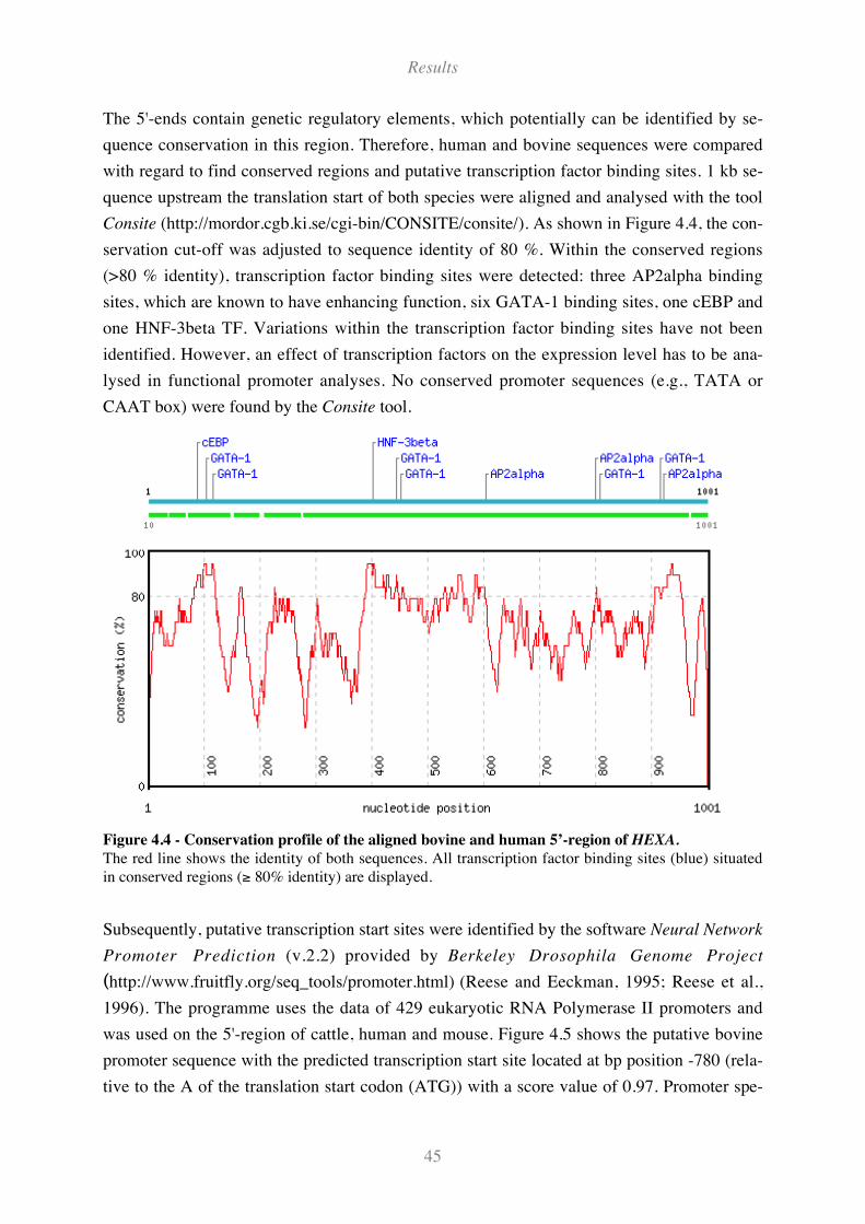
Results
45
The 5'-ends contain genetic regulatory elements, which potentially can be identified by se-
quence conservation in this region. Therefore, human and bovine sequences were compared
with regard to find conserved regions and putative transcription factor binding sites. 1 kb se-
quence upstream the translation start of both species were aligned and analysed with the tool
Consite (http://mordor.cgb.ki.se/cgi-bin/CONSITE/consite/). As shown in Figure 4.4, the con-
servation cut-off was adjusted to sequence identity of 80 %. Within the conserved regions
(>80 % identity), transcription factor binding sites were detected: three AP2alpha binding
sites, which are known to have enhancing function, six GATA-1 binding sites, one cEBP and
one HNF-3beta TF. Variations within the transcription factor binding sites have not been
identified. However, an effect of transcription factors on the expression level has to be ana-
lysed in functional promoter analyses. No conserved promoter sequences (e.g., TATA or
CAAT box) were found by the Consite tool.
Figure 4.4 - Conservation profile of the aligned bovine and human 5’-region of HEXA.
The red line shows the identity of both sequences. All transcription factor binding sites (blue) situated
in conserved regions (' 80% identity) are displayed.
Subsequently, putative transcription start sites were identified by the software Neural Network
Promoter Prediction (v.2.2) provided by Berkeley Drosophila Genome Project
(http://www.fruitfly.org/seq_tools/promoter.html) (Reese and Eeckman, 1995; Reese et al.,
1996). The programme uses the data of 429 eukaryotic RNA Polymerase II promoters and
was used on the 5'-region of cattle, human and mouse. Figure 4.5 shows the putative bovine
promoter sequence with the predicted transcription start site located at bp position -780 (rela-
tive to the A of the translation start codon (ATG)) with a score value of 0.97. Promoter spe-
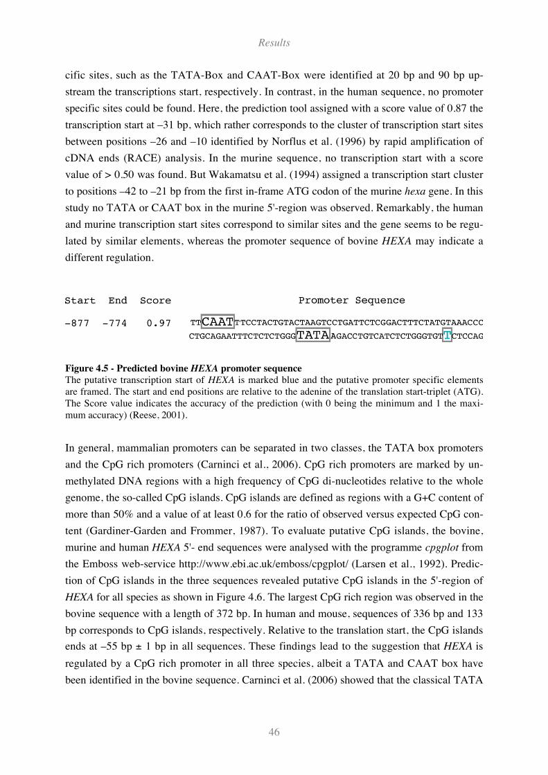
Results
46
cific sites, such as the TATA-Box and CAAT-Box were identified at 20 bp and 90 bp up-
stream the transcriptions start, respectively. In contrast, in the human sequence, no promoter
specific sites could be found. Here, the prediction tool assigned with a score value of 0.87 the
transcription start at –31 bp, which rather corresponds to the cluster of transcription start sites
between positions –26 and –10 identified by Norflus et al. (1996) by rapid amplification of
cDNA ends (RACE) analysis. In the murine sequence, no transcription start with a score
value of > 0.50 was found. But Wakamatsu et al. (1994) assigned a transcription start cluster
to positions –42 to –21 bp from the first in-frame ATG codon of the murine hexa gene. In this
study no TATA or CAAT box in the murine 5'-region was observed. Remarkably, the human
and murine transcription start sites correspond to similar sites and the gene seems to be regu-
lated by similar elements, whereas the promoter sequence of bovine HEXA may indicate a
different regulation.
Figure 4.5 - Predicted bovine HEXA promoter sequence
The putative transcription start of HEXA is marked blue and the putative promoter specific elements
are framed. The start and end positions are relative to the adenine of the translation start-triplet (ATG).
The Score value indicates the accuracy of the prediction (with 0 being the minimum and 1 the maxi-
mum accuracy) (Reese, 2001).
In general, mammalian promoters can be separated in two classes, the TATA box promoters
and the CpG rich promoters (Carninci et al., 2006). CpG rich promoters are marked by un-
methylated DNA regions with a high frequency of CpG di-nucleotides relative to the whole
genome, the so-called CpG islands. CpG islands are defined as regions with a G+C content of
more than 50% and a value of at least 0.6 for the ratio of observed versus expected CpG con-
tent (Gardiner-Garden and Frommer, 1987). To evaluate putative CpG islands, the bovine,
murine and human HEXA 5'- end sequences were analysed with the programme cpgplot from
the Emboss web-service http://www.ebi.ac.uk/emboss/cpgplot/ (Larsen et al., 1992). Predic-
tion of CpG islands in the three sequences revealed putative CpG islands in the 5'-region of
HEXA for all species as shown in Figure 4.6. The largest CpG rich region was observed in the
bovine sequence with a length of 372 bp. In human and mouse, sequences of 336 bp and 133
bp corresponds to CpG islands, respectively. Relative to the translation start, the CpG islands
ends at –55 bp ± 1 bp in all sequences. These findings lead to the suggestion that HEXA is
regulated by a CpG rich promoter in all three species, albeit a TATA and CAAT box have
been identified in the bovine sequence. Carninci et al. (2006) showed that the classical TATA
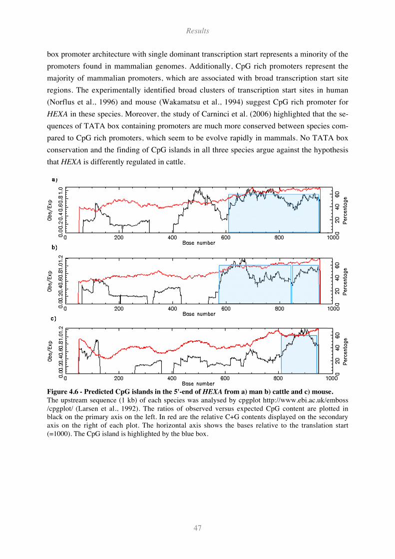
Results
47
box promoter architecture with single dominant transcription start represents a minority of the
promoters found in mammalian genomes. Additionally, CpG rich promoters represent the
majority of mammalian promoters, which are associated with broad transcription start site
regions. The experimentally identified broad clusters of transcription start sites in human
(Norflus et al., 1996) and mouse (Wakamatsu et al., 1994) suggest CpG rich promoter for
HEXA in these species. Moreover, the study of Carninci et al. (2006) highlighted that the se-
quences of TATA box containing promoters are much more conserved between species com-
pared to CpG rich promoters, which seem to be evolve rapidly in mammals. No TATA box
conservation and the finding of CpG islands in all three species argue against the hypothesis
that HEXA is differently regulated in cattle.
Figure 4.6 - Predicted CpG islands in the 5'-end of HEXA from a) man b) cattle and c) mouse.
The upstream sequence (1 kb) of each species was analysed by cpgplot http://www.ebi.ac.uk/emboss
/cpgplot/ (Larsen et al., 1992). The ratios of observed versus expected CpG content are plotted in
black on the primary axis on the left. In red are the relative C+G contents displayed on the secondary
axis on the right of each plot. The horizontal axis shows the bases relative to the translation start
(=1000). The CpG island is highlighted by the blue box.
Results
48
4.2 Fine-mapping of the region surrounding HEXA
4.2.1 Elucidation of the structure of the region surrounding HEXA.
4.2.1.1 Isolation of BAC clones for the bovine HEXA region
Screening the bovine RPCI-42 BAC library with a HEXA-specific PCR-product revealed six
BAC-clones (Table 4.3). Colony-PCR with several primer systems covering the entire gene
showed that each clone contained HEXA from exon 1 to exon 14. Using the corresponding
human genomic draft sequence as shown in Contig View in Ensembl (v39)
(http://www.ensembl.org/ Homo_sapiens/), the genes were identified within a 300-kb region
centred on HEXA. BAC-end sequencing and testing the BACs with specific primers from the
genes that were listed in the human region allowed building a BAC-contig. For this, the BAC
end sequences were subjects of BLAST searches against the human and bovine draft sequen-
ces, which allowed assigning their corresponding position on HSA 15 and BTA 10 as shown
in Figure 4.7. The bovine genomic region and the corresponding region in human beings is
oriented from centromere to telomere. Therefore, PARP6, BRUNOL6 and HEXA are here as-
signed on the negative strand (reverse-complement).
Analysis of the BLAST results revealed that the T7 end sequences of TUM910 andTUM924
are identical and the T7 end of TUM916 is located 200 bp upstream. All three BAC end se-
quences start in BRUNOL6, intron 2. Both BAC ends of TUM909 (SP6) and TUM 920 (T7)
are situated in PARP6, intron 15 and intron 8, respectively. Except for the SP6 end of
TUM910, which end in ARIH1 intron 2, all annotated BAC ends are located between HEXA
and ARIH1. TUM907 BAC ends showed no similarities to sequence entries for the extended
HEXA region, neither for the human nor the bovine draft sequence (Btau 2.0). A possible
explanation for this could be that the end sequences of TUM907 do not match with the e-
xisting sequences because the corresponding part has not been sequenced yet and the sequen-
ce contains Ns at that position. The newest assembly of the cow genome (Btau 3.0) was fi-
nally used to annotate the TUM907 BAC ends: BLAST hits were found for SP6 on an unno-
tated scaffold and for T7 on BTA26. This suggests that TUM907 is a chimerical clone contai-
ning an insert composed of two or three different sequence fragments.
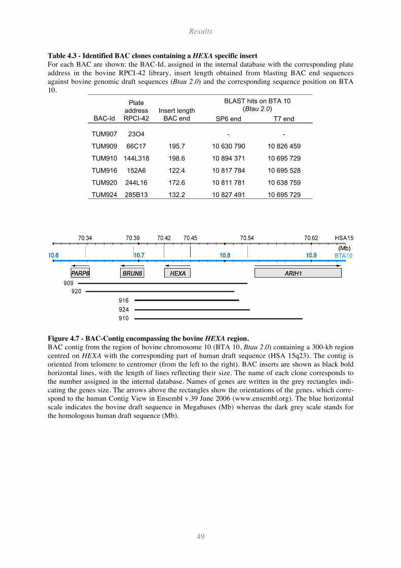
Results
49
Table 4.3 - Identified BAC clones containing a HEXA specific insert
For each BAC are shown: the BAC-Id, assigned in the internal database with the corresponding plate
address in the bovine RPCI-42 library, insert length obtained from blasting BAC end sequences
against bovine genomic draft sequences (Btau 2.0) and the corresponding sequence position on BTA
10.
BLAST hits on BTA 10(Btau 2.0)
BAC-Id
PlateaddressRPCI-42
Insert lengthBAC end SP6 end T7 end
TUM907 23O4 - -
TUM909 66C17 195.7 10 630 790 10 826 459
TUM910 144L318 198.6 10 894 371 10 695 729
TUM916 152A6 122.4 10 817 784 10 695 528
TUM920 244L16 172.6 10 811 781 10 638 759
TUM924 285B13 132.2 10 827 491 10 695 729
Figure 4.7 - BAC-Contig encompassing the bovine HEXA region.
BAC contig from the region of bovine chromosome 10 (BTA 10, Btau 2.0) containing a 300-kb region
centred on HEXA with the corresponding part of human draft sequence (HSA 15q23). The contig is
oriented from telomere to centromer (from the left to the right). BAC inserts are shown as black bold
horizontal lines, with the length of lines reflecting their size. The name of each clone corresponds to
the number assigned in the internal database. Names of genes are written in the grey rectangles indi-
cating the genes size. The arrows above the rectangles show the orientations of the genes, which corre-
spond to the human Contig View in Ensembl v.39 June 2006 (www.ensembl.org). The blue horizontal
scale indicates the bovine draft sequence in Megabases (Mb) whereas the dark grey scale stands for
the homologous human draft sequence (Mb).
Results
50
4.2.1.2 Using Btau 1.0
In October 2004, the first bovine genomic sequence was available at the Ensembl web-service
(www.ensembl.org; Cow v.25, Btau 1.0). By the date of completion of this work, the
preliminary version of the bovine draft sequence was not accessible anymore at the Ensemble
web service. However, the first release had an extreme impact on resolving the region because
primer design was facilitated and therefore sequencing could be optimised and accelerated.
Until then, for instance for the 5'-end, re-sequencing was only possible with preceding primer
walk on BAC DNA. This approach could be skipped with the release of the scaffolds. Further,
the PCR systems and their fragment length could be improved easily by an adjustment of the
fragment length to the ideal size for sequencing of 1000 bp.
The bovine draft sequences for the four genes of the extended HEXA region was obtained by
blasting the corresponding human reference mRNAs. Subsequently, twelve scaffolds ranging
in size from 0.95 kb to 28.7 kb could be identified (Table 4.4). For HEXA, two scaffolds were
found, one spanning from the 5'-end to intron 1 with a size of 15.3 kb (SCAFFOLD95258)
and the second spanning from intron 1 to the 3'-end with a size of 28.7 kb (SCAFFOLD5566).
The sequences of both did not overlap and the gap in intron 1 could not be closed by PCR
systems with primers designed at the putative transition of the scaffolds, respectively. A pos-
sible reason for the failure of the primer system is the unreliability and imprecision of the se-
quences at the beginning and end of the scaffolds. For ARIH1, located upstream of HEXA, one
scaffold (SCAFFOLD295439) was found containing the 5'-end and exon 1. For BRUNOL6
and PARP6, both located downstream of HEXA, two and six scaffolds were identified, re-
spectively (Table 4.4).
In order to reveal the structure of the bovine genes and to identify the coding regions, the
scaffolds were compared with the homologous human sequence and corresponding gene
structure was applied. The scaffolds were mainly used to re-sequence the adjacent region of
HEXA and the neighbouring genes.
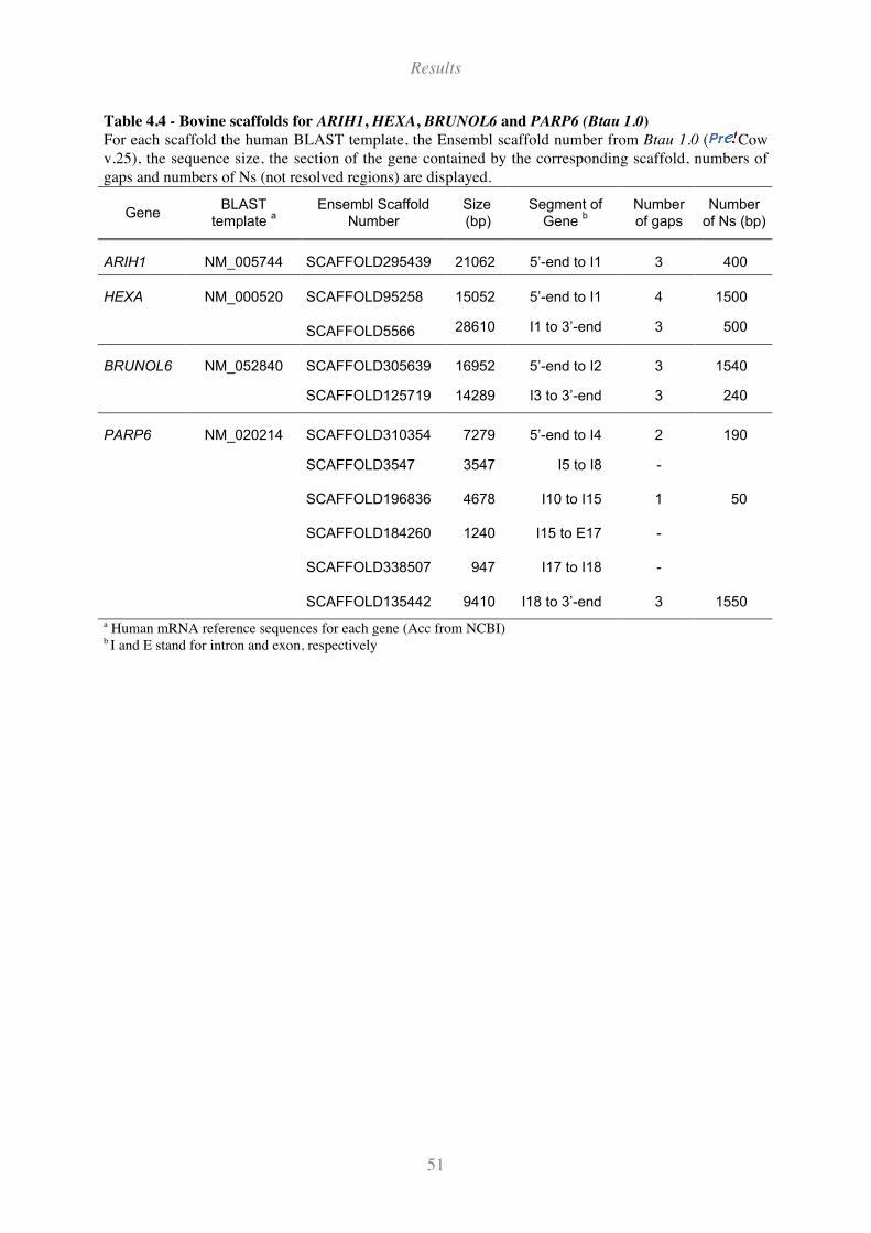
Results
51
Table 4.4 - Bovine scaffolds for ARIH1, HEXA, BRUNOL6 and PARP6 (Btau 1.0)
For each scaffold the human BLAST template, the Ensembl scaffold number from Btau 1.0 ( Cow
v.25), the sequence size, the section of the gene contained by the corresponding scaffold, numbers of
gaps and numbers of Ns (not resolved regions) are displayed.
GeneBLAST
template a
Ensembl ScaffoldNumber
Size(bp)
Segment ofGene
bNumberof gaps
Numberof Ns (bp)
ARIH1 NM_005744 SCAFFOLD295439 21062 5’-end to I1 3 400
HEXA NM_000520 SCAFFOLD95258 15052 5’-end to I1 4 1500
SCAFFOLD5566 28610 I1 to 3’-end 3 500
BRUNOL6 NM_052840 SCAFFOLD305639 16952 5’-end to I2 3 1540
SCAFFOLD125719 14289 I3 to 3’-end 3 240
PARP6 NM_020214 SCAFFOLD310354 7279 5’-end to I4 2 190
SCAFFOLD3547 3547 I5 to I8 -
SCAFFOLD196836 4678 I10 to I15 1 50
SCAFFOLD184260 1240 I15 to E17 -
SCAFFOLD338507 947 I17 to I18 -
SCAFFOLD135442 9410 I18 to 3’-end 3 1550
a Human mRNA reference sequences for each gene (Acc from NCBI)b I and E stand for intron and exon, respectively
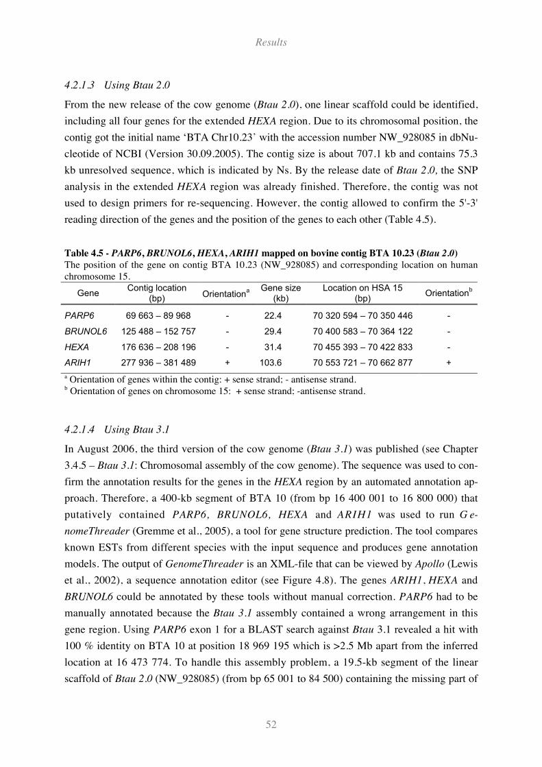
Results
52
4.2.1.3 Using Btau 2.0
From the new release of the cow genome (Btau 2.0), one linear scaffold could be identified,
including all four genes for the extended HEXA region. Due to its chromosomal position, the
contig got the initial name ‘BTA Chr10.23’ with the accession number NW_928085 in dbNu-
cleotide of NCBI (Version 30.09.2005). The contig size is about 707.1 kb and contains 75.3
kb unresolved sequence, which is indicated by Ns. By the release date of Btau 2.0, the SNP
analysis in the extended HEXA region was already finished. Therefore, the contig was not
used to design primers for re-sequencing. However, the contig allowed to confirm the 5'-3'
reading direction of the genes and the position of the genes to each other (Table 4.5).
Table 4.5 - PARP6, BRUNOL6, HEXA, ARIH1 mapped on bovine contig BTA 10.23 (Btau 2.0)
The position of the gene on contig BTA 10.23 (NW_928085) and corresponding location on human
chromosome 15.
GeneContig location
(bp)Orientation
a Gene size(kb)
Location on HSA 15(bp)
Orientationb
PARP6 69 663 – 89 968 - 22.4 70 320 594 – 70 350 446 -
BRUNOL6 125 488 – 152 757 - 29.4 70 400 583 – 70 364 122 -
HEXA 176 636 – 208 196 - 31.4 70 455 393 – 70 422 833 -
ARIH1 277 936 – 381 489 + 103.6 70 553 721 – 70 662 877 +
a Orientation of genes within the contig: + sense strand; - antisense strand.b Orientation of genes on chromosome 15: + sense strand; -antisense strand.
4.2.1.4 Using Btau 3.1
In August 2006, the third version of the cow genome (Btau 3.1) was published (see Chapter
3.4.5 – Btau 3.1: Chromosomal assembly of the cow genome). The sequence was used to con-
firm the annotation results for the genes in the HEXA region by an automated annotation ap-
proach. Therefore, a 400-kb segment of BTA 10 (from bp 16 400 001 to 16 800 000) that
putatively contained PARP6, BRUNOL6, HEXA and ARIH1 was used to run G e-
nomeThreader (Gremme et al., 2005), a tool for gene structure prediction. The tool compares
known ESTs from different species with the input sequence and produces gene annotation
models. The output of GenomeThreader is an XML-file that can be viewed by Apollo (Lewis
et al., 2002), a sequence annotation editor (see Figure 4.8). The genes ARIH1, HEXA and
BRUNOL6 could be annotated by these tools without manual correction. PARP6 had to be
manually annotated because the Btau 3.1 assembly contained a wrong arrangement in this
gene region. Using PARP6 exon 1 for a BLAST search against Btau 3.1 revealed a hit with
100 % identity on BTA 10 at position 18 969 195 which is >2.5 Mb apart from the inferred
location at 16 473 774. To handle this assembly problem, a 19.5-kb segment of the linear
scaffold of Btau 2.0 (NW_928085) (from bp 65 001 to 84 500) containing the missing part of
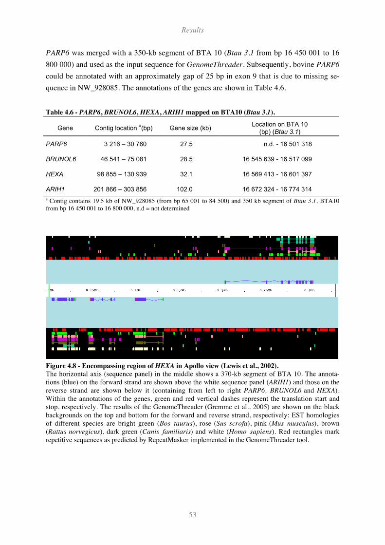
Results
53
PARP6 was merged with a 350-kb segment of BTA 10 (Btau 3.1 from bp 16 450 001 to 16
800 000) and used as the input sequence for GenomeThreader. Subsequently, bovine PARP6
could be annotated with an approximately gap of 25 bp in exon 9 that is due to missing se-
quence in NW_928085. The annotations of the genes are shown in Table 4.6.
Table 4.6 - PARP6, BRUNOL6, HEXA, ARIH1 mapped on BTA10 (Btau 3.1).
Gene Contig location a(bp) Gene size (kb)
Location on BTA 10(bp) (Btau 3.1)
PARP6 3 216 – 30 760 27.5 n.d. - 16 501 318
BRUNOL6 46 541 – 75 081 28.5 16 545 639 - 16 517 099
HEXA 98 855 – 130 939 32.1 16 569 413 - 16 601 397
ARIH1 201 866 – 303 856 102.0 16 672 324 - 16 774 314
a Contig contains 19.5 kb of NW_928085 (from bp 65 001 to 84 500) and 350 kb segment of Btau 3.1, BTA10
from bp 16 450 001 to 16 800 000, n.d = not determined
Figure 4.8 - Encompassing region of HEXA in Apollo view (Lewis et al., 2002).
The horizontal axis (sequence panel) in the middle shows a 370-kb segment of BTA 10. The annota-
tions (blue) on the forward strand are shown above the white sequence panel (ARIH1) and those on the
reverse strand are shown below it (containing from left to right PARP6, BRUNOL6 and HEXA).
Within the annotations of the genes, green and red vertical dashes represent the translation start and
stop, respectively. The results of the GenomeThreader (Gremme et al., 2005) are shown on the black
backgrounds on the top and bottom for the forward and reverse strand, respectively: EST homologies
of different species are bright green (Bos taurus), rose (Sus scrofa), pink (Mus musculus), brown
(Rattus norvegicus), dark green (Canis familiaris) and white (Homo sapiens). Red rectangles mark
repetitive sequences as predicted by RepeatMasker implemented in the GenomeThreader tool.
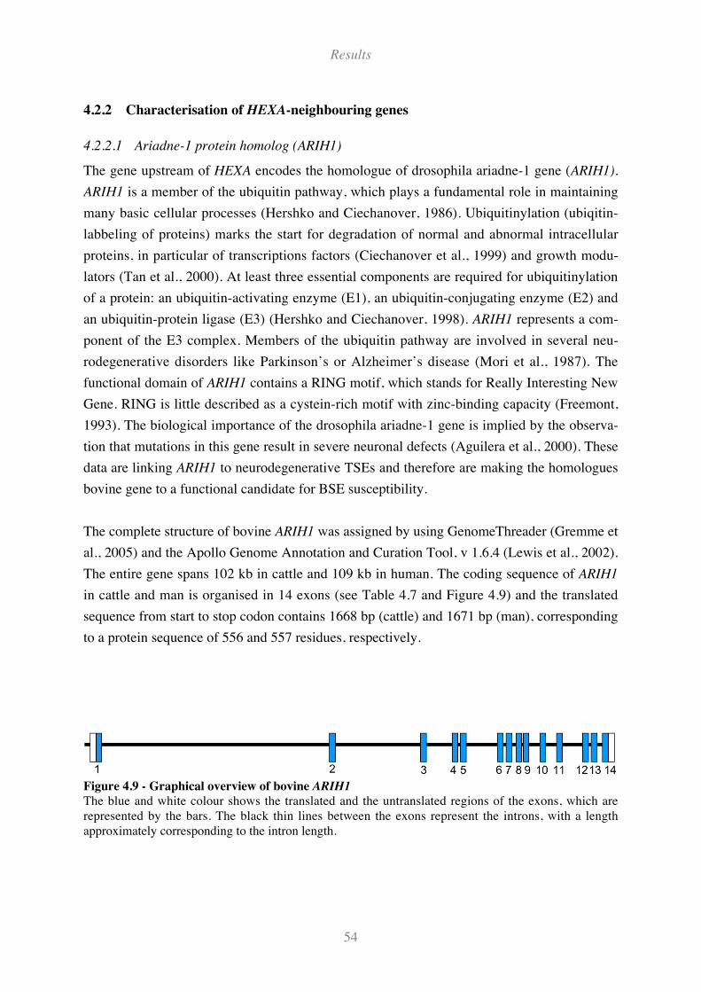
Results
54
4.2.2 Characterisation of HEXA-neighbouring genes
4.2.2.1 Ariadne-1 protein homolog (ARIH1)
The gene upstream of HEXA encodes the homologue of drosophila ariadne-1 gene (ARIH1).
ARIH1 is a member of the ubiquitin pathway, which plays a fundamental role in maintaining
many basic cellular processes (Hershko and Ciechanover, 1986). Ubiquitinylation (ubiqitin-
labbeling of proteins) marks the start for degradation of normal and abnormal intracellular
proteins, in particular of transcriptions factors (Ciechanover et al., 1999) and growth modu-
lators (Tan et al., 2000). At least three essential components are required for ubiquitinylation
of a protein: an ubiquitin-activating enzyme (E1), an ubiquitin-conjugating enzyme (E2) and
an ubiquitin-protein ligase (E3) (Hershko and Ciechanover, 1998). ARIH1 represents a com-
ponent of the E3 complex. Members of the ubiquitin pathway are involved in several neu-
rodegenerative disorders like Parkinson’s or Alzheimer’s disease (Mori et al., 1987). The
functional domain of ARIH1 contains a RING motif, which stands for Really Interesting New
Gene. RING is little described as a cystein-rich motif with zinc-binding capacity (Freemont,
1993). The biological importance of the drosophila ariadne-1 gene is implied by the observa-
tion that mutations in this gene result in severe neuronal defects (Aguilera et al., 2000). These
data are linking ARIH1 to neurodegenerative TSEs and therefore are making the homologues
bovine gene to a functional candidate for BSE susceptibility.
The complete structure of bovine ARIH1 was assigned by using GenomeThreader (Gremme et
al., 2005) and the Apollo Genome Annotation and Curation Tool, v 1.6.4 (Lewis et al., 2002).
The entire gene spans 102 kb in cattle and 109 kb in human. The coding sequence of ARIH1
in cattle and man is organised in 14 exons (see Table 4.7 and Figure 4.9) and the translated
sequence from start to stop codon contains 1668 bp (cattle) and 1671 bp (man), corresponding
to a protein sequence of 556 and 557 residues, respectively.
Figure 4.9 - Graphical overview of bovine ARIH1
The blue and white colour shows the translated and the untranslated regions of the exons, which are
represented by the bars. The black thin lines between the exons represent the introns, with a length
approximately corresponding to the intron length.
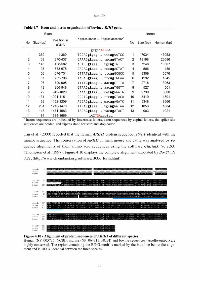
Results
55
Table 4.7 - Exon and intron organisation of bovine ARIH1 gene.
Exon Intron
No Size (bp)Position in
cDNA
5’splice donor … 3’splice acceptora
No Size (bp) Human (bp)
…gcgccATGGA…
1 369 1-369 TCCAGgtgag … tttagAATCC 1 47034 43053
2 68 370-437 GAAAGgtaag … tgcagGTACT 2 18198 26686
3 145 438-582 ACTCGgtgag … tgcagTATTT 3 7248 10307
4 93 583-675 GACAGgtaaa … tccagACTAT 4 506 489
5 56 676-731 GTTATgtaag … ttcagGCGCC 5 8309 5576
6 67 732-798 TAGAGgtaag … ttcagTGCAA 6 1292 1845
7 107 799-905 TTTTGgtaag … aacagCTTTA 7 2718 3063
8 43 906-948 GTAAGgtgag … aacagTGGTT 8 527 501
9 72 949-1020 CAAAGgttgg … catagGAATG 9 2730 3000
10 131 1021-1151 GCCTGgtagg … ttcagGTACA 10 3419 1801
11 58 1152-1209 AGGAGgtaag … gacagAGATC 11 5348 8566
12 261 1210-1470 TTGAGgtagg … tgcagAATAA 12 1053 1084
13 113 1471-1583 TACAGgtaag … tacagATACT 13 983 1021
14 84 1584-1669 …ACTGAgaatg…a Intron sequences are indicated by lowercase letters, exon sequences by capital letters, the splice site
sequences are bolded, red triplets stand for start and stop codon.
Tan et al. (2000) reported that the human ARIH1 protein sequence is 98% identical with the
murine sequence. The conservation of ARIH1 in man, mouse and cattle was analysed by se-
quence alignments of their amino acid sequences using the software ClustalX (v. 1.83)
(Thompson et al., 1997). Figure 4.10 displays the complete alignment annotated by BoxShade
3.21, (http://www.ch.embnet.org/software/BOX_form.html).
Figure 4.10 - Alignment of protein sequences of ARIH1 of different species.
Human (NP_005735, NCBI), murine (NP_064311, NCBI) and bovine sequences (Apollo-output) are
highly conserved. The region containing the RING-motif is marked by the blue line below the align-
ment and is 100 % identical between the three species.
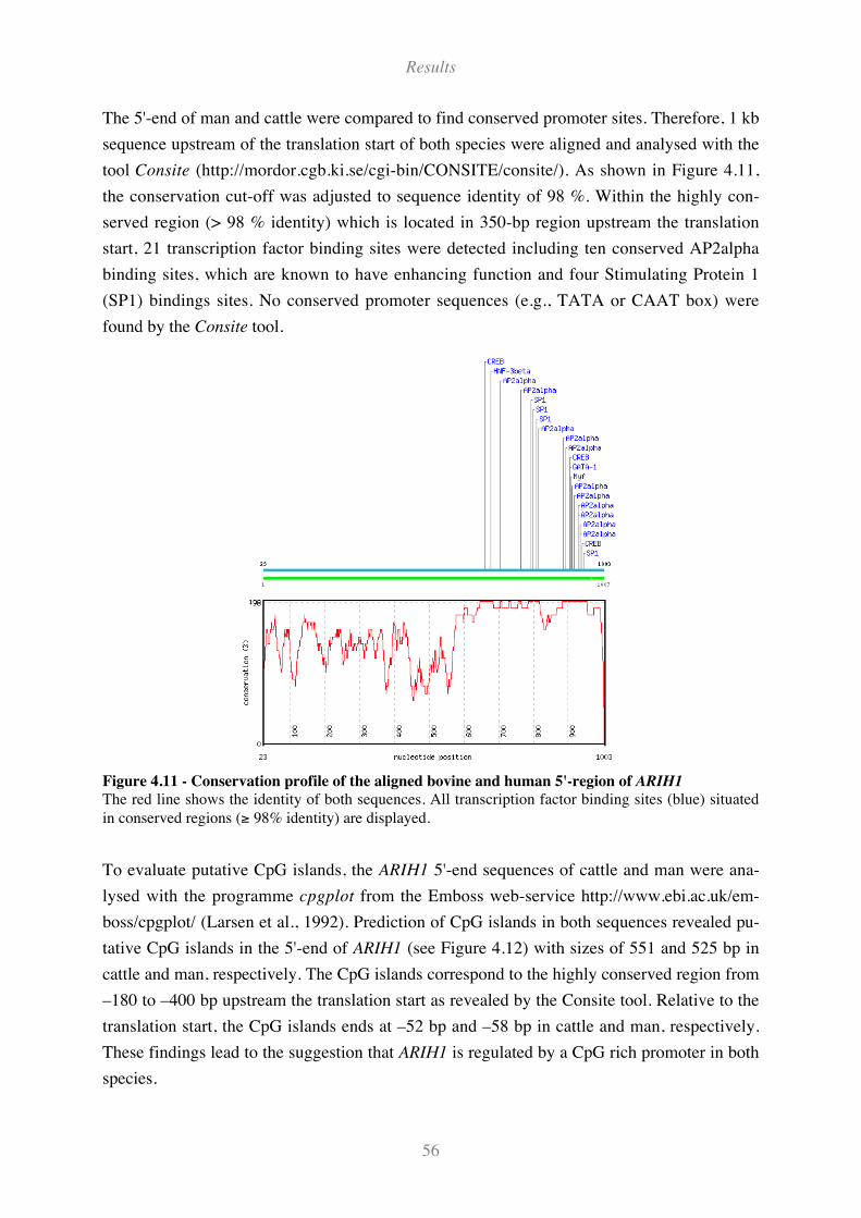
Results
56
The 5'-end of man and cattle were compared to find conserved promoter sites. Therefore, 1 kb
sequence upstream of the translation start of both species were aligned and analysed with the
tool Consite (http://mordor.cgb.ki.se/cgi-bin/CONSITE/consite/). As shown in Figure 4.11,
the conservation cut-off was adjusted to sequence identity of 98 %. Within the highly con-
served region (> 98 % identity) which is located in 350-bp region upstream the translation
start, 21 transcription factor binding sites were detected including ten conserved AP2alpha
binding sites, which are known to have enhancing function and four Stimulating Protein 1
(SP1) bindings sites. No conserved promoter sequences (e.g., TATA or CAAT box) were
found by the Consite tool.
Figure 4.11 - Conservation profile of the aligned bovine and human 5'-region of ARIH1
The red line shows the identity of both sequences. All transcription factor binding sites (blue) situated
in conserved regions (' 98% identity) are displayed.
To evaluate putative CpG islands, the ARIH1 5'-end sequences of cattle and man were ana-
lysed with the programme cpgplot from the Emboss web-service http://www.ebi.ac.uk/em-
boss/cpgplot/ (Larsen et al., 1992). Prediction of CpG islands in both sequences revealed pu-
tative CpG islands in the 5'-end of ARIH1 (see Figure 4.12) with sizes of 551 and 525 bp in
cattle and man, respectively. The CpG islands correspond to the highly conserved region from
–180 to –400 bp upstream the translation start as revealed by the Consite tool. Relative to the
translation start, the CpG islands ends at –52 bp and –58 bp in cattle and man, respectively.
These findings lead to the suggestion that ARIH1 is regulated by a CpG rich promoter in both
species.
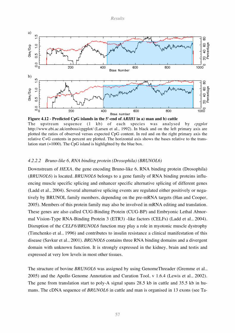
Results
57
a)
b)
Figure 4.12 - Predicted CpG islands in the 5'-end of ARIH1 in a) man and b) cattle
The upstream sequence (1 kb) of each species was analysed by cpgplot
http://www.ebi.ac.uk/emboss/cpgplot/ (Larsen et al., 1992). In black and on the left primary axis are
plotted the ratios of observed versus expected CpG content. In red and on the right primary axis the
relative C+G contents in percent are plotted. The horizontal axis shows the bases relative to the trans-
lation start (=1000). The CpG island is highlighted by the blue box.
4.2.2.2 Bruno-like 6, RNA binding protein (Drosophila) (BRUNOL6)
Downstream of HEXA, the gene encoding Bruno-like 6, RNA binding protein (Drosophila)
(BRUNOL6) is located. BRUNOL6 belongs to a gene family of RNA binding proteins influ-
encing muscle specific splicing and enhancer specific alternative splicing of different genes
(Ladd et al., 2004). Several alternative splicing events are regulated either positively or nega-
tively by BRUNOL family members, depending on the pre-mRNA targets (Han and Cooper,
2005). Members of this protein family may also be involved in mRNA editing and translation.
These genes are also called CUG-Binding Protein (CUG-BP) and Embryonic Lethal Abnor-
mal Vision-Type RNA-Binding Protein 3 (ETR3) -like factors (CELFs) (Ladd et al., 2004).
Disruption of the CELF6/BRUNOL6 function may play a role in myotonic muscle dystrophy
(Timchenko et al., 1996) and contributes to insulin resistance a clinical manifestation of this
disease (Savkur et al., 2001). BRUNOL6 contains three RNA binding domains and a divergent
domain with unknown function. It is strongly expressed in the kidney, brain and testis and
expressed at very low levels in most other tissues.
The structure of bovine BRUNOL6 was assigned by using GenomeThreader (Gremme et al.,
2005) and the Apollo Genome Annotation and Curation Tool, v 1.6.4 (Lewis et al., 2002).
The gene from translation start to poly-A signal spans 28.5 kb in cattle and 35.5 kb in hu-
mans. The cDNA sequence of BRUNOL6 in cattle and man is organised in 13 exons (see Ta-
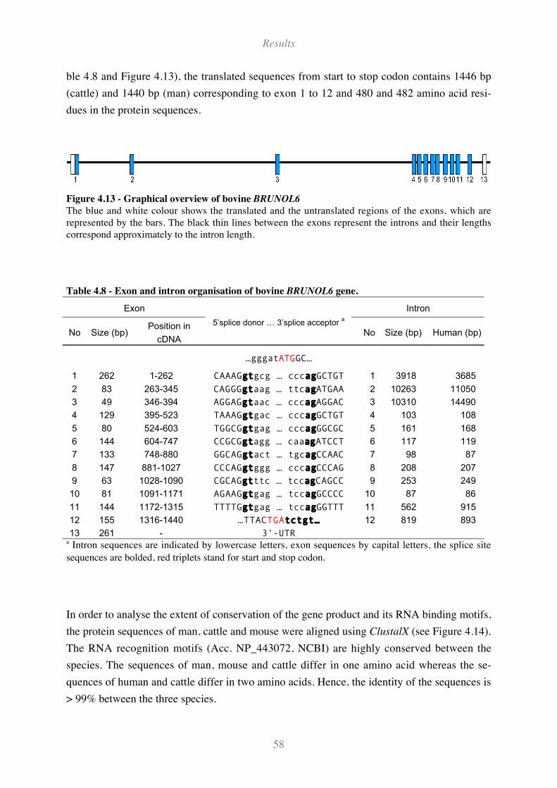
Results
58
ble 4.8 and Figure 4.13), the translated sequences from start to stop codon contains 1446 bp
(cattle) and 1440 bp (man) corresponding to exon 1 to 12 and 480 and 482 amino acid resi-
dues in the protein sequences.
Figure 4.13 - Graphical overview of bovine BRUNOL6
The blue and white colour shows the translated and the untranslated regions of the exons, which are
represented by the bars. The black thin lines between the exons represent the introns and their lengths
correspond approximately to the intron length.
Table 4.8 - Exon and intron organisation of bovine BRUNOL6 gene.
Exon Intron
No Size (bp)Position in
cDNA
5’splice donor … 3’splice acceptor a
No Size (bp) Human (bp)
…gggatATGGC…
1 262 1-262 CAAAGgtgcg … cccagGCTGT 1 3918 3685
2 83 263-345 CAGGGgtaag … ttcagATGAA 2 10263 11050
3 49 346-394 AGGAGgtaac … cccagAGGAC 3 10310 14490
4 129 395-523 TAAAGgtgac … cccagGCTGT 4 103 108
5 80 524-603 TGGCGgtgag … cccagGGCGC 5 161 168
6 144 604-747 CCGCGgtagg … caaagATCCT 6 117 119
7 133 748-880 GGCAGgtact … tgcagCCAAC 7 98 87
8 147 881-1027 CCCAGgtggg … cccagCCCAG 8 208 207
9 63 1028-1090 CGCAGgtttc … tccagCAGCC 9 253 249
10 81 1091-1171 AGAAGgtgag … tccagGCCCC 10 87 86
11 144 1172-1315 TTTTGgtgag … tccagGGTTT 11 562 915
12 155 1316-1440 …TTACTGAtctgt… 12 819 893
13 261 - 3’-UTRa Intron sequences are indicated by lowercase letters, exon sequences by capital letters, the splice site
sequences are bolded, red triplets stand for start and stop codon.
In order to analyse the extent of conservation of the gene product and its RNA binding motifs,
the protein sequences of man, cattle and mouse were aligned using ClustalX (see Figure 4.14).
The RNA recognition motifs (Acc. NP_443072, NCBI) are highly conserved between the
species. The sequences of man, mouse and cattle differ in one amino acid whereas the se-
quences of human and cattle differ in two amino acids. Hence, the identity of the sequences is
> 99% between the three species.
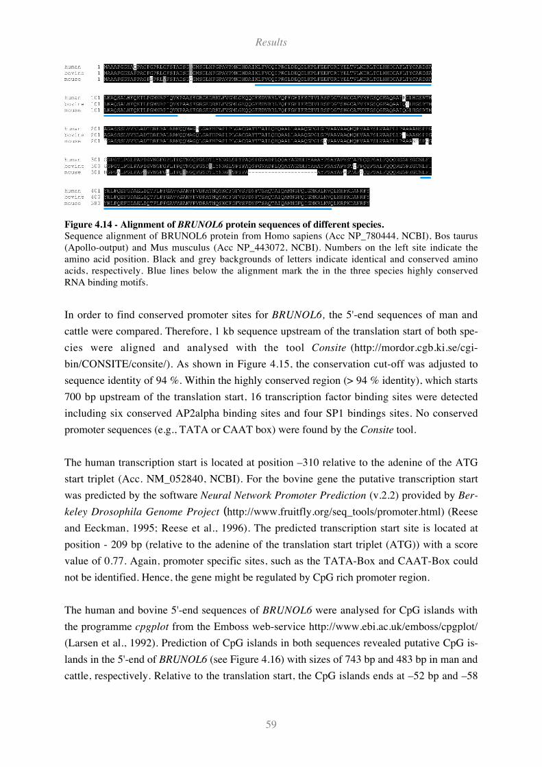
Results
59
Figure 4.14 - Alignment of BRUNOL6 protein sequences of different species.
Sequence alignment of BRUNOL6 protein from Homo sapiens (Acc NP_780444, NCBI), Bos taurus
(Apollo-output) and Mus musculus (Acc NP_443072, NCBI). Numbers on the left site indicate the
amino acid position. Black and grey backgrounds of letters indicate identical and conserved amino
acids, respectively. Blue lines below the alignment mark the in the three species highly conserved
RNA binding motifs.
In order to find conserved promoter sites for BRUNOL6, the 5'-end sequences of man and
cattle were compared. Therefore, 1 kb sequence upstream of the translation start of both spe-
cies were aligned and analysed with the tool Consite (http://mordor.cgb.ki.se/cgi-
bin/CONSITE/consite/). As shown in Figure 4.15, the conservation cut-off was adjusted to
sequence identity of 94 %. Within the highly conserved region (> 94 % identity), which starts
700 bp upstream of the translation start, 16 transcription factor binding sites were detected
including six conserved AP2alpha binding sites and four SP1 bindings sites. No conserved
promoter sequences (e.g., TATA or CAAT box) were found by the Consite tool.
The human transcription start is located at position –310 relative to the adenine of the ATG
start triplet (Acc. NM_052840, NCBI). For the bovine gene the putative transcription start
was predicted by the software Neural Network Promoter Prediction (v.2.2) provided by Ber-
keley Drosophila Genome Project (http://www.fruitfly.org/seq_tools/promoter.html) (Reese
and Eeckman, 1995; Reese et al., 1996). The predicted transcription start site is located at
position - 209 bp (relative to the adenine of the translation start triplet (ATG)) with a score
value of 0.77. Again, promoter specific sites, such as the TATA-Box and CAAT-Box could
not be identified. Hence, the gene might be regulated by CpG rich promoter region.
The human and bovine 5'-end sequences of BRUNOL6 were analysed for CpG islands with
the programme cpgplot from the Emboss web-service http://www.ebi.ac.uk/emboss/cpgplot/
(Larsen et al., 1992). Prediction of CpG islands in both sequences revealed putative CpG is-
lands in the 5'-end of BRUNOL6 (see Figure 4.16) with sizes of 743 bp and 483 bp in man and
cattle, respectively. Relative to the translation start, the CpG islands ends at –52 bp and –58
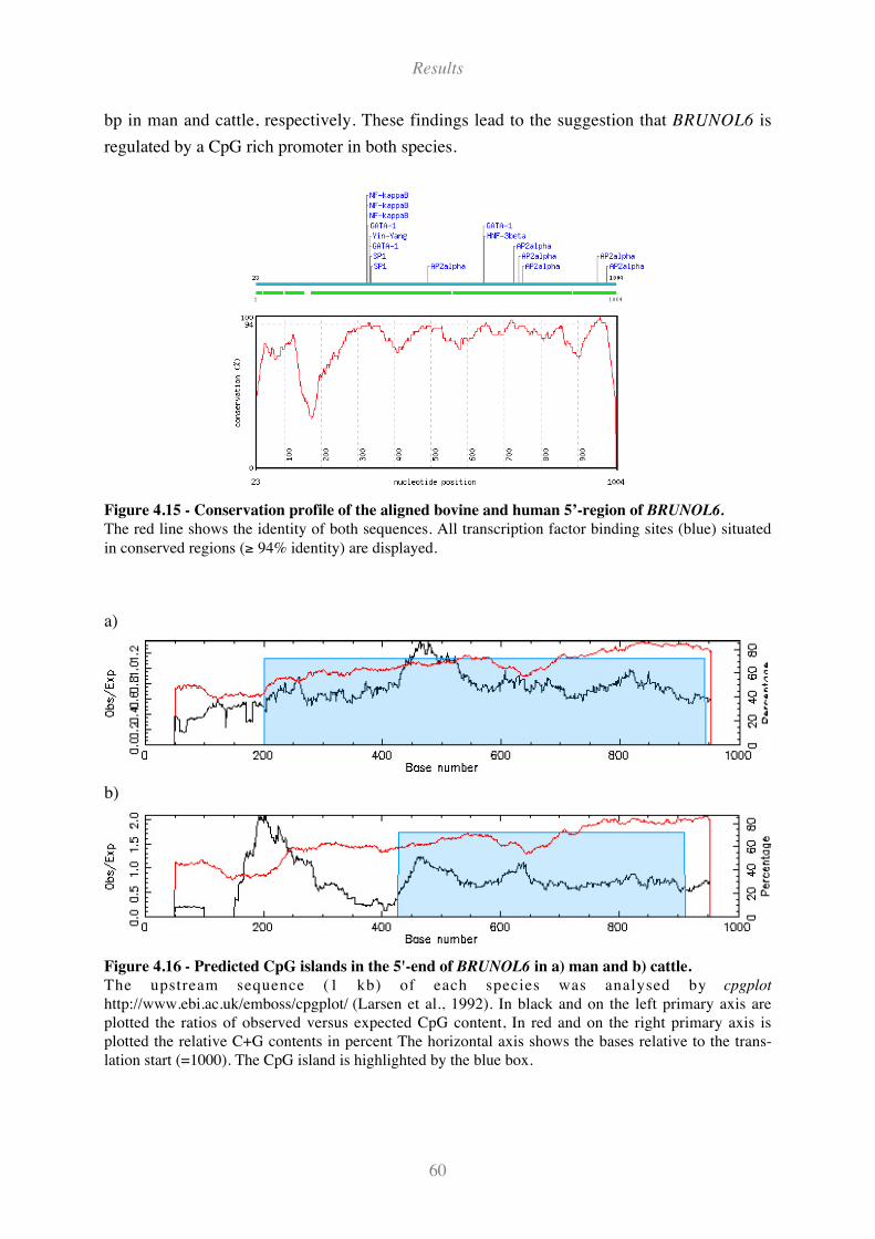
Results
60
bp in man and cattle, respectively. These findings lead to the suggestion that BRUNOL6 is
regulated by a CpG rich promoter in both species.
Figure 4.15 - Conservation profile of the aligned bovine and human 5’-region of BRUNOL6.
The red line shows the identity of both sequences. All transcription factor binding sites (blue) situated
in conserved regions (' 94% identity) are displayed.
a)
b)
Figure 4.16 - Predicted CpG islands in the 5'-end of BRUNOL6 in a) man and b) cattle.
The upstream sequence (1 kb) of each species was analysed by cpgplot
http://www.ebi.ac.uk/emboss/cpgplot/ (Larsen et al., 1992). In black and on the left primary axis are
plotted the ratios of observed versus expected CpG content, In red and on the right primary axis is
plotted the relative C+G contents in percent The horizontal axis shows the bases relative to the trans-
lation start (=1000). The CpG island is highlighted by the blue box.
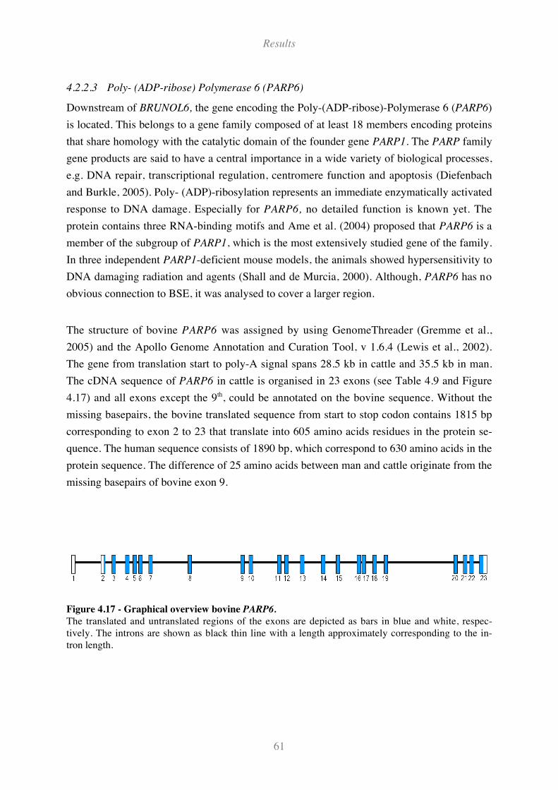
Results
61
4.2.2.3 Poly- (ADP-ribose) Polymerase 6 (PARP6)
Downstream of BRUNOL6, the gene encoding the Poly-(ADP-ribose)-Polymerase 6 (PARP6)
is located. This belongs to a gene family composed of at least 18 members encoding proteins
that share homology with the catalytic domain of the founder gene PARP1. The PARP family
gene products are said to have a central importance in a wide variety of biological processes,
e.g. DNA repair, transcriptional regulation, centromere function and apoptosis (Diefenbach
and Burkle, 2005). Poly- (ADP)-ribosylation represents an immediate enzymatically activated
response to DNA damage. Especially for PARP6, no detailed function is known yet. The
protein contains three RNA-binding motifs and Ame et al. (2004) proposed that PARP6 is a
member of the subgroup of PARP1, which is the most extensively studied gene of the family.
In three independent PARP1-deficient mouse models, the animals showed hypersensitivity to
DNA damaging radiation and agents (Shall and de Murcia, 2000). Although, PARP6 has no
obvious connection to BSE, it was analysed to cover a larger region.
The structure of bovine PARP6 was assigned by using GenomeThreader (Gremme et al.,
2005) and the Apollo Genome Annotation and Curation Tool, v 1.6.4 (Lewis et al., 2002).
The gene from translation start to poly-A signal spans 28.5 kb in cattle and 35.5 kb in man.
The cDNA sequence of PARP6 in cattle is organised in 23 exons (see Table 4.9 and Figure
4.17) and all exons except the 9th, could be annotated on the bovine sequence. Without the
missing basepairs, the bovine translated sequence from start to stop codon contains 1815 bp
corresponding to exon 2 to 23 that translate into 605 amino acids residues in the protein se-
quence. The human sequence consists of 1890 bp, which correspond to 630 amino acids in the
protein sequence. The difference of 25 amino acids between man and cattle originate from the
missing basepairs of bovine exon 9.
Figure 4.17 - Graphical overview bovine PARP6.
The translated and untranslated regions of the exons are depicted as bars in blue and white, respec-
tively. The introns are shown as black thin line with a length approximately corresponding to the in-
tron length.
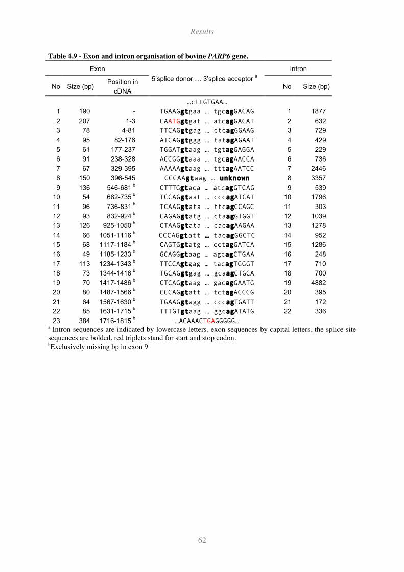
Results
62
Table 4.9 - Exon and intron organisation of bovine PARP6 gene.
Exon Intron
No Size (bp)Position in
cDNA
5’splice donor … 3’splice acceptor a
No Size (bp)
…cttGTGAA…
1 190 - TGAAGgtgaa … tgcagGACAG 1 1877
2 207 1-3 CAATGgtgat … atcagGACAT 2 632
3 78 4-81 TTCAGgtgag … ctcagGGAAG 3 729
4 95 82-176 ATCAGgtggg … tatagAGAAT 4 429
5 61 177-237 TGGATgtaag … tgtagGAGGA 5 229
6 91 238-328 ACCGGgtaaa … tgcagAACCA 6 736
7 67 329-395 AAAAAgtaag … tttagAATCC 7 2446
8 150 396-545 CCCAAgtaag … unknown 8 3357
9 136 546-681 b
CTTTGgtaca … atcagGTCAG 9 539
10 54 682-735 b
TCCAGgtaat … cccagATCAT 10 1796
11 96 736-831 b
TCAAGgtata … ttcagCCAGC 11 303
12 93 832-924 b
CAGAGgtatg … ctaagGTGGT 12 1039
13 126 925-1050 b
CTAAGgtata … cacagAAGAA 13 1278
14 66 1051-1116 b
CCCAGgtatt … tacagGGCTC 14 952
15 68 1117-1184 b
CAGTGgtatg … cctagGATCA 15 1286
16 49 1185-1233 b
GCAGGgtaag … agcagCTGAA 16 248
17 113 1234-1343 b
TTCCAgtgag … tacagTGGGT 17 710
18 73 1344-1416 b
TGCAGgtgag … gcaagCTGCA 18 700
19 70 1417-1486 b
CTCAGgtaag … gacagGAATG 19 4882
20 80 1487-1566 b
CCCAGgtatt … tctagACCCG 20 395
21 64 1567-1630 b
TGAAGgtagg … cccagTGATT 21 172
22 85 1631-1715 b
TTTGTgtaag … ggcagATATG 22 336
23 384 1716-1815 b
…ACAAACTGAGGGGG…a Intron sequences are indicated by lowercase letters, exon sequences by capital letters, the splice site
sequences are bolded, red triplets stand for start and stop codon.bExclusively missing bp in exon 9
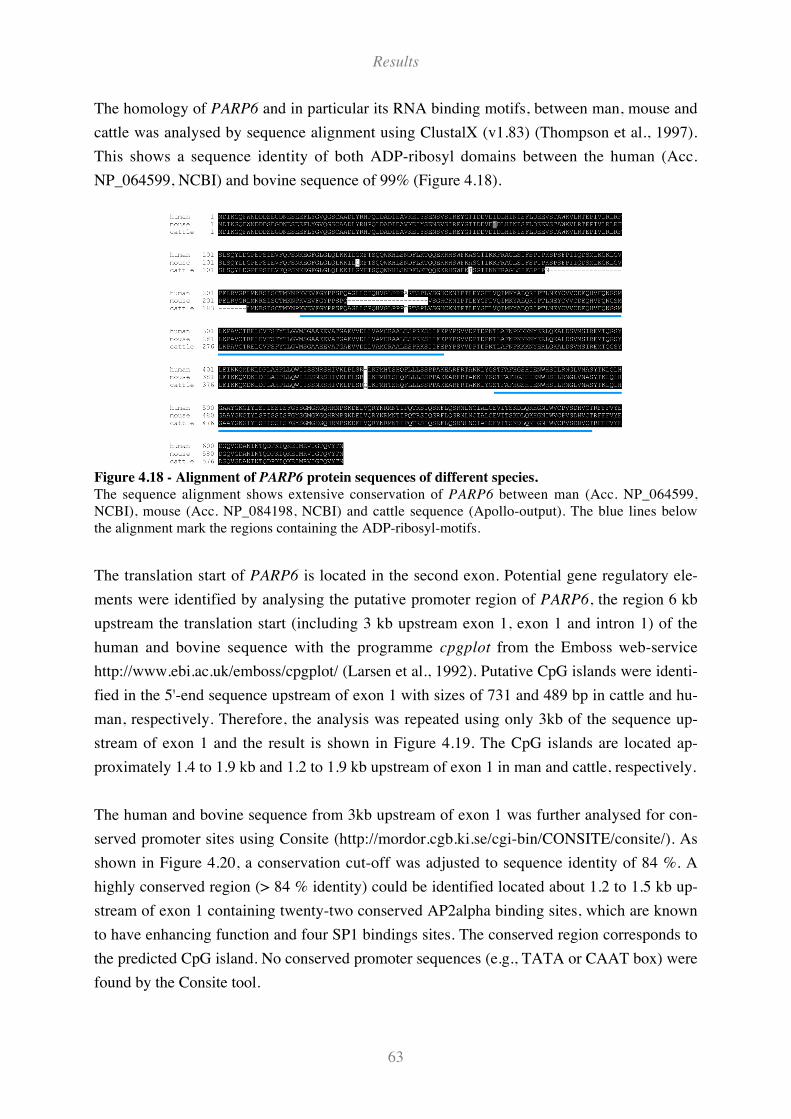
Results
63
The homology of PARP6 and in particular its RNA binding motifs, between man, mouse and
cattle was analysed by sequence alignment using ClustalX (v1.83) (Thompson et al., 1997).
This shows a sequence identity of both ADP-ribosyl domains between the human (Acc.
NP_064599, NCBI) and bovine sequence of 99% (Figure 4.18).
Figure 4.18 - Alignment of PARP6 protein sequences of different species.
The sequence alignment shows extensive conservation of PARP6 between man (Acc. NP_064599,
NCBI), mouse (Acc. NP_084198, NCBI) and cattle sequence (Apollo-output). The blue lines below
the alignment mark the regions containing the ADP-ribosyl-motifs.
The translation start of PARP6 is located in the second exon. Potential gene regulatory ele-
ments were identified by analysing the putative promoter region of PARP6, the region 6 kb
upstream the translation start (including 3 kb upstream exon 1, exon 1 and intron 1) of the
human and bovine sequence with the programme cpgplot from the Emboss web-service
http://www.ebi.ac.uk/emboss/cpgplot/ (Larsen et al., 1992). Putative CpG islands were identi-
fied in the 5'-end sequence upstream of exon 1 with sizes of 731 and 489 bp in cattle and hu-
man, respectively. Therefore, the analysis was repeated using only 3kb of the sequence up-
stream of exon 1 and the result is shown in Figure 4.19. The CpG islands are located ap-
proximately 1.4 to 1.9 kb and 1.2 to 1.9 kb upstream of exon 1 in man and cattle, respectively.
The human and bovine sequence from 3kb upstream of exon 1 was further analysed for con-
served promoter sites using Consite (http://mordor.cgb.ki.se/cgi-bin/CONSITE/consite/). As
shown in Figure 4.20, a conservation cut-off was adjusted to sequence identity of 84 %. A
highly conserved region (> 84 % identity) could be identified located about 1.2 to 1.5 kb up-
stream of exon 1 containing twenty-two conserved AP2alpha binding sites, which are known
to have enhancing function and four SP1 bindings sites. The conserved region corresponds to
the predicted CpG island. No conserved promoter sequences (e.g., TATA or CAAT box) were
found by the Consite tool.
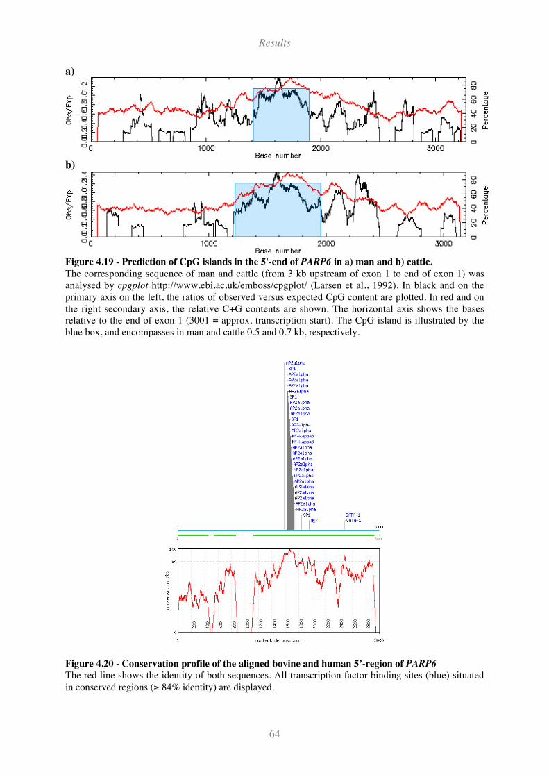
Results
64
a)
b)
Figure 4.19 - Prediction of CpG islands in the 5'-end of PARP6 in a) man and b) cattle.
The corresponding sequence of man and cattle (from 3 kb upstream of exon 1 to end of exon 1) was
analysed by cpgplot http://www.ebi.ac.uk/emboss/cpgplot/ (Larsen et al., 1992). In black and on the
primary axis on the left, the ratios of observed versus expected CpG content are plotted. In red and on
the right secondary axis, the relative C+G contents are shown. The horizontal axis shows the bases
relative to the end of exon 1 (3001 = approx. transcription start). The CpG island is illustrated by the
blue box, and encompasses in man and cattle 0.5 and 0.7 kb, respectively.
Figure 4.20 - Conservation profile of the aligned bovine and human 5’-region of PARP6
The red line shows the identity of both sequences. All transcription factor binding sites (blue) situated
in conserved regions (' 84% identity) are displayed.
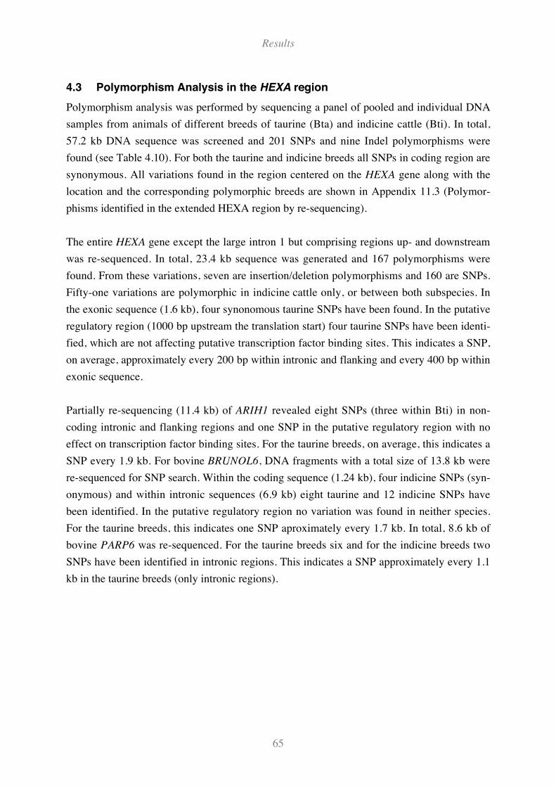
Results
65
4.3 Polymorphism Analysis in the HEXA region
Polymorphism analysis was performed by sequencing a panel of pooled and individual DNA
samples from animals of different breeds of taurine (Bta) and indicine cattle (Bti). In total,
57.2 kb DNA sequence was screened and 201 SNPs and nine Indel polymorphisms were
found (see Table 4.10). For both the taurine and indicine breeds all SNPs in coding region are
synonymous. All variations found in the region centered on the HEXA gene along with the
location and the corresponding polymorphic breeds are shown in Appendix 11.3 (Polymor-
phisms identified in the extended HEXA region by re-sequencing).
The entire HEXA gene except the large intron 1 but comprising regions up- and downstream
was re-sequenced. In total, 23.4 kb sequence was generated and 167 polymorphisms were
found. From these variations, seven are insertion/deletion polymorphisms and 160 are SNPs.
Fifty-one variations are polymorphic in indicine cattle only, or between both subspecies. In
the exonic sequence (1.6 kb), four synonomous taurine SNPs have been found. In the putative
regulatory region (1000 bp upstream the translation start) four taurine SNPs have been identi-
fied, which are not affecting putative transcription factor binding sites. This indicates a SNP,
on average, approximately every 200 bp within intronic and flanking and every 400 bp within
exonic sequence.
Partially re-sequencing (11.4 kb) of ARIH1 revealed eight SNPs (three within Bti) in non-
coding intronic and flanking regions and one SNP in the putative regulatory region with no
effect on transcription factor binding sites. For the taurine breeds, on average, this indicates a
SNP every 1.9 kb. For bovine BRUNOL6, DNA fragments with a total size of 13.8 kb were
re-sequenced for SNP search. Within the coding sequence (1.24 kb), four indicine SNPs (syn-
onymous) and within intronic sequences (6.9 kb) eight taurine and 12 indicine SNPs have
been identified. In the putative regulatory region no variation was found in neither species.
For the taurine breeds, this indicates one SNP aproximately every 1.7 kb. In total, 8.6 kb of
bovine PARP6 was re-sequenced. For the taurine breeds six and for the indicine breeds two
SNPs have been identified in intronic regions. This indicates a SNP approximately every 1.1
kb in the taurine breeds (only intronic regions).
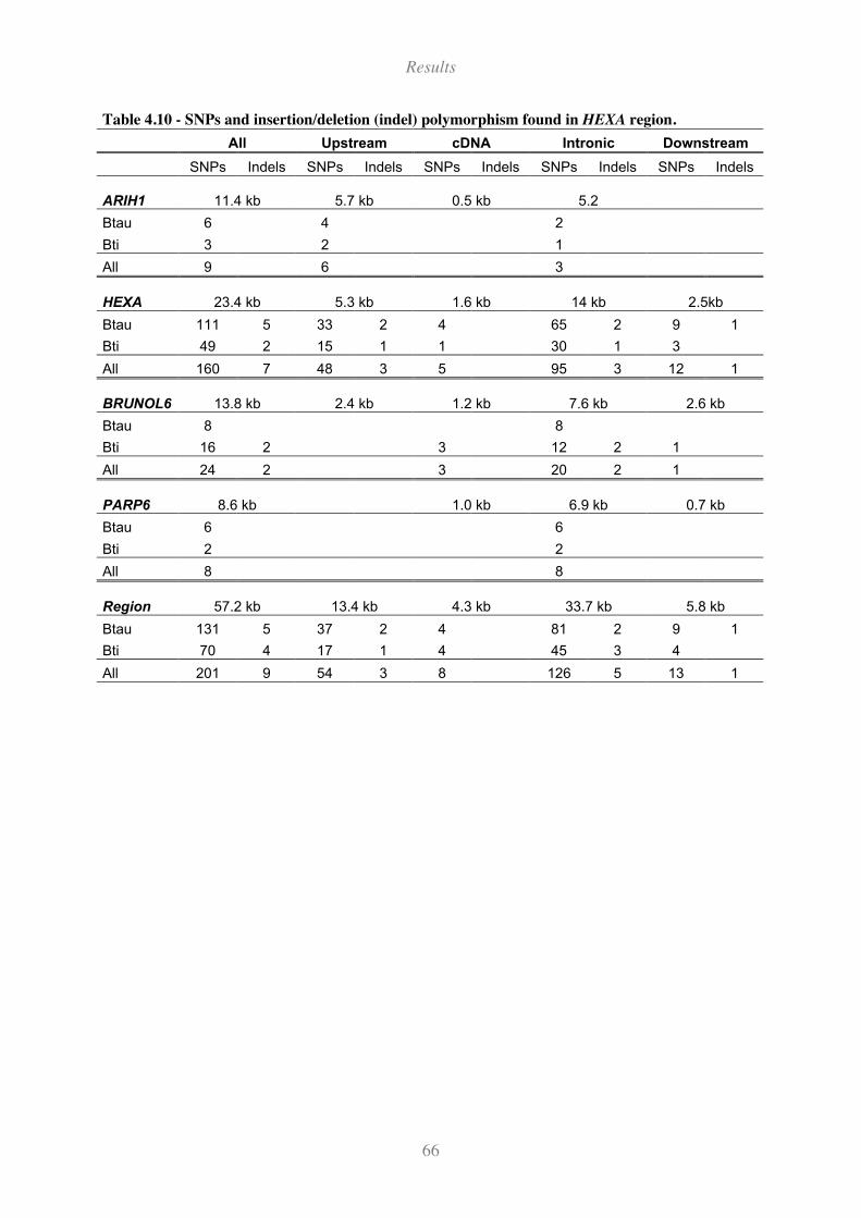
Results
66
Table 4.10 - SNPs and insertion/deletion (indel) polymorphism found in HEXA region.
All Upstream cDNA Intronic Downstream
SNPs Indels SNPs Indels SNPs Indels SNPs Indels SNPs Indels
ARIH1 11.4 kb 5.7 kb 0.5 kb 5.2
Btau 6 4 2
Bti 3 2 1
All 9 6 3
HEXA 23.4 kb 5.3 kb 1.6 kb 14 kb 2.5kb
Btau 111 5 33 2 4 65 2 9 1
Bti 49 2 15 1 1 30 1 3
All 160 7 48 3 5 95 3 12 1
BRUNOL6 13.8 kb 2.4 kb 1.2 kb 7.6 kb 2.6 kb
Btau 8 8
Bti 16 2 3 12 2 1
All 24 2 3 20 2 1
PARP6 8.6 kb 1.0 kb 6.9 kb 0.7 kb
Btau 6 6
Bti 2 2
All 8 8
Region 57.2 kb 13.4 kb 4.3 kb 33.7 kb 5.8 kb
Btau 131 5 37 2 4 81 2 9 1
Bti 70 4 17 1 4 45 3 4
All 201 9 54 3 8 126 5 13 1
Results
67
4.4 Genomic control (GC)
In order to detect possible population stratification among cases and controls of UK and Ger-
man Holsteins, GC after Devlin and Roeder (1999) was performed. This methodology allows
correcting the significance threshold according to the extent of population stratification de-
tected by genotyping a panel of neutral SNPs. This avoids excess in the rate of false positives
results in the presence of population stratification. For this purpose both cases and controls
were genotyped by the hME method and MALDI-TOF for a panel of 37 SNPs that was ini-
tially developed for paternal testing and identity control (Werner et al., 2004). These SNPs are
considered as so-called null-loci having no effect on the phenotype. After further examination
of the genotypes, eight SNPs were excluded from the calculations due to monomorphism (two
SNPs), strong deviance from HWE caused by an excess of heterozygous genotypes (three
SNPs) and unspecific calling in the genotyping procedure (three SNPs). In Figure 4.21, the
minor allele frequencies for the remaining 29 SNPs are presented for the cases and controls of
both, the UK and the German Holstein animals. The corresponding trend values are obtained
by Armitage Trend test, which tests for differences in the genotype frequencies between cases
and controls. The median of the trend values across all 29 SNPs is similar for both popula-
tions: 0.48 and 0.47 for the UK and the German Holsteins, respectively. In Appendices 11.5,
11.6 and 11.7, the genotyping results for the null-loci for the UK and German Holsteins and
for the sequencing panel animals consisting of German Fleckvieh, German Brown and Ger-
man Holstein are presented, respectively.
The inflation factor # is used to correct the significance threshold for the detected extend of
population stratification. # is calculated by dividing the median value of the Armitage Trend
statistic across all null-loci by 0.456 (see Chapter 3.15.8 – Inferring the inflation factor as
GC). Virtually no stratification could be detected for both populations. As shown in the Table
4.11, the inflation factors constitute 1.05 and 1.03 for the UK and German Holstein animals,
respectively. Therefore, the significance threshold of the corresponding type 1 error rate of 5
% increases only slightly from 3.84 to 4.03 and from 3.84 to 3.96 for UK and German Hol-
steins, respectively. The detected effect of inflation is marginal in both populations, indicating
that the groups are not stratified. Therefore, the changes in the P-values of the association test
due to correction of the $2-test statistics by the inflation factors 1.05 (UK Holstein) and 1.03
(German Holsteins) are only marginally.
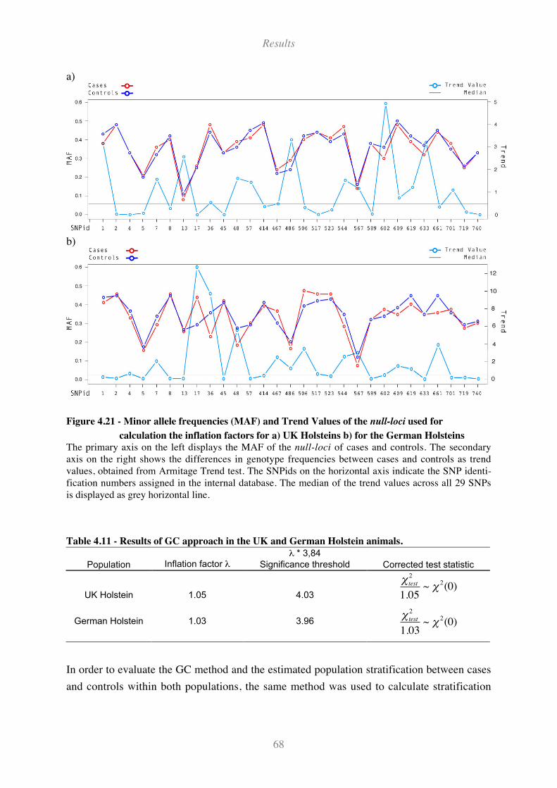
Results
68
a)
b)
Figure 4.21 - Minor allele frequencies (MAF) and Trend Values of the null-loci used for
calculation the inflation factors for a) UK Holsteins b) for the German Holsteins
The primary axis on the left displays the MAF of the null-loci of cases and controls. The secondary
axis on the right shows the differences in genotype frequencies between cases and controls as trend
values, obtained from Armitage Trend test. The SNPids on the horizontal axis indicate the SNP identi-
fication numbers assigned in the internal database. The median of the trend values across all 29 SNPs
is displayed as grey horizontal line.
Table 4.11 - Results of GC approach in the UK and German Holstein animals.
Population Inflation factor ## * 3,84
Significance threshold Corrected test statistic
UK Holstein 1.05 4.03
!
"test
2
1.05~ " 2(0)
German Holstein 1.03 3.96
!
"test
2
1.03~ " 2(0)
In order to evaluate the GC method and the estimated population stratification between cases
and controls within both populations, the same method was used to calculate stratification
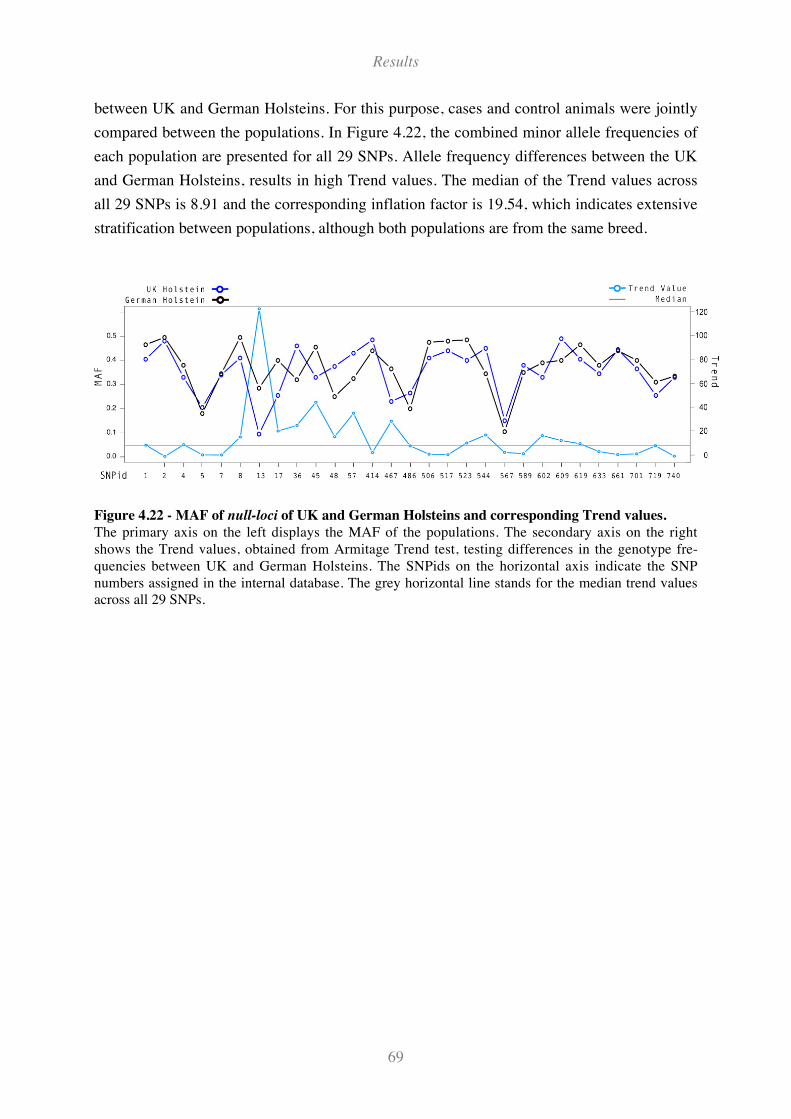
Results
69
between UK and German Holsteins. For this purpose, cases and control animals were jointly
compared between the populations. In Figure 4.22, the combined minor allele frequencies of
each population are presented for all 29 SNPs. Allele frequency differences between the UK
and German Holsteins, results in high Trend values. The median of the Trend values across
all 29 SNPs is 8.91 and the corresponding inflation factor is 19.54, which indicates extensive
stratification between populations, although both populations are from the same breed.
Figure 4.22 - MAF of null-loci of UK and German Holsteins and corresponding Trend values.
The primary axis on the left displays the MAF of the populations. The secondary axis on the right
shows the Trend values, obtained from Armitage Trend test, testing differences in the genotype fre-
quencies between UK and German Holsteins. The SNPids on the horizontal axis indicate the SNP
numbers assigned in the internal database. The grey horizontal line stands for the median trend values
across all 29 SNPs.
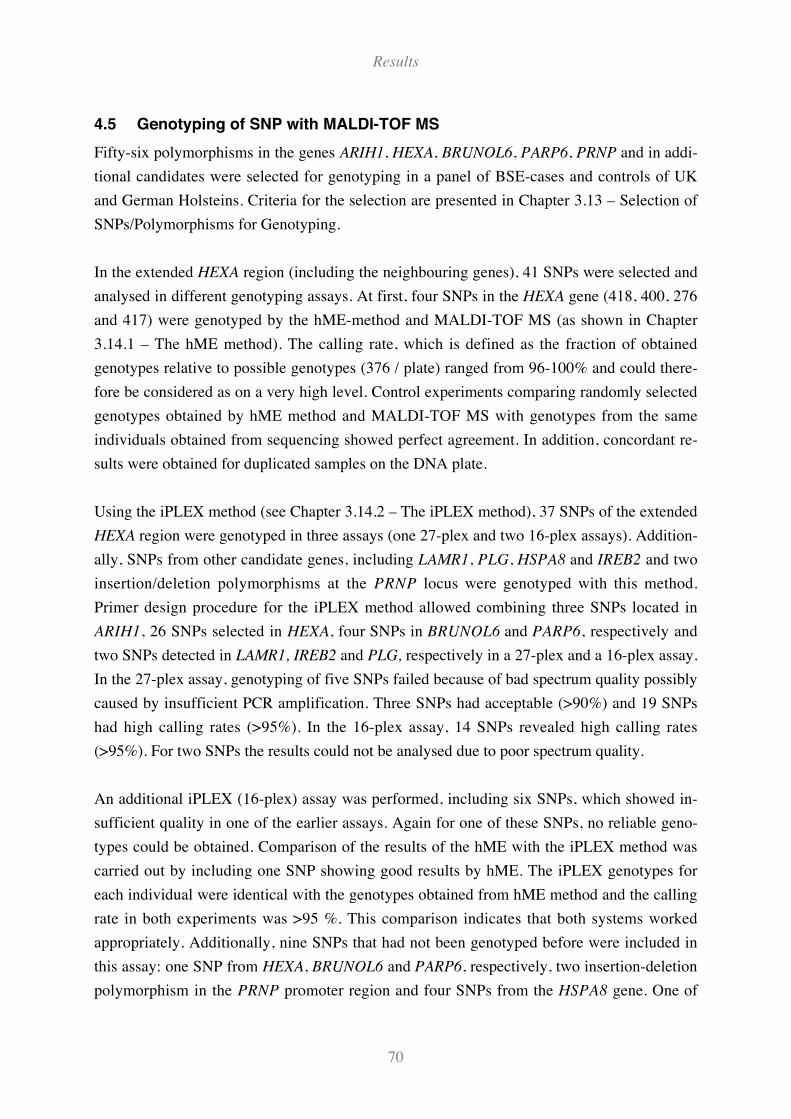
Results
70
4.5 Genotyping of SNP with MALDI-TOF MS
Fifty-six polymorphisms in the genes ARIH1, HEXA, BRUNOL6, PARP6, PRNP and in addi-
tional candidates were selected for genotyping in a panel of BSE-cases and controls of UK
and German Holsteins. Criteria for the selection are presented in Chapter 3.13 – Selection of
SNPs/Polymorphisms for Genotyping.
In the extended HEXA region (including the neighbouring genes), 41 SNPs were selected and
analysed in different genotyping assays. At first, four SNPs in the HEXA gene (418, 400, 276
and 417) were genotyped by the hME-method and MALDI-TOF MS (as shown in Chapter
3.14.1 – The hME method). The calling rate, which is defined as the fraction of obtained
genotypes relative to possible genotypes (376 / plate) ranged from 96-100% and could there-
fore be considered as on a very high level. Control experiments comparing randomly selected
genotypes obtained by hME method and MALDI-TOF MS with genotypes from the same
individuals obtained from sequencing showed perfect agreement. In addition, concordant re-
sults were obtained for duplicated samples on the DNA plate.
Using the iPLEX method (see Chapter 3.14.2 – The iPLEX method), 37 SNPs of the extended
HEXA region were genotyped in three assays (one 27-plex and two 16-plex assays). Addition-
ally, SNPs from other candidate genes, including LAMR1, PLG, HSPA8 and IREB2 and two
insertion/deletion polymorphisms at the PRNP locus were genotyped with this method.
Primer design procedure for the iPLEX method allowed combining three SNPs located in
ARIH1, 26 SNPs selected in HEXA, four SNPs in BRUNOL6 and PARP6, respectively and
two SNPs detected in LAMR1, IREB2 and PLG, respectively in a 27-plex and a 16-plex assay.
In the 27-plex assay, genotyping of five SNPs failed because of bad spectrum quality possibly
caused by insufficient PCR amplification. Three SNPs had acceptable (>90%) and 19 SNPs
had high calling rates (>95%). In the 16-plex assay, 14 SNPs revealed high calling rates
(>95%). For two SNPs the results could not be analysed due to poor spectrum quality.
An additional iPLEX (16-plex) assay was performed, including six SNPs, which showed in-
sufficient quality in one of the earlier assays. Again for one of these SNPs, no reliable geno-
types could be obtained. Comparison of the results of the hME with the iPLEX method was
carried out by including one SNP showing good results by hME. The iPLEX genotypes for
each individual were identical with the genotypes obtained from hME method and the calling
rate in both experiments was >95 %. This comparison indicates that both systems worked
appropriately. Additionally, nine SNPs that had not been genotyped before were included in
this assay: one SNP from HEXA, BRUNOL6 and PARP6, respectively, two insertion-deletion
polymorphism in the PRNP promoter region and four SNPs from the HSPA8 gene. One of
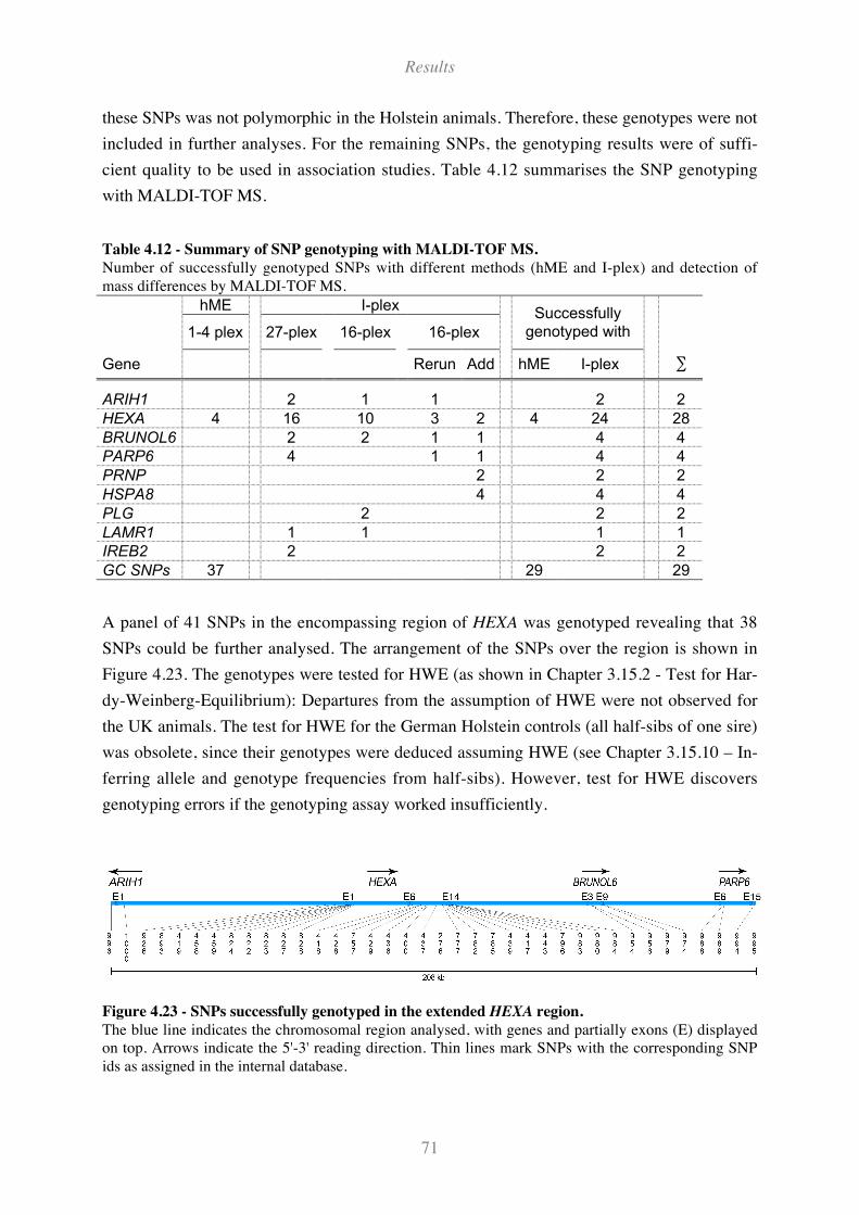
Results
71
these SNPs was not polymorphic in the Holstein animals. Therefore, these genotypes were not
included in further analyses. For the remaining SNPs, the genotyping results were of suffi-
cient quality to be used in association studies. Table 4.12 summarises the SNP genotyping
with MALDI-TOF MS.
Table 4.12 - Summary of SNP genotyping with MALDI-TOF MS.
Number of successfully genotyped SNPs with different methods (hME and I-plex) and detection of
mass differences by MALDI-TOF MS.
hME I-plex
1-4 plex 27-plex 16-plex 16-plex
Successfully
genotyped with
Gene Rerun Add hME I-plex (
ARIH1 2 1 1 2 2
HEXA 4 16 10 3 2 4 24 28
BRUNOL6 2 2 1 1 4 4
PARP6 4 1 1 4 4
PRNP 2 2 2
HSPA8 4 4 4
PLG 2 2 2
LAMR1 1 1 1 1
IREB2 2 2 2
GC SNPs 37 29 29
A panel of 41 SNPs in the encompassing region of HEXA was genotyped revealing that 38
SNPs could be further analysed. The arrangement of the SNPs over the region is shown in
Figure 4.23. The genotypes were tested for HWE (as shown in Chapter 3.15.2 - Test for Har-
dy-Weinberg-Equilibrium): Departures from the assumption of HWE were not observed for
the UK animals. The test for HWE for the German Holstein controls (all half-sibs of one sire)
was obsolete, since their genotypes were deduced assuming HWE (see Chapter 3.15.10 – In-
ferring allele and genotype frequencies from half-sibs). However, test for HWE discovers
genotyping errors if the genotyping assay worked insufficiently.
Figure 4.23 - SNPs successfully genotyped in the extended HEXA region.
The blue line indicates the chromosomal region analysed, with genes and partially exons (E) displayed
on top. Arrows indicate the 5'-3' reading direction. Thin lines mark SNPs with the corresponding SNP
ids as assigned in the internal database.
Results
72
4.6 Association of single markers with BSE
4.6.1 SNPs in the extended HEXA region
UK and German Holstein
The minor allele frequencies for both, the UK and the German BSE cases and controls for the
38 SNPs in the HEXA region and the corresponding Trend-values obtained from Armitage
Trend test are demonstrated in Figure 4.24. The allele frequencies of the German Holsteins
are similar to the frequencies of the UK Holstein, whereas significant differences between
cases and controls within each population were only found in the UK animals. The single
marker analysis by Armitage trend test revealed that the genotypes of six intronic SNPs (276,
796, 956, 988, 989 and 995) were significantly different between cases and control animals of
UK Holstein at the SNP-wise 5% type I error rate with correction for population stratification.
The genotyping and association results for the candidate SNPs are presented in Appendices
11.8 and 11.9, respectively.
Description Figure 4.24 (page 72):
Figure 4.24 - MAF and Trend values of the SNPs genotyped in (a) the UK and (b) German
Holsteins BSE-cases and controls.
The primary axis on the left displays the MAF of cases and controls. The secondary axis on the right
shows the Trend values, obtained from Armitage Trend test, testing differences in the genotype fre-
quencies between cases and controls. The SNP ids on the horizontal axis indicate the SNP numbers as
assigned in the internal database and thin lines mark the SNP position on the chromosomal region.
Arrows indicate the 5'-3' reading direction of the genes. The Figure is not to scale according to the
physical map locations; the SNPs are equidistant to allow easy visualisation of the association test
results. The significance threshold (p = 0.05) corrected for population stratification is displayed as
grey horizontal line.
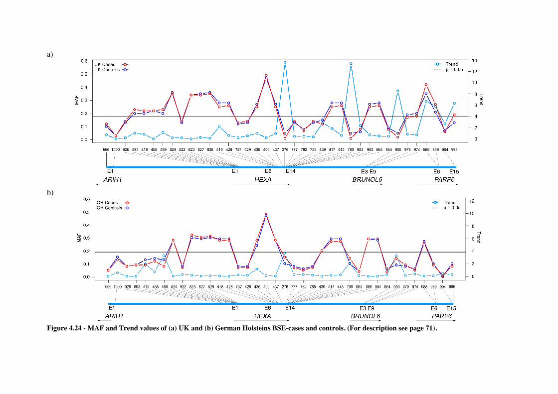
a)
b)
Figure 4.24 - MAF and Trend values of (a) UK and (b) German Holsteins BSE-cases and controls. (For description see page 71).
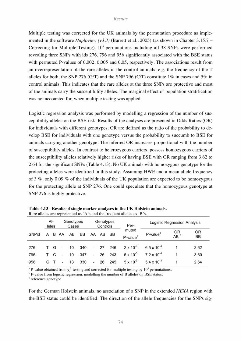
Results
74
Multiple testing was corrected for the UK animals by the permutation procedure as imple-
mented in the software Haploview (v3.3) (Barrett et al., 2005) (as shown in Chapter 3.15.7 –
Correcting for Multiple Testing). 105 permutations including all 38 SNPs were performed
revealing three SNPs with ids 276, 796 and 956 significantly associated with the BSE status
with permuted P-values of 0.002, 0.005 and 0.05, respectively. The associations result from
an overrepresentation of the rare alleles in the control animals, e.g. the frequency of the T
alleles for both, the SNP 276 (G/T) and the SNP 796 (C/T) constitute 1% in cases and 5% in
control animals. This indicates that the rare alleles at the three SNPs are protective and most
of the animals carry the susceptibility alleles. The marginal effect of population stratification
was not accounted for, when multiple testing was applied.
Logistic regression analysis was performed by modelling a regression of the number of sus-
ceptibility alleles on the BSE risk. Results of the analyses are presented in Odds Ratios (OR)
for individuals with different genotypes. OR are defined as the ratio of the probability to de-
velop BSE for individuals with one genotype versus the probability to succumb to BSE for
animals carrying another genotype. The inferred OR increases proportional with the number
of susceptibility alleles. In contrast to heterozygous carriers, possess homozygous carriers of
the susceptibility alleles relatively higher risks of having BSE with OR ranging from 3.62 to
2.64 for the significant SNPs (Table 4.13). No UK animals with homozygous genotype for the
protecting alleles were identified in this study. Assuming HWE and a mean allele frequency
of 3 %, only 0.09 % of the individuals of the UK population are expected to be homozygous
for the protecting allele at SNP 276. One could speculate that the homozygous genotype at
SNP 276 is highly protective.
Table 4.13 - Results of single marker analyses in the UK Holstein animals.
Rare alleles are represented as ‘A’s and the frequent alleles as ‘B’s.
Al-leles
GenotypesCases
GenotypesControls
Logistic Regression Analysis
SNPid A B AA AB BB AA AB BB
Per-muted
P-valuea P-value
b ORAB
cORBB
276 T G - 10 340 - 27 246 2 x 10⁻³
6.5 x 10⁻⁴
1 3.62
796 T C - 10 347 - 26 243 5 x 10⁻³
7.2 x 10⁻⁴
1 3.60
956 G T - 13 330 - 26 245 5 x 10⁻²
5.4 x 10⁻³
1 2.64
a P-value obtained from !2 -testing and corrected for multiple testing by 105 permutations.b P-value from logistic regression, modelling the number of B alleles on BSE status.c reference genotype
For the German Holstein animals, no association of a SNP in the extended HEXA region with
the BSE status could be identified. The direction of the allele frequencies for the SNPs sig-
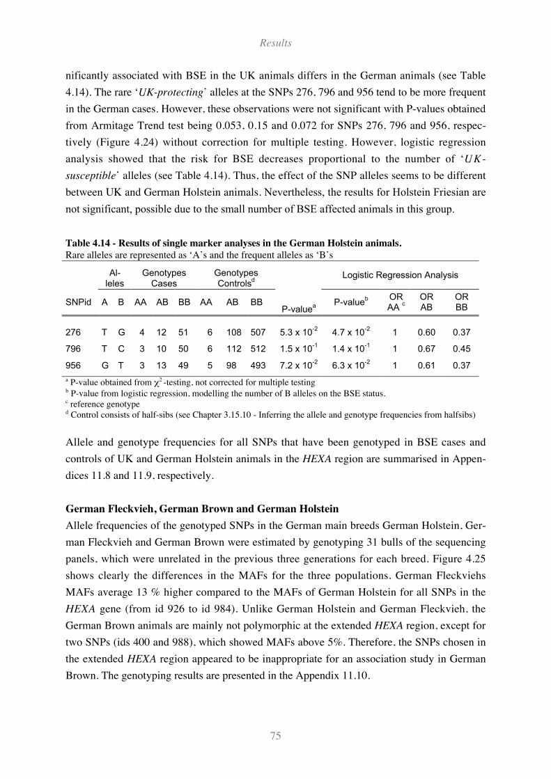
Results
75
nificantly associated with BSE in the UK animals differs in the German animals (see Table
4.14). The rare ‘UK-protecting’ alleles at the SNPs 276, 796 and 956 tend to be more frequent
in the German cases. However, these observations were not significant with P-values obtained
from Armitage Trend test being 0.053, 0.15 and 0.072 for SNPs 276, 796 and 956, respec-
tively (Figure 4.24) without correction for multiple testing. However, logistic regression
analysis showed that the risk for BSE decreases proportional to the number of ‘UK-
susceptible’ alleles (see Table 4.14). Thus, the effect of the SNP alleles seems to be different
between UK and German Holstein animals. Nevertheless, the results for Holstein Friesian are
not significant, possible due to the small number of BSE affected animals in this group.
Table 4.14 - Results of single marker analyses in the German Holstein animals.
Rare alleles are represented as ‘A’s and the frequent alleles as ‘B’s
Al-leles
GenotypesCases
GenotypesControls
dLogistic Regression Analysis
SNPid A B AA AB BB AA AB BBP-value
a P-valueb OR
AA c
ORAB
ORBB
276 T G 4 12 51 6 108 507 5.3 x 10⁻²
4.7 x 10⁻²
1 0.60 0.37
796 T C 3 10 50 6 112 512 1.5 x 10⁻¹
1.4 x 10⁻¹
1 0.67 0.45
956 G T 3 13 49 5 98 493 7.2 x 10⁻²
6.3 x 10⁻²
1 0.61 0.37
a P-value obtained from !2 -testing, not corrected for multiple testingb P-value from logistic regression, modelling the number of B alleles on the BSE status.c reference genotyped Control consists of half-sibs (see Chapter 3.15.10 - Inferring the allele and genotype frequencies from halfsibs)
Allele and genotype frequencies for all SNPs that have been genotyped in BSE cases and
controls of UK and German Holstein animals in the HEXA region are summarised in Appen-
dices 11.8 and 11.9, respectively.
German Fleckvieh, German Brown and German Holstein
Allele frequencies of the genotyped SNPs in the German main breeds German Holstein, Ger-
man Fleckvieh and German Brown were estimated by genotyping 31 bulls of the sequencing
panels, which were unrelated in the previous three generations for each breed. Figure 4.25
shows clearly the differences in the MAFs for the three populations. German Fleckviehs
MAFs average 13 % higher compared to the MAFs of German Holstein for all SNPs in the
HEXA gene (from id 926 to id 984). Unlike German Holstein and German Fleckvieh, the
German Brown animals are mainly not polymorphic at the extended HEXA region, except for
two SNPs (ids 400 and 988), which showed MAFs above 5%. Therefore, the SNPs chosen in
the extended HEXA region appeared to be inappropriate for an association study in German
Brown. The genotyping results are presented in the Appendix 11.10.
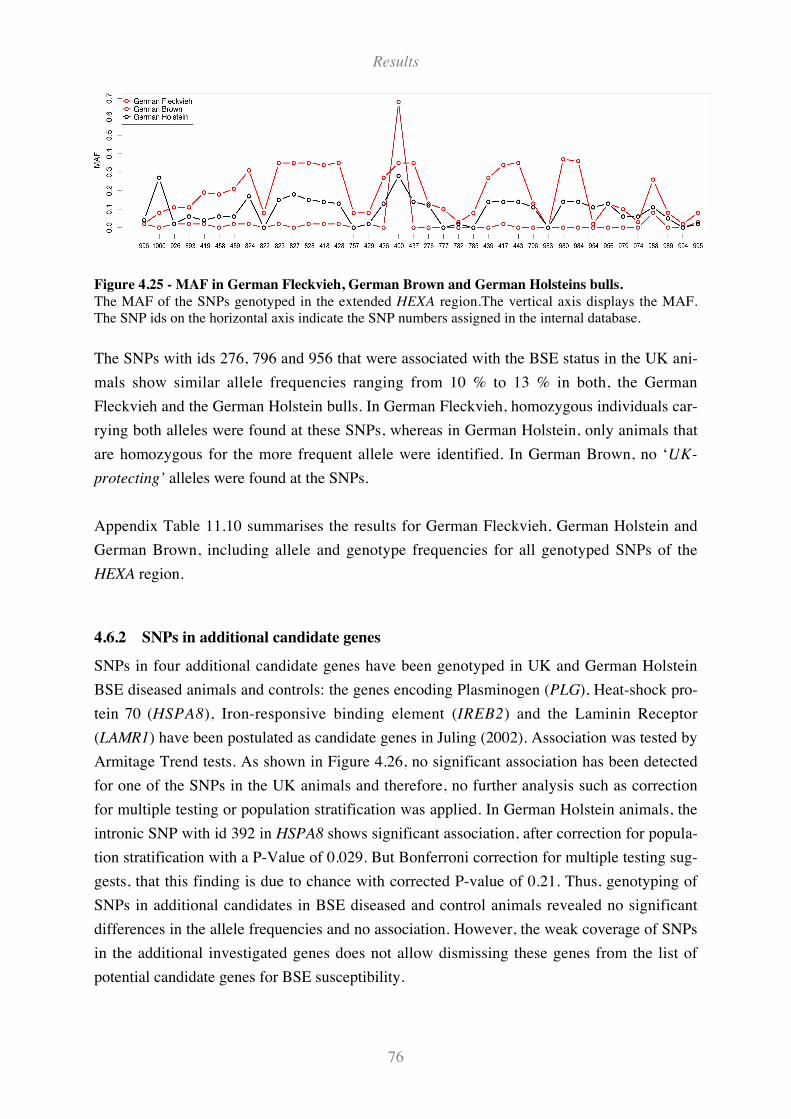
Results
76
Figure 4.25 - MAF in German Fleckvieh, German Brown and German Holsteins bulls.
The MAF of the SNPs genotyped in the extended HEXA region.The vertical axis displays the MAF.The SNP ids on the horizontal axis indicate the SNP numbers assigned in the internal database.
The SNPs with ids 276, 796 and 956 that were associated with the BSE status in the UK ani-
mals show similar allele frequencies ranging from 10 % to 13 % in both, the German
Fleckvieh and the German Holstein bulls. In German Fleckvieh, homozygous individuals car-
rying both alleles were found at these SNPs, whereas in German Holstein, only animals that
are homozygous for the more frequent allele were identified. In German Brown, no ‘UK-
protecting’ alleles were found at the SNPs.
Appendix Table 11.10 summarises the results for German Fleckvieh, German Holstein and
German Brown, including allele and genotype frequencies for all genotyped SNPs of the
HEXA region.
4.6.2 SNPs in additional candidate genes
SNPs in four additional candidate genes have been genotyped in UK and German Holstein
BSE diseased animals and controls: the genes encoding Plasminogen (PLG), Heat-shock pro-
tein 70 (HSPA8), Iron-responsive binding element (IREB2) and the Laminin Receptor
(LAMR1) have been postulated as candidate genes in Juling (2002). Association was tested by
Armitage Trend tests. As shown in Figure 4.26, no significant association has been detected
for one of the SNPs in the UK animals and therefore, no further analysis such as correction
for multiple testing or population stratification was applied. In German Holstein animals, the
intronic SNP with id 392 in HSPA8 shows significant association, after correction for popula-
tion stratification with a P-Value of 0.029. But Bonferroni correction for multiple testing sug-
gests, that this finding is due to chance with corrected P-value of 0.21. Thus, genotyping of
SNPs in additional candidates in BSE diseased and control animals revealed no significant
differences in the allele frequencies and no association. However, the weak coverage of SNPs
in the additional investigated genes does not allow dismissing these genes from the list of
potential candidate genes for BSE susceptibility.
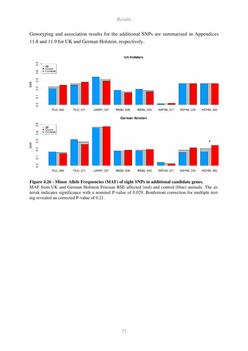
Results
77
Genotyping and association results for the additional SNPs are summarised in Appendices
11.8 and 11.9 for UK and German Holstein, respectively.
Figure 4.26 - Minor Allele Frequencies (MAF) of eight SNPs in additional candidate genes.
MAF from UK and German Holstein Friesian BSE affected (red) and control (blue) animals. The as-terisk indicates significance with a nominal P-value of 0.029. Bonferroni correction for multiple test-ing revealed an corrected P-value of 0.21.
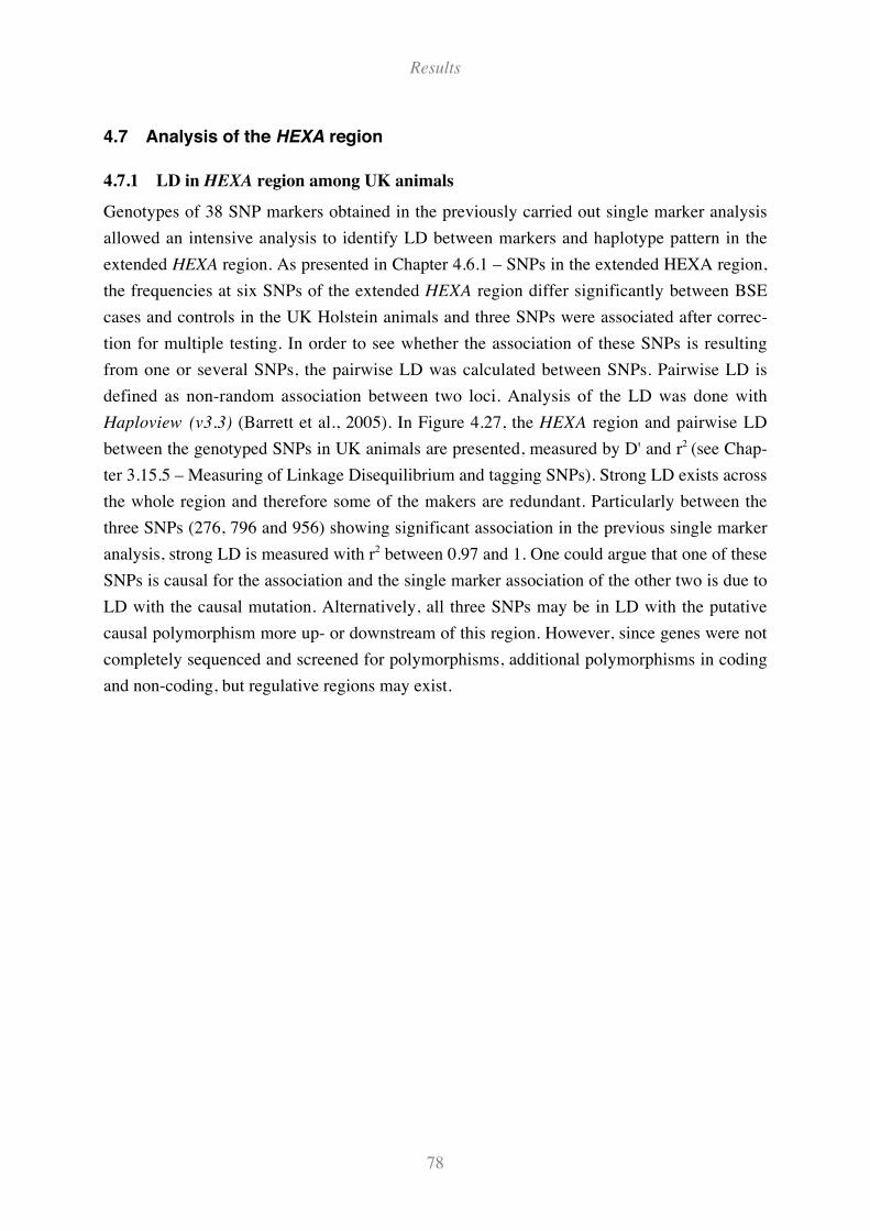
Results
78
4.7 Analysis of the HEXA region
4.7.1 LD in HEXA region among UK animals
Genotypes of 38 SNP markers obtained in the previously carried out single marker analysis
allowed an intensive analysis to identify LD between markers and haplotype pattern in the
extended HEXA region. As presented in Chapter 4.6.1 – SNPs in the extended HEXA region,
the frequencies at six SNPs of the extended HEXA region differ significantly between BSE
cases and controls in the UK Holstein animals and three SNPs were associated after correc-
tion for multiple testing. In order to see whether the association of these SNPs is resulting
from one or several SNPs, the pairwise LD was calculated between SNPs. Pairwise LD is
defined as non-random association between two loci. Analysis of the LD was done with
Haploview (v3.3) (Barrett et al., 2005). In Figure 4.27, the HEXA region and pairwise LD
between the genotyped SNPs in UK animals are presented, measured by D' and r2 (see Chap-
ter 3.15.5 – Measuring of Linkage Disequilibrium and tagging SNPs). Strong LD exists across
the whole region and therefore some of the makers are redundant. Particularly between the
three SNPs (276, 796 and 956) showing significant association in the previous single marker
analysis, strong LD is measured with r2 between 0.97 and 1. One could argue that one of these
SNPs is causal for the association and the single marker association of the other two is due to
LD with the causal mutation. Alternatively, all three SNPs may be in LD with the putative
causal polymorphism more up- or downstream of this region. However, since genes were not
completely sequenced and screened for polymorphisms, additional polymorphisms in coding
and non-coding, but regulative regions may exist.
Results
79
Figure 4.27 - LD plot of the extended HEXA region (208 kb) among UK Holsteins.
The triangle on the top shows the LD measured by D' while the lower triangle visualises LD measuredby r2. Regions of high and low LD are presented by red and white shading for D' and black and whiteshading for r2, respectively. The darker the colour of the squares, the higher are the values for D' and r2
and therefore the stronger the LD between both corresponding markers. The SNP ids on the horizontalaxis indicate the SNP numbers assigned in the internal database.
4.7.2 Haplotype analysis and SNP tagging for UK animals
In order to elucidate the potential effect of combinations of SNPs on the BSE risk, a haplo-
type analysis was performed. Haplotypes were estimated using Haploview (v3.3) (Barrett et
al., 2005) that uses an accelerated EM algorithm similar to the partition/ligation method de-
scribed in Qin et al. (2002). Including all genotyped SNPs and assuming no haplotype block
structure, twelve haplotypes with a frequency of > 1 % were identified in total (see Figure
4.28). This analysis revealed that all ‘UK-protecting’ alleles of SNPs 276, 796 and 956, repre-
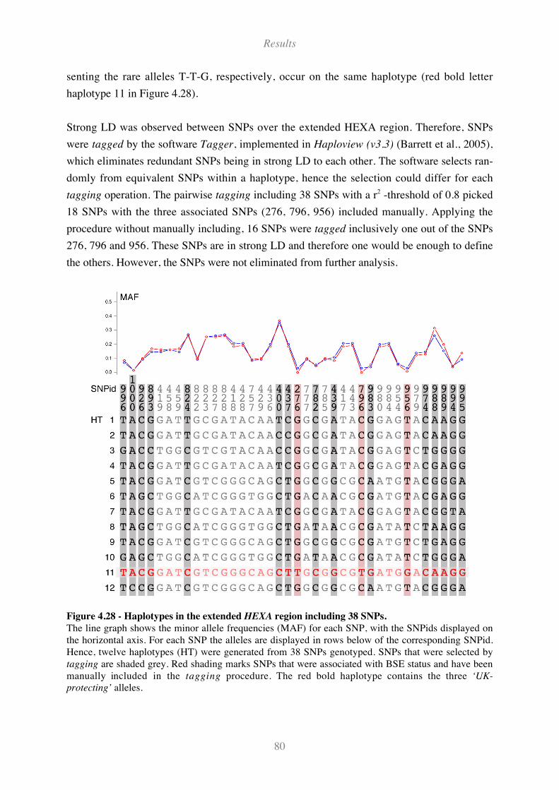
Results
80
senting the rare alleles T-T-G, respectively, occur on the same haplotype (red bold letter
haplotype 11 in Figure 4.28).
Strong LD was observed between SNPs over the extended HEXA region. Therefore, SNPs
were tagged by the software Tagger, implemented in Haploview (v3.3) (Barrett et al., 2005),
which eliminates redundant SNPs being in strong LD to each other. The software selects ran-
domly from equivalent SNPs within a haplotype, hence the selection could differ for each
tagging operation. The pairwise tagging including 38 SNPs with a r2 -threshold of 0.8 picked
18 SNPs with the three associated SNPs (276, 796, 956) included manually. Applying the
procedure without manually including, 16 SNPs were tagged inclusively one out of the SNPs
276, 796 and 956. These SNPs are in strong LD and therefore one would be enough to define
the others. However, the SNPs were not eliminated from further analysis.
Figure 4.28 - Haplotypes in the extended HEXA region including 38 SNPs.
The line graph shows the minor allele frequencies (MAF) for each SNP, with the SNPids displayed onthe horizontal axis. For each SNP the alleles are displayed in rows below of the corresponding SNPid.Hence, twelve haplotypes (HT) were generated from 38 SNPs genotyped. SNPs that were selected bytagging are shaded grey. Red shading marks SNPs that were associated with BSE status and have beenmanually included in the tagging procedure. The red bold haplotype contains the three ‘UK-
protecting’ alleles.
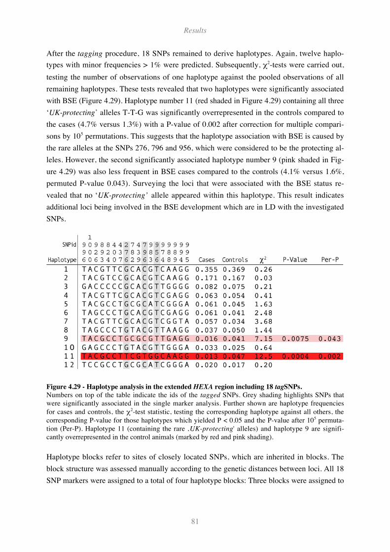
Results
81
After the tagging procedure, 18 SNPs remained to derive haplotypes. Again, twelve haplo-
types with minor frequencies > 1% were predicted. Subsequently, !2-tests were carried out,
testing the number of observations of one haplotype against the pooled observations of all
remaining haplotypes. These tests revealed that two haplotypes were significantly associated
with BSE (Figure 4.29). Haplotype number 11 (red shaded in Figure 4.29) containing all three
‘UK-protecting’ alleles T-T-G was significantly overrepresented in the controls compared to
the cases (4.7% versus 1.3%) with a P-value of 0.002 after correction for multiple compari-
sons by 105 permutations. This suggests that the haplotype association with BSE is caused by
the rare alleles at the SNPs 276, 796 and 956, which were considered to be the protecting al-
leles. However, the second significantly associated haplotype number 9 (pink shaded in Fig-
ure 4.29) was also less frequent in BSE cases compared to the controls (4.1% versus 1.6%,
permuted P-value 0.043). Surveying the loci that were associated with the BSE status re-
vealed that no ‘UK-protecting’ allele appeared within this haplotype. This result indicates
additional loci being involved in the BSE development which are in LD with the investigated
SNPs.
Figure 4.29 - Haplotype analysis in the extended HEXA region including 18 tagSNPs.
Numbers on top of the table indicate the ids of the tagged SNPs. Grey shading highlights SNPs thatwere significantly associated in the single marker analysis. Further shown are haplotype frequenciesfor cases and controls, the !2-test statistic, testing the corresponding haplotype against all others, thecorresponding P-value for those haplotypes which yielded P < 0.05 and the P-value after 105 permuta-tion (Per-P). Haplotype 11 (containing the rare ‚UK-protecting' alleles) and haplotype 9 are signifi-cantly overrepresented in the control animals (marked by red and pink shading).
Haplotype blocks refer to sites of closely located SNPs, which are inherited in blocks. The
block structure was assessed manually according to the genetic distances between loci. All 18
SNP markers were assigned to a total of four haplotype blocks: Three blocks were assigned to
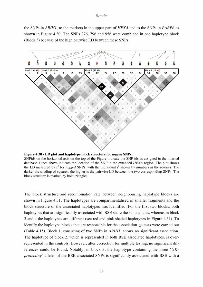
Results
82
the SNPs in ARIH1, to the markers in the upper part of HEXA and to the SNPs in PARP6 as
shown in Figure 4.30. The SNPs 276, 796 and 956 were combined in one haplotype block
(Block 3) because of the high pairwise LD between these SNPs.
Figure 4.30 - LD plot and haplotype block structure for tagged SNPs.
SNPids on the horizontal axis on the top of the Figure indicate the SNP ids as assigned in the internaldatabase. Lines above indicate the location of the SNP in the extended HEXA region. The plot showsthe LD measured by r2 for tagged SNPs, with the individual r2 shown by numbers in the squares. Thedarker the shading of squares, the higher is the pairwise LD between the two corresponding SNPs. Theblock structure is marked by bold triangles.
The block structure and recombination rate between neighbouring haplotype blocks are
shown in Figure 4.31. The haplotypes are compartmentalised in smaller fragments and the
block structure of the associated haplotypes was identified. For the first two blocks, both
haplotypes that are significantly associated with BSE share the same alleles, whereas in block
3 and 4 the haplotypes are different (see red and pink shaded haplotypes in Figure 4.31). To
identify the haplotype blocks that are responsible for the association, !2-tests were carried out
(Table 4.15). Block 1, consisting of two SNPs in ARIH1, shows no significant association.
The haplotype of block 2, which is represented in both BSE associated haplotypes, is over-
represented in the controls. However, after correction for multiple testing, no significant dif-
ferences could be found. Notably, in block 3, the haplotype containing the three ‘UK-
protecting’ alleles of the BSE associated SNPs is significantly associated with BSE with a
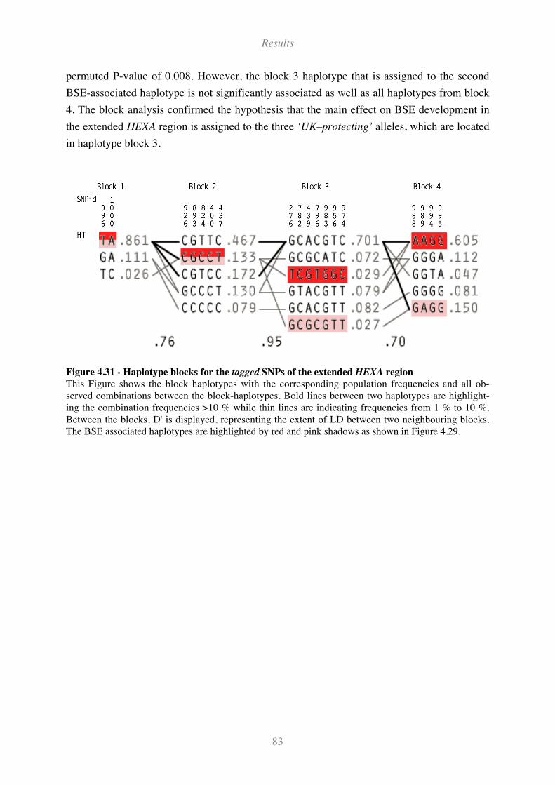
Results
83
permuted P-value of 0.008. However, the block 3 haplotype that is assigned to the second
BSE-associated haplotype is not significantly associated as well as all haplotypes from block
4. The block analysis confirmed the hypothesis that the main effect on BSE development in
the extended HEXA region is assigned to the three ‘UK–protecting’ alleles, which are located
in haplotype block 3.
Figure 4.31 - Haplotype blocks for the tagged SNPs of the extended HEXA region
This Figure shows the block haplotypes with the corresponding population frequencies and all ob-served combinations between the block-haplotypes. Bold lines between two haplotypes are highlight-ing the combination frequencies >10 % while thin lines are indicating frequencies from 1 % to 10 %.Between the blocks, D' is displayed, representing the extent of LD between two neighbouring blocks.The BSE associated haplotypes are highlighted by red and pink shadows as shown in Figure 4.29.
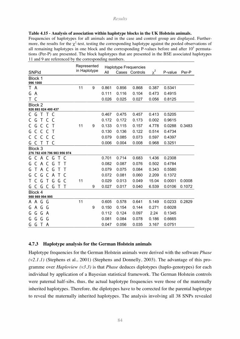
Results
84
Table 4.15 - Analysis of association within haplotype blocks in the UK Holstein animals.
Frequencies of haplotypes for all animals and in the case and control group are displayed. Further-more, the results for the !2-test, testing the corresponding haplotype against the pooled observations ofall remaining haplotypes in one block and the corresponding P-values before and after 105 permuta-tions (Per-P) are presented. The block haplotypes that are presented in the BSE associated haplotypes11 and 9 are referenced by the corresponding numbers.
Haplotype Frequencies
SNPid
Representedin Haplotype All Cases Controls !
2P-value Per-P
Block 1996 1000
T A 11 9 0.861 0.856 0.868 0.387 0.5341
G A 0.111 0.116 0.104 0.473 0.4915
T C 0.026 0.025 0.027 0.056 0.8125
Block 2926 893 824 400 437
C G T T C 0.467 0.475 0.457 0.413 0.5205
C G T C C 0.172 0.172 0.173 0.002 0.9615
C G C C T 11 9 0.133 0.115 0.157 4.778 0.0288 0.3483
G C C C T 0.130 0.136 0.122 0.514 0.4734
C C C C C 0.079 0.085 0.073 0.597 0.4397
G C T T C 0.006 0.004 0.008 0.968 0.3251
Block 3276 782 439 796 983 956 974
G C A C G T C 0.701 0.714 0.683 1.436 0.2308
G C A C G T T 0.082 0.087 0.076 0.502 0.4784
G T A C G T T 0.079 0.075 0.084 0.343 0.5580
G C G C A T C 0.072 0.081 0.060 2.209 0.1372
T C G T G G C 11 0.029 0.013 0.049 15.04 0.0001 0.0008
G C G C G T T 9 0.027 0.017 0.040 6.539 0.0106 0.1072
Block 4988 989 994 995
A A G G 11 0.605 0.578 0.641 5.149 0.0233 0.2829
G A G G 9 0.150 0.154 0.144 0.271 0.6028
G G G A 0.112 0.124 0.097 2.24 0.1345
G G G G 0.081 0.084 0.078 0.186 0.6665
G G T A 0.047 0.056 0.035 3.167 0.0751
4.7.3 Haplotype analysis for the German Holstein animals
Haplotype frequencies for the German Holstein animals were derived with the software Phase
(v2.1.1) (Stephens et al., 2001) (Stephens and Donnelly, 2003). The advantage of this pro-
gramme over Haploview (v3.3) is that Phase deduces diplotypes (haplo-genotypes) for each
individual by application of a Bayesian statistical framework. The German Holstein controls
were paternal half-sibs, thus, the actual haplotype frequencies were those of the maternally
inherited haplotypes. Therefore, the diplotypes have to be corrected for the parental haplotype
to reveal the maternally inherited haplotypes. The analysis involving all 38 SNPs revealed
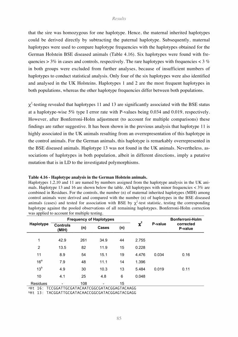
Results
85
that the sire was homozygous for one haplotype. Hence, the maternal inherited haplotypes
could be derived directly by subtracting the paternal haplotype. Subsequently, maternal
haplotypes were used to compare haplotype frequencies with the haplotypes obtained for the
German Holstein BSE diseased animals (Table 4.16). Six haplotypes were found with fre-
quencies > 3% in cases and controls, respectively. The rare haplotypes with frequencies < 3 %
in both groups were excluded from further analyses, because of insufficient numbers of
haplotypes to conduct statistical analysis. Only four of the six haplotypes were also identified
and analysed in the UK Holsteins. Haplotypes 1 and 2 are the most frequent haplotypes in
both populations, whereas the other haplotype frequencies differ between both populations.
!2-testing revealed that haplotypes 11 and 13 are significantly associated with the BSE status
at a haplotype-wise 5% type I error rate with P-values being 0.034 and 0.019, respectively.
However, after Bonferroni-Holm adjustment (to account for multiple comparisons) these
findings are rather suggestive. It has been shown in the previous analysis that haplotype 11 is
highly associated in the UK animals resulting from an overrepresentation of this haplotype in
the control animals. For the German animals, this haplotype is remarkably overrepresented in
the BSE diseased animals. Haplotype 13 was not found in the UK animals. Nevertheless, as-
sociations of haplotypes in both population, albeit in different directions, imply a putative
mutation that is in LD to the investigated polymorphisms.
Table 4.16 - Haplotype analysis in the German Holstein animals.
Haplotypes 1,2,10 and 11 are named by numbers assigned from the haplotype analysis in the UK ani-mals. Haplotype 13 and 16 are shown below the table. All haplotypes with minor frequencies < 3% arecombined in Residues. For the controls, the number (n) of maternal inherited haplotypes (MIH) amongcontrol animals were derived and compared with the number (n) of haplotypes in the BSE diseasedanimals (cases) and tested for association with BSE by !2-test statistic, testing the correspondinghaplotype against the pooled observations of all remaining haplotypes. Bonferroni-Holm correctionwas applied to account for multiple testing.
Frequency of HaplotypesHaplotype Controls
(MIH)(n) Cases (n)
!2
P-valueBonferroni-Holm
correctedP-value
1 42.9 261 34.9 44 2.755
2 13.5 82 11.9 15 0.228
11 8.9 54 15.1 19 4.476 0.034 0.16
16a
7.9 48 11.1 14 1.396
13b
4.9 30 10.3 13 5.484 0.019 0.11
10 4.1 25 4.8 6 0.048
Residues - 108 - 15aHt 16: TCCGGATTGCGATACAATCGGCGATACGGAGTACAAGGbHt 13: TACGGATTGCGATACAACCGGCGATACGGAGTACGAGG
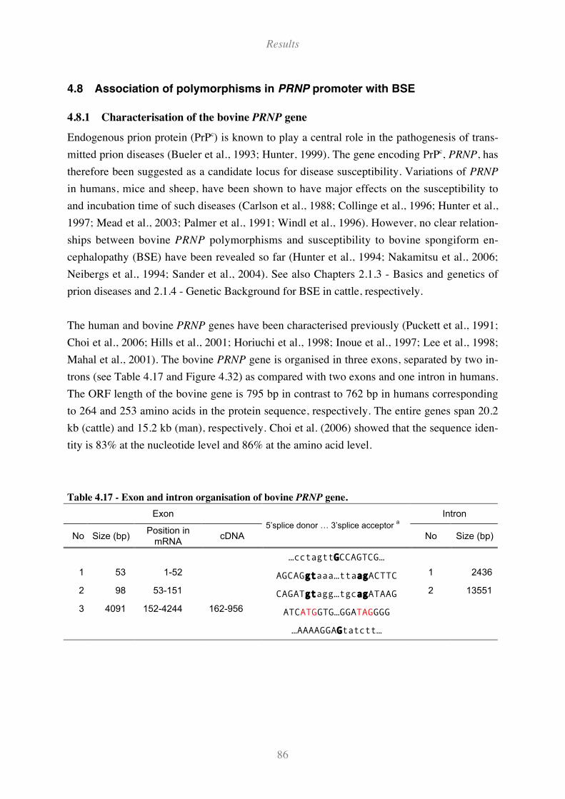
Results
86
4.8 Association of polymorphisms in PRNP promoter with BSE
4.8.1 Characterisation of the bovine PRNP gene
Endogenous prion protein (PrPc) is known to play a central role in the pathogenesis of trans-
mitted prion diseases (Bueler et al., 1993; Hunter, 1999). The gene encoding PrPc, PRNP, has
therefore been suggested as a candidate locus for disease susceptibility. Variations of PRNP
in humans, mice and sheep, have been shown to have major effects on the susceptibility to
and incubation time of such diseases (Carlson et al., 1988; Collinge et al., 1996; Hunter et al.,
1997; Mead et al., 2003; Palmer et al., 1991; Windl et al., 1996). However, no clear relation-
ships between bovine PRNP polymorphisms and susceptibility to bovine spongiform en-
cephalopathy (BSE) have been revealed so far (Hunter et al., 1994; Nakamitsu et al., 2006;
Neibergs et al., 1994; Sander et al., 2004). See also Chapters 2.1.3 - Basics and genetics of
prion diseases and 2.1.4 - Genetic Background for BSE in cattle, respectively.
The human and bovine PRNP genes have been characterised previously (Puckett et al., 1991;
Choi et al., 2006; Hills et al., 2001; Horiuchi et al., 1998; Inoue et al., 1997; Lee et al., 1998;
Mahal et al., 2001). The bovine PRNP gene is organised in three exons, separated by two in-
trons (see Table 4.17 and Figure 4.32) as compared with two exons and one intron in humans.
The ORF length of the bovine gene is 795 bp in contrast to 762 bp in humans corresponding
to 264 and 253 amino acids in the protein sequence, respectively. The entire genes span 20.2
kb (cattle) and 15.2 kb (man), respectively. Choi et al. (2006) showed that the sequence iden-
tity is 83% at the nucleotide level and 86% at the amino acid level.
Table 4.17 - Exon and intron organisation of bovine PRNP gene.
Exon Intron
No Size (bp)Position in
mRNAcDNA
5’splice donor … 3’splice acceptor a
No Size (bp)
…cctagttGCCAGTCG…
1 53 1-52 AGCAGgtaaa…ttaagACTTC 1 2436
2 98 53-151 CAGATgtagg…tgcagATAAG 2 13551
3 4091 152-4244 162-956 ATCATGGTG…GGATAGGGG
…AAAAGGAGtatctt…
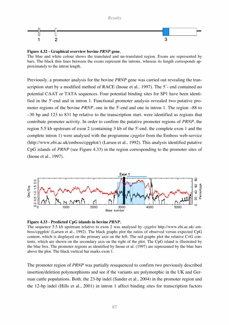
Results
87
Figure 4.32 - Graphical overview bovine PRNP gene.
The blue and white colour shows the translated and un-translated region. Exons are represented bybars. The black thin lines between the exons represent the introns, whereas its length corresponds ap-proximately to the intron length.
Previously, a promoter analysis for the bovine PRNP gene was carried out revealing the tran-
scription start by a modified method of RACE (Inoue et al., 1997). The 5’- end contained no
potential CAAT or TATA sequences. Four potential binding sites for SP1 have been identi-
fied in the 5'-end and in intron 1. Functional promoter analysis revealed two putative pro-
moter regions of the bovine PRNP, one in the 5'-end and one in intron 1. The region –88 to
–30 bp and 123 to 831 bp relative to the transcription start, were identified as regions that
contribute promoter activity. In order to confirm the putative promoter regions of PRNP, the
region 5.5 kb upstream of exon 2 (containing 3 kb of the 5'-end, the complete exon 1 and the
complete intron 1) were analysed with the programme cpgplot from the Emboss web-service
(http://www.ebi.ac.uk/emboss/cpgplot/) (Larsen et al., 1992). This analysis identified putative
CpG islands of PRNP (see Figure 4.33) in the region corresponding to the promoter sites of
(Inoue et al., 1997).
Figure 4.33 - Predicted CpG islands in bovine PRNP.
The sequence 5.5 kb upstream relative to exon 2 was analysed by cpgplot http://www.ebi.ac.uk/ em-boss/cpgplot/ (Larsen et al., 1992). The black graphs plot the ratios of observed versus expected CpGcontent, which is displayed on the primary axis on the left. The red graphs plot the relative C+G con-tents, which are shown on the secondary axis on the right of the plot. The CpG island is illustrated bythe blue box. The promoter regions as identified by Inoue et al. (1997) are represented by the blue barsabove the plot. The black vertical bar marks exon 1.
The promoter region of PRNP was partially resequenced to confirm two previously described
insertion/deletion polymorphisms and see if the variants are polymorphic in the UK and Ger-
man cattle populations. Both, the 23-bp indel (Sander et al., 2004) in the promoter region and
the 12-bp indel (Hills et al., 2001) in intron 1 affect binding sites for transcription factors

Results
88
(RP58 and SP1, respectively), and thus might affect the expression of PRNP (Sander et al.,
2005). Both polymorphisms showed tentative association with BSE in a small association
study (Sander et al., 2004) and were therefore selected for association analysis in the BSE
cases and control animals of four different populations: Holstein-Friesian cattle from the
United Kingdom (UK Holstein) and Germany (German Holstein), German Brown and Ger-
man Fleckvieh.
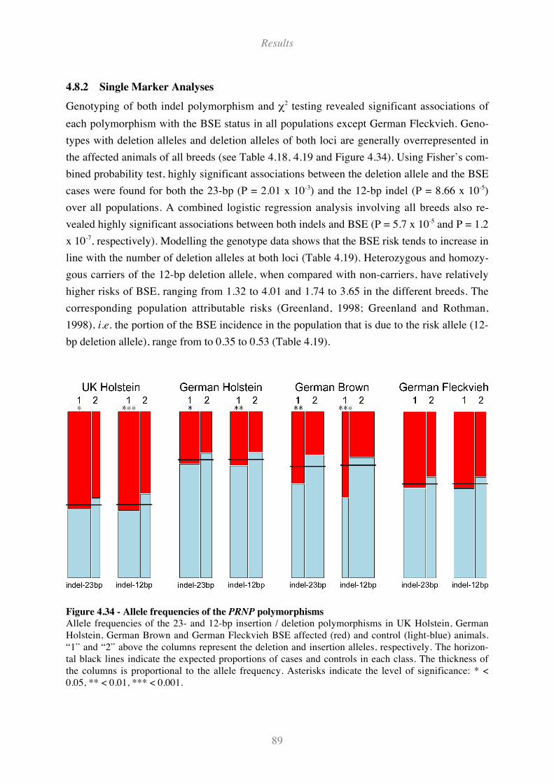
Results
89
4.8.2 Single Marker Analyses
Genotyping of both indel polymorphism and !2 testing revealed significant associations of
each polymorphism with the BSE status in all populations except German Fleckvieh. Geno-
types with deletion alleles and deletion alleles of both loci are generally overrepresented in
the affected animals of all breeds (see Table 4.18, 4.19 and Figure 4.34). Using Fisher’s com-
bined probability test, highly significant associations between the deletion allele and the BSE
cases were found for both the 23-bp (P = 2.01 x 10⁻³) and the 12-bp indel (P = 8.66 x 10⁻⁵)
over all populations. A combined logistic regression analysis involving all breeds also re-
vealed highly significant associations between both indels and BSE (P = 5.7 x 10⁻⁵ and P = 1.2
x 10-7, respectively). Modelling the genotype data shows that the BSE risk tends to increase in
line with the number of deletion alleles at both loci (Table 4.19). Heterozygous and homozy-
gous carriers of the 12-bp deletion allele, when compared with non-carriers, have relatively
higher risks of BSE, ranging from 1.32 to 4.01 and 1.74 to 3.65 in the different breeds. The
corresponding population attributable risks (Greenland, 1998; Greenland and Rothman,
1998), i.e. the portion of the BSE incidence in the population that is due to the risk allele (12-
bp deletion allele), range from to 0.35 to 0.53 (Table 4.19).
Figure 4.34 - Allele frequencies of the PRNP polymorphisms
Allele frequencies of the 23- and 12-bp insertion / deletion polymorphisms in UK Holstein, GermanHolstein, German Brown and German Fleckvieh BSE affected (red) and control (light-blue) animals.“1” and “2” above the columns represent the deletion and insertion alleles, respectively. The horizon-tal black lines indicate the expected proportions of cases and controls in each class. The thickness ofthe columns is proportional to the allele frequency. Asterisks indicate the level of significance: * <0.05, ** < 0.01, *** < 0.001.
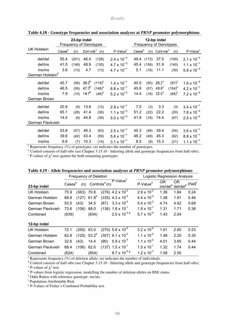
Results
90
Table 4.18 - Genotype frequencies and association analyses at PRNP promoter polymorphisms
23-bp indel 12-bp indelFrequency of Genotypes Frequency of Genotypes
UK Holstein(n) (n) P-Value
c(n) (n) P-Value
c
del/del 55.4 (201) 46.4 (128) 2.4 x 10⁻² 49.4 (173) 37.0 (100) 2.1 x 10
–3
del/ins 41.0 (149) 48.9 (135) 4.7 x 10⁻² 45.4 (159) 51.9 (140) 1.1 x 10
–1
ins/ins 3.6 (13) 4.7 (13) 4.7 x 10⁻¹ 5.1 (18) 11.1 (30) 5.8 x 10
–3
German Holsteinb
del/del 45.7 (58) (119)b
1.4 x 10⁻¹ 40.0 (50) (87)
b1.6 x 10
–2
del/ins 46.5 (59) (148)b
8.8 x 10⁻¹ 45.6 (57) (154)
b4.2 x 10
–1
ins/ins 7.9 (10) (46)b
5.2 x 10⁻² 14.4 (18) (68)
b7.2 x 10
–2
German Brown
del/del 20.9 (9) 13.8 (12) 2.9 x 10⁻¹ 7.0 (3) 3.3 (3) 3.4 x 10
–1
del/ins 65.1 (28) 41.4 (36) 1.1 x 10⁻² 51.2 (22) 22.2 (20) 7.8 x 10
–4
ins/ins 14.0 (6) 44.8 (39) 5.0 x 10⁻⁴ 41.9 (18) 74.4 (67) 2.5 x 10
–4
German Fleckvieh
del/del 53.8 (57) 46.3 (63) 2.5 x 10⁻¹ 45.3 (48) 39.4 (54) 3.6 x 10
–1
del/ins 39.6 (42) 43.4 (59) 5.6 x 10⁻¹ 46.2 (49) 45.3 (62) 8.8 x 10
–1
ins/ins 6.6 (7) 10.3 (14) 3.1 x 10⁻¹ 8.5 (9) 15.3 (21) 1.1 x 10
–1
a Represents frequency (%) of genotypes; (n) indicates the number of genotypes.b Control consists of half-sibs (see Chapter 3.15.10 - Inferring allele and genotype frequencies from half-sibs).c P-values of !2-test against the both remaining genotypes
Table 4.19 - Allele frequencies and association analyses at PRNP promoter polymorphisms
Frequency of Deletion Logistic Regression Analysis
OR OR23-bp indel
Casesa
(n) Controlsa
(n)P-Value
c
P-Valued
ins/dele
del/dele PAR
f
UK Holstein 75.9 (363) 70.8 (276) 4.2 x 10⁻²
2.9 x 10⁻²
1.36 1.84 0.24
German Holstein 68.9 (127) 61.8b
(335) 4.3 x 10⁻²
4.4 x 10⁻²
1.38 1.91 0.46
German Brown 53.5 (43) 34.5 (87) 3.3 x 10⁻³
5.4 x 10⁻³
4.74 4.62 0.69
German Fleckvieh 73.6 (106) 68.0 (136) 1.8 x 10⁻¹
1.9 x 10⁻¹
1.31 1.71 0.36
Combined (639) (834) 2.0 x 10⁻³ g
5.7 x 10⁻⁵
1.43 2.04
12-bp indel
UK Holstein 72.1 (350) 63.0 (270) 5.8 x 10⁻⁴
3.2 x 10⁻⁴
1.61 2.60 0.53
German Holstein 62.8 (125) 53.2b
(357) 9.1 x 10⁻³
1.1 x 10⁻²
1.48 2.20 0.35
German Brown 32.6 (43) 14.4 (90) 5.9 x 10⁻⁴
1.1 x 10⁻²
4.01 3.65 0.44
German Fleckvieh 68.4 (106) 62.0 (137) 1.5 x 10⁻¹
1.5 x 10⁻¹
1.32 1.74 0.44
Combined (624) (854) 8.7 x 10⁻⁵ g
1.2 x 10⁻⁷
1.58 2.50a Represents frequency (%) of deletion allele; (n) indicates the number of individuals.b Control consists of half-sibs (see Chapter 3.15.10 - Inferring allele and genotype frequencies from half-sibs).c P-values of !2-test.d P-values from logistic regression, modelling the number of deletion alleles on BSE status.e Odds Ratios with reference genotype: ins/ins.f Population Attributable Riskg P-Values of Fisher’s Combined Probability test.
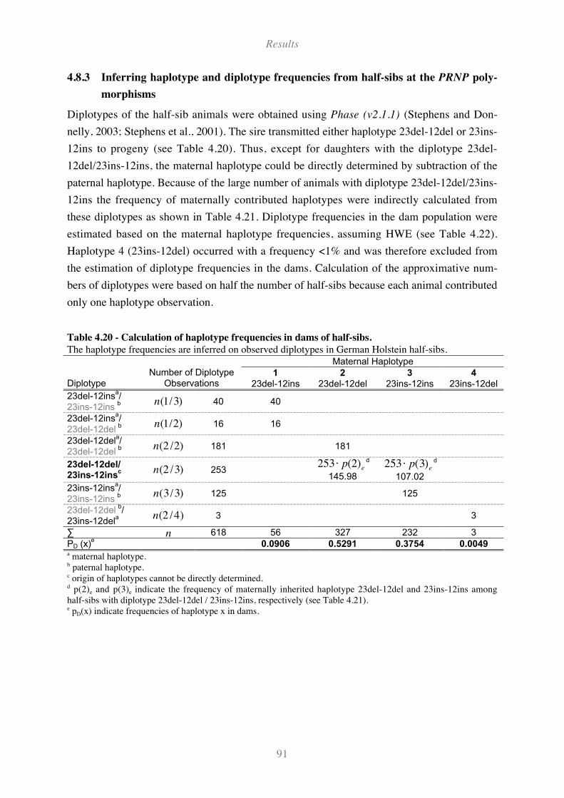
Results
91
4.8.3 Inferring haplotype and diplotype frequencies from half-sibs at the PRNP poly-
morphisms
Diplotypes of the half-sib animals were obtained using Phase (v2.1.1) (Stephens and Don-
nelly, 2003; Stephens et al., 2001). The sire transmitted either haplotype 23del-12del or 23ins-
12ins to progeny (see Table 4.20). Thus, except for daughters with the diplotype 23del-
12del/23ins-12ins, the maternal haplotype could be directly determined by subtraction of the
paternal haplotype. Because of the large number of animals with diplotype 23del-12del/23ins-
12ins the frequency of maternally contributed haplotypes were indirectly calculated from
these diplotypes as shown in Table 4.21. Diplotype frequencies in the dam population were
estimated based on the maternal haplotype frequencies, assuming HWE (see Table 4.22).
Haplotype 4 (23ins-12del) occurred with a frequency <1% and was therefore excluded from
the estimation of diplotype frequencies in the dams. Calculation of the approximative num-
bers of diplotypes were based on half the number of half-sibs because each animal contributed
only one haplotype observation.
Table 4.20 - Calculation of haplotype frequencies in dams of half-sibs.
The haplotype frequencies are inferred on observed diplotypes in German Holstein half-sibs.Maternal Haplotype
DiplotypeNumber of Diplotype
Observations1
23del-12ins2
23del-12del3
23ins-12ins4
23ins-12del
23del-12insa/
23ins-12ins b
!
n(1/3) 40 40
23del-12insa/
23del-12del b
!
n(1/2) 16 16
23del-12dela/
23del-12del b
!
n(2 /2) 181 181
23del-12del/23ins-12ins
c
!
n(2 /3) 253
!
253 " p(2)ed
145.98
!
253 " p(3)ed
107.02
23ins-12insa/
23ins-12ins b
!
n(3/3) 125 125
23del-12del b
/23ins-12del
a
!
n(2 /4) 3 3
!
!
n 618 56 327 232 3
PD (x)e
0.0906 0.5291 0.3754 0.0049a maternal haplotype.b paternal haplotype.c origin of haplotypes cannot be directly determined.d p(2)e and p(3)e indicate the frequency of maternally inherited haplotype 23del-12del and 23ins-12ins amonghalf-sibs with diplotype 23del-12del / 23ins-12ins, respectively (see Table 4.21).e pD(x) indicate frequencies of haplotype x in dams.
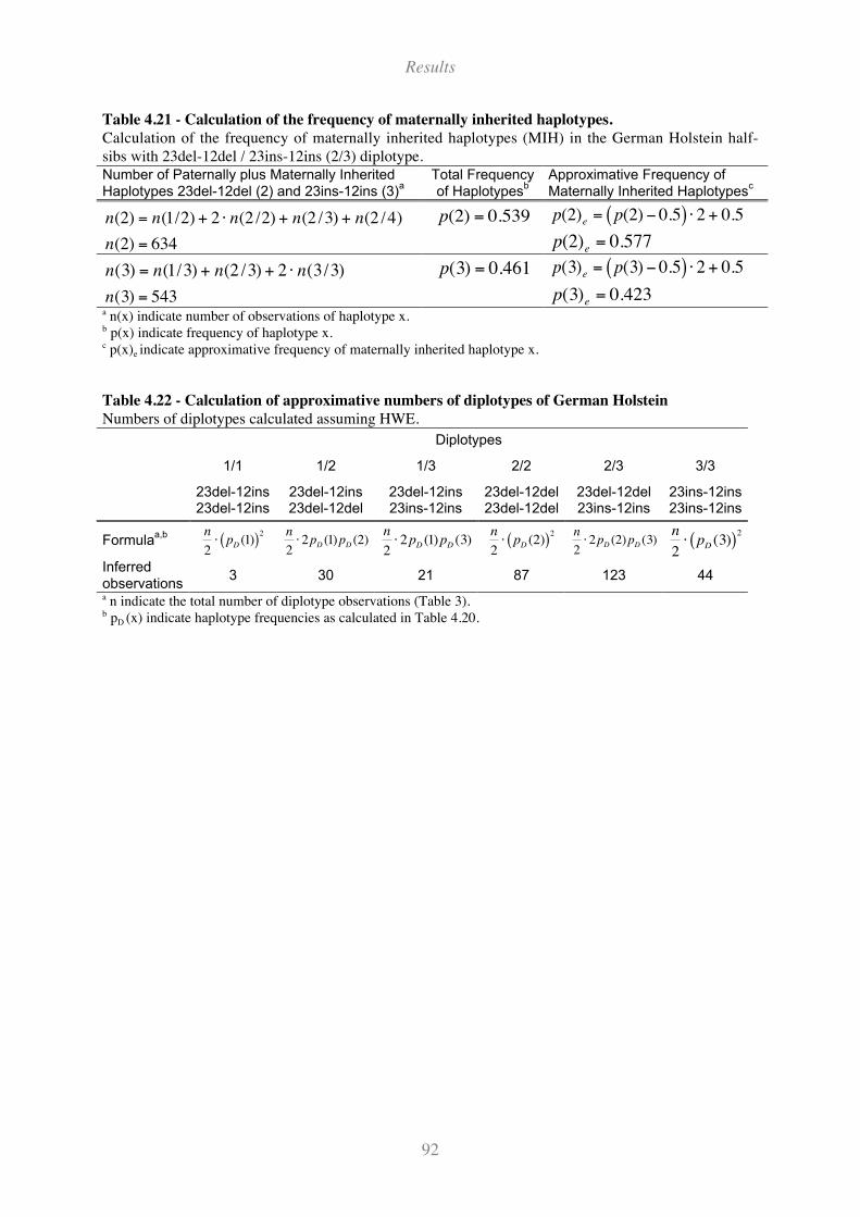
Results
92
Table 4.21 - Calculation of the frequency of maternally inherited haplotypes.
Calculation of the frequency of maternally inherited haplotypes (MIH) in the German Holstein half-sibs with 23del-12del / 23ins-12ins (2/3) diplotype.Number of Paternally plus Maternally InheritedHaplotypes 23del-12del (2) and 23ins-12ins (3)
aTotal Frequencyof Haplotypes
bApproximative Frequency ofMaternally Inherited Haplotypes
c
!
n(2) = n(1/2) + 2 " n(2 /2) + n(2 /3) + n(2 /4)
!
n(2) = 634
!
p(2) = 0.539
!
p(2)e = p(2) " 0.5( ) # 2 + 0.5
!
p(2)e = 0.577
!
n(3) = n(1/3) + n(2 /3) + 2 " n(3/3)
!
n(3) = 543
!
p(3) = 0.461
!
p(3)e = p(3) " 0.5( ) # 2 + 0.5
!
p(3)e = 0.423a n(x) indicate number of observations of haplotype x.b p(x) indicate frequency of haplotype x.c p(x)e indicate approximative frequency of maternally inherited haplotype x.
Table 4.22 - Calculation of approximative numbers of diplotypes of German Holstein
Numbers of diplotypes calculated assuming HWE.
Diplotypes
1/1 1/2 1/3 2/2 2/3 3/3
23del-12ins23del-12ins
23del-12ins23del-12del
23del-12ins23ins-12ins
23del-12del23del-12del
23del-12del23ins-12ins
23ins-12ins23ins-12ins
Formulaa,b
!
n
2" pD (1)( )
2
!
n
2" 2pD (1)pD (2)
!
n
2" 2pD (1)pD (3)
!
n
2" pD (2)( )
2
!
n
2" 2pD (2)pD (3)
!
n
2" pD (3)( )
2
Inferredobservations
3 30 21 87 123 44
a n indicate the total number of diplotype observations (Table 3).b pD (x) indicate haplotype frequencies as calculated in Table 4.20.
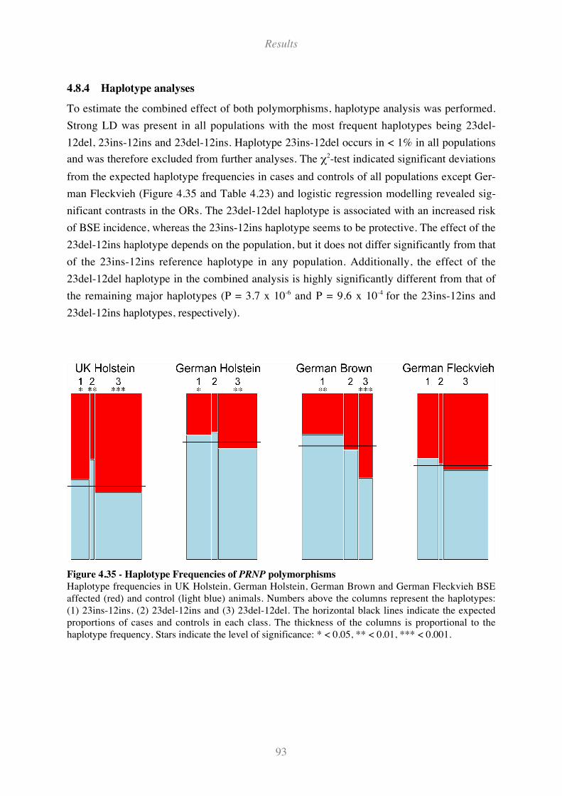
Results
93
4.8.4 Haplotype analyses
To estimate the combined effect of both polymorphisms, haplotype analysis was performed.
Strong LD was present in all populations with the most frequent haplotypes being 23del-
12del, 23ins-12ins and 23del-12ins. Haplotype 23ins-12del occurs in < 1% in all populations
and was therefore excluded from further analyses. The !2-test indicated significant deviations
from the expected haplotype frequencies in cases and controls of all populations except Ger-
man Fleckvieh (Figure 4.35 and Table 4.23) and logistic regression modelling revealed sig-
nificant contrasts in the ORs. The 23del-12del haplotype is associated with an increased risk
of BSE incidence, whereas the 23ins-12ins haplotype seems to be protective. The effect of the
23del-12ins haplotype depends on the population, but it does not differ significantly from that
of the 23ins-12ins reference haplotype in any population. Additionally, the effect of the
23del-12del haplotype in the combined analysis is highly significantly different from that of
the remaining major haplotypes (P = 3.7 x 10⁻⁶ and P = 9.6 x 10⁻⁴ for the 23ins-12ins and
23del-12ins haplotypes, respectively).
Figure 4.35 - Haplotype Frequencies of PRNP polymorphisms
Haplotype frequencies in UK Holstein, German Holstein, German Brown and German Fleckvieh BSEaffected (red) and control (light blue) animals. Numbers above the columns represent the haplotypes:(1) 23ins-12ins, (2) 23del-12ins and (3) 23del-12del. The horizontal black lines indicate the expectedproportions of cases and controls in each class. The thickness of the columns is proportional to thehaplotype frequency. Stars indicate the level of significance: * < 0.05, ** < 0.01, *** < 0.001.
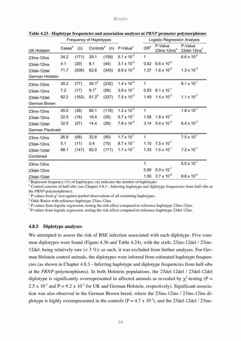
Results
94
Table 4.23 - Haplotype frequencies and association analyses at PRNP promoter polymorphisms
Frequency of Haplotypes Logistic Regression Analysis
UK HolsteinCases
a(n) Controls
a(n) P-Value
cOR
d P-Value23ins-12ins
eP-Value23del-12ins
f
23ins-12ins 24.2 (171) 29.1 (159) 5.1 x 10⁻²
1 6.6 x 10⁻²
23del-12ins 4.1 (29) 8.1 (44) 3.1 x 10⁻³
0.62 6.6 x 10⁻²
23del-12del 71.7 (506) 62.8 (343) 8.9 x 10⁻⁴
1.37 1.6 x 10⁻²
1.3 x 10⁻³
German Holstein
23ins-12ins 30.2 (77) 39.1b
(232) 1.4 x 10⁻²
1 8.1 x 10⁻¹
23del-12ins 7.2 (17) 9.1b
(56) 3.9 x 10⁻¹
0.93 8.1 x 10⁻¹
23del-12del 62.2 (162) 51.3b
(327) 7.5 x 10⁻³
1.49 1.4 x 10⁻²
1.1 x 10⁻¹
German Brown
23ins-12ins 45.0 (39) 66.1 (119) 1.3 x 10⁻³
1 1.8 x 10⁻¹
23del-12ins 22.5 (18) 19.4 (35) 5.7 x 10⁻¹
1.58 1.8 x 10⁻¹
23del-12del 32.5 (27) 14.4 (26) 7.8 x 10⁻⁴
3.14 5.4 x 10⁻⁴
8.4 x 10⁻²
German Fleckvieh
23ins-12ins 26.8 (58) 32.6 (90) 1.7 x 10⁻¹
1 7.5 x 10⁻¹
23del-12ins 5.1 (11) 5.4 (15) 8.7 x 10⁻¹
1.15 7.5 x 10⁻¹
23del-12del 68.1 (147) 62.0 (171) 1.7 x 10⁻¹
1.33 1.5 x 10⁻¹
7.2 x 10⁻¹
Combined
23ins-12ins 1 5.0 x 10⁻¹
23del-12ins 0.90 5.0 x 10⁻¹
23del-12del 1.50 3.7 x 10⁻⁶
9.6 x 10⁻⁴
a Represent frequency (%) of haplotypes; (n) indicates the number of haplotypesb Control consists of half-sibs (see Chapter 4.8.3 - Inferring haplotype and diplotype frequencies from half-sibs atthe PRNP-polymorphisms).c P-values from !2-test against pooled observations of all remaining haplotypes.d Odds Ratios with reference haplotype 23ins-12ins.e P-values from logistic regression, testing the risk effect compared to reference haplotype 23ins-12ins.f P-values from logistic regression, testing the risk effect compared to reference haplotype 23del-12ins.
4.8.5 Diplotype analyses
We attempted to assess the risk of BSE infection associated with each diplotype. Five com-
mon diplotypes were found (Figure 4.36 and Table 4.24), with the sixth, 23ins-12del / 23ins-
12del, being relatively rare (< 3 %); as such, it was excluded from further analyses. For Ger-
man Holstein control animals, the diplotypes were inferred from estimated haplotype frequen-
cies (as shown in Chapter 4.8.3 - Inferring haplotype and diplotype frequencies from half-sibs
at the PRNP-polymorphisms). In both Holstein populations, the 23del-12del / 23del-12del
diplotype is significantly overrepresented in affected animals as revealed by !2-testing (P =
2.5 x 10⁻³ and P = 9.2 x 10⁻³ for UK and German Holstein, respectively). Significant associa-
tion was also observed in the German Brown breed, where the 23ins-12ins / 23ins-12ins di-
plotype is highly overrepresented in the controls (P = 4.7 x 10⁻⁴), and the 23del-12del / 23ins-
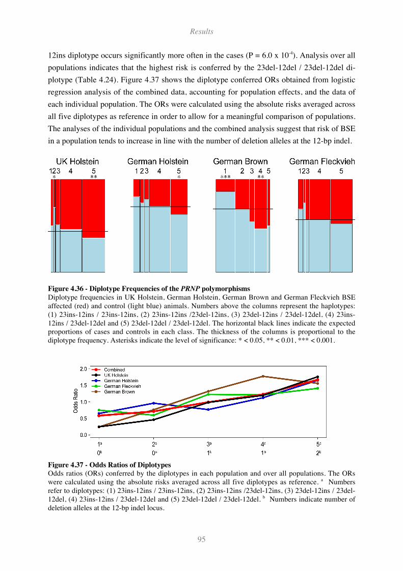
Results
95
12ins diplotype occurs significantly more often in the cases (P = 6.0 x 10⁻⁴). Analysis over all
populations indicates that the highest risk is conferred by the 23del-12del / 23del-12del di-
plotype (Table 4.24). Figure 4.37 shows the diplotype conferred ORs obtained from logistic
regression analysis of the combined data, accounting for population effects, and the data of
each individual population. The ORs were calculated using the absolute risks averaged across
all five diplotypes as reference in order to allow for a meaningful comparison of populations.
The analyses of the individual populations and the combined analysis suggest that risk of BSE
in a population tends to increase in line with the number of deletion alleles at the 12-bp indel.
Figure 4.36 - Diplotype Frequencies of the PRNP polymorphisms
Diplotype frequencies in UK Holstein, German Holstein, German Brown and German Fleckvieh BSEaffected (red) and control (light blue) animals. Numbers above the columns represent the haplotypes:(1) 23ins-12ins / 23ins-12ins, (2) 23ins-12ins /23del-12ins, (3) 23del-12ins / 23del-12del, (4) 23ins-12ins / 23del-12del and (5) 23del-12del / 23del-12del. The horizontal black lines indicate the expectedproportions of cases and controls in each class. The thickness of the columns is proportional to thediplotype frequency. Asterisks indicate the level of significance: * < 0.05, ** < 0.01, *** < 0.001.
Figure 4.37 - Odds Ratios of Diplotypes
Odds ratios (ORs) conferred by the diplotypes in each population and over all populations. The ORswere calculated using the absolute risks averaged across all five diplotypes as reference. a Numbersrefer to diplotypes: (1) 23ins-12ins / 23ins-12ins, (2) 23ins-12ins /23del-12ins, (3) 23del-12ins / 23del-12del, (4) 23ins-12ins / 23del-12del and (5) 23del-12del / 23del-12del. b Numbers indicate number ofdeletion alleles at the 12-bp indel locus.
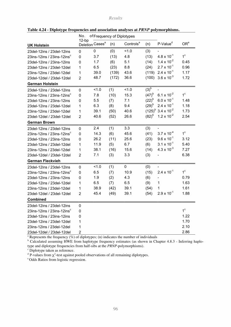
Results
96
Table 4.24 - Diplotype frequencies and association analyses at PRNP polymorphisms.
Frequency of Diplotypes
UK Holstein
No. of12-bpDeletion Cases
a(n) Controls
a(n) P-Value
dOR
e
23del-12ins / 23del-12ins 0 0 (0) <1.0 (3) -
23ins-12ins / 23ins-12insc
0 3.7 (13) 4.8 (13) 4.8 x 10⁻¹
1c
23del-12ins / 23ins-12ins 0 1.7 (6) 5.1 (14) 1.4 x 10⁻²
0.45
23del-12ins / 23del-12del 1 6.5 (23) 8.8 (24) 2.7 x 10⁻¹
0.96
23ins-12ins / 23del-12del 1 39.0 (139) 43.6 (119) 2.4 x 10⁻¹
1.17
23del-12del / 23del-12del 2 48.7 (172) 36.6 (100) 3.6 x 10⁻³
1.72
German Holstein
23del-12ins / 23del-12ins 0 <1.0 (1) <1.0 (3)b
-
23ins-12ins / 23ins-12insc
0 7.8 (10) 15.3 (47)b
6.1 x 10⁻²
1c
23del-12ins / 23ins-12ins 0 5.5 (7) 7.1 (22)b
6.0 x 10⁻¹
1.48
23del-12ins / 23del-12del 1 6.3 (8) 9.4 (29)b
2.4 x 10⁻¹
1.18
23ins-12ins / 23del-12del 1 39.1 (50) 40.6 (125)b
3.4 x 10⁻²
1.73
23del-12del / 23del-12del 2 40.6 (52) 26.6 (82)b
1.2 x 10⁻²
2.54
German Brown
23del-12ins / 23del-12ins 0 2.4 (1) 3.3 (3) -
23ins-12ins / 23ins-12insc
0 14.3 (6) 45.6 (41) 3.7 x 10⁻⁴
1c
23del-12ins / 23ins-12ins 0 26.2 (11) 25.6 (23) 9.6 x 10⁻¹
3.12
23del-12ins / 23del-12del 1 11.9 (5) 6.7 (6) 3.1 x 10⁻¹
5.40
23ins-12ins / 23del-12del 1 38.1 (16) 15.6 (14) 4.3 x 10⁻³
7.27
23del-12del / 23del-12del 2 7.1 (3) 3.3 (3) - 6.38
German Fleckvieh
23del-12ins / 23del-12ins 0 <1.0 (1) 0 (0) -
23ins-12ins / 23ins-12insc
0 6.5 (7) 10.9 (15) 2.4 x 10⁻¹
1c
23del-12ins / 23ins-12ins 0 1.9 (2) 4.3 (6) - 0.79
23del-12ins / 23del-12del 1 6.5 (7) 6.5 (9) 1 1.63
23ins-12ins / 23del-12del 1 38.9 (42) 39.1 (54) 1 1.61
23del-12del / 23del-12del 2 45.4 (49) 39.1 (54) 2.9 x 10⁻¹
1.88
Combined
23del-12ins / 23del-12ins 0
23ins-12ins / 23ins-12insc
0 1c
23del-12ins / 23ins-12ins 0 1.22
23del-12ins / 23del-12del 1 1.70
23ins-12ins / 23del-12del 1 2.10
23del-12del / 23del-12del 2 2.86a Represents the frequency (%) of diplotypes; (n) indicates the number of individualsb Calculated assuming HWE from haplotype frequency estimates (as shown in Chapter 4.8.3 - Inferring haplo-type and diplotype frequencies from half-sibs at the PRNP-polymorphisms).c Diplotype taken as reference.d P-values from !2-test against pooled observations of all remaining diplotypes.e Odds Ratios from logistic regression.
Results
97
4.8.6 Modelling the modes of allelic action and relative contribution of both polymor-
phisms
Likelihood ratio tests were applied as proposed by North et al. (2005) to investigate both the
modes of allelic action for both loci (additive versus dominance effects) and for possible
epistatic effects (additive by additive, additive by dominance and dominance by dominance
interactions). The results indicate that for the individual populations as well as for the com-
bined analysis neither the inclusion of dominance effects nor inclusion of epistatic effects
leads to a significantly better fit compared to a model that accounts for additive effects only.
Hence, likelihood ratio tests were performed to verify whether fitting an additive effect for
either indel locus reduces the likelihood significantly compared to a full model that includes
additive effects of both polymorphisms. This analysis revealed that exclusion of the 23-bp
indel does not reduce the likelihood significantly in any of the individual populations or in the
combined data. However, exclusion of the 12-bp indel polymorphism reduces the likelihood
significantly in UK Holstein (P = 1.04 x 10⁻³) and in the combined analysis (P = 6.89 x 10⁻⁴).
Thus, the main effect on BSE susceptibility seems to result from the 12-bp indel. This is sup-
ported by the haplotype analysis, which showed that the effect of the 23del-12ins haplotype
does not differ significantly from that of 23ins-12ins, whereas the 23del-12del haplotype is
significantly associated with higher BSE risk in the Holstein populations and in German
Brown (Table 4.23).
Discussion
98
5 Discussion
5.1 Characterisation of the extended HEXA region
In this study, fine mapping of a 300-kb genomic region encompassing four genes was con-
ducted in cattle. The region has been initially proposed by Hernandez-Sanchez et al. (2002) to
be a promising candidate region of BSE susceptibility because of putative linkage to a marker
on BTA 10, which showed significant segregation distortion in BSE affected animals. Moreo-
ver, the homologous region in mice has been identified to show suggestive evidence of QTL
affecting prion incubation time after experimental challenge (Stephenson et al., 2000). The
central candidate gene in the 300-kb region was HEXA, the gene encoding the alpha subunit
of the lysosomal enzyme hexosaminidase A (HexA). Various polymorphisms in HEXA cause
Tay-Sachs disease, a autosomal recessive, progressive neurodegenerative disorder in human
belonging to the Lysosomal Storage Diseases caused by accumulation of intercellular compo-
nents in the lysosome (Chavany and Jendoubi, 1998). This storage of ‚waste’ in the lysosome
of nerve cells can also be observed in prion diseases. The turnover of PrPc to PrPSc generates
protease-resistant components (Prusiner, 1998a), which are indigestible for the lysosomal
enzymes. Therefore, lysosomal enzyme efficiency could influence BSE development.
Starting with sequencing and characterisation of the HEXA gene, SNPs were identified and as
a preliminary study, four intronic SNPs were genotyped in a panel of BSE affected and con-
trol animals from UK and Germany. One of these SNPs showed highly significant association
with BSE in the UK animals. Subsequently, a 300-kb region centred on HEXA with the genes
PARP6, BRUNOL6 and ARIH1 was characterised, partially re-sequenced and SNPs identified
within the genes. Fine mapping of this region in cattle showed that the gene order on BTA10
coincidences with the homologous region in man on HSA 15. By BAC sequencing it has been
established that the locus order is PARP6 (-) BRUNOL6 (-), HEXA (-) and ARIH1 (+). This
gene order is consistent with this of the chromosomal annotation in Btau 2.0 (June 2006) gene
assembly. The newest version of bovine gene assembly Btau 3.1 (August 2006) contains
misassembled sequences at the PARP6 locus. The sequence publisher at the Baylor College of
Medicine warn of typical errors in the draft genome sequence including misassembles, but the
number of errors in the bovine sequence assembly is difficult to predict.
Comparison of the protein sequences encoded by the genes within the contig across species
showed high conservation with a sequence identity of > 84.5 %. Thus, it can be assumed that
the function for HEXA, PARP6, BRUNOL6 and ARIH1 is also conserved in human, mouse
and cattle. Homologues of ARIH1 display the highest sequence identity of > 99% between
cattle and man and as proposed by Tan et al. (2000) of > 98% between mouse and man, re-
Discussion
99
spectively. Partially re-sequencing of the ARIH1 gene in cattle identified approximately one
SNP every 1900 bp in the non-coding sequence which differs from a previous bovine study,
in which one SNP every 180 bp was detected by sequencing a similar panel of animals
(Werner et al., 2004). The low level of polymorphism within cattle and the highest conserva-
tion between species underlines the potentially important function of ARIH1. As previously
shown, ARIH1 function can be linked to neurodegenerative diseases and thus, may be in-
volved in TSE development. Mutations in the functional homologue (ariadne gene) from
Drosophila cause severe neuronal defects highlighting its crucial biological function (Aguilera
et al., 2000). The gene product plays a putative role in ubiquitylation (Tan et al., 2000), which
is the first step of intracellular protein degradation. Strong sequence conservation of
BRUNOL6 and PARP6 notably in the functional domains have also been observed.
BRUNOL6 belongs to a gene family of RNA binding proteins influencing muscle specific
splicing and enhancer specific alternative splicing of different genes (Ladd et al., 2004).
However, BRUNOL6 also expressed in the brain could indirectly influence TSE development
by alternative splicing of yet unidentified genes, which are involved in prion diseases.
PARP6s specific function is unknown, but as a member of the PARP gene family which is
involved in many biological processes (e.g. DNA repair, apoptosis or transcriptional regula-
tion) (Diefenbach and Burkle, 2005) it could be involved in TSE development. If PARP6
plays a role in neurodegenerative diseases it might be a indirect, e.g. as an interactor with
other genes or gene products. Although connections of both genes to TSE diseases are rather
speculative, their gene structure and regulation were analysed to cover a larger genomic re-
gion.
The promoter analyses for the investigated candidate genes revealed CpG (Cytosin-
phosphatidyl-Guanosin) rich regulatory elements in all 5'-ends. CpG islands are mostly un-
methylated DNA regions and are thus accessible for transcription factors. CpG rich promoters
represent the majority of mammalian promoters, which are associated with broad transcription
start site regions (Carninci et al., 2006).
5.2 SNP analysis
5.2.1 SNP identification and selection
One goal of this dissertation was to identify polymorphisms in candidate genes, which are
presumably influencing BSE susceptibility. Therefore, sequence information for designing
PCR systems and re-sequencing for SNP identification was necessary. The increasing number
of accessible bovine sequence data in recent years facilitates primer design for re-sequencing
tremendously. But still the limiting element in this study was the cost and time consuming re-
Discussion
100
sequencing and SNP search compared to the later carried out genotyping. Usage of an auto-
mated sequencer by poly-acrylamid gel electrophoresis with parallel detection of 96 samples
is comparable with the daily throughput of a 4-capillary automated sequencer, but requires a
trained handling with the harmful acrylamid and routine in pouring the gels. The costs per
sequencing reaction is mainly depending on the input of sequencing dye, containing the
flourescence labelled di-desoxy nucleotides. During this study, the input of sequencing dye
could be halved (from 4 to 2 µl/reaction) and the costs including PCR, PCR cleanup and se-
quencing reaction cleanup ranged from 4.90 to 2.90 Euro. These expenses could be further
reduced considerably to 1 - 1.50 Euro per reaction by using a capillary sequencer which only
requires 0.25 - 0.5 µl sequencing dye per reaction.
SNP search was performed in a panel of pooled and individual DNA from animals of the
taurine breeds German Holstein, German Fleckvieh and German Brown and from indicine
breeds. A total of 136 taurine DNA variations (131 SNPs and 5 Indels) were identified in the
extended HEXA region, 83 of them in intronic regions, 39 in the 5'-end with five of them in
putative regulatory regions, eight in the 3' end and four synonymous SNPs in coding regions.
From these SNPs, an informative panel had to be selected in order to genotype BSE affected
and control animals to identify association of SNP alleles and haplotypes with BSE. Initially,
the number of SNPs had to be minimized while simultaneously maintaining the information
provided by all other SNPs (= SNP tagging). Therefore, preliminary determination of pair-
wise LD and haplotypes is necessary (Byng et al., 2003). However, an automated approach to
derive provisional LD and haplotypes over the whole region including all SNPs could not be
conducted, because the genotype data of 136 SNPs from nine individuals (three of each breed
German Holstein, German Fleckvieh and German Brown) were not sufficient. Due to lack of
DNA for a few individuals, those had to be replaced while screening the region. Moreover,
the German Brown animals were mostly not polymorphic at the identified SNPs in the ex-
tended HEXA region and therefore actually less individuals remained for deriving LD. Thus,
41 SNPs were manually selected by the following scheme. First, all exonic SNPs, although
synonymous, and all SNPs in regulatory regions were chosen. Finally intronic SNPs were
selected such that they represent evenly distributed markers over the whole region. If pairwise
LD and haplotype phases were clearly recognised for neighbouring SNPs by comparison of
the genotypes of the animals, these SNPs would be treated as redundant. Nevertheless, tag-
ging after successful genotyping of 38 from 42 SNPs in a larger sample revealed that 16
tagSNPs were representing all information. This shows that the preliminary SNP selection
was rather inefficient, but required for maintaining the overall information. Despite rapid ad-
vances in cattle genetics, in comparison, substantial progress has been made in human genet-
ics by the HapMap project, supplying a catalogue of already tagged common human genetic
variants, from which their organisation on the chromosome is known (HapMap-Consortium,
Discussion
101
2003; HapMap-Consortium, 2005). This project is conducted by the HapMap consortium
consisting of at least 25 institutes and 14 genotyping centres all contributing to the work. In a
first step, 269 individuals from four populations were genotyped at more than 1 million SNPs
which was aimed to be at least one common SNP every 5 kb. From these data, the tagSNP
and common haplotypes for the human genome were derived which can be used now for high
efficient SNP selection for association studies and comparative haplotype analysis.
5.2.2 SNP genotyping with MALDI-TOF MS
The genotyping of the SNPs was performed with a high-throughput genotyping platform, us-
ing the mass differences of allele specific extension products (hME and iPLEX, Sequenom,
Hamburg, Germany) detected by Matrix Assisted Laser Desorption Ionisation Time of Flight
Mass Spectroscopy (MALDI-TOF MS). Compared to other genotyping methods, e.g. restric-
tion enzyme digestion of Restriction Fragment Length Polymorphism (RFLP) or sequencing,
the costs are at least one order of magnitude lower with MALDI-TOF MS because of the pos-
sibility to multiplex up to 27 fold and parallel analysis of 376 samples with this method. The
expenses for the analysis of one genotype with iPLEX and MALDI-TOF MS range from 0.05
and 0.10 Euro, whereas genotyping by RFLP assays costs on average 0.50 Euro and the se-
quencing of one sample costs at least 1.50 Euro. In addition to the cost benefit and the ad-
vantage of the high-throughput system of MALDI-TOF MS, the amount of sample DNA per
animal needed, regardless of the multiplexing grade is 10 fold less than common genotyping
assays using PCR (5ng versus 50ng). DNA input per genotype is even lower when genotyping
with the MALDI-TOF MS and iPLEX method with a multiplexing grade from 16 to 27,
which requires only 0.18 - 0.31 ng DNA per animal and genotype. Further, all steps can be
performed with automated pipetting stations.
5.3 Genomic control (GC)
Correction for population stratification by GC (Devlin and Roeder, 1999) was performed to
prevent spurious association and false positives due to cryptic substructures. The impact of
population stratification on case-control association studies is discussed in numerous publica-
tions by different authors (Marchini et al., 2004; Thomas and Witte, 2002; Wacholder et al.,
2002). Population stratification affects association studies when cases and controls dispropor-
tional represent genetic subpopulations, so that cases and controls have differences in disease
prevalence and variations in allele frequency. This can then bias the statistical evidence to-
wards an association (spurious association) between allele and phenotype. Population stratifi-
cation is probably the most cited reason for non-repeatability of association results.
Discussion
102
The GC suggests that in presence of population stratification the standard !2-statistic used in
case-control studies is inflated by a multiplicative factor, which is proportional to the degree
of stratification. This factor is called inflation factor " and is estimated from a set of unlinked
genetic markers (so-called null-loci) scattered around the genome. " is used to correct the test
statistic of the candidate loci if " > 1.
In this thesis, the GC approach was conducted in cattle for the first time. As null-loci, a set of
37 SNP markers was chosen and genotyped in two cattle populations. Due to the exclusion of
eight SNPs with unreliable results, 29 SNPs were used for the estimation of ". It was inferred
for the German and the UK Holstein Friesians revealing values of 1.03 and 1.05, respectively.
Thus, the effect of inflation is only marginal in both populations suggesting no stratification
within both groups.
As Freedman et al. (2004) compared the genotypes of 35 to 40 non-coding SNPs of European,
African and Asian Americans to assess stratification levels and to evaluate the SNPs used, GC
was performed between the UK and the German Holstein population. Unexpectedly, strong
population stratification was observed. The inflation factor between the cases and controls of
both groups constituted at a level of no stratification, whereas the comparison of the pooled
populations consisting each of both, cases and controls revealed that the populations are ge-
netically different, resulting in a high inflation factor (" = 19.54). Despite a intense interna-
tional exchange of breeding stock in Holstein Friesian, the revealed genetic distinctions be-
tween UK and German Holstein animals highlight that both groups should not a priori be
merged for an association study. Moreover, the term ‘different populations’ for the UK and
German Holstein animals is apparently correct in the context of genetic association studies.
However, the minor inflation factors found between cases and controls within each population
shows that controls in both populations are well suited as reference for an association study.
5.4 Association of SNPs in the extended HEXA region with BSE
In this study, for the first time, remarkably association of SNPs and haplotypes in a candidate
region not belonging to the prion gene complex with BSE was shown. Successfully genotyp-
ing of 38 SNPs of the extended HEXA region (including the genes ARIH1, HEXA, BRUNOL6
and PARP6) in BSE diseased and control animals from UK Holstein cattle population re-
vealed three SNPs associated with the BSE status after correction for multiple testing. The
rare alleles of the three SNPs are all presented on one haplotype, which is significantly over-
represented in the controls (5% versus 1% with an permuted p-value of 0.002) and may con-
stitute a factor that protects against BSE infection or are associated with such a factor. The
alleles and the haplotype were postulated as the UK-protecting alleles or haplotype, respec-
Discussion
103
tively. A second haplotype, significantly overrepresented in the control animals, was identi-
fied, which does not contain any UK-protecting allele, but confers protecting effects. How-
ever, these findings could not be confirmed in the German Holstein animals. Here, albeit not
significant, the UK-protecting alleles are represented more often in the BSE cases, suggesting
the SNPs are not causal but in LD with the putative causal mutation. It is likely that in the
German animals the putative risk allele was transferred to one or more haplotypes by crossing
over events and the effect of the risk allele are not measurable in this population. Also the
second BSE-associated haplotype in the UK animals, which does not contain any protecting
allele of the single markers, could have emerged from a crossing-over event, where the puta-
tive causal variant was transferred to the haplotype.
A promising potential functional candidate gene can be found in the upstream region, the
gene encoding for the metalloproteinase thrombospondin, type I, domain containing 4
(THSD4), which contains the spacer and TSP1 repeat domains of the ADAM-TS (a disin-
tegrin and metalloproteinase domain, with thrombospondin type I motifs) protein family.
These domains are required to bind and cleave substrates, (e.g. the Transforming Growth
Factor (TGF)-beta) and may regulate the function of ADAM-TS enzymes (Hirohata et al.,
2002). These enzymes are catalysing the hydrolysis of polypeptides in the extra-cellular ma-
trix. In a transgenic Alzheimer disease mouse model, it has been shown that one member of
the metalloproteinase family (ADAM10) reduced the amyloid plaque formation and hippo-
campal defects when it was moderately over-expressed in mice (Postina et al., 2004). Another
metalloproteinase can breakdown the aggregated amyloid fibrils, which are preliminarily
thought to be resistant to degradation in Alzheimer disease. The plaque formation in Alz-
heimer disease is similar to the prion plaque formation in TSEs (Meyer-Luehmann et al.,
2006). Earlier studies indicate that over-expression of TGF-beta may initiate or promote
amyloidogenesis risk factor for developing Alzheimer's disease (Wyss-Coray et al., 1997).
The TGF-beta binding and activating capacity of thrombospondin links the gene product to
the neurodegenerative disorders. Therefore, metalloproteinases are promising candidates for
BSE susceptibility.
5.5 Association of SNPs in the promoter region of PRNP
Analysis of the PRNP promoter showed significant association between PRNP promoter indel
polymorphisms (23-bp and 12-bp) and the BSE status in three cattle populations, the UK and
German Holsteins and German Brown, respectively but no significant association in the Ger-
man Fleckvieh population. However, like in the other populations, the deletion alleles are
overrepresented in BSE-affected animals of German Fleckvieh. Furthermore, including the
German Fleckvieh population into the combined analyses leads to more significant overall
Discussion
104
association. Thus, it can be assumed that the effect of the indel polymorphisms on BSE sus-
ceptibility in German Fleckvieh is equivalent to the other three populations. Haplotype analy-
sis and likelihood ratio tests identified that the main effect on BSE susceptibility is due to the
12-bp indel. Although suggestive, the findings cannot directly verify a causal role for either or
both indel polymorphisms in the aetiology of BSE. The observed associations could result
from another, genetic variant in LD with the indel polymorphisms, although a functional role
for these two polymorphisms is supported by their location in regulatory regions of PRNP. In
vitro analyses have shown that the 12-bp deletion disrupts binding of the SP1 transcription
factor and in vivo and in vitro investigations suggest that the two polymorphisms affect PRNP
expression, albeit with the direction of the effects remaining to be clarified (Sander et al.,
2005). One could speculate that, all other factors being equal, susceptibility to BSE might be
reduced with a lowered expression of endogenous prion protein. Elevated expression of the
prion protein, in contrast, would result in more substrate for conversion into the pathogenic
form and possibly higher BSE susceptibility.
The calculated population attributable risks allow assessing the effect of the indel polymor-
phisms on the BSE epidemic. For example, 53% and 35% of the Holstein BSE cases in UK
and Germany, respectively, can be explained by the 12-bp deletion allele. Thus, if the UK
Holstein population had been fixed for the alternative 12-bp insertion allele, roughly 90,000
BSE cases would have occurred instead of the 184,000 cases that were recorded. Similarly,
the number of cases in German Holstein would have been reduced from 138 to about 90. Al-
though the two populations have similar frequencies of the risk increasing deletion alleles, the
BSE-incidence is orders of magnitude smaller in the German than in the UK population,
which is most likely explained by differences in environmental exposure like the common
usage of animal protein in the feed in UK. Thus, although the indel polymorphisms, and par-
ticularly the 12-bp indel, are associated with the BSE risk, they are not the main risk factors.
Instead, the decisive factor is environmental: whether or not an animal is sufficiently exposed
to the infectious agent. Eliminating or minimizing exposure to the infectious agent should
therefore be considered to be the primary measure to reduce BSE incidence, even in the light
of the strong genetic component of BSE susceptibility as shown in this thesis. However, se-
lective breeding to reduce the frequency of the susceptibility alleles would still bring an addi-
tional protective component that should not be discounted.
Conclusion and Outlook
105
6 Conclusions and Outlook
The present study suggests that variation on BTA 10 confers protective effects for BSE sus-
ceptibility. The examination of a 300-kb region centred on the HEXA gene revealed three in-
tronic SNPs with the rare alleles significantly overrepresented in the control animals com-
pared with BSE affected animals from the UK. These rare alleles are all combined on one
haplotype. However, the association could not be confirmed in the panel of German Holstein
BSE affected and control animals. Thus, it can be concluded that the association seems to
result from a putative mutation which is in LD with the associated SNPs. Additional SNP
analyses and association studies in the direction of the centromer might help to clarify the
origin of the protective effects in the UK animals.
Futhermore, it has been shown that two indel polymorphism are strongly associated with the
BSE status in three of four investigated cattle populations. It can be concluded, that the main
effect on BSE susceptibility result from the 12-bp indel. The causality of either or both poly-
morphism cannot be verified in this thesis, however the data highlight that the 12-bp deletion
allele is associated with increased risk for an animal to succumb to feed-borne BSE. Thus, the
findings show a substantial genetic component for the susceptibility of cattle to BSE and, con-
ferred by variants in the regulatory region of PRNP, a gene that has been shown to be in-
volved in prion disease susceptibility/resistance in other species. However, the different di-
mensions of the BSE epidemic in UK and German cattle, on the one hand and the similar fre-
quencies of the PRNP-associated susceptibility alleles in UK and German cattle on the other,
indicate, that the main BSE risk factor for a cattle is environmental, i.e. exposure to contami-
nated feed, and not genetic. Additional association studies with polymorphisms in the pro-
moter and in the coding region of PRNP might be appropriate to go further in the elucidation
of the association’s origin. The causality of the polymorphisms might be confirmed by ex-
pression studies testing differences in PRNP-transcript levels depending on genotype or di-
plotype of individuals.
There might be additional loci affecting BSE susceptibility or prion incubation time. In order
to identify these regions and promising candidate genes, whole genome association studies
will be performed at the institute in the next future. Therefore, a dense set of 10 000 SNP
markers spread over the whole genome will be genotyped in a panel of 100 BSE affected and
100 control animals and analysed for association. At date, for cattle, two SNP sets containing
10 000 and 25 000 SNP markers, respectively are available from Affymetrix (Santa Clara,

Conclusion and Outlook
106
CA, USA) and next year Illumina (San Diego, CA, USA) will provide bovine SNP sets com-
prising 40 000 to 75 000 markers.
Summary
107
7 Summary
Bovine Spongiform Encephalopathy (BSE) belongs to a group of neurodegenerative diseases,
which are known as transmissible prion diseases. BSE is most likely caused by the ingestion
of feedstuffs contaminated with infectious prions leading to a progressive degeneration of the
brain of the affected animals. In humans, mice and sheep, coding variants of PRNP, the gene
encoding the endogenous prion protein, have been shown to have major effects on the sus-
ceptibility to and incubation time of such diseases. However, up to date, the effects of poly-
morphisms in the coding and regulatory regions of bovine PRNP on BSE susceptibility have
been considered marginal or non-existent. Hence, it has been suggested that additional regions
and therein located genes with their gene products might be involved in the disease develop-
ment. Recently, whole genome marker scans have been conducted and additional putative
candidate regions have been identified. In this thesis, such a candidate region on BTA 10
which is located close to a marker on BTA 10 with significant segregation distortion in BSE
affected animals (Hernandez-Sanchez et al., 2002) and the PRNP-Promoter region have been
investigated for association with BSE susceptibility in cattle.
From the candidate region on BTA 10, a 300-kb region encompassing four genes (ARIH1,
HEXA, BRUNOL6 and PARP6) has been characterised and screened for polymorphisms,
which were subsequently used for an association study with BSE. Therefore, BSE affected
and control animals of Holstein Friesian from UK and Germany have been analysed. Success-
ful genotyping of 38 SNPs in the UK Holsteins (350 diseased and 270 control animals), re-
vealed three intronic SNPs as associated with the BSE status with permuted p-values ranging
from 5 x 10⁻² to 2 x 10⁻³ conferring potential BSE protecting effects. The three SNPs are in
strong LD with the rare alleles presented on the so-called ‚UK-protective’ haplotype, which is
significantly overrepresented in the controls with a permuted p-value of 2 x 10⁻³. However,
these findings could not be confirmed in the panel of German Holstein animals (73 diseased
and 627 controls). Albeit not significant, the protecting haplotype and alleles are slightly ove-
rexpressed in the German Holstein BSE affected animals. Thus, it is rather inprobable that
one of the three SNPs is causative. It is more likely that a putative causal mutation is in LD to
the associated SNPs and is probably located downstream of PARP6 in the direction of the
centromer. However, SNP analyses in this region and additional association studies might
help to clarify the origin of the protective effects assigned to the associated haplotype in the
UK animals.
Summary
108
Furthermore in this thesis, polymorphisms in the bovine PRNP promoter region have been
investigated for association with BSE. It has been shown that two previously reported pro-
moter insertion/deletion polymorphism (23-bp and 12-bp, respectively) are significantly asso-
ciated with the BSE status in three of four cattle populations. Genotyping of BSE-diseased
and control animals of UK Holstein (350 cases vs. 270 controls), German Holstein (127 cases
vs. 627 controls), German Brown (43 cases vs. 90 controls) and German Fleckvieh (106 cases
vs. 137 controls) revealed a significant overrepresentation of the deletion alleles at both po-
lymorphic sites in diseased animals. The main effect on susceptibility is associated with the
12-bp indel polymorphism. Compared with non carriers, heterozygous and homozygous car-
riers of the 12-bp deletion allele posess relatively higher risks of having BSE, ranging from
1.32 to 4.01 and 1.74 to 3.65 in the different breeds. These values correspond to population
attributable risks ranging from 35% to 53%. The result demonstrate a substantial genetic
PRNP associated component for BSE susceptibility in cattle, which have not been shown be-
fore in this form and impact and over different population. However, the findings cannot veri-
fy a causal role for either or both indel polymorphisms in the aetiology of BSE. On the one
hand, a functional role is supported by their location in the regulatory CpG rich region. More-
over, the indel-polymorphisms affect putative transcription factor binding sites, suggesting
that they influence directly PRNP expression. On the other hand, the observed association
could result from a putative causal variant in LD with the indel polymorphism. This variant
might be located in the regulatory or in the coding sequence of PRNP. More association stu-
dies with additional polymorphisms and expression studies in vitro and in vivo could help to
elucidate the origin of the association. However, although the BSE risk conferred by the dele-
tion allele is considerable, the main risk factor for BSE in cattle is environmental, i.e. exposu-
re to feedstuffs contaminated with the infectious agent.
Zusammenfassung
109
8 Zusammenfassung
Bovine Spongiforme Enzephalopathie (BSE) gehört zu einer Gruppe neurodegenerativer Er-
krankungen, die als transmissible Prionenkrankheiten bezeichnet werden. BSE wird sehr
wahrscheinlich durch eine über das Futter aufgenommene krankmachende Form des Pri-
onproteins verursacht und führt zu einer fortschreitenden Degeneration des Gehirns erkrankter
Rinder. Bei anderen Spezies, wie bspw. beim Mensch, bei der Maus und beim Schaf konnte
gezeigt werden, dass Polymorphismen im Prionprotein-Gen (PRNP) die Anfälligkeit gegen-
über oder die Inkubationszeit der Prionenkrankheiten beeinflussen. Bis heute konnten jedoch
beim Rind keine oder nur marginale Effekte nachgewiesen werden, die auf Polymorphismen
in der kodierenden bzw. regulatorischen Region des PRNP zurückzuführen wären. Daher wird
angenommen, dass zusätzliche Genomregionen und die darin befindlichen Gene und deren
Genprodukte in das Krankheitsgeschehen verwickelt sind. Mittels Mikrosatellitenmarkern
wurden kürzlich weitere Regionen beim Rind identifiziert, die einen Einfluss auf die BSE-
Entwicklung haben könnten. In der vorliegenden Arbeit wurde solch eine Kandidatengenregi-
on auf BTA 10 nahe eines BSE assoziierten Markers (Hernandez-Sanchez et al., 2002) und
der PRNP-Promoterbereich nach einer Assoziation mit BSE hin untersucht.
Von der Kandidatengenregion auf BTA 10 wurden ca. 300 Kilobasen analysiert, die darin
enthaltenen vier Gene ARIH1, HEXA, BRUNOL6 und PARP6 charakterisiert, DNA Variatio-
nen gesucht und diese auf Assoziation mit BSE hin untersucht. Die hier gezeigte Assoziati-
onsstudie wurde in BSE betroffenen und Kontroll-Tieren der Rasse Holstein Friesian aus
Großbritannien (UK) und Deutschland durchgeführt. Nach dem erfolgreichen Genotypisieren
von 38 SNPs in den UK Holsteins (350 BSE-betroffene und 270 Kontrolltiere) wurden drei
intronische SNPs identifiziert, die signifikant mit dem BSE Status assoziiert sind mit permu-
tierten P-Werten von 5 x 10⁻² bis 2 x 10⁻³ und deren seltenen Allele einen potenziell schützen-
den Effekt übertragen. Die drei SNPs liegen im starken Kopplungsungleichgewicht, wobei
sich die jeweils selteneren Varianten alle auf einem, dem sogenannten „UK-schützenden“
Haplotypen befinden, der signifikant häufiger bei den Kontrolltieren auftritt mit einem per-
mutierten P-Wert von 2 x 10⁻³. Diese Assoziation konnte allerdings in einer Auswahl von
deutschen Holstein Tieren (73 BSE-betroffene und 627 Kontrollen) nicht reproduziert wer-
den. Das Ergebnis ist zwar nicht signifikant, aber bei dieser Tiergruppe ist der „UK-
schützende“ Haplotyp in den BSE Tieren leicht übervertreten. Daher erscheint es eher un-
wahrscheinlich dass einer der drei SNPs ursächlich für die Assoziation ist. Es ist eher vor-
stellbar, dass sich die potentielle kausale Mutation im Kopplungsungleichgewicht zu den as-
soziierten SNPs und stromabwärts von PARP6 in Richtung des Zentromers befindet. Weitere
Zusammenfassung
110
SNP-Analysen in dieser Region und zusätzliche Assoziationsstudien könnten den Ursprungs
des schützenden Effekts, der dem assoziierten Haplotypen zugewiesen wurde, aufklären.
Des weiteren wurden in dieser Arbeit Polymorphismen in der PRNP-Promoter Region auf
eine Assoziation mit BSE hin untersucht. Dabei konnte gezeigt werden, dass zwei bekannte
Insertions-Deletions-Polymorphismen (23-bp und 12-bp Indel) signifikant mit dem BSE Sta-
tus in drei von vier untersuchten Rinderrassen assoziiert sind. Die Genotypisierung von BSE-
betroffenen und Kontrolltieren der Rassen UK Holstein Friesian (350 BSE-Fälle und 270
Kontrollen), Deutsche Holstein (127 BSE-Fälle und 627 Kontrollen), Deutsches Braunvieh
(43 BSE-Fälle und 90 Kontrollen) und Deutsches Fleckvieh (106 BSE-Fälle und 137 Kon-
trollen) ergab, dass die Deletionsallele an beiden Polymorphismen über alle BSE-Tiere hin-
weg signifikant häufiger vorkommen als in den gesunden Kontrollen. Der stärkste Einfluss
auf die BSE-Anfälligkeit scheint jedoch vom 12-bp Indel Polymorphismus auszugehen. Im
Vergleich zu Individuen die kein 12-bp Deletionsallel besitzen, haben heterozygote und ho-
mozygote Träger ein relativ höheres Risiko an BSE zu erkranken (von 1.32 bis 4.01 bzw. von
1.74 bis 3.65 in den verschiedenen Rassen). Das dem 12-bp Deletionsallel zuzuschreibende
Risiko für die Population (Population Attributable Risk) reicht von 35 % bis 53 % in den ver-
schiedenen Rassen. Die Ergebnisse veranschaulichen eine substantielle genetische Kompone-
nete für die BSE Anfälligkeit, die in dieser Form und Stärke und über mehrere Populationen
hinweg vorher noch nicht gezeigt werden konnte. Über die Frage, ob einer oder beide Poly-
morphismen eine funktionale Rolle in der Ätiologie von BSE spielen, konnte in dieser Arbeit
allerdings nur spekuliert werden. Da die Indel-Polymorphismen Transkriptionsfaktorbin-
dungsstellen verändern und sie sich in CpG-reichen also putativen regulatorischen Regionen
befinden, könnten Sie einen direkten, also kausalen Einfluss auf die Genexpression haben.
Falls keiner der Indel-Polymorphismen einen direkten Effekt übertragen sollte, dann lägen
beide im Kopplungsungleichgewicht zu der ursächlichen Mutation, die möglicherweise noch
im Promoterbereich oder stromabwärts in der kodierenden Sequenz zu vermuten wäre. Weite-
re Assoziationsstudien an zusätzlichen Polymorphismen und Expressionsstudien in vitro und
in vivo könnten zur Aufklärung dieser Frage betragen. Es bleibt anzumerken, dass obwohl das
von den Deletionsallelen übertragene genetische Risko beträchtlich ist, der Hauptrisikofaktor
für eine BSE-Erkrankung die Umwelt darstellt, d.h. vor allem die Erregerexposition durch
verseuchtes Futter.

Acknowledgements
111
9 Acknowledgements
First and foremost, I would like to express my gratitude to the head of the institute, my super-
visor Prof. Ruedi Fries for giving me the opportunity to do this exciting and challenging work
and for providing me with excellent facilities.
For the funding, I thank the Bavarian State Ministry of Environment, Public Health and Con-
sumer Protection and the Bavarian State Ministry of Sciences, Research and Arts. Sincere
thanks to Rosi Lederer for the organisation of the Bavarian Research Cooperation Prions
(FORPRION) and her very friendly support.
I thank Martin Groschup and Ute Ziegler of the Friedrich-Löffler Institute for Novel and E-
merging Infectious Diseases on Riems Island for providing DNA samples of German BSE
cases and Franz Conraths of the Friedrich-Löffler Institute of Epidemiology at Wusterhausen
for breed information. DNA of German Holstein animals was kindly provided by the Institute
of Animal Breeding of the Christian-Albrechts-University of Kiel (Prof. Kalm), the Depart-
ment of Animal Breeding and Genetics of the Justus-Liebig-University of Gießen (Prof. Er-
hardt) and the Molecular Biology Unit of the Research Institute for the Biology of Farm Ani-
mals, Dummerstorf (Christa Kühn).
Special thanks to John L. Williams from Roslin Institute for providing the UK samples. Dan-
ny Matthews of the Veterinary Laboratories Agency Weybridge, formally from MAFF, is
acknowledged for facilitating the collection of the UK samples, which was funded by various
MAFF projects.
I also thank the following persons from the Institute of Human Genetics of GSF National Re-
search Center for Environment and Health, Neuherberg: Prof. Thomas Meitinger for provi-
ding access to the genotyping facility, Peter Lichtner for the advice in the setup of genotyping
assays and for his patience and all technical assistants for their great help.
Warmly thanks also to Olaf Bininda-Emonds and Sabine Schneider for their diligent English
language editing.
For their help in all administrative matters I especially thank Rita Popken and Birgit Hoff-
mann.
My special thanks go to Ulrike Frankenberg for her valuable practical assistance during her
master thesis and for her contribution to my thesis, to Sabine Wiedemann for her initial sup-

Acknowledgements
112
port and introduction to laboratory work and to Federica Bellagamba for her assistance in
DNA preparation.
Further, I express my gratitude to Hermann Schwarzenbacher for the support in statistics and
for his enthusiasm for my data.
My special thanks to all colleagues not mentioned by name at the institute of animal breeding
for their help and friendship. In particular, I thank Franz Seefried for our outstanding coe-
xistence in one office.
Finally, I thank my dear friend Reinhard Fiedler for his boundless support and my family and
friends who helped me to relax.
Katrin Juling
Freising, February 2007
Bibliography
113
10 Bibliography
Adams, M. D., Kelley, J. M., Gocayne, J. D., Dubnick, M., Polymeropoulos, M. H., Xiao, H., Merril, C. R., Wu,A., Olde, B., Moreno, R. F., and et al. (1991). Complementary DNA sequencing: expressed sequence tags
and human genome project. Science 252, 1651-1656.
Aguilera, M., Oliveros, M., Martinez-Padron, M., Barbas, J. A., and Ferrus, A. (2000). Ariadne-1: a vital Dro-
sophila gene is required in development and defines a new conserved family of ring-finger proteins.Genetics 155, 1231-1244.
Altschul, S. F., Gish, W., Miller, W., Myers, E. W., and Lipman, D. J. (1990). Basic local alignment search
tool. J Mol Biol 215, 403-410.
Ame, J. C., Spenlehauer, C., and de Murcia, G. (2004). The PARP superfamily. Bioessays 26, 882-893.
Armitage, P. (1955). Tests for linear trends in proportion and frequencies. Biometrics 11, 375-386.
Barrett, J. C., Fry, B., Maller, J., and Daly, M. J. (2005). Haploview: analysis and visualization of LD and
haplotype maps. Bioinformatics 21, 263-265.
Botstein, D., White, R. L., Skolnick, M., and Davis, R. W. (1980). Construction of a genetic linkage map in
man using restriction fragment length polymorphisms. Am J Hum Genet 32, 314-331.
Bueler, H., Aguzzi, A., Sailer, A., Greiner, R. A., Autenried, P., Aguet, M., and Weissmann, C. (1993). Mice
devoid of PrP are resistant to scrapie. Cell 73, 1339-1347.
Byng, M. C., Whittaker, J. C., Cuthbert, A. P., Mathew, C. G., and Lewis, C. M. (2003). SNP subset selection
for genetic association studies. Ann Hum Genet 67, 543-556.
Carlson, G. A., Goodman, P. A., Lovett, M., Taylor, B. A., Marshall, S. T., Peterson-Torchia, M., Westaway, D.,and Prusiner, S. B. (1988). Genetics and polymorphism of the mouse prion gene complex: control of
scrapie incubation time. Mol Cell Biol 8, 5528-5540.
Carninci, P., Sandelin, A., Lenhard, B., Katayama, S., Shimokawa, K., Ponjavic, J., Semple, C. A., Taylor, M.S., Engstrom, P. G., Frith, M. C., et al. (2006). Genome-wide analysis of mammalian promoter architec-
ture and evolution. Nat Genet 38, 626-635.
Chavany, C., and Jendoubi, M. (1998). Biology and potential strategies for the treatment of GM2 gangliosi-
doses. Mol Med Today 4, 158-165.
Choi, S. H., Kim, I. C., Kim, D. S., Kim, D. W., Chae, S. H., Choi, H. H., Choi, I., Yeo, J. S., Song, M. N., andPark, H. S. (2006). Comparative genomic organization of the human and bovine PRNP locus. Genomics87, 598-607.
Church, G. M., and Gilbert, W. (1984). Genomic sequencing. Proc Natl Acad Sci U S A 81, 1991-1995.
Ciechanover, A., Breitschopf, K., Hatoum, O. A., and Bengal, E. (1999). Degradation of MyoD by the ubiqui-
tin pathway: regulation by specific DNA-binding and identification of a novel site for ubiquitination.Mol Biol Rep 26, 59-64.
Collinge, J. (2001). Prion diseases of humans and animals: their causes and molecular basis. Annu RevNeurosci 24, 519-550.
Bibliography
114
Collinge, J., Beck, J., Campbell, T., Estibeiro, K., and Will, R. G. (1996). Prion protein gene analysis in new
variant cases of Creutzfeldt-Jakob disease. Lancet 348, 56.
Collinge, J., and Rossor, M. (1996). A new variant of prion disease. Lancet 347, 916-917.
Commission-of-the-European-Union (2003). COMMISSION DECISION of 13 February 2003 laying down
minimum requirements for the establishment of breeding programmes for resistance to transmissible
spongiform encephalopathies in sheep. Official Journal of the European Union L41, 41-45.
Cork, L. C., Munnell, J. F., and Lorenz, M. D. (1978). The pathology of feline GM2 gangliosidosis. Am J Pa-thol 90, 723-734.
Curwen, V., Eyras, E., Andrews, T. D., Clarke, L., Mongin, E., Searle, S. M., and Clamp, M. (2004). The En-
sembl automatic gene annotation system. Genome Res 14, 942-950.
de Bakker, P. I., Yelensky, R., Pe'er, I., Gabriel, S. B., Daly, M. J., and Altshuler, D. (2005). Efficiency and
power in genetic association studies. Nat Genet 37, 1217-1223.
Devlin, B., and Roeder, K. (1999). Genomic control for association studies. Biometrics 55, 997-1004.
Diefenbach, J., and Burkle, A. (2005). Introduction to poly(ADP-ribose) metabolism. Cell Mol Life Sci 62,721-730.
Donnelly, C. A., Ferguson, N. M., Ghani, A. C., Wilesmith, J. W., and Anderson, R. M. (1997). Analysis of
dam-calf pairs of BSE cases: confirmation of a maternal risk enhancement. Proc R Soc Lond B Biol Sci264, 1647-1656.
Ewing, B., and Green, P. (1998). Base-calling of automated sequencer traces using phred. II. Error proba-
bilities. Genome Res 8, 186-194.
Ewing, B., Hillier, L., Wendl, M. C., and Green, P. (1998). Base-calling of automated sequencer traces using
phred. I. Accuracy assessment. Genome Res 8, 175-185.
Ferguson, N. M., Donnelly, C. A., Woolhouse, M. E., and Anderson, R. M. (1997). A genetic interpretation of
heightened risk of BSE in offspring of affected dams. Proc R Soc Lond B Biol Sci 264, 1445-1455.
Freedman, M. L., Reich, D., Penney, K. L., McDonald, G. J., Mignault, A. A., Patterson, N., Gabriel, S. B.,Topol, E. J., Smoller, J. W., Pato, C. N., et al. (2004). Assessing the impact of population stratification on
genetic association studies. Nat Genet 36, 388-393.
Freemont, P. S. (1993). The RING finger. A novel protein sequence motif related to the zinc finger. Ann NY Acad Sci 684, 174-192.
Gajdusek, D. C., Gibbs, C. J., and Alpers, M. (1966). Experimental transmission of a Kuru-like syndrome to
chimpanzees. Nature 209, 794-796.
Gardiner-Garden, M., and Frommer, M. (1987). CpG islands in vertebrate genomes. J Mol Biol 196, 261-282.
Geldermann, H., He, H., Bobal, P., Bartenschlager, H., and Preuss, S. (2006). Comparison of DNA variants in
the PRNP and NF1 regions between bovine spongiform encephalopathy and control cattle. Anim Genet37, 469-474.
Gordon, D., Abajian, C., and Green, P. (1998). Consed: a graphical tool for sequence finishing. Genome Res8, 195-202.
Gray, I. C., Campbell, D. A., and Spurr, N. K. (2000). Single nucleotide polymorphisms as tools in human
genetics. Hum Mol Genet 9, 2403-2408.
Bibliography
115
Greenland, S. (1998). Applications of Stratified Analysis Methods. In Modern Epidemiology, S. Greenland,and K. J. Rothman, eds. (Philadelphia, Lippincott Williams & Wilkins), pp. 281-300.
Greenland, S., and Rothman, K. J. (1998). Measures of Effects and Measures of Association. In Modern Epi-demiology, S. Greenland, and K. J. Rothman, eds. (Philadelphia, Lippincott Williams & Wilkins), pp. 47-64.
Gremme, G., Brendel, V., Sparks, M. E., and Kurtz, S. (2005). Engineering a software tool for gene structure
prediction in higher organisms. Information and Software Technology 47, 965-978.
Han, J., and Cooper, T. A. (2005). Identification of CELF splicing activation and repression domains in
vivo. Nucleic Acids Res 33, 2769-2780.
HapMap-Consortium (2003). The International HapMap Project. Nature 426, 789-796.
HapMap-Consortium (2005). A haplotype map of the human genome. Nature 437, 1299-1320.
Havlak, P., Chen, R., Durbin, K. J., Egan, A., Ren, Y., Song, X. Z., Weinstock, G. M., and Gibbs, R. A. (2004).The Atlas genome assembly system. Genome Res 14, 721-732.
Heaton, M. P., Grosse, W. M., Kappes, S. M., Keele, J. W., Chitko-McKown, C. G., Cundiff, L. V., Braun, A.,Little, D. P., and Laegreid, W. W. (2001). Estimation of DNA sequence diversity in bovine cytokine ge-
nes. Mamm Genome 12, 32-37.
Heinze, G., and Ploner, M. (2004). A SAS-macro, S-PLUS library and R package to perform logistic regres-
sion without convergence problems. Technical Report 2/2004.
Herms, J., Tings, T., Gall, S., Madlung, A., Giese, A., Siebert, H., Schurmann, P., Windl, O., Brose, N., andKretzschmar, H. (1999). Evidence of presynaptic location and function of the prion protein. J Neurosci19, 8866-8875.
Hernandez-Sanchez, J., Waddington, D., Wiener, P., Haley, C. S., and Williams, J. L. (2002). Genome-wide
search for markers associated with bovine spongiform encephalopathy. Mamm Genome 13, 164-168.
Hershko, A., and Ciechanover, A. (1986). The ubiquitin pathway for the degradation of intracellular prote-
ins. Prog Nucleic Acid Res Mol Biol 33, 19-56, 301.
Hershko, A., and Ciechanover, A. (1998). The ubiquitin system. Annu Rev Biochem 67, 425-479.
Hill, W. G., and Robertson, A. (1968). Linkage Disequilibrium in Finite Populations. Theoretical and AppliedGenetics 38, 226-231.
Hills, D., Comincini, S., Schlaepfer, J., Dolf, G., Ferretti, L., and Williams, J. L. (2001). Complete genomic
sequence of the bovine prion gene (PRNP) and polymorphism in its promoter region. Anim Genet 32,231-232.
Hirohata, S., Wang, L. W., Miyagi, M., Yan, L., Seldin, M. F., Keene, D. R., Crabb, J. W., and Apte, S. S.(2002). Punctin, a novel ADAMTS-like molecule, ADAMTSL-1, in extracellular matrix. J Biol Chem277, 12182-12189.
Horiuchi, M., Ishiguro, N., Nagasawa, H., Toyoda, Y., and Shinagawa, M. (1998). Genomic structure of the
bovine PrP gene and complete nucleotide sequence of bovine PrP cDNA. Anim Genet 29, 37-40.
Hunter, N. (1999). Molecular biology and genetics of bovine spongiform encephalopathy. In The Genetics ofCattle, R. Fries, and A. Ruvinsky, eds. (Wallingford, CABI Publishing), pp. 229-246.
Hunter, N., Cairns, D., Foster, J. D., Smith, G., Goldmann, W., and Donnelly, K. (1997). Is scrapie solely a
genetic disease? Nature 386, 137.
Bibliography
116
Hunter, N., Goldmann, W., Smith, G., and Hope, J. (1994). Frequencies of PrP gene variants in healthy cattle
and cattle with BSE in Scotland. Vet Rec 135, 400-403.
Inoue, S., Tanaka, M., Horiuchi, M., Ishiguro, N., and Shinagawa, M. (1997). Characterization of the bovine
prion protein gene: the expression requires interaction between the promoter and intron. J Vet Med Sci59, 175-183.
Juling, K. (2002) SNP-Analyse von Kandidatengenen für BSE-Prädisposition, Diplomarbeit, TechnischeUniversität München, Freising.
Kopacek, J., Sakaguchi, S., Shigematsu, K., Nishida, N., Atarashi, R., Nakaoke, R., Moriuchi, R., Niwa, M., andKatamine, S. (2000). Upregulation of the genes encoding lysosomal hydrolases, a perforin- like protein,
and peroxidases in the brains of mice affected with an experimental prion disease. J Virol 74, 411-417.
Ladd, A. N., Nguyen, N. H., Malhotra, K., and Cooper, T. A. (2004). CELF6, a member of the CELF family
of RNA-binding proteins, regulates muscle-specific splicing enhancer-dependent alternative splicing. JBiol Chem 279, 17756-17764.
Lander, E. S., and Schork, N. J. (1994). Genetic dissection of complex traits. Science 265, 2037-2048.
Larsen, F., Gundersen, G., Lopez, R., and Prydz, H. (1992). CpG islands as gene markers in the human ge-
nome. Genomics 13, 1095-1107.
Lee, I. Y., Westaway, D., Smit, A. F., Wang, K., Seto, J., Chen, L., Acharya, C., Ankener, M., Baskin, D., Coo-per, C., et al. (1998). Complete genomic sequence and analysis of the prion protein gene region from
three mammalian species. Genome Res 8, 1022-1037.
Lewis, S. E., Searle, S. M., Harris, N., Gibson, M., Lyer, V., Richter, J., Wiel, C., Bayraktaroglir, L., Birney, E.,Crosby, M. A., et al. (2002). Apollo: a sequence annotation editor. Genome Biol 3, RESEARCH0082.
Lewontin, R. C. (1964). The Interaction of Selection and Linkage. Ii. Optimum Models. Genetics 50, 757-782.
Li, L., Li, C. T., Li, R. Y., Liu, Y., Lin, Y., Que, T. Z., Sun, M. Q., and Li, Y. (2006). SNP genotyping by mul-
tiplex amplification and microarrays assay for forensic application. Forensic Sci Int 162, 74-79.
LMU-Project-Network-BSE-Risk (2004). Risikoanalyse im Zusammenhang mit dem Auftreten von BSE
einschließlich einer Untersuchung zum Vorkommen von vCJD in Bayern.
Mahal, S. P., Asante, E. A., Antoniou, M., and Collinge, J. (2001). Isolation and functional characterisation of
the promoter region of the human prion protein gene. Gene 268, 105-114.
Marchini, J., Cardon, L. R., Phillips, M. S., and Donnelly, P. (2004). The effects of human population structu-
re on large genetic association studies. Nat Genet 36, 512-517.
Mead, S., Stumpf, M. P., Whitfield, J., Beck, J. A., Poulter, M., Campbell, T., Uphill, J. B., Goldstein, D., Al-pers, M., Fisher, E. M., and Collinge, J. (2003). Balancing selection at the prion protein gene consistent
with prehistoric kurulike epidemics. Science 300, 640-643.
Meyer-Luehmann, M., Coomaraswamy, J., Bolmont, T., Kaeser, S., Schaefer, C., Kilger, E., Neuenschwander,A., Abramowski, D., Frey, P., Jaton, A. L., et al. (2006). Exogenous induction of cerebral beta-
amyloidogenesis is governed by agent and host. Science 313, 1781-1784.
Mori, H., Kondo, J., and Ihara, Y. (1987). Ubiquitin is a component of paired helical filaments in Alzhei-
mer's disease. Science 235, 1641-1644.
Bibliography
117
Nakamitsu, S., Miyazawa, T., Horiuchi, M., Onoe, S., Ohoba, Y., Kitagawa, H., and Ishiguro, N. (2006). Se-
quence variation of bovine prion protein gene in Japanese cattle (Holstein and Japanese Black). J VetMed Sci 68, 27-33.
National-CJD-Surveillance-Unit (2004). 13th Annual Report 2004: Creutzfeldt-Jakob Disease Surveillance
in the UK.
Neibergs, H. L., Ryan, A. M., Womack, J. E., Spooner, R. L., and Williams, J. L. (1994). Polymorphism analy-
sis of the prion gene in BSE-affected and unaffected cattle. Anim Genet 25, 313-317.
Nickerson, D. A., Tobe, V. O., and Taylor, S. L. (1997). PolyPhred: automating the detection and genotyping
of single nucleotide substitutions using fluorescence-based resequencing. Nucleic Acids Res 25, 2745-2751.
Norflus, F., Yamanaka, S., and Proia, R. L. (1996). Promoters for the human beta-hexosaminidase genes,
HEXA and HEXB. DNA Cell Biol 15, 89-97.
North, B. V., Curtis, D., and Sham, P. C. (2005). Application of logistic regression to case-control association
studies involving two causative loci. Hum Hered 59, 79-87.
Palmer, M. S., Dryden, A. J., Hughes, J. T., and Collinge, J. (1991). Homozygous prion protein genotype pre-
disposes to sporadic Creutzfeldt-Jakob disease. Nature 352, 340-342.
Papassotiropoulos, A., Stephan, D. A., Huentelman, M. J., Hoerndli, F. J., Craig, D. W., Pearson, J. V., Huynh,K. D., Brunner, F., Corneveaux, J., Osborne, D., et al. (2006). Common Kibra alleles are associated with
human memory performance. Science 314, 475-478.
Peden, A. H., Head, M. W., Ritchie, D. L., Bell, J. E., and Ironside, J. W. (2004). Preclinical vCJD after blood
transfusion in a PRNP codon 129 heterozygous patient. Lancet 364, 527-529.
Postina, R., Schroeder, A., Dewachter, I., Bohl, J., Schmitt, U., Kojro, E., Prinzen, C., Endres, K., Hiemke, C.,Blessing, M., et al. (2004). A disintegrin-metalloproteinase prevents amyloid plaque formation and hip-
pocampal defects in an Alzheimer disease mouse model. J Clin Invest 113, 1456-1464.
Proia, R. L. (1988). Gene encoding the human beta-hexosaminidase beta chain: extensive homology of
intron placement in the alpha- and beta-chain genes. Proc Natl Acad Sci U S A 85, 1883-1887.
Proia, R. L., and Soravia, E. (1987). Organization of the gene encoding the human beta-hexosaminidase
alpha-chain. J Biol Chem 262, 5677-5681.
Prusiner, S. B. (1982). Novel proteinaceous infectious particles cause scrapie. Science 216, 136-144.
Prusiner, S. B. (1991). Molecular biology of prion diseases. Science 252, 1515-1522.
Prusiner, S. B. (1998a). The prion diseases. Brain Pathol 8, 499-513.
Prusiner, S. B. (1998b). Prions. Proc Natl Acad Sci U S A 95, 13363-13383.
Puckett, C., Concannon, P., Casey, C., and Hood, L. (1991). Genomic structure of the human prion protein
gene. Am J Hum Genet 49, 320-329.
Qin, Z. S., Niu, T., and Liu, J. S. (2002). Partition-ligation-expectation-maximization algorithm for haploty-
pe inference with single-nucleotide polymorphisms. Am J Hum Genet 71, 1242-1247.
Reese, M. G. (2001). Application of a time-delay neural network to promoter annotation in the Drosophila
melanogaster genome. Comput Chem 26, 51-56.
Bibliography
118
Reese, M. G., and Eeckman, F. H. (1995). Novel Neural Network Algorithms for Improved Eukaryotic
Promoter Site Recognition. Paper presented at: The seventh International Genome Sequencing and AnalysisConference (Hilton Head Island, South Carolina).
Reese, M. G., Harris, N. L., and Eeckman, F. H. (1996). Large Scale Sequencing Specific Neural Networks
for Promoter and Splice Site Recognition. Paper presented at: Biocomputing: Proceedings of the 1996 Pa-cific Symposium (World Scientific Publishing Co, Singapore 1996).
Roucou, X., Gains, M., and LeBlanc, A. C. (2004). Neuroprotective functions of prion protein. J NeurosciRes 75, 153-161.
Rozen, S., and Skaletsky, H. (2000). Primer3 on the WWW for general users and for biologist program-
mers. Methods Mol Biol 132, 365-386.
Sander, P., Hamann, H., Drogemuller, C., Kashkevich, K., Schiebel, K., and Leeb, T. (2005). Bovine prion
protein gene (PRNP) promoter polymorphisms modulate PRNP expression and may be responsible for
differences in bovine spongiform encephalopathy susceptibility. J Biol Chem 280, 37408-37414.
Sander, P., Hamann, H., Pfeiffer, I., Wemheuer, W., Brenig, B., Groschup, M. H., Ziegler, U., Distl, O., andLeeb, T. (2004). Analysis of sequence variability of the bovine prion protein gene (PRNP) in German
cattle breeds. Neurogenetics 5, 19-25.
Sanger, F., Nicklen, S., and Coulson, A. R. (1977). DNA sequencing with chain-terminating inhibitors. ProcNatl Acad Sci U S A 74, 5463-5467.
Sasieni, P. D. (1997). From genotypes to genes: doubling the sample size. Biometrics 53, 1253-1261.
Savkur, R. S., Philips, A. V., and Cooper, T. A. (2001). Aberrant regulation of insulin receptor alternative
splicing is associated with insulin resistance in myotonic dystrophy. Nat Genet 29, 40-47.
Shall, S., and de Murcia, G. (2000). Poly(ADP-ribose) polymerase-1: what have we learned from the defi-
cient mouse model? Mutat Res 460, 1-15.
Shorter, J., and Lindquist, S. (2005). Prions as adaptive conduits of memory and inheritance. Nat Rev Genet6, 435-450.
Singer, H. S., and Cork, L. C. (1989). Canine GM2 gangliosidosis: morphological and biochemical analysis.Vet Pathol 26, 114-120.
Smit, A. F., Hubley, R., and Green, P. (1996-2004). RepeatMasker Open-3.0.
Stephens, M., and Donnelly, P. (2003). A comparison of bayesian methods for haplotype reconstruction
from population genotype data. Am J Hum Genet 73, 1162-1169.
Stephens, M., Smith, N. J., and Donnelly, P. (2001). A new statistical method for haplotype reconstruction
from population data. Am J Hum Genet 68, 978-989.
Stephenson, D. A., Chiotti, K., Ebeling, C., Groth, D., DeArmond, S. J., Prusiner, S. B., and Carlson, G. A.(2000). Quantitative trait loci affecting prion incubation time in mice. Genomics 69, 47-53.
Tan, N. G., Ardley, H. C., Rose, S. A., Leek, J. P., Markham, A. F., and Robinson, P. A. (2000). Characterisa-
tion of the human and mouse orthologues of the Drosophila ariadne gene. Cytogenet Cell Genet 90, 242-245.
Thomas, D. C., and Witte, J. S. (2002). Point: population stratification: a problem for case-control studies of
candidate-gene associations? Cancer Epidemiol Biomarkers Prev 11, 505-512.
Bibliography
119
Thompson, J. D., Gibson, T. J., Plewniak, F., Jeanmougin, F., and Higgins, D. G. (1997). The CLUSTAL_X
windows interface: flexible strategies for multiple sequence alignment aided by quality analysis tools.Nucleic Acids Res 25, 4876-4882.
Timchenko, L. T., Miller, J. W., Timchenko, N. A., DeVore, D. R., Datar, K. V., Lin, L., Roberts, R., Caskey, C.T., and Swanson, M. S. (1996). Identification of a (CUG)n triplet repeat RNA-binding protein and its
expression in myotonic dystrophy. Nucleic Acids Res 24, 4407-4414.
Vassallo, N., and Herms, J. (2003). Cellular prion protein function in copper homeostasis and redox signal-
ling at the synapse. J Neurochem 86, 538-544.
Wacholder, S., Rothman, N., and Caporaso, N. (2002). Counterpoint: bias from population stratification is
not a major threat to the validity of conclusions from epidemiological studies of common poly-
morphisms and cancer. Cancer Epidemiol Biomarkers Prev 11, 513-520.
Wakamatsu, N., Benoit, G., Lamhonwah, A. M., Zhang, Z. X., Trasler, J. M., Triggs-Raine, B. L., and Gravel, R.A. (1994). Structural organization, sequence, and expression of the mouse HEXA gene encoding the al-
pha subunit of hexosaminidase A. Genomics 24, 110-119.
Wang, D. G., Fan, J. B., Siao, C. J., Berno, A., Young, P., Sapolsky, R., Ghandour, G., Perkins, N., Winchester,E., Spencer, J., et al. (1998). Large-scale identification, mapping, and genotyping of single-nucleotide
polymorphisms in the human genome. Science 280, 1077-1082.
Warren, W., Smith, T. P., Rexroad, C. E., 3rd, Fahrenkrug, S. C., Allison, T., Shu, C. L., Catanese, J., and deJong, P. J. (2000). Construction and characterization of a new bovine bacterial artificial chromosome
library with 10 genome-equivalent coverage. Mamm Genome 11, 662-663.
Werner, F. A., Durstewitz, G., Habermann, F. A., Thaller, G., Kramer, W., Kollers, S., Buitkamp, J., Georges,M., Brem, G., Mosner, J., and Fries, R. (2004). Detection and characterization of SNPs useful for identity
control and parentage testing in major European dairy breeds. Anim Genet 35, 44-49.
Wigginton, J. E., Cutler, D. J., and Abecasis, G. R. (2005). A note on exact tests of Hardy-Weinberg equi-
librium. Am J Hum Genet 76, 887-893.
Wijeratne, W. V., and Curnow, R. N. (1990). A study of the inheritance of susceptibility to bovine spongi-
form encephalopathy. Vet Rec 126, 5-8.
Wilesmith, J. W., Wells, G. A., Ryan, J. B., Gavier-Widen, D., and Simmons, M. M. (1997). A cohort study to
examine maternally-associated risk factors for bovine spongiform encephalopathy. Vet Rec 141, 239-243.
Will, R. G., Ironside, J. W., Zeidler, M., Cousens, S. N., Estibeiro, K., Alperovitch, A., Poser, S., Pocchiari, M.,Hofman, A., and Smith, P. G. (1996). A new variant of Creutzfeldt-Jakob disease in the UK. Lancet 347,921-925.
Windl, O., Dempster, M., Estibeiro, J. P., Lathe, R., de Silva, R., Esmonde, T., Will, R., Springbett, A., Camp-bell, T. A., Sidle, K. C., et al. (1996). Genetic basis of Creutzfeldt-Jakob disease in the United Kingdom:
a systematic analysis of predisposing mutations and allelic variation in the PRNP gene. Hum Genet 98,259-264.
Wong, G. K., Passey, D. A., and Yu, J. (2001). Most of the human genome is transcribed. Genome Res 11,1975-1977.
World Organisation of Animal Health - Bovine Spongiform Encephalopathy (BSE),http://www.oie.int/eng/info/en_esb.htm.
Bibliography
120
Wyss-Coray, T., Masliah, E., Mallory, M., McConlogue, L., Johnson-Wood, K., Lin, C., and Mucke, L. (1997).Amyloidogenic role of cytokine TGF-beta1 in transgenic mice and in Alzheimer's disease. Nature 389,603-606.
Xiang, W., Windl, O., Wunsch, G., Dugas, M., Kohlmann, A., Dierkes, N., Westner, I. M., and Kretzschmar, H.A. (2004). Identification of differentially expressed genes in scrapie-infected mouse brains by using
global gene expression technology. J Virol 78, 11051-11060.
Zhang, C., De Koning, D. J., Hernandez-Sanchez, J., Haley, C. S., Williams, J. L., and Wiener, P. (2004). Map-
ping of multiple quantitative trait loci affecting bovine spongiform encephalopathy. Genetics 167, 1863-1872.
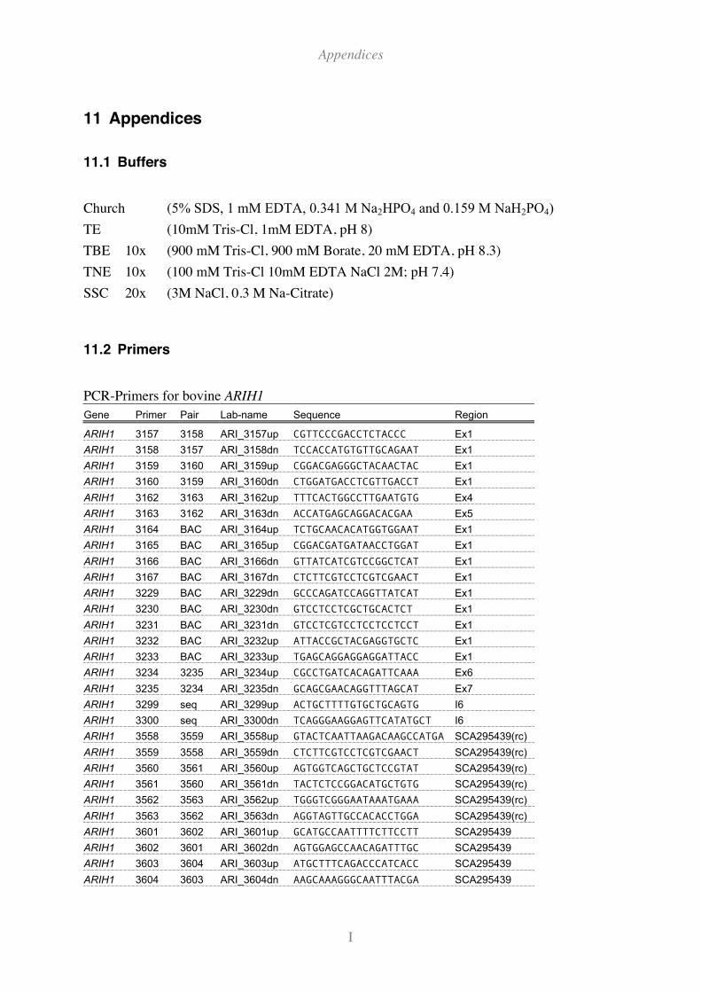
Appendices
I
11 Appendices
11.1 Buffers
Church (5% SDS, 1 mM EDTA, 0.341 M Na2HPO4 and 0.159 M NaH2PO4)
TE (10mM Tris-Cl, 1mM EDTA, pH 8)
TBE 10x (900 mM Tris-Cl, 900 mM Borate, 20 mM EDTA, pH 8.3)
TNE 10x (100 mM Tris-Cl 10mM EDTA NaCl 2M; pH 7.4)
SSC 20x (3M NaCl, 0.3 M Na-Citrate)
11.2 Primers
PCR-Primers for bovine ARIH1
Gene Primer Pair Lab-name Sequence Region
ARIH1 3157 3158 ARI_3157up CGTTCCCGACCTCTACCC Ex1
ARIH1 3158 3157 ARI_3158dn TCCACCATGTGTTGCAGAAT Ex1
ARIH1 3159 3160 ARI_3159up CGGACGAGGGCTACAACTAC Ex1
ARIH1 3160 3159 ARI_3160dn CTGGATGACCTCGTTGACCT Ex1
ARIH1 3162 3163 ARI_3162up TTTCACTGGCCTTGAATGTG Ex4
ARIH1 3163 3162 ARI_3163dn ACCATGAGCAGGACACGAA Ex5
ARIH1 3164 BAC ARI_3164up TCTGCAACACATGGTGGAAT Ex1
ARIH1 3165 BAC ARI_3165up CGGACGATGATAACCTGGAT Ex1
ARIH1 3166 BAC ARI_3166dn GTTATCATCGTCCGGCTCAT Ex1
ARIH1 3167 BAC ARI_3167dn CTCTTCGTCCTCGTCGAACT Ex1
ARIH1 3229 BAC ARI_3229dn GCCCAGATCCAGGTTATCAT Ex1
ARIH1 3230 BAC ARI_3230dn GTCCTCCTCGCTGCACTCT Ex1
ARIH1 3231 BAC ARI_3231dn GTCCTCGTCCTCCTCCTCCT Ex1
ARIH1 3232 BAC ARI_3232up ATTACCGCTACGAGGTGCTC Ex1
ARIH1 3233 BAC ARI_3233up TGAGCAGGAGGAGGATTACC Ex1
ARIH1 3234 3235 ARI_3234up CGCCTGATCACAGATTCAAA Ex6
ARIH1 3235 3234 ARI_3235dn GCAGCGAACAGGTTTAGCAT Ex7
ARIH1 3299 seq ARI_3299up ACTGCTTTTGTGCTGCAGTG I6
ARIH1 3300 seq ARI_3300dn TCAGGGAAGGAGTTCATATGCT I6
ARIH1 3558 3559 ARI_3558up GTACTCAATTAAGACAAGCCATGA SCA295439(rc)
ARIH1 3559 3558 ARI_3559dn CTCTTCGTCCTCGTCGAACT SCA295439(rc)
ARIH1 3560 3561 ARI_3560up AGTGGTCAGCTGCTCCGTAT SCA295439(rc)
ARIH1 3561 3560 ARI_3561dn TACTCTCCGGACATGCTGTG SCA295439(rc)
ARIH1 3562 3563 ARI_3562up TGGGTCGGGAATAAATGAAA SCA295439(rc)
ARIH1 3563 3562 ARI_3563dn AGGTAGTTGCCACACCTGGA SCA295439(rc)
ARIH1 3601 3602 ARI_3601up GCATGCCAATTTTCTTCCTT SCA295439
ARIH1 3602 3601 ARI_3602dn AGTGGAGCCAACAGATTTGC SCA295439
ARIH1 3603 3604 ARI_3603up ATGCTTTCAGACCCATCACC SCA295439
ARIH1 3604 3603 ARI_3604dn AAGCAAAGGGCAATTTACGA SCA295439
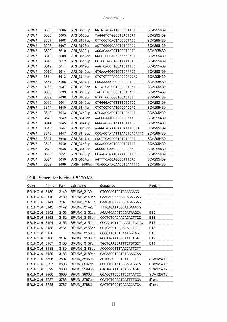
Appendices
II
ARIH1 3605 3606 ARI_3605up GGTGTACAGTTGCCCCAAGT SCA295439
ARIH1 3606 3605 ARI_3606dn TAGGGTCTGGCCTCAGTGAT SCA295439
ARIH1 3607 3608 ARI_3607up GTTGGCTCAGTAGCGGTAGC SCA295439
ARIH1 3608 3607 ARI_3608dn ACTTGGGGCAACTGTACACC SCA295439
ARIH1 3609 3610 ARI_3609up AGGACAAATGTTCCGTGGTC SCA295439
ARIH1 3610 3609 ARI_3610dn GGCCTCCGAGAGAAAACAGT SCA295439
ARIH1 3611 3612 ARI_3611up CCTCCTGCCTGGTAAAACAC SCA295439
ARIH1 3612 3611 ARI_3612dn AAGTCACCTTGCATCTTTGG SCA295439
ARIH1 3613 3614 ARI_3613up GTGAAAGCGCTGGTGAAACT SCA295439
ARIH1 3614 3613 ARI_3614dn CTGTGTTTTACCAGGCAGGAG SCA295439
ARIH1 3637 3166 ARI_3637up CGGAAAAATCCACCACCTG SCA295439
ARIH1 3166 3637 ARI_3166dn GTTATCATCGTCCGGCTCAT SCA295439
ARIH1 3638 3639 ARI_3638up TACTCTGTTCGCTGCTGAGG SCA295439
ARIH1 3639 3638 ARI_3639dn GTCCTCCTCGCTGCACTCT SCA295439
ARIH1 3640 3641 ARI_3640up CTGGGGACTGTTTTCTCTCG SCA295439
ARIH1 3641 3640 ARI_3641dn GTCTGCTCTATCCCCAGCAG SCA295439
ARIH1 3642 3643 ARI_3642up GTCAACGAGGTCATCCAGGT SCA295439
ARIH1 3643 3642 ARI_3643dn AACCCAAACGAACAGCAAAC SCA295439
ARIH1 3644 3645 ARI_3644up GGGCAGTGGTATTTCTTTCG SCA295439
ARIH1 3645 3644 ARI_3645dn AAGGCACAATCAACATTTGCTA SCA295439
ARIH1 3646 3647 ARI_3646up CCCAGCTATATTTAACTCACATTG SCA295439
ARIH1 3647 3646 ARI_3647dn CGCTTCAGTCGTGTCTGACT SCA295439
ARIH1 3648 3649 ARI_3648up GCAACCCACTCCAGTGTTCT SCA295439
ARIH1 3649 3648 ARI_3649dn AGGGGTGAAGAAAACCCAAC SCA295439
ARIH1 3650 3651 ARI_3650up CCAACATGATCAAAAGCTTGG SCA295439
ARIH1 3651 3650 ARI_3651dn AGTTTCACCAGCGCTTTCAC SCA295439
ARIH1 3698 3699 ARIH_3698up TGAGGCATACAACCTCAATTTC SCA295439
PCR-Primers for bovine BRUNOL6
Gene Primer Pair Lab-name Sequence Region
BRUNOL6 3139 3140 BRUN6_3139up GTGGCACTAGTGGAGGAGG
BRUNOL6 3140 3139 BRUN6_3140dn CAACAGGAAAGGCAGAGGAG
BRUNOL6 3141 3141 BRUN6_3141up CAACAGGAAAGGCAGAGGAG
BRUNOL6 3142 3142 BRUN6_3142dn TTTCAGATTGGCATGAAACG
BRUNOL6 3152 3153 BRUN6_3152up AGAAGCACCTCGGATAAGCA E15
BRUNOL6 3153 3152 BRUN6_3153dn GGCTGTGACAACAGACTTGG E15
BRUNOL6 3154 3155 BRUN6_3154up GCGAATCTTCCAAGTCTGTTG E15
BRUNOL6 3155 3154 BRUN6_3155dn GCTGAGCTGAGACACCTCCT E15
BRUNOL6 3156 BRUN6_3156up CCCCTTCTCTCAATGGCAGT E15
BRUNOL6 3186 3187 BRUN6_3186up GCCATGAATGGCTTTCAGAT E12
BRUNOL6 3187 3186 BRUN6_3187dn TGCTCAAGCATTTCTGTGCT E13
BRUNOL6 3188 3189 BRUN6_3188up AGGCCGCTTTAAGGATTGTT
BRUNOL6 3189 3188 BRUN6_3189dn CAGAAGGTGGTCTGGAGCAA
BRUNOL6 3596 3597 BRUN_3596up ACTCCAGCCATCTTCCCTCT SCA125719
BRUNOL6 3597 3596 BRUN_3597dn CGCTTCCTATGGGAGTGGTA SCA125719
BRUNOL6 3599 3600 BRUN_3599up CACAGCATTGACAGGCAGAT SCA125719
BRUNOL6 3600 3599 BRUN_3600dn GGAGCTTGGGTTCCTAATCC SCA125719
BRUNOL6 3787 3788 BRUN_3787up CCATCTGCAGTGATTTTGGA 5’-end
BRUNOL6 3788 3787 BRUN_3788dn GACTGTGGCTCAGACCATGA 5’-end
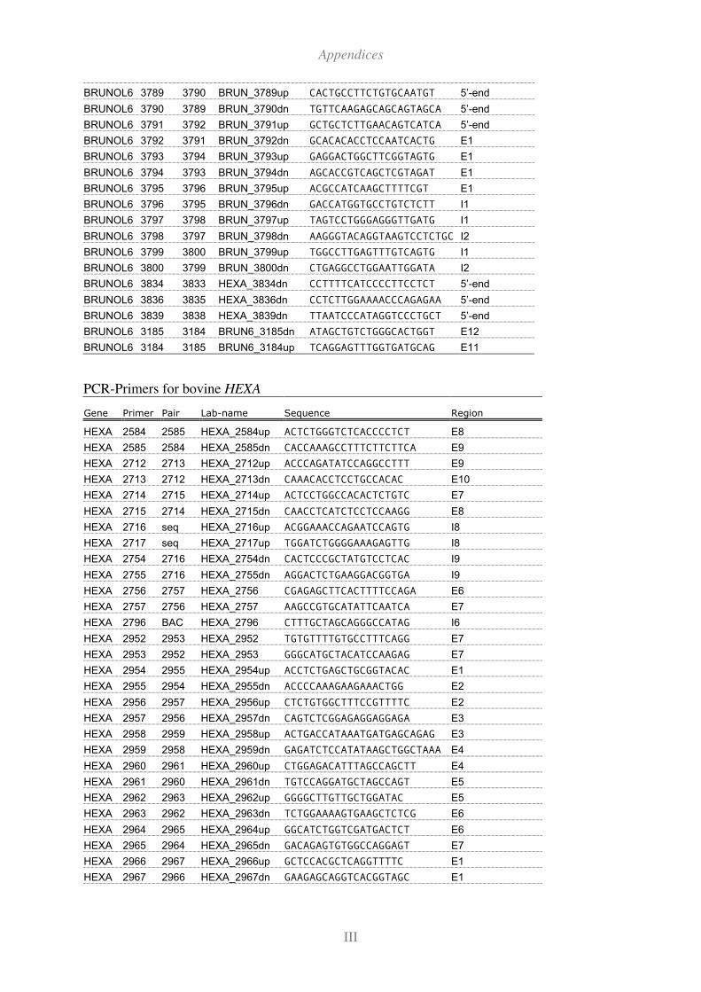
Appendices
III
BRUNOL6 3789 3790 BRUN_3789up CACTGCCTTCTGTGCAATGT 5’-end
BRUNOL6 3790 3789 BRUN_3790dn TGTTCAAGAGCAGCAGTAGCA 5’-end
BRUNOL6 3791 3792 BRUN_3791up GCTGCTCTTGAACAGTCATCA 5’-end
BRUNOL6 3792 3791 BRUN_3792dn GCACACACCTCCAATCACTG E1
BRUNOL6 3793 3794 BRUN_3793up GAGGACTGGCTTCGGTAGTG E1
BRUNOL6 3794 3793 BRUN_3794dn AGCACCGTCAGCTCGTAGAT E1
BRUNOL6 3795 3796 BRUN_3795up ACGCCATCAAGCTTTTCGT E1
BRUNOL6 3796 3795 BRUN_3796dn GACCATGGTGCCTGTCTCTT I1
BRUNOL6 3797 3798 BRUN_3797up TAGTCCTGGGAGGGTTGATG I1
BRUNOL6 3798 3797 BRUN_3798dn AAGGGTACAGGTAAGTCCTCTGC I2
BRUNOL6 3799 3800 BRUN_3799up TGGCCTTGAGTTTGTCAGTG I1
BRUNOL6 3800 3799 BRUN_3800dn CTGAGGCCTGGAATTGGATA I2
BRUNOL6 3834 3833 HEXA_3834dn CCTTTTCATCCCCTTCCTCT 5’-end
BRUNOL6 3836 3835 HEXA_3836dn CCTCTTGGAAAACCCAGAGAA 5’-end
BRUNOL6 3839 3838 HEXA_3839dn TTAATCCCATAGGTCCCTGCT 5’-end
BRUNOL6 3185 3184 BRUN6_3185dn ATAGCTGTCTGGGCACTGGT E12
BRUNOL6 3184 3185 BRUN6_3184up TCAGGAGTTTGGTGATGCAG E11
PCR-Primers for bovine HEXA
Gene Primer Pair Lab-name Sequence Region
HEXA 2584 2585 HEXA_2584up ACTCTGGGTCTCACCCCTCT E8
HEXA 2585 2584 HEXA_2585dn CACCAAAGCCTTTCTTCTTCA E9
HEXA 2712 2713 HEXA_2712up ACCCAGATATCCAGGCCTTT E9
HEXA 2713 2712 HEXA_2713dn CAAACACCTCCTGCCACAC E10
HEXA 2714 2715 HEXA_2714up ACTCCTGGCCACACTCTGTC E7
HEXA 2715 2714 HEXA_2715dn CAACCTCATCTCCTCCAAGG E8
HEXA 2716 seq HEXA_2716up ACGGAAACCAGAATCCAGTG I8
HEXA 2717 seq HEXA_2717up TGGATCTGGGGAAAGAGTTG I8
HEXA 2754 2716 HEXA_2754dn CACTCCCGCTATGTCCTCAC I9
HEXA 2755 2716 HEXA_2755dn AGGACTCTGAAGGACGGTGA I9
HEXA 2756 2757 HEXA_2756 CGAGAGCTTCACTTTTCCAGA E6
HEXA 2757 2756 HEXA_2757 AAGCCGTGCATATTCAATCA E7
HEXA 2796 BAC HEXA_2796 CTTTGCTAGCAGGGCCATAG I6
HEXA 2952 2953 HEXA_2952 TGTGTTTTGTGCCTTTCAGG E7
HEXA 2953 2952 HEXA_2953 GGGCATGCTACATCCAAGAG E7
HEXA 2954 2955 HEXA_2954up ACCTCTGAGCTGCGGTACAC E1
HEXA 2955 2954 HEXA_2955dn ACCCCAAAGAAGAAACTGG E2
HEXA 2956 2957 HEXA_2956up CTCTGTGGCTTTCCGTTTTC E2
HEXA 2957 2956 HEXA_2957dn CAGTCTCGGAGAGGAGGAGA E3
HEXA 2958 2959 HEXA_2958up ACTGACCATAAATGATGAGCAGAG E3
HEXA 2959 2958 HEXA_2959dn GAGATCTCCATATAAGCTGGCTAAA E4
HEXA 2960 2961 HEXA_2960up CTGGAGACATTTAGCCAGCTT E4
HEXA 2961 2960 HEXA_2961dn TGTCCAGGATGCTAGCCAGT E5
HEXA 2962 2963 HEXA_2962up GGGGCTTGTTGCTGGATAC E5
HEXA 2963 2962 HEXA_2963dn TCTGGAAAAGTGAAGCTCTCG E6
HEXA 2964 2965 HEXA_2964up GGCATCTGGTCGATGACTCT E6
HEXA 2965 2964 HEXA_2965dn GACAGAGTGTGGCCAGGAGT E7
HEXA 2966 2967 HEXA_2966up GCTCCACGCTCAGGTTTTC E1
HEXA 2967 2966 HEXA_2967dn GAAGAGCAGGTCACGGTAGC E1
Appendices
IV
HEXA 2990 seq HEXA_2990up CTGCAGGGAGTGTTCTCCTC I3
HEXA 2991 seq HEXA_2991dn TCCTATGTGGCAGAGCACAG I3
HEXA 2992 seq HEXA_2992up TTAGGATTCTGGGGTGATGG I5
HEXA 2993 seq HEXA_2993dn TCAGAGCACACACTGTGAACC I5
HEXA 2994 2995 HEXA_2994up CTGTGCTCTGCCACATAGGA I3
HEXA 2995 2994 HEXA_2995dn GGGACCATCTCAAGCCACTA I4
HEXA 2997 2998 HEXA_2997up CCTCTCGGAACTGAGCAAAC E10
HEXA 2998 2997 HEXA_2998dn ACCAGTGCCAACTCCTTCAC E11
HEXA 2999 3000 HEXA_2999up ATCATCCAGGTATGGCGAGA E11
HEXA 3000 2999 HEXA_3000dn CAGGTTTGTGCTGTCCACAT E12
HEXA 3001 3002 HEXA_3001up GGCCTGTATGTGGGGAGAGT E12
HEXA 3002 3001 HEXA_3002dn CAGCTCACAGCGGAAGTGT E13
HEXA 3003 3004 HEXA_3003up AGGCTGTGGAGCAACAAGAT E13
HEXA 3004 3003 HEXA_3004dn CTCTCCTAGGGCCAGTACCC E14
HEXA 3005 3006 HEXA_3005up ACGCACACAGTTTGTTCAGC I3
HEXA 3006 3005 HEXA_3006dn TGCCCCTCCTAGCAATACAC I3
HEXA 3007 3008 HEXA_3007up TTCTCTGAACAAGGGCAGCTA I5
HEXA 3008 3007 HEXA_3008dn CCCCAGCTTCTTGCTAAGTG I5
HEXA 3009 3010 HEXA_3009up CTGGGTTCACAGTGTGTGCT I5
HEXA 3010 3009 HEXA_3010dn CTTTGCTAGCAGGGCCATAG I6
HEXA 3011 3012 HEXA_3011up GTTGAGGCCTGTCTTTGCTT I11
HEXA 3012 3011 HEXA_3012dn GAGAGCCCATGCCACAAG I12
HEXA 3013 seq HEXA_3013up AGAGGGTCAGTTCCCTGGTT I13
HEXA 3014 3015 HEXA_3014up CCCCATAGAAAAACGGCATA E2
HEXA 3015 3014 HEXA_3015dn GACAGTCTCGGAGAGGAGGA E3
HEXA 3044 3045 HEXA_3044up CACTGGACCACCAGGAAAGT I2
HEXA 3045 3044 HEXA_3045dn CTCCCTCTGCTTCCCAGAGT I3
HEXA 3046 HEXA_3046up GCGTTTTGGAGAAACAGCAT I3
HEXA 3059 3060 HEXA_3059up ACGTGGGGCTTCTATCCTCT 5’-UTR
HEXA 3060 3059 HEXA_3060dn ACTGGAATTGGAAGCTTTGC E1
HEXA 3061 3062 HEXA_3061up ACAGAAGCAGGGAGGCATT E14
HEXA 3062 3061 HEXA_3062dn CTCCAGGGGCAGATACTGAG 3’-UTR
HEXA 3063 2955 HEXA_3063up ATGGCCCCAGTACATTCAGA E1
HEXA 3064 3065 HEXA_3064up AGCTGCGGTACACCATCTTC E1
HEXA 3065 3064 HEXA_3065dn CCAGACAAGTGCTGGCTTCT E2
HEXA 3078 3079 HEXA_3078up AACCGCCTGAACTTGAACC 5´-end
HEXA 3079 3078 HEXA_3079dn CAGAGGAAGGGCGTTTCAG I1
HEXA 3080 BAC HEXA_3080up TCTGTAATCCTGCCCTCCTG I1
HEXA 3125 SBE HEXA_3111dn TGCTCAGAGATGGTAAGGAACTC I13
HEXA 3112 SBE HEXA_3112up AACTGTACCATTAATTTCCTCTGTGA I6
HEXA 3113 SBE HEXA_3113dn AACTCTCCTCAGGCCATTTCAT I11
HEXA 3114 SBE HEXA_3114dn GGGCTCCAGGCCTAGCAT I2
HEXA 3115 3116 HEXA_3115up AAGCCAGCACTTGTCTGGAG I2
HEXA 3116 3115 HEXA_3116dn TCAGACGCTGGTTAGAGTGC I2
HEXA 3117 3118 HEXA_3117up ACCAGCCAGTTTAAGGGACA I6
HEXA 3118 3117 HEXA_3118dn CCATGATGCCAGTGAGACAA I6
HEXA 3119 3120 HEXA_3119up ACTCTGGGGAAACAGCTTCA I13
HEXA 3120 3119 HEXA_3120dn ATCTCAGCCTCACCAGTTCC I13
HEXA 3126 3127 HEXA_3126up AGGAGCTGTAGCGGGTCAC E1
HEXA 3127 3126 HEXA_3127dn GAGCCCGGGAACGAGACT E1
Appendices
V
HEXA 3128 BAC HEXA_3128dn GACCGAAAGCAGTCCAGAAG 5´-end
HEXA 3130 3129 HEXA_3130up GCGTAGGCTACTGTGACATGG 3´-end
HEXA 3129 3130 HEXA_3129dn GGGGTGTGTGTCTGGACTCT 3´-end
HEXA 3132 3131 HEXA_3132up CTCAGTATCTGCCCCTGGAG 3´-end
HEXA 3131 3132 HEXA_3131dn TTTGTGGAAGAGGGGTTCAC 3´-end
HEXA 3133 BAC HEXA_3133up TGAACGCGGAATAAAAGGTC 3´-end
HEXA 3134 3135 HEXA_3134up TCTCTAGCTGAGCCCATTCTG 5´-end
HEXA 3135 3134 HEXA_3135dn AGAGAGAACCCGAAGCTCCT 5´-end
HEXA 3136 BAC HEXA_3136dn CCAGGGAACTTCAGAAGCAA 5´-end
HEXA 3137 BAC HEXA_3137up GGGTCTTTGGGGACTCTCTC 3´-end
HEXA 3138 BAC HEXA_3138up GTGAACCCCTCTTCCACAAA 3´-end
HEXA 3147 3148 HEXA_3147up CCTAGCCTGTTTGTGGCATT 5´-end
HEXA 3148 3147 HEXA_3148dn GTGACCCGGGAGTACTGACT 5´-end
HEXA 3149 BAC HEXA_3149dn TGCAAGCGATAAGACATTGC 5´-end
HEXA 3150 BAC HEXA_3150up ATGCCTCTCCTAGCTCACCA 3´-end
HEXA 3151 BAC HEXA_3151dn GGCTGGGAACGAAACTTGTA 3´-end
HEXA 3161 3064 HEXA_3161dn TCGGTGATTTTCCTCTCACA I1
HEXA 3190 3191 HEXA_3190up GGTTGCAAAGAGCTGCTG I1
HEXA 3191 3190 HEXA_3191dn GACGGTTCTGGGCACTTG I2
HEXA 3192 BAC HEXA_3192dn GGTGCCACCTAGTCACCTGT I1
HEXA 3474 3475 HEXA_3474up CCAGAGATTGACAGGGTGGT 5'-end (SCA95258)
HEXA 3475 3474 HEXA_3475dn CCTGAGGAAGTGGTTTCCAA 5'-end (SCA95258)
HEXA 3476 3477 HEXA_3476up TGATTCCACTTTATGAGCCAAA 5'-end
HEXA 3477 3476 HEXA_3477dn TGCCATAACTCCCCTTTCTG 5’-end
HEXA 3478 3479 HEXA_3478up CTGGGAAAACTGGACAGCTC SCA95258
HEXA 3479 3478 HEXA_3479dn CCACGCACCAAAACTACTGA SCA5566
HEXA 3480 3481 HEXA_3480up CACAGCACGTGAGAATGGTC 5’-end (SCA95258)
HEXA 3481 3480 HEXA_3481dn TGCCTGTCCATTTGTCTGAG 5’-end (SCA95258)
HEXA 3482 3483 HEXA_3482up ATTCAGCTCGCCCTCTCTC 3’-end (SCA5566)
HEXA 3483 3482 HEXA_3483dn GCTAAGTATCAGATTTCCAGAGGA 3’-end (SCA5566)
HEXA 3484 3485 HEXA_3484up TGGAACCCACTCAGAAAAGG 3’-end (SCA5566)
HEXA 3485 3484 HEXA_3485dn CCTCAGTGAGAGCAGCCTTC 3’-end (SCA5566)
HEXA 3486 3487 HEXA_3486up GCATTGGCCCAAAGACTACT SCA184260
HEXA 3487 3486 HEXA_3487dn CCCTTTCTAGCCTGTTTTGC SCA184260
HEXA 3488 3489 HEXA_3488up CTCATCCAGCGCTCTTTAGC SCA15309
HEXA 3489 3488 HEXA_3489dn GAATCCCATCGTCTGACTGC SCA15309
HEXA 3496 3497 HEXA_3496up CCGAAGACCTTGGGAAGAAT SCA125719
HEXA 3497 3496 HEXA_3497dn GGATGCAATCTGGGTGTCTT SCA125719
HEXA 3498 3499 HEXA_3498up GCATTGTGCTGGTGTACAGA SCA125719
HEXA 3499 3498 HEXA_3499dn TGACAGCCTTTCCCGTAGAA SCA125719
HEXA 3500 3501 HEXA_3500up AGTTTTGCTGCCCAACTCAT SCA95258
HEXA 3501 3500 HEXA_3501dn AAGTTGCCTTGTGGGAAAAC SCA95258
HEXA 3502 3503 HEXA_3502up ACCAGAAGGCGACAGAAAGA SCA5566
HEXA 3503 3502 HEXA_3503dn GGGGAACCTGAGACCATTTT SCA5566
HEXA 3526 3527 HEXA_3526up ACAGCCCCAAACTGAGGATT SCA125719
HEXA 3527 3526 HEXA_3527dn CAGGAGTTTGGTGATGCAGA SCA125719
HEXA 3528 3529 HEXA_3528up GGCAGGAATGTCTGGATGAG SCA125719
HEXA 3529 3528 HEXA_3529dn CCAGGCTCGGACAGTCTCTA SCA125719
HEXA 3530 3531 HEXA_3530up AGACTGTCCGAGCCTGGTT SCA125719
HEXA 3531 3530 HEXA_3531dn GAGGAGTGCACCGTCTTACG SCA125719
Appendices
VI
HEXA 3532 3533 HEXA_3532up CAGGGGTCAGCTCAAGTCAC SCA125719
HEXA 3533 3532 HEXA_3533dn TAGGTGGCTACTGGGTCTGC SCA125719
HEXA 3538 3539 HEXA_3538up CAGTTCCACATGGTGTATGAAGA SCA125719
HEXA 3539 3538 HEXA_3539dn CCAAACTGCCATAGTTCAACC SCA125719
HEXA 3652 3653 HEXA_3652up GGAGAAGGGAACAGCTACCC 5’-end
HEXA 3653 3652 HEXA_3653dn ATGAAGAAGCTGGACCCAAA 5’-end
HEXA 3654 3655 HEXA_3654up GATCCGCTGGTGAAGGAATA 5’-end
HEXA 3655 3654 HEXA_3655dn TAATTCCCTGGTGAGGGATG 5’-end
HEXA 3656 3657 HEXA_3656up AAGCAACCTAGGTGCATCGT 5’-end
HEXA 3657 3656 HEXA_3657dn GTGTGTTGCCATTTCCTCCT 5’-end
HEXA 3658 3659 HEXA_3658up AGGAGGAAATGGCAACACAC 5’-end
HEXA 3659 3658 HEXA_3659dn AGGAAACGGGCTCTGAGAAT 5’-end
HEXA 3660 3661 HEXA_3660up GGCATAGAAGACTTGGGTTCA 5’-end
HEXA 3661 3660 HEXA_3661dn CTGGGCATATCTCCTTGGAA 5’-end
HEXA 3662 3663 HEXA_3662up CCAGGGCTAGGAATACAGCA 5’-end
HEXA 3663 3662 HEXA_3663dn TCCACCCCATGGACTATACA 5’-end
HEXA 3801 3802 HEXA_3801up ATGCCTCTCCTAGCTCACCA 3’-end
HEXA 3802 3801 HEXA_3802dn CGAGCTCAGCTTTCCCTATG 3’-end
HEXA 3833 3834 HEXA_3833up TGAACTGAACAGCACCATGA 3’-end
HEXA 3835 3836 HEXA_3835up TGCTCCATCATCAAGTCCTG 3’-end
HEXA 3837 3836 HEXA_3837up CCCCCATTAAAGGACAAAGA 5’-end
HEXA 3838 3839 HEXA_3838up AGCTCTAGCAAGATGCATGACT 5’-end
PCR Primers for bovine PARP6
Gene Primer Pair Lab-name Sequence Region
PARP6 3490 3491 HEXA_3490up ATGCGCTTCCTGCCATAAG SCA184260
PARP6 3491 3490 HEXA_3491dn GTCCCCAACCGTGGTTTC SCA184260
PARP6 3492 3493 HEXA_3492up TTCTTCCCCTTCTCCTCAGC SCA3547
PARP6 3493 3492 HEXA_3493dn GCCACCAGACTGACTTACACC SCA3547
PARP6 3494 3495 HEXA_3494up GCCTTTGAAGACTCATGTTTGA SCA3547
PARP6 3495 3494 HEXA_3495dn ACCCCAAAGAGCCTAATGTC SCA3547
PARP6 3534 3535 HEXA_3534up TTTCTGACATGTGCCCAAGA PARP6
PARP6 3535 3534 HEXA_3535dn TTCATCCCACAAACTTGTTCC PARP6
PARP6 3536 3537 HEXA_3536up GTGAGTGATTGGCCACAAAG PARP6
PARP6 3537 3536 HEXA_3537dn AATTCAGGCTTGGAGACTGC PARP6
PARP6 3615 3616 PARP_3615up TCCCTGATCTCCCATTTCTG SCA184260
PARP6 3616 3615 PARP_3616dn GCACGTTCATCGCTAGCTT SCA338507
PARP6 3618 3615 PARP_3617dn GTGTGAGAATGGGTGGGAAT SCA338507
PARP6 3746 3747 PARP_3746up TCCCTGATCTCCCATTTCTG E17
PARP6 3747 3746 PARP_3747dn CAGACTTCCCCGACATGAGT E18
PARP6 3748 3749 PARP_3748up GGAGTCTTGTTCCCAATGCT E6
PARP6 3749 3748 PARP_3749dn TGATGGTTCTGCAAAGAGAAGA E7
PARP6 3750 3751 PARP_3750up CCCTTATTTCTTGTTTTTCATCA E3
PARP6 3751 3750 PARP_3751dn CCCCTACCATCCCTGAAGTA E4
PARP6 3752 3753 PARP_3752up GGAGAAATAACTGGGGATAAAGA E2
PARP6 3753 3752 PARP_3753dn TACTGTTTCCATGCCCCATC E2
PARP6 3754 3755 PARP_3754up CAGAAAGCAAGCAGCAACAA E1
PARP6 3755 3754 PARP_3755dn TCAAGCACAAAAGGCAGAAG E1
PARP6 3756 3757 PARP_3756up TGAAGAAACCAAGGCTCAAGT E11
Appendices
VII
PARP6 3757 3756 PARP_3757dn TTAGGGCATGAGTTTGATCC E12
PARP6 3758 3759 PARP_3758up AATGTGTTCATTTCTGCTACACAG E13
PARP6 3759 3758 PARP_3759dn GCCTGGTACTTCTCAGCCTTC E14
PARP6 3760 3761 PARP_3760up TGGGTGAATGAACTGGTTTG E19
PARP6 3761 3760 PARP_3761dn TACCCATCCTCATCCTCCAA E20
PARP6 3762 3763 PARP_3762up TTGGAGGATGAGGATGGGTA E22
PARP6 3763 3762 PARP_3763dn AATAGCTGGGAGGAGGAGGA E22
PARP6 3764 3765 PARP_3764up AGAGATAATGCCCCCTTGCT E16
PARP6 3765 3764 PARP_3765dn GGAGGAACTGGTGTGAGGTG E17
Primers for direct sequencing of BAC DNABAC Primer No Lab-name Sequence Region
All 1658 SP6 TTTGCGATCTGCCGTTTC vector pBACe3.6
All 1659 T7 CCGCTAATACGACTCACTATAGGG vector pBACe3.6
909 3429 909_3429up TGCTGCTGCTGCTAAGTCAC 909_T7
920 3430 920_3430up TGGTTCCTCTGCCTTTCCTA 920_SP6
907 3431 907_3431up CATTCTTGGCAACATGGCTA 907_SP6
909 3434 909_3434up GGAAGGGCTTGAGACAGAGA 909_SP6
910 3435 910_3435up AGGGAATAAGGCGATAGGG 910_SP6
907 3438 907_3438up GCAGTCAGACGATGGGATTC 907_T7
910 3439 910_3439up CCACTAGGGGGCTAGGGTAG 910_T7
910 3440 910_3440up TGGATTTAGATCCTGGCTTCA 910_T7
920 3441 920_3441up TACTTGGGGATGGGTGAGAA 920_T7
920 3442 920_3442up TGATGGTACCGCTTGTCTTG 920_T7
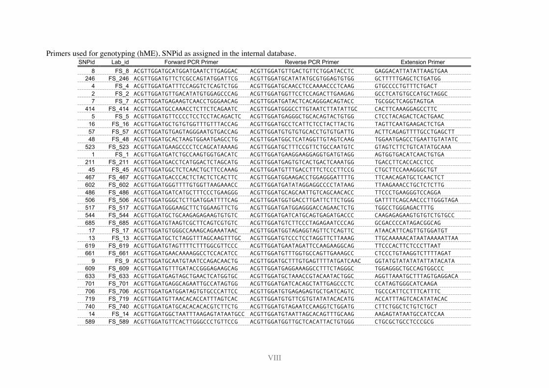
VIII
Primers used for genotyping (hME), SNPid as assigned in the internal database.SNPid Lab_id Forward PCR Primer Reverse PCR Primer Extension Primer
8 FS_8 ACGTTGGATGCATGGATGAATCTTGAGGAC ACGTTGGATGTTGACTGTTCTGGATACCTC GAGGACATTATATTAAGTGAA
246 FS_246 ACGTTGGATGTTCTCGCCAGTATGGATTCG ACGTTGGATGCATATATGCGTGGAGTGTGG GCTTTTTGAGCTCTGATGG
4 FS_4 ACGTTGGATGATTTCCAGGTCTCAGTCTGG ACGTTGGATGCAACCTCCAAAACCCTCAAG GTGCCCCTGTTTCTGACT
2 FS_2 ACGTTGGATGTTGACATATGTGGAGCCCAG ACGTTGGATGGTTCCTCCAGACTTGAAGAG GCCTCATGTGCCATGCTAGGC
7 FS_7 ACGTTGGATGAGAAGTCAACCTGGGAACAG ACGTTGGATGATACTCACAGGGACAGTACC TGCGGCTCAGGTAGTGA
414 FS_414 ACGTTGGATGCCAAACCTCTTCTCAGAATC ACGTTGGATGGGCCTTGTAATCTTATATTGC CACTTCAAAGGAGCCTTC
5 FS_5 ACGTTGGATGTTCCCCTCCTCCTACAGACTC ACGTTGGATGAGGGCTGCACAGTACTGTGG CTCCTACAGACTCACTGAAC
16 FS_16 ACGTTGGATGCTGTGTGGTTTGTTTACCAG ACGTTGGATGCCTCATTCTCCTACTTACTG TAGTTCAATGAAGACTCTGA
57 FS_57 ACGTTGGATGTGAGTAGGGAATGTGACCAG ACGTTGGATGTGTGTGCACCTGTGTGATTG ACTTCAGAGTTTTGCCTGAGCTT
48 FS_48 ACGTTGGATGCACTAAGTGGAATGAGCCTG ACGTTGGATGGCTCATAGGTTGTAGTCAAG TGGAATGAGCCTGAATTGTATATC
523 FS_523 ACGTTGGATGAAGCCCCTCCAGCATAAAAG ACGTTGGATGCTTTCCGTTCTGCCAATGTC GTAGTCTTCTGTCATATGCAAA
1 FS_1 ACGTTGGATGATCTGCCAAGTGGTGACATC ACGTTGGATGAAGGAAGGAGGTGATGTAGG AGTGGTGACATCAACTGTGA
211 FS_211 ACGTTGGATGACCTCATGGACTCTAGCATG ACGTTGGATGAGTGTCACTGACTCAAATGG TGACCTTCACCACCTCC
45 FS_45 ACGTTGGATGGCTCTCAACTGCTTCCAAAG ACGTTGGATGTTTGACCTTTCTCCCTTCCG CTGCTTCCAAAGGGCTGT
467 FS_467 ACGTTGGATGACCCACTCTACTCTCACTTC ACGTTGGATGGAAGACCTGGAGGGATTTTG TTCAACAGATGCTCAACTCT
602 FS_602 ACGTTGGATGGGTTTTGTGGTTAAGAAACC ACGTTGGATGATATAGGAGGCCCCTATAAG TTAAGAAACCTGCTCTCTTG
486 FS_486 ACGTTGGATGATCATGCTTTCCCTGAAGGG ACGTTGGATGCAGCAATTGTCAGCAACACC TTCCCTGAAGGGTCCAGGA
506 FS_506 ACGTTGGATGGGCTCTTGATGGATTTTCAG ACGTTGGATGGTGACCTTGATTCTTCTGGG GATTTTCAGCAACCCTTGGGTAGA
517 FS_517 ACGTTGGATGGGAAGCTTCTGGAAGTTCTG ACGTTGGATGATGGAGGGACCAGAACTCTG TGGCCTGGGAGACTTTG
544 FS_544 ACGTTGGATGCTGCAAGAGAGAAGTGTGTC ACGTTGGATGATCATGCAGTGAGATGACCC CAAGAGAGAAGTGTGTCTGTGCC
685 FS_685 ACGTTGGATGTAAGTCGCTTCAGTCGTGTC ACGTTGGATGTCTTCCCTAGAGAATCCCAG GCGACCCCATAGACGGCAG
17 FS_17 ACGTTGGATGTGGGCCAAAGCAGAAATAAC ACGTTGGATGGTAGAGGTAGTTCTCAGTTC ATAACATTCAGTTGTGGATGT
13 FS_13 ACGTTGGATGCTCTAGGTTTAGCAAGTTTGC ACGTTGGATGTCCCTCCTAGGTTCTTAAAG TTGCAAAAACATAATAAAAATTAA
619 FS_619 ACGTTGGATGTAGTTTTCTTTGGCGTTCCC ACGTTGGATGAATAGATTCCAAGAAGGCAG TTCCCACTTCTCCCTTAAT
661 FS_661 ACGTTGGATGAACAAAAGGCCTCCACATCC ACGTTGGATGTTTGGTGCCAGTTGAAAGCC CTCCCTGTAAGGTCTTTTAGAT
9 FS_9 ACGTTGGATGCAATGTAATCCAGACAACTG ACGTTGGATGCTTTGTGAGTTTTATGATCAAC GGTATGTATATATATTATACATA
609 FS_609 ACGTTGGATGTTTGATACCGGGAGAAGCAG ACGTTGGATGAGGAAAGGCCTTTCTAGGGC TGGAGGGCTGCCAGTGGCCC
633 FS_633 ACGTTGGATGAGTAGCTGAACTCATGGTGC ACGTTGGATGCTAAACCGTACAATACTGGC AGGTTAAATGCTTTAGTGAGGACA
701 FS_701 ACGTTGGATGAGGCAGAATTGCCATAGTGG ACGTTGGATGATCACAGCTATTGAGCCCTC CCATAGTGGGCATCAAGA
706 FS_706 ACGTTGGATGATGGATAGTGTGCCCATTCC ACGTTGGATGTGAGAGAGTGCTGATCAGTC TGCCCATTCCTTTCATTTC
719 FS_719 ACGTTGGATGTTAACACACCATTTAGTCAC ACGTTGGATGTGTTCGTGTATATACACATG ACCATTTAGTCACATATACAC
740 FS_740 ACGTTGGATGATGCACACACACGTCTTCTG ACGTTGGATGTAGAATCCAAGGTCTGGATG CTTCTGGCTCTGTCTGCT
14 FS_14 ACGTTGGATGGCTAATTTAAGAGTATAATGCC ACGTTGGATGTAATTAGCACAGTTTGCAAG AAGAGTATAATGCCATCCAA
589 FS_589 ACGTTGGATGTTCACTTGGGCCCTGTTCCG ACGTTGGATGGTTGCTCACATTACTGTGGG CTGCGCTGCCTCCCGCG
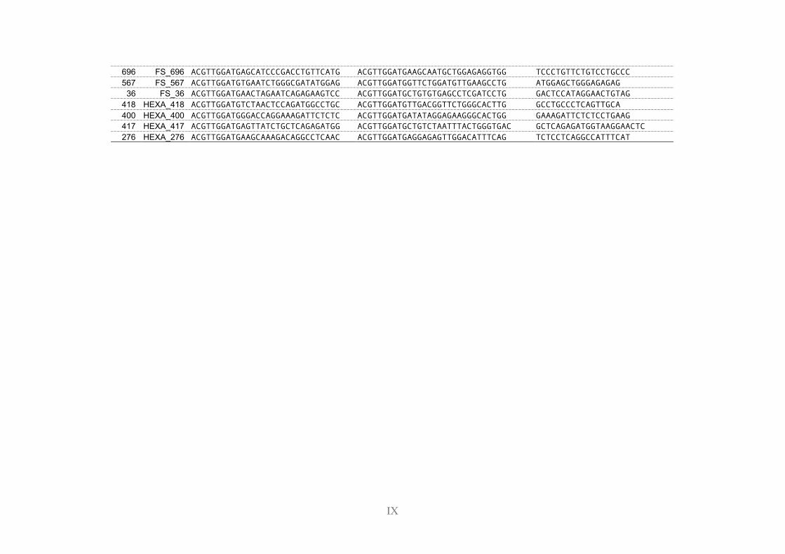
IX
696 FS_696 ACGTTGGATGAGCATCCCGACCTGTTCATG ACGTTGGATGAAGCAATGCTGGAGAGGTGG TCCCTGTTCTGTCCTGCCC
567 FS_567 ACGTTGGATGTGAATCTGGGCGATATGGAG ACGTTGGATGGTTCTGGATGTTGAAGCCTG ATGGAGCTGGGAGAGAG
36 FS_36 ACGTTGGATGAACTAGAATCAGAGAAGTCC ACGTTGGATGCTGTGTGAGCCTCGATCCTG GACTCCATAGGAACTGTAG
418 HEXA_418 ACGTTGGATGTCTAACTCCAGATGGCCTGC ACGTTGGATGTTGACGGTTCTGGGCACTTG GCCTGCCCTCAGTTGCA
400 HEXA_400 ACGTTGGATGGGACCAGGAAAGATTCTCTC ACGTTGGATGATATAGGAGAAGGGCACTGG GAAAGATTCTCTCCTGAAG
417 HEXA_417 ACGTTGGATGAGTTATCTGCTCAGAGATGG ACGTTGGATGCTGTCTAATTTACTGGGTGAC GCTCAGAGATGGTAAGGAACTC
276 HEXA_276 ACGTTGGATGAAGCAAAGACAGGCCTCAAC ACGTTGGATGAGGAGAGTTGGACATTTCAG TCTCCTCAGGCCATTTCAT
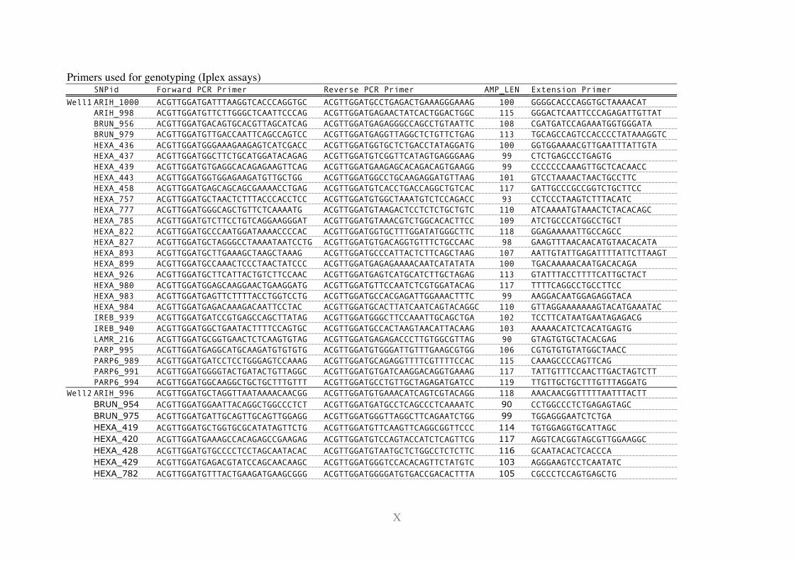
X
Primers used for genotyping (Iplex assays)! SNPid Forward PCR Primer Reverse PCR Primer AMP_LEN Extension Primer
Well1 ARIH_1000 ACGTTGGATGATTTAAGGTCACCCAGGTGC ACGTTGGATGCCTGAGACTGAAAGGGAAAG 100 GGGGCACCCAGGTGCTAAAACAT
ARIH_998 ACGTTGGATGTTCTTGGGCTCAATTCCCAG ACGTTGGATGAGAACTATCACTGGACTGGC 115 GGGACTCAATTCCCAGAGATTGTTAT
BRUN_956 ACGTTGGATGACAGTGCACGTTAGCATCAG ACGTTGGATGAGAGGGCCAGCCTGTAATTC 108 CGATGATCCAGAAATGGTGGGATA
BRUN_979 ACGTTGGATGTTGACCAATTCAGCCAGTCC ACGTTGGATGAGGTTAGGCTCTGTTCTGAG 113 TGCAGCCAGTCCACCCCTATAAAGGTC
HEXA_436 ACGTTGGATGGGAAAGAAGAGTCATCGACC ACGTTGGATGGTGCTCTGACCTATAGGATG 100 GGTGGAAAACGTTGAATTTATTGTA
HEXA_437 ACGTTGGATGGCTTCTGCATGGATACAGAG ACGTTGGATGTCGGTTCATAGTGAGGGAAG 99 CTCTGAGCCCTGAGTG
HEXA_439 ACGTTGGATGTGAGGCACAGAGAAGTTCAG ACGTTGGATGAAGAGCACAGACAGTGAAGG 99 CCCCCCCAAAGTTGCTCACAACC
HEXA_443 ACGTTGGATGGTGGAGAAGATGTTGCTGG ACGTTGGATGGCCTGCAAGAGGATGTTAAG 101 GTCCTAAAACTAACTGCCTTC
HEXA_458 ACGTTGGATGAGCAGCAGCGAAAACCTGAG ACGTTGGATGTCACCTGACCAGGCTGTCAC 117 GATTGCCCGCCGGTCTGCTTCC
HEXA_757 ACGTTGGATGCTAACTCTTTACCCACCTCC ACGTTGGATGTGGCTAAATGTCTCCAGACC 93 CCTCCCTAAGTCTTTACATC
HEXA_777 ACGTTGGATGGGCAGCTGTTCTCAAAATG ACGTTGGATGTAAGACTCCTCTCTGCTGTC 110 ATCAAAATGTAAACTCTACACAGC
HEXA_785 ACGTTGGATGTCTTCCTGTCAGGAAGGGAT ACGTTGGATGTAAACGTCTGGCACACTTCC 109 ATCTGCCCATGGCCTGCT
HEXA_822 ACGTTGGATGCCCAATGGATAAAACCCCAC ACGTTGGATGGTGCTTTGGATATGGGCTTC 118 GGAGAAAAATTGCCAGCC
HEXA_827 ACGTTGGATGCTAGGGCCTAAAATAATCCTG ACGTTGGATGTGACAGGTGTTTCTGCCAAC 98 GAAGTTTAACAACATGTAACACATA
HEXA_893 ACGTTGGATGCTTGAAAGCTAAGCTAAAG ACGTTGGATGCCCATTACTCTTCAGCTAAG 107 AATTGTATTGAGATTTTATTCTTAAGT
HEXA_899 ACGTTGGATGCCAAACTCCCTAACTATCCC ACGTTGGATGAGAGAAAACAATCATATATA 100 TGACAAAAACAATGACACAGA
HEXA_926 ACGTTGGATGCTTCATTACTGTCTTCCAAC ACGTTGGATGAGTCATGCATCTTGCTAGAG 113 GTATTTACCTTTTCATTGCTACT
HEXA_980 ACGTTGGATGGAGCAAGGAACTGAAGGATG ACGTTGGATGTTCCAATCTCGTGGATACAG 117 TTTTCAGGCCTGCCTTCC
HEXA_983 ACGTTGGATGAGTTCTTTTACCTGGTCCTG ACGTTGGATGCCACGAGATTGGAAACTTTC 99 AAGGACAATGGAGAGGTACA
HEXA_984 ACGTTGGATGAGACAAAGACAATTCCTAC ACGTTGGATGCACTTATCAATCAGTACAGGC 110 GTTAGGAAAAAAAGTACATGAAATAC
IREB_939 ACGTTGGATGATCCGTGAGCCAGCTTATAG ACGTTGGATGGGCTTCCAAATTGCAGCTGA 102 TCCTTCATAATGAATAGAGACG
IREB_940 ACGTTGGATGGCTGAATACTTTTCCAGTGC ACGTTGGATGCCACTAAGTAACATTACAAG 103 AAAAACATCTCACATGAGTG
LAMR_216 ACGTTGGATGCGGTGAACTCTCAAGTGTAG ACGTTGGATGAGAGACCCTTGTGGCGTTAG 90 GTAGTGTGCTACACGAG
PARP_995 ACGTTGGATGAGGCATGCAAGATGTGTGTG ACGTTGGATGTGGGATTGTTTGAAGCGTGG 106 CGTGTGTGTATGGCTAACC
PARP6_989 ACGTTGGATGATCCTCCTGGGAGTCCAAAG ACGTTGGATGCAGAGGTTTTCGTTTTCCAC 115 CAAAGCCCCAGTTCAG
PARP6_991 ACGTTGGATGGGGTACTGATACTGTTAGGC ACGTTGGATGTGATCAAGGACAGGTGAAAG 117 TATTGTTTCCAACTTGACTAGTCTT
! PARP6_994 ACGTTGGATGGCAAGGCTGCTGCTTTGTTT ACGTTGGATGCCTGTTGCTAGAGATGATCC 119 TTGTTGCTGCTTTGTTTAGGATG
Well2 ARIH_996 ACGTTGGATGCTAGGTTAATAAAACAACGG ACGTTGGATGTGAAACATCAGTCGTACAGG 118 AAACAACGGTTTTTAATTTACTT
BRUN_954 ACGTTGGATGGAATTACAGGCTGGCCCTCT ACGTTGGATGATGCCTCAGCCCTCAAAATC 90 CCTGGCCCTCTGAGAGTAGC
BRUN_975 ACGTTGGATGATTGCAGTTGCAGTTGGAGG ACGTTGGATGGGTTAGGCTTCAGAATCTGG 99 TGGAGGGAATCTCTGA
HEXA_419 ACGTTGGATGCTGGTGCGCATATAGTTCTG ACGTTGGATGTTCAAGTTCAGGCGGTTCCC 114 TGTGGAGGTGCATTAGC
HEXA_420 ACGTTGGATGAAAGCCACAGAGCCGAAGAG ACGTTGGATGTCCAGTACCATCTCAGTTCG 117 AGGTCACGGTAGCGTTGGAAGGC
HEXA_428 ACGTTGGATGTGCCCCTCCTAGCAATACAC ACGTTGGATGTAATGCTCTGGCCTCTCTTC 116 GCAATACACTCACCCA
HEXA_429 ACGTTGGATGAGACGTATCCAGCAACAAGC ACGTTGGATGGGTCCACACAGTTCTATGTC 103 AGGGAAGTCCTCAATATC
HEXA_782 ACGTTGGATGTTTACTGAAGATGAAGCGGG ACGTTGGATGGGGATGTGACCGACACTTTA 105 CGCCCTCCAGTGAGCTG
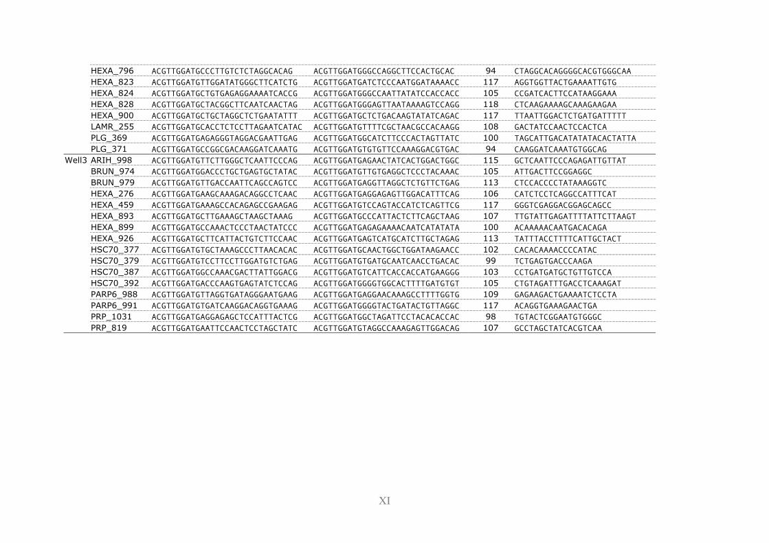
XI
HEXA_796 ACGTTGGATGCCCTTGTCTCTAGGCACAG ACGTTGGATGGGCCAGGCTTCCACTGCAC 94 CTAGGCACAGGGGCACGTGGGCAA
HEXA_823 ACGTTGGATGTTGGATATGGGCTTCATCTG ACGTTGGATGATCTCCCAATGGATAAAACC 117 AGGTGGTTACTGAAAATTGTG
HEXA_824 ACGTTGGATGCTGTGAGAGGAAAATCACCG ACGTTGGATGGGCCAATTATATCCACCACC 105 CCGATCACTTCCATAAGGAAA
HEXA_828 ACGTTGGATGCTACGGCTTCAATCAACTAG ACGTTGGATGGGAGTTAATAAAAGTCCAGG 118 CTCAAGAAAAGCAAAGAAGAA
HEXA_900 ACGTTGGATGCTGCTAGGCTCTGAATATTT ACGTTGGATGCTCTGACAAGTATATCAGAC 117 TTAATTGGACTCTGATGATTTTT
LAMR_255 ACGTTGGATGCACCTCTCCTTAGAATCATAC ACGTTGGATGTTTTCGCTAACGCCACAAGG 108 GACTATCCAACTCCACTCA
PLG_369 ACGTTGGATGAGAGGGTAGGACGAATTGAG ACGTTGGATGGCATCTTCCCACTAGTTATC 100 TAGCATTGACATATATACACTATTA
PLG_371 ACGTTGGATGCCGGCGACAAGGATCAAATG ACGTTGGATGTGTGTTCCAAAGGACGTGAC 94 CAAGGATCAAATGTGGCAG
Well3 ARIH_998 ACGTTGGATGTTCTTGGGCTCAATTCCCAG ACGTTGGATGAGAACTATCACTGGACTGGC 115 GCTCAATTCCCAGAGATTGTTAT
BRUN_974 ACGTTGGATGGACCCTGCTGAGTGCTATAC ACGTTGGATGTTGTGAGGCTCCCTACAAAC 105 ATTGACTTCCGGAGGC
BRUN_979 ACGTTGGATGTTGACCAATTCAGCCAGTCC ACGTTGGATGAGGTTAGGCTCTGTTCTGAG 113 CTCCACCCCTATAAAGGTC
HEXA_276 ACGTTGGATGAAGCAAAGACAGGCCTCAAC ACGTTGGATGAGGAGAGTTGGACATTTCAG 106 CATCTCCTCAGGCCATTTCAT
HEXA_459 ACGTTGGATGAAAGCCACAGAGCCGAAGAG ACGTTGGATGTCCAGTACCATCTCAGTTCG 117 GGGTCGAGGACGGAGCAGCC
HEXA_893 ACGTTGGATGCTTGAAAGCTAAGCTAAAG ACGTTGGATGCCCATTACTCTTCAGCTAAG 107 TTGTATTGAGATTTTATTCTTAAGT
HEXA_899 ACGTTGGATGCCAAACTCCCTAACTATCCC ACGTTGGATGAGAGAAAACAATCATATATA 100 ACAAAAACAATGACACAGA
HEXA_926 ACGTTGGATGCTTCATTACTGTCTTCCAAC ACGTTGGATGAGTCATGCATCTTGCTAGAG 113 TATTTACCTTTTCATTGCTACT
HSC70_377 ACGTTGGATGTGCTAAAGCCCTTAACACAC ACGTTGGATGCAACTGGCTGGATAAGAACC 102 CACACAAAACCCCATAC
HSC70_379 ACGTTGGATGTCCTTCCTTGGATGTCTGAG ACGTTGGATGTGATGCAATCAACCTGACAC 99 TCTGAGTGACCCAAGA
HSC70_387 ACGTTGGATGGCCAAACGACTTATTGGACG ACGTTGGATGTCATTCACCACCATGAAGGG 103 CCTGATGATGCTGTTGTCCA
HSC70_392 ACGTTGGATGACCCAAGTGAGTATCTCCAG ACGTTGGATGGGGTGGCACTTTTGATGTGT 105 CTGTAGATTTGACCTCAAAGAT
PARP6_988 ACGTTGGATGTTAGGTGATAGGGAATGAAG ACGTTGGATGAGGAACAAAGCCTTTTGGTG 109 GAGAAGACTGAAAATCTCCTA
PARP6_991 ACGTTGGATGTGATCAAGGACAGGTGAAAG ACGTTGGATGGGGTACTGATACTGTTAGGC 117 ACAGGTGAAAGAACTGA
PRP_1031 ACGTTGGATGAGGAGAGCTCCATTTACTCG ACGTTGGATGGCTAGATTCCTACACACCAC 98 TGTACTCGGAATGTGGGC
PRP_819 ACGTTGGATGAATTCCAACTCCTAGCTATC ACGTTGGATGTAGGCCAAAGAGTTGGACAG 107 GCCTAGCTATCACGTCAA
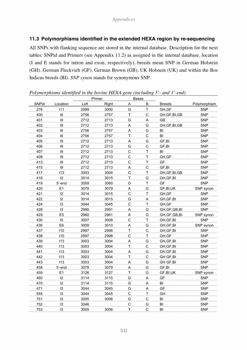
Appendices
XII
11.3 Polymorphisms identified in the extended HEXA region by re-sequencing
All SNPs with flanking sequence are stored in the internal database. Description for the next
tables: SNPid and Primers (see Appendix 11.2) as assigned in the internal database, location
(I and E stands for intron and exon, respectively), breeds mean SNP in German Holstein
(GH), German Fleckvieh (GF), German Brown (GB), UK Holstein (UK) and within the Bos
Indicus breeds (BI). SNP synon stands for synonymous SNP.
Polymorphisms identified in the bovine HEXA gene (including 5’- and 3’-end)
Primer Bases
SNPid Location Left Right A B Breeds Polymorphism
276 I11 2999 3000 G T GH,GF SNP
400 I6 2756 2757 T C GH,GF,BI,GB SNP
401 I9 2712 2713 G A GB SNP
402 I9 2712 2713 A G GH,GF,BI,GB SNP
403 I6 2756 2757 A G BI SNP
404 I6 2756 2757 T C BI SNP
405 I9 2712 2713 A G GF,BI SNP
406 I9 2712 2713 G C GF,BI SNP
407 I9 2712 2713 C T BI SNP
408 I9 2712 2713 C T GH,GF SNP
413 I9 2712 2713 C T GF SNP
415 I9 2712 2713 A C GF,BI SNP
417 I13 3003 3004 C T GH,GF,BI,GB SNP
418 I2 3014 3015 T G GH,GF,BI SNP
419 5’-end 3059 3060 G T GF SNP
420 E1 3078 3079 A G GF,BI,UK SNP synon
421 I2 3014 3015 C T GH,GF SNP
422 I2 3014 3015 G A GH,GF,BI SNP
424 I3 3044 3045 C T GH,GF SNP
428 I3 2990 2991 A G GH,GF,GB,BI SNP
429 E5 2960 2961 A G GH,GF,GB,BI SNP synon
430 I5 3007 3008 C T GH,GF,BI SNP
436 E6 3009 3010 A G GH,GF,BI SNP synon
437 I10 2997 2998 T C GH,GF,BI SNP
438 I10 2997 2998 C T GH,GF SNP
439 I13 3003 3004 A G GH,GF,BI SNP
440 I13 3003 3004 T C GH,GF,BI SNP
441 I13 3003 3004 A G GH,GF,BI SNP
442 I13 3003 3004 T C GH GF,BI SNP
443 I13 3003 3004 A G GH GF,BI SNP
458 5’-end 3078 3079 A G GF,BI SNP
459 E1 3126 3127 T G GF,BI,UK SNP synon
460 I2 3114 3115 G A GF SNP
470 I2 3114 3115 G A BI SNP
471 I3 3044 3045 G A GF SNP
555 I3 3044 3045 C T GH SNP
751 I3 3005 3006 G C BI SNP
752 I3 3046 C G BI SNP
753 I3 3005 3006 T C BI SNP
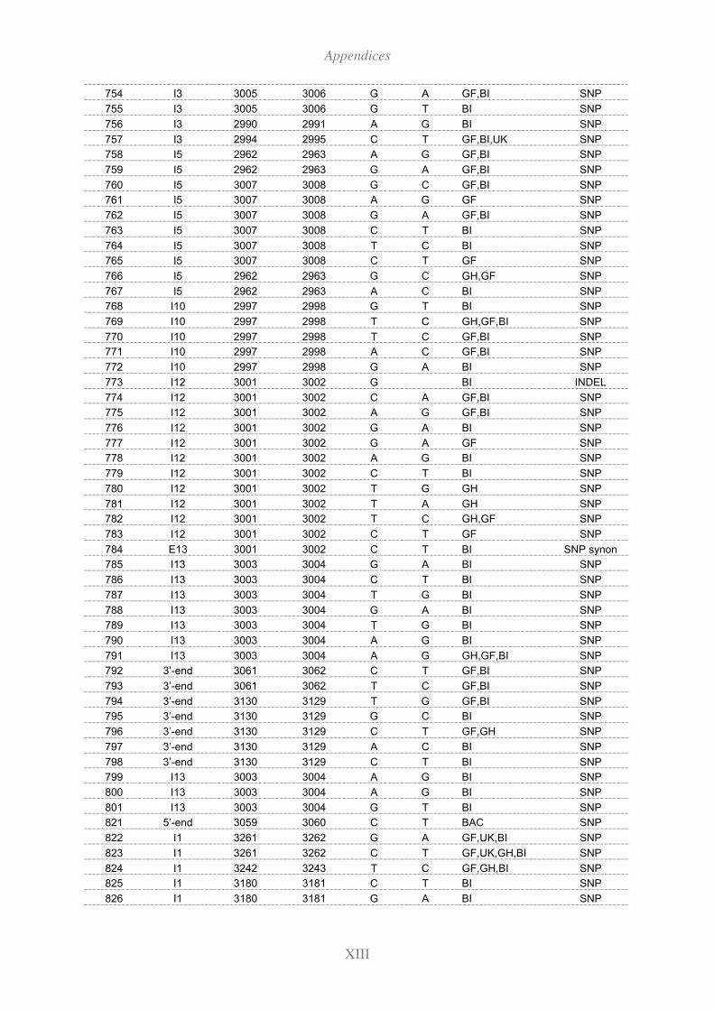
Appendices
XIII
754 I3 3005 3006 G A GF,BI SNP
755 I3 3005 3006 G T BI SNP
756 I3 2990 2991 A G BI SNP
757 I3 2994 2995 C T GF,BI,UK SNP
758 I5 2962 2963 A G GF,BI SNP
759 I5 2962 2963 G A GF,BI SNP
760 I5 3007 3008 G C GF,BI SNP
761 I5 3007 3008 A G GF SNP
762 I5 3007 3008 G A GF,BI SNP
763 I5 3007 3008 C T BI SNP
764 I5 3007 3008 T C BI SNP
765 I5 3007 3008 C T GF SNP
766 I5 2962 2963 G C GH,GF SNP
767 I5 2962 2963 A C BI SNP
768 I10 2997 2998 G T BI SNP
769 I10 2997 2998 T C GH,GF,BI SNP
770 I10 2997 2998 T C GF,BI SNP
771 I10 2997 2998 A C GF,BI SNP
772 I10 2997 2998 G A BI SNP
773 I12 3001 3002 G BI INDEL
774 I12 3001 3002 C A GF,BI SNP
775 I12 3001 3002 A G GF,BI SNP
776 I12 3001 3002 G A BI SNP
777 I12 3001 3002 G A GF SNP
778 I12 3001 3002 A G BI SNP
779 I12 3001 3002 C T BI SNP
780 I12 3001 3002 T G GH SNP
781 I12 3001 3002 T A GH SNP
782 I12 3001 3002 T C GH,GF SNP
783 I12 3001 3002 C T GF SNP
784 E13 3001 3002 C T BI SNP synon
785 I13 3003 3004 G A BI SNP
786 I13 3003 3004 C T BI SNP
787 I13 3003 3004 T G BI SNP
788 I13 3003 3004 G A BI SNP
789 I13 3003 3004 T G BI SNP
790 I13 3003 3004 A G BI SNP
791 I13 3003 3004 A G GH,GF,BI SNP
792 3’-end 3061 3062 C T GF,BI SNP
793 3’-end 3061 3062 T C GF,BI SNP
794 3’-end 3130 3129 T G GF,BI SNP
795 3’-end 3130 3129 G C BI SNP
796 3’-end 3130 3129 C T GF,GH SNP
797 3’-end 3130 3129 A C BI SNP
798 3’-end 3130 3129 C T BI SNP
799 I13 3003 3004 A G BI SNP
800 I13 3003 3004 A G BI SNP
801 I13 3003 3004 G T BI SNP
821 5’-end 3059 3060 C T BAC SNP
822 I1 3261 3262 G A GF,UK,BI SNP
823 I1 3261 3262 C T GF,UK,GH,BI SNP
824 I1 3242 3243 T C GF,GH,BI SNP
825 I1 3180 3181 C T BI SNP
826 I1 3180 3181 G A BI SNP
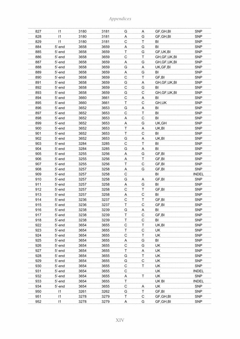
Appendices
XIV
827 I1 3180 3181 G A GF,GH,BI SNP
828 I1 3180 3181 A G GF,GH,BI SNP
829 I1 3180 3181 C T BI SNP
884 5’-end 3658 3659 A G BI SNP
885 5’-end 3658 3659 T G GF,UK,BI SNP
886 5’-end 3658 3659 C T GH,GF,UK,BI SNP
887 5’-end 3658 3659 A G GH,GF,UK,BI SNP
888 5’-end 3658 3659 G A UK,GF,BI SNP
889 5’-end 3658 3659 A G BI SNP
890 5’-end 3658 3659 C T GF,BI SNP
891 5’-end 3658 3659 G A GH,GF,UK,BI SNP
892 5’-end 3658 3659 C G BI SNP
893 5’-end 3658 3659 G C GH,GF,UK,BI SNP
894 5’-end 3660 3661 C A BI SNP
895 5’-end 3660 3661 T C GH,UK SNP
896 5’-end 3652 3653 G A BI SNP
897 5’-end 3652 3653 C T BI SNP
898 5’-end 3652 3653 A C BI SNP
899 5’-end 3652 3653 A G UK,GH SNP
900 5’-end 3652 3653 T A UK,BI SNP
901 5’-end 3652 3653 T C BI SNP
902 5’-end 3652 3653 G A UK,BI SNP
903 5’-end 3284 3285 C T BI SNP
904 5’-end 3284 3285 G A BI SNP
905 5’-end 3255 3256 A G GF,BI SNP
906 5’-end 3255 3256 A T GF,BI SNP
907 5’-end 3255 3256 T C GF,BI SNP
908 5’-end 3257 3258 A G GF,BI SNP
909 5’-end 3257 3258 C BI INDEL
910 5’-end 3257 3258 G A GF,BI SNP
911 5’-end 3257 3258 A G BI SNP
912 5’-end 3257 3258 C T GF,BI SNP
913 5’-end 3257 3258 A C BI SNP
914 5’-end 3236 3237 C T GF,BI SNP
915 5’-end 3236 3237 T C GF,BI SNP
916 5’-end 3238 3239 G A BI SNP
917 5’-end 3238 3239 T C GF,BI SNP
918 5’-end 3238 3239 T C BI SNP
922 5’-end 3654 3655 C T UK,BI SNP
923 5’-end 3654 3655 T C UK SNP
924 5’-end 3654 3655 C T UK SNP
925 5’-end 3654 3655 A G BI SNP
926 5’-end 3654 3655 C G UK SNP
927 5’-end 3654 3655 T A UK SNP
928 5’-end 3654 3655 G T UK SNP
929 5’-end 3654 3655 G C UK SNP
930 5’-end 3654 3655 C T UK SNP
931 5’-end 3654 3655 C UK INDEL
932 5’-end 3654 3655 A T UK SNP
933 5’-end 3654 3655 T UK BI INDEL
934 5’-end 3654 3655 C A UK SNP
950 I1 3261 3262 G T GF,BI SNP
951 I1 3278 3279 T C GF,GH,BI SNP
952 I1 3278 3279 A G GF,GH,BI SNP
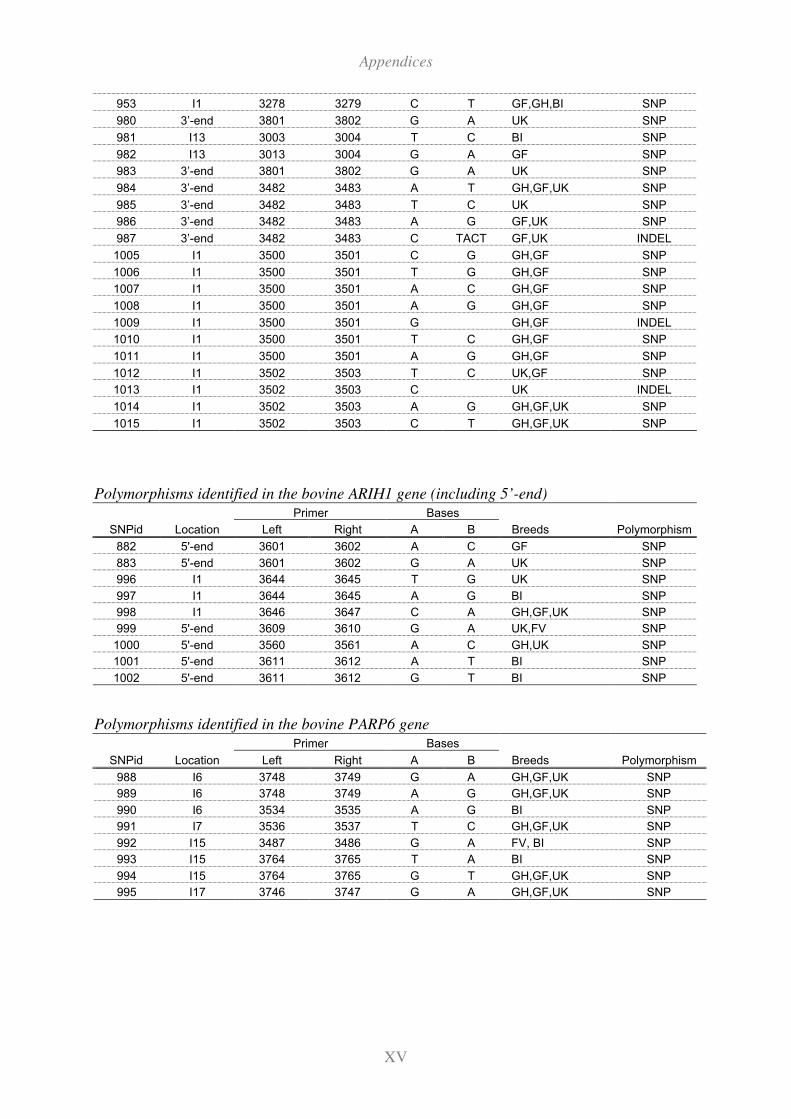
Appendices
XV
953 I1 3278 3279 C T GF,GH,BI SNP
980 3’-end 3801 3802 G A UK SNP
981 I13 3003 3004 T C BI SNP
982 I13 3013 3004 G A GF SNP
983 3’-end 3801 3802 G A UK SNP
984 3’-end 3482 3483 A T GH,GF,UK SNP
985 3’-end 3482 3483 T C UK SNP
986 3’-end 3482 3483 A G GF,UK SNP
987 3’-end 3482 3483 C TACT GF,UK INDEL
1005 I1 3500 3501 C G GH,GF SNP
1006 I1 3500 3501 T G GH,GF SNP
1007 I1 3500 3501 A C GH,GF SNP
1008 I1 3500 3501 A G GH,GF SNP
1009 I1 3500 3501 G GH,GF INDEL
1010 I1 3500 3501 T C GH,GF SNP
1011 I1 3500 3501 A G GH,GF SNP
1012 I1 3502 3503 T C UK,GF SNP
1013 I1 3502 3503 C UK INDEL
1014 I1 3502 3503 A G GH,GF,UK SNP
1015 I1 3502 3503 C T GH,GF,UK SNP
Polymorphisms identified in the bovine ARIH1 gene (including 5’-end)
Primer Bases
SNPid Location Left Right A B Breeds Polymorphism
882 5'-end 3601 3602 A C GF SNP
883 5'-end 3601 3602 G A UK SNP
996 I1 3644 3645 T G UK SNP
997 I1 3644 3645 A G BI SNP
998 I1 3646 3647 C A GH,GF,UK SNP
999 5'-end 3609 3610 G A UK,FV SNP
1000 5'-end 3560 3561 A C GH,UK SNP
1001 5'-end 3611 3612 A T BI SNP
1002 5'-end 3611 3612 G T BI SNP
Polymorphisms identified in the bovine PARP6 gene
Primer Bases
SNPid Location Left Right A B Breeds Polymorphism
988 I6 3748 3749 G A GH,GF,UK SNP
989 I6 3748 3749 A G GH,GF,UK SNP
990 I6 3534 3535 A G BI SNP
991 I7 3536 3537 T C GH,GF,UK SNP
992 I15 3487 3486 G A FV, BI SNP
993 I15 3764 3765 T A BI SNP
994 I15 3764 3765 G T GH,GF,UK SNP
995 I17 3746 3747 G A GH,GF,UK SNP
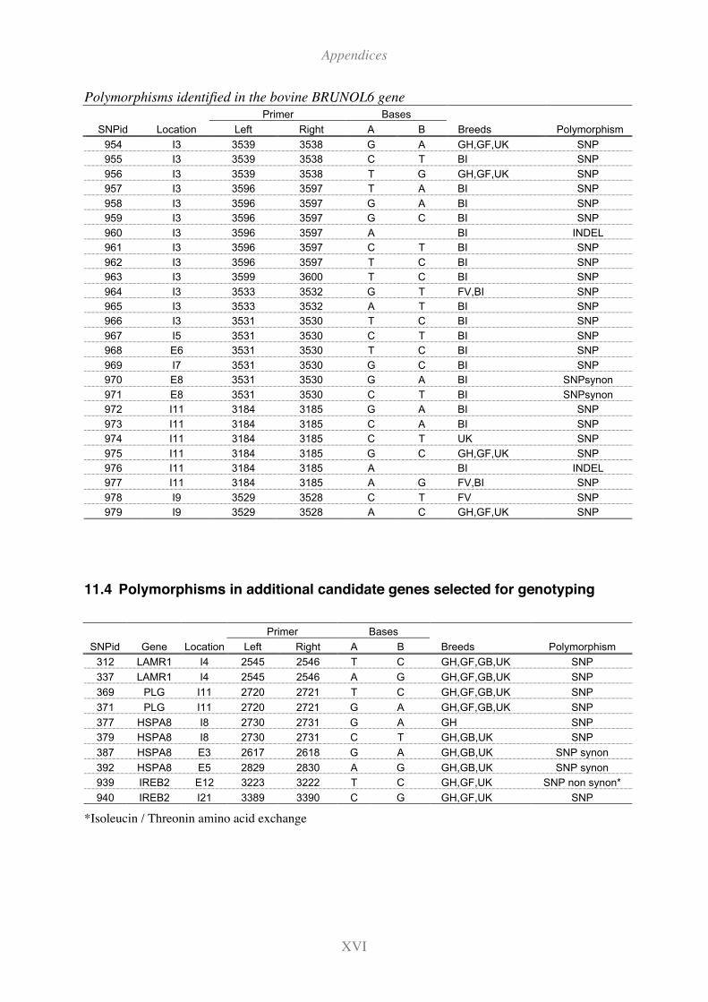
Appendices
XVI
Polymorphisms identified in the bovine BRUNOL6 gene
Primer Bases
SNPid Location Left Right A B Breeds Polymorphism
954 I3 3539 3538 G A GH,GF,UK SNP
955 I3 3539 3538 C T BI SNP
956 I3 3539 3538 T G GH,GF,UK SNP
957 I3 3596 3597 T A BI SNP
958 I3 3596 3597 G A BI SNP
959 I3 3596 3597 G C BI SNP
960 I3 3596 3597 A BI INDEL
961 I3 3596 3597 C T BI SNP
962 I3 3596 3597 T C BI SNP
963 I3 3599 3600 T C BI SNP
964 I3 3533 3532 G T FV,BI SNP
965 I3 3533 3532 A T BI SNP
966 I3 3531 3530 T C BI SNP
967 I5 3531 3530 C T BI SNP
968 E6 3531 3530 T C BI SNP
969 I7 3531 3530 G C BI SNP
970 E8 3531 3530 G A BI SNPsynon
971 E8 3531 3530 C T BI SNPsynon
972 I11 3184 3185 G A BI SNP
973 I11 3184 3185 C A BI SNP
974 I11 3184 3185 C T UK SNP
975 I11 3184 3185 G C GH,GF,UK SNP
976 I11 3184 3185 A BI INDEL
977 I11 3184 3185 A G FV,BI SNP
978 I9 3529 3528 C T FV SNP
979 I9 3529 3528 A C GH,GF,UK SNP
11.4 Polymorphisms in additional candidate genes selected for genotyping
Primer Bases
SNPid Gene Location Left Right A B Breeds Polymorphism
312 LAMR1 I4 2545 2546 T C GH,GF,GB,UK SNP
337 LAMR1 I4 2545 2546 A G GH,GF,GB,UK SNP
369 PLG I11 2720 2721 T C GH,GF,GB,UK SNP
371 PLG I11 2720 2721 G A GH,GF,GB,UK SNP
377 HSPA8 I8 2730 2731 G A GH SNP
379 HSPA8 I8 2730 2731 C T GH,GB,UK SNP
387 HSPA8 E3 2617 2618 G A GH,GB,UK SNP synon
392 HSPA8 E5 2829 2830 A G GH,GB,UK SNP synon
939 IREB2 E12 3223 3222 T C GH,GF,UK SNP non synon*
940 IREB2 I21 3389 3390 C G GH,GF,UK SNP
*Isoleucin / Threonin amino acid exchange
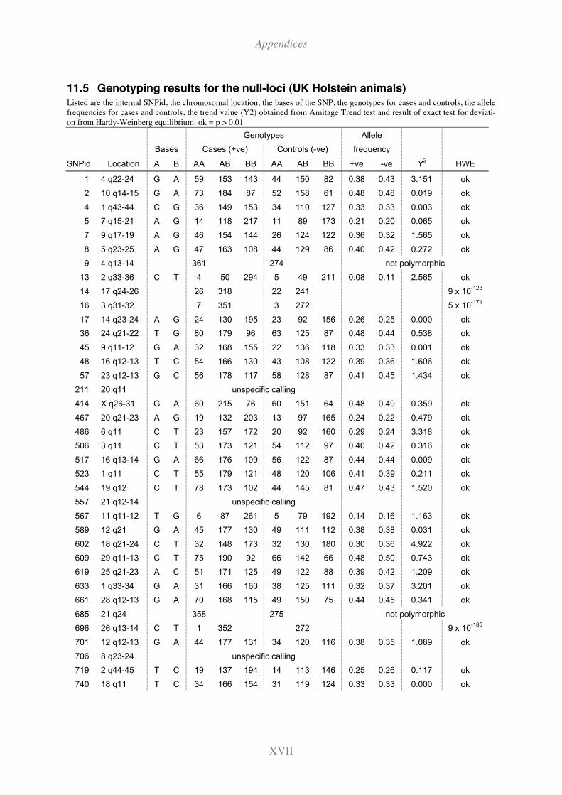
Appendices
XVII
11.5 Genotyping results for the null-loci (UK Holstein animals)Listed are the internal SNPid, the chromosomal location, the bases of the SNP, the genotypes for cases and controls, the allele
frequencies for cases and controls, the trend value (Y2) obtained from Amitage Trend test and result of exact test for deviati-
on from Hardy-Weinberg equilibrium: ok = p > 0.01
Genotypes Allele
Bases Cases (+ve) Controls (-ve) frequency
SNPid Location A B AA AB BB AA AB BB +ve -ve Y2
HWE
1 4 q22-24 G A 59 153 143 44 150 82 0.38 0.43 3.151 ok
2 10 q14-15 G A 73 184 87 52 158 61 0.48 0.48 0.019 ok
4 1 q43-44 C G 36 149 153 34 110 127 0.33 0.33 0.003 ok
5 7 q15-21 A G 14 118 217 11 89 173 0.21 0.20 0.065 ok
7 9 q17-19 A G 46 154 144 26 124 122 0.36 0.32 1.565 ok
8 5 q23-25 A G 47 163 108 44 129 86 0.40 0.42 0.272 ok
9 4 q13-14 361 274 not polymorphic
13 2 q33-36 C T 4 50 294 5 49 211 0.08 0.11 2.565 ok
14 17 q24-26 26 318 22 241 9 x 10-123
16 3 q31-32 7 351 3 272 5 x 10-171
17 14 q23-24 A G 24 130 195 23 92 156 0.26 0.25 0.000 ok
36 24 q21-22 T G 80 179 96 63 125 87 0.48 0.44 0.538 ok
45 9 q11-12 G A 32 168 155 22 136 118 0.33 0.33 0.001 ok
48 16 q12-13 T C 54 166 130 43 108 122 0.39 0.36 1.606 ok
57 23 q12-13 G C 56 178 117 58 128 87 0.41 0.45 1.434 ok
211 20 q11 unspecific calling
414 X q26-31 G A 60 215 76 60 151 64 0.48 0.49 0.359 ok
467 20 q21-23 A G 19 132 203 13 97 165 0.24 0.22 0.479 ok
486 6 q11 C T 23 157 172 20 92 160 0.29 0.24 3.318 ok
506 3 q11 C T 53 173 121 54 112 97 0.40 0.42 0.316 ok
517 16 q13-14 G A 66 176 109 56 122 87 0.44 0.44 0.009 ok
523 1 q11 C T 55 179 121 48 120 106 0.41 0.39 0.211 ok
544 19 q12 C T 78 173 102 44 145 81 0.47 0.43 1.520 ok
557 21 q12-14 unspecific calling
567 11 q11-12 T G 6 87 261 5 79 192 0.14 0.16 1.163 ok
589 12 q21 G A 45 177 130 49 111 112 0.38 0.38 0.031 ok
602 18 q21-24 C T 32 148 173 32 130 180 0.30 0.36 4.922 ok
609 29 q11-13 C T 75 190 92 66 142 66 0.48 0.50 0.743 ok
619 25 q21-23 A C 51 171 125 49 122 88 0.39 0.42 1.209 ok
633 1 q33-34 G A 31 166 160 38 125 111 0.32 0.37 3.201 ok
661 28 q12-13 G A 70 168 115 49 150 75 0.44 0.45 0.341 ok
685 21 q24 358 275 not polymorphic
696 26 q13-14 C T 1 352 272 9 x 10-185
701 12 q12-13 G A 44 177 131 34 120 116 0.38 0.35 1.089 ok
706 8 q23-24 unspecific calling
719 2 q44-45 T C 19 137 194 14 113 146 0.25 0.26 0.117 ok
740 18 q11 T C 34 166 154 31 119 124 0.33 0.33 0.000 ok
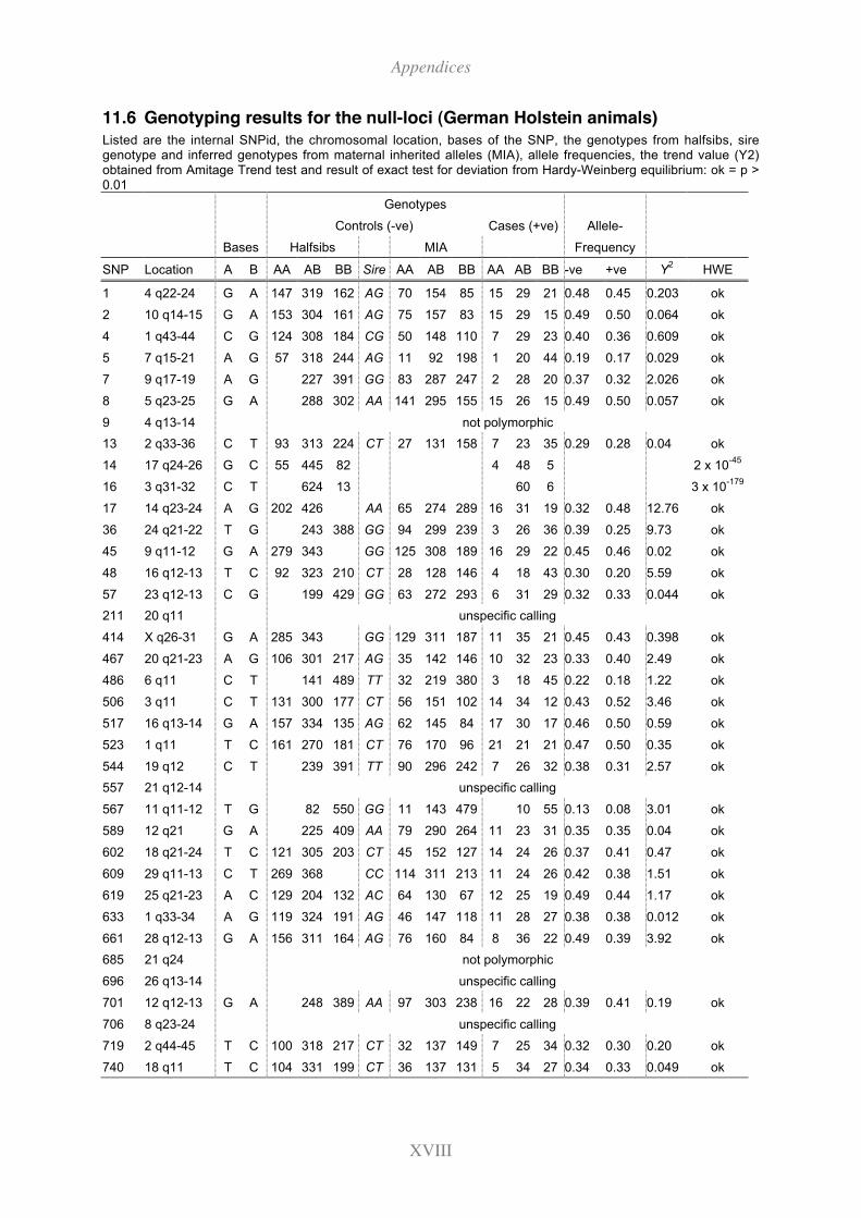
Appendices
XVIII
11.6 Genotyping results for the null-loci (German Holstein animals)
Listed are the internal SNPid, the chromosomal location, bases of the SNP, the genotypes from halfsibs, siregenotype and inferred genotypes from maternal inherited alleles (MIA), allele frequencies, the trend value (Y2)obtained from Amitage Trend test and result of exact test for deviation from Hardy-Weinberg equilibrium: ok = p >0.01
Genotypes
Controls (-ve) Cases (+ve) Allele-
Bases Halfsibs MIA Frequency
SNP Location A B AA AB BB Sire AA AB BB AA AB BB -ve +ve Y2
HWE
1 4 q22-24 G A 147 319 162 AG 70 154 85 15 29 21 0.48 0.45 0.203 ok
2 10 q14-15 G A 153 304 161 AG 75 157 83 15 29 15 0.49 0.50 0.064 ok
4 1 q43-44 C G 124 308 184 CG 50 148 110 7 29 23 0.40 0.36 0.609 ok
5 7 q15-21 A G 57 318 244 AG 11 92 198 1 20 44 0.19 0.17 0.029 ok
7 9 q17-19 A G 227 391 GG 83 287 247 2 28 20 0.37 0.32 2.026 ok
8 5 q23-25 G A 288 302 AA 141 295 155 15 26 15 0.49 0.50 0.057 ok
9 4 q13-14 not polymorphic
13 2 q33-36 C T 93 313 224 CT 27 131 158 7 23 35 0.29 0.28 0.04 ok
14 17 q24-26 G C 55 445 82 4 48 5 2 x 10-45
16 3 q31-32 C T 624 13 60 6 3 x 10-179
17 14 q23-24 A G 202 426 AA 65 274 289 16 31 19 0.32 0.48 12.76 ok
36 24 q21-22 T G 243 388 GG 94 299 239 3 26 36 0.39 0.25 9.73 ok
45 9 q11-12 G A 279 343 GG 125 308 189 16 29 22 0.45 0.46 0.02 ok
48 16 q12-13 T C 92 323 210 CT 28 128 146 4 18 43 0.30 0.20 5.59 ok
57 23 q12-13 C G 199 429 GG 63 272 293 6 31 29 0.32 0.33 0.044 ok
211 20 q11 unspecific calling
414 X q26-31 G A 285 343 GG 129 311 187 11 35 21 0.45 0.43 0.398 ok
467 20 q21-23 A G 106 301 217 AG 35 142 146 10 32 23 0.33 0.40 2.49 ok
486 6 q11 C T 141 489 TT 32 219 380 3 18 45 0.22 0.18 1.22 ok
506 3 q11 C T 131 300 177 CT 56 151 102 14 34 12 0.43 0.52 3.46 ok
517 16 q13-14 G A 157 334 135 AG 62 145 84 17 30 17 0.46 0.50 0.59 ok
523 1 q11 T C 161 270 181 CT 76 170 96 21 21 21 0.47 0.50 0.35 ok
544 19 q12 C T 239 391 TT 90 296 242 7 26 32 0.38 0.31 2.57 ok
557 21 q12-14 unspecific calling
567 11 q11-12 T G 82 550 GG 11 143 479 10 55 0.13 0.08 3.01 ok
589 12 q21 G A 225 409 AA 79 290 264 11 23 31 0.35 0.35 0.04 ok
602 18 q21-24 T C 121 305 203 CT 45 152 127 14 24 26 0.37 0.41 0.47 ok
609 29 q11-13 C T 269 368 CC 114 311 213 11 24 26 0.42 0.38 1.51 ok
619 25 q21-23 A C 129 204 132 AC 64 130 67 12 25 19 0.49 0.44 1.17 ok
633 1 q33-34 A G 119 324 191 AG 46 147 118 11 28 27 0.38 0.38 0.012 ok
661 28 q12-13 G A 156 311 164 AG 76 160 84 8 36 22 0.49 0.39 3.92 ok
685 21 q24 not polymorphic
696 26 q13-14 unspecific calling
701 12 q12-13 G A 248 389 AA 97 303 238 16 22 28 0.39 0.41 0.19 ok
706 8 q23-24 unspecific calling
719 2 q44-45 T C 100 318 217 CT 32 137 149 7 25 34 0.32 0.30 0.20 ok
740 18 q11 T C 104 331 199 CT 36 137 131 5 34 27 0.34 0.33 0.049 ok
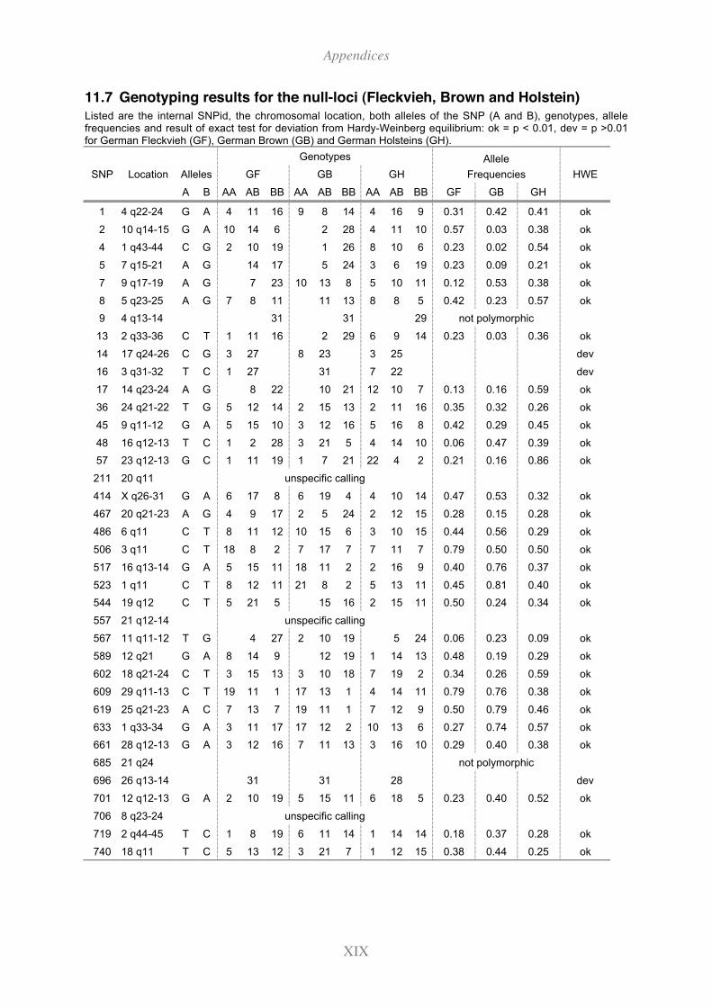
Appendices
XIX
11.7 Genotyping results for the null-loci (Fleckvieh, Brown and Holstein)
Listed are the internal SNPid, the chromosomal location, both alleles of the SNP (A and B), genotypes, allelefrequencies and result of exact test for deviation from Hardy-Weinberg equilibrium: ok = p < 0.01, dev = p >0.01for German Fleckvieh (GF), German Brown (GB) and German Holsteins (GH).
Genotypes Allele
SNP Location Alleles GF GB GH Frequencies HWE
A B AA AB BB AA AB BB AA AB BB GF GB GH
1 4 q22-24 G A 4 11 16 9 8 14 4 16 9 0.31 0.42 0.41 ok
2 10 q14-15 G A 10 14 6 2 28 4 11 10 0.57 0.03 0.38 ok
4 1 q43-44 C G 2 10 19 1 26 8 10 6 0.23 0.02 0.54 ok
5 7 q15-21 A G 14 17 5 24 3 6 19 0.23 0.09 0.21 ok
7 9 q17-19 A G 7 23 10 13 8 5 10 11 0.12 0.53 0.38 ok
8 5 q23-25 A G 7 8 11 11 13 8 8 5 0.42 0.23 0.57 ok
9 4 q13-14 31 31 29 not polymorphic
13 2 q33-36 C T 1 11 16 2 29 6 9 14 0.23 0.03 0.36 ok
14 17 q24-26 C G 3 27 8 23 3 25 dev
16 3 q31-32 T C 1 27 31 7 22 dev
17 14 q23-24 A G 8 22 10 21 12 10 7 0.13 0.16 0.59 ok
36 24 q21-22 T G 5 12 14 2 15 13 2 11 16 0.35 0.32 0.26 ok
45 9 q11-12 G A 5 15 10 3 12 16 5 16 8 0.42 0.29 0.45 ok
48 16 q12-13 T C 1 2 28 3 21 5 4 14 10 0.06 0.47 0.39 ok
57 23 q12-13 G C 1 11 19 1 7 21 22 4 2 0.21 0.16 0.86 ok
211 20 q11 unspecific calling
414 X q26-31 G A 6 17 8 6 19 4 4 10 14 0.47 0.53 0.32 ok
467 20 q21-23 A G 4 9 17 2 5 24 2 12 15 0.28 0.15 0.28 ok
486 6 q11 C T 8 11 12 10 15 6 3 10 15 0.44 0.56 0.29 ok
506 3 q11 C T 18 8 2 7 17 7 7 11 7 0.79 0.50 0.50 ok
517 16 q13-14 G A 5 15 11 18 11 2 2 16 9 0.40 0.76 0.37 ok
523 1 q11 C T 8 12 11 21 8 2 5 13 11 0.45 0.81 0.40 ok
544 19 q12 C T 5 21 5 15 16 2 15 11 0.50 0.24 0.34 ok
557 21 q12-14 unspecific calling
567 11 q11-12 T G 4 27 2 10 19 5 24 0.06 0.23 0.09 ok
589 12 q21 G A 8 14 9 12 19 1 14 13 0.48 0.19 0.29 ok
602 18 q21-24 C T 3 15 13 3 10 18 7 19 2 0.34 0.26 0.59 ok
609 29 q11-13 C T 19 11 1 17 13 1 4 14 11 0.79 0.76 0.38 ok
619 25 q21-23 A C 7 13 7 19 11 1 7 12 9 0.50 0.79 0.46 ok
633 1 q33-34 G A 3 11 17 17 12 2 10 13 6 0.27 0.74 0.57 ok
661 28 q12-13 G A 3 12 16 7 11 13 3 16 10 0.29 0.40 0.38 ok
685 21 q24 not polymorphic
696 26 q13-14 31 31 28 dev
701 12 q12-13 G A 2 10 19 5 15 11 6 18 5 0.23 0.40 0.52 ok
706 8 q23-24 unspecific calling
719 2 q44-45 T C 1 8 19 6 11 14 1 14 14 0.18 0.37 0.28 ok
740 18 q11 T C 5 13 12 3 21 7 1 12 15 0.38 0.44 0.25 ok
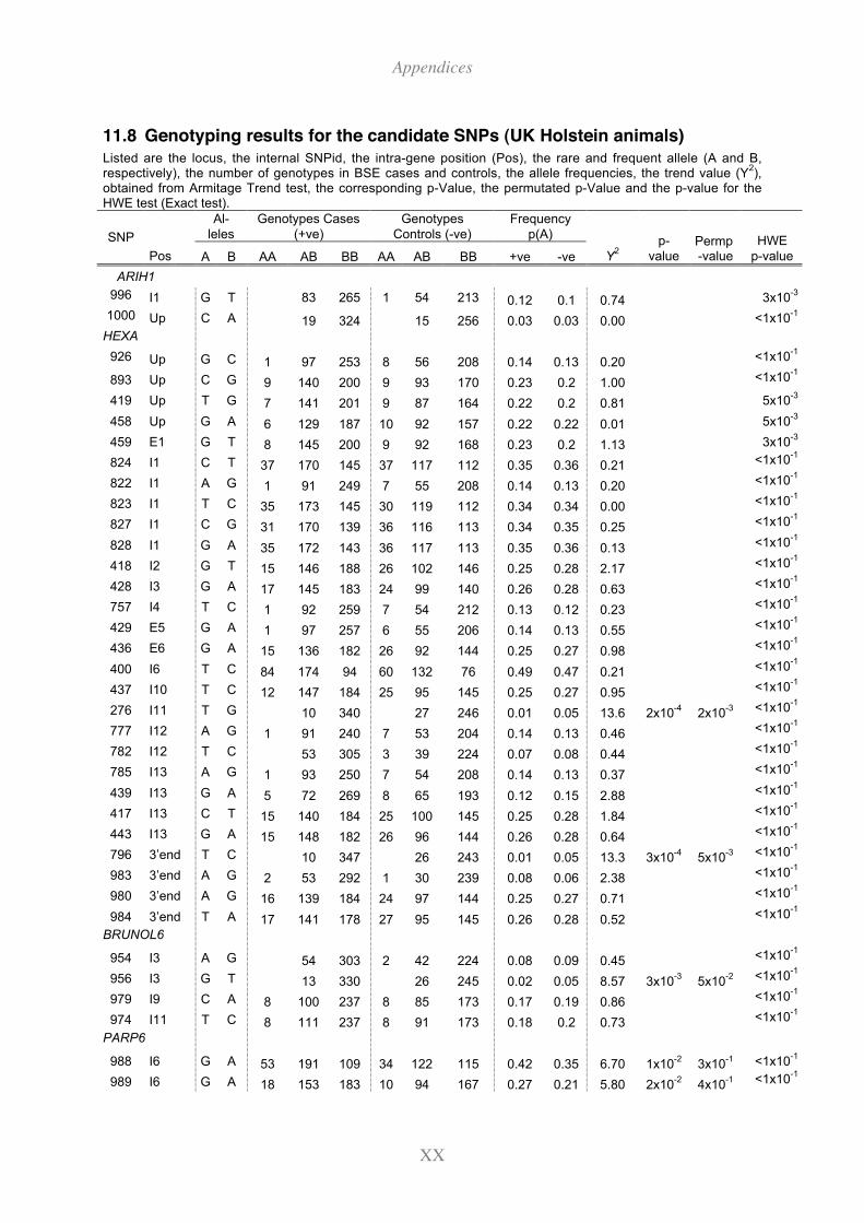
Appendices
XX
11.8 Genotyping results for the candidate SNPs (UK Holstein animals)
Listed are the locus, the internal SNPid, the intra-gene position (Pos), the rare and frequent allele (A and B,respectively), the number of genotypes in BSE cases and controls, the allele frequencies, the trend value (Y
2),
obtained from Armitage Trend test, the corresponding p-Value, the permutated p-Value and the p-value for theHWE test (Exact test).
Al-
leles
Genotypes Cases
(+ve)
Genotypes
Controls (-ve)
Frequency
p(A)SNP
Pos A B AA AB BB AA AB BB +ve -ve Y2
p-
valuePermp-value
HWE
p-value
ARIH1
996 I1 G T 83 265 1 54 213 0.12 0.1 0.74 3x10⁻³
1000 Up C A 19 324 15 256 0.03 0.03 0.00 <1x10⁻¹
HEXA
926 Up G C 1 97 253 8 56 208 0.14 0.13 0.20 <1x10⁻¹
893 Up C G 9 140 200 9 93 170 0.23 0.2 1.00 <1x10⁻¹
419 Up T G 7 141 201 9 87 164 0.22 0.2 0.81 5x10⁻³
458 Up G A 6 129 187 10 92 157 0.22 0.22 0.01 5x10⁻³
459 E1 G T 8 145 200 9 92 168 0.23 0.2 1.13 3x10⁻³
824 I1 C T 37 170 145 37 117 112 0.35 0.36 0.21 <1x10⁻¹
822 I1 A G 1 91 249 7 55 208 0.14 0.13 0.20 <1x10⁻¹
823 I1 T C 35 173 145 30 119 112 0.34 0.34 0.00 <1x10⁻¹
827 I1 C G 31 170 139 36 116 113 0.34 0.35 0.25 <1x10⁻¹
828 I1 G A 35 172 143 36 117 113 0.35 0.36 0.13 <1x10⁻¹
418 I2 G T 15 146 188 26 102 146 0.25 0.28 2.17 <1x10⁻¹
428 I3 G A 17 145 183 24 99 140 0.26 0.28 0.63 <1x10⁻¹
757 I4 T C 1 92 259 7 54 212 0.13 0.12 0.23 <1x10⁻¹
429 E5 G A 1 97 257 6 55 206 0.14 0.13 0.55 <1x10⁻¹
436 E6 G A 15 136 182 26 92 144 0.25 0.27 0.98 <1x10⁻¹
400 I6 T C 84 174 94 60 132 76 0.49 0.47 0.21 <1x10⁻¹
437 I10 T C 12 147 184 25 95 145 0.25 0.27 0.95 <1x10⁻¹
276 I11 T G 10 340 27 246 0.01 0.05 13.6 2x10⁻⁴
2x10⁻³ <1x10
-1
777 I12 A G 1 91 240 7 53 204 0.14 0.13 0.46 <1x10⁻¹
782 I12 T C 53 305 3 39 224 0.07 0.08 0.44 <1x10⁻¹
785 I13 A G 1 93 250 7 54 208 0.14 0.13 0.37 <1x10⁻¹
439 I13 G A 5 72 269 8 65 193 0.12 0.15 2.88 <1x10⁻¹
417 I13 C T 15 140 184 25 100 145 0.25 0.28 1.84 <1x10⁻¹
443 I13 G A 15 148 182 26 96 144 0.26 0.28 0.64 <1x10⁻¹
796 3’end T C 10 347 26 243 0.01 0.05 13.3 3x10⁻⁴
5x10⁻³ <1x10
-1
983 3’end A G 2 53 292 1 30 239 0.08 0.06 2.38 <1x10⁻¹
980 3’end A G 16 139 184 24 97 144 0.25 0.27 0.71 <1x10⁻¹
984 3’end T A 17 141 178 27 95 145 0.26 0.28 0.52 <1x10⁻¹
BRUNOL6
954 I3 A G 54 303 2 42 224 0.08 0.09 0.45 <1x10⁻¹
956 I3 G T 13 330 26 245 0.02 0.05 8.57 3x10⁻³
5x10⁻² <1x10
-1
979 I9 C A 8 100 237 8 85 173 0.17 0.19 0.86 <1x10⁻¹
974 I11 T C 8 111 237 8 91 173 0.18 0.2 0.73 <1x10⁻¹
PARP6
988 I6 G A 53 191 109 34 122 115 0.42 0.35 6.70 1x10⁻²
3x10⁻¹ <1x10
-1
989 I6 G A 18 153 183 10 94 167 0.27 0.21 5.80 2x10⁻²
4x10⁻¹ <1x10
-1
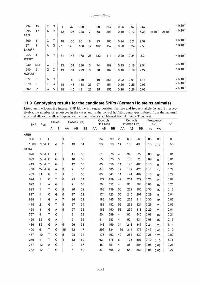
Appendices
XXI
994 I15 T G 1 37 300 20 247 0.06 0.07 2.67 <1x10⁻¹
995 I17 A G 12 107 228 7 58 203 0.19 0.13 6.33 1x10⁻²
2x10⁻¹ <1x10
-1
PLG
369 I11 C T 18 135 201 8 93 166 0.24 0.2 2.57 <1x10⁻¹
371 I11 A G 27 143 186 12 102 152 0.28 0.24 2.58 <1x10⁻¹
LAMR1
255 I4 A G 31 146 178 25 132 111 0.29 0.34 3.2 <1x10⁻¹
IREB2
939 E12 C T 13 101 230 3 74 189 0.15 0.18 2.54 <1x10⁻¹
940 I21 G C 13 104 229 3 78 189 0.16 0.19 2.27 <1x10⁻¹
HSPA8
377 I8 A G 8 349 10 263 0.02 0.01 1.13 <1x10⁻¹
379 I8 T C 18 148 188 23 97 151 0.26 0.26 0.03 <1x10⁻¹
392 E5 G A 18 145 191 23 95 153 0.26 0.26 0.03 <1x10⁻¹
11.9 Genotyping results for the candidate SNPs (German Holsteins animals)
Listed are the locus, the internal SNP Id, the intra-gene position, the rare and frequent allele (A and B, respec-
tively), the number of genotypes in the cases and in the control halfsibs, genotypes inferred from the maternal
inherited alleles, the allele frequencies, the trend value (Y2), obtained from Armitage Trend test
Alleles Cases (+ve)ControlsHalf-Sibs
ControlsInferred (-ve)
Frequencyp(A)SNP Pos
A B AA AB BB AA AB BB AA AB BB -ve +ve
Y2
ARIH1
996 I1 G T 1 5 60 34 599 2 63 565 0.05 0.05 0.00
1000 5’end C A 2 13 51 93 510 14 156 430 0.15 0.13 0.55
HEXA
926 5’end G C 11 55 51 576 4 94 529 0.08 0.08 0.01
893 5’end C G 1 10 55 55 570 5 100 520 0.09 0.09 0.01
419 5’end T G 12 55 85 556 11 146 480 0.13 0.09 1.95
458 5’end G A 3 9 53 84 500 12 142 426 0.14 0.12 0.72
459 E1 G T 1 8 56 83 541 11 144 469 0.13 0.08 3.29
824 I1 C T 6 25 34 177 459 49 254 329 0.28 0.28 0.02
822 I1 A G 9 56 50 552 4 90 504 0.08 0.07 0.26
823 I1 T C 8 26 32 188 439 56 262 305 0.30 0.32 0.18
827 I1 C G 6 27 32 174 423 50 245 297 0.29 0.30 0.04
828 I1 G A 7 26 32 188 445 56 263 311 0.30 0.31 0.06
418 I2 G T 5 27 34 183 452 53 262 321 0.29 0.28 0.05
428 I3 G A 5 27 33 183 450 53 259 318 0.29 0.28 0.01
757 I4 T C 9 59 50 589 4 92 540 0.08 0.07 0.21
429 E5 G A 9 56 51 583 4 92 534 0.08 0.07 0.17
436 E6 G A 5 26 33 143 459 34 218 347 0.24 0.28 1.14
400 I6 T C 15 32 17 296 334 139 314 177 0.47 0.48 0.10
437 I10 T C 5 28 34 176 462 49 254 332 0.28 0.28 0.02
276 I11 T G 4 12 50 62 575 6 108 507 0.10 0.15 3.76
777 I12 A G 9 57 48 551 4 88 504 0.08 0.07 0.25
782 I12 T C 6 59 37 598 2 68 561 0.06 0.05 0.27
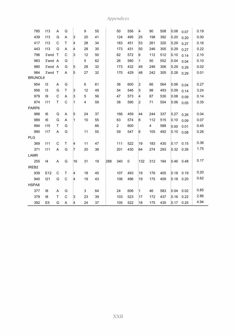
Appendices
XXII
785 I13 A G 9 55 50 556 4 90 508 0.08 0.07 0.19
439 I13 G A 3 20 41 124 495 25 198 392 0.20 0.20 0.00
417 I13 C T 4 28 34 183 451 53 261 320 0.29 0.27 0.16
443 I13 G A 4 28 35 173 431 50 246 305 0.29 0.27 0.22
796 3’end T C 3 12 50 62 572 6 112 512 0.10 0.14 2.10
983 3’end A G 5 62 26 580 1 50 552 0.04 0.04 0.10
980 3’end A G 5 28 32 173 432 49 246 306 0.29 0.29 0.02
984 3’end T A 5 27 32 170 429 48 242 305 0.28 0.29 0.01
BRUNOL6
954 I3 A G 6 61 36 600 2 66 564 0.06 0.04 0.27
956 I3 G T 3 12 49 54 546 5 98 493 0.09 0.14 3.24
979 I9 C A 3 5 56 47 573 4 87 530 0.08 0.09 0.14
974 I11 T C 1 4 59 38 590 2 71 554 0.06 0.05 0.35
PARP6
988 I6 G A 5 24 37 166 459 44 244 337 0.27 0.26 0.04
989 I6 G A 1 10 55 63 574 6 112 515 0.10 0.09 0.07
994 I15 T G 66 2 600 4 588 0.00 0.01 0.45
995 I17 A G 11 55 59 547 6 105 492 0.10 0.08 0.26
PLG
369 I11 C T 4 11 47 111 522 19 183 430 0.17 0.15 0.36
371 I11 A G 7 20 38 201 430 64 274 293 0.32 0.26 1.75
LAMR
255 I4 A G 16 31 19 288 340 0 132 312 184 0.46 0.48 0.17
IREB2
939 E12 C T 4 18 45 107 493 19 176 405 0.18 0.19 0.20
940 I21 G C 4 19 43 106 496 19 175 409 0.18 0.20 0.62
HSPA8
377 I8 A G 3 64 24 606 1 46 583 0.04 0.02 0.85
379 I8 T C 3 23 39 103 523 17 172 437 0.16 0.22 2.86
392 E5 G A 4 24 37 105 522 18 175 435 0.17 0.25 4.94
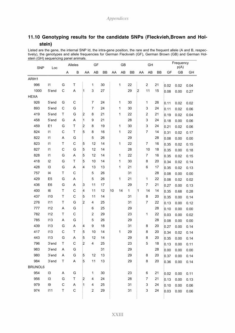
Appendices
XXIII
11.10 Genotyping results for the candidate SNPs (Fleckvieh,Brown and Hol-
stein)
Listed are the gene, the internal SNP Id, the intra-gene position, the rare and the frequent allele (A and B, respec-tively), the genotypes and allele frequencies for German Fleckvieh (GF), German Brown (GB) and German Hol-stein (GH) sequencing panel animals.
Alleles GF GB GHFrequency
p(A)SNP Loc
A B AA AB BB AA AB BB AA AB BB GF GB GH
ARIH1
996 I1 G T 1 30 1 22 2 21 0.02 0.02 0.04
1000 5’end C A 1 3 27 29 2 11 15 0.08 0.00 0.27
HEXA
926 5’end G C 7 24 1 30 1 26 0.11 0.02 0.02
893 5’end C G 7 24 1 30 3 24 0.11 0.02 0.06
419 5’end T G 2 8 21 1 22 2 21 0.19 0.02 0.04
458 5’end G A 1 9 21 28 3 24 0.18 0.00 0.06
459 E1 G T 2 8 19 1 30 3 24 0.21 0.02 0.06
824 I1 C T 5 8 16 1 22 7 14 0.31 0.02 0.17
822 I1 A G 5 26 29 28 0.08 0.00 0.00
823 I1 T C 5 12 14 1 22 7 16 0.35 0.02 0.15
827 I1 C G 5 12 14 28 10 18 0.35 0.00 0.18
828 I1 G A 5 12 14 1 22 7 16 0.35 0.02 0.15
418 I2 G T 5 10 14 1 30 8 20 0.34 0.02 0.14
428 I3 G A 4 13 13 1 21 6 17 0.35 0.02 0.13
757 I4 T C 5 26 31 28 0.08 0.00 0.00
429 E5 G A 5 26 1 21 1 22 0.08 0.02 0.02
436 E6 G A 3 11 17 29 7 21 0.27 0.00 0.13
400 I6 T C 4 11 12 10 14 1 1 14 14 0.35 0.68 0.28
437 I10 T C 5 11 14 31 8 20 0.35 0.00 0.14
276 I11 T G 2 4 25 31 7 22 0.13 0.00 0.12
777 I12 A G 6 25 29 28 0.10 0.00 0.00
782 I12 T C 2 29 23 1 22 0.03 0.00 0.02
785 I13 A G 5 26 29 28 0.08 0.00 0.00
439 I13 G A 4 9 18 31 8 20 0.27 0.00 0.14
417 I13 C T 5 10 14 1 29 8 20 0.34 0.02 0.14
443 I13 G A 5 12 14 29 8 20 0.35 0.00 0.14
796 3’end T C 2 4 25 23 5 18 0.13 0.00 0.11
983 3’end A G 31 29 28 0.00 0.00 0.00
980 3’end A G 5 12 13 29 8 20 0.37 0.00 0.14
984 3’end T A 5 11 13 29 8 20 0.36 0.00 0.14
BRUNOL6
954 I3 A G 1 30 23 6 21 0.02 0.00 0.11
956 I3 G T 2 4 24 28 7 21 0.13 0.00 0.13
979 I9 C A 1 4 25 31 3 24 0.10 0.00 0.06
974 I11 T C 2 29 31 3 24 0.03 0.00 0.06
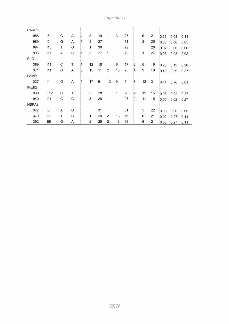
Appendices
XXIV
PARP6
988 I6 G A 4 8 19 1 3 27 6 21 0.26 0.08 0.11
989 I6 G A 1 3 27 31 3 25 0.08 0.00 0.05
994 I15 T G 1 30 29 28 0.02 0.00 0.00
995 I17 A G 1 3 27 1 29 1 27 0.08 0.03 0.02
PLG
369 I11 C T 1 12 18 6 17 2 5 16 0.23 0.13 0.20
371 I11 G A 5 15 11 2 13 7 4 9 10 0.40 0.39 0.37
LAMR
337 I4 G A 5 17 9 13 9 1 8 12 3 0.44 0.76 0.61
IREB2
939 E12 C T 3 28 1 28 2 11 15 0.05 0.02 0.27
940 I21 G C 3 28 1 28 2 11 15 0.05 0.02 0.27
HSPA8
377 I8 A G 31 31 5 22 0.00 0.00 0.09
379 I8 T C 1 29 2 13 16 6 21 0.02 0.27 0.11
392 E5 G A 2 29 2 13 16 6 21 0.03 0.27 0.11
XXV
Curriculum vitae
KATRIN JULING
Birthday July 31, 1976
Birthplace Offenbach / Main, Germany
EDUCATION AND STUDY
1982-1986 Primary school - Basic education in Eching, Munich, Germany
1986-1996 Secondary school - Dom-Gymnasium, Freising, Germany
1996 Abitur (German university-entrance diploma)
1996 three month stay in Berkeley, CA, USA
1997-2002 Study of Agricultural Science with focus on Animal Science at the
Life Science Centre of the Technical University of Munich
2001 Instructor qualification
2002 Diploma thesis: SNP-Analyse in Kandidatengenen für BSE-
Prädisposition (Chair of Animal Breeding, TUM)
2002 Diploma degree (Dipl. Ing. agr. Univ.)
POST GRADUATE EDUCATION
2002-2007 PhD position at the Chair of Animal Breeding of TUM
Topic: BSE-Genetics
2005 Project leader qualification and delegate for bio safety (§§ 15 and
17 of Gentechniksicherheitsverordnung)
2007 Promotion (Dr.rer.nat.)
Dissertation thesis: Genomic Characterisation, Polymorphism
Analysis and Association studies of candidate genes for BSE
susceptibility