PHYSICAL REVIEW E 87, 012716 (2013)

Channel-based Langevin approach for the stochastic Hodgkin-Huxley neuron

Yandong Huang,1 Sten Rudiger,2 and Jianwei Shuai1,*

1Department of Physics and Institute of Theoretical Physics and Astrophysics, Xiamen University, Xiamen 361005, China2Institute of Physics, Humboldt-Universitat zu Berlin, Berlin, Germany

(Received 17 September 2012; revised manuscript received 7 December 2012; published 22 January 2013)

Stochasticity in ion channel gating is the major source of intrinsic neuronal noise, which can induce manyimportant effects in neuronal dynamics. Several numerical implementations of the Langevin approach have beenproposed to approximate the Markovian dynamics of the Hodgkin-Huxley neuronal model. In this work animproved channel-based Langevin approach is proposed by introducing a truncation procedure to limit the statefractions in the range of [0, 1]. The truncated fractions are put back into the state fractions in the next timestep for channel noise calculation. Our simulations show that the bounded Langevin approaches combined withthe restored process give better approximations to the statistics of action potentials with the Markovian method.As a result, in our approach the channel state fractions are disturbed by two terms of noise: an uncorrelatedGaussian noise and a time-correlated noise obtained from the truncated fractions. We suggest that the restorationof truncated fractions is a critical process for a bounded Langevin method.

DOI: 10.1103/PhysRevE.87.012716 PACS number(s): 87.19.ll, 87.10.Mn, 87.19.Hh

I. INTRODUCTION

Neuronal excitability and information transfer are deter-mined by the currents through ion channels on the neuronalmembrane. Hodgkin and Huxley first described the nervemembrane ion currents deterministically and established whatis now called the Hodgkin-Huxley (HH) model [1]. The HHmodel is expressed by a set of differential equations to providea deterministic description of the mean behavior of ion channelstates. Later, from patch-clamp studies, the stochasticity of theopening and closing of ion channels, known as channel noise,has been observed [2].

With the stochastic HH model, many effects of channelnoise on action potentials were studied, such as sponta-neous action potentials [3,4], interspike interval statistics[5], stochastic resonance [6,7], and entropically enhancedexcitability [8]. Beyond the basic HH model, the contribu-tion of channel noise to neuronal dynamics has also beenaddressed with biophysically detailed model neurons, such asthe entorhinal cortex neuron [9] and the cerebellar granulecell [10]. The critical roles of channel noise in the generation,propagation, and integration of neuronal signals have beeninvestigated in a morphologically detailed neuronal modelwith extensive dendritic or axonal arborizations, such as inretinal ganglion cell [11], hippocampal neuron [12,13], andunmyelinated axon [14,15]. Besides intrinsic channel noise,external noise also exists in neural networks and is significantfor neuronal activities [16]. The contribution of channel noisehas become of interest also in many other systems or cells, suchas intracellular calcium signaling system [17,18] and barnaclegiant muscle fiber [19].

Besides the discussion of the effects of channel noise,a fundamental question is how to characterize the channelnoise accurately. During the last 30 years, fractal ion-channel

*Corresponding author: Department of Physics, Xiamen University,Xiamen, Fujian 361005, China. FAX: (86) 592-218-9426. Emailaddress: jianweishuai@xmu.edu.cn

behavior and history-dependent ionic current signals have beencaptured in experiment through analyzing the patch-clampdata [20–25]. Moreover, the analysis of the power spectraof nanochannel currents showed that such currents havethe properties of the so-called 1/f (flicker) noise [26–28].Actually, a biologically realistic neuronal system is complexwith composite axon and dendritic structures, having a non-Markovian channel dynamics, and is affected by internalfluctuation of ion concentration and external noises. However,in this paper we focus only on the intrinsic Markovian noisedescribed within a standard stochastic HH model.

By the HH model, all subunits in a channel are independentand each subunit has two discrete configuration states, i.e., theopen and the closed states. Thus the channel dynamics can besimulated by a two-state Markovian process, which is termedthe Markovian method [7,8,17,18,29,30]. In this paper the two-state Markovian method is considered as the standard methodfor comparison. For small channel numbers, a Markovianprocess can also be exactly simulated via a Gillespie-typealgorithm [4,31–33]. However, these Markovian methods arecomputationally demanding in the case of many channels,leaving approximate methods more favorable [34].

Several approximate methods have been suggested toaccount for the Markovian channel noise. In the frameworkof Fox and Lu’s work, two classes of approximations, termedsubunit-based approaches and channel-based approaches,were proposed to represent the Markovian channel noise[17,35–37]. They are different essentially in the place wherechannel noise is added to the stochastic differential equations(SDEs). In detail, subunit-based Fox-Lu approaches addGaussian noise to the equations that describe the fractionsof subunit states of channels, while channel-based Fox-Luapproaches introduce Gaussian noise directly into the fractionsof channel states. Subunit-based approaches are simpler andrequire less computational resources, which is why they havebeen applied extensively to stochastic neuron models [6], aswell as calcium signaling models with stochastic IP3 receptors[17,18]. However, in comparison with the standard Markovmethod, subunit-based approaches could not capture correctly

012716-11539-3755/2013/87(1)/012716(9) ©2013 American Physical Society

YANDONG HUANG, STEN RUDIGER, AND JIANWEI SHUAI PHYSICAL REVIEW E 87, 012716 (2013)

the microscopic statistical properties of channel gating and theaccuracy could not be improved with increasing numbers ofchannels [37–42].

On the other hand, the channel-based Fox-Lu approach wasdemonstrated to better replicate the statistical properties of theMarkovian HH neuron [42]. However, there is an unreasonabletreatment of channel state fractions in the channel-basedFox-Lu approach. Due to the addition of Gaussian noiseto the SDEs, the fractions of channel states may be out ofthe range of [0, 1], which will lack biological meaning. Theoriginal channel-based Fox-Lu approach does not considerconfinement within [0, 1] for the fractions of the eight statesfor Na+ channels and five states for K+ channels, but rather, theapproach lets these fractions evolve freely without boundarylimitation [42]. In the channel-based approach, two diffusionmatrices have to be defined to calculate the state fractionsfor Na+ and K+ channels, respectively. The diffusion matrixhas to be positive semidefinite in order to obtain real valuedmatrix square roots. Once a state fraction is out of [0, 1],the diffusion matrices will no longer be guaranteed to bepositive semidefinite. To avoid this problem, the equilibriumstate fractions, rather than the real-time state fractions, of thechannel are applied for the calculation of the diffusion matricesin the channel-based approach [42].

Another Langevin approach was developed recently basedon the realization of an Ornstein-Uhlenbeck process [43].However, this approach rests on the assumption that thechannel number is large. At small channel number, thisapproach also generates negative open fractions for Na+ andK+ channels. Moreover, it has been found that this approachfails to track the Markov chain variance during the spikes evenat large channel number [44]. More recently, a method withreflection was applied to the channel-based approach to makesure that the state fractions stay in the region of [0, 1]. However,it has also been pointed out that this reflected approach fails atsmall channel numbers [45]. In this paper we will show thatthe reflected approach could not give a satisfying estimate ofthe interspike interval even at large channel numbers.

Thus currently, although the Langevin approaches of theMarkovian process are widely applied for the study ofstochastic channel dynamics, none of them guarantees aprecise description of channel noise in the neuronal system.In consequence, the use of the oversimplified channel noise inLangevin approaches may thereby lead to qualitatively correctbut quantitatively incorrect conclusions. Thus, an importantquestion is how to construct a better Langevin approach inorder to correctly describe the Markovian channel dynamics.

In this paper we introduce an efficient Langevin methodbased on the channel-based Fox-Lu approach. In order toovercome the boundary-free problem, we consider a truncatingmethod to hold the state fraction in the range of [0, 1].Rather than simply cutting off the state fraction to [0, 1],we feed the extra state fraction back into the system inthe next time step for numerical calculation. Simulationresults show that such a bounded channel-based approachcan give a better approximation of the Markovian dynamics.Furthermore, we show that the restoring method, which isa key part in our bounded approach, can also be applied tothe reflected Langevin approach to induce a better numericalresult.

II. SIMULATION METHODS

In this section, we briefly review the HH model [1] andthe corresponding Markov method. Then after introducing theoriginal channel-based Langevin approach proposed by Foxand Lu [35,42] and the reflected SDEs approach proposedin [45], we present our improved bounded approach withthe restoration process of truncated fractions. In the end, therestoration process is incorporated into the reflected SDEsapproach.

A. HH model with subunit-based expression

We consider a single-compartment HH model [46], inwhich the neuronal membrane voltage evolution is governedby [1]

−CdV

dt= INa + IK + IL − IStim (1)

where V is the membrane potential in millivolts; C =1 μF/cm2 the membrane capacitance, and IStim is the stimuluscurrent added to the neuron in μA/cm2. INa, IK, and IL arethe currents of the sodium channels, potassium channels, andleakage channels, respectively, given by

INa = gNahm3(V − ENa), (2)

IK = gKn4(V − EK), (3)

IL = gL(V − EL), (4)

where ENa = 50 mV, EK = −77 mV, and EL = −54.3 mV arethe reversal potential of sodium channels, potassium channels,and leakage channels, respectively, and gNa = 120ms/cm2,gK = 36ms/cm2, and gL = 0.3ms/cm2 are the total conduc-tance of sodium channels, potassium channels, and leakagechannels, respectively.

The currents given by Eqs. (2) and (3) indicate that there arefour identical and independent n subunits for each K+ channeland three m subunits and one h subunit for each Na+ channel.The original derivation of the HH equations was based onsubunits, where the open probability w = {m,h,n} of eachsubunit is described by the relaxation equations:

dw

dt= αw(1 − w) − βww. (5)

Here αw and βw are subunit opening and closing rates withthe unit of m s−1 and depend on the membrane potential V

according to the following formulas:

αm = 0.1(V + 40)

1 − exp[−(V + 40)/10], (6)

βm = 4 exp[−(V + 65)/18], (7)

αh = 0.07 exp[−(V + 65)/20], (8)

βh = 1

1 + exp[−(V + 35)/10], (9)

012716-2

CHANNEL-BASED LANGEVIN APPROACH FOR THE . . . PHYSICAL REVIEW E 87, 012716 (2013)

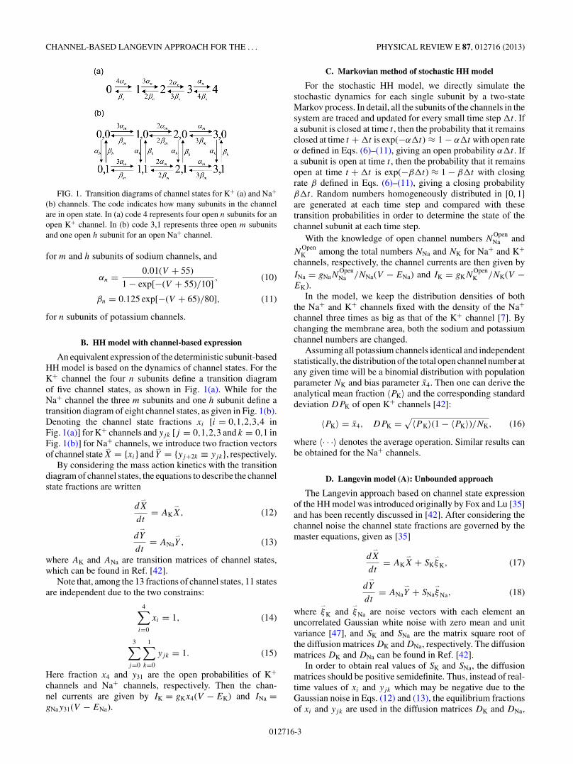
FIG. 1. Transition diagrams of channel states for K+ (a) and Na+

(b) channels. The code indicates how many subunits in the channelare in open state. In (a) code 4 represents four open n subunits for anopen K+ channel. In (b) code 3,1 represents three open m subunitsand one open h subunit for an open Na+ channel.

for m and h subunits of sodium channels, and

αn = 0.01(V + 55)

1 − exp[−(V + 55)/10], (10)

βn = 0.125 exp[−(V + 65)/80], (11)

for n subunits of potassium channels.

B. HH model with channel-based expression

An equivalent expression of the deterministic subunit-basedHH model is based on the dynamics of channel states. For theK+ channel the four n subunits define a transition diagramof five channel states, as shown in Fig. 1(a). While for theNa+ channel the three m subunits and one h subunit define atransition diagram of eight channel states, as given in Fig. 1(b).Denoting the channel state fractions xi [i = 0,1,2,3,4 inFig. 1(a)] for K+ channels and yjk [j = 0,1,2,3 and k = 0,1 inFig. 1(b)] for Na+ channels, we introduce two fraction vectorsof channel state

⇀

X = {xi} and⇀

Y = {yj+2k ≡ yjk}, respectively.By considering the mass action kinetics with the transition

diagram of channel states, the equations to describe the channelstate fractions are written

d⇀

X

dt= AK

⇀

X, (12)

d⇀

Y

dt= ANa

⇀

Y , (13)

where AK and ANa are transition matrices of channel states,which can be found in Ref. [42].

Note that, among the 13 fractions of channel states, 11 statesare independent due to the two constrains:

4∑i=0

xi = 1, (14)

3∑j=0

1∑k=0

yjk = 1. (15)

Here fraction x4 and y31 are the open probabilities of K+channels and Na+ channels, respectively. Then the chan-nel currents are given by IK = gKx4(V − EK) and INa =gNay31(V − ENa).

C. Markovian method of stochastic HH model

For the stochastic HH model, we directly simulate thestochastic dynamics for each single subunit by a two-stateMarkov process. In detail, all the subunits of the channels in thesystem are traced and updated for every small time step �t . Ifa subunit is closed at time t , then the probability that it remainsclosed at time t + �t is exp(−α�t) ≈ 1 − α�t with open rateα defined in Eqs. (6)–(11), giving an open probability α�t . Ifa subunit is open at time t , then the probability that it remainsopen at time t + �t is exp(−β�t) ≈ 1 − β�t with closingrate β defined in Eqs. (6)–(11), giving a closing probabilityβ�t . Random numbers homogeneously distributed in [0, 1]are generated at each time step and compared with thesetransition probabilities in order to determine the state of thechannel subunit at each time step.

With the knowledge of open channel numbers NOpenNa and

NOpenK among the total numbers NNa and NK for Na+ and K+

channels, respectively, the channel currents are then given byINa = gNaN

OpenNa /NNa(V − ENa) and IK = gKN

OpenK /NK(V −

EK).In the model, we keep the distribution densities of both

the Na+ and K+ channels fixed with the density of the Na+channel three times as big as that of the K+ channel [7]. Bychanging the membrane area, both the sodium and potassiumchannel numbers are changed.

Assuming all potassium channels identical and independentstatistically, the distribution of the total open channel number atany given time will be a binomial distribution with populationparameter NK and bias parameter x4. Then one can derive theanalytical mean fraction 〈PK〉 and the corresponding standarddeviation DPK of open K+ channels [42]:

〈PK〉 = x4, DPK =√

〈P K〉(1 − 〈PK〉)/NK, (16)

where 〈· · ·〉 denotes the average operation. Similar results canbe obtained for the Na+ channels.

D. Langevin model (A): Unbounded approach

The Langevin approach based on channel state expressionof the HH model was introduced originally by Fox and Lu [35]and has been recently discussed in [42]. After considering thechannel noise the channel state fractions are governed by themaster equations, given as [35]

d⇀

X

dt= AK

⇀

X + SK⇀

ξK, (17)

d⇀

Y

dt= ANa

⇀

Y + SNa⇀

ξNa, (18)

where⇀

ξK and⇀

ξNa are noise vectors with each element anuncorrelated Gaussian white noise with zero mean and unitvariance [47], and SK and SNa are the matrix square root ofthe diffusion matrices DK and DNa, respectively. The diffusionmatrices DK and DNa can be found in Ref. [42].

In order to obtain real values of SK and SNa, the diffusionmatrices should be positive semidefinite. Thus, instead of real-time values of xi and yjk which may be negative due to theGaussian noise in Eqs. (12) and (13), the equilibrium fractionsof xi and yjk are used in the diffusion matrices DK and DNa,

012716-3

YANDONG HUANG, STEN RUDIGER, AND JIANWEI SHUAI PHYSICAL REVIEW E 87, 012716 (2013)

given by

xi =(

4

i

)αi

nβ4−in

(α + β)4 , (19)

yjk =(

3

j

)α

jmβ

3−jm αk

hβ1−kh

(αm + βm)3(αh + βh). (20)

For numerical simulation, Eq. (17) will be rewritten as thefollowing difference iteration equation:

⇀

Xt+�t = ⇀

Xt + �tAK⇀

Xt +√

�tSK⇀

ξ t (21)

In the simulation, each Gaussian noise is calculated by twowhite noises homogeneously distributed from 0 to 1. Thereis a similar difference equation for the fraction vector

⇀

Y inEq. (18).

Numerically, although the normalization condition given byEqs. (14) and (15) can be always satisfied with the differenceequation Eq. (21), the large enough Gaussian noises may drivethe state fractions xi and yjk out of range [0, 1]. Thus in therest of this paper we call this original channel-based Langevinapproach the unbounded method.

In the deterministic HH model, the open fractions x4 andy31 of sodium and potassium channels change in the rangesof [0, 0.35) and [0, 0.25) during an action potential. Withthe unbounded Langevin approach we did not observe thesituation of x4 and y31 larger than 1; however, x4 and y31 arefrequently found to be negative. The probabilities for the openfractions x4 and y31 to be negative are calculated, showing thateven for a channel number as large as N = 10 000, the openfraction y31 can become negative with a probability of 5%. Atsmall channel number, the state fractions xi and yjk violatethe physical constraint [0, 1] seriously, which will cause theoverflow and breakdown of the simulation program.

E. Langevin model (B): Reflected approach

The reflected approach was proposed in [45] to bound thesolutions of the channel state fractions by incorporating thereflecting process with an orthogonal projection method (formore detail see [48]). Besides, an equivalent representationof the noise term is adopted so as to avoid the calculation ofthe square root of the diffusion matrix. The following is thecorresponding formulations used in the numerical simulationof the reflected approach.

⇀

Xt+�t = ⇀

Xt + AK⇀

X�t + 1√NK

LKJK⇀

ξK

√�t + �

⇀

RK,

(22)

⇀

Y t+�t = ⇀

Y t + ANa⇀

Y�t + 1√NNa

LNaJNa⇀

ξNa

√�t + �

⇀

RNa,

(23)

where the matrices LK, LNa, JK, JNa as well as the definitionof the reflecting processes

⇀

RK and⇀

RNa can be obtained inRef. [45].

F. Langevin model (C): Truncated and restored approach

Since the fractions of channel states should not be out of therange [0, 1] we here introduce another scheme to confine the

state fractions xi and yjk within [0, 1]. In this method, we firstcut off the state fractions that are out of the range [0, 1]. Beforethe cutting off, the state fractions obey the normalizationcondition. After cutting off, the normalization condition isbroken. Thus a second step in our method is to consider arenormalization process for the state fractions. Thirdly, insteadof simply throwing away the truncated values, we propose inour approach to store the truncated values for inclusion in thenext time step.

Taking the K+ channels as an example, we introduce aresidue vector

⇀

E = {ei} in the numerical iteration function ofEq. (21),

κt+�ti = xt

i +∑

j

AKij xtj�t +

∑j

SKij ξj

√�t + et

i . (24)

Compared to Eq. (21), a term eti which is obtained from κt

i isadded at the right-hand side of Eq. (24). Then we split κt+�t

i

into the following two terms: κt+�ti ≡ xt+�t

i + et+�ti , where

the residue vector⇀

E = {ei} is the truncated value from theunbound vector

⇀

K = {κi}.The truncation procedure is as follows: If all elements κt+�t

i

in the unbounded vector⇀

K = {κi} are in the range of [0, 1], thenxt+�t

i = κt+�ti and et+�t

i = 0, and we go directly to the nextiteration with Eq. (24). If any element κt+�t

i is out of the rangeof [0, 1], we consider the following truncating procedure:

If there is an element κt+�ti > 1, then we define xt+�t

i = 1and et+�t

i = κt+�ti − 1. In order to preserve the normalization

condition, we define xt+�tj = 0 and et+�t

j = κt+�tj for other

elements j �= i.Otherwise, if there is a term κt+�t

i < 0, then we de-fine xt+�t

i = 0 and et+�ti = κt+�t

i . In order to preservethe normalization condition, we define xt+�t

j = κt+�tj /sum

and et+�tj = κt+�t

j − κt+�tj /sum with sum = ∑

j �=i κt+�tj for

other elements j �= i.By this truncating procedure, the unbounded vector

⇀

K ={κi} is split into two parts: the bounded vector

⇀

X and theresidue vector

⇀

E. Then we put⇀

Xt+�t into the iteration equationof Eq. (24) to calculate the state fractions at the next step. At thesame time the residue vector

⇀

Et+�t is restored to the fractions⇀

Xt+�t by directly adding it to the right-hand side of Eq. (24)to obtain

⇀

Kt+2�t .As a result, the bounded approach defines the following two

vector equations:

⇀

Kt+�t = ⇀

Xt + AK⇀

Xt�t + SK⇀

ξ tK

√�t + ⇀

Et ,(25)⇀

Xt+�t = ⇀

Kt+�t − ⇀

Et+�t .

We repeat such truncating procedure at each time step withei = 0 at the beginning t = 0. Similar iteration equations canbe written for Na+ channels. With the above procedure, allthe elements of vector

⇀

X and⇀

Y are bounded within [0, 1].Thus, instead of using the equilibrium state fractions given byEqs. (19) and (20), the instantaneous state fractions xi and yjk

are directly applied for the calculation of the diffusion matricesof DK and DNa in the bounded approach.

Obviously, since∑4

i=0 xi = 1 is always maintained, wehave

∑4i=0 ei = 0.0. Putting two equations in Eq. (25) together,

012716-4

CHANNEL-BASED LANGEVIN APPROACH FOR THE . . . PHYSICAL REVIEW E 87, 012716 (2013)

we have the following equation:⇀

Xt+�t = ⇀

Xt + AK⇀

Xt�t + (SK⇀

ξ tK − ⇀

ηtK)

√�t,

(26)⇀

ηtK = (

⇀

Et+�t − ⇀

Et )/√

�t,

where vector ⇀η

t

K = {υti } with element υi (i = 0,1,2,3,4).

Similar as ⇀ηK = {υi} for K+ channels, vector ⇀

ηNa = {ωjk} canalso be defined for Na+ channels. By comparing the differenceiteration equations of Eqs. (21) and (26), one can see thatthe vectors ⇀

ηK and ⇀ηNa in our Langevin approach can be

considered as correlated or memory noise with zero mean,i.e., 〈υt

i 〉 = 〈ωtjk〉 = 0.0.

G. Langevin model (D): Simple truncated approach

Alternatively, one may consider a simpler approach byapplying Eq. (24) with the truncating and renormalizingprocedures, but throwing away the residue vector

⇀

E, i.e.,⇀

Kt = ⇀

Xt + AK⇀

Xt�t + SK⇀

ξ tK

√�t,

(27)⇀

Xt+�t = ⇀

Kt − ⇀

Et+�t .

However, our simulation results show that this approach couldnot reproduce the channel noise correctly for N < 2000 (datanot shown). Thus in our paper we will not consider thisapproach.

H. Langevin model (E): Reflected and restored approach

The reflected approach applies the projection process tolimit the fractions of channel states into the region of [0, 1], andsimply ignore the residue values which are also important inreplicating correctly the stochastic channel dynamics. Here, weintroduce the restoration operation into the original reflectedapproach. Taking Eq. (22) for the potassium channel as anexample, the numerical iteration equation becomes

⇀

Kt+�t = ⇀

Xt + AK⇀

X�t + 1√NK

LKJK⇀

ζ K

√�t + ⇀

Et (28)

With the reflected procedure, we have⇀

Xt+�t = ⇀

Kt+�t +�

⇀

Rt+�tK . Here

⇀

Xt+�t is the channel state fraction after thereflected procedure. We then define the truncated fraction⇀

Et+�t = −�⇀

Rt+�t . This residue will be restored back inEq. (28) for calculation in the next time step.

III. RESULTS

In this section, different Langevin approaches with diffu-sion matrices are discussed and compared with the two-stateMarkovian chain method (Markov). The original channel-based Fox-Lu approach will be called the unbounded approach(Unbound), the reflected Langevin approach suggested inRef. [45] will be called the reflected approach (Reflected), thechannel-based Langevin approach with truncated and restoredstate fractions is termed the truncated and restored approach(Truncated-Restored), and the reflected Langevin approachwith restored state fractions is called the reflected and restoredapproach (Reflected-Restored). In all the following figures, weuse a set of fixed symbols to represent the results obtained withthe four methods. In detail, the black open squares are for theMarkov method, the green plus symbols for the unbounded

approach, the purple cross symbols for the reflected approach,the red (gray) open squares for the reflected and restoredapproach, and the blue stars for the truncated and restoredapproach.

If not specified otherwise, we denote the K+ channelnumber by N (i.e., N ≡ NK) in the following, and the cor-responding Na+ channel number is then three times as large asN , (i.e. NNa = 3N ). Two typical stimulus currents are studied,i.e., IStim = 0 and 15 μA/cm2, deterministically yielding astable fixed point and a periodic oscillation, respectively.

A. Correlated noise for the truncated and restored approach

First, we discuss the equilibrium state which simulates thevoltage-clamp experiments with a fixed membrane voltage V .Here we discuss the statistical properties of the memory noisedefined in Eq. (26) for the truncated and restored approach andthe memory noise for the reflected and restored approach.

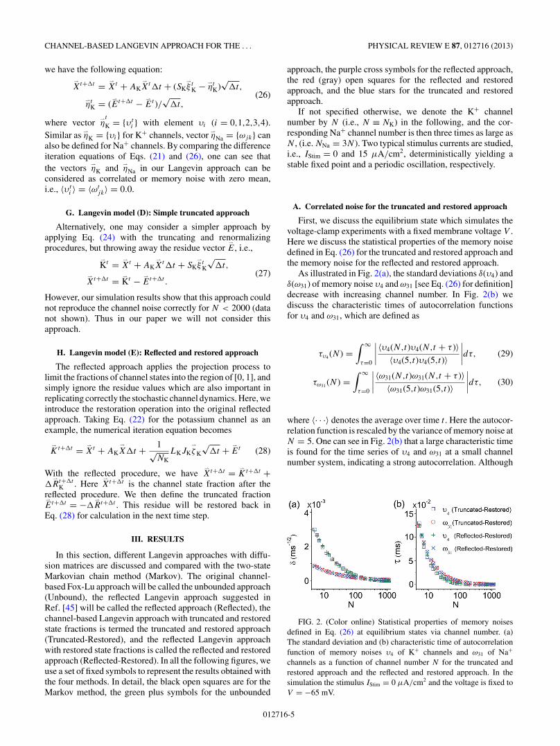
As illustrated in Fig. 2(a), the standard deviations δ(υ4) andδ(ω31) of memory noise υ4 and ω31 [see Eq. (26) for definition]decrease with increasing channel number. In Fig. 2(b) wediscuss the characteristic times of autocorrelation functionsfor υ4 and ω31, which are defined as

τυ4 (N ) =∫ ∞

τ=0

∣∣∣∣ 〈υ4(N,t)υ4(N,t + τ )〉〈υ4(5,t)υ4(5,t)〉

∣∣∣∣dτ, (29)

τω31 (N ) =∫ ∞

τ=0

∣∣∣∣ 〈ω31(N,t)ω31(N,t + τ )〉〈ω31(5,t)ω31(5,t)〉

∣∣∣∣dτ, (30)

where 〈· · ·〉 denotes the average over time t . Here the autocor-relation function is rescaled by the variance of memory noise atN = 5. One can see in Fig. 2(b) that a large characteristic timeis found for the time series of υ4 and ω31 at a small channelnumber system, indicating a strong autocorrelation. Although

FIG. 2. (Color online) Statistical properties of memory noisesdefined in Eq. (26) at equilibrium states via channel number. (a)The standard deviation and (b) characteristic time of autocorrelationfunction of memory noises υ4 of K+ channels and ω31 of Na+

channels as a function of channel number N for the truncated andrestored approach and the reflected and restored approach. In thesimulation the stimulus IStim = 0 μA/cm2 and the voltage is fixed toV = −65 mV.

012716-5

YANDONG HUANG, STEN RUDIGER, AND JIANWEI SHUAI PHYSICAL REVIEW E 87, 012716 (2013)

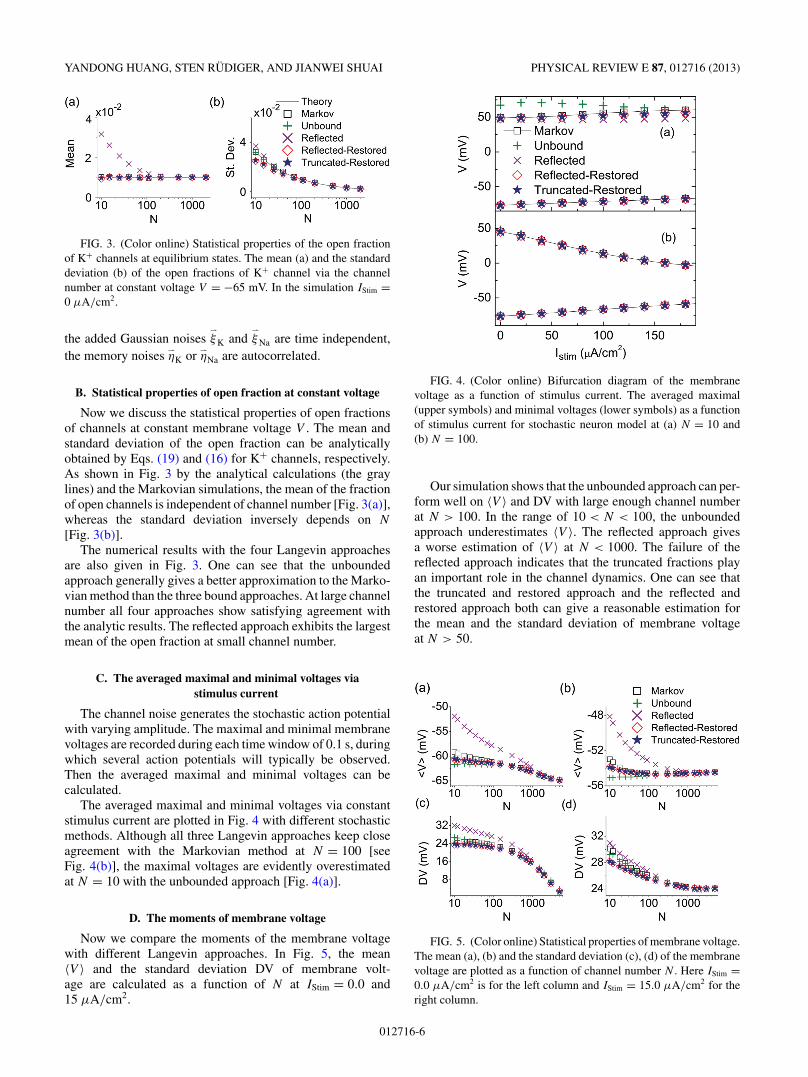
FIG. 3. (Color online) Statistical properties of the open fractionof K+ channels at equilibrium states. The mean (a) and the standarddeviation (b) of the open fractions of K+ channel via the channelnumber at constant voltage V = −65 mV. In the simulation IStim =0 μA/cm2.

the added Gaussian noises⇀

ξK and⇀

ξNa are time independent,the memory noises ⇀

ηK or ⇀ηNa are autocorrelated.

B. Statistical properties of open fraction at constant voltage

Now we discuss the statistical properties of open fractionsof channels at constant membrane voltage V . The mean andstandard deviation of the open fraction can be analyticallyobtained by Eqs. (19) and (16) for K+ channels, respectively.As shown in Fig. 3 by the analytical calculations (the graylines) and the Markovian simulations, the mean of the fractionof open channels is independent of channel number [Fig. 3(a)],whereas the standard deviation inversely depends on N

[Fig. 3(b)].The numerical results with the four Langevin approaches

are also given in Fig. 3. One can see that the unboundedapproach generally gives a better approximation to the Marko-vian method than the three bound approaches. At large channelnumber all four approaches show satisfying agreement withthe analytic results. The reflected approach exhibits the largestmean of the open fraction at small channel number.

C. The averaged maximal and minimal voltages viastimulus current

The channel noise generates the stochastic action potentialwith varying amplitude. The maximal and minimal membranevoltages are recorded during each time window of 0.1 s, duringwhich several action potentials will typically be observed.Then the averaged maximal and minimal voltages can becalculated.

The averaged maximal and minimal voltages via constantstimulus current are plotted in Fig. 4 with different stochasticmethods. Although all three Langevin approaches keep closeagreement with the Markovian method at N = 100 [seeFig. 4(b)], the maximal voltages are evidently overestimatedat N = 10 with the unbounded approach [Fig. 4(a)].

D. The moments of membrane voltage

Now we compare the moments of the membrane voltagewith different Langevin approaches. In Fig. 5, the mean〈V 〉 and the standard deviation DV of membrane volt-age are calculated as a function of N at IStim = 0.0 and15 μA/cm2.

FIG. 4. (Color online) Bifurcation diagram of the membranevoltage as a function of stimulus current. The averaged maximal(upper symbols) and minimal voltages (lower symbols) as a functionof stimulus current for stochastic neuron model at (a) N = 10 and(b) N = 100.

Our simulation shows that the unbounded approach can per-form well on 〈V 〉 and DV with large enough channel numberat N > 100. In the range of 10 < N < 100, the unboundedapproach underestimates 〈V 〉. The reflected approach givesa worse estimation of 〈V 〉 at N < 1000. The failure of thereflected approach indicates that the truncated fractions playan important role in the channel dynamics. One can see thatthe truncated and restored approach and the reflected andrestored approach both can give a reasonable estimation forthe mean and the standard deviation of membrane voltageat N > 50.

FIG. 5. (Color online) Statistical properties of membrane voltage.The mean (a), (b) and the standard deviation (c), (d) of the membranevoltage are plotted as a function of channel number N . Here IStim =0.0 μA/cm2 is for the left column and IStim = 15.0 μA/cm2 for theright column.

012716-6

CHANNEL-BASED LANGEVIN APPROACH FOR THE . . . PHYSICAL REVIEW E 87, 012716 (2013)

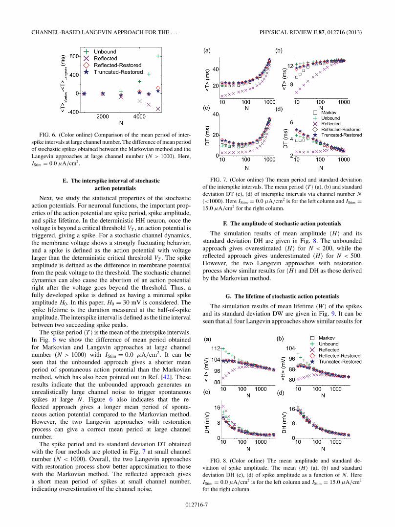
FIG. 6. (Color online) Comparison of the mean period of inter-spike intervals at large channel number. The difference of mean periodof stochastic spikes obtained between the Markovian method and theLangevin approaches at large channel number (N > 1000). Here,IStim = 0.0 μA/cm2.

E. The interspike interval of stochasticaction potentials

Next, we study the statistical properties of the stochasticaction potentials. For neuronal functions, the important prop-erties of the action potential are spike period, spike amplitude,and spike lifetime. In the deterministic HH neuron, once thevoltage is beyond a critical threshold VT , an action potential istriggered, giving a spike. For a stochastic channel dynamics,the membrane voltage shows a strongly fluctuating behavior,and a spike is defined as the action potential with voltagelarger than the deterministic critical threshold VT . The spikeamplitude is defined as the difference in membrane potentialfrom the peak voltage to the threshold. The stochastic channeldynamics can also cause the abortion of an action potentialright after the voltage goes beyond the threshold. Thus, afully developed spike is defined as having a minimal spikeamplitude H0. In this paper, H0 = 30 mV is considered. Thespike lifetime is the duration measured at the half-of-spikeamplitude. The interspike interval is defined as the time intervalbetween two succeeding spike peaks.

The spike period 〈T 〉 is the mean of the interspike intervals.In Fig. 6 we show the difference of mean period obtainedfor Markovian and Langevin approaches at large channelnumber (N > 1000) with IStim = 0.0 μA/cm2. It can beseen that the unbounded approach gives a shorter meanperiod of spontaneous action potential than the Markovianmethod, which has also been pointed out in Ref. [42]. Theseresults indicate that the unbounded approach generates anunrealistically large channel noise to trigger spontaneousspikes at large N . Figure 6 also indicates that the re-flected approach gives a longer mean period of sponta-neous action potential compared to the Markovian method.However, the two Langevin approaches with restorationprocess can give a correct mean period at large channelnumber.

The spike period and its standard deviation DT obtainedwith the four methods are plotted in Fig. 7 at small channelnumber (N < 1000). Overall, the two Langevin approacheswith restoration process show better approximation to thosewith the Markovian method. The reflected approach givesa short mean period of spikes at small channel number,indicating overestimation of the channel noise.

FIG. 7. (Color online) The mean period and standard deviationof the interspike intervals. The mean period 〈T 〉 (a), (b) and standarddeviation DT (c), (d) of interspike intervals via channel number N

(<1000). Here IStim = 0.0 μA/cm2 is for the left column and IStim =15.0 μA/cm2 for the right column.

F. The amplitude of stochastic action potentials

The simulation results of mean amplitude 〈H 〉 and itsstandard deviation DH are given in Fig. 8. The unboundedapproach gives overestimated 〈H 〉 for N < 200, while thereflected approach gives underestimated 〈H 〉 for N < 500.However, the two Langevin approaches with restorationprocess show similar results for 〈H 〉 and DH as those derivedby the Markovian method.

G. The lifetime of stochastic action potentials

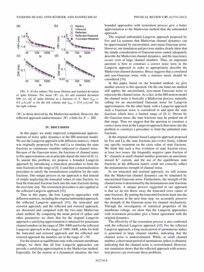
The simulation results of mean lifetime 〈W 〉 of the spikesand its standard deviation DW are given in Fig. 9. It can beseen that all four Langevin approaches show similar results for

FIG. 8. (Color online) The mean amplitude and standard de-viation of spike amplitude. The mean 〈H 〉 (a), (b) and standarddeviation DH (c), (d) of spike amplitude as a function of N . HereIStim = 0.0 μA/cm2 is for the left column and IStim = 15.0 μA/cm2

for the right column.

012716-7

YANDONG HUANG, STEN RUDIGER, AND JIANWEI SHUAI PHYSICAL REVIEW E 87, 012716 (2013)

FIG. 9. (Color online) The mean lifetime and standard deviationof spike lifetime. The mean 〈W 〉 (a), (b) and standard deviationDW (c), (d) of spike lifetime as a function of N . Here IStim =0.0 μA/cm2 is for the left column and IStim = 15.0 μA/cm2 forthe right column.

〈W 〉 as those derived by the Markovian method. However, thereflected approach underestimates 〈W 〉 a little for N < 200.

IV. DISCUSSION

In this paper, we study improved computational approxi-mations of noisy spike dynamics in the HH neuronal model.We use the Langevin approach with diffusion matrices, whichwas originally proposed by Fox and Lu to simulate the statefractions as continuous variables subjected to channel noise.Because of the Gaussian noise, the fractions of channel statesin this approximation can in principle depart the interval [0, 1].To amend this problem, we propose a bounded Langevinapproach by introducing a truncation procedure to limit thestate fractions in the range of [0, 1] and then a renormalizationprocedure to satisfy the normalization condition for the statefractions. One unique process in our approach is that insteadof simply neglecting the truncated values of state fraction, wefeed the truncated fractions back into the state fractions duringthe next time step. The restoration procedure is also applied inthe reflected Langevin approach [45].

Thus in this paper, the four Langevin approaches withdiffusion matrices, including the original unbounded approach,the reflected Langevin approach [45], the truncated andrestored approach, and the reflected and restored approach,are discussed and compared with the two-state Markovianchain method. By comparing the mean period of spikes andother parameters we show that for the original Langevinapproach a satisfying approximation is obtained for potassiumchannel numbers in the range of 200–3000 and for the reflectedLangevin approach in the range of 1000–3000, while for boththe truncated and restored approach and the reflected andrestored approach the numbers are in the range of >50.

For the neuron at equilibrium state with constant membranevoltage, we show that all four Langevin approaches canprovide a satisfying approximation to the Markovian method.Especially, for the neuron at a dynamical situation, the two

bounded approaches with restoration process give a betterapproximation to the Markovian method than the unboundedapproach.

The original unbounded Langevin approach proposed byFox and Lu assumes that Markovian channel dynamics canbe approximated by uncorrelated, zero-mean Gaussian noise.However, our simulation and previous studies clearly show thatthe simple consideration of Gaussian noise cannot adequatelydescribe the Markovian channel dynamics, and the inaccuracyoccurs even at large channel numbers. Thus, an importantquestion is how to construct a correct noise term in theLangevin approach in order to appropriately describe theMarkovian channel dynamics. Bruce suggests that a correlatedand non-Gaussian noise with a nonzero mean should beconsidered [39].

In this paper, based on our bounded method, we giveanother answer to this question. On the one hand our methodstill applies the uncorrelated, zero-mean Gaussian noise torepresent the channel noise. As a fact, in the HH neuron modelthe channel noise is basically a Markovian process, naturallycalling for an uncorrelated Gaussian noise for Langevinapproximation. On the other hand, with a Langevin approachsuch a Gaussian noise is considered to add upon the statefractions which have a limited range of [0, 1]. Driven bythe Gaussian noise, the state fractions may be pushed out ofthat range. Thus we suggest that the question to construct acorrect noise term in the Langevin approach then turns into theproblem to construct a procedure to limit the unlimited statefractions.

In the original channel-based Langevin approach proposedby Fox and Lu, the state fractions just evolve freely, withoutany specific treatment on the extra value of state fractions.We think that such a free evolution of state fraction raisesat least two issues: the frequently negative open fraction ofK+ channels at small channel number generates an unrealisticinward K+ current, and the use of the equilibrium statefractions in the diffusion matrix could not correctly reflectthe instantaneous strength of channel noise.

In our truncated and restored approach, we still assumethat the Markovian channel dynamics can be simulated byuncorrelated Gaussian noise. Furthermore, the strength of thechannel noise is determined by the instantaneous state fractionsof channels. A unique process suggested in our approachis that we do not throw away the truncated extra values ofstate fractions. By putting the truncated fractions back into thestate fractions in the next time step, we accurately preservethe strength of the Gaussian noise for channel stochasticity.Through the investigation of statistical properties of themembrane voltage, we show that the Langevin approacheswith restoration procedure give a better agreement with theoriginal dynamics.

The effectivity of the restoration process is also confirmedwith the reflected Langevin approach [45]. For the reflectedLangevin approach, a long mean period of spontaneous spikesis generated at large channel number, indicating that thechannel noise is underestimated. While, at small channelnumber, a short mean period of spontaneous spikes is obtained,indicating that the channel noise is overestimated. However,our simulation shows that the reflected approach with restora-tion process can overcome these problems.

012716-8

CHANNEL-BASED LANGEVIN APPROACH FOR THE . . . PHYSICAL REVIEW E 87, 012716 (2013)

The procedure of truncation and restoration can be treatedas a reorganization of the white Gaussian noise. As a result, thechannel state fractions are disturbed by two sources of noise:an uncorrelated Gaussian noise and a time-correlated noiseobtained from the truncation of unlimited state fractions.

The stochastic channel dynamics is found not only inneuron dynamics, but also in intracellular calcium signalingsystem [17,18] and muscle cells [19]. We suggest that theLangevin approach with the restoration of truncated statefractions can be applied to other Markovian channel systems.A similar procedure on state fractions may be considered toother Langevin approaches to avoid the state fraction out ofrange of [0, 1]. Our method is especially applicable to systemswith large channel number. Recently, a binomial noise hasbeen proposed to replace the Gaussian noise at small receptornumber in nonlinear biochemical signaling [49]. It has beenshown that the dynamics of most biologically realistic channels

are non-Markovian which should be produced with non-Gaussian noise. The two-state Markovian process, as well asthe corresponding Langevin approaches with Gaussian noise,is a simple approximation. We believe that, with accurate rep-resentation of stochastic channel dynamics more quantitativeinsights on how channel noise modulates electrophysiologicaldynamics and function in cellular systems can emerge.

ACKNOWLEDGMENTS

J.S. acknowledges support from the National NaturalScience Foundation of China under Grant No. 30970970 andthe China National Funds for Distinguished Young Scientistsunder Grant No. 11125419. Computational support from theKey Laboratory for Chemical Biology of Fujian Province,Xiamen University, is gratefully acknowledged. S.R. acknowl-edges support from the Deutsche Forschungsgemeinschaft.

[1] A. L. Hodgkin and A. F. Huxley, J. Physiol. 117, 500 (1952).[2] B. Sakmann and E. Neher, Single-Channel Recording, 2nd ed.

(Plenum Press, New York, 1995).[3] J. Clay and L. DeFelice, Biophys. J. 42, 151 (1983).[4] C. Chow and J. White, Biophys. J. 71, 3013 (1996).[5] P. Rowat, Neural Comput. 19, 1215 (2007).[6] G. Schmid, I. Goychuk, and P. Hanggi, Europhys. Lett. 56, 22

(2001).[7] P. Jung and J. W. Shuai, Europhys. Lett. 56, 29 (2001).[8] J. W. Shuai and P. Jung, Phys. Rev. Lett. 95, 114501 (2005).[9] J. A. White, R. Klink, A. Alonso, and A. R. Kay, J. Neurophysiol.

80, 262 (1998).[10] A. Saarinen, M.-L. Linne, and O. Yli-Harja, PLoS Comput. Biol.

4, e1000004 (2008).[11] M. C. W. van Rossum, B. J. O’Brien, and R. G. Smith, J.

Neurophysiol. 89, 2406 (2003).[12] K. Diba, H. A. Ester, and C. Koch, J. Neurosci. 24, 9723 (2004).[13] R. C. Cannon, C. O’Donnell, and M. F. Nolan, PLoS. Comput.

Biol. 6, e1000886 (2010).[14] S. Zeng, Y. Tang, and P. Jung, Phys. Rev. E 76, 011905 (2007).[15] A. A. Faisal and S. B. Laughlin, PLoS Comput. Biol. 3, e79

(2007).[16] A. Carpio and I. Peral, J. Nonlinear Sci. 21, 499 (2011).[17] J. W. Shuai and P. Jung, Phys. Rev. Lett. 88, 68102 (2002).[18] P. Jung and J. W. Shuai, Proc. Natl. Acad. Sci. USA 100, 506

(2003).[19] W. Gilles, T. Michele, and P. Khashayar, Biol. Cybern. 103, 43

(2010).[20] L. S. Liebovitch and J. M. Sullivan, Biophys. J. 52, 979 (1987).[21] S. J. Korn and R. Horn, Biophys. J. 54, 871 (1988).[22] A. Fulinski, Z. Grzywna, I. Mellor, Z. Siwy, and P. N. R.

Usherwood, Phys. Rev. E 58, 919 (1998).[23] S. Mercik and K. Weron, Phys. Rev. E 60, 7343 (1999).[24] S. B. Lowen, L. S. Liebovitch, and J. A. White, Phys. Rev. E 59,

5970 (1999).[25] L. Liebovitch, D. Scheurle, M. Rusek, and M. Zochowski,

Methods 24, 359 (2001).[26] S. M. Bezrukov and M. Winterhalter, Phys. Rev. Lett. 85, 202

(2000).

[27] Z. Siwy and A. Fulinski, Phys. Rev. Lett. 89, 158101 (2002).[28] I. D. Kosinska and A. Fulinski, Europhys. Lett. 81, 50006

(2008).[29] J. W. Shuai, R. Sheng, and P. Jung, Phys. Rev. E 81, 051913

(2010).[30] S. Rudiger, J. W. Shuai, and I. M. Sokolov, Phys. Rev. Lett. 105,

048103 (2010).[31] E. Skaugen and L. Walloe, Acta Physiol. Scand. 107, 343 (1979).[32] D. T. Gillespie, J. Phys. Chem. 81, 2340 (1977).[33] S. Rudiger, J. W. Shuai, W. Huisinga, C. Nagaiah, G. Warnecke,

I. Parker, and M. Falckey, Biophys. J. 93, 1847 (2007).[34] H. Mino, J. T. Rubinstein, and J. A. White, Ann. Biomed. Eng.

30, 578 (2002).[35] R. F. Fox and Y. N. Lu, Phys. Rev. E 49, 3421 (1994).[36] R. F. Fox, Biophys. J. 72, 2068 (1997).[37] Y. D. Huang, S. Rudiger, and J. W. Shuai, Eur. Phys. J. B 83,

401 (2011).[38] I. Bruce, Ann. Biomed. Eng. 35, 315 (2006).[39] I. Bruce, Ann. Biomed. Eng. 37, 824 (2009).[40] S. Zeng and P. Jung, Phys. Rev. E 70, 011903 (2004).[41] B. Sengupta, S. B. Laughlin, and J. E. Niven, Phys. Rev. E 81,

011918 (2010).[42] J. H. Goldwyn, N. S. Imennov, M. Famulare, and E. Shea-Brown,

Phys. Rev. E 83, 041908 (2011).[43] D. Linaro, M. Storace, and M. Giugliano, PLoS Comput. Biol.

7, e1001102 (2011).[44] J. H. Goldwyn and E. Shea-Brown, PLoS Comput. Biol. 7,

e1002247 (2011).[45] C. E. Dangerfield, D. Kay, and K. Burrage, Phys. Rev. E 85,

051907 (2012).[46] P. Dayan and L. Abbott, Theoretical Neuroscience: Compu-

tational and Mathematical Modeling of Neural Systems (MITPress, Cambridge, MA, 2001).

[47] A. Papoulis and S. U. Pillai, Probability, Random Vari-ables, and Stochastic Processes, 4th ed. (McGraw-Hill Sci-ence/Engineering/Math, New York, 2002).

[48] Y. Chen and X. Ye, arXiv:1101.6081v2.[49] N. Bostani, D. A. Kessler, N. M. Shnerb, W. J. Rappel, and

H. Levine, Phys. Rev. E 85, 011901 (2012).

012716-9