SFB 649 Discussion Paper 2007-037

Calibrating CAT Bonds for Mexican Earthquakes

Wolfgang Härdle*

Brenda López Cabrera*

* Humboldt-Universität zu Berlin, Germany

This research was supported by the Deutsche Forschungsgemeinschaft through the SFB 649 "Economic Risk".

http://sfb649.wiwi.hu-berlin.de

ISSN 1860-5664

SFB 649, Humboldt-Universität zu Berlin Spandauer Straße 1, D-10178 Berlin

SFB

6

4 9

E

C O

N O

M I

C

R

I S

K

B

E R

L I

N

Calibrating CAT bonds for Mexican earthquakes

Wolfgang Karl Hardle, Brenda Lopez Cabrera

CASE - Center for Applied Statistics and EconomicsHumboldt-Universitat zu Berlin

Abstract

The study of natural catastrophe models plays an important role inthe prevention and mitigation of disasters. After the occurrence of a nat-ural disaster, the reconstruction can be financed with catastrophe bonds(CAT bonds) or reinsurance. This paper examines the calibration of a realparametric CAT bond for earthquakes that was sponsored by the Mexicangovernment. The calibration of the CAT bond is based on the estimationof the intensity rate that describes the earthquake process from the twosides of the contract, the reinsurance and the capital markets, and from thehistorical data. The results demonstrate that, under specific conditions,the financial strategy of the government, a mix of reinsurance and CATbond, is optimal in the sense that it provides coverage of USD 450 millionfor a lower cost than the reinsurance itself. Since other variables can af-fect the value of the losses caused by earthquakes, e.g. magnitude, depth,city impact, etc., we also derive the price of a hypothetical modeled-index(zero) coupon CAT bond for earthquakes, which is based on a compounddoubly stochastic Poisson pricing methodology. In essence, this hybrid trig-ger combines modeled loss and index trigger types, trying to reduce basisrisk borne by the sponsor while still preserving a non-indemnity triggermechanism. Our results indicate that the (zero) coupon CAT bond priceincreases as the threshold level increases, but decreases as the expirationtime increases. Due to the quality of the data, the results show that theexpected loss is considerably more important for the valuation of the CATbond than the entire distribution of losses.

Keywords: CAT bonds, Reinsurance, Earthquakes, Doubly Stochastic PoissonProcess, Trigger mechanism

JEL classification: G19, G29, N26, N56, Q29, Q54

Acknowledgements: The financial support from the Deutsche Forschungsgemein-schaft via SFB 649 ”Okonomisches Risiko”, Humboldt-Universitat zu Berlin isgratefully acknowledged.

1

1 Introduction

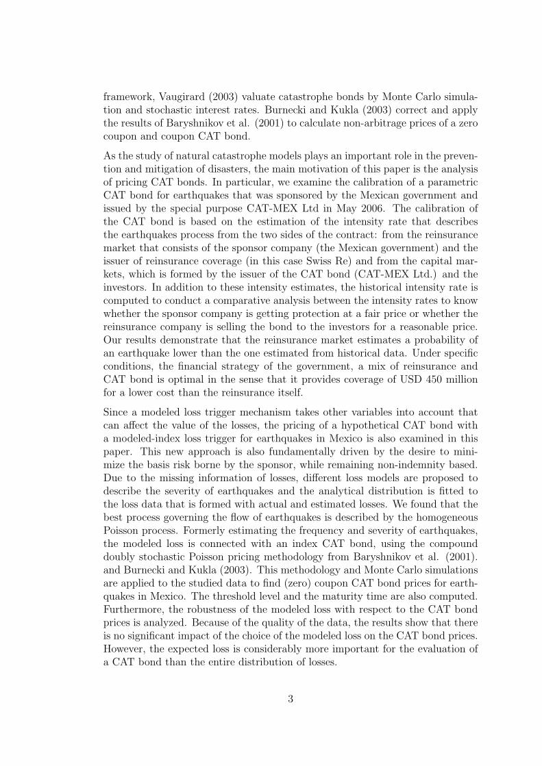
By its geographical position, Mexico finds itself under a great variety of naturalphenomena which can cause disasters, like earthquakes, eruptions, hurricanes,burning forest, floods and aridity (dryness). In case of disaster, the effects onfinancial and natural resources are huge and volatile. In Mexico the first risk totransfer is the seismic risk, because although it is the less recurrent, it has thebiggest impact on the population and country. For example, an earthquake ofmagnitude 8.1 Mw Richter scale that hit Mexico in 1985, destroyed hundredsof buildings and caused thousands of deaths. Figure 1 depicts the number ofearthquakes higher than 6.5 Mw occurred in Mexico during the years 1900-2003.

1900 1920 1940 1960 1980 2000Time (years)

12

34

56

7

Num

ber

of e

arth

quak

es

Figure 1: Number of earthquakes occurred in Mexico during 1900-2003.

After the occurrence of a natural disaster, the reconstruction can be financedwith catastrophe bonds (CAT bonds) or reinsurance. For insurers, reinsurers andother corporations CAT bonds are hedging instruments that offer multi year pro-tection without the credit risk present in reinsurance by providing full collateralfor the risk limits offered throught the transaction. For investors CAT bonds offerattractive returns and reduction of portfolio risk, since CAT bonds defaults areuncorrelated with defaults of other securities.

Baryshnikov et al. (2001) present an arbitrage free solution to the pricing of CATbonds under conditions of continous trading and according to the statistical char-acteristics of the dominant underlying processes. Instead of pricing, Anderson etal. (2000) devoted to the CAT bond benefits by providing an extensive relativevalue analysis. Others, like Croson and Kunreuther (2000) focus on the CATmanagement and their combination with reinsurance. Lee and Yu (2002) analyzedefault risk on CAT bonds and therefore their pricing methodology is focusedonly on CAT bonds that are issued by insurers. Also under an arbitrage-free

2

framework, Vaugirard (2003) valuate catastrophe bonds by Monte Carlo simula-tion and stochastic interest rates. Burnecki and Kukla (2003) correct and applythe results of Baryshnikov et al. (2001) to calculate non-arbitrage prices of a zerocoupon and coupon CAT bond.

As the study of natural catastrophe models plays an important role in the preven-tion and mitigation of disasters, the main motivation of this paper is the analysisof pricing CAT bonds. In particular, we examine the calibration of a parametricCAT bond for earthquakes that was sponsored by the Mexican government andissued by the special purpose CAT-MEX Ltd in May 2006. The calibration ofthe CAT bond is based on the estimation of the intensity rate that describesthe earthquakes process from the two sides of the contract: from the reinsurancemarket that consists of the sponsor company (the Mexican government) and theissuer of reinsurance coverage (in this case Swiss Re) and from the capital mar-kets, which is formed by the issuer of the CAT bond (CAT-MEX Ltd.) and theinvestors. In addition to these intensity estimates, the historical intensity rate iscomputed to conduct a comparative analysis between the intensity rates to knowwhether the sponsor company is getting protection at a fair price or whether thereinsurance company is selling the bond to the investors for a reasonable price.Our results demonstrate that the reinsurance market estimates a probability ofan earthquake lower than the one estimated from historical data. Under specificconditions, the financial strategy of the government, a mix of reinsurance andCAT bond is optimal in the sense that it provides coverage of USD 450 millionfor a lower cost than the reinsurance itself.

Since a modeled loss trigger mechanism takes other variables into account thatcan affect the value of the losses, the pricing of a hypothetical CAT bond witha modeled-index loss trigger for earthquakes in Mexico is also examined in thispaper. This new approach is also fundamentally driven by the desire to mini-mize the basis risk borne by the sponsor, while remaining non-indemnity based.Due to the missing information of losses, different loss models are proposed todescribe the severity of earthquakes and the analytical distribution is fitted tothe loss data that is formed with actual and estimated losses. We found that thebest process governing the flow of earthquakes is described by the homogeneousPoisson process. Formerly estimating the frequency and severity of earthquakes,the modeled loss is connected with an index CAT bond, using the compounddoubly stochastic Poisson pricing methodology from Baryshnikov et al. (2001).and Burnecki and Kukla (2003). This methodology and Monte Carlo simulationsare applied to the studied data to find (zero) coupon CAT bond prices for earth-quakes in Mexico. The threshold level and the maturity time are also computed.Furthermore, the robustness of the modeled loss with respect to the CAT bondprices is analyzed. Because of the quality of the data, the results show that thereis no significant impact of the choice of the modeled loss on the CAT bond prices.However, the expected loss is considerably more important for the evaluation ofa CAT bond than the entire distribution of losses.

3

Our paper is structured as follows. In the next section we discuss fundamentals ofCAT bonds and how this financial instrument can transfer seismic risk. Section3 is devoted to the calibration of the real parametric CAT bond for earthquakesin Mexico. Section 4 presents the valuation framework of a modeled-index CATbond fitted to earthquake data in Mexico. Section 5 summarizes the article andsuggests a possible extension. All quotations of money in this paper will be inUSD and therefore we will omit the explicit notion of the currency.

2 CAT bonds

In the mid-1990’s catastrophe bonds (CAT bonds), also named as Act of God orInsurance-linked bond, were developed to ease the transfer of catastrophe basedinsurance risk from insurers, reinsurers and corporations (sponsors) to capitalmarket investors. CAT bonds are bonds whose coupons and principal paymentsdepend on the performance of a pool or index of natural catastrophe risks, oron the presence of specified trigger conditions. They protect sponsor companiesfrom financial losses caused by large natural disasters by offering an alternativeor complement to traditional reinsurance.

The transaction involves four parties: the sponsor or ceding company (governmentagencies, insurers, reinsurers), the special purpose vehicle SPV (or issuer), thecollateral and the investors (institutional investors, insurers, reinsurers, and hedgefunds). The basic structure is shown in Figure 2. The sponsor sets up a SPVas an issuer of the bond and a source of reinsurance protection. The issuer sellsbonds to capital market investors and the proceeds are deposited in a collateralaccount, in which earnings from assets are collected and from which a floating rateis payed to the SPV. The sponsor enters into a reinsurance or derivative contractwith the issuer and pays him a premium. The SPV usually gives quarterly couponpayments to the investors. The premium and the investment bond proceeds thatthe SPV received from the collateral are a source of interest or coupons paid toinvestors. If there is no trigger event during the life of the bonds, the SPV givesthe principal back to the investors with the final coupon or the generous interest,otherwise the SPV pays the ceding according to the terms of the reinsurancecontract and sometimes pays nothing or partially the principal and interest tothe investors.

There is a variety of trigger mechanisms to determine when the losses of a naturalcatastrophe should be covered by the CAT bond. These include the indemnity,the industry index, the pure parametric, the parametric index, the modeled lossand the hybrid trigger. Each of these mechanisms shows a range of levels of basisrisks and transparency to investors.

The Indemnity trigger involves the actual loss of the ceding company. The ced-ing company receives reimbursement for its actual losses from the covered event,

4

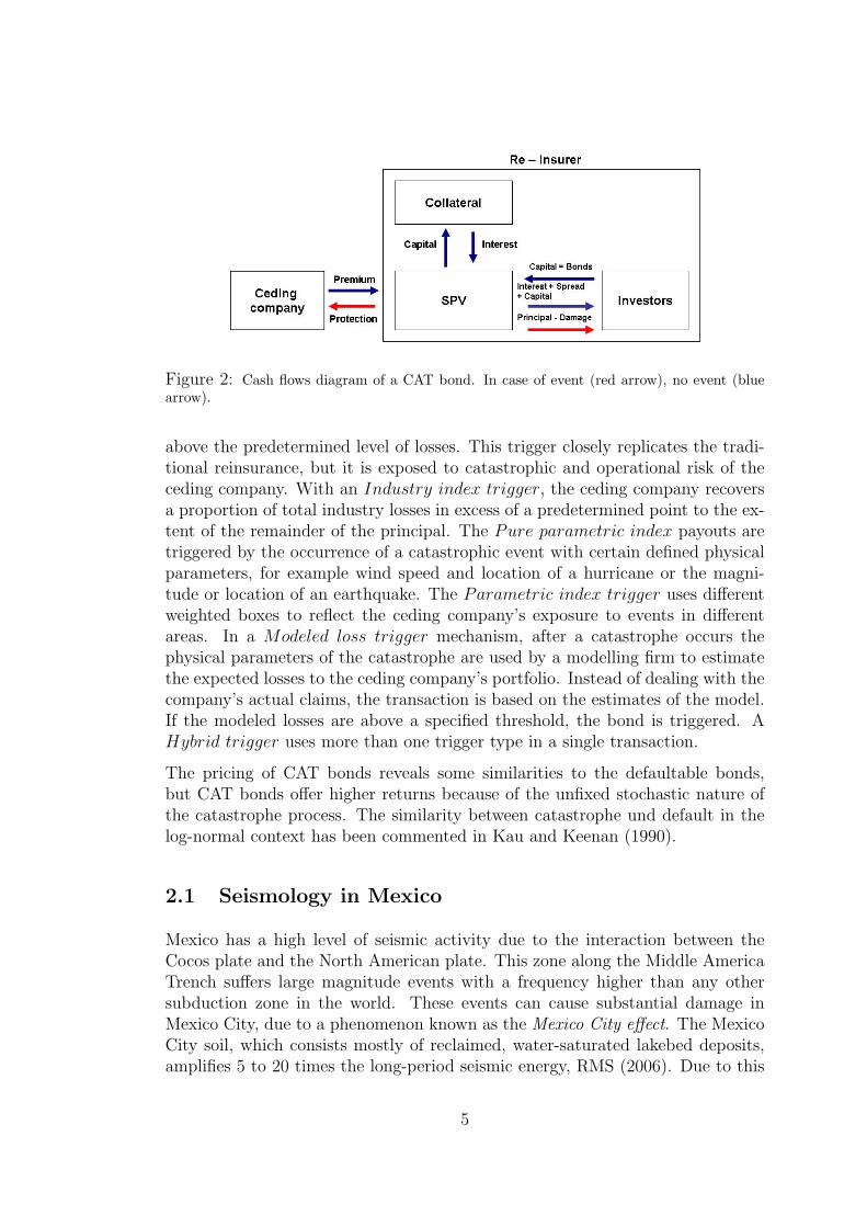
Figure 2: Cash flows diagram of a CAT bond. In case of event (red arrow), no event (bluearrow).

above the predetermined level of losses. This trigger closely replicates the tradi-tional reinsurance, but it is exposed to catastrophic and operational risk of theceding company. With an Industry index trigger, the ceding company recoversa proportion of total industry losses in excess of a predetermined point to the ex-tent of the remainder of the principal. The Pure parametric index payouts aretriggered by the occurrence of a catastrophic event with certain defined physicalparameters, for example wind speed and location of a hurricane or the magni-tude or location of an earthquake. The Parametric index trigger uses differentweighted boxes to reflect the ceding company’s exposure to events in differentareas. In a Modeled loss trigger mechanism, after a catastrophe occurs thephysical parameters of the catastrophe are used by a modelling firm to estimatethe expected losses to the ceding company’s portfolio. Instead of dealing with thecompany’s actual claims, the transaction is based on the estimates of the model.If the modeled losses are above a specified threshold, the bond is triggered. AHybrid trigger uses more than one trigger type in a single transaction.

The pricing of CAT bonds reveals some similarities to the defaultable bonds,but CAT bonds offer higher returns because of the unfixed stochastic nature ofthe catastrophe process. The similarity between catastrophe und default in thelog-normal context has been commented in Kau and Keenan (1990).

2.1 Seismology in Mexico

Mexico has a high level of seismic activity due to the interaction between theCocos plate and the North American plate. This zone along the Middle AmericaTrench suffers large magnitude events with a frequency higher than any othersubduction zone in the world. These events can cause substantial damage inMexico City, due to a phenomenon known as the Mexico City effect. The MexicoCity soil, which consists mostly of reclaimed, water-saturated lakebed deposits,amplifies 5 to 20 times the long-period seismic energy, RMS (2006). Due to this

5

effect and the high concentration of exposure in Mexico City, seismic risk is onthe top of the list for catastrophic risk in Mexico.

Historically, the Cocos plate boundary produced the 1985 Michoacan earthquakeof magnitude 8.1 Mw Richter scale. It destroyed hundreds of buildings andcaused thousand of deaths in Mexico City and other parts of the country. It isconsidered the most damaging earthquake in the history of Mexico City. TheMexican insurance industry officials estimated payouts of four billion dollars. Inthe last decades, other earthquakes have reached the magnitude 7.8 Mw Richterscale.

For earthquakes, the Mexican insurance market has traditionally been highlyregulated, with limited protection provided to homeowners and reinsurance bythe government. Today, after the occurrence of an earthquake, the reconstructioncan be financed by transferring the risk to the capital markets with catastrophic(CAT) bonds that would pass the risk on to investors. The first successful CATbond against earthquakes losses in California was issued in 1997 by Swiss Re andthe first CAT bond by a non-financial firm was issued in 1999 in order to coverearthquake losses in Tokyo region for Oriental Land Company Ltd., the owner ofTokyo Disneyland. Also for the first time since 2003, a non-(re)insurance sponsor,the government of Mexico, elected to access the CAT bond market directly. Froot(2001) described other transactions on the market for catastrophic risk and Clarkeet al. (2007) give a catastrophe bond market update.

3 Calibrating a Mexican Parametric CAT Bond

In 1996, the Mexican government established the Mexico’s Fund for NaturalDisasters (FONDEN) in order to reduce the exposure to the impact of naturalcatastrophes and to recover quickly as soon as they occur. However, FONDEN isfunded by fiscal resources which are limited and have been insufficient to meet thegovernment’s obligations. Faced with the shortage of the FONDEN’s resourcesand the high probability of earthquake occurrence, in May 2006 the Mexican gov-ernment sponsored a parametric CAT bond against earthquake risk. The decisionwas taken because the instrument design protects and magnifies, with a degreeof transparency, the resources of the trust. The CAT bond payment is basedon some physical parameters of the underlying event (e.g. the magnitude Mw),thereby there is no justification of losses. The parametric CAT bond helps thegovernment with emergency services and rebuilding after a big earthquake.

The CAT bond was issued by a SPV Cayman Islands CAT-MEX Ltd. and struc-tured by Swiss Reinsurance Company (SRC) and Deutsche Bank Securities. The160 million CAT bond pays a tranche equal to the London Inter-Bank OfferedRate (LIBOR) plus 235 basis points. The CAT bond is part of a total coverageof 450 million provided by the reinsurer for three years against earthquake risk

6

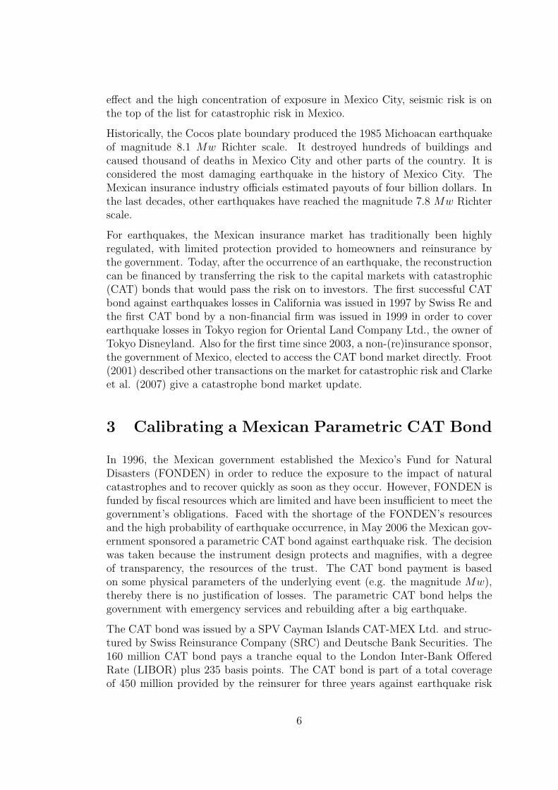
and with total premiums of 26 million. The payment of losses is conditional uponconfirmation by a leading independent consulting firm which develops catastro-phe risk assessment. This event verification agent (Applied Insurance ResearchWorldwide Corporation - AIR) modeled the seismic risk and detected nine seismiczones, see Figure 3. Given the federal governmental budget plan, just three outof these nine zones were insured in the transaction: zone 1, zone 2 and zone 5,with coverage of 150 million in each case, SHCP (2004). The CAT bond paymentwould be triggered if there is an event, i.e. an earthquake higher or equal than8 Mw hitting zone 1 or zone 2, or an earthquake higher or equal than 7.5 Mwhitting zone 5.

Figure 3: Map of seismic regions in Mexico. Source: SHCP

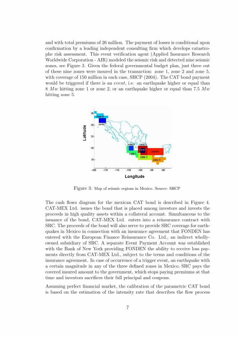
The cash flows diagram for the mexican CAT bond is described in Figure 4.CAT-MEX Ltd. issues the bond that is placed among investors and invests theproceeds in high quality assets within a collateral account. Simultaneous to theissuance of the bond, CAT-MEX Ltd. enters into a reinsurance contract withSRC. The proceeds of the bond will also serve to provide SRC coverage for earth-quakes in Mexico in connection with an insurance agreement that FONDEN hasentered with the European Finance Reinsurance Co. Ltd., an indirect wholly-owned subsidiary of SRC. A separate Event Payment Account was establishedwith the Bank of New York providing FONDEN the ability to receive loss pay-ments directly from CAT-MEX Ltd., subject to the terms and conditions of theinsurance agreement. In case of occurrence of a trigger event, an earthquake witha certain magnitude in any of the three defined zones in Mexico, SRC pays thecovered insured amount to the government, which stops paying premiums at thattime and investors sacrifices their full principal and coupons.

Assuming perfect financial market, the calibration of the parametric CAT bondis based on the estimation of the intensity rate that describes the flow process

7

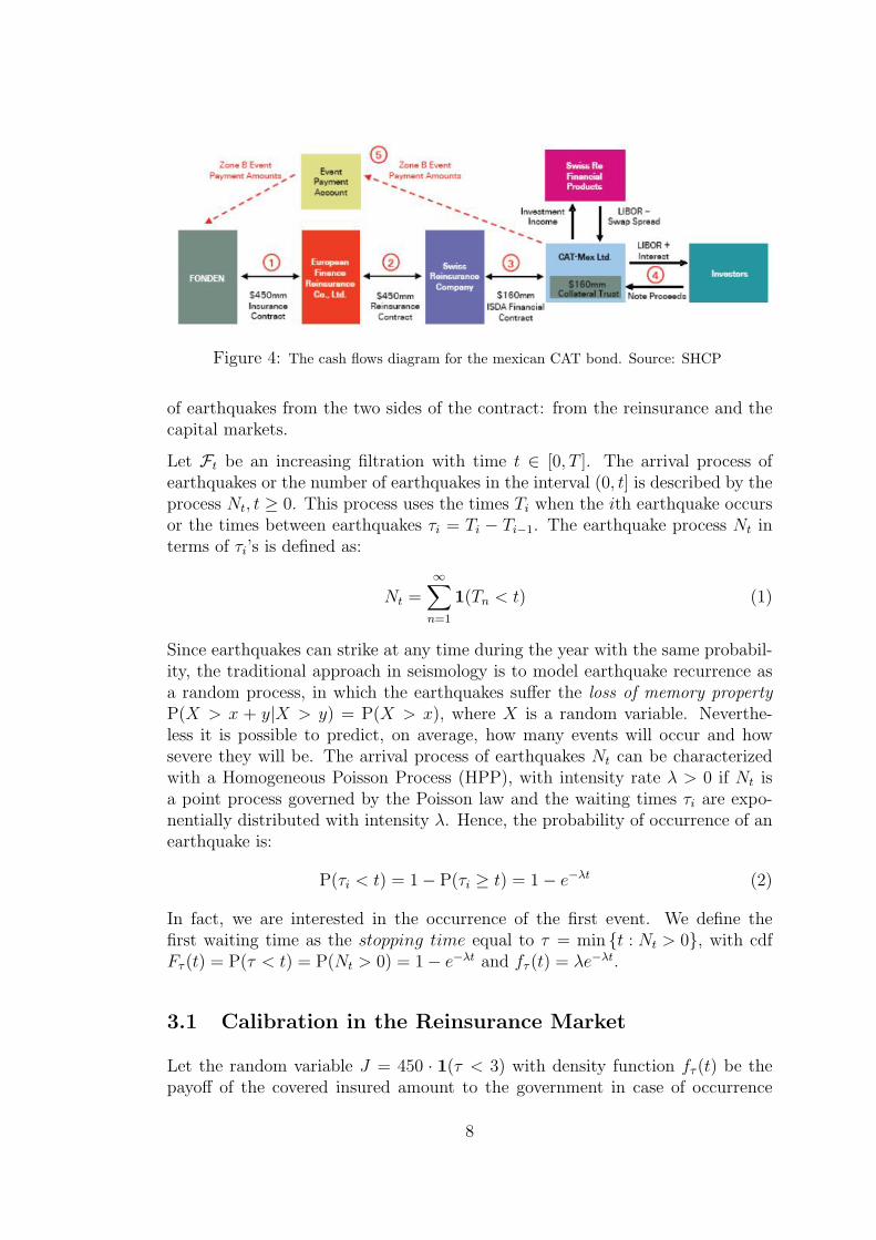
Figure 4: The cash flows diagram for the mexican CAT bond. Source: SHCP

of earthquakes from the two sides of the contract: from the reinsurance and thecapital markets.

Let Ft be an increasing filtration with time t ∈ [0, T ]. The arrival process ofearthquakes or the number of earthquakes in the interval (0, t] is described by theprocess Nt, t ≥ 0. This process uses the times Ti when the ith earthquake occursor the times between earthquakes τi = Ti − Ti−1. The earthquake process Nt interms of τi’s is defined as:

Nt =∞∑

n=1

1(Tn < t) (1)

Since earthquakes can strike at any time during the year with the same probabil-ity, the traditional approach in seismology is to model earthquake recurrence asa random process, in which the earthquakes suffer the loss of memory propertyP(X > x + y|X > y) = P(X > x), where X is a random variable. Neverthe-less it is possible to predict, on average, how many events will occur and howsevere they will be. The arrival process of earthquakes Nt can be characterizedwith a Homogeneous Poisson Process (HPP), with intensity rate λ > 0 if Nt isa point process governed by the Poisson law and the waiting times τi are expo-nentially distributed with intensity λ. Hence, the probability of occurrence of anearthquake is:

P(τi < t) = 1− P(τi ≥ t) = 1− e−λt (2)

In fact, we are interested in the occurrence of the first event. We define thefirst waiting time as the stopping time equal to τ = min {t : Nt > 0}, with cdfFτ (t) = P(τ < t) = P(Nt > 0) = 1− e−λt and fτ (t) = λe−λt.

3.1 Calibration in the Reinsurance Market

Let the random variable J = 450 · 1(τ < 3) with density function fτ (t) be thepayoff of the covered insured amount to the government in case of occurrence

8

of an event over a three year period T = 3. Denote H as the total premiumpaid by the government equal to 26 million. Suppose a flat term structure ofcontinuously compounded discount interest rates and a HPP with intensity λ1 todescribe the arrival process of earthquakes. Under the non-arbitrage framework,a compounded discount actuarially fair insurance price at time t = 0 in thereinsurance market is defined as:

H = E[Je−τrτ

]= E

[450 · 1(τ < 3)e−τrτ

]= 450

∫ 3

0

e−rttfτ (t)dt

= 450

∫ 3

0

e−rttλ1e−λ1tdt (3)

i.e. the insurance premium is equal to the value of the expected discounted lossfrom earthquake. Substituing the values of H and assuming an annual continouslycompounded discount interest rate rt = log(1.0541) constant and equal to theLIBOR in May 2006, we get:

26 = 450

∫ 3

0

e− log(1.0541)tλ1e−λ1tdt (4)

where 1 − e−λ1t is the probability of occurrence of an event. The estimation ofthe intensity rate from the reinsurance market λ1 is equal to 0.0214. That meansthat the premium paid by the government to the insurance company considers aprobability of occurrence of an event in three years equal to 0.0624 or the insurerexpects 2.15 events in one hundred years.

3.2 Calibration in the Capital Market

For computing the intensity in the capital markets λ2, we suppose that the con-tract structure defines a coupon CAT bond that pays to the investors the prin-cipal P equal to 160 million at time to maturity T = 3 and gives coupons Cevery 3 months during the bond’s life in case of no event. If there is an event,the investors sacrifice their principal and coupons. These coupon bonds offeredby CAT-MEX Ltd. pay to the investors a fixed spread rate z equal to 235 basispoints over LIBOR. We consider the annual discretely compounded discount in-terest rate rt = 5.4139% to be constant and equal to LIBOR in May 2006. Thefixed coupons payments C have a value of:

C =

(rt + z

4

)P =

(5.4139% + 2.35%

4

)160 = 3.1055 (5)

Let the random variable G be the investors’ gain from investing in the bond,which consists of the principal and coupons. Moreover, assume that the arrival

9

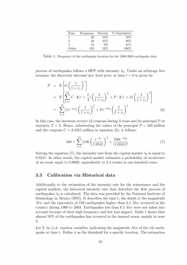
Zone Frequency Percent % Cumulative1 30 16% 16%2 42 22% 38%5 18 9% 47%Other 102 53% 100%

Table 1: Frequency of the earthquake location for the 1900-2003 earthquake data

process of earthquakes follows a HPP with intensity λ2. Under an arbitrage freescenario, the discretely discount fair bond price at time t = 0 is given by:

P = E

[G

(1

1 + rτ

)τ]= E

[12∑

t=1

C · 1(τ >t

4)

(1

1 + rt

) t4

+ P · 1(τ > 3)

(1

1 + rt

)3]

=12∑

t=1

Ce−λ2t4

(1

1 + rt

) t4

+ Pe−3λ2

(1

1 + rt

)3

(6)

In this case, the investors receive 12 coupons during 3 years and its principal P atmaturity T = 3. Hence, substituting the values of the principal P = 160 millionand the coupons C = 3.1055 million in equation (6), it follows:

160 =12∑

t=1

3.06

(e−λ2

1.0541

) t4

+160e−3λ2

(1.0541)3(7)

Solving the equation (7), the intensity rate from the capital market λ2 is equal to0.0241. In other words, the capital market estimates a probability of occurrenceof an event equal to 0.0699, equivalently to 2.4 events in one hundred years.

3.3 Calibration via Historical data

Additionally to the estimation of the intensity rate for the reinsurance and thecapital markets, the historical intensity rate that describes the flow process ofearthquakes λ3 is calculated. The data was provided by the National Institute ofSeismology in Mexico (SSN). It describes the time t, the depth d, the magnitudeMw and the epicenters of 192 earthquakes higher than 6.5 Mw occurred in thecountry during 1900 to 2003. Earthquakes less than 6.5 Mw were not taken intoaccount because of their high frequency and low loss impact. Table 1 shows thatalmost 50% of the earthquakes has occurred in the insured zones, mainly in zone2.

Let Yi be i.i.d. random variables, indicating the magnitude Mw of the ith earth-quake at time t. Define u as the threshold for a specific location. The estimation

10

of the historical λ3 is based on the intensity model. This model assumes thatthere exist i.i.d. random variables εi called trigger events that characterize earth-quakes with magnitude Yi higher than a defined threshold u for a specific location,i.e. εi = 1(Yi ≥ u). Then the trigger event process Bt is characterized as:

Bt =Nt∑i=1

εi (8)

where Nt is a HPP describing the arrival process of earthquakes with intensityλ > 0. Bt is a process which counts only earthquakes that trigger the CAT bond’spayoff. However, the dataset contains only three such events, what leads to thecalibration of the intensity of Bt be based on only two waiting times. Thereforein order to compute λ3, consider the process Bt and define p as the probabilityof occurrence of a trigger event conditional on the occurrence of the earthquake.Then the probability of no event up to time t is equal to:

P(Bt = 0) = P(Nt = 0) + P(Nt = 1)(1− p) + P(Nt = 2)(1− p)2 + . . .

=∞∑

k=0

P(Nt = k)(1− p)k =∞∑

k=0

(λt)k

k!e(−λt)(1− p)k

=∞∑

k=0

{λ(1− p)t}k

k!e(−λt)e−λ(1−p)teλ(1−p)t = e−λpt = e−λ3t (9)

by definition of the Poisson distribution and since∑∞

k=0{λ(1−p)t}k

k!e−λ(1−p)t = 1.

Now the calibration of the λ3 can be decomposed into the calibration of the inten-sity of all earthquakes with a magnitude higher than 6.5 Mw and the estimationof the probability of the trigger event.

Since the historical data contains three earthquakes with magnitude Mw higherthan the defined thresholds by the modelling company, the probability of occur-rence of the trigger event is equal to p =

(3

192

). The estimation of the annual

intensity is obtained by taking the mean of the daily number of earthquakes times360 i.e. λ = (0.005140)(360) = 1.8504. Consequently the annual historical inten-sity rate for a trigger event is equal to λ3 = λp = 1.8504

(3

192

)= 0.0289. This

means that approximately 2.89 events are expected to occur in the insured areasof the country within one hundred years.

Table 2 summarizes the values of the intensities rates λ′s and the probabilitiesof occurrence of a trigger event in one and three years. Whereas the reinsurancemarket expects 2.15 events to occur in one hundred years, the capital marketanticipates 2.22 events and the historical data predicts 2.89 events. Observethat the value of the λ3 depends on the time period of the historical data, itis estimated from the years 1900 to 2003 and it is not very accurate since it isbased on three events only. For a different period, λ3 might be smaller than λ1

or λ2. The magnitude of earthquakes above 6.5 Mw that occurred in Mexico

11

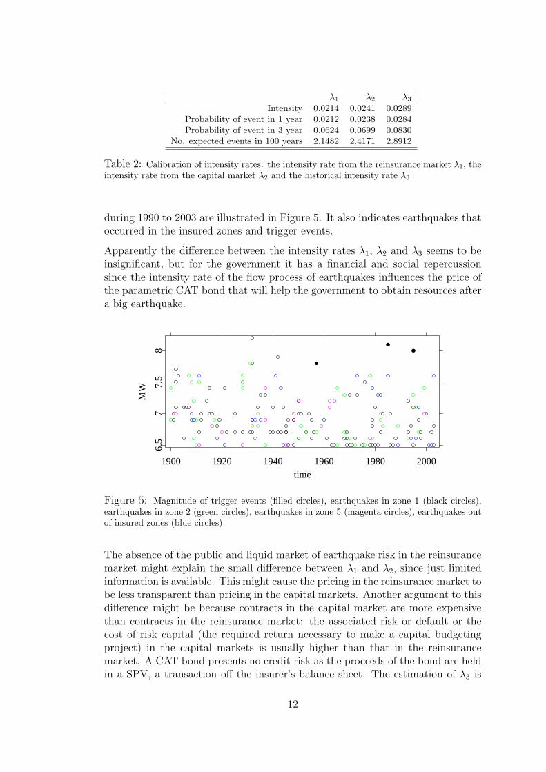
λ1 λ2 λ3

Intensity 0.0214 0.0241 0.0289Probability of event in 1 year 0.0212 0.0238 0.0284Probability of event in 3 year 0.0624 0.0699 0.0830

No. expected events in 100 years 2.1482 2.4171 2.8912

Table 2: Calibration of intensity rates: the intensity rate from the reinsurance market λ1, theintensity rate from the capital market λ2 and the historical intensity rate λ3

during 1990 to 2003 are illustrated in Figure 5. It also indicates earthquakes thatoccurred in the insured zones and trigger events.

Apparently the difference between the intensity rates λ1, λ2 and λ3 seems to beinsignificant, but for the government it has a financial and social repercussionsince the intensity rate of the flow process of earthquakes influences the price ofthe parametric CAT bond that will help the government to obtain resources aftera big earthquake.

1900 1920 1940 1960 1980 2000time

6.5

77.

58

MW

Figure 5: Magnitude of trigger events (filled circles), earthquakes in zone 1 (black circles),earthquakes in zone 2 (green circles), earthquakes in zone 5 (magenta circles), earthquakes outof insured zones (blue circles)

The absence of the public and liquid market of earthquake risk in the reinsurancemarket might explain the small difference between λ1 and λ2, since just limitedinformation is available. This might cause the pricing in the reinsurance market tobe less transparent than pricing in the capital markets. Another argument to thisdifference might be because contracts in the capital market are more expensivethan contracts in the reinsurance market: the associated risk or default or thecost of risk capital (the required return necessary to make a capital budgetingproject) in the capital markets is usually higher than that in the reinsurancemarket. A CAT bond presents no credit risk as the proceeds of the bond are heldin a SPV, a transaction off the insurer’s balance sheet. The estimation of λ3 is

12

not very precise since it is based on the time period of the historical data, but forinterpretations we suppose that λ3 is the real intensity rate describing the flowof process of earthquakes.

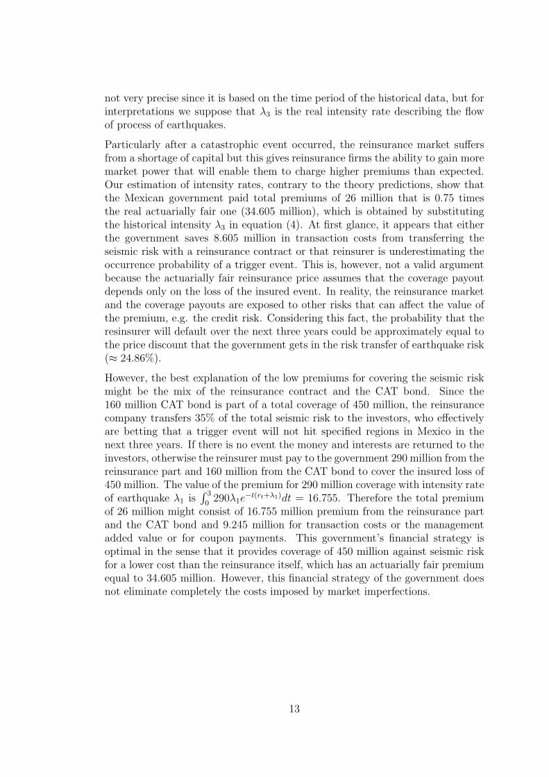
Particularly after a catastrophic event occurred, the reinsurance market suffersfrom a shortage of capital but this gives reinsurance firms the ability to gain moremarket power that will enable them to charge higher premiums than expected.Our estimation of intensity rates, contrary to the theory predictions, show thatthe Mexican government paid total premiums of 26 million that is 0.75 timesthe real actuarially fair one (34.605 million), which is obtained by substitutingthe historical intensity λ3 in equation (4). At first glance, it appears that eitherthe government saves 8.605 million in transaction costs from transferring theseismic risk with a reinsurance contract or that reinsurer is underestimating theoccurrence probability of a trigger event. This is, however, not a valid argumentbecause the actuarially fair reinsurance price assumes that the coverage payoutdepends only on the loss of the insured event. In reality, the reinsurance marketand the coverage payouts are exposed to other risks that can affect the value ofthe premium, e.g. the credit risk. Considering this fact, the probability that theresinsurer will default over the next three years could be approximately equal tothe price discount that the government gets in the risk transfer of earthquake risk(≈ 24.86%).

However, the best explanation of the low premiums for covering the seismic riskmight be the mix of the reinsurance contract and the CAT bond. Since the160 million CAT bond is part of a total coverage of 450 million, the reinsurancecompany transfers 35% of the total seismic risk to the investors, who effectivelyare betting that a trigger event will not hit specified regions in Mexico in thenext three years. If there is no event the money and interests are returned to theinvestors, otherwise the reinsurer must pay to the government 290 million from thereinsurance part and 160 million from the CAT bond to cover the insured loss of450 million. The value of the premium for 290 million coverage with intensity rateof earthquake λ1 is

∫ 3

0290λ1e

−t(rt+λ1)dt = 16.755. Therefore the total premiumof 26 million might consist of 16.755 million premium from the reinsurance partand the CAT bond and 9.245 million for transaction costs or the managementadded value or for coupon payments. This government’s financial strategy isoptimal in the sense that it provides coverage of 450 million against seismic riskfor a lower cost than the reinsurance itself, which has an actuarially fair premiumequal to 34.605 million. However, this financial strategy of the government doesnot eliminate completely the costs imposed by market imperfections.

13

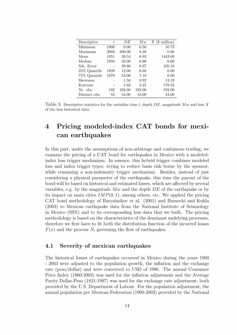
Descriptive t DE Mw X ($ million)Minimum 1900 0.00 6.50 10.73Maximum 2003 200.00 8.20 0.00Mean 1951 39.54 6.93 1443.69Median 1950 33.00 6.90 0.00Sdt. Error - 39.66 0.37 105.1625% Quantile 1928 12.00 6.60 0.0075% Quantile 1979 53.00 7.10 0.00Skewness - 1.58 0.92 13.19Kurtosis - 5.63 3.25 179.52Nr. obs. 192 192.00 192.00 192.00Distinct obs. 82 54.00 18.00 24.00

Table 3: Descriptive statistics for the variables time t, depth DE, magnitude Mw and loss Xof the loss historical data

4 Pricing modeled-index CAT bonds for mexi-

can earthquakes

In this part, under the assumptions of non-arbitrage and continuous trading, weexamine the pricing of a CAT bond for earthquakes in Mexico with a modeled-index loss trigger mechanism. In essence, this hybrid trigger combines modeledloss and index trigger types, trying to reduce basis risk borne by the sponsor,while remaining a non-indemnity trigger mechanism. Besides, instead of justconsidering a physical parameter of the earthquake, this time the payout of thebond will be based on historical and estimated losses, which are affected by severalvariables, e.g. by the magnitude Mw and the depth DE of the earthquake or byits impact on main cities IMP (0, 1), among others, etc. We applied the pricingCAT bond methodology of Baryshnikov et al. (2001) and Burnecki and Kukla(2003) to Mexican earthquake data from the National Institute of Seismologyin Mexico (SSN) and to its corresponding loss data that we built. The pricingmethodology is based on the characteristics of the dominant undelying processes,therefore we first have to fit both the distribution function of the incurred lossesF (x) and the process Nt governing the flow of earthquakes.

4.1 Severity of mexican earthquakes

The historical losses of earthquakes occurred in Mexico during the years 1900- 2003 were adjusted to the population growth, the inflation and the exchangerate (peso/dollar) and were converted to USD of 1990. The annual ConsumerPrice Index (1860-2003) was used for the inflation adjustment and the AverageParity Dollar-Peso (1821-1997) was used for the exchange rate adjustment, bothprovided by the U.S. Department of Labour. For the population adjustment, theannual population per Mexican Federation (1900-2003) provided by the National

14

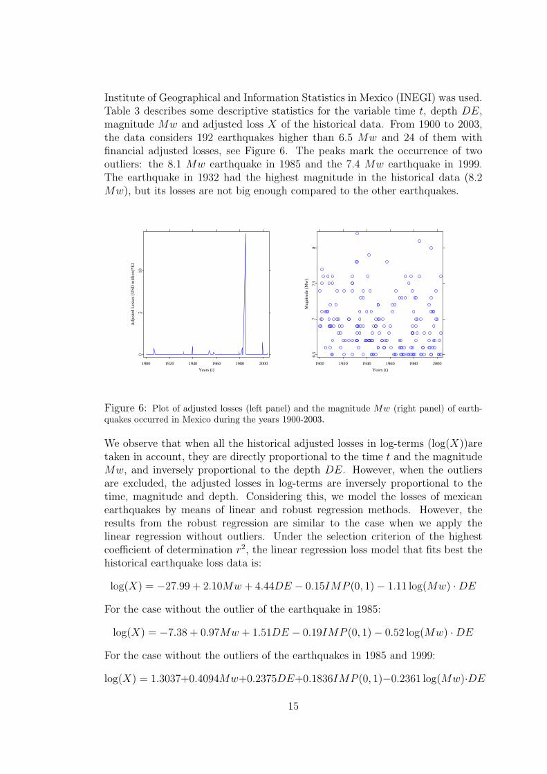
Institute of Geographical and Information Statistics in Mexico (INEGI) was used.Table 3 describes some descriptive statistics for the variable time t, depth DE,magnitude Mw and adjusted loss X of the historical data. From 1900 to 2003,the data considers 192 earthquakes higher than 6.5 Mw and 24 of them withfinancial adjusted losses, see Figure 6. The peaks mark the occurrence of twooutliers: the 8.1 Mw earthquake in 1985 and the 7.4 Mw earthquake in 1999.The earthquake in 1932 had the highest magnitude in the historical data (8.2Mw), but its losses are not big enough compared to the other earthquakes.

1900 1920 1940 1960 1980 2000

Years (t)

05

10

Adj

uste

d L

osse

s (U

SD m

illio

n)*E

2

1900 1920 1940 1960 1980 2000

Years (t)

6.5

77.

58

Mag

nitu

de (

Mw

)

Figure 6: Plot of adjusted losses (left panel) and the magnitude Mw (right panel) of earth-quakes occurred in Mexico during the years 1900-2003.

We observe that when all the historical adjusted losses in log-terms (log(X))aretaken in account, they are directly proportional to the time t and the magnitudeMw, and inversely proportional to the depth DE. However, when the outliersare excluded, the adjusted losses in log-terms are inversely proportional to thetime, magnitude and depth. Considering this, we model the losses of mexicanearthquakes by means of linear and robust regression methods. However, theresults from the robust regression are similar to the case when we apply thelinear regression without outliers. Under the selection criterion of the highestcoefficient of determination r2, the linear regression loss model that fits best thehistorical earthquake loss data is:

log(X) = −27.99 + 2.10Mw + 4.44DE − 0.15IMP (0, 1)− 1.11 log(Mw) ·DE

For the case without the outlier of the earthquake in 1985:

log(X) = −7.38 + 0.97Mw + 1.51DE − 0.19IMP (0, 1)− 0.52 log(Mw) ·DE

For the case without the outliers of the earthquakes in 1985 and 1999:

log(X) = 1.3037+0.4094Mw+0.2375DE+0.1836IMP (0, 1)−0.2361 log(Mw)·DE

15

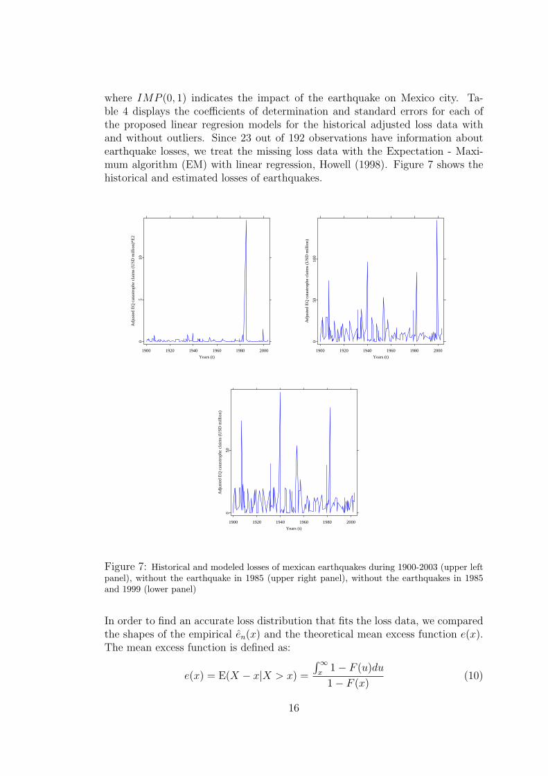
where IMP (0, 1) indicates the impact of the earthquake on Mexico city. Ta-ble 4 displays the coefficients of determination and standard errors for each ofthe proposed linear regresion models for the historical adjusted loss data withand without outliers. Since 23 out of 192 observations have information aboutearthquake losses, we treat the missing loss data with the Expectation - Maxi-mum algorithm (EM) with linear regression, Howell (1998). Figure 7 shows thehistorical and estimated losses of earthquakes.

1900 1920 1940 1960 1980 2000

Years (t)

05

10

Adj

uste

d E

Q c

atas

trop

he c

laim

s (U

SD m

illio

n)*E

2

1900 1920 1940 1960 1980 2000

Years (t)

050

100

Adj

uste

d E

Q c

atas

trop

he c

laim

s (U

SD m

illio

n)

1900 1920 1940 1960 1980 2000

Years (t)

050

Adj

uste

d E

Q c

atas

trop

he c

laim

s (U

SD m

illio

n)

Figure 7: Historical and modeled losses of mexican earthquakes during 1900-2003 (upper leftpanel), without the earthquake in 1985 (upper right panel), without the earthquakes in 1985and 1999 (lower panel)

In order to find an accurate loss distribution that fits the loss data, we comparedthe shapes of the empirical en(x) and the theoretical mean excess function e(x).The mean excess function is defined as:

e(x) = E(X − x|X > x) =

∫ ∞x

1− F (u)du

1− F (x)(10)

16

r2LR1 r2

LR2 r2LR3 SELR1 SELR2 SELR3

0.226 0.151 0.129 2.869 2.830 2.838

Table 4: Coefficients of determination and standard errors of the linear regression modelsapplied to the adjusted loss data (r2

LR1, SELR1), without the outlier of the earthquake in 1985(r2

LR2, SELR2) and without the outliers of the earthquakes in 1985 and 1999 (r2LR3, SELR3)

The empirical mean excess function is calculated as:

en(x) =

∑xi>x xi

#i : xi > x− x

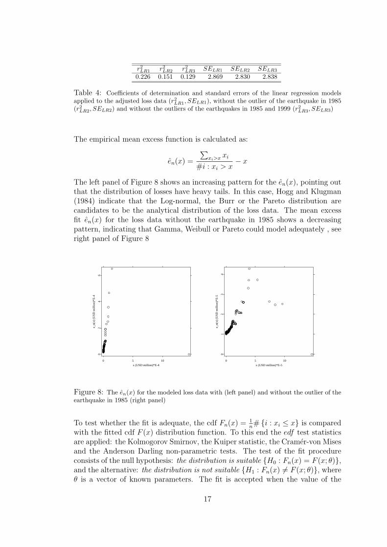
The left panel of Figure 8 shows an increasing pattern for the en(x), pointing outthat the distribution of losses have heavy tails. In this case, Hogg and Klugman(1984) indicate that the Log-normal, the Burr or the Pareto distribution arecandidates to be the analytical distribution of the loss data. The mean excessfit en(x) for the loss data without the earthquake in 1985 shows a decreasingpattern, indicating that Gamma, Weibull or Pareto could model adequately , seeright panel of Figure 8

0 5 10

x (USD million)*E-4

02

46

e_n(

x) (

USD

mill

ion)

*E-4

0 5 10

x (USD million)*E-5

01

23

4

e_n(

x) (

USD

mill

ion)

*E-5

Figure 8: The en(x) for the modeled loss data with (left panel) and without the outlier of theearthquake in 1985 (right panel)

To test whether the fit is adequate, the cdf Fn(x) = 1n# {i : xi ≤ x} is compared

with the fitted cdf F (x) distribution function. To this end the edf test statisticsare applied: the Kolmogorov Smirnov, the Kuiper statistic, the Cramer-von Misesand the Anderson Darling non-parametric tests. The test of the fit procedureconsists of the null hypothesis: the distribution is suitable {H0 : Fn(x) = F (x; θ)},and the alternative: the distribution is not suitable {H1 : Fn(x) 6= F (x; θ)}, whereθ is a vector of known parameters. The fit is accepted when the value of the

17

Distrib. Log-normal Pareto Burr Exponential Gamma WeibullParameter µ = 1.456 α = 2.199 α = 3.354 β = 0.132 α = 0.145 β = .214

σ = 1.677 λ = 12.53 λ = 17.33 β = −0.0 τ = .747τ = 0.895

Kolmogorov S. 0.185 0.142 0.150 0.149 0.299 0.157(D test) (< 0.005) (< 0.005) (< 0.005) (< 0.005) (< 0.005) (< 0.005)Kuiper 0.308 0.265 0.278 0.245 0.570 0.298

(V test) (< 0.005) (< 0.005) (< 0.005) (< 0.005) (< 0.005) (< 0.005)Cramer-von M. 1.447 0.879 0.987 0.911 6.932 1.16

(W 2 test) (< 0.005) (< 0.005) (< 0.005) (< 0.005) (< 0.005) (< 0.005)Anderson D. 10.490 6.131 6.018 10.519 35.428 6.352

(A2 test) (< 0.005) (< 0.005) (< 0.005) (< 0.005) (< 0.005) (< 0.005)

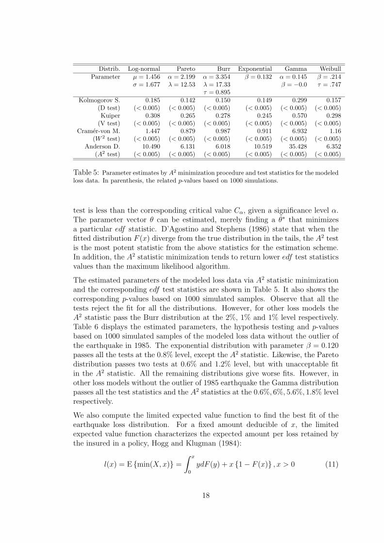
Table 5: Parameter estimates by A2 minimization procedure and test statistics for the modeledloss data. In parenthesis, the related p-values based on 1000 simulations.

test is less than the corresponding critical value Cα, given a significance level α.The parameter vector θ can be estimated, merely finding a θ∗ that minimizesa particular edf statistic. D’Agostino and Stephens (1986) state that when thefitted distribution F (x) diverge from the true distribution in the tails, the A2 testis the most potent statistic from the above statistics for the estimation scheme.In addition, the A2 statistic minimization tends to return lower edf test statisticsvalues than the maximum likelihood algorithm.

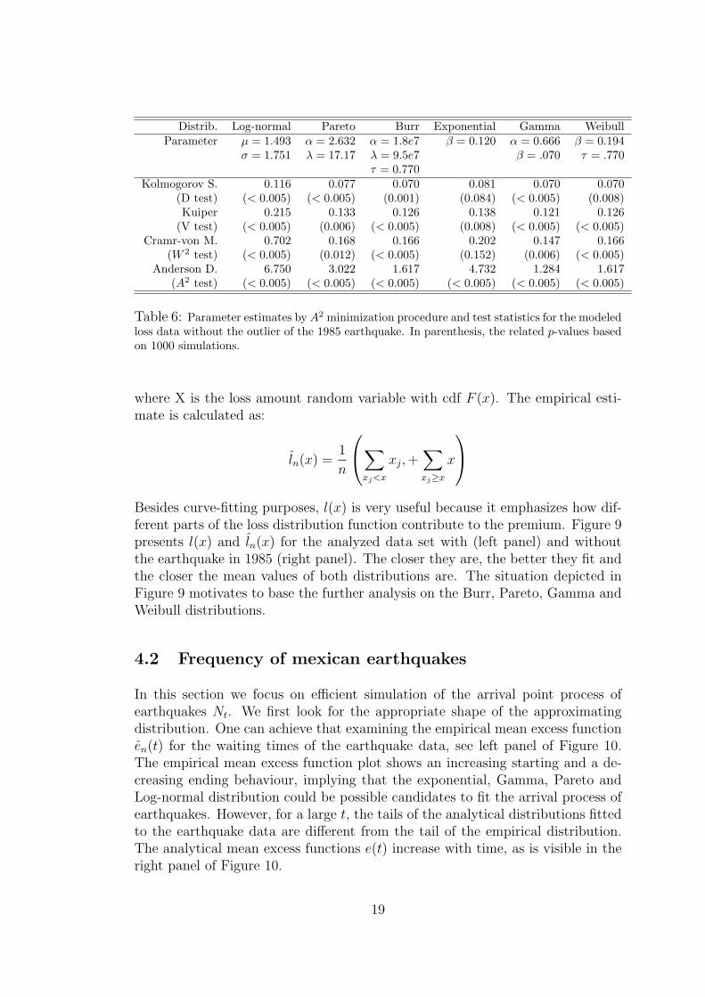
The estimated parameters of the modeled loss data via A2 statistic minimizationand the corresponding edf test statistics are shown in Table 5. It also shows thecorresponding p-values based on 1000 simulated samples. Observe that all thetests reject the fit for all the distributions. However, for other loss models theA2 statistic pass the Burr distribution at the 2%, 1% and 1% level respectively.Table 6 displays the estimated parameters, the hypothesis testing and p-valuesbased on 1000 simulated samples of the modeled loss data without the outlier ofthe earthquake in 1985. The exponential distribution with parameter β = 0.120passes all the tests at the 0.8% level, except the A2 statistic. Likewise, the Paretodistribution passes two tests at 0.6% and 1.2% level, but with unacceptable fitin the A2 statistic. All the remaining distributions give worse fits. However, inother loss models without the outlier of 1985 earthquake the Gamma distributionpasses all the test statistics and the A2 statistics at the 0.6%, 6%, 5.6%, 1.8% levelrespectively.

We also compute the limited expected value function to find the best fit of theearthquake loss distribution. For a fixed amount deducible of x, the limitedexpected value function characterizes the expected amount per loss retained bythe insured in a policy, Hogg and Klugman (1984):

l(x) = E {min(X, x)} =

∫ x

0

ydF (y) + x {1− F (x)} , x > 0 (11)

18

Distrib. Log-normal Pareto Burr Exponential Gamma WeibullParameter µ = 1.493 α = 2.632 α = 1.8e7 β = 0.120 α = 0.666 β = 0.194

σ = 1.751 λ = 17.17 λ = 9.5e7 β = .070 τ = .770τ = 0.770

Kolmogorov S. 0.116 0.077 0.070 0.081 0.070 0.070(D test) (< 0.005) (< 0.005) (0.001) (0.084) (< 0.005) (0.008)Kuiper 0.215 0.133 0.126 0.138 0.121 0.126

(V test) (< 0.005) (0.006) (< 0.005) (0.008) (< 0.005) (< 0.005)Cramr-von M. 0.702 0.168 0.166 0.202 0.147 0.166

(W 2 test) (< 0.005) (0.012) (< 0.005) (0.152) (0.006) (< 0.005)Anderson D. 6.750 3.022 1.617 4.732 1.284 1.617

(A2 test) (< 0.005) (< 0.005) (< 0.005) (< 0.005) (< 0.005) (< 0.005)

Table 6: Parameter estimates by A2 minimization procedure and test statistics for the modeledloss data without the outlier of the 1985 earthquake. In parenthesis, the related p-values basedon 1000 simulations.

where X is the loss amount random variable with cdf F (x). The empirical esti-mate is calculated as:

ln(x) =1

n

∑xj<x

xj, +∑xj≥x

x

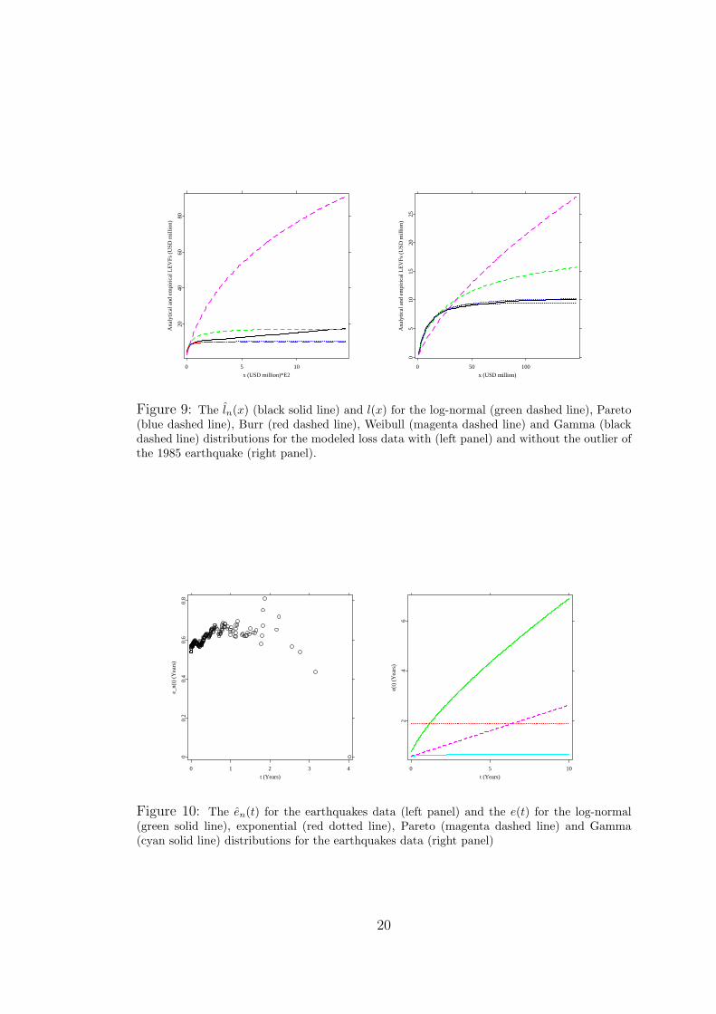
Besides curve-fitting purposes, l(x) is very useful because it emphasizes how dif-ferent parts of the loss distribution function contribute to the premium. Figure 9presents l(x) and ln(x) for the analyzed data set with (left panel) and withoutthe earthquake in 1985 (right panel). The closer they are, the better they fit andthe closer the mean values of both distributions are. The situation depicted inFigure 9 motivates to base the further analysis on the Burr, Pareto, Gamma andWeibull distributions.

4.2 Frequency of mexican earthquakes

In this section we focus on efficient simulation of the arrival point process ofearthquakes Nt. We first look for the appropriate shape of the approximatingdistribution. One can achieve that examining the empirical mean excess functionen(t) for the waiting times of the earthquake data, see left panel of Figure 10.The empirical mean excess function plot shows an increasing starting and a de-creasing ending behaviour, implying that the exponential, Gamma, Pareto andLog-normal distribution could be possible candidates to fit the arrival process ofearthquakes. However, for a large t, the tails of the analytical distributions fittedto the earthquake data are different from the tail of the empirical distribution.The analytical mean excess functions e(t) increase with time, as is visible in theright panel of Figure 10.

19

0 5 10

x (USD million)*E2

2040

6080

Ana

lytic

al a

nd e

mpi

rica

l LE

VFs

(U

SD m

illio

n)

0 50 100

x (USD million)

05

1015

2025

Ana

lytic

al a

nd e

mpi

rica

l LE

VFs

(U

SD m

illio

n)

Figure 9: The ln(x) (black solid line) and l(x) for the log-normal (green dashed line), Pareto(blue dashed line), Burr (red dashed line), Weibull (magenta dashed line) and Gamma (blackdashed line) distributions for the modeled loss data with (left panel) and without the outlier ofthe 1985 earthquake (right panel).

0 1 2 3 4

t (Years)

00.

20.

40.

60.

8

e_n(

t) (

Yea

rs)

0 5 10

t (Years)

24

6

e(t)

(Y

ears

)

Figure 10: The en(t) for the earthquakes data (left panel) and the e(t) for the log-normal(green solid line), exponential (red dotted line), Pareto (magenta dashed line) and Gamma(cyan solid line) distributions for the earthquakes data (right panel)

20

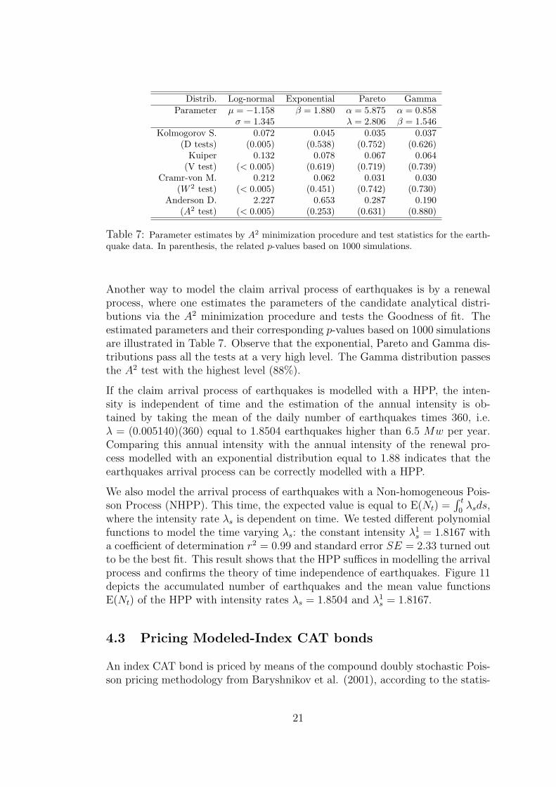
Distrib. Log-normal Exponential Pareto GammaParameter µ = −1.158 β = 1.880 α = 5.875 α = 0.858

σ = 1.345 λ = 2.806 β = 1.546Kolmogorov S. 0.072 0.045 0.035 0.037

(D tests) (0.005) (0.538) (0.752) (0.626)Kuiper 0.132 0.078 0.067 0.064

(V test) (< 0.005) (0.619) (0.719) (0.739)Cramr-von M. 0.212 0.062 0.031 0.030

(W 2 test) (< 0.005) (0.451) (0.742) (0.730)Anderson D. 2.227 0.653 0.287 0.190

(A2 test) (< 0.005) (0.253) (0.631) (0.880)

Table 7: Parameter estimates by A2 minimization procedure and test statistics for the earth-quake data. In parenthesis, the related p-values based on 1000 simulations.

Another way to model the claim arrival process of earthquakes is by a renewalprocess, where one estimates the parameters of the candidate analytical distri-butions via the A2 minimization procedure and tests the Goodness of fit. Theestimated parameters and their corresponding p-values based on 1000 simulationsare illustrated in Table 7. Observe that the exponential, Pareto and Gamma dis-tributions pass all the tests at a very high level. The Gamma distribution passesthe A2 test with the highest level (88%).

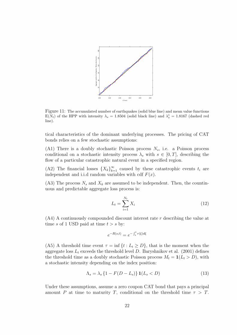
If the claim arrival process of earthquakes is modelled with a HPP, the inten-sity is independent of time and the estimation of the annual intensity is ob-tained by taking the mean of the daily number of earthquakes times 360, i.e.λ = (0.005140)(360) equal to 1.8504 earthquakes higher than 6.5 Mw per year.Comparing this annual intensity with the annual intensity of the renewal pro-cess modelled with an exponential distribution equal to 1.88 indicates that theearthquakes arrival process can be correctly modelled with a HPP.

We also model the arrival process of earthquakes with a Non-homogeneous Pois-son Process (NHPP). This time, the expected value is equal to E(Nt) =

∫ t

0λsds,

where the intensity rate λs is dependent on time. We tested different polynomialfunctions to model the time varying λs: the constant intensity λ1

s = 1.8167 witha coefficient of determination r2 = 0.99 and standard error SE = 2.33 turned outto be the best fit. This result shows that the HPP suffices in modelling the arrivalprocess and confirms the theory of time independence of earthquakes. Figure 11depicts the accumulated number of earthquakes and the mean value functionsE(Nt) of the HPP with intensity rates λs = 1.8504 and λ1

s = 1.8167.

4.3 Pricing Modeled-Index CAT bonds

An index CAT bond is priced by means of the compound doubly stochastic Pois-son pricing methodology from Baryshnikov et al. (2001), according to the statis-

21

1900 1920 1940 1960 1980 2000

t (Years)

030

6090

120

150

180

Agg

rega

te n

umbe

r of

ear

thqu

akes

/ M

ean

valu

e fu

nctio

n

Figure 11: The accumulated number of earthquakes (solid blue line) and mean value functionsE(Nt) of the HPP with intensity λs = 1.8504 (solid black line) and λ1

s = 1.8167 (dashed redline).

tical characteristics of the dominant underlying processes. The pricing of CATbonds relies on a few stochastic assumptions:

(A1) There is a doubly stochastic Poisson process Ns, i.e. a Poisson processconditional on a stochastic intensity process λs with s ∈ [0, T ], describing theflow of a particular catastrophic natural event in a specified region.

(A2) The financial losses {Xk}∞k=1 caused by these catastrophic events ti areindependent and i.i.d random variables with cdf F (x).

(A3) The process Ns and Xk are assumed to be independent. Then, the countin-uous and predictable aggregate loss process is:

Lt =Nt∑i=1

Xi (12)

(A4) A continuously compounded discount interest rate r describing the value attime s of 1 USD paid at time t > s by:

e−R(s,t) = e−∫ t

s r(ξ)dξ

(A5) A threshold time event τ = inf {t : Lt ≥ D}, that is the moment when theaggregate loss Lt exceeds the threshold level D. Baryshnikov et al. (2001) definesthe threshold time as a doubly stochastic Poisson process Mt = 1(Lt > D), witha stochastic intensity depending on the index position:

Λs = λs {1− F (D − Ls)}1(Ls < D) (13)

Under these assumptions, assume a zero coupon CAT bond that pays a principalamount P at time to maturity T , conditional on the threshold time τ > T .

22

Let P be a predictable process Ps = E(P |Fs), i.e. the payment at maturity isindependent from the occurrence and timing of the threshold D. Consider thatin case of occurrence of the trigger event the principal P is fully lost.

The non arbitrage price of the zero coupon CAT bond V 1t associated with the

threshold D, earthquake flow process Ns with intensity λs, a loss distributionfunction F and paying the principal P at maturity is thus given by, Burnecki andKukla (2003):

V 1t = E

[Pe−R(t,T ) (1−MT ) |Ft

]= E

[Pe−R(t,T )

{1−

∫ T

t

λs {1− F (D − Ls)}1(Ls < D)ds

}|Ft

](14)

i.e. the price of a zero coupon CAT bond is equal to the expected discountedvalue of the principal P contingent on the threshold time τ > T . Here thecompounded Poisson process is used to incorporate the various characteristicsof the earthquake process, where the rates at which earthquakes occur and theimpact of their occurrence are regarded as doubly stochastic Poisson processes.

Similarly, under the same assumptions that the zero coupon bonds, a couponCAT bond V 2

t that pays the principal P at time to maturity T and gives couponCs until the threshold time τ is given by, Burnecki and Kukla (2003):

V 2t = E

[Pe−R(t,T ) (1−MT ) +

∫ T

t

e−R(t,s)Cs (1−Ms) ds|Ft

]= E

[Pe−R(t,T ) +

∫ T

t

e−R(t,s)

{Cs

(1−

∫ s

t

λξ {1− F (D − Lξ)}

1(Lξ < D)dξ

)− Pe−R(s,T )λs {1− F (D − Ls)}1(Ls < D)

}ds|Ft

](15)

These coupon bonds usually pay a fixed spread z over LIBOR that reflects thevalue of the premium paid for the insured event, and LIBOR reflects the gain forinvesting in the bond.

Following this pricing methodology, we obtain the values of a (zero) coupon CATbond for earthquakes at t = 0. We consider that the continuously compoundeddiscount interest rate r = log(1.054139) is constant and equal to the LIBOR inMay 2006, P = 160 million and the expiration time T ∈ [0.25, 3] years. Define nowthe threshold D ∈ [100, 135] million, corresponding to the 0.7 and 0.8-quantilesof the three yearly accumulated modeled losses, i.e. approximately three payoffsare expected to occur in one hundred years (see Table 8).

After applying 1000 Monte Carlo simulations, the price of the zero coupon CATbond at t = 0 is calculated with respect to the threshold level D and expirationtime T . The Burr and Pareto distribution are considered as loss distributionsfor the modeled loss data, while the Gamma, Pareto and Weibull distribution

23

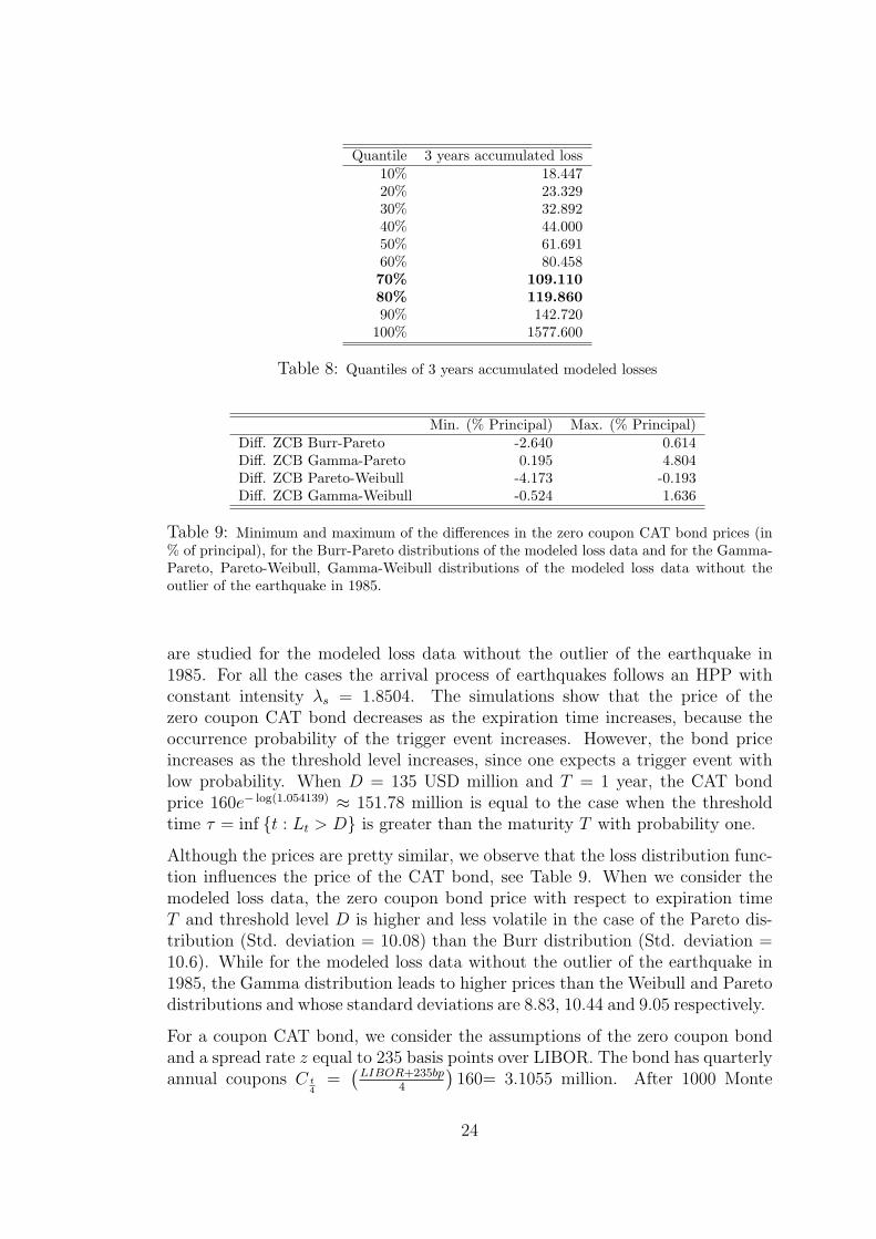
Quantile 3 years accumulated loss10% 18.44720% 23.32930% 32.89240% 44.00050% 61.69160% 80.45870% 109.11080% 119.86090% 142.720

100% 1577.600

Table 8: Quantiles of 3 years accumulated modeled losses

Min. (% Principal) Max. (% Principal)Diff. ZCB Burr-Pareto -2.640 0.614Diff. ZCB Gamma-Pareto 0.195 4.804Diff. ZCB Pareto-Weibull -4.173 -0.193Diff. ZCB Gamma-Weibull -0.524 1.636

Table 9: Minimum and maximum of the differences in the zero coupon CAT bond prices (in% of principal), for the Burr-Pareto distributions of the modeled loss data and for the Gamma-Pareto, Pareto-Weibull, Gamma-Weibull distributions of the modeled loss data without theoutlier of the earthquake in 1985.

are studied for the modeled loss data without the outlier of the earthquake in1985. For all the cases the arrival process of earthquakes follows an HPP withconstant intensity λs = 1.8504. The simulations show that the price of thezero coupon CAT bond decreases as the expiration time increases, because theoccurrence probability of the trigger event increases. However, the bond priceincreases as the threshold level increases, since one expects a trigger event withlow probability. When D = 135 USD million and T = 1 year, the CAT bondprice 160e− log(1.054139) ≈ 151.78 million is equal to the case when the thresholdtime τ = inf {t : Lt > D} is greater than the maturity T with probability one.

Although the prices are pretty similar, we observe that the loss distribution func-tion influences the price of the CAT bond, see Table 9. When we consider themodeled loss data, the zero coupon bond price with respect to expiration timeT and threshold level D is higher and less volatile in the case of the Pareto dis-tribution (Std. deviation = 10.08) than the Burr distribution (Std. deviation =10.6). While for the modeled loss data without the outlier of the earthquake in1985, the Gamma distribution leads to higher prices than the Weibull and Paretodistributions and whose standard deviations are 8.83, 10.44 and 9.05 respectively.

For a coupon CAT bond, we consider the assumptions of the zero coupon bondand a spread rate z equal to 235 basis points over LIBOR. The bond has quarterlyannual coupons C t

4=

(LIBOR+235bp

4

)160= 3.1055 million. After 1000 Monte

24

Min. (% Principal) Max. (% Principal)Diff. ZCB-CB Burr -6.228 -0.178Diff. ZCB-CB Pareto -5.738 -0.375Diff. ZCB-CB Gamma -7.124 -0.475Diff. ZCB-CB Pareto (no outlier ’85) -5.250 -0.376Diff. ZCB-CB Weibull -5.290 -0.475Diff. CB Burr-Pareto -1.552 0.809Diff. CB Gamma-Pareto 0.295 6.040Diff. CB Pareto-Weibull -3.944 -0.295Diff. CB Gamma-Weibull -0.273 3.105

Table 10: Minimum and maximum of the differences in the (zero) coupon CAT bond prices(in % of principal), for the Burr-Pareto distributions of the modeled loss data and the Gamma-Pareto, Pareto-Weibull, Gamma-Weibull distributions of the modeled loss data without theoutlier of the earthquake in 1985.

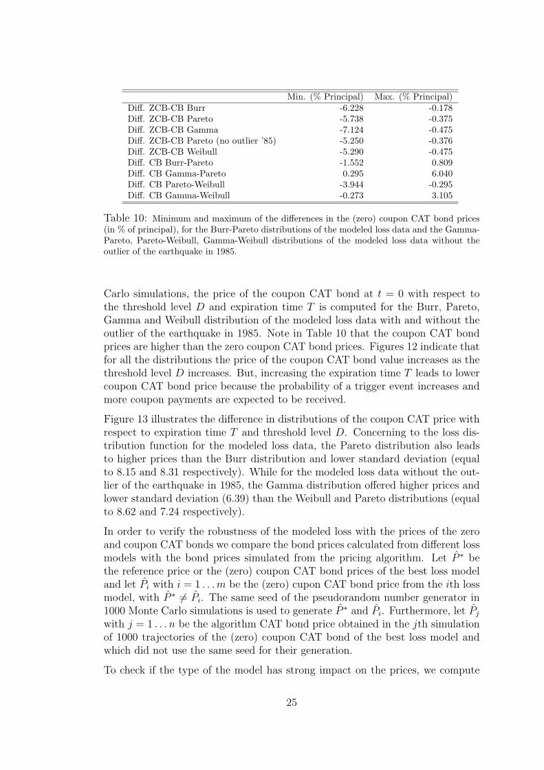
Carlo simulations, the price of the coupon CAT bond at t = 0 with respect tothe threshold level D and expiration time T is computed for the Burr, Pareto,Gamma and Weibull distribution of the modeled loss data with and without theoutlier of the earthquake in 1985. Note in Table 10 that the coupon CAT bondprices are higher than the zero coupon CAT bond prices. Figures 12 indicate thatfor all the distributions the price of the coupon CAT bond value increases as thethreshold level D increases. But, increasing the expiration time T leads to lowercoupon CAT bond price because the probability of a trigger event increases andmore coupon payments are expected to be received.

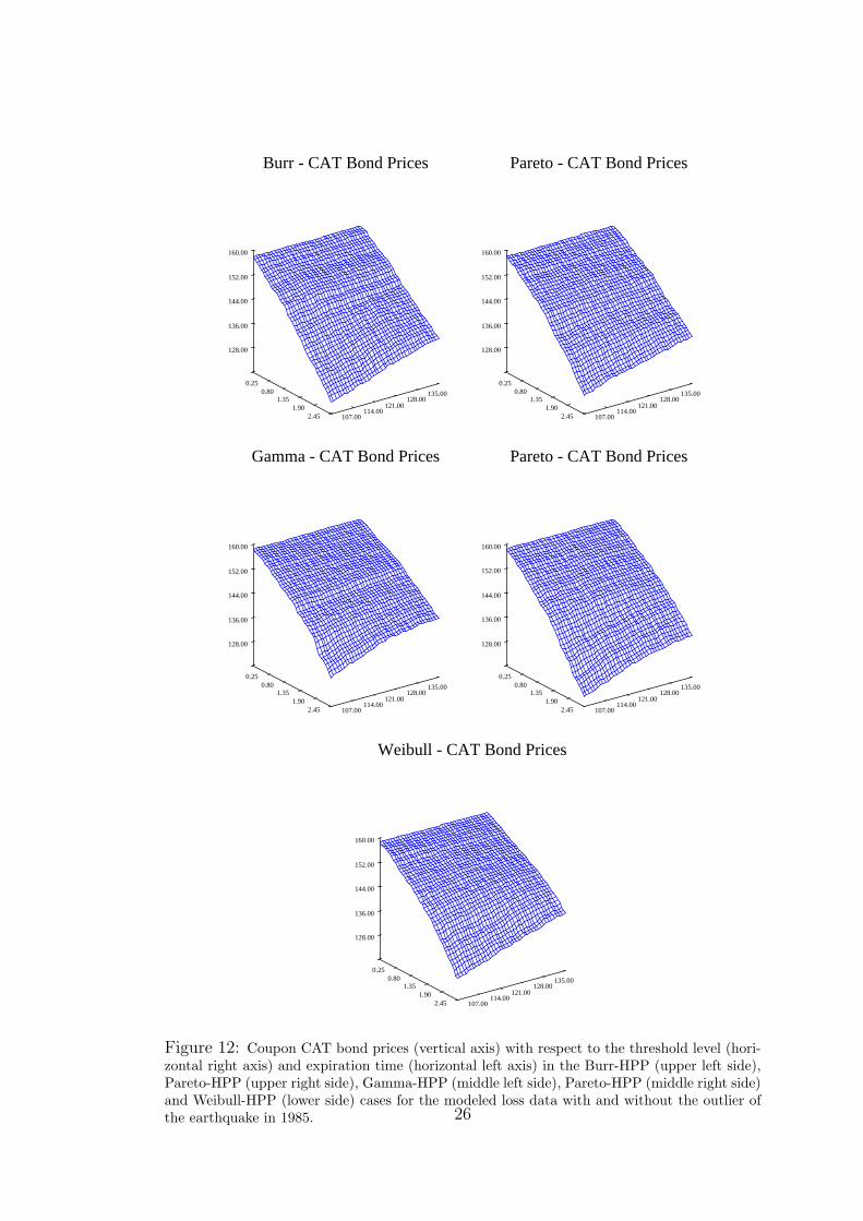
Figure 13 illustrates the difference in distributions of the coupon CAT price withrespect to expiration time T and threshold level D. Concerning to the loss dis-tribution function for the modeled loss data, the Pareto distribution also leadsto higher prices than the Burr distribution and lower standard deviation (equalto 8.15 and 8.31 respectively). While for the modeled loss data without the out-lier of the earthquake in 1985, the Gamma distribution offered higher prices andlower standard deviation (6.39) than the Weibull and Pareto distributions (equalto 8.62 and 7.24 respectively).

In order to verify the robustness of the modeled loss with the prices of the zeroand coupon CAT bonds we compare the bond prices calculated from different lossmodels with the bond prices simulated from the pricing algorithm. Let P ∗ bethe reference price or the (zero) coupon CAT bond prices of the best loss modeland let Pi with i = 1 . . . m be the (zero) cupon CAT bond price from the ith lossmodel, with P ∗ 6= Pi. The same seed of the pseudorandom number generator in1000 Monte Carlo simulations is used to generate P ∗ and Pi. Furthermore, let Pj

with j = 1 . . . n be the algorithm CAT bond price obtained in the jth simulationof 1000 trajectories of the (zero) coupon CAT bond of the best loss model andwhich did not use the same seed for their generation.

To check if the type of the model has strong impact on the prices, we compute

25

Burr - CAT Bond Prices

107.00114.00

121.00128.00

135.00

0.250.80

1.351.90

2.45

128.00

136.00

144.00

152.00

160.00

Pareto - CAT Bond Prices

107.00114.00

121.00128.00

135.00

0.250.80

1.351.90

2.45

128.00

136.00

144.00

152.00

160.00

Gamma - CAT Bond Prices

107.00114.00

121.00128.00

135.00

0.250.80

1.351.90

2.45

128.00

136.00

144.00

152.00

160.00

Pareto - CAT Bond Prices

107.00114.00

121.00128.00

135.00

0.250.80

1.351.90

2.45

128.00

136.00

144.00

152.00

160.00

Weibull - CAT Bond Prices

107.00114.00

121.00128.00

135.00

0.250.80

1.351.90

2.45

128.00

136.00

144.00

152.00

160.00

Figure 12: Coupon CAT bond prices (vertical axis) with respect to the threshold level (hori-zontal right axis) and expiration time (horizontal left axis) in the Burr-HPP (upper left side),Pareto-HPP (upper right side), Gamma-HPP (middle left side), Pareto-HPP (middle right side)and Weibull-HPP (lower side) cases for the modeled loss data with and without the outlier ofthe earthquake in 1985. 26

the mean of absolute differences (MAD) i.e. the mean of the differences of thebond prices Pi with the reference bond prices P ∗ and the mean of the differencesof the algorithm bond prices Pj with the reference bond prices P ∗. If the MAD’sare similar then the type of the model has no influence on the prices of the (zero)coupon CAT bond:

m∑i=1

Pi − P ∗

m'

n∑j=1

Pj − P ∗

n, m > 0, n > 0 (16)

In terms of relative differences, if the means of the absolute values of the relative

Burr - Pareto fifferences in CAT Bond Prices

107.00114.00

121.00128.00

135.00

0.250.80

1.351.90

2.45

-2.58

-1.85

-1.13

-0.41

0.31

Gamma - Pareto differences in CAT Bond Prices

107.00114.00

121.00128.00

135.00

0.250.80

1.351.90

2.45

1.46

2.92

4.38

5.84

7.30

Pareto- Weibull differences in CAT Bond Prices

107.00114.00

121.00128.00

135.00

0.250.80

1.351.90

2.45

-4.25

-3.19

-2.12

-1.06

0.00

Gamma - Weibull differences in CAT Bond Prices

107.00114.00

121.00128.00

135.00

0.250.80

1.351.90

2.45

-0.18

0.80

1.78

2.75

3.73

Figure 13: Difference in the coupon CAT bond price (vertical axis) in the Burr-Pareto (upperleft side), the Gamma-Pareto (upper right side), the Pareto-Weibull (lower left side) and theGamma-Weibull (lower right side) distributions under an HPP, with respect to the thresholdlevel (horizontal right axis) and expiration time (horizontal left axis)

differences (MAVRD) are similar then the model has no impact on the zero andcoupon CAT bond prices:

m∑i=1

1

m

∣∣∣∣∣ Pi − P ∗

P ∗

∣∣∣∣∣ 'n∑

j=1

1

n

∣∣∣∣∣ Pj − P ∗

P ∗

∣∣∣∣∣ , m > 0, n > 0 (17)

27

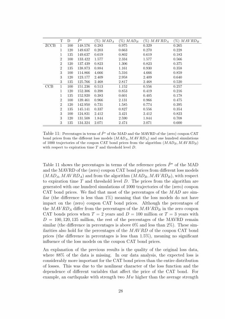
T D P ∗ (%) MADA (%) MADB (%) MAV RDA (%) MAV RDB

ZCCB 1 100 148.576 0.283 0.975 0.329 0.2651 120 149.637 0.203 0.663 0.270 0.2281 135 149.637 0.619 0.802 0.619 0.1832 100 133.422 1.577 2.334 1.577 0.5662 120 137.439 0.823 1.306 0.823 0.3752 135 138.873 0.884 1.161 0.930 0.3583 100 114.866 4.666 5.316 4.666 0.8593 120 123.177 2.409 2.958 2.409 0.6403 135 125.766 2.468 2.817 2.468 0.520

CCB 1 100 151.236 0.513 1.152 0.556 0.2571 120 152.306 0.398 0.853 0.419 0.2161 135 152.920 0.383 0.601 0.405 0.1782 100 139.461 0.966 2.131 0.966 0.4752 120 142.950 0.731 1.585 0.774 0.3952 135 145.141 0.337 0.827 0.556 0.3543 100 124.831 2.412 3.421 2.412 0.8233 120 131.508 1.844 2.590 1.844 0.7083 135 134.324 2.071 2.474 2.071 0.600

Table 11: Percentages in terms of P ∗ of the MAD and the MAVRD of the (zero) coupon CATbond prices from the different loss models (MADA,MAV RDA) and one hundred simulationsof 1000 trajectories of the coupon CAT bond prices from the algorithm (MADB ,MAV RDB)with respect to expiration time T and threshold level D.

Table 11 shows the percentages in terms of the reference prices P ∗ of the MADand the MAVRD of the (zero) coupon CAT bond prices from different loss models(MADA, MAV RDA) and from the algorithm (MADB, MAV RDB), with respectto expiration time T and threshold level D. The prices from the algorithm aregenerated with one hundred simulations of 1000 trajectories of the (zero) couponCAT bond prices. We find that most of the percentages of the MAD are sim-ilar (the difference is less than 1%) meaning that the loss models do not haveimpact on the (zero) coupon CAT bond prices. Although the percentages ofthe MAV RDA differ from the percentages of the MAV RDB in the zero couponCAT bonds prices when T = 2 years and D = 100 million or T = 3 years withD = 100, 120, 135 million, the rest of the percentages of the MAVRD remainsimilar (the difference in percentages is above 0% and less than 2%). These sim-ilarities also hold for the percentages of the MAV RD of the coupon CAT bondprices (the difference in percentages is less than 1.5%), meaning no significantinfluence of the loss models on the coupon CAT bond prices.

An explanation of the previous results is the quality of the original loss data,where 88% of the data is missing. In our data analysis, the expected loss isconsiderably more important for the CAT bond prices than the entire distributionof losses. This was due to the nonlinear character of the loss function and thedependence of different variables that affect the price of the CAT bond. Forexample, an earthquake with strength two Mw higher than the average strength

28

100 110 120 130

Threshold level

110

120

130

140

ZC

B a

t T=

3 (U

SD m

illio

n)

100 110 120 130

Threshold level

110

120

130

140

CB

at T

=3

(USD

mill

ion)

Figure 14: The zero coupon (left panel) and coupon (right panel) CAT bond prices at timeto maturity T = 3 years with respect to the threshold level D ∈ [100, 135] million. The CATbond prices under the Burr distribution (solid lines), the Pareto distribution (dotted lines) andunder different loss models (different color lines).

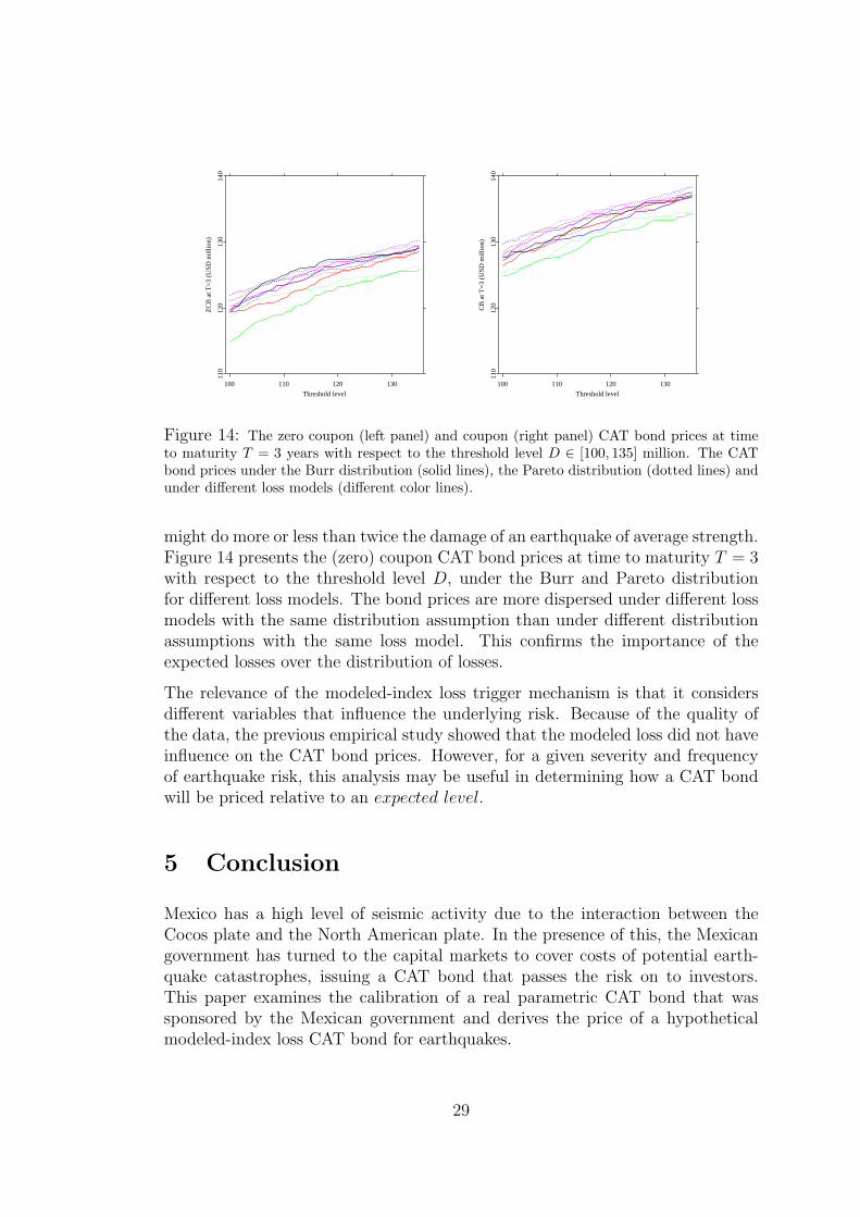
might do more or less than twice the damage of an earthquake of average strength.Figure 14 presents the (zero) coupon CAT bond prices at time to maturity T = 3with respect to the threshold level D, under the Burr and Pareto distributionfor different loss models. The bond prices are more dispersed under different lossmodels with the same distribution assumption than under different distributionassumptions with the same loss model. This confirms the importance of theexpected losses over the distribution of losses.

The relevance of the modeled-index loss trigger mechanism is that it considersdifferent variables that influence the underlying risk. Because of the quality ofthe data, the previous empirical study showed that the modeled loss did not haveinfluence on the CAT bond prices. However, for a given severity and frequencyof earthquake risk, this analysis may be useful in determining how a CAT bondwill be priced relative to an expected level.

5 Conclusion

Mexico has a high level of seismic activity due to the interaction between theCocos plate and the North American plate. In the presence of this, the Mexicangovernment has turned to the capital markets to cover costs of potential earth-quake catastrophes, issuing a CAT bond that passes the risk on to investors.This paper examines the calibration of a real parametric CAT bond that wassponsored by the Mexican government and derives the price of a hypotheticalmodeled-index loss CAT bond for earthquakes.

29

Under the assumption of perfect markets, the calibration of the bond is based onthe estimation of the intensity rate that describes the flow process of earthquakesfrom the two sides of the contract: from the reinsurance and the capital markets.Additionally, we estimate the historical intensity rate using the intensity modelthat accounts only earthquakes that trigger the CAT bond’s payoff. However,the dataset contained only three such events, what leads to the decomposition ofthe calibration of the historical intensity rate into the calibration of the intensityof all earthquakes with a magnitude higher than 6.5 Mw and the estimationof the probability of the trigger event. The intensity rate estimates from thereinsurance λ1 and capital market λ2 are approximately equal but they deviatefrom the historical intensity rate λ3. Assuming that the historical intensity ratewould be the adequately correct one, the best argument to the low premiumsfor covering the seismic risk of 450 million might be the financial strategy of thegovernment, a mix of reinsurance and CAT bond, where 35% of the total seismicrisk is transferred to the investors.

This paper also derives the price of a hypothetical CAT bond for earthquakeswith a modeled-index loss trigger mechanism, which takes other variables intoaccount that can affect the value of losses, e.g. the physical characteristics ofan earthquake. We price a modeled-index CAT bond price by means of a com-pound doubly stochastic Poisson process, where the trigger event depends on thefrequency and severity of earthquakes. We observe that the (zero) coupon CATbond prices increased as the threshold level D increased, but decreased as theexpiration time T increased. This is mainly because the probability of a triggerevent increases and more coupon payments are expected to be received. Becauseof the quality of the data, different loss models reveal no impact on the CAT bondprices and the expected loss is considerably more important for the evaluation ofthe modeled-index CAT bond than the entire distribution of losses.

The CAT bond’s spread rate is reflected by the intensity rate of the earthquakeprocess in the parametric trigger, while for the modeled loss trigger mechanism thespread rate is represented by the intensity rate of the earthquake process and thelevel of accumulated losses Ls. The trigger mechanism matters for the CAT bondpricing, as long as the risk of the underlying is adequately estimated. Withoutdoubt, the availability of information and the quality of the data provided byresearch institutions attempting earthquakes has a direct impact on the accuracyof this risk analysis and for the evaluation of CAT bonds.

30

References

Anderson, R.,Bendimerad, F., Canabarro, E. & Finkemeier, M. (1998). FixedIncome Research: Analyzing Insurance-Linked Securities, Quantitative Re-search, Goldman Sachs & Co.

Baryshnikov, Y., Mayo, A. & Taylor, D.R. (2001). Pricing of CAT Bonds,preprint.

Burnecki, K. & Kukla, G. & Weron, R. (2000). Property insurance loss distribu-tions, Physica A 287:269-278.

Burnecki, K. & Kukla, G. (2003). Pricing of Zero-Coupon and Coupon CATBonds, Appl. Math (Warsaw) 30(3):315-324.

Burnecki, K. & Hardle, W. & Weron, R. (2004). Simulation of risk processes,Encyclopedia of Actuarial Science in J. Teugels, B. Sundt (eds.), Wiley,Chichester.

Clarke, R., Faust, J. & Mcghee, C. (2005). The Catastrophe Bond Market at Year-End 2004: The Growing Appetite for Catastrophic Risk, Studies Paper. GuyCarpenter & Company, Inc.

Clarke, R., Faust, J. & Mcghee, C. (2006). The Catastrophe Bond Market atYear-End 2005: Ripple Effects from record storms, Studies Paper. GuyCarpenter & Company, Inc.

Clarke, R., Collura, J. & Mcghee, C. (2007). The Catastrophe Bond Marketat Year-End 2006: Ripple into Waves, Studies Paper. Guy Carpenter &Company, Inc.

Croson, D.C & Kunreuther, H.C. (2007). Customizing indemnity contracts andindexed cat bonds for natural hazard risks, Journal of Fixed Income; 1,46-57.

D’Agostino & Stephens, M.A. (1986). Goodness-of-Fit Techniques, MarcelDekker, New York.

Dubinsky, W. & Laster, D. (2005). Insurance Link Securities SIGMA, Swiss Republications.

Froot, K.A. (2001 ). The Market for Catastrophe Risk: A Clinical Examination,Journal of Financial Economics ; 60: 529-571.

Grandell, J. (1999 ). Aspects of Risk Theory, Springer, New York.

Hogg, R.V. & Klugman, S.A. (1984 ). Loss distributions, Wiley, New York.

Howell, D. (1998). Treatment of missing data, http://www.uvm.edu/ dhowell

31

IAIS, International Association of Insurance Supervisors. (2003). Non-Life Insur-ance Securitisation, Issues papers and other reports

Kau, J.B. & Keenan, D.C. (1996 ). An Option-Theoretic Model of Catastrophesapplied to Mortage insurance, Journal of risk and Insurance; 63(4): 639-656.

Lee, J. & Yu, M. (2002). Pricing Default Risky CAT Bonds with Moral Hazardand Basis Risk, Journal of Risk and Insurance, Vol.69, No.1;25-44.

Mcghee, C. (2004). The Catastrophe Bond Market at Year-End 2003: MarketUpdate, Studies Paper. Guy Carpenter & Company, Inc.

Mooney, S. (2005). The World Catastrophe reinsurance market 2005,Studies pa-per. Guy Carpenter & Company, Inc.

RMS: Risk Management Solutions Mexico earthquake,www.rms.com/Catastrophe/Models/Mexico.asp

SHCP: Secretarıa de Hacienda y Credito Publico Mexico. (2001). Acuerdo que es-tablece las Reglas de Operacion del Fondo de Desastres Naturales FONDEN.Mexico.

SHCP: Secretarıa de Hacienda y Credito Publico Mexico. (2004). Administracinde Riesgos Catastroficos del FONDEN. Mexico.

SSN Ingenieros: Estrada, J. & Perez, J. & Cruz, J.L & Santiago, J. & Cardenas,A. & Yi , T. & Cardenas, C. & Ortiz, J. & Jimenez, C. (2006). Servicio Sis-mologico Nacional Instituto de Geosifısica UNAM, Earthquakes Data Base1900-2003.

SIGMA. (1996). Insurance Derivatives and Securitization: New Hedging Perspec-tives for the US catastrophe Insurance Market?, Report, Number 5, SwissRe.

Vaugirard, G. (2002). Valuing catastrophe bonds by Monte Carlo simulations,Journal Applied Mathematical Finance 10 ; 75-90.

Working Group on California Earthquake Probabilities (1998). Probabilities oflarge earthquakes occurring in California on the San Andreas Fault, Openfile report :88-398. U.S. Department of the Interior.

32

SFB 649 Discussion Paper Series 2007

For a complete list of Discussion Papers published by the SFB 649, please visit http://sfb649.wiwi.hu-berlin.de.

001 "Trade Liberalisation, Process and Product Innovation, and Relative Skill Demand" by Sebastian Braun, January 2007. 002 "Robust Risk Management. Accounting for Nonstationarity and Heavy Tails" by Ying Chen and Vladimir Spokoiny, January 2007. 003 "Explaining Asset Prices with External Habits and Wage Rigidities in a DSGE Model." by Harald Uhlig, January 2007. 004 "Volatility and Causality in Asia Pacific Financial Markets" by Enzo Weber, January 2007. 005 "Quantile Sieve Estimates For Time Series" by Jürgen Franke, Jean- Pierre Stockis and Joseph Tadjuidje, February 2007. 006 "Real Origins of the Great Depression: Monopolistic Competition, Union Power, and the American Business Cycle in the 1920s" by Monique Ebell and Albrecht Ritschl, February 2007. 007 "Rules, Discretion or Reputation? Monetary Policies and the Efficiency of Financial Markets in Germany, 14th to 16th Centuries" by Oliver Volckart, February 2007. 008 "Sectoral Transformation, Turbulence, and Labour Market Dynamics in Germany" by Ronald Bachmann and Michael C. Burda, February 2007. 009 "Union Wage Compression in a Right-to-Manage Model" by Thorsten Vogel, February 2007. 010 "On σ−additive robust representation of convex risk measures for unbounded financial positions in the presence of uncertainty about the market model" by Volker Krätschmer, March 2007. 011 "Media Coverage and Macroeconomic Information Processing" by

Alexandra Niessen, March 2007. 012 "Are Correlations Constant Over Time? Application of the CC-TRIGt-test

to Return Series from Different Asset Classes." by Matthias Fischer, March 2007.

013 "Uncertain Paternity, Mating Market Failure, and the Institution of Marriage" by Dirk Bethmann and Michael Kvasnicka, March 2007.

014 "What Happened to the Transatlantic Capital Market Relations?" by Enzo Weber, March 2007.

015 "Who Leads Financial Markets?" by Enzo Weber, April 2007. 016 "Fiscal Policy Rules in Practice" by Andreas Thams, April 2007. 017 "Empirical Pricing Kernels and Investor Preferences" by Kai Detlefsen, Wolfgang Härdle and Rouslan Moro, April 2007. 018 "Simultaneous Causality in International Trade" by Enzo Weber, April 2007. 019 "Regional and Outward Economic Integration in South-East Asia" by Enzo Weber, April 2007. 020 "Computational Statistics and Data Visualization" by Antony Unwin,

Chun-houh Chen and Wolfgang Härdle, April 2007. 021 "Ideology Without Ideologists" by Lydia Mechtenberg, April 2007. 022 "A Generalized ARFIMA Process with Markov-Switching Fractional Differencing Parameter" by Wen-Jen Tsay and Wolfgang Härdle, April 2007.

SFB 649, Spandauer Straße 1, D-10178 Berlin http://sfb649.wiwi.hu-berlin.de

This research was supported by the Deutsche

Forschungsgemeinschaft through the SFB 649 "Economic Risk".

SFB 649, Spandauer Straße 1, D-10178 Berlin http://sfb649.wiwi.hu-berlin.de

This research was supported by the Deutsche

Forschungsgemeinschaft through the SFB 649 "Economic Risk".

023 "Time Series Modelling with Semiparametric Factor Dynamics" by Szymon Borak, Wolfgang Härdle, Enno Mammen and Byeong U. Park, April 2007. 024 "From Animal Baits to Investors’ Preference: Estimating and Demixing of the Weight Function in Semiparametric Models for Biased Samples" by Ya’acov Ritov and Wolfgang Härdle, May 2007. 025 "Statistics of Risk Aversion" by Enzo Giacomini and Wolfgang Härdle, May 2007. 026 "Robust Optimal Control for a Consumption-Investment Problem" by Alexander Schied, May 2007. 027 "Long Memory Persistence in the Factor of Implied Volatility Dynamics" by Wolfgang Härdle and Julius Mungo, May 2007. 028 "Macroeconomic Policy in a Heterogeneous Monetary Union" by Oliver Grimm and Stefan Ried, May 2007. 029 "Comparison of Panel Cointegration Tests" by Deniz Dilan Karaman Örsal, May 2007. 030 "Robust Maximization of Consumption with Logarithmic Utility" by Daniel Hernández-Hernández and Alexander Schied, May 2007. 031 "Using Wiki to Build an E-learning System in Statistics in Arabic Language" by Taleb Ahmad, Wolfgang Härdle and Sigbert Klinke, May 2007. 032 "Visualization of Competitive Market Structure by Means of Choice Data" by Werner Kunz, May 2007. 033 "Does International Outsourcing Depress Union Wages? by Sebastian Braun and Juliane Scheffel, May 2007. 034 "A Note on the Effect of Outsourcing on Union Wages" by Sebastian Braun and Juliane Scheffel, May 2007. 035 "Estimating Probabilities of Default With Support Vector Machines" by Wolfgang Härdle, Rouslan Moro and Dorothea Schäfer, June 2007. 036 "Yxilon – A Client/Server Based Statistical Environment" by Wolfgang Härdle, Sigbert Klinke and Uwe Ziegenhagen, June 2007. 037 "Calibrating CAT Bonds for Mexican Earthquakes" by Wolfgang Härdle and Brenda López Cabrera, June 2007.