blue water scarcity and the economic impacts of future agricultural trade and demand

Blue water scarcity and the economic impacts of future agriculturaltrade and demand

Christoph Schmitz,1,2 Hermann Lotze-Campen,1 Dieter Gerten,3 Jan Philipp Dietrich,4

Benjamin Bodirsky,1,5 Anne Biewald,1 and Alexander Popp4

Received 6 August 2012; revised 4 February 2013; accepted 8 March 2013; published 21 June 2013.

[1] An increasing demand for agricultural goods affects the pressure on global waterresources over the coming decades. In order to quantify these effects, we have developed anew agroeconomic water scarcity indicator, considering explicitly economic processes inthe agricultural system. The indicator is based on the water shadow price generated by aneconomic land use model linked to a global vegetation-hydrology model. Irrigationefficiency is implemented as a dynamic input depending on the level of economicdevelopment. We are able to simulate the heterogeneous distribution of water supply andagricultural water demand for irrigation through the spatially explicit representation ofagricultural production. This allows in identifying regional hot spots of blue water scarcityand explicit shadow prices for water. We generate scenarios based on moderate policiesregarding future trade liberalization and the control of livestock-based consumption,dependent on different population and gross domestic product (GDP) projections. Resultsindicate increased water scarcity in the future, especially in South Asia, the Middle East,and north Africa. In general, water shadow prices decrease with increasing liberalization,foremost in South Asia, Southeast Asia, and the Middle East. Policies to reduce livestockconsumption in developed countries not only lower the domestic pressure on water but alsoalleviate water scarcity to a large extent in developing countries. It is shown that one of thetwo policy options would be insufficient for most regions to retain water scarcity in 2045 onlevels comparable to 2005.

Citation: Schmitz, C., H. Lotze-Campen, D. Gerten, J. P. Dietrich, B. Bodirsky, A. Biewald, and A. Popp (2013), Blue water scarcityand the economic impacts of future agricultural trade and demand, Water Resour. Res., 49, 3601–3617, doi :10.1002/wrcr.20188.

1. Introduction

[2] More than ever before, the question of water scarcityshapes debates on current and future food production[Rosegrant et al., 2009; Hanjra and Qureshi, 2010;Godfray et al., 2010]. Water scarcity is mainly driven bypopulation growth [Falkenmark et al., 1989; Vörösmartyet al., 2000] and is, from this perspective, a relatively newphenomenon in human history [Kummu et al., 2010]. As

global population is expected to grow to 9–10 billion bythe middle of the 21st century [Lutz et al., 2001], waterscarcity is expected to increase. Furthermore, disposableincomes in developing countries will continue to rise [Rose-grant and Cline, 2003] and recent changes in diets of indus-trial countries will likely be adopted by many developingsocieties in the near future [Pingali, 2006]. This will lead tohigher consumption of livestock products [Delgado, 2003]and aggravate stress on water resources, as animal-basedcalories are produced in a much more water-intensive waythan plant-based calories [Hoekstra and Chapagain, 2007].

[3] The focus of this study is on blue water located insurface water and aquifers, which is defined as the rainfallwater escaping evaporation [Falkenmark et al., 2007]. Sev-eral indicators have been evolved to measure blue waterscarcity. Calculations of water scarcity started with the Fal-kenmark indicator, relating total freshwater resources toper capita requirements [Falkenmark, 1989]. In contrast tothe absolute Falkenmark indicator, several relative indicatorscompute the water withdrawal-to-availability (WTA) ratio[Vörösmarty et al., 2000; Alcamo et al., 2003; Oki andKanae, 2006; Islam et al., 2006; Hanasaki et al., 2008b].Smakhtin et al. [2004] went a step further by adding environ-mental aspects to the WTA analysis. Another group of indi-cators emphasizes the social dimension of water scarcity.Ohlsson [2000] uses an indicator based on an aggregation of

Additional supporting information may be found in the online version ofthis article.

1Climate Impacts and Vulnerabilities (RD2), Potsdam Institute for Cli-mate Impact Research (PIK), Potsdam, Germany.

2Department of Agricultural Economics and Social Sciences, HumboldtUniversity, Berlin, Germany.

3Earth System Analysis (RD1), Potsdam Institute for Climate ImpactResearch (PIK), Potsdam, Germany.

4Sustainable Solutions (RD3), Potsdam Institute for Climate ImpactResearch (PIK), Potsdam, Germany.

5Economics of Climate Change, Technical University Berlin, Berlin,Germany.

Corresponding author: C. Schmitz, Climate Impacts and Vulnerabilities(RD2), Potsdam Institute for Climate Impact Research (PIK), D-14473Potsdam, Germany. ([email protected])

©2013. American Geophysical Union. All Rights Reserved.0043-1397/13/10.1002/wrcr.20188

3601

WATER RESOURCES RESEARCH, VOL. 49, 3601–3617, doi:10.1002/wrcr.20188, 2013

established hydrological indices and the U.N. human devel-opment index (HDI) as an approximation for the socialadaptive capacity of a society. More comprehensiveness isprovided by the watershed sustainability index [Chavez andAlipaz, 2007], where in addition to HDI, the water povertyindex and the environmental sustainability index (ESI) areconsidered. A first attempt of a rather simple economic waterscarcity indicator has been designed by the InternationalWater Management Institute [Molden, 2007]. A region iscalled economic water scarce, if a lack of investment inwater infrastructure or a lack of human capacity to satisfythe demand for water is observed.

[4] In our study, we look explicitly on agricultural freshwater use, since around 70%–80% of human freshwaterwithdrawals [Gleick et al., 2009] and around 90% of theconsumed blue water [Shiklomanov and Rodda, 2003] areused for agriculture. A specific indicator for agriculturalwater stress has been recently developed by Vörösmartyet al. [2010]. The authors have estimated the burden thatcrop production places on renewable water resources byconsidering water supply and irrigation water demand.Gerten et al. [2011] follows a similar approach but calcu-lates the WTA ratio based on blue and green water avail-ability; with green water defined as water originatingdirectly from precipitation.

[5] Although all of those indicators have different perspec-tives on water scarcity, they consistently lack crucial eco-nomic processes. None of the indicators has an integratedview based on the interplay between biophysical availabilityof water and economic-driven demand [Sauer et al., 2010].As de Fraiture [2007] points out, current indicators solelyfocus on the water and biophysical sector and largely ignoremacroeconomic drivers, such as income, trade, and economicpolicy as well as microeconomic drivers, such as productioncosts and productivity growth. To fill large parts of this gap,we have developed a new agroeconomic water scarcity indi-cator on grid cell level, which considers blue water used forirrigation agriculture. The indicator is based on the watershadow price (WSP) generated uniquely through the couplingof a global biophysical vegetation model and an economicland use model. The indicator has the advantage of includingeconomic processes and drivers, such as production costs,technological change (TC), and international trade. Thisallows for analyzing policies in an international context bytaking economic processes related to land use endogenouslyinto account. The IMPACT-WATER model [Cai and Rose-grant, 2002], the related WATERSIM model [de Fraiture,2007], and the Global Trade Analysis Project - Water(GTAP-W) model [Calzadilla et al., 2011b] are approachesto integrate the economics of water into an agricultural mod-eling framework. Although the first two models are partialequilibrium models, focusing on the agricultural sector,GTAP-W is a computable equilibrium model (CGE) takingall economic sectors into account. These models are wellsuited for the short- and medium term and have the strengthto be very detailed on economic parameters. However, incontrast to our approach, they are neither working on a highspatial resolution nor are they directly linked to a biophysicalmodel. Both features are essential for analyzing local phe-nomena, such as water scarcity.

[6] In our analysis, we focus on two possible policy areasand their interaction. The first is the option of increased food

trade via trade liberalization. Agricultural goods contain asignificant amount of so-called virtual water, which isdefined as the amount of freshwater embedded in the pro-duction process [Hoekstra and Chapagain, 2007)]. Tradinggoods internationally plays an important role for increasingthe global efficiency of water use [Fader et al., 2011]. Sev-eral studies have quantified the importance of current virtualwater trade and demonstrated that some water-scarce regionsare major importers of water-intensive products [Konaret al., 2011; Fader et al., 2011; Hanasaki et al., 2010; Cha-pagain and Hoekstra, 2008; Hoekstra and Hung, 2005; Okiand Kanae, 2004]. In contrast to virtual water assessments,we explicitly analyze the effects of different trade liberaliza-tion scenarios on agroeconomic water scarcity and assess theimpact on future water scarcity.

[7] The second policy parameter enforces a changingdiet toward lower consumption of animal products. At theturn of the millennium, around 2 billion people based theirdiets largely on animal products, whereas more than 4 bil-lion people lived primarily on a plant-based diet [Pimenteland Pimentel, 2003]. No global study has assessed theimpact of changing diets on global water resources indetail. Gerten et al. [2011] has assessed the sensitivity oftheir results by calculating the likelihood of water scarcityunder a scenario of lower animal calorie intake. Renaultand Wallender [2000] have analyzed in a simple regionalmodel the percentage of additional water that could besaved according to different scenarios until 2025. Apartfrom those studies, the influence of changing diets has beeneither shown globally on land use [Wirsenius et al., 2010]and greenhouse gas emissions [Popp et al., 2010; Stehfestet al., 2009] or regionally on water consumption [Liu andSavenije, 2008]. Finally, in order to evaluate the sensitivityof the simulations, we run the model with different popula-tion and gross domestic product (GDP) scenarios.

[8] We start our analysis by describing the involvedmodels, the creation of the agroeconomic water scarcity in-dicator, and the scenario implementation. Furthermore,water-related input data, i.e., water discharge and irrigationdemand from the dynamic global vegetation and water bal-ance model Lund-Potsdam-Jena managed Land (LPJmL)[Bondeau et al., 2007], are compared with the outcome ofthe global water resources model H08 [Hanasaki et al.,2008a, 2008b]. In section 3, we present the outcome of thescenarios with a special attention to WSPs, TC rates, andland use changes as well as the sensitivity of the results.Subsequently, we discuss methods and results in relation toprevious studies. In the last section, we draw conclusionsand policy implications from our analysis.

2. Modeling Approach and Methods

2.1. Model Descriptions

2.1.1. MAgPIE Model[9] For the analysis, we use model of agricultural pro-

duction and its impact on the environment (MAgPIE), anonlinear recursive dynamic optimization model [Lotze-Campen et al., 2008; Schmitz et al., 2012]. It is linked tothe dynamic vegetation model LPJmL on a 0:5

�resolution

(see section 2.1.2), to simulate spatially explicit land andwater use patterns. This approach provides a high flexibilityto integrate various types of biophysical constraints into an

SCHMITZ ET AL.: BLUE WATER SCARCITY-ON AGRICULTURAL TRADE AND DEMAND

3602

economic decision-making process. The dual solution ofthe economic optimization model MAgPIE allows for com-puting shadow prices (or implicit economic values) forbinding constraints on grid cell basis. The shadow pricesdefine the potential cost savings the model would achieveby relaxing the constraint by one unit. In this study, wefocus on the WSP, which reflects the implicit economicvalue for one additional cubic meter of water in a particulargrid cell (see section 2.2.3).

[10] Each grid cell is assigned to 1 of the 10 economicworld regions (Appendix A, Table A1). The initializationyear is 1995 with data on income (GDP) [World Bank,2001], population [Center for International Earth ScienceInformation Network (CIESIN), 2000], demand for foodenergy [Food and Agriculture Organization (FAO), 2010],average costs for different production activities [Nar-ayanan and Walmsley, 2008], and food self-sufficiencyratios [FAO, 2010]. All activities on the supply side arespecific for each grid cell (0:5

�resolution), whereas activ-

ities on the demand side are aggregated to the regionallevel. Future demand of calories and the share of livestockproducts are dependent on income and population, and theyare based on a detailed regression analysis (Figure 1 andAppendix B).

[11] With flexible minimum self-sufficiency ratios,MAgPIE is able to represent international trade and allo-cates global food demand to the supply regions. Agricul-tural self-sufficiency ratios describe the ability of countriesto produce as much food as they demand. As an example, acountry with a self-sufficiency of 0.75 for wheat produces75% of its demand by itself and imports 25%. In MAgPIE,two virtual trading pools are implemented, which distributethe demand to the 10 regions in a different way (Figure 1).The fixed trade pool (first pool) allocates the demandaccording to self-sufficiency ratios based on Food andAgriculture Organization (FAO) food balance sheets [FAO,2010]. The self-sufficiency ratios assign the quantity that isproduced domestically, and the corresponding exportshares [FAO, 2010] define the share of the regions in globalexports. The free trade pool (second pool) distributes thedemand to the supply regions according to comparativeadvantage criteria. This means that the region with the low-est production costs per ton will export. The parameter ptb

determines the share of demand for each of the two pools.If ptb equals 1, total demand will be allocated according tothe predefined self-sufficiency ratios and the export sharesto the supply regions. If ptb is equal to 0, all trading quan-tity will hit the second pool and is allocated according tocomparative advantages. More details of the implementa-tion are provided in Schmitz et al. [2012] and in the mathe-matical description in Appendix C.

[12] The resulting demand calories are produced by 16cropping activities and 5 livestock activities (see AppendixA). The five livestock activities depend on specific feedenergy requirements derived from Wirsenius [2000], whichconsist of a mixture of pasture, fodder, and food crops. Allthese inputs are specific for each region and animal typeand are on the basis of preconditions for lactation, mainte-nance, reproduction, growth, and various other biologicalneeds. Inputs for the calculation of feedstock (crops, by-products, and pasture) and livestock-related greenhouse gasemissions in MAgPIE are calculated in Weindl et al. [2010].

[13] For future projections, the model works on timesteps of 10 years in a recursive dynamic mode. The landuse pattern of each period is used as the initial land pool forthe consecutive period. MAgPIE minimizes global costs,consisting of four different cost categories: First, produc-tion costs, containing factor costs for labor, capital, and in-termediate inputs, are taken from GTAP [Narayanan andWalmsley, 2008]. Production costs per area unit evolvewith the yield level in a linear relationship [Schmitz et al.,2010]. Second, investments in yield-increasing TC increaseexponentially based on the state of agricultural develop-ment of a region [Dietrich et al., 2012; Dietrich et al.2013]. This endogenous implementation allows MAgPIE toproject future yield increases and the costs involved. Interms of water, TC increases demand for blue water, sincewater requirements are dependent on yield. Third, costs forland expansion which is the other alternative for MAgPIEto increase food production [Krause et al., 2009; Poppet al., 2011] and costs for irrigation area expansion are con-sidered. Land conversion costs (for the conversion of forestinto cropland) are based on marginal access costs on coun-try level from the global timber model [Sohngen et al.,2009]. Additionally, expansion of irrigation area involvesregional costs, which were aggregated from the AQUA-STAT-Database [FAO, 2011]. Fourth, intraregional trans-port costs accrue for every commodity unit as a function ofthe distance to intraregional markets, the quality of theinfrastructure (both based on a detailed data set on traveltime [Nelson, 2008]) and average transport costs (based onGTAP [Narayanan and Walmsley, 2008]). A mathematicaldescription of the model is provided in the supportinginformation.2.1.2. LPJmL Model

[14] Biophysical inputs for MAgPIE, such as potentialcrop productivity and related water use as well as land andwater constraints, are supplied for each grid cell (0:5

�reso-

lution) by the Lund-Potsdam-Jena dynamic global vegeta-tion and water balance model with managed Land (LPJmL)[Bondeau et al., 2007]. LPJmL models dynamic processeslinking biophysical processes like soil and climate condi-tions, plant growth and water availability, and directly con-siders the impacts of CO2, temperature and radiation onagricultural yields. For this study, however, those inputsare not subject to any climate change impacts. LPJmL alsocovers surface and subsurface water flows (though withoutexplicit distinction of groundwater), as carbon and water-related processes are closely linked in plant physiology.Also, blue and green water consumption is separated, withthe former occurring on areas equipped for irrigation [Dölland Siebert, 2000], which allows for the distinction ofrainfed and irrigated yields. Green water originates directlyfrom precipitation and is taken up by plants and soil. Bluewater is the amount of evapotranspiring irrigation wateroriginating from rivers, lakes, aquifers, and reservoirs[Gerten et al., 2004]. The computation of blue water stocksand flows and the separation of blue and green water flowson irrigated areas in LPJmL are illustrated in detail in Rostet al. [2008]. The river-routing module in LPJmL distrib-utes the natural runoff and its downstream movement asadditional water to irrigated areas (see Rost et al. [2008]for a detailed description of this module). The water dis-charge value for each grid cell from LPJmL is used as a


3603

constraint for irrigation in MAgPIE. From a modified ver-sion of the MIRCA2000 land use data set [Portmann et al.,2010], the information about rainfed and irrigated land usefractions is derived [Fader et al., 2010].

2.2. Blue Water Implementation and Related ShadowPrice

[15] The implementation of blue water in MAgPIE isbased on data inputs from LPJmL. LPJmL delivers two rel-evant cell-specific water inputs for MAgPIE: First, bluewater discharge available to the agricultural sector, andsecond, the water requirement per plant and cell that isneeded for irrigation. For this analysis, we compared thoseinputs with the outcome of an independent hydrology

model (section 2.2.1). The water discharge from LPJmL isreduced in MAgPIE by an efficiency factor that representsthe losses in the water and irrigation system (section 2.2.2).Finally, the WSP can be determined based on the waterconsumption per cell calculated in MAgPIE (section 2.2.3).2.2.1. Comparison of Water Inputs

[16] Both LPJmL inputs blue water discharge and waterrequirement per plant are crucial factors for the analysis.Therefore, for an evaluation use analogous results from theH08 model, which similar to LPJmL provides water-with-drawal values specifically for agriculture on a grid celllevel (Hanasaki et al. [2008a] and applied in Hanasakiet al. [2008b]). For comparison, we computed the WTA ra-tio from both models, where the model runs are based on

Figure 1. Simplified MAgPIE flowchart of key processes highlighted in this study (demand and tradeimplementation, data inputs from LPJmL and spatially explicit WSP). With exogenous data about popu-lation and GDP development, we calculate regional demand and the livestock share. The former is thentranslated to regional supply depending on the international trade scenario. Further inputs for MAgPIEare socioeconomic data like production costs and biophysical inputs from LPJmL. After the optimizationof MAgPIE, one of the outputs is cropping patterns of the different crops, which is the basis for the WSP.


3604

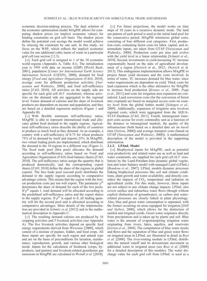
climate projections from the general circulation model Eu-ropean Centre Hamburg Model 5 (ECHAM5) [Roeckneret al., 2003] and special report on emission scenarios(SRES A2) [Nakicenovic and Swart, 2000]. We followedthe approach by Vörösmarty et al. [2010] and ranked it rel-atively to the highest value. This means the highest value isequal to 1, whereas the lowest value is almost 0. In total,14,382 cells of 59,199 cells contain a WTA ratio in bothmodels. With the help of the map comparison kit [Visserand de Nijs, 2006], which allows for the numerical compar-ison of two different maps, we compared both maps. Thecomparison index c is calculated by taking the differenceof both model indices on cell level j.

cj ¼ H08j � LPJmL j: (1)

[17] Figure 2a illustrates the ranked agricultural WTAratio calculated for the LPJmL model and the graph in themiddle for the H08 model. Highest values are modeled forsoutheast Australia, northern China, north India, Pakistan,the Middle East, north Africa, southern Europe, and partsof the United States and Mexico. The map in the middleshows the same for H08 model (Figure 2b).

[18] Figure 2c shows the difference of the ranked WTAratio between the H08 model and the LPJmL model. Larg-est differences are in Southern Europe and Turkey, whereLPJmL has higher WTA values and for southern China,where LPJmL has lower values than H08. The validationdiscloses that both data sets, although independently derived(LPJmL is primarily a vegetation model, while H08 is a spe-cialized hydrology model), the outcomes are very similar.Comparing the LPJmL outputs with the recently publishedindicator by Vörösmarty et al. [2010], it appears that theLPJmL values are higher in Western United States and Mid-dle East and lower in Central Asia and Argentina, whereasthe remaining regions are similar.2.2.2. Irrigation Efficiency

[19] Improving irrigation efficiency is one of the mainoptions to reduce water consumption [Molden, 2007]. Morethan 50% of global water resources, which are intended forirrigation, are lost due to bad management, losses in the con-veyance system, and inefficient application to the plant [Rog-ers et al., 1997]. In MAgPIE, irrigation efficiency isimplemented through an efficiency factor that comprisesmanagement, conveyance, and application efficiency. Thedata are from Rohwer et al. [2007], who calculated specificefficiency levels for 134 countries for the year 1995. In con-trast to most other studies, irrigation efficiency in MAgPIE isa dynamic input. In order to project future irrigation efficien-cies, we tested several hypotheses concerning the relationshipbetween the efficiency factor and independent variables, suchas GDP per capita [Heston et al., 2011], irrigation area share[Döll and Siebert, 2000], and the level of agricultural inten-sity [Dietrich et al., 2012]. Cross-sectional regression analy-ses with different functional forms reveals that only GDP percapita is significant as an explanatory variable for irrigationefficiency. For the analysis, we included 149 countries withdocumented irrigation areas. However, in order to reducedata errors by small countries (with respect to irrigated agri-culture), those below an irrigation area share 5% of total crop-land, and an absolute irrigation area of 3 million hectare was

clustered together to nine world regions. Together with the 13countries, which fulfilled the minimum criteria, 22 data pointshave been used for the regression.

[20] The regression determines the following linear rela-tionship between the level of economic development (meas-ured in GDP per capita gdp i=pop iÞ and irrigation efficiency� on regional level i :

�i ¼ 0:381þ gdp i

pop i

� �5:28� 10�6: (2)

[21] The results of the weighted linear regression gavean adjusted R2 of 0.55, but highly significant P-values ofthe t-tests for the constant and the slope (P¼ 0.000).The conducted regression specification error test (RESET)

Figure 2. Upper and central map: (a) Relative ranked ra-tio of water WTA of the LPJmL model and the (b) H08model in 1995. Values of both graphs are displayed asshare compared to the highest rank with 1 as the highestvalue and 0 the lowest. Lower map: (c) Comparisonbetween ranked WTA ratio of LPJmL and H08 model.


3605

[Ramsey, 1969] offers a high significance level, whichmeans that no important variables seem to be omitted(F 3; 18½ � ¼ 1:59 and F0:05 ¼ 3:16). Figure 3 shows thegraph of the regression analysis with the correspondingcountries and regions.

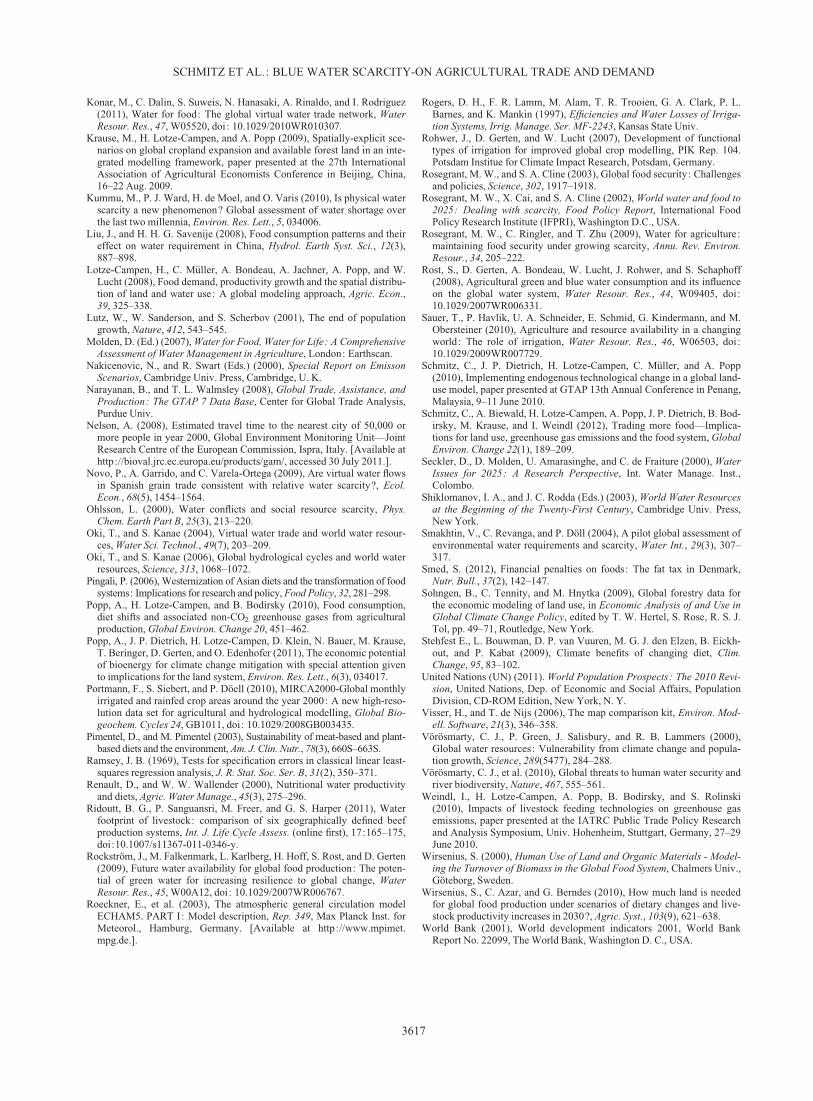
[22] The irrigation efficiencies increase over time due toincreasing GDP per capita in all regions (Figure D1 in Ap-pendix D). Highest efficiencies are achieved in developedregions, like North America (NAM) (from 56% in 2005 to67% in 2045) and Europe (EUR) (from 48% to 60%), andPacific OECD (PAO) (from 51% to 62%). Europe is behindNAM, since the Eastern European countries have very lowvalues. Sub-Saharan Africa (40%) and South Asia (42%)have the lowest efficiencies in 2045.

[23] Finally, in MAgPIE available water for irrigation,pwater is calculated on cell level j by the product of waterdischarge pdischarge and the regional specific irrigation effi-ciency �i.

pwaterj � pdischarge

j � �i: (3)

2.2.3. Water Shadow Price[24] Since MAgPIE is an economic optimization model

operating under constrained conditions, it is possible togenerate a shadow price for every independent constraint.The shadow price is defined as an achievable rate ofincrease in the objective function per unit increase inresource x [Aucamp and Steinberg, 1982]. Because ourobjective function minimizes costs, we have to reframe thedefinition to ‘‘the achievable rate of decrease in the objec-tive function if the constraint x is relaxed by one unit.’’ Forour analysis we, use the available water constraint pwater

j .

wsp j ¼@g�t@pwater

j

; (4)

where wspj stands for the water shadow price in each cell jand g�t denotes the optimal value of the goal function(defined in the supporting information). The water con-straint for each cell j is defined as

Xv

xareat;j;v;0ir0p

yield t ct;j;v;0ir0p

watreqj;v þ

Xl

xprodt;j;l pwatreq

j;l � pwaterj ; (5)

where xareat;j;v;0ir0 is the total irrigated area of each crop v, each

cell j, and each time step t ; pyield tct;j;v;0ir0 is the irrigated yield

(including TC) for each time step, each cell, and each crop;pwatreq

j;k is the cellular water requirements for product (v for

crops and l for livestock); xprodt;j;l is the total production of

each livestock product l, for each cell at each time step.From the constraint specification, it follows that therequired amount of water is proportional to the productionvolume. The cellular water available for production sets thelimit for the consumption for water in each cell.

[25] In economic terms, wsp is defined as the saved mar-ginal costs, when one additional unit of water would beavailable in a particular grid cell. With cell-specific WSPswe are able to generate maps in order to define hot spots ofwater scarcity under different future scenarios.

2.3. Scenario Definition and Sensitivity Analysis

[26] We consider one reference scenario and three policyscenarios which are based on medium population and GDPprojections. The reference scenario is based on the descrip-tion in section 2.1.1. It is assumed that 50% of the intactand frontier forest (which is mainly the rainforest in SouthAmerica, central Africa, and Pacific Asia) must be saveduntil 2045. Furthermore, we do not model different climatechange scenarios in this study. The three policy scenariosdiffer from the reference scenario in their policies regard-ing trade liberalization and the consumption of livestockproducts (Table 1). We created those scenarios with theaim to consider a range of future policies, and, therefore,we chose moderate scenarios. This contrasts with manyother studies, which usually present extreme scenarios inorder to characterize the theoretical range.

[27] We assume two different trade policies [cf. Schmitzet al., 2012]. The bilateral trade implementation reflects thecase that no new global trade agreement is implemented. Itreflects largely the situation under the Doha World TradeOrganization (WTO) Negotiation Round of the past dec-ade, during which a joint trade agreement could not beagreed upon. In contrast, our global trade policy scenariofollows a historically derived pathway of trade liberaliza-tion, considering the two decades before the Doha Round(1980–2000). The trade study by Dollar and Kraay [2004]found out that between the 1980s and 1990s nonglobalizingcountries have cut tariffs by 22%, globalizing countries by11%, and rich countries by 0%. Hence, as a plausible

Figure 3. Regression between irrigation efficiency andGDP per capita (in $PPP/capita). a ¼ Vietnam, b ¼ Pakistan,c ¼ Thailand, d¼ Central America, e ¼ Turkey, f¼ Bangla-desh, g ¼ Indonesia, h ¼ India, i ¼ Philippines, j ¼ CentralAsia (including China), k ¼ rest of South Asia, l ¼ rest offormer Soviet Union, m ¼ Malaysia, n ¼ Middle East/northAfrica, o ¼ Sub-Saharan Africa, p ¼ South America, q ¼Ukraine, s ¼ Spain, r ¼ North America, t ¼ France, u ¼ restof Europe, v ¼ Pacific OECD Countries

Table 1. Scenario Definition

Scenarios Demand Pattern

Trade liberalization BAU Diet Healthy livestock dietBilateral Reference (0) Livestock (2)Global Trade (1) Trade-livestock (3)


3606

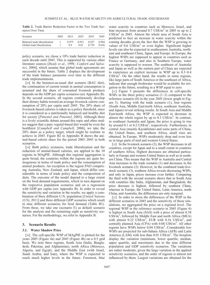
policy scenario, we chose a 10% trade barrier reduction ineach decade until 2045. This is supported by various otherliterature sources [Healy et al., 1998; Conforti and Salva-tici, 2004], which assume that global trade agreements aresuccessful in the future. Table 2 displays the developmentof the trade balance parameter over time in the differenttrade implementations.

[28] In the business-as-usual diet scenario (BAU diet),the continuation of current trends in animal consumption isassumed and the share of consumed livestock productsdepends on the GDP per capita scenarios (see Appendix B).In the second scenario, all regions continuously developtheir dietary habits toward an average livestock calorie con-sumption of 20% per capita until 2045. The 20% share oflivestock-based calories is taken as a policy threshold, sinceit is considered as a nutritionally balanced and healthy dietfor society [Pimentel and Pimentel, 2003]. Although thereis a lively scientific debate around this topic and other stud-ies suggest that a pure vegetal-based diet would be even thehealthiest [Campbell and Campbell, 2006], we take the20% share as a policy target, which might be realistic toachieve in 2045. Figure B2 in Appendix B shows the ani-mal-based calorie share for the period 2005–2045 in bothscenarios.

[29] Both policy scenarios, trade liberalization and thereduction of animal-based calories, are applied to the 10regions in MAgPIE. Although this regional aggregation isquite broad, the countries within the regions are quite ho-mogenous in terms of trade policy and the consumption ofanimal products. An exception is the region PAO compris-ing Australia, New Zealand, and Japan, which differ con-siderable in terms of trade policy and the composition ofdiets. The outcome of the model depend to a large extenton the food demand requirements, which in turn depend onthe respective population scenarios and on a regressionwith GDP per capita (see Appendix B). In order to revealthe sensitivity and variation in the results, we apply a com-bination of three different U.N. population [United Nations(UN), 2011] and three different GDP scenarios which resultin nine different scenarios for food demand (Table B1).From these, we take one (scenario E) as default scenariofor the analysis and the remaining eight as sensitivity sce-narios. For the methodology, we refer to Appendix B.

3. Scenario Results

3.1. Water Shadow Price

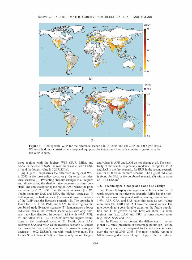
[30] The cell-specific WSP of MAgPIE is plotted for theyears 2005 (Figure 4a) and 2045 (Figure 4b) on a 0.5 gridbasis. We note three regions, South Asia (India, Bangla-desh, Pakistan, and Afghanistan), north Africa (Morocco,Algeria, and Egypt), and the Middle East (with Israel,Saudi Arabia, and Iran), where the WSP is expected toreach much higher levels in the future. Foremost, blue

water scarcity in countries such as Morocco, Israel, andIran increases from around 0.7 US$/m3 in 2005 to up to 2US$/m3 in 2045. Almost the whole area of South Asia ispredicted to face an increase in water scarcity within thecoming decades given the fact that the WSP is growing tovalues of 0.6 US$/m3 or even higher. Significant higherlevels can also be expected in southeastern Australia, north-east and southeast China, Japan, and Europe. In Europe, thehighest WSPs are supposed to appear in countries such asFrance or Germany, and also in Southern Europe, waterscarcity is supposed to worsen. The southeast of Australiaand Japan as well as the eastern part of China are expectedto experience an explicit increase in WSP up to 0.3–0.4US$/m3. On the other hand, the results in some regions,like large parts of South America or the southeast of Africa,indicate that enough freshwater would be available for irri-gation in the future, resulting in a WSP equal to zero.

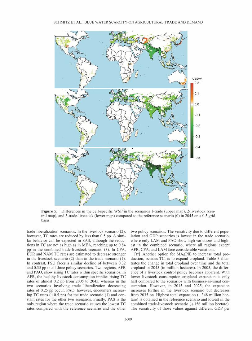
[31] Figure 5 presents the differences in cell-specificWSPs in the three policy scenarios (1–3) compared to thereference scenario (0) in the year 2045 (lower graph in Fig-ure 5). Starting with the trade scenario (1), four regions(South Asia, Middle East/north Africa, southeast Australia,and Japan) reveal striking results. In South Asia and MiddleEast/north Africa, the WSP is expected to decrease inalmost the whole region by up to 0.3 US$/m3. In contrast,in southeast Australia and Japan, the price is going to riseby around 0.1 or 0.2 US$/m3, respectively. Furthermore, incentral Asia (mainly Kazakhstan) and some parts of China,the United States, and southern Africa, small rises areobtained. In Europe, WSPs moderately drop and even lessso in large parts of mid and western United States.

[32] In the livestock scenario (2), the WSP decreases in allcountries, except for Japan and to a small extent in countriesof southern Africa. Highest decreases are obtained particu-larly in Europe and western United States as well as in south-ern China. This means that the WSP in Australia and CentralAsia increases in the trade scenario (1) and decreases in thelivestock scenario (2). However, in the combined trade-live-stock scenario (3), southern Africa reveals decreasing WSPs,and only in Japan, prices increase even further. Comparingthe third with the second scenario shows that in South Asiawith countries like India, Afghanistan, and Bangladesh, theprice decrease is highest, followed by southern China,whereas in Europe, the United States, Latin America, northChina, and Australia, the differences are only marginal.

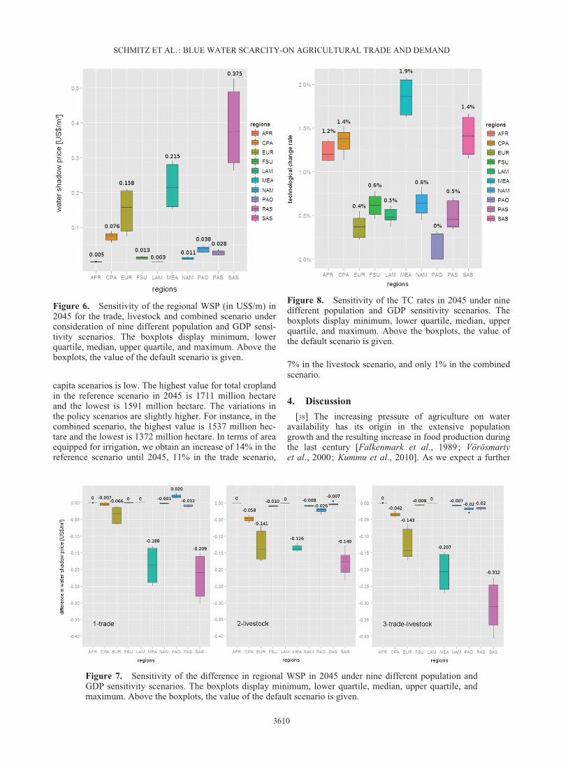
[33] In order to stress the differences of the WSP in thedifferent scenarios in 2045 and the sensitivity of those sim-ulations, we aggregated the price on a regional level. Theregional WSP in the reference scenario in 2045 (Figure 6)is highest in South Asia (SAS) with a price of almost 0.38US$/m3, followed by Middle East and north Africa (MEA)with almost 0.22 US$/m3, EUR with 0.16 US$/m3, andcentrally planned Asia (CPA) with 0.08 US$/m3. All otherregions have WSPs below 0.04 US$/m3. Considerable lowWSPs are projected for sub-Sahara Africa (AFR) and LatinAmerica (LAM) with less than 0.01 US$/m3. The boxplotsdisplay the variation (minimum, lower quartile, median,upper quartile, and maximum) due to the nine differentpopulation and GDP sensitivity scenarios. The variationsare rather moderate, given the large variation in the appliedsensitivity scenarios, and the order of regions is almost notinfluenced by them. Largest variations are obtained for the

Table 2. Trade Barrier Reduction Factor in the Two Trade Sce-narios Over Time

Scenario 2005 2015 2025 2035 2045

Bilateral trade liberalization 1 0.975 0.951 0.927 0.904Global trade liberalization 1 0.9 0.81 0.729 0.656


3607

three regions with the highest WSP (EUR, MEA, andSAS). In the case of SAS, the maximum value is 0.53 US$/m3 and the lowest value is 0.26 US$/m3.

[34] Figure 7 emphasizes the difference in regional WSPin 2045 in the three policy scenarios (1–3) versus the refer-ence scenario (0). Presenting absolute changes in all regionsand all scenarios, the shadow price decreases or stays con-stant. The only exception is the region PAO, where the priceincreases by 0.02 US$/m3 in the trade scenario (1). Weobtain again for SAS and MEA the highest decreases. Inboth regions, the trade scenario (1) shows stronger reductionsof the WSP than the livestock scenario (2). The opposite isfound for EUR, CPA, PAO, and NAM. In these regions, thecombined trade-livestock scenario (3) demonstrates a lowerreduction than in the livestock scenario (2) with only bilat-eral trade liberalization. In contrast, SAS with �0.31 US$/m3 and MEA with �0.21 US$/m3 have the highest reduc-tions in the combined scenario (3). Pacific Asia (PAS)resembles SAS and MEA as the livestock scenario (2) causesthe lowest decrease and the combined scenario the strongestdecrease (�0.02 US$/m3), but with much lower rates. Forformer Soviet Union (FSU), we observe only minor changes,

and values in AFR and LAM do not change at all. The sensi-tivity of the results is generally moderate, except for MEAand SAS in the first scenario, for EUR in the second scenarioand for all three in the third scenario. The highest reductionis found for SAS in the combined scenario (3) with a valueof�0.41 US$/m3.

3.2. Technological Change and Land Use Change

[35] Figure 8 displays average annual TC rates for the 10world regions in the reference scenario. MEA has the high-est TC rates over this period with an average annual rate of1.9%. AFR, CPA, and SAS have high rates as well valuesmore than 1%. EUR and PAO have the lowest values. Therate depends to a considerable extent on the future popula-tion and GDP growth as the boxplots show; in someregions less (e.g., LAM and FSU) in some regions more(e.g. MEA, SAS, and PAS).

[36] In Figure 9, we present the differences in the re-gional TC rates (presented in percentage points (pp)) of thethree policy scenarios compared to the reference scenarioover the period 2005–2045. The most notable region isMEA showing decreases of up to 1 pp in the two global

Figure 4. Cell-specific WSP for the reference scenario in (a) 2005 and (b) 2045 on a 0.5 grid basis.White cells do not consist of any cropland equipped for irrigation. Gray cells contain irrigation area butthe WSP is zero.


3608

trade liberalization scenarios. In the livestock scenario (2),however, TC rates are reduced by less than 0.5 pp. A simi-lar behavior can be expected in SAS, although the reduc-tions in TC are not as high as in MEA, reaching up to 0.84pp in the combined trade-livestock scenario (3). In CPA,EUR and NAM TC rates are estimated to decrease strongerin the livestock scenario (2) than in the trade scenario (1).In contrast, FSU faces a similar decline of between 0.32and 0.35 pp in all three policy scenarios. Two regions, AFRand PAO, show rising TC rates within specific scenarios. InAFR, the healthy livestock consumption implies rising TCrates of almost 0.2 pp from 2005 to 2045, whereas in thetwo scenarios involving trade liberalization decreasingrates of 0.25 pp occur. PAO, however, encounters increas-ing TC rates (þ0.5 pp) for the trade scenario (1) and con-stant rates for the other two scenarios. Finally, PAS is theonly region where the trade scenario causes the lowest TCrates compared with the reference scenario and the other

two policy scenarios. The sensitivity due to different popu-lation and GDP scenarios is lowest in the trade scenario,where only LAM and PAO show high variations and high-est in the combined scenario, where all regions exceptAFR, CPA, and LAM face considerable variations.

[37] Another option for MAgPIE to increase total pro-duction, besides TC, is to expand cropland. Table 3 illus-trates the change in total cropland over time and the totalcropland in 2045 (in million hectares). In 2005, the differ-ence of a livestock control policy becomes apparent. Withlower livestock consumption cropland expansion is onlyhalf compared to the scenarios with business-as-usual con-sumption. However, in 2015 and 2025, the expansionincreases further in the livestock scenario but decreasesfrom 2035 on. Highest total expansion (þ348 million hec-tare) is obtained in the reference scenario and lowest in thecombined trade-livestock scenario (þ156 million hectare).The sensitivity of those values against different GDP per

Figure 5. Differences in the cell-specific WSP in the scenarios 1-trade (upper map), 2-livestock (cen-tral map), and 3-trade-livestock (lower map) compared to the reference scenario (0) in 2045 on a 0.5 gridbasis.


3609

capita scenarios is low. The highest value for total croplandin the reference scenario in 2045 is 1711 million hectareand the lowest is 1591 million hectare. The variations inthe policy scenarios are slightly higher. For instance, in thecombined scenario, the highest value is 1537 million hec-tare and the lowest is 1372 million hectare. In terms of areaequipped for irrigation, we obtain an increase of 14% in thereference scenario until 2045, 11% in the trade scenario,

7% in the livestock scenario, and only 1% in the combinedscenario.

4. Discussion

[38] The increasing pressure of agriculture on wateravailability has its origin in the extensive populationgrowth and the resulting increase in food production duringthe last century [Falkenmark et al., 1989; Vörösmartyet al., 2000; Kummu et al., 2010]. As we expect a further

Figure 6. Sensitivity of the regional WSP (in US$/m) in2045 for the trade, livestock and combined scenario underconsideration of nine different population and GDP sensi-tivity scenarios. The boxplots display minimum, lowerquartile, median, upper quartile, and maximum. Above theboxplots, the value of the default scenario is given.

Figure 7. Sensitivity of the difference in regional WSP in 2045 under nine different population andGDP sensitivity scenarios. The boxplots display minimum, lower quartile, median, upper quartile, andmaximum. Above the boxplots, the value of the default scenario is given.

Figure 8. Sensitivity of the TC rates in 2045 under ninedifferent population and GDP sensitivity scenarios. Theboxplots display minimum, lower quartile, median, upperquartile, and maximum. Above the boxplots, the value ofthe default scenario is given.


3610

increase in population and an even more dramatic increasein agricultural demand, the pressure on water resources willrise considerably throughout the coming decades. In orderto quantify this relationship, we have developed an agroe-conomic water scarcity indicator, the WSP.

4.1. Water Shadow Price

[39] The WSP is the outcome of coupling a biophysicalvegetation model and an economic land use model. It linksspatially explicit water withdrawal and availability witheconomic processes in the land use and agricultural sector.Hence, the WSP considers explicitly economic processesof water demand in an optimization approach, which hasbeen consistently neglected by previous indicators [Saueret al., 2010]. It takes important economic drivers, such asincome, trade, production costs, and productivity growth,into account which are crucial for assessing water scarcity.In general, the WSP provides a more comprehensive pic-ture of water scarcity than purely biophysically basedindicators.

[40] Before calculating the WSP, the amount of availableirrigation water in MAgPIE is derived from water discharge(from LPJmL) reduced by an irrigation efficiency parame-ter. In most studies, irrigation efficiency is a static input orit changes only due to exogenous scenarios [i.e., Fischeret al., 2007]. An exception is the model created by Saueret al. 2010, which is able to invest endogenously in animproved irrigation system based on population growth. Incontrast to this approach, we have implemented irrigation

efficiency as a dynamic input depending on the level ofeconomic development (GDP per capita). Although incomedoes not explain the whole variation, we demonstrate withthe regression analysis that it is strongly correlated to effi-ciency improvement (also confirmed by Sauer et al. [2010]and Calzadilla et al. [2011a]). Our irrigation efficienciesincrease between 2% and 12% points from 2005 to 2045.Fischer et al. [2007] assume exogenous increases in effi-ciency of 10% per decade, whereas Sauer et al. [2010] arein line with our rather moderate estimates.

[41] The projected WSP of MAgPIE ranges between0 and 0.3 US$/m3 for 2005 and between 0 and 2 US$/m3

for 2045. Comparing these values with real market pricesof water led to biases since market prices are often highlydetermined by local policies (subsidies), market distortions(environmental externalities), or missing information. Forinstance, real prices in Europe vary between 0.01 US$/m3

in Bulgaria and 1.4 US$/m3 in Netherlands [Berbel et al.,2007]. Studies about WSPs are rare. One study assessedWSPs for Spain for 2005 and found a shadow price in aver-age of 0.19–0.39 US$/m3 [Novo et al., 2009], which fitswell to our results for 2005.

4.2. Limitations of the Indicator

[42] The WSP has certain limitations to serve as an agro-economic water scarcity indicator. First of all, it is basedon blue water, ignoring the interactions and influences ofgreen water on the agricultural system. Those are especiallyimportant in the livestock sector, where the differences ofgreen and blue water use are huge [Hoekstra and Chapa-gain, 2007], comparing, for instance, extensive beef pro-duction on grasslands (mainly green water) with industriallivestock farming (partially fed with imported irrigatedfeed crops). Hence, more detailed water-related studieswith a focus on the future development of livestock sys-tems are needed. Further limitations are related to theMAgPIE model, since the shadow price itself is directlylinked to the overall goal function of minimizing produc-tion costs. Important shortcomings of the model are miss-ing direct production distortions like tariffs and subsidiesas well as the consideration of only intraregional but no

Figure 9. Sensitivity of the difference in TC rates in 2045 under nine different population and GDPsensitivity scenarios. The boxplots display minimum, lower quartile, median, upper quartile, and maxi-mum. Above the boxplots the value of the default scenario is given.

Table 3. Total Cropland Expansion (in Million Hectare) From2005 Until 2045 and Total Cropland (in Million Hectare) in 2045

Scenario

ExpansionTotal

Cropland

2005 2015 2025 2035 2045 2045

0-refernce 104 74 60 59 51 16481-trade 103 37 49 51 39 15802-livestock 53 69 60 36 7 15263-trade-livestock 53 41 40 11 10 1456


3611

interregional transport costs. Although those limitationsreduce the WSP, others increase it. One is the demand rep-resentation in MAgPIE, which is exogenously given byregressions between income and calorie consumption(described in Appendix B). The exogenous implementationimplies that price elasticities of demand are zero, i.e., con-sumption cannot be adjusted endogenously to changing pri-ces. As a consequence, the model has less flexibility tosubstitute the demand, which results in higher shadow pri-ces. Another limitation is irrigation efficiency. While it is adynamic input dependent on economic development, it can-not be changed endogenously by investments. This maylower efficiency levels in the future, although the study bySauer et al. [2010] reveals rather low levels/low rates ofinvestment-related efficiency improvements.

4.3. Scenario Assessment and Uncertainty

[43] The most general finding of our scenario analysis isthat water scarcity in all regions increases until 2050. InSub-Saharan Africa and Latin America, it increases withlow rates, whereas in South Asia and the Middle East/northAfrica region with high rates. Although no other study hasexamined an agroeconomic water scarcity at high spatialresolution, we can at least compare our results with studiesdisplaying regional values. Rosegrant et al. [2002] projectwater scarcity levels with the IMPACT-WATER model upto 2025 and show generally moderate increases withdecreasing rates in developed countries. As in our study,they found strong increases in north Africa, Middle East,China, and India. In contrast to our findings, they also pro-ject high increases in Latin America.

[44] Our simulations indicate that with trade liberaliza-tion, the reallocation of agricultural land use can help toreduce regional water scarcity in the long run. This holdsespecially in world regions where water will becomeextremely scarce over the coming decades. The only excep-tions to this rule are Australia, Japan, and parts of CentralAsia (mainly Kazakhstan), where water becomes a bitscarcer. Other trade studies, like the CGE analysis by Ber-rittella et al. [2008], found rather small effects (changes inwater use below 10%). In contrast to our results, trade lib-eralization leads to higher water use in the United Statesand China and lower water use in Japan, whereas theremaining regions encounter similar trends. Since the studyhighlights only the period 1997–2010, comparability is lim-ited. The same model, GTAP-W, is used by Calzadillaet al. [2011b] for analyzing trade liberalization scenariosuntil 2050. Compared to our model, Australia has the high-est increase in water scarcity due to liberalization, whereasSoutheast Asia, South Asia, Middle East, and FormerSoviet Union benefit from lower pressure on water resour-ces. Simulations by the WATERSIM model confirm thatincreased trade between water-abundant regions and water-scarce regions avoid further stress on water scarcity [deFraiture et al., 2007]. The comparison with our simulationshas to be interpreted with caution since they assume perfectfree trade, which is a more extreme scenario than ours.

[45] Agricultural trade is largely driven by economicforces. Local water prices, indicating the level of water scar-city, lead to more economic appreciation of water as ascarce resource and to more water-efficient trade from abun-dant to scarce regions. An improved system of agricultural

trade also addresses the issue of local production risks asthose will likely increase in the future due to climatechange. Production failure in certain regions due to extremeweather events could be balanced out through trade fromother production regions [Fraser and Rimas, 2010]. Exam-ples for national policies are the reduction of export andimport barriers for agricultural products, or on internationallevel, the WTO negotiations, where the consequences offurther trade liberalization and protection are discussed.Besides, chances for beneficial trade liberalization, whichrelax pressure on regional water scarcity, should not beoverestimated in the short to medium term. As experiencesfrom the WTO Doha Round show, political processes onthe global level are slow and dominated by national inter-ests instead of efficient resource use from global perspec-tives. Furthermore, developing countries would have tofinance imports by foreign exchange [Seckler et al., 2000],which have to be generated by the export of other products.In the past, many countries in Africa and South Asia havenot been successful in developing competitive products.

[46] The second policy option is a shift from a business-as-usual diet to a healthy livestock diet, which contains thesame share of animal-based products for every worldregion. If this shift is simulated, the pressure on water scar-city in all regions is reduced, as plant-based calories con-tain less water in its production than animal-based calories.This is an unexpected outcome since the livestock share insome regions, for instance, in SAS and MEA, increases inthe healthy livestock diet scenario. The reason behind thelower WSP is the linkage between regions through trade.Trade translates less animal-based consumption in thedeveloped countries into lower pressure in water-scarceregions like India or the Middle East. As a consequence,the effects on WSP in developing regions are highest in thecombined scenario of trade liberalization and diet shift,whereas in developed countries, the diet shift effectslargely outweigh the trade effects. Possible policies toreduce consumption of animal products include the intro-duction of a tax on animal based products, a qualified banon consumption or awareness raising and knowledge trans-fer through educational programs [Deckers, 2010]. Anexample for this is Denmark, which has recently introduceda tax on saturated fat to achieve a lower consumption oflivestock products [Smed, 2012].

[47] To our knowledge, there is no other study that hasquantified the effects of lower animal-based consumption inspatial detail. Yet, Gerten et al. [2011] found out that thelikelihood for a country to be water scarce would bereduced, particularly in African countries, if animal calorieswere halved. Renault and Wallender [2000] analyzed thepercentage of additional water, which is saved according todifferent scenarios until 2025. The scenario that replaces50% of meat by vegetal products counts water savings of23% and the one that replaces 50% of animal products yieldsin 39% savings. Comparing this to our healthy livestock dietscenario (scenario 2) without any trade changes, we calcu-lated savings of 40% until 2025 and 28% until 2050. Liu andSavenije [2008] found positive effects of lower meat con-sumption for China and concluded that virtual water trade andimprovement of rainfed agriculture are the more promisingstrategies. Other studies, examining livestock reducing sce-narios, found positive effects on the reduction of greenhouse


3612

gas emissions [Popp et al., 2010; Stehfest et al., 2009]) andthe pressure on cropland [Wirsenius et al., 2010].

[48] The MAgPIE model has the unique feature of generat-ing TC rates endogenously based on investments in agricul-tural research and development. Our analysis reveals a lowerpressure on agricultural productivity due to the aforemen-tioned policies. The average global annual rate of TC in agri-culture until 2045 is 0.9% in the reference scenario, comparedto 0.6% in the trade scenario, 0.7% in the healthy livestockdiet scenario, and 0.5% in the combined scenario. At the re-gional level, those effects are much higher in regions likeMEA and SAS but also NAM. We can state that increasedtrade and a healthy livestock diet not only help to reducewater scarcity but also to lower the pressure for intensificationin agriculture. Furthermore, the policy scenarios lead to lowercropland expansion globally. As shown in Schmitz et al.[2012], this differs on a regional level, and trade liberalizationleads to further deforestation in tropical regions like SouthAmerica, with negative implications for greenhouse gas emis-sions. Area equipped for irrigation expands by 14% until2045, which is roughly in line with the study by Sauer et al.[2010], who estimate an increase of 14% of the irrigated areauntil 2030. In this context, we have to emphasize again thatno impacts of climate change are considered in this study.Those impacts are mainly changing temperature and precipi-tation patterns and have heterogeneous effects on the regionalwater balance. Especially in many developing regions, thisimplies further threats on water availability [Gerten et al.,2011; Rockström et al., 2009; Vörösmarty et al., 2000]. Adetailed study by Fischer et al. [2007] concluded that climatechange causes globally up to 20% more irrigation until 2080,which is of similar magnitude than the expansion requireddue to socioeconomic drivers in this time span.

[49] Our sensitivity analysis is focused on different popu-lation and GDP scenarios. Although we used extreme sensi-tivity scenarios, the variation in results is rather moderate.Water scarce regions like South Asia and the Middle East aremost affected, but the ranking order is hardly affected by dif-ferent demand projections. The study by Schmitz et al. [2012]estimates the sensitivity of MAgPIE regarding TC and landexpansion and finds changing results in the range of �10%and þ16% in terms of emissions and production costs. How-ever, since only a limited number of model parameters havebeen tested, a more comprehensive sensitivity analysis wouldbe necessary to reveal the whole range of possibilities.

[50] Overall, our analysis indicates that only one of theconsidered policy measures in this study is not enough tokeep water scarcity at levels observed in 2005. Only the com-bination of both policies can reduce global WSPs in 2045 inmost regions below the values in 2005. This does not hold forChina, Australia, Japan, and countries in Sub-Saharan Africa,where additional strategies have to be developed in order tokeep the pressure on water resources at current levels. Exam-ples, which could be picked up by subsequent studies, areoptions to increase irrigation efficiency, improvements ininfrastructure, institutional reforms, and also the issue of waterpricing.

5. Conclusion and Policy Implications

[51] In many regions of the world, water is a scarceresource. Due to insufficient price signals, this is not yet

recognized in all its consequences by many social factors.Many developing countries, which are heavily dependenton the agricultural sector and located in dry areas, are espe-cially affected by water shortage. Water shortage is likelyto lead to higher food prices threatening regional food secu-rity further.

[52] Under different GDP and population scenarios, theMAgPIE model computes food demand and generates spa-tially explicit projections of WSPs and regional TC rates.As water scarcity is increasing and severe in regions likeSouth Asia, Middle East, and north Africa, trade liberaliza-tion and policies to control livestock consumption arepromising measures to curtail water scarcity. The pressureto intensify is particularly reduced in importing regions,which are the regions with higher water scarcity. In thecase of further trade liberalization, we found that intensifi-cation is less effective in terms of reducing water scarcityfor developed countries than for developing countries. Thisis particularly important since developed countries havehampered further liberalization efforts in the past.

[53] Lower animal-based consumption in developedcountries, as a second policy option, does not only reducethe domestic pressure on water but also reduce water scar-city in developing countries. However, as Ridoutt et al.[2011] points out, production of livestock-based goods isvery diverse in terms of water consumption. Rather thancondemning the whole animal sector, a focus on low-waterinput systems should be an alternative policy strategy indeveloped countries.

[54] In order to reach a level of water consumption thatdoes not increase water scarcity in developing regions inthe future despite population growth, it is not sufficient tocount on trade liberalization and reduced livestock con-sumption in developed countries. Measures to improvewater-use efficiency, such as investment in breeding ofwater-saving plants, the promotion of water-saving produc-tion systems, or improved irrigation infrastructure, areneeded. Furthermore, incentives for improved water man-agement have to be institutionalized. In many regions,water is seriously undervalued and lacking defined propertyrights, especially in the agricultural sector.

Appendix A: Regions and Products in MAgPIE

[55] The regional disaggregation of MAgPIE is shown inTable A1.

[56] MAgPIE distinguishes 16 different cropping activ-ities and 5 livestock activities (Table A2).

Table A1. World Regions in MAgPIE

Abbreviation Regions

AFR Sub-Sahara AfricaCPA Centrally planned Asia (including China)EUR Europe (including Turkey)FSU Former Soviet UnionLAM Latin AmericaMEA Middle East and north AfricaNAM North AmericaPAO Pacific OECD (Australia, Japan, and New Zealand)PAS Pacific AsiaSAS South Asia (including India)


3613

Appendix B: Future Demand in MAgPIE andSensitivity Scenarios

[57] In MAgPIE, demand for agricultural products is fixedfor every region and every time step and cannot be influ-enced by the optimization process. Future trends in fooddemand are computed as a function of income (measured interms of GDP) per capita based on a cross-country regres-sion. The underlining GDP scenarios are calculated by fol-lowing the methodology proposed by Hawksworth [2006],who model the output with a Cobb-Douglas production func-tion based on investment data from Heston et al. [2011]. Wecombine the GDP output scenarios with the three differentU.N. population scenarios to get, in total, nine different GDPper capita scenarios (Table B1), which result in nine differ-ent scenarios for food demand. The scenario with the label Eis taken as the default scenario in our study, whereas theother eight scenarios are used for the sensitivity analysis.

[58] For the calculation of food demand, we use the rela-tion between total calories CT and income IMER (measuredin market exchange rate per capita). This relation is definedby a power function and estimated with a fixed effectmodel with time-dependent variables. Equation (B1) showsthe estimated function

CT ¼ exp 2:83� 10�3 þ 2:13� 10�3years� �

� I0:16þ �3:12�10�5yearsÞ:ðMER

(B1)

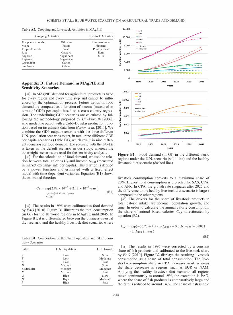
[59] The results in 1995 were calibrated to food demandby FAO [2010]. Figure B1 illustrates the total consumption(in GJ) for the 10 world regions in MAgPIE until 2045. InFigure B1, it is differentiated between the business-as-usualdiet scenario and the healthy livestock diet scenario, where

livestock consumption converts to a maximum share of20%. Highest total consumption is projected for SAS, CPA,and AFR. In CPA, the growth rate stagnates after 2025 andthe difference to the healthy livestock diet scenario is largestcompared to the other regions.

[60] The drivers for the share of livestock products intotal caloric intake are income, population growth, andtime. In order to calculate the animal calorie consumption,the share of animal based calories CAS is estimated byequation (B2).

CAS ¼ exp �36:73þ 4:5 � ln IMERð Þ þ 0:016 � year � 0:0021ð� ln IMERð Þ � year Þ

:

(B2)

[61] The results in 1995 were corrected by a constantshare of fish products and calibrated to the livestock shareby FAO [2010]. Figure B2 displays the resulting livestockconsumption as a share of total consumption. The live-stock-consumption share in CPA increases most, whereasthe share decreases in regions, such as EUR or NAM.Applying the healthy livestock diet scenario, all regionsmove continuously to around 19%, the exception is PAO,where the share of fish products is comparatively large andthe rate is reduced to around 14%. The share of fish is held

Table A2. Cropping and Livestock Activities in MAgPIE

Cropping Activities Livestock Activities

Temperate cereals Oil palm Ruminant meatMaize Pulses Pig meatTropical cereals Potato Poultry meatRice Cassava EggsSoybean Sugar beet MilkRapeseed SugarcaneGroundnut CottonSunflower Others

Table B1. Composition of the Nine Population and GDP Sensi-tivity Scenarios

Label U.N. Population GDP Growth

A Low SlowB Low ModerateC Low FastD Medium SlowE (default) Medium ModerateF Medium FastG High SlowH High ModerateI High Fast

Figure B1. Food demand (in GJ) in the different worldregions under the U.N. scenario (solid line) and the healthylivestock diet scenario (dashed line).


3614

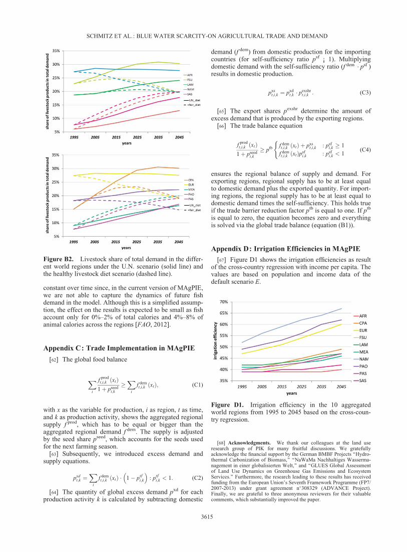
constant over time since, in the current version of MAgPIE,we are not able to capture the dynamics of future fishdemand in the model. Although this is a simplified assump-tion, the effect on the results is expected to be small as fishaccount only for 0%–2% of total calories and 4%–8% ofanimal calories across the regions [FAO, 2012].

Appendix C: Trade Implementation in MAgPIE

[62] The global food balance

Xi

f prodt;i;k xtð Þ

1þ pseedi;k

X

i

f demt;i;k xtð Þ; (C1)

with x as the variable for production, i as region, t as time,and k as production activity, shows the aggregated regionalsupply f prod, which has to be equal or bigger than theaggregated regional demand f dem. The supply is adjustedby the seed share pseed, which accounts for the seeds usedfor the next farming season.

[63] Subsequently, we introduced excess demand andsupply equations.

pxdt;k ¼

Xi

f demt;i;k xtð Þ � 1� psf

i;k

� �: psf

i;k < 1: (C2)

[64] The quantity of global excess demand pxd for eachproduction activity k is calculated by subtracting domestic

demand (f dem) from domestic production for the importingcountries (for self-sufficiency ratio psf ¡ 1). Multiplyingdomestic demand with the self-sufficiency ratio (f dem � psf )results in domestic production.

pxst;i;k ¼ pxd

t;k � pexshrt;i;k : (C3)

[65] The export shares pexshr determine the amount ofexcess demand that is produced by the exporting regions.

[66] The trade balance equation

f prodt;i;k xtð Þ

1þ pseedi;k

ptb f demt;i;k xtð Þ þ pxs

t;i;k : psfi;k 1

f demt;i;k xtð Þpsf

i;k : psfi;k < 1

((C4)

ensures the regional balance of supply and demand. Forexporting regions, regional supply has to be at least equalto domestic demand plus the exported quantity. For import-ing regions, the regional supply has to be at least equal todomestic demand times the self-sufficiency. This holds trueif the trade barrier reduction factor ptb is equal to one. If ptb

is equal to zero, the equation becomes zero and everythingis solved via the global trade balance (equation (B1)).

Appendix D: Irrigation Efficiencies in MAgPIE

[67] Figure D1 shows the irrigation efficiencies as resultof the cross-country regression with income per capita. Thevalues are based on population and income data of thedefault scenario E.

[68] Acknowledgments. We thank our colleagues at the land useresearch group of PIK for many fruitful discussions. We gratefullyacknowledge the financial support by the German BMBF Projects ‘‘Hydro-thermal Carbonization of Biomass,’’ ‘‘NaWaMa Nachhaltiges Wasserma-nagement in einer globalisierten Welt,’’ and ‘‘GLUES Global Assessmentof Land Use Dynamics on Greenhouse Gas Emissions and EcosystemServices.’’ Furthermore, the research leading to these results has receivedfunding from the European Union’s Seventh Framework Programme (FP7/2007-2013) under grant agreement n�308329 (ADVANCE Project).Finally, we are grateful to three anonymous reviewers for their valuablecomments, which substantially improved the paper.

Figure B2. Livestock share of total demand in the differ-ent world regions under the U.N. scenario (solid line) andthe healthy livestock diet scenario (dashed line).

Figure D1. Irrigation efficiency in the 10 aggregatedworld regions from 1995 to 2045 based on the cross-coun-try regression.


3615

ReferencesAlcamo, J., P. Döll, T. Heinrichs, F. Kaspar, B. Lehner, T. Rösch, and

S. Siebert (2003), Global estimates of water withdrawals and availabilityunder current and future ‘‘business-as-usual’’ conditions, Hydrol. Sci.,48(3), 339–348.

Aucamp, D. C., and D. I. Steinberg (1982), The computation of shadow pri-ces in linear programming, J. Oper. Res. Soc., 33(6), 557–565.

Berbel, J., A. Garrido, and J. Calatrava (2007), Water pricing and irriga-tion: A review of the European Experience, in Irrigation Water Pric-ing—The Gap between Theory and Practice, edited by F. Molle andJ. Berkoff, pp. 295–327, CAB Int., Oxfordshire, U. K.

Berrittella, M., K. Rehdanz, R. S. J. Tol, and J. Zhang (2008), The impactof trade liberalization on water use: A computable general equilibriumanalysis, J. Econ. Integrat., 23(3), 631–655.

Bondeau, A., P. Smith, S. Zaehle, S. Schaphoff, W. Cramer, D. Gerten,H. Lotze-Campen, C. M€uller, M. Reichstein, and B. Smith (2007), Mod-elling the role of agriculture for the 20th century global terrestrial carbonbalance, Global Change Biol., 13(3), 679–706.

Chavez, H. M. L., and S. Alipaz (2007), An integrated indicator based onbasin hydrology, environment, life, and policy: The watershed sustain-ability index, Water Resour. Manage., 21, 883–895.

Cai, X., and M. W. Rosegrant (2002), Global water demand and supply pro-jections—Part 1: A modeling approach, Water Int., 27(2), 159–169.

Calzadilla, A., K. Rehdanz, and R. S. J. Tol (2011a), Water scarcity and theimpact of improved irrigation management: A computable general equi-librium analysis, Agric. Econ., 42(3), 305–323.

Calzadilla, A., K. Rehdanz, and R. S. J. Tol (2011b), Trade liberalizationand climate change: A computable general equilibrium analysis of theimpacts on global agriculture, Water, 3, 526–550, doi:10.3390/w3020526.

Campbell, T. C., and T. Campbell (2006), The China Study: StartlingImplications for Diet, Weight Loss and Long-Term Health, BenBellaBooks, Dallas, Tex.

Chapagain, A., and A. Hoekstra (2008), The global component of fresh-water demand and supply: An assessment of virtual water flows betweennations as a results of trade in agricultural and industrial products, WaterInt., 33(1), 19–32.

Center for International Earth Science Information Network (CIESIN)(2000), Gridded population of the world, Center for Int. Earth Sci. Infor-mation Network (CIESIN) Columbia Univ., Int. Food Policy Res. Inst.(IFPRI) and World Resour. Inst. (WRI), Palisades, N. Y.

Conforti, P., and L. Salvatici (2004), Agricultural trade liberalisation in theDoha round—Alternative scenarios and strategic interactions betweendeveloped and developing countries, FAO Commodity and Trade PolicyRes. Working Pap. 10, Rome, Italy.

Deckers, J. (2010), What policy should be adopted to curtail the negativeglobal health impacts associated with the consumption of farmed animalproducts?, Res. Publicat., 16(1), 57–72.

de Fraiture, C. (2007), Integrated water and food analysis at the global andbasin level. An application of WATERSIM, Water Resour. Manage., 21,pp. 185–198.

de Fraiture, C., D. Wichelns, J. Rockström, and E. Kemp-Benedict (2007),Looking ahead to 2050: Scenarios of alternative investment approaches,in Water for Food, Water for Life: A Comprehensive Assesment of WaterManagement in Agriculture, edited by D. Molden, pp. 91–145, Earth-scan, London.

Delgado, C. L. (2003), Rising consumption of meat and milk in developingcountries has created a new food revolution, J. Nutr., 133(11), 3907S–3910S.

Dietrich J.P., C. Schmitz, C. M€uller, M. Fader, H. Lotze-Campen, A. Popp(2012), Measuring agricultural land-use intensity – A global analysisusing a model-assisted approach, Ecol. Modell., 232, 109–118, doi:10.1016/j.ecolmodel.2012.03.002.

Dietrich J.P., C. Schmitz, H. Lotze-Campen, A. Popp, C. M€uller (2013),Forecasting technological change in agriculture – An endogenous imple-mentation in a global land use model. Technological Forecasting &Social Change, doi: 10.1016/j.techfore.2013.02.003, in press.

Döll, P., and S. Siebert (2000), A digital global map of irrigated areas, ICIDJ., 49(2), 55–66.

Dollar, D., and A. Kraay (2004), Trade, growth and poverty, Econ. J., 114,22–49.

Fader, M., S. Rost, C. M€uller, A. Bondeau, and D. Gerten (2010), Virtualwater content of temperate cereals and maize: Present and potentialfuture patterns, J. Hydrol., 384(3–4), 218–231.

Fader, M., D. Gerten, M. Thammer, J. Heinke, H. Lotze-Campen,W. Lucht, and W. Cramer (2011), Internal and external green-blue agri-cultural water footprints of nations, and related water and land savingsthrough trade, Hydrol. Earth Syst. Sci., 15, 1641–1660.

Falkenmark, M. (1989), The massive water scarcity threatening Africa—why isn’t it being addressed, Ambio, 18(2), 112–118.

Falkenmark, M., J. Lundqvist, and C. Widstrand (1989), Macro-scale waterscarcity requires micro-scale approaches. Aspects of vulnerability insemi-arid development, Natl. Resour. Forum 13(4), 258–267.

Falkenmark M., A. Berntell, A.J€agerskog, J. Lundqvist, M. Matz, andH. Tropp (2007), On the verge of a new water scarcity: A call for goodgovernance and human ingenuity, SIWI Policy Brief 11, Stockholm Int.Water Inst. (SIWI).

Food and Agriculture Organization (FAO) (2010), FAOSTAT—Food andAgriculture Organization of the United Nations Statistics Division.[Available at http://faostat.fao.org/, accessed 11 July 2010.].

Food and Agriculture Organization (FAO) (2011), AQUASTAT—Data-base on investment costs in irrigation. [Available at http://www.fao.org/nr/water/aquastat/investment/index.stm/, accessed 23 July 2011.].

Food and Agriculture Organization (FAO) (2012), FAOSTAT—Food andAgriculture Organization of the United Nations Statistics Division.[Available at http://faostat.fao.org/, accessed 11 Dec. 2012.].

Fraser, E. D. G., and A. Rimas (2010), Empires of Food: Feast, Famine,and the Rise and Fall of Civilizations, Free Press, New York.

Fischer, G., F. N. Tubiello, H. van Velthuizen, and D. A. Wiberg (2007),Climate change impacts on irrigation water requirements: Effects of mit-igation, 1990–2080, Technol. Forecast. Social Change, 74(7), 1083–1107.

Gerten, D., S. Schaphoff, U. Haberlandt, W. Lucht, and S. Sitch(2004), Terrestrial vegetation and water balance: Hydrological eval-uation of a dynamic global vegetation model, J. Hydrol., 286, 249–270.

Gerten, D., J. Heinke, H. Hoff, H. Biemans, M. Fader, and K. Waha (2011),Global water availability and requirements for future food production, J.Hydrometeorol., 12, 885–899, doi:10.1175/2011JHM1328.1.

Gleick, P. H., H. Cooley, and M. Morikawa (2009), The Worlds Water2008–2009: The Biennial Report on Freshwater Resources, Island Press,Washington D.C., USA.

Godfray, H. C. J., J. R. Beddington, I. R. Crute, L. Haddad, D. Lawrence,J. F. Muir, J. Pretty, S. Robinson, S. M. Thomas, and C. Toulmin (2010),Food security: The challenge of feeding 9 billion people, Science,327(5967), 812–818.

Hanasaki, N., S. Kanae, T. Oki, K. Masuda, K. Motoya, N. Shirakawa,Y. Shen, and K. Tanaka (2008a), An integrated model for the assessmentof global water—Part 1: Model description and input meteorologicalforcing, Hydrol. Earth Syst. Sci., 12(4), 1007–1025.

Hanasaki, N., S. Kanae, T. Oki, K. Masuda, K. Motoya, N. Shirakawa,Y. Shen, and K. Tanaka (2008b), An integrated model for the assessmentof global water—Part 2: Applications and assessments, Hydrol. EarthSyst. Sci., 12(4), 1027–1037.

Hanasaki, N., T. Inuzuka, S. Kanae, and T. Oki (2010), An estimation ofglobal virtual water flow and sources of water withdrawal for major cropsand livestock products using a global hydrological model, J. Hydrol.,384(3-4), 232–244.

Hanjra, M. A., and M. E. Qureshi (2010), Global water crisis and futurefood security in an era of climate change, Food Policy, 35(5), 365–377.

Hawksworth, J. (2006), The world in 2050: How big will the major emerg-ing market economies get and how can the OECD compete, Price Water-house Coopers Report, London, UK.

Healy, S., R. Pearce, and M. Stockbridge (1998), The implications of theUruguay round agreement on agriculture for developing countries. Train-ing Material for Agricultural Planning, FAO (Food and AgricultureOrganisation of the UN, Rome, Italy.

Heston A., R. Summers, and B. Aten (2011), Penn world table version 7.0,Center for Int. Comparisons of Production, Income and Prices at the Uni-versity of Pennsylvania, Philadelphia, Pa.

Hoekstra, A. Y., and P. Q. Hung (2005), Globalisation of water resources:international virtual water flows in relation to crop trade, Global Environ.Change, 15, 45–56.

Hoekstra, A. Y., and A. K. Chapagain (2007), Water footprints of nations:Water use by people as a function of their consumption pattern, WaterResour. Manage., 21(1), 35–48.

Islam, M. S., T. Oki, S. Kanae, N. Hanasaki, Y. Agata, and K. Yoshimura(2006), A grid-based assessment of global water scarcity including vir-tual water trading, Water Resour. Manage., 21, 19–33.


3616

http://faostat.fao.org/

http://www.fao.org/nr/water/aquastat/investment/index.stm/

http://www.fao.org/nr/water/aquastat/investment/index.stm/

http://faostat.fao.org/

Konar, M., C. Dalin, S. Suweis, N. Hanasaki, A. Rinaldo, and I. Rodriguez(2011), Water for food: The global virtual water trade network, WaterResour. Res., 47, W05520, doi: 10.1029/2010WR010307.

Krause, M., H. Lotze-Campen, and A. Popp (2009), Spatially-explicit sce-narios on global cropland expansion and available forest land in an inte-grated modelling framework, paper presented at the 27th InternationalAssociation of Agricultural Economists Conference in Beijing, China,16–22 Aug. 2009.

Kummu, M., P. J. Ward, H. de Moel, and O. Varis (2010), Is physical waterscarcity a new phenomenon? Global assessment of water shortage overthe last two millennia, Environ. Res. Lett., 5, 034006.

Liu, J., and H. H. G. Savenije (2008), Food consumption patterns and theireffect on water requirement in China, Hydrol. Earth Syst. Sci., 12(3),887–898.

Lotze-Campen, H., C. M€uller, A. Bondeau, A. Jachner, A. Popp, and W.Lucht (2008), Food demand, productivity growth and the spatial distribu-tion of land and water use: A global modeling approach, Agric. Econ.,39, 325–338.

Lutz, W., W. Sanderson, and S. Scherbov (2001), The end of populationgrowth, Nature, 412, 543–545.

Molden, D. (Ed.) (2007), Water for Food, Water for Life: A ComprehensiveAssessment of Water Management in Agriculture, London: Earthscan.

Nakicenovic, N., and R. Swart (Eds.) (2000), Special Report on EmissonScenarios, Cambridge Univ. Press, Cambridge, U. K.

Narayanan, B., and T. L. Walmsley (2008), Global Trade, Assistance, andProduction: The GTAP 7 Data Base, Center for Global Trade Analysis,Purdue Univ.

Nelson, A. (2008), Estimated travel time to the nearest city of 50,000 ormore people in year 2000, Global Environment Monitoring Unit—JointResearch Centre of the European Commission, Ispra, Italy. [Available athttp://bioval.jrc.ec.europa.eu/products/gam/, accessed 30 July 2011.].

Novo, P., A. Garrido, and C. Varela-Ortega (2009), Are virtual water flowsin Spanish grain trade consistent with relative water scarcity?, Ecol.Econ., 68(5), 1454–1564.

Ohlsson, L. (2000), Water conflicts and social resource scarcity, Phys.Chem. Earth Part B, 25(3), 213–220.

Oki, T., and S. Kanae (2004), Virtual water trade and world water resour-ces, Water Sci. Technol., 49(7), 203–209.

Oki, T., and S. Kanae (2006), Global hydrological cycles and world waterresources, Science, 313, 1068–1072.

Pingali, P. (2006), Westernization of Asian diets and the transformation of foodsystems: Implications for research and policy, Food Policy, 32, 281–298.

Popp, A., H. Lotze-Campen, and B. Bodirsky (2010), Food consumption,diet shifts and associated non-CO2 greenhouse gases from agriculturalproduction, Global Environ. Change 20, 451–462.

Popp, A., J. P. Dietrich, H. Lotze-Campen, D. Klein, N. Bauer, M. Krause,T. Beringer, D. Gerten, and O. Edenhofer (2011), The economic potentialof bioenergy for climate change mitigation with special attention givento implications for the land system, Environ. Res. Lett., 6(3), 034017.

Portmann, F., S. Siebert, and P. Döell (2010), MIRCA2000-Global monthlyirrigated and rainfed crop areas around the year 2000: A new high-reso-lution data set for agricultural and hydrological modelling, Global Bio-geochem. Cycles 24, GB1011, doi: 10.1029/2008GB003435.

Pimentel, D., and M. Pimentel (2003), Sustainability of meat-based and plant-based diets and the environment, Am. J. Clin. Nutr., 78(3), 660S–663S.

Ramsey, J. B. (1969), Tests for specification errors in classical linear least-squares regression analysis, J. R. Stat. Soc. Ser. B, 31(2), 350–371.

Renault, D., and W. W. Wallender (2000), Nutritional water productivityand diets, Agric. Water Manage., 45(3), 275–296.

Ridoutt, B. G., P. Sanguansri, M. Freer, and G. S. Harper (2011), Waterfootprint of livestock: comparison of six geographically defined beefproduction systems, Int. J. Life Cycle Assess. (online first), 17:165–175,doi:10.1007/s11367-011-0346-y.

Rockström, J., M. Falkenmark, L. Karlberg, H. Hoff, S. Rost, and D. Gerten(2009), Future water availability for global food production: The poten-tial of green water for increasing resilience to global change, WaterResour. Res., 45, W00A12, doi: 10.1029/2007WR006767.

Roeckner, E., et al. (2003), The atmospheric general circulation modelECHAM5. PART I: Model description, Rep. 349, Max Planck Inst. forMeteorol., Hamburg, Germany. [Available at http://www.mpimet.mpg.de.].

Rogers, D. H., F. R. Lamm, M. Alam, T. R. Trooien, G. A. Clark, P. L.Barnes, and K. Mankin (1997), Efficiencies and Water Losses of Irriga-tion Systems, Irrig. Manage. Ser. MF-2243, Kansas State Univ.

Rohwer, J., D. Gerten, and W. Lucht (2007), Development of functionaltypes of irrigation for improved global crop modelling, PIK Rep. 104.Potsdam Institue for Climate Impact Research, Potsdam, Germany.

Rosegrant, M. W., and S. A. Cline (2003), Global food security: Challengesand policies, Science, 302, 1917–1918.

Rosegrant, M. W., X. Cai, and S. A. Cline (2002), World water and food to2025: Dealing with scarcity, Food Policy Report, International FoodPolicy Research Institute (IFPRI), Washington D.C., USA.

Rosegrant, M. W., C. Ringler, and T. Zhu (2009), Water for agriculture:maintaining food security under growing scarcity, Annu. Rev. Environ.Resour., 34, 205–222.

Rost, S., D. Gerten, A. Bondeau, W. Lucht, J. Rohwer, and S. Schaphoff(2008), Agricultural green and blue water consumption and its influenceon the global water system, Water Resour. Res., 44, W09405, doi:10.1029/2007WR006331.

Sauer, T., P. Havlik, U. A. Schneider, E. Schmid, G. Kindermann, and M.Obersteiner (2010), Agriculture and resource availability in a changingworld: The role of irrigation, Water Resour. Res., 46, W06503, doi:10.1029/2009WR007729.

Schmitz, C., J. P. Dietrich, H. Lotze-Campen, C. M€uller, and A. Popp(2010), Implementing endogenous technological change in a global land-use model, paper presented at GTAP 13th Annual Conference in Penang,Malaysia, 9–11 June 2010.

Schmitz, C., A. Biewald, H. Lotze-Campen, A. Popp, J. P. Dietrich, B. Bod-irsky, M. Krause, and I. Weindl (2012), Trading more food—Implica-tions for land use, greenhouse gas emissions and the food system, GlobalEnviron. Change 22(1), 189–209.

Seckler, D., D. Molden, U. Amarasinghe, and C. de Fraiture (2000), WaterIssues for 2025: A Research Perspective, Int. Water Manage. Inst.,Colombo.

Shiklomanov, I. A., and J. C. Rodda (Eds.) (2003), World Water Resourcesat the Beginning of the Twenty-First Century, Cambridge Univ. Press,New York.

Smakhtin, V., C. Revanga, and P. Döll (2004), A pilot global assessment ofenvironmental water requirements and scarcity, Water Int., 29(3), 307–317.

Smed, S. (2012), Financial penalties on foods: The fat tax in Denmark,Nutr. Bull., 37(2), 142–147.

Sohngen, B., C. Tennity, and M. Hnytka (2009), Global forestry data forthe economic modeling of land use, in Economic Analysis of and Use inGlobal Climate Change Policy, edited by T. W. Hertel, S. Rose, R. S. J.Tol, pp. 49–71, Routledge, New York.

Stehfest E., L. Bouwman, D. P. van Vuuren, M. G. J. den Elzen, B. Eickh-out, and P. Kabat (2009), Climate benefits of changing diet, Clim.Change, 95, 83–102.

United Nations (UN) (2011). World Population Prospects: The 2010 Revi-sion, United Nations, Dep. of Economic and Social Affairs, PopulationDivision, CD-ROM Edition, New York, N. Y.

Visser, H., and T. de Nijs (2006), The map comparison kit, Environ. Mod-ell. Software, 21(3), 346–358.

Vörösmarty, C. J., P. Green, J. Salisbury, and R. B. Lammers (2000),Global water resources: Vulnerability from climate change and popula-tion growth, Science, 289(5477), 284–288.

Vörösmarty, C. J., et al. (2010), Global threats to human water security andriver biodiversity, Nature, 467, 555–561.

Weindl, I., H. Lotze-Campen, A. Popp, B. Bodirsky, and S. Rolinski(2010), Impacts of livestock feeding technologies on greenhouse gasemissions, paper presented at the IATRC Public Trade Policy Researchand Analysis Symposium, Univ. Hohenheim, Stuttgart, Germany, 27–29June 2010.

Wirsenius, S. (2000), Human Use of Land and Organic Materials - Model-ing the Turnover of Biomass in the Global Food System, Chalmers Univ.,Göteborg, Sweden.

Wirsenius, S., C. Azar, and G. Berndes (2010), How much land is neededfor global food production under scenarios of dietary changes and live-stock productivity increases in 2030?, Agric. Syst., 103(9), 621–638.

World Bank (2001), World development indicators 2001, World BankReport No. 22099, The World Bank, Washington D. C., USA.


3617

http://bioval.jrc.ec.europa.eu/products/gam/

http://www.mpimet.mpg.de

http://www.mpimet.mpg.de

blue water scarcity and the economic impacts of future agricultural trade and demand

Documents