Accepted Manuscript

Biased Reduction Method by Combining Improved Modified PoleClustering and Improved Pade Approximations

Jay Singh , C.B. Vishwakarma , Kalyan Chattterjee

PII: S0307-904X(15)00440-0DOI: 10.1016/j.apm.2015.07.014Reference: APM 10659

To appear in: Applied Mathematical Modelling

Received date: 9 April 2013Revised date: 13 May 2015Accepted date: 21 July 2015

Please cite this article as: Jay Singh , C.B. Vishwakarma , Kalyan Chattterjee , Biased ReductionMethod by Combining Improved Modified Pole Clustering and Improved Pade Approximations, AppliedMathematical Modelling (2015), doi: 10.1016/j.apm.2015.07.014

This is a PDF file of an unedited manuscript that has been accepted for publication. As a serviceto our customers we are providing this early version of the manuscript. The manuscript will undergocopyediting, typesetting, and review of the resulting proof before it is published in its final form. Pleasenote that during the production process errors may be discovered which could affect the content, andall legal disclaimers that apply to the journal pertain.

ACCEPTED MANUSCRIPT

ACCEPTED MANUSCRIP

T

Highlights

We propose a biased method for model order reduction of any linear dynamic system.

It generates 𝑘 − number of reduced order models for the 𝑘𝑡ℎ − order reduction.

It maintains the stability, transient and steady state values of the original model.

Decreasing error index will increase the performance of reduced models.

ACCEPTED MANUSCRIPT

ACCEPTED MANUSCRIP

T

Biased Reduction Method by Combining Improved Modified Pole

Clustering and Improved Pade Approximations Jay Singh

a, C. B. Vishwakarma

b, Kalyan Chattterjeec

1&2Department of Electrical Engineering, GCET, Greater Noida, U. P. India

3Department of Electrical Engineering, Indian School of Mines, Dhanbad, Jharkhand, India

Abstract

This paper presents a mixed method to reduce the order of the linear high order dynamic

systems by combining improved modified pole clustering technique and improved Pade

approximations. The denominator of the reduced order model is computed by improved

modified pole clustering while the numerator coefficients are obtained by improved Pade

approximations. The proposed method is competent in generating ‘k’ number of reduced

order models form the original high order system. The superiority of the proposed method is

concluded through numerical examples taken from literature and compared with existing

well- known order reduction methods. Keywords

Modified Pole clustering; Order reduction; Improved Pade approximations; Stability; Transfer function.

1. Introduction

Model order reduction (MOR) technique is a smart idea in computer aided design (CAD)

area since few decades. It converts an original high order system into low order system, yet

still retains the main characteristics of original system in an optimum manner. Therefore, by

converting the original model to a reduced model, the higher order original system can be

analyzed easily. Model order reduction technique has become an interesting tool in the field

of engineering design such as control theory, power system, fluid dynamics etc. For linear

dynamic systems, there are several reduction techniques in time domains and frequency

domains both, are available in the literature [1-4]. Also, some mixed reduction techniques

have been suggested by combining two frequency domain methods [5-7]. In clustering

technique [8], zeroes and poles are freely collected to form clusters and then clusters are

formulated by inverse distance measure (IDM) criterion to find cluster centers. For the

reduced order model, in method [9], to synthesize the reduced order denominator polynomial,

the pole cluster centers are obtained by pole clusters. Further, Vishwakarma [10] has

suggested a seven step algorithm based on IDM criterion known as modified pole clustering

technique, which is capable of generating more dominant cluster centers as compared to

obtained in [8, 9]. In the proposed method, a small modification in the algorithm [10] is

suggested in order to improve the pole cluster centers and calling it improved modified pole

clustering technique. Pade approximation method [11], which is computationally simple and

retains even small initial time-moments, is used to match the forced response of the original

system. The drawback of the method [11] is its inability to retain stability in the reduced

order model even though the original system is stable. This problem was removed by

improved Pade approximations method [12]. The important features of the both techniques

i.e. improved modified pole clustering technique and improved Pade approximations [12] are

combined together to develop a more powerful algorithm for order reduction of the linear

dynamic systems.

The proposed biased method has few major advantages i.e. computational simplicity,

stability retention and robustness etc. In addition to these advantages, it is able to generate ‘k’

number of reduced order models for thk order reduction, and also a reduced order model

with better response may be further preferred for the design and analysis. Sometimes,

reduced order models obtained by proposed method have tendency to turn into non-minimum

phase, which may be considered as a drawback of the method.

ACCEPTED MANUSCRIPT

ACCEPTED MANUSCRIP

T

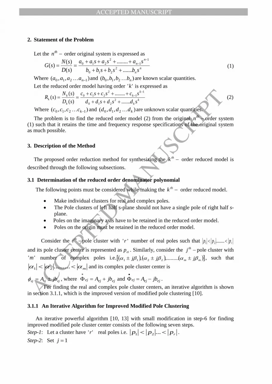
2. Statement of the Problem

Let the thn order original system is expressed as

n

n

n

n

sbsbsbb

sasasaa

sD

sNsG

.......

........

)(

)()(

2

210

1

1

2

210

(1)

Where ),,( 1210 naaaa and ),,( 210 nbbbb are known scalar quantities.

Let the reduced order model having order ''k is expressed as

k

k

k

k

k

k

ksdsdsdd

scscscc

sD

sNsR

.......

........

)(

)()(

2

210

1

1

2

210

(2)

Where ),,( 1210 kcccc and ),,( 210 kdddd are unknown scalar quantities.

The problem is to find the reduced order model (2) from the original thn order system (1) such that it retains the time and frequency response specifications of the original system as much possible.

3. Description of the Method

The proposed order reduction method for synthesizing the thk order reduced model is

described through the following subsections.

3.1 Determination of the reduced order denominator polynomial

The following points must be considered while making the thk order reduced model.

Make individual clusters for real and complex poles.

The Pole clusters of left half s-plane should not have a single pole of right half s-

plane.

Poles on the imaginary axis have to be retained in the reduced order model.

Poles on the origin must be retained in the reduced order model.

Consider the thi pole cluster with ' 'r number of real poles such that rppp .........21

and its pole cluster center is represented as eip . Similarly, consider the thj pole cluster with

' 'm number of complex poles i.e. mm jjj ,........., 2211, such that

m .........21 and its complex pole cluster center is

ejejej jbA , where ejejej jbA

and ejejej jbA

.

For finding the real and complex pole cluster centers, an iterative algorithm is shown

in section 3.1.1, which is the improved version of modified pole clustering [10].

3.1.1 An Iterative Algorithm for Improved Modified Pole Clustering

An iterative powerful algorithm [10, 13] with small modification in step-6 for finding

improved modified pole cluster center consists of the following seven steps.

Step-1: Let a cluster have ''r real poles i.e. rppp ...21 .

Step-2: Set 1j

ACCEPTED MANUSCRIPT

ACCEPTED MANUSCRIP

T

Step-3: Estimate pole cluster center

1

0

1

r

ii

j rp

q

Step-4: Set 1 jj

Step-5: Generate an improved modified pole cluster center from

1

11

211

j

jqp

q

Step-6: Is, ?)1( rj if no go to Step-4, else go to Step-7.

Step-7: For thk cluster, an improved modified pole cluster center is obtained as jek qp .

After finding ‘ ekp ’, the reduced order denominator )(sDk can be obtained from the

following cases.

Case-1: If, all improved modified pole cluster centers are real then reduced order

denominator polynomial )(sDk can be obtained as

))...()(()( 21 ekeek pspspssD (3)

where ekee ppp ..., 21 are thndst k...2,1 improved modified cluster centers respectively.

Case-2: If, all improved modified pole cluster centers are complex conjugates, then )(sDk

can be obtained as

))()...()(()( 2/2/11 ekekeek sssssD

(4)

Case-3: If, )2( k improved modified pole cluster centers are real and one pair of improved

modified pole cluster center is complex conjugates, then )(sDk can be obtained as

))()()...()(()( 11)2(21 eekeeek sspspspssD

(5)

Finally, )(sDk can be rewritten as

2

o 1 2( ) s s ....+ s k

k kD s d d d d (6)

3.2 Determination of the reduced order numerator

A high order original system is the series expansion of

0

1)(i

i

i sMsG (about )s (7)

i

i

i sT

0

(about )0s (8)

where iT and iM are the thi Time moment and Markov parameter of )(sG

respectively. The thk order reduced model is considered as

k

i

i

i

k

i

i

i

k

kk

sd

sc

sD

sNsR

0

1

0

)(

)()( (9)

ACCEPTED MANUSCRIPT

ACCEPTED MANUSCRIP

T

The coefficients of the reduced order numerator )(sNk can be obtained from the following

set of equations [12].

01

0112

02133121

0112211

011221101

0211202

01101

...

...

...

...

...

...

...

Mdc

MdMdc

MdMdMdMdc

MdMdMdMdc

TdTdTdTdc

TdTdTdc

TdTdc

Tdc

kk

kkk

kkkkk

kkkkk

ooo

(10)

The coefficients )1...(2,1,0; kjc j of the numerator can be calculated by solving the

above ''k linear equations. Finally, the numerator )(sNk is obtained as

1

1

2

210 ...)(

k

kk scscsccsN (11)

4. Numerical Examples

To check the effectiveness of the proposed method, four original high order systems are

selected from the literature [5,8,15]. To understand the proposed algorithm, few examples are

solved in details and remaining examples are described only with the results. The proposed

method has been compared with existing methods [4,5,6,7,10,14,15,16] through performance

indices i.e. an integral of the absolute magnitude of error (IAE) and integral of square of error

(ISE) in between the transient portion of reduced and original order systems. Simulations

have been done by MATLAB simulation environment. Lower value of performance index

means, nearby the time/frequency response of )(sRk to )(sG .

IAE

0

)()( dttyty k (12)

ISE

0

2)()( dttyty k (13)

where )(tyk and )(ty are the unit step responses of the reduced model and original systems

respectively.

Example 1. Consider a system of eight-order taken from Mukherjee [5].

403201095841181246728422449453654636

40320185760222088122664.36380598251418)(

2345678

234567

ssssssss

ssssssssG

Poles of the above system are as: )8,7,6,5,4,3,2,1(

ACCEPTED MANUSCRIPT

ACCEPTED MANUSCRIP

T

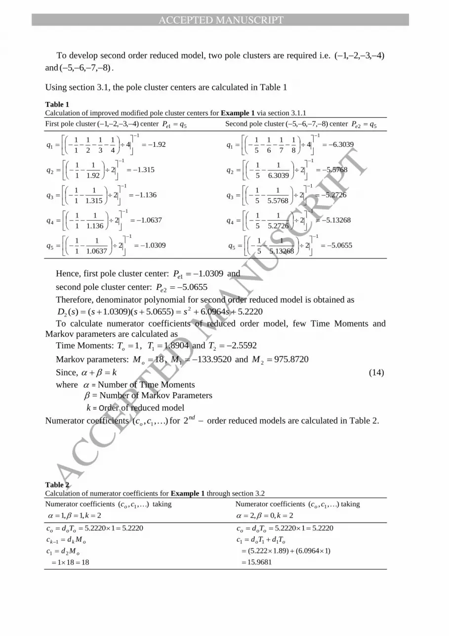
To develop second order reduced model, two pole clusters are required i.e. )4,3,2,1(

and )8,7,6,5( .

Using section 3.1, the pole cluster centers are calculated in Table 1

Table 1

Calculation of improved modified pole cluster centers for Example 1 via section 3.1.1

First pole cluster )4,3,2,1( center 51 qPe Second pole cluster )8,7,6,5( center 52 qPe

92.144

1

3

1

2

1

1

11

1

q 3039.648

1

7

1

6

1

5

11

1

q

315.1292.1

1

1

11

2

q 5768.523039.6

1

5

11

2

q

136.12315.1

1

1

11

3

q 2726.525768.5

1

5

11

3

q

0637.12136.1

1

1

11

4

q 13268.522726.5

1

5

11

4

q

0309.120637.1

1

1

11

5

q 0655.5213268.5

1

5

11

5

q

Hence, first pole cluster center: 0309.11 eP and

second pole cluster center: 0655.52 eP

Therefore, denominator polynomial for second order reduced model is obtained as

2220.50964.6)0655.5)(0309.1()( 2

2 sssssD

To calculate numerator coefficients of reduced order model, few Time Moments and

Markov parameters are calculated as

Time Moments: 1oT , 8904.11 T and 5592.22 T

Markov parameters: 18oM , 9520.1331 M and 8720.9752 M

Since, k (14)

where = Number of Time Moments

= Number of Markov Parameters

k = Order of reduced model

Numerator coefficients ),,( 1 cco for nd2 order reduced models are calculated in Table 2.

Table 2

Calculation of numerator coefficients for Example 1 through section 3.2

Numerator coefficients ),,( 1 cco taking Numerator coefficients ),,( 1 cco taking

2,1,1 k 2,0,2 k

2220.512220.5 ooo Tdc 2220.512220.5 ooo Tdc

18181

21

1

o

okk

Mdc

Mdc

9681.15

)10964.6()89.1222.5(

111

oo TdTdc

ACCEPTED MANUSCRIPT

ACCEPTED MANUSCRIP

T

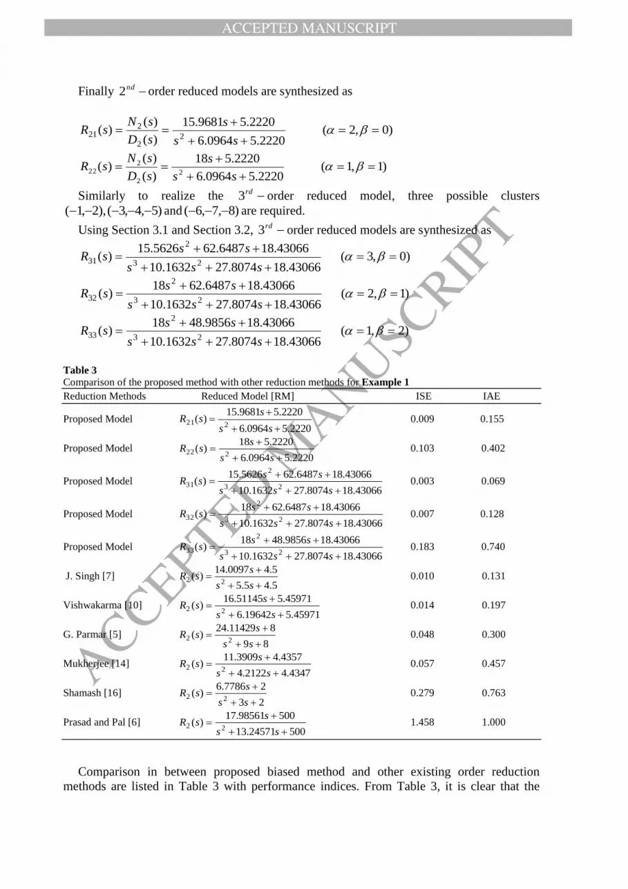
Finally nd2 order reduced models are synthesized as

)0,2(2220.50964.6

2220.59681.15

)(

)()(

22

221

ss

s

sD

sNsR

)1,1(2220.50964.6

2220.518

)(

)()(

2

2

222

ss

s

sD

sNsR

Similarly to realize the rd3 order reduced model, three possible clusters

)5,4,3(),2,1( and )8,7,6( are required.

Using Section 3.1 and Section 3.2, rd3 order reduced models are synthesized as

)0,3(43066.188074.271632.10

43066.186487.625626.15)(

23

2

31

sss

sssR

)1,2(43066.188074.271632.10

43066.186487.6218)(

23

2

32

sss

sssR

)2,1(43066.188074.271632.10

43066.189856.4818)(

23

2

33

sss

sssR

Table 3

Comparison of the proposed method with other reduction methods for Example 1

Reduction Methods Reduced Model [RM] ISE IAE

Proposed Model 2220.50964.6

2220.59681.15)(

221

ss

ssR 0.009 0.155

Proposed Model 2220.50964.6

2220.518)(

222

ss

ssR 0.103 0.402

Proposed Model 43066.188074.271632.10

43066.186487.625626.15)(

23

2

31

sss

sssR 0.003 0.069

Proposed Model 43066.188074.271632.10

43066.186487.6218)(

23

2

32

sss

sssR 0.007 0.128

Proposed Model 43066.188074.271632.10

43066.189856.4818)(

23

2

33

sss

sssR 0.183 0.740

J. Singh [7] 5.45.5

5.40097.14)(

22

ss

ssR

0.010 0.131

Vishwakarma [10] 45971.519642.6

45971.551145.16)(

22

ss

ssR

0.014 0.197

G. Parmar [5] 89

811429.24)(

22

ss

ssR

0.048 0.300

Mukherjee [14] 4347.42122.4

4357.43909.11)(

22

ss

ssR

0.057 0.457

Shamash [16] 23

27786.6)(

22

ss

ssR

0.279 0.763

Prasad and Pal [6] 50024571.13

50098561.17)(

22

ss

ssR

1.458 1.000

Comparison in between proposed biased method and other existing order reduction

methods are listed in Table 3 with performance indices. From Table 3, it is clear that the

ACCEPTED MANUSCRIPT

ACCEPTED MANUSCRIP

T

second order reduced model )(21 sR and third order reduced model )(31 sR have low

performance indices and may be suitable for controllers design. The time response and

frequency response of the reduced order models are compared with the original high order

system in Fig.1 and 2 respectively, which shows good response matching with original high

order system.

Fig. 1. Comparison of the step responses for example 1

Fig. 2. Comparison of the Bode plots for example 1

Example 2. Consider a fourth order system taken from Lucas T.N. [15].

ACCEPTED MANUSCRIPT

ACCEPTED MANUSCRIP

T

240360204362

2400180049628)(

234

23

ssss

ssssG

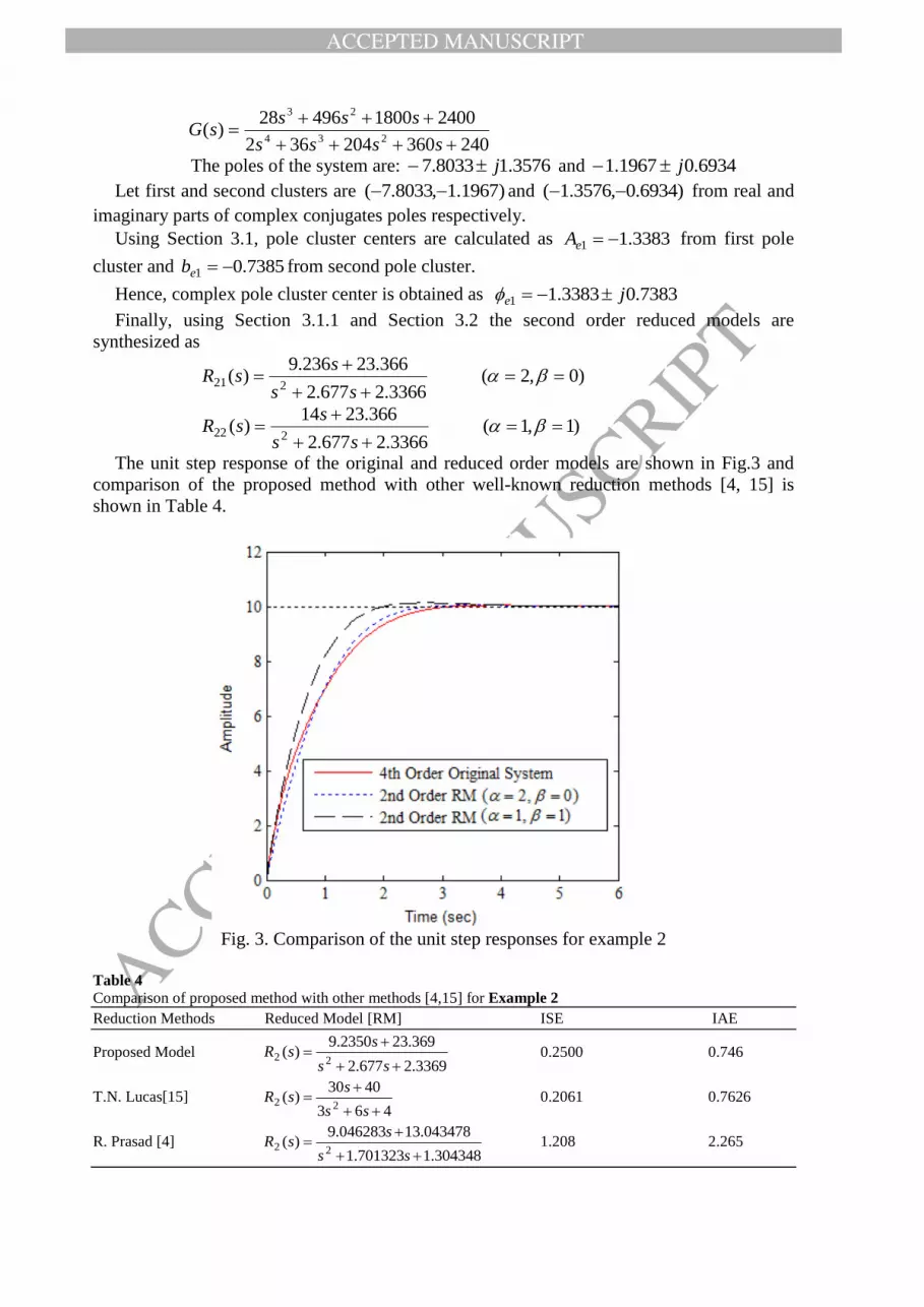
The poles of the system are: 3576.18033.7 j and 6934.01967.1 j

Let first and second clusters are )1967.1,8033.7( and )6934.0,3576.1( from real and

imaginary parts of complex conjugates poles respectively.

Using Section 3.1, pole cluster centers are calculated as 3383.11 eA from first pole

cluster and 7385.01 eb from second pole cluster.

Hence, complex pole cluster center is obtained as 7383.03383.11 je

Finally, using Section 3.1.1 and Section 3.2 the second order reduced models are

synthesized as

)0,2(3366.2677.2

366.23236.9)(

221

ss

ssR

)1,1(3366.2677.2

366.2314)(

222

ss

ssR

The unit step response of the original and reduced order models are shown in Fig.3 and

comparison of the proposed method with other well-known reduction methods [4, 15] is

shown in Table 4.

Fig. 3. Comparison of the unit step responses for example 2

Table 4

Comparison of proposed method with other methods [4,15] for Example 2

Reduction Methods Reduced Model [RM] ISE IAE

Proposed Model 3369.2677.2

369.232350.9)(

22

ss

ssR 0.2500 0.746

T.N. Lucas[15] 463

4030)(

22

ss

ssR

0.2061

0.7626

R. Prasad [4] 304348.1701323.1

043478.13046283.9)(

22

ss

ssR

1.208 2.265

ACCEPTED MANUSCRIPT

ACCEPTED MANUSCRIP

T

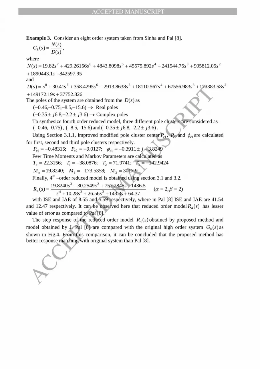
Example 3. Consider an eight order system taken from Sinha and Pal [8].

)(

)()(8

sD

sNsG ,

where

95.8425971.1890443

05.90581275.241544892.455758098.484326156.42982.19)( 234567

s

sssssssN

and

826.3775219.149172

58.173383983.67556567.181108638.29134295.35841.30)( 2345678

s

ssssssssD

The poles of the system are obtained from the )(sD as

)6.15,5.8,75.0,46.0( Real poles

)6.32.2,8.635.0( jj Complex poles

To synthesize fourth order reduced model, three different pole clusters are considered as

)75.0,46.0( , )6.15,5.8( and )6.32.2,8.635.0( jj .

Using Section 3.1.1, improved modified pole cluster center 1eP , 2eP and 1e are calculated

for first, second and third pole clusters respectively.

8249.33911.0;0127.9;48315.0 121 jPP eee

Few Time Moments and Markov Parameters are calculated as

9424.142;9741.71;0876.38;3156.22 321 TTTTo

9.3017;5358.173;8240.19 21 MMM o

Finally, 4th

–order reduced model is obtained using section 3.1 and 3.2.

)2,2(37.648.14356.2628.10

5.14362845.7572549.308240.19)(

234

23

4

ssss

ssssR

with ISE and IAE of 8.55 and 5.59 respectively, where in Pal [8] ISE and IAE are 41.54

and 12.47 respectively. It can be observed here that reduced order model )(4 sR has lesser

value of error as compared to Pal [8].

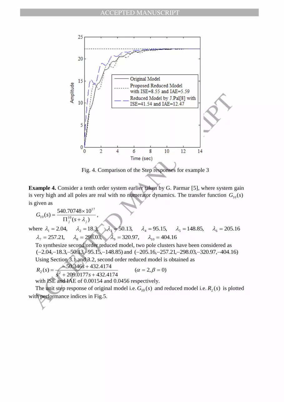
The step response of the reduced order model )(4 sR obtained by proposed method and

model obtained by J. Pal [8] are compared with the original high order system )(8 sG as

shown in Fig.4. From this comparison, it can be concluded that the proposed method has

better response matching with original system than Pal [8].

ACCEPTED MANUSCRIPT

ACCEPTED MANUSCRIP

T

Fig. 4. Comparison of the Step responses for example 3

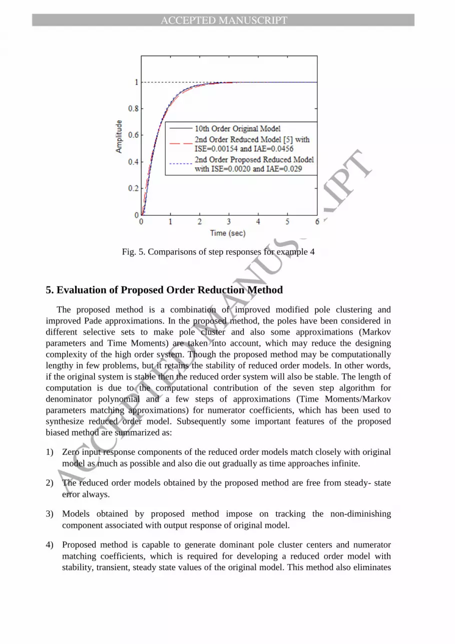
Example 4. Consider a tenth order system earlier taken by G. Parmar [5], where system gain

is very high and all poles are real with no numerator dynamics. The transfer function )(10 sG

is given as

)(

1070748.540)(

10

17

10

jj ssG

,

where 16.205,85.148,15.95,13.50,3.18,04.2 654321

16.404,97.320,03.298,21.257 10987

To synthesize second order reduced model, two pole clusters have been considered as

)85.148,15.95,13.50,3.18,04.2( and )16.404,97.320,03.298,21.257,16.205(

Using Section 3.1 and 3.2, second order reduced model is obtained as

)0,2(

4174.4320177.209

4174.432346.50)(

22

ss

ssR

with ISE and IAE of 0.00154 and 0.0456 respectively.

The unit step response of original model i.e. )(10 sG and reduced model i.e. )(2 sR is plotted

with performance indices in Fig.5.

ACCEPTED MANUSCRIPT

ACCEPTED MANUSCRIP

T

Fig. 5. Comparisons of step responses for example 4

5. Evaluation of Proposed Order Reduction Method

The proposed method is a combination of improved modified pole clustering and

improved Pade approximations. In the proposed method, the poles have been considered in

different selective sets to make pole cluster and also some approximations (Markov

parameters and Time Moments) are taken into account, which may reduce the designing

complexity of the high order system. Though the proposed method may be computationally

lengthy in few problems, but it retains the stability of reduced order models. In other words,

if the original system is stable then the reduced order system will also be stable. The length of

computation is due to the computational contribution of the seven step algorithm for

denominator polynomial and a few steps of approximations (Time Moments/Markov

parameters matching approximations) for numerator coefficients, which has been used to

synthesize reduced order model. Subsequently some important features of the proposed

biased method are summarized as:

1) Zero input response components of the reduced order models match closely with original

model as much as possible and also die out gradually as time approaches infinite.

2) The reduced order models obtained by the proposed method are free from steady- state

error always.

3) Models obtained by proposed method impose on tracking the non-diminishing

component associated with output response of original model.

4) Proposed method is capable to generate dominant pole cluster centers and numerator

matching coefficients, which is required for developing a reduced order model with

stability, transient, steady state values of the original model. This method also eliminates

ACCEPTED MANUSCRIPT

ACCEPTED MANUSCRIP

T

the weakness [6], where a stable reduced order model is obtained through stability

equation method.

5) Method is applicable for model order reduction of any linear dynamic system having

real, complex or real-complex poles from 2nd

- order onwards unlike[7,17], where most

dominant pole is retained and remaining poles are acquired in a group, to find another

dominant pole. Also, proposed method overcomes the drawback [7,17], where method is

applicable for systems having real or complex conjugates poles only.

6) Method provides a good approximations of original system for a healthy reduced order

model rather than approximations taken by authors [4,11,16,18,19].

6. Conclusions

This paper suggested a new mixed order reduction method for the large-scale single-input

single-output (SISO) systems. The denominator polynomial of the reduced model is obtained

using improved modified pole clustering while the numerator coefficients are computed by

improved Pade approximations. Biased method has been tested on four numerical examples

having real poles, complex poles and both. Natural and forced responses of the reduced

models, matches closely with response of original system as shown in figure 1, 3, 4 and 5.

The proposed reduction method has been compared with some existing order reduction

techniques via performance indices, i.e. ISE and IAE. The proposed algorithm is also valid

for large scale multi-input multi-output (MIMO) systems. From the results of the numerical

examples, it may be concluded that method is efficient and computationally simple. The

algorithm of the proposed method will be helpful to the scholars and engineers working on

model order reduction and controller design areas.

References

[1] Vimal Singh, Dinesh Chandra, Haranath Kar, Improved Routh Pade approximants: a computer aided

approach, IEEE Transactions on Automatic Control, 49(2) (2004) 292-296.

[2] C.B. Vishwakarma, R. Prasad, Time domain model order reduction using Hankel matrix approach,

Journal of the Franklin Institute, 351(2014) 3445-3456.

[3] Sastry G.V.K.R, Raja Rao R., Mallikarjuna Rao P., Large scale interval system modelling using Routh

approximant, Electronic Letters, 36(8) (2000) 768-769.

[4] R. Prasad, Pade type model order reduction for multivariable systems using Routh approximations,

Computer and Electrical Engineering, 26 (2000) 445-459.

[5] G. Parmar, S. Mukherjee, R. Prasad, System reduction using factor division algorithm and eigen

spectrum analysis, Applied Mathematical Modelling, 31 (2007) 2542-2552.

[6] R. Prasad, J. Pal, Stable reduction of linear systems by continued fractions, Journal of Institution of

Engineers (India), 72 (1991) 113-116.

[7] Jay singh, Kalyan Chattterjee, C.B. Vishwakarma, System reduction by eigen permutation algorithm and

improved Pade approximations, Journal of Mathematical, Computational Science and Engineering, 8(1)

(2014) 1-5.

[8] A.K. Sinha, Jayanta Pal, Simulation based reduced order modelling using a clustering technique,

Computers and Electrical Engineering, 16(3) (1990) 159-169.

[9] J. Pal, A.K. Sinha, N.K. Sinha, Reduced order modelling using pole clustering and time moment

matching, Journal of the Institution of Engineers(India) (EED), 76 (1995) 1-6.

[10] CB Vishwakarma, Order reduction using Modified pole clustering and Pade approximations, World

Academy of Science, Engineering and Technology, 56 (2011) 787-791.

[11] H. Padé, Sur la représentation approchée d’une fonction par des fractions rationelles, Ann. Sci. Ecole

Norm. Sup., 9(3) (1892) 3–93.

ACCEPTED MANUSCRIPT

ACCEPTED MANUSCRIP

T

[12] Jayanta Pal, Improved Pade approximants using stability equation methods, Electronics Letters, 19 (11)

(1983) 426-427.

[13] C.B. Vishwakarma, R. Prasad, MIMO system reduction using modified pole clustering & genetic

algorithm, Modelling and Simulation in Engineering, 2009 (2009) 1-6.

[14] S. Mukherjee, Satakshi, R.C. Mittal, Model order reduction using response-matching technique, Journal

of the Franklin Institute, 342 (2005) 503–519.

[15] Smith ID, Lucas TN, Least-squares moment matching reduction methods, Electronics Letters, 31(11)

(1995) 929-930.

[16] Y. Shamash, Linear system reduction using Pade approximations to allow retention of dominant modes,

International Journal of Control, 21(2) (1975) 257–272.

[17] Jay Singh, Kalyan Chattterjee, C.B.Vishwakarma, MIMO system using eigen algorithm and improved

Pade approximations, SOP Transaction of Applied Mathematics, 1(1) (2014) 60-70.

[18] Avadh P., Awadhesh K., D. Chandra, Suboptimal control using model order reduction, Chinese Journal

of Engineering, 2014 (2014) 1-5.

[19] Othman M.K. Alsmadi, Zaer S. Abo-Hammour, Substructure preservation model order reduction with

power system model investigation, Wulfenia Journal, 22(3) (2015) 44-55.