autonomous navigation of distributed spacecraft using
TRANSCRIPT
Autonomous Navigation of Distributed Spacecraftusing Intersatellite Laser Communications
byPratik K. Dave
B.S., University of Maryland (2009)S.M., Massachusetts Institute of Technology (2014)
Submitted to the Department of Aeronautics and Astronauticsin partial fulfillment of the requirements for the degree of
Doctor of Philosophy in Space Systemsat the
MASSACHUSETTS INSTITUTE OF TECHNOLOGYFebruary 2020
c Massachusetts Institute of Technology 2020. All rights reserved.
Author . . . . . . . . . . . . . . . . . . . . . . . . . . . . . . . . . . . . . . . . . . . . . . . . . . . . . . . . . . . . . . . .Department of Aeronautics and Astronautics
January 30, 2020Certified by. . . . . . . . . . . . . . . . . . . . . . . . . . . . . . . . . . . . . . . . . . . . . . . . . . . . . . . . . . . .
Kerri L. CahoyAssociate Professor of Aeronautics and Astronautics
Thesis SupervisorCertified by. . . . . . . . . . . . . . . . . . . . . . . . . . . . . . . . . . . . . . . . . . . . . . . . . . . . . . . . . . . .
Richard LinaresAssistant Professor of Aeronautics and Astronautics
Certified by. . . . . . . . . . . . . . . . . . . . . . . . . . . . . . . . . . . . . . . . . . . . . . . . . . . . . . . . . . . .Timothy M. Yarnall
Assistant Group Leader, MIT Lincoln LaboratoryAccepted by . . . . . . . . . . . . . . . . . . . . . . . . . . . . . . . . . . . . . . . . . . . . . . . . . . . . . . . . . . .
Sertac KaramanAssociate Professor of Aeronautics and Astronautics
Chair, Graduate Program Committee

2
Autonomous Navigation of Distributed Spacecraft using
Intersatellite Laser Communications
by
Pratik K. Dave
Submitted to the Department of Aeronautics and Astronauticson January 30, 2020, in partial fulfillment of the
requirements for the degree ofDoctor of Philosophy in Space Systems
Abstract
Autonomous navigation refers to satellites performing on-board, real-time navigationwithout external input. As satellite systems evolve into more distributed architec-tures, autonomous navigation can help mitigate challenges in ground operations, suchas determining and disseminating orbit solutions. Several autonomous navigationmethods have been previously studied, using some combination of on-board sensorsthat can measure relative range or bearing to known bodies, such as horizon and starsensors (Hicks and Wiesel, 1992) or magnetometers and sun sensors (Psiaki, 1999),however these methods are typically limited to low Earth orbit (LEO) altitudes orother specific orbit cases.
Another autonomous navigation method uses intersatellite data, or direct obser-vations of the relative position vector from one satellite to another, to estimate theorbital positions of both spacecraft simultaneously. The seminal study of the inter-satellite method assumes the use of radio time-of-flight measurements of intersatelliterange, and a visual tracking camera system for measuring the inertial bearing fromone satellite to another (Markley, 1984). Due to the limited range constraints ofpassively illuminated visual tracking systems, many of the previous studies restrictthe separation between satellites to less than 1,000 kilometers (e.g., Psiaki, 2011), orsimply drop the use of measuring intersatellite bearing and rely solely on obtaining alarge distribution of intersatellite range measurements for state estimation (e.g., Xuet al., 2014). These assumptions have limited the assessment of the performance ca-pability of autonomous navigation using intersatellite measurements for more generalmission applications.
In this thesis, we investigate the performance of using laser communication (laser-com) crosslinks in order to achieve all necessary intersatellite measurements for au-tonomous navigation. Lasercom systems are capable of measuring both range andbearing to a receiving terminal with greater precision than traditional methods, andcan do so over larger separations between satellites. We develop a simulation frame-work to model the measurements of intersatellite range and bearing using lasercomcrosslinks in distributed satellite systems, with consideration of varying orbital op-
3
erating environments, constellation size and distribution, and network topologies.We implement two estimation algorithms: an extended Kalman filter (EKF) usedwith Monte Carlo sampling for performance analyses, and a Cramér-Rao lower-bound(CRLB) computation for uncertainty analyses.
We evaluate several case studies modeled off of existing and planned constella-tion missions in order to demonstrate the new capabilities of performing intersatellitenavigation with lasercom links in both near-Earth and deep-space orbital applica-tions. Performance targets are generated from the current state-of-the-art navigationcapabilities demonstrated by Global Navigation Satellite Systems (GNSS) in Earth-orbit, and by radiometric tracking and orbit estimation using the Deep Space Network(DSN) in deep-space orbits.
For Earth-orbiting applications, we simulate a relay satellite system in geosyn-chronous orbit (GEO) inspired by current optical communications missions in de-velopment by both ESA and NASA, and Walker constellations in LEO inspired bythe upcoming mega-constellations for global broadband internet service, such as thoseproposed by SpaceX and Telesat. In both case studies, we demonstrate improved nav-igation performance over the current state-of-the-art in GNSS receiver technologies byusing intersatellite measurements from lasercom crosslinks. Monte Carlo simulationsshow median total position errors better than 3 meters in LEO, 12 meters in GEO,and 45 meters in high-altitude or highly-eccentric orbits (HEO), showing promise asan alternative navigation method to GNSS in Earth-orbiting environments.
We also simulate current and future Mars-orbiting missions as examples of deep-space applications. In one case study, we create an ad-hoc constellation comprisedof low-altitude Mars exploration orbiters modeled off of current Mars-orbiting mis-sions. In a second case study, we focus on a high-altitude constellation proposed fordedicated Earth-to-Mars networked communications. Again, in both case studies,we demonstrate improved navigation performance over the current state-of-the-art inDSN radiometric orbit solutions by using intersatellite measurements from lasercomcrosslinks. Monte Carlo simulations show stable median total position errors betterthan 25 meters for Mars-orbit, which demonstrates a notable improvement both spa-tially and temporally versus DSN orbit estimation, mitigating the large cost and timeconstraints associated with DSN tracking.
These results demonstrate the promise of using lasercom intersatellite links forautonomous navigation, offering enhanced performance over current state-of-the-artcapabilities, and a greater applicability to missions both near Earth and beyond.
Thesis Supervisor: Kerri L. CahoyTitle: Associate Professor of Aeronautics and Astronautics
Thesis Committee Member: Richard LinaresTitle: Assistant Professor of Aeronautics and Astronautics
Thesis Committee Member: Timothy M. YarnallTitle: Assistant Group Leader, MIT Lincoln Laboratory
4
Acknowledgments
This material is based upon work supported by the United States Air Force under
Air Force Contract No. FA8721-05-C-0002 and/or FA8702-15-DO001. Any opinions,
findings, and conclusions or recommendations expressed in this material are those of
the author and do not necessarily reflect the views of the United States Air Force.
I would like to begin by acknowledging the MIT Lincoln Laboratory for the oppor-
tunities to work on interesting and consequential projects in the aerospace domain,
and to pursue both of my graduate degrees at MIT. My education and research were
funded by the Lincoln Scholars Program with the support of my group and divi-
sion leadership. Special thanks to Greg Berthiaume, Marshall Brenizer, and Diane
DeCastro.
I am very grateful for my academic and thesis advisor, Prof. Kerri Cahoy, who
plucked me out of the crowd of graduate student applications, and provided me with
a home and community at the institute. She gave me the flexibility and freedom to
embark on this journey whichever way I’d like, and guidance and advice when I most
needed it.
I am also grateful for my thesis committee members, past and present, for all of
their guidance throughout this process. Prof. David Miller and Dr. Jon Kadish sup-
ported the early exploration into my thesis research, and Dr. Tim Yarnall and Prof.
Richard Linares willingly stepped in to lend their expertise in laser communications
and satellite navigation, respectively. I’d like to extend this gratitude to my external
advisors as well, most notably my thesis readers Dr. Todd Ely and Dr. Robert Legge.
I appreciate and value your input on my work.
There are many thanks I would like to give to my family and friends. First and
foremost, the most significant sentiment of appreciation goes to my parents, who have
always given me the freedom to pursue all that I’m interested in, supported me with
an unwavering vote of confidence that I can achieve everything I set my mind to, and
instilled in me the virtues of hard-work, dedication, and patience – thanks, Mom and
Dad. Right behind them are my loving sister, Stuti, and brother(-in-law), Parvish –
5
plus the amazing bundle of joy and love that they created in my niece, Elana, and
my playful nephew-pup, Orion. They always know exactly when and how to provide
an escape from my stress, even without trying. Special thanks to Chris, Matt, Kit,
and Kat – you’ve become some of my best friends over the years, so much so that
it’s strange to remember that it was grad school that brought us together in the first
place. And countless thanks for all of the love and support of my extended Dave,
Desai, Patel, Shah, and Vakharia families – as well as my SSL, STAR Lab, GA3,
volleyball, UMD, and NJ friends.
Finally, a special thank-you to Janaki, for all of your love, support, companionship,
playfulness, joy, devotion, and understanding. We met shortly before I started on this
path towards a doctoral degree, and who would have known that our stars would align
the way they have. I appreciate all of the things you do, especially your reminders to
let loose, have fun, and celebrate life every once in a while. 2020 is a big year for us,
and I can’t wait for what’s to come!
6
Contents
1 Introduction 29
1.1 Motivation . . . . . . . . . . . . . . . . . . . . . . . . . . . . . . . . . 29
1.2 Context . . . . . . . . . . . . . . . . . . . . . . . . . . . . . . . . . . 31
1.2.1 Satellite Navigation . . . . . . . . . . . . . . . . . . . . . . . . 31
1.2.2 Crosslink Communications . . . . . . . . . . . . . . . . . . . . 35
1.3 Thesis Overview . . . . . . . . . . . . . . . . . . . . . . . . . . . . . . 38
1.3.1 Research Contributions . . . . . . . . . . . . . . . . . . . . . . 40
1.3.2 Organization . . . . . . . . . . . . . . . . . . . . . . . . . . . 41
2 Background & Literature Review 43
2.1 Spacecraft Navigation Methodology . . . . . . . . . . . . . . . . . . . 43
2.1.1 Estimation Methods . . . . . . . . . . . . . . . . . . . . . . . 43
2.1.2 Measurement Types . . . . . . . . . . . . . . . . . . . . . . . 47
2.2 Autonomous Navigation with Intersatellite Data . . . . . . . . . . . . 49
2.2.1 Seminal Research . . . . . . . . . . . . . . . . . . . . . . . . . 49
2.2.2 Other Relevant Studies & Analyses . . . . . . . . . . . . . . . 50
2.2.3 Research Gaps . . . . . . . . . . . . . . . . . . . . . . . . . . 53
3 Simulation Approach 55
3.1 Orbit Generation & Propagation . . . . . . . . . . . . . . . . . . . . 55
3.1.1 Input: Scenario Configuration . . . . . . . . . . . . . . . . . . 57
3.1.2 Output: “Truth” State Data for All Satellites . . . . . . . . . . 60
3.2 Link-Access Availability Computation . . . . . . . . . . . . . . . . . . 63
7
3.2.1 Input: Link-Access Model . . . . . . . . . . . . . . . . . . . . 63
3.2.2 Output: Satellite Pairs, Available Links, & Duty Cycles . . . . 67
3.3 State & Measurement Simulation . . . . . . . . . . . . . . . . . . . . 69
3.3.1 Input: Navigation Filter Models . . . . . . . . . . . . . . . . . 69
3.3.2 Output: Predicted States & Simulated Measurements . . . . . 73
3.4 Link-Access Selection . . . . . . . . . . . . . . . . . . . . . . . . . . . 74
3.4.1 Overview of Inputs and Outputs . . . . . . . . . . . . . . . . . 75
3.4.2 Output: Selected Links based on CRLB . . . . . . . . . . . . 75
3.5 Navigation Performance Estimation & Analysis . . . . . . . . . . . . 79
3.5.1 Overview of Inputs and Outputs . . . . . . . . . . . . . . . . . 80
3.5.2 EKF Output: Estimation Error & Uncertainty . . . . . . . . . 81
3.5.3 CRLB Output: Predicted Uncertainty . . . . . . . . . . . . . 87
4 Earth-Orbiting Applications 89
4.1 Case Study E1: GEO Relay Satellite Systems . . . . . . . . . . . . . 89
4.1.1 Setup of Scenarios . . . . . . . . . . . . . . . . . . . . . . . . 90
4.1.2 Single GEO-Relay with Single User . . . . . . . . . . . . . . . 93
4.1.3 Multiple Relays and/or Multiple Users . . . . . . . . . . . . . 101
4.2 Case Study E2: LEO Constellations . . . . . . . . . . . . . . . . . . . 106
4.2.1 Setup of Scenarios . . . . . . . . . . . . . . . . . . . . . . . . 107
4.2.2 Two-satellite Navigation . . . . . . . . . . . . . . . . . . . . . 109
4.2.3 Walker Constellation Navigation . . . . . . . . . . . . . . . . . 113
4.3 Summary of Results . . . . . . . . . . . . . . . . . . . . . . . . . . . 120
4.3.1 LEO Satellites . . . . . . . . . . . . . . . . . . . . . . . . . . . 120
4.3.2 GEO Satellites . . . . . . . . . . . . . . . . . . . . . . . . . . 120
4.3.3 HEO Satellites . . . . . . . . . . . . . . . . . . . . . . . . . . 122
5 Deep-Space Orbital Applications 123
5.1 Case Study M1: Existing Mars Mission Orbits . . . . . . . . . . . . . 123
5.1.1 Setup of Scenarios . . . . . . . . . . . . . . . . . . . . . . . . 125
5.1.2 Two-satellite Cases . . . . . . . . . . . . . . . . . . . . . . . . 126
8
5.1.3 Ad-hoc Constellations . . . . . . . . . . . . . . . . . . . . . . 128
5.2 Case Study M2: Future Comms. Constellation . . . . . . . . . . . . . 131
5.2.1 Setup of Scenarios . . . . . . . . . . . . . . . . . . . . . . . . 131
5.2.2 CRLB Uncertainty Analysis . . . . . . . . . . . . . . . . . . . 137
5.2.3 EKF Performance Results . . . . . . . . . . . . . . . . . . . . 138
5.3 Summary of Results . . . . . . . . . . . . . . . . . . . . . . . . . . . 140
6 Conclusion 143
6.1 Summary of Contributions . . . . . . . . . . . . . . . . . . . . . . . . 143
6.2 Future Work . . . . . . . . . . . . . . . . . . . . . . . . . . . . . . . . 147
9

THIS PAGE INTENTIONALLY LEFT BLANK
10
List of Figures
1-1 Overview of satellite navigation methods, categorized into three areas:
ground-based precise orbit determination, semi-autonomous naviga-
tion, and fully autonomous navigation. . . . . . . . . . . . . . . . . . 31
1-2 Typical 1-sigma orbit estimation error achieved using ground-based
tracking and autonomous navigation methods. SLR: Satellite laser
ranging, VLBI: Very-long baseline interferometry, UHF: Ultra-high
frequency radio ranging, NORAD (TLEs): Two-line element sets pub-
lished by the North American Aerospace Defense Command, DORIS/DIODE:
Doppler Orbitography and Radiopositioning Integrated by Satellite
ground-beacon system and on-board OD software, DF-/SF-GNSS: Dual-
/Single-frequency GNSS receivers, Landmark: Autonomous naviga-
tion using landmarks, Pulsars: X-ray pulsar-based navigation, Inter-
sat: Autonomous navigation using intersatellite measurement data,
Mag-SS: Autonomous navigation using magnetometer and sun-sensors,
EHS-ST: Autonomous navigation using Earth-horizon sensors and star-
tracker [1–13]. . . . . . . . . . . . . . . . . . . . . . . . . . . . . . . . 34
11
1-3 Diagram of proposed method of autonomous navigation using laser
communication crosslinks between two or more satellites, co-orbital
around any central-body with known gravity characteristics (mass and
J2-term). This method assumes that the observing spacecraft have
star-trackers for inertial attitude knowledge, and known angular off-
sets between the boresights of the star tracker and the lasercom termi-
nal, and other on-board systems necessary to establish and maintain a
crosslink signal with another satellite. . . . . . . . . . . . . . . . . . . 39
3-1 Block diagram of simulation approach: green ovals indicate inputs, blue
boxes indicate written functions, and the gray box denotes external
software or functions. . . . . . . . . . . . . . . . . . . . . . . . . . . . 56
3-2 Results for the GEO-LEO example case: 50th percentile navigation er-
ror over 100 Monte Carlo samples of simulated lasercom crosslink mea-
surements fed through an EKF intersatellite navigation filter. Results
for ARTEMIS (GEO) are in black, while results for OICETS (LEO)
are in red. Gray vertical bars are used to denote data-gap periods due
to inaccessible crosslink geometry. . . . . . . . . . . . . . . . . . . . . 56
3-3 Summary of inputs and outputs for the “orbit generation and propa-
gation” step in the simulation approach. . . . . . . . . . . . . . . . . 57
3-4 Summary of actions taken to configure a simulation scenario. . . . . . 58
3-5 Summary of inputs and outputs for the “link-access availability com-
putation” step in the simulation approach. . . . . . . . . . . . . . . . 63
3-6 Summary of link-access constraints developed for use in this thesis. . 64
3-7 Summary of inputs and outputs for the “state and measurement simu-
lation” step in the simulation approach. . . . . . . . . . . . . . . . . . 69
3-8 Summary of inputs and outputs for the “link-access selection” step in
the simulation approach. . . . . . . . . . . . . . . . . . . . . . . . . . 76
12
3-9 Notional diagram for the link-selection process developed for use in this
thesis. Each simulation scenario is divided in time into duty-cycles,
which are used as evaluation periods for link-selection. Each possible
link-access partner is used in a two-satellite CRLB computation with a
particular satellite (Sat11 in this case). The final CRLB value of each
possible partner is compared, and the link that minimizes this value is
selected. The full scenario is propagated forward using this selection,
up until the start of the next duty-cycle or evaluation period. This
process is repeated until the end of the simulation scenario. . . . . . . 78
3-10 Summary of inputs and outputs for the “state estimation” function in
the simulation approach. . . . . . . . . . . . . . . . . . . . . . . . . . 80
3-11 Summary of inputs and outputs for the “performance analysis” function
in the simulation approach. . . . . . . . . . . . . . . . . . . . . . . . 81
3-12 Summary of inputs and outputs for the “Monte Carlo analysis” step in
the simulation approach. . . . . . . . . . . . . . . . . . . . . . . . . . 82
3-13 Summary of EKF results (50th percentile error averaged over final 0.5
hour) from Monte Carlo simulations (N=100) of simulation approach
sensitivity to time-step, 𝑇 , in the GEO-LEO example case: a sin-
gle GEO-relay satellite, ARTEMIS (black), with a single LEO user,
OICETS (red). . . . . . . . . . . . . . . . . . . . . . . . . . . . . . . 84
3-14 Summary of EKF results (50th percentile error averaged over final 0.5
hour) from Monte Carlo simulations (N=100) of simulation approach
sensitivity to initial state uncertainty, P0, in the GEO-LEO example
case: a single GEO-relay satellite, ARTEMIS (black), with a single
LEO user, OICETS (red). . . . . . . . . . . . . . . . . . . . . . . . . 84
3-15 Summary of EKF results (50th percentile error averaged over final 0.5
hour) from Monte Carlo simulations (N=100) of simulation approach
sensitivity to position-estimation process noise, Qr, in the GEO-LEO
example case: a single GEO-relay satellite, ARTEMIS (black), with a
single LEO user, OICETS (red). . . . . . . . . . . . . . . . . . . . . . 85
13
3-16 Summary of EKF results (50th percentile error averaged over final 0.5
hour) from Monte Carlo simulations (N=100) of simulation approach
sensitivity to velocity-estimation process noise, Qv, in the GEO-LEO
example case: a single GEO-relay satellite, ARTEMIS (black), with a
single LEO user, OICETS (red). . . . . . . . . . . . . . . . . . . . . . 85
3-17 Summary of EKF results (50th percentile error averaged over final 0.5
hour) from Monte Carlo simulations (N=100) of simulation approach
sensitivity to measurement noise, R, in the GEO-LEO example case: a
single GEO-relay satellite, ARTEMIS (black), with a single LEO user,
OICETS (red). . . . . . . . . . . . . . . . . . . . . . . . . . . . . . . 86
4-1 Diagram of orbital scenario for the GEO Relay case study, generated
using AGI STK. . . . . . . . . . . . . . . . . . . . . . . . . . . . . . . 90
4-2 EKF results (10/50/90 percentiles) from Monte Carlo simulations (N=100)
of baseline GEO-relay example: a single GEO-relay satellite, ARTEMIS
(black), with a single LEO user, OICETS (red). . . . . . . . . . . . . 93
4-3 CRLB analysis results for GEO satellite (ARTEMIS) with other Earth-
orbiting satellites in varying orbital altitudes and inclinations. LEO
altitudes are shown in blue, lower MEO altitudes in green, GPS altitude
in gray, and GEO altitude in black. Baseline GEO-LEO example of
ARTEMIS & OICETS is shown in red. Lower altitude is better. . . . 95
4-4 Summary of minimum achieved CRLB over 24-hour simulation for
GEO satellite (ARTEMIS) with LEO satellites in varying orbital alti-
tudes and inclinations. . . . . . . . . . . . . . . . . . . . . . . . . . . 96
4-5 CRLB analysis results for the parameter-sweep satellite (varying orbit)
in simulations of GEO satellite with other Earth-orbiting satellites in
varying orbital altitudes and inclinations. LEO altitudes are shown in
blue, lower MEO altitudes in green, GPS altitude in gray, and GEO al-
titude in black. Baseline GEO-LEO example of ARTEMIS & OICETS
is shown in red. Lower altitude is better. . . . . . . . . . . . . . . . . 97
14
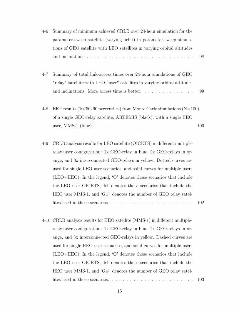
4-6 Summary of minimum achieved CRLB over 24-hour simulation for the
parameter-sweep satellite (varying orbit) in parameter-sweep simula-
tions of GEO satellite with LEO satellites in varying orbital altitudes
and inclinations. . . . . . . . . . . . . . . . . . . . . . . . . . . . . . . 98
4-7 Summary of total link-access times over 24-hour simulations of GEO
"relay" satellite with LEO "user" satellites in varying orbital altitudes
and inclinations. More access time is better. . . . . . . . . . . . . . . 99
4-8 EKF results (10/50/90 percentiles) from Monte Carlo simulations (N=100)
of a single GEO-relay satellite, ARTEMIS (black), with a single HEO
user, MMS-1 (blue). . . . . . . . . . . . . . . . . . . . . . . . . . . . 100
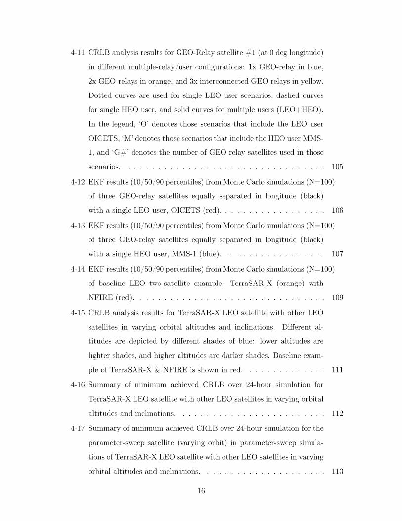
4-9 CRLB analysis results for LEO satellite (OICETS) in different multiple-
relay/user configuration: 1x GEO-relay in blue, 2x GEO-relays in or-
ange, and 3x interconnected GEO-relays in yellow. Dotted curves are
used for single LEO user scenarios, and solid curves for multiple users
(LEO+HEO). In the legend, ‘O’ denotes those scenarios that include
the LEO user OICETS, ‘M’ denotes those scenarios that include the
HEO user MMS-1, and ‘G#’ denotes the number of GEO relay satel-
lites used in those scenarios. . . . . . . . . . . . . . . . . . . . . . . . 102
4-10 CRLB analysis results for HEO satellite (MMS-1) in different multiple-
relay/user configuration: 1x GEO-relay in blue, 2x GEO-relays in or-
ange, and 3x interconnected GEO-relays in yellow. Dashed curves are
used for single HEO user scenarios, and solid curves for multiple users
(LEO+HEO). In the legend, ‘O’ denotes those scenarios that include
the LEO user OICETS, ‘M’ denotes those scenarios that include the
HEO user MMS-1, and ‘G#’ denotes the number of GEO relay satel-
lites used in those scenarios. . . . . . . . . . . . . . . . . . . . . . . . 103
15
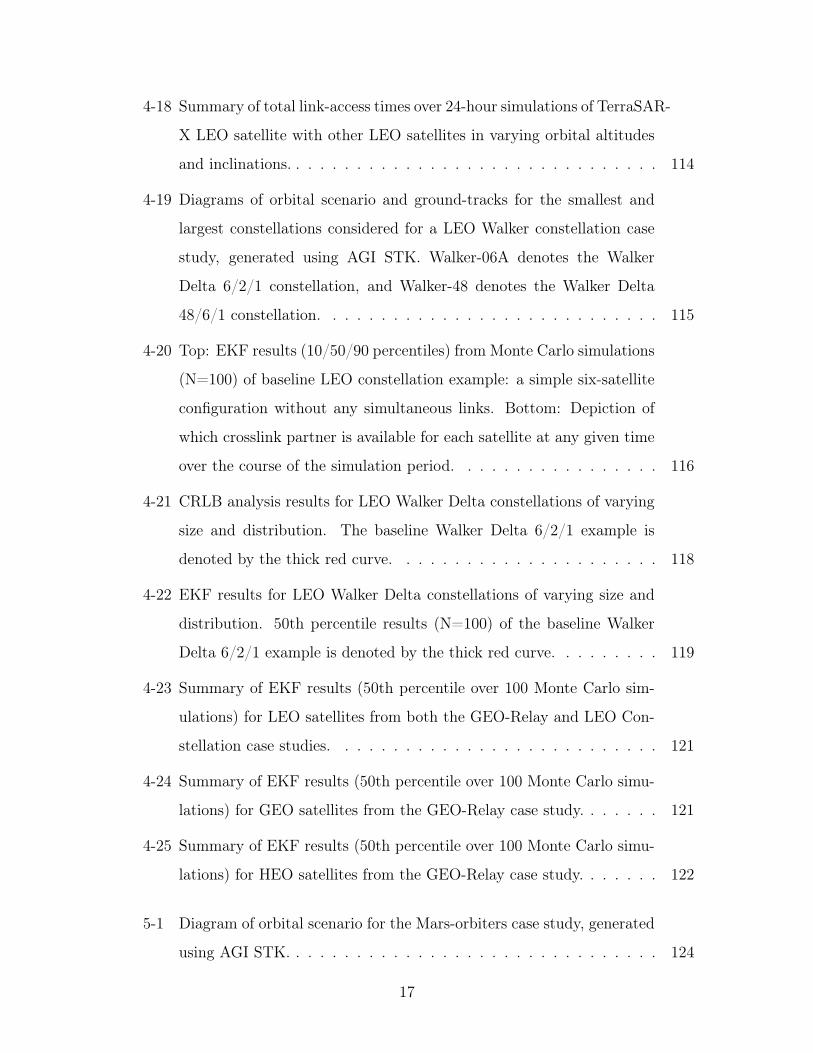
4-11 CRLB analysis results for GEO-Relay satellite #1 (at 0 deg longitude)
in different multiple-relay/user configurations: 1x GEO-relay in blue,
2x GEO-relays in orange, and 3x interconnected GEO-relays in yellow.
Dotted curves are used for single LEO user scenarios, dashed curves
for single HEO user, and solid curves for multiple users (LEO+HEO).
In the legend, ‘O’ denotes those scenarios that include the LEO user
OICETS, ‘M’ denotes those scenarios that include the HEO user MMS-
1, and ‘G#’ denotes the number of GEO relay satellites used in those
scenarios. . . . . . . . . . . . . . . . . . . . . . . . . . . . . . . . . . 105
4-12 EKF results (10/50/90 percentiles) from Monte Carlo simulations (N=100)
of three GEO-relay satellites equally separated in longitude (black)
with a single LEO user, OICETS (red). . . . . . . . . . . . . . . . . . 106
4-13 EKF results (10/50/90 percentiles) from Monte Carlo simulations (N=100)
of three GEO-relay satellites equally separated in longitude (black)
with a single HEO user, MMS-1 (blue). . . . . . . . . . . . . . . . . . 107
4-14 EKF results (10/50/90 percentiles) from Monte Carlo simulations (N=100)
of baseline LEO two-satellite example: TerraSAR-X (orange) with
NFIRE (red). . . . . . . . . . . . . . . . . . . . . . . . . . . . . . . . 109
4-15 CRLB analysis results for TerraSAR-X LEO satellite with other LEO
satellites in varying orbital altitudes and inclinations. Different al-
titudes are depicted by different shades of blue: lower altitudes are
lighter shades, and higher altitudes are darker shades. Baseline exam-
ple of TerraSAR-X & NFIRE is shown in red. . . . . . . . . . . . . . 111
4-16 Summary of minimum achieved CRLB over 24-hour simulation for
TerraSAR-X LEO satellite with other LEO satellites in varying orbital
altitudes and inclinations. . . . . . . . . . . . . . . . . . . . . . . . . 112
4-17 Summary of minimum achieved CRLB over 24-hour simulation for the
parameter-sweep satellite (varying orbit) in parameter-sweep simula-
tions of TerraSAR-X LEO satellite with other LEO satellites in varying
orbital altitudes and inclinations. . . . . . . . . . . . . . . . . . . . . 113
16
4-18 Summary of total link-access times over 24-hour simulations of TerraSAR-
X LEO satellite with other LEO satellites in varying orbital altitudes
and inclinations. . . . . . . . . . . . . . . . . . . . . . . . . . . . . . . 114
4-19 Diagrams of orbital scenario and ground-tracks for the smallest and
largest constellations considered for a LEO Walker constellation case
study, generated using AGI STK. Walker-06A denotes the Walker
Delta 6/2/1 constellation, and Walker-48 denotes the Walker Delta
48/6/1 constellation. . . . . . . . . . . . . . . . . . . . . . . . . . . . 115
4-20 Top: EKF results (10/50/90 percentiles) from Monte Carlo simulations
(N=100) of baseline LEO constellation example: a simple six-satellite
configuration without any simultaneous links. Bottom: Depiction of
which crosslink partner is available for each satellite at any given time
over the course of the simulation period. . . . . . . . . . . . . . . . . 116
4-21 CRLB analysis results for LEO Walker Delta constellations of varying
size and distribution. The baseline Walker Delta 6/2/1 example is
denoted by the thick red curve. . . . . . . . . . . . . . . . . . . . . . 118
4-22 EKF results for LEO Walker Delta constellations of varying size and
distribution. 50th percentile results (N=100) of the baseline Walker
Delta 6/2/1 example is denoted by the thick red curve. . . . . . . . . 119
4-23 Summary of EKF results (50th percentile over 100 Monte Carlo sim-
ulations) for LEO satellites from both the GEO-Relay and LEO Con-
stellation case studies. . . . . . . . . . . . . . . . . . . . . . . . . . . 121
4-24 Summary of EKF results (50th percentile over 100 Monte Carlo simu-
lations) for GEO satellites from the GEO-Relay case study. . . . . . . 121
4-25 Summary of EKF results (50th percentile over 100 Monte Carlo simu-
lations) for HEO satellites from the GEO-Relay case study. . . . . . . 122
5-1 Diagram of orbital scenario for the Mars-orbiters case study, generated
using AGI STK. . . . . . . . . . . . . . . . . . . . . . . . . . . . . . . 124
17
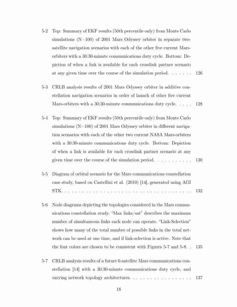
5-2 Top: Summary of EKF results (50th percentile only) from Monte Carlo
simulations (N=100) of 2001 Mars Odyssey orbiter in separate two-
satellite navigation scenarios with each of the other five current Mars-
orbiters with a 30:30-minute communications duty cycle. Bottom: De-
piction of when a link is available for each crosslink partner scenario
at any given time over the course of the simulation period. . . . . . . 126
5-3 CRLB analysis results of 2001 Mars Odyssey orbiter in additive con-
stellation navigation scenarios in order of launch of other five current
Mars-orbiters with a 30:30-minute communications duty cycle. . . . . 128
5-4 Top: Summary of EKF results (50th percentile only) from Monte Carlo
simulations (N=100) of 2001 Mars Odyssey orbiter in different naviga-
tion scenarios with each of the other two current NASA Mars-orbiters
with a 30:30-minute communications duty cycle. Bottom: Depiction
of when a link is available for each crosslink partner scenario at any
given time over the course of the simulation period. . . . . . . . . . . 130
5-5 Diagram of orbital scenario for the Mars communications constellation
case study, based on Castellini et al. (2010) [14], generated using AGI
STK. . . . . . . . . . . . . . . . . . . . . . . . . . . . . . . . . . . . . 132
5-6 Node diagrams depicting the topologies considered in the Mars commu-
nications constellation study. “Max links/sat” describes the maximum
number of simultaneous links each node can operate. “Link-Selection”
shows how many of the total number of possible links in the total net-
work can be used at one time, and if link-selection is active. Note that
the font colors are chosen to be consistent with Figures 5-7 and 5-8. . 135
5-7 CRLB analysis results of a future 6-satellite Mars communications con-
stellation [14] with a 30:30-minute communications duty cycle, and
varying network topology architectures. . . . . . . . . . . . . . . . . . 137
18
5-8 Summary of EKF results (50th percentile only) from Monte Carlo sim-
ulations (N=100) of a future 6-satellite Mars communications constel-
lation [14] with a 30:30-minute communications duty cycle, and varying
network topology architectures. . . . . . . . . . . . . . . . . . . . . . 139
5-9 Summary of EKF results (50th percentile over 100 Monte Carlo simu-
lations) for satellites from the Mars-orbiters and Mars communications
constellation case studies. . . . . . . . . . . . . . . . . . . . . . . . . 141
19

THIS PAGE INTENTIONALLY LEFT BLANK
20
List of Tables
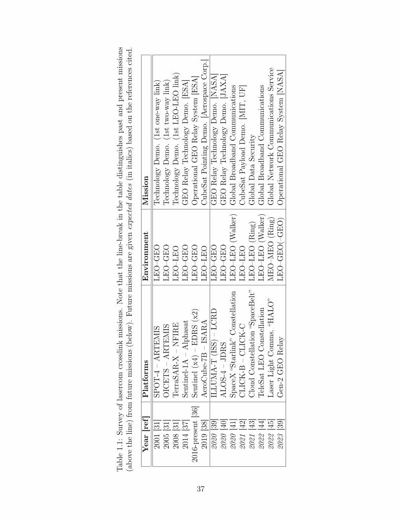
1.1 Survey of lasercom crosslink missions. Note that the line-break in the
table distinguishes past and present missions (above the line) from
future missions (below). Future missions are given expected dates (in
italics) based on the references cited. . . . . . . . . . . . . . . . . . . 37
2.1 Review of previous studies in autonomous navigation using intersatel-
lite measurements. Values in bold indicate those that fit the objective
criteria of this thesis. . . . . . . . . . . . . . . . . . . . . . . . . . . . 52
3.1 Orbital parameters for GEO-LEO example scenario. . . . . . . . . . . 59
3.2 STK settings as used to producing “truth” data for all simulations. . . 60
3.3 Central-body constants used in dynamics model, taken directly from
STK gravity model files. . . . . . . . . . . . . . . . . . . . . . . . . . 71
3.4 Input parameters and values tested for sensitivity in simulation ap-
proach. Note that the values selected for use in this thesis are shown
in bold. . . . . . . . . . . . . . . . . . . . . . . . . . . . . . . . . . . 83
3.5 Overview of case studies considered in this thesis. . . . . . . . . . . . 88
4.1 Orbital parameters for GEO-Relay scenario. . . . . . . . . . . . . . . 91
4.2 Orbital parameters for simulated near-Earth orbiters in parameter-
sweep analysis, valid at time of epoch 𝑡𝑒 = 𝑡0. . . . . . . . . . . . . . 91
4.3 Orbital parameters for simulated GEO-Relay satellites, modeled off of
the orbital parameters of EDRS-C, valid at time of epoch 𝑡𝑒 = 𝑡0. . . 92
4.4 Orbital parameters for LEO-LEO scenario. . . . . . . . . . . . . . . . 108
21
4.5 Walker constellation configurations at 𝑎=7445.83 km, 𝑒=0, and 𝑖=60∘. 116
5.1 Orbital parameters for considered Mars-orbiter missions. Note that 𝑅
= 3,396 km for Mars. . . . . . . . . . . . . . . . . . . . . . . . . . . . 125
5.2 Orbital parameters for Mars communications constellation, as pro-
posed by Castellini et al. (2010). . . . . . . . . . . . . . . . . . . . . 133
5.3 Network architectures used in Mars communications constellation study.134
5.4 “One-to-one” case network map, implemented as “network rules” in
Link-Selection framework. . . . . . . . . . . . . . . . . . . . . . . . . 135
22
Nomenclature
Symbols
𝛼 Right-ascension angle
𝛿 Declination angle
𝜆 Longitude
𝜇 Standard gravitational parameter
𝜈 True anomaly
Ω Right-ascension of the ascending node
𝜔 Argument of periapsis
𝜑 Azimuth angle
𝜌 Range, or distance
𝜎 Uncertainty/noise
𝜃 Elevation angle
𝑎 Semi-major axis
𝑒 Eccentricity
ℎ Height, or altitude
𝑖 Inclination
23
𝐽2 Dynamic oblateness, the gravity model spherical harmonic coefficient
of degree 2 and order 0
𝑀 Mean anomaly
𝑛 Mean motion
𝑅 Equatorial radius
𝑇 Duration of time
𝑡 Time
Satellite Missions
ARTEMIS Advanced Relay and Technology Mission Satellite (ESA)
EDRS-A First EDRS payload (ESA), on Eutelsat-9B
EDRS-C Second EDRS payload (ESA), on dedicated satellite of same name
LADEE Lunar Atmosphere and Dust Environment Explorer (NASA)
LCRD Laser Communications Relay Demonstration (NASA), on STPSat-6
LLCD Lunar Laser Communications Demonstration (NASA)
MAVEN Mars Atmosphere and Volatile Evolution orbiter (NASA)
MEX Mars Express orbiter (ESA)
MMS Magnetospheric Multiscale (NASA)
MO 2001 Mars Odyssey orbiter (NASA)
MOM Mars Orbiter Mission (ISRO), also called “Mangalyaan” which trans-
lates to “Mars-craft” in English
MRO Mars Reconnaissance Orbiter (NASA)
24
NFIRE Near Field Infrared Experiment satellite (DoD)
OICETS Optical Inter-orbit Communications Engineering Test Satellite (JAXA),
also called “Kirari” which translates to “glitter” or “twinkle” in English
STPSat-6 Space Test Program Satellite-6 (DoD)
TGO ExoMars Trace Gas Orbiter (ESA/Roscosmos)
TSX TerraSAR-X satellite (DLR)
Agencies & Organizations
AGI Analytical Graphics, Inc. (U.S. company)
CNES Centre National D’Etudes Spatiales (France), which translates to “Na-
tional Center for Space Studies” in English
CSpOC Combined Space Operations Center (DoD), formerly JSpOC
DLR Deutsches Zentrum für Luft- und Raumfahrt (Germany), which tran-
lates to “German Center for Aviation and Space Flight” in English
DoD Department of Defense (U.S.A.)
ESA European Space Agency (22 member states)
ISRO Indian Space Research Organisation (India)
JAXA Japan Aerospace Exploration Agency (Japan)
JPL Jet Propulsion Laboratory (NASA)
NASA National Aeronautics and Space Administration (U.S.A.)
NGA National Geospatial-Intelligence Agency (DoD)
NORAD North American Aerospace Defense Command (U.S.A./Canada)
25
Roscosmos State Corporation for Space Activities (Russia)
Official Programs, Products, or Technologies
DIODE DORIS Immediate Orbit Determination (CNES)
DORIS Doppler Orbitography and Radiopositioning Integrated by Satellite
(CNES)
DSAC Deep Space Atomic Clock (JPL)
DSN Deep Space Network (NASA)
DSOC Deep Space Optical Communications (NASA)
EDRS European Data Relay System (ESA)
EGM2008 2008 Earth Gravitational Model (NGA)
GNSS Global Navigation Satellite System
HORIZONS On-line solar system data and ephemeris computation service (JPL)
HPOP High-Precision Orbit Propagator (AGI)
IGS International GNSS Service
MRO110C 2012 Mars gravity model with MRO data, to degree & order 110 (JPL)
STK Systems Took Kit (AGI)
Other Abbreviations
ADC Attitude determination and control
C&DH Command and data-handling
CRLB Cramér-Rao lower bound
26
DDOR Delta differential one-way ranging
DF Dual-frequency
DOR Differential one-way ranging
DTE Direct-to-Earth communication
EHS Earth horizon sensor
EKF Extended Kalman filter
FSOC Free-space optical communication
GEO Geosynchronous orbit
GSO Geostationary orbit
HEO Highly-elliptical orbit
ISL Intersatellite links
KF Kalman filter
Lasercom Laser communication
LEO Low Earth orbit
MEO Medium Earth orbit
OD Orbit determination
ODE Ordinary differential equation
OpNav Optical navigation
PF Particle filter
PNT Positioning, navigation, and timing
POD Precise orbit determination
27
RF Radio frequency
RMSE Root-mean-square error
RTN Radial, tangential/transverse, normal reference frame
SAR Synthetic aperture radar
SF Single-frequency
SLR Satellite laser ranging
SRIF Square-root information filter
SS Sun sensor
SSO Sun-synchronous orbit
ST Star tracker
SWaP Size, weight, and power
TLE Two-line element set
TT&C Tracking, telemetry, and command
UHF Ultra-high frequency
UKF Unscented Kalman filter
UTC Primary world time standard, known as “Coordinated Universal Time"
in English and “Temps Universel Coordonné” in French
VLBI Very-long baseline interferometry
XNAV X-ray pulsar-based navigation and timing
28
Chapter 1
Introduction
1.1 Motivation
The satellite industry is undergoing a shift towards smaller and more affordable space-
craft that can take advantage of reduced cost to launch [15]. This trend is ushering in
new distributed satellite architectures to address critical mission areas. For example,
Planet Labs Inc. has achieved unprecedented Earth imaging data with their 175+
small-satellite constellation providing global coverage and rapid revisits [16]. Beyond
Earth, NASA JPL successfully demonstrated the first interplanetary CubeSats as
technology demonstrators of a “carry-your-own-relay” concept, launching two MarCO
spacecraft alongside the InSight Mars lander spacecraft specifically for the purpose
of relaying data during InSight’s critical landing sequence back to Earth [17].
Distributed architectures, however, come with a fair share of challenges. Though
satellite development and manufacturing should benefit from the economy of scale,
the same cannot yet be said for ground operations. Typical satellite operations for
monitoring vehicle health and status, data processing, orbit determination, task plan-
ning and scheduling, and fault response are handled by teams of people per satellite.
The brute-force method of handling the operations of many satellites would be build-
ing more ground stations and training more staff, thus resulting in greater cost and
higher risk/complexity across a global system.
Another way to tackle concerns in operating large numbers of satellites is to de-
29
velop higher levels of autonomy within the satellite system. Tasks typically performed
by an operator and/or ground station could be shared with or fully performed by
the spacecraft. Examples include planning and scheduling tasks to meet multiple
objectives (e.g., maximizing data return while minimizing latency) [18], on-board
data-processing to identify issues [19] or deliver data products more quickly [20], and
open-loop instrument operation to obtain higher-quality data (e.g., changing sensing
configurations based on geolocation or features identified in the sensor data) [8].
In order to achieve higher levels of autonomous operations, satellites should be
able to precisely estimate their position and velocity states in real-time. Many ad-
dress orbit determination and navigation using Global Navigation Satellite Systems
(GNSS). GNSS-based navigation has become more widely used as receivers and an-
tennas have become more volume- and cost-effective, as they have shown the ability
to provide sub-meter positioning accuracy for low Earth orbit (LEO) objects. How-
ever, achieving those small errors is highly dependent on regular or continuous receipt
of ultra-rapid ephemerides and clock products from the International GNSS Service
(IGS) [7]. GNSS-equipped LEO satellites more commonly achieve real-time naviga-
tion solutions on the order of 5 meters [21]. Missions in higher altitude orbits see
further degraded performance as the primary service volume currently ends at 3,000
km in altitude [22].
Certain missions and applications require an alternative and enhanced autonomous
navigation solution to GNSS. Military satellite applications may require redundancy
in order to continue operations in potential GNSS-denied environments. Missions
operating at high altitudes or orbiting other bodies (e.g., the moon or Mars) are not
able to rely on GNSS-like navigation without additional relay/navigation satellite
infrastructure.
The purpose of this thesis is to demonstrate an autonomous navigation method
leveraging the distribution and potential connectivity of satellites in a constellation
architecture to provide an alternative and enhanced navigation solution to GNSS
for Earth-orbit and DSN for deep-space orbital missions. Section 1.2 provides an
overview of the topics of satellite navigation methods, intersatellite links, and laser
30
communications in satellite systems. Section 1.3 summarizes the research objectives
and contributions contained in this thesis.
1.2 Context
1.2.1 Satellite Navigation
The field of satellite navigation can be divided into two categories: (1) traditional
methods of precise orbit determination (POD) using ground-sensors, and (2) au-
tonomous methods using on-board sensors and navigational references. Autonomous
navigation can be further separated into fully-autonomous methods, which are com-
pletely independent of man-made or ground-based resources, and semi-autonomous
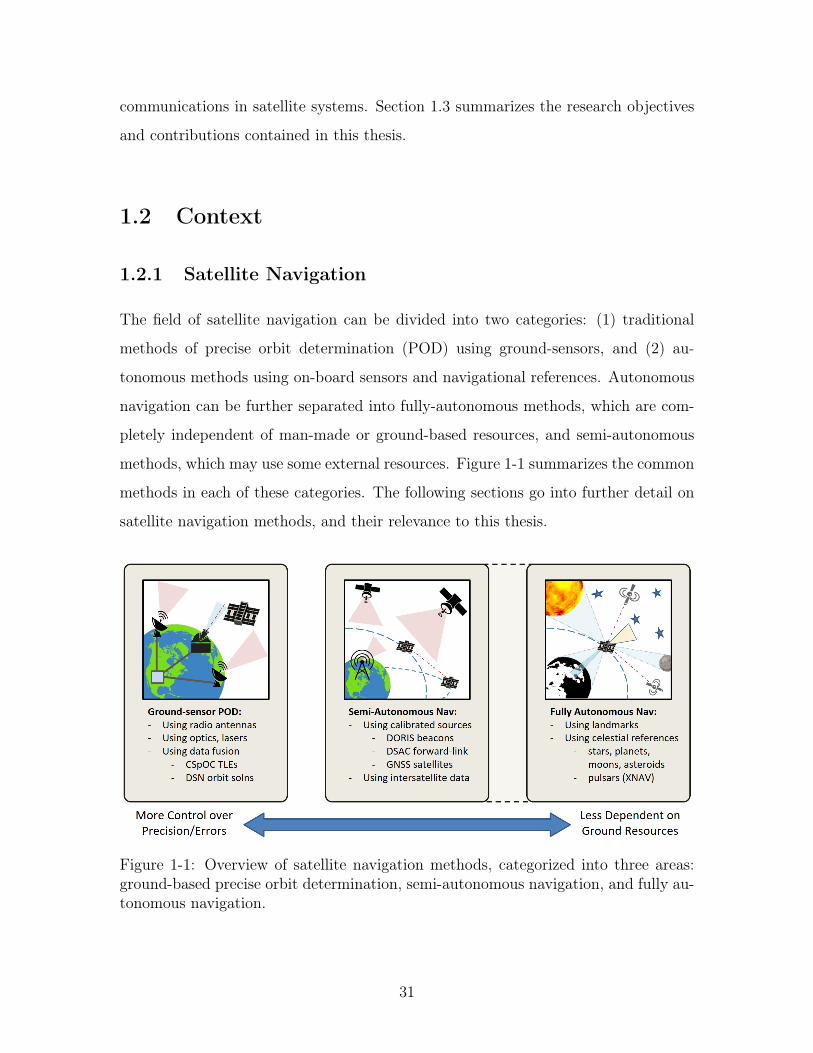
methods, which may use some external resources. Figure 1-1 summarizes the common
methods in each of these categories. The following sections go into further detail on
satellite navigation methods, and their relevance to this thesis.
Figure 1-1: Overview of satellite navigation methods, categorized into three areas:ground-based precise orbit determination, semi-autonomous navigation, and fully au-tonomous navigation.
31
Traditional Methods
Traditional methods of satellite orbit determination involve the use of ground-based
sensors to track satellites and collect measurements, such as radars for range and
range-rate, and telescopes for bearing angles [1, 3, 4]. This data is then processed in
a filtering algorithm to estimate the six-element state of the satellite, in the form of
either classical Keplerian elements such as (𝑎, 𝑒, 𝑖, Ω, 𝜔, 𝜈) or 3-dimensional position
and velocity (𝑥, 𝑦, 𝑧, , , ).
The U.S. Combined Space Operations Center (CSpOC) tracks all satellites using
a global network of radar and optical sensors, and publishes estimated state results
in the form of two-line element sets (TLEs) for general public use. While this is
useful state information for propagation forward or backward in time, performance
is limited and degrades over time since the TLE epoch [23]. CSpOC’s published
TLE data is also prone to errors if/when satellites are in close proximity (e.g., when
multiple satellites are inserted into the same orbit around the same time) [24].
Autonomous Methods
To mitigate reliance on TLEs or building additional networks of ground sensors,
several methods of autonomous navigation have been proposed and used over the
last few decades. Autonomous navigation refers to satellites performing on-board,
real-time navigation without external input. Such methods allow for reduced cost
and risk in ground operations by eliminating the computational and logistical load of
regularly tracking the satellites, estimating their individual states, and transmitting
the solutions to the spacecraft [25, 26].
Fully autonomous navigation is performed without any external input, only us-
ing the sensors and instruments on-board the spacecraft. Multiple techniques exist
using some combination of sensors, such as cameras and infrared sensors (which can
estimate state with respect to known reference points or landmarks) [13], magne-
tometers (which can estimate state with respect to a known magnetic field) [12], and
X-ray detectors (which can estimate state with respect to known pulsars) [10]. Semi-
32
autonomous navigation is also performed using sensors and instruments on-board the
spacecraft, but with some external input. This includes any observations made with
respect to another man-made object, such as another satellite, a ground station, or a
beacon. All satellite navigation using a Global Navigation Satellite System (GNSS)
receiver is considered semi-autonomous, since it uses signals from a man-made source
[27].
Figure 1-2 illustrates orders of magnitude of position errors demonstrated using
several different techniques of precise orbit determination and autonomous navigation.
Only two satellite payloads have demonstrated sub-meter real-time navigation accu-
racy: GNSS receivers and DORIS/DIODE. DORIS/DIODE is a positioning method
developed by the French space agency, CNES, that relies on ground beacons trans-
mitting to the DORIS receiver onboard the satellite [5]. Orbit determination software
specially developed to process the DORIS data (DIODE) is used to generate naviga-
tion solutions on the order of centimeters, however this has only been demonstrated
for low-altitude satellites in circular orbits [28].
Since the objective of this thesis is to provide an alternative navigation method
to GNSS, other methods are investigated. The fully autonomous methods shown
in Figure 1-2 are only capable of providing solutions on the order of 10s-100s of
meters, and utilize sensors that are heavily dependent on orbit conditions and well-
characterized references. For instance, magnetometers and landmark-based sensors
will likely lose sensing observability at higher altitudes; plus magnetic field models
and well-characterized landmarks cannot be readily assumed for other central-bodies.
The semi-autonomous navigation method using intersatellite data shows promise
for use in distributed constellations. Intersatellite data refers to measurements of
relative range, range-rate, or angles between two spacecraft. Previous work has found
the intersatellite autonomous navigation method to be accurate on the order of 10s
of meters [9, 11], which is better than the fully autonomous methods and resembles
the performance of single-frequency GNSS receivers, though results have not yet been
experimentally demonstrated on-orbit. Still, the promise of the intersatellite method
to this thesis is realized in its independence of the orbit configuration of either satellite,
33
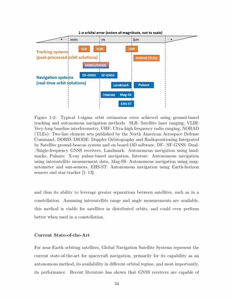
Figure 1-2: Typical 1-sigma orbit estimation error achieved using ground-basedtracking and autonomous navigation methods. SLR: Satellite laser ranging, VLBI:Very-long baseline interferometry, UHF: Ultra-high frequency radio ranging, NORAD(TLEs): Two-line element sets published by the North American Aerospace DefenseCommand, DORIS/DIODE: Doppler Orbitography and Radiopositioning Integratedby Satellite ground-beacon system and on-board OD software, DF-/SF-GNSS: Dual-/Single-frequency GNSS receivers, Landmark: Autonomous navigation using land-marks, Pulsars: X-ray pulsar-based navigation, Intersat: Autonomous navigationusing intersatellite measurement data, Mag-SS: Autonomous navigation using mag-netometer and sun-sensors, EHS-ST: Autonomous navigation using Earth-horizonsensors and star-tracker [1–13].
and thus its ability to leverage greater separations between satellites, such as in a
constellation. Assuming intersatellite range and angle measurements are available,
this method is viable for satellites in distributed orbits, and could even perform
better when used in a constellation.
Current State-of-the-Art
For near-Earth orbiting satellites, Global Navigation Satellite Systems represent the
current state-of-the-art for spacecraft navigation, primarily for its capability as an
autonomous method, its availability in different orbital regime, and most importantly,
its performance. Recent literature has shown that GNSS receivers are capable of
34
achieving solution errors on the order of 3-5 meters in low Earth orbit (LEO) [21]. A
few missions have also been used to test GNSS receivers at altitudes greater than the
constellation altitude, and have admirably shown solution errors on the order of 12-15
meters in geosynchronous orbit (GEO) [29], and 25-65 meters in highly eccentric orbit
(HEO) [22].
For deep-space applications, the Deep Space Network of tracking stations rep-
resents the current state-of-the-art for spacecraft navigation, capable of navigation
accuracy (for Mars-orbiters) down to 25 meters during periods of DSN downlink, and
100 meters during periods without downlink [30].
These navigation performance values are used to generate performance targets for
the intersatellite navigation method using lasercom crosslinks. In each case, we set
a threshold to which we will compare the results of different orbital scenarios in this
thesis. These are 3 meters for LEO, 12 meters in GEO, 45 meters in HEO, and 25
meters in Mars-orbit.
1.2.2 Crosslink Communications
Intersatellite measurements may easily be made if the constellation is designed for
crosslink communications, also known as intersatellite links (ISLs). One benefit of
implementing crosslinks in a satellite system is increasing ground access for space-
craft tracking, telemetry, and command (TT&C) operations without needing to add
more ground stations. For communications and Earth-observing missions, crosslinks
can also serve to increase data-to-ground by mitigating downlink bottlenecks and re-
ducing latency between terminals [18, 31]. For Positioning, Navigation, and Timing
(PNT) missions, crosslinks are used to improve the quality of the PNT information,
increase system reliability and robustness, and enhance availability to higher alti-
tude orbits [32, 33]. In addition to intersatellite measurements, crosslinks also enable
other new capabilities in satellite systems, such as distributed processing, and new
methods of navigation or formation-control by communicating measurements or state
estimates between vehicles [34]. A number of previous studies make the assumption
that intersatellite links exist in future constellation systems, and can be leveraged for
35
autonomous navigation. A more detailed review of previous work can be found in
Section 2.2. This thesis also assumes the existence of crosslinks for use in autonomous
navigation.
Lasercom Links
Lasercom provides improved energy efficiency, data rates, latency, and security com-
pared with traditional radio-frequency (RF) communications systems [35]. Muri and
McNair (2012) performed a survey of all intersatellite link demonstrations until 2012
as well as those that were expected to launch through 2015 [31]. Since the time of Muri
and McNair (2012), there has been an notable uptick in the number of launched and
proposed missions to utilize optical ISLs, as shown in Table 1.1. Recent years have
seen multiple European Data Relay Satellite (EDRS) systems launched into GEO for
the purpose of quickly and efficiently relaying critical Earth-observation data from
ESA’s Copernicus/Sentinel satellites to ground [36]. The upcoming slate includes
similar relay technology demonstrators from JAXA, NASA, and Airbus.
36
Tabl
e1.
1:Su
rvey
ofla
serc
omcr
ossl
ink
mis
sion
s.N
ote
that
the
line-
brea
kin
the
tabl
edi
stin
guis
hes
past
and
pres
ent
mis
sion
s(a
bove
the
line)
from
futu
rem
issi
ons
(bel
ow).
Futu
rem
issi
ons
are
give
nex
pect
edda
tes
(in
ital
ics)
base
don
the
refe
renc
esci
ted.
Yea
r[r
ef]
Pla
tfor
ms
Env
iron
men
tM
issi
on20
01[3
1]SP
OT
-4–
ART
EM
ISLE
O–G
EO
Tech
nolo
gyD
emo.
(1st
one-
way
link)
2005
[31]
OIC
ET
S–
ART
EM
ISLE
O–G
EO
Tech
nolo
gyD
emo.
(1st
two-
way
link)
2008
[31]
Terr
aSA
R-X
–N
FIR
ELE
O–L
EO
Tech
nolo
gyD
emo.
(1st
LEO
-LE
Olin
k)20
14[3
7]Se
ntin
el-1
A–
Alp
hasa
tLE
O–G
EO
GE
OR
elay
Tech
nolo
gyD
emo.
[ESA
]20
16-p
rese
nt[3
6]Se
ntin
el(x
4)–
ED
RS
(x2)
LEO
–GE
OO
pera
tion
alG
EO
Rel
aySy
stem
[ESA
]20
19[3
8]A
eroC
ube-
7B–
ISA
RA
LEO
–LE
OC
ubeS
atPoi
ntin
gD
emo.
[Aer
ospa
ceC
orp.
]20
20[3
9]IL
LUM
A-T
(ISS
)–
LCR
DLE
O–G
EO
GE
OR
elay
Tech
nolo
gyD
emo.
[NA
SA]
2020
[40]
ALO
S-4
–JD
RS
LEO
–GE
OG
EO
Rel
ayTe
chno
logy
Dem
o.[J
AX
A]
2020
[41]
Spac
eX“S
tarl
ink”
Con
stel
lati
onLE
O–L
EO
(Wal
ker)
Glo
balB
road
band
Com
mun
icat
ions
2021
[42]
CLI
CK
-B–
CLI
CK
-CLE
O–L
EO
Cub
eSat
Pay
load
Dem
o.[M
IT,U
F]
2021
[43]
Clo
udC
onst
ella
tion
“Spa
ceB
elt”
LEO
–LE
O(R
ing)
Glo
balD
ata
Secu
rity
2022
[44]
Tele
Sat
LEO
Con
stel
lati
onLE
O–L
EO
(Wal
ker)
Glo
balB
road
band
Com
mun
icat
ions
2022
[45]
Lase
rLi
ght
Com
ms.
“HA
LO”
ME
O–M
EO
(Rin
g)G
loba
lNet
wor
kC
omm
unic
atio
nsSe
rvic
e20
23[3
9]G
en-2
GE
OR
elay
LEO
–GE
O(–
GE
O)
Ope
rati
onal
GE
OR
elay
Syst
em[N
ASA
]
37
McCandless and Martin-Mur (2016) also investigated a future DSN-like network
using optical communications systems and performed simulations to compare position
accuracy with the current capability of DSN radiometric tracking for a future Mars
lander and Mars orbiter. The authors concluded that optical tracking stations could
feasibly be an improvement over the current radiometric capability [30].
This thesis builds on the notion of using lasercom systems for crosslinks in order
to collect intersatellite data measurements for autonomous navigation.
1.3 Thesis Overview
In order to measure intersatellite range and bearing between satellites in a constel-
lation, we propose using lasercom crosslinks, expanding on the concept studied by
Yong et al. (1983) [46]. Figure 1-3 provides a depiction of our proposed method.
Time-of-flight ranging measurements can be captured using time-embedded sig-
nals over communications links [47]. Laser communications payloads operate at op-
tical wavelengths with greater frequency bandwidth than RF systems. The higher
bandwidth enables lasercom systems to measure range between two terminals with
more precision. RF systems typically achieve meter-level ranging precision [48].
Lasercom systems can achieve centimeter-level precision; the current state-of-the-art
performance in satellite lasercom ranging was demonstrated to about 1-cm precision
in two-way links from Earth to lunar orbit during the Lunar Laser Communication
Demonstration (LLCD) mission in 2015 [49]. However, this was a ground-to-satellite
demonstration, not satellite-to-satellite.
When compared to RF systems, intersatellite lasercom systems have narrow beamwidths,
typically less than 1 degree [42]. In order to point the narrow beam signal directly at
the receiving terminal, lasercom demands highly accurate pointing systems, which can
be leveraged to obtain the bearing between the two satellites. Assuming a lasercom
crosslink can be established between two satellites, we propose deriving intersatellite
bearing by determining the body attitude of the spacecraft using an on-board star
tracker, using any angular offsets between boresights of the lasercom transceiver and
38
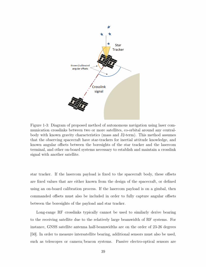
Figure 1-3: Diagram of proposed method of autonomous navigation using laser com-munication crosslinks between two or more satellites, co-orbital around any central-body with known gravity characteristics (mass and J2-term). This method assumesthat the observing spacecraft have star-trackers for inertial attitude knowledge, andknown angular offsets between the boresights of the star tracker and the lasercomterminal, and other on-board systems necessary to establish and maintain a crosslinksignal with another satellite.
star tracker. If the lasercom payload is fixed to the spacecraft body, these offsets
are fixed values that are either known from the design of the spacecraft, or defined
using an on-board calibration process. If the lasercom payload is on a gimbal, then
commanded offsets must also be included in order to fully capture angular offsets
between the boresights of the payload and star tracker.
Long-range RF crosslinks typically cannot be used to similarly derive bearing
to the receiving satellite due to the relatively large beamwidth of RF systems. For
instance, GNSS satellite antenna half-beamwidths are on the order of 23-26 degrees
[50]. In order to measure intersatellite bearing, additional sensors must also be used,
such as telescopes or camera/beacon systems. Passive electro-optical sensors are
39
limited by observability constraints that effectively limit the separation between the
two satellites in which bearing can be measured. For example, cameras are affected
by apparent magnitude and proper illumination of the other spacecraft [48], and can
only work for separations of a few hundreds of kilometers between satellites. Active
sensors, such as beacon systems, can be used for longer ranges [51, 52]. Lasercom
crosslinks can be considered a form of an active electro-optical system, capable of
working over longer ranges [38, 42].
For this study, we assume that all satellites have at least one lasercom termi-
nal, with parameters consistent with those offered by commercial companies [53] or
currently being developed [42], along with the accompanying subsystems for power,
attitude determination and control (ADC), and command & data handling (C&DH).
These systems must operate together in order to establish and maintain a lasercom
crosslink between two communicating spacecraft. We assume that crosslinks are es-
tablished using methods such as performing a scanning maneuver or implementing a
coarse beacon system [42].
1.3.1 Research Contributions
The three contributions in this thesis are:
∙ Creation of a simulation framework to estimate the performance of autonomous
navigation methods using intersatellite measurements for varying orbital envi-
ronments, satellite constellations, sensor network configurations, and measure-
ment models. This includes a kinematic uncertainty approximation algorithm
using Cramér Rao lower bound (CRLB) covariance estimates as a link selection
heuristic when multiple links are available.
∙ Analysis of the navigation performance over relevant past, present, and future
crosslinked satellite missions to demonstrate the method’s applicability to both
near Earth and deep space environments, including assessment of lasercom in-
terconnectivity on constellation navigation.
40
∙ Demonstration of improved navigation performance using autonomous laser-
com crosslinks over current spacecraft navigation techniques (GNSS for Earth
orbiters, DSN for deep space) with median total position errors (from Monte
Carlo simulations) better than 3 meters for LEO, 12 meters for GEO, 45 meters
for HEO, and 25 meters for Mars orbiters.
1.3.2 Organization
Chapter 2 contains background in spacecraft navigation and a review of previous
literature in the area of intersatellite navigation with the goal of identifying research
gaps to be addressed by the work in this thesis. Chapter 3 describes the simulation
approach, and Chapters 4 and 5 present the results of simulations in Earth-orbiting
and Mars-orbiting applications, respectively. Chapter 6 summarizes the contributions
and conclusions made in this thesis.
41

THIS PAGE INTENTIONALLY LEFT BLANK
42
Chapter 2
Background & Literature Review
This chapter provides a high-level review of traditional spacecraft navigation esti-
mators and measurements, then performs a deeper analysis of previous work in au-
tonomous navigation using intersatellite measurements in order to identify research
gaps and highlight relevant insights towards achieving the objectives of this thesis.
2.1 Spacecraft Navigation Methodology
Spacecraft navigation estimation relies on using a time-series of measurements to
estimate observables that are directly influenced by the gravitational forces existing
in the space environment. This section describes commonly used estimation methods
and measurements for spacecraft navigation.
2.1.1 Estimation Methods
State estimation can either be done by considering measurements all-at-once (a batch
process) or as each measurement is made (a sequential process). Batch processes rep-
resent the traditional methods for determining post-processed orbit solutions. Sequen-
tial processes represent filtering methods that can be used for real-time navigation
solutions.
43
Batch Least-Squares Processing
Least-squares estimation is a commonly used method for approximating the values
of unknown parameters that best-fit the input data based on an expected model of
behavior. The term “least-squares” refers to the objective of minimizing the sum of
the square of the difference between an observed value and an expected value based
on the model. This is captured by the following equation:
x = (H𝑇H)−1H𝑇y (2.1)
where x is the estimated state, and H is the measurement model that describes the
relationship between the state vector, x, and the measurements, y. For a nonlinear,
differentiable measurement model function ℎ(x) and measurement noise v:
y = ℎ(x) + v (2.2)
the following Jacobian can be calculated to linearize the model at each measurement
time-step:
H =𝜕ℎ
𝜕x(2.3)
Sequential Kalman Filtering
The Kalman Filter (KF) is an optimal estimator for linear Gaussian systems. As a
method of sequential processing, it is commonly used for real-time navigation solu-
tions. The filter is divided into two phases, the prediction phase, which propagates
the most recent state estimate and covariance to the current time-step, and the up-
date phase, which uses any available measurements at the current time-step to update
the predicted state estimate and covariance.
The dynamics model (or state-transition model) F𝑘 is described by:
x𝑘 = F𝑘x𝑘−1 + w𝑘 (2.4)
where x𝑘 are the state variables to be estimated at each filter step 𝑘 ∈ 1, · · · , 𝑁,
44
and w𝑘 is the process noise with normal distribution and covariance Q𝑘.
The measurement model is described by:
y𝑘 = H𝑘x𝑘 + v𝑘 (2.5)
where y𝑘 are the measurements observed at each filter step 𝑘 ∈ 1, · · · , 𝑁, and v𝑘
is the measurement noise with normal distribution and covariance R𝑘.
The prediction phase is:
x𝑘|𝑘−1 = F𝑘x𝑘−1 (2.6)
P𝑘|𝑘−1 = F𝑘P𝑘−1F𝑇𝑘 + Q𝑘 (2.7)
where x0 and P0 reflect the a priori knowledge of the initial state and covariance
values.
The update phase is:
x𝑘 = x𝑘|𝑘−1 + K𝑘[y𝑘 −H𝑘x𝑘|𝑘−1] (2.8)
P𝑘 = (I−K𝑘H𝑘)P𝑘|𝑘−1 (2.9)
where K𝑘 is the Kalman gain:
K𝑘 = P𝑘|𝑘−1H𝑇𝑘 (H𝑘P𝑘|𝑘−1H
𝑇𝑘 + R𝑘)−1 (2.10)
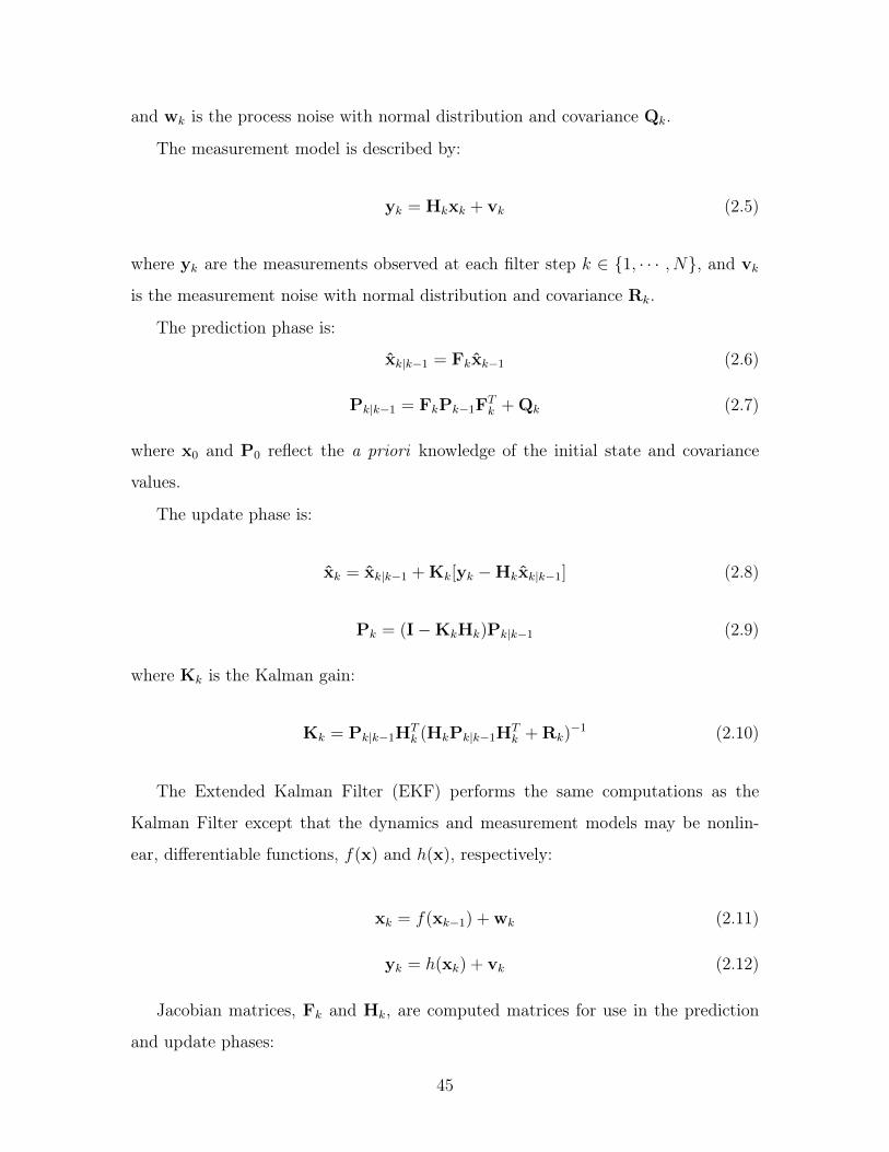
The Extended Kalman Filter (EKF) performs the same computations as the
Kalman Filter except that the dynamics and measurement models may be nonlin-
ear, differentiable functions, 𝑓(x) and ℎ(x), respectively:
x𝑘 = 𝑓(x𝑘−1) + w𝑘 (2.11)
y𝑘 = ℎ(x𝑘) + v𝑘 (2.12)
Jacobian matrices, F𝑘 and H𝑘, are computed matrices for use in the prediction
and update phases:
45
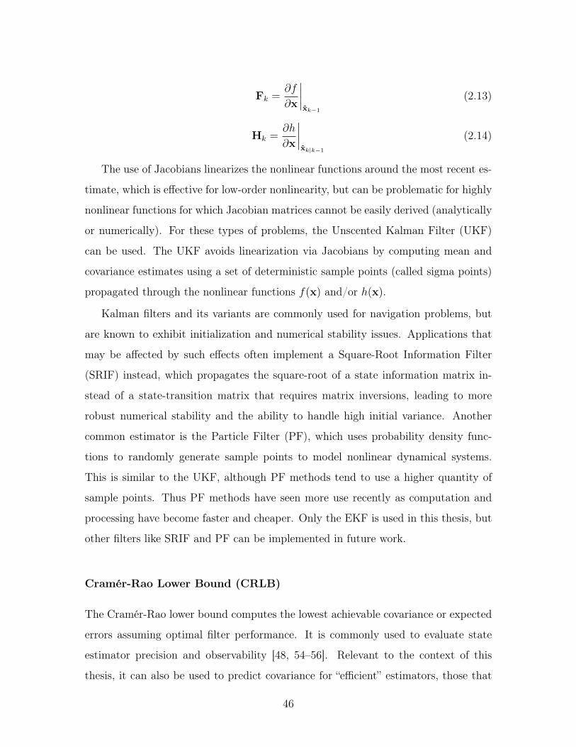
F𝑘 =𝜕𝑓
𝜕x
x𝑘−1
(2.13)
H𝑘 =𝜕ℎ
𝜕x
x𝑘|𝑘−1
(2.14)
The use of Jacobians linearizes the nonlinear functions around the most recent es-
timate, which is effective for low-order nonlinearity, but can be problematic for highly
nonlinear functions for which Jacobian matrices cannot be easily derived (analytically
or numerically). For these types of problems, the Unscented Kalman Filter (UKF)
can be used. The UKF avoids linearization via Jacobians by computing mean and
covariance estimates using a set of deterministic sample points (called sigma points)
propagated through the nonlinear functions 𝑓(x) and/or ℎ(x).
Kalman filters and its variants are commonly used for navigation problems, but
are known to exhibit initialization and numerical stability issues. Applications that
may be affected by such effects often implement a Square-Root Information Filter
(SRIF) instead, which propagates the square-root of a state information matrix in-
stead of a state-transition matrix that requires matrix inversions, leading to more
robust numerical stability and the ability to handle high initial variance. Another
common estimator is the Particle Filter (PF), which uses probability density func-
tions to randomly generate sample points to model nonlinear dynamical systems.
This is similar to the UKF, although PF methods tend to use a higher quantity of
sample points. Thus PF methods have seen more use recently as computation and
processing have become faster and cheaper. Only the EKF is used in this thesis, but
other filters like SRIF and PF can be implemented in future work.
Cramér-Rao Lower Bound (CRLB)
The Cramér-Rao lower bound computes the lowest achievable covariance or expected
errors assuming optimal filter performance. It is commonly used to evaluate state
estimator precision and observability [48, 54–56]. Relevant to the context of this
thesis, it can also be used to predict covariance for “efficient” estimators, those that
46
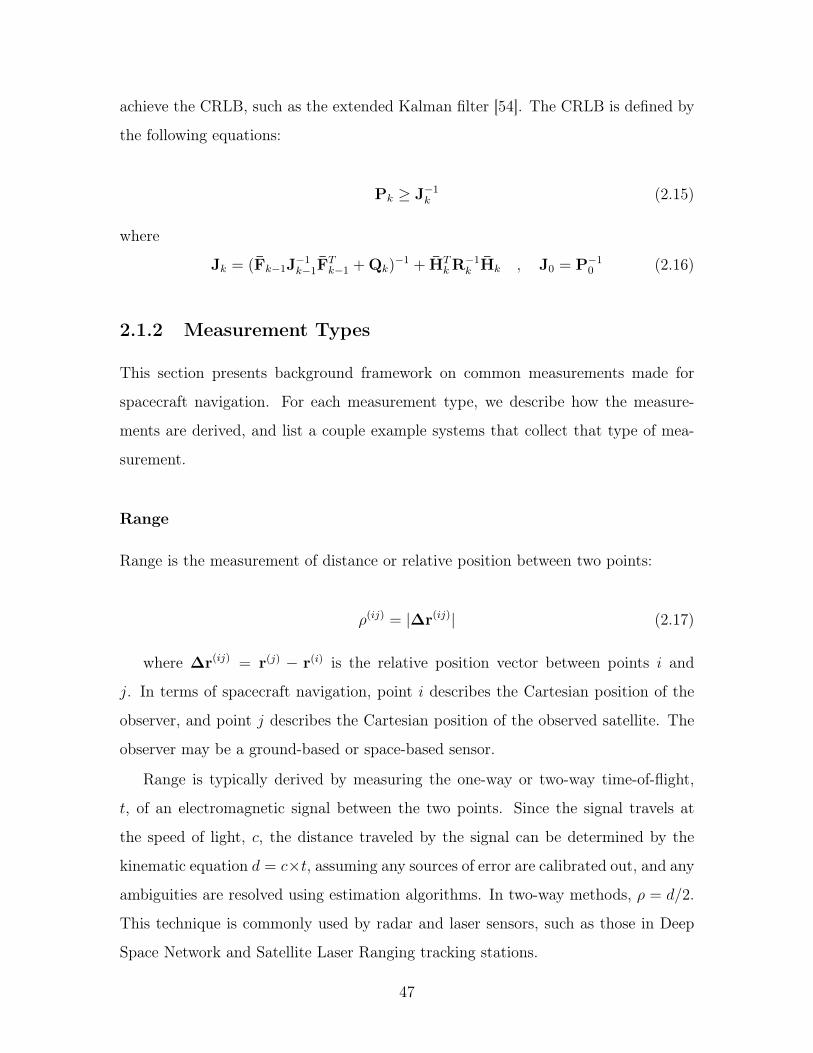
achieve the CRLB, such as the extended Kalman filter [54]. The CRLB is defined by
the following equations:
P𝑘 ≥ J−1𝑘 (2.15)
where
J𝑘 = (F𝑘−1J−1𝑘−1F
𝑇𝑘−1 + Q𝑘)−1 + H𝑇
𝑘R−1𝑘 H𝑘 , J0 = P−1
0 (2.16)
2.1.2 Measurement Types
This section presents background framework on common measurements made for
spacecraft navigation. For each measurement type, we describe how the measure-
ments are derived, and list a couple example systems that collect that type of mea-
surement.
Range
Range is the measurement of distance or relative position between two points:
𝜌(𝑖𝑗) = |Δr(𝑖𝑗)| (2.17)
where Δr(𝑖𝑗) = r(𝑗) − r(𝑖) is the relative position vector between points 𝑖 and
𝑗. In terms of spacecraft navigation, point 𝑖 describes the Cartesian position of the
observer, and point 𝑗 describes the Cartesian position of the observed satellite. The
observer may be a ground-based or space-based sensor.
Range is typically derived by measuring the one-way or two-way time-of-flight,
𝑡, of an electromagnetic signal between the two points. Since the signal travels at
the speed of light, 𝑐, the distance traveled by the signal can be determined by the
kinematic equation 𝑑 = 𝑐×𝑡, assuming any sources of error are calibrated out, and any
ambiguities are resolved using estimation algorithms. In two-way methods, 𝜌 = 𝑑/2.
This technique is commonly used by radar and laser sensors, such as those in Deep
Space Network and Satellite Laser Ranging tracking stations.
47
Range can also be derived via signal intensity. One example of this technique is
in optical astrometry, in which the size of an observed target on its sensor plane is
mapped to a specific range value via a well-characterized and calibrated function of
size versus range. This is commonly used for optical autonomous navigation (OpNav).
Range-Rate
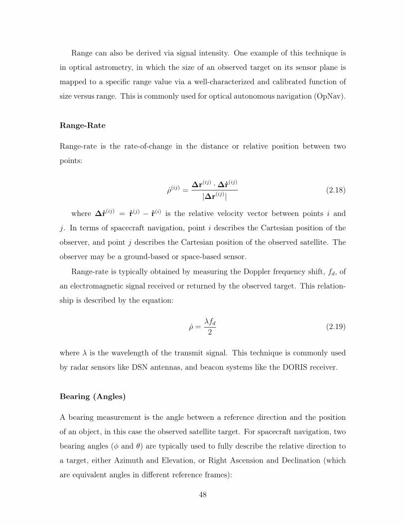
Range-rate is the rate-of-change in the distance or relative position between two
points:
(𝑖𝑗) =Δr(𝑖𝑗) ·Δr(𝑖𝑗)
|Δr(𝑖𝑗)|(2.18)
where Δr(𝑖𝑗) = r(𝑗) − r(𝑖) is the relative velocity vector between points 𝑖 and
𝑗. In terms of spacecraft navigation, point 𝑖 describes the Cartesian position of the
observer, and point 𝑗 describes the Cartesian position of the observed satellite. The
observer may be a ground-based or space-based sensor.
Range-rate is typically obtained by measuring the Doppler frequency shift, 𝑓𝑑, of
an electromagnetic signal received or returned by the observed target. This relation-
ship is described by the equation:
=𝜆𝑓𝑑2
(2.19)
where 𝜆 is the wavelength of the transmit signal. This technique is commonly used
by radar sensors like DSN antennas, and beacon systems like the DORIS receiver.
Bearing (Angles)
A bearing measurement is the angle between a reference direction and the position
of an object, in this case the observed satellite target. For spacecraft navigation, two
bearing angles (𝜑 and 𝜃) are typically used to fully describe the relative direction to
a target, either Azimuth and Elevation, or Right Ascension and Declination (which
are equivalent angles in different reference frames):
48
𝜑(𝑖𝑗) = arctan
(∆𝑦(𝑖𝑗)
∆𝑥(𝑖𝑗)
), from 0 to 2𝜋 (2.20)
𝜃(𝑖𝑗) = − arcsin
(∆𝑧(𝑖𝑗)
|Δr(𝑖𝑗)|
)(2.21)
where
∆𝑥(𝑖𝑗) = 𝑥(𝑗) − 𝑥(𝑖) , ∆𝑦(𝑖𝑗) = 𝑦(𝑗) − 𝑦(𝑖) , ∆𝑧(𝑖𝑗) = 𝑧(𝑗) − 𝑧(𝑖) (2.22)
Bearing angles can be derived from measuring mechanical displacement (i.e., the
angular displacement of a telescope mount or a gimbaled platform in mechanically-
pointed sensors), measuring relative signal delays at known positions (e.g., the method
used in very-long baseline interferometry, or VLBI), or via astrometry (i.e., determin-
ing the attitude of a sensor image relative to the directions of known, fixed objects
in the image like stars).
2.2 Autonomous Navigation with Intersatellite Data
2.2.1 Seminal Research
The first study of using intersatellite range and inertially-referenced bearing measure-
ments for determining the orbits of two satellites without any a priori information
was conducted by F.L. Markley and published in 1984. The author first performed an
observability analysis to determine the feasibility of such a method. Using a simple
spherical Earth gravity model, Markley concluded that a few certain orbit cases are
unobservable using this method: when both spacecraft have equal semi-major axis 𝑎,
equal eccentricity 𝑒, equal “phasing” (i.e., mean-anomaly, 𝜈), and are either coplanar,
or “oriented so that the two spacecraft cross the line of intersection of the two planes
simultaneously” when non-coplanar [9].
These findings were furthered in a study by M.L. Psiaki in 1999, using a higher-
fidelity Earth gravitational model with 𝐽2 secular perturbations. This study con-
49
cluded that only one orbit case is absolutely unobservable: the same case as described
earlier (when both spacecraft have equal 𝑎, equal 𝑒, and equal 𝜈), but specifically when
the satellites are coplanar at the inclination 𝑖 of 0∘ . This means that inclined and
non-coplanar orbit cases are semi-observable due to the non-spherical Earth, and that
errors would grow as the two-spacecraft system more closely resembles the absolute
unobservable case. This conclusion largely affects satellites in GEO observing each
other, as they are all in low-inclination circular orbits. Missions in other orbits can be
affected too, though satellites in LEO and MEO tend to be inclined. We would also
like to note that the absolute unobservable case can still be mitigated by observing
satellites at other altitudes, such as between GEO and LEO. This is of particular
interest for study in this thesis.
Psiaki also established some baseline performance references by reporting posi-
tion uncertainty as a function of altering intersatellite geometry between two Earth-
orbiting satellites. This analysis showed observability errors caused by small sepa-
rations between satellites (on the order of 100 km), lack of measurement variability
in specific state elements, proximity to the absolute unobservable case, orbital alti-
tude, and high angle measurement uncertainty [11]. We intend to report on similar
effects but in an expanded range of potential orbital geometries afforded by the longer
separations possible using lasercom links.
In this thesis, while the source of the measurement is different from those used
in the aforementioned observability analyses (RF systems vs. lasercom systems), the
measurement types (range and bearing) have not changed; therefore an observability
analysis is not repeated in this work. However, we are interested in evaluating the
effect of estimation observability on navigation performance. As mentioned Section
2.1.1, one way to evaluate the effect of observability on error performance is to com-
pute the CRLB. Thus, CRLB computations are an important part of our analyses.
2.2.2 Other Relevant Studies & Analyses
Table 2.1 shows a summary of previous work in autonomous navigation using inter-
satellite measurements. In reviewing this area of research, we report a few differenti-
50
ating characteristics of each study that are of particular interest to this thesis. These
include the quantity and distribution of satellites and the uncertainty values of the
measurements, all as modeled and used in each study’s respective simulations. In
the final column, we report the magnitude of the resulting navigation performance of
each study.
Of the 17 studies reviewed, five studies simulate constellations larger than 4 satel-
lites, five studies simulate intersatellite geometry with separations on the order of
tens of thousands of kilometers, six studies model ranging precision below 1 meter,
and six studies model angular precision below 5 arcsec. However, only four studies
possessed two or more of these characteristics, while only one possessed all, Gao et
al. (2014).
Psiaki (1999) modeled precise range and bearing measurements for largely sep-
arated satellites, but only for two-satellite Earth-orbiting systems [11]. Zhao et al.
(2011) simulated a 30-satellite constellation comprised of distributed satellites in both
LEO and GEO using a neutral value of ranging precision, but did not model any
bearing measurements (possibly due to the large separations between satellites) [61].
Li et al. (2017) simulates a 6-satellite constellation with very precise bearing mea-
surements, but a strangely high uncertainty in ranging [68]. This study also does
not provide any details regarding the orbital configuration of the constellation, and
therefore the actual modeled distribution of satellites is unknown.
Gao et al. (2014) was the only study to possess all of the characteristics of interest
in this thesis [63]. In this study, the authors propose a navigation constellation com-
prised of 12 GNSS satellites in MEO and 4 satellites in Earth-Moon Lagrangian point
orbits (LPO). Three cases are considered: (1) only GNSS satellites with only ranging
measurements, (2) only GNSS satellites with range and angle measurements, and (3)
GNSS + LPO satellites with only ranging measurements. The authors conclude that
while range and angle measurements (case 2) show improved precision and stability
over case 1, ranging with satellites in Lagrangian points demonstrates even better
performance. Position errors were reported on the order to tens of meters. Case 2
is of most immediate relevance to this thesis, however no details are given regarding
51
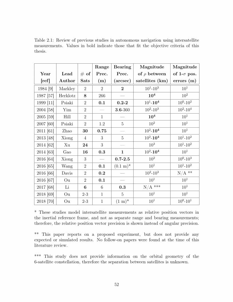
Table 2.1: Review of previous studies in autonomous navigation using intersatellitemeasurements. Values in bold indicate those that fit the objective criteria of thisthesis.
Range Bearing Magnitude MagnitudeYear Lead # of Prec. Prec. of 𝜌 between of 1-𝜎 pos.[ref] Author Sats (m) (arcsec) satellites (km) errors (m)
1984 [9] Markley 2 2 2 101-103 101
1987 [57] Herklotz 8 266 — 104 102
1999 [11] Psiaki 2 0.1 0.2-2 101-104 100-102
2004 [58] Yim 2 — 3.6-360 102-103 102-104
2005 [59] Hill 2 1 — 104 101
2007 [60] Psiaki 2 1.2 5 102 101
2011 [61] Zhao 30 0.75 — 102-104 101
2013 [48] Xiong 4 3 5 102-104 101-102
2014 [62] Xu 24 3 — 103 101-102
2014 [63] Gao 16 0.3 1 102-104 101
2016 [64] Xiong 3 — 0.7-2.5 102 100-103
2016 [65] Wang 2 0.1 (0.1 m)* 101 101-102
2016 [66] Davis 2 0.2 — 102-103 N/A **2016 [67] Ou 2 0.1 — 101 101
2017 [68] Li 6 6 0.3 N/A *** 101
2018 [69] Ou 2-3 1 5 101 101
2018 [70] Ou 2-3 1 (1 m)* 101 100-101
* These studies model intersatellite measurements as relative position vectors inthe inertial reference frame, and not as separate range and bearing measurements;therefore, the relative position vector precision is shown instead of angular precision.
** This paper reports on a proposed experiment, but does not provide anyexpected or simulated results. No follow-on papers were found at the time of thisliterature review.
*** This study does not provide information on the orbital geometry of the6-satellite constellation, therefore the separation between satellites is unknown.
52
how the measurements are made in order to achieve such precise uncertainty values.
It is possible that this analysis was simply a thought-exercise in order to demonstrate
the enhanced performance of the third case. Case 3 is notable in itself as it highlights
another possible orbital scenario that takes advantage of the circular restricted three-
body problem (CRTBP) dynamical system, though it does not model any bearing
measurements.
2.2.3 Research Gaps
Based on our review of literature in the research area of autonomous navigation using
intersatellite measurements, we identify a couple of research gaps that we address
in this thesis. One gap is the development of simulation frameworks for evaluating
navigation error performance using intersatellite measurements with consideration
for variable orbital scenarios, noise/uncertainty models, and network architectures.
Another is satellite navigation simulations of distributed constellation architectures
using measurement and link-access models consistent with lasercom crosslink systems.
Addressing these gaps is part of the research objectives and contributions of this
thesis.
53

THIS PAGE INTENTIONALLY LEFT BLANK
54
Chapter 3
Simulation Approach
This chapter introduces the simulation approach we use in this thesis to predict
and evaluate the performance of the proposed navigation method using intersatellite
lasercom measurements. The simulation environment developed for this study is
written in Matlab with input data generated using AGI’s Systems Tool Kit (STK)
software. An overview of the full simulation process is shown in Figure 3-1, and an
overview of the case studies considered in this thesis can be found in Table 3.5 (at
the end of the chapter). Each of the steps of the simulation framework is described
in detail in the following sections.
Throughout this chapter, we use a two-satellite GEO-LEO configuration to serve
as an illustrative example for the simulation approach. This configuration is modeled
off of the satellites ARTEMIS (in GEO) and OICETS (in LEO), which were used in
the first bi-directional lasercom crosslink in 2005 [31]. Figure 3-2 shows the primary
end-product of our simulation approach for this example scenario, which plots total
position error of the satellites in the scenario over the full simulation period, as affected
by geometric and network constraints.
3.1 Orbit Generation & Propagation
The first step in our approach is to select and define the simulation scenario to be
studied. The constellation is configured in STK, which is used to propagate and
55
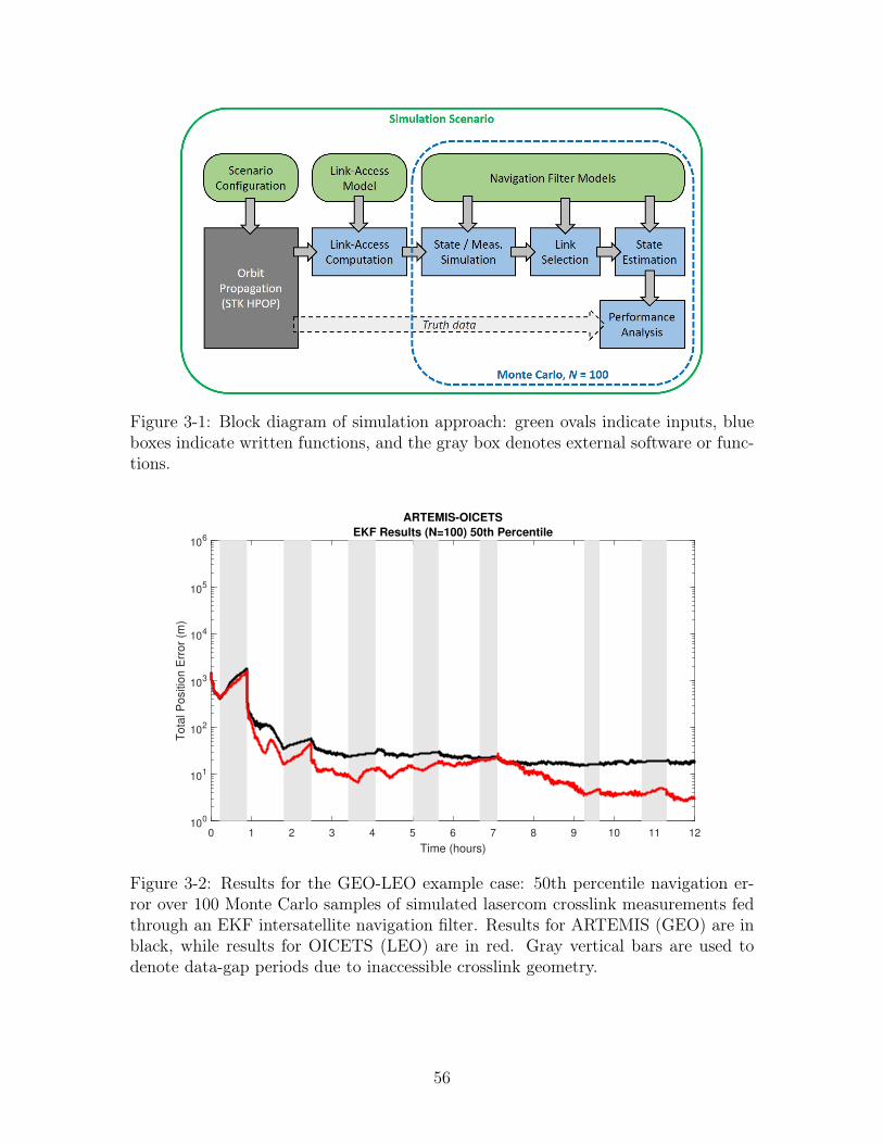
Figure 3-1: Block diagram of simulation approach: green ovals indicate inputs, blueboxes indicate written functions, and the gray box denotes external software or func-tions.
0 1 2 3 4 5 6 7 8 9 10 11 12
Time (hours)
100
101
102
103
104
105
106
Tota
l P
ositio
n E
rror
(m)
ARTEMIS-OICETS
EKF Results (N=100) 50th Percentile
Figure 3-2: Results for the GEO-LEO example case: 50th percentile navigation er-ror over 100 Monte Carlo samples of simulated lasercom crosslink measurements fedthrough an EKF intersatellite navigation filter. Results for ARTEMIS (GEO) are inblack, while results for OICETS (LEO) are in red. Gray vertical bars are used todenote data-gap periods due to inaccessible crosslink geometry.
56
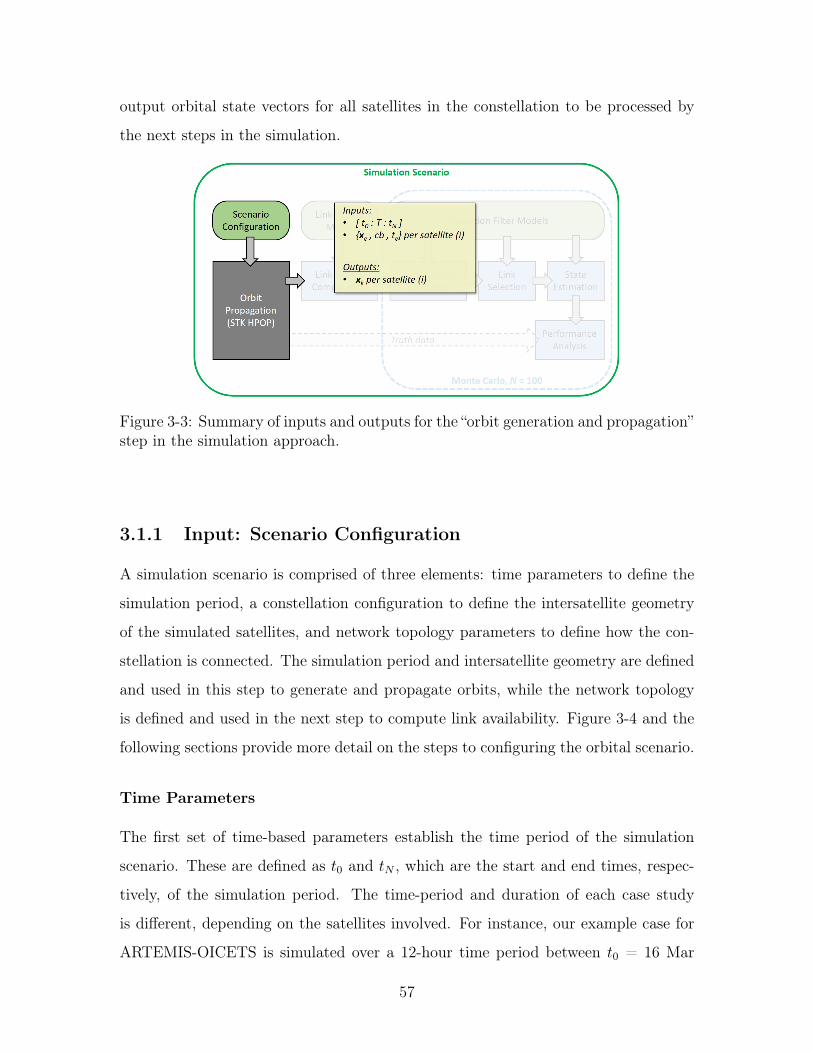
output orbital state vectors for all satellites in the constellation to be processed by
the next steps in the simulation.
Figure 3-3: Summary of inputs and outputs for the “orbit generation and propagation”step in the simulation approach.
3.1.1 Input: Scenario Configuration
A simulation scenario is comprised of three elements: time parameters to define the
simulation period, a constellation configuration to define the intersatellite geometry
of the simulated satellites, and network topology parameters to define how the con-
stellation is connected. The simulation period and intersatellite geometry are defined
and used in this step to generate and propagate orbits, while the network topology
is defined and used in the next step to compute link availability. Figure 3-4 and the
following sections provide more detail on the steps to configuring the orbital scenario.
Time Parameters
The first set of time-based parameters establish the time period of the simulation
scenario. These are defined as 𝑡0 and 𝑡𝑁 , which are the start and end times, respec-
tively, of the simulation period. The time-period and duration of each case study
is different, depending on the satellites involved. For instance, our example case for
ARTEMIS-OICETS is simulated over a 12-hour time period between 𝑡0 = 16 Mar
57
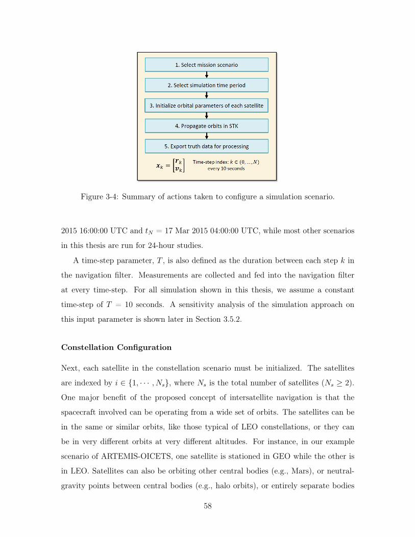
Figure 3-4: Summary of actions taken to configure a simulation scenario.
2015 16:00:00 UTC and 𝑡𝑁 = 17 Mar 2015 04:00:00 UTC, while most other scenarios
in this thesis are run for 24-hour studies.
A time-step parameter, 𝑇 , is also defined as the duration between each step 𝑘 in
the navigation filter. Measurements are collected and fed into the navigation filter
at every time-step. For all simulation shown in this thesis, we assume a constant
time-step of 𝑇 = 10 seconds. A sensitivity analysis of the simulation approach on
this input parameter is shown later in Section 3.5.2.
Constellation Configuration
Next, each satellite in the constellation scenario must be initialized. The satellites
are indexed by 𝑖 ∈ 1, · · · , 𝑁𝑠, where 𝑁𝑠 is the total number of satellites (𝑁𝑠 ≥ 2).
One major benefit of the proposed concept of intersatellite navigation is that the
spacecraft involved can be operating from a wide set of orbits. The satellites can be
in the same or similar orbits, like those typical of LEO constellations, or they can
be in very different orbits at very different altitudes. For instance, in our example
scenario of ARTEMIS-OICETS, one satellite is stationed in GEO while the other is
in LEO. Satellites can also be orbiting other central bodies (e.g., Mars), or neutral-
gravity points between central bodies (e.g., halo orbits), or entirely separate bodies
58
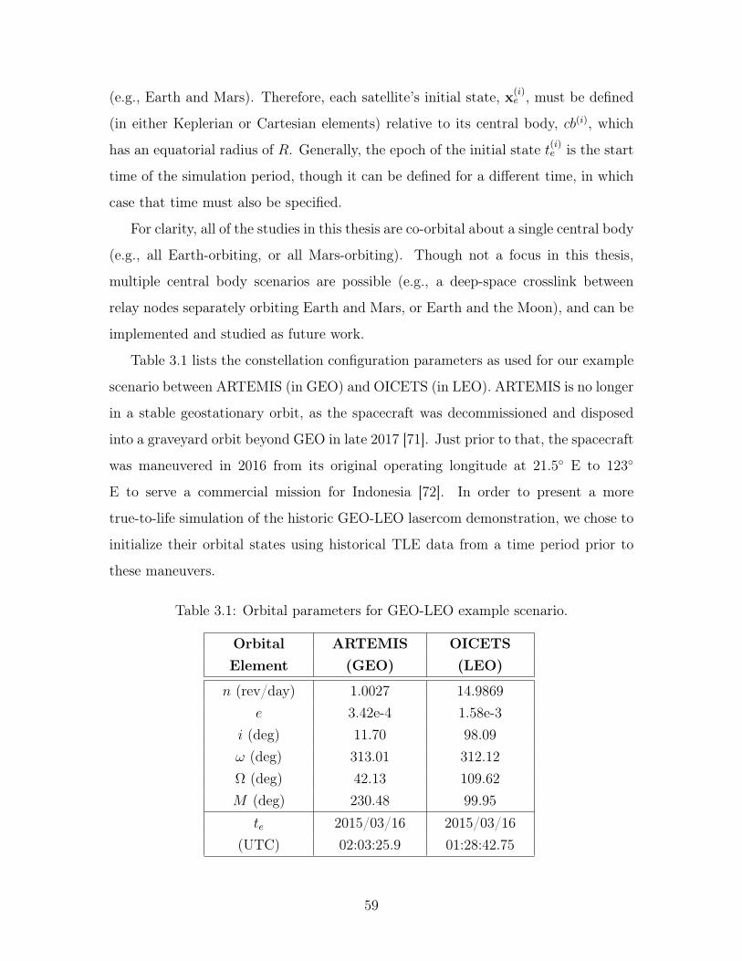
(e.g., Earth and Mars). Therefore, each satellite’s initial state, x(𝑖)𝑒 , must be defined
(in either Keplerian or Cartesian elements) relative to its central body, 𝑐𝑏(𝑖), which
has an equatorial radius of 𝑅. Generally, the epoch of the initial state 𝑡(𝑖)𝑒 is the start
time of the simulation period, though it can be defined for a different time, in which
case that time must also be specified.
For clarity, all of the studies in this thesis are co-orbital about a single central body
(e.g., all Earth-orbiting, or all Mars-orbiting). Though not a focus in this thesis,
multiple central body scenarios are possible (e.g., a deep-space crosslink between
relay nodes separately orbiting Earth and Mars, or Earth and the Moon), and can be
implemented and studied as future work.
Table 3.1 lists the constellation configuration parameters as used for our example
scenario between ARTEMIS (in GEO) and OICETS (in LEO). ARTEMIS is no longer
in a stable geostationary orbit, as the spacecraft was decommissioned and disposed
into a graveyard orbit beyond GEO in late 2017 [71]. Just prior to that, the spacecraft
was maneuvered in 2016 from its original operating longitude at 21.5∘ E to 123∘
E to serve a commercial mission for Indonesia [72]. In order to present a more
true-to-life simulation of the historic GEO-LEO lasercom demonstration, we chose to
initialize their orbital states using historical TLE data from a time period prior to
these maneuvers.
Table 3.1: Orbital parameters for GEO-LEO example scenario.
Orbital ARTEMIS OICETSElement (GEO) (LEO)
𝑛 (rev/day) 1.0027 14.9869𝑒 3.42e-4 1.58e-3
𝑖 (deg) 11.70 98.09𝜔 (deg) 313.01 312.12Ω (deg) 42.13 109.62𝑀 (deg) 230.48 99.95
𝑡𝑒 2015/03/16 2015/03/16(UTC) 02:03:25.9 01:28:42.75
59
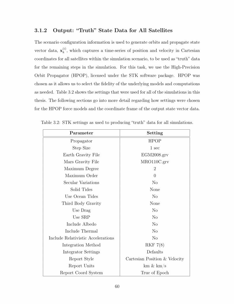
3.1.2 Output: “Truth” State Data for All Satellites
The scenario configuration information is used to generate orbits and propagate state
vector data, x(𝑖)𝑘 , which captures a time-series of position and velocity in Cartesian
coordinates for all satellites within the simulation scenario, to be used as “truth” data
for the remaining steps in the simulation. For this task, we use the High-Precision
Orbit Propagator (HPOP), licensed under the STK software package. HPOP was
chosen as it allows us to select the fidelity of the underlying models and computations
as needed. Table 3.2 shows the settings that were used for all of the simulations in this
thesis. The following sections go into more detail regarding how settings were chosen
for the HPOP force models and the coordinate frame of the output state vector data.
Table 3.2: STK settings as used to producing “truth” data for all simulations.
Parameter Setting
Propagator HPOPStep Size 1 sec
Earth Gravity File EGM2008.grvMars Gravity File MRO110C.grvMaximum Degree 2Maximum Order 0Secular Variations No
Solid Tides NoneUse Ocean Tides No
Third Body Gravity NoneUse Drag NoUse SRP No
Include Albedo NoInclude Thermal No
Include Relativistic Accelerations NoIntegration Method RKF 7(8)Integrator Settings Defaults
Report Style Cartesian Position & VelocityReport Units km & km/s
Report Coord System True of Epoch
60
Force Models
A number of perturbing forces can affect a given satellite’s orbit to varying degrees.
Satellites in GEO and other high-altitude orbits are more affected by third-body
perturbations and solar radiation pressure, while satellites in LEO are more affected
by gravitational perturbations and atmospheric drag. A satellite’s navigation filter is
generally only as good as how well its dynamics model matches the forces affecting
that satellite’s orbit. While a sufficient navigation filter would account for just the
primary perturbing forces, a highly accurate filter would need to account for any
smaller forces as well. Therefore, depending on the application or what is being
studied, different force models can be used to represent the orbital dynamics.
The research scope of this thesis is to evaluate the performance of intersatellite
navigation measurements from lasercom crosslinks. Given that the navigation filter
based on intersatellite measurements gains observability in estimating the absolute
states of the spacecraft based on how their relative position vector is affected by their
individual orbital dynamics, a higher fidelity of perturbing forces included in the
dynamics model can lead to greater performance. However, high-fidelity dynamics
models also require a higher knowledge of certain time-varying parameters, which can
introduce additional sources of error, and also require a higher order of computation
and processing in the filter.
In order to focus on the capabilities of the lasercom measurements, and not on how
accurately the dynamics model reflects the force models of the propagator, we sought
to strike a balance between including any relevant force models and limiting additional
sources of filtering error, and deemed it sufficient to only include the perturbing forces
that are necessary and can be easily implemented in the dynamics model. As such,
we chose to limit the perturbing force models used in the filter dynamics model to
only gravitational effects based on the J2-term of the non-spherical gravity model
coefficients.
Atmospheric drag and solar radiation pressure are both highly dependent on the
geometric characteristics of a spacecraft’s physical design and its orientation with
61
respect to the source of the perturbing force. While the parameters related to the ge-
ometric design of each spacecraft would be constant, the attitude of each spacecraft’s
body, and the magnitude and direction of the forces acting upon the spacecraft are all
time-variant. Third-body perturbations are easier to model than atmospheric drag or
solar radiation pressure, but were not implemented for the simulations in this thesis,
and are slated for future work.
For clarity, though STK includes a built-in analytic J2 propagator, this was not
used in this study due to potential for introducing unknown “black-box” sources of
error. HPOP, a fully numerical propagator, is preferred, as it can be transparently
configured as needed, and also provides the opportunity for future iterations of this
work to readily implement and activate additional force models, such as third-body
effects.
Coordinate Frames
Including non-spherical gravitational perturbations in the filter’s dynamics model
leads to a need to properly select the coordinate frame in which the “truth” state
vector data is generated. Gravity model coefficients are based on a specific definition
of the central body’s Z-axis, and each coordinate frame defines their axes to different
references.
In order to mitigate the need for time-variant coordinate transformations, we
sought to perform all computation in a coordinate frame that is non-rotating (inertial)
and shares the same Z-axis as the Fixed coordinate system, the frame in which the
gravity model is defined. After inspecting and testing each of the coordinate frames
natively offered in STK1, we determined that the “True of Epoch” coordinate system,
with the epoch defined as the start time of each simulation scenario, was best-suited
for our simulation approach.
1See summary of the different coordinate frames that are offered in STK at<http://help.agi.com/stk/index.htm#stk/referenceFramesCBdescriptions.htm>.
62
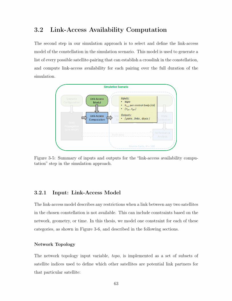
3.2 Link-Access Availability Computation
The second step in our simulation approach is to select and define the link-access
model of the constellation in the simulation scenario. This model is used to generate a
list of every possible satellite-pairing that can establish a crosslink in the constellation,
and compute link-access availability for each pairing over the full duration of the
simulation.
Figure 3-5: Summary of inputs and outputs for the “link-access availability compu-tation” step in the simulation approach.
3.2.1 Input: Link-Access Model
The link-access model describes any restrictions when a link between any two satellites
in the chosen constellation is not available. This can include constraints based on the
network, geometry, or time. In this thesis, we model one constraint for each of these
categories, as shown in Figure 3-6, and described in the following sections.
Network Topology
The network topology input variable, topo, is implemented as a set of subsets of
satellite indices used to define which other satellites are potential link partners for
that particular satellite:
63
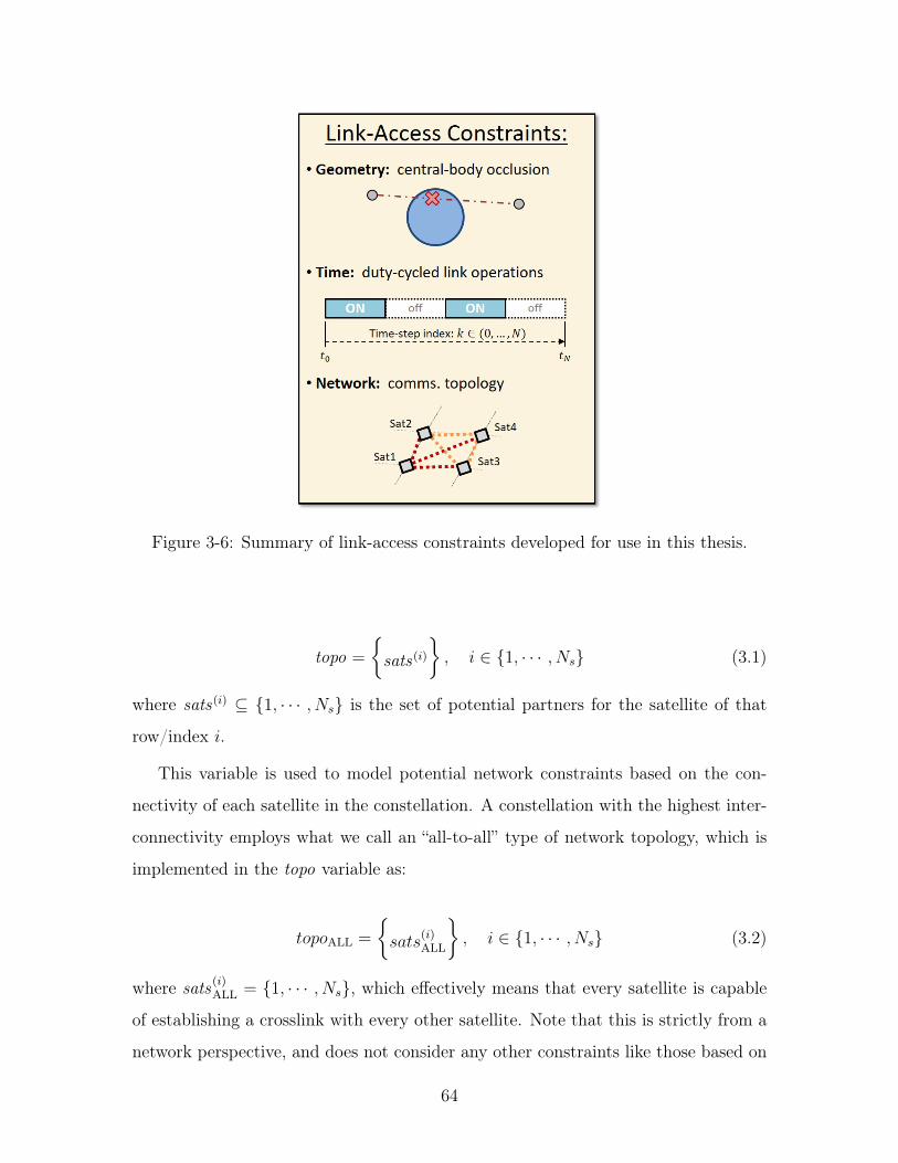
Figure 3-6: Summary of link-access constraints developed for use in this thesis.
topo =
sats(𝑖)
, 𝑖 ∈ 1, · · · , 𝑁𝑠 (3.1)
where sats(𝑖) ⊆ 1, · · · , 𝑁𝑠 is the set of potential partners for the satellite of that
row/index 𝑖.
This variable is used to model potential network constraints based on the con-
nectivity of each satellite in the constellation. A constellation with the highest inter-
connectivity employs what we call an “all-to-all” type of network topology, which is
implemented in the topo variable as:
𝑡𝑜𝑝𝑜ALL =
𝑠𝑎𝑡𝑠
(𝑖)ALL
, 𝑖 ∈ 1, · · · , 𝑁𝑠 (3.2)
where sats (𝑖)ALL = 1, · · · , 𝑁𝑠, which effectively means that every satellite is capable
of establishing a crosslink with every other satellite. Note that this is strictly from a
network perspective, and does not consider any other constraints like those based on
64
geometry or other system design parameters.
Different topology combinations can be created for each constellation. The number
of combinations is dependent on the size of the constellation. For instance, in two-
satellite systems like that of our ARTEMIS-OICETS example scenario, there is only
one possible combination of network topology, defined as:
𝑡𝑜𝑝𝑜2SAT =
⎧⎪⎨⎪⎩1, 2
1, 2
⎫⎪⎬⎪⎭ =
⎧⎪⎨⎪⎩2
1
⎫⎪⎬⎪⎭ (3.3)
If we were to introduce a third satellite into this constellation, there would now
be four possible combinations of network topology (not counting those that exclude
a satellite since that would effectively reduce down to a two-satellite system):
𝑡𝑜𝑝𝑜3𝑆𝐴𝑇 =
⎧⎪⎪⎪⎪⎪⎨⎪⎪⎪⎪⎪⎩2, 3
1, 3
1, 2
;
2, 3
1
1
;
2
1, 3
2
;
3
3
1, 2
⎫⎪⎪⎪⎪⎪⎬⎪⎪⎪⎪⎪⎭(3.4)
The first combination is an “all-to-all” type of topology for a three-satellite system,
where each satellite is capable of linking with every other satellite. The other three
combinations are what we consider different variants of a “some-to-some” network
topology. In particular, with only three satellites, the three “some-to-some” com-
binations are equivalent to a “hub-node” type of model, where particular satellites
(the “hubs”) are able to establish links with all of the other satellites, but the other
satellites (the “nodes”) can only establish links with hubs and not other nodes.
As one can imagine, were the constellation to have more than three satellites,
the number of possible network topology combinations would grow exponentially.
Examining all possible combinations for any given constellation is not within the
scope of this thesis, however this can be studied in future work. Instead, we define a
small set of topologies to study for any constellations larger than two satellites, based
on what we expect to be the mission of that given scenario. For example, in relay
missions, we expect that a few satellites will serve as hubs in the constellation, and
65
the rest will serve as nodes that can only establish links with hubs. For each of the
larger satellite constellation scenarios studied in this thesis, topology definitions will
be clearly stated.
Minimum Link Altitude
The minimum link altitude input parameter, ℎ𝑚𝑖𝑛, is used to model a simple geometric
constraint for the lowest altitude at which a crosslink can be established. Therefore,
the link-access availability computation will consider the grazing altitude of all po-
tential crosslinks, and only allow those that are above the ℎ𝑚𝑖𝑛 set for that scenario.
At a minimum, this value could be 0, effectively using the central-body alone as a
link-occluding geometric constraint, based on its average radius 𝑅. In order to ac-
count for atmospheric density and its effect in occluding crosslink communications,
we use the Karman line as the minimum link altitude for both Earth and Mars, set
to 100 and 80 kilometers, respectively [73].
Duty-cycle Timing
A simple duty-cycle model is used to emulate potential time constraints due to other
mission operations and priorities restricting the time or ability for crosslink commu-
nications. This could be due to limited resources (e.g., power) or due to mission
operating modes (e.g., science vs. communications, or downlink vs. crosslink). Two
variables are used to define the duty-cycle timing, 𝑇on and 𝑇off, which are the du-
rations for how long crosslink communications mode is “on” and “off”, respectively.
During the “on” mode, crosslinks are available and intersatellite measurements are
captured. During the “off” mode, the satellite may be idle and charging or perform-
ing any other task besides crosslink communications. One duty-cycle is defined as
one 𝑇on duration followed by one 𝑇off duration, followed by the next duty-cycle, and
continuously repeating for the duration of the simulation.
66
Other potential parameters
Other potential constraints were considered but not implemented, and can be explored
in future work. These include constraints based on relative range, relative velocity, or
link duration, which can be used to model different design or operations configurations
of the lasercom system. Consideration can also be given to geometric keep-out zones
with respect to background objects (e.g., sun, planets, moons), or implementing a
time-delay model to account for the time needed to establish links based on the state
uncertainty of link-access partners.
3.2.2 Output: Satellite Pairs, Available Links, & Duty Cycles
Generating Satellite-Pairings
The first main output variable is a set of all possible satellite-pairings in the simulated
constellation, coded as the 𝑁𝑝 × 2 matrix pairs, where 𝑁𝑝 is the total number of
satellite-pairings. This is generated by expanding each entry in the network topology
model, topo, and trimming any self-to-self entries and repeat connections, such that:
pairs = 𝑖, 𝑗, 𝑖 ∈ 1, · · · , 𝑁𝑠, 𝑗 ∈ 𝑠𝑎𝑡𝑠(𝑖), 𝑖 = 𝑗 (3.5)
where 𝑖 is the observing (or receiving) satellite, and 𝑗 is a potential link partner.
To provide an example of a repeat connection, an ARTEMIS-OICETS pairing is
the same as an OICETS-ARTEMIS pairing in a two-way lasercom crosslink topology.
Note that this would not necessarily be true for a different scenario. For instance, in
a broadcast RF crosslink topology, the order of the pairing would now matter, since
either satellite involved could operate in either transmit-only, receive-only, or both
transmit-and-receive modes.
Computing Link-Availability
The second output variable is an 𝑁𝑝 ×𝑁 matrix links encoding Boolean data for the
availability of link-access between satellite pairings over the full simulation period.
67
Link-access availability is evaluated for each satellite-pairing 𝑝 ∈ 1, 𝑁𝑝 at each time
step 𝑘 ∈ 1, 𝑁 using the propagated truth data from STK, with consideration of the
network, geometry, and time constraints supplied by the link-access model.
Gaps in link-access availability are coded as 0, while periods of available links
are coded as 𝑙(𝑝)𝑘 > 0, as the incremental link-access number for that satellite-pairing
𝑝. 𝑁𝑙 is the total number of available links for the full constellation (between all
satellite-pairings) over the full simulation period, and is computed as:
𝑁𝑙 =
𝑁𝑝∑𝑝=1
max𝑘∈[𝑁 ]
𝑙(𝑝)𝑘 (3.6)
Simulating Duty-Cycles
The third output variable is another matrix encoding Boolean data, this time for
the on/off mode schedule of duty-cycles over the full simulation period, dcycs. As
mentioned earlier, one duty-cycle is comprised of one 𝑇on duration of time immediately
followed by one 𝑇off duration of time, continuously repeating from the start time of
the simulation, 𝑡0, to the end time, 𝑡𝑁 . The dcycs matrix is implemented similar to
links, where “off” durations are coded as 0, while “on” durations are coded as 𝑑𝑘 > 0,
as the incremental duty-cycle number over the course of the simulation period.
𝑁𝑑 is the total number of duty-cycles over the full simulation period, and is com-
puted as:
𝑁𝑑 = max𝑘∈[𝑁 ]
𝑑𝑘 (3.7)
To simplify the model, and mitigate the complexity of mismatched duty-cycles
within a constellation, all satellites in a simulation scenario are assumed to be syn-
chronized to follow the same duty-cycle schedule. This means that the full constella-
tion goes into a “crosslink” mode during the “on” durations of the dcycs schedule, and
collects zero intersatellite measurements during the “off” durations. Note that for a
particular link to be active and collecting intersatellite measurements at given time,
that row/column entry must be greater than zero in both links and dcycs.
68
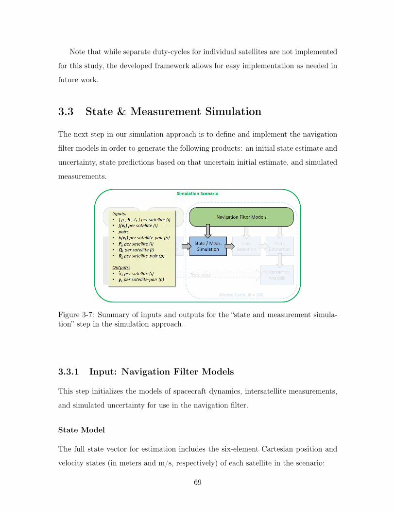
Note that while separate duty-cycles for individual satellites are not implemented
for this study, the developed framework allows for easy implementation as needed in
future work.
3.3 State & Measurement Simulation
The next step in our simulation approach is to define and implement the navigation
filter models in order to generate the following products: an initial state estimate and
uncertainty, state predictions based on that uncertain initial estimate, and simulated
measurements.
Figure 3-7: Summary of inputs and outputs for the “state and measurement simula-tion” step in the simulation approach.
3.3.1 Input: Navigation Filter Models
This step initializes the models of spacecraft dynamics, intersatellite measurements,
and simulated uncertainty for use in the navigation filter.
State Model
The full state vector for estimation includes the six-element Cartesian position and
velocity states (in meters and m/s, respectively) of each satellite in the scenario:
69
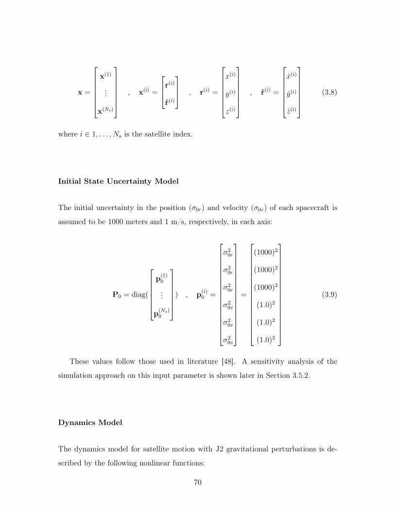
x =
⎡⎢⎢⎢⎢⎢⎣x(1)
...
x(𝑁𝑠)
⎤⎥⎥⎥⎥⎥⎦ , x(𝑖) =
⎡⎢⎣r(𝑖)r(𝑖)
⎤⎥⎦ , r(𝑖) =
⎡⎢⎢⎢⎢⎢⎣𝑥(𝑖)
𝑦(𝑖)
𝑧(𝑖)
⎤⎥⎥⎥⎥⎥⎦ , r(𝑖) =
⎡⎢⎢⎢⎢⎢⎣(𝑖)
(𝑖)
(𝑖)
⎤⎥⎥⎥⎥⎥⎦ (3.8)
where 𝑖 ∈ 1, . . . , 𝑁𝑠 is the satellite index.
Initial State Uncertainty Model
The initial uncertainty in the position (𝜎0𝑟) and velocity (𝜎0𝑣) of each spacecraft is
assumed to be 1000 meters and 1 m/s, respectively, in each axis:
P0 = diag(
⎡⎢⎢⎢⎢⎢⎣p(1)0
...
p(𝑁𝑠)0
⎤⎥⎥⎥⎥⎥⎦) , p(𝑖)0 =
⎡⎢⎢⎢⎢⎢⎢⎢⎢⎢⎢⎢⎢⎢⎢⎢⎢⎣
𝜎20𝑟
𝜎20𝑟
𝜎20𝑟
𝜎20𝑣
𝜎20𝑣
𝜎20𝑣
⎤⎥⎥⎥⎥⎥⎥⎥⎥⎥⎥⎥⎥⎥⎥⎥⎥⎦=
⎡⎢⎢⎢⎢⎢⎢⎢⎢⎢⎢⎢⎢⎢⎢⎢⎢⎣
(1000)2
(1000)2
(1000)2
(1.0)2
(1.0)2
(1.0)2
⎤⎥⎥⎥⎥⎥⎥⎥⎥⎥⎥⎥⎥⎥⎥⎥⎥⎦(3.9)
These values follow those used in literature [48]. A sensitivity analysis of the
simulation approach on this input parameter is shown later in Section 3.5.2.
Dynamics Model
The dynamics model for satellite motion with J2 gravitational perturbations is de-
scribed by the following nonlinear functions:
70
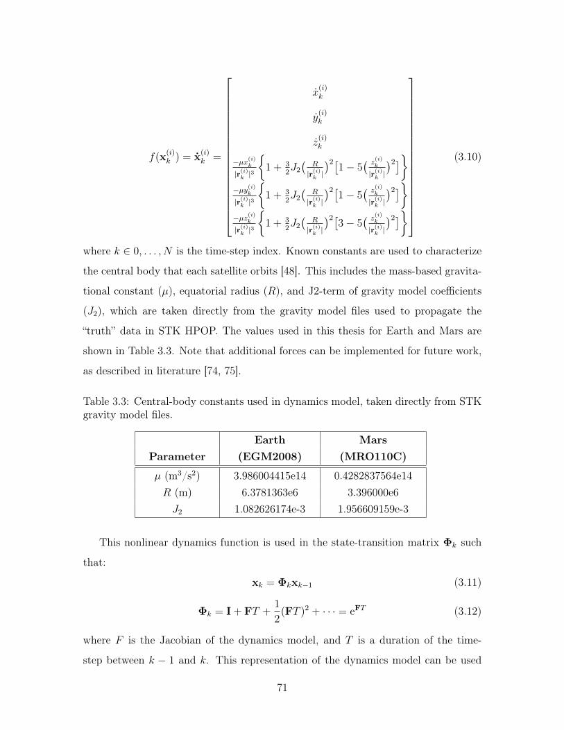
𝑓(x(𝑖)𝑘 ) = x
(𝑖)𝑘 =
⎡⎢⎢⎢⎢⎢⎢⎢⎢⎢⎢⎢⎢⎢⎢⎢⎢⎢⎢⎣
(𝑖)𝑘
(𝑖)𝑘
(𝑖)𝑘
−𝜇𝑥(𝑖)𝑘
|r(𝑖)𝑘 |3
1 + 3
2𝐽2(
𝑅
|r(𝑖)𝑘 |
)2[1 − 5
( 𝑧(𝑖)𝑘
|r(𝑖)𝑘 |
)2]−𝜇𝑦
(𝑖)𝑘
|r(𝑖)𝑘 |3
1 + 3
2𝐽2(
𝑅
|r(𝑖)𝑘 |
)2[1 − 5
( 𝑧(𝑖)𝑘
|r(𝑖)𝑘 |
)2]−𝜇𝑧
(𝑖)𝑘
|r(𝑖)𝑘 |3
1 + 3
2𝐽2(
𝑅
|r(𝑖)𝑘 |
)2[3 − 5
( 𝑧(𝑖)𝑘
|r(𝑖)𝑘 |
)2]
⎤⎥⎥⎥⎥⎥⎥⎥⎥⎥⎥⎥⎥⎥⎥⎥⎥⎥⎥⎦
(3.10)
where 𝑘 ∈ 0, . . . , 𝑁 is the time-step index. Known constants are used to characterize
the central body that each satellite orbits [48]. This includes the mass-based gravita-
tional constant (𝜇), equatorial radius (𝑅), and J2-term of gravity model coefficients
(𝐽2), which are taken directly from the gravity model files used to propagate the
“truth” data in STK HPOP. The values used in this thesis for Earth and Mars are
shown in Table 3.3. Note that additional forces can be implemented for future work,
as described in literature [74, 75].
Table 3.3: Central-body constants used in dynamics model, taken directly from STKgravity model files.
Earth MarsParameter (EGM2008) (MRO110C)
𝜇 (m3/s2) 3.986004415e14 0.4282837564e14𝑅 (m) 6.3781363e6 3.396000e6𝐽2 1.082626174e-3 1.956609159e-3
This nonlinear dynamics function is used in the state-transition matrix Φ𝑘 such
that:
x𝑘 = Φ𝑘x𝑘−1 (3.11)
Φ𝑘 = I + F𝑇 +1
2(F𝑇 )2 + · · · = eF𝑇 (3.12)
where 𝐹 is the Jacobian of the dynamics model, and 𝑇 is a duration of the time-
step between 𝑘 − 1 and 𝑘. This representation of the dynamics model can be used
71
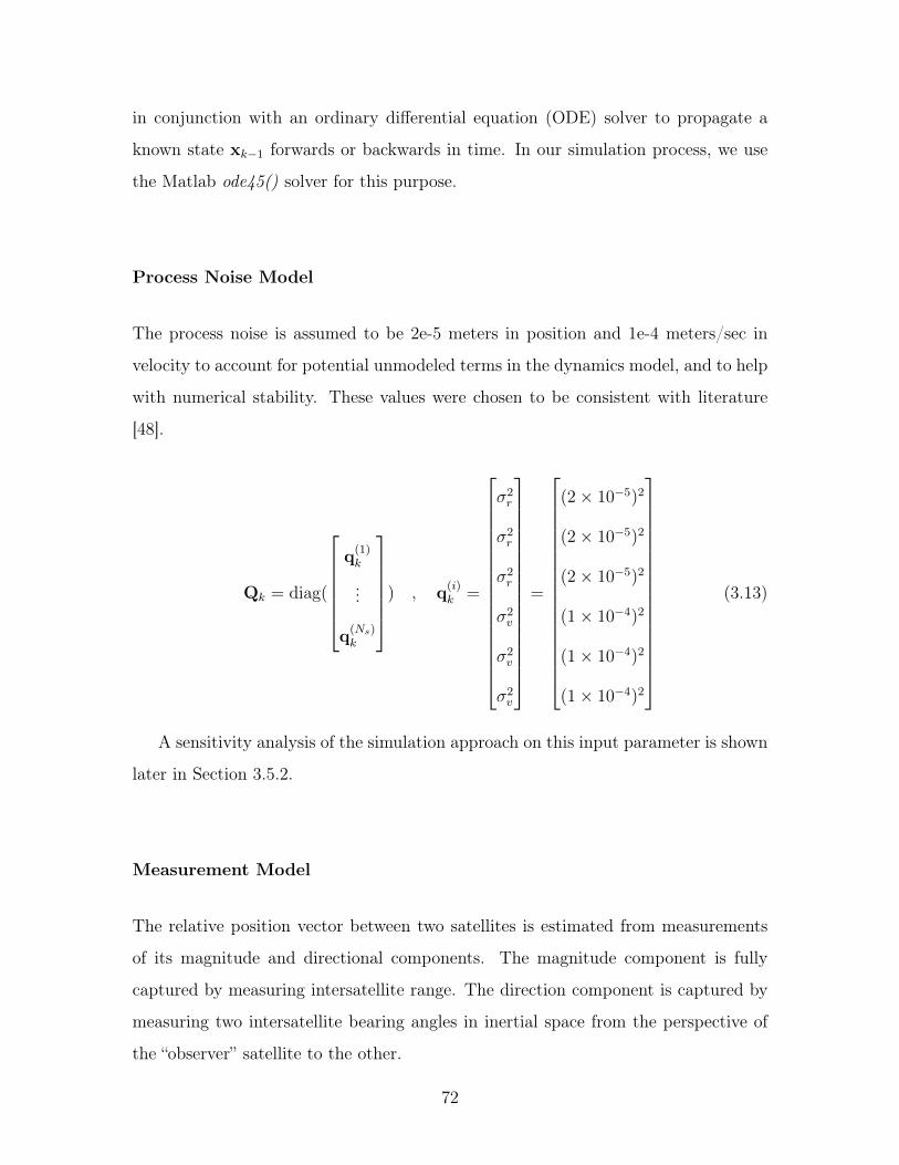
in conjunction with an ordinary differential equation (ODE) solver to propagate a
known state x𝑘−1 forwards or backwards in time. In our simulation process, we use
the Matlab ode45() solver for this purpose.
Process Noise Model
The process noise is assumed to be 2e-5 meters in position and 1e-4 meters/sec in
velocity to account for potential unmodeled terms in the dynamics model, and to help
with numerical stability. These values were chosen to be consistent with literature
[48].
Q𝑘 = diag(
⎡⎢⎢⎢⎢⎢⎣q(1)𝑘
...
q(𝑁𝑠)𝑘
⎤⎥⎥⎥⎥⎥⎦) , q(𝑖)𝑘 =
⎡⎢⎢⎢⎢⎢⎢⎢⎢⎢⎢⎢⎢⎢⎢⎢⎢⎣
𝜎2𝑟
𝜎2𝑟
𝜎2𝑟
𝜎2𝑣
𝜎2𝑣
𝜎2𝑣
⎤⎥⎥⎥⎥⎥⎥⎥⎥⎥⎥⎥⎥⎥⎥⎥⎥⎦=
⎡⎢⎢⎢⎢⎢⎢⎢⎢⎢⎢⎢⎢⎢⎢⎢⎢⎣
(2 × 10⁻⁵)2
(2 × 10⁻⁵)2
(2 × 10⁻⁵)2
(1 × 10⁻⁴)2
(1 × 10⁻⁴)2
(1 × 10⁻⁴)2
⎤⎥⎥⎥⎥⎥⎥⎥⎥⎥⎥⎥⎥⎥⎥⎥⎥⎦(3.13)
A sensitivity analysis of the simulation approach on this input parameter is shown
later in Section 3.5.2.
Measurement Model
The relative position vector between two satellites is estimated from measurements
of its magnitude and directional components. The magnitude component is fully
captured by measuring intersatellite range. The direction component is captured by
measuring two intersatellite bearing angles in inertial space from the perspective of
the “observer” satellite to the other.
72
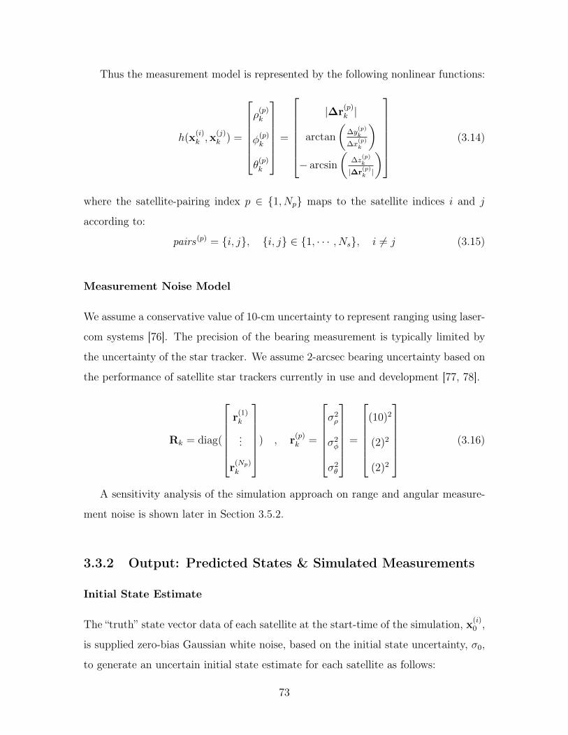
Thus the measurement model is represented by the following nonlinear functions:
ℎ(x(𝑖)𝑘 ,x
(𝑗)𝑘 ) =
⎡⎢⎢⎢⎢⎢⎣𝜌(𝑝)𝑘
𝜑(𝑝)𝑘
𝜃(𝑝)𝑘
⎤⎥⎥⎥⎥⎥⎦ =
⎡⎢⎢⎢⎢⎢⎢⎣|Δr
(𝑝)𝑘 |
arctan
(Δ𝑦
(𝑝)𝑘
Δ𝑥(𝑝)𝑘
)− arcsin
(Δ𝑧
(𝑝)𝑘
|Δr(𝑝)𝑘 |
)
⎤⎥⎥⎥⎥⎥⎥⎦ (3.14)
where the satellite-pairing index 𝑝 ∈ 1, 𝑁𝑝 maps to the satellite indices 𝑖 and 𝑗
according to:
pairs(𝑝) = 𝑖, 𝑗, 𝑖, 𝑗 ∈ 1, · · · , 𝑁𝑠, 𝑖 = 𝑗 (3.15)
Measurement Noise Model
We assume a conservative value of 10-cm uncertainty to represent ranging using laser-
com systems [76]. The precision of the bearing measurement is typically limited by
the uncertainty of the star tracker. We assume 2-arcsec bearing uncertainty based on
the performance of satellite star trackers currently in use and development [77, 78].
R𝑘 = diag(
⎡⎢⎢⎢⎢⎢⎣r(1)𝑘
...
r(𝑁𝑝)𝑘
⎤⎥⎥⎥⎥⎥⎦) , r(𝑝)𝑘 =
⎡⎢⎢⎢⎢⎢⎣𝜎2𝜌
𝜎2𝜑
𝜎2𝜃
⎤⎥⎥⎥⎥⎥⎦ =
⎡⎢⎢⎢⎢⎢⎣(10)2
(2)2
(2)2
⎤⎥⎥⎥⎥⎥⎦ (3.16)
A sensitivity analysis of the simulation approach on range and angular measure-
ment noise is shown later in Section 3.5.2.
3.3.2 Output: Predicted States & Simulated Measurements
Initial State Estimate
The “truth” state vector data of each satellite at the start-time of the simulation, x(𝑖)0 ,
is supplied zero-bias Gaussian white noise, based on the initial state uncertainty, 𝜎0,
to generate an uncertain initial state estimate for each satellite as follows:
73
x0 = x0 + 𝜎0 , 𝐸𝜎0𝜎𝑇0 = P0 (3.17)
𝜎0 = [𝜎0𝑟 , 𝜎0𝑣]𝑇 (3.18)
A priori State Prediction
The dynamics model, 𝑓(x(𝑖)𝑘 ), is then used to propagate state vectors for all satellites
for the full simulation period from those uncertain initial estimates, x𝑘(𝑖), using the
Matlab ode45 solver over all time-steps, 𝑇 , between the start and end times of the
simulation scenario, 𝑡0 and 𝑡𝑁 , respectively. This output product is not used by the
navigation filter (as that computes a new prediction based on the latest estimate at
each time-step) but by the link-selection algorithm described in the next section.
Measurement Simulation
Using the “truth” state vector data x(𝑖)𝑘 and the pairs list of satellite-pairings, true
measurements are computed for each link at each time step using the measurement
model ℎ(x(𝑖)𝑘 ,x
(𝑗)𝑘 ). All measurements are then supplied zero-bias Gaussian white
noise, based on the measurement uncertainty v𝑘, to generate simulated measurements
to be used in the navigation filter. The measurement noise is applied as follows:
y𝑘 = ℎ(x𝑘,x𝑘) + v𝑘 , 𝐸v𝑘v𝑇𝑘 = R𝑘 (3.19)
v𝑘 = [𝜎𝜌 , 𝜎𝜑 , 𝜎𝜃]𝑇 (3.20)
3.4 Link-Access Selection
Generally, a single satellite lasercom system may only establish and maintain one link
at a given time, due to the narrow beamwidth of the signal requiring precise pointing
to the receiving terminal. Additional links can be supported by a given satellite by
including additional lasercom payloads in the spacecraft design, although this can
become difficult since each payload would also require separate pointing and tracking
74
systems. This limitation in simultaneous links adds some complexity to the overall
network communications architecture of a lasercom crosslink constellation, since a
satellite may have more links available than it is able to support at any given time.
For comparison, the larger beamwidth of RF transmission allows for broadcast
signals (which can be transmitted from a single source and received by many), and
also low-gain antennas (which can receive signals from a wide range of directions).
This simplifies the communications architecture, as it enables satellites to transmit
to and/or receive from any other satellites within a given satellite’s antenna pattern,
and mitigates the need for planning and scheduling particular links.
In order to solve this problem for lasercom constellations, there must be some
process by which links can be planned and scheduled for crosslink communications.
Typically, this will be dictated by other priorities within the constellation’s mission,
in particular routing or distributing data. However, in this thesis, we seek to de-
termine the best possible navigation performance achievable by crosslink networked
satellites, and we therefore require a process of selecting links based on navigation-
specific priorities.
Having predicted the future states of each satellite based on the uncertain initial
estimates, x(𝑖)𝑘 , we can use this knowledge to predetermine a schedule by using some
heuristic to help decide which links are preferred over others. This step in the simula-
tion process provides one way to approach this problem using a heuristic of predicted
uncertainty derived using the Cramér-Rao lower bound (CRLB).
3.4.1 Overview of Inputs and Outputs
3.4.2 Output: Selected Links based on CRLB
CRLB uses the same filtering structure and input models as a Kalman filter, as
described in Section 2.1.1. Thus, the CRLB is able to provide a relevant and accurate
prediction of the effect that a given intersatellite link will have on that spacecraft’s
state uncertainty. Therefore, we have chosen to use the CRLB computed uncertainty
as the heuristic for deciding which links to select and schedule during the simulation
75
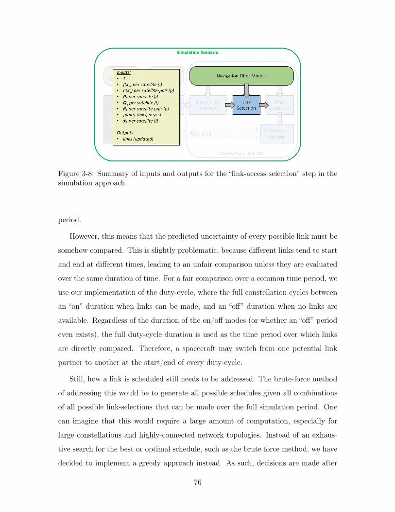
Figure 3-8: Summary of inputs and outputs for the “link-access selection” step in thesimulation approach.
period.
However, this means that the predicted uncertainty of every possible link must be
somehow compared. This is slightly problematic, because different links tend to start
and end at different times, leading to an unfair comparison unless they are evaluated
over the same duration of time. For a fair comparison over a common time period, we
use our implementation of the duty-cycle, where the full constellation cycles between
an “on” duration when links can be made, and an “off” duration when no links are
available. Regardless of the duration of the on/off modes (or whether an “off” period
even exists), the full duty-cycle duration is used as the time period over which links
are directly compared. Therefore, a spacecraft may switch from one potential link
partner to another at the start/end of every duty-cycle.
Still, how a link is scheduled still needs to be addressed. The brute-force method
of addressing this would be to generate all possible schedules given all combinations
of all possible link-selections that can be made over the full simulation period. One
can imagine that this would require a large amount of computation, especially for
large constellations and highly-connected network topologies. Instead of an exhaus-
tive search for the best or optimal schedule, such as the brute force method, we have
decided to implement a greedy approach instead. As such, decisions are made after
76
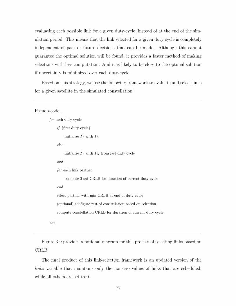
evaluating each possible link for a given duty-cycle, instead of at the end of the sim-
ulation period. This means that the link selected for a given duty cycle is completely
independent of past or future decisions that can be made. Although this cannot
guarantee the optimal solution will be found, it provides a faster method of making
selections with less computation. And it is likely to be close to the optimal solution
if uncertainty is minimized over each duty-cycle.
Based on this strategy, we use the following framework to evaluate and select links
for a given satellite in the simulated constellation:
Pseudo-code:
for each duty cycle
if first duty cycle
initialize 𝑃0 with 𝑃0
else
initialize 𝑃0 with 𝑃𝑁 from last duty cycle
end
for each link partner
compute 2-sat CRLB for duration of current duty cycle
end
select partner with min CRLB at end of duty cycle
(optional) configure rest of constellation based on selection
compute constellation CRLB for duration of current duty cycle
end
Figure 3-9 provides a notional diagram for this process of selecting links based on
CRLB.
The final product of this link-selection framework is an updated version of the
links variable that maintains only the nonzero values of links that are scheduled,
while all others are set to 0.
77
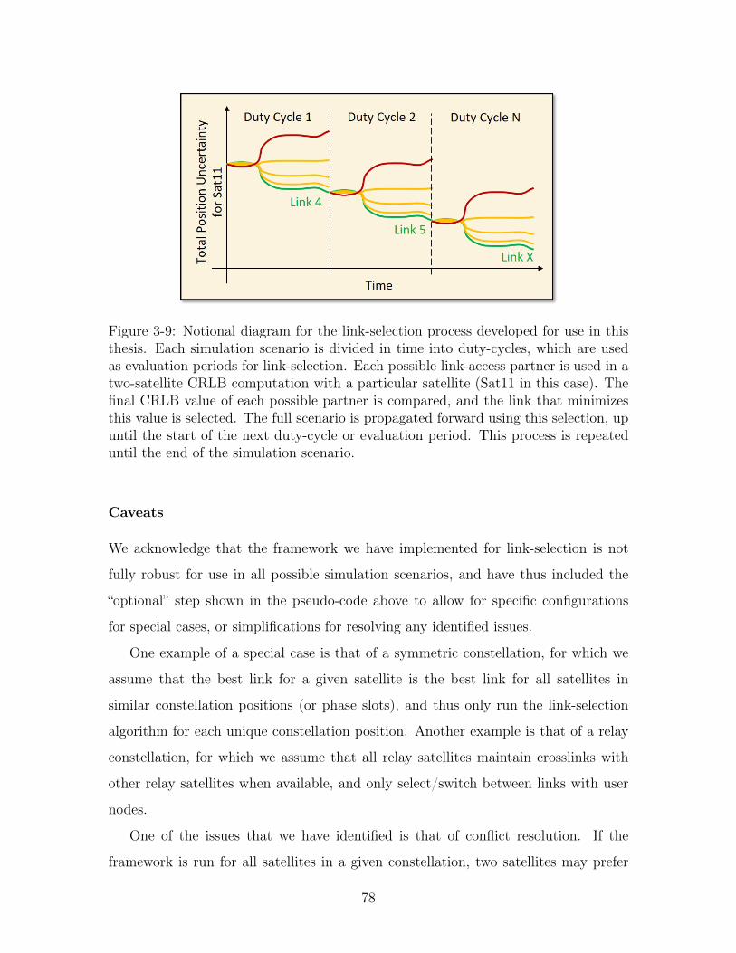
Figure 3-9: Notional diagram for the link-selection process developed for use in thisthesis. Each simulation scenario is divided in time into duty-cycles, which are usedas evaluation periods for link-selection. Each possible link-access partner is used in atwo-satellite CRLB computation with a particular satellite (Sat11 in this case). Thefinal CRLB value of each possible partner is compared, and the link that minimizesthis value is selected. The full scenario is propagated forward using this selection, upuntil the start of the next duty-cycle or evaluation period. This process is repeateduntil the end of the simulation scenario.
Caveats
We acknowledge that the framework we have implemented for link-selection is not
fully robust for use in all possible simulation scenarios, and have thus included the
“optional” step shown in the pseudo-code above to allow for specific configurations
for special cases, or simplifications for resolving any identified issues.
One example of a special case is that of a symmetric constellation, for which we
assume that the best link for a given satellite is the best link for all satellites in
similar constellation positions (or phase slots), and thus only run the link-selection
algorithm for each unique constellation position. Another example is that of a relay
constellation, for which we assume that all relay satellites maintain crosslinks with
other relay satellites when available, and only select/switch between links with user
nodes.
One of the issues that we have identified is that of conflict resolution. If the
framework is run for all satellites in a given constellation, two satellites may prefer
78
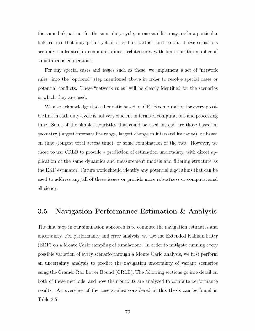
the same link-partner for the same duty-cycle, or one satellite may prefer a particular
link-partner that may prefer yet another link-partner, and so on. These situations
are only confronted in communications architectures with limits on the number of
simultaneous connections.
For any special cases and issues such as these, we implement a set of “network
rules” into the “optional” step mentioned above in order to resolve special cases or
potential conflicts. These “network rules” will be clearly identified for the scenarios
in which they are used.
We also acknowledge that a heuristic based on CRLB computation for every possi-
ble link in each duty-cycle is not very efficient in terms of computations and processing
time. Some of the simpler heuristics that could be used instead are those based on
geometry (largest intersatellite range, largest change in intersatellite range), or based
on time (longest total access time), or some combination of the two. However, we
chose to use CRLB to provide a prediction of estimation uncertainty, with direct ap-
plication of the same dynamics and measurement models and filtering structure as
the EKF estimator. Future work should identify any potential algorithms that can be
used to address any/all of these issues or provide more robustness or computational
efficiency.
3.5 Navigation Performance Estimation & Analysis
The final step in our simulation approach is to compute the navigation estimates and
uncertainty. For performance and error analysis, we use the Extended Kalman Filter
(EKF) on a Monte Carlo sampling of simulations. In order to mitigate running every
possible variation of every scenario through a Monte Carlo analysis, we first perform
an uncertainty analysis to predict the navigation uncertainty of variant scenarios
using the Cramér-Rao Lower Bound (CRLB). The following sections go into detail on
both of these methods, and how their outputs are analyzed to compute performance
results. An overview of the case studies considered in this thesis can be found in
Table 3.5.
79
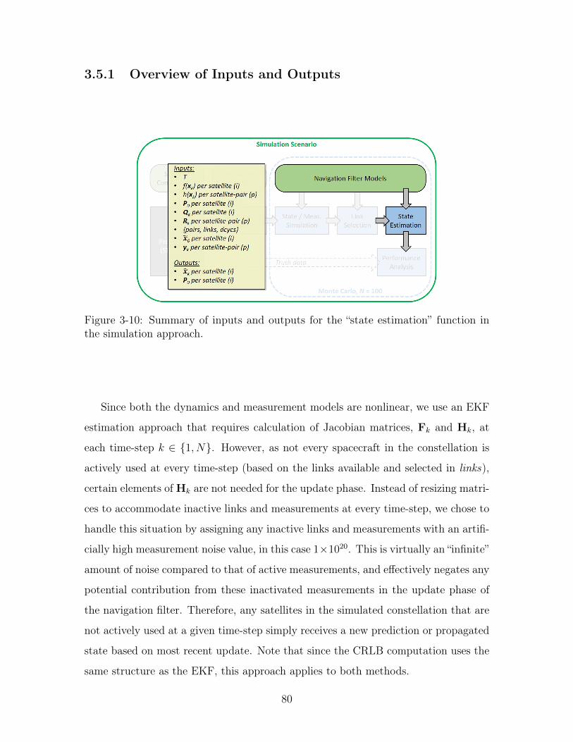
3.5.1 Overview of Inputs and Outputs
Figure 3-10: Summary of inputs and outputs for the “state estimation” function inthe simulation approach.
Since both the dynamics and measurement models are nonlinear, we use an EKF
estimation approach that requires calculation of Jacobian matrices, F𝑘 and H𝑘, at
each time-step 𝑘 ∈ 1, 𝑁. However, as not every spacecraft in the constellation is
actively used at every time-step (based on the links available and selected in links),
certain elements of H𝑘 are not needed for the update phase. Instead of resizing matri-
ces to accommodate inactive links and measurements at every time-step, we chose to
handle this situation by assigning any inactive links and measurements with an artifi-
cially high measurement noise value, in this case 1×10²⁰. This is virtually an “infinite”
amount of noise compared to that of active measurements, and effectively negates any
potential contribution from these inactivated measurements in the update phase of
the navigation filter. Therefore, any satellites in the simulated constellation that are
not actively used at a given time-step simply receives a new prediction or propagated
state based on most recent update. Note that since the CRLB computation uses the
same structure as the EKF, this approach applies to both methods.
80
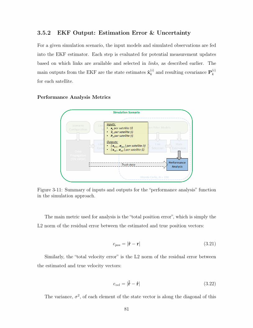
3.5.2 EKF Output: Estimation Error & Uncertainty
For a given simulation scenario, the input models and simulated observations are fed
into the EKF estimator. Each step is evaluated for potential measurement updates
based on which links are available and selected in links, as described earlier. The
main outputs from the EKF are the state estimates x(𝑖)𝑘 and resulting covariance P
(𝑖)𝑘
for each satellite.
Performance Analysis Metrics
Figure 3-11: Summary of inputs and outputs for the “performance analysis” functionin the simulation approach.
The main metric used for analysis is the “total position error”, which is simply the
L2 norm of the residual error between the estimated and true position vectors:
𝑒𝑝𝑜𝑠 = |r− r| (3.21)
Similarly, the “total velocity error” is the L2 norm of the residual error between
the estimated and true velocity vectors:
𝑒𝑣𝑒𝑙 = |r− r| (3.22)
The variance, 𝜎2, of each element of the state vector is along the diagonal of this
81
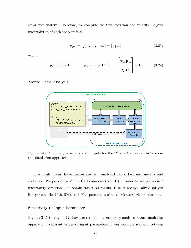
covariance matrix. Therefore, we compute the total position and velocity 1-sigma
uncertainties of each spacecraft as:
𝜎𝑝𝑜𝑠 = |√p𝑟𝑟| , 𝜎𝑣𝑒𝑙 = |√p| (3.23)
where
p𝑟𝑟 = diag(P𝑟𝑟) , p = diag(P) ,
⎡⎢⎣P𝑟𝑟P𝑟
P𝑟P
⎤⎥⎦ = P (3.24)
Monte Carlo Analysis
Figure 3-12: Summary of inputs and outputs for the “Monte Carlo analysis” step inthe simulation approach.
The results from the estimator are then analyzed for performance metrics and
statistics. We perform a Monte Carlo analysis (N=100) in order to sample noise /
uncertainty variations and obtain statistical results. Results are typically displayed
in figures as the 10th, 50th, and 90th percentiles of these Monte Carlo simulations.
Sensitivity to Input Parameters
Figures 3-13 through 3-17 show the results of a sensitivity analysis of our simulation
approach to different values of input parameters in our example scenario between
82
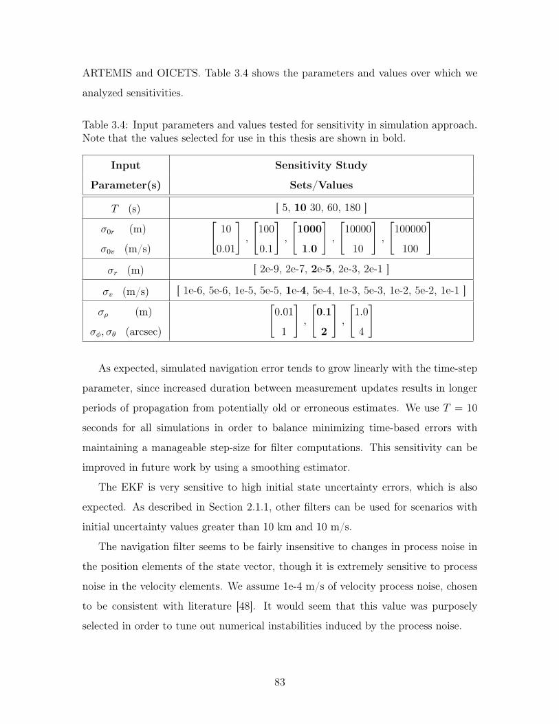
ARTEMIS and OICETS. Table 3.4 shows the parameters and values over which we
analyzed sensitivities.
Table 3.4: Input parameters and values tested for sensitivity in simulation approach.Note that the values selected for use in this thesis are shown in bold.
Input Sensitivity Study
Parameter(s) Sets/Values
𝑇 (s) [ 5, 10 30, 60, 180 ]
𝜎0𝑟 (m)
𝜎0𝑣 (m/s)
[10
0.01
],
[100
0.1
],
[1000
1.0
],
[10000
10
],
[100000
100
]
𝜎𝑟 (m) [ 2e-9, 2e-7, 2e-5, 2e-3, 2e-1 ]
𝜎𝑣 (m/s) [ 1e-6, 5e-6, 1e-5, 5e-5, 1e-4, 5e-4, 1e-3, 5e-3, 1e-2, 5e-2, 1e-1 ]
𝜎𝜌 (m)
𝜎𝜑, 𝜎𝜃 (arcsec)
[0.01
1
],
[0.1
2
],
[1.0
4
]
As expected, simulated navigation error tends to grow linearly with the time-step
parameter, since increased duration between measurement updates results in longer
periods of propagation from potentially old or erroneous estimates. We use 𝑇 = 10
seconds for all simulations in order to balance minimizing time-based errors with
maintaining a manageable step-size for filter computations. This sensitivity can be
improved in future work by using a smoothing estimator.
The EKF is very sensitive to high initial state uncertainty errors, which is also
expected. As described in Section 2.1.1, other filters can be used for scenarios with
initial uncertainty values greater than 10 km and 10 m/s.
The navigation filter seems to be fairly insensitive to changes in process noise in
the position elements of the state vector, though it is extremely sensitive to process
noise in the velocity elements. We assume 1e-4 m/s of velocity process noise, chosen
to be consistent with literature [48]. It would seem that this value was purposely
selected in order to tune out numerical instabilities induced by the process noise.
83
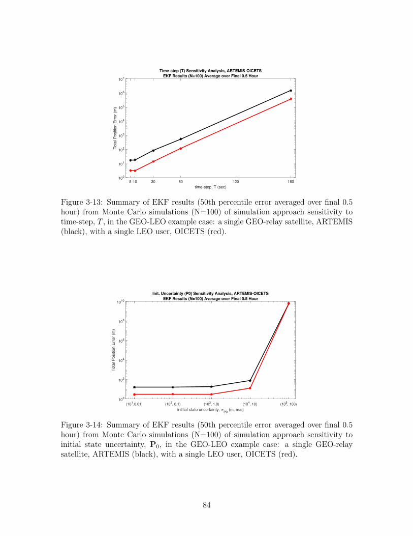
5 10 30 60 120 180
time-step, T (sec)
100
101
102
103
104
105
106
107
To
tal P
ositio
n E
rro
r (m
)
Time-step (T) Sensitivity Analysis, ARTEMIS-OICETS
EKF Results (N=100) Average over Final 0.5 Hour
Figure 3-13: Summary of EKF results (50th percentile error averaged over final 0.5hour) from Monte Carlo simulations (N=100) of simulation approach sensitivity totime-step, 𝑇 , in the GEO-LEO example case: a single GEO-relay satellite, ARTEMIS(black), with a single LEO user, OICETS (red).
(101,0.01) (10
2, 0.1) (10
3, 1.0) (10
4, 10) (10
5, 100)
inittial state uncertainty, P0
(m, m/s)
100
102
104
106
108
1010
To
tal P
ositio
n E
rro
r (m
)
Init. Uncertainty (P0) Sensitivity Analysis, ARTEMIS-OICETS
EKF Results (N=100) Average over Final 0.5 Hour
Figure 3-14: Summary of EKF results (50th percentile error averaged over final 0.5hour) from Monte Carlo simulations (N=100) of simulation approach sensitivity toinitial state uncertainty, P0, in the GEO-LEO example case: a single GEO-relaysatellite, ARTEMIS (black), with a single LEO user, OICETS (red).
84
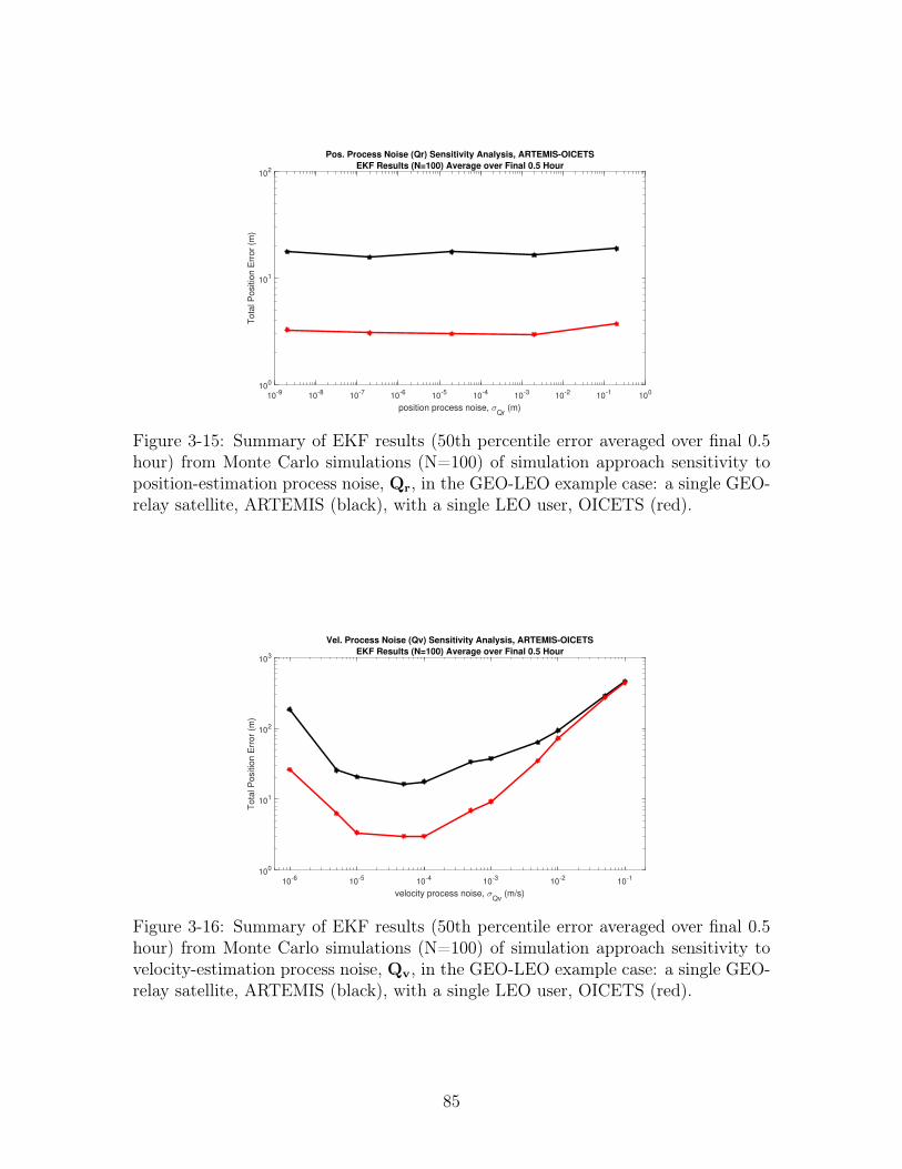
10-9
10-8
10-7
10-6
10-5
10-4
10-3
10-2
10-1
100
position process noise, Qr
(m)
100
101
102
To
tal P
ositio
n E
rro
r (m
)
Pos. Process Noise (Qr) Sensitivity Analysis, ARTEMIS-OICETS
EKF Results (N=100) Average over Final 0.5 Hour
Figure 3-15: Summary of EKF results (50th percentile error averaged over final 0.5hour) from Monte Carlo simulations (N=100) of simulation approach sensitivity toposition-estimation process noise, Qr, in the GEO-LEO example case: a single GEO-relay satellite, ARTEMIS (black), with a single LEO user, OICETS (red).
10-6
10-5
10-4
10-3
10-2
10-1
velocity process noise, Qv
(m/s)
100
101
102
103
To
tal P
ositio
n E
rro
r (m
)
Vel. Process Noise (Qv) Sensitivity Analysis, ARTEMIS-OICETS
EKF Results (N=100) Average over Final 0.5 Hour
Figure 3-16: Summary of EKF results (50th percentile error averaged over final 0.5hour) from Monte Carlo simulations (N=100) of simulation approach sensitivity tovelocity-estimation process noise, Qv, in the GEO-LEO example case: a single GEO-relay satellite, ARTEMIS (black), with a single LEO user, OICETS (red).
85
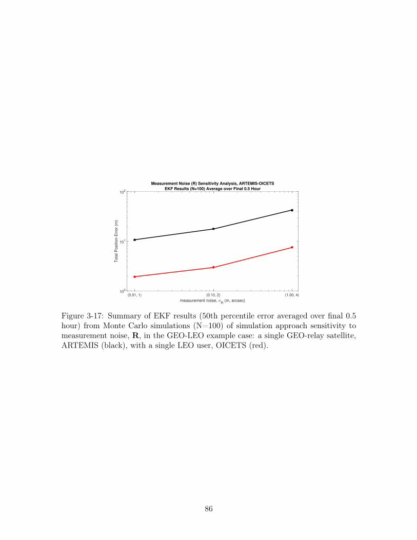
(0.01, 1) (0.10, 2) (1.00, 4)
measurement noise, R
(m, arcsec)
100
101
102
To
tal P
ositio
n E
rro
r (m
)
Measurement Noise (R) Sensitivity Analysis, ARTEMIS-OICETS
EKF Results (N=100) Average over Final 0.5 Hour
Figure 3-17: Summary of EKF results (50th percentile error averaged over final 0.5hour) from Monte Carlo simulations (N=100) of simulation approach sensitivity tomeasurement noise, R, in the GEO-LEO example case: a single GEO-relay satellite,ARTEMIS (black), with a single LEO user, OICETS (red).
86
3.5.3 CRLB Output: Predicted Uncertainty
For studies that explore potential trends based on wide ranges of parameter values or
orbital configurations, we first perform an uncertainty analysis in order to mitigate
running full Monte Carlo error analyses on every variation of every scenario. For
a given uncertainty analysis study, we compute and compare the CRLB predicted
uncertainty of each variant scenario in order to determine which scenario has the
greater likelihood of performing better.
To achieve this, the input models and initial state estimate are fed into the CRLB
computation. Each step is evaluated for potential measurement updates based on
which links are available and processed through link-selection, as described earlier.
The main output from the CRLB computation are the covariance estimates for each
satellite in the simulated constellation at every time-step in the simulation period,
P(𝑖)𝑘 .
Similar to the estimated variance from the EKF, the predicted variance, 2, of
each element of the state vector is along the diagonal of the predicted covariance
matrix. Therefore, we compute the total position and velocity 1-sigma uncertainties
of each spacecraft as:
𝑝𝑜𝑠 = |√p𝑟𝑟| , 𝑣𝑒𝑙 = |
√p| (3.25)
where
p𝑟𝑟 = diag(P𝑟𝑟) , p = diag(P) ,
⎡⎢⎣P𝑟𝑟P𝑟
P𝑟P
⎤⎥⎦ = P (3.26)
In particular, we use the minimum uncertainty value achieved over a given simu-
lation period as the primary metric for comparison between scenarios.
87
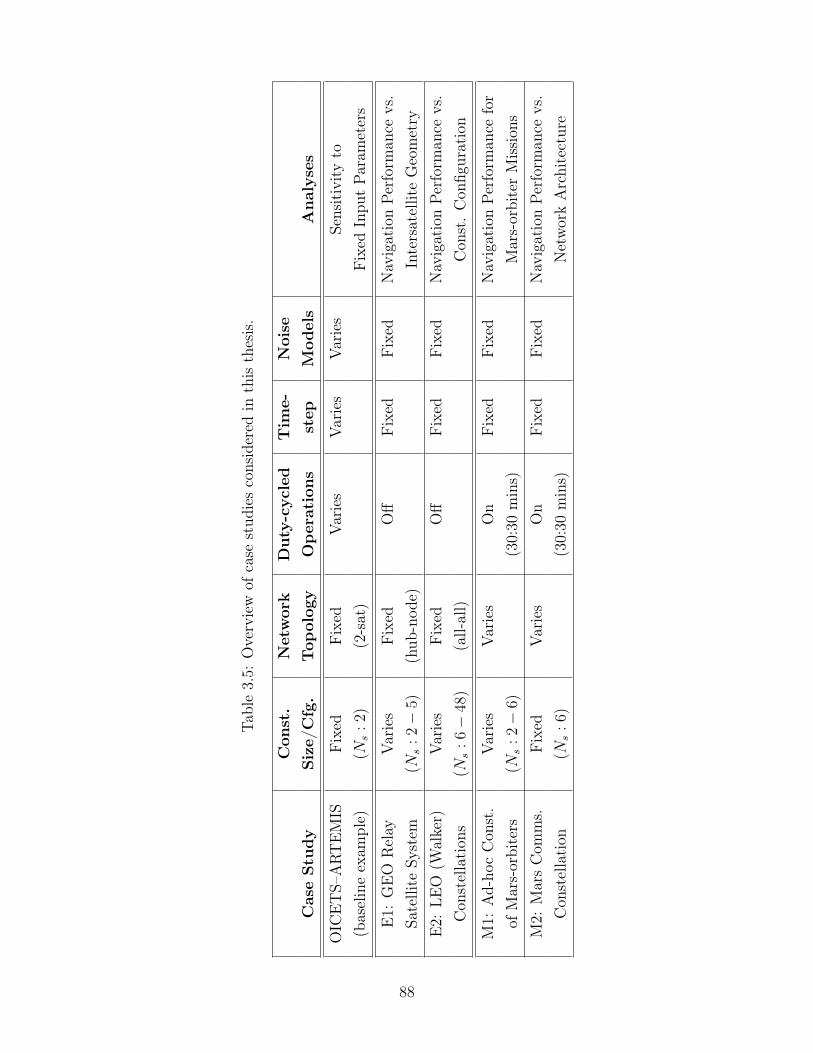
Tabl
e3.
5:O
verv
iew
ofca
sest
udie
sco
nsid
ered
inth
isth
esis
.
Con
st.
Net
wor
kD
uty
-cyc
led
Tim
e-N
oise
Cas
eStu
dy
Siz
e/C
fg.
Top
olog
yO
per
atio
ns
step
Mod
els
Anal
yses
OIC
ET
S–A
RT
EM
ISFix
edFix
edVar
ies
Var
ies
Var
ies
Sens
itiv
ityto
(bas
elin
eex
ampl
e)(𝑁
𝑠:
2)(2
-sat
)Fix
edIn
put
Par
amet
ers
E1:
GE
OR
elay
Var
ies
Fix
edO
ffFix
edFix
edN
avig
atio
nPer
form
ance
vs.
Sate
llite
Syst
em(𝑁
𝑠:
2−
5)(h
ub-n
ode)
Inte
rsat
ellit
eG
eom
etry
E2:
LEO
(Wal
ker)
Var
ies
Fix
edO
ffFix
edFix
edN
avig
atio
nPer
form
ance
vs.
Con
stel
lati
ons
(𝑁𝑠
:6−
48)
(all-
all)
Con
st.
Con
figur
atio
n
M1:
Ad-
hoc
Con
st.
Var
ies
Var
ies
On
Fix
edFix
edN
avig
atio
nPer
form
ance
for
ofM
ars-
orbi
ters
(𝑁𝑠
:2−
6)(3
0:30
min
s)M
ars-
orbi
ter
Mis
sion
sM
2:M
ars
Com
ms.
Fix
edVar
ies
On
Fix
edFix
edN
avig
atio
nPer
form
ance
vs.
Con
stel
lati
on(𝑁
𝑠:
6)(3
0:30
min
s)N
etw
ork
Arc
hite
ctur
e
88
Chapter 4
Earth-Orbiting Applications
This chapter describes the results and analysis from evaluating the performance of
the proposed navigation method using intersatellite lasercom measurements for dif-
ferent Earth-orbiting applications. In the first case study, we explore the potential
performance of intersatellite navigation using lasercom in a geostationary relay satel-
lite system operating with users in different orbits. In the second case study, we
analyze lasercom navigation performance for LEO constellations of varying size and
distribution.
4.1 Case Study E1: GEO Relay Satellite Systems
In this case study, we evaluate the navigation performance for system architectures
designed around optical relay satellites in geosynchronous orbit. This configuration
has relevance to past, present, and future missions. The first demonstrations of laser-
com crosslinks occurred between satellites in GEO and LEO [31]. More recently,
the European Space Agency partnered with Airbus to launch two lasercom payloads
into geosynchronous orbit (EDRS-A in 2016 and EDRS-C in 2019) in an effort to
establish what it calls a “SpaceDataHighway” for its Copernicus program of Earth-
observation satellites [36]. NASA is currently preparing its own GEO optical relay
satellite, LCRD, estimated to launch in late 2020 as part of an initial phase towards
optical communications for both near-Earth and deep-space missions [39]. It is clear
89
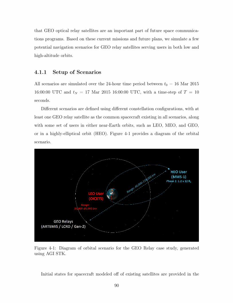
that GEO optical relay satellites are an important part of future space communica-
tions programs. Based on these current missions and future plans, we simulate a few
potential navigation scenarios for GEO relay satellites serving users in both low and
high-altitude orbits.
4.1.1 Setup of Scenarios
All scenarios are simulated over the 24-hour time period between 𝑡0 = 16 Mar 2015
16:00:00 UTC and 𝑡𝑁 = 17 Mar 2015 16:00:00 UTC, with a time-step of 𝑇 = 10
seconds.
Different scenarios are defined using different constellation configurations, with at
least one GEO relay satellite as the common spacecraft existing in all scenarios, along
with some set of users in either near-Earth orbits, such as LEO, MEO, and GEO,
or in a highly-elliptical orbit (HEO). Figure 4-1 provides a diagram of the orbital
scenario.
Figure 4-1: Diagram of orbital scenario for the GEO Relay case study, generatedusing AGI STK.
Initial states for spacecraft modeled off of existing satellites are provided in the
90
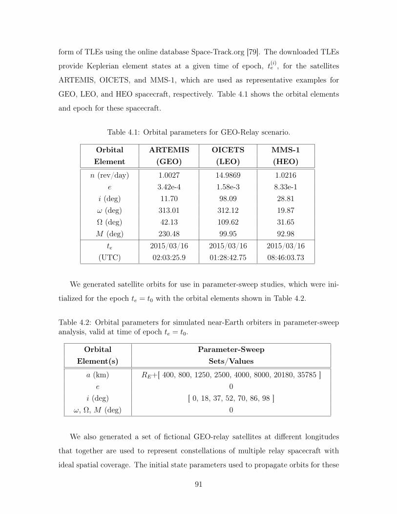
form of TLEs using the online database Space-Track.org [79]. The downloaded TLEs
provide Keplerian element states at a given time of epoch, 𝑡(𝑖)𝑒 , for the satellites
ARTEMIS, OICETS, and MMS-1, which are used as representative examples for
GEO, LEO, and HEO spacecraft, respectively. Table 4.1 shows the orbital elements
and epoch for these spacecraft.
Table 4.1: Orbital parameters for GEO-Relay scenario.
Orbital ARTEMIS OICETS MMS-1Element (GEO) (LEO) (HEO)
𝑛 (rev/day) 1.0027 14.9869 1.0216𝑒 3.42e-4 1.58e-3 8.33e-1
𝑖 (deg) 11.70 98.09 28.81𝜔 (deg) 313.01 312.12 19.87Ω (deg) 42.13 109.62 31.65𝑀 (deg) 230.48 99.95 92.98
𝑡𝑒 2015/03/16 2015/03/16 2015/03/16(UTC) 02:03:25.9 01:28:42.75 08:46:03.73
We generated satellite orbits for use in parameter-sweep studies, which were ini-
tialized for the epoch 𝑡𝑒 = 𝑡0 with the orbital elements shown in Table 4.2.
Table 4.2: Orbital parameters for simulated near-Earth orbiters in parameter-sweepanalysis, valid at time of epoch 𝑡𝑒 = 𝑡0.
Orbital Parameter-SweepElement(s) Sets/Values
𝑎 (km) 𝑅𝐸+[ 400, 800, 1250, 2500, 4000, 8000, 20180, 35785 ]𝑒 0
𝑖 (deg) [ 0, 18, 37, 52, 70, 86, 98 ]𝜔, Ω, 𝑀 (deg) 0
We also generated a set of fictional GEO-relay satellites at different longitudes
that together are used to represent constellations of multiple relay spacecraft with
ideal spatial coverage. The initial state parameters used to propagate orbits for these
91
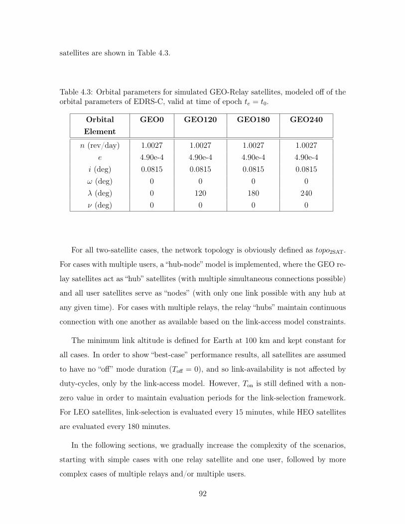
satellites are shown in Table 4.3.
Table 4.3: Orbital parameters for simulated GEO-Relay satellites, modeled off of theorbital parameters of EDRS-C, valid at time of epoch 𝑡𝑒 = 𝑡0.
Orbital GEO0 GEO120 GEO180 GEO240Element
𝑛 (rev/day) 1.0027 1.0027 1.0027 1.0027𝑒 4.90e-4 4.90e-4 4.90e-4 4.90e-4
𝑖 (deg) 0.0815 0.0815 0.0815 0.0815𝜔 (deg) 0 0 0 0𝜆 (deg) 0 120 180 240𝜈 (deg) 0 0 0 0
For all two-satellite cases, the network topology is obviously defined as 𝑡𝑜𝑝𝑜2SAT.
For cases with multiple users, a “hub-node” model is implemented, where the GEO re-
lay satellites act as “hub” satellites (with multiple simultaneous connections possible)
and all user satellites serve as “nodes” (with only one link possible with any hub at
any given time). For cases with multiple relays, the relay “hubs” maintain continuous
connection with one another as available based on the link-access model constraints.
The minimum link altitude is defined for Earth at 100 km and kept constant for
all cases. In order to show “best-case” performance results, all satellites are assumed
to have no “off” mode duration (𝑇off = 0), and so link-availability is not affected by
duty-cycles, only by the link-access model. However, 𝑇on is still defined with a non-
zero value in order to maintain evaluation periods for the link-selection framework.
For LEO satellites, link-selection is evaluated every 15 minutes, while HEO satellites
are evaluated every 180 minutes.
In the following sections, we gradually increase the complexity of the scenarios,
starting with simple cases with one relay satellite and one user, followed by more
complex cases of multiple relays and/or multiple users.
92
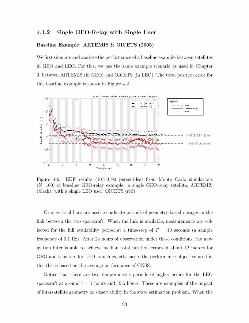
4.1.2 Single GEO-Relay with Single User
Baseline Example: ARTEMIS & OICETS (2005)
We first simulate and analyze the performance of a baseline example between satellites
in GEO and LEO. For this, we use the same example scenario as used in Chapter
3, between ARTEMIS (in GEO) and OICETS (in LEO). The total position error for
this baseline example is shown in Figure 4-2.
Figure 4-2: EKF results (10/50/90 percentiles) from Monte Carlo simulations(N=100) of baseline GEO-relay example: a single GEO-relay satellite, ARTEMIS(black), with a single LEO user, OICETS (red).
Gray vertical bars are used to indicate periods of geometry-based outages in the
link between the two spacecraft. When the link is available, measurements are col-
lected for the full availability period at a time-step of 𝑇 = 10 seconds (a sample
frequency of 0.1 Hz). After 24 hours of observation under these conditions, the nav-
igation filter is able to achieve median total position errors of about 12 meters for
GEO and 3 meters for LEO, which exactly meets the performance objective used in
this thesis based on the average performance of GNSS.
Notice that there are two temporaneous periods of higher errors for the LEO
spacecraft at around t = 7 hours and 19.5 hours. These are examples of the impact
of intersatellite geometry on observability in the state estimation problem. When the
93
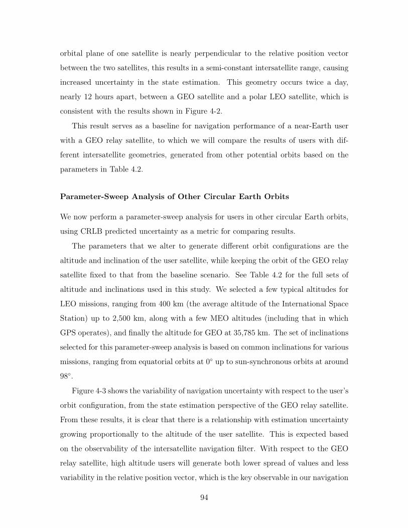
orbital plane of one satellite is nearly perpendicular to the relative position vector
between the two satellites, this results in a semi-constant intersatellite range, causing
increased uncertainty in the state estimation. This geometry occurs twice a day,
nearly 12 hours apart, between a GEO satellite and a polar LEO satellite, which is
consistent with the results shown in Figure 4-2.
This result serves as a baseline for navigation performance of a near-Earth user
with a GEO relay satellite, to which we will compare the results of users with dif-
ferent intersatellite geometries, generated from other potential orbits based on the
parameters in Table 4.2.
Parameter-Sweep Analysis of Other Circular Earth Orbits
We now perform a parameter-sweep analysis for users in other circular Earth orbits,
using CRLB predicted uncertainty as a metric for comparing results.
The parameters that we alter to generate different orbit configurations are the
altitude and inclination of the user satellite, while keeping the orbit of the GEO relay
satellite fixed to that from the baseline scenario. See Table 4.2 for the full sets of
altitude and inclinations used in this study. We selected a few typical altitudes for
LEO missions, ranging from 400 km (the average altitude of the International Space
Station) up to 2,500 km, along with a few MEO altitudes (including that in which
GPS operates), and finally the altitude for GEO at 35,785 km. The set of inclinations
selected for this parameter-sweep analysis is based on common inclinations for various
missions, ranging from equatorial orbits at 0∘ up to sun-synchronous orbits at around
98∘.
Figure 4-3 shows the variability of navigation uncertainty with respect to the user’s
orbit configuration, from the state estimation perspective of the GEO relay satellite.
From these results, it is clear that there is a relationship with estimation uncertainty
growing proportionally to the altitude of the user satellite. This is expected based
on the observability of the intersatellite navigation filter. With respect to the GEO
relay satellite, high altitude users will generate both lower spread of values and less
variability in the relative position vector, which is the key observable in our navigation
94
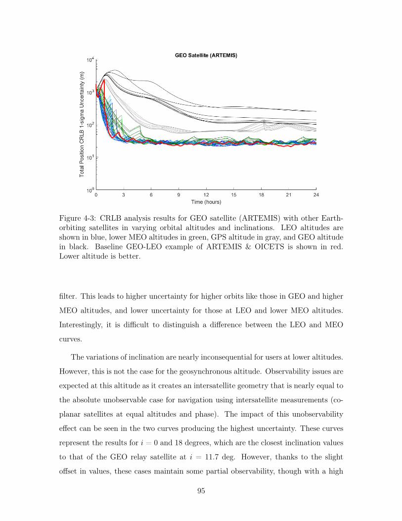
Figure 4-3: CRLB analysis results for GEO satellite (ARTEMIS) with other Earth-orbiting satellites in varying orbital altitudes and inclinations. LEO altitudes areshown in blue, lower MEO altitudes in green, GPS altitude in gray, and GEO altitudein black. Baseline GEO-LEO example of ARTEMIS & OICETS is shown in red.Lower altitude is better.
filter. This leads to higher uncertainty for higher orbits like those in GEO and higher
MEO altitudes, and lower uncertainty for those at LEO and lower MEO altitudes.
Interestingly, it is difficult to distinguish a difference between the LEO and MEO
curves.
The variations of inclination are nearly inconsequential for users at lower altitudes.
However, this is not the case for the geosynchronous altitude. Observability issues are
expected at this altitude as it creates an intersatellite geometry that is nearly equal to
the absolute unobservable case for navigation using intersatellite measurements (co-
planar satellites at equal altitudes and phase). The impact of this unobservability
effect can be seen in the two curves producing the highest uncertainty. These curves
represent the results for 𝑖 = 0 and 18 degrees, which are the closest inclination values
to that of the GEO relay satellite at 𝑖 = 11.7 deg. However, thanks to the slight
offset in values, these cases maintain some partial observability, though with a high
95
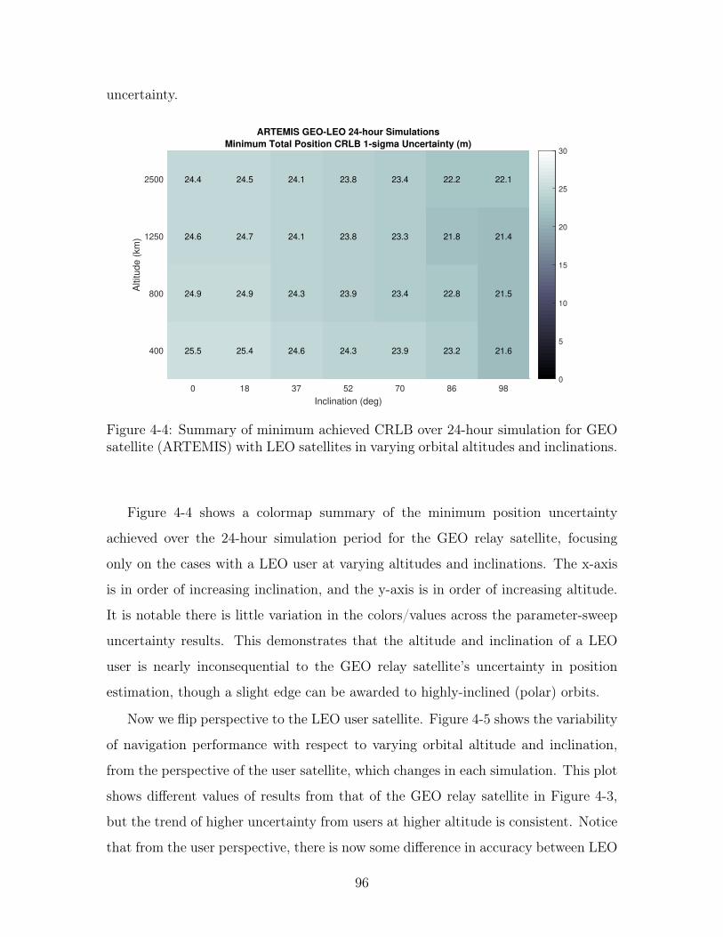
uncertainty.
0 18 37 52 70 86 98
Inclination (deg)
400
800
1250
2500
Altitude (
km
)ARTEMIS GEO-LEO 24-hour Simulations
Minimum Total Position CRLB 1-sigma Uncertainty (m)
25.5 25.4 24.6 24.3 23.9 23.2 21.6
24.9 24.9 24.3 23.9 23.4 22.8 21.5
24.6 24.7 24.1 23.8 23.3 21.8 21.4
24.4 24.5 24.1 23.8 23.4 22.2 22.1
0
5
10
15
20
25
30
Figure 4-4: Summary of minimum achieved CRLB over 24-hour simulation for GEOsatellite (ARTEMIS) with LEO satellites in varying orbital altitudes and inclinations.
Figure 4-4 shows a colormap summary of the minimum position uncertainty
achieved over the 24-hour simulation period for the GEO relay satellite, focusing
only on the cases with a LEO user at varying altitudes and inclinations. The x-axis
is in order of increasing inclination, and the y-axis is in order of increasing altitude.
It is notable there is little variation in the colors/values across the parameter-sweep
uncertainty results. This demonstrates that the altitude and inclination of a LEO
user is nearly inconsequential to the GEO relay satellite’s uncertainty in position
estimation, though a slight edge can be awarded to highly-inclined (polar) orbits.
Now we flip perspective to the LEO user satellite. Figure 4-5 shows the variability
of navigation performance with respect to varying orbital altitude and inclination,
from the perspective of the user satellite, which changes in each simulation. This plot
shows different values of results from that of the GEO relay satellite in Figure 4-3,
but the trend of higher uncertainty from users at higher altitude is consistent. Notice
that from the user perspective, there is now some difference in accuracy between LEO
96
Figure 4-5: CRLB analysis results for the parameter-sweep satellite (varying orbit)in simulations of GEO satellite with other Earth-orbiting satellites in varying orbitalaltitudes and inclinations. LEO altitudes are shown in blue, lower MEO altitudes ingreen, GPS altitude in gray, and GEO altitude in black. Baseline GEO-LEO exampleof ARTEMIS & OICETS is shown in red. Lower altitude is better.
and lower MEO altitudes, which was not seen in Figure 4-3. Also, satellites at the
same altitude seem to have variability in performance, which may imply correlation
with the other varying parameter, orbital inclination, as investigated next.
Figure 4-6 shows a colormap summary of the minimum position uncertainty
achieved over the 24-hour simulation period focusing only on user satellites in LEO
altitudes and inclinations. As before, the x-axis is in order of increasing inclination,
and the y-axis is in order of increasing altitude, though we changed the colors of the
colormap in order to differentiate the new range of values. These results demonstrate
clear improvement at lower altitudes and higher inclinations from the perspective of
the user satellite. The improvement at lower altitudes is understandable, given that
lower altitudes better sample the dominant forces of the dynamics model, and thus
see gains in estimation observability and reductions in uncertainty. However, in order
to understand the improvement at higher inclinations, we must look at a different
97
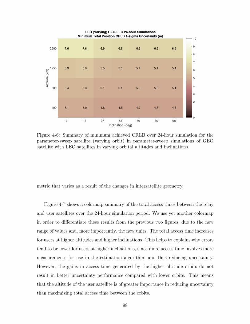
0 18 37 52 70 86 98
Inclination (deg)
400
800
1250
2500A
ltitude (
km
)
LEO (Varying) GEO-LEO 24-hour Simulations
Minimum Total Position CRLB 1-sigma Uncertainty (m)
5.1 5.0 4.8 4.8 4.7 4.8 4.8
5.4 5.3 5.1 5.1 5.0 5.0 5.1
5.9 5.9 5.5 5.5 5.4 5.4 5.4
7.6 7.6 6.9 6.8 6.6 6.6 6.6
0
1
2
3
4
5
6
7
8
9
10
Figure 4-6: Summary of minimum achieved CRLB over 24-hour simulation for theparameter-sweep satellite (varying orbit) in parameter-sweep simulations of GEOsatellite with LEO satellites in varying orbital altitudes and inclinations.
metric that varies as a result of the changes in intersatellite geometry.
Figure 4-7 shows a colormap summary of the total access times between the relay
and user satellites over the 24-hour simulation period. We use yet another colormap
in order to differentiate these results from the previous two figures, due to the new
range of values and, more importantly, the new units. The total access time increases
for users at higher altitudes and higher inclinations. This helps to explains why errors
tend to be lower for users at higher inclinations, since more access time involves more
measurements for use in the estimation algorithm, and thus reducing uncertainty.
However, the gains in access time generated by the higher altitude orbits do not
result in better uncertainty performance compared with lower orbits. This means
that the altitude of the user satellite is of greater importance in reducing uncertainty
than maximizing total access time between the orbits.
98
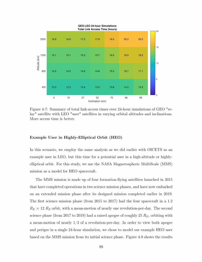
0 18 37 52 70 86 98
Inclination (km)
400
800
1250
2500A
ltitude (
km
)
GEO-LEO 24-hour Simulations
Total Link Access Time (hours)
13.3 13.3 13.4 13.5 13.8 14.2 15.2
14.5 14.5 14.6 14.8 15.3 16.7 17.1
15.1 15.1 15.3 15.7 16.5 18.0 18.2
16.9 16.9 17.2 17.8 19.5 20.2 20.2
0
6
12
18
24
Figure 4-7: Summary of total link-access times over 24-hour simulations of GEO "re-lay" satellite with LEO "user" satellites in varying orbital altitudes and inclinations.More access time is better.
Example User in Highly-Elliptical Orbit (HEO)
In this scenario, we employ the same analysis as we did earlier with OICETS as an
example user in LEO, but this time for a potential user in a high-altitude or highly-
elliptical orbit. For this study, we use the NASA Magnetospheric MultiScale (MMS)
mission as a model for HEO spacecraft.
The MMS mission is made up of four formation-flying satellites launched in 2015
that have completed operations in two science mission phases, and have now embarked
on an extended mission phase after its designed mission completed earlier in 2019.
The first science mission phase (from 2015 to 2017) had the four spacecraft in a 1.2
𝑅𝐸 × 12 𝑅𝐸 orbit, with a mean-motion of nearly one revolution-per-day. The second
science phase (from 2017 to 2019) had a raised apogee of roughly 25 𝑅𝐸, orbiting with
a mean-motion of nearly 1/3 of a revolution-per-day. In order to view both apogee
and perigee in a single 24-hour simulation, we chose to model our example HEO user
based on the MMS mission from its initial science phase. Figure 4-8 shows the results
99
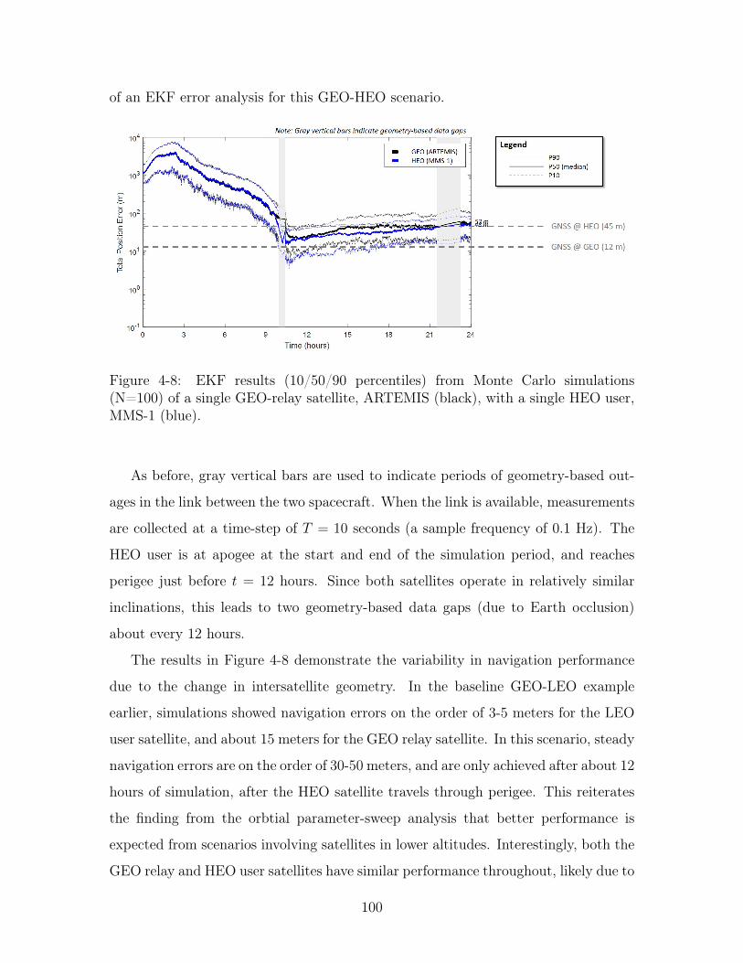
of an EKF error analysis for this GEO-HEO scenario.
Figure 4-8: EKF results (10/50/90 percentiles) from Monte Carlo simulations(N=100) of a single GEO-relay satellite, ARTEMIS (black), with a single HEO user,MMS-1 (blue).
As before, gray vertical bars are used to indicate periods of geometry-based out-
ages in the link between the two spacecraft. When the link is available, measurements
are collected at a time-step of 𝑇 = 10 seconds (a sample frequency of 0.1 Hz). The
HEO user is at apogee at the start and end of the simulation period, and reaches
perigee just before 𝑡 = 12 hours. Since both satellites operate in relatively similar
inclinations, this leads to two geometry-based data gaps (due to Earth occlusion)
about every 12 hours.
The results in Figure 4-8 demonstrate the variability in navigation performance
due to the change in intersatellite geometry. In the baseline GEO-LEO example
earlier, simulations showed navigation errors on the order of 3-5 meters for the LEO
user satellite, and about 15 meters for the GEO relay satellite. In this scenario, steady
navigation errors are on the order of 30-50 meters, and are only achieved after about 12
hours of simulation, after the HEO satellite travels through perigee. This reiterates
the finding from the orbtial parameter-sweep analysis that better performance is
expected from scenarios involving satellites in lower altitudes. Interestingly, both the
GEO relay and HEO user satellites have similar performance throughout, likely due to
100
the reduced impact of J2 perturbing dynamics beyond a certain altitude. This result
would likely be different if third-body perturbations is included in the filter dynamics
model, as higher altitude satellites are more affected by the moon and sun, and this
should be investigated for its impact on performance for high-altitude satellites in
future work.
4.1.3 Multiple Relays and/or Multiple Users
CRLB Analysis of Different Scenarios
Multiple GEO-relay satellites can be deployed in order to maintain custody of user
satellites on either side of the Earth, such that there are no geometry-based data
gaps from the perspective of the user. We analyzed this concept by performing a
CRLB uncertainty analysis for different scenarios of two or three GEO-relay satellites
equally-spaced in longitude around the Earth, and either a single user in LEO or HEO
(modeled by OICETS and MMS-1, respectively), or a heterogeneous set of both LEO
and HEO users.
In the case of three GEO relay satellites (at 0∘, 120∘, and 240∘ longitude), all
three relay hubs maintain constant crosslinks with one another, emulating a concept
where user satellite data can be relayed to the optimal GEO spacecraft for downlink.
Note that this is not geometrically possible with only two GEO relay satellites as
their relative position vector is intersected by the Earth, being directly opposite one
another in longitude at 0∘ and 180∘. In all cases with multiple relay satellites, the
user satellite(s) can have 1 or 2 GEO satellites available for a crosslink at any given
time, therefore the link-selection framework developed in this thesis is activated in
this scenario, with evaluation cycles every 15 minutes for LEO users and every 180
minutes for HEO users.
Figures 4-9, 4-10, and 4-11 show the predicted uncertainty results of these sim-
ulations from the perspective of the LEO user, the HEO user, and the GEO relay
satellites, respectively. Dotted lines are used to denote scenarios with a single LEO
user, dashed lines are used to denote scenarios with a single HEO user, and solid lines
101
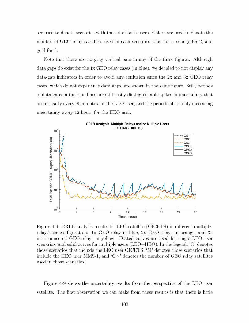
are used to denote scenarios with the set of both users. Colors are used to denote the
number of GEO relay satellites used in each scenario: blue for 1, orange for 2, and
gold for 3.
Note that there are no gray vertical bars in any of the three figures. Although
data gaps do exist for the 1x GEO relay cases (in blue), we decided to not display any
data-gap indicators in order to avoid any confusion since the 2x and 3x GEO relay
cases, which do not experience data gaps, are shown in the same figure. Still, periods
of data gaps in the blue lines are still easily distinguishable spikes in uncertainty that
occur nearly every 90 minutes for the LEO user, and the periods of steadily increasing
uncertainty every 12 hours for the HEO user.
0 3 6 9 12 15 18 21 24
Time (hours)
100
101
102
103
104
Tota
l P
ositio
n C
RLB
1-s
igm
a U
ncert
ain
ty (
m)
CRLB Analysis: Multiple Relays and/or Multiple Users
LEO User (OICETS)
OG1
OG2
OG3
OMG1
OMG2
OMG3
Figure 4-9: CRLB analysis results for LEO satellite (OICETS) in different multiple-relay/user configuration: 1x GEO-relay in blue, 2x GEO-relays in orange, and 3xinterconnected GEO-relays in yellow. Dotted curves are used for single LEO userscenarios, and solid curves for multiple users (LEO+HEO). In the legend, ‘O’ denotesthose scenarios that include the LEO user OICETS, ‘M’ denotes those scenarios thatinclude the HEO user MMS-1, and ‘G#’ denotes the number of GEO relay satellitesused in those scenarios.
Figure 4-9 shows the uncertainty results from the perspective of the LEO user
satellite. The first observation we can make from these results is that there is little
102
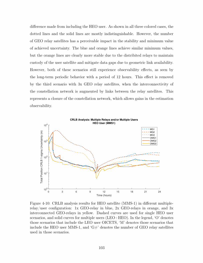
difference made from including the HEO user. As shown in all three colored cases, the
dotted lines and the solid lines are mostly indistinguishable. However, the number
of GEO relay satellites has a perceivable impact in the stability and minimum value
of achieved uncertainty. The blue and orange lines achieve similar minimum values,
but the orange lines are clearly more stable due to the distribited relays to maintain
custody of the user satellite and mitigate data gaps due to geometric link availability.
However, both of these scenarios still experience observability effects, as seen by
the long-term periodic behavior with a period of 12 hours. This effect is removed
by the third scenario with 3x GEO relay satellites, when the interconnectivity of
the constellation network is augmented by links between the relay satellites. This
represents a closure of the constellation network, which allows gains in the estimation
observability.
0 3 6 9 12 15 18 21 24
Time (hours)
100
101
102
103
104
Tota
l P
ositio
n C
RLB
1-s
igm
a U
ncert
ain
ty (
m)
CRLB Analysis: Multiple Relays and/or Multiple Users
HEO User (MMS1)
MG1
MG2
MG3
OMG1
OMG2
OMG3
Figure 4-10: CRLB analysis results for HEO satellite (MMS-1) in different multiple-relay/user configuration: 1x GEO-relay in blue, 2x GEO-relays in orange, and 3xinterconnected GEO-relays in yellow. Dashed curves are used for single HEO userscenarios, and solid curves for multiple users (LEO+HEO). In the legend, ‘O’ denotesthose scenarios that include the LEO user OICETS, ‘M’ denotes those scenarios thatinclude the HEO user MMS-1, and ‘G#’ denotes the number of GEO relay satellitesused in those scenarios.
103
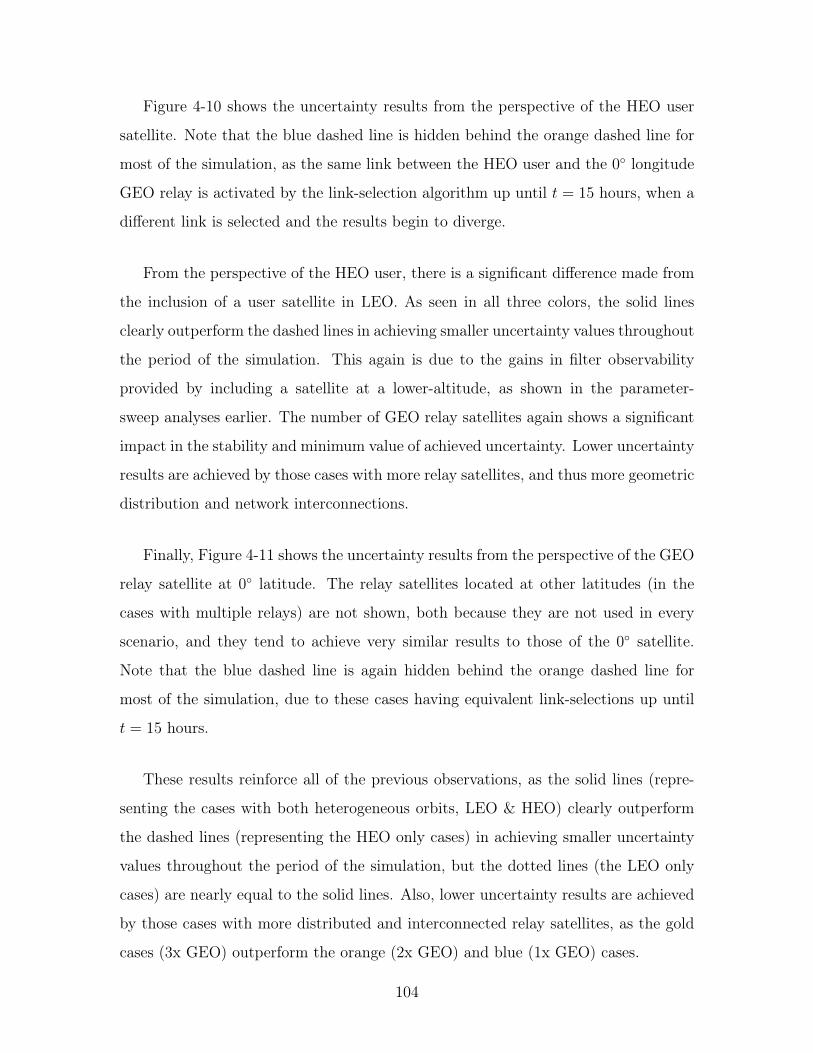
Figure 4-10 shows the uncertainty results from the perspective of the HEO user
satellite. Note that the blue dashed line is hidden behind the orange dashed line for
most of the simulation, as the same link between the HEO user and the 0∘ longitude
GEO relay is activated by the link-selection algorithm up until 𝑡 = 15 hours, when a
different link is selected and the results begin to diverge.
From the perspective of the HEO user, there is a significant difference made from
the inclusion of a user satellite in LEO. As seen in all three colors, the solid lines
clearly outperform the dashed lines in achieving smaller uncertainty values throughout
the period of the simulation. This again is due to the gains in filter observability
provided by including a satellite at a lower-altitude, as shown in the parameter-
sweep analyses earlier. The number of GEO relay satellites again shows a significant
impact in the stability and minimum value of achieved uncertainty. Lower uncertainty
results are achieved by those cases with more relay satellites, and thus more geometric
distribution and network interconnections.
Finally, Figure 4-11 shows the uncertainty results from the perspective of the GEO
relay satellite at 0∘ latitude. The relay satellites located at other latitudes (in the
cases with multiple relays) are not shown, both because they are not used in every
scenario, and they tend to achieve very similar results to those of the 0∘ satellite.
Note that the blue dashed line is again hidden behind the orange dashed line for
most of the simulation, due to these cases having equivalent link-selections up until
𝑡 = 15 hours.
These results reinforce all of the previous observations, as the solid lines (repre-
senting the cases with both heterogeneous orbits, LEO & HEO) clearly outperform
the dashed lines (representing the HEO only cases) in achieving smaller uncertainty
values throughout the period of the simulation, but the dotted lines (the LEO only
cases) are nearly equal to the solid lines. Also, lower uncertainty results are achieved
by those cases with more distributed and interconnected relay satellites, as the gold
cases (3x GEO) outperform the orange (2x GEO) and blue (1x GEO) cases.
104
0 3 6 9 12 15 18 21 24
Time (hours)
100
101
102
103
104
Tota
l P
ositio
n C
RLB
1-s
igm
a U
ncert
ain
ty (
m)
CRLB Analysis: Multiple Relays and/or Multiple Users
GEO-Relay1 (0 deg longitude)
OG1
OG2
OG3
MG1
MG2
MG3
OMG1
OMG2
OMG3
Figure 4-11: CRLB analysis results for GEO-Relay satellite #1 (at 0 deg longitude) indifferent multiple-relay/user configurations: 1x GEO-relay in blue, 2x GEO-relays inorange, and 3x interconnected GEO-relays in yellow. Dotted curves are used for singleLEO user scenarios, dashed curves for single HEO user, and solid curves for multipleusers (LEO+HEO). In the legend, ‘O’ denotes those scenarios that include the LEOuser OICETS, ‘M’ denotes those scenarios that include the HEO user MMS-1, and‘G#’ denotes the number of GEO relay satellites used in those scenarios.
EKF Error Analysis of 3x GEO Relay Scenarios
In order to gauge the navigation performance of a multiple relay/user scenario, and
how it compares to our earlier performance results of a single relay and a single
user, we simulated the best-performing scenario from the previous CRLB analy-
sis (3x GEO) in a full error analysis using 100 Monte Carlo simulations (sampling
noise/uncertainty in the measurements and estimation) with the EKF estimator. Fig-
ures 4-12 shows the result of a 3x GEO relay satellite scenario with a LEO user.
At the end of the 24-hour simulation period, the median total position errors are
about 8 meters for the GEO satellites, and 1.4 meters for the LEO satellite. These
results demonstrate improved performance (50% reductions in total position error)
over the single GEO-relay case shown in Figure 4-2. This is expected due to the
continuous availability of intersatellite measurements.
105
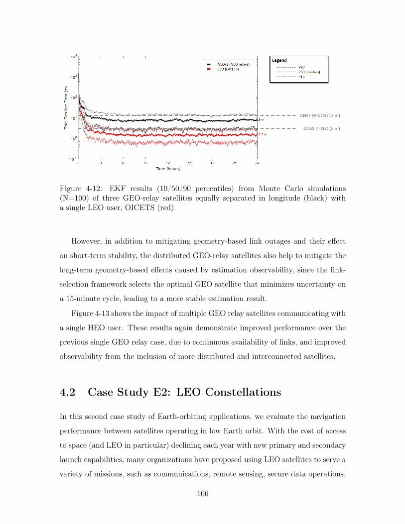
Figure 4-12: EKF results (10/50/90 percentiles) from Monte Carlo simulations(N=100) of three GEO-relay satellites equally separated in longitude (black) witha single LEO user, OICETS (red).
However, in addition to mitigating geometry-based link outages and their effect
on short-term stability, the distributed GEO-relay satellites also help to mitigate the
long-term geometry-based effects caused by estimation observability, since the link-
selection framework selects the optimal GEO satellite that minimizes uncertainty on
a 15-minute cycle, leading to a more stable estimation result.
Figure 4-13 shows the impact of multiple GEO relay satellites communicating with
a single HEO user. These results again demonstrate improved performance over the
previous single GEO relay case, due to continuous availability of links, and improved
observability from the inclusion of more distributed and interconnected satellites.
4.2 Case Study E2: LEO Constellations
In this second case study of Earth-orbiting applications, we evaluate the navigation
performance between satellites operating in low Earth orbit. With the cost of access
to space (and LEO in particular) declining each year with new primary and secondary
launch capabilities, many organizations have proposed using LEO satellites to serve a
variety of missions, such as communications, remote sensing, secure data operations,
106
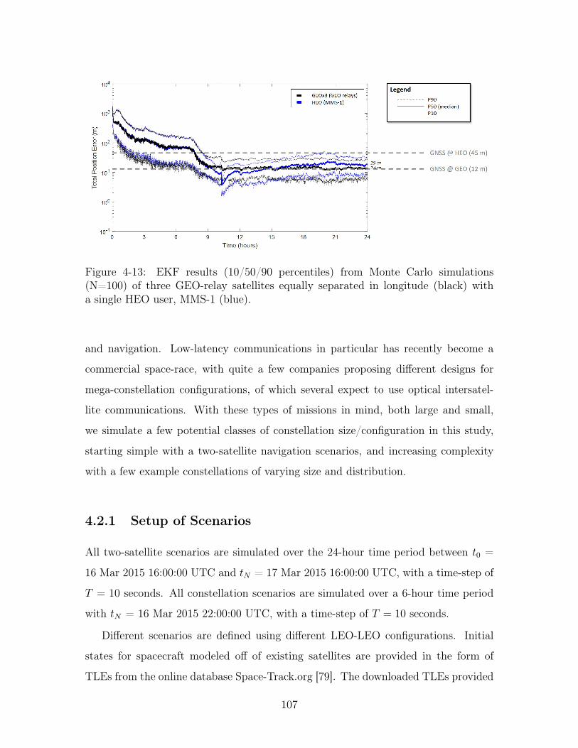
Figure 4-13: EKF results (10/50/90 percentiles) from Monte Carlo simulations(N=100) of three GEO-relay satellites equally separated in longitude (black) witha single HEO user, MMS-1 (blue).
and navigation. Low-latency communications in particular has recently become a
commercial space-race, with quite a few companies proposing different designs for
mega-constellation configurations, of which several expect to use optical intersatel-
lite communications. With these types of missions in mind, both large and small,
we simulate a few potential classes of constellation size/configuration in this study,
starting simple with a two-satellite navigation scenarios, and increasing complexity
with a few example constellations of varying size and distribution.
4.2.1 Setup of Scenarios
All two-satellite scenarios are simulated over the 24-hour time period between 𝑡0 =
16 Mar 2015 16:00:00 UTC and 𝑡𝑁 = 17 Mar 2015 16:00:00 UTC, with a time-step of
𝑇 = 10 seconds. All constellation scenarios are simulated over a 6-hour time period
with 𝑡𝑁 = 16 Mar 2015 22:00:00 UTC, with a time-step of 𝑇 = 10 seconds.
Different scenarios are defined using different LEO-LEO configurations. Initial
states for spacecraft modeled off of existing satellites are provided in the form of
TLEs from the online database Space-Track.org [79]. The downloaded TLEs provided
107
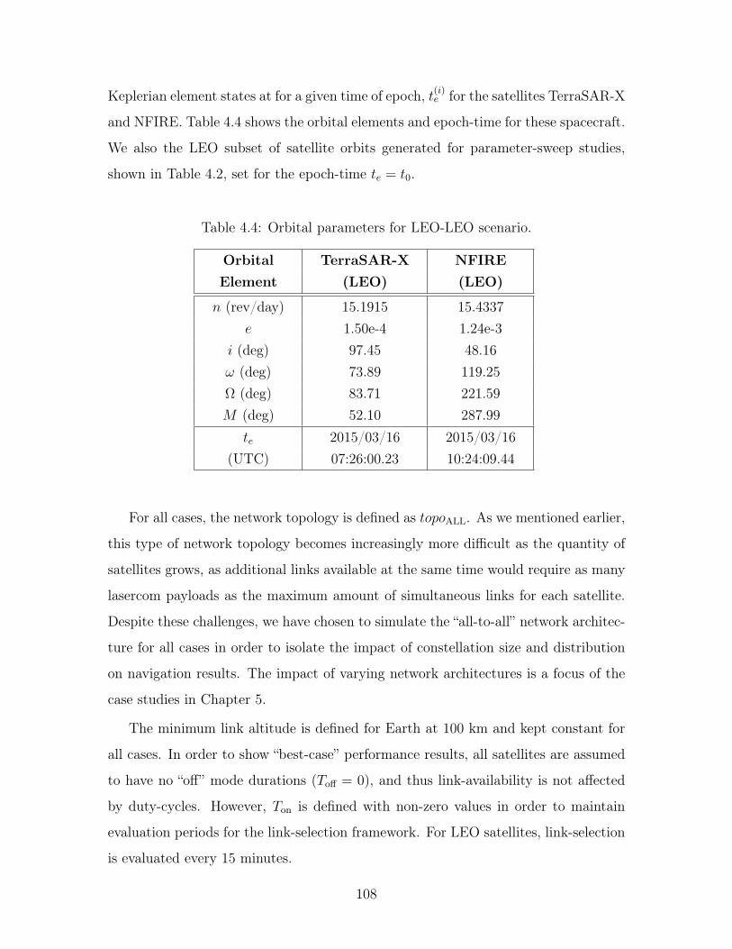
Keplerian element states at for a given time of epoch, 𝑡(𝑖)𝑒 for the satellites TerraSAR-X
and NFIRE. Table 4.4 shows the orbital elements and epoch-time for these spacecraft.
We also the LEO subset of satellite orbits generated for parameter-sweep studies,
shown in Table 4.2, set for the epoch-time 𝑡𝑒 = 𝑡0.
Table 4.4: Orbital parameters for LEO-LEO scenario.
Orbital TerraSAR-X NFIREElement (LEO) (LEO)
𝑛 (rev/day) 15.1915 15.4337𝑒 1.50e-4 1.24e-3
𝑖 (deg) 97.45 48.16𝜔 (deg) 73.89 119.25Ω (deg) 83.71 221.59𝑀 (deg) 52.10 287.99
𝑡𝑒 2015/03/16 2015/03/16(UTC) 07:26:00.23 10:24:09.44
For all cases, the network topology is defined as 𝑡𝑜𝑝𝑜ALL. As we mentioned earlier,
this type of network topology becomes increasingly more difficult as the quantity of
satellites grows, as additional links available at the same time would require as many
lasercom payloads as the maximum amount of simultaneous links for each satellite.
Despite these challenges, we have chosen to simulate the “all-to-all” network architec-
ture for all cases in order to isolate the impact of constellation size and distribution
on navigation results. The impact of varying network architectures is a focus of the
case studies in Chapter 5.
The minimum link altitude is defined for Earth at 100 km and kept constant for
all cases. In order to show “best-case” performance results, all satellites are assumed
to have no “off” mode durations (𝑇off = 0), and thus link-availability is not affected
by duty-cycles. However, 𝑇on is defined with non-zero values in order to maintain
evaluation periods for the link-selection framework. For LEO satellites, link-selection
is evaluated every 15 minutes.
108
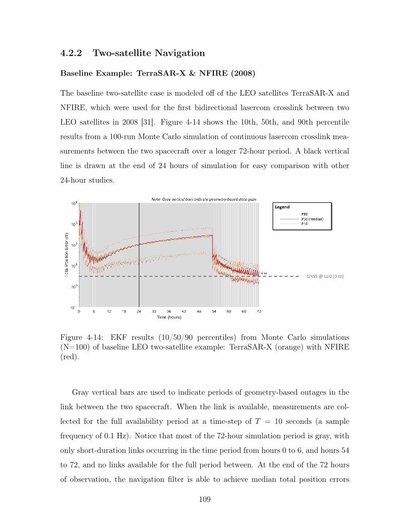
4.2.2 Two-satellite Navigation
Baseline Example: TerraSAR-X & NFIRE (2008)
The baseline two-satellite case is modeled off of the LEO satellites TerraSAR-X and
NFIRE, which were used for the first bidirectional lasercom crosslink between two
LEO satellites in 2008 [31]. Figure 4-14 shows the 10th, 50th, and 90th percentile
results from a 100-run Monte Carlo simulation of continuous lasercom crosslink mea-
surements between the two spacecraft over a longer 72-hour period. A black vertical
line is drawn at the end of 24 hours of simulation for easy comparison with other
24-hour studies.
Figure 4-14: EKF results (10/50/90 percentiles) from Monte Carlo simulations(N=100) of baseline LEO two-satellite example: TerraSAR-X (orange) with NFIRE(red).
Gray vertical bars are used to indicate periods of geometry-based outages in the
link between the two spacecraft. When the link is available, measurements are col-
lected for the full availability period at a time-step of 𝑇 = 10 seconds (a sample
frequency of 0.1 Hz). Notice that most of the 72-hour simulation period is gray, with
only short-duration links occurring in the time period from hours 0 to 6, and hours 54
to 72, and no links available for the full period between. At the end of the 72 hours
of observation, the navigation filter is able to achieve median total position errors
109
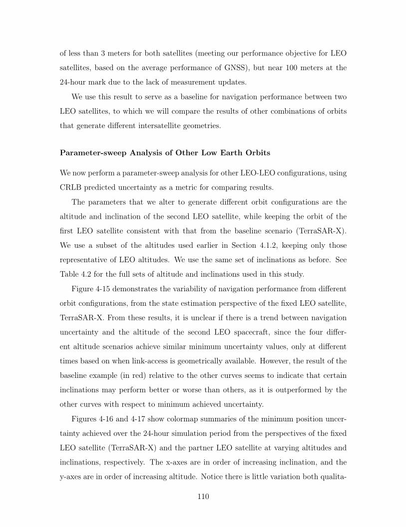
of less than 3 meters for both satellites (meeting our performance objective for LEO
satellites, based on the average performance of GNSS), but near 100 meters at the
24-hour mark due to the lack of measurement updates.
We use this result to serve as a baseline for navigation performance between two
LEO satellites, to which we will compare the results of other combinations of orbits
that generate different intersatellite geometries.
Parameter-sweep Analysis of Other Low Earth Orbits
We now perform a parameter-sweep analysis for other LEO-LEO configurations, using
CRLB predicted uncertainty as a metric for comparing results.
The parameters that we alter to generate different orbit configurations are the
altitude and inclination of the second LEO satellite, while keeping the orbit of the
first LEO satellite consistent with that from the baseline scenario (TerraSAR-X).
We use a subset of the altitudes used earlier in Section 4.1.2, keeping only those
representative of LEO altitudes. We use the same set of inclinations as before. See
Table 4.2 for the full sets of altitude and inclinations used in this study.
Figure 4-15 demonstrates the variability of navigation performance from different
orbit configurations, from the state estimation perspective of the fixed LEO satellite,
TerraSAR-X. From these results, it is unclear if there is a trend between navigation
uncertainty and the altitude of the second LEO spacecraft, since the four differ-
ent altitude scenarios achieve similar minimum uncertainty values, only at different
times based on when link-access is geometrically available. However, the result of the
baseline example (in red) relative to the other curves seems to indicate that certain
inclinations may perform better or worse than others, as it is outperformed by the
other curves with respect to minimum achieved uncertainty.
Figures 4-16 and 4-17 show colormap summaries of the minimum position uncer-
tainty achieved over the 24-hour simulation period from the perspectives of the fixed
LEO satellite (TerraSAR-X) and the partner LEO satellite at varying altitudes and
inclinations, respectively. The x-axes are in order of increasing inclination, and the
y-axes are in order of increasing altitude. Notice there is little variation both qualita-
110
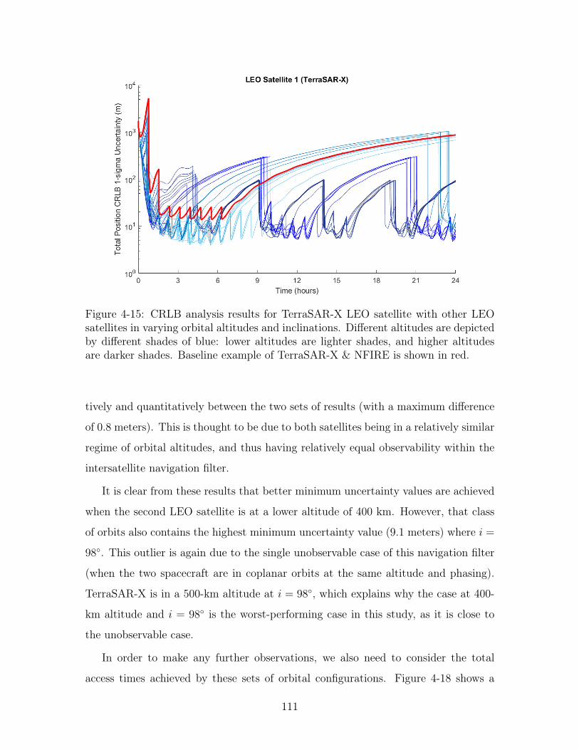
Figure 4-15: CRLB analysis results for TerraSAR-X LEO satellite with other LEOsatellites in varying orbital altitudes and inclinations. Different altitudes are depictedby different shades of blue: lower altitudes are lighter shades, and higher altitudesare darker shades. Baseline example of TerraSAR-X & NFIRE is shown in red.
tively and quantitatively between the two sets of results (with a maximum difference
of 0.8 meters). This is thought to be due to both satellites being in a relatively similar
regime of orbital altitudes, and thus having relatively equal observability within the
intersatellite navigation filter.
It is clear from these results that better minimum uncertainty values are achieved
when the second LEO satellite is at a lower altitude of 400 km. However, that class
of orbits also contains the highest minimum uncertainty value (9.1 meters) where 𝑖 =
98∘. This outlier is again due to the single unobservable case of this navigation filter
(when the two spacecraft are in coplanar orbits at the same altitude and phasing).
TerraSAR-X is in a 500-km altitude at 𝑖 = 98∘, which explains why the case at 400-
km altitude and 𝑖 = 98∘ is the worst-performing case in this study, as it is close to
the unobservable case.
In order to make any further observations, we also need to consider the total
access times achieved by these sets of orbital configurations. Figure 4-18 shows a
111
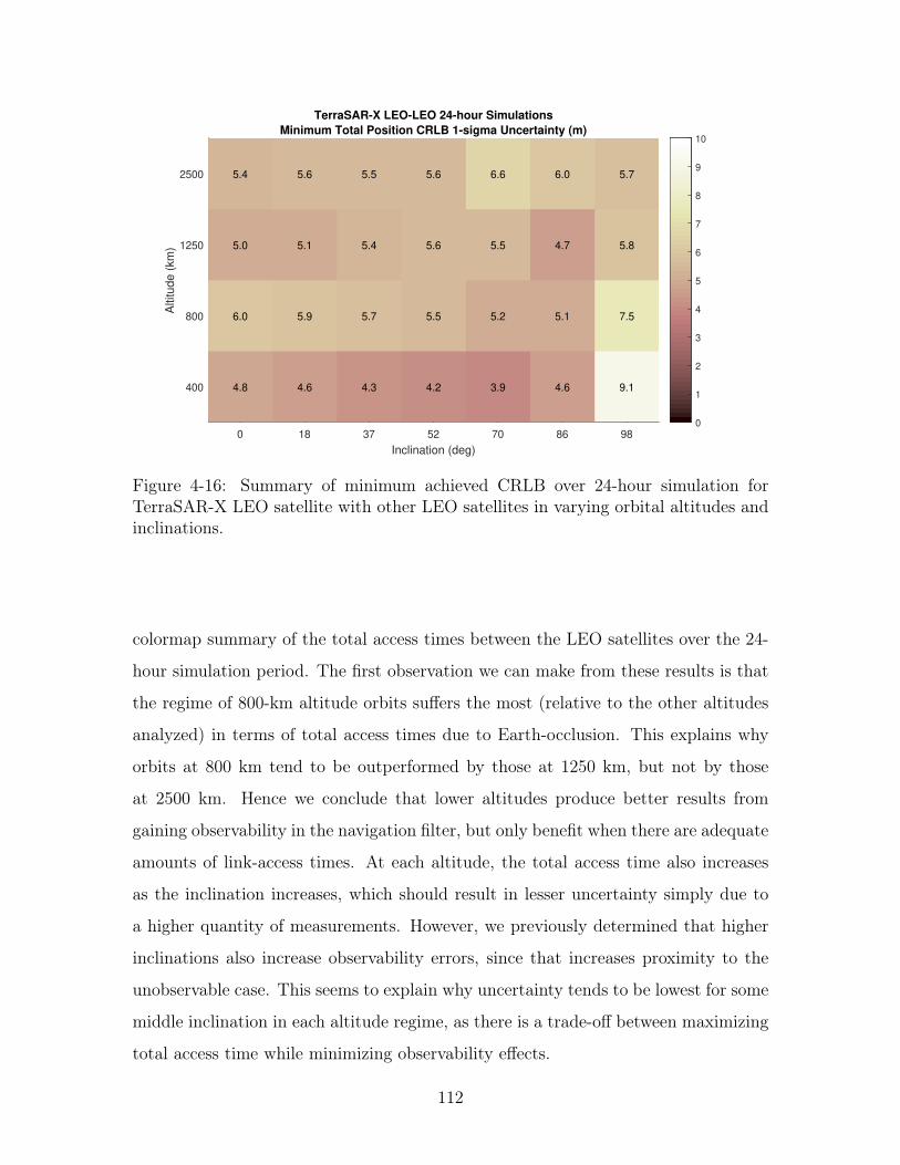
0 18 37 52 70 86 98
Inclination (deg)
400
800
1250
2500A
ltitude (
km
)
TerraSAR-X LEO-LEO 24-hour Simulations
Minimum Total Position CRLB 1-sigma Uncertainty (m)
4.8 4.6 4.3 4.2 3.9 4.6 9.1
6.0 5.9 5.7 5.5 5.2 5.1 7.5
5.0 5.1 5.4 5.6 5.5 4.7 5.8
5.4 5.6 5.5 5.6 6.6 6.0 5.7
0
1
2
3
4
5
6
7
8
9
10
Figure 4-16: Summary of minimum achieved CRLB over 24-hour simulation forTerraSAR-X LEO satellite with other LEO satellites in varying orbital altitudes andinclinations.
colormap summary of the total access times between the LEO satellites over the 24-
hour simulation period. The first observation we can make from these results is that
the regime of 800-km altitude orbits suffers the most (relative to the other altitudes
analyzed) in terms of total access times due to Earth-occlusion. This explains why
orbits at 800 km tend to be outperformed by those at 1250 km, but not by those
at 2500 km. Hence we conclude that lower altitudes produce better results from
gaining observability in the navigation filter, but only benefit when there are adequate
amounts of link-access times. At each altitude, the total access time also increases
as the inclination increases, which should result in lesser uncertainty simply due to
a higher quantity of measurements. However, we previously determined that higher
inclinations also increase observability errors, since that increases proximity to the
unobservable case. This seems to explain why uncertainty tends to be lowest for some
middle inclination in each altitude regime, as there is a trade-off between maximizing
total access time while minimizing observability effects.
112
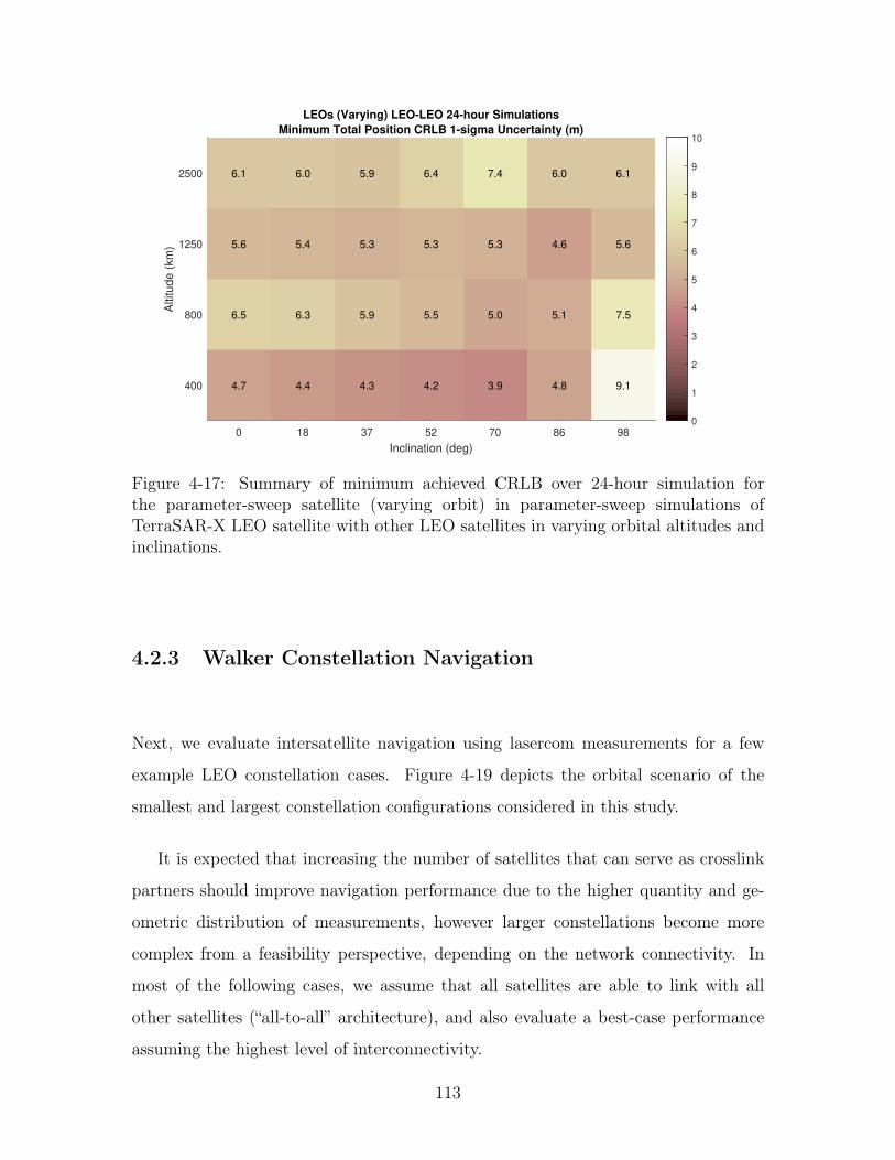
0 18 37 52 70 86 98
Inclination (deg)
400
800
1250
2500A
ltitude (
km
)
LEOs (Varying) LEO-LEO 24-hour Simulations
Minimum Total Position CRLB 1-sigma Uncertainty (m)
4.7 4.4 4.3 4.2 3.9 4.8 9.1
6.5 6.3 5.9 5.5 5.0 5.1 7.5
5.6 5.4 5.3 5.3 5.3 4.6 5.6
6.1 6.0 5.9 6.4 7.4 6.0 6.1
0
1
2
3
4
5
6
7
8
9
10
Figure 4-17: Summary of minimum achieved CRLB over 24-hour simulation forthe parameter-sweep satellite (varying orbit) in parameter-sweep simulations ofTerraSAR-X LEO satellite with other LEO satellites in varying orbital altitudes andinclinations.
4.2.3 Walker Constellation Navigation
Next, we evaluate intersatellite navigation using lasercom measurements for a few
example LEO constellation cases. Figure 4-19 depicts the orbital scenario of the
smallest and largest constellation configurations considered in this study.
It is expected that increasing the number of satellites that can serve as crosslink
partners should improve navigation performance due to the higher quantity and ge-
ometric distribution of measurements, however larger constellations become more
complex from a feasibility perspective, depending on the network connectivity. In
most of the following cases, we assume that all satellites are able to link with all
other satellites (“all-to-all” architecture), and also evaluate a best-case performance
assuming the highest level of interconnectivity.
113
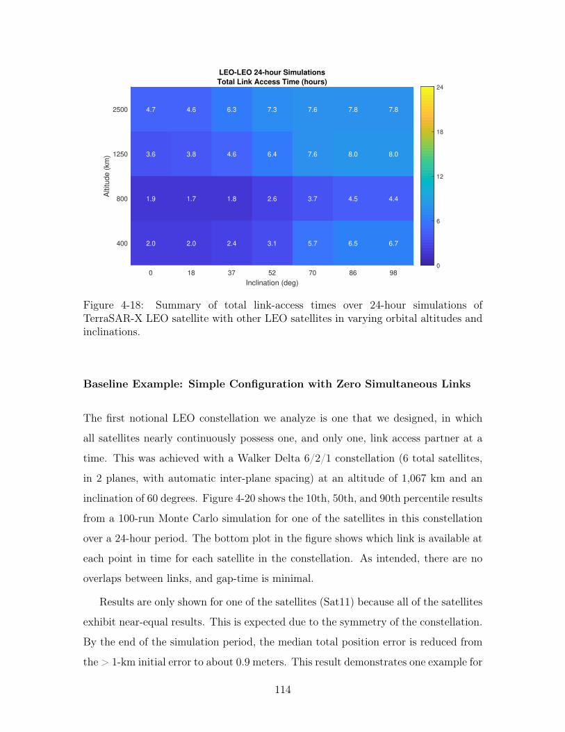
0 18 37 52 70 86 98
Inclination (deg)
400
800
1250
2500A
ltitude (
km
)
LEO-LEO 24-hour Simulations
Total Link Access Time (hours)
2.0 2.0 2.4 3.1 5.7 6.5 6.7
1.9 1.7 1.8 2.6 3.7 4.5 4.4
3.6 3.8 4.6 6.4 7.6 8.0 8.0
4.7 4.6 6.3 7.3 7.6 7.8 7.8
0
6
12
18
24
Figure 4-18: Summary of total link-access times over 24-hour simulations ofTerraSAR-X LEO satellite with other LEO satellites in varying orbital altitudes andinclinations.
Baseline Example: Simple Configuration with Zero Simultaneous Links
The first notional LEO constellation we analyze is one that we designed, in which
all satellites nearly continuously possess one, and only one, link access partner at a
time. This was achieved with a Walker Delta 6/2/1 constellation (6 total satellites,
in 2 planes, with automatic inter-plane spacing) at an altitude of 1,067 km and an
inclination of 60 degrees. Figure 4-20 shows the 10th, 50th, and 90th percentile results
from a 100-run Monte Carlo simulation for one of the satellites in this constellation
over a 24-hour period. The bottom plot in the figure shows which link is available at
each point in time for each satellite in the constellation. As intended, there are no
overlaps between links, and gap-time is minimal.
Results are only shown for one of the satellites (Sat11) because all of the satellites
exhibit near-equal results. This is expected due to the symmetry of the constellation.
By the end of the simulation period, the median total position error is reduced from
the > 1-km initial error to about 0.9 meters. This result demonstrates one example for
114
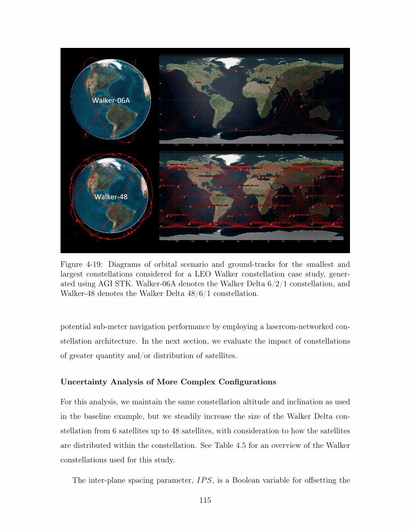
Figure 4-19: Diagrams of orbital scenario and ground-tracks for the smallest andlargest constellations considered for a LEO Walker constellation case study, gener-ated using AGI STK. Walker-06A denotes the Walker Delta 6/2/1 constellation, andWalker-48 denotes the Walker Delta 48/6/1 constellation.
potential sub-meter navigation performance by employing a lasercom-networked con-
stellation architecture. In the next section, we evaluate the impact of constellations
of greater quantity and/or distribution of satellites.
Uncertainty Analysis of More Complex Configurations
For this analysis, we maintain the same constellation altitude and inclination as used
in the baseline example, but we steadily increase the size of the Walker Delta con-
stellation from 6 satellites up to 48 satellites, with consideration to how the satellites
are distributed within the constellation. See Table 4.5 for an overview of the Walker
constellations used for this study.
The inter-plane spacing parameter, 𝐼𝑃𝑆, is a Boolean variable for offsetting the
115
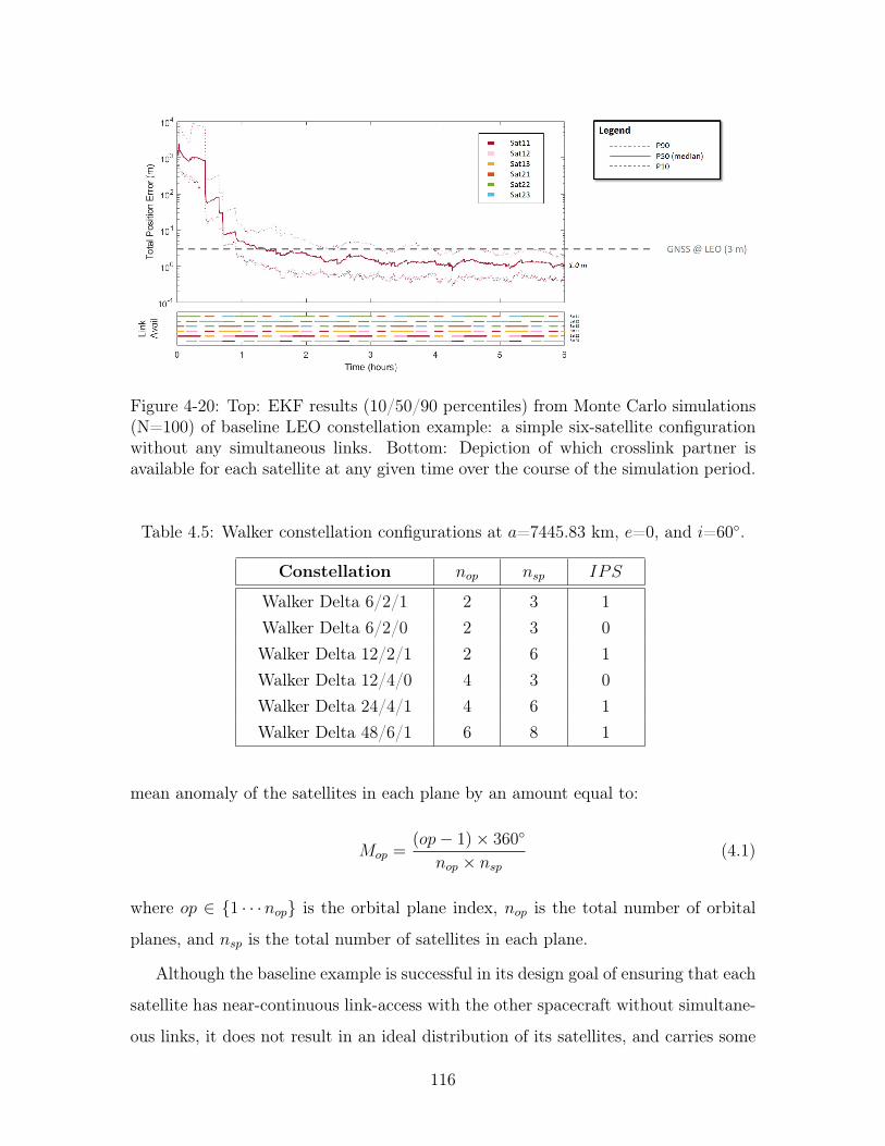
Figure 4-20: Top: EKF results (10/50/90 percentiles) from Monte Carlo simulations(N=100) of baseline LEO constellation example: a simple six-satellite configurationwithout any simultaneous links. Bottom: Depiction of which crosslink partner isavailable for each satellite at any given time over the course of the simulation period.
Table 4.5: Walker constellation configurations at 𝑎=7445.83 km, 𝑒=0, and 𝑖=60∘.
Constellation 𝑛𝑜𝑝 𝑛𝑠𝑝 𝐼𝑃𝑆
Walker Delta 6/2/1 2 3 1Walker Delta 6/2/0 2 3 0Walker Delta 12/2/1 2 6 1Walker Delta 12/4/0 4 3 0Walker Delta 24/4/1 4 6 1Walker Delta 48/6/1 6 8 1
mean anomaly of the satellites in each plane by an amount equal to:
𝑀𝑜𝑝 =(𝑜𝑝− 1) × 360∘
𝑛𝑜𝑝 × 𝑛𝑠𝑝
(4.1)
where 𝑜𝑝 ∈ 1 · · ·𝑛𝑜𝑝 is the orbital plane index, 𝑛𝑜𝑝 is the total number of orbital
planes, and 𝑛𝑠𝑝 is the total number of satellites in each plane.
Although the baseline example is successful in its design goal of ensuring that each
satellite has near-continuous link-access with the other spacecraft without simultane-
ous links, it does not result in an ideal distribution of its satellites, and carries some
116
concern for orbital collisions (also known as conjunctions) where the planes intersect.
This is partially due to the inter-plane spacing being set to 1, such that the mean
anomaly offset is in phase with the natural spacing of the satellites in each plane.
In a real-life utilization of this constellation design, conjunctions can still be miti-
gated by inserting an additional small offset in mean anomaly, or offsetting any of
the other orbital parameters. In this case, the greatest distribution of the satellites
is achieved by setting the inter-plane spacing to 0, and thus not using any offsets in
mean anomaly between planes.
The first case we simulate is this six-satellite, two-plane configuration with the
inter-plane spacing set to 0. Compared to the baseline case, this change effectively
eliminates one of the three possible crosslink partners of each satellite, and thus
reduces constellation connectivity. The second and third cases double the size of the
constellation to 12 satellites, the prior by doubling the number of satellites in each
plane 𝑛𝑠𝑝, and the latter by doubling the number of planes 𝑛𝑜𝑝. The fourth case
doubles the constellation size again to 24 satellites by combining the two previous
12-satellite designs. The final case is a 48-satellite constellation which augments both
quantities 𝑛𝑠𝑝 and 𝑛𝑜𝑝, instead of doubling either one individually. For each, the
inter-plane spacing parameter is set for greatest satellite distribution (and thus no
conjunctions).
As mentioned earlier, an “all-to-all” network topology architecture is assumed for
all cases. Though the complexity of implementing this increases exponentially with
respect to constellation size, this assumption allows us to examine the effect of the
quantity and distribution of satellites without additional modifications to the network
connectivity, and also results in a best-case scenario. Figure 4-21 shows the resulting
CRLB position uncertainty for these constellation cases.
As expected, the reduced connectivity of the Walker Delta 6/2/0 constellation
results in higher uncertainty than the baseline example of a Walker Delta 6/2/1
configuration. When the constellation size is doubled to 12 satellites, the uncertainty
drops by nearly 50%. This trend continues as the constellation size increases, as
doing so opens new network links for each satellite and augments the total number of
117
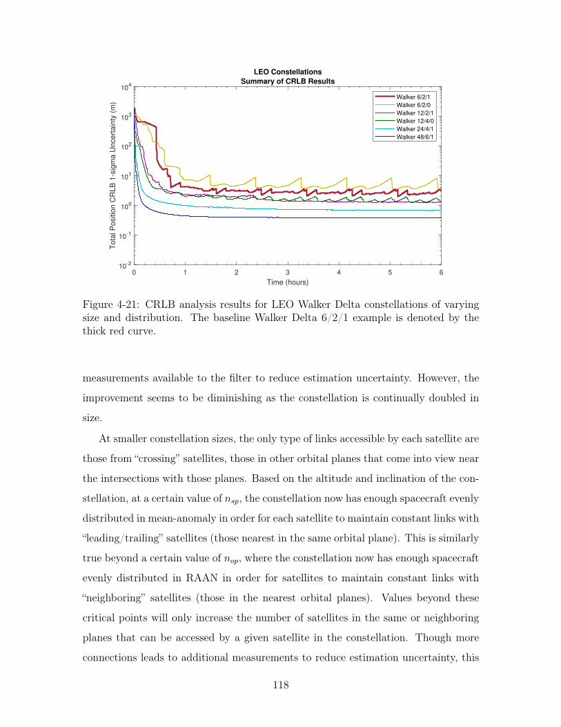
0 1 2 3 4 5 6
Time (hours)
10-2
10-1
100
101
102
103
104
Tota
l P
ositio
n C
RLB
1-s
igm
a U
ncert
ain
ty (
m)
LEO Constellations
Summary of CRLB Results
Walker 6/2/1
Walker 6/2/0
Walker 12/2/1
Walker 12/4/0
Walker 24/4/1
Walker 48/6/1
Figure 4-21: CRLB analysis results for LEO Walker Delta constellations of varyingsize and distribution. The baseline Walker Delta 6/2/1 example is denoted by thethick red curve.
measurements available to the filter to reduce estimation uncertainty. However, the
improvement seems to be diminishing as the constellation is continually doubled in
size.
At smaller constellation sizes, the only type of links accessible by each satellite are
those from “crossing” satellites, those in other orbital planes that come into view near
the intersections with those planes. Based on the altitude and inclination of the con-
stellation, at a certain value of 𝑛𝑠𝑝, the constellation now has enough spacecraft evenly
distributed in mean-anomaly in order for each satellite to maintain constant links with
“leading/trailing” satellites (those nearest in the same orbital plane). This is similarly
true beyond a certain value of 𝑛𝑜𝑝, where the constellation now has enough spacecraft
evenly distributed in RAAN in order for satellites to maintain constant links with
“neighboring” satellites (those in the nearest orbital planes). Values beyond these
critical points will only increase the number of satellites in the same or neighboring
planes that can be accessed by a given satellite in the constellation. Though more
connections leads to additional measurements to reduce estimation uncertainty, this
118
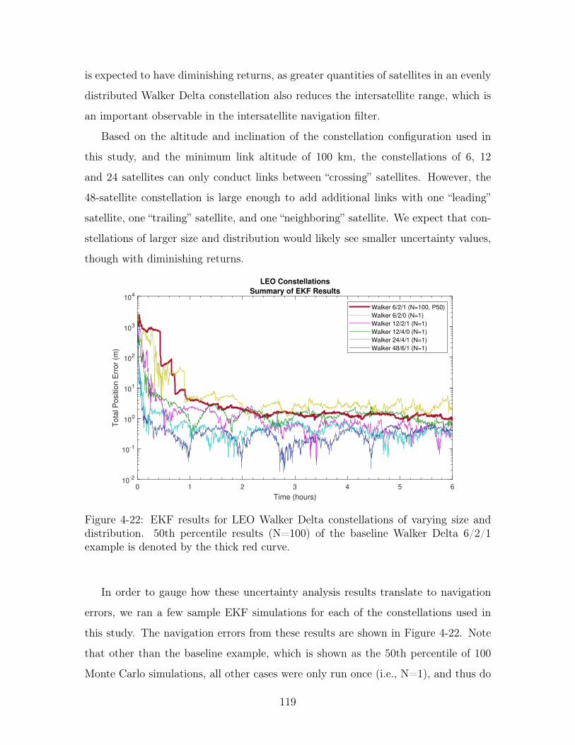
is expected to have diminishing returns, as greater quantities of satellites in an evenly
distributed Walker Delta constellation also reduces the intersatellite range, which is
an important observable in the intersatellite navigation filter.
Based on the altitude and inclination of the constellation configuration used in
this study, and the minimum link altitude of 100 km, the constellations of 6, 12
and 24 satellites can only conduct links between “crossing” satellites. However, the
48-satellite constellation is large enough to add additional links with one “leading”
satellite, one “trailing” satellite, and one “neighboring” satellite. We expect that con-
stellations of larger size and distribution would likely see smaller uncertainty values,
though with diminishing returns.
0 1 2 3 4 5 6
Time (hours)
10-2
10-1
100
101
102
103
104
Tota
l P
ositio
n E
rror
(m)
LEO Constellations
Summary of EKF Results
Walker 6/2/1 (N=100, P50)
Walker 6/2/0 (N=1)
Walker 12/2/1 (N=1)
Walker 12/4/0 (N=1)
Walker 24/4/1 (N=1)
Walker 48/6/1 (N=1)
Figure 4-22: EKF results for LEO Walker Delta constellations of varying size anddistribution. 50th percentile results (N=100) of the baseline Walker Delta 6/2/1example is denoted by the thick red curve.
In order to gauge how these uncertainty analysis results translate to navigation
errors, we ran a few sample EKF simulations for each of the constellations used in
this study. The navigation errors from these results are shown in Figure 4-22. Note
that other than the baseline example, which is shown as the 50th percentile of 100
Monte Carlo simulations, all other cases were only run once (i.e., N=1), and thus do
119
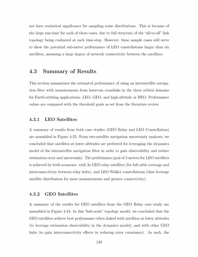
not have statistical significance for sampling noise distributions. This is because of
the large run-time for each of these cases, due to full structure of the “all-to-all” link
topology being evaluated at each time-step. However, these sample cases still serve
to show the potential sub-meter performance of LEO constellations larger than six
satellites, assuming a large degree of network connectivity between the satellites.
4.3 Summary of Results
This section summarizes the estimated performance of using an intersatellite naviga-
tion filter with measurements from lasercom crosslinks in the three orbital domains
for Earth-orbiting applications: LEO, GEO, and high-altitude or HEO. Performance
values are compared with the threshold goals as set from the literature review.
4.3.1 LEO Satellites
A summary of results from both case studies (GEO Relay and LEO Constellation)
are assembled in Figure 4-23. From two-satellite navigation uncertainty analyses, we
concluded that satellites at lower altitudes are preferred for leveraging the dynamics
model of the intersatellite navigation filter in order to gain observability and reduce
estimation error and uncertainty. The performance goal of 3 meters for LEO satellites
is achieved by both scenarios: with 3x GEO relay satellites (for full orbit coverage and
interconnectivity between relay hubs), and LEO Walker constellations (that leverage
satellite distribution for more measurements and greater connectivity).
4.3.2 GEO Satellites
A summary of the results for GEO satellites from the GEO Relay case study are
assembled in Figure 4-24. In this “hub-node” topology model, we concluded that the
GEO satellites achieve best performance when linked with satellites at lower altitudes
(to leverage estimation observability in the dynamics model), and with other GEO
hubs (to gain interconnectivity effects in reducing error covariance). As such, the
120
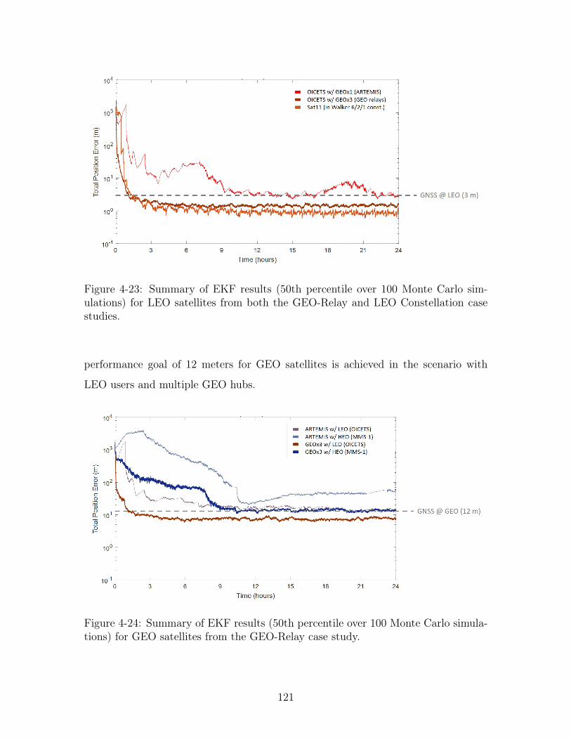
Figure 4-23: Summary of EKF results (50th percentile over 100 Monte Carlo sim-ulations) for LEO satellites from both the GEO-Relay and LEO Constellation casestudies.
performance goal of 12 meters for GEO satellites is achieved in the scenario with
LEO users and multiple GEO hubs.
Figure 4-24: Summary of EKF results (50th percentile over 100 Monte Carlo simula-tions) for GEO satellites from the GEO-Relay case study.
121
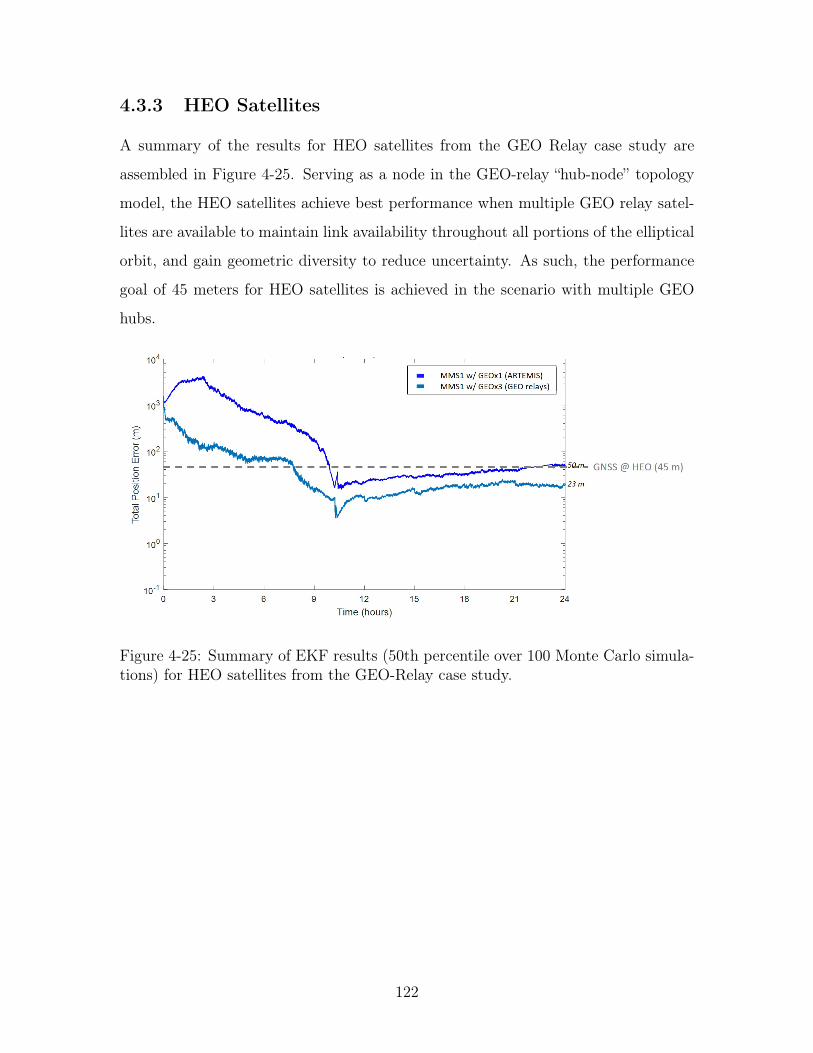
4.3.3 HEO Satellites
A summary of the results for HEO satellites from the GEO Relay case study are
assembled in Figure 4-25. Serving as a node in the GEO-relay “hub-node” topology
model, the HEO satellites achieve best performance when multiple GEO relay satel-
lites are available to maintain link availability throughout all portions of the elliptical
orbit, and gain geometric diversity to reduce uncertainty. As such, the performance
goal of 45 meters for HEO satellites is achieved in the scenario with multiple GEO
hubs.
Figure 4-25: Summary of EKF results (50th percentile over 100 Monte Carlo simula-tions) for HEO satellites from the GEO-Relay case study.
122
Chapter 5
Deep-Space Orbital Applications
This chapter describes the results and analysis from evaluating the performance of
the proposed navigation method using intersatellite lasercom measurements for deep-
space orbital applications. We chose to focus on applications for Mars, as it is the
location of many past, present, and future exploration missions that can be used as
case studies. However, the lasercom navigation method can also be applied to other
deep-space bodies, assuming that its mass and gravity characteristics are known well
enough to model its primary gravitational forces. Thanks to a long history of Mars
orbiter missions, Mars is well-characterized to over 100 terms in degree & order in
the latest gravity models produced by NASA JPL [80]. In our first Mars case study,
we simulate the performance of intersatellite navigation using lasercom for future
science/exploration Mars-orbiters using the current missions as proxies. In the second
case study, we simulate lasercom navigation performance for a possible six-satellite
Mars communications constellation as proposed by Castellini et al. (2010) [14].
5.1 Case Study M1: Existing Mars Mission Orbits
In this first case study, we evaluate the navigation performance of different con-
figurations of Mars exploration orbiters based on the orbital parameters of current
Mars-orbiting missions. The purpose of using the current mission orbits is that they
serve as ready-made examples for a set of potential future missions that could have
123
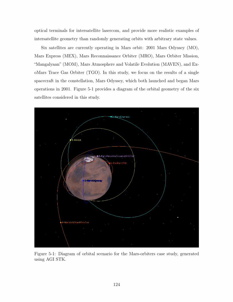
optical terminals for intersatellite lasercom, and provide more realistic examples of
intersatellite geometry than randomly generating orbits with arbitrary state values.
Six satellites are currently operating in Mars orbit: 2001 Mars Odyssey (MO),
Mars Express (MEX), Mars Reconnaissance Orbiter (MRO), Mars Orbiter Mission,
“Mangalyaan” (MOM), Mars Atmosphere and Volatile Evolution (MAVEN), and Ex-
oMars Trace Gas Orbiter (TGO). In this study, we focus on the results of a single
spacecraft in the constellation, Mars Odyssey, which both launched and began Mars
operations in 2001. Figure 5-1 provides a diagram of the orbital geometry of the six
satellites considered in this study.
Figure 5-1: Diagram of orbital scenario for the Mars-orbiters case study, generatedusing AGI STK.
124
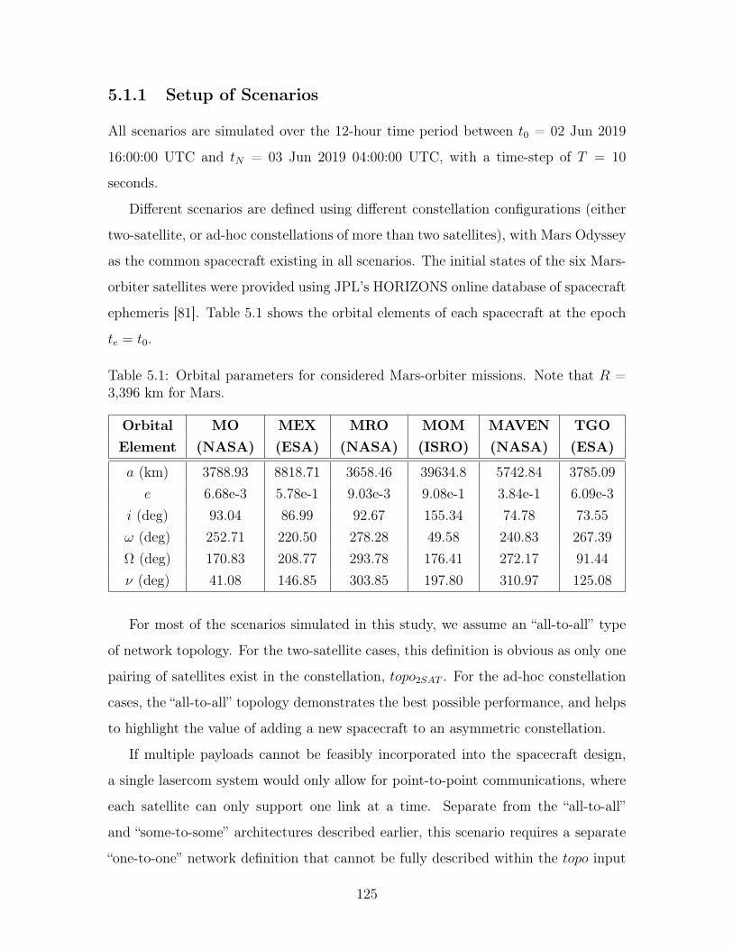
5.1.1 Setup of Scenarios
All scenarios are simulated over the 12-hour time period between 𝑡0 = 02 Jun 2019
16:00:00 UTC and 𝑡𝑁 = 03 Jun 2019 04:00:00 UTC, with a time-step of 𝑇 = 10
seconds.
Different scenarios are defined using different constellation configurations (either
two-satellite, or ad-hoc constellations of more than two satellites), with Mars Odyssey
as the common spacecraft existing in all scenarios. The initial states of the six Mars-
orbiter satellites were provided using JPL’s HORIZONS online database of spacecraft
ephemeris [81]. Table 5.1 shows the orbital elements of each spacecraft at the epoch
𝑡𝑒 = 𝑡0.
Table 5.1: Orbital parameters for considered Mars-orbiter missions. Note that 𝑅 =3,396 km for Mars.
Orbital MO MEX MRO MOM MAVEN TGOElement (NASA) (ESA) (NASA) (ISRO) (NASA) (ESA)
𝑎 (km) 3788.93 8818.71 3658.46 39634.8 5742.84 3785.09𝑒 6.68e-3 5.78e-1 9.03e-3 9.08e-1 3.84e-1 6.09e-3
𝑖 (deg) 93.04 86.99 92.67 155.34 74.78 73.55𝜔 (deg) 252.71 220.50 278.28 49.58 240.83 267.39Ω (deg) 170.83 208.77 293.78 176.41 272.17 91.44𝜈 (deg) 41.08 146.85 303.85 197.80 310.97 125.08
For most of the scenarios simulated in this study, we assume an “all-to-all” type
of network topology. For the two-satellite cases, this definition is obvious as only one
pairing of satellites exist in the constellation, 𝑡𝑜𝑝𝑜2𝑆𝐴𝑇 . For the ad-hoc constellation
cases, the “all-to-all” topology demonstrates the best possible performance, and helps
to highlight the value of adding a new spacecraft to an asymmetric constellation.
If multiple payloads cannot be feasibly incorporated into the spacecraft design,
a single lasercom system would only allow for point-to-point communications, where
each satellite can only support one link at a time. Separate from the “all-to-all”
and “some-to-some” architectures described earlier, this scenario requires a separate
“one-to-one” network definition that cannot be fully described within the 𝑡𝑜𝑝𝑜 input
125

parameter. This is because the topology describes which satellites are available to a
given satellite from a networking perspective, not how many links can be supported at
a given time. For select scenarios, we also evaluate this “one-to-one” network topology
in order to evaluate a more feasible scenario that can be implemented using current
technologies and capabilities.
The minimum link altitude is defined for Mars at 80 km and kept constant for all
cases. Since these are Mars exploration orbiters, we assume that 50% of the mission
time will be spent performing tasks other than crosslink communications with a 30:30
minute duty-cycle (on:off).
5.1.2 Two-satellite Cases
We first evaluate any potential differences based on the orbit of the crosslinked partner
satellite in two-satellite cases of Mars-orbiter navigation. Figure 5-2 shows the 50th
percentile position navigation results for the Mars Odyssey spacecraft in different
two-satellite configurations with the other current Mars-orbiters.
Figure 5-2: Top: Summary of EKF results (50th percentile only) from Monte Carlosimulations (N=100) of 2001 Mars Odyssey orbiter in separate two-satellite naviga-tion scenarios with each of the other five current Mars-orbiters with a 30:30-minutecommunications duty cycle. Bottom: Depiction of when a link is available for eachcrosslink partner scenario at any given time over the course of the simulation period.
126
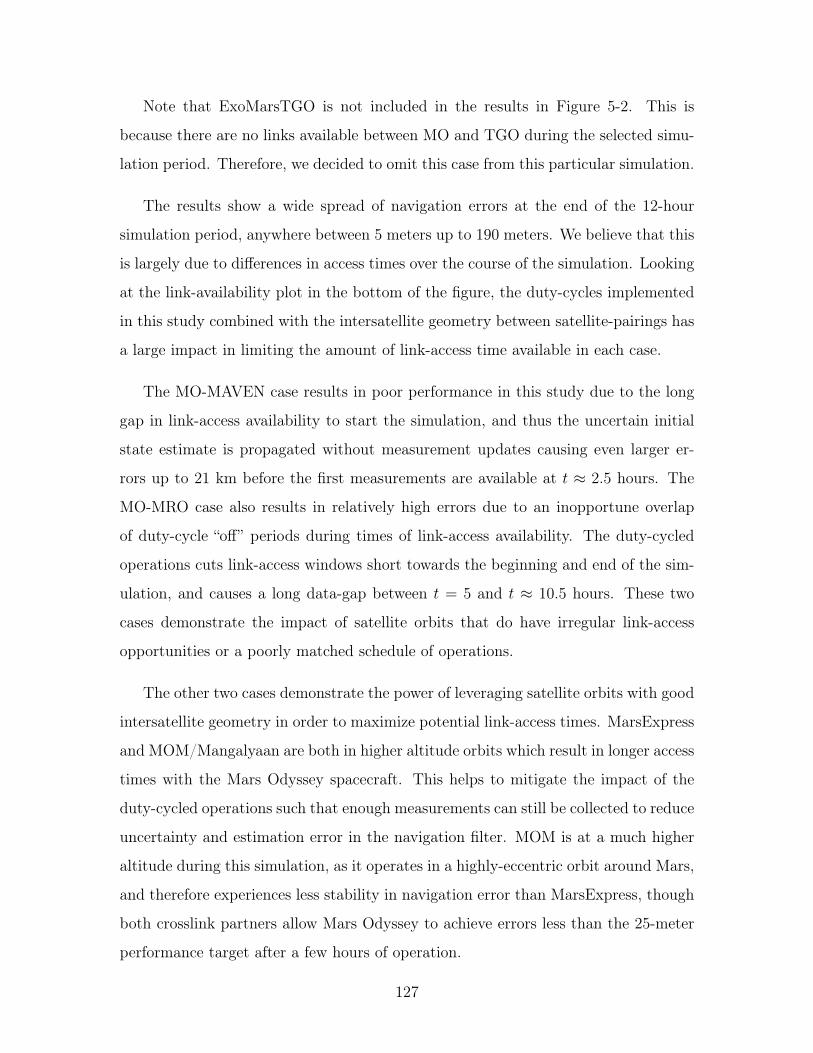
Note that ExoMarsTGO is not included in the results in Figure 5-2. This is
because there are no links available between MO and TGO during the selected simu-
lation period. Therefore, we decided to omit this case from this particular simulation.
The results show a wide spread of navigation errors at the end of the 12-hour
simulation period, anywhere between 5 meters up to 190 meters. We believe that this
is largely due to differences in access times over the course of the simulation. Looking
at the link-availability plot in the bottom of the figure, the duty-cycles implemented
in this study combined with the intersatellite geometry between satellite-pairings has
a large impact in limiting the amount of link-access time available in each case.
The MO-MAVEN case results in poor performance in this study due to the long
gap in link-access availability to start the simulation, and thus the uncertain initial
state estimate is propagated without measurement updates causing even larger er-
rors up to 21 km before the first measurements are available at 𝑡 ≈ 2.5 hours. The
MO-MRO case also results in relatively high errors due to an inopportune overlap
of duty-cycle “off” periods during times of link-access availability. The duty-cycled
operations cuts link-access windows short towards the beginning and end of the sim-
ulation, and causes a long data-gap between 𝑡 = 5 and 𝑡 ≈ 10.5 hours. These two
cases demonstrate the impact of satellite orbits that do have irregular link-access
opportunities or a poorly matched schedule of operations.
The other two cases demonstrate the power of leveraging satellite orbits with good
intersatellite geometry in order to maximize potential link-access times. MarsExpress
and MOM/Mangalyaan are both in higher altitude orbits which result in longer access
times with the Mars Odyssey spacecraft. This helps to mitigate the impact of the
duty-cycled operations such that enough measurements can still be collected to reduce
uncertainty and estimation error in the navigation filter. MOM is at a much higher
altitude during this simulation, as it operates in a highly-eccentric orbit around Mars,
and therefore experiences less stability in navigation error than MarsExpress, though
both crosslink partners allow Mars Odyssey to achieve errors less than the 25-meter
performance target after a few hours of operation.
127
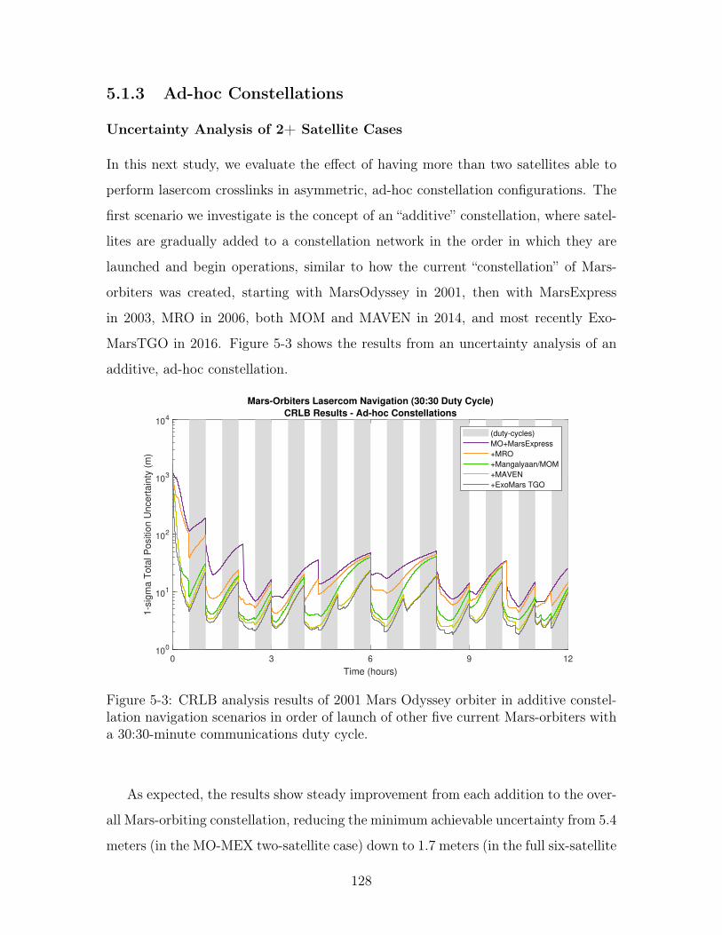
5.1.3 Ad-hoc Constellations
Uncertainty Analysis of 2+ Satellite Cases
In this next study, we evaluate the effect of having more than two satellites able to
perform lasercom crosslinks in asymmetric, ad-hoc constellation configurations. The
first scenario we investigate is the concept of an “additive” constellation, where satel-
lites are gradually added to a constellation network in the order in which they are
launched and begin operations, similar to how the current “constellation” of Mars-
orbiters was created, starting with MarsOdyssey in 2001, then with MarsExpress
in 2003, MRO in 2006, both MOM and MAVEN in 2014, and most recently Exo-
MarsTGO in 2016. Figure 5-3 shows the results from an uncertainty analysis of an
additive, ad-hoc constellation.
0 3 6 9 12
Time (hours)
100
101
102
103
104
1-s
igm
a T
ota
l P
ositio
n U
ncert
ain
ty (
m)
Mars-Orbiters Lasercom Navigation (30:30 Duty Cycle)
CRLB Results - Ad-hoc Constellations
(duty-cycles)
MO+MarsExpress
+MRO
+Mangalyaan/MOM
+MAVEN
+ExoMars TGO
Figure 5-3: CRLB analysis results of 2001 Mars Odyssey orbiter in additive constel-lation navigation scenarios in order of launch of other five current Mars-orbiters witha 30:30-minute communications duty cycle.
As expected, the results show steady improvement from each addition to the over-
all Mars-orbiting constellation, reducing the minimum achievable uncertainty from 5.4
meters (in the MO-MEX two-satellite case) down to 1.7 meters (in the full six-satellite
128
case), which represents a 68% reduction in uncertainty. The results clearly show the
added benefit of connecting more satellites into a crosslinked constellation. However,
these results also assume that all satellites can communicate with each other, which
becomes increasingly difficult with each satellite added to the constellation.
Baseline Example: NASA Spacecraft Constellation
In the second scenario of an ad-hoc constellation, we further investigate the impact of
adding an additional satellite into an ad-hoc constellation. Of the six current Mars-
orbiter missions, three were developed by NASA: Mars Odyssey, MRO, and MAVEN.
As such, all three were designed with a common communications technology archi-
tecture in that frequencies, protocols, and even payload designs are consistent across
all three satellites, simplifying ground communications and mission operations. If we
were to assume that future NASA spacecraft could instead utilize common lasercom
technology architectures, they could potentially communicate with one another.
In the previous study of two-satellite scenarios, the NASA satellites coincidentally
represented the two worst-performing cases, MO-MRO and MO-MAVEN. In this
study, we enable MRO and MAVEN to establish links with each other in addition
to their links with MO, in order to close the network topology in a three-satellite
fully connected configuration. We implement two network architectures, the “all-
to-all” case and the “one-to-one” case. In the “all-to-all” case, each of the three
spacecraft require the capability of maintaining two simultaneous crosslinks, most
readily implemented by having two lasercom terminals, one that can track each of
the other satellites. This mitigates the need for any link-selection, as each link can be
made whenever it is available. In the “one-to-one” case, each spacecraft only possesses
one lasercom terminal, and is thus only able to track and establish a crosslink with one
other satellite at a given time. This represents a more readily achievable constellation
case, as it simplifies the design of the spacecraft, though it does require a way to
select between two simultaneously available links. This is implemented within the
“network rules” portion of the link-selection framework developed in this thesis. Link-
selection is executed from the perspective of the Mars Odyssey spacecraft, therefore
129
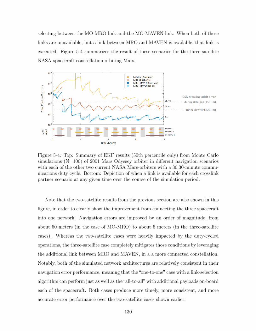
selecting between the MO-MRO link and the MO-MAVEN link. When both of these
links are unavailable, but a link between MRO and MAVEN is available, that link is
executed. Figure 5-4 summarizes the result of these scenarios for the three-satellite
NASA spacecraft constellation orbiting Mars.
Figure 5-4: Top: Summary of EKF results (50th percentile only) from Monte Carlosimulations (N=100) of 2001 Mars Odyssey orbiter in different navigation scenarioswith each of the other two current NASA Mars-orbiters with a 30:30-minute commu-nications duty cycle. Bottom: Depiction of when a link is available for each crosslinkpartner scenario at any given time over the course of the simulation period.
Note that the two-satellite results from the previous section are also shown in this
figure, in order to clearly show the improvement from connecting the three spacecraft
into one network. Navigation errors are improved by an order of magnitude, from
about 50 meters (in the case of MO-MRO) to about 5 meters (in the three-satellite
cases). Whereas the two-satellite cases were heavily impacted by the duty-cycled
operations, the three-satellite case completely mitigates those conditions by leveraging
the additional link between MRO and MAVEN, in a a more connected constellation.
Notably, both of the simulated network architectures are relatively consistent in their
navigation error performance, meaning that the “one-to-one” case with a link-selection
algorithm can perform just as well as the “all-to-all” with additional payloads on-board
each of the spacecraft. Both cases produce more timely, more consistent, and more
accurate error performance over the two-satellite cases shown earlier.
130
5.2 Case Study M2: Future Comms. Constellation
In the second Mars case study, we evaluate the navigation performance of a Mars-
orbiting communications constellation for supporting future human and robotic oper-
ations, as proposed by Castellini et al. [14], consisting of six total satellites equipped
with lasercom payloads for downlink communications with Earth. Although the au-
thors assumed that intersatellite links would be conducted using radio transmissions,
for the purposes of our study, we assume that they can be performed using lasercom
payloads instead. Figure 5-5 provides a diagram of the orbital configuration of the
considered constellation.
The constellation is configured as a Walker constellation with 𝑛𝑜𝑝 = 2 orbital
planes and 𝑛𝑠𝑝 = 3 satellites per plane. The satellites are described to be at an
altitude of 17,030 km (therefore 𝑎 ≈ 20, 426 km and 𝑒 = 0) and an inclination of 37∘.
The phase shift (in mean-anomaly) between orbital planes is 5∘, while the RAAN
separation between orbital planes is 180∘. We label satellites in the first plane as
Sat11, Sat12, and Sat13, and satellites in the second plane are Sat21, Sat22, and
Sat23.
5.2.1 Setup of Scenarios
All scenarios are simulated over a 24-hour time period, between 𝑡0 = 02 Jun 2019
16:00:00 UTC and 𝑡𝑁 = 03 Jun 2019 16:00:00 UTC, with a time-step of 𝑇 = 10
seconds. All scenarios use all six satellites in the constellation. Table 5.2 shows the
orbital elements of each spacecraft, based on the Walker constellation configuration
described above, for the epoch 𝑡𝑒 = 𝑡0.
The minimum link altitude is defined for Mars at 80 km and kept constant for all
cases. Similar to the previous case study, we model that 50% of the mission time will
be spent performing tasks other than crosslink communications with a 30:30 minute
duty-cycle (on:off).
131
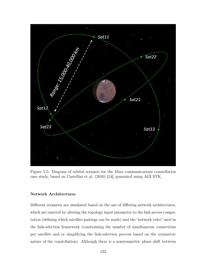
Figure 5-5: Diagram of orbital scenario for the Mars communications constellationcase study, based on Castellini et al. (2010) [14], generated using AGI STK.
Network Architectures
Different scenarios are simulated based on the use of differing network architectures,
which are enacted by altering the topology input parameter to the link-access compu-
tation (defining which satellite-pairings can be made) and the “network rules” used in
the link-selection framework (constraining the number of simultaneous connections
per satellite and/or simplifying the link-selection process based on the symmetric
nature of the constellation). Although there is a nonsymmetric phase shift between
132
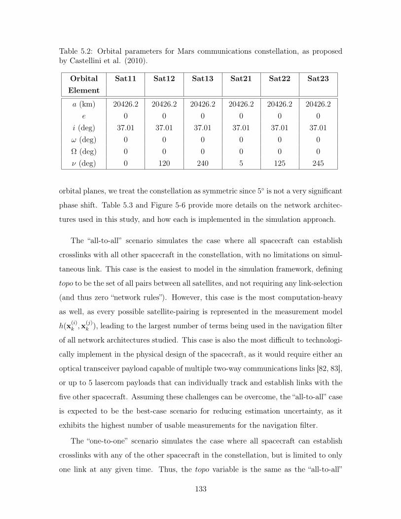
Table 5.2: Orbital parameters for Mars communications constellation, as proposedby Castellini et al. (2010).
Orbital Sat11 Sat12 Sat13 Sat21 Sat22 Sat23Element
𝑎 (km) 20426.2 20426.2 20426.2 20426.2 20426.2 20426.2𝑒 0 0 0 0 0 0
𝑖 (deg) 37.01 37.01 37.01 37.01 37.01 37.01𝜔 (deg) 0 0 0 0 0 0Ω (deg) 0 0 0 0 0 0𝜈 (deg) 0 120 240 5 125 245
orbital planes, we treat the constellation as symmetric since 5∘ is not a very significant
phase shift. Table 5.3 and Figure 5-6 provide more details on the network architec-
tures used in this study, and how each is implemented in the simulation approach.
The “all-to-all” scenario simulates the case where all spacecraft can establish
crosslinks with all other spacecraft in the constellation, with no limitations on simul-
taneous link. This case is the easiest to model in the simulation framework, defining
𝑡𝑜𝑝𝑜 to be the set of all pairs between all satellites, and not requiring any link-selection
(and thus zero “network rules”). However, this case is the most computation-heavy
as well, as every possible satellite-pairing is represented in the measurement model
ℎ(x(𝑖)𝑘 ,x
(𝑗)𝑘 ), leading to the largest number of terms being used in the navigation filter
of all network architectures studied. This case is also the most difficult to technologi-
cally implement in the physical design of the spacecraft, as it would require either an
optical transceiver payload capable of multiple two-way communications links [82, 83],
or up to 5 lasercom payloads that can individually track and establish links with the
five other spacecraft. Assuming these challenges can be overcome, the “all-to-all” case
is expected to be the best-case scenario for reducing estimation uncertainty, as it
exhibits the highest number of usable measurements for the navigation filter.
The “one-to-one” scenario simulates the case where all spacecraft can establish
crosslinks with any of the other spacecraft in the constellation, but is limited to only
one link at any given time. Thus, the 𝑡𝑜𝑝𝑜 variable is the same as the “all-to-all”
133
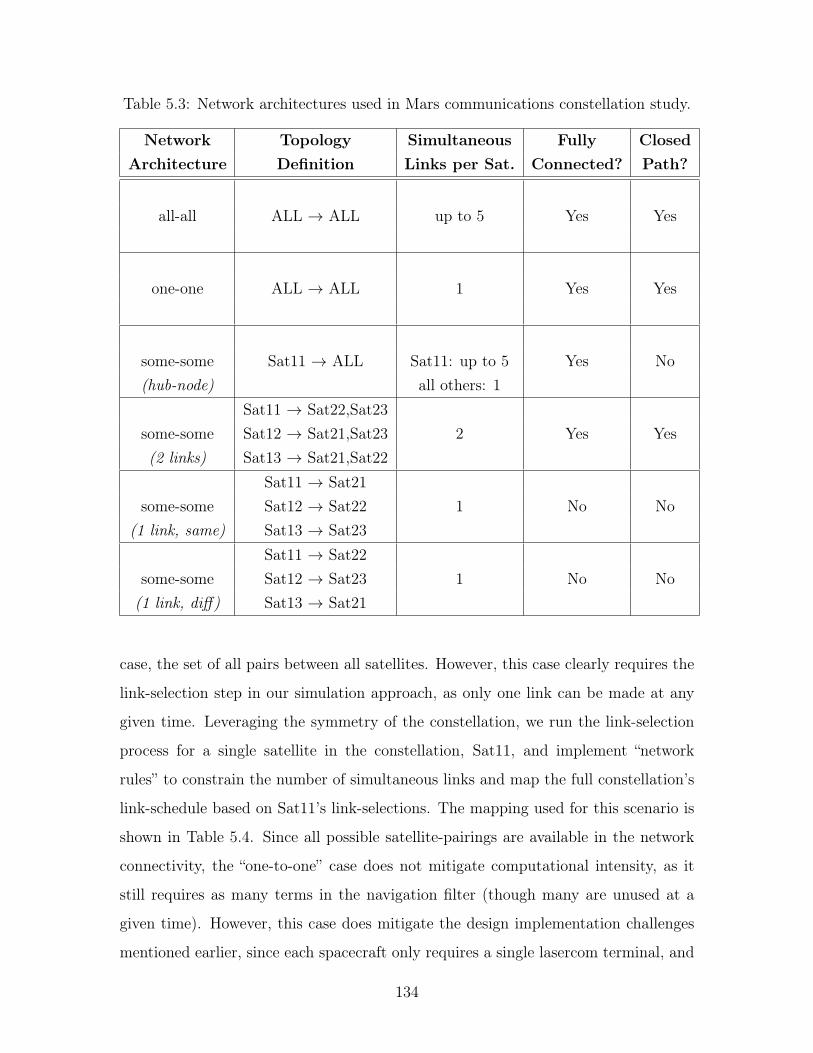
Table 5.3: Network architectures used in Mars communications constellation study.
Network Topology Simultaneous Fully ClosedArchitecture Definition Links per Sat. Connected? Path?
all-all ALL → ALL up to 5 Yes Yes
one-one ALL → ALL 1 Yes Yes
some-some Sat11 → ALL Sat11: up to 5 Yes No(hub-node) all others: 1
Sat11 → Sat22,Sat23some-some Sat12 → Sat21,Sat23 2 Yes Yes(2 links) Sat13 → Sat21,Sat22
Sat11 → Sat21some-some Sat12 → Sat22 1 No No
(1 link, same) Sat13 → Sat23Sat11 → Sat22
some-some Sat12 → Sat23 1 No No(1 link, diff) Sat13 → Sat21
case, the set of all pairs between all satellites. However, this case clearly requires the
link-selection step in our simulation approach, as only one link can be made at any
given time. Leveraging the symmetry of the constellation, we run the link-selection
process for a single satellite in the constellation, Sat11, and implement “network
rules” to constrain the number of simultaneous links and map the full constellation’s
link-schedule based on Sat11’s link-selections. The mapping used for this scenario is
shown in Table 5.4. Since all possible satellite-pairings are available in the network
connectivity, the “one-to-one” case does not mitigate computational intensity, as it
still requires as many terms in the navigation filter (though many are unused at a
given time). However, this case does mitigate the design implementation challenges
mentioned earlier, since each spacecraft only requires a single lasercom terminal, and
134
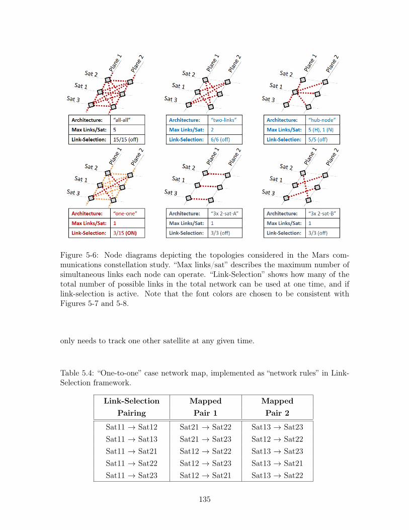
Figure 5-6: Node diagrams depicting the topologies considered in the Mars com-munications constellation study. “Max links/sat” describes the maximum number ofsimultaneous links each node can operate. “Link-Selection” shows how many of thetotal number of possible links in the total network can be used at one time, and iflink-selection is active. Note that the font colors are chosen to be consistent withFigures 5-7 and 5-8.
only needs to track one other satellite at any given time.
Table 5.4: “One-to-one” case network map, implemented as “network rules” in Link-Selection framework.
Link-Selection Mapped MappedPairing Pair 1 Pair 2
Sat11 → Sat12 Sat21 → Sat22 Sat13 → Sat23Sat11 → Sat13 Sat21 → Sat23 Sat12 → Sat22Sat11 → Sat21 Sat12 → Sat22 Sat13 → Sat23Sat11 → Sat22 Sat12 → Sat23 Sat13 → Sat21Sat11 → Sat23 Sat12 → Sat21 Sat13 → Sat22
135
Between these two network scenarios are the “some-to-some” cases where certain
spacecraft may only be able to establish links with a limited subset of the other
satellites in the constellation, and/or maintain a limited number of simultaneous links.
There are many different possible enumerations of a “some-to-some” architecture. We
limit this to a few cases that are easy to implement in our simulation approach
and/or in a physical spacecraft design. The first is the “hub-node” model where
certain spacecraft act as “hubs” capable of communicating with any and all of the
other satellites, while the others act as “nodes” capable of communicating only with
one hub at any time. Up to five satellites can act as hubs (not six, since that would be
the same as the “all-to-all” case), but for this study, we implement the simplest case of
a single hub, Sat11. This is an open network topology, since there is no path through
the topology that returns to the originating satellite (in this case Sat11) through a
separate link. However, it is fully connected since all spacecraft are contained within
the same network, through the hub sat, Sat11.
A second “some-to-some” case is defined where every satellite can only communi-
cate with a specific set of two other satellites in the constellation. That specific set is
two satellites in the opposite orbital plane in the other two phase slots. For instance,
Sat11 can link with Sat22 and Sat23, but not with Sat21 as it is in the same phase
slot in the opposite plane. This is an example of a closed network topology, since a
path can be made from Sat11 through the other satellites that returns to Sat11 from
a separate link (Sat11 → Sat22 → Sat13 → Sat21 → Sat12 → Sat23 → Sat11). This
is also clearly a fully connected network topology, as all satellites are represented in
the closed network path.
The final network scenarios we evaluate are those where each satellite can only
communicate one other satellite in the constellation, with no overlapping assignments.
This is a special case of the “some-to-some” architecture definition, but essentially is
the same as a two-satellite case, since it generates three unconnected networks with
two satellites each. These are evaluated in this study to represent the lower order of
network connectivity. For the constellation used in this study, there are two possible
variations of this scenario that utilize both planes (to avoid coplanar unobservability
136
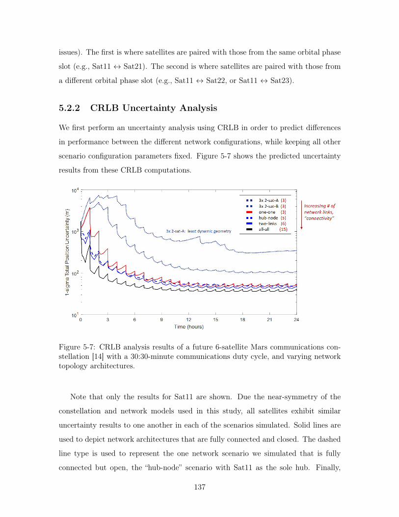
issues). The first is where satellites are paired with those from the same orbital phase
slot (e.g., Sat11 ↔ Sat21). The second is where satellites are paired with those from
a different orbital phase slot (e.g., Sat11 ↔ Sat22, or Sat11 ↔ Sat23).
5.2.2 CRLB Uncertainty Analysis
We first perform an uncertainty analysis using CRLB in order to predict differences
in performance between the different network configurations, while keeping all other
scenario configuration parameters fixed. Figure 5-7 shows the predicted uncertainty
results from these CRLB computations.
Figure 5-7: CRLB analysis results of a future 6-satellite Mars communications con-stellation [14] with a 30:30-minute communications duty cycle, and varying networktopology architectures.
Note that only the results for Sat11 are shown. Due the near-symmetry of the
constellation and network models used in this study, all satellites exhibit similar
uncertainty results to one another in each of the scenarios simulated. Solid lines are
used to depict network architectures that are fully connected and closed. The dashed
line type is used to represent the one network scenario we simulated that is fully
connected but open, the “hub-node” scenario with Sat11 as the sole hub. Finally,
137
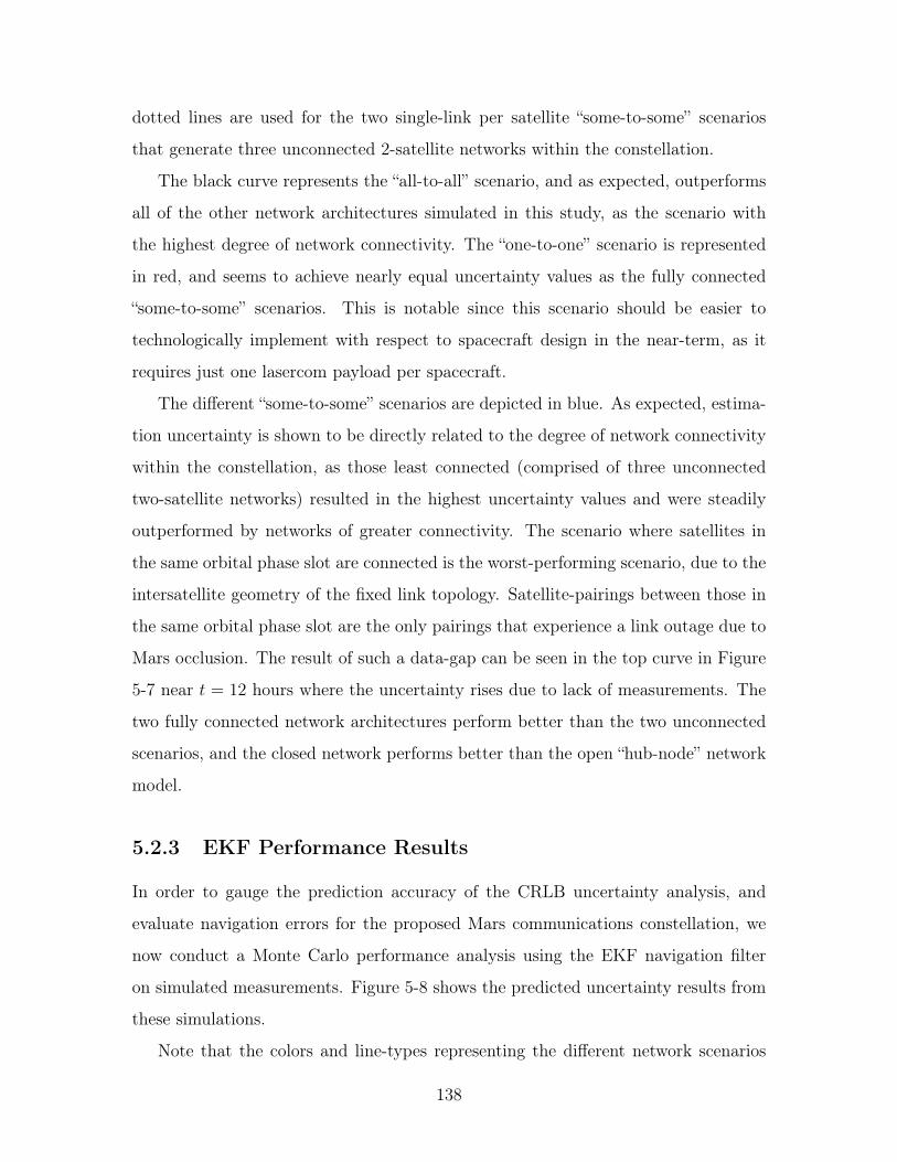
dotted lines are used for the two single-link per satellite “some-to-some” scenarios
that generate three unconnected 2-satellite networks within the constellation.
The black curve represents the “all-to-all” scenario, and as expected, outperforms
all of the other network architectures simulated in this study, as the scenario with
the highest degree of network connectivity. The “one-to-one” scenario is represented
in red, and seems to achieve nearly equal uncertainty values as the fully connected
“some-to-some” scenarios. This is notable since this scenario should be easier to
technologically implement with respect to spacecraft design in the near-term, as it
requires just one lasercom payload per spacecraft.
The different “some-to-some” scenarios are depicted in blue. As expected, estima-
tion uncertainty is shown to be directly related to the degree of network connectivity
within the constellation, as those least connected (comprised of three unconnected
two-satellite networks) resulted in the highest uncertainty values and were steadily
outperformed by networks of greater connectivity. The scenario where satellites in
the same orbital phase slot are connected is the worst-performing scenario, due to the
intersatellite geometry of the fixed link topology. Satellite-pairings between those in
the same orbital phase slot are the only pairings that experience a link outage due to
Mars occlusion. The result of such a data-gap can be seen in the top curve in Figure
5-7 near 𝑡 = 12 hours where the uncertainty rises due to lack of measurements. The
two fully connected network architectures perform better than the two unconnected
scenarios, and the closed network performs better than the open “hub-node” network
model.
5.2.3 EKF Performance Results
In order to gauge the prediction accuracy of the CRLB uncertainty analysis, and
evaluate navigation errors for the proposed Mars communications constellation, we
now conduct a Monte Carlo performance analysis using the EKF navigation filter
on simulated measurements. Figure 5-8 shows the predicted uncertainty results from
these simulations.
Note that the colors and line-types representing the different network scenarios
138
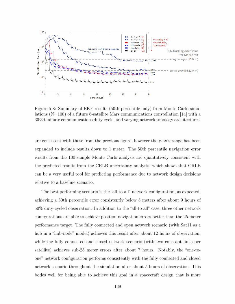
Figure 5-8: Summary of EKF results (50th percentile only) from Monte Carlo simu-lations (N=100) of a future 6-satellite Mars communications constellation [14] with a30:30-minute communications duty cycle, and varying network topology architectures.
are consistent with those from the previous figure, however the y-axis range has been
expanded to include results down to 1 meter. The 50th percentile navigation error
results from the 100-sample Monte Carlo analysis are qualitatively consistent with
the predicted results from the CRLB uncertainty analysis, which shows that CRLB
can be a very useful tool for predicting performance due to network design decisions
relative to a baseline scenario.
The best performing scenario is the “all-to-all” network configuration, as expected,
achieving a 50th percentile error consistently below 5 meters after about 9 hours of
50% duty-cycled observation. In addition to the “all-to-all” case, three other network
configurations are able to achieve position navigation errors better than the 25-meter
performance target. The fully connected and open network scenario (with Sat11 as a
hub in a “hub-node” model) achieves this result after about 12 hours of observation,
while the fully connected and closed network scenario (with two constant links per
satellite) achieves sub-25 meter errors after about 7 hours. Notably, the “one-to-
one” network configuration performs consistently with the fully connected and closed
network scenario throughout the simulation after about 5 hours of observation. This
bodes well for being able to achieve this goal in a spacecraft design that is more
139
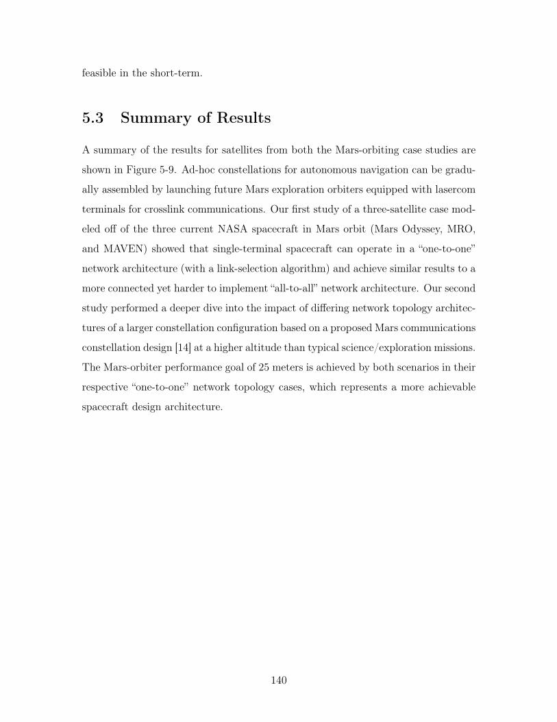
feasible in the short-term.
5.3 Summary of Results
A summary of the results for satellites from both the Mars-orbiting case studies are
shown in Figure 5-9. Ad-hoc constellations for autonomous navigation can be gradu-
ally assembled by launching future Mars exploration orbiters equipped with lasercom
terminals for crosslink communications. Our first study of a three-satellite case mod-
eled off of the three current NASA spacecraft in Mars orbit (Mars Odyssey, MRO,
and MAVEN) showed that single-terminal spacecraft can operate in a “one-to-one”
network architecture (with a link-selection algorithm) and achieve similar results to a
more connected yet harder to implement “all-to-all” network architecture. Our second
study performed a deeper dive into the impact of differing network topology architec-
tures of a larger constellation configuration based on a proposed Mars communications
constellation design [14] at a higher altitude than typical science/exploration missions.
The Mars-orbiter performance goal of 25 meters is achieved by both scenarios in their
respective “one-to-one” network topology cases, which represents a more achievable
spacecraft design architecture.
140
Figure 5-9: Summary of EKF results (50th percentile over 100 Monte Carlo simu-lations) for satellites from the Mars-orbiters and Mars communications constellationcase studies.
141

THIS PAGE INTENTIONALLY LEFT BLANK
142
Chapter 6
Conclusion
This chapter concludes this thesis by summarizing all of the findings, contributions,
and suggestions for future work.
6.1 Summary of Contributions
For this thesis, we have created a simulation environment to estimate the performance
of autonomous spacecraft navigation using intersatellite measurements under vary-
ing configurations of orbital environments, constellation size and distribution, net-
work architectures, and measurement models. This simulation environment includes
a kinematic uncertainty approximation algorithm using Cramér Rao lower bound
(CRLB) covariance estimates as a link-selection heuristic when multiple links are
available. This link-selection framework is especially pertinent when a constellation
network features a high degree of connectivity, but a limited number of simultaneous
connections per spacecraft, which was a design tradeoff of particular interest in this
thesis.
We first simulated a GEO-LEO example scenario in order to demonstrate the
capability of the developed simulation environment, and illustrate any potential sen-
sitivities to fixed input parameters. From this, we were able to confirm the expectation
that an EKF estimator, which is used for this thesis, is sensitive to high uncertainty
in the initial state estimate. We found that initial state uncertainty should be kept
143
below 10 km and 10 m/s for each Cartesian element of the position and velocity, re-
spectively, in order to maintain capability of converging to a solution. We also learned
that the filter is highly sensitive to both the time-step 𝑇 , and the velocity component
of process noise 𝑄𝑣. Values for these input parameters were selected to minimize er-
rors in our simulation approach. Finally, two additional classes of measurement noise
were simulated, one that represents a less capable system than the one we assume,
and one that represents a more capable system. Simulations of these cases showed an
expected result in that navigation performance is proportional to the measurement
noise, though not significantly so within the range of values we selected.
We then utilized our simulation environment to evaluate navigation performance
in a few relevant past, present, and future satellite missions in order to demonstrate
the applicability of navigation using lasercom measurements to both near-Earth and
deep-space environments. For potential Earth-orbiting applications, we simulated a
GEO relay satellite system, akin to the currently active EDRS operations developed
by ESA as well as future missions developed by NASA (e.g., LCRD), and LEO-LEO
systems, starting with two-satellite systems and followed by larger Walker constel-
lations. In both case studies, we evaluated different scenarios where we varied the
quantity and distribution of satellites in order to determine effects from different inter-
satellite geometries. The GEO relay case study utilized the link-selection framework
we developed in order for the user satellites to predict which relay satellite would
best reduce uncertainty, and thus generate a schedule for the day of observations.
The best performing LEO-GEO case resulted in errors of about 1.5 meters for the
LEO satellite and 8 meters for the GEO satellite(s), as shown in Figure 4-12.
We performed parameter-sweep analyses to evaluate the relationship of estimation
uncertainty to differences in the user satellite’s orbital altitude and inclination, and
confirmed observability effects in the navigation filter. We learned that low-altitude
spacecraft have the most value in reducing estimation errors and uncertainty, due
to their ability to more dynamically sample the the space where the primary forces
exist, in closer proximity to the central-body. Thus, it is recommended to include
a low-altitude satellite in any navigation system design based on intersatellite laser-
144
com measurements, or to schedule crosslink operations during low-altitude portions
of satellites in eccentric orbits. We also learned that the orbits of the satellites should
be properly configured in order to maximize link-access time without sacrificing the
navigation performance benefits of lower altitudes, and while avoiding proximity to
the filter’s unobservable scenario. Finally, we confirmed our hypothesis that constel-
lations of higher connectivity can be beneficial for a few reasons. Higher quantities
of satellites increase the number of available measurements in order to converge to a
better solution. Greater distributions of satellites increases observability in the esti-
mator in order to reduce uncertainties in the different state vector elements, leading
to better navigation performance.
For potential deep-space applications, we chose to focus on Mars, since there are
number of past, present, and future missions that can be used for case studies. In our
first case study simulated ad-hoc constellations of future Mars exploration orbiters.
For a second case study, we simulated a future Mars communications constellation,
as proposed by Castellini et al. (2010) [14]. Through both case studies, we investi-
gated the effects of different orbital geometries, duty-cycled operations, and network
architectures on constellation navigation. These studies reiterated the importance of
considering intersatellite orbital geometry in order to maximize potential link-access
times, especially considering any duty-cycled operations due to competing priori-
ties of other mission tasks that must be scheduled and performed. In investigating
different network architectures, we modeled network constraints that relate to the
technological feasibility of designing satellites for crosslink operations. At the high-
est connectivity, the “all-to-all” architecture enables each satellite to perform multiple
links at the same time, but would require a complex set of on-board systems to achieve
this. At the lowest connectivity, the spacecraft are configured to only establish links
with one fixed partnering satellite, but this would require the least implementation
effort in the design and operations of the spacecraft. We also modeled a few other
network architectures between the two extremes that represent more feasible designs
for immediate demonstration potential. Most notable of these architectures is the
“one-to-one” case, where each satellite can only perform one link at any given time,
145
but makes use of the the link-selection algorithm developed in this thesis in order to
fully connect the constellation in a closed network design. From these simulations, we
learned that fully-connected and closed network designs are preferred in order to gain
observability in the state estimation filter, and that different network configurations
can be employed to best utilize the capabilities afforded by different system design
choices, such as the spacecraft design (which constrains the number of simultaneous
links achievable per satellite), and the constellation configuration (which dictates the
link-accesses available per satellite).
Finally, through the course of performing these case studies in different oper-
ating environments, we have demonstrated the potential for improved navigation
performance over the current state-of-the-art spacecraft navigation techniques. In
the Earth-orbiting domain, comparing against typical GNSS-based navigation perfor-
mance, GEO relay satellite systems were shown to achieve median total position errors
better than the 12-meter target for GEO satellites, and 45-meter target for HEO satel-
lites. A dedicated 6-satellite LEO constellation was shown to achieve navigation error
performance better than the 3-meter target for LEO satellites, while larger Walker
constellations showed promise for achieving sub-meter navigation performance, as-
suming a feasible design can be made balancing constellation size/distribution with
network connectivity.
Lastly, both Mars-orbiting case studies demonstrated achievement of median total
position errors below the 25-meter target set by typical performance by orbit estima-
tion based on DSN radiometric tracking data. Both an ad-hoc constellation comprised
of three or more exploration orbiters at low altitudes, and a dedicated high-altitude
Mars communications constellation were able to maintain navigation errors on the
order of 5-10 meters by using a reasonably feasible “one-to-one” network architecture
with a link-selection framework.
146
6.2 Future Work
This thesis paves the way for a few areas for future work, mostly with respect to
increasing the fidelity of individual components in the simulation environment in
order to more accurately model operations of a real spacecraft system.
∙ Dynamics & Estimation:
– Incorporate smoothing to reduce noise in state estimates
– Convert satellite state definition to Keplerian elements, which can be ben-
eficial with smoothing or narrow ranges of known possible values for po-
tentially faster and more reliable convergence
– Implement distributed filters instead of a centralized filter to emulate true-
to-life navigation aboard individual satellites [65, 68, 84]
– Increase fidelity of dynamics model – in particular, adding third-body per-
turbations, for additional domains of estimation observability
∙ Systems Modeling:
– Simulate other additional orbital scenarios (e.g., lunar-orbit, cis-lunar space-
craft, halo orbits, heliocentric orbits, interplanetary relays)
– Simulate other network topology options – in particular, expand all possi-
ble combinations for error/uncertainty comparison analysis
– Increase fidelity of lasercom measurement models (e.g., dependencies to
timing bias/uncertainty, orbital position, pointing vector, or relative posi-
tion/velocity)
– Increase fidelity of link-access model (e.g., additional constraints due to
geometry, time, or network)
– Model different classes of capability for different satellites (different or
time-variant values for initial state knowledge or measurement uncertainty)
147
– Include additional measurements – in particular, range-rate, to mitigate
sensitivity to velocity process noise
– Include additional sources of measurements – in particular, from down-
links, to provide updates to state estimate or on-board clock
∙ Autonomy & Decision-making:
– More efficient link-selection heuristic (e.g., filtered/smoothed dilution-of-
precision)
– More robust link-selection algorithm for handling large constellations, asym-
metric constellations, and selection conflicts
148
Bibliography
[1] Gang Zhao, Xuhua Zhou, and Bin Wu. Precise orbit determination of Haiyang-2using satellite laser ranging. Chinese Science Bulletin, 58(6):589–597, 2013. doi:10.1007/s11434-012-5564-6.
[2] J. S. Ulvestad. Use of the VLBI Delay Observable for Orbit Determi-nation of Earth-Orbiting VLBi Satellites. TDA Progress Report, (42-110),1992. URL https://ntrs.nasa.gov/archive/nasa/casi.ntrs.nasa.gov/19930010230.pdf.
[3] Cyrus Foster, Henry Hallam, and James Mason. Orbit Determination andDifferential-Drag Control of Planet Labs CubeSat Constellations. AAS/AIAAAstrodynamics Specialist Conference, 2015. URL https://arxiv.org/pdf/1509.03270.pdf.
[4] Michael R. Greene and Robert E. Zee. Increasing the Accuracy of Or-bital Position Information from NORAD SGP4 Using Intermittent GPSReadings. AIAA/USU Conference on Small Satellites, 2009. URLhttps://digitalcommons.usu.edu/cgi/viewcontent.cgi?article=1326&context=smallsat.
[5] M. Brunet, A. Auriol, P. Agnieray, and F. Nouel. DORIS precise orbit deter-mination and localization system description and USOs performances. IEEEInternational Frequency Control Symposium, pages 282–287, 1995. URL http://tf.nist.gov/general/pdf/1141.pdf.
[6] Christian Jayles, Jean Pierre Chauveau, and Albert Auriol. DORIS/DIODE:Real-Time Orbit Determination Performance on Board SARAL/AltiKa. MarineGeodesy, 38(February):233–248, 2015. ISSN 1521060X. doi: 10.1080/01490419.2015.1015695.
[7] Xiucong Sun, Chao Han, and Pei Chen. Precise Real-Time Navigation of LEOSatellites Using a Single- Frequency GPS Receiver and Ultra-Rapid Ephemerides.Aerospace Science and Technology, 67:228–236, 2017. URL https://arxiv.org/ftp/arxiv/papers/1704/1704.02094.pdf.
[8] Andre Hauschild, Javier Tegedor, Oliver Montenbruck, Hans Visser, andMarkus Markgraf. Innovation: Orbit determination of LEO satellites with
149
real-time corrections, 2017. URL http://gpsworld.com/innovation-orbit-determination-of-leo-satellites-with-real-time-corrections/.
[9] F.L. Markley. Autonomous navigation using landmark and intersatellite data.AIAA/AAS Astrodynamics Conference, 1984. ISSN 01463705. doi: 10.2514/6.1984-1987. URL http://arc.aiaa.org/doi/10.2514/6.1984-1987.
[10] Suneel I. Sheikh, Darryll J. Pines, Paul S. Ray, Kent S. Wood, Michael N.Lovellette, and Michael T. Wolff. Spacecraft Navigation Using X-Ray Pulsars.Journal of Guidance, Control, and Dynamics, 29(1), 2006. doi: 10.2514/1.13331.
[11] Mark L. Psiaki. Autonomous Orbit Determination for Two Spacecraft fromRelative Position Measurements. Journal of Guidance, Control, and Dynamics,22(2):305–312, 1999. ISSN 0731-5090. doi: 10.2514/2.4379. URL http://arc.aiaa.org/doi/10.2514/2.4379.
[12] Mark L. Psiaki. Autonomous Low-Earth-Orbit Determination from Magnetome-ter and Sun Sensor Data. Journal of Guidance, Control, and Dynamics, 22(2):296–304, 1999. ISSN 0731-5090. doi: 10.2514/2.4378.
[13] Kerry D. Hicks and William E. Iesel. Autonomous orbit determination systemfor earth satellites. Journal of Guidance, Control, and Dynamics, 15(3):562–566,1992. ISSN 07315090. doi: 10.2514/3.20876. URL http://arc.aiaa.org/doi/pdf/10.2514/3.20876.
[14] Francesco Castellini, Andrea Simonetto, Roberto Martini, and Michèle Lavagna.A mars communication constellation for human exploration and network sci-ence. Advances in Space Research, 45(1):183–199, 1 2010. doi: 10.1016/j.asr.2009.10.019. URL https://linkinghub.elsevier.com/retrieve/pii/S0273117709006826.
[15] Eberhard Gill. Together in Space: Potentials and Challenges of DistributedSpace Systems. Technical report, TU Delft, 2008.
[16] Planet Labs Inc. Planet Imagery and Archive, 2018. URL https://www.planet.com/products/planet-imagery/.
[17] Andrew Klesh, Brian Clement, Cody Colley, John Essmiller, Daniel Forgette,Joel Krajewski, Anne Marinan, Tomas Martin-Mur, Joel Steinkraus, DavidSternberg, Thomas Werne, and Brian Young. MarCO: Early Operations of theFirst CubeSats to Mars. In AIAA/USU Conference on Small Satellites, 2018.
[18] Andrew K. Kennedy and Kerri L. Cahoy. Initial Results from ACCESS:An Autonomous CubeSat Constellation Scheduling System for EarthObservation. AIAA/USU Conference on Small Satellites, 2017. URLhttp://digitalcommons.usu.edu/cgi/viewcontent.cgi?article=3629&context=smallsat.
150
[19] Joseph Howard, Dipak Oza, and Danford S. Smith. Best Practices for Operationsof Satellite Constellations. SpaceOps Conference, 2006. doi: 10.2514/6.2006-5866.
[20] Emil Vassev and Mike Hinchey. Autonomy Requirements Engineering for SpaceMissions. Springer, 2014. ISBN 978-3-319-09815-9. doi: 10.1007/978-3-319-09816-6. URL http://link.springer.com/10.1007/978-3-319-09816-6.
[21] Andre Hauschild, Markus Markgraf, and Oliver Montenbruck. The Navigationand Occultation eXperiment: GPS Receiver Performance On Board a LEO Satel-lite. Inside GNSS, pages 48–57, 2014.
[22] Luke B. Winternitz, William A. Bamford, Samuel R. Price, J. Russell Carpenter,Anne C. Long, and Mitra Farahmand. Global positioning system navigationabove 76,000 KM for NASA’s Magnetospheric Multiscale Mission. Navigation,64(2):289–300, 2017. ISSN 00281522. doi: 10.1002/navi.198.
[23] Brian G. Coffee, Kerri Cahoy, and Rebecca L. Bishop. Propagation of CubeSatsin LEO using NORAD Two Line Element Sets: Accuracy and Update Frequency.AIAA Guidance, Navigation, and Control Conference, 2013. doi: 10.2514/6.2013-4944.
[24] Kathleen Riesing and Kerri Cahoy. Orbit Determination from Two Line ElementSets of ISS-Deployed CubeSats. AIAA/USU Conference on Small Satellites,2015.
[25] Kerry D. Hicks. An Autonomous Orbit Determination System for Earth Satel-lites. PhD thesis, Air Force Institute of Technology, 1989.
[26] John T. Collins, Simon Dawson, and James R. Wertz. Autonomous Con-stellation Maintenance System. AIAA/USU Conference on Small Satel-lites, 1996. URL https://digitalcommons.usu.edu/cgi/viewcontent.cgi?article=2475&context=smallsat.
[27] James R. Wertz. Autonomous Navigation and Autonomous Orbit Control inPlanetary Orbits as a Means of Reducing Operations Cost. International Sym-posium on Reducing the Cost of Spacecraft Ground Systems and Operations, (5),2003. URL http://descanso.jpl.nasa.gov/RCSGSO/Paper/A0029Paper.pdf.
[28] C. Jayles, J.P. Chauveau, and F. Rozo. DORIS/Jason-2: Better than 10cmon-board orbits available for Near-Real-Time Altimetry. Advances in Space Re-search, 46:1497–1512, 2010. doi: 10.1016/j.asr.2010.04.030.
[29] Stephen Winkler, Graeme Ramsey, Charles Frey, Jim Chapel, Donald Chu,Douglas Freesland, Alexander Krimchansky, and Marco Concha. GPS Re-ceiver On-Orbit Performance for the GOES-R Spacecraft. International ESAConference on Guidance, Navigation & Control Systems (GNC), 2017. URLhttps://ntrs.nasa.gov/search.jsp?R=20170004849.
151
[30] Sarah Elizabeth McCandless and Tomas Martin-Mur. Navigation Using Deep-Space Optical Communication Systems. AIAA/AAS Astrodynamics SpecialistConference, 2016. doi: 10.2514/6.2016-5567. URL https://arc.aiaa.org/doi/pdf/10.2514/6.2016-5567.
[31] Paul Muri and Janise McNair. A survey of communication sub-systems for in-tersatellite linked systems and cubesat missions. Journal of Communications, 7(4):290–308, 2012. ISSN 17962021. doi: 10.4304/jcm.7.4.290-308.
[32] Yong Xu, Qing Chang, and ZhiJian Yu. On new measurement and commu-nication techniques of GNSS inter-satellite links. Science China TechnologicalSciences, 55(1):285–294, 2012. doi: 10.1007/s11431-011-4586-7.
[33] Yinyin Tang, Yueke Wang, and Jianyun Chen. The Availability ofSpace Service for Inter-Satellite Links in Navigation Constellations.Sensors, 16(8), 8 2016. ISSN 1424-8220. doi: 10.3390/s16081327.URL http://www.ncbi.nlm.nih.gov/pubmed/27548181http://www.pubmedcentral.nih.gov/articlerender.fcgi?artid=PMC5017492.
[34] Radhika Radhakrishnan, William W. Edmonson, Fatemeh Afghah, Ramon Mar-tinez Rodriguez-Osorio, Frank Pinto, and Scott C. Burleigh. Survey of Inter-satellite Communication for Small Satellite Systems: Physical Layer to NetworkLayer View. IEEE Communications Surveys & Tutorials, 18(4):2442–2473, 2016.URL http://arxiv.org/abs/1609.08583.
[35] Ryan Kingsbury. Optical Communications for Small Satellites. PhD thesis,Massachusetts Institute of Technology, 2015.
[36] ESA - Europe’s SpaceDataHighway relays first Sentinel-1 images via laser,2016. URL https://www.esa.int/Applications/Telecommunications_Integrated_Applications/EDRS/Europe_s_SpaceDataHighway_relays_first_Sentinel-1_images_via_laser.
[37] ESA - Laser link offers high-speed delivery, 2014. URL https://www.esa.int/Applications/Observing_the_Earth/Copernicus/Sentinel-1/Laser_link_offers_high-speed_delivery.
[38] Richard P Welle, Christopher M Coffman, Dee W Pack, and John R Santiago.CubeSat Laser Communication Crosslink Pointing Demonstration. AIAA/USUConference on Small Satellites, 2019.
[39] Donald Cornwell, William Marinelli, and Badri Younes. NASA’s Optical Com-munications Missions in 2020-2022. Technical report, NASA SCaN, 2019.
[40] Yohei Satoh, Yuko Miyamoto, Yutaka Takano, Shiro Yamakawa, and Hiroki Ko-hata. Current status of Japanese optical data relay system (JDRS). In 2017IEEE International Conference on Space Optical Systems and Applications, IC-SOS 2017, pages 240–242. Institute of Electrical and Electronics Engineers Inc.,5 2018. ISBN 9781509065110. doi: 10.1109/ICSOS.2017.8357398.
152
[41] Inigo Del Portillo, Bruce G. Cameron, and Edward F. Crawley. A TechnicalComparison of Three Low Earth Orbit Satellite Constellation Systems to Pro-vide Global Broadband. In International Astronautical Congress (IAC), Bremen,Germany, 2018. MIT. URL https://iafastro.directory/iac/proceedings/IAC-18/IAC-18/B2/1/manuscripts/IAC-18,B2,1,7,x45506.pdf.
[42] Kerri Cahoy, Peter Grenfell, Angela Crews, Michael Long, Paul Serra,Anh Nguyen, Riley Fitzgerald, Christian Haughwout, Rodrigo Diez, AlexaAguilar, John Conklin, Cadence Payne, Joseph Kusters, Chloe Sackier, MiaLaRocca, and Laura Yenchesky. The CubeSat Laser Infrared CrosslinKMission (CLICK). In Nikos Karafolas, Zoran Sodnik, and Bruno Cugny,editors, International Conference on Space Optics — ICSO 2018, page 33.SPIE, 7 2019. ISBN 9781510630772. doi: 10.1117/12.2535953. URLhttps://www.spiedigitallibrary.org/conference-proceedings-of-spie/11180/2535953/The-CubeSat-Laser-Infrared-CrosslinK-Mission-CLICK/10.1117/12.2535953.full.
[43] Alan Boyle. Cloud Constellation chooses LeoStella to build cloud data satel-lites – GeekWire, 2019. URL https://www.geekwire.com/2019/cloud-constellation-chooses-leostella-build-cloud-data-satellites-seattle-area/.
[44] Telesat LEO - Why LEO? | Telesat, 2020. URL https://www.telesat.com/services/leo/why-leo.
[45] Bob Brumley and Glenn Colby. Deep Space Communications Colloquium PanelOverview. Technical report, Laser Light Communications, 2019.
[46] K. Yong, C. Chao, and A. Liu. Autonomous navigation for satellites usinglasercom systems. AIAA Aerospace Sciences Meeting, 1983. doi: 10.2514/6.1983-428. URL http://arc.aiaa.org/doi/10.2514/6.1983-428.
[47] R. Sun, D. Maessen, J. Guo, and E. Gill. Enabling Inter-satellite Communi-cation and Ranging for Small Satellites. Small Satellite Systems and ServicesSymposium, 2010. URL https://www.researchgate.net/publication/228975384_ENABLING_INTER-SATELLITE_COMMUNICATION_AND_RANGING_FOR_SMALL_SATELLITES.
[48] Kai Xiong, Chunling Wei, and Liangdong Liu. Autonomous navigationfor a group of satellites with star sensors and inter-satellite links. ActaAstronautica, 86:10–23, 2013. doi: 10.1016/j.actaastro.2012.12.001. URLhttps://ac.els-cdn.com/S009457651200481X/1-s2.0-S009457651200481X-main.pdf?_tid=20df2482-11db-11e8-a30a-00000aab0f01&acdnat=1518649528_e18f238909e05d4e19e2a6a6b6fd23b8.
[49] M. L. Stevens, R. R. Parenti, M. M. Willis, J. A. Greco, F. I. Khatri, B. S.Robinson, and D. M. Boroson. The lunar laser communication demonstration
153
time-of-flight measurement system: overview, on-orbit performance, and rang-ing analysis. Free-Space Laser Communication and Atmospheric PropagationXXVIII, 9739, 2016. doi: 10.1117/12.2218624. URL http://proceedings.spiedigitallibrary.org/proceeding.aspx?doi=10.1117/12.2218624.
[50] Dale A. Force. Individual Global Navigation Satellite Systems in the SpaceService Volume. In ION International Technical Meeting, 2013. URL https://ntrs.nasa.gov/archive/nasa/casi.ntrs.nasa.gov/20130011788.pdf.
[51] M. Guelman, A. Kogan, A. Kazarian, A. Livne, M. Orenstein, H. Michalik, andS. Arnon. Acquisition and pointing control for inter-satellite laser communica-tions. IEEE Transactions on Aerospace and Electronic Systems, 40(4):1239–1248,2004. ISSN 00189251. doi: 10.1109/TAES.2004.1386877.
[52] Mark L. Psiaki. Absolute Orbit and Gravity Determination Using Relative Po-sition Measurements Between Two Satellites. Journal of Guidance, Control, andDynamics, 34(5):1285–1297, 2011. ISSN 0731-5090. doi: 10.2514/1.47560. URLhttp://arc.aiaa.org/doi/10.2514/1.47560.
[53] Edoardo Benzi, Daniel C. Troendle, Ian Shurmer, Mark James, Michael Lutzer,and Sven Kuhlmann. Optical Inter-Satellite Communication: the Alphasat andSentinel-1A in-orbit experience. SpaceOps Conference, (May), 2016. doi: 10.2514/6.2016-2389. URL http://arc.aiaa.org/doi/10.2514/6.2016-2389.
[54] James Taylor. The Cramer-Rao estimation error lower bound computation fordeterministic nonlinear systems. In IEEE Conference on Decision and Control,pages 1178–1181. IEEE, 1 1978. doi: 10.1109/CDC.1978.268121. URL http://ieeexplore.ieee.org/document/4046308/.
[55] A. Farina, B. Ristic, and D. Benvenuti. Tracking a ballistic target: Comparisonof several nonlinear filters. IEEE Transactions on Aerospace and Electronic Sys-tems, 38(3):854–867, 2002. ISSN 00189251. doi: 10.1109/TAES.2002.1039404.
[56] R. Karlsson and F. Gustafsson. Particle filter for underwater terrain navigation.IEEE Workshop on Statistical Signal Processing Proceedings, 2003-Janua(3):526–529, 2003. doi: 10.1109/SSP.2003.1289507.
[57] Robert L. Herklotz. Incorporation of Cross-link Range Measurements in theOrbit Determination Process to Increase Satellite Constellation Autonomy. PhDthesis, Massachusetts Institute of Technology, 1987.
[58] Jo Ryeong Yim, John L. Crassidis, and John L. Junkins. Autonomous orbit nav-igation of two spacecraft system using relative line of sight vector measurements.AAS/AIAA Space Flight Mechanics Meeting, 2004. ISSN 00653438.
[59] Keric Hill, Martin W. Lo, and George H. Born. Linked, Autonomous, Interplan-etary Satellite Orbit Navigation (LiAISON). AAS/AIAA Astrodynamics Spe-cialist Conference, 2005. URL http://ccar.colorado.edu/geryon/papers/Conference/AAS-05-399.pdf.
154
[60] Mark L. Psiaki. Absolute Orbit and Gravity Determination using Relative Po-sition Measurements Between Two Satellites. AIAA Guidance, Navigation, andControl Conference, 2007. URL https://pdfs.semanticscholar.org/309a/eb75a9b5fca68897693c19ff0483a2d1d8a9.pdf.
[61] Xiaofang Zhao, Shenggang Liu, and Chao Han. Performance analysis of au-tonomous navigation of constellation based on inter satellite range measurement.Procedia Engineering, 15:4094–4098, 2011. doi: 10.1016/j.proeng.2011.08.768.
[62] Liuqing Xu, Xiaoxu Zhao, and Lili Guo. An autonomous navigation study ofWalker constellation based on reference satellite and inter-satellite distance mea-surement. IEEE Chinese Guidance, Navigation and Control Conference, pages2553–2557, 2014. doi: 10.1109/CGNCC.2014.7007568.
[63] Youtao Gao, Bo Xu, and Lei Zhang. Feasibility study of autonomous orbit deter-mination using only the crosslink range measurement for a combined navigationconstellation. Chinese Journal of Aeronautics, 27(5):1199–1210, 2014. ISSN10009361. doi: 10.1016/j.cja.2014.09.005.
[64] Kai Xiong, Chunling Wei, and Liangdong Liu. An Augmented Multiple-ModelAdaptive Estimation for Time-Varying Uncertain Systems. In Y. Jia, J. Du,W. Zhang, and H. Li, editors, Chinese Intelligent Systems Conference, pages 503–517. Springer, Singapore, 2016. doi: 10.1007/978-981-10-2338-5\_47. URLhttp://link.springer.com/10.1007/978-981-10-2338-5_47.
[65] Xiaogang Wang, Wutao Qin, Yuliang Bai, and Naigang Cui. A novel decen-tralized relative navigation algorithm for spacecraft formation flying. AerospaceScience and Technology, 48:28–36, 2016. doi: 10.1016/j.ast.2015.10.014. URLhttps://ac.els-cdn.com/S1270963815003235/1-s2.0-S1270963815003235-main.pdf?_tid=69437575-5e81-4616-b98d-433ba64842f9&acdnat=1525984645_3520f49e685425700afa88d4d0a95ba8.
[66] Byron T. Davis and Brian C. Gunter. The Augmentation of Precision Or-bit Determination through Constellation Intersatellite Ranging. AIAA/AASAstrodynamics Specialist Conference, 2016. doi: 10.2514/6.2016-5368. URLhttps://arc.aiaa.org/doi/pdf/10.2514/6.2016-5368.
[67] Yangwei Ou, Hongbo Zhang, and Jianjun Xing. Autonomous orbit determinationand observability analysis for formation satellites. Chinese Control Conference,pages 5294–5300, 2016. ISSN 21612927. doi: 10.1109/ChiCC.2016.7554179.
[68] Ruipeng Li, Hongzhuan Qiu, and Kai Xiong. Autonomous Navigation for Con-stellation Based on inter-satellite ranging and directions. In Conference of theIEEE Industrial Electronics Society, pages 2985–2990. IEEE, 10 2017. ISBN9781538611265. doi: 10.1109/IECON.2017.8216504. URL http://ieeexplore.ieee.org/document/8216504/.
155
[69] Yangwei Ou, Hongbo Zhang, and Bin Li. Absolute orbit determination using line-of-sight vector measurements between formation flying spacecraft. Astrophysicsand Space Science, 363(4):76, 4 2018. ISSN 0004-640X. doi: 10.1007/s10509-018-3293-2. URL http://link.springer.com/10.1007/s10509-018-3293-2.
[70] Yangwei Ou and Hongbo Zhang. Observability-based Mars AutonomousNavigation Using Formation Flying Spacecraft. The Journal of Nav-igation, 71:21–43, 2018. doi: 10.1017/S0373463317000510. URLhttps://www.cambridge.org/core/services/aop-cambridge-core/content/view/AA7D0E2CD59B0CE2C42644B32587A2DD/S0373463317000510a.pdf/observabilitybased_mars_autonomous_navigation_using_formation_flying_spacecraft.pdf.
[71] Artemis - Gunter’s Space Page, 2019. URL https://space.skyrocket.de/doc_sdat/artemis.htm.
[72] Caleb Henry. Indonesia ordered to pay Avanti $20 million formissed satellite lease payments - SpaceNews.com, 2018. URL https://spacenews.com/indonesia-ordered-to-pay-avanti-20-million-for-missed-satellite-lease-payments/.
[73] Frank Heine, Patricia Martin-Pimentel, Hartmut Kaempfner, Gerd Muehlnikel,Daniel Troendle, Herwig Zech, Christoph Rochow, Daniel Dallmann, MartinReinhardt, Mark Gregory, Michael Lutzer, Sabine Philipp-May, Rolf Meyer,Edoardo Benzi, Philippe Sivac, Mike Krassenburg, Ian Shurmer, and Uwe Sterr.Alphasat and sentinel 1A, the first 100 links. In 2015 IEEE International Con-ference on Space Optical Systems and Applications, ICSOS 2015. Institute ofElectrical and Electronics Engineers Inc., 3 2016. ISBN 9781509002818. doi:10.1109/ICSOS.2015.7425059.
[74] Elizabeth M. Keil. Kalman Filter Implementation to Determine Orbit and At-titude of a Satellite in a Molniya Orbit to Determine Orbit and Attitude of aSatellite in a Molniya Orbit. PhD thesis, Virginia Polytechnic Institute and StateUniversity, 2014. URL https://vtechworks.lib.vt.edu/bitstream/handle/10919/49102/Keil_EM_T_2014.pdf.
[75] Jeroen L Geeraert. Multi-Satellite Orbit Determination Using InterferometricObservables with RF Localization Applications. PhD thesis, University of Col-orado at Boulder, 2017.
[76] Reza Raymond Karimi, Tomas Martin-Mur, and Sarah Elizabeth McCand-less. A Performance-Based Comparison of Deep-Space Navigation using Optical-Communication and Conventional Navigation Techniques: Small Body Missions.AIAA/AAS Space Flight Mechanics Meeting, 2018. doi: 10.2514/6.2018-1979.URL https://arc.aiaa.org/doi/pdf/10.2514/6.2018-1979.
156
[77] Peter Davidsen and Hans Henrik Bonde. T1 & T2 Star Trackers. Technical re-port, Terma, 2018. URL https://www.terma.com/media/437079/t1_t2_star_tracker_rev2.pdf.
[78] John Enright, Doug Sinclair, and Tom Dzamba. The Things You Can’t Ignore:Evolving a Sub-Arcsecond Star Tracker. AIAA/USU Conference on Small Satel-lites, 2012.
[79] Space-Track.Org, 2019. URL https://www.space-track.org/auth/login.
[80] Alex S. Konopliv, Ryan S. Park, and William M. Folkner. An improved JPLMars gravity field and orientation from Mars orbiter and lander tracking data.Icarus, 274:253–260, 8 2016. ISSN 10902643. doi: 10.1016/j.icarus.2016.02.052.
[81] HORIZONS Web-Interface, 2019. URL https://ssd.jpl.nasa.gov/horizons.cgi.
[82] Multi-Access Laser Communications Terminal. Technical report, NASA, LaserData Technology, 1992.
[83] Kerri Cahoy. MOSAIC: Miniature Optical Steered Antenna for Intersatel-lite Communica | NASA, 2018. URL https://www.nasa.gov/directorates/spacetech/esi/esi2018/MOSAIC/.
[84] Jingwei Wang and Eric A. Butcher. Decentralized Estimation of SpacecraftRelative Motion Using Consensus Extended Kalman Filter. AIAA/AAS SpaceFlight Mechanics Meeting, 2018. doi: 10.2514/6.2018-1965. URL https://arc.aiaa.org/doi/pdf/10.2514/6.2018-1965.
157