a 3-level autonomous mobile robot navigation system designed by using reasoning/search approaches

Robotics and Autonomous Systems 54 (2006) 989–1004www.elsevier.com/locate/robot

A 3-level autonomous mobile robot navigation system designed by usingreasoning/search approaches

Jasmin Velagic∗, Bakir Lacevic, Branislava Perunicic

University of Sarajevo, Faculty of Electrical Engineering, Zmaja od Bosne bb, 71000 Sarajevo, Bosnia and Herzegovina

Received 3 November 2004; received in revised form 24 April 2006; accepted 15 May 2006Available online 14 July 2006

Abstract

This paper describes how soft computing methodologies such as fuzzy logic, genetic algorithms and the Dempster–Shafer theory of evidencecan be applied in a mobile robot navigation system. The navigation system that is considered has three navigation subsystems. The lower-levelsubsystem deals with the control of linear and angular volocities using a multivariable PI controller described with a full matrix. The positioncontrol of the mobile robot is at a medium level and is nonlinear. The nonlinear control design is implemented by a backstepping algorithmwhose parameters are adjusted by a genetic algorithm. We propose a new extension of the controller mentioned, in order to rapidly decrease thecontrol torques needed to achieve the desired position and orientation of the mobile robot. The high-level subsystem uses fuzzy logic and theDempster–Shafer evidence theory to design a fusion of sensor data, map building, and path planning tasks. The fuzzy/evidence navigation basedon the building of a local map, represented as an occupancy grid, with the time update is proven to be suitable for real-time applications. Thepath planning algorithm is based on a modified potential field method. In this algorithm, the fuzzy rules for selecting the relevant obstacles forrobot motion are introduced. Also, suitable steps are taken to pull the robot out of the local minima. Particular attention is paid to detection of therobot’s trapped state and its avoidance. One of the main issues in this paper is to reduce the complexity of planning algorithms and minimize thecost of the search. The performance of the proposed system is investigated using a dynamic model of a mobile robot. Simulation results show agood quality of position tracking capabilities and obstacle avoidance behavior of the mobile robot.c© 2006 Elsevier B.V. All rights reserved.

Keywords: Dynamic model of mobile robot; Backstepping algorithm; Hybrid position controller; Map building; Genetic algorithm; Fuzzy logic; Path planning;Pruning of relevant obstacles; Local minima problem

1. Introduction

The basic feature of an autonomous mobile robot is itscapability to operate independently in unknown or partiallyknown environments. The autonomy implies that the robotis capable of reacting to static obstacles and unpredictabledynamic events that may impede the successful execution ofa task [10]. To achieve this level of robustness, methods need tobe developed to provide solutions to localization, map building,planning and control. The development of such techniques forautonomous robot navigation is one of the major trends incurrent robotics research [23].

The robot has to find a collision-free trajectory betweenthe starting configuration and the goal configuration in a static

∗ Corresponding author. Tel.: +387 33 25 07 65; fax: +387 33 25 07 25.E-mail address: [email protected] (J. Velagic).

0921-8890/$ - see front matter c© 2006 Elsevier B.V. All rights reserved.doi:10.1016/j.robot.2006.05.006

or dynamic environment containing some obstacles. To thisend, the robot needs the capability to build a map of theenvironment, which is essentially a repetitive process of movingto a new position, sensing the environment, updating the map,and planning subsequent motion.

Most of the difficulties in this process originate in thenature of the real world [17]: unstructured environmentsand inherent large uncertainties. First, any prior knowledgeabout the environment is, in general, incomplete, uncertain,and approximate. For example, maps typically omit somedetails and temporary features; also, spatial relations betweenobjects may have changed since the map was built. Second,perceptually acquired information is usually unreliable.Third, a real-world environment typically has complex andunpredictable dynamics: objects can move, other agents canmodify the environment, and apparently stable features maychange with time. Finally, the effects of control actions are not

http://www.elsevier.com/locate/robot

mailto:[email protected]

http://dx.doi.org/10.1016/j.robot.2006.05.006

990 J. Velagic et al. / Robotics and Autonomous Systems 54 (2006) 989–1004

completely reliable, e.g. the wheels of a mobile robot may slip,resulting in accumulated odometric errors.

Robot navigation can be defined as the combination of threebasic activities [4,16]:

• Map building. This is the process of constructing a mapfrom sensor readings taken at different robot locations. Thecorrect treatment of sensor data and the reliable localizationof the robot are fundamental in the map-building process.

• Localization. This is the process of getting the actual robot’slocation from sensor readings and the most recent map. Anaccurate map and reliable sensors are crucial to achievinggood localization.

• Path planning. This is the process of generating a feasibleand safe trajectory from the current robot location to agoal based on the current map. In this case, it is alsovery important to have an accurate map and a reliablelocalization.

Path planning is one of the key issues in mobile robotnavigation. Path planning is traditionally divided into twocategories: global path planning and local path planning. Inglobal path planning, prior knowledge of the workspace isavailable [21]. Local path planning methods use ultrasonicsensors, laser range finders, and on-board vision systems toperceive the environment to perform on-line planning [1,8]. Inour paper, the workspace for the navigation of the mobile robotis assumed to be unknown and it has stationary obstacles only.

In local path planning methods, particular attention is paidto local minima problem. This problem occurs when a robotnavigates towards a desired target with no prior knowledge ofthe environment and gets trapped in a loop [7,14]. This happensusually if the environment consists of concave obstacles,mazes, and such objects. To get out of the loop, the robotmust comprehend its repeated traversal through the sameenvironment, which involves memorizing the environment thathas already been seen [12].

The main contribution of this paper is the design of arobust autonomous mobile robot control system suitable foron-line applications with real-time requirements by usingsoft computing methodologies. This system provides themobile robot that may navigate in an a priori unknownindoor environment using sonar sensor information. To achievethese requirements, the proposed system is hierarchicallyorganized into three distinct separated subsystems witharbitrary responsibility. At each level of this system, one ormore soft computing methodologies are adopted to solve itsspecific problems.

A low-level velocity controller is developed using thestandard PI multivariable control law. The medium-levelposition control law has to be nonlinear in order to ensurestability of the error, that is, its convergence to zero [6,18].Some of the control parameters are continuous time functions,and usually the backstepping method [6,15,22] was used fortheir adjustment. In order to achieve the optimal parametervalues, we used a genetic algorithm. Both controllers are basedon a dynamic model of a differential drive mobile robot havingangular velocities as main variables.

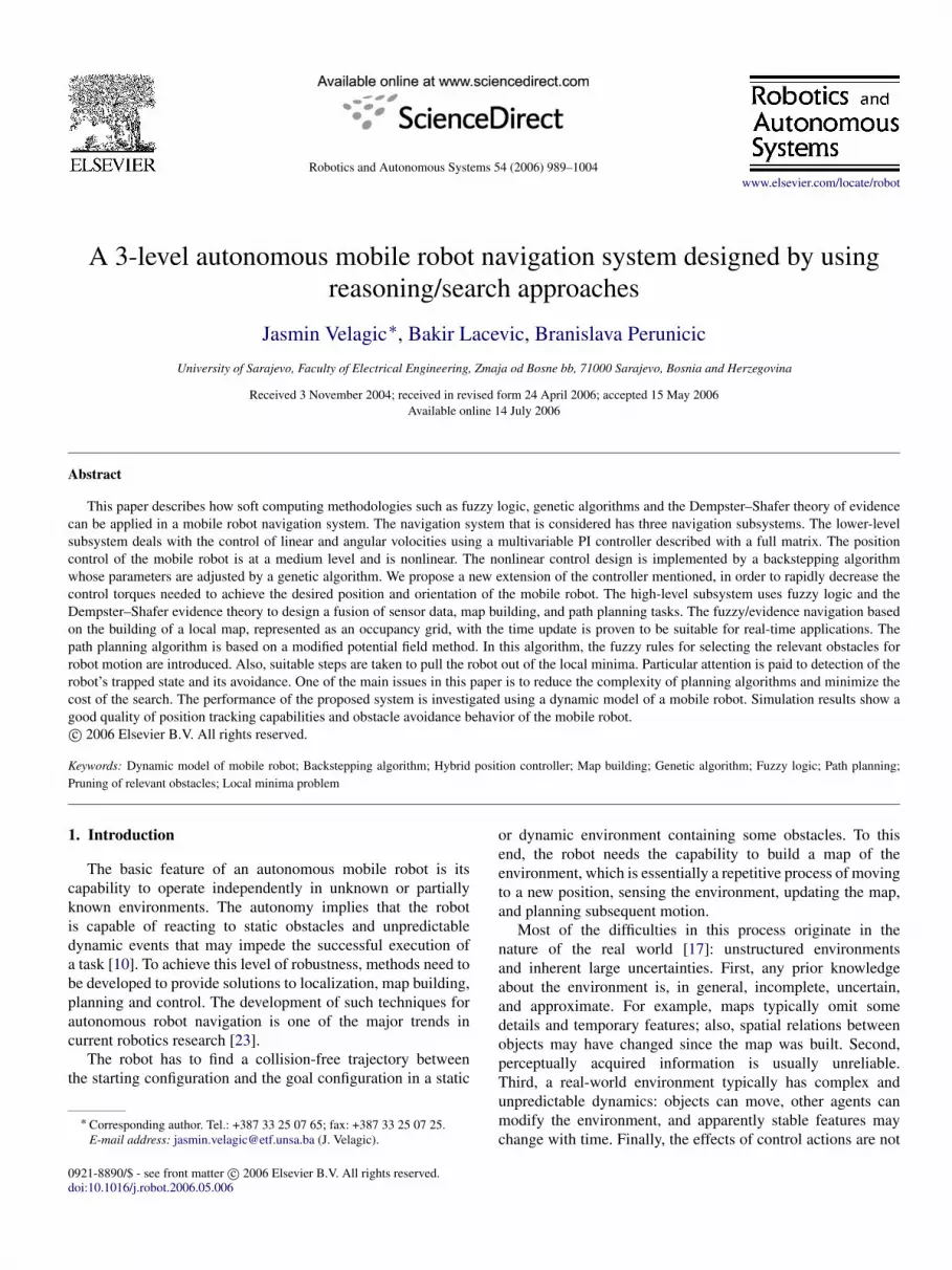
Fig. 1. Mobile robot navigation system for real-time requirements.

A high-level subsystem contains map-building and path-planning algorithms. In this paper, the application of anoccupancy-based map [17] using Dempster–Shafer evidencetheory based on sonar measurements is demonstrated. Theintegration of sonar data is obtained by a low-level fusion [9].The building of occupancy maps is well suited to path planningand obstacle avoidance [10]. In this paper, we propose a newpath-planning approach based on the repulsive and attractiveforces, which sets the fuzzy rules for determining whichobstacles should have an influence on the mobile robot motion.Fuzzy logic offers the possibility to mimic expert humanknowledge [2,3,11,26]. This approach provides both obstacle-avoidance and target-following behaviors and uses only thelocal information for decision making for the next action. Also,we propose a new algorithm for the identification and solutionof the local minima situation during the robot’s traversal usingthe set of fuzzy rules.

2. Navigation system

The proposed three-level control navigation system is shownin Fig. 1.

The low-level velocity control system is composed of amultivariable PI controller and a dynamic model of a mobilerobot and actuators. At the medium level, the position controlsystem generates a nonlinear control law whose parametersare obtained using a genetic algorithm. The high-level systemperforms map-building and path-planning tasks. This systemis in charge of sensor interpretation, sensor data fusion, mapbuilding, and path planning. All the modules are designed usingfuzzy logic and the Dempster–Shafer theory of evidence.

In the following sections, the design of the navigation systemblocks from Fig. 1 is described.

3. Dynamics of mobile robot

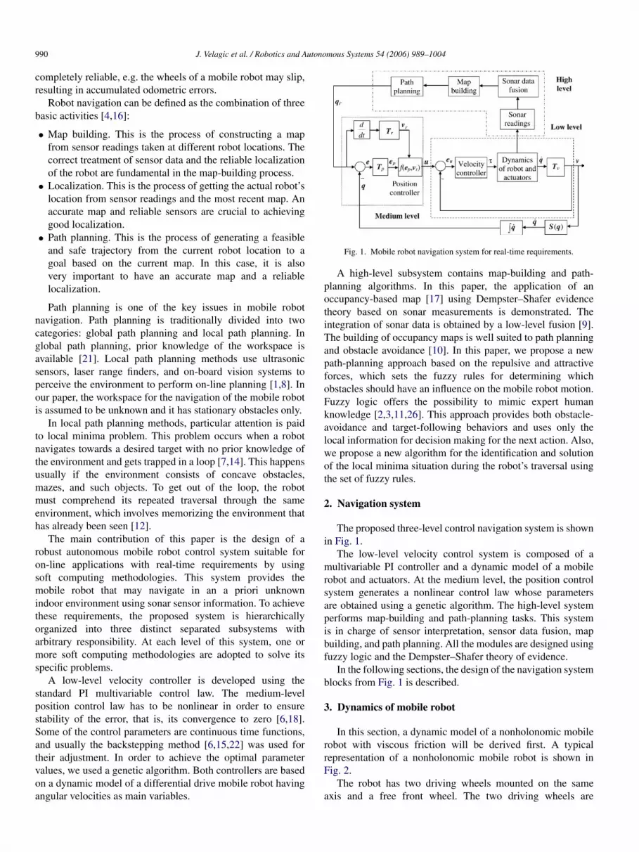
In this section, a dynamic model of a nonholonomic mobilerobot with viscous friction will be derived first. A typicalrepresentation of a nonholonomic mobile robot is shown inFig. 2.

The robot has two driving wheels mounted on the sameaxis and a free front wheel. The two driving wheels are

J. Velagic et al. / Robotics and Autonomous Systems 54 (2006) 989–1004 991

Fig. 2. The representation of a nonholonomic mobile robot.

independently driven by two actuators to achieve both transitionand orientation. The position of the mobile robot in theglobal frame {X, O, Y } can be defined by the position of themass center of the mobile robot system, denoted by C , oralternatively by the position A, which is the center of themobile robot gear, and the angle between the robot’s local frame{xm, C, ym} and the global frame. The kinetic energy of thewhole structure is given by the following equation:

T = Tl + Tr + Tkr , (1)

where Tl is the kinetic energy that is the consequence of puretranslation of the entire vehicle, Tr is the kinetic energy ofrotation of the vehicle in the XOY plane, and Tkr is the kineticenergy of rotation of the wheels and rotors of the DC motors.The values of energy terms introduced can be expressed by Eqs.(2)–(4):

Tl =12

Mv2c =

12

M(x2c + y2

c ), (2)

Tr =12

IAθ2, (3)

Tkr =12

I0θ2R +

12

I0θ2L , (4)

where M is the mass of the entire vehicle, vc is the linearvelocity of the vehicle’s center of mass C , IA is the momentof inertia of the entire vehicle considering point A, θ is theangle that represents the orientation of the vehicle (Fig. 2), I0 isthe moment of inertia of the rotor/wheel complex, and dθR/dtand dθL/dt are the angular velocities of the right- and left-handwheels, respectively.

Further, the components of the velocity of the point A canbe expressed in terms of dθR/dt and dθL/dt :

xA =r

2(θR + θL) cos θ, (5)

yA =r

2(θR + θL) sin θ, (6)

θ =r(θR − θL)

2R. (7)

Since xC = xA − d θ sin θ and yC = yA + d θ cos θ , whered is the distance between points A and C , it is obvious that the

equations below follow:

xC =r

2(θR + θL) cos θ − d θ sin θ, (8)

yC =r

2(θR + θL) sin θ + d θ cos θ. (9)

By substituting terms in Eq. (1) with expressions in Eqs.(2)–(9), the total kinetic energy of the vehicle can be calculatedin terms of dθR/dt and dθL/dt :

T (θR, θR) =

(Mr2

8+

(IA + Md2)r2

8R2 +I0

2

)θ2

R

+

(Mr2

8+

(IA + Md2)r2

8R2 +I0

2

)θ2

L

+

(Mr2

4−

(IA + Md2)r2

4R2

)θR θL . (10)

Now, the Lagrange equations:

ddt

(∂L

∂θR

)−

∂L

∂θR= τR − K θR, (11)

ddt

(∂L

∂θL

)−

∂L

∂θL= τL − K θL , (12)

are applied.Here, τR and τL are right and left actuation torques and

K dθR/dt and K dθL/dt are the viscous friction torques of rightand left wheel-motor systems, respectively.

Finally, the dynamic equations of motion can be expressedas:

AθR + BθL = τR − K θR, (13)

BθR + AθL = τL − K θL , (14)

where

A =

(Mr2

4+

(IA + Md2)r2

4R2 + I0

)B =

(Mr2

4−

(IA + Md2)r2

4R2

).

(15)

In this paper, we used a mobile robot with the followingparameters: M = 10 kg, IA = 1 kg m2, r = 0.035 m,R = 0.175 m, d = 0.05 m, m0 = 0.2 kg and I0 = 0.001 kg m2.

In the following section, a design for both velocity andposition controls will be established.

4. Position and velocity control designs

The function of this controller is to implement a mappingbetween the known information (e.g. reference position,velocity and sensor information) and the actuator commandsdesigned to achieve the robot task. For a mobile robot, thecontroller design problem can be described as follows: giventhe reference position qr (t) and velocity qr (t), design a controllaw for the actuator torques so that the mobile robot velocitymay track a given reference control path with a given smooth


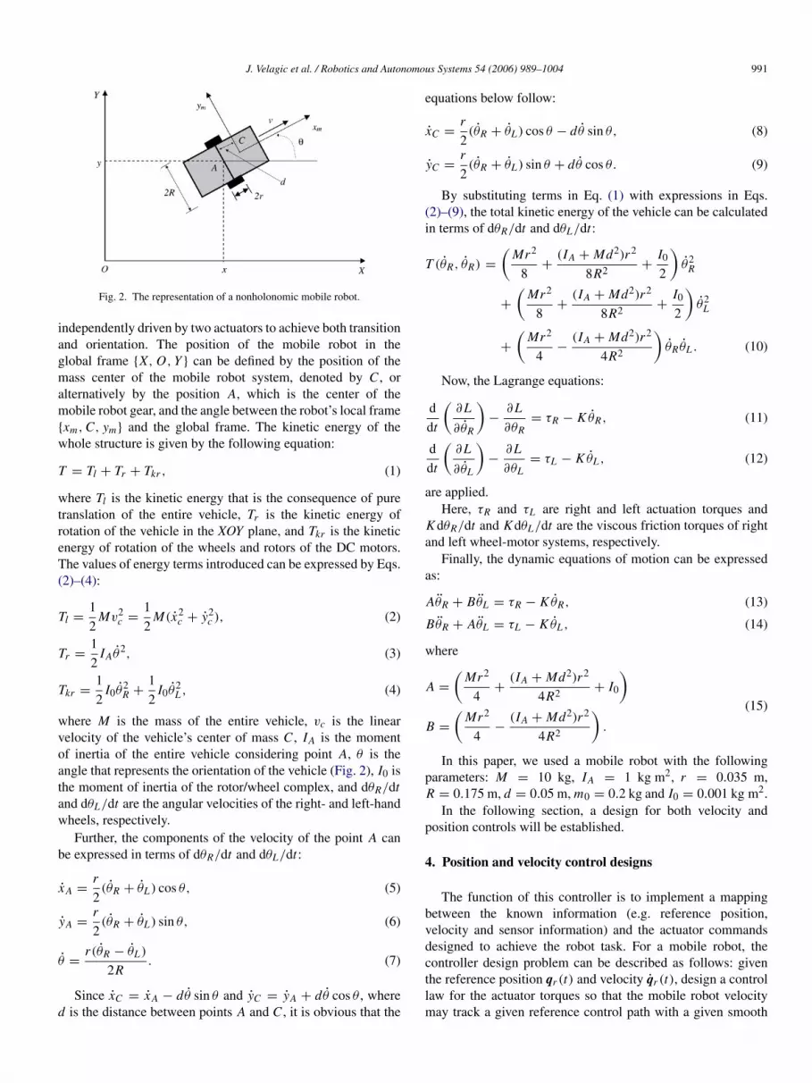
Fig. 3. The concept of tracking of a virtual reference robot.

velocity. Let the velocity and position of the reference robot(Fig. 3) be given as:

qr = [xr yrθr ]T, (16)

where xr = vr cos θr , yr = vr sin θr , θr = ωr , and vr > 0is the reference linear velocity and ωr is the reference angularvelocity.

4.1. Position control

The trajectory tracking problem for a mobile robot is basedon a virtual reference robot [5] that has to be tracked (Fig. 3).The tracking position error between the reference robot and theactual robot can be expressed in the robot frame as:

ep =

e1e2e3

= Tpeq =

cos θ sin θ 0− sin θ cos θ 0

0 0 1

xr − xyr − yθr − θ

, (17)

where eq =[ex ey eθ

]T.The dynamics of the position error derived in (17) is

postulated as:

e1 = ωe2 + u1,

e2 = −ωe1 + vr sin e3,

e3 = u2,

(18)

where inputs u1 and u2 are new control inputs.In this paper, we propose the following control inputs in the

velocity control loop:

u1 = vr cos e3 +k1e1√

k4 + e21 + e2

2

,

u2 = ωr +k2vr e2√

k5 + e21 + e2

2

+k3vr sin e3√

k6 + e23

,

(19)

where k1, k2, k3, k4, k5 and k6 are positive parameters.Eq. (19) is a modified backstepping control law given

first in [6]. The modification consists of the introduction ofdenominators. In [6], Lyapunov’s stability theory was usedto prove that the control law that is considered provides auniformly bounded norm of error ‖ep(t)‖. The issue of rigorousproof of stability for the control law introduced (19) remains

open. However, usage of this law is justified by simulationresults.

The key problem in such a control design is to obtain controlcoefficients k1 to k6. To solve this problem, a genetic algorithmis used to find the optimal values of those coefficients. To applythis method, a low-level velocity controller has to be designedfirst.

4.2. Velocity control

The dynamics of the velocity controller is given by thefollowing equations in the Laplace domain:

τ (s) =

[τR(s)τL(s)

]=

1r

[g1(s) g2(s)g1(s) −g2(s)

] [ev(s)eω(s)

], (20)

where ev(s) is the linear velocity error and eω(s) is theangular velocity error. This structure differs from previouslyused diagonal structures. Transfer functions g j (s) are chosento represent PI controllers:

g1(s) = K1

(1 +

1Ti1s

)· R,

g2(s) = K2

(1 +

1Ti2s

)· R.

(21)

The particular choice of the adopted multivariable PIcontroller described by Eqs. (20) and (21) is justified with thefollowing theorem.

Theorem. Torque control (20) ensures tracking servo inputs u1and u2 with zero steady-state errors.

Proof. When we substitute θR with ωR , θL with ωL , andconsider (20), we can write another form of (13) and (14):[

As + K BsBs As + K

] [ωR(s)ωL(s)

]=

1r

[g1(s) g2(s)g1(s) −g2(s)

] [u1(s) − v(s)u2(s) − ω(s)

], (22)

where ωR and ωL can be expressed in terms of ω and v as:

ωR =v + Rω

r, ωL =

v − Rω

rand then (22) can be transformed to:[

As + K BsBs As + K

] [v(s) + Rω(s)v(s) − Rω(s)

]=

[g1(s) g2(s)g1(s) −g2(s)

] [u1(s) − v(s)u2(s) − ω(s)

]and further to:[

α1(s) α2(s)α1(s) −α2(s)

] [v(s)ω(s)

]=

[g1(s) g2(s)g1(s) −g2(s)

] [u1(s)u2(s)

], (23)

where

α1(s) =(A + B)s2

+ (K + K1Ti1)s + K1

s

α2(s) =R(A − B)s2

+ (RK + K2Ti2)s + K2

s.

(24)


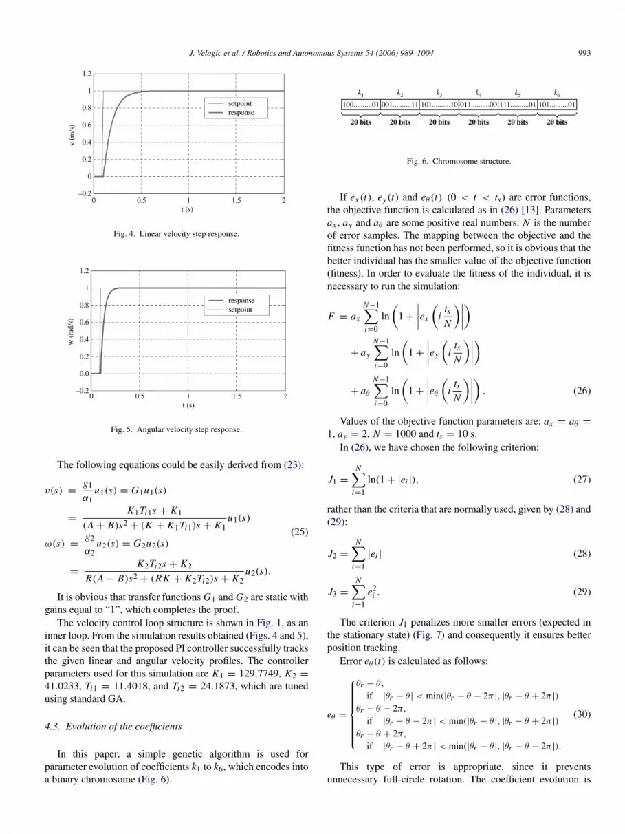
Fig. 4. Linear velocity step response.

Fig. 5. Angular velocity step response.

The following equations could be easily derived from (23):

v(s) =g1

α1u1(s) = G1u1(s)

=K1Ti1s + K1

(A + B)s2 + (K + K1Ti1)s + K1u1(s)

ω(s) =g2

α2u2(s) = G2u2(s)

=K2Ti2s + K2

R(A − B)s2 + (RK + K2Ti2)s + K2u2(s).

(25)

It is obvious that transfer functions G1 and G2 are static withgains equal to “1”, which completes the proof.

The velocity control loop structure is shown in Fig. 1, as aninner loop. From the simulation results obtained (Figs. 4 and 5),it can be seen that the proposed PI controller successfully tracksthe given linear and angular velocity profiles. The controllerparameters used for this simulation are K1 = 129.7749, K2 =

41.0233, Ti1 = 11.4018, and Ti2 = 24.1873, which are tunedusing standard GA.

4.3. Evolution of the coefficients

In this paper, a simple genetic algorithm is used forparameter evolution of coefficients k1 to k6, which encodes intoa binary chromosome (Fig. 6).

Fig. 6. Chromosome structure.

If ex (t), ey(t) and eθ (t) (0 < t < ts) are error functions,the objective function is calculated as in (26) [13]. Parametersax , ay and aθ are some positive real numbers. N is the numberof error samples. The mapping between the objective and thefitness function has not been performed, so it is obvious that thebetter individual has the smaller value of the objective function(fitness). In order to evaluate the fitness of the individual, it isnecessary to run the simulation:

F = ax

N−1∑i=0

ln(

1 +

∣∣∣∣ex

(i

tsN

)∣∣∣∣)

+ ay

N−1∑i=0

ln(

1 +

∣∣∣∣ey

(i

tsN

)∣∣∣∣)

+ aθ

N−1∑i=0

ln(

1 +

∣∣∣∣eθ

(i

tsN

)∣∣∣∣) . (26)

Values of the objective function parameters are: ax = aθ =

1, ay = 2, N = 1000 and ts = 10 s.In (26), we have chosen the following criterion:

J1 =

N∑i=1

ln(1 + |ei |), (27)

rather than the criteria that are normally used, given by (28) and(29):

J2 =

N∑i=1

|ei | (28)

J3 =

N∑i=1

e2i . (29)

The criterion J1 penalizes more smaller errors (expected inthe stationary state) (Fig. 7) and consequently it ensures betterposition tracking.

Error eθ (t) is calculated as follows:

eθ =

θr − θ,

if |θr − θ | < min(|θr − θ − 2π |, |θr − θ + 2π |)

θr − θ − 2π,

if |θr − θ − 2π | < min(|θr − θ |, |θr − θ + 2π |)

θr − θ + 2π,

if |θr − θ + 2π | < min(|θr − θ |, |θr − θ − 2π |).

(30)

This type of error is appropriate, since it preventsunnecessary full-circle rotation. The coefficient evolution is


Fig. 7. Graphical illustration of different criteria.

Fig. 8. Change of the best fitness in the population through generations.

performed using a lemniscate as a suitable complex trajectory:

xr (t) =a sin(αt)

1 + sin2(αt)

yr (t) =a sin(αt) cos(αt)

1 + sin2(αt)

θr (t) = arctan(

yr (αt)

xr (αt)

),

(31)

where a = α = 1. The evolution process (population size is 40)is depicted in Fig. 8.

This evolution yielded the following coefficient values:K1 = 6.2457, K2 = 221.2306, K3 = 2.3433, K4 =

13.5117, K5 = 3.1933, K6 = 8.3361.

4.4. Design of hybrid position controller

It has been noticed that, during the preliminary simulations,at the beginning of tracking the control torques increase rapidlyif the initial position of the reference robot does not belong

Fig. 9. Tracking robot does not “see” virtual robot.

Fig. 10. Producing ωs (t).

to the straight line, determined with the robot and its initialorientation (Fig. 9).

For that purpose, the following control law, which providesvelocity servo inputs, is proposed:

u1(t) = α(t)u1(t)

u2(t) = α(t)u2(t) + (1 − α(t))ωs(t).(32)

Function ωs(t) is generated as the output of the followingsystem (Fig. 10).

The input d(t) is given by:

d(t) = sgn(atan2(ey(t), ex (t)) − θ(t)). (33)

The function α(t) satisfy the following differential equation:

b0d2α(t)

dt2 + b1dα(t)

dt+ α(t) = z(t), (34)

where z(t) is close to a step function and is given by:

z(t) =

{1, if ∃t1 ∈ [0, t] : θ(t1) = atan2(ey(t1), ex (t1))0, otherwise.

(35)

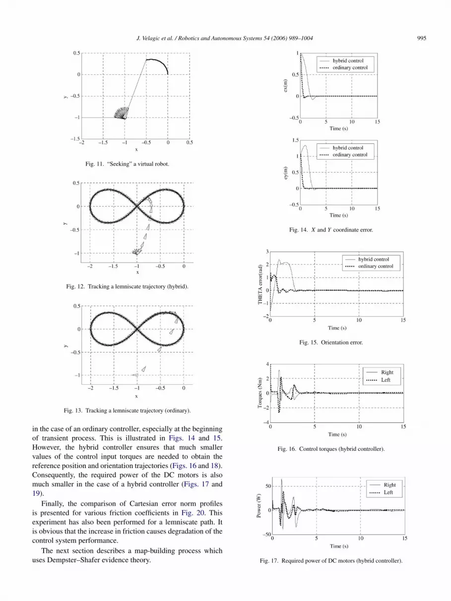
This way, the robot does not start tracking the virtual robotinstantly; it first rotates around its own axis with an increasingangular velocity ωs(t), until it “sees” the virtual robot(Fig. 11).

4.5. Simulation results

The validation of the proposed hybrid controller was testedwith a lamniscate trajectory using an ordinary backsteppingalgorithm [13] and a hybrid backstepping algorithm.

The results of the trajectory tracking in both cases are shownin Figs. 12 and 13.

From these figures, it can be concluded that satisfactorytracking results are obtained using both control strategies.However, better tracking of the reference trajectory is achieved


Fig. 11. “Seeking” a virtual robot.

Fig. 12. Tracking a lemniscate trajectory (hybrid).

Fig. 13. Tracking a lemniscate trajectory (ordinary).

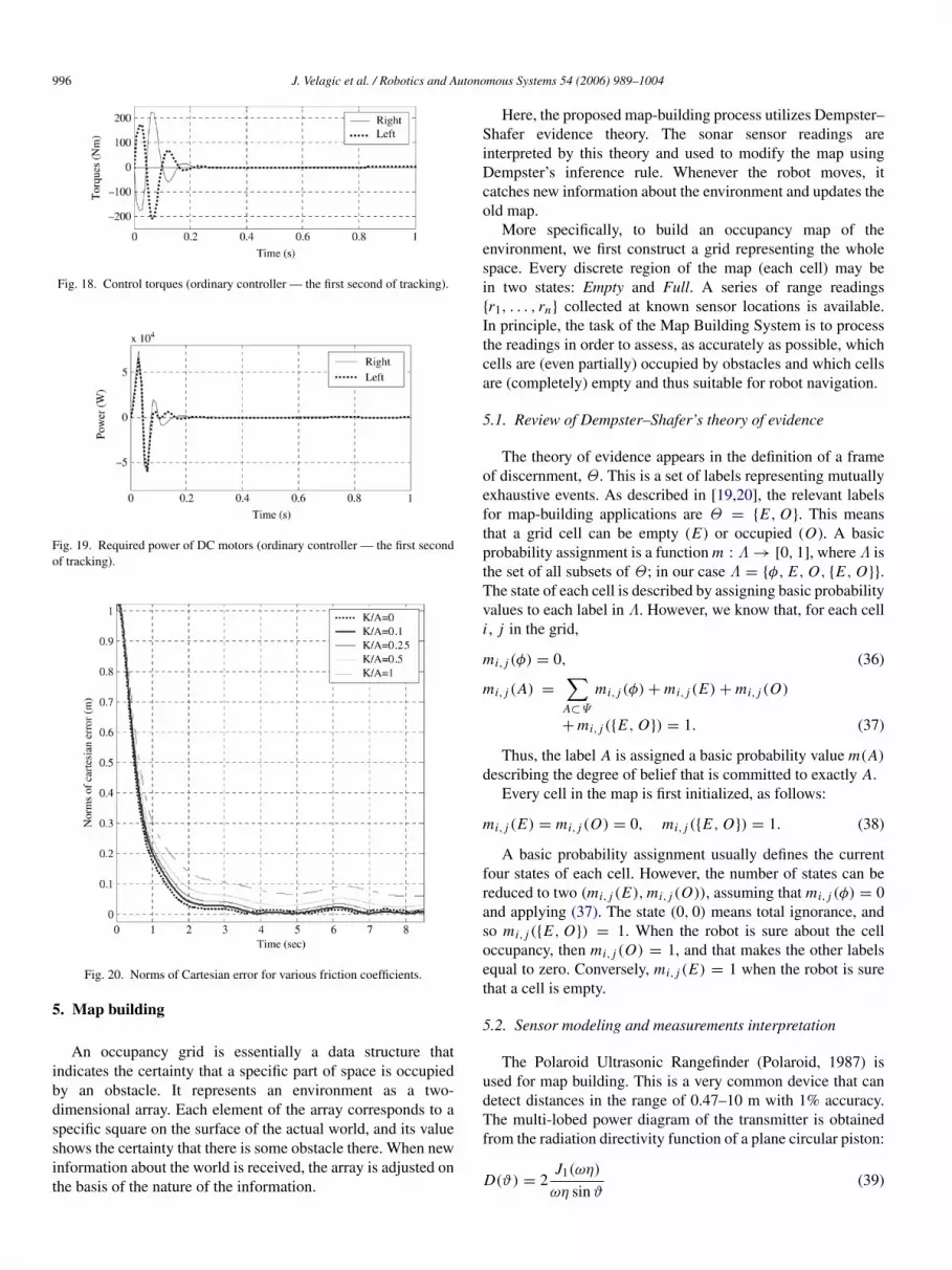
in the case of an ordinary controller, especially at the beginningof transient process. This is illustrated in Figs. 14 and 15.However, the hybrid controller ensures that much smallervalues of the control input torques are needed to obtain thereference position and orientation trajectories (Figs. 16 and 18).Consequently, the required power of the DC motors is alsomuch smaller in the case of a hybrid controller (Figs. 17 and19).

Finally, the comparison of Cartesian error norm profilesis presented for various friction coefficients in Fig. 20. Thisexperiment has also been performed for a lemniscate path. Itis obvious that the increase in friction causes degradation of thecontrol system performance.

The next section describes a map-building process whichuses Dempster–Shafer evidence theory.

Fig. 14. X and Y coordinate error.

Fig. 15. Orientation error.

Fig. 16. Control torques (hybrid controller).

Fig. 17. Required power of DC motors (hybrid controller).


Fig. 18. Control torques (ordinary controller — the first second of tracking).

Fig. 19. Required power of DC motors (ordinary controller — the first secondof tracking).

Fig. 20. Norms of Cartesian error for various friction coefficients.

5. Map building

An occupancy grid is essentially a data structure thatindicates the certainty that a specific part of space is occupiedby an obstacle. It represents an environment as a two-dimensional array. Each element of the array corresponds to aspecific square on the surface of the actual world, and its valueshows the certainty that there is some obstacle there. When newinformation about the world is received, the array is adjusted onthe basis of the nature of the information.

Here, the proposed map-building process utilizes Dempster–Shafer evidence theory. The sonar sensor readings areinterpreted by this theory and used to modify the map usingDempster’s inference rule. Whenever the robot moves, itcatches new information about the environment and updates theold map.

More specifically, to build an occupancy map of theenvironment, we first construct a grid representing the wholespace. Every discrete region of the map (each cell) may bein two states: Empty and Full. A series of range readings{r1, . . . , rn} collected at known sensor locations is available.In principle, the task of the Map Building System is to processthe readings in order to assess, as accurately as possible, whichcells are (even partially) occupied by obstacles and which cellsare (completely) empty and thus suitable for robot navigation.

5.1. Review of Dempster–Shafer’s theory of evidence

The theory of evidence appears in the definition of a frameof discernment, Θ . This is a set of labels representing mutuallyexhaustive events. As described in [19,20], the relevant labelsfor map-building applications are Θ = {E, O}. This meansthat a grid cell can be empty (E) or occupied (O). A basicprobability assignment is a function m : Λ → [0, 1], where Λ isthe set of all subsets of Θ ; in our case Λ = {φ, E, O, {E, O}}.The state of each cell is described by assigning basic probabilityvalues to each label in Λ. However, we know that, for each celli , j in the grid,

mi, j (φ) = 0, (36)

mi, j (A) =

∑A⊂Ψ

mi, j (φ) + mi, j (E) + mi, j (O)

+ mi, j ({E, O}) = 1. (37)

Thus, the label A is assigned a basic probability value m(A)

describing the degree of belief that is committed to exactly A.Every cell in the map is first initialized, as follows:

mi, j (E) = mi, j (O) = 0, mi, j ({E, O}) = 1. (38)

A basic probability assignment usually defines the currentfour states of each cell. However, the number of states can bereduced to two (mi, j (E), mi, j (O)), assuming that mi, j (φ) = 0and applying (37). The state (0, 0) means total ignorance, andso mi, j ({E, O}) = 1. When the robot is sure about the celloccupancy, then mi, j (O) = 1, and that makes the other labelsequal to zero. Conversely, mi, j (E) = 1 when the robot is surethat a cell is empty.

5.2. Sensor modeling and measurements interpretation

The Polaroid Ultrasonic Rangefinder (Polaroid, 1987) isused for map building. This is a very common device that candetect distances in the range of 0.47–10 m with 1% accuracy.The multi-lobed power diagram of the transmitter is obtainedfrom the radiation directivity function of a plane circular piston:

D(ϑ) = 2J1(ωη)

ωη sin ϑ(39)


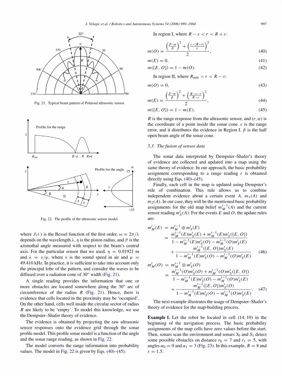
Fig. 21. Typical beam pattern of Polaroid ultrasonic sensor.

Fig. 22. The profile of the ultrasonic sensor model.

where J1(·) is the Bessel function of the first order, ω = 2π/λ

depends on the wavelength λ, η is the piston radius, and ϑ is theazimuthal angle measured with respect to the beam’s centralaxis. For the particular sensor that we used, η = 0.01921 mand λ = v/ϕ, where v is the sound speed in air and ϕ =

49.410 kHz. In practice, it is sufficient to take into account onlythe principal lobe of the pattern, and consider the waves to bediffused over a radiation cone of 30◦ width (Fig. 21).

A single reading provides the information that one ormore obstacles are located somewhere along the 30◦ arc ofcircumference of the radius R (Fig. 21). Hence, there isevidence that cells located in the proximity may be ‘occupied’.On the other hand, cells well inside the circular sector of radiusR are likely to be ‘empty’. To model this knowledge, we usethe Dempster–Shafer theory of evidence.

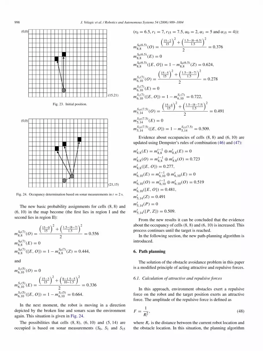
The evidence is obtained by projecting the raw ultrasonicsensor responses onto the evidence grid through the sonarprofile model. This profile sonar model is a function of the angleand the sonar range reading, as shown in Fig. 22.

The model converts the range information into probabilityvalues. The model in Fig. 22 is given by Eqs. (40)–(45).

In region I, where R − ε < r < R + ε:

m(O) =

(β−α

β

)2+

(ε−|R−r |

ε

)2

2, (40)

m(E) = 0, (41)

m({E, O}) = 1 − m(O). (42)

In region II, where Rmin < r < R − ε:

m(O) = 0, (43)

m(E) =

(β−α

β

)2+

(R−ε−r

R−ε

)2

2, (44)

m({E, O}) = 1 − m(E). (45)

R is the range response from the ultrasonic sensor, and (r, α) isthe coordinate of a point inside the sonar cone. ε is the rangeerror, and it distributes the evidence in Region I. β is the halfopen beam angle of the sonar cone.

5.3. The fusion of sensor data

The sonar data interpreted by Dempster–Shafer’s theoryof evidence are collected and updated into a map using thesame theory of evidence. In our approach, the basic probabilityassignment corresponding to a range reading r is obtaineddirectly using Eqs. (40)–(45).

Finally, each cell in the map is updated using Dempster’srule of combination. This rule allows us to combineindependent evidence about a certain event A, m1(A) andm2(A). In our case, they will be the mentioned basic probabilityassignments for the old map belief mt−1

M (A) and the currentsensor reading mt

S(A). For the events E and O , the update rulesare:

mtM (E) = mt−1

M ⊕ mtS(E)

=mt−1

M (E)mtS(E) + mt−1

M (E)mtS({E, O})

1 − mt−1M (E)mt

S(O) − mt−1M (O)mt

S(E)

+mt−1

M ({E, O})mtS(E)

1 − mt−1M (E)mt


S(E)(46)

mtM (O) = mt−1

M ⊕ mtS(O)

=mt−1

M (O)mtS(O) + mt−1

M (O)mtS({E, O})

1 − mt−1M (E)mt


S(E)

+mt−1

M ({E, O})mtS(O)

1 − mt−1M (E)mt


S(E). (47)

The next example illustrates the usage of Dempster–Shafer’stheory of evidence for the map-building process.

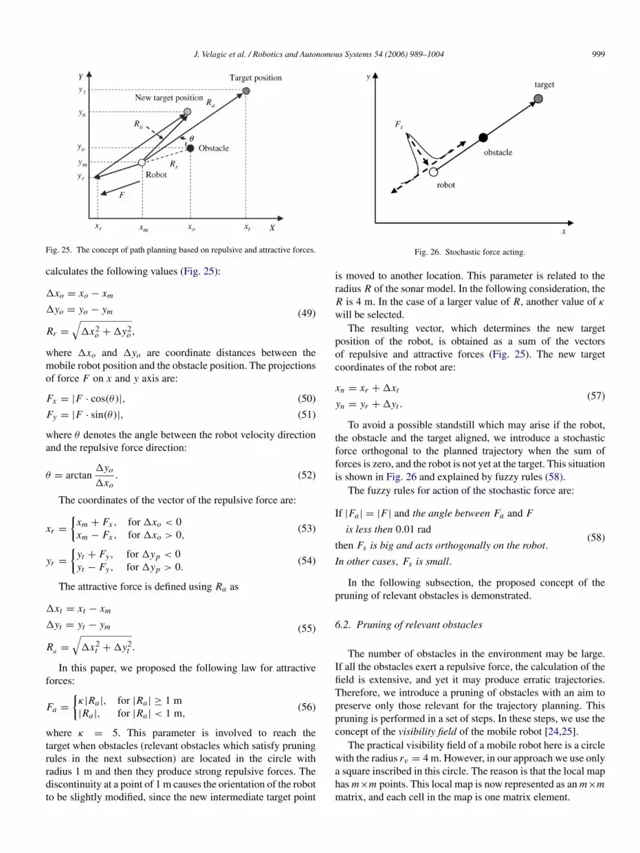
Example 1. Let the robot be located in cell (14, 10) in thebeginning of the navigation process. The basic probabilityassignments of the map cells have zero values before the start.Then, sonars scan the environment and sonars S0 and S1 detectsome possible obstacles on distance r0 = 7 and r1 = 5, withangles α0 = 0 and α1 = 3 (Fig. 23). In this example, R = 8 andε = 1.5.


Fig. 23. Initial position.

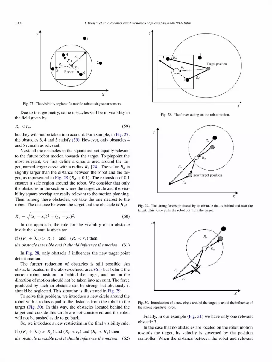
Fig. 24. Occupancy determination based on sonar measurements in t = 2 s.

The new basic probability assignments for cells (8, 8) and(6, 10) in the map become (the first lies in region I and thesecond lies in region II):

mS0(7)8,8 (O) =

(15−0

15

)2+

(1.5−|8−7|

1.5

)2

2= 0.556

mS0(7)8,8 (E) = 0

mS0(7)8,8 ({E, O}) = 1 − mS0(7)

8,8 (Z) = 0.444,

and

mS1(5)6,10 (O) = 0

mS1(5)6,10 (E) =

(15−3

15

)2+

(8−1.5−510−1.5

)2

2= 0.336

mS1(5)6,10 ({E, O}) = 1 − mS1(5)

6,10 = 0.664.

In the next moment, the robot is moving in a directiondepicted by the broken line and sonars scan the environmentagain. This situation is given in Fig. 24.

The possibilities that cells (8, 8), (6, 10) and (5, 14) areoccupied is based on sonar measurements (S0, S1 and S15

(r0 = 6.5, r1 = 7, r15 = 7.5, α0 = 2, α1 = 5 and α15 = 4)):

mS0(6.5)8,8 (O) =

(15−2

15

)2+

(1.5−|8−6.5|

1.5

)2

2= 0.376

mS0(6.5)8,8 (E) = 0

mS0(6.5)8,8 ({E, O}) = 1 − mS0(6.5)

8,8 (Z) = 0.624,

mS1(7)6,10 (O) =

(15−5

15

)2+

(1.5−|8−7|

1.5

)2

2= 0.278

mS1(7)6,10 (E) = 0

mS1(7)6,10 ({E, O}) = 1 − mS1(7)

6,10 = 0.722,

mS15(7.5)5,14 (O) =

(15−4

15

)2+

(1.5−|8−7.5|

1.5

)2

2= 0.491

mS15(7.5)5,14 (E) = 0

mS15(7.5)5,14 ({E, O}) = 1 − mS15(7.5)

5,14 = 0.509.

Evidence about occupancies of cells (8, 8) and (6, 10) areupdated using Dempster’s rules of combination (46) and (47):

mt8,8(E) = mt−1

8,8 ⊕ mt8,8(E) = 0

mt8,8(O) = mt−1

8,8 ⊕ mt8.8(O) = 0.723

mt8,8({E, O}) = 0.277,

mt6,10(E) = mt−1

6,10 ⊕ mt6,10(E) = 0

mt6,10(O) = mt−1

6,10 ⊕ mt6.10(O) = 0.519

mt6,10({E, O}) = 0.481,

mt5,14(Z) = 0.491

mt5,14(P) = 0

mt5,14({P, Z}) = 0.509.

From the new results it can be concluded that the evidenceabout the occupancy of cells (8, 8) and (6, 10) is increased. Thisprocess continues until the target is reached.

In the following section, the new path-planning algorithm isintroduced.

6. Path planning

The solution of the obstacle avoidance problem in this paperis a modified principle of acting attractive and repulsive forces.

6.1. Calculation of attractive and repulsive forces

In this approach, environment obstacles exert a repulsiveforce on the robot and the target position exerts an attractiveforce. The amplitude of the repulsive force is defined as

F =1

R2r

, (48)

where Rr is the distance between the current robot location andthe obstacle location. In this situation, the planning algorithm


Fig. 25. The concept of path planning based on repulsive and attractive forces.

calculates the following values (Fig. 25):

1xo = xo − xm

1yo = yo − ym

Rr =

√1x2

o + 1y2o ,

(49)

where 1xo and 1yo are coordinate distances between themobile robot position and the obstacle position. The projectionsof force F on x and y axis are:

Fx = |F · cos(θ)|, (50)

Fy = |F · sin(θ)|, (51)

where θ denotes the angle between the robot velocity directionand the repulsive force direction:

θ = arctan1yo

1xo. (52)

The coordinates of the vector of the repulsive force are:

xr =

{xm + Fx , for 1xo < 0xm − Fx , for 1xo > 0,

(53)

yr =

{yt + Fy, for 1yp < 0yt − Fy, for 1yp > 0.

(54)

The attractive force is defined using Ra as

1xt = xt − xm

1yt = yt − ym

Ra =

√1x2

t + 1y2t .

(55)

In this paper, we proposed the following law for attractiveforces:

Fa =

{κ|Ra |, for |Ra | ≥ 1 m|Ra |, for |Ra | < 1 m,

(56)

where κ = 5. This parameter is involved to reach thetarget when obstacles (relevant obstacles which satisfy pruningrules in the next subsection) are located in the circle withradius 1 m and then they produce strong repulsive forces. Thediscontinuity at a point of 1 m causes the orientation of the robotto be slightly modified, since the new intermediate target point

Fig. 26. Stochastic force acting.

is moved to another location. This parameter is related to theradius R of the sonar model. In the following consideration, theR is 4 m. In the case of a larger value of R, another value of κ

will be selected.The resulting vector, which determines the new target

position of the robot, is obtained as a sum of the vectorsof repulsive and attractive forces (Fig. 25). The new targetcoordinates of the robot are:

xn = xr + 1xt

yn = yr + 1yt .(57)

To avoid a possible standstill which may arise if the robot,the obstacle and the target aligned, we introduce a stochasticforce orthogonal to the planned trajectory when the sum offorces is zero, and the robot is not yet at the target. This situationis shown in Fig. 26 and explained by fuzzy rules (58).

The fuzzy rules for action of the stochastic force are:

If |Fa | = |F | and the angle between Fa and F

is less then 0.01 rad

then Fs is big and acts orthogonally on the robot.

In other cases, Fs is small.

(58)

In the following subsection, the proposed concept of thepruning of relevant obstacles is demonstrated.

6.2. Pruning of relevant obstacles

The number of obstacles in the environment may be large.If all the obstacles exert a repulsive force, the calculation of thefield is extensive, and yet it may produce erratic trajectories.Therefore, we introduce a pruning of obstacles with an aim topreserve only those relevant for the trajectory planning. Thispruning is performed in a set of steps. In these steps, we use theconcept of the visibility field of the mobile robot [24,25].

The practical visibility field of a mobile robot here is a circlewith the radius rv = 4 m. However, in our approach we use onlya square inscribed in this circle. The reason is that the local maphas m×m points. This local map is now represented as an m×mmatrix, and each cell in the map is one matrix element.


Fig. 27. The visibility region of a mobile robot using sonar sensors.

Due to this geometry, some obstacles will be in visibility inthe field given by

Rr < rv. (59)

but they will not be taken into account. For example, in Fig. 27,the obstacles 3, 4 and 5 satisfy (59). However, only obstacles 4and 5 remain as relevant.

Next, all the obstacles in the square are not equally relevantto the future robot motion towards the target. To pinpoint themost relevant, we first define a circular area around the tar-get, named target circle with a radius Ra [24]. The value Ra isslightly larger than the distance between the robot and the tar-get, as represented in Fig. 28 (Ra + 0.1). The extension of 0.1ensures a safe region around the robot. We consider that onlythe obstacles in the section where the target circle and the visi-bility square overlap are really relevant to the motion planning.Then, among these obstacles, we take the one nearest to therobot. The distance between the target and the obstacle is Rp:

Rp =

√(xt − xo)2 + (yt − yo)2. (60)

In our approach, the rule for the visibility of an obstacleinside the square is given as:

If ((Ra + 0.1) > Rp) and (Rr < rv) then

the obstacle is visible and it should influence the motion. (61)

In Fig. 28, only obstacle 3 influences the new target pointdetermination.

The further reduction of obstacles is still possible. Anobstacle located in the above-defined area (61) but behind thecurrent robot position, or behind the target, and not on thedirection of motion should not be taken into account. The forceproduced by such an obstacle can be strong, but obviously itshould be neglected. This situation is illustrated in Fig. 29.

To solve this problem, we introduce a new circle around therobot with a radius equal to the distance from the robot to thetarget (Fig. 30). In this way, the obstacles located behind thetarget and outside this circle are not considered and the robotwill not be pushed aside to go back.

So, we introduce a new restriction in the final visibility rule:

If ((Ra + 0.1) > Rp) and (Rr < rv) and (Rr < Ra) then

the obstacle is visible and it should influence the motion. (62)

Fig. 28. The forces acting on the robot motion.

Fig. 29. The strong forces produced by an obstacle that is behind and near thetarget. This force pulls the robot out from the target.

Fig. 30. Introduction of a new circle around the target to avoid the influence ofthe strong repulsive force.

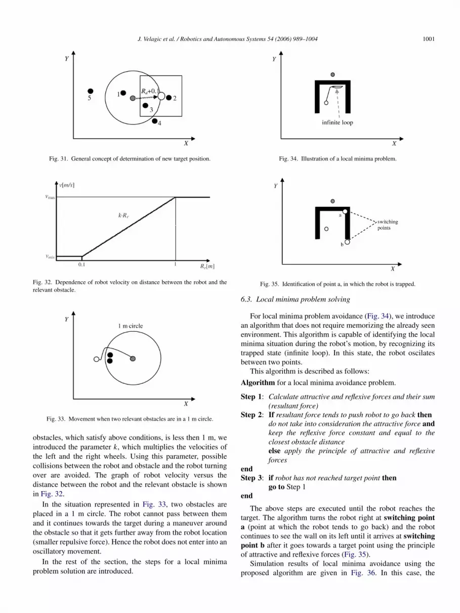
Finally, in our example (Fig. 31) we have only one relevantobstacle 3.

In the case that no obstacles are located on the robot motiontowards the target, its velocity is governed by the positioncontroller. When the distance between the robot and relevant


Fig. 31. General concept of determination of new target position.

Fig. 32. Dependence of robot velocity on distance between the robot and therelevant obstacle.

Fig. 33. Movement when two relevant obstacles are in a 1 m circle.

obstacles, which satisfy above conditions, is less then 1 m, weintroduced the parameter k, which multiplies the velocities ofthe left and the right wheels. Using this parameter, possiblecollisions between the robot and obstacle and the robot turningover are avoided. The graph of robot velocity versus thedistance between the robot and the relevant obstacle is shownin Fig. 32.

In the situation represented in Fig. 33, two obstacles areplaced in a 1 m circle. The robot cannot pass between themand it continues towards the target during a maneuver aroundthe obstacle so that it gets further away from the robot location(smaller repulsive force). Hence the robot does not enter into anoscillatory movement.

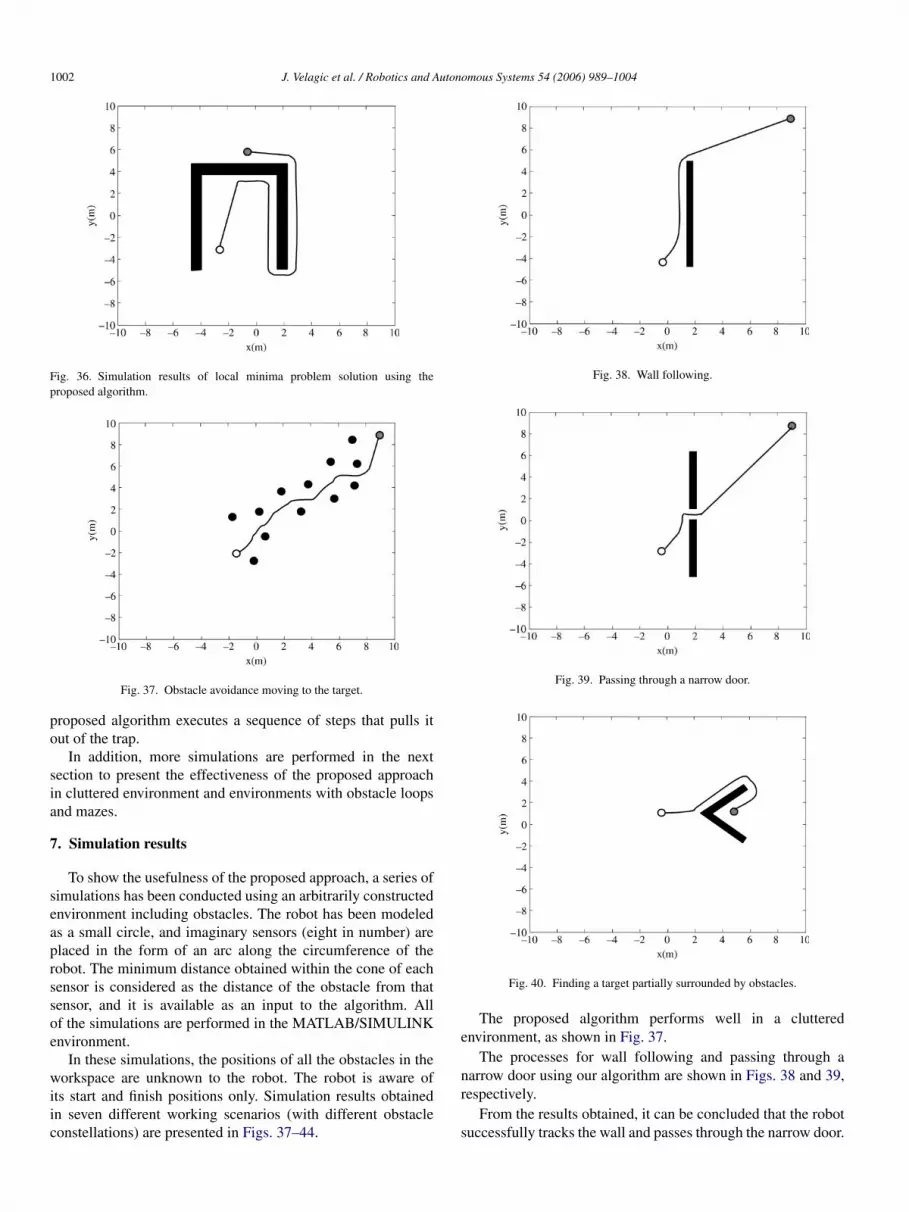
In the rest of the section, the steps for a local minimaproblem solution are introduced.

Fig. 34. Illustration of a local minima problem.

Fig. 35. Identification of point a, in which the robot is trapped.

6.3. Local minima problem solving

For local minima problem avoidance (Fig. 34), we introducean algorithm that does not require memorizing the already seenenvironment. This algorithm is capable of identifying the localminima situation during the robot’s motion, by recognizing itstrapped state (infinite loop). In this state, the robot oscilatesbetween two points.

This algorithm is described as follows:

Algorithm for a local minima avoidance problem.

Step 1: Calculate attractive and reflexive forces and their sum(resultant force)

Step 2: If resultant force tends to push robot to go back thendo not take into consideration the attractive force andkeep the reflexive force constant and equal to theclosest obstacle distanceelse apply the principle of attractive and reflexiveforces

endStep 3: if robot has not reached target point then

go to Step 1end

The above steps are executed until the robot reaches thetarget. The algorithm turns the robot right at switching pointa (point at which the robot tends to go back) and the robotcontinues to see the wall on its left until it arrives at switchingpoint b after it goes towards a target point using the principleof attractive and reflexive forces (Fig. 35).

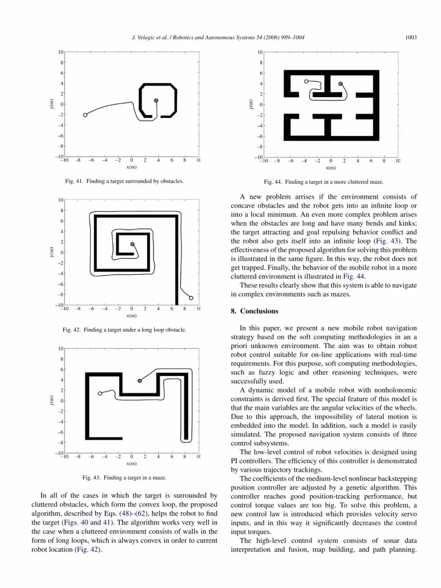
Simulation results of local minima avoidance using theproposed algorithm are given in Fig. 36. In this case, the


Fig. 36. Simulation results of local minima problem solution using theproposed algorithm.

Fig. 37. Obstacle avoidance moving to the target.

proposed algorithm executes a sequence of steps that pulls itout of the trap.

In addition, more simulations are performed in the nextsection to present the effectiveness of the proposed approachin cluttered environment and environments with obstacle loopsand mazes.

7. Simulation results

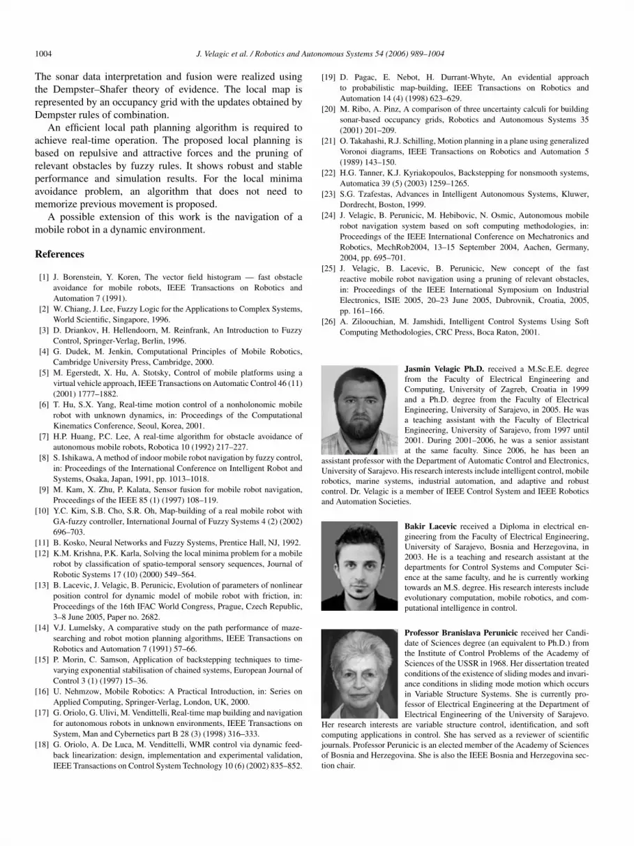
To show the usefulness of the proposed approach, a series ofsimulations has been conducted using an arbitrarily constructedenvironment including obstacles. The robot has been modeledas a small circle, and imaginary sensors (eight in number) areplaced in the form of an arc along the circumference of therobot. The minimum distance obtained within the cone of eachsensor is considered as the distance of the obstacle from thatsensor, and it is available as an input to the algorithm. Allof the simulations are performed in the MATLAB/SIMULINKenvironment.

In these simulations, the positions of all the obstacles in theworkspace are unknown to the robot. The robot is aware ofits start and finish positions only. Simulation results obtainedin seven different working scenarios (with different obstacleconstellations) are presented in Figs. 37–44.

Fig. 38. Wall following.

Fig. 39. Passing through a narrow door.

Fig. 40. Finding a target partially surrounded by obstacles.

The proposed algorithm performs well in a clutteredenvironment, as shown in Fig. 37.

The processes for wall following and passing through anarrow door using our algorithm are shown in Figs. 38 and 39,respectively.

From the results obtained, it can be concluded that the robotsuccessfully tracks the wall and passes through the narrow door.


Fig. 41. Finding a target surrounded by obstacles.

Fig. 42. Finding a target under a long loop obstacle.

Fig. 43. Finding a target in a maze.

In all of the cases in which the target is surrounded bycluttered obstacles, which form the convex loop, the proposedalgorithm, described by Eqs. (48)–(62), helps the robot to findthe target (Figs. 40 and 41). The algorithm works very well inthe case when a cluttered environment consists of walls in theform of long loops, which is always convex in order to currentrobot location (Fig. 42).

Fig. 44. Finding a target in a more cluttered maze.

A new problem arrises if the environment consists ofconcave obstacles and the robot gets into an infinite loop orinto a local minimum. An even more complex problem ariseswhen the obstacles are long and have many bends and kinks;the target attracting and goal repulsing behavior conflict andthe robot also gets itself into an infinite loop (Fig. 43). Theeffectiveness of the proposed algorithm for solving this problemis illustrated in the same figure. In this way, the robot does notget trapped. Finally, the behavior of the mobile robot in a morecluttered environment is illustrated in Fig. 44.

These results clearly show that this system is able to navigatein complex environments such as mazes.

8. Conclusions

In this paper, we present a new mobile robot navigationstrategy based on the soft computing methodologies in an apriori unknown environment. The aim was to obtain robustrobot control suitable for on-line applications with real-timerequirements. For this purpose, soft computing methodologies,such as fuzzy logic and other reasoning techniques, weresuccessfully used.

A dynamic model of a mobile robot with nonholonomicconstraints is derived first. The special feature of this model isthat the main variables are the angular velocities of the wheels.Due to this approach, the impossibility of lateral motion isembedded into the model. In addition, such a model is easilysimulated. The proposed navigation system consists of threecontrol subsystems.

The low-level control of robot velocities is designed usingPI controllers. The efficiency of this controller is demonstratedby various trajectory trackings.

The coefficients of the medium-level nonlinear backsteppingposition controller are adjusted by a genetic algorithm. Thiscontroller reaches good position-tracking performance, butcontrol torque values are too big. To solve this problem, anew control law is introduced which provides velocity servoinputs, and in this way it significantly decreases the controlinput torques.

The high-level control system consists of sonar datainterpretation and fusion, map building, and path planning.


The sonar data interpretation and fusion were realized usingthe Dempster–Shafer theory of evidence. The local map isrepresented by an occupancy grid with the updates obtained byDempster rules of combination.

An efficient local path planning algorithm is required toachieve real-time operation. The proposed local planning isbased on repulsive and attractive forces and the pruning ofrelevant obstacles by fuzzy rules. It shows robust and stableperformance and simulation results. For the local minimaavoidance problem, an algorithm that does not need tomemorize previous movement is proposed.

A possible extension of this work is the navigation of amobile robot in a dynamic environment.

References

[1] J. Borenstein, Y. Koren, The vector field histogram — fast obstacleavoidance for mobile robots, IEEE Transactions on Robotics andAutomation 7 (1991).

[2] W. Chiang, J. Lee, Fuzzy Logic for the Applications to Complex Systems,World Scientific, Singapore, 1996.

[3] D. Driankov, H. Hellendoorn, M. Reinfrank, An Introduction to FuzzyControl, Springer-Verlag, Berlin, 1996.

[4] G. Dudek, M. Jenkin, Computational Principles of Mobile Robotics,Cambridge University Press, Cambridge, 2000.

[5] M. Egerstedt, X. Hu, A. Stotsky, Control of mobile platforms using avirtual vehicle approach, IEEE Transactions on Automatic Control 46 (11)(2001) 1777–1882.

[6] T. Hu, S.X. Yang, Real-time motion control of a nonholonomic mobilerobot with unknown dynamics, in: Proceedings of the ComputationalKinematics Conference, Seoul, Korea, 2001.

[7] H.P. Huang, P.C. Lee, A real-time algorithm for obstacle avoidance ofautonomous mobile robots, Robotica 10 (1992) 217–227.

[8] S. Ishikawa, A method of indoor mobile robot navigation by fuzzy control,in: Proceedings of the International Conference on Intelligent Robot andSystems, Osaka, Japan, 1991, pp. 1013–1018.

[9] M. Kam, X. Zhu, P. Kalata, Sensor fusion for mobile robot navigation,Proceedings of the IEEE 85 (1) (1997) 108–119.

[10] Y.C. Kim, S.B. Cho, S.R. Oh, Map-building of a real mobile robot withGA-fuzzy controller, International Journal of Fuzzy Systems 4 (2) (2002)696–703.

[11] B. Kosko, Neural Networks and Fuzzy Systems, Prentice Hall, NJ, 1992.[12] K.M. Krishna, P.K. Karla, Solving the local minima problem for a mobile

robot by classification of spatio-temporal sensory sequences, Journal ofRobotic Systems 17 (10) (2000) 549–564.

[13] B. Lacevic, J. Velagic, B. Perunicic, Evolution of parameters of nonlinearposition control for dynamic model of mobile robot with friction, in:Proceedings of the 16th IFAC World Congress, Prague, Czech Republic,3–8 June 2005, Paper no. 2682.

[14] V.J. Lumelsky, A comparative study on the path performance of maze-searching and robot motion planning algorithms, IEEE Transactions onRobotics and Automation 7 (1991) 57–66.

[15] P. Morin, C. Samson, Application of backstepping techniques to time-varying exponential stabilisation of chained systems, European Journal ofControl 3 (1) (1997) 15–36.

[16] U. Nehmzow, Mobile Robotics: A Practical Introduction, in: Series onApplied Computing, Springer-Verlag, London, UK, 2000.

[17] G. Oriolo, G. Ulivi, M. Vendittelli, Real-time map building and navigationfor autonomous robots in unknown environments, IEEE Transactions onSystem, Man and Cybernetics part B 28 (3) (1998) 316–333.

[18] G. Oriolo, A. De Luca, M. Vendittelli, WMR control via dynamic feed-back linearization: design, implementation and experimental validation,IEEE Transactions on Control System Technology 10 (6) (2002) 835–852.

[19] D. Pagac, E. Nebot, H. Durrant-Whyte, An evidential approachto probabilistic map-building, IEEE Transactions on Robotics andAutomation 14 (4) (1998) 623–629.

[20] M. Ribo, A. Pinz, A comparison of three uncertainty calculi for buildingsonar-based occupancy grids, Robotics and Autonomous Systems 35(2001) 201–209.

[21] O. Takahashi, R.J. Schilling, Motion planning in a plane using generalizedVoronoi diagrams, IEEE Transactions on Robotics and Automation 5(1989) 143–150.

[22] H.G. Tanner, K.J. Kyriakopoulos, Backstepping for nonsmooth systems,Automatica 39 (5) (2003) 1259–1265.

[23] S.G. Tzafestas, Advances in Intelligent Autonomous Systems, Kluwer,Dordrecht, Boston, 1999.

[24] J. Velagic, B. Perunicic, M. Hebibovic, N. Osmic, Autonomous mobilerobot navigation system based on soft computing methodologies, in:Proceedings of the IEEE International Conference on Mechatronics andRobotics, MechRob2004, 13–15 September 2004, Aachen, Germany,2004, pp. 695–701.

[25] J. Velagic, B. Lacevic, B. Perunicic, New concept of the fastreactive mobile robot navigation using a pruning of relevant obstacles,in: Proceedings of the IEEE International Symposium on IndustrialElectronics, ISIE 2005, 20–23 June 2005, Dubrovnik, Croatia, 2005,pp. 161–166.

[26] A. Ziloouchian, M. Jamshidi, Intelligent Control Systems Using SoftComputing Methodologies, CRC Press, Boca Raton, 2001.

Jasmin Velagic Ph.D. received a M.Sc.E.E. degreefrom the Faculty of Electrical Engineering andComputing, University of Zagreb, Croatia in 1999and a Ph.D. degree from the Faculty of ElectricalEngineering, University of Sarajevo, in 2005. He wasa teaching assistant with the Faculty of ElectricalEngineering, University of Sarajevo, from 1997 until2001. During 2001–2006, he was a senior assistantat the same faculty. Since 2006, he has been an

assistant professor with the Department of Automatic Control and Electronics,University of Sarajevo. His research interests include intelligent control, mobilerobotics, marine systems, industrial automation, and adaptive and robustcontrol. Dr. Velagic is a member of IEEE Control System and IEEE Roboticsand Automation Societies.

Bakir Lacevic received a Diploma in electrical en-gineering from the Faculty of Electrical Engineering,University of Sarajevo, Bosnia and Herzegovina, in2003. He is a teaching and research assistant at thedepartments for Control Systems and Computer Sci-ence at the same faculty, and he is currently workingtowards an M.S. degree. His research interests includeevolutionary computation, mobile robotics, and com-putational intelligence in control.

Professor Branislava Perunicic received her Candi-date of Sciences degree (an equivalent to Ph.D.) fromthe Institute of Control Problems of the Academy ofSciences of the USSR in 1968. Her dissertation treatedconditions of the existence of sliding modes and invari-ance conditions in sliding mode motion which occursin Variable Structure Systems. She is currently pro-fessor of Electrical Engineering at the Department ofElectrical Engineering of the University of Sarajevo.

Her research interests are variable structure control, identification, and softcomputing applications in control. She has served as a reviewer of scientificjournals. Professor Perunicic is an elected member of the Academy of Sciencesof Bosnia and Herzegovina. She is also the IEEE Bosnia and Herzegovina sec-tion chair.

a 3-level autonomous mobile robot navigation system designed by using reasoning/search approaches

Documents