ACAV100M: Automatic Curation of Large-Scale Datasets forAudio-Visual Video Representation Learning

Sangho Lee∗∗, Jiwan Chung∗, Youngjae Yu, Gunhee KimSeoul National University

Thomas Breuel, Gal ChechikNVIDIA Research

Yale SongMicrosoft Research

https://acav100m.github.io

Abstract

The natural association between visual observationsand their corresponding sound provides powerful self-supervisory signals for learning video representations,which makes the ever-growing amount of online videos anattractive source of training data. However, large portionsof online videos contain irrelevant audio-visual signalsbecause of edited/overdubbed audio, and models trainedon such uncurated videos have shown to learn subopti-mal representations. Therefore, existing self-supervised ap-proaches rely on datasets with predetermined taxonomies ofsemantic concepts, where there is a high chance of audio-visual correspondence. Unfortunately, constructing suchdatasets require labor intensive manual annotation and/orverification, which severely limits the utility of online videosfor large-scale learning. In this work, we present an au-tomatic dataset curation approach based on subset opti-mization where the objective is to maximize the mutual in-formation between audio and visual channels in videos.We demonstrate that our approach finds videos with highaudio-visual correspondence and show that self-supervisedmodels trained on our data achieve competitive perfor-mances compared to models trained on existing manuallycurated datasets. The most significant benefit of our ap-proach is scalability: We release ACAV100M that contains100 million videos with high audio-visual correspondence,ideal for self-supervised video representation learning.

1. IntroductionOur long-term objective is learning to recognize objects,

actions, and sound in videos without the need for manualground-truth labels. This is not only a theoretically in-teresting problem, since it mimics the development of au-

∗Equal Contribution

UncuratedInternet Videos

ACAV100M

High AV Correspondence

Dataset Curation

Conventional: Labor Intensive

Annotation Verification

Ours: Subset Optimization

max!⊂#

$$∈!

𝑀𝐼(𝐴$ , 𝑉$)

Noisy AV Correspondence

x

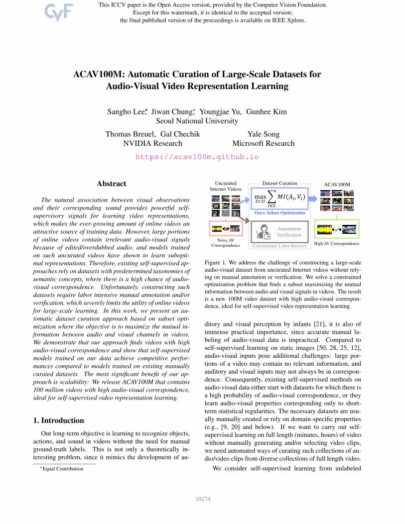
Figure 1. We address the challenge of constructing a large-scaleaudio-visual dataset from uncurated Internet videos without rely-ing on manual annotation or verification. We solve a constrainedoptimization problem that finds a subset maximizing the mutualinformation between audio and visual signals in videos. The resultis a new 100M video dataset with high audio-visual correspon-dence, ideal for self-supervised video representation learning.

ditory and visual perception by infants [21], it is also ofimmense practical importance, since accurate manual la-beling of audio-visual data is impractical. Compared toself-supervised learning on static images [50, 28, 25, 12],audio-visual inputs pose additional challenges: large por-tions of a video may contain no relevant information, andauditory and visual inputs may not always be in correspon-dence. Consequently, existing self-supervised methods onaudio-visual data either start with datasets for which there isa high probability of audio-visual correspondence, or theylearn audio-visual properties corresponding only to short-term statistical regularities. The necessary datasets are usu-ally manually created or rely on domain-specific properties(e.g., [9, 20] and below). If we want to carry out self-supervised learning on full length (minutes, hours) of videowithout manually generating and/or selecting video clips,we need automated ways of curating such collections of au-dio/video clips from diverse collections of full length video.

We consider self-supervised learning from unlabeled

10274

videos as a two-step process: (1) an automatic dataset cura-tion process that generates short, relevant clips with usefulself-supervisory signals, e.g., audio-visual correspondence,and (2) a self-supervised learning approach that operates onthe collection of short clips. This paper focuses on step (1)and not on step (2), providing an automated way of taking acollection of general or domain-specific videos of arbitrarylength and reducing it to a collection of shorter clips con-taining a high portion of relevant audio-video correspon-dences. The output of this step is a dataset, which canbe used as input to existing self-supervised algorithms onaudio-visual data [34, 3, 54], as well as the development ofnovel self-supervised techniques.

To achieve step (1), we assume access to a large collec-tion of unconstrained videos and solve a subset selectionproblem with an information-theoretic measure of audio-visual correspondence as a selection criterion. Specifically,we find a subset that maximizes mutual information (MI)between audio and visual channels of videos. This is anecessary condition for self-supervised learning approachesthat rely on audio-visual correspondence [17]. The maintechnical challenge we address is how to efficiently measurethe audio-visual MI and find a subset that maximizes the MIin a scalable manner. Given that video processing is noto-riously compute and storage intensive, we put a particularemphasis on scalability, i.e., we want an approach that caneasily handle hundreds of millions of video clips.

MI estimation has a long history of research [53, 35],including the recent self-supervised approaches [50, 28, 12]that use noise contrastive estimation [23] as the learning ob-jective. While it is tempting to use such approaches to es-timate MI in our work, we quickly encounter the “chicken-and-egg” problem: to obtain such models for estimatingaudio-visual MI, we need a training dataset where we canreliably construct positive pairs with a high probability ofaudio-visual correspondence; but that is what we are set outto find in the first place! One might think that randomly cho-sen videos from the Internet could be sufficient, but this hasshown to produce suboptimal representations [3]; our em-pirical results also show that self-supervised models indeedsuffer from noisy real-world audio-visual correspondences.

In this work, we turn to a clustering-based solution thatestimates the MI by measuring the agreement between twopartitions of data [42, 67]. To circumvent the “chicken-and-egg” issue, we use off-the-shelf models as feature extractorsand obtain multiple audio and visual clusters to estimate theMI. The use of off-the-shelf models is a standard practice invideo dataset generation. Unlike existing approaches thatuse them as concept classifiers [8, 1, 43, 47, 11], here weuse them as generic feature extractors. To avoid estimatingthe MI based on a restricted set of concepts the off-the-shelfmodels are trained on, we perform clustering over featurescomputed across multiple layers (instead of just the penul-

timate layers), which has been shown to provide generalfeature descriptors not tied to specific concepts [76].

To make our approach scalable, we avoid using memory-heavy components such as the Lloyd’s algorithm [52] andinstead use SGD [7] to perform K-means clustering. Fur-ther, we approximately solve the subset maximization ob-jective with a mini-batch greedy method [13]. Throughcontrolled experiments with ground-truth and noisy real-world correspondences, we show that our clustering-basedapproach is more robust to the real-world correspondencepatterns, leading to superior empirical performances thanthe contrastive MI estimation approaches.

We demonstrate our approach on a large collection ofvideos at an unprecedented scale: We process 140 mil-lion full-length videos (total duration 1,030 years) and pro-duce a dataset of 100 million 10-second clips (31 years)with high audio-visual correspondence. We call this datasetACAV100M (short for automatically curated audio-visualdataset of 100M videos). It is two orders of magni-tude larger than the current largest video dataset used inthe audio-visual learning literature, i.e., AudioSet [20] (8months), and twice as large as the largest video dataset inthe literature, i.e., HowTo100M [44] (15 years).

To evaluate the utility of our approach in self-supervisedaudio-visual representation learning, we produce datasetsat varying scales and compare them with existing datasetsof similar sizes that are frequently used in the audio-visuallearning literature, i.e., Kinetics-Sounds [4] at 20K-scale,VGG-Sound [11] at 200K-scale, and AudioSet [20] at 2M-scale. Under the linear evaluation protocol with three down-stream datasets, UCF101 [62], ESC-50 [56], and Kinetics-Sounds [4], we demonstrate that models pretrained on ourdatasets perform competitively or better than the ones pre-trained on the baseline datasets, which were constructedwith careful annotation or manual verification.

To summarize, our main contributions are: 1) We pro-pose an information-theoretic subset optimization approachto finding a large-scale video dataset with a high portionof relevant audio-visual correspondences. 2) We evalu-ate different components of our pipeline via controlled ex-periments using both the ground-truth and the noisy real-world correspondence patterns. 3) We release ACAV100M,a large-scale open-domain dataset of 100M videos for fu-ture research in audio-visual representation learning.

2. Related WorkLarge-Scale Data Curation. Several different types of

audio-visual video datasets have been collected: (1) man-ually labeled, e.g., AudioSet [20], AVE [65], (2) domainspecific, e.g., AVA ActiveSpeaker [58], AVA Speech [10],Greatest Hits [51], FAIR-Play [19], YouTube-ASMR-300K [75], and (3) unlabeled, unrestricted collections fromconsumer video sites, e.g., Flickr-SoundNet [5, 4].

10275

AudioSet [20] contains about 2M clips corresponding toaudio events retrieved from YouTube by keyword search;human raters verified the presence of audio events in thecandidate videos. Moments in Time [46] contains over onemillion clips of diverse visual and auditory events; videoclips were selected using keywords (verbs) and manuallyreviewed for high correspondence between the clips andthe keywords. HowTo100M [44] contains 136M clips seg-mented from 1.22M narrated instructional web videos re-trieved by text search from YouTube, with an additionalfiltering step based on metadata. Web Videos and Text(WVT) [64] contains 70M clips obtained by searching theweb with keywords based on the Kinetics-700 [9] categoriesand retaining both the video and the associated text. Chen etal. [11] created a dataset of 200K clips for audio-visual re-search; clips were originally obtained by keyword search onYouTube and frames were classified with pretrained visualclassifiers. Since keywords and visual classes do not per-fectly correspond, such correspondences needed to be man-ually reviewed and corrected on randomly sampled clips inan iterative and interactive process.

We are building systems for learning audio-visual cor-respondence on diverse, unrestricted inputs. This requireslarge amounts of training data, making manual collec-tion and labeling costly and impractical. Unlike previousdataset curation processes that involve costly human inter-vention, we introduce an automatic and scalable data cura-tion pipeline for large-scale audio-visual datasets.

Subset Selection. Our work focuses on data subset se-lection; extensive prior work exists in supervised [66, 72,61, 71], unsupervised [24, 73], and active learning set-tings [39, 60]. Different criteria for subset selection havebeen explored in the literature. Submodular functions nat-urally model notions of information, diversity and cover-age [70], and can be optimized efficiently using greedy al-gorithms [45, 48]. Geometric criteria like the coreset [2]aim to approximate geometric extent measures over a largedataset with a relatively small subset.

Mutual-information (MI) between input feature valuesand/or labels has been used successfully [22, 40, 63] as aprobablistically motivated criterion. We propose to use MIas an objective function for subset selection and make thefollowing two unique contributions: First, we use MI tomeasure audio-visual correspondence within videos by for-mulating MI between the audio and visual features. Second,we apply MI for the large-scale video dataset curation prob-lem. In case of clustering-based MI estimation, we demon-strate that optimizing MI objective with a greedy algorithmis a practical solution for building a large-scale pipeline.

3. Data Collection PipelineOur pipeline consists of four steps: (i) acquiring raw

videos from the web and filtering them based on metadata,

(ii) segmenting the videos into clips and extracting featureswith pretrained extractors, (iii) estimating mutual informa-tion (MI) between audio and visual representations, and (iv)selecting a subset of clips that maximizes the MI.

3.1. Obtaining Candidate Videos

We crawl YouTube to download videos with a wide va-riety of topics. Unlike previous work that use a carefullycurated set of keywords [11], which could inadvertently in-troduce bias, we aim for capturing the natural distributionof topics present in the website. To ensure the diversityin topics, cultures and languages, we create combinationsof search queries with diverse sets of keywords, locations,events, categories, etc., to obtain an initial video list.

Before downloading videos, we process the search re-sults using metadata (provided by YouTube API) to filter outpotentially low quality / low audio-visual correspondencevideos. We use the duration to exclude videos shorter than30 seconds (to avoid low quality videos) and longer than600 seconds (to avoid large storage costs). We also excludevideos that contain selected keywords (in either title or de-scription) or from certain categories – i.e., gaming, anima-tion, screencast, and music videos – because most videosexhibit non-natural scenes (computer graphics) and/or lowaudio-visual correspondence. Finally, we detect languagefrom the titles and descriptions using fastText [31, 32] andkeep the ones that constitute a cumulative ratio of 0.9, re-sulting in eight languages (English, Spanish, Portuguese,Russian, Japanese, French, German, and Korean).

The result is 140 million full-length videos with a totalduration of 1,030 years (median: 198 seconds). To mini-mize the storage cost we download 360p resolution videos;this still consumes 1.8 petabytes of storage. Handling suchlarge-scale data requires a carefully designed data pipeline.We discuss our modularized pipeline below.

3.2. Segmentation & Feature Extraction

Clip Segmentation. To avoid redundant clips, we ex-tract up to three 10-second clips from each full-lengthvideo. We do this by detecting shot boundaries (using thescdet filter in FFmpeg) and computing pairwise clip sim-ilarities based on the MPEG-7 video signatures (using thesignature filter in FFmpeg). We then select up to 3clips that give the minimum total pairwise scores using localsearch [30]. This gives us about 300M clips.

Feature Extraction. To measure correspondence be-tween audio and visual channels of the 300M clips, we needgood feature representations. An ideal representation wouldcapture a variety of important aspects from low-level details(e.g., texture and flow) to high-level concepts (e.g., seman-tic categories). However, such an oracle extractor is hardto obtain, and the sheer scale of data makes it impracticalto learn optimal feature extractors end-to-end. Therefore,

10276

we use the “off-the-shelf” pretrained models to extract fea-tures, i.e., SlowFast [15] pretrained on Kinetics-400 [33]and VGGish [27] pretrained on YouTube-8M [1] for visualand audio features, respectively.

3.3. Subset Selection via MI Maximization

Next, we select clips that exhibit strong correspondencebetween visual and audio channels. To this end, we esti-mate the mutual information (MI) between audio and visualsignals. Computing the exact MI is infeasible because it re-quires estimating the joint distribution of high dimensionalvariables, but several approximate solutions do exist [68].Here we implement and compare two approaches: a noise-contrastive estimator (NCE) [23], which measures MI in acontinuous feature space, and a clustering-based estimatorthat computes MI in a discrete space via vector quantiza-tion. The former estimates MI for each video clip, whilethe latter estimates MI for a set of video clips. As we showlater in our experiments, we find the clustering-based MIestimator to be more robust to real-world noise.

3.3.1 NCE-based MI Estimation

Contrastive approaches have become a popular way of es-timating MI between different views of the data [50, 28].We add linear projection heads over the precomputed au-dio/visual features and train them using the contrastiveloss [12]. From a mini-batch {(vi, ai)}Nb

i=1 where vi andai are visual and audio features, respectively, we minimize

l(vi, ai) = − logexp(S(zvi , z

ai )/τ)∑Nb

j=1 exp(S(zvi , z

aj )/τ)

, (1)

where zvi and zai are embeddings from the linear projectionheads, S(·, ·) measures the cosine similarity, and τ is a tem-perature term (we set τ = 0.1). For each mini-batch wecompute l(vi, ai) and l(ai, vi) to make the loss symmetric.

Once trained, we can directly use S(zv, za) to estimateaudio-visual MI and find a subset by taking the top N can-didates from a ranked list of video clips.

3.3.2 Clustering-based MI Estimation

MI Estimation. Clustering is one of the classical ways ofestimating MI [42, 67]. Given two partitions of a dataset Xw.r.t. audio and visual features, A = {A1, · · · ,A|A|} andV = {V1, · · · ,V|V|}, we estimate their MI as:

MI(A,V) =|A|∑i=1

|V|∑j=1

|Ai ∩Vj ||X|

log|X||Ai ∩Vj ||Ai||Vj |

. (2)

This formulation estimates MI in a discrete (vector-quantized) space induced by clustering, and thus the quality

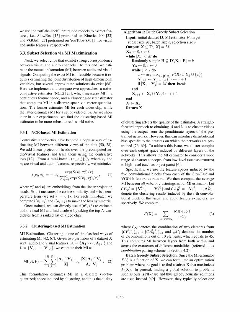
Algorithm 1: Batch Greedy Subset SelectionInput: initial dataset D, MI estimator F , target

subset size M , batch size b, selection size sOutput: X ⊆ D, |X| = MX0 ← ∅, i← 0while |Xi| < M do

Randomly sample B ⊆ D\Xi, |B| = bY0 ← ∅, j ← 0while j < s do

x← argmaxx∈B\YjF (Xi ∪Yj ∪ {x})

Yj+1 ← Yj ∪ {x}, j ← j + 1if |Xi ∪Yj | = M then break

endXi+1 ← Xi ∪Yj , i← i+ 1

endX← Xi

Return X

of clustering affects the quality of the estimator. A straight-forward approach to obtaining A and V is to cluster videosusing the output from the penultimate layers of the pre-trained networks. However, this can introduce distributionalbias specific to the datasets on which the networks are pre-trained [76, 69]. To address this issue, we cluster samplesover each output space induced by different layers of thenetworks. This allows the MI estimator to consider a widerange of abstract concepts, from low-level (such as textures)to high-level (such as object parts) [6].

Specifically, we use the feature spaces induced by thefive convolutional blocks from each of the SlowFast andVGGish feature extractors. We then compute the averageMI between all pairs of clusterings as our MI estimator. LetCV(i)

X = {V(i)1 , · · · ,V(i)

ni } and CA(i)X = {A(i)

1 , · · · ,A(i)mi}

denote the clustering results induced by the i-th convolu-tional block of the visual and audio feature extractors, re-spectively. We compute:

F (X) =∑

(X ,Y)∈CX

MI(X ,Y)10C2

, (3)

where CX denotes the combination of two elements from{CV(i)

X }5i=1 ∪ {CA(j)X }5j=1 and 10C2 denotes the number

of 2-combinations out of 10 elements, which equals to 45.This computes MI between layers from both within andacross the extractors of different modalities (referred to ascombination pairing scheme in Section 4.2).

Batch Greedy Subset Selection. Since the MI estimatorF (·) is a function of X, we can formulate an optimizationproblem where the goal is to find a subset X that maximizesF (X). In general, finding a global solution to problemssuch as ours is NP-hard and thus greedy heuristic solutionsare used instead [49]. However, they typically select one

10277

sample in each iteration and re-evaluate the goodness func-tion, e.g., F (·), on all the remaining candidates. This intro-duces a challenge to our setting because the time complexityis quadratic to the size of the population; this is clearly notscalable to 300 million instances.

Therefore, we approximate the typical greedy solutionusing the batch greedy algorithm [13], as shown in Algo-rithm 1. It randomly samples a batch B from the remain-ing pool of candidates, and searches for the next element tobe included in the active solution set only within B. Thisbatch trick reduces the time complexity down to linear, i.e.,O(N × |B|), where N is the size of the input dataset. Wedemonstrate the efficacy of the algorithm in Section 4.

Stochastic Clustering. One missing piece in thispipeline is an efficient clustering algorithm scalable to hun-dreds of millions of instances. The most popular choiceamong various clustering methods is K-means cluster-ing [74], which is a special case of mixture density es-timation for isotropic normal and other densities. Typi-cally, an expectation-maximization (EM) algorithm, suchas Lloyd’s [52], is used to find the cluster centers. Such al-gorithms require repeated computation of the distances ofall samples from all k cluster centers, followed by clus-ter assignment, until convergence. Lloyd’s algorithm up-dates cluster centers only after each pass through the entiredataset. But for very large datasets (like ours), a small sub-set usually contains enough information to obtain good es-timates of the cluster centers, meaning that EM-style algo-rithms tend to take (perhaps too) many epochs to converge.

There are different strategies for addressing this issue,including random sampling and subsetting, but a straight-forward approach is to replace EM algorithm with anSGD [41, 7, 59]. In such an approach, for large datasets,convergence rate and final accuracy of the cluster centersare determined not by the total dataset size, but by the learn-ing rate schedule. A straightforward SGD update rule isto compute the nearest cluster centers for each sample ina batch and then update the cluster centers using a convexcombination of the cluster centers and their nearest samples,weighting the samples with a learning rate λ and the clustercenters with (1 − λ). However, mixture density estimatorsin general suffer from the problem that adding mixture com-ponents with zero probability does not change the mixturedensity; in practice, this means EM and SGD-based algo-rithms may end up with cluster centers that stop receivingupdates at some point during the optimization.

We address this problem by estimating the mixture com-ponent utilization rate as the ratio of the total number ofupdates to the cluster center divided by the total number ofestimation steps, and reinitializing cluster centers when thatprobability falls below (1/k)2. In Section 4.2, we demon-strate that our mini-batch SGD update shows comparableaccuracy to batch update in correspondence retrieval tasks.

4. Evaluation on Correspondence RetrievalWe systematically evaluate different components of

our pipeline with synthetic correspondence-retrieval tasks,where we generate corresponding and non-correspondingpairs using CIFAR-10 [36], MNIST [38] and FSDD [29].In each correspondence retrieval task, the goal is to dis-cover the known corresponding samples among the non-corresponding pairs. To show the generality of the findings,we also experiment with Kinetics-Sounds [4] which exhibitreal-world audio-visual correspondence.

4.1. Experimental Setting

Datasets We construct five datasets where each instanceis a pair of samples with different correspondence types.

1/2) CIFAR10-Rotation/Flip. We use images from fiverandomly selected categories to construct a “positive pair”set, and use the rest for a “negative pair” set. For the posi-tive set, we create pairs of images by sampling two differentimages from the same category (e.g., two images of a bird),and apply a geometric transformation to one of them; weapply either a 90◦ CCW rotation (CIFAR10-Rotation) or ahorizontal flip (CIFAR10-Flip). The negative set followsthe same process but each pair contains images from differ-ent categories. We categorize this type of correspondence as“Natural Class Correspondence” because pairings are madeover natural semantic categories.

3/4) MNIST-CIFAR10/FSDD. We use images from fivedigit categories to construct a positive set and use the restfor a negative set. Different from above, correspondence isdefined via an arbitrary class-level mapping, e.g., “digit 0”images map to the “car” images in CIFAR-10 or “digit 0”audio samples in FSDD. We take samples from the samecategories to construct the positive set and samples fromdifferent categories for the negative set. We call these “Ar-bitrary Class Correspondence” to differentiate from above.

5) Kinetics-Sounds. Unlike the above datasets wherethe correspondence is defined over class categories, here thecorrespondence is defined at the sample level, i.e., a positiveset contains pairs of audio and visual channels of the samevideo, and a negative set contains randomly permuted pairs.We do not utilize class labels to construct the dataset.

Methods We compare our pipeline (both contrastive-based and clustering-based) to three ranking-based ap-proaches. All the methods use the same precomputed fea-tures. For images, we use ResNet-50 [26] pretrained on Im-ageNet [14]. For videos, we use SlowFast [15] pretrained onKinetics-400 [33] and VGGish [27] pretrained on YouTube-8M [1] for visual and audio features, respectively. For theranking baselines, we apply PCA [55] to reduce the fea-ture dimensionality to 64 and rank the instances based onthree similarity metrics: inner product, cosine similarity,and (negative) l2 distance. Because all our datasets have an

10278

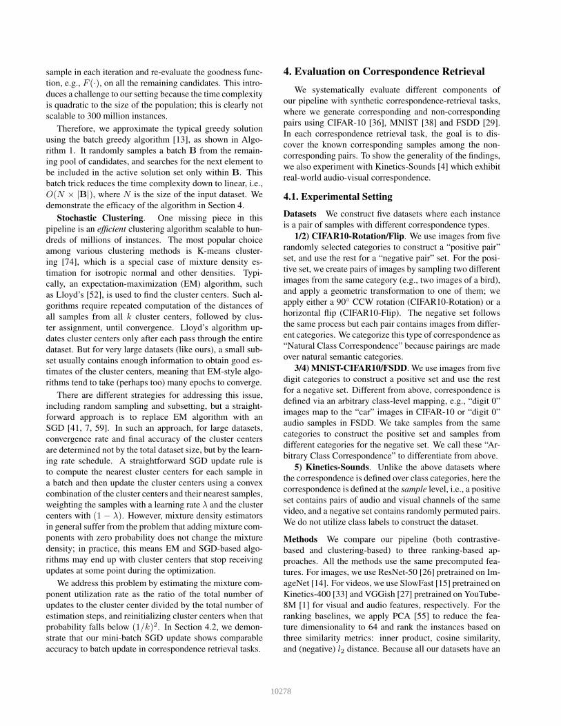
Natural Class Correspondence Arbitrary Class Correspondence Audio-VisualMethod CIFAR10-Rotation CIFAR10-Flip MNIST-CIFAR10 MNIST-FSDD Kinetics-SoundsRanking-inner 87.872 ± 0.002 87.044 ± 0.001 63.076 ± 0.001 64.453 ± 0.003 52.558 ± 0.002Ranking-cos 87.872 ± 0.002 87.044 ± 0.001 67.600 ± 0.002 61.893 ± 0.004 60.108 ± 0.001Ranking-l2 87.872 ± 0.002 87.044 ± 0.001 66.796 ± 0.001 62.933 ± 0.003 51.236 ± 0.001Ours-Contrastive 99.395 ± 0.000 99.480 ± 0.001 73.252 ± 0.040 73.733 ± 0.027 73.066 ± 0.036Ours-Clustering 87.292 ± 0.014 87.248 ± 0.010 77.224 ± 0.009 69.440 ± 0.049 88.705 ± 0.004

Table 1. Correspondence retrieval results. We conduct a total of five runs and report the precision with the 99% confidence interval. Weuse the clustering pairing scheme which gives the highest score in each configuration: combination, except diagonal for Ranking-inner,Ranking-cos and Rank-l2 on CIFAR10-Rotation and CIFAR10-Flip.

equal number of positive and negative instances, we simplyselect the top 50% instances as the retrieval result.

Protocol We split each dataset into train and test parti-tions of the same size. We conduct a total of five runs foreach of the five datasets and report results on the test splits.We use train sets only for the contrastive estimator to trainthe projection heads. When constructing each dataset, wesample at most n = 1000 instances from each categoryof the source datasets. For the noise contrastive estimator,we train the linear projection heads for 100 epochs usingthe AMSGrad of Adam optimizer [57] with a learning rateof 2e-4. We randomly take one sample from each class tobuild a mini-batch for class-level correspondence datasets,and sample random Nb = 10 clips to build a mini-batchfor the sample-level correspondence dataset. When apply-ing our clustering-based method, we perform the SGD K-means clustering with the “ground-truth” number of cen-troids as the number of classes in each source dataset; weuse the batch greedy algorithm with a batch size b = 100and a selection size s = 25.

4.2. Ablation Results & Discussion

Table 1 shows that the two variants of our approach –contrastive and clustering – achieve overall higher precisionrates than the ranking baselines. The contrastive approachperforms well on the two datasets with the “natural classcorrespondence,” conforming to the previous results thatshows contrastive learning is robust to geometric transfor-mations [12]. The clustering approach excels on Kinetics-Sounds that contains natural audio-visual correspondence,which is closer to our intended scenario. Therefore, we con-duct various ablation studies on Kinetics-Sounds to validatedifferent components of our clustering-based approach.

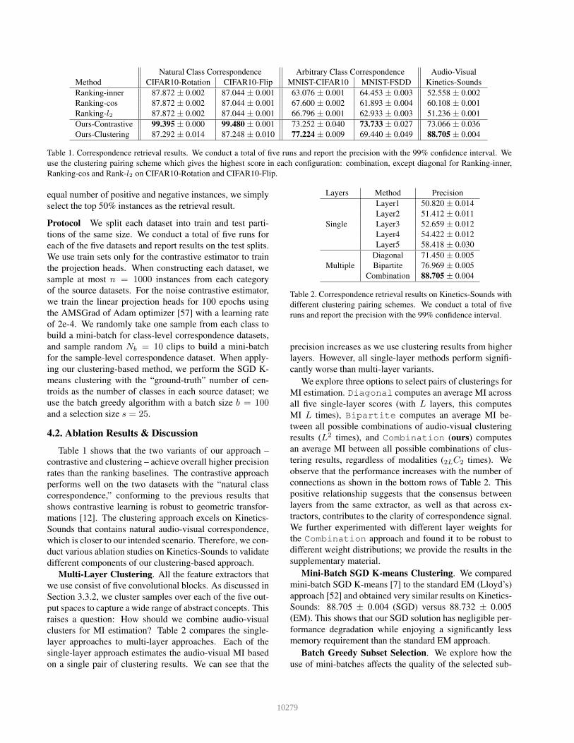
Multi-Layer Clustering. All the feature extractors thatwe use consist of five convolutional blocks. As discussed inSection 3.3.2, we cluster samples over each of the five out-put spaces to capture a wide range of abstract concepts. Thisraises a question: How should we combine audio-visualclusters for MI estimation? Table 2 compares the single-layer approaches to multi-layer approaches. Each of thesingle-layer approach estimates the audio-visual MI basedon a single pair of clustering results. We can see that the

Layers Method Precision

Single

Layer1 50.820 ± 0.014Layer2 51.412 ± 0.011Layer3 52.659 ± 0.012Layer4 54.422 ± 0.012Layer5 58.418 ± 0.030

MultipleDiagonal 71.450 ± 0.005Bipartite 76.969 ± 0.005

Combination 88.705 ± 0.004

Table 2. Correspondence retrieval results on Kinetics-Sounds withdifferent clustering pairing schemes. We conduct a total of fiveruns and report the precision with the 99% confidence interval.

precision increases as we use clustering results from higherlayers. However, all single-layer methods perform signifi-cantly worse than multi-layer variants.

We explore three options to select pairs of clusterings forMI estimation. Diagonal computes an average MI acrossall five single-layer scores (with L layers, this computesMI L times), Bipartite computes an average MI be-tween all possible combinations of audio-visual clusteringresults (L2 times), and Combination (ours) computesan average MI between all possible combinations of clus-tering results, regardless of modalities (2LC2 times). Weobserve that the performance increases with the number ofconnections as shown in the bottom rows of Table 2. Thispositive relationship suggests that the consensus betweenlayers from the same extractor, as well as that across ex-tractors, contributes to the clarity of correspondence signal.We further experimented with different layer weights forthe Combination approach and found it to be robust todifferent weight distributions; we provide the results in thesupplementary material.

Mini-Batch SGD K-means Clustering. We comparedmini-batch SGD K-means [7] to the standard EM (Lloyd’s)approach [52] and obtained very similar results on Kinetics-Sounds: 88.705 ± 0.004 (SGD) versus 88.732 ± 0.005(EM). This shows that our SGD solution has negligible per-formance degradation while enjoying a significantly lessmemory requirement than the standard EM approach.

Batch Greedy Subset Selection. We explore how theuse of mini-batches affects the quality of the selected sub-

10279

0.00K 3.00K 6.00K 9.00Kiterations

60

80

100

prec

ision

Greedy vs. Batch Greedy

greedyratio=0.0312ratio=0.0625ratio=0.1250ratio=0.2500ratio=0.5000

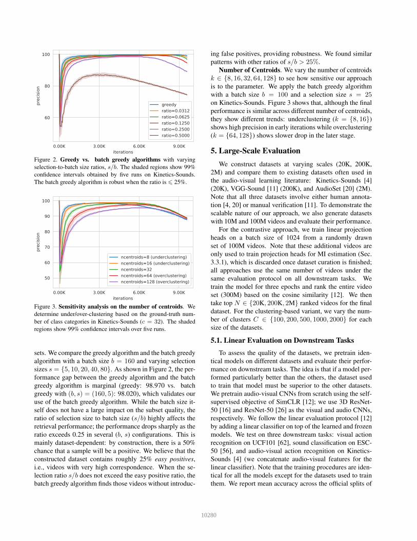
Figure 2. Greedy vs. batch greedy algorithms with varyingselection-to-batch size ratios, s/b. The shaded regions show 99%confidence intervals obtained by five runs on Kinetics-Sounds.The batch greedy algorithm is robust when the ratio is ⩽ 25%.

0.00K 3.00K 6.00K 9.00Kiterations

50

60

70

80

90

100

prec

ision

ncentroids=8 (underclustering)ncentroids=16 (underclustering)ncentroids=32ncentroids=64 (overclustering)ncentroids=128 (overclustering)

Figure 3. Sensitivity analysis on the number of centroids. Wedetermine under/over-clustering based on the ground-truth num-ber of class categories in Kinetics-Sounds (c = 32). The shadedregions show 99% confidence intervals over five runs.

sets. We compare the greedy algorithm and the batch greedyalgorithm with a batch size b = 160 and varying selectionsizes s = {5, 10, 20, 40, 80}. As shown in Figure 2, the per-formance gap between the greedy algorithm and the batchgreedy algorithm is marginal (greedy: 98.970 vs. batchgreedy with (b, s) = (160, 5): 98.020), which validates ouruse of the batch greedy algorithm. While the batch size it-self does not have a large impact on the subset quality, theratio of selection size to batch size (s/b) highly affects theretrieval performance; the performance drops sharply as theratio exceeds 0.25 in several (b, s) configurations. This ismainly dataset-dependent: by construction, there is a 50%chance that a sample will be a positive. We believe that theconstructed dataset contains roughly 25% easy positives,i.e., videos with very high correspondence. When the se-lection ratio s/b does not exceed the easy positive ratio, thebatch greedy algorithm finds those videos without introduc-

ing false positives, providing robustness. We found similarpatterns with other ratios of s/b > 25%.

Number of Centroids. We vary the number of centroidsk ∈ {8, 16, 32, 64, 128} to see how sensitive our approachis to the parameter. We apply the batch greedy algorithmwith a batch size b = 100 and a selection size s = 25on Kinetics-Sounds. Figure 3 shows that, although the finalperformance is similar across different number of centroids,they show different trends: underclustering (k = {8, 16})shows high precision in early iterations while overclustering(k = {64, 128}) shows slower drop in the later stage.

5. Large-Scale EvaluationWe construct datasets at varying scales (20K, 200K,

2M) and compare them to existing datasets often used inthe audio-visual learning literature: Kinetics-Sounds [4](20K), VGG-Sound [11] (200K), and AudioSet [20] (2M).Note that all three datasets involve either human annota-tion [4, 20] or manual verification [11]. To demonstrate thescalable nature of our approach, we also generate datasetswith 10M and 100M videos and evaluate their performance.

For the contrastive approach, we train linear projectionheads on a batch size of 1024 from a randomly drawnset of 100M videos. Note that these additional videos areonly used to train projection heads for MI estimation (Sec.3.3.1), which is discarded once dataset curation is finished;all approaches use the same number of videos under thesame evaluation protocol on all downstream tasks. Wetrain the model for three epochs and rank the entire videoset (300M) based on the cosine similarity [12]. We thentake top N ∈ {20K, 200K, 2M} ranked videos for the finaldataset. For the clustering-based variant, we vary the num-ber of clusters C ∈ {100, 200, 500, 1000, 2000} for eachsize of the datasets.

5.1. Linear Evaluation on Downstream Tasks

To assess the quality of the datasets, we pretrain iden-tical models on different datasets and evaluate their perfor-mance on downstream tasks. The idea is that if a model per-formed particularly better than the others, the dataset usedto train that model must be superior to the other datasets.We pretrain audio-visual CNNs from scratch using the self-supervised objective of SimCLR [12]; we use 3D ResNet-50 [16] and ResNet-50 [26] as the visual and audio CNNs,respectively. We follow the linear evaluation protocol [12]by adding a linear classifier on top of the learned and frozenmodels. We test on three downstream tasks: visual actionrecognition on UCF101 [62], sound classification on ESC-50 [56], and audio-visual action recognition on Kinetics-Sounds [4] (we concatenate audio-visual features for thelinear classifier). Note that the training procedures are iden-tical for all the models except for the datasets used to trainthem. We report mean accuracy across the official splits of

10280

Kinetics-SoundsESC-50UCF101

Top 1 Accuracy Top 5 Accuracy

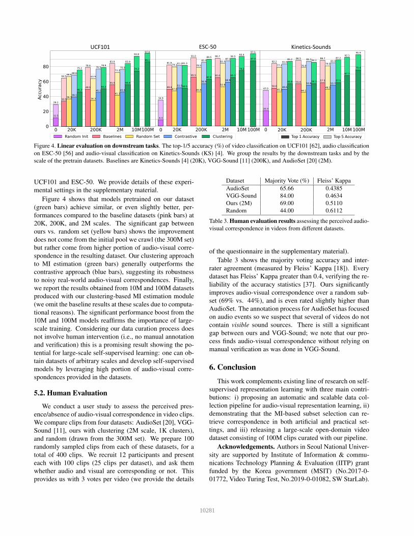
Figure 4. Linear evaluation on downstream tasks. The top-1/5 accuracy (%) of video classification on UCF101 [62], audio classificationon ESC-50 [56] and audio-visual classification on Kinetics-Sounds (KS) [4]. We group the results by the downstream tasks and by thescale of the pretrain datasets. Baselines are Kinetics-Sounds [4] (20K), VGG-Sound [11] (200K), and AudioSet [20] (2M).

UCF101 and ESC-50. We provide details of these experi-mental settings in the supplementary material.

Figure 4 shows that models pretrained on our dataset(green bars) achieve similar, or even slightly better, per-formances compared to the baseline datasets (pink bars) at20K, 200K, and 2M scales. The significant gap betweenours vs. random set (yellow bars) shows the improvementdoes not come from the initial pool we crawl (the 300M set)but rather come from higher portion of audio-visual corre-spondence in the resulting dataset. Our clustering approachto MI estimation (green bars) generally outperforms thecontrastive approach (blue bars), suggesting its robustnessto noisy real-world audio-visual correspondences. Finally,we report the results obtained from 10M and 100M datasetsproduced with our clustering-based MI estimation module(we omit the baseline results at these scales due to computa-tional reasons). The significant performance boost from the10M and 100M models reaffirms the importance of large-scale training. Considering our data curation process doesnot involve human intervention (i.e., no manual annotationand verification) this is a promising result showing the po-tential for large-scale self-supervised learning: one can ob-tain datasets of arbitrary scales and develop self-supervisedmodels by leveraging high portion of audio-visual corre-spondences provided in the datasets.

5.2. Human Evaluation

We conduct a user study to assess the perceived pres-ence/absence of audio-visual correspondence in video clips.We compare clips from four datasets: AudioSet [20], VGG-Sound [11], ours with clustering (2M scale, 1K clusters),and random (drawn from the 300M set). We prepare 100randomly sampled clips from each of these datasets, for atotal of 400 clips. We recruit 12 participants and presenteach with 100 clips (25 clips per dataset), and ask themwhether audio and visual are corresponding or not. Thisprovides us with 3 votes per video (we provide the details

Dataset Majority Vote (%) Fleiss’ KappaAudioSet 65.66 0.4385VGG-Sound 84.00 0.4634Ours (2M) 69.00 0.5110Random 44.00 0.6112

Table 3. Human evaluation results assessing the perceived audio-visual correspondence in videos from different datasets.

of the questionnaire in the supplementary material).Table 3 shows the majority voting accuracy and inter-

rater agreement (measured by Fleiss’ Kappa [18]). Everydataset has Fleiss’ Kappa greater than 0.4, verifying the re-liability of the accuracy statistics [37]. Ours significantlyimproves audio-visual correspondence over a random sub-set (69% vs. 44%), and is even rated slightly higher thanAudioSet. The annotation process for AudioSet has focusedon audio events so we suspect that several of videos do notcontain visible sound sources. There is still a significantgap between ours and VGG-Sound; we note that our pro-cess finds audio-visual correspondence without relying onmanual verification as was done in VGG-Sound.

6. Conclusion

This work complements existing line of research on self-supervised representation learning with three main contri-butions: i) proposing an automatic and scalable data col-lection pipeline for audio-visual representation learning, ii)demonstrating that the MI-based subset selection can re-trieve correspondence in both artificial and practical set-tings, and iii) releasing a large-scale open-domain videodataset consisting of 100M clips curated with our pipeline.

Acknowledgements. Authors in Seoul National Univer-sity are supported by Institute of Information & commu-nications Technology Planning & Evaluation (IITP) grantfunded by the Korea government (MSIT) (No.2017-0-01772, Video Turing Test, No.2019-0-01082, SW StarLab).

10281

References[1] Sami Abu-El-Haija, Nisarg Kothari, Joonseok Lee, Paul

Natsev, George Toderici, Balakrishnan Varadarajan, andSudheendra Vijayanarasimhan. Youtube-8M: A Large-Scale Video Classification Benchmark. arXiv preprintarXiv:1609.08675, 2016.

[2] Pankaj K Agarwal, Sariel Har-Peled, and Kasturi RVaradarajan. Geometric Approximation via Coresets. Com-binatorial and Computational Geometry, 52:1–30, 2005.

[3] Humam Alwassel, Dhruv Mahajan, Lorenzo Torresani,Bernard Ghanem, and Du Tran. Self-Supervised Learningby Cross-Modal Audio-Video Clustering. arXiv preprintarXiv:1911.12667, 2019.

[4] Relja Arandjelovic and Andrew Zisserman. Look, Listen andLearn. In ICCV, 2017.

[5] Yusuf Aytar, Carl Vondrick, and Antonio Torralba. Sound-Net: Learning Sound Representations from UnlabeledVideo. In NeurIPS, 2016.

[6] David Bau, Bolei Zhou, Aude Oliva, and Antonio Torralba.Interpreting Deep Visual Representations via Network Dis-section. PAMI, 41(9):2131–2145, 2019.

[7] Leon Bottou and Yoshua Bengio. Convergence Properties ofthe K-Means Algorithms. In NeurIPS, 1995.

[8] Fabian Caba Heilbron, Victor Escorcia, Bernard Ghanem,and Juan Carlos Niebles. ActivityNet: A Large-Scale VideoBenchmark for Human Activity Understanding. In CVPR,2015.

[9] Joao Carreira, Eric Noland, Chloe Hillier, and Andrew Zis-serman. A Short Note on the Kinetics-700 Human ActionDataset. arXiv preprint arXiv:1907.06987, 2019.

[10] Sourish Chaudhuri, Joseph Roth, Daniel P. W. Ellis, AndrewGallagher, Liat Kaver, Radhika Marvin, Caroline Pantofaru,Nathan Reale, Loretta Guarino Reid, Kevin Wilson, andZhonghua Xi. AVA-Speech: A Densely Labeled Dataset ofSpeech Activity in Movies. In Interspeech, 2018.

[11] Honglie Chen, Weidi Xie, Andrea Vedaldi, and Andrew Zis-serman. VGGSound: A Large-Scale Audio-Visual Dataset.In ICASSP, 2020.

[12] Ting Chen, Simon Kornblith, Mohammad Norouzi, and Ge-offrey Hinton. A Simple Framework for Contrastive Learn-ing of Visual Representations. In ICML, 2020.

[13] Yuxin Chen and Andreas Krause. Near-optimal Batch ModeActive Learning and Adaptive Submodular Optimization.ICML, 2013.

[14] Jia Deng, Wei Dong, Richard Socher, Li-Jia Li, Kai Li, andLi Fei-Fei. ImageNet: A Large-Scale Hierarchical ImageDatabase. In CVPR, 2009.

[15] Christoph Feichtenhofer, Haoqi Fan, Jitendra Malik, andKaiming He. SlowFast Networks for Video Recognition. InICCV, 2019.

[16] Christoph Feichtenhofer, Axel Pinz, and Richard Wildes.Spatiotemporal Residual Networks for Video Action Recog-nition. In NeurIPS, 2016.

[17] John W Fisher and Trevor Darrell. Probabalistic Models andInformative Subspaces for Audiovisual Correspondence. InECCV, 2002.

[18] Joseph L Fleiss. Measuring Nominal Scale AgreementAmong Many Raters. Psychological Bulletin, 76(5):378,1971.

[19] Ruohan Gao and Kristen Grauman. 2.5D Visual Sound. InCVPR, 2019.

[20] Jort F. Gemmeke, Daniel P. W. Ellis, Dylan Freedman, ArenJansen, Wade Lawrence, R. Channing Moore, Manoj Plakal,and Marvin Ritter. Audio Set: An Ontology and Human-Labeled Dataset for Audio Events. In ICASSP, 2017.

[21] Eleanor Jack Gibson. Principles of Perceptual Learning andDevelopment. Appleton-Century-Crofts, 1969.

[22] Yuhong Guo. Active Instance Sampling via Matrix Partition.In NeurIPS, 2010.

[23] Michael Gutmann and Aapo Hyvarinen. Noise-ContrastiveEstimation: A New Estimation Principle for UnnormalizedStatistical Models. In AISTATS, 2010.

[24] Sariel Har-Peled and Soham Mazumdar. On Coresets for K-Means and K-Median Clustering. In STOC, 2004.

[25] Kaiming He, Haoqi Fan, Yuxin Wu, Saining Xie, and RossGirshick. Momentum Contrast for Unsupervised Visual Rep-resentation Learning. In CVPR, 2020.

[26] Kaiming He, Xiangyu Zhang, Shaoqing Ren, and Jian Sun.Deep Residual Learning for Image Recognition. In CVPR,2016.

[27] Shawn Hershey, Sourish Chaudhuri, Daniel PW Ellis, Jort FGemmeke, Aren Jansen, R Channing Moore, Manoj Plakal,Devin Platt, Rif A Saurous, Bryan Seybold, et al. CNN Ar-chitectures for Large-Scale Audio Classification. In ICASSP,2017.

[28] R Devon Hjelm, Alex Fedorov, Samuel Lavoie-Marchildon,Karan Grewal, Phil Bachman, Adam Trischler, and YoshuaBengio. Learning Deep Representations by Mutual Informa-tion Estimation and Maximization. In ICLR, 2019.

[29] Zohar Jackson, Cesar Souza, Jason Flaks, Yuxin Pan, Here-man Nicolas, and Adhish Thite. Free Spoken Digit Dataset:v1.0.8, Aug. 2018.

[30] David S Johnson, Christos H Papadimitriou, and MihalisYannakakis. How Easy Is Local Search? Journal of com-puter and system sciences, 37(1):79–100, 1988.

[31] Armand Joulin, Edouard Grave, Piotr Bojanowski, MatthijsDouze, Herve Jegou, and Tomas Mikolov. FastText.zip:Compressing Text Classification Models. arXiv preprintarXiv:1612.03651, 2016.

[32] Armand Joulin, Edouard Grave, Piotr Bojanowski, andTomas Mikolov. Bag of Tricks for Efficient Text Classifi-cation. In EACL, 2017.

[33] Will Kay, Joao Carreira, Karen Simonyan, Brian Zhang,Chloe Hillier, Sudheendra Vijayanarasimhan, Fabio Vi-ola, Tim Green, Trevor Back, Paul Natsev, et al. TheKinetics Human Action Video Dataset. arXiv preprintarXiv:1705.06950, 2017.

[34] Bruno Korbar, Du Tran, and Lorenzo Torresani. CooperativeLearning of Audio and Video Models from Self-SupervisedSynchronization. In NeurIPS, 2018.

[35] Alexander Kraskov, Harald Stogbauer, and Peter Grass-berger. Estimating Mutual Information. Physical review E,69(6), 2004.

10282

[36] Alex Krizhevsky and Geoffrey Hinton. Learning MultipleLayers of Features from Tiny Images. Technical report, Uni-versity of Toronto, 2009.

[37] J Richard Landis and Gary G Koch. The Measurement ofObserver Agreement for Categorical Data. Biometrics, pages159–174, 1977.

[38] Yann LeCun, Leon Bottou, Yoshua Bengio, and PatrickHaffner. Gradient-Based Learning Applied to DocumentRecognition. Proceedings of the IEEE, 86(11):2278–2324,1998.

[39] David D Lewis and William A Gale. A Sequential Algorithmfor Training Text Classifiers. In SIGIR, 1994.

[40] Xin Li and Yuhong Guo. Adaptive Active Learning for Im-age Classification. In CVPR, 2013.

[41] Thomas Martinetz and Klaus Schulten. A “Neural-Gas” Net-work Learns Topologies. In ICANN, 1991.

[42] Marina Meila. Comparing Clusterings—An InformationBased Distance. Journal of multivariate analysis, 98(5),2007.

[43] N Michele Merler, Khoi-Nguyen C. Mac, Dhiraj Joshi,Quoc-Bao Nguyen, Stephen Hammer, John Kent, Jin-jun Xiong, Minh N. Do, John R. Smith, and RogerioSchmidt Feris. Automatic Curation of Sports Highlights Us-ing Multimodal Excitement Features. IEEE Trans Multime-dia, 21(5), 2019.

[44] Antoine Miech, Dimitri Zhukov, Jean-Baptiste Alayrac,Makarand Tapaswi, Ivan Laptev, and Josef Sivic.HowTo100M: Learning a Text-Video Embedding byWatching Hundred Million Narrated Video Clips. In ICCV,2019.

[45] Michel Minoux. Accelerated Greedy Algorithms for Max-imizing Submodular Set Functions. In Optimization tech-niques, pages 234–243. Springer, 1978.

[46] Mathew Monfort, Alex Andonian, Bolei Zhou, Kandan Ra-makrishnan, Sarah Adel Bargal, Tom Yan, Lisa Brown,Quanfu Fan, Dan Gutfruend, and Carl Vondrick. Moments inTime Dataset: One Million Videos for Event Understanding.PAMI, pages 1–8, 2019.

[47] Arsha Nagrani, Joon Son Chung, Weidi Xie, and AndrewZisserman. Voxceleb: Large-scale speaker verification in thewild. Computer Science and Language, 2019.

[48] G. L. Nemhauser, L. A. Wolsey, and M. L. Fisher. An Anal-ysis of Approximations for Maximizing Submodular SetFunctions–I. Mathematical Programming, 14(1):265–294,1978.

[49] George L Nemhauser, Laurence A Wolsey, and Marshall LFisher. An Analysis of Approximations for MaximizingSubmodular Set Functions—I. Mathematical programming,14(1):265–294, 1978.

[50] Aaron van den Oord, Yazhe Li, and Oriol Vinyals. Represen-tation Learning with Contrastive Predictive Coding. arXivpreprint arXiv:1807.03748, 2018.

[51] Andrew Owens, Phillip Isola, Josh McDermott, Antonio Tor-ralba, Edward H Adelson, and William T Freeman. VisuallyIndicated Sounds. In CVPR, 2016.

[52] Stuart P. Lloyd. Least Squares Quantization in PCM. IEEETransactions on Information Theory, 28(2):129–137, 1982.

[53] Liam Paninski. Estimation of Entropy and Mutual Informa-tion. Neural computation, 15(6):1191–1253, 2003.

[54] Mandela Patrick, Yuki M Asano, Ruth Fong, Joao F Hen-riques, Geoffrey Zweig, and Andrea Vedaldi. Multi-modalSelf-Supervision from Generalized Data Transformations.arXiv preprint arXiv:2003.04298, 2020.

[55] Karl Pearson. LIII. On Lines and Planes of Closest Fitto Systems of Points in Space. The London, Edinburgh,and Dublin Philosophical Magazine and Journal of Science,2(11):559–572, 1901.

[56] Karol J. Piczak. ESC: Dataset for Environmental SoundClassification. In ACM-MM, 2015.

[57] Sashank J Reddi, Satyen Kale, and Sanjiv Kumar. On theConvergence of Adam and Beyond. In ICLR, 2018.

[58] Joseph Roth, Sourish Chaudhuri, Ondrej Klejch, Rad-hika Marvin, Andrew Gallagher, Liat Kaver, SharadhRamaswamy, Arkadiusz Stopczynski, Cordelia Schmid,Zhonghua Xi, and Caroline Pantofaru. AVA-ActiveSpeaker:An Audio-Visual Dataset for Active Speaker Detection.arXiv preprint arXiv:1901.01342, 2019.

[59] David Sculley. Web-Scale K-Means Clustering. In WWW,2010.

[60] Burr Settles. Active Learning Literature Survey. Science,10(3):237–304, 1995.

[61] Yusuke Shinohara. A Submodular Optimization Approachto Sentence Set Selection. In ICASSP, 2014.

[62] Khurram Soomro, Amir Roshan Zamir, and Mubarak Shah.UCF101: A Dataset of 101 Human Actions Classes FromVideos in The Wild. arXiv preprint arXiv:1212.0402, 2012.

[63] Jamshid Sourati, Murat Akcakaya, Jennifer G Dy, Todd KLeen, and Deniz Erdogmus. Classification Active LearningBased on Mutual Information. Entropy, 18(2):51, 2016.

[64] Jonathan C Stroud, David A Ross, Chen Sun, Jia Deng,Rahul Sukthankar, and Cordelia Schmid. Learning VideoRepresentations from Textual Web Supervision. arXivpreprint arXiv:2007.14937, 2020.

[65] Yapeng Tian, Jing Shi, Bochen Li, Zhiyao Duan, and Chen-liang Xu. Audio-Visual Event Localization in UnconstrainedVideos. In ECCV, 2018.

[66] Ivor W Tsang, James T Kwok, and Pak-Ming Cheung. CoreVector Machines: Fast SVM Training on Very Large DataSets. Journal of Machine Learning Research, 6(Apr):363–392, 2005.

[67] Nguyen Xuan Vinh, Julien Epps, and James Bailey. Informa-tion Theoretic Measures for Clusterings Comparison: Vari-ants, Properties, Normalization and Correction for Chance.Journal of Machine Learning Research, 11, 2010.

[68] Janett Walters-Williams and Yan Li. Estimation of MutualInformation: A Survey. In RSKT, 2009.

[69] Mei Wang and Weihong Deng. Deep Visual Domain Adap-tation: A Survey. Neurocomputing, 312:135–153, 2018.

[70] Kai Wei, Rishabh Iyer, and Jeff Bilmes. Submodularity inData Subset Selection and Active Learning. In ICML, 2015.

[71] Kai Wei, Yuzong Liu, Katrin Kirchhoff, Chris Bartels, andJeff Bilmes. Submodular Subset Selection for Large-ScaleSpeech Training Data. In ICASSP, 2014.

10283

[72] Kai Wei, Yuzong Liu, Katrin Kirchhoff, and Jeff Bilmes. Us-ing Document Summarization Techniques for Speech DataSubset Selection. In NAACL, 2013.

[73] Kai Wei, Yuzong Liu, Katrin Kirchhoff, and Jeff Bilmes. Un-supervised Submodular Subset Selection for Speech Data. InICASSP, 2014.

[74] Xindong Wu, Vipin Kumar, J Ross Quinlan, Joydeep Ghosh,Qiang Yang, Hiroshi Motoda, Geoffrey J McLachlan, AngusNg, Bing Liu, S Yu Philip, et al. Top 10 Algorithms in DataMining. Knowledge and Information Systems, 14(1):1–37,2008.

[75] Karren Yang, Bryan Russell, and Justin Salamon. TellingLeft From Right: Learning Spatial Correspondence of Sightand Sound. In CVPR, 2020.

[76] Jason Yosinski, Jeff Clune, Yoshua Bengio, and Hod Lipson.How Transferable are Features in Deep Neural Networks? InNeurIPS, 2014.

10284