automatic abstraction in reinforcement learning using data mining techniques

Robotics and Autonomous Systems 57 (2009) 1119–1128

Contents lists available at ScienceDirect

Robotics and Autonomous Systems

journal homepage: www.elsevier.com/locate/robot

Automatic abstraction in reinforcement learning using data mining techniquesGhorban Kheradmandian ∗, Mohammad RahmatiDepartment of Computer Eng., Amirkabir University of Technology, Tehran, Iran

a r t i c l e i n f o

Article history:Received 4 October 2008Received in revised form1 July 2009Accepted 6 July 2009Available online 10 July 2009

Keywords:Reinforcement learningAbstractionData miningClusteringSequence mining

a b s t r a c t

In this paper,weused datamining techniques for the automatic discovering of useful temporal abstractionin reinforcement learning. This idea was motivated by the ability of data mining algorithms in automaticdiscovering of structures and patterns, when applied to large data sets. The state transitions and actiontrajectories of the learning agent are stored as the data sets for data mining techniques. The proposedstate clustering algorithms partition the state space to different regions. Policies for reaching differentparts of the space are separately learned and added to the model in a form of options (macro-actions).The main idea of the proposed action sequence mining is to search for patterns that occur frequentlywithin an agent’s accumulated experience. The mined action sequences are also added to the model in aform of options. Our experiments with different data sets indicate a significant speedup of the Q-learningalgorithm using the options discovered by the state clustering and action sequence mining algorithms.

© 2009 Elsevier B.V. All rights reserved.

1. Introduction

Reinforcement Learning (RL) [1,2] is a promising approach forestablishing autonomous agents that improve their performancewith experience. A fundamental problem of its standard algo-rithms is that, although many tasks can asymptotically be learnedby adopting the Markov Decision Process (MDP) framework andusing reinforcement learning techniques, in practice they are notsolvable in a reasonable amount of time. ‘‘Difficult’’ tasks are usu-ally characterized by either a very large state space, or a lack ofimmediate reinforcement signals.Scaling up reinforcement learning to large domains requires

leveraging the structure in these domains. Hierarchical Reinforce-ment Learning (HRL) providesmechanisms throughwhich domainstructure can be exploited to constrain the value function andpolicy space of the learner, and hence speed up learning [3–5].Many large problems have some structure that allows them

to be broken down into sub-problems and represented morecompactly. The sub-problems, being smaller, are often solvedmoreeasily. The solutions to the sub-problems may be combined toprovide the solution for the original larger problem. The automateddiscovery of such task hierarchies [3,6–11] is compelling for atleast two reasons. First, it avoids the significant human effort inengineering the task-subtask structural decomposition, alongwiththe associated state abstractions and subtask goals. Second, if the

∗ Corresponding author.E-mail addresses: [email protected] (G. Kheradmandian),

[email protected] (M. Rahmati).

0921-8890/$ – see front matter© 2009 Elsevier B.V. All rights reserved.doi:10.1016/j.robot.2009.07.002

same hierarchy is useful inmultiple domains, it leads to significanttransfer of learned structural knowledge from one domain to theother.The ability to create and use abstractions, that is, to systemat-

ically ignore irrelevant details in complex environments, is a keyreason that humans are effective problem solvers. An abstractionis a compact representation of the knowledge gained in one taskthat allows the knowledge to be re-used in related tasks. This rep-resentation enables an agent to learn and plan at a higher level.By allowing a system to ignore details that are not immediately

relevant to the current task, the size of the space that an agentmustsearch to find a solution can be reduced. Onemethod for achievingthis is to reduce the branching factor of the search by creating a hi-erarchy of actions. A second approach reduces the size of the statespace by dropping irrelevant state variables. These approaches rep-resent the two main categories of abstractions that have beenstudied: state and temporal abstractions. By state abstraction, wemean an abstraction that generalizes or aggregates over state vari-ables [4,12,13]. By temporal abstraction, wemean an encapsulationof a complex set of actions into a single higher-level action that al-lows an agent to learn and plan atmultiple scales in time. Temporalabstractions create a hierarchy of actions [4,6,7,12,13].In this paper, we have used datamining techniques as solutions

for the automatic discovering of structures or patterns emergingduring solving a problem by a reinforcement learning agent.We adopted the two well known techniques of data mining,i.e., clustering and frequent pattern mining for finding usefulpatterns in problems to be solved by reinforcement learning.The paper is organized as follows: Literature review is discussed

in Section 2. In Section 3, we describe the reinforcement learningbasics and its extension to use options. The proposed data mining

http://www.elsevier.com/locate/robot

http://www.elsevier.com/locate/robot

mailto:[email protected]

mailto:[email protected]

http://dx.doi.org/10.1016/j.robot.2009.07.002

1120 G. Kheradmandian, M. Rahmati / Robotics and Autonomous Systems 57 (2009) 1119–1128

techniques are represented in Section 4. The experimental resultsare described in Sections 5 and 6 represents concluding remarks.

2. Literature review

Recent methods in Reinforcement Learning (RL) allow an agentto plan, act, and learn with temporally extended actions [4,5,14].A temporally-extended action, or a macro action, is a suitablesequence of primary actions. A suitable set of macro actionscan help improve an agent’s efficiency in learning to solvedifficult problems. If an agent can develop such macro action setsautomatically, it should be able to efficiently solve a variety ofproblems without relying on hand-coded macro actions tailoredto specific problems. A number of methods have been suggestedtowards this end [6,9–11].A common approach is to define subtasks in the state space

context. The learning agent identifies important states, whichare believed to possess some ‘‘strategic’’ importance and areworthwhile reaching. The agent learns sub-policies for reachingthose key states. One approach is to look for stateswith non-typicalreinforcement (a high reinforcement gradient) for example, as inDigney [7]. This approach may not prove useful in domains withdelayed reinforcement. Another approach is to choose states basedon their frequency of appearance [6]. The motivation here is thatstates that have been visited often in the past are likely to be a partof the agent’s optimal path. States serve as potential sub-goals ifthey are frequently visited on successful paths but are not visitedon unsuccessful ones. A problemwith frequency based solutions isthat the agent may need excessive exploration of the environmentin order to distinguish between ‘‘important’’ and ‘‘regular’’ states,so that options are defined at relatively advanced stages of thelearning process.Thrun and Schwartz [15], Pickett and Barto [16] generated

temporal abstractions by finding commonly occurring subpoliciesin solutions to a set of tasks. Hengst [12] proposed the Hexqapproach for the construction of a hierarchy of abstractions inproblems with factored state spaces. His method orders statevariableswith respect to their frequency of change and adds a layerof hierarchy for each variable.Jonsson [13] used the VISA approach for decomposing factored

MDPs into hierarchies of options dynamically. The VISA algorithmassumes that the Dynamic Bayesian Network (DBN) model of afactoredMDP is given prior to learning, and uses the DBNmodel toconstruct a causal graph describing how state variables are related.Both the Hexq and VISA approaches are suitable for factoredMDPsand assume some constraints for behaviour of the state variables.Other researchers use graph-theoretic approaches to decom-

pose tasks. Menache et al. [17] construct a state transitions graphand introduce activities that reach states on the border of stronglyconnected regions of the graph. The authors use a max-flow/min-cut algorithm to identify border states in the transitions graph.Mannor et al. [10] use a clustering algorithm to partition the statespace into different regions and introduce activities formoving be-tween regions. Simsek et al. [11] identify sub-goals by partitioninglocal state transitions graphs that represent only themost recentlyrecorded experience. These suggested graph based approachessuffer from the computational complexity issue and they usepolynomial time algorithms for partitioning the transitions graphand finding sub-goal states.

3. Reinforcement learning with options

In this section, we define the basics of the RL with an extensionto use options; see Sutton [5] and McGovern et al. [18] for furtherdetails. We consider a discrete time MDP with a finite set of statesS and a finite set of actions A. At each time step t , t = 1, 2, . . . ,

the learning agent is in some state st ∈ S. The agent can choosean action at from the set of available actions at state st , A(st),causing a state transition to st+1 ∈ S. The agent observes a scalarreward rt which is a (possibly random) function of the current stateand the action performed by the agent. The agent’s goal is to finda map from states to actions, called a policy, which maximizesthe expected discounted reward over time, E

{∑∞

t=0 γt rt}, where

γ < 1 is the discount factor and expectation is taken with respectto the random transitions, random rewards, and possibly randompolicy of the agent.A popular RL algorithm is the Q-Learning algorithm [19]. In Q-

Learning the agent updates theQ-function at every time epoch. TheQ -functionmaps every state-action pair to the expected reward fortaking this action at that state, and following an optimal strategyfrom that point on.We now recall the extension of Q-Learning to Macro-Q-

Learning (or learning with options, see McGovern et al. [18]). Anoption is a sequence of (primitive) actions that are executed by theagent (governed by a ‘‘local’’ policy) until a termination conditionis met.Formally, an option is defined by a triplet 〈I, π, β〉, where I is

the options input set, i.e., all the states from which the option canbe initiated; π is the option’s policy, mapping states belonging to Ito a sequence of actions; β is the termination condition over statesi.e., β(s) denotes the termination probability of the option whenreaching state s. When the agent is following an option, it mustfollow it until it terminates. When not following an option, theagent can choose, at any given state, either a primitive action orto initiate an option, if available (we shall use the notation A′(st)for denoting all choices, i.e., the collection of primitives and optionsavailable at state st ). The update rule for an option ot , initiated atstate st , is:

Q (st , ot) = Q (st , ot)+ α (n(t, st , ot))(γ τ max

a′∈A′(st+τ )Q (st+τ ,a′)

− Q (st , ot)+ rt + γ rt+1 + · · · + γ τ−1rt+τ−1

)(1)

where τ is the actual duration of the option ot , α (n(t, st , ot)) is thelearning rate functionwhich depends on n(t, st , ot), the number oftimes ot was exercised in state st until time t . The update rule for aprimitive action is similar with τ = 1.

4. Our proposed approach

Data mining is the analysis of (often large) observational datafor automated discovery of previously unknown, valid, novel, use-ful and understandable patterns in large databases [20]. The rela-tionships and summaries derived through a data mining exerciseare often referred to as models or patterns. Examples include lin-ear equations, rules, clusters, graphs, tree structures, and recurrentpatterns in time series.Our main idea is based on this concept that various data mining

techniques could be applied for the automatic discovering ofuseful structures and patterns within the reinforcement learningframework. In fact, these patterns and regularities are very usefulfor making good abstractions both for actions and states.We have used the two well known data mining techniques

i.e. clustering and sequence mining for automatic discovering ofstructures and patterns. Our approach is to let the agent roamsaround the environment and then after some possibly inaccurateinformation is collected, data mining techniques are used. Theinput to the datamining algorithms consists of the agent’s recordedstate transitions and action trajectories.

G. Kheradmandian, M. Rahmati / Robotics and Autonomous Systems 57 (2009) 1119–1128 1121

Fig. 1. The pseudo code of our topology clustering algorithm.

4.1. State clustering

Clustering is an important technique in data mining process fordiscovering groups and identifying homogeneous distributions ofpatterns in underlying data. Clustering is referred to as partitioninga set of data into some groups, such that similar patterns fallinto one set. In a reinforcement learning domain, clustering canbe applied based on similarity of different features, includingtopology, the amount of reward and states values. An importantadvantage of the clustering approach is that exploration maybecomemore efficient since the agent can quicklywander to statesthat would be otherwise less explored, since theymay be harder toreach from the initial states.

4.1.1. Topology clusteringThe aim of our proposed topology clustering method is to

discover bottleneck states as sub-goal states. By bottleneck states,we mean those states that connect two regions of state space,in which all transitions from one region to another region gothrough these states. A simple example is a doorway betweentwo rooms, all transitions from one room to another go throughthe doorway. The input to the clustering algorithm consists of theagent recorded state transitions graph. This graph G is generatedas follows. Each visited state becomes a node in the graph G. Eachobserved transition s→ s′ or s′ → s,where (s, s′) ∈ S is translatedto an edge (s, s′) in the graph G.The proposed topology clustering algorithm intends to identify

the edges of the graph G that connect the bottleneck states.Removing these edges from G cause G to be partitioned to somedistinct sub-graphs, each corresponding with a cluster.Let A denotes as the set of nodes of G, E represents the set of all

edges of G and As indicates to the neighbour nodes of the node s,e.g. those nodes connected to the swith an edge in G.

Definition. An edge (s, s′) is called as a border edge, if followingcondition is satisfied.

!∃(s1, s2) ∈ |s1 ∈ As and s2 ∈ As′ . (2)

In other words, if there is not any edge in E, that connectsneighbour nodes of s to the neighbour nodes of s′, then, the edge(s, s′) is identified as a border edge.

Our topology clustering algorithm includes two major steps. Inthe first step, all edges of the graph G, are examined and for eachedge (s, s′) one of the following decisions is made.

- If the edge is a border edge, it is labeled.- If the edge is not a border edge, then all edges that connectneighbour nodes of s to the neighbour nodes of s′ are identifiedas the NeighborConnector set.- If there are some border edges belonging to the NeighborCon-nector, one of them is labeled randomly.- If there is not any border edge belonging to the NeighborCon-nector, then, one of the edges of NeighborConnector is labeledrandomly.

In the second step, each labeled edge (s, s′) is removed from G,if it satisfies the following relation,

∃s1 ∈ A&∃s2 ∈ A|(s1, s) ∈ E&(s′, s2) ∈ E. (3)

Depending on the underlying state space, two steps of thealgorithmmay be iterated a few times. Finally, having removed therelevant labeled edges during each iteration of the twomajor steps,the graphG is partitioned into sub-graphs, inwhich each sub-graphwould be a cluster. The pseudo code of our algorithm is shown inFig. 1.For example, consider the graph of Fig. 2(a), the output of our

topology clustering algorithm with one iteration for the graph of


a b

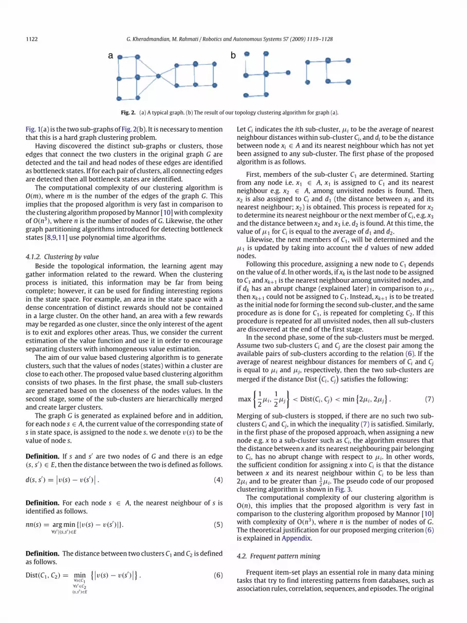
Fig. 2. (a) A typical graph. (b) The result of our topology clustering algorithm for graph (a).

Fig. 1(a) is the two sub-graphs of Fig. 2(b). It is necessary tomentionthat this is a hard graph clustering problem.Having discovered the distinct sub-graphs or clusters, those

edges that connect the two clusters in the original graph G aredetected and the tail and head nodes of these edges are identifiedas bottleneck states. If for each pair of clusters, all connecting edgesare detected then all bottleneck states are identified.The computational complexity of our clustering algorithm is

O(m), where m is the number of the edges of the graph G. Thisimplies that the proposed algorithm is very fast in comparison tothe clustering algorithmproposed byMannor [10]with complexityof O(n3), where n is the number of nodes of G. Likewise, the othergraph partitioning algorithms introduced for detecting bottleneckstates [8,9,11] use polynomial time algorithms.

4.1.2. Clustering by valueBeside the topological information, the learning agent may

gather information related to the reward. When the clusteringprocess is initiated, this information may be far from beingcomplete; however, it can be used for finding interesting regionsin the state space. For example, an area in the state space with adense concentration of distinct rewards should not be containedin a large cluster. On the other hand, an area with a few rewardsmay be regarded as one cluster, since the only interest of the agentis to exit and explores other areas. Thus, we consider the currentestimation of the value function and use it in order to encourageseparating clusters with inhomogeneous value estimation.The aim of our value based clustering algorithm is to generate

clusters, such that the values of nodes (states) within a cluster areclose to each other. The proposed value based clustering algorithmconsists of two phases. In the first phase, the small sub-clustersare generated based on the closeness of the nodes values. In thesecond stage, some of the sub-clusters are hierarchically mergedand create larger clusters.The graph G is generated as explained before and in addition,

for each node s ∈ A, the current value of the corresponding state ofs in state space, is assigned to the node s. we denote v(s) to be thevalue of node s.

Definition. If s and s′ are two nodes of G and there is an edge(s, s′) ∈ E, then the distance between the two is defined as follows.

d(s, s′) =∣∣v(s)− v(s′)∣∣ . (4)

Definition. For each node s ∈ A, the nearest neighbour of s isidentified as follows.

nn(s) = argmin∀s′|(s,s′)∈E

{|v(s)− v(s′)|}. (5)

Definition. The distance between two clusters C1 and C2 is definedas follows.

Dist(C1, C2) = min∀s∈C1∀s′∈C2(s,s′)∈E

{∣∣v(s)− v(s′)∣∣} . (6)

Let Ci indicates the ith sub-cluster, µi to be the average of nearestneighbour distances within sub-cluster Ci, and di to be the distancebetween node xi ∈ A and its nearest neighbour which has not yetbeen assigned to any sub-cluster. The first phase of the proposedalgorithm is as follows.

First, members of the sub-cluster C1 are determined. Startingfrom any node i.e. x1 ∈ A, x1 is assigned to C1 and its nearestneighbour e.g. x2 ∈ A, among unvisited nodes is found. Then,x2 is also assigned to Ci and d1 (the distance between x1 and itsnearest neighbour; x2) is obtained. This process is repeated for x2to determine its nearest neighbour or the nextmember of Ci, e.g. x3and the distance between x2 and x3 i.e. d2 is found. At this time, thevalue of µ1 for Ci is equal to the average of d1 and d2.Likewise, the next members of C1, will be determined and the

µ1 is updated by taking into account the d values of new addednodes.Following this procedure, assigning a new node to C1 depends

on the value of d. In otherwords, if xk is the last node to be assignedto C1 and xk+1 is the nearest neighbour among unvisited nodes, andif dk has an abrupt change (explained later) in comparison to µ1,then xk+1 could not be assigned to C1. Instead, xk+1 is to be treatedas the initial node for forming the second sub-cluster, and the sameprocedure as is done for C1, is repeated for completing C2. If thisprocedure is repeated for all unvisited nodes, then all sub-clustersare discovered at the end of the first stage.In the second phase, some of the sub-clusters must be merged.

Assume two sub-clusters Ci and Cj are the closest pair among theavailable pairs of sub-clusters according to the relation (6). If theaverage of nearest neighbour distances for members of Ci and Cjis equal to µi and µj, respectively, then the two sub-clusters aremerged if the distance Dist

(Ci, Cj

)satisfies the following:

max{12µi,12µj

}< Dist(Ci, Cj) < min

{2µi, 2µj

}. (7)

Merging of sub-clusters is stopped, if there are no such two sub-clusters Ci and Cj, in which the inequality (7) is satisfied. Similarly,in the first phase of the proposed approach, when assigning a newnode e.g. x to a sub-cluster such as Ci, the algorithm ensures thatthe distance between x and its nearest neighbouring pair belongingto Ci, has no abrupt change with respect to µi. In other words,the sufficient condition for assigning x into Ci is that the distancebetween x and its nearest neighbour within Ci to be less than2µi and to be greater than 12µi. The pseudo code of our proposedclustering algorithm is shown in Fig. 3.The computational complexity of our clustering algorithm is

O(n), this implies that the proposed algorithm is very fast incomparison to the clustering algorithm proposed by Mannor [10]with complexity of O(n3), where n is the number of nodes of G.The theoretical justification for our proposed merging criterion (6)is explained in Appendix.

4.2. Frequent pattern mining

Frequent item-set plays an essential role in many data miningtasks that try to find interesting patterns from databases, such asassociation rules, correlation, sequences, and episodes. The original


Fig. 3. Pseudo code of our proposed value based clustering algorithm.

motivation for searching frequent item-set came from the need toanalyze so called supermarket transaction data [21].The second type of temporal abstraction that our methods

create is an action sequence. The ability to form new actionsout of sequences of actions has several advantages to an agent.These sequences give to an agent the immediate ability to searchmore deeply in a search tree by shortening the path to a solution.The method that we use to discover useful action sequences isbased on searching for sequences that occur frequently on actiontrajectories. Searching for all combinations of actions in orderto find sequences of length 2, 3, 4, . . . for all recorded actiontrajectories as McGovern [6] method, is time consuming. Our ideais that useful and frequent action sequences aim to reach sub-goalor goal states. Our proposed sequence discovery algorithm seeksfor sequences that direct the learning agent to reach a sub-goal orgoal state.The proposed clustering algorithms are used for detecting sub-

goal states. In other words, states that lie at the border of clustersand connect the clusters, are regarded as sub-goal states. Having

identified sub-goal states, our sequence detection algorithm foreach sub-goal, searches for the biggest sequence that frequentlyoccurs for reaching that sub-goal in the recorded action trajec-tories. For discovering a frequent sequence ending at a sub-goal,all action trajectories that direct the learning agent to the sub-goal are extracted. The last action of these trajectories that oc-curs frequently is detected and is labeled as the last member ofthe frequent sequence. Then, all trajectories whose last item isequal to the labeled action are selected, the last item of them is re-moved and searching for the other frequent actions is performedsimilarly. In other words, the elements of the frequent sequence,are found one by one, in backward. The pseudo code of our pro-posed algorithm for discovering frequent action sequence is shownin Fig. 4.

4.3. Q-Learning with options

The proposed topology and value based clustering and se-quence detection algorithms are used for discovering macroactions or options within the state space of a learning agent.


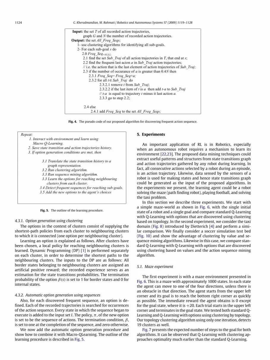
Fig. 4. The pseudo code of our proposed algorithm for discovering frequent action sequence.

Fig. 5. The outline of the learning procedure.

4.3.1. Option generation using clusteringThe options in the context of clusters consist of supplying the

shortest-path policies from each cluster to neighbouring clustersto which it is connected (one option per neighbouring cluster).Learning an option is explained as follows. After clusters have

been chosen, a local policy for reaching neighbouring clusters islearned. Dynamic Programming (DP) [1] is performed separatelyon each cluster, in order to determine the shortest paths to theneighbouring clusters. The inputs to the DP are as follows: Allborder states belonging to neighbouring clusters are assigned anartificial positive reward; the recorded experience serves as anestimation for the state transitions probabilities. The terminationprobability of the option β(s) is set to 1 for border states and 0 forinternal states.

4.3.2. Automatic option generation using sequencesAlso, for each discovered frequent sequence, an option is de-

fined. Each of the recorded trajectories is searched for occurrencesof the action sequence. Every state in which the sequence began toexecute is added to the input set I . The policy, π , of the new optionis set to be the sequence of actions. The termination condition, β ,is set to one at the completion of the sequence, and zero otherwise.We now add the automatic option generation procedure and

show how to combine it with Macro-QLearning. The outline of thelearning procedure is described in Fig. 5.

5. Experiments

An important application of RL is in Robotics, especiallywhen an autonomous robot requires a mechanism to learn itsenvironment [22,23]. The proposed data mining techniques couldextract useful patterns and structures from state transitions graphand action trajectories gathered by any robot during learning. Infact, all consecutive actions selected by a robot during an episode,is an action trajectory. Likewise, data sensed by the sensors of arobot is used for making states and hence state transitions graphcould be generated as the input of the proposed algorithms. Inthe experiments we present, the learning agent could be a robotsolving the maze (path finding robot), playing football, and solvingthe taxi problem.In this section we describe three experiments. We start with

a simple maze-world as shown in Fig. 6, with the single initialstate of a robot and a single goal and compare standard Q-Learningwith Q-Learning with options that are discovered using clusteringbased on topology. In the second experiment, we consider the taxidomain (Fig. 8) introduced by Dietterich [4] and perform a simi-lar comparison. We finally consider a soccer simulation test bed(Fig. 10) and show the advantage of clustering by value and se-quencemining algorithms. Likewise in this case, we compare stan-dard Q-Learning with Q-Learning with options that are discoveredusing clustering based on values and the action sequence miningalgorithm.

5.1. Maze experiment

The first experiment is with a maze environment presented inFig. 6. This is a maze with approximately 1000 states. In each statethe agent can move to one of the four directions, unless there isan obstacle in that direction. The agent starts from the upper leftcorner and its goal is to reach the bottom right corner as quicklyas possible. The immediate reward the agent obtains is 0 exceptfor the goal state, where it is+20. Each trial starts in the upper leftcorner and terminates in the goal state.We tested both standardQ-Learning andQ-Learningwith options using clustering by topology.Our topology clustering algorithm using only one iteration, detects19 clusters as well.Fig. 7 presents the expected number of steps to the goal for both

algorithms. It can be observed that Q-Learning with clustering ap-proaches optimality much earlier than the standard Q-Learning.


Fig. 6. The simple maze containing 19 rooms and a single goal. The goal is markedas ‘‘G’’ in the bottom right corner. The initial state ismarked ‘‘S’’ in the top left corner.The optimal policy is shown using arrows.

Fig. 7. Comparison of the Q learning and Q learning with clustering approaches forsolving the maze of Fig. 6. The comparison has been made with respect to the stepsneeded to transit from ‘S’ to ‘G’ state.

5.2. Taxi experiment

The taxi task has been a popular illustrative problem for RLalgorithms since its introduction by Dietterich [4]. The task isto pick-up and deliver a passenger to him/her destination on a5 × 5 grid depicted in Fig. 8. There are four possible source anddestination marked by actions for the passenger: the grid squaresmarked by R, G, B, Y. The source and destination are randomly andindependently chosen in each episode. The initial location of thetaxi is one of the 25 grid squares, picked uniformly random. Ateach grid location, the taxi has a total of six primitive actions: north,east, south, west, pick-up, put-down. The navigation actions succeedin moving the taxi in the intended direction with probability0.8; the action takes the taxi to the right or left of the intendeddirection with a probability of 0.2. If the direction of movementis blocked, the taxi remains in the same location. The action pick-up places the passenger in the taxi if the taxi is at the same gridlocation as the passenger; otherwise it has no effect. Similarly,put-down delivers the passenger if the passenger is inside the taxiand the taxi is at the destination; otherwise it has no effect. Thereward is −1 for each action, an additional +20 for passengerdelivery and an additional−10 for an unsuccessful pick-up or put-down action. We tested both standard Q-Learning and Q-Learningwith options using clustering by topology. Sub-goals detected byour topology clustering algorithm correspond to arriving at thepassenger location or picking up the passenger and grid squares

Fig. 8. The taxi task domain.

Fig. 9. Comparison of the Q learning and Q learning with clustering approaches forsolving the taxi task. The number of steps to reach goal for both algorithm is shown.

(2, 3) and (3, 3), the main navigational bottlenecks in the domain.Fig. 9 shows the number of steps required to reach the goal statefor both algorithms. As illustrated in Fig. 9, Q-Learningwith optionsshows an early improvement in performance in comparison withQ-learning.

5.3. Soccer test-bed

The soccer simulation environment (Fig. 10) is a 6×9 grid withtwo players. At each time step the ball is owned by a player andwhen the player is moved, the ball is also moved along with theplayer. Each player has five primitive actions: Move-Left, Move-Right, Move-Up, Move-Down and Hold and at each time step, theplayer must select an action. The Hold action causes an agent toremain in its locations without movement.If the direction of movement is blocked, the player remains

in the same location. In this game, each learning agent aims atdefeating the opponent with more scored goals. To score a goal,each player owning the ball must reach to the opponent goal andselect the Move-Right action. When a player scores a goal, theopponent owns the ball and two players are placed at specifiedlocation in front of their goal.When two players encounteringwithdifferent choices of actions, which lead to the situation that theplayers must be placed in the same location, new positions of theplayers and owning of the ball are determined by following rules:- If the player owning the ball is not moving and the other playeris going to enter the fixed player location, then with probabilityof 0.8 the owning of the ball does not change and the locationsof the players remain unchanged.- If the player owning the ball is going to enter the location of theotherwith nomoving player, then owning of the ball is changedand the locations of the players remain unchanged.- If none of the player is not moving, with probability of 0.5 eachplayer owns the ball and is located in the intended position andthe location of the other player remains unchanged.


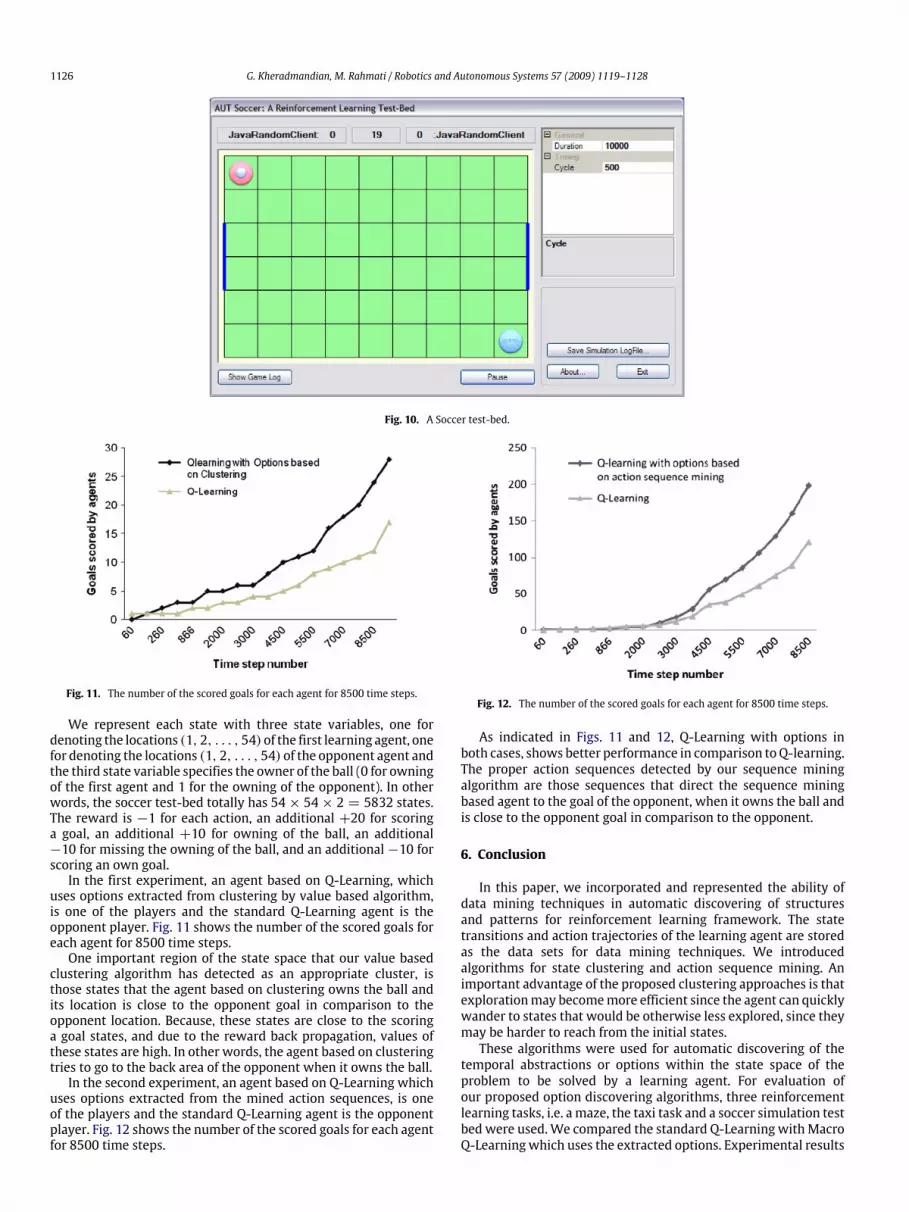
Fig. 10. A Soccer test-bed.

Fig. 11. The number of the scored goals for each agent for 8500 time steps.

We represent each state with three state variables, one fordenoting the locations (1, 2, . . . , 54)of the first learning agent, onefor denoting the locations (1, 2, . . . , 54) of the opponent agent andthe third state variable specifies the owner of the ball (0 for owningof the first agent and 1 for the owning of the opponent). In otherwords, the soccer test-bed totally has 54× 54× 2 = 5832 states.The reward is −1 for each action, an additional +20 for scoringa goal, an additional +10 for owning of the ball, an additional−10 for missing the owning of the ball, and an additional−10 forscoring an own goal.In the first experiment, an agent based on Q-Learning, which

uses options extracted from clustering by value based algorithm,is one of the players and the standard Q-Learning agent is theopponent player. Fig. 11 shows the number of the scored goals foreach agent for 8500 time steps.One important region of the state space that our value based

clustering algorithm has detected as an appropriate cluster, isthose states that the agent based on clustering owns the ball andits location is close to the opponent goal in comparison to theopponent location. Because, these states are close to the scoringa goal states, and due to the reward back propagation, values ofthese states are high. In other words, the agent based on clusteringtries to go to the back area of the opponent when it owns the ball.In the second experiment, an agent based on Q-Learning which

uses options extracted from the mined action sequences, is oneof the players and the standard Q-Learning agent is the opponentplayer. Fig. 12 shows the number of the scored goals for each agentfor 8500 time steps.

Fig. 12. The number of the scored goals for each agent for 8500 time steps.

As indicated in Figs. 11 and 12, Q-Learning with options inboth cases, shows better performance in comparison toQ-learning.The proper action sequences detected by our sequence miningalgorithm are those sequences that direct the sequence miningbased agent to the goal of the opponent, when it owns the ball andis close to the opponent goal in comparison to the opponent.

6. Conclusion

In this paper, we incorporated and represented the ability ofdata mining techniques in automatic discovering of structuresand patterns for reinforcement learning framework. The statetransitions and action trajectories of the learning agent are storedas the data sets for data mining techniques. We introducedalgorithms for state clustering and action sequence mining. Animportant advantage of the proposed clustering approaches is thatexplorationmay becomemore efficient since the agent can quicklywander to states that would be otherwise less explored, since theymay be harder to reach from the initial states.These algorithms were used for automatic discovering of the

temporal abstractions or options within the state space of theproblem to be solved by a learning agent. For evaluation ofour proposed option discovering algorithms, three reinforcementlearning tasks, i.e. a maze, the taxi task and a soccer simulation testbed were used.We compared the standard Q-Learning withMacroQ-Learningwhich uses the extracted options. Experimental results


0

5

10

15

20

25

freq

uen

cy

0.2 0.3 0.4 0.5 0.6 0.7 0.8

distance

0.1 0.90.2 0.3 0.4 0.5 0.6 0.7 0.80.10 0.9 1

0.2

0.3

0.4

0.5

0.6

0.7

0.8

0.1

0

0.9

1a b

Fig. A.1. (a) A typical cluster. (b) Fitted exponential distribution for the dataset in (a).

indicate that the Macro Q-Learning reaches early improvementin performance in comparison to Q-learning. In addition, ourclustering algorithms and the action sequence mining algorithmare fast algorithms in comparison to other similar works.

Appendix. Theoretical justification

The theoretical justification for our proposed merging criterionis based on the characteristic of clusters. In our various experi-ments, we realized that, if the distance between each element ofa cluster and its nearest neighbour is obtained and the histogramof these distances is evaluated, then, plotting these distances typ-ically exhibit an exponential distribution. Fig. A.1 plots the his-togram and corresponding fitted distribution for a sample data set.As shown in Fig. A.1, the statistical distribution of the nearest

neighbour distances within a context has a decaying function.Theoretical analysis of the exponential distribution leads to aninteresting result. An exponential distribution is represented as:

p(x) = βe−βx, x > 0, (A.1)

where, x is the distance between neighbouring patterns.A random variable, X , with exponential distribution, has mean

value E {X} = x̄ = 1β. The slope of the distribution at points which

are multiple of the mean, x = kx̄ = kβ, are found by:

dp(x)dx

∣∣∣∣x= k

β

= −β2e−βkβ = −β2ek. (A.2)

The equation of a tangential line at any one of these points is givenby:

y = −β2ekx+ y0. (A.3)

Since y = p(x = kβ) = βe−k, then Eq. (3) may be written as

βe−k = −β2ekkβ+ y0, (A.4)

simplifying this equation, y0 is obtained, which is:

y0 = βe−k(k+ 1). (A.5)

The crossing point of this tangential line with the x-axis, which isdenoted by x0 can be found by:

y = 0⇒ 0 = −β2e−kx0 + βe−k(k+ 1),

or,

βe−k(k+ 1− βx0) = 0.

Solving for x0 then,

x0 =k+ 1β= (k+ 1)x̄. (A.6)

This implies that, the crossing of the tangential line, at pointswhicharemultiples of the distribution’smean value, k× 1

β, with x-axis are

given by (k+1)× 1β. In otherwords, points such as 2× 1

β, 3× 1

βand

4× 1βmust be very close to the end of the tail of the distribution;

because the tangential lines at these points are nearly parallel withthe x-axis and they cross the x-axis at a very far point, near theend of the tail of the distribution. Since, tail of the distributioncorresponds to the patterns lying in the border of a cluster, wemay conclude that, for those patterns that lie at the boundary ofa cluster (with quantity equals toµ), the distance between each ofthese patterns and their nearest neighbor pair, is more likely to begreater than 2× 1

βand 3× 1

β.

As mentioned before, the histogram of the nearest neighbourdistances for a cluster, exhibits an exponential distribution withmean value 1

β. Since, the quantity, µ, is the average of the nearest

neighbor distances, therefore, µ ≈ 1β. So, for those patterns that

lie at the boundary of a cluster (with quantity equals to µ), thedistance between each of these patterns and their nearest neighborpair, is more likely to be greater than 2 × µ and 3 × µ. In fact,through various experiments, we realized that a value of 2 is a goodchoice for coefficient of µ.The essence of our proposed clustering criterion is explained

based on this context. Let two clusters Ci (with quantity of µi) andCj (with quantity of µj) assumed to be as well separated clusters.For the boundary patterns of cluster Ci, the distance between thosepatterns and their nearest neighbors belonging to theCi, are greaterthen 2µi. In addition, all members of the cluster Cj are consideredas far boundary patterns of cluster Ci, so, the distance betweeneach of the members of the Cj and their nearest neighbors pairbelonging to the Ci, must be greater than 2µi. Also, the distanceof these two clusters, d(Ci, Cj), is the distance between a memberof Cj and its nearest neighbor pair belonging to the Ci. Hence thedistance between clusters is:

d(Ci, Cj) > 2µi. (A.7)

Similarly, the same reasoning may be extended to Cj and thedistance between the clusters should also satisfies:

d(Ci, Cj) > 2µj. (A.8)

From inequities (A.7) and (A.8), it implies that for two wellseparated clusters Ci and Cj, their distance should satisfy thefollowing.

d(Ci, Cj) > min{2µi, 2µj

}. (A.9)


Therefore we use this concept to merge two clusters. Otherwise,two clusters Ci and Cj, are merged if following inequality issatisfied.

d(Ci, Cj) < min{2µi, 2µj

}. (A.10)

References

[1] R. Sutton, A. Barto, Introduction to Reinforcement Learning, MIT Press,Cambridge, 1998.

[2] L.P. Kaelbling, M.L. Littman, A.W. Moore, Reinforcement learning: A survey,Journal of Artificial Intelligence Research 4 (1996) 237–285.

[3] A. Barto, S. Mahadevan, Recent advances in hierarchical reinforcementlearning, Discrete Event Systems Journal 13 (2003) 41–77.

[4] T. Dietterich, Hierarchical reinforcement learning with the MAXQ valuefunction decomposition, Journal of Artificial Intelligence Research 3 (2000)227–303.

[5] R. Sutton, D. Precup, S. Singh, Between MDPs and Semi-MDPs: A frameworkfor temporal abstraction in reinforcement learning, Artificial Intelligence 112(1999) 181–211.

[6] Amy E. McGovern, Autonomous discovery of temporal abstraction frominteraction with an environment, Ph.D. Thesis, University of Massachusetts,Amherst, MA 2002.

[7] Bruce L. Digney, Learning hierarchical control structures formultiple tasks andchanging environments, in: Proceedings of the Fifth International Conferenceon Simulation of Adaptive Behaviour, 1998.

[8] Ishai Menache, Shie Mannor, Nahum Shimkin, Q-Cut: Dynamic Discovery ofSub-Goals in Reinforcement Learning, in: Lecture Notes in Computer Science,vol. 24, Springer, 2002.

[9] O. Simsek, A. Barto, Using relative novelty to identify useful temporalabstractions in reinforcement learning, in: Proceedings of the InternationalConferenceon Machine Learning, vol. 21, 2004, pp. 751–758.

[10] S.Mannor, I. Menache, A. Hoze, U. Klein, Dynamic abstraction in reinforcementlearning via clustering, in: Proceedings of the International Conference onMachine Learning, vol. 21, 2004, pp. 560–567.

[11] O. Simsek, A. Wolfe, A. Barto, Identifying useful sub-goals in reinforcementlearning by local graph partitioning, in: Proceedings of the InternationalConference on Machine Learning, 2005.

[12] Hengst Bernhard, Discovering hierarchy in reinforcement learning, Ph.D.Thesis, University of New South Wales, Australia, 2004.

[13] Jonsson Anders, A causal approach to hierarchical decomposition in reinforce-ment learning, Ph.D. Thesis, University of Massachusetts Amherst, 2006.

[14] R. Parr, S. Russell, Reinforcement learning with hierarchies of machines,Advances in Neural Information Processing Systems 10 (1998) 1043–1049.

[15] S. Thrun, A. Schwartz, Finding structure in reinforcement learning,in: Advances in Neural Information Processing Systems, MIT Press, 1995,pp. 385–392.

[16] M. Pickett, A.G. Barto, PolicyBlocks: An algorithm for creating usefulmacro-actions in reinforcement learning, in: Proceedings of the NineteenthInternational Conference on Machine Learning 2002, pp. 506–513.

[17] I. Menache, S. Mannor, N. Shimkin, Q-Cut-Dynamic discovery of sub-goalsin reinforcement learning, in: Proceedings of the Thirteenth EuropeanConference on Machine Learning, Springer, 2002, pp. 295–306.

[18] Amy McGovern, Richard S. Sutton, Macro-actions in reinforcement learning:An empirical analysis, Technical Report, University ofMassachusetts, Amherst,1998.

[19] P. Dayan, C. Watkins, Q-learning, Machine Learning 8 (1992) 279–292.[20] Jiawei Han, Micheline Kamber, Data Mining: Concepts and Techniques,

Morgan Kaufmann Publishers, 2000.[21] Bart Goethals, Survey on frequent pattern mining, HIIT Basic Research unit,

University of Helsinki, Finland.[22] K.H. Park, Y.J. Kim, J.H. Kim, Modular Q-learning based multi-agent coopera-

tion for robot soccer, Robotics and Autonomous Systems 35 (2001) 109–122.[23] M.A.S. Kamal, Junichi Murata, Reinforcement learning for problems with

symmetrical restricted states, Robotics and Autonomous Systems 56 (9) (30September 2008) 717–727.

Gorban Kheradmandian received the Bachelor of Sciencein Computer Engineering from the Isfahan University,Iran in 2000 and the M.Sc. In Computer Engineeringfrom the Amir Kabir University of Technology (TehranPolytechnic), Iran in 2002. Currently, he is a Ph.D.Candidate in the Computer Engineering Department atAmir Kabir University of Technology (Tehran Polytechnic).His research interests include: Reinforcement Learning,Data Mining and Pattern recognition.

Mohammad Rahmati received the M.Sc. in Electrical En-gineering from the University of NewOrleans, USA in 1997and the Ph.D. degree in Electrical and Computer Engineer-ing from University of Kentucky, Lexington, KY USA in2003.Currently, he is a assistant professor in the Com-

puter Engineering Department at Amir Kabir Universityof Technology (Tehran Polytechnic). His research interestsinclude: Pattern recognition, Image Processing, Bioinfor-matics, video processing, and Data Mining.

automatic abstraction in reinforcement learning using data mining techniques

Documents