audio-visual event recognition with graphical models
TRANSCRIPT

TECHNISCHE UNIVERSITAT MUNCHENLehrstuhl fur Mensch-Maschine-Kommunikation
Audio-Visual Event Recognition
with Graphical Models
Benedikt Hornler
Vollstandiger Abdruck der von der Fakultat fur Elektrotechnik und Informationstechnikder Technischen Universitat Munchen zur Erlangung des akademischen Grades eines
Doktor-Ingenieurs (Dr.-Ing.)
genehmigten Dissertation.
Vorsitzender: Univ.-Prof. Dr.-Ing. K. Diepold
Prufer der Dissertation: 1. Univ.-Prof. Dr.-Ing. habil. G. Rigoll
2. Univ.-Prof. Dr.rer.nat. M. Kranz
Die Dissertation wurde am 15.09.2010 bei der Technischen Universitat Munchen einge-reicht und durch die Fakultat fur Elektrotechnik und Informationstechnik am 10.12.2010angenommen.

Abstract
In this work, different applications for the automated detection of events have beeninvestigated utilizing audio-visual pattern recognition methods. The recorded datahas been taken both from video surveillance or video conferences. Acoustic, visualand semantic features are extracted from the available data and are subsequentlyanalysed with the help of graphical models. These are particularly suitable formodeling multi-modal feature sequences and provide an efficient way for automaticfeature fusion. All models are first described in detail theoretically and then thenecessary structure for both the learning of required parameters and the classificationprocess are presented. Finally a conclusion is drawn by describing the results andfurther possible research approaches. Graphical models are suitable for these tasks,but the results are strongly depending on the kind of problem.
i

Zusammenfassung
In dieser Arbeit wurden unterschiedliche Aufgabenstellungen zur Erkennung vonEvents in Aufzeichnungen aus Videouberwachung oder Videokonferenzen mit Hilfevon audio-visuellen Mustererkennungsverfahren analysiert. Aus den vorliegendenDaten werden hierfur akustische, visuelle und semantische Merkmale extrahiert undmit Hilfe von Graphischen Modellen verarbeitet. Diese eignen sich besonders furdie Modellierung von multimodalen Merkmalssequenzen und bieten eine effizienteMoglichkeit fur die automatische Datenfusion. Alle Modelle werden zunachst aus-fuhrlich theoretisch beschrieben und anschließend werden die notwendigen Struk-turen fur das Lernen der benotigten Parameter und die Erkennung dargestellt. Ab-schließend werden die Ergebnisse und weitere mogliche Forschungsansatze prasen-tiert. Graphische Modelle eignen sich fur die vorliegende Aufgabenstellung, allerd-ings hangen die Ergebnisse relativ stark von der Art der Aufgabe ab.
iii

Contents
1 Introduction 1
2 The Used Data Sets 5
2.1 Meeting corpus . . . . . . . . . . . . . . . . . . . . . . . . . . . . . . 5
2.1.1 Audio recordings . . . . . . . . . . . . . . . . . . . . . . . . . 6
2.1.2 Video recordings . . . . . . . . . . . . . . . . . . . . . . . . . 7
2.1.3 Annotation . . . . . . . . . . . . . . . . . . . . . . . . . . . . 7
2.2 Surveillance corpus . . . . . . . . . . . . . . . . . . . . . . . . . . . . 13
2.3 Interest Corpus . . . . . . . . . . . . . . . . . . . . . . . . . . . . . . 14
2.3.1 Annotation . . . . . . . . . . . . . . . . . . . . . . . . . . . . 15
3 Feature Extraction and Preprocessing 19
3.1 Acoustic features . . . . . . . . . . . . . . . . . . . . . . . . . . . . . 19
3.2 Visual features . . . . . . . . . . . . . . . . . . . . . . . . . . . . . . 22
3.2.1 Skin blobs . . . . . . . . . . . . . . . . . . . . . . . . . . . . . 22
3.2.2 Global Motion Features . . . . . . . . . . . . . . . . . . . . . 23
3.2.3 Selected Regions of Interest . . . . . . . . . . . . . . . . . . . 25
3.3 Semantic features . . . . . . . . . . . . . . . . . . . . . . . . . . . . . 27
3.3.1 Group Actions . . . . . . . . . . . . . . . . . . . . . . . . . . 27
3.3.2 Person Actions . . . . . . . . . . . . . . . . . . . . . . . . . . 28
3.3.3 Person Speaking . . . . . . . . . . . . . . . . . . . . . . . . . 29
3.3.4 Person Movements . . . . . . . . . . . . . . . . . . . . . . . . 29
3.3.5 Slide Changes . . . . . . . . . . . . . . . . . . . . . . . . . . . 29
3.4 Preprocessing of the Extracted Features . . . . . . . . . . . . . . . . 30
3.4.1 Feature Normalisation . . . . . . . . . . . . . . . . . . . . . . 30
3.4.2 Reduction of the Feature Dimension . . . . . . . . . . . . . . 30
v
Contents
4 Graphical Model 37
4.1 Nomenclature . . . . . . . . . . . . . . . . . . . . . . . . . . . . . . . 38
4.2 Bayesian Networks . . . . . . . . . . . . . . . . . . . . . . . . . . . . 39
4.3 Efficient Calculations of Graphical Models . . . . . . . . . . . . . . . 40
4.4 Training of Bayesian Networks . . . . . . . . . . . . . . . . . . . . . . 41
4.4.1 EM-Training for Bayesian Networks . . . . . . . . . . . . . . . 42
4.4.2 Training Structure . . . . . . . . . . . . . . . . . . . . . . . . 43
4.5 Decoding of Graphical Models . . . . . . . . . . . . . . . . . . . . . . 49
4.6 Evaluation of the Different Model Structures . . . . . . . . . . . . . . 51
5 Multi-modal Surveillance 53
5.1 The Recognition Process . . . . . . . . . . . . . . . . . . . . . . . . . 55
5.2 Used Graphical Models . . . . . . . . . . . . . . . . . . . . . . . . . . 56
5.2.1 Single Stream Classifying Graphical Model (GM1) . . . . . . . 56
5.2.2 Single Stream Segmenting Graphical Model (GM2) . . . . . . 63
5.2.3 Multi Stream Classifying Graphical Model (GM3) . . . . . . . 66
5.2.4 Hierarchical Graphical Model (GM4) . . . . . . . . . . . . . . 68
5.3 Comparison of the Results . . . . . . . . . . . . . . . . . . . . . . . . 75
5.4 Comparison with other Approaches . . . . . . . . . . . . . . . . . . . 78
5.5 Outlook . . . . . . . . . . . . . . . . . . . . . . . . . . . . . . . . . . 79
6 Automatic Video Editing in Meetings 81
6.1 Related Work . . . . . . . . . . . . . . . . . . . . . . . . . . . . . . . 82
6.2 The Video Editing System . . . . . . . . . . . . . . . . . . . . . . . . 85
6.3 Used Graphical Models . . . . . . . . . . . . . . . . . . . . . . . . . . 85
6.3.1 Single Stream Segmenting Graphical Model (GM1) . . . . . . 87
6.3.2 Multi Stream Segmenting Graphical Model (GM2) . . . . . . 90
6.3.3 Two Layer Graphical Model (GM3) . . . . . . . . . . . . . . . 92
6.3.4 Video Editing with Eight Video Modes . . . . . . . . . . . . . 95
6.4 Comparison of the Results . . . . . . . . . . . . . . . . . . . . . . . . 96
6.5 Outlook . . . . . . . . . . . . . . . . . . . . . . . . . . . . . . . . . . 97
7 Activity Detection in Meetings 99
7.1 Related Work . . . . . . . . . . . . . . . . . . . . . . . . . . . . . . . 100
7.2 The Activity Detection System . . . . . . . . . . . . . . . . . . . . . 101
7.3 Used Graphical Models . . . . . . . . . . . . . . . . . . . . . . . . . . 102
7.3.1 Single Stream Segmenting Graphical Model (GM1) . . . . . . 102
7.3.2 Multi Stream Segmenting Graphical Model (GM2) . . . . . . 106
7.3.3 Two Layer Multi Stream Graphical Model (GM3) . . . . . . . 107
7.4 Comparison of the Results . . . . . . . . . . . . . . . . . . . . . . . . 108
7.5 Outlook . . . . . . . . . . . . . . . . . . . . . . . . . . . . . . . . . . 109
vi
Contents
8 Multi-modal Interest Detection 1118.1 Related Work . . . . . . . . . . . . . . . . . . . . . . . . . . . . . . . 1128.2 The Dialogue Control System . . . . . . . . . . . . . . . . . . . . . . 1138.3 Used Models . . . . . . . . . . . . . . . . . . . . . . . . . . . . . . . . 114
8.3.1 Support Vector Machines . . . . . . . . . . . . . . . . . . . . . 1148.3.2 Graphical Model Structure . . . . . . . . . . . . . . . . . . . . 115
8.4 Comparison of the Results . . . . . . . . . . . . . . . . . . . . . . . . 1178.5 Outlook . . . . . . . . . . . . . . . . . . . . . . . . . . . . . . . . . . 118
9 Summary 1199.1 Conclusion . . . . . . . . . . . . . . . . . . . . . . . . . . . . . . . . . 1219.2 Outlook . . . . . . . . . . . . . . . . . . . . . . . . . . . . . . . . . . 122
A Used Measures 123A.1 Recognition Accuracy Rate . . . . . . . . . . . . . . . . . . . . . . . 123A.2 F-Measure . . . . . . . . . . . . . . . . . . . . . . . . . . . . . . . . . 123A.3 Frame Error Rate . . . . . . . . . . . . . . . . . . . . . . . . . . . . . 124A.4 Action Error Rate . . . . . . . . . . . . . . . . . . . . . . . . . . . . . 124
Acronyms 125
List of Symbols 127
References 131
vii

1
Introduction
Many unsolved problems exist in real applications in the field of information process-ing. For some of them it is possible to find a description which can be transformedinto a pattern recognition problem. Here, modern and popular pattern recognitionmethods, as for example support vector machines or graphical models, can be ap-plied to solve the problem or at least come up with a solution which is useful forthe mankind. These solutions help people by running their daily business moreefficiently, for example observing public areas or selling something.
In this thesis, graphical models (GM) are used to come up with solutions. A GMdescribes a complex problem very intuitively [Bil06] and to calculate the outcome ofthe model often less computational effort is needed, as when the complex problem issolved directly [JLO90]. Moreover, a GM is adapted to the problem and not the otherway around, as it happens with many other approaches, for example support vectormachines, where no adaptation is possible. For this reasons, GMs are commonlyused for the description of problems and for rapid-prototyping of solutions.
A GM, as it is used in this thesis, consists of vertices and directed edges. A di-rected edge describes a relation between two vertices. Many algorithms are describedin the graph theory [BM76], which for example shows if two vertices are dependingon each other or if exchanging of information between two sub graphs is possible.All these allow fast and efficient calculations performed on the graphs. Since thevertices and edges in a GM applied to pattern recognition problems describe randomvariables and dependences between them, not only the graph theory is important,but also the probability theory [Jor01]. Therefore, GMs are a combination of graph-and probability theory with benefits from both sides. Easy calculations are per-formed directly via probability theory, but if it is getting more complex the graphtheory is used to reduce the complexity first. As mentioned above it often happensthat the calculations are getting more efficient, if they are performed on the graphthan direct calculation of the probability.
GMs are applied in three different domains in this thesis: surveillance, meetinganalysis and interest detection. The surveillance scenario contains a setting, where
1
1. Introduction
passengers of an aircraft are analysed, if they are acting normal or suspicious. Forthe meeting analysis, two tasks are chosen to evaluate: automatic video editing andactivity recognition. Activity recognition detects the activity and dominance of eachparticipant during the meeting. The most relevant view of the ongoing meeting isautomatically selected by the video editing system. The interest detection scenariois about the interaction of a subject with an intelligent machine. This machinerecognises the level of interest and accordingly selects the topic.
All the described problems have access to multi-modal recordings of the scenarios,therefore it is only the consequent next step to evaluate multi-modal features for allapproaches. Most GMs developed and evaluated are using multi-modal feature as aninput, but some do not. They are used to see if an improvement of the performanceexists between single- and multi-modality. The use of different modalities at thesame time has shown its performance in various works in the field of human-machine-communication [KPI04, PR03, CDCT+01]. Furthermore, the robustness and relia-bility of the models are improved by multi-modal data [PR03, SAR+07, WSA+08].
Starting with the results of the analysis of the chosen domains, it has beenpossible to formulate pattern recognition problems. Various graphical models havebeen developed theoretically and the needed equations for the calculations havebeen derived to solve these problems. Afterwards, the models have been trainedand evaluated on different data sets. In the following paragraphs, an outline of thechapters which are presented is given:
Chapter 2 describes all the used data sets. It contains a data set recorded at theTechnische Universitat Munchen (TUM) which simulates an aircraft scenario.In this setting, the behaviour of passengers is analysed, which means the cur-rent status in terms of aggressiveness and threat is detected. The second dataset is from the AMI project [CAB+06] and contains recorded meetings withfour participants. The last corpus was once again recorded at TUM and isused for the analysis of a dialogue, especially for the emotions of the subject.For all these data sets the annotations are described and statistics about thedistributions of the classes are given.
Chapter 3 presents information about the extracted features from the data sets.The work uses multi-modal features, which are derived from the acoustic, vi-sual and semantic domain. From the acoustic recordings, low level descriptorsand according functionals of short segments are extracted. Two different visualfeatures are derived: skin blobs and global motions. Both are calculated fromall available camera views. Furthermore, the subject’s face is detected andtracked. The last group of features is the semantic information which existsonly for the meeting corpus. It contains data about what the group is doing,what the participants are doing and where they are moving, who is speakingand when a foil is changed during a presentation. Overall more than 3000
2
features are extracted, thus it is necessary to reduce the feature space. This isdone by principal component analysis or sequential forward selection.
Chapter 4 contains a short introduction to graphical models and gives a nomencla-ture for all the models following in all the other chapters. The introduction iskept short and provides a brief overview, as a wide range of books and tutorialsare available which go into more detail. Moreover, all the important modelstructures of the this thesis are described in detail.
Chapter 5 presents a surveillance system which is based on graphical models. Thepassengers of an aircraft are audio-visually captured and the recordings areanalysed. Various model structures are developed and evaluated. It containsmodels which automatically segment the data and hierarchical models whichclassify the features in two steps in order to achieve better results. The chapteris closed with a comparison of the achieved results with performances foundin other works.
Chapter 6 discusses models which can learn segment boundaries from training data.This means, not only the sequence of classes, as it is common for automaticspeech recognition, is learned but the point of time of a class boundary. This isimportant for video editing, since a cut between two perspectives has to takeplace at the correct time frame, otherwise information would be lost or theoutput video is very disturbing for the watcher. Again in the end the resultsare compared and an outlook is given.
Chapter 7 is about the activity and dominance recognition in meetings. For thefirst time, it is evaluated if low level descriptors are applicable for the detectionof activity levels during a meeting. Graphical models are used for the classifi-cation of the low level features, which are capable of segmenting the meetinginto short segments of the same level of activity. Moreover, related work ispresented and the results are compared.
Chapter 8 shows an approach for the combination of support vector machinesand graphical models to perform a detection of the level of interest during ahuman-machine dialogue. Support vector machines are used for a classificationof each frame on feature level. Functionals of the acoustic features used forthat are extracted from a window of 25 frames and therefore should containinformation about the development of a feature, which is very important fora good performance. The performance achieved by this approach is evaluatedagainst previous work and a discussion about it is given.
Overall the work describes and discusses different applications of pattern recog-nition methods in the field of human-machine-communication which can be imple-mented as a graphical model. All the developed models are theoretically analysed
3

1. Introduction
and practically evaluated. Furthermore, different modalities, such as acoustic, vi-sual and semantic, and various types of features are evaluated. For all the problems,related work is presented and the results are discussed.
4
2
The Used Data Sets
In this chapter the three data sets which are used for this thesis are described. Thefirst one is a subset of the AMI corpus, the second is known as the Aircraft BehaviourCorpus and the third is the Audiovisual Interest Corpus.
2.1 Meeting corpus
The meeting data for this work has been collected within the AMI project [CAB+06]and is publicly available1. The recording of the AMI corpus took place in three dif-ferent smart meeting rooms and the total duration of freely available recordings isapproximately 100 hours. The meeting rooms were located at the IDIAP ResearchInstitute in Switzerland, at the University of Edinburgh in Scotland, and at Uni-versity of Twente in the Netherlands. The setting of each room is slightly differentfrom each other but all meetings are discussing the development of a new remotecontrol. Four participants (Per.1 - Per.4) are attending the meeting in a single roomand they are for example discussing, giving presentations, taking notes, or writingon the whiteboard. The same four subjects are participating in four meetings andeach of them has a predefined role, such as being the project manager, the industrialdesigner, the interface designer or the marketing expert. Due to the fact that eachsubject is participating in four meetings and is not attending any other meeting, itis possible to create subject disjoint training- and test-sets for a cross-validation.
In this thesis, a subset of the data form the IDIAP smart meeting room [Moo02] isused. Hence the cameras in this room are mostly facing the faces of the participants.Moreover, the hands are visible as well, thus it is possible to extract information fromthem. In figure 2.1 the schematic of the IDIAP smart meeting room is shown. Theroom is equipped with a table, a whiteboard, a projector with a screen and variousdifferent recording devices. A device captures for example the (x, y)-coordinates andthe pressure from the pen which is used on the whiteboard and four Logitech I/O
1http://www.amiproject.org
5

2. The Used Data Sets
Per. 3
Per. 4Per. 2
Per. 1 Legend:
Microphon Microphon array Cameras Closeup Camera Centre Camera Left/Right
Whiteboard
ProjectorScreen
Recordingdevices
A1A2
BM
Figure 2.1: Schematic of the IDIAP smart meeting room. 22 microphonesand seven cameras are installed. Each participant wears two close-talking micro-phones and additionally two microphone arrays are located in the room. Fourclose-up cameras, a centre camera and one camera at each of the long sides ofthe room are capturing the ongoing meeting.
digital pen devices collect the notes from each participant. In order to create timesynchronized recordings, it is necessary to add timestamps to each captured framein each data stream. Therefore, it is later possible to align all the streams for themulti-modal analysis which is especially necessary for low level feature fusion.
The duration of a meeting in the AMI corpus is between 30 minutes and onehour. The subset used in this thesis consists of 36 five-minute meetings, recorded atthe IDIAP smart meeting room, and contains audio and video streams. Each chunkis taken from different parts of different meetings and is not overlapping, thus thedata is disjoint. In total the subset has a length of 180 minutes.
2.1.1 Audio recordings
The IDIAP smart meeting room, shown in figure 2.1, is equipped with 22 micro-phones. Far field recordings are performed by two microphone arrays and a binauralmanikin. One, containing eight microphones, is placed in the middle of the table(A1) and the second is mounted between the table and the projector screen on theceiling (A2) with four microphones. The binaural manikin (BM) is placed at the endof the table for two further audio recordings by replicating a human head and ears.Furthermore, two different types of close-talking microphones, an omni-directionallapel microphone and a headset condenser microphone, have been worn by every par-ticipant for the recordings. The lapel microphone has been attached to the user’scollar. Only the four headset condenser microphones are used for the feature extrac-tion, which is described in section 3.1 and a mixed signal of them is streamed intothe created output videos.
6
2.1. Meeting corpus
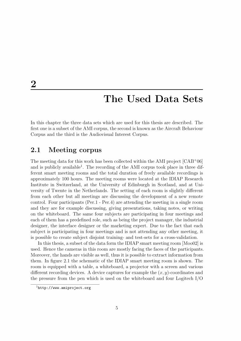
(a) Camera Left (b) Camera Centre (c) Camera Close-up
Figure 2.2: Samples output of three available cameras from the IDIAP smartmeeting room.
2.1.2 Video recordings
Seven cameras are located in the room. Four close-up cameras record the faces ofthe meeting participants, if they are sitting at the table. Two cameras (left resp.right camera) are mounted on each of the sides of the room. They capture the tableand two participants of the opposite side. These cameras can be used for handtracking, because the hands are visible in case the persons are located at the side ofthe table. An overview of the room, which contains the table, the whiteboard, theprojector screen, and all participants, records the centre camera. Figure 2.2 showsthree example views from cameras which have been recorded in one of the meetings.All available camera views are used for the video editing task in section 6. Duringthe activity detection task, described in section 7, features are only extracted fromthe close-up cameras.
2.1.3 Annotation
This subset has been annotated for various applications and pattern recognitiontasks. Some annotations are publicly available with the AMI corpus, for examplethe person movements. These movements describe what the person is doing inconjunction with her location in the smart meeting room. Further annotationshave been conducted through out this work and are described in more detail here.Annotations can be done via tools like ANVIL [Kip01]. In the case of this work, theannotations, which are needed, are performed by applying tools especially createdfor the specific annotation.
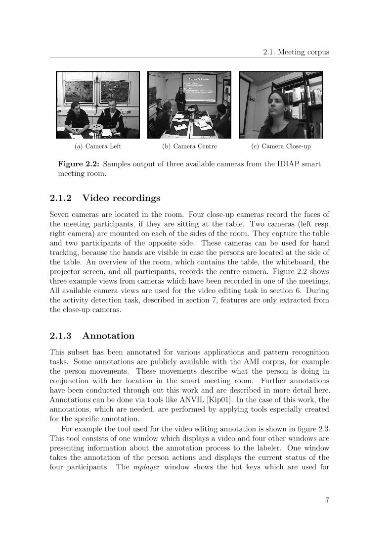
For example the tool used for the video editing annotation is shown in figure 2.3.This tool consists of one window which displays a video and four other windows arepresenting information about the annotation process to the labeler. One windowtakes the annotation of the person actions and displays the current status of thefour participants. The mplayer window shows the hot keys which are used for
7
2. The Used Data Sets
Figure 2.3: A screen shot of the annotation tool which is used during theannotation task for the video editing system. The tool consists of five differentwindows. One which shows a combination of the three cameras centre, left andright. Two windows display information about the mplayer, which is used forplaying the video including the audio recordings, and the available labels forthe annotation. The information window presents the current status for eachof the participants, which is taken from the annotation of the person actions.The last windows displays the information about the position within the videoand the selected video mode.
controlling of the video and audio player. The window with the label keys displaysall available labels for the annotation and the according hot key for selection of thelabel. The last window gives the user feedback about the annotation which hasbeen performed and shows information about the start and end frame of the currentselected label. The tools for the other labeling tasks are similar with some changessince other annotations are used for the information bar or the labels which areavailable are different. The tool is easy to use, since the user only needs to press thebutton according to the label, which should be selected, once an action occurs.
2.1.3.1 Video Editing
For the annotation of the meeting corpus for the video editing task video modesare defined. This is necessary because several views can be projected out of eachavailable camera. A video mode is the selected view for a single frame. This view canbe a camera view, a selected regions of a camera view, an image or a picture, slidesor text in the case a description of somebody or something is needed. Moreover,combinations of cameras or pictures are possible. The video mode is always selected
8

2.1. Meeting corpus
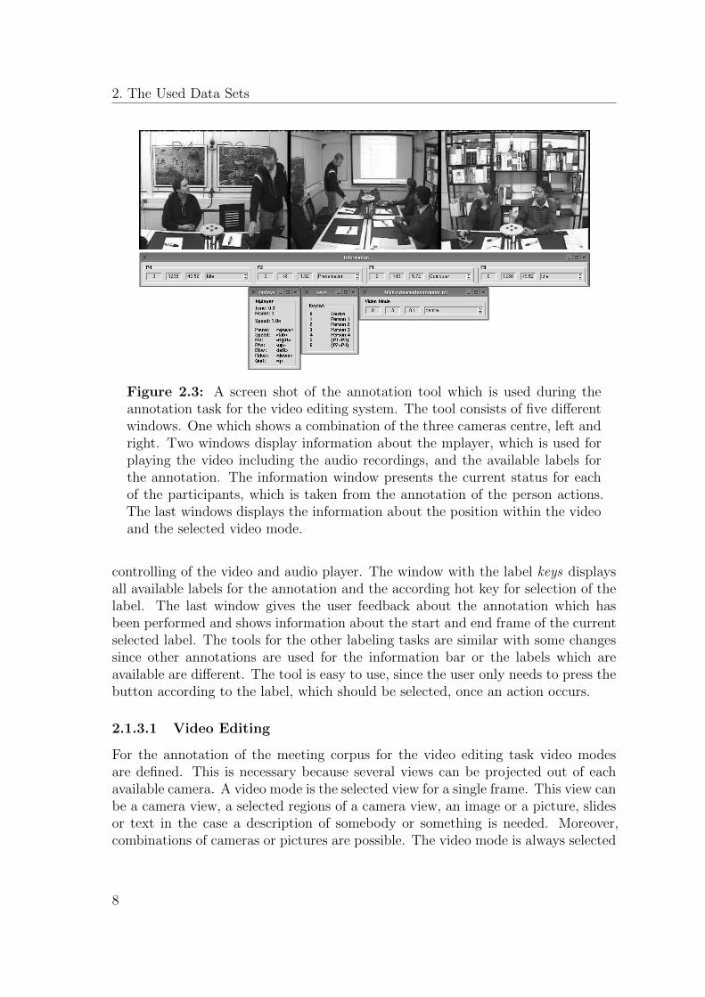
for a single frame and therefore it can be changed each frame. These video modescan be stored to a database for a later browsing of the meeting, or in the case ofa video conference only the stream of the chosen video mode can be transmittedto the remote participants. Restricted to the recordings from the smart meetingroom, the possible definitions of video modes are all available cameras, subregionof camera views, and combinations of cameras and/or subregions. A set of videomodes has been defined, based on the user requirements, the available views andadditional information, which are recorded and stored with the meeting data. Thecurrently used video modes are shown in figure 2.4 and shall be described shortly:
Video modes 1 - 4 show the close-up camera of one of the four participants Person1 - Person 4. These modes are used when a person is talking, shaking itshead or nodding. The modes 1 - 4 are normally used most frequently duringa meeting, because the participants are talking most of the time.
Video mode 5 shows the left camera view and thus Person 1 and Person 3. Thismode is perfectly suitable for a discussion of these two persons or as an addi-tional view if Person 1 or Person 3 are talking for a long time and it is necessaryto switch to a different shot as video mode 1 or 3. This is used for example ifPerson 1 or Person 3 talks for a long time and no other actions are worth tomake a cut of and to show it. It may also be applied if Person 1 or Person 3 aretalking and the other participant on the same side shows a facial expression.Moreover, it shows when Person 1 or Person 3 are pointing at something, arehandling an item such as a prototype of a remote control, or are taking notes.
Video mode 6 presents the right camera and shows Person 2 and Person 4. Thecamera is used in the same way as in video mode 5 and has the same properties.
Video mode 7 shows the total view of the meeting room from the position of thecentre camera. The view contains the projector screen, the whiteboard, thetable, and all four participants. Therefore, this video mode can be applied, forexample for group discussions, showing an item, or the giving a presentation orwriting on the whiteboard. However, the participants are too small in the viewto recognise important facial expressions and often the persons are looking atthe projector screen, thus no face is visible in this perspective.
Video mode 8 inserts a defined image which is annotated into the video outputinstead of a video frame taken from a camera. Therefore, this mode is ideal ifa slide change occurs during a presentation. Furthermore, it is very suitable foradding relevant information at the beginning of a video, such as the recordingdate or names of the participants.
Video mode 9 is a combination of video modes 5 and 6. A predefined region of theleft camera view is shown at the top of a cutout of the right camera, so that
9
2. The Used Data Sets
P1 P1 P3
Slide titleSlide title
Figure 2.4: Different video modes for the video editing system: from left toright video mode 1, 5, 7, 8, and 9 are presented in an abstract way. The modes2 to 4, and 6 are left out because the are similar to 1, respectively to 5.
all participants are shown from the front. Therefore, this mode can be usedfor group discussions, note-taking and group interactions. On the other handthe selecting of predefined regions in the camera streams contains some risk ofcutting out interesting parts of the body, for example head or arms.
Additional video modes can be created very easily. For example, a picture inpicture mode, as known from news shows on several TV-channels, can be added.This mode is one where the speaker is presented in the front and a second person,who is interacting with him, is placed as a small portrait in the upper right corner.It is also possible to create additional video modes similar to video mode 5 or 6 bycombining predefined regions from the close-up cameras from participant Person 1or Person 3 with Person 2 or Person 4, which can be used for a discussion betweento persons seated at opposite sides of the table. A problem with this video modeis, that it causes confusion, because participants are suddenly located next to eachother, which are seated on different sides of the table.
For the pattern recognition approach, which is pursued in this thesis, it is nec-essary to know which video mode should be shown at each frame. Therefore, adata set of three hours has been annotated in order to train pattern recognitionmodels on a training set and to evaluate the results on a predefined test set. Forthe annotation task, a small set of rules has been defined which contains some basicguidelines for creating a good, watchable movie [Bel05]. Most important for a goodvideo is the duration of a shot. Therefore, the rules prevent the annotators fromswitching too fast or too slow. For example the close-up has to be shown for at leasttwo seconds and the longest shot should be no more than 20 seconds. The time isdifferent for each of the video modes, depending on how much information is visiblein the scene. Another important issue is, that an establishing shot should be addedat the beginning of the meeting and when a new scene starts. For example this is thecase if a participant gets up and starts walking to the front to give a presentation.The annotators did not get any information about which camera is preferred for thedifferent situations. Therefore, the degree of freedom for the annotators is ratherhigh which leads to a low inter annotator agreement on the data set, the averageis κ = 0.3, which is a fair agreement [Gwe01]. This result shows that the task ofannotating the video mode is very subjective, because it depends on the own tasteof each annotator. If one annotator does the same meeting twice, with a couple of
10
2.1. Meeting corpus
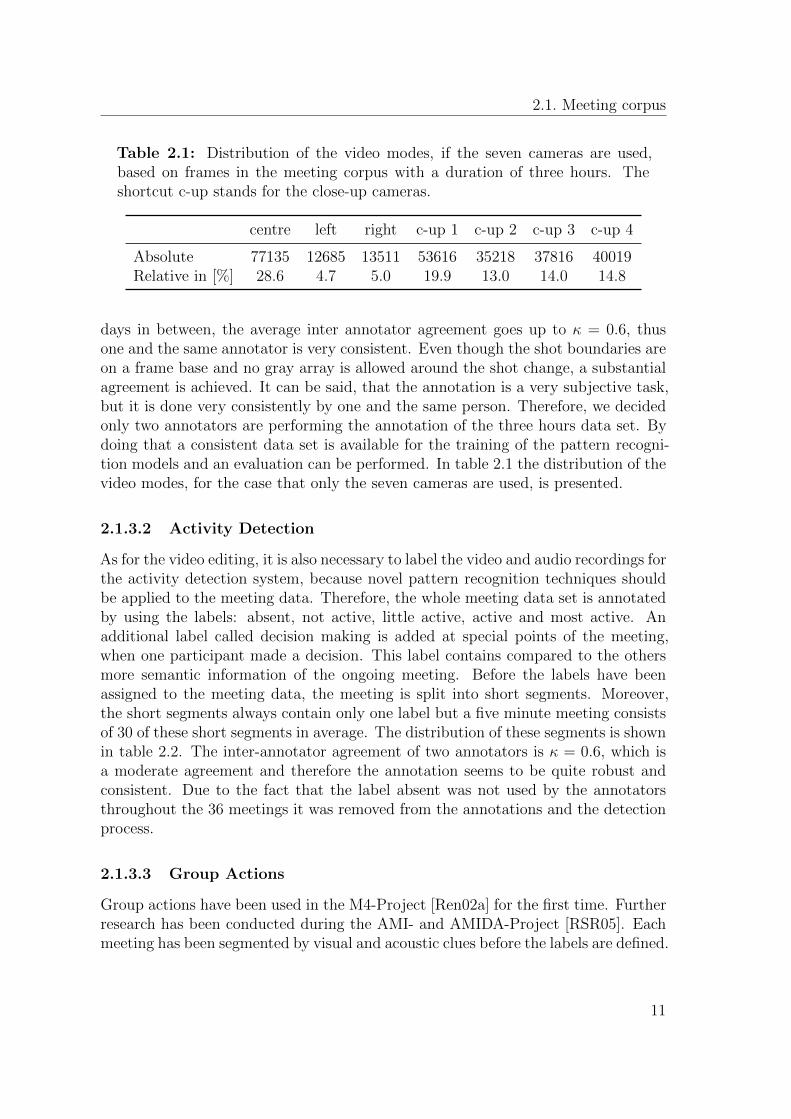
Table 2.1: Distribution of the video modes, if the seven cameras are used,based on frames in the meeting corpus with a duration of three hours. Theshortcut c-up stands for the close-up cameras.
centre left right c-up 1 c-up 2 c-up 3 c-up 4
Absolute 77135 12685 13511 53616 35218 37816 40019Relative in [%] 28.6 4.7 5.0 19.9 13.0 14.0 14.8
days in between, the average inter annotator agreement goes up to κ = 0.6, thusone and the same annotator is very consistent. Even though the shot boundaries areon a frame base and no gray array is allowed around the shot change, a substantialagreement is achieved. It can be said, that the annotation is a very subjective task,but it is done very consistently by one and the same person. Therefore, we decidedonly two annotators are performing the annotation of the three hours data set. Bydoing that a consistent data set is available for the training of the pattern recogni-tion models and an evaluation can be performed. In table 2.1 the distribution of thevideo modes, for the case that only the seven cameras are used, is presented.
2.1.3.2 Activity Detection
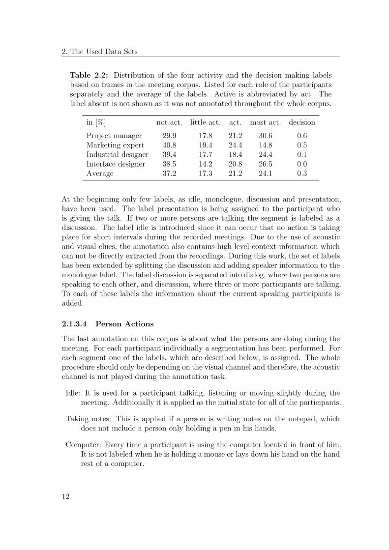
As for the video editing, it is also necessary to label the video and audio recordings forthe activity detection system, because novel pattern recognition techniques shouldbe applied to the meeting data. Therefore, the whole meeting data set is annotatedby using the labels: absent, not active, little active, active and most active. Anadditional label called decision making is added at special points of the meeting,when one participant made a decision. This label contains compared to the othersmore semantic information of the ongoing meeting. Before the labels have beenassigned to the meeting data, the meeting is split into short segments. Moreover,the short segments always contain only one label but a five minute meeting consistsof 30 of these short segments in average. The distribution of these segments is shownin table 2.2. The inter-annotator agreement of two annotators is κ = 0.6, which isa moderate agreement and therefore the annotation seems to be quite robust andconsistent. Due to the fact that the label absent was not used by the annotatorsthroughout the 36 meetings it was removed from the annotations and the detectionprocess.
2.1.3.3 Group Actions
Group actions have been used in the M4-Project [Ren02a] for the first time. Furtherresearch has been conducted during the AMI- and AMIDA-Project [RSR05]. Eachmeeting has been segmented by visual and acoustic clues before the labels are defined.
11
2. The Used Data Sets
Table 2.2: Distribution of the four activity and the decision making labelsbased on frames in the meeting corpus. Listed for each role of the participantsseparately and the average of the labels. Active is abbreviated by act. Thelabel absent is not shown as it was not annotated throughout the whole corpus.
in [%] not act. little act. act. most act. decision
Project manager 29.9 17.8 21.2 30.6 0.6Marketing expert 40.8 19.4 24.4 14.8 0.5Industrial designer 39.4 17.7 18.4 24.4 0.1Interface designer 38.5 14.2 20.8 26.5 0.0Average 37.2 17.3 21.2 24.1 0.3
At the beginning only few labels, as idle, monologue, discussion and presentation,have been used. The label presentation is being assigned to the participant whois giving the talk. If two or more persons are talking the segment is labeled as adiscussion. The label idle is introduced since it can occur that no action is takingplace for short intervals during the recorded meetings. Due to the use of acousticand visual clues, the annotation also contains high level context information whichcan not be directly extracted from the recordings. During this work, the set of labelshas been extended by splitting the discussion and adding speaker information to themonologue label. The label discussion is separated into dialog, where two persons arespeaking to each other, and discussion, where three or more participants are talking.To each of these labels the information about the current speaking participants isadded.
2.1.3.4 Person Actions
The last annotation on this corpus is about what the persons are doing during themeeting. For each participant individually a segmentation has been performed. Foreach segment one of the labels, which are described below, is assigned. The wholeprocedure should only be depending on the visual channel and therefore, the acousticchannel is not played during the annotation task.
Idle: It is used for a participant talking, listening or moving slightly during themeeting. Additionally it is applied as the initial state for all of the participants.
Taking notes: This is applied if a person is writing notes on the notepad, whichdoes not include a person only holding a pen in his hands.
Computer: Every time a participant is using the computer located in front of him.It is not labeled when he is holding a mouse or lays down his hand on the handrest of a computer.
12
2.2. Surveillance corpus
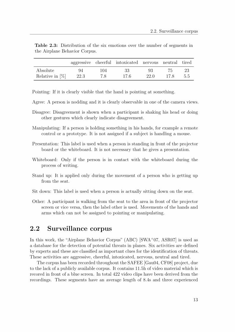
Table 2.3: Distribution of the six emotions over the number of segments inthe Airplane Behavior Corpus.
aggressive cheerful intoxicated nervous neutral tired
Absolute 94 104 33 93 75 23Relative in [%] 22.3 7.8 17.6 22.0 17.8 5.5
Pointing: If it is clearly visible that the hand is pointing at something.
Agree: A person is nodding and it is clearly observable in one of the camera views.
Disagree: Disagreement is shown when a participant is shaking his head or doingother gestures which clearly indicate disagreement.
Manipulating: If a person is holding something in his hands, for example a remotecontrol or a prototype. It is not assigned if a subject is handling a mouse.
Presentation: This label is used when a person is standing in front of the projectorboard or the whiteboard. It is not necessary that he gives a presentation.
Whiteboard: Only if the person is in contact with the whiteboard during theprocess of writing.
Stand up: It is applied only during the movement of a person who is getting upfrom the seat.
Sit down: This label is used when a person is actually sitting down on the seat.
Other: A participant is walking from the seat to the area in front of the projectorscreen or vice versa, then the label other is used. Movements of the hands andarms which can not be assigned to pointing or manipulating.
2.2 Surveillance corpus
In this work, the “Airplane Behavior Corpus” (ABC) [SWA+07, ASR07] is used asa database for the detection of potential threats in planes. Six activities are definedby experts and these are classified as important clues for the identification of threats.These activities are aggressive, cheerful, intoxicated, nervous, neutral and tired.
The corpus has been recorded throughout the SAFEE [Gau04, CF08] project, dueto the lack of a publicly available corpus. It contains 11.5h of video material which isrecored in front of a blue screen. In total 422 video clips have been derived from therecordings. These segments have an average length of 8.4s and three experienced
13
2. The Used Data Sets
cheerful intoxicated
nervous neutral tired
aggressive
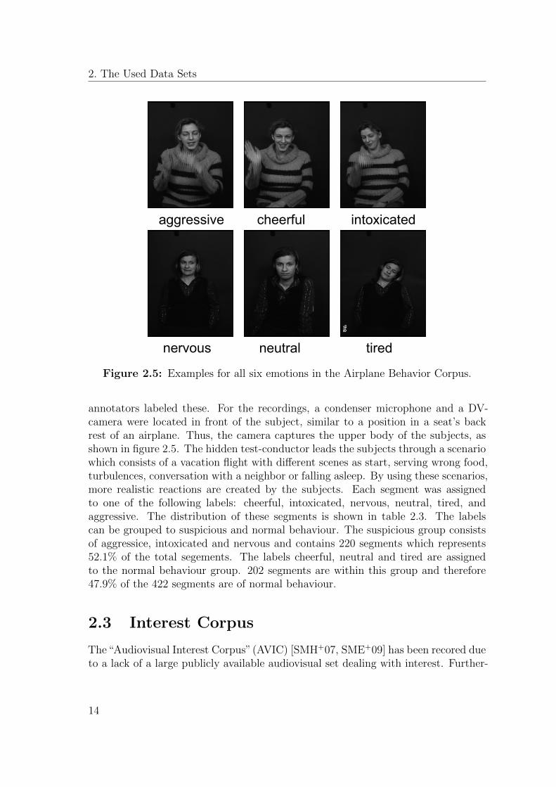
Figure 2.5: Examples for all six emotions in the Airplane Behavior Corpus.
annotators labeled these. For the recordings, a condenser microphone and a DV-camera were located in front of the subject, similar to a position in a seat’s backrest of an airplane. Thus, the camera captures the upper body of the subjects, asshown in figure 2.5. The hidden test-conductor leads the subjects through a scenariowhich consists of a vacation flight with different scenes as start, serving wrong food,turbulences, conversation with a neighbor or falling asleep. By using these scenarios,more realistic reactions are created by the subjects. Each segment was assignedto one of the following labels: cheerful, intoxicated, nervous, neutral, tired, andaggressive. The distribution of these segments is shown in table 2.3. The labelscan be grouped to suspicious and normal behaviour. The suspicious group consistsof aggressice, intoxicated and nervous and contains 220 segments which represents52.1% of the total segements. The labels cheerful, neutral and tired are assignedto the normal behaviour group. 202 segments are within this group and therefore47.9% of the 422 segments are of normal behaviour.
2.3 Interest Corpus
The“Audiovisual Interest Corpus”(AVIC) [SMH+07, SME+09] has been recored dueto a lack of a large publicly available audiovisual set dealing with interest. Further-
14
2.3. Interest Corpus
LOI2
LOI1
LOI0
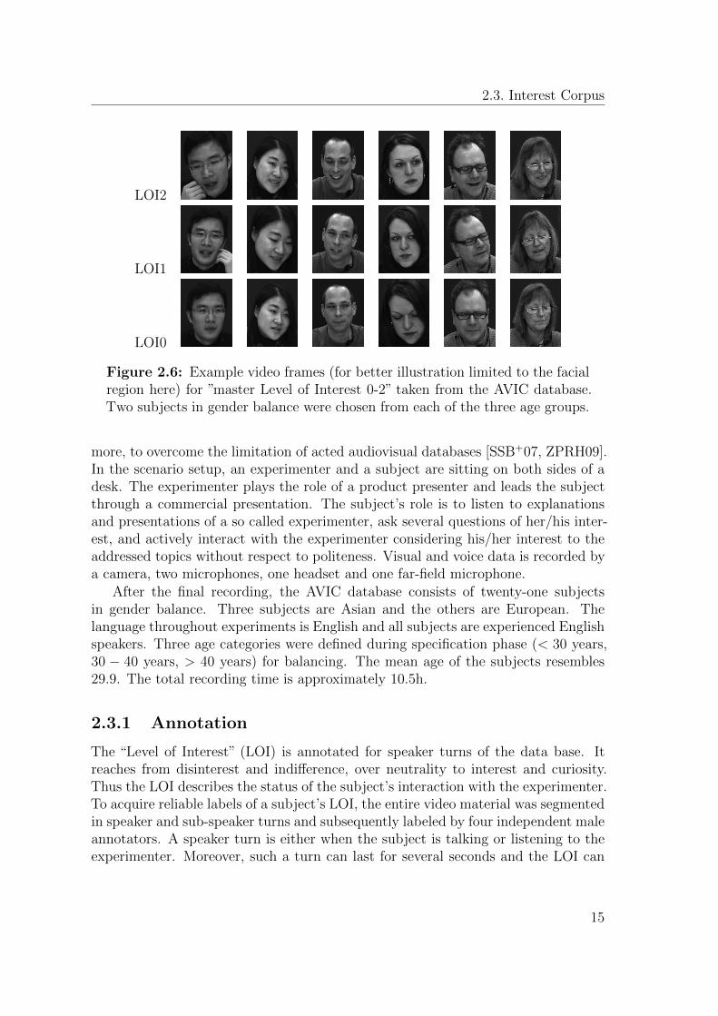
Figure 2.6: Example video frames (for better illustration limited to the facialregion here) for ”master Level of Interest 0-2” taken from the AVIC database.Two subjects in gender balance were chosen from each of the three age groups.
more, to overcome the limitation of acted audiovisual databases [SSB+07, ZPRH09].In the scenario setup, an experimenter and a subject are sitting on both sides of adesk. The experimenter plays the role of a product presenter and leads the subjectthrough a commercial presentation. The subject’s role is to listen to explanationsand presentations of a so called experimenter, ask several questions of her/his inter-est, and actively interact with the experimenter considering his/her interest to theaddressed topics without respect to politeness. Visual and voice data is recorded bya camera, two microphones, one headset and one far-field microphone.
After the final recording, the AVIC database consists of twenty-one subjectsin gender balance. Three subjects are Asian and the others are European. Thelanguage throughout experiments is English and all subjects are experienced Englishspeakers. Three age categories were defined during specification phase (< 30 years,30 − 40 years, > 40 years) for balancing. The mean age of the subjects resembles29.9. The total recording time is approximately 10.5h.
2.3.1 Annotation
The “Level of Interest” (LOI) is annotated for speaker turns of the data base. Itreaches from disinterest and indifference, over neutrality to interest and curiosity.Thus the LOI describes the status of the subject’s interaction with the experimenter.To acquire reliable labels of a subject’s LOI, the entire video material was segmentedin speaker and sub-speaker turns and subsequently labeled by four independent maleannotators. A speaker turn is either when the subject is talking or listening to theexperimenter. Moreover, such a turn can last for several seconds and the LOI can
15
2. The Used Data Sets
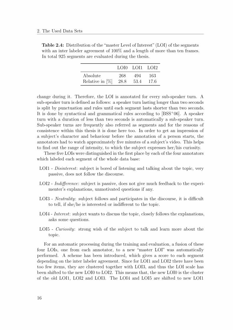
Table 2.4: Distribution of the“master Level of Interest” (LOI) of the segmentswith an inter labeler agreement of 100% and a length of more than ten frames.In total 925 segments are evaluated during the thesis.
LOI0 LOI1 LOI2
Absolute 268 494 163Relative in [%] 28.8 53.4 17.6
change during it. Therefore, the LOI is annotated for every sub-speaker turn. Asub-speaker turn is defined as follows: a speaker turn lasting longer than two secondsis split by punctuation and rules until each segment lasts shorter than two seconds.It is done by syntactical and grammatical rules according to [BSS+06]. A speakerturn with a duration of less than two seconds is automatically a sub-speaker turn.Sub-speaker turns are frequently also referred as segments and for the reasons ofconsistence within this thesis it is done here too. In order to get an impression ofa subject’s character and behaviour before the annotation of a person starts, theannotators had to watch approximately five minutes of a subject’s video. This helpsto find out the range of intensity, to which the subject expresses her/his curiosity.
These five LOIs were distinguished in the first place by each of the four annotatorswhich labeled each segment of the whole data base:
LOI1 - Disinterest : subject is bored of listening and talking about the topic, verypassive, does not follow the discourse.
LOI2 - Indifference: subject is passive, does not give much feedback to the experi-menter’s explanations, unmotivated questions if any.
LOI3 - Neutrality : subject follows and participates in the discourse, it is difficultto tell, if she/he is interested or indifferent to the topic.
LOI4 - Interest : subject wants to discuss the topic, closely follows the explanations,asks some questions.
LOI5 - Curiosity : strong wish of the subject to talk and learn more about thetopic.
For an automatic processing during the training and evaluation, a fusion of thesefour LOIs, one from each annotator, to a new “master LOI” was automaticallyperformed. A scheme has been introduced, which gives a score to each segmentdepending on the inter labeler agreement. Since for LOI1 and LOI2 there have beentoo few items, they are clustered together with LOI3, and thus the LOI scale hasbeen shifted to the new LOI0 to LOI2. This means that, the new LOI0 is the clusterof the old LOI1, LOI2 and LOI3. The LOI4 and LOI5 are shifted to new LOI1
16

2.3. Interest Corpus
respectively LOI2. Thereby, values of κ = 0.66 with σ = 0.20 are observed for allsegments when the new LOIs are used for the calculation. For this work the interlabeler agreement has to be 100%, which is equal to the case that all annotatorsgive the same rating to one segment. This is the case for in total 996 segments.Since 71 segments are shorter than ten frames these segments are removed beforethe evaluation takes place. The exact LOI distribution for the new shifted LOI scaleis shown in table 2.4 for all 925 segments with an inter labeler agreement of 100%and a length of more than ten frames. Example video frames for LOI0 - LOI2 afterclustering and inter labeler agreement based reduction are depicted in figure 2.6.
17

3
Feature Extraction andPreprocessing
In this chapter the features which are applied to the different tasks in this thesis arepresented. Three modalities of features are used: acoustic, visual and semantic. Thefirst two are directly derived from the recording devices. The semantic ones containmore high level information and therefore these are created by different detectionsystems or have been hand annotated during this work.
3.1 Acoustic features
Information about the mood, the feelings, or the emotions can be gathered [SRL03]from the acoustic channel. To achieve good results in analyzing the people, differentfeatures have to be evaluated. Therefore, a large amount of features is extractedfrom the recorded acoustic channels.
For the meeting corpus only the Mel Frequency Cepstral Coefficients [YEH+02,FGZ01] (MFCC) have been independently extracted from each of the participant’sclose-talking microphones. The first and the second derivations are calculated fromthe MFCCs, and this results in a 39 dimensional acoustic feature space for eachparticipant’s microphone. These 39 features are derived from not overlapping win-dows with a size of 40ms, which fits to the framerate of the video recordings in themeeting corpus. In total, for each time window in the meetings, a 156 dimensionalacoustic vector is extracted, because of the four participants’ microphones which areanalysed.
For the behaviour and the emotion corpuses not only the MFCCs are extracted,but also other features which have been developed for interpretation of speech andmusic. Due to the fact that a large number of features has to be extracted and eval-uated, the novel feature extractor openSMILE 1 [EWS09] is used. It is a real-time
1The open source project openSMILE is available at http://sourceforge.net/projects/
19
3. Feature Extraction and Preprocessing
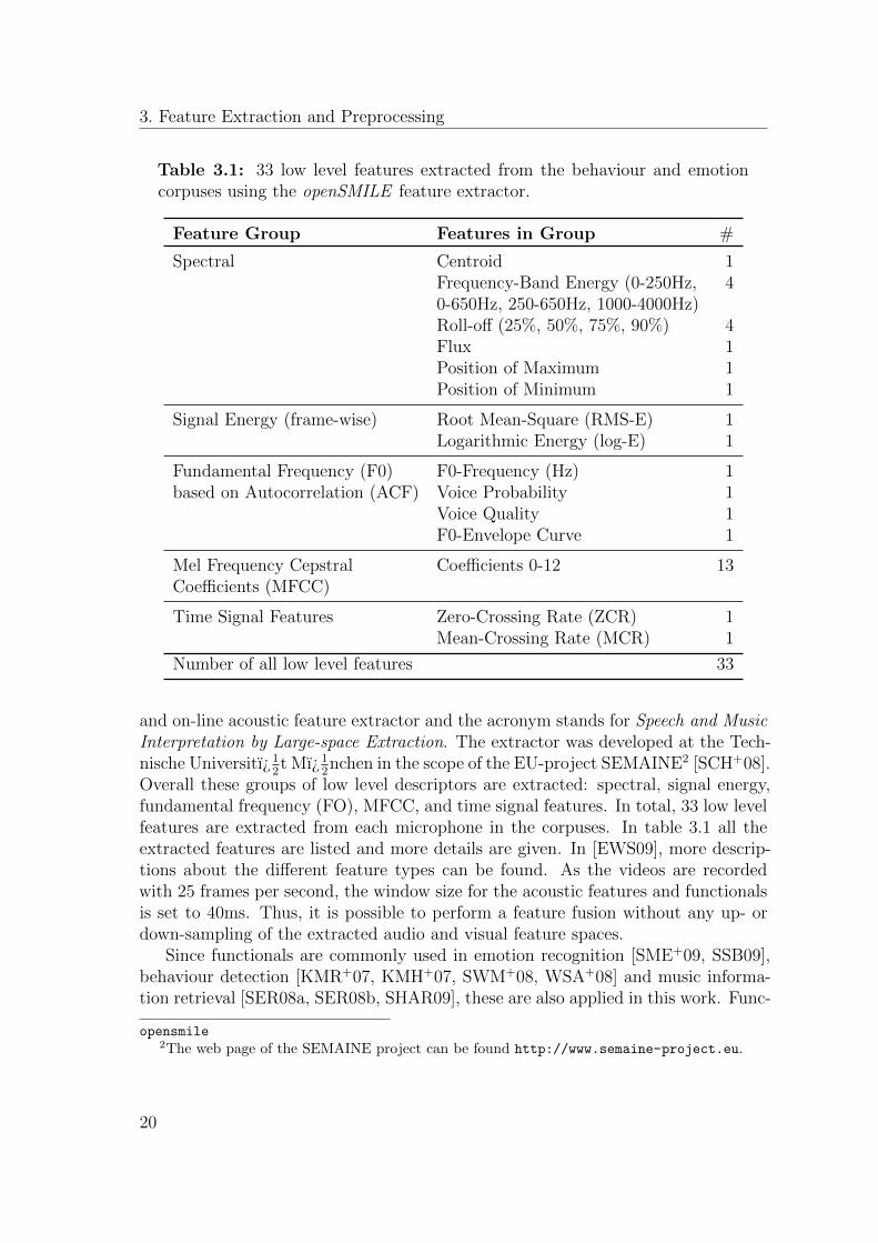
Table 3.1: 33 low level features extracted from the behaviour and emotioncorpuses using the openSMILE feature extractor.
Feature Group Features in Group #
Spectral Centroid 1Frequency-Band Energy (0-250Hz, 40-650Hz, 250-650Hz, 1000-4000Hz)Roll-off (25%, 50%, 75%, 90%) 4Flux 1Position of Maximum 1Position of Minimum 1
Signal Energy (frame-wise) Root Mean-Square (RMS-E) 1Logarithmic Energy (log-E) 1
Fundamental Frequency (F0) F0-Frequency (Hz) 1based on Autocorrelation (ACF) Voice Probability 1
Voice Quality 1F0-Envelope Curve 1
Mel Frequency Cepstral Coefficients 0-12 13Coefficients (MFCC)
Time Signal Features Zero-Crossing Rate (ZCR) 1Mean-Crossing Rate (MCR) 1
Number of all low level features 33
and on-line acoustic feature extractor and the acronym stands for Speech and MusicInterpretation by Large-space Extraction. The extractor was developed at the Tech-nische Universitı¿1
2t Mı¿1
2nchen in the scope of the EU-project SEMAINE2 [SCH+08].
Overall these groups of low level descriptors are extracted: spectral, signal energy,fundamental frequency (FO), MFCC, and time signal features. In total, 33 low levelfeatures are extracted from each microphone in the corpuses. In table 3.1 all theextracted features are listed and more details are given. In [EWS09], more descrip-tions about the different feature types can be found. As the videos are recordedwith 25 frames per second, the window size for the acoustic features and functionalsis set to 40ms. Thus, it is possible to perform a feature fusion without any up- ordown-sampling of the extracted audio and visual feature spaces.
Since functionals are commonly used in emotion recognition [SME+09, SSB09],behaviour detection [KMR+07, KMH+07, SWM+08, WSA+08] and music informa-tion retrieval [SER08a, SER08b, SHAR09], these are also applied in this work. Func-
opensmile2The web page of the SEMAINE project can be found http://www.semaine-project.eu.
20

3.1. Acoustic features
Table 3.2: 56 functionals are extracted by the openSMILE feature extractor.
Functionals Group Functionals in Group #
Min/Max Maximum/Minimum Value 2Relative Position of Maximum/Minimum Value 2Maximum/Minimum Value - Arithmetic Mean 2Range 1
Linear Regression 2 Coefficients (m,t) 2Linear and Quadratic Regression Error 2
Quadratic 3 Coefficients (a,b,c) 3Regression Linear and Quadratic Regression Error 2
Centroid Centroid: Centre of Gravity 1
Moments Variance, Skewness, and Kurtosis 3Standard Deviation 1
Discrete Cosine Coefficients 0-5 6Transformation
Quartiles 25%, 50% (Median), and 75% Quartile 3Inter-Quartile Range (IQR): 2-1, 3-2, 3-1 3
Percentiles 95%, 98% Percentile 2
Threshold Crossing Zero-Crossing Rate 1Rates Mean-Crossing Rate 1
Mean Arithmetic Mean 1
Segments Number of Segments, based on Delta Thresholding 1Mean Segment Length 1Maximum/Minimum Segment Length 2
Peaks Number of Peaks (Maxima) 1Mean Distance between Peaks 1Mean Value of all Peaks 1Mean Value of all Peaks - Arithmetic Mean 1
Times Values are above 25% of the total Range 1Values are below 25% of the total Range 1Values are above 50% of the total Range 1Rise Time and Fall Time 2Curve is convex/concave 2Values are below 50% of the total Range 1Values are above 90% of the total Range 1Values are below 90% of the total Range 1
Number of all Functionals 56
21
3. Feature Extraction and Preprocessing
tionals combine information from previous frames, thus the current frame containsmore information, especially about changes over time in the extracted features. InopenSMILE, not only low level feature extractors are implemented, but also variousfilters, functionals and transformations. Therefore, not only low level descriptorsbut also functionals [EWS09], such as maximum, minimum, range, different typesof means, quartiles, standard deviation, or variance, are calculated. Additional tothose, linear and quadratic regression coefficients, discrete cosine transformationcoefficients, autocorrelation functions and cross-correlation functions are extractedform the audio sources. Table 3.2 shows the derived 56 functionals from the featureextractor. Furthermore, the first derivation of each functional is calculated. Overall3729 acoustical features are extracted from each frame. The list of all available lowlevel features and the functionals, which openSMILE can extract in real-time andon-line from an audio source is available on the sourceforge project page3.
3.2 Visual features
In this section, the extracted features from video recordings of all available camerasare described. In human to human communication, not only the speech is impor-tant also the visual clues which are exchanged between dialog partners are containinginformation[JR64, BB73]. Visual clues are already used by infants to communicatewith her/his caretaker before they can even speak [Hal77, Bul79]. Therefore, the in-vestigation of the visual recordings is of interest for the meeting analysis. Moreover,it is true for the surveillance task, too. First, the used visual features are charac-terized in detail and then the regions are pictured where the features are extractedfrom.
3.2.1 Skin blobs
The first features give the opportunity to derive certain information from the handand head movements of the participants. In [YKA02], various face detection algo-rithms are described, one of them is a skin colour detector. An adaptive skin colourdetector is presented in [WR05]. This approach can be applied both for the faceand hands of participants. In [PSS04], face and hand movements are suggested tobe used for video editing. Face movements are also important for the behaviourrecognition, which has been shown in [AHSR09]. Therefore, skin blobs are added asthe first visual feature. The first step to extract the face and hand movements, is tofind the skin colour in the frame. It is performed by a comparing each pixel with askin colour look-up table, which has been trained on 5.7 million pixels from picturesof people from all over the world. For more details about the training see [Koh06].The look-up table is a 16 bit rg-table thus the the recorded image is transformed
3http://sourceforge.net/projects/opensmile
22
3.2. Visual features
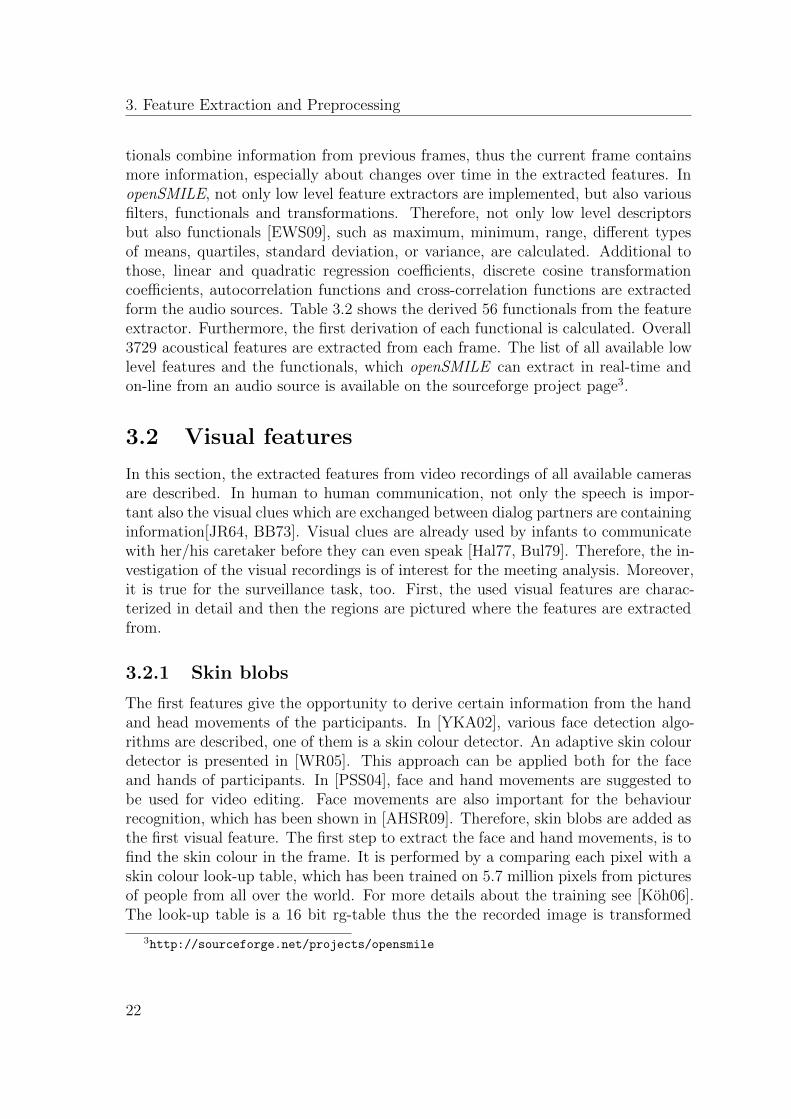
Figure 3.1: The first picture shows a single frame taken from a sample videofor illustration of the skin blob detection. In the second picture all detectedskin colour pixels are marked by white dots. The frame has been split forthe detection task into a head region and a hand region. Especially at theboundaries of the image and of the regions of interest, detection errors arevisible. The last image shows the bounding boxes, which are found by thealgorithm for the face and the hands. Additionally, the norm of the motionvector for each of these bounding boxes is drawn as a white bar in the cornersof the image. The image shows that only the left arm is moved therefore thelower right bar is longer than the other two bars.
from the RGB colour space to the rg colour space. After the comparison, a binaryimage of the same size as the colour image, is available where each possible skin pixelis marked as one. To fill gaps in the possible skin areas in the binary image, a 5x5dilation filter [Pra01] is applied to it. The located skin areas are then analyzed fortheir shape, the relation of their eigenvalues, and context knowledge about possiblepositions of the head and the hands. Before the analysis is performed several possibil-ities are available for the searched body parts. Thereafter, the most accurate blobsare selected, which then become the face and the hands. Each of them are markedby a rectangle, as shown in Figure 3.1 for a single frame of a sample video. Thefeature vector for each bounding box contains the coordinates of the lower left andthe upper right corner, the size in x- and y-direction and the movement of the cen-ter of the bounding box between two boxes extracted from consecutive frames. Themovement is described by the shift along the x- and y-axis and the square-distance.In total 15 parameters are extracted for each bounding box.
3.2.2 Global Motion Features
The second visual feature group estimates the motions from the recorded meeting par-ticipants. In [RK97], these features, which represent the motion in a defined region ofinterest, are introduced for gesture recognition. In [EKR98], the so called global mo-
23
3. Feature Extraction and Preprocessing
tion features have been used for gesture recognition in acted videos. These featureshave been successfully applied in the meeting domain in [WZR04] and [ZWR03].For behaviour recognition the same features have been extracted in [ASR07]. Theglobal motion features can be extracted in real-time with only one frame latencytherefore these features are applied to all the tasks in this work.
The extraction of the features is outlined in this paragraph here. First, a dif-ference image Id(x, y) is calculated from the video stream by subtracting the pixelvalues of two subsequent frames. Seven features are extracted from the sequenceof difference images, by calculating equation 3.1 to 3.7 and concatenated for eachtime step t into the motion vector ~b(t). By applying the feature extraction, thehigh dimensional video is reduced to a seven dimensional vector, but it preservesthe major characteristics of the motion. The following seven global motion featuresare derived from the sequence of difference images for the whole video. The centerof motion is calculated for the x- and y-direction according to:
mLx (t) =
∑(x,y) x · |ILd (x, y, t)|∑(x,y) |ILd (x, y, t)|
(3.1)
and
mLy (t) =
∑(x,y) y · |ILd (x, y, t)|∑(x,y) |ILd (x, y, t)|
. (3.2)
The changes in motion are used to express the dynamics of movements:
∆mLx (t) = mL
x (t)−mLx (t− 1) (3.3)
and∆mL
y (t) = mLy (t)−mL
y (t− 1). (3.4)
Furthermore, the mean absolute deviation of the difference pixels relative to thecenter of motion is computed:
σLx (t) =
∑(x,y) |ILd (x, y, t)| ·
(x−mL
x (t))∑
(x,y) |ILd (x, y, t)|(3.5)
and
σLy (t) =
∑(x,y) |ILd (x, y, t)| ·
(y −mL
y (t))∑
(x,y) |ILd (x, y, t)|. (3.6)
Finally, the intensity of motion is calculated from the average absolute values of themotion distribution:
iL(t) =
∑(x,y) |ILd (x, y, t)|∑
x
∑y 1
. (3.7)
Figure 3.2 pictures the procedure of the extraction of the global motion featuresfrom a sample video.
24
3.2. Visual features
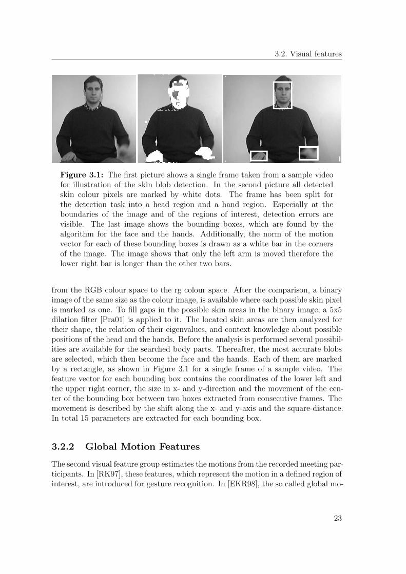
Figure 3.2: The first two pictures show two consecutive frames taken froman example video. The third image shows the difference image of these twoframes. The frames are split into two regions, one for the head and one for thehands, and for each of them the difference image is calculated separately. Inthe last picture, the difference image is presented, but additionally the valuesof the global motion vectors are drawn into it. There is no visible movement inthe head region and therefore only a small light gray circle and a gray ellipsisare shown in the upper half. The light gray line connects the current centerof motion (small light gray circle) with the last one and the white bar showsthe intensity of motion for the hand region. The gray ellipsis represents thedeviation of the motion in x- and y-direction.
3.2.3 Selected Regions of Interest
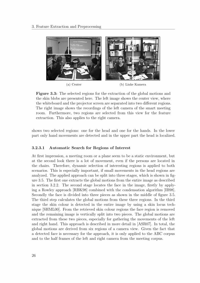
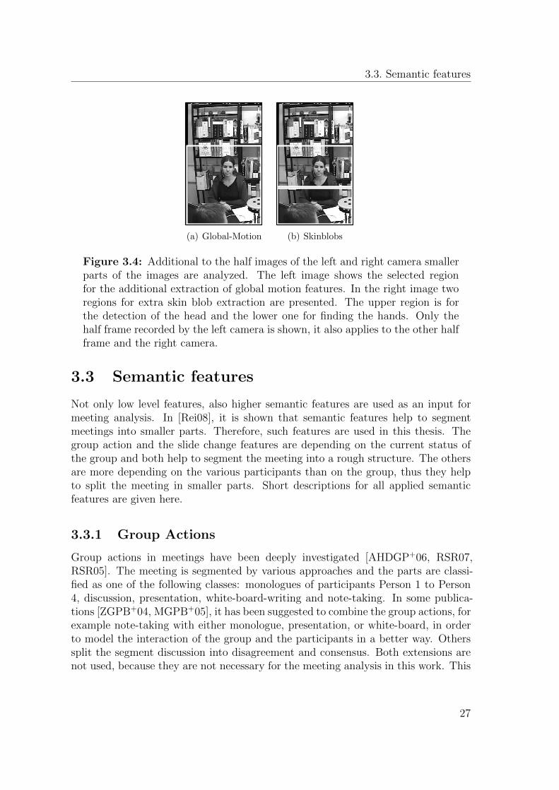
The selection of different regions of interest is important to get the most relevantinformation from the recordings. It can be done either manually or automaticallywith constraints to the scenarios. In this section several regions, within the viewsof the cameras, are presented where they visual feature extractors are applied to.First the regions of interest are set manually, which is shown in figure 3.3 and 3.4,and later in this section the regions are detected automatically. The left image offigure 3.3 shows the center camera and two selected areas. These areas mark thewhiteboard and the projection screen which are important because, if a participantis located there, she normally gives a speech or is writing on the whiteboard. Theseare two interesting actions for the video editing and for the activity detection. Theright or left camera is vertically cut into two pieces to separate the two participantslocated in the view. This is presented for the left camera view in the right imageof figure 3.3. The resulting half images of the left and right camera are analyzed intotal, as well as defined sub regions of it. This sub regions are marked in figure 3.4.In the left image the upper body of the sitting person is the region of interest. Thisis sometimes necessary because other participants are passing by behind the chairand the skin colour of them interferes with the head detector applied to the seatedperson, if the whole image is analyzed. The movement of the hands often givesa good impression what the person is currently doing. Therefore, the right image
25
3. Feature Extraction and Preprocessing
(a) Center (b) Linke Kamera
Figure 3.3: The selected regions for the extraction of the global motions andthe skin blobs are presented here. The left image shows the center view, wherethe whiteboard and the projector screen are separated into two different regions.The right image shows the recordings of the left camera of the smart meetingroom. Furthermore, two regions are selected from this view for the featureextraction. This also applies to the right camera.
shows two selected regions: one for the head and one for the hands. In the lowerpart only hand movements are detected and in the upper part the head is localized.
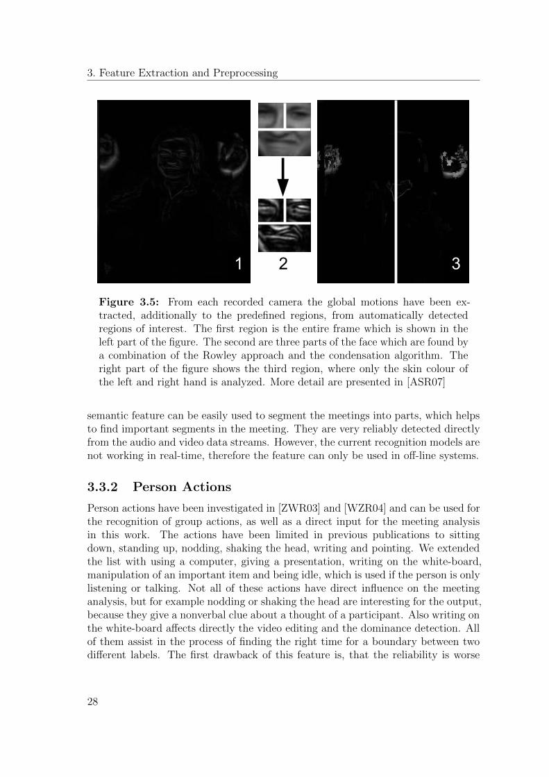
3.2.3.1 Automatic Search for Regions of Interest
At first impression, a meeting room or a plane seem to be a static environment, butat the second look there is a lot of movement, even if the persons are located inthe chairs. Therefore, dynamic selection of interesting regions is applied to bothscenarios. This is especially important, if small movements in the head regions areanalyzed. The applied approach can be split into three stages, which is shown in fig-ure 3.5. The first one extracts the global motions from the entire image as describedin section 3.2.2. The second stage locates the face in the image, firstly by apply-ing a Rowley approach [RBK98] combined with the condensation algorithm [IB98].Secondly the face is divided into three pieces as shown in the middle of figure 3.5.The third step calculates the global motions from these three regions. In the thirdstage the skin colour is detected in the entire image by using a skin locus tech-nique [SHML00]. From the retrieved skin colour regions the face region is removedand the remaining image is vertically split into two pieces. The global motions areextracted from these two pieces, especially for gathering the movements of the leftand right hand. This approach is described in more detail in [ASR07]. In total, theglobal motions are derived from six regions of a camera view. Given the fact thata detected face is necessary for the approach, it is only applied to the ABC corpusand to the half frames of the left and right camera from the meeting corpus.
26
3.3. Semantic features
(a) Global-Motion (b) Skinblobs
Figure 3.4: Additional to the half images of the left and right camera smallerparts of the images are analyzed. The left image shows the selected regionfor the additional extraction of global motion features. In the right image tworegions for extra skin blob extraction are presented. The upper region is forthe detection of the head and the lower one for finding the hands. Only thehalf frame recorded by the left camera is shown, it also applies to the other halfframe and the right camera.
3.3 Semantic features
Not only low level features, also higher semantic features are used as an input formeeting analysis. In [Rei08], it is shown that semantic features help to segmentmeetings into smaller parts. Therefore, such features are used in this thesis. Thegroup action and the slide change features are depending on the current status ofthe group and both help to segment the meeting into a rough structure. The othersare more depending on the various participants than on the group, thus they helpto split the meeting in smaller parts. Short descriptions for all applied semanticfeatures are given here.
3.3.1 Group Actions
Group actions in meetings have been deeply investigated [AHDGP+06, RSR07,RSR05]. The meeting is segmented by various approaches and the parts are classi-fied as one of the following classes: monologues of participants Person 1 to Person4, discussion, presentation, white-board-writing and note-taking. In some publica-tions [ZGPB+04, MGPB+05], it has been suggested to combine the group actions, forexample note-taking with either monologue, presentation, or white-board, in orderto model the interaction of the group and the participants in a better way. Otherssplit the segment discussion into disagreement and consensus. Both extensions arenot used, because they are not necessary for the meeting analysis in this work. This
27
3. Feature Extraction and Preprocessing
1 32
Figure 3.5: From each recorded camera the global motions have been ex-tracted, additionally to the predefined regions, from automatically detectedregions of interest. The first region is the entire frame which is shown in theleft part of the figure. The second are three parts of the face which are found bya combination of the Rowley approach and the condensation algorithm. Theright part of the figure shows the third region, where only the skin colour ofthe left and right hand is analyzed. More detail are presented in [ASR07]
semantic feature can be easily used to segment the meetings into parts, which helpsto find important segments in the meeting. They are very reliably detected directlyfrom the audio and video data streams. However, the current recognition models arenot working in real-time, therefore the feature can only be used in off-line systems.
3.3.2 Person Actions
Person actions have been investigated in [ZWR03] and [WZR04] and can be used forthe recognition of group actions, as well as a direct input for the meeting analysisin this work. The actions have been limited in previous publications to sittingdown, standing up, nodding, shaking the head, writing and pointing. We extendedthe list with using a computer, giving a presentation, writing on the white-board,manipulation of an important item and being idle, which is used if the person is onlylistening or talking. Not all of these actions have direct influence on the meetinganalysis, but for example nodding or shaking the head are interesting for the output,because they give a nonverbal clue about a thought of a participant. Also writing onthe white-board affects directly the video editing and the dominance detection. Allof them assist in the process of finding the right time for a boundary between twodifferent labels. The first drawback of this feature is, that the reliability is worse
28
3.3. Semantic features
because of occlusions and of the perspectives at the persons. The fact that therecognition models are not working in real-time is the second disadvantage, howeverwith emerging computer power it will become possible in the future. Therefore, thisfeature currently only applies to the browsing of past meetings.
3.3.3 Person Speaking
Person speaking is a feature which contains information whether a person is cur-rently speaking or not. As all meetings used in this thesis have four participants, afour dimensional vector for each frame is extracted. The information about who iscurrently speaking is derived from a speaker diarization system, which automaticallydetects the participants and assigns the spoken words to them. More details aboutspeaker diarization can be found in [MMF+06, WH09]. For this feature it is notnecessary to know what the person is speaking.
3.3.4 Person Movements
Movements of hands and the face of a person, which are used in [PSS04] as aninput for the video editing are normally too disturbing during a meeting to be useddirectly as a feature. Therefore, a set of different movements and positions whichare common in meetings are defined as follows: off camera, sit, other, move, standwhiteboard, stand screen and take notes. These describe some important taskswhich each person can perform in an ongoing meeting. Again the movements of aperson are not directly connected with the video modes or the level of activity, butthe boundaries are helpful for estimating the point in time of a change. This featurecould be used for the recognition of the person action, as well as vice versa. Thegroup action is also closely related.
3.3.5 Slide Changes
Another important information which helps to segment the meeting is the changeof the slide, which is projected on the screen. The knowledge about it helps tointegrate a picture of the slide into the output video of the system. The feature canbe extracted in real-time with a latency of only one frame. Therefore, the differenceimage of two consecutive frames is calculated and the intensity of the changes ismeasured. In the case of a peak above a certain threshold a slide change is detected.In [Zak07], this easy approach works well for the detection of the slide changes, as aperson, which is moving in front of screen, is creating a high intensity for a long timecompared to a slide change. The extraction of images from the projector screen ismore critical, because of occlusions which happen often at the moment of the slidechange. For a video conference we need a different approach of capturing the slidesas described in [VO06]. Another possibility is to have direct file access to the slides.
29
3. Feature Extraction and Preprocessing
3.4 Preprocessing of the Extracted Features
Two types of preprocessing are performed during this thesis: normalisation andfeature selection. As the range of the different features varies, a normalisation of themean and the variance of the whole databases is done. Due to the huge amount offeatures and the dependences among the features it is reasonable to perform a featureselection on the other side. In this theses a principal component analysis, describedin section 3.4.2.1, and a sequential forward feature selection (see section 3.4.2.2) areconducted.
3.4.1 Feature Normalisation
Two possibilities for a feature normalisation exist. In the first one features arenormalized in a way that their values are located within a predefined range. Thesecond method is one where all features have the same mean and the same varianceafter the normalisation. During this thesis, the second approach is used and thefollowing values are used: mean µ = 0 and variance σ2 = 1. This leads to nolimitation of the value range.
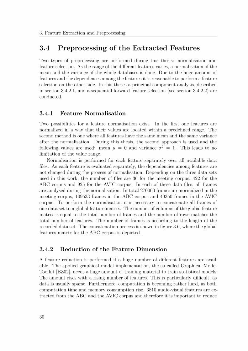
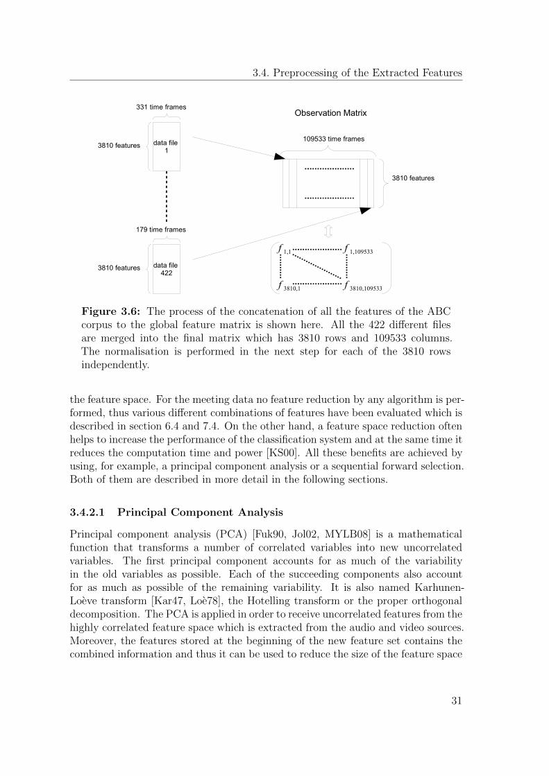
Normalisation is performed for each feature separately over all available datafiles. As each feature is evaluated separately, the dependencies among features arenot changed during the process of normalisation. Depending on the three data setsused in this work, the number of files are 36 for the meeting corpus, 422 for theABC corpus and 925 for the AVIC corpus. In each of these data files, all framesare analysed during the normalisation. In total 270000 frames are normalized in themeeting corpus, 109533 frames in the ABC corpus and 49350 frames in the AVICcorpus. To perform the normalisation it is necessary to concatenate all frames ofone data set to a global feature matrix. The number of columns of the global featurematrix is equal to the total number of frames and the number of rows matches thetotal number of features. The number of frames is according to the length of therecorded data set. The concatenation process is shown in figure 3.6, where the globalfeatures matrix for the ABC corpus is depicted.
3.4.2 Reduction of the Feature Dimension
A feature reduction is performed if a huge number of different features are avail-able. The applied graphical model implementation, the so called Graphical ModelToolkit [BZ02], needs a huge amount of training material to train statistical models.The amount rises with a rising number of features. This is particularly difficult, asdata is usually sparse. Furthermore, computation is becoming rather hard, as bothcomputation time and memory consumption rise. 3810 audio-visual features are ex-tracted from the ABC and the AVIC corpus and therefore it is important to reduce
30
3.4. Preprocessing of the Extracted Features
3810 features
3810 features
Observation Matrix
f 1,1 f 1,109533
f 3810,1 f 3810,109533
data file 1
331 time frames
3810 features data file 422
109533 time frames
179 time frames
Figure 3.6: The process of the concatenation of all the features of the ABCcorpus to the global feature matrix is shown here. All the 422 different filesare merged into the final matrix which has 3810 rows and 109533 columns.The normalisation is performed in the next step for each of the 3810 rowsindependently.
the feature space. For the meeting data no feature reduction by any algorithm is per-formed, thus various different combinations of features have been evaluated which isdescribed in section 6.4 and 7.4. On the other hand, a feature space reduction oftenhelps to increase the performance of the classification system and at the same time itreduces the computation time and power [KS00]. All these benefits are achieved byusing, for example, a principal component analysis or a sequential forward selection.Both of them are described in more detail in the following sections.
3.4.2.1 Principal Component Analysis
Principal component analysis (PCA) [Fuk90, Jol02, MYLB08] is a mathematicalfunction that transforms a number of correlated variables into new uncorrelatedvariables. The first principal component accounts for as much of the variabilityin the old variables as possible. Each of the succeeding components also accountfor as much as possible of the remaining variability. It is also named Karhunen-Loeve transform [Kar47, Loe78], the Hotelling transform or the proper orthogonaldecomposition. The PCA is applied in order to receive uncorrelated features from thehighly correlated feature space which is extracted from the audio and video sources.Moreover, the features stored at the beginning of the new feature set contains thecombined information and thus it can be used to reduce the size of the feature space
31
3. Feature Extraction and Preprocessing
by using only features from the beginning of the new set. In these features mostof the relevant information from the original data is preserved. Therefore, it breaksdown the complexity of the classification problem by transforming the originallylarge feature space into a low dimensional new one. A short description of thecalculation which has to be performed for the PCA are given in the next paragraph.
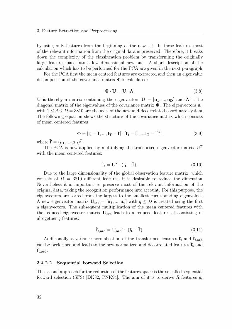
For the PCA first the mean centred features are extracted and then an eigenvaluedecomposition of the covariance matrix Φ is calculated:
Φ ·U = U ·Λ. (3.8)
U is thereby a matrix containing the eigenvectors U = [u1, ...,uD] and Λ is thediagonal matrix of the eigenvalues of the covariance matrix Φ. The eigenvectors ud
with 1 ≤ d ≤ D = 3810 are the axes of the new and decorrelated coordinate system.The following equation shows the structure of the covariance matrix which consistsof mean centered features
Φ = [f1 − f , ..., fT − f ] · [f1 − f , ..., fT − f ]T , (3.9)
where f = (µ1, ..., µD)T .The PCA is now applied by multiplying the transposed eigenvector matrix UT
with the mean centered features:
ft = UT · (ft − f). (3.10)
Due to the large dimensionality of the global observation feature matrix, whichconsists of D = 3810 different features, it is desirable to reduce the dimension.Nevertheless it is important to preserve most of the relevant information of theoriginal data, taking the recognition performance into account. For this purpose, theeigenvectors are sorted from the largest to the smallest corresponding eigenvalues.A new eigenvector matrix Uord = [u1, ...,uq] with q ≤ D is created using the firstq eigenvectors. The subsequent multiplication of the mean centered features withthe reduced eigenvector matrix Uord leads to a reduced feature set consisting ofaltogether q features:
ft,ord = UordT · (ft − f). (3.11)
Additionally, a variance normalisation of the transformed features ft and ft,ordcan be performed and leads to the new normalized and decorrelated features ft andft,ord.
3.4.2.2 Sequential Forward Selection
The second approach for the reduction of the features space is the so called sequentialforward selection (SFS) [DK82, PNK94]. The aim of it is to derive R features yr
32
3.4. Preprocessing of the Extracted Features
out of the complete audiovisual feature set FD = {f1, ..., fD}, here D = 3810, withR ≤ D and concatenate them to a new feature set YR = {y1, ..., yr} with YR ∈ FD.In order to do this, it is necessary to compare two different sets of features Yi andYj. Therefore, a cost function J(·) is introduced in the form that J(Yi) > J(Yj).This means that the feature set Yi performs better as set Yj. As cost function therecognition accuracy rate, which is calculated from the number of correct classifiedsegments and the total number of available segments, is used for the ABC corpus.Additionally to the cost function, an individual significance S0(fi) of each featurefi with 1 ≤ i ≤ D and the joint significance S(fi,Y) with a feature set Y areintroduced.
The first step of the SFS is to evaluate the cost function for each of the 3810features separately. Consequently, all features fi are evaluated and the feature withthe highest individual significance is selected and will be the first element of the newfeature set Y1.
y1 = argmaxfi∈F
J(fi). (3.12)
Then the feature yk+1 = fi which leads to the maximum joint significance is addedrecursively to the current set Yk using the following equation:
yk+1 = argmaxfi∈F\Yk
S+(fi,Yk), (3.13)
Yk+1 = Yk ∪ yk+1. (3.14)
Thereby S+(fi,Yk) indicates the difference in recognition accuracy rate between thefeature set Yk and the feature set Yk ∪ fi:
S+(fi,Yk) = J(Yk ∪ fi)− J(Yk), fi ∈ F \ Yk. (3.15)
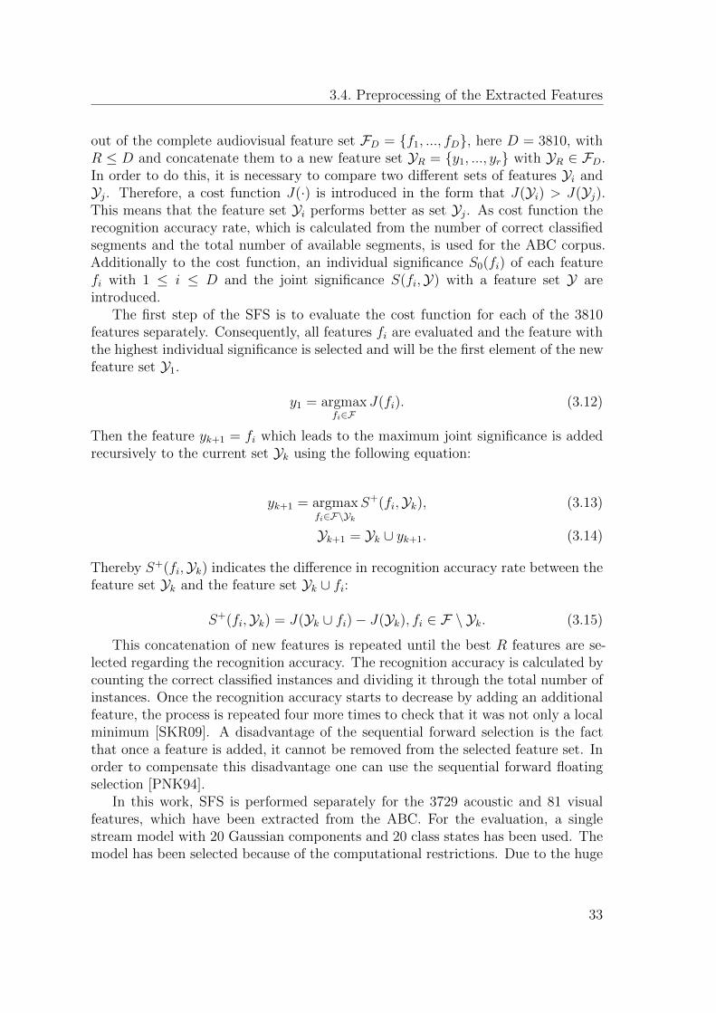
This concatenation of new features is repeated until the best R features are se-lected regarding the recognition accuracy. The recognition accuracy is calculated bycounting the correct classified instances and dividing it through the total number ofinstances. Once the recognition accuracy starts to decrease by adding an additionalfeature, the process is repeated four more times to check that it was not only a localminimum [SKR09]. A disadvantage of the sequential forward selection is the factthat once a feature is added, it cannot be removed from the selected feature set. Inorder to compensate this disadvantage one can use the sequential forward floatingselection [PNK94].
In this work, SFS is performed separately for the 3729 acoustic and 81 visualfeatures, which have been extracted from the ABC. For the evaluation, a singlestream model with 20 Gaussian components and 20 class states has been used. Themodel has been selected because of the computational restrictions. Due to the huge
33
3. Feature Extraction and Preprocessing
1 2 3 4 5 6 7 80
5
1 0
1 5
2 0
2 5
3 0
3 5
4 0
4 5
5 0
5 5
% A
CC
r number of features
bestmeanworst
1 2 3 4 5 6 7 80
5
10
15
20
25
30
35
40
45
50
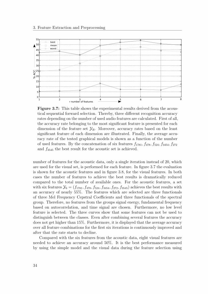
55
Figure 3.7: This table shows the experimental results derived from the acous-tical sequential forward selection. Thereby, three different recognition accuracyrates depending on the number of used audio features are calculated. First of all,the accuracy rate belonging to the most significant feature is presented for eachdimension of the feature set YR. Moreover, accuracy rates based on the leastsignificant feature of each dimension are illustrated. Finally, the average accu-racy rate of the tested graphical models is shown as a function of the numberof used features. By the concatenation of six features f1781, f478, f524, f3454, f272and f3545 the best result for the acoustic set is achieved.
number of features for the acoustic data, only a single iteration instead of 20, whichare used for the visual set, is performed for each feature. In figure 3.7 the evaluationis shown for the acoustic features and in figure 3.8, for the visual features. In bothcases the number of features to achieve the best results is dramatically reducedcompared to the total number of available ones. For the acoustic features, a setwith six features Y6 = (f1781, f478, f524, f3454, f272, f3545) achieves the best results withan accuracy of nearly 55%. The features which are selected are three functionalsof three Mel Frequency Cepstral Coefficients and three functionals of the spectralgroup. Therefore, no features from the groups signal energy, fundamental frequencybased on autocorrelation, and time signal are chosen. Furthermore, no low levelfeature is selected. The three curves show that some features can not be used todistinguish between the classes. Even after combining several features the accuracydoes not get higher than 15%. Furthermore, it is displayed that the average accuracyover all feature combinations for the first six iterations is continuously improved andafter that the rate starts to decline.
Compared with the six features from the acoustic data, eight visual features areneeded to achieve an accuracy around 50%. It is the best performance measuredby using the simple model and the visual data during the feature selection using
34
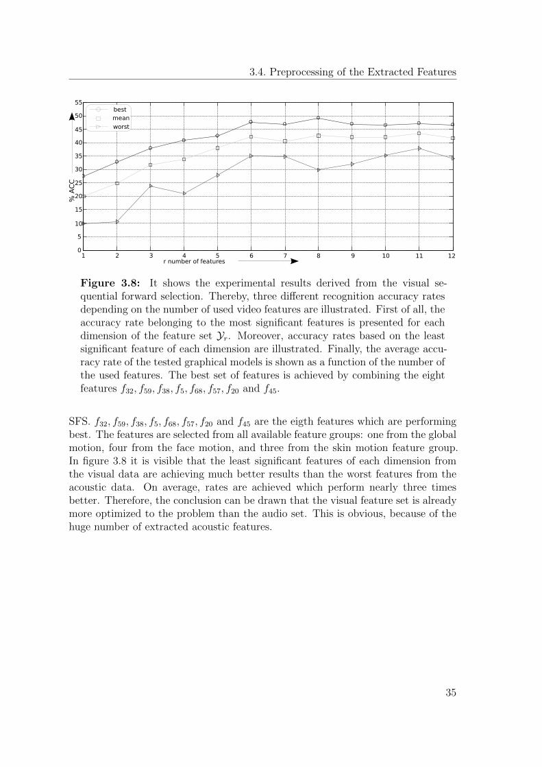
3.4. Preprocessing of the Extracted Features
1 2 3 4 5 6 7 8 9 1 0 1 1 1 20
5
1 0
1 5
2 0
2 5
3 0
3 5
4 0
4 5
5 0
5 5
% A
CC
r number of features
bestmeanworst
1 2 3 4 5 6 7 8 9 10 11 120
5
10
15
20
25
30
35
40
45
50
55
Figure 3.8: It shows the experimental results derived from the visual se-quential forward selection. Thereby, three different recognition accuracy ratesdepending on the number of used video features are illustrated. First of all, theaccuracy rate belonging to the most significant features is presented for eachdimension of the feature set Yr. Moreover, accuracy rates based on the leastsignificant feature of each dimension are illustrated. Finally, the average accu-racy rate of the tested graphical models is shown as a function of the number ofthe used features. The best set of features is achieved by combining the eightfeatures f32, f59, f38, f5, f68, f57, f20 and f45.
SFS. f32, f59, f38, f5, f68, f57, f20 and f45 are the eigth features which are performingbest. The features are selected from all available feature groups: one from the globalmotion, four from the face motion, and three from the skin motion feature group.In figure 3.8 it is visible that the least significant features of each dimension fromthe visual data are achieving much better results than the worst features from theacoustic data. On average, rates are achieved which perform nearly three timesbetter. Therefore, the conclusion can be drawn that the visual feature set is alreadymore optimized to the problem than the audio set. This is obvious, because of thehuge number of extracted acoustic features.
35


4
Graphical Model
Graphical models (GM) are a graph-based representation for joint distributions ofrandom variables. Such a distribution is usually very complex and frequently ap-pears to be intractable. A GM provides a compact representation of complex prob-abilistic problems [KF09] and therefore GMs are often used, for example in expertsystems for differential diagnosis [WTVS61, GB68]. Vertices and edges are the twobuilding blocks of a graph [Lau96]. A vertex corresponds to random variables inthe probabilistic domain and the edges correspond to direct probabilistic dependen-cies between these. Therefore, GMs are combining both graph- and probabilistictheory [Jor01]. In [Kno69, Kau71, BM76], more details are provided on the graphtheory. The theory of GMs is based on the research in the field of message passingand conditional independence done by Pearl [Pea86, PV87, Pea88]. Later Lauritzensummed up Pearl’s work in [Lau96]. In [Smy97, Whi91, Edw95, CDLS99], mes-sage passing is analysed in more detail and the efficiency of the algorithms areevaluated and proved. Introductions, especially for GMs can be found for examplein [Bil03, Bil06, AH08, KF09].
Today GMs are used in image processing [Win03], in expert systems [Jen96]and for data mining [BK02]. Since the introduction of toolkits, as Bayes Net Tool-box [Mur01], Graphical Model Toolkit (GMTK) [BZ02] or Torch [CBM02], GMs aregetting more popular for pattern recognition in the last couple of years.
There is a close relation between different types of graphical models and theprobabilistic models [Pea88]. Markov random fields consist of undirected edges andthus two vertices can interact with each other. Causal models, which only allowdirected edges and acyclic graphs, are referred to as Baysian Networks (BN) [Cha91,Jen96, Dar09, Jen10]. Probabilistic models which can be described by a BN anda markov random field are named chordal graphs, because such a graph is alreadytriangulated. Not only BNs and markov random fields can be described by graph-ical models, but also neural networks [JS01, Rig94] and even fuzzy logic [BK02].Chain graphs [Bun95], which can be considered as general representation of BNsand markov randon fields, are used to model neural networks as a graphical model.
37
4. Graphical Model
Edges Vertices
Probabilistic
Deterministic
Switching
Determining
Discrete
Continuous
Deterministic
Observed (discrete)
Figure 4.1: Nomenclature, which is used for the graphical models throughoutthis thesis according to [Mur02]. For the deterministic components the nomen-clature is taken from [BB05]. The third edge changes between probabilisticand deterministic depending on a switching parent, which is connected via thezigzag edge.
4.1 Nomenclature
The nomenclature which follows [Mur02] is described in figure 4.1 and is further usedfor the graphical models during this thesis. Because of the need of deterministiccomponents for some models, additional vertices and edges are utilised accordingto [BB05]. Directed edges, as the ones used in this thesis, always start at the parentand end at the child vertex [BM76]. A probabilistic (continuous) edge is appliedif the child is conditionally depending on his parent. This means, depending on thestatus of the parent, the child’s status is defined by a probability distribution. In casethe deterministic (dashed) edge connects two vertices, the child has a definedstatus depending on the parent. The third edge is a combination of probabilisticand deterministic edges. Which type of edges connects the two vertices is definedby the determining edge. The probabilistic connection of the switching edge is usedfor example if a class transition occurs, which is modeled in a deterministic vertex.The next class for the new segment has to be defined by the evaluation of the classtransition probability. In the case that no class transition occurs, the deterministicedge is selected and the class is inherited from the previous class. The determining(zigzagged) edge starts at a deterministic vertex, a so called switching parent, andhas to end at the same vertex as the switching edge.
A vertex is either discrete, continuous or deterministic. Moreover, it is eitherhidden or observed. In case a vertex is observed, then this is characterised byshading it. The status of a hidden vertex is unknown, but it can be calculated bymarginalisation over all possible statuses [Jor01] or the maximum can be derivedby Viterbi-Decoding [Vit77]. A square represents a discrete vertex and is usedfor a random variable which is limited to N different values. Circles characterisecontinuous vertices and contain probability density functions. An octagon is usedfor deterministic vertices. These perform a predefined action depending on theirparents, which is a special case of the discrete vertex. The vertex is important for
38
4.2. Bayesian Networks
the automatic segmentation, because it is a starting point of a zigzagged edge andin this case it is a switching parent. The switching parent decides about the type ofthe connection between other vertices.
4.2 Bayesian Networks
A BN consists of directed edges and vertices as shown in the right part of figure 4.2. Itdescribes conditional dependencies between random variables [Cha91, Jen96, Jen02,Jen10]. Since directed edges always connect a child vertex with its parent vertices,there exists a direct influence from the parents to the child. A BN is defined asa directed acyclic graph (DAG) GD that encodes the independence properties of aprobability distribution p(xV1 , . . . , xVN ) [Jen96]. The definition of a DAG is, thata graph contains only directed edges for the connection of vertices and no cycles.A cycle is a directed path which starts and ends at the same vertex. A positivefunction exists for each random variable XVi which is only depending on his ownand on a list of his parents pa(Vi)
1:
0 ≤ fVi(xVi , pa(xVi)
)≤ 1, (4.1)
with ∑v∈V
fv(xv, pa(xv)
)= 1. (4.2)
Furthermore, the probability distribution p(xV1 , . . . , xVN ) can be recursively fac-torised, which leads to
p(xV1 , . . . , xVN ) =∏v∈V
fv(xv, pa(xv)
). (4.3)
The function is often expressed as conditional probability
fVi(xVi , pa(xVi)
)= p(xVi | pa(xVi)), (4.4)
but other formulas are possible, as long as equations 4.1 and 4.2 are fulfilled.BNs describe static problems and the number of vertices is known and can not
be changed during the training or testing without presegmentation. Therefore, it isimpossible to model data with an unknown number of time frames. To overcome thislimitation, an extension called a Dynamic Bayesian Network (DBN) is introducedin [Mur02, Bil04, BB05]. It is split into prologue, chunk and epilogue and each ofthese describes a static BN. The prologue is used for the first time frame (t=1) andthe epilogue for the last one (t=T) respectively. The chunk is unrolled as many
1The parents pa(Vi) is a list of all vertices which are connected to vertex XVi via a directededge ending at it.
39
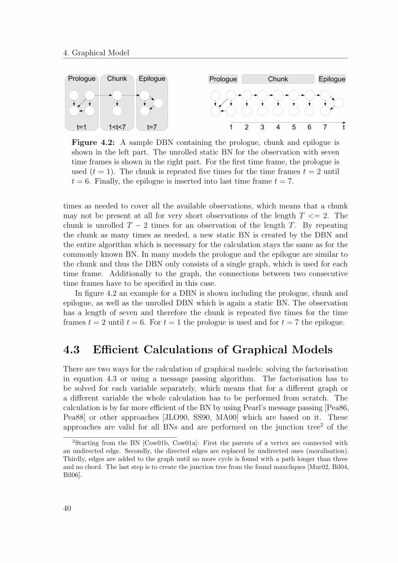
4. Graphical Model
Prologue Chunk EpiloguePrologue Chunk Epilogue
t=1 1<t<7 t=7 1 2 3 4 5 6 7 t
Figure 4.2: A sample DBN containing the prologue, chunk and epilogue isshown in the left part. The unrolled static BN for the observation with seventime frames is shown in the right part. For the first time frame, the prologue isused (t = 1). The chunk is repeated five times for the time frames t = 2 untilt = 6. Finally, the epilogue is inserted into last time frame t = 7.
times as needed to cover all the available observations, which means that a chunkmay not be present at all for very short observations of the length T <= 2. Thechunk is unrolled T − 2 times for an observation of the length T . By repeatingthe chunk as many times as needed, a new static BN is created by the DBN andthe entire algorithm which is necessary for the calculation stays the same as for thecommonly known BN. In many models the prologue and the epilogue are similar tothe chunk and thus the DBN only consists of a single graph, which is used for eachtime frame. Additionally to the graph, the connections between two consecutivetime frames have to be specified in this case.
In figure 4.2 an example for a DBN is shown including the prologue, chunk andepilogue, as well as the unrolled DBN which is again a static BN. The observationhas a length of seven and therefore the chunk is repeated five times for the timeframes t = 2 until t = 6. For t = 1 the prologue is used and for t = 7 the epilogue.
4.3 Efficient Calculations of Graphical Models
There are two ways for the calculation of graphical models: solving the factorisationin equation 4.3 or using a message passing algorithm. The factorisation has tobe solved for each variable separately, which means that for a different graph ora different variable the whole calculation has to be performed from scratch. Thecalculation is by far more efficient of the BN by using Pearl’s message passing [Pea86,Pea88] or other approaches [JLO90, SS90, MA00] which are based on it. Theseapproaches are valid for all BNs and are performed on the junction tree2 of the
2Starting from the BN [Cow01b, Cow01a]: First the parents of a vertex are connected withan undirected edge. Secondly, the directed edges are replaced by undirected ones (moralisation).Thirdly, edges are added to the graph until no more cycle is found with a path longer than threeand no chord. The last step is to create the junction tree from the found maxcliques [Mur02, Bil04,Bil06].
40
4.4. Training of Bayesian Networks
BN [LS88]. Therefore, all variables can be calculated from the junction tree byusing a message passing algorithm.
It is necessary to calculate the probability of the observation sequence (p(~o |λ)),to perform Viterbi-Decoding and to adjust the model parameters (λ) [Rab89] for anefficient calculation of GMs. Viterbi-Decoding [Vit77] is expressed by
~h∗ = argmax~h
p(~h, ~o |λ), (4.5)
and parameter learning is described by
λk = argmaxλ
I∑i=1
log p(~oi |λ), (4.6)
where ~oi is the observation of the i sample from I samples in the data set. The modelparameters λ are learned for example either by a gradient descent procedure [Mur02]
or by the Expectation-Maximisation algorithm (EM) [DLR77]. ~h is the set of hidden
vertices and ~h∗ is the configuration of them with the highest probability of a model.The junction tree of the GM is important for a high performance, as all calculationscan be traced back to an estimation of the status of one or several vertices. Beforethe calculations can be performed, the probabilities of the BN have to be assignedto the according junction tree, since it has been created only by using algorithmsfrom graph theory. This assignment is depending on the selected message passingalgorithm, in this work the HUGIN3 procedure [JLO90, AOJJ90] is used. It is cur-rently the most common message passing procedure and is based on [Pea86, Pea88]as many others, too. The HUGIN procedure is split into the initialisation, which as-signs probabilities to the junction tree, and the global propagation of information toall maxcliques. The initialisation is performed only once while creating the junctiontree. The global propagation is done each time new information is available at anyof the vertices of the junction tree, respectively the graph. This means whenever anew observation arrives at a vertex.
4.4 Training of Bayesian Networks
The training of a BN is performed in two steps. Both steps can be done automaticallyfrom data or the parameters are defined by an expert.
• The structure of the model has to be found, which includes the number ofvertices, the connections between the vertices (edges) and the types of theprobability distributions for each vertex.
3HUGIN stands for Handling Uncertainty in General Inference Network.
41
4. Graphical Model
• The estimation of the parameters of the probability distributions, for examplemean and variance, of each vertex.
In this thesis the structure of the GM is based on expert knowledge. Thereare some approaches which perform this step automatically by analysing the database [Hec01], but these are not used due to the fact that structure learning is verydifficult for dynamic data. At the end of this chapter, various structures, which areused during the training and decoding procedure are described.
Due to the fact, that BNs are applied to pattern recognition problems where datafor training is available, an automatic learning of the parameters of the probabilitydistributions is used in this thesis. Various supervised and unsupervised approachesare known [Hec01, Nea03, Jor01, Gha98, Mur02] for the learning procedure. Sincethe data used is not completely observed, the EM-algorithm [DLR77] is appliedto learn the model parameters. Incomplete data means, that not for all verticestraining data is available or some vertices are hidden. In the next section the learningprocedure is described in more detail.
4.4.1 EM-Training for Bayesian Networks
Often not all variables are observed for dynamic problems of different observationlength and in this case the EM-algorithm is chosen for the training of models, as itdeals with hidden or unknown variables. Overall, the likelihood for a GM with NV
vertices is
L(λ | O) = logI∏i=1
p(~oi |λ) =I∑i=1
NV∑v=1
log fv (xv, pa(xv) |~oi) (4.7)
with I training data samples O = {~o1, . . . , ~oI}. For a BN with hidden vertices thedata-likelihood is described as
L(λ | O) =I∑i=1
logH∑h′=1
p(xh = h′, xo = ~oi), (4.8)
with xh being the set of hidden variables and h′ ∈ {1, . . . , H} describing all pos-sible configurations of them. The current observation is ~oi which is assigned tothe observation variable xo. The optimisation of the function can only be doneby an approximation procedure, because of the sum inside the logarithm. The EM-algorithm [DLR77, Moo96, Bil97, AHR06] is commonly used for this approximations.A new parameter set λ is found by the maximisation of
λ = argmaxλ
Q(λ, λ′) (4.9)
42
4.4. Training of Bayesian Networks
starting with a known parameter set λ′ for the probability distributions of all verticesof the GM. This is the maximisation step of the algorithm, where the initial param-eters λ′ are improved. In [DLR77], it is shown that in case Q(λ, λ′) is maximisedthe data-likelihood L(λ | O) is also maximised. The function Q(λ, λ′) is defined by
Q(λ, λ′) =⟨
log p(O, h′ |λ)⟩O,λ′
=I∑i=1
H∑h′=1
log p(xh = h′, xo = ~oi |λ) p(xh = h′ |xo = ~oi, λ′).
(4.10)
The factorisation of it yields
Q(λ, λ′) =I∑i=1
H∑h′=1
log
NV∏v=1
p(xv | pa(xv), xo = ~oi, x
h = h′) p(xh = h′ |xo = ~oi, λ′)
=I∑i=1
H∑h′=1
NV∑v=1
log p(xv | pa(xv), xo = ~oi, x
h = h′) p(xh = h′ |xo = ~oi, λ′).
(4.11)
p(xh = h′ |xo = ~oi, λ′) is thereby the expectation step of the EM-algorithm, which is
calculated from the junction tree via message passing of any BN. For the expectationstep the updated parameters from the maximisation step are used. Only for the firststep the parameters are chosen randomly. The expectation and maximisation stepsare performed iteratively until the algorithm converges.
4.4.2 Training Structure
In this section, several used training structures of the GMs are described. For all ofthese the production probability of the models is specified and for the training theEM-algorithm is used.
4.4.2.1 Linear Model
The first model is used during the evaluation of pre-segmented data, as it is the casefor both the ABC and AVIC corpuses. It is described in figure 4.3 and selects asingle class for the entire sample. This means, it does not perform any segmentationand only the class with the highest probability for the sample is selected duringevaluation. During the training the frame counter t, class ct and the observation ~otare known. Every other vertex is hidden and the probability distributions of themhave to be learned. Going into more detail of the model structure, it can be seenthat each chunk consists of the vertices frame counter t, class ct, class position qct ,
43
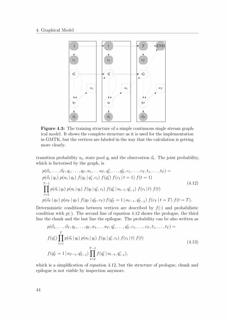
4. Graphical Model
1 t T END
c1 ct cT
qc1 qct qcT
a1 at aT
q1 qt qT
~o1 ~ot ~oT
Figure 4.3: The training structure of a simple continuous single stream graph-ical model. It shows the complete structure as it is used for the implementationin GMTK, but the vertices are labeled in the way that the calculation is gettingmore clearly.
transition probability at, state pool qt and the observation ~ot. The joint probability,which is factorised by the graph, is
p(~o1, . . . , ~oT , q1, . . . , qT , a1, . . . aT , qct , . . . , q
cT , c1, . . . , cT , t1, . . . , tT ) =
p(~o1 | q1) p(a1 | q1) f(q1 | qc1, c1) f(qc1) f(c1 | t = 1) f(t = 1)
T−1∏t=2
p(~ot | qt) p(at | qt) f(qt | qct , ct) f(qct | at−1, qct−1) f(ct | t) f(t)
p(~oT | qT ) p(aT | qT ) f(qT | qcT , cT ) f(qcT = 1 | aT−1, qcT−1) f(cT | t = T ) f(t = T ).
(4.12)
Deterministic conditions between vertices are described by f(·) and probabilisticcondition with p(·). The second line of equation 4.12 shows the prologue, the thirdline the chunk and the last line the epilogue. The probability can be also written as
p(~o1, . . . , ~oT , q1, . . . , qT , a1, . . . aT , qct , . . . , q
cT , c1, . . . , cT , t1, . . . , tT ) =
f(qc1)T∏t=1
p(~ot | qt) p(at | qt) f(qt | qct , ct) f(ct | t) f(t)
f(qcT = 1 | aT−1, qcT−1)T−1∏t=2
f(qct | at−1, qct−1),
(4.13)
which is a simplification of equation 4.12, but the structure of prologue, chunk andepilogue is not visible by inspection anymore.
44
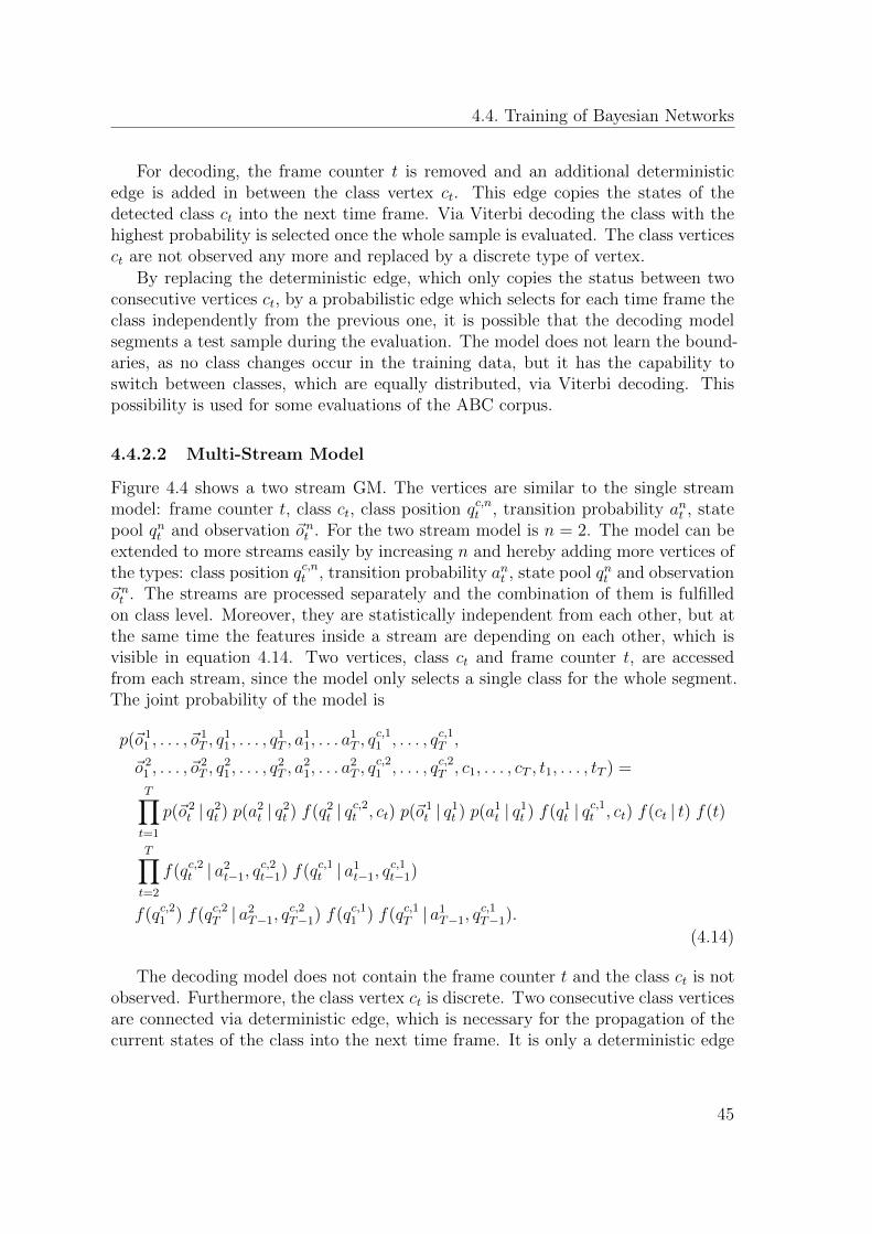
4.4. Training of Bayesian Networks
For decoding, the frame counter t is removed and an additional deterministicedge is added in between the class vertex ct. This edge copies the states of thedetected class ct into the next time frame. Via Viterbi decoding the class with thehighest probability is selected once the whole sample is evaluated. The class verticesct are not observed any more and replaced by a discrete type of vertex.
By replacing the deterministic edge, which only copies the status between twoconsecutive vertices ct, by a probabilistic edge which selects for each time frame theclass independently from the previous one, it is possible that the decoding modelsegments a test sample during the evaluation. The model does not learn the bound-aries, as no class changes occur in the training data, but it has the capability toswitch between classes, which are equally distributed, via Viterbi decoding. Thispossibility is used for some evaluations of the ABC corpus.
4.4.2.2 Multi-Stream Model
Figure 4.4 shows a two stream GM. The vertices are similar to the single streammodel: frame counter t, class ct, class position qc,nt , transition probability ant , statepool qnt and observation ~ont . For the two stream model is n = 2. The model can beextended to more streams easily by increasing n and hereby adding more vertices ofthe types: class position qc,nt , transition probability ant , state pool qnt and observation~ont . The streams are processed separately and the combination of them is fulfilledon class level. Moreover, they are statistically independent from each other, but atthe same time the features inside a stream are depending on each other, which isvisible in equation 4.14. Two vertices, class ct and frame counter t, are accessedfrom each stream, since the model only selects a single class for the whole segment.The joint probability of the model is
p(~o 11 , . . . , ~o
1T , q
11, . . . , q
1T , a
11, . . . a
1T , q
c,11 , . . . , qc,1T ,
~o 21 , . . . , ~o
2T , q
21, . . . , q
2T , a
21, . . . a
2T , q
c,21 , . . . , qc,2T , c1, . . . , cT , t1, . . . , tT ) =
T∏t=1
p(~o 2t | q2t ) p(a2t | q2t ) f(q2t | q
c,2t , ct) p(~o
1t | q1t ) p(a1t | q1t ) f(q1t | q
c,1t , ct) f(ct | t) f(t)
T∏t=2
f(qc,2t | a2t−1, qc,2t−1) f(qc,1t | a1t−1, q
c,1t−1)
f(qc,21 ) f(qc,2T | a2T−1, q
c,2T−1) f(qc,11 ) f(qc,1T | a
1T−1, q
c,1T−1).
(4.14)
The decoding model does not contain the frame counter t and the class ct is notobserved. Furthermore, the class vertex ct is discrete. Two consecutive class verticesare connected via deterministic edge, which is necessary for the propagation of thecurrent states of the class into the next time frame. It is only a deterministic edge
45
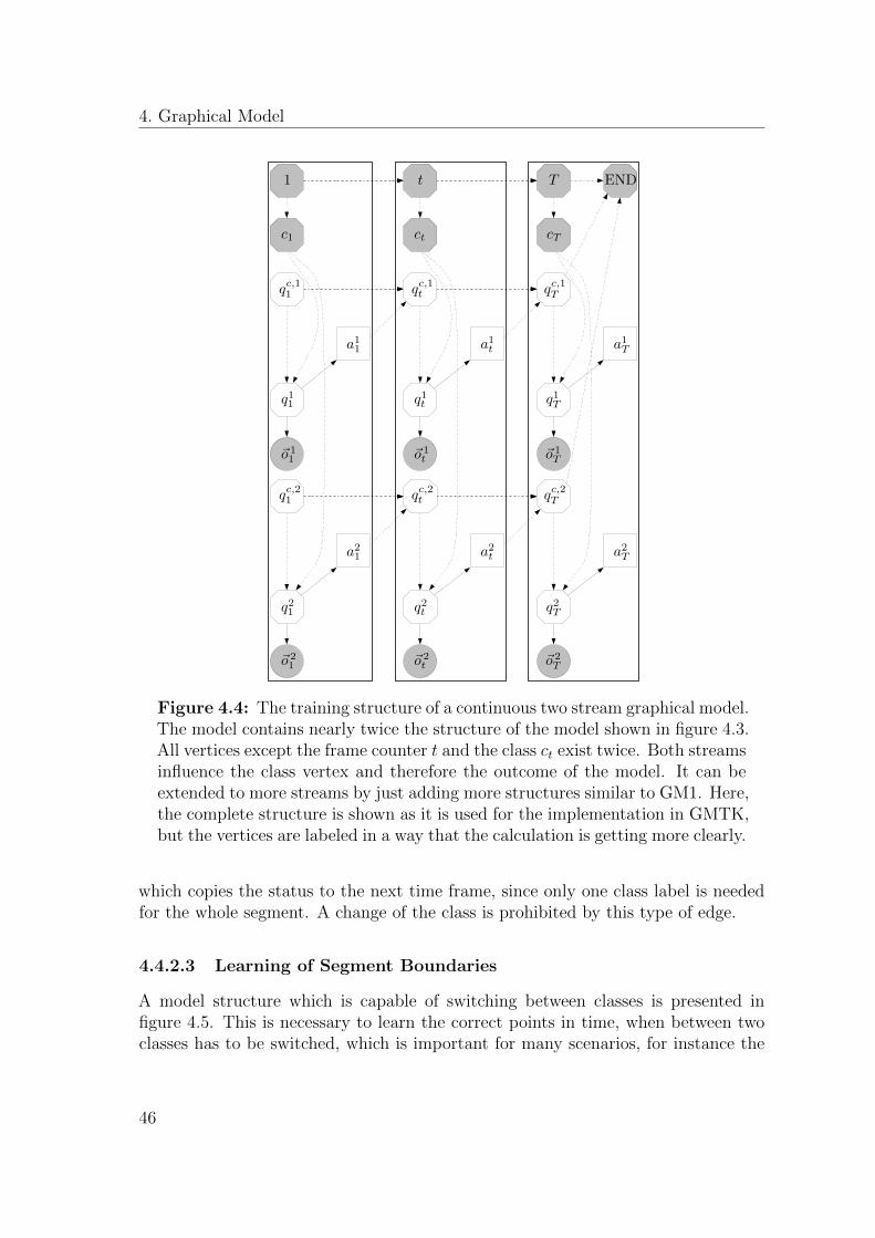
4. Graphical Model
1 t T END
c1 ct cT
qc,11 qc,1t qc,1T
a11 a1t a1T
q11 q1t q1T
~o 11 ~o 1
t ~o 1T
qc,21 qc,2t qc,2T
a21 a2t a2T
q21 q2t q2T
~o 21 ~o 2
t ~o 2T
Figure 4.4: The training structure of a continuous two stream graphical model.The model contains nearly twice the structure of the model shown in figure 4.3.All vertices except the frame counter t and the class ct exist twice. Both streamsinfluence the class vertex and therefore the outcome of the model. It can beextended to more streams by just adding more structures similar to GM1. Here,the complete structure is shown as it is used for the implementation in GMTK,but the vertices are labeled in a way that the calculation is getting more clearly.
which copies the status to the next time frame, since only one class label is neededfor the whole segment. A change of the class is prohibited by this type of edge.
4.4.2.3 Learning of Segment Boundaries
A model structure which is capable of switching between classes is presented infigure 4.5. This is necessary to learn the correct points in time, when between twoclasses has to be switched, which is important for many scenarios, for instance the
46
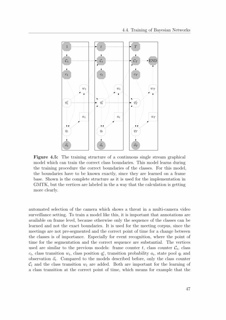
4.4. Training of Bayesian Networks
1 t T
C1 Ct CT END
c1 ct cT
w1 wt wT
qc1 qct qcT
a1 at aT
q1 qt qT
~o1 ~ot ~oT
Figure 4.5: The training structure of a continuous single stream graphicalmodel which can train the correct class boundaries. This model learns duringthe training procedure the correct boundaries of the classes. For this model,the boundaries have to be known exactly, since they are learned on a framebase. Shown is the complete structure as it is used for the implementation inGMTK, but the vertices are labeled in the a way that the calculation is gettingmore clearly.
automated selection of the camera which shows a threat in a multi-camera videosurveillance setting. To train a model like this, it is important that annotations areavailable on frame level, because otherwise only the sequence of the classes can belearned and not the exact boundaries. It is used for the meeting corpus, since themeetings are not pre-segmented and the correct point of time for a change betweenthe classes is of importance. Especially for event recognition, where the point oftime for the segmentation and the correct sequence are substantial. The verticesused are similar to the previous models: frame counter t, class counter Ct, classct, class transition wt, class position qct , transition probability at, state pool qt andobservation ~ot. Compared to the models described before, only the class counterCt and the class transition wt are added. Both are important for the learning ofa class transition at the correct point of time, which means for example that the
47
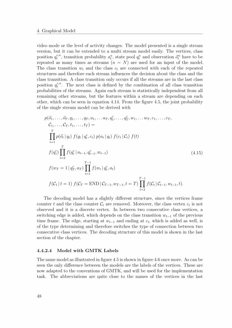
4. Graphical Model
video mode or the level of activity changes. The model presented is a single streamversion, but it can be extended to a multi stream model easily. The vertices, classposition qc,nt , transition probability ant , state pool qnt and observation ~ont have to berepeated as many times as streams (n = N) are used for an input of the model.The class transition wt and the class ct are connected with each of the repeatedstructures and therefore each stream influences the decision about the class and theclass transition. A class transition only occurs if all the streams are in the last classposition qc,nt . The next class is defined by the combination of all class transitionprobabilities of the streams. Again each stream is statistically independent from allremaining other streams, but the features within a stream are depending on eachother, which can be seen in equation 4.14. From the figure 4.5, the joint probabilityof the single stream model can be derived with
p(~o1, . . . , ~oT , q1, . . . , qT , a1, . . . aT , qc1, . . . , q
cT , w1, . . . wT , c1, . . . , cT ,
C1, . . . , CT , t1, . . . , tT ) =
T∏t=1
p(~ot | qt) f(qt | qct , ct) p(at | qt) f(ct | Ct) f(t)
f(qc1)T∏t=2
f(qct | at−1, qct−1, wt−1)
f(wT = 1 | qcT , aT )T−1∏t=1
f(wt | qct , at)
f(C1 | t = 1) f(CT = END | CT−1, wT−1, t = T )T−1∏t=2
f(Ct | Ct−1, wt−1, t).
(4.15)
The decoding model has a slightly different structure, since the vertices framecounter t and the class counter Ct are removed. Moreover, the class vertex ct is notobserved and it is a discrete vertex. In between two consecutive class vertices, aswitching edge is added, which depends on the class transition wt−1 of the previoustime frame. The edge, starting at wt−1 and ending at ct, which is added as well, isof the type determining and therefore switches the type of connection between twoconsecutive class vertices. The decoding structure of this model is shown in the lastsection of the chapter.
4.4.2.4 Model with GMTK Labels
The same model as illustrated in figure 4.5 is shown in figure 4.6 once more. As can beseen the only difference between the models are the labels of the vertices. These arenow adapted to the conventions of GMTK, and will be used for the implementationtask. The abbreviations are quite close to the names of the vertices in the last
48
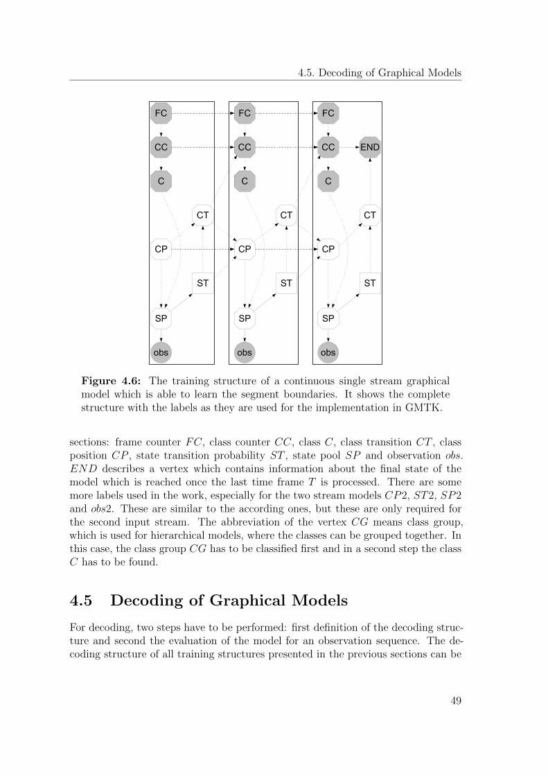
4.5. Decoding of Graphical Models
obs
SP
obs
SP
ST
CP
obs
SP
ST
CP
ST
CT
END
CP
C
FC FCFC
CT
CC
CT
CCCC
C C
Figure 4.6: The training structure of a continuous single stream graphicalmodel which is able to learn the segment boundaries. It shows the completestructure with the labels as they are used for the implementation in GMTK.
sections: frame counter FC, class counter CC, class C, class transition CT , classposition CP , state transition probability ST , state pool SP and observation obs.END describes a vertex which contains information about the final state of themodel which is reached once the last time frame T is processed. There are somemore labels used in the work, especially for the two stream models CP2, ST2, SP2and obs2. These are similar to the according ones, but these are only required forthe second input stream. The abbreviation of the vertex CG means class group,which is used for hierarchical models, where the classes can be grouped together. Inthis case, the class group CG has to be classified first and in a second step the classC has to be found.
4.5 Decoding of Graphical Models
For decoding, two steps have to be performed: first definition of the decoding struc-ture and second the evaluation of the model for an observation sequence. The de-coding structure of all training structures presented in the previous sections can be
49
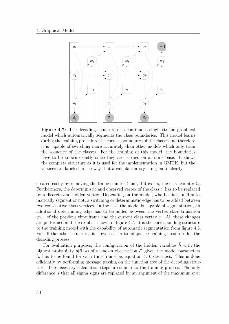
4. Graphical Model
c1 ct cT = 1
w1 wt wT
qc1 qct qcT
a1 at aT
q1 qt qT
~o1 ~ot ~oT
Figure 4.7: The decoding structure of a continuous single stream graphicalmodel which automatically segments the class boundaries. This model learnsduring the training procedure the correct boundaries of the classes and thereforeit is capable of switching more accurately than other models which only trainthe sequence of the classes. For the training of this model, the boundarieshave to be known exactly since they are learned on a frame base. It showsthe complete structure as it is used for the implementation in GMTK, but thevertices are labeled in the way that a calculation is getting more clearly.
created easily by removing the frame counter t and, if it exists, the class counter Ct.Furthermore, the deterministic and observed vertex of the class ct has to be replacedby a discrete and hidden vertex. Depending on the model, whether it should auto-matically segment or not, a switching or deterministic edge has to be added betweentwo consecutive class vertices. In the case the model is capable of segmentation, anadditional determining edge has to be added between the vertex class transitionwt−1 of the previous time frame and the current class vertex ct. All these changesare performed and the result is shown in figure 4.7. It is the corresponding structureto the training model with the capability of automatic segmentation from figure 4.5.For all the other structures it is even easier to adapt the training structure for thedecoding process.
For evaluation purposes, the configuration of the hidden variables ~h with thehighest probability p(~o |λ) of a known observation ~o, given the model parametersλ, has to be found for each time frame, as equation 4.16 describes. This is doneefficiently by performing message passing on the junction tree of the decoding struc-ture. The necessary calculation steps are similar to the training process. The onlydifference is that all sigma signs are replaced by an argument of the maximum over
50
4.6. Evaluation of the Different Model Structures
the hidden variables of the graphical model ~h. This means, that in each time frameall possible configurations, which are leading to a state of the model, are evaluatedand compared. After that, for each state the path with the highest probability ispursued into the next time frame. This procedure is continued until only a singlepath exists, which is described by the sequence of the best fitting configurations ~h∗
and has the highest probability for the evaluated observations ~o. This procedure isknown as Viterbi-Decoding [Vit77] and is formulateded as follows
~h∗ = argmax~h
p(~h, ~o |λ). (4.16)
4.6 Evaluation of the Different Model Structures
The evaluation always contains both the learning and the testing of a model. There-fore, it is necessary to develop a training structure and the according decodingstructure. Different parameters can be adjusted, for example the number of states,Gaussian mixtures and iterations of EM-algorithm. Moreover, the input data streamcan be varied, which means different feature sets are evaluated. Except the numberof iterations of the EM-algorithm all other parameters influence the model structure,which has to be adapted for the training and decoding structure simultaneously. Ifthe number of states per class is changed, which means the state pool vertex qt hasa different size, also the class position gkt and the transition probability at have tobe adjusted accordingly. More Gaussian mixtures usually mean that the observa-tion vertex ~ot has to be changed. If other feature sets are evaluated as an inputto the structure with a different number of features, the observation vertex ~ot hasto be adapted again. All these adaptations to the structure can be automaticallyperformed in case the number of features used as an input is known and the numberof states and the number of Gaussian mixtures are predefined.
51

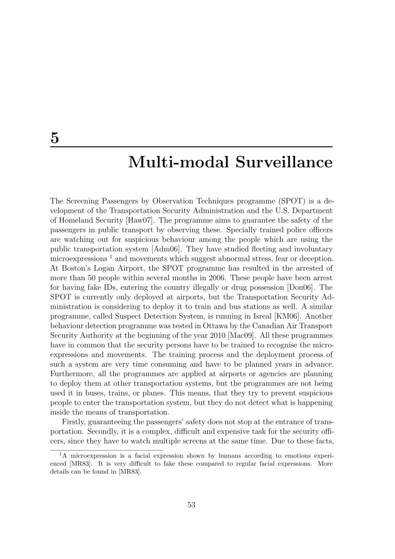
5
Multi-modal Surveillance
The Screening Passengers by Observation Techniques programme (SPOT) is a de-velopment of the Transportation Security Administration and the U.S. Departmentof Homeland Security [Haw07]. The programme aims to guarantee the safety of thepassengers in public transport by observing these. Specially trained police officersare watching out for suspicious behaviour among the people which are using thepublic transportation system [Adm06]. They have studied fleeting and involuntarymicroexpressions 1 and movements which suggest abnormal stress, fear or deception.At Boston’s Logan Airport, the SPOT programme has resulted in the arrested ofmore than 50 people within several months in 2006. These people have been arrestfor having fake IDs, entering the country illegally or drug possession [Don06]. TheSPOT is currently only deployed at airports, but the Transportation Security Ad-ministration is considering to deploy it to train and bus stations as well. A similarprogramme, called Suspect Detection System, is running in Isreal [KM06]. Anotherbehaviour detection programme was tested in Ottawa by the Canadian Air TransportSecurity Authority at the beginning of the year 2010 [Mac09]. All these programmeshave in common that the security persons have to be trained to recognise the micro-expressions and movements. The training process and the deployment process ofsuch a system are very time consuming and have to be planned years in advance.Furthermore, all the programmes are applied at airports or agencies are planningto deploy them at other transportation systems, but the programmes are not beingused it in buses, trains, or planes. This means, that they try to prevent suspiciouspeople to enter the transportation system, but they do not detect what is happeninginside the means of transportation.
Firstly, guaranteeing the passengers’ safety does not stop at the entrance of trans-portation. Secondly, it is a complex, difficult and expensive task for the security offi-cers, since they have to watch multiple screens at the same time. Due to these facts,
1A microexpression is a facial expression shown by humans according to emotions experi-enced [MR83]. It is very difficult to fake these compared to regular facial expressions. Moredetails can be found in [MR83].
53
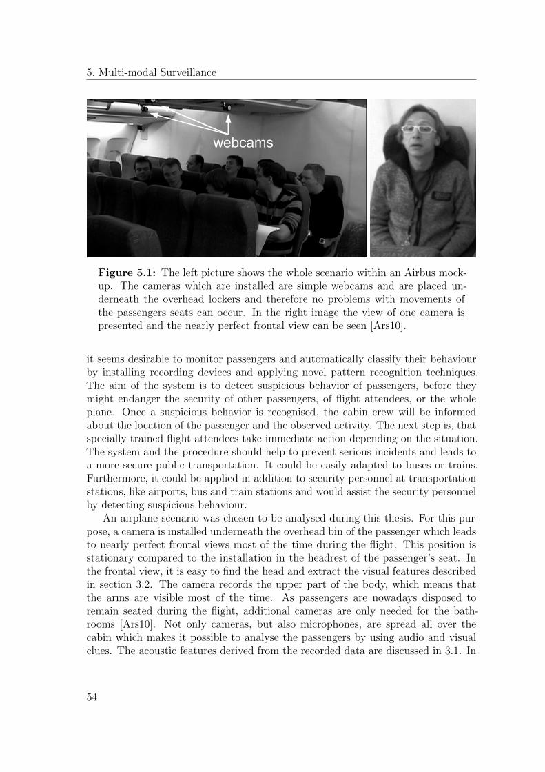
5. Multi-modal Surveillance
webcams
Figure 5.1: The left picture shows the whole scenario within an Airbus mock-up. The cameras which are installed are simple webcams and are placed un-derneath the overhead lockers and therefore no problems with movements ofthe passengers seats can occur. In the right image the view of one camera ispresented and the nearly perfect frontal view can be seen [Ars10].
it seems desirable to monitor passengers and automatically classify their behaviourby installing recording devices and applying novel pattern recognition techniques.The aim of the system is to detect suspicious behavior of passengers, before theymight endanger the security of other passengers, of flight attendees, or the wholeplane. Once a suspicious behavior is recognised, the cabin crew will be informedabout the location of the passenger and the observed activity. The next step is, thatspecially trained flight attendees take immediate action depending on the situation.The system and the procedure should help to prevent serious incidents and leads toa more secure public transportation. It could be easily adapted to buses or trains.Furthermore, it could be applied in addition to security personnel at transportationstations, like airports, bus and train stations and would assist the security personnelby detecting suspicious behaviour.
An airplane scenario was chosen to be analysed during this thesis. For this pur-pose, a camera is installed underneath the overhead bin of the passenger which leadsto nearly perfect frontal views most of the time during the flight. This position isstationary compared to the installation in the headrest of the passenger’s seat. Inthe frontal view, it is easy to find the head and extract the visual features describedin section 3.2. The camera records the upper part of the body, which means thatthe arms are visible most of the time. As passengers are nowadays disposed toremain seated during the flight, additional cameras are only needed for the bath-rooms [Ars10]. Not only cameras, but also microphones, are spread all over thecabin which makes it possible to analyse the passengers by using audio and visualclues. The acoustic features derived from the recorded data are discussed in 3.1. In
54
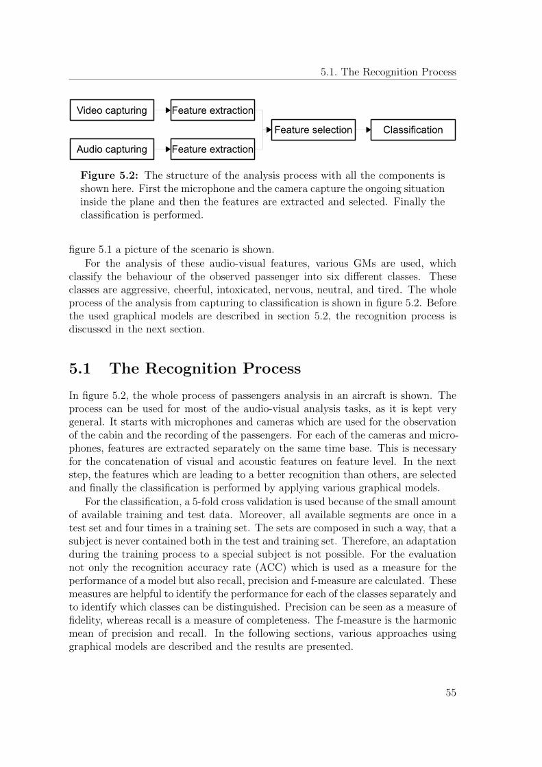
5.1. The Recognition Process
Video capturing
Audio capturing
Feature extraction
Feature extraction
Feature selection Classification
Figure 5.2: The structure of the analysis process with all the components isshown here. First the microphone and the camera capture the ongoing situationinside the plane and then the features are extracted and selected. Finally theclassification is performed.
figure 5.1 a picture of the scenario is shown.
For the analysis of these audio-visual features, various GMs are used, whichclassify the behaviour of the observed passenger into six different classes. Theseclasses are aggressive, cheerful, intoxicated, nervous, neutral, and tired. The wholeprocess of the analysis from capturing to classification is shown in figure 5.2. Beforethe used graphical models are described in section 5.2, the recognition process isdiscussed in the next section.
5.1 The Recognition Process
In figure 5.2, the whole process of passengers analysis in an aircraft is shown. Theprocess can be used for most of the audio-visual analysis tasks, as it is kept verygeneral. It starts with microphones and cameras which are used for the observationof the cabin and the recording of the passengers. For each of the cameras and micro-phones, features are extracted separately on the same time base. This is necessaryfor the concatenation of visual and acoustic features on feature level. In the nextstep, the features which are leading to a better recognition than others, are selectedand finally the classification is performed by applying various graphical models.
For the classification, a 5-fold cross validation is used because of the small amountof available training and test data. Moreover, all available segments are once in atest set and four times in a training set. The sets are composed in such a way, that asubject is never contained both in the test and training set. Therefore, an adaptationduring the training process to a special subject is not possible. For the evaluationnot only the recognition accuracy rate (ACC) which is used as a measure for theperformance of a model but also recall, precision and f-measure are calculated. Thesemeasures are helpful to identify the performance for each of the classes separately andto identify which classes can be distinguished. Precision can be seen as a measure offidelity, whereas recall is a measure of completeness. The f-measure is the harmonicmean of precision and recall. In the following sections, various approaches usinggraphical models are described and the results are presented.
55
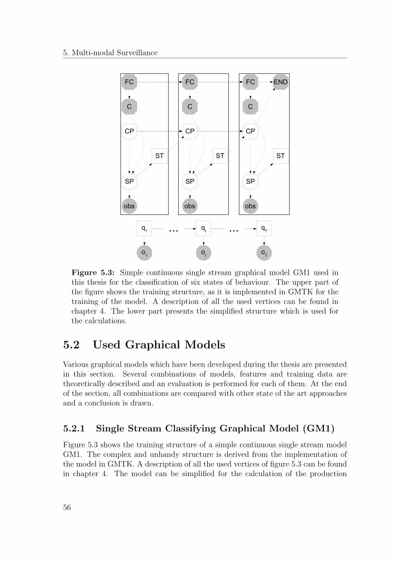
5. Multi-modal Surveillance
obs
SP
obs
SP
ST
CP
obs
SP
ST ST
END
CP
C
FC FCFC
CP
C C
o1
q1
ot
qt
oT
qT... ...
Figure 5.3: Simple continuous single stream graphical model GM1 used inthis thesis for the classification of six states of behaviour. The upper part ofthe figure shows the training structure, as it is implemented in GMTK for thetraining of the model. A description of all the used vertices can be found inchapter 4. The lower part presents the simplified structure which is used forthe calculations.
5.2 Used Graphical Models
Various graphical models which have been developed during the thesis are presentedin this section. Several combinations of models, features and training data aretheoretically described and an evaluation is performed for each of them. At the endof the section, all combinations are compared with other state of the art approachesand a conclusion is drawn.
5.2.1 Single Stream Classifying Graphical Model (GM1)
Figure 5.3 shows the training structure of a simple continuous single stream modelGM1. The complex and unhandy structure is derived from the implementation ofthe model in GMTK. A description of all the used vertices of figure 5.3 can be foundin chapter 4. The model can be simplified for the calculation of the production
56
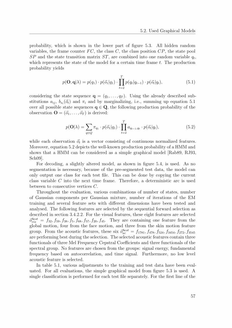
5.2. Used Graphical Models
probability, which is shown in the lower part of figure 5.3. All hidden randomvariables, the frame counter FC, the class C, the class position CP , the state poolSP and the state transition matrix ST , are combined into one random variable qt,which represents the state of the model for a certain time frame t. The productionprobability yields
p(O,q|λ) = p(q1) · p(~o1|q1) ·T∏t=2
p(qt|qt−1) · p(~ot|qt), (5.1)
considering the state sequence q = (q1, . . . , qT ). Using the already described sub-stitutions aij, bsi(~ot) and πi and by marginalizing, i.e., summing up equation 5.1over all possible state sequences q ∈ Q, the following production probability of theobservation O = (~o1, . . . , ~oT ) is derived:
p(O|λ) =∑q∈Q
πq1 · p(~o1|q1) ·T∏t=2
aqt−1,qt · p(~ot|qt), (5.2)
while each observation ~ot is a vector consisting of continuous normalized features.Moreover, equation 5.2 depicts the well-known production probability of a HMM andshows that a HMM can be considered as a simple graphical model [Rab89, RJ93,Sch09].
For decoding, a slightly altered model, as shown in figure 5.4, is used. As nosegmentation is necessary, because of the pre-segmented test data, the model canonly output one class for each test file. This can be done by copying the currentclass variable C into the next time frame. Therefore, a deterministic arc is usedbetween to consecutive vertices C.
Throughout the evaluation, various combinations of number of states, numberof Gaussian components per Gaussian mixture, number of iterations of the EMtraining and several feature sets with different dimensions have been tested andanalysed. The following features are selected by the sequential forward selection asdescribed in section 3.4.2.2. For the visual features, these eight features are selected~o bestvis = f32, f59, f38, f5, f68, f57, f20, f45. They are containing one feature from theglobal motion, four from the face motion, and three from the skin motion featuregroup. From the acoustic features, these six ~o bestac = f1781, f478, f524, f3454, f272, f3545are performing best during the selection. The selected acoustic features contain threefunctionals of three Mel Frequency Cepstral Coefficients and three functionals of thespectral group. No features are chosen from the groups: signal energy, fundamentalfrequency based on autocorrelation, and time signal. Furthermore, no low levelacoustic feature is selected.
In table 5.1, various adjustments to the training and test data have been eval-uated. For all evaluations, the simple graphical model from figure 5.3 is used. Asingle classification is performed for each test file separately. For the first line of the
57
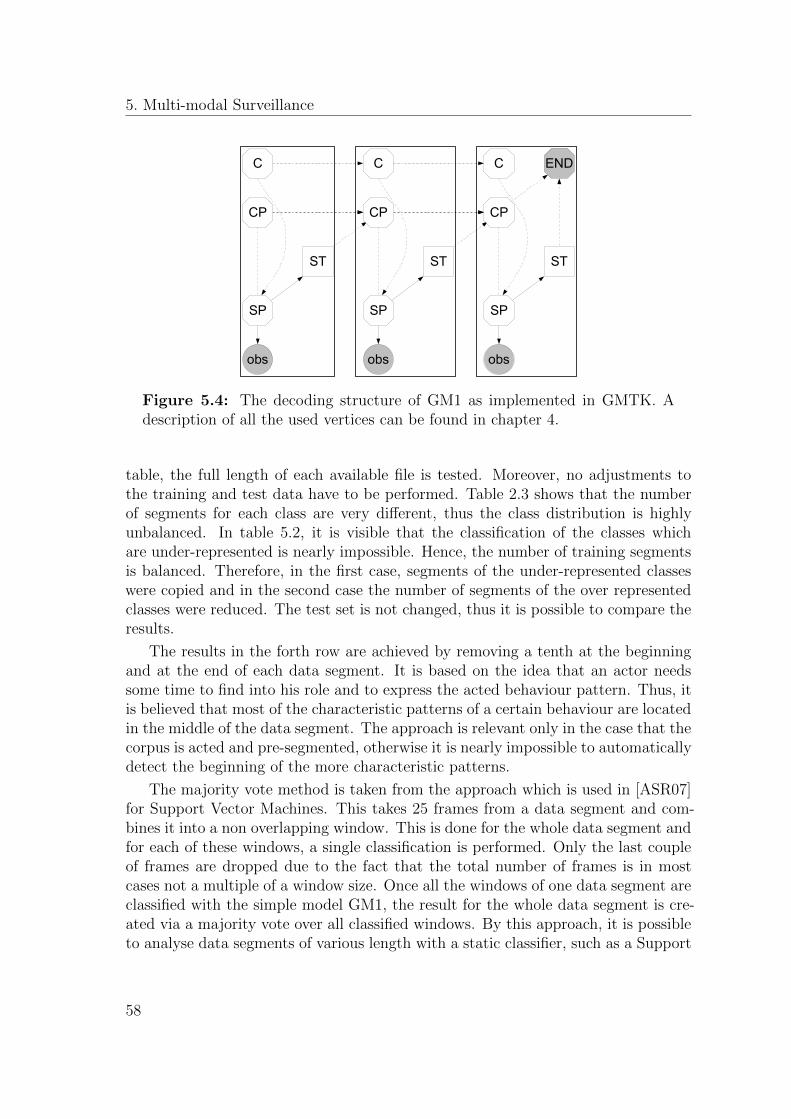
5. Multi-modal Surveillance
obs
SP
obs
SP
ST
CP
obs
SP
ST
CP
ST
END
CP
C C C
Figure 5.4: The decoding structure of GM1 as implemented in GMTK. Adescription of all the used vertices can be found in chapter 4.
table, the full length of each available file is tested. Moreover, no adjustments tothe training and test data have to be performed. Table 2.3 shows that the numberof segments for each class are very different, thus the class distribution is highlyunbalanced. In table 5.2, it is visible that the classification of the classes whichare under-represented is nearly impossible. Hence, the number of training segmentsis balanced. Therefore, in the first case, segments of the under-represented classeswere copied and in the second case the number of segments of the over representedclasses were reduced. The test set is not changed, thus it is possible to compare theresults.
The results in the forth row are achieved by removing a tenth at the beginningand at the end of each data segment. It is based on the idea that an actor needssome time to find into his role and to express the acted behaviour pattern. Thus, itis believed that most of the characteristic patterns of a certain behaviour are locatedin the middle of the data segment. The approach is relevant only in the case that thecorpus is acted and pre-segmented, otherwise it is nearly impossible to automaticallydetect the beginning of the more characteristic patterns.
The majority vote method is taken from the approach which is used in [ASR07]for Support Vector Machines. This takes 25 frames from a data segment and com-bines it into a non overlapping window. This is done for the whole data segment andfor each of these windows, a single classification is performed. Only the last coupleof frames are dropped due to the fact that the total number of frames is in mostcases not a multiple of a window size. Once all the windows of one data segment areclassified with the simple model GM1, the result for the whole data segment is cre-ated via a majority vote over all classified windows. By this approach, it is possibleto analyse data segments of various length with a static classifier, such as a Support
58
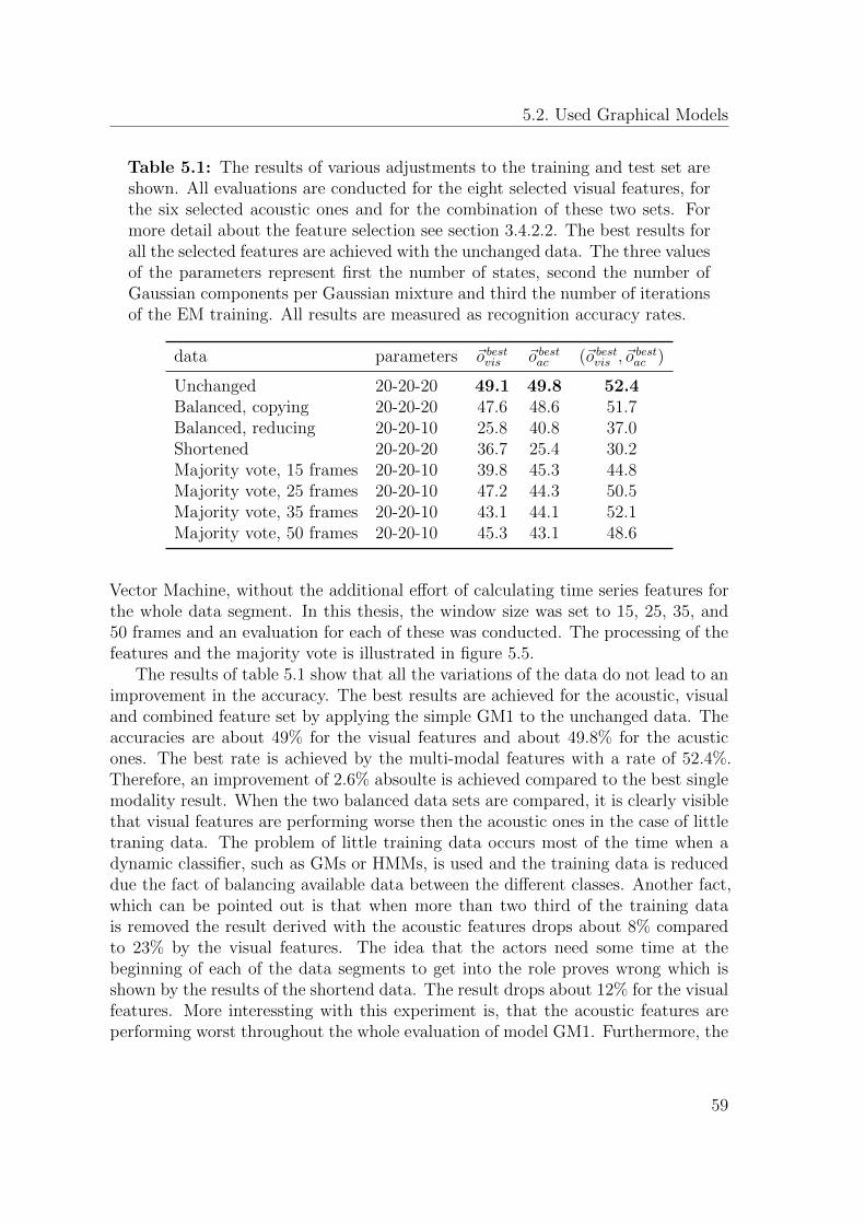
5.2. Used Graphical Models
Table 5.1: The results of various adjustments to the training and test set areshown. All evaluations are conducted for the eight selected visual features, forthe six selected acoustic ones and for the combination of these two sets. Formore detail about the feature selection see section 3.4.2.2. The best results forall the selected features are achieved with the unchanged data. The three valuesof the parameters represent first the number of states, second the number ofGaussian components per Gaussian mixture and third the number of iterationsof the EM training. All results are measured as recognition accuracy rates.
data parameters ~o bestvis ~o bestac (~o bestvis , ~obestac )
Unchanged 20-20-20 49.1 49.8 52.4Balanced, copying 20-20-20 47.6 48.6 51.7Balanced, reducing 20-20-10 25.8 40.8 37.0Shortened 20-20-20 36.7 25.4 30.2Majority vote, 15 frames 20-20-10 39.8 45.3 44.8Majority vote, 25 frames 20-20-10 47.2 44.3 50.5Majority vote, 35 frames 20-20-10 43.1 44.1 52.1Majority vote, 50 frames 20-20-10 45.3 43.1 48.6
Vector Machine, without the additional effort of calculating time series features forthe whole data segment. In this thesis, the window size was set to 15, 25, 35, and50 frames and an evaluation for each of these was conducted. The processing of thefeatures and the majority vote is illustrated in figure 5.5.
The results of table 5.1 show that all the variations of the data do not lead to animprovement in the accuracy. The best results are achieved for the acoustic, visualand combined feature set by applying the simple GM1 to the unchanged data. Theaccuracies are about 49% for the visual features and about 49.8% for the acusticones. The best rate is achieved by the multi-modal features with a rate of 52.4%.Therefore, an improvement of 2.6% absoulte is achieved compared to the best singlemodality result. When the two balanced data sets are compared, it is clearly visiblethat visual features are performing worse then the acoustic ones in the case of littletraning data. The problem of little training data occurs most of the time when adynamic classifier, such as GMs or HMMs, is used and the training data is reduceddue the fact of balancing available data between the different classes. Another fact,which can be pointed out is that when more than two third of the training datais removed the result derived with the acoustic features drops about 8% comparedto 23% by the visual features. The idea that the actors need some time at thebeginning of each of the data segments to get into the role proves wrong which isshown by the results of the shortend data. The result drops about 12% for the visualfeatures. More interessting with this experiment is, that the acoustic features areperforming worst throughout the whole evaluation of model GM1. Furthermore, the
59
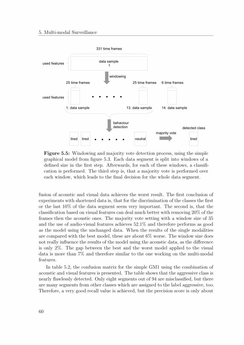
5. Multi-modal Surveillance
used features data sample 1
331 time frames
used features
25 time frames 25 time frames
windowing
behaviour detection
tired
1. data sample 13. data sample
neutraltiredmajority vote
tired
detected class
6 time frames
14. data sample
Figure 5.5: Windowing and majority vote detection process, using the simplegraphical model from figure 5.3. Each data segment is split into windows of adefined size in the first step. Afterwards, for each of these windows, a classifi-cation is performed. The third step is, that a majority vote is performed overeach window, which leads to the final decision for the whole data segment.
fusion of acoustic and visual data achieves the worst result. The first conclusion ofexperiments with shortened data is, that for the discrimination of the classes the firstor the last 10% of the data segment seem very important. The second is, that theclassification based on visual features can deal much better with removing 20% of theframes then the acoustic ones. The majority vote setting with a window size of 35and the use of audio-visual features achieves 52.1% and therefore performs as goodas the model using the unchanged data. When the results of the single modalitiesare compared with the best model, these are about 6% worse. The window size doesnot really influence the results of the model using the acoustic data, as the differenceis only 2%. The gap between the best and the worst model applied to the visualdata is more than 7% and therefore similar to the one working on the multi-modalfeatures.
In table 5.2, the confusion matrix for the simple GM1 using the combination ofacoustic and visual features is presented. The table shows that the aggressive class isnearly flawlessly detected. Only eight segments out of 94 are misclassified, but thereare many segments from other classes which are assigned to the label aggressive, too.Therefore, a very good recall value is achieved, but the precision score is only about
60
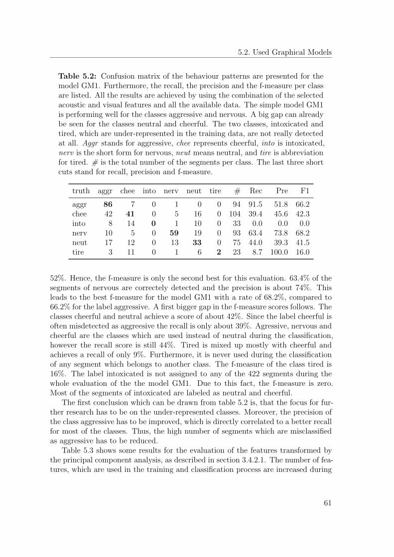
5.2. Used Graphical Models
Table 5.2: Confusion matrix of the behaviour patterns are presented for themodel GM1. Furthermore, the recall, the precision and the f-measure per classare listed. All the results are achieved by using the combination of the selectedacoustic and visual features and all the available data. The simple model GM1is performing well for the classes aggressive and nervous. A big gap can alreadybe seen for the classes neutral and cheerful. The two classes, intoxicated andtired, which are under-represented in the training data, are not really detectedat all. Aggr stands for aggressive, chee represents cheerful, into is intoxicated,nerv is the short form for nervous, neut means neutral, and tire is abbreviationfor tired. # is the total number of the segments per class. The last three shortcuts stand for recall, precision and f-measure.
truth aggr chee into nerv neut tire # Rec Pre F1
aggr 86 7 0 1 0 0 94 91.5 51.8 66.2chee 42 41 0 5 16 0 104 39.4 45.6 42.3into 8 14 0 1 10 0 33 0.0 0.0 0.0nerv 10 5 0 59 19 0 93 63.4 73.8 68.2neut 17 12 0 13 33 0 75 44.0 39.3 41.5tire 3 11 0 1 6 2 23 8.7 100.0 16.0
52%. Hence, the f-measure is only the second best for this evaluation. 63.4% of thesegments of nervous are correctely detected and the precision is about 74%. Thisleads to the best f-measure for the model GM1 with a rate of 68.2%, compared to66.2% for the label aggressive. A first bigger gap in the f-measure scores follows. Theclasses cheerful and neutral achieve a score of about 42%. Since the label cheerful isoften misdetected as aggreesive the recall is only about 39%. Agressive, nervous andcheerful are the classes which are used instead of neutral during the classification,however the recall score is still 44%. Tired is mixed up mostly with cheerful andachieves a recall of only 9%. Furthermore, it is never used during the classificationof any segment which belongs to another class. The f-measure of the class tired is16%. The label intoxicated is not assigned to any of the 422 segments during thewhole evaluation of the the model GM1. Due to this fact, the f-measure is zero.Most of the segments of intoxicated are labeled as neutral and cheerful.
The first conclusion which can be drawn from table 5.2 is, that the focus for fur-ther research has to be on the under-represented classes. Moreover, the precision ofthe class aggressive has to be improved, which is directly correlated to a better recallfor most of the classes. Thus, the high number of segments which are misclassifiedas aggressive has to be reduced.
Table 5.3 shows some results for the evaluation of the features transformed bythe principal component analysis, as described in section 3.4.2.1. The number of fea-tures, which are used in the training and classification process are increased during
61
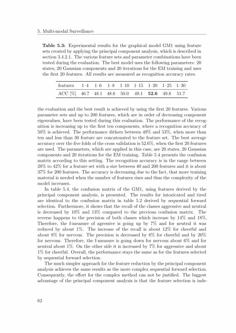
5. Multi-modal Surveillance
Table 5.3: Experimental results for the graphical model GM1 using featuresets created by applying the principal component analysis, which is described insection 3.4.2.1. The various feature sets and parameter combinations have beentested during the evaluation. The best model uses the following parameters: 20states, 20 Gaussian components and 20 iterations for the EM training and usesthe first 20 features. All results are measured as recognition accuracy rates.
features 1–4 1–6 1–8 1–10 1–15 1–20 1–25 1–30
ACC [%] 46.7 48.1 48.6 50.0 49.1 52.6 49.8 51.7
the evaluation and the best result is achieved by using the first 20 features. Variousparameter sets and up to 200 features, which are in order of decreasing componenteigenvalues, have been tested during this evaluation. The performance of the recog-nition is increasing up to the first ten components, where a recognition accuracy of50% is achieved. The performance dithers between 49% and 53%, when more thanten and less than 30 feature are concatenated to the feature set. The best averageaccuracy over the five folds of the cross validation is 52.6%, when the first 20 featuresare used. The parameters, which are applied in this case, are 20 states, 20 Gaussiancomponents and 20 iterations for the EM training. Table 5.4 presents the confusionmatrix according to this setting. The recognition accuracy is in the range between28% to 42% for a feature set with a size between 40 and 200 features and it is about37% for 200 features. The accuracy is decreasing due to the fact, that more trainingmaterial is needed when the number of features rises and thus the complexity of themodel increases.
In table 5.4, the confusion matrix of the GM1, using features derived by theprincipal component analysis, is presented. The results for intoxicated and tiredare identical to the confusion matrix in table 5.2 derived by sequential forwardselection. Furthermore, it shows that the recall of the classes aggressive and neutralis decreased by 10% and 13% compared to the previous confusion matrix. Thereverse happens to the precision of both classes which increase by 14% and 18%.Therefore, the f-measure of agressive is going up by 7% and for neutral it wasreduced by about 1%. The increase of the recall is about 12% for cheerful andabout 8% for nervous. The precision is decreased by 8% for cheerful and by 20%for nervous. Therefore, the f-measure is going down for nervous about 6% and forneutral about 1%. On the other side it is increased by 7% for aggressive and about1% for cheerful. Overall, the performance stays the same as for the features selectedby sequential forward selection.
The much simpler approach for the feature reduction by the principal componentanalysis achieves the same results as the more complex sequential forward selection.Consequently, the effort for the complex method can not be justified. The biggestadvantage of the principal component analysis is that the feature selection is inde-
62
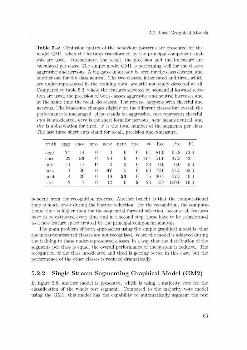
5.2. Used Graphical Models
Table 5.4: Confusion matrix of the behaviour patterns are presented for themodel GM1, when the features transformed by the principal component anal-ysis are used. Furthermore, the recall, the precision and the f-measure arecalculated per class. The simple model GM1 is performing well for the classesaggressive and nervous. A big gap can already be seen for the class cheerful andanother one for the class neutral. The two classes, intoxicated and tired, whichare under-represented in the training data, are still not really detected at all.Compared to table 5.2, where the features selected by sequential forward selec-tion are used, the precision of both classes aggressive and neutral increases andat the same time the recall decreases. The reverse happens with cheerful andnervous. The f-measure changes slightly for the different classes but overall theperformance is unchanged. Aggr stands for aggressive, chee represents cheerful,into is intoxicated, nerv is the short form for nervous, neut means neutral, andtire is abbreviation for tired. # is the total number of the segments per class.The last three short cuts stand for recall, precision and f-measure.
truth aggr chee into nerv neut tire # Rec Pre F1
aggr 77 14 0 3 0 0 94 81.9 65.8 73.0chee 22 53 0 20 9 0 104 51.0 37.3 43.1into 11 17 0 2 3 0 33 0.0 0.0 0.0nerv 1 20 0 67 5 0 93 72.0 54.5 62.0neut 4 29 0 19 23 0 75 30.7 57.5 40.0tire 2 7 0 12 0 2 23 8.7 100.0 16.0
pendent from the recognition process. Another benefit is that the computationaltime is much lower during the feature reduction. For the recognition, the computa-tional time is higher than for the sequential forward selection, because all featureshave to be extracted every time and in a second step, these have to be transformedto a new feature space created by the principal component analysis.
The main problem of both approaches using the simple graphical model is, thatthe under-represented classes are not recognised. When the model is adapted duringthe training to these under-represented classes, in a way that the distribution of thesegments per class is equal, the overall performance of the system is reduced. Therecognition of the class intoxicated and tired is getting better in this case, but theperformance of the other classes is reduced dramatically.
5.2.2 Single Stream Segmenting Graphical Model (GM2)
In figure 5.6, another model is presented, which is using a majority vote for theclassification of the whole test segment. Compared to the majority vote modelusing the GM1, this model has the capability to automatically segment the test
63
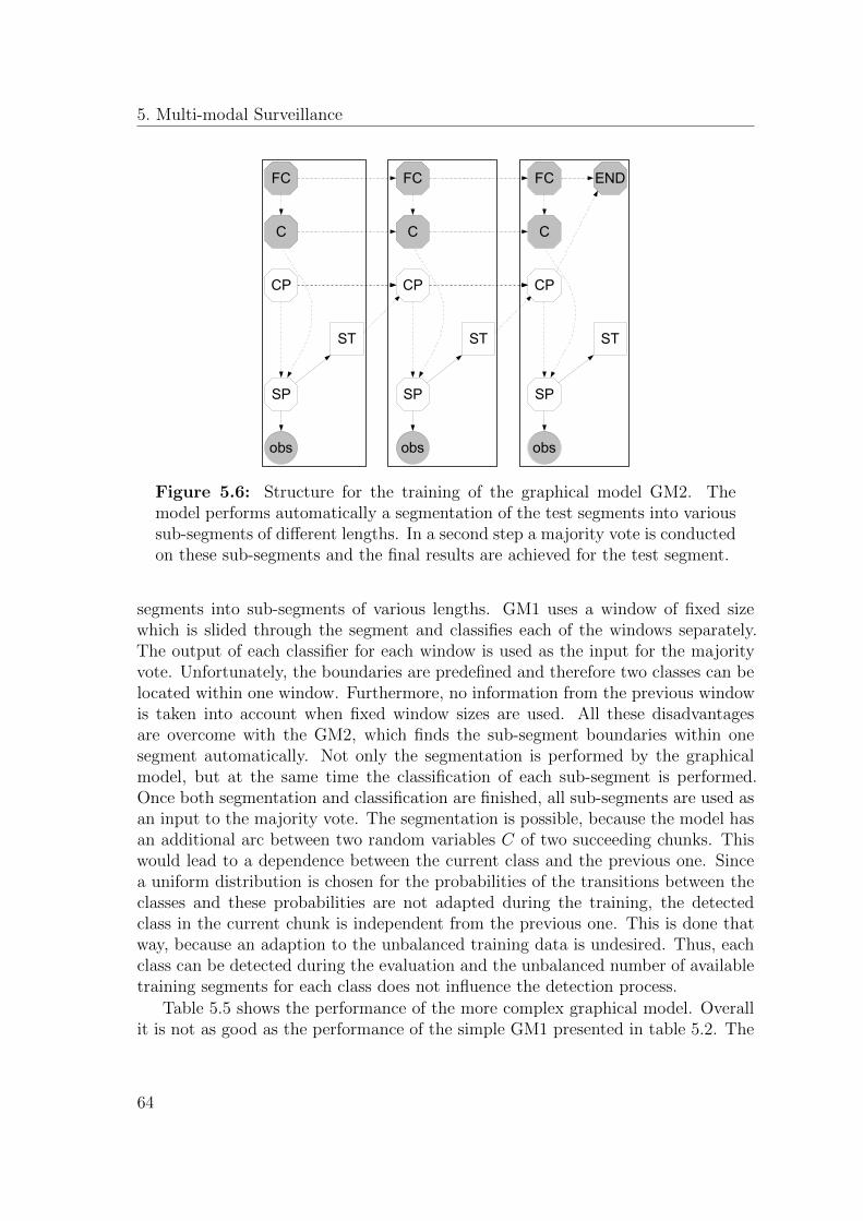
5. Multi-modal Surveillance
obs
SP
obs
SP
ST
CP
obs
SP
ST ST
END
CP
C
FC FCFC
CP
C C
Figure 5.6: Structure for the training of the graphical model GM2. Themodel performs automatically a segmentation of the test segments into varioussub-segments of different lengths. In a second step a majority vote is conductedon these sub-segments and the final results are achieved for the test segment.
segments into sub-segments of various lengths. GM1 uses a window of fixed sizewhich is slided through the segment and classifies each of the windows separately.The output of each classifier for each window is used as the input for the majorityvote. Unfortunately, the boundaries are predefined and therefore two classes can belocated within one window. Furthermore, no information from the previous windowis taken into account when fixed window sizes are used. All these disadvantagesare overcome with the GM2, which finds the sub-segment boundaries within onesegment automatically. Not only the segmentation is performed by the graphicalmodel, but at the same time the classification of each sub-segment is performed.Once both segmentation and classification are finished, all sub-segments are used asan input to the majority vote. The segmentation is possible, because the model hasan additional arc between two random variables C of two succeeding chunks. Thiswould lead to a dependence between the current class and the previous one. Sincea uniform distribution is chosen for the probabilities of the transitions between theclasses and these probabilities are not adapted during the training, the detectedclass in the current chunk is independent from the previous one. This is done thatway, because an adaption to the unbalanced training data is undesired. Thus, eachclass can be detected during the evaluation and the unbalanced number of availabletraining segments for each class does not influence the detection process.
Table 5.5 shows the performance of the more complex graphical model. Overallit is not as good as the performance of the simple GM1 presented in table 5.2. The
64
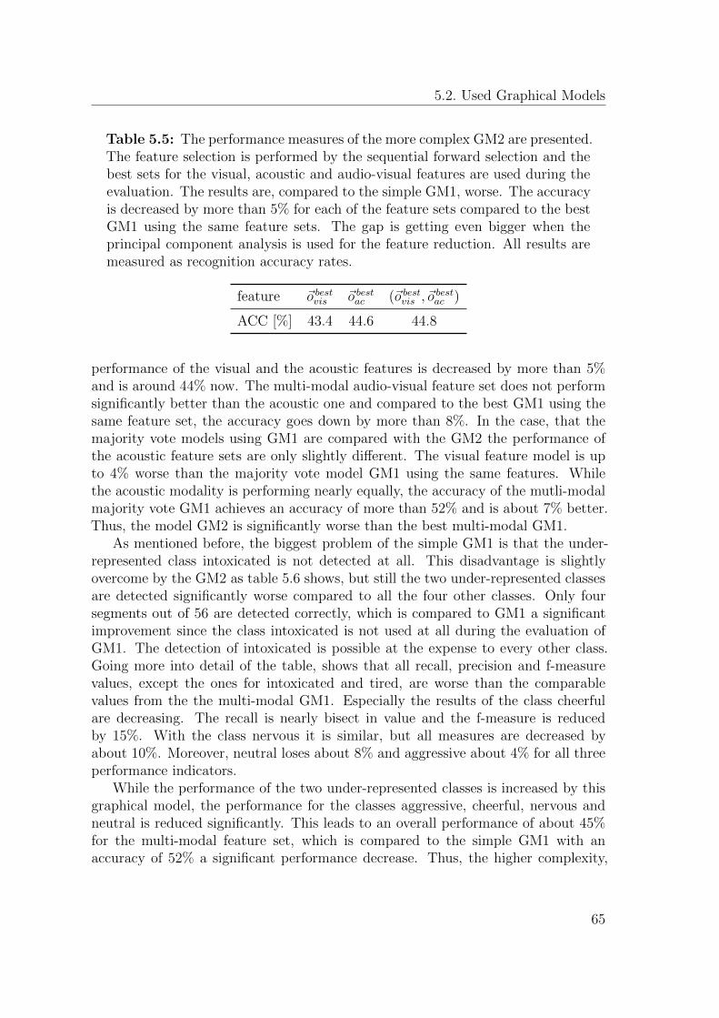
5.2. Used Graphical Models
Table 5.5: The performance measures of the more complex GM2 are presented.The feature selection is performed by the sequential forward selection and thebest sets for the visual, acoustic and audio-visual features are used during theevaluation. The results are, compared to the simple GM1, worse. The accuracyis decreased by more than 5% for each of the feature sets compared to the bestGM1 using the same feature sets. The gap is getting even bigger when theprincipal component analysis is used for the feature reduction. All results aremeasured as recognition accuracy rates.
feature ~o bestvis ~o bestac (~o bestvis , ~obestac )
ACC [%] 43.4 44.6 44.8
performance of the visual and the acoustic features is decreased by more than 5%and is around 44% now. The multi-modal audio-visual feature set does not performsignificantly better than the acoustic one and compared to the best GM1 using thesame feature set, the accuracy goes down by more than 8%. In the case, that themajority vote models using GM1 are compared with the GM2 the performance ofthe acoustic feature sets are only slightly different. The visual feature model is upto 4% worse than the majority vote model GM1 using the same features. Whilethe acoustic modality is performing nearly equally, the accuracy of the mutli-modalmajority vote GM1 achieves an accuracy of more than 52% and is about 7% better.Thus, the model GM2 is significantly worse than the best multi-modal GM1.
As mentioned before, the biggest problem of the simple GM1 is that the under-represented class intoxicated is not detected at all. This disadvantage is slightlyovercome by the GM2 as table 5.6 shows, but still the two under-represented classesare detected significantly worse compared to all the four other classes. Only foursegments out of 56 are detected correctly, which is compared to GM1 a significantimprovement since the class intoxicated is not used at all during the evaluation ofGM1. The detection of intoxicated is possible at the expense to every other class.Going more into detail of the table, shows that all recall, precision and f-measurevalues, except the ones for intoxicated and tired, are worse than the comparablevalues from the the multi-modal GM1. Especially the results of the class cheerfulare decreasing. The recall is nearly bisect in value and the f-measure is reducedby 15%. With the class nervous it is similar, but all measures are decreased byabout 10%. Moreover, neutral loses about 8% and aggressive about 4% for all threeperformance indicators.
While the performance of the two under-represented classes is increased by thisgraphical model, the performance for the classes aggressive, cheerful, nervous andneutral is reduced significantly. This leads to an overall performance of about 45%for the multi-modal feature set, which is compared to the simple GM1 with anaccuracy of 52% a significant performance decrease. Thus, the higher complexity,
65
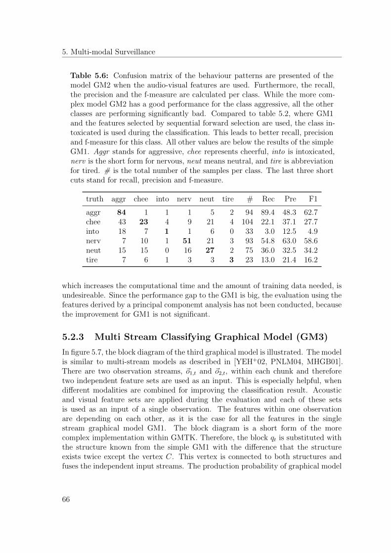
5. Multi-modal Surveillance
Table 5.6: Confusion matrix of the behaviour patterns are presented of themodel GM2 when the audio-visual features are used. Furthermore, the recall,the precision and the f-measure are calculated per class. While the more com-plex model GM2 has a good performance for the class aggressive, all the otherclasses are performing significantly bad. Compared to table 5.2, where GM1and the features selected by sequential forward selection are used, the class in-toxicated is used during the classification. This leads to better recall, precisionand f-measure for this class. All other values are below the results of the simpleGM1. Aggr stands for aggressive, chee represents cheerful, into is intoxicated,nerv is the short form for nervous, neut means neutral, and tire is abbreviationfor tired. # is the total number of the samples per class. The last three shortcuts stand for recall, precision and f-measure.
truth aggr chee into nerv neut tire # Rec Pre F1
aggr 84 1 1 1 5 2 94 89.4 48.3 62.7chee 43 23 4 9 21 4 104 22.1 37.1 27.7into 18 7 1 1 6 0 33 3.0 12.5 4.9nerv 7 10 1 51 21 3 93 54.8 63.0 58.6neut 15 15 0 16 27 2 75 36.0 32.5 34.2tire 7 6 1 3 3 3 23 13.0 21.4 16.2
which increases the computational time and the amount of training data needed, isundesireable. Since the performance gap to the GM1 is big, the evaluation using thefeatures derived by a principal componemt analysis has not been conducted, becausethe improvement for GM1 is not significant.
5.2.3 Multi Stream Classifying Graphical Model (GM3)
In figure 5.7, the block diagram of the third graphical model is illustrated. The modelis similar to multi-stream models as described in [YEH+02, PNLM04, MHGB01].There are two observation streams, ~o1,t and ~o2,t, within each chunk and thereforetwo independent feature sets are used as an input. This is especially helpful, whendifferent modalities are combined for improving the classification result. Acousticand visual feature sets are applied during the evaluation and each of these setsis used as an input of a single observation. The features within one observationare depending on each other, as it is the case for all the features in the singlestream graphical model GM1. The block diagram is a short form of the morecomplex implementation within GMTK. Therefore, the block qt is substituted withthe structure known from the simple GM1 with the difference that the structureexists twice except the vertex C. This vertex is connected to both structures andfuses the independent input streams. The production probability of graphical model
66
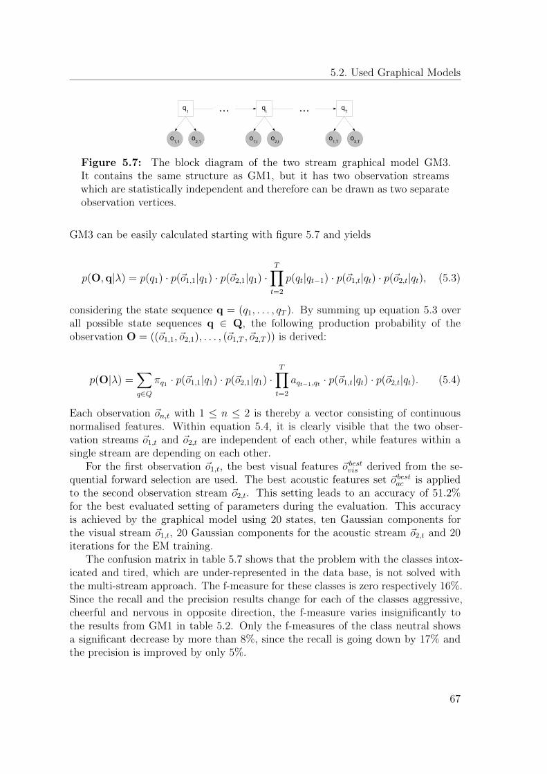
5.2. Used Graphical Models
q1
o1,1
o2,1
o1,t
o2,t
qT
o1,T
o2,T
qt ......
Figure 5.7: The block diagram of the two stream graphical model GM3.It contains the same structure as GM1, but it has two observation streamswhich are statistically independent and therefore can be drawn as two separateobservation vertices.
GM3 can be easily calculated starting with figure 5.7 and yields
p(O,q|λ) = p(q1) · p(~o1,1|q1) · p(~o2,1|q1) ·T∏t=2
p(qt|qt−1) · p(~o1,t|qt) · p(~o2,t|qt), (5.3)
considering the state sequence q = (q1, . . . , qT ). By summing up equation 5.3 overall possible state sequences q ∈ Q, the following production probability of theobservation O = ((~o1,1, ~o2,1), . . . , (~o1,T , ~o2,T )) is derived:
p(O|λ) =∑q∈Q
πq1 · p(~o1,1|q1) · p(~o2,1|q1) ·T∏t=2
aqt−1,qt · p(~o1,t|qt) · p(~o2,t|qt). (5.4)
Each observation ~on,t with 1 ≤ n ≤ 2 is thereby a vector consisting of continuousnormalised features. Within equation 5.4, it is clearly visible that the two obser-vation streams ~o1,t and ~o2,t are independent of each other, while features within asingle stream are depending on each other.
For the first observation ~o1,t, the best visual features ~o bestvis derived from the se-quential forward selection are used. The best acoustic features set ~o bestac is appliedto the second observation stream ~o2,t. This setting leads to an accuracy of 51.2%for the best evaluated setting of parameters during the evaluation. This accuracyis achieved by the graphical model using 20 states, ten Gaussian components forthe visual stream ~o1,t, 20 Gaussian components for the acoustic stream ~o2,t and 20iterations for the EM training.
The confusion matrix in table 5.7 shows that the problem with the classes intox-icated and tired, which are under-represented in the data base, is not solved withthe multi-stream approach. The f-measure for these classes is zero respectively 16%.Since the recall and the precision results change for each of the classes aggressive,cheerful and nervous in opposite direction, the f-measure varies insignificantly tothe results from GM1 in table 5.2. Only the f-measures of the class neutral showsa significant decrease by more than 8%, since the recall is going down by 17% andthe precision is improved by only 5%.
67
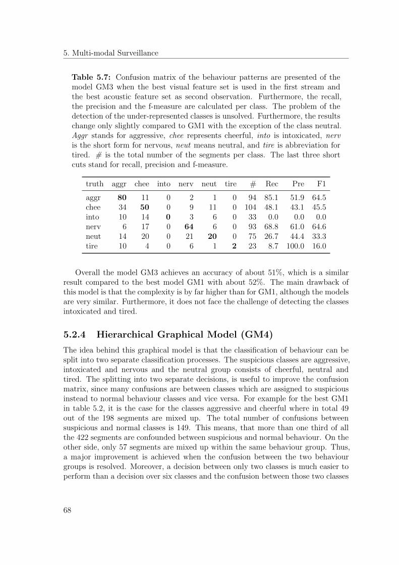
5. Multi-modal Surveillance
Table 5.7: Confusion matrix of the behaviour patterns are presented of themodel GM3 when the best visual feature set is used in the first stream andthe best acoustic feature set as second observation. Furthermore, the recall,the precision and the f-measure are calculated per class. The problem of thedetection of the under-represented classes is unsolved. Furthermore, the resultschange only slightly compared to GM1 with the exception of the class neutral.Aggr stands for aggressive, chee represents cheerful, into is intoxicated, nervis the short form for nervous, neut means neutral, and tire is abbreviation fortired. # is the total number of the segments per class. The last three shortcuts stand for recall, precision and f-measure.
truth aggr chee into nerv neut tire # Rec Pre F1
aggr 80 11 0 2 1 0 94 85.1 51.9 64.5chee 34 50 0 9 11 0 104 48.1 43.1 45.5into 10 14 0 3 6 0 33 0.0 0.0 0.0nerv 6 17 0 64 6 0 93 68.8 61.0 64.6neut 14 20 0 21 20 0 75 26.7 44.4 33.3tire 10 4 0 6 1 2 23 8.7 100.0 16.0
Overall the model GM3 achieves an accuracy of about 51%, which is a similarresult compared to the best model GM1 with about 52%. The main drawback ofthis model is that the complexity is by far higher than for GM1, although the modelsare very similar. Furthermore, it does not face the challenge of detecting the classesintoxicated and tired.
5.2.4 Hierarchical Graphical Model (GM4)
The idea behind this graphical model is that the classification of behaviour can besplit into two separate classification processes. The suspicious classes are aggressive,intoxicated and nervous and the neutral group consists of cheerful, neutral andtired. The splitting into two separate decisions, is useful to improve the confusionmatrix, since many confusions are between classes which are assigned to suspiciousinstead to normal behaviour classes and vice versa. For example for the best GM1in table 5.2, it is the case for the classes aggressive and cheerful where in total 49out of the 198 segments are mixed up. The total number of confusions betweensuspicious and normal classes is 149. This means, that more than one third of allthe 422 segments are confounded between suspicious and normal behaviour. On theother side, only 57 segments are mixed up within the same behaviour group. Thus,a major improvement is achieved when the confusion between the two behaviourgroups is resolved. Moreover, a decision between only two classes is much easier toperform than a decision over six classes and the confusion between those two classes
68
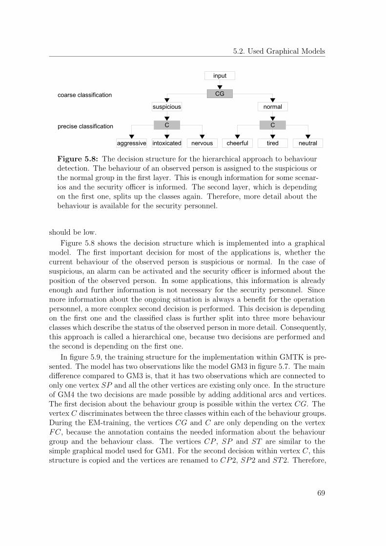
5.2. Used Graphical Models
input
suspicious normal
aggressive intoxicated nervous cheerful tired neutral
CG
C C
coarse classification
precise classification
Figure 5.8: The decision structure for the hierarchical approach to behaviourdetection. The behaviour of an observed person is assigned to the suspicious orthe normal group in the first layer. This is enough information for some scenar-ios and the security officer is informed. The second layer, which is dependingon the first one, splits up the classes again. Therefore, more detail about thebehaviour is available for the security personnel.
should be low.
Figure 5.8 shows the decision structure which is implemented into a graphicalmodel. The first important decision for most of the applications is, whether thecurrent behaviour of the observed person is suspicious or normal. In the case ofsuspicious, an alarm can be activated and the security officer is informed about theposition of the observed person. In some applications, this information is alreadyenough and further information is not necessary for the security personnel. Sincemore information about the ongoing situation is always a benefit for the operationpersonnel, a more complex second decision is performed. This decision is dependingon the first one and the classified class is further split into three more behaviourclasses which describe the status of the observed person in more detail. Consequently,this approach is called a hierarchical one, because two decisions are performed andthe second is depending on the first one.
In figure 5.9, the training structure for the implementation within GMTK is pre-sented. The model has two observations like the model GM3 in figure 5.7. The maindifference compared to GM3 is, that it has two observations which are connected toonly one vertex SP and all the other vertices are existing only once. In the structureof GM4 the two decisions are made possible by adding additional arcs and vertices.The first decision about the behaviour group is possible within the vertex CG. Thevertex C discriminates between the three classes within each of the behaviour groups.During the EM-training, the vertices CG and C are only depending on the vertexFC, because the annotation contains the needed information about the behaviourgroup and the behaviour class. The vertices CP , SP and ST are similar to thesimple graphical model used for GM1. For the second decision within vertex C, thisstructure is copied and the vertices are renamed to CP2, SP2 and ST2. Therefore,
69
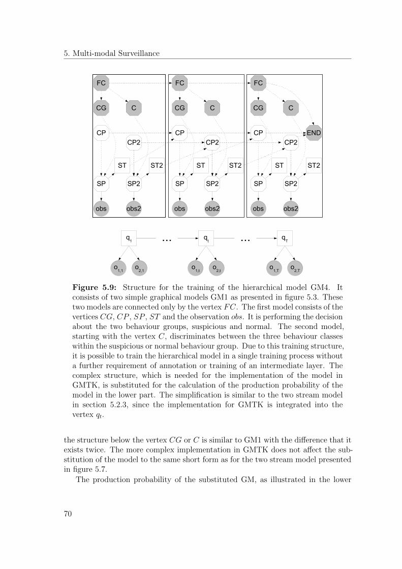
5. Multi-modal Surveillance
obs
SP
ST
ENDCP
CG
obs2
SP2
ST2
CP2
C
FC
obs
SP
ST
CP
CG
obs2
SP2
ST2
CP2
C
FC
obs
SP
ST
CG
obs2
SP2
ST2
C
FC
CP2CP
q1
o1,1
o2,1
o1,t
o2,t
qT
o1,T
o2,T
qt ......
Figure 5.9: Structure for the training of the hierarchical model GM4. Itconsists of two simple graphical models GM1 as presented in figure 5.3. Thesetwo models are connected only by the vertex FC. The first model consists of thevertices CG, CP , SP , ST and the observation obs. It is performing the decisionabout the two behaviour groups, suspicious and normal. The second model,starting with the vertex C, discriminates between the three behaviour classeswithin the suspicious or normal behaviour group. Due to this training structure,it is possible to train the hierarchical model in a single training process withouta further requirement of annotation or training of an intermediate layer. Thecomplex structure, which is needed for the implementation of the model inGMTK, is substituted for the calculation of the production probability of themodel in the lower part. The simplification is similar to the two stream modelin section 5.2.3, since the implementation for GMTK is integrated into thevertex qt.
the structure below the vertex CG or C is similar to GM1 with the difference that itexists twice. The more complex implementation in GMTK does not affect the sub-stitution of the model to the same short form as for the two stream model presentedin figure 5.7.
The production probability of the substituted GM, as illustrated in the lower
70
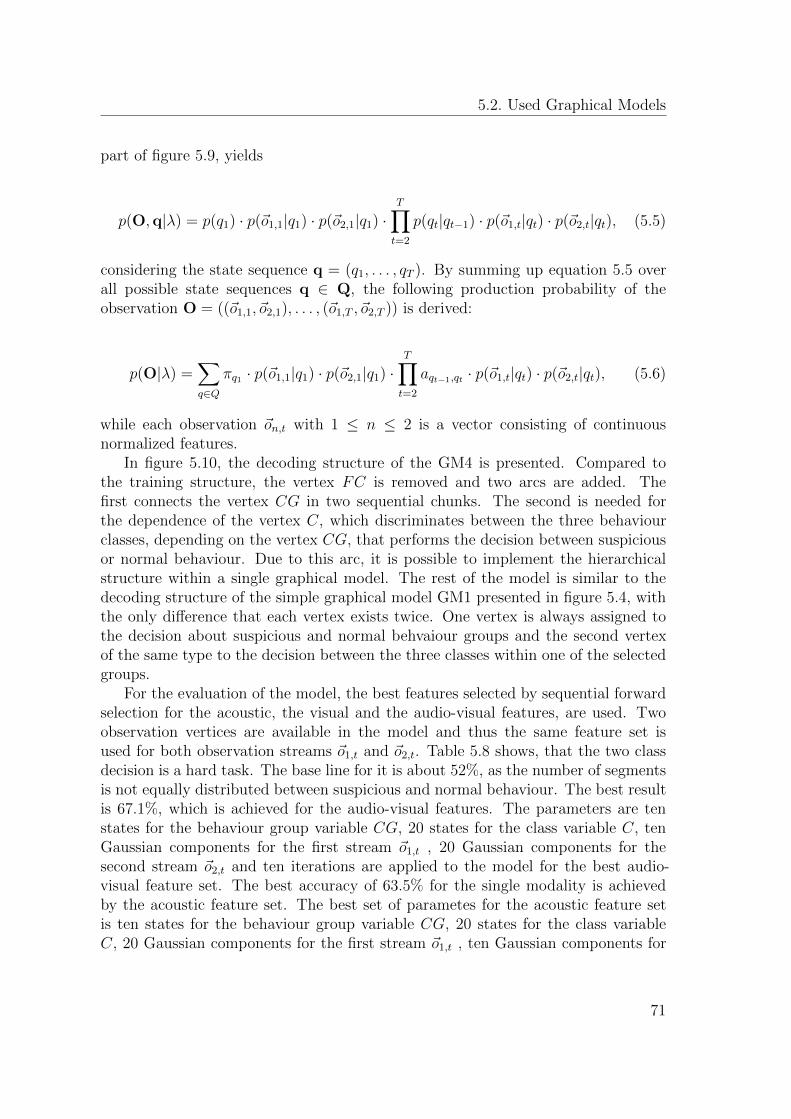
5.2. Used Graphical Models
part of figure 5.9, yields
p(O,q|λ) = p(q1) · p(~o1,1|q1) · p(~o2,1|q1) ·T∏t=2
p(qt|qt−1) · p(~o1,t|qt) · p(~o2,t|qt), (5.5)
considering the state sequence q = (q1, . . . , qT ). By summing up equation 5.5 overall possible state sequences q ∈ Q, the following production probability of theobservation O = ((~o1,1, ~o2,1), . . . , (~o1,T , ~o2,T )) is derived:
p(O|λ) =∑q∈Q
πq1 · p(~o1,1|q1) · p(~o2,1|q1) ·T∏t=2
aqt−1,qt · p(~o1,t|qt) · p(~o2,t|qt), (5.6)
while each observation ~on,t with 1 ≤ n ≤ 2 is a vector consisting of continuousnormalized features.
In figure 5.10, the decoding structure of the GM4 is presented. Compared tothe training structure, the vertex FC is removed and two arcs are added. Thefirst connects the vertex CG in two sequential chunks. The second is needed forthe dependence of the vertex C, which discriminates between the three behaviourclasses, depending on the vertex CG, that performs the decision between suspiciousor normal behaviour. Due to this arc, it is possible to implement the hierarchicalstructure within a single graphical model. The rest of the model is similar to thedecoding structure of the simple graphical model GM1 presented in figure 5.4, withthe only difference that each vertex exists twice. One vertex is always assigned tothe decision about suspicious and normal behvaiour groups and the second vertexof the same type to the decision between the three classes within one of the selectedgroups.
For the evaluation of the model, the best features selected by sequential forwardselection for the acoustic, the visual and the audio-visual features, are used. Twoobservation vertices are available in the model and thus the same feature set isused for both observation streams ~o1,t and ~o2,t. Table 5.8 shows, that the two classdecision is a hard task. The base line for it is about 52%, as the number of segmentsis not equally distributed between suspicious and normal behaviour. The best resultis 67.1%, which is achieved for the audio-visual features. The parameters are tenstates for the behaviour group variable CG, 20 states for the class variable C, tenGaussian components for the first stream ~o1,t , 20 Gaussian components for thesecond stream ~o2,t and ten iterations are applied to the model for the best audio-visual feature set. The best accuracy of 63.5% for the single modality is achievedby the acoustic feature set. The best set of parametes for the acoustic feature setis ten states for the behaviour group variable CG, 20 states for the class variableC, 20 Gaussian components for the first stream ~o1,t , ten Gaussian components for
71
5. Multi-modal Surveillance
obs
SP
ST
ENDCP
obs2
SP2
ST2
CP2
C
obs
SP
ST
CP
obs2
SP2
ST2
CP2
C
obs
SP
ST
obs2
SP2
ST2
C
CP2CP
CG CGCG
Figure 5.10: The decoding structure of the GM4. The additional arc betweenCG and C makes it possible to perform the hierarchical decision about thebehaviour. The structure is similar to GM1, with the difference that all verticesexist twice. One is for the decision about the behaviour group and the secondfor the final decision about the behaviour class. The arcs are totally similarwithin one of the copies of GM1.
the second stream ~o2,t and 20 iterations for the EM training. The visual featuresare performing insignificantly worse. Consequently, the improvement from the baseline is about 15% for the feature sets and about 11% for both single modalities. Forthe six classes decision it looks slightly different, because the acoustic set performsworst with an accuracy of 48.8%. The visual set achieves a result of 49.3%, whichis marginally better than the acoustic ones. The performance of the audio-visualfeature set is best and achieves an accuracy of 53.1%, which is the best one whenthe feature set derived by the sequential forward selection is applied. Therefore, theaccuracy is higher than the one achieved by the GM1 using the same features. It isalso better than the results of the GM1 using the feature set derived by principalcomponent analysis. In both cases the improvment is only marginally, since it isbelow 1% absolute. When the single modality results are compared to GM1, it isvisible that the visual set performs insignificantly better and the acoustic one slightlyworse. Thus, no tendency for the use of the different feature sets is found.
The confusion matrix for the best audio-visual feature set is presented in table 5.9.For the two class decision the the number of confusions compared to model GM3is reduced. Instead of 149 confusions between the behaviour groups suspicious andnormal, the number is going down to 139 which is an improvement of 6.7%. Thismeans, that the system performs better for the two class decision as the GM3 does,but the improvement is not as big as expected. The number of misclassifications
72
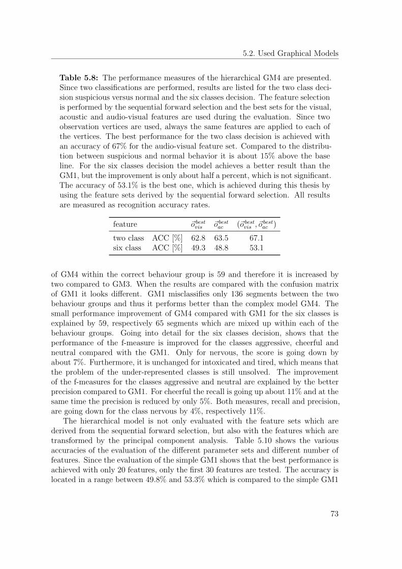
5.2. Used Graphical Models
Table 5.8: The performance measures of the hierarchical GM4 are presented.Since two classifications are performed, results are listed for the two class deci-sion suspicious versus normal and the six classes decision. The feature selectionis performed by the sequential forward selection and the best sets for the visual,acoustic and audio-visual features are used during the evaluation. Since twoobservation vertices are used, always the same features are applied to each ofthe vertices. The best performance for the two class decision is achieved withan accuracy of 67% for the audio-visual feature set. Compared to the distribu-tion between suspicious and normal behavior it is about 15% above the baseline. For the six classes decision the model achieves a better result than theGM1, but the improvement is only about half a percent, which is not significant.The accuracy of 53.1% is the best one, which is achieved during this thesis byusing the feature sets derived by the sequential forward selection. All resultsare measured as recognition accuracy rates.
feature ~o bestvis ~o bestac (~o bestvis , ~obestac )
two class ACC [%] 62.8 63.5 67.1six class ACC [%] 49.3 48.8 53.1
of GM4 within the correct behaviour group is 59 and therefore it is increased bytwo compared to GM3. When the results are compared with the confusion matrixof GM1 it looks different. GM1 misclassifies only 136 segments between the twobehaviour groups and thus it performs better than the complex model GM4. Thesmall performance improvement of GM4 compared with GM1 for the six classes isexplained by 59, respectively 65 segments which are mixed up within each of thebehaviour groups. Going into detail for the six classes decision, shows that theperformance of the f-measure is improved for the classes aggressive, cheerful andneutral compared with the GM1. Only for nervous, the score is going down byabout 7%. Furthermore, it is unchanged for intoxicated and tired, which means thatthe problem of the under-represented classes is still unsolved. The improvementof the f-measures for the classes aggressive and neutral are explained by the betterprecision compared to GM1. For cheerful the recall is going up about 11% and at thesame time the precision is reduced by only 5%. Both measures, recall and precision,are going down for the class nervous by 4%, respectively 11%.
The hierarchical model is not only evaluated with the feature sets which arederived from the sequential forward selection, but also with the features which aretransformed by the principal component analysis. Table 5.10 shows the variousaccuracies of the evaluation of the different parameter sets and different number offeatures. Since the evaluation of the simple GM1 shows that the best performance isachieved with only 20 features, only the first 30 features are tested. The accuracy islocated in a range between 49.8% and 53.3% which is compared to the simple GM1
73
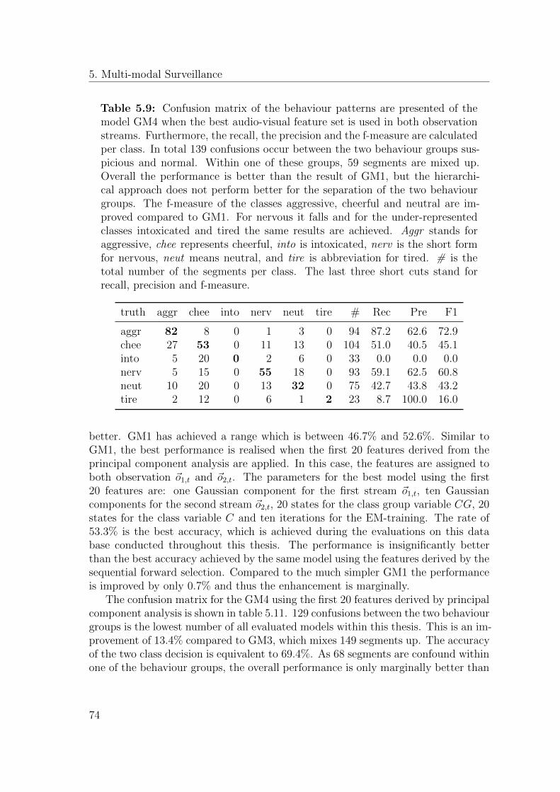
5. Multi-modal Surveillance
Table 5.9: Confusion matrix of the behaviour patterns are presented of themodel GM4 when the best audio-visual feature set is used in both observationstreams. Furthermore, the recall, the precision and the f-measure are calculatedper class. In total 139 confusions occur between the two behaviour groups sus-picious and normal. Within one of these groups, 59 segments are mixed up.Overall the performance is better than the result of GM1, but the hierarchi-cal approach does not perform better for the separation of the two behaviourgroups. The f-measure of the classes aggressive, cheerful and neutral are im-proved compared to GM1. For nervous it falls and for the under-representedclasses intoxicated and tired the same results are achieved. Aggr stands foraggressive, chee represents cheerful, into is intoxicated, nerv is the short formfor nervous, neut means neutral, and tire is abbreviation for tired. # is thetotal number of the segments per class. The last three short cuts stand forrecall, precision and f-measure.
truth aggr chee into nerv neut tire # Rec Pre F1
aggr 82 8 0 1 3 0 94 87.2 62.6 72.9chee 27 53 0 11 13 0 104 51.0 40.5 45.1into 5 20 0 2 6 0 33 0.0 0.0 0.0nerv 5 15 0 55 18 0 93 59.1 62.5 60.8neut 10 20 0 13 32 0 75 42.7 43.8 43.2tire 2 12 0 6 1 2 23 8.7 100.0 16.0
better. GM1 has achieved a range which is between 46.7% and 52.6%. Similar toGM1, the best performance is realised when the first 20 features derived from theprincipal component analysis are applied. In this case, the features are assigned toboth observation ~o1,t and ~o2,t. The parameters for the best model using the first20 features are: one Gaussian component for the first stream ~o1,t, ten Gaussiancomponents for the second stream ~o2,t, 20 states for the class group variable CG, 20states for the class variable C and ten iterations for the EM-training. The rate of53.3% is the best accuracy, which is achieved during the evaluations on this database conducted throughout this thesis. The performance is insignificantly betterthan the best accuracy achieved by the same model using the features derived by thesequential forward selection. Compared to the much simpler GM1 the performanceis improved by only 0.7% and thus the enhancement is marginally.
The confusion matrix for the GM4 using the first 20 features derived by principalcomponent analysis is shown in table 5.11. 129 confusions between the two behaviourgroups is the lowest number of all evaluated models within this thesis. This is an im-provement of 13.4% compared to GM3, which mixes 149 segments up. The accuracyof the two class decision is equivalent to 69.4%. As 68 segments are confound withinone of the behaviour groups, the overall performance is only marginally better than
74
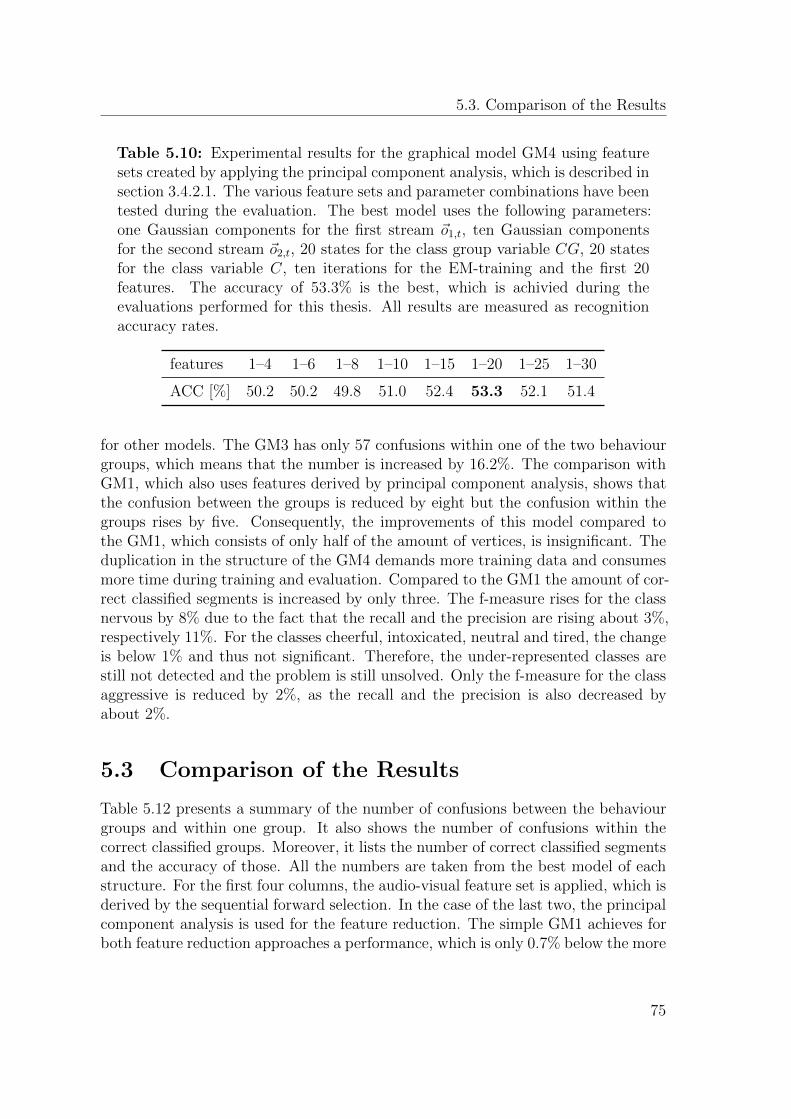
5.3. Comparison of the Results
Table 5.10: Experimental results for the graphical model GM4 using featuresets created by applying the principal component analysis, which is described insection 3.4.2.1. The various feature sets and parameter combinations have beentested during the evaluation. The best model uses the following parameters:one Gaussian components for the first stream ~o1,t, ten Gaussian componentsfor the second stream ~o2,t, 20 states for the class group variable CG, 20 statesfor the class variable C, ten iterations for the EM-training and the first 20features. The accuracy of 53.3% is the best, which is achivied during theevaluations performed for this thesis. All results are measured as recognitionaccuracy rates.
features 1–4 1–6 1–8 1–10 1–15 1–20 1–25 1–30
ACC [%] 50.2 50.2 49.8 51.0 52.4 53.3 52.1 51.4
for other models. The GM3 has only 57 confusions within one of the two behaviourgroups, which means that the number is increased by 16.2%. The comparison withGM1, which also uses features derived by principal component analysis, shows thatthe confusion between the groups is reduced by eight but the confusion within thegroups rises by five. Consequently, the improvements of this model compared tothe GM1, which consists of only half of the amount of vertices, is insignificant. Theduplication in the structure of the GM4 demands more training data and consumesmore time during training and evaluation. Compared to the GM1 the amount of cor-rect classified segments is increased by only three. The f-measure rises for the classnervous by 8% due to the fact that the recall and the precision are rising about 3%,respectively 11%. For the classes cheerful, intoxicated, neutral and tired, the changeis below 1% and thus not significant. Therefore, the under-represented classes arestill not detected and the problem is still unsolved. Only the f-measure for the classaggressive is reduced by 2%, as the recall and the precision is also decreased byabout 2%.
5.3 Comparison of the Results
Table 5.12 presents a summary of the number of confusions between the behaviourgroups and within one group. It also shows the number of confusions within thecorrect classified groups. Moreover, it lists the number of correct classified segmentsand the accuracy of those. All the numbers are taken from the best model of eachstructure. For the first four columns, the audio-visual feature set is applied, which isderived by the sequential forward selection. In the case of the last two, the principalcomponent analysis is used for the feature reduction. The simple GM1 achieves forboth feature reduction approaches a performance, which is only 0.7% below the more
75
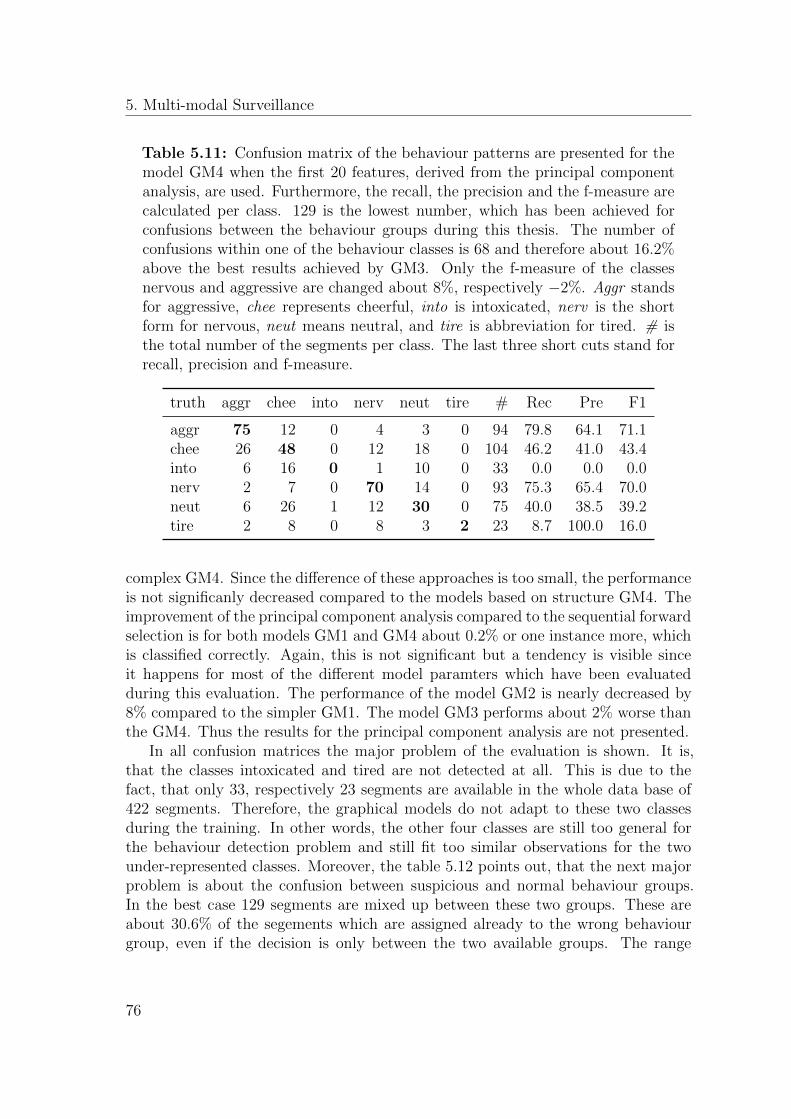
5. Multi-modal Surveillance
Table 5.11: Confusion matrix of the behaviour patterns are presented for themodel GM4 when the first 20 features, derived from the principal componentanalysis, are used. Furthermore, the recall, the precision and the f-measure arecalculated per class. 129 is the lowest number, which has been achieved forconfusions between the behaviour groups during this thesis. The number ofconfusions within one of the behaviour classes is 68 and therefore about 16.2%above the best results achieved by GM3. Only the f-measure of the classesnervous and aggressive are changed about 8%, respectively −2%. Aggr standsfor aggressive, chee represents cheerful, into is intoxicated, nerv is the shortform for nervous, neut means neutral, and tire is abbreviation for tired. # isthe total number of the segments per class. The last three short cuts stand forrecall, precision and f-measure.
truth aggr chee into nerv neut tire # Rec Pre F1
aggr 75 12 0 4 3 0 94 79.8 64.1 71.1chee 26 48 0 12 18 0 104 46.2 41.0 43.4into 6 16 0 1 10 0 33 0.0 0.0 0.0nerv 2 7 0 70 14 0 93 75.3 65.4 70.0neut 6 26 1 12 30 0 75 40.0 38.5 39.2tire 2 8 0 8 3 2 23 8.7 100.0 16.0
complex GM4. Since the difference of these approaches is too small, the performanceis not significanly decreased compared to the models based on structure GM4. Theimprovement of the principal component analysis compared to the sequential forwardselection is for both models GM1 and GM4 about 0.2% or one instance more, whichis classified correctly. Again, this is not significant but a tendency is visible sinceit happens for most of the different model paramters which have been evaluatedduring this evaluation. The performance of the model GM2 is nearly decreased by8% compared to the simpler GM1. The model GM3 performs about 2% worse thanthe GM4. Thus the results for the principal component analysis are not presented.
In all confusion matrices the major problem of the evaluation is shown. It is,that the classes intoxicated and tired are not detected at all. This is due to thefact, that only 33, respectively 23 segments are available in the whole data base of422 segments. Therefore, the graphical models do not adapt to these two classesduring the training. In other words, the other four classes are still too general forthe behaviour detection problem and still fit too similar observations for the twounder-represented classes. Moreover, the table 5.12 points out, that the next majorproblem is about the confusion between suspicious and normal behaviour groups.In the best case 129 segments are mixed up between these two groups. These areabout 30.6% of the segements which are assigned already to the wrong behaviourgroup, even if the decision is only between the two available groups. The range
76
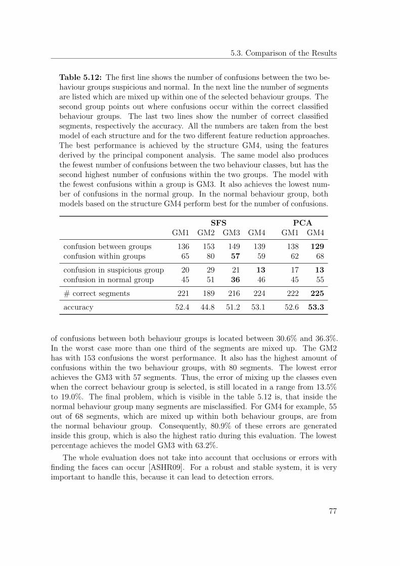
5.3. Comparison of the Results
Table 5.12: The first line shows the number of confusions between the two be-haviour groups suspicious and normal. In the next line the number of segmentsare listed which are mixed up within one of the selected behaviour groups. Thesecond group points out where confusions occur within the correct classifiedbehaviour groups. The last two lines show the number of correct classifiedsegments, respectively the accuracy. All the numbers are taken from the bestmodel of each structure and for the two different feature reduction approaches.The best performance is achieved by the structure GM4, using the featuresderived by the principal component analysis. The same model also producesthe fewest number of confusions between the two behaviour classes, but has thesecond highest number of confusions within the two groups. The model withthe fewest confusions within a group is GM3. It also achieves the lowest num-ber of confusions in the normal group. In the normal behaviour group, bothmodels based on the structure GM4 perform best for the number of confusions.
SFS PCAGM1 GM2 GM3 GM4 GM1 GM4
confusion between groups 136 153 149 139 138 129confusion within groups 65 80 57 59 62 68
confusion in suspicious group 20 29 21 13 17 13confusion in normal group 45 51 36 46 45 55
# correct segments 221 189 216 224 222 225
accuracy 52.4 44.8 51.2 53.1 52.6 53.3
of confusions between both behaviour groups is located between 30.6% and 36.3%.In the worst case more than one third of the segments are mixed up. The GM2has with 153 confusions the worst performance. It also has the highest amount ofconfusions within the two behaviour groups, with 80 segments. The lowest errorachieves the GM3 with 57 segments. Thus, the error of mixing up the classes evenwhen the correct behaviour group is selected, is still located in a range from 13.5%to 19.0%. The final problem, which is visible in the table 5.12 is, that inside thenormal behaviour group many segments are misclassified. For GM4 for example, 55out of 68 segments, which are mixed up within both behaviour groups, are fromthe normal behaviour group. Consequently, 80.9% of these errors are generatedinside this group, which is also the highest ratio during this evaluation. The lowestpercentage achieves the model GM3 with 63.2%.
The whole evaluation does not take into account that occlusions or errors withfinding the faces can occur [ASHR09]. For a robust and stable system, it is veryimportant to handle this, because it can lead to detection errors.
77
5. Multi-modal Surveillance
5.4 Comparison with other Approaches
In the past, other promising approaches have been evaluated on the ABC corpus andthose will be compared to the results achieved during this work. The best result inthis work is achieved by the GM4 using 20 features derived by principal componentanalysis. It reaches an accuracy of 53.3%.
In [AHSR09], an accuracy of 52.6% is presented when HMMs are used. TheseHMMs have been implemented with HTK [YEH+02]. For the features the same 81visual features have been applied as used in this work. The description for thesefeatures can be found in section 3.2.2. Since the gaps between the HMMs and thebest model of this work is only about 0.7% the improvement of the performanceis not significant. On the other hand, the GM4 uses only 20 features, which leadsto lower computational effort and the computational power is also reduced. Thus,GM4 should be prefered to the HMM presented in [AHSR09]. When the HMMis compared to GM1, it performs about 3.5% better. It looks different when thenumber of used feautres are compared, since the HMM uses 81 features and theGM1 applies only eight visual features. The simple GM1 can be seen as a HMMimplemented in GMTK and therefore the performance should be similar with theHMMs from [AHSR09]. The performance gap has due to with the integration ofHMMs in various toolkits. It is not the first time that a mismatch between similarmodels evaluated with HTK and GMTK occurs. The performance gap betweenthese two implemenations has been analysed for online recognition of whiteboardnotes in [SHBR09]. To sum up, graphical models are performing on a similar levelas HMMs, but use by far less features.
There are also other approaches with static classifiers as Support Vector Machinesand different modalities of features which are using the ABC corpus. In [Ars10], thefirst comparable result is performed by a simple Support Vector Machine (SVM)approach which is trained on the same visual features as used in this work (seesection 3.2.2). The accuracy of this approach is 60.1% and therefore outperforms allthe dynamic classifiers evaluated in this thesis.
Another visual feature set, which is evaluated in [SWA+07] is created by de-formable models. These deformable models are fitted to the passengers’ faces inorder to extract the features. Since the number of extracted features is huge, asequential forward selection has been performed to reduce the feature space to 157dimensions. After the reduction, a time series analysis is performed over each fea-ture for all the available segments from the data base. The used SVMs performwith 61.1% only marginally better as the approach with the simple global motionfeatures. Since the computational effort for the sequential forward selection and thetime series analysis is massive compared to the extraction of global motion features,this approach is not the first choice.
Another visual approach which is comparable to the hierarchical graphical modeldeveloped in this thesis, is presented in [AHSR09]. The approach classifies the 81
78
5.5. Outlook
global motions in two layers. The first layer decides between the two behaviourgroups suspicious and normal. Within each of these groups a second decision isperformed about three classes. The first decision results in an performance of 87.9%which is more than 18% better than the performance of the best hierarchical GM4presented in this work. Since only 25% of the features are used by GM4, a smallperformance drop could be considered, but this big drop is too much. Thus, theperformance of the GM4 is far below the hierarchical SVM approach. The recog-nition rate of the hierarchical SVM approach is 74.9% and therefore outperformsGM4 by more than 21%. Form other results of this SVM approach, which are pre-sented in [Ars10], it is clear that the performance of the decision within the normalbehaviour group is the most difficult one.
In [SWA+08], an acoustic behaviour detection system is presented. This ap-proach extracts a large set of low level audio descriptors and functionals. Thesefeatures are comparable to the features used in this work. More details about theacoustic set can be found in section 3.1. The experiments result in an accuracy of73.3%.
The best results for this data base is presented in [WSA+08]. The audio-visualapproach, which combines the work from [SWA+08] and [SWA+07], achieves an accu-racy of 81.1%. This approach uses more complex facial features, as active appearancemodels [BH05], and a time series analysis over all the audio-visual features.
Graphical models and HMMs are dynamic classifiers and these are by far outper-formed by static classifiers as SVMs. The approaches with the hierarchical structureimprove the results of both classifier types. Probably, the best results are achievedwhen an audio-visual feature set is used as an input for a multi-layer SVM classifier.
5.5 Outlook
The accuracy is so low, because one third of the segments are assigned to the wrongbehaviour group and another 15% are detected as the wrong class, even if the cor-rect behaviour group is detected before. These are also two points, where furtherresearch can be conducted to achieve better results. One idea would be to use differ-ent types of features, for example features derived from active appearance models. Asecond is to add more semantic information and create a model which can deal withsemantic information. For the case, that more training material is available, morecomplex models could be tested. A model structure, which uses audio and visualfeatures, both separately derived by principal component analysis as two indepen-dent observation streams for each of two hierarchical observations could be tested.Furthermore, it would be possbile to create models, where not only two consecutivechunks are connected, but also more different streams could be connected. A database could be improved to recordings from real flights with the drawback that veryfew suspicious situations will occur. Moreover, an approach, which takes into ac-
79

5. Multi-modal Surveillance
count that not in every segment the face is found by the visual feature extractor andon the other hand not each segment audio data is available could help to improvethe performance.
80
6
Automatic Video Editing inMeetings
Various projects, such as the meeting project of the International Computer ScienceInstitute at Berkley (ICSI) [MBB+03], Computers in the Human Interaction Loop(CHIL) [WSS04] or Augmented Multi-party Interaction (AMI) [CAB+06] investigatethe use of modern pattern recognition tools to increase the efficiency of meetings.The idea arises from the problem that many people think that most meetings arejust a waste of time [HNR06] and therefore should be automatically processed, forexample for meeting browsing or remote participation. On the other hand, meetingsare often mandatory for many of us and consume large parts of our working days.In this section, the multi-modal problem of selecting one relevant field of view fromvarious available cameras in a meeting room is addressed. The problem derives fromthe fact that video conferences are getting more popular at the same time as itis getting more and more common that meeting rooms are equipped with variousrecording devices. This points out the two main usage scenarios of the system:On-line video conferences [SP85] and browsing of past meetings [WFG04].
Most of the current video conference systems transmit all available visual par-ticipants’ recordings to each attendee and display all of them. The main differencebetween the systems is the way these are presenting the video data. Normally,cheap systems show different small windows on a computer monitor, while high endsystems are using multiple large screens for that purpose. These approaches arelimited to a few participants, because the video of the individual participant is get-ting smaller if more persons are connected. Few other systems are using the audiochannel for selecting the stream and therefore they transmit only one video to allparticipants, which saves bandwidth. The main drawback of this approach is, thatinteresting non-verbal gestures are left aside, because these cannot be detected fromthe acoustic channel and thus cannot be recognized in small videos. This shows themulti-modal nature of meetings, thus it can be very important to show people whocurrently do not speak. In talk-shows for example, professional editors follow this
81
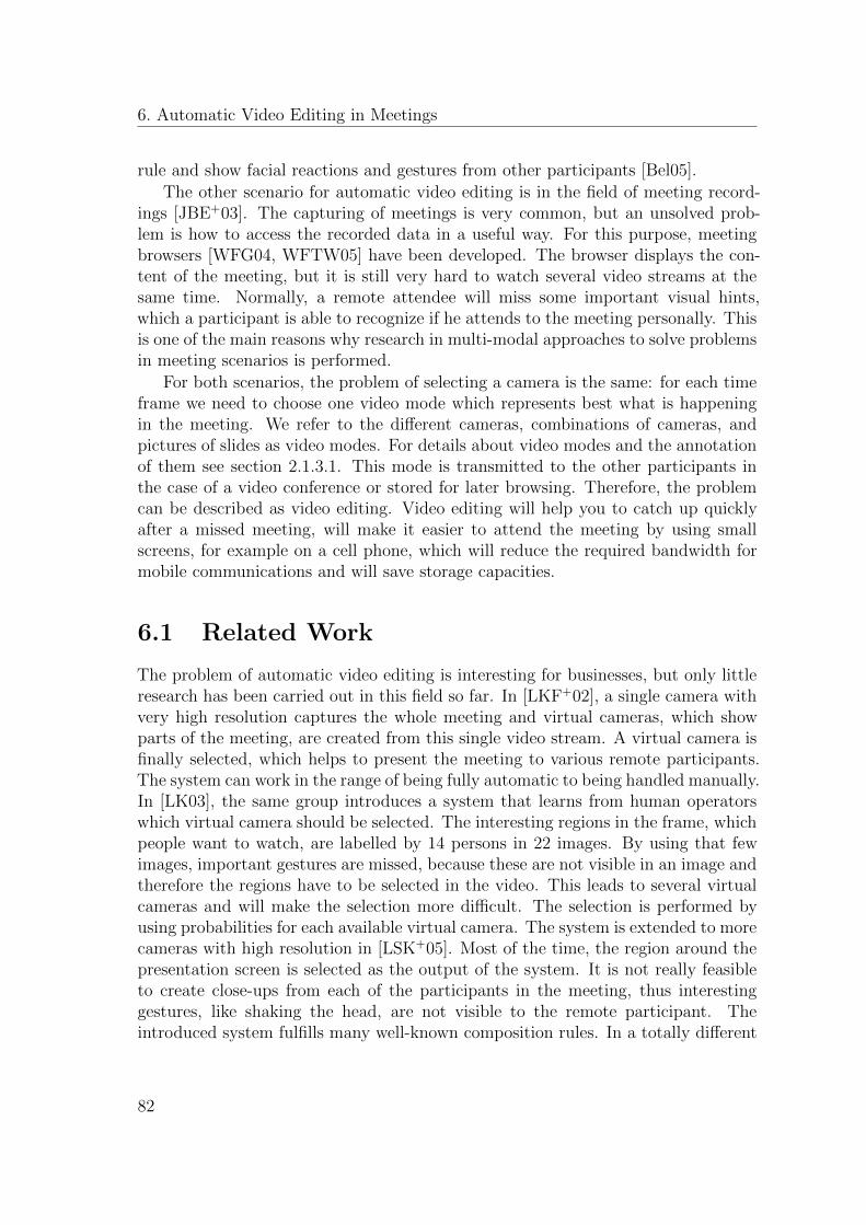
6. Automatic Video Editing in Meetings
rule and show facial reactions and gestures from other participants [Bel05].
The other scenario for automatic video editing is in the field of meeting record-ings [JBE+03]. The capturing of meetings is very common, but an unsolved prob-lem is how to access the recorded data in a useful way. For this purpose, meetingbrowsers [WFG04, WFTW05] have been developed. The browser displays the con-tent of the meeting, but it is still very hard to watch several video streams at thesame time. Normally, a remote attendee will miss some important visual hints,which a participant is able to recognize if he attends to the meeting personally. Thisis one of the main reasons why research in multi-modal approaches to solve problemsin meeting scenarios is performed.
For both scenarios, the problem of selecting a camera is the same: for each timeframe we need to choose one video mode which represents best what is happeningin the meeting. We refer to the different cameras, combinations of cameras, andpictures of slides as video modes. For details about video modes and the annotationof them see section 2.1.3.1. This mode is transmitted to the other participants inthe case of a video conference or stored for later browsing. Therefore, the problemcan be described as video editing. Video editing will help you to catch up quicklyafter a missed meeting, will make it easier to attend the meeting by using smallscreens, for example on a cell phone, which will reduce the required bandwidth formobile communications and will save storage capacities.
6.1 Related Work
The problem of automatic video editing is interesting for businesses, but only littleresearch has been carried out in this field so far. In [LKF+02], a single camera withvery high resolution captures the whole meeting and virtual cameras, which showparts of the meeting, are created from this single video stream. A virtual camera isfinally selected, which helps to present the meeting to various remote participants.The system can work in the range of being fully automatic to being handled manually.In [LK03], the same group introduces a system that learns from human operatorswhich virtual camera should be selected. The interesting regions in the frame, whichpeople want to watch, are labelled by 14 persons in 22 images. By using that fewimages, important gestures are missed, because these are not visible in an image andtherefore the regions have to be selected in the video. This leads to several virtualcameras and will make the selection more difficult. The selection is performed byusing probabilities for each available virtual camera. The system is extended to morecameras with high resolution in [LSK+05]. Most of the time, the region around thepresentation screen is selected as the output of the system. It is not really feasibleto create close-ups from each of the participants in the meeting, thus interestinggestures, like shaking the head, are not visible to the remote participant. Theintroduced system fulfills many well-known composition rules. In a totally different
82
6.1. Related Work
field, automatic camera selection is performed in [SNVF03]. A multi camera systemrecords an outdoor scenario for video surveillance. The criteria for selecting a camerais depending on the quality of the detection of the person in the video stream. Themain focus of this work is to become more reliable under changing weather conditions.In [Uch01], a user study for developing a user interface for video editing in meetingswas conducted with professional editors as subjects. The interface should supportnon professional editors by the task of video editing. For home videos a system called
“Hitchcock” was described in [GBC+00]. This system is searching for unsuitableframes in a single video stream, and applies standard editing rules which leads to asegmentation of the stream. All segments are ranked and the segments with highscores are selected for the final video. The system is not selecting different cameras,it is summarizing the home video. Early work in the field of video editing is basedon rules. Three examples which work on the same data base are described closerupcoming paragraphs.
In [Sum04], a rule based system is introduced for video editing in lecture hallsand meeting rooms. The system has two operation modes; one for a video conferenceand the second for stored meetings which are performed in the past. The algorithmof the system is taking into account some technical aspects of video editing, as wellas aesthetic ones. For example, the duration of showing the same camera is the mostimportant aesthetic aspect. From the technical point of view, it is important: Whois speaking? How long is someone speaking? Who is moving the head or hands? Allthis information is combined to a weight for each camera at each time frame and thecamera with the highest weight is selected. The system is also using virtual camerasfor creating more camera changes, if for a long time no camera change happenssince, for example, the same participant is still speaking. The main drawback ofthis system is that the selected camera is highly depending on the current speakerand important non verbals, as shaking the head or nodding, are not shown in theedited video. Visual clues can be added easily to the system if they are availableas annotations. All the information which is used for the camera selection arehand annotated and no automatic detectors have been created. The only availableevaluation is that various subjects have watched the created videos and have rankedthem. Therefore, no comparison to other approaches using the same data base ispossible.
In [AHHSR06], an approach to video editing for smart meeting rooms is in-troduced, which is based on different thresholds for different extracted features.Therefore, different acoustic, visual, and semantic features based on time framesare extracted from the meeting data. The influence of different feature types on thetask of automatic video editing is investigated. First tests show that frame basedvideo editing by a rule based system can lead to unintentional twitches. Therefore,additional features are derived by windowing a range of subsequent frames for acous-tic and visual features. For the selection of the video mode, it is tried to choose themost relevant camera for each frame in the meeting. This is done by mapping each
83
6. Automatic Video Editing in Meetings
close-up camera as well as each lapel microphone to one participant. In case a mono-logue takes place, the close-up camera of the according person is chosen and thereforethe camera is the most relevant one. The centre camera is used if the group is inthe state of discussion, whiteboard or presentation. The selection is performed bychoosing the “most active” person, that means for the acoustic feature for examplethe audio channel which is the loudest. This process is performed on frame baseddata as well as on windowed data. The results of the approach are: The direct useof acoustic and visual features is not leading to success, because of a high numberof camera changes per minute. The problem is solved by using windowed features.On the other hand, too few camera changes occurred when semantic features areused, since the group state only changes every minute. A second evaluation is doneby performing late fusion of the results of different features. The outcome is, thatthe combination of audio and video information is required for a sufficient selectiontask. In [AHHSR06], only the number of shot changes per minute and the time ofthe longest shot are objective measures which give an impression about the videoquality. Furthermore, a user rating is given which expresses the significance of theevaluated features from a user’s point of view. Therefore, a comparison of theseresults with the results achieved in this work is not possible.
In [AHHM+07], a video editing system based on HMMs [Rab89] is introduced.For each of the seven video modes a HHM is trained using the EM algorithm [DLR77].The best sequence of video modes is derived by Viterbi decoding [Vit77] and of thissequence an output video is created. The system uses low level acoustic and visualfeatures which are similar to the features used in this work. Various combinationsof features and many different parameter settings have been evaluated. The bestresult is a frame error rate of 47.9%.
In [Len07], an approach is presented which uses an Asynchronous Hidden MarkovModel [Ben03]. It works on the same data base and the same features as used forthe system described in [AHHM+07] and the evaluation of this thesis is based. Witha frame error rate of 32.3% it performs by far better than all known approaches, butstill only two third of the frames are classified correctly. The system is state of theart for the AMI database, which is the same as used in this thesis .
Graphical models are used for video editing in [AH08]. These models are capableof automatic segmentation and classification of the seven video modes. The bestperformance is achieved by a combination of acoustic and visual features with aframe error rate of 47.7%. The data base and the features which have been usedin the work are the same as in this thesis, thus a comparison is feasible. Since theimplementation of graphical models in GMTK [BZ02] is not yet as optimised as forHMMs in HTK [YEH+02], the performance can be further improved in the futureby optimising the used toolkit, especially the implementation of the EM training.
In [AHR08], a system using support vector machines [Vap95] is presented. It usesglobal motion features and the person speaking features for the automatic selectionof the video modes. The work is using the same features and the same data base
84
6.2. The Video Editing System
Cut & MuxFeature extraction Video mode selection
Figure 6.1: Block diagram of the video editing system is depicted. It showsthe seven video streams and the four audio streams which are used as an inputto the feature extraction and the cut and multiplex unit. The extracted featuresare the input of the selection block which selected the most relevant video mode.This video mode and the mixed audio stream of the participants are combinedto the final output video.
as used in this thesis. The performance of the approach using the support vectormachines is with a frame error rate of 39% better than the HMM approaches, butworse than the Asynchronous Hidden Markov Model.
6.2 The Video Editing System
In figure 6.1, an overview of the video editing system is presented. The first step is,that from the four audio channels and the seven video cameras various audio-visualfeatures are extracted. More details about the features can be found in chapter 3.The second building block contains the classification and segmentation process whichmakes a decision about when and which video mode should be shown. The final blockuses the audio and video sources and the selected video mode sequence to createan output video. This video contains the mixed audio sources of each participantand the most relevant video mode for each frame. The structure is similar for mostapproaches described in the related work section as well as for the developed modelsin this thesis. For similar approaches, the feature extraction is done by hand sincethe input data is not created reliably by automatic systems.
Figure 6.2 shows an example of an output video. It contains a sequence of shotsover the time axis which are for a better illustration only presented by a single framefor each shot. Each shot is automatically selected by the video editing system usinga combination of features described in section 3. The duration of one shot, whichalways contains only a single video mode, is also found automatically by the systemduring the decoding process.
6.3 Used Graphical Models
In this section different graphical models are presented which have been evaluatedduring this thesis. Since for the automatic video editing a segmentation of the
85
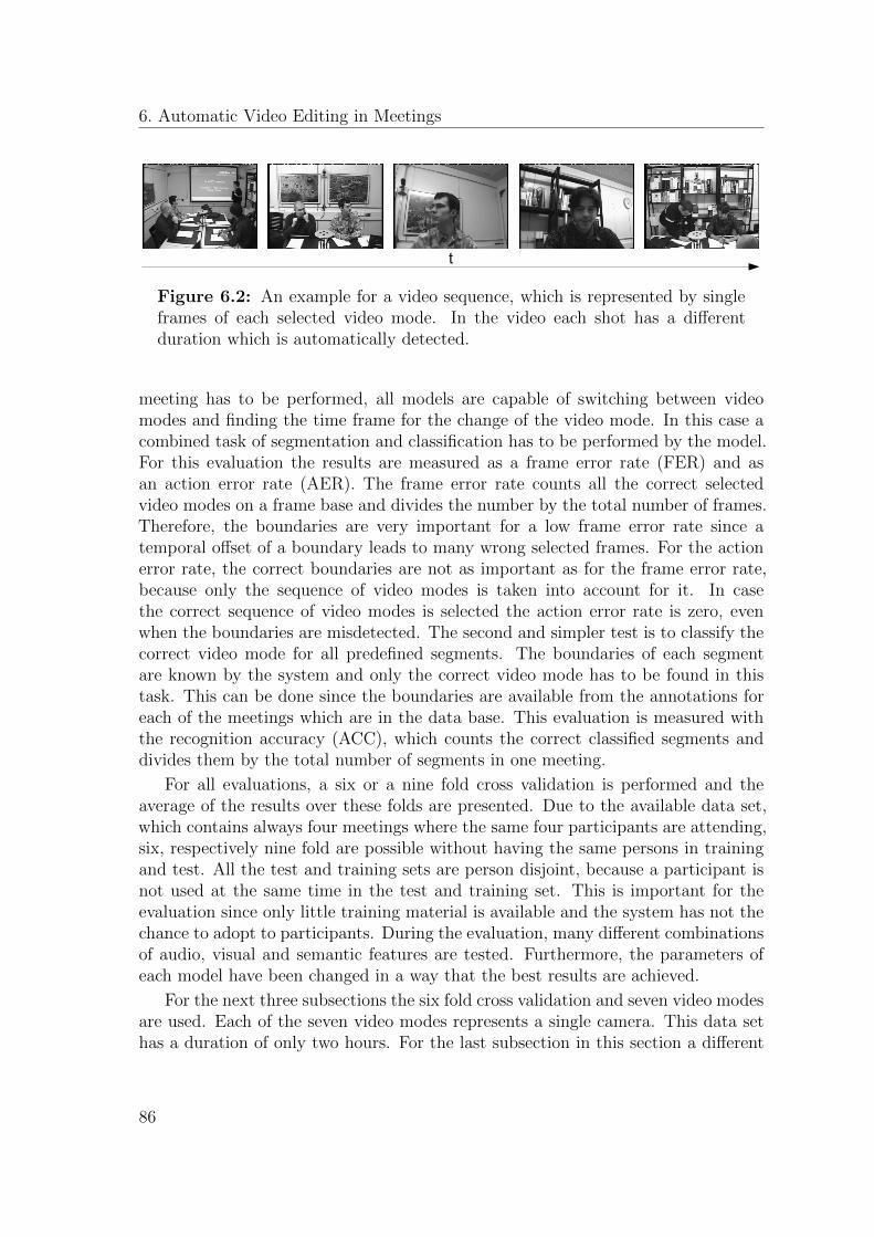
6. Automatic Video Editing in Meetings
t
Figure 6.2: An example for a video sequence, which is represented by singleframes of each selected video mode. In the video each shot has a differentduration which is automatically detected.
meeting has to be performed, all models are capable of switching between videomodes and finding the time frame for the change of the video mode. In this case acombined task of segmentation and classification has to be performed by the model.For this evaluation the results are measured as a frame error rate (FER) and asan action error rate (AER). The frame error rate counts all the correct selectedvideo modes on a frame base and divides the number by the total number of frames.Therefore, the boundaries are very important for a low frame error rate since atemporal offset of a boundary leads to many wrong selected frames. For the actionerror rate, the correct boundaries are not as important as for the frame error rate,because only the sequence of video modes is taken into account for it. In casethe correct sequence of video modes is selected the action error rate is zero, evenwhen the boundaries are misdetected. The second and simpler test is to classify thecorrect video mode for all predefined segments. The boundaries of each segmentare known by the system and only the correct video mode has to be found in thistask. This can be done since the boundaries are available from the annotations foreach of the meetings which are in the data base. This evaluation is measured withthe recognition accuracy (ACC), which counts the correct classified segments anddivides them by the total number of segments in one meeting.
For all evaluations, a six or a nine fold cross validation is performed and theaverage of the results over these folds are presented. Due to the available data set,which contains always four meetings where the same four participants are attending,six, respectively nine fold are possible without having the same persons in trainingand test. All the test and training sets are person disjoint, because a participant isnot used at the same time in the test and training set. This is important for theevaluation since only little training material is available and the system has not thechance to adopt to participants. During the evaluation, many different combinationsof audio, visual and semantic features are tested. Furthermore, the parameters ofeach model have been changed in a way that the best results are achieved.
For the next three subsections the six fold cross validation and seven video modesare used. Each of the seven video modes represents a single camera. This data sethas a duration of only two hours. For the last subsection in this section a different
86
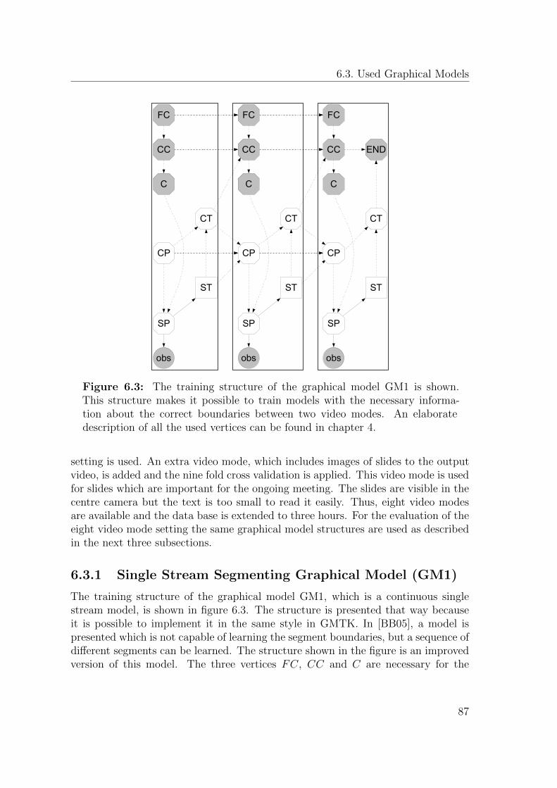
6.3. Used Graphical Models
obs
SP
obs
SP
ST
CP
obs
SP
ST
CP
ST
CT
END
CP
C
FC FCFC
CT
CC
CT
CCCC
C C
Figure 6.3: The training structure of the graphical model GM1 is shown.This structure makes it possible to train models with the necessary informa-tion about the correct boundaries between two video modes. An elaboratedescription of all the used vertices can be found in chapter 4.
setting is used. An extra video mode, which includes images of slides to the outputvideo, is added and the nine fold cross validation is applied. This video mode is usedfor slides which are important for the ongoing meeting. The slides are visible in thecentre camera but the text is too small to read it easily. Thus, eight video modesare available and the data base is extended to three hours. For the evaluation of theeight video mode setting the same graphical model structures are used as describedin the next three subsections.
6.3.1 Single Stream Segmenting Graphical Model (GM1)
The training structure of the graphical model GM1, which is a continuous singlestream model, is shown in figure 6.3. The structure is presented that way becauseit is possible to implement it in the same style in GMTK. In [BB05], a model ispresented which is not capable of learning the segment boundaries, but a sequence ofdifferent segments can be learned. The structure shown in the figure is an improvedversion of this model. The three vertices FC, CC and C are necessary for the
87
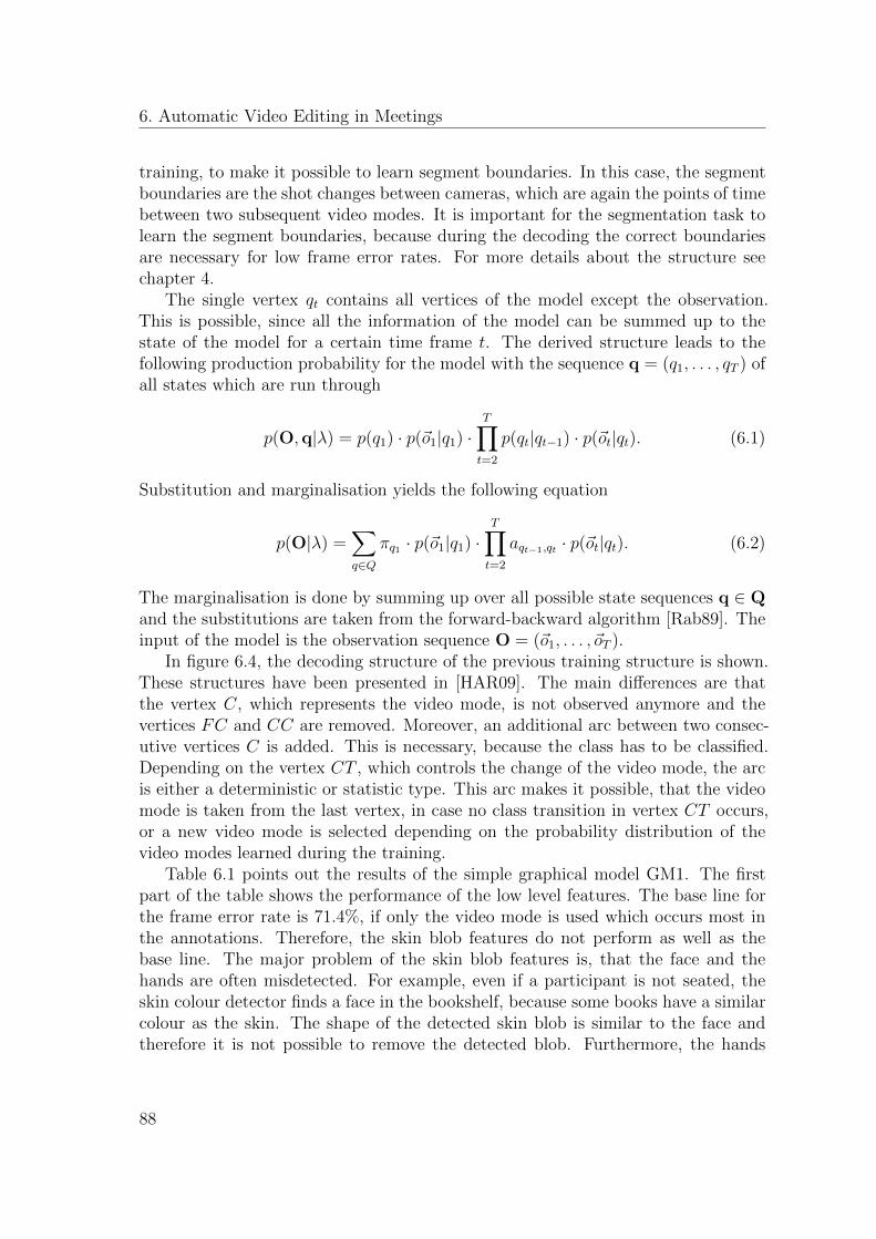
6. Automatic Video Editing in Meetings
training, to make it possible to learn segment boundaries. In this case, the segmentboundaries are the shot changes between cameras, which are again the points of timebetween two subsequent video modes. It is important for the segmentation task tolearn the segment boundaries, because during the decoding the correct boundariesare necessary for low frame error rates. For more details about the structure seechapter 4.
The single vertex qt contains all vertices of the model except the observation.This is possible, since all the information of the model can be summed up to thestate of the model for a certain time frame t. The derived structure leads to thefollowing production probability for the model with the sequence q = (q1, . . . , qT ) ofall states which are run through
p(O,q|λ) = p(q1) · p(~o1|q1) ·T∏t=2
p(qt|qt−1) · p(~ot|qt). (6.1)
Substitution and marginalisation yields the following equation
p(O|λ) =∑q∈Q
πq1 · p(~o1|q1) ·T∏t=2
aqt−1,qt · p(~ot|qt). (6.2)
The marginalisation is done by summing up over all possible state sequences q ∈ Qand the substitutions are taken from the forward-backward algorithm [Rab89]. Theinput of the model is the observation sequence O = (~o1, . . . , ~oT ).
In figure 6.4, the decoding structure of the previous training structure is shown.These structures have been presented in [HAR09]. The main differences are thatthe vertex C, which represents the video mode, is not observed anymore and thevertices FC and CC are removed. Moreover, an additional arc between two consec-utive vertices C is added. This is necessary, because the class has to be classified.Depending on the vertex CT , which controls the change of the video mode, the arcis either a deterministic or statistic type. This arc makes it possible, that the videomode is taken from the last vertex, in case no class transition in vertex CT occurs,or a new video mode is selected depending on the probability distribution of thevideo modes learned during the training.
Table 6.1 points out the results of the simple graphical model GM1. The firstpart of the table shows the performance of the low level features. The base line forthe frame error rate is 71.4%, if only the video mode is used which occurs most inthe annotations. Therefore, the skin blob features do not perform as well as thebase line. The major problem of the skin blob features is, that the face and thehands are often misdetected. For example, even if a participant is not seated, theskin colour detector finds a face in the bookshelf, because some books have a similarcolour as the skin. The shape of the detected skin blob is similar to the face andtherefore it is not possible to remove the detected blob. Furthermore, the hands
88
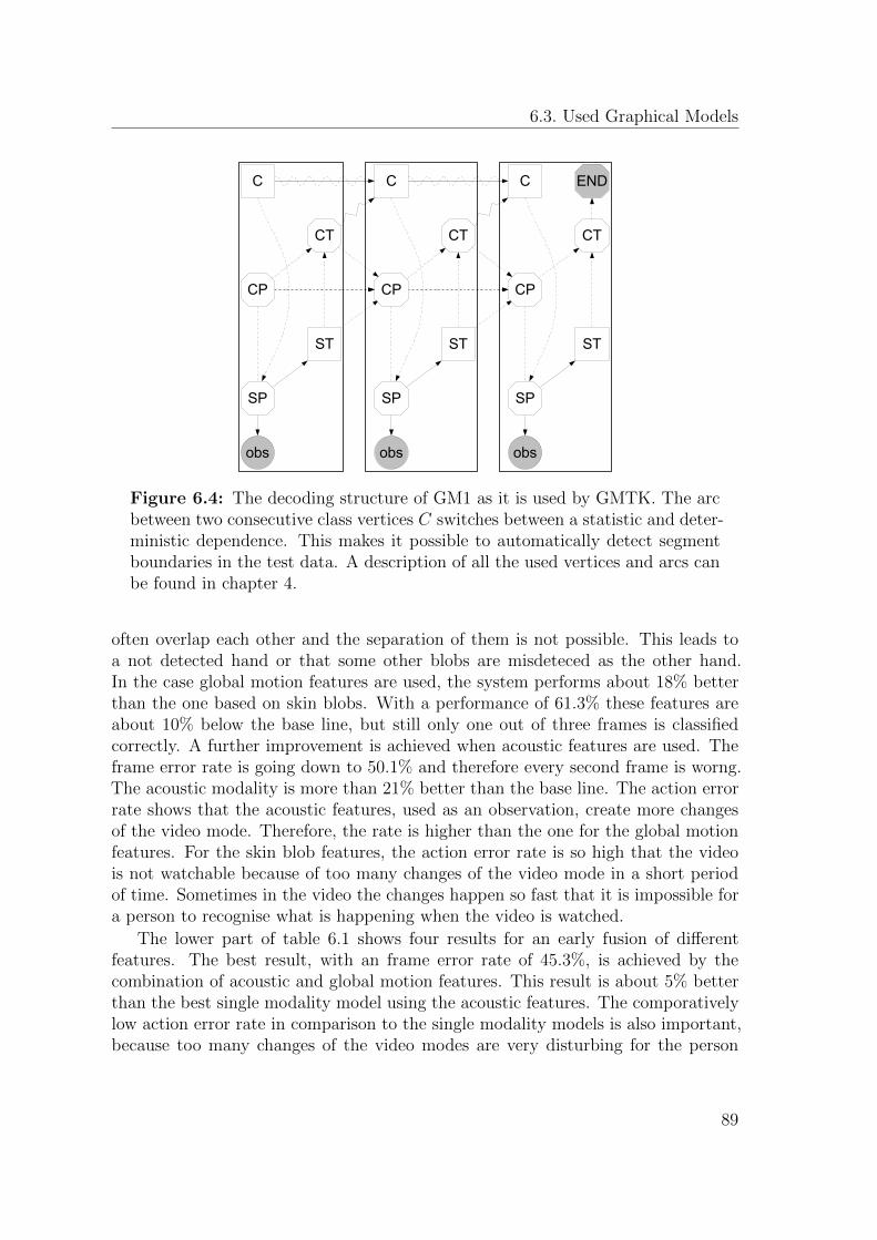
6.3. Used Graphical Models
obs
SP
C
obs
SP
ST
CP
C
CT
obs
SP
ST
CP
C
CT
ST
CT
END
CP
Figure 6.4: The decoding structure of GM1 as it is used by GMTK. The arcbetween two consecutive class vertices C switches between a statistic and deter-ministic dependence. This makes it possible to automatically detect segmentboundaries in the test data. A description of all the used vertices and arcs canbe found in chapter 4.
often overlap each other and the separation of them is not possible. This leads toa not detected hand or that some other blobs are misdeteced as the other hand.In the case global motion features are used, the system performs about 18% betterthan the one based on skin blobs. With a performance of 61.3% these features areabout 10% below the base line, but still only one out of three frames is classifiedcorrectly. A further improvement is achieved when acoustic features are used. Theframe error rate is going down to 50.1% and therefore every second frame is worng.The acoustic modality is more than 21% better than the base line. The action errorrate shows that the acoustic features, used as an observation, create more changesof the video mode. Therefore, the rate is higher than the one for the global motionfeatures. For the skin blob features, the action error rate is so high that the videois not watchable because of too many changes of the video mode in a short periodof time. Sometimes in the video the changes happen so fast that it is impossible fora person to recognise what is happening when the video is watched.
The lower part of table 6.1 shows four results for an early fusion of differentfeatures. The best result, with an frame error rate of 45.3%, is achieved by thecombination of acoustic and global motion features. This result is about 5% betterthan the best single modality model using the acoustic features. The comporativelylow action error rate in comparison to the single modality models is also important,because too many changes of the video modes are very disturbing for the person
89
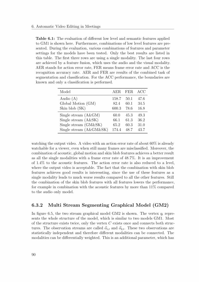
6. Automatic Video Editing in Meetings
Table 6.1: The evaluation of different low level and semantic features appliedto GM1 is shown here. Furthermore, combinations of low level features are pre-sented. During the evaluation, various combinations of features and parametersettings for the models have been tested. Only the best results are listed inthis table. The first three rows are using a single modality. The last four rowsare achieved by a feature fusion, which uses the audio and the visual modality.AER stands for action error rate, FER means frame error rate and ACC is therecognition accuracy rate. AER and FER are results of the combined task ofsegmentation and classification. For the ACC performance, the boundaries areknown and only a classification is performed.
Model AER FER ACC
Audio (A) 158.7 50.1 47.6Global Motion (GM) 82.4 60.1 34.5Skin blob (SK) 600.3 78.6 16.8
Single stream (A&GM) 60.0 45.3 49.3Single stream (A&SK) 66.1 61.3 36.2Single stream (GM&SK) 65.2 60.3 31.0Single stream (A&GM&SK) 174.4 48.7 43.7
watching the output video. A video with an action error rate of about 60% is alreadywatchable for a viewer, even when still many frames are misclassified. Moreover, thecombination of acoustic, global motion and skin blob features achieves a better resultas all the single modalities with a frame error rate of 48.7%. It is an improvementof 1.4% to the acoustic features. The action error rate is also reduced to a level,where the output video is acceptable. The fact that the combination with skin blobfeatures achieves good results is interessting, since the use of these features as asingle modality leads to much worse results compared to all the other features. Stillthe combination of the skin blob features with all features lowers the performance,for example in combination with the acoustic features by more than 11% comparedto the audio only model.
6.3.2 Multi Stream Segmenting Graphical Model (GM2)
In figure 6.5, the two stream graphical model GM2 is shown. The vertex qt repre-sents the whole structure of the model, which is similar to two models GM1. Mostof the structure exists twice, only the vertex C exists once and connects both struc-tures. The observation streams are called ~o1,t and ~o2,t. These two observations arestatistically independent and therefore different modalities can be connected. Themodalities can be differentially weighted. This is an additional parameter, which has
90
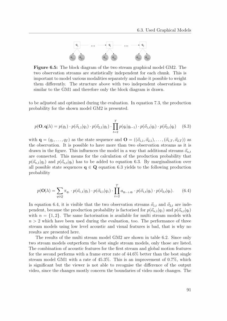
6.3. Used Graphical Models
q1
o1,1
o2,1
o1,t
o2,t
qT
o1,T
o2,T
qt ......
Figure 6.5: The block diagram of the two stream graphical model GM2. Thetwo observation streams are statistically independent for each chunk. This isimportant to model various modalities separately and make it possible to weightthem differently. The structure above with two independent observations issimilar to the GM1 and therefore only the block diagram is drawn.
to be adjusted and optimised during the evaluation. In equation 7.3, the productionprobability for the shown model GM2 is presented.
p(O,q|λ) = p(q1) · p(~o1,1|q1) · p(~o2,1|q1) ·T∏t=2
p(qt|qt−1) · p(~o1,t|qt) · p(~o2,t|qt) (6.3)
with q = (q1, . . . , qT ) as the state sequence and O = ((~o1,1, ~o2,1), . . . , (~o1,T , ~o2,T )) asthe observation. It is possible to have more than two observation streams as it isdrawn in the figure. This influences the model in a way that additional streams ~on,tare connected. This means for the calculation of the production probability thatp(~on,1|q1) and p(~on,t|qt) has to be added to equation 6.3. By marginalisation overall possible state sequences q ∈ Q equation 6.3 yields to the following productionprobability
p(O|λ) =∑q∈Q
πq1 · p(~o1,1|q1) · p(~o2,1|q1) ·T∏t=2
aqt−1,qt · p(~o1,t|qt) · p(~o2,t|qt). (6.4)
In equation 6.4, it is visible that the two observation streams ~o1,t and ~o2,t are inde-pendent, because the production probability is factorised for p(~on,1|q1) and p(~on,t|qt)with n = {1, 2}. The same factorisation is available for multi stream models withn > 2 which have been used during the evaluation, too. The performance of threestream models using low level acoustic and visual features is bad, that is why noresults are presented here.
The results of the multi stream model GM2 are shown in table 6.2. Since onlytwo stream models outperform the best single stream models, only those are listed.The combination of acoustic features for the first stream and global motion featuresfor the second performs with a frame error rate of 44.6% better than the best singlestream model GM1 with a rate of 45.3%. This is an improvement of 0.7%, whichis significant but the viewer is not able to recognise the difference of the outputvideo, since the changes mostly concern the boundaries of video mode changes. The
91
6. Automatic Video Editing in Meetings
Table 6.2: The table shows two results of the best audio-visual feature combi-nations using GM2. Various other combinations and parameter settings havebeen evaluated, but the results are not better than the single stream models.The first model uses 20 states per class and the second five. The feature combi-nations contain acoustic (A), global motion (GM) and skin blob features (SK).AER stands for action error rate, FER means frame error rate and ACC is therecognition accuracy rate. AER and FER are results of the combined task ofsegmentation and classification. For the ACC performance, the boundaries areknown and only a classification is performed.
Model AER FER ACC
Two streams (A/GM) 60.8 44.6 52.9Two streams (A/SK) 64.8 57.1 38.7
slightly higher action error rate does not really influence the quality of the outputvideo. The second result is achieved for the combination of acoustic and skin blobfeatures. The frame error rate and the action error rate are improved by 4.2%,respectively by 1.3% compared to the same features used in the single stream modelGM1.
6.3.3 Two Layer Graphical Model (GM3)
In figure 6.6, the block diagram of the third graphical model is presented. Thismodel has the capability to combine both semantic information and low level featuresduring the detection process. The low level acoustic and visual features are describedin section 3.1, respectively in section 3.2. Semantic information comes from groupand person actions, person movements and slide changes. All this information canbe derived by automatic systems, which have been developed in the last couple ofyears. In [Rei08], the group actions are recognised by using Markov random fields.Moreover, an approach applying graphical models is found in [AHDGP+06] and bothapproaches are working on the same meeting data from the M4 corpus [Ren02a,Ren02b]. It would be feasible to transfer both approaches to the meeting corpusused in this thesis. An HMM based approach for the recognition of person actions isdescribed in [AHHSR06]. During this thesis some tests have been conducted in thefield of person movement recognition. HMMs have been used for the classificationof the movements of the four participants in the smart meeting room. Slide changesare detected by an easy approach which was also developed during this thesis. Moredetails about this can be found in [Zak07].
Most of these approaches can be implemented in GMTK, therefore the wholemodel can be represented in a more complex GMTK implementation. Due to follow-ing reasons, the complex structure is not presented in this thesis and for the proof
92
6.3. Used Graphical Models
q1,T
q2,T
o2,T
o1,T
q1,t
q2,t
o2,t
o1,t
q1,1
q2,1
o2,1
......
o1,1
Figure 6.6: The block diagram of the two layer graphical model GM3 isshown. It combines semantic informations and low level descriptors within asingle graphical model. The first layer detects various semantic informationsand these results are used as additional inputs for the second layer, which usesthe low level descriptors, too. The semantic informations are: group and personactions, person movements and slide changes. For example, the group actionis derived by graphical models in [AHDGP+06] or by Markov Random Fieldsin [Rei08]. Thus, the structure of the first layer can be represented in GMTK.Moreover, an implementation of the complete structure is feasible in GMTK,but the combined training of the whole model would not work, due to the hugenumber of dependencies and random variables. The second layer contains thesame structure as GM1 or GM2.
of concept of the two layer model the hand made annotations are used:
• The training of the whole model is probably not feasible due to the hugenumber of dependencies and random variables.
• The amount of training data of the semantic information and of the videoediting is not sufficient for the training of a discriminative model of thesecomplex structures.
• The training would last several days for each of the evaluations.
• The structure of the models has to be changed for each test as various combi-nations of semantic information have to be evaluated.
• The results of the recognitions systems for the semantic information is good,but there is much space for improvement.
• An evaluation and comparison of the models detecting the semantic informa-tion is impossible, because of the multi-layer structure.
The second layer can be of the similar structure as model GM1 or GM2. Dur-ing this thesis, various combinations of semantic and low level features and model
93

6. Automatic Video Editing in Meetings
Table 6.3: The results of the evaluation with the additional semantic infor-mation are shown. The first two parts use no additional low level features forthe classification of the video mode. The third part uses acoustic features aslow level descriptors. As additional semantic features in combination with theacoustic feature have been used: person speaking (PS), person actions (PA)and group actions (GA). AER stands for action error rate, FER means frameerror rate and ACC is the recognition accuracy rate. AER and FER are re-sults of the combined task of segmentation and classification. For the ACCperformance, the boundaries are known and only a classification is performed.
Model AER FER ACC
Group Actions (GA) 84.8 61.0 26.2Person Actions (PA) 72.2 62.8 28.2Person Speaking (PS) 62.2 51.5 48.3
PA&PS 58.3 40.6 53.3GA&PA&PS 58.3 39.6 54.8
Two layer (GA) 63.1 49.2 48.3Two layer (PA) 60.2 42.5 51.5Two layer (PS&PA) 56.6 39.0 53.6Two layer (GA&PA&PS) 56.2 38.1 53.9
structures for the second layer have been evaluated. The best results of these com-binations are presented in table 6.3. In the upper two parts, results are presentedwhich are using only semantic information. When only the group actions, which areonly a one dimensional feature vector, are used as an input for the model, the frameerror rate is 61% and thus it is already about 10% better than the base line. Thebase line of 71.4% is achieved when only the video mode is selected, which is selectedmostly by the human annotators during the annoation of the meeting corpus. Thefour dimensional person actions are performing with a frame error rate of 62.8%and about 9% better than the base line. The best performing semantic informationis to know who is speaking, which tells a four dimensional person speaking featurevector. The frame error rate is 51.5% and consequently still every second frame ismisclassified. As all of these semantic features stay very stable over time and onlychanges happen when something important occurs in the meeting, the action errorrate is between 62% and 84%. This is compared, for example, to the acoustic fea-tures already a good result. When these results are compared with the best singlemodality model of GM1, there is a gap of 1% to the acoustic, which achieves aperformance of 50.1%. The main difference is that GM1 uses 156 features comparedto 4 features used by GM3 and that the action error rate is reduced by nearly 100%absolute or by 60% relative compared to GM1.
94
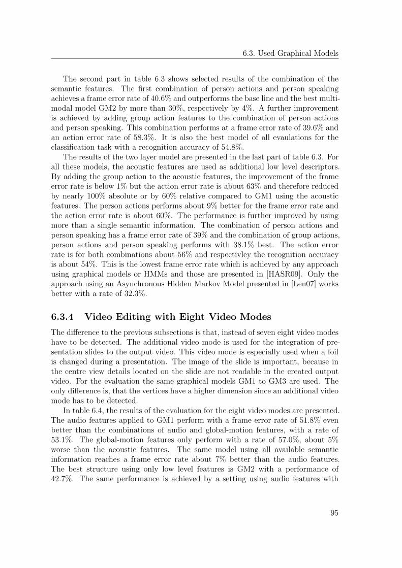
6.3. Used Graphical Models
The second part in table 6.3 shows selected results of the combination of thesemantic features. The first combination of person actions and person speakingachieves a frame error rate of 40.6% and outperforms the base line and the best multi-modal model GM2 by more than 30%, respectively by 4%. A further improvementis achieved by adding group action features to the combination of person actionsand person speaking. This combination performs at a frame error rate of 39.6% andan action error rate of 58.3%. It is also the best model of all evaulations for theclassification task with a recognition accuracy of 54.8%.
The results of the two layer model are presented in the last part of table 6.3. Forall these models, the acoustic features are used as additional low level descriptors.By adding the group action to the acoustic features, the improvement of the frameerror rate is below 1% but the action error rate is about 63% and therefore reducedby nearly 100% absolute or by 60% relative compared to GM1 using the acousticfeatures. The person actions performs about 9% better for the frame error rate andthe action error rate is about 60%. The performance is further improved by usingmore than a single semantic information. The combination of person actions andperson speaking has a frame error rate of 39% and the combination of group actions,person actions and person speaking performs with 38.1% best. The action errorrate is for both combinations about 56% and respectivley the recognition accuracyis about 54%. This is the lowest frame error rate which is achieved by any approachusing graphical models or HMMs and those are presented in [HASR09]. Only theapproach using an Asynchronous Hidden Markov Model presented in [Len07] worksbetter with a rate of 32.3%.
6.3.4 Video Editing with Eight Video Modes
The difference to the previous subsections is that, instead of seven eight video modeshave to be detected. The additional video mode is used for the integration of pre-sentation slides to the output video. This video mode is especially used when a foilis changed during a presentation. The image of the slide is important, because inthe centre view details located on the slide are not readable in the created outputvideo. For the evaluation the same graphical models GM1 to GM3 are used. Theonly difference is, that the vertices have a higher dimension since an additional videomode has to be detected.
In table 6.4, the results of the evaluation for the eight video modes are presented.The audio features applied to GM1 perform with a frame error rate of 51.8% evenbetter than the combinations of audio and global-motion features, with a rate of53.1%. The global-motion features only perform with a rate of 57.0%, about 5%worse than the acoustic features. The same model using all available semanticinformation reaches a frame error rate about 7% better than the audio features.The best structure using only low level features is GM2 with a performance of42.7%. The same performance is achieved by a setting using audio features with
95
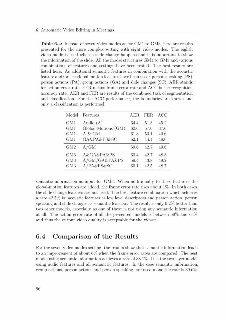
6. Automatic Video Editing in Meetings
Table 6.4: Instead of seven video modes as for GM1 to GM3, here are resultspresented for the more complex setting with eight video modes. The eighthvideo mode is used when a slide change happens and it is important to showthe information of the slide. All the model structures GM1 to GM3 and variouscombinations of features and settings have been tested. The best results arelisted here. As additional semantic features in combination with the acousticfeature and/or the global motion features have been used: person speaking (PS),person actions (PA), group actions (GA) and slide changes (SC). AER standsfor action error rate, FER means frame error rate and ACC is the recognitionaccuracy rate. AER and FER are results of the combined task of segmentationand classification. For the ACC performance, the boundaries are known andonly a classification is performed.
Model Features AER FER ACC
GM1 Audio (A) 64.4 51.8 45.2GM1 Global-Motions (GM) 62.6 57.0 37.6GM1 A & GM 61.3 53.1 40.6GM1 GA&PA&PS&SC 62.1 44.4 48.0
GM2 A/GM 59.6 42.7 49.6
GM3 A&GA&PA&PS 60.4 42.7 48.8GM3 A/GM/GA&PA&PS 59.4 43.8 49.2GM3 A/PA&PS&SC 60.1 42.5 48.7
semantic information as input for GM3. When additionally to these features, theglobal-motion features are added, the frame error rate rises about 1%. In both cases,the slide change features are not used. The best feature combination which achievesa rate 42.5% is: acoustic features as low level descriptors and person action, personspeaking and slide changes as semantic featuers. The result is only 0.2% better thantwo other models, especially as one of these is not using any semantic informationat all. The action error rate of all the presented models is between 59% and 64%and thus the output video quality is acceptable for the viewer.
6.4 Comparison of the Results
For the seven video modes setting, the results show that semantic information leadsto an improvement of about 6% when the frame error rates are compared. The bestmodel using semantic information achieves a rate of 38.1%. It is the two layer modelusing audio features and all semanctic features. In the case semantic information,group actions, person actions and person speaking, are used alone the rate is 39.6%.
96
6.5. Outlook
Consequently, an improvement of 5% to the low level descriptors is achieved. Theaction error rate of all these models is about 58%. The combination of acousticand global-motion features by the two stream model GM2 is the best setting usingonly low level descriptors. The frame error rate of this model is 44.6%. When lowlevel descriptor models are compared, it is observable that the more complex multi-stream model GM2 outperforms the simple single stream model GM1. The modelGM2 improves the performance by 0.7% when the feature combination acoustic andglobal-motions is used. For the acoustic and skin blob features the improvement isabout 4%.
When the results achieved in this thesis are compared with other approaches, itbecomes clear that some improvements have been achieved. The performance of thebest multi-modal low level feature model using a HMM is reported with 47.7% andthus the frame error rate is reduced by more than 3% in this work. In the case,semantic information is added to a similar model the performance can be improvedby 9.6% absolute. The achieved frame error rate is 38.1%. This result is comparableto the support vector machine approach also using semantic information about whois speaking. The performance of this approach is 39%. The best results achieved byan Asynchronous Hidden Markov Model is 32.3%. The gap to this model has beenreduced from 15.4% to 5.8% by using similar graphical models.
The performance of the eight video modes setting is nearly as good as for theseven video mode settings. The best performance is achieved by model GM3 usingacoustic features and the semantic information of person action, person speakingand slide changes. The frame error rate is 42.5% and is only 4.4% worse than thebest model GM3 for the seven video mode settings.
6.5 Outlook
The best approach using an Asynchronous Hidden Markov Model has still a frameerror rate of 32.3%, which means that one third of the frames are misclassified. Therelatively high number points out, that in one third of the meeting the wrong camerais shown, but still the output video is watchable. Watchable, means that humanviewers are not disturbed by watching the video and get a good, but not the best,impression what is going on in the recorded meeting. This is shown by a user studyconducted during a lab course. The user study with 60 subjects shows that theviewers like the video and they do not recognise a difference between the annotatedvideo and the automatically created one. Moreover, the frame error rate and theaction error rate are very high, even the video is watchable and contains all informa-tion from the subjects’ point of view. Due to this reasons, a new measurement forthe quality of the output video is necessary.
One third of misclassified frames leaves a lot of space for improvement. Themain problem of all the approaches is finding the correct boundaries in between two
97

6. Automatic Video Editing in Meetings
video modes. Different features, for example slide changes, have the capability tosegment the meeting into meaningful boundaries. This should help to segment theoutput video and thus the quality of it can be improved. Further research can beconducted in the field of different types of fusion. An integration of different featuremodalities and types into a model structure which deals with different time scalesof these inputs should also lead to an improvement.
98
7
Activity Detection in Meetings
In every face-to-face meeting – even if the participants do not know each otherat the beginning – an order of dominance is established after a short period oftime [RM79, LO81]. An important aspect of dominance is the ability to influenceother participants and thus it stands in an close relation to power and prestige.Dominance is very important in group meetings since decisions have to be made orsolutions have to be found. According to [Wig79], dominance is one of the mostimportant dimension in social interaction.
However, not only a dominance level will be found in the meeting, also theactivity of the different participants is observable [Sha71]. This dimension includesmore physical action than social interaction and it indicates the level of attentionof the participants to the ongoing meeting. These social signals are connected toeach other, for example if one participant is talking more than others, this one willbe recognized as more active and furthermore as more dominant than the otherparticipants [BC79]. Still, it is possible that a person who is not talking at all has ahigh level of dominance, because he is shaking the head for a short moment in theongoing discussion and so his level of activity will be low.
Not only an order of dominance and activity level, but also a hierarchical rankingis observable in a face-to-face meeting [FO70]. One of the most important factorswhich influences the rank is that high quality contributions are normally assignedto participants who rank high. Therefore, a person, even with a low hierarchicalposition inside the company, can get a high ranking during the meeting if his con-tributions are of high quality. Furthermore, it is also highly correlated with the roleeach participant has in the group or in the company, for example a manager willhave one of the highest ranks at least at the beginning.
The system, described in this chapter, is developed to automatically detect acombination of these three factors during a meeting for each of the participantsseparately, since a close relation between the dominance, the activity and the hier-archical rank is given. It helps the moderator of the meeting to react for example ifa participant talks too much or one is getting too dominant compared to the others.
99
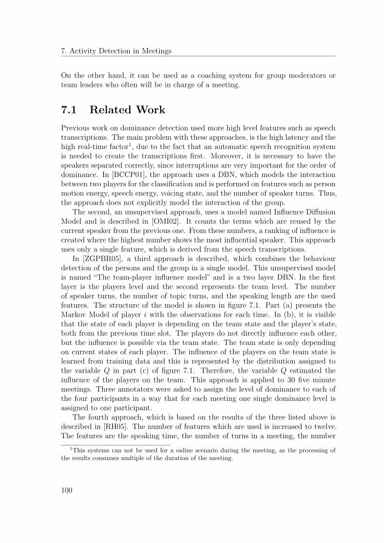
7. Activity Detection in Meetings
On the other hand, it can be used as a coaching system for group moderators orteam leaders who often will be in charge of a meeting.
7.1 Related Work
Previous work on dominance detection used more high level features such as speechtranscriptions. The main problem with these approaches, is the high latency and thehigh real-time factor1, due to the fact that an automatic speech recognition systemis needed to create the transcriptions first. Moreover, it is necessary to have thespeakers separated correctly, since interruptions are very important for the order ofdominance. In [BCCP01], the approach uses a DBN, which models the interactionbetween two players for the classification and is performed on features such as personmotion energy, speech energy, voicing state, and the number of speaker turns. Thus,the approach does not explicitly model the interaction of the group.
The second, an unsupervised approach, uses a model named Influence DiffusionModel and is described in [OMI02]. It counts the terms which are reused by thecurrent speaker from the previous one. From these numbers, a ranking of influence iscreated where the highest number shows the most influential speaker. This approachuses only a single feature, which is derived from the speech transcriptions.
In [ZGPBR05], a third approach is described, which combines the behaviourdetection of the persons and the group in a single model. This unsupervised modelis named “The team-player influence model” and is a two layer DBN. In the firstlayer is the players level and the second represents the team level. The numberof speaker turns, the number of topic turns, and the speaking length are the usedfeatures. The structure of the model is shown in figure 7.1. Part (a) presents theMarkov Model of player i with the observations for each time. In (b), it is visiblethat the state of each player is depending on the team state and the player’s state,both from the previous time slot. The players do not directly influence each other,but the influence is possible via the team state. The team state is only dependingon current states of each player. The influence of the players on the team state islearned from training data and this is represented by the distribution assigned tothe variable Q in part (c) of figure 7.1. Therefore, the variable Q estimated theinfluence of the players on the team. This approach is applied to 30 five minutemeetings. Three annotators were asked to assign the level of dominance to each ofthe four participants in a way that for each meeting one single dominance level isassigned to one participant.
The fourth approach, which is based on the results of the three listed above isdescribed in [RH05]. The number of features which are used is increased to twelve.The features are the speaking time, the number of turns in a meeting, the number
1This systems can not be used for a online scenario during the meeting, as the processing ofthe results consumes multiple of the duration of the meeting.
100
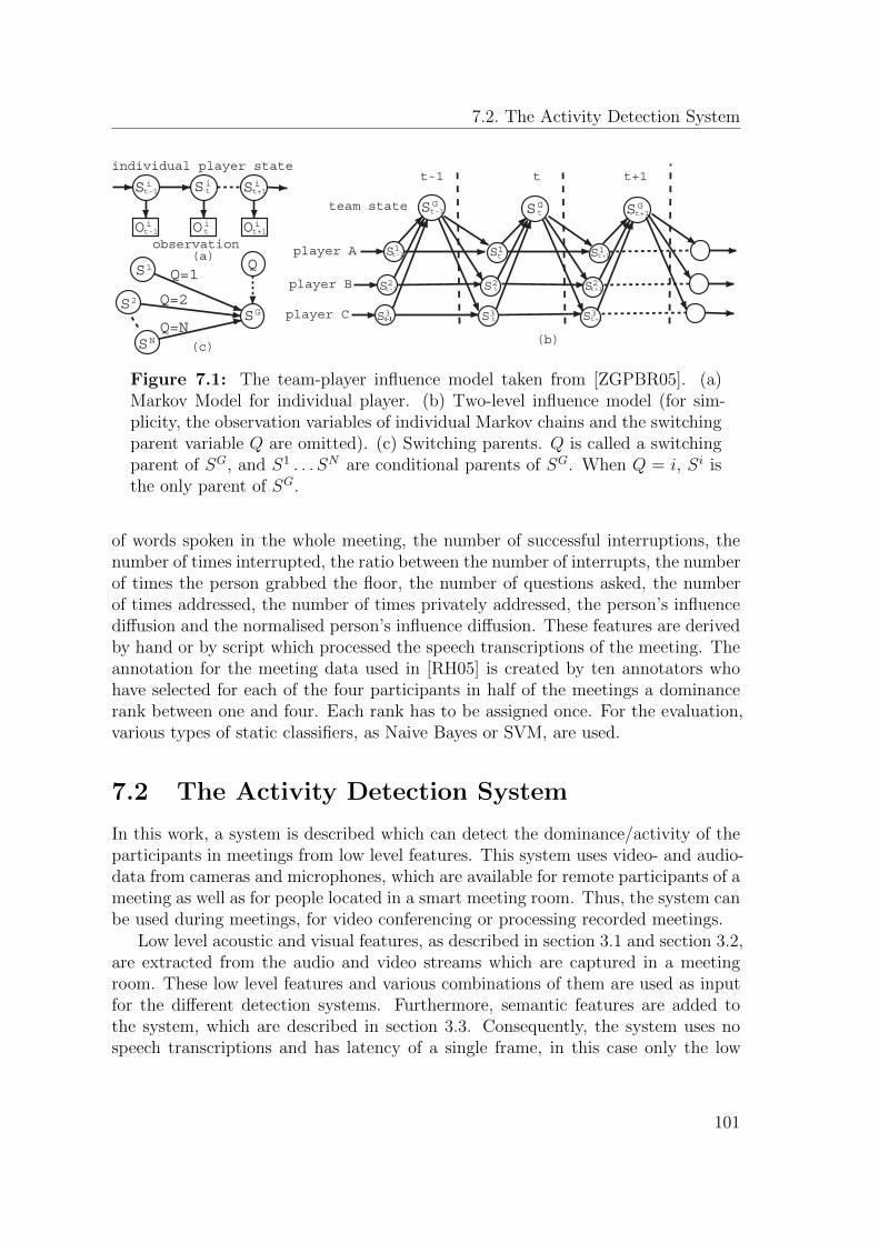
7.2. The Activity Detection System
(a)observation
individual player state
(b)
S
S
S
team state
player A
player B
player C
t-1 t t+1
GS t-1 GS t GS t+1
1S t 1S t-1 1S t+1
2S t-1 2S t
3S t 3S t-1 3S t+1
2S t+1
iS t-1
iO t-1 iO t
iS t+1
iO t+1
Q=1
Q=2
Q=N
Q
GS
(c)NS
2S
1S
iS t
Figure 7.1: The team-player influence model taken from [ZGPBR05]. (a)Markov Model for individual player. (b) Two-level influence model (for sim-plicity, the observation variables of individual Markov chains and the switchingparent variable Q are omitted). (c) Switching parents. Q is called a switchingparent of SG, and S1 . . . SN are conditional parents of SG. When Q = i, Si isthe only parent of SG.
of words spoken in the whole meeting, the number of successful interruptions, thenumber of times interrupted, the ratio between the number of interrupts, the numberof times the person grabbed the floor, the number of questions asked, the numberof times addressed, the number of times privately addressed, the person’s influencediffusion and the normalised person’s influence diffusion. These features are derivedby hand or by script which processed the speech transcriptions of the meeting. Theannotation for the meeting data used in [RH05] is created by ten annotators whohave selected for each of the four participants in half of the meetings a dominancerank between one and four. Each rank has to be assigned once. For the evaluation,various types of static classifiers, as Naive Bayes or SVM, are used.
7.2 The Activity Detection System
In this work, a system is described which can detect the dominance/activity of theparticipants in meetings from low level features. This system uses video- and audio-data from cameras and microphones, which are available for remote participants of ameeting as well as for people located in a smart meeting room. Thus, the system canbe used during meetings, for video conferencing or processing recorded meetings.
Low level acoustic and visual features, as described in section 3.1 and section 3.2,are extracted from the audio and video streams which are captured in a meetingroom. These low level features and various combinations of them are used as inputfor the different detection systems. Furthermore, semantic features are added tothe system, which are described in section 3.3. Consequently, the system uses nospeech transcriptions and has latency of a single frame, in this case only the low
101
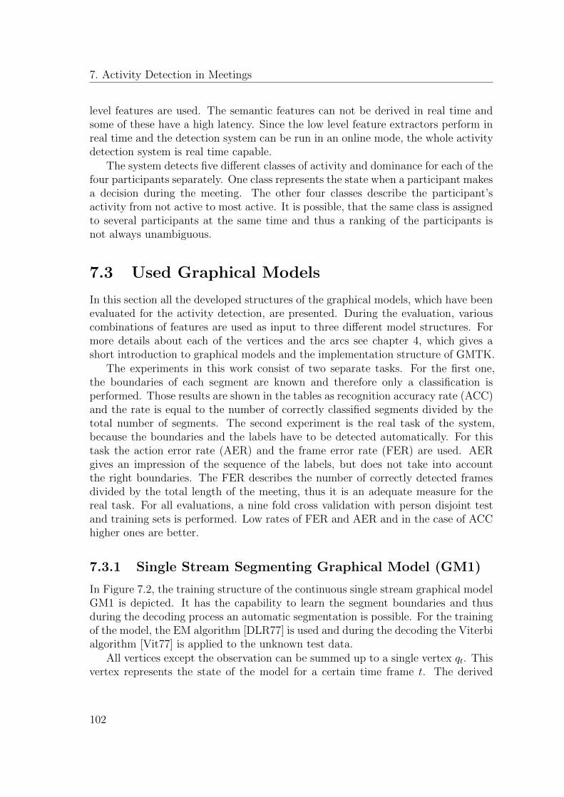
7. Activity Detection in Meetings
level features are used. The semantic features can not be derived in real time andsome of these have a high latency. Since the low level feature extractors perform inreal time and the detection system can be run in an online mode, the whole activitydetection system is real time capable.
The system detects five different classes of activity and dominance for each of thefour participants separately. One class represents the state when a participant makesa decision during the meeting. The other four classes describe the participant’sactivity from not active to most active. It is possible, that the same class is assignedto several participants at the same time and thus a ranking of the participants isnot always unambiguous.
7.3 Used Graphical Models
In this section all the developed structures of the graphical models, which have beenevaluated for the activity detection, are presented. During the evaluation, variouscombinations of features are used as input to three different model structures. Formore details about each of the vertices and the arcs see chapter 4, which gives ashort introduction to graphical models and the implementation structure of GMTK.
The experiments in this work consist of two separate tasks. For the first one,the boundaries of each segment are known and therefore only a classification isperformed. Those results are shown in the tables as recognition accuracy rate (ACC)and the rate is equal to the number of correctly classified segments divided by thetotal number of segments. The second experiment is the real task of the system,because the boundaries and the labels have to be detected automatically. For thistask the action error rate (AER) and the frame error rate (FER) are used. AERgives an impression of the sequence of the labels, but does not take into accountthe right boundaries. The FER describes the number of correctly detected framesdivided by the total length of the meeting, thus it is an adequate measure for thereal task. For all evaluations, a nine fold cross validation with person disjoint testand training sets is performed. Low rates of FER and AER and in the case of ACChigher ones are better.
7.3.1 Single Stream Segmenting Graphical Model (GM1)
In Figure 7.2, the training structure of the continuous single stream graphical modelGM1 is depicted. It has the capability to learn the segment boundaries and thusduring the decoding process an automatic segmentation is possible. For the trainingof the model, the EM algorithm [DLR77] is used and during the decoding the Viterbialgorithm [Vit77] is applied to the unknown test data.
All vertices except the observation can be summed up to a single vertex qt. Thisvertex represents the state of the model for a certain time frame t. The derived
102
7.3. Used Graphical Models
obs
SP
obs
SP
ST
CP
obs
SP
ST
CP
ST
CT
END
CP
C
FC FCFC
CT
CC
CT
CCCC
C C
Figure 7.2: The continuous single stream graphical model GM1 is used in thisthesis for the segmentation of the meeting and the classification of five labels ofactivity and decision making. Therefore, five classes have to be trained by theEM algorithm. The figure shows the training structure as it is implemented inGMTK for the training of the model. This structure trains in a single processboth the segmentation and classification. An elaborate description of all theused vertices can be found in chapter 4.
structure leads to the following production probability for the model
p(O,q|λ) = p(q1) · p(~o1|q1) ·T∏t=2
p(qt|qt−1) · p(~ot|qt), (7.1)
considering the sequence q = (q1, . . . , qT ) of all states which are run through. Whenthe substitutions, known from the forward-backward algorithm for HMMs, and themarginalization, by summing up over all possible state sequences q ∈ Q, are appliedto the equation 7.1 the following equation is derived:
p(O|λ) =∑q∈Q
πq1 · p(~o1|q1) ·T∏t=2
aqt−1,qt · p(~ot|qt). (7.2)
103
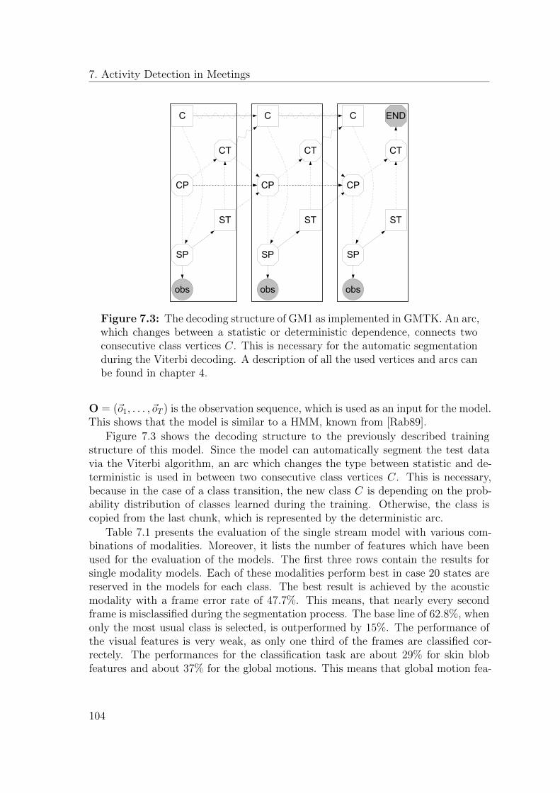
7. Activity Detection in Meetings
obs
SP
C
obs
SP
ST
CP
C
CT
obs
SP
ST
CP
C
CT
ST
CT
END
CP
Figure 7.3: The decoding structure of GM1 as implemented in GMTK. An arc,which changes between a statistic or deterministic dependence, connects twoconsecutive class vertices C. This is necessary for the automatic segmentationduring the Viterbi decoding. A description of all the used vertices and arcs canbe found in chapter 4.
O = (~o1, . . . , ~oT ) is the observation sequence, which is used as an input for the model.This shows that the model is similar to a HMM, known from [Rab89].
Figure 7.3 shows the decoding structure to the previously described trainingstructure of this model. Since the model can automatically segment the test datavia the Viterbi algorithm, an arc which changes the type between statistic and de-terministic is used in between two consecutive class vertices C. This is necessary,because in the case of a class transition, the new class C is depending on the prob-ability distribution of classes learned during the training. Otherwise, the class iscopied from the last chunk, which is represented by the deterministic arc.
Table 7.1 presents the evaluation of the single stream model with various com-binations of modalities. Moreover, it lists the number of features which have beenused for the evaluation of the models. The first three rows contain the results forsingle modality models. Each of these modalities perform best in case 20 states arereserved in the models for each class. The best result is achieved by the acousticmodality with a frame error rate of 47.7%. This means, that nearly every secondframe is misclassified during the segmentation process. The base line of 62.8%, whenonly the most usual class is selected, is outperformed by 15%. The performance ofthe visual features is very weak, as only one third of the frames are classified cor-rectely. The performances for the classification task are about 29% for skin blobfeatures and about 37% for the global motions. This means that global motion fea-
104
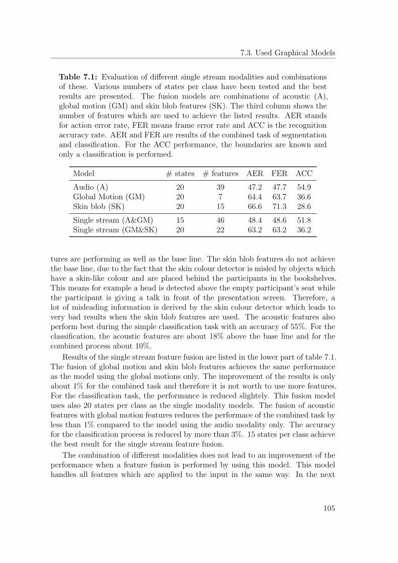
7.3. Used Graphical Models
Table 7.1: Evaluation of different single stream modalities and combinationsof these. Various numbers of states per class have been tested and the bestresults are presented. The fusion models are combinations of acoustic (A),global motion (GM) and skin blob features (SK). The third column shows thenumber of features which are used to achieve the listed results. AER standsfor action error rate, FER means frame error rate and ACC is the recognitionaccuracy rate. AER and FER are results of the combined task of segmentationand classification. For the ACC performance, the boundaries are known andonly a classification is performed.
Model # states # features AER FER ACC
Audio (A) 20 39 47.2 47.7 54.9Global Motion (GM) 20 7 64.4 63.7 36.6Skin blob (SK) 20 15 66.6 71.3 28.6
Single stream (A&GM) 15 46 48.4 48.6 51.8Single stream (GM&SK) 20 22 63.2 63.2 36.2
tures are performing as well as the base line. The skin blob features do not achievethe base line, due to the fact that the skin colour detector is misled by objects whichhave a skin-like colour and are placed behind the participants in the bookshelves.This means for example a head is detected above the empty participant’s seat whilethe participant is giving a talk in front of the presentation screen. Therefore, alot of misleading information is derived by the skin colour detector which leads tovery bad results when the skin blob features are used. The acoustic features alsoperform best during the simple classification task with an accuracy of 55%. For theclassification, the acoustic features are about 18% above the base line and for thecombined process about 10%.
Results of the single stream feature fusion are listed in the lower part of table 7.1.The fusion of global motion and skin blob features achieves the same performanceas the model using the global motions only. The improvement of the results is onlyabout 1% for the combined task and therefore it is not worth to use more features.For the classification task, the performance is reduced slightely. This fusion modeluses also 20 states per class as the single modality models. The fusion of acousticfeatures with global motion features reduces the performace of the combined task byless than 1% compared to the model using the audio modality only. The accuracyfor the classification process is reduced by more than 3%. 15 states per class achievethe best result for the single stream feature fusion.
The combination of different modalities does not lead to an improvement of theperformance when a feature fusion is performed by using this model. This modelhandles all features which are applied to the input in the same way. In the next
105
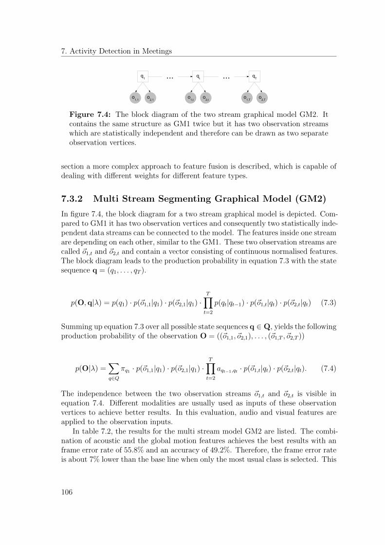
7. Activity Detection in Meetings
q1
o1,1
o2,1
o1,t
o2,t
qT
o1,T
o2,T
qt ......
Figure 7.4: The block diagram of the two stream graphical model GM2. Itcontains the same structure as GM1 twice but it has two observation streamswhich are statistically independent and therefore can be drawn as two separateobservation vertices.
section a more complex approach to feature fusion is described, which is capable ofdealing with different weights for different feature types.
7.3.2 Multi Stream Segmenting Graphical Model (GM2)
In figure 7.4, the block diagram for a two stream graphical model is depicted. Com-pared to GM1 it has two observation vertices and consequently two statistically inde-pendent data streams can be connected to the model. The features inside one streamare depending on each other, similar to the GM1. These two observation streams arecalled ~o1,t and ~o2,t and contain a vector consisting of continuous normalised features.The block diagram leads to the production probability in equation 7.3 with the statesequence q = (q1, . . . , qT ).
p(O,q|λ) = p(q1) · p(~o1,1|q1) · p(~o2,1|q1) ·T∏t=2
p(qt|qt−1) · p(~o1,t|qt) · p(~o2,t|qt) (7.3)
Summing up equation 7.3 over all possible state sequences q ∈ Q, yields the followingproduction probability of the observation O = ((~o1,1, ~o2,1), . . . , (~o1,T , ~o2,T ))
p(O|λ) =∑q∈Q
πq1 · p(~o1,1|q1) · p(~o2,1|q1) ·T∏t=2
aqt−1,qt · p(~o1,t|qt) · p(~o2,t|qt). (7.4)
The independence between the two observation streams ~o1,t and ~o2,t is visible inequation 7.4. Different modalities are usually used as inputs of these observationvertices to achieve better results. In this evaluation, audio and visual features areapplied to the observation inputs.
In table 7.2, the results for the multi stream model GM2 are listed. The combi-nation of acoustic and the global motion features achieves the best results with anframe error rate of 55.8% and an accuracy of 49.2%. Therefore, the frame error rateis about 7% lower than the base line when only the most usual class is selected. This
106
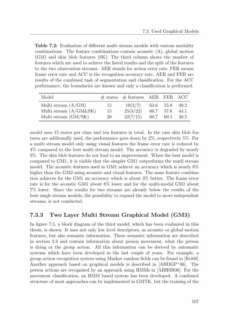
7.3. Used Graphical Models
Table 7.2: Evaluation of different multi stream models with various modalitycombinations. The feature combinations contain acoustic (A), global motion(GM) and skin blob features (SK). The third column shows the number offeatures which are used to achieve the listed results and the split of the featuresto the two observation streams. AER stands for action error rate, FER meansframe error rate and ACC is the recognition accuracy rate. AER and FER areresults of the combined task of segmentation and classification. For the ACCperformance, the boundaries are known and only a classification is performed.
Model # states # features AER FER ACC
Multi stream (A/GM) 15 10(3/7) 63.6 55.8 49.2Multi stream (A/GM&SK) 15 25(3/22) 60.7 57.6 44.1Multi stream (GM/SK) 20 22(7/15) 60.7 60.1 40.5
model uses 15 states per class and ten features in total. In the case skin blob fea-tures are additonally used, the performance goes down by 2%, respectively 5%. Fora multi stream model only using visual features the frame error rate is reduced by4% compared to the best multi stream model. The accuracy is degraded by nearly9%. The skin blob features do not lead to an improvement. When the best model iscompared to GM1, it is visible that the simpler GM1 outperforms the mutli streammodel. The acoustic features used in GM1 achieve an accuracy which is nearly 6%higher than the GM2 using acoustic and visual features. The same feature combina-tion achieves for the GM1 an accuracy which is about 3% better. The frame errorrate is for the acoustic GM1 about 8% lower and for the multi-modal GM1 about7% lower. Since the results for two streams are already below the results of thebest single stream models, the possibility to expand the model to more independentstreams, is not conducted.
7.3.3 Two Layer Multi Stream Graphical Model (GM3)
In figure 7.5, a block diagram of the third model, which has been evaluated in thisthesis, is shown. It uses not only low level descriptors, as acoustic or global motionfeatures, but also semantic information. These semantic information are describedin section 3.3 and contain information about person movement, what the personis doing or the group action. All this information can be derived by automaticsystems which have been developed in the last couple of years. For example, agroup action recognition system using Markov random fields can be found in [Rei08].Another approach based on graphical models is described in [AHDGP+06]. Theperson actions are recognised by an approach using HMMs in [AHHSR06]. For themovement classification, an HMM based system has been developed. A combinedstructure of most approaches can be implemented in GMTK, but the training of the
107
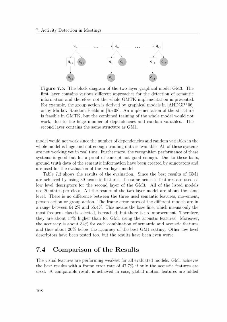
7. Activity Detection in Meetings
q1,T
q2,T
o2,T
o1,T
q1,t
q2,t
o2,t
o1,t
q1,1
q2,1
o2,1
......
o1,1
Figure 7.5: The block diagram of the two layer graphical model GM3. Thefirst layer contains various different approaches for the detection of semanticinformation and therefore not the whole GMTK implementation is presented.For example, the group action is derived by graphical models in [AHDGP+06]or by Markov Random Fields in [Rei08]. An implementation of the structureis feasible in GMTK, but the combined training of the whole model would notwork, due to the huge number of dependencies and random variables. Thesecond layer contains the same structure as GM1.
model would not work since the number of dependencies and random variables in thewhole model is huge and not enough training data is available. All of these systemsare not working yet in real time. Furthermore, the recognition performance of thesesystems is good but for a proof of concept not good enough. Due to these facts,ground truth data of the semantic information have been created by annotators andare used for the evaluation of the two layer model.
Table 7.3 shows the results of the evaluation. Since the best results of GM1are achieved by using 39 acoustic features, the same acoustic features are used aslow level descriptors for the second layer of the GM3. All of the listed modelsuse 20 states per class. All the results of the two layer model are about the samelevel. There is no difference between the three used semantic features, movement,person action or group action. The frame error rates of the different models are ina range between 64.2% and 65.4%. This means the base line, which means only themost frequent class is selected, is reached, but there is no improvement. Therefore,they are about 17% higher than for GM1 using the acoustic features. Moreover,the accuracy is about 34% for each combination of semantic and acoustic featuresand thus about 20% below the accuracy of the best GM1 setting. Other low leveldescriptors have been tested too, but the results have been even worse.
7.4 Comparison of the Results
The visual features are performing weakest for all evaluated models. GM1 achievesthe best results with a frame error rate of 47.7% if only the acoustic features areused. A comparable result is achieved in case, global motion features are added
108
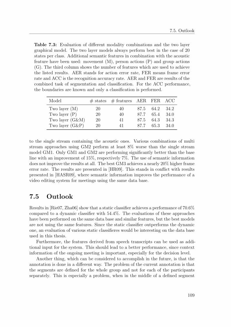
7.5. Outlook
Table 7.3: Evaluation of different modality combinations and the two layergraphical model. The two layer models always perform best in the case of 20states per class. Additional semantic features in combination with the acousticfeature have been used: movement (M), person actions (P) and group actions(G). The third column shows the number of features which are used to achievethe listed results. AER stands for action error rate, FER means frame errorrate and ACC is the recognition accuracy rate. AER and FER are results of thecombined task of segmentation and classification. For the ACC performance,the boundaries are known and only a classification is performed.
Model # states # features AER FER ACC
Two layer (M) 20 40 87.5 64.2 34.2Two layer (P) 20 40 87.7 65.4 34.0Two layer (G&M) 20 41 87.5 64.3 34.3Two layer (G&P) 20 41 87.7 65.3 34.0
to the single stream containing the acoustic ones. Various combinations of multistream approaches using GM2 perform at least 8% worse than the single streammodel GM1. Only GM1 and GM2 are performing significantly better than the baseline with an improvement of 15%, respectively 7%. The use of semantic informationdoes not improve the results at all. The best GM3 achieves a nearly 20% higher frameerror rate. The results are presented in [HR09]. This stands in conflict with resultspresented in [HASR09], where semantic information improves the performance of avideo editing system for meetings using the same data base.
7.5 Outlook
Results in [Rie07, Zha06] show that a static classifier achieves a performance of 70.6%compared to a dynamic classifier with 54.4%. The evaluations of these approacheshave been performed on the same data base and similar features, but the best modelsare not using the same features. Since the static classifier outperforms the dynamicone, an evaluation of various static classifieres would be interesting on the data baseused in this thesis.
Furthermore, the features derived from speech transcripts can be used as addi-tional input for the system. This should lead to a better performance, since contextinformation of the ongoing meeting is important, especially for the decision level.
Another thing, which can be considered to accomplish in the future, is that theannotation is done in a different way. The problem of the current annotation is thatthe segments are defined for the whole group and not for each of the participantsseparately. This is especially a problem, when in the middle of a defined segment
109

7. Activity Detection in Meetings
a person stops speaking and another participant starts speaking. The annotationwould get more precise and this is good for the training of the classifiers. It wouldlead to better results for the classification process, but the segmentation and classifi-cation task would get more difficult because several boundaries for each participanthave to be found.
110
8
Multi-modal Interest Detection
For the communication between people, many different techniques are used for theinteraction. Various different techniques are commonly used when people communi-cate and interact with each other. Not only spoken words, even gaze, facial expres-sions, gestures and intonation of speech are essential for the human communicationand interaction. For a natural dialogue between a machine and a human subject itis important to take all these interaction skills into account. A machine has to un-derstand the natural way of human communication, in order to provide interactionthat is close to human to human dialogue [AC75, NL86].
In the last couple of years multi-model dialogue systems are becoming more com-mon. These systems are capable to detect reactions of human users and respond tothem in an appropriate way. Such reactions can be in a wide range from non-verbalover social and emotional perception to interaction and behavioural capabilities.Various publications illustrate which combinations of interaction skills are impor-tant [TKB92, Tho93]. Numerous research projects are developing such dialogue sys-tems [SBE+09, Sch10], for example the SEMAINE project1. In [SKMR06, SMH+07],systems are introduced which detect the level of interest of a human user. The infor-mation on interest has great potential for the Human-Machine Interaction [PM05,Shr05] and consequently for many commercial applications, as advertisement sys-tems and virtual guides. Furthermore, the level of interest has been analysed inmeeting scenarios in many publications, for example [SYW02, KE03, GPMZB05].Another application is described in [MP03], where a tutor system for children isdeveloped. Not only in the field of interest, research has been conducted, but alsosystems for the detection of the curiosity have been developed [QBZ05].
In the literature, numerous publications can be found about the recognition ofaffective and emotional states of users. The emotional states are closely related tothe interest in the topic of the ongoing dialogue. Many of these works only applyacoustic speech parameters [SRL03, BSH+05]. In [KPI04, ALC+07], for example,
1The aim of the SEMAINE project is to build a Sensitive Artificial Listener. The funding forthe research project comes from the European Community’s Seventh Framework Programme.
111
8. Multi-modal Interest Detection
systems are described which use vision based features for the task. There are fewerapproaches using visual features than systems performing on acoustic parameters.The fusion of all available input features generally helps to improve the results, yetonly few publications are available which deal with multi-model approaches for thedetection of emotional states [GPMZB05, MP07, SMH+07, SME+09]. In general,not only the performance is improved, but also the reliability and the robustness ofsuch a system [CDCT+01, PR03, SAR+07, WSA+08].
8.1 Related Work
There is only little published work on the same data base as used for the interestrecognition in this thesis. An approach is introduced in [SKMR06], which analysesacoustic and linguistic cues of spoken segments. More than 5.000 features andfunctionals are extracted from each segment. The statistical analysis of individualsegments is important, since most information of the level of interest is availableby analysing the development of the feature values over a segment. A subsequentfeature space reduction has to be performed to find the most relevant attributes.Linguistic information is added by a bag-of-words2 representation taken from thespeech recogniser. The prototype achieves a remarkable performance using supportvector machines for the selection of one of the three level of interest classes.
The first audio-visual approach for the recognition of spontaneous interest hasbeen presented in [SMH+07]. Active appearance models are used for the detection offacial expressions. Moreover, the movement of the eyes are recorded by an eye trackerand the activity of the eyes is further analysed. Speech is analyzed with respect toacoustic properties. This is based on a high-dimensional prosodic, articulatory, andvoice quality feature space. Furthermore, the linguistic analysis of spoken contentis modeled by a large-vocabulary continuous speech recognition engine and a bag-of-words vector space including non-verbals. A person-independent system is evaluatedand the results show the high potential of such a multi-modal approach applyingsupport vector machines as classifiers.
The multi-modal approach from [SMH+07] is extended by the use of temporalcontext information in [SME+09]. Consequently, Active-Appearance-Model-basedfacial expression, vision-based eye-activity estimation, acoustic features, linguisticanalysis, non-linguistic vocalisations, and temporal context information are com-bined by an early feature fusion. Support vector machines are trained for the eval-uation and subject disjunct test and training sets are used. Moreover, a real-lifesystem has been developed and is tested during a user-study. The theoretical andpractical proof of effectiveness is demonstrated.
2Bag-of-words means, that various words are combined into one bag. A bag is found if the samewords, as stored inside the bag, are recognised without taking into account the word order.
112

8.2. The Dialogue Control System
In [SR09], a comparison of bag of frames and supra-segmental features is de-scribed. Supra-segmental features are functionals, which are calculated for eachsegment from the low level features extracted from each frame. Based on the func-tionals, support vector machines are trained. For the bag of frames also supportvector machines are trained, but multi-instance learning is performed on the fea-tures which are based on frames [ATH03]. A comparison shows that some featuregroups, for example pitch and energy, perform far better on the segments than onframe base. The mel frequency cepstral coefficients still suffer from the frame basedapproach but not as much as other feature groups.
8.2 The Dialogue Control System
The dialogue control system developed in this thesis analyses both audio and visualrecordings. From the audio stream various low level features and functionals areextracted, as described in section 3.1. These functionals are calculated for segmentswith a duration of one second, respectively 25 frames, compared to the function-als used in the related work, where these are calculated for segments of differentdurations. The acoustic functionals have an overlap of 24 frames, since these arecalculated for each frame. Global motion features are extracted from the visualrecordings, as specified in section 3.2.2. Furthermore, a principal component analy-sis is performed and the derived features are also evaluated. An audio-visual fusionis performed on feature level and therefore the segments are classified on a framebase. This is the main difference to most publications described in the related worksection, which classifies on segment base. In [SR09], it is shown that the classifi-cation with support vector machines performs better on segments as it does on aframe base.
In this thesis, only the detection of the level of interest is described and all theevaluations are taking place on data which is recorded from a human-to-humanconversation. For the user study, a shift of the paradigm is necessary. The setting ofthe whole dialogue control system is in a way, that a subject is seated in front of amonitor, which means a human-to-machine conversation takes place. A camera anda microphone is located close to the monitor for audio-visual recordings. A maleanimated embodied conversational agent is shown on the screen and it guides thesubject through the topics. This dialogue system, which is capable of switching toa different topic if the subject is bored, has been developed for a user study. Thisuser study is performed as a Wizard-Of-Oz experiment [Nie93, NSGN02], where thedialogue is controlled by a human operator. Moreover, the system is able to switchthe topics automatically depending on the results of the level of interest detection.The results of a study can be found in [SME+09].
113
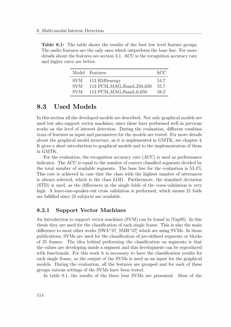
8. Multi-modal Interest Detection
Table 8.1: The table shows the results of the best low level feature groups.The audio features are the only ones which outperform the base line. For moredetails about the features see section 3.1. ACC is the recognition accuracy rateand higher rates are better.
Model Features ACC
SVM 113 RMSenergy 54.7SVM 113 PCM MAG fband 250 650 55.7SVM 113 PCM MAG fband 0 650 58.2
8.3 Used Models
In this section all the developed models are described. Not only graphical models areused but also support vector machines, since these have performed well in previousworks on the level of interest detection. During the evaluation, different combina-tions of features as input and parameters for the models are tested. For more detailsabout the graphical model structure, as it is implemented in GMTK, see chapter 4.It gives a short introduction to graphical models and to the implementation of themin GMTK.
For the evaluation, the recognition accuracy rate (ACC) is used as performanceindicator. The ACC is equal to the number of correct classified segments divided bythe total number of available segments. The base line for the evaluation is 53.4%.This rate is achieved in case that the class with the highest number of utterancesis always selected, which is the class LOI1. Furthermore, the standard deviation(STD) is used, as the differences in the single folds of the corss-validation is veryhigh. A leave-one-speaker-out cross validation is performed, which means 21 foldsare fulfilled since 21 subjects are available.
8.3.1 Support Vector Machines
An introduction to support vector machines (SVM) can be found in [Vap95]. In thisthesis they are used for the classification of each single frame. This is also the maindifference to most other works [SWA+07, SMH+07] which are using SVMs. In thosepublications, SVMs are used for the classification of pre-defined segments or blocksof 25 frames. The idea behind performing the classification on segments is thatthe values are developing inside a segment and this development can be reproducedwith functionals. For this work it is necessary to have the classification results foreach single frame, as the output of the SVMs is used as an input for the graphicalmodels. During the evaluation, all the features are grouped and for each of thesegroups various settings of the SVMs have been tested.
In table 8.1, the results of the three best SVMs are presented. Most of the
114
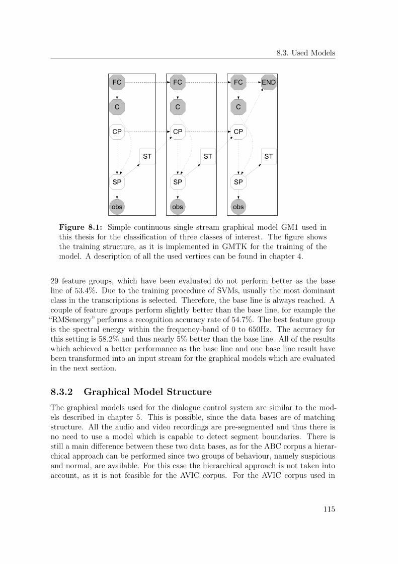
8.3. Used Models
obs
SP
obs
SP
ST
CP
obs
SP
ST ST
END
CP
C
FC FCFC
CP
C C
Figure 8.1: Simple continuous single stream graphical model GM1 used inthis thesis for the classification of three classes of interest. The figure showsthe training structure, as it is implemented in GMTK for the training of themodel. A description of all the used vertices can be found in chapter 4.
29 feature groups, which have been evaluated do not perform better as the baseline of 53.4%. Due to the training procedure of SVMs, usually the most dominantclass in the transcriptions is selected. Therefore, the base line is always reached. Acouple of feature groups perform slightly better than the base line, for example the
“RMSenergy” performs a recognition accuracy rate of 54.7%. The best feature groupis the spectral energy within the frequency-band of 0 to 650Hz. The accuracy forthis setting is 58.2% and thus nearly 5% better than the base line. All of the resultswhich achieved a better performance as the base line and one base line result havebeen transformed into an input stream for the graphical models which are evaluatedin the next section.
8.3.2 Graphical Model Structure
The graphical models used for the dialogue control system are similar to the mod-els described in chapter 5. This is possible, since the data bases are of matchingstructure. All the audio and video recordings are pre-segmented and thus there isno need to use a model which is capable to detect segment boundaries. There isstill a main difference between these two data bases, as for the ABC corpus a hierar-chical approach can be performed since two groups of behaviour, namely suspiciousand normal, are available. For this case the hierarchical approach is not taken intoaccount, as it is not feasible for the AVIC corpus. For the AVIC corpus used in
115
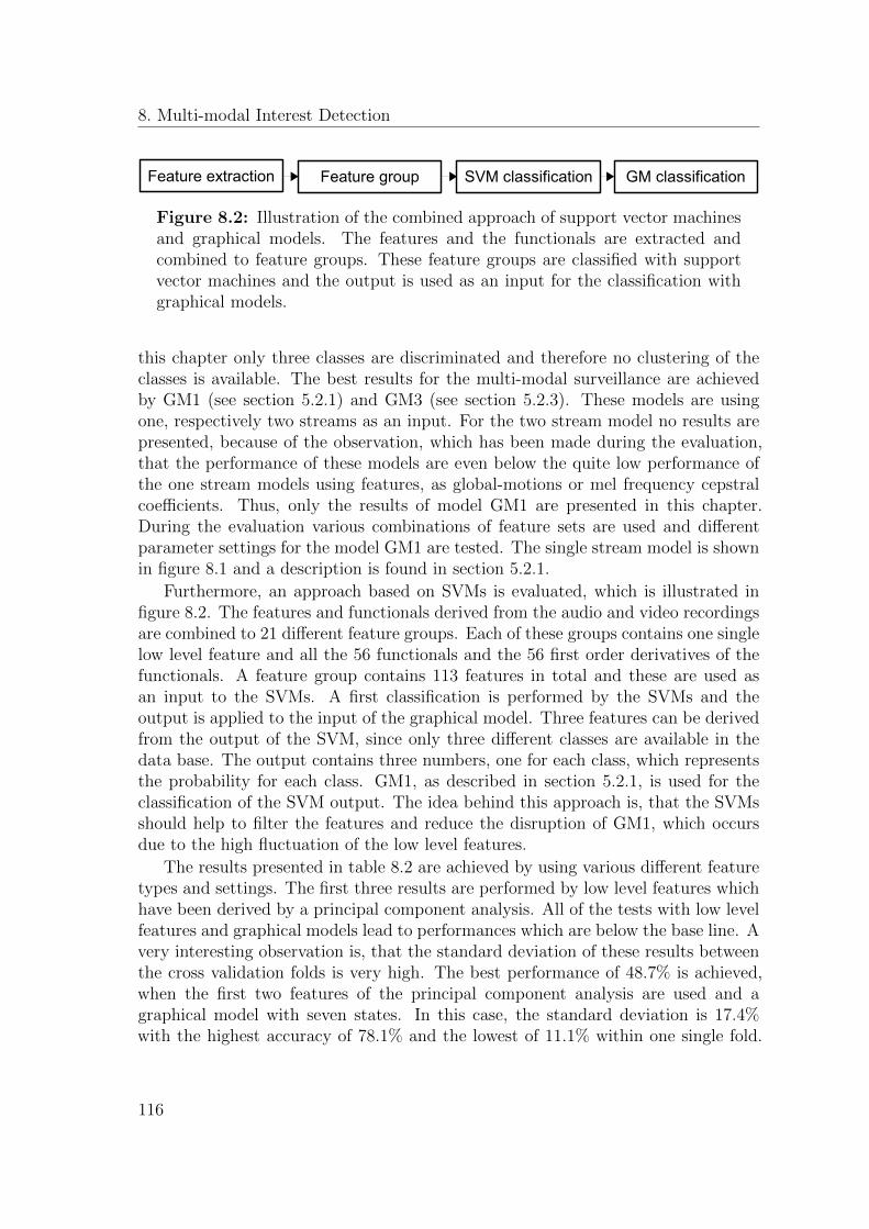
8. Multi-modal Interest Detection
Feature extraction Feature group SVM classification GM classification
Figure 8.2: Illustration of the combined approach of support vector machinesand graphical models. The features and the functionals are extracted andcombined to feature groups. These feature groups are classified with supportvector machines and the output is used as an input for the classification withgraphical models.
this chapter only three classes are discriminated and therefore no clustering of theclasses is available. The best results for the multi-modal surveillance are achievedby GM1 (see section 5.2.1) and GM3 (see section 5.2.3). These models are usingone, respectively two streams as an input. For the two stream model no results arepresented, because of the observation, which has been made during the evaluation,that the performance of these models are even below the quite low performance ofthe one stream models using features, as global-motions or mel frequency cepstralcoefficients. Thus, only the results of model GM1 are presented in this chapter.During the evaluation various combinations of feature sets are used and differentparameter settings for the model GM1 are tested. The single stream model is shownin figure 8.1 and a description is found in section 5.2.1.
Furthermore, an approach based on SVMs is evaluated, which is illustrated infigure 8.2. The features and functionals derived from the audio and video recordingsare combined to 21 different feature groups. Each of these groups contains one singlelow level feature and all the 56 functionals and the 56 first order derivatives of thefunctionals. A feature group contains 113 features in total and these are used asan input to the SVMs. A first classification is performed by the SVMs and theoutput is applied to the input of the graphical model. Three features can be derivedfrom the output of the SVM, since only three different classes are available in thedata base. The output contains three numbers, one for each class, which representsthe probability for each class. GM1, as described in section 5.2.1, is used for theclassification of the SVM output. The idea behind this approach is, that the SVMsshould help to filter the features and reduce the disruption of GM1, which occursdue to the high fluctuation of the low level features.
The results presented in table 8.2 are achieved by using various different featuretypes and settings. The first three results are performed by low level features whichhave been derived by a principal component analysis. All of the tests with low levelfeatures and graphical models lead to performances which are below the base line. Avery interesting observation is, that the standard deviation of these results betweenthe cross validation folds is very high. The best performance of 48.7% is achieved,when the first two features of the principal component analysis are used and agraphical model with seven states. In this case, the standard deviation is 17.4%with the highest accuracy of 78.1% and the lowest of 11.1% within one single fold.
116
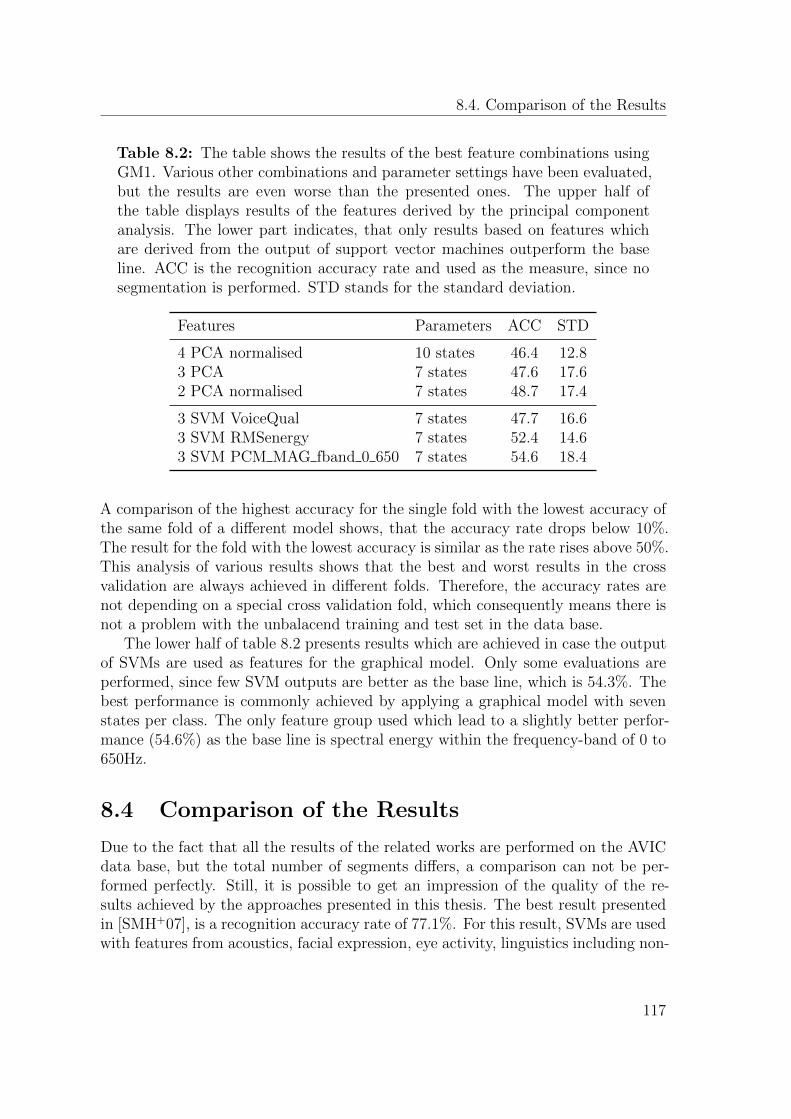
8.4. Comparison of the Results
Table 8.2: The table shows the results of the best feature combinations usingGM1. Various other combinations and parameter settings have been evaluated,but the results are even worse than the presented ones. The upper half ofthe table displays results of the features derived by the principal componentanalysis. The lower part indicates, that only results based on features whichare derived from the output of support vector machines outperform the baseline. ACC is the recognition accuracy rate and used as the measure, since nosegmentation is performed. STD stands for the standard deviation.
Features Parameters ACC STD
4 PCA normalised 10 states 46.4 12.83 PCA 7 states 47.6 17.62 PCA normalised 7 states 48.7 17.4
3 SVM VoiceQual 7 states 47.7 16.63 SVM RMSenergy 7 states 52.4 14.63 SVM PCM MAG fband 0 650 7 states 54.6 18.4
A comparison of the highest accuracy for the single fold with the lowest accuracy ofthe same fold of a different model shows, that the accuracy rate drops below 10%.The result for the fold with the lowest accuracy is similar as the rate rises above 50%.This analysis of various results shows that the best and worst results in the crossvalidation are always achieved in different folds. Therefore, the accuracy rates arenot depending on a special cross validation fold, which consequently means there isnot a problem with the unbalacend training and test set in the data base.
The lower half of table 8.2 presents results which are achieved in case the outputof SVMs are used as features for the graphical model. Only some evaluations areperformed, since few SVM outputs are better as the base line, which is 54.3%. Thebest performance is commonly achieved by applying a graphical model with sevenstates per class. The only feature group used which lead to a slightly better perfor-mance (54.6%) as the base line is spectral energy within the frequency-band of 0 to650Hz.
8.4 Comparison of the Results
Due to the fact that all the results of the related works are performed on the AVICdata base, but the total number of segments differs, a comparison can not be per-formed perfectly. Still, it is possible to get an impression of the quality of the re-sults achieved by the approaches presented in this thesis. The best result presentedin [SMH+07], is a recognition accuracy rate of 77.1%. For this result, SVMs are usedwith features from acoustics, facial expression, eye activity, linguistics including non-
117
8. Multi-modal Interest Detection
linguistic vocalisations and context, which are extracted from each segment of thedata base with 996 segments in total. The data base evaluated in this thesis hasonly 925 segements, due to the fact that some segments of the 996 have a durationof less than ten frames. The best performance achieved during this thesis is 54.6%,which is nearly 20% below the best performance reported in [SMH+07]. Therefore,the approach using SVMs on frame base is not leading to an improvement. Allgraphical models do not reach the base line of 54.3%.
In [SR09], a frame based approach is compared with the approach applied tosegments and the results show that SVMs perform better on segments than onframes. This can be explained, since the development of values is much betterrepresented in functionals which are calculated from the whole segment, than infeatures derived from a single frame. Even functionals, which are calculated overseveral frames, as it has been done in this thesis, do not lead to an improvement ofthe performance.
8.5 Outlook
A different approach for the training of SVMs can be evaluated, as the performancein [SR09] shows that multi-instance learning helps to achieve good results even onfeatures which are extracted on the frame level. A similar training algorithm can bedeveloped for graphical models [ZZ03], which should help to improve the results ofthose models, too.
Moreover, the features can be analysed if there is much noise overlaid and filterscan solve that problem. The data base can be scanned for segments where no speechsignals are available and the duration of the segments can be investigated. At themoment, the shortest segments have a duration of only 400ms which is very shortfor a proper classification of an emotion state, such as level of interest for example.
118
9
Summary
In this work some real life problems have been transformed into a form which allowsapplying modern pattern recognition methods to them. By doing this, it is possibleto come up with solutions for these problems which help people with their dailybusiness. In this thesis, the focus is on surveillance, meetings and dialogue scenarios.For all of these the access to multi-modal recordings of the subject is possible. Thisis very important since performance and robustness are increased compared to singlemodality recordings. Various graphical models are evaluated for each of the scenariosand the performances are compared to publications on the same topic.
A graphical model is a combination of graph- and probability theory. The graphtheory allows a simplification by performing algorithms based on the graph andtherefore the calculations of the required probabilities can be easier. This is veryimportant, because a slight change of the graph or of the probability leads to havingto start each calculation form scratch. By using algorithms based on the graph,many calculations do not start from the beginning, but previous results can bereused. Furthermore, the graph gives an intuitive description of complex problemswhich depends on many different random variables. This makes a graphical modelespecially suitable for rapid-prototyping and expert-systems, where the probabilitiesare defined by the expert. Finally, graphical models can be adapted to any complexproblem and not the problem has to be abstracted to fit to the pattern recognitionmethod.
As an input to the graphical models, various types of features are used. Thesefeatures are extracted from audio and visual recordings. Furthermore, semanticinformation is derived from the meeting data which is also used as an input. Not onlylow level descriptors are used, but especially from the acoustic features functionalshave been calculated which help to detect a development in time of different features.In total, more than 3000 features are extracted. Since graphical models can not dealwith the huge amount of features, a feature space reduction is performed dependingon the different scenarios. Two types are evaluated: the sequential forward selectionand the principal component analysis.
119
9. Summary
In the following paragraphs the four scenarios are summed up shortly. Thefirst scenario is about surveillance of passengers in an aircraft. Via audio-visualrecordings, a passenger which is located in his or her seat, is analysed if he or she actssuspiciously or normally. Therefore, various sets of features, graphical models anddifferent parameters are evaluated. The best results are achieved by a hierarchicalmodel which makes a decision about suspicious or normal behaviour in the first layerand a more specific decision within these two behaviour groups in the second layer.The recognition accuracy of the models is 53.3%. An approach using support vectormachines achieves 81.1%, which is 27.8% above the graphical model and thereforethe graphical models should not be used for this scenario.
The second scenario is automatic video editing in meetings. This means, thatthe meeting is recorded with several cameras and the most relevant view of thesecameras has to be found for each time frame. This view is transmitted to the remoteparticipants during a video conference or is shown in case an archived meeting iswatched. The meeting is not only recorded with cameras but also microphones areused for that. Depending on audio, visual and semantic information the best view isfound by a graphical model. The best graphical model achieves a frame error rate of38.1% which is 5.8% lower as an Asynchronous Hidden Markov Model found in theliterature. Compared to other apporaches using graphical models or hidden markovmodels, the performance has been improved by 9.6%.
Detection of activity and dominance in meetings is the third scenario. During themeeting for each participant separately, the level of activity is recognised from thesame information as used for the video editing. Each participant is automaticallyassigned by a graphical model for each time frame to one of the labels in the rangebetween absent to most active. The output can be used for assisting the moderatorof the meeting, because it shows for example if a participant is not involved in themeeting. The lowest frame error rate with 47.7% is achieved by graphical models, us-ing only the acoustic features. Due to the lack of comparable results in the litrature,it is not possible to compare them, but the best dynamic classifier found achieves arecognition rate of 54.4%, using a similar data base and different features. This iscomparable with the performance of the graphical model presented in this work.
The last scenario is an interest detection system for a human-machine-interaction.A subject is talking with a machine and at the same time it is recorded by a cameraand a microphone. From these recordings, an audio-visual analysis of the subject’slevel of interest is performed. This means that the subject is assigned to a predefinedlevel for short segments during the dialogue. Depending on these levels the machinerecognises if the topic is interesting for the subject and makes a decision if a topicchange makes sense. Since graphical models perform very badly in this scenario, anew approach combining support vector machines and graphical models has beenevaluated. Even this approach does not lead to a significant improvement comparedto the base line. If the results are compared with other approaches using supportvector machines and different features, the performance is nearly 20% below the best
120
9.1. Conclusion
result presented in other works.
9.1 Conclusion
In this work graphical models have been applied to very different applications, whichshows the high flexibility of graphical models. The models have been adapted tothe different applications, which is very important for further research in differentother fields of application. Another important point is that graphical models allowto describe complex problems in a simple form, which also helps to get into otherapplication fields and helps to formulate problems in a way many people can un-derstand. Furthermore, graphical models provide a universal description of variousapplications and therefore it is simple for an expert in graphical models to provideanalysis and results for a model developed by someone else. Since a general formal-ism exists for these models, many instructions and algorithms are available whichcan be applied to all types of graphical models.
The main drawback of the possibility to develop models depending on the prob-lem is that the number of parameters which have to be adjusted and trained canrise fast. In this case, more training samples are needed or for very complex modelsthe training gets in intractable. The high flexibility of graphical models allows todevelop multi-layer models, which take into account various levels of information,for example low level features, results from classifiers or high level semantic informa-tion. A model like this needs for the training annotated information from each layer,which means that complex annotation has to be done on each layer separately.
The implementation of toolkits for graphical models is very complex. It is some-times necessary for the development of models to implement new types of edges orvertices, which have to be performed directly in the toolkit. This stands in conflictwith the idea that graphical models can be easily transfered from paper to a runningsystem. The graphical model toolkit used in this work is still in beta status, whichmeans that many improvements and optimisation steps are needed to get a toolkitwhich is really useful. There is a gap of several percent of performance if differenttoolkits are used for the same model, especially between GMTK and HTK. In manydifferent applications the HTK has outperformed GMTK by about 3%.
The performance of graphical models is highly depending on the features whichare used as an input. The use of multi-modal features is promising for many applica-tions tested in this thesis, but not for all. Furthermore, the use of functionals, whichare calculated over windows of the size of one second, does not improve the results.Graphical models, which are developed for dynamic segments always analyse theentire segment and therefore the functionals are not needed. In case support vectormachines are used as classifier, the functionals are the most important features, sincethey have the possibility to represent the development of signals over time. Thisis very important for support vector machines, because otherwise they only take a
121
9. Summary
single frame into account for the decision about the class.Graphical models are very powerful and achieve good results if the test data
is not pre-segmented. This means, the model has to find the correct boundariesbetween two classes. Ideally, the model has been trained on a data set where theclass boundaries are exactly known. On the other side, the performance is better ifmore classes have to be distinguished.
9.2 Outlook
In the future, some developments can be performed to further improve graphicalmodels and make them even more powerful. The research should not be limited tonew applications or other real life problems, but should also include some theoreticalimprovements for the research community.
The toolkits can be improved and optimised. It should be easier to integrate anew model into a toolkit, if the structure has been developed on paper, than withthe current toolkits. This whould help to improve rapid-prototyping with graphicalmodels and it would get more common. Theoretical improvements exist for thelearning algorithms, but they are not implemented in the toolkits. Furthermore,asynchronous data streams should be possible, because for many multi-modal appli-cations it is very difficult to get the data perfectly synchronised.
Very complex models need approximation to be tractable. Until now, only fewresearch has been conducted in this field. The approximation during the calculationswould allow the training of complex models, which for example can consist of variousexisting models of different applications in the same domain which influence eachother. This could be done in the meeting scenario where different applications havebeen analysed and some are depending on each other. As mentioned above, moreflexible toolkits would help to integrate such a complex model.
The last very interesting field of research is the automatic learning of modelstructures. In this field, few research has been conducted for static problems, butno research for dynamic problems is known. Since brute force algorithms are usedfor static problems, they can not be transfered to dynamic problems, because ofthe computational power which would be needed. An algorithm which finds thebest structure would come up with the best solution for the problem, as it finds theoptimized dependencies between all variables.
To sum up this work, graphical models are getting more popular in the future,if the toolkits are getting more optimised und more flexible. They will be usedfor many real-life problems, which can be formulated as a pattern recognition task,where dynamic segmentation of the multi-modal input data is needed.
122
A
Used Measures
A.1 Recognition Accuracy Rate
The recognition accuracy rate (ACC) is calculated in the case that pre-defined seg-ments are available and only a classification for these segments have to be performed.It is used for all corpuses, as the annotations are either based on segments or bound-aries are defined. Therefore, segments can be extracted from the data via the anno-tation. The ACC is calculated by counting all the correct classified segments anddividing the number by the total count of segments. A high ACC points out thatthe classifiers work well.
ACC =number of correct classified segments
total number of segments× 100%.
A.2 F-Measure
For the calculation of the f-measure, recall and precision have to be evaluated first.These measures are helpful to identify the performance for each of the classes sepa-rately and to identify which classes can be distinguished. Precision can be seen asa measure of fidelity, whereas recall is a measure of completeness. The f-measureis the harmonic mean of precision and recall. For the calculation, the number ofrelevant segments, which are taken from the annotation of the class, and the numberof retrieved segments, which are taken from the classification results of the class, areneeded. These scores are calculated for the ABC corpus only. All these measuresare in a range between 0 and 1. The best score of them is 1.
Recall =|number of relevant segments ∩ number of retrieved segments|
|number of relevant segments|
Precision =|number of relevant segments ∩ number of retrieved segments|
|number of retrieved segments|
123
A. Used Measures
f-measure = 2× Recall× Precision
Recall + Precision
A.3 Frame Error Rate
The frame error rate (FER) is used for the evaluation of videos which have tobe segmented. This is necessary for the meeting corpus, as the meetings are notpre-segmented. The measure gives an impression of the quality of the automaticallysegmented and classified meeting. Compared to the first two measures, which do nottake into account any sequence of segments, the sequence and the correct boundariesare important to achieve a good score. Each frame is compared with the annotationand if a mismatch is detected the number of wrong classified frames is increased. Ifall frames are compared, this number is divided by the total number of availableframes. As it is an error rate, lower scores are better. The best performance whouldbe 0, which means that all frames are classified correctly.
FER =number of wrong classified frames
total number of frames× 100%.
A.4 Action Error Rate
The action error rate (AER) is again used for the evaluation of automatically seg-mented data. Compared to the frame error rate, only the sequence of classifiedsegments are taken into account. This means, that the boundaries between twosegments are not necessarily at the correct point of time. If the sequence does notmatch, it is checked if additional segments are added (Insertions), if segments havebeen removed (Deletions) or if a segment has been replaced by another one (Substi-tutions). The sum of these is divided by the total number of annotated segments.The best AER is 0, which does not necessarily mean that the output is good, becauseonly the sequence is correct, but the boundaries have not to be at the correct pointof time. An upper limit does not exist, as the number of insertions, deletions andsubstitutions can be higher than the total number of annotated segments.
AER =Insertions + Deletions + Substitutions
number of annotated segments× 100%.
124

Acronyms
ABC . . . . . . . . . . . Aircraft Behaviour Corpus
ACC . . . . . . . . . . . Recognition Accuracy Rate
AER . . . . . . . . . . . Action Error Rate
aggr . . . . . . . . . . . .Aggressive
AMI . . . . . . . . . . . Augmented Multi-party Interaction
AMIDA . . . . . . . . Augmented Multi-party Interaction with Distant Access
AVIC . . . . . . . . . . Audiovisual Interest Corpus
BN. . . . . . . . . . . . .Bayesian Network
C . . . . . . . . . . . . . . Vertex class
CC. . . . . . . . . . . . .Vertex class counter
CG. . . . . . . . . . . . .Vertex class group
chee . . . . . . . . . . . . Cheerful
CHIL . . . . . . . . . . Computers in the Human Interaction Loop
CP,CP2 . . . . . . . . Vertex class position
CT. . . . . . . . . . . . .Vertex class transition
DBN . . . . . . . . . . . Dynamic Bayesian Network
DAG . . . . . . . . . . . Directed Acyclic Graph
FC . . . . . . . . . . . . . Vertex frame counter
EM . . . . . . . . . . . . Expectation-Maximisation
FER . . . . . . . . . . . Frame Error Rate
F1 . . . . . . . . . . . . . F-measure
125
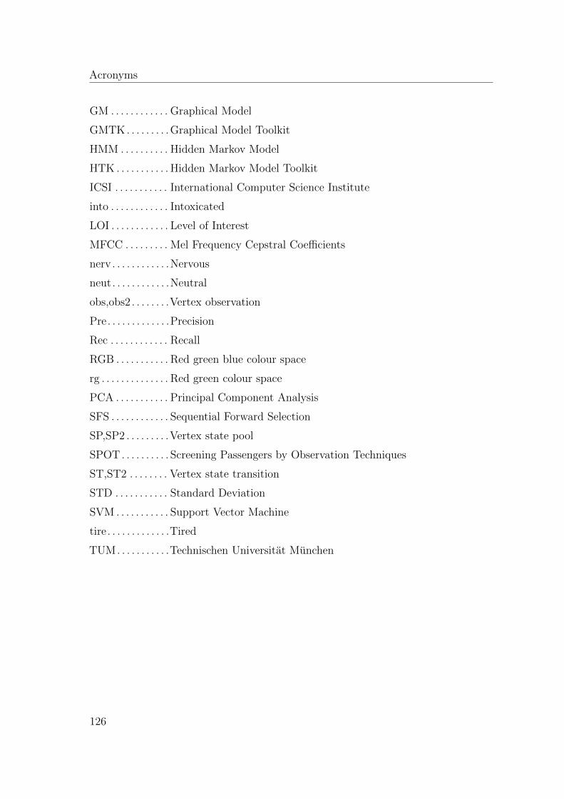
Acronyms
GM . . . . . . . . . . . . Graphical Model
GMTK. . . . . . . . .Graphical Model Toolkit
HMM . . . . . . . . . . Hidden Markov Model
HTK . . . . . . . . . . . Hidden Markov Model Toolkit
ICSI . . . . . . . . . . . International Computer Science Institute
into . . . . . . . . . . . . Intoxicated
LOI . . . . . . . . . . . . Level of Interest
MFCC . . . . . . . . . Mel Frequency Cepstral Coefficients
nerv . . . . . . . . . . . .Nervous
neut. . . . . . . . . . . .Neutral
obs,obs2 . . . . . . . .Vertex observation
Pre. . . . . . . . . . . . .Precision
Rec . . . . . . . . . . . . Recall
RGB . . . . . . . . . . . Red green blue colour space
rg . . . . . . . . . . . . . . Red green colour space
PCA . . . . . . . . . . . Principal Component Analysis
SFS . . . . . . . . . . . . Sequential Forward Selection
SP,SP2 . . . . . . . . .Vertex state pool
SPOT . . . . . . . . . . Screening Passengers by Observation Techniques
ST,ST2 . . . . . . . . Vertex state transition
STD . . . . . . . . . . . Standard Deviation
SVM . . . . . . . . . . . Support Vector Machine
tire . . . . . . . . . . . . .Tired
TUM. . . . . . . . . . .Technischen Universitat Munchen
126

List of Symbols
at . . . . . . . . . . . . . . Transition probability at time frame t
~b(t) . . . . . . . . . . . . Motion vector
ct . . . . . . . . . . . . . . Class at time frame t
Ct . . . . . . . . . . . . . . Class counter at time frame t
D . . . . . . . . . . . . . . Dimension of a matrix
∆mLx (t) . . . . . . . . Global motion: movement of the center of motion in x-direction
for a location L
∆mLy (t) . . . . . . . . Global motion: movement of the center of motion in y-direction
for a location LE . . . . . . . . . . . . . . Set of all edges of a graph
FD . . . . . . . . . . . . .D dimensional acoustic, visual or audiovisual feature set
ft . . . . . . . . . . . . . . Feature vector at time frame t
ft,ord . . . . . . . . . . . Sorted feature vector at time frame t
G . . . . . . . . . . . . . . Graph containing vertices V and edges E
GD . . . . . . . . . . . . . Directed Acyclic Graph
~h . . . . . . . . . . . . . . .Hidden vertices of a model
~h∗ . . . . . . . . . . . . . . Configuration of hidden vertices with the highest probability ofa model
I . . . . . . . . . . . . . . . Number of available data samples for the training or the evalua-tion
Id(x, y) . . . . . . . . . Different image sequence
iL(t) . . . . . . . . . . . Global motion: intensity of motion for a location L
J(·) . . . . . . . . . . . . Cost function for the SFS
127
List of Symbols
κ . . . . . . . . . . . . . . . Inter-annotator agreement
L . . . . . . . . . . . . . . Location within an image
L . . . . . . . . . . . . . . Data likelihood
Λ . . . . . . . . . . . . . . Diagonal matrix of the eigenvalues of the covariance matrix Φ
λ . . . . . . . . . . . . . . .Model parameters of the graphical model
mLx (t) . . . . . . . . . . Global motion: center of motion x-value for a location L
mLy (t) . . . . . . . . . . Global motion: center of motion y-value for a location L
µ . . . . . . . . . . . . . . .Mean value
O . . . . . . . . . . . . . . Set of all observations for one training or test
~ot . . . . . . . . . . . . . . Observation at time frame t
~on,t . . . . . . . . . . . . . Feature vector of stream n at time frame t
~ot . . . . . . . . . . . . . . Feature vector at time frame t
~o bestac . . . . . . . . . . . .Best acoustic feature vector selected by SFS
~o bestvis . . . . . . . . . . . .Best visual feature vector selected by SFS
p(xi) . . . . . . . . . . . Probability that random variable X has the value xi
pa(Vi) . . . . . . . . . . Parents of the vertex Vi
Φ . . . . . . . . . . . . . . Covariance matrix
qt . . . . . . . . . . . . . . State pool at time frame t
qct . . . . . . . . . . . . . . Class position at time frame t
R . . . . . . . . . . . . . . Dimension of the by SFS selected feature space
S0(fi) . . . . . . . . . . Individual significance of feature fi
S(fi,X ) . . . . . . . . Joint significance of feature fi and feature set Xσ2 . . . . . . . . . . . . . .Variance
σLx (t) . . . . . . . . . . . Global motion: mean absolute deviation of the difference pixelsin x-direction for a location L
σLy (t) . . . . . . . . . . . Global motion: mean absolute deviation of the difference pixelsin y-direction for a location L
T . . . . . . . . . . . . . . Length of an observation
t . . . . . . . . . . . . . . . time or time frame
U . . . . . . . . . . . . . . Matrix containing the eigenvectors
ud . . . . . . . . . . . . . Eigenvector
128

List of Symbols
V . . . . . . . . . . . . . . Set of all vertices of a graph
wt . . . . . . . . . . . . . .Class transition at time frame t
Vi . . . . . . . . . . . . . . Vertex i of a graph
XVi . . . . . . . . . . . . Random variable of vertex Vi
yr . . . . . . . . . . . . . . By SFS selected features
Yk . . . . . . . . . . . . . Current best selected feature set by SFS
YR . . . . . . . . . . . . . Best selected feature set by SFS
# . . . . . . . . . . . . . . Total number of samples or instances
129

Bibliography
[AC75] M. Argyle and M. Cook. Gaze and Mutual Gaze. Cambridge Univer-sity Press, Cambridge, England, 1975.
[Adm06] Transportation Security Administration. Train police officers to spotterrorist related activity. http://www.tsa.gov/press/releases/
2006/press_release_0655.shtm, April 6, 2006.
[AH08] M. Al-Hames. Graphische Modelle in der Mustererkennung. Disser-tation, Technische Universitat Munchen, Munich, Germany, 2008.
[AHDGP+06] M. Al-Hames, A. Dielmann, D. Gatica-Perez, S. Reiter, S. Renals,G. Rigoll, and D. Zhang. Multimodal integration for meeting groupaction segmentation and recognition. In S. Renals and S. Bengio, ed-itors, Proceedings of the 2nd International WorkshopMachine Learn-ing for Multimodal Interaction (MLMI), volume LNCS 3869, pages52–63, Edinburgh, Scotland, 2006.
[AHHM+07] M. Al-Hames, B. Hornler, R. Muller, J. Schenk, and G. Rigoll. Au-tomatic multi-modal meeting camera selection for video-conferencesand meeting browsing. In Proceedings of the 8th International Con-ference on Multimedia and Expo (ICME), 2007.
[AHHSR06] M. Al-Hames, B. Hornler, C. Scheuermann, and G. Rigoll. Usingaudio, visual, and lexical features in a multi-modal virtual meetingdirector. In S. Renals and S. Bengio, editors, Proceedings of the 3ndInternational Workshop on Machine Learning for Multimodal Inter-action (MLMI). Springer Verlag, 2006.
[AHR06] M. Al-Hames and G. Rigoll. Der EM-Algorithmus und Gauß-Mixtur-Modelle. Skript zum Praktikum Praxis der Mensch-Maschine-Kom-munikation, Technische Universitat Munchen, Lehrstuhl fur Mensch-Maschine-Kommunikation, 2006.
131
Bibliography
[AHR08] D. Arsic, B. Hornler, and G. Rigoll. Automated video editing formeeting scenarios applying multimodal low level feature fusion. InProceedings of the 5th International Workshop on Machine Learningand Multimodal Interaction (MLMI), September 2008.
[AHSR09] D. Arsic, B. Hornler, B. Schuller, and G. Rigoll. A hierarchical ap-proach for visual suspicious behavior detection in aircrafts. In Pro-ceedings of the 16th IEEE International Conference on Digital Sig-nal Processing (DSP2009), Special Session Biometric recognition andverification of persons and their activities for video surveillance, San-torini, Greece, July 2009.
[ALC+07] A.B. Ashraf, S. Lucey, T. Chen, K. Prkachin, P. Solomon, Z. Am-badar, and J.F. Cohn. The painful face: Pain expression recognitionusing active appearance models. In Proceedings of the 9th Interna-tional Conference on Multimodal Interfaces (ICMI), Special Sessionon Multimodal Analysis of Human Spontaneous Behaviour, pages 9–14, Nagoya, Japan, 2007. ACM SIGCHI.
[AOJJ90] S. Andersen, K. Olesen, F.V. Jensen, and F. Jensen. Hugin: a shellfor building bayesian belief universes for expert systems. In G. Shaferand J. Pearl, editors, Readings in Uncertain Reasoning, pages 332–337. Morgan Kaufmann, 1990.
[Ars10] D. Arsic. Detection and Tracking of Objects for Behavioral Analysisin Sensor Networks. Dissertation, Technische Universitat Munchen,Munich, Germany, 2010.
[ASHR09] D. Arsic, B. Schuller, B. Hornler, and G. Rigoll. Resolving partial oc-clusions in crowded environments utilizing range data an video cam-eras. In Proceedings of the 16th IEEE International Conference onDigital Signal Processing (DSP2009), Special Session Fusion of Het-erogeneous Data for Robust Estimation and Classification, Santorini,Greece, July 2009.
[ASR07] D. Arsic, B. Schuller, and G. Rigoll. Suspicious behavior detectionin public transport by fusion of low-level video descriptors. In Pro-ceedings of the 8th International Conference on Multimedia and Expo(ICME), pages 2018–2021, Beijing, China, July 2–5 2007.
[ATH03] S. Andrews, I. Tsochantaridis, and T. Hofmann. Support vector ma-chines for multiple-instance learning. In S. Thrun S. Becker andK. Obermayer, editors, Advances in Neural Information Processing
132
Bibliography
Systems 15 (NIPS), pages 561–568. MIT Press, Cambridge, MA, USA,2003.
[BB73] K. Burns and E. Beier. Significance of vocal and visual channels inthe decoding of emotional meaning. The Journal of Communication,23(1):118–130, 1973.
[BB05] J. Bilmes and C. Bartels. Graphical model architectures for speechrecognition. IEEE Signal Processing Magazine, 22(5):89–100, 2005.
[BC79] R. Bales and S. Cohen. SYMLOG: A System for the Multiple LevelObservation of Groups. Free Press, New York, 1979.
[BCCP01] S. Basu, T. Choudhury, B. Clarkson, and A. Pentland. Learninghuman interactions with the influence model. Technical report, MITMedia Laboratory Technical Note, 2001.
[Bel05] H. Beller. Handbuch der Filmmontage - Praxis und Prinzipien desFilmschnitts. TR-Verlagsunion, Munchen, 5. edition edition, 2005.
[Ben03] S. Bengio. An asynchronous Hidden Markov Model for audio-visualspeech recognition. In S. Becker, S. Thrun, and K. Obermayer, editors,Advances in Neural Information Processing Systems (NIPS) 15, pages1237–1244. MIT Press, 2003.
[BH05] A.U. Batur and M.H. Hayes. Adaptive active appearance models.IEEE Transactions on Image Processing, 14:1707–1721, 2005.
[Bil97] J. Bilmes. A gentle tutorial on the EM algorithm and its applicationto parameter estimation for gaussian mixture and Hidden MarkovModels. Technical Report ICSI-TR-97-021, University of Berkeley,1997.
[Bil03] J. Bilmes. Graphical models in speech and language, and the graphi-cal models toolkit. http://www.clsp.jhu.edu/ws03/preworkshop/lecture_bilmes.pdf, 2003. The Center for Language and SpeechProcessing Workshop 2003 at Johns Hopkins University.
[Bil04] J. Bilmes. Graphical models and automatic speech recognition. InM. Johnson, S.P. Khudanpur, M. Ostendorf, and R. Rosenfeld, edi-tors, Mathematical Foundations of Speech and Language Processing,pages 191–246. Springer-Verlag, 2004.
[Bil06] J. Bilmes. Graphical models. http://ssli.ee.washington.edu/
courses/ee512, 2006. Lecture EE512, University of Washington, De-partment of Electrical Engineering.
133
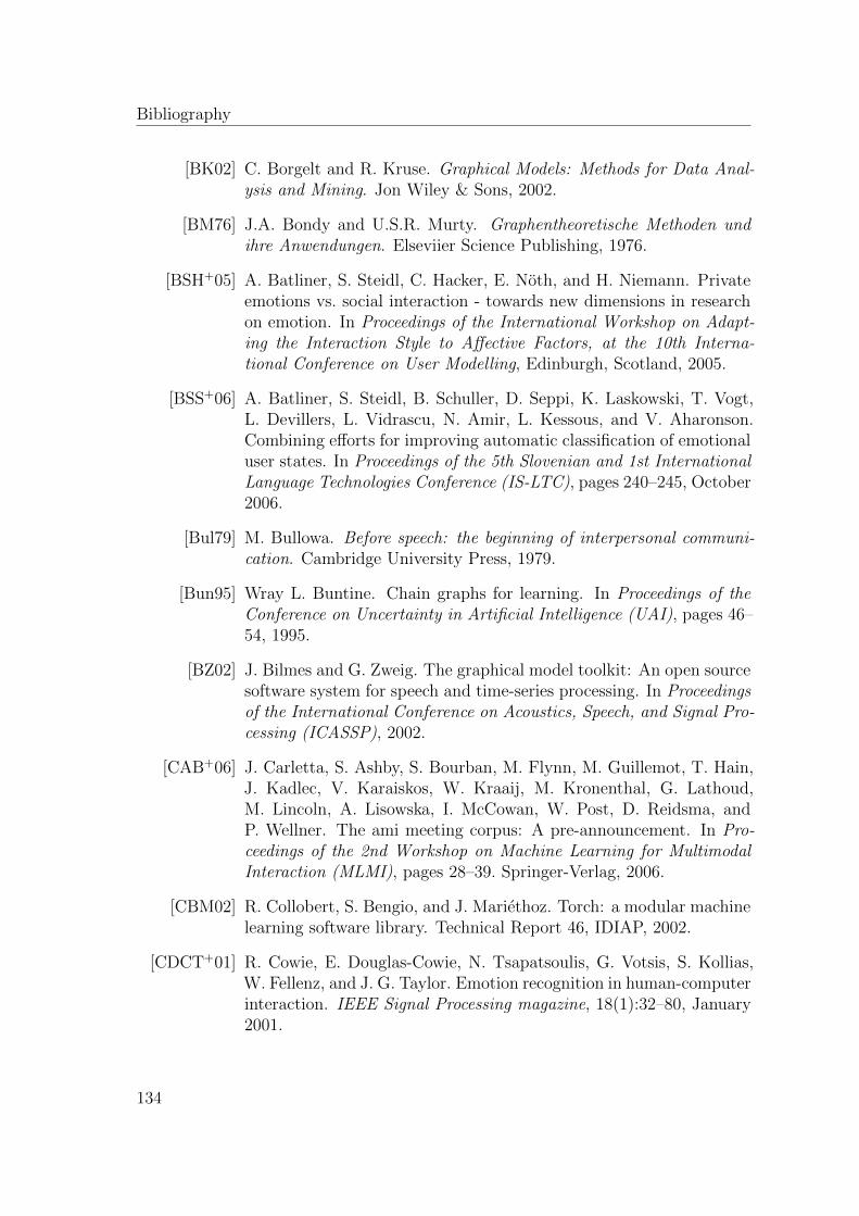
Bibliography
[BK02] C. Borgelt and R. Kruse. Graphical Models: Methods for Data Anal-ysis and Mining. Jon Wiley & Sons, 2002.
[BM76] J.A. Bondy and U.S.R. Murty. Graphentheoretische Methoden undihre Anwendungen. Elseviier Science Publishing, 1976.
[BSH+05] A. Batliner, S. Steidl, C. Hacker, E. Noth, and H. Niemann. Privateemotions vs. social interaction - towards new dimensions in researchon emotion. In Proceedings of the International Workshop on Adapt-ing the Interaction Style to Affective Factors, at the 10th Interna-tional Conference on User Modelling, Edinburgh, Scotland, 2005.
[BSS+06] A. Batliner, S. Steidl, B. Schuller, D. Seppi, K. Laskowski, T. Vogt,L. Devillers, L. Vidrascu, N. Amir, L. Kessous, and V. Aharonson.Combining efforts for improving automatic classification of emotionaluser states. In Proceedings of the 5th Slovenian and 1st InternationalLanguage Technologies Conference (IS-LTC), pages 240–245, October2006.
[Bul79] M. Bullowa. Before speech: the beginning of interpersonal communi-cation. Cambridge University Press, 1979.
[Bun95] Wray L. Buntine. Chain graphs for learning. In Proceedings of theConference on Uncertainty in Artificial Intelligence (UAI), pages 46–54, 1995.
[BZ02] J. Bilmes and G. Zweig. The graphical model toolkit: An open sourcesoftware system for speech and time-series processing. In Proceedingsof the International Conference on Acoustics, Speech, and Signal Pro-cessing (ICASSP), 2002.
[CAB+06] J. Carletta, S. Ashby, S. Bourban, M. Flynn, M. Guillemot, T. Hain,J. Kadlec, V. Karaiskos, W. Kraaij, M. Kronenthal, G. Lathoud,M. Lincoln, A. Lisowska, I. McCowan, W. Post, D. Reidsma, andP. Wellner. The ami meeting corpus: A pre-announcement. In Pro-ceedings of the 2nd Workshop on Machine Learning for MultimodalInteraction (MLMI), pages 28–39. Springer-Verlag, 2006.
[CBM02] R. Collobert, S. Bengio, and J. Mariethoz. Torch: a modular machinelearning software library. Technical Report 46, IDIAP, 2002.
[CDCT+01] R. Cowie, E. Douglas-Cowie, N. Tsapatsoulis, G. Votsis, S. Kollias,W. Fellenz, and J. G. Taylor. Emotion recognition in human-computerinteraction. IEEE Signal Processing magazine, 18(1):32–80, January2001.
134
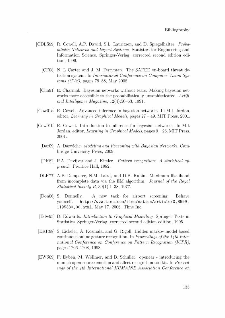
Bibliography
[CDLS99] R. Cowell, A.P. Dawid, S.L. Lauritzen, and D. Spiegelhalter. Proba-bilistic Networks and Expert Systems. Statistics for Engineering andInformation Science. Springer-Verlag, corrected second edition edi-tion, 1999.
[CF08] N. L Carter and J. M. Ferryman. The SAFEE on-board threat de-tection system. In International Conference on Computer Vision Sys-tems (CVS), pages 79–88, May 2008.
[Cha91] E. Charniak. Bayesian networks without tears: Making bayesian net-works more accessible to the probabilistically unsophisticated. Artifi-cial Intelligence Magazine, 12(4):50–63, 1991.
[Cow01a] R. Cowell. Advanced inference in bayesian networks. In M.I. Jordan,editor, Learning in Graphical Models, pages 27 – 49. MIT Press, 2001.
[Cow01b] R. Cowell. Introduction to inference for bayesian networks. In M.I.Jordan, editor, Learning in Graphical Models, pages 9 – 26. MIT Press,2001.
[Dar09] A. Darwiche. Modeling and Reasoning with Bayesian Networks. Cam-bridge University Press, 2009.
[DK82] P.A. Devijver and J. Kittler. Pattern recognition: A statistical ap-proach. Prentice Hall, 1982.
[DLR77] A.P. Dempster, N.M. Laird, and D.B. Rubin. Maximum likelihoodfrom incomplete data via the EM algorithm. Journal of the RoyalStatistical Society B, 39(1):1–38, 1977.
[Don06] S. Donnelly. A new tack for airport screening: Behaveyourself. http://www.time.com/time/nation/article/0,8599,
1195330,00.html, May 17, 2006. Time Inc.
[Edw95] D. Edwards. Introduction to Graphical Modelling. Springer Texts inStatistics. Springer-Verlag, corrected second edition edition, 1995.
[EKR98] S. Eickeler, A. Kosmala, and G. Rigoll. Hidden markov model basedcontinuous online gesture recognition. In Proceedings of the 14th Inter-national Conference on Conference on Pattern Recognition (ICPR),pages 1206–1208, 1998.
[EWS09] F. Eyben, M. Wollmer, and B. Schuller. openear - introducing themunich open-source emotion and affect recognition toolkit. In Proceed-ings of the 4th International HUMAINE Association Conference on
135
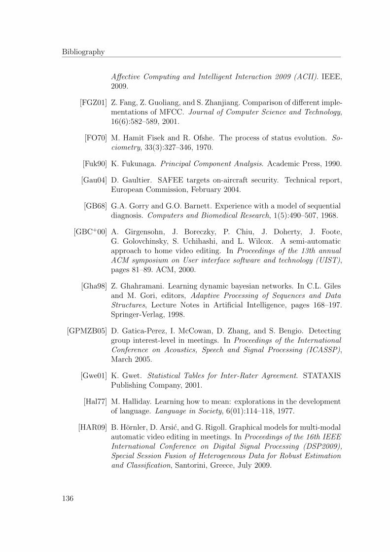
Bibliography
Affective Computing and Intelligent Interaction 2009 (ACII). IEEE,2009.
[FGZ01] Z. Fang, Z. Guoliang, and S. Zhanjiang. Comparison of different imple-mentations of MFCC. Journal of Computer Science and Technology,16(6):582–589, 2001.
[FO70] M. Hamit Fisek and R. Ofshe. The process of status evolution. So-ciometry, 33(3):327–346, 1970.
[Fuk90] K. Fukunaga. Principal Component Analysis. Academic Press, 1990.
[Gau04] D. Gaultier. SAFEE targets on-aircraft security. Technical report,European Commission, February 2004.
[GB68] G.A. Gorry and G.O. Barnett. Experience with a model of sequentialdiagnosis. Computers and Biomedical Research, 1(5):490–507, 1968.
[GBC+00] A. Girgensohn, J. Boreczky, P. Chiu, J. Doherty, J. Foote,G. Golovchinsky, S. Uchihashi, and L. Wilcox. A semi-automaticapproach to home video editing. In Proceedings of the 13th annualACM symposium on User interface software and technology (UIST),pages 81–89. ACM, 2000.
[Gha98] Z. Ghahramani. Learning dynamic bayesian networks. In C.L. Gilesand M. Gori, editors, Adaptive Processing of Sequences and DataStructures, Lecture Notes in Artificial Intelligence, pages 168–197.Springer-Verlag, 1998.
[GPMZB05] D. Gatica-Perez, I. McCowan, D. Zhang, and S. Bengio. Detectinggroup interest-level in meetings. In Proceedings of the InternationalConference on Acoustics, Speech and Signal Processing (ICASSP),March 2005.
[Gwe01] K. Gwet. Statistical Tables for Inter-Rater Agreement. STATAXISPublishing Company, 2001.
[Hal77] M. Halliday. Learning how to mean: explorations in the developmentof language. Language in Society, 6(01):114–118, 1977.
[HAR09] B. Hornler, D. Arsic, and G. Rigoll. Graphical models for multi-modalautomatic video editing in meetings. In Proceedings of the 16th IEEEInternational Conference on Digital Signal Processing (DSP2009),Special Session Fusion of Heterogeneous Data for Robust Estimationand Classification, Santorini, Greece, July 2009.
136
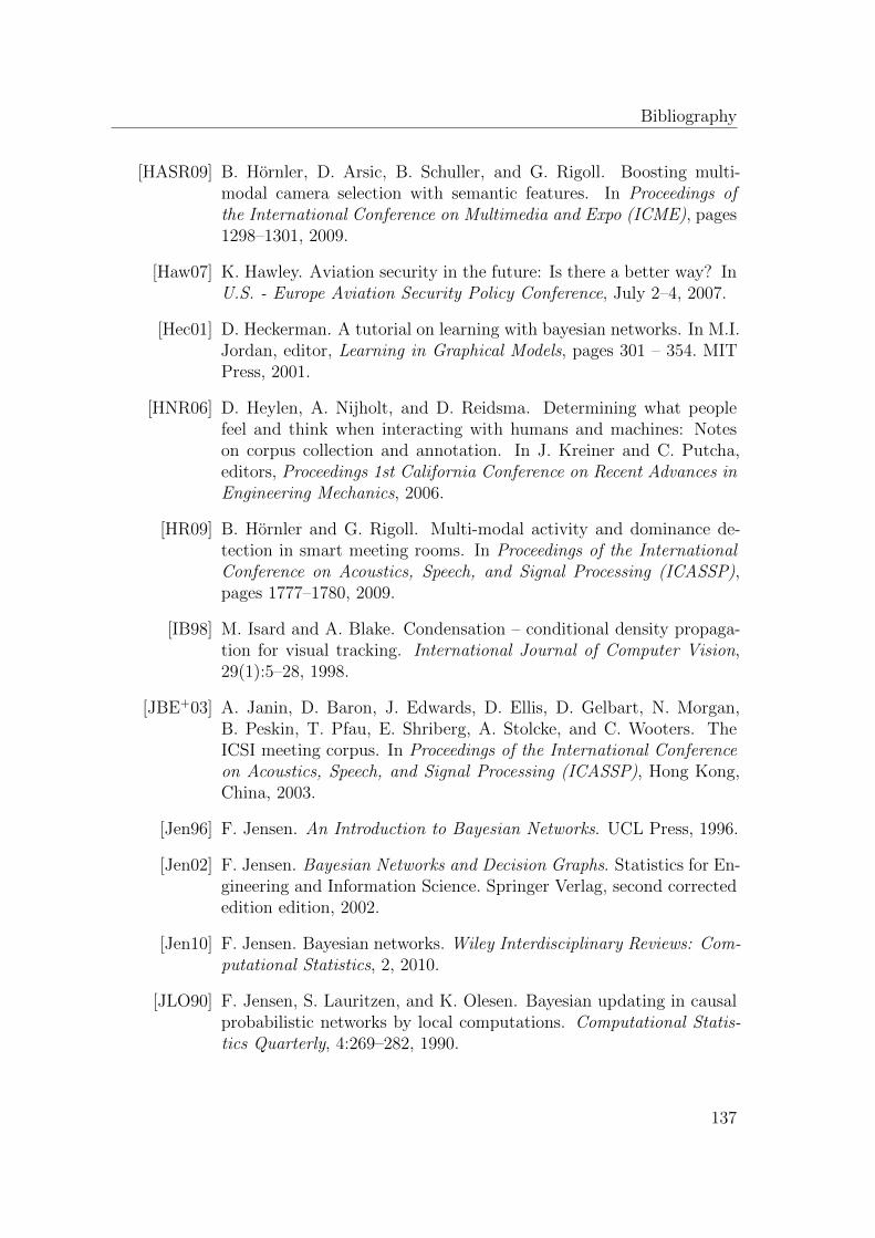
Bibliography
[HASR09] B. Hornler, D. Arsic, B. Schuller, and G. Rigoll. Boosting multi-modal camera selection with semantic features. In Proceedings ofthe International Conference on Multimedia and Expo (ICME), pages1298–1301, 2009.
[Haw07] K. Hawley. Aviation security in the future: Is there a better way? InU.S. - Europe Aviation Security Policy Conference, July 2–4, 2007.
[Hec01] D. Heckerman. A tutorial on learning with bayesian networks. In M.I.Jordan, editor, Learning in Graphical Models, pages 301 – 354. MITPress, 2001.
[HNR06] D. Heylen, A. Nijholt, and D. Reidsma. Determining what peoplefeel and think when interacting with humans and machines: Noteson corpus collection and annotation. In J. Kreiner and C. Putcha,editors, Proceedings 1st California Conference on Recent Advances inEngineering Mechanics, 2006.
[HR09] B. Hornler and G. Rigoll. Multi-modal activity and dominance de-tection in smart meeting rooms. In Proceedings of the InternationalConference on Acoustics, Speech, and Signal Processing (ICASSP),pages 1777–1780, 2009.
[IB98] M. Isard and A. Blake. Condensation – conditional density propaga-tion for visual tracking. International Journal of Computer Vision,29(1):5–28, 1998.
[JBE+03] A. Janin, D. Baron, J. Edwards, D. Ellis, D. Gelbart, N. Morgan,B. Peskin, T. Pfau, E. Shriberg, A. Stolcke, and C. Wooters. TheICSI meeting corpus. In Proceedings of the International Conferenceon Acoustics, Speech, and Signal Processing (ICASSP), Hong Kong,China, 2003.
[Jen96] F. Jensen. An Introduction to Bayesian Networks. UCL Press, 1996.
[Jen02] F. Jensen. Bayesian Networks and Decision Graphs. Statistics for En-gineering and Information Science. Springer Verlag, second correctededition edition, 2002.
[Jen10] F. Jensen. Bayesian networks. Wiley Interdisciplinary Reviews: Com-putational Statistics, 2, 2010.
[JLO90] F. Jensen, S. Lauritzen, and K. Olesen. Bayesian updating in causalprobabilistic networks by local computations. Computational Statis-tics Quarterly, 4:269–282, 1990.
137
Bibliography
[Jol02] I.T. Jolliffe. Principal Component Analysis. Springer-Verlag, 2 edi-tion, 2002.
[Jor01] M.I. Jordan, editor. Learning in Graphical Models. MIT Press, secondprinting edition, 2001.
[JR64] W. Kees J. Ruesch. Nonverbal Communication. University of Califor-nia Press, 1964.
[JS01] M.I. Jordan and T.J. Sejnowski, editors. Graphical Models: Founda-tions of Neural Computation. MIT Press, 2001.
[Kar47] K. Karhunen. Uber lineare methoden in der wahrscheinlichkeitsrech-nung. Annales AcademiæScientiarum FennicæMathematica, 1947.
[Kau71] A. Kaufmann. Einfuhrung in die Graphentheorie. Orientierung undEntscheidung. Verlag R. Oldenbourg Munchen und Wien, 1971.
[KE03] L. Kennedy and D. Ellis. Pitch-based emphasis detection for char-acterization of meeting recordings. In Proceedings of the Interna-tional Workshop on Automatic Speech Recognition and Understanding(ASRU), December 2003.
[KF09] D. Koller and N. Friedman. Probabilistic Graphical Models. MITPress, 2009.
[Koh06] N. Kohler. Skalierungsinvariante Augenlokalisation und Konzeption-ierung eines Systems zur automatischen Mimikerkennung. Diplomar-beit, Technische Universitat Munchen, 2006.
[Kip01] Michael Kipp. ANVIL - a generic annotation tool for multimodaldialogue, 2001.
[KM06] J. Karp and L. Meckler. Which travelers have hos-tile intent? biometric device may have the an-swer. http://online.wsj.com/public/article/
SB115551793796934752-Vns0SEJ5cKlwnUhTbmkwBeMPIAE_
20080510.html, August 14, 2006. The Wall Street Journal.
[KMH+07] M. Kranz, A. Maldonado, B. Hornler, R.B. Rusu, M. Beetz, G. Rigoll,and A. Schmidt. A knife and a cutting board as implicit user inter-face - towards context-aware kitchen utilities. In Proceedings of the1st International Conference on Tangible and Embedded Interaction(TEI), 2007.
138
Bibliography
[KMR+07] M. Kranz, A. Maldonado, R.B. Rusu, B. Hornler, G. Rigoll, M. Beetz,and A. Schmidt. Sensing technologies and the player-middlewarefor context-awareness in kitchen environments. In Proceedings of the4th International Conference on Networked Sensing Systems (INSS),2007.
[Kno69] W. Knodel. Graphentheoretische Methoden und ihre Anwendungen.Okonometrie und Unternehmensforschung. Springer-Verlag, 1969.
[KPI04] A. Kapoor, R.W. Picard, and Y. Ivanov. Probabilistic combinationof multiple modalities to detect interest. In Proceedings of the 19thInternational Workshop on Pattern Recognition, (ICPR), volume 3,pages 969–972, 2004.
[KS00] M. Kudo and J. Slansky. Comparison of algorithms that select fea-tures for pattern classifiers. Pattern Recognition Journal, 22:25–41,2000.
[Lau96] S.L. Lauritzen. Graphical Models. Oxford Statistical Science Series.Oxford Science Publications, 1996.
[Len07] C. Lenz. Das asynchrone hidden markov modell und seine anwendungin der multimodalen meetinganalyse, 2007. Diplomarbeit, TechnischeUniversitat Munchen.
[LK03] Q. Liu and D. Kimber. Learning automatic video capture from hu-man’s camera operations. In Proceedings of the International Confer-ence on Image Processing (ICIP), 2003.
[LKF+02] Qiong Liu, Don Kimber, Jonathan Foote, Lynn Wilcox, and JohnBoreczky. Flyspec: a multi-user video camera system with hybridhuman and automatic control. In Proceedings of the 10th ACM inter-national conference on Multimedia (ACMMM), pages 484–492. ACM,2002.
[LO81] M.T. Lee and R. Ofshe. The impact of behavioral style and statuscharacteristics on social influence: A test of two competing theories.Social Psychology Quarterly, 44(2):73–82, 1981.
[Loe78] M. Loeve. Probability theory vol. II. Graduate Tests in Mathematics,46, 1978.
[LS88] S.L. Lauritzen and D.J. Spiegelhalter. Local computations with prob-abilities on graphical structures and their application to expert sys-tems. Journal of the Royal Statistical Society, Series B, 50:157 – 224,1988.
139
Bibliography
[LSK+05] Q. Liu, X. Shi, D. Kimber, F. Zhao, and F. Raab. An online videocomposition system. In Proceedings of the International Conferenceon Multimedia and Expo (ICME), 2005.
[MA00] R. McEliece and S. M. Aji. The generalized distributive law. IEEETransactions on Information Theory, 46(2):325–343, 2000.
[Mac09] I. MacLeod. Canadian airport to test behaviour detec-tion program. http://www.puppetgov.com/2009/08/14/
canadian-airport-to-test-Sbehaviour-detectionS-program/,August 14, 2009.
[MBB+03] N. Morgan, D. Baron, S. Bhagat, H. Carvey, R. Dhillon, J. Edwards,D. Gelbart, A. Janin, A. Krupski, B. Peskin, T. Pfau, E. Shriberg,A. Stolcke, and C. Wooters. Meetings about meetings: Researchat ICSI on speech in multiparty conversations. In Proceedings of theInternational Conference on Acoustics, Speech, and Signal Processing(ICASSP), 2003.
[MGPB+05] I. McCowan, D. Gatica-Perez, S. Bengio, G. Lathoud, M. Barnard,and D. Zhang. Automatic analysis of multimodal group actions inmeetings. IEEE Transactions on Pattern Analysis and Machine In-telligence, 27:305–317, 2005.
[MHGB01] A. Morris, A. Hagen, H. Glotin, and H. Bourlard. Multi-stream adap-tive evidence combination for noise robust ASR. Speech Communica-tion, 34(1–2):25–40, 2001.
[MMF+06] S. Meignier, D. Moraru, C. Fredouille, J.-F. Bonastre, and L. Besacier.Step-by-step and integrated approaches in broadcast news speakerdiarization. Computer Speech & Language, 20(2-3):303 – 330, 2006.
[Moo96] T.K. Moon. The expectation-maximization algorithm. IEEE SignalProcessing Magazine, 13(6):47 – 60, 1996.
[Moo02] D. Moore. The IDIAP smart meeting room. Technical Report 07,IDIAP, 2002.
[MP03] S. Mota and R. Picard. Automated posture analysis for detectinglearner’s interest level. In Proceedings of the International Workshopon Computer Vision and Pattern Recognition (CVPR) for HCI, June2003.
140
Bibliography
[MP07] L. Maat and M. Pantic. Gaze-x: Adaptive, affective, multimodal in-terface for single-user office scenarios. In Artifical Intelligence for Hu-man Computing, volume 4451/2007, pages 251–271. Springer LNCS,Berlin, Heidelberg, 2007.
[MR83] P.L. McLeod and R. Rosenthal. Micromomentary movement and thedeconding of face and body cues. Journal of Nonverbal Behavior, 8(2),1983.
[Mur01] K. Murphy. The bayes net toolbox for matlab. Computing Scienceand Statistics, 33, 2001.
[Mur02] K. Murphy. Dynamic Bayesian Networks: Representation, Inferenceand Learning. PhD thesis, University of California, Berkeley, 2002.
[MYLB08] A.A. Miranda and G. Bontempi Y. Le Borgne. New routes from mini-mal approximation error to principal components. Neural ProcessingLetters, 27(3), 2008.
[Nea03] R.E. Neapolitan. Learning Bayesian Networks. Artificial IntelligenceSeries. Prentice Hall, 2003.
[Nie93] J. Nielsen. Usability Engineering. Academic Press, Inc., 1993.
[NL86] J.-L. Nespoulous and A.R. Lecours. Gestures: Nature and function.In J.-L. Nespoulous, P. Perron, and A.R. Lecours, editors, The Bi-ological foundations of gestures: motor and semiotic aspects, pages49–62. Lawrence Erlbaum Associates, Hillsdale, NJ, USA, 1986.
[NSGN02] R. Nieschulz, B. Schuller, M. Geiger, and R. Neuss. Aspects of ef-ficient usability engineerings. it+ti journal, ”Usability Engeneering”,44(1):23–30, 2002.
[OMI02] Y. Ohsawa, N. Matsumura, and M. Ishizuka. Influence diffusionmodel in text-based communication. In Proceedings of the 11th Inter-national Conference on world wide web, 2002.
[Pea86] J. Pearl. Fusion, propagation, and structuring in belief networks.Artificial Intelligence, 29:241 – 288, 1986.
[Pea88] J. Pearl. Probabilistic Reasoning in Intelligent Systems: Networksof Plausible Inference. Morgan Kaufmann Publishers, San Fransisco,California, revised second printing edition, 1988.
141
Bibliography
[PM05] A. Pentland and A. Madan. Perception of social interest. In Pro-ceedings of the 10th International Conference on Computer Vision,Workshop on Modeling People and Human Interaction (ICCV-PHI),Beijing, China, October 2005.
[PNK94] P. Pudil, J. Novovicova, and J. Kittlera. Floating search methods infeature selection. Pattern Recognition Letters, 14, 1994.
[PNLM04] G. Potamianos, C. Neti, J. Luettin, and I. Matthews. Audio-visualautomatic speech recognition: An overview. In G. Bailly, E. Vatikiotis-Bateson, and P. Perrier, editors, Issues in Visual and Audio-visualSpeech Processing, chapter 10. MIT Press, 2004.
[PR03] M. Pantic and L. Rothkrantz. Toward an affect-sensitive multimodalhuman-computer interaction. Proccedings of the IEEE, 91:1370–1390,September 2003.
[Pra01] W.K. Pratt. Digital image processing. John Wiley & Sons, 2001.
[PSS04] I. Potucek, S. Sumec, and M. Spanel. Participant activity detectionby hands and face movement tracking in the meeting room. In Pro-ceedings of the IEEE Computer Graphics International (CGI), 2004.
[PV87] J. Pearl and T. Verma. The logic of representing dependencies bydirected graphs. In Sixth National Conference on Artificial Intelli-gence, volume 1, pages 374–379. American Association of ArtificialIntelligence (AAAI), 1987.
[QBZ05] P. Qvarfordt, D. Beymer, and S. X. Zhai. RealTourist - A Studyof Augmenting Human-Human and Human-Computer Dialogue withEye-Gaze Overlay, volume LNCS 3585, pages 767–780. SpringerBerlin / Heidelberg, 2005.
[Rab89] L.R. Rabiner. A tutorial on Hidden Markov Models and selected appli-cations in speech recognition. Proceedings of the IEEE, 77(2):257–285,1989.
[RBK98] H. Rowley, S. Baluja, and T. Kanade. Neural network-based facedetection. IEEE Transactions on Pattern Analysis and Machine In-telligence (TPAMI), 20(1):23–38, January 1998.
[Rei08] S. Reiter. Multimodale Modellierung von Gruppenaktionen zur Seg-mentierung von Besprechungen. Dissertation, Technische UniversitatMunchen, Munich, Germany, 2008.
142
Bibliography
[Ren02a] S. Renals. The M4-Project – multimodal meeting manager. http:
//www.dcs.shef.ac.uk/spandh/projects/m4/index.html, 2002.
[Ren02b] S. Renals. The M4-Project – multimodal meeting manager, projectleaflet. http://www.dcs.shef.ac.uk/spandh/projects/m4/pdf/
leaflet_lowres.pdf, 2002.
[RH05] R. Rienks and D. Heylen. Automatic dominance detection in meetingsusing easily obtainable features. In S. Renals and S. Bengio, editors,Proceedings of the 2nd International Workshop on Machine Learningfor Multimodal Interaction (MLMI), volume LNCS 3869, pages 76–86,Edinburgh, Scotland, 2005.
[Rie07] R. Rienks. Meetings in smart environments : implications of progress-ing technology. PhD thesis, University of Twente, Enschede, Nether-lands, 2007.
[Rig94] G. Rigoll. Neuronale Netze. Eine Einfuhrung fur Ingenieure, Infor-matiker und Naturwissenschaftler. Expert-Verlag, 1994.
[RJ93] L.R. Rabiner and B.-H. Juang. Theory and implementation of HiddenMarkov Models. In Fundamentals of Speech Recognition, pages 321 –389. Prentice Hall PTR, 1993.
[RK97] G. Rigoll and A. Kosmala. New improved feature extraction methodsfor real-time high performance image sequence recognition. In Pro-ceedings of the 22nd International Conference on Acoustics, Speech,and Signal Processing (ICASSP), volume 4, pages 2901–2904, April1997.
[RM79] E. Rosa and A. Mazur. Incipient status in small groups. Social Forces,58(1):18–37, 1979.
[RSR05] S. Reiter, S. Schreiber, and G. Rigoll. Multimodal meeting analy-sis by segmentation and classification of meeting events based on ahigher level semantic approach. In Proceedings of the InternationalConference on Acoustics, Speech, and Signal Processing (ICASSP),pages 161–164, 2005.
[RSR07] S. Reiter, B. Schuller, and G. Rigoll. Hidden conditional random fieldsfor meeting segmentation. In Proceedings of the 8th InternationalConference on Multimedia and Expo (ICME), pages 639–642, Beijing,China, 2007.
143
Bibliography
[SAR+07] B. Schuller, D. Arsic, G. Rigoll, M. Wimmer, and B. Radig. Audiovi-sual behaviour modeling by combined feature spaces. In Proceedingsof the International Conference on Acoustics, Speech and Signal Pro-cessing (ICASSP), volume II, pages 733–736, Honolulu, HY, USA,2007.
[SBE+09] M. Schroder, E. Bevacqua, F. Eyben, H. Gunes, D. Heylen, M. terMaat, S. Pammi, M. Pantic, C. Pelachaud, B. Schuller, E. de Sevin,M. Valstar, and M. Wollmer. A demonstration of audiovisual sensitiveartificial listeners. In Proceedings of the 4th International HUMAINEAssociation Conference on Affective Computing and Intelligent Inter-action (ACII), pages 263–264, 2009.
[SCH+08] M. Schroder, R. Cowie, D. Heylen, M. Pantic, C. Pelachaud, andB. Schuller. Towards responsive sensitive artificial listeners. In Pro-ceedings of the 4th International Workshop on Human-Computer Con-versation, 2008.
[Sch09] J. Schenk. Online-Erkennung handgeschriebener Whiteboard-Notizen.Dissertation, Technische Universit’at Munchen, Munchen, 2009.
[Sch10] M. Schroder. The SEMAINE API: Towards a standards-based frame-work for building emotion-oriented systems. Advances in Human-Machine Interaction, 2010.
[SER08a] B. Schuller, F. Eyben, and G. Rigoll. Beat-synchronous data-drivenautomatic chord labeling. In U. Jekosch and R. Hoffmann, editors,Proceedings of the Deutschen Arbeitsgemeinschaft fur Akustik, DAGA,pages 555–556. DEGA, 2008. 10.-13.03.2008.
[SER08b] B. Schuller, F. Eyben, and G. Rigoll. Tango or waltz?: Puttingballroom dance style into tempo detection. EURASIP Journal onAudio, Speech, and Music Processing, 2008(Article ID 846135):12 p,2008.
[Sha71] M.E. Shaw. Group Dynamics: The Psychology of Small Group Be-havior. McGraw Hill, New York, 1971.
[SHAR09] B. Schuller, B. Hornler, D. Arsic, and G. Rigoll. Audio chord labelingby musiological modeling and beat-synchronization. In Proceedingsof the 9th International Conference on Multimedia and Expo (ICME),2009.
144
Bibliography
[SHBR09] J. Schenk, B. Hornler, A. Braun, and G. Rigoll. Graphical mod-els: Statistical inference vs. determination. In Proceedings of the In-ternational Conference on Acoustics, Speech, and Signal Processing(ICASSP), pages 1717–1720, 2009.
[SHML00] M. Soriano, S. Huovinen, B. Martinkauppi, and M. Laaksonen. Skindetection in video under changing illumination conditions. In Pro-ceedings of the 15th International Conference on Pattern Recognition(ICPR), pages 839–842, 2000.
[Shr05] E. Shriberg. Spontaneous speech: How people really talk and whyengineers should care. In Proceedings of the 9th European Conferenceon Speech Communication and Technology (Eurospeech), Lisbon, Por-tugal, September 2005.
[SKMR06] B. Schuller, N. Kohler, R. Muller, and G. Rigoll. Recognition ofinterest in human conversational speech. In Proceedings of the 9thInternational Conference on Spoken Language Processing (ICSLP -Interspeech), pages 793–796, 2006.
[SKR09] J. Schenk, M. Kaiser, and G. Rigoll. Selecting features in on-linehandwritten whiteboard note recognition: SFS or SFFS? In 10th In-ternational Conference on Document Analysis and Recognition, 2009.
[SME+09] B. Schuller, R. Muller, F. Eyben, J. Gast, B. Hornler, M. Wollmer,G. Rigoll, A. Hothker, and H. Konosu. Being bored? recognising nat-ural interest by extensive audiovisual integration for real-life applica-tion. Image and Vision Computing Journal (IMAVIS), 27:1760–1774,2009. Special Issue on Visual and Multimodal Analysis of HumanSpontaneous Behavior. Elsevier, Issue 12.
[SMH+07] B. Schuller, R. Muller, B. Hornler, A. Hothker, H. Konosu, andG. Rigoll. Audiovisual recognition of spontaneous interest within con-versations. In Proceedings of International Conference on MultimodalInterfaces (ICMI), pages 30–37, 2007. Special Session on MultimodalAnalysis of Human Spontaneous Behaviour.
[Smy97] P. Smyth. Belief networks, hidden markov models, and markov ran-dom fields: a unifying view. Pattern Recognition Letters, 18(11-13):1261–1268, 1997.
[SNVF03] L. Snidaro, R. Niu, P. K. Varshney, and G. L. Foresti. Automaticcamera selection and fusion for outdoor surveillance under changingweather conditions. In Proceedings of the Conference on AdvancedVideo and Signal Based Surveillance (AVSS), 2003.
145
Bibliography
[SP85] S. Sabri and B. Prasada. Video conferencing systems. Proceedings ofthe IEEE, 73(4):671–688, 1985.
[SR09] B. Schuller and G. Rigoll. Recognising interest in conversationalspeech - comparing bag of frames and supra-segmental features. InProceedings of the 10th Annual Conference of the International SpeechCommunication Association (Interspeech), pages 1999–2002. ISCA,2009.
[SRL03] B. Schuller, G. Rigoll, and M. Lang. Hidden markov model-basedspeech emotion recognition. In Proceedings of the International Con-ference on Acoustics, Speech, and Signal Processing (ICASSP), vol-ume II, pages 1–4, 2003.
[SS90] G. Shafer and P. Shenoy. Probability propagation. Annals of Mathe-matics and Artificial Intelligence, 2:327–351, 1990.
[SSB+07] B. Schuller, D. Seppi, A. Batliner, A. Maier, and S. Steidl. Towardsmore reality in the recognition of emotional speech. In Proceedingsof the International Conference on Acoustics, Speech, and Signal Pro-cessing (ICASSP), April 2007.
[SSB09] B. Schuller, S. Steidl, and A. Batliner. The interspeech 2009 emotionchallenge. In Proceedings of the 10th International Conference ofSpeech Communication Association (Interspeech), 2009. to appear.
[Sum04] S. Sumec. Multi camera automatic video editing. In Proceedingsof the International Conference on Computer Vision and Graphics(ICCVG), pages 935–945, Warsaw, Poland, 2004. Kluwer Verlag.
[SWA+07] B. Schuller, M. Wimmer, D. Arsic, G. Rigoll, and B. Radig. Audio-visual behavior modeling by combined feature spaces. In Proceedingsof the International Conference on Acoustics, Speech, and Signal Pro-cessing (ICASSP), April 2007.
[SWA+08] B. Schuller, M. Wimmer, D. Arsic, T. Moosmayr, and G. Rigoll. De-tection of security related affect and behaviour in passenger transport.In Proceedings of the 9th International Conference of Speech Com-munication Association (Interspeech) incorp. 12th Australasian Inter-national Conference on Speech Science and Technology SST, pages265–268, Brisbane, Australia, 2008. ISCA.
[SWM+08] B. Schuller, M. Wimmer, L. Mosenlechner, C. Kern, D. Arsic, andG. Rigoll. Brute-forcing hierarchical functionals for paralinguistics: Awaste of feature space? In Proceedings of the International Conference
146
Bibliography
on Acoustics, Speech, and Signal Processing (ICASSP), pages 4501–4504, 2008.
[SYW02] R. Stiefelhagen, Jie Yang, and A. Waibel. Modeling focus of attentionfor meeting indexing based on multiple cues. IEEE Transactions onNeural Networks, 13(4):928 – 938, July 2002.
[Tho93] K.R. Thorisson. Dialogue control in social interface agents. In Proceed-ings of the Conference Companion on Human factors in ComputingSystems (CHI), pages 139–140, New York, NY, USA, 1993. ACM.
[TKB92] K.R. Thorisson, D.B. Koons, and R.A. Bolt. Multi-modal naturaldialogue. In Proceedings of the Special Interest Group on Computer-Human Interaction (SIGCHI) Conference on Human factors in Ccom-puting Systems (CHI), pages 653–654, New York, NY, USA, 1992.ACM.
[Uch01] S. Uchihashi. Direct camera control for capturing meetings into mul-timedia documents. In Proceedings of the International Conferenceon Multimedia and Expo (ICME), 2001.
[Vap95] V. Vapnik. The Nature of Statistical Learning Theory. Springer Ver-lag, 1995.
[Vit77] A. Viterbi. Error bounds for convolutional codes and an asymptoti-cally optimum decoding algorithm. IEEE Transactions on Informa-tion Theory, 13(2):260 – 269, 1977.
[VO06] A. Vinciarelli and J. Odobez. Application of information retrievaltechnologies to presentation slides. IEEE Transactions on Multimedia,8(5):981–995, 2006.
[WFG04] P. Wellner, M. Flynn, and M. Guillemot. Browsing recorded meet-ings with ferret. In S. Renals and S. Bengio, editors, Proceedings ofthe 1st International Workshop on Machine Learning for MultimodalInteraction (MLMI). Springer Verlag, 2004.
[WFTW05] P. Wellner, M. Flynn, S. Tucker, and S. Whittaker. A meeting browserevaluation test. In CHI ’05 extended abstracts on Human factorsin computing systems, pages 2021–2024, New York, NY, USA, 2005.ACM Press.
[WH09] C. Wooters and M. Huijbregts. The ICSI RT07s speaker diarizationsystem. In Multimodal Technologies for Perception of Humans, Lec-ture Notes in Computer Science, pages 509 – 519. Springer Berlin /Heidelberg, 2009.
147
Bibliography
[Whi91] J. Whittaker. Graphical Models in Applied Multivariate Statistics.Wiley Series in Probability & Mathematical Statistics. Jon Wiley &Sons, 1991.
[Wig79] J.S. Wiggins. A psychological taxonomy of trait-descriptive terms:The interpersonal domain. Journal of Personality and Social Psychol-ogy, 37(3):395–412, 1979.
[Win03] G. Winkler. Image Analysis, Random Field and Markov Chain MonteCarlo Methods. Applications of Mathematics, Stochastic Modellingand Applied Probability. Springer, second edition edition, 2003.
[WR05] M. Wimmer and B. Radig. Adaptive skin color classificator. In Pro-ceedings of the first International Conference on Graphics, Vision andImage Processing (ICGST), volume 1, pages 324–327, 2005.
[WSA+08] M. Wimmer, B. Schuller, D. Arsic, B. Radig, and G. Rigoll. Low-level fusion of audio and video feature for multi-modal emotion recog-nition. In A. Ranchordas and H. Araujo, editors, Proceedings of the3rd International Conference Computer Vision Theory and Applica-tions VISAPP, volume 2, pages 145–151, Funchal, Madeira, Portugal,2008.
[WSS04] A. Waibel, H. Steusloff, and R. Stiefelhagen. Chil - computers inthe human interaction loop. In Proceedings of the the NIST ICASSPMeeting Recognition Workshop, 2004.
[WTVS61] H.R. Warner, A.F. Toronto, L.G. Veasey, and R. Stephenson. A math-ematical approach to medical diagnosis: Application to congenitalheart disease. Journal of the American Medical Association (JAMA),177(3):177–183, 1961.
[WZR04] F. Wallhoff, M. Zobl, and G. Rigoll. Action segmentation and recog-nition in meeting room scenarios. In Proceedings of the InternationalConference on Image Processing (ICIP), 2004.
[YEH+02] S. Young, G. Evermann, T. Hain, D. Kershaw, G. Moore, J. Odell,D. Ollason, D. Povey, V. Valtchev, and P. Woodland. The HTKBook (for HTK Version 3.2.1). Cambridge University EngineeringDepartment, 2002.
[YKA02] M.-H. Yang, D.J. Kriegman, and N. Ahuja. Detecting faces in images:A survey. IEEE Transasctions on Pattern Analysis and Machine In-telligence, 24(1):34–58, 2002.
148
Bibliography
[Zak07] P. Zak. Slide extraction in meetings. Technical Report, TechnischeUniversitat Munchen, 2007.
[ZGPB+04] D. Zhang, D. Gatica-Perez, S. Bengio, I. McCowan, and G. Lathoud.Modeling individual and group actions in meetings: a two-layer HMMframework. In Proceedings of the Second IEEE Workshop on EventMining: Detection and Recognition of Events in Video, in Associationwith CVPR, 2004.
[ZGPBR05] D. Zhang, D. Gatica-Perez, S. Bengio, and D. Roy. Learning influenceamong interacting markov chains. In Y. Weiss, B. Scholkopf, andJ. Platt, editors, Advances in Neural Information Processing Systems18 (NIPS), pages 1577–1584. MIT Press, Cambridge, MA, USA, 2005.
[Zha06] D. Zhang. Probabilistic Graphical Models for Human Interaction Anal-ysis. PhD thesis, Ecole Polytechnique Federale de Lausanne, Lau-sanne, Switzerland, 2006.
[ZPRH09] Z. Zeng, M. Pantic, G. I. Roisman, and T. S. Huang. A survey ofaffect recognition methods: Audio, visual and spontaneous expres-sions. IEEE Transactions on Pattern Analysis and Machine Intelli-gence, pages 39–58, Januar 2009.
[ZWR03] M. Zobl, F. Wallhoff, and G. Rigoll. Action recognition in meet-ing scenarios using global motion features. In J. Ferryman, editor,Proceedings of the Fourth International Workshop on PerformanceEvaluation of Tracking and Surveillance (PETS-ICVS), pages 32–36,2003.
[ZZ03] Z. Zhou and M. Zhang. Ensembles of multi-instance learners. InProceedings of the 14th European Conference on Machine Learning,pages 492–502. Springer, 2003.
149