graphical objects

omp {er

Graphical objects

J o n a s G o m e s 1, B r u n o C o s t a 1'2, Luc i a D a r s a 1'2, Lu iz V e l h o 1

1 IMPA - Institute of Pure and Applied Mathematics, Estrada Dona Castorina, I10, 22460-320, Rio de Janeiro, R J, Brazil e-mail: {jonas, bruno, lucia, lvelho}@visgraf.impa.br z Computer Science Department, State University of New York at Stony Brook, Stony Brook, NY 11794, U.S.A.

We introduce the concept of graphical objects, the abstraction paradigms to study them, and their applications in computer graphics. Intuitively, graphical objects encompass all the entities manipulated in a graphics system. This notion makes it possible to unify similar research topics appearing in the literature sepa- rately. We study the problem of object metamorphosis, which includes the problem of image metamorphosis. Although we are not primarily concerned with implementation issues in this paper, the concepts we introduce can be exploited for system design and development that use object-oriented programming.

Key words: Objects - Morphing - Object representation - Shape representation

1 Introduction

To understand, pose, and solve various problems in computer graphics, we must devise abstraction paradigms. These paradigms encapsulate the problem in various levels and enable us to obtain a global view of it. An example of the use of abstraction paradigms in computer graphics first appeared in the area of geometric and solid modeling (Requicha 1980). Gomes and Velho (1994) show that the abstraction levels introduced by Requicha (1980) can be used to study problems in various areas of graphics (modeling, rendering, illumination, color, image processing, etc.). This paradigm uses four levels of abstraction, called universes, as shown in Fig. 1. The first level is used to understand the problem from the point of view of the physical world; the second level is used to study the problem from the mathematical point of view; the third representation level allows us to understand the various issues of discretizing the elements from the mathematical universe; and the fourth or implementation level is used to map the discretized elements from the representation universe into the structures of a computer language. To use the abstraction paradigms effectively, we must understand the elements of each universe and the relationships between them. In computer graphics, a multitude of elements such as points, curves, surfaces, solids, images, volumes, and data sets constitute the mathematical universe. These objects are manipulated on the computer with similar techniques. However, in general, the relationship between these techniques is hindered because there is no unifying concept that en- compasses the various objects, their representation, and implementation on the computer. The objective of this paper is twofold:

• To introduce the concept of a graphical object, so as to include, in a unified way, the many different elements manipulated in a computer graphics environment • To study the problem of representing a graphical object: how are different graphical objects mapped into the representational universe?

The concept of a graphical object and its representations enable us to relate seemingly different algorithms and techniques in the graphics literature. Besides the impact on the development of new algorithms and on the understanding of

The Visual Computer (1996) 12:269 282 269 © Springer-Verlag 1996

l. omp ter

: . . . . . Unive[se :

1 Unive#se

1 Uoi erse .... J

! Imp lemen ia t i en Universe

Fig. 1. Abstraction levels

existing ones, this concept has also a great influence on the design and development of graphics systems. In fact, these problems deal with the relationship between the representational and the implementational universes. We intend to discuss them elsewhere. The structure of the paper is as follows. In Sect. 2 we introduce the concept of the graphical object and give examples; in Sect. 3 we discuss the problem of object representation. In Sect. 4 we apply the concept of a graphical object to study the problem of object metamorphosis, which includes, as a particular case, the problem of image morphing. In Sect. 5 we discuss the problem of geometrical representation on the computer, in the framework of this paper. In Sect. 6 we discuss some research topics related to the framework introduced in the paper.

2 Graphical objects

Intuitively, a graphical object consists of any of the elements that are used in a computer graphics system (points, curves, 2D vector graphics, 3D vector graphics, images, 3D images, volume data, etc.). A simple definition, broad enough to encompass all of these elements, is given here.

Definition. A graphical object (9 consists of a finite collection ~/l = { U t, -.-, Urn}, of subsets, Ui c IR", of a euclidean space IR", and a function

f : U1 w .-- u Um -~ IRv. The family ~ is called the geometric data set of the object. The union U = U1 w ..- ,.JUm defines the shape of the object, and f is the attribute function of the object. The dimension of the shape U is called the dimension of the graphical object.

Intuitively, the shape U defines the geometry and the topology of the object, and the functionfde- fines the attributes of the object. These attributes specify the properties associated with the object's shape. These properties are closely related to the application areas. As examples we mention object color, object texture, and scalar or vector fields defined on the object. Each of the object's attributes is defined by a functionf~: U ~ IRm, j = 1, . . . , k, such that Pl + Pz + "'" + Pk = P, and the attribute function f i s defined as f = (ft, -.. ,fi). The reader should observe the subtle distinction between the shape and the geometric data set of a graphical object. The examples clarify why this distinction is necessary.

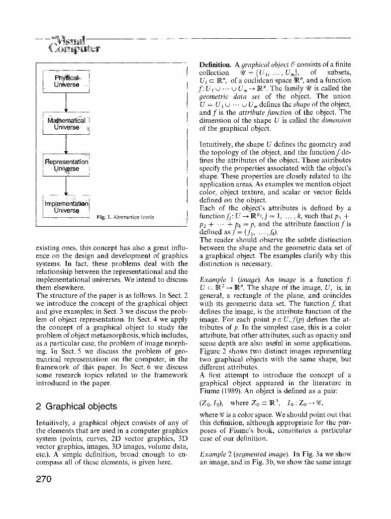
Example 1 (image). An image is a function f: U C I N 2 --4 I~ n. The shape of the image, U, is, in general, a rectangle of the plane, and coincides with its geometric data set. The function f, that defines the image, is the attribute function of the image. For each point p ~ U, f(p) defines the attributes of p. In the simplest case, this is a color attribute, but other attributes, such as opacity and scene depth are also useful in some applications. Figure 2 shows two distinct images representing two graphical objects with the same shape, but different attributes. A first attempt to introduce the concept of a graphical object appeared in the literature in Flume (1989). An object is defined as a pair:

(Zo, I0), where Zo c IR a, Io : Zo -~ <g,

where ~ is a color space. We should point out that this definition, although appropriate for the pur- poses of Fiume's book, constitutes a particular case of our definition.

Example 2 (segmented image). In Fig. 3a we show an image, and in Fig. 3b, we show the same image

270

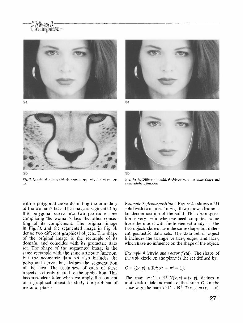
Fig. 2. Graphical objects with the same shape but different attributes

Fig. 3a, b. Different graphical objects with the same shape and same attribute function

with a polygonal curve delimiting the boundary of the woman's face. The image is segmented by this polygonal curve into two partitions, one comprising the woman's face the other consis- ting of its complement. The original image in Fig. 3a and the segmented image in Fig. 3b define two different graphical objects. The shape of the original image is the rectangle of its domain, and coincides with its geometric data set. The shape of the segmented image is the same rectangle with the same attribute function, but the geometric data set also includes the polygonal curve that defines the segmentation of the face. The usefulness of each of these objects is closely related to the application. This becomes clear later when we apply the concept of a graphical object to study the problem of metamorphosis.

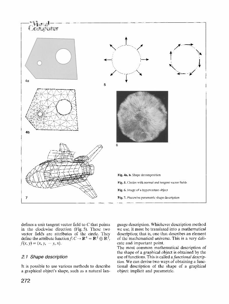
Example 3 (decomposition). Figure 4a shows a 2D solid with two holes. In Fig. 4b we show a triangu- lar decomposition of the solid. This decomposition is very useful when we need compute a value from the model with finite element analysis. The two objects shown have the same shape, but different geometric data sets. The data set of object b includes the triangle vertices, edges, and faces, which have no influence on the shape of the object.

Example 4 (circle and vector field). The shape of the unit circle on the plane is the set defined by:

C = { ( x , y ) elRZ;x 2 + y a = l } .

The map N: C ~ IR 2, N(x, y) = (x, y), defines a unit vector field normal to the circle C. In the same way, the map T : C ~ IR 2, T(x , y) = (y, - x),

271

t t//

/ \// /'

4b

Fig. 4a, b. Shape decomposition

Fig. 5. Circles with normal and tangent vector fields

Fig. 6. Image of a hypertexture object

Fig. 7. Piecewise parametric shape description

defines a unit tangent vector field to C that points in the clockwise direction (Fig. 5). These two vector fields are attributes of the circle. They define the attribute function f: C - , IR 4 = 11t 2 ® 11t 2, f ( x , y) = (x, y, - y, x ) .

2.1 Shape description

It is possible to use various methods to describe a graphical object's shape, such as a natural lan-

guage description. Whichever description method we use, it must be translated into a mathematical description; that is, one that describes an element of the mathematical universe. This is a very deli- cate and important point. The most common mathematical description of the shape of a graphical object is obtained by the use of functions. This is called afimctional description. We can devise two ways of obtaining a functional description of the shape of a graphical object: implicit and parametric.

272

2. 1.1 Implicit shape description

The implicit description of a shape U c IRk is defined by U = g- t(A), where g : V = U --, IR" is a function, and A is a subset of IRm. The most common case occurs when m -- 1 and the set A is a unit set {c}. In this case, the definition is reduced to the inverse image of the value c; that is, U = g-1(c), g is called the implicit function. Intu- itively, the implicit function is a density function of the graphical object. When the shape of a graphical object (9 is described implicitly, we say that (9 is an implicit object. We should observe that if f : U ~ IRP is the attribute function of an implicit object (9, then (9 is completely described in a functional form by the function h: U ~ IRp+m, defined by h = (g,f). Implicitly defined shapes have been widely used in computer graphics. They are very flexible in describing a huge variety of shapes, as illustrated by the example here.

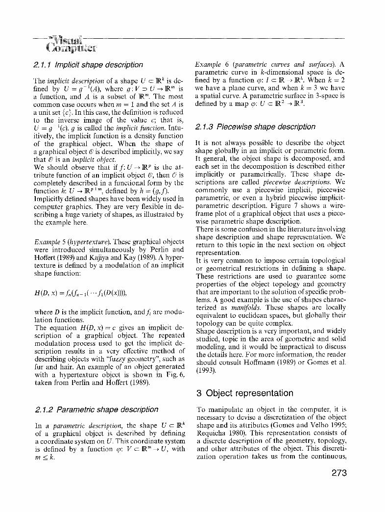
Example 5 (hypertexture). These graphical objects were introduced simultaneously by Perlin and Hoffert (1989) and Kajiya and Kay (1989). A hypertexture is defined by a modulation of an implicit shape function:

H(D, x) = f,, (f, -1 ("" fl (D (x)))),

where D is the implicit function, andJ~ are modulation functions. The equation H(D, x)= c gives an implicit description of a graphical object. The repeated modulation process used to get the implicit description results in a very effective method of describing objects with "fuzzy geometry", such as fur and hair. An example of an object generated with a hypertexture object is shown in Fig. 6, taken from Perlin and Hoffert (1989).

Example 6 (parametric curves and surfaces). A parametric curve in k-dimensional space is defined by a function cp: I ~ IR ~ IR k. When k = 2 we have a plane curve, and when k = 3 we have a spatial curve. A parametric surface in 3-space is defined by a map cp: U ~ IR2 ~ IR3.

2. 1.3 Piecewise shape description

It is not always possible to describe the object shape globally in an implicit or parametric form. It general, the object shape is decomposed, and each set in the decomposition is described either implicitly or parametrically. These shape descriptions are called piecewise descriptions. We commonly use a piecewise implicit, piecewise parametric, or even a hybrid piecewise implicit- parametric description. Figure 7 shows a wire- frame plot of a graphical object that uses a piecewise parametric shape description. There is some confusion in the literature involving shape description and shape representation. We return to this topic in the next section on object representation. It is very common to impose certain topological or geometrical restrictions in defining a shape. These restrictions are used to guarantee some properties of the object topology and geometry that are important to the solution of specific problems. A good example is the use of shapes charac- terized as manifolds. These shapes are locally equivalent to euclidean spaces, but globally their topology can be quite complex. Shape description is a very important, and widely studied, topic in the area of geometric and solid modeling, and it would be impractical to discuss the details here. For more information, the reader should consult Hoffmann (1989) or Gomes et al. (1993).

3 Object representation

2. 1.2 Parametric shape description

In a parametric description, the shape U c IRk of a graphical object is described by defining a coordinate system on U. This coordinate system is defined by a function (p: V c IRm~ U, with m<_k.

To manipulate an object in the computer, it is necessary to devise a discretization of the object shape and its attributes (Gomes and Velho 1995; Requicha 1980). This representation consists of a discrete description of the geometry, topology, and other attributes of the object. This discretization operation takes us from the continuous,

273

mathematical universe, to the discretized, representational universe. In geometric modeling this operation is called a representation, and in image processing it is called a discretization. The reason for this distinction is related to the fact that images and geometric models have historically been considered as completely different graphical objects. In fact, an image has a very well defined and trivial shape (in general, a rectangle in the plane); therefore, the discretization process is focused on the attribute function. The problem is reduced to function representation, which is widely used in the area of signal processing. In a geometric model, the emphasis is on the object shape, and it does not seem natural to associate the shape representation with a signal discretization problem. It should be clear that by the representation of an object we mean a discretization of the shape and its attribute function. When the shape is described by functions (functional description), shape representation is reduced to the problem of function representation. Since the attributes of a graphical object are defined by a function whose domain is the object shape, their representation is also reduced to the problem of function representation. The discretization of the attribute function of a graphical object is called quantization, in accor- dance with the classical use of this term in the area of signal processing. The quantization operation discretizes elements of the attribute vector space. Depending on the nature of these attributes, we may face either perceptual or computational problems. In the first case we could mention the problem of image quantization, while in the second we could mention the number of bits used to represent the coordinates of a vector field defined over a graphical object.

3. 1 Representation and reconstruction

When we observe an image on the monitor screen, it has undergone a reconstruction process to transform its digital, discrete representation into the analogical optical-electronic image we observe. This reconstruction should be taken into consideration when dealing with object representation in general. Ideally, the various representation/ reconstruction involved should be such that the

/ representation reconstruction

" '" ' --- . o "

9a 9b 9c 9d

0 0 lOa lOb 10c lOd

Fig. 8. Discretization and reconstruction of graphical objects

Fig. 9a-& Representation and reconstruction of a circle

Fig. 10ad . Linear and cubical reconstruction

artifacts are minimized and the materialization is as faithful as possible to the desired goals. In general, to compute with a graphical object, we should work on the continuous, mathematical universe, instead of working on the discrete object representation. Therefore, when defining a representation (9', of some graphical object (9, it is very important that we are able to reconstruct (9 from its representation (9'. The mathematical and representational universes are related by the operations of discretization and reconstruction, as illustrated in Fig. 8. The exact topology of the representation and the elements of the geometrical representation, should enable us to reconstruct the original object. When the object shape is very simple (e.g., an image), the problem of representation is reduced to the problem of discretization and reconstruction of its attribute function. When the object

274

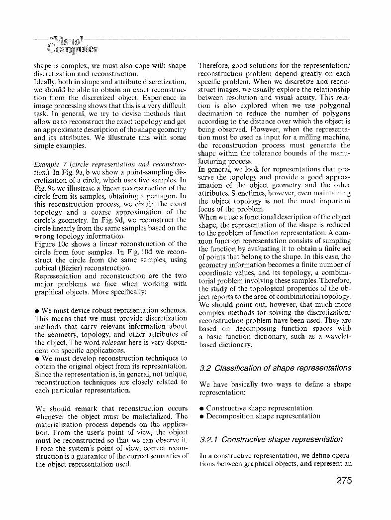
l omp, ter shape is complex, we must also cope with shape discretization and reconstruction. Ideally, both in shape and attribute discretization, we should be able to obtain an exact reconstruction from the discretized object. Experience in image processing shows that this is a very difficult task. In general, we try to devise methods that allow us to reconstruct the exact topology and get an approximate description of the shape geometry and its attributes. We illustrate this with some simple examples.

Example 7 (circle representation and reconstruction.) In Fig. 9a, b we show a point-sampling discretization of a circle, which uses five samples. In Fig. 9c we illustrate a linear reconstruction of the circle from its samples, obtaining a pentagon. In this reconstruction process, we obtain the exact topology and a coarse approximation of the circle's geometry. In Fig. 9d, we reconstruct the circle linearly from the same samples based on the wrong topology information. Figure 10c shows a linear reconstruction of the circle from four samples. In Fig. 10d we reconstruct the circle from the same samples, using cubical (B6zier) reconstruction. Representation and reconstruction are the two major problems we face when working with graphical objects. More specifically:

• We must device robust representation schemes. This means that we must provide discretization methods that carry relevant information about the geometry, topology, and other attributes of the object. The word relevant here is very depen- dent on specific applications. • We must develop reconstruction techniques to obtain the original object from its representation. Since the representation is, in general, not unique, reconstruction techniques are closely related to each particular representation.

Therefore, good solutions for the representation/ reconstruction problem depend greatly on each specific problem. When we discretize and reconstruct images, we usually explore the relationship between resolution and visual acuity. This relation is also explored when we use polygonal decimation to reduce the number of polygons according to the distance over which the object is being observed. However, when the representation must be used as input for a milling machine, the reconstruction process must generate the shape within the tolerance bounds of the manu- facturing process. In general, we look for representations that pre- serve the topology and provide a good approximation of the object geometry and the other attributes. Sometimes, however, even maintaining the object topology is not the most important focus of the problem. When we use a functional description of the object shape, the representation of the shape is reduced to the problem of function representation. A common function representation consists of sampling the function by evaluating it to obtain a finite set of points that belong to the shape. In this case, the geometry information becomes a finite number of coordinate values, and its topology, a combinatorial problem involving these samples. Therefore, the study of the topological properties of the object reports to the area of combinatorial topology. We should point out, however, that much more complex methods for solving the discretization/ reconstruction problem have been used. They are based on decomposing function spaces with a basic function dictionary, such as a wavelet- based dictionary.

3.2 Classification of shape representations

We have basically two ways to define a shape representation:

We should remark that reconstruction occurs whenever the object must be materialized. The materialization process depends on the application. From the user's point of view, the object must be reconstructed so that we can observe it. From the system's point of view, correct reconstruction is a guarantee of the correct semantics of the object representation used.

• Constructive shape representation • Decomposition shape representation

3.2. 1 Constructive shape representation

In a constructive representation, we define operations between graphical objects, and represent an

275

r h ~ N "~

i emputer object by writing the arithmetic expression of the object involving the operations. Intuitively, the operations act on a family of primitive graphical objects to obtain more complex objects. These primitive objects are charac- terized by the fact that they are very easy to describe and represent. When the objects are described by functions (functional description), the constructive representation consists in devising a set of operations with functions that enable us to obtain complex functions from simpler ones. A classical example of constructive shape representation is given by constructive solid geometry (CSG) representation used for solid modeling (Re- quicha 1980). Another important example is the use of binary space partitioning (BSP) trees. In Naylor (1994) the reader can find a good description of the use of BSP trees to represent object shape. Radha (1993) uses BSP trees to represent images.

3.2.2 Decomposition shape representation

In a decomposition representation, the object shape is decomposed into a family of subsets. This representation uses the well-known "divide and conquer" paradigm. The geometry of each piece is easier to describe, and a combinatorial scheme allows us to reconstruct the original object with at least a good degree of approximation. The decomposition representation is essentially an ex- tension of the point-sampling representation for functions for objects of arbitrary topology. A classical use of decomposition representation is the boundary representation (B-rep) used in geometric modeling. In this representation, the object shape is defined by its limiting boundary, and the boundary is represented by decomposing it into vertices, edges, and faces (Baumgart 1975). A combinatorial scheme is necessary to guarantee the correct topology of the shape of the reconstructed object. A common technique to obtain this cor- rectness involves using Euler operators. We should point out that it is possible to obtain hybrid representations of graphical objects by mixing constructive and decomposition representations. A typical, and classical, example is the combination of CSG representation and B-rep. Some types of representation can be classified either as constructive or decomposition repre-

sentations, depending on how they are specified. A typical example is the matrix representation described here.

Example 8 (matrix representation). The most used representation for an image f: U ~ IR" is obtained by decomposing the image shape uniformly:

U = [a, b] x [c, d]

= {(x, y) ~ IR2; a _< x _< b, and c _< y _< d}.

This uniform decomposition is obtained by defining a grid, A v, on U,

Av = {(xj, yk) ~ U; xj = j" Ax,

Yk = k ' A y j, k ~ Z , Ax, Ay e IR}.

This is illustrated in Fig. 11. Each rectangle in the decomposition is completely described by the coordinates (x j, Yk). The image function can be sam- pled in each rectangle, and the value obtained is associated with the integer coordinates (j, k). The matrix representation can also be specified as a constructive representation, given by the union of the grid cells. In both cases, the image is conveniently represented by the m x n matrix A = (a~k) = (f(xj , Yk)). The matrix representation can also be used to represent arbitrary graphical objects. The bi- dimensional grid defined on the image domain U is easily extended for n-dimensional euclidean space. By enumerating the grid cells, we define the object's geometry and topology. The combinatorial topology of the shape U becomes an enumeration of the rectangles. In each cell, we define the object's attributes by restricting the attribute function to the cell. In Fig. 12 we show a matrix representation of 1D, 2D, and 3D graphical objects. In the area of solid modeling the matrix representation is called spatial enumeration. It is a very popular representation method for volume data (Kaufman 1994); it is known as volume array by the graphics community, and sometimes it is called a 3D image, specially by the researchers from image processing. The matrix representation uses a uniform decomposition of the space. More flexible decomposition representations use an adaptive subdivision

276

11

f + Az

Fig. 11. Matrix representation of an image

Fig. 12. Matrix representations of various objects

of the space, where the size of each piece varies from region to region of the decomposed object. This is nicely illustrated by the decomposition of the object shown in Fig. 4. The adaptiveness criteria in general exploit some of the object's attribute functions. Well-known examples of these representations are the quadtree, for 2D graphical objects, and the octree, for 3D objects. We should point out here the poor choice of the names historically used for these adaptive representations by decomposition: these names confuse the representation method and the subjacent spatial data structures used to implement the decomposition.

3.3 Levels of discretization

Before closing this section, we should clarify one point. The continuous and representational universes are different levels of abstraction used to describe graphical objects. In fact, continuous objects only exist abstractly, because in a computer

all objects should be represented in digital form and, therefore, they are discretized. However, we should point out that, from a computational point of view, the use of the term "discrete" should be associated with our perception of the graphical object. The color space is a good example of this. A color is a signal represented by its spectral distribution function. When we discretize the visible spectrum into three bands, red, green and blue, we obtain a representation of the color space as a 3D space IR 3. However, to represent color on the computer, we must employ a second level of discretization by using a floating-point representation for each of the color components. From a perceptual point of view, a floating-point representation of color is not necessary. In fact, for video resolution, eight bits for each color coordinate is enough. Thus, it is common practice to consider a floating-point representation of the color components as a continuous representation. This common practice is used in our everyday perception of the physical world. The universe is

277

discretized into atomic and subatomic particles; light is also quantized, but in our perceptual resolution scale, we assume that we live in a continuous universe. The reasons exposed above explain why sometimes we use the sentence "continuous representation of a graphical object on the computer".

4 Graphical object metamorphosis

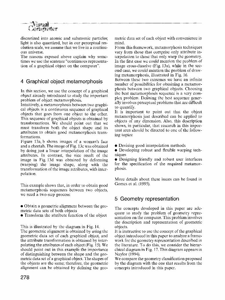
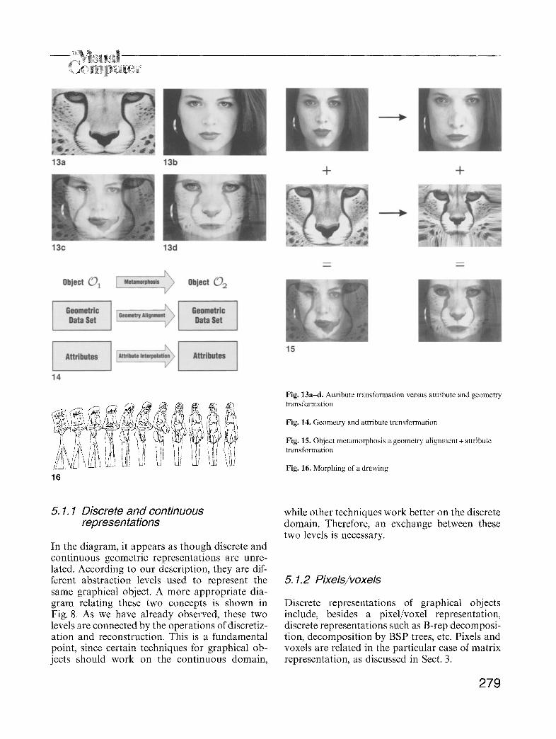
In this section, we use the concept of a graphical object already introduced to study the important problem of object metamorphosis. Intuitively, a metamorphosis between two graphical objects is a continuous sequence of graphical objects that goes from one object to the other. This sequence of graphical objects is obtained by transformations. We should point out that we must transform both the object shape and its attributes to obtain good metamorphosis transformations. Figure 13a, b shows images of a woman's face and a cheetah. The image of Fig. 13c was obtained by doing just a linear interpolation of the image attributes. In contrast, the nice result of the image in Fig. 13d was obtained by deforming (warping) the image shape, along with the transformation of the image attributes, with interpolation.

This example shows that, in order to obtain good metamorphosis sequences between two objects, we need a two-step process:

• Obtain a geometric alignment between the geometric data sets of both objects • Transform the attribute function of the object

This is illustrated by the diagram in Fig. 14. The geometric alignment is obtained by using the geometric data set of each graphical object, and the attribute transformation is obtained by inter- polating the attributes of each object (Fig. 15). We should point out in this example the importance of distinguishing between the shape and the geometric data set of a graphical object. The shapes of the objects are the same; therefore, the geometric alignment can be obtained by defining the geo-

metric data set of each object with convenience in mind. From this framework, metamorphosis techniques vary from those that comprise only attribute interpolation to those that only warp the geometry. In the first case we could mention the problem of image cross-dissolve (Fig. 13a), while in the second case, we could mention the problem of drawing metamorphosis, illustrated in Fig. 16. Between these two extremes we have an infinite number of possibilities for obtaining a metamorphosis between two graphical objects. Choosing the best metamorphosis sequence is a very complex problem. Defining the best sequence gener- ally involves perceptual problems that are difficult to quantify. It is important to point out that the object metamorphosis just described can be applied to objects of any dimension. Also, this description shows, in particular, that research in this important area should be directed to one of the follow- ing topics:

• Devising good interpolation methods • Developing robust and flexible warping techniques • Designing friendly and robust user interfaces for the specification of the required metamorphosis.

More details about these issues can be found in Gomes et al. (1995).

5 Geometry representation

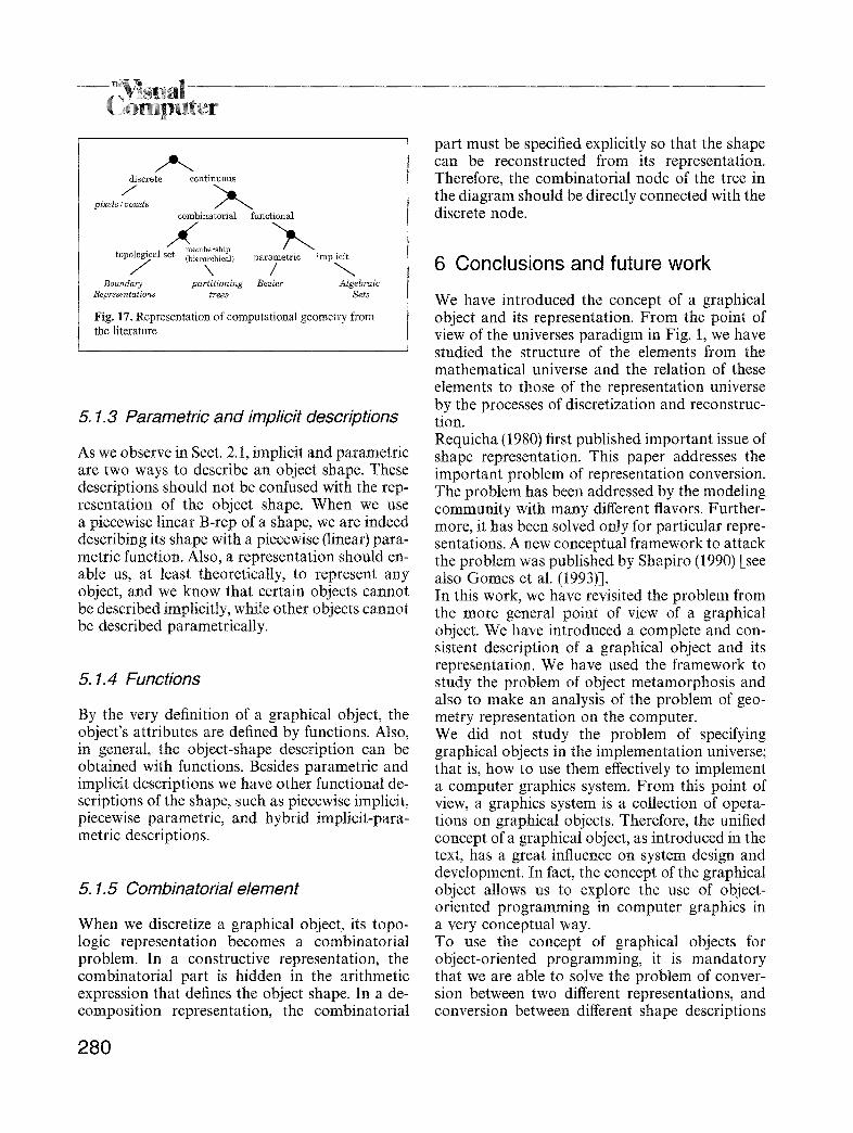
The concepts developed in this paper are ade- quate to study the problem of geometry representation on the computer. This problem involves the description and representation of geometric objects. It is instructive to use the concept of the graphical object introduced in this paper to analyze a framework for the geometry representation described in the literature. To do this, we consider the hierarchical diagram in Fig. 17. This diagram appears in Naytor (1994). We compare the geometry classification proposed by the diagram with the one that results from the concepts introduced in this paper.

278

16

Fig. 13a-d. Attribute transformation versus attribute and geometry transformation

Fig. 14. Geometry and attribute transformation

Fig. 15. Object metamorphosis = geometry alignment + attribute transformation

Fig. 16. Morphing of a drawing

5. 1.1 Discrete and continuous representations

In the diagram, it appears as though discrete and continuous geometric representations are unre- lated. According to our description, they are different abstraction levels used to represent the same graphical object. A more appropriate diagram relating these two concepts is shown in Fig. 8. As we have already observed, these two levels are connected by the operations of discretization and reconstruction. This is a fundamental point, since certain techniques for graphical objects should work on the continuous domain,

while other techniques work better on the discrete domain. Therefore, an exchange between these two levels is necessary.

5. 1.2 Pixels/voxels

Discrete representations of graphical objects include, besides a pixel/voxel representation, discrete representations such as B-rep decomposition, decomposition by BSP trees, etc. Pixels and voxels are related in the particular case of matrix representation, as discussed in Sect. 3.

279

"~;N Te N

discrete corttinuous

pixels / voxels combinatorial functional

topological set membership (hierarchical) parametric implicit J ,, /

Boundary partitioning Bezier Algebraic Representations trees Sets

Fig. 17. Representation of computational geometry from the literature

5. 1.3 Parametric and implicit descriptions

As we observe in Sect. 2.1, implicit and parametric are two ways to describe an object shape. These descriptions should not be confused with the representation of the object shape. When we use a piecewise linear B-rep of a shape, we are indeed describing its shape with a piecewise (linear) parametric function. Also, a representation should enable us, at least theoretically, to represent any object, and we know that certain objects cannot be described implicitly, while other objects cannot be described parametrically.

5. 1.4 Functions

By the very definition of a graphical object, the object's attributes are defined by functions. Also, in general, the object-shape description can be obtained with functions. Besides parametric and implicit descriptions we have other functional descriptions of the shape, such as piecewise implicit, piecewise parametric, and hybrid implicit-parametric descriptions.

5. 1.5 Combinatorial element

When we discretize a graphical object, its topo- logic representation becomes a combinatorial problem. In a constructive representation, the combinatorial part is hidden in the arithmetic expression that defines the object shape. In a decomposition representation, the combinatorial

part must be specified explicitly so that the shape can be reconstructed from its representation. Therefore, the combinatorial node of the tree in the diagram should be directly connected with the discrete node.

6 Conclusions and future work

We have introduced the concept of a graphical object and its representation. From the point of view of the universes paradigm in Fig. 1, we have studied the structure of the elements from the mathematical universe and the relation of these elements to those of the representation universe by the processes of discretization and reconstruction. Requicha (1980) first published important issue of shape representation. This paper addresses the important problem of representation conversion. The problem has been addressed by the modeling community with many different flavors. Further- more, it has been solved only for particular representations. A new conceptual framework to attack the problem was published by Shapiro (1990) [see also Gomes et al. (1993)J. In this work, we have revisited the problem from the more general point of view of a graphical object. We have introduced a complete and con- sistent description of a graphical object and its representation. We have used the framework to study the problem of object metamorphosis and also to make an analysis of the problem of geometry representation on the computer. We did not study the problem of specifying graphical objects in the implementation universe; that is, how to use them effectively to implement a computer graphics system. From this point of view, a graphics system is a collection of operations on graphical objects. Therefore, the unified concept of a graphical object, as introduced in the text, has a great influence on system design and development. In fact, the concept of the graphical object allows us to explore the use of object- oriented programming in computer graphics in a very conceptual way. To use the concept of graphical objects for object-oriented programming, it is mandatory that we are able to solve the problem of conversion between two different representations, and conversion between different shape descriptions

280

(specially between implicit and parametric shape descriptions). This is a well-known, and difficult, problem in the area of modeling. Nonetheless, we should point out that the work in this area has been directed towards the search for exact conversion operations. In most applications we need to devise a robust and efficient approximate conversion between different representations because we are working on the representation universe. We are currently doing research in this direction, so that we will be able to obtain the prototype of an object-oriented graphics system that uses the concept of the graphical object introduced in this paper.

Acknowledgements. We thank the reviewers for their suggestions and questions that were very useful in clarifying parts of this paper.

References

Baumgart B (1975) A polyhedron representation for computer vision. Proceedings of the AFIPS Conference, pp 589-596

Flume E (1989) The mathematical structure of raster graphics. Academic Press, Boston

Gomes J, Costa B, Darsa L, Berton J, Velho L, Wolberg G (1995) Warping and morphing of graphical objects. (Ed) SIGGRAPtt '95 Course Notes

Gomes J, Velho L (1995) Abstraction paradigms for computer graphics. Vis Comput 11:227-239

Gomes J, Hoffmann C, Shapiro V, Velho L (1993) Modeling in graphics. (Ed) SIGGRAPH '93 Course Notes

Hoffinann C (1989) Geometric and solid modeling: an introduction. Morgan Kaufmann

Kajiya JT, Kay TL (1989) Rendering fur with three-dimensional textures. Comput Graph 23:271-280

Kaufman A (1994) Voxels as a computational representation of geometry. In: The computational representation of geometry. SIGGRAPH '94 Course Notes

Naylor B (1994) Computational representations of geometry. In: The computational representation of geometry. SIGGRAPtt '94 Course Notes

Perlin K, Hoffert EM (1989) Hypertexture. Comput Graph 23:253-262

Radha HS (1993) Efficient image representation using binary space partitioning trees. PhD dissertation, cu/ctr/tr 343-93-23, Columbia University

Requicha A (1980) Representations for rigid solids: theory methods and systems. ACM Comput Surveys 12:437-464

Shapiro V (1990) Representations of semi-algebraic sets in finite algebras generated by space decompositions. PhD thesis, Cornell University

JONAS GOMES received his Ph.D. in Mathematics in 1984 from the Institute of Pure and Applied Mathematics (IMPA) in Rio de Janeiro. He worked as the R&D manager of the computer graphics group at Globo TV network from 1984 to 1988. Since 1989, he is a Research Associate at IMPA, where he started the VisGraf project, a computer graphics research group. His current research interests include modeling, digital publishing and conceptual issues in graphics. He has published

several papers in these areas, and was the organizer of a course on Modeling at SIGGRAPH '93.

LUCIA DARSA is currently working towards a Ph.D. degree at SUNY at Stony Brook. She graduated in Computer Engin- eering at Pontificia Univer- sidade Cat61ica do Rio de Janeiro, Brazil obtaining her M.Sc. degree in Computer Science in 1994 from a joint pro- gram between PUC-RJ and IMPA. She has been a member of the VisGraf project at IMPA since 1990, having worked with implicit surfaces rendering and modeling, motion control hard- ware and compositing, and im-

age processing. She has been involved with morphing research and development since 1992, being a co-author of Visionaire, a commercial warping and morphing software.

BRUNO COSTA has a computer engineering and M.Sc. degree in computer science from PUC at Rio de Janeiro Brazil, and is currently pursuing his Ph.D. also in computer science at SUNY Stony Brook. He has been involved with the Visgraf project at IMPA since its begin- nings in 1990, where he has worked on realistic rendering, image and implicit objects transformations, warping and morphing in particular. He has coauthored a commercial morphing software, as a by-product

of his Master's research. His current interests also include computer graphics aspects of interactive environments, and volume graphics.

281

L U I Z V E L H O graduated in Industrial Design from ESDI - Universidade do Rio de Janeiro in 1979. He received a MS in Computer Graphics from the Massachusetts Institute of Technology, Media Laborat- ory in 1985, and a Ph.D. in Computer Science from the Uni- versity of Toronto in t994. Dur- ing 1982 he was a visiting researcher at the National Film Board of Canada. From 1985 to 1987 he was a Systems Engineer at the Fantastic Animation Ma- chine in New York, where he

developed the company's 3D visualization system. From 1987 to 1991 he was a Principal Engineer at Globo TV Network in Brazil. His research interests include theoretical foundations of computer graphics, physically-based methods, wavelets and modeling with implicit objects. He is currently an associate researcher at IMPA - Instituto de Matematica Pura e Aplicada.

282

graphical objects

Documents