1

ASSIGNMENT OF WORK SHIFTS TO PUBLIC TRANSIT DRIVERS

BASED ON STATED PREFERENCES

Sonia Montalva, Juan Carlos Muñoz,1 Ricardo Paredes

Escuela de Ingeniería, Pontificia Universidad Católica de Chile

ABSTRACT Transit agencies periodically assign each of their drivers with a shift describing when and for how long they will work each day in the following months. Since drivers are not indifferent to which shift they receive, transit agencies define different assignment methods often based on driver seniority. This article study and compare different shift assignment policies assuming that the agency has some information regarding the approximate utility that each shift represents to each driver. Additionally, based on a study that analyzes driver utilities for flexible shifts (i.e. in which the weekly number of hours is not distributed uniformly along weekly working days), it shows that implementing flexible shifts offer a win-win opportunity for the agency and the drivers. On one hand drivers improve their productivity; on the other they increment their satisfaction with their job. This is particularly relevant since transit operational costs are strongly dependent on their labor force. Some of the benefits obtained by the firm should finally be captured by the users of the system.

1. INTRODUCTION

The demand for trips on public transportation displays significant daily and weekly seasonalities. In response to such variations, public transit companies adjust their schedules to provide greater frequency of service during periods when demand is high. The need for drivers’ services is therefore also variable, and operators normally find it convenient to adapt their schedules accordingly. In practice, however, their ability to do so is limited by several restrictions, particularly those imposed by labor legislation. This leads to scheduling mismatches with on-duty drivers left idle during off-peak periods, generating higher costs and poorer service. Muñoz (2002) concluded on the basis of a typical supply curve for urban transit systems that with exclusive use of fixed and continuous eight-hour shifts, the underutilization of driver hours would be about 20% to 30%. To reduce off-peak driver idleness and the losses they engender, companies have designed various scheduling strategies that deviate from the prevailing labor standards. Some of these are resisted by drivers and often make excessive use of overtime, with its consequent cost increases.

1 Correspondent author.

2

Muñoz (2002) proposes a strategy that would enable public transit operators to adapt to demand by minimizing costs associated with personnel overcapacity. The method is based on flexible shifts (FS) under which drivers work a quantity of hours that varies from day to day but does so according to a well-defined pattern, with total weekly hours worked remaining as stipulated in their employment contract. Muñoz also shows that by employing such shifts, the number of on-duty drivers can be adjusted almost perfectly to the schedule seasonalities typical of urban public transportation systems.

The abovementioned study further suggests that given the diversity of personal preferences and situations, it is highly likely that there will be drivers who would prefer a menu of contracts to a homogenous one. Flexible shifts would thus represent an opportunity for all players to benefit. The hypothesis that drivers display heterogeneity of preferences – and indeed, a preference for heterogeneity – is developed and supported in Miranda et al. (2007). In other words, drivers do have varying preferences, and some of them value day-to-day variation in the shifts they work.

This paper estimates drivers’ utility functions for various shift structures (i.e., the distribution of the weekly work schedule over a given period of time, such as four weeks) on the basis of their stated preferences (SP). To determine these preferences, drivers are first made to choose among alternative hypothetical structures. The data are then employed to create a series of attributes relating both to the shifts chosen and the drivers’ socioeconomic status. The results support the idea that preferences of a significant proportion of them for flexible shifts exist and that it is possible to identify the driver’s types which are most inclined to elect such structures.

However, the viability of this strategy requires that all players benefit, which in turn depends on the mechanism defined for assigning shifts and compensating the drivers. This study is devoted to finding the mechanisms that correspond to the most viable strategy.

For each assignment mechanism we identify the benefits to the transit operators of adopting flexible shift structures, as these additional gains can be employed to compensate drivers who prefer a standard shift to the one they are actually assigned. We also explore several levels of worker participation and discrimination in the assignment process in order to compare the costs of different viable applications.

The impact on workers is assumed to be the change in their group welfare measured by the difference in the sum of their individual utilities. We also consider the increase in individual dissatisfaction compared to a standard shift and the consequent compensation that would have to be paid. Thus, a mechanism is considered viable if all players benefit and no workers perceive that they will be worse off. The operator must therefore compensate any workers who are adversely affected.2 The difference between the sum of

2 The amount of such compensation is that needed to restore the level of satisfaction perceived on the newly assigned shift to that of the current one in cases where the latter is higher.

3

these compensations and the savings obtained via the use of flexible shifts determine the employer’s increase in welfare.

As already noted, the utility functions calibrated in Miranda et al. (2007), which include a deterministic (or expected) utility and a stochastic element, display a high degree of heterogeneity in individual preferences. This is reflected in the significant values found for variance relative to expected utility. They also show that the deterministic element of a driver’s utility for a given shift structure may differ considerably from what he or she actually perceives. This is taken into account when proposed shift structure assignment mechanisms are analyzed.

The remainder of this paper is divided into four sections. Section 2 outlines the main findings given in Miranda et al. (2007), with emphasis on those directly affecting the objectives of the present study. Section 3 analyzes different driver shift assignment mechanisms, which are classified as either centralized or participatory. Finally, Section 4 sets out our conclusions and SUMS UP ON their viability.

2. DRIVER SHIFT PREFERENCES

The methodology proposed in this paper is based on the possibility of obtaining a perceived utility function for each driver in respect of each type of shift. Such functions are found in Miranda et al. (2007) and will be used here. In this section we begin by reviewing their methodology and findings.

To break out a set of workers’ utility functions by shift, a stated preference (SP) survey was conducted of drivers at two public transit operators in Santiago, Chile. We opted for the stated-choice method because among other advantages, it places interviewees in a context similar to a real-world situation in which they must elect only one of the alternatives presented (Ortúzar and Garrido, 1994).

Following a methodology similar to Ortúzar et al. (1997), the attributes to be included in the experimental SP model were first identified. A Delphi survey and focus groups are used to define the attributes, determine their appropriate value ranges and identify groups of drivers whose work schedule preferences might be similar. In their study, Miranda et al. (2007) assume that all drivers work 48 hours per week3 from Monday to Saturday. A base or standard shift structure of 8 hours daily is defined,4 which we will refer to as the 8H structure. As for the flexible shifts (FS), they are represented in terms of the weekly distribution of hours. Thus, the work sequence A-B-C-D-E-F denotes a shift in which the driver works A hours on Monday, B hours on Tuesday, C hours on Wednesday, and so on. Shifts of less than 4 hours or more than 12 hours are excluded

3 This was the maximum number of hours permitted under Chile’s labour standards legislation until December 31, 2004, when the number was reduced to 45 hours per week. 4 Under the Chilean Labor Code, urban public transit drivers may work no more than 8 hours per day and six days consecutively. Drivers must also have two Sundays off per month. This is the only permitted way of distributing the weekly work schedule.

4

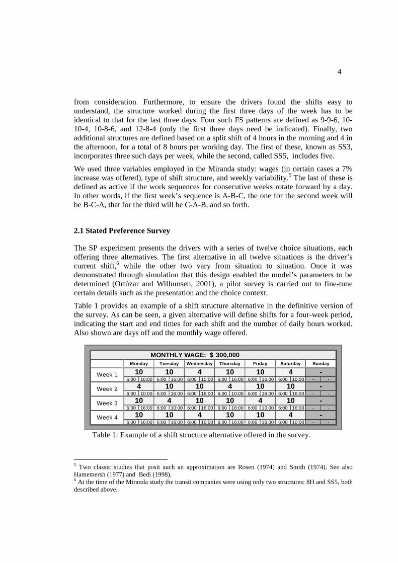
from consideration. Furthermore, to ensure the drivers found the shifts easy to understand, the structure worked during the first three days of the week has to be identical to that for the last three days. Four such FS patterns are defined as 9-9-6, 10-10-4, 10-8-6, and 12-8-4 (only the first three days need be indicated). Finally, two additional structures are defined based on a split shift of 4 hours in the morning and 4 in the afternoon, for a total of 8 hours per working day. The first of these, known as SS3, incorporates three such days per week, while the second, called SS5, includes five.

We used three variables employed in the Miranda study: wages (in certain cases a 7% increase was offered), type of shift structure, and weekly variability.5 The last of these is defined as active if the work sequences for consecutive weeks rotate forward by a day. In other words, if the first week’s sequence is A-B-C, the one for the second week will be B-C-A, that for the third will be C-A-B, and so forth.

2.1 Stated Preference Survey

The SP experiment presents the drivers with a series of twelve choice situations, each offering three alternatives. The first alternative in all twelve situations is the driver’s current shift,6 while the other two vary from situation to situation. Once it was demonstrated through simulation that this design enabled the model’s parameters to be determined (Ortúzar and Willumsen, 2001), a pilot survey is carried out to fine-tune certain details such as the presentation and the choice context.

Table 1 provides an example of a shift structure alternative in the definitive version of the survey. As can be seen, a given alternative will define shifts for a four-week period, indicating the start and end times for each shift and the number of daily hours worked. Also shown are days off and the monthly wage offered.

6:00 16:00 6:00 16:00 6:00 10:00 6:00 16:00 6:00 16:00 6:00 10:00 - -

6:00 10:00 6:00 16:00 6:00 16:00 6:00 10:00 6:00 16:00 6:00 16:00 - -

6:00 16:00 6:00 10:00 6:00 16:00 6:00 16:00 6:00 10:00 6:00 16:00 - -

6:00 16:00 6:00 16:00 6:00 10:00 6:00 16:00 6:00 16:00 6:00 10:00 - -10 10 4 -Week 4 10 10 4

10 4 10 -Week 3 10 4 10

4 10 10 -Week 2 4 10 10

10 10 4 -Week 1 10 10 4

MONTHLY WAGE: $ 300,000Monday Tuesday Wednesday Thursday Friday Saturday Sunday

Table 1: Example of a shift structure alternative offered in the survey.

5 Two classic studies that posit such an approximation are Rosen (1974) and Smith (1974). See also Hamemersh (1977) and Bedi (1998). 6 At the time of the Miranda study the transit companies were using only two structures: 8H and SS5, both described above.

5

The experiment places drivers in a hypothetical situation in which they receive a job offer from a new public transit company offering three alternative shift schedules. The survey itself consists of three parts. In the first part, personal data are obtained from the drivers on their weekly day off and workday period preferences as well as their monthly wage and time availability. This information is used to personalize the remainder of the survey for each driver. Data on the drivers’ socio-economic background was also gathered.

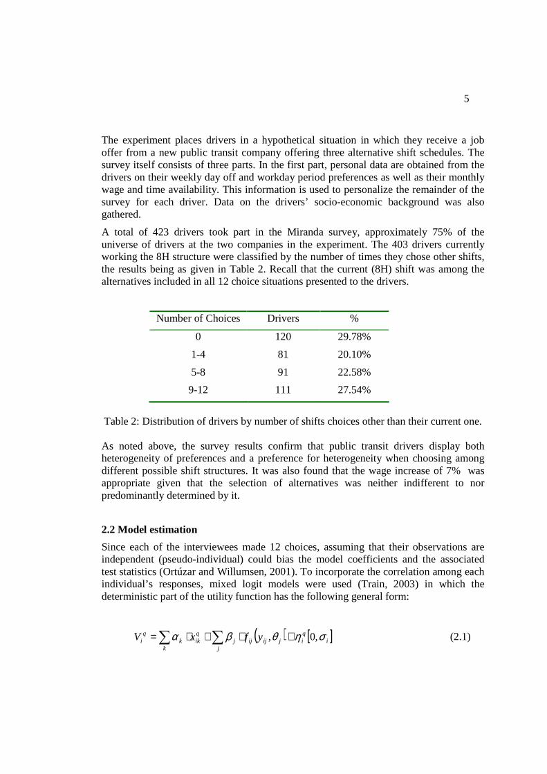
A total of 423 drivers took part in the Miranda survey, approximately 75% of the universe of drivers at the two companies in the experiment. The 403 drivers currently working the 8H structure were classified by the number of times they chose other shifts, the results being as given in Table 2. Recall that the current (8H) shift was among the alternatives included in all 12 choice situations presented to the drivers.

Number of Choices Drivers %

0 120 29.78%

1-4 81 20.10%

5-8 91 22.58%

9-12 111 27.54%

Table 2: Distribution of drivers by number of shifts choices other than their current one. As noted above, the survey results confirm that public transit drivers display both heterogeneity of preferences and a preference for heterogeneity when choosing among different possible shift structures. It was also found that the wage increase of 7% was appropriate given that the selection of alternatives was neither indifferent to nor predominantly determined by it.

2.2 Model estimation

Since each of the interviewees made 12 choices, assuming that their observations are independent (pseudo-individual) could bias the model coefficients and the associated test statistics (Ortúzar and Willumsen, 2001). To incorporate the correlation among each individual’s responses, mixed logit models were used (Train, 2003) in which the deterministic part of the utility function has the following general form:

( ) [ ]iqi

jjijijj

k

qikk

qi yfxV σηθβα ,0, +⋅+⋅= ∑∑ (2.1)

6

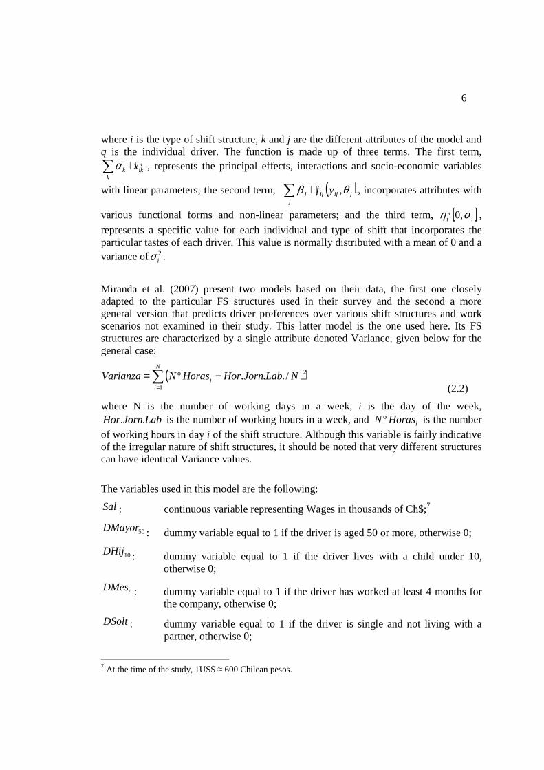
where i is the type of shift structure, k and j are the different attributes of the model and q is the individual driver. The function is made up of three terms. The first term,

∑ ⋅k

qikk xα , represents the principal effects, interactions and socio-economic variables

with linear parameters; the second term, ( )∑ ⋅j

jijijj yf θβ , , incorporates attributes with

various functional forms and non-linear parameters; and the third term, [ ]iqi ση ,0 ,

represents a specific value for each individual and type of shift that incorporates the particular tastes of each driver. This value is normally distributed with a mean of 0 and a variance of 2

iσ .

Miranda et al. (2007) present two models based on their data, the first one closely adapted to the particular FS structures used in their survey and the second a more general version that predicts driver preferences over various shift structures and work scenarios not examined in their study. This latter model is the one used here. Its FS structures are characterized by a single attribute denoted Variance, given below for the general case:

( )∑=

−=N

ii NLabJornHorHorasNVarianza

1

2/...º (2.2)

where N is the number of working days in a week, i is the day of the week, LabJornHor .. is the number of working hours in a week, and iHorasN º is the number

of working hours in day i of the shift structure. Although this variable is fairly indicative of the irregular nature of shift structures, it should be noted that very different structures can have identical Variance values.

The variables used in this model are the following:

Sal : continuous variable representing Wages in thousands of Ch$;7

50DMayor : dummy variable equal to 1 if the driver is aged 50 or more, otherwise 0;

10DHij : dummy variable equal to 1 if the driver lives with a child under 10, otherwise 0;

4DMes : dummy variable equal to 1 if the driver has worked at least 4 months for the company, otherwise 0;

DSolt : dummy variable equal to 1 if the driver is single and not living with a partner, otherwise 0;

7 At the time of the study, 1US$ ≈ 600 Chilean pesos.

7

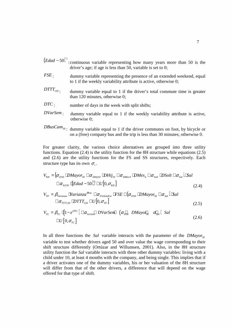
( )+− 50Edad : continuous variable representing how many years more than 50 is the driver’s age; if age is less than 50, variable is set to 0;

FSE : dummy variable representing the presence of an extended weekend, equal to 1 if the weekly variability attribute is active, otherwise 0;

120DTTT : dummy variable equal to 1 if the driver’s total commute time is greater than 120 minutes, otherwise 0;

DTC : number of days in the week with split shifts;

DVarSem : dummy variable equal to 1 if the weekly variability attribute is active, otherwise 0;

30DBusCam : dummy variable equal to 1 if the driver commutes on foot, by bicycle or on a (free) company bus and the trip is less than 30 minutes; otherwise 0.

For greater clarity, the various choice alternatives are grouped into three utility functions. Equation (2.4) is the utility function for the 8H structure while equations (2.5) and (2.6) are the utility functions for the FS and SS structures, respectively. Each structure type has its own iσ .

( )

( ) [ ]HEd

SalSoltDMesDHijDH

UEdad

SalDSoltDMesDHijDMayorV

850

44101050508

,050 σα

ααααα

+−⋅+

⋅+⋅+⋅+⋅+⋅=+

(2.4)

( )[ ]TFTTT

SalDFinSemExtVar

VarianzaTF

UDTTT

SalDMayorFSEVarianzaV

σααααβ θ

,0 120120

5050

+⋅+⋅+⋅+⋅+⋅=

(2.5)

( ) ( )[ ]

50 501

0,

DTCTC TC VarSem D Sal

TC

V e DVarSem DMayor Sal

U

β α α α

σ

= ⋅ − + ⋅ + ⋅ + ⋅

+ (2.6)

In all three functions the Sal variable interacts with the parameter of the 50DMayor

variable to test whether drivers aged 50 and over value the wage corresponding to their shift structure differently (Ortúzar and Willumsen, 2001). Also, in the 8H structure utility function the Sal variable interacts with three other dummy variables: living with a child under 10, at least 4 months with the company, and being single. This implies that if a driver activates one of the dummy variables, his or her valuation of the 8H structure will differ from that of the other drivers, a difference that will depend on the wage offered for that type of shift.

8

To model the utility of the FS structures, we assumed the existence of a functional form that varies with the extent of their divergence (Variance) from the 8H structure. The FSE dummy, which represents the presence of extended weekends, begins to be relevant only once the variance reaches 48 (that is, for structures 10-4-10 and 6-12-6). With the 10-6-8 structure (Variance equal to 16), the presence of an extended weekend does not seem to affect drivers’ perceptions. This can be interpreted to mean that a weekend extended by only 2 hours does not represent a significant difference for them, and it is therefore not clear at what precise point this benefit does begin to take on importance. In the case of the 6-12-6 structure, recall that weekly variability reduces the length of some weekends; for this reason FSE is modeled with a negative value (-1). Thus, the model proposes that the utility of FSE in this structure is the same as in the 12-4-8 and 10-4-10 structures.

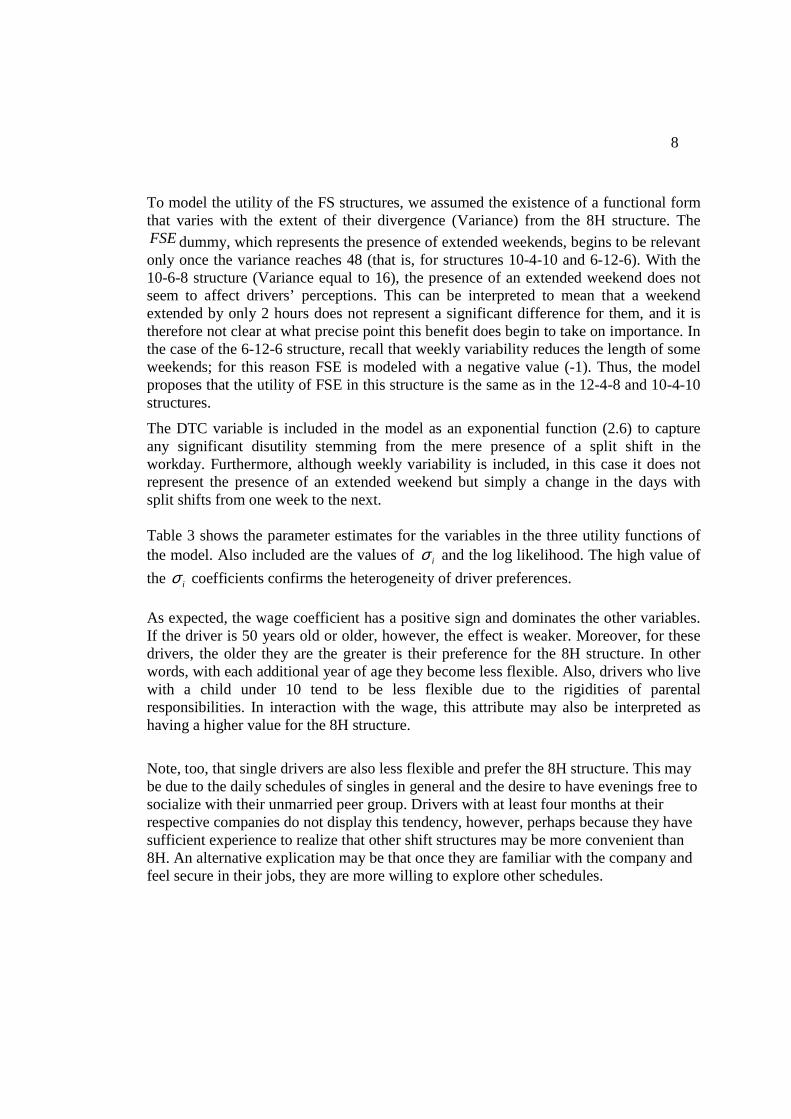
The DTC variable is included in the model as an exponential function (2.6) to capture any significant disutility stemming from the mere presence of a split shift in the workday. Furthermore, although weekly variability is included, in this case it does not represent the presence of an extended weekend but simply a change in the days with split shifts from one week to the next. Table 3 shows the parameter estimates for the variables in the three utility functions of the model. Also included are the values of iσ and the log likelihood. The high value of

the iσ coefficients confirms the heterogeneity of driver preferences.

As expected, the wage coefficient has a positive sign and dominates the other variables. If the driver is 50 years old or older, however, the effect is weaker. Moreover, for these drivers, the older they are the greater is their preference for the 8H structure. In other words, with each additional year of age they become less flexible. Also, drivers who live with a child under 10 tend to be less flexible due to the rigidities of parental responsibilities. In interaction with the wage, this attribute may also be interpreted as having a higher value for the 8H structure.

Note, too, that single drivers are also less flexible and prefer the 8H structure. This may be due to the daily schedules of singles in general and the desire to have evenings free to socialize with their unmarried peer group. Drivers with at least four months at their respective companies do not display this tendency, however, perhaps because they have sufficient experience to realize that other shift structures may be more convenient than 8H. An alternative explication may be that once they are familiar with the company and feel secure in their jobs, they are more willing to explore other schedules.

9

Coefficients HV8 TFV TCV

Wage (thousands of pesos) ( Salα ) 0.100 (23.03)

0.100 (23.03)

0.100 (23.03)

Aged 50 and over ( 50Dα ) -0.040 (-4.26)

-0.040 (-4.26)

-0.040 (-4.26)

Child under 10 ( 10Hijα ) 2.28E-03 (1.70)

More than 4 months ( 4DMesα ) -5.87E-03

(-2.80)

Single ( Soltα ) 5.22E-03 (2.33)

(Age-50)+ ( 50Edα ) 0.234 (3.65)

Variance ( Varianzaβ ) -0.73

(-2.49)

Variance exponent ( Varθ ) 0.18

(2.65)

Extended weekend ( FSEα ) 0.251 (3.67)

TCT > 120 mins ( 120TTTα ) 1.907 (2.54)

SS modif ( TCβ ) -6.200

(-10.31)

Weekly variab. with SS ( VarSemα ) -0.810 (-3.67)

Free commute < 30 mins ( 30DBusCamα ) 0.538 (1.06)

8Hσ 3.074

(11.73)

TFσ 1.972 (5.00)

TCσ 3.428 (9.15)

Log-Likelihood (C) -4450.33

Log-Likelihood (θ) -2678.20

2ρ (C) 0.398

Table 3: Model coefficients.

10

The results also support the view that drivers with a total commute time of more than 2 hours value positively flexible structure types, to the extent that their utility may even exceed that of 8H.

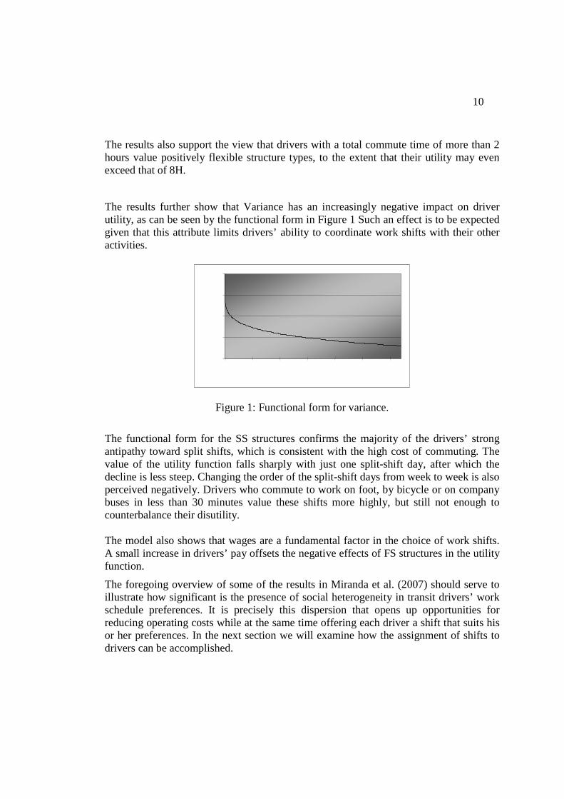
The results further show that Variance has an increasingly negative impact on driver utility, as can be seen by the functional form in Figure 1 Such an effect is to be expected given that this attribute limits drivers’ ability to coordinate work shifts with their other activities.

Figure 1: Functional form for variance.

The functional form for the SS structures confirms the majority of the drivers’ strong antipathy toward split shifts, which is consistent with the high cost of commuting. The value of the utility function falls sharply with just one split-shift day, after which the decline is less steep. Changing the order of the split-shift days from week to week is also perceived negatively. Drivers who commute to work on foot, by bicycle or on company buses in less than 30 minutes value these shifts more highly, but still not enough to counterbalance their disutility. The model also shows that wages are a fundamental factor in the choice of work shifts. A small increase in drivers’ pay offsets the negative effects of FS structures in the utility function.

The foregoing overview of some of the results in Miranda et al. (2007) should serve to illustrate how significant is the presence of social heterogeneity in transit drivers’ work schedule preferences. It is precisely this dispersion that opens up opportunities for reducing operating costs while at the same time offering each driver a shift that suits his or her preferences. In the next section we will examine how the assignment of shifts to drivers can be accomplished.

11

3. IDENTIFYING FLEXIBLE WORK SHIFT ASSIGNMENT

MECHANISMS

Ascertaining driver preferences as was done in the previous section is the first step in implementing less rigid work schedules that allow drivers to move from standard shifts to more flexible ones adapted to their preferences. The diversity of preferences, as shown by Miranda et al. (2007), complicates the shift assignment task, however. Although the authors provide some guidelines on which types of driver are likely to prefer a given shift alternative, they confine themselves to presenting expected utilities per worker which display considerable dispersion of real preferences. Thus, although the model predicts that on average, drivers of type i will prefer shift j to shift k, a significant proportion of them (up to 50%) may feel otherwise. It is therefore worthwhile to study the suitability of the various shift assignment mechanisms for public transit drivers. For example, we might want to compare a centralized system that simply assigns shifts unilaterally with one that allows drivers to choose their shift sequentially from among a list of alternatives. To make such comparisons we must be able to detect for each one of them which drivers are made better off, which are worse off, and how reliable are these welfare estimates. In addition, for each assignment it is quite possible that a certain proportion of drivers end up dissatisfied in comparison with their original schedule (previous to the assignment of flexible shifts) if no compensation is paid. For this reason, to ensure the implementation of the flexible shift plan is viable with the existing drivers, the cost to the operator of absorbing this dissatisfaction must be less than the benefits it receives. Since the company may be required to pay the same level of compensation to all workers on a given shift, the effort to assure viability must take this factor into account. We next analyze a number of assignment mechanisms and apply them to a sample of public transit drivers taken from the same driver set used in Miranda et al. (2007).

3.1 Centralized shift assignment mechanisms

In this subsection we describe some centralized shift assignment mechanisms and identify the impacts of their implementation on the transit operator and the drivers. By centralized assignment mechanism we mean one in which the operator assigns a shift to each driver without the latter’s active participation in the process. The objectives of the mechanisms are to assign the shifts that are best adapted to each driver’s personal preferences (assuming their utility functions are known) and to ensure the associated costs of such assignments (if any) are as low as possible. Recall that the random utility function estimated for each driver has a stochastic term in respect of which the operator only knows its functional form. It is therefore convenient to study two families of assignment mechanisms, the first one based exclusively on the

12

deterministic component (qiV ) and the second one taking into account the complete

individual utility function (thus basing the assignment on utilities qiU which include the

error term qiε ). Clearly, the random case is difficult to implement unless each driver

manifests his or her preferences in such a way that the complete utility function can be captured. Some progress towards this end may be possible if the drivers themselves order the various shifts in accordance with their preferences. In any event, knowing the optimum stochastic assignment provides a point of comparison for judging more realistic assignment mechanisms.

In the descriptions of the assignment mechanisms that follow, we assume that there are N drivers and N shifts. The shifts are classified into T types, with nj shifts of type j

( NnT

jj =∑

=1

). The base situation is defined as that in which all drivers work standard

shifts with the same daily number of hours. In each case we also assume that the utility perceived by each driver for each type of shift is known, whether it be observable (deterministic) or complete (stochastic).

3.1.1 Maximization of the sum of individual utilities for assigned shifts

An initial attempt at shift assignment might consist of assigning a shift to each driver so as to maximize global driver welfare. In the absence of compensation such an assignment may require that some individual drivers are made worse off in the interests of the global result. Assuming that the utility function is the best welfare indicator, the variable to be maximized would be the sum of the individual utilities. This assignment is easily obtained once these individual utilities for each shift have been calculated by solving the following standard assignment problem:

},..,1{},,..,1{ {0,1}

},..,1{

},..,1{ 1

..

1

1

1 1

TjNix

Tjnx

Nix

ts

xuMax

ij

j

N

iij

T

jij

N

i

T

jijij

∈∀∈∀∈

∈∀=

∈∀=

∑

∑

∑∑

=

=

= =

where uij is the utility of shift j for driver i and

13

= otherwise 0

shift type assigned is driver if 1 jixij

The solution to this problem will give the shift assignments for all drivers, and therefore also the associated utility levels as perceived by the shift assigner. We can then determine which drivers would be unhappy under the new assignment by simply comparing these levels to those perceived under a standard shift (i.e., type s) and pinpointing the drivers whose utility had declined ( ijis uu > ).

The viability of implementing flexible shifts would be enhanced if it were possible to identify shift assignments for which the situations of both the drivers and the operator improved (or at least did not worsen) in comparison to the base situation. It is therefore of interest to identify what compensation would have to be paid to any dissatisfied drivers to restore their utility level to that of a standard shift. If we assume that under our assignment mechanism such compensation is provided strictly in the form of a wage increase, we can then determine the required amount from the solution to the foregoing assignment problem in combination with the wage multipliers defined in the utility functions. More specifically, the amount pij necessary to compensate individual i assigned shift j for whom ( ijis uu − ) is greater than zero is defined as this difference

divided by the corresponding wage multiplier θij. In formal terms,

ijisij

ijisij uu

uup >

−= if

θ

Adding this compensation to the wages of driver i on shift j will ensure that all individual drivers are at least as well off as they were initially. Note, too, that this analysis is valid for both the deterministic and the random cases. The difference between the savings to the employer due to the reduction in workers for a given level of operations and the compensation paid to the formerly worse-off drivers can be interpreted as the net social benefit of using flexible shift structures subject to the constraint that no one is made worse off. Since this net social benefit is the difference between savings in wages and worker compensation payments, one way of determining what incentives could be offered to the operators to implement this shift plan would be to find shift assignments that minimize those compensations. This is the objective of the next assignment mechanism we will study.

14

3.1.2 Minimization of compensation payments with discrimination

This second assignment mechanism seeks to minimize compensation payments by operators while ensuring workers remain at least as well off as they were under the standard shift. We begin by calculating the compensation to be paid to each worker if shifts are assigned as in the preceding analysis (note that these payments are all non-negative). The objective function for the assignment mechanism thus becomes

∑∑= =

N

i

T

jijij xpMin

1 1

Note, however, that this mechanism discriminates among workers assigned to the same shift. In other words, the wage level may vary from driver to driver working identical shift structures to the extent their personal utility derived from that shift differs. Indeed, some drivers on a given shift may receive compensation while others on the same shift do not. This may be an obstacle to the implementation of the mechanism in some companies, and may also affect the revelation of driver preferences. It would be advisable, therefore, to also examine non-discriminatory mechanisms that make the same payments to all workers assigned to a given shift. The next mechanism taken up here does just that.

3.1.3 Minimization of compensation payments without discrimination

The assignment mechanism we consider now is similar to the previous one, but requires that any wage increases be the same for all individuals working a given shift structure. This may lead to situations in which certain drivers receive compensation payments regardless of whether their perceived utilities under the new structure are greater than under the standard one. The problem may be expressed formally as follows:

},..,1{},,..,1{ {0,1}

},..,1{ 0y

},..,1{},,..,1{ y

},..,1{

},..,1{ 1

..

1

1

1

TjNix

Tj

TjNixp

Tjnx

Nix

ts

nyMin

ij

j

ijijj

j

N

iij

T

jij

T

jjj

∈∀∈∀∈

∈∀≥

∈∀∈∀≥

∈∀=

∈∀=

∑

∑

∑

=

=

=

15

This model incorporates a new variable denoted yj representing the compensation paid to workers on shift j. The objective function now consists in minimizing total compensation subject to the constraint that the compensation payments to workers of type j be greater than or equal to the individual payments for all workers on that shift. Needless to say, this method will be as least as costly to the operator as the previous one.

3.2 Application of assignment mechanisms to a bus operator

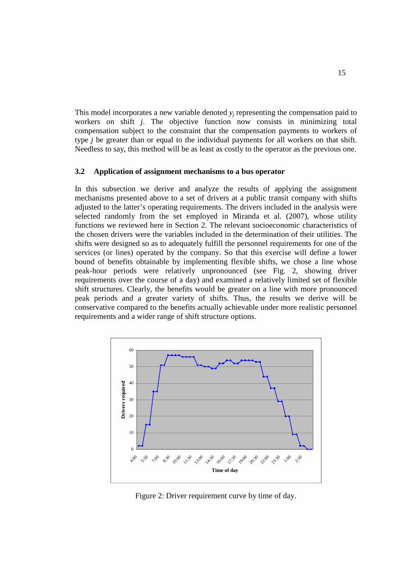
In this subsection we derive and analyze the results of applying the assignment mechanisms presented above to a set of drivers at a public transit company with shifts adjusted to the latter’s operating requirements. The drivers included in the analysis were selected randomly from the set employed in Miranda et al. (2007), whose utility functions we reviewed here in Section 2. The relevant socioeconomic characteristics of the chosen drivers were the variables included in the determination of their utilities. The shifts were designed so as to adequately fulfill the personnel requirements for one of the services (or lines) operated by the company. So that this exercise will define a lower bound of benefits obtainable by implementing flexible shifts, we chose a line whose peak-hour periods were relatively unpronounced (see Fig. 2, showing driver requirements over the course of a day) and examined a relatively limited set of flexible shift structures. Clearly, the benefits would be greater on a line with more pronounced peak periods and a greater variety of shifts. Thus, the results we derive will be conservative compared to the benefits actually achievable under more realistic personnel requirements and a wider range of shift structure options.

0

10

20

30

40

50

60

4:00

5:30

7:00

8:30

10:00

11:30

13:00

14:3

016

:00

17:30

19:00

20:3

022

:00

23:30

1:00

2:30

Time of day

Dri

vers

req

uire

d

Figure 2: Driver requirement curve by time of day.

16

The shift structures used in the application were all based on a 45-hour week divided into six working days. The standard structure was defined as a 7½-hour shift on each working day, and just two types of flexible structures were considered, both chosen for their practical viability and close fit to the operator’s personnel requirements. They are as follows: Shift Structure 1: Six working days per week, three with 10-hour shifts and the other three with 5-hour shifts. Shift Structure 2: Six working days per week, two with 10-hour shifts, three with 7-hour shifts and one with a 4-hour shift. The standard structure alternative will be denoted Shift Structure 3. Following Muñoz (2002) we use a mathematical programming model to determine the minimum number of drivers that would cover operating requirements, first using only the standard structure and then using the flexible ones. In the former case the number of drivers required was 150, while for the latter, only 135 were needed (see Table 4). In other words, the company would save 10% on labor costs (i.e., 15 wage equivalents) if it opted for flexible shifts and the drivers accepted them without additional compensation.8 In addition to this reference point we also calculated the minimum number of workers that would be required if flexibility were total and the operator could hire workers on an hourly basis. In such a case only 130 drivers would be needed, a figure that can be taken as the upper bound for potential savings from shift flexibility. Also, we note that the rather modest 10% figure just cited may be explained by the relatively unpronounced variability in daily requirements of the line chosen for study. Muñoz (2002) reported savings of more than 25% for the Oakland, California public transit system where a similar analysis was conducted.

8 This is the strict measurement of social welfare that would guide decisions in a purely economic evaluation of a project. Our approximation using a non-discriminatory assignment mechanism is more restrictive in that the project’s viability depends on no worker being made worse off.

17

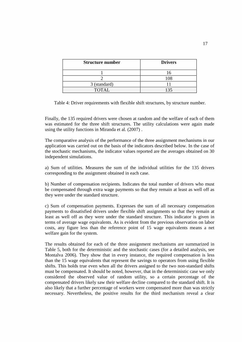
Structure number Drivers

1 16 2 108

3 (standard) 11 TOTAL 135

Table 4: Driver requirements with flexible shift structures, by structure number.

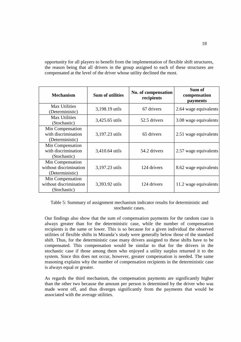
Finally, the 135 required drivers were chosen at random and the welfare of each of them was estimated for the three shift structures. The utility calculations were again made using the utility functions in Miranda et al. (2007) . The comparative analysis of the performance of the three assignment mechanisms in our application was carried out on the basis of the indicators described below. In the case of the stochastic mechanisms, the indicator values reported are the averages obtained on 30 independent simulations. a) Sum of utilities. Measures the sum of the individual utilities for the 135 drivers corresponding to the assignment obtained in each case. b) Number of compensation recipients. Indicates the total number of drivers who must be compensated through extra wage payments so that they remain at least as well off as they were under the standard structure. c) Sum of compensation payments. Expresses the sum of all necessary compensation payments to dissatisfied drivers under flexible shift assignments so that they remain at least as well off as they were under the standard structure. This indicator is given in terms of average wage equivalents. As is evident from the previous observation on labor costs, any figure less than the reference point of 15 wage equivalents means a net welfare gain for the system. The results obtained for each of the three assignment mechanisms are summarized in Table 5, both for the deterministic and the stochastic cases (for a detailed analysis, see Montalva 2006). They show that in every instance, the required compensation is less than the 15 wage equivalents that represent the savings to operators from using flexible shifts. This holds true even when all the drivers assigned to the two non-standard shifts must be compensated. It should be noted, however, that in the deterministic case we only considered the observed value of random utility, so a certain percentage of the compensated drivers likely saw their welfare decline compared to the standard shift. It is also likely that a further percentage of workers were compensated more than was strictly necessary. Nevertheless, the positive results for the third mechanism reveal a clear

18

opportunity for all players to benefit from the implementation of flexible shift structures, the reason being that all drivers in the group assigned to each of these structures are compensated at the level of the driver whose utility declined the most.

Mechanism Sum of utilities No. of compensation

recipients

Sum of compensation

payments Max Utilities

(Deterministic) 3,198.19 utils 67 drivers 2.64 wage equivalents

Max Utilities (Stochastic)

3,425.65 utils 52.5 drivers 3.08 wage equivalents

Min Compensation with discrimination

(Deterministic) 3,197.23 utils 65 drivers 2.51 wage equivalents

Min Compensation with discrimination

(Stochastic) 3,410.64 utils 54.2 drivers 2.57 wage equivalents

Min Compensation without discrimination

(Deterministic) 3,197.23 utils 124 drivers 8.62 wage equivalents

Min Compensation without discrimination

(Stochastic) 3,393.92 utils 124 drivers 11.2 wage equivalents

Table 5: Summary of assignment mechanism indicator results for deterministic and stochastic cases.

Our findings also show that the sum of compensation payments for the random case is always greater than for the deterministic case, while the number of compensation recipients is the same or lower. This is so because for a given individual the observed utilities of flexible shifts in Miranda’s study were generally below those of the standard shift. Thus, for the deterministic case many drivers assigned to these shifts have to be compensated. This compensation would be similar to that for the drivers in the stochastic case if those among them who enjoyed a utility surplus returned it to the system. Since this does not occur, however, greater compensation is needed. The same reasoning explains why the number of compensation recipients in the deterministic case is always equal or greater. As regards the third mechanism, the compensation payments are significantly higher than the other two because the amount per person is determined by the driver who was made worst off, and thus diverges significantly from the payments that would be associated with the average utilities.

19

All mechanisms so far analyzed exclude driver participation in the assignment process. In the next subsection, new mechanisms are presented in which this constraint is relaxed.

3.3 Participatory shift assignment mechanisms

Assigning shifts to workers without consulting them may undermine confidence in their viability given that the shift assigner is required to make assumptions regarding the values of the random term in the utility function whose variance is significant. In what follows, we address this problem by considering assignment mechanisms in which workers choose their own shift structures to ensure the process takes into account their true preferences. Each of these mechanisms defines the order in which drivers choose their shift according to various criteria, simulating the utilities they perceive for each available structure. As the drivers make their choices one by one according to this defined selection priority order, the remaining alternatives to drivers yet to choose are fewer and fewer; by the time the last driver in the ordering is reached, there is only one alternative left. This being the case, we will also analyze the advantages and disadvantages of different ways of ordering and identify ones that give better collective results than others. The four criteria adopted for placing the drivers in descending order of selection priority are the following: i) MAX: the maximum utility perceived for any shift. ii) MAX-MIN: the utility difference between the shift producing the greatest satisfaction for a driver and the one producing the greatest dissatisfaction. iii) MAX2: the utility difference between the shift producing the greatest satisfaction for a driver and the one producing the second highest satisfaction. iv) SENIORITY: priority by driver’s years of service at the company. The SENIORITY criteria is widely used among public transit operators, but poses a particular problem in that it assigns the most experienced drivers to the easiest shifts. To analyze the virtues of each of these criteria we conducted thirty simulations using the same 135 drivers and the same shift structures as those in the previous experiment. The driver ordering on each criteria was arrived at as a function of the utilities observed by

the shift assigner (that is, the deterministic element ijV), but the process simulated the

drivers choosing by comparing the various shifts in terms of their complete utilities ijU

.

20

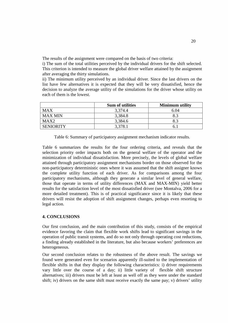
The results of the assignment were compared on the basis of two criteria: i) The sum of the total utilities perceived by the individual drivers for the shift selected. This criterion is intended to measure the global driver welfare attained by the assignment after averaging the thirty simulations. ii) The minimum utility perceived by an individual driver. Since the last drivers on the list have few alternatives it is expected that they will be very dissatisfied, hence the decision to analyze the average utility of the simulations for the driver whose utility on each of them is the lowest. Sum of utilities Minimum utility MAX 3,374.4 6.04 MAX MIN 3,384.8 8.3 MAX2 3,384.6 8.3 SENIORITY 3,378.1 6.1

Table 6: Summary of participatory assignment mechanism indicator results. Table 6 summarizes the results for the four ordering criteria, and reveals that the selection priority order impacts both on the general welfare of the operator and the minimization of individual dissatisfaction. More precisely, the levels of global welfare attained through participatory assignment mechanisms border on those observed for the non-participatory deterministic ones where it was assumed that the shift assigner knows the complete utility function of each driver. As for comparisons among the four participatory mechanisms, although they generate a similar level of general welfare, those that operate in terms of utility differences (MAX and MAX-MIN) yield better results for the satisfaction level of the most dissatisfied driver (see Montalva, 2006 for a more detailed treatment). This is of practical significance since it is likely that these drivers will resist the adoption of shift assignment changes, perhaps even resorting to legal action.

4. CONCLUSIONS

Our first conclusion, and the main contribution of this study, consists of the empirical evidence favoring the claim that flexible work shifts lead to significant savings in the operation of public transit systems, and do so not only through operating cost reductions, a finding already established in the literature, but also because workers’ preferences are heterogeneous.

Our second conclusion relates to the robustness of the above result. The savings we found were generated even for scenarios apparently ill-suited to the implementation of flexible shifts in that they display the following characteristics: i) driver requirements vary little over the course of a day; ii) little variety of flexible shift structure alternatives; iii) drivers must be left at least as well off as they were under the standard shift; iv) drivers on the same shift must receive exactly the same pay; v) drivers’ utility

21

functions are such that they prefer homogeneous shifts over the course of a week to flexible ones. Scenarios where peak periods are relatively pronounced (as is the case in the majority of urban transit systems), and in which a larger set of flexible shift alternatives is offered, will generate significantly superior benefits to those reported here.

The robustness of our results is also founded on the fact that all of the proposed compensation methods support the hypothesis according to which there are significant opportunities for labor productivity increments, and that the benefits therefrom exceed any additional wage costs that may be involved. Once again, we note the very demanding scenario in which our experiments were conducted worked against the corroboration of this hypothesis. The preferences considered were exclusively those of drivers already working for the company, which clearly involves a bias towards current shift structures. Given the natural evolution of the work force over time, operators would have greater chances of finding drivers whose preferences coincide with structures designed to reflect the seasonality of demand. In this sense our results indicate a lower bound of welfare gain for a company that adopts a flexible shift system.

The analyses and results of this study are particularly relevant today given that public transit systems in many cities around the world are facing severe pressures to achieve financial sustainability, while other cities are struggling to justify certain transit services because of their questionable social returns. The employment strategy here presented provides a way of lowering transit operating costs and thereby reduce the need for public funding, cut fares and generate social and/or private returns for projects where such benefits are currently insufficient.

But these findings are not limited to the realm of public transit, and in fact can be extended to any other activity where companies experience marked hourly and daily seasonalities in their need for certain types of labor such as call-centers telephone operators, supermarket cashiers, etc. This is supported in a study by Chávez (2005) of the stated shift preferences of retail workers, which generated even better results than those found by Miranda et al. (2007) in that, unlike the reaction of public transit drivers, these workers greeted flexible shifts more enthusiastically than the standard ones.

In the past, assigning work shifts to employees was a drawn-out and difficult task whose results were far from optimal. In such conditions businesses found it reasonable to choose the simple route by defining shifts that were as similar as possible for each worker. However, today’s computer systems makes it possible to accomplish such complex assignment tasks within realistic time frames. Hundreds of workers can be assigned to meet labor requirements that vary over the course of a day or a week using a variety of shift structures to minimize total labor costs. As we have demonstrated, there exist ample opportunities for companies to reap significant savings through flexible work schedules that will be well-received by their employees, making the adoption of such systems merely a matter of time.

22

ACKNOWLEDGEMENTS

We would like to thank the National Fund for the Development of Scientific and Technological Research (FONDECYT Project 1040604 and Anillos Tecnológicos ACT-32) for the valuable contribution to financing this study.

5. BIBLIOGRAPHY

BEDI, S. A. (1998) Sector Choice, Multiple Job Holding and Wage Differentials: Evidence from Poland. The Journal of Development Studies, Vol. 35, no. 1, 162-179.

CHAVEZ, P. (2005). Preferencias reveladas de trabajadores de multitiendas por

estructuras de horarios de trabajo. Memoria de Título. Escuela de Ingeniería, Universidad Católica de Chile.

MIRANDA, F.A., MUÑOZ, J.C. y ORTUZAR, J. de D (2007). Identifying Driver

Preferences for Work Shift Structures. Accepted for publication in Transportation Science.

MONTALVA, S. (2006). Asignación de turnos de trabajo a conductores de transporte

público, basadas en sus preferencias declaradas. Master Thesis. Universidad Católica de Chile.

MUÑOZ, J.C. (2002) Crew-Shift Design for Transportation Systems with Uncertain

Demand. Ph.D. Thesis, Institute of Transportation Studies, University of California at Berkeley.

ORTUZAR, J. DE D. y GARRIDO, R.A. (1994) A practical assessment of stated

preference methods. Transportation 21, 289-305. ORTUZAR, J. DE D., IVELIC, A.M., y CANDIA, A. (1997) User perception of public

transport level of service. In P. Stopher, and M. Lee-Gosselin (eds.), Understanding Travel Behaviour in an Era of Change. Elsevier, Oxford.

ORTUZAR, J. DE D. y WILLUMSEN, L.G. (2001) Modelling Transport. Third

Edition, John Wiley and Sons, Chichester.

ROSEN, S. (1974) Hedonic prices and implicit markets. Journal of Political Economy, 82: 34-55.

SMITH, E. C. (1974) Compensating wage differentials and public policy: A Review.

Industrial and Labor Relations Review.

23

HAMEMERSH, D. (1977) Economic Aspects of Job Satisfaction. In O. Ashenfelter y

W. Oates eds., Essays in Labor Market and Population Analysis. Princeton.