are mutual fund investors in jail?
TRANSCRIPT

F E P W O R K I N G P A P E R SF E P W O R K I N G P A P E R S
Are mutualAre mutual fund investors in fund investors in jailjail??
Carlos F. Alves*
Victor Mendes
*CEMPRE - Centro de Estudos Macroeconómicos e Previsão
Research – Work in Progress – n. 203, February 2006
Rua Dr. Roberto Frias, 4200-464 Porto | Tel. 225 571 100Faculdade de Economia da Universidade do Porto
Tel. 225571100 | www.fep.up.pt
1
ARE MUTUAL FUND INVESTORS IN JAIL?
Carlos Alves CEMPRE•, Faculty of Economics, University of Porto
Rua Dr. Roberto Frias 4200-464 Porto
Portugal Telephone: +351 225 571 100
Fax: +351 225 505 050 Email: [email protected]
Victor Mendes CMVM - Portuguese Securities Commission
Avenida da Liberdade, 252 1056-801 Lisboa
Portugal Telephone: +351 213177000
Fax: +351 213537077/8 Email: [email protected]
JEL: G20, G23 and G28
KEYWORDS: Mutual Fund, Performance Reaction, Load Costs, Investor Behaviour
ABSTRACT
The absence of investor reaction to the poor performance of mutual funds is a widely reported phenomenon. This paper investigates the role of load costs as an explanation for the phenomenon and concludes that back-end load fees are an obstacle to reaction. We find that investors with a high likelihood of undergoing a liquidity crisis, preferring liquidity in decision making, act contrary to the reaction hypothesis, and investors with broader investment horizons do not react to poor performances due to the fact that they are “imprisoned” by back-end load fees.
• CEMPRE is supported by CFT through POCTI of the QCAIII, which is financed by FEDER and Portuguese funds.
2
1. INTRODUCTION
In addition to the costs intrinsic to transactions concerning the sale and purchase of securities,
mutual funds are, in general, subject to four types of fees: front-end, back-end, management and
custodian. The first two are directly borne by the investor on subscribing to new mutual fund
units and when redeeming units, respectively. Management and custodian fees are borne by the
fund over time and, therefore, these are reflected in the fund’s net asset value (NAV).
The argument, used by the industry and (generally) accepted by regulatory authorities, for the
existence of load costs is that the aim of such fees is to prevent investors from investing for a
short period of time, which could cause portfolios to suffer liquidity shocks. The underlying idea
is that the frequent purchase and sale of units would require a large part of the portfolio to remain
liquid, therefore reducing the fund’s yield and passing on the resulting loss to all other unit
holders. Hence, the purpose of the purchase and redemption fees is to prevent such a scenario.
The lack of mass investor reaction to the poor performance of funds is a puzzle that has still not
been solved. The hypothesis that load costs have a significant role to play was accepted a long
time ago (Ippolito, 1992). The contingent diversity of investor profile regarding sensitivity to
liquidity shocks has also been formulated in theoretical terms (Nanda et al., 2000).
The type of response that investors provide to mutual fund performance has been the subject of
significant research. Various studies have reported the phenomenon of asymmetry: the better the
past performance of top performing funds the greater the flows attracted, whereas low
performances do not encompass the sale of fund shares (Ippolito (1992), Chevalier and Ellison
(1997), Goetzmann and Peles (1997), Sirri and Tufano (1998), Lynch and Musto (2000),
Christoffersen (2001) and Del Guercio and Tkac (2001)).
In relation to the possible causes of this behaviour asymmetry, Ippolito (1992), assuming no load
costs and persistent performance, finds that the investor will tend to choose funds with better
recent performances instead of randomly selecting a fund. Similarly, investors will tend to avoid
the worst performing funds by, on the one hand, not channelling new capital flows to these funds
and, on the other, redeeming investments previously made in the worst performing funds. The

3
load costs are, in this scenario, the (rational) explanation as to why large parts of the market are
not transferred from one fund to the other when the performances are reported. In support of this
theory, Ippolito (1992) documents that the net flows of funds that do not charge front-end and/or
bach-end fees are more sensitive to performance than the net flows of funds that charge these
kind of fees1.
Sirri and Tufano (1992), on the other hand, explain investor behaviour based on the idea that the
operating complexity of the industry leads to increased information costs. Investors therefore, in
order to avoid these costs, decide based on the information made available to them, either through
marketing instruments or through the media.
It is not easy in an extremely complex market, like the US market, to separate out the effect of
information costs from the effect of load costs. In such a complex market, exchanging one mutual
fund for another always involves, besides the load costs resulting from the outflow from the
losing fund to the inflow in the winning fund, costs associated to the search for and processing of
information that allows the characteristics and performances of the many funds to be classified.
In a smaller-sized market, such as the Portuguese one, information costs are lower, and they can
be deemed irrelevant2. However, there are relevant front-end fees and, in particular, significant
back-end costs that may similarly function as an obstacle to the mass movement of capitals
between different funds.
The purpose of this study is to assess whether back-end fees serve as an obstacle to disinvestment
from poorly performing funds. Acknowledging the existence of two types of investors (as
assumed by Nanda et al., 2000), this study seeks to investigate whether investors with a high
likelihood of undergoing liquidity crises, preferring liquidity in decision making, are or are not
influenced to act in a manner contrary to the performance reaction hypothesis. If liquidity is the
determining factor in selection, investors will tend to prefer funds with lower back-end fees for
short investment horizons, subscribing much more to funds of this type, even if they record worse
1 Sirri and Tufano (1998) also concluded that funds with larger fees tend to have more sluggish growth than funds with lower fees. 2 Despite the fact that Portugal has had mutual funds since 1986, as of March 2001 there were only 261 mutual funds, managing a total NAV of 21,390 million euros. These mutual funds were managed by a total of 19 management companies. The Portuguese market is, therefore, substantially less complex than the US market, and the respective information costs are, consequently, considerably lower.

4
performances than funds with higher back-end fees. The other hypothesis under analysis concerns
the possibility that investors with longer investment horizons (i.e. less exposed to liquidity
shocks) do not react to poor performances given that they find themselves “imprisoned” by back-
end fees. The notion is that the high back-end fees for broad investment horizons, associated to
poor performance, are a dissuasive factor to the mobilisation of capital flows from poorly
performing funds to winning funds.
The importance of performing this study for a small market (such as the Portuguese one) is raised
by the fact that the absence of reaction to poor performances is a reality in these types of markets
(Alves and Mendes, 2006). Another reason to study the Portuguese case is based on the fact that
the information available to the public is unlike that of any other market, given that not only is
the value of the portfolios managed by the funds and their composition published monthly, but
also the value of each investment unit is published daily3,4. Finally, given the lower complexity of
the Portuguese mutual fund industry, and the public availability of information, information costs
may be assumed irrelevant, and we are able to isolate the effect of load costs on fund flows.
This study analyses the relationship between back-end load costs and investor reaction relative to
equity funds investing in domestic Portuguese shares, over a period of 7 ¼ years, using
contingency table analysis. The results obtained strongly support the “entrenchment hypothesis”
associated to 12 and 24-month investment horizons. We conclude that when the cost of
disinvestment is high it acts as an obstacle to the penalisation of funds with poor performances;
when such costs are low, there occurs disinvestment from better performing funds whenever
liquidity requirements compel such. Conversely, corroboration of the liquidity hypothesis was
established regarding fees for very short term redemptions (one or three months), according to
which investors, due to the high likelihood of suffering liquidity shocks, choose funds according
to the reduced value of back-end load costs and, therefore, preferentially subscribe to funds with
lower back-end fees and worse performances.
3 As far as we know, Hungary is the only other country in the EU that publishes portfolios (and their value) each month, but not for all mutual fund categories. In the USA, for instance, there is only quarterly portfolio and demand information. 4 This information is available at the Portuguese Securities Commission website since 2002. Before 2002, daily newspapers published this information in the markets section. Thus, the cost of monitoring a portfolio of risky assets is negligible.
5
The paper includes a description of the sample and the demand variables in section 2. Section 3
contains a two- and three-dimensional analysis of the relationship between demand, performance
and redemption costs. Section 4 contains the main conclusions.
2. DATASET AND MAIN VARIABLES
(i) Sample
The sample includes all 30 Portuguese open-end mutual funds which were classified as
“domestic equity funds” by APFIN5, between 31st December 1993 and 31st March 2001, and is
therefore identical to the population.
The sample possesses characteristics that are of great bearing on the purposes of this
investigation: (i) it refers only to the equity funds of one single country6; (ii) by including all
funds we avoid survivorship bias; (iii) investments in bonds are of little significance7. These facts
contribute to increase the effectiveness of performance measurements.
The total assets (monthly average) under the management of these funds is 635.2 million euros,
with a maximum of 1805.6 million euros (April 1998) and a minimum of 90.4 million euros
(December 1995). At the end of March 2001 the total NAV was 495.8 million euros.
(ii) Mutual Fund Investment Flow Variables
The absolute capital flows (CF) and the normalized capital flows (NCF) are alternatively used to
measure the monthly investment flow of each fund.. The absolute capital flows is given by
( )ttttt RNAVINAVCF +−+= − 11 [1]
where: NAVt is the total net value of the fund’s portfolio, at date t, after the distribution of
income; It is the income distributed by the mutual fund; and Rt is the return achieved by the fund
between t-1 and t8/9.
5 APFIN is the Portuguese association of mutual fund management companies. 6 The inclusion of foreign shares would mean taking into consideration the systematic risk of other countries. The importance of local factors in the calculation of the price of the risk of each one of the return generating factors is documented by Serra (2000). 7 The mean aggregate percentage of domestic shares in the NAV managed by the samples’ funds is 82.0%. 8 We assume that the income distribution occurs on date t. Events, such as fund mergers, are handled using the follow the money approach (Gruber, 1996).

6
The normalised capital flows is given by10:
1t
tt NAV
CFNCF
−
= . [2]
The first metric favours larger funds that tend to have greater absolute cash flows disassociated
from performance, while NCF tends to amplify the results of smaller funds (Gruber, 1996).
Therefore, it is important to use both measurement methods. The exclusive use of the former
could hide the reaction of the clients of large funds, in much the same way that the exclusive use
of the latter metric could lead to the excessive prominence of the reaction of clients of smaller
funds.
(iii) Sources of Information
The daily price quotation of each fund, the dates and the sums of the distributed incomes, and the
funds monthly portfolios are from Dathis11. Market and accounting information for listed
companies is also from Dathis, from the annual publications issued by Euronext Lisbon with
yearly accounting information on listed companies, and from the daily quotation bulletins of
Euronext Lisbon. Information regarding the fees charged by each fund was obtained from the
funds’ management rules published in the quotation bulletins of Euronext Lisbon. Accounting
information relative to the management companies of the funds is from the same quotation
bulletins and from CMVM (Portuguese Securities Commission).
3. PERFORMANCE, DEMAND AND REDEMPTION FEES
Mutual funds in Portugal are, in general, subject to four types of fees, in addition to the
transaction costs associated to the sale and purchase of securities. These fees are: front-end, back-
end, management and custodian. The front-end load fee is wholly borne by the investor at the
time of subscription. The back-end load fee is payable by the investor when redeeming
investment units. The management and custodian fees are borne by the fund and, therefore,
impact on the respective NAV. Front-end and back-end load costs can both be an obstacle to
9 Purchases (net of sales) made by fund of funds of the same financial group were deducted from the total flow, thereby ensuring that only capital flows originating from clients outside of the fund complex is considered. 10 NCF is used by Ippolito (1992), Sirri and Tufano (1998) and Zheng (1999), among others. 11 Financial information disclosure service of Euronext Lisbon.

7
performance reaction, due not only to the fact that the subscription of funds with a good
performance is expensive, but also because the disinvestment from a badly performing fund is
excessively costly.
The majority of the funds in our sample did not charge front-end fees. Only about 20% of the
funds required the payment of this fee, which reached a maximum of 5% in some years. The
analysis of the relationship between front-end fees and demand12 allows one to conclude that the
funds with the highest fees are more often those that occupy the top positions in the demand
rankings. This means that investors, in general, more intensively seek out funds with higher
front-end load fees.
The following sub-sections analyse the relationship between back-end load fees, demand and
performance.
3.1 TWO-DIMENSIONAL ANALYSIS
(i) Demand vs. Back-end Load Fees
The practice of charging these fees is generalised amongst equity funds in Portugal. The fee
usually varies according to the investment period. In order to standardize the analysis, the
variables CR1M, CR3M, CR6M, CR12M, CR24M and CR60M were constructed. These
variables represent fixed back-end load fees in force for 1-month, 3-month, 6-month, one-year,
two-year and five-year investments, respectively. These variables are in Table 1, and we can
conclude that back-end load costs decrease as the timeline from purchase increases.
TABLE 1 – EVOLUTION OF VARIABLES CR1M, CR3M, CR6M, CR12M, CR24M and CR60M 1994 1995 1996 1997 1998 1999 2000 1994 1995 1996 1997 1998 1999 2000
Average 2,03% 1,94% 1,96% 1,93% 1,95% 1,99% 1,92% 0,93% 0,83% 0,91% 0,77% 0,88% 0,91% 0,86%Median 2,00% 2,00% 2,00% 2,00% 1,56% 2,00% 1,63% 1,00% 1,00% 1,00% 0,75% 1,00% 1,00% 1,00%
Maximum 5,00% 5,00% 5,00% 5,00% 5,00% 5,00% 4,00% 2,00% 2,00% 3,00% 3,00% 3,00% 3,00% 3,00%Minimum 1,00% 1,00% 1,00% 1,00% 1,00% 0,63% 1,00% 0,00% 0,00% 0,00% 0,00% 0,00% 0,00% 0,00%
Average 1,60% 1,58% 1,62% 1,57% 1,60% 1,63% 1,63% 0,78% 0,67% 0,72% 0,64% 0,57% 0,52% 0,52%Median 2,00% 1,75% 1,50% 1,50% 1,50% 1,50% 1,50% 0,25% 0,13% 0,25% 0,00% 0,25% 0,25% 0,25%
Maximum 2,50% 2,50% 3,00% 3,00% 3,00% 3,00% 3,00% 2,00% 2,00% 3,00% 3,00% 3,00% 3,00% 3,00%Minimum 0,00% 0,00% 0,00% 0,00% 0,38% 0,63% 1,00% 0,00% 0,00% 0,00% 0,00% 0,00% 0,00% 0,00%
Average 1,33% 1,26% 1,32% 1,30% 1,41% 1,44% 1,36% 0,75% 0,63% 0,68% 0,57% 0,37% 0,28% 0,30%Median 1,50% 1,00% 1,00% 1,00% 1,50% 1,50% 1,00% 0,00% 0,00% 0,00% 0,00% 0,00% 0,00% 0,00%
Maximum 2,50% 2,50% 3,00% 3,00% 3,00% 3,00% 3,00% 2,00% 2,00% 3,00% 3,00% 3,00% 3,00% 3,00%Minimum 0,00% 0,00% 0,00% 0,00% 0,38% 0,50% 0,50% 0,00% 0,00% 0,00% 0,00% 0,00% 0,00% 0,00%
CR1M
CR3M
CR6M
CR12M
CR24M
CR60M
Obs.: CR1M, CR3M, CR6M, CR12M, CR24M and CR60M are, respectively, the redemption fees applicable for investments with the duration of 1 month, 3 months, 6 months, 1 year, 2 years and 5 years. 12 Not reported in order to save space. The analysis was performed for quarterly, half-yearly and annual flows.
8
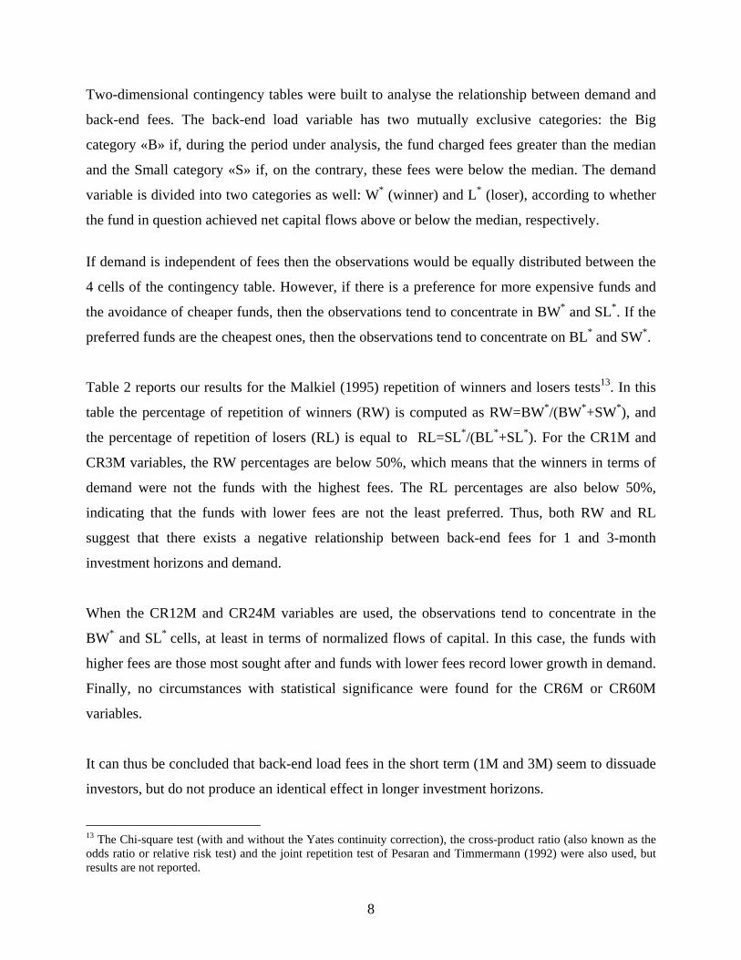
Two-dimensional contingency tables were built to analyse the relationship between demand and
back-end fees. The back-end load variable has two mutually exclusive categories: the Big
category «B» if, during the period under analysis, the fund charged fees greater than the median
and the Small category «S» if, on the contrary, these fees were below the median. The demand
variable is divided into two categories as well: W* (winner) and L* (loser), according to whether
the fund in question achieved net capital flows above or below the median, respectively.
If demand is independent of fees then the observations would be equally distributed between the
4 cells of the contingency table. However, if there is a preference for more expensive funds and
the avoidance of cheaper funds, then the observations tend to concentrate in BW* and SL*. If the
preferred funds are the cheapest ones, then the observations tend to concentrate on BL* and SW*.
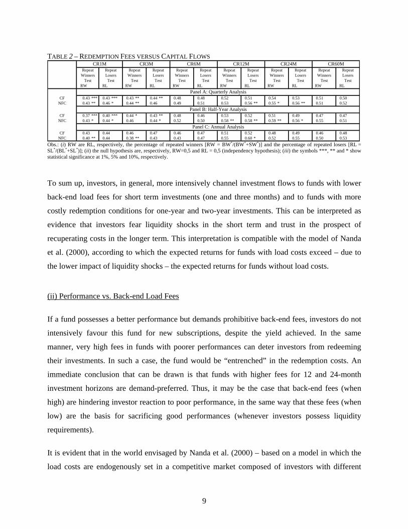
Table 2 reports our results for the Malkiel (1995) repetition of winners and losers tests13. In this
table the percentage of repetition of winners (RW) is computed as RW=BW*/(BW*+SW*), and
the percentage of repetition of losers (RL) is equal to RL=SL*/(BL*+SL*). For the CR1M and
CR3M variables, the RW percentages are below 50%, which means that the winners in terms of
demand were not the funds with the highest fees. The RL percentages are also below 50%,
indicating that the funds with lower fees are not the least preferred. Thus, both RW and RL
suggest that there exists a negative relationship between back-end fees for 1 and 3-month
investment horizons and demand.
When the CR12M and CR24M variables are used, the observations tend to concentrate in the
BW* and SL* cells, at least in terms of normalized flows of capital. In this case, the funds with
higher fees are those most sought after and funds with lower fees record lower growth in demand.
Finally, no circumstances with statistical significance were found for the CR6M or CR60M
variables.
It can thus be concluded that back-end load fees in the short term (1M and 3M) seem to dissuade
investors, but do not produce an identical effect in longer investment horizons.
13 The Chi-square test (with and without the Yates continuity correction), the cross-product ratio (also known as the odds ratio or relative risk test) and the joint repetition test of Pesaran and Timmermann (1992) were also used, but results are not reported.
9
TABLE 2 – REDEMPTION FEES VERSUS CAPITAL FLOWS
RW RL RW RL RW RL RW RL RW RL RW RL
0.43 *** 0.43 *** 0.43 ** 0.44 ** 0.48 0.48 0.52 0.51 0.54 0.53 0.51 0.500.43 ** 0.46 * 0.44 ** 0.46 0.49 0.51 0.53 0.56 ** 0.55 * 0.56 ** 0.51 0.52
0.37 *** 0.40 *** 0.44 * 0.43 ** 0.48 0.46 0.53 0.52 0.51 0.49 0.47 0.470.43 * 0.44 * 0.46 0.44 * 0.52 0.50 0.58 ** 0.58 ** 0.59 ** 0.56 * 0.55 0.51
0.43 0.44 0.46 0.47 0.46 0.47 0.51 0.52 0.48 0.49 0.46 0.480.40 ** 0.44 0.38 ** 0.43 0.43 0.47 0.55 0.60 * 0.52 0.55 0.50 0.53
Test Test TestLosers Losers LosersTest Test
NFC
Test Test
CFPanel A: Quarterly Analysis
Test Test Test
CR1MRepeat Repeat
TestTest
NFC
NFCCF
CF
CR6MRepeat Repeat
CR3MRepeat Repeat
CR24MRepeat Repeat
CR12MRepeat Repeat
CR60MRepeat Repeat
Winners
Panel B: Half-Year Analysis
Panel C: Annual Analysis
Winners Winners Winners Winners WinnersLosers LosersLosers
Obs.: (i) RW are RL, respectively, the percentage of repeated winners [RW = BW*/(BW*+SW*)] and the percentage of repeated losers [RL = SL*/(BL*+SL*)]; (ii) the null hypothesis are, respectively, RW=0,5 and RL = 0,5 (independency hypothesis); (iii) the symbols ***, ** and * show statistical significance at 1%, 5% and 10%, respectively.
To sum up, investors, in general, more intensively channel investment flows to funds with lower
back-end load fees for short term investments (one and three months) and to funds with more
costly redemption conditions for one-year and two-year investments. This can be interpreted as
evidence that investors fear liquidity shocks in the short term and trust in the prospect of
recuperating costs in the longer term. This interpretation is compatible with the model of Nanda
et al. (2000), according to which the expected returns for funds with load costs exceed – due to
the lower impact of liquidity shocks – the expected returns for funds without load costs.
(ii) Performance vs. Back-end Load Fees
If a fund possesses a better performance but demands prohibitive back-end fees, investors do not
intensively favour this fund for new subscriptions, despite the yield achieved. In the same
manner, very high fees in funds with poorer performances can deter investors from redeeming
their investments. In such a case, the fund would be “entrenched” in the redemption costs. An
immediate conclusion that can be drawn is that funds with higher fees for 12 and 24-month
investment horizons are demand-preferred. Thus, it may be the case that back-end fees (when
high) are hindering investor reaction to poor performance, in the same way that these fees (when
low) are the basis for sacrificing good performances (whenever investors possess liquidity
requirements).
It is evident that in the world envisaged by Nanda et al. (2000) – based on a model in which the
load costs are endogenously set in a competitive market composed of investors with different
10
liquidity requirements – the “entrenchment” hypothesis would not be pertinent, considering that
the funds with higher back-end fees would be those providing greater return. In this model,
investors exposed to liquidity shocks prefer funds without back-end fees whereas investors with
longer investment horizons prefer funds with load costs considering that they offer (expected)
higher returns14. Nevertheless, such a world does not only lack empirical foundation, particularly
in relation to the ex-post existence of a positive relationship between returns and back-end fees,
but it also behaves as a temporal space of adjustment in which investors find themselves
“entrenched”. To all intents and purposes, a minimum period of time is necessary so that the
greater performance of funds not subject to liquidity shocks – if these exist – can compensate the
higher back-end fee15.
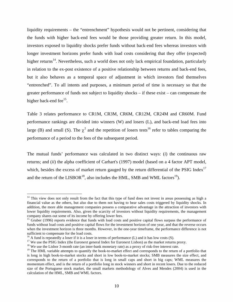
Table 3 relates performance to CR1M, CR3M, CR6M, CR12M, CR24M and CR60M. Fund
performance rankings are divided into winners (W) and losers (L), and back-end load fees into
large (B) and small (S). The χ2 and the repetition of losers tests16 refer to tables comparing the
performance of a period to the fees of the subsequent period.
The mutual funds’ performance was calculated in two distinct ways: (i) the continuous raw
returns; and (ii) the alpha coefficient of Carhart's (1997) model (based on a 4 factor APT model,
which, besides the excess of market return gauged by the return differential of the PSIG Index17
and the return of the LISBOR18, also includes the HML, SMB and WML factors19).
14 This view does not only result from the fact that this type of fund does not invest in areas possessing as high a financial value as the others, but also due to them not having to bear sales costs triggered by liquidity shocks. In addition, the more able management companies possess a comparative advantage in the attraction of investors with lower liquidity requirements. Also, given the scarcity of investors without liquidity requirements, the management company shares out some of its income by offering lower fees. 15 Gruber (1996) reports evidence that funds with load costs and positive capital flows surpass the performance of funds without load costs and positive capital flows for the investment horizon of one year, and that the reverse occurs when the investment horizon is three months. However, in the one-year timeframe, the performance difference is not sufficient to compensate for the load costs. 16 A fund is repeatedly a loser if it is a loser in terms of performance (L) and it has low costs (S). 17 We use the PSIG Index (the Euronext general Index for Euronext Lisbon) as the market returns proxy. 18 We use the Lisbor 3-month rate (an inter-bank monetary rate) as a proxy of risk-free interest rate. 19 The HML variable attempts to quantify the book-to-market effect and corresponds to the return of a portfolio that is long in high book-to-market stocks and short in low book-to-market stocks; SMB measures the size effect, and corresponds to the return of a portfolio that is long in small caps and short in big caps; WML measures the momentum effect, and is the return of a portfolio long in stock winners and short in recent losers. Due to the reduced size of the Portuguese stock market, the small markets methodology of Alves and Mendes (2004) is used in the calculation of the HML, SMB and WML factors.
11
TABLE 3 – PERFORMANCE VERSUS REDEMPTION FEES
PerformanceMeasure χ2 RL χ2 RL χ2 RL
Raw Returns 14.80 *** 0.59 *** 12.79 *** 0.57 ** 0.31 0.50Carhart Alpha 4.56 ** 0.59 *** 4.14 ** 0.57 ** 0.52 0.50
Raw Returns 1.38 0.46 * 0.15 0.53 0.16 0.68 ***Carhart Alpha 0.50 0.46 * 0.14 0.53 0.05 0.68 ***
Raw Returns 2.66 * 0.70 *** 12.58 *** 0.62 *** 0.00 0.54Carhart Alpha 12.18 *** 0.70 *** 7.84 *** 0.62 *** 0.26 0.54
Raw Returns 0.05 0.48 0.55 0.52 0.52 0.65 ***Carhart Alpha 1.05 0.48 1.04 0.52 0.29 0.65 ***
Raw Returns 1.71 * 0.51 1.99 * 0.54 0.09 0.53Carhart Alpha 1.21 0.51 0.21 0.54 0.08 0.53
Raw Returns 0.17 0.46 1.28 0.47 0.01 0.63 **Carhart Alpha 0.02 0.46 2.85 ** 0.47 0.21 0.63 **
CR60MCR12M
Losers Test
CR1M CR3M CR6MPanel A: Quarterly Analysis
CR1M CR3M CR6M
CR12M CR24M CR60M
Panel C: Annual Analysis
CR24M CR60M
CR1M CR3M CR6M
CR12M
Repeat Test of Χ2Test of Χ2
Panel B: Half-Year Analysis
Repeat Test of Χ2 RepeatLosers Test Losers Test
CR24M
Obs: (i) χ2 is the χ2 statistic; (ii) RL is the percentage of repeated losers [RL = SL/(BL+SL)]; (iii) the symbols ***, ** and * show statistical significance at 1%, 5% and 10%, respectively.
There exists (for all quarterly, half-yearly and annual analysis) a positive relationship between
performance and back-end fees for investments made more than two and less than five years
previously (CR60M). Similarly, there is a positive relationship for short investment periods
(CR1M and CR3M).
The results obtained can be read from the perspective of either new subscriptions (inflows) or
redemptions (outflows) to performance reaction. In terms of inflows, an economic agent with
high liquidity requirements chooses, according to Nanda et al. (2000), a fund with low short-term
back-end costs. According to Table 3, if a fund is chosen as a function of CR1M or CR3M, a
poorly performing fund will probably be chosen. Subscriptions from this type of investor will be
contributing to an inverse reaction, instead of contributing to the penalisation of poorly
performing funds. On the other hand, if new subscribers are economic agents with a reduced
probability of experiencing liquidity shocks, they will select funds with higher back-end fees.
Consequently, if those investors have an investment horizon that is greater than two years but less
than five they shall choose based on CR60M, which – according to Table 3 – leads to the
selection of better performing funds. In this case, these subscriptions shall contribute to
supporting the performance reaction hypothesis.
12
In relation to outflows, Table 3 permits conclusions to be drawn that support both hypotheses.
Lets assume that an investor verifies that the fund held in its portfolio performed badly (L) and,
furthermore, that the investment in the fund was made less than three months previously. Very
probably, a fund with a reduced value (S) for CR1M and CR3M is held. In this event, the back-
end fee is not, in theory, an obstacle to the performance reaction sale. If the investment was made
more than two and less than five years previously, then, in much the same way, it is very
probable that the investor possesses an «S» fund. In this situation, back-end fees do not seem to
hinder performance reaction. However, if the timeframe is one year, the probability that the fund
held is a «B» type is greater than 50%20. The same can be said, in the annual analysis, for
investments that are more than one and less than two years old (CR24). If the circumstances refer
to a Nanda et al. (2000) agent, who is certain that not enough time has elapsed for the positive
impact of the absence of liquidity shocks to generate greater returns, then no reaction is
registered. If, on the contrary, the investor is convinced that the fund has not been managed as
well as other funds, then, nonetheless, the agent may prefer not to react since this would imply
the payment of heavy back-end fees21. In such a case, it may be preferable to wait for sufficient
time to elapse so that no or lower fees are payable, even if subject to management that is not as
good as that exhibited by other funds. Investors feel that they are “prisoners” to the back-end fees
in force. Consequently, in relation to outflows, the investor profile, investment horizon and back-
end load fee can all interact with performance, generating behaviour that does not comply with
the reaction hypothesis.
3.2 THREE-DIMENSIONAL ANALYSIS
The previous paragraphs clearly show that the joint study of the performance rankings of a given
period, the rankings of net flows of capital and the back-end fee rankings of the subsequent
period is essential. Three-dimensional contingency tables with performance – high (W) and low
(L) -, demand - increased (W*) or decreased (L*) -, and fees – big (B) or small (S) -, are suitable
for the purpose.
These tables allow four different hypotheses to be tested. The first is the hypothesis of
independence of the three variables: k...j...iijk0 pppp:H = , [3]
20 Even though statistical significance is only observed with the quarterly analysis. 21 Added to which would be the possible payment of front-end fees for a new fund.
13
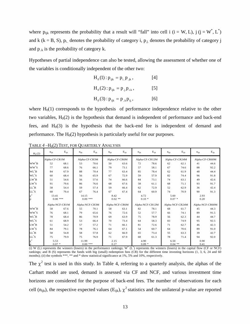
where pijk represents the probability that a result will “fall” into cell i (i = W, L), j (j = W*, L*)
and k (k = B, S), pi.. denotes the probability of category i, p.j. denotes the probability of category j
and p..k is the probability of category k.
Hypotheses of partial independence can also be tested, allowing the assessment of whether one of
the variables is conditionally independent of the other two:
jk...iijk0 ppp:)1(H = , [4]
k.i.j.ijk0 ppp:)2(H = , [5]
.ijk..ijk0 ppp:)3(H = , [6]
where H0(1) corresponds to the hypothesis of performance independence relative to the other
two variables, H0(2) is the hypothesis that demand is independent of performance and back-end
fees, and H0(3) is the hypothesis that the back-end fee is independent of demand and
performance. The H0(2) hypothesis is particularly useful for our purposes.
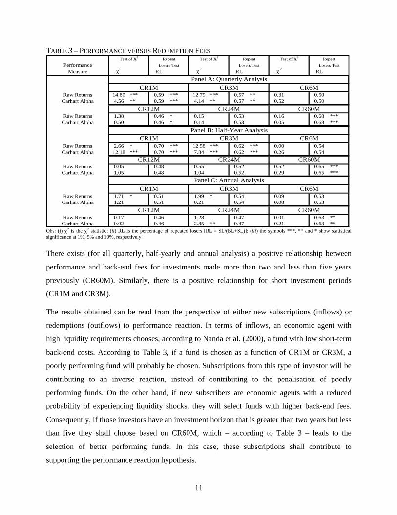
TABLE 4 –H0(2) TEST, FOR QUARTERLY ANALYSIS
H0 (2)nijk Eijk nijk Eijk nijk Eijk nijk Eijk nijk Eijk nijk Eijk
WW*B 52 68.1 53 70.6 50 63.6 72 78.6 62 62.1 41 44.6WW*S 77 68.6 76 66.1 79 73.1 57 58.1 67 74.6 88 92.2WL*B 84 67.9 88 70.4 77 63.4 85 78.4 62 61.9 48 44.4WL*S 60 68.4 56 65.9 67 72.9 59 57.9 82 74.4 96 91.8LW*B 51 54.6 56 57.6 74 66.6 84 73.1 74 63.1 49 42.6LW*S 91 79.6 86 76.6 68 67.6 58 61.1 68 71.1 93 91.7LL*B 58 54.4 59 57.4 59 66.4 62 72.9 52 62.9 36 42.4LL*S 68 79.4 67 76.4 67 67.4 64 60.9 74 70.9 90 91.3χ2 13.41 14.15 8.42 4.72 5.60 2.93p 0.00 *** 0.00 *** 0.02 ** 0.10 * 0.07 * 0.20
WW*B 58 67.6 55 70.1 58 63.1 82 78.1 68 61.7 45 44.3WW*S 76 68.1 79 65.6 76 72.6 52 57.7 66 74.1 89 91.5WL*B 78 68.4 86 70.9 69 63.9 75 78.9 56 62.3 44 44.7WL*S 61 68.9 53 66.4 70 73.4 64 58.3 83 74.9 95 92.5LW*B 51 54.2 57 57.2 71 66.1 81 72.6 71 62.7 46 42.3LW*S 84 79.1 78 76.1 64 67.1 54 60.7 64 70.6 89 91.0LL*B 58 54.8 58 57.8 62 66.9 65 73.4 55 63.3 39 42.7LL*S 75 79.9 75 76.9 71 67.9 68 61.3 78 71.4 94 92.0χ2 5.53 11.99 2.15 4.90 6.50 0.90p 0.07 * 0.00 *** 0.27 0.09 * 0.04 ** 0.41
Alpha-CF-CR24M Alpha-CF-CR60M
Alpha-NCF-CR24M Alpha-NCF-CR60M
Alpha-CF-CR1M Alpha-CF-CR3M
Alpha-NCF-CR1M Alpha-NCF-CR3M Alpha-NCF-CR6M Alpha-NCF-CR12M
Alpha-CF-CR6M Alpha-CF-CR12M
(i) W (L) represents the winners (losers) in the performance rankings; W* (L*) represents the winners (losers) in the capital flow (CF or NCF) rankings; and B (S) represents the funds with big (small) redemption fees (CR) for the different time investing horizons (1, 3, 6, 24 and 60 months); (ii) the symbols ***, ** and * show statistical significance at 1%, 5% and 10%, respectively.
The χ2 test is used in this study. In Table 4, referring to a quarterly analysis, the alphas of the
Carhart model are used, demand is assessed via CF and NCF, and various investment time
horizons are considered for the purpose of back-end fees. The number of observations for each
cell (nijk), the respective expected values (Eijk), χ2 statistics and the unilateral p-value are reported
14
for each case. The significance levels are also stated, and the null hypothesis is described by [5]22.
At the 10% significance level, the hypothesis that demand is independent of both performance
and back-end load fees is rejected in 9 of the 12 reported situations.
The “entrenchment” hypothesis requires that, given the performance and redemption costs, the
demand rankings favour funds with heavier back-end load. Thus, it is expected that WW*B
surpasses its expected value and that WL*B is lower than its expected value. This is the case with
Alpha/NCF/CR12M: the value observed for WW*B (82) exceeds the expected value (78.1) and
the value observed for WL*B (75) is lower than the respective expected value (78.9). However,
Alpha/NCF/CR1M records the opposite. The “entrenchment” hypothesis likewise states that
WL*S surpasses the expected value and WW*S is below the expected value. This means that
winning funds relative to performance are more likely to be converted into losing funds relative
to demand when they possess lower back-end fees. In contrast, funds with winning performances
are much less likely to be transformed into losing funds if they are protected by high fees23.
Similarly, where “entrenchment” exists, it is expected that LW*B surpasses its expected value
and the opposite occurs with LL*B. Moreover, it is expected that funds with poor performances
and low back-end fees would more likely be penalised, which means that it can be forecasted that
LL*S surpasses LW*S. In other words, LL*S can be expected to overtake the expected value and
the opposite will occur vis-à-vis LW*S24.
The hypothesis that demand is steered by liquidity concerns implies a relationship between the
observed values and the expected values which is the opposite of the “entrenchment” hypothesis.
In these circumstances it would be expected that funds with lower fees are favoured (in terms of
demand) in each performance category. It can be concluded that there is evidence of
“entrenchment” in Alpha/NCF/CR12M, and evidence of demand dominated by liquidity
concerns in Alpha/CF/CR1M. In all the other cases of rejection of the null hypothesis, situations
that are wholly in agreement with the “entrenchment” hypothesis for Alpha /NCF/CR24M are
verified. Conversely, Alpha/NCF/CR1M, Alpha/CF/CR3M and Alpha/NCF/CR3M are totally
contrary to this hypothesis. The results of Alpha/CF/CR12M and Alpha/CF/CR24M are
22 In order to save space identical tables drafted for the different time horizons and different null hypotheses are not reproduced herein. 23 This is the case of Alpha/CF/CR12M, but not Alpha /CF/CR1M. 24 Alpha/NCF/CR12M, once again, behaves according to the “entrenchment” hypothesis. The reverse is true of Alpha /CF/CR1M.
15
consistent with the “entrenchment” hypothesis in 6 of the 8 cells, whereas with
Alpha/CF/CR12M this is true for only two cells.
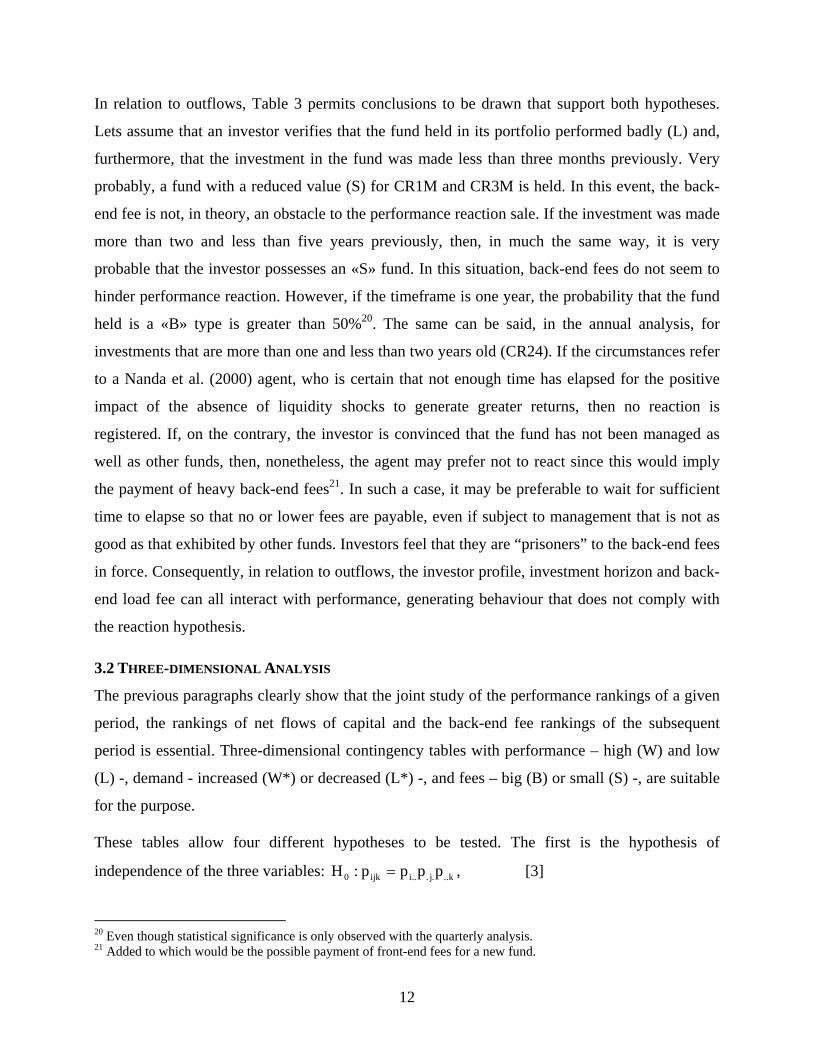
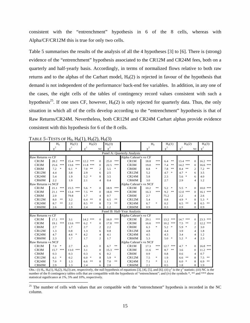
Table 5 summarises the results of the analysis of all the 4 hypotheses [3] to [6]. There is (strong)
evidence of the “entrenchment” hypothesis associated to the CR12M and CR24M fees, both on a
quarterly and half-yearly basis. Accordingly, in terms of normalized flows relative to both raw
returns and to the alphas of the Carhart model, H0(2) is rejected in favour of the hypothesis that
demand is not independent of the performance/ back-end fee variables. In addition, in any one of
the cases, the eight cells of the tables of contingency record values consistent with such a
hypothesis25. If one uses CF, however, H0(2) is only rejected for quarterly data. Thus, the only
situation in which all of the cells develop according to the “entrenchment” hypothesis is that of
Raw Returns/CR24M. Nevertheless, both CR12M and CR24M Carhart alphas provide evidence
consistent with this hypothesis for 6 of the 8 cells.
TABLE 5–TESTS OF H0, H0(1), H0(2), H0(3) H0(3) H0
χ2 χ2 χ2NC χ2 χ2 χ2 χ2
NC χ2
Raw Returns vs CF Alpha Cahrart's vs CFCR1M 28.2 *** 15.4 *** 12.2 *** 0 25.0 *** CR1M 18.8 *** 6.4 ** 13.4 *** 0 16.2 ***CR3M 25.6 *** 13.6 *** 11.8 *** 0 22.5 *** CR3M 19.0 *** 7.4 ** 14.2 *** 0 16.6 ***CR6M 7.2 * 6.1 * 7.0 ** 2 5.5 * CR6M 8.8 * 7.8 ** 8.4 ** 2 7.2 **CR12M 4.4 3.8 2.9 6 2.5 CR12M 5.2 4.7 * 4.7 * 6 3.5CR24M 5.4 1.9 5.2 * 8 3.5 CR24M 5.8 2.3 5.6 * 6 4.0CR60M 2.2 1.9 2.1 4 0.4 CR60M 3.0 2.7 2.9 4 1.2
Raw Returns vs NCF Alpha Cahrart's vs NCFCR1M 21.1 *** 15.5 *** 5.6 * 0 18.9 *** CR1M 10.2 ** 5.2 * 5.5 * 0 10.0 ***CR3M 21.1 *** 13.4 *** 7.5 ** 0 18.8 *** CR3M 16.3 *** 9.2 ** 12.0 *** 0 16.1 ***CR6M 2.0 79.8 1.7 4 0.7 CR6M 2.7 75.2 2.2 4 2.6CR12M 8.0 ** 3.2 6.4 ** 8 6.5 ** CR12M 5.4 0.8 4.9 * 8 5.3 *CR24M 8.7 ** 2.2 8.5 ** 8 7.3 ** CR24M 6.7 * 0.2 6.5 ** 8 6.5 **CR60M 2.6 1.9 2.4 6 1.2 CR60M 0.9 0.3 0.9 8 0.9
Raw Returns vs CF Alpha Cahrart's vs CFCR1M 17.1 *** 3.1 14.2 *** 0 16.0 *** CR1M 29.1 *** 13.2 *** 14.7 *** 0 23.3 ***CR3M 19.1 *** 13.6 *** 6.2 * 0 17.8 *** CR3M 16.6 *** 10.2 *** 7.5 ** 2 12.2 ***CR6M 2.7 1.7 2.7 2 2.2 CR6M 6.3 * 5.2 * 5.9 * 2 3.0CR12M 1.3 0.8 1.3 6 0.8 CR12M 4.8 4.4 3.9 4 1.8CR24M 4.7 4.6 * 4.2 4 4.1 CR24M 4.5 4.3 3.4 4 1.2CR60M 2.3 1.7 1.7 2 1.7 CR60M 5.3 5.0 * 5.2 * 4 2.3
Raw Returns vs NCF Alpha Cahrart's vs NCFCR1M 7.0 * 2.7 4.3 0 6.7 ** CR1M 17.3 *** 12.7 *** 4.7 * 0 16.8 ***CR3M 15.7 *** 13.0 *** 3.1 0 15.3 *** CR3M 11.6 ** 8.7 ** 3.6 0 11.2 ***CR6M 0.3 0.3 0.3 6 0.2 CR6M 0.9 0.8 0.6 4 0.7CR12M 6.1 * 0.2 6.0 * 8 5.9 * CR12M 7.5 * 1.9 6.6 ** 8 7.5 **CR24M 7.0 * 1.3 6.6 ** 8 7.0 ** CR24M 7.1 * 1.1 6.0 * 8 6.9 **CR60M 2.9 1.3 2.4 6 2.8 CR60M 2.1 0.5 1.8 8 1.9
Panel A: Quarterly Analysis
Panel B: Half-Year Analysis
H0(2)H0 H0(1) H0(2) H0(3)H0(1)
Obs.: (i) H0, H0(1), H0(2), H0(3) are, respectively, the null hypothesis of equations [3], [4], [5], and [6]; (ii) χ2 is the χ2 statistic; (iii) NC is the number of the 8 contingency tables cells that are compatible with the hypothesis of “entrenchment”; and (iv) the symbols *, ** and *** show statistical significance at 1%, 5% and 10%, respectively.
25 The number of cells with values that are compatible with the “entrenchment” hypothesis is recorded in the NC column.
16
The hypothesis that demand is independent of the performance/ back-end fee variables for 12 and
24-month timeframes is rejected in terms of both absolute flows and, above all, normalized
flows. The “entrenchment” hypothesis is accepted, and it can be concluded that when
disinvestment costs are high they are an obstacle to the penalisation of poor performances, and
when they are low, the reduced costs allow the mobilisation of better performing funds due to
liquidity shocks.
Simultaneously, for the NCF variable and for the 12 and 24-month investment horizons, the i)
three-variable independence hypothesis (H0) is rejected, and ii) the hypothesis that back-end fees
are independent of the performance/demand binomial (H0(3)) is also rejected. These results
support the “entrenchment” hypothesis. Lastly, performance is conditionally independent of the
demand/ back-end fees pair (H0(1)).
In relation to other investment horizons, the independence hypothesis is never rejected in
CR60M, and the same is true of CR6M in terms of NCF. In all other cases, multiple rejections of
the tested hypotheses are recorded, but never on a scale comparable with that of the
“entrenchment” hypothesis. As it happens, CR1M and CR3M have zero cells compatible with the
“entrenchment” hypothesis. This means that all the cells contain values that are consistent with
the liquidity hypothesis.
To summarise, our results are compatible with the hypothesis that medium-term investors (1 and
2 years) do not react to poor performances given the fact that they feel “imprisoned” by back-end
load fees, in the same way that the results are in line with the hypothesis that investors likely to
suffer liquidity shocks shall act in exactly the opposite manner to that indicated by the reaction
hypothesis.
4. CONCLUSIONS
The relationship between back-end load fees, mutual fund net capital flows and the performance
of mutual funds in a small market was studied in this paper. The conclusions drawn from the two-
dimensional analysis of demand /load costs are that investors more intensively channel
investment flows to funds with higher back-end fees. Furthermore, investors penalise funds with

17
the highest redemption costs for investment horizons of one and three-months, favouring funds
with heavier redemption conditions for one or two-year investment horizons.
These results corroborate the theory that investors are concerned with possible liquidity shocks
and, on the other hand, they trust in the capacity – predicted by the model of Nanda et al. (2000)
and (only partially) confirmed by Gruber (1996) – that over (sufficiently) long investment
horizons the skills of the more expensive management entities shall allow them to recover the
increased costs borne.
The comparison of performance with redemption costs produced results that provide an
explanation for the absence of reaction to poor performances. It was observed that investors
making choices that are restricted by the existence of liquidity shocks and are sensitive to the 1
and 3 month back-end fees, prefer funds with lower fees and tend to invest in funds with worse
performances. It was also concluded that the fees charged by funds can be an obstacle to the
reaction of investors with 6-to-24 month investment horizons, precisely because of the (high)
back-end fees payable.
The three-dimensional analysis of demand, performance and redemption costs corroborated the
thesis that, over specific investment horizons, back-end fees are – as established by Ippolito
(1992) – an obstacle to performance reaction. We conclude that there is (strong) evidence of the
“entrenchment” hypothesis associated to the fees for 12 and 24-month timeframes. Thus, when
disinvestment costs are high they are an obstacle to the penalization of poor performances and
when they are low, such costs induce disinvestment from better performing funds whenever
liquidity requirements compel the mobilisation of resources. Conversely, in relation to short-term
(one and three months) back-end load fees, evidence supporting the liquidity hypothesis was
found: investors likely to undergo liquidity shocks preferentially invest in funds with lower fees
(and worse past performances). In summary, the existence of two types of investors hypothesized
by Nanda et al. (2000) provides an explanation for the lack of performance reaction. Investors
with a high likelihood of undergoing a liquidity crisis, preferring liquidity in decision making, act
contrary to the reaction hypothesis, and investors with broader investment horizons do not react
to poor performances due to the fact that they are “imprisoned” by back-end fees.

18
Our results do have important policy implications. From a regulatory standpoint, the
implementation of measures that seek to permit the transfer of capital between funds without cost
would be capable of freeing those investors that feel ‘trapped’ in poorly performing funds,
thereby making the punitive effect provided by the said movement of capital effective.
Otherwise, poorly performing funds shall continue to benefit from the protective umbrella
provided by the imposition of high back-end fees. Such a measure would lead to an increase in
competition between the different mutual fund management companies.

19
REFERENCES:
Alves, C. and V. Mendes (2006), Mutual Fund Flows’ Performance Reaction: Does Convexity Apply To
Small Markets?, Working Papers, Faculdade de Economia do Porto.
Alves, C. and V. Mendes (2004), Corporate Governance Policy and Company Performance: The Case of
Portugal, Corporate Governance: an International Review, 12, 290-301.
Carhart, M. (1997), On Persistence in Mutual Fund Performance, Journal of Finance, 52, 57-82.
Chevalier, J. and G. Ellison (1997), Risk Taking by Mutual Funds as a Response to Incentives, Journal of
Political Economy, 105, 1167-201.
Christoffersen, S. (2001), Why Do Money Fund Managers Voluntarily Waive Their Fees?, Journal of
Finance, 56, 1117-40.
Del Guercio, D. and P. Tkac (2001), Star Power: the Effect of Morningstar Ratings on Mutual Fund
Flows, Working Paper Series, nº 2001-15, Federal Reserve Bank of Atlanta.
Goetzmann, W. and N. Peles (1997), Cognitive Dissonance and Mutual Fund Investors, Journal of
Financial Research, 20, 145-58.
Gruber, M. (1996), Another Puzzle: The Growth in Actively Managed Mutual Funds, Journal of Finance,
51, 783-810.
Ippolito, R. (1992), Consumer Reaction to Measures of Poor Quality: Evidence from the Mutual Fund
Industry, Journal of Law and Economics, 35, 45-70.
Lynch, A. and D. Musto (2000), How Investors Interpret Past Fund Returns, Working Paper, New York
University.
Malkiel, B. (1995), Returns from Investing in Equity Mutual Funds 1971 to 1991, Journal of Finance, 50,
549-72.
Nanda, V., M. Narayanan, and V. Warther (2000), Liquidity, Investment Ability, and Mutual Fund
Structure, Journal of Financial Economics, 57, 417-43.
Pesaran, M. and A. Timmermann (1992), A Simple Nonparametric Test of Predictive Performance,
Journal of Business and Economic Statistics, 10, 461-65.

20
Serra, A. (2000), Country and Industry Factors in Returns: Evidence from Emerging Markets’ Stocks,
Emerging Markets Review, 1, 127-51.
Sirri, E. and P. Tufano (1992), Competition and Change in the Mutual Fund Industry, in Financial
Services: Perspectives and Challenges (Ed.) Hayes III, S, Harvard Business School Press, Boston, MA,
pp. 181-214.
Sirri, E. e P. Tufano (1998), Costly Search and Mutual Fund Flows, Journal of Finance, 53, 1589-622.
Zheng, L. (1999), Is Money Smart? A Study of Mutual Fund Investors' Fund Selection Ability, Journal of
Finance, 54, 901-33.
Recent FEP Working Papers
Nº 202 Óscar Afonso and Paulo B. Vasconcelos, Numerical computation for initial value problems in economics, February 2006
Nº 201 Manuel Portugal Ferreira, Ana Teresa Tavares, William Hesterly and Sungu Armagan, Network and firm antecedents of spin-offs: Motherhooding spin-offs, February 2006
Nº 200 Aurora A.C. Teixeira, Vinte anos (1985-2005) de FEP Working Papers: um estudo sobre a respectiva probabilidade de publicação nacional e internacional, January 2006
Nº 199 Samuel Cruz Alves Pereira, Aggregation in activity-based costing and the short run activity cost function, January 2006
Nº 198
Samuel Cruz Alves Pereira and Pedro Cosme Costa Vieira, How to control market power of activity centres? A theoretical model showing the advantages of implementing competition within organizations, January 2006
Nº 197 Maria de Fátima Rocha and Aurora A.C. Teixeira, College cheating in Portugal: results from a large scale survey, December 2005
Nº 196 Stephen G. Donald, Natércia Fortuna and Vladas Pipiras, Local and global rank tests for multivariate varying-coefficient models, December 2005
Nº 195 Pedro Rui Mazeda Gil, The Firm’s Perception of Demand Shocks and the Expected Profitability of Capital under Uncertainty, December 2005
Nº 194 Ana Oliveira-Brochado and Francisco Vitorino Martins, Assessing the Number of Components in Mixture Models: a Review., November 2005
Nº 193 Lúcia Paiva Martins de Sousa and Pedro Cosme da Costa Vieira, Um ranking das revistas científicas especializadas em economia regional e urbana, November 2005
Nº 192 António Almodovar and Maria de Fátima Brandão, Is there any progress in Economics? Some answers from the historians of economic thought, October 2005
Nº 191 Maria de Fátima Rocha and Aurora A.C. Teixeira, Crime without punishment: An update review of the determinants of cheating among university students, October 2005
Nº 190 Joao Correia-da-Silva and Carlos Hervés-Beloso, Subjective Expectations Equilibrium in Economies with Uncertain Delivery, October 2005
Nº 189 Pedro Cosme da Costa Vieira, A new economic journals’ ranking that takes into account the number of pages and co-authors, October 2005
Nº 188 Argentino Pessoa, Foreign direct investment and total factor productivity in OECD countries: evidence from aggregate data, September 2005
Nº 187 Ana Teresa Tavares and Aurora A. C. Teixeira, Human Capital Intensity in Technology-Based Firms Located in Portugal: Do Foreign Multinationals Make a Difference?, August 2005
Nº 186 Jorge M. S. Valente, Beam search algorithms for the single machine total weighted tardiness scheduling problem with sequence-dependent setups, August 2005
Nº 185 Sofia Castro and João Correia-da-Silva, Past expectations as a determinant of present prices – hysteresis in a simple economy, July 2005
Nº 184 Carlos F. Alves and Victor Mendes, Institutional Investor Activism: Does the Portfolio Management Skill Matter?, July 2005
Nº 183 Filipe J. Sousa and Luís M. de Castro, Relationship significance: is it sufficiently explained?, July 2005
Nº 182 Alvaro Aguiar and Manuel M. F. Martins, Testing for Asymmetries in

the Preferences of the Euro-Area Monetary Policymaker, July 2005
Nº 181 Joana Costa and Aurora A. C. Teixeira, Universities as sources of knowledge for innovation. The case of Technology Intensive Firms in Portugal, July 2005
Nº 180 Ana Margarida Oliveira Brochado and Francisco Vitorino Martins, Democracy and Economic Development: a Fuzzy Classification Approach, July 2005
Nº 179 Mário Alexandre Silva and Aurora A. C. Teixeira, A Model of the Learning Process with Local Knowledge Externalities Illustrated with an Integrated Graphical Framework, June 2005
Nº 178 Leonor Vasconcelos Ferreira, Dinâmica de Rendimentos, Persistência da Pobreza e Políticas Sociais em Portugal, June 2005
Nº 177 Carlos F. Alves and F. Teixeira dos Santos, The Informativeness of Quarterly Financial Reporting: The Portuguese Case, June 2005
Nº 176 Leonor Vasconcelos Ferreira and Adelaide Figueiredo, Welfare Regimes in the UE 15 and in the Enlarged Europe: An exploratory analysis, June 2005
Nº 175
Mário Alexandre Silva and Aurora A. C. Teixeira, Integrated graphical framework accounting for the nature and the speed of the learning process: an application to MNEs strategies of internationalisation of production and R&D investment, May 2005
Nº 174 Ana Paula Africano and Manuela Magalhães, FDI and Trade in Portugal: a gravity analysis, April 2005
Nº 173 Pedro Cosme Costa Vieira, Market equilibrium with search and computational costs, April 2005
Nº 172 Mário Rui Silva and Hermano Rodrigues, Public-Private Partnerships and the Promotion of Collective Entrepreneurship, April 2005
Nº 171 Mário Rui Silva and Hermano Rodrigues, Competitiveness and Public-Private Partnerships: Towards a More Decentralised Policy, April 2005
Nº 170 Óscar Afonso and Álvaro Aguiar, Price-Channel Effects of North-South Trade on the Direction of Technological Knowledge and Wage Inequality, March 2005
Nº 169 Pedro Cosme Costa Vieira, The importance in the papers' impact of the number of pages and of co-authors - an empirical estimation with data from top ranking economic journals, March 2005
Nº 168 Leonor Vasconcelos Ferreira, Social Protection and Chronic Poverty: Portugal and the Southern European Welfare Regime, March 2005
Nº 167 Stephen G. Donald, Natércia Fortuna and Vladas Pipiras, On rank estimation in symmetric matrices: the case of indefinite matrix estimators, February 2005
Nº 166 Pedro Cosme Costa Vieira, Multi Product Market Equilibrium with Sequential Search, February 2005
Nº 165 João Correia-da-Silva and Carlos Hervés-Beloso, Contracts for uncertain delivery, February 2005
Nº 164 Pedro Cosme Costa Vieira, Animals domestication and agriculture as outcomes of collusion, January 2005
Nº 163 Filipe J. Sousa and Luís M. de Castro, The strategic relevance of business relationships: a preliminary assessment, December 2004
Nº 162 Carlos Alves and Victor Mendes, Self-Interest on Mutual Fund Management: Evidence from the Portuguese Market, November 2004
Nº 161 Paulo Guimarães, Octávio Figueiredo and Douglas Woodward, Measuring the Localization of Economic Activity: A Random Utility Approach, October 2004
Editor: Prof. Aurora Teixeira ([email protected]) Download available at: http://www.fep.up.pt/investigacao/workingpapers/workingpapers.htmalso in http://ideas.repec.org/PaperSeries.html

www.fep.up.pt