Approximating State of DES Using Fuzzy TimedPetri Nets

Juan Carlos González-Castolo, Ernesto López-Mellado

Abstract– This paper addresses state estimation of dis-crete event systems (DES) modeled by Fuzzy Timed PetriNets (FTPN). A definition of FTPN in which fuzzy sets,associated to places, represent the ending time uncer-tainty of activities is presented; then the fuzzy state equa-tion composed by a set of matrix expressions is devel-oped, allowing computing the marking evolution of DESexhibiting cyclic behavior. A method for approximatingthe marking of strongly connected state machines is pro-posed.

I. Introduction.

State estimation of dynamic systems useful when onlya subset of the state variables can be directly measured;observers are the entities computing the system statefrom the knowledge of its internal structure and its (par-tially) measured behavior. The problem of discrete eventsystems (DES) estimation has been addressed in [6]; inthat work the marking of a Petri net (PN) model of apartially observed event driven system is computed fromthe evolution of its inputs and outputs.The state of a system can be also inferred using the

knowledge on the duration of activities. However thistask becomes complex when, besides the absence of sen-sors, the durations of the operations are uncertain; in thissituation the observer obtains and revise a belief that ap-proximates the current system state. Consequently thisapproach is useful for non critical applications of statemonitoring and feedback in which it is enough an ap-proximate computation of the state.The uncertainty of activities duration in DES can be

handled using fuzzy PN (FPN) [5], [3], [13], [2], [4]; thisPN extension has been applied to knowledge modelling[7], [9], [11], planning [12] , reasoning [10] and controllerdesign [1],[14]. In these works the proposed techniquesinclude the computation of imprecise markings; howeverthe class of models dealt does not include PN modelingcyclic behavior.In this paper we address the problem of state esti-

mation of DES for calculating the fuzzy marking of aFTPN ; for this purpose a set of matrix expressions forthe recursive computing the current fuzzy marking is de-veloped. The paper focuses on FTPN whose structure isa state machine; the firing of transitions in a conflict ishandled through relative weights for updating the mark-ing belief.

J.C. González-Castolo and E. López-Mellado are with CINVES-TAV Unidad Guadalajara, Av. Científica 1145, Col. El Bajío,45010 Zapopan, Jal. México. {castolo, elopez}@gdl.cinvestav.mx

The remainder of this paper is structured as follows.In the next Section, theories of fuzzy sets and Petri netsare overviewed. In Section III, FTPN are presented andthe fuzzy state generalized equation is proposed. SectionIV presents the fuzzy state estimation in the FTPN . Fi-nally, in Section V the procedure for marking estimationis proposed.

II. Background.

A. Possibility Theory.

In theory of possibility, a fuzzy set a is used for de-limiting ill-known values or for representing values char-acterized by symbolic expressions. The set is defined asa = (a1, a2, a3, a4) such that a1, a2, a3, a4 ∈ R+, a1 ≤ a2and a3 ≤ a4. [a1, a4] is the support of a.A fuzzy set a is referred indistinctly by the function

α(τ) or the characterization (a1, a2, a3, a4). For simplic-ity, the fuzzy possibility distribution of the time is de-scribed with a trapezoidal form or triangular form.Definition 1: Let a = (a1, a2, a3, a4) and b =

(b1, b2, b3, b4) be two trapezoidal fuzzy sets. The fuzzysets addition operation as: a ⊕ b = (a1 + b1, a2 + b2,a3 + b3, a4 + b4) [15].Definition 2: The distribution of possibility before and

after a are the fuzzy sets ab = (−∞, a2, a3, a4) andaa = (a1, a2, a3,+∞), respectively; they are defined in[1] as a function α(−∞,a](τ) = sup

τ≥τα(τ) and α(a,+∞](τ) =

supτ≤τ

α(τ), respectively.

Definition 3: The intersection and union of fuzzy setsare defined in terms of min and max. (f ∩ g) =min(f , g) = min(αf (τ), αg(τ)) | {τ ∈ support of f ∧ g}and (f ∪ g) = max(f , g) = max(αf (τ), αg(τ)) | {τ ∈support of f ∨ g}, where the min(max) operator gets theminimum (maximum) x of X. We used these operators,intersection and union, as t-norm and s-norm, respec-tively.

B. Petri Nets.

Definition 4: An ordinary PN structure G is a bipar-tite digraph represented by the 4-tuple G = (P, T, I,O)where P = {p1, p2, ..., pn} and T = {t1, t2, ..., tm} arefinite sets of vertices called respectively places and tran-sitions, I(O) : P × T → {0, 1} is a function representingthe arcs going from places to transitions (transitions toplaces).

Proceedings of the 3rd AnnualIEEE Conference on Automation Science and EngineeringScottsdale, AZ, USA, Sept 22-25, 2007

MoRP-B03.6

1-4244-1154-8/07/$25.00 ©2007 IEEE. 722

Authorized licensed use limited to: IEEE Xplore. Downloaded on October 27, 2008 at 13:37 from IEEE Xplore. Restrictions apply.

Pictorially, places are represented by circles, transi-tions are represented by rectangles, and arcs are depictedas arrows. The symbol •tj(tj•) denotes the set of allplaces pi such that I(pi, tj) 6= 0 (O(pi, tj) 6= 0). Analo-gously, •pi(pi•) denotes the set of all transitions tj suchthat O(pi, tj) 6= 0 (I(pi, tj) 6= 0).The pre-incidence matrix of G is C− = [c−ij ] where

c−ij = I(pi, tj); the post-incidence matrix of G is C+ =[c+ij ] where c

+ij = O(pi, tj); the incidence matrix of G is

C = C+ − C−.A marking function M : P → Z+represents the num-

ber of tokens (depicted as dots) residing inside each place.The marking of a PN is usually expressed as an n-entryvector.Definition 5: A Petri Net system or Petri Net (PN) is

the pair N = (G,M0), where G is a PN structure andM0 is an initial token distribution.In a PN system, a transition tj is enabled at the mark-

ing Mk if ∀pi ∈ P , Mk(pi) ≥ I(pi, tj); an enabled transi-tion tj can be fired reaching a new marking Mk+1 whichcan be computed using the PN state equation:

Mk+1 =Mk + C+vk − C−vk (1)

where vk(i) = 0, i 6= j, vk(j) = 1.The reachability set of a PN is the set of all possible

reachable marking from M0 firing only enabled transi-tions; this set is denoted by R(G,M0).A structural conflict is a PN sub-structure in which

two or more transitions share one or more input places;such transitions are simultaneously enabled and the firingof one of them may disable the others.Definition 6: A transition tk ∈ T is live, for a marking

M0, if ∀Mk ∈ R(G,M0), ∃Mn ∈ R(G,M0) such that tkis enabled

³Mn

tk→´. A PN is live if all its transitions

are live.Definition 7: A PN is said 1-bounded, or safe, for a

marking M0, if ∀pi ∈ P and ∀Mj ∈ R(G,M0), it holdsthat Mj(pi) ≤ 1.In this work we deal with live and safe PN .Definition 8: A p-invariant Yi (t-invariantXi) of a PN

is a positive integer solution of the equation Y Ti C = 0

(CXi = 0). The support of the p-invariant Yi (t-invariant Xi) is the set kYik = {pj | Yi(pj) 6= 0}(kXik = {tj | Xi(tj) 6= 0}).Definition 9: Let Yi a p-invariant of a Petri net

(G,M0), kYik the support of Yi, then the induced subnetby Yi is PCi = (Pi = kYik , Ti = ∪tk ∈ •pj , tl ∈ pj•,where pj ∈ kYik , Ii, Oi) named p-component, and Ii =Pi × Ti ∩ I, and Oi = Pi × Ti ∩O.Definition 10: Let Xi be a t-invariant of a PN , and

kXik be the support of Xi, then the induced subnet byXi is TCi = (Pi = {∪pk ∈ •tj , pl ∈ tj• | tj ∈ kXik}, Ti =kXik , Ii, Oi) named t-component. Ii = Pi × Ti ∩ I, andOi = Pi × Ti ∩O.Definition 11: A invariant Zi is minimal if no invariant

Zj satisfies kZjk ⊂ kZik, where Zi, Zj are p-invariantsor t-invariants and ∀z ∈ Zi : z ≥ 0.Definition 12: Let Z = {Z1, ..., Zq} be the set of mini-

mal invariants [8] of a PN , then Z is called the invariantsbase. The cardinality of Z is represented as |Z|.

III. Fuzzy Timed Petri nets.

A. Basic Operators.

We introduce first some useful operators.Definition 13: In order to get the fuzzy set between f

and g, the lmax function is defined as

lmax(f , g) = min(fa, gb) (2)Definition 14: The latest (earliest) operation selects

the latest (earliest) fuzzy set among n fuzzy sets; theyare calculated as follows:

latestnf1, . . . , fn

o=

minnmax

nfb1 , ..., f

bn

o,min

nfa1 , ..., f

an

oo (3)

earliestnf1, ..., fn

o=

minnmin

nfb1 , ..., f

bn

o,max

nfa1 , ..., f

an

oo (4)

B. FTPN Definition.

Definition 15: A fuzzy timed Petri net structure is a3-tuple FTPN = (N,Γ, ξ); where N = (G,M0) is a PN ,Γ = {a1, a2, ..., an} is a collection of fuzzy sets, ξ : P −→Γ is a function that associates a fuzzy set ai ∈ Γ to eachplace pi ∈ P ; i = 1, ..., |P |.Fuzzy timing of places.The fuzzy set a = (a1, a2, a3, a4) represents the static

possibility distribution α(τa) ∈ [0, 1] of the instant atwhich a token leaves a place p ∈ P, starting from the in-stant when p is marked. This set does not change duringthe FTPN execution.Fuzzy timing of tokens.The fuzzy set b = (b1, b2, b3, b4) represents the dynamic

possibility distribution β(τ b) ∈ [0, 1] associated to a to-ken residing within a p ∈ P ; it also represents the instantτ b at which such a token leaves the place, starting fromthe instant when p is marked. b is computed from a everytime the place is marked during the marking evolution ofthe FTPN .A token begins to be available for enabling output tran-

sitions at β(b1). Thus ba = (b1, b2, b3,+∞) represents thepossibility distribution of available tokens.The fuzzy set c = (c1, c2, c3, c4), known as fuzzy times-

tamp, is a dynamic possibility distribution ς(τ c) ∈ [0, 1]that represents the duration of a token within a placep ∈ P .

C. Enabling and firing of transitions.

Fuzzy enabling date.The fuzzy enabling time etk(τ) of a transition tk is

a possibility distribution of the latest leaving instant

MoRP-B03.6

723

Authorized licensed use limited to: IEEE Xplore. Downloaded on October 27, 2008 at 13:37 from IEEE Xplore. Restrictions apply.

among the leaving instants bpi of all tokens within thepi ∈ •t.

etk(τ) = latestnbpi

o∀pi ∈ •tk (5)

The latest operation obtains the latest date in which theinput places pi to tk have a token.Fuzzy firing date.The firing transition date otk(τ) of a transition tk is

determined with respect to the set of transitions {tj}simultaneously enabled. This date, expressed as a possi-bility distribution, is computed as follows:

otk(τ) = min©etk(τ), earliest

©etj (τ)

ªª∀tk ∈ pn•; pn ∈ •tj (6)

The earliest operation obtains the earliest date in whichthe transitions in a structural conflict are enabled.Fuzzy timestamp.For a given place ps, the possibility distribution bps

may be computed from aps and the firing dates otj (τ) ofa tj ∈ •ps using the following expression:

bps = lmax©otj (τ)

ª⊕ aps∀tj ∈ •ps (7)

The tokens do not disappear of •t and appear in t•instantaneously. The fuzzy timestamp cps is the timeelapse possibility that a token is in a place ps ∈ P . Thepossibility distribution cps is computed from the occur-rence dates of both •ps and ps•.

cps = lmax¡earliest{oti(τ)}, latest{otj (τ)}

¢∀ti ∈ •ps, tj ∈ ps• (8)

Actually, cps represents the fuzzy marking at instant τ .

IV. Marking estimation in Fuzzy Timed StateMachines (FTSM).

A. The branching rate.

The fuzzy state equation of Marked Graphs was pre-sented in [16] as:

M (τ) = minnM (τ −4τ) + C+4O(τb)

−C−4O(τa),→1o

(9)However the Petri net State Machine has attribution

and selection places. We must get especial attention inthe selection places because they induce a structural con-flict. At this point, we can consider some firing policies,for example:1. The order and the number of firings transitions instructural conflict are known.2. The firings of the transition are controlled.3. The belief of firing in the model is added and thebranching rate concept is introduced.The branching rate is the certainty degree on the tra-

jectory that the token follows. This concept refers to thebelief of transitions enabling possibility; it is named en-abling ratio. Also, the branching rate includes the firingdegree and token presence belief concepts.

Definition 16: The enabling-ratio (eR) is the functionw : t→ [0, 1]. The w (t) value, denoted as wt, is a staticvalue associated to a transition t where the following con-straint is held. X

t∈p•wt = 1;∀p ∈ P (10)

A diagonal matrix W represent the values wti | ti ∈ Tshow the transitions firing level in order to put the tokenat p ∈ t•. We assume that the input places are marked.

W = diag£wt1 wt2 ... wt|T |

¤(11)

Definition 17: The firing degree (fD) is the functiong : t → [0, 1]. The g (t) value, denoted as gt, is a dy-namic value associated to transition t. This characterizesthe belief of the transition firing t due to the marking ofthe input places M(p) | p ∈ •t and the associated en-abling ratio wt. The vector Gη represent the system’sfD, where η is the trace of the fired transitions. Whengti = 1 it means that the transition ti is certainty fired.Definition 18: The token presence belief (tPB) is the

function h : p → [0, 1]. The h (p) value, denoted as hp,is a dynamic value associated to an hypothetical tokenin the place p. This represents the belief of the markedplaces due to the input transitions firing. The vector Hη

represents the system tPB, where η is the trace of theinvolved transitions. When hpi = 1, it means that theplace pi is certainty marked.

B. Computing the branching rate.

The branching rate alludes a previous knowledge onthe proportion of transition firings in a conflict set.Initially w is defined for every conflict set, otherwisewti = wtj | ti, tj ∈ p•.For the initial markingM(0) =M0 we have a full tPB

in the marked places, therefore their vectorial represen-tations are alike i.e. Hε ≡M (0); ε represents the emptytrace, H is the tPB generalized of a set of places. Thegeneralized notation is applied to fD i.e. G. Consider aFTPN with n places and m transitions; the procedurefor obtaining the fD and tPB dynamic vectors is givenbelow.Algorithm 19: Branching rate.

Input: C−, C+,W, Hη

Output: Hη, Gη for every iteration

Init: As η = ε then Hη = Hε. The t-invariant base

X =£X1 ... X|X|

¤Tand the involved places in ev-

ery t-component X are obtained: X = C−¡XT

¢=h

X1 ... X |X|

i. The marking of these places is called

t-component marking MXi| i = 1, ..., |X|. The eR ma-

trix W is obtained from the previous information of theFTPN —the weight associated to each transition.

MoRP-B03.6

724

Authorized licensed use limited to: IEEE Xplore. Downloaded on October 27, 2008 at 13:37 from IEEE Xplore. Restrictions apply.

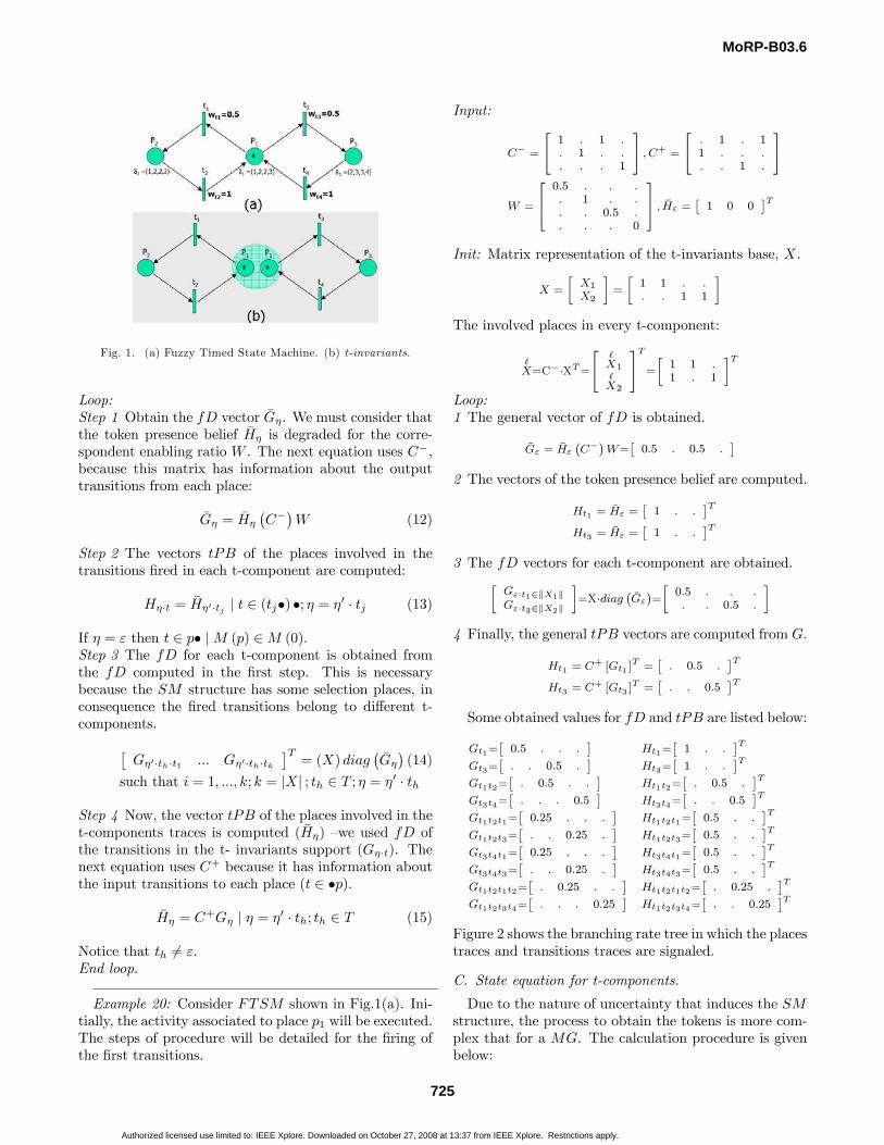
Fig. 1. (a) Fuzzy Timed State Machine. (b) t-invariants.

Loop:Step 1 Obtain the fD vector Gη. We must consider thatthe token presence belief Hη is degraded for the corre-spondent enabling ratio W . The next equation uses C−,because this matrix has information about the outputtransitions from each place:

Gη = Hη

¡C−¢W (12)

Step 2 The vectors tPB of the places involved in thetransitions fired in each t-component are computed:

Hη·t = Hη0·tj | t ∈ (tj•) •; η = η0 · tj (13)

If η = ε then t ∈ p• |M (p) ∈M (0).Step 3 The fD for each t-component is obtained fromthe fD computed in the first step. This is necessarybecause the SM structure has some selection places, inconsequence the fired transitions belong to different t-components.£

Gη0·th·t1 ... Gη0·th·tk¤T= (X) diag

¡Gη

¢(14)

such that i = 1, ..., k; k = |X| ; th ∈ T ; η = η0 · th

Step 4 Now, the vector tPB of the places involved in thet-components traces is computed (Hη) —we used fD ofthe transitions in the t- invariants support (Gη·t). Thenext equation uses C+ because it has information aboutthe input transitions to each place (t ∈ •p).

Hη = C+Gη | η = η0 · th; th ∈ T (15)

Notice that th 6= ε.End loop.

Example 20: Consider FTSM shown in Fig.1(a). Ini-tially, the activity associated to place p1 will be executed.The steps of procedure will be detailed for the firing ofthe first transitions.

Input:

C− =

⎡⎣ 1 . 1 .. 1 . .. . . 1

⎤⎦ , C+ =⎡⎣ . 1 . 11 . . .. . 1 .

⎤⎦

W =

⎡⎢⎣ 0.5 . . .. 1 . .. . 0.5 .. . . 0

⎤⎥⎦ , Hε = 1 0 0T

Init: Matrix representation of the t-invariants base, X.

X =X1

X2=

1 1 . .. . 1 1

The involved places in every t-component:

X=C−·XT=⎡⎣ X1

X2

⎤⎦T= 1 1 .1 . 1

T

Loop:1 The general vector of fD is obtained.

Gε = Hε C− W= 0.5 . 0.5 .

2 The vectors of the token presence belief are computed.

Ht1 = Hε = 1 . .T

Ht3 = Hε = 1 . .T

3 The fD vectors for each t-component are obtained.

Gε·t1∈kX1kGε·t3∈kX2k

=X·diag Gε =0.5 . . .. . 0.5 .

4 Finally, the general tPB vectors are computed from G.

Ht1 = C+ [Gt1 ]T = . 0.5 .

T

Ht3 = C+ [Gt3 ]T = . . 0.5

T

Some obtained values for fD and tPB are listed below:

Gt1= 0.5 . . . Ht1= 1 . .T

Gt3= . . 0.5 . Ht3= 1 . .T

Gt1t2= . 0.5 . . Ht1t2= . 0.5 .T

Gt3t4= . . . 0.5 Ht3t4= . . 0.5T

Gt1t2t1= 0.25 . . . Ht1t2t1= 0.5 . .T

Gt1t2t3= . . 0.25 . Ht1t2t3= 0.5 . .T

Gt3t4t1= 0.25 . . . Ht3t4t1= 0.5 . .T

Gt3t4t3= . . 0.25 . Ht3t4t3= 0.5 . .T

Gt1t2t1t2= . 0.25 . . Ht1t2t1t2= . 0.25 .T

Gt1t2t3t4= . . . 0.25 Ht1t2t3t4= . . 0.25T

Figure 2 shows the branching rate tree in which the placestraces and transitions traces are signaled.

C. State equation for t-components.

Due to the nature of uncertainty that induces the SMstructure, the process to obtain the tokens is more com-plex that for a MG. The calculation procedure is givenbelow:

MoRP-B03.6

725

Authorized licensed use limited to: IEEE Xplore. Downloaded on October 27, 2008 at 13:37 from IEEE Xplore. Restrictions apply.

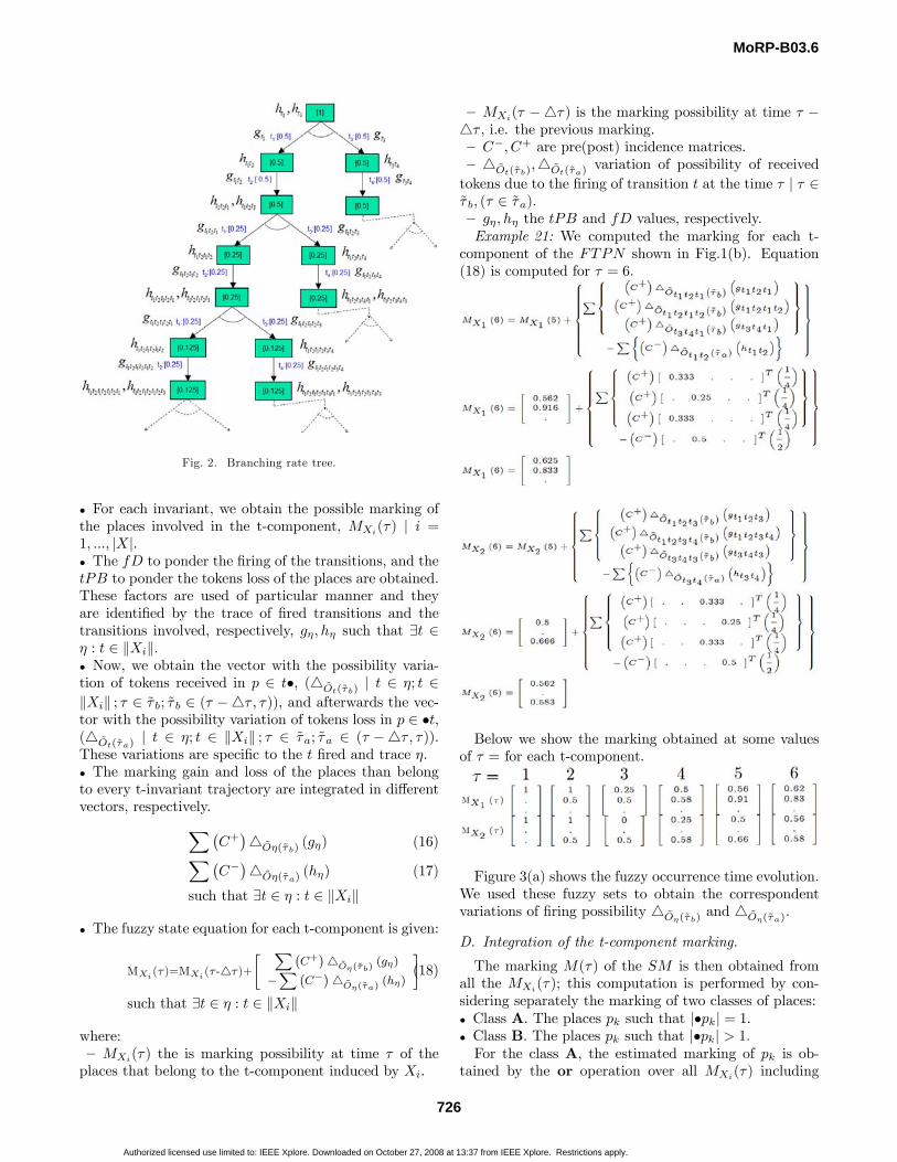
Fig. 2. Branching rate tree.

• For each invariant, we obtain the possible marking ofthe places involved in the t-component, MXi(τ) | i =1, ..., |X|.• The fD to ponder the firing of the transitions, and thetPB to ponder the tokens loss of the places are obtained.These factors are used of particular manner and theyare identified by the trace of fired transitions and thetransitions involved, respectively, gη, hη such that ∃t ∈η : t ∈ kXik.• Now, we obtain the vector with the possibility varia-tion of tokens received in p ∈ t•, (4Ot(τb)

| t ∈ η; t ∈kXik ; τ ∈ τ b; τ b ∈ (τ −4τ , τ)), and afterwards the vec-tor with the possibility variation of tokens loss in p ∈ •t,(4Ot(τa)

| t ∈ η; t ∈ kXik ; τ ∈ τa; τa ∈ (τ −4τ , τ)).These variations are specific to the t fired and trace η.• The marking gain and loss of the places than belongto every t-invariant trajectory are integrated in differentvectors, respectively.X¡

C+¢4Oη(τb)

(gη) (16)X¡C−¢4Oη(τa)

(hη) (17)

such that ∃t ∈ η : t ∈ kXik

• The fuzzy state equation for each t-component is given:

MXi (τ)=MXi (τ -4τ)+C+ 4Oη(τb)

(gη)

− C− 4Oη(τa)(hη)

(18)

such that ∃t ∈ η : t ∈ kXik

where:— MXi(τ) the is marking possibility at time τ of theplaces that belong to the t-component induced by Xi.

— MXi(τ −4τ) is the marking possibility at time τ −

4τ , i.e. the previous marking.— C−, C+ are pre(post) incidence matrices.— 4Ot(τb)

,4Ot(τa)variation of possibility of received

tokens due to the firing of transition t at the time τ | τ ∈τ b, (τ ∈ τa).— gη, hη the tPB and fD values, respectively.Example 21: We computed the marking for each t-

component of the FTPN shown in Fig.1(b). Equation(18) is computed for τ = 6.

Below we show the marking obtained at some valuesof τ = for each t-component.

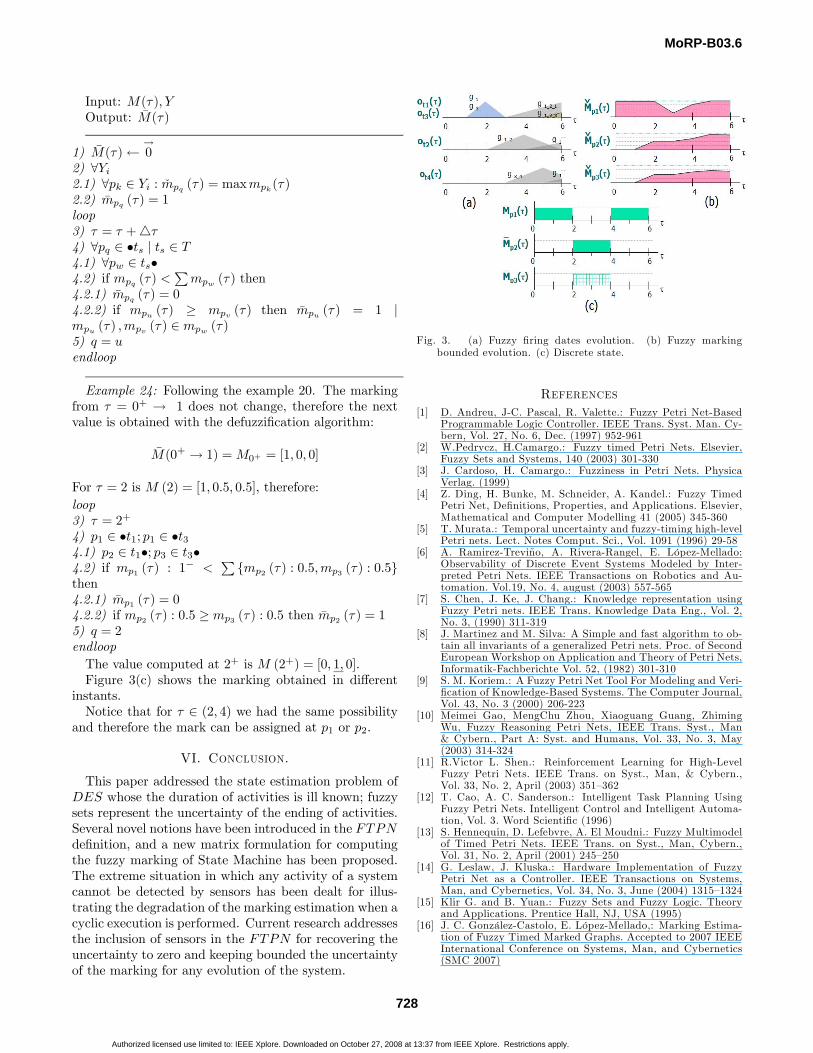
Figure 3(a) shows the fuzzy occurrence time evolution.We used these fuzzy sets to obtain the correspondentvariations of firing possibility 4Oη(τb)

and 4Oη(τa).

D. Integration of the t-component marking.

The marking M(τ) of the SM is then obtained fromall the MXi

(τ); this computation is performed by con-sidering separately the marking of two classes of places:• Class A. The places pk such that |•pk| = 1.• Class B. The places pk such that |•pk| > 1.For the class A, the estimated marking of pk is ob-

tained by the or operation over all MXi(τ) including

MoRP-B03.6

726

Authorized licensed use limited to: IEEE Xplore. Downloaded on October 27, 2008 at 13:37 from IEEE Xplore. Restrictions apply.

MXi,pk(τ); this marking is denoted as M(τ)or. For the

class B it is necessary to consider the contribution ofall MXi

(τ) corresponding to •pk as follows: for everyinput transition tl ∈ •pk belonging to more than onet-component, the marking over the pk involving tl is ob-tained by the or operation; then this marking integrationis added to other MXi,pk(τ) obtained for the other in-put transitions tm 6= tl; this partial marking is M(τ)add.Then the fuzzy marking is obtained as:

M (τ) =M (τ)or +M (τ)add (19)

This procedure is systematized below. Compute selectionmasks Sori and Saddi as follows. For every t-invariant Xi

obtain a vector Si that contains 1 in the entries that cor-respond to common transitions with other Xj in the base(0 otherwise); then Sori = C+Si. For every Xi obtain avector Ri that contains 1 in the entries that correspondto transitions non shared by other t-invariants (0 other-wise); then Saddi = C+Ri.

M (τ)or

= or {MXi(τ)♦Sori } (20)

M (τ)add =X©

MXi(τ)♦Saddi

ª(21)

Where ♦ is the bit-wise masking operation between twovectors.As the FTPN are safe then the fuzzy marking is com-

puted by:

M (τ) = min(M (τ) ,→1 ) (22)

Example 22: Following the previous example, for theFig.1 we computed the operation of t-component mark-ing. First we use (20).

Next, we compute the marking by (21).

The fuzzy marking is obtained with (19) as follows:

M(τ)=

⎡⎣ Mp1 (τ)Mp2 (τ)Mp3 (τ)

⎤⎦=⎡⎣ Mp1 (τ)

add

Mp2 (τ)add

Mp3 (τ)add

⎤⎦+⎡⎣ Mp1 (τ)

or

Mp2 (τ)or

Mp3 (τ)or

⎤⎦⎡⎣ Mp1 (τ)

Mp2 (τ)Mp3 (τ)

⎤⎦=⎡⎣ MX1,p1 (τ) +MX2,p1 (τ)

Mp2∈X1 (τ)Mp3∈X2 (τ)

⎤⎦ (23)

Finally, we got the fuzzy marking bounded:⎡⎣ Mp1 (τ)Mp2 (τ)Mp3 (τ)

⎤⎦=min⎛⎝⎡⎣ Mp1 (τ)

Mp2 (τ)Mp3 (τ)

⎤⎦ ,⎡⎣ 111

⎤⎦⎞⎠ (24)

Below we show the evolution of the fuzzy marking forτ = 1, ..., 6. We use (23).

M (1) M (2) M (3)⎡⎣ 1 + 100

⎤⎦ ⎡⎣ 1 + 10.50.5

⎤⎦ ⎡⎣ 0.250.50.5

⎤⎦M (4) M (5) M (6)⎡⎣ 0.5 + 0.250.5830.583

⎤⎦ ⎡⎣ 0.56 + 0.50.9160.666

⎤⎦ ⎡⎣ 0.62 + 0.560.8330.583

⎤⎦Now, the equation (24) is used to obtain the fuzzy mark-ing bounded at τ = 2. Figure 3(b) shows the evolutionof fuzzy marking bounded.

£MX1

(2) MX2(2)

¤=

⎡⎣ 1 10.5 .. 0.5

⎤⎦M(2)=min

⎧⎨⎩⎡⎣ 20.50.5

⎤⎦ ,⎡⎣ 111

⎤⎦⎫⎬⎭=⎡⎣ 10.50.5

⎤⎦

V. Discrete state from the FTPN.

In order to obtain a possible discrete marking M(τ) ofthe FTPN it is necessary to “defuzzify”M(τ). This canbe accomplished taking into account the fuzzy markingof FTPN .Before describing the procedure to obtain M(τ), we

define M(τ) as:

M(τ) =£mp1(τ) . . . mpn(τ)

¤T, n = |P | (25)

where mpk(τ) | k = 1, ..., n is the estimated marking ofthe place pk ∈ P . Now, the discrete marking can beobtained with the following procedure.Algorithm 23: Defuzzification.

MoRP-B03.6

727

Authorized licensed use limited to: IEEE Xplore. Downloaded on October 27, 2008 at 13:37 from IEEE Xplore. Restrictions apply.

Input: M(τ), YOutput: M(τ)

1) M(τ)← →0

2) ∀Yi2.1) ∀pk ∈ Yi : mpq (τ) = maxmpk(τ)2.2) mpq (τ) = 1loop3) τ = τ +4τ4) ∀pq ∈ •ts | ts ∈ T4.1) ∀pw ∈ ts•4.2) if mpq (τ) <

Pmpw (τ) then

4.2.1) mpq (τ) = 04.2.2) if mpu (τ) ≥ mpv (τ) then mpu (τ) = 1 |mpu (τ) ,mpv (τ) ∈ mpw (τ)5) q = uendloop

Example 24: Following the example 20. The markingfrom τ = 0+ → 1 does not change, therefore the nextvalue is obtained with the defuzzification algorithm:

M(0+ → 1) =M0+ = [1, 0, 0]

For τ = 2 is M (2) = [1, 0.5, 0.5], therefore:loop3) τ = 2+

4) p1 ∈ •t1; p1 ∈ •t34.1) p2 ∈ t1•; p3 ∈ t3•4.2) if mp1 (τ) : 1

− <P {mp2 (τ) : 0.5,mp3 (τ) : 0.5}

then4.2.1) mp1 (τ) = 04.2.2) if mp2 (τ) : 0.5 ≥ mp3 (τ) : 0.5 then mp2 (τ) = 15) q = 2endloopThe value computed at 2+ is M (2+) = [0, 1, 0].Figure 3(c) shows the marking obtained in different

instants.Notice that for τ ∈ (2, 4) we had the same possibility

and therefore the mark can be assigned at p1 or p2.

VI. Conclusion.

This paper addressed the state estimation problem ofDES whose the duration of activities is ill known; fuzzysets represent the uncertainty of the ending of activities.Several novel notions have been introduced in the FTPNdefinition, and a new matrix formulation for computingthe fuzzy marking of State Machine has been proposed.The extreme situation in which any activity of a systemcannot be detected by sensors has been dealt for illus-trating the degradation of the marking estimation when acyclic execution is performed. Current research addressesthe inclusion of sensors in the FTPN for recovering theuncertainty to zero and keeping bounded the uncertaintyof the marking for any evolution of the system.

Fig. 3. (a) Fuzzy firing dates evolution. (b) Fuzzy markingbounded evolution. (c) Discrete state.

References[1] D. Andreu, J-C. Pascal, R. Valette.: Fuzzy Petri Net-Based

Programmable Logic Controller. IEEE Trans. Syst. Man. Cy-bern, Vol. 27, No. 6, Dec. (1997) 952-961

[2] W.Pedrycz, H.Camargo.: Fuzzy timed Petri Nets. Elsevier,Fuzzy Sets and Systems, 140 (2003) 301-330

[3] J. Cardoso, H. Camargo.: Fuzziness in Petri Nets. PhysicaVerlag. (1999)

[4] Z. Ding, H. Bunke, M. Schneider, A. Kandel.: Fuzzy TimedPetri Net, Definitions, Properties, and Applications. Elsevier,Mathematical and Computer Modelling 41 (2005) 345-360

[5] T. Murata.: Temporal uncertainty and fuzzy-timing high-levelPetri nets. Lect. Notes Comput. Sci., Vol. 1091 (1996) 29-58

[6] A. Ramirez-Treviño, A. Rivera-Rangel, E. López-Mellado:Observability of Discrete Event Systems Modeled by Inter-preted Petri Nets. IEEE Transactions on Robotics and Au-tomation. Vol.19, No. 4, august (2003) 557-565

[7] S. Chen, J. Ke, J. Chang.: Knowledge representation usingFuzzy Petri nets. IEEE Trans. Knowledge Data Eng., Vol. 2,No. 3, (1990) 311-319

[8] J. Martinez and M. Silva: A Simple and fast algorithm to ob-tain all invariants of a generalized Petri nets. Proc. of SecondEuropean Workshop on Application and Theory of Petri Nets,Informatik-Fachberichte Vol. 52, (1982) 301-310

[9] S. M. Koriem.: A Fuzzy Petri Net Tool For Modeling and Veri-fication of Knowledge-Based Systems. The Computer Journal,Vol. 43, No. 3 (2000) 206-223

[10] Meimei Gao, MengChu Zhou, Xiaoguang Guang, ZhimingWu, Fuzzy Reasoning Petri Nets, IEEE Trans. Syst., Man& Cybern., Part A: Syst. and Humans, Vol. 33, No. 3, May(2003) 314-324

[11] R.Victor L. Shen.: Reinforcement Learning for High-LevelFuzzy Petri Nets. IEEE Trans. on Syst., Man, & Cybern.,Vol. 33, No. 2, April (2003) 351—362

[12] T. Cao, A. C. Sanderson.: Intelligent Task Planning UsingFuzzy Petri Nets. Intelligent Control and Intelligent Automa-tion, Vol. 3. Word Scientific (1996)

[13] S. Hennequin, D. Lefebvre, A. El Moudni.: Fuzzy Multimodelof Timed Petri Nets. IEEE Trans. on Syst., Man, Cybern.,Vol. 31, No. 2, April (2001) 245—250

[14] G. Leslaw, J. Kluska.: Hardware Implementation of FuzzyPetri Net as a Controller. IEEE Transactions on Systems,Man, and Cybernetics, Vol. 34, No. 3, June (2004) 1315—1324

[15] Klir G. and B. Yuan.: Fuzzy Sets and Fuzzy Logic. Theoryand Applications. Prentice Hall, NJ, USA (1995)

[16] J. C. González-Castolo, E. López-Mellado,: Marking Estima-tion of Fuzzy Timed Marked Graphs. Accepted to 2007 IEEEInternational Conference on Systems, Man, and Cybernetics(SMC 2007)

MoRP-B03.6

728

Authorized licensed use limited to: IEEE Xplore. Downloaded on October 27, 2008 at 13:37 from IEEE Xplore. Restrictions apply.