applied learning networks (aln)

AFRL-IF-RS-TR-2007-7 Final Technical Report January 2007 APPLIED LEARNING NETWORKS (ALN) University of Southern California Sponsored by Defense Advanced Research Projects Agency DARPA Order No. 4E20

APPROVED FOR PUBLIC RELEASE; DISTRIBUTION UNLIMITED.

STINFO COPY The views and conclusions contained in this document are those of the authors and should not be interpreted as necessarily representing the official policies, either expressed or implied, of the Defense Advanced Research Projects Agency or the U.S. Government.

AIR FORCE RESEARCH LABORATORY INFORMATION DIRECTORATE

ROME RESEARCH SITE ROME, NEW YORK

NOTICE AND SIGNATURE PAGE Using Government drawings, specifications, or other data included in this document for any purpose other than Government procurement does not in any way obligate the U.S. Government. The fact that the Government formulated or supplied the drawings, specifications, or other data does not license the holder or any other person or corporation; or convey any rights or permission to manufacture, use, or sell any patented invention that may relate to them. This report was cleared for public release by the Air Force Research Laboratory Rome Research Site Public Affairs Office and is available to the general public, including foreign nationals. Copies may be obtained from the Defense Technical Information Center (DTIC) (http://www.dtic.mil). AFRL-IF-RS-TR-2007-7 HAS BEEN REVIEWED AND IS APPROVED FOR PUBLICATION IN ACCORDANCE WITH ASSIGNED DISTRIBUTION STATEMENT. FOR THE DIRECTOR: /s/ /s/ DAVID E. KRZYZIAK WARREN H. DEBANY, Jr. Work Unit Manager Technical Advisor, Information Grid Division Information Directorate This report is published in the interest of scientific and technical information exchange, and its publication does not constitute the Government’s approval or disapproval of its ideas or findings.

REPORT DOCUMENTATION PAGE Form Approved OMB No. 0704-0188

Public reporting burden for this collection of information is estimated to average 1 hour per response, including the time for reviewing instructions, searching data sources, gathering and maintaining the data needed, and completing and reviewing the collection of information. Send comments regarding this burden estimate or any other aspect of this collection of information, including suggestions for reducing this burden to Washington Headquarters Service, Directorate for Information Operations and Reports, 1215 Jefferson Davis Highway, Suite 1204, Arlington, VA 22202-4302, and to the Office of Management and Budget, Paperwork Reduction Project (0704-0188) Washington, DC 20503. PLEASE DO NOT RETURN YOUR FORM TO THE ABOVE ADDRESS. 1. REPORT DATE (DD-MM-YYYY)

JAN 2007 2. REPORT TYPE

Final 3. DATES COVERED (From - To)

Mar 05 – Sep 06 5a. CONTRACT NUMBER

5b. GRANT NUMBER FA8750-05-1-0051

4. TITLE AND SUBTITLE APPLIED LEARNING NETWORKS (ALN)

5c. PROGRAM ELEMENT NUMBER 62301E

5d. PROJECT NUMBER T981

5e. TASK NUMBER US

6. AUTHOR(S) Joseph Bannister, Wei-Min Shen, Joseph Touch, Feili Hou and Venkata Pingali

5f. WORK UNIT NUMBER C1

7. PERFORMING ORGANIZATION NAME(S) AND ADDRESS(ES) University of Southern California – ISI 4676 Admiralty Way Marina Del Ray CA 90292

8. PERFORMING ORGANIZATION REPORT NUMBER

10. SPONSOR/MONITOR'S ACRONYM(S)

9. SPONSORING/MONITORING AGENCY NAME(S) AND ADDRESS(ES) Defense Advanced Research Projects Agency AFRL/IFGA 3701 North Fairfax Dr. 525 Brooks Rd Arlington VA 22203-1714 Rome NY 13441-4505

11. SPONSORING/MONITORING AGENCY REPORT NUMBER AFRL-IF-RS-TR-2007-7

12. DISTRIBUTION AVAILABILITY STATEMENT APPROVED FOR PUBLIC RELEASE; DISTRIBUTION UNLIMITED. PA# 07-002

13. SUPPLEMENTARY NOTES

14. ABSTRACT Applied Learning Networks (ALN) demonstrates that a network protocol can learn to improve its performance over time, showing how to incorporate learning methods into a general class of network protocols. ALN applies accumulated experience with previous network connections to help tune future network connections. ALN provides demonstration of non-trivial learning in complex communication protocols. It also provides proof that learning results in task specific performance enhancements.

15. SUBJECT TERMS Networks, applied learning networks, internet transport protocol, wireless networks

16. SECURITY CLASSIFICATION OF: 19a. NAME OF RESPONSIBLE PERSON David Krzysiak

a. REPORT U

b. ABSTRACT U

c. THIS PAGE U

17. LIMITATION OF ABSTRACT

UL

18. NUMBER OF PAGES

29 19b. TELEPHONE NUMBER (Include area code)

Standard Form 298 (Rev. 8-98)

Prescribed by ANSI Std. Z39.18

i

TABLE OF CONTENTS

1. Overview..................................................................................................................... ii

2. Progress....................................................................................................................... 2

i) Background............................................................................................................. 2

ii) Specific Achievements............................................................................................ 3

3. Discussion of Established Targets ............................................................................ 22

4. Publications............................................................................................................... 22

5. Personnel................................................................................................................... 22

6. Presentations ............................................................................................................. 23

7. Consultative and Advisory Functions....................................................................... 23

8. New Discoveries ....................................................................................................... 23

9. References................................................................................................................. 23

ii

List of Figures

Figure 1. Experimental setup that combines Web100 kernel instrumentation with ALN …….. 4

Figure 2. Learning and Prediction …………………………………………………………….. 5

Figure 3. Training Instances Between 5/22/06 and 7/21/2006………………………………… 6

Figure 4. Data Pattern for MaxCwnd …………………………………………………………. 7

Figure 5. Most connections have a small congestion window ………………………………. 10

Figure 6. Most connections are short but most bytes belong to long connections. ………….. 10

Figure 7. ALN can improve connections ……………………………………………………..11

Figure 8. Most RTTs are less than 400ms……………………………………………………..11

Figure 9. Simple model used to estimate potential speedup…………………………………..12

Figure 10. Potential for low load on the prediction mechanism ……………………………… 12

Figure 11. 70% of the bytes transferred see 20% or more gain……………………………….. 13

Figure 12. RTTs less than 400ms account for bulk of the gain………………………………. 13

Figure 13. Poor (under)prediction is better than none…………………………………… 14

Figure 14. Prediction time for each output variable increases…………………………………. 15

Figure 15. Prediction time for output variables…………………………………………………15

Figure 16. Prediction time for each output increases…………………………………………. 15

Figure 17. At high rates, the time to tune is high……………………………………………… 17

Figure 18. At high rates, most connections to untuned because of high load. ……………….. 17

Figure 19. Average performance gain is around 1.2x………………………………………… 19

Figure 20. Speedups observed are best for RTTs in the middle of the RTT range…………… 20

Figure 21. The weighted speedups across RTTs……………………………………………… 20

Figure 22. Conservative prediction strategy…………………………………………………... 20

Figure 23. More work is required to accurately identify connections………………………… 21

1

1. Overview Applied Learning Networks (ALN) demonstrates that a network protocol can learn to improve its performance over time, showing how to incorporate learning methods into a general class of network protocols.

ALN applies accumulated experience with previous network connections to help tune future network connections. Current Internet hosts open new connections that are initialized with a number of default parameters. These defaults are intended to be conservative, such as ‘start with one packet at a time’ and ‘assume you know nothing about the round trip time.’ ALN provides seminal demonstration of nontrivial learning in complex communication protocols (the specific instance used in this project being the Transmission Control Protocol [10]). It also provides proof that learning results in task-specific performance enhancements. In particular, ALN demonstrated that:

• Learning does not adversely impact the performance of a typical web server

o ALN would be feasible to deploy in an operational environment.

• Although only 20% of connections would benefit from ALN, they could speedup by a factor of 17% (1.2x faster).

o TCP is fairly well optimized, so it’s notable that any statistically significant improvement is even possible.

• When ALN was deployed, the results were mixed, where some connections were improved while others were slowed; the net result was positive, but only marginally so.

o It’s not clear whether the result was due to the challenge of predicting nondeterministic data, the challenge of discretizing widely ranging data sufficient for tractable learning, or whether the predicted values simply had unpredictable effects when coupled with traffic in the global Internet.

On the positive side, the accuracy of the prediction system was less important than fast, rough prediction, which further bodes well for operational use of these kinds of techniques. On the negative side, even though this was a highly constrained application, substantial extensions were required to process the data to make it suitable for learning and to augment the learning system to interface to the control mechanisms used in one of the most basic network protocols, and the results were mixed. Overall, the opportunity to apply learning to manage other network control systems such as dynamic routing, network management and configuration, and other types of tuning are likely to be even more challenging.

Finally, the ALN system resulted in three software artifacts. The first is an extended instrumentation platform, based on Web100, augmented to gather additional ‘kitchen sink’ data as well as to record support information (such as DNS resolutions) at the time of recording the statistics of each TCP connection [9]. The second is a software system to

2

train on that data and provide predictions on future connection initial conditions. The third is an integration of the first two into the FreeBSD OS that demonstrates their interoperation and performance. This software is available on the ALN website, www.isi.edu/aln

Progress

i) Background

Experience with TCP has shown that it can be useful to apply past observations to help tune some of these parameters for future connections. ALN assumes that TCP does a good job converging on TCP Control Block (TCB) state over time, but a poor job of guessing initial conditions. ALN also assumes that TCP experiences stable net conditions over the connection, and stable offered load. Under those conditions, ALN records TCP end-of-connection state, as well as 'kitchen sink' data (weather, endpoint loc, etc.), trains an adaptive learning module on the state data (e.g., TCB state, kitchen sink state), and applies TCBs of new connections based on predictive lookup (i.e., lookup kitchen sink state and retrieve expected TCP initial state).

Current transport protocols train their parameters during individual connections, always from a static set of initial conditions, relearning for each new connection. ALN enables transport protocols to train from more appropriate, context-sensitive initial state, converging more quickly and reducing overall connection duration. The goal of this effort is to provide real, empirical metrics to determine the utility of applied machine learning to a highly constrained subset of network optimization, focusing on this area of transport protocol parameter prediction. The effort is based on the three component investigations of (1) data collection and analysis, (2) search for domain-specific knowledge, and (3) development of adaptive applied machine learning.

There are a few systems that have investigated long-timescale sharing of configuration parameters among a number of connections. The use of inter-connection sharing was first developed to overcome the limits of very brief TCP connections (called Transaction TCP) in obtaining RTT trends [3]. This was extended for conventional connections, both in sequence and in parallel, called TCB Sharing [13]. The Congestion Manager (CM) provided a different approach based on a unified packet scheduler and feedback system, rather than explicitly coordinating separate connections, and included support for both TCP and non-TCP associations [2]. None of these systems have integrated learning of network parameters with prediction, which is the focus of ALN.

Other systems have focused on tuning individual connections to long-range parameters because existing TCP congestion control is too slow, e.g., high-speed, high-latency connections [6] characteristic of satellite-based networks. The more challenging issue for ALNs is how to extend these systems to handle imprecise input over much longer timescales, and how to resolve changes in tuning within existing constraints of ongoing connections. The API for such tuning, including these constraints and feedback, needs to be developed. There have been numerous systems for recognizing long-term trends in

3

data sequences, as well as systems for applying that learning. These include neural networks as well as genetic algorithms [1][11].

ii) Specific Achievements

An experimental prototype was built to experiment with automatic learning-driven application-independent congestion window tuning. The primary result is that for narrowly framed problems such as predicting the congestion window the learning networks are promising in terms of accuracy and performance. A method to integrate the learning algorithms was developed that is simple and readily usable. The experimental setup is presented first. The next subsections discuss the high-level observations from the connection data collected, opportunities available for optimization and expected gain. The next two subsections discuss actual performance limits of the experiment design and actual performance measurements on a live website.

Experimental Setup The experimental system consists of three basic components - the Web100 TCP instrumentation [9], a Bayesian learning network, and a user-space connection-tuning daemon that combines the other two components with connection information processing functions. Each is discussed in greater detail below.

The experiment was conducted in two phases – a data collection and analysis phase, and performance evaluation phase. The former was intended to evaluate the potential for performance gain. The latter was intended to measure real system performance of the integrated system to identify parameter ranges within which the system can operate and the impact on actual connections.

The data collection and tuning was performed on a readily available relatively slower machine with two-processor 1Ghz Intel Pentium III running Linux Fedora Core 4 (upgraded later to Core 5) with 1GB memory. The stress testing used three machines – one as the server and two as traffic generators. All the nodes were on a single private LAN connected using a Gigabit Switch and links. The server had two-processor Intel Core Duo with 2.4 GHz P4s with hyper-threading enabled and 1GB memory. The traffic generator nodes had two-processor 2.4Ghz P4 each with 1GB memory. This difference in setups was deemed reasonable because the load on the host in terms of connections/sec is very light (<10/sec) almost all the time during data collection and tuning. The stress testing on the other hand required faster machines to test the limits of the design.

4

TUNINGDAEMON

NNet

Kernel

UserRaw stats

Recorder

TCP

Analyzer

www.postel.org:80

Stats

TCBtable

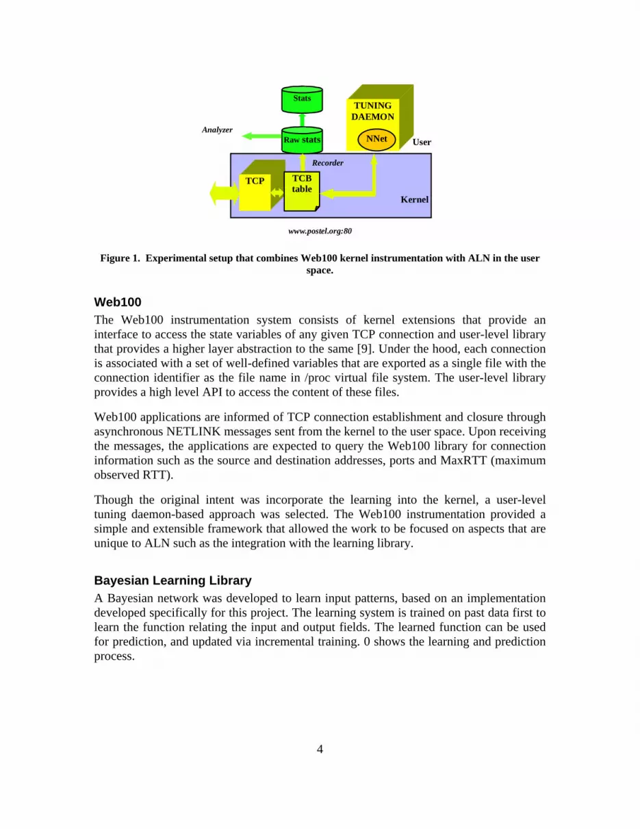
Figure 1. Experimental setup that combines Web100 kernel instrumentation with ALN in the user

space.

Web100 The Web100 instrumentation system consists of kernel extensions that provide an interface to access the state variables of any given TCP connection and user-level library that provides a higher layer abstraction to the same [9]. Under the hood, each connection is associated with a set of well-defined variables that are exported as a single file with the connection identifier as the file name in /proc virtual file system. The user-level library provides a high level API to access the content of these files.

Web100 applications are informed of TCP connection establishment and closure through asynchronous NETLINK messages sent from the kernel to the user space. Upon receiving the messages, the applications are expected to query the Web100 library for connection information such as the source and destination addresses, ports and MaxRTT (maximum observed RTT).

Though the original intent was incorporate the learning into the kernel, a user-level tuning daemon-based approach was selected. The Web100 instrumentation provided a simple and extensible framework that allowed the work to be focused on aspects that are unique to ALN such as the integration with the learning library.

Bayesian Learning Library A Bayesian network was developed to learn input patterns, based on an implementation developed specifically for this project. The learning system is trained on past data first to learn the function relating the input and output fields. The learned function can be used for prediction, and updated via incremental training. 0 shows the learning and prediction process.

5

Fxxxxx1

Y1

Offline Training Period

Fxxxxx1

Y1

Predicting Period

Figure 2. Learning and Prediction

In the TCP protocol, the input fields are “address”, “hour”, “day”, “month”, “Loc_latitude”, “Loc_longitude”, and the output fields are “MaxCwnd”, “MinRTT”, “MaxRTT”, “PcktsIn”, “PcksIn”, “PcksOut”. The function to be learned is F (address, hour, day, month, Loc_latitude, Loc_longitude) -> the correct initial value for “MaxCwnd, MinRTT, PcktsIn, PcksIn, PcksOut”.

Discretization The primary limitation of the learning network is its inability to handle large ranges for input variables. A simple variable-specific quantization function that maps a large range of values to a small range (10-30) was used. The learning and prediction is in terms of the smaller range. An inverse map is used to translate predicted values to appropriate. The quantization function used is a either a static table that is based on empirical data collected or a simple linear function. For example, mapping function for latitude maps the -90° to +90° to the range 0-11 (f(x) = 6+ x/15). In case of MaxRTT, the quantization function is a table is constructed by analyzing the connection data. An inverse quantization function maps the quantized values back to the original range. The form of the inverse function, as before, depends on individual tables.

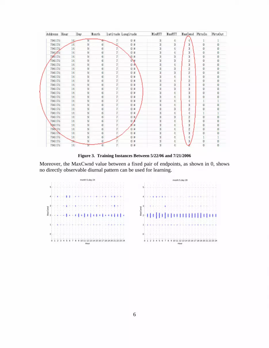
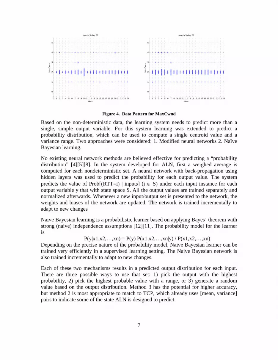
Nondeterministic Inputs ALN trained on a large data set (~ 1 million entries), and the data are non-deterministic. Even under the same input data set, the output value can vary. For example, 0 shows some instances extracted from collected data. For example, the same input vector has multiple MaxCwnd values.

6

Figure 3. Training Instances Between 5/22/06 and 7/21/2006

Moreover, the MaxCwnd value between a fixed pair of endpoints, as shown in 0, shows no directly observable diurnal pattern can be used for learning.

0 1 2 3 4 5 6 7 8 9 10 11 12 13 14 15 16 17 18 19 20 21 22 23 24

0

1

2

3

4

5

Hour

Max

Cw

nd

month:5,day:24

0 1 2 3 4 5 6 7 8 9 10 11 12 13 14 15 16 17 18 19 20 21 22 23 24

0

1

2

3

4

5

Hour

Max

Cw

nd

month:5,day:28

7

0 1 2 3 4 5 6 7 8 9 10 11 12 13 14 15 16 17 18 19 20 21 22 23 24

0

1

2

3

4

5

Hour

Max

Cw

nd

month:5,day:26

0 1 2 3 4 5 6 7 8 9 10 11 12 13 14 15 16 17 18 19 20 21 22 23 24

0

1

2

3

4

5

Hour

Max

Cw

nd

month:5,day:28

Figure 4. Data Pattern for MaxCwnd

Based on the non-deterministic data, the learning system needs to predict more than a single, simple output variable. For this system learning was extended to predict a probability distribution, which can be used to compute a single centroid value and a variance range. Two approaches were considered: 1. Modified neural networks 2. Naïve Bayesian learning.

No existing neural network methods are believed effective for predicting a “probability distribution” [4][5][8]. In the system developed for ALN, first a weighed average is computed for each nondeterministic set. A neural network with back-propagation using hidden layers was used to predict the probability for each output value. The system predicts the value of Prob[(RTT=i) | inputs] (i ∈ S) under each input instance for each output variable y that with state space S. All the output values are trained separately and normalized afterwards. Whenever a new input/output set is presented to the network, the weights and biases of the network are updated. The network is trained incrementally to adapt to new changes

Naive Bayesian learning is a probabilistic learner based on applying Bayes’ theorem with strong (naive) independence assumptions [12][11]. The probability model for the learner is

P(y|x1,x2,…,xn) = P(y) P(x1,x2,…,xn|y) / P(x1,x2,…,xn) Depending on the precise nature of the probability model, Naive Bayesian learner can be trained very efficiently in a supervised learning setting. The Naive Bayesian network is also trained incrementally to adapt to new changes.

Each of these two mechanisms results in a predicted output distribution for each input. There are three possible ways to use that set: 1) pick the output with the highest probability, 2) pick the highest probable value with a range, or 3) generate a random value based on the output distribution. Method 3 has the potential for higher accuracy, but method 2 is most appropriate to match to TCP, which already uses [mean, variance] pairs to indicate some of the state ALN is designed to predict.

8

Learning accuracy Ideally, if the true distribution of the output values is known, its mean and variance can be compared with that of the learned probability. However, in TCP, the true probability of the output values is unknown. A rough measure is the “exact-hit-ratio”. However, even if the probability is exactly known, the “exact-hit-ratio” will not be perfect. For example, flipping a coin and knowing the probability to be heads is 0.5, the “exact-hit-ratio” is only 50%.

The ALN learning network was trained on 90% of the data set and tested on the remaining 10% for preliminary analysis. The system converts a predicted distribution into the value that has the highest probability. To measure the accuracy of learning, fixed-prediction is used as the benchmark. Fixed prediction always predicts the output to be the value that occurs most frequently, no matter what inputs are. Comparison results are given below with Exact-hit-ratio H and Error-Variance S.

Results from Fixed prediction MinRTT: (H = 30.47%, S=1.9451); MaxCwnd: (H = 68.45%, S=0.8657)

PktIn: (H = 88.41%, S=0.5962)

Results from Neural Network learner: MinRTT: (H = 45.69%, S=1.3378); MaxCwnd: (H = 68.31%, S=0.8685)

PktIn: (H = 87.93%, S=0.6587)

Results from Naive Bayesian learner: MinRTT: (H = 47.55%, S =1.3697) MaxCwnd: (H = 68.34%, S=0.8709);

PktIn: (H = 88.41%, S=0.5965)

For the variable has more uncertainty feature (MinRTT), ALN prediction improves the “exact-hit-ratio” compared with fixed value predictions. For the other two variables, fixed prediction is already good enough.

Lookup Modules Lookup modules are used to compute ALN-specific variables. Examples include GeoIP for translating IP address into location information, calendar module to identify location-specific holidays, weather module to lookup weather information for any given location and a time module to compute day of the week, etc. [7]. The data analysis integrated these modules but the final experimentation only used GeoIP module. Some of issues associated with these lookup modules include incomplete and possibly inaccurate information (GeoIP, weather), ambiguous information (weather), textual word mismatch (location, weather) and cost (weather). The performance evaluation phase only uses the GeoIP module.

9

Tuning Daemon The tuning daemon, written in C, interfaces on one side with the Web100 library to set the congestion window variable of selected connections to appropriate value and on another side with the neural network to determine what that value should be. The primary function of the tuning daemon, as discussed in earlier sections, is to carefully ramp up the congestion window for a small subset of the connections.

The implementation is based on existing implementation of a Web100 tuning daemon called WAD (Work Around Daemon). It has been significantly rewritten and extended with ALN-specific code since then.

Data Collection Two modes of data collection were explored – client mode and server mode. In the client mode, a proxy server was setup to intercept all outgoing web accesses from a small set of users. In the server mode, a host was setup to serve www.postel.org. In both cases, the kernel was instrumented and user level process extracted all the connection information from the kernel and wrote them into a MySQL database.

Analysis showed that the client mode setup did not provide any opportunities for performance improvement because the congestion window depends on the amount of outgoing traffic and there was little traffic other than TCP acknowledgements. As a result, the client mode was not pursued and all discussion of results henceforth assumes a server mode setup.

In the server mode, only a subset of connections was considered for analysis. IPv6 connections were ignored for simplicity reasons. Also accesses from the search engine web crawlers were ignored. The website maintains an archive of hundreds of large documents. Sequential accesses to these documents skewed the data transfer patterns by accounting for up to 80% of the data transferred. Although they have to be accounted for in reality, the website is not a typical website in terms of file size distribution and claims about overall performance impact are extrapolated based only on the subset of connections considered here.

In all 173 parameters were collected for each connection. They include 147 parameters from Web100 and 26 parameters associated with ALN. Although Web100 variables focused on the connection parameters, ALN variables covered aspects such as weather, location and time. The first phase of the experiment which involved analysis stored all the information in multiple tables in a local MySQL database. Postprocessing scripts ensure that tables are complete and referential integrity is maintained. These scripts also generated input for analysis and testing the learning mechanism. The performance evaluation phase differs from the data analysis phase in two ways – primarily due to the limited nature of the experiment. First, it does not use any offline information/learning. Second, only the location and time information is used for prediction.

ALN requires the connections be long enough that there is value to optimizing through the reduction in the roundtrips but not too long. Since ALN optimizes only the slow start,

10

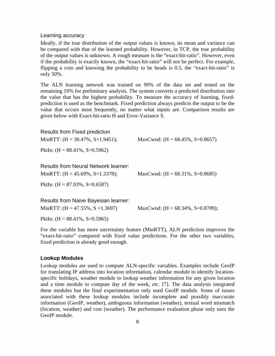
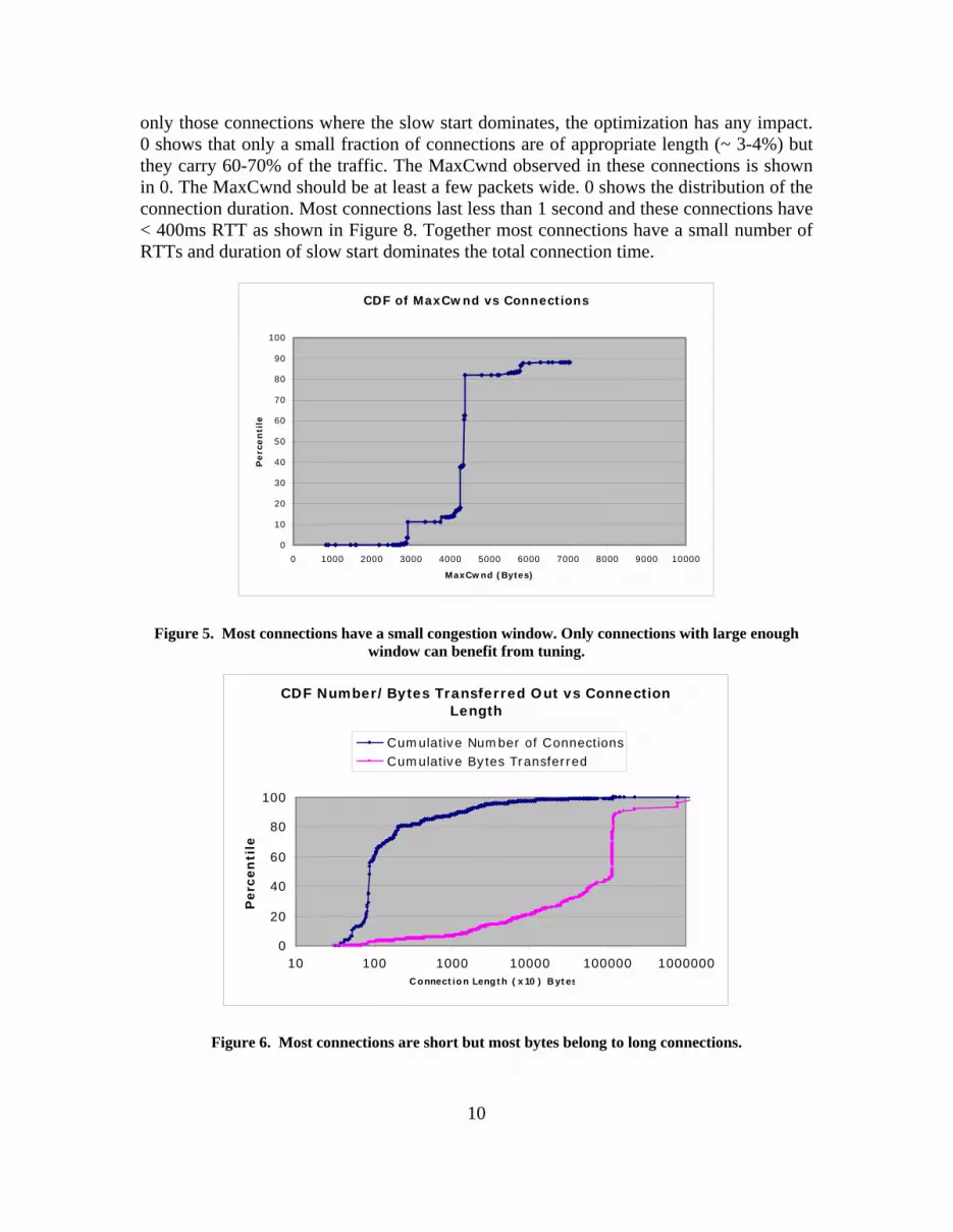
only those connections where the slow start dominates, the optimization has any impact. 0 shows that only a small fraction of connections are of appropriate length (~ 3-4%) but they carry 60-70% of the traffic. The MaxCwnd observed in these connections is shown in 0. The MaxCwnd should be at least a few packets wide. 0 shows the distribution of the connection duration. Most connections last less than 1 second and these connections have < 400ms RTT as shown in Figure 8. Together most connections have a small number of RTTs and duration of slow start dominates the total connection time.

CDF of MaxCwnd vs Connections

0

10

20

30

40

50

60

70

80

90

100

0 1000 2000 3000 4000 5000 6000 7000 8000 9000 10000

MaxCwnd (Bytes)

Perc

en

tile

Figure 5. Most connections have a small congestion window. Only connections with large enough window can benefit from tuning.

CDF Number/Bytes Transferred Out vs Connection Length

0

20

40

60

80

100

10 100 1000 10000 100000 1000000C o nnect io n Leng t h ( x 10 ) B yt es

Perc

en

tile

Cumulative Number of ConnectionsCumulative Bytes Transferred

Figure 6. Most connections are short but most bytes belong to long connections.

11

CDF of Connection Duration

0

10

20

30

40

50

60

70

80

90

100

10 100 1000 10000 100000

Dur a t i on of Conne c t i on ( ms)

Number of Connect ions

Figure 7. ALN can improve connections that last long enough to open the congestion window but short enough that transients dominate.

CDF of MaxRTT

0

10

20

30

40

50

60

70

80

90

100

0 50 100 150 200 250 300 350 400

MaxRTT (ms)

Perc

en

tile

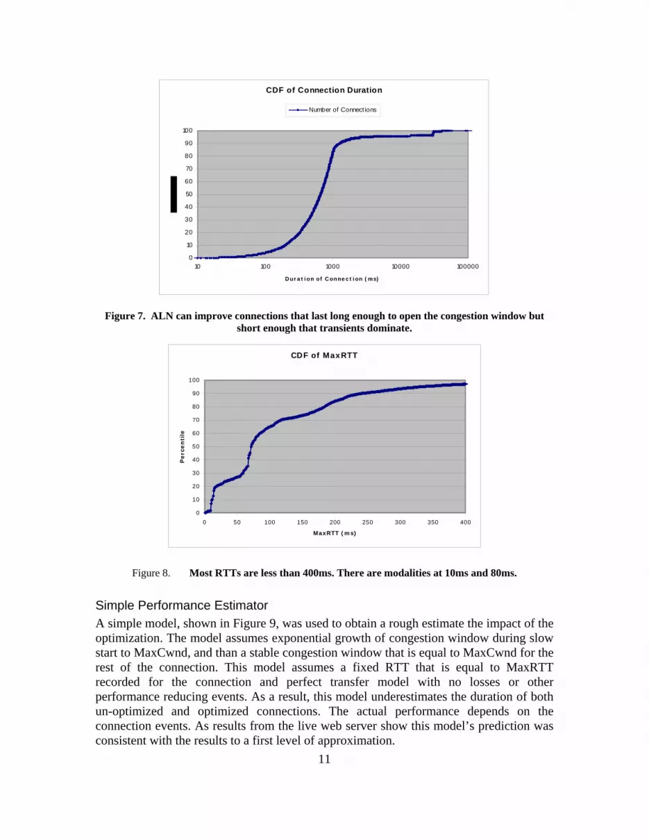
Figure 8. Most RTTs are less than 400ms. There are modalities at 10ms and 80ms.

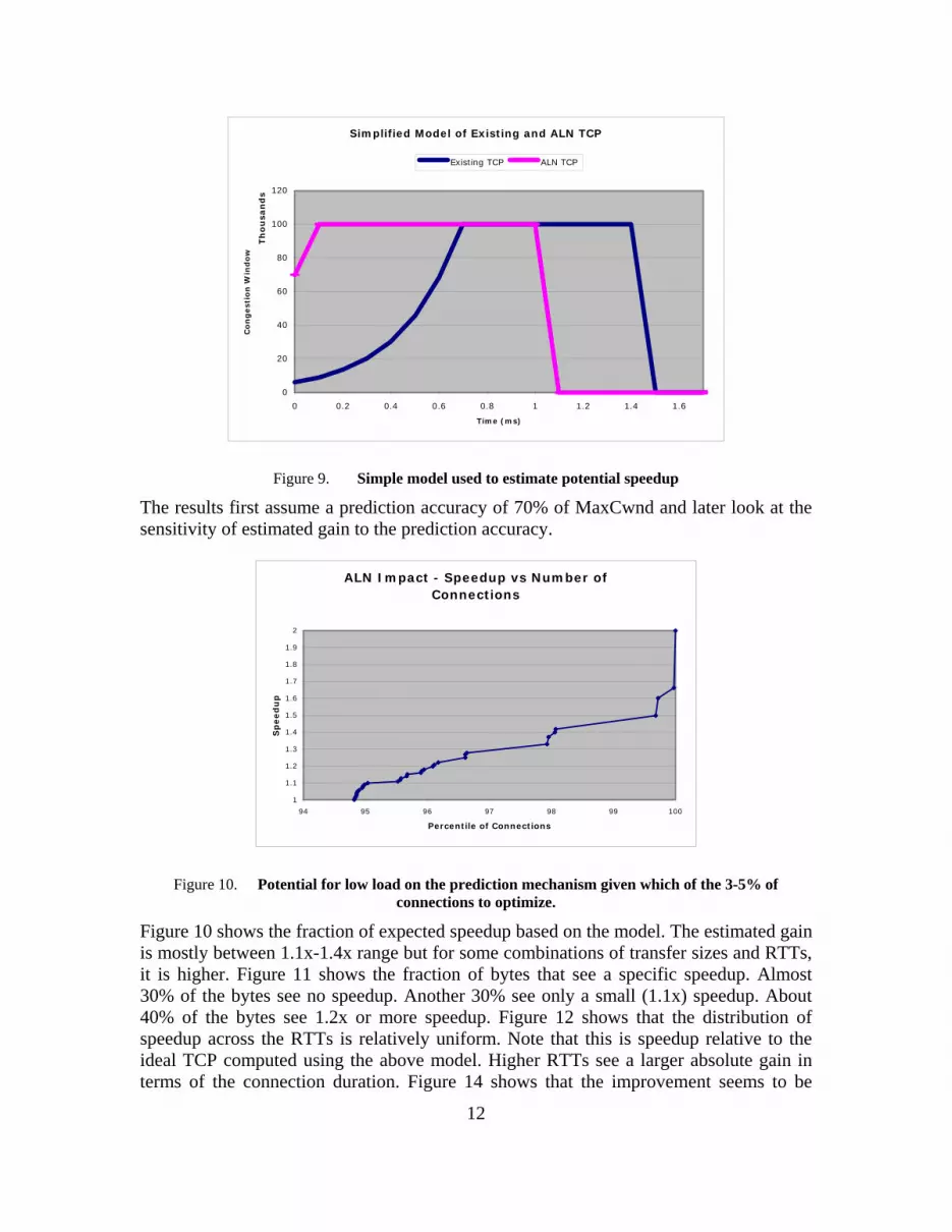
Simple Performance Estimator A simple model, shown in Figure 9, was used to obtain a rough estimate the impact of the optimization. The model assumes exponential growth of congestion window during slow start to MaxCwnd, and than a stable congestion window that is equal to MaxCwnd for the rest of the connection. This model assumes a fixed RTT that is equal to MaxRTT recorded for the connection and perfect transfer model with no losses or other performance reducing events. As a result, this model underestimates the duration of both un-optimized and optimized connections. The actual performance depends on the connection events. As results from the live web server show this model’s prediction was consistent with the results to a first level of approximation.

12

Simplified Model of Existing and ALN TCP

0

20

40

60

80

100

120

0 0.2 0.4 0.6 0.8 1 1.2 1.4 1.6

Th

ou

san

ds

Time (ms)

Co

ng

est

ion

Win

do

w

Existing TCP ALN TCP

Figure 9. Simple model used to estimate potential speedup

The results first assume a prediction accuracy of 70% of MaxCwnd and later look at the sensitivity of estimated gain to the prediction accuracy.

ALN Impact - Speedup vs Number of Connections

1

1.1

1.2

1.3

1.4

1.5

1.6

1.7

1.8

1.9

2

94 95 96 97 98 99 100

Percentile of Connections

Sp

eed

up

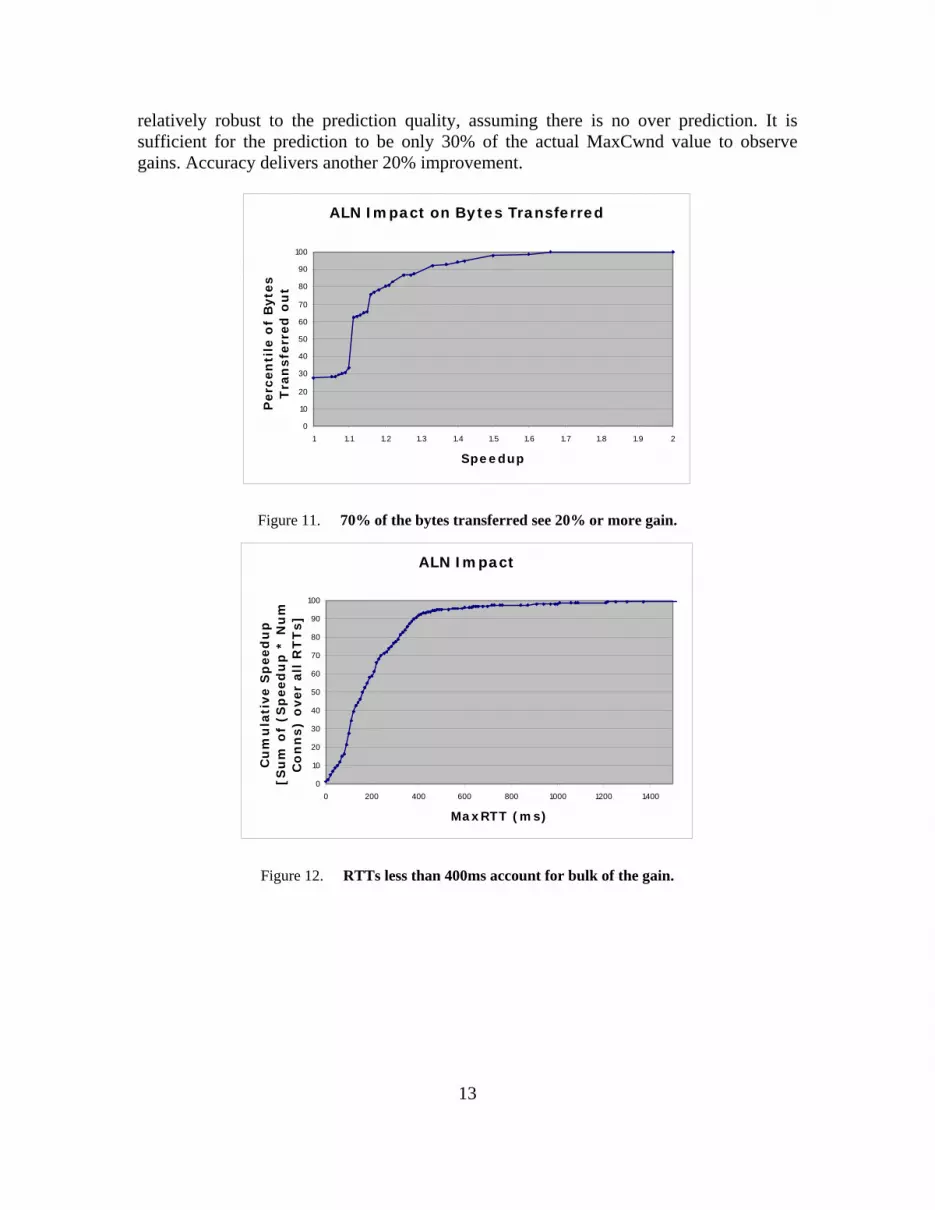
Figure 10. Potential for low load on the prediction mechanism given which of the 3-5% of connections to optimize.

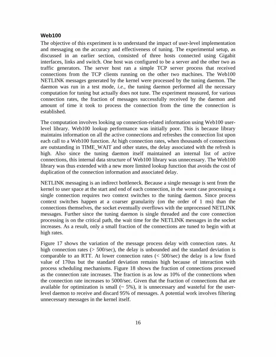
Figure 10 shows the fraction of expected speedup based on the model. The estimated gain is mostly between 1.1x-1.4x range but for some combinations of transfer sizes and RTTs, it is higher. Figure 11 shows the fraction of bytes that see a specific speedup. Almost 30% of the bytes see no speedup. Another 30% see only a small (1.1x) speedup. About 40% of the bytes see 1.2x or more speedup. Figure 12 shows that the distribution of speedup across the RTTs is relatively uniform. Note that this is speedup relative to the ideal TCP computed using the above model. Higher RTTs see a larger absolute gain in terms of the connection duration. Figure 14 shows that the improvement seems to be

13

relatively robust to the prediction quality, assuming there is no over prediction. It is sufficient for the prediction to be only 30% of the actual MaxCwnd value to observe gains. Accuracy delivers another 20% improvement.

ALN Impact on Bytes Transferred

0

10

20

30

40

50

60

70

80

90

100

1 1.1 1.2 1.3 1.4 1.5 1.6 1.7 1.8 1.9 2

Speedup

Perc

en

tile

of

Byte

s

Tra

nsfe

rred

ou

t

Figure 11. 70% of the bytes transferred see 20% or more gain.

ALN Impact

0

10

20

30

40

50

60

70

80

90

100

0 200 400 600 800 1000 1200 1400

MaxRTT (ms)

Cu

mu

lati

ve S

peed

up

[S

um

of

(Sp

eed

up

* N

um

C

on

ns)

over

all

RT

Ts]

Figure 12. RTTs less than 400ms account for bulk of the gain.

14

Estimated ALN Speedup vs Prediction Accuracy

0

10

20

30

40

50

60

70

80

90

100

1 1.2 1.4 1.6 1.8 2

Speedup

Byte

s T

ran

sferr

ed

Ou

t (P

erc

en

tile

)

Accuracy=10%

Accuracy=20%

Accuracy=30%

Accuracy=40%

Accuracy=50%

Accuracy=60%

Accuracy=70%

Accuracy=80%

Accuracy=90%

Figure 13. Poor (under)prediction is better than none. Fair prediction can add another 20% improvement.

Stress Testing The objective of the stress tests is to find out potential bottlenecks in the system. The basic result here is that (1) for the Bayesian learning system and parameters explored, learning performance is not the issue, and (2) the asynchronous messaging used by Web100, and therefore by the user-space tuning daemon, results in a negative interaction with the process scheduler at high connection rates. This has a significant impact on the accuracy and fraction of connections tuned.

Bayesian Learning Library The Bayesian learning network was trained using 10,000 examples and evaluated the prediction performance over another 10,000 examples. All the data was randomly generated. However that does not materially affect the results since the data structure accesses are fairly independent of the values of the individual inputs and depend on structural aspects such as the number and range of inputs. Further, the performance, and not accuracy, of the prediction is being evaluated here.

Experiments determined the scalability of the learning network. The parameters associated with the learning system were varied - the number of input variables, output variables and the range associated with each variable. The normalized time to predict an output variable linearly increases with the number of input variables as shown in Figure 14. However prediction time for each output is almost independent of the number of the output parameters, as shown in Figure 15. Note that the y-axis scale is in terms of microseconds and in absolute terms the speed of prediction is not an issue unless each of the parameters is at the higher end of the ranges considered (Figure 16). The experiments use 4 input variables, 1 output variable and range of up to 24.

15

Normalized Prediction Time (per output) vs. Number of Inputs

0

5

10

15

20

25

30

35

40

0 5 10 15 20 25 30 35

Number of Input Variables

Pre

dic

tio

n T

ime/

Ou

tpu

t (i

n m

icro

secs

)

Figure 14. Prediction time for each output variable increases linearly with input parameters.

Normalized Prediction Time (per output) vs Number of Outputs

5

7

9

11

13

15

17

19

0 2 4 6 8 10 12

Number of Outputs

Pre

dic

tio

n T

ime/

Ou

tpu

t (i

n m

icro

secs

)

Figure 15. Prediction time for output variables is independent of the number of output variables.

Normalized Prediction Time (per Output) vs Range of Variables

0

10

20

30

40

50

60

70

0 10 20 30 40 50 60

Range of Variable (Both Input and Output Variables)

Pre

dic

tio

n T

ime p

er

Ou

tpu

t (i

n

mic

rose

cs)

Figure 16. Prediction time for each output increases linearly with range of each variable.

16

Web100 The objective of this experiment is to understand the impact of user-level implementation and messaging on the accuracy and effectiveness of tuning. The experimental setup, as discussed in an earlier section, consisted of three hosts connected using Gigabit interfaces, links and switch. One host was configured to be a server and the other two as traffic generators. The server host ran a simple TCP server process that received connections from the TCP clients running on the other two machines. The Web100 NETLINK messages generated by the kernel were processed by the tuning daemon. The daemon was run in a test mode, i.e., the tuning daemon performed all the necessary computation for tuning but actually does not tune. The experiment measured, for various connection rates, the fraction of messages successfully received by the daemon and amount of time it took to process the connection from the time the connection is established.

The computation involves looking up connection-related information using Web100 user-level library. Web100 lookup performance was initially poor. This is because library maintains information on all the active connections and refreshes the connection list upon each call to a Web100 function. At high connection rates, when thousands of connections are outstanding in TIME_WAIT and other states, the delay associated with the refresh is high. Also since the tuning daemon itself maintained an internal list of active connections, this internal data structure of Web100 library was unnecessary. The Web100 library was thus extended with a new more limited lookup function that avoids the cost of duplication of the connection information and associated delay.

NETLINK messaging is an indirect bottleneck. Because a single message is sent from the kernel to user space at the start and end of each connection, in the worst case processing a single connection requires two context switches to the tuning daemon. Since process context switches happen at a coarser granularity (on the order of 1 ms) than the connections themselves, the socket eventually overflows with the unprocessed NETLINK messages. Further since the tuning daemon is single threaded and the core connection processing is on the critical path, the wait time for the NETLINK messages in the socket increases. As a result, only a small fraction of the connections are tuned to begin with at high rates.

Figure 17 shows the variation of the message process delay with connection rates. At high connection rates (> 500/sec), the delay is unbounded and the standard deviation is comparable to an RTT. At lower connection rates (< 500/sec) the delay is a low fixed value of 170us but the standard deviation remains high because of interaction with process scheduling mechanisms. Figure 18 shows the fraction of connections processed as the connection rate increases. The fraction is as low as 10% of the connections when the connection rate increases to 5000/sec. Given that the fraction of connections that are available for optimization is small (~ 5%), it is unnecessary and wasteful for the user-level daemon to receive and discard 95% of messages. A potential work involves filtering unnecessary messages in the kernel itself.

17

Time to Tune

0

5000

10000

15000

20000

25000

30000

35000

40000

45000

0 500 1000 1500 2000 2500 3000 3500 4000 4500 5000

Connection Delay Units (1 unit is 0.5 us approx)

Un

its

(dep

en

ds

on

vari

ab

le)

Rate (Connections/sec)

Time to Tune from Connection Start (microsecs)

Standard Deviation of Time to Tune (in microsecs)

Figure 17. At high rates, the time to tune is high both in absolute terms and in terms of standard deviation. At rates <= 500 connections/sec, the time to tune is a low fixed value (170us).

Tuning Efficiency

0

500

1000

1500

2000

2500

3000

3500

4000

4500

5000

0 1000 2000 3000 4000 5000

Delay Units (1 = approx 0.4 us)

Con

nect

ion

s/se

c

0

10

20

30

40

50

60

70

80

90

100

Perc

en

tag

e o

f C

on

nect

ion

s T

un

ed

Rate (Connections/sec) Fraction of Connections Tuned

Figure 18. At high rates, most connections to untuned because of high load.

Performance The experiment was setup as follows: A live web server (www.postel.org) with real traffic was used. The configuration of the machine is same as described in the previous section for data collection including the hardware (Dual 1Ghz PIII with 1GB memory) and operating system (Linux Fedora Core 5 patched with Web100 kernel extension). The http server used was Apache version 2.0.54. The Web100 components were extended in two ways. First, a Web100 variable was added to the kernel component to enable updating the congestion window in the kernel (CurCwnd). Second, the user-level Web100 library was extended with a new primitive to reduce connection lookup costs, as discussed in the previous section. The performance of the Bayesian learning library or the user-kernel messaging is not an issue because of the low connection rate. An ALN-specific output filter was written for the Apache web server [3] to compute the expected

18

size of the transfer for each connection and inform the tuning daemon of the same. This information is used only to determine whether or not to tune and not during the tuning process. In general this information is not available with the tuning daemon or sometimes even to the application itself. The learning system would have to be extended in future to predict the transfer size before deciding to tune or not. Due to limited time and scope of the experiment, this line of enquiry could not be pursued. Also, for the same reason the tuning phase has fewer samples than the data collection phase. The results therefore should be considered as indicative of the potential more rather than absolute performance levels.

For each incoming connection, the tuning daemon selects a tuning strategy at random from a fixed set that includes a “null” strategy i.e., no tuning. The strategies differ in terms of how to interpret the results of the prediction. Note that the prediction by the Bayesian learning library is a two-tuple (mean, standard deviation). Further this mean and standard deviation are in terms of the quantized values and not actual values as discussed in the experimental setup section. As mentioned before, a quantization function maps the actual values of each variable to a small range and an inverse quantization function maps the value back to the actual range.

i) Null: Do not tune.

ii) FixedCwnd: Ignore the prediction. Use an arbitrary but fixed congestion window size of 72400

iii) PredMean (Low): Use the mean, but rounded to the nearest lower integer value, as input to the inverse quantization function.

iv) PredMean (High): Use the mean, but rounded to the nearest higher integer value, as input to the inverse quantization function.

v) PredMean (Round): Use the mean, but rounded to the nearest integer value, as input to the inverse quantization function.

Four variables were used as input to the learning system and one as output. The input variables include latitude, longitude, day of the month, and hour of the day. The output variable is the MaxCwnd. The value for the congestion window (CurCwnd) is based on the prediction for MaxCwnd. The choice of the four input variables is somewhat arbitrary. Future work will explore combinations of variables to identify which ones are better predictors and which ones are not.

The results compare performance of the various tuning strategies for connections to/from the same subnet. The null strategy is used as the baseline performance. To reduce spurious measurements, the comparison is reported only for those destinations that have more than a threshold number (10) of connections using the null strategy.

A total of 57,093 connections were observed during the experimental duration. A total of 7,772 connections (13.6% in number, 38.9% in bytes) were tuned using the various strategies out of which performance over 3852 connections (6.7%) is reported here.

19

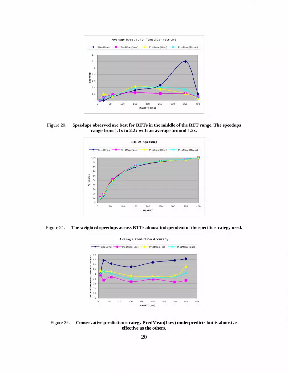
Figure 19 shows that the average speedups observed are between 1.16x and 1.22x. The distribution across the RTT range is shown in Figure 20. Connections with RTTs around 100-200ms have the most to gain. Too short RTTs and long RTTs don’t benefit as much because of short connection durations and small MaxCwnd respectively. Figure 19 shows the overall gain weighted with the number of connections across various RTTs. It shows that although there is variation in terms of gains for individual connections, the overall gain is same across the various strategies i.e., the gain is not too sensitive to the particular strategy used. Figure 21 shows the prediction accuracy of individual strategies. Any prediction ratio over 1.0 is over-prediction that makes the connection more aggressive than the untuned connection. Clearly the FixedCwnd strategy over predicts most of the time. PredMean(High) also consistently over-predicts. Although PredMean(Round) reduces the overprediction, and PredMean(Low) predicts the best. It consistently under-predicts but by not too much - only by 20-30%.

A few observations are in order. First, the basic results suggest that at some level any prediction is better than none. In this experiment the learning algorithm was simple, the quantization was coarse, and variables used were few. Even then the performance is quite reasonable. Second, the average gain reported is consistent with the simple performance model used in the previous section. Second, the coverage in terms of bytes is within the estimated range but towards the lower end. Third, the connections that can be tuned is significantly more than 4% estimated from the data collection phase which indicates a dependency on the particular website, file size and access distribution.

Average Speedup

1.13

1.14

1.15

1.16

1.17

1.18

1.19

1.2

1.21

1.22

1.23

FixedCwnd PredMean(Low) PredMean(High) PredMean(Round)

Strategy

Sp

eed

up

Figure 19. Average performance gain is around 1.2x

20

Average Speedup for Tuned Connections

1

1.2

1.4

1.6

1.8

2

2.2

2.4

0 50 100 150 200 250 300 350 400

MaxRTT (ms)

Sp

eed

up


Figure 20. Speedups observed are best for RTTs in the middle of the RTT range. The speedups range from 1.1x to 2.2x with an average around 1.2x.

CDF of Speedup

0

10

20

30

40

50

60

70

80

90

100

0 50 100 150 200 250 300 350 400

MaxRTT

Perc

en

tile


Figure 21. The weighted speedups across RTTs almost independent of the specific strategy used.

Average Prediction Accuracy

0

0.2

0.4

0.6

0.8

1

1.2

1.4

1.6

1.8

0 50 100 150 200 250 300 350 400 450

MaxRTT (ms)

Rati

o o

f P

red

icte

d/A

ctu

al

MaxC

wn

d


Figure 22. Conservative prediction strategy PredMean(Low) underpredicts but is almost as effective as the others.

21

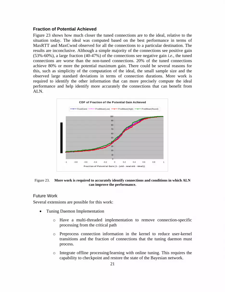
Fraction of Potential Achieved Figure 23 shows how much closer the tuned connections are to the ideal, relative to the situation today. The ideal was computed based on the best performance in terms of MaxRTT and MaxCwnd observed for all the connections to a particular destination. The results are inconclusive. Although a simple majority of the connections see positive gain (53%-60%), a large fraction (40-47%) of the connections see negative gain i.e., the tuned connections are worse than the non-tuned connections. 20% of the tuned connections achieve 80% or more the potential maximum gain. There could be several reasons for this, such as simplicity of the computation of the ideal, the small sample size and the observed large standard deviations in terms of connection durations. More work is required to identify the other information that can more precisely compute the ideal performance and help identify more accurately the connections that can benefit from ALN.

CDF of Fraction of the Potential Gain Achieved

0

10

20

30

40

50

60

70

80

90

100

-1 -0.8 -0.6 -0.4 -0.2 0 0.2 0.4 0.6 0.8 1

Fr a c t i on of P ot e nt i a l Ga i n ( 1 - ( ol d - ne w/ ol d - i de a l ) )


Figure 23. More work is required to accurately identify connections and conditions in which ALN can improve the performance.

Future Work Several extensions are possible for this work:

• Tuning Daemon Implementation

o Have a multi-threaded implementation to remove connection-specific processing from the critical path

o Preprocess connection information in the kernel to reduce user-kernel transitions and the fraction of connections that the tuning daemon must process.

o Integrate offline processing/learning with online tuning. This requires the capability to checkpoint and restore the state of the Bayesian network.

22

• Lookup Modules

o Build uniform representation to integrate multiple sources of information

o Identify a strategy to consistently handle the issues with the source (completeness, accuracy, performance)

• Prediction process

o Predict the transfer size in addition to the tuning

o Experiment with more variables such as weather and holidays.

o Use fine grained ranges for the input and output variables for greater accuracy

• Quantization

o Make the quantization table more dynamic and data dependent

Discussion of Established Targets Overall, this work was intended to measure the potential for performance improvement of a learning system on tuning TCP, to determine the feasibility of deploying an operational version of such a system, and to measure the benefit of such a system.

ALN developed models to predict the potential for speedup which accurately predicted the approximate range of such speedups when they occur, approximately 1.2x faster.

ALN deployed learning in an operational web server and found that it did not substantially impact server performance.

ALN measured the benefit of the deployed system, and found that the resulting system had mixed results.

Overall, the exercise showed that the application of learning to protocol tuning is feasible and possible, but that a number of substantial impediments remain to exploring this work further. These include the need for adaptive input discretization and methods to accommodate nondeterminism in the output values.

Publications (none)

Personnel Project Leader: Joseph Bannister.

Co-Project Leaders: Wei-Min Shen, Joseph D. Touch

23

Graduate research assistants:

o Feili Hou

o Venkata Pingali

Presentations No external presentations have been made.

Consultative and Advisory Functions There were no applicable functions performed during this report.

New Discoveries There were no new discoveries as part of this effort.

References [1] Adlib, J., Shen, W., Noorbakhsh, E., “Self-Similar Hidden Markov Model for

Predictive Modeling of Network Data,” SIPE DM: Data Mining and Knowledge Discovery: Theory, Tools, and Technology Intelligent Data Analysis, Florida 2002.

[2] Balakrishnan, H., Rahul, H., Seshan, S., “An Integrated Congestion Management Architecture for Internet Hosts,” Proc. ACM SIGCOMM, Cambridge, MA, September 1999.

[3] Braden, R., “T/TCP -- TCP Extensions for Transactions Functional Specification,” RFC-1644, July 1994.

[4] Bridle, J.S. “Training Stochastic Model Recognition Algorithms as Networks can lead to Maximum Mutual Information Estimation of Parameters.” In Touretzky, D., edit, Advances in Neural Information Processing Systems, Vol. 2, NIPS-89, Denver. Morgan Kaufman.

[5] Denke, J., leCun, Y., “Transforming Neural-Net Output Levels to Probability Distributions,” (AT&T Bell Labs Technical Memorandum 11359-901120-05, 1990.) Advances in Neural Information Processing Systems, Vol. 3 853-859. Morgan Kaufman, 1991.

[6] Floyd, S., “HighSpeed TCP for Large Congestion Windows,” RFC-3649, Experimental, December 2003.

[7] GeoIP http://www.maxmind.com [8] Hoekstra, A., Tholen, S., Duin,, R., “Estimating the reliability of neural network

classifications,” Proceedings of the ICANN’96, 53-58, 1996. [9] Mathis, M., Heffner, J., Reddy, R., “Web100: Extended TCP Instrumentation for

Research, Education and Diagnosis,” ACM Computer Communications Review, Vol 33, Num 3, July 2003.

[10] Postel, J. (ed.), “Transmission Control Protocol,” RFC 793, Sept.1981.

24

[11] Shen, W-M., Autonomous Learning from the Environment, W. H. Freeman, Computer Science Press, 1994. (Foreword by Herbert A. Simon)

[12] Stuart Russell and Peter Norvig. Artificial Intelligence: A Modern Approach. Prentice Hall, 1995

[13] Touch, J., “TCP Control Block Interdependence,” RFC-2140, ISI, April, 1997. The ALN project website is maintained at: http://www.isi.edu/aln

applied learning networks (aln)

Documents