applications of numerical limit analysis (nla) to stability problems of rock and soil masses

ARTICLE IN PRESS

1365-1609/$ - se

doi:10.1016/j.ijr

�CorrespondE-mail addr

International Journal of Rock Mechanics & Mining Sciences 43 (2006) 408–425

www.elsevier.com/locate/ijrmms

Applications of numerical limit analysis (NLA) to stability problems ofrock and soil masses

A.F. Duranda, E.A. Vargas Jr.b,�, L.E. Vazc

aCivil Engineering Laboratory, State University of Northern Rio de Janeiro (UENF), Av. Alberto Lamego, 2000, Campos dos Goytacazes,

CEP 28013-602, BrazilbDepartment of Civil Engineering, Catholic University of Rio de Janeiro (PUC-Rio), Rua Marques de Sao Vicente 225, Gavea,

CEP 22453-060, Rio de Janeiro, BrazilcDepartment of Civil Engineering, Federal University of Rio de Janeiro (UFRJ), Cidade Universitaria, CEP 21495-970, Rio de Janeiro, Brazil

Accepted 31 July 2005

Available online 3 November 2005

Abstract

This work presents formulations and results obtained with computer implementations of an alternative to the more standard

techniques for the determination of the state of collapse of geotechnical structures in rock or soil masses. Examples of normally available

and used techniques for those purposes are limit equilibrium based procedures and elasto-plastic finite elements. As an alternative to

these techniques, the present paper describes Numerical Limit Analysis (NLA). The fundamentals for limit analysis, summarized in the

so-called bound theorems, have been known for decades. Analytical solutions obtained with limit analysis are however limited in scope

and are seldom used in the engineering practice. NLA on the other hand, by solving the limit analysis equations through numerical

methods are general and applicable to a wide range of problems. The paper presents a discussion on available alternatives for the

formulation of NLA specialized for the determination of collapse load factors of geotechnical structures in/on rock (fractured or not)

and soil masses. Rock masses in particular are modelled as standard continua, Cosserat equivalent continua and true discontinua formed

by discrete blocks. Finite elements are used for the solution of NLA equations of standard continua and Cosserat continua. The paper

presents derivation of the pertinent equations, the numerical formulations used and details of their numerical implementation in

computer programs. Attempt was made to validate all the implementations through existing analytical solutions. The obtained results

permit to state that NLA is a promising and very often advantageous numerical technique to establish collapse states of geotechnical

structures in rock and soil masses.

r 2005 Elsevier Ltd. All rights reserved.

Keywords: Limit analysis; Numerical limit analysis; Fractured rocks; Discrete blocks; Cosserat continua; Standard continua

1. Introduction

In the design stage of a number of geotechnical problemssuch as the ones found in bearing capacity of foundations,retaining structures, slope stability and undergroundexcavations, a primary objective consists in the determina-tion of a collapse load, a maximum load the geotechnicalsystem is able to support before it collapses. These loadsare generally determined by limit equilibrium methods orelasto-plastic finite element analyses. In the present work,

e front matter r 2005 Elsevier Ltd. All rights reserved.

mms.2005.07.010

ing author. Tel.: +55 21 3114 1188; fax: +55 21 3114 1195.

ess: [email protected] (E.A. Vargas Jr.).

use is made of numerical limit analysis (NLA), analternative, often very advantageous technique in relationto the ones described but in general seldom used inpractice. The paper presents a theoretical background oflimit analysis and possibilities of its numerical implementa-tion. Main emphasis of the paper concerns applications ofthe technique for both continuum and discontinuumproblems. In the latter case, more relevant to RockMechanics situations, the medium can be represented bothby discrete blocks (true discontinua) and by Cosserat-typecontinua. Initially, the paper formulates the general limitanalysis problem. Subsequently, it describes its specializa-tion and numerical implementation for analysis of

www.elsevier.com/locate/ijrmms

ARTICLE IN PRESSA.F. Durand et al. / International Journal of Rock Mechanics & Mining Sciences 43 (2006) 408–425 409

standard continuua, Cosserat continua and true disconti-nuua (discrete blocks) problems. Application and valida-tion examples are presented and discussed. Finally, ageneral discussion on the possibilities of the use of NLA inpractical problems is presented.

2. Fundamentals of limit analysis

The interest in the study of collapse of engineeringstructures began with Coulomb in 1773 [1]. Coulombdeveloped plasticity concepts applied to soils as well as theconcept of a plastic limit as applied to retaining structures.Later, in 1857, Rankine introduced the concept of slip linesin order to interpret the plastic equilibrium of soils. Basedin such studies, the concept of limit analysis evolved, moreor less heuristically, until approximately 1950 in differentareas of engineering. In 1952, Drucker and Prager, in astudy of plastic materials obeying Mohr–Coulomb’s yieldcriterion [2,3], defined bounds (upper and lower) for thecollapse load.

The collapse load in stability problems can be obtainedin an independent way through the application of thetheorems of the limit analysis (upper bound or lowerbound). When the collapse load is obtained from anestablished statically admissible stress field, it is consideredto be a lower bound to the true collapse load. In the sameway, if the collapse load is obtained by means of anestablished kinematically compatible failure mechanism, itis considered to be an upper bound to the true collapseload. In practice, the establishment of kinematicallyadmissible failure mechanisms is in general easier whencompared with the establishment of statically admissiblestress fields. In this way, various analytical solutions areavailable today using various forms of simplified collapsemechanisms [4].

2.1. Limit analysis theorems

The application of the limit analysis theorems is possiblefor solid materials that present the following properties [1]:

1.
The plastic behavior of the material is perfect or ideallyplastic, i.e., the yield surface is fixed in the stress space.
2.
The yield surface is convex and the rates of plasticdeformation are obtained from a yield function throughan associated flow rule.
3.
Changes in the geometry of the body are consideredinsignificant when the loads reach the limit load state.The principle of virtual work can therefore be applied.
Central in the theory of limit analysis is the determinationof a collapse load factor, roughly speaking an analogousmeasure to the factor of safety in limit equilibrium. In thelower bound formulation, the collapse load factor, or (orsimply) the load factor can be defined as a multiplyingfactor (a scalar) by which the external loads have to bemultiplied in order that the structural system reaches

collapse. Similarly, in the upper bound formulation, theload factor is defined as a multiplying factor (also a scalar)by which the external work (work performed by theexternal loads) has to be multiplied in order that thestructural system reaches collapse. Formally, the lowerbound (or static) and the upper bound (kinematic)theorems can be stated as in the following:

Lower bound theorem (static theorem). A load factor lsthat corresponds to a statically admissible stress field, onethat satisfies (a) equilibrium equations in the domain, (b)equilibrium equations on the boundary and (c) nowhere inthe domain the yield function is violated, will not exceedthe true load factor of the structure.

Upper bound theorem (kinematic theorem). The kinematicload factor lk as determined by equating the rate ofexternal work with the rate of internal dissipation of energyalong a kinematically admissible velocity field (_u), one thatsatisfies (a) the velocity boundary condition and (b) thecompatibility relations between strain rates and velocity, isnot less than the true collapse load factor.According to the principles of continuum mechanics, the

statements contained in both upper and lower boundtheorems can be stated mathematically by the followingequations:Given

f in O ðbody forcesÞ;

t on Gt ðboundary forces; tractionsÞ;

Find l, r, _u, _e, e, _c such that the following conditions aresatisfied:Static equilibrium:

rTr ¼ lf in O;

rg ¼ lt on Gt;(1)

Yield criterion:

f ðrÞp0 in O, (2)

Kinematic consistency:

_e ¼ r _u in O;

_u ¼ 0 on Gu;(3)

Flow rule:

_ep ¼ _gqfqs

_g ¼ 0 if f ðrÞo0;

_gX0 if f ðrÞ ¼ 0;(4)

where f is the vector of body forces, t the boundary forces,tractions, g the unit vector normal to surface Gt, r thestress field, _u the velocity (displacement rate) field, _ep theplastic strain rates field, l the collapse load factor and _g theplastification factor.The complete solution of the problem of establishing

collapse of a system considering both statically andkinematically admissible fields must use Eqs. (1)–(4). Theproblem however can be solved by considering either astatically admissible field or a kinematically admissiblefield. When the collapse load of the system is obtained

ARTICLE IN PRESSA.F. Durand et al. / International Journal of Rock Mechanics & Mining Sciences 43 (2006) 408–425410

through conditions represented by Eqs. (1) and (2), theformulation is denominated static (lower bound). On theother hand if the collapse load of the system is obtainedthrough the use of Eqs. (3) and (4), the formulation isdenominated kinematic (or upper bound). Alternativeformulations, denominated mixed formulations, are theones that consider at the same time all Eqs. (1)–(4).However, obtaining solutions to all equations is in generalvery cumbersome and difficult.

3. Numerical limit analysis of geotechnical problems

Lower ðlsÞ and upper ðlkÞ bound estimates of thecollapse load factor can be obtained by both analyticaland computational methods. Finding analytical solutionsfor practical engineering soil and rock mechanics problemsis, however, a difficult task. Chen [1], Chen and Liu [4] andFinn [5] have presented purely analytical applications oflimit analysis to some practical geotechnical problems. Inthe case of lower bound solutions, statically admissiblestress fields have to be assumed, whereas in the case ofupper bound solutions, a kinematically admissible velocityfield must be assumed. In the latter case, this can be doneby establishing a failure mechanism. In the seventies,numerical methods, the finite element method in particular,together with mathematical programming techniques, werebrought into use to solve limit analysis problems. Thesimultaneous solution of Eqs. (1)–(4), even numerically, isno easy task due to the complexity in finding simulta-neously statically admissible stress fields and kinematicallyadmissible velocity fields. Formally, for any of the above-mentioned formulations, the set of corresponding equa-tions constitute a mathematical programming (optimiza-tion) constrained problem. This optimization problem canbe either linear or non-linear. In the particular case of limitanalysis this distinction will depend on the form of the yieldcondition (2) used.

A number of alternative formulations and numericalimplementations are available in the technical literature[3,6–20]. Basically, the strategies described in above-mentioned papers differ in the way the equilibrium andcompatibility equations are considered and assumptionsmade about the stress and velocity fields. In the sequence,based on the characteristics of the existing formulations, anattempt is made on classifying them. Initially, the strategiesare classified according to the method used for discretizingthe equilibrium and compatibility equations. In sequencethe strategies are classified according to the assumptionsmade regarding stress and velocity fields.

3.1. Classification according to the method used for

discretizing the equilibrium and compatibility equations

When the discretization of the equilibrium or compat-ibility equations is obtained through the explicit applica-tion of the differential equations of equilibrium orcompatibility (Eqs. (1) and (3)), in points and predeter-

mined directions, the corresponding strategies are denomi-nated strong formulations of limit analysis. In contrast,weak formulations can be obtained via the use of theprinciple of virtual work.

3.2. Classification according to assumptions made about

admissibility of stress and velocity fields

When the solution of the problem posed guarantees that,in all points of the domain, the stress field is staticallyadmissible, the formulation is denominated as lowerbound. Alternatively, when the solution of the problemguarantees that the velocity field is kinematically admis-sible, the formulation is denominated as upper bound.When, on the other hand, the formulations do notguarantee these conditions in the domain, they aredesignated as approximate formulations. In this case, it isexpected that the solution converges to the true solutionwhen the mesh is refined but the convergence does notrespect bounds.Besides the two broad classes of formulations described

above, one also distinguishes the so-called mixed formula-tions, so denominated because they consider as unknownsboth the stress and the kinematic fields satisfying partiallyor totally, respectively, the static and kinematic conditions.It is, therefore, possible to classify some of the published

formulations for the problem of limit analysis. Theformulations presented by [3,7,11] could be classified asstrong formulations with statically admissible stress fields.The formulations presented by [7,12,19] could be classifiedas strong formulations with kinematically admissiblevelocity fields. Examples of weak formulations withstatically approximated stress fields are described by [6,20].

3.3. Formulations used in the present work

The present work does not intend to present a discussionon pros and cons of the different formulations. Instead,two particular formulations are described and usedthroughout the paper, emphasis being on their applicabilityto stability problems in Rock and Soil Mechanics. A strongformulation with statically admissible stress field is appliedto systems of discrete rigid blocks simulating a fractured(blocky) rock mass. A weak formulation with a staticallyapproximate stress fields is applied to the solution of rockand soil mechanics problems where the geological mediumis modelled by both conventional and Cosserat continua[17,21].

4. Numerical formulation of limit analysis

4.1. Rock mass modelled as a discontinuum (discrete

blocks)

This section describes the use of a strong formulationassociated with a statically admissible stress field toperform limit analysis of a discontinuum simulating a

ARTICLE IN PRESS

Block j

Block i

C

x i

x c

x j

y jy i y cx

y

f s ci

f n ci

f n cj

f s cj

Block i

Block j

C

(a) (b)

α

α

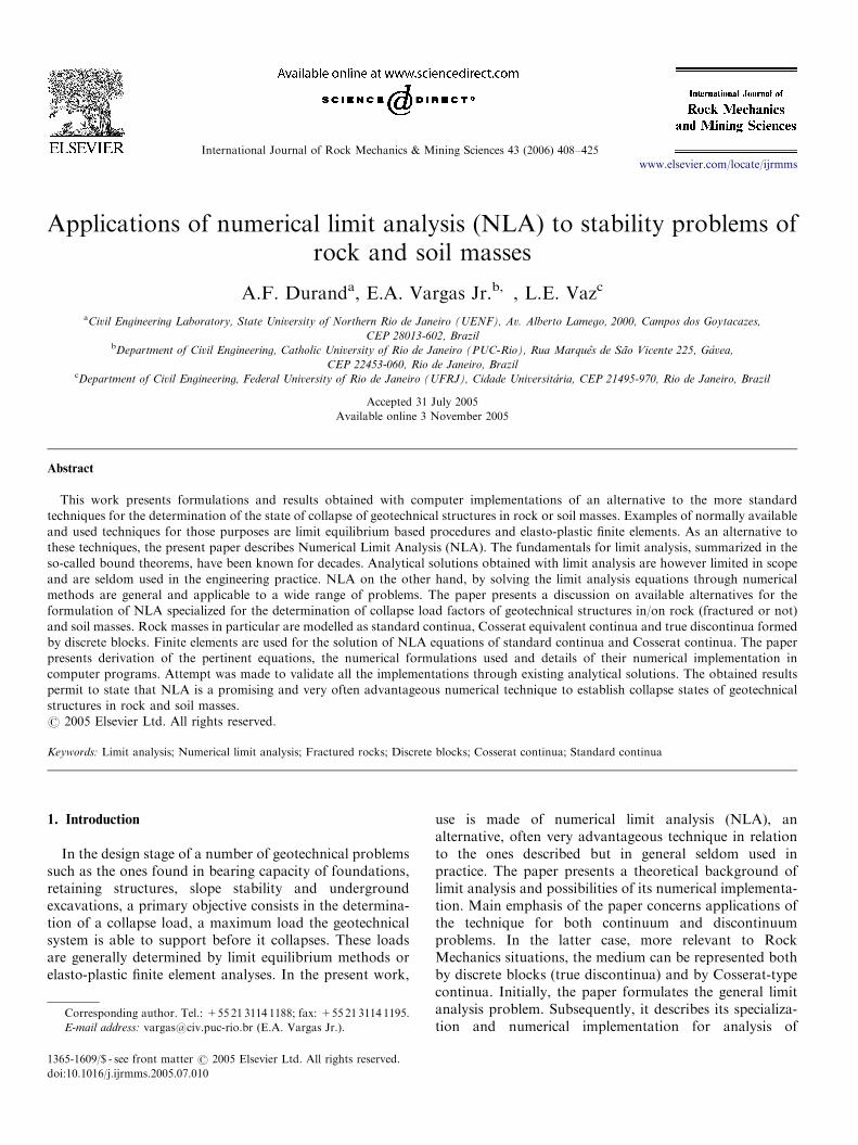
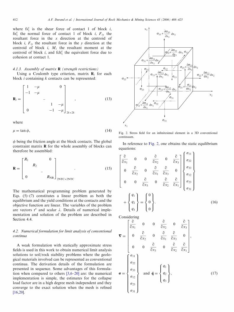
Fig. 1. Geometry of block contacts: (a) global reference system; (b)

normal and tangential forces in contact C. Angle a is the angle between the

block surface and the horizontal.

A.F. Durand et al. / International Journal of Rock Mechanics & Mining Sciences 43 (2006) 408–425 411

fractured (blocky type) rock mass. The medium iscomposed of a system of discrete rigid blocks. The

L ¼

cos a1 sin a1� sin a1 cos a1 0

cos a2 sin a2� sin a2 cos a2

:::

0 cos ak sin ak

� sin ak cos ak

2666666666664

37777777777752k�2k

, (9)

A ¼

1 0 1 0 ::: 1 0

0 1 0 1 ::: 0 1

ðyc1 � yiÞ ðxc

1 � xiÞ ðyc2 � yiÞ ðxc

2 � xiÞ ::: ðyck � yiÞ ðxc

k � xiÞ

264

3753�2k

, (10)

procedure adopted follows the work of Livesley [22] whostated that the collapse behavior of a structure formed bydiscrete, rigid blocks (Fig. 1) can be formulated byequilibrium statements for each block and by strengthconstraints at each block interface. In the context of thepresent work, a linear Coulomb type criterion is used forthat matter. The mathematical programming (optimiza-tion) problem can in this case be stated as:

Maximize l (5)

subject to

Hrc ¼ lq equilibrium condition, (6)

Rrcprf yield condition, (7)

where NB is the total number of blocks of the system, NCthe total number of contacts of all blocks, H theequilibrium matrix which relates the forces at each blockcontact with the forces and moments and each blockcentroid (3NB� 2NC), R the matrix of coefficients of thefailure (yield ) criterion (2NC� 2NC), q the vector offorces and moments at each block centroid (3NB), rc thevector of forces at each contact (2NC) and rf the vector offailure criterion constants (2NC).

The assembly of the described matrices and vectors aredescribed next according to the diagrams shown in Fig. 1.A more complete derivation of the matrices presentedbelow can be found in [23].

4.1.1. Assembly of matrix H (equilibrium of blocks)

The assembly of matrix H for the whole structure isobtained by incorporation of each individual Hi matrix foreach block. With reference to Fig. 1, the assembly of eachHi for a block i is given by

Hi ¼ AL, (8)

where L is the local to global reference system transforma-tion matrix, and A the equilibrium matrix consideringforces and moments at the centroid of each block i, and L

and A are given by

where k is the number of contact points for each block i.The global matrix H for the whole assembly of blocks

can therefore be assembled:

H ¼

H1 0

H2

:::

0 HNB

26664

377753NB�2NTC

. (11)

4.1.2. Assembly of vectors q, rc and ruiVectors qi, r

c and uui are given by

rci ¼

fscs1

fnc1

fsc2

fnc2

:

:

fsck

fnck

8>>>>>>>>>>>>>><>>>>>>>>>>>>>>:

9>>>>>>>>>>>>>>=>>>>>>>>>>>>>>;

2k

; qi

F ix

F iy

Mi

8><>:

9>=>;; rfi ¼

fchc1

fchc1

fchc2

fchc2

:

:

fchck

fchck

8>>>>>>>>>>>>>><>>>>>>>>>>>>>>:

9>>>>>>>>>>>>>>=>>>>>>>>>>>>>>;

2k

, (12)

ARTICLE IN PRESS

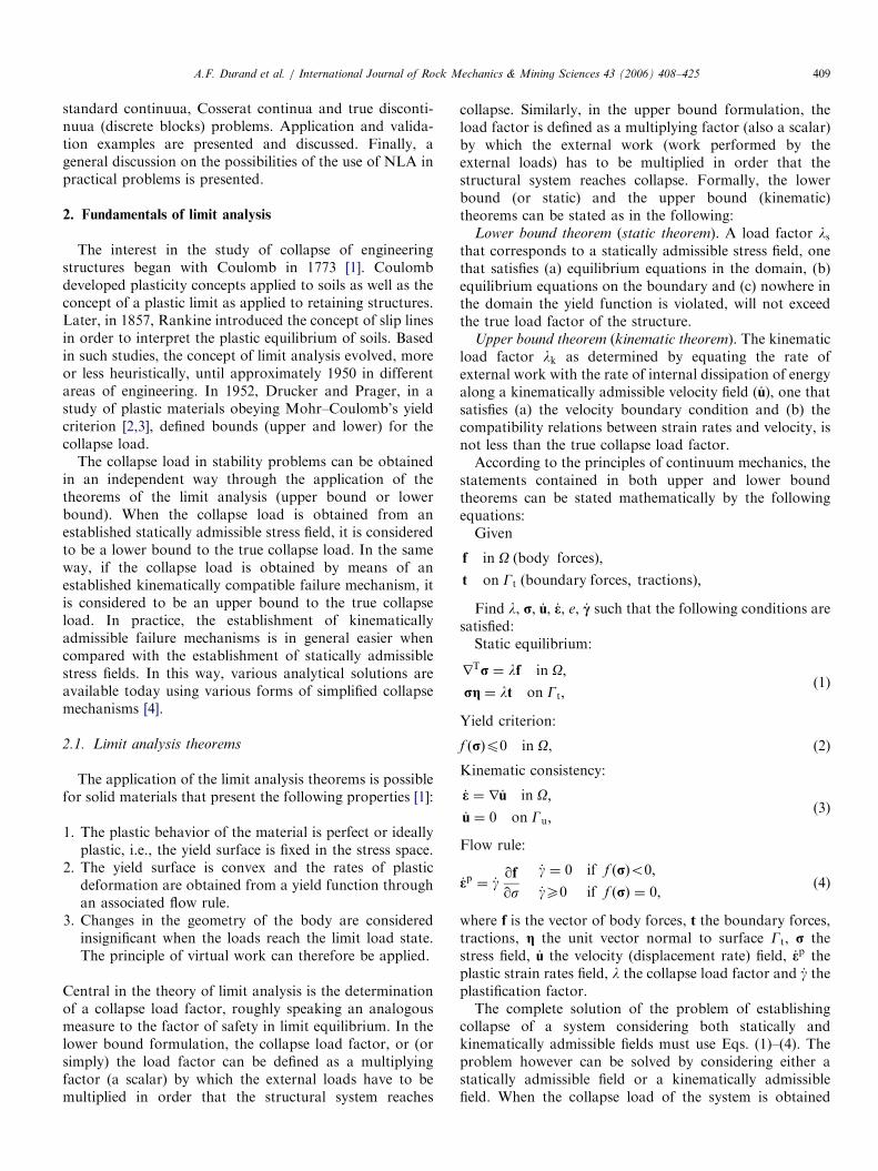
dx3+σ33

x3

σ11∂x3

∂x3

∂σ31

∂σ32

∂σ33

σ32 dx3+

A.F. Durand et al. / International Journal of Rock Mechanics & Mining Sciences 43 (2006) 408–425412

where fsc1 is the shear force of contact 1 of block i,fnc1 the normal force of contact 1 of block i, F ix theresultant force in the x direction at the centroid ofblock i, Fiy the resultant force in the y direction at thecentroid of block i, Mi the resultant moment at thecentroid of block i, and fchc1 the equivalent force due tocohesion at contact 1.

dx2+σ22

x1

x2

σ12

σ33

σ22

dx1∂x1

∂σ11

dx1∂x1

∂x1

∂x2

∂x3

∂σ12

∂σ13

∂σ23

∂σ22

+σ11

σ12

σ13

σ21

σ23

σ31

σ32

+

dx1+σ13

dx2σx2

σx2

σ21 +σ21

dx2 +σ23

dx3+σ31

Fig. 2. Stress field for an infinitesimal element in a 3D conventional

continuum.

4.1.3. Assembly of matrix R (strength restrictions)

Using a Coulomb type criterion, matrix Ri for eachblock i containing k contacts can be represented:

Ri ¼

1 �m 0

�1 �m

::

1 �m

0 �1 �m

26666664

377777752k�2k

, (13)

where

m ¼ tanf, (14)

f being the friction angle at the block contacts. The globalconstraint matrix R for the whole assembly of blocks cantherefore be assembled:

R ¼

R1 0

R2

::

0 RNB

26664

377752NTC�2NTC

. (15)

The mathematical programming problem generated byEqs. (5)–(7) constitutes a linear problem as both theequilibrium and the yield conditions at the contacts and theobjective function are linear. The variables of the problemare vectors rc and scalar l. Details of numerical imple-mentation and solution of the problem are described inSection 4.4.

4.2. Numerical formulation for limit analysis of conventional

continua

A weak formulation with statically approximate stressfields is used in this work to obtain numerical limit analysissolutions to soil/rock stability problems where the geolo-gical materials involved can be represented as conventionalcontinua. The derivation details of the formulation arepresented in sequence. Some advantages of this formula-tion when compared to others [3,6–20] are: the numericalimplementation is simple, the estimates for the collapseload factor are in a high degree mesh independent and theyconverge to the exact solution when the mesh is refined[16,20].

In reference to Fig. 2, one obtains the static equilibriumequations:

qqx1

0 0qqx2

0qqx3

0qqx2

0qqx1

qqx3

0

0 0qqx3

0qqx2

qqx1

2666666664

3777777775

s11

s22

s33

s12

s23

s31

8>>>>>>>>>>><>>>>>>>>>>>:

9>>>>>>>>>>>=>>>>>>>>>>>;

þ

q1

q2

q3

8>><>>:

9>>=>>; ¼

0

0

0

8>><>>:

9>>=>>;. ð16Þ

Considering

= ¼

qqx1

0 0qqx2

0qqx3

0qqx2

0qqx1

qqx3

0

0 0qqx3

0qqx2

qqx1

2666666664

3777777775,

r ¼

s11

s22

s33

s12

s23

s31

8>>>>>>>>>>><>>>>>>>>>>>:

9>>>>>>>>>>>=>>>>>>>>>>>;

and q ¼

q1

q2

q3

8>><>>:

9>>=>>;, ð17Þ


where r is the stress field vector, q the applied body forcesvector, = the differential operator matrix.

Eq. (16) may be written as

=rþ q ¼ 0. (18)

The deformation rates are related to the velocity field by[24]

_e ¼ =T _u, (19)

where

_e ¼

_e11_e22_e33_e12_e23_e31

8>>>>>>>>><>>>>>>>>>:

9>>>>>>>>>=>>>>>>>>>;; _u ¼

_u1

_u2

_u3

8><>:

9>=>;. (20)

In the above equations, _e is the deformation rates vectorand _u is the velocities vector.

The discrete equilibrium equations used in the weakmixed formulation for limit analysis can be derived fromthe principle of virtual velocities field:ZOðd_eTrÞdO ¼ l

ZOðd_uTfÞdOþ

ZGt

ðd_uTtÞdGt

� �. (21)

In Eq. (21), the term on the left-hand side represents thevirtual work performed by the stresses in the domain onvirtual strain rates. The first term on the right-hand siderepresents the virtual work of the body forces distributed inthe domain and the second term represents the virtual workof the tractions applied at the surface. Particular forms of(21) can be generated when the collapse factor multipliesonly the body forces and, therefore, only these forces willbe maximized (volume loads are active and the externalsurface loads are passive loads) and when the collapsefactor multiplies only the surface forces, therefore, onlythese forces will be maximized (external surface loads areactive and the volume loads are passive loads).

Considering the numerical discretization for the velocityand stress fields, we have

r ¼ Hsr; _u ¼ Huu (22)

where r is the finite element stress field, _u the finite elementvelocity field, r the nodal stress vector, u the nodal velocityvector and Hs, Hu are the stress field and velocity fieldinterpolation matrices, respectively. The vector for thevelocity deformation rates ð_eÞ is defined by

_e ¼ r u _u ¼ r uHuu ¼ Buu, (23)

where the matrix Bu is obtained from

Bu ¼ r uHu. (24)

The substitution of Eqs. (22) and (23) into (21) yieldsZO

duTBTuHsrdO ¼ lduT

ZOHT

u f dOþZGt

HTu tdGt

� �.

SimplifyingZOðBT

uHsÞdO ¼ lZOHT

u f dOþZGt

HTu tdGt

� �(25)

which in compact form may be written as

Gr ¼ lp, (26)

where

G ¼

ZOðBT

uHsÞdO; p ¼

ZOHT

u f dOþZGt

HTu tdGt

� �.

(27)

G is the equilibrium matrix and p is the vector of appliednodal forces.Using the discrete form of the equilibrium equations

derived above and the failure criterion defined for eachelement of the finite element mesh, the collapse load factorproblem can be formulated as a lower bound limit analysisproblem. Once the stress field is not an admissible one, theproblem is not strictly a lower bound limit analysisproblem and there is no guarantee of convergence to alower bound solution. On the other hand, as the mesh isrefined, the stress field can approach an admissible one andthe estimate converges to the true collapse load factor. Thecompact form of the optimization problem generated is inthis case:

Maximize l (28)

subject to

Gr ¼ lp equilibrium condition, (29)

f ðrÞp0 failure criterion for each element; (30)

where f ðrÞ is the function which represents the failurecriterion for the material.

4.2.1. Failure criteria for a conventional continuum f ðrÞFailure criteria for geological materials are a function of

the stress vector. In the present work the following failurecriteria were used and implemented: Mohr–Coulomb (31),Hoek and Brown (32) and Drucker–Prager (33) failurecriteria:

f ðrÞM2C : s1½1� sinðfÞ� � s3½1þ sinðfÞ� � 2c cosðfÞp0,

(31)

f ðrÞH2B : ½s1 � s3�2 � ½ss2c þmscs3�p0, (32)

f ðrÞD2P :ffiffiffiffiffiffiffiffiJ2D

p� aJ1 � kp0, (33)

where s1 is the maximum principal stress, s3 the minimumprincipal stress, J2D the second invariant of the deviatoricstress tensor, J1 the first invariant of the stress tensor, scthe uniaxial compression strength of the material, c and fare the cohesion and friction angle of the material for theMohr–Coulomb yield function, respectively, s and m arethe material parameters of the Hoek and Brown failurecriterion and a and k the material parameters of theDrucker–Prager failure criterion.

ARTICLE IN PRESS

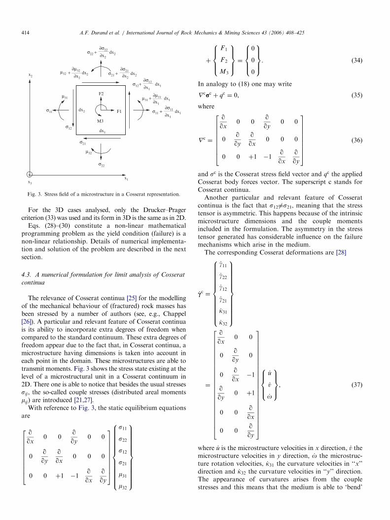
σ22 + dx2

σ12+ dx1

σ21 + dx2

σ11

∂σ11

∂σ12

∂σ21

∂σ22

∂µ31

∂µ32

∂x1

∂x1

∂x1

∂x2∂x2

∂x2

+ dx1

σ12

σ21

σ22

σ11

dx1

dx2

dx1+µ31

dx2 +µ32

µ31

µ32

x1

x2

x3

F2

F1

M3

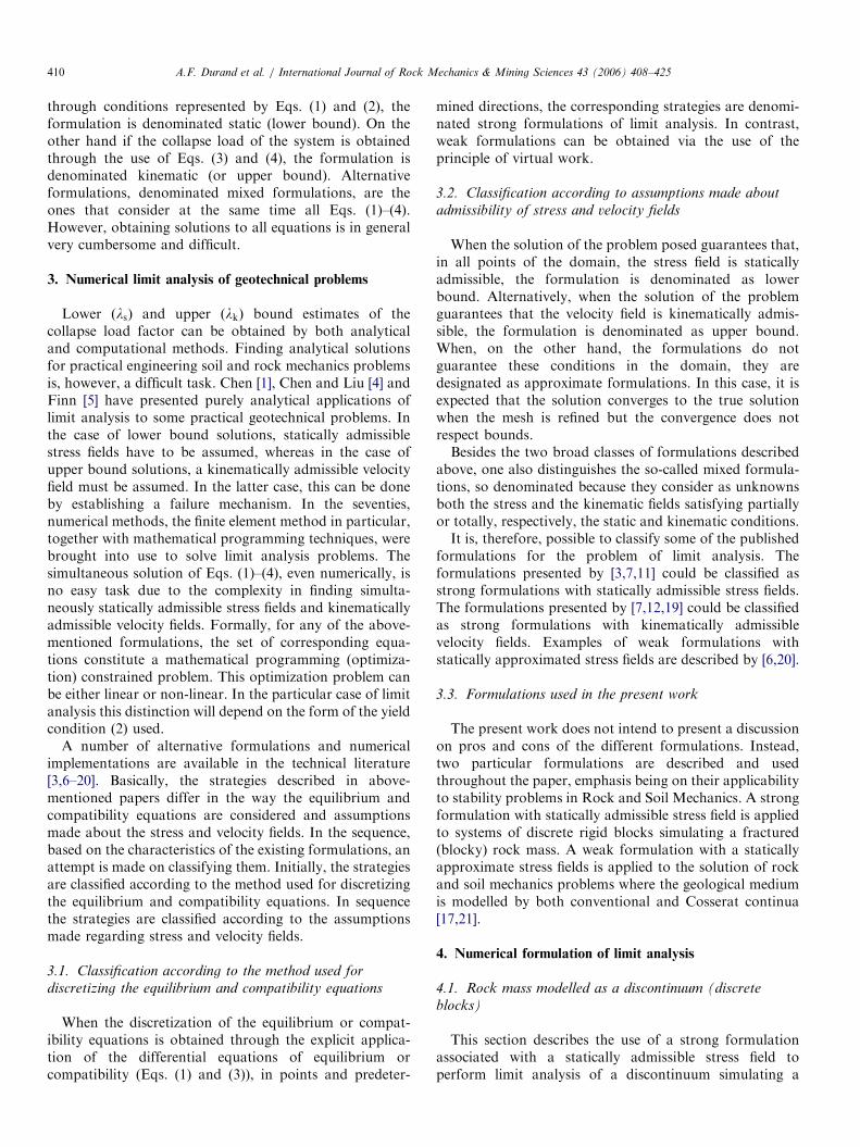
Fig. 3. Stress field of a microstructure in a Cosserat representation.


For the 3D cases analysed, only the Drucker–Pragercriterion (33) was used and its form in 3D is the same as in 2D.

Eqs. (28)–(30) constitute a non-linear mathematicalprogramming problem as the yield condition (failure) is anon-linear relationship. Details of numerical implementa-tion and solution of the problem are described in the nextsection.

4.3. A numerical formulation for limit analysis of Cosserat

continua

The relevance of Cosserat continua [25] for the modellingof the mechanical behaviour of (fractured) rock masses hasbeen stressed by a number of authors (see, e.g., Chappel[26]). A particular and relevant feature of Cosserat continuais its ability to incorporate extra degrees of freedom whencompared to the standard continuum. These extra degrees offreedom appear due to the fact that, in Cosserat continua, amicrostructure having dimensions is taken into account ineach point in the domain. These microstructures are able totransmit moments. Fig. 3 shows the stress state existing at thelevel of a microstructural unit in a Cosserat continuum in2D. There one is able to notice that besides the usual stressessij, the so-called couple stresses (distributed areal momentsmij) are introduced [21,27].

With reference to Fig. 3, the static equilibrium equationsare

qqx

0 0qqy

0 0

0qqy

qqx

0 0 0

0 0 þ1 �1qqx

qqy

2666666664

3777777775

s11

s22

s12

s21

m31

m32

8>>>>>>>>>>><>>>>>>>>>>>:

9>>>>>>>>>>>=>>>>>>>>>>>;

þ

F 1

F 2

M3

8>><>>:

9>>=>>; ¼

0

0

0

8>><>>:

9>>=>>;. ð34Þ

In analogy to (18) one may write

r crc þ qc ¼ 0, (35)

where

r c ¼

qqx

0 0qqy

0 0

0qqy

qqx

0 0 0

0 0 þ1 �1qqx

qqy

266666664

377777775

(36)

and sc is the Cosserat stress field vector and qc the appliedCosserat body forces vector. The superscript c stands forCosserat continua.Another particular and relevant feature of Cosserat

continua is the fact that s126¼s21, meaning that the stresstensor is asymmetric. This happens because of the intrinsicmicrostructure dimensions and the couple momentsincluded in the formulation. The asymmetry in the stresstensor generated has considerable influence on the failuremechanisms which arise in the medium.The corresponding Cosserat deformations are [28]

_cc ¼

_g11

_g22

_g12

_g21

_k31

_k32

8>>>>>>>>>>><>>>>>>>>>>>:

9>>>>>>>>>>>=>>>>>>>>>>>;

¼

qqx

0 0

0qqy

0

0qqx

�1

qqy

0 þ1

0 0qqx

0 0qqy

266666666666666666666664

377777777777777777777775

_u

_v

_o

8>><>>:

9>>=>>;, ð37Þ

where _u is the microstructure velocities in x direction, _v themicrostructure velocities in y direction, _o the microstruc-ture rotation velocities, _k31 the curvature velocities in ‘‘x’’direction and _k32 the curvature velocities in ‘‘y’’ direction.The appearance of curvatures arises from the couplestresses and this means that the medium is able to ‘bend’

ARTICLE IN PRESS

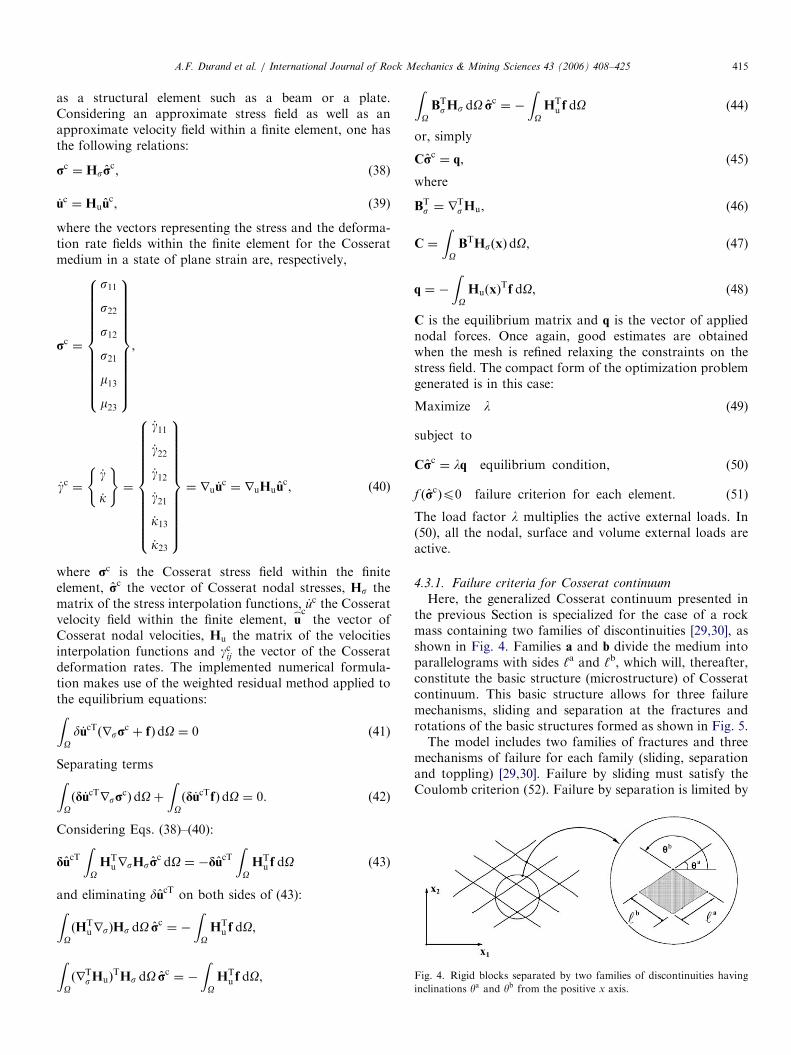
Fig. 4. Rigid blocks separated by two families of discontinuities having

inclinations ya and yb from the positive x axis.


as a structural element such as a beam or a plate.Considering an approximate stress field as well as anapproximate velocity field within a finite element, one hasthe following relations:

rc ¼ Hsrc, (38)

_uc ¼ Huuc, (39)

where the vectors representing the stress and the deforma-tion rate fields within the finite element for the Cosseratmedium in a state of plane strain are, respectively,

rc ¼

s11

s22

s12

s21

m13

m23

8>>>>>>>>>>><>>>>>>>>>>>:

9>>>>>>>>>>>=>>>>>>>>>>>;

,

_gc ¼_g

_k

( )¼

_g11

_g22

_g12

_g21

_k13

_k23

8>>>>>>>>>>><>>>>>>>>>>>:

9>>>>>>>>>>>=>>>>>>>>>>>;

¼ ru _uc ¼ ruHuu

c, ð40Þ

where rc is the Cosserat stress field within the finiteelement, rc the vector of Cosserat nodal stresses, Hs thematrix of the stress interpolation functions, _uc the Cosseratvelocity field within the finite element, u

_cthe vector of

Cosserat nodal velocities, Hu the matrix of the velocitiesinterpolation functions and gcij the vector of the Cosseratdeformation rates. The implemented numerical formula-tion makes use of the weighted residual method applied tothe equilibrium equations:ZOd_ucTðrsr

c þ fÞdO ¼ 0 (41)

Separating termsZOðd_ucTrsr

cÞdOþZOðd_ucTfÞdO ¼ 0. (42)

Considering Eqs. (38)–(40):

ducTZOHT

ursHsrc dO ¼ �ducT

ZOHT

u f dO (43)

and eliminating ducT on both sides of (43):ZOðHT

ursÞHs dO rc¼ �

ZOHT

u f dO,

ZOðrT

sHuÞTHs dO rc

¼ �

ZOHT

u f dO,

ZOBTsHs dO rc

¼ �

ZOHT

u f dO (44)

or, simply

Crc¼ q, (45)

where

BTs ¼ r

TsHu, (46)

C ¼

ZOBTHsðxÞdO, (47)

q ¼ �

ZOHuðxÞ

Tf dO, (48)

C is the equilibrium matrix and q is the vector of appliednodal forces. Once again, good estimates are obtainedwhen the mesh is refined relaxing the constraints on thestress field. The compact form of the optimization problemgenerated is in this case:

Maximize l (49)

subject to

Crc¼ lq equilibrium condition, (50)

f ðrcÞp0 failure criterion for each element: (51)

The load factor l multiplies the active external loads. In(50), all the nodal, surface and volume external loads areactive.

4.3.1. Failure criteria for Cosserat continuum

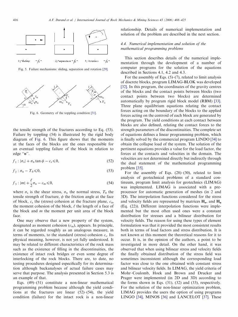
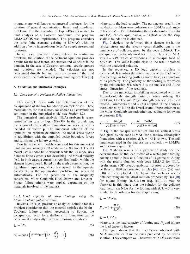
Here, the generalized Cosserat continuum presented inthe previous Section is specialized for the case of a rockmass containing two families of discontinuities [29,30], asshown in Fig. 4. Families a and b divide the medium intoparallelograms with sides ‘a and ‘b, which will, thereafter,constitute the basic structure (microstructure) of Cosseratcontinuum. This basic structure allows for three failuremechanisms, sliding and separation at the fractures androtations of the basic structures formed as shown in Fig. 5.The model includes two families of fractures and three

mechanisms of failure for each family (sliding, separationand toppling) [29,30]. Failure by sliding must satisfy theCoulomb criterion (52). Failure by separation is limited by

ARTICLE IN PRESS

Fig. 5. Failure mechanisms: sliding, separation and rotation [29].

ασα

τα

mα

o

σ~

l

o

Fn

Fs

mα

l

Fn

Cm

o mα

Fig. 6. Geometry of the toppling condition [31].


the tensile strength of the fractures according to Eq. (53).Failure by toppling (54) is illustrated by the rigid bodydiagram of Fig. 6. This figure shows that the momentsat the faces of the blocks are the ones responsible foran eventual toppling failure of the block in relation toedge ‘‘o’’.

f 1 : jssj þ sn tanf� csp0, (52)

f 2 : sn � T0p0, (53)

f 3 : jmj þ‘

2sn � cmp0, (54)

where ss is the shear stress, sn the normal stress, T0 thetensile strength of fracture, f the friction angle at the faceof block, cs the (stress) cohesion at the fracture plane, cmthe moment cohesion of the block, ‘ the length of a face ofthe block and m the moment per unit area of the blockface.

One may observe that a new property of the system,designated as moment cohesion (cm), appears. In principle,it can be regarded roughly as an analogous measure, interms of moments, to the standard (stress) cohesion cs. Itsphysical meaning, however, is not yet fully understood. Itmay be related to different characteristics of the rock masssuch as the existence of filling in the discontinuities, theexistence of intact rock bridges or even some degree ofinterlocking of the rock blocks. There are, to date, notesting procedures designed especifically for its determina-tion although backanalyses of actual failure cases mayserve that purpose. The analysis presented in Section 5.3 isan example of that.

Eqs. (49)–(51) constitute a non-linear mathematicalprogramming problem because although the yield condi-tions at the fractures are linear (52)–(54), the yieldcondition (failure) for the intact rock is a non-linear

relationship. Details of numerical implementation andsolution of the problem are described in the next section.

4.4. Numerical implementation and solution of the

mathematical programming problems

This section describes details of the numerical imple-mentation through the development of a number ofcomputer programs for the solution of the equationsdescribed in Sections 4.1, 4.2 and 4.3.For the assembly of Eqs. (5)–(7), related to limit analysis

of discrete blocks, program LIMAG-BLOK was developed[32]. In this program, the coordinates of the gravity centresof the blocks and the contact points between blocks (twocontact points between two blocks) are determinedautomatically by program rigid block model (RBM) [33].Three plane equilibrium equations relating the contactforces acting on the boundary of the blocks to the appliedforces acting on the centroid of each block are generated bythe program. The yield conditions at each contact betweenblocks are also defined, relating the contact forces to thestrength parameters of the discontinuities. The complete setof equations defines a linear programming problem, whichis finally solved by the commercial program LINDO [34] toobtain the collapse load of the system. The solution of thepertinent equations provides a value for the load factor, theforces at the contacts and velocities in the domain. Thevelocities are not determined directly but indirectly throughthe dual statement of the mathematical programmingproblem [35].For the assembly of Eqs. (28)–(30), related to limit

analysis of geotechnical problems of a standard con-tinuum, program limit analysis for geotechnics (LIMAG)was implemented. LIMAG is associated with a pre-processor for automatic generation of meshes (in 2 and3D). The interpolation functions considered for the stressand velocity fields are represented by matrices Hr, and Hu

(Eq. (22)). Different interpolation functions were imple-mented but the most often used ones were a constantdistribution for stresses and a bilinear distribution forvelocity fields. The reason for using these types of elementformulation was that it provided the most consistent resultsboth in terms of load factors and stress distribution. It isnot known at this moment the theoretical reasons for it tooccur. It is, in the opinion of the authors, a point to beinvestigated in more detail. On the other hand, it wasobserved that when using bilinear stress and velocity fieldsthe finally obtained distribution of the stress field wassometimes inconsistent although the corresponding loadfactor was close to the one obtained with constant stressand bilinear velocity fields. In LIMAG, the yield criteria ofMohr–Coulomb, Hoek and Brown and Drucker andPrager were implemented (in 2D and 3D) according tothe forms shown in Eqs. (31), (32) and (33), respectively.For the solution of the non-linear optimization problem,LIMAG provides the users the option of using programsLINGO [34], MINOS [36] and LANCELOT [37]. These


programs are well known commercial packages for thesolution of general optimization, linear and non-linearproblems. For the assembly of Eqs. (49)–(51) related tolimit analysis of a Cosserat continuum, the programLIMAG/COS was implemented. This program considersthe same finite elements existing in LIMAG with theaddition of extra interpolation fields for couple stresses androtations.

In all cases described above related to continuumproblems, the solution of the pertinent equations providesa value for the load factor, the stresses and velocities in thedomain. In the case of Cosserat continua, couple stressesand rotations are included. The velocities are notdetermined directly but indirectly by means of the dualstatement of the mathematical programming problem [35].

5. Validation and illustrative examples

5.1. Load capacity problem in shallow foundations

This example deals with the determination of thecollapse load of shallow foundations on rock or soil. Thesematerials are, for that matter, considered as a conventionalcontinuum in the numerical model (see Section 4.2).

The numerical limit analysis (NLA) problem is repre-sented in this case by Eqs. (28)–(30). In the formulation,the action of the shallow foundation on rock or soil isincluded in vector p. The numerical solution of theoptimization problem determines the nodal stress vectorin equilibrium with the amplified active boundary forcesand satisfying the failure criterion.

Two finite element models were used for this numericallimit analysis, namely a 2D model and a 3D model. The 2Dmodel uses 4-noded finite elements while the 3D model uses8-noded finite elements for describing the virtual velocityfield. In both cases, a constant stress distribution within theelement is considered. Based on the mesh discretization, theequilibrium equations, which correspond to the equalityconstraints in the optimization problem, are generatedautomatically. For the generation of the inequalityconstraints, Mohr–Coulomb, Hoek–Brown and Drucker–Prager failure criteria were applied depending on thematerials involved in the analysis.

5.1.1. Load capacity of strip footings using the

Mohr– Coulomb failure criterion

Bowles (1977) [38] presents an analytical solution for thisproblem considering that the material satisfies the Mohr–Coulomb failure criterion. According to Bowles, thecollapse load factor for a shallow strip foundation can bedetermined analytically from the following equations:

qu ¼ cNc (55)

Nc ¼ cotf ep tanftan2 45þf2

� �� 1

� �, (56)

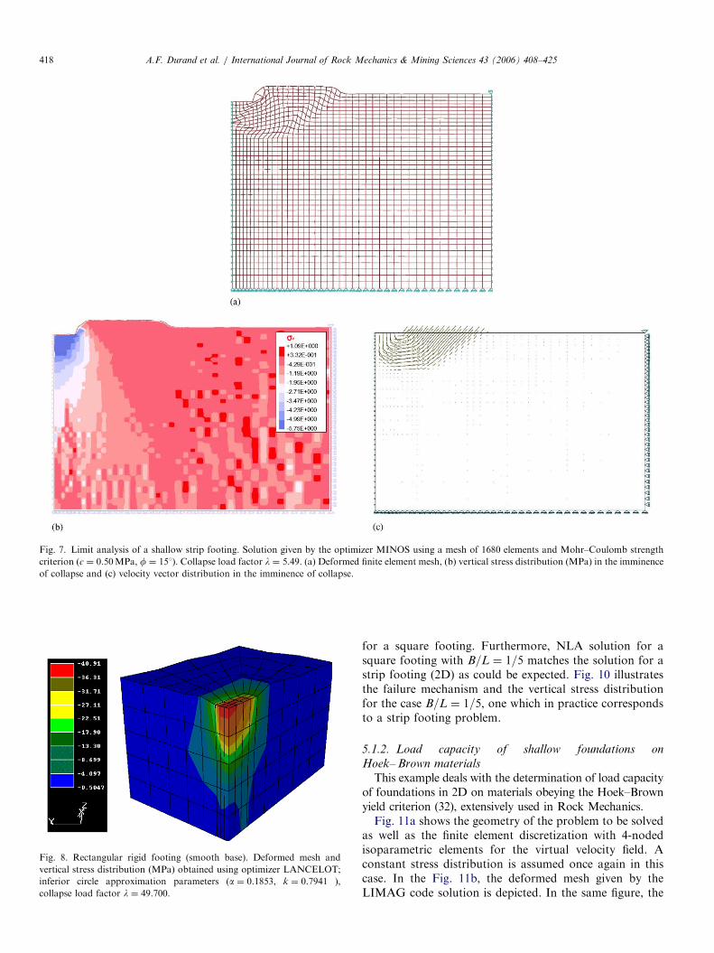
where qu is the load capacity. The parameters used in thevalidation problem were cohesion c ¼ 0:5MPa and angleof friction f ¼ 151. Substituting these values into Eqs. (56)and (55), the collapse load qu ¼ 5:488MPa for the stripshallow foundation is obtained.Fig. 7 depicts the deformed finite element mesh, the

vertical stress and the velocity vector distributions in theimminence of collapse, given by the code LIMAG. Thecollapse load factor obtained for this problem with NLAwas l ¼ 5:49, which corresponds to a collapse load of5.49MPa. This value is quite close to the result obtainedwith the analytical solution.In the sequence, a 3D load capacity problem is

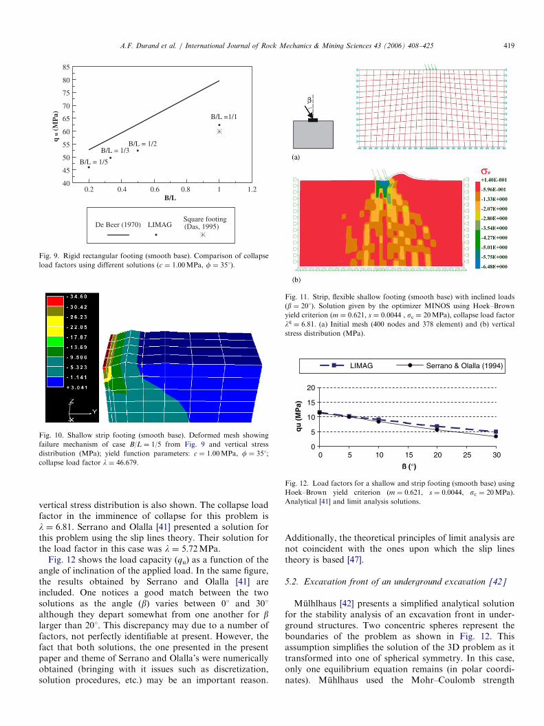
considered. It involves the determination of the load factorof a rectangular footing (with a smooth base) as a functionof its geometry. The geometry of the footing is expressedby the relationship B/L where B is the smallest and L thelargest dimension of the rectangle.Due to the numerical instabilities encountered with the

Mohr–Coulomb strength criterion when solving 3Dproblems, Drucker and Prager strength criterion was usedinstead. Parameters a and k (33) adopted in the analysiswere defined by fitting the Drucker and Prager criterion tothe Mohr–Coulomb strength criterion, leading to followingexpressions [39]:

a ¼2ffiffiffi3p

sinðfÞ½3þ sinðfÞ�

; k ¼6cffiffiffi3p

cosðfÞ½3þ sinðfÞ�

. (57)

In Fig. 8 the collapse mechanism and the vertical stressfield given by the code LIMAG for a shallow rectangularfoundation with a relation B=L ¼ 1=3 is shown. The soilparameters used in the analysis were cohesion ¼ 1:0MPaand friction angle ¼ 351.Fig. 9 shows results of a parametric study for the

determination of the load factor of a rectangular footinghaving a smooth base as a function of its geometry. Alongwith the results obtained with code LIMAG for NLA,results using a 3D pseudo-analytical solution proposed byde Beer in 1970 as presented by Das [40] (Eqs. (58) and(60)) are also plotted. The figure also includes resultsobtained using an analytical solution proposed by Das [40]for square footing (B=L ¼ 1:0) (Eq. (60)). It may beobserved in this figure that the solution for the collapseload factor via NLA for the footing with B=L ¼ 5 is verysimilar to the solution for the strip footing.

qu ¼ cNcF cs, (58)

F cs ¼ 1þB

L

Nq

Nc

, (59)

qu ¼ 1:3cNc, (60)

where qu is the load capacity of footing and Nc and Nq arethe load capacity factors.The figure shows that the load factors obtained with

NLA are smaller than the ones predicted by de Beer’ssolution. They compare well, however, with Das’s solution

ARTICLE IN PRESS

Fig. 8. Rectangular rigid footing (smooth base). Deformed mesh and

vertical stress distribution (MPa) obtained using optimizer LANCELOT;

inferior circle approximation parameters (a ¼ 0.1853, k ¼ 0.7941 ),

collapse load factor l ¼ 49.700.

Fig. 7. Limit analysis of a shallow strip footing. Solution given by the optimizer MINOS using a mesh of 1680 elements and Mohr–Coulomb strength

criterion (c ¼ 0.50MPa, f ¼ 151). Collapse load factor l ¼ 5.49. (a) Deformed finite element mesh, (b) vertical stress distribution (MPa) in the imminence

of collapse and (c) velocity vector distribution in the imminence of collapse.


for a square footing. Furthermore, NLA solution for asquare footing with B=L ¼ 1=5 matches the solution for astrip footing (2D) as could be expected. Fig. 10 illustratesthe failure mechanism and the vertical stress distributionfor the case B=L ¼ 1=5, one which in practice correspondsto a strip footing problem.

5.1.2. Load capacity of shallow foundations on

Hoek– Brown materials

This example deals with the determination of load capacityof foundations in 2D on materials obeying the Hoek–Brownyield criterion (32), extensively used in Rock Mechanics.Fig. 11a shows the geometry of the problem to be solved

as well as the finite element discretization with 4-nodedisoparametric elements for the virtual velocity field. Aconstant stress distribution is assumed once again in thiscase. In the Fig. 11b, the deformed mesh given by theLIMAG code solution is depicted. In the same figure, the

ARTICLE IN PRESS

0.2 0.4 140

45

50

55

60

65

70

75

80

85

q u

(MP

a) B/L =1/1

B/L = 1/2B/L = 1/3

B/L = 1/5

De Beer (1970) LIMAGSquare footing(Das, 1995)

0.6 0.8 1.2 B/L

Fig. 9. Rigid rectangular footing (smooth base). Comparison of collapse

load factors using different solutions (c ¼ 1.00MPa, f ¼ 351).

Fig. 10. Shallow strip footing (smooth base). Deformed mesh showing

failure mechanism of case B/L ¼ 1/5 from Fig. 9 and vertical stress

distribution (MPa); yield function parameters: c ¼ 1.00MPa, f ¼ 351;

collapse load factor l ¼ 46.679.

Fig. 11. Strip, flexible shallow footing (smooth base) with inclined loads

(b ¼ 201). Solution given by the optimizer MINOS using Hoek–Brown

yield criterion (m ¼ 0.621, s ¼ 0.0044 , sc ¼ 20MPa), collapse load factor

lq ¼ 6.81. (a) Initial mesh (400 nodes and 378 element) and (b) vertical

stress distribution (MPa).

0

5

10

15

20

0 5 10 15 20 25 30

ß (°)

qu

(M

Pa)

LIMAG Serrano & Olalla (1994)

Fig. 12. Load factors for a shallow and strip footing (smooth base) using

Hoek–Brown yield criterion (m ¼ 0:621, s ¼ 0:0044, sc ¼ 20MPa).

Analytical [41] and limit analysis solutions.


vertical stress distribution is also shown. The collapse loadfactor in the imminence of collapse for this problem isl ¼ 6:81. Serrano and Olalla [41] presented a solution forthis problem using the slip lines theory. Their solution forthe load factor in this case was l ¼ 5:72MPa.

Fig. 12 shows the load capacity (qu) as a function of theangle of inclination of the applied load. In the same figure,the results obtained by Serrano and Olalla [41] areincluded. One notices a good match between the twosolutions as the angle (b) varies between 01 and 301although they depart somewhat from one another for blarger than 201. This discrepancy may due to a number offactors, not perfectly identifiable at present. However, thefact that both solutions, the one presented in the presentpaper and theme of Serrano and Olalla’s were numericallyobtained (bringing with it issues such as discretization,solution procedures, etc.) may be an important reason.

Additionally, the theoretical principles of limit analysis arenot coincident with the ones upon which the slip linestheory is based [47].

5.2. Excavation front of an underground excavation [42]

Mulhlhaus [42] presents a simplified analytical solutionfor the stability analysis of an excavation front in under-ground structures. Two concentric spheres represent theboundaries of the problem as shown in Fig. 12. Thisassumption simplifies the solution of the 3D problem as ittransformed into one of spherical symmetry. In this case,only one equilibrium equation remains (in polar coordi-nates). Muhlhaus used the Mohr–Coulomb strength

ARTICLE IN PRESS

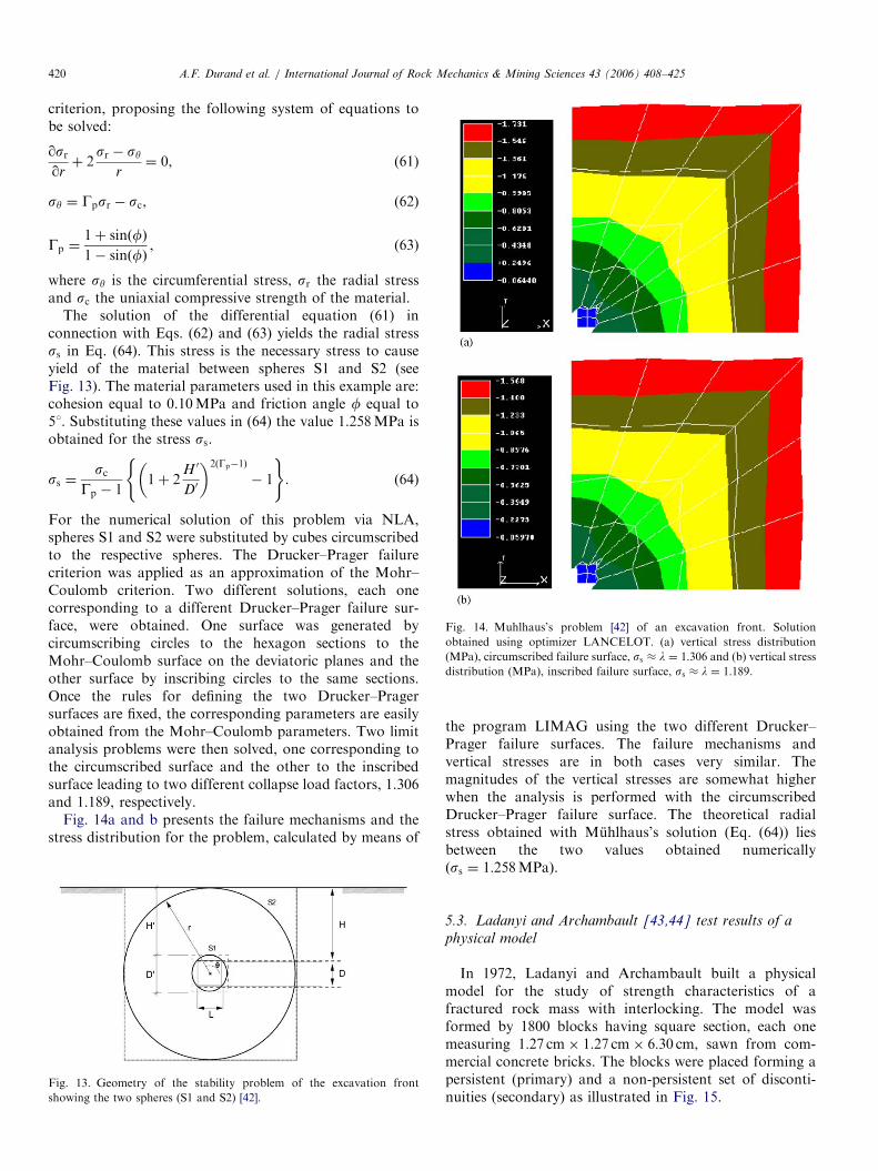
Fig. 14. Muhlhaus’s problem [42] of an excavation front. Solution

obtained using optimizer LANCELOT. (a) vertical stress distribution

(MPa), circumscribed failure surface, ss � l ¼ 1:306 and (b) vertical stress

distribution (MPa), inscribed failure surface, ss � l ¼ 1:189.


criterion, proposing the following system of equations tobe solved:

qsrqrþ 2

sr � syr¼ 0, (61)

sy ¼ Gpsr � sc, (62)

Gp ¼1þ sinðfÞ1� sinðfÞ

, (63)

where sy is the circumferential stress, sr the radial stressand sc the uniaxial compressive strength of the material.

The solution of the differential equation (61) inconnection with Eqs. (62) and (63) yields the radial stressss in Eq. (64). This stress is the necessary stress to causeyield of the material between spheres S1 and S2 (seeFig. 13). The material parameters used in this example are:cohesion equal to 0.10MPa and friction angle f equal to51. Substituting these values in (64) the value 1.258MPa isobtained for the stress ss.

ss ¼sc

Gp � 11þ 2

H 0

D0

� �2ðGp�1Þ

� 1

( ). (64)

For the numerical solution of this problem via NLA,spheres S1 and S2 were substituted by cubes circumscribedto the respective spheres. The Drucker–Prager failurecriterion was applied as an approximation of the Mohr–Coulomb criterion. Two different solutions, each onecorresponding to a different Drucker–Prager failure sur-face, were obtained. One surface was generated bycircumscribing circles to the hexagon sections to theMohr–Coulomb surface on the deviatoric planes and theother surface by inscribing circles to the same sections.Once the rules for defining the two Drucker–Pragersurfaces are fixed, the corresponding parameters are easilyobtained from the Mohr–Coulomb parameters. Two limitanalysis problems were then solved, one corresponding tothe circumscribed surface and the other to the inscribedsurface leading to two different collapse load factors, 1.306and 1.189, respectively.

Fig. 14a and b presents the failure mechanisms and thestress distribution for the problem, calculated by means of

Fig. 13. Geometry of the stability problem of the excavation front

showing the two spheres (S1 and S2) [42].

the program LIMAG using the two different Drucker–Prager failure surfaces. The failure mechanisms andvertical stresses are in both cases very similar. Themagnitudes of the vertical stresses are somewhat higherwhen the analysis is performed with the circumscribedDrucker–Prager failure surface. The theoretical radialstress obtained with Muhlhaus’s solution (Eq. (64)) liesbetween the two values obtained numericallyðss ¼ 1:258MPaÞ.

5.3. Ladanyi and Archambault [43,44] test results of a

physical model

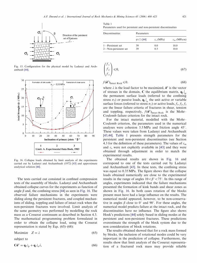
In 1972, Ladanyi and Archambault built a physicalmodel for the study of strength characteristics of afractured rock mass with interlocking. The model wasformed by 1800 blocks having square section, each onemeasuring 1:27 cm� 1:27 cm� 6:30 cm, sawn from com-mercial concrete bricks. The blocks were placed forming apersistent (primary) and a non-persistent set of disconti-nuities (secondary) as illustrated in Fig. 15.

ARTICLE IN PRESS

Table 1

Parameters used for persistent and non-persistent discontinuities

Discontinuities Parameters

f (1) [44] cs (MPa) cm (MPam)

1—Persistent set 39 0.0 10.0

2—Non-persistent set 39 0.5 10.0

Fig. 15. Configuration for the physical model by Ladanyi and Arch-

ambault [44].

Fig. 16. Collapse loads obtained by limit analysis of the experiments

carried out by Ladanyi and Archambault (1972) [43] and approximate

analytical solution [44].


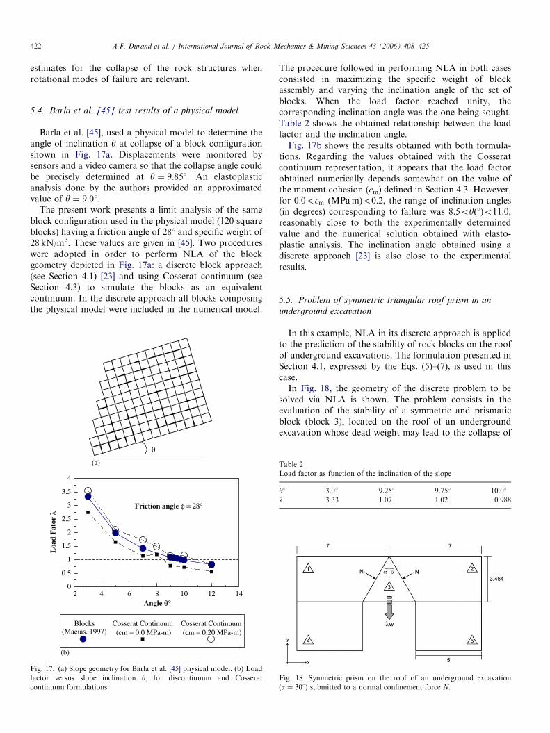
The tests carried out consisted in confined compressiontests of the assembly of blocks. Ladanyi and Archambaultobtained collapse curves for the experiments as function ofangle b and, the confining stress [44] as seen in Fig. 16. Theobserved failure mechanisms in the experiments weresliding along the persistent fractures, and coupled mechan-isms of sliding, toppling and failure of intact rock when thenon-persistent fractures were involved. Limit analysis ofthe same geometry was performed by modelling the rockmass as a Cosserat continuum as described in Section 4.3.The mathematical programming problem formulated inorder to obtain the collapse load, using the Cosseratrepresentation is stated by Eqs. (65)–(68):

Maximize Z ¼ l (65)

subject to

Crc¼ qGjp þ qGjal, (66)

f 1

f 2

f 3

0B@

1CAp0; (67)

f ðrcÞIntact Rockp0: (68)

where l is the load factor to be maximized, rc is the vectorof stresses in the domain, C the equilibrium matrix, qG

��p

the permanent surface loads (referred to the confiningstress s3) or passive loads, qG

��athe unit active or variable

surface forces (referred to stress s1) or active loads, f1, f2, f3are the linear failure criteria of fractures in shear, tensionand toppling, respectively, f ðrc

ÞIntact Rock is the Mohr–Coulomb failure criterion for the intact rock.For the intact material, modelled with the Mohr–

Coulomb criterion, the parameters used in the numericalanalyses were cohesion 5.5MPa and friction angle 451.These values were taken from Ladanyi and Archambault[43,44]. Table 1 presents strength parameters for thepersistent and non-persistent discontinuities (see Section4.3 for the definition of these parameters). The values of cmand cs were not explicitly available in [43] and they wereobtained through adjustment in order to match theexperimental results.The obtained results are shown in Fig. 16 and

correspond to one of the tests carried out by Ladanyiand Archambault [43]. In these tests, the confining stresswas equal to 0.35MPa. The figure shows that the collapseloads obtained numerically are close to the experimentalresults in the range of angles 10ob1o751. In this range ofangles, experiments indicated that the failure mechanismspresented the formation of kink bands and shear zones asshown in Fig. 16. In both cases rotation of the blockspresent must have had a large influence on the results. Thenumerical model appeared, however, to be non-conserva-tive in angles b close to 01 and 901. For these angles, thenumerical model predicts failure at the intact rock, and thediscontinuities have no influence. The figure also showsHoek’s predictions [44] solely based in sliding modes at thepersistent and non-persistent fractures. These predictionsoverestimate the strength of the block system due to thenon consideration of block rotations.The results obtained showed that for a rock mass formed

by blocks, the inclusion of rotational modes could be veryimportant in the prediction of collapse. Furthermore, theresults show that limit analysis of the Cosserat representa-tion of a fractured rock mass may provide reliable

ARTICLE IN PRESSA.F. Durand et al. / International Journal of Rock Mechanics & Mining Sciences 43 (2006) 408–425422

estimates for the collapse of the rock structures whenrotational modes of failure are relevant.

5.4. Barla et al. [45] test results of a physical model

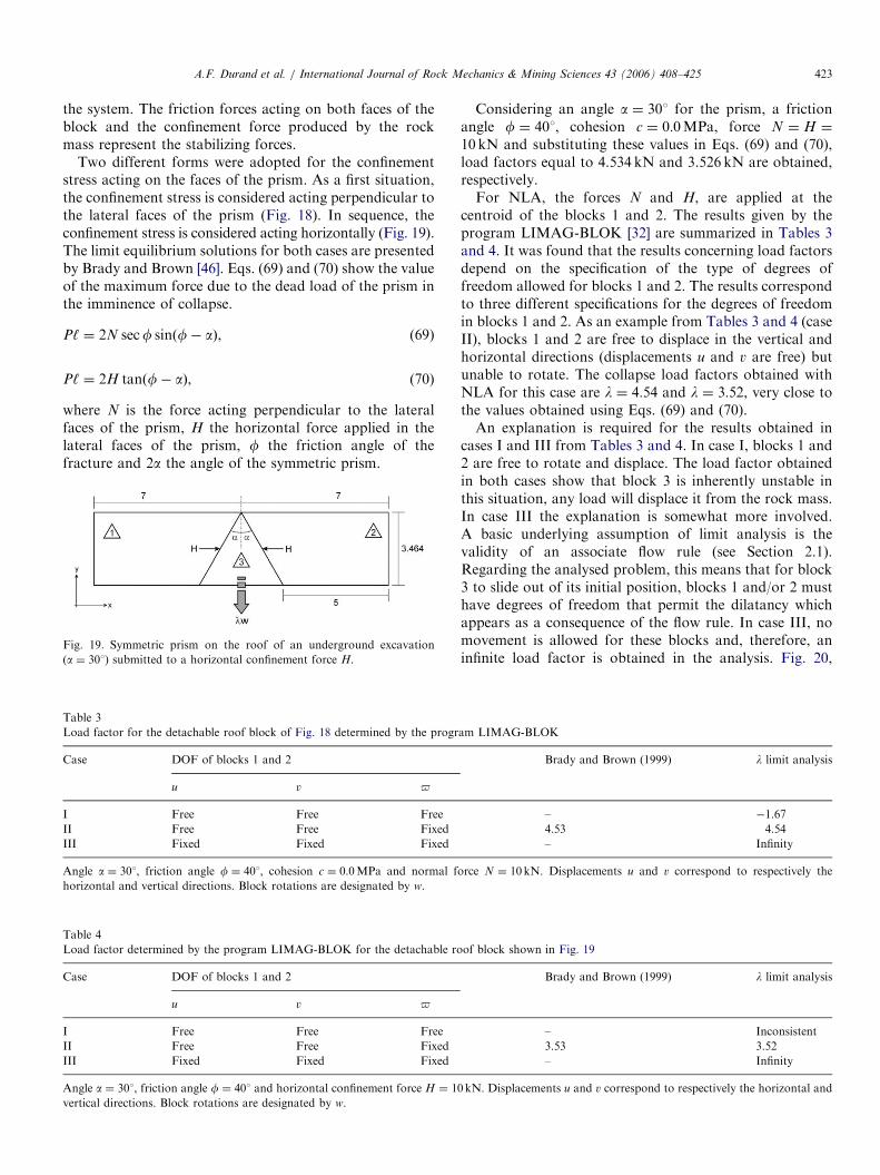
Barla et al. [45], used a physical model to determine theangle of inclination y at collapse of a block configurationshown in Fig. 17a. Displacements were monitored bysensors and a video camera so that the collapse angle couldbe precisely determined at y ¼ 9:851. An elastoplasticanalysis done by the authors provided an approximatedvalue of y ¼ 9:01.

The present work presents a limit analysis of the sameblock configuration used in the physical model (120 squareblocks) having a friction angle of 281 and specific weight of28 kN/m3. These values are given in [45]. Two procedureswere adopted in order to perform NLA of the blockgeometry depicted in Fig. 17a: a discrete block approach(see Section 4.1) [23] and using Cosserat continuum (seeSection 4.3) to simulate the blocks as an equivalentcontinuum. In the discrete approach all blocks composingthe physical model were included in the numerical model.

θ

Friction angle φ = 28= 28°

2 864 10 12 140

0.5

1

1.5

2

2.5

3

3.5

4

Angle θ°

Loa

d F

ator

λ

Blocks(Macias. 1997)

Cosserat Continuum(cm = 0.0 MPa-m)

Cosserat Continuum(cm = 0.20 MPa-m)

(b)

(a)

Fig. 17. (a) Slope geometry for Barla et al. [45] physical model. (b) Load

factor versus slope inclination y, for discontinuum and Cosserat

continuum formulations.

The procedure followed in performing NLA in both casesconsisted in maximizing the specific weight of blockassembly and varying the inclination angle of the set ofblocks. When the load factor reached unity, thecorresponding inclination angle was the one being sought.Table 2 shows the obtained relationship between the loadfactor and the inclination angle.Fig. 17b shows the results obtained with both formula-

tions. Regarding the values obtained with the Cosseratcontinuum representation, it appears that the load factorobtained numerically depends somewhat on the value ofthe moment cohesion (cm) defined in Section 4.3. However,for 0:0ocm ðMPamÞo0:2, the range of inclination angles(in degrees) corresponding to failure was 8:5oyð1Þo11:0,reasonably close to both the experimentally determinedvalue and the numerical solution obtained with elasto-plastic analysis. The inclination angle obtained using adiscrete approach [23] is also close to the experimentalresults.

5.5. Problem of symmetric triangular roof prism in an

underground excavation

In this example, NLA in its discrete approach is appliedto the prediction of the stability of rock blocks on the roofof underground excavations. The formulation presented inSection 4.1, expressed by the Eqs. (5)–(7), is used in thiscase.In Fig. 18, the geometry of the discrete problem to be

solved via NLA is shown. The problem consists in theevaluation of the stability of a symmetric and prismaticblock (block 3), located on the roof of an undergroundexcavation whose dead weight may lead to the collapse of

Table 2

Load factor as function of the inclination of the slope

y1 3.01 9.251 9.751 10.01

l 3.33 1.07 1.02 0.988

Fig. 18. Symmetric prism on the roof of an underground excavation

(a ¼ 301) submitted to a normal confinement force N.


the system. The friction forces acting on both faces of theblock and the confinement force produced by the rockmass represent the stabilizing forces.

Two different forms were adopted for the confinementstress acting on the faces of the prism. As a first situation,the confinement stress is considered acting perpendicular tothe lateral faces of the prism (Fig. 18). In sequence, theconfinement stress is considered acting horizontally (Fig. 19).The limit equilibrium solutions for both cases are presentedby Brady and Brown [46]. Eqs. (69) and (70) show the valueof the maximum force due to the dead load of the prism inthe imminence of collapse.

P‘ ¼ 2N secf sinðf� aÞ, (69)

P‘ ¼ 2H tanðf� aÞ, (70)

where N is the force acting perpendicular to the lateralfaces of the prism, H the horizontal force applied in thelateral faces of the prism, f the friction angle of thefracture and 2a the angle of the symmetric prism.

Fig. 19. Symmetric prism on the roof of an underground excavation

(a ¼ 301) submitted to a horizontal confinement force H.

Table 3

Load factor for the detachable roof block of Fig. 18 determined by the progr

Case DOF of blocks 1 and 2

u v $

I Free Free Free

II Free Free Fixed

III Fixed Fixed Fixed

Angle a ¼ 301, friction angle f ¼ 401, cohesion c ¼ 0.0MPa and normal f

horizontal and vertical directions. Block rotations are designated by w.

Table 4

Load factor determined by the program LIMAG-BLOK for the detachable ro

Case DOF of blocks 1 and 2

u v $

I Free Free Free

II Free Free Fixed

III Fixed Fixed Fixed

Angle a ¼ 301, friction angle f ¼ 401 and horizontal confinement force H ¼ 1

vertical directions. Block rotations are designated by w.

Considering an angle a ¼ 301 for the prism, a frictionangle f ¼ 401, cohesion c ¼ 0:0MPa, force N ¼ H ¼

10 kN and substituting these values in Eqs. (69) and (70),load factors equal to 4.534 kN and 3.526 kN are obtained,respectively.For NLA, the forces N and H, are applied at the

centroid of the blocks 1 and 2. The results given by theprogram LIMAG-BLOK [32] are summarized in Tables 3and 4. It was found that the results concerning load factorsdepend on the specification of the type of degrees offreedom allowed for blocks 1 and 2. The results correspondto three different specifications for the degrees of freedomin blocks 1 and 2. As an example from Tables 3 and 4 (caseII), blocks 1 and 2 are free to displace in the vertical andhorizontal directions (displacements u and v are free) butunable to rotate. The collapse load factors obtained withNLA for this case are l ¼ 4:54 and l ¼ 3:52, very close tothe values obtained using Eqs. (69) and (70).An explanation is required for the results obtained in

cases I and III from Tables 3 and 4. In case I, blocks 1 and2 are free to rotate and displace. The load factor obtainedin both cases show that block 3 is inherently unstable inthis situation, any load will displace it from the rock mass.In case III the explanation is somewhat more involved.A basic underlying assumption of limit analysis is thevalidity of an associate flow rule (see Section 2.1).Regarding the analysed problem, this means that for block3 to slide out of its initial position, blocks 1 and/or 2 musthave degrees of freedom that permit the dilatancy whichappears as a consequence of the flow rule. In case III, nomovement is allowed for these blocks and, therefore, aninfinite load factor is obtained in the analysis. Fig. 20,

am LIMAG-BLOK

Brady and Brown (1999) l limit analysis

– �1.67

4.53 4.54

– Infinity

orce N ¼ 10kN. Displacements u and v correspond to respectively the

of block shown in Fig. 19

Brady and Brown (1999) l limit analysis

– Inconsistent

3.53 3.52

– Infinity

0kN. Displacements u and v correspond to respectively the horizontal and

ARTICLE IN PRESS

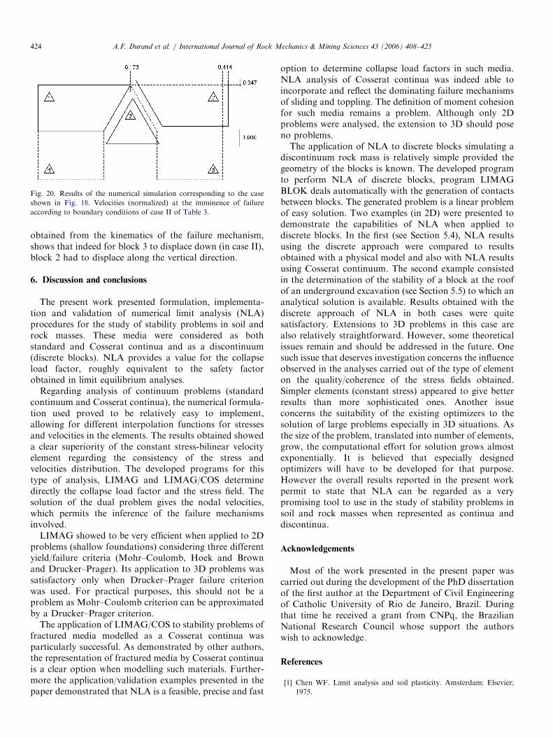
Fig. 20. Results of the numerical simulation corresponding to the case

shown in Fig. 18. Velocities (normalized) at the imminence of failure

according to boundary conditions of case II of Table 3.


obtained from the kinematics of the failure mechanism,shows that indeed for block 3 to displace down (in case II),block 2 had to displace along the vertical direction.

6. Discussion and conclusions

The present work presented formulation, implementa-tion and validation of numerical limit analysis (NLA)procedures for the study of stability problems in soil androck masses. These media were considered as bothstandard and Cosserat continua and as a discontinuum(discrete blocks). NLA provides a value for the collapseload factor, roughly equivalent to the safety factorobtained in limit equilibrium analyses.

Regarding analysis of continuum problems (standardcontinuum and Cosserat continua), the numerical formula-tion used proved to be relatively easy to implement,allowing for different interpolation functions for stressesand velocities in the elements. The results obtained showeda clear superiority of the constant stress-bilinear velocityelement regarding the consistency of the stress andvelocities distribution. The developed programs for thistype of analysis, LIMAG and LIMAG/COS determinedirectly the collapse load factor and the stress field. Thesolution of the dual problem gives the nodal velocities,which permits the inference of the failure mechanismsinvolved.

LIMAG showed to be very efficient when applied to 2Dproblems (shallow foundations) considering three differentyield/failure criteria (Mohr–Coulomb, Hoek and Brownand Drucker–Prager). Its application to 3D problems wassatisfactory only when Drucker–Prager failure criterionwas used. For practical purposes, this should not be aproblem as Mohr–Coulomb criterion can be approximatedby a Drucker–Prager criterion.

The application of LIMAG/COS to stability problems offractured media modelled as a Cosserat continua wasparticularly successful. As demonstrated by other authors,the representation of fractured media by Cosserat continuais a clear option when modelling such materials. Further-more the application/validation examples presented in thepaper demonstrated that NLA is a feasible, precise and fast

option to determine collapse load factors in such media.NLA analysis of Cosserat continua was indeed able toincorporate and reflect the dominating failure mechanismsof sliding and toppling. The definition of moment cohesionfor such media remains a problem. Although only 2Dproblems were analysed, the extension to 3D should poseno problems.The application of NLA to discrete blocks simulating a

discontinuum rock mass is relatively simple provided thegeometry of the blocks is known. The developed programto perform NLA of discrete blocks, program LIMAGBLOK deals automatically with the generation of contactsbetween blocks. The generated problem is a linear problemof easy solution. Two examples (in 2D) were presented todemonstrate the capabilities of NLA when applied todiscrete blocks. In the first (see Section 5.4), NLA resultsusing the discrete approach were compared to resultsobtained with a physical model and also with NLA resultsusing Cosserat continuum. The second example consistedin the determination of the stability of a block at the roofof an underground excavation (see Section 5.5) to which ananalytical solution is available. Results obtained with thediscrete approach of NLA in both cases were quitesatisfactory. Extensions to 3D problems in this case arealso relatively straightforward. However, some theoreticalissues remain and should be addressed in the future. Onesuch issue that deserves investigation concerns the influenceobserved in the analyses carried out of the type of elementon the quality/coherence of the stress fields obtained.Simpler elements (constant stress) appeared to give betterresults than more sophisticated ones. Another issueconcerns the suitability of the existing optimizers to thesolution of large problems especially in 3D situations. Asthe size of the problem, translated into number of elements,grow, the computational effort for solution grows almostexponentially. It is believed that especially designedoptimizers will have to be developed for that purpose.However the overall results reported in the present workpermit to state that NLA can be regarded as a verypromising tool to use in the study of stability problems insoil and rock masses when represented as continua anddiscontinua.

Acknowledgements

Most of the work presented in the present paper wascarried out during the development of the PhD dissertationof the first author at the Department of Civil Engineeringof Catholic University of Rio de Janeiro, Brazil. Duringthat time he received a grant from CNPq, the BrazilianNational Research Council whose support the authorswish to acknowledge.

References

[1] Chen WF. Limit analysis and soil plasticity. Amsterdam: Elsevier;

1975.


[2] Drucker DC, Prager W. Soil mechanics and plastic analysis on limit

design. Q Appl Math 1952;10:157–65.

[3] Lysmer J. Limit analysis of plane problems in soil mechanics. J Soil

Mech Found Div ASCE 1970;96:1311–34.

[4] Chen WF, Liu XL. Limit analysis in soil mechanics. Amsterdam:

Elsevier; 1990.

[5] Finn WDL. Application of limit plasticity in soil mechanics. J Soil

Mech Found Div ASCE 1967;101–20.

[6] Anderheggen E, Knopfel H. Finite element limit analysis using linear

programming. Int J Solids Struct 1972;8:1413–31.

[7] Bottero A, Negre R, Pastor J, Turgeman S. Finite element method

and limit analysis theory for soil mechanics problems. Comput

Methods Appl Mech Eng 1980;22:131–49.

[8] Christiansen E. Computation of limit loads. Int J Numer Anal

Methods Eng 1981;17:1547–70.

[9] Munro J. Plastic analysis in geomechanics by mathematical

programming. In: Martins B, editor. Numerical methods in

geomechanics. Dordrecht: D. Reidel Publishing Company; 1982.

p. 247–72.

[10] Casciaro R, Cascini L. A mixed formulation and mixed finite

elements for limit analysis. Int J Numer Anal Methods Eng

1982;18:211–43.

[11] Sloan SW. Lower bound limit analysis using finite elements and

linear programming. Int J Numer Anal Methods Geomech 1988;12:

61–77.

[12] Sloan SW. Upper bound limit analysis using finite elements and

linear programming. Department of Civil Engineering and

Surveying, University of Newcastle, Australia: Report No. 025.09.1987;

1987.

[13] Arai K, Jinki R. A lower-bound approach to active and passive earth

pressure problems. Soils Found 1990;30(4):25–41.

[14] Assadi A, Sloan SW. Undrained stability of shallow square tunnel.

J Geotech Eng Div ASCE 1991;117(8).

[15] Chuang PH. Stability analysis in geomechanics by linear program-

ming I: formulation. J Geotech Eng Div ASCE 1992;118(11).

[16] Singh DN, Basudhar PK. Optimal lower bound bearing capacity of

strip footings. Soils Found 1993;33(4).

[17] Araujo LG. Numerical study of stability problems in rock mass using

limit analysis. PhD thesis, Pontifıcia Universidade Catolica do Rio de

Janeiro, Rio de Janeiro, Brazil; 1997 [in Portuguese].

[18] Yu HS, Salgado R, Sloan SW, Kim JM. Limit analysis versus limit

equilibrium for slope stability. J Geotech Geoenviron Eng ASCE

1998;January:1–11.

[19] Lyamin AV, Sloan SW. Upper bound limit analysis using linear finite

elements and non-linear programming. Int J Numer Anal Methods

Geomech 2002;26:181–216.

[20] Pontes IDS. Non-linear limit analysis in geotechnics problems. PhD

thesis, COPPE-UFRJ (Federal University of Rio de Janeiro), Rio de

Janeiro, Brazil; 1993. 172pp. [in Portuguese].

[21] Durand AF. Applications of limit analysis as conventional con-

tinuum and Cosserat continua to geotechnics problems. PhD thesis,

Pontifıcia Universidade Catolica do Rio de Janeiro, Rio de Janeiro,

Brazil; 2000 [in Portuguese].

[22] Livesley RK. Limit analysis of structures formed from rigid blocks.

Int J Numer Method Eng 1978;12:1853–71.

[23] Macıas AJE. Computational implementations for the study of the

stability of fractured rock masses. Msc dissertation, Pontifıcia

Universidade Catolica do Rio de Janeiro, Rio de Janeiro, Brazil;

1997 [in Portuguese].

[24] Chou PC, Pagano NJ. Elasticity tensor, dyadic, and engineering

approaches. New York: Dover; 1992.

[25] Cosserat E, Cosserat F. Theorie des corps deformables. Paris:

Hermann et fils; 1909.

[26] Chappell BA. Load distribution and redistribution in discontinua. Int

J Rock Mech Min Sci Geomech Abstr 1979;16:391–9.

[27] Unterreiner P. Contribution a l’etude et a la Modelisation Numerıque

des Sols Cloues: Application au Calcul en Deformation des Ouvrages

de Soutenement, 2 vols. PhD Thesis, Ecole Nationale des Ponts et

Chaussees, Paris; 1995. 775pp.

[28] Eringen AC. Mechanics of micromorphic continua. Mechanics of

generalized continua—IUTAM symposium. Freudenstadt & Stutt-

gart, Kroner: Springer, 1968. p. 18–35.

[29] Dawson EM. Micropolar continuum models for jointed rock. PhD

thesis, University of Minnesota, Minneapolis, USA; 1995.

[30] Besdo D. A plasticity theory of frictionless sliding systems of rocks

basing on the Cosserat model. In: Desai, et al., editors. Second

conference on constitutive laws for engineering materials: theory and

applications; 1987. p. 761–8.

[31] Durand AF, Vargas Jr, EA, Vaz LE, Macias JA. Stability of

fractured rock masses by limit analysis. In: Ayres da Silva LA,

Quadros EF, Gonc-alves HHS, editors. Design and construction in

mining, petroleum and civil engineering. Brazil: Sao Paulo; 1998.

p. 341–9.

[32] Durand AF, Vargas Jr, EA, Vaz LE. Analysis of the stability of

discrete blocks through limit analysis (NLA). In: 12th Panamerican

conference on soil and rock mechanics, 2003, vol. 1, Cambridge, MA,

USA; 2003. p. 1099–1104 [in Spanish].

[33] Maini T, Cundall P, Marti J, Beresford P, Last N, Asgian M.

Computer modeling of jointed rock masses. Technical Report

N-78-4, US Army Engineer Waterways Experiment Station, Vicks-

burg, MI; 1978.

[34] Schrage L. LINDO—user’s manual. The Scientific Press; 1991.

[35] Arora JS. Introduction to optimum design. New York: McGraw-Hill;

1989 624 pp.

[36] Murtagh BA, Saunders MA. MINOS 5.1 user’s guide. Technical

report SOL 83-20R, Stanford University, California; 1987.

[37] Conn AR, Gould NIM, Toint Ph L. LANCELOT—a Fortran

package for large-scale nonlinear optimization (Release A). Berlin:

Springer; 1992. 330pp.

[38] Bowles JE. Foundation analysis and design. 2nd ed. New York:

McGraw-Hill; 1977 750pp.

[39] Chen WF, Han DJ. Plasticity for structural engineers. New York,

Berlin, Heidelberg: Springer; 1988.

[40] Das B M. Principles of foundation engineering. 3rd ed. Boston: PWS

Publishing Company; 1995.

[41] Serrano A, Olalla C. Ultimate bearing capacity of rock. Int J Mech

Sci Geomech 1994;31(2):93–106.

[42] Muhlhaus HB. Lower bound solutions for circular tunnels in two and

tree dimension. Rock Mech Rock Eng 1985;18:37–52.

[43] Ladanyi B, Archambault G. Direct and indirect determination of

shear strength of rock mass. AIME Annual Meeting, Las Vegas, NV;

1980, Preprint 80–25.

[44] Hoek E. Strength of jointed rock masses. 23rd Rankine Lecture.

Geotechnique 1983;33(3):187–223.

[45] Barla G, Bruneto MB, Gerbaudo G, Zaninetti A. Physical and

mathematical modeling of a jointed mass for the study of block

toppling. In: Myer, Cook, Goodman, Tsang, editors. Conference of

fractured and jointed rock masses; 1995. p. 647–53.

[46] Brady BHG, Brown ET. Rock mechanics for underground mining.

UK: Chapman & Hall; 1999.

[47] Mendelson A. Plasticity: theory and application. Florida: Krieger

Publishing Company; 1983.

applications of numerical limit analysis (nla) to stability problems of rock and soil masses

Documents