Application Of Ultrasonic Sensors In A Smart

Environment

Viet Thang Pham, Qiang Qiu, Aung Aung Phyo Wai and Jit Biswas

Systems & Security Department,Institute for Infocomm Research (I2R)

21 Heng Mui Keng Terrace, Singapore 119613{vtpham, qiu, apwaung, biswas}@i2r.a-star.edu.sg

Abstract

A key application of sensor networks in smart environments is in monitoring activi-ties of people. We develop several scenarios in which ultrasonic sensors are used forpatient and elderly monitoring. In each scenario, we apply different algorithms fordata fusion and sensor selection using quality-based or time division approaches.We have devised trajectory-matching algorithms to classify trajectories of move-ment of people in indoor environments. The trajectories are divided into severalroutine classes and the current trajectory is compared against the known routinetrajectories. The initial results are quite promising, and show the potential usabilityof ultrasonic sensors in monitoring indoor movements of people, and in capturingand classifying trajectories.

Key words: Sensor network, Ultrasonic sensor, Information quality, Sensorselection, Elderly monitoring

1 Introduction

One of the key applications of sensor networks is in the field of smart environ-ments. In such smart environment applications, one or more types of sensorsare deployed to collect data and fuse the data to obtain useful information.However, given a specific application, for example the monitoring of patientswith dementia, which kind of sensor should one choose? This issue has beenwell studied in the literature. There is work using vision-based systems (10),(9), (22), (23), (21), (19), where a camera is used to capture the image or sil-houette of the target. In non-vision based systems (8), (11), the target needsto wear special devices such as accelerometers. In our system we use very low

Preprint submitted to Elsevier Science 12 June 2006

cost non-intrusive devices such as ultrasonic sensors. However, the main prob-lem with these devices is that the quality of the data from these sensors varieswith many factors such as temperature, target location, target composition,and transmission media and interference from other sensors. The problem ofquality at the level of individual sensors manifests itself as the problem ofinformation quality at the level of networks of distributed sensors.

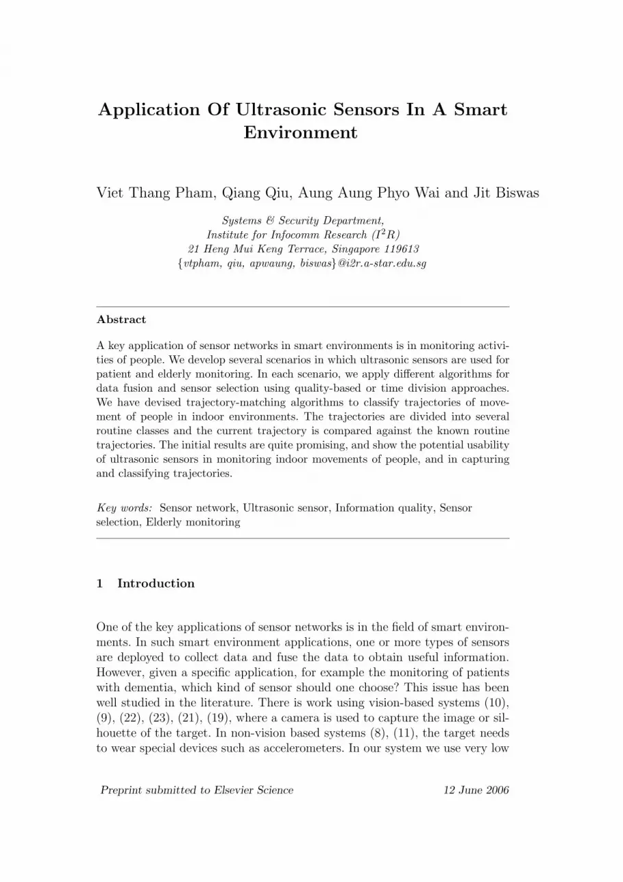
Fig. 1. Overall architecture of sensor-based application

The overall architecture of any sensor-based application can be broadly di-vided into a 4-layer architecture as shown in Figure 1. At each level there areseveral research challenges such as sensor management, sensor selection, datafusion and data inference. In this paper we apply this general architecture tothe specific problem of monitoring an elderly person’s activities at home or inthe hospital ward. We have investigated three scenarios with different sensordeployment, sensor selection and data fusion strategies. In our first scenario,sensors are deployed around a room, sensor selection is based on the qualityprofile of individual sensors, and data fusion uses triangulation. The secondscenario is similar to the first one, only the data fusion stage uses Kalmanfilters. In the third scenario, we deploy the sensors in a grid on the ceiling,and sensor scheduling is done on the basis of time division. All three scenariosuse the ultrasonic sensor to capture trajectories of an elderly person or pa-tient, and then to classify the captured trajectories for the purpose of activityanalysis. The results reported herein, were obtained as a part of a joint-projectbetween Institute for Infocomm Research and Alexandra Hospital (1). Thispaper concentrates on the ultrasound sensor, sensor quality profile, trajectorymatching and the use of the Extended Kalman filter. Reported elsewhere (2),are results that focus more on other sensing modalities such as fiber opticalsensors, accelerometers, and multi-modal data fusion. Table 1 presents a com-parative study showing how our methods differ from those in the literature.The motivation of our work is to illustrate the advantages of applying ultra-sound sensors for tracking people in a non-intrusive, low cost manner, whileconsidering the quality abnormalities of these sensors.

2

Table 1Comparison of different schemes to detect and monitor people

Research Sensor Goal System Complexity Privacy Quality

type cost issues aware

M.Chan Infrared Monitoring High

et. al (13) elderly Medium No No

K.Matsuoka 167 sensors Life Very Very

et. al (16) of 15 kinds activities high high Yes No

A.G.Hauptmann Audio Automated

et. al (14) and video analysis High High Yes No

A.Sixmith Infrared Fall

et. al (20) integrated detection Low Low No No

thermal

S.K. Das Several Health

et. al (15) different monitoring Very Not No

sensors by activity High high clear

prediction

Our work Ultrasonic Motion and

sound trajectory Low Low No Yes

sensors detection

The rest of the paper is organized as follows. Section 2 presents some back-ground about the information quality profile, what it is and how to obtain it.The first and second scenarios are presented in section 3, and the third sce-nario in section 4. Section 5 compares the result of our different approaches.Section 6 concludes the paper with a discussion of future work.

2 Background

In this section, we present an informal definition of quality profile, and demon-strate how to obtain and use the quality profile in the case of ultrasound sen-sors. We also present the definition of a trajectory and introduce the trajectorymatching algorithm.

2.1 Quality profile characterization

Information quality criteria are those criteria that allow us to characterizethe measure of goodness of data or information in a given situation. Thequality profile of a sensor is the set of values associated with each informationquality criterion that is relevant to the sensor. Note that the quality profilecan change from time to time based on environmental conditions, location,battery life, wear and tear etc. A sensor’s quality profile is measured in acalibration experiment, which may be conducted partly in the factory duringmanufacture, and partly on site during deployment.

3

2.1.1 Quality profile generation

The following is a non-exhaustive list of information quality criteria that arenecessary to define the quality profile of wireless ultrasound sensors:

Accuracy: The maximum percentage of error between the expected valueand the actual sensor reading, compared to the range.

Accuracy =Actualmax − Expected

Actualmax − Actualmin

(1)

Repeatability: The percentage error between the reading generated by asecond calibration measurement and the benchmark value, compared to therange.

Repeatability =Actualaverage − Expected

Actualmax − Actualmin

(2)

Sensitivity: The ratio between the sensor output changes and the change inthe sensor input causing such output change.

Linearity: The measure of constancy of the ratio of input to output.Response Time: The time required for a change in input to be observable

in the output.Resolution: The smallest observable increment in input.Energy Capacity: The power remaining in a sensor if it operates on battery.

Note that sometimes sensing and communication use the same power source.However for the purpose of this definition we assume that the power sourceis used only for sensing.

The quality profile of a sensor consists of a set of profile entries, with val-ues provided for different locations within the sensor’s coverage, and differentvelocities of a target object. The fields in a profile entry are:

• Radial: Distance from object to sensor• HAngle: Horizontal angular coordinate (Off center beam)• VAngle: Vertical angular coordinate (Off center beam)• Velocity: Speed of object• Accuracy: Difference between actual and measured value• Repeatability: Difference between successive measurements

To generate the sensor quality profile, we need to conduct a calibration ex-periment that produces data known as Sensor Calibration Data. This data isstored in a file in which each entry represents a point in the coverage range ofthe sensor, defined by polar coordinates. The schema of the sensor calibrationdata file is thus as follows:

4

d1, HAngle1, reading1, reading2....readingn

d1, HAngle2, reading1, reading2....readingn

d1, HAngle3, reading1, reading2....readingn

d2, HAngle1, reading1, reading2....readingn

d2, HAngle2, reading1, reading2....readingn

d2, HAngle3, reading1, reading2....readingn

. . . . . . . . . . . . . . . . . . . . . . . . . .di, HAnglej, reading1, reading2....readingn

. . . . . . . . . . . . . . . . . . . . . . . . . .

in which

di ∈ {0.5, 1, 1.5, 2, 2.5, 3, 3.5, 4, 4.5, 5}HAnglej ∈ {0, 5, 10}

readingi : ith experiment data

After generating the sensor calibration data file, we apply the equations (1)and (2) to each sensor calibration entry. This gives us the sensor quality profilefor each point in the sensor’s coverage range. The quality profile is also savedin a file, according to the following schema:

Distance, HAngle These values determine a point in the coverage range ofthe sensor

Accuracy, Repeatability The values of the two quality criteria at this point

The sensor quality profile file is used as a lookup table. When we wish to assessthe quality of any point in the coverage range, we select the nearest point inthe lookup table, and extract the accuracy and repeatability values.

2.1.2 Experiment for quality assessment

The floor in the coverage range of a sensor is divided in the shape of a conicalgrid, as shown in Figure 2(a). We use polar coordinates to represent a pointin the sensor’s coverage range. To obtain the grid points, three angular coor-dinates on the horizontal plane are used: 0o, 5o and 10o. Radially, the distancebetween two consecutive points along a radial line is 0.5m.

The central idea of the calibration experiment is to use a moving object witha constant acceleration, to calibrate the information produced by an ultra-sound sensor tracking the object. Knowing that the acceleration of the objectis constant, we can compute the velocity and the distance of the object atany given time. The constant acceleration is obtained by exploiting the grav-itational pull of the Earth. Figure 2(b) depicts an approach to generate suchmovement by an object. The object we used in our experiment slides along

5

an inclined plane, created by a wire connecting a point at a specific height toa point below. By measuring the height, we can compute the velocity of theobject at a particular time and hence, determine the distance that the objecthas traveled.

This configuration allows us to know the position of the object at a particulartime. If we conduct the experiment at different points in a sensor’s coveragerange with the same conditions, then the obtained results would reflect thecalibrated accuracy values of the sensor. In this manner, we can characterizethe quality of a sonar sensor at different points in its range.

S

(a) Grid sensor’s range on the floor

S

h

(b) Generate a sliding object

Fig. 2. Experiment design

Figure 3 shows the result of our experiment. From the experimental result,we can infer the accuracy at each point. The difference between each data setand the actual movement of the object indicates which is better. If the shapeof the sensed data curve is closer to the shape of actual data, it means thatthe sensor has a higher accuracy.

2.2 Quality-driven sonar sensor selection

This section addresses the problem of how to select a sensor to continue keep-ing track of the target. We assume that we have redundant sensor coveragei.e. the sensors are deployed in such a way that at any given time, the targetis always in the range of at least two sensors. We are therefore interested indetermining how to select sensors to keep track of the target. Figure 4 presentsa scenario of sensor deployment, that illustrates the need for sensor selection.

Given a set of sensors S={S1, S2....Sn} all deployed in one room, if the targettends to go out of range of one sensor or when the tracking quality is decreas-ing, a hand-over algorithm is initiated upon a neighboring sensor which hasbetter coverage of the target. This algorithm also includes a “wake-up andsynchronize procedure”. In this manner, energy conservation is accomplishedby ensuring that at any given time, at most two sensors are actively trackingthe target. The algorithm consists of several steps which are presented in thefollowing sections.

6

0 0.005 0.01 0.015 0.02 0.025 0.030.5

1

1.5

2

2.5

3Distance=3m

Time

Dis

tanc

e to

sen

sor

Ground truth0−degree data5−degree data10−degree data

(a) Sliding from 3m

0 0.005 0.01 0.015 0.02 0.0252

2.5

3

3.5

4Distance=4m

Time

Dis

tanc

e to

sen

sor

Ground truth0−degree data5−degree data10−degree data

(b) Sliding from 4m

0 0.005 0.01 0.015 0.02 0.0253

3.5

4

4.5

5Distance=5m

Time

Dis

tanc

e to

sen

sor

Ground truth0−degree data5−degree data

(c) Sliding from 5m

0 0.005 0.01 0.015 0.02 0.0254

4.5

5

5.5

6Distance=6m

Time

Dis

tanc

e to

sen

sor

Ground truth0−degree data5−degree data

(d) Sliding from 6m

Fig. 3. Data experiment object’s slidingGround truth vs. sensed data

Fig. 4. Sensor selection scenarioGiven a set of sensors, which ones should be active to keep track of the

target?

7

2.2.1 Sensor characterizing

Each sensor in the network has a set of parameters which define and charac-terize its location and properties. Figure 5 represents a sensor Si in the globalcoordinate system and its parameters as listed below:

(Six, Siy) : Global coordinate to determine the location of sensor in the room.Siα : angle between the center beam of center and the global X-axis, thisvalue indicates the sensing direction of sensor Si. Siα ∈ [0..360].

β : Valid angle of the sensor’s range. This property can be defined by themanufacturer but we need to verify it by experiment. For our sensor, β = 10o

for all sensors.d : is the maximum distance at which a sensor can detect an object. This

parameter may not be the maximum distance that the sensor is capable ofmeasuring, since there may be obstacles in the range of sensor. Differentfrom other parameters, this distance d is dynamic, it can only be obtainedin situ, during calibration of the sensor.

O X

Y

S i

S iy

S ix

d 1

d 2

Fig. 5. Sensor in global coordinate system and its parametersSix, Siy: XY-coordinate

α : Angle between center beam and X-axisd1, d2 : Boundary lines

2.2.2 Sensor Candidate Set

The sensor candidate set is the collection of sensors which can detect thetarget at a given time. This set changes dynamically for each position of thetarget in the coordinate system. Below we present a mathematical model togenerate a sensor candidate set corresponding to a specific target’s location.This mathematical model is based on the coordinates of the target and theparameters of the sensors as described in section 2.2.1.To determine the relative position between target and sensor, we need tocalculate the distance between target and sensor and the angle made by theline joining target to sensor with the X-axis. The simplicity of calculating

8

distance leads us to focus on the angle determination.

θ = cos−1(Ox − Sx

|−→Si0|) = cos−1(

Ox − Sx√(Ox − Sx)2 + (Oy − Sy)2

)

If we call the angle made by the line joining sensor to target with the X-axisφ, then we have the following two cases:

φ =

θ if 0 ≤ Siα < 180

360− θ otherwise(3)

The object is in range of a sensor Si if its location satisfies the two conditions:

Siα − β2≤ φ ≤ Siα + β

2

0.5 ≤ OSi ≤ Si.d(4)

2.2.3 Grade and select sensor in candidate set

In this section the sensor selection algorithm is presented. We use the qualityprofile as the criteria to grade the sensors in the sensors candidate set, thenselect the entry with highest IQ (Information Quality) score.

Recall that the quality profile, is an instantiation of a set of quality crite-ria. To grade the IQ score of an individual sensor, we require a weight-vectorW=(w1, w2, ..., wn), specified by the user such that

∑ni=1 wi equals to 1. The

length of the weight-vector,n, is equal to the number of criteria in the qualityprofile. In general we can set the weight to zero for the absent criteria. Theweight-vector component reflects the importance of the corresponding crite-rion to the users. If the users prefer accuracy to repeatability, i.e. accuracyis more important than repeatability, they set the weight for accuracy higherthan the weight for repeatability, keeping the sum of the weights equal to 1.For each individual sensor Si, the overall quality score IQ(Si) for a particularpoint in its range is calculated as a weighted sum, as follows:

IQ(Si) =∑n

j=1 wj.vij

in which vi is the vector corresponding to the evaluated point in the qual-ity profile. The sensor selection procedure is presented in Algorithm 1, Sen-sor Selection(O,S).

Algorithm 1 Sensor Selection(O,S)

9

1: S ← {S1, S2, ...., Sn}2: O ←Current target location3: Candidate Set ← ∅4: for i ← 1 to n do5: if (O ∈ Si’s range) then6: Candidate Set ← Candidate Set

⋃Si

7: end if8: end for9: for each Si in Candidate Set do

10: Find entry kth in IQ profile which is closest to 011: vi ← k12: IQ(Si) =

∑nj=1 wj.vij

13: end for14: Select the two sensors with highest IQ(Si) score from Candidate Set

We can see in line 5 of Algorithm 1, the equation (4) is applied to verifycurrent position in the range of sensor Si.

2.3 Trajectory monitoring

2.3.1 Trajectory representation

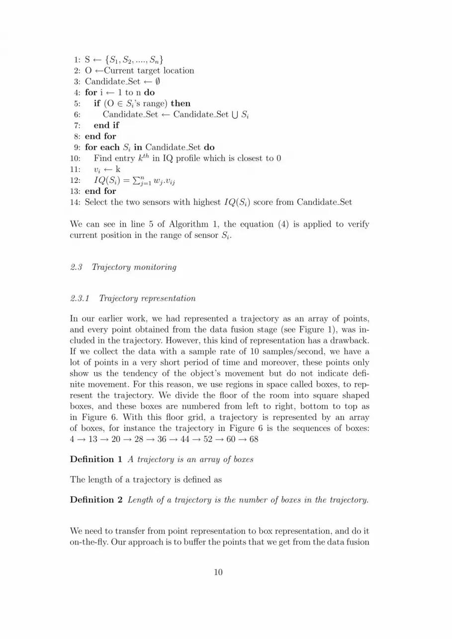
In our earlier work, we had represented a trajectory as an array of points,and every point obtained from the data fusion stage (see Figure 1), was in-cluded in the trajectory. However, this kind of representation has a drawback.If we collect the data with a sample rate of 10 samples/second, we have alot of points in a very short period of time and moreover, these points onlyshow us the tendency of the object’s movement but do not indicate defi-nite movement. For this reason, we use regions in space called boxes, to rep-resent the trajectory. We divide the floor of the room into square shapedboxes, and these boxes are numbered from left to right, bottom to top asin Figure 6. With this floor grid, a trajectory is represented by an arrayof boxes, for instance the trajectory in Figure 6 is the sequences of boxes:4 → 13 → 20 → 28 → 36 → 44 → 52 → 60 → 68

Definition 1 A trajectory is an array of boxes

The length of a trajectory is defined as

Definition 2 Length of a trajectory is the number of boxes in the trajectory.

We need to transfer from point representation to box representation, and do iton-the-fly. Our approach is to buffer the points that we get from the data fusion

10

stage, and then find the box that has the maximum density of points in thebuffer. This single box will represent the collection of points in buffer. Whenthe person is moving, the points are transferred to boxes and the trajectoryis formed on the fly.

Fig. 6. Example of trajectory on a floordivided by a grid of boxes of dimension 8x10

2.4 Trajectory Classification

Since we have represented the trajectory as a array of box numbers, the tra-jectory classification problem can be seen as follows:We have a set of known trajectories T1, T2..., Tn, and we have an unknowntrajectory U that we would like to classify. The objective of the procedureis to try to match U with one of the known trajectories Ti. If no match canbe made, we report U as a new trajectory. The following definitions will beneeded:

Definition 3 Distance from a box b to a trajectory T with an array of boxesa1 → a2 → ... → an, only count from box index j, aj, is defined as:

d(b, T ) = min{d(b, ai)|i > j}Definition 4 The most matching trajectory (MMT) to a box b is the trajec-tory whose distance to the box is minimum among all the distances from othertrajectories. This minimum distance has to be less than a predefined threshold.

MMT (b) = {i| d(b, Ti) < d(B, Tj), ∀j 6= i and d(b, Ti) < Threshold}

The key step of the trajectory classification algorithm is to find the mostmatching trajectory from the known trajectories for each box in U, then findthe maximum appearance of matching trajectories for all the boxes. This tra-jectory could be the closest trajectory to U. The details of the algorithm arepresented in pseudo code format as shown in Algorithm 2.

11

Algorithm 2 Trajectory Classification

1: Input T1, T2, ...Tn

2: U : b1 → b2... → bm

3: Output Ti or New trajectory4: Initialize5: NoAppear(0..n) ← 0 {Number of appearance}6: index(1..n) ← 1 {Current compared index}7: MMT SET ← ∅8: for j ← 1 to m do9: min ← 1000

10: MMT SET ← ∅{Find the minimum distance from this box to all trajectory}

11: for i ← 1 to n do12: if min ≤ d(bj, Ti) then13: min ← d(bj, Ti)14: end if15: end for

{Take the index of the MMT for this current box and put it in MMT SET}16: for i ← 1 to n do17: if min = d(bj, Ti) then18: index(i)← index of the closest box to bj in Ti

19: MMT SET ← MMT SET⋃

i20: end if21: end for

{Check the minimum distance smaller than a pre-defined threshold}22: if min ≤ THRESHOLD DISTANCE then23: for each i in MMT SET do24: NoAppear(i) ← NoAppear(i) + 1 {Increase the number of appear-

ance for MMT trajectory}25: end for26: else27: NoAppear(0) ← NoAppear(0) + 1 {Index 0 means that there is no

MMT for this box}28: end if29: end for

{Find the trajectory index which is the most-appeared}30: Find k such that NoAppear(k)=max{NoAppear(i)}31: if k = 0 then32: Return “New Trajectory” {Index 0 is the maximum of number of ap-

pearance}33: else34: if (NoAppear(k)/Len(Tk)>THRESHOLD)

and (NoAppear(k)/Len(U)>THRESHOLD) then35: Return Tk

12

36: else37: Return “New Trajectory”38: end if39: end if

3 Conventional sensor deployment

3.1 Trilateration data fusion algorithm

In this section we present an algorithm which is similar to a simple mathe-matical principle called trilateration (6). Given two sensors, S1 and S2 and atarget O in the detected range of both sensors, we create a local coordinatesystem with the origin point is S1, X-axis being the line S1S2 as shown inFigure 7. Suppose that we know the location of each sensor, so the coordinateof S2 is (d,0). At time t, target O is detected by both sensor S1 and S2. Theraw data we read from these two sensors are distances from sensor S1, S2 totarget O, we call them d1, d2 respectively. If the coordinates of target O are(xo, yo), we have

x2o + y2

o = d21

(xo − d)2 + y2o = d2

2

hence

xo =d2 + d2

1 − d22

2d

yo =√

d21 − x2

o

s X

Y

o

d 1

V

d

v 1

v 2

d 2

1

s 2

Fig. 7. Data fusion algorithmS1, S2 : the two ultrasonic sensors

O : target’s position

We transform the coordinates of the target from local coordinate system toglobal coordinate system. This requires two steps; the first step is rotationaltransformation and the second step is translational transformation. For the

13

first step, we have to determine the rotation angle between the local coordinatesystem and global coordinate system. This rotation angle is equal to the anglebetween the two X axes of the two coordinate systems.If S1(x1, y1) and S2(x2, y2) then the angle α is

α =

arctan( y1 − y2x2 − x1

) if x1 6= x2

90o if x1 = x2

If we call x′o and y′o the coordinate of the target in the global coordinatesystem, we have

x′o = x1 + xocos(α) + yosin(α)

y′o = y1 + yocos(α)− xosin(α)

We have seen how a simple algorithm based on triangulation geometry canbe applied to solve the data fusion problem, i.e. to fuse data from ultrasoundsensors. This algorithm requires only two sensors and that the target be intheir coverage range.

3.2 Data fusion quality: Spatial loss

In the data fusion algorithm described in the previous section, we have madethe simplifying assumption that the target detected by both sensors is dimen-sionless, i.e. its coordinates are given by a single point in space, the coordinatesof which are obtained from the data fusion. However, in most cases, this is nottrue, because the tracked object, for example in our case the person, has vol-ume and when he is walking or standing, each sensor detects different parts ofhis body. By assuming that two sensors are detecting the same point in space,we lose information quality. This is called spatial information quality (IQ) loss.The objective of data fusion correction is to minimize the spatial IQ loss andhence increase the accuracy of the data fusion algorithm. Figure 8 depicts thissituation. If O is the detected point from the data fusion algorithm, the targetmay be anywhere in the area made by three points O, A and B.

A way to estimate the location of the target is to take the centroid of the tri-angle OAB to represent the target location. The steps to compute the centroidare as follows.

• i) Determine the two points at the boundary of one sensor• ii) Select the point which is further from the other sensor• iii)Compute the centroid of the triangle OAB.

14

If the angle in the direction of sensor S1 is α1, and the valid coverage rangeof sensor is β, d1 is the distance from S1 to O, then the two points at theboundary of sensor S1 are:

B

x = S1.x + d1.sin(α1 + β2)

y = S1.y + d1.cos(α1 + β2)

B′

x = S1.x + d1.sin(α1 − β2)

y = S1.y + d1.cos(α1 − β2)

s X

Y

o B

B’ A’

A

1 s

2 1

1

2

2

Fig. 8. Data Fusion Correction - Minimize Spatial IQ LossS1, S2 : the two sensors

O : Fused pointB and B’: the two points at the boundary of S1 : S1O=S1B=S1B

′

A and A’: the two points at the boundary of S2 : S2O=S2A=S2A′

From the two points B and B’, we eliminate the point which is closer to sensorS2; suppose this is B’. So we have point B at the boundary of sensor S1.Similarly for sensor S2, we have point A at the boundary of the sensor S2.Hence, the estimation of the target location is

Target− estimation

x = O.x+A.x+B.x3

y = O.y+A.y+A.y3

3.3 Extended Kalman Filter data fusion

The Kalman filter is well known for target tracking from its first publicationin the early of 1960s (7). In this section, we show how can we use the Kalmanfilter to predict the position of a person using ultrasonic sensor networks. Inour particular case, we use the Extended Kalman Filter (EKF) algorithm,since our measurement function is non-linear. Before going into the details,we present the general extended Kalman filter algorithm. If we have a systemof equations:

15

x(k + 1) = f [x(k), k] + w(k)

z(k) = h[x(k), k] + v(k)(5)

in which:x(k) ∈ Rn : the state vectorz(k) ∈ Rp : the measurement vectorw(k), v(k) : the process and measurement noises with covariances Q(k), R(k).If the system function f has form:

f =

f1(x1, x2, ..., xn)

f2(x1, x2, ..., xn)

...

fn(x1, x2, ..., xn)

Then the Jacobian matrix of function f at x(k|k)

F (x(k|k), k) =δf

δx

∣∣∣∣x=x(k|k)

=

δf1

δx1

δf1

δx2... δf1

δxn

δf2

δx1

δf2

δx2... δf2

δxn

...

δfn

δx1

δfn

δx2... δfn

δxn

∣∣∣∣∣∣∣∣∣∣∣∣∣∣x=x(k|k)

The basic steps of the computational procedures for the extended Kalmanfilter are as follow:

(1) Prediction:State prediction: x(k + 1|k) = f [x(k|k), k]Covariance: P (k + 1|k) = F [x(k|k), k]P (k|k)F T [x(k|k), k] + Q(k)Measurement prediction: z(k + 1|k) = h[x(k + 1|k), k]Covariance : S(k + 1) = F [x(k|k), k]P (k|k)F T [x(k|k), k] + Q(k)

(2) EKF gainK(k + 1) = P (k + 1|k)HT [x(k + 1|k), k]S−1(k + 1)

(3) Update the estimate using z(k+1)x(k + 1|k + 1) = x(k + 1|k) + K(k + 1)[z(k + 1)− z(k + 1|k)]Update the state covarianceP (k + 1|k + 1) = P (k + 1|k)−K(k + 1)S(k + 1)KT (k + 1)

Our specific problem can be described as follows: We have two ultrasonicsensors, and a target is moving around in their common range. Each sensorreports the distances from itself to the target. We need to predict the positionof the target based on the readings from two sensors.

16

Given two sensors, located at known position (xS1, yS1) and (xS2, yS2), thesystem vector state is:

Xk = [x[k], y[k], x[k], y[k]]T

where x[k] and y[k] are the x and y coordinates of the target, and x[k] andy[k] are its x and y velocity components.If we assume that in a period of time 4t, the velocity is constant, then therelation between state k and state (k+1) is

Xk+1 =

1 0 4t 0

0 1 0 4t

0 0 1 0

0 0 0 1

Xk + Wk

where the covariance of Wk is

Q = q

(4t)3

30 (4t)2

20

0 (4t)3

30 (4t)2

2

(4t)2

20 4t 0

0 (4t)2

20 4t

The measured values for our problem are two distances dS1[k], dS2[k]:

Zk =

dS1[k]

dS2[k]

+ Vk

where Vk has the covariance:

R =

1 0

0 1

and dS1[k], dS2[k] are the distances from target to sensors S1, S2 respectively.

dS1[k] =√

(x[k]− xS1)2 + (y[k]− yS1)2

dS2[k] =√

(x[k]− xS2)2 + (y[k]− yS2)2(6)

To implement the EKF, we need to compute the Jacobian matrix H.

17

Hk =

δdS1[k]δx[k]

δdS1[k]δy[k]

δdS1[k]δx[k]

δdS1[k]δy[k]

δdS2[k]δx[k]

δdS2[k]δy[k]

δdS2[k]δx[k]

δdS2[k]δy[k]

∣∣∣∣∣∣∣X=X(k|k−1)

Applying (6), we have:

Hk =

xk−xS1

dS1[k]yk−xS1

dS1[k]0 0

xk−xS2

dS2[k]yk−xS2

dS2[k]0 0

The result of our implementation is presented in the section 5.

4 New approach: Grid sensors on the ceiling

In this section, we demonstrate the capability of ultrasonic sensors to monitorpeoples’ movement if they are mounted on the ceiling.

4.1 Sensor deployment

In our demonstration prototype, we have deployed the sensors in a room ofdimension 2x4m, with 10 wireless ultrasonic sensors mounted on the ceiling ina 2 by 5 grid. In other words we have two rows of sensors, each with 5 sensors.Figure 9 shows the deployment scenario.

Fig. 9. Sensor deployment : grid sensors on the ceiling

A major problem with using multiple ultrasonic sensors is interference. Wrongreadings may be caused by interference with neighboring sensors, or by thesound wave bouncing off the environment in unforeseen ways. We found twomajor factors that influence interference, namely a) distance between sensors

18

and b) sample rate. The optimal distance and the sample rate are selected onthe basis of the following two guidelines:

• Reduce the interference as much as possible.• Maximize the total number of sensors that can be deployed by minimizing

the inter-sensor distance. In this manner the coverage of the room can bemaximized.

The optimal distance and sample rate were determined by experiment. Weadjusted the distance between sensors and changed the sample rate until wesaw accurate and stable readings. Our experiment shows that if the sensors arepositioned at a height of around 2.5m, the optimal distance between sensorsis 0.7m and the sample rate is 2 samples/second.

Sensor deployment is also a major problem in sensor networks. For ultrasoundsensors, sensor deployment has specific requirements:

• Redundant coverage: Every point in the need-to-detect area, requires atleast two sensors to cover it.

• Minimization of interference: For example, the sensor may not be placedface to face within their range.

• Maximization of coverage area. We should try to maximize the coverage areaby introducing as many sensors as possible, subject to the other constraints.

4.2 Data fusion

Total body movement data fusion (TBM)

In this section we briefly describe a real life application in which we havedeployed ultrasound sensors. Our work is based on the Scale to Observe Agi-tation in Persons with Dementia of the Alzheimer Type (SOAPD) (24). Thisscale seeks to objectively classify the degree of agitation experienced by aperson with dementia. Currently, rating for the SOAPD scale is an extremelylaborious task, carried out by clinicians who rate the duration of the personsbodily movements and vocalizations for periods of five minutes at a time, andassign a subjective rating for each manifested behavior. The objective of ourwork is to automate this tedious and subjective task with the help of sensors.

Herein we report our initial work on two of the behavioral features of SOAPD,namely the Total Body Movement (TBM) and Up/Down Movement (UDM).With the ceiling deployment of section 4.1, it is possible to monitor bothTBM and UDM. For TBM detection, we use ultrasound sensors for accuraterecognition and tracking instead of the typical video based solutions which areoften considered too intrusive. For UDM detection, we demonstrate the use

19

of two types of sensors working together in concert, namely pressure sensorsand ultrasound sensors. The fusion of data produced by these two sensingmodalities enables more accurate detection.

Corresponding to sensor deployment, sensor readings are stored in a 2x5 ma-trix. Whenever we have data sent from one of the sensors, we create a snapshotof the matrix representing the current reading value of all the sensors. Sincethe data we have from ultrasonic sensors are the distances from sensors to thenearest object, obviously the person should be under the sensor which givesus the smallest reading.

Scanning the matrix and finding the minimum element, we may assume thissensor should be the location of the person in the room. Figure 10 shows thereadings from 10 sensors as the person is moving. At any time, the shortestbar represents the position of the person in the room.

Fig. 10. Continuous reading from 10 sensorsThe shortest bar (in black) represents the position of the person in the room

Recall that the trajectory of movement has the format of an array of boxes.We also record the time when person moves from underneath one sensor toanother, so that we know the duration of staying under each sensor up to themillisecond. Our system was demonstrated to record with 90% correctness,the position of the person in the room. The reason for 10% loss of accuracy isinterference. Although we tried to deploy the sensors and select the appropri-ate sample rate, the interference is still present, and sometimes causes wrongreadings.

Up and down movement data fusion

If a person is sitting in a chair, the ceiling deployment of ultrasound sensors candetect the Up and Down Movement (UDM) behavior of the person. Figure11 shows the data from one sensor when a person repeats UDM behavior.The peaks or spikes in the data show the times at which the person is risingup towards a standing position. The data fusion algorithm used for UDMbehavior recognition uses the current reading from sensor, and maintains awindow frame of its past readings. By observing the relation between thecurrent reading value and the previous ones, we know whether the personchanges his/her posture between sitting and standing.

Some details of our algorithm are now discussed. We define two states: sitting

20

and standing and maintain a window of past values, of size L. We also needa value of threshold between sitting and standing. We calculate the sum Sof all the differences between the current value and each value in the window.

if (currState==STANDING)

if (sum(S) > threshold)

currState=SITTING;

else

if (sum(S) < - threshold)

currState=STANDING;

Fig. 11. Up down movement under ultrasonic sensor

The parameters, L and threshold need to be tuned depending on the appli-cation. Several repetitions of UDM detection have shown that for an averageperson going from a sitting to a fully standing position, the parameters shouldbe L=3 and threshold=15cm. With these values we can detect UDM behavior90% of the times. However dementia patients are usually locked in the chairwith the help of a restraint, and are unable to rise to a fully standing posi-tion. They are only able to move to a semi-standing position. In this case,the parameters should be L=4 and threshold=8cm. With these values we cansuccessfully detect UDM behavior 50% to 70% of the time.

Up and down movement detection illustrates the dynamic trade-off betweensample rate, interference and accuracy of detection. If we increase the samplerate, it can cause a lot of interference, but if the sample rate is low, we losedata. For example, if the sample rate is low, and the person changes statefrom standing to sitting, we may not capture the state-change event.

4.3 Sensor management: Time division scheduling

As mentioned previously, a very common problem with ultrasonic sensorsis the interference caused by receiving the unexpected reflected waves fromother sensors in the neighborhood. We experienced this symptom with ourceiling deployment of ten sensors (Figure 9). If all ten sensors are turned onat the same time, and they emit sound simultaneously. Thus the chance for

21

interference to take place is very high. To overcome this problem, we haveimplemented a mechanism to schedule the sensors intelligently, meaning thatsensors should be turned on and off at the right time, thereby reducing as muchas possible, interference to other sensors. We call this scheme time divisionscheduling(12).

The basic idea of time division scheduling is to make sure there is one and onlyone sensor operating at any given time. So the sensors work in a round-robinmanner. A sensor sends out a signal, then comes to an idle state, waitingfor all the others to send their signals before sending its signal once moreand coming to an idle state again. In the beginning, when we turn on allthe sensors, each sensor has to have a different delay time before sending itssignal. The computation of how long each sensor should go to sleep and andhow long is the delay for each sensor in the beginning, depends on the numberof sensors in the sensor network and the sample rate we would like to have foreach sensor.

The drawback of the round-robin scheduling method is that it could drasticallyreduce the sampling rate in case of large deployments of sensors, since insuch a case, one sensor would be required to wait till all other sensors havehad their turn. It is possible to propose ways to modify a pure round-robinscheduling strategy, by activating multiple sensors simultaneously, given thatthese sensors are far enough from each other, so as not to cause any mutualinterference. This approach is left for future work.

5 Implementation and Results

In this section, we present a combination of all the above algorithms andcomponents to form an application called “Elderly Trajectory Monitoring andClassification”. Two types of ultrasound sensors were used, wired and wireless.Wired sensors were used in the laboratory to classify trajectories, and wirelesssensors were deployed in both lab and site (hospital) environments. The wiredsensor used was the Vernier MDO-BTD motion detector (3). This sensor needsa hub device (called LabPro), to communicate with a PC via COM port orUSB port. One LabPro device supports up to 4 motion detectors. The costfor a motion detector and a LabPro device are $75 and $220 respectively. Thewireless sensor used was the Daventech SRF04 Ultrasonic Ranger (4), oper-ating on MicaZ mote (5) platform, which has been used in diverse industrialand environmental monitoring applications, for example (17). Also requiredfor the wireless version, is a programming board to communicate with a PC,and a base station device, the MIB600 gateway, which is capable of supportingup to 254 sensors. The cost for one ultrasound sensor is $25 and that of oneMIB600 programming board is $360.

22

With their longer range, the wired sensors were used in the lab deploymentfor trajectory classification, using trilateration and Extended Kalman filterdata fusion algorithms, whereas the wireless sensors were used in the ceilingdeployment scenario which was tested in a hospital room.

In the next few paragraphs we discuss the wired sensor application. Foursensors were used, and each was positioned laterally, i.e. in a manner that thesound waves traveled in the horizontal plane to detect people moving withintheir coverage range. Because of range limitations of each sensor, we triedto position them in a way that would allow us to get maximum coveragearea from the four sensors. Figure 12 shows the graphical user interface of ourapplication. On the left is the raw data we get from four sensors when a personwalks in the room. These points show us the direction of movement of theelderly person. As described in section 2.3.1, these raw points were convertedto an array of boxes, so as to represent the corresponding trajectory. On theright of Figure 12 is the abstract data, shown as the boxes in a room. For thesake of demonstration, we also put the array of boxes on the screen.

The steps to begin a new sensor data recording session are as follows:- Calibration : Recall from section 2.2.1, that every sensor has a dynamic pa-rameter, the maximum distance for the range of this sensor. This parameter isdefined by the manufacturer’s specifications, but when we deploy the sensor ina room, there may be obstacles. Thus calibration has to be carried out whenthere is no one in the room to determine the maximum reading value of eachsensor.- “Learning” new trajectory : At the beginning, the program has no known tra-jectory, and the set of trajectories is empty. We need to algorithmically “teach”the system to recognize new trajectories by repeating the same movement foreach class of trajectories.

In our evaluation, we used only four wired ultrasound sensors. During deploy-ment we tried our best to maximize the common coverage range of the foursensors. Since the range of each sensor is quite narrow, the common coveragewas just around 2mx4m. With this coverage area, the complexity of trajecto-ries was limited. The trajectory matching algorithm presented earlier workswell, given that we are able to collect sufficient data. The complexity of thetrajectory captured is related to the number of sensors and their coveragearea. For complex classes of trajectories more sensors are required to coverthe area of the trajectories.

For our demonstration, we created two classes of trajectories, namely, ClassA: Going toward the sensors, Class B: Going across the sensors. For eachclass, we repeated our experiment 50 times. Figure 12 presents a trajectoryin which a person moves from door to kitchen, corresponding to Class A.We can see that on the left are the points captured and fused from four

23

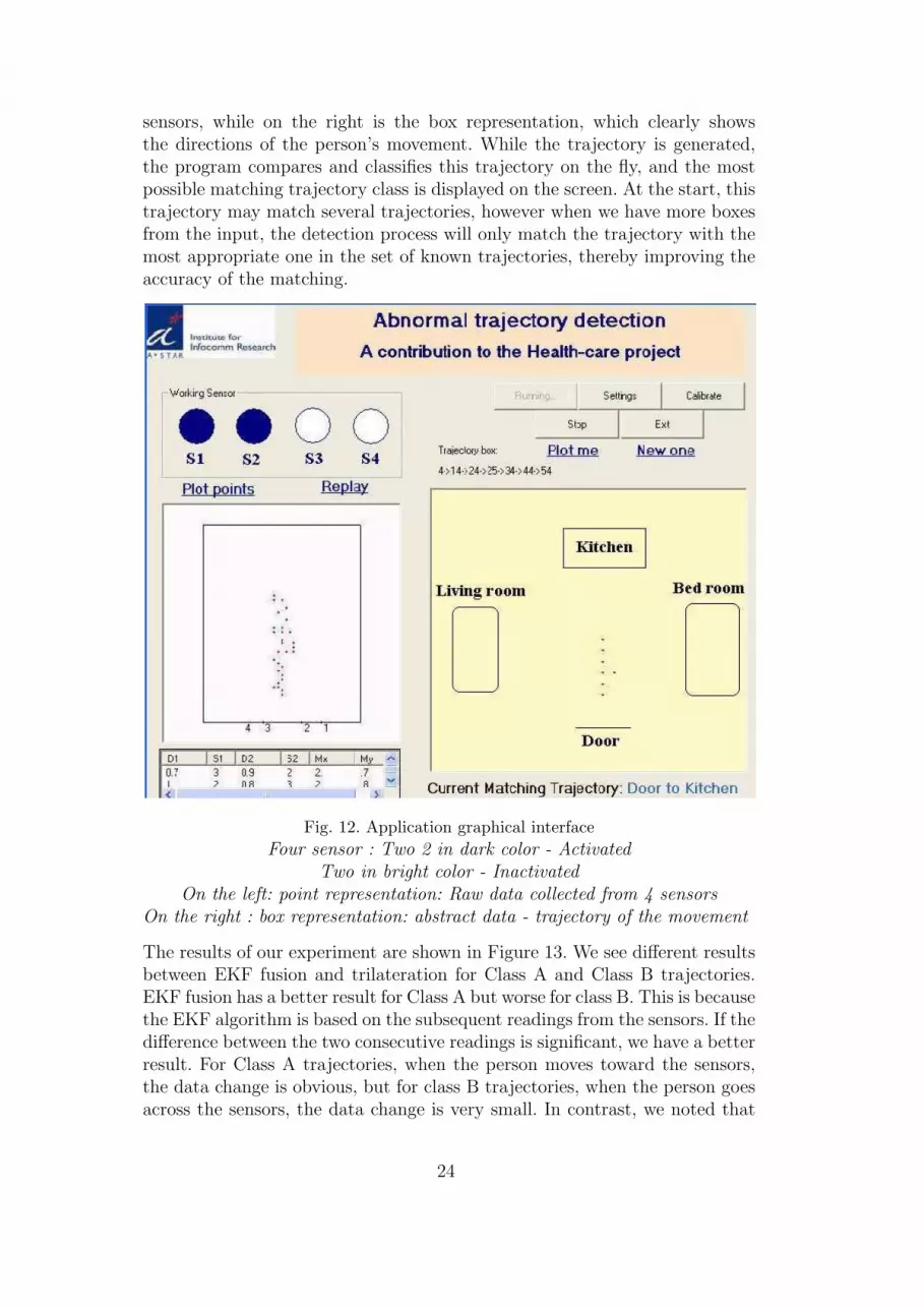
sensors, while on the right is the box representation, which clearly showsthe directions of the person’s movement. While the trajectory is generated,the program compares and classifies this trajectory on the fly, and the mostpossible matching trajectory class is displayed on the screen. At the start, thistrajectory may match several trajectories, however when we have more boxesfrom the input, the detection process will only match the trajectory with themost appropriate one in the set of known trajectories, thereby improving theaccuracy of the matching.

Fig. 12. Application graphical interfaceFour sensor : Two 2 in dark color - Activated

Two in bright color - InactivatedOn the left: point representation: Raw data collected from 4 sensors

On the right : box representation: abstract data - trajectory of the movement

The results of our experiment are shown in Figure 13. We see different resultsbetween EKF fusion and trilateration for Class A and Class B trajectories.EKF fusion has a better result for Class A but worse for class B. This is becausethe EKF algorithm is based on the subsequent readings from the sensors. If thedifference between the two consecutive readings is significant, we have a betterresult. For Class A trajectories, when the person moves toward the sensors,the data change is obvious, but for class B trajectories, when the person goesacross the sensors, the data change is very small. In contrast, we noted that

24

for the ceiling sensor deployment, for both Class A and Class B trajectories,the accuracy is the same at 90%. This is because the sensor deployment isindependent of the trajectories.

Class A Class B0

10

20

30

40

50

60

70

80

90

100

Mat

chin

g P

erce

ntag

e(%

)

EKFTrilaterationTBM

Fig. 13. Comparison of data fusionEKF vs. Trilateration vs. Total Body Movement(TBM)

1 2 3 4 50

10

20

30

40

50

60

70

80

90

100

Speed (km/h)

Acc

urat

e M

atch

ing

(%)

Class AClass B

Fig. 14. Accuracy at various speeds

The system does not perform well in a cluttered room environment due to thenature of ultrasound sensors. These sensors can only detect the nearest objectin their range. So if the person is behind a sensor, he/she cannot be detectedby the sensor. If an obstruction is present between a person and a sensor, thesensor is unable to detect the person’s movement. However, in the case of theceiling deployment for TBM, the performance depends on the height of the

25

patient. If the patient is taller than, (or in a higher position relative to) otherobjects nearby, the system still works well. This is another advantage of theceiling-based deployment.

Beside the technical problems, typically, low cost ultrasonic sensors are knownto make a chirping sound. Wired ultrasound sensors give audible sounds thatare quite apparent in a closed room environment, but the chirping soundproduced by wireless ultrasound sensors can be heard only if the user is quiteclose to the sensor (30cm away from sensor). Due to deployment considerationssuch as physical design and cabling to sensors, wired sensors are placed on thefloor or above the floor on walls all around the room. Thus the chance ofhearing the chirping sound from wired ultrasound sensors is quite high, andmay cause annoyance to the person in the room. However for wireless sensors,we hang/install these sensors on the ceiling so as to achieve coverage of thewhole room, and its direction is almost perpendicular to the floor. Because ofconsiderable distance between ceiling and floor (2.2m minimum), the soundcaused by wireless sensors will cause little or no annoyance to the person inthe room and he/she even may not even notice the existence of these sensors.

5.1 How the speed affects the matching

To study how the speed of movement of the target affects the matching al-gorithm, we also conducted a set of experiments in which we learned the tra-jectories at various speeds, ranging from 1km/h to 5km/h. We thought thiswas reasonable for typical cases of people walking indoors. At each speed, wehad a set of known or learned trajectories. We used these learned trajectoriesduring actual trajectory matching with unknown users. The performance ofthe trajectory matching algorithm for various speeds is presented in Figure14. The result shows that the trajectory matching algorithm performs best ifwe learn the trajectories at speed 3km/h.

5.2 How the spatial information quality loss affects the inference

In section 3.2, we mentioned spatial IQ loss and presented a simple algorithmto reduce this loss. To evaluate this algorithm when applied to trajectorymatching, we conducted an experiment with and without data fusion correc-tion. Figure 15 presents the results of this experiment for both class A andclass B trajectories. We see from the graph that the spatial IQ loss correctionincreases significantly the percentage of classification. For class A trajecto-ries we obtain 80% classification with spatial IQ loss correction, versus 40%without correction. For class B, the result is even better, 80% with correc-tion, compared to 30% without correction. This proves that spatial IQ loss

26

correction significantly improves the performance of the trajectory matchingalgorithm.

The performance of the trajectory matching algorithm also depends on thesample rate. If we set a high sample rate (20 samples per sec or more), wehave a lot of interference between adjacent sensors. For a fixed sample rate, ifthe person walks slowly, the density of the points generated is very high, andthe prediction is not so accurate. In this case we need to reduce the samplerate to improve the accuracy of prediction. On the other hand if the person ismoving fast, the number of points obtained is small, and hence the trajectoryis not clear. In this case, we need to increase the sample rate. In general, thereis a relationship among sample rate, speed and accuracy. A high sample rateis good for fast moving trajectories, but causes interference. If the sample rateis low, the interference is low too, but we lose location sampling information.We are unable to characterize this tradeoff analytically, and the only way tocharacterize it is through experimentation.

Class A Class B0

10

20

30

40

50

60

70

80

90

100

Acc

urat

e M

atch

ing

(%)

With Fusion CorrectionWithout Fusion Correction

Fig. 15. Comparison of fusion correctionWith correction vs. without correction

6 Conclusion

In this paper, we have presented the characteristics of ultrasonic sensors usedas non-invasive devices to monitor the movement of elderly in indoor envi-ronments. We also brought out the quality related issues which are usuallyignored by the research community. Our experiments show that the sensorquality footprint changes with the spatial dimension; therefore, it is possibleto select good quality sensors depending on the position of the target. We firstcharacterized the quality profile of individual sensors and then developed algo-rithms to improve the combined information quality from two or more sensors.Three scenarios of using ultrasound sensor are in presented our study. The firsttwo use the techniques of Extended Kalman Filter (EKF) and Trilateration.

27

The third scenario investigates agitation rating feature known as Total BodyMovement (TBM). Finally, all the proposed algorithms were implemented andtested. The characteristics of the three scenarios are summarized in Table 2.

Table 2Comparison of three implemented scenario

Scenario Sensor Data Sensor Result

deployment fusion management

Trilateration Around the room Trilateration Select sensor based Matched trajectory: 70% - 80%

on quality profile

Extended Select sensor based Matched trajectory: 55% - 92%

EKF Around the room Kalman Filter on quality profile (depends on relative position between

trajectory and sensor position)

TBM Mounting Least Value Time division Matched trajectory: 90 %

on the ceiling Matrix Extra capacity:

Up-down movement detection

Tracking multiple targets is a challenging problem. In our case, it is even morecomplicated because we have no information other than that coming fromultrasound sensors. For trilateration and EKF, tracking of multiple individualsis almost impossible. The ceiling-based sensor deployment approach may beapplicable in this case, since these sensors works independently and thus wecan keep track of more than one target simultaneously. The approach to beused is similar to the single target case, i.e. we need to select two sensors withthe smallest readings and apply a tracking algorithm such as the Kalman filteror particle filter, to keep track of the individual. This study is left for futurework.

In the future, we plan to use other sensors in conjunction with ultrasound sen-sors to improve the classification rate. We also plan to develop more advanceddata fusion and trajectory matching algorithms.

7 Acknowledgements

Some of the work reported herein was done as a part of an ongoing collabo-ration with Dr Philip Yap of the Alexandra Hospital, Singapore. The authorswould also like to acknowledge the contribution of Mr. Santos K. Das andMr. Chava V. Saradhi for help with sensor calibration and trajectory analysisrespectively.

28

References

[1] J. Biswas, Q. Qiu, V. Pham, V. Foo and Q. Guopei. Agitation Monitor-ing in Dementia Patients, Joint Project between Institute for InfocommResearch (I2R) and Alexandra Hospital, Singapore, August 2005.

[2] J. Biswas et. al. Agitation monitoring of persons with dementia basedon acoustic sensors, pressure sensors and ultrasound sensors: a feasibil-ity study. In the Proceedings of the International Conference On AgingDisabilities and Independence (ICADI), Feb 2006.

[3] Vernier Software & Technology - Motion detector. 15th May 2006.<http://www.vernier.com/probes/motion.html>.

[4] SRF04 - Ultra-Sonic Ranger. Technical Specification. 15th May 2006.<http://www.robot-electronics.co.uk/htm/srf04tech.htm>.

[5] MICAz ZigBee Series. CrossBow Technology. 15th May 2006.<http://www.xbow.com/Products/productsdetails.aspx?sid=101>.

[6] Trilateration. From Wikipedia, the free encyclopedia. 15th May 2006.<http://en.wikipedia.org/wiki/Trilateration>.

[7] A.P. Andrews. Kalman Filtering Theory and Practice. Prentice-Hall, En-glewood Cliffs, New Jersey, 1993

[8] Aminian K, Robert P, Buchser EE, Rutschmann B, Hayoz D, Depairon M.Physical activity monitoring based on accelerometry: validation and com-parison with video observation. Med. Biol. Eng. Comput. 37-3, 304/308,1999.

[9] R. Bodor, B. Jackson, O. Masoud, and N. Ppanikolopoulos. Image-basedreconstruction for view-independent human motion recognition. In Int.Conf. on Intel. Robots and Sys., 27-31 Oct 2003.

[10] C. Barron and I. Kakadiaris. A convex penalty method for optical humanmotion tracking. In IWVS03, volume Nov, Berkeley, pages 110, 2003.

[11] K. Motoi, S. Tanaka, M. Nogawa, K. Yamakoshi. Evaluation of a newsensor system for ambulatory monitoring of human posture and walkingspeed using accelerometers and gyroscope. SICE Ann. Conf. 2003 Proc.,563/566, 2003

[12] Wendong Xiao, Yiqun Li, Chris Wirianto and Jian Kang Wu.Test-bedfor Tracking Moving Targets using Ultrasonic Sensor Network. IPSN05Demo Proposal

[13] M Chan, E. Campo, and D. Esteve. Monitoring elderly people using amultisensor system. Proceedings of 2nd International Conference on SmartHomes and Health Telematics (ICOST’04), pp. 162-169, IOS press 2004.

[14] A. G. Hauptmann, J. Gao, R. Yan, Y. Qi, J. Yang, and H. D. Wactlar.Automated analysis of nursing home observation. Pervasive computing,May-June 2004.

[15] Sajal K. Das and Daine J. Cook. Health monitoring in an Agent-basedSmart Home by Activity Prediction. Proceedings of 2nd International Con-ference on Smart Homes and Health Telematics (ICOST’04), pp. 3-14,IOS press 2004.

29

[16] K. Matsuoka. Aware home understanding life activities. Proceedingsof 2nd International Conference On Smart Homes and Health Telem-atic(ICOST’04), pp. 186-193, IOS press 2004.

[17] K. Mayer, K. Ellis, and K. Taylor. Cattle Health Monitoring using Wire-less Sensor Networks. Proceeding of Communication and Computer Net-works, 2004.

[18] Pham Viet Thang. Quality-driven sensor selection in target tracking.Master thesis submitted to National University of Singapore, December2004.

[19] K.Takahashi, T.Sakaguchi, and J.Ohya. Real-time Estimation of HumanBody Postures using Kalman Filter. RO-MAN99 8th International Work-shop on Robot and Human Interaction, September 27-29, Pisa, Italy,1999.

[20] A. Sixsmith and N. Johnson. A smart sensor to detect the falls of theelderly. Pervasive computing, May-June 2004.

[21] C. Sminchisescu and B. Triggs. Covariance scaled sampling for monocular3d body tracking. In Proceedings of the Conference on Computer Visionand Pattern Recognition, pages 447454, Kauai, Hawaii 2001.

[22] K. Sato, T. Maeda, H. Kato, and S. Inokuchi. Cad-based object trackingwith distributed monocular camera for security monitoring. In Proc. 2ndCAD-Based Vision Workshop, pages 291297, 1994.

[23] N. Shimada, K. Kimura, Y. Shirai, and Y. Kuno. Hand posture estimationby combining 2-d appearance-based and 3-d model-based approaches. InICPR00, 2000.

[24] Ann C. Hurley, et al., Measurement of Observed Agitation in Patientswith Dementia of the Alzhiemer’s Type, In Journal of Mental Health andAging, 1999

30