March 23, 2000 17:17 WSPC/130-JCA 0015

Journal of Computational Acoustics, Vol. 8, No. 1 (2000) 121–137c© IMACS

ANALYTICAL AND NUMERICAL STUDIES

OF A FINITE ELEMENT PML

FOR THE HELMHOLTZ EQUATION

ISAAC HARARI and MICHAEL SLAVUTIN

Department of Solid Mechanics, Materials and StructuresTel Aviv University, 69978 Ramat Aviv, Israel

ELI TURKEL

School of Mathematical SciencesTel Aviv University, 69978 Ramat Aviv, Israel

Received 3 June 1999Revised 4 November 1999

A symmetric PML formulation that is suitable for finite element computation of time-harmonicacoustic waves in exterior domains is analyzed. Dispersion analysis displays the dependence of thediscrete representation of the PML parameters on mesh refinement. Stabilization by modification ofthe coefficients is employed to improve PML performance, in conjunction with standard stabilizedfinite elements in the Helmholtz region. Numerical results validate the good performance of thisfinite element PML approach.

1. Introduction

The concept of a perfectly matched layer (PML) was conceived by Berenger1 as a tool

for finite difference computation of time-dependent electromagnetic waves in unbounded

domains. By splitting a scalar field into two nonphysical “components,” the original PML

equations describe decaying waves. Proper selection of the PML coefficients assures that the

interface of such a region with a region governed by the standard Maxwell equations does

not reflect plane waves at any angle of incidence. Berenger later extended this formulation

to three dimensions.2

The PML method rapidly gained immense popularity among practitioners in computa-

tional electromagnetics. A large body of literature contains alternative PML formulations

and extensions of this concept to additional geometries and applications. Among these are

an approach based on a Lorentz material model.3 PML equations are also derived by intro-

ducing anisotropy,4 instead of field splitting as in the original concept. This formulation is

well-suited for finite element analysis. Alternatively, anisotropic properties may be obtained

by a complex coordinate transformation.5 This procedure is employed to extend the for-

mulation to curvilinear coordinates.6,7 The boundary conditions specified on the truncation

boundary of the PML region seem to have little effect on performance.7,8

121

March 23, 2000 17:17 WSPC/130-JCA 0015

122 I. Harari, M. Slavutin & E. Turkel

An alternative formulation is the uniaxial PML layer formulated by Gedney.9,10 Some

of these approaches are reviewed in Refs. 11 and 12. The method was also applied to

computational acoustics.13 This work examines an alternative approach, specific to time-

harmonic acoustics and based on complex-valued anisotropic properties.12

While a great deal of numerical experience has accumulated, the understanding of the

mathematical framework underlying this methodology seems to lag behind. Recent analysis

indicates that the two-dimensional PML equations in their original form are ill posed due

to a weak instability,14 although little numerical evidence has been reported.

In this work, we study the properties of the finite element approximation of the PML

equation for exterior problems of acoustics, presented in Sec. 2. A PML formulation with

complex-valued anisotropic properties12 is presented in Sec. 3. The discretized equations

are analyzed in Sec. 4, and an improvement is proposed by means of modified coefficients.

The performance of this method is tested numerically in Sec. 5 and compared to alternative

techniques.

2. Exterior Boundary-Value Problem of Acoustics

Let R ⊂ Rd be a d-dimensional unbounded region. The boundary of R, denoted by Γ, is

internal and assumed piecewise smooth (Fig. 1). The outward unit vector normal to Γ is

denoted by n. We assume that Γ admits the partition Γ = Γg⋃

Γh, where Γg⋂

Γh = ∅.We consider a boundary-value problem related to acoustic radiation and scattering gov-

erned by the Helmholtz equation: find u:R → C, the spatial component of the acoustic

pressure or velocity potential, such that

−Lu = f in R (2.1)

u = p on Γg (2.2)

∂u

∂n= ikv on Γh (2.3)

R

n

Fig. 1. An unbounded region with an internal boundary.

March 23, 2000 17:17 WSPC/130-JCA 0015

Analytical and Numerical Studies of a Finite Element PML for the Helmholtz Equation 123

limr→∞

rd−1

2

(∂u

∂r+ iku

)= 0 (2.4)

Here Lu := ∆u + k2u is the Helmholtz operator, ∆ is the Laplace operator and k ∈ Cis the wave number, Im k ≥ 0; ∂u/∂n := ∇u · n is the normal derivative and ∇ is the

gradient operator; i =√−1 is the imaginary unit; r is the distance from the origin; and

f :R→ C, p: Γg → C and v: Γh → C are the prescribed data.

Equation (2.4) is the Sommerfeld radiation condition and allows only outgoing waves

at infinity. The radiation condition requires that energy flux at infinity be positive, thereby

guaranteeing that the solution to the boundary-value problem (2.1)–(2.4) is unique (see

pp. 296–299 in Stakgold15 and pp. 55–60 in Wilcox,16 and references therein). It can be

shown that the PML layer enforces the Sommerfeld radiation condition.17 Appropriate rep-

resentation of this condition is crucial to the reliability of any numerical formulation of the

problem (2.1)–(2.4). This form of the radiation condition, by which outgoing waves are of

the form exp(−ikr) is adopted for consistency with common PML notation.

3. PML Formulation

The PML equations were originally formulated for the time-dependent Maxwell equations

by employing auxiliary fields.1 This formulation was later applied to the Helmholtz equation,

replacing the auxiliary fields by complex-valued coefficients.12 Based on this approach, the

PML equation for two-dimensional time-harmonic acoustics can be written as(Ky

Kxu,x

),x

+

(Kx

Kyu,y

),y

+KxKyu = 0 (3.1)

where

Kx = k − iσx(x) (3.2)

Ky = k − iσy(y) (3.3)

The equation reduces to Helmholtz when σx = σy = 0. The coefficients σx and σy are usually

taken to vary from a value of zero at the interface (for the “perfect match”) to a maximal

value at the truncation of the layer. In the layers to the right and left of the physical domain

σy = 0 and similarly on the top and bottom layers σx = 0. Only in corner regions are both

σx and σy nonzero.

In abstract notation we write

∇ · (D∇u) +KxKyu = 0 (3.4)

where

D =

Ky

Kx0

0Kx

Ky

(3.5)

March 23, 2000 17:17 WSPC/130-JCA 0015

124 I. Harari, M. Slavutin & E. Turkel

Note that D is symmetric (but not Hermitian) and det D = 1. However, D can be made

truly symmetric by choosing as the unknown variables (Re(u),−Im(u)).

A weak form of the Dirichlet problem is to find u, such that ∀w (weighting functions

that satisfy w = 0 on the boundary)∫Ω

(∇w ·D∇u− wKxKyu) dΩ = 0 (3.6)

(The treatment of other boundary conditions is straightforward.)

Incorporating the PML approach in finite element analysis has several implementational

ramifications:

(i) The PML interface is frequently a rectangle in two dimensions, easily fitting around slen-

der bodies that are often of interest in naval and aerospace applications. Furthermore,

interfaces need not be closed surfaces. For example, the computation of unbounded

wave guides does not require special treatment. In contrast, competing approaches such

as nonreflecting boundary conditions and infinite elements often employ closed circular

interfaces. The consideration of elongated geometries and open interfaces then requires

additional treatment.18,19

(ii) The PML equation is fully compatible with element-based data structures typical of

finite elements. Standard programming techniques and efficient solution algorithms that

exploit the special structure of the coefficient matrices may be employed. Again, this is

in contrast to several approaches that couple degrees of freedom on the interface.

(iii) The PML approach increases the size of the coefficient matrices considerably due to the

need to discretize the PML region. This drawback may entirely offset the advantageous

effect of the special structure of the matrices on the cost of computation. This important

issue requires further investigation that is beyond the scope of the current work.

4. Analysis

The justification for employing the PML technique for domain-based computation of exterior

problems stems from analysis of its performance on continuous forms of the problem. In

particular, plane waves at any angle of incidence are not reflected from PML interfaces

(with properly chosen coefficients),1,2 and waves decay in the PML region so that there is

essentially no adverse effect from truncating the PML region itself. The degree to which

these properties are retained after discretization has not been studied sufficiently.

On a uniform d-dimensional mesh in the PML region, when the wave number is constant

the finite element representation of the propagation of a plane wave along the mesh lines

perpendicular to the interface is identical to the one-dimensional problem. Similar analyses

may be performed for other directions of propagation. In those cases, one needs to assume

the orientation of the mesh with respect to the direction of propagation. Dispersion may then

be analyzed and corrected in a manner similar to the analysis performed in the following

for propagation along mesh lines.20,21

March 23, 2000 17:17 WSPC/130-JCA 0015

Analytical and Numerical Studies of a Finite Element PML for the Helmholtz Equation 125

In general, the direction of propagation is unknown in advance. We expect results of

the analysis of propagation along mesh lines to be useful even for these cases. Numerical

results support this conjecture. Consequently, we analyze the one-dimensional case. In this

case σy = 0. For simplicity we denote σ = σx and K = k − iσ, and the PML equation is(u′

K

)′+Ku = 0 (4.1)

An outgoing solution to this equation is22

u = exp

(− i∫ x

0K(ξ) dξ

)(4.2)

4.1. Dispersion

The first step in characterizing the PML formulation is to determine its dispersion properties,

following the procedure for finite elements with the Helmholtz equation.20,23–26 Dispersion

analyses are usually performed for homogeneous media. In this case we consider K to be a

constant in an unbounded PML region.

Consider a uniform one-dimensional mesh of linear elements of length h with nodal points

at xA = Ah. Values of the outgoing exact solution (4.2) at the nodal points are

u(xA) = (exp(−iKh))A (4.3)

Corresponding nodal values of the finite element solution are

uA = (exp(−iKhh))A (4.4)

where uA = uh(xA) and Kh = kh − iσh. Here, kh and σh, the approximations of k and σ,

respectively, are determined by the following dispersion analysis.

We consider a general lumping of the lower order term

−uA−1 + 2uA − uA+1

Kh−Kh(αuA−1 + (1− 2α)uA + αuA+1) = 0 (4.5)

For α = 1/12 this gives a fourth order scheme.27,28 For α = 1/6 this is equivalent to finite

elements using linear elements. The finite element equation at interior node A reduces to

−uA−1 + 2uA − uA+1

Kh−KhuA−1 + 4uA + uA+1

6= 0 (4.6)

By (4.4) this yields

0 =

(1 +

(Kh)2

6

)/exp(−iKhh)− 2

(1− (Kh)2

3

)+

(1 +

(Kh)2

6

)exp(−iKhh)

= 2

(1 +

(Kh)2

6

)cos(Khh)− 2

(1− (Kh)2

3

)(4.7)

March 23, 2000 17:17 WSPC/130-JCA 0015

126 I. Harari, M. Slavutin & E. Turkel

Thus, the finite element dispersion relation in the PML region

Khh = arccos

(1− (Kh)2/3

1 + (Kh)2/6

)= Kh− 1

24(Kh)3 +

3

640(Kh)5 − 103

193536(Kh)7 +O((Kh)9) (4.8)

is identical in form to the finite element dispersion relation in the standard acoustic region

(for khh in terms of kh). This relation may be parameterized in terms of wave resolution,

the number of nodes per wavelength, G = 2π/(kh), and either σh or σ/k. The dispersion

relation (4.8) can be written in more explicit form

cos(khh) cosh(σhh) =1− 2a2 − a− 2b2

1 + 2a+ a2 + b2(4.9)

sin(khh) sinh(σhh) =3b

1 + 2a+ a2 + b2(4.10)

where

a =(kh)2 − (σh)2

6(4.11)

b = (kh)(σh)/3 (4.12)

Figure 2 shows the discrete representations of the wave number kh and decay rate σh. Note

the reduction in the relative value of the decay rate at low wave resolutions.

The value of σ on the interface with the standard acoustic region is zero. The curve in

the σ = 0 plane of the left figure depicts the standard acoustic finite element dispersion

relation

khh = arccos

(1− (kh)2/3

1 + (kh)2/6

)(4.13)

0

0.2

0.40

0.5

1

1.5

0.8

1

1.2

1.4

σ/k1/G = kh/(2π)

kh /k

0

0.2

0.40

0.5

1

1.5

0.4

0.6

0.8

1

σ/k1/G = kh/(2π)

σh /σ

Fig. 2. Discrete representations of the wave number (left) and decay rate for constant coefficient K.

March 23, 2000 17:17 WSPC/130-JCA 0015

Analytical and Numerical Studies of a Finite Element PML for the Helmholtz Equation 127

Numerical dispersion of discrete formulations gives rise to spurious reflection at transitions

in wave resolution.20 The fact that the dispersion relation is identical on the interface of the

acoustic and PML regions suggests that the meshing of the PML region should maintain

the same resolution as the outer parts of the standard acoustic region, to reduce spurious

reflection at the interface.

4.2. Stabilization

Spurious dispersion in the computation is related to the pollution effect, in which numeri-

cal solutions of the Helmholtz equation differ significantly from the best approximation,29

leading to loss of guaranteed performance at any mesh refinement. Many approaches

to alleviating this difficulty, often referred to as stabilization, have been proposed, usu-

ally based on modifications of the classical Galerkin method. Among these methods are:

Galerkin/least-squares20 and generalizations there-of,30 residual-free bubbles,31 and varia-

tional multiscale.32

While accuracy in the PML region is of little consequence, reflection from its truncation

should be minimized, and the interaction of PML with stabilized finite elements is of interest.

In the following, we propose a rudimentary approach to stabilization of the PML formulation,

based on concepts that arise in Galerkin/least-squares. We exploit the absence of sources in

the PML region, and the structured meshing typical of most applications. This allows us to

define simple modifications of the wave number and decay rate, that are applicable to linear

elements for problems in which the physical wave number is constant. The modifications

are based on the dispersion analysis of Sec. 4.1, for a constant PML coefficient on a uniform

mesh in one dimension, yet the results may be applied to typical implementations of PML

with varying coefficients, on nonuniform meshes in multi-dimensional configurations.

On a uniform mesh of linear elements, the Galerkin/least-squares stabilization of the

constant-coefficient, homogeneous Helmholtz equation may also be obtained by modifying

the wave number. (Similar improvements have been obtained in finite differences by general-

ized definitions of derivatives.27) We design a modified wave number approach for PML that

is motivated by the Galerkin/least-squares method. This simplistic approach lacks the gen-

erality of Galerkin/least-squares for higher-order elements and unstructured meshes, yet it

is easy to implement. The PML parameter K (= k− iσ) is replaced by a modified coefficient

K that is defined so that the approximation Kh in (4.5) is exact, namely

Kh =

√2(1− cos(Kh))

2α cos(Kh) + 1− 2α(4.14)

Nehrbass33 modified the coefficient to achieve higher-order phase error rather than making

it exact. For the finite element method (4.6) this reduces to

Kh =

√6

1− cos(Kh)

2 + cos(Kh)(4.15)

March 23, 2000 17:17 WSPC/130-JCA 0015

128 I. Harari, M. Slavutin & E. Turkel

Modifications of k and σ are obtained as the real and imaginary parts of K, respectively.

The modification is consistent in the sense that

limh→0

K = K (4.16)

We also note that limσh→∞ Kh = −√

6i. This gives an indication of the numerical values

of the modified parameters for large values of the decay rate, which may occur at the

truncation of the PML region. The proposed stabilization scheme thus consists of employing

the modified parameters in the PML region, and standard stabilized finite elements in the

Helmholtz region.

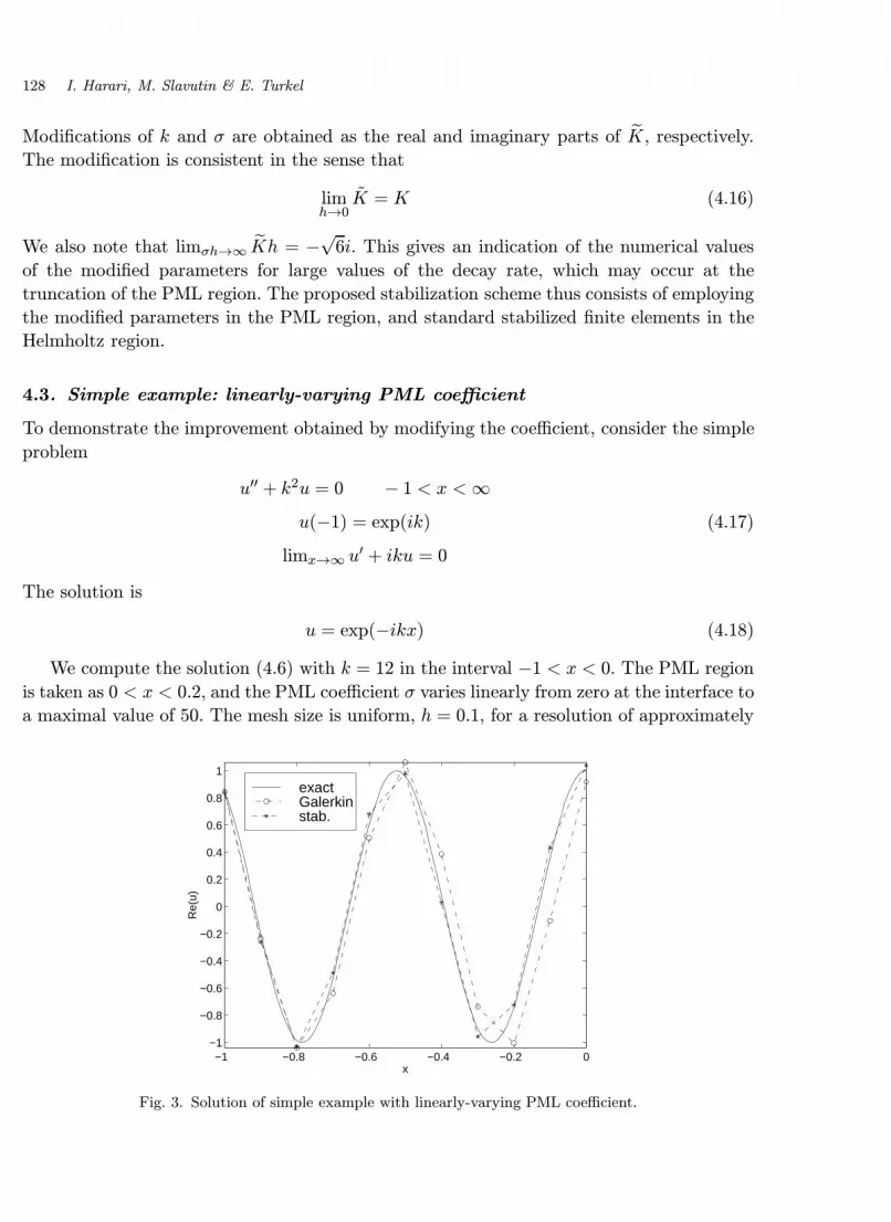
4.3. Simple example: linearly-varying PML coefficient

To demonstrate the improvement obtained by modifying the coefficient, consider the simple

problem

u′′ + k2u = 0 − 1 < x <∞

u(−1) = exp(ik)

limx→∞ u′ + iku = 0

(4.17)

The solution is

u = exp(−ikx) (4.18)

We compute the solution (4.6) with k = 12 in the interval −1 < x < 0. The PML region

is taken as 0 < x < 0.2, and the PML coefficient σ varies linearly from zero at the interface to

a maximal value of 50. The mesh size is uniform, h = 0.1, for a resolution of approximately

−1 −0.8 −0.6 −0.4 −0.2 0−1

−0.8

−0.6

−0.4

−0.2

0

0.2

0.4

0.6

0.8

1

x

Re(

u)

exactGalerkinstab.

Fig. 3. Solution of simple example with linearly-varying PML coefficient.

March 23, 2000 17:17 WSPC/130-JCA 0015

Analytical and Numerical Studies of a Finite Element PML for the Helmholtz Equation 129

five points per wavelength (recall, G = 2π/(kh)). The standard finite element solution,

denoted Galerkin, is compared in Fig. 3 to the stabilized solution in which the Helmholtz

region is modified according to Galerkin/least-squares and the treatment of the PML region

follows the modifications proposed in Sec. 4.2. The improvement obtained by the stabilized

approach, even for this case with a varying PML coefficient, is evident.

5. Numerical Results

Numerical results of PML formulations are compared to exact and DtN solutions. The DtN

method is a general scheme for handling boundary-value problems in unbounded domains.

The method for general linear elliptic problems was developed by Givoli and Keller34,35 and

is related to similar work in acoustics.36,37 The DtN method introduces artificial boundaries

(typically spherical) to form bounded computational domains that are suitable for domain-

based discretization. Correct far-field behavior is enforced by specifying proper boundary

conditions on this boundary. The DtN map is usually expressed in the form of an infinite

series. In practice the map is approximated by truncating the series, so that it is based on a

representation that is not complete. Uniqueness of solutions to two- and three-dimensional

problems is guaranteed by selecting the number of terms in the truncated DtN map so that

it is no less than kR, where R is the radius of the artificial boundary.38,39 DtN boundary

conditions can be very accurate, but all of the degrees of freedom on the artificial boundary

are coupled, potentially increasing the cost of computation.

5.1. Wave guide

We consider a wave guide in two dimensions, represented by a semi-infinite strip of constant

width b = π, aligned along the positive x-axis with walls at y = 0 and y = π. Homogeneous

Dirichlet boundary conditions are specified at the walls. The radiation condition (2.4) is

replaced by the condition that u is bounded and does not contain incoming waves at x→∞.

(Radiation conditions for wave guides are treated rigorously elsewhere.17,40) The boundary

x = 0 is a radiating wall with

u(0, y) = c1 sin(`1y) + c2 sin(`2y), 0 < y < π (5.1)

Here c1 and c2 are given constants, and `1 and `2 are given integers that satisfy `1 < k < `2.

The exact solution is composed of a propagating and an evanescent wave

u = c1 exp

(−i√k2 − `21 x

)sin(`1y) + c2 exp

(−√`22 − k2 x

)sin(`2y) (5.2)

For finite element computation, the wave guide is truncated at x = 5π (Fig. 4). The

resulting computational domain is meshed with 50 × 10 square, bilinear elements, so that

the element length is uniform (h = b/10). The PML region is parallel to the y-axis, starting

at x = 5π, with 10 elements in the direction transverse to the layer. The PML parameter

σx(x) varies quadratically from a value of zero at the interface to 40 at the outer edge of

the layer, and σy = 0.

March 23, 2000 17:17 WSPC/130-JCA 0015

130 I. Harari, M. Slavutin & E. Turkel

x

y

5 π

π

0

Fig. 4. Wave guide with PML.

The problem is solved by Gauss elimination with kb = 1.25π (a resolution of 16 points

per wavelength), `1 = 1, `2 = 2, c1 = 2 and c2 = 1. The contours in Fig. 5 show that

the absorbing layer performs well. The evanescent wave produces a lack of symmetry near

the radiating wall, which decays further along the wave guide. The numerical dispersion of

standard finite elements is relatively small at this resolution, yet it leads to the increasing

error evident in the propagating wave along the wave guide.

In order to emphasize the deleterious effects of numerical dispersion, consider the

degenerate case in which `1 = k (c2 = 0). The exact solution is constant along the wave

guide. The problem is solved with kb = π (20 points per wavelength) and c1 = 1, so that the

exact solution is real valued. Figure 6 shows the solution along the axis of the wave guide

(y = π/2). The standard finite element solution (by the Galerkin method) exhibits strong

decay in the real part (bold line) due to numerical dispersion, along with an imaginary part

that does not exist in the exact solution. Stabilization by the Galerkin/least-squares method

in the Helmholtz region and the modifications proposed in Sec. 4.2 in the PML region reduces

numerical dispersion and improves the results significantly. This example demonstrates the

potential of exploiting existing concepts of stabilized finite element methodology to improve

the performance of PML finite elements.

0 0.5 1 1.5 2 2.5 3 3.5 4 4.5 50

0.1

0.2

0.3

0.4

0.5

0.6

0.7

0.8

0.9

1

x/π

y/π

Fig. 5. Real part of the wave guide solution kb = 1.25π (exact solution is dashed).

March 23, 2000 17:17 WSPC/130-JCA 0015

Analytical and Numerical Studies of a Finite Element PML for the Helmholtz Equation 131

0 1 2 3 4 5

0

0.2

0.4

0.6

0.8

1

x/π

u

Real

Imaginary

exact Galerkin stabilized

Fig. 6. Real (bold lines) and imaginary parts of degenerate wave guide solutions along the axis y = π/2.

5.2. Circumferentially harmonic radiation from a cylinder

In the following, numerical results are presented for exterior problems bounded internally

by an infinite circular cylinder of radius a. Soft (Dirichlet) boundary conditions are specified

on the wet surface (r = a) to represent a pressure-release cylinder.

The cylinder is centered within the computational domain. For finite element computa-

tion with PML, the computational domain is a square of side 2a. The finite element mesh

employed, composed of approximately 560 elements, is shown in Fig. 7 (left). The PML

region surrounds the finite element domain with strips of ten elements of length 0.1 in the

width of each strip, adding 1,200 elements to the mesh, increasing the cost of directly solving

Fig. 7. The computational domain exterior to a cylinder of radius a with: a square PML interface of side 2a(left); a circular DtN interface at R = 2a, discretized by 5× 80 linear quadrilateral finite elements (right).

March 23, 2000 17:17 WSPC/130-JCA 0015

132 I. Harari, M. Slavutin & E. Turkel

Fig. 8. Circumferentially harmonic (n = 4) radiation from a cylinder of radius a, ka = 2, ∼ 16 points perwavelength (solid contours denote exact solution, dotted contours denote PML, and dashed contours denoteDtN, N = 10).

the equations by more than an order of magnitude. On the PML strips parallel to the x-axis

σx = 0, and σy(y) varies quadratically from a value of 0 at the interface to 30 at the outer

edge of the layer. On the strips parallel to the y-axis σy = 0, and σx(x) varies quadratically

from 0 to 30. In the corners, both parameters are varied appropriately. From here on, no

stabilization is employed.

The circular artificial boundary of the DtN formulation is located at R = 2a. The

computational domain is discretized by 5× 80 bilinear quadrilateral finite elements (Fig. 7,

right). The global DtN boundary conditions couple all of the degrees of freedom on

the artificial boundary, increasing the bandwidth of the matrix equations, and conse-

quently the computational cost rises, again by more than an order of magnitude for direct

solvers.

Consider a cylinder with circumferentially harmonic loading. For a load distribution

cosnθ, the normalized exact solution is u = H(1)n (kr) cosnθ/H

(1)n (ka). We examine the

problem with a geometrically nondimensionalized wave number ka = 2 (the wavelength is

about one and a half times the diameter of the cylinder and three times the width of the

domain), and a typical resolution of approximately 16 nodal points per wavelength in the

finite element meshes (Fig. 7).

We consider the fifth circumferential mode, n = 4. Figure 8 shows the real part of the

analytical and numerical solutions, for the PML and the DtN formulations (with 10 terms in

the DtN operator, sufficient for uniqueness). Both computations clearly represent the main

features of the analytical solution. Note that DtN condition itself (with N = 10) is exact

for this problem, and the error is due to finite element discretization in the domain and

approximation of the DtN condition on the interface. The PML elements are not an exact

representation of the radiation condition, but the results are comparable to DtN.

March 23, 2000 17:17 WSPC/130-JCA 0015

Analytical and Numerical Studies of a Finite Element PML for the Helmholtz Equation 133

5.3. Radiation from a sector of a cylinder

We consider the nonuniform radiation from an infinite circular cylinder with a constant

inhomogeneous value on an arc (−α < θ < α) and vanishing elsewhere, so that there are

two points of discontinuity in the boundary data. The normalized analytical solution to this

problem for a cylinder of radius a is

u =2

π

∞∑n=0

′ sinnα

n

H(1)n (kr)

H(1)n (ka)

cosnθ (5.3)

The prime on the sum indicates that the first term is halved. For low wave numbers this

solution is relatively uniform in the circumferential direction. The directionality of the so-

lution grows as the wave number is increased, and the solution becomes attenuated at the

side of the cylinder opposite the radiating element.

Numerical results of PML formulations for this problem are compared to Trefftz infinite

element (TIE) solutions, in addition to exact and DtN solutions. The term infinite elements

refers to a class of methods which is based on interpolation with suitable behavior in the

complement of the computational domain.18,41–44 In contrast to global DtN boundary con-

ditions, infinite elements retain the element-based data structure of finite elements, thus

preserving the bandedness of the discrete equations. The Trefftz infinite elements employed

in the following are developed by a novel approach to exterior problems of time-harmonic

acoustics.45 This approach is based on a variational framework for finite element compu-

tation in unbounded domains.46 Weakly coupling inner fields to outgoing outer field repre-

sentations that satisfy the Helmholtz equation yields problems on bounded domains. This

treatment of the outer field is in the framework of the Trefftz approach.47 The computational

Fig. 9. Radiation from a sector of a cylinder of radius a, ka = 2, ∼ 16 points per wavelength (solid contoursdenote analytical solution (5.3), dotted contours denote PML, dashed contours denote DtN, N = 10, anddash-dotted contours denote TIE).

March 23, 2000 17:17 WSPC/130-JCA 0015

134 I. Harari, M. Slavutin & E. Turkel

Table 1. Relative errors for radi-ation from a sector of a cylinderof radius a, (ka = 2, ∼ 16 pointsper wavelength).

Method|uh − uI|1|uI|1

[%]

PML 8.6DtN 9.6TIE 9.8

domain of the infinite element formulation is formed by a circular interface, and, as in DtN,

is located at R = 2a (Fig. 7).

We select α = π/8. Figure 9 shows the real part of the analytical and numerical solutions

(without stabilization), for the PML, DtN (with ten terms in the operator), and TIE for-

mulations (of lowest order). The low-amplitude oscillations of the analytical solution in the

vicinity of the wet surface are merely an artifact of the truncated series representation (60

terms) of the discontinuity in the boundary data, and are not relevant to the validation of

the numerical results. The numerical solutions capture the essential physics of the problem,

without visible reflection from the interfaces.

Errors relative to the interpolation of the analytic solution uI, measured in the H1 semi-

norm, are presented in Table 1. Despite the noticeable deviations of the TIE contours from

those of the other methods in parts of the domain (Fig. 9), the global error is similar. This is

due to the fact that the errors in the vicinity of the boundary data discontinuities dominate

in all methods, and contributions of errors on other regions, where solutions vary slowly, are

much smaller.

6. Conclusions

The performance of a PML finite element method for solving exterior problems of time-

harmonic acoustics is examined in this work. The PML approach easily accommodates

elongated geometries and open boundaries, retaining the element-based data structure of

finite elements. The computational efficiency of this approach in comparison to competing

techniques requires further investigation.

The dispersion analysis in this work is restricted to plane waves at normal incidence to

the interface of an unbounded PML region with a constant coefficient. A degradation in

the discrete representation of the PML decay rate is observed. The finite element dispersion

properties at the interface are identical to those in the standard acoustic region. This suggests

keeping the mesh uniform, and at a resolution similar to that of the acoustic region in the

vicinity of the interface, in order to reduce spurious reflection.

A simplistic approach to improved performance by stabilization exploits the structured

meshes and absence of sources in typical PML implementations. Stabilization for linear

March 23, 2000 17:17 WSPC/130-JCA 0015

Analytical and Numerical Studies of a Finite Element PML for the Helmholtz Equation 135

elements is then attained by modifying the coefficients. This approach is applicable to layers

with varying coefficients in multi-dimensional configurations.

Numerical results validate the good performance of this finite element PML approach to

exterior problems of time-harmonic acoustics. Several problems are examined. PML results

compare favorably to analytical solutions, as well as to computation with DtN boundary

conditions and Trefftz infinite elements.

Acknowledgments

The authors wish to thank Paul Barbone for helpful discussions.

References

1. J.-P. Berenger, “A perfectly matched layer for the absorption of electromagnetic waves,” J.Comput. Phys. 114(2) (1994), 185–200.

2. J.-P. Berenger, “Three-dimensional perfectly matched layer for the absorption of electromagneticwaves,” J. Comput. Phys. 127(2) (1996), 363–379.

3. R. W. Ziolkowski, “Time-derivative Lorentz material model-based absorbing boundary condi-tion,” IEEE Trans. Antennas Propagat. 45(10) (1997), 1530–1535.

4. J.-Y. Wu, D. M. Kingsland, J.-F. Lee, and R. Lee, “A comparison of anisotropic PML toBerenger’s PML and its application to the finite-element method for EM scattering,” IEEETrans. Antennas Propagat. 45(1) (1997), 40–50.

5. F. L. Teixeira and W. C. Chew, “A general approach to extend Berenger’s absorbing boundarycondition to anisotropic and dispersive media,” IEEE Trans. Antennas Propagat. 46(9) (1998),1386–1387.

6. F. Collino and P. Monk, “The perfectly matched layer in curvilinear coordinates,” SIAM J. Sci.Comput. 19(6) (1998), 2061–2090.

7. F. Collino and P. B. Monk, “Optimizing the perfectly matched layer,” Comput. Meths. Appl.Mech. Eng. 164(1–2) (1998), 157–171.

8. P. G. Petropoulos, “On the termination of the perfectly matched layer with local absorbingboundary conditions,” J. Comput. Phys. 143(2) (1998), 665–673.

9. S. D. Gedney, “An anisotropic perfectly matched layer-absorbing medium for the truncation ofFDTD lattices,” IEEE Trans. Antennas Propagat. 44(12) (1996), 1630–1639.

10. J. A. Roden and S. D. Gedney, “Efficient implementation of the uniaxial-based PML media inthree-dimensional nonorthogonal coordinates with the use of the FDTD technique,” Microw.Opt. Technol. Lett. 14(2) (1997), 71–75.

11. S. D. Gedney, “The perfectly matched layer absorbing medium,” Advances in ComputationalElectrodynamics, ed. A. Taflove (Artech House Inc., Boston, MA, 1998), pp. 263–343.

12. E. Turkel and A. Yefet, “Absorbing PML boundary layers for wave-like equations,” Appl. Numer.Math. 27(4) (1998), 533–557.

13. Q. Qi and T. L. Geers, “Evaluation of the perfectly matched layer for computational acoustics,”J. Comput. Phys. 139(1) (1998), 166–183.

14. S. S. Abarbanel and D. Gottlieb, “A mathematical analysis of the PML method,” J. Comput.Phys. 134(2) (1997), 357–363.

15. I. Stakgold, Boundary Value Problems of Mathematical Physics, Volume II (The Macmillan Co.,New York, 1968).

16. C. H. Wilcox, Scattering Theory for the d’Alembert Equation in Exterior Domains (Springer-Verlag, Berlin, 1975).

March 23, 2000 17:17 WSPC/130-JCA 0015

136 I. Harari, M. Slavutin & E. Turkel

17. S. V. Tsynkov and E. Turkel, “A Cartesian perfectly matched layer for the Helmholtz equation,”Artificial Boundary Conditions, with Applications to CFD Problems, ed. L. Tourrette (NovaScience Publishers Inc., Commack, NY, 2000).

18. D. S. Burnett, “A three-dimensional acoustic infinite element based on a prolate spheroidalmultipole expansion,” J. Acoust. Soc. Am. 96(5) (1994), 2798–2816.

19. I. Harari, I. Patlashenko, and D. Givoli, “Dirichlet-to-Neumann maps for unbounded waveguides,” J. Comput. Phys. 143(1) (1998), 200–223.

20. I. Harari, “Reducing spurious dispersion, anisotropy and reflection in finite element analysis oftime-harmonic acoustics,” Comput. Meths. Appl. Mech. Eng. 140(1–2) (1997), 39–58.

21. L. L. Thompson and P. M. Pinsky, “A Galerkin least-squares finite element method for thetwo-dimensional Helmholtz equation,” Int. J. Num. Meth. Eng. 38(3) (1995), 371–397.

22. S. S. Abarbanel and D. Gottlieb, “On the construction and analysis of absorbing layers in CEM,”Appl. Num. Math. 27(4) (1998), 331–340.

23. N. N. Abboud and P. M. Pinsky, “Finite element dispersion analysis for the three-dimensionalsecond-order scalar wave equation,” Int. J. Num. Meth. Eng. 35(6) (1992), 1183–1218.

24. K. Grosh and P. M. Pinsky, “Complex wave-number dispersion analysis of Galerkin and Galerkinleast squares methods for fluid-loaded plates,” Comput. Meths. Appl. Mech. Eng. 113(1–2)(1994), 67–98.

25. I. Harari and T. J. R. Hughes, “Finite element methods for the Helmholtz equation in an exteriordomain: Model problems,” Comput. Meths. Appl. Mech. Eng. 87(1) (1991), 59–96.

26. F. Ihlenburg and I. Babuska, “Dispersion analysis and error estimation of Galerkin finite elementmethods for the Helmholtz equation,” Int. J. Num. Meth. Eng. 38(22) (1995), 3745–3774.

27. I. Harari and E. Turkel, “Accurate finite difference methods for time-harmonic wave propaga-tion,” J. Comput. Phys. 119(2) (1995), 252–270.

28. I. Singer and E. Turkel, “High order finite difference methods for the Helmholtz equation,”Comput. Meths. Appl. Mech. Eng. 163 (1998), 343–358.

29. I. Babuska, F. Ihlenburg, E. T. Paik, and S. A. Sauter, “A generalized finite element methodfor solving the Helmholtz equation in two dimensions with minimal pollution,” Comput. Meths.Appl. Mech. Eng. 128(3–4) (1995), 325–359.

30. A. A. Oberai and P. M. Pinsky, “A residual-based finite element method for the Helmholtzequation,” Int. J. Num. Meth. Eng. (1999) Submitted.

31. L. P. Franca and A. Russo, “Unlocking with residual-free bubbles,” Comput. Meths. Appl. Mech.Eng. 142(3–4) (1997), 361–364.

32. T. J. R. Hughes, “Multiscale phenomena: Green’s functions, the Dirichlet-to-Neumann formu-lation, subgrid scale models, bubbles and the origins of stabilized methods,” Comput. Meths.Appl. Mech. Eng. 127(1–4) (1995), 387–401.

33. J. W. Nehrbass, J. O. Jevtic, and R. Lee, “Reducing the phase error for finite-difference methodswithout increasing the order,” IEEE Trans. Antennas Propagat. 46(8) (1998), 1194–1201.

34. D. Givoli and J. B. Keller, “A finite element method for large domains,” Comput. Meths. Appl.Mech. Eng. 76(1) (1989), 41–66.

35. J. B. Keller and D. Givoli, “Exact nonreflecting boundary conditions,” J. Comput. Phys. 82(1)(1989), 172–192.

36. K. Feng, “Asymptotic radiation conditions for reduced wave equation,” J. Comput. Math. 2(2)(1984), 130–138.

37. M. Masmoudi, “Numerical solution for exterior problems,” Numer. Math. 51(1) (1987),87–101.

38. I. Harari and T. J. R. Hughes, “Analysis of continuous formulations underlying the computationof time-harmonic acoustics in exterior domains,” Comput. Meths. Appl. Mech. Eng. 97(1) (1992),103–124.

March 23, 2000 17:17 WSPC/130-JCA 0015

Analytical and Numerical Studies of a Finite Element PML for the Helmholtz Equation 137

39. I. Harari and T. J. R. Hughes, “Studies of domain-based formulations for computing exteriorproblems of acoustics,” Int. J. Num. Meth. Eng. 37(17) (1994), 2935–2950.

40. A. I. Nosich and V. P. Shestopalov, “Radiation conditions and uniqueness theorems for openwaveguides,” Soviet J. Comm. Tech. Electron. 34(7) (1989), 107–115.

41. R. J. Astley, G. J. Macaulay, and J.-P. Coyette, “Mapped wave envelope elements for acousticalradiation and scattering,” J. Sound Vib. 170(1) (1994), 97–118.

42. P. Bettess, “Infinite elements,” Int. J. Num. Meth. Eng. 11(1) (1977), 53–64.43. K. Gerdes and L. Demkowicz, “Solution of 3D-Laplace and Helmholtz equations in exte-

rior domains using hp-infinite elements,” Comput. Meths. Appl. Mech. Eng. 137(3–4) (1996),239–273.

44. O. C. Zienkiewicz, K. Bando, P. Bettess, C. Emson, and T. C. Chiam, “Mapped infinite elementsfor exterior wave problems,” Int. J. Num. Meth. Eng. 21(7) (1985), 1229–1251.

45. I. Harari, P. E. Barbone, M. Slavutin, and R. Shalom, “Boundary infinite elements for theHelmholtz equation in exterior domains,” Int. J. Num. Meth. Eng. 41(6) (1998), 1105–1131.

46. I. Harari, “A unified variational approach to domain-based computation of exterior problems oftime-harmonic acoustics,” Appl. Num. Math. 27(4) (1998), 417–441.

47. J. Jirousek and A. Wroblewski, “T -elements: State of the art and future trends,” Arch. Comput.Methods Engrg. 3(4) (1996), 323–434.