the topological asymptotic for the helmholtz equation with dirichlet condition on the boundary of an...

THE TOPOLOGICAL ASYMPTOTIC FOR THEHELMHOLTZ EQUATION WITH DIRICHLET CONDITION ON

THE BOUNDARY OF AN ARBITRARILY SHAPED HOLE∗

JULIEN POMMIER† AND BESSEM SAMET‡

SIAM J. CONTROL OPTIM. c© 2004 Society for Industrial and Applied MathematicsVol. 43, No. 3, pp. 899–921

Abstract. The aim of the topological sensitivity analysis is to obtain an asymptotic expansionof a design functional with respect to the creation of a small hole in the domain. In this paper,such an expansion is obtained for the Helmholtz equation, in two and three space dimensions, witha Dirichlet condition on the boundary of an arbitrarily shaped hole. In this case, the main difficultyis related to the nonhomogeneous symbol of the Helmholtz operator. In the numerical part of thiswork, we will show that the topological sensitivity method is very promising for solving shape inverseproblems in electromagnetic applications.

Key words. topological optimization, topological asymptotic, topological gradient, nonhomoge-neous problem, Helmholtz equation, shape inversion, electromagnetic applications, inverse scattering

AMS subject classifications. 49Q10, 49Q12, 78A25, 78A40, 78A45, 78A50, 35J05

DOI. 10.1137/S036301290241616X

1. Introduction. The same numerical methods are generally used in shape in-version and optimal shape design. There are mainly two categories of shape inversionor shape optimization methods. In the first category we deform continuously theboundary of the object to be optimized in order to decrease a given cost function[5, 20, 25, 28, 31]. The final shape has the same topology as the initial shape given bythe designer. Therefore, to reach the optimal geometry, we need a priori knowledge ofits topology. However, the topology of the optimal shape is often the main unknownin object detection problems. For example, the knowledge of the number and thelocations of buried mines is more important than their accurate shapes. The secondcategory of algorithms allows topology modifications. Many important contributionsin this field are concerned with structural mechanics and, in particular, the optimiza-tion of the compliance (external work) subject to a volume constraint [4, 16]. In viewof the fact that the optimal structure has generally a large number of small holes,most authors [1, 3, 14] have considered composite material optimization. Using thehomogenization theory, Allaire and Kohn [1] exhibit a class of laminated materialswith an explicit expression for the optimal material at any point of the structure. Inthis case, the optimal solution is not a classical design—it is a distribution of com-posite materials. Then penalization methods must be applied in order to retrieve arealistic shape. For all these reasons, global optimization methods are used to solvemore general problems [15, 26]. Unfortunately these methods are quite slow.

More recently, Eschenauer and Olhoff [7], Schumacher [27], Cea et al. [6], Garreau,Guillaume, and Masmoudi [8], Sokolowski and Zochowski [29, 30], and Nazarov andSokolowski [21] presented a method to obtain the optimal topology by calculating theso-called topological gradient (or topological derivative). This gradient is a function

∗Received by the editors October 16, 2002; accepted for publication (in revised form) December11, 2003; published electronically September 18, 2004.

http://www.siam.org/journals/sicon/43-3/41616.html†Departement de Genie Mathematique, INSA Toulouse and CNRS UMR 5640 MIP, Complex

Scientifique de Rangueil, F-31077 Toulouse cedex 4, France ([email protected]).‡UMR MIG, Universite Paul Sabatier and CNRS UMR 5640 MIP, 118 route de Narbonne, F-31062

Toulouse cedex, France ([email protected]).

899

900 JULIEN POMMIER AND BESSEM SAMET

defined in the domain of interest where, at each point, it gives the sensitivity of thecost function when a small hole is created at that point. This approach seems to begeneral and efficient. To present the basic idea, we consider Ω a domain of R

n, wheren equals 2 or 3, and j(Ω) = J(uΩ) a cost function to be minimized, where uΩ is thesolution to a given PDE problem defined in Ω. For ε > 0, let Ωε = Ω\x0 + εω be thesubset obtained by removing a small part x0 + εω from Ω, where x0 ∈ Ω and ω ⊂ R

n

is a fixed open and bounded subset containing the origin. We can generally provethat the variation of the criterion is given by the asymptotic expansion

j(Ωε) = j(Ω) + f(ε)g(x0) + o(f(ε)),(1.1)

limε→0

f(ε) = 0, f(ε) > 0.(1.2)

This expansion is called the topological asymptotic. To minimize the criterion, wehave to create holes where g (called the topological gradient) is negative.

In this paper, using the adjoint method and the domain truncation techniqueintroduced in [17], we compute the topological asymptotic expansion for the Helmholtzequation in two and three space dimensions with a Dirichlet condition on the boundaryof an arbitrarily shaped hole. The originality of this work is that the symbol of theHelmholtz operator is nonhomogeneous. The basic idea is to say that the leadingterm of the topological asymptotic expansion is given by the principal part of theoperator in the case of a Dirichlet condition on the boundary of the hole. Our workgeneralizes the contribution of Guillaume and Sid Idris [9] for the Poisson equationand is easily applicable to other problems for which the symbol of the operator isnonhomogeneous, as, for example, the quasi-Stokes problem and the elastic wavesproblem. In the numerical part, we present some applications that illustrate theability of the topological sensitivity approach to solve inverse scattering problems.

As a background to our work, we cite the contributions of Il’in [11, 12, 13] forthe construction of asymptotic expansions of solutions to boundary value problems indomains with small holes, as in the case of second order scalar equations, by the use ofthe method of matched asymptotic expansions. Various spectral problems in domainswith small holes are investigated by Maz’ya et al. [23, 24, 18, 22]. In [32], Vogelius andVolkov provided a rigorous derivation for solutions to the time-harmonic Maxwell’sequations of a transverse electric (TE) nature, in the presence of a finite number ofdiametrically small inhomogeneities. Based on layer potential techniques, Ammariand Kang [2] provided a rigorous derivation of complete asymptotic expansions forsolutions to the Helmholtz equation in two and three dimensions, in the presence ofsmall inhomogeneities in the domain. In our work, we derive asymptotic expansionsnot for solutions, but for a given cost function.

The generalized adjoint method is recalled in section 2. Next, the formulation ofthe Helmholtz problem is presented in section 3 and its truncated version is describedin section 4. Section 5 presents the main results whose proofs are given in section 6.Finally, numerical examples illustrate in section 7 the abilities of the topological sen-sitivity to solve inverse scattering problems.

2. A generalized adjoint method. In this section, the generalized adjointmethod introduced in [17, 8] is slightly modified. The first modification is due to thefact that the cost function is defined in a C-Hilbert space and takes values in R; thenit is not differentiable. For this reason, the differentiability property is replaced bythe formulation (2.5). The second modification is due to the fact that the sesquilinearform associated with our problem is not coercive. For this reason, the coercivityproperty is replaced by the inf-sup condition (see Hypothesis 2).

https://www.researchgate.net/publication/45501109_Asymptotic_formulas_for_perturbations_in_the_electromagnetic_fields_due_to_the_presence_of_inhomogeneities_of_small_diameter?el=1_x_8&enrichId=rgreq-808d6b00-99b3-4853-9ede-3300e124541e&enrichSource=Y292ZXJQYWdlOzIzNTczMTM2OTtBUzo5OTE2MjMwMTQwMzE1NUAxNDAwNjUzNTQ0MDMz

https://www.researchgate.net/publication/266685323_Study_of_the_asymptotic_behavior_of_the_solution_of_an_elliptic_boundary_value_problem_in_a_domain_with_a_small_hole?el=1_x_8&enrichId=rgreq-808d6b00-99b3-4853-9ede-3300e124541e&enrichSource=Y292ZXJQYWdlOzIzNTczMTM2OTtBUzo5OTE2MjMwMTQwMzE1NUAxNDAwNjUzNTQ0MDMz

https://www.researchgate.net/publication/258262716_A_boundary_value_problem_for_the_elliptic_equation_of_second_order_in_a_domain_with_a_narrow_slit_I_The_two-dimensional_case?el=1_x_8&enrichId=rgreq-808d6b00-99b3-4853-9ede-3300e124541e&enrichSource=Y292ZXJQYWdlOzIzNTczMTM2OTtBUzo5OTE2MjMwMTQwMzE1NUAxNDAwNjUzNTQ0MDMz

https://www.researchgate.net/publication/238872289_Book_Review_Matching_of_asymptotic_expansions_of_solutions_of_boundary_value_problems?el=1_x_8&enrichId=rgreq-808d6b00-99b3-4853-9ede-3300e124541e&enrichSource=Y292ZXJQYWdlOzIzNTczMTM2OTtBUzo5OTE2MjMwMTQwMzE1NUAxNDAwNjUzNTQ0MDMz

https://www.researchgate.net/publication/258262457_Asymptotic_expansions_of_eigenvalues_of_boundary_value_problems_for_the_Laplace_operator_in_domains_with_small_holes?el=1_x_8&enrichId=rgreq-808d6b00-99b3-4853-9ede-3300e124541e&enrichSource=Y292ZXJQYWdlOzIzNTczMTM2OTtBUzo5OTE2MjMwMTQwMzE1NUAxNDAwNjUzNTQ0MDMz

https://www.researchgate.net/publication/220259225_The_Topological_Asymptotic_Expansion_for_the_Dirichlet_Problem?el=1_x_8&enrichId=rgreq-808d6b00-99b3-4853-9ede-3300e124541e&enrichSource=Y292ZXJQYWdlOzIzNTczMTM2OTtBUzo5OTE2MjMwMTQwMzE1NUAxNDAwNjUzNTQ0MDMz

https://www.researchgate.net/publication/222183088_Boundary_layer_techniques_for_solving_the_Helmholtz_equation_in_the_presence_of_small_inhomogeneities?el=1_x_8&enrichId=rgreq-808d6b00-99b3-4853-9ede-3300e124541e&enrichSource=Y292ZXJQYWdlOzIzNTczMTM2OTtBUzo5OTE2MjMwMTQwMzE1NUAxNDAwNjUzNTQ0MDMz

TOPOLOGICAL ASYMPTOTIC FOR THE HELMHOLTZ EQUATION 901

Let V be a fixed complex Hilbert space. For ε ≥ 0, let aε(., .) be a sesquilinearand continuous form on V and let lε be a semilinear and continuous form on V. Weconsider the following assumptions.

Hypothesis 1. There exists a sesquilinear and continuous form δa, a semilinearand continuous form δl, and a real function f(ε) > 0 defined on R

∗+ such that

limε→0

f(ε) = 0,(2.1)

‖aε − a0 − f(ε)δa‖L2(V) = o(f(ε)),(2.2)

‖lε − l0 − f(ε)δl‖L(V) = o(f(ε)),(2.3)

where L(V) (respectively, L2(V)) denotes the space of continuous and semilinear (re-spectively, sesquilinear) forms on V.

Hypothesis 2. There exists a constant α > 0 such that

infu =0

supv =0

|a0(u, v)|‖u‖V‖v‖V

≥ α.

We say that a0 satisfies the inf-sup condition.According to (2.2), there exists a constant β > 0 independent of ε such that

infu =0

supv =0

|aε(u, v)|‖u‖V‖v‖V

≥ β.

For ε ≥ 0, let uε be the solution to the following problem: Find uε ∈ V such that

aε(uε, v) = lε(v) ∀v ∈ V.(2.4)

We have the following lemma.Lemma 2.1. If Hypotheses 1 and 2 are satisfied, then

‖uε − u0‖V = O(f(ε)).

Proof. It follows from Hypothesis 2 that there exists vε ∈ V, vε = 0, such that

β‖uε − u0‖V‖vε‖V ≤ |aε(uε − u0, vε)|,

which implies

β‖uε − u0‖V‖vε‖V ≤ |aε(u0, vε) − lε(vε)|= |aε(u0, vε) − (lε − l0 − f(ε)δl)(vε) − l0(vε) − f(ε)δl(vε)|= |(aε(u0, vε) − a0(u0, vε)) − (lε − l0 − f(ε)δl)(vε) − f(ε)δl(vε)|≤ |aε(u0, vε) − a0(u0, vε) − f(ε)δa(u0, vε)|

+|lε(vε) − l0(vε) − f(ε)δl(vε)| + f(ε)(|δa(u0, vε)| + |δl(vε)|).

Using Hypothesis 1 we obtain

β ‖ uε − u0 ‖V ‖vε‖V ≤(o(f(ε)) + f(ε)(‖δa‖L2(V)‖u0‖V + ‖δl‖L(V))

)‖vε‖V .

Consider now a cost function j(ε) = J(uε), where the functional J satisfies

J(u + h) = J(u) + (Lu(h)) + o(‖h‖) ∀u, h ∈ V,(2.5)

where Lu is a linear and continuous form on V.


For ε ≥ 0, we define the Lagrangian operator Lε by

Lε(u, v) = J(u) + aε(u, v) − lε(v) ∀u, v ∈ V.

The next theorem gives the asymptotic expansion of j(ε).Theorem 2.2. If Hypotheses 1 and 2 are satisfied, then

j(ε) − j(0) = f(ε)(δL(u0, p0)) + o(f(ε)),(2.6)

where u0 is the solution to (2.4) with ε = 0, and p0 is the solution to the followingadjoint problem: Find p0 ∈ V such that

a0(v, p0) = −Lu0(v) ∀v ∈ V(2.7)

and

δL(u, v) = δa(u, v) − δl(v) ∀u, v ∈ V.

Proof. We have that

j(ε) = Lε(uε, v) ∀ε ≥ 0 ∀v ∈ V.

Next, choosing v = p0, we obtain

j(ε) − j(0) = Lε(uε, p0) − L0(u0, p0)

= J(uε) − J(u0) + aε(uε, p0) − a0(u0, p0) + l0(p0) − lε(p0)

= J(uε) − J(u0) + (aε(uε, p0) − a0(u0, p0)) −(lε(p0) − l0(p0))

= J(uε) − J(u0) + (aε(uε, p0) − a0(uε, p0) + a0(uε − u0, p0))

−(lε(p0) − l0(p0) − f(ε)δl(p0)) − f(ε)(δl(p0)).

Using (2.5), we have that

J(uε) − J(u0) = (Lu0(uε − u0)) + o(‖uε − u0‖).

Hence,

j(ε) − j(0) = (aε(uε, p0) − a0(uε, p0)) + (a0(uε − u0, p0) + Lu0(uε − u0))

+o(‖uε − u0‖) −(lε(p0) − l0(p0) − f(ε)δl(p0)) − f(ε)(δl(p0)).

Using that p0 is the adjoint solution, we obtain

j(ε) − j(0) = (aε(uε, p0) − a0(uε, p0)) + o(‖uε − u0‖)−(lε(p0) − l0(p0) − f(ε)δl(p0)) − f(ε)(δl(p0))

= ((aε − a0)(u0, p0)) + ((aε − a0)(uε − u0, p0)) + o(‖uε − u0‖)−(lε(p0) − l0(p0) − f(ε)δl(p0)) − f(ε)(δl(p0)).

It follows from Hypothesis 1 that

j(ε) − j(0)=f(ε)(δa(u0, p0)) + o(f(ε)) + f(ε)(δa(uε − u0, p0)) + o(f(ε))‖uε − u0‖+o(‖uε − u0‖) − f(ε)(δl(p0)).

Finally, from Lemma 2.1 and the hypothesis limε→0 f(ε) = 0, we have

j(ε) = j(0) + f(ε)(δa(u0, p0) − δl(p0)) + o(f(ε)),

since δa is continuous by assumption.


3. The Helmholtz problem in a domain with a small hole. Let Ω bean open and bounded subset of R

n with boundary Γ = Γ0 ∪ Γ1, n = 2 or 3. TheHelmholtz problem is ⎧⎪⎨

⎪⎩∆uΩ + k2uΩ = 0 in Ω,uΩ = 0 on Γ0,∂uΩ

∂n= ΛuΩ + Θ on Γ1,

(3.1)

where k ∈ R∗, Θ ∈ H

1200(Γ1)

′, and Λ ∈ L(H1200(Γ1), H

1200(Γ1)

′).We define⎧⎪⎪⎪⎨

⎪⎪⎪⎩V(Ω) = v ∈ H1(Ω), v = 0 on Γ0,

a(Ω, u, v) =

∫Ω

∇u.∇v dx− k2

∫Ω

uv dx− 〈Λu, v〉,

(v) = 〈Θ, v〉,

(3.2)

where 〈, 〉 is the duality product between H1200(Γ1)

′ and H1200(Γ1). The variational

formulation associated with (3.1) is the following: Find uΩ ∈ V(Ω) such that

a(Ω, uΩ, v) = (v) ∀v ∈ V(Ω).(3.3)

We consider the following assumption.

Hypothesis 3. The operator Λ is split into Λ0+Λ1, with Λ1 ∈ L(H1200(Γ1), H

1200(Γ1)

′),and satisfies

〈Λ1ψ,ψ〉 ≤ 0 ∀ψ ∈ H1200(Γ1),(3.4)

and Λ2 ∈ L(H1200(Γ1), H

1200(Γ1)). We assume the following property of uniqueness.

Hypothesis 4. We have

a(Ω, u, v) = 0 ∀v ∈ V(Ω) ⇒ u = 0,(3.5)

a(Ω, u, v) = 0 ∀u ∈ V(Ω) ⇒ v = 0.(3.6)

From the Lax–Milgram theorem and the fact that the imbeddings VΩ → L2(Ω) and

H1200(Γ1) → L2(Γ1) are compact, and due to the Fredholm alternative, we obtain the

following result (see, e.g., [10] for a detailed argument).Proposition 3.1. If Hypotheses 3 and 4 are satisfied, we have the following:1. Problem (3.3) has one and only one solution.2. The sesquilinear form a(Ω, ., .) satisfies the inf-sup condition: There exists a

constant a > 0 such that

infu =0

supv =0

|aΩ(u, v)|‖u‖V(Ω)‖v‖V(Ω)

≥ a.(3.7)

For a given x0 ∈ Ω, consider the modified open subset Ωε = Ω\ωε, ωε = x0 + εω,where ω is a fixed open and bounded subset of R

n containing the origin (ωε = ∅ ifε = 0), whose boundary ∂ω is connected and piecewise of class C1. The modifiedsolution uΩε satisfies⎧⎪⎪⎪⎨

⎪⎪⎪⎩∆uΩε + k2uΩε

= 0 in Ωε,uΩε = 0 on Γ0,uΩε

= 0 on ∂ωε,∂uΩε

∂n= ΛuΩε

+ Θ on Γ1.

(3.8)

https://www.researchgate.net/publication/243096290_Finite_Element_Solution_of_the_Helmholtz_Equation_with_High_Wave_Number_Part_II_The_h-p_Version_of_the_FEM?el=1_x_8&enrichId=rgreq-808d6b00-99b3-4853-9ede-3300e124541e&enrichSource=Y292ZXJQYWdlOzIzNTczMTM2OTtBUzo5OTE2MjMwMTQwMzE1NUAxNDAwNjUzNTQ0MDMz


The function uΩε is defined on the variable open set Ωε, and thus belongs to afunctional space which depends on ε. Hence, if we want to derive the asymptoticexpansion of a function of the form

j(ε) = J(uΩε),(3.9)

we cannot apply directly the tools of section 2, which require a fixed functional space.For this reason, we use the domain truncation method introduced in [17] to avoid thiscomplication.

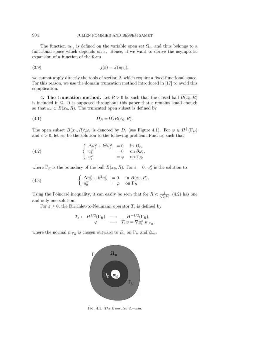
4. The truncation method. Let R > 0 be such that the closed ball B(x0, R)is included in Ω. It is supposed throughout this paper that ε remains small enoughso that ωε ⊂ B(x0, R). The truncated open subset is defined by

ΩR = Ω\B(x0, R).(4.1)

The open subset B(x0, R)\ωε is denoted by Dε (see Figure 4.1). For ϕ ∈ H12 (ΓR)

and ε > 0, let uϕε be the solution to the following problem: Find uϕ

ε such that⎧⎨⎩

∆uϕε + k2uϕ

ε = 0 in Dε,uϕε = 0 on ∂ωε,

uϕε

= ϕ on ΓR,(4.2)

where ΓR is the boundary of the ball B(x0, R). For ε = 0, uϕ0 is the solution to

∆uϕ0 + k2uϕ

0 = 0 in B(x0, R),uϕ

0 = ϕ on ΓR.(4.3)

Using the Poincare inequality, it can easily be seen that for R < 1√2|k| , (4.2) has one

and only one solution.

For ε ≥ 0, the Dirichlet-to-Neumann operator Tε is defined by

Tε : H1/2(ΓR) −→ H−1/2(ΓR),ϕ −→ Tεϕ = ∇uϕ

ε .n|ΓR,

where the normal n|ΓRis chosen outward to Dε on ΓR and ∂ωε.

Γ

ΓDε ωε

Ω R

R

Fig. 4.1. The truncated domain.


Finally, we define for ε ≥ 0 the solution uε to the truncated problem⎧⎪⎪⎪⎪⎪⎨⎪⎪⎪⎪⎪⎩

∆uε + k2uε = 0 in ΩR,uε = 0 on Γ0,∂uε

∂n= Λuε + Θ on Γ1,

∂uε

∂n− Tεuε|ΓR

= 0 on ΓR.

(4.4)

The variational formulation associated with (4.4) is as follows: Find uε ∈ VR suchthat

aε(uε, v) = (v) ∀v ∈ VR,(4.5)

where the functional space VR and the sesquilinear form aε are defined by

VR = v ∈ H1(ΩR); v|Γ0= 0,(4.6)

aε(u, v) =

∫ΩR

∇u.∇v dx− k2

∫ΩR

u.v dx− 〈Λu, v〉 +

∫ΓR

Tεu|ΓRv dγ(x).(4.7)

Here,∫ΓR

denotes the duality product between H1/2(ΓR) and H−1/2(ΓR). The fol-lowing result is standard in PDE theory.

Proposition 4.1. Problems (3.8) and (4.4) have a unique solution. Moreover,the restriction to ΩR of the solution uΩε

to (3.8) is the solution uε to (4.4).We now have at our disposal the fixed Hilbert space VR required by section 2.

We assume that the following hypothesis holds.Hypothesis 5. The function J introduced in (3.9) is defined in a neighboring part

of Γ and satisfies

J(u + h) = J(u) + (Lu(h)) + o (‖h‖) ∀u, h ∈ VR,

where Lu is a linear and continuous form on VR.Then we obtain that

j(ε) = J(uΩε) = J(uε) ∀ε ≥ 0.(4.8)

Remark 1. We can also consider a more general cost function (see, e.g., [9]); thetruncation method does not restrict the choice of the function. In the numerical partof this work, only measurements on the boundary of the domain are used. For thisreason and to simplify the presentation, we considered the previous assumption aboutthe cost function.

Let vΩ be the solution to the adjoint problem

a(Ω, w, vΩ) = −LuΩ(w) ∀w ∈ V(Ω),(4.9)

where the functional space V(Ω) and the sesquilinear form a(Ω, ., .) are defined in(3.2). It has been shown in Proposition 4.1 that u0 is the restriction to ΩR of uΩ.Similarly, v0, the solution to

a0(w, v0) = −Lu0(w) ∀w ∈ VR,(4.10)

is the restriction to ΩR of vΩ.

https://www.researchgate.net/publication/220259225_The_Topological_Asymptotic_Expansion_for_the_Dirichlet_Problem?el=1_x_8&enrichId=rgreq-808d6b00-99b3-4853-9ede-3300e124541e&enrichSource=Y292ZXJQYWdlOzIzNTczMTM2OTtBUzo5OTE2MjMwMTQwMzE1NUAxNDAwNjUzNTQ0MDMz


5. The main results. This section contains the main results of this paper. Allthe proofs are reported in section 6. Henceforth, we have to distinguish between thecases n = 2 and n = 3. This is due to the fact that the fundamental solutions to theLaplace equation in R

2 and R3 have an essentially different asymptotic expansion at

infinity, and (5.1) has generally no solution if n = 2.

5.1. The three-dimensional case. Possibly changing the coordinate system,we can suppose for convenience that x0 = 0. In order to derive the topologicalsensitivity of the function j, we introduce two auxiliary problems.

The first problem, called the exterior problem, is formulated in R3\ω and consists

of finding vω, solution to ⎧⎨⎩

−∆vω = 0 in R3\ω,

vω = 0 at ∞,vω = uΩ(x0) on ∂ω,

(5.1)

where uΩ is the solution to the direct problem (3.1). Here, one can remark thatjust the principal part of the Helmholtz operator is used, which was described by theLaplace equation. The function vω can be expressed by a single layer potential on∂ω. Let

E(y) =1

4πr(5.2)

with r = ||y||. It is a fundamental solution for the Laplace equation in R3. Then the

function vω reads

vω(y) =

∫∂ω

E(y − x)pω(x) dγ(x), y ∈ R3\ω,(5.3)

where pω ∈ H− 12 (∂ω) is the solution to boundary integral equation∫

∂ω

E(y − x)pω(x) dγ(x) = uΩ(x0) ∀y ∈ ∂ω.(5.4)

For x bounded and large r = ||y||, we have

E(y − x) = E(y) + O

(1

r2

),(5.5)

and the asymptotic expansion at infinity of the function vω is given by

vω(y) = Pω(y) + Wω(y),(5.6)

Pω(y) = Aω (uΩ(x0))E(y),(5.7)

Aω (uΩ(x0)) =

∫∂ω

pω(x) dγ(x),(5.8)

Wω(y) = O

(1

r2

).(5.9)

Notice that Pω ∈ Lmloc for all m < 3. Clearly, the function α −→ Aω(α) is linear on

R, and the number Aω(α) depends on the shape of ω.


The second problem, which we call interior problem, is formulated in D0 =B(x0, R) and consists to find Q1

ω solution to∆Q1

ω + k2Q1ω = 0 in D0,

Q1ω = Pω |ΓR

on ΓR.(5.10)

Here, the idea is to consider an interior and exterior problem that gives a good “firstorder approximation” of (uϕ

ε − uϕ0 )|Dε

, ϕ = uΩ|ΓR, in the form f(ε)(Q1

ω − Pω), in a

way which will be stated precisely in section 6. But the given formulation (5.10) of theinterior problem, which is the “natural” choice, is not sufficient to get the behaviorneeded by the adjoint technique described in section 2. More precisely, in this caseone can construct the sesquilinear form δa but there is no positive function f(ε) suchthat ||aε−a0−f(ε)δa||L2(VR) = o(f(ε)). Indeed, one can observe through the proof ofProposition 6.7 that the behavior of ||aε−a0 − f(ε)δa||L2(VR) is not of order o(ε), butonly of order O(ε). This is due to the approximation used on the exterior problem(5.1), where just the principal part of the operator is considered. For this reason, anew term Q2

ω is used in order to correct the error caused by this approximation. Weconstruct Q2

ω as the solution to∆Q2

ω + k2Q2ω = k2Pω in D0,

Q2ω = 0 on ΓR.

(5.11)

Setting Qω = Q1ω + Q2

ω, then Qω is the solution to∆Qω + k2Qω = k2Pω in D0,Qω = Pω |ΓR

on ΓR.(5.12)

Using the corrected interior problem (5.12), one can derive the good approxi-mation of (uϕ

ε − uϕ0 )|Dε

. The main result is the following, which will be proved insection 6.

Theorem 5.1. Let j(ε) = J(uΩε) be a cost function satisfying Hypothesis 5.Then the topological asymptotic expansion is given by

j(ε) − j(0) = ε(Aω (uΩ(x0)) vΩ(x0)

)+ o(ε),(5.13)

where uΩ is the direct state solution to (3.1) and vΩ is the adjoint state solution to(4.9).

Then the topological gradient is given by

g(x) = (Aω (uΩ(x)) vΩ(x)

)∀x ∈ Ω,

and only two systems must be solved in order to compute g(x) for all x ∈ Ω.When ω is the unit ball B(0, 1), then vω(y), Pω(y), and Wω(y) can be computed

explicitly:

vω(y) =uΩ(x0)

r= Pω(y), Wω(y) = 0, 0 = y ∈ R

3.(5.14)

Then it follows from (5.2) and (5.7) that

Aω (uΩ(x0)) = 4πuΩ(x0).(5.15)

We have the following result.Corollary 5.2. Under the assumptions of Theorem 5.1 and when ω is the unit

ball B(0, 1), the topological asymptotic expansion is given by

j(ε) − j(0) = 4πε(uΩ(x0)vΩ(x0)

)+ o(ε).(5.16)


5.2. The two-dimensional case. In this section, we intend to derive theasymptotic expansion of the function j in the two-dimensional case. The techniqueused is similar to that of the three-dimensional case. We use the principal part of theHelmholtz operator to derive the topological sensitivity expression. Next, we brieflydescribe the transposition of the previous results to the two-dimensional case. Asbefore, uΩ and the adjoint state vΩ are, respectively, the solutions to (3.1) and (4.9).

The exterior problem must now be defined differently than in (5.1). It consists offinding vω, the solution to⎧⎨

⎩−∆vω = 0 in R

2\ω,vω(y)/ log r = uΩ(x0) at ∞,vω = 0 on ∂ω.

(5.17)

A fundamental solution for the Laplace equation in R2 is given by

E(y) = − 1

2πlog r.(5.18)

The function vω has the form

vω(y) = uΩ(x0) log ‖y‖ + Pω + Wω(y),(5.19)

where Pω is constant and Wω(y) = o(1) at infinity [9]. In the next proposition (whereω is not supposed to be a ball), one can observe that in the two-dimensional case thetopological sensitivity does not depend on the shape of the hole ω, in contrast to thethree-dimensional case.

Theorem 5.3. The assumptions are the same as in Theorem 5.1. The functionj has the asymptotic expansion

j(ε) = j(0) − 2π

log ε(uΩ(x0)vΩ(x0)

)+ o

(1

log ε

).(5.20)

The proof for the two-dimensional case uses the same tools as the three-dimensional case (see section 6) and will not be repeated.

6. Proofs. This section consists of the proof of Theorem 5.1. The variation ofthe sesquilinear form aε reads

aε(u, v) − a0(u, v) =

∫ΓR

(Tε − T0)uv dγ(x).(6.1)

Hence, the problem reduces to the analysis of (Tε − T0)ϕ for ϕ ∈ H12 (ΓR). More

precisely, it will be shown that there exists an operator δT ∈ L(H12 (ΓR), H− 1

2 (ΓR))such that

‖Tε − T0 − εδT‖L(H

12 (ΓR),H− 1

2 (ΓR))= O(ε3/2).(6.2)

Consequently, defining δa by

δa(u, v) =

∫ΓR

δTuv dγ(x) ∀u, v ∈ VR(6.3)

will yield straightforwardly

‖aε − a0 − εδa‖L(H

12 (ΓR),H− 1

2 (ΓR))= O(ε3/2).(6.4)

First we need some definitions and preliminary lemmas.


6.1. Definitions. For convenience, the following norms and seminorms are cho-sen for the functional spaces which will be used.

• For a bounded and open subset O ⊂ R3 and m ≥ 0, the Sobolev space Hm(O)

is equipped with the norm defined by

‖u‖2m,O =

m∑j=0

|u|2j,O,

where the seminorms |u|j,O are given by

|u|2j,O =∑|α|=j

∫O|∂αu|2 dx.(6.5)

• For a given ε > 0, the space H12 (ΓR/ε) is equipped with the norm

‖u‖ 12 ,ΓR/ε

= inf‖v‖1,C(R/2ε,R/ε); v|ΓR/ε= u,

where C(r, r′) = x ∈ R3; r < ||x|| < r′.

• The dual space H− 12 (ΓR/ε) is equipped with the natural norm

‖w‖− 12 ,ΓR/ε

= sup|〈w, v〉− 12 ,

12; v ∈ H

12 (ΓR/ε); ‖v‖ 1

2 ,ΓR/ε= 1,

where 〈, 〉− 12 ,

12

is the duality product between H12 (ΓR/ε) and H− 1

2 (ΓR/ε).

6.2. Preliminary lemmas. Recall that x0 = 0. We will use extensively thefollowing change of variable: For a given function u defined on a subset O, the functionu is defined on O = O/ε by

u(y) = u(x), y =x

ε.

Lemma 6.1. We have that

|u|1,O = ε1/2|u|1,O,(6.6)

‖u‖0,O = ε3/2‖u‖0,O.(6.7)

Proof. Due to ∇u(x) = ∇u(y)/ε and to definition (6.5), we have

|u|21,O =

∫O|∇u|2 dx =

1

ε2

∫O|∇u|2ε3 dy.

Similarly, we have

‖u‖0,O = ε3/2‖u‖0,O.

Lemma 6.2 (see [9]). For ϕ ∈ H12 (∂ω), let v be the solution to the problem⎧⎨

⎩−∆v = 0 in R

3\ω,v = 0 at ∞,v = ϕ on ∂ω.

(6.8)


The function v is split into

v(y) = V (y) + W (y),

V (y) = E(y)

∫∂ω

p(x) dγ(x),

where E(y) = 14π‖y‖ and p ∈ H− 1

2 (∂ω) is the unique solution to∫∂ω

E(y − x)p(x) dγ(x) = ϕ(y) ∀y ∈ ∂ω.(6.9)

There exists a constant c > 0 (independent of ϕ and ε) such that

‖V ‖0,C(R/2ε,R/ε) ≤ cε−1/2‖ϕ‖ 12 ,∂ω

,

|V |1,C(R/2ε,R/ε) ≤ cε1/2‖ϕ‖ 12 ,∂ω

,

‖V ‖0,Dε/ε ≤ cε−1/2‖ϕ‖ 12 ,∂ω

,

|V |1,Dε/ε ≤ c‖ϕ‖ 12 ,∂ω

,

‖W‖0,C(R/2ε,R/ε) ≤ cε1/2‖ϕ‖ 12 ,∂ω

,

|W |1,C(R/2ε,R/ε) ≤ cε3/2‖ϕ‖ 12 ,∂ω

,

‖W‖0,Dε/ε ≤ c‖ϕ‖ 12 ,∂ω

.

Lemma 6.3. We assume that R < 1√2|k| . For a given ε > 0, fε ∈ L2(Dε), and

ϕ ∈ H12 (ΓR), let vε be the solution to⎧⎨

⎩∆vε + k2vε = fε in Dε,vε = 0 on ∂ωε,vε = ϕ on ΓR.

(6.10)

There exists a constant C(R, k) > 0 (independent of ϕ and ε) such that

‖vε‖1,Dε≤ C(R, k)

(‖ϕ‖ 1

2 ,ΓR+ ‖fε‖0,Dε

).(6.11)

Proof. Let Rϕ be the lifting of ϕ in the space H1 (C(R/2, R)) such that Rϕ|ΓR/2=

0. We extend Rϕ by zero to the domain Dε. We denote this extension by Rϕ. Itbelongs to H1(Dε). We introduce

uε = Rϕ− vε,(6.12)

gε = −fε + ∆Rϕ + k2Rϕ.(6.13)

The function gε belongs to the space H−1(Dε) and the new unknown uε is the solutionto ⎧⎨

⎩∆uε + k2uε = gε in Dε,uε = 0 on ∂ωε,uε = 0 on ΓR.

(6.14)

Using the Poincare inequality and the elliptic regularity, we obtain

‖uε‖1,Dε ≤(

1 + 2R2

1 − 2k2R2

)‖gε‖−1,Dε .(6.15)

Finally, the result follows from (6.12), (6.13), (6.15), and the continuity of the lift-ing R.


Here and in what follows, we assume that R < 1√2|k| .

Lemma 6.4. For ε > 0 and ψ ∈ H1(D0), let Xε be the solution to the problem⎧⎨⎩

∆Xε + k2Xε = 0 in Dε,Xε = ψ on ∂ωε,Xε = 0 on ΓR.

(6.16)

There exists a constant c > 0 (independent of ϕ and ε) such that for all ε > 0,

|Xε|1,C(R/2,R) ≤ cε‖ψ(εy)‖ 12 ,∂ω

,(6.17)

‖Xε‖0,Dε≤ cε‖ψ(εy)‖ 1

2 ,∂ω,(6.18)

|Xε|1,Dε≤ cε1/2‖ψ(εy)‖ 1

2 ,∂ω.(6.19)

Proof. Let vε be the solution to the exterior problem⎧⎨⎩

−∆vε = 0 in R3\ω,

vε = 0 at ∞,vε = ψ(εy) on ∂ω.

(6.20)

The function Xε can be written

Xε = vε − wε,

where vε(x) = vε(xε

). The function wε itself is the solution to⎧⎨

⎩∆wε + k2wε = k2vε in Dε,wε = 0 on ∂ωε,wε = vε on ΓR.

(6.21)

It follows from Lemma 6.3 that there exists a constant c > 0 such that

‖wε‖1,Dε≤ c

(‖vε|ΓR

‖ 12 ,ΓR

+ k2‖vε‖0,Dε

).(6.22)

It follows from Lemmas 6.1 and 6.2 that

‖vε|ΓR‖ 1

2 ,ΓR≤ c‖vε‖1,C(R/2,R)(6.23)

≤ c(‖vε‖0,C(R/2,R) + |vε|1,C(R/2,R)

)(6.24)

= c(ε3/2‖vε‖0,C(R/2ε,R/ε) + ε1/2|vε|1,C(R/2ε,R/ε)

)(6.25)

≤ cε‖ψ(εy)‖ 12 ,∂ω

.(6.26)

We have that

‖vε‖0,Dε = ε3/2‖vε‖0,Dε/ε(6.27)

≤ cε‖ψ(εy)‖ 12 ,∂ω

.(6.28)

From (6.22), (6.26), and (6.28), we obtain that

‖wε‖1,Dε ≤ cε‖ψ(εy)‖ 12 ,∂ω

.(6.29)


Then we have

|Xε|1,C(R/2,R) = |vε − wε|1,C(R/2,R)(6.30)

≤ |vε|1,C(R/2,R) + |wε|1,C(R/2,R)(6.31)

≤ cε‖ψ(εy)‖ 12 ,∂ω

+ ‖wε‖1,Dε(6.32)

≤ cε‖ψ(εy)‖ 12 ,∂ω

,(6.33)

‖Xε‖0,Dε ≤ ‖vε‖0,Dε+ ‖wε‖1,Dε(6.34)

≤ cε‖ψ(εy)‖ 12 ,∂ω

,(6.35)

|Xε|1,Dε≤ |vε|1,Dε + |wε|1,Dε(6.36)

≤ ε1/2|vε|1,Dε/ε + ‖wε‖1,Dε(6.37)

≤ cε1/2‖ψ(εy)‖ 12 ,∂ω

+ cε‖ψ(εy)‖ 12 ,∂ω

(6.38)

≤ cε1/2‖ψ(εy)‖ 12 ,∂ω

.(6.39)

This completes the proof.Lemmas 6.3 and 6.4 are summarized in the following lemma.Lemma 6.5. For ε > 0, ϕ ∈ H

12 (ΓR), ψ ∈ H1(D0), and fε ∈ L2(Dε), let vε be

the solution to the problem⎧⎨⎩

∆vε + k2vε = fε in Dε,vε = ψ on ∂ωε,vε = ϕ on ΓR.

(6.40)

There exists a constant c > 0 (independent of ϕ, ψ, fε, and ε) such that for all ε > 0,

|vε|1,C(R/2,R) ≤ c(ε‖ψ(εy)‖ 1

2 ,∂ω+ ‖ϕ‖ 1


),(6.41)

‖vε‖0,Dε≤ c

(ε‖ψ(εy)‖ 1

2 ,∂ω+ ‖ϕ‖ 1


),(6.42)

|vε|1,Dε≤ c

(ε1/2‖ψ(εy)‖ 1

2 ,∂ω+ ‖ϕ‖ 1


).(6.43)

Lemma 6.6. Let u belong to the space H1 (C(R/2, R)) and satisfy ∆u + k2u = 0in C(R/2, R), u|ΓR

= 0. Then there exists a constant c > 0 (independent of u) suchthat

‖∇u.n|ΓR‖− 1

2 ,ΓR≤ c|u|1,C(R/2,R).(6.44)

Proof. Let ϕ ∈ H12 (ΓR). We define v as the solution to the problem⎧⎨

⎩∆v = 0 in C(R/2, R),v = 0 on ΓR/2,v = ϕ on ΓR.

Using the Green formula, we obtain∫ΓR

∇u.n|ΓRϕ dγ(x) =

∫C(R/2,R)

∇u.∇v dx− k2

∫C(R/2,R)

uv dx.

Then we have∣∣∣∣∫

ΓR

∇u.n|ΓRϕ dγ(x)

∣∣∣∣ ≤ |u|1,C(R/2,R)‖v‖1,C(R/2,R) + k2‖u‖0,C(R/2,R)||v||1,C(R/2,R)

≤ |u|1,C(R/2,R)‖ϕ‖ 12 ,ΓR

+ ck2|u|1,C(R/2,R)‖ϕ‖ 12 ,ΓR

≤ c|u|1,C(R/2,R)‖ϕ‖ 12 ,ΓR

.

This completes the proof.


6.3. Variation of the sesquilinear form. The variation of the sesquilinearform aε reads

aε(u, v) − a0(u, v) =

∫ΓR

(Tε − T0)uv dγ(x).

For ϕ ∈ H12 (ΓR), recall that uϕ

ε is the solution to (4.2), or to (4.3) if ε = 0. Let vϕωbe the solution to the problem⎧⎨

⎩∆vϕω = 0 in R

3\ω,vϕω = 0 at ∞,vϕω = uϕ

0 (x0) on ∂ω.(6.45)

As in (5.6) and (5.7), let Pϕω (y) = Aω (uϕ

0 (x0))E(y) be the dominant part of vϕω , andlet Qϕ

ω be the solution to the associated interior problem∆Qϕ

ω + k2Qϕω = k2Pϕ

ω in D0,Qϕ

ω = Pϕω |ΓR

on ΓR.(6.46)

The linear operator δT (independent of ε) is defined as follows:

δT : H1/2(ΓR) −→ H−1/2(ΓR),ϕ −→ δTϕ = ∇(Qϕ

ω − Pϕω ).n|ΓR

.(6.47)

Proposition 6.7. The operator Tε admits the following asymptotic expansion:


12 (ΓR),H− 1

2 (ΓR))= O(ε3/2).

Proof. Let ϕ ∈ H12 (ΓR). For simplicity we drop the superscript (.)

ϕ. For y = x/ε,

we have

vω(y) = Pω(y) + Wω(y),

with Pω(xε ) = εPω(x) and Wω(y) = O( 1||y||2 ). Let

ψε(x) = (Tε − T0 − εδT )ϕ(x).

We have

ψε(x) = (∇uε −∇u0 − ε(∇Qω −∇Pω)) .n|ΓR

= ∇(wε(x) −Wω

(xε

)).n|ΓR

,

where wε is defined by

wε(x) = uε(x) − u0(x) − εQω(x) + vω

(xε

).

The function wε is the solution to⎧⎨⎩

∆wε + k2wε = k2Wω(x/ε) in Dε,wε = Wω(x/ε) on ΓR,wε = −u0(x) + u0(0) − εQω(x) on ∂ωε.

(6.48)

In order to apply Lemma 6.5, we have to estimate the right-hand side terms, asfollows.


• In Dε, we have

‖Wω(x/ε)‖0,Dε= ε3/2‖Wω(y)‖0,Dε/ε.

Using Lemma 6.2, we obtain

‖Wω(y)‖0,Dε/ε ≤ c‖u0(x0)‖ 12 ,∂ω

≤ c|u0(x0)|≤ c‖ϕ‖ 1

2 ,ΓR.

Then we have

‖Wω(x/ε)‖0,Dε ≤ cε3/2‖ϕ‖ 12 ,ΓR

.

• On ΓR, using Lemmas 6.1 and 6.2 and the elliptic regularity, we obtain

‖Wω(x/ε)‖ 12 ,ΓR

≤ c‖Wω(x/ε)‖1,C(R/2,R)

≤ c(‖Wω(x/ε)‖0,C(R/2,R) + |Wω(x/ε)|1,C(R/2,R)

)= c

(ε3/2‖Wω(y)‖0,C(R/2ε,R/ε) + ε1/2|Wω(y)|1,C(R/2ε,R/ε)

)≤ cε2‖u0(x0)‖ 1

2 ,∂ω

≤ cε2|u0(x0)|≤ cε2‖ϕ‖ 1

2 ,ΓR.

• On ∂ωε, putting

θε(x) =−u0(x) + u0(x0) − εQω(x)

ε,

we have for small ε

‖θε(εy)‖ 12 ,∂ω

≤ c‖θε(εy)‖1,ω

= c

∥∥∥∥u0(εy) − u0(x0)

ε+ Qω(εy)

∥∥∥∥1,ω

≤ c(‖u0‖C2(B(0,R/2)) + ‖Qω‖C1(B(0,R/2))

)≤ c‖ϕ‖ 1

2 ,ΓR.

We can now apply Lemma 6.5, which gives

|wε|1,C(R/2,R) ≤ c(ε3/2‖ϕ‖ 1

2 ,ΓR+ ε2‖ϕ‖ 1

2 ,ΓR+ ε‖εθε(εy)‖ 1

2 ,∂ω

)≤ cε3/2‖ϕ‖ 1

2 ,ΓR.

Finally, it follows from Lemmas 6.1 and 6.6 that

‖ψ‖− 12 ,ΓR

= ‖∇(wε −Wω(x/ε)).n|ΓR‖− 1

2 ,ΓR

≤ c(|wε|1,C(R/2,R) + |Wω(x/ε)|1,C(R/2,R)

)= c

(|wε|1,C(R/2,R) + ε1/2|Wω(y)|1,C(R/2ε,R/ε)

)≤ c

(ε3/2‖ϕ‖ 1

2 ,ΓR+ ε2‖ϕ‖ 1

2 ,ΓR

)≤ cε3/2‖ϕ‖ 1

2 ,ΓR.


Hence,


12 (ΓR),H− 1

2 (ΓR))= O(ε3/2).

The asymptotic expansion of the sesquilinear form aε follows now straightfor-wardly.

Proposition 6.8. Let

δa(u, v) =

∫ΓR

δTuv dγ(x), u, v ∈ VR.

Then the asymptotic expansion of the sesquilinear form aε is given by

‖aε − a0 − εδa‖L(H

12 (ΓR),H− 1

2 (ΓR))= O(ε3/2).

6.4. Proof of Theorem 5.1. The proof of this theorem is done in two steps.First, we prove that Hypothesis 2 is satisfied. More precisely, we prove that thesesquilinear form a0 satisfies the inf-sup condition. Second, we apply Theorem 2.2 tocompute the topological asymptotic expansion.

6.4.1. The first step: The inf-sup condition. For all u ∈ VR, we set

u =

u in ΩR,uϕ

0 in B(x0, R),

where ϕ = u|ΓRand uϕ

0 is the solution to∆uϕ

0 + k2uϕ0 = 0 in B(x0, R),

uϕ0 = ϕ on ΓR.

It can easily be proved that

a0(u, v|ΩR) = a(Ω, u, v) ∀u ∈ VR ∀v ∈ V(Ω),

where the functional space V(Ω) and the sesquilinear form a(Ω, ., .) are defined by(3.2). From Proposition 3.1, the sesquilinear form a(Ω, ., .) satisfies the inf-sup con-dition. As a consequence, there exists v ∈ V(Ω), v = 0, such that

a0(u, v|ΩR) = a(Ω, u, v) ≥ a‖u‖V(Ω)‖v‖V(Ω)

≥ a‖u‖VR‖v|ΩR

‖VR.

Then a0 satisfies the inf-sup condition and Hypothesis 2 is satisfied.

6.4.2. Applying Theorem 2.2. All the hypotheses of section 2 are satisfiedand we can apply Theorem 2.2. We obtain the following asymptotic formula:

j(ε) − j(0) = ε(δa(uΩ, vΩ)) + o(ε)

= ε(∫

ΓR

∇(Qϕω − Pϕ

ω ).n|ΓRvΩ dγ(x)

)+ o(ε),

where ϕ = uΩ|ΓR= u0|ΓR

. Thanks to Green’s formula and (6.46), we obtain that∫ΓR

∇(Qϕω − Pϕ

ω ).n|ΓRvΩ dγ(x) = k2

∫D0

PωvΩ dx +

∫ΓR

∇vΩ.n|ΓRPω dγ(x)

−∫

ΓR

∇Pω.n|ΓRvΩ dγ(x).(6.49)


It can be shown that

∫ΓR

∇vΩ.n|ΓRPω dγ(x) −

∫ΓR

∇Pω.n|ΓRvΩ dγ(x) =Aω (uΩ(x0)) 〈−∆E, vΩψ〉D′(D0),D(D0)

−k2

∫D0

PωvΩ dx

=Aω (uΩ(x0)) 〈δ, vΩψ〉D′(D0),D(D0)

−k2

∫D0

PωvΩ dx

=Aω (uΩ(x0)) vΩ(x0) − k2

∫D0

PωvΩ dx,

where ψ ∈ D(D0) satisfies ψ(x0) = 1. We insert this expression into (6.49) and obtainthe desired result.

7. Numerical results: Buried objects detection. We consider a simpleproblem of detection of metallic objects buried in soil. The aim is to find the numberand the positions of metallic objects (supposedly infinite in the ez direction) us-ing scattered field measurements from a monostatic antenna horizontally translatedabove the soil. This is a rough model of the facilities described in [19]. The two-dimensional Helmholtz equation is solved with time-domain finite differences (FDTD),the frequency-domain solution obtained with a Fourier transform. The antenna isroughly approximated by a single source point, which will be translated at variouslocations above the soil. At each point of the mesh, the topological sensitivity will becomputed.

Let X = xii=1,... ,nxbe the set of the successive locations of the source (and

sensors, since the antenna is supposed to be monostatic), and let F = fii=1,... ,nf

be the set of measurement frequencies. Let εs be the soil permittivity. The set ofmetallic objects buried in the soil is denoted by Ω.

We associate with Ω a set of “measurements” M(Ω). At each couple (xi, fj) ∈X × F , we first define the field uΩ

xi,fj, the solution of

⎧⎪⎨⎪⎩

∆u + k2ju = sxi

in R2 \ Ω,

u = 0 on ∂Ω,limr→∞

√r(∂ru− iku) = 0,

(7.1)

where sxi represents a source point centered at xi, and where

k2j (x) = ε(x)µω2

j ,wj = 2πfj ,

ε(x) =

ε0 if x ≥ 0,εs if x < 0.

Then the “measurements” are M(Ω) = mxi,fj (Ω). In our numerical tests, mxi,fj (Ω)is the value of the scattered field at point xi.


0.000m 0.500m 1.000m 1.500m 2.000m

–0.600m

–0.400m

–0.200m

+0.000m

+0.200m

+0.400m

soil

air

successive locations of the antenna

metallic buried objects

–0.08

–0.06

–0.04

–0.02

0

0.02

0.04

0.06

0.08

0.1

0.000m 0.500m 1.000m 1.500m 2.000m

–0.600m

–0.400m

–0.200m

+0.000m

+0.200m

+0.400m

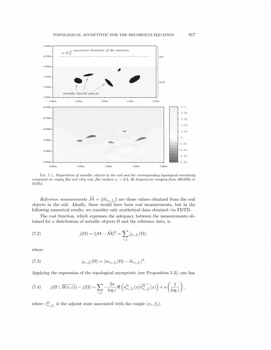
Fig. 7.1. Repartition of metallic objects in the soil and the corresponding topological sensitivitycomputed on empty flat soil (dry soil, flat surface εr = 2.3, 20 frequencies ranging from 400MHz to2GHz).

Reference measurements M = mxi,fj are those values obtained from the realobjects in the soil. Ideally, these would have been real measurements, but in thefollowing numerical results, we consider only synthetical data obtained via FDTD.

The cost function, which expresses the adequacy between the measurements ob-tained for a distribution of metallic objects Ω and the reference data, is

j(Ω) = ‖M− M‖2 =∑i,j

jxi,fj (Ω),(7.2)

where

jxi,fj (Ω) = |mxi,fj (Ω) − mxi,fj |2.(7.3)

Applying the expression of the topological asymptotic (see Proposition 5.3), one has

j(Ω \B(x, ε)) − j(Ω) =∑i,j

− 2π

log ε(uΩxi,fj (x)vΩ

xi,fj(x)

)+ o

(1

log ε

),(7.4)

where vΩxi,fj

is the adjoint state associated with the couple (xi, fj).


0.000m 0.500m 1.000m 1.500m 2.000m

–0.600m

–0.400m

–0.200m

+0.000m

+0.200m

+0.400m

(a)

–0.002

–0.0016

–0.0012

–0.0008

–0.0004

0

0.0004

0.0008

0.0012

0.0016

0.002

0.000m 0.500m 1.000m 1.500m 2.000m

–0.600m

–0.400m

–0.200m

+0.000m

+0.200m

+0.400m

(b)

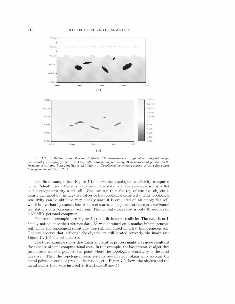
Fig. 7.2. (a) Reference distribution of objects. The measures are computed on a dry inhomoge-neous soil (εs ranging from 1.6 to 4.15) with a rough surface, using 29 measurement points and 20frequencies ranging from 260MHz to 1.86GHz. (b) Topological sensitivity computed on a flat emptyhomogeneous soil (εs = 2.3).

The first example (see Figure 7.1) shows the topological sensitivity computedon an “ideal” case: There is no noise on the data, and the reference soil is a flatand homogeneous dry sand soil. One can see that the top of the five objects isclearly identified by the negative values of the topological sensitivity. This topologicalsensitivity can be obtained very quickly since it is evaluated on an empty flat soil,which is invariant by translation: All direct states and adjoint states are just horizontaltranslations of a “canonical” solution. The computational cost is only 10 seconds ona 300MHz personal computer.

The second example (see Figure 7.2) is a little more realistic: The data is arti-

ficially noised since the reference data M was obtained on a nonflat inhomogeneoussoil, while the topological sensitivity was still computed on a flat homogeneous soil.One can observe that, although the objects are still located correctly, the image (seeFigure 7.2(b)) is a bit distorted.

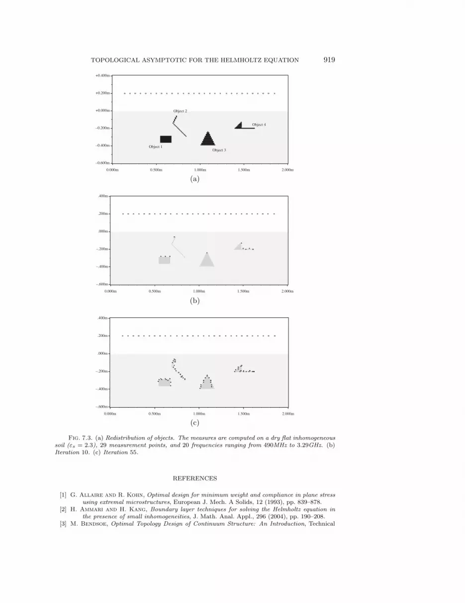
The third example shows that using an iterative process might give good results atthe expense of some computational cost. In this example, the basic iterative algorithmjust inserts a metal point at the point where the topological sensitivity is the mostnegative. Then the topological sensitivity is reevaluated, taking into account themetal points inserted at previous iterations, etc. Figure 7.3 shows the objects and themetal points that were inserted at iterations 10 and 55.


0.000m 0.500m 1.000m 1.500m 2.000m

–0.600m

–0.400m

–0.200m

+0.000m

+0.200m

+0.400m

Object 3

Object 4

Object 1

Object 2

(a)

0.000m 0.500m 1.000m 1.500m 2.000m

–.600m

–.400m

–.200m

.000m

.200m

.400m

(b)

0.000m 0.500m 1.000m 1.500m 2.000m

–.600m

–.400m

–.200m

.000m

.200m

.400m

(c)

Fig. 7.3. (a) Redistribution of objects. The measures are computed on a dry flat inhomogeneoussoil (εs = 2.3), 29 measurement points, and 20 frequencies ranging from 490MHz to 3.29GHz. (b)Iteration 10. (c) Iteration 55.

REFERENCES

[1] G. Allaire and R. Kohn, Optimal design for minimum weight and compliance in plane stressusing extremal microstructures, European J. Mech. A Solids, 12 (1993), pp. 839–878.

[2] H. Ammari and H. Kang, Boundary layer techniques for solving the Helmholtz equation inthe presence of small inhomogeneities, J. Math. Anal. Appl., 296 (2004), pp. 190–208.

[3] M. Bendsoe, Optimal Topology Design of Continuum Structure: An Introduction, Technical


report, Technical University of Denmark, Lyngby, Denmark, 1996.[4] E. Bonnetier and C. Conca, Approximation of Young measures by functions and application

to a problem of optimal design for plates with variable thickness, Proc. Roy. Soc. EdinburghSect. A, 124 (1994), pp. 399–422.

[5] J. Cea, Conception optimale ou identification de forme, calcul rapide de la derivee direction-nelle de la fonction cout, RAIRO Model. Math. Anal. Numer., 20 (1986), pp. 371–402.

[6] J. Cea, S. Garreau, Ph. Guillaume, and M. Masmoudi, Shape and topological optimizationsconnection, Comput. Methods Appl. Mech. Engrg., 188 (2000), pp. 713–726.

[7] H. A. Eschenauer and N. Olhoff, Topology optimization of continuum structures: A review,Appl. Mech. Rev., 54 (2001), pp. 331–390.

[8] S. Garreau, Ph. Guillaume, and M. Masmoudi, The topological asymptotic for PDE sys-tems: The elasticity case, SIAM J. Control Optim., 39 (2001), pp. 1756–1778.

[9] Ph. Guillaume and K. Sid Idris, The topological asymptotic expansion for the Dirichletproblem, SIAM J. Control Optim., 41 (2002), pp. 1042–1072.

[10] F. Ihlenburg and I. Babuska, Finite element solution of the Helmholtz equation with highwave number II: The h-p version of the FEM, SIAM J. Numer. Anal., 34 (1997), pp. 315–358.

[11] A. M. Il’in, A boundary value problem for the elliptic equation of second order in a domainwith a narrow slit. I. The two-dimensional case, Math. USSR-Sb., 28 (1976), pp. 459–480(in English).

[12] A. M. Il’in, Study of the asymptotic behavior of the solution of an elliptic boundary valueproblem in a domain with a small hole, Trudy Sem. Petrovsk., 6 (1981), pp. 57-82 (inRussian).

[13] A. M. Il’in, Matching of Asymptotic Expansions of Solutions of Boundary Value Problems,Transl. Math. Monogr. 102, American Mathematical Society, Providence, RI, 1992.

[14] J. Jacobsen, N. Olhoff, and E. Ronholt, Generalized Shape Optimization of Three-Dimensional Structures Using Materials with Optimum Microstructures, Technical report,Institute of Mechanical Engineering, Aalborg University, Aalborg, Denmark, 1996.

[15] C. Kane and M. Schoenauer, Optimization topologique de formes par algorithmes genetiques,Rev. Francaise de Mecanique, 4 (1997), pp. 237–246.

[16] R. V. Kohn and M. S. Vogelius, Thin plates with rapidly varying thickness, and their relationto structural optimization, in Homogenization and Effective Moduli of Materials and Media,J. L. Ericksen et al., eds., IMA Vol. Math. Appl. 1, Springer-Verlag, New York, 1986,pp. 126–149.

[17] M. Masmoudi, The topological asymptotic expansion, in Computational Methods for Con-trol Applications, H. Kawarada and J. Periaux, eds., GAKUTO Internat. Ser. Math. Sci.Appl. 16, Tokyo, 2002, pp. 53–72.

[18] V. G. Maz’ya, S. A. Nazarov, and B. A. Plamenevskij, Asymptotic expansions of theeigenvalues of boundary value problems for the Laplace operator in domains with smallholes, Math USSR-Izv., 48 (1984), pp. 347–371 (in Russian); Math. USSR-Izv., 24 (1985),pp. 321–345 (in English).

[19] P. Millot, J. C. Bureau, P. Borderies, E. Bachelier, C. Pichot, E. Lebrusq, E. Lebrusq,

E. Guilianton, and J. Y. Dauvignac, Experimental study of near surface radar imagingof buried objects with adaptive focussed synthetic aperture processing, in Subsurface SensingTechnologies and Applications II, Proceedings of SPIE 4129, 2000, pp. 515–523.

[20] F. Murat and S. Simon, Etudes de problemes d’optimal design, in Optimization Techniques:Modeling and Optimization in the Service of Man. Part 2, Lecture Notes in Comput. Sci.41, Springer-Verlag, Berlin, 1976, pp. 54–62.

[21] S. A. Nazarov and J. Sokolowski, Asymptotic Analysis of Shape Functionals, Rapport derecherche de l’INRIA, RR-4633, 2002.

[22] S. A. Nazarov, Asymptotic expansions of eigenvalues, Leningrad University, 1987 (in Russian).[23] S. Ozawa, Singular Hadamard’s variation of domains and eigenvalues of Laplacian, Part 1,

Proc. Japan Acad. Ser. A Math. Sci., 56 (1980), pp. 306–310.[24] S. Ozawa, Singular Hadamard’s variation of domains and eigenvalues of Laplacian, Part 2,

Proc. Japan Acad. Ser. A Math. Sci., 57 (1981), pp. 242–246.[25] O. Pironneau, Optimal Shape Design for Elliptic Systems, Springer-Verlag, New York, 1984.[26] M. Schoenauer, L. Kallel, and F. Jouve, Mechanics inclusions identification by evolution-

ary computation, Rev. Europeenne Elem. Finis, 5 (1996), pp. 619–648.[27] A. Schumacher, Topologieoptimierung von Bauteilstrukturen unter Verwendung von Lochpo-

sitionierungkriterien, Doctoral Thesis, Siegen University, Siegen, Germany, 1996.[28] J. Simon, Differentiation with respect to the domain in boundary value problems, Numer. Funct.

Anal. Optim., 2 (1980), pp. 649–687.


[29] J. Sokolowski and A. Zochowski, On the topological derivative in shape optimization, SIAMJ. Control Optim., 37 (1999), pp. 1251–1272.

[30] J. Sokolowski and A. Zochowski, Topological derivatives for elliptic problems, Inverse Prob-lems, 15 (1999), pp. 123–134.

[31] J. Sokolowski and J. P. Zolesio, Introduction to Shape Optimization: Shape SensitivityAnalysis, Springer Ser. Comput. Math. 16, Springer-Verlag, Berlin, 1992.

[32] M. S. Vogelius and D. Volkov, Asymptotic formulas for perturbations in the electromagneticfields due to the presence of inhomogeneities of small diameter, Math. Model. Numer.Anal., 34 (2000), pp. 723–748.

the topological asymptotic for the helmholtz equation with dirichlet condition on the boundary of an...

Documents