analysis of physical mechanisms underlying density
TRANSCRIPT
Analysis of Physical Mechanisms
Underlying Density-Dependent
Transport in Porous Media

Analysis of Physical Mechanisms
Underlying Density-Dependent
Transport in Porous Media
Proefschrift
ter verkrijging van de graad van doctor
aan de Technische Universiteit Delft,
op gezag van de Rector Magnificus Prof. dr. ir. J.T. Fokkema,
voorzitter van het College voor Promoties,
in het openbaar te verdedigen op dinsdag 28 juni 2005 om 13.00 uur
door
Anke Jannie LANDMAN
natuurkundig ingenieur
geboren te Assen
Dit proefschrift is goedgekeurd door de promotor:
Prof. dr. ir. S.M. Hassanizadeh
Toegevoegd promotor:
Dr. R.J. Schotting
Samenstelling promotiecommissie:
Rector Magnificus, voorzitter
Prof. dr. ir. S.M. Hassanizadeh, Technische Universiteit Delft, promotor
Dr. R.J. Schotting, Technische Universiteit Delft, toegevoegd
promotor
Prof. dr. ir. G.S. Stelling, Technische Universiteit Delft
Prof. dr. ir. T.H. van der Meer, Universiteit Twente
Prof. dr. -ing. R. Helmig, Universitat Stuttgart
Dr. rer. nat. K. Johannsen, Universitat Heidelberg
Dr. A. Egorov, Kazan State University
Prof. ir. C.P.J.W. van Kruijsdijk, Technische Universiteit Delft, reservelid
Copyright c© 2005 by A.J. Landman
All rights reserved. No part of the material protected by this copyright notice maybe reproduced or utilized in any form or by any means, electronic or mechanical,including photocopying, recording or by any information storage and retrievalsystem, without the prior permission of the author.
Contents
1 Introduction 1
1.1 Background . . . . . . . . . . . . . . . . . . . . . . . . . . . . . . . . . 1
1.1.1 Radioactive waste disposal in deep salt formations . . . . . . . 1
1.1.2 High salt concentrations and underground applications . . . . . 3
1.2 Outline and objectives . . . . . . . . . . . . . . . . . . . . . . . . . . . 4
2 Basic equations of flow and transport in porous media 7
2.1 Introduction . . . . . . . . . . . . . . . . . . . . . . . . . . . . . . . . . 7
2.2 Governing equations . . . . . . . . . . . . . . . . . . . . . . . . . . . . 8
2.3 Density- and viscosity-driven rotational flow . . . . . . . . . . . . . . . 13
2.3.1 Stable versus unstable configurations . . . . . . . . . . . . . . . 13
2.3.2 Density versus viscosity effect . . . . . . . . . . . . . . . . . . . 16
3 The Oberbeck-Boussinesq approximation 19
3.1 Introduction . . . . . . . . . . . . . . . . . . . . . . . . . . . . . . . . . 19
3.2 Governing equations . . . . . . . . . . . . . . . . . . . . . . . . . . . . 20
3.3 The Boussinesq limit revisited . . . . . . . . . . . . . . . . . . . . . . . 23
3.3.1 Isothermal brine transport . . . . . . . . . . . . . . . . . . . . . 23
3.3.2 Heat transfer in fresh water . . . . . . . . . . . . . . . . . . . . 24
3.3.3 Simultaneous heat and brine transport . . . . . . . . . . . . . . 26
3.4 Conclusions . . . . . . . . . . . . . . . . . . . . . . . . . . . . . . . . . 26
4 Similarity solutions for 1-D simultaneous heat and solute transport 29
4.1 Two example problems . . . . . . . . . . . . . . . . . . . . . . . . . . . 29
4.2 Similarity transformations . . . . . . . . . . . . . . . . . . . . . . . . . 30
4.2.1 Transformed equations . . . . . . . . . . . . . . . . . . . . . . . 30
4.2.2 Transformed boundary conditions . . . . . . . . . . . . . . . . 32
4.3 Similarity and numerical solutions compared . . . . . . . . . . . . . . 32
4.4 The characteristic length and velocity . . . . . . . . . . . . . . . . . . 36
4.5 Velocity-dependent dispersion . . . . . . . . . . . . . . . . . . . . . . . 37
4.6 Conclusions . . . . . . . . . . . . . . . . . . . . . . . . . . . . . . . . . 38
i
ii Contents
5 Closed-form approximate solutions for 1-D brine transport 39
5.1 Introduction . . . . . . . . . . . . . . . . . . . . . . . . . . . . . . . . . 395.2 Governing equations . . . . . . . . . . . . . . . . . . . . . . . . . . . . 405.3 Initial and boundary conditions . . . . . . . . . . . . . . . . . . . . . . 405.4 Approximate closed-form solutions . . . . . . . . . . . . . . . . . . . . 41
5.4.1 Solution based on APPROX1 . . . . . . . . . . . . . . . . . . . 425.4.2 Solution based on APPROX2 . . . . . . . . . . . . . . . . . . . 445.4.3 Solution based on APPROX3 . . . . . . . . . . . . . . . . . . . 46
5.5 Approximations compared . . . . . . . . . . . . . . . . . . . . . . . . . 485.6 Conclusions . . . . . . . . . . . . . . . . . . . . . . . . . . . . . . . . . 53
6 High-concentration-gradient dispersion: introduction and overview 55
6.1 Introduction . . . . . . . . . . . . . . . . . . . . . . . . . . . . . . . . . 556.2 Review of experiments . . . . . . . . . . . . . . . . . . . . . . . . . . . 566.3 Theoretical advancements . . . . . . . . . . . . . . . . . . . . . . . . . 63
6.3.1 The nonlinear theory of Hassanizadeh . . . . . . . . . . . . . . 636.3.2 The stochastic theory of Welty and Gelhar . . . . . . . . . . . 646.3.3 Homogenization theory by Egorov and Demidov . . . . . . . . 67
6.4 Conclusions . . . . . . . . . . . . . . . . . . . . . . . . . . . . . . . . . 68
7 High-concentration-gradient dispersion: numerical experiments 71
7.1 Introduction . . . . . . . . . . . . . . . . . . . . . . . . . . . . . . . . . 717.1.1 Outline and objectives . . . . . . . . . . . . . . . . . . . . . . . 717.1.2 Experimental set-up and measurement method . . . . . . . . . 727.1.3 Stochastic transport . . . . . . . . . . . . . . . . . . . . . . . . 73
7.2 Numerical model . . . . . . . . . . . . . . . . . . . . . . . . . . . . . . 757.3 Test cases . . . . . . . . . . . . . . . . . . . . . . . . . . . . . . . . . . 787.4 Convergence of computations . . . . . . . . . . . . . . . . . . . . . . . 81
7.4.1 Numerical convergence . . . . . . . . . . . . . . . . . . . . . . . 817.4.2 Convergence of ensemble averaging . . . . . . . . . . . . . . . . 86
7.5 Results . . . . . . . . . . . . . . . . . . . . . . . . . . . . . . . . . . . . 897.5.1 Concentration variance . . . . . . . . . . . . . . . . . . . . . . 897.5.2 Longitudinal dispersivities . . . . . . . . . . . . . . . . . . . . . 94
7.6 Conclusions . . . . . . . . . . . . . . . . . . . . . . . . . . . . . . . . . 99
8 High-concentration-gradient dispersion: nonlinear theories 101
8.1 Introduction . . . . . . . . . . . . . . . . . . . . . . . . . . . . . . . . . 1018.2 The nonlinear model of Hassanizadeh . . . . . . . . . . . . . . . . . . 102
8.2.1 Model implementation . . . . . . . . . . . . . . . . . . . . . . . 1028.2.2 Results . . . . . . . . . . . . . . . . . . . . . . . . . . . . . . . 1058.2.3 Conclusions . . . . . . . . . . . . . . . . . . . . . . . . . . . . . 115
8.3 Homogenization model of Egorov . . . . . . . . . . . . . . . . . . . . . 1158.3.1 Derivation of the macroscale model . . . . . . . . . . . . . . . . 1168.3.2 Comparison with numerical experiments . . . . . . . . . . . . . 1218.3.3 Conclusions . . . . . . . . . . . . . . . . . . . . . . . . . . . . . 128
Contents iii
8.4 Homogenization model of Demidov . . . . . . . . . . . . . . . . . . . . 1288.4.1 Comparison with numerical experiments . . . . . . . . . . . . . 1308.4.2 Conclusions . . . . . . . . . . . . . . . . . . . . . . . . . . . . . 133
8.5 Comparison and discussion . . . . . . . . . . . . . . . . . . . . . . . . 1338.5.1 Comparison of predictions . . . . . . . . . . . . . . . . . . . . . 1338.5.2 Comparison of fluxes . . . . . . . . . . . . . . . . . . . . . . . . 1368.5.3 Comparison of effective dispersivities . . . . . . . . . . . . . . . 139
8.6 Summary . . . . . . . . . . . . . . . . . . . . . . . . . . . . . . . . . . 141
9 Conclusions and recommendations 143
9.1 Conclusions . . . . . . . . . . . . . . . . . . . . . . . . . . . . . . . . . 1439.2 Recommendations . . . . . . . . . . . . . . . . . . . . . . . . . . . . . 148
Appendices
A Determination of longitudinal dispersivity 151
B Simplified analysis of density stabilization 153
C Scaling of density, mass fraction, and concentration 159
C.1 Scaled variables compared . . . . . . . . . . . . . . . . . . . . . . . . . 159C.2 Different forms of the salt mass balance . . . . . . . . . . . . . . . . . 161
D The cell problem 163
D.1 Derivation of the cell problem . . . . . . . . . . . . . . . . . . . . . . . 163D.2 Solution of the cell problem . . . . . . . . . . . . . . . . . . . . . . . . 165
Bibliography 169
List of Symbols 184
Publications 185
Summary 187
Samenvatting 189
Acknowledgements 191
Curriculum vitae 193

Chapter 1
Introduction
In this first chapter, the background of this thesis is discussed, and examples ofpractical problems related to its topic are given. Furthermore, the outline of thethesis and the objectives are given.
1.1 Background
The thesis analyses some physical mechanisms underlying density-dependent flow andtransport in porous media. A porous medium can be any medium that consists of atleast two separate phases: a solid matrix and a connected void space that is (partly)filled with fluid. For geohydrologists, the porous medium of study is the subsurface:soil (e.g. sand, clay or rock) with pore spaces that are usually filled with groundwater,but can also be partly occupied by air (unsaturated soils), gas, or NAPL (non-aqueousphase liquid).
The importance of studying groundwater and its movement is related to the im-portance of groundwater itself. Groundwater is a main source of drinking water, andtherefore of vital importance to society. Besides sensible management of water re-sources, protection of groundwater quality is a necessity. Many processes can be athreat to groundwater quality.
An example of a natural process that causes pollution is the intrusion of salty seawater in fresh water coastal aquifers. These aquifers are sources of drinking water,especially in urban areas. Unfortunately, soil and groundwater are also subject topollution due to human activities, e.g. spills of contaminants at industrial facilities, orleakage from sanitary landfills. It can also be a side effect of the use of the undergroundfor human purposes. For example, heating of the underground may occur whenaquifers are used for storage of thermal energy on a long-term basis. Another possibleuse of the deep underground is for disposal of radioactive waste, involving a risk ofradionuclides reaching the groundwater. As this application has an important relationto the work in this thesis, some background is given below.
1.1.1 Radioactive waste disposal in deep salt formations
With 16% of the world’s electricity supplied by nuclear energy, the problem of nuclearwaste remains an important, yet unsolved issue. Long-term disposal of radioactive
1
2 Chapter 1. Introduction
waste in deep geological formations has been considered since its recommendation bythe US National Academy of Sciences in 1957. In this classical report it is stated that:”The most promising method of disposal of high-level waste at the present time seemsto be in salt deposits.” However, the first actual storage of nuclear waste in a deep saltformation in the US (in Carlsbad, New Mexico) could not begin until 1999. A longperiod of development and testing was necessary, and political and public oppositionto this controversial idea needed to be overcome (Rempe, 1995). Currently the WIPP(Waste Isolation Pilot Project) in Carlsbad is in use.
In Europe, low-level waste is disposed of mainly in shallow final repositories. How-ever, consensus exists that the safest way for final disposal of high-level, heat gen-erating waste is in deep geological formations. Disposal of hazardous waste in deepgeological formations has advantages over disposal on land for a number of reasons.Geological formations like rock salt have existed for many millions of years. Evidenceindicates that in many cases these formations have not significantly changed oververy large periods of time. These formations therefore offer the opportunity to iso-late high-level radioactive waste, with extremely large half-life times, for over periodsextending 100,000 years. Moreover, due to the depth of the formations, and the veryslow flow rates, possibly escaped radionuclides lose their activity by the time theyare expected to reach the biosphere. Finally, deep underground storage is safer thanon-land storage with respect to human influences (e.g. terrorism) and to climatal andnatural impact (e.g. flooding, earthquakes).
Salt rock deposits are considered to be the best option for hazardous wastedisposal. Rock salt or halite (NaCl) is the most common evaporite on earth. Natu-rally, salt deposits exist in two forms: as bedded (flat-lying) formations and as saltdomes (also called diapirs). Natural rock salt formations have a number of advantagesas possible repositories for radioactive wastes (International Atomic Energy Agency,1977). First, rock salt is essentially impermeable due to its plastic properties andthe absence of interstitial porosity. As a result, circulating groundwater within saltdeposits very rarely occurs. Furthermore, the plastic properties of rock salt preventsthe occurrence of fissures and gives it the capacity to heal them. Despite its highplasticity, the compressive strength of rock salt is as large as that of concrete. In ad-dition, the high thermal conductivity is beneficial for the heat dissipation of high-levelwastes. Finally, rock salt can be mined easily, and the expertise exists.
The first experimental final repository in Europe is the Asse salt mine, locatedin the North of Germany. Until 1979, disposal of radioactive waste took place inthe mine which is still under investigation (Stempel and Brewitz, 1995). In EasternEurope, nuclear waste disposal in salt formations is examined as well. In Lithuania,where about 75% of the electricity is supplied by nuclear power, suitable storage sitesin salt formations have been found (Kadunas and Valiunas, 1996). Also in Romania(Durdun and Marunteanu, 1998), Ukraine (Shestopalova, 1995), and Russia (Smirnovet al., 1995), disposal in salt rock is considered to be a solution for the waste problem.The salt domes in the North of the Netherlands have been found suitable for wastedisposal as well. However, the Dutch government permits underground storage ofradioactive waste only if that waste remains retrievable for a long time (CommissieOpberging Radioactief Afval, 2001). In the case of undesirable events—or in the future
1.1 Background 3
when insights will have changed and techniques improved—it should be possible toremove the waste from the underground deposit. In this light, and considering the factthat the Netherlands possess only a small amount of (largely low- and medium-level)radioactive waste, the government has decided to continue with on-land temporarydisposal. Nevertheless, if in the future the use of nuclear power is considered again asan alternative for fossil fuels, undoubtedly the discussion about nuclear waste storagein salt domes will revive again.
The disadvantages of salt rock as a repository may be (International Atomic En-ergy Agency, 1977): dissolution by groundwater, the occurrence of brine1 streams,the presence of brine filled inclusions (Nikiforov et al., 1987), and the lack of sorptionproperties for restricting the migration of radionuclides. When a salt mine is not wellmaintained, the danger exists of groundwater penetrating the repository (CommissieOpberging Radioactief Afval, 2001). The salt mine in Morsleben (former GermanDemocratic Republic) has been closed because of salt dome ceilings threatening tocollapse, involving the risk of groundwater contamination. In October 2000, the fed-eral government of Germany placed a moratorium on the exploration of the salt minein Gorleben, which for a long time had been considered to be suitable for storage ofhigh-level radioactive waste. The reason for ceasing the exploration was a large publicand political resistance, as well as scientific doubts about the suitability of the mine.The salt dome in Gorleben lacks a covering clay layer and as a result the salt is indirect contact with groundwater.
Transport by groundwater is the most probable mechanism for contaminantsescaping from a geological repository to reach the biosphere (Roxburg, 1987; Sanderand Herbert, 1985). For any specific site, the possible release of radionuclides with wa-ter as a transport medium must be assessed to ensure the long-term safety (Warneckeet al., 1986). If, in spite of the many precautions, radionuclides will get in contactwith groundwater, it is necessary to be able to predict the environmental impact.Therefore, knowledge of the hydrological surroundings and flow paths is needed.
1.1.2 High salt concentrations and underground applications
In the vicinity of salt domes or bedded salt formations, highly concentrated brines arefound. In aquifers overlying salt formations, concentrations up to that of saturatedbrine have been reported (Giesel and Fielitz, 1983; Boehme et al., 1985). These highconcentrations are associated with high densities as well: brines densities larger than1200 kg/m3 are found in the Netherlands (Visser, 1974; Stheeman, 1963). Also, inthe crystalline rock of the Canadian Shield the occurrence of highly saline waters iswidespread at depths below 1 km (Fritz and Frape, 1982). Brine with a density of1204 kg/m3 is encountered in the groundwaters of the Canadian Shield at a depth of1.5 km (Frape et al., 1984).
High salt concentrations are also encountered in aquifers in the Netherlands whichpotentially could be exploited for geothermal energy (see Mot, 1984). In the US, saltdomes are sufficiently hot to be used as a renewable energy source (Hickerson and
1Brine is water that contains a large amount of dissolved salt.
4 Chapter 1. Introduction
Hickerson, 1997). In Germany (Schulz, 1990) and France (Coudert and Jaudin, 1988),highly saline water is encountered in geothermal resources. In Mexico, methods havebeen developed to recover salt from waste brine from geothermal fields (Angulo et al.,1987).
Finally, geological sequestration of carbon dioxide (CO2) is a topic that has re-ceived much attention recently. The release of CO2 into the atmosphere contributesgreatly to the global warming problem. A potential solution is sequestration in ge-ological media, such as injection into deep saline aquifers or storage in salt caverns(Bachu and Stewart, 2002). The interaction of CO2 with brine in these cases playsan important role, according to Kaszuba et al. (2003).
Many examples have been given of the occurrence of high salt concentrations inrelation to underground applications. It should be noted that high salt concentrationsalso give rise to high concentration gradients, and as a result, to large density gradi-ents. For example, the density of groundwater in the layers overlying the Gorlebensalt dome in Germany increases from about 1040 kg/m3 to 1180 kg/m3 over a dis-tance of 30 m (Schelkes and Vogel, 1992). For risk-assessment studies it is thereforeimportant to take these groundwater density variations into consideration.
1.2 Outline and objectives
For the examples given above, and many other groundwater related problems, knowl-edge of flow and transport in porous media is essential for the prevention and limi-tation of soil and groundwater pollution. Models that adequately describe transportprocesses are needed to predict environmental effects of human activities. Thesepredictions can play an important role in decision making processes. In addition,transport models are essential tools in groundwater remediation studies. This thesisfocuses on a particular aspect of modelling flow and transport in porous media: theeffect of density variations. It attempts to contribute to the fundamental understand-ing and the further development of models for density-dependent flow and transportin porous media.
In the past, any variation of fluid properties was often neglected for simplificationpurposes. Although in many studies of groundwater flow this may be a justifiableassumption, it is not when high concentration or temperature variations are present.When densities vary significantly, this affects the flow pattern and the transport ofheat or solute. In the last decades, growing awareness of this problem has led tothe development of a number of computer codes that can handle coupled flow andtransport with variable fluid properties. However, some aspects of density effects onflow and transport in porous media have not been clarified yet. In this study, two ofthose aspects are investigated.
The first aspect deals with the effect of fluid volume changes on the flow field.Density variations affect the flow field in two ways: through changes in fluid volumeand through gravity forces. The relative volume change that a fluid element under-goes is often neglected, assuming that the flow is incompressible. Neglecting densityvariations in this respect, while retaining the gravity effect, is what is done in the
1.2 Outline and objectives 5
so-called (Oberbeck-)Boussinesq approximation. This is the subject of the first partof this thesis, starting after a general introduction to the theory in Chapter 2.
The objective of Chapter 3 is to derive the limits that yield the equations as in theBoussinesq approximation. This is done analytically, starting from the fully coupledequations. The limits, for which fluid volume changes can be neglected while thegravity term is retained, are derived for (simultaneous) transport of heat and dissolvedsalt. Simultaneous heat and salt transport may take place in the surroundings of heat-generating waste disposal sites, or in saline aquifers used as geothermal reservoirs.
Chapter 4 discusses some example problems to illustrate the effect of variationsin fluid volume. For one-dimensional simultaneous heat and salt transport, similaritysolutions are presented. These semi-analytical solutions are compared to numericalsolutions of the original system of partial differential equations.
Explicit solutions cannot be found for the fully coupled system. However, us-ing some simplifications but without adopting the Boussinesq approximation, it ispossible to find approximate solutions for one-dimensional density-dependent solutetransport. These approximate closed-form solutions are given in Chapter 5. Likethe similarity solutions of Chapter 4, these solutions are useful for computer codeverification purposes.
The second part of the thesis deals with the interaction between gravity forcesand dispersive transport in heterogeneous porous media. Any natural porous mediumshows some level of heterogeneity, on the pore scale as well as on the macroscopicscale. This heterogeneity results in locally non-uniform flow, causing a spreading ofdissolved matter which is much larger than the spreading attributed to moleculardiffusion. This phenomenon, called hydrodynamical dispersion, is described on theaveraged scale by incorporating a dispersive flux term in the macroscopic transportequation. Usually, the dispersive flux is described by a linear dependence on thedriving gradient, similar to Fick’s law for diffusion. The dispersion coefficient tradi-tionally is a constant that depends on the average velocity and medium properties,but not on fluid properties. Experimental results have shown that this approach isnot adequate to describe dispersive processes in the case of large concentration vari-ations. Chapter 6 summarizes these experimental results, and gives an overview oftheoretical achievements in relation to density-dependent dispersion.
Chapter 6 serves as an introduction to Chapters 7 and 8, which cover an exten-sive numerical study. In this study, numerical experiments are performed in whichsalt water displaces fresh water in a gravitationally stable manner. The numeri-cal simulations in two-dimensional porous media with small-scale heterogeneities arevery similar to the various laboratory experiments performed in nearly homogeneousmedia. The flow is simulated for multiple-realizations of randomly generated per-meability fields with certain stochastic properties. Average concentration profiles areused for comparison with laboratory experiments and with predictions of macroscopicdispersion models.
The objective of Chapter 7 is twofold. A first objective is to demonstrate withtest cases that gravity is indeed responsible for the nonlinear effect that is found inthe laboratory experiments. Second, the objective of Chapter 7 is to demonstratethe accuracy of the simulation results. Two types of convergence of computations
6 Chapter 1. Introduction
are discussed: numerical convergence and convergence of the averaging procedure.Numerical convergence requires that errors resulting from the spatial and temporaldiscretization are negligible. Convergence in this respect is ensured by comparing so-lutions at systematically refined grid and time discretization levels. The second typeof convergence is related to the averaging of the computed concentrations. Concentra-tions are averaged in the transversal direction, and over an ensemble of realizations.Results are only statistically meaningful when these averaged concentrations haveconverged.
Simulations are performed for a range of different density contrasts between freshwater and brine. Chapter 7 discusses the effect of the density contrast on the nu-merical convergence and the convergence of ensemble averaging, on the concentrationvariance, and on the observed dispersivity. For the tracer simulations, in which nodensity variations are present at all, the dispersivities are compared to existing theo-retical results. Furthermore, with respect to the density effect on the dispersivity, acomparison with various laboratory experiments is made.
Chapter 8 uses the numerical results to test and compare three nonlinearmodels for density-dependent dispersion. The first is the nonlinear theory ofHassanizadeh (1990; 1995), which has been validated against the results of variouslaboratory experiments. In this nonlinear model, the equation for the dispersive fluxcontains a second order term, involving an extra dispersion parameter. The relationbetween this parameter and the flow rate, density difference, travel time, and hetero-geneity is investigated. Predictions based on the nonlinear model are compared tothe ensemble averaged results of the numerical experiments.
The two other models are both based on mathematical upscaling of the local scaleequations using homogenization theory. The model of Egorov is similar to the theoryof Welty and Gelhar (1991), who employ a stochastic technique to obtain a macro-scopic model for density and viscosity dependent dispersion. A new result of Egorov’sapproach is an expression for the concentration variance, which is validated againstthe numerical experiments. The predictions of Egorov’s homogenization model aredirectly comparable to the results of the numerical experiments, because the same lo-cal scale processes are considered in identical types of media. On the other hand, thehomogenization model of Demidov considers flow around microscale heterogeneities.This model has shown to be able to predict the laboratory experiments in essentiallyhomogeneous (microscale heterogeneous) porous media. Because the numerical exper-iments show a lot of similarity to these type of laboratory experiments, a comparisonto Demidov’s model is also made. Chapter 8 furthermore compares the predictive ca-pacity of the three different models, and discusses their applicability and limitations.
Finally, Chapter 9 summarizes the conclusions of the thesis, and gives recommen-dations for future research.
Chapter 2
Basic equations of flow and
transport in porous media
This chapter gives an introduction to the theory of density-dependent flow and trans-port in porous media, as far as relevant to this thesis. The basic equations are given,and the topic of rotational flow induced by density and viscosity gradients is discussed.
2.1 Introduction
A porous medium consists of a solid matrix with interconnected void space. The voidspace may be completely or partly filled with water and/or other fluids like oil or gas.In this thesis, only water saturated porous media are considered, such as aquifersbelow the water table.
Water is able to flow through the pore space, driven by a pressure or hydraulichead gradient. In fluid dynamics, the fluid is considered to be a continuum, whereall fluid properties are averages over small fluid volume elements. These fluid volumeelements are large compared to the molecular scale, so that representative averagesare obtained. At the same time, they are small compared to the scale of the flowproblem, over which fluid properties (e.g. temperature, viscosity, velocity) may varyin space. Fluid flow is described by the Navier-Stokes equations, which can be foundin any fluid dynamics textbook.
The geometry of porous media is very complex, with its distribution of poresthat vary in shape, size and direction. For an idealized porous medium, solving theNavier-Stokes equations with the appropriate boundary conditions is possible, but atime consuming task. In typical laboratory and field experiments, porous mediumquantities are measured over areas or volumes much larger than the pore size. Simi-larly, the theoretical approach to porous media is to look at average quantities.
Starting from the microscopic balance equations, quantities are averaged over aso-called representative elementary volume (REV) (see Bear, 1988). Like the fluidvolume element in the first averaging step, the REV should be large compared to thepore scale, but small compared to the macroscopic scale of the flow domain. Theporous medium is then treated as a continuum, in which individual pores and grainsare no longer recognized (like the individual molecules within a fluid element).
7
8 Chapter 2. Basic equations
The macroscopic porous medium equations can be obtained with different meth-ods: spatial averaging, statistical averaging, and homogenization (a mathematicalupscaling technique for periodic media). See for the spatial averaging method Bearand Bachmat (1991) or Hassanizadeh and Gray (1979), and for details about the ho-mogenization technique Hornung (1997). Starting point are the microscopic equationsbased on the conservation principles for momentum, energy, and mass (fluid mass andsolute mass).
2.2 Governing equations
Flow in porous media is commonly described by Darcy’s law, the famous result ofHenry Darcy’s experimental investigations in 1856. The same law can be obtainedfrom averaging of the momentum balance (Navier-Stokes) equations, when local iner-tial forces can be neglected with respect to viscous (resistance) forces and when theporous medium is non-deformable. See for the volume averaging of the microscopicmomentum equation, and the assumptions under which it reduces to Darcy’s law,Gray and O’Neill (1976), Hassanizadeh and Gray (1980), and Bear (1988).
Darcy’s law
q = −k
µ(∇p− ρg). (2.1)
In this equation, q denotes the specific discharge, p the fluid pressure, k the (intrinsic)permeability tensor, µ the dynamic fluid viscosity, ρ the fluid density, and g theacceleration of gravity. The specific discharge, or Darcy velocity, is defined as thevolume of fluid that flows through an area of porous medium. To obtain the averagepore fluid velocity, the discharge needs to be divided by the porosity n. The porosityis the volumetric fraction of porous medium that is occupied by pore space.
The intrinsic permeability, i.e. the ability of the porous medium to conduct water,in general is a second-order tensor. Many geological formations are anisotropic, thepermeability being larger in the direction of the geological layers than in the per-pendicular direction. Moreover, in heterogeneous media the permeability varies inspace. Permeabilities in natural soils may vary from 10−8 m2 for very conductingto 10−16 m2 for poorly conducting aquifers (Bear, 1988). The permeability dependson the microscale geometry of the medium, i.e. the grain sizes and the interconnect-edness and orientation of pores. Several empirical and theoretical relationships existthat relate the permeability to the porosity, the effective grain diameter, and othermedium parameters. In general it can be said that the permeability increases withthe grain size (squared).
In hydrology, it is common to use Darcy’s law written in terms of the hydraulicconductivity and hydraulic head ϕ, i.e.
q = −K ·∇ϕ. (2.2)
In an isotropic medium, the hydraulic conductivity K is a scalar, which may still de-pend on the spatial coordinates in the case of an inhomogeneous medium. It is related
2.2 Governing equations 9
to the intrinsic permeability by K = kρg/µ.Therefore, the hydraulic conductivity notonly depends on the geometry of the medium, but also on the fluid properties viscos-ity and density. This formulation, in which ϕ = z + p/ρg, is only applicable when theviscosity and density are constants. In reality, the viscosity and density both dependon concentration, on temperature, and to a lesser degree on pressure. This thesisfocuses on the effect of density variations. Therefore, the first formulation of Darcy’slaw, equation (2.1), is used.
Darcy’s law, in which the specific discharge is linearly dependent on the pressuregradient, is valid for small velocities only. Several extensions of Darcy’s law exist,which include the effects of inertia, boundary friction, and viscous dissipation. See fora review of Darcy’s law, its limitations and extensions, the chapter by Lage in Inghamand Pop (1998), and for a discussion of the importance of the various extension termsthe chapter by Nield in Ingham and Pop (2002).
Conservation of fluid mass in a non-deformable porous medium is given by
Fluid mass balance
n∂ρ
∂t+∇·(ρq) = 0, (2.3)
in which the porosity n is a constant, and t denotes time. For a compressible porousmedium, in which the porosity varies as a result of exerted pressures, the porosityshould be placed inside the time derivative.
The energy balances over the fluid and solid phases are given by, respectively
nρcf∂Tf
∂t+ ρqcf∇·Tf − n∇·(λf∇Tf) = hsfasf (Ts − Tf) + nq′′′f , (2.4)
and
(1− n)ρscs∂Ts
∂t− (1− n)∇·(λs∇Ts) = hsfasf (Tf − Ts) + (1− n)q′′′s , (2.5)
where the subscripts f and s denote the fluid and the solid phase respectively. Thetemperatures T are the average temperatures of the phases, c is the specific heat atconstant pressure, λ is the thermal conductivity, hsf is the heat transfer coefficientbetween the solid and fluid phase, asf is the specific surface area common to bothphases, and q′′′f(s) is the heat production per unit volume of the fluid (solid) phase.
A commonly used assumption is that the solid and fluid phases are in thermalequilibrium, i.e. Tf = Ts. This assumption breaks down when a significant heatproduction is present in any of the phases, or when the conductivities of the phasesdiffer largely. Heat production occurs as a result of dissipation due to friction, or asa result of chemical or nuclear reactions. It can be large in porous media applicationslike fixed bed nuclear propulsion systems or nuclear reactors (Amiri and Vafai, 1994).The local thermal equilibrium assumption also breaks down in the case of exteriorboundary thermal conditions, unless the two phases have equal thermal conductivities(Lage, 1999). See for an extensive treatment of many aspects of heat transfer in porousmedia Kaviany (1995), or Nield and Bejan (1999), and for a discussion of the validity
10 Chapter 2. Basic equations
of the local thermal equilibrium assumption in transient heat conduction Quintardand Whitaker (1995).
Here, the local thermal equilibrium assumption is adopted. Without heat produc-tion equations (2.4) and (2.5) can then be combined into
Energy balance
nρcf∂T
∂t+ (1− n)ρscs
∂T
∂t+ ρcf q ·∇T −∇·λeff∇T = 0, (2.6)
where λeff is the effective conductivity of the porous medium. The effective conduc-tivity not only depends on the porosity and the conductivities of the solid and fluidphases, but also on the pore geometry and the interconnectedness of solid particles.See for a review of different models for steady conduction under local thermal equi-librium the chapter by Hsu in Ingham and Pop (1998). In general, upper and lowerbounds for λeff are given by the arithmetic mean λeff = nλf + (1 − n)λs and theharmonic mean 1/λeff = n/λf +(1−n)/λs, which apply to the idealized cases of solidand fluid layers oriented respectively parallel and perpendicular to the temperaturegradient.
The last balance equation is that for solute mass. For a non-reactive, non-adsorbing solute, the mass balance reads
Solute mass balance
n∂(ρω)
∂t+∇·(ρqω + J) = 0, (2.7)
where ω is the solute mass fraction and J is the dispersive mass flux. The massfraction (a dimensionless variable) is defined as the ratio of mass concentration tofluid density, i.e. ω = C/ρ.
Additional terms should be added to equation (2.7) when reactions, adsorp-tion, or radioactive decay play a role. In this thesis transport of salt, i.e. sodiumchloride (NaCl), is considered, which is assumed not to take part in any dissolu-tion/precipitation reactions, and which is non-adsorbing, i.e. it is present in the fluidphase only. This is an important difference with heat transfer, as heat is transportedthrough the solid phase as well. Therefore, salt is convected with the average fluidvelocity q/n, whereas the heat capacity of the solid phase causes a retardation. Heatis convected with an effective velocity of qcfρ/(ncfρ + (1− n)csρs).
As was explained in Section 2.1, a porous medium is mostly treated on an averaged(macroscopic) scale. However, the medium geometry on the microscale has an effecton mass or heat transport on the averaged scale. On the scale of grains and pores(microscale), solutes are not convected with the average fluid velocity. Firstly, within apore the velocity distribution is non-uniform, like laminar flow in a channel, being zeroat the solid boundaries and achieving a maximum in the center. Secondly, the averagefluid velocity differs from one pore to the next, due to differences in pore diameter.Thirdly, the orientation and geometry of the pores is variable. So, fluid elements followdifferent flow paths through the complicated geometry, having different velocities.
2.2 Governing equations 11
This phenomenon, called mechanical dispersion, causes a spreading of solute. Initiallysharp fronts between fluids smear out and plumes of contaminants spread, whiletransition zones become smoother. These effects are similar to effects caused bymolecular diffusion, only usually much larger.
The macroscopic dispersive flux, i.e. the mass flux of solute with respect to theaverage flow velocity, is commonly described analogues to Fick’s first law of diffusion(Bird et al., 2002).
Fick’s law
J = −ρD ·∇ω. (2.8)
For molecular diffusion, D is replaced by the (scalar) diffusion coefficient of a certainspecies in a solution. For hydrodynamic dispersion, D is the hydrodynamic dispersiontensor, incorporating the effects of both molecular diffusion and mechanical dispersion.
Hydrodynamic dispersion does not only occur as a result of the pore system, butalso at a higher (averaged) level, in macroscopically heterogeneous media. At theREV scale, the permeability may vary from one location to the next, giving rise tovariations in the (averaged) velocity. Roughly three different approaches are employedto arrive at a macroscopic description of dispersion, see Bear (1988) for a review ofdifferent theories. The first approach is to replace the porous medium by a fictitious,greatly simplified model, such as a bundle of capillaries or an array of cells. Forthe simplified structure the mixing can be described by exact analytical models. Afamous example is dispersion in a single capillary tube, as analyzed by Taylor (1953).
The second approach is to use a statistical description. Due to the large number ofunknown factors, it is impossible to describe the motion of a single particle in an exactway. However, using probability theory, the spatial distribution of particles can bepredicted. To that end, instead of considering a specific porous medium, an ensembleof porous media having identical macroscopic properties is investigated, as suggestedby Scheidegger (1954). For this approach it is assumed that the porous medium canbe described by statistical parameters, e.g. a (log-)permeability distribution (with acertain average and variance) and a correlation function.
Scheidegger’s first work (1954) did not take molecular diffusion into account andresulted in a direction-independent scalar dispersion coefficient. De Josseling deJong (1958), who treated the porous medium as a network of interconnected straightchannels, expressed in an analytical way that longitudinal dispersion, i.e. in the di-rection of flow, is larger than transversal dispersion. The work of Saffman (1959) isbased on very a similar model, but includes the effect of molecular diffusion, allowingparticles to move across the tube from one streamline to the next.
The third approach is spatial averaging of the microscale equations over an REV.Under certain assumptions, the macroscale equation for the dispersive flux takes theFickian form (2.8) (see Bear, 1988). Whitaker (1967) arrives at a different form of thedispersion equation. Hassanizadeh (1986) derives generalized forms of Darcy’s andFick’s laws which are valid for multi-component transport and account for the effectof high concentrations. For low concentrations and isothermal conditions, the generalform of the dispersion equation reduces again to classical Fick’s law.
12 Chapter 2. Basic equations
Classical Fick’s law (2.8) is commonly used to describe the dispersive mass flux,where the dispersion tensor in an isotropic medium is given by (Scheidegger, 1961)
D = (Dm + αT|q|)I + (αL − αT)qq/|q|. (2.9)
Here, Dm is the effective porous medium molecular diffusion coefficient (incorporatingthe porosity and tortuosity), αT and αL are the transversal and longitudinal disper-sivities, I is the unit tensor, and |q| is the magnitude of the specific discharge vector.The dispersivities are assumed to be medium properties, α‖ usually being (a factor10) larger than α⊥. In principle, the dispersivities can only be determined from fieldtests or laboratory experiments.
The theoretical approach is to describe a heterogeneous medium with statisticalparameters, often assuming a log-normal permeability distribution. The stochasticanalysis of Gelhar and Axness (1983) has led to expressions for macroscale dispersioncoefficients in terms of the stochastic parameters for both isotropic and anisotropicporous media. Their analysis is valid in the limit of large displacements only, whenthe scale of the flow system is large compared to the scale of heterogeneities. Dagan’stheory (1984) is able to describe the evolution of the macrodispersivity with time, andfor large time approaches the results of Gelhar and Axness (1983). The dispersivitiesdepend on the type of correlation function assumed.
As the dispersivity only becomes constant after large enough time, the Fickiandescription is not valid for short times. Furthermore, the linear description breaksdown when large concentration differences play a role. This topic will be discussedextensively in Chapters 6 to 8, considering solute dispersion under high-concentration-gradient conditions.
In principle, dispersion also plays a role in heat transfer. However, it is lessimportant in comparison with heat conduction. Typically, diffusion (conduction)of heat is much larger than molecular diffusion of solutes. For example, the thermaldiffusion coefficient of water at 20 ◦C is 1.4·10−7 m2/s, whereas the diffusion coefficientof Sodium ions in water at 25 ◦C is 1.3 · 10−9 m2/s (Janssen and Warmoeskerken,1991). Therefore, dispersion plays a less important role, with respect to diffusion, inheat transfer problems.
Finally, coupling between equations (2.1), (2.3), (2.6), and (2.7) is establishedby the equations of state, which relate the fluid density and viscosity to the saltmass fraction, temperature and pressure. Holzbecher (1998) summarizes differentrelations that exist in the literature for both density and viscosity. In this thesis, theexponential form is used for the fluid density (Hassanizadeh and Leijnse, 1988).
Equation of state
ρ = ρ0 exp[γρ ω + βp (p− p0)− α (T − T0)
], (2.10)
where the parameter γρ is defined as
γρ =1
ρ
(∂ρ
∂ω
)
p,T
, (2.11)
2.3 Density- and viscosity-driven rotational flow 13
the fluid compressibility βp as
βp =1
ρ
(∂ρ
∂p
)
ω,T
, (2.12)
and the thermal expansion coefficient α as
α = −1
ρ
(∂ρ
∂T
)
ω, p
. (2.13)
The reference fluid density ρ0 is the density of fresh water (ω = 0) at the referencetemperature T0 and pressure p0.
Only density variations caused by concentration and/or temperature gradientsare considered in this thesis, i.e. pressure effects are disregarded. Due to the smallcompressibility of water, βp = 5.11·10−5 bar−1 (Joseph, 1976), pressure changes needto be extremely large to affect the density significantly. For example, to produce thesame change in the water density as a temperature difference of 1 ◦C, the pressurehas to change by approximately five atmospheres.
The variability of the fluid viscosity is mostly disregarded in this thesis. Themain interest in this research is the effect of density variations. However, disregardingviscosity variations does not seem justified, because in reality the viscosity varies morestrongly with both mass fraction and temperature than the density. For instance, thecoefficient −∂ ln µ/∂T is two orders of magnitude larger than the thermal expansioncoefficient α. However, the problems that involve heat transfer in this thesis are allone-dimensional. In these cases Darcy’s law, which is the only equation in which theviscosity enters, is not needed. Therefore, the viscosity dependence on temperaturewill not be used.
The variation of viscosity with salt mass fraction is given by (Hassanizadeh andLeijnse, 1988)
µ = µf
(1 + 1.85ω − 4.10ω2 + 44.50ω3
), (2.14)
where µf is the viscosity of fresh water.Chapters 6 to 8 discuss dispersive solute transport in the case of high concentration
gradients. An important phenomenon that occurs there is rotational flow induced byhorizontal density gradients. Viscosity gradients induce rotational flow as well, butthis effect can be disregarded for low enough specific discharges, as is explained in thenext section.
2.3 Density- and viscosity-driven rotational flow
2.3.1 Stable versus unstable configurations
This section is meant to give insight in a phenomenon that plays a crucial role in thisthesis: rotational flow. Consider a non-horizontal interface between salt and freshwater in a two-dimensional porous medium in the absence of a background flow, as
14 Chapter 2. Basic equations
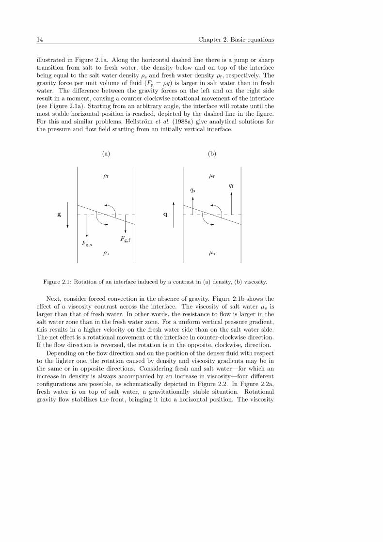
illustrated in Figure 2.1a. Along the horizontal dashed line there is a jump or sharptransition from salt to fresh water, the density below and on top of the interfacebeing equal to the salt water density ρs and fresh water density ρf , respectively. Thegravity force per unit volume of fluid (Fg = ρg) is larger in salt water than in freshwater. The difference between the gravity forces on the left and on the right sideresult in a moment, causing a counter-clockwise rotational movement of the interface(see Figure 2.1a). Starting from an arbitrary angle, the interface will rotate until themost stable horizontal position is reached, depicted by the dashed line in the figure.For this and similar problems, Hellstrom et al. (1988a) give analytical solutions forthe pressure and flow field starting from an initially vertical interface.
(a)
?
g
ρf
ρs
?Fg,s
?Fg,f
-
�
(b)
6q
µf
µs
6
qs
6
qf
-
�
Figure 2.1: Rotation of an interface induced by a contrast in (a) density, (b) viscosity.
Next, consider forced convection in the absence of gravity. Figure 2.1b shows theeffect of a viscosity contrast across the interface. The viscosity of salt water µs islarger than that of fresh water. In other words, the resistance to flow is larger in thesalt water zone than in the fresh water zone. For a uniform vertical pressure gradient,this results in a higher velocity on the fresh water side than on the salt water side.The net effect is a rotational movement of the interface in counter-clockwise direction.If the flow direction is reversed, the rotation is in the opposite, clockwise, direction.
Depending on the flow direction and on the position of the denser fluid with respectto the lighter one, the rotation caused by density and viscosity gradients may be inthe same or in opposite directions. Considering fresh and salt water—for which anincrease in density is always accompanied by an increase in viscosity—four differentconfigurations are possible, as schematically depicted in Figure 2.2. In Figure 2.2a,fresh water is on top of salt water, a gravitationally stable situation. Rotationalgravity flow stabilizes the front, bringing it into a horizontal position. The viscosity
2.3 Density- and viscosity-driven rotational flow 15
(a)
?
6
g
q
ρs µs
ρf µf
q
i
(b)
? ?
g q
ρs µs
ρf µf
qi
(c)
?
6
g
q
ρs µs
ρf µf
q
i
(d)
? ?
g q
ρs µs
ρf µf
qi
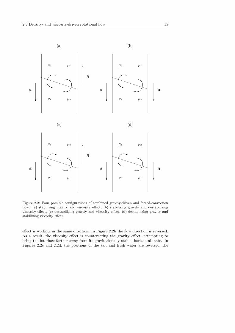
Figure 2.2: Four possible configurations of combined gravity-driven and forced-convectionflow: (a) stabilizing gravity and viscosity effect, (b) stabilizing gravity and destabilizingviscosity effect, (c) destabilizing gravity and viscosity effect, (d) destabilizing gravity andstabilizing viscosity effect.
effect is working in the same direction. In Figure 2.2b the flow direction is reversed.As a result, the viscosity effect is counteracting the gravity effect, attempting tobring the interface farther away from its gravitationally stable, horizontal state. InFigures 2.2c and 2.2d, the positions of the salt and fresh water are reversed, the
16 Chapter 2. Basic equations
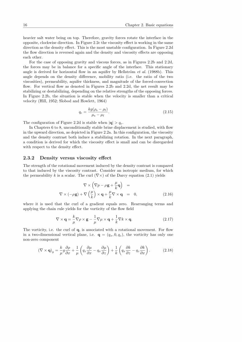
heavier salt water being on top. Therefore, gravity forces rotate the interface in theopposite, clockwise direction. In Figure 2.2c the viscosity effect is working in the samedirection as the density effect. This is the most unstable configuration. In Figure 2.2dthe flow direction is reversed again and the density and viscosity effects are opposingeach other.
For the case of opposing gravity and viscous forces, as in Figures 2.2b and 2.2d,the forces may be in balance for a specific angle of the interface. This stationaryangle is derived for horizontal flow in an aquifer by Hellstrom et al. (1988b). Thisangle depends on the density difference, mobility ratio (i.e. the ratio of the twoviscosities), permeability, aquifer thickness, and magnitude of the forced-convectionflow. For vertical flow as denoted in Figures 2.2b and 2.2d, the net result may bestabilizing or destabilizing, depending on the relative strengths of the opposing forces.In Figure 2.2b, the situation is stable when the velocity is smaller than a criticalvelocity (Hill, 1952; Slobod and Howlett, 1964)
qc =kg(ρs − ρf)
µs − µf. (2.15)
The configuration of Figure 2.2d is stable when |q| > qc.In Chapters 6 to 8, unconditionally stable brine displacement is studied, with flow
in the upward direction, as depicted in Figure 2.2a. In this configuration, the viscosityand the density contrast both induce a stabilizing rotation. In the next paragraph,a condition is derived for which the viscosity effect is small and can be disregardedwith respect to the density effect.
2.3.2 Density versus viscosity effect
The strength of the rotational movement induced by the density contrast is comparedto that induced by the viscosity contrast. Consider an isotropic medium, for whichthe permeability k is a scalar. The curl (∇×) of the Darcy equation (2.1) yields
∇×(
∇p− ρg +µ
kq)
=
∇× (−ρg) +∇(µ
k
)
× q +µ
k∇× q = 0, (2.16)
where it is used that the curl of a gradient equals zero. Rearranging terms andapplying the chain rule yields for the vorticity of the flow field
∇× q =k
µ∇ρ× g− 1
µ∇µ× q +
1
k∇k × q. (2.17)
The vorticity, i.e. the curl of q, is associated with a rotational movement. For flowin a two-dimensional vertical plane, i.e. q = (qx, 0, qz), the vorticity has only onenon-zero component
(∇× q)y =k
µg∂ρ
∂x+
1
µ
(
qz∂µ
∂x− qx
∂µ
∂z
)
+1
k
(
qx∂k
∂z− qz
∂k
∂x
)
. (2.18)
2.3 Density- and viscosity-driven rotational flow 17
A positive vorticity, i.e. pointing in the positive y direction perpendicular to the (x, z)plane, expresses the magnitude of the rotational velocity in clockwise direction. Forinstance, in Figure 2.1a the horizontal density gradient ∂ρ/∂x across the interface isnegative. A negative vorticity is associated with a rotational movement in counter-clockwise direction, as illustrated by the arrows in Figure 2.1a.
Disregarding the effect of gradients in permeability, and assuming that the flow ismainly in the z direction, i.e.
qz∂µ
∂x� qx
∂µ
∂z, (2.19)
leaves only two terms in equation (2.18). Writing the density and viscosity gradientsin terms of the salt mass fraction, using expression (2.11) and γµ = ∂(ln µ)/∂ω, gives
(∇× q)y =
(k
µgργρ + qzγµ
)∂ω
∂x. (2.20)
The vorticity induced by the viscosity contrast is small compared to that induced bythe density contrast when
qz �kgργρ
µγµ, (2.21)
where γµ can be approximated by the first coefficient in equation of state (2.14) forsmall salt mass fractions. Note that, when the density variation is approximatedlinearly, i.e. ∆ρ = ργρ∆ω, and a similar approximation for ∆µ is adopted, the righthand side of inequality (2.21) reduces to the critical velocity qc defined in (2.15).

Chapter 3
The Oberbeck-Boussinesq
approximation
This chapter discusses the Oberbeck-Boussinesq approximation for heat and solutetransport in porous media. In this commonly used approximation, all density vari-ations are disregarded except for the gravity term in Darcy’s law. However, in thelimit of vanishing density differences, the gravity term should disappear as well. Themain purpose of this chapter is to give the correct limits in which the gravity term isretained, while other density effects can be neglected.
3.1 Introduction
The Oberbeck-Boussinesq approximation is a widely used and powerful simplificationin studies of density-dependent flows. In the literature, this approximation is com-monly named after Boussinesq (1903), though Oberbeck (1879) was the first scientistwho made use of it. The approximation in its strictest form includes the followingfour assumptions (Gartling and Hickox, 1985; Joseph, 1976; Gray and Giorgini, 1976):
1. Density variations—induced by variations in temperature and/or solute concen-tration—are neglected in all equations, with the exception of the gravity termin the equation of motion.
2. All other material properties (e.g. viscosity, heat capacity, thermal conductivity,solute molecular diffusivity) are assumed constant.
3. Viscous dissipation is assumed negligible.
4. The equation of state is linearized.
Different versions and extensions of the Oberbeck-Boussinesq approximation are inuse. For instance, Gartling and Hickox (1985) employ the so-called “relaxed” or“extended” Boussinesq approximation, in which fluid properties other than densityare allowed to vary.
The present study only focuses on the first and most important assumption. Mostresearchers state that this assumption is valid in cases where density variations are
19
20 Chapter 3. The Oberbeck-Boussinesq approximation
small. However, in the limit of density differences approaching zero, the governingequations do not reduce to those used in the Boussinesq approximation. In this limit,the gravitational term in the equation of motion vanishes as well. In many practicalcases, such as problems involving the intrusion of sea water or storage of thermalenergy in aquifers, gravity can play an important role. In those cases the Boussinesqapproximation often works well. In the words of Daniel Joseph (1976): ”. . . there isno special reason, besides our lack of proofs, to doubt the validity of the Oberbeck-Boussinesq equations in some limit of small parameters.”
Numerous researchers have tried to derive the Boussinesq equations for ordinaryfluids. See for example Rajagopal et al. (1996), who give a short overview of thedifferent approaches. For fluids in porous media, the validity of the Boussinesq ap-proximation has been tested numerically by various authors (Gartling and Hickox,1985; Leijnse, 1989; Peirotti et al., 1987; Johannsen, 2003). The present study dealswith the Boussinesq approximation in a different way. An attempt is made to givethe formal limits in which the Boussinesq equations for transport in porous mediaare obtained. This is done by deriving explicit equations for the relative changes influid volume. These volume changes are neglected in the Boussinesq approximation,yielding the continuity equation in its incompressible form: ∇·q = 0. Three cases arediscussed: isothermal brine transport, heat transfer in fresh water, and simultaneoustransport of heat and brine.
3.2 Governing equations
The standard set of equations for salt and heat transport, as discussed in Chapter 2, isrepeated here. The porous medium is assumed to be non-deformable, homogeneous,and isotropic. The five governing equations are: the mass balances of the fluid andthe salt, the energy balance, Darcy’s law, and an equation of state that relates thefluid density to the temperature and the salt mass fraction.
Fluid mass balance
n∂ρ
∂t+∇·(ρq) = 0, (3.1)
where t denotes time, n the porosity, ρ the fluid density, and q the specific dischargevector.
Salt mass balance
n∂(ρω)
∂t+∇·(ρqω −Dρ∇ω) = 0, (3.2)
where ω is the salt mass fraction and D is the diffusion/dispersion tensor. The saltmass fraction (a dimensionless variable) is defined as the ratio of salt mass concen-tration to fluid density, i.e. ω = C/ρ.
3.2 Governing equations 21
Energy balance
ncf∂(ρT )
∂t+ (1− n)ρscs
∂T
∂t+∇·(cfρqT − λeff∇T ) = 0, (3.3)
where cf and cs denote the specific heat of fluid and solid (soil particles), respec-tively. Moreover, ρs is the solid phase density, T is the temperature, and λeff theeffective thermal conductivity of the porous medium. This equation assumes thermalequilibrium between the fluid and solid phases.
Darcy’s law
q +k
µ(∇p− ρg) = 0, (3.4)
where p denotes the fluid pressure, k the intrinsic permeability, µ the dynamic fluidviscosity and g the acceleration of gravity.
Equation of state
ρ = ρ0 eγρω − α(T − T0), (3.5)
where ρ0 and T0 are the reference density and the reference temperature, γρ =∂ ln ρ/∂ ω is a curve fitting constant (γρ ≈ 0.692), and α is the thermal expansioncoefficient of the fluid.
Using the equation of state (3.5) to eliminate the salt mass fraction in (3.2), andcombining the fluid mass balance (3.1) with (3.3) and (3.2), yields for the salt massand energy balances
n∂ρ
∂t+ nαρ
∂T
∂t+ q·∇ρ + αρq·∇T −∇·(D∇ρ + αDρ∇T ) = 0, (3.6)
(ncfρ + (1− n)ρscs)∂T
∂t+ cfρq·∇T −∇·(λeff∇T ) = 0. (3.7)
Starting point in the following analysis is the set of coupled nonlinear partial differ-ential equations given by (3.1), (3.4), (3.6), and (3.7). Next, the equations are scaledusing
ρ∗ =ρ− ρ0
ρmax − ρ0, T ∗ =
T − Tmin
T0 − Tmin, p∗ =
pk
µq0x0, and ω∗ =
ω
ωmax, (3.8)
where Tmin, ρmax, and ωmax denote the minimum temperature and the maximumdensity and salt mass fraction. Note that the reference density ρ0 is the minimumdensity, corresponding to the maximum temperature (reference temperature T0) anda zero salt mass fraction. With the use of scaling definitions (3.8), the temperature,
22 Chapter 3. The Oberbeck-Boussinesq approximation
density, and mass fraction, are scaled to have values between zero and one. Further-more, the specific discharge, spatial coordinates, and time, are rendered dimensionlessintroducing
q∗ =q
q0, x∗ =
x
x0, and t∗ =
tq0
nx0, (3.9)
where q0 and x0 are a characteristic discharge and length scale respectively. Moreover,the following dimensionless coefficients are introduced:
N =kρ0g
µq0, A =
(1− n)ρscs
nρ0cf, α∗ = α(T0 − Tmin), and γ∗ρ = γρωmax. (3.10)
Note that N resembles the gravity number (Ng = Ra/Pe), with the difference that itcontains the absolute reference density instead of the density difference. The param-eter A incorporates the effect of thermal retardation caused by heat storage in thesolid phase.
The Peclet number expresses the ratio of convective transport to molecular diffu-sion. In addition, the ratio of thermal diffusion to solute diffusion is needed, given bythe Lewis number
Le =λeff
ρ0cfD=
a
D, and Pe =
q0x0
D, (3.11)
where a is the effective thermal diffusion coefficient. For the moment, velocity-dependent dispersion is disregarded and it is assumed that λeff and D are constants.The last parameter that is introduced is the one that describes the maximum rela-tive density difference in a specific density-dependent flow problem. This importantparameter is given by
ε =ρmax − ρ0
ρ0. (3.12)
The resulting set of dimensionless equations is given by (omitting the asterisks nota-tion for convenience)
ε∂ρ
∂t+∇·[(1 + ερ)q ] = 0, (3.13)
ε∂ρ
∂t+ α(1 + ερ)
∂T
∂t+ εq·∇ρ + α(1 + ερ)q·∇T − ε
Pe∆ρ
− α
Pe∇·[(1 + ερ)∇T ] = 0, (3.14)
(1 + ερ + A)∂T
∂t+ (1 + ερ)q·∇T − Le
Pe∆T = 0, (3.15)
q +∇p + N(1 + ερ)ez = 0, (3.16)
3.3 The Boussinesq limit revisited 23
where ez denotes the unit vector in the z-direction. The scaled version of the equationof state is given by
ρ =1
ε
(
eγρω − α(T − 1) − 1)
. (3.17)
As observed by Joseph (1976), the formal limit ε ↓ 0 in equations (3.13)–(3.16)does not yield equations consistent with the Boussinesq approximation. In this limit,the density effects vanish from all equations, including Darcy’s law. However, in theBoussinesq approximation the density dependency in Darcy’s law is retained.
3.3 The Boussinesq limit revisited
This section investigates the limits in which the equations are obtained as in theBoussinesq approximation. Three cases are discussed: isothermal brine transport,heat transfer in fresh water, and simultaneous transport of heat and brine.
3.3.1 Isothermal brine transport
The scaled equations for the case of isothermal brine transport are given by (3.13),(3.14), and (3.16). Note that under isothermal conditions, equation (3.14) reduces to
∂ρ
∂t+ q ·∇ρ− 1
Pe∆ρ = 0. (3.18)
Expanding the divergence term in fluid mass balance (3.13), and subtracting (3.18)multiplied by ε, after rearranging terms results in
∇· q = − ε
Pe (1 + ερ)∆ρ. (3.19)
Taking the divergence of Darcy’s equation (3.16), and substituting (3.19) in the resultyields the elliptic pressure equation
∆p =ε
Pe(1 + ερ)∆ρ
︸ ︷︷ ︸
Volume changes
−Nε∂ρ
∂z︸ ︷︷ ︸
Gravity
. (3.20)
Note that both terms in (3.20) contain the relative density difference ε. It is generallysaid that volume changes can be neglected for small density differences, i.e. small ε.This is true, but at the same time the second term in equation (3.20) becomes smallwhen ε ↓ 0. Disregarding the volume changes but retaining the gravity term can onlybe done when NPe� 1. Note that this condition is independent of ε, because
NPe =Ra
ε=
kgρ0x0
µD. (3.21)
The role of the diffusion coefficient D can be explained as follows. When for ex-ample two equal volumes of a high and a low salt concentration are added, eventually
24 Chapter 3. The Oberbeck-Boussinesq approximation
the concentration will distribute itself evenly as a result of molecular diffusion. Theresulting total volume is slightly smaller than the sum of the two volumes. In thehypothetic case of zero molecular diffusion, no mixing would occur at all when thetwo volumes are added, and no change in fluid volume would take place. Therefore,when the diffusion coefficient is very small, Pe is large and the condition stating thatvolume changes are negligible, i.e. NPe� 1, is easily satisfied.
The other parameters in NPe are fixed (g), medium (k), or fluid (ρ0, µ) properties,except for x0. When the characteristic length of interest is small, volume effects arerelatively more important than for larger length scales. The effect of volume changeson the flow field is a local phenomenon, observed where high density gradients occur.This is illustrated with some examples in Chapter 4.
Finally, the transport equation (3.18) is rewritten in terms of the salt mass fractionω, using equation of state (3.17) with constant T . Without any further assumptions,the following equation is obtained:
∂ω
∂t+ q ·∇ω − 1
Pe∆ω =
γρ
Pe(∇ω)2. (3.22)
In the Boussinesq approximation, equation (3.22) is used with the difference thatthe right-hand side is zero. That equation would be obtained directly from the orig-inal salt mass balance equation (3.2), under the assumption of a constant density.However, the constant density assumption also implies disregarding the gravity termin pressure equation (3.20). The constant density assumption therefore is not con-sistent with the Boussinesq approximation. To obtain the transport equation as inthe Boussinesq approximation, the right-hand side of equation (3.22) should be smallenough to be disregarded, in comparison with the terms on the left-hand side. This isthe case when the gradient of ω is small (but not zero). In addition, when γρω � 1,the equation of state (3.17) can be linearized to ρ = γρ ω/ε, yielding the desiredtransport equation directly from equation (3.18). This linearization is often done (seePoint 4 in the Introduction), but not strictly necessary.
3.3.2 Heat transfer in fresh water
In this section only heat transfer is considered, which is described by equations (3.13),(3.15), and (3.16). The equation of state (3.17) is used to write fluid mass balanceequation (3.13) in terms of the temperature. Note that the salt mass fraction is omit-ted in the equation of state, because fresh water is considered. Combining equations(3.13) and (3.15) yields
∇· q =α
1 + ερ + A
[
Aq ·∇T +Le
Pe∆T
]
, (3.23)
or, with the right-hand side written in terms of the density only:
∇· q = − 1
1 + ερ + A
[εA
1 + ερq ·∇ρ + ε
Le
Pe∇·(
1
(1 + ερ)∇ρ
)]
. (3.24)
3.3 The Boussinesq limit revisited 25
Finally, after combining equations (3.24) and (3.16):
∆p = − 1
1 + ερ + A
Heat convection︷ ︸︸ ︷
εA
1 + ερq ·∇ρ +
Heat diffusion︷ ︸︸ ︷
εLe
Pe∇·(
1
(1 + ερ)∇ρ
)
︸ ︷︷ ︸
Fluid volume changes
+Nε∂ρ
∂z︸ ︷︷ ︸
Gravity
. (3.25)
Note that in Section 3.2, the Peclet number is defined for solute transport. As aconsequence, the ratio of Le and Pe appears in the heat transfer equations. Thisratio is nothing else than the reciprocal of Pe defined for heat transfer, i.e. PeT =q0x0ρ0cf/λeff .
In comparison with the case of isothermal brine transport, the situation is nowslightly more complicated. The term in pressure equation (3.25) that accounts for fluidvolume changes consists of two parts: a convective term (due to thermal retardation)and a diffusive term (due to effective heat conduction). Hence, the limit Le/Pe� Nis not sufficient to reduce (3.25) to the equation for incompressible flow. In this limit,only the diffusive term vanishes, while the convective term remains unaffected. Tobe able to disregard all volume changes and retain the gravity term, the condition|q| � N must be fulfilled as well (A and (1 + ερ) being of order 1).
In one sense, the convective term in pressure equation (3.25) plays a peculiar role.To elucidate its consequences, the following one-dimensional heat convection problemis considered: let Le = 0 (no heat conduction), while the initial temperature distribu-tion is given by T (x, 0) = Ti(x), corresponding to ρ(x, 0) = ρi(x), and q(−∞, t) = qL.For this particular case, equation (3.15) reduces to
∂ρ
∂t+
(1 + ερ)q
(1 + ερ + A)
∂ρ
∂x= 0, (3.26)
and combining (3.13) and (3.15) yields
∂q
∂x= − εAq
(1 + ερ + A)(1 + ερ)
∂ρ
∂x. (3.27)
This is the one-dimensional version of equation (3.24), without the diffusive term.Integration of equation (3.27) yields
q =(1 + ερ + A)
(1 + ερ)C1. (3.28)
Substitution in (3.26) gives
∂ρ
∂t+ C1
∂ρ
∂x= 0, (3.29)
where C1 is a constant that can be determined by applying the boundary conditions forq and ρ at x = −∞. For example, when ρ(−∞, t) = 1, then C1 = qL (1+ε)/(1+ε+A).
26 Chapter 3. The Oberbeck-Boussinesq approximation
Due to the hyperbolic character of equation (3.29), the initial temperature/densitydistribution moves with a constant speed C1—without changing shape—even thoughthe specific discharge q is non-uniform. In the limit ε ↓ 0 a constant front velocityC1 = qL/(1 + A) is obtained. Hence, the difference between this limit and the exactequations is a small change in the front velocity of order ε. On the other hand, if adivergence free discharge is assumed, i.e. q = qL, the front velocity (1 + ερ)qL/(1 +ερ + A) is non-uniform. As a result—even though diffusion is absent—the densitydistribution changes in shape.
3.3.3 Simultaneous heat and brine transport
This section discusses the transport of both heat and brine. The governing equationsare given in their scaled form by (3.13)–(3.16). Combining equation (3.13) and (3.14)yields an expression for ∇·q in terms of ρ and T . Eliminating the time-dependentterm using the energy balance (3.15) results in
∇· q =α(Le/Pe)∆T + αAq ·∇T
1 + ερ + A− ε∆ρ
Pe(ερ + 1)
− α
Pe(ερ + 1)∇·[(ερ + 1)∇T ] . (3.30)
This expression can be compared to equations (3.19) and (3.23), the separate cases ofbrine transport and heat transport. The first term in (3.30) is equal to the right-handside of equation (3.23). It expresses the contribution of temperature gradients to thechanges in fluid volume. The remaining part of equation (3.30) seems to contain anextra term compared to equation (3.19). However, ∆ρ in equation (3.19) contains theeffect of concentration only, whereas ∆ρ in equation (3.30) accounts for temperaturedifferences as well. When the latter is expressed in terms of ω and T using theequation of state (3.17), the part that depends on the temperature cancels out thelast term in equation (3.30). Consequently, the remaining part of (3.30) is equal tothe right-hand side of equation (3.19). This means that the fluid volume changes ina problem that considers transport of both heat and brine are simply a summationof the fluid volume changes caused by the two separate effects.
Combining equation (3.30) with the equation of motion (3.16) gives a pressureequation similar to (3.25) with the fluid volume changes given by (3.30). To obtainthe equations in the Boussinesq approximation, the conditions for the separate casesof heat and brine transport must both be fulfilled.
3.4 Conclusions
In the Boussinesq approximation, all density variations are disregarded, except forthe gravity term in Darcy’s law. The limit of vanishing density differences, ε ↓ 0, is incontradiction with this assumption, because the gravity effect in this limit disappearsas well.
3.4 Conclusions 27
Comparing the term accounting for fluid volume changes (∇·q 6= 0) to the gravityterm in the scaled pressure equation, explains why and when it is justified to disregardthe first, while retaining the latter. For isothermal brine transport, a condition needsto be fulfilled for a dimensionless number, independent of the density difference andcharacteristic discharge:
NPe =Ra
ε=
kgρ0x0
µD� 1. (3.31)
For heat transfer in a porous medium, two conditions must be met to obtain theequations as in the Boussinesq approximation:
NPe
Le= NPeT � 1, and N� |q|. (3.32)
The extra condition involving the specific discharge results from the fact that thesolid grains absorb heat as well, causing thermal retardation.
When transport of both heat and brine is considered, the fluid volume changesthat occur are simply a sum of the volume changes caused by the two separate effects.Therefore, to be able to neglect the volume changes in comparison with the gravityterm, the conditions for both cases must be fulfilled.

Chapter 4
Similarity solutions for 1-D
simultaneous heat and solute
transport in porous media
This chapter elaborates on the discussion of the Boussinesq approximation in Chap-ter 3. Two one-dimensional (1-D) example problems of simultaneous heat and brinetransport are discussed, for which similarity solutions of the full equations are pre-sented. These examples are meant to illustrate the enhancement or reduction of thespecific discharge as a result of fluid volume changes, the effect that is neglected inthe Boussinesq approximation. The choice of the characteristic length and velocity,introduced in Chapter 3, is discussed. Additionally, an example is given that incorpo-rates the effect of a velocity-dependent dispersion coefficient on the specific dischargeprofile. Due to their one-dimensionality, gravity does not play a role in the examplesin this chapter.
4.1 Two example problems
Similarity solutions are presented for two 1-D examples of heat and brine transport.The complete system of equations (3.13)–(3.15) is solved. The two problems ini-tially have a discontinuity in the density at x = 0, caused by discontinuities in thetemperature and salt mass fraction. The initial conditions for Problem I are (scaledvariables)
T = 0 and ω = 1 for x < 0,
T = 1 and ω = 0 for x > 0. (4.1)
So, for negative x the temperature and salt mass fraction equal their minimum andmaximum values respectively, resulting in the maximum density possible. For positivex the density equals its minimum value. In Problem II the initial profile of the saltmass fraction is reversed:
T = 0 and ω = 0 for x < 0,
T = 1 and ω = 1 for x > 0. (4.2)
29
30 Chapter 4. Similarity solutions
Whereas in Problem I the temperature and mass fraction distributions enhance eachother in their effect on the density, they have an opposing effect in Problem II.
The specific discharge q is chosen to be zero at infinity for all times:
q = 0 for x→∞. (4.3)
For these two cases, semi-analytical solutions are constructed with the use of similaritytransformations. This method is described in the next section.
4.2 Similarity transformations
4.2.1 Transformed equations
In the following derivation, 1-D equations are considered. Darcy’s law is not neededto calculate the specific discharge q, since q is treated as an unknown variable. Theother two unknowns are the scaled density ρ, and the scaled temperature T . Thethree equations that must be solved are the fluid mass balance, the salt mass balanceand the energy balance. Starting point is the system of governing equations given bythe 1-D versions of (3.13)–(3.15). This system of coupled partial differential equationsis transformed into a set of ordinary differential equations using
η =x√t, T (x, t) = f(η), ρ(x, t) = u(η), and q(x, t) =
v(η)√t
. (4.4)
These substitutions are similar to those used by Van Duijn et al. (1998), who considerisothermal brine transport in porous media. After rearrangement the three equationsbecome
ε(
v − 1
2η)
u′ + (1 + εu)v′ = 0, (4.5)
(1 + εu)(
v − 1
2η)
f ′ − 1
2Aηf ′ − Le
Pef ′′ = 0, (4.6)
(
v − 1
2η)(
εu′ + α(1 + εu)f ′)
− ε
Peu′′ − α
Pe
(
(1 + εu)f ′)′
= 0, (4.7)
where ′ denotes the derivative with respect to η. Differentiating equation (4.6) andrearranging terms yields
(f ′′
f ′
)′= ε
Pe
Le
(
Av + Le f ′′
f ′
)
u′
1 + εu + A+
Pe
Le(1 + εu)v′ − 2
Pe
Le
(1 + εu + A
). (4.8)
Substituting (4.7) into (4.6) to eliminate η gives for u′′:
u′′ = −α
ε
((1 + εu)f ′
)′+ Pe
εu′ + α(1 + εu)f ′
εD(1 + εu + A)
(
Lef ′′
f ′+ Av
)
. (4.9)
4.2 Similarity transformations 31
Furthermore, an expression for v′ is obtained by combining equations (4.5) and (4.6):
v′ =
−εu′(
Av +Le
Pe
f ′′
f ′
)
(1 + εu)(1 + εu + A). (4.10)
Note that equation (4.8) is a third order differential equation. This implies thatto solve this system of equations a third boundary condition for f is needed. Toavoid this problem, a temperature flux y is introduced that reduces the order ofdifferential equation (4.8). Now all variables are considered to be functions of finstead of functions of η, which is allowed because f is a monotonous function of η.The advantage of this is that the domain becomes finite. So:
y = y(f) = −f ′(η(f)), u = u(f), v = v(f). (4.11)
All derivatives with respect to η are substituted by derivatives with respect to f using
d
dη=
d
df
df
dη= −y
d
df. (4.12)
Finally, the following set of equations is obtained:
yd2y
df2+
ε
Le/Pe
Av − Le
Pe
dy
df
(1 + εu + A)ydu
df+
(1 + εu)
Le/Peydv
df+
1 + εu + A
2Le/Pe= 0, (4.13)
d
df
(
ydu
df
)
+α
ε
(
εydu
df+ (1 + εu)
dy
df
)
−Pe
εdu
df+ α(1 + εu)
ε(1 + εu + A)
(Le
Pe
dy
df−Av
)
= 0, (4.14)
dv
df= −
εdu
df
(
Av − Le
Pe
dy
df
)
(1 + εu)(1 + εu + A). (4.15)
With appropriate boundary conditions these equations can be solved numerically.When y, u and v are known as functions of f , the last step is to transform them backto functions of the similarity variable η. Therefore, an additional expression for η interms of y, u, and v is needed. From (4.6), (4.11), and (4.12) it follows that
η = 2
(1 + εu)v +Le
Pe
dy
df
1 + εu + A. (4.16)
32 Chapter 4. Similarity solutions
4.2.2 Transformed boundary conditions
The initial conditions of Problem I, given by (4.1), correspond to the following con-ditions for u(η), f(η), and v(η):
f(−∞) = 0, u(−∞) = 1,
f(∞) = 1, u(∞) = 0, v(∞) = 0. (4.17)
Note that for a non-zero background flow at x → ∞ the boundary condition for vbecomes a function of time (see transformation definitions (4.4)). In that case, asimilarity solution cannot be found. For the case of brine transport, this problemcan be overcome by decomposing the specific discharge q into a constant part (thebackground flow) and a deviation, i.e. q = q0+q. In addition, the similarity variable isadjusted: v(η) = q
√t. Unfortunately, this procedure does not work for simultaneous
heat and brine transport, because the temperature profile does not move with the samevelocity as the salt mass fraction profile due to thermal retardation. Consequently, azero background velocity is a necessary choice.
The boundary conditions needed to solve the system of equations (4.13)–(4.15)are given by
u(0) = 1, u(1) = 0,
y(0) = 0, y(1) = 0,
v(1) = 0. (4.18)
In Problem II, the initial profile of the salt mass fraction is reversed. As the tempera-ture and mass fraction distributions have opposite effects on the density, the minimumand maximum density are not reached in this case. The conditions for u(η), f(η),and v(η) are
f(−∞) = 0, u(−∞) =1
ε(eα − 1) ,
f(∞) = 1, u(∞) =1
ε(eγρ − 1) , v(∞) = 0. (4.19)
Note that the maximum temperature difference and salt mass fraction are incorpo-rated in α and γρ (see definitions (3.10)). To obtain the similarity solution for ProblemII, the system of equations (4.13)–(4.15) is solved subject to boundary conditions
u(0) =1
ε(eα − 1) , u(1) =
1
ε(eγρ − 1) ,
y(0) = 0, y(1) = 0,
v(1) = 0. (4.20)
4.3 Similarity and numerical solutions compared
The similarity solutions are not fully analytical, as a numerical method is also neces-sary to solve the resulting set of ordinary differential equations (4.13)–(4.15). The sys-tem is discretized using finite differences and solved using a Newton-Raphson method.
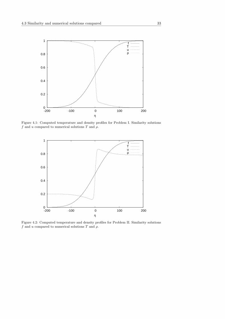
4.3 Similarity and numerical solutions compared 33
0
0.2
0.4
0.6
0.8
1
-200 -100 0 100 200
η
fTuρ
Figure 4.1: Computed temperature and density profiles for Problem I. Similarity solutionsf and u compared to numerical solutions T and ρ.
0
0.2
0.4
0.6
0.8
1
-200 -100 0 100 200
η
fTuρ
Figure 4.2: Computed temperature and density profiles for Problem II. Similarity solutionsf and u compared to numerical solutions T and ρ.
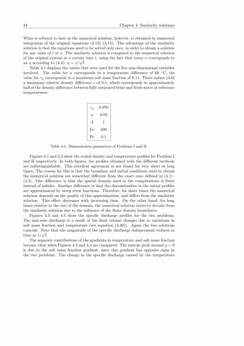
34 Chapter 4. Similarity solutions
What is referred to here as the numerical solution, however, is obtained by numericalintegration of the original equations (3.13)–(3.15). The advantage of the similaritysolution is that the equations need to be solved only once, in order to obtain a solutionfor any value of t or x. The similarity solution is compared to the numerical solutionof the original system at a certain time t, using the fact that every x corresponds toan η according to (4.4): η = x/
√t.
Table 4.1 displays the values that were used for the five non-dimensional variablesinvolved. The value for α corresponds to a temperature difference of 60 ◦C, thevalue for γρ corresponds to a maximum salt mass fraction of 0.11. These values yielda maximum relative density difference ε of 0.1, which corresponds to approximatelyhalf of the density difference between fully saturated brine and fresh water at referencetemperatures.
γρ 0.076
α 0.02
A 1
Le 400
Pe 0.1
Table 4.1: Dimensionless parameters of Problems I and II.
Figures 4.1 and 4.2 show the scaled density and temperature profiles for Problem Iand II respectively. In both figures, the profiles obtained with the different methodsare indistinguishable. This excellent agreement is not found for very short or longtimes. The reason for this is that the boundary and initial conditions used to obtainthe numerical solution are somewhat different from the exact ones defined in (4.1)–(4.3). One difference is that the spatial domain used in the computations is finiteinstead of infinite. Another difference is that the discontinuities in the initial profilesare approximated by steep error functions. Therefore, for short times the numericalsolution depends on the quality of this approximation, and differs from the similaritysolution. This effect decreases with increasing time. On the other hand, for longtimes relative to the size of the domain, the numerical solution starts to deviate fromthe similarity solution due to the influence of the finite domain boundaries.
Figures 4.3 and 4.4 show the specific discharge profiles for the two problems.The non-zero discharge is a result of the fluid volume changes due to variations insalt mass fraction and temperature (see equation (3.30)). Again the two solutionscoincide. Note that the magnitude of the specific discharge enhancement reduces intime as 1/
√t.
The separate contributions of the gradients in temperature and salt mass fractionbecome clear when Figures 4.3 and 4.4 are compared. The narrow peak around η = 0is due to the salt mass fraction gradient, since this gradient has opposite signs inthe two problems. The change in the specific discharge caused by the temperature
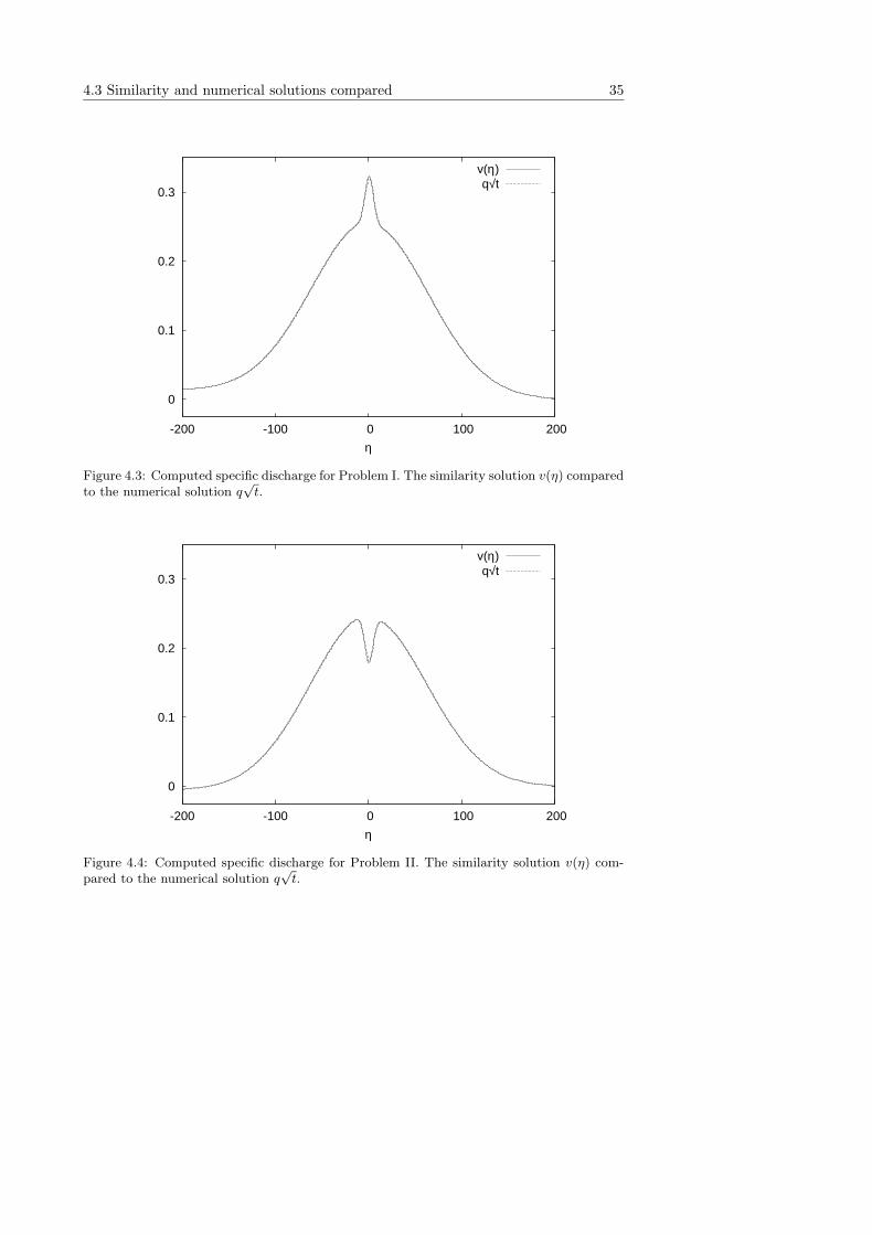
4.3 Similarity and numerical solutions compared 35
0
0.1
0.2
0.3
-200 -100 0 100 200
η
v(η)q√t
Figure 4.3: Computed specific discharge for Problem I. The similarity solution v(η) comparedto the numerical solution q
√
t.
0
0.1
0.2
0.3
-200 -100 0 100 200
η
v(η)q√t
Figure 4.4: Computed specific discharge for Problem II. The similarity solution v(η) com-pared to the numerical solution q
√
t.
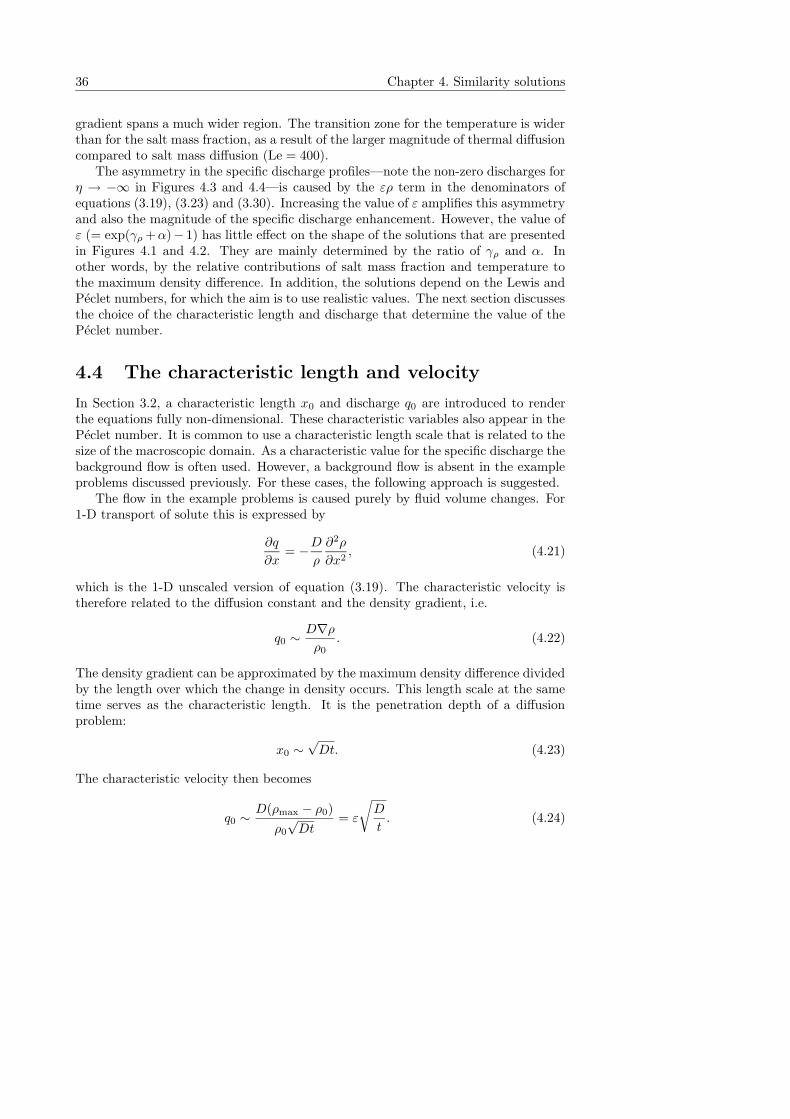
36 Chapter 4. Similarity solutions
gradient spans a much wider region. The transition zone for the temperature is widerthan for the salt mass fraction, as a result of the larger magnitude of thermal diffusioncompared to salt mass diffusion (Le = 400).
The asymmetry in the specific discharge profiles—note the non-zero discharges forη → −∞ in Figures 4.3 and 4.4—is caused by the ερ term in the denominators ofequations (3.19), (3.23) and (3.30). Increasing the value of ε amplifies this asymmetryand also the magnitude of the specific discharge enhancement. However, the value ofε (= exp(γρ +α)− 1) has little effect on the shape of the solutions that are presentedin Figures 4.1 and 4.2. They are mainly determined by the ratio of γρ and α. Inother words, by the relative contributions of salt mass fraction and temperature tothe maximum density difference. In addition, the solutions depend on the Lewis andPeclet numbers, for which the aim is to use realistic values. The next section discussesthe choice of the characteristic length and discharge that determine the value of thePeclet number.
4.4 The characteristic length and velocity
In Section 3.2, a characteristic length x0 and discharge q0 are introduced to renderthe equations fully non-dimensional. These characteristic variables also appear in thePeclet number. It is common to use a characteristic length scale that is related to thesize of the macroscopic domain. As a characteristic value for the specific discharge thebackground flow is often used. However, a background flow is absent in the exampleproblems discussed previously. For these cases, the following approach is suggested.
The flow in the example problems is caused purely by fluid volume changes. For1-D transport of solute this is expressed by
∂q
∂x= −D
ρ
∂2ρ
∂x2, (4.21)
which is the 1-D unscaled version of equation (3.19). The characteristic velocity istherefore related to the diffusion constant and the density gradient, i.e.
q0 ∼D∇ρ
ρ0. (4.22)
The density gradient can be approximated by the maximum density difference dividedby the length over which the change in density occurs. This length scale at the sametime serves as the characteristic length. It is the penetration depth of a diffusionproblem:
x0 ∼√
Dt. (4.23)
The characteristic velocity then becomes
q0 ∼D(ρmax − ρ0)
ρ0
√Dt
= ε
√
D
t. (4.24)
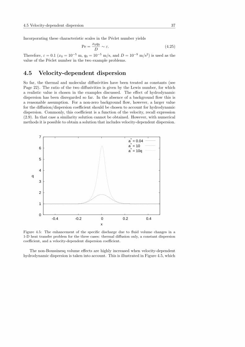
4.5 Velocity-dependent dispersion 37
Incorporating these characteristic scales in the Peclet number yields
Pe =x0q0
D∼ ε. (4.25)
Therefore, ε = 0.1 (x0 = 10−5 m, q0 = 10−5 m/s, and D = 10−9 m/s2) is used as thevalue of the Peclet number in the two example problems.
4.5 Velocity-dependent dispersion
So far, the thermal and molecular diffusivities have been treated as constants (seePage 22). The ratio of the two diffusivities is given by the Lewis number, for whicha realistic value is chosen in the examples discussed. The effect of hydrodynamicdispersion has been disregarded so far. In the absence of a background flow this isa reasonable assumption. For a non-zero background flow, however, a larger valuefor the diffusion/dispersion coefficient should be chosen to account for hydrodynamicdispersion. Commonly, this coefficient is a function of the velocity, recall expression(2.9). In that case a similarity solution cannot be obtained. However, with numericalmethods it is possible to obtain a solution that includes velocity-dependent dispersion.
0
1
2
3
4
5
6
7
-0.4 -0.2 0 0.2 0.4
x
q
a* = 0.04a* = 10 a* = 10q
Figure 4.5: The enhancement of the specific discharge due to fluid volume changes in a1-D heat transfer problem for the three cases: thermal diffusion only, a constant dispersioncoefficient, and a velocity-dependent dispersion coefficient.
The non-Boussinesq volume effects are highly increased when velocity-dependenthydrodynamic dispersion is taken into account. This is illustrated in Figure 4.5, which
38 Chapter 4. Similarity solutions
shows the computed initial specific discharge profile of a 1-D heat transfer problem.For simplicity, solute transport is disregarded here. Similar to the examples discussedbefore, a steep temperature/density gradient at x = 0 causes an enhancement of thespecific discharge in this region. In contrast to the earlier examples a backgroundflow is considered in this case.
Three lines are shown in Figure 4.5. The solid line corresponds to the case inwhich only thermal diffusion is taken into account, where the scaled thermal diffusioncoefficient a∗ = a/q0 equals 0.04 (corresponding to a porous medium thermal diffu-sivity of 4.0 ·10−7 m2/s). The increase in the specific discharge due to the volumeeffects is very small compared to the background flow and therefore not visible in thefigure. In the second case, hydrodynamic dispersion is taken into account by taking amuch larger but constant diffusion/dispersion coefficient. This coefficient equals tentimes the background flow. The dashed line shows that in this case the dischargeis almost doubled around x = 0. Since the specific discharge is not constant alongx, a realistic dispersion coefficient should not be a constant either. When the diffu-sion/dispersion coefficient is made velocity-dependent (a∗ = 10q), the non-Boussinesqeffect is strongly increased. This is illustrated by the dotted line in Figure 4.5.
When the Boussinesq approximation is adopted, the increase of the specific dis-charge in the vicinity of x = 0 is disregarded. Figure 4.5 shows that the effects canbe large. However, the discharge enhancement is a very local effect. Furthermore, itsmagnitude decreases rapidly in time as the gradients causing it diminish, as a resultof the diffusion/dispersion processes.
4.6 Conclusions
One-dimensional similarity solutions for simultaneous transport of heat and brine areobtained. These solutions are consistent with those obtained by numerical integrationof the original partial differential equations. The similarity solutions can be usedfor computer code verification purposes. Solutions are presented for two diffusiondominated problems (Pe of order ε), which illustrate the effect of fluid volume changeson the flow velocity. This effect is disregarded when the Boussinesq approximation isadopted, introducing an error that is enlarged when velocity-dependent hydrodynamicdispersion is taken into account.
Due to the one-dimensionality, gravity does not play a role in the two exampleproblems discussed. The following chapters of this thesis involve gravity induced flow.The relative importance of the effect of fluid volume changes as opposed to the gravityeffect is one of the things discussed in Chapter 7.
Chapter 5
Closed-form approximate
solutions for one-dimensional
brine transport
5.1 Introduction
In Chapter 4, similarity solutions for one-dimensional simultaneous heat and brinetransport are presented. However, these solutions cannot be found explicitly, but aresemi-analytical. Moreover, Van Duijn and Schotting (1998) constructed exact semi-analytical solutions for several simple brine transport problems using similarity andVon Mises transformations. The resulting set of ordinary differential equations couldnot be solved in terms of a closed-form solution, implying that they had to rely onnumerical techniques.
Due to the nonlinear nature of the set of partial differential equations describingdensity-dependent flow in porous media, it is virtually impossible to construct closed-form exact solutions. However, exact analytical solutions play an important role incomputer code verification. As a consequence of the lack of closed-form solutions,authors of computer codes have to rely on so-called benchmark problems for codeverification purposes, such as the Henry (Henry, 1964), the Elder (Elder, 1967a,b),and the Saltpool (Johannsen et al., 2002) problems. See for a discussion of variousresults for the Henry problem Croucher and O’Sullivan (1995), and for the Elderproblem Diersch and Kolditz (2002). Johannsen (2003) investigates the effect ofthe Boussinesq approximation on the solutions of the Elder problem. Simpson andClement (2003) review both the Henry and Elder problems and discuss their usefulnessfor benchmarking.
In this chapter, approximate analytical solutions for one-dimensional brine trans-port are presented. It should be emphasized that, due to their one-dimensional char-acter, the buoyancy term in Darcy’s law does not play a role in these problems. Inthe approximate solutions, the nonlinear coupling between the density and the spe-cific discharge is retained, though slightly simplified. Three different simplificationsare discussed, for which closed-form solutions are constructed. These approximatesolutions are compared to the exact semi-analytical solution of Van Duijn and Schot-ting (1998).
39
40 Chapter 5. approximate brine solutions
5.2 Governing equations
The same scaling as in Chapter 3 is applied here, with the exception of the massfraction ω, which remains unscaled. Using scaling definitions (3.8) and (3.9), andthe non-dimensional parameters defined in (3.11) and (3.12), and assuming that thediffusion/dispersion coefficient D is a constant (independent of the specific discharge),the equations for isothermal brine transport in a non-deformable porous medium aregiven by (3.18) and (3.19). In one-dimensional form, the governing equations aregiven by
∂q
∂x= − ε
Pe(1 + ερ)
∂2ρ
∂x2, (5.1)
and
∂ρ
∂t+ q
∂ρ
∂x− 1
Pe
∂2ρ
∂x2= 0. (5.2)
The equation of state for the scaled density is given by
ρ =1
ε
(eγρω − 1
), (5.3)
where γρ ≈ 0.692. Equations (5.1) and (5.2) in terms of the mass fraction ω read
∂q
∂x= −γρe−γρω 1
Pe
∂
∂x
(
eγρω ∂ω
∂x
)
, (5.4)
and
∂ω
∂t+ q
∂ω
∂x− γρ
Pe
(∂ω
∂x
)2
− 1
Pe
∂2ω
∂x2= 0. (5.5)
Note that the specific discharge q can be found by direct integration of equation(5.1) or (5.4). It is interesting to remark that Darcy’s law, equation (2.1), has beenextended by various authors (Mitchell, 1976; Yeung and Mitchell, 1993) to include anadditional coupling flux term, proportional to ∂ω/∂x. Clearly, equation (5.4) supportsa formulation of this kind.
Equations (5.1)–(5.5) form the starting point for the mathematical analysis in thischapter.
5.3 Initial and boundary conditions
The problem under consideration is the displacement of fresh water by brine inan infinite domain. The stable situation is considered, though, due to the one-dimensionality, gravitational instabilities are not an issue. At x = −∞, a constantbrine flux in the positive x-direction is prescribed, given by
q(−∞, t) = 1 ∀ t ≥ 0. (5.6)
5.4 Approximate closed-form solutions 41
The initial density distribution is
ρ(x, 0) =
1 for x < 0,
0 for x > 0,(5.7)
corresponding to the boundary conditions
ρ(−∞, t) = 1 and ρ(+∞, t) = 0 ∀ t > 0. (5.8)
In terms of ω, which remains unscaled, the initial and boundary conditions are givenby
ω(z, 0) =
ln(1 + ε)/γρ for x < 0,
0 for x > 0,(5.9)
and
ω(−∞, t) = ln(1 + ε)/γρ and ω(+∞, t) = 0 ∀ t > 0. (5.10)
Semi-explicit solutions of equations (5.1) and (5.2), subject to (5.6), (5.7) and(5.8) are given by Van Duijn et al. (1998), and Van Duijn and Schotting (1998).
5.4 Approximate closed-form solutions
The specific discharge q can be obtained after integration of equation (5.1) (in termsof ρ) or equation (5.4) (in terms of ω). Integration by parts yields respectively
q = q0(t)−1
Pe
∂ ln(1 + ερ)
∂x− 1
Pe
∫ (∂ ln(1 + ερ)
∂x
)2
dx, (5.11)
and
q = q0(t)−γρ
Pe
∂ω
∂x−
γ2ρ
Pe
∫ (∂ω
∂x
)2
dx, (5.12)
where q0 is an arbitrary function of time, taken as a constant throughout the restof this chapter, i.e. q0(t) = q(−∞, t) = 1. Note that both expressions consist of acombination of local (point-wise) and integral terms. Approximate versions of ex-pressions (5.11) and (5.12) will be employed to obtain three different closed-formsolutions. These solutions are referred to as APPROX1 (most accurate), APPROX2,and APPROX3 (less accurate). The most accurate approximate solution is based uponan approximation of expression (5.12). Integration by parts of the integral term in(5.12) yields
q = 1− γρ(1 + γρω)1
Pe
∂ω
∂x+
γ2ρ
Pe
∫
ω∂2ω
∂x2dx. (5.13)
42 Chapter 5. approximate brine solutions
For the three different cases, the truncated approximate expressions for the specificdischarge in terms of both the salt mass fraction and the density are given by
APPROX1
q ≈ 1− γρ(1 + γρω)1
Pe
∂ω
∂x︸ ︷︷ ︸
a
= 1− ε
Pe
[1 + ln(1 + ερ)
1 + ερ
]∂ρ
∂x︸ ︷︷ ︸
b
(5.14)
APPROX2
q ≈ 1− γρ1
Pe
∂ω
∂x︸ ︷︷ ︸
a
= 1− ε
Pe(1 + ερ)
∂ρ
∂x︸ ︷︷ ︸
b
(5.15)
APPROX3
q ≈ 1− γρeγρω 1
Pe
∂ω
∂x︸ ︷︷ ︸
a
= 1− ε
Pe
∂ρ
∂x︸ ︷︷ ︸
b
(5.16)
Expression (5.14a) is obtained disregarding the integral term in expression (5.13).Furthermore, expression (5.15a) is the result of disregarding the integral term inexpression (5.12). Note that under the assumption γρ ω � 1, expression (5.14a) alsoreduces to (5.15a). Similarly, under the assumption ερ� 1, both (5.14b) and (5.15b)reduce to the linearized expression (5.16b). Applying this assumption directly to exactequation (5.1) yields, after integration and application of the boundary conditionon q, the same approximate expression (5.16b). Expression (5.16a) simply followsfrom (5.16b) by applying the equation of state (5.3).
5.4.1 Solution based on APPROX1
As a first approximation, the non-local term in expression (5.13) is disregarded. Theresulting truncated expression for the specific discharge (5.14a) can be substituted intransport equation (5.5), yielding an equation in ω only. For reasons of simplicity, ωrather than ρ is used as the primary variable. The resulting transport equation is
∂ω
∂t+
∂ω
∂x− γρ(2 + γρω)
1
Pe
(∂ω
∂x
)2
− 1
Pe
∂2ω
∂x2= 0. (5.17)
Next, a moving coordinate is introduced:
s(x, t) = x− t, (5.18)
implying ω(x, t) = ω(s(x, t), t). Under this transformation, transport equation (5.17)reduces to
∂ω
∂t− γρ(2 + γρ ω)
1
Pe
(∂ω
∂s
)2
− 1
Pe
∂2ω
∂s2= 0. (5.19)
5.4 Approximate closed-form solutions 43
This equation allows similarity transformation of the form ω(s, t) = w(ξ), whereξ = s/
√t. Under this transformation, equation (5.19) becomes
w′′ + γ(2 + γρw)(w′)2 +1
2ξPew′ = 0, (5.20)
subject to the boundary conditions
w(−∞) =1
γρln(1 + ε) and w(+∞) = 0. (5.21)
The primes in equation (5.20) denote differentiation with respect to ξ. Note that(5.20) is known as Liouville’s equation. The solution of Liouville’s equation is givenby an implicit equation (see Goldstein and Braun, 1972):
−√
2
γρe−2
∫ √2( 1
2γρw(ξ)+1)
0
es2
ds + Cε1 erf
(1
2ξ√
Pe
)
+ Cε2 = 0, (5.22)
where Cε1 and Cε
2 are integration constants, which depend on ε. Application of theboundary conditions (5.21) yields
Cε1 = − e−2
√2γρ
∫ √2( 1
2ln(1+ε)+1)
√2
es2
ds, (5.23)
and
Cε2 =
e−2
√2γρ
[∫ √
2( 12
ln(1+ε)+1)
0
es2
ds +
∫ √2
0
es2
ds
]
. (5.24)
Note that, when ω is scaled as well (by its maximum value ωmax), the first boundarycondition in (5.21) is replaced by w(−∞) = 1. In that case, ε does not enter thesolution, but the density dependence is captured in γρ, which is then multiplied byωmax. In the end, the solutions are independent of the scaling, but more elegantlyexpressed in terms of the unscaled ω and ε. In the limit ε ↓ 0, the constants given by(5.23) and (5.24) respectively reduce to
C01 = 0 and C0
2 =
√2
γρe−2
∫ √2
0
es2
ds, (5.25)
implying the correct trivial solution, i.e. w(ξ) = 0.Differentiation of expression (5.22) with respect to ξ gives
w′ = Cε1
√Pe exp
[
−(
1
4ξ2Pe +
1
2γρw(ξ)
[
γρw(ξ) + 4])]
. (5.26)
The specific discharge can be transformed using
v(ξ) = (q − 1)√
t, (5.27)
44 Chapter 5. approximate brine solutions
where q = q(s(x, t), t) = q(x, t). In (5.27), the boundary value is subtracted from q(see boundary condition (5.6)). Substituting expression (5.26) into (5.14a), where∂ω/∂x = w′(ξ)/
√t, results in the expression
v(ξ) = − γρ√Pe
[
1 + γρw(ξ)]
Cε1 exp
[
−(
1
4ξ2Pe +
1
2γρw(ξ)
[
γρw(ξ) + 4])]
. (5.28)
It should be noted that this expression contains both ξ and w(ξ), where the latter isimplicitly given by equation (5.22).
5.4.2 Solution based on APPROX2
The next aim is to derive an explicit approximate solution based on the assumptionthat the non-local term in expression (5.12) can be disregarded. Substitution of thetruncated expression (5.15a) in transport equation (5.5) gives
∂ω
∂t+
∂ω
∂x− 2
γρ
Pe
(∂ω
∂x
)2
− 1
Pe
∂2ω
∂x2= 0. (5.29)
Introduction of the moving frame coordinate (5.18), reduces (5.29) to
∂ω
∂t− 2
γρ
Pe
(∂ω
∂s
)2
− 1
Pe
∂2ω
∂s2= 0. (5.30)
As equation (5.19), this equation (subject to the initial and boundary conditions(5.6), (5.9) and (5.10)) allows a similarity transformation ω(s, t) = w(ξ), where againξ = s/
√t. This transformation yields
1
2ξPew′ + 2γρ(w′)2 + w′′ = 0, (5.31)
subject to the boundary conditions
w(−∞) =1
γρln(1 + ε) and w(+∞) = 0. (5.32)
Note that equation (5.31) can be further reduced to a Bernoulli equation in terms ofw′, for which an explicit closed-form solution can be found, see e.g. Zwillinger (1998)or again Goldstein and Braun (1972). Consequently, the solution of equation (5.31),subject to (5.32), is given by
w(ξ) =1
2γρln
(
1
2
[
1− (1 + ε)2]
erf
(1
2ξ√
Pe
)
+1
2
[
(1 + ε)2 + 1])
. (5.33)
This implies for the first-order derivative with respect to ξ
w′(ξ) = −√
Pe/π
2γρ
ε(2 + ε)e−14ξ2Pe
[
1− (1 + ε)2]
erf(
12ξ√
Pe)
+[
(1 + ε)2 + 1] . (5.34)
5.4 Approximate closed-form solutions 45
Hence, the solution for the transformed specific discharge is given by
v(ξ) =1
2√
πPe
ε(2 + ε)e−14ξ2Pe
[
1− (1 + ε)2]
erf(
12ξ√
Pe)
+ (1 + ε)2 + 1. (5.35)
Similar to ω, the density ρ can be transformed, i.e. u(ξ) = ρ(s(x, t), t) = ρ(x, t). Withthe equation of state (5.3), expression (5.33) can be written as
u(ξ) =1
ε
(√
1
2
[
1− (1 + ε)2]
erf
(1
2ξ√
Pe
)
+1
2
[
(1 + ε)2 + 1]
− 1
)
. (5.36)
An alternative approach to find the solution according to APPROX2 is to solve theproblem in terms of the specific discharge q. In that case, expression (5.15) is rewrittenas
∂ω
∂x=
Pe
γρ(1− q). (5.37)
Next, transport equation (5.5) is differentiated with respect to x. Substitution ofexpression (5.37) in the result to eliminate ω, after rearranging terms, yields
∂q
∂t+
∂q
∂x+ 4(q − 1)
∂q
∂x− 1
Pe
∂2q
∂x2= 0. (5.38)
Introduction of the moving frame coordinate s = x− t in (5.38) gives
∂q
∂t+ 4(q − 1)
∂q
∂s− 1
Pe
∂2q
∂s2= 0, (5.39)
where q(s(x, t), t) = q(x, t). Subsequently, the new variable q = q − 1 is introduced,reducing (5.39) to
∂q
∂t+ 4q
∂q
∂s− 1
Pe
∂2q
∂s2= 0. (5.40)
This equation can be written as a standard (”viscous”) Burgers’ equation in termsof q, in which the kinematic viscosity is given by 1/(16Pe). The piecewise constantinitial condition (5.7) is recast into
ω(x, 0) = ω0(x) =ln(1 + ε)
γρ
[1−H(x)
], (5.41)
where H(x) is the Heaviside step function
H(x) =
0 for x < 0,
12 for x = 0,
1 for x > 0.
(5.42)
46 Chapter 5. approximate brine solutions
Hence, the corresponding initial condition for q is given by
q(s, 0) = − γρ
Pe
∂ω(s, 0)
∂s= − ln(1 + ε)
Pe
∂
∂s
[1−H(s)
]=
1
Peln(1 + ε)δ(s), (5.43)
where δ(s) denotes the Dirac delta function. The solution of Burgers’ equation (5.40)subject to the initial condition (5.43) is given in terms of the transformed dischargeby expression (5.35), where v(ξ) = q
√t. Note that the boundary conditions are
incorporated in initial condition (5.43).
5.4.3 Solution based on APPROX3
Under the assumption ερ � 1 and after integration, exact expression (5.1) directlyreduces to the approximate expression (5.16b). Substitution of (5.16b) in equation(5.2) gives
∂ρ
∂t+
∂ρ
∂x− ε
Pe
(∂ρ
∂x
)2
− 1
Pe
∂2ρ
∂x2= 0. (5.44)
Again, the moving frame coordinate (5.18) is introduced, implying redefinition of thedensity according to ρ(x, t) = ρ(s, t). Then, equation (5.44) reduces to a second-ordernonlinear convection diffusion equation given by
∂ρ
∂t− ε
Pe
(∂ρ
∂s
)2
− 1
Pe
∂2ρ
∂s2= 0. (5.45)
The corresponding initial and boundary conditions are respectively
ρ(s, 0) =
1 for s < 0,
0 for s > 0,(5.46)
and
ρ(−∞, t) = 1 and ρ(+∞, t) = 0 ∀ t > 0. (5.47)
The problem defined by (5.45), subject to (5.46) and (5.47), allows similarity trans-formation in the Boltzmann variable ξ = s/
√t, similar to the problems for APPROX1
and APPROX2. Under this transformation, and defining ρ(s, t) = u(ξ), the problemfor APPROX3 reduces to
1
2ξPeu′ + ε (u′)
2+ u′′ = 0, (5.48)
subject to boundary conditions
u(−∞) = 1 and u(+∞) = 0. (5.49)
5.4 Approximate closed-form solutions 47
Again, the primes denote differentiation with respect to ξ. Note that equation (5.48)is similar to equation (5.31) for ω in APPROX2, and a Bernoulli equation in termsof u′. Its general closed-form solution is given by
u(ξ) =1
εln
[
Cε1 erf
(1
2ξ√
Pe
)
+ Cε2
]
, (5.50)
where Cε1 and Cε
2 are integration constants. Application of the boundary conditions(5.49) yields
Cε1 =
1
2(1− eε) and Cε
2 =1
2(1 + eε) . (5.51)
In the original scaled variables, the density is given by
ρ(x, t) =1
εln
[
1
2
(1− eε
)erf
(
x− t
2√
t/Pe
)
+1
2
(
1 + eε)]
, (5.52)
which in the limit ε ↓ 0 reduces to the solution in the Boussinesq limit, i.e.
ρ(x, t) =1
2erfc
(
x− t
2√
t/Pe
)
. (5.53)
Using expression (5.50), the transformed specific discharge v(ξ) = (q(s, t) − 1)√
taccording to expression (5.16b) becomes
v(ξ) = − ε
Pe
du
dξ= − 1√
Pe π
e−14ξ2Pe
erf(
12ξ√
Pe)
+1 + eε
1− eε
. (5.54)
This expression in the limit ε ↓ 0 reduces to v(ξ) = 0, so that for the specific dischargeq(x, t) = 1 is obtained, as to be expected.
Similar to the case of APPROX2, it is also possible to solve the problem in termsof the specific discharge. Differentiation of equation (5.44), substitution of the linearapproximate expression (5.16b) into the result, and the introduction of the movingframe coordinate (5.18), yields
∂q
∂t+ 2q
∂q
∂s− 1
Pe
∂2q
∂s2= 0, (5.55)
where q = q(s, t) = q(x, t). This again is in the form of a one-dimensional (’vis-cous’) Burgers’ equation. The appropriate initial condition, corresponding to theone-dimensional brine displacement problem is
q(s, 0) =ε
Peδ(s). (5.56)
The solution of Burgers’ equation (5.55), subject to (5.56), is given in terms of thetransformed discharge v(ξ) = (q − 1)
√t by expression (5.54).
48 Chapter 5. approximate brine solutions
5.5 Approximations compared
In this section, the solutions based on APPROX1, APPROX2, and APPROX3 are com-pared. Whereas APPROX2 and APPROX3 yield explicit expressions for the salt massfraction and the density, the solution for APPROX1 is given by an implicit equation.The integral in equation (5.22) can be written as an imaginary error function, whichis defined as
erfi(z) = −i erf(iz) =2√π
∫ z
0
es2
ds. (5.57)
Rearranging terms in the implicit solution (5.22) yields
erfi
(√
2[1
2γρw(ξ) + 1
])
=
[
Cε2 + Cε
1
√π erf
(1
2ξ√
Pe
)]
γρe2√
2/π. (5.58)
A solution for a given ξ is found by iteration using Newton’s method, starting froman initial guess for w(ξ) determining the left-hand side of equation (5.58). When theargument of erfi in iteration k is argk, and the value of the right-hand side of (5.58)minus erfi(argk) is denoted by δk, the argument for the next iteration is found using
argk+1 = δk
(
derfi(x)
dx
∣∣∣∣x=argk
)−1
+ argk
= δk
√π
2e−(argk)2
+ argk. (5.59)
Iteration stops when δk is smaller than the desired accuracy, which is achieved quicklyin this manner. For a range of ξ values, the corresponding w values are obtained fromthe final argument of erfi.
Figure 5.1 compares the mass fractions obtained for APPROX1–APPROX3 to theexact similarity solution of Van Duijn and Schotting (1998). This last solution isnot a closed-form solution, but is obtained numerically. For APPROX2, the solutionis given by expression (5.33). For APPROX3, the solution is given in terms of thedensity by expression (5.52). The mass fraction is derived easily using the equation ofstate (5.3). In terms of the similarity variable ξ, the mass fraction based on APPROX3
is given by
w(ξ) =1
γρln
(
1 + ln
[1
2
(1− eε
)erf
(1
2ξ√
Pe
)
+1
2
(1 + eε
)])
. (5.60)
Figure 5.1 plots the scaled mass fraction w/wmax for a relative density differenceε = 0.2, which corresponds to the maximum possible salt mass fraction for SodiumChloride (NaCl) in water. Even for ε as large as 0.2, the three approximate solutionscoincide, and can hardly be distinguished from the exact solution. However, theydiffer significantly from the solution in the Boussinesq limit, i.e. when the specific
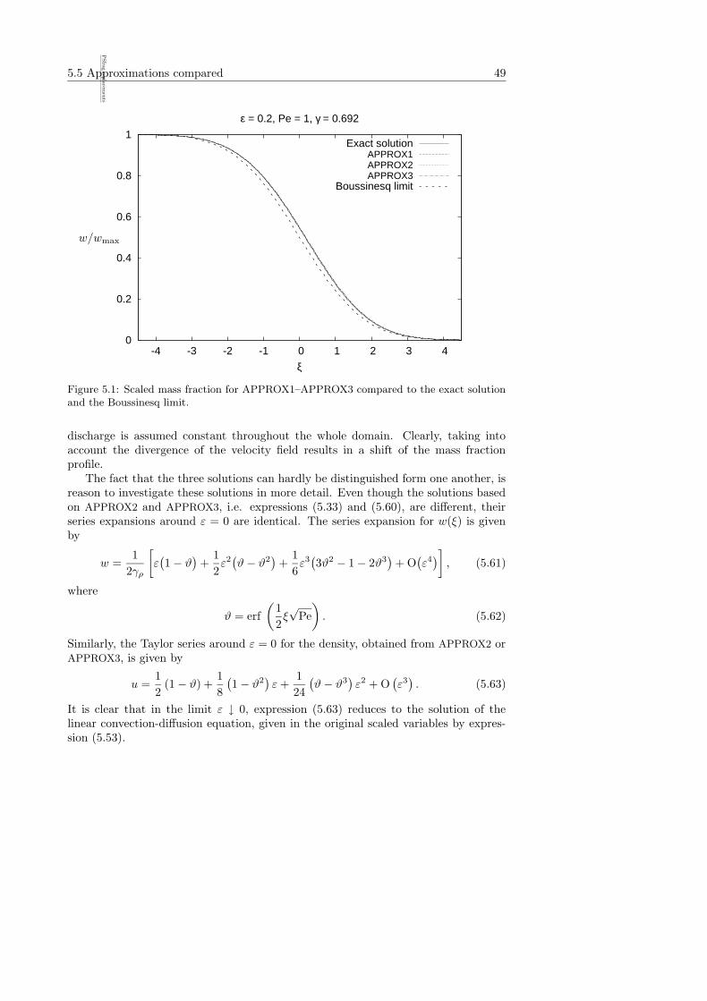
5.5 Approximations compared 49
0
0.2
0.4
0.6
0.8
1
-4 -3 -2 -1 0 1 2 3 4
ξ
ε = 0.2, Pe = 1, γ = 0.692
Exact solutionAPPROX1APPROX2APPROX3
Boussinesq limit
PSfrag
replacem
ents
w/wmax
Figure 5.1: Scaled mass fraction for APPROX1–APPROX3 compared to the exact solutionand the Boussinesq limit.
discharge is assumed constant throughout the whole domain. Clearly, taking intoaccount the divergence of the velocity field results in a shift of the mass fractionprofile.
The fact that the three solutions can hardly be distinguished form one another, isreason to investigate these solutions in more detail. Even though the solutions basedon APPROX2 and APPROX3, i.e. expressions (5.33) and (5.60), are different, theirseries expansions around ε = 0 are identical. The series expansion for w(ξ) is givenby
w =1
2γρ
[
ε(1− ϑ
)+
1
2ε2(ϑ− ϑ2
)+
1
6ε3(3ϑ2 − 1− 2ϑ3
)+ O
(ε4)]
, (5.61)
where
ϑ = erf
(1
2ξ√
Pe
)
. (5.62)
Similarly, the Taylor series around ε = 0 for the density, obtained from APPROX2 orAPPROX3, is given by
u =1
2(1− ϑ) +
1
8
(1− ϑ2
)ε +
1
24
(ϑ− ϑ3
)ε2 + O
(ε3). (5.63)
It is clear that in the limit ε ↓ 0, expression (5.63) reduces to the solution of thelinear convection-diffusion equation, given in the original scaled variables by expres-sion (5.53).
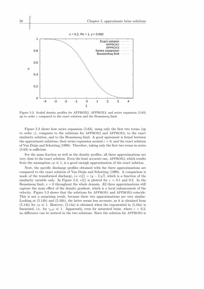
50 Chapter 5. approximate brine solutions
0
0.2
0.4
0.6
0.8
1
-4 -3 -2 -1 0 1 2 3 4
ξ
ε = 0.2, Pe = 1, γ = 0.692
Exact solutionAPPROX2APPROX3
Series expansionBoussinesq limit
PSfrag
replacem
ents
u
Figure 5.2: Scaled density profiles for APPROX2, APPROX3, and series expansion (5.63)up to order ε compared to the exact solution and the Boussinesq limit.
Figure 5.2 shows how series expansion (5.63), using only the first two terms (upto order ε), compares to the solutions for APPROX2 and APPROX3, to the exactsimilarity solution, and to the Boussinesq limit. A good agreement is found betweenthe approximate solutions, their series expansion around ε = 0, and the exact solutionof Van Duijn and Schotting (1998). Therefore, taking only the first two terms in series(5.63) is sufficient.
For the mass fraction as well as the density profiles, all three approximations arevery close to the exact solution. Even the least accurate one, APPROX3, which resultsfrom the assumption ερ� 1, is a good enough approximation of the exact solution.
Next, the specific discharge profiles obtained with the three approximations arecompared to the exact solution of Van Duijn and Schotting (1998). A comparison ismade of the transformed discharge, i.e v(ξ) = (q − 1)
√t, which is a function of the
similarity variable only. In Figure 5.3, v(ξ) is plotted for ε = 0.1 and 0.2. In theBoussinesq limit, v = 0 throughout the whole domain. All three approximations stillcapture the main effect of the density gradient, which is a local enhancement of thevelocity. Figure 5.3 shows that the solutions for APPROX1 and APPROX3 coincide.This is not a surprising result, because these two approximations are very similar.Looking at (5.14b) and (5.16b), the latter seems less accurate, as it is obtained from(5.14b) for ερ � 1. However, (5.14a) is obtained when the exponential in (5.16a) islinearized, i.e. for γρ ω � 1. Apparently, even for saturated brine, where ε = 0.2,no difference can be noticed in the two solutions. Since the solution for APPROX3 is
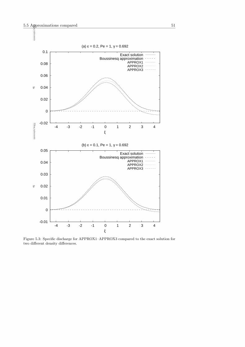
5.5 Approximations compared 51
-0.02
0
0.02
0.04
0.06
0.08
0.1
-4 -3 -2 -1 0 1 2 3 4
ξ
(a) ε = 0.2, Pe = 1, γ = 0.692
Exact solutionBoussinesq approximation
APPROX1APPROX2APPROX3
PSfrag
replacem
ents
v
-0.01
0
0.01
0.02
0.03
0.04
0.05
-4 -3 -2 -1 0 1 2 3 4
ξ
(b) ε = 0.1, Pe = 1, γ = 0.692
Exact solutionBoussinesq approximation
APPROX1APPROX2APPROX3
PSfrag
replacem
ents
v
Figure 5.3: Specific discharge for APPROX1–APPROX3 compared to the exact solution fortwo different density differences.
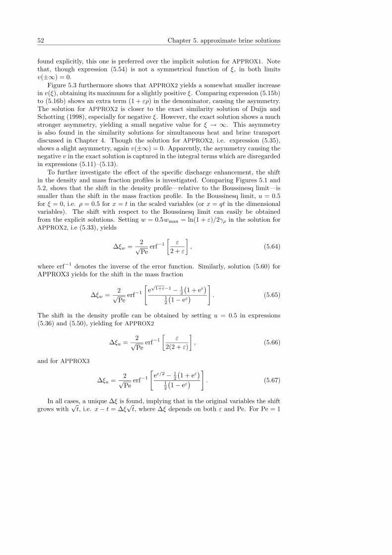
52 Chapter 5. approximate brine solutions
found explicitly, this one is preferred over the implicit solution for APPROX1. Notethat, though expression (5.54) is not a symmetrical function of ξ, in both limitsv(±∞) = 0.
Figure 5.3 furthermore shows that APPROX2 yields a somewhat smaller increasein v(ξ), obtaining its maximum for a slightly positive ξ. Comparing expression (5.15b)to (5.16b) shows an extra term (1 + ερ) in the denominator, causing the asymmetry.The solution for APPROX2 is closer to the exact similarity solution of Duijn andSchotting (1998), especially for negative ξ. However, the exact solution shows a muchstronger asymmetry, yielding a small negative value for ξ → ∞. This asymmetryis also found in the similarity solutions for simultaneous heat and brine transportdiscussed in Chapter 4. Though the solution for APPROX2, i.e. expression (5.35),shows a slight asymmetry, again v(±∞) = 0. Apparently, the asymmetry causing thenegative v in the exact solution is captured in the integral terms which are disregardedin expressions (5.11)–(5.13).
To further investigate the effect of the specific discharge enhancement, the shiftin the density and mass fraction profiles is investigated. Comparing Figures 5.1 and5.2, shows that the shift in the density profile—relative to the Boussinesq limit—issmaller than the shift in the mass fraction profile. In the Boussinesq limit, u = 0.5for ξ = 0, i.e. ρ = 0.5 for x = t in the scaled variables (or x = qt in the dimensionalvariables). The shift with respect to the Boussinesq limit can easily be obtainedfrom the explicit solutions. Setting w = 0.5wmax = ln(1 + ε)/2γρ in the solution forAPPROX2, i.e (5.33), yields
∆ξw =2√Pe
erf−1
[ε
2 + ε
]
, (5.64)
where erf−1 denotes the inverse of the error function. Similarly, solution (5.60) forAPPROX3 yields for the shift in the mass fraction
∆ξw =2√Pe
erf−1
[
e√
1+ε−1 − 12
(1 + eε
)
12
(1− eε
)
]
. (5.65)
The shift in the density profile can be obtained by setting u = 0.5 in expressions(5.36) and (5.50), yielding for APPROX2
∆ξu =2√Pe
erf−1
[ε
2(2 + ε)
]
, (5.66)
and for APPROX3
∆ξu =2√Pe
erf−1
[
eε/2 − 12
(1 + eε
)
12
(1− eε
)
]
. (5.67)
In all cases, a unique ∆ξ is found, implying that in the original variables the shiftgrows with
√t, i.e. x− t = ∆ξ
√t, where ∆ξ depends on both ε and Pe. For Pe = 1
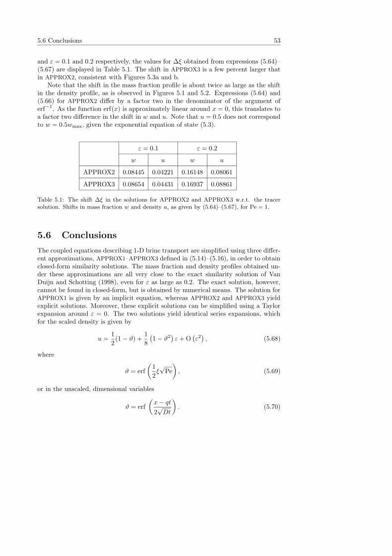
5.6 Conclusions 53
and ε = 0.1 and 0.2 respectively, the values for ∆ξ obtained from expressions (5.64)–(5.67) are displayed in Table 5.1. The shift in APPROX3 is a few percent larger thatin APPROX2, consistent with Figures 5.3a and b.
Note that the shift in the mass fraction profile is about twice as large as the shiftin the density profile, as is observed in Figures 5.1 and 5.2. Expressions (5.64) and(5.66) for APPROX2 differ by a factor two in the denominator of the argument oferf−1. As the function erf(x) is approximately linear around x = 0, this translates toa factor two difference in the shift in w and u. Note that u = 0.5 does not correspondto w = 0.5wmax, given the exponential equation of state (5.3).
ε = 0.1 ε = 0.2
w u w u
APPROX2 0.08445 0.04221 0.16148 0.08061
APPROX3 0.08654 0.04431 0.16937 0.08861
Table 5.1: The shift ∆ξ in the solutions for APPROX2 and APPROX3 w.r.t. the tracersolution. Shifts in mass fraction w and density u, as given by (5.64)–(5.67), for Pe = 1.
5.6 Conclusions
The coupled equations describing 1-D brine transport are simplified using three differ-ent approximations, APPROX1–APPROX3 defined in (5.14)–(5.16), in order to obtainclosed-form similarity solutions. The mass fraction and density profiles obtained un-der these approximations are all very close to the exact similarity solution of VanDuijn and Schotting (1998), even for ε as large as 0.2. The exact solution, however,cannot be found in closed-form, but is obtained by numerical means. The solution forAPPROX1 is given by an implicit equation, whereas APPROX2 and APPROX3 yieldexplicit solutions. Moreover, these explicit solutions can be simplified using a Taylorexpansion around ε = 0. The two solutions yield identical series expansions, whichfor the scaled density is given by
u =1
2(1− ϑ) +
1
8
(1− ϑ2
)ε + O
(ε2), (5.68)
where
ϑ = erf
(1
2ξ√
Pe
)
, (5.69)
or in the unscaled, dimensional variables
ϑ = erf
(x− qt
2√
Dt
)
. (5.70)
54 Chapter 5. approximate brine solutions
For ε ↓ 0, expression (5.68) reduces to the solution of the linear system, where itis assumed that ∇ · q = 0 (Boussinesq approximation). The first two terms in theseries expansion, up to order ε, are sufficient to obtain a good agreement with theexact similarity solution of Van Duijn and Schotting (1998). The difference betweenthe exact and approximate solutions on one hand, and the solution in the Boussinesqlimit on the other hand, is a shift in the profiles due to a local enhancement of thespecific discharge.
Though no significant difference between the approximate solutions is visible inthe mass fraction and density profiles, some differences are observed in the specificdischarge. The specific discharges computed with APPROX1 and APPROX3 coincide;these two approximations are very similar. Though the solutions for all three approx-imations are mathematically not symmetrical, in all cases the discharge approacheszero for large ξ. The exact similarity solution, however, tends to a constant butslightly negative value for ξ → ∞. This distinct asymmetry evolves from integralterms that are disregarded in all three approximations. Furthermore, the magnitudeof the velocity enhancement is somewhat smaller for the exact solution. However, theinfluence of these differences on the density and mass fraction profiles is insignificant.The solution for APPROX2 is closest to the exact solution, especially for negative ξ.A consequence of the similarity is that the shift in the mass fraction and densityprofiles—with respect to the Boussinesq limit—is proportional to
√t.
Chapter 6
High-concentration-gradient
dispersion: introduction and
overview
This chapter is an introduction to the second part of the thesis, dealing with high-concentration-gradient dispersion. The objective of this chapter is to give a briefoverview of the laboratory experiments and theoretical achievements on this topic.
6.1 Introduction
In Chapter 2, the phenomenon of hydrodynamic dispersion in porous media is intro-duced and explained. Hydrodynamic dispersion is the macroscopic result of spreadingof dissolved matter due to local variations in fluid velocity. These velocity variationsare caused by the irregular geometry of the medium at the pore scale level, as well asby variations in permeability at the REV level.
Since the late fifties, a large amount of research effort has been put into model-ling and understanding hydrodynamic dispersion. As discussed in Chapter 2, theclassical approach to model the dispersive mass flux is to assume the validity of alinear relation between the mass flux and the mass fraction gradient. The dispersivemass flux equation is in analogy with Fick’s law for diffusion, but includes a velocity-dependent dispersion tensor. In this formulation, the dispersive mass flux vector J isgiven by
J = −ρD ·∇ω, (6.1)
where ρ is the fluid density, ω is the mass fraction of a dissolved species, and D is thedispersion tensor given by
D = (Dm + αT|q|)I + (αL − αT)qq/|q|. (6.2)
Here, Dm denotes the effective molecular diffusion coefficient, αT and αL the transver-sal and longitudinal dispersivity, I the unit tensor, and |q| the magnitude of thespecific discharge vector q.
In the case of low mass fractions, i.e. when ω does not significantly affect the bulkdensity of the fluid, the Fickian dispersion theory in most cases is satisfactory for
55
56 Chapter 6. HCG dispersion
modelling hydrodynamic dispersion. When short time scales are of interest, however,dispersive transport may be non-Fickian. The dispersivities in expression (6.2) canbe determined from low-concentration (tracer) displacement experiments in porouscolumns or field tracer tests. When the dispersion parameters are known, break-through curves and concentration profiles can be predicted using the Fickian theory.
In the last decades, the problem of disposal of hazardous waste, and in partic-ular high-level radioactive waste, has received much attention. (See Chapter 1 formore background information.) One of the most suitable options to isolate these haz-ardous wastes for an extremely long time is storage in deep geological salt formations.The greatest danger of such disposal sites—besides human intrusion—is formed bycontaminants that might escape and reach the groundwater. Transport by ground-water is considered to be the most probable mechanism for radionuclides to enterthe biosphere (Roxburg, 1987; Sander and Herbert, 1985). Therefore, groundwaterflow and transport modelling plays an important role in risk-assessment studies ofpossible underground waste disposal sites (Warnecke et al., 1986). In the vicinity ofsalt formations, e.g. salt domes or bedded salt formations, brine densities larger than1200 kg/m3 are found (Visser, 1974; Stheeman, 1963; Frape et al., 1984). It is impor-tant to note that in such natural systems, the existence of high salt concentrationsgives rise to high concentration gradients as well.
In the 1980’s, numerous feasibility studies were initiated to assess the potential ofsalt-rock formations for long-term storage of radioactive and chemical waste. At thattime, the only groundwater and transport models available had been developed for sit-uations where the solute (salt) concentration is equal to or less than that of seawater.These models employ assumptions and approximations that may not be admissible athigh concentrations. This motivated several researchers to initiate laboratory studiesto verify whether flow and transport under high-concentration-gradient (HCG) condi-tions can be modelled using the classical theory based on Fick’s law and Darcy’s law.Stable displacement experiments were conducted, i.e. experiments in which a stablebrine front displaces fresh water in a porous column. The most striking observationwas that the longitudinal dispersivity significantly decreases with increasing densitydifference between the brine and the displaced fluid. This phenomenon could not beexplained using the classical dispersion theory.
The objective of this chapter is to give an overview of the advancements in the fieldof high-concentration-gradient dispersion, both from the experimental and theoreticalpoints of view. The focus is on isothermal, stable displacements of brine fronts.
6.2 Review of experiments
Hill (1952) was one of the first researchers to experiment with fluids differing in densityand viscosity displacing one another in a column of porous material. He distinguishedthree configurations: a) inherently stable, b) inherently unstable, and c) stable orunstable depending on the velocity. His concept of a critical velocity has also beenpublished by Slobod and Howlett (1964). Slobod and Howlett defined four differentflow configurations. For the cases in which both viscosity µ and density ρ increase
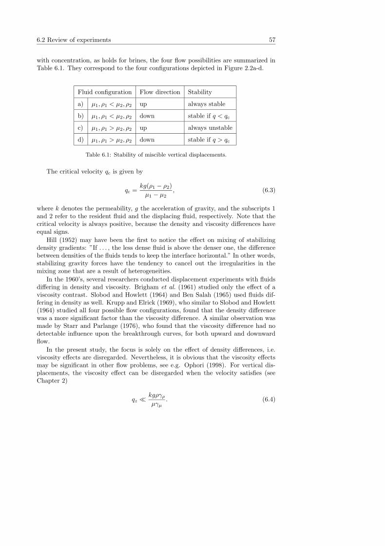
6.2 Review of experiments 57
with concentration, as holds for brines, the four flow possibilities are summarized inTable 6.1. They correspond to the four configurations depicted in Figure 2.2a-d.
Fluid configuration Flow direction Stability
a) µ1, ρ1 < µ2, ρ2 up always stable
b) µ1, ρ1 < µ2, ρ2 down stable if q < qc
c) µ1, ρ1 > µ2, ρ2 up always unstable
d) µ1, ρ1 > µ2, ρ2 down stable if q > qc
Table 6.1: Stability of miscible vertical displacements.
The critical velocity qc is given by
qc =kg(ρ1 − ρ2)
µ1 − µ2, (6.3)
where k denotes the permeability, g the acceleration of gravity, and the subscripts 1and 2 refer to the resident fluid and the displacing fluid, respectively. Note that thecritical velocity is always positive, because the density and viscosity differences haveequal signs.
Hill (1952) may have been the first to notice the effect on mixing of stabilizingdensity gradients: ”If . . . , the less dense fluid is above the denser one, the differencebetween densities of the fluids tends to keep the interface horizontal.” In other words,stabilizing gravity forces have the tendency to cancel out the irregularities in themixing zone that are a result of heterogeneities.
In the 1960’s, several researchers conducted displacement experiments with fluidsdiffering in density and viscosity. Brigham et al. (1961) studied only the effect of aviscosity contrast. Slobod and Howlett (1964) and Ben Salah (1965) used fluids dif-fering in density as well. Krupp and Elrick (1969), who similar to Slobod and Howlett(1964) studied all four possible flow configurations, found that the density differencewas a more significant factor than the viscosity difference. A similar observation wasmade by Starr and Parlange (1976), who found that the viscosity difference had nodetectable influence upon the breakthrough curves, for both upward and downwardflow.
In the present study, the focus is solely on the effect of density differences, i.e.viscosity effects are disregarded. Nevertheless, it is obvious that the viscosity effectsmay be significant in other flow problems, see e.g. Ophori (1998). For vertical dis-placements, the viscosity effect can be disregarded when the velocity satisfies (seeChapter 2)
qz �kgργρ
µγµ. (6.4)
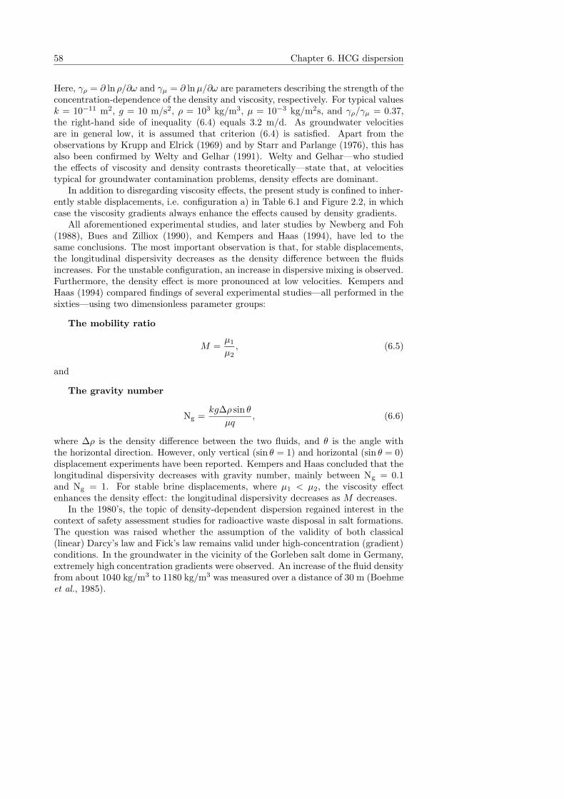
58 Chapter 6. HCG dispersion
Here, γρ = ∂ ln ρ/∂ω and γµ = ∂ ln µ/∂ω are parameters describing the strength of theconcentration-dependence of the density and viscosity, respectively. For typical valuesk = 10−11 m2, g = 10 m/s2, ρ = 103 kg/m3, µ = 10−3 kg/m2s, and γρ/γµ = 0.37,the right-hand side of inequality (6.4) equals 3.2 m/d. As groundwater velocitiesare in general low, it is assumed that criterion (6.4) is satisfied. Apart from theobservations by Krupp and Elrick (1969) and by Starr and Parlange (1976), this hasalso been confirmed by Welty and Gelhar (1991). Welty and Gelhar—who studiedthe effects of viscosity and density contrasts theoretically—state that, at velocitiestypical for groundwater contamination problems, density effects are dominant.
In addition to disregarding viscosity effects, the present study is confined to inher-ently stable displacements, i.e. configuration a) in Table 6.1 and Figure 2.2, in whichcase the viscosity gradients always enhance the effects caused by density gradients.
All aforementioned experimental studies, and later studies by Newberg and Foh(1988), Bues and Zilliox (1990), and Kempers and Haas (1994), have led to thesame conclusions. The most important observation is that, for stable displacements,the longitudinal dispersivity decreases as the density difference between the fluidsincreases. For the unstable configuration, an increase in dispersive mixing is observed.Furthermore, the density effect is more pronounced at low velocities. Kempers andHaas (1994) compared findings of several experimental studies—all performed in thesixties—using two dimensionless parameter groups:
The mobility ratio
M =µ1
µ2, (6.5)
and
The gravity number
Ng =kg∆ρ sin θ
µq, (6.6)
where ∆ρ is the density difference between the two fluids, and θ is the angle withthe horizontal direction. However, only vertical (sin θ = 1) and horizontal (sin θ = 0)displacement experiments have been reported. Kempers and Haas concluded that thelongitudinal dispersivity decreases with gravity number, mainly between Ng = 0.1and Ng = 1. For stable brine displacements, where µ1 < µ2, the viscosity effectenhances the density effect: the longitudinal dispersivity decreases as M decreases.
In the 1980’s, the topic of density-dependent dispersion regained interest in thecontext of safety assessment studies for radioactive waste disposal in salt formations.The question was raised whether the assumption of the validity of both classical(linear) Darcy’s law and Fick’s law remains valid under high-concentration (gradient)conditions. In the groundwater in the vicinity of the Gorleben salt dome in Germany,extremely high concentration gradients were observed. An increase of the fluid densityfrom about 1040 kg/m3 to 1180 kg/m3 was measured over a distance of 30 m (Boehmeet al., 1985).
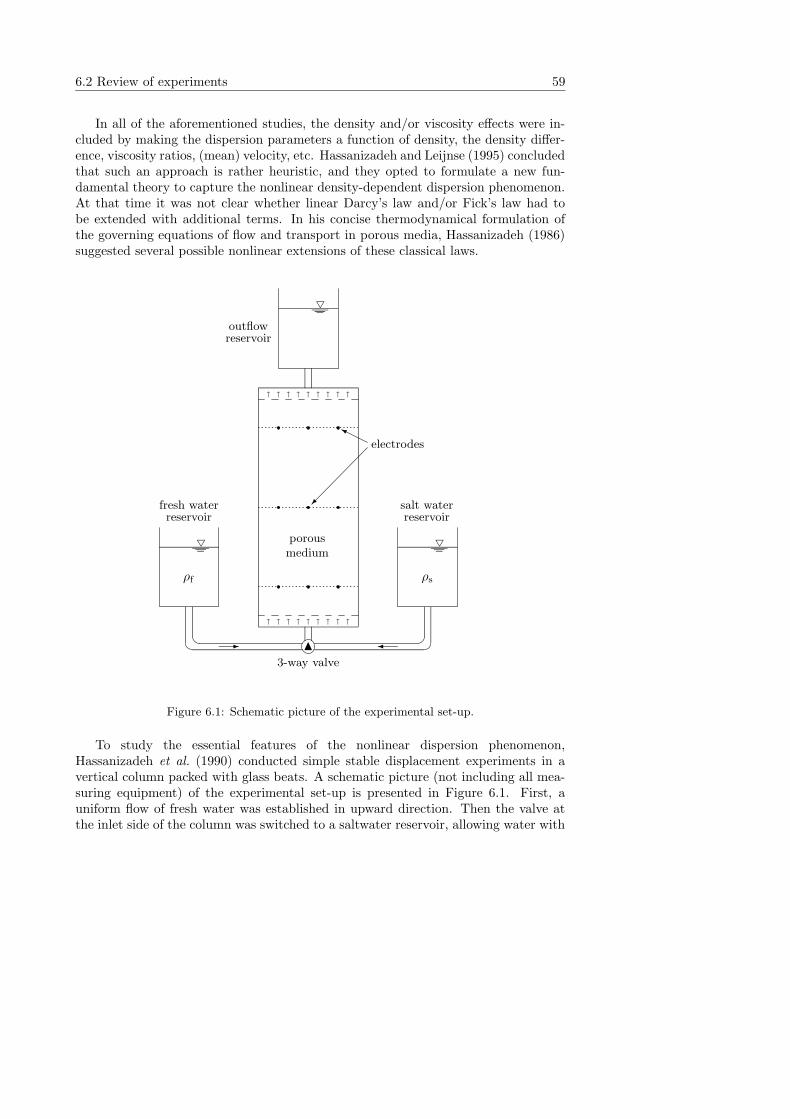
6.2 Review of experiments 59
In all of the aforementioned studies, the density and/or viscosity effects were in-cluded by making the dispersion parameters a function of density, the density differ-ence, viscosity ratios, (mean) velocity, etc. Hassanizadeh and Leijnse (1995) concludedthat such an approach is rather heuristic, and they opted to formulate a new fun-damental theory to capture the nonlinear density-dependent dispersion phenomenon.At that time it was not clear whether linear Darcy’s law and/or Fick’s law had tobe extended with additional terms. In his concise thermodynamical formulation ofthe governing equations of flow and transport in porous media, Hassanizadeh (1986)suggested several possible nonlinear extensions of these classical laws.
porousmedium
N
3-way valve
↑ ↑ ↑ ↑ ↑ ↑ ↑ ↑ ↑
↑ ↑ ↑ ↑ ↑ ↑ ↑ ↑ ↑
5
�
salt waterreservoir
ρs
5
-
fresh waterreservoir
ρf
5
outflowreservoir
electrodes
Y
Figure 6.1: Schematic picture of the experimental set-up.
To study the essential features of the nonlinear dispersion phenomenon,Hassanizadeh et al. (1990) conducted simple stable displacement experiments in avertical column packed with glass beats. A schematic picture (not including all mea-suring equipment) of the experimental set-up is presented in Figure 6.1. First, auniform flow of fresh water was established in upward direction. Then the valve atthe inlet side of the column was switched to a saltwater reservoir, allowing water with
60 Chapter 6. HCG dispersion
a certain constant amount of dissolved salt to enter the column. The salt concentra-tions in the initial experiments were such that the density of the displacing fluid wasnot significantly affected due to the presence of the salt, i.e. tracer concentrations.These tracer experiments allowed to determine the classical longitudinal dispersion co-efficient of the porous medium. Subsequently, identical experiments were conducted,but now with an increasing density difference between the resident fluid (fresh water)and the displacing brine. From the breakthrough curves, measured with electricalconductivity transducers, the apparent longitudinal dispersivity could be determined.As to be expected, a significant decrease in apparent dispersivity was observed withincreasing density difference between the resident and displacing fluids.
Although these experiments clearly indicated the failure of the classical theory,and, moreover, gave preliminary evidence that an alternative nonlinear theory (to bediscussed in the next section) could be formulated to describe the nonlinear disper-sion phenomenon, the experiments had serious drawbacks. First of all, due to theexperimental procedure, it was not possible to maintain a constant flow rate duringthe experiments. Secondly, the mean flow rate in the column was not varied over acertain well-defined range, so no explicit statements could be made about the velocitydependence of the nonlinear dispersion process.
Independently, Bouhroum (1988, 1989) and Moser (1995) conducted similar stabledisplacement experiments. Bouhroum (1989) used different combinations of solutions,such that he was able to investigate the effect of density differences independently ofviscosity effects. Moser (1995) performed four different series of carefully conductedexperiments:
• Tracer experiments, i.e. very small density differences between the resident andinvading fluids
• Experiments with various density differences and a constant mean flow rate
• Experiments with a constant (high) density difference and a variety of (constant)mean flow rates
• Experiments with a brine being displaced by a brine with a slightly higherdensity, such that the density difference is in the tracer range
The same tendency was observed as in the experiments reported in Hassanizadehet al. (1990) and the earlier experiments: longitudinal dispersivity decreases withincreasing density difference. Moreover, from Moser’s experiments the influence ofthe mean flow rate in the column could be determined. The earlier observationby Slobod and Howlett (1964) and Krupp and Elrick (1969), that the decrease indispersivity becomes less prominent with increasing flow rate, was confirmed. Anotherimportant conclusion was drawn from the brine-brine displacement experiments ofMoser (1995). These experiments were conducted, such that the density differencesbetween the concentrated brines were always within the tracer range. It turned outthat these experiments could be modelled with the classical theory, i.e. using linearDarcy’s and Fick’s laws. This implies that the nonlinear dispersion phenomenon doesnot depend on the absolute salt concentration or density, but only depends on the
6.2 Review of experiments 61
concentration gradients or density gradients. This is in accordance with some newnonlinear dispersion theories, as to be discussed in the next section.
Independently of Bouhroum (1989), Hassanizadeh et al. (1990), and Moser (1995),Anderson (1997) performed similar stable brine displacement experiments, but nowwith adequate instrumentation to regulate the flow in the column. Moreover, as op-posed to the other researchers, she used different porous media: coarse sand, mediumfine sand, and silica flour. The first two sands gave reliable and reproducible results,while the silica flour experiments suffered from all kinds of experimental complica-tions. The outcome of these experiments (coarse and medium fine sands), publishedby Watson et al. (2002b), confirmed the findings of Hassanizadeh and Leijnse (1995)and Moser (1995). Moreover, due to the accurate flow monitoring instrumentation,from these experiments the important conclusion could be drawn that classical Darcy’slaw remains valid under high-concentration conditions, see Watson et al. (2002a).
Recently, more experimental studies have been published. Kretz et al. (2003) stud-ied miscible displacements, both stable and unstable, for two artificial porous mediaconstructed using different arrangements of glass beads with different sizes. Theyused an acoustic technique for concentration measurements. Whereas Bouhroum(1989), Hassanizadeh et al. (1990), Moser (1995), and Anderson (1997) attempted toconstruct homogeneous porous columns, Kretz et al. (2003) studied the effect of het-erogeneity. One of their conclusions was that the decrease in dispersivity found withincreasing density contrast is independent of the medium used. However, it should benoted that although the structural arrangement of the two media was different, theiraverage permeabilities and variances were the same.
The most recent experimental study is the one by Jiao and Hotzl (2004), whostudied the effect of both density and viscosity contrasts independently, for stableand unstable displacements. They concluded, like among others Bouhroum (1989)and Kempers and Haas (1994) did earlier, that in all cases the measured break-through curves could successfully be described by the classical advection-dispersionformulation. However, for a given porous medium and flow condition, the dispersioncoefficient is not a constant but dependent on fluid properties. This fact contradictsthe statement that linear Fick’s law is valid.
Many researchers followed the approach of fitting the dispersivity to the measuredbreakthrough curves using linear Fick’s law. Figure 6.2 compares the fitted disper-sivities of Moser (1995), Bouhroum (1989), and Jiao and Hotzl (2004) against thegravity number, given by expression (6.6). In Figure 6.2, the plotted dispersivitiesare scaled by the tracer values, i.e. the dispersivities observed in the experiments withthe smallest gravity number. Each point corresponds to an individual experiment,where the gravity number is computed based on the flow rate and density differencereported. All four sets of experiments by Moser (1995) are plotted, covering a widerange of gravity numbers. The data supplied by Jiao and Hotzl (2004) are mostlyin the tracer range, i.e. small gravity numbers. However, they have one experimentthat shows a significant decrease in dispersivity (for Ng = 0.13), and is close to thedata of Bouhroum (1989) and Moser (1995). All data points plotted in Figure 6.2were obtained from breakthrough curves at the end of the columns. The observeddispersivities therefore are supposed to have converged to asymptotic values. Ander-
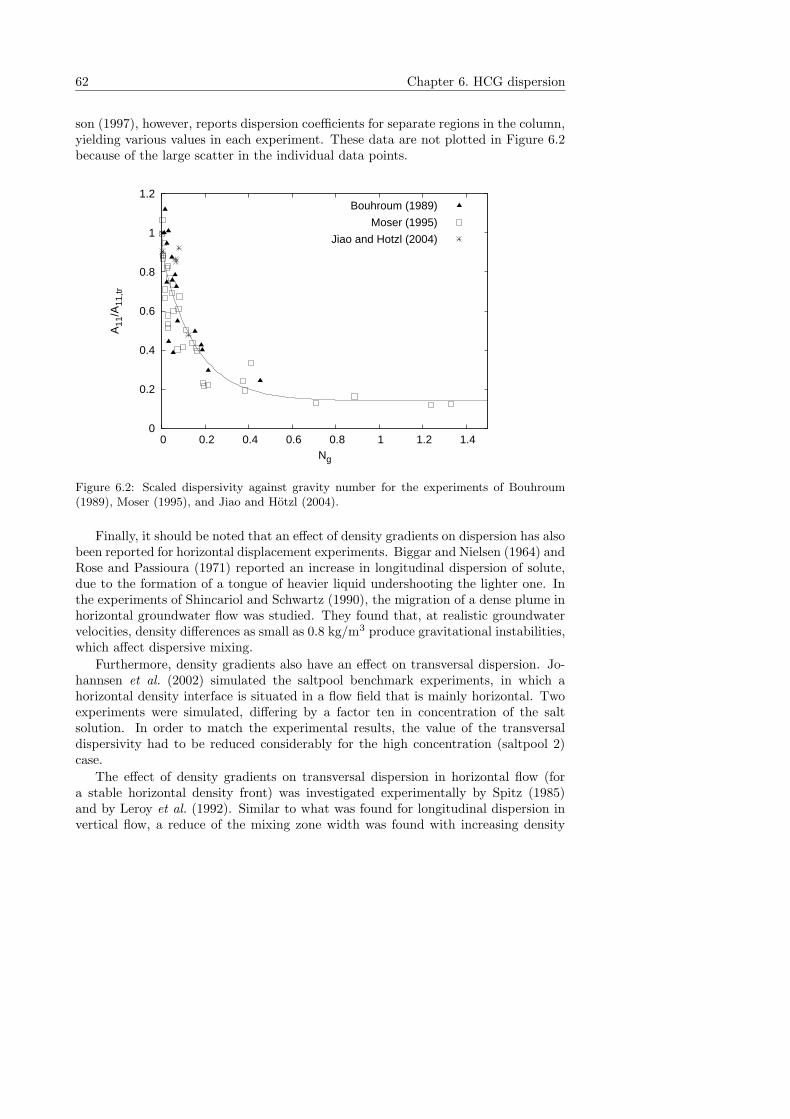
62 Chapter 6. HCG dispersion
son (1997), however, reports dispersion coefficients for separate regions in the column,yielding various values in each experiment. These data are not plotted in Figure 6.2because of the large scatter in the individual data points.
0
0.2
0.4
0.6
0.8
1
1.2
0 0.2 0.4 0.6 0.8 1 1.2 1.4
A11
/A11
,tr
Ng
Bouhroum (1989)
Moser (1995)
Jiao and Hotzl (2004)
Figure 6.2: Scaled dispersivity against gravity number for the experiments of Bouhroum(1989), Moser (1995), and Jiao and Hotzl (2004).
Finally, it should be noted that an effect of density gradients on dispersion has alsobeen reported for horizontal displacement experiments. Biggar and Nielsen (1964) andRose and Passioura (1971) reported an increase in longitudinal dispersion of solute,due to the formation of a tongue of heavier liquid undershooting the lighter one. Inthe experiments of Shincariol and Schwartz (1990), the migration of a dense plume inhorizontal groundwater flow was studied. They found that, at realistic groundwatervelocities, density differences as small as 0.8 kg/m3 produce gravitational instabilities,which affect dispersive mixing.
Furthermore, density gradients also have an effect on transversal dispersion. Jo-hannsen et al. (2002) simulated the saltpool benchmark experiments, in which ahorizontal density interface is situated in a flow field that is mainly horizontal. Twoexperiments were simulated, differing by a factor ten in concentration of the saltsolution. In order to match the experimental results, the value of the transversaldispersivity had to be reduced considerably for the high concentration (saltpool 2)case.
The effect of density gradients on transversal dispersion in horizontal flow (fora stable horizontal density front) was investigated experimentally by Spitz (1985)and by Leroy et al. (1992). Similar to what was found for longitudinal dispersion invertical flow, a reduce of the mixing zone width was found with increasing density
6.3 Theoretical advancements 63
difference. Moreover, this effect was found to be more pronounced at low velocities.Spitz (1985) and Leroy et al. (1992) furthermore reported that the gravity effect ismuch larger for stratified media than for homogeneous materials.
6.3 Theoretical advancements
As discussed in the previous section, the traditional approach to high-concentration-gradient dispersion is to alter the dispersion parameters in the classical theory, suchthat they become functions of the concentration, concentration difference, flow rate,etc. With this approach, however, dispersion coefficients are not known a-priori. Itdoes not lead to the formulation of a physically based, consistent theory, which canbe applied for any experimental condition.
In this section, two major independent theoretical approaches to high-concen-tration-gradient dispersion are discussed: the nonlinear theory of Hassanizadeh(1990,1995), and the stochastic approach of Welty and Gelhar (1991). As a thirdapproach, the application of homogenization theory is discussed. This new approachshows a lot of similarities to the stochastic approach of Welty and Gelhar (1991),but employs a different mathematical upscaling technique.
6.3.1 The nonlinear theory of Hassanizadeh
In 1990, Hassanizadeh first published his nonlinear model for high-concentration-gradient dispersion. After concluding that Fick’s law was not adequate to predict theexperiments for high concentration differences, he tried several extensions of Fick’slaw. With only one of those extensions, using one additional dispersion parameter,all experiments could be modelled. In 1995, Hassanizadeh and Leijnse gave the theo-retical considerations that led to the formulation of the nonlinear dispersion equation.A solute is assumed to spread from areas with high chemical potential to areas withlow chemical potential. Hassanizadeh and Leijnse claim that this force is opposed bythe resistance of the porous medium to solute dispersion, a resistance force offeredby water molecules and solid grains. This force is assumed to depend on the specificdischarge q, the dispersive mass flux J, and state variables. In principle, this resis-tance force may be represented by a Taylor series in terms of J. If terms of higherthan second order in the series expansion are disregarded, the following nonlineardispersion equation is derived:
(1 + β |J|)J = −ρD ·∇ω. (6.7)
In this equation, β is a new dispersion parameter, J is the magnitude of the disper-sive mass flux vector, while D is still given by the (classical) dispersion tensor, seeexpression (6.2). It is interesting to observe that this equation is analogous to theForchheimer equation for high-velocity flow in porous media. Note that linear Fick’slaw is obtained in the limit of small dispersive mass fluxes, and when β is set to zero.
The experiments reported in Hassanizadeh et al. (1990), and in Hassanizadeh andLeijnse (1995), were used to validate nonlinear equation (6.7). From the tracer exper-
64 Chapter 6. HCG dispersion
iments, the (tracer) longitudinal dispersivity could be determined, which is essentialin the righthand-side of equation (6.7). From the brine displacement experiments, aunique value of the new dispersion parameter β was determined. With this β andnonlinear equation (6.7), all experiments for different density differences between theresident and displacing fluids could be satisfactorily modelled.
Based on the experimental data of Moser (1995), Schotting et al. (1999) showedthat the parameter β is inversely related to the mean specific discharge. The velocitydependence of β was confirmed with the experimental data of Anderson (1997). Thisvelocity dependence points to the underlying physics of the problem. It implies theexistence of two time scales in the column experiments: the time scale of the actionof gravity, and the convection time scale associated with the mean specific dischargein the column.
Even though Hassanizadeh and Leijnse (1995) did not explicitly account for gravityeffects in their derivation, it is believed now that gravity is the stabilizing effect whichcauses the reduction of dispersive mixing. Hassanizadeh and Leijnse (1995) statedthat their findings could not be due to macroscopic heterogeneities, because theystudied an essentially homogeneous system. Nevertheless, micro-heterogeneities arebound to have been present in the experiments. The interaction between stabilizinggravity forces and local velocity variations induced by these micro-heterogeneities,must have been the cause of the nonlinear effect. Welty and Gelhar (1991) found asimilar reduction of the longitudinal dispersivity in their study of density-dependentdisplacements in macroscopically heterogeneous media. Perkins and Johnston, intheir 1963 review of diffusion and dispersion in porous media, already recognized thesuppression of dispersion by stabilizing gravity forces on both the scale of individualpores, and the scale of permeability heterogeneities.
6.3.2 The stochastic theory of Welty and Gelhar
In 1991, Welty and Gelhar were the first to derive a theory for density- and viscosity-dependent dispersion in heterogeneous porous media. To derive expressions forthe macrodispersivities, they followed the spectrally based stochastic continuum ap-proach. Actually, this work is an extension of the work by Gelhar and Axness(1983), and by Gelhar (1987). The stochastic approach assumes that observed three-dimensional variations in intrinsic permeability can be modelled as random fields.The heterogeneity of the porous medium is then characterized by statistical param-eters instead of by a detailed point-by-point description. Welty and Gelhar (1991)evaluate the effects of the log-permeability field on the concentration field, as well asthe feedback effects of the concentration field on the flow field. The concentrationfield affects the flow field through concentration-dependent density and viscosity.
Welty and Gelhar (1991) consider the effects of both density and viscosity vari-ations for unidirectional mean flow (upward or downward) in a three-dimensionalisotropic medium. The log-permeability is assumed to be a statistically homogeneousrandom field, which can be decomposed in a mean value and a zero-mean perturba-
6.3 Theoretical advancements 65
tion:
ln k(x) = f(x) = 〈f(x)〉+ f ′(x), (6.8)
where f is the log-permeability and x the vector of spatial coordinates. Then thelog-permeability covariance is given by
Cov = 〈f ′(x+h)f ′(x)〉 , (6.9)
where h is a vector separating two points. The (auto)correlation function is relatedto the covariance by
R(h) = Cov/σ2, (6.10)
where σ2 denotes the log-permeability variance. Welty and Gelhar (1991) use theexponential correlation function, which in the isotropic case only depends on theabsolute separation—or lag, h:
R(h) = e−h/λ. (6.11)
The log-permeability variance σ2 is a measure of the degree of heterogeneity, and thecorrelation scale λ characterizes the length over which ln k is correlated.
Welty and Gelhar (1991) obtain the one-dimensional macro-scale transport equa-tion
n∂ 〈C〉
∂t+ q
∂ 〈C〉∂z
=∂
∂z
([
d‖ + A11|q|]∂ 〈C〉
∂z
)
, (6.12)
where n is the porosity, t is time, z is the vertical coordinate, q is the specific discharge,〈C〉 is the mean concentration and A11 is the macroscale longitudinal dispersivity.The microscale longitudinal dispersion coefficient d‖ incorporates the effects of bothmolecular diffusion and microscale dispersion, i.e. d‖ = Dm + α‖|q|.
The concentration C is scaled by its maximum value, and therefore lies between 0and 1. It is equivalent to the scaled mass fraction, because Welty and Gelhar (1991)adopt the Boussinesq approximation. In this approximation (see Chapter 3), it isassumed that ρ is a constant, except for the gravity term in Darcy’s law. As a result,salt mass balance equation (6.12) no longer contains the density.
In the steady state limit, the macroscale longitudinal dispersivity is expressed as
A11 =σ2λ
γ2f
[1− b1 + b1 ln b1
(1− b1)2
]
, (6.13)
where
b1 =γµG1λ
2
α⊥
[1
γf+
dρ
dµ
k0g
q
]
. (6.14)
In these expressions, k0 is the mean permeability, G1 is the mean concentration gra-dient −∂ 〈C〉 /∂z, and the flow factor can be approximated by γf ≈ 1 + σ2/6.
The dimensionless parameter b1 incorporates the effect of both viscosity and den-sity differences. When viscosity effects are disregarded, b1 reduces to the dimensionlessdensity gradient
b1 =−λ2gk0
d⊥µ
(∂ρ
∂z
)
, (6.15)
66 Chapter 6. HCG dispersion
where d⊥ = Dm + α⊥|q| is the microscale transversal dispersion coefficient. Forthe case of density gradients only, expression (6.13) has recently been confirmed byEgorov, who applies homogenization theory (to be discussed in the next section).
Welty and Gelhar (1991) also derive an expression for A11 for the transient case.For the stable configuration, they find that the macrodispersivity increases exponen-tially for early times, and then decreases exponentially to an asymptotic value. Forlarge, but not infinite time, their result is given by
A11 =σ2λ
γ2f
e−2a1 , (6.16)
where a1 is given by
a1 = γµG1z
[1
γf+
dρ
dµ
k0g
q
]
. (6.17)
Expression (6.16) suggests that A11 will tend to zero for large z. However, the gra-dient G1 always decreases with time, decreasing a1 for the stable case. Therefore,to examine the true behavior of A11, expression (6.16) and equation (6.12) need tobe solved simultaneously. Welty and Gelhar (1992) solve this system numerically, toinvestigate the nonlinear effect of the concentration gradient on A11 in a field-scaleone-dimensional model. Recently, Welty et al. (2003) have extended the stochasticanalysis to transversal dispersion.
It must be emphasized that several assumptions implicit in the stochastic analysismay limit the applicability of the results. Important assumptions are for example theuse of small perturbations, the assumption of ergodicity, statistical homogeneity andisotropy of the log-permeability field, and Fickian solute transport throughout theflow domain. Most of the assumptions are valid only for very large travel times.
Despite its limitations, the theory gives insight into the fundamental processesthat affect the macrodispersivity for field-scale variable density and viscosity transporttrough a heterogeneous porous medium. However, while the theory of Hassanizadehand Leijnse (1995) has been extensively tested against independently conducted ex-periments, experimental validation of the stochastic theory is still lacking.
In the next chapters of this thesis, numerical experiments of dispersion in het-erogeneous media are presented, which could be used to validate Welty and Gelhar’stheory. However, the simulations are two-dimensional, whereas the results of Weltyand Gelhar (1991) apply to three-dimensional porous media. In addition, the randompermeability fields have slightly different correlation functions, and viscosity effectsare disregarded in the numerical experiments. Instead of using the approach of Weltyand Gelhar, homogenization theory is applied to the specific case matching the nu-merical experiments. The homogenization procedure is based on many of the sameassumptions as the stochastic analysis by Welty and Gelhar (1991). The homogeni-zation and stochastic approach take different mathematical routes, which lead to thesame result. Therefore, when the homogenization results match the numerical exper-iments, it is expected that this is true for the results of the stochastic approach aswell.
6.3 Theoretical advancements 67
6.3.3 Homogenization theory by Egorov and Demidov
The most recent development in the theoretical description of density-dependent dis-persion in porous media is the application of homogenization theory by Egorov andby Demidov. Both Egorov and Demidov consider uni-directional mean flow in a sta-ble configuration with variations in density only, i.e. viscosity effects are disregarded.Egorov et al. (2005) recently published results for a medium consisting of two layersdiffering in permeability. In yet unpublished work, Demidov furthermore studies thedensity effect starting from the pore scale level. He considers Stokes flow around microheterogeneities (squares), and performs a mathematical upscaling to obtain averagebalance equations. Demidov’s analysis leads to results that are comparable to theexperiments in homogeneous porous media, i.e. with heterogeneity only at the porescale level. Egorov on the other hand considers weakly heterogeneous porous media,i.e. small variations in the log-permeability. Similar to the analysis of Welty andGelhar (1991), the log-permeability is assumed to be an isotropic stationary randomfield characterized by a correlation function.
Egorov’s analysis starts with the classical equations (Darcy’s law, Fick’s law) atthe local scale. Furthermore it is assumed that the flow is incompressible, i.e. ∇·q = 0.The local dispersion coefficient is assumed to depend on the mean velocity rather thanon the fluctuating local velocity.
The homogenization procedure relies on the separation of two scales: the mi-croscale and the macroscale. The first is determined by the size of the heterogeneities,i.e. the integral scale, and the second by the width of the front. After large enoughtime the two scales are well separated, regardless of the initial sharpness of the front.
Egorov obtains the same macroscopic balance equation as Welty and Gelhar (6.12),but written in terms of the mean density 〈ρ〉:1
n∂ 〈ρ〉∂t
+ q∂ 〈ρ〉∂z
=∂
∂z
([
d‖ + σ2 l|q|D0(γ)]∂ 〈ρ〉
∂z
)
. (6.18)
Here, l denotes the integral scale, defined by
l =
∞∫
0
R(h) dh. (6.19)
The dimensionless density gradient γ is defined as
γ = − l2gk0
α⊥qµ
∂ 〈ρ〉∂z
. (6.20)
This expression equals (6.15), where the correlation scale λ is replaced by the inte-gral scale l. For the exponential correlation function defined in (6.11), the two areequivalent. Depending on the definition of the correlation function, the correlationscale may differ from the integral scale. For example, when the Gaussian correlation
1The salt mass balance can be written in this form when the exponential equation of state isused, see Appendix C.2.
68 Chapter 6. HCG dispersion
function is defined as R(r) = exp(−r2/λ2), the relation between the integral andcorrelation scale is l = λ
√π/2.
The effective dispersion coefficient D0(γ), which multiplies the long time asymp-totic tracer dispersion coefficient σ2 l|q|, is derived from D0(γ) = I(γ)/γ, where
I(γ) = I0(γ) + εtI1
(
γ,∂γ
∂t
)
+ ε2xI2
(
γ,∂γ
∂z,∂2γ
∂z2
)
. (6.21)
In this expression, εt and εx are small temporal and spatial scaling parameters that forwell separated scales approach zero. So, for large enough time and a front width muchlarger than the integral scale, I(γ) can be approximated by I0(γ). Table 6.2 presentsthe results obtained for the isotropic exponential and the Gaussian log-permeabilitycorrelation functions in two and three-dimensional systems. For the case of the 3-Dexponential correlation function, the result of Welty and Gelhar (1991), i.e. expression(6.13), is reproduced, assuming the flow factor γf equals one.
In addition, the homogenization procedure yields an expression for the density (orconcentration) variance, i.e. a measure of the deviations of local values with respectto their mean. The nonlinear system defined by equation (6.18) and D0(γ) needs tobe solved numerically. In Chapter 8, the homogenization procedure is discussed inmore detail and its model predictions are compared to the numerical experiments.
R(h) 2-D 3-D
e−(
hl
)1
1− γ
(
1−√
γ√1− γ
arctan
(√1− γ√
γ
))1− γ + γ ln γ
(1− γ)2
e−π4
(hl
)2
1−√γ eγ/π erfc(√
γ/π) 1− γ/π eγ/π Ei(γ/π)
Table 6.2: Effective dispersion coefficient D0(γ) for the isotropic 2-D and 3-D exponentialand Gaussian correlation functions.
6.4 Conclusions
This chapter gives a review of laboratory studies on the effect of density differences ondispersion of miscible fluids, with the focus on stable displacements. Classical lineardispersion theory has been found to be inadequate to model the experiments for largeconcentration and density differences. With the nonlinear theory of Hassanizadeh(1990,1995), however, all experiments ranging from tracer to very large concentrationscan be modelled adequately. This is confirmed by Schotting et al. (1999) and Watsonet al. (2002b).
The main difference between the theory of Hassanizadeh (1990,1995) on one hand,and the results of Welty and Gelhar (1991) and homogenization theory (Egorov andDemidov) on the other hand, is the specific form of the dispersion equation. Whilethe equation of Hassanizadeh contains a second order term in the dispersive flux, the
6.4 Conclusions 69
other two theories essentially still use the classical form of linear Fick’s law, with thedifference that the dispersion coefficient is a function of the dimensionless densitygradient. Another difference is the way in which the dispersion equations are derived.Both Welty and Gelhar (1991) and Egorov take the local scale balance equations asa starting point. With slightly different mathematical methods, similar macroscopicbalance equations are obtained. These results are directly related to the physicalprocesses that occur on the local scale. Gravity forces are believed to be responsible forthe decrease in longitudinal dispersivity that is observed in the experiments. Thoughthe velocity-dependence of β supports this physical explanation, in the derivation ofHassanizadeh and Leijnse (1995) gravity forces do not play any role.
It should be noted that an important limitation of the stochastic and the homogen-ization theory is that the mean flow is uni-directional, the macroscopic problem beingone-dimensional. Though Hassanizadeh’s nonlinear equation for the dispersive massflux, equation (6.7), in principle is valid for three dimensions, it has only been testedagainst one-dimensional flow experiments. The stabilizing gravity effect is largestwhen the mean flow is in the vertical direction, the interface being horizontal. So far,the dispersive behavior for flow under an arbitrary angle with the gravity vector hasnot been investigated in laboratory experiments. Numerical simulations of miscibledisplacements under various angles with gravity have been performed by Rogersonand Meiburg (1993). However, their focus was on viscous fingering in unstable dis-placements in homogeneous porous media.
The following two chapters of this thesis discuss a series of numerical experimentsperformed in the present study. These experiments are similar in set-up as the lab-oratory experiments discussed in Section 6.2. Two-dimensional porous media withvery small heterogeneities are used, to mimic the behavior in (almost) homogeneousmedia. The tracer dispersivities are in the same order as those obtained by Bouhroum(1989), Moser (1995), and Jiao and Hotzl (2004). Like in the approaches by Weltyand Gelhar (1991) and Egorov, it is assumed that Darcy’s law and linear Fick’s laware valid at the local scale.
A first objective of the numerical experiments is to demonstrate that the nonlineareffect is indeed caused by gravity. More importantly, the results are meant to validatethe nonlinear theories discussed in this chapter.

Chapter 7
High-concentration-gradient
dispersion: numerical
experiments
7.1 Introduction
7.1.1 Outline and objectives
This chapter describes high-resolution numerical experiments, in which a dense salt so-lution vertically displaces fresh water in a stable manner. The two-dimensional porousmedia are weakly heterogeneous at a small scale. The purpose of these simulations,conducted for a range of density differences, is to obtain accurate concentration pro-files that can be used to validate the nonlinear models for high-concentration-gradientdispersion discussed in Chapter 6. The present chapter focuses on convergence of thecomputations, in numerical and statistical sense, to ensure that the uncertainty inthe results is small enough.
First, the set-up of the numerical experiments and the ”measurement” methodare discussed. Next, some conclusions related to transport in stochastic media arereviewed that are of interest for this study. In Section 7.2, the numerical model andits assumptions are presented in more detail. Section 7.3 describes the first numericaltest cases, which demonstrate the effect of gravity forces and fluid volume changeson dispersion of the brine front. Section 7.4 discusses the numerical convergenceand accuracy of the computations, as well as the convergence to ensemble statis-tics. The influence of the density contrast on both types of convergence is discussed.Estimates of the errors caused by the numerical scheme and by the use of a finitenumber of realizations are given and compared. In section 7.5 results are presented,and the differences between tracer and high-density transport are analyzed, for theirconcentration profiles, concentration variances, and macrodispersivities. For tracertransport, longitudinal macrodispersivities are compared to analytical results. Fordensity-dependent transport a comparison with laboratory experiments is made.
A comparison between the numerical results and the predictions of three nonlineardispersion models is given in the next chapter. The objective of Chapter 8 is to testand compare the nonlinear models, and to discuss their applicability and limitations.
71
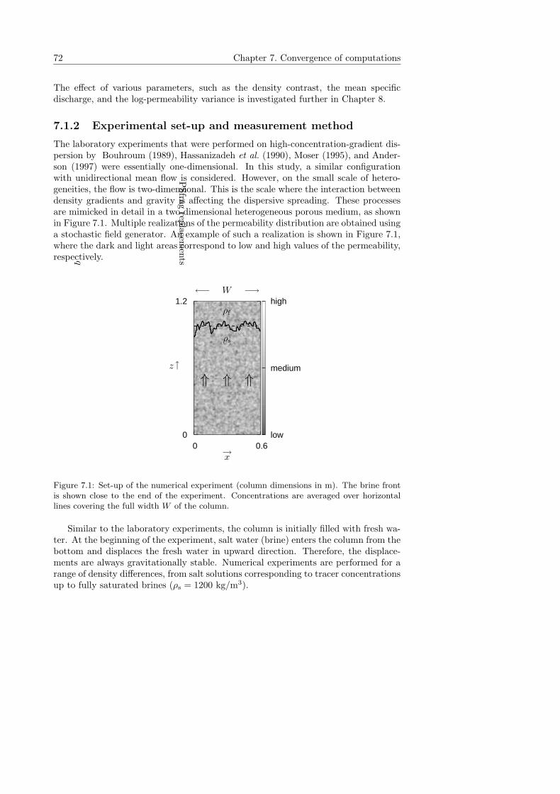
72 Chapter 7. Convergence of computations
The effect of various parameters, such as the density contrast, the mean specificdischarge, and the log-permeability variance is investigated further in Chapter 8.
7.1.2 Experimental set-up and measurement method
The laboratory experiments that were performed on high-concentration-gradient dis-persion by Bouhroum (1989), Hassanizadeh et al. (1990), Moser (1995), and Ander-son (1997) were essentially one-dimensional. In this study, a similar configurationwith unidirectional mean flow is considered. However, on the small scale of hetero-geneities, the flow is two-dimensional. This is the scale where the interaction betweendensity gradients and gravity is affecting the dispersive spreading. These processesare mimicked in detail in a two-dimensional heterogeneous porous medium, as shownin Figure 7.1. Multiple realizations of the permeability distribution are obtained usinga stochastic field generator. An example of such a realization is shown in Figure 7.1,where the dark and light areas correspond to low and high values of the permeability,respectively.
high
medium
low 0 0.6
0
1.2
PSfrag
replacem
ents
⇑ ⇑⇑
ρs
ρf
←− W −→
x
z ↑
→
qFigure 7.1: Set-up of the numerical experiment (column dimensions in m). The brine frontis shown close to the end of the experiment. Concentrations are averaged over horizontallines covering the full width W of the column.
Similar to the laboratory experiments, the column is initially filled with fresh wa-ter. At the beginning of the experiment, salt water (brine) enters the column from thebottom and displaces the fresh water in upward direction. Therefore, the displace-ments are always gravitationally stable. Numerical experiments are performed for arange of density differences, from salt solutions corresponding to tracer concentrationsup to fully saturated brines (ρs = 1200 kg/m3).
7.1 Introduction 73
The computed concentrations are averaged over the horizontal (transversal) di-rection, to obtain 1-D concentration profiles for comparison to macroscopic modelpredictions and laboratory experiments. Averages are taken over a line (correspond-ing to a surface in 3-D), rather than a surface (volume in 3-D), see for example thedashed line in Figure 7.1. Note that surface (or volume) averaging, as is usually donein measurements in porous media, for this problem would smear out the gradient inthe direction of interest.1
The horizontally averaged concentration (in realization i) is defined as
ci(z, t) =1
W
∫ W
0
ci(x, z, t)dx. (7.1)
Next, averages over multiple realizations are obtained. The ensemble average concen-tration is given by
〈c(z, t)〉 = 1
N
N∑
i=1
ci(z, t), (7.2)
where N denotes the number of realizations.Furthermore, concentration variances are computed. The concentration variance is
a measure of the deviations of local concentration values with respect to the ensembleaverage. The concentration variance at height z and time t (omitted for convenience)is defined by
σ2c =
⟨
(c− 〈c〉)2⟩
. (7.3)
Additionally, the concentration variance of a single realization σ2i is defined as
σ2i = (c− ci)
2, (7.4)
and the variance of the horizontally averaged concentration σ2c as
σ2c =
⟨
(ci − 〈c〉)2⟩
. (7.5)
In the expressions above, the overlying horizontal line denotes averaging by meansof horizontal integration, whereas 〈 〉 denotes arithmetic averaging over all realiza-tions N .
The convergence of the average concentration with respect to the horizontal aver-aging width and the ensemble size is discussed in Section 7.4.2.
7.1.3 Stochastic transport
In this paragraph, some observations with regard to transport in stochastic media arereviewed that are of interest here. Dispersion of non-reactive tracers has been thesubject of many studies. It is common to describe the heterogeneous porous medium
1This can be done, but then the initial and boundary conditions would have to be averaged overthe same surface. This does not add any information and results in similar local dispersivity values.
74 Chapter 7. Convergence of computations
in terms of stochastic parameters. Generally, the permeability is assumed to be log-normally distributed, characterized by a mean value and a variance. The correlationfunction describes how permeability values are spatially correlated, where the correla-tion scale can be interpreted as a measure of the characteristic size of heterogeneities.However, even in cases where the domain under consideration is large compared to thecorrelation scale, the uncertainty in predicted concentration values can be very large.Individual porous media realizations with the same statistical characteristics can gen-erate very different results. Therefore, averaging over an ensemble of realizations isnecessary in order to obtain statistically meaningful results.
In the famous work of Gelhar and Axness (1983), expressions for macroscale dis-persion coefficients are given in terms of the stochastic parameters for both isotropicand anisotropic porous media. Their analysis is valid in the limit of large displace-ments only, when the scale of the flow system is large compared to the correlationscale. Dagan’s theory (1984) is able to describe the evolution of macrodispersivitywith time, and for large time approaches the results of Gelhar and Axness (1983).
From numerous numerical and theoretical studies on dispersive tracer transportin stochastic media, some conclusions can be drawn that are of interest for this study:
1. Under ergodic conditions, dispersion coefficients tend to constant values aftertens of correlation lengths (Dagan, 1984). The ergodic hypothesis holds foraveraging over large areas compared to the correlation scale, or equivalentlyover an ensemble of realizations.
2. For single realizations there is no evidence that asymptotic macrodispersivitiesare reached, even after hundreds of correlation lengths (Trefry et al., 2003).According to Dagan (1990), ergodic conditions are eventually reached in thelimit t → ∞, but for initial solute source sizes that are small compared to thecorrelation scale, travel times need to be extremely large to reach the asymptoticlimit.
3. Results differ greatly between individual porous medium realizations having thesame stochastic parameters (Smith and Schwartz, 1981). Therefore, to makepredictions of solute concentrations in field situations (single realizations), notonly ensemble averaged results are needed, but also a measure of the deviation(uncertainty).
4. The uncertainty in concentration values in single realizations can be very large,and is highest in areas where the concentration gradients are large (Graham andMcLaughlin, 1989; Vomvoris and Gelhar, 1990; Cvetkovic et al., 1992). The un-certainty decreases with increasing microscale dispersion (Black and Freyberg,1987; Graham and McLaughlin, 1989; Kapoor and Gelhar, 1994b; Dagan andFiori, 1997; Andricevic, 1998).
5. Where breakthrough is considered at a plane transversal to the flow direction,the uncertainty in the averaged concentration decreases with increasing size ofthe averaging area (in 3-D) or line (in 2-D) (Black and Freyberg, 1987; Cvetkovicet al., 1992; Dagan and Fiori, 1997).
7.2 Numerical model 75
Applying the above conclusions to the problem under consideration here, we donot expect single realization results to yield constant dispersion coefficients after tensor even hundreds of correlation lengths (Conclusion 2). Averaging needs to be doneover a number of realizations (Conclusion 1), depending on the width of the columnwith respect to the correlation length (Conclusion 5). In order to make predictionsfor field situations, it is important to know how strongly concentrations in individualrealizations (or in the field) may deviate from their ensemble average (Conclusion 3).Therefore, the topic of concentration variance is investigated thoroughly. The rele-vance of this topic has been emphasized by various authors, e.g. Smith and Schwartz(1981), Vomvoris and Gelhar (1990), Kapoor and Gelhar (1994a). New in the presentstudy is the effect of (stabilizing) density gradients on the concentration variance.
7.2 Numerical model
The main assumption in this analysis is that the standard equations for mass transportin porous media are valid at the local scale, i.e. the scale of heterogeneities. The localscale therefore is already an averaged scale (Darcy scale) and should not be confusedwith the microscale of individual grains and pores.
The two-dimensional porous media used in this study are assumed to be non-deformable (i.e. the porosity is assumed to be constant), and heterogeneous only inthe intrinsic permeability. The domain under consideration is large compared to thescale of these heterogeneities. Though heterogeneous, the permeability is a scalar, i.e.the medium is assumed to be isotropic. The flow is described by Darcy’s law
q = −k
µ(∇p− ρg), (7.6)
where q is the specific discharge vector, k the (intrinsic) permeability, p the fluidpressure, and g the gravity acceleration vector.
The viscosity µ and density ρ of the fluid in principle depend on temperature, onsolute concentration, and to a lesser degree on pressure. In this study isothermal flowis considered, and the dependence on pressure is neglected. Therefore, the density is afunction of the salt concentration only. The main focus is on the interaction betweenlocal permeability heterogeneities and gravity effects induced by density gradients.To isolate this effect, and to keep the number of variables limited, the viscosity isassumed to be constant.
With regard to the induced vorticity, the effect of viscosity variations is smallcompared to the density effect when (see Chapter 2)
qz �k0gργρ
µγµ, (7.7)
where γρ = ∂ ln ρ/∂ω and γµ = ∂ ln µ/∂ω. With their ratio γρ/γµ = 0.37, theaverage permeability k0 = 5 ·10−12 m2, g = 9.81 m/s2, and µ = 10−3 kg/ms, thisimplies qz � 1.83·10−5 m/s. In the simulations presented in this chapter, a value of
76 Chapter 7. Convergence of computations
0.6 ·10−5 m/s is used for the mean specific discharge in the vertical direction. Thismeans that the viscosity effect is smaller than the density effect, but not negligible.However, inclusion of the viscosity effect would only enhance the stabilizing effect ofgravity.
For a non-adsorbing, non-reactive solute in a non-deformable porous medium, themass balance is given by
n∂(ρc)
∂t+∇·(ρcq− ρD∇c) = 0, (7.8)
where n is the porosity, and c = ω∗ = ω/ωs is a scaled mass fraction, where ωs isthe mass fraction of the brine, i.e. the maximum value attained. The scaled massfraction, c, therefore varies between 0 (fresh water) and 1 (brine).
It is important to note that c is referred to as concentration instead of (scaled)mass fraction. The scaled mass concentration C/Cs and the scaled mass fraction areidentical when tracer transport is considered (ρ = constant, ω = C/ρ). In the liter-ature, tracer transport is commonly discussed in terms of the concentration and theconcentration variance, rather than in terms of mass fractions. The same terminologyis used here, despite the fact that for density-dependent transport the scaled massfraction and scaled mass concentration are not equivalent. See for a comparison ofthese scaled variables Appendix C.
The diffusion/dispersion tensor D is given by (Scheidegger, 1961)
D = (Dm + αT|q|)I + (αL − αT)qq/|q|, (7.9)
where Dm is the effective molecular diffusivity, α⊥ and α‖ the transversal and lon-gitudinal dispersivities resulting from microscale dispersion, I is the unit tensor and|q| the magnitude of the specific discharge vector. Conservation of total fluid mass isdescribed by
n∂ρ
∂t+∇·(ρq) = 0. (7.10)
Finally, the equations are coupled by the fluid density, given by the equation of state
ρ = ρf eγsc, (7.11)
where γs = ln(ρs/ρf) = γρ ωs, with ρf the density of fresh water, and ρs the brinedensity, corresponding to c = 1.
Initially, there is a steady flow of fresh water, i.e.
c(x, z, t = 0) = 0. (7.12)
Then, at t = 0, salt water (with concentration c = 1) enters at the bottom of thecolumn and displaces the resident fluid. The boundary conditions are given by
z = 0 : c(x, t) = 1, p(x, t) = p0, (7.13)
z = H : c(x, t) = 0, q(x, t) = (0, q0), (7.14)
x = 0,W : ∇c · n = 0, q · n = 0, (7.15)
7.2 Numerical model 77
where n denotes the unit vector normal to the boundary. Constant concentrationsare prescribed at the bottom and top of the column. The pressure is fixed at thebottom, and the discharge at the top. There is no flow across the vertical boundaries.According to Lessoff et al. (2000), a constant velocity boundary condition increasesthe variability of the pressure and flow transverse to the mean flow rate. In comparisonto a constant pressure (or head) boundary condition, this leads to a small decrease oflongitudinal dispersion in the vicinity of the boundary. With the choice of a constantvelocity boundary at the top of the column, instead of at the bottom, this effect ondispersion is avoided. Furthermore, it is ensured that at the end of the experiment,the brine front is still far enough from the outflow boundary for the results not to beinfluenced by the particular choice of the boundary conditions.
To simulate the flow and transport the computer code d3f is used, which hasbeen developed to simulate variable density flow in porous media in two- or three-dimensional geometries (Fein, 1998). The program is based on the software packageUG (Bastian et al., 1997), a toolbox for discretizing and solving partial differentialequations. This package incorporates innovative numerical techniques such as adap-tive local grid refinement on unstructured meshes, and robust multigrid methods. Animplementation for massively parallel MIMD computers is available. The applica-tion for density-driven flow in porous media, d3f , has been applied to several modelproblems (see Johannsen et al., 2002; Johannsen, 2003).
Our two-dimensional computational domain is spatially discretized by means ofa uniform grid of square cells. The set of equations given by (7.6), (7.8), and (7.10)is discretized using a finite volume method with central differences in space. Forthe time discretization the fractional step θ scheme (Rannacher, 1988) is used withconstant time steps. It is second order consistent. For details, see Johannsen et al.(2002). The set of nonlinear algebraic equations is solved using a Newton multigridmethod. In our case, the grid refinement is always uniform.
The permeability fields are generated using FGEN, a random field generator de-veloped by Robin et al. (1993). An isotropic Gaussian correlation function for thelog-permeability is used, i.e. R(h) = exp(−h/λ)2. This correlation function has azero gradient at h = 0, and generates smoother fields than the also frequently usedexponential correlation function R(h) = exp(−h/λ), which decays more rapidly andhas less correlation for small values of the two-point distance h. Kapoor and Gel-har (1994b) recommend not to use the exponential correlation function in numericalmodelling for a number of reasons. Moreover, Lessoff et al. (2000) state that theGaussian correlation function yields statistical moments of flow and transport thatare representative of other ln k correlation functions.
The porous medium characteristics are given in Table 7.2. With the small log-permeability variance σ2 = 0.1, the permeability varies over about one order of mag-nitude. Note that the microscale transversal and longitudinal dispersivities are chosento be equal, i.e. the dispersion tensor is isotropic. Due to the smallness of σ2, themicroscale dispersion tensor is hardly affected by velocity variations, and is approxi-mately constant (proportional to the mean discharge). This was verified by choosinga molecular diffusion coefficient with a magnitude equal to α‖q0, and setting the mi-croscale dispersivities to zero. The results were not significantly different from those
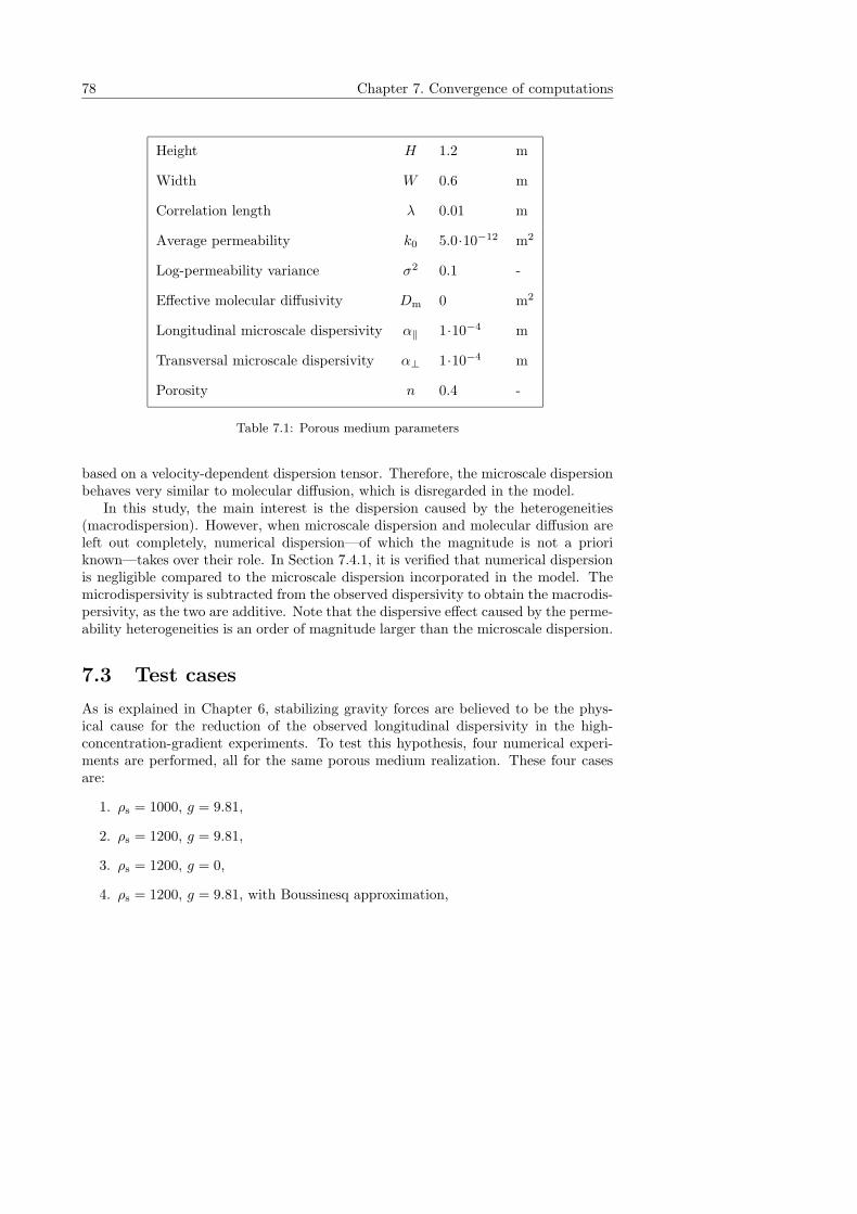
78 Chapter 7. Convergence of computations
Height H 1.2 m
Width W 0.6 m
Correlation length λ 0.01 m
Average permeability k0 5.0·10−12 m2
Log-permeability variance σ2 0.1 -
Effective molecular diffusivity Dm 0 m2
Longitudinal microscale dispersivity α‖ 1·10−4 m
Transversal microscale dispersivity α⊥ 1·10−4 m
Porosity n 0.4 -
Table 7.1: Porous medium parameters
based on a velocity-dependent dispersion tensor. Therefore, the microscale dispersionbehaves very similar to molecular diffusion, which is disregarded in the model.
In this study, the main interest is the dispersion caused by the heterogeneities(macrodispersion). However, when microscale dispersion and molecular diffusion areleft out completely, numerical dispersion—of which the magnitude is not a prioriknown—takes over their role. In Section 7.4.1, it is verified that numerical dispersionis negligible compared to the microscale dispersion incorporated in the model. Themicrodispersivity is subtracted from the observed dispersivity to obtain the macrodis-persivity, as the two are additive. Note that the dispersive effect caused by the perme-ability heterogeneities is an order of magnitude larger than the microscale dispersion.
7.3 Test cases
As is explained in Chapter 6, stabilizing gravity forces are believed to be the phys-ical cause for the reduction of the observed longitudinal dispersivity in the high-concentration-gradient experiments. To test this hypothesis, four numerical experi-ments are performed, all for the same porous medium realization. These four casesare:
1. ρs = 1000, g = 9.81,
2. ρs = 1200, g = 9.81,
3. ρs = 1200, g = 0,
4. ρs = 1200, g = 9.81, with Boussinesq approximation,
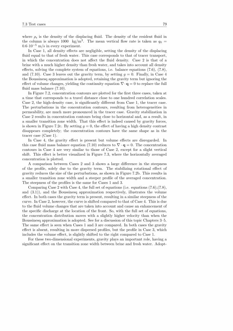
7.3 Test cases 79
where ρs is the density of the displacing fluid. The density of the resident fluid inthe column is always 1000 kg/m3. The mean vertical flow rate is taken as q0 =0.6·10−5 m/s in every experiment.
In Case 1, all density effects are negligible, setting the density of the displacingfluid equal to that of fresh water. This case corresponds to that of tracer transport,in which the concentration does not affect the fluid density. Case 2 is that of abrine with a much higher density than fresh water, and takes into account all densityeffects, solving the complete system of equations, i.e. balance equations (7.6), (7.8),and (7.10). Case 3 leaves out the gravity term, by setting g = 0. Finally, in Case 4the Boussinesq approximation is adopted, retaining the gravity term but ignoring theeffect of volume changes, yielding the continuity equation ∇·q = 0 to replace the fullfluid mass balance (7.10).
In Figure 7.2, concentration contours are plotted for the first three cases, taken ata time that corresponds to a travel distance close to one hundred correlation scales.Case 2, the high-density case, is significantly different from Case 1, the tracer case.The perturbations in the concentration contours, resulting from heterogeneities inpermeability, are much more pronounced in the tracer case. Gravity stabilization inCase 2 results in concentration contours being close to horizontal and, as a result, ina smaller transition zone width. That this effect is indeed caused by gravity forces,is shown in Figure 7.2c. By setting g = 0, the effect of having a high density contrastdisappears completely; the concentration contours have the same shape as in thetracer case (Case 1).
In Case 4, the gravity effect is present but volume effects are disregarded. Inthis case fluid mass balance equation (7.10) reduces to ∇ · q = 0. The concentrationcontours in Case 4 are very similar to those of Case 2, except for a slight verticalshift. This effect is better visualized in Figure 7.3, where the horizontally averagedconcentration is plotted.
A comparison between Cases 2 and 3 shows a large difference in the steepnessof the profile, solely due to the gravity term. The stabilizing rotational effect ofgravity reduces the size of the perturbations, as shown in Figure 7.2b. This results ina smaller transition zone width and a steeper profile of the averaged concentration.The steepness of the profiles is the same for Cases 1 and 3.
Comparing Case 2 with Case 4, the full set of equations (i.e. equations (7.6),(7.8),and (3.1)), and the Boussinesq approximation respectively, illustrates the volumeeffect. In both cases the gravity term is present, resulting in a similar steepness of thecurve. In Case 2, however, the curve is shifted compared to that of Case 4. This is dueto the fluid volume changes that are taken into account and cause an enhancement ofthe specific discharge at the location of the front. So, with the full set of equations,the concentration distribution moves with a slightly higher velocity than when theBoussinesq approximation is adopted. See for a discussion of this topic Chapters 3–5.The same effect is seen when Cases 1 and 3 are compared. In both cases the gravityeffect is absent, resulting in more dispersed profiles, but the profile in Case 3, whichincludes the volume effect, is slightly shifted to the right compared to Case 1.
For these two-dimensional experiments, gravity plays an important role, having asignificant effect on the transition zone width between brine and fresh water. Adopt-
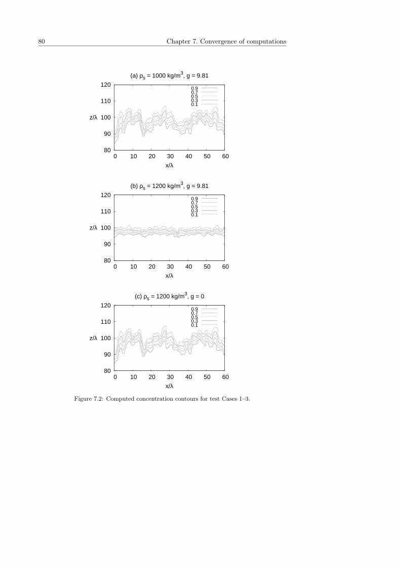
80 Chapter 7. Convergence of computations
80
90
100
110
120
0 10 20 30 40 50 60
x/λ
(a) ρs = 1000 kg/m3, g = 9.81
z/λ
0.90.70.50.30.1
80
90
100
110
120
0 10 20 30 40 50 60
x/λ
(b) ρs = 1200 kg/m3, g = 9.81
z/λ
0.90.70.50.30.1
80
90
100
110
120
0 10 20 30 40 50 60
x/λ
(c) ρs = 1200 kg/m3, g = 0
z/λ
0.90.70.50.30.1
Figure 7.2: Computed concentration contours for test Cases 1–3.
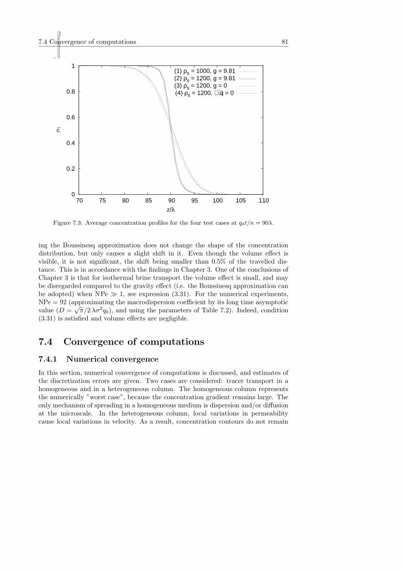
7.4 Convergence of computations 81
0
0.2
0.4
0.6
0.8
1
70 75 80 85 90 95 100 105 110
z/λ
c
(1) ρs = 1000, g = 9.81(2) ρs = 1200, g = 9.81(3) ρs = 1200, g = 0 (4) ρs = 1200, ∇⋅q = 0
PSfrag
replacem
entsc
Figure 7.3: Average concentration profiles for the four test cases at q0t/n = 90λ.
ing the Boussinesq approximation does not change the shape of the concentrationdistribution, but only causes a slight shift in it. Even though the volume effect isvisible, it is not significant, the shift being smaller than 0.5% of the travelled dis-tance. This is in accordance with the findings in Chapter 3. One of the conclusions ofChapter 3 is that for isothermal brine transport the volume effect is small, and maybe disregarded compared to the gravity effect (i.e. the Boussinesq approximation canbe adopted) when NPe � 1, see expression (3.31). For the numerical experiments,NPe = 92 (approximating the macrodispersion coefficient by its long time asymptoticvalue (D =
√π/2λσ2q0), and using the parameters of Table 7.2). Indeed, condition
(3.31) is satisfied and volume effects are negligible.
7.4 Convergence of computations
7.4.1 Numerical convergence
In this section, numerical convergence of computations is discussed, and estimates ofthe discretization errors are given. Two cases are considered: tracer transport in ahomogeneous and in a heterogeneous column. The homogeneous column representsthe numerically ”worst case”, because the concentration gradient remains large. Theonly mechanism of spreading in a homogeneous medium is dispersion and/or diffusionat the microscale. In the heterogeneous column, local variations in permeabilitycause local variations in velocity. As a result, concentration contours do not remain
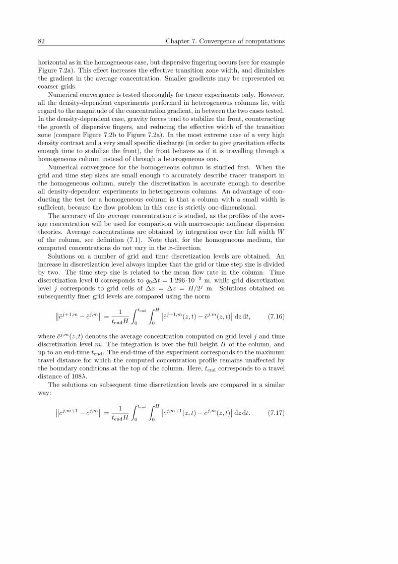
82 Chapter 7. Convergence of computations
horizontal as in the homogeneous case, but dispersive fingering occurs (see for exampleFigure 7.2a). This effect increases the effective transition zone width, and diminishesthe gradient in the average concentration. Smaller gradients may be represented oncoarser grids.
Numerical convergence is tested thoroughly for tracer experiments only. However,all the density-dependent experiments performed in heterogeneous columns lie, withregard to the magnitude of the concentration gradient, in between the two cases tested.In the density-dependent case, gravity forces tend to stabilize the front, counteractingthe growth of dispersive fingers, and reducing the effective width of the transitionzone (compare Figure 7.2b to Figure 7.2a). In the most extreme case of a very highdensity contrast and a very small specific discharge (in order to give gravitation effectsenough time to stabilize the front), the front behaves as if it is travelling through ahomogeneous column instead of through a heterogeneous one.
Numerical convergence for the homogeneous column is studied first. When thegrid and time step sizes are small enough to accurately describe tracer transport inthe homogeneous column, surely the discretization is accurate enough to describeall density-dependent experiments in heterogeneous columns. An advantage of con-ducting the test for a homogeneous column is that a column with a small width issufficient, because the flow problem in this case is strictly one-dimensional.
The accuracy of the average concentration c is studied, as the profiles of the aver-age concentration will be used for comparison with macroscopic nonlinear dispersiontheories. Average concentrations are obtained by integration over the full width Wof the column, see definition (7.1). Note that, for the homogeneous medium, thecomputed concentrations do not vary in the x-direction.
Solutions on a number of grid and time discretization levels are obtained. Anincrease in discretization level always implies that the grid or time step size is dividedby two. The time step size is related to the mean flow rate in the column. Timediscretization level 0 corresponds to q0∆t = 1.296·10−3 m, while grid discretizationlevel j corresponds to grid cells of ∆x = ∆z = H/2j m. Solutions obtained onsubsequently finer grid levels are compared using the norm
∥∥cj+1,m − cj,m
∥∥ =
1
tendH
∫ tend
0
∫ H
0
∣∣cj+1,m(z, t)− cj,m(z, t)
∣∣ dzdt, (7.16)
where cj,m(z, t) denotes the average concentration computed on grid level j and timediscretization level m. The integration is over the full height H of the column, andup to an end-time tend. The end-time of the experiment corresponds to the maximumtravel distance for which the computed concentration profile remains unaffected bythe boundary conditions at the top of the column. Here, tend corresponds to a traveldistance of 108λ.
The solutions on subsequent time discretization levels are compared in a similarway:
∥∥cj,m+1 − cj,m
∥∥ =
1
tendH
∫ tend
0
∫ H
0
∣∣cj,m+1(z, t)− cj,m(z, t)
∣∣ dzdt. (7.17)
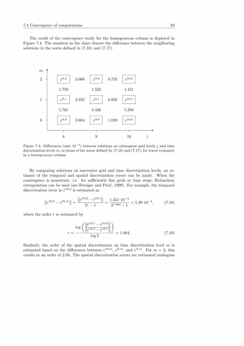
7.4 Convergence of computations 83
The result of the convergence study for the homogeneous column is depicted inFigure 7.4. The numbers in the chart denote the difference between the neighboringsolutions in the norm defined in (7.16) and (7.17).
j8 9 10
0
1
2
-
6m
c8,0 c9,0
c8,1
c8,2
c9,1
c9,2
c10,0
c10,1
c10,2
3.684 1.020
3.232
3.006
0.850
0.735
5.761
1.759
5.436
1.522
5.358
1.451
Figure 7.4: Differences (unit 10−3) between solutions on subsequent grid levels j and timediscretization levels m, in terms of the norm defined by (7.16) and (7.17), for tracer transportin a homogeneous column.
By comparing solutions on successive grid and time discretization levels, an es-timate of the temporal and spatial discretization errors can be made. When theconvergence is monotonic, i.e. for sufficiently fine grids or time steps, Richardsonextrapolation can be used (see Ferziger and Peric, 1999). For example, the temporaldiscretization error in c10,2 is estimated as
∥∥c10,2 − c10,∞∥∥ =
∥∥c10,2 − c10,1
∥∥
2r − 1=
1.451·10−3
21.884 − 1= 5.39·10−4, (7.18)
where the order r is estimated by
r =
log
(∥∥c10,1 − c10,0
∥∥
∥∥c10,2 − c10,1
∥∥
)
log 2= 1.884. (7.19)
Similarly, the order of the spatial discretization on time discretization level m isestimated based on the differences between c10,m, c9,m, and c8,m. For m = 2, thisresults in an order of 2.03. The spatial discretization errors are estimated analogous
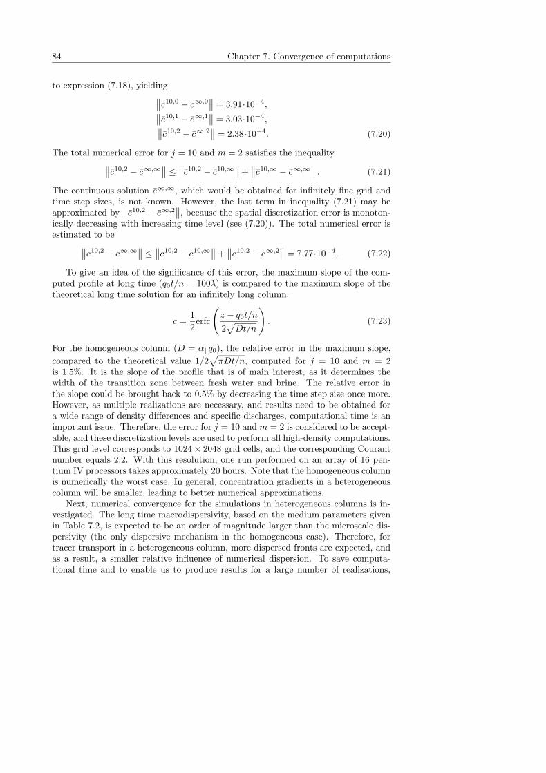
84 Chapter 7. Convergence of computations
to expression (7.18), yielding∥∥c10,0 − c∞,0
∥∥ = 3.91·10−4,
∥∥c10,1 − c∞,1
∥∥ = 3.03·10−4,
∥∥c10,2 − c∞,2
∥∥ = 2.38·10−4. (7.20)
The total numerical error for j = 10 and m = 2 satisfies the inequality∥∥c10,2 − c∞,∞∥∥ ≤
∥∥c10,2 − c10,∞∥∥+
∥∥c10,∞ − c∞,∞∥∥ . (7.21)
The continuous solution c∞,∞, which would be obtained for infinitely fine grid andtime step sizes, is not known. However, the last term in inequality (7.21) may beapproximated by
∥∥c10,2 − c∞,2
∥∥, because the spatial discretization error is monoton-
ically decreasing with increasing time level (see (7.20)). The total numerical error isestimated to be
∥∥c10,2 − c∞,∞∥∥ ≤
∥∥c10,2 − c10,∞∥∥+
∥∥c10,2 − c∞,2
∥∥ = 7.77·10−4. (7.22)
To give an idea of the significance of this error, the maximum slope of the com-puted profile at long time (q0t/n = 100λ) is compared to the maximum slope of thetheoretical long time solution for an infinitely long column:
c =1
2erfc
(
z − q0t/n
2√
Dt/n
)
. (7.23)
For the homogeneous column (D = α‖q0), the relative error in the maximum slope,
compared to the theoretical value 1/2√
πDt/n, computed for j = 10 and m = 2is 1.5%. It is the slope of the profile that is of main interest, as it determines thewidth of the transition zone between fresh water and brine. The relative error inthe slope could be brought back to 0.5% by decreasing the time step size once more.However, as multiple realizations are necessary, and results need to be obtained fora wide range of density differences and specific discharges, computational time is animportant issue. Therefore, the error for j = 10 and m = 2 is considered to be accept-able, and these discretization levels are used to perform all high-density computations.This grid level corresponds to 1024× 2048 grid cells, and the corresponding Courantnumber equals 2.2. With this resolution, one run performed on an array of 16 pen-tium IV processors takes approximately 20 hours. Note that the homogeneous columnis numerically the worst case. In general, concentration gradients in a heterogeneouscolumn will be smaller, leading to better numerical approximations.
Next, numerical convergence for the simulations in heterogeneous columns is in-vestigated. The long time macrodispersivity, based on the medium parameters givenin Table 7.2, is expected to be an order of magnitude larger than the microscale dis-persivity (the only dispersive mechanism in the homogeneous case). Therefore, fortracer transport in a heterogeneous column, more dispersed fronts are expected, andas a result, a smaller relative influence of numerical dispersion. To save computa-tional time and to enable us to produce results for a large number of realizations,
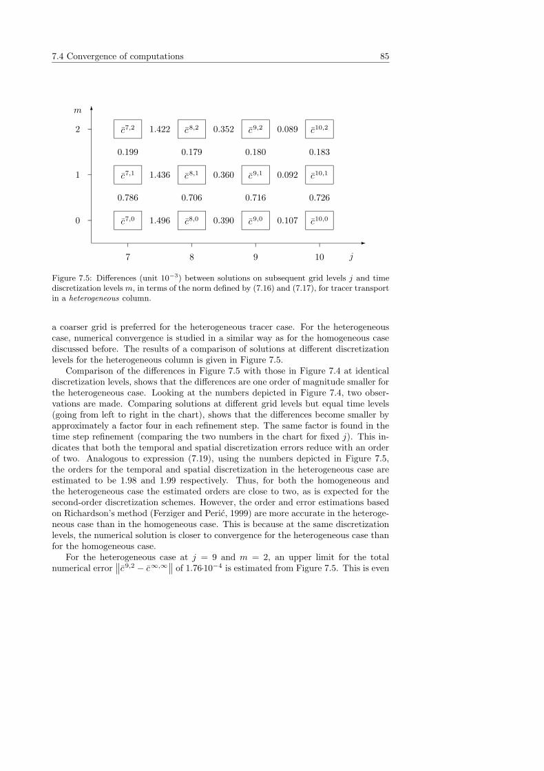
7.4 Convergence of computations 85
j7 8 9 10
0
1
2
-
6m
c7,0 c8,0
c7,1
c7,2
c8,1
c8,2
c9,0
c9,1
c9,2
c10,0
c10,1
c10,2
1.496 0.390
1.436
1.422
0.360
0.352
0.107
0.092
0.089
0.786
0.199
0.706
0.179
0.716
0.180
0.726
0.183
Figure 7.5: Differences (unit 10−3) between solutions on subsequent grid levels j and timediscretization levels m, in terms of the norm defined by (7.16) and (7.17), for tracer transportin a heterogeneous column.
a coarser grid is preferred for the heterogeneous tracer case. For the heterogeneouscase, numerical convergence is studied in a similar way as for the homogeneous casediscussed before. The results of a comparison of solutions at different discretizationlevels for the heterogeneous column is given in Figure 7.5.
Comparison of the differences in Figure 7.5 with those in Figure 7.4 at identicaldiscretization levels, shows that the differences are one order of magnitude smaller forthe heterogeneous case. Looking at the numbers depicted in Figure 7.4, two obser-vations are made. Comparing solutions at different grid levels but equal time levels(going from left to right in the chart), shows that the differences become smaller byapproximately a factor four in each refinement step. The same factor is found in thetime step refinement (comparing the two numbers in the chart for fixed j). This in-dicates that both the temporal and spatial discretization errors reduce with an orderof two. Analogous to expression (7.19), using the numbers depicted in Figure 7.5,the orders for the temporal and spatial discretization in the heterogeneous case areestimated to be 1.98 and 1.99 respectively. Thus, for both the homogeneous andthe heterogeneous case the estimated orders are close to two, as is expected for thesecond-order discretization schemes. However, the order and error estimations basedon Richardson’s method (Ferziger and Peric, 1999) are more accurate in the heteroge-neous case than in the homogeneous case. This is because at the same discretizationlevels, the numerical solution is closer to convergence for the heterogeneous case thanfor the homogeneous case.
For the heterogeneous case at j = 9 and m = 2, an upper limit for the totalnumerical error
∥∥c9,2 − c∞,∞∥∥ of 1.76·10−4 is estimated from Figure 7.5. This is even
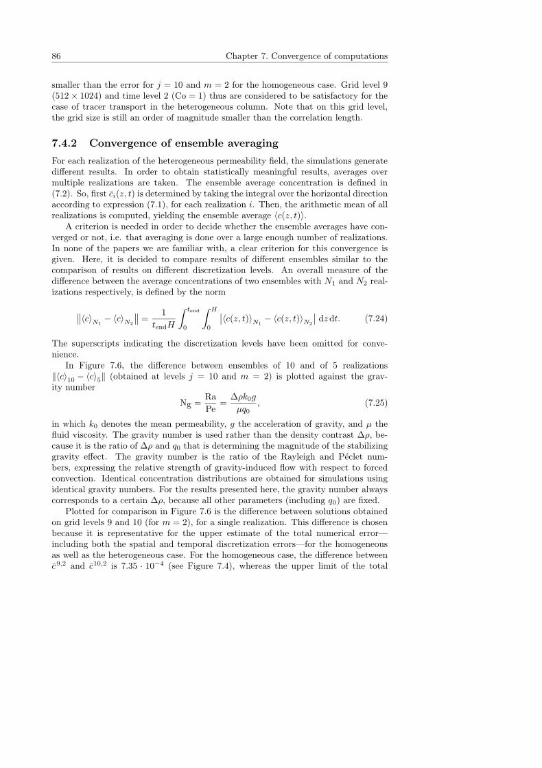
86 Chapter 7. Convergence of computations
smaller than the error for j = 10 and m = 2 for the homogeneous case. Grid level 9(512× 1024) and time level 2 (Co = 1) thus are considered to be satisfactory for thecase of tracer transport in the heterogeneous column. Note that on this grid level,the grid size is still an order of magnitude smaller than the correlation length.
7.4.2 Convergence of ensemble averaging
For each realization of the heterogeneous permeability field, the simulations generatedifferent results. In order to obtain statistically meaningful results, averages overmultiple realizations are taken. The ensemble average concentration is defined in(7.2). So, first ci(z, t) is determined by taking the integral over the horizontal directionaccording to expression (7.1), for each realization i. Then, the arithmetic mean of allrealizations is computed, yielding the ensemble average 〈c(z, t)〉.
A criterion is needed in order to decide whether the ensemble averages have con-verged or not, i.e. that averaging is done over a large enough number of realizations.In none of the papers we are familiar with, a clear criterion for this convergence isgiven. Here, it is decided to compare results of different ensembles similar to thecomparison of results on different discretization levels. An overall measure of thedifference between the average concentrations of two ensembles with N1 and N2 real-izations respectively, is defined by the norm
∥∥〈c〉N1
− 〈c〉N2
∥∥ =
1
tendH
∫ tend
0
∫ H
0
∣∣〈c(z, t)〉N1
− 〈c(z, t)〉N2
∣∣ dzdt. (7.24)
The superscripts indicating the discretization levels have been omitted for conve-nience.
In Figure 7.6, the difference between ensembles of 10 and of 5 realizations‖〈c〉10 − 〈c〉5‖ (obtained at levels j = 10 and m = 2) is plotted against the grav-ity number
Ng =Ra
Pe=
∆ρk0g
µq0, (7.25)
in which k0 denotes the mean permeability, g the acceleration of gravity, and µ thefluid viscosity. The gravity number is used rather than the density contrast ∆ρ, be-cause it is the ratio of ∆ρ and q0 that is determining the magnitude of the stabilizinggravity effect. The gravity number is the ratio of the Rayleigh and Peclet num-bers, expressing the relative strength of gravity-induced flow with respect to forcedconvection. Identical concentration distributions are obtained for simulations usingidentical gravity numbers. For the results presented here, the gravity number alwayscorresponds to a certain ∆ρ, because all other parameters (including q0) are fixed.
Plotted for comparison in Figure 7.6 is the difference between solutions obtainedon grid levels 9 and 10 (for m = 2), for a single realization. This difference is chosenbecause it is representative for the upper estimate of the total numerical error—including both the spatial and temporal discretization errors—for the homogeneousas well as the heterogeneous case. For the homogeneous case, the difference betweenc9,2 and c10,2 is 7.35 · 10−4 (see Figure 7.4), whereas the upper limit of the total
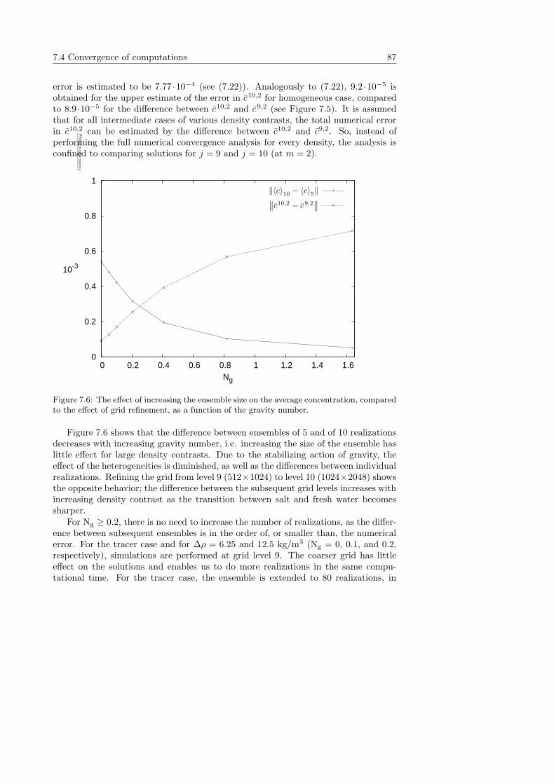
7.4 Convergence of computations 87
error is estimated to be 7.77 ·10−4 (see (7.22)). Analogously to (7.22), 9.2 ·10−5 isobtained for the upper estimate of the error in c10,2 for homogeneous case, comparedto 8.9·10−5 for the difference between c10,2 and c9,2 (see Figure 7.5). It is assumedthat for all intermediate cases of various density contrasts, the total numerical errorin c10,2 can be estimated by the difference between c10,2 and c9,2. So, instead ofperforming the full numerical convergence analysis for every density, the analysis isconfined to comparing solutions for j = 9 and j = 10 (at m = 2).
0
0.2
0.4
0.6
0.8
1
0 0.2 0.4 0.6 0.8 1 1.2 1.4 1.6Ng
10-3
PSfrag
replacem
ents
‖〈c〉10 − 〈c〉5‖∥∥c10,2 − c9,2
∥∥
Figure 7.6: The effect of increasing the ensemble size on the average concentration, comparedto the effect of grid refinement, as a function of the gravity number.
Figure 7.6 shows that the difference between ensembles of 5 and of 10 realizationsdecreases with increasing gravity number, i.e. increasing the size of the ensemble haslittle effect for large density contrasts. Due to the stabilizing action of gravity, theeffect of the heterogeneities is diminished, as well as the differences between individualrealizations. Refining the grid from level 9 (512×1024) to level 10 (1024×2048) showsthe opposite behavior; the difference between the subsequent grid levels increases withincreasing density contrast as the transition between salt and fresh water becomessharper.
For Ng ≥ 0.2, there is no need to increase the number of realizations, as the differ-ence between subsequent ensembles is in the order of, or smaller than, the numericalerror. For the tracer case and for ∆ρ = 6.25 and 12.5 kg/m3 (Ng = 0, 0.1, and 0.2,respectively), simulations are performed at grid level 9. The coarser grid has littleeffect on the solutions and enables us to do more realizations in the same compu-tational time. For the tracer case, the ensemble is extended to 80 realizations, in
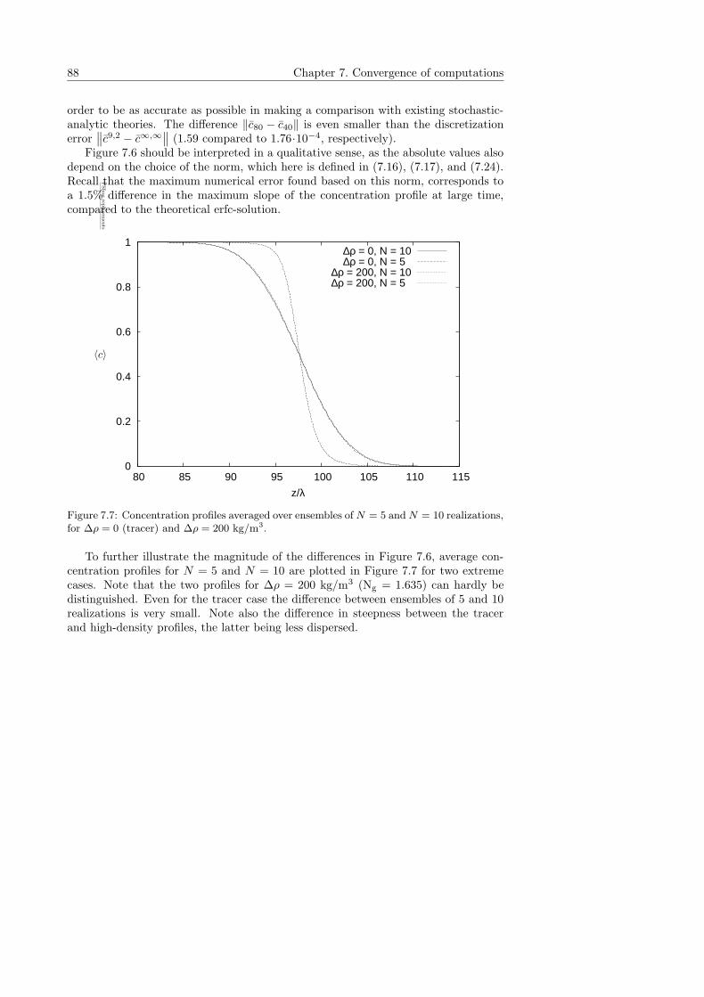
88 Chapter 7. Convergence of computations
order to be as accurate as possible in making a comparison with existing stochastic-analytic theories. The difference ‖c80 − c40‖ is even smaller than the discretizationerror
∥∥c9,2 − c∞,∞∥∥ (1.59 compared to 1.76·10−4, respectively).
Figure 7.6 should be interpreted in a qualitative sense, as the absolute values alsodepend on the choice of the norm, which here is defined in (7.16), (7.17), and (7.24).Recall that the maximum numerical error found based on this norm, corresponds toa 1.5% difference in the maximum slope of the concentration profile at large time,compared to the theoretical erfc-solution.
0
0.2
0.4
0.6
0.8
1
80 85 90 95 100 105 110 115
z/λ
∆ρ = 0, N = 10∆ρ = 0, N = 5
∆ρ = 200, N = 10∆ρ = 200, N = 5
PSfrag
replacem
ents
〈c〉
Figure 7.7: Concentration profiles averaged over ensembles of N = 5 and N = 10 realizations,for ∆ρ = 0 (tracer) and ∆ρ = 200 kg/m3.
To further illustrate the magnitude of the differences in Figure 7.6, average con-centration profiles for N = 5 and N = 10 are plotted in Figure 7.7 for two extremecases. Note that the two profiles for ∆ρ = 200 kg/m3 (Ng = 1.635) can hardly bedistinguished. Even for the tracer case the difference between ensembles of 5 and 10realizations is very small. Note also the difference in steepness between the tracerand high-density profiles, the latter being less dispersed.
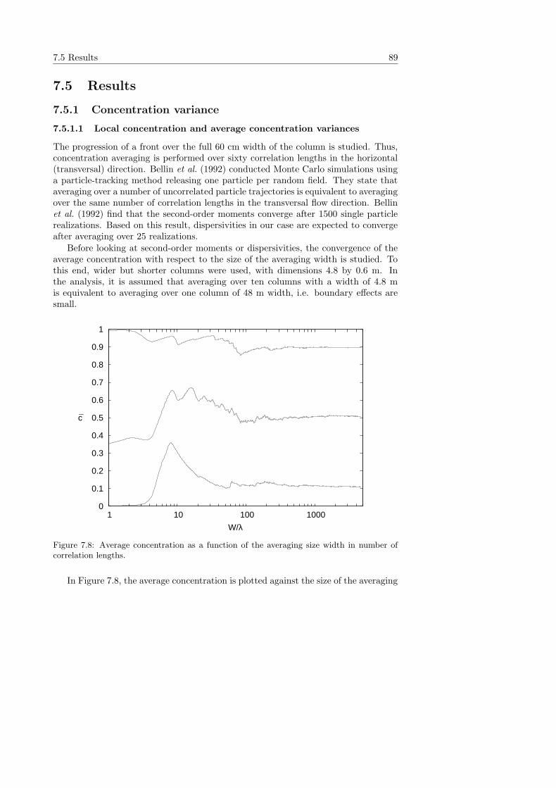
7.5 Results 89
7.5 Results
7.5.1 Concentration variance
7.5.1.1 Local concentration and average concentration variances
The progression of a front over the full 60 cm width of the column is studied. Thus,concentration averaging is performed over sixty correlation lengths in the horizontal(transversal) direction. Bellin et al. (1992) conducted Monte Carlo simulations usinga particle-tracking method releasing one particle per random field. They state thataveraging over a number of uncorrelated particle trajectories is equivalent to averagingover the same number of correlation lengths in the transversal flow direction. Bellinet al. (1992) find that the second-order moments converge after 1500 single particlerealizations. Based on this result, dispersivities in our case are expected to convergeafter averaging over 25 realizations.
Before looking at second-order moments or dispersivities, the convergence of theaverage concentration with respect to the size of the averaging width is studied. Tothis end, wider but shorter columns were used, with dimensions 4.8 by 0.6 m. Inthe analysis, it is assumed that averaging over ten columns with a width of 4.8 mis equivalent to averaging over one column of 48 m width, i.e. boundary effects aresmall.
0
0.1
0.2
0.3
0.4
0.5
0.6
0.7
0.8
0.9
1
1 10 100 1000
W/λ
c
Figure 7.8: Average concentration as a function of the averaging size width in number ofcorrelation lengths.
In Figure 7.8, the average concentration is plotted against the size of the averaging
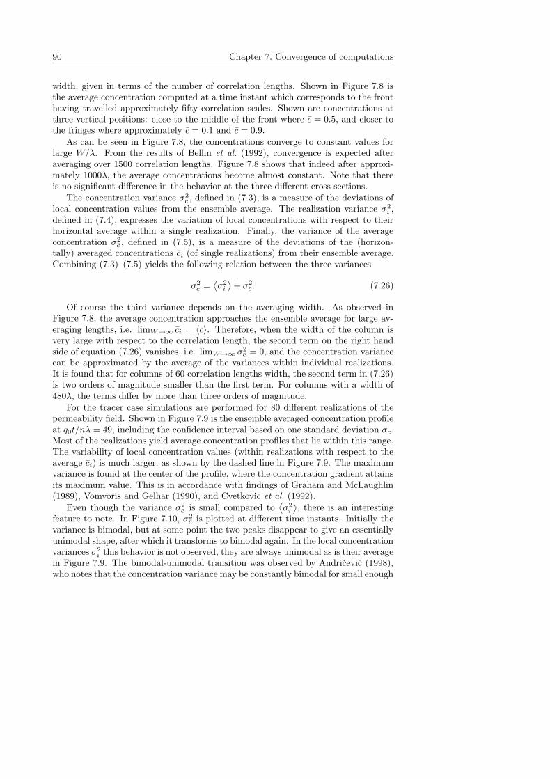
90 Chapter 7. Convergence of computations
width, given in terms of the number of correlation lengths. Shown in Figure 7.8 isthe average concentration computed at a time instant which corresponds to the fronthaving travelled approximately fifty correlation scales. Shown are concentrations atthree vertical positions: close to the middle of the front where c = 0.5, and closer tothe fringes where approximately c = 0.1 and c = 0.9.
As can be seen in Figure 7.8, the concentrations converge to constant values forlarge W/λ. From the results of Bellin et al. (1992), convergence is expected afteraveraging over 1500 correlation lengths. Figure 7.8 shows that indeed after approxi-mately 1000λ, the average concentrations become almost constant. Note that thereis no significant difference in the behavior at the three different cross sections.
The concentration variance σ2c , defined in (7.3), is a measure of the deviations of
local concentration values from the ensemble average. The realization variance σ2i ,
defined in (7.4), expresses the variation of local concentrations with respect to theirhorizontal average within a single realization. Finally, the variance of the averageconcentration σ2
c , defined in (7.5), is a measure of the deviations of the (horizon-tally) averaged concentrations ci (of single realizations) from their ensemble average.Combining (7.3)–(7.5) yields the following relation between the three variances
σ2c =
⟨σ2
i
⟩+ σ2
c . (7.26)
Of course the third variance depends on the averaging width. As observed inFigure 7.8, the average concentration approaches the ensemble average for large av-eraging lengths, i.e. limW→∞ ci = 〈c〉. Therefore, when the width of the column isvery large with respect to the correlation length, the second term on the right handside of equation (7.26) vanishes, i.e. limW→∞ σ2
c = 0, and the concentration variancecan be approximated by the average of the variances within individual realizations.It is found that for columns of 60 correlation lengths width, the second term in (7.26)is two orders of magnitude smaller than the first term. For columns with a width of480λ, the terms differ by more than three orders of magnitude.
For the tracer case simulations are performed for 80 different realizations of thepermeability field. Shown in Figure 7.9 is the ensemble averaged concentration profileat q0t/nλ = 49, including the confidence interval based on one standard deviation σc.Most of the realizations yield average concentration profiles that lie within this range.The variability of local concentration values (within realizations with respect to theaverage ci) is much larger, as shown by the dashed line in Figure 7.9. The maximumvariance is found at the center of the profile, where the concentration gradient attainsits maximum value. This is in accordance with findings of Graham and McLaughlin(1989), Vomvoris and Gelhar (1990), and Cvetkovic et al. (1992).
Even though the variance σ2c is small compared to
⟨σ2
i
⟩, there is an interesting
feature to note. In Figure 7.10, σ2c is plotted at different time instants. Initially the
variance is bimodal, but at some point the two peaks disappear to give an essentiallyunimodal shape, after which it transforms to bimodal again. In the local concentrationvariances σ2
i this behavior is not observed, they are always unimodal as is their averagein Figure 7.9. The bimodal-unimodal transition was observed by Andricevic (1998),who notes that the concentration variance may be constantly bimodal for small enough
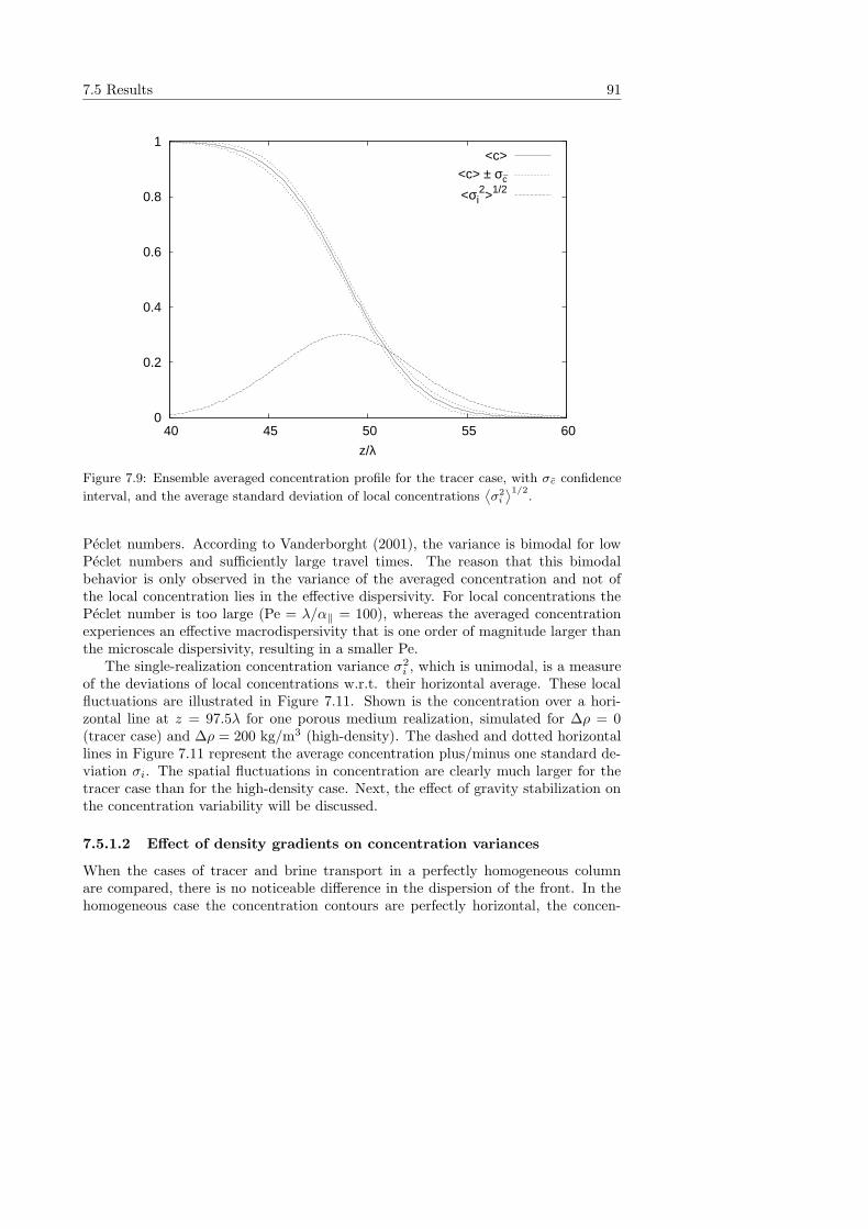
7.5 Results 91
0
0.2
0.4
0.6
0.8
1
40 45 50 55 60
z/λ
<c><c> ± σc
<σi2>1/2
Figure 7.9: Ensemble averaged concentration profile for the tracer case, with σc confidence
interval, and the average standard deviation of local concentrations⟨σ2
i
⟩1/2
.
Peclet numbers. According to Vanderborght (2001), the variance is bimodal for lowPeclet numbers and sufficiently large travel times. The reason that this bimodalbehavior is only observed in the variance of the averaged concentration and not ofthe local concentration lies in the effective dispersivity. For local concentrations thePeclet number is too large (Pe = λ/α‖ = 100), whereas the averaged concentrationexperiences an effective macrodispersivity that is one order of magnitude larger thanthe microscale dispersivity, resulting in a smaller Pe.
The single-realization concentration variance σ2i , which is unimodal, is a measure
of the deviations of local concentrations w.r.t. their horizontal average. These localfluctuations are illustrated in Figure 7.11. Shown is the concentration over a hori-zontal line at z = 97.5λ for one porous medium realization, simulated for ∆ρ = 0(tracer case) and ∆ρ = 200 kg/m3 (high-density). The dashed and dotted horizontallines in Figure 7.11 represent the average concentration plus/minus one standard de-viation σi. The spatial fluctuations in concentration are clearly much larger for thetracer case than for the high-density case. Next, the effect of gravity stabilization onthe concentration variability will be discussed.
7.5.1.2 Effect of density gradients on concentration variances
When the cases of tracer and brine transport in a perfectly homogeneous columnare compared, there is no noticeable difference in the dispersion of the front. In thehomogeneous case the concentration contours are perfectly horizontal, the concen-
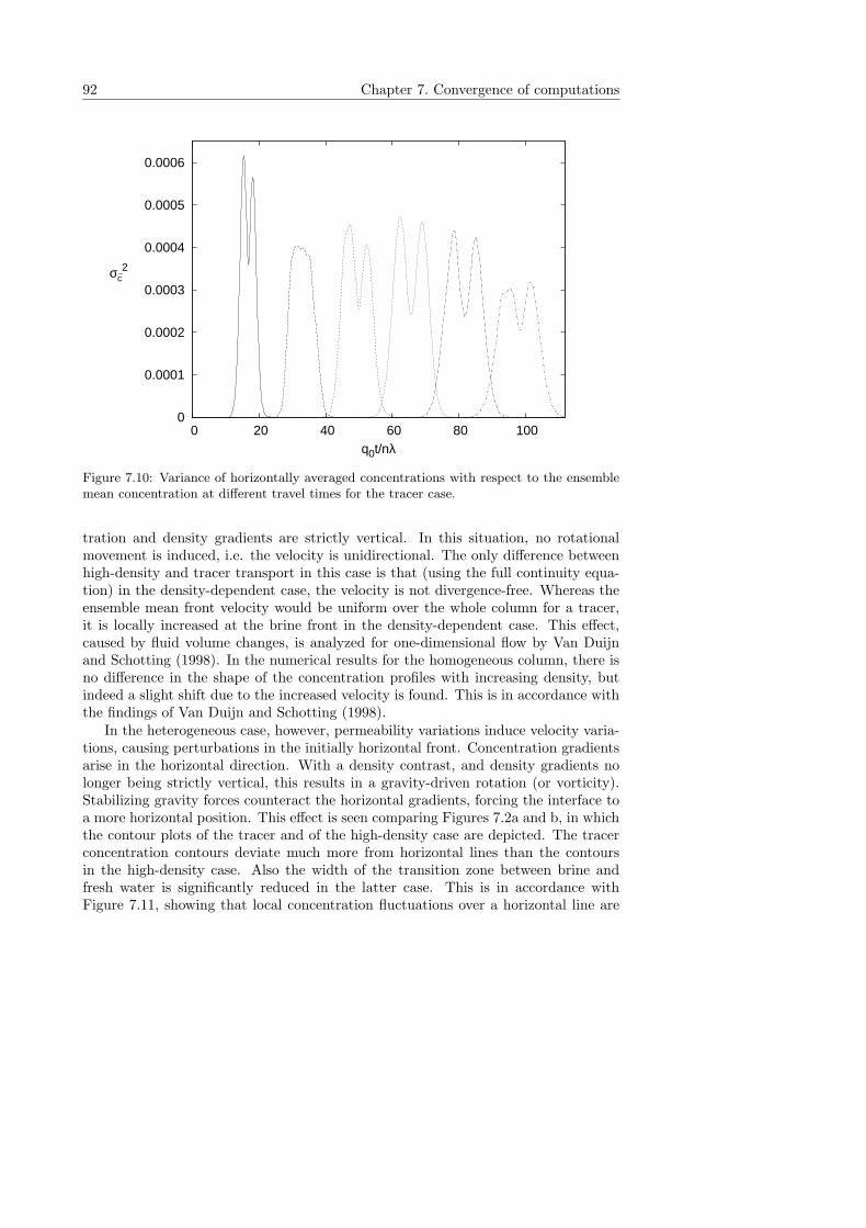
92 Chapter 7. Convergence of computations
0
0.0001
0.0002
0.0003
0.0004
0.0005
0.0006
0 20 40 60 80 100q0t/nλ
σc2
Figure 7.10: Variance of horizontally averaged concentrations with respect to the ensemblemean concentration at different travel times for the tracer case.
tration and density gradients are strictly vertical. In this situation, no rotationalmovement is induced, i.e. the velocity is unidirectional. The only difference betweenhigh-density and tracer transport in this case is that (using the full continuity equa-tion) in the density-dependent case, the velocity is not divergence-free. Whereas theensemble mean front velocity would be uniform over the whole column for a tracer,it is locally increased at the brine front in the density-dependent case. This effect,caused by fluid volume changes, is analyzed for one-dimensional flow by Van Duijnand Schotting (1998). In the numerical results for the homogeneous column, there isno difference in the shape of the concentration profiles with increasing density, butindeed a slight shift due to the increased velocity is found. This is in accordance withthe findings of Van Duijn and Schotting (1998).
In the heterogeneous case, however, permeability variations induce velocity varia-tions, causing perturbations in the initially horizontal front. Concentration gradientsarise in the horizontal direction. With a density contrast, and density gradients nolonger being strictly vertical, this results in a gravity-driven rotation (or vorticity).Stabilizing gravity forces counteract the horizontal gradients, forcing the interface toa more horizontal position. This effect is seen comparing Figures 7.2a and b, in whichthe contour plots of the tracer and of the high-density case are depicted. The tracerconcentration contours deviate much more from horizontal lines than the contoursin the high-density case. Also the width of the transition zone between brine andfresh water is significantly reduced in the latter case. This is in accordance withFigure 7.11, showing that local concentration fluctuations over a horizontal line are
7.5 Results 93
0
0.2
0.4
0.6
0.8
1
0 10 20 30 40 50 60
x/λ
c
∆ρ = 0 ∆ρ = 200
Figure 7.11: Local concentrations at z = 97.5λ, with one σi confidence intervals, for ∆ρ = 0(tracer) and ∆ρ = 200 kg/m3 (q0 = 0.6·10−5m/s).
much smaller for the high-density case than for the tracer case.
The transition zone width not only depends on the density contrast, but also onthe mean velocity of the front. When the velocity is large, gravity has relatively lesstime to smoothen the irregularities in the front, whereas for a very small velocity itmay be able to eliminate the horizontal gradients almost completely. The parameterthat controls the shape of the average concentration profiles is the ratio between thedensity difference and the mean specific discharge, or more specifically, the gravitynumber defined in (7.25). For instance, the difference between Figure 7.2a and bis apparent not only because of the large density contrast, but also because of therelatively small discharge (q0 = 0.6 ·10−5m/s), corresponding to an effective frontvelocity q0/n of 1.3 m/day (yielding Ng = 1.635).
The variance of local concentrations decreases with increasing gravity number (orwith the density difference when q0 and other parameters are kept constant). Thevariance attains its maximum at the center of the front, as seen in Figure 7.9. InFigure 7.12 this maximum is plotted against dimensionless time, for several densitydifferences (and corresponding gravity numbers). Figure 7.12 is in a qualitative sensesimilar to Figure 2 in the paper of Dagan and Fiori (1997), which gives the con-centration variance at the center of an infinitesimal square plume as a function oftime. Dagan and Fiori (1997) observe a decrease in concentration variance with in-creasing microscale transversal dispersion (decreasing Pe⊥) similar to the decreasethat is found with increasing density difference (or gravity number). The effect of
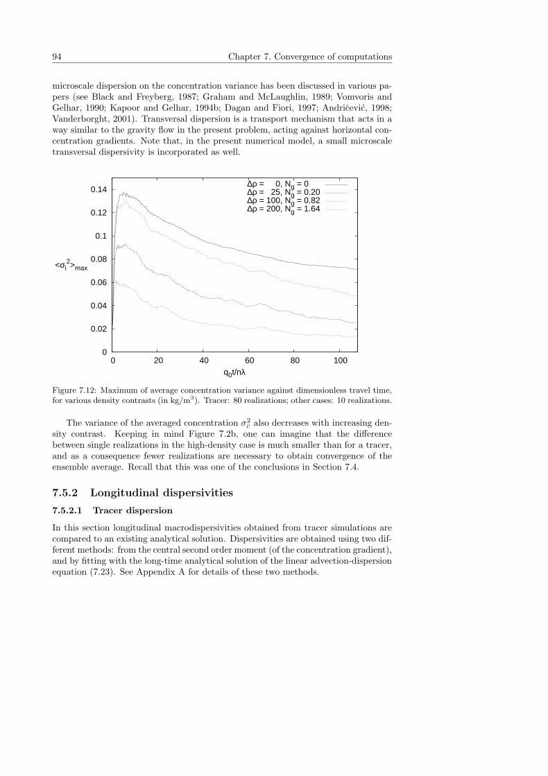
94 Chapter 7. Convergence of computations
microscale dispersion on the concentration variance has been discussed in various pa-pers (see Black and Freyberg, 1987; Graham and McLaughlin, 1989; Vomvoris andGelhar, 1990; Kapoor and Gelhar, 1994b; Dagan and Fiori, 1997; Andricevic, 1998;Vanderborght, 2001). Transversal dispersion is a transport mechanism that acts in away similar to the gravity flow in the present problem, acting against horizontal con-centration gradients. Note that, in the present numerical model, a small microscaletransversal dispersivity is incorporated as well.
0
0.02
0.04
0.06
0.08
0.1
0.12
0.14
0 20 40 60 80 100q0t/nλ
<σi2>max
∆ρ = 0, Ng = 0 ∆ρ = 25, Ng = 0.20∆ρ = 100, Ng = 0.82∆ρ = 200, Ng = 1.64
Figure 7.12: Maximum of average concentration variance against dimensionless travel time,for various density contrasts (in kg/m3). Tracer: 80 realizations; other cases: 10 realizations.
The variance of the averaged concentration σ2c also decreases with increasing den-
sity contrast. Keeping in mind Figure 7.2b, one can imagine that the differencebetween single realizations in the high-density case is much smaller than for a tracer,and as a consequence fewer realizations are necessary to obtain convergence of theensemble average. Recall that this was one of the conclusions in Section 7.4.
7.5.2 Longitudinal dispersivities
7.5.2.1 Tracer dispersion
In this section longitudinal macrodispersivities obtained from tracer simulations arecompared to an existing analytical solution. Dispersivities are obtained using two dif-ferent methods: from the central second order moment (of the concentration gradient),and by fitting with the long-time analytical solution of the linear advection-dispersionequation (7.23). See Appendix A for details of these two methods.
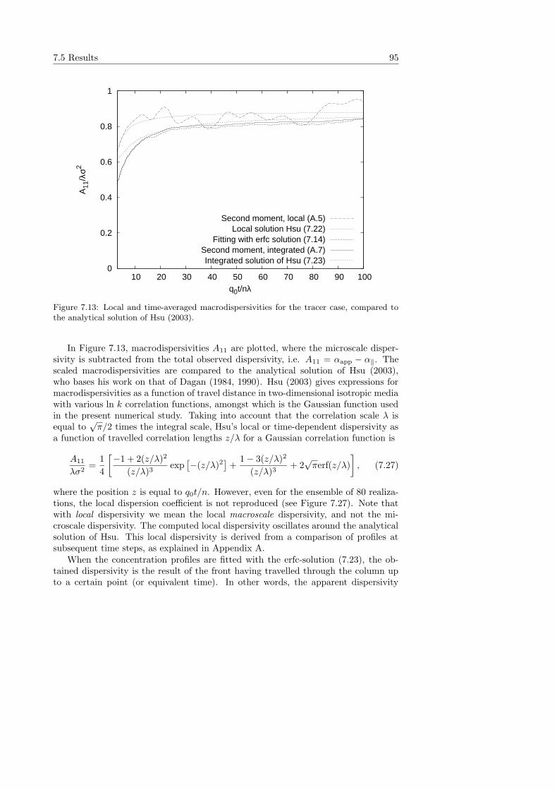
7.5 Results 95
0
0.2
0.4
0.6
0.8
1
10 20 30 40 50 60 70 80 90 100
A11
/λσ2
q0t/nλ
Second moment, local (A.5)Local solution Hsu (7.22)
Fitting with erfc solution (7.14)Second moment, integrated (A.7)Integrated solution of Hsu (7.23)
Figure 7.13: Local and time-averaged macrodispersivities for the tracer case, compared tothe analytical solution of Hsu (2003).
In Figure 7.13, macrodispersivities A11 are plotted, where the microscale disper-sivity is subtracted from the total observed dispersivity, i.e. A11 = αapp − α‖. Thescaled macrodispersivities are compared to the analytical solution of Hsu (2003),who bases his work on that of Dagan (1984, 1990). Hsu (2003) gives expressions formacrodispersivities as a function of travel distance in two-dimensional isotropic mediawith various ln k correlation functions, amongst which is the Gaussian function usedin the present numerical study. Taking into account that the correlation scale λ isequal to
√π/2 times the integral scale, Hsu’s local or time-dependent dispersivity as
a function of travelled correlation lengths z/λ for a Gaussian correlation function is
A11
λσ2=
1
4
[−1 + 2(z/λ)2
(z/λ)3exp
[−(z/λ)2
]+
1− 3(z/λ)2
(z/λ)3+ 2√
πerf(z/λ)
]
, (7.27)
where the position z is equal to q0t/n. However, even for the ensemble of 80 realiza-tions, the local dispersion coefficient is not reproduced (see Figure 7.27). Note thatwith local dispersivity we mean the local macroscale dispersivity, and not the mi-croscale dispersivity. The computed local dispersivity oscillates around the analyticalsolution of Hsu. This local dispersivity is derived from a comparison of profiles atsubsequent time steps, as explained in Appendix A.
When the concentration profiles are fitted with the erfc-solution (7.23), the ob-tained dispersivity is the result of the front having travelled through the column upto a certain point (or equivalent time). In other words, the apparent dispersivity
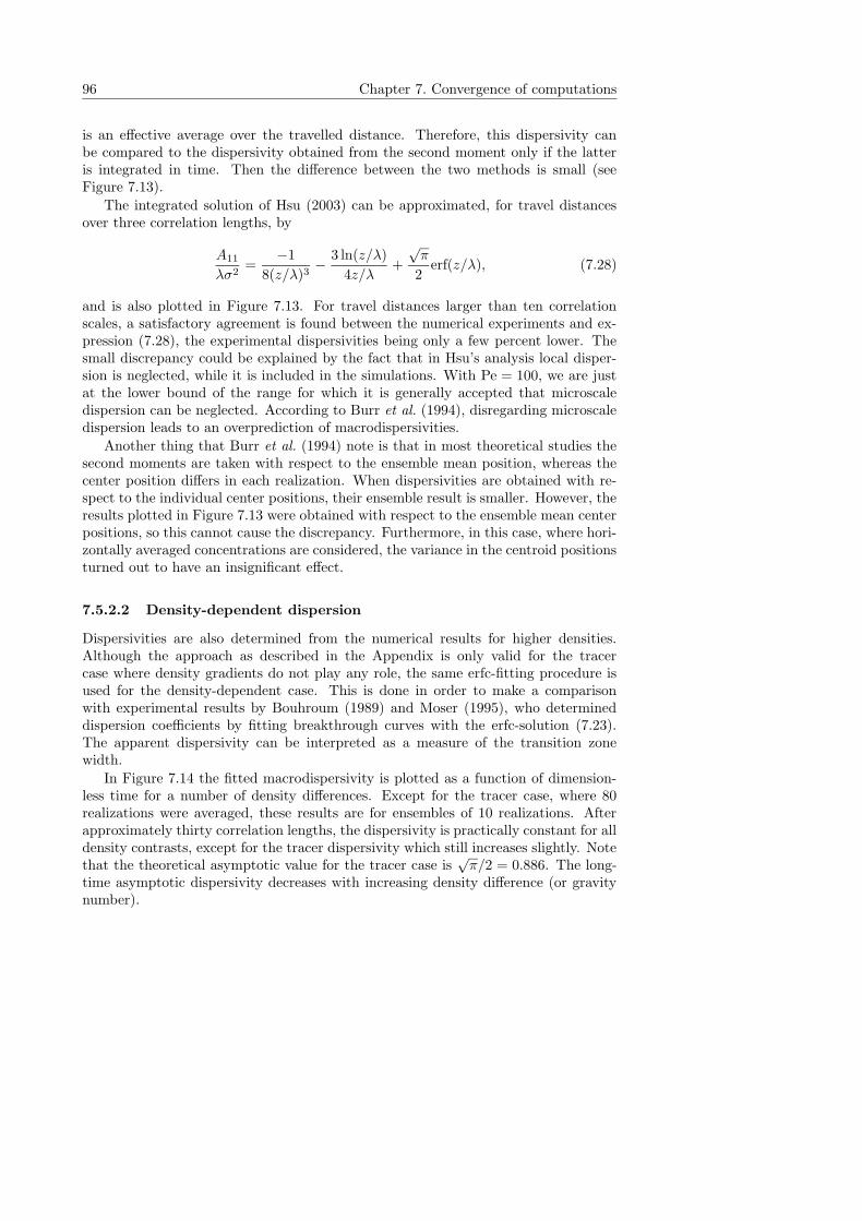
96 Chapter 7. Convergence of computations
is an effective average over the travelled distance. Therefore, this dispersivity canbe compared to the dispersivity obtained from the second moment only if the latteris integrated in time. Then the difference between the two methods is small (seeFigure 7.13).
The integrated solution of Hsu (2003) can be approximated, for travel distancesover three correlation lengths, by
A11
λσ2=
−1
8(z/λ)3− 3 ln(z/λ)
4z/λ+
√π
2erf(z/λ), (7.28)
and is also plotted in Figure 7.13. For travel distances larger than ten correlationscales, a satisfactory agreement is found between the numerical experiments and ex-pression (7.28), the experimental dispersivities being only a few percent lower. Thesmall discrepancy could be explained by the fact that in Hsu’s analysis local disper-sion is neglected, while it is included in the simulations. With Pe = 100, we are justat the lower bound of the range for which it is generally accepted that microscaledispersion can be neglected. According to Burr et al. (1994), disregarding microscaledispersion leads to an overprediction of macrodispersivities.
Another thing that Burr et al. (1994) note is that in most theoretical studies thesecond moments are taken with respect to the ensemble mean position, whereas thecenter position differs in each realization. When dispersivities are obtained with re-spect to the individual center positions, their ensemble result is smaller. However, theresults plotted in Figure 7.13 were obtained with respect to the ensemble mean centerpositions, so this cannot cause the discrepancy. Furthermore, in this case, where hori-zontally averaged concentrations are considered, the variance in the centroid positionsturned out to have an insignificant effect.
7.5.2.2 Density-dependent dispersion
Dispersivities are also determined from the numerical results for higher densities.Although the approach as described in the Appendix is only valid for the tracercase where density gradients do not play any role, the same erfc-fitting procedure isused for the density-dependent case. This is done in order to make a comparisonwith experimental results by Bouhroum (1989) and Moser (1995), who determineddispersion coefficients by fitting breakthrough curves with the erfc-solution (7.23).The apparent dispersivity can be interpreted as a measure of the transition zonewidth.
In Figure 7.14 the fitted macrodispersivity is plotted as a function of dimension-less time for a number of density differences. Except for the tracer case, where 80realizations were averaged, these results are for ensembles of 10 realizations. Afterapproximately thirty correlation lengths, the dispersivity is practically constant for alldensity contrasts, except for the tracer dispersivity which still increases slightly. Notethat the theoretical asymptotic value for the tracer case is
√π/2 = 0.886. The long-
time asymptotic dispersivity decreases with increasing density difference (or gravitynumber).
7.5 Results 97
0
0.2
0.4
0.6
0.8
1
0 20 40 60 80 100
A11
/λσ2
q0t/nλ
∆ρ = 0, Ng = 0∆ρ = 6.25, Ng = 0.051∆ρ = 12.5, Ng = 0.102∆ρ = 25, Ng = 0.205∆ρ = 50, Ng = 0.409∆ρ = 100, Ng = 0.819∆ρ = 200, Ng = 1.638
Figure 7.14: Apparent macrodispersivities fitted with the erfc-solution (7.23) as a functionof dimensionless time, for various density contrasts (in kg/m3).
The decrease in the long-time dispersivity with gravity number is compared tothe results of Bouhroum (1989), Moser (1995), Jiao and Hotzl (2004), and Kretzet al. (2003). Moser (1995); Schotting et al. (1999) performed four series of labo-ratory column displacement experiments: low (tracer) concentrations, high absoluteconcentrations, constant density but variable flow rate, and constant flow rate butvariable density. For each experiment, the gravity number is calculated, as given in(7.25), based on the fluid densities and flow rates given by Moser (1995). Even forthe low-concentration experiments the density effect can be large when the flow rateis small. The set of experiments with high absolute concentrations was performedwith two fluids of high concentration, differing slightly in density. These experimentsproved that not the absolute density, but the difference in density between the fluidsis of importance.
The experiments of Bouhroum (1989) were similar to Moser’s experiments, andcover a wide range of gravity numbers. The gravity numbers computed from the dataof Jiao and Hotzl (2004) are all but one in the tracer range. These experimentalistsall attempted to build porous media as homogeneous as possible. However, smallscale heterogeneities are bound to have been present. On the other hand, Kretz et al.(2003) studied heterogeneous media, build up from different arrangements of blocksof glass beads of various sizes.
In Figure 7.15, the experimental dispersivities are plotted against the correspond-ing gravity number, together with the numerical results. The dispersivities are scaled
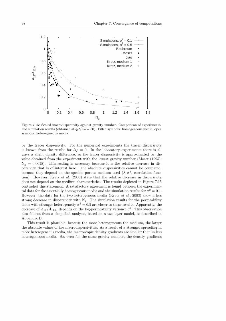
98 Chapter 7. Convergence of computations
0
0.2
0.4
0.6
0.8
1
1.2
0 0.2 0.4 0.6 0.8 1 1.2 1.4 1.6 1.8
A11
/A11
,tr
Ng
Simulations, σ2 = 0.1Simulations, σ2 = 0.5
BouhroumMoser
JiaoKretz, medium 1Kretz, medium 2
Figure 7.15: Scaled macrodispersivity against gravity number. Comparison of experimentaland simulation results (obtained at q0t/nλ = 80). Filled symbols: homogeneous media; opensymbols: heterogeneous media.
by the tracer dispersivity. For the numerical experiments the tracer dispersivityis known from the results for ∆ρ = 0. In the laboratory experiments there is al-ways a slight density difference, so the tracer dispersivity is approximated by thevalue obtained from the experiment with the lowest gravity number (Moser (1995):Ng = 0.0018). This scaling is necessary because it is the relative decrease in dis-persivity that is of interest here. The absolute dispersivities cannot be compared,because they depend on the specific porous medium used (λ, σ2, correlation func-tion). However, Kretz et al. (2003) state that the relative decrease in dispersivitydoes not depend on the medium characteristics. The results depicted in Figure 7.15contradict this statement. A satisfactory agreement is found between the experimen-tal data for the essentially homogeneous media and the simulation results for σ2 = 0.1.However, the data for the two heterogenous media (Kretz et al., 2003) show a lessstrong decrease in dispersivity with Ng. The simulation results for the permeabilityfields with stronger heterogeneity σ2 = 0.5 are closer to these results. Apparently, thedecrease of A11/A11,tr depends on the log-permeability variance σ2. This observationalso follows from a simplified analysis, based on a two-layer model, as described inAppendix B.
This result is plausible, because the more heterogeneous the medium, the largerthe absolute values of the macrodispersivities. As a result of a stronger spreading inmore heterogeneous media, the macroscopic density gradients are smaller than in lessheterogeneous media. So, even for the same gravity number, the density gradients

7.6 Conclusions 99
differ for different media. Therefore, the gravity effects in a medium with larger σ2
are relatively smaller. Apparently, even for the scaled dispersivity A11/A11,tr thisresults in a slower reduction with gravity number for larger σ2. The experimentalresults of Bouhroum (1989), Moser (1995), Jiao and Hotzl (2004), and the simulationresults for σ2 = 0.1 are alike because the tracer dispersivities are all in the order of amillimeter.
The fact that the macrodispersivity is a function of the gravity number, and thusof fluid and flow parameters, is in contradiction with the basic premise of traditionaldispersion theory that considers dispersivity to be a property of the porous mediumonly. The linear dispersion model, using a fixed dispersivity, can only model the nu-merical and laboratory experiments for the tracer case, i.e. when ∆ρ = 0. Whenhigh density gradients are present, this approach is no longer adequate (this workHassanizadeh and Leijnse, 1995; Schotting et al., 1999; Anderson, 1997). An alterna-tive approach is proposed by Hassanizadeh (1990; 1995), who introduces a nonlineardispersion equation. This equation contains an additional parameter (besides theclassical tracer dispersivity), with which experiments for any density contrast canbe modelled. In Chapter 8, the numerical results will be compared to predictionswith Hassanizadeh’s model, as well as with two other recently developed nonlineardispersion models.
7.6 Conclusions
The test cases show that stabilizing gravity forces are responsible for the reductionin the transition zone width between brine and fresh water during column displace-ment experiments. The effect of density gradients through fluid volume changes isvery small, which is in accordance with the findings in Chapter 3. Concentrationprofiles, obtained by averaging the local concentrations over horizontal lines, becomesteeper as the density contrast between the fluids increases. The parameter that con-trols the relative strength of the density effect as opposed to forced convection is thegravity number Ng = Ra/Pe. In the limit of large Ng, gravity forces eliminate allperturbations in the front that are caused by local velocity variations. The front thenbehaves as if it is travelling through a homogeneous medium, where the only mecha-nism of spreading is molecular diffusion, or (in the case of the numerical experiments)microscale dispersion.
In heterogeneous media, the local fluctuations in concentration decrease in sizewith increasing gravity number. This behavior is similar to what is found for anincrease in the microscale dispersivity (Dagan and Fiori, 1997). Like microscaletransversal dispersion, the gravity forces counteract horizontal concentration/densitygradients. The variance in the averaged concentration (of a single realization withrespect to the ensemble mean concentration) also becomes smaller for higher densitycontrasts. As a result, in the case of high density differences fewer realizations areneeded to reach ensemble convergence.
For the tracer case, reasonably good agreement is found between dispersivitiesobtained from the computed ensemble averaged profiles and the analytical result of
100 Chapter 7. Convergence of computations
Hsu (2003), when a time-average of the dispersivity is compared. The time-dependentdispersivity obtained using the second central moments fluctuates around Hsu’s ana-lytical solution.
The simulations for the log-permeability variance of σ2 = 0.1 resemble the behav-ior observed in essentially homogeneous porous media. The decrease of the scaledmacrodispersivity with gravity number is found to be in satisfactory agreement withthe experimental results of Bouhroum (1989) and Moser (1995). However, the rela-tion between the scaled macrodispersivity and the gravity number depends on themagnitude of the heterogeneity, i.e. on σ2.
A thorough investigation was performed to ensure that the numerical and sta-tistical uncertainties in the results are small and of the same order. The computedprofiles can be used to test the validity of nonlinear dispersion models applicable forhigh-concentration-gradient dispersion.
Chapter 8
High-concentration-gradient
dispersion: comparison with
nonlinear theories
8.1 Introduction
The results of the high-resolution numerical experiments described in Chapter 7—interms of ensemble averaged concentration profiles—are compared to results of threedifferent nonlinear macroscopic dispersion models. The objective of this chapter isto compare the predictive capacity of these nonlinear models, and to discuss theirapplicability and limitations.
The first model is the nonlinear model of Hassanizadeh (1990; 1995), also discussedin Chapter 6. This model has been tested against various laboratory experiments inessentially homogeneous media, whereas the numerical simulations are performed inheterogeneous media. However, the two-dimensional media used in the numericalexperiments are only weakly heterogeneous, characterized by small values of the log-permeability variance σ2 and the correlation scale λ. The results in Chapter 7 showthat the numerical experiments are comparable to the laboratory experiments in ho-mogeneous porous columns, in the sense that the observed dispersivities are of thesame order, and show a similar decrease with increasing strength of the density effect.Therefore, we expect that the nonlinear model of Hassanizadeh (1990; 1995) can beapplied here as well. As opposed to the laboratory experiments, the numerical experi-ments produce concentration data at many time instants, and in addition, informationabout the concentration variances. Results are obtained for a range of density con-trasts and various fixed mean flow rates, so that the relation between Hassanizadeh’snonlinear dispersion parameter β and these variables can be established.
The second and third dispersion models are based on the application of homo-genization theory by Egorov and Demidov, respectively. Egorov et al. (2005) havepublished results for the case of a layered medium. The work discussed here is yetunpublished. Egorov starts from the same balance equations at the local scale asare solved in the numerical simulations. With homogenization (a mathematical up-scaling technique), a macroscopic model is derived. Predictions based on this modelare compared to the ensemble averaged concentration profiles. The homogenization
101
102 Chapter 8. Nonlinear theories
approach is in many ways similar to the stochastic approach of Welty and Gelhar(1991), and leads—with the same assumptions—to the same result. However, Weltyand Gelhar (1991) study a three-dimensional porous medium with a different typeof correlation function, and their model therefore is not directly comparable to thenumerical experiments. Moreover, the homogenization approach of Egorov yields anexpression for the concentration variance, which can be compared to the variancesobtained in the numerical experiments. In this chapter the main steps in the homo-genization procedure are explained, while details of the derivation and solution of theso-called cell problem are given in Appendix D.
Finally, Demidov applies the homogenization approach to density-dependent flowat the pore scale level, considering Stokes flow around micro-heterogeneities. Demi-dov’s analysis leads to results that are comparable to the experiments in essentially ho-mogeneous porous media. Since the numerical simulations for σ2 = 0.1 show enoughsimilarity to these type of laboratory experiments, a comparison with Demidov’smodel predictions is also made.
8.2 The nonlinear model of Hassanizadeh
8.2.1 Model implementation
In this section, predictions based on Hassanizadeh’s nonlinear model are used forcomparison with the ensemble averaged concentration profiles of the numerical exper-iments described in Chapter 7. On the averaged (macroscopic) scale, the flow systemis one-dimensional. The governing equations in a non-deformable porous medium aregiven by the fluid mass balance
n∂ρ
∂t+
∂
∂z(ρq) = 0, (8.1)
and the salt mass balance
n∂ρω
∂t+
∂
∂z(ρωq + J) = 0, (8.2)
where, following Hassanizadeh and Leijnse (1995), the dispersive mass flux J is givenby the one-dimensional version of equation (6.7):
(1 + β|J |) J = −ρD∂ω
∂z. (8.3)
In the above equations, n denotes the porosity (assumed constant), t denotes time,ρ denotes the fluid density, and q denotes the specific discharge in the z-direction(positive pointing upward). The dispersion coefficient is given by
D = Dm + αtr|q|, (8.4)
in which Dm = ndmol is the effective porous medium molecular diffusivity, |q| is themagnitude of the specific discharge, and αtr is the longitudinal tracer dispersivity.
8.2 The nonlinear model of Hassanizadeh 103
The parameter β is an additional dispersion parameter. Finally, the equation of staterelates the fluid density to the mass fraction of dissolved salt, by
ρ = ρf eγρω, (8.5)
where ρf is the density of fresh water, and γρ = 0.692 is a curve fitting constant. Withthe exponential form of the equation of state, the mass fraction in equations (8.2) and(8.3) can be eliminated conveniently using the fluid mass balance (8.1), yielding
n∂ρ
∂t+ q
∂ρ
∂z+ γρ
∂J
∂z= 0, (8.6)
and
J (1 + β|J |) = −D1
γρ
∂ρ
∂z. (8.7)
Next, the density is scaled using
% =ρ− ρf
ρs − ρf, (8.8)
where ρs denotes the salt water (brine) density. Note that we use a different symbol forthe scaled density, in order to make a clear distinction with the dimensional density.Finally, the salt mass balance (8.6) reads
nε∂%
∂t+ εq
∂%
∂z+
γρ
ρf
∂J
∂z= 0, (8.9)
where the parameter ε denotes the relative density difference
ε =ρs − ρf
ρf. (8.10)
Second order equation (8.7) can be solved for the dispersive mass flux J . For stabledisplacements, i.e. J > 0, the root of (8.7) is given by
J =−1 +
√
1− P ∂%∂z
2β, (8.11)
with P = 4βDερf/γρ. Combining the salt mass balance (8.6), and the fluid massbalance (8.1), results in the following differential equation for q:
∂q
∂z=
γρ
(ερ + 1) ρf
∂J
∂z. (8.12)
The nonlinear system given by equations (8.9), (8.11), and (8.12) cannot be solvedanalytically, unless some simplifying assumptions are made (see Schotting et al., 1999).
104 Chapter 8. Nonlinear theories
Therefore, the system is solved numerically using an explicit finite difference scheme.The boundary conditions are
q = q0 at z = H, (8.13)
% =
{
0 at z = H,
1 at z = 0.(8.14)
The flow is in upward direction, i.e. q0 > 0. The constant velocity boundary conditionis chosen at the end z = H rather than at the start of the domain z = 0, to be inaccordance with the boundary conditions of the numerical experiments, as given inChapter 7. However, the height H is chosen to be 1.5 times the height of the columnin the numerical experiments. The step function in the initial density distributionis approximated by a steep error function, which is centered far enough from theinlet boundary in order to avoid boundary effects. Moreover, it is verified that thesteepness of the initial profile is large enough, i.e. a further increase of the steepnessdoes not significantly affect the computed profiles.
For the explicit finite difference scheme, stability criteria can be derived. For thetime step size ∆t it follows that the scheme is stable if
∆t ≤ 1
2
(∆z)2√
1− P ∂%∂z
D/n, (8.15)
where ∆z is the distance between grid points. This condition very much resembles thestability criterion for the diffusion equation based on the Fourier number. In termsof a modified Fourier number Foβ , this criterion reads
Foβ =D∆t/n
(∆z)2√
1− P ∂%∂z
≤ 1
2. (8.16)
Thus, the standard Fourier number is divided by a factor√
1− P ∂%∂z . A similar
stability criterion can be derived for the spatial discretization size:
∆z ≤ 2D
q√
1− P ∂%∂z
, (8.17)
or, in terms of a modified Peclet number
Peβ =q∆z
√
1− P ∂%∂z
D≤ 2. (8.18)
This means that the Peclet number is multiplied by a factor√
1− P ∂%∂z .
The density gradient in the stable case is always negative, so that the multipli-cation factor is always larger than one. The factor increases with β, and with the
8.2 The nonlinear model of Hassanizadeh 105
magnitude of the density gradient. Necessarily, the grid size ∆z for the nonlinearmodel is smaller than that in the case of a linear convection-diffusion equation. Asa result, also the time step size is more restricted. For the results presented in thenext section, it is verified that a further decrease of the time step and grid sizes hasno significant effect on the computed density profiles.
The optimal value of the parameter β is determined using an iterative procedure.First, an estimate of the fitting parameter β is used to compute J and q from the initialdensity profile, solving equations (8.11) and (8.12) in discretized form. The solutionsare used in the transport equation (8.9), to compute the density distribution at thenext time instant. Next, the new values of J and q are computed and subsequentlyused to calculate %. This process is repeated until the desired experimental time isreached. The maximum gradient in the computed density profile is then compared tothe maximum gradient in the experimental profile. The value of β is then increasedor decreased by a certain value and the process is repeated starting from t = 0. Fromthe third iteration, the estimation of the new β is based on Newton’s method andconverges rapidly.
An alternative approach is to perform a least-squares fitting based on the completeprofile rather than only matching the maximum slope. However, although comparedat the same time instant, the experimental and computed profiles may be slightlyshifted with respect to one another. This is because the exact position of the frontdepends slightly on the density gradient, and as a result also on β itself. Because theBoussinesq approximation is not adopted, i.e. ∇· q 6= 0, the specific discharge is notuniform, but increases locally at the front. See for an analysis of this volume effectfor one-dimensional flow the papers by Duijn et al. (1998) and Duijn and Schotting(1998), and Chapters 3–5 of this thesis. It is the shape and maximum slope of theprofile that is of main interest, rather than its exact position. Therefore, the maximumslope fitting is preferred, which is independent of the exact position of the profile.
Finally, note that the profiles in the numerical experiments are computed in termsof a scaled mass fraction ω/ωs (referred to as concentration), instead of the scaleddensity %, see Chapter 7. For small enough mass fractions (ρs ≤ 1025 kg/m3), the twoare identical because the relation between the density and the mass fraction is almostlinear, i.e. ρ = ρfe
γρω ≈ ρf (1 + γρω). However, for larger densities there is a slightdifference between the two scaled variables. Therefore, the experimental profiles areconverted to scaled density profiles before comparison with the nonlinear model. Formore details and a comparison of the scaling of the mass fraction ω, concentration C,and density ρ, see Appendix C.
8.2.2 Results
Density profiles computed with the nonlinear model of Hassanizadeh are comparedto the numerical experiments. The solutions of the nonlinear model depend on fourparameters: the density difference ε (= ∆ρ/ρf), the mean specific discharge q0, thetracer dispersivity αtr, and the nonlinear dispersion parameter β. The three param-eters that vary in the numerical experiments are: ∆ρ, q0, and the log-permeabilityvariance σ2. The latter—a measure of the magnitude of the permeability variations—
106 Chapter 8. Nonlinear theories
determines the model parameter αtr.Based on fitting the nonlinear model to the experiments of Moser (1995), Schotting
et al. (1999) conclude that the nonlinear dispersion parameter β is only dependent onthe flow rate, and not on the density difference. This means that, for a certain mediumand flow rate, experiments with different density contrasts can be described using thesame value of β. Watson et al. (2002b) conclude that β decreases with increasingdensity and viscosity contrasts, although it is unclear on which result this conclusionis based. Furthermore, they show that β varies slightly between the different types ofsand used.
By fitting the nonlinear model to the various numerical experiments, the depen-dency of β on ∆ρ (or ε), on q0, and on σ2 (or αtr) is investigated. Furthermore,using density profiles obtained at different experimental times, the dependence of βon travel-time (or corresponding distance) is investigated. This time-dependency hasnot been studied before: both Schotting et al. (1999) and Watson et al. (2002b) usesolely the concentration profiles measured at the end of the column to determine β.
The best-fit values of β can be extremely sensitive to a change in the desiredmaximum slope of the density profile. This sensitivity is discussed first, and it is usedto estimate the uncertainties in the β values.
8.2.2.1 Uncertainty in β
Running the model for a certain set of parameters (ε, q0, and αtr) with an increasedvalue of β, always results in steeper density profiles. This can be explained lookingat the dispersive mass flux. The effect of the nonlinear term in equation (8.3) isto decrease the dispersive flux, with respect to the flux given by linear Fick’s law.According to expression (8.11), the dispersive mass flux J for a certain gradientdecreases with increasing β. In particular, when −P ∂%
∂z � 1, the flux decreases with
the square root of β, i. e. J ∼ β−1/2. A decrease in the dispersive flux has a slowingeffect on the smearing of the density profiles, so that the profiles remain steeper.
The value of β is adjusted until the maximum gradient of the computed densityprofile matches that of the experimental profile. Using the value of the last twoiterations, the sensitivity of β to the maximum density gradient is determined. Thissensitivity largely increases with decreasing density contrast. For small ∆ρ, a smallchange in the desired slope of the profile results in a large variation in β. In otherwords, a change in β has little effect on the computed density gradient. This createsan uncertainty in the β-fitting procedure.
Figure 8.1 presents the sensitivity of β with respect to a variation in the maximumgradient γmax. Here, γ is a dimensionless density gradient, defined as
γ = −g k0π4 λ2 ∆ρ
µα⊥ q0
∂%
∂z, (8.19)
where g is the acceleration of gravity, k0 the average permeability, µ the fluid viscosity,and α⊥ the local transversal dispersivity. Note that % in expression (8.19) is the scaleddensity, whereas the other parameters are dimensional. The dimensionless densitygradient γ is introduced here, because it is the main parameter in the homogenization
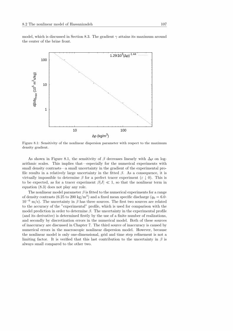
8.2 The nonlinear model of Hassanizadeh 107
model, which is discussed in Section 8.3. The gradient γ attains its maximum aroundthe center of the brine front.
1
10
100
10 100
dβ/d
γ max
(10
5 m2 s/
kg)
∆ρ (kg/m3)
1.29⋅103(∆ρ)-1.44
Figure 8.1: Sensitivity of the nonlinear dispersion parameter with respect to the maximumdensity gradient.
As shown in Figure 8.1, the sensitivity of β decreases linearly with ∆ρ on log-arithmic scales. This implies that—especially for the numerical experiments withsmall density contrasts—a small uncertainty in the gradient of the experimental pro-file results in a relatively large uncertainty in the fitted β. As a consequence, it isvirtually impossible to determine β for a perfect tracer experiment (ε ↓ 0). This isto be expected, as for a tracer experiment β|J | � 1, so that the nonlinear term inequation (8.3) does not play any role.
The nonlinear model parameter β is fitted to the numerical experiments for a rangeof density contrasts (6.25 to 200 kg/m3) and a fixed mean specific discharge (q0 = 6.0·10−6 m/s). The uncertainty in β has three sources. The first two sources are relatedto the accuracy of the ”experimental” profile, which is used for comparison with themodel prediction in order to determine β. The uncertainty in the experimental profile(and its derivative) is determined firstly by the use of a finite number of realizations,and secondly by discretization errors in the numerical model. Both of these sourcesof inaccuracy are discussed in Chapter 7. The third source of inaccuracy is caused bynumerical errors in the macroscopic nonlinear dispersion model. However, becausethe nonlinear model is only one-dimensional, grid and time step refinement is not alimiting factor. It is verified that this last contribution to the uncertainty in β isalways small compared to the other two.
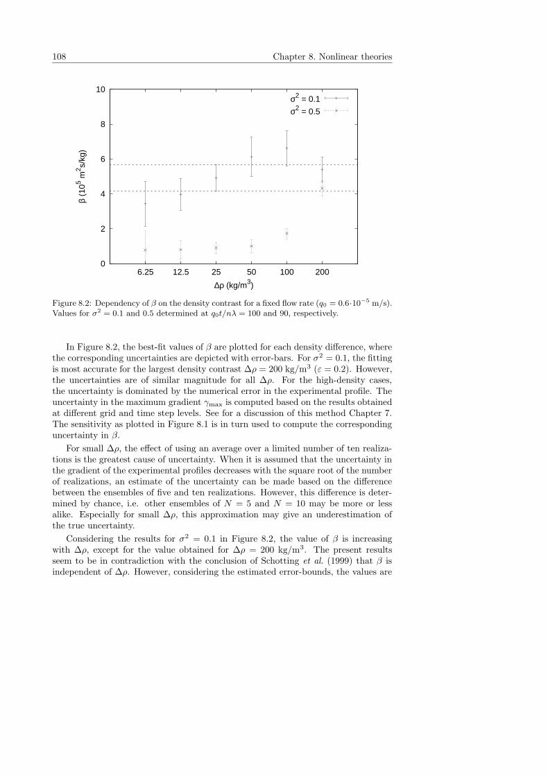
108 Chapter 8. Nonlinear theories
0
2
4
6
8
10
200100502512.56.25
β (1
05 m2 s/
kg)
∆ρ (kg/m3)
σ2 = 0.1
σ2 = 0.5
Figure 8.2: Dependency of β on the density contrast for a fixed flow rate (q0 = 0.6·10−5 m/s).Values for σ2 = 0.1 and 0.5 determined at q0t/nλ = 100 and 90, respectively.
In Figure 8.2, the best-fit values of β are plotted for each density difference, wherethe corresponding uncertainties are depicted with error-bars. For σ2 = 0.1, the fittingis most accurate for the largest density contrast ∆ρ = 200 kg/m3 (ε = 0.2). However,the uncertainties are of similar magnitude for all ∆ρ. For the high-density cases,the uncertainty is dominated by the numerical error in the experimental profile. Theuncertainty in the maximum gradient γmax is computed based on the results obtainedat different grid and time step levels. See for a discussion of this method Chapter 7.The sensitivity as plotted in Figure 8.1 is in turn used to compute the correspondinguncertainty in β.
For small ∆ρ, the effect of using an average over a limited number of ten realiza-tions is the greatest cause of uncertainty. When it is assumed that the uncertainty inthe gradient of the experimental profiles decreases with the square root of the numberof realizations, an estimate of the uncertainty can be made based on the differencebetween the ensembles of five and ten realizations. However, this difference is deter-mined by chance, i.e. other ensembles of N = 5 and N = 10 may be more or lessalike. Especially for small ∆ρ, this approximation may give an underestimation ofthe true uncertainty.
Considering the results for σ2 = 0.1 in Figure 8.2, the value of β is increasingwith ∆ρ, except for the value obtained for ∆ρ = 200 kg/m3. The present resultsseem to be in contradiction with the conclusion of Schotting et al. (1999) that β isindependent of ∆ρ. However, considering the estimated error-bounds, the values are
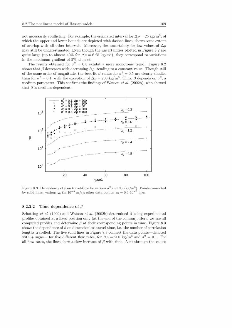
8.2 The nonlinear model of Hassanizadeh 109
not necessarily conflicting. For example, the estimated interval for ∆ρ = 25 kg/m3, ofwhich the upper and lower bounds are depicted with dashed lines, shows some extentof overlap with all other intervals. Moreover, the uncertainty for low values of ∆ρmay still be underestimated. Even though the uncertainties plotted in Figure 8.2 arequite large (up to almost 40% for ∆ρ = 6.25 kg/m3), they correspond to variationsin the maximum gradient of 5% at most.
The results obtained for σ2 = 0.5 exhibit a more monotonic trend. Figure 8.2shows that β decreases with decreasing ∆ρ, tending to a constant value. Though stillof the same order of magnitude, the best-fit β values for σ2 = 0.5 are clearly smallerthan for σ2 = 0.1, with the exception of ∆ρ = 200 kg/m3. Thus, β depends on σ2, amedium parameter. This confirms the findings of Watson et al. (2002b), who showedthat β is medium-dependent.
106
105
104
103
20 40 60 80 100q0t/nλ
β
q0 = 0.3
q0 = 0.6
q0 = 1.2
q0 = 2.4
q0 = 4.8
σ2 = 0.1, ∆ρ = 200σ2 = 0.1, ∆ρ = 100σ2 = 0.1, ∆ρ = 50σ2 = 0.5, ∆ρ = 200σ2 = 0.5, ∆ρ = 100
Figure 8.3: Dependency of β on travel-time for various σ2 and ∆ρ (kg/m3). Points connectedby solid lines: various q0 (in 10−5 m/s); other data points: q0 = 0.6·10−5 m/s.
8.2.2.2 Time-dependence of β
Schotting et al. (1999) and Watson et al. (2002b) determined β using experimentalprofiles obtained at a fixed position only (at the end of the column). Here, we use allcomputed profiles and determine β at their corresponding points in time. Figure 8.3shows the dependence of β on dimensionless travel-time, i.e. the number of correlationlengths travelled. The five solid lines in Figure 8.3 connect the data points—denotedwith + signs— for five different flow rates, for ∆ρ = 200 kg/m3 and σ2 = 0.1. Forall flow rates, the lines show a slow increase of β with time. A fit through the values
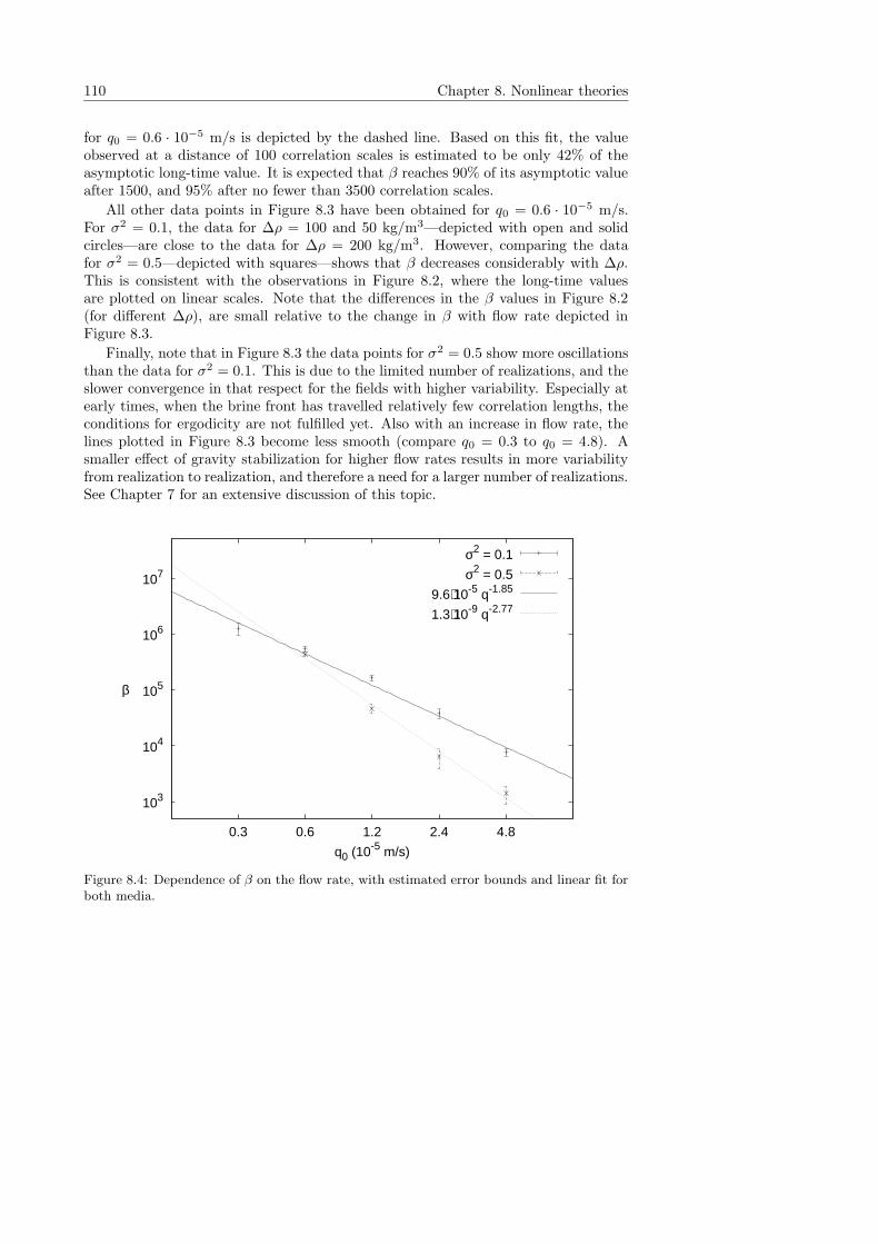
110 Chapter 8. Nonlinear theories
for q0 = 0.6 · 10−5 m/s is depicted by the dashed line. Based on this fit, the valueobserved at a distance of 100 correlation scales is estimated to be only 42% of theasymptotic long-time value. It is expected that β reaches 90% of its asymptotic valueafter 1500, and 95% after no fewer than 3500 correlation scales.
All other data points in Figure 8.3 have been obtained for q0 = 0.6 · 10−5 m/s.For σ2 = 0.1, the data for ∆ρ = 100 and 50 kg/m3—depicted with open and solidcircles—are close to the data for ∆ρ = 200 kg/m3. However, comparing the datafor σ2 = 0.5—depicted with squares—shows that β decreases considerably with ∆ρ.This is consistent with the observations in Figure 8.2, where the long-time valuesare plotted on linear scales. Note that the differences in the β values in Figure 8.2(for different ∆ρ), are small relative to the change in β with flow rate depicted inFigure 8.3.
Finally, note that in Figure 8.3 the data points for σ2 = 0.5 show more oscillationsthan the data for σ2 = 0.1. This is due to the limited number of realizations, and theslower convergence in that respect for the fields with higher variability. Especially atearly times, when the brine front has travelled relatively few correlation lengths, theconditions for ergodicity are not fulfilled yet. Also with an increase in flow rate, thelines plotted in Figure 8.3 become less smooth (compare q0 = 0.3 to q0 = 4.8). Asmaller effect of gravity stabilization for higher flow rates results in more variabilityfrom realization to realization, and therefore a need for a larger number of realizations.See Chapter 7 for an extensive discussion of this topic.
107
106
105
104
103
4.82.41.20.60.3
q0 (10-5 m/s)
β
σ2 = 0.1
σ2 = 0.5
9.6⋅10-5 q-1.85
1.3⋅10-9 q-2.77
Figure 8.4: Dependence of β on the flow rate, with estimated error bounds and linear fit forboth media.
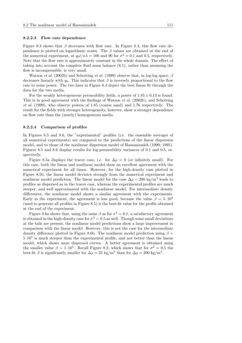
8.2 The nonlinear model of Hassanizadeh 111
8.2.2.3 Flow rate dependence
Figure 8.3 shows that β decreases with flow rate. In Figure 8.4, this flow rate de-pendence is plotted on logarithmic scales. The β values are obtained at the end ofthe numerical experiment, at q0t/nλ = 100 and 90 for σ2 = 0.1 and 0.5, respectively.Note that the flow rate is approximately constant in the whole domain. The effect oftaking into account the complete fluid mass balance (8.1), rather than assuming theflow is incompressible, is very small.
Watson et al. (2002b) and Schotting et al. (1999) observe that, in log-log space, βdecreases linearly with q0. This indicates that β is inversely proportional to the flowrate to some power. The two lines in Figure 8.4 depict the best linear fit through thedata for the two media.
For the weakly heterogeneous permeability fields, a power of 1.85± 0.13 is found.This is in good agreement with the findings of Watson et al. (2002b), and Schottinget al. (1999), who observe powers of 1.85 (coarse sand) and 1.76 respectively. Theresult for the fields with stronger heterogeneity, however, show a stronger dependenceon flow rate than the (nearly) homogeneous media.
8.2.2.4 Comparison of profiles
In Figures 8.5 and 8.6, the ”experimental” profiles (i.e. the ensemble averages ofall numerical experiments) are compared to the predictions of the linear dispersionmodel, and to those of the nonlinear dispersion model of Hassanizadeh (1990; 1995).Figures 8.5 and 8.6 display results for log-permeability variances of 0.1 and 0.5, re-spectively.
Figure 8.5a displays the tracer case, i.e. for ∆ρ = 0 (or infinitely small). Forthis case, both the linear and nonlinear model show an excellent agreement with thenumerical experiment for all times. However, for the high-density case plotted inFigure 8.5b, the linear model deviates strongly from the numerical experiment andnonlinear model prediction. The linear model for the case ∆ρ = 200 kg/m3 leads toprofiles as dispersed as in the tracer case, whereas the experimental profiles are muchsteeper, and well approximated with the nonlinear model. For intermediate densitydifferences, the nonlinear model shows a similar agreement with the experiments.Early in the experiment, the agreement is less good, because the value β = 5 ·105
(used to generate all profiles in Figure 8.5) is the best-fit value for the profile obtainedat the end of the experiment.
Figure 8.6a shows that, using the same β as for σ2 = 0.1, a satisfactory agreementis obtained in the high-density case for σ2 = 0.5 as well. Though some small deviationsat the tails are present, the nonlinear model predictions show a large improvement incomparison with the linear model. However, this is not the case for the intermediatedensity difference plotted in Figure 8.6b. The nonlinear model prediction using β =5 ·105 is much steeper than the experimental profile, and not better than the linearmodel, which shows more dispersed curves. A better agreement is obtained usingthe smaller value β = 1 ·105. Recall Figure 8.2, which shows that for σ2 = 0.5 thebest-fit β is significantly smaller for ∆ρ = 25 kg/m3 than for ∆ρ = 200 kg/m3.

112 Chapter 8. Nonlinear theories
0
0.2
0.4
0.6
0.8
1
0 20 40 60 80 100 120q0t/nλ
(a) ∆ρ = 0
ExperimentLinear
Nonlinear
PSfrag
replacem
ents
%
0
0.2
0.4
0.6
0.8
1
0 20 40 60 80 100 120q0t/nλ
(b) ∆ρ = 200 kg/m3
ExperimentLinear
Nonlinear
PSfrag
replacem
ents
%
Figure 8.5: Density profiles of the numerical experiment for σ2 = 0.1, q0 = 0.6 ·10−5 m/s,with linear and nonlinear model predictions. (a) tracer case; (b) high-density case.
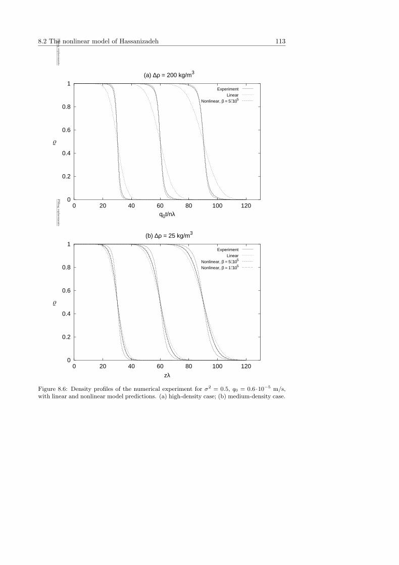
8.2 The nonlinear model of Hassanizadeh 113
0
0.2
0.4
0.6
0.8
1
0 20 40 60 80 100 120q0t/nλ
(a) ∆ρ = 200 kg/m3
ExperimentLinear
Nonlinear, β = 5⋅ 105
PSfrag
replacem
ents
%
0
0.2
0.4
0.6
0.8
1
0 20 40 60 80 100 120
zλ
(b) ∆ρ = 25 kg/m3
ExperimentLinear
Nonlinear, β = 5⋅ 105
Nonlinear, β = 1⋅ 105
PSfrag
replacem
ents
%
Figure 8.6: Density profiles of the numerical experiment for σ2 = 0.5, q0 = 0.6 ·10−5 m/s,with linear and nonlinear model predictions. (a) high-density case; (b) medium-density case.
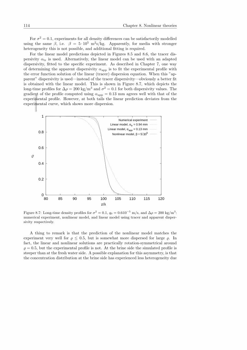
114 Chapter 8. Nonlinear theories
For σ2 = 0.1, experiments for all density differences can be satisfactorily modelledusing the same β, i.e. β = 5 · 105 m2s/kg. Apparently, for media with strongerheterogeneity this is not possible, and additional fitting is required.
For the linear model predictions depicted in Figures 8.5 and 8.6, the tracer dis-persivity αtr is used. Alternatively, the linear model can be used with an adapteddispersivity, fitted to the specific experiment. As described in Chapter 7, one wayof determining the apparent dispersivity αapp is to fit the experimental profile withthe error function solution of the linear (tracer) dispersion equation. When this ”ap-parent” dispersivity is used—instead of the tracer dispersivity—obviously a better fitis obtained with the linear model. This is shown in Figure 8.7, which depicts thelong-time profiles for ∆ρ = 200 kg/m3 and σ2 = 0.1 for both dispersivity values. Thegradient of the profile computed using αapp = 0.13 mm agrees well with that of theexperimental profile. However, at both tails the linear prediction deviates from theexperimental curve, which shows more dispersion.
0
0.2
0.4
0.6
0.8
1
80 85 90 95 100 105 110 115 120
z/λ
Numerical experiment
Linear model, αtr = 0.94 mm
Linear model, αapp = 0.13 mm
Nonlinear model, β = 5⋅ 105
PSfrag
replacem
ents
%
Figure 8.7: Long-time density profiles for σ2 = 0.1, q0 = 0.6·10−5 m/s, and ∆ρ = 200 kg/m3:numerical experiment, nonlinear model, and linear model using tracer and apparent disper-sivity respectively.
A thing to remark is that the prediction of the nonlinear model matches theexperiment very well for % ≤ 0.5, but is somewhat more dispersed for large %. Infact, the linear and nonlinear solutions are practically rotation-symmetrical around% = 0.5, but the experimental profile is not. At the brine side the simulated profile issteeper than at the fresh water side. A possible explanation for this asymmetry, is thatthe concentration distribution at the brine side has experienced less heterogeneity due
8.3 Homogenization model of Egorov 115
to the smaller travel-time (fewer correlation scales). In addition, stabilizing densityeffects, which inhibit dispersion, are stronger for higher concentrations.
8.2.3 Conclusions
• For nearly homogeneous media, i.e. σ2 = 0.1, the present results confirm twoimportant findings of Hassanizadeh and Leijnse (1995), Schotting et al. (1999),and Watson et al. (2002b):
1. With one value of β, the nonlinear model of Hassanizadeh (1990; 1995) isable to predict the experiments for different density contrasts (for a fixedflow rate).
2. β is inversely proportional to the flow rate to a power close to two.
• Within the time range of the numerical experiments, the best-fit value of β doesnot reach an asymptotic value, but increases slowly with time.
• For σ2 = 0.5, experiments for the whole range of density contrasts cannotbe modelled adequately using the same value of β. In addition, a strongerdependence of β on the flow rate is found.
• Therefore, the nonlinear model of Hassanizadeh (1990; 1995) is most suitablefor essentially homogeneous media, i.e. for small σ2.
• The value of the nonlinear parameter β depends not only on the flow rate, butalso on travel time, on medium characteristics (σ2), and possibly on the densitycontrast. As the value of β is not known beforehand, a fitting procedure isrequired. In this respect it has little advantage over the linear model, exceptthat a better fit with experimental results is obtained.
8.3 Homogenization model of Egorov
In this section, the homogenization model of Egorov1 is discussed and its predictionsare compared to the numerical experiments. Homogenization theory is applied to thecase of brine dispersion in weakly heterogeneous porous media. Starting with the localscale equations in two dimensions, a one-dimensional macroscopic model is derived.In this section, the main steps in the homogenization procedure are discussed and thefinal results are given: a macroscopic balance equation and a relation between thedispersive mass flux and the density gradient. Next, this macroscopic model is usedto predict the concentration profiles of the numerical experiments. Comparisons aremade for various ∆ρ and q0 values, and for media with log-permeability variancesσ2 = 0.1 and 0.5.
1This work of Andrey Egorov, Kazan State University, is part of an article in preparation by A.J.Landman, A.Egorov, and R.J. Schotting.
116 Chapter 8. Nonlinear theories
8.3.1 Derivation of the macroscale model
8.3.1.1 Problem definition
The problem of brine displacing fresh water in a two-dimensional non-deformableporous medium is considered, where the mean flow is in vertical direction. As in thenumerical experiments, it is assumed that the flow can be described by Darcy’s law,and the microscale dispersion by the classical linear relation (Fick’s law). In addition,the Boussinesq approximation is adopted, yielding for the fluid mass balance
∇· q = 0, (8.20)
where q is the specific discharge or Darcy velocity vector, with components q1 andq2 in vertical and horizontal direction respectively. With the use of the exponentialequation of state (8.5), the salt mass balance written in terms of the density is givenby
n∂ρ
∂t+ q ·∇ρ = d‖
∂2ρ
∂x21
+ d⊥∂2ρ
∂x22
, (8.21)
where x1 and x2 are the two spatial coordinates in vertical and horizontal directionrespectively. On the right-hand side, d‖ and d⊥ denote the longitudinal and transver-sal components of the microscale dispersion tensor respectively. It is convenient touse the rotation of Darcy’s law
∂
∂x2
(µq1
k+ ρg
)
=∂
∂x1
(µq2
k
)
, (8.22)
where µ is the dynamic fluid viscosity, and k is the intrinsic permeability. It isassumed that n, µ, g, d‖, and d⊥ are given constants, while the permeability k isa function of spatial coordinates. Like in the numerical experiments, the effect ofviscosity variations is disregarded. With regard to the induced vorticity (rotationalflow), the viscosity effect is small compared to the density effect for small flow rates,see criterion (2.21) in Chapter 2. The dominance of the density effect is observed byWelty and Gelhar (1991), and also in the experiments of Krupp and Elrick (1969)and of Starr and Parlange (1976).
Permeability distributions in the field resemble log-normal distributions. There-fore, in stochastic subsurface hydrology, it is common to deal with log-permeabilityfields, see e.g. Dagan (1989) or Gelhar (1993). The permeability is represented as
k = k0 exp(σK), (8.23)
where k0 is the average permeability. It is assumed that σ is small and K(x) isan isotropic homogeneous random field with zero mean and unity variance. Thedimensionless log-permeability K is assumed to be spatially correlated, by definitionof a proper correlation function
R(h) = 〈K(x′)K(x′′)〉, h = |x′ − x′′|, (8.24)
8.3 Homogenization model of Egorov 117
where the angular brackets denote average quantities. Here, spatial averaging isapplied, which for stationary random fields—according to the principle of ergodicity—is equivalent to ensemble averaging over all possible realizations.
Generally, the term ∇· d∇ρ appears on the right-hand side of salt mass bal-ance equation (8.21), where the microscale dispersion tensor d, following Scheidegger(1961), reads
d = (ndmol + α⊥ |q|) I +(α‖ − α⊥
|q| . (8.25)
Here, α‖ and α⊥ are the microscale longitudinal and transversal dispersivities re-spectively, I is the unit tensor, and dmol is the molecular diffusion coefficient. Thedispersion tensor d in principle varies in space, due to the local fluctuations in thevelocity field. These fluctuations are proportional to the fluctuations in the perme-ability field, i.e. q1 = q0 + O(σ), and q2 = O(σ). Therefore, when σ is small, it canbe assumed that the microscale dispersion is proportional to the mean velocity q0,rather than to the local velocity. Then, the microscale dispersion can be described bythe right-hand side of equation (8.21), provided that d⊥ and d‖ are defined as
d⊥ = ndmol + α⊥ |q0| , d‖ = ndmol + α‖ |q0| . (8.26)
Equations (8.20)–(8.22) form a coupled system of equations, which need to be solvedsimultaneously in order to obtain the flow and density fields.
The vertical movement of an initially horizontal front between fresh water andbrine is considered. Therefore, it is assumed that the brine density, the mean verticalflow rate, and the mean transverse pressure derivative, attain constant values asx1 → ±∞:
x1 → ±∞ : ρ = ρ±, 〈q1〉 = q0,⟨e−σKq2
⟩= 0. (8.27)
Depending on the sign of ∆ρ = ρ− − ρ+, two completely different flow schemes arepossible. When ∆ρ < 0, the front is unstable, and gravitational fingering may occur.However, this study is restricted to the gravitationally stable case, in which freshwater is on top of the heavier brine, so that ∆ρ = ρs − ρf > 0.
8.3.1.2 Dimensionless variables
The main goal is to derive a macroscale balance equation, describing the long-timebehavior of the brine front. To start, all variables are rendered dimensionless, usingcharacteristic spatial and temporal scales. There are two spatial scales in the problem:the local scale and the macroscopic scale. The first is determined by the heterogeneitysize, a measure of the distance over which the permeability is correlated. The commonway to define this local scale is to use the integral scale
l =
∞∫
0
R(h) dh. (8.28)
Note that so far, the correlation scale λ has been used to characterize the size of theheterogeneities. The numerical model described in Chapter 7 uses the Gaussian cor-relation function R(r) = exp(−h2/λ2). In this definition, however, λ is not equivalent
118 Chapter 8. Nonlinear theories
with the integral scale l; their relation is given by l = λ√
π/2. In the homogenizationprocedure, l will be used as the ”microscale”. However, where comparisons with thenumerical experiments are made, the correlation scale λ is still used in order to beconsistent with the terminology of Section 8.2 and Chapter 7.
The second scale, i.e. the ”macroscale”, is given by the width L of the brine front.A basic assumption in this analysis is that the microscale and macroscale are ”wellseparated”, i.e. εx = l/L � 1 (see Lunati et al., 2002). This assumption is directlyrelated to the objective of describing the long-time behavior. The width of the frontincreases with time due to dispersive spreading, and therefore, at large enough timethe assumption εx � 1 is valid, independent of the width of the initial density profile.
Two spatial scales produce two types of dimensionless spatial coordinates,according to the general approach of the homogenization theory (see e.g. Bakhvalovand Panasenko, 1989; Sanchez-Palencia, 1980; Bensoussan et al., 1987). The firsttype, the so-called ”fast” coordinates, is related to the microscale while the secondtype, the ”slow” coordinates, is related to the macroscale. The macroscale process isone-dimensional, and only dependent on the slow coordinate. It is convenient to usea moving frame macroscale coordinate, introducing
x1 =x1
l, x2 =
x2
l, z =
x1 − q0t/n
L(8.29)
as the two fast coordinates and the slow coordinate respectively. The velocity anddensity fields will be considered as two-scale functions to investigate the transportproblem with a two-scale expansion technique.
There are two intrinsic characteristic time scales involved. Firstly, the time τv =nl/|q0|, during which the salt is transported convectively over the distance of oneintegral scale l. Secondly, the time τd = nl2/d⊥, during which the solute is spread bylocal transversal dispersion over the distance of one integral scale. The ratio betweenthe convective and the dispersive timescale defines the Peclet number
Pe⊥ =τd
τv=|q0|ld⊥
=l
α⊥. (8.30)
In most groundwater applications, the Peclet number is in the range of 102–104, andtherefore τd � τv. The long-time asymptotic behavior of the density front is reachedonly after large enough time compared to the (large) dispersive timescale. So, thedimensionless time is introduced as
t =t
tscale, tscale =
τd
εt, (8.31)
where εt � 1 is a small parameter.Finally, we introduce the dimensionless velocity and density as
q =q
|q0|, % =
ρ− ρf
ρs − ρf. (8.32)
Furthermore, the derivatives are substituted by
∂
∂x2=
1
l
∂
∂x2,
∂
∂x1=
1
l
(∂
∂x1+ εx
∂
∂z
)
,∂
∂t=
d⊥nl2
(
εt∂
∂t∓ Pe⊥εx
∂
∂z
)
, (8.33)
8.3 Homogenization model of Egorov 119
so that equations (8.20)–(8.22) and (8.27) are recast into
εt∂%
∂t− ∂2ρ
∂x22
− d
(∂
∂x1+ εx
∂
∂z
)2
% + Pe⊥q·∇% + Pe⊥εx(q1 ∓ 1)∂%
∂z= 0, (8.34)
∇· q + εx∂q1
∂z= 0, (8.35)
∂
∂x2
(q1e−σK + Ng%
)=
(∂
∂x1+ ε
∂
∂z
)
q2e−σK, (8.36)
z → ±∞ : % =
{
0
1,⟨e−σKq2
⟩= 0, 〈q1〉 = ±1. (8.37)
The sign + (−) corresponds to the flow direction, where positive is pointing upward.From now on, we continue to work in the scaled system, but drop the tilde notation.
In addition to the Peclet number (8.30), the scaling yields the dimensionless pa-rameters
d =d‖d⊥
, Ng =∆ρk0g
µ|q0|, (8.38)
where Ng denotes the gravity number. The correlation function R, as a result of thescaling, has the properties
R(0) = 1,
∫ ∞
0
R(h) dh = 1. (8.39)
Note that K is a function of the fast coordinates x only, whereas ρ and q dependon x, z, and t. All these functions are random processes in x-space. It is natural toclaim that at fixed z and t, the random fields ρ(x) and q(x) have the same propertyof translation invariancy as K. So, ρ(x) and q(x) are required to be homogeneousrandom fields as well.
The term with the gravity number Ng in equation (8.36) is responsible for thestabilizing gravity effect. This number ranges from zero for the tracer case, to severalunits for slow seepage of highly concentrated brines. Large values of Ng are exceptionsrather than the rule. For instance, even if ∆ρ = 102 kg/m3, Ng = 1, for the typicalvalues k0 = 10−11 m2, and |q0| = 10−5 m/s. Therefore, only the cases Ng � 1 (tracertransport), and Ng ∼ 1 are considered here.
8.3.1.3 Macroscale equations
For the brine transport problem under consideration, the macroscale equations arederived following the standard homogenization method, consisting of two steps. First,the macroscale salt mass balance equation is obtained. The corresponding equationhas the standard form of the convection-diffusion equation, and is written in termsof the average density 〈%〉 and the dispersive mass flux J , which are functions of thevertical coordinate z and time t only. The second step is based on the assumption ofweakly heterogeneous media, i.e. small σ. It consists of deriving with O(σ2) accuracy
120 Chapter 8. Nonlinear theories
the dependence of J on 〈%〉. This phenomenological relation is of great interest in thisanalysis. In addition, a relation is derived for the variance
σ2% =
⟨
(%− 〈%〉)2⟩
. (8.40)
Obtaining the macroscale balance equation is a trivial task. It is done simply byspatial averaging of equation (8.34) in the fast coordinate space. Using the property〈∇f〉 = 0, valid for any homogeneous random field f, with the equation of incompres-sibility of the flow (8.35), gives
εt∂ 〈%〉∂t
+ ε2x
∂J
∂z= 0, (8.41)
J =Pe⊥εx〈(q1 ∓ 1)(%− 〈%〉)〉 − d
∂ 〈%〉∂z
. (8.42)
Note that equation (8.41) does not contain a convective term, because we work in amoving frame coordinate system. Furthermore, another notation for the macroscopicbalance equation is used, which is derived from expression (8.41) by differentiation:
εt∂γ
∂t= ε2
x
∂2J
∂z2, (8.43)
J = dγ + Pe2⊥Ng 〈(q1 ∓ 1)(%− 〈%〉)〉 , (8.44)
in which γ denotes the dimensionless density gradient
γ = −εxPe⊥Ng∂ 〈%〉∂z
. (8.45)
Note that Pe⊥Ng = Ra, and that γ can be considered as a local Rayleigh number.Expression (8.45) is equivalent to (8.19), where the latter is written in the originalphysical variables.
Averaging of equations (8.35) and (8.36) yields
∂
∂z〈q1〉 = 0,
∂
∂z
⟨e−σKq2
⟩= 0. (8.46)
The boundary conditions (8.37) for q1 and q2 remain unaffected.The relation for the dispersive mass flux J , in terms of the density gradient γ,
can be found solving the so-called cell problem. The derivation of the cell problem isgiven in Appendix D.1. The solution of the cell problem is described in Appendix D.2.Here, only the final results are presented. The total dispersive mass flux is of the form
J = dγ + σ2Pe⊥I(γ), (8.47)
where the first term on the right-hand side is the microscale dispersive flux, while thesecond term describes macrodispersion. In the macrodispersive flux term, operatorI(γ) can be written as
I(γ) = I0(γ) + εtI1 + ε2xI2, (8.48)
8.3 Homogenization model of Egorov 121
where the second and third term on the right-hand side are the relaxation and inter-action term respectively, which will not be used in this thesis. Based on the smallnessof εt and εx, the simplest case is obtained where only the term I0 is retained. For the2-D Gaussian correlation function, in dimensionless variables
R(h) = e−πh2/4, (8.49)
the following explicit relation is obtained:
I0(γ) = γ(
1−√γeγ/π erfc√
γ/π)
. (8.50)
The dispersion coefficient is obtained by dividing the dispersive flux J by the gra-dient γ. In the original dimensional variables, the dispersion coefficient D can bewritten as
D = d‖ + lσ2|q0|D0(γ), (8.51)
where d‖ = ndmol + α‖|q0| is the microscale dispersion coefficient. The coefficientD0(γ) = I(γ)/γ multiplies the asymptotic dispersion coefficient for the tracer case,i.e. lσ2|q0|, and can be interpreted as a correction factor due to the stabilizing gravityeffect. Table 6.2 presents the results for this effective dispersion coefficient for theexponential and Gaussian correlation functions in two and three dimensions.
Finally, we present the expression for the concentration variance
σ2% =
σ2
Pe⊥Ng2 γ3/2eγ/π erfc
(√
γ/π)
, (8.52)
again for the case of the 2-D Gaussian correlation function. Note that the variance inexpression (8.52) is the variance of the scaled density. This variance will be directlycompared to the local ”concentration” variance σ2
c , determined from the numerical ex-periments as described in Chapter 7. The difference between the two scaled variablesis small, see Appendix C.
8.3.2 Comparison with numerical experiments
A comparison is made between the homogenization model for the 2-D Gaussian cor-relation function and the numerical experiments described in Chapter 7. The sim-plest macroscopic model is used, i.e. with the algebraic relation I = I0(γ). Thismodel will be referred to as the homogenization model of Egorov. It consists of themacroscale balance equation (8.43), the dispersive flux given by expression (8.47),and the phenomenological relation (8.50). This system of equations is solved nu-merically, in order to obtain the time evolution of γ(z, t). Subsequently, the densityprofiles are obtained by integration of γ. The system is solved in the dimension-less variables, with parameter values chosen to match the numerical experiments.Therefore, l = (
√π/2)λ = 0.886 cm,Pe⊥ = l/α⊥ = 88.6, and d = 1 (isotropic mi-
croscale dispersion). The gravity number Ng depends on the values of q0 and ∆ρin the specific experiment, according to expression (8.38), in which g = 9.81 m/s2,
122 Chapter 8. Nonlinear theories
µ = 1·10−3 kg/ms, and k0 = 5·10−12 m2. In the numerical experiments, Ng rangesfrom zero (tracer case) to 1.64.
As initial condition for γ a smooth profile is used, instead of taking a delta-function (corresponding to a step function in the density). The initial distribution iscomputed using an experimental density profile, taken at an early time correspondingto a travelled length of ten integral scales.
8.3.2.1 Density profiles
In Figures 8.8–8.10, density profiles computed with the homogenization model ofEgorov are compared to the numerical experiments, and to the predictions of the linearmodel. Figures 8.8 and 8.9 display results for σ2 = 0.1. Figures 8.8a and 8.8b show thecases of a relatively low and a high density contrast, where ∆ρ = 12.5 and 100 kg/m3
respectively. The homogenization model prediction in the latter case is very good,but shows deviations from the experimental results for ∆ρ = 12.5 kg/m3. However,the homogenization model in the low-density case is still better than the linear model.When the density difference is taken infinitely small, the dispersion coefficient in thehomogenization model effectively reduces to the tracer dispersion coefficient. Forthis case, the computed profiles coincide with the experimental profiles, exactly as inFigure 8.5a for Hassanizadeh’s nonlinear model.
Next, it is shown that the homogenization model of Egorov is able to predictthe experiments for different flow rates. Figure 8.9 shows the results for the largestdensity difference, ∆ρ = 200 kg/m3, and two different flow rates. In both cases, thehomogenization model generates good predictions of the experiments. The predictionsof the linear model, also depicted in Figure 8.9, are much more dispersed than theexperimental profiles.
Recall that with the nonlinear model of Hassanizadeh (1990; 1995), the valueof the nonlinear dispersion parameter β has to be adapted for different flow rates.No fitting nor additional parameter is necessary when the homogenization model ofEgorov is used.
The homogenization model is based on the assumption of a small log-permea-bility variance σ2. Figures 8.8 and 8.9 show a satisfactory agreement between themodel predictions and the numerical experiments for σ2 = 0.1. In Figure 8.10, themodel predictions are compared to the experimental results for σ2 = 0.5. For ∆ρ =200 kg/m3, the homogenization model predictions do not agree as well as for σ2 = 0.1(compare Figure 8.10a to Figure 8.8b), but they are clearly better than the linearmodel predictions. For the moderate density contrast ∆ρ = 25 kg/m3, however,the homogenization model is not closer to the experiment than the linear model.Figure 8.10b shows that Egorov’s model computes steeper profiles.
8.3.2.2 Concentration variances
The concentration variance is computed with expression (8.52), in which the exper-imental values of γ are used. With regard to the numerical experiments, Chapter 7gives the definitions of three different concentration variances and their relations.
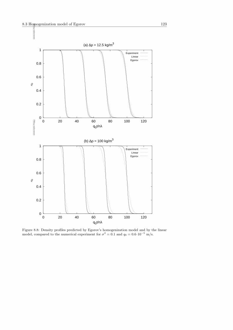
8.3 Homogenization model of Egorov 123
0
0.2
0.4
0.6
0.8
1
0 20 40 60 80 100 120q0t/nλ
(a) ∆ρ = 12.5 kg/m3
ExperimentLinear
Egorov
PSfrag
replacem
ents
%
0
0.2
0.4
0.6
0.8
1
0 20 40 60 80 100 120q0t/nλ
(b) ∆ρ = 100 kg/m3
ExperimentLinear
Egorov
PSfrag
replacem
ents
%
Figure 8.8: Density profiles predicted by Egorov’s homogenization model and by the linearmodel, compared to the numerical experiment for σ2 = 0.1 and q0 = 0.6·10−5 m/s.
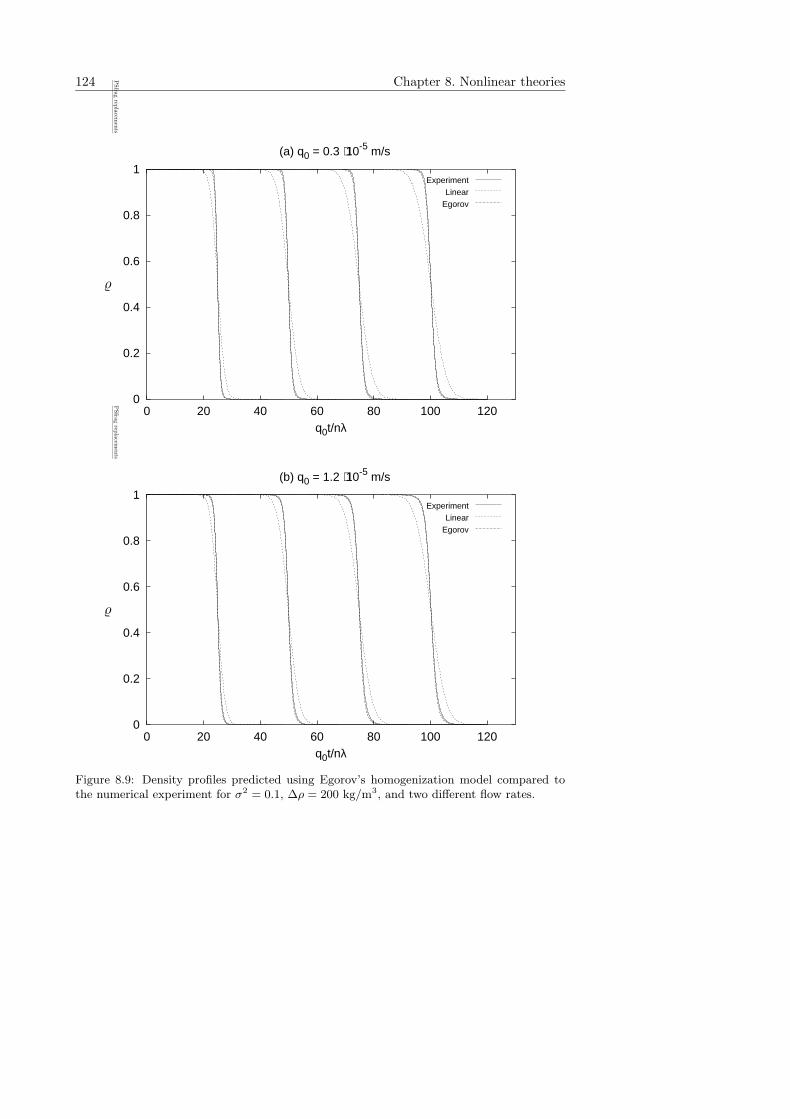
124 Chapter 8. Nonlinear theories
0
0.2
0.4
0.6
0.8
1
0 20 40 60 80 100 120q0t/nλ
(a) q0 = 0.3 ⋅10-5 m/s
ExperimentLinear
Egorov
PSfrag
replacem
ents
%
0
0.2
0.4
0.6
0.8
1
0 20 40 60 80 100 120q0t/nλ
(b) q0 = 1.2 ⋅10-5 m/s
ExperimentLinear
Egorov
PSfrag
replacem
ents
%
Figure 8.9: Density profiles predicted using Egorov’s homogenization model compared tothe numerical experiment for σ2 = 0.1, ∆ρ = 200 kg/m3, and two different flow rates.
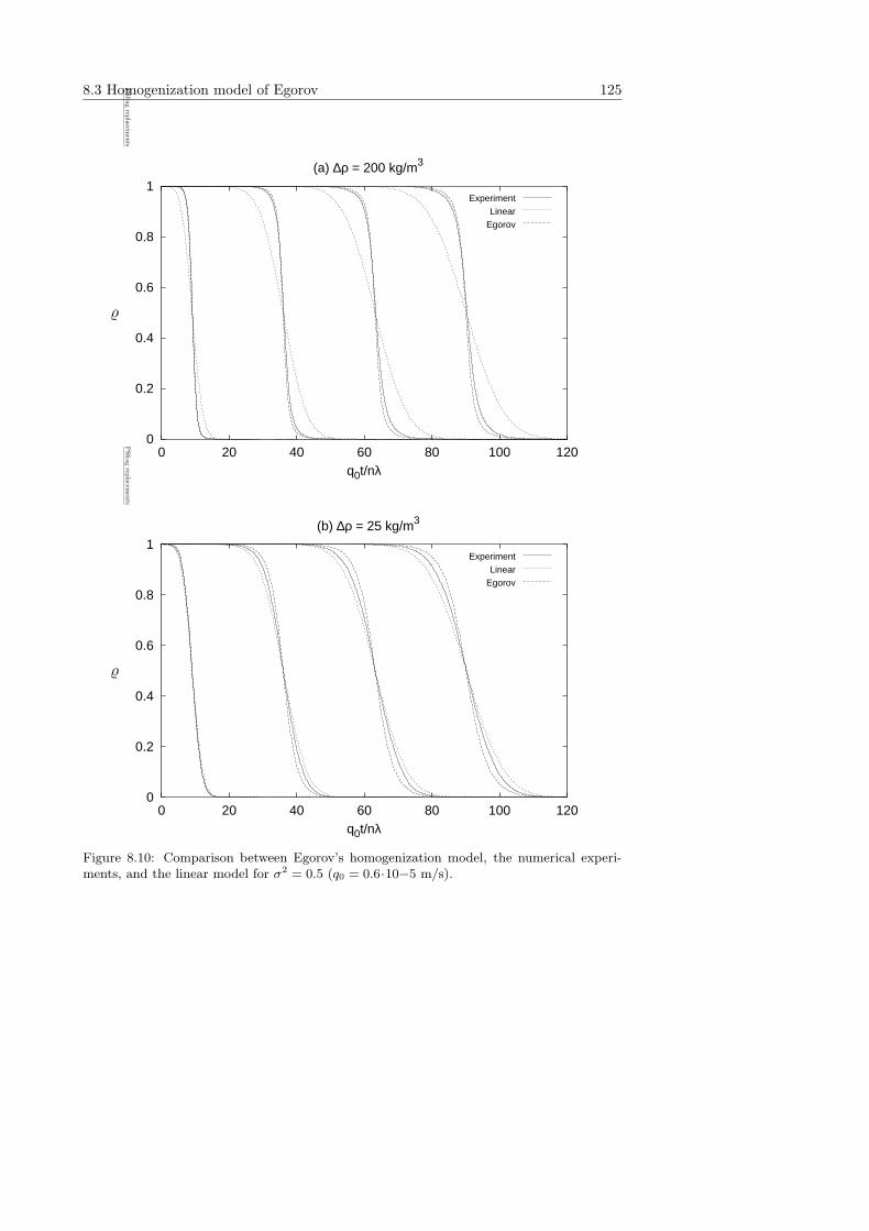
8.3 Homogenization model of Egorov 125
0
0.2
0.4
0.6
0.8
1
0 20 40 60 80 100 120q0t/nλ
(a) ∆ρ = 200 kg/m3
ExperimentLinear
Egorov
PSfrag
replacem
ents
%
0
0.2
0.4
0.6
0.8
1
0 20 40 60 80 100 120q0t/nλ
(b) ∆ρ = 25 kg/m3
ExperimentLinear
Egorov
PSfrag
replacem
ents
%
Figure 8.10: Comparison between Egorov’s homogenization model, the numerical experi-ments, and the linear model for σ2 = 0.5 (q0 = 0.6·10−5 m/s).
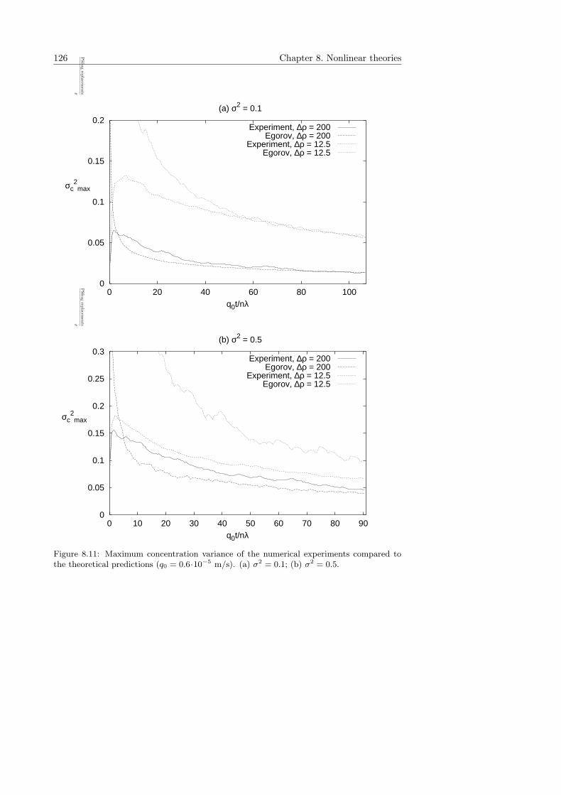
126 Chapter 8. Nonlinear theories
0
0.05
0.1
0.15
0.2
0 20 40 60 80 100q0t/nλ
(a) σ2 = 0.1
σc2
max
Experiment, ∆ρ = 200 Egorov, ∆ρ = 200
Experiment, ∆ρ = 12.5 Egorov, ∆ρ = 12.5
PSfrag
replacem
ents%
0
0.05
0.1
0.15
0.2
0.25
0.3
0 10 20 30 40 50 60 70 80 90q0t/nλ
(b) σ2 = 0.5
σc2
max
Experiment, ∆ρ = 200 Egorov, ∆ρ = 200
Experiment, ∆ρ = 12.5 Egorov, ∆ρ = 12.5
PSfrag
replacem
ents%
Figure 8.11: Maximum concentration variance of the numerical experiments compared tothe theoretical predictions (q0 = 0.6·10−5 m/s). (a) σ2 = 0.1; (b) σ2 = 0.5.
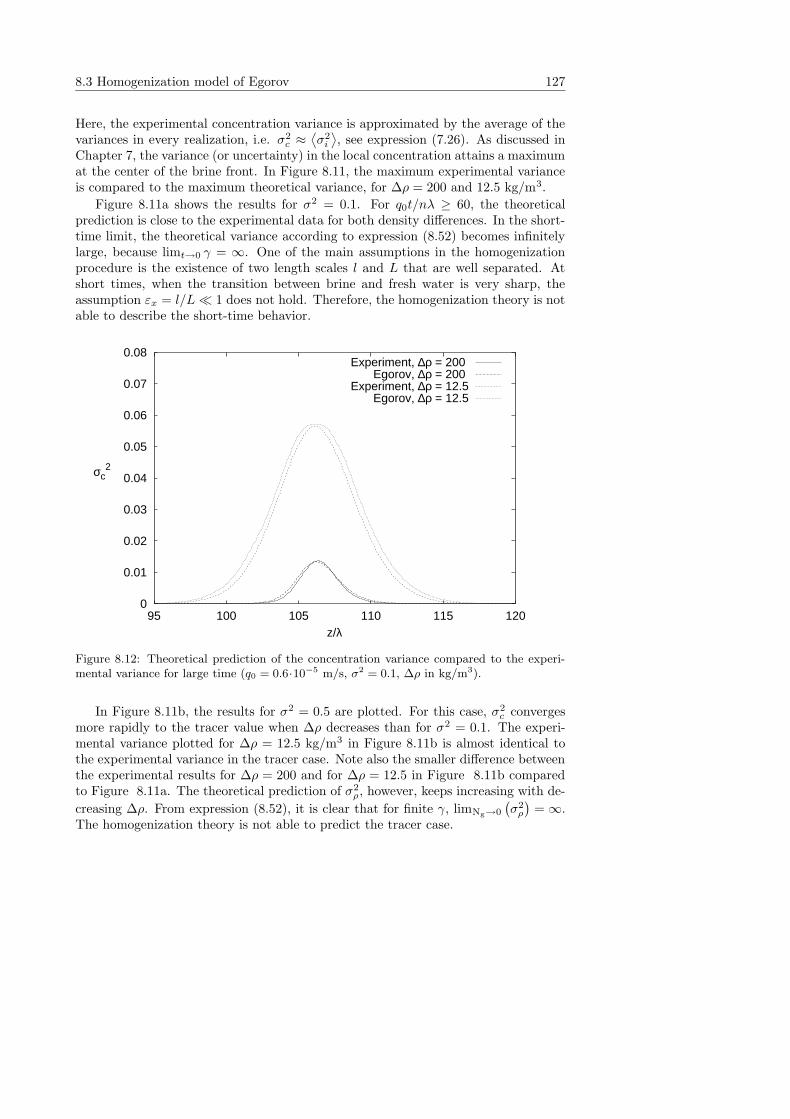
8.3 Homogenization model of Egorov 127
Here, the experimental concentration variance is approximated by the average of thevariances in every realization, i.e. σ2
c ≈⟨σ2
i
⟩, see expression (7.26). As discussed in
Chapter 7, the variance (or uncertainty) in the local concentration attains a maximumat the center of the brine front. In Figure 8.11, the maximum experimental varianceis compared to the maximum theoretical variance, for ∆ρ = 200 and 12.5 kg/m3.
Figure 8.11a shows the results for σ2 = 0.1. For q0t/nλ ≥ 60, the theoreticalprediction is close to the experimental data for both density differences. In the short-time limit, the theoretical variance according to expression (8.52) becomes infinitelylarge, because limt→0 γ = ∞. One of the main assumptions in the homogenizationprocedure is the existence of two length scales l and L that are well separated. Atshort times, when the transition between brine and fresh water is very sharp, theassumption εx = l/L� 1 does not hold. Therefore, the homogenization theory is notable to describe the short-time behavior.
0
0.01
0.02
0.03
0.04
0.05
0.06
0.07
0.08
95 100 105 110 115 120z/λ
σc2
Experiment, ∆ρ = 200 Egorov, ∆ρ = 200
Experiment, ∆ρ = 12.5Egorov, ∆ρ = 12.5
Figure 8.12: Theoretical prediction of the concentration variance compared to the experi-mental variance for large time (q0 = 0.6·10−5 m/s, σ2 = 0.1, ∆ρ in kg/m3).
In Figure 8.11b, the results for σ2 = 0.5 are plotted. For this case, σ2c converges
more rapidly to the tracer value when ∆ρ decreases than for σ2 = 0.1. The experi-mental variance plotted for ∆ρ = 12.5 kg/m3 in Figure 8.11b is almost identical tothe experimental variance in the tracer case. Note also the smaller difference betweenthe experimental results for ∆ρ = 200 and for ∆ρ = 12.5 in Figure 8.11b comparedto Figure 8.11a. The theoretical prediction of σ2
ρ, however, keeps increasing with de-
creasing ∆ρ. From expression (8.52), it is clear that for finite γ, limNg→0
(σ2
ρ
)= ∞.
The homogenization theory is not able to predict the tracer case.
128 Chapter 8. Nonlinear theories
Even for ∆ρ = 200 kg/m3, the agreement between theory and experiment forσ2 = 0.5 is bad compared to that for σ2 = 0.1. However, the theoretical predictionsin Figure 8.11b still seem to converge towards the experimental profile with time,but much slower than in Figure 8.11a. Note also that the theoretical predictions forσ2 = 0.5 show more oscillations than for σ2 = 0.1. This is a result of the γ profilesbeing less smooth, even though a larger number of realizations was used for σ2 = 0.5than for σ2 = 0.1. Increasing the number of realizations would yield smoother curves,but would not change their essential features.
In Figure 8.12, σ2ρ given by expression (8.52) is compared to the experimental σ2
c
at a time instant close to the end of the experiment. For both density differences,the theoretical prediction shows a satisfactory agreement with the experimental vari-ance. The maximum value of σ2
c (plotted in Figure 8.11) is well predicted, but thetheoretical profile is somewhat wider than the experimental one. Note that this dis-crepancy, apparent for ∆ρ = 12.5 kg/m3, is not caused by the difference in scaling.The difference between the scaled mass fraction and density for ∆ρ = 12.5 kg/m3 isnegligible, see Appendix C.
8.3.3 Conclusions
• The homogenization approach of Egorov leads to a dispersive flux equation thatstill has the form of Fick’s law, but in which the dispersion coefficient dependson the (dimensionless) density gradient.
• When the same assumptions are employed, the homogenization approach ofEgorov reproduces the earlier result of Welty and Gelhar (1991).
• The homogenization model predictions of Egorov (for the 2-D Gaussian correla-tion function) are in agreement with the numerical results for σ2 = 0.1, withoutany fitting or additional parameters.
• The homogenization approach is only valid for weakly heterogeneous porousmedia: it relies on the smallness of σ. Moreover, the theory is not able todescribe the short time behavior of the front, as the approach assumes well-separated scales.
• Egorov’s expression for the concentration variance is a satisfactory predictionof the experimental variance for σ2 = 0.1, Ng � 0.2, and large enough time.
8.4 Homogenization model of Demidov
In contrast to Welty and Gelhar (1991) and Egorov, who consider averaged balanceequations at the local scale, Demidov2 starts at the pore scale level. Demidov ap-plies the homogenization method to flow around microscale heterogeneities, rather
2Details of this model will be published in the PhD thesis Upscaling of brine-transport equations
in micro-heterogeneous porous media (in Russian), by Denis Demidov, Kazan State University.
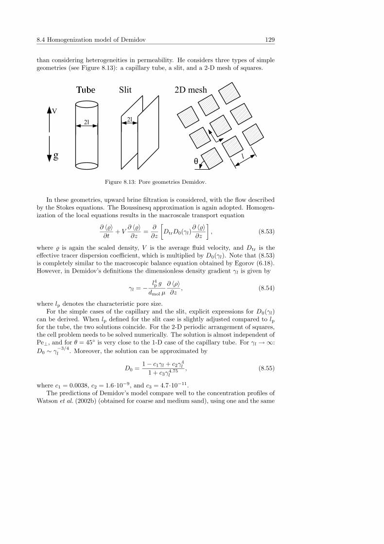
8.4 Homogenization model of Demidov 129
than considering heterogeneities in permeability. He considers three types of simplegeometries (see Figure 8.13): a capillary tube, a slit, and a 2-D mesh of squares.
θ
�����e
Figure 8.13: Pore geometries Demidov.
In these geometries, upward brine filtration is considered, with the flow describedby the Stokes equations. The Boussinesq approximation is again adopted. Homogen-ization of the local equations results in the macroscale transport equation
∂ 〈%〉∂t
+ V∂ 〈%〉∂z
=∂
∂z
[
DtrD0(γl)∂ 〈%〉∂z
]
, (8.53)
where % is again the scaled density, V is the average fluid velocity, and Dtr is theeffective tracer dispersion coefficient, which is multiplied by D0(γl). Note that (8.53)is completely similar to the macroscopic balance equation obtained by Egorov (6.18).However, in Demidov’s definitions the dimensionless density gradient γl is given by
γl = −l4p g
dmol µ
∂ 〈ρ〉∂z
, (8.54)
where lp denotes the characteristic pore size.For the simple cases of the capillary and the slit, explicit expressions for D0(γl)
can be derived. When lp defined for the slit case is slightly adjusted compared to lpfor the tube, the two solutions coincide. For the 2-D periodic arrangement of squares,the cell problem needs to be solved numerically. The solution is almost independent ofPe⊥, and for θ = 45◦ is very close to the 1-D case of the capillary tube. For γl →∞:
D0 ∼ γ−3/4l . Moreover, the solution can be approximated by
D0 =1− c1γl + c2γ
4l
1 + c3γ4.75l
, (8.55)
where c1 = 0.0038, c2 = 1.6·10−9, and c3 = 4.7·10−11.The predictions of Demidov’s model compare well to the concentration profiles of
Watson et al. (2002b) (obtained for coarse and medium sand), using one and the same
130 Chapter 8. Nonlinear theories
ratio between the grain size and the characteristic pore size lp. In order to make acomparison with the numerical experiments in macroscopically heterogeneous media,a relation between k0, l (or λ), and lp is needed. Note that, comparing expression(8.54) to (8.19), the factor k0λ
2π/4(= kl2) in expression (8.19) is substituted by l4p inexpression (8.54). Furthermore, the molecular diffusion coefficient dmol plays the roleof d⊥.
Consider a porous medium consisting of a bundle of capillary tubes, arrangedin a 3-D lattice with periodic size L. For laminar (Poiseuille) flow of a Newtonianfluid through a straight circular tube with radius lp, the volume flow rate is given by(Janssen and Warmoeskerken, 1991)
φv = −πl4p8µ
∂p
∂z, (8.56)
where p denotes the fluid pressure. To obtain the specific discharge, φv needs to bedivided by the area of one periodic cell L2. Expression (8.56) is equivalent to Darcy’slaw, when
k =πl4p
24T L2, (8.57)
where a tortuosity factor T ≥ 1 is taken into account. The porosity can be expressedas
n = 3πl2p/L2. (8.58)
Furthermore, assume that the pore radius lp and the heterogeneity size l are relatedas
lp = Sl, (8.59)
where S ∼ 1 is a scaling factor. Using expressions (8.58) and (8.59), yields
l4pkl2
= F, (8.60)
where F = 24T S2/n is the factor relating γ to γl, i.e. γ = γl/F . For example(assuming n = 0.4), F = 15 for S = 0.5 and T = 1, while F = 360 for S = 2 andT = 1.5. In principle, F needs to be obtained by fitting the model to the experimentalresults.
8.4.1 Comparison with numerical experiments
A comparison between Demidov’s model and the numerical experiments is made.The approximate formula (8.55) is used, which together with equation (8.53) formsa system of equations that needs to be solved numerically. In order to match thenumerical experiments, the model parameters are chosen as Dtr = lσ2q0, V = q0/n,and γl = γF . The experiments for σ2 = 0.1 can all be satisfactorily modelled usingF = 240. A comparison between the computed and experimental profiles is givenin Figure 8.14, for density differences ∆ρ = 12.5 and 100 kg/m3. The linear modelpredictions are plotted as well. Figure 8.14 can be compared to Figure 8.8, which
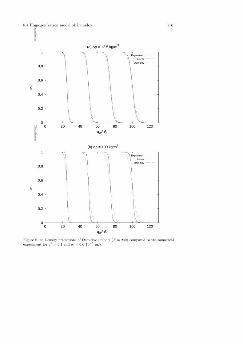
8.4 Homogenization model of Demidov 131
0
0.2
0.4
0.6
0.8
1
0 20 40 60 80 100 120q0t/nλ
(a) ∆ρ = 12.5 kg/m3
ExperimentLinear
Demidov
PSfrag
replacem
ents
%
0
0.2
0.4
0.6
0.8
1
0 20 40 60 80 100 120q0t/nλ
(b) ∆ρ = 100 kg/m3
ExperimentLinear
Demidov
PSfrag
replacem
ents
%
Figure 8.14: Density predictions of Demidov’s model (F = 240) compared to the numericalexperiment for σ2 = 0.1 and q0 = 0.6·10−5 m/s.
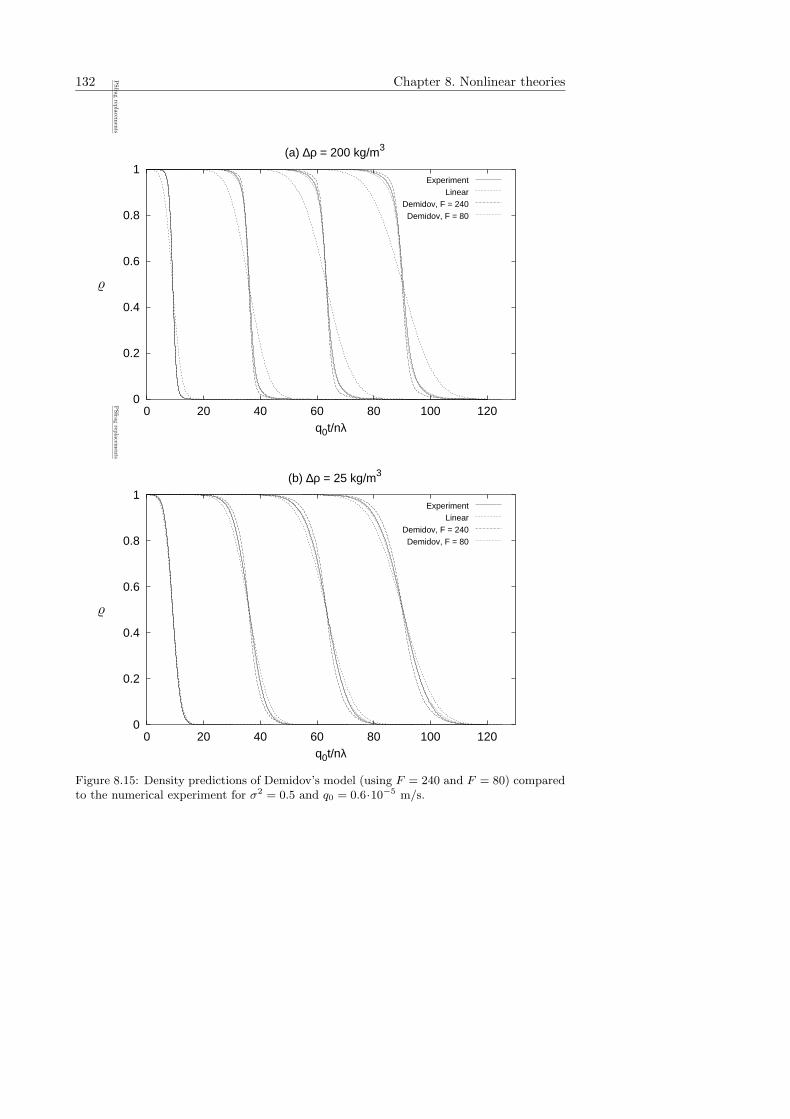
132 Chapter 8. Nonlinear theories
0
0.2
0.4
0.6
0.8
1
0 20 40 60 80 100 120q0t/nλ
(a) ∆ρ = 200 kg/m3
ExperimentLinear
Demidov, F = 240Demidov, F = 80
PSfrag
replacem
ents
%
0
0.2
0.4
0.6
0.8
1
0 20 40 60 80 100 120q0t/nλ
(b) ∆ρ = 25 kg/m3
ExperimentLinear
Demidov, F = 240Demidov, F = 80
PSfrag
replacem
ents
%
Figure 8.15: Density predictions of Demidov’s model (using F = 240 and F = 80) comparedto the numerical experiment for σ2 = 0.5 and q0 = 0.6·10−5 m/s.
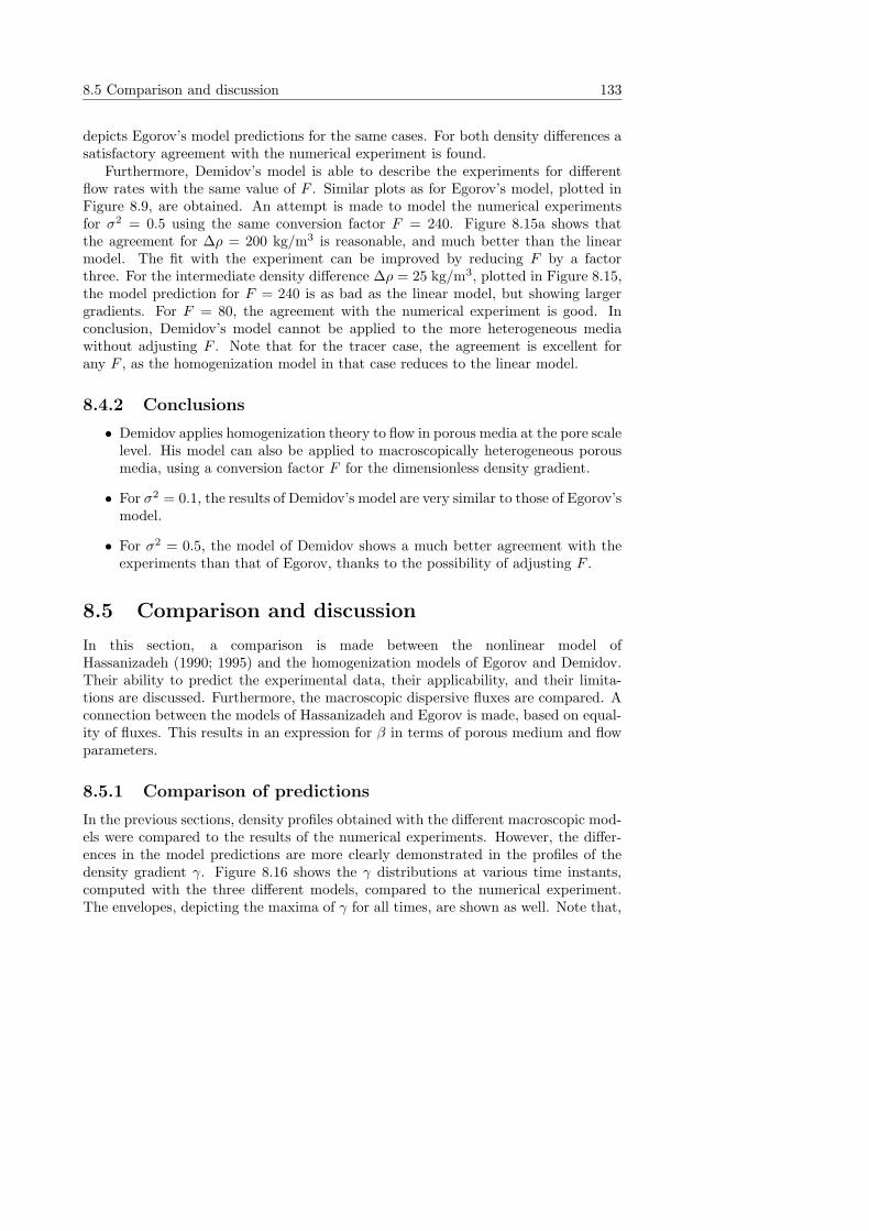
8.5 Comparison and discussion 133
depicts Egorov’s model predictions for the same cases. For both density differences asatisfactory agreement with the numerical experiment is found.
Furthermore, Demidov’s model is able to describe the experiments for differentflow rates with the same value of F . Similar plots as for Egorov’s model, plotted inFigure 8.9, are obtained. An attempt is made to model the numerical experimentsfor σ2 = 0.5 using the same conversion factor F = 240. Figure 8.15a shows thatthe agreement for ∆ρ = 200 kg/m3 is reasonable, and much better than the linearmodel. The fit with the experiment can be improved by reducing F by a factorthree. For the intermediate density difference ∆ρ = 25 kg/m3, plotted in Figure 8.15,the model prediction for F = 240 is as bad as the linear model, but showing largergradients. For F = 80, the agreement with the numerical experiment is good. Inconclusion, Demidov’s model cannot be applied to the more heterogeneous mediawithout adjusting F . Note that for the tracer case, the agreement is excellent forany F , as the homogenization model in that case reduces to the linear model.
8.4.2 Conclusions
• Demidov applies homogenization theory to flow in porous media at the pore scalelevel. His model can also be applied to macroscopically heterogeneous porousmedia, using a conversion factor F for the dimensionless density gradient.
• For σ2 = 0.1, the results of Demidov’s model are very similar to those of Egorov’smodel.
• For σ2 = 0.5, the model of Demidov shows a much better agreement with theexperiments than that of Egorov, thanks to the possibility of adjusting F .
8.5 Comparison and discussion
In this section, a comparison is made between the nonlinear model ofHassanizadeh (1990; 1995) and the homogenization models of Egorov and Demidov.Their ability to predict the experimental data, their applicability, and their limita-tions are discussed. Furthermore, the macroscopic dispersive fluxes are compared. Aconnection between the models of Hassanizadeh and Egorov is made, based on equal-ity of fluxes. This results in an expression for β in terms of porous medium and flowparameters.
8.5.1 Comparison of predictions
In the previous sections, density profiles obtained with the different macroscopic mod-els were compared to the results of the numerical experiments. However, the differ-ences in the model predictions are more clearly demonstrated in the profiles of thedensity gradient γ. Figure 8.16 shows the γ distributions at various time instants,computed with the three different models, compared to the numerical experiment.The envelopes, depicting the maxima of γ for all times, are shown as well. Note that,
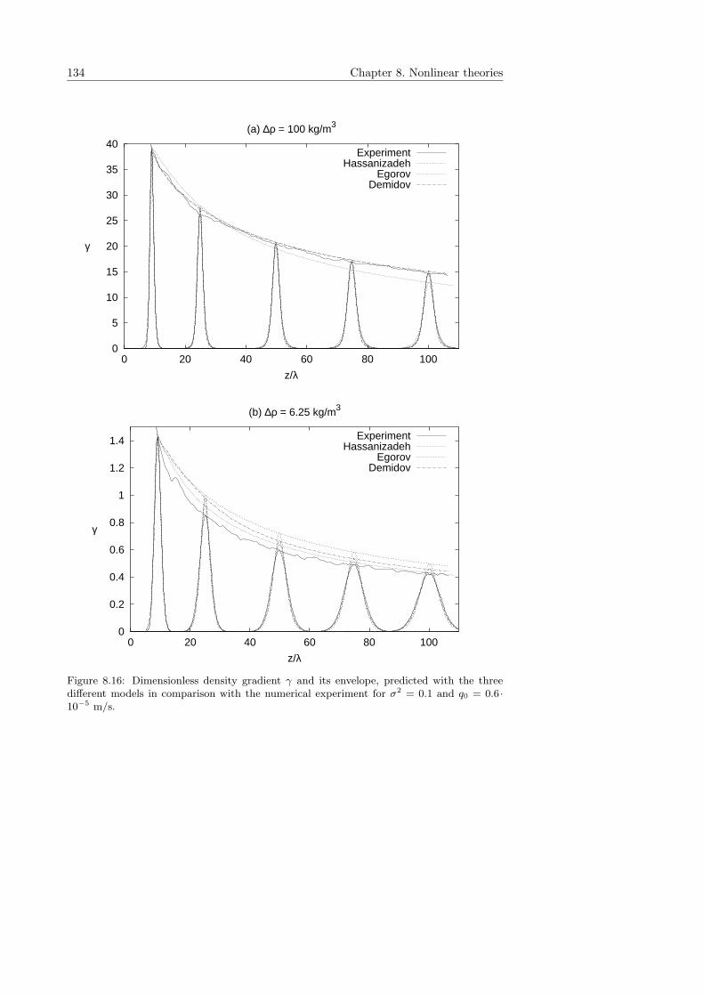
134 Chapter 8. Nonlinear theories
0
5
10
15
20
25
30
35
40
0 20 40 60 80 100
z/λ
(a) ∆ρ = 100 kg/m3
γ
ExperimentHassanizadeh
EgorovDemidov
0
0.2
0.4
0.6
0.8
1
1.2
1.4
0 20 40 60 80 100
z/λ
(b) ∆ρ = 6.25 kg/m3
γ
ExperimentHassanizadeh
EgorovDemidov
Figure 8.16: Dimensionless density gradient γ and its envelope, predicted with the threedifferent models in comparison with the numerical experiment for σ2 = 0.1 and q0 = 0.6 ·10−5 m/s.
8.5 Comparison and discussion 135
0
5
10
15
20
25
30
35
40
45
50
0 20 40 60 80 100
z/λ
(a) ∆ρ = 200 kg/m3
γ
ExperimentHassanizadeh, β = 5 ⋅ 105
EgorovDemidov, F = 80
0
0.5
1
1.5
2
2.5
3
0 20 40 60 80 100
z/λ
(b) ∆ρ = 25 kg/m3
γ
ExperimentHassanizadeh, β = 1 ⋅ 105
EgorovDemidov, F = 80
Figure 8.17: Dimensionless density gradient γ and its envelope, predicted with the threedifferent models in comparison with the numerical experiment for σ2 = 0.5 and q0 = 0.6 ·10−5 m/s.
136 Chapter 8. Nonlinear theories
to obtain the data for the figures in this section, the initial condition for the nonlinearmodel of Hassanizadeh (1990; 1995) is taken identical to those of the homogenizationmodels, i.e. based on an early-time experimental profile rather than a step function.
For ∆ρ = 100 kg/m3, depicted in Figure 8.16a, an excellent agreement with theexperiment is found for both homogenization models. For large time, Hassanizadeh’smodel with β = 5 ·105 generates smaller gradients. A better fit can be obtained byadjusting β, but the idea behind the model is to use the same β for every densitycontrast.
For the small density contrast plotted in Figure 8.16b, the nonlinear model ofHassanizadeh is closest to the experiments. Moreover, the model predictions of Demi-dov for ∆ρ = 6.25 kg/m3 are closer to the experiment than those of Egorov. Accordingto Egorov’s formula for the 2-D Gaussian correlation function (8.50), D0 approaches 1at an infinite angle as γ ↓ 0. In Demidov’s case, limγl→0 (D0) = 1−c1γl, so that D0 ap-proaches 1 at a finite angle. For small γ, i.e. approaching the tracer case, the approx-imation of Demidov is closer to reality. The nonlinear model of Hassanizadeh (1990;1995) for small density gradients simply reduces to the classical linear model.
In Figure 8.17, a comparison is made with the numerical experiments for σ2 = 0.5.As shown earlier in Figure 8.10, the homogenization theory of Egorov is not adequateto describe the experiments for the more heterogeneous fields. This is confirmedin Figure 8.17, where the computed γ with Egorov’s model is much larger than theexperimental value, regardless of the density difference. In contrast to Egorov’s model,some extent of parameter fitting is possible with Demidov’s model. The model ofDemidov shows a good agreement for σ2 = 0.5 using F = 80, in both Figures 8.17aand b. Note that F = 240 is used in Figure 8.16 for the case σ2 = 0.1.
The nonlinear model of Hassanizadeh (1990; 1995) in Figures 8.17a and b showsa good agreement for both density contrasts. However, this agreement is obtainedusing different values for β (see the legends in the figures). Hassanizadeh and Leijnse(1995) and Schotting et al. (1999) claim that β is independent of ∆ρ. In other words:experiments for any density difference can be modelled with one and the same β.Though this is the case for σ2 = 0.1, the results for σ2 = 0.5 contradict this statement.(See also Figure 8.6.)
8.5.2 Comparison of fluxes
The important difference between the theory of Welty and Gelhar (1991) and theresults of the homogenization procedure (Egorov et al., 2005) on one hand, and thenonlinear theory of Hassanizadeh (1990; 1995) on the other hand, is the form of thedispersive flux equation. In this section, the fluxes given by the linear theory, thenonlinear theory of Hassanizadeh (1990; 1995), and the homogenization/stochastictheory (Welty and Gelhar, 1991) are compared.
According to the linear Fickian theory, the dispersive mass flux in terms of thedensity in 1-D is given by
Jρ = −Dtr∂ρ
∂z. (8.61)
In the stochastic and homogenization models, the macroscopic flux in dimensional
8.5 Comparison and discussion 137
variables is expressed as
Jρ = −DtrD0∂ρ
∂z. (8.62)
It should be noted that these fluxes are different from the flux J , given by expression(8.11), in Hassanizadeh’s model. As a result of writing the salt mass balance (8.2)in terms of the density using the equation of state (8.5), the flux J in mass balanceequation (8.6) is multiplied by γρ. Therefore, Jρ = γρJ .
Next, the fluxes are expressed in dimensionless form using
J∗ =Jρ
J0, J0 =
µd⊥Dtr
k0gl2. (8.63)
In terms of the dimensionless density gradient γ, we obtain J∗ = γ and J∗ = I(γ) =D0(γ)γ in the linear and homogenization/stochastic model respectively. The modelof Hassanizadeh (1995) yields
J = γρ−1 +
√1 + 4βJ0γ
2βJ0. (8.64)
The fluxes given by the three models are depicted in Figure 8.18, where for Dtr
the values of the numerical experiments for σ2 = 0.1 and σ2 = 0.5 are used, withβ = 5·105 and β = 1·105 respectively. These two cases yield nearly identical fluxesaccording to expression (8.64), because (as expected) the ratio between the fittedtracer dispersivities is nearly five, yielding the same value for the product J0β. Forthe homogenization/stochastic model, J∗ is independent of Dtr or σ2. For a givendensity gradient γ, the dispersive mass flux for all other models is significantly lowerthan for the linear model. Note that the 3-D exponential correlation function usedby Welty and Gelhar (1991) yields larger dispersive fluxes than the 2-D Gaussian.
The flux according to nonlinear relation (8.64) depends on β. In order to obtaina flux equal to that in the homogenization/stochastic model, β should satisfy
β =β0
D0(γ)γ
(1
D0(γ)− 1
)
, (8.65)
where β0 = γρ/J0 depends on medium and fluid parameters. Note that—in theabsence of molecular diffusion—d⊥ = α⊥q0 and Dtr = αtrq0. Therefore, β dependson the flow rate through β0 ∼ q−2
0 . The numerical experiments for σ2 = 0.1 show avery similar flow rate dependence, for which a power of −1.85±0.13 is obtained. Thenonlinear parameter β according to (8.65) further depends on γ, and through D0(γ)on the type of correlation function, see Table 6.2.
Figure 8.19 shows the predictions based on expression (8.65), for the two mediawith the Gaussian correlation function, using β0 = 8·10−9/Dtr. The β values fittedto the experimental results including the estimated error bounds (see also Figure 8.2)are plotted as well.
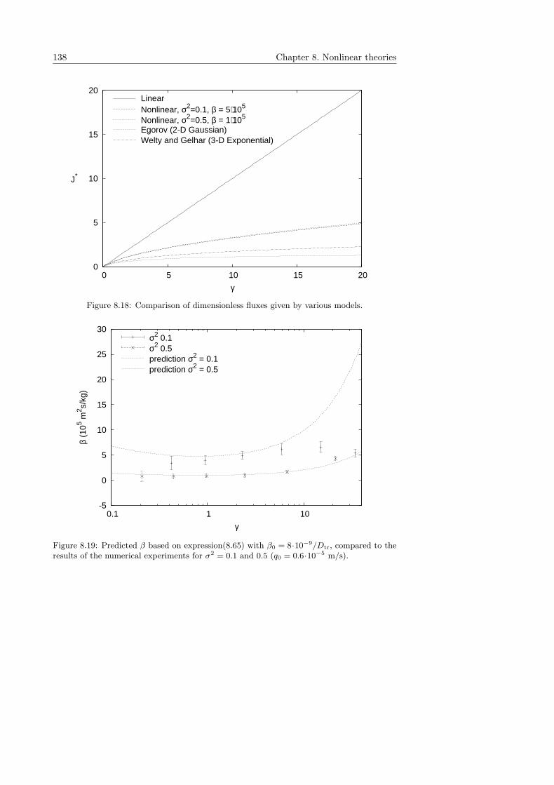
138 Chapter 8. Nonlinear theories
0
5
10
15
20
0 5 10 15 20
γ
J*
LinearNonlinear, σ2=0.1, β = 5⋅105
Nonlinear, σ2=0.5, β = 1⋅105
Egorov (2-D Gaussian)Welty and Gelhar (3-D Exponential)
Figure 8.18: Comparison of dimensionless fluxes given by various models.
-5
0
5
10
15
20
25
30
0.1 1 10
β (1
05 m2 s/
kg)
γ
σ2 0.1σ2 0.5prediction σ2 = 0.1prediction σ2 = 0.5
Figure 8.19: Predicted β based on expression(8.65) with β0 = 8·10−9/Dtr, compared to theresults of the numerical experiments for σ2 = 0.1 and 0.5 (q0 = 0.6·10−5 m/s).
8.5 Comparison and discussion 139
8.5.3 Comparison of effective dispersivities
In Chapter 7, the macroscale dispersivities (scaled by the tracer values) of variouslaboratory experiments are compared against the gravity number Ng. The numericalexperiments for σ2 = 0.1 show a similar decrease of A11/A11,tr = D0 as the laboratoryexperiments in homogenous media, as shown in Figure 7.15. The relation betweenD0 and Ng is not unique, but depends on σ2, see also the analysis in Appendix B.The models of Welty and Gelhar (1991) and Egorov and Demidov, however, sug-gest that D0 is a function of the (dimensionless) density gradient rather than of thegravity number. Moreover, from the theory of Hassanizadeh (1990; 1995), an appar-ent dispersivity can be found that is also dependent on the density gradient. Whenmolecular diffusion is disregarded, the dispersive flux in the nonlinear model is givenby equation (8.3), where D = αtr|q|. Setting this flux equal to the flux given by thelinear relation, i.e. Fick’s law, where D = αapp|q|, yields
αapp
αtr=
2
1 +√
1 + P ∂ρ∂z
. (8.66)
Note that the right-hand side of this expression also depends on αtr, because P =4βαtr|q|ερf/γρ.
In the nonlinear model microscale dispersion is not treated separately, as it is inthe numerical experiments and homogenization model. Therefore, in order to make acomparison with D0(γ), expression (8.66) needs to be scaled as
D0 =D − d‖Dtr − d‖
=αapp − α‖αtr − α‖
=2
1 +√
1 + P ∂ρ∂z
(αtr
αtr − α‖
)
− α‖αtr − α‖
. (8.67)
In Figure 8.20, expression (8.67) is compared to the solutions of Welty and Gel-har (1991) (for the 3-D exponential correlation function) and the homogenizationtheory (for the 2-D exponential and Gaussian correlation functions). See for theseexplicit solutions Table 6.2. Demidov’s results for the 2-D mesh are plotted as well,for Pe⊥ = 90 (corresponding to the numerical experiment), where again F = 240.A comparison is made with the results of the numerical experiments. However, theexperimental data are not directly comparable to the theoretical data, because nodirect relation between D0 and γ can be established. The dimensionless density gra-dient γ in the experiment varies in both space and time. The dispersion coefficientsin Figure 8.20 are obtained by fitting the erfc-solution to the profiles obtained atlarge time (q0t/nλ = 100 and q0t/nλ = 80). The shape of the profile at large timeis determined by its travel from t = 0 up to that time. These dispersion coefficientsare therefore effective time averages. The corresponding density gradients are takenfrom the maximum gradients of the long-time profiles. Taking the maximum gradientoverestimates the average gradient in space. However, the long-time gradient under-estimates the average gradient in time (although the gradient decreases only slowlyin time, as can be seen for example in Figures 8.5–8.10).
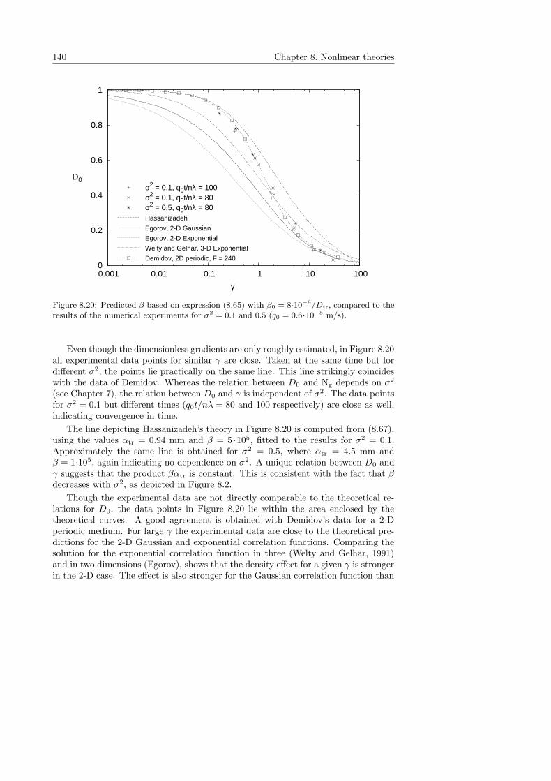
140 Chapter 8. Nonlinear theories
0
0.2
0.4
0.6
0.8
1
0.001 0.01 0.1 1 10 100
γ
D0σ2 = 0.1, q0t/nλ = 100σ2 = 0.1, q0t/nλ = 80 σ2 = 0.5, q0t/nλ = 80 Hassanizadeh
Egorov, 2-D Gaussian
Egorov, 2-D Exponential
Welty and Gelhar, 3-D Exponential
Demidov, 2D periodic, F = 240
Figure 8.20: Predicted β based on expression (8.65) with β0 = 8·10−9/Dtr, compared to theresults of the numerical experiments for σ2 = 0.1 and 0.5 (q0 = 0.6·10−5 m/s).
Even though the dimensionless gradients are only roughly estimated, in Figure 8.20all experimental data points for similar γ are close. Taken at the same time but fordifferent σ2, the points lie practically on the same line. This line strikingly coincideswith the data of Demidov. Whereas the relation between D0 and Ng depends on σ2
(see Chapter 7), the relation between D0 and γ is independent of σ2. The data pointsfor σ2 = 0.1 but different times (q0t/nλ = 80 and 100 respectively) are close as well,indicating convergence in time.
The line depicting Hassanizadeh’s theory in Figure 8.20 is computed from (8.67),using the values αtr = 0.94 mm and β = 5 ·105, fitted to the results for σ2 = 0.1.Approximately the same line is obtained for σ2 = 0.5, where αtr = 4.5 mm andβ = 1·105, again indicating no dependence on σ2. A unique relation between D0 andγ suggests that the product βαtr is constant. This is consistent with the fact that βdecreases with σ2, as depicted in Figure 8.2.
Though the experimental data are not directly comparable to the theoretical re-lations for D0, the data points in Figure 8.20 lie within the area enclosed by thetheoretical curves. A good agreement is obtained with Demidov’s data for a 2-Dperiodic medium. For large γ the experimental data are close to the theoretical pre-dictions for the 2-D Gaussian and exponential correlation functions. Comparing thesolution for the exponential correlation function in three (Welty and Gelhar, 1991)and in two dimensions (Egorov), shows that the density effect for a given γ is strongerin the 2-D case. The effect is also stronger for the Gaussian correlation function than
8.6 Summary 141
for the exponential. In all cases however, the dispersion coefficient decreases to 10%of its tracer value when γ is in the order of 10. Demidov’s results for large γ are closeto the results for both 2-D correlation functions. For small γ, however, Demidov’sresult coincides with the result of Hassanizadeh’s model. The latter reduces to thelinear model for infinitely small γ. Therefore, Demidov’s model yields a more realisticdescription than Egorov’s model when small density contrasts are considered.
8.6 Summary
The second order term in Hassanizadeh’s nonlinear equation for the dispersive massflux involves an additional dispersion parameter β. Hassanizadeh and Leijnse (1995)claim that experiments for any density contrast can be modelled using the same βfor a specific medium and flow rate. Their findings are confirmed by Schotting et al.(1999), who analyzes the experiments of Moser (1995) in homogeneous media. Themodel of Hassanizadeh (1990; 1995) is developed for essentially homogeneous media.In the present study, the model predictions are compared to the results of a series ofnumerical experiments in weakly heterogeneous media, i.e. media characterized by asmall correlation scale λ and a small log-permeability variance σ2. Indeed, we findthat for σ2 = 0.1, even though the best-fit β value is variable, the experiments for alldensities can be satisfactorily modelled with the same β. Furthermore, the findingsfor σ2 = 0.1 confirm the flow-rate dependence of β that is reported by Schotting et al.(1999) and by Watson et al. (2002b).
In this study, the travel-time dependency of β is studied as well. The best-fitvalue of β increases slowly with time, and does not reach an asymptotic value withinthe time-range of the numerical experiments. Moreover, for media with strongerheterogeneities (σ2 = 0.5) it is no longer possible to describe the experiments fordifferent density contrasts using the same β. When ∆ρ decreases, the value of βneeds to be reduced considerably in order to match the experimental results. Thenon-uniqueness of β implies that the value of β is not known beforehand, but needsto be fitted to the specific experiment.
The linear model, which is strictly only valid for tracer transport, is still often usedfor density- and/or viscosity-dependent dispersion problems. Then, the dispersivityis adjusted in order to match the experimental data, in contradiction with the basicpremise of the classical dispersion theory, which considers dispersivity to be a mediumproperty. This argument against using the linear dispersion model also holds for thenonlinear model, which still involves a fitting procedure (and is more complex). Theadvantage of the nonlinear model, in particular for small σ2, is that β needs to bedetermined less often. Moreover, with two parameters a better fit is achieved thanwith the linear model.
Another thing that should be noted is that in the derivation of the theory ofHassanizadeh (1990; 1995), stabilizing gravity effects are not explicitly accounted for,while these are the main cause of the nonlinear effect. The theory of Welty and Gelhar(1991) and the homogenization theory (Egorov et al., 2005) are both derived fromthe physical processes at the local scale. These processes include rotational gravity-
142 Chapter 8. Nonlinear theories
flow induced by horizontal density gradients as a result of local velocity variations.Upscaling of these local processes results in a system of macroscale equations in whichthe macroscopic dispersion coefficient depends on the mean density gradient.
The approach of Welty and Gelhar (1991) or the homogenization approach canbe applied to different types of media, i.e. two- or three-dimensional with differentlog-permeability correlation functions, see the results in Table 6.2. An importantlimitation of these approaches, however, is the assumption of a uni-directional meanflow (in vertical direction). The homogenization model of Egorov is based on thesame assumptions as the numerical experiments and does not require any fitting, oradditional parameters. The model predictions show a satisfactory to good agreementwith the numerical experiments for σ2 = 0.1. Unfortunately, the theory is only appli-cable to weakly heterogeneous media, i.e. σ2 � 1. For σ2 = 0.5 the homogenizationmodel cannot adequately describe the numerical experiments.
Another nice result of the homogenization procedure is the expression for theconcentration variance. For σ2 = 0.1, Ng ≥ 0.2, and large enough time, a satisfactoryagreement is found between the predicted and experimental concentration variances.At short times or for small Ng, however, the theoretical variance becomes infinitelylarge.
Demidov applies the homogenization method to microscale heterogeneous media.The different pore geometries (capillary tube, slit, and 2-D mesh of squares) withan appropriate choice of the characteristic pore sizes yield a very similar decreasein the effective dispersion coefficient. The macroscale transport equation is identicalto that in Welty and Gelhar and Egorov’s models. Using a factor which relates thecharacteristic pore size to the permeability and correlation length, Demidov’s modelcan also describe the experiments in weakly heterogeneous media. The agreementwith the numerical experiments for σ2 = 0.1 is good. However, for σ2 = 0.5 thescaling parameter needs to be adjusted in order to obtain a satisfactory agreement.In a way this can be seen as an advantage of the model. Using the same value for thescaling parameter, all experiments for σ2 = 0.5 can be modelled, whereas the modelof Egorov cannot be applied in this case at all.
The theory of Welty and Gelhar (1991) as well as the homogenization modelssuggest that the scaled macroscale dispersion coefficient (or dispersivity) D0(γ) is afunction of the (dimensionless) density gradient rather than of the gravity number Ng.The results of the numerical experiments support this conclusion. Whereas the re-lation between D0 and Ng still depends on σ2, the dependence on γ is unique for acertain type of correlation function. Moreover, for the theory of Hassanizadeh (1990;1995) an apparent dispersivity can be derived which depends on γ. For this relation-ship to be unique, the product β αtr needs to be constant. In addition, a relationbetween β and γ is derived based on equality of fluxes in the two different formula-tions.
Chapter 9
Conclusions and
recommendations
In this final chapter, the conclusions of the thesis are summarized. Second, openquestions and recommendations for future research are given.
9.1 Conclusions
This thesis deals with the interaction between density gradients and flow and transportin porous media. Interfaces between two miscible fluids with different densities areconsidered. The density gradient affects the flow field and mass transport mainlyin two ways: by fluid volume changes (the compressibility effect) and by inducinggravity forces (which can be either stabilizing or destabilizing).
Chapter 2 introduces the theory of density-dependent flow and transport inporous media relevant to this thesis. A conclusion that is drawn is that, for flow in a2-D vertical plane, the vorticity induced by viscosity gradients can be disregarded incomparison with the vorticity induced by density gradients, when
qz �kgργρ
µγµ. (9.1)
Generally, the compressibility effect is less important than the gravity effect. Whendealing with density-dependent flow problems, many researchers employ the simpli-fying Oberbeck-Boussinesq approximation. In this approximation, the density is as-sumed to be constant everywhere in the governing equations except for the gravityterm in Darcy’s law. So, apart from the gravity effect, all other density effects aredisregarded. Though this approximation often works well, it is unclear what exactcondition makes the approximation valid. It is often stated that the Boussinesq ap-proximation can be adopted when density variations are small. However, in the limitof vanishing density differences, the density-dependence in Darcy’s law disappearsas well. This contradiction is the motivation behind Chapter 3, which attempts toclarify the validity of the Boussinesq approximation in porous media applications.
143
144 Chapter 9. Conclusions and recommendations
The conclusion of Chapter 3 is that the Boussinesq approximation can beadopted, i.e. the compressibility effect is small compared to the gravity term, when
NPe� 1, (9.2)
for isothermal brine transport, and
NPeT � 1 and N� |q|, (9.3)
for heat transfer in fresh water. Here, N = kgρ0/µq0 is independent of the densitydifference. In the case of simultaneous heat and solute transport, both conditions(9.2) and (9.2) must be fulfilled.
The dispersion coefficient D plays an important role through the Peclet number,where Pe = x0q0/D. This is explained by the fact that without diffusion or dispersionno mixing would occur. When two volumes of fluids with different salt concentrationare added, their total volume can only change when they are able to mix. For D ↓ 0,no mixing and as a result no volume change occurs.
In Chapter 4, similarity solutions are constructed for two one-dimensional exam-ple problems involving simultaneous heat and brine transport. The semi-analyticalsolutions are based on the full set of equations, and illustrate the effect of fluid volumechanges on the flow field. The similarity solutions coincide with numerical solutions ofthe original partial differential equations. The compressibility effect locally changesthe velocity of the density front. This effect is enlarged when velocity-dependentdispersion is taken into account.
Similarity solutions are useful for computer-code verification purposes. However,the solutions given in Chapter 4, as well as similarity solutions for several other brinetransport problems, cannot be given in closed-form. A numerical method is necessaryto obtain these solutions. Explicit analytical solutions of the convection-diffusion (oradvection-dispersion) equation are known solely for the case where density effects aredisregarded, i.e. for tracer transport.
In Chapter 5, approximate analytical solutions for 1-D brine transport are ob-tained. To obtain these solutions, the density-coupling between the fluid and saltmass balance is maintained, but simplified. Three simplifications are discussed, twoof which generate different explicit solutions. The other simplification yields a solutionin implicit form. All three solutions are good approximations of the exact (numerical)similarity solution. A nice result is given by series expansion
u =1
2(1− ϑ) +
1
8
(1− ϑ2
)ε + O(ε2), (9.4)
where u is the scaled density, ε = (ρs − ρf)/ρf is the relative density difference, and
ϑ = erf
(x− q0t
2√
Dt
)
. (9.5)
For ε ↓ 0, expression (9.4) reduces to the long-time solution of the linear system, i.e.the tracer solution. Including only the second term in expression (9.4) yields a good
9.1 Conclusions 145
agreement with the exact density-dependent solution. Expression (9.4) is a simpleand valuable extension of the known erfc-type solution.
The approximate similarity solutions are shifted with respect to the solution basedon the Boussinesq approximation, as a result of the velocity enhancement. The factthat similarity solutions exist, implies that this shift is proportional to
√t. Note that,
relative to the front position (given by q0t in the case of incompressible flow), theshift diminishes in time.
The solutions given in Chapters 4 and 5 are for one-dimensional problems, andtherefore do not involve any gravity effects. In the second part of the thesis, consistingof Chapters 6 to 8, gravity plays an important role. The effect of stabilizing gravityforces on dispersion in a heterogeneous porous medium is considered. Fresh wateris displaced upwardly by a denser brine. Small scale heterogeneities in the porousmedium permeability generate local variations in the velocity. As a result, pertur-bations in the initially horizontal interface evolve, which grow to so-called dispersivefingers. Horizontal density gradients that arise induce a stabilizing, gravity-drivenrotational movement, which counteracts the growth of dispersive fingers. Dispersivemixing in this way is inhibited, resulting in a steeper transition between fresh waterand brine than in the case of tracer transport.
Chapter 6 reviews the topic of dispersion under high-concentration-gradient con-ditions, by discussing the various laboratory experiments and three, relatively new,theoretical approaches. Important conclusions obtained from the various laboratoryexperiments are:
• For gravitationally stable displacements, the observed longitudinal dispersivitydecreases with increasing density difference between the fluids.
• The decrease in dispersivity is more pronounced at low flow velocities
• The controlling parameter appears to be the gravity number:
Ng =Ra
Pe=
kg∆ρ
µq,
which expresses the strength of gravity-induced flow in relation to forced-convection flow.
• The classical dispersion formulation, i.e. linear Fick’s law, yields satisfactorypredictions of the tracer experiments. However, for large gravity numbers, thedispersivity needs to be adjusted in order to adequately model the experiments.
• The fact that the dispersivity is made a function of fluid and flow parameters isin contradiction with the basic premise of traditional dispersion theory, whichconsiders dispersivity to be a porous medium property.
• An alternative, nonlinear dispersion model is introduced by Hassanizadeh(1990). With an extra dispersion parameter, in addition to the classical tracerdispersivity, the nonlinear model adequately predicts the experiments for thewhole range of density differences.
146 Chapter 9. Conclusions and recommendations
Three dispersion theories that include the nonlinear density effect are discussed inChapter 6: the theory of Hassanizadeh (1990; 1995), the stochastic analysis of Weltyand Gelhar (1991), and the application of homogenization theory by Egorov et al.(2005). With respect to these three theoretical approaches, the following conclusionscan be drawn:
• The nonlinear dispersion equation of Hassanizadeh (1990; 1995) is an extensionof Fick’s law, which includes a second order term in the dispersive flux and anadditional dispersion parameter.
• The stochastic analysis of Welty and Gelhar (1991) and the homogenizationapproach of Egorov and Demidov lead to a dispersive flux equation that stillhas the form of Fick’s law, but in which the dispersion coefficient depends onthe (dimensionless) density gradient.
• In the stochastic and the homogenization approach, mathematical upscalingof the local governing equations—including the gravity effect—yields a macro-scopic model for density-dependent dispersion.
• In the derivation of the nonlinear model (Hassanizadeh and Leijnse, 1995), grav-ity is not explicitly taken into account.
• The velocity-dependence of the nonlinear dispersion parameter β (Schottinget al., 1999; Watson et al., 2002b) points to gravity as the underlying physicalforce causing the nonlinear effect.
• When the same assumptions are employed, the homogenization approach ofEgorov reproduces the earlier result of Welty and Gelhar (1991).
• In addition, Egorov derives an expression for the concentration variance.
• A great limitation of the stochastic and homogenization approaches (Welty andGelhar, 1991; Egorov et al., 2005) is the one-dimensionality of the macroscopicmodels. The mean flow rate is uni-directional, and moreover, in the verticaldirection.
Chapter 7 describes numerical experiments of gravitationally stable, miscibledisplacements in heterogeneous porous columns. Averages over multiple stochasticrealizations are obtained. Numerical convergence of computations is discussed, aswell as convergence of the ensemble averages. The conclusions of Chapter 7 aresummarized below:
• Test cases show that gravity is indeed responsible for the decrease of longitudinaldispersion in stable displacements.
• The effect of fluid volume changes is small: it does not affect the shape ofthe concentration contours, but only shifts their position slightly. This con-firms the result of Chapter 3. For the test cases, condition (9.2) is satisfied:NPe = 92� 1.
9.1 Conclusions 147
• The shape of the average concentration profiles is entirely determined by thegravity number.
• Local fluctuations in concentration, with respect to the average concentration,decrease with increasing gravity number.
• For high gravity numbers, fewer realizations are needed for ensemble averagedconcentrations to converge.
• The results of the tracer experiments are in good agreement with the analyticalsolution of Hsu (2003), when time-averaged dispersivities are compared. Thelocal (time-dependent) dispersivity fluctuates around Hsu’s solution.
• The numerical experiments show a decrease in the dispersivity with increasinggravity number. For a small log-permeability variance, σ2 = 0.1, the resultsare in accordance with the laboratory experiments of Bouhroum (1989), Moser(1995), and Jiao and Hotzl (2004), which were performed in almost homogeneousmedia. For porous media with stronger heterogeneity, the dispersivity decreasesmore slowly.
Chapter 8 compares the results of the numerical experiments to predictions ofthe three dispersion models discussed in Chapter 6. The conclusions, with respect tothe applicability and limitations of the different theories, are:
• For nearly homogeneous media, i.e. σ2 = 0.1, the present results confirm twoimportant findings of Hassanizadeh and Leijnse (1995), Schotting et al. (1999),and Watson et al. (2002b):
1. With one value of β, the nonlinear model of Hassanizadeh (1990; 1995) isable to predict the experiments for different density contrasts (for a fixedflow rate).
2. β is inversely proportional to the flow rate to a power close to two.
• Within the time range of the numerical experiments, the best-fit value of β doesnot reach an asymptotic value, but increases slowly with time.
• For σ2 = 0.5, experiments for different density contrasts cannot be modelledadequately using the same value of β. In addition, a stronger dependence of βon the flow rate is found. Therefore, the nonlinear model of Hassanizadeh (1990;1995)is most suitable for essentially homogeneous media, i.e. for small σ2.
• The non-uniqueness of the parameter β, i.e. its dependence on the flow rate, ontravel time, on medium characteristics, and possibly on the density contrast, is adisadvantage of the nonlinear model. As the value of β is not known beforehand,a fitting procedure is required.
• The homogenization model predictions of Egorov (for the 2-D Gaussian correla-tion function) are in agreement with the numerical results for σ2 = 0.1, withoutany fitting or additional parameters.
148 Chapter 9. Conclusions and recommendations
• The homogenization approach is only valid for weakly heterogeneous porousmedia: it relies on the smallness of σ. Moreover, the theory is not able todescribe the short time behavior of the front, as the approach assumes well-separated scales.
• Egorov’s expression for the concentration variance is a satisfactory predictionof the experimental variance for σ2 = 0.1, Ng � 0.2, and large enough time.
• Demidov applies homogenization theory to flow in porous media at the pore scalelevel. His model can also be applied to macroscopically heterogeneous porousmedia, using a conversion factor F for the dimensionless density gradient.
• For σ2 = 0.1, the results of Demidov’s model are very similar to those of Egorov’smodel.
• For σ2 = 0.5, the model of Demidov shows a much better agreement with theexperiments than that of Egorov, thanks to the possibility of adjusting F .
• The theory of Welty and Gelhar (1991) and the homogenization approaches(Egorov et al., 2005) suggest that the dispersion coefficient (for a certain cor-relation function) is a unique function of the dimensionless density gradient,rather than of the gravity number. The results of the numerical experimentsconfirm this.
9.2 Recommendations
Following the conclusions of Chapter 3, it should be verified before adopting theBoussinesq approximation that condition (9.2) is fulfilled. For the typical valuesk = 10−11 m2, g = 10 m/s2, ρ = 103 kg/m3, µ = 10−3 kg/ms, and q = 10−5 m/s,this implies Pe � 10. For brine convection-diffusion problems, this is usually valid,because the molecular diffusion coefficient is small (in the order of 10−12 m/s2).However, when a generally much larger (velocity-dependent) hydrodynamic dispersioncoefficient is considered, Pe is expected to be smaller, and condition (9.2) may notbe satisfied. Figure 4.5 shows that inclusion of velocity-dependent dispersion greatlyenhances the local effect of compressibility on the velocity.
The Peclet number for heat transfer, PeT , is generally smaller than Pe for masstransfer, because the heat diffusion coefficient is much larger than the mass diffusioncoefficient. Therefore, it is harder to satisfy the first condition in (9.3) then condition(9.2). Another difference with mass transfer is that heat is able to penetrate into thesolid phase, causing thermal retardation. The extra condition that follows in this case,see (9.3), is fulfilled easily for groundwater velocities. For the same typical values fork, g, ρ, and µ, this condition reads |q| � 10−2 m/s.
For one-dimensional density-dependent convection-diffusion problems, expres-sion (9.4) is preferred over the simplified linear solution. Expression (9.4) is an ap-proximate analytical solution that takes the compressibility effect into account, and
9.2 Recommendations 149
can hardly be distinguished from the exact numerical solution of the fully coupledsystem.
With regard to the laboratory experiments described in Chapter 6, the followingrecommendation for future research is made. The laboratory experiments have mostlybeen performed in vertical columns. In this configuration, the effect of gravity forcesis the largest. It would be interesting to perform displacement experiments under ar-bitrary angles with the gravity vector. Kempers and Haas (1994) suggest that in thiscase the gravity number is modified by a factor sin θ (see expression (6.6)), where θ isthe angle with the horizontal direction. However, only horizontal and vertical displace-ment experiments have been reported to our knowledge. The effect of an arbitraryangle between the flow direction and the gravity vector may not be as straightforwardas Kempers and Haas (1994) suggest. The vorticity induced by density gradients (seeequation (2.18)), in the case of a gravity vector g = (g cos θ, 0,−g sin θ), changes to
(∇× q)y =k
µg
(∂ρ
∂zcos θ +
∂ρ
∂xsin θ
)
, (9.6)
where z and x denote the longitudinal and transversal flow directions.The theoretical approaches are also limited to flow in the vertical direction. The
nonlinear dispersion equation of Hassanizadeh (1990; 1995) in principle is three-dimensional, but has only been tested against one-dimensional vertical displacementexperiments. The stochastic (Welty and Gelhar, 1991) and homogenization (Egorovet al., 2005) approaches also assume a mean flow rate in the vertical (up- or down-ward) direction. It is a challenge to see if similar approaches can be used for anarbitrary flow direction.
Spitz (1985) and Leroy et al. (1992) experimentally investigated the effect of avertical density gradient on transversal dispersion in horizontal flow. Stabilizing den-sity gradients decrease the transversal mixing zone width, very similar to the decreasein longitudinal dispersion that is found in vertical flow experiments. Recently, Weltyet al. (2003) extended their stochastic analysis to the case of transversal dispersion.It is therefore likely that the homogenization approach will work for this case as well.Similar to what is done in this thesis, numerical experiments should be performedto validate the macroscopic theory for density-dependent transversal dispersion inhorizontal flow. The horizontal flow problem is very interesting, because in manypractical cases the groundwater flow is mainly horizontal. Density stratification leadsto stable, horizontal density contours, i.e. a stabilizing vertical density gradient.
In the numerical experiments, viscosity variations have been disregarded, eventhough criterion (9.1) is not satisfied in all cases. The homogenization model ofEgorov also disregards the viscosity effect. This model can be extended to incorporatethe viscosity effect, as is done by Welty and Gelhar (1991). In his laboratory study,Bouhroum (1989) separates the viscosity and density effects completely, by usingdifferent types of solutions in order to create two fluids differing in density, but havingequal viscosities, or vise versa. Moser (1995) uses NaCl solutions, for which a densitydifference is always accompanied by a viscosity difference. Therefore, in order tomimic this type of experiments, a viscosity difference should be taken into account aswell.
150 Chapter 9. Conclusions and recommendations
Two numerical experiments are carried out that include the variation of viscositywith concentration. In the first experiment, ρs = 1200 kg/m3 and µs = 2 ·10−3 kg/ms,which is a factor two larger than the viscosity of fresh water (see expression (2.14)).Furthermore, q0 = 6·10−6 m/s, so that Ng = 1.635. Criterion (9.1), with γρ/γµ = 0.1for this case reduces to qz � 5 ·10−6 m/s. This numerical experiment results ina macrodispersivity that is reduced by 93% with respect to the tracer experiment,whereas the experiment with a constant viscosity shows a reduction of 92%. So, inspite of the relatively large contrast in viscosity, the result is only slightly differentfrom that for a constant viscosity. The reason for this is that the density effect isvery large (Ng = 1.635), so that perturbations in the front are almost completelyeliminated.
In the second viscosity-dependent experiment, ρs = 1025 kg/m3 and µs = 1.063·10−3. In this experiment, where Ng = 0.2, the dispersivity is reduced by 57% withrespect to the tracer dispersivity, against 50% for the constant viscosity experiment.Thus, for relatively small gravity numbers—and especially for larger flow rates—theviscosity effect can become significant and should be taken into account when a morerealistic description is desired.
The maximum distance over which the brine front travels in the numerical experi-ments is in the order of one meter, corresponding to one hundred correlation lengths.Figure 7.14 shows that the observed dispersivities become practically constant afterthirty correlation lengths. Moreover, the figure suggests that they remain constant.However, according to the results of Chapter 8, the dispersivity is a function of the (di-mensionless) density gradient, which reduces with time. The fact that the dispersivityremains practically constant within the time frame of the experiment, is explainedby the fact that the density gradient changes only slowly, especially for large gravitynumbers. It is expected that, as the gradient decreases with time, eventually the ob-served dispersivity will increase. For extremely long time, when the density gradienthas diminished considerably, the dispersive behavior will become more and more likethat of a tracer. It would be interesting to test in a numerical experiment if this isindeed the case. For this purpose, the column needs to be very long. For example, forthe density gradient to reduce to half its size, the column needs to be four times aslong. As computational time will become extremely large, the test should be limitedto a single medium realization, for which a tracer simulation can be compared to ahigh-density simulation.
Appendix A
Determination of longitudinal
dispersivity
In this appendix, two methods for determining the dispersivity from one-dimensionalconcentration profiles are explained. Both approaches are valid only for tracer concen-trations, because they rely on the linear one-dimensional convection-diffusion equa-tion. This equation is obtained from the more general solute transport equation (7.8)written in one-dimensional form with the assumption of a constant density. Using acoordinate system moving with the mean front velocity q0/n, i.e. x∗ := x− q0t/n andt∗ = t/n gives (dropping the asterisk)
∂c
∂t= Dl(t)
∂2c
∂x2, (A.1)
where the local (time-dependent) dispersion coefficient Dl is assumed independentof x.
The method of moments is commonly used to determine dispersion coefficients instudies of travelling plumes. In the study of an interface between brine and fresh waterthe same method is applied , but slightly altered. Instead of taking the second momentof the concentration itself, the gradient of concentration is used. The concentrationgradient in our case is similar in shape and behaves like the concentration distributionof a travelling plume, originating from an initial pulse input and vanishing at thedomain boundaries. For the gradient of concentration c′ = ∂c/∂x the same transportequation holds
∂c′
∂t= Dl(t)
∂2c′
∂x2. (A.2)
Multiplication by x2 and integration over space yields
∫ ∞
−∞
∂c′
∂tx2 dx = Dl(t)
∫ ∞
−∞x2 d
(∂c′
∂x
)
. (A.3)
Performing integration by parts twice to the right hand side integral and using thefact that c′′ = c′ = 0 at x = ±∞ gives
∂
∂t
(∫ ∞
−∞c′x2 dx
)
= −Dl(t)
∫ ∞
−∞
∂c′
∂x2xdx = 2Dl(t)
∫ ∞
−∞c′dx. (A.4)
151
152 Appendix A. Determination of longitudinal dispersivity
Finally, using the boundary conditions c = 1 at x = −∞ and c = 0 at x = ∞, thelocal dispersion coefficient is given by
Dl(t) = −1
2
∂
∂tIxx, (A.5)
where Ixx is the central second moment of the concentration gradient c′
Ixx =
∫ ∞
−∞c′x2 dx. (A.6)
The central second moment Ixx is computed from the concentration profile at everytime step. Its time derivative is approximated by taking the difference on two subse-quent times and dividing by the time step size. The local dispersion coefficient Dl(t)computed by (A.5) is the factor that determines the change of the concentration pro-file from one time to the next. However, one profile at a certain time t is the result oftravelling through the column up to a certain point q0t/n (in the original coordinate).During its travel the profile at time t has experienced an average dispersion coefficientgiven by
Dave(t) =1
t
∫ t
0
Dl(τ)dτ. (A.7)
This average dispersion coefficient can be compared to the dispersion coefficient de-termined by another method. This second method fits the concentration profile attime t with the analytical long time solution of (A.1), where D is assumed to beconstant in space and time:
c =1
2erfc
(x
2√
Dt
)
. (A.8)
The apparent dispersivity αapp can be obtained by dividing the fitted dispersioncoefficient by the mean discharge q0, when molecular diffusion is negligible. Thisdispersivity contains the combined effect of microscale dispersion and the variablevelocity field. To obtain the macrodispersivity A11 only, the microscale dispersivityis subtracted.
Finally, note that in experimental studies dispersivities are often obtained byfitting the breakthrough curve (measured at a certain height H) with (A.8), wherein the original variables x is substituted by H − q0t/n. A three point fitting methodas described in Bear (1988) is often sufficient. Fitting the concentration profile yieldssimilar results as fitting the breakthrough curve, but is more exact. Fitting thebreakthrough curve introduces a small error because t in the denominator of (A.8)varies along the breakthrough curve while it is assumed to be constant.
Appendix B
Simplified analysis of density
stabilization
In this appendix the two main processes involved in the density-dependent brinedisplacements are described in a simple manner. The first process is forced convectioninteracting with the heterogeneity of the medium. The second process is rotationalflow driven by gravity forces. The objective is to derive the dimensionless numberthat governs the reduction of the dispersivity that is found in the stable displacementexperiments.
Consider a simplified porous medium structure consisting of two vertical layersdiffering in permeability, as depicted in Figure B.1. Figure B.1a shows the dispersionof the density front as a result of the fluid velocity difference between the two layers,where the permeability in the left layer k1 is smaller than that in the right layer k2.Assuming that the driving pressure gradient is uniform, and that the viscosity isconstant, the two velocities q1 and q2 are linearly related to the corresponding per-meabilities. The growth of the transition zone width dz with time due to the variableconvection is then given by
dz,conv =q2 − q1
nt =
q
n
k2 − k1
kt. (B.1)
The forced convection effect is opposed by gravity induced flow. The horizontaldensity gradient, arising from the nonuniform velocity, causes a stabilizing gravitydriven rotational movement. The gravity-induced vorticity is expressed by
ωg = ∇× q =k
µg∂ρ
∂x, (B.2)
where the direction of rotation in this example is clockwise, as depicted in Figure B.1b.Simply stated, the gravity induced flow is pointing upward in layer 1, and downwardin layer 2. The effect is a reduction of the transition zone width dz. In average terms,w1 = ωgλ/2 and w2 = −ωgλ/2. With time, the transition zone dz as a result ofgravity forces reduces with the difference w2 − w1 = −ωgλ.
Next, ∂ρ/∂x needs to be approximated. In reality the front is not a sharp transi-tion, as is suggested in the schematic pictures of Figure B.1. The thick line depictingthe front could rather be interpreted as the line corresponding to a density lying
153
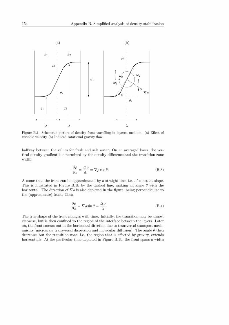
154 Appendix B. Simplified analysis of density stabilization
(a)
6
6
q1 q2
k1 k2
ρf
ρs?
6
dz
� -
λ
� -
λ
(b)
ρf
ρs
s
6ωg
∇ρ
..
..
..
..6
w1
..........?
w2
ϑ
� -
λ
Figure B.1: Schematic picture of density front travelling in layered medium. (a) Effect ofvariable velocity (b) Induced rotational gravity flow.
halfway between the values for fresh and salt water. On an averaged basis, the ver-tical density gradient is determined by the density difference and the transition zonewidth:
−∂ρ
∂z=4ρ
dz= ∇ρ cos θ. (B.3)
Assume that the front can be approximated by a straight line, i.e. of constant slope.This is illustrated in Figure B.1b by the dashed line, making an angle θ with thehorizontal. The direction of ∇ρ is also depicted in the figure, being perpendicular tothe (approximate) front. Then,
∂ρ
∂x= ∇ρ sin θ =
∆ρ
λ. (B.4)
The true shape of the front changes with time. Initially, the transition may be almoststepwise, but is then confined to the region of the interface between the layers. Lateron, the front smears out in the horizontal direction due to transversal transport mech-anisms (microscale transversal dispersion and molecular diffusion). The angle θ thendecreases but the transition zone, i.e. the region that is affected by gravity, extendshorizontally. At the particular time depicted in Figure B.1b, the front spans a width
155
of λ. More general, it can be said that
∂ρ
∂x= C1
∆ρ
λ, (B.5)
where C1 is related to the slope of the front.
Substituting (B.4) in (B.2), and adding the gravity effect −ωgλ to the forcedconvection effect (B.1), yields for the transition zone width
dz =
(q
n
∆k
k− k
µg∆ρ
)
t, (B.6)
where ∆k = k2 − k1.
In a diffusive problem, the transition zone width grows with the square root ofthe diffusion coefficient multiplied by time. The apparent dispersivity αapp is relatedto the transition zone width by
αapp =d2
z
C2q
nt, (B.7)
where C2 is a constant depending on the exact definition of dz. For example, for thelong-time solution of the linear convection-diffusion equation (i.e. for tracer trans-port), when dz is taken as the distance between the points having concentrations of0.16 (= 1
2erfc( 12
√2)) and 0.84 respectively, C2 = 8. For the comparison of the dis-
persivity in the density-dependent case to that in the tracer case, the value of C2
does not play any role. Substituting (B.6) in (B.7) gives for the dispersivity in thedensity-dependent case
αapp =1
C2
n
q
[(q
n
∆k
k
)2
− 2g∆ρ∆kq
µn+
(kg∆ρ
µ
)2]
t. (B.8)
For the tracer case, setting ∆ρ = 0 reduces (B.8) to
αtr =1
C2
q
n
(∆k
k
)2
t. (B.9)
The ratio between the two dispersivities is then given by
αapp
αtr= 1− 2nNg
(k
∆k
)
+ (nNg)2
(k
∆k
)2
, (B.10)
where Ng is the gravity number, describing the ratio of gravity to viscous forces.
Ng =Ra
Pe=
g∆ρk
µq. (B.11)
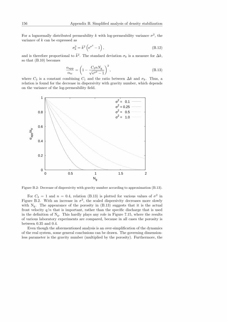
156 Appendix B. Simplified analysis of density stabilization
For a lognormally distributed permeability k with log-permeability variance σ2, thevariance of k can be expressed as
σ2k = k2
(
eσ2 − 1)
, (B.12)
and is therefore proportional to k2. The standard deviation σk is a measure for ∆k,so that (B.10) becomes
αapp
αtr=
(
1− C3nNg√eσ2 − 1
)2
, (B.13)
where C3 is a constant combining C1 and the ratio between ∆k and σk. Thus, arelation is found for the decrease in dispersivity with gravity number, which dependson the variance of the log-permeability field.
0
0.2
0.4
0.6
0.8
1
0 0.5 1 1.5 2
α app
/αtr
Ng
σ2 = 0.1
σ2 = 0.25
σ2 = 0.5
σ2 = 1.0
Figure B.2: Decrease of dispersivity with gravity number according to approximation (B.13).
For C3 = 1 and n = 0.4, relation (B.13) is plotted for various values of σ2 inFigure B.2. With an increase in σ2, the scaled dispersivity decreases more slowlywith Ng. The appearance of the porosity in (B.13) suggests that it is the actualfront velocity q/n that is important, rather than the specific discharge that is usedin the definition of Ng. This hardly plays any role in Figure 7.15, where the resultsof various laboratory experiments are compared, because in all cases the porosity isbetween 0.35 and 0.4.
Even though the aforementioned analysis is an over-simplification of the dynamicsof the real system, some general conclusions can be drawn. The governing dimension-less parameter is the gravity number (multiplied by the porosity). Furthermore, the
157
reduction in dispersivity depends on the magnitude of the permeability variations.Based on this simple analysis, it does not seem to depend on the correlation length λ.

Appendix C
Scaling of density, mass
fraction, and concentration
In this appendix, the differences between the scaled density, mass fraction, and con-centration are clarified and illustrated. In addition, it is shown under which assump-tions the various forms of the salt mass balance—in terms of different variables—areobtained.
C.1 Scaled variables compared
The concentration c as it is denoted in the numerical model d3f (see Chapter 7), isactually a scaled mass fraction, living between 0 and 1. The true mass concentration Cis defined as
C = ωρ, (C.1)
where ω is the mass fraction (dimensionless), and ρ the fluid density. The scaled massfraction ω∗ is defined as
ω∗ =ω
ωs, (C.2)
where ωs is the maximum salt mass fraction, i.e. the mass fraction of the brine,corresponding to the brine density ρs. Furthermore, the density is scaled as
ρ∗ =ρ− ρf
ρs − ρf, (C.3)
where ρf is the fresh water density. Note that in Chapter 8, this scaled density isdenoted by %.
The concentration C is scaled to lie between 0 and 1 using
C∗ =C
Cs=
ωρ
ωsρs= ω∗
ρ
ρs. (C.4)
Finally, using the equation of state
ρ = ρf eγρω, (C.5)
159
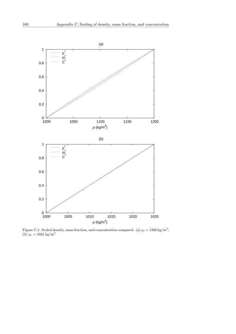
160 Appendix C. Scaling of density, mass fraction, and concentration
0
0.2
0.4
0.6
0.8
1
1000 1050 1100 1150 1200
ρ (kg/m3)
(a)
ρ*
ω*
C*
0
0.2
0.4
0.6
0.8
1
1000 1005 1010 1015 1020 1025
ρ (kg/m3)
(b)
ρ*
ω*
C*
Figure C.1: Scaled density, mass fraction, and concentration compared. (a) ρs = 1200 kg/m3;(b) ρs = 1025 kg/m3
C.2 Different forms of the salt mass balance 161
the scaled mass fraction ω∗ can be expressed in terms of ρ as
ω∗ =ω
ωs=
1γρ
ln(
ρρs
)
1γρ
ln(
ρs
ρf
)
=ln ρ− ln ρf
ln ρs − ln ρf. (C.6)
In Figure C.1, the scaled density (C.3), scaled concentration (C.4), and scaled massfraction (C.6) are compared. Figure C.1a shows the three variables over the completedensity range for a maximum density ρs = 1200 kg/m3. The scaled mass fractionis always slightly higher, whereas the scaled concentration is always slightly lowerthan the scaled density. The differences attain their maximum close to ρ∗ = 0.5,where ω∗ = 0.523 and C∗ = 0.479, and approach zero in the limits ρ∗ ↓ 0 andρ∗ ↑ 1. In Figure C.1b, the same variables are plotted for a maximum density ofρs = 1025 kg/m3. For this density range, the differences between the three scaledvariables are insignificant.
C.2 Different forms of the salt mass balance
In its full form, the salt mass balance, assuming a constant porosity, n, and a fluxdescribed by linear Fick’s law (see expression (2.8)), is given by
n∂(ρω)
∂t+∇·(ρqω − ρD ·∇ω) = 0, (C.7)
where q is the specific discharge, and D is the diffusion/dispersion tensor (see ex-pression (2.9)). Using the fluid mass balance equation, (2.3), (C.7) can be rewrittenas
nρ∂ω
∂t+ ρq ·∇ω −∇·(ρD ·∇ω) = 0. (C.8)
Now, when the exponential equation of state (C.5) is used, equation (C.8) can bewritten in terms of the density only:
n∂ρ
∂t+ q ·∇ρ−∇·(D ·∇ρ) = 0. (C.9)
Writing the salt mass balance in this form therefore implies the use of the exponentialequation of state.
Alternatively, the salt mass balance can be written in terms of the mass concen-tration C, using (C.1). However, the dispersive mass flux can be written as
J = −D ·∇C, (C.10)
only when it is assumed that ρ is constant. This is done in the so-called Boussinesqapproximation, for which equation (C.7) reduces to
n∂C
∂t+ q ·∇C −∇·(D ·∇C) = 0. (C.11)
162 Appendix C. Scaling of density, mass fraction, and concentration
Note that the Boussinesq approximation goes further than the assumption of incom-pressible flow, i.e. ∇· q = 0. In this assumption, where the density is kept constanteverywhere—except for the gravity term in Darcy’s law—lies a contradiction. Thistopic is discussed thoroughly in Chapter 3. Assuming that the density is constant,salt mass balance equation (C.7) can simply be divided by ρ, with the fluid massbalance ∇·q = 0 yielding an equation similar to (C.11), in which C is replaced by ω.In this case, the scaled mass fraction and scaled concentration are equivalent.
The mass balance equation written in terms of ρ, equation (C.9), is more exactthan equation (C.11). The only underlying assumption is related to the form ofthe equation of state. In addition, the assumption of incompressible flow may beemployed—as is done in the homogenization model of Egorov. That equation (C.9)still makes sense in this case can be understood when the density is scaled accordingto (C.3). When the relative density difference is introduced as
ε =ρs − ρf
ρf, (C.12)
the fluid mass balance becomes
ε
(
n∂ρ∗
∂t+ q ·∇ρ∗
)
+∇·q = 0, (C.13)
where ε denotes the relative density difference.In the limit ε ↓ 0, the fluid mass balance (C.13) reduces to the continuity equation
∇·q = 0. (C.14)
However, this does not imply that the term between brackets in equation (C.13) equalszero. When the same scaling is applied to the salt mass balance (C.9), ε appears infront of each term in the mass balance equation and can be eliminated. Therefore,equation (C.9) is maintained, where ρ is replaced by the scaled density ρ∗.
Appendix D
The cell problem
In this appendix, the details of the homogenization procedure— applied to the prob-lem of dispersion of a brine front in a weakly heterogeneous porous medium—aregiven.1 The so-called cell problem is derived, with its simplest solution. This solu-tion yields an algebraic macroscopic model, which is used for comparison with thenumerical experiments, as is described in Chapter 8.
D.1 Derivation of the cell problem
The solution of the system (8.34)–(8.36) is decomposed into a series of powers of thesmall parameter σ:
% = %(0)(z, t) + σ%(1)(z, t;x) + O(σ2), (D.1)
q1 = ±1 + σq(1)1 (z, t;x) + O(σ2), (D.2)
q2 = 0 + σq(1)2 (z, t;x) + O(σ2). (D.3)
Additionally, it is required that for n ≥ 1
⟨
%(n)⟩
= 0,⟨
q(n)1
⟩
= 0,
⟨n∑
k=1
(−1)(n−k)
(n− k)!q(k)2 Kn−k
⟩
= 0. (D.4)
The first condition leads to the equality of %(0) to the mean density 〈%〉, which ap-pears in the macroscale balance equation. The other two conditions follow from theboundary condition for the vertical velocity component and the condition for themean transverse pressure gradient, see (8.37).
After substitution of the series (D.1)–(D.3) into equations (8.35) and (8.36), theterms having equal powers of σ are gathered. For n = 1, we obtain
∂q(1)1
∂x1+
∂q(1)2
∂x2+ εx
∂q(1)1
∂z= 0, (D.5)
∂
∂x2
(
q(1)1 ∓K + Ng%(1)
)
=
(∂
∂x1+ εx
∂
∂z
)
q(1)2 . (D.6)
1This is work of Andrey Egorov, Kazan State University, and will be part of a joint article.
163
164 Appendix D. The cell problem
Substituting the series into (8.34) yields
A0 + σA1 + σ2A2 + · · · = 0, (D.7)
where (taking into account (D.5))
A0 = εt∂%(0)
∂t− dε2
x
∂2%(0)
∂z2, (D.8)
A1 = εt∂%(1)
∂t− ∂2%(1)
∂x22
− d
(∂
∂x1+ εx
∂
∂z
)2
%(1)±
Pe∂%(1)
∂x1+ Peεxq
(1)1
∂%(0)
∂z. (D.9)
We require An to be independent of the fast coordinates, i.e. An = 〈An〉. Withthis requirement, relation (D.7) becomes an alternative expression for the macroscalebalance equation (8.43). The first of these requirements, A0 = 〈A0〉, is automaticallysatisfied, while the second, A1 = 〈A1〉 = 0, together with (D.5) and (D.6) constitutes
a system of coupled linear equations for deriving %(1), q(1)1 , and q
(1)2 . These three
equations in the terminology of homogenization theory are referred to as the cellproblem. It is important to note that the macroscale density gradient ∂%(0)/∂z isa parameter of the cell problem. After solution of the cell problem, the macroscaledispersive flux J and uncertainty σ2
% are calculated using
J = dγ + σ2Pe2 ·Ng
⟨
q(1)1 %(1)
⟩
, (D.10)
σ2% = σ2
⟨
%(1)%(1)⟩
, (D.11)
which are obtained by substitution of the series (D.1) and (D.2) in (8.40) and (8.44).The parameter γ (8.45) will appear in these relations.
The same cell problem at εx = 0 was derived by Welty and Gelhar (1991) forthe case of a three-dimensional exponential correlation function. Welty and Gelhar’sanalysis was based on Fourier transformation of the cell problem. The same transfor-
mation is applied here, and after elimination of q(1)2 the cell problem is rewritten in
the frequency plane as
k22(v + c− 1) =
(
εx∂
∂z+ ik1
)2
v, (D.12)
εt∂c
∂t± iPek1c− γv + k2
2c = d
(
εx∂
∂z+ ik1
)2
c, (D.13)
where
c = ∓NgF%(1)
FK , v = ∓Fq(1)1
FK , (D.14)
D.2 Solution of the cell problem 165
and F denotes the Fourier transform
Ff =
+∞∫∫
−∞
eik·xf(x)dx1dx2. (D.15)
Using a standard technique (see Gelhar, 1993) the macroscopic flux J can be expressedin terms of c, v, and the Fourier transform φ(|k|) = FR of the correlation function:
J = dγ + σ2Pe ·I, (D.16)
I =Pe
(2π)2
+∞∫∫
−∞
φ(|k|) Re(c∗v) dk1dk2, (D.17)
where the asterisk denotes the complex conjugate. A similar expression is obtainedfor the uncertainty
σ2% = σ2Pe−1Ng
−2Iσ, (D.18)
Iσ =Pe
(2π)2
+∞∫∫
−∞
φ(|k|) |c|2dk1dk2. (D.19)
The first term on the right hand side of equation (D.16) is the microscale dispersiveflux, while the second term is the macroscale dispersive flux. In order to obtain thephenomenological relations for I and Iσ in terms of the density gradient γ, the system(D.12)–(D.13) needs to be solved. The solutions c and v are used to calculate theintegrals (D.17) and (D.19). In the general case, this procedure defines a nonlinear,nonlocal in space z and time t, phenomenological operator γ → I, and an analogousoperator γ → Iσ.
D.2 Solution of the cell problem
To simplify the derivation of the operator I, the smallness of the parameters εx andεt is used. The simplest algebraic phenomenological relationship can be derived whenthe terms with εx and εt in equations (D.12) and (D.13) are disregarded.
Posing εx = εt = 0 reduces equations (D.12) and (D.13) to the algebraic system
v + c = 1, ±Pek1c + k22c− γv = 0. (D.20)
From (D.20) we observe that the large term Pe k1c dominates the other terms in(D.20). The only way to arrive at a nontrivial solution is by re-normalization of theparameter k1 with a large factor. Without loss of generality, this factor is chosen tobe Pe, i.e.
k1 = Pek1. (D.21)
The necessity of the re-normalization is a common conclusion, see e.g. Gelhar (1993)and Welty and Gelhar (1991). It means that the major contribution to the integrals
166 Appendix D. The cell problem
(D.17) and (D.19) is made up of a small neighborhood around k1 = 0. As a result ofthe re-normalization, we obtain
c = c0(γ) =γ
κ + γ, v = v0(γ) =
κ
κ + γ, κ = k2
2 ± ik1, (D.22)
and rewrite the integrals (D.17) and (D.19) as
I =1
(2π)2
+∞∫∫
−∞
φ(|k2|) Re(c∗v)dk1dk2, (D.23)
Iσ =1
(2π)2
+∞∫∫
−∞
φ(|k2|) |c |2dk1dk2. (D.24)
These integrals are very similar to the integrals given in (D.17) and (D.19), but, as aresult of the re-normalization, φ becomes a function of |k2| instead of |k|. This allowsus to take the inner integrals in (D.23) and (D.24) explicitly and find I and Iσ as
I = I0(γ) =γ
4π
+∞∫
−∞
φ(|k2|)k22
γ + k22
dk2, (D.25)
Iσ =γ2
4π
+∞∫
−∞
φ(|k2|)1
γ + k22
dk2. (D.26)
If the spectrum φ is specified, the derivations of the functions I0(γ) and Iσ are simpleexercises in calculus. For the two-dimensional isotropic Gaussian correlation function,with spectrum φ(k) = 4e−k2/π, we obtain
I0(γ) = γ(
1−√γeγ/π erfc√
γ/π)
, (D.27)
Iσ(γ) = γ3/2eγ/π erfc√
γ/π. (D.28)
These results apply to the case of the numerical experiment. For the case of a three-dimensional exponential correlation function, Welty and Gelhar (1991) derived ananalogous expression, see Table 6.2.
Note that the asymptotic behavior of I0 at small γ can be expressed universallyas
γ → 0 : I0 = γ − aγ3/2 + O(γ3/2), (D.29)
where the constant a depends on the integral characteristic of the correlation function:
a =φ(0)
4=
π
2
∞∫
0
R(r)r dr. (D.30)
D.2 Solution of the cell problem 167
The limit of small γ corresponds to the classical tracer case. In this case the phe-nomenological relation is reduced to the well known result I = γ. In the originaldimensional coordinates, this implies a linear dependence of the dispersive flux onthe density gradient, with a constant dispersion coefficient σ2 l, see Dagan (1989) orGelhar (1993). This classical relation is valid for large travel time, consistent withεx = εt = 0.
The macroscale balance equation (8.43), expression (D.16), and phenomenologi-cal relation I = I0(γ), form a system of equations for deriving the average densitygradient γ and the dispersive mass flux J . This algebraic macroscale model is usedfor comparison with the numerical experiments.
When the terms disregarded so far are retained in the cell problem defined inequations D.13 and D.12, and c and v are solved up to their next two orders, a morecomplex model is derived. This ”relaxation-interaction” model is not used in thisthesis and will therefore not be discussed here. The end result is given in generalterms in expression 6.21.

References
Amiri, A. and Vafai, K., Analysis of dispersion effects and non-thermal equilibrium,non-Darcian, variable porosity incompressible flow through porous media. Interna-tional Journal of Heat and Mass Transfer, 37(6):939–954, 1994.
Anderson, S. J., An experimental investigation of high concentration displacements insaturated porous media. Ph.D. thesis, The university of Western Australia, 1997.
Andricevic, R., Effects of local dispersion and sampling volume on the evolution ofconcentration fluctuations in aquifers. Water Resources Research, 34(5):1115–1129,1998.
Angulo, R., Gonzalez, J., and Lam, L., Developements in thermal energy in Mexico -part ten: solar evaporation applied to chemical recovery from cerro prieto I brines.Heat Recovery Systems and CHP, 7(2):129–138, 1987.
Bachu, S. and Stewart, S., Geological sequestration of anthropogenic carbon dioxide inthe Western Canada sedimentary basin: suitability analysis. Journal of CanadianPetroleum Technology, 41(2):32–40, 2002.
Bakhvalov, N. S. and Panasenko, G. P., Homogenisation: averaging Processes inPeriodic Media; Mathematical Problems in the Mechanics of Composite Materials.,vol. 36 of Mathematics and its Applications. Kluwer, Dordrecht, 1989.
Bastian, P. et al., UG - a flexible software toolbox for solving partial differentialequations. Computing and visualization in science, 1:27–40, 1997.
Bear, J., Dynamics of Fluids in Porous Media. Dover, New York, 1988.
Bear, J. and Bachmat, Y., Introduction to Modelling of Transport Phenomena inPorous Media. Kluwer Academic, 1991.
Bellin, A., Salandin, P., and Rinaldo, A., Simulation of dispersion in heterogeneousporous formations: statistics, first-order theories, convergence of computations.Water Resources Research, 28(9):2211–2227, 1992.
Ben Salah, M. D., Influence des contrastes de viscosite et de densite sur le deplacementen milieu poreux de deux fluides miscibles. Revue de l’Institut Francais du Petrole,20:1237–1255, 1965.
169
170 References
Bensoussan, A., Lions, J. L., and Papanicolaou, G., Asymptotic analysis for periodicstructures. NHPC, Amsterdam, 1987.
Biggar, J. W. and Nielsen, D. R., Chloride-36 diffusion during stable and unstableflow through glass beads. Soil Science Society of America Proceedings, 28:591–595,1964.
Bird, R. B., Stewart, W. E., and Lightfoot, E. N., Transport Phenomena. John Wiley& Sons, New York, 2nd edn., 2002.
Black, T. C. and Freyberg, D. L., Stochastic modeling of vertically averaged con-centration uncertainty in a perfectly stratified aquifer. Water Resources Research,23(6):997–1004, 1987.
Boehme, J. et al., Grundwasserbewegung im Deckgebirge uber dem SalzstockGorleben, Datenermittlung, Interpretation und Modellrechnungen. Report KWA5107/3, Federal Institute for Geosciences and Natural Resources, Hannover, 1985.
Bouhroum, A., Einfluß der Viskositats - und Dichteunterschiede zweier mischbarerFlussigkeiten auf den Koeffizienten der longitudinalen hydrodynamischen Disper-sion. Teil I Viskositatsunterschiede. Deutsche Gewasserkundliche Mitteilungen,32:144–154, 1988.
Bouhroum, A., Einfluß der Viskositats - und Dichteunterschiede zweier mischbarerFlussigkeiten auf den Koeffizienten der longitudinalen hydrodynamischen Disper-sion. Teil II Dichteunterschiede. Deutsche Gewasserkundliche Mitteilungen, 33:9–13, 1989.
Boussinesq, J., Theorie Analytique de la Chaleur, vol. 2. Gauthier-Villars, Paris, 1903.
Brigham, W. E., Reed, P. W., and Dew, J. N., Experiments on mixing during miscibledisplacements in porous media. Society of Petroleum Engineers Journal, 1:1–8,1961.
Bues, M. A. and Zilliox, L., Deplacement miscible avec contrastes de densite et deviscosite en milieu poreux. Identification des parametres de deplacement et stabiliteen regime de dispersion mechanique. Journal of Hydrology, 120:125–141, 1990.
Burr, D. T., Sudicky, E. A., and Naff, R. L., Nonreactive and reactive solute trans-port in three-dimensional heterogeneous porous media: mean displacement, plumespreading, and uncertainty. Water Resources Research, 30(3):791–815, 1994.
Commissie Opberging Radioactief Afval, Terugneembare berging, een begaanbaarpad? Eindrapport, CORA, Den Haag, 2001.
Coudert, J. M. and Jaudin, F., French experience in geothermal energy. Geothermics,17(1):195–203, 1988.
Croucher, A. E. and O’Sullivan, M. J., The Henry problem for salt water intrusion.Water Resources Research, 31(7):1809–1814, 1995.
References 171
Cvetkovic, V., Shapiro, A. M., and Dagan, G., A solute flux approach to transportin heterogeneous formations 2. Uncertainty analysis. Water Resources Research,28(5):1377–1388, 1992.
Dagan, G., Solute transport in heterogeneous porous formations. Journal of FluidMechanics, 145:151–177, 1984.
Dagan, G., Flow and Transport in Porous Formations. Springer, Berlin, 1989.
Dagan, G., Transport in heterogeneous porous formations: spatial moments, ergod-icity, and effective dispersion. Water Resources Research, 26(6):1281–1290, 1990.
Dagan, G. and Fiori, A., The influence of pore-scale dispersion on concentrationstatistical moments in transport through heterogeneous aquifers. Water ResourcesResearch, 33(7):1595–1605, 1997.
Diersch, H.-J. G. and Kolditz, O., variable-density flow and transport in porous media:approaches and challenges. Advances in Water Resources, 25(8–12):899–944, 2002.
Duijn, C. J. v., Peletier, L. A., and Schotting, R. J., Brine transport in porous media:self-similar solutions. Advances in Water Resources, 22(3):285–297, 1998.
Duijn, C. J. v. and Schotting, R. J., Brine transport in porous media: on the use ofvon mises and similarity transformations. Computational Geosciences, 2:125–149,1998.
Durdun, I. and Marunteanu, C., Site selection criteria for the disposal of spent nuclearfuel in Romania. Environmental Geology, 35(1):3–8, 1998.
Egorov, A. G., Demidov, D. E., and Schotting, R. J., On the interaction betweengravity forces and dispersive brine fronts in micro-heterogeneous porous media.Advances in Water Resources, 28(1):55–68, 2005.
Elder, J. W., Steady free convection in a porous medium heated from below. Journalof Fluid Mechanics, 27:29–48, 1967a.
Elder, J. W., Transient convection in a porous medium. Journal of Fluid Mechanics,27:609–623, 1967b.
Fein, E., D3f - ein Programmpaket zur Modellierung von Dichtestromungen. Tech.Rep. GRS-139, GRS, Braunschweig, Germany, 1998.
Ferziger, H. and Peric, M., Computational Methods for Fluid Dynamics. Springer,1999.
Frape, S. K., Fritz, P., and McNutt, R. H., Water-rock interaction and chemistryof groundwaters from the Canadian shield. Geochemica et Cosmochimica Acta,48:1617–1627, 1984.
Fritz, P. and Frape, S. K., Saline groundwaters in the Canadian Shield: a firstoverview. Chemical Geology, 36:179–190, 1982.
172 References
Gartling, D. K. and Hickox, C. E., A numerical study of the applicability of the Boussi-nesq approximation for a fluid-saturated porous medium. International Journal forNumerical Methods in Fluids, 5:995–1013, 1985.
Gelhar, L., Stochastic Subsurface Hydrology. Prentice-Hall, Old Tappan N.J., 1993.
Gelhar, L. W., Stochastic analysis of solute transport in saturated and unsaturatedporous media. In: J. B. . M. Corapcioglu, ed., Advances in transport phenomena inporous media, NATO ASI Ser., pp. 657–670, Martinus Nijhoff, Dordrecht, 1987.
Gelhar, L. W. and Axness, C. L., Three dimensional stochastic analysis of macrodis-persion in aquifers. Water Resources Research, 19(1):161–180, 1983.
Giesel, W. and Fielitz, K., Evaluation of groundwater salinity from well logs andconclusions on flow of highly saline water. Report 11656/83, Federal Institute forGeosciences and Natural Resources, Hannover, 1983.
Goldstein, M. E. and Braun, W. H., Advanced Methods for the Solution of Differen-tial Equations. NASA SP-316, U.S. Government Printing Office, Washington D.C.,1972.
Graham, W. and McLaughlin, D., Stochastic analysis of nonstationary subsurfacesolute transport 1. Unconditional moments. Water Resources Research, 25(2):215–232, 1989, 1989.
Gray, D. D. and Giorgini, A., The validity of the Boussinesq approximation for liquidsand gases. International Journal of Heat and Mass Transfer, 19:545–551, 1976.
Gray, W. G. and O’Neill, K., On the general equations for flow in porous media andtheir reduction to Darcy’s law. Water Resources Research, 12(2):148–154, 1976.
Hassanizadeh, M. and Gray, W., General conservation equations for multi-phase sys-tems: 1. Averaging procedure. Advances in Water Resources, 2:131–144, 1979.
Hassanizadeh, M. and Gray, W., General conservation equations for multi-phase sys-tems: 3. Constitutive theory for porous media flows. Advances in Water Resources,3:25–40, 1980.
Hassanizadeh, S. M., Derivation of basic equations of mass transport in porous media.Part 2. Generalized Darcy’s and Fick’s laws. Advances in Water Resources, 9:207–222, 1986.
Hassanizadeh, S. M., Experimental study of coupled flow and mass transport: a modelvalidation exercise. In: K. Kovar, ed., ModelCARE 90: calibration and Reliabilityin Groundwater Modelling, IAHS Publ. no. 195, pp. 241–250, Wallingford, 1990.
Hassanizadeh, S. M. and Leijnse, A., A non-linear theory of high-concentration-gradient dispersion in porous media. Advances in Water Resources, 18(4):203–215,1995.
References 173
Hassanizadeh, S. M., Leijnse, A., de Vries, W. J., and Stapper, R. A. M., Experimentalstudy of brine transport in porous media. RIVM Report 728514005, Bilthoven, TheNetherlands, 1990.
Hassanizadeh, S. M. and Leijnse, T., On the modeling of brine transport in porousmedia. Water Resources Research, 24(3):321–330, 1988.
Hellstrom, G., Tsang, C. F., and Claesson, J., Buoyancy flow at a two-fluid interfacein a porous medium: analytical studies. Water Resources Research, 24(4):493–506,1988a.
Hellstrom, G., Tsang, C. F., and Claesson, J., Combined forced-convection and buoy-ancy flow at a two-fluid interface in a porous medium: analytical studies. WaterResources Research, 24(4):507–515, 1988b.
Henry, H. R., Effects of dispersion on salt water encroachment in coastal aquifers. USGeological Survey Water Supply Paper, 1613-C:C71–C84, 1964.
Hickerson, B. and Hickerson, R., Geothermal energy from hot salt domes. In: Proceed-ings of the 1997 Annual Meeting of the Geothermal Resources Council. GeothermalResources Council Transactions, vol. 21, pp. 533–537, 1997.
Hill, S., Channeling in packed columns. Chemical Engineering Science, 1(6):247–253,1952.
Holzbecher, E. O., Modeling density driven flow in porous media. Springer, Berlin,1998.
Hornung, U., Homogenization and Porous Media. Springer, New York, 1997.
Hsu, K. C., The influence of the log-conductivity autovariance structure on macrodis-persion coefficients. Journal of Contaminant Hydrology, 65:65–77, 2003.
Ingham, D. B. and Pop, I., eds., Transport Phenomena in Porous Media. Pergamon,Oxford, 1998.
Ingham, D. B. and Pop, I., eds., Transport Phenomena in Porous Media II. Pergamon,Oxford, 2002.
International Atomic Energy Agency, Site selection factors for repositories of solidhigh-level and alpha-bearing wastes in geological formations. Technical Report 177,IAEA, Vienna, 1977.
Janssen, L. P. B. M. and Warmoeskerken, M. M. C. G., Transport Phenomena DataCompanion. Delftse Uitgevers Maatschappij, Delft, 2nd edn., 1991.
Jiao, C.-Y. and Hotzl, H., An experimental study of miscible displacements in porousmedia with variation of fluid density and viscosity. Transport in Porous Media,54:125–144, 2004.
174 References
Johannsen, K., On the validity of the Boussinesq approximation for the Elder problem.Computational Geosciences, 7(3):169–182, 2003.
Johannsen, K., Kinzelbach, W., Oswald, S., and Wittum, G., The saltpool benchmarkproblem - numerical simulation of saltwater upconing in a porous medium. Advancesin Water Resources, 25(3):335–345, 2002.
Joseph, D. D., Stability of Fluid Motions II. Springer-Verlag, Berlin, 1976.
Josseling De Jong, G. D., Longitudinal and transverse diffusion in granular deposits.Transactions of the American Geophysical Union, 39:67–74, 1958.
Kadunas, V. and Valiunas, J., Geoenvironmental evaluation of geological formationsof Lithuania for radioactive waste disposal. In: Proceedings of the 7th Annual In-ternational Conference on High-Level Radioactive Waste Management, pp. 83–85,ASCE, New York, 1996.
Kapoor, V. and Gelhar, L. W., Transport in heterogeneous aquifers 1. Dynamics ofconcentration fluctuations. Water Resources Research, 30(6):1775–1788, 1994a.
Kapoor, V. and Gelhar, L. W., Transport in heterogeneous aquifers 2. Predictions andobservations of concentration fluctuations. Water Resources Research, 30(6):1789–1801, 1994b.
Kaszuba, J. P., Janecky, D. R., and Snow, M. G., Carbon dioxide reaction processes ina model brine aquifer at 200 ◦C and 200 bars: implications for geologic sequestrationof carbon. Applied Geochemistry, 18(7):1065–1080, 2003.
Kaviany, M., Principles of Heat Transfer in Porous Media. Springer, New York, 2ndedn., 1995.
Kempers, L. J. T. M. and Haas, H., The dispersion zone between fluids with dif-ferent density and viscosity in a heterogeneous porous medium. Journal of FluidMechanics, 267:299–324, 1994.
Kretz, V., Berest, P., Hulin, J. P., and Salin, D., An experimental study of theeffects of density and viscosity contrasts on macrodispersion in porous media. WaterResources Research, 39(2):1032–1040, 2003.
Krupp, H. K. and Elrick, D. E., Density effects in miscible displacement experiments.Soil Science, 107(5):372–380, 1969.
Lage, J. L., The implications of the thermal equilibrium assumption for surrounding-driven steady conduction within a saturated porous medium layer. InternationalJournal of Heat and Mass Transfer, 42:477–485, 1999.
Leijnse, T., Free convection for high concentration solute transport in porous media.In: Kobus and Kinzelbach, eds., Contaminant Transport in Groundwater, pp. 341–346, Balkema, Rotterdam, 1989.
References 175
Leroy, C., Hulin, J. P., and Lenormand, R., Tracer dispersion in stratified porousmedia: influence of transverse dispersion and gravity. Journal of Contaminant Hy-drology, 11:51–68, 1992.
Lessoff, S. C., Indelman, P., and Dagan, G., A note on the influence of a constantvelocity boundary condition on flow and transport in heterogeneous formations.Water Resources Research, 63(10):3095–3101, 2000.
Lunati, I., Attinger, S., and Kinzelbach, W., Macrodispersivity for transport in arbi-trary nonuniform flowfields: asymptotic and preasymptotic results. Water ResouresResearch, 38(10):1187, 2002.
Mitchell, J., Fundamentals of soil behavior. J. Wiley and Sons, New York, 1976.
Moser, H., Einfluß der Salzkonzentration auf die hydrodynamische Dispersion imporosen Medium. Mitteilung nr. 128, Technische Universitat Berlin, 1995.
Mot, E., Verslag van het nationaal onderzoekprogramma aardwarmte en warmteop-slag. Report, Projectbureau Energieonderzoek, Utrecht, 1984.
Newberg, M. A. and Foh, S. E., Measurement of longitudinal dispersion coefficientsof gas flowing through porous media. SPE Papers, (17731), 1988.
Nield, D. A. and Bejan, A., Convection in Porous Media. Springer, New York, 2ndedn., 1999.
Nikiforov, A. S., Polyakov, A. S., Kashcheev, V. A., and Poluektov, P. P., Structureof salt formations and the reliability of burying solidified radioactive waste. SovietAtomic Energy, 63(2):601–607, 1987.
Oberbeck, A., Uber die warmeleitung der flussigkeiten bei berucksichtig derstromungen infolge von temperaturdifferenzen. Annalen der Physik und Chemie,7:271–292, 1879.
Ophori, D. U., The significance of viscosity in density-dependent flow of groundwater.Journal of Hydrology, 204:261–270, 1998.
Peirotti, M. B., Giavedoni, M. D., and Deiber, J. A., Natural convective heat transferin a recangular cavity with variable fluid properties - validity of the Boussinesq ap-proximation. International Journal of Heat and Mass Transfer, 30(12):2571–2581,1987.
Quintard, M. and Whitaker, S., Local thermal equilibrium for transient heat conduc-tion: theory and comparison with numerical experiments. International Journal ofHeat and Mass Transfer, 38(15):2779–2796, 1995.
Rajagopal, K. R., Ruzicka, M., and Srinivasa, A. R., On the Oberbeck-Boussinesqapproximation. Mathematical Models and Methods in Applied Sciences, 6(8):1157–1167, 1996.
176 References
Rannacher, R., Numerical analysis of nonstationary fluid flow. Technical Report SFB123 Preprint 492, University of Heidelberg, Germany, 1988.
Rempe, N. T., Champion for radioactive waste disposal host of the WIPP: Carlsbad,New Mexico. In: International Conference on Radioactive Waste Management andEnvironmental Remediation, vol. 1, pp. 149–151, ASME, New York, 1995.
Robin, M. J. L., Gutjar, A. L., Sudicky, E. A., and Wilson, J. L., Cross-correlatedrandom field generaiotn with the direct fourier transform method. Water ResourcesResearch, 29(7):2385–2397, 1993.
Rogerson, A. and Meiburg, E., Numerical simulation of miscible displacement pro-cesses in porous medis flows under gravity. Physics of Fluids A. Fluid Dynamics,5(11):2644–2660, 1993.
Rose, D. A. and Passioura, J. B., Gravity segregation during miscible displacementexperiments. Soil Science, 111(4):258–265, 1971.
Roxburg, I. S., Geology of High-Level Nuclear Waste Disposal. Chapman and Hall,London, 1987.
Saffman, P. G., A theory of dispersion in a porous medium. Journal of Fluid Mechan-ics, 6(3):321–349, 1959.
Sanchez-Palencia, E., Non Homogeneous Media and Vibration Theory, vol. 127 ofLecture Notes in Physics. Springer, Berlin, 1980.
Sander, W. and Herbert, H. J., NaCl crystallization at the MgCl2/NaCl solutionboundary - a possible natural barrier to the transport of radionuclides. MineralogicalMagazine, 49:265–270, 1985.
Scheidegger, A. E., Statistical hydrodynamics in porous media. Journal of AppliedPhysics, 25(8):994–1001, 1954.
Scheidegger, A. E., General theory of dispersion in porous media. Journal of Geo-physical Research, 66:3273–3278, 1961.
Schelkes, K. and Vogel, P., Paleohydrological information as an important toolfor groundwater modeling of the Gorleben site. In: Paleohydrological Methodsand Their Applications for Radioactive Waste Disposal. Proceedings OECD/NEAWorkshop., pp. 237–250, OECD, Paris, 1992.
Schotting, R. J., Moser, H., and Hassanizadeh, S. M., High-concentration-gradientdispersion in porous media: experiments, analysis and approximations. Advancesin Water Resources, 22(7):665–680, 1999.
Schulz, R., Geothermal energy utilized in the Federal Republic of Germany. In: Inter-national Symposium on Geothermal Energy. Geothermal Resources Council Trans-actions, vol. 14, pp. 71–77, 1990.
References 177
Shestopalova, O. V., Geological suitability studies as to burial of radioactive wastein salts and tuffs of the Transcarpathian depression. In: Proceedings of the 6thAnnual International Conference on High-Level Radioactive Waste Management,pp. 36–38, ASCE, New York, 1995.
Shincariol, R. A. and Schwartz, F. W., An experimental investigation of variabledensity flow and mixing in homogeneous and heterogeneous media. Water ResourcesResearch, 26(10):2317–2329, 1990.
Simpson, M. J. and Clement, T. P., Theoretical analysis of the worthiness of Henryand Elder problems as benchmarks of density-dependent groundwater flow models.Advances in Water Resources, 26(1):17–31, 2003.
Slobod, R. L. and Howlett, W. E., The effects of gravity segregation in laboratorystudies of miscible displacement in vertical unconsolidated porous media. Societyof Petroleum Engineers Journal, 4:1–8, 1964.
Smirnov, V. I., Igoshin, A. I., Kazaryin, W., and Barinov, A. S., Project of an under-ground burial of radioactive waste of mean and low activity for the central region ofRussia. In: Proceedings of the 6th Annual International Conference on High-LevelRadioactive Waste Management, pp. 29–30, ASCE, New York, 1995.
Smith, L. and Schwartz, F., Mass transport 2. Analysis of uncertainty in prediction.Water Resources Research, 17(2):351–369, 1981.
Spitz, K., Dispersion in Porosen Medien: Einfluß von Inhomogenitaten und Dichte-unterschieden. Mitteilungen heft 60, Institut fur Wasserbau, Universitat Stuttgart,1985.
Starr, J. L. and Parlange, J., Solute dispersion in saturated soil columns. Soil Science,121(6):364–380, 1976.
Stempel, C. V. and Brewitz, W., Hydrogeological characterization and surveillanceof the Asse site. In: International Conference on Radioactive Waste Managementand Environmental Remediation, vol. 1, pp. 791–796, ASME, New York, 1995.
Stheeman, H. A., Petroleum developement in the Netherlands, with special refer-ence to the origin, subsurface migration and geological history of the country’s oiland gas resources. Verhandelingen van het Koninklijk Nederlands Geologisch Mijn-bouwkundig Genootschap. Geologische Serie, 21:57–95, 1963.
Taylor, G. I., Dispersion of soluble matter in solvent flowing slowly through a pipe.Proceedings of the Royal Society of London. Series A., 219(1137):186–203, 1953.
Trefry, M. G., Ruan, F. P., and McLaughlin, D., Numerical simulations of preasymp-totic transport in heterogeneous porous media: departures from the Gaussian limit.Water Resources Research, 39(3):1063–1077, 2003.
178 References
Vanderborght, J., Concentration variance and spatial covariance in second-order sta-tionary heterogeneous conductivity fields. Water Resources Research, 37(7):1893–1912, 2001.
Visser, W. A., Waste disposal and underground waters. Geologie and Mijnbouw,53:249–256, 1974.
Vomvoris, E. G. and Gelhar, L. W., Stochastic analysis of the concentration vari-ability in a three-dimensional heterogeneous aquifer. Water Resources Research,26(10):2591–2602, 1990.
Warnecke, E. et al., Experimental investigations of possible radionuclide releases fromthe planned repositories in the Gorleben salt dome and Konrad iron ore mine as partof the long term safety assessment. In: Proceedings of an International Symposiumon the Siting, Design and Construction of Underground Repositories for RadioactiveWastes, pp. 401–416, IAEA, Vienna, 1986.
Watson, S. J., Barry, D. A., Schotting, R. J., and Hassanizadeh, S. M., On the valid-ity of Darcy’s law for stable high-concentration displacements in granular porousmedia. Transport in Porous Media, 47:149–167, 2002a.
Watson, S. J., Barry, D. A., Schotting, R. J., and Hassanizadeh, S. M., Validation ofclassical density-dependent solute transport theory for stable, high-concentration-gradient brine displacements in coarse and medium sands. Advances in Water Re-sources, 25:611–635, 2002b.
Welty, C., A. C. Kane III, and Kauffman, L. J., Stochastic analysis of transversedispersion in density-coupled transport in aquifers. Water Resources Research,39(6):Art. No. 1150, 2003.
Welty, C. and Gelhar, L., Stochastic analysis of the effect of fluid density and viscosityvariability on macrodispersion in heterogeneous porous media. Water ResourcesResearch, 27(8):2061–2075, 1991.
Welty, C. and Gelhar, L., Simulation of large-scale transport of variable densityand viscosity fluids using a stochastic mean model. Water Resources Research,28(3):815–827, 1992.
Whitaker, S., Diffusion and dispersion in porous media. AICHE Journal, 13(3):420–427, 1967.
Yeung, A. and Mitchell, J., Coupled fluid, electrical and chemical flows in soil.Geotechnique, 43(1):121–134, 1993.
Zwillinger, D., Handbook of Differential Equations. Academic Press, San Diego, 3rdedn., 1998.
List of Symbols
α thermal expansion coeffient 1/◦C
α‖ microscale longitudinal dispersivity m
α⊥ microscale transversal dispersivity m
αapp apparent dispersivity (density-dependent dispersion) m
αL longitudinal dispersivity m
αT transversal dispersivity m
αtr tracer dispersivity m
β nonlinear dispersion parameter, see equation (6.7), page 63 m2s/kg
β0 γρ/J0, see equation (8.65), page 137 m2s/kg
βp fluid compressibility 1/Pa
γ macroscopic dimensionless density gradient, see equation (6.20), page 67 -
γµ ∂ ln µ/∂ω -
γρ ∂ ln ρ/∂ω -
γf flow factor, page 65 -
γl local scale dimensionless density gradient, see equation (8.53), page 129 -
γmax maximum dimensionless density gradient -
γs ln(ρf/ρs) = γρ ωs, page 76 -
ε maximum relative density difference, see equation (3.12), page 22 -
εt temporal scaling parameter -
εx spatial scaling parameter -
η similarity variable, see equation (4.4), page 30 -
179
180 List of Symbols
θ angle with horizontal rad
λ log-permeability correlation scale m
λeff effective porous medium thermal conductivity W/m ◦C
λf(s) thermal conductivity of the fluid (solid) phase W/m ◦C
µ dynamic fluid viscosity kg/ms
µf fresh water viscosity kg/ms
µs salt water viscosity kg/ms
ξ similarity variable, page 42 -
ρ fluid density kg/m3
ρ0 reference fluid density kg/m3
ρf fresh water density kg/m3
ρmax maximum fluid density kg/m3
ρs salt water (brine) density kg/m3
∆ρ density difference, i.e. ∆ρ = ρs − ρf kg/m3
% scaled density, see equation (8.8), page 103 -
σ2 log-permeability variance -
σ2% variance of scaled density -
σ2c concentration variance, see equation (7.3), page 73 -
σ2c variance of averaged concentration, see equation (7.5), page 73 -
σ2i concentration variance within realization i, see equation (7.4), page 73 -
σ2k permeability variance m4
τd characteristic diffusive time scale, page 118 s
τv characteristic convective time scale, page 118 s
ϕ hydraulic head m
φv volume flow rate m3/s
ω solute mass fraction -
ωg gravity-induced vorticity, see equation (B.2), page 157 1/s
List of Symbols 181
ωmax maximum salt mass fraction -
ωs salt water (brine) mass fraction -
A dimensionless coefficient, see equation (3.10), page 22 -
A11 macroscale longitudinal dispersivity m
A11,tr tracer macroscale longitudinal dispersivity m
a porous medium thermal diffusivity m2/s
a1 dimensionless parameter group, see equation (6.17), page 66 -
asf specific surface area common to fluid and solid phase -
b1 dimensionless parameter group, see equation (6.14), page 65 -
C solute mass concentration kg/m3
Cs salt mass concentration of brine kg/m3
c concentration, i.e. scaled mass fraction c = ω/ωs -
c horizontally averaged concentration, see equation (7.1), page 73 -
〈c〉 ensemble average concentration, see equation (7.2), page 73 -
cf(s) specific heat of the fluid (solid) phase J/kg ◦C
Co Courant number -
Cov log-permeability covariance, see equation (6.9), page 65 -
D hydrodynamic dispersion tensor m2/s
D scalar diffusion/dispersion coefficient m2/s
D0 effective dispersion coefficient, see equation (6.18), page 67 -
Dave time-averaged dispersion coefficient, see equation (A.7), page 156 m2/s
Dl local dispersion coefficient, see equation (A.5), page 156 m2/s
Dm effective porous medium molecular diffusion coefficient m2/s
Dtr tracer dispersion coefficient m2/s
d microscale dispersion tensor, see equation (8.25), page 117 m2/s
d dimensionless microscale dispersion coefficient, i.e. d = d‖/d⊥ -
d‖ microscale longitudinal dispersion coefficient m2/s
182 List of Symbols
d⊥ microscale transversal dispersion coefficient m2/s
dmol molecular diffusion coefficient m2/s
dz transition zone width m
F γl/γ, see equation (8.60), page 130 -
Fg gravity force per unit volume N/m3
f natural log-permeability, i.e. ln k -
f transformed temperature, see equation (4.4), page 30 -
Foβ modified Fourier number, see equation (8.16), page 104 -
G1 mean concentration gradient 1/m
g gravity acceleration vector m/s2
g magnitude of gravity acceleration vector m/s2
H column height m
h two-point separation vector m
h separation distance (lag) m
hsf heat transfer coefficient between solid and fluid phases W/m2 ◦C
I unit tensor -
I dispersive flux operator, page 120 -
Ixx central second moment, see equation (A.5), page 156 m2
i realization index, page 73 -
J dispersive mass flux vector kg/m2s
J dispersive mass flux (1-D) kg/m2s
J0 characteristic mass flux, see equation (8.63), page 137 kg/m2s
Jρ dispersive mass flux in terms of density, page 137 kg/m2s
j grid discretization level index -
K hydraulic conductivity tensor m/s
K hydraulic conductivity (isotropic medium) m/s
K dimensionless log-permeability, page 116 -
List of Symbols 183
k (intrinsic) permeability tensor m2
k intrinsic permeability (isotropic medium) m2
k0 average permeability m2
L macroscale m
l integral scale, see equation (6.19), page 67 m
lp characteristic pore size m
Le Lewis number, see equation (3.11), page 22 -
M mobility ratio, see equation (6.5), page 58 -
m time discretization level index -
N dimensionless coefficient, see equation (3.10), page 22 -
N number of realizations -
Ng gravity number, see equation (6.6), page 58 -
n unit normal vector -
n porosity -
P parameter group, see equation (8.11), page 103 m
p fluid pressure Pa
p0 reference fluid pressure Pa
Pe Peclet number for mass transfer, see equation (3.11), page 22 -
Pe⊥ Peclet number for transversal dispersion, see equation (8.30), page 118 -
Peβ modified Peclet number, see equation (8.18), page 104 -
PeT Peclet number for heat transfer, page 25 -
q specific discharge vector (Darcy velocity) m/s
q specific discharge (1-D) m/s
q0 characteristic specific discharge (mean or boundary value) m/s
qc critical velocity, see equation (2.15), page 16 m/s
qx horizontal velocity m/s
qz vertical velocity m/s
184 List of Symbols
q′′′f(s) heat generation in the fluid (solid) phase W/m3
R log-permeability correlation function, see equation (6.10), page 65 -
r order of convergence -
Ra Rayleigh number, see equation (3.31), page 27 -
S scaling factor, see equation (8.59), page 130 -
s moving frame coordinate, see equation (5.18), page 42 -
T temperature ◦C
T0 reference temperature ◦C
Tf(s) temperature of the fluid (solid) phase respectively ◦C
Tmin minimum temperature ◦C
T tortuosity factor -
t time s
tend end-time of experiment s
tscale characteristic time scale s
∆t time step size s
u transformed density, see equation (4.4), page 30 -
V average pore fluid velocity m/s
v transformed specific discharge, see equation (4.4), page 30 -
W column width m
w transformed mass fraction -
x spatial coordinate vector m
x horizontal coordinate m
x0 characteristic length m
y transformed temperature flux -
z vertical coordinate m
∆z distance between grid points m
〈· · ·〉 ensemble or volume averaged quantity
(· · · ) horizontally averaged quantity
Publications
Based on the work in this thesis, a number of articles have been prepared or are stillin preparation:
• Chapters 3 and 4 have been submitted as an article to Advances in WaterResources:
Heat and brine transport in porous media: the Oberbeck-Boussinesq approxi-mation revisited, A.J. Landman and R.J. Schotting.
• Based on Chapter 5, the following article is in preparation:
Closed-form approximate solutions for one-dimensional brine transport, R.J.Schotting and A.J. Landman.
• Chapter 6 is an extension of the conference paper:
Towards a physically based theory of high-concentration-gradient dispersion inporous media. An overview of experimental, theoretical and numerical studies,R.J. Schotting and A.J. Landman, In: Emerging Technologies and Techniquesin Porous Media (Eds: D. Ingham et al.), Kluwer Academic Publishers, 2004.
• Based on Chapter 7, the following manuscript is in preparation for Advances inWater Resources:
Density-dependent dispersion in heterogeneous porous media Part I: a numericalstudy, A.J. Landman, K. Johannsen, and R.J. Schotting.
• Based on Chapter 8, the following manuscript is in preparation for Advances inWater Resources:
Density-dependent dispersion in heterogeneous porous media Part II: compari-son with nonlinear theories, A.J. Landman, A. Egorov, and R.J. Schotting.
185

Summary
Analysis of Physical Mechanisms Underlying
Density-Dependent Transport in Porous Media
In this thesis, the interaction between (large) density gradients and flow and transportin porous media is studied. In particular, we consider salt transport in water-saturatedporous media, such as aquifers below the water table. Large density gradients exist forexample near deep salt rock formations, which are considered as possible long-termstorage sites for dangerous wastes. Groundwater flow and transport models thatcan deal with the effects of large density gradients are essential for risk-assessmentstudies of such underground disposal sites. Furthermore, many other groundwaterrelated applications exist, in which density effects can be significant even for lowconcentrations.
Density gradients mainly affect the flow field and mass transport in two ways:by fluid volume changes (the compressibility effect) and by inducing gravity forces.Generally, the compressibility effect—as a result of which the flow field is no longerdivergence-free—is of less importance than the gravity effect. When dealing withdensity-dependent flow problems, many researchers employ the simplifying Oberbeck-Boussinesq approximation. In this approximation, all density effects are disregarded,except for the gravity term in Darcy’s law. Contrary to the general belief, the Boussi-nesq approximation is not consistent with the limit of infinitely small density vari-ations. In this limit, the density-dependence in Darcy’s law disappears as well. InChapter 3, the limits are derived for which the compressibility effect can be neglectedin comparison with the gravity effect. Conditions are presented for the cases of isother-mal brine transport, heat transfer in fresh water, and simultaneous heat and brinetransport.
In Chapters 4 and 5, diffusion/dispersion dominated problems are studied in whichcompressibility effects play a role. Chapter 4 presents similarity solutions for two one-dimensional examples of simultaneous heat and brine transport. Similarity solutionsare useful for computer-code verification purposes. The solutions given in Chapter 4,as well as similarity solutions for several other brine transport problems, cannot begiven in closed-form. A numerical method is necessary to obtain these solutions. Ex-plicit analytical solutions of the convection-diffusion equation are known solely forthe case where density effects are disregarded, i.e. for tracer transport. In Chapter 5,approximate analytical solutions for one-dimensional density-dependent transport areobtained. To obtain these solutions, the density-coupling between the fluid and saltmass balance is maintained, but the continuity equation is simplified. A series expan-sion yields a simple analytical expression which can hardly be distinguished from theexact numerical solution. This approximate analytical solution is an extension of theclassical tracer solution.
In the second part of the thesis, consisting of Chapters 6 to 8, gravity plays animportant role. The effect of stabilizing gravity forces on hydrodynamic dispersionin a heterogeneous porous medium is investigated. Fresh water is displaced upward
187
188 Summary
by a denser brine. Heterogeneities in the porous medium permeability generate localvariations in the velocity. As a result, perturbations in the initially horizontal interfaceevolve, which grow to so-called dispersive fingers. However, when significant densitygradients are present, they induce a stabilizing, gravity-driven rotational movement,which counteracts the growth of dispersive fingers. Dispersive mixing in this way isinhibited, resulting in a steeper transition between fresh water and brine than in thecase of tracer transport.
Two-dimensional numerical simulations are performed for multiple realizations ofpermeability fields with small-scale heterogeneities. The accuracy of the numericalresults is investigated thoroughly in Chapter 7. Test cases show that stabilizinggravity forces are indeed responsible for a decrease in longitudinal dispersivity. Theparameter that controls the mixing under influence of a stabilizing density gradientis the gravity number. This number expresses the strength of gravity-induced flowin relation to forced-convection flow. The decrease of the longitudinal dispersivitywith gravity number that is found in the numerical experiments is in accordance withvarious laboratory experiments performed in nearly homogeneous media. However,the fact that dispersivity is a function of the gravity number, and thus of fluid and flowparameters, is in contradiction with the basic premise of classical dispersion theory,which considers dispersivity to be a medium property. The predictive capacity of theclassical theory is limited, because when density differences play a role, the dispersivityis not known beforehand, and cannot be determined in tracer tests.
In Chapter 8, two main alternative theoretical approaches are investigated. Acomparison with the results of the numerical experiments is made. The first theory—proposed and tested in the literature—consists of a nonlinear equation for the disper-sive mass flux. In this model, an additional dispersion parameter plays a role, whichneeds to be determined at least once for every flow rate. For a fixed flow rate, experi-ments for any density difference can be modelled using the same set of parameters inthe case of nearly homogeneous media. For media with larger permeability variations,additional parameter fitting is required in order to obtain a satisfactory agreementwith the numerical experiments.
The second theoretical approach is based on mathematical upscaling of the localequations, either by stochastic techniques or by homogenization. This approach re-sults in a macroscopic dispersive flux equation similar to Fick’s law, but in which thedispersion coefficient depends on the (dimensionless) density gradient. The homogen-ization model is directly comparable to the numerical experiments, as it relies on thesame assumptions. Without any additional parameters, the homogenization modelgenerates good predictions of the numerical experiments. Unfortunately, the applica-bility is limited to media with small variations in permeability only. Another resultobtained with the homogenization method is an expression for the concentration vari-ance, which is a measure of the deviations of local concentrations with respect to theirensemble average. The concentration variance decreases with increasing gravity num-ber. For large enough time and a significant density effect, the theoretical predictionis in agreement with the results of the numerical experiments.
Anke Jannie Landman
Samenvatting
Analyse van fysische mechanismen ten grondslag aan
dichtheidsafhankelijk transport in poreuze media
In dit proefschrift wordt het samenspel tussen (hoge) gradienten in de vloeistof-dichtheid en stroming en transport in poreuze media onderzocht. In het bijzon-der wordt gekeken naar transport van opgelost zout in een met water verzadigdporeus medium, zoals watervoerende zandlagen onder de grondwaterspiegel. Zeerhoge gradienten in de vloeistofdichtheid komen bijvoorbeeld voor in de omgeving vanzoutmijnen, die worden beschouwd als mogelijke locaties voor langdurige opslag vanradioactief afval. Modellen voor dichtheidsafhankelijk transport in grondwater zijneen onontbeerlijk middel in het onderzoek naar de risico’s van dit soort ondergrondseopslag. Bovendien zijn er tal van andere aan grondwater gerelateerde toepassingenwaarbij dichtheidseffecten al bij lage concentraties een rol kunnen spelen.
Twee effecten van de dichtheid op de stroming worden onderzocht: het effect vancompressibiliteit (door volume veranderingen) en het effect van de zwaartekracht.In het algemeen is het compressibiliteitseffect – waardoor de stroming niet meerdivergentievrij is – klein in vergelijking met het zwaartekrachtseffect, en kan hier-bij dan ook vaak verwaarloosd worden. Dit gebeurt in de veelvuldig gebruikteOberbeck-Boussinesq aanname, waarin alle dichtheidseffecten buiten beschouwingworden gelaten, behalve de zwaartekrachtsterm in de wet van Darcy. In tegen-stelling tot de algemene veronderstelling strookt de Boussinesq aanname niet metde wiskundige limiet van oneindig kleine dichtheidsverschillen. In Hoofdstuk 3 vandit proefschrift worden voorwaarden afgeleid waaronder het compressibiliteitseffectkan worden verwaarloosd ten opzichte van het zwaartekrachtseffect. Drie gevallenworden beschouwd: isotherm transport van zout, warmtetransport in zoet water, engelijktijdig transport van warmte en zout.
In Hoofdstukken 4 en 5 worden door diffussie/dispersie gedomineerde problemenbeschreven waarbij compressibiliteit de stroming beınvloedt. Hoofdstuk 4 geeft gelijk-vormigheidsoplossingen voor een tweetal voorbeelden van eendimensionaal gelijktijdigtransport van warmte en zout. De gelijkvormigheidsoplossingen in Hoofdstuk 4 zijnsemi-analytisch. Expliciete oplossingen worden alleen gevonden wanneer dichtheids-effecten totaal buiten beschouwing wordt gelaten, in zogenaamd ”tracer” transport.In Hoofdstuk 5 worden volledig analytische oplossingen gepresenteerd voor eendimen-sionaal transport van zout, die een benadering zijn van de exacte numerieke oplos-sing. Deze oplossingen worden verkregen door middel van een vereenvoudiging vande continuıteitsvergelijking, waarbij het effect van compressibiliteit wordt behouden.De uitkomst is een eenvoudige uitbreiding van de tracer-oplossing, die nauwelijks vande exacte oplossing te onderscheiden is.
In het tweede deel van dit proefschrift, bestaande uit Hoofdstukken 6 t/m 8, speeltde zwaartekracht een belangrijke rol. De stabiliserende werking van de zwaartekrachtop dispersie in een heterogeen poreus medium wordt onderzocht. Zoet water wordtopwaarts verdrongen door zout water met een hogere dichtheid. Heterogeniteiten in
189
190 Samenvatting
de doorlatendheid veroorzaken lokale verschillen in de stroomsnelheid, zodat de ver-plaatsing van het zoute front niet uniform is. Dit resulteert in groeiende verstoringenin het grensvlak tussen zout en zoet water, waardoor de scheiding tussen de tweevervaagt. Wanneer er echter sprake is van significante dichtheidsverschillen wordt hetgrensvlak gestabiliseerd door de zwaartekracht, die daarmee de dispersieve mengingtegengaat. Dit resulteert in een scherpere overgang tussen zout en zoet water dan inhet geval van tracer transport.
Tweedimensionale numerieke simulaties worden uitgevoerd voor een veelvoud aanrealisaties van het permeabiliteitsveld, dat bestaat uit vele kleinschalige heterogeni-teiten. De nauwkeurigheid van de berekeningen wordt uitvoerig onderzocht in Hoofd-stuk 7. Testberekeningen tonen aan dat de zwaartekracht inderdaad verantwoordelijkis voor de afname van de dispersiviteit die wordt waargenomen. De bepalende factoris het dimensieloze zwaartekrachtsgetal (gravity number). De afname van de disper-siviteit die in de numerieke experimenten wordt gevonden is in goede overeenstemmingmet de bevindingen van een aantal verschillende laboratorium studies. Het feit datde dispersiviteit afhangt van vloeistofeigenschappen is echter strijdig met de vooron-derstelling van de klassieke dispersietheorie, die de dispersiviteit als een medium pa-rameter beschouwt. Het vermogen om met de klassieke theorie voorspellingen te doenvoor gevallen waarbij dichtheidsverschillen een rol spelen is beperkt, omdat de dis-persiviteit in die gevallen niet op voorhand bekend is, en niet uit tracer experimentenkan worden bepaald.
In Hoofdstuk 8 worden de resultaten van de numerieke experimenten vergelekenmet twee alternatieve dispersietheorieen. De eerste theorie, die getoetst is aan expe-rimenten, is een niet-lineaire vergelijking voor de dispersieve massa flux. In dit modelspeelt een extra dispersie-parameter een rol, die tenminste eenmaal voor elk debietmoet worden bepaald. Voor een vast debiet kunnen experimenten met verschillendecontrasten in dichtheid worden gemodelleerd met dezelfde parameters in het gevalvan bijna homogene media. Voor media met sterkere variaties in de permeabiliteitmoet de niet-lineaire dispersieparameter vaker worden gefit.
De tweede aanpak is gebaseerd op het wiskundig middelen van de vergelijkingendie ter plaatse gelden, zodat nieuwe vergelijkingen worden verkregen die op hogereschaal geldig zijn. De homogenisatie methode leidt tot een dispersievergelijking opmacroschaal die dezelfde vorm heeft als de klassieke wet van Fick, maar waarin dedispersiecoefficient afhankelijk is van de (dimensieloze) gradient in de dichtheid. Hethomogenisatie model is volledig vergelijkbaar met de numerieke experimenten, omdathet op dezelfde aannamen gebaseerd is. Zonder dat er extra parameters nodig zijngeeft het homogenisatie model goede voorspellingen van de experimenten. Helaasis de toepasbaarheid beperkt tot media met zeer kleine variaties in permeabiliteit.Een ander resultaat van de homogenisatie is een uitdrukking voor de variantie van delocale concentratie ten opzichte van het ensemble gemiddelde. Deze variantie neemt afmet een toenemend zwaartekrachtsgetal. Voor voldoende grote tijd en een significantdichtheidsverschil is de theoretische voorspelling in goede overeenstemming met denumerieke resultaten.
Anke Jannie Landman
Acknowledgements
I would like to thank a few people that were of great help to me in writing this thesis.Above all Ruud Schotting, who has been my supervisor from the start. Thank you foryour guidance and ideas, for your inexhaustible enthusiasm, and for your confidencein me at times when I lost it. But also, thank you for being a friend. I enjoyedrunning with you in Nice, San Francisco, Kazan, and Oxford!
I thank my colleague PhD students for providing support, welcome distraction,and pleasure (to keep things bearable at times). I would like to name a few people inparticular: Twan, Birgitta, Laurien, Neeltje, Phil, Sam, and Bert-Rik. Furthermore, Ithank Cor van Kruijsdijk and the Petroleum Engineering group for hosting me duringthe last year.
A great part of the simulations have been performed on the cluster of the FluidMechanics Section. I would like to thank Guus Stelling for allowing me to use thecluster. I also thank the IWR in Heidelberg for using their cluster.
I would not have been able to perform all these simulations without the help ofKlaus Johannsen. Thank you for taking the time to work with me, and to makechanges to the code. My stays in Heidelberg were very useful and pleasant.
I am also very grateful to have come in contact with Andrey Egorov and DenisDemidov. Your work greatly contributed to this thesis. Thank you very much foryour collaboration, and for answering many of my questions. I also thank you foryour kindness and for making my stays in Kazan such a great experience.
Finally, I thank Majid Hassanizadeh for being my promotor. Thank you for yourconfidence and support, and for your critical view at times. You helped me to lookat things differently and to go one step further.
191

Curriculum vitae
Anke Jannie Landman werd geboren op 8 oktober 1974 te Assen. Zij behaalde in 1992het VWO-diploma aan het Zernike College in Groningen. Vervolgens begon zij aaneen studie Biologie aan de Rijksuniversiteit Groningen, waarvan zij het propedeutischdiploma cum laude behaalde.
In 1993 vervolgde zij haar opleiding aan de Technische Universiteit Delft, in derichting Technische Natuurkunde. Zij studeerde in 1999 af in de vakgroep Warmte enStroming. Van september 1999 tot februari 2005 was zij als promovenda in dienst vande TU Delft, aan de faculteit Civiele Techniek en Geowetenschappen. De resultatenvan het promotie-onderzoek zijn in dit proefschrift beschreven.
193