analysis of a simply supported beam

Analysis of a Simply Supported Beam

Zeinab El-SayeghID: 7126247

Department of Engineering and Computer SciencePresented in a Partial Fulfillment of the Requirement For The

MECH 6441

Concordia UniversityMontreal, Quebec, Canada

December , 2014

Analysis of a Simply Supported Beam

by

Zeinab El-SayeghID: 7126247

December 2014

A Project Submitted to the Graduate Facultyof The University of Concordia in Partial Fulfillment

of the MECH 6441Requirements for the Degree

Master of Engineering

Mechanical Engineering

2014

4

Abstract

This project will deal with the analysis of a simply supported beam that consistof two materials with applied complex loading. Calculation of the Airy stressfunction, stress tensor, principal stresses, maximum shear stress, and octahedralshear stress. Similar calculation will be done for the strain components. Inaddition study on the displacements, change in length will be done. Finallydesign parametric study on the maximum of the maximum principal stress andminimum of the minimum principal stress in the beam with respect to the aspectratio of the beam and forces will be performed.

Index words: simply supported beam, complex loading, Airystress/strain, stress/strain tensor, principalstresses/strains, maximum shear stress/strains,octahedral shear stress/strains, parametric design.

Contents

1 Introduction and Literature Review 11

1.1 Simply Supported beam . . . . . . . . . . . . . . . . . . . . . . 11

1.1.1 Definition . . . . . . . . . . . . . . . . . . . . . . . . . . . 11

1.1.2 Material properties . . . . . . . . . . . . . . . . . . . . . 12

1.1.3 Model Used . . . . . . . . . . . . . . . . . . . . . . . . . 12

1.2 Stress Analysis . . . . . . . . . . . . . . . . . . . . . . . . . . . 13

1.2.1 Stress . . . . . . . . . . . . . . . . . . . . . . . . . . . . . 13

1.2.2 Strain . . . . . . . . . . . . . . . . . . . . . . . . . . . . . 13

1.2.3 Airy Stress/strain . . . . . . . . . . . . . . . . . . . . . . 13

1.2.4 Stress/strain Tensor . . . . . . . . . . . . . . . . . . . . . 14

1.2.5 Principle Stresses/strains . . . . . . . . . . . . . . . . . . 14

1.2.6 Maximum Shear Stress/strains . . . . . . . . . . . . . . . 14

1.2.7 Octahedral Shear Stress/strains . . . . . . . . . . . . . . 14

1.2.8 Displacement . . . . . . . . . . . . . . . . . . . . . . . . . 14

1.3 Load Analysis . . . . . . . . . . . . . . . . . . . . . . . . . . . . 15

2 Stress Calculation 17

2.1 Airy Stress . . . . . . . . . . . . . . . . . . . . . . . . . . . . . . 17

2.2 Stress Tensor . . . . . . . . . . . . . . . . . . . . . . . . . . . . 23

2.3 Principal Stresses . . . . . . . . . . . . . . . . . . . . . . . . . . 24

2.4 Maximum Shear Stress . . . . . . . . . . . . . . . . . . . . . . . 25

2.5 Octahedral Shear Stress . . . . . . . . . . . . . . . . . . . . . . 25

2.6 Maximum of all stresses . . . . . . . . . . . . . . . . . . . . . . . 26

3 Strain Calculation 27

3.1 Strain Tensor . . . . . . . . . . . . . . . . . . . . . . . . . . . . 27

3.2 Principal Strains . . . . . . . . . . . . . . . . . . . . . . . . . . 28

3.3 Maximum Shear Strain . . . . . . . . . . . . . . . . . . . . . . . 29

3.4 Maximum of all Strains . . . . . . . . . . . . . . . . . . . . . . . 29

3.5 Geometric Calculations . . . . . . . . . . . . . . . . . . . . . . . 31

3.6 Displacement . . . . . . . . . . . . . . . . . . . . . . . . . . . . . 31

3.7 Length Change . . . . . . . . . . . . . . . . . . . . . . . . . . . . 32

5

6 CONTENTS

4 Complement Study 354.1 Parametric Study . . . . . . . . . . . . . . . . . . . . . . . . . . 354.2 Bending Beam . . . . . . . . . . . . . . . . . . . . . . . . . . . . 364.3 Results . . . . . . . . . . . . . . . . . . . . . . . . . . . . . . . . 37

A MATLAB Coding 39A.1 Stress . . . . . . . . . . . . . . . . . . . . . . . . . . . . . . . . . 39A.2 strain . . . . . . . . . . . . . . . . . . . . . . . . . . . . . . . . . 40

List of Figures

1.1 Typical Simply Supported Beam [1] . . . . . . . . . . . . . . . . 111.2 The beam model used in this study . . . . . . . . . . . . . . . . . 121.3 The Model used with Load . . . . . . . . . . . . . . . . . . . . . 15

2.1 Model with Located Co-Ordinate System . . . . . . . . . . . . . 182.2 The variation of the principle stress as a function of the position 26

3.1 Variation of the maximum principle strain as a function of and y 303.2 Variation of the minimum principle strain as a function of x and y 303.3 The variation of x displacement as a function of x and y . . . . . 323.4 The variation of y displacement as a function of x and y . . . . . 32

4.1 Bending Simply Supported Beam . . . . . . . . . . . . . . . . . 364.2 Bending Beam with couple moments . . . . . . . . . . . . . . . . 36

7

8 LIST OF FIGURES

List of Tables

1.1 Steel and Aluminum Material Properties [2] . . . . . . . . . . . . 12

9

10 LIST OF TABLES

Chapter 1

Introduction and LiteratureReview

This chapter includes an introduction about the project content. Definition ofsimply supported beam will be introduced, stress and strain definitions will beproposed, and the methodology used to solve this project will be suggested.

1.1 Simply Supported beam

In this section it is required to define the simply supported beam term, highlighton few properties of this structure and produce a model of the beam with therequired complex loading.

1.1.1 Definition

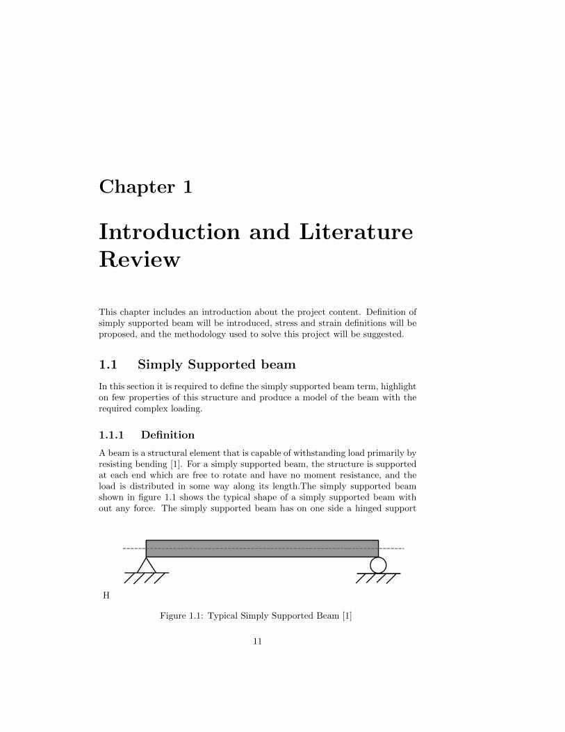
A beam is a structural element that is capable of withstanding load primarily byresisting bending [1]. For a simply supported beam, the structure is supportedat each end which are free to rotate and have no moment resistance, and theload is distributed in some way along its length.The simply supported beamshown in figure 1.1 shows the typical shape of a simply supported beam without any force. The simply supported beam has on one side a hinged support

H

Figure 1.1: Typical Simply Supported Beam [1]

11

12 CHAPTER 1. INTRODUCTION AND LITERATURE REVIEW

and on the other side a roller support. If the load was vertical and their is nomoment then both supports produce only vertical forces, however in the generalcase the hinged support is able to produce vertical and horizontal forces.

1.1.2 Material properties

In this project we assume that the beam of length L, depth 2c and unit width.Has the top half of the beam made of aluminum, and bottom half made ofsteel. A small search is made to conduct the material properties which is shownin table 1.1, typical properties of shown are assumed at room temperature (25 C ), we also assume that the materials is stainless steel 304 and aluminumwrought alloy 6061-T6 [2] These properties are based on the assumptions made,

Table 1.1: Steel and Aluminum Material Properties [2]

Properties Stainless Steel Aluminum

Density ( Mg/m3) 7.86 2.71Modulus of Elasticity (GPa) 193 68.9Modulus of Rigidity ( GPa) 75 26

Poisson’s Ratio 0.27 0.35Yield Strength of tension (MPa) 207 225

and according the reference used. Other values may be conducted for differentassumptions and using different references.

1.1.3 Model Used

In this part a new model of the beam will be defined according to the materialproperties , and the material assumptions. Figure 1.2 shows the new modelwith the two surfaces of aluminum and steel over each others.

Figure 1.2: The beam model used in this study

1.2. STRESS ANALYSIS 13

This new model only defines the new material combination and loading isnot applied yet, next step will be to define the appropriate loading on the beam.

1.2 Stress Analysis

In this section definitions of related types of stress and strains will be defined,summarized demonstration to indicate the relation between the definitions andthe related problem.

1.2.1 Stress

Stress is a physical quantity that expresses the internal forces that neighboringparticles of a continuous material exert on each other [3]. So basically stress isdirectly related to the force, it can be said that the stress is the force per unitarea. In this area one may also define the shear stress which is the he componentof stress coplanar with a material cross section. Shear stress is derived from theforce vector component parallel to the cross section [3].

1.2.2 Strain

In a similar manner as in section 1.2.1 a definition of strain may be implemented.physically strain is defined as deformation of a solid due to stress, so wheneverwe have stress their will be strain. A similar concept of the shear stress isfound in the strain which is called engineering shear strain and it represents themeasure of the change in angle along a certain axis.

1.2.3 Airy Stress/strain

This function can be used as a scaler potential to find the stress/strain tensor,it satisfies the equilibrium in the absence of body forces,but it should be notedthat it can only be used for two dimensional problems ex. plane stress/ planestrain. for the case of the airy stress function the governing equation is:

5φ4 + (1− υ)52ϕ = 0 (1.1)

for the case of equilibrium the equation becomes:

5φ4 = 0 (1.2)

while for the case of airy strain function, the governing equation becomes:

5φ4 +(1− 2υ)

1− υ52ϕ = 0 (1.3)

In these equations function φ(x, y) is the stress/strain function and ϕ is thepotential term.


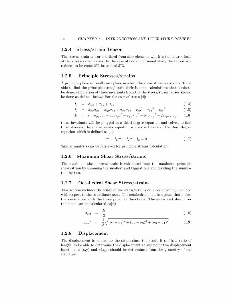
1.2.4 Stress/strain Tensor

The stress/strain tensor is defined from nine elements which is the matrix formof the stresses over axises. In the case of two dimensional study the tensor sizereduces to be come 2*2 instead of 3*3.

1.2.5 Principle Stresses/strains

A principle plane is usually any plane in which the shear stresses are zero. To beable to find the principle stress/strain their is some calculations that needs tobe done, calculation of three invariants from the the stress/strain tensor shouldbe done as defined below: For the case of stress [4]:

I1 = σxx + σyy + σzz (1.4)

I2 = σxxσyy + σyyσzz + σxxσzz − τxy2 − τyz2 − τxz2 (1.5)

I3 = σxxσyyσzz − σxxτyz2 − σyyτxz2 − σzzτxy2 − 2τxyτxzτyz (1.6)

these invariants will be plugged in a third degree equation and solved to findthree stresses, the characteristic equation is a second name of the third degreeequation which is defined as [4]:

σ3 − I1σ2 + I2σ − I3 = 0 (1.7)

Similar analysis can be retrieved for principle strains calculation.

1.2.6 Maximum Shear Stress/strains

The maximum shear stress/strain is calculated from the maximum principleshear/strain by summing the smallest and biggest one and dividing the summa-tion by two.

1.2.7 Octahedral Shear Stress/strains

This section includes the study of the stress/strains on a plane equally inclinedwith respect to the co-ordinate axes. The octahedral plane is a plane that makesthe same angle with the three principle directions. The stress and shear overthe plane can be calculated as[4]:

σoct =I13

(1.8)

τoct2 =

1

3

√(σ1 − σ2)

2+ (σ2 − σ3)

2+ (σ3 − σ1)

2(1.9)

1.2.8 Displacement

The displacement is related to the strain since the strain it self is a ratio oflength, to be able to determine the displacement at any point two displacementfunctions u (x,y) and v(x,y) should be determined from the geometry of thestructure.

1.3. LOAD ANALYSIS 15

1.3 Load Analysis

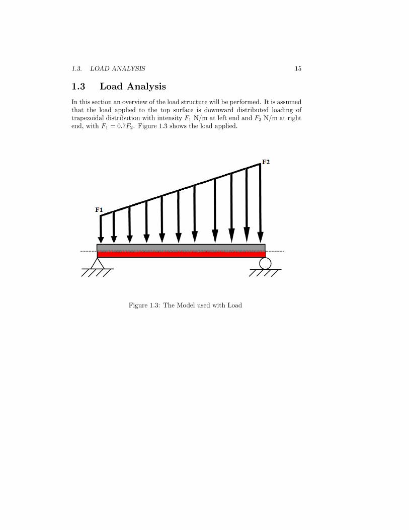
In this section an overview of the load structure will be performed. It is assumedthat the load applied to the top surface is downward distributed loading oftrapezoidal distribution with intensity F1 N/m at left end and F2 N/m at rightend, with F1 = 0.7F2. Figure 1.3 shows the load applied.

Figure 1.3: The Model used with Load

Chapter 2

Stress Calculation

In this chapter solution for the stress constants listed in chapter one will besolved. The solution will be on two ways , solution by hand with analyticalresults and solution with MATLAB that can facilitate the solving of high orderequations. A study for the stress/strain and displacement will be conductedaccording to the defined parameters in chapter one. Certain study of the stressover the materials will be done using hand calculations and software calculations.Some assumptions are taken into consideration in this section and dimensionsare given as:

L = 4m,

c = 0.25m,

w = 1m,

f1 = 3.5KN/m,

f2 = 5KN/m,

These assumptions satisfy the problem condition of F1 = 0.7F2 and are appli-cable to real life problems.

2.1 Airy Stress

The strategy used in this section is to take a general form of the solution andstart eliminating some constants according to the boundary conditions. Letsstart by defining an axis co-ordinate to start identifying the boundary condi-tions.

17

18 CHAPTER 2. STRESS CALCULATION

Figure 2.1: Model with Located Co-Ordinate System

Figure 2.1 shows the co-ordinate system used, where the origin is one thegeometric center of the beam. All parameters are kept parameters and novalue is assumed till now, figure 2.1 shows the dimensions of the beam. Nowwe can write the boundary conditions which are classified to strong and weakconditions. The strong boundary conditions are:

y = ±b; τxy = 0 (2.1)

y = −b;σy = 0 (2.2)

y = b;σy = −f1 − 0.3f2Lx (2.3)

These boundary conditions should be satisfied in the strong sense. We shallnow require three linearly independent weak boundary conditions on the endswhen x = ±L/2, but since our model is not symmetric we should define eachcondition alone, for x = L/2

Fx(L/2) =

∫ b

−bσx(L/2, y)dy = 0 (2.4)

Fy(L/2) =

∫ b

−bτxy(L/2, y)dy = FB (2.5)

M(L/2) =

∫ b

−bσx(L/2, y)ydy = 0 (2.6)

2.1. AIRY STRESS 19

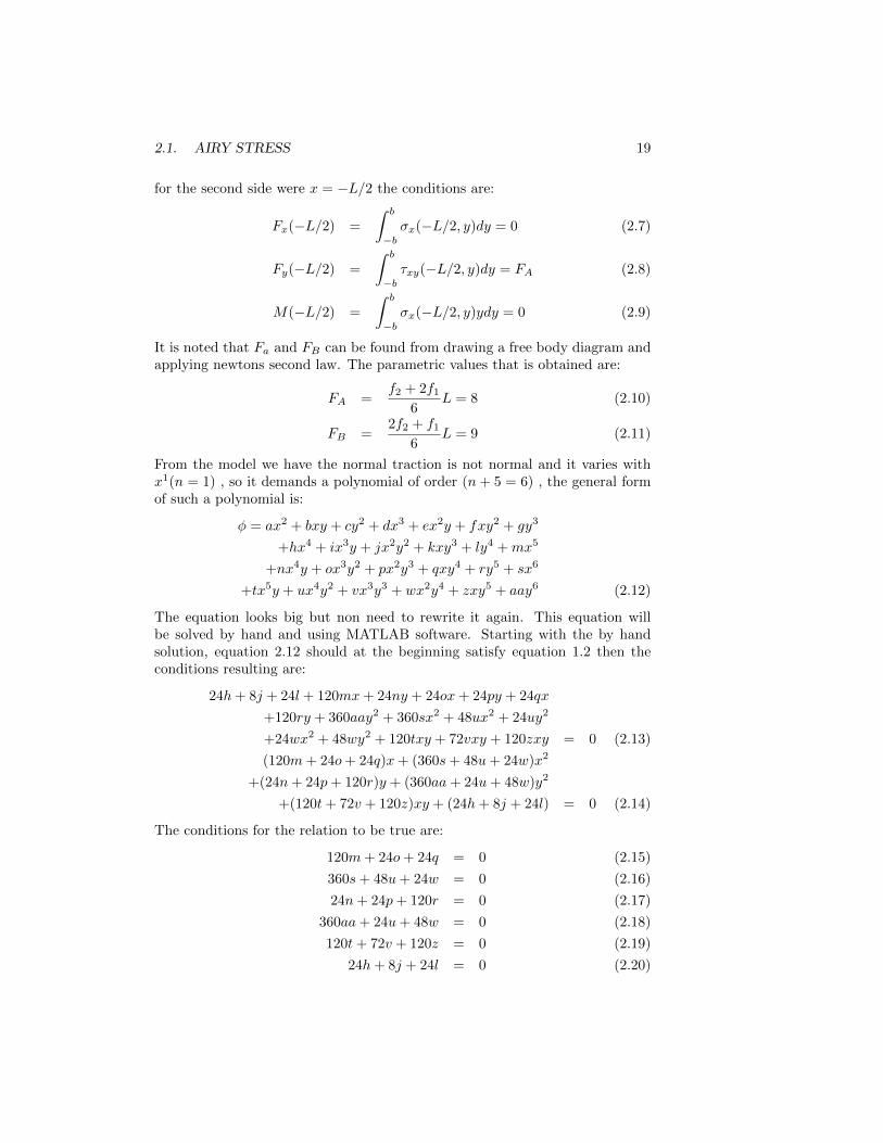
for the second side were x = −L/2 the conditions are:

Fx(−L/2) =

∫ b

−bσx(−L/2, y)dy = 0 (2.7)

Fy(−L/2) =

∫ b

−bτxy(−L/2, y)dy = FA (2.8)

M(−L/2) =

∫ b

−bσx(−L/2, y)ydy = 0 (2.9)

It is noted that Fa and FB can be found from drawing a free body diagram andapplying newtons second law. The parametric values that is obtained are:

FA =f2 + 2f1

6L = 8 (2.10)

FB =2f2 + f1

6L = 9 (2.11)

From the model we have the normal traction is not normal and it varies withx1(n = 1) , so it demands a polynomial of order (n+ 5 = 6) , the general formof such a polynomial is:

φ = ax2 + bxy + cy2 + dx3 + ex2y + fxy2 + gy3

+hx4 + ix3y + jx2y2 + kxy3 + ly4 +mx5

+nx4y + ox3y2 + px2y3 + qxy4 + ry5 + sx6

+tx5y + ux4y2 + vx3y3 + wx2y4 + zxy5 + aay6 (2.12)

The equation looks big but non need to rewrite it again. This equation willbe solved by hand and using MATLAB software. Starting with the by handsolution, equation 2.12 should at the beginning satisfy equation 1.2 then theconditions resulting are:

24h+ 8j + 24l + 120mx+ 24ny + 24ox+ 24py + 24qx

+120ry + 360aay2 + 360sx2 + 48ux2 + 24uy2

+24wx2 + 48wy2 + 120txy + 72vxy + 120zxy = 0 (2.13)

(120m+ 24o+ 24q)x+ (360s+ 48u+ 24w)x2

+(24n+ 24p+ 120r)y + (360aa+ 24u+ 48w)y2

+(120t+ 72v + 120z)xy + (24h+ 8j + 24l) = 0 (2.14)

The conditions for the relation to be true are:

120m+ 24o+ 24q = 0 (2.15)

360s+ 48u+ 24w = 0 (2.16)

24n+ 24p+ 120r = 0 (2.17)

360aa+ 24u+ 48w = 0 (2.18)

120t+ 72v + 120z = 0 (2.19)

24h+ 8j + 24l = 0 (2.20)


From the first condition 6 equations were established. Now to apply the bound-ary condition one must first get an explicit form of the stress and shears,

σx =∂2φ

∂y2

= 2ux4 + 6vx3y + 2ox3

+ 12wx2y2 + 6px2y + 2jx2 + 20zxy3

+ 12qxy2 + 6kxy + 2fx+ 30aay4

+ 20ry3 + 12ly2 + 6gy + 2c (2.21)

σy =∂2φ

∂x2

= 30sx4 + 20tx3y + 20mx3

+ 12ux2y2 + 12nx2y + 12hx2

+ 6vxy3 + 6oxy2 + 6ixy

+ 6dx+ 2wy4 + 2py3

+ 2jy2 + 2ey + 2a (2.22)

τxy = − ∂2φ

∂x∂y

= −5tx4 − 8ux3y − 4nx3

− 9vx2y2 − 6ox2y − 3ix2 − 8wxy3

− 6pxy2 − 4jxy − 2ex− 5zy4

− 4qy3 − 3ky2 − 2fy − b (2.23)

Now solving the boundary conditions one by one to eliminate and solve for theconstants, starting with equation 2.1:

y = ±b; τxy = 0

τxy(x,−1/2) = f − b− (3k)/4 + q/2− (5z)/16− 2ex+ 2jx

− (3px)/2 + wx− 3ix2 − 4nx3 + 3ox2 − 5tx4

+ 4ux3 − (9vx2)/4 (2.24)

= (f − b− (3k)/4 + q/2− (5z)/16) + x(−2e+ 2j − 3p/2 + w)

+ x2(3i+ 3o− 9v/4) + x3(−4n+ 4u) + x4(−5t) (2.25)

τxy(x, 1/2) = −b− f − (3k)/4− q/2− (5z)/16− 2ex− 2jx

− (3px)/2− wx− 3ix2 − 4nx3 − 3ox2 − 5tx4

− 4ux3 − (9vx2)/4 (2.26)

= −b− f − (3k)/4− q/2− (5z)/16 + x(−2e− 2j − 3p/2− w)

+ x2(−3i− 3o− 9v/4) + x3(−4n− 4u)x4(−5t) (2.27)

2.1. AIRY STRESS 21

Quitting the equations to zero a set of equations can be determined:

f − b− (3k)/4 + q/2− (5z)/16 = 0 (2.28)

−2e+ 2j − 3p/2 + w = 0 (2.29)

3i+ 3o− 9v/4 = 0 (2.30)

−4n+ 4u = 0 (2.31)

−5t = 0 (2.32)

−b− f − (3k)/4− q/2− (5z)/16 = 0 (2.33)

−2e− 2j − 3p/2− w = 0 (2.34)

−3i+ 3o− 9v/4 = 0 (2.35)

4n+ 4u = 0 (2.36)

(2.37)

One can conclude that, t = 0 , n = u = 0. Writing equation 2.2 :

y = −b;σy = 0

= 2a− e+ j/2− p/4 + w/8 + 6dx− 3ix

+ (3ox)/2− (3vx)/4 + 12hx2 + 20mx3

− 6nx2 + 30sx4 − 10tx3 + 3ux2 (2.38)

= (2a− e+ j/2− p/4 + w/8) + x(6d− 3i+ 3o/2− 3v/4)

+ x2(12h− 6n+ 3u) + x3(20m− 10t) + 30sx4 (2.39)

The conditions becomes:

2a− e+ j/2− p/4 + w/8 = 0 (2.40)

6d− 3i+ 3o/2− 3v/4 = 0 (2.41)

12h− 6n+ 3u = 12h = 0 (2.42)

20m− 10t = 20m = 0 (2.43)

s = 0 (2.44)

Three more parameters are reviled s = m = h = 0. Similarly with equation 2.3:

y = b;σy = −f1 − 0.3f2L

(x+ L/2) (2.45)

= 2a+ e+ j/2 + p/4 + w/8 + 6dx+ 3ix+ (3ox)/2

+ (3vx)/4 + 12hx2 + 20mx3 + 6nx2 + 30sx4 + 10tx3 + 3ux2 (2.46)

= 2a+ e+ j/2 + p/4 + w/8 + 6dx+ 3ix+ (3ox)/2 + (3vx)/4 (2.47)

= (2a+ e+ j/2 + p/4 + w/8) + x(6d+ 3i+ 3o/2 + 3v/4) (2.48)

Setting the equations to its correspondence,

2a+ e+ j/2 + p/4 + w/8 = −4.25 (2.49)

6d+ 3i+ 3o/2 + 3v/4 = −0.375 (2.50)


The above 22 equations represent the dominant equations that should be sat-isfied, taking into consideration that the initial number of unknowns where 25,we still have 3 more to compose, but lets do a small evaluation of the equationswe have using the MATLAB coding, it is shown that w = aa = 0. The leftequations are:

7.5r − 6l − 2e = 0 (2.51)

2a+ e− 1.5l − 1.25r + 4.25 = 0 (2.52)

6d+ 1.5q + 0.375 = 0 (2.53)

Now we should solve the weak conditions to find the remaining parametersit is only required to find one weak condition for example equation 2.4, theparameters become:

• a = −1.0625

• b = 34.5

• c = −1

• d = −0.0156

• e = −3.1875

• f = −0.03125

• g = 92

• h = 0

• i = −0.0625

• j = 0

• k = −46

• l = 0

• m = 0

• n = 0

• o = −0.0625

• p = −4.25

• q = 0.0625

• r = −0.85

• s = 0

• t = 0

• u = 0

• v = 0

• w = 0

• z = 0

• aa = 0

For more details about the MATLAB coding and the use of boundary con-ditions, please refer to appendix A.1. Now the airy function, stresses, and shear

2.2. STRESS TENSOR 23

becomes:

φ(x, y) = −0.0625x3y2 − 0.0625x3y − 0.0156x3 + 4.25x2y3 − 3.1875x2y

− 1.0625x2 + 0.0625xy4 − 46xy3 − 0.03125xy2

+ 34.5xy − 0.85y5 + 92y3 − y2 (2.54)

σx(x, y) = −0.125x3 + 25.5x2y + 0.75xy2 − 276xy − 0.0625x

− 17y3 + 552y − 2 (2.55)

σy(x, y) = 8.5y3 − 6.375y − 0.375xy − 0.375xy2 − 0.0936x− 2.125 (2.56)

τxy(x, y) = 0.375x2y + 0.1875x2 − 25.5xy2 + 6.375x− 0.25y3 + 138y2

+ 0.0625y − 34.5 (2.57)

2.2 Stress Tensor

The Tensor is in two dimensional form of:

[σx τxyτxy σy

]

The stress tensor can be found from the Airy stress values, using equations 2.55, 2.56, and 2.57 . It is noted that the tensor depends on the position of theparticle relevant to (x ,y) ,

−0.125x3 + 25.5x2y + 0.75xy2 0.375x2y + 0.1875x2 − 25.5xy2 + 6.375x

−276xy − 0.0625x− 17y3 + 552y − 2 −0.25y3 + 138y2 + 0.0625y − 34.5

0.375x2y + 0.1875x2 − 25.5xy2 + 6.375x 8.5y3 − 6.375y − 0.375xy

−0.25y3 + 138y2 + 0.0625y − 34.5 −0.375xy2 − 0.0936x− 2.125

If the matrix seems small please refer to the indicated equations. The stresstensor is not affected with the material properties due to the fact that the stressdeals with the force and area, but does not deal with the body properties it self.


2.3 Principal Stresses

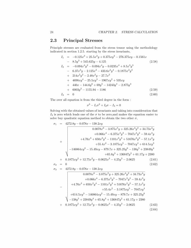
Principle stresses are evaluated from the stress tensor using the methodologyindicated in section 1.2.5. starting by the stress invariants,

I1 = −0.125x3 + 25.5x2y + 0.375xy2 − 276.375xy − 0.1561x

− 8.5y3 + 545.625y − 4.125 (2.58)

I2 = −0.094x4y2 − 0.094x4y − 0.0235x4 + 8.5x3y3

− 6.37x3y − 2.125x3 − 433.6x2y4 − 0.1875x2y3

+ 214x2y2 − 2.48x2y − 27.7x2

+ 4698xy4 − 25.5xy3 − 1967xy2 + 535xy

+ 440x− 144.6y6 + 69y5 − 14243y4 − 2.875y3

+ 6003y2 − 1155.94− 1186 (2.59)

I3 = 0 (2.60)

The over all equation is from the third degree in the form :

σ3 − I1σ2 + I2σ − I3 = 0

Solving with the obtained values of invariants and taking into consideration thatI3 is zero which leads one of the σ to be zero,and makes the equation easier tosolve buy quadratic equation method to obtain the two other σ,

σ1 = 4272.8y − 0.078x− 138.2xy

+

√√√√√√√√√√√√√√

0.0078x6 − 3.875x5y + 325.26x4y2 + 34.73x4y

+0.066x4 − 6.375x3y3 − 7047x3y2 − 59.4x3y

+4.76x3 + 650x2y4 − 1101x2y3 + 51676x2y2 − 57.1x2y

+55.4x2 − 3.1875xy5 − 7047xy4 + 614.5xy3

−146864xy2 − 15.49xy − 879.7x+ 325.25y6 − 138y5 + 23849y4

+65.8y3 + 136847y2 + 61.17y + 2380

+ 0.1875xy2 + 12.75x2y − 0.0625x3 − 4.25y3 − 2.0625 (2.61)

σ2 = 0 (2.62)

σ3 = 4272.8y − 0.078x− 138.2xy

−

√√√√√√√√√√√√√√

0.0078x6 − 3.875x5y + 325.26x4y2 + 34.73x4y

+0.066x4 − 6.375x3y3 − 7047x3y2 − 59.4x3y

+4.76x3 + 650x2y4 − 1101x2y3 + 51676x2y2 − 57.1x2y

+55.4x2 − 3.1875xy5 − 7047xy4

+614.5xy3 − 146864xy2 − 15.49xy − 879.7x+ 325.25y6

−138y5 + 23849y4 + 65.8y3 + 136847y2 + 61.17y + 2380

+ 0.1875xy2 + 12.75x2y − 0.0625x3 − 4.25y3 − 2.0625 (2.63)

(2.64)

2.4. MAXIMUM SHEAR STRESS 25

It is noted that these principle stresses are obtained using MATLAB coding formore details about the coding please refer to Appendix A.1 , and they are asa function of the position point p(x,y). For example, taking the center pointwhich is the point of origin p(0,0) the principle stresses become:

σ1 =√

304705/16− 33/16 = 32.437KPa

σ2 = 0

σ3 = −√

304705/16− 33/16 = −36.56KPa

And similarly at every point of the model we are able to find the localizedprinciple stresses.

2.4 Maximum Shear Stress

The maximum shear stress is obtained from the equation:

τmax =σ1 + σ3

2

τmax = −0.0625x3 + 12.75x2y + 0.1875xy2 − 138.2xy

− 0.078x− 4.25y3 + 273y − 2.0625 (2.65)

where σ1, and σ3 are the minimum and maximum principle stresses , then themaximum shear stress becomes. As indicated before this is a function of thepoint position (x,y).

2.5 Octahedral Shear Stress

The octahedral shear stress is calculated as indicated in equations 1.8, and 1.9,

σoct =I13

σoct = −0.0417x3 + 8.5x2y + 0.125xy2 − 92.125xy − 0.052x

− 2.83y3 + 181.875y − 1.375 (2.66)

τoct2 =

1

3

√(σ1 − σ2)

2+ (σ2 − σ3)

2+ (σ3 − σ1)

2

τoct2 =

√√√√√√√√√√√√√√

0.01x6 − 4.25x5y + 433.625x4y2 + 46.25x4y

+0.073x4 − 2.83x3y3 − 9396.8x3y2

−83.5x3y + 4.9x3 + 578.3x2y4 − 137.8x2y3 + 69045x2y2

−77.8x2y + 55.4x2 − 4.25xy5 − 6264.5xy4 + 683xy3 − 197130xy2

+336xy − 879.5x+ 112.4y6 − 13.67y5

+22303y4 + 77.5y3 + 186465y2 − 689y + 2383


2.6 Maximum of all stresses

As illustrated before the stresses are as a function of the position point p(x,y).In this section an analysis of the stresses will be performed to identify themaximum stresses and their location. Starting with the principle stresses andplotting the variation of the principle stress as a function of the x and y is shownin figure 2.2.

Figure 2.2: The variation of the principle stress as a function of the position

From the graph it is shown that the maximum principle stress occurs happensat the point x = −2, and y = 0.5.The principle stresses at this point are:

σ1 = 596.13KPa

σ2 = 0

σ3 = −3.5040KPa

One may also check for the lowest principle stress and it happens to be σmin =−602.1250, and this point which is p(-2,-0.5) the other principle stress is σ =−3∗10−4. The maximum octahedral stress will happen for the first case becausethe difference is bigger then,

σoct = 198.7082KPa

τoct2 = 283.4972KPa

Chapter 3

Strain Calculation

In this chapter the strain will be calculated according to the known equationσ = Eε, but the strain change along the y axis will depend on the materialproperty due to the combination of the materials ( aluminum, steel ).

3.1 Strain Tensor

The strain tensor will be divided to two parts for the section −0.5 ≤ y ≤ 0 inthis part E will be for steel, and the second part 0 ≤ y ≤ 0.5, in this part E willbe for Aluminum. Using Hooke’s Law σ = Eε it can be known that:

if − 0.5 ≤ y ≤ 0

εst = 1.45 ∗ 10−5σ (3.1)

if0 ≤ y ≤ 0.5

εal = 5.18 ∗ 10−6σ (3.2)

It can be also written in the form of a matrix, for −0.5 ≤ y ≤ 0 ,

5.18 ∗ 10−6(−0.125x3 + 25.5x2y + 0.75xy2 5.18 ∗ 10−6(0.375x2y + 0.1875x2 − 25.5xy2

−276xy − 0.0625x− 17y3 + 552y − 2) +6.375x− 0.25y3 + 138y2 + 0.0625y − 34.5)

5.18 ∗ 10−6(0.375x2y + 0.1875x2 − 25.5xy2 5.18 ∗ 10−6(8.5y3 − 6.375y − 0.375xy

+6.375x− 0.25y3 + 138y2 + 0.0625y − 34.5) −0.375xy2 − 0.0936x− 2.125)

In case of 0 ≤ y ≤ 0.5 the stress tensor will be ,

1.45 ∗ 10−5(−0.125x3 + 25.5x2y + 0.75xy2 1.45 ∗ 10−5(0.375x2y + 0.1875x2 − 25.5xy2

−276xy − 0.0625x− 17y3 + 552y − 2) +6.375x− 0.25y3 + 138y2 + 0.0625y − 34.5)

1.45 ∗ 10−5(0.375x2y + 0.1875x2 − 25.5xy2 1.45 ∗ 10−5(8.5y3 − 6.375y − 0.375xy

+6.375x− 0.25y3 + 138y2 + 0.0625y − 34.5) −0.375xy2 − 0.0936x− 2.125)

27

28 CHAPTER 3. STRAIN CALCULATION

3.2 Principal Strains

The principle stresses will be evaluated under the two conditions also, in thiscan we will get εst and εAl, for the case of steel, −0.5 ≤ y ≤ 0

ε1 = 1582y − 0.45x− 801xy

+ 0.5

√√√√√√√√√√√√√√√√√

0.5x6 − 214x5y + 21884x4y2 + 2337x4 ∗ y+4.5x4 − 429x3y3 − 474160x3y2 − 3999x3y

+320x3 + 43766x2y4 − 6947.7x2y3 + 3476795x2y2

−3840.8x2y + 3727x2 − 214xy5 − 474160xy4

+41352xy3 − 988xy2 − 1042xy − 59189x

+21882y6 − 9284y5 + 1604585y4 + 4428y3

+9207088y2 + 4115.6y + 160160

+ 1.08xy2 + 73.95x2y − 0.3625x3 − 24.65y3 − 11.96 (3.3)

ε2 = 0 (3.4)

ε3 = 1582y − 0.45x− 801xy

− 0.5

√√√√√√√√√√√√√√√√√

0.5x6 − 214x5y + 21884x4y2 + 2337x4 ∗ y+4.5x4 − 429x3y3 − 474160x3y2 − 3999x3y

+320x3 + 43766x2y4 − 6947.7x2y3 + 3476795x2y2

−3840.8x2y + 3727x2 − 214xy5 − 474160xy4

+41352xy3 − 988xy2 − 1042xy − 59189x

+21882y6 − 9284y5 + 1604585y4 + 4428y3

+9207088y2 + 4115.6y + 160160

+ 1.08xy2 + 73.95x2y − 0.3625x3 − 24.65y3 − 11.96 (3.5)

for the case of Aluminum 0 ≤ y ≤ 0.5, the principle stresses become

ε1 = 3955.78y − 1.13x− 2003xy + 2.72xy2 + 184.9x2y − 0.9x3 − 61.6y3

+ 0.5

√√√√√√√√√√√√√√

3.28x6 − 1340x5y + 136774x4y2 + 14605x4y + 28x4 − 2681x3y3

−2963500x3y2 − 24995x3y + 2004x3 + 273538x2y4 − 4342x2y3

+21729973x2y2 − 24005x2y + 2329x2 − 1340xy5

−2963500xy4 + 258451xy3 − 61756298xy2 − 6515xy

−369933x+ 136767y6 − 58029y5

+10028662y4 + 27674y3 + 57544301y2 + 25722y + 1001003

− 29.9 (3.6)

ε2 = 0 (3.7)

3.3. MAXIMUM SHEAR STRAIN 29

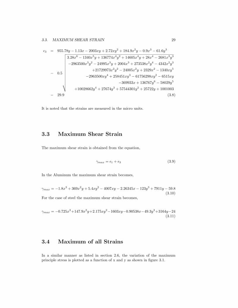
ε3 = 955.78y − 1.13x− 2003xy + 2.72xy2 + 184.9x2y − 0.9x3 − 61.6y3

− 0.5

√√√√√√√√√√√√√√

3.28x6 − 1340x5y + 136774x4y2 + 14605x4y + 28x4 − 2681x3y3

−2963500x3y2 − 24995x3y + 2004x3 + 273538x2y4 − 4342x2y3

+21729973x2y2 − 24005x2y + 2329x2 − 1340xy5

−2963500xy4 + 258451xy3 − 61756298xy2 − 6515xy

−369933x+ 136767y6 − 58029y5

+10028662y4 + 27674y3 + 57544301y2 + 25722y + 1001003

− 29.9 (3.8)

It is noted that the strains are measured in the micro units.

3.3 Maximum Shear Strain

The maximum shear strain is obtained from the equation,

γmax = ε1 + ε3 (3.9)

In the Aluminum the maximum shear strain becomes,

γmax = −1.8x3 + 369x2y + 5.4xy2 − 4007xy − 2.26345x− 123y3 + 7911y − 59.8(3.10)

For the case of steel the maximum shear strain becomes,

γmax = −0.725x3+147.9x2y+2.175xy2−1603xy−0.90538x−49.3y3+3164y−24(3.11)

3.4 Maximum of all Strains

In a similar manner as listed in section 2.6, the variation of the maximumprinciple stress is plotted as a function of x and y as shown in figure 3.1.


Figure 3.1: Variation of the maximum principle strain as a function of and y

The plot shown contains both the aluminum and the steel it can be noticedthat at the point (0,y) their is discontinuity due to the joining of both materialsat this point. It also can be noticed that the maximum principle strain occursat the point p(-2,0.5) where the maximum strain happens to be εmax = 8694.6, in this case the minimum strain is εmin = −50.8. Now plotting the minimumprinciple strain which is ε3 for example is shown in figure 3.2,

Figure 3.2: Variation of the minimum principle strain as a function of x and y

for the minimum case the values are at p(-2,-0.5) where εmin = −3492.325 ,in this case the maximum strain is εmin = −0.00174.

3.5. GEOMETRIC CALCULATIONS 31

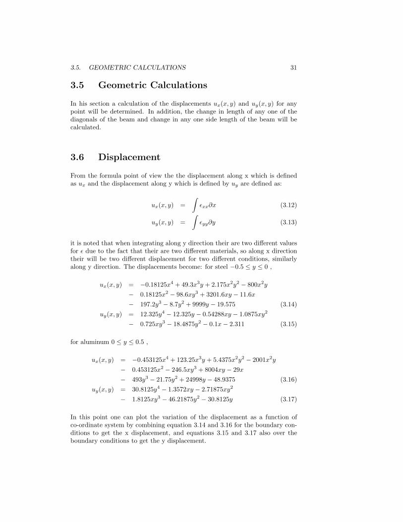
3.5 Geometric Calculations

In his section a calculation of the displacements ux(x, y) and uy(x, y) for anypoint will be determined. In addition, the change in length of any one of thediagonals of the beam and change in any one side length of the beam will becalculated.

3.6 Displacement

From the formula point of view the the displacement along x which is definedas ux and the displacement along y which is defined by uy are defined as:

ux(x, y) =

∫εxx∂x (3.12)

uy(x, y) =

∫εyy∂y (3.13)

it is noted that when integrating along y direction their are two different valuesfor ε due to the fact that their are two different materials, so along x directiontheir will be two different displacement for two different conditions, similarlyalong y direction. The displacements become: for steel −0.5 ≤ y ≤ 0 ,

ux(x, y) = −0.18125x4 + 49.3x3y + 2.175x2y2 − 800x2y

− 0.18125x2 − 98.6xy3 + 3201.6xy − 11.6x

− 197.2y3 − 8.7y2 + 9999y − 19.575 (3.14)

uy(x, y) = 12.325y4 − 12.325y − 0.54288xy − 1.0875xy2

− 0.725xy3 − 18.4875y2 − 0.1x− 2.311 (3.15)

for aluminum 0 ≤ y ≤ 0.5 ,

ux(x, y) = −0.453125x4 + 123.25x3y + 5.4375x2y2 − 2001x2y

− 0.453125x2 − 246.5xy3 + 8004xy − 29x

− 493y3 − 21.75y2 + 24998y − 48.9375 (3.16)

uy(x, y) = 30.8125y4 − 1.3572xy − 2.71875xy2

− 1.8125xy3 − 46.21875y2 − 30.8125y (3.17)

In this point one can plot the variation of the displacement as a function ofco-ordinate system by combining equation 3.14 and 3.16 for the boundary con-ditions to get the x displacement, and equations 3.15 and 3.17 also over theboundary conditions to get the y displacement.


Figure 3.3: The variation of x displacement as a function of x and y

Figure 3.4: The variation of y displacement as a function of x and y

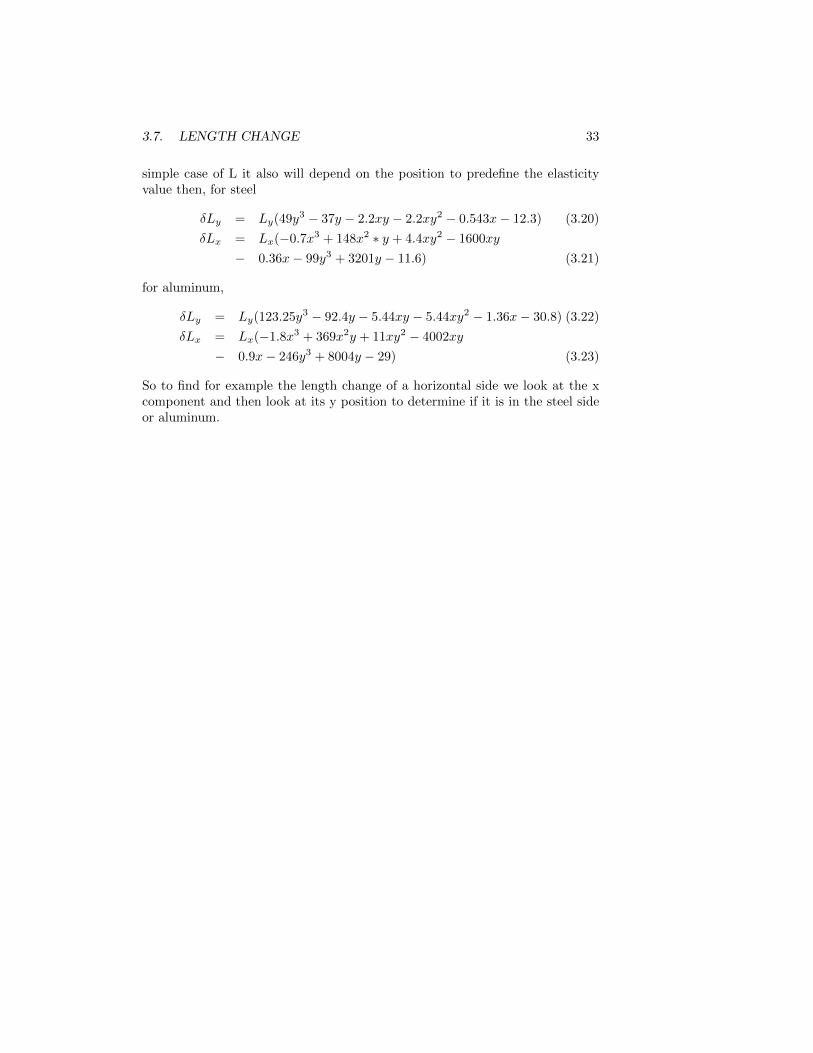
3.7 Length Change

The length change depend directly on u(x,y) and ε, to find the change in lengthat a certain point either along x or along y :

εyy =δLyLy

(3.18)

εxx =δLxLx

(3.19)

L it self should be horizontal or vertical, if L is a combination then anotherformula should be written that includes an angle orientation, to get back to the

3.7. LENGTH CHANGE 33

simple case of L it also will depend on the position to predefine the elasticityvalue then, for steel

δLy = Ly(49y3 − 37y − 2.2xy − 2.2xy2 − 0.543x− 12.3) (3.20)

δLx = Lx(−0.7x3 + 148x2 ∗ y + 4.4xy2 − 1600xy

− 0.36x− 99y3 + 3201y − 11.6) (3.21)

for aluminum,

δLy = Ly(123.25y3 − 92.4y − 5.44xy − 5.44xy2 − 1.36x− 30.8) (3.22)

δLx = Lx(−1.8x3 + 369x2y + 11xy2 − 4002xy

− 0.9x− 246y3 + 8004y − 29) (3.23)

So to find for example the length change of a horizontal side we look at the xcomponent and then look at its y position to determine if it is in the steel sideor aluminum.

Chapter 4

Complement Study

Two main topics will be discussed in this chapter the bending of the beam, andparametric study on some ratios.

4.1 Parametric Study

In this chapter a design parametric study will be conducted for the maximumof the maximum principal stress and minimum of the minimum principal stressin the beam with respect to the aspect ratio of the beam and F2. It is notedthat F2 is related to F1 and the aspect ratio is related to the length of the sidewhich is actually in this case the length to the width as ( 4 : 1 ) or in general (L : 1 ).As the force F2 increase the force F1 will increase with it too, due to the relationF1 = 0.7F2 in general case the maximum of the maximum principle stress willbe located at the P ( -2 , 0.5 ) and the minimum of the minimum principlestresses will be located the point P ( -2 , -0.5 ) this is the general case for whatever the force vary, due to the fact that it will have the same distribution of thetrapezoidal shape.The aspect ratio will affect the deflection and the displacement, as the beam getslonger the displacement and increase and the beam will start bending more andmore on its center point which is the deepest point form the pin and roller. Asthe beam gets longer the probability of bending gets larger and larger especiallyif the width remains one unit or gets smaller.Considering the relation between the aspect ratio and the principle stresses, themaximum of the maximum and the minimum of the minimum will always belocated on the extreme points, even when the aspect ratio changes these stresseswill be located at the extreme of the new dimensions. This is due to the pointof application of the forces and the type of the load applied which is constantin this case as trapezoidal. The location where the pin and roller are connectedalso play an important role in determining the position of the stresses, but inthe scope of this project they are fix connected at the extreme of the beam. The

35

36 CHAPTER 4. COMPLEMENT STUDY

aspect ratio can also have a significant effect on the break and fatigue of thesystem, as the aspect ratio gets bigger in a sense that the difference between thelength and the width gets larger this will increase the probability of the failureof the system.

4.2 Bending Beam

Assuming that the beam undergoes a bending moment with the same load forceapplied, then the beam will become as shown in figure 4.1 ,

Figure 4.1: Bending Simply Supported Beam

In this case we assume that the load is presented by moments and that thebeam is symmetrical and only have couple moments are the free ends, theseassumptions lead to the drawing shown in figure 4.2

Figure 4.2: Bending Beam with couple moments

Now and using the missioned assumptions it will be easy to solve the prob-

4.3. RESULTS 37

lem, the radial and tangential stresses are defined as:

σr =4M

tb2N

[(1− a2

b2

)lnr

a−(

1− a2

r2

)lnb

a

](4.1)

σθ =4M

tb2N

[(1− a2

b2

)(1 + ln

r

a

)−(

1 +a2

r2

)lnb

a

](4.2)

for the purpose of this section we will assume that a = 100mm, b = 150mmand that r = 50mm. Taking into consideration that,

M = moment (4.3)

N =

(1− a2

b2

)2

− 4a2

b2ln2 b

a(4.4)

for these values we get that:

σr = 332KPa (4.5)

σθ = −743KPa (4.6)

on the other hand we know that the moment is,

M = (3.5 ∗ 4) ∗ 2 + 1.5 ∗ 2 ∗ 8/3

= 36KN.m

knowing the inertial of the system to be, Iy = 0.0415m4, Iz = 0.0104m4, andIyz = 0m4 then the stress along x direction will be,

σx =Mc

I(4.7)

=36 ∗ 0.5

0.0415= 433.7KPa

4.3 Results

From the bending moments analysis we found that the maximum stress thatcan be found is σ = 433.7KPa, it is useful to compare this result with a similarone from the airy stress functions that were derived, the maximum σ of all thebeam is calculate to be σ = 596KPa the error then is 27%. This error is due tothe shearing stress which is not taken into consideration in the bending beamtheory in addition to the assumption of point force and not load force.

38 CHAPTER 4. COMPLEMENT STUDY

Appendix A

MATLAB Coding

MATLAB coding for the stress/ strain analysis is listed below.

A.1 Stress

syms x y;

syms sigmax(x,y)sigmay(x,y)taux(x,y)tauxy(x,y)

p(x,y) phi(x,y)eq(x,y);

t=0;

u=0;

n=0;

s=0;

m=0;

h=0;

w=0;

aa=0;

d=-0.0156;

q=0.0625;

l=0;

a=-1.0625;

z=0;

p=4.25;

o=-0.0625;

jj=0;

b=34.5;

v=0;

ii=-0.0625;

e=-3.1875;

g=92;

c=-1;

k=-46;

39

40 APPENDIX A. MATLAB CODING

r=-0.85;

f=-0.03125;

theta=a*x^2+b*x*y +c*y^2+d*x^3+e*x^2*y+f*x*y^2+g*y^3

+h*x^4+ii*x^3*y+jj*x^2*y^2 +k*x*y^3+l*y^4+m*x^5

+n*x^4*y +o*x^3*y^2+p*x^2*y^3+q*x*y^4+r*y^5

+s*x^6 +t*x^5*y+u*x^4*y^2+v*x^3*y^3

+w*x^2*y^4+z*x*y^5+aa*y^6;

phi(x,y)=diff(theta,x,4)+diff(theta,y,4)

+2*diff(diff(theta,x,2),y,2)

sigmax(x,y)=diff(theta,y,2)

sigmay(x,y)=diff(theta,x,2)

taux(x,y)=diff(theta,x)

tauxy(x,y)=diff(taux,y)

tauxy(x,y)=-tauxy(x,y)

int(sigmax(x,y),y,-0.5,0.5)

Ione(x,y)=sigmax(x,y)+sigmay(x,y)

Itwo(x,y)=sigmax(x,y)*sigmay(x,y)-(tauxy(x,y))^2

delta=expand(Ione^2-4*Itwo);

sigmaone(x,y)=simplify(0.5*Ione+0.5*sqrt(delta))

sigmatwo(x,y)=expand(0.5*Ione-0.5*sqrt(delta))

taumax=simplify(0.5*(sigmaone(x,y)+sigmatwo(x,y)))

tauoct=expand((1/3)*sqrt((sigmaone(x,y))^2

+(sigmatwo(x,y))^2+(sigmatwo(x,y)-sigmaone(x,y))^2))

%sigmatwo(-2,-0.5)

%sigmaone(-2,-0.5)

%Ione(-2,0.5)

A.2 strain

syms x y strainx(x,y) strainy(x,y) strainxy(x,y);

syms Ione(x,y)Itwo(x,y)strainone(x,y)straintwo(x,y)

% aluminum

%E=1.45*10^-5;

%steel

%E=5.8*10^-6;

strainx(x,y)=vpa(E*10^6*(- x^3/8 + (51*x^2*y)/2

+ (3*x*y^2)/4 - 276*x*y - x/16 - 17*y^3 + 552*y - 2))

strainy(x,y)=vpa(E*10^6*((17*y^3)/2 - (51*y)/8 -

(3*x*y)/8 - (3*x*y^2)/8 - (117*x)/1250 - 17/8))

strainxy(x,y)=E*10^6*((3*x^2*y)/8 + (3*x^2)/16

- (51*x*y^2)/2 + (51*x)/8 - y^3/4 + 138*y^2 + y/16 - 69/2);

Ione(x,y)=strainx(x,y)+strainy(x,y);

Itwo(x,y)=strainx(x,y)*strainy(x,y)-(strainxy(x,y))^2;

delta=expand(Ione^2-4*Itwo);

strainone(x,y)=vpa(expand(0.5*Ione+0.5*sqrt(delta)));

A.2. STRAIN 41

straintwo(x,y)=vpa(expand(0.5*Ione-0.5*sqrt(delta)));

strainmax= vpa(strainone(x,y)+straintwo(x,y));

vpa(expand(int(strainx(x,y),x,-2,x)));

vpa(expand(int(strainy(x,y),y,0,y)));

42 APPENDIX A. MATLAB CODING

Bibliography

[1] William Dwight Whitney and Benjamin E. Smith. Beam. The centurydictionary and cyclopedia. vol, 1. new york: Century co., 1901. 487 edition.

[2] R.C. Hibbeler. Mechanics of Materials. Seventh edition edition.

[3] Jacob Lubliner. Plasticity Theory. revised edition edition.

[4] Dr. RajamohanGanesan. Stress Analysis in Mechanical Design.

43

analysis of a simply supported beam

Documents