python simply - techteach
TRANSCRIPT
Python Simply
Finn Aakre Haugen
12th November 2019

Contents
1 Introduction 3
1.1 About Python . . . . . . . . . . . . . . . . . . . . . . . 3
1.1.1 Python - in few words . . . . . . . . . . . . . . 3
1.1.2 Why choose Python? . . . . . . . . . . . . . . . 3
1.1.3 How popular is Python? . . . . . . . . . . . . . 4
1.1.4 When is Python not useful? . . . . . . . . . . . 6
1.1.5 Who holds the threads? . . . . . . . . . . . . . 6
1.2 Impatient? . . . . . . . . . . . . . . . . . . . . . . . . . 8
1.3 Program input, output and workspace . . . . . . . . . 12
1.4 Why include programming in teaching? . . . . . . . . . 14
2 Programming environments 17
2.1 Installation of Python . . . . . . . . . . . . . . . . . . 17
2.2 Spyder . . . . . . . . . . . . . . . . . . . . . . . . . . . 19
2.2.1 How to open Spyder . . . . . . . . . . . . . . . 19
2.2.2 How to run Python program code in Spyder . . 20
2.2.2.1 Run program code on command line . 21
2.2.2.2 Run program code via script . . . . . 23
2
CONTENTS CONTENTS
2.2.3 Setting the preferences of Spyder . . . . . . . . 26
2.2.4 Help in Spyder . . . . . . . . . . . . . . . . . . 27
2.3 Jupyter Notebook . . . . . . . . . . . . . . . . . . . . . 30
2.3.1 How to start Jupyter Notebook . . . . . . . . . 30
2.3.2 How to create and edit Notebook documents . . 31
2.3.3 How to run Notebook documents . . . . . . . . 33
2.3.4 How to Save Notebook Documents . . . . . . . 34
2.3.5 Help in Jupyter Notebook . . . . . . . . . . . . 35
2.4 Visual Studio Code . . . . . . . . . . . . . . . . . . . . 36
2.4.1 How to install and launch Visual Studio Code . 36
2.4.2 Connect Python to VS Code . . . . . . . . . . . 37
2.4.3 Open (create) workspace . . . . . . . . . . . . . 38
2.4.4 How to create and run a Python program . . . 39
2.5 The Python command line in the Anaconda commandwindow . . . . . . . . . . . . . . . . . . . . . . . . . . 40
2.6 Import and use of Python packages and modules . . . . 41
2.6.1 Packages management with conda or pip . . . . 41
2.6.2 Built-in functions in Python (standard package) 43
2.6.3 Import of packages included with the Anacondadistribution . . . . . . . . . . . . . . . . . . . . 44
2.6.4 Installation and import of packages not includedwith the Anaconda distribution . . . . . . . . . 49
3 Variables and data types 50
3.1 Introduction . . . . . . . . . . . . . . . . . . . . . . . . 50
3.2 How to run the code samples? . . . . . . . . . . . . . . 50
3

CONTENTS CONTENTS
3.3 Variables . . . . . . . . . . . . . . . . . . . . . . . . . . 51
3.3.1 What is a variable? . . . . . . . . . . . . . . . . 51
3.3.2 Why use variables when you can always use values? 52
3.3.3 How to choose variable name . . . . . . . . . . 53
3.4 A little about functions . . . . . . . . . . . . . . . . . . 54
3.5 Numbers and basic mathematical operations . . . . . . 56
3.5.1 Numbers types . . . . . . . . . . . . . . . . . . 57
3.5.2 How to format numbers in print() function . . . 57
3.5.3 Mathematical operators . . . . . . . . . . . . . 59
3.6 Text strings (strings) . . . . . . . . . . . . . . . . . . . 61
3.7 From numbers to text and from text to numbers . . . . 62
3.8 Boolean variables, logical operators and comparison op-erators . . . . . . . . . . . . . . . . . . . . . . . . . . . 65
3.8.1 Introduction . . . . . . . . . . . . . . . . . . . . 65
3.8.2 Boolean variable . . . . . . . . . . . . . . . . . 66
3.8.3 Logical operators . . . . . . . . . . . . . . . . . 66
3.8.4 Comparison operators . . . . . . . . . . . . . . 68
3.9 Lists . . . . . . . . . . . . . . . . . . . . . . . . . . . . 69
3.9.1 What are lists? . . . . . . . . . . . . . . . . . . 69
3.9.2 Operations on lists . . . . . . . . . . . . . . . . 70
3.9.2.1 Reading list elements . . . . . . . . . . 70
3.9.2.2 How to update list items with new values 73
3.9.2.3 Expand lists with new items . . . . . . 74
3.9.2.4 Remove list items . . . . . . . . . . . . 76
4
CONTENTS CONTENTS
3.9.2.5 List manipulation with + and * . . . . 76
3.10 Tuples . . . . . . . . . . . . . . . . . . . . . . . . . . . 77
3.11 Dictionary . . . . . . . . . . . . . . . . . . . . . . . . . 79
3.12 Arrays . . . . . . . . . . . . . . . . . . . . . . . . . . . 80
3.12.1 Introduction . . . . . . . . . . . . . . . . . . . . 80
3.12.2 How to convert lists to arrays and vice versa . . 81
3.12.2.1 Conversion from list to array . . . . . 81
3.12.2.2 Conversion from array to list . . . . . 81
3.12.3 Create arrays of special design . . . . . . . . . . 82
3.12.3.1 Arrays with equal element values . . . 82
3.12.3.2 Array with fixed increment between el-ements . . . . . . . . . . . . . . . . . . 84
3.12.3.3 Multidimensional or n-dimensional arrays 85
3.12.4 Array operations . . . . . . . . . . . . . . . . . 87
3.12.4.1 Introduction . . . . . . . . . . . . . . 87
3.12.4.2 The size of an array . . . . . . . . . . 87
3.12.4.3 Read element values in an array . . . . 88
3.12.4.4 Update elements in an array . . . . . . 90
3.12.4.5 Expand arrays with new elements . . . 90
3.12.4.6 Remove elements from arrays . . . . . 91
3.12.4.7 Find the maximum and minimum in ar-rays . . . . . . . . . . . . . . . . . . . 92
3.12.5 Mathematical operations on arrays, including ma-trices . . . . . . . . . . . . . . . . . . . . . . . . 92
3.12.5.1 Scalar addition and scalar multiplication 92
5

CONTENTS CONTENTS
3.12.5.2 How to create row vectors and columnvectors and arrays . . . . . . . . . . . 93
3.12.5.3 Vector and matrix multiplications . . . 96
3.12.6 Matrix functions for linear algebra . . . . . . . 100
3.12.7 Vectorized calculations . . . . . . . . . . . . . . 100
4 Presenting data in charts and diagrams 106
4.1 Introduction . . . . . . . . . . . . . . . . . . . . . . . . 106
4.2 Line plot . . . . . . . . . . . . . . . . . . . . . . . . . . 106
4.2.1 Basic plot functions . . . . . . . . . . . . . . . . 107
4.2.2 Viewing Plots in the Spyder Console or ExternalWindow? . . . . . . . . . . . . . . . . . . . . . 110
4.2.2.1 Plot figures to be shown in the Spyderconsole . . . . . . . . . . . . . . . . . 110
4.2.3 How to plot multiple curves at the same time . 113
4.2.3.1 Multiple curves in one and the same di-agram . . . . . . . . . . . . . . . . . . 113
4.2.3.2 Multiple plots in a figure using subplot 117
4.2.4 Mathematical symbols in chart title . . . . . . . 119
4.2.5 How to set the size of the plot figure . . . . . . 120
4.3 Bar charts . . . . . . . . . . . . . . . . . . . . . . . . . 121
4.4 Pie charts . . . . . . . . . . . . . . . . . . . . . . . . . 123
4.5 Histogram . . . . . . . . . . . . . . . . . . . . . . . . . 125
4.6 Interactive plots . . . . . . . . . . . . . . . . . . . . . . 127
5 Programming of functions 134
5.1 Introduction . . . . . . . . . . . . . . . . . . . . . . . . 134
6

CONTENTS CONTENTS
5.2 How to program functions . . . . . . . . . . . . . . . . 135
5.2.1 Basic function definition . . . . . . . . . . . . . 135
5.2.2 How to return more than one value . . . . . . . 138
5.2.3 Default value function arguments . . . . . . . . 139
5.2.4 Function call using keyword argument . . . . . 140
5.2.5 * args and ** kwargs . . . . . . . . . . . . . . . 141
5.2.6 Documentation text (docstring) . . . . . . . . . 142
5.3 Namespace . . . . . . . . . . . . . . . . . . . . . . . . . 144
5.4 Programming of modules . . . . . . . . . . . . . . . . . 147
5.5 Lambda functions . . . . . . . . . . . . . . . . . . . . . 150
6 Testing your own code 152
6.1 Introduction . . . . . . . . . . . . . . . . . . . . . . . . 152
6.2 How to test for functional errors? . . . . . . . . . . . . 153
6.3 How to run only part of the program? . . . . . . . . . . 157
7 Conditional program execution with if-structures 159
7.1 if-else . . . . . . . . . . . . . . . . . . . . . . . . . . . . 159
7.2 Without else . . . . . . . . . . . . . . . . . . . . . . . . 161
7.3 elif . . . . . . . . . . . . . . . . . . . . . . . . . . . . . 163
8 Iterated program runs with for loops and while loops 164
8.1 Introduction . . . . . . . . . . . . . . . . . . . . . . . . 164
8.2 For loops . . . . . . . . . . . . . . . . . . . . . . . . . . 165
8.2.1 Basic programming of for loops . . . . . . . . . 165
8.2.2 How to write to array elements in a for loop . . 167
7

CONTENTS CONTENTS
8.2.3 Preallocation of arrays to save execution time . 169
8.3 While loops . . . . . . . . . . . . . . . . . . . . . . . . 172
9 Write and read file data 175
9.1 Introduction . . . . . . . . . . . . . . . . . . . . . . . . 175
9.2 File Formats . . . . . . . . . . . . . . . . . . . . . . . . 175
9.2.1 Textual data files . . . . . . . . . . . . . . . . . 175
9.2.2 Binary data files . . . . . . . . . . . . . . . . . 177
9.3 Write data to file . . . . . . . . . . . . . . . . . . . . . 178
9.4 Read data from file . . . . . . . . . . . . . . . . . . . . 180
Bibliography 182
8

Preface
This book is written for anyone who wants to learn how to program in Python forcalculations – students and academic staff at universities and colleges, studentsand teachers in schools and professionals in business.
A little about my own background: I am a professor1 at the University ofSouth-Eastern Norway (USN), campus Porsgrunn. My field of expertise isengineering cybernetics, or automatic control in simpler terms. My education isMSc at the Norwegian Institute of Technology (which is now part of theNorwegian University of Science and Technology) and a PhD at TelemarkUniversity College (which is now part of the USN). I have long experience fromteaching in universities and in the industry.
Programming is an important part of all the courses I teach. Students useprogramming in both theoretical and practical assignments. The programminglanguages that I use in these courses are Python, LabVIEW and MATLAB.
It is great for us, users, that Python is free! So, you can install the Pythoninterpreter – the Python machine – and good programming tools on your own PC- free of charge. (How to get Python is described in Chap. 2.)
Most illustrations in the book are in the form of hand drawings (drawn inPowerpoint on a touch screen PC), not rectilinear drawings. It is a consciouschoice. Drawing by hand is more natural and makes it easier to express themeaning of the illustration.
I have chosen to use the same font type and font size for both plain text andPython (Python-specific) names and concepts. It should be clear from the contextwhat is English and what is Python code.
The book contains many numbered examples. Some of the examples illustrate amethod or approach and follow after the method is explained. Other examples areused to introduce a method.
The book contains no exercises, but maybe there will be exercises in a lateredition. In any case, a teaching program for learning Python programming must
1Norwegian title is “dosent”.
1
CONTENTS
include practice assignments adapted to students or the student’s backgroundsand the nature of the subject or course.
I hope the book is easy to understand. If you have comments on the book(negative and positive criticism, or suggestions for changes), please feel free tosend them to my email address listed below. The comments will be helpful whenrevising the book.
Thanks to Marius Lysaker for professional comments, and to Mercedes NoemiMurillo Abril for assistance with translation.
This book is based on Python version 3.7.3 installed on a PC running Windows10.
The book and program files are freely available on home.usn.no/finnh/books. Incase of any revisions, earlier versions of the book and a changelog will be availableat the address mentioned above.
This book focuses on Python programming techniques, and not so much onapplications. Some good references for applying Python for scientific computing,with applications are (Langtangen 2016) and (Linge & Langtangen 2016). I alsomention Haugen (2019) which contains Python examples about simulation,control, optimization, modeling, etc.
Finn Aakre Haugen
Website: home.usn.no/finnh
Email: [email protected]
University of South-Eastern Norway, campus PorsgrunnAugust 2019
2

Chapter 1
Introduction
1.1 About Python
1.1.1 Python - in few words
Python is a programming language developed by Guido van Rossum.Python was launched in 1991 and is constantly evolving. Through thisbook, you will learn the basics of Python programming and how to applyPython to obtain numerical solutions to mathematical problems. Pythoncan also be used for many applications other than calculations like textprocessing, file processing, and data communication, but this book isfocused on using Python for calculations.
1.1.2 Why choose Python?
There are many alternative programming languages. Why choose Python?Some reasons:
• Python is free.
• Python python can run on different platforms: Windows, Mac andLinux.
• Python python is a powerful language for calculations (on the samelevel as MATLAB).
• Python makes (really: forces) the programmer to create programcode with good visual structure.
3
1.1. ABOUT PYTHON
• Python is popular and widespread.1
• A great amount of material is freely available online.
1.1.3 How popular is Python?
StackOverflow’s assessment
StackOverflow2 runs a popular programming site. If you search for help inprogramming on Google, StackOverflow is often among the highest on thehit list – that can have a variety of causes, of course, you can read:
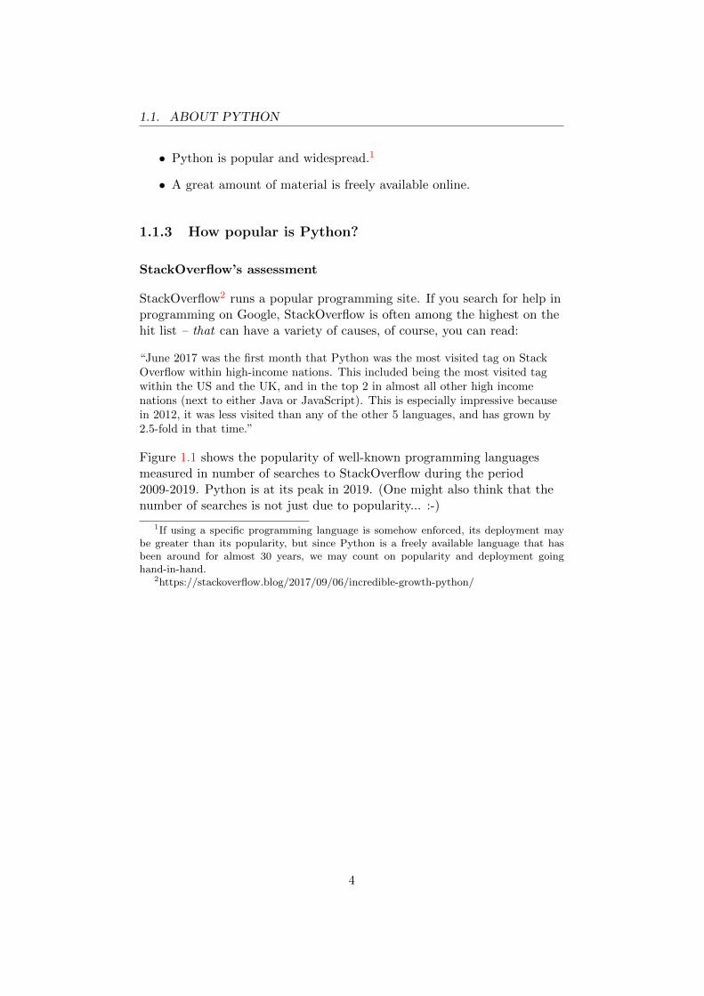
“June 2017 was the first month that Python was the most visited tag on StackOverflow within high-income nations. This included being the most visited tagwithin the US and the UK, and in the top 2 in almost all other high incomenations (next to either Java or JavaScript). This is especially impressive becausein 2012, it was less visited than any of the other 5 languages, and has grown by2.5-fold in that time.”
Figure 1.1 shows the popularity of well-known programming languagesmeasured in number of searches to StackOverflow during the period2009-2019. Python is at its peak in 2019. (One might also think that thenumber of searches is not just due to popularity... :-)
1If using a specific programming language is somehow enforced, its deployment maybe greater than its popularity, but since Python is a freely available language that hasbeen around for almost 30 years, we may count on popularity and deployment goinghand-in-hand.
2https://stackoverflow.blog/2017/09/06/incredible-growth-python/
4
1.1. ABOUT PYTHON
Figure 1.1: The popularity of well-known programming languages measuredby the number of searches to StackOverflow during the period 2009-2019
TIOBE’s assessment
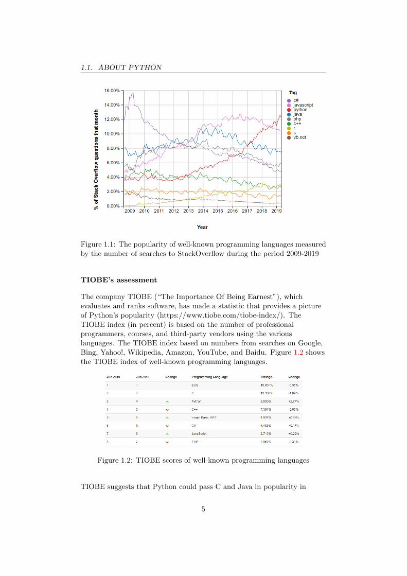
The company TIOBE (“The Importance Of Being Earnest”), whichevaluates and ranks software, has made a statistic that provides a pictureof Python’s popularity (https://www.tiobe.com/tiobe-index/). TheTIOBE index (in percent) is based on the number of professionalprogrammers, courses, and third-party vendors using the variouslanguages. The TIOBE index based on numbers from searches on Google,Bing, Yahoo!, Wikipedia, Amazon, YouTube, and Baidu. Figure 1.2 showsthe TIOBE index of well-known programming languages.
Figure 1.2: TIOBE scores of well-known programming languages
TIOBE suggests that Python could pass C and Java in popularity in
5

1.1. ABOUT PYTHON
2022-2023:
“TIOBE Index for June 2019 June Headline: Python continues to soar in theTIOBE index This month Python has reached again an all time high in TIOBEindex of 8.5%. If Python can keep this pace, it will probably replace C and Javain 3 to 4 years time, thus becoming the most popular programming language ofthe world. The main reason for this is that software engineering is booming. Itattracts lots of newcomers to the field. Java’s way of programming is too verbosefor beginners. In order to fully understand and run a simple program such as"hello world" in Java you need to have knowledge of classes, static methods andpackages. In C this is a bit easier, but then you will be hit in the face withexplicit memory management. In Python this is just a one-liner. Enough said.”
1.1.4 When is Python not useful?
Python is a textuial programming language. Python can not be used forgraphical programming. By graphic programming I mean here thatfunction blocks are linked with signal lines in a digital “drawing sheet”, iethe output of one block is connected to input of another block, graphically.(LabVIEW and Simulink are examples of graphical programming tools.)
1.1.5 Who holds the threads?
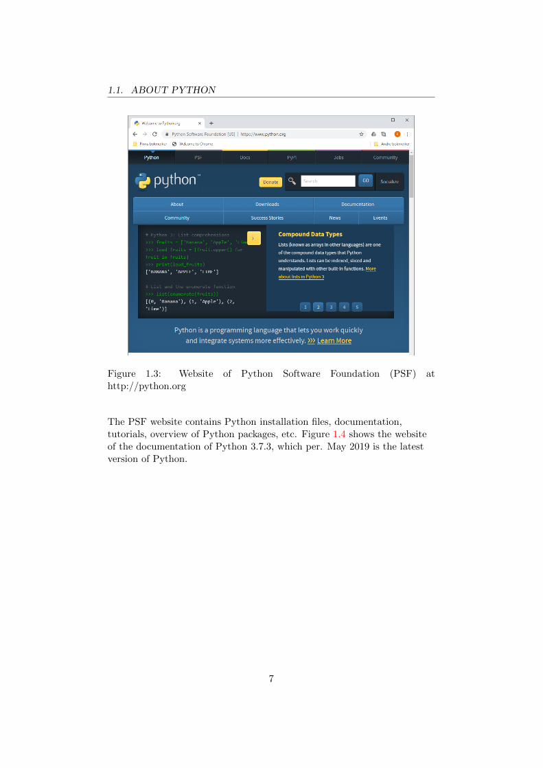
Who makes sure Python is tame and trustworthy? The Pythondevelopment and publishing organization is The Python SoftwareFoundation (PSF)3, whose website is
http://python.org
Figure 1.3 shows the PSF website.
3From PSFs website: “The Python Software Foundation is an organization devoted toadvancing open source technology related to the Python programming language.”
6
1.1. ABOUT PYTHON
Figure 1.3: Website of Python Software Foundation (PSF) athttp://python.org
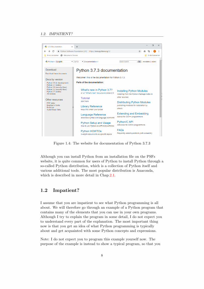
The PSF website contains Python installation files, documentation,tutorials, overview of Python packages, etc. Figure 1.4 shows the websiteof the documentation of Python 3.7.3, which per. May 2019 is the latestversion of Python.
7
1.2. IMPATIENT?
Figure 1.4: The website for documentation of Python 3.7.3
Although you can install Python from an installation file on the PSFswebsite, it is quite common for users of Python to install Python through aso-called Python distribution, which is a collection of Python itself andvarious additional tools. The most popular distribution is Anaconda,which is described in more detail in Chap.2.1.
1.2 Impatient?
I assume that you are impatient to see what Python programming is allabout. We will therefore go through an example of a Python program thatcontains many of the elements that you can use in your own programs.Although I try to explain the program in some detail, I do not expect youto understand every part of the explanation. The most important thingnow is that you get an idea of what Python programming is typicallyabout and get acquainted with some Python concepts and expressions.
Note: I do not expect you to program this example yourself now. Thepurpose of the example is instead to show a typical program, so that you
8
1.2. IMPATIENT?
get a realistic idea of what a typical Python program looks like and how itworks.
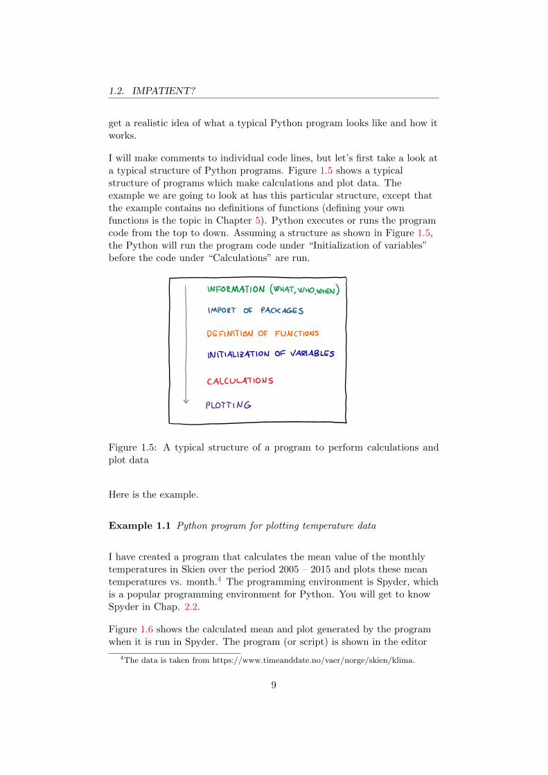
I will make comments to individual code lines, but let’s first take a look ata typical structure of Python programs. Figure 1.5 shows a typicalstructure of programs which make calculations and plot data. Theexample we are going to look at has this particular structure, except thatthe example contains no definitions of functions (defining your ownfunctions is the topic in Chapter 5). Python executes or runs the programcode from the top to down. Assuming a structure as shown in Figure 1.5,the Python will run the program code under “Initialization of variables”before the code under “Calculations” are run.
Figure 1.5: A typical structure of a program to perform calculations andplot data
Here is the example.
Example 1.1 Python program for plotting temperature data
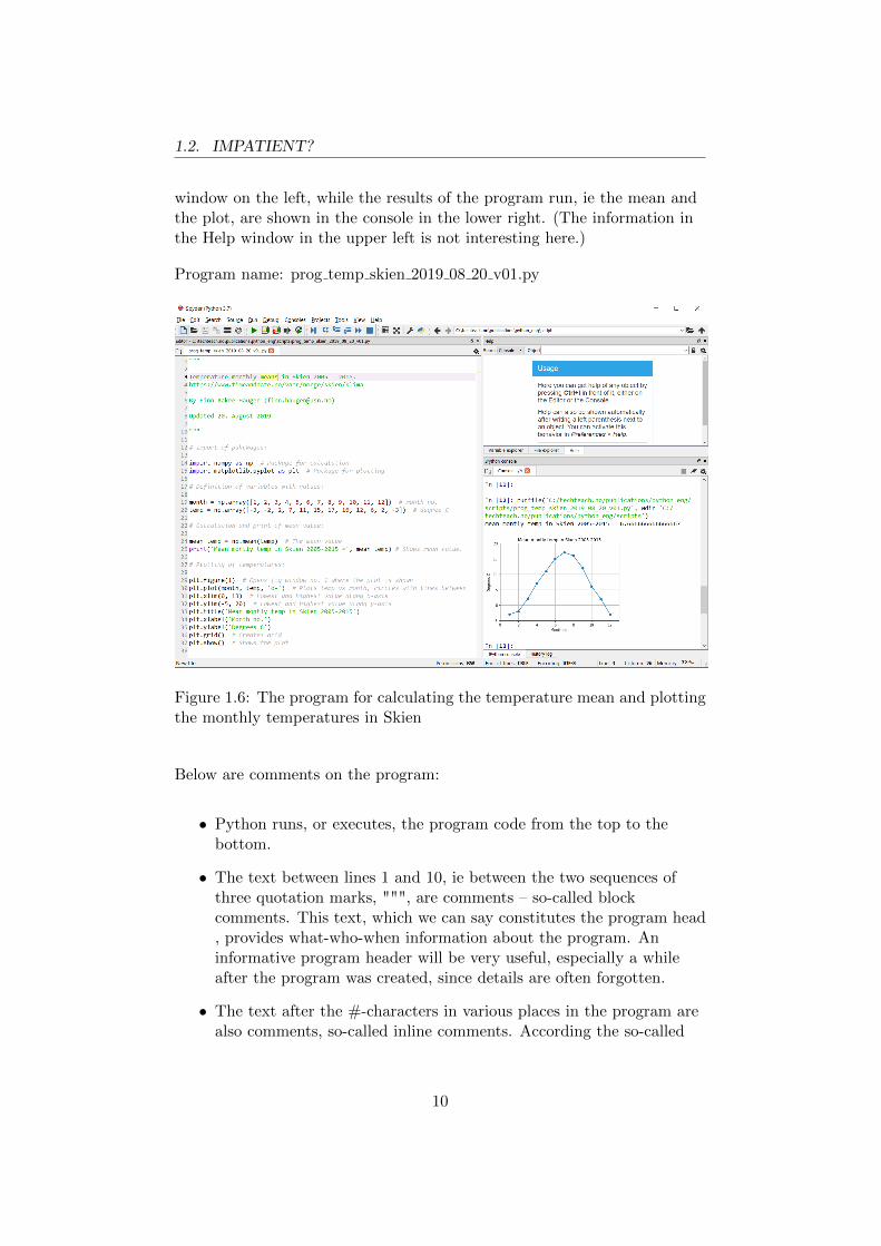
I have created a program that calculates the mean value of the monthlytemperatures in Skien over the period 2005 – 2015 and plots these meantemperatures vs. month.4 The programming environment is Spyder, whichis a popular programming environment for Python. You will get to knowSpyder in Chap. 2.2.
Figure 1.6 shows the calculated mean and plot generated by the programwhen it is run in Spyder. The program (or script) is shown in the editor
4The data is taken from https://www.timeanddate.no/vaer/norge/skien/klima.
9
1.2. IMPATIENT?
window on the left, while the results of the program run, ie the mean andthe plot, are shown in the console in the lower right. (The information inthe Help window in the upper left is not interesting here.)
Program name: prog temp skien 2019 08 20 v01.py
Figure 1.6: The program for calculating the temperature mean and plottingthe monthly temperatures in Skien
Below are comments on the program:
• Python runs, or executes, the program code from the top to thebottom.
• The text between lines 1 and 10, ie between the two sequences ofthree quotation marks, """, are comments – so-called blockcomments. This text, which we can say constitutes the program head, provides what-who-when information about the program. Aninformative program header will be very useful, especially a whileafter the program was created, since details are often forgotten.
• The text after the #-characters in various places in the program arealso comments, so-called inline comments. According the so-called
10
1.2. IMPATIENT?
PEP 8 for good code style rules5, there should be two blankcharacters in front of #, and one blank after.
• Python neglects both block comments and inline comments when itruns the program. You can take advantage of this whenprogramming: Suppose you have written some program lines thatyou do not want to include during program execution. Instead ofremoving the program lines completely, you can hide or “commentoff” the code lines.6
• According to the PEP 8 rules, comments should be written inEnglish, but I believe that “educational” comments, ie explanatoryand “over-detailed” comments, may well be written in Norwegian inNorway and Vietnamese in Vietnam, etc.
• In the program, the temperature values are integers. Had thetemperatures been decimal, or floating point, numbers, we shouldhave written e.g. 2.1 (period, not comma, is used as decimalseparator in Python).
• Line 14: The command imports numpy as np command imports thepackage named numpy (“numeric python”) into Python and makesthe package available in our program through the name np. It iscommon Python tradition to rename numpy to np. The numpypackage contains mathematical functions. In our program we use twodifferent functions from the numpy package, as explained below.
• Line 15: The command imports matplotlib.pyplot as plt imports thematplotlib package with its module (a module is a collection offunctions) called pyplot and makes the module available in ourprogram through the name plt. Also this renaming is tradition inPython.
• Line 19: We use the numpy function array to define the array namedmonths consisting of numbers representing the month numbers. Notethat we put the package name before the function name, ie np.array.We say that month is a variable of the data type array.
• Line 20: We use the numpy function array to define the array calledtemp consisting of the temperature value for each month. temp is avariable of the data type array.
5PEP is short for Python Enhancement Proposal. PEP8: Style Guide for PythonCode, see https://www.python.org/dev/peps/pep-0008/.
6You can switch between commenting/uncommenting with the keyboard combinationCtrl+1.
11
1.3. PROGRAM INPUT, OUTPUT AND WORKSPACE
• Line 24: We use the numpy function named mean to calculate themean of the array temp (which was defined in line 20). The variablemean temp gets (or is assigned) a value equal to this calculatedmean.
• Line 25: The command is used to “print” or present in the Spyderconsole, the text “Mean montly ...” followed by the value ofmean temp. The console is the window to the bottom right ofSpyder, see Figure1.6.
• Lines 29-37 open (make) Figure # 1, and plot the temperatures as afunction of the month numbers, with filled circles for each point orpair of pairs and with a straight line between the points. The lowestand highest values of the x and y axes are defined (xlim and ylim,respectively). Figure title (title) and axes (xlabel and ylabel) aregenerated. The plot gets grid. And finally, the figure with the showfunction appears. All of these different functions that help create thefigure, belong to the plt module. Therefore, plt is in front of eachfunction name.
• Line 38: According to the PEP 8 rules mentioned above, thereshould be a blank line at the end.
[End of Example 1.1]
We will come back to more details about these topics throughout the book.
1.3 Program input, output and workspace
A Python program is an abstract “thing”. You cannot physically touch aprogram, and so it is often called software. When the computermicroprocessor executes the instructions expressed in the program code,the program runs. It is when it runs, that it does something, and it canthen be considered a “process”. This chapter will develop an understandingof the fundamental aspects of this process, ie the running of a program.
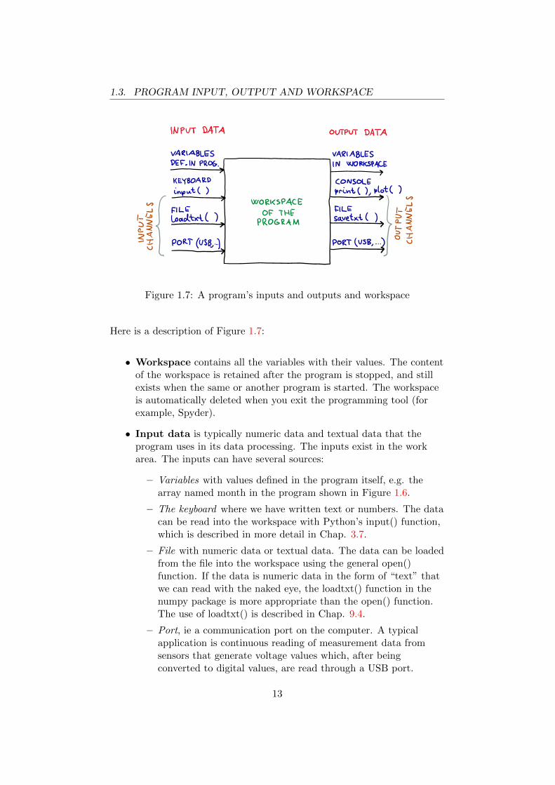
A running Python program produces an output from an input. Theprogram has a workspace which is kind of a worktable of the program.Figure 1.7 illustrates the input and output and workspace.
12
1.3. PROGRAM INPUT, OUTPUT AND WORKSPACE
Figure 1.7: A program’s inputs and outputs and workspace
Here is a description of Figure 1.7:
• Workspace contains all the variables with their values. The contentof the workspace is retained after the program is stopped, and stillexists when the same or another program is started. The workspaceis automatically deleted when you exit the programming tool (forexample, Spyder).
• Input data is typically numeric data and textual data that theprogram uses in its data processing. The inputs exist in the workarea. The inputs can have several sources:
– Variables with values defined in the program itself, e.g. thearray named month in the program shown in Figure 1.6.
– The keyboard where we have written text or numbers. The datacan be read into the workspace with Python’s input() function,which is described in more detail in Chap. 3.7.
– File with numeric data or textual data. The data can be loadedfrom the file into the workspace using the general open()function. If the data is numeric data in the form of “text” thatwe can read with the naked eye, the loadtxt() function in thenumpy package is more appropriate than the open() function.The use of loadtxt() is described in Chap. 9.4.
– Port, ie a communication port on the computer. A typicalapplication is continuous reading of measurement data fromsensors that generate voltage values which, after beingconverted to digital values, are read through a USB port.
13

1.4. WHY INCLUDE PROGRAMMING IN TEACHING?
• Output data is typically the numeric or textual data that theprogram generates when running. The output exists in theworkspace. The output may have multiple recipients:
– The workspace itself. Variables that get their values as a resultof the program run are available for use in the running programcode.
– The console in the current programming tool, e.g. Spyderconsole shown in the lower right in 1.6. The print() function,which we encounter throughout the book, is used to writenumeric data and textual values to the console. The plot()function of the numpy package can be used to plot data inFigures in the console, or alternatively in separate Figures,outside the Spyder window, cf. Section 4).
– File. Data in the workspace can be written to file using. thegeneral open() function. If the data is numeric data in the formof "text", the savetxt() function in the numpy package is moreappropriate than the open() function. The use of savetxt() isdescribed in Chap. 9.3.
– Port. A typical application is continuous writing of controlsignals calculated by our Python program, to so-called actuatorssuch as motors, pumps, valves, heating elements, lamps,switches, etc. via a USB port.
1.4 Why include programming in teaching?
You probably have your own opinion on the extent to which programmingis important in teaching STEM courses (science, technology, engineering,mathematics). My opinion is that programming can play an importantrole in teaching because programming is in line with the core principles ofteaching: motivation, concretization, activation, collaboration andindividualization:
• Motivation : Programming motivates for theory in mathematicsand science because learners see that programming is useful forapplying theory. It is also motivating to see that programming is avery important tool for solving practical problems in variousdisciplines, such as simulation, mathematics, data analysis, statistics,mathematical modeling, monitoring and control of physical systems,etc.
14

1.4. WHY INCLUDE PROGRAMMING IN TEACHING?
• Activation : Through programming, students will work activelywith the theory, and understanding and learning of the theory will bedeveloped. Programming also provides an increased opportunity forexperimentation. One can greatly benefit from pre-made programs,but in my experience, it is more instructive to program solutionsyourself than to use pre-made programs, as illustrated in Figure 1.8.
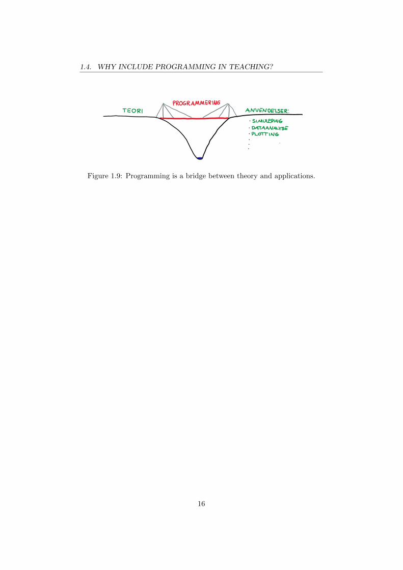
• Concretization : Programming is a bridge between theory andapplications, see Figure 1.9. With programming, theory can beapplied to concrete applications. This develops understanding andlearning of the theory, and one can also see to what extent the theoryis effective in practice.
• Individualization : Programming provides good opportunities forindividual adaptation of the teaching since one can work or try outat one’s own pace.
• Collaboration : Programming also provides good opportunities forcollaboration by having students or students discuss solutions and/orcontribute to common programming tasks.
Figure 1.8: Through programming, students will work actively with theory,and understanding and learning will be developed.
15
1.4. WHY INCLUDE PROGRAMMING IN TEACHING?
Figure 1.9: Programming is a bridge between theory and applications.
16

Chapter 2
Programming environments
2.1 Installation of Python
There are several ways to get Python:
• http://python.org, which is the home page of the official Pythonorganization The Python Software Foundation (PSF).
• http://anaconda.com, which is the website of the companyAnaconda. From this homepage you can download and install theso-called Anaconda distribution, which is arguably the world’s mostpopular distribution for Python. This distribution contains the“Python machine” itself, which runs the program code, and varioususeful tools for the programming (writing programs). Lots of usefulPython packages are automatically installed with the Anacondadistribution, which may save you some work related to finding andinstalling packages yourself (but how to do it yourself, is described inSection 2.6.4).
I recommend installing the Anaconda distribution, which is available forWindows, Mac and Linux. Mac and Linux are only available in 64-bitversions. For Windows, you can choose between 32-bit version and 64-bitversion. It is common with 64-bit PCs today, so it is natural to choose the64-bit version.
After installing the Anaconda distribution, Anaconda is on the PC startmenu, see Figure 2.1.
17

2.1. INSTALLATION OF PYTHON
Figure 2.1: Anaconda on the PC start menu
Some information about the various tools available under the Anacondamenu:
• Anaconda Navigator , presenting the various tools included withthe Anaconda distribution, see Figure 2.2.
• Anaconda Prompt , which is an Anaconda command windowwhere we can start a (simple) programming environment for Pythonprogramming.
• Jupyter Notebook , which is a Python programming environmentdisplayed in a web browser. In Jupyter Notebook we can createso-called Notebook documents, which can contain a mixture ofPython program code and information (not program code) in theform of plain text, Latex formatted text (to display mathematicalexpressions in “book quality”), plots, user interface graphic elements,etc.
• Spyder , which is a thoroughbred programming environment forPython. (I use Spyder in my own programming.)
18

2.2. SPYDER
We will become acquainted with all the three programming environmentsmentioned above in the subsequent subsections.
Figure 2.2: Anaconda Navigator
2.2 Spyder
2.2.1 How to open Spyder
We can open Spyder in two ways:
• Via Spyder button in Anaconda Navigator, see Figure 2.2.
• Via Spyder button under Anaconda on the PC start menu, seeFigure 2.1.It can also be convenient to make Spyder available also via a buttonon your PC’s taskbar: Right-click the Spyder icon in the Start menu/ More / Pin to the taskbar.
Figure 2.3 show Spyder with its three standard windows:
• Editor . The scripts you open will be accessible via their own tab atthe top of the editor window.
19

2.2. SPYDER
• Console . The console usually displays the IPython console(interactive Python console). The History log tab shows previouscommands.
• Help. The Help window normally displays information aboutfunctions. The Variable explorer tab in the Help window displays thevariables found in Python’s workspace. The File explorer tab showsthe files that are in the Pythons workbook, which is the folder wherethe most recently run program (script) is stored.
Editor
Console
Help
Figure 2.3: Spyder with the three standard windows
2.2.2 How to run Python program code in Spyder
There are two ways to make your PC run Python program code:
• Command line : You enter the program code on the command linein the console, and execute the code by clicking the Enter key on thekeyboard.
• Script : You write the program code in a script in the editor. Ascript is a text file where you have entered the program code. To runthe script, you can either press the F5 key on the keyboard or click
20

2.2. SPYDER
the green Run file button in the toolbar in Spyder. We may sayprogram instead of script, although a program can actually be in theform of code run one by one the command line. (So program is amore general term than script.)
Let’s try both ways. It is a general tradition in programming that theHello World example is the very first programming code example, so let’stake that example.
2.2.2.1 Run program code on command line
Type the program code print (’Hello World’) on the command line in theconsole, see Figure 2.4. (Do nothing else for now than write this programcode. In other words, do not press any keys other than the appropriatetext keys.)
Figure 2.4: The program code print (’Hello World’) written on the commandline in the Spyder’s console
The text In [1]: on the command line indicates that the expression thatfollows is a so-called command or program code that Python should run orexecute. The text In is the abbreviation for input. The number after In,here 1, indicates the command number counted from when this consolewas opened or started after we opened Spyder.
21

2.2. SPYDER
print(), which is part of this first example of program code, is a function inPython used to display values in the console. As with all other functions,print() needs an input argument which is the “food” or “raw material”that the function is to process. The input argument is specified in theparentheses. In this example, the input argument is the text string ’HelloWorld’ (remember to include the quotation marks).
So far we have only written the program code
print(’Hello World’)
on the command line, but have not yet run the code. To run the code, wepress the Enter key. Python then presents the result in the console, seeFigure 2.5.
Figure 2.5: The result is that the program code print(’Hello World’) is runon the command line in the Spyder console.
Figure 2.4 shows how we enter the program code print (’Hello World’) inthe console in Spyder and Figure2.5 shows how the result of the programrun is presented in the console. If I were to show pictures of the console forall the examples in the book, the book would be unnecessarily large.Instead, the program code that we will write in the console or in a scriptwill be displayed in a box, as shown below.
>>> print(’Hello World’)
22
2.2. SPYDER
Where applicable, I show the result of the program run at the end of thesame text box (possibly in a separate text box), as here:
>>> print(’Hello World’)Hello World
Some useful techniques when using the console command line
• You can enter multiple program expressions one after the other onthe command line. They are separated by a semicolon (;) Example:print (’Hello World’); print (’Hello Moon’).
• Long program expressions can be broken and placed on new lineswith backslash (\).Example:1 + 2 + 3 + 4 + 5 + 6 + 7 + 8 + 9 + 10 \+ 11 + 12 + 13 + 14 + 15
• You can delete anything on the command line so that it is blank,with the Esc button on the keyboard.
• You can find old lines that have text beginning with a givencharacter sequence by typing the character sequence and thenpressing the up arrow key on the keyboard, such as param↑, as whenwe show lines that contain e.g. parameter1 and parameter2 and thelike. as the first character sequence.
• You can cancel running program code or a command with the Stopthe current command button in the upper right corner of the console.
2.2.2.2 Run program code via script
The script is a text file containing program code. (As I already pointedout, we often just say program instead of script.) There are good reasonsto create a script and run program code via a script instead of running theindividual program expressions from the command line in the console:
• Automation : When the program code is comprehensive andconsists of many program lines. When running the script, allprogram code is executed automatically.1
1While it is possible to write many and long program lines in the console, it can beimpractical to run programs this way.
23
2.2. SPYDER
• Storing (filing): When you want to store the program in a file, e.g.for later use or for distribution.
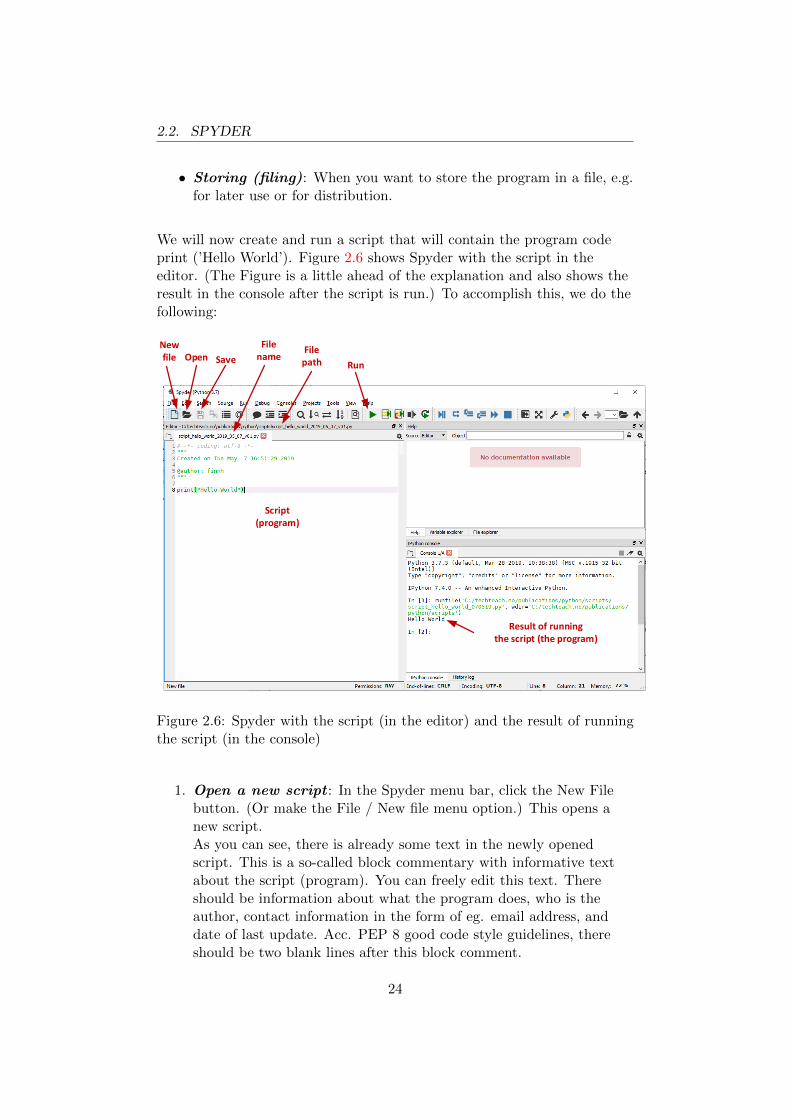
We will now create and run a script that will contain the program codeprint (’Hello World’). Figure 2.6 shows Spyder with the script in theeditor. (The Figure is a little ahead of the explanation and also shows theresult in the console after the script is run.) To accomplish this, we do thefollowing:
Newfile
RunOpen Save
Filepath
Filename
Script (program)
Result of runningthe script (the program)
Figure 2.6: Spyder with the script (in the editor) and the result of runningthe script (in the console)
1. Open a new script : In the Spyder menu bar, click the New Filebutton. (Or make the File / New file menu option.) This opens anew script.As you can see, there is already some text in the newly openedscript. This is a so-called block commentary with informative textabout the script (program). You can freely edit this text. Thereshould be information about what the program does, who is theauthor, contact information in the form of eg. email address, anddate of last update. Acc. PEP 8 good code style guidelines, thereshould be two blank lines after this block comment.
24
2.2. SPYDER
2. Write the program code in the script : You can print (’HelloWorld’) as shown in Figure 2.6. Acc. PEP 8 guidelines, scriptsshould have a blank line at the end. When you have finished writing,you can save the script (again). You can edit the text in Spyder as inother editors (Word, Notepad, etc.):
• Copy-and-paste (Ctrl-c followed by Ctrl-v)
• Cut-and-paste (Ctrl-x followed by Ctrl-v)
• Delete (Ctrl-x)
• Undo (Ctrl-z)
• Redo (Ctrl-Shift-z)
3. Save the script : Although we have not yet written any programcode in the script, we can save the script using the Save button or theFile / Save menu option or the keyboard combination Ctrl-s. Chooseyour own folder and file name. The file name will have so-called fileextension (extension) py, e.g. minfil.py. As you can see, I havechosen the file name script hello world 2019 05 08 v01.py (where vstands for version). In general, it is a good idea to save the scriptfrequently, often with new filenames if there are significant changesbetween each time you save. One possible strategy for giving filenames is to include a brief description and time (date) and the letterv followed by a number (1, 2, 3, ...) that tells which version of thefile I am now editing. Example: prog hello world 2019 05 08 v01.py.
4. Run the script : There are three alternative ways to run the script,as listed below. The result of the run is shown in Figure 2.6.
(a) Run the file button in Spyder’s menu bar
(b) Function key F5 on the keyboard
(c) With the% run filename.py command, e.g.prog hello world 2019 05 08 v01.py, on the console commandline. % run is a so-called magic command, which belongs toIPython (abbreviation for Interactive Python), which is the userinterface to Python implemented in i.a. Spyder. There arevarious magic commands. (In terms of plotting, we will meetthe magic command% matplotlib that we can use to decidewhether a plot should appear inside the Spyder console or in aseparate window, outside of Spyder.)
25
2.2. SPYDER
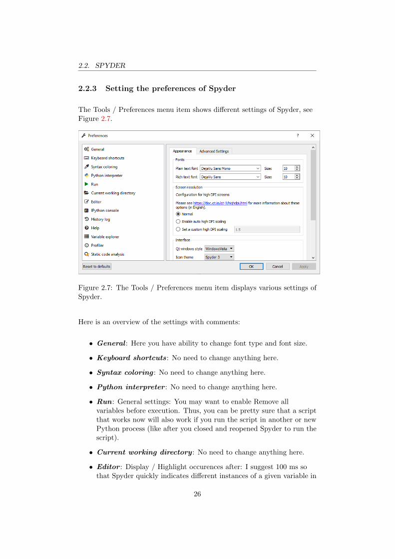
2.2.3 Setting the preferences of Spyder
The Tools / Preferences menu item shows different settings of Spyder, seeFigure 2.7.
Figure 2.7: The Tools / Preferences menu item displays various settings ofSpyder.
Here is an overview of the settings with comments:
• General : Here you have ability to change font type and font size.
• Keyboard shortcuts: No need to change anything here.
• Syntax coloring : No need to change anything here.
• Python interpreter : No need to change anything here.
• Run : General settings: You may want to enable Remove allvariables before execution. Thus, you can be pretty sure that a scriptthat works now will also work if you run the script in another or newPython process (like after you closed and reopened Spyder to run thescript).
• Current working directory : No need to change anything here.
• Editor : Display / Highlight occurences after: I suggest 100 ms sothat Spyder quickly indicates different instances of a given variable in
26
2.2. SPYDER
the script. With the default setting of 1500 ms, Spyder seemsunnecessarily slow in terms of such an indication. I also suggestenabling Real-time code style analysis, which means that a warningtriangle will appear in the left part of the editor if the code-stylerules as defined in PEP 82 wrap.
• IPython console : Graphics / Backend: The default setting Inlinemeans that plots (graphs) are displayed in the console. I usuallychange to Automatic which allows plots to appear in a separatewindow outside of Spyder, with various options for manipulating andediting the plot.
• History log : No need to change anything here.
• Help: Here I propose to enable Editor and IPython console, whichmeans that information about a function is displayed in the Helpwindow, see Figure 2.3, when you type a parenthesis after thefunction name, e.g. print().
• Variable explorer : No need to change anything here.
• Profiler : No need to change anything here.
• Static code analysis: No need to change anything here.
2.2.4 Help in Spyder
You totally depend on help when doing programming:
• Help find a suitable way to perform a programming task , eg.help find a function that can calculate the square root of a number.Some alternative ways to get help are:
– Textbooks
– Documentation and tutorials on the internet, eg. on the officialwebsite of Python: http://python.org.
– Google search, which often leads to hitshttp://stackoverflow.com.
– Ask people, e.g. fellow students and fellow students and tutorsand teachers
2PEP 8: Style Guide for Python Code, se https://www.python.org/dev/peps/pep-0008/. (PEP = Python Enhancement Proposals)
27
2.2. SPYDER
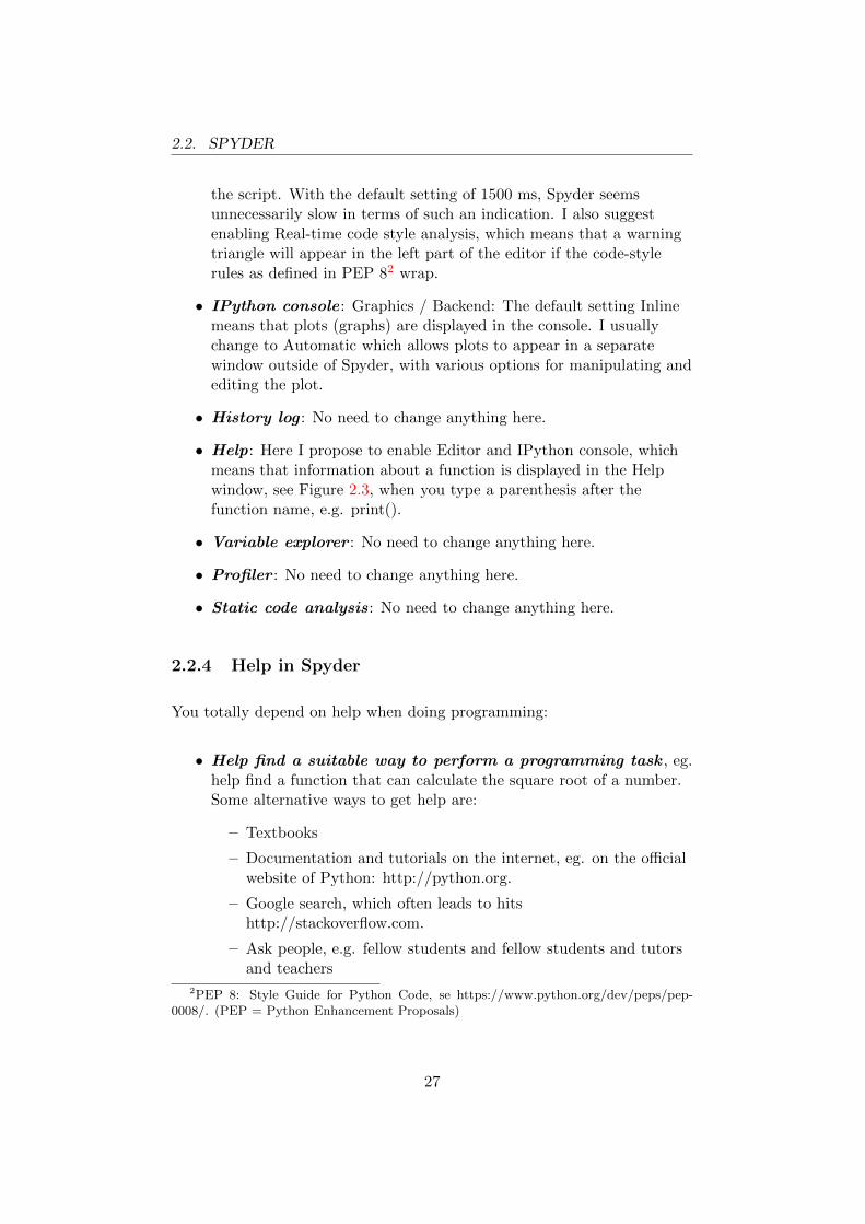
• Help find syntax errors in your program code . A syntax erroris a program technical error.Spyder finds syntax errors. Figure 2.8 shows an example where thereis a syntax error in the program code. Unfortunately, I wrote prnt(’Hello World’) instead of the correct print (’Hello World’). We seethat Spyder already finds the bug in the editor before running theprogram, and also gives an error message in the console after theprogram is run.
The error is indicated during editing (i.e. before the program is run)
Erroneous program code(correct is print)
The error is reported by Python after you have
run the program.
Figure 2.8: Spyder finds syntax errors.
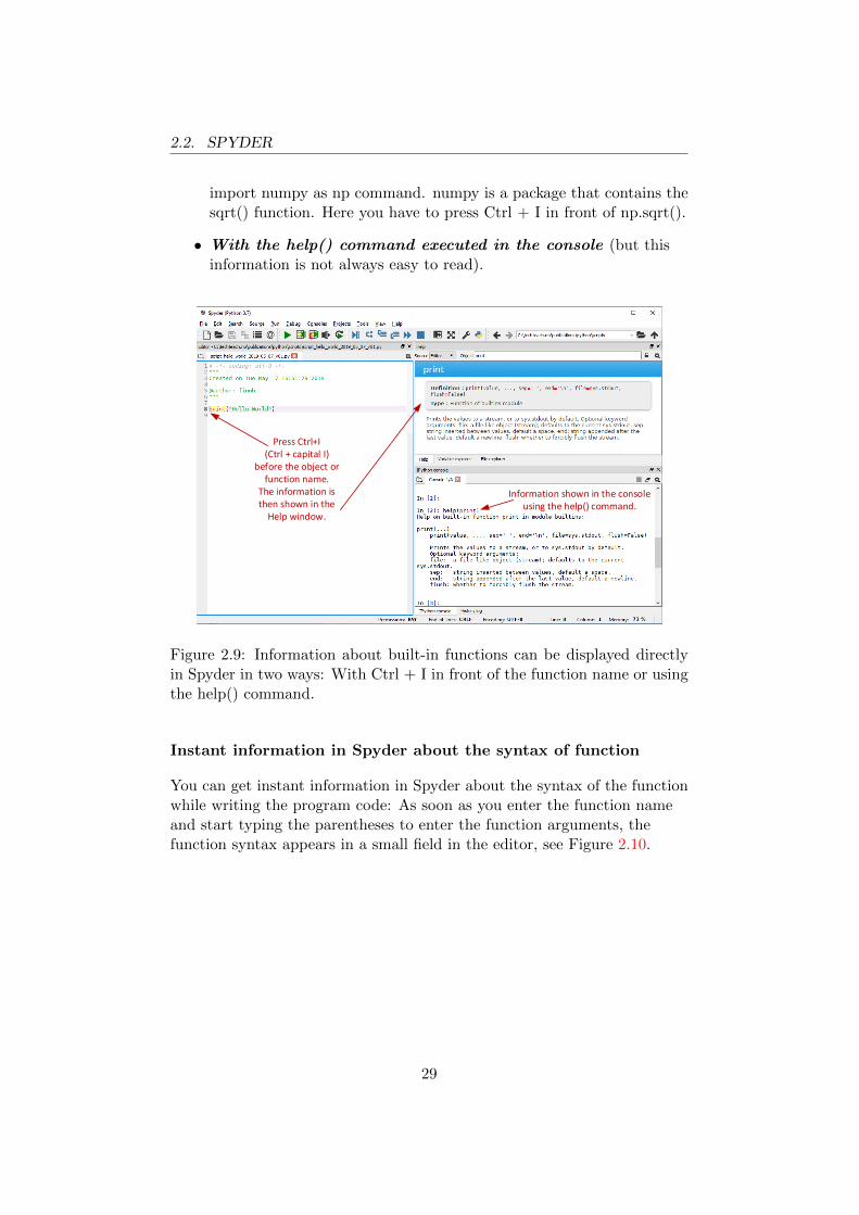
Usually you use some built-in (pre-made) Python function in yourprograms, e.g. print() function. You can get information on how to usesuch functions, as mentioned above. Alternatively, you can get informationabout such functions – or general objects – directly in Spyder in two ways,see Figure 2.9:
• By pressing Ctrl + I (capital I) in front of the functionname in the script (possibly on the command line). The informationis then displayed in the Help window.Note: If the function you are using comes from a package or modulethat you have imported into Python using the import command(such import is discussed in Chap. 2.6), you must include thepackage or module name in front of the function name itself andpress Ctrl + I in front of the package or module name. Example:np.sqrt(), where it is assumed that you have previously executed the
28
2.2. SPYDER
import numpy as np command. numpy is a package that contains thesqrt() function. Here you have to press Ctrl + I in front of np.sqrt().
• With the help() command executed in the console (but thisinformation is not always easy to read).
Press Ctrl+I(Ctrl + capital I)
before the object or function name.
The information is then shown in the
Help window.
Information shown in the console using the help() command.
Figure 2.9: Information about built-in functions can be displayed directlyin Spyder in two ways: With Ctrl + I in front of the function name or usingthe help() command.
Instant information in Spyder about the syntax of function
You can get instant information in Spyder about the syntax of the functionwhile writing the program code: As soon as you enter the function nameand start typing the parentheses to enter the function arguments, thefunction syntax appears in a small field in the editor, see Figure 2.10.
29

2.3. JUPYTER NOTEBOOK
Figure 2.10: In Spyder, the function syntax is displayed in a small field inthe editor as soon as you enter the function name and begin writing theparentheses for the input arguments.
2.3 Jupyter Notebook
Jupyter Notebook is a Python programming environment that can be usedin a web browser. In Jupyter Notebook we can create and run Notebookdocuments3, which may contain a mixture of Python program code andinformation (not program code). Notebook documents can be used locallyon the user’s PC or over the Internet. Jyputer Notebook runs Notebookdocuments using. a built-in program called kernel . We will see how wecan create Notebook documents running Python, but there is support forother languages as well, e.g. R which is widely used in statistics.
In this chapter we will only look at the very basic use of the JupyterNotebook.
2.3.1 How to start Jupyter Notebook
We can start Jupyter Notebook in two ways:
• Via the Jupyter Notebook button in Anaconda Navigator, see Figure2.2.
• Via the Jupyter Notebook button under Anaconda on the PC’s startmenu, see Figure 2.1.
3We can simply refer to Jupyter Notebook documents as Notebook documents.
30

2.3. JUPYTER NOTEBOOK
You can also make Jupyter Notebook accessible via a button on yourPC’s taskbar: Right-click the Jupyter Notebook icon in the Startmenu / More / Attach to the taskbar.
When Jupyter Notebook is started, Jupyter Notebook’s dashboard appearsin a tab of the browser, see Figure 2.11.
Figure 2.11: The Jupyter Notebook Dashboard in a browser tab
The dashboard has three tabs:
• Files, which works like Window Explorer on a Windows PC.
• Running , which displays Notebook documents that are beingprocessed, i.e. running on the current kernel (Python, R, or another).From here you can stop any (Python) processes running.
• Clusters, which applies to the use of parallel processing(simultaneous processing) on multiple cores with a tool calledIPython Parallel, but we will not go into this.
2.3.2 How to create and edit Notebook documents
To create a new Jupyter Notebook document, click the New button on thedashboard, cf. Figure 2.11, and choose the current kernel, which for ouruse is Python 3 (by the way the only kernel available here). This opens anew Notebook document in a new tab in the browser to the right of thedashboard tab. The notebook is initially given a default name, hereUntitled, but you can change this by clicking on the name field or via theFile / Rename menu option.
Figure 2.12 Notebook document after renaming hello world 05 08 v01.
31
2.3. JUPYTER NOTEBOOK
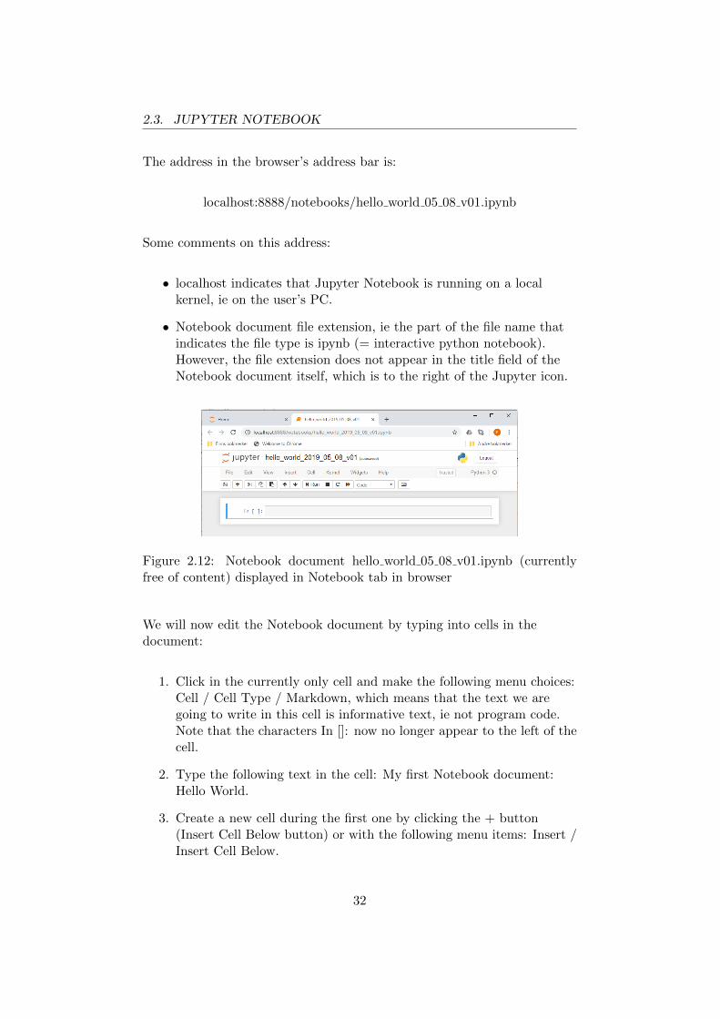
The address in the browser’s address bar is:
localhost:8888/notebooks/hello world 05 08 v01.ipynb
Some comments on this address:
• localhost indicates that Jupyter Notebook is running on a localkernel, ie on the user’s PC.
• Notebook document file extension, ie the part of the file name thatindicates the file type is ipynb (= interactive python notebook).However, the file extension does not appear in the title field of theNotebook document itself, which is to the right of the Jupyter icon.
Figure 2.12: Notebook document hello world 05 08 v01.ipynb (currentlyfree of content) displayed in Notebook tab in browser
We will now edit the Notebook document by typing into cells in thedocument:
1. Click in the currently only cell and make the following menu choices:Cell / Cell Type / Markdown, which means that the text we aregoing to write in this cell is informative text, ie not program code.Note that the characters In []: now no longer appear to the left of thecell.
2. Type the following text in the cell: My first Notebook document:Hello World.
3. Create a new cell during the first one by clicking the + button(Insert Cell Below button) or with the following menu items: Insert /Insert Cell Below.
32
2.3. JUPYTER NOTEBOOK
4. Click in the newly created cell and make the following menu choices:Cell / Cell Type / Code, which means that the text we are going towrite in this cell is program code, ie not informative text. Thecharacters In []: are now displayed to the left of the cell.
5. Enter the following text in the newly created cell: print (’HelloWorld’).
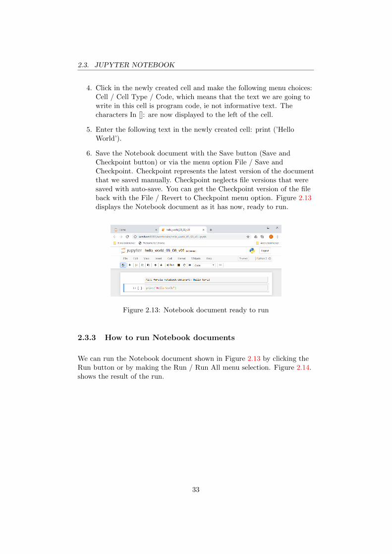
6. Save the Notebook document with the Save button (Save andCheckpoint button) or via the menu option File / Save andCheckpoint. Checkpoint represents the latest version of the documentthat we saved manually. Checkpoint neglects file versions that weresaved with auto-save. You can get the Checkpoint version of the fileback with the File / Revert to Checkpoint menu option. Figure 2.13displays the Notebook document as it has now, ready to run.
Figure 2.13: Notebook document ready to run
2.3.3 How to run Notebook documents
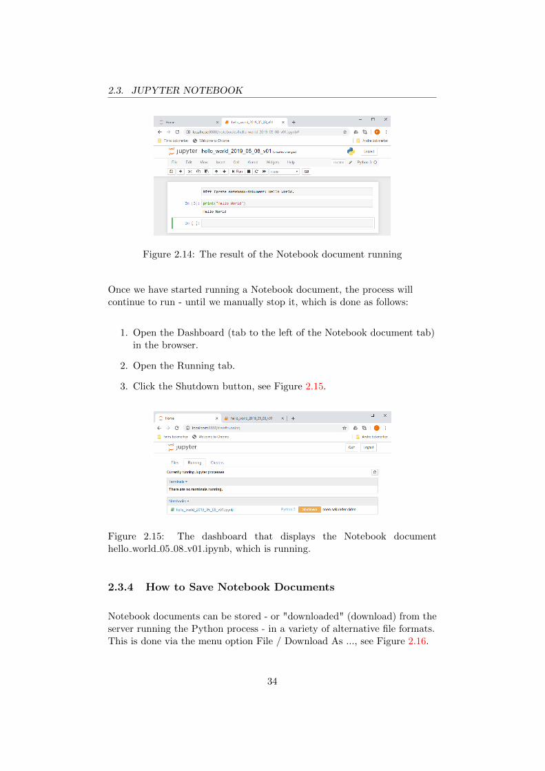
We can run the Notebook document shown in Figure 2.13 by clicking theRun button or by making the Run / Run All menu selection. Figure 2.14.shows the result of the run.
33
2.3. JUPYTER NOTEBOOK
Figure 2.14: The result of the Notebook document running
Once we have started running a Notebook document, the process willcontinue to run - until we manually stop it, which is done as follows:
1. Open the Dashboard (tab to the left of the Notebook document tab)in the browser.
2. Open the Running tab.
3. Click the Shutdown button, see Figure 2.15.
Figure 2.15: The dashboard that displays the Notebook documenthello world 05 08 v01.ipynb, which is running.
2.3.4 How to Save Notebook Documents
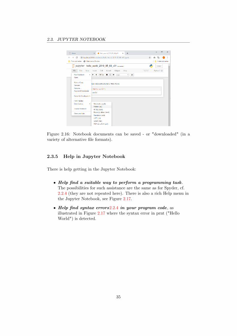
Notebook documents can be stored - or "downloaded" (download) from theserver running the Python process - in a variety of alternative file formats.This is done via the menu option File / Download As ..., see Figure 2.16.
34
2.3. JUPYTER NOTEBOOK
Figure 2.16: Notebook documents can be saved - or "downloaded" (in avariety of alternative file formats).
2.3.5 Help in Jupyter Notebook
There is help getting in the Jupyter Notebook:
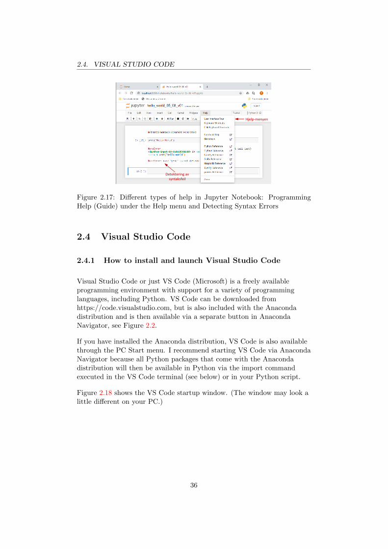
• Help find a suitable way to perform a programming task .The possibilities for such assistance are the same as for Spyder, cf.2.2.4 (they are not repeated here). There is also a rich Help menu inthe Jupyter Notebook, see Figure 2.17.
• Help find syntax errors2.2.4 in your program code , asillustrated in Figure 2.17 where the syntax error in prnt ("HelloWorld") is detected.
35
2.4. VISUAL STUDIO CODE
Detektering av syntaksfeil
Hjelp-menyen
Figure 2.17: Different types of help in Jupyter Notebook: ProgrammingHelp (Guide) under the Help menu and Detecting Syntax Errors
2.4 Visual Studio Code
2.4.1 How to install and launch Visual Studio Code
Visual Studio Code or just VS Code (Microsoft) is a freely availableprogramming environment with support for a variety of programminglanguages, including Python. VS Code can be downloaded fromhttps://code.visualstudio.com, but is also included with the Anacondadistribution and is then available via a separate button in AnacondaNavigator, see Figure 2.2.
If you have installed the Anaconda distribution, VS Code is also availablethrough the PC Start menu. I recommend starting VS Code via AnacondaNavigator because all Python packages that come with the Anacondadistribution will then be available in Python via the import commandexecuted in the VS Code terminal (see below) or in your Python script.
Figure 2.18 shows the VS Code startup window. (The window may look alittle different on your PC.)
36

2.4. VISUAL STUDIO CODE
Figure 2.18: Startup window in VS Code
You may disagree, but I think it’s a bit dull with such a dark programmingenvironment. I prefer more light and therefore make this menu selection:
File / Preferences / Color Theme / Light (Visual Studio)
Figure 2.19 shows again the startup window in VS Code, now with theLight color them.
Figure 2.19: The VS Code startup window after the File / Preferences /Color Theme / Light (Visual Studio) menu option
2.4.2 Connect Python to VS Code
VS Code can be used to program and run programs in a variety oflanguages. We will now connect Python to VS Code so that we can run
37

2.4. VISUAL STUDIO CODE
Python programs from VS Code:
1. Select the View Extensions menu option (or click the Extensionsbutton in the button bar shown on the left of Figure 2.19), whichautomatically opens and selects Anaconda Extensions and Pythonand YAML.4 Python is now entered in the status bar at the bottomof the VS Code window, see Figure.
Figure 2.20: The View Extensions menu option opens and selects AnacondaExtensions and Python and YAML. (We keep the choices.)
2.4.3 Open (create) workspace
We are going to create a simple Python program, which we will store in afolder that belongs to a workspace. Various settings of VS Code are storedin the current workspace.
We start by opening a new workspace with the menu selection
File / Save Workspace As
This opens a file explorer window called Save Workspace. In this window,create or select an existing folder. Then create a workspace associated withthis folder by entering a self-selected Workspace name (I chose the name
4YAML = YAML Ain’t Markup Language, which is a recursive name definition thatcan be difficult to understand :-) YAML is used to create configuration files of varioustypes.
38

2.4. VISUAL STUDIO CODE
vs workspace finnh) and clicking the Save button. Figure 2.21 shows asection of the VS Code window where the newly created workspace isdisplayed under the Explorer view. (You can access the Explorer viewusing the View / Explorer menu option or by clicking the Explorer buttonin the upper left of the VS Code window.)
Figure 2.21: VS Code window where the newly created workspace(vs workspace finnh) is displayed under the Explorer view
2.4.4 How to create and run a Python program
We can create a Python program as follows, cf. Figure 2.21:
1. Make the menu view View / Explorer.
2. Right-click on the folder name (vscode finnh) that is listed under theworkspace name (vs workspace finnh).
3. Velg New File i menyen som apnes.
4. Enter a file name. I have chosen prog hello world.py.
5. Run the program by right-clicking somewhere in the editor windowof the current Python program and selecting Run Python File inTerminal. (Alternatively, you can right-click the current Pythonprogram in the Explorer window to the left of the editor window.)Figure 2.22 shows the result of the run.
39
2.5. THE PYTHON COMMAND LINE IN THE ANACONDACOMMAND WINDOW
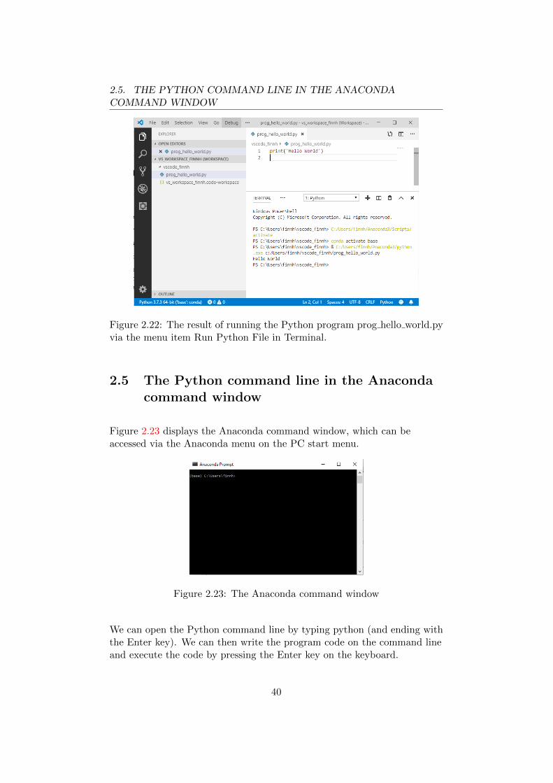
Figure 2.22: The result of running the Python program prog hello world.pyvia the menu item Run Python File in Terminal.
2.5 The Python command line in the Anacondacommand window
Figure 2.23 displays the Anaconda command window, which can beaccessed via the Anaconda menu on the PC start menu.
Figure 2.23: The Anaconda command window
We can open the Python command line by typing python (and ending withthe Enter key). We can then write the program code on the command lineand execute the code by pressing the Enter key on the keyboard.
40

2.6. IMPORT AND USE OF PYTHON PACKAGES AND MODULES
Figure 2.24 shows the result of executing the program code print (’HelloWorld’) on the Python command line in the Anaconda command window.
Figure 2.24: The result of executing the program code print (’Hello World’)on the Python command line in the Anaconda command window.
Generally, it is more appropriate to use Spyder or Jupyter Notebook thanthe Python command line as a programming environment. But even if wedo not use the Anaconda command window for programming itself, we cangreatly benefit from the Anaconda command window for eg. to manageso-called packages of Python functions. By package management is meantlisting of already installed packages (on your PC), searching for packagesthat are not yet installed, and installing packages. We will discuss this inmore detail in Chap. 2.6.
2.6 Import and use of Python packages andmodules
2.6.1 Packages management with conda or pip
Packages
functions that we can use in our Python programs, e.g. print(), sqrt(),sum(), etc., are aggregated into packages for special purposes. Here are afew examples of such packages:
• numpy, which contains elementary mathematical functions
41

2.6. IMPORT AND USE OF PYTHON PACKAGES AND MODULES
• matplotlib, which contains data plotting functions
• scipy, which contains advanced mathematical functions for eg.optimization and signal processing, etc.
• pygame, which contains functions for programming animations
The packages come in different shapes:
• One package, which we can call the standard package, isautomatically installed when the Anaconda deployment is installed,and the functions there are immediately available for use in theprograms we create.
• Many packages are installed automatically when the Anacondadistribution is installed. We must also import them to Python inorder to use them.
• And there are many packages "out there" that are not included withthe Anaconda distribution. If we need functions in some suchpackages, we must install them ourselves and then import them intoPython.
Package Management
There are tools available for package management or package management.Such package management can be listing, installation, uninstallingpackages, etc. Once we install the Anaconda distribution, we have twopackage management tools available:
• conda , which is an Anaconda product.
• pip , which is quite similar to conda, but is a tool developed byPyPA - The Python Packaging Authority - which is a working groupthat develops and maintains tools for Python packages. Also pip ispart of the Anaconda distribution.5
5
– Pip is supposedly an abbreviation for “pip installs packages”, ie Pip is a so-called re-cursive acronym (abbreviation). This is not a particularly clear definition, I think :-)Alternatively, we can consider pip as an abbreviation for “Python installation pack-age” or “package management system used to install and manage software packageswritten in Python” (Wikipedia).
42

2.6. IMPORT AND USE OF PYTHON PACKAGES AND MODULES
Both conda and pip can be used in Anaconda command window, cfr.Ch.2.5. They can also be used from the command line in Spyder, but Iwould not recommend this as there is sometimes little or no runninginformation displayed in Spyder while pip or conda is running (eginstalling or uninstalling a package), and I have also experienced thatcommands seemingly hanging. The Anaconda command window is betterin that way, but should we use conda or pip there? My experience is thatconda has not always succeeded with the job, while pip always worked.Then I land on: pip in the Anaconda window.
Figure 2.25 displays some basic pip commands. (On the Anacondacommand line, we do not need to type the § character.)
Figure 2.25: Some basic pip commands.(Https://pip.pypa.io/en/stable/quickstart/)
We will use pip commands in some of the following sections.
2.6.2 Built-in functions in Python (standard package)
Python is said to come with battery included, which means that in Pythonthere is a collection of built-in functions that you can use in your
43

2.6. IMPORT AND USE OF PYTHON PACKAGES AND MODULES
programs. We can consider this collection of built-in functions as Python’sstandard package of functions. An overview of the built-in functions inPython version 3.7.3 is available athttps://docs.python.org/3/library/functions.html, see Figure 2.26. We seethat the well-known print() function is in the standard package.
Figure 2.26: Pythons standard package of built-in functions (Python version3.7.3)
2.6.3 Import of packages included with the Anacondadistribution
When we install the Anaconda distribution, a large number of functionpackages are automatically installed on your PC. These packages are(automatically) installed in addition to the standard package discussed inChap. 2.6.2.
Figure 2.27 shows an excerpt of an overview of the 601 packages availablefor Python version 3.7.3, Windows 64 bits. (Source:https://docs.anaconda.com/anaconda/packages/py3.7 win-64/.) Of thesepackages, slightly less than half (that is, a few hundred) of packages areautomatically installed when the Anaconda distribution is installed. Thepackages that are installed are marked with a check mark in the overview.
44

2.6. IMPORT AND USE OF PYTHON PACKAGES AND MODULES
Figure 2.27: Packages that are installed with the Anaconda distribution for64-bit Windows are marked with a check mark.(https://docs.anaconda.com/anaconda/packages/py3.7 win-64/)
List of packages installed on your PC
The pip command list can be used to list packages that are installed on thePC. Figure 2.28 shows the result of the pip list command executed on theAnaconda command line.
Figure 2.28: The result of the pip list command executed on the Anacondacommand line
45
2.6. IMPORT AND USE OF PYTHON PACKAGES AND MODULES
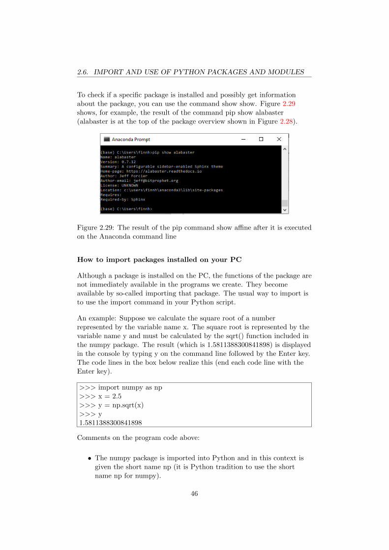
To check if a specific package is installed and possibly get informationabout the package, you can use the command show show. Figure 2.29shows, for example, the result of the command pip show alabaster(alabaster is at the top of the package overview shown in Figure 2.28).
Figure 2.29: The result of the pip command show affine after it is executedon the Anaconda command line
How to import packages installed on your PC
Although a package is installed on the PC, the functions of the package arenot immediately available in the programs we create. They becomeavailable by so-called importing that package. The usual way to import isto use the import command in your Python script.
An example: Suppose we calculate the square root of a numberrepresented by the variable name x. The square root is represented by thevariable name y and must be calculated by the sqrt() function included inthe numpy package. The result (which is 1.5811388300841898) is displayedin the console by typing y on the command line followed by the Enter key.The code lines in the box below realize this (end each code line with theEnter key).
>>> import numpy as np>>> x = 2.5>>> y = np.sqrt(x)>>> y1.5811388300841898
Comments on the program code above:
• The numpy package is imported into Python and in this context isgiven the short name np (it is Python tradition to use the shortname np for numpy).
46
2.6. IMPORT AND USE OF PYTHON PACKAGES AND MODULES
• The import command should be followed by two blank lines, cf. therecommendation in PEP 8.
• The package name, here np, must be set as the prefix to the sqrt()function, cf. the code np.sqrt (x).
• If we had imported numpy with the code import numpy, we shouldhave written numpy.sqrt (x) instead of np.sqrt (x). Actually, we canchoose whether or not to rename a package. import, but I think weshould follow name traditions in Python programming.
Although the main focus here is really the import of packages, it fits withsome comments that do not have to do with packages:
• x is a variable, given value 2.5. (We shall take a closer look at theterm variable in Chap. 3.3.)
• y is variable, which gets value equal to the square root of x.
How to import modules included in packages
In some cases, we need to import so-called modules which is included inpackages. A module is in principle a collection of functions. A package canthen contain a number of modules, which in turn consists of a number offunctions.
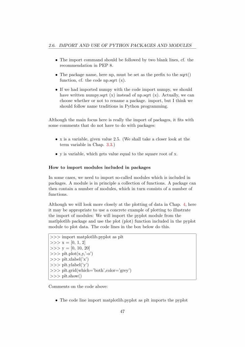
Although we will look more closely at the plotting of data in Chap. 4, hereit may be appropriate to use a concrete example of plotting to illustratethe import of modules: We will import the pyplot module from thematlplotlib package and use the plot (plot) function included in the pyplotmodule to plot data. The code lines in the box below do this.
>>> import matplotlib.pyplot as plt>>> x = [0, 1, 2]>>> y = [0, 10, 20]>>> plt.plot(x,y,’-o’)>>> plt.xlabel(’x’)>>> plt.ylabel(’y’)>>> plt.grid(which=’both’,color=’grey’)>>> plt.show()
Comments on the code above:
• The code line import matplotlib.pyplot as plt imports the pyplot
47
2.6. IMPORT AND USE OF PYTHON PACKAGES AND MODULES
module into the matplotlib library and renames pyplot to plt in thatregard (it is Python tradition to use the short name plt for pyplot).
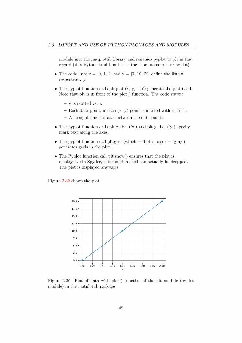
• The code lines x = [0, 1, 2] and y = [0, 10, 20] define the lists xrespectively y.
• The pyplot function calls plt.plot (x, y, ’- o’) generate the plot itself.Note that plt is in front of the plot() function. The code states:
– y is plotted vs. x
– Each data point, ie each (x, y) point is marked with a circle.
– A straight line is drawn between the data points.
• The pyplot function calls plt.xlabel (’x’) and plt.ylabel (’y’) specifymark text along the axes.
• The pyplot function call plt.grid (which = ’both’, color = ’gray’)generates grids in the plot.
• The Pyplot function call plt.show() ensures that the plot isdisplayed. (In Spyder, this function shell can actually be dropped.The plot is displayed anyway.)
Figure 2.30 shows the plot.
0.00 0.25 0.50 0.75 1.00 1.25 1.50 1.75 2.00x
0.0
2.5
5.0
7.5
10.0
12.5
15.0
17.5
20.0
y
Figure 2.30: Plot of data with plot() function of the plt module (pyplotmodule) in the matplotlib package
48
2.6. IMPORT AND USE OF PYTHON PACKAGES AND MODULES
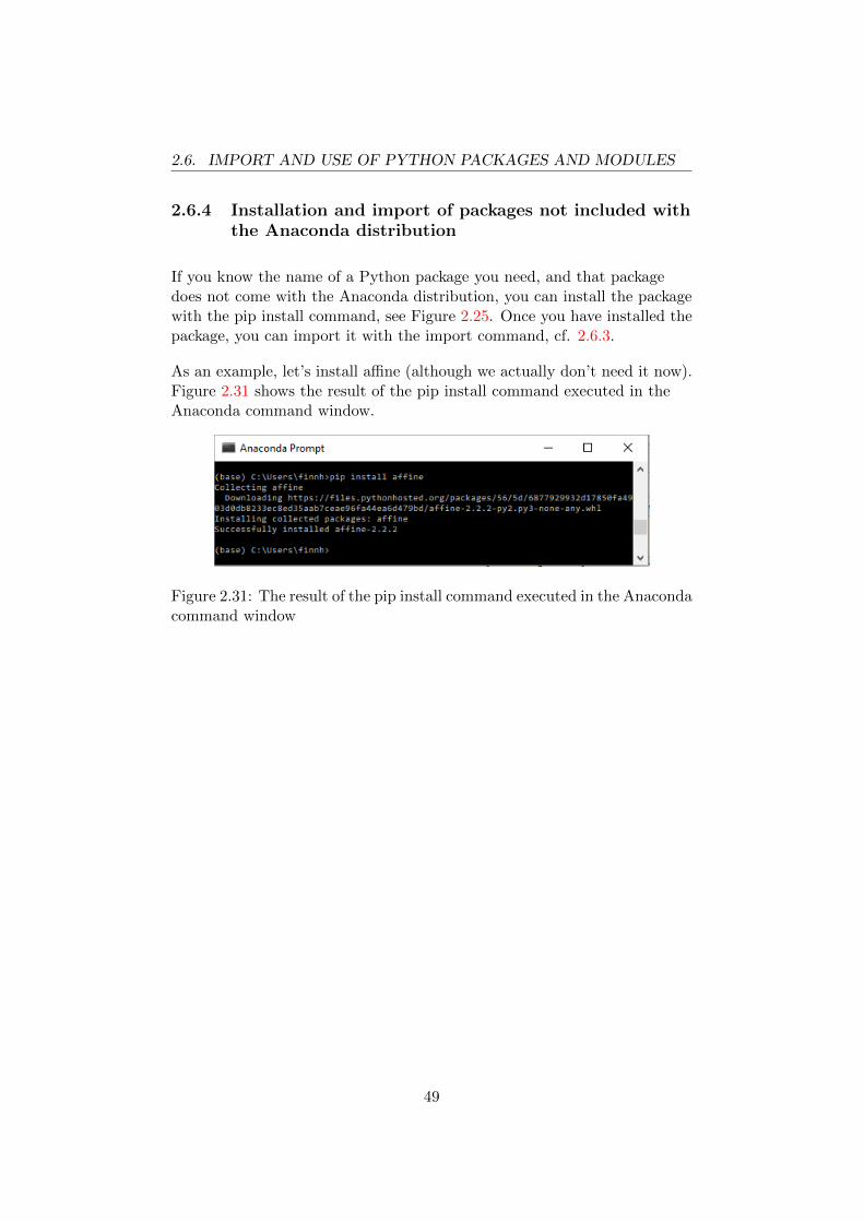
2.6.4 Installation and import of packages not included withthe Anaconda distribution
If you know the name of a Python package you need, and that packagedoes not come with the Anaconda distribution, you can install the packagewith the pip install command, see Figure 2.25. Once you have installed thepackage, you can import it with the import command, cf. 2.6.3.
As an example, let’s install affine (although we actually don’t need it now).Figure 2.31 shows the result of the pip install command executed in theAnaconda command window.
Figure 2.31: The result of the pip install command executed in the Anacondacommand window
49
Chapter 3
Variables and data types
3.1 Introduction
You have to understand what variables and data types are, in order toprogram. Of course, programming requires knowledge of many otherthings as well, but variables and data types are fundamental concepts.This chapter provides sufficient knowledge of variables and data types.
3.2 How to run the code samples?
The chapter, and the rest of the book, contains many examples of programcode that you can / should run yourself. The code examples are set inframes. In general, you can choose whether to run the commands from thecommand line in e.g. Spyder or via a script that you create. Smallexamples, which I suppose can be tested on the command line (withoutcreating scripts), I type after the so-called Python prompt (or the Phytoncommand sign) >>>.
In the programming environments Jupyter Notebook and Spyder areprompted
In [n]
(there is a running command number) instead
>>>
50
3.3. VARIABLES
If you use one of these programming environments, you enter the codeafter the In [n] prompt.
After you enter the code on the command line, run the code by pressingthe Enter key on the keyboard.
3.3 Variables
3.3.1 What is a variable?
A variable is a data element with a name. We can create or define avariable and assign it a value by using equals. If the number value has aunit, you must keep track of the unit yourself.
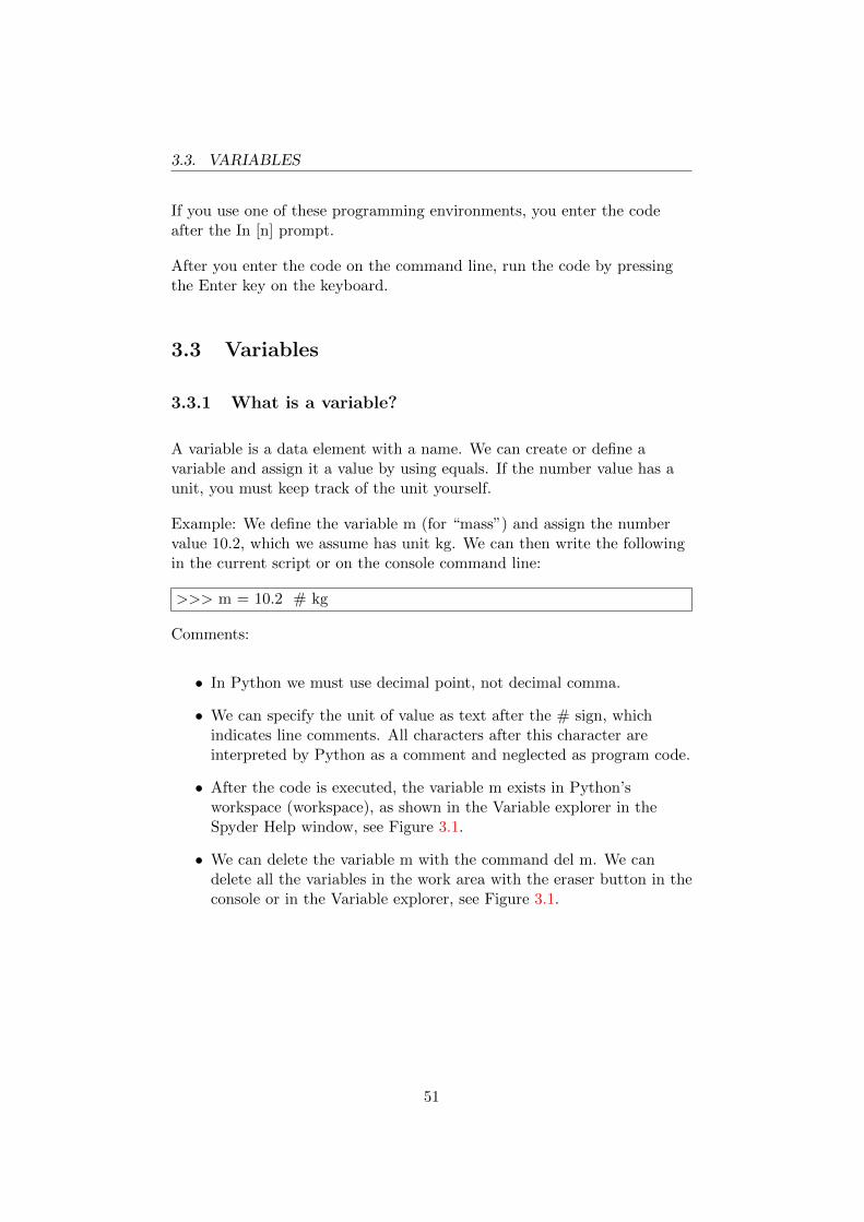
Example: We define the variable m (for “mass”) and assign the numbervalue 10.2, which we assume has unit kg. We can then write the followingin the current script or on the console command line:
>>> m = 10.2 # kg
Comments:
• In Python we must use decimal point, not decimal comma.
• We can specify the unit of value as text after the # sign, whichindicates line comments. All characters after this character areinterpreted by Python as a comment and neglected as program code.
• After the code is executed, the variable m exists in Python’sworkspace (workspace), as shown in the Variable explorer in theSpyder Help window, see Figure 3.1.
• We can delete the variable m with the command del m. We candelete all the variables in the work area with the eraser button in theconsole or in the Variable explorer, see Figure 3.1.
51
3.3. VARIABLES
Figure 3.1: After executing the code, the variable m exists in Python’sworkspace, as shown in the Variable explorer in the Spyder help window.
The built-in variable (underscore) has value from the lastcalculation
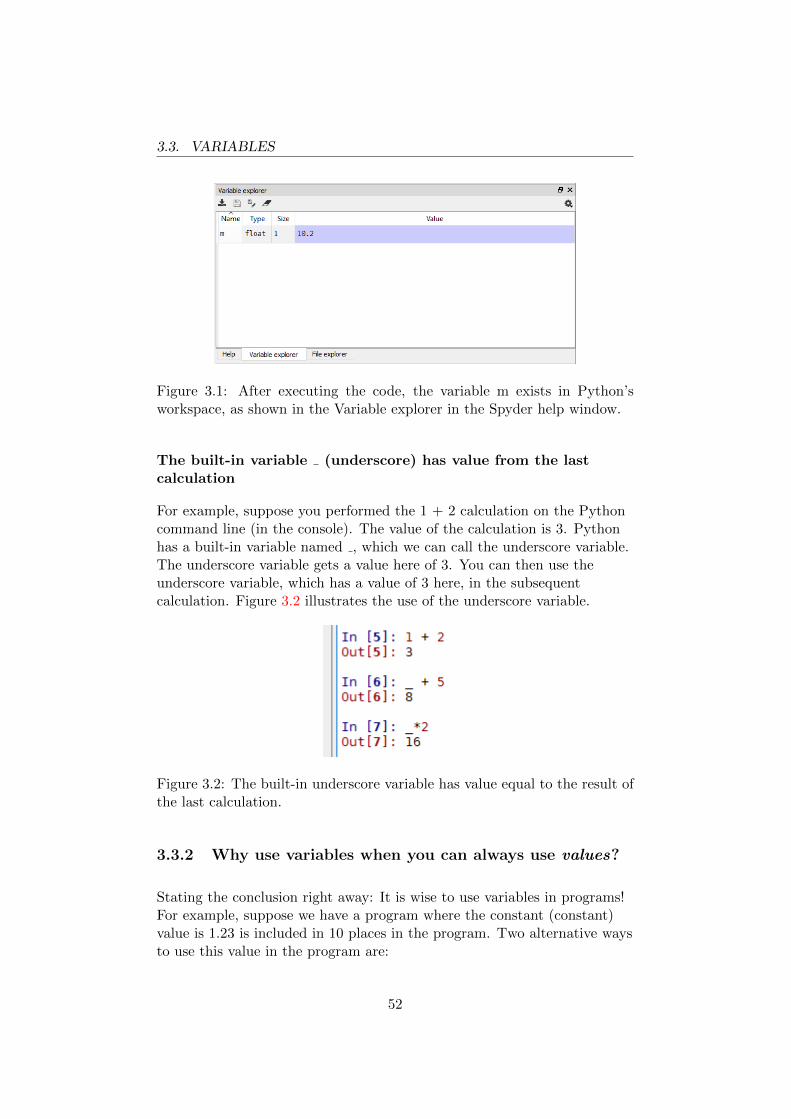
For example, suppose you performed the 1 + 2 calculation on the Pythoncommand line (in the console). The value of the calculation is 3. Pythonhas a built-in variable named , which we can call the underscore variable.The underscore variable gets a value here of 3. You can then use theunderscore variable, which has a value of 3 here, in the subsequentcalculation. Figure 3.2 illustrates the use of the underscore variable.
Figure 3.2: The built-in underscore variable has value equal to the result ofthe last calculation.
3.3.2 Why use variables when you can always use values?
Stating the conclusion right away: It is wise to use variables in programs!For example, suppose we have a program where the constant (constant)value is 1.23 is included in 10 places in the program. Two alternative waysto use this value in the program are:
52
3.3. VARIABLES
1. We can write the value 1.23 at all 10 places in the program.
2. We can define a variable let’s say with name a and assign that value1.23 one place in the program, ie we write the code a = 1.23, we alsouse a at all 10 places in the program.
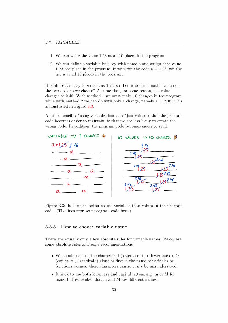
It is almost as easy to write a as 1.23, so then it doesn’t matter which ofthe two options we choose? Assume that, for some reason, the value ischanges to 2.46. With method 1 we must make 10 changes in the program,while with method 2 we can do with only 1 change, namely a = 2.46! Thisis illustrated in Figure 3.3.
Another benefit of using variables instead of just values is that the programcode becomes easier to maintain, ie that we are less likely to create thewrong code. In addition, the program code becomes easier to read.
Figure 3.3: It is much better to use variables than values in the programcode. (The lines represent program code here.)
3.3.3 How to choose variable name
There are actually only a few absolute rules for variable names. Below aresome absolute rules and some recommendations.
• We should not use the characters l (lowercase l), o (lowercase o), O(capital o), I (capital i) alone or first in the name of variables orfunctions because these characters can so easily be misunderstood.
• It is ok to use both lowercase and capital letters, e.g. m or M formass, but remember that m and M are different names.
53

3.4. A LITTLE ABOUT FUNCTIONS
• In names or parts of multi-letter names, lowercase letters should beused, e.g. mass, not MASS, nor Mass.
• The names may consist of a combination of letters and numbers, butnot special characters such as. %, (, + and], etc., but underline, , isok. Numbers should not be first characters in a name. Examples:
– 3 usable names: mass bil 1, m bil 1, M bil 1
– 2 illegal names: 1 car mass,% rate
• Names of built-in functions in Python should not be used as namesof variables because the built-in function then loses its originalmeaning. Example: If you, unfortunately, have given a variable thename “print”, then the built-in function print() loses its originalmeaning. An unfortunate name selection can be reversed by deletingthe variable with the del print command, and then, the print()function is again available as normal.
3.4 A little about functions
In mathematics, variables and functions (or formulas) are fundamentalconcepts. Just think of square root calculation:
y =√x
there
• x is the function’s input or input argument,
• y is the output or output argument of the function
• √ (square root calculation) is the function.
Figure 3.4 illustrates this function.
Figure 3.4: Mathematical function (square root calculation)
54

3.4. A LITTLE ABOUT FUNCTIONS
Similarly, it is in programming : Variable and Functions are fundamentalconcepts. This chapter focuses on variables and the various data types thatvariables can have (such as integers, floating numbers, text, etc.). However,since variables and functions often appear together, it is reasonable tointroduce the concept of functions and some different forms of functionshere. However, functions are treated in much more detail in Chapter 5.
A function “does something” with the input, or input argument, to thefunction. The result of what the function does is called the functionoutput, or output argument or return argument. Figure3.5 illustrates theconcept of functions in Python.
Figure 3.5: Function with input argument and output argument, or returnargument
Functions come in different forms:
• Function
• Method
You will become more familiar with these forms through some simpleexamples.
Function
The built-in numpy package contains the sqrt() function for calculatingsquare root. It is used as follows:
>>> import numpy as np>>> x = 2.0>>> y = np.sqrt(x)>>> y1.4142135623730951
55

3.5. NUMBERS AND BASIC MATHEMATICAL OPERATIONS
The first line of code causes the numpy package to be imported intoPython and renamed in that connection to np (which is a pythontradition). Python also has some functions that come with its standardpackage. They can be used directly, without importing any package, cf.2.6.2.
Method
Simply put, all variables in Python are so-called objects. And with theobjects, there are a number of so-called methods, which are functions that"belong" to the object and operate on it. The syntax is
objekt.metode()
In the example below, we first create a variable named L of data type list,that consists of the two numbers 0 and 1 (we will learn more about lists inCh. 3.9). Then we expand the list with an element of value 2 using theappend() method which can be applied to list objects. We see that theappend() method basically works as a function.
>>> L = [0, 1]>>> L.append(5)>>> L[0, 1, 5]
Above I wrote L (+ enter) on the command line to display the value of L. Icould also have used the print() function:
>>> L = [0, 1]>>> L.append(5)>>> print(L)[0, 1, 5]
3.5 Numbers and basic mathematical operations
Here we will look at different ways of representing numbers and basicmathematical operations. More advanced calculations, and the special butvery effective calculation method called vectorized calculation, aredescribed in Ch. 3.12.7.
56

3.5. NUMBERS AND BASIC MATHEMATICAL OPERATIONS
3.5.1 Numbers types
In Python we can use different types of numbers:
• Integer .Example: 2Example: −10
• Floating point , or decimal number. In Python, dots, not commas,are used as decimal separators.Example: 1.23
• Complex numbers. The symbol j is used as a complex unit.Example: 1 + 1j (just 1 + j will give an error message).
Numbers can be expressed with powers of 10 as follows:
• Example: 1.234e2 that is the number 1.234 · 102 = 123.4. The lettere stands for 10’s exponent.
• Example: 1.234e−2 that is the number 0.01234.
3.5.2 How to format numbers in print() function
The print() function is probably the most frequently used function inPython. It is one of Python’s built-in functions, cf. Figure 2.26. We haveused this function many times already. When we use it to print numbers,the numbers are displayed by default with a large number of digits (14)after the decimal point. Often we want fewer digits, and we can obtain thisby specifying the format (number) to print.
There are several ways to format the arguments of the print() function.The program (script) below demonstrates the most relevant ways. Theprogram prints text, and numbers mixed with the text. Comments on theindividual code lines and their results are given below.
Program name: prog print format.py.
57
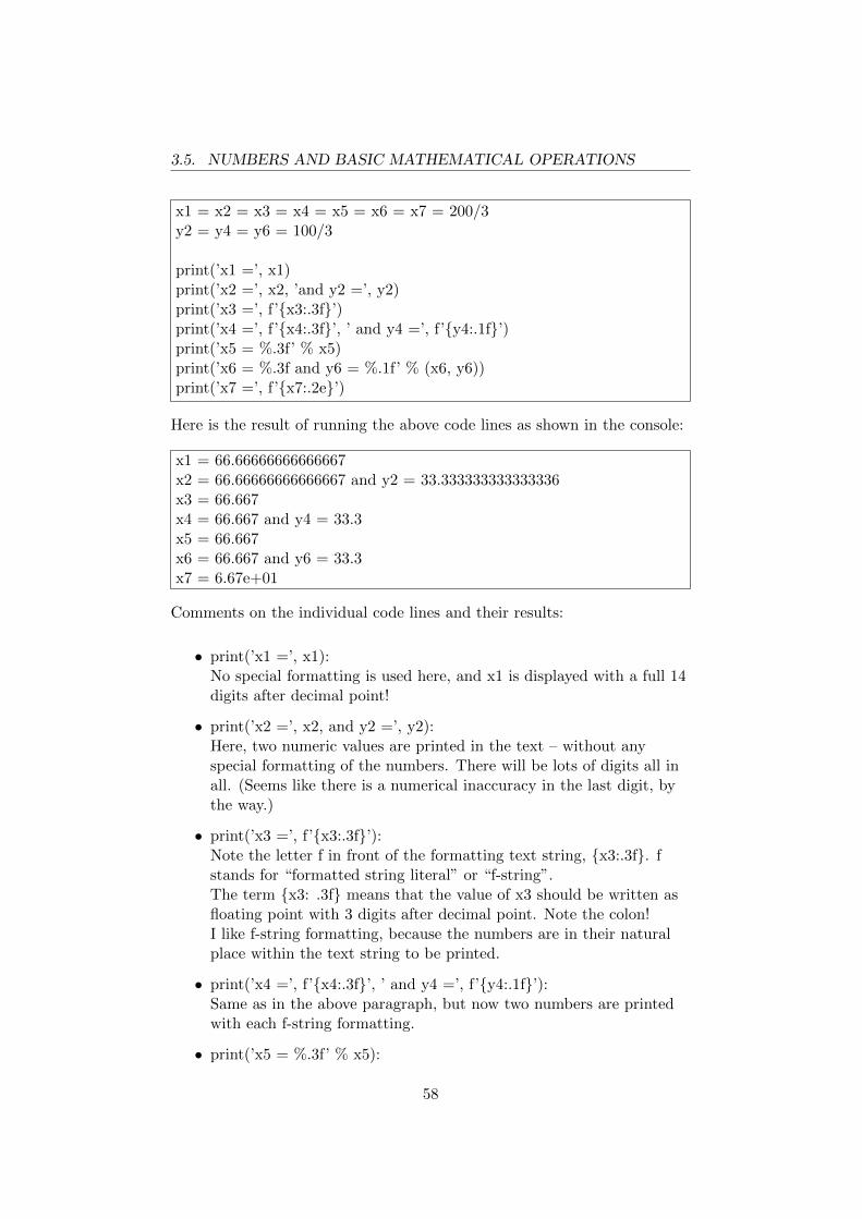
3.5. NUMBERS AND BASIC MATHEMATICAL OPERATIONS
x1 = x2 = x3 = x4 = x5 = x6 = x7 = 200/3y2 = y4 = y6 = 100/3
print(’x1 =’, x1)print(’x2 =’, x2, ’and y2 =’, y2)print(’x3 =’, f’{x3:.3f}’)print(’x4 =’, f’{x4:.3f}’, ’ and y4 =’, f’{y4:.1f}’)print(’x5 = %.3f’ % x5)print(’x6 = %.3f and y6 = %.1f’ % (x6, y6))print(’x7 =’, f’{x7:.2e}’)
Here is the result of running the above code lines as shown in the console:
x1 = 66.66666666666667x2 = 66.66666666666667 and y2 = 33.333333333333336x3 = 66.667x4 = 66.667 and y4 = 33.3x5 = 66.667x6 = 66.667 and y6 = 33.3x7 = 6.67e+01
Comments on the individual code lines and their results:
• print(’x1 =’, x1):No special formatting is used here, and x1 is displayed with a full 14digits after decimal point!
• print(’x2 =’, x2, and y2 =’, y2):Here, two numeric values are printed in the text – without anyspecial formatting of the numbers. There will be lots of digits all inall. (Seems like there is a numerical inaccuracy in the last digit, bythe way.)
• print(’x3 =’, f’{x3:.3f}’):Note the letter f in front of the formatting text string, {x3:.3f}. fstands for “formatted string literal” or “f-string”.The term {x3: .3f} means that the value of x3 should be written asfloating point with 3 digits after decimal point. Note the colon!I like f-string formatting, because the numbers are in their naturalplace within the text string to be printed.
• print(’x4 =’, f’{x4:.3f}’, ’ and y4 =’, f’{y4:.1f}’):Same as in the above paragraph, but now two numbers are printedwith each f-string formatting.
• print(’x5 = %.3f’ % x5):
58

3.5. NUMBERS AND BASIC MATHEMATICAL OPERATIONS
Note where the% sign is.This is a traditional way to format the print. On python.org1 it isreferred to as “old-string formatting”, and it is stated that there maybe certain technical problems with this formatting. Of course, it isused in many applications.I think it is natural that we drop using this formatting method, butit is useful to know about it because it is probably used in existingcode.
• print(’x6 = %.3f and y6 = %.1f’ % (x6, y6)):Same as the point above, but now two number values are printed.(x6, y6) is a tuple. The order of the elements in the tuple correspondsto the order of formatting in the text string to be printed.
• print(’x7 =’, f’{x7:.2e}’):This is f-string formatted printing, as for x3 above. The formattingcharacter e, which stands for “exponential,” indicates that thenumber is printed in 10s exponential form. The number 2 in front ofe indicates that it must be 2 digits after the decimal point. Printing6.67e+01 means 6.67·101.
I admit there are many details in the above, but I would say it’s worth theeffort since we – and others – use the print() function often.
I would like to repeat the request from python.org to Python programmersto use print with f-string formatting in the print() function, as for x3 andx4 and y4 above.
3.5.3 Mathematical operators
The basic mathematical operators are:
+ (addition)
− (subtraction)
* (multiplication)
/ (division)
** (power), e.g. 2**0.5 (= 20,5 =√
2)
1https://docs.python.org/3/library/stdtypes.html#old-string-formatting
59

3.5. NUMBERS AND BASIC MATHEMATICAL OPERATIONS
Example 3.1 Basic mathematical operations
The following commands written on the command line demonstrate basicmathematical operations (the results are also shown):
>>> 2 + 5.17.1>>> 2 - 5.1-3.1>>> 1.2*1.51.7999999999999998>>> 1.2/1.50.7999999999999999>>> 2**0.51.4142135623730951
[End of Example 3.1]
The relative precedence of the operator
The operators have relative precedence or rank as follows:
1. **Example:
>>> 2**3 + 412>>> 2**(3+4)128
2. * and / (ie equal precedence, and the calculation is done from left toright).Example:
>>> 8/4*24.0
3. +and - (ie equal precedence, and the calculation is done from left toright).Example:>>> 3 + 2 −23
Note: In a series of ** operators, the calculation is performed - fromnormal - from right to left.
60
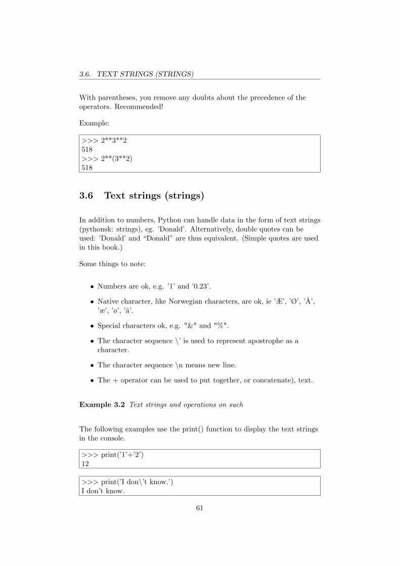
3.6. TEXT STRINGS (STRINGS)
With parentheses, you remove any doubts about the precedence of theoperators. Recommended!
Example:
>>> 2**3**2518>>> 2**(3**2)518
3.6 Text strings (strings)
In addition to numbers, Python can handle data in the form of text strings(pythonsk: strings), eg. ’Donald’. Alternatively, double quotes can beused: ’Donald’ and “Donald” are thus equivalent. (Simple quotes are usedin this book.)
Some things to note:
• Numbers are ok, e.g. ’1’ and ’0.23’.
• Native character, like Norwegian characters, are ok, ie ’Æ’, ’Ø’, ’A’,’æ’, ’ø’, ’a’.
• Special characters ok, e.g. "&" and "%".
• The character sequence \’ is used to represent apostrophe as acharacter.
• The character sequence \n means new line.
• The + operator can be used to put together, or concatenate), text.
Example 3.2 Text strings and operations on such
The following examples use the print() function to display the text stringsin the console.
>>> print(’1’+’2’)12
>>> print(’I don\’t know.’)I don’t know.
61

3.7. FROM NUMBERS TO TEXT AND FROM TEXT TO NUMBERS
>>> print(’Line 1.\nLine 2.’)Line 1.Line 2.
[End of Example 3.2]
3.7 From numbers to text and from text tonumbers
A short rehearsal: Three basic data types in Python are
• float (floating point), e.g. 59.82
• int (integer), e.g. 2
• str (text string), e.g. ’59.8’
Python requires that you use the correct data type in current programexpressions. It may therefore be necessary to convert mbetween some ofthe data types. Python has built-in functions that perform type conversion(pythonsk: datatype casting), cf. Figure 2.26:
• float() converts from str or int to float.
• int() converts from str or float to int with any rounding against null.3
• str() convert from float or int to str.
Example 3.3 Conversion from float to str
>>> vekt float = 59.8 # Flyttall>>> info = ’Hun veier ’ + str(vekt float) + ’ kg.’>>> infoHun veier 59.8 kg.
The code above uses the + operator to merge text strings.
2
– I Python brukes desimalpunktum, ikke desimalkomma.
3numpy.ceil() rounds up to the nearest integer.
62

3.7. FROM NUMBERS TO TEXT AND FROM TEXT TO NUMBERS
If we slurp by dropping the type conversion for the variable weight fromfloat to size, Python gives clear message:
>>> vekt float = 59.8>>> info = ’Hun veier ’ + vekt float + ’ kg.’TypeError: can only concatenate str (not "float") to str
[End of Example 3.3]
Then we have an example of the opposite conversion:
Example 3.4 Conversion from str to float
The float() function is used here to convert text string to float number inpreparation for a mathematical operation, namely multiplication:
>>> vekt str = ’59.8’ # Tekststreng>>> vekt i gram float = float(vekt str)*1000>>> vekt i gram float59800.0
[End of Example 3.4]
Fortunately, the print() function is quite flexible
In the examples above, we had to convert between floating point and textstring and vice versa. But it can be useful to keep in mind that the print()function itself is quite flexible since it can print (present in the console) amix of text and numbers.
Example 3.5 The print() function accepts a mix of different data types
print() function prints both text and numbers:
>>> weight float = 59.8 # Flyttall>>> print(’She would like to weigh’, weight float, ’kg.’)She would like to weigh 59.8 kg.
[End of Example 3.5]
Type conversion regarding the input() function
Suppose you have created a program where the floating point variable x isto be included in a calculation. Of course, you can assign x a value in the
63

3.7. FROM NUMBERS TO TEXT AND FROM TEXT TO NUMBERS
program code itself. Alternatively, the user can enter a value in the consolewhile the program is running using the input() function, which is a built-infunction in Python, see Figure 2.26. The input() function returns text. If xis to have data type floating point, we need to converte the type from textto number. This is demonstrated in the following example.
Example 3.6 Type conversion ifm. input() - function
The program in the box below uses the input() function to ask the user toenter a number on the command line in the console. The input() functionconsiders this number as text. It is therefore necessary to convert the textto an actual number (data type float), and we do so with the float()function.
x = float(input(Enter the number, x: ’))y = x + 3.4print(’y =’, y)
When the above program is run, the program pauses while the text ’Enterthe number x:’ appears on the command line. When the user (I) hasentered a "number" (actual text) – and I entered “1.2”, the programproceeds with code succeding the input() code, which here is the additiony = x + 2.3, which gives the result 4.6. The box below shows theinformation that is presented in the console.
Enter the number x: 1.2y = 4.6
If I had dropped the type conversion with the float() function, like this:
x = input(’Enter the number x: ’)y = x + 3.4print(’y =’, y)
then, Python would react negatively and give an error message:
...y = x + 3.4
TypeError: can only concatenate str (not "float") to str
[End of Example 3.6]
64

3.8. BOOLEAN VARIABLES, LOGICAL OPERATORS ANDCOMPARISON OPERATORS
3.8 Boolean variables, logical operators andcomparison operators
Programming is often about logical operations. This section introduces thebasics about programming logical operations in Python.
3.8.1 Introduction
Suppose that you have created a program that contains two alternativeprogram parts, program part 1 and program part 2. Suppose that programpart 1 is to be executed if the floating point variable A is larger than thefloating point variable B, otherwise program part 2 will be executed. inFigure 3.6. The program flow is thus determined by the comparisonbetween A and B. More specifically: It is the result of the comparison
A > B
that determines the program flow. This comparison gives results eitherlogically true or logically false, or in Python: True or False, as the twopossible logical values in Python.
Figure 3.6: Program flowchart expressing that program flow is determinedby the logical value of equation A > B.
The content of the diamond square, ie the test A> B?, can be realizedwith a so-called if expression. We will get closer to the if-expression inSection 7, but let us indulge in a little taste of how this can be expressedwith Python code:
65

3.8. BOOLEAN VARIABLES, LOGICAL OPERATORS ANDCOMPARISON OPERATORS
if A > B:Program code 1
else:Program code 2
Above we have become familiar with some terms that we will look at inthe sections that follow:
• Logical values
• Comparisons
3.8.2 Boolean variable
Boolean or logical variables are variables that can have only one of twopossible values:
• True
• False
Note: In contexts other than Python programming, e.g. in otherprogramming languages, True and False may have other names:
• True can be named as "on"or "high" or "1" (logical one).
• False can be named as "off" or "low" or "0" (logical zero).
Boolean variables are useful for comparisons, etc.
3.8.3 Logical operators
In Python there are three logical operators which you can apply toBoolean variables:
• and
• or
• not
66
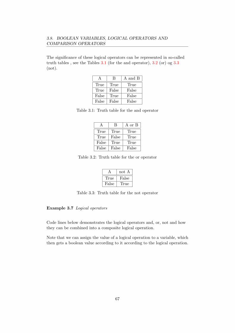
3.8. BOOLEAN VARIABLES, LOGICAL OPERATORS ANDCOMPARISON OPERATORS
The significance of these logical operators can be represented in so-calledtruth tables , see the Tables 3.1 (for the and operator), 3.2 (or) og 3.3(not).
A B A and B
True True True
True False False
False True False
False False False
Table 3.1: Truth table for the and operator
A B A or B
True True True
True False True
False True True
False False False
Table 3.2: Truth table for the or operator
A not A
True False
False True
Table 3.3: Truth table for the not operator
Example 3.7 Logical operators
Code lines below demonstrates the logical operators and, or, not and howthey can be combined into a composite logical operation.
Note that we can assign the value of a logical operation to a variable, whichthen gets a boolean value according to it according to the logical operation.
67
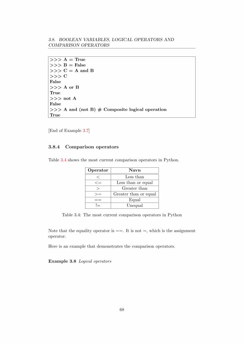
3.8. BOOLEAN VARIABLES, LOGICAL OPERATORS ANDCOMPARISON OPERATORS
>>> A = True>>> B = False>>> C = A and B>>> CFalse>>> A or BTrue>>> not AFalse>>> A and (not B) # Composite logical operationTrue
[End of Example 3.7]
3.8.4 Comparison operators
Table 3.4 shows the most current comparison operators in Python.
Operator Navn
< Less than
<= Less than or equal
> Greater than
>= Greater than or equal
== Equal
!= Unequal
Table 3.4: The most current comparison operators in Python
Note that the equality operator is ==. It is not =, which is the assignmentoperator.
Here is an example that demonstrates the comparison operators.
Example 3.8 Logical operators
68

3.9. LISTS
>>> 1 < 2True>>> 1 <= 2True>>> 1 > 2False>>> 1 >= 2False>>> 1 == 2False>>> 1 != 2True
[End of Example 3.8]
3.9 Lists
3.9.1 What are lists?
One of the data types in Python is the so-called list .
Here is an example of a list of 4 elements of floating point numbers (I havechosen to give the list name L1 here):
>>> L1 = [0.1, 2.3, 4.5, 6.7]>>> L1[0.1, 2.3, 4.5, 6.7]
Note:
• The elements are separated by commas (with or without spaces afterthe comma).
• The brackets are brackets (square brackets).
Each element has a so-called element index, which is an integer. The firstelement always has index 0 (not 1)4. The 4 elements in L1 then have theelement indices 0, 1, 2 respectively. 3.
4In MATLAB, the first index of vectors or arrays, which in some ways are comparablewith lists in Python, is 1
69

3.9. LISTS
Figure 3.7 illustrates, based on the example above, the data type list.
Figure 3.7: Illustration of a list. Note that the first element has index 0.
List elements can have data type text strings. An example:
>>> L2 = [’zero’, ’one’, ’two’]
And here’s a list of mix drops - numbers, text and list:
>>> L3 = [0.1, ’one’, [1.0, ’two’]]
How long is the list?
The built-in Python function len(), cf. Figure 2.26, find the length of alist. Example:
>>> L1 = [0.1, 2.3, 4.5, 6.7]>>> n = len(L1)>>> n4
Sequences
Lists are sequences of data. There are other data types than lists thatconsist of sequences of data, namely arrays and tuples, which arementioned in their respective sections. All of these data types fall underthe general Python terms sequences and iterables.
3.9.2 Operations on lists
3.9.2.1 Reading list elements
Reading one list element
Let’s assume we have a list named L (but we could of course have assumed
70

3.9. LISTS
another name). We can then assign a variable, here named E, the value ofthe list element with index i with the code
E = L[i]
As mentioned earlier, the first element has index 0. But what is the indexof the last element? It is -1, which will apply to all lists. It sounds strange,but Figure3.8 shows logic: We consider the list as a closed sequence ofelements! For a specific list of n elements, the last element index canalternatively be specified as n− 1.
Figure 3.8: A list considered as a closed sequence of elements.
Example 3.9 Read one element in a list
Below are some examples of reading items in list L = [0.1, 2.3, 4.5, 6.7], aswe defined above and illustrated in Figure 3.7.
>>> L = [0.1, 2.3, 4.5, 6.7]>>> L[0]0.1>>> L[2]4.5>>> L[3]6.7>>> L[-1]6.7
[End of Example 3.9]
Read a series of list items
71

3.9. LISTS
To read item values in a list, we must access (or index or address) therelevant elements by specifying their indexes. We use the operator: (colon)to access a series of list items (python for serial accessing: slicing). Theterm L [i: j] accesses the elements starting with the element i to – but notwith – element j. This is illustrated in the figure 3.9. In particular, wenote that element j in list L is not included in list extract L2, and thereforethis element is marked in gray. (The white elements are not included inthe list excerpt either.)
Figure 3.9: List extract L2 = L [i: j]. We especially notice that element jin list L is not included in the list excerpt.
If the start index is 0, we can drop typing 0. For example, L [0: 2] isequivalent to L [: 2].
Example 3.10 Read a series of items in a list
We are going to read the series of elements from index 0 to (but not with)index 2 in list L as we defined above:
>>> L = [0.1, 2.3, 4.5, 6.7]>>> L[0:2][0.1, 2.3]>>> L[:2] # Ekvivalent med L[0:2][0.1, 2.3]
[End of Example 3.10]
If we are going to access the items from index i and "out list", ie even thelast item, we can write L [i:].
Example 3.11 Read a series of items through the last item in the list
Here we read the items from index 1 and out list:
72
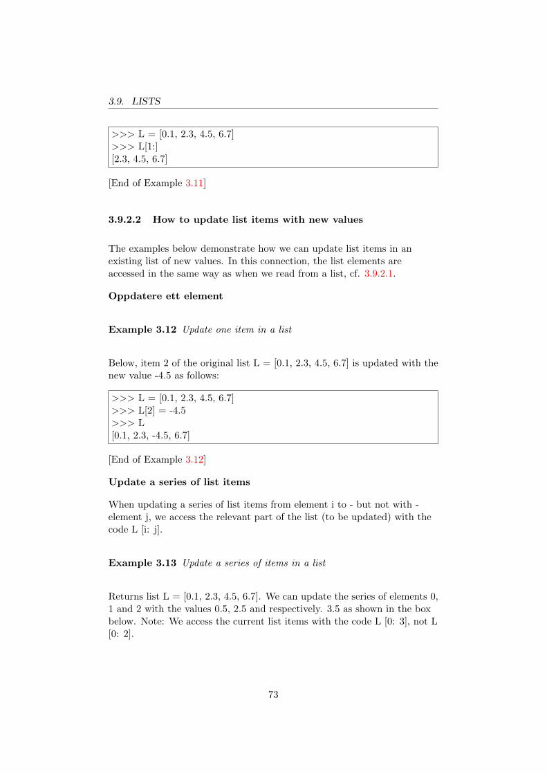
3.9. LISTS
>>> L = [0.1, 2.3, 4.5, 6.7]>>> L[1:][2.3, 4.5, 6.7]
[End of Example 3.11]
3.9.2.2 How to update list items with new values
The examples below demonstrate how we can update list items in anexisting list of new values. In this connection, the list elements areaccessed in the same way as when we read from a list, cf. 3.9.2.1.
Oppdatere ett element
Example 3.12 Update one item in a list
Below, item 2 of the original list L = [0.1, 2.3, 4.5, 6.7] is updated with thenew value -4.5 as follows:
>>> L = [0.1, 2.3, 4.5, 6.7]>>> L[2] = -4.5>>> L[0.1, 2.3, -4.5, 6.7]
[End of Example 3.12]
Update a series of list items
When updating a series of list items from element i to - but not with -element j, we access the relevant part of the list (to be updated) with thecode L [i: j].
Example 3.13 Update a series of items in a list
Returns list L = [0.1, 2.3, 4.5, 6.7]. We can update the series of elements 0,1 and 2 with the values 0.5, 2.5 and respectively. 3.5 as shown in the boxbelow. Note: We access the current list items with the code L [0: 3], not L[0: 2].
73
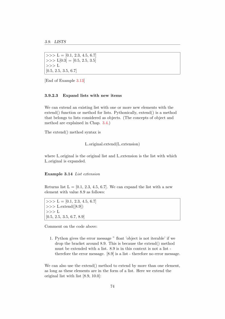
3.9. LISTS
>>> L = [0.1, 2.3, 4.5, 6.7]>>> L[0:3] = [0.5, 2.5, 3.5]>>> L[0.5, 2.5, 3.5, 6.7]
[End of Example 3.13]
3.9.2.3 Expand lists with new items
We can extend an existing list with one or more new elements with theextend() function or method for lists. Pythonically, extend() is a methodthat belongs to lists considered as objects. (The concepts of object andmethod are explained in Chap. 3.4.)
The extend() method syntax is
L original.extend(L extension)
where L original is the original list and L extension is the list with whichL original is expanded.
Example 3.14 List extension
Returns list L = [0.1, 2.3, 4.5, 6.7]. We can expand the list with a newelement with value 8.9 as follows:
>>> L = [0.1, 2.3, 4.5, 6.7]>>> L.extend([8.9])>>> L[0.5, 2.5, 3.5, 6.7, 8.9]
Comment on the code above:
1. Python gives the error message ” float ’object is not iterable’ if wedrop the bracket around 8.9. This is because the extend() methodmust be extended with a list. 8.9 is in this context is not a list -therefore the error message. [8.9] is a list - therefore no error message.
We can also use the extend() method to extend by more than one element,as long as these elements are in the form of a list. Here we extend theoriginal list with list [8.9, 10.0]:
74
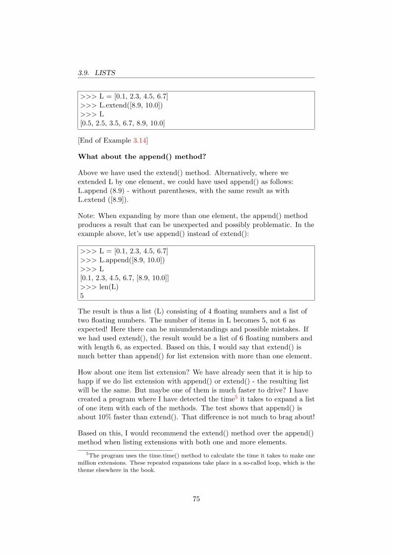
3.9. LISTS
>>> L = [0.1, 2.3, 4.5, 6.7]>>> L.extend([8.9, 10.0])>>> L[0.5, 2.5, 3.5, 6.7, 8.9, 10.0]
[End of Example 3.14]
What about the append() method?
Above we have used the extend() method. Alternatively, where weextended L by one element, we could have used append() as follows:L.append (8.9) - without parentheses, with the same result as withL.extend ([8.9]).
Note: When expanding by more than one element, the append() methodproduces a result that can be unexpected and possibly problematic. In theexample above, let’s use append() instead of extend():
>>> L = [0.1, 2.3, 4.5, 6.7]>>> L.append([8.9, 10.0])>>> L[0.1, 2.3, 4.5, 6.7, [8.9, 10.0]]>>> len(L)5
The result is thus a list (L) consisting of 4 floating numbers and a list oftwo floating numbers. The number of items in L becomes 5, not 6 asexpected! Here there can be misunderstandings and possible mistakes. Ifwe had used extend(), the result would be a list of 6 floating numbers andwith length 6, as expected. Based on this, I would say that extend() ismuch better than append() for list extension with more than one element.
How about one item list extension? We have already seen that it is hip tohapp if we do list extension with append() or extend() - the resulting listwill be the same. But maybe one of them is much faster to drive? I havecreated a program where I have detected the time5 it takes to expand a listof one item with each of the methods. The test shows that append() isabout 10% faster than extend(). That difference is not much to brag about!
Based on this, I would recommend the extend() method over the append()method when listing extensions with both one and more elements.
5The program uses the time.time() method to calculate the time it takes to make onemillion extensions. These repeated expansions take place in a so-called loop, which is thetheme elsewhere in the book.
75

3.9. LISTS
3.9.2.4 Remove list items
We can remove items from a list with the command del (abbreviation fordelete). We access the elements to be removed in the same way as whenreading list items, cf. 3.9.2.1. The syntax for removing an indexed itemfrom list L is
del L[i]
Syntax to remove items from index i to (but not with) index j from list L is
del L[i:j]
Example 3.15 Remove items from a list
Returns list L = [0.1, 2.3, 4.5, 6.7]. Let’s remove item 2 from the list:
>>> L = [0.1, 2.3, 4.5, 6.7]>>> del L[2]>>> L[0.1, 2.3, 6.7]
Let’s start again with list L = [0.1, 2.3, 4.5, 6.7] and remove the twoelements with indexes 1 and 1 respectively. 2 from the list:
>>> L = [0.1, 2.3, 4.5, 6.7]>>> del L[1:3]>>> L[0.1, 6.7]
[End of Example 3.15]
3.9.2.5 List manipulation with + and *
Usually the + and * operators are used for mathematical operations. Butwhen these operators are used on lists, they do not work mathematically.Instead, they are used to manipulate the list. So here we are in aminefield: -o
If you want to use the + operator to add a number value to all the listitems and the * operator to multiply all the list items by a number value,
76

3.10. TUPLES
you must convert the list to array, and then use the operators on the array.This is explained in Chap. 3.12.
The + operator used between two lists is used to merge (python:concatenate) listae, as demonstrated here:
>>> L = [10, 20, 30]>>> L1 = [40, 50, 60]>>> L + L1[10, 20, 30, 40, 50, 60]
The * operator applied to a list is used to create a new list consisting of asequence of the original list, e.g. 3 times the original list, as in thefollowing example:
>>> L = [10, 20, 30]>>> L*3[10, 20, 30, 10, 20, 30, 10, 20, 30]
3.10 Tuples
Tuples are used to group data elements of the same or different data types.Tuples are very similar to lists. Two important differences are:
• The elements in tuples are gathered in regular parentheses, ie(),while lists are gathered in square brackets, [].
• Tuples cannot be manipulated, ie they can be considered static lists.
When using tuples, they are often the starting arguments of functions youcreate yourself:
(ut arg 1, ut arg 2) = en eller annen funksjon(inn arg)
where (ut arg 1, ut arg 2) is a tuple with two elements (Programming yourown functions is covered in Ch. 5.)
How to define tuples
Here is an example of defining a tuple, which consists of the floating pointnumber 1.0 and the text string ’a’:
77
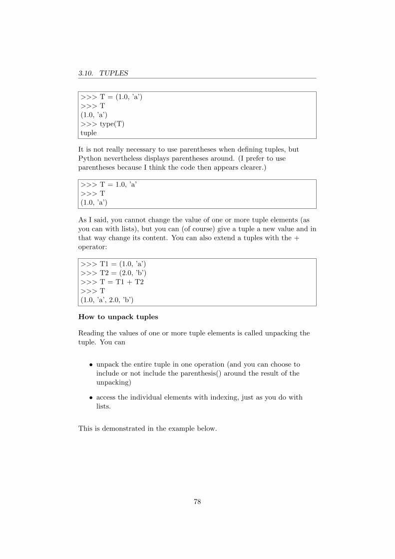
3.10. TUPLES
>>> T = (1.0, ’a’)>>> T(1.0, ’a’)>>> type(T)tuple
It is not really necessary to use parentheses when defining tuples, butPython nevertheless displays parentheses around. (I prefer to useparentheses because I think the code then appears clearer.)
>>> T = 1.0, ’a’>>> T(1.0, ’a’)
As I said, you cannot change the value of one or more tuple elements (asyou can with lists), but you can (of course) give a tuple a new value and inthat way change its content. You can also extend a tuples with the +operator:
>>> T1 = (1.0, ’a’)>>> T2 = (2.0, ’b’)>>> T = T1 + T2>>> T(1.0, ’a’, 2.0, ’b’)
How to unpack tuples
Reading the values of one or more tuple elements is called unpacking thetuple. You can
• unpack the entire tuple in one operation (and you can choose toinclude or not include the parenthesis() around the result of theunpacking)
• access the individual elements with indexing, just as you do withlists.
This is demonstrated in the example below.
78

3.11. DICTIONARY
>>> T = (1.0, ’a’)>>> (num1, text1) = (1.0, ’a’) # Unpacking the whole tuple using paren-theses>>> num11.0>>> text1’a’>>> num1, text1 = (1.0, ’a’) # Unpacking the whole tuple without usingparentheses>>> num11.0>>> text1’a’>>> text1 = T[1] # Unpacking of one of the elements>>> text1’a’
3.11 Dictionary
A dictionary is a collection of data elements that can have different datatypes, and the data elements are indexed (accessed) with keys in the formof text strings. A nice feature of dictionaries is that the keys (indexes) canbe made “readable” (such as “teams”’). Lists, cf. 3.9, also consists of acollection of data elements, but in lists the indices are just integers.
Below you will see how to create a dictionary. Comments on the code:
• ’Team’ is key, and ’ManU’ is its value .
• ’Points’ is also key, and 100 is its value.
>>> D = {} # Creates an empty dictionary>>> D[’Team’] = ’ManU’ # Adds an element to the dictionary>>> D[’Points’] = 100 # Adds another element>>> D{’Team’: ’ManU’, ’Points’: 100} # In their dreams
You can read the value of a key as shown below:
>>> D[’Team’]’ManU’>>> D[’Points’]100
79
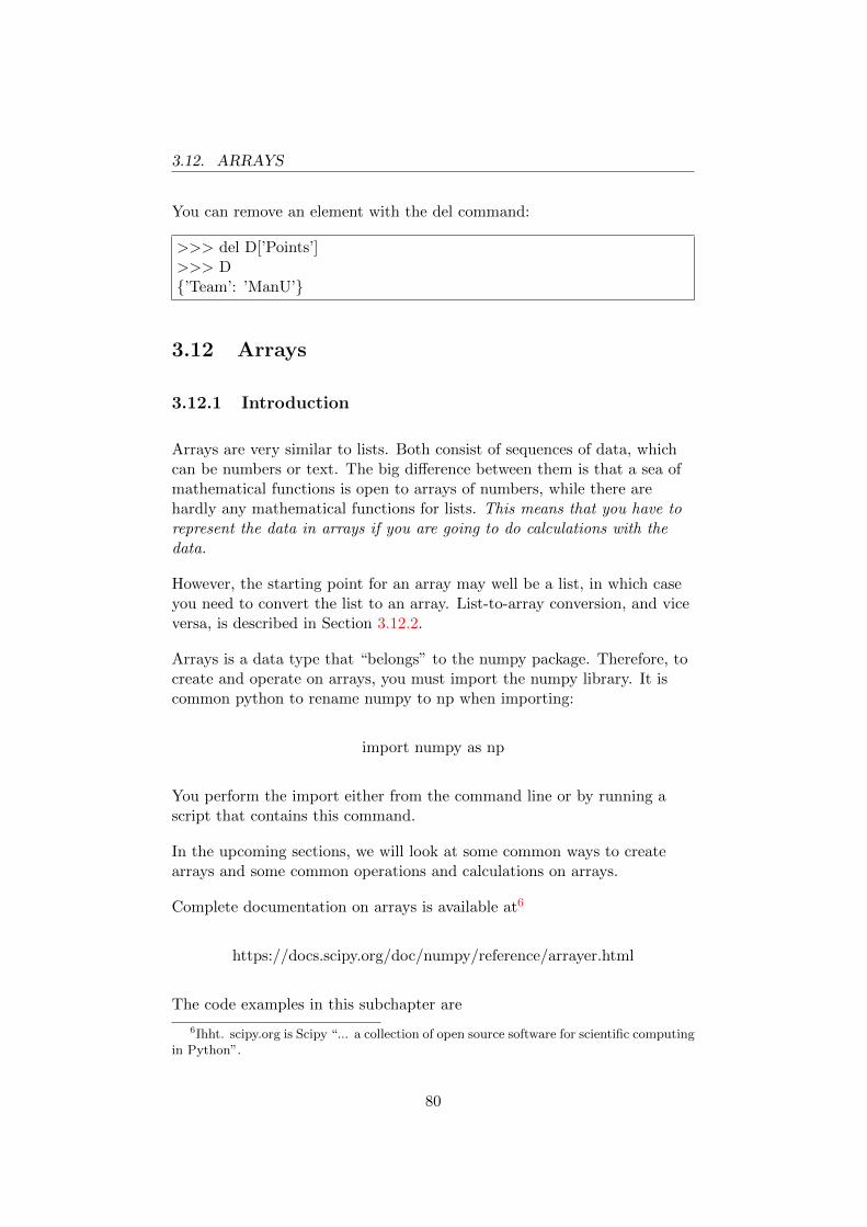
3.12. ARRAYS
You can remove an element with the del command:
>>> del D[’Points’]>>> D{’Team’: ’ManU’}
3.12 Arrays
3.12.1 Introduction
Arrays are very similar to lists. Both consist of sequences of data, whichcan be numbers or text. The big difference between them is that a sea ofmathematical functions is open to arrays of numbers, while there arehardly any mathematical functions for lists. This means that you have torepresent the data in arrays if you are going to do calculations with thedata.
However, the starting point for an array may well be a list, in which caseyou need to convert the list to an array. List-to-array conversion, and viceversa, is described in Section 3.12.2.
Arrays is a data type that “belongs” to the numpy package. Therefore, tocreate and operate on arrays, you must import the numpy library. It iscommon python to rename numpy to np when importing:
import numpy as np
You perform the import either from the command line or by running ascript that contains this command.
In the upcoming sections, we will look at some common ways to createarrays and some common operations and calculations on arrays.
Complete documentation on arrays is available at6
https://docs.scipy.org/doc/numpy/reference/arrayer.html
The code examples in this subchapter are
6Ihht. scipy.org is Scipy “... a collection of open source software for scientific computingin Python”.
80

3.12. ARRAYS
import numpy as np
as the first command. You do not need to execute this command in eachinstance if you are constantly in the programming environment (such asspears), but if you exit and re-enter, you must execute the command.
3.12.2 How to convert lists to arrays and vice versa
3.12.2.1 Conversion from list to array
How do we convert a numeric list to an array? We can use the array()function in the numpy package. Suppose the list has name L and the arrayshould have name A. We can then convert L to A with:
A = np.array(L)
Example 3.16 Conversion of a list to an array
The following code converts the list L = [0.1, 2.3, 4.5, 6.7] to an array herecalled A:
>>> import numpy as np>>> L = [0.1, 2.3, 4.5, 6.7]>>> A = np.array(L)>>> Aarray([0.1, 2.3, 4.5, 6.7])
[End of Example 3.16]
Note: Even if we say that we convert a list to an array, the original list willstill exist after the conversion.
3.12.2.2 Conversion from array to list
If you need to convert an array, called A, to a list, called L, you can usePython’s built-in list() function:
L = list(A)
81
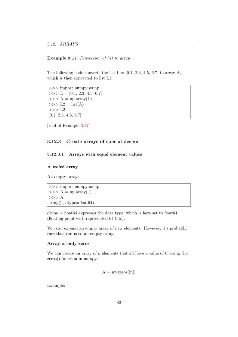
3.12. ARRAYS
Example 3.17 Conversion of list to array
The following code converts the list L = [0.1, 2.3, 4.5, 6.7] to array A,which is then converted to list L1:
>>> import numpy as np>>> L = [0.1, 2.3, 4.5, 6.7]>>> A = np.array(L)>>> L2 = list(A)>>> L2[0.1, 2.3, 4.5, 6.7]
[End of Example 3.17]
3.12.3 Create arrays of special design
3.12.3.1 Arrays with equal element values
A weird array
An empty array:
>>> import numpy as np>>> A = np.array([])>>> Aarray([], dtype=float64)
dtype = float64 expresses the data type, which is here set to float64(floating point with represented 64 bits).
You can expand an empty array of new elements. However, it’s probablyrare that you need an empty array.
Array of only zeros
We can create an array of n elements that all have a value of 0, using thezeros() function in numpy:
A = np.zeros([n])
Example:
82

3.12. ARRAYS
>>> import numpy as np>>> A = np.zeros([3])>>> Aarray([0., 0., 0.])
Array of only ones
We can create an array of n items that all have value 1, using the theones() function:
A = np.ones([n])
Example:
>>> import numpy as np>>> A = np.ones([3])>>> Aarray([1., 1., 1.])
Array with all elements having the same value
We can create an array of n elements that all have value k (whatever youset it to) by starting with an array of only 0’s, which we then add k to:
A = np.zeros([n]) + k
The result is that k is added to each of the elements. (It may seem strangethat one can add one number, that is, a scalar, to an array of numbers, butit is thus allowed.)
Alternatively, we can use the ones() function, which gives the same result:
A = k*np.ones([n])
Example:
>>> import numpy as np>>> A = np.zeros([3]) + 5.2>>> Aarray([5.2, 5.2, 5.2])
Note that here the array differs from lists, since the + operator applied toa list means to expand list, not elemental addition as for arrays. Check theresult of adding an element, here 5.2, to a list:
83

3.12. ARRAYS
>>> import numpy as np>>> L = list(np.zeros([3])) + [5.2]>>> L[0.0, 0.0, 0.0, 5.2]
3.12.3.2 Array with fixed increment between elements
It is often necessary to create an array with fixed increment (distance)between the element values, e.g. an array of times with fixed time stepsbetween times. The linspace() function in the numpy package can be doneas follows:
A = np.linspace(start, stopp, antall)
there
• start is a given start value, like are included in the array.
• stop is a given stop value, like are included in the array.
• number is the number of elements in the array.
• A is the resulting – or returned – array. (Of course, you can choose aname other than A on the array.)
Example 3.18 Using np.linspace() to create an array of points of time
The code below creates an array of points of time, from (included) thestart time t start = 0 s to (included) the end time t stop = 1.0 s, withtime step Ts = 0.1 s between each point of time.
>>> import numpy as np>>> t start = 0.0>>> t stop = 1.0>>> Ts = 0.1>>> n = int((t stop - t start)/Ts) + 1 # int() rounds downwards.>>> t = np.linspace(t start,t stop,n)>>> tarray([0. , 0.1, 0.2, 0.3, 0.4, 0.5, 0.6, 0.7, 0.8, 0.9, 1. ])>>> n11
84

3.12. ARRAYS
[End of Example 3.18]
np.arange() instead of np.linspace()?
As an alternative to np.linspace (start, stop, number), we have np.arange(start, stop, step). One difference between these functions is that they use,respectively, number and steps as arguments to specify the distance (stepsize) between the element values. Another difference – and that is themost important difference – is that linspace includes the stop value in thearray, while arange() does not include the stop value.7
Example 3.19 Using arange() to create an array of points of time
This example is pretty much the example 3.18 based on linspace(), butlet’s use arange() instead:
>>> import numpy as np>>> t start = 0.0>>> t stopp = 1.0>>> Ts = 0.1>>> t = np.arange(t start,t stopp,Ts)>>> tarray([0. , 0.1, 0.2, 0.3, 0.4, 0.5, 0.6, 0.7, 0.8, 0.9])>>> n10
The number of elements becomes (of course) one less for arange() than forlinspace(), ie 10 and 11 respectively, given that the time step is the same(set to Ts = 0.1 s in both cases).
[End of Example 3.19]
3.12.3.3 Multidimensional or n-dimensional arrays
So far we have used one-dimensional arrays. In general, Python/numpysupports multidimensional arrays, or n-dimensional arrays where n is aninteger: 1 or 2 or 3, etc. More specifically:
• One-dimensional arrays, or 1D arrays, have the elements (whatevertheir value) located along one dimension or axis. Such arrays are also
7I prefer linspace() over arange().
85

3.12. ARRAYS
called vectors. Visually, 1D arrays are similar to horizontal orvertical lines (you can choose to consider 1D arrays as horizontal orvertical lines).
• Two-dimensional arrays, or 2D arrays, have the elements locatedalong two dimensions or axes. Such arrays are also called matrix.Visually, 2D arrays are similar to surfaces.
• Three-dimensional arrays, or 3D arrays, have elements placed alongthree dimensions or axes. Such arrays are also called tensors.Visually, 3D arrays resembles cubes.
• Etc.
Figure 3.10 illustrates 1D, 2D and 3D arrays. The Figure shows examplesof addressing specific elements (but I have not specified any the value ofthe elements (numbers or text) in these examples).
Figure 3.10: 1D, 2D and 3D arrays
Here is an example where we create a matrix (2D array).
Example 3.20 Matrix (2D array)
We create a 2D array with 2 rows and 3 columns:
86

3.12. ARRAYS
>>> import numpy as np>>> A = np.array([[0, 10, 20], [30, 40, 50]])>>> Aarray([[ 0, 10, 20],[30, 40, 50]])
[End of Example 3.20]
We can generally create n-dimensional arrays, e.g. 19-dimensional arrays,but we will not look into this.
3.12.4 Array operations
3.12.4.1 Introduction
In Chap. 3.9.2 we learned about various operations on lists, namely
• Find the length
• Read element values
• Update element with new values
• Expand with new elements
• Remove element
• Find maximum values and minimum values
The same operations can be performed on arrays and with the samesyntax as for lists. This is shown in the sections below.
3.12.4.2 The size of an array
Example 3.21 The length of an array
The length or number of elements in an array can be found with Python’sbuilt-in len() function:
87
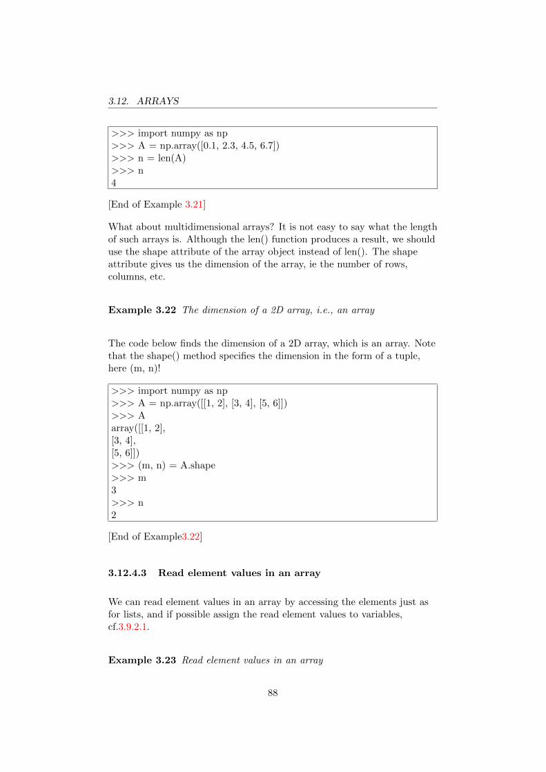
3.12. ARRAYS
>>> import numpy as np>>> A = np.array([0.1, 2.3, 4.5, 6.7])>>> n = len(A)>>> n4
[End of Example 3.21]
What about multidimensional arrays? It is not easy to say what the lengthof such arrays is. Although the len() function produces a result, we shoulduse the shape attribute of the array object instead of len(). The shapeattribute gives us the dimension of the array, ie the number of rows,columns, etc.
Example 3.22 The dimension of a 2D array, i.e., an array
The code below finds the dimension of a 2D array, which is an array. Notethat the shape() method specifies the dimension in the form of a tuple,here (m, n)!
>>> import numpy as np>>> A = np.array([[1, 2], [3, 4], [5, 6]])>>> Aarray([[1, 2],[3, 4],[5, 6]])>>> (m, n) = A.shape>>> m3>>> n2
[End of Example3.22]
3.12.4.3 Read element values in an array
We can read element values in an array by accessing the elements just asfor lists, and if possible assign the read element values to variables,cf.3.9.2.1.
Example 3.23 Read element values in an array
88

3.12. ARRAYS
>>> import numpy as np>>> A = np.array([0.1, 2.3, 4.5, 6.7])>>> x = A[1]>>> x2.3
[End of Example 3.23]
Read a series of elements
Now we will read the series of elements fom. index 0 to (but not including)index 2 in array A as we defined in example 3.23:
Example 3.24 Read a series of element values in an array
>>> import numpy as np>>> A = np.array([0.1, 2.3, 4.5, 6.7])>>> A[0:2]array([0.1, 2.3])
[End of Example 3.24]
Read element values in a 2D array (array)
Example 3.25 Read element values in a 2D array (array)
We create a 2D array with 2 rows and 3 columns, which is the same arrayas in the example 3.20:
>>> import numpy as np>>> A = np.array([[0, 10, 20], [30, 40, 50]])>>> Aarray([[ 0, 10, 20],[30, 40, 50]])
Then we can read e.g. the element in row 1 and column 2 in the array -remember that the lowest index for both rows and columns is 0, and notethe addressing method with square brackets in series:
>>> x = A[1][2]>>> x50
[End of Example 3.25]
89
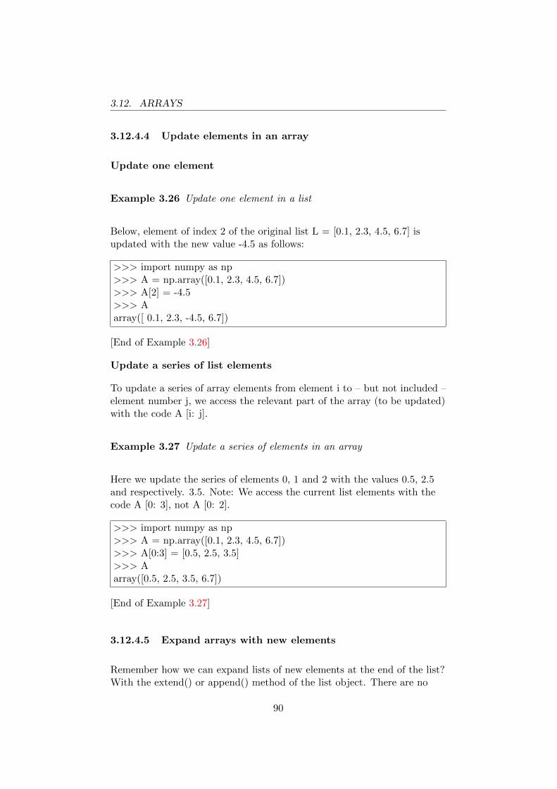
3.12. ARRAYS
3.12.4.4 Update elements in an array
Update one element
Example 3.26 Update one element in a list
Below, element of index 2 of the original list L = [0.1, 2.3, 4.5, 6.7] isupdated with the new value -4.5 as follows:
>>> import numpy as np>>> A = np.array([0.1, 2.3, 4.5, 6.7])>>> A[2] = -4.5>>> Aarray([ 0.1, 2.3, -4.5, 6.7])
[End of Example 3.26]
Update a series of list elements
To update a series of array elements from element i to – but not included –element number j, we access the relevant part of the array (to be updated)with the code A [i: j].
Example 3.27 Update a series of elements in an array
Here we update the series of elements 0, 1 and 2 with the values 0.5, 2.5and respectively. 3.5. Note: We access the current list elements with thecode A [0: 3], not A [0: 2].
>>> import numpy as np>>> A = np.array([0.1, 2.3, 4.5, 6.7])>>> A[0:3] = [0.5, 2.5, 3.5]>>> Aarray([0.5, 2.5, 3.5, 6.7])
[End of Example 3.27]
3.12.4.5 Expand arrays with new elements
Remember how we can expand lists of new elements at the end of the list?With the extend() or append() method of the list object. There are no
90
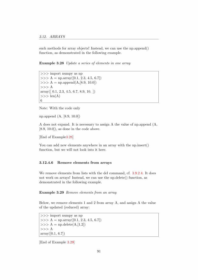
3.12. ARRAYS
such methods for array objects! Instead, we can use the np.append()function, as demonstrated in the following example.
Example 3.28 Update a series of elements in one array
>>> import numpy as np>>> A = np.array([0.1, 2.3, 4.5, 6.7])>>> A = np.append(A,[8.9, 10.0])>>> Aarray([ 0.1, 2.3, 4.5, 6.7, 8.9, 10. ])>>> len(A)6
Note: With the code only
np.append (A, [8.9, 10.0])
A does not expand. It is necessary to assign A the value of np.append (A,[8.9, 10.0]), as done in the code above.
[End of Example3.28]
You can add new elements anywhere in an array with the np.insert()function, but we will not look into it here.
3.12.4.6 Remove elements from arrays
We remove elements from lists with the del command, cf. 3.9.2.4. It doesnot work on arrays! Instead, we can use the np.delete() function, asdemonstrated in the following example.
Example 3.29 Remove elements from an array
Below, we remove elements 1 and 2 from array A, and assign A the valueof the updated (reduced) array:
>>> import numpy as np>>> A = np.array([0.1, 2.3, 4.5, 6.7])>>> A = np.delete(A,[1,2])>>> Aarray([0.1, 6.7])
[End of Example 3.29]
91
3.12. ARRAYS
3.12.4.7 Find the maximum and minimum in arrays
We can find the index of the element that has the maximum value in anarray with the np.argmax() function. The same applies to the minimumvalue; just replace argmax() with argmin(). Once this index is found, themaximum element value can be found with regular addressing.
Example 3.30 How to find maximum value in an array
The following code finds the index of the maximum value element in thelist, as well as the value of this element:
>>> import numpy as np>>> A = np.array([0.1, 2.3, 4.5, 6.7])>>> i max = np.argmax(A)>>> i max3>>> A[i max]6.7
[End of Example 3.30]
3.12.5 Mathematical operations on arrays, includingmatrices
3.12.5.1 Scalar addition and scalar multiplication
In many contexts we need
• to add a scalar to each array element
• to multiply each array element by a scalar
This can be done very easily in Python with, respectively, the + and *operator (below, A is the array and s is the scalar):
A + s
and
92
3.12. ARRAYS
A*s
You may say that the syntax does not make sense, because we cannotreally add an array and a number, but you just have to bow our thanks.
Example 3.31 Addition of scalars to each element of an array
Here, we add 1 to an array:
>>> import numpy as np>>> A = np.array([10, 20, 30])>>> A + 1array([11, 21, 31])
[End of Example 3.31]
Example 3.32 Multiplying each array element by a scalar
Here, we multiply by 3:
>>> import numpy as np>>> A = np.array([10, 20, 30])>>> A*3array([30, 60, 90])
[End of Example 3.32]
3.12.5.2 How to create row vectors and column vectors andarrays
In mathematics (linear algebra) we distinguish between row vectors andcolumn vectors. You can create row vectors and column vectors in Pythonfor 2D arrays only. In a sense, 1D arrays are neither row vector nor columnvector – just vector. You can also create matrices from given row vectorsand/or column vectors. We need to take a closer look at this.
How to make a row vector
Row vector (note that there are two square brackets in code line 2):
93

3.12. ARRAYS
>>> import numpy as np>>> R = np.array([[1.1, 2.2, 3.3]])>>> Rarray([[1.1, 2.2, 3.3]])>>> R.shape(1, 3)
If you drops one of the square brackets, you get an array, but you can’t tellif the array is a row vector or column vector, see the following example:
>>> import numpy as np>>> R = np.array([1.1, 2.2, 3.3])>>> Rarray([1.1, 2.2, 3.3])>>> R.shape(3,)
The fact that R.shape gives (3,) means that R is only a vector with 3elements, and cannot be classified as neither a row vector nor a columnvector.
How to create a column vector
We can create column vectors as follows:
>>> import numpy as np>>> K = np.array([[1.1], [2.2], [3.3]])>>> Karray([[1.1],[2.2],[3.3]])>>> K.shape(3, 1)
Alternatively, we can create a column vector a the transpose of a rowvector. To transpose is to reflect on an imaginary axis (diagonal), seeFigure 3.11. The figure shows, for example, the transposition of an arrayin the form of a (2, 6) array, but the principle is the same regardless of thenumber of rows and columns.
94

3.12. ARRAYS
Figure 3.11: Matrix transposition (2D Array)
Transposing can be achieved with the T method of the array object, whichis here the row vector R:
>>> import numpy as np>>> R = np.array([[1.1, 2.2, 3.3]])>>> K = R.T>>> Karray([[1.1],[2.2],[3.3]])>>> K.shape(3, 1)
So, we got exactly the same K-vector as earlier.
Note: Trying to transpose a 1D array in Python is useless, as you only getback the original 1D array. Transposing only works in higher dimensionalarrays.
How to create a matrix with given 1D arrays as column vectors
Suppose you create an array where the columns are to be formed fromexisting 1D arrays. Eg. we can have two arrays like this:
• A 1D array named t that contains times for a series of measurements.
• A 1D array named m containing the measurement values of aparticular sensor (measurement element).
95
3.12. ARRAYS
All in all we have two 1D arrays, which we would like to collect in a dataarray in the form of a 2D array named say d, where the two columnsoriginate. When we create such a matrix, we get a challenge because the1D arrays cannot be considered as neither row vectors nor column vectors– they are just vectors. The challenge can be solved by first creating amatrix where the 1D arrays become row vectors, and then creating thefinal matrix as the one transposed by this matrix. This is demonstrated byexample 3.33 below.
Example 3.33 An array of column vectors from given 1D arrays
Below are the t and m 1D arrays. The matrix d is made as the transposeof the 2D array that has t and m as rows.
The 2D array d1 is generated as an intermediate result for the sake ofillustration. Of course, you can drop generating d1, and type d = np.array([t, m]).T directly.
>>> import numpy as np>>> t = np.array([0, 1, 2, 3, 4])>>> m = np.array([30.0, 30.1, 30.2, 30.3, 30.4])>>> d1 = np.array([t, m])>>> d1array([[ 0. , 1. , 2. , 3. , 4. ],
[30. , 30.1, 30.2, 30.3, 30.4]])>>> d1.shape(2, 5)>>> darray([[ 0. , 30. ],
[ 1. , 30.1],[ 2. , 30.2],[ 3. , 30.3],[ 4. , 30.4]])
>>> d.shape(5, 2)
[End of Example 3.33]
3.12.5.3 Vector and matrix multiplications
In linear algebra we encounter both addition and multiplication of vectorsand matrices always. Python actually has the ability to transform arrays
96

3.12. ARRAYS
into arrays – or rather: array objects – with the np.mat() function, whichworks like this:
M = np.mat(A)
so that one can use the syntax for addition and multiplication with + and* on the matrix object (just like in the known MATLAB calculation tool).
But now the Python developers have decided that the matrix object willsoon be out of life. Therefore, it is just as easy to forget matrix objects:
M = np.mat(A)
Therefore:
We should use array objects in vector and matrix multiplications becausematrix objects have an uncertain future!
How do we then add and multiply vectors and matrices? There are severalways to do this, but I think the neatest thing is to make sure that thevectors and matrices are 2D arrays, and then perform the mathematicaloperation on these 2D arrays:
Addition:
A1 = A1 + A2
That is, the syntax is as for matrix objects.
But for multiplication, there are news:
A3 = A1 @ A2
So instead of *, we use @ (the at character).
Here is an important rarity when it comes to multiplication: To multiply amatrix in the form of a 2D array with a scalar, then the @ operatorunfortunately does not work; then you must use the * operator just like inSection 3.12.5.1:
A * s
97

3.12. ARRAYS
About the use of words: As a result of what has been said above, I herebystop talking about matrices in the form of matrix objects in Python. But Iwill continue to talk about matrices, assuming they are 2D arrays inPython.
Multiplication of vectors
From mathematics we know that the scalar product (also called the innerproduct or the dot product) between two vectors a and b where both areassumed to be row vectors, are8
p = a · bT
In Python we can calculate this with the @ operator for multiplication:
p = a @ b.T
Example 3.34 Scalar product
Here we create two row vectors, then calculate their scalar product, whichactually becomes in the form of a 2D array. We should have liked the resultas a floating point, and we get that with Python’s built-in float() function:
>>> import numpy as np>>> a = np.array([[0, 1, 2]])>>> b = np.array([[3, 4, 5]])>>> p = a @ b.T>>> parray([[14]])>>> f = float(p)>>> f14.0
Python can actually calculate the scalar product with a simpler syntax, seebelow. Maybe you like this syntax better than the “rigid” syntax above.
>>> import numpy as np>>> a = np.array([0, 1, 2])>>> b = np.array([3, 4, 5])>>> p = a @ b>>> p14.0
8If a and b are one and the same vector, i.e. a = b, the scalar product is the square ofthe length of the vector.
98

3.12. ARRAYS
Question: Can we use the “natural” product operator * to calculate thescalar product, ie, can we write p = a * b? Just try it!9
Finally, I mention that numpy offers the vdot() function to calculate thescalar product (dot product) of vectors:
>>> import numpy as np>>> a = np.array([0, 1, 2])>>> b = np.array([3, 4, 5])>>> p = np.vdot(a, b)>>> p14
[End of Example 3.34]
Multiplication of matrices and vectors
Matrices and vectors are naturally multiplied by the @ operator, asdemonstrated in the following example.
Example 3.35 Multiplication of matrix and vector
Given the matrix
M =
[1 00 2
]and the vector
v =
[34
]The product of M and v is
p = Mv =
[1 00 2
]·[
34
]=
[38
]
The following code calculates this product:
>>> import numpy as np>>> M = np.array([[1, 0], [0, 2]])>>> v = np.array([[3], [4]]) # Column vector>>> p = M @ v>>> parray([[3],
[8]])
9The answer is no.
99

3.12. ARRAYS
Want to see if p = M * v gives the same result?
[End of Example 3.35]
Multiplication of Matrices
Matrices are naturally multiplied by the @-operator, just as whenmultiplying matrices and vectors. I skip an example on this.
3.12.6 Matrix functions for linear algebra
The numpy package with its linealg module has a large collection of matrixfunctions for linear algebra. The examples below illustrate its use.
Example 3.36 A couple of examples of matrix functions in linear algebra
Here, the determinant of a matrix is calculated:
>>> import numpy as np>>> M = np.array([[1, 0], [0, 2]])>>> det M = np.linalg.det(M)>>> det M2.0
Here, an array is inverted:
>>> import numpy as np>>> M = np.array([[1, 0], [0, 2]])>>> inv M = np.linalg.inv(M)>>> inv Marray([[1. , 0. ],
[0. , 0.5]])
[End of Example 3.36]
3.12.7 Vectorized calculations
Suppose you use a given function in Python on each of the n elements ofan array, which we call vector. Initially, you must then apply the functiononce to each of the n elements, ie n times. It can be cumbersome.Fortunately, Python developers have thought of this. They have facilitated
100
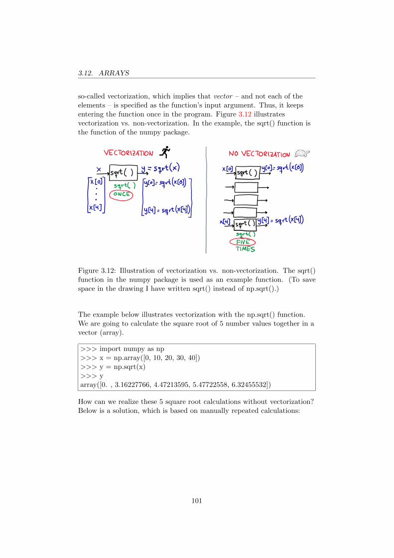
3.12. ARRAYS
so-called vectorization, which implies that vector – and not each of theelements – is specified as the function’s input argument. Thus, it keepsentering the function once in the program. Figure 3.12 illustratesvectorization vs. non-vectorization. In the example, the sqrt() function isthe function of the numpy package.
Figure 3.12: Illustration of vectorization vs. non-vectorization. The sqrt()function in the numpy package is used as an example function. (To savespace in the drawing I have written sqrt() instead of np.sqrt().)
The example below illustrates vectorization with the np.sqrt() function.We are going to calculate the square root of 5 number values together in avector (array).
>>> import numpy as np>>> x = np.array([0, 10, 20, 30, 40])>>> y = np.sqrt(x)>>> yarray([0. , 3.16227766, 4.47213595, 5.47722558, 6.32455532])
How can we realize these 5 square root calculations without vectorization?Below is a solution, which is based on manually repeated calculations:
101
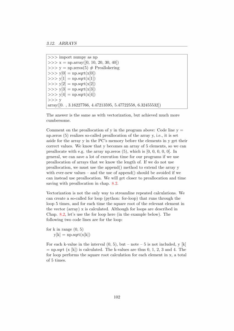
3.12. ARRAYS
>>> import numpy as np>>> x = np.array([0, 10, 20, 30, 40])>>> y = np.zeros(5) # Preallokering>>> y[0] = np.sqrt(x[0])>>> y[1] = np.sqrt(x[1])>>> y[2] = np.sqrt(x[2])>>> y[3] = np.sqrt(x[3])>>> y[4] = np.sqrt(x[4])>>> yarray([0. , 3.16227766, 4.47213595, 5.47722558, 6.32455532])
The answer is the same as with vectorization, but achieved much morecumbersome.
Comment on the preallocation of y in the program above: Code line y =np.zeros (5) realizes so-called preallocation of the array y, i.e., it is setaside for the array y in the PC’s memory before the elements in y get theircorrect values. We know that y becomes an array of 5 elements, so we canpreallocate with e.g. the array np.zeros (5), which is [0, 0, 0, 0, 0]. Ingeneral, we can save a lot of execution time for our programs if we usepreallocation of arrays that we know the length of. If we do not usepreallocation, we must use the append() method to extend the array ywith ever-new values – and the use of append() should be avoided if wecan instead use preallocation. We will get closer to preallocation and timesaving with preallocation in chap. 8.2.
Vectorization is not the only way to streamline repeated calculations. Wecan create a so-called for loop (python: for-loop) that runs through theloop 5 times, and for each time the square root of the relevant element inthe vector (array) x is calculated. Although for loops are described inChap. 8.2, let’s use the for loop here (in the example below). Thefollowing two code lines are for the loop:
for k in range (0, 5)y[k] = np.sqrt(x[k])
For each k-value in the interval (0, 5), but – note – 5 is not included, y [k]= np.sqrt (x [k]) is calculated. The k-values are thus 0, 1, 2, 3 and 4. Thefor loop performs the square root calculation for each element in x, a totalof 5 times.
102

3.12. ARRAYS
>>> import numpy as np>>> x = np.array([0, 10, 20, 30, 40])>>> y = np.zeros(5)>>> for k in range(0, 5):
y[k] = np.sqrt(x[k])>>> yarray([0. , 3.16227766, 4.47213595, 5.47722558, 6.32455532])
Vectorization used in ordinary mathematical expressions
Figure 3.13: Body in free fall
Figure 3.13 shows a body in free fall, without air resistance, that wasreleased at time 0 s. From physics, we know, that, at time t, the body hasfallen the distance s [m] given by:
s =1
2gt2 (3.1)
g = 9.81 m/s2 is the acceleration of gravity. Suppose we calculate s foreach of the times fom. 0 tom. 5 s with time steps 1.0 s. The programbelow realizes this.10
10All Python prompts (>>>) indicate that the code is executed from a command line,but you can alternatively write all the code lines in a script and run the script.
103
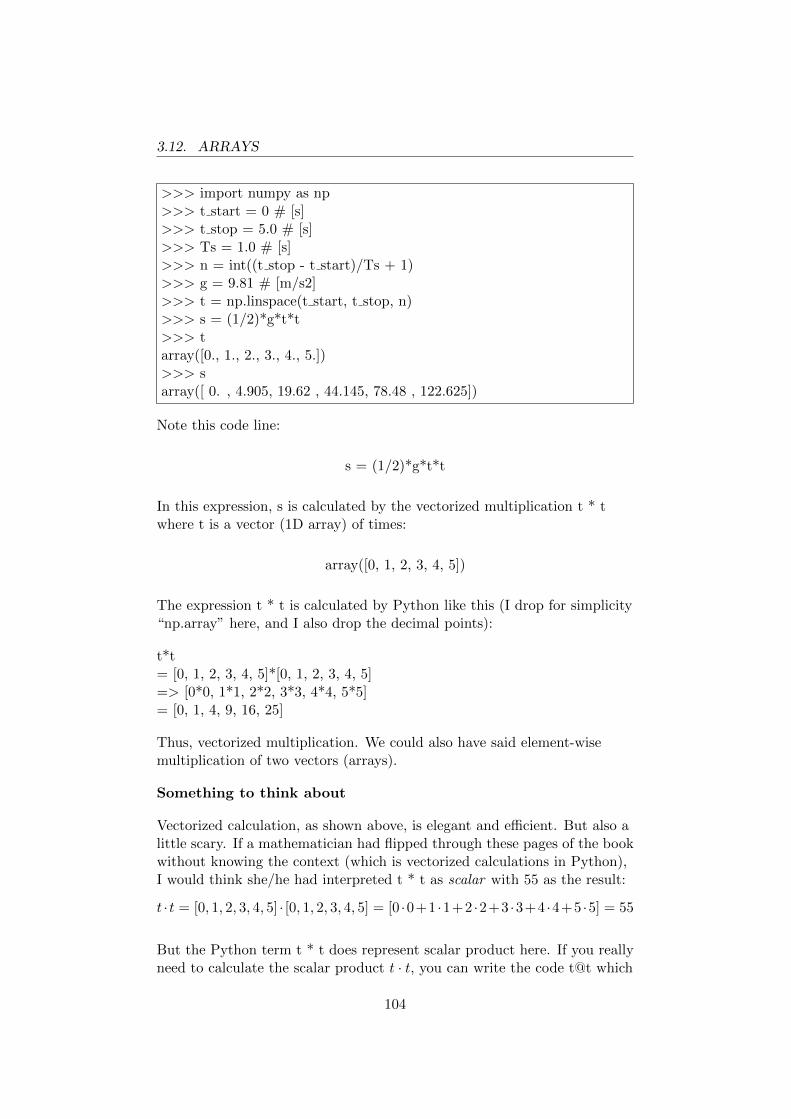
3.12. ARRAYS
>>> import numpy as np>>> t start = 0 # [s]>>> t stop = 5.0 # [s]>>> Ts = 1.0 # [s]>>> n = int((t stop - t start)/Ts + 1)>>> g = 9.81 # [m/s2]>>> t = np.linspace(t start, t stop, n)>>> s = (1/2)*g*t*t>>> tarray([0., 1., 2., 3., 4., 5.])>>> sarray([ 0. , 4.905, 19.62 , 44.145, 78.48 , 122.625])
Note this code line:
s = (1/2)*g*t*t
In this expression, s is calculated by the vectorized multiplication t * twhere t is a vector (1D array) of times:
array([0, 1, 2, 3, 4, 5])
The expression t * t is calculated by Python like this (I drop for simplicity“np.array” here, and I also drop the decimal points):
t*t= [0, 1, 2, 3, 4, 5]*[0, 1, 2, 3, 4, 5]=> [0*0, 1*1, 2*2, 3*3, 4*4, 5*5]= [0, 1, 4, 9, 16, 25]
Thus, vectorized multiplication. We could also have said element-wisemultiplication of two vectors (arrays).
Something to think about
Vectorized calculation, as shown above, is elegant and efficient. But also alittle scary. If a mathematician had flipped through these pages of the bookwithout knowing the context (which is vectorized calculations in Python),I would think she/he had interpreted t * t as scalar with 55 as the result:
t · t = [0, 1, 2, 3, 4, 5] · [0, 1, 2, 3, 4, 5] = [0 ·0+1 ·1+2 ·2+3 ·3+4 ·4+5 ·5] = 55
But the Python term t * t does represent scalar product here. If you reallyneed to calculate the scalar product t · t, you can write the code t@t which
104
3.12. ARRAYS
will be ok since t is a 1D array. Alternatively, you can define t as a rowvector in the form of a 2D array, and calculate the scalar product [email protected], cf. Section 3.12.5.3. Another alternative for calculating the scalarproduct, is the vdot function: np.vdot (t, t).
Summary
There are alternative ways of realizing repeated function calculations.They can be ranked this way, by both ease of use and efficiency:
1. Vectorization
2. For Loops
3. Manually repeated calculations
105
Chapter 4
Presenting data in chartsand diagrams
4.1 Introduction
Probably the most commonly used Python package for presenting datagraphically in charts and diagrams is matplotlib, which has website on
https://matplotlib.org
Matplotlib allows for a variety of different types of graphical presentations.We will in this chapter take a look at some of the most common types,namely:
• line plots
• bar charts
• pie charts
• histograms
4.2 Line plot
As a starting point to learn more about plotting, we will use the programfor plotting temperatures in Skien from Chap. 1.2. The program is
106

4.2. LINE PLOT
reproduced below, but now - for simplicity - almost without comments inthe code. I commented the program in Chap. 1.2. I will now provide evenmore comments, and then show some extensions of the program that Iassume are of particular interest.
4.2.1 Basic plot functions
Running the program below generates the line plot shown in Figure 4.1.
Program name: prog plot temp skien.py
import numpy as npimport matplotlib.pyplot as plt
mnd = np.array([1, 2, 3, 4, 5, 6, 7, 8, 9, 10, 11, 12]) # monthno.temp = np.array([-3, -2, 2, 7, 11, 15, 17, 16, 12, 6, 2, -3]) # deg Cmean temp = np.mean(temp) # Mean values
# Plotting av temperaturverdiene:
plt.close(’all’)plt.figure(’Monthly mean temp i Skien’)plt.plot(mnd, temp, ’o-’)plt.xlim(1, 12)plt.ylim(-5, 20)plt.title(’Monthly mean temp in Skien year 2005-2015’)plt.xlabel(Month no.’)plt.ylabel(Deg C’)plt.grid()plt.show()
plt.savefig(’temp skien.pdf’)
107

4.2. LINE PLOT
0 2 4 6 8 10 12Month no.
5
0
5
10
15
20[D
eg C
]Monthly mean temp in Skien year 2005-2015
Figure 4.1: Line plot of montly mean temperatures in Skien
Comments on the part of the program concerning plotting (here is a littlerepetition from chap. 1.2):
• The code import matplotlib.pyplot as plt imports the pyplot modulewhich is part of the matplotlib package and makes the moduleavailable to us through the name plt. This rename is Pythontradition. the pyplot module allows you to set e.g. line type (e.g.,dotted), line color (e.g., blue), grid, descriptive text, etc.
• The code plt.close (’all’) closes all existing figure windows, whichmay be fine to clean up and reset before new plotting.
• The code plt.figure (’Monthly mean temp in Skien’) opens a figurewindow which gets a “number” similar to the text ’Monthly meantemp in Skien’, and prepares the figure for plotting with subsequentplot commands. You can also use numbers such as figure numbers,e.g. plt.figure (1).
• The code plt.plot (month, temp, ’o-’) plots the temp (y values) arrayagainst the mnd (x values) array. Basically, the points (month [0],temp [0]), (month [1], temp [1]), etc. are plotted. Of course, thesearrays must have the same number of elements. In this example,data in arrays is plotted, but lists can also be plotted.
108

4.2. LINE PLOT
• The text string ’o-’ in the code plt.plot (month, temp, ’o-’)determines the appearance of the curve: ’o’ means that each point isplotted with a filled circle. ’-’ indicates the straight line between thepoints. You can also set color. The codes can be combined fairlyfreely, as ’o-’ is an example of. The most relevant codes are:
– Dot mark: ’o’ for open circle. ’*’ for star. ’.’ (dot) for dot.Default (ie the dot mark that Python selects, if no code isentered) is dot.
– Line (interpolation) between the points: ’-’ for the solid line. ’-’for dotted line. ’-.’ for line + point. Default is the solid line.
– Color: ’b’ for blue. ’r’ for red. ’y’ for yellow. ’g’ for green. ’k’for black. Default is blue.
• The code plt.xlim (1, 12) and the code plt.ylim (-5, 20) indicate thesmallest and largest value along the x-axis and the y-axis,respectively.
• The code plt.xlim (1, 12) and the code plt.ylim (-5, 20) indicate thesmallest and largest value along the x-axis and the y-axis,respectively.
• The codes plt.xlabel (’Month no.’) and plt.ylabel (’Deg C’) is writtenalong the x-axis and the y-axis, respectively. The arguments are textstrings.
• The code plt.grid() creates a grid.
• The code plt.show() ensures that the figure is displayed. In Spyder,the figure is shown even though plt.show() is omitted, but in otherprogramming environments, eg. Visual Studio Code, it may benecessary to include plt.show().
• The code plt.savefig (’temp skien.pdf’) creates a pdf file of the plot.If you want a png file, replace ’temp skien.pdf’ with’temp skien.png’. The same applies to jpg files. The file is stored inthe same directory where the script is stored.
Plot in multiple figure windows?
So far we have plotted in a figure window. If you want to have multipleplots in their own figure window, open new figure windows with respectiveplt.figure (figure name) expressions, where figure names can be text orinteger, e.g.
• plt.figure(’Monthly temp in Porsgrunn’) or
109

4.2. LINE PLOT
• plt.figure(2).
After the plt.figure() expression, type the appropriate plot commands,which will then apply to the last opened figure window.
4.2.2 Viewing Plots in the Spyder Console or ExternalWindow?
You can decide whether a plot figure (plot Figure) should appear in theSpyder console or in an external window. The two options are discussed inmore detail below.1
4.2.2.1 Plot figures to be shown in the Spyder console
Figure 1.6 shows a Figure of a plot shown in the Spyder console. Anadvantage of such a view is that then the figure will be displayed togetherwith the result of calculations, in the same order as in the program code.One disadvantage is that the figure becomes quite small since it must fit inthe console.
How do you get Spyder to show characters in the console? One way is toexecute the command
%matplotlib inline
on the console command line. % matplotlib inline is an example of aso-called magic command, which belongs to IPython (Interactive Python),which is the user interface to Python implemented in e.g. Spyder.
An alternative to the magic command mentioned above is the followingmenu options in Spyder:
Tools / Preferences / IPython console / Graphics / Graphics backend /Backend
where you select Inline in the menu, see Figure 4.2.
1I myself tend to use external window.
110

4.2. LINE PLOT
Figure 4.2: How to set Graphics backend to Inline via the Tools / Preferencesmenu in Spyder
By right-clicking on the figure in the console, you get the following twooptions:
• Copy Image, which makes a copy of thefFigure on the PC’sclipboard. From there you can paste the figure into a word processor(eg MS Word) or a drawing program (eg with the shortcut ctrl + V).
• Save Image As, which allows you to save the image as a png file.
The choice to display plot figures inline, ie in the console, remains untilyou choose to display the plot figures in an external window. Te choice isremembered between each time you run programs, and it is alsoremembered if you exit Spyder and enter again.
Plot figures to be shown in an external window
Plot figures can be displayed in an external window (outside the Spyderwindow), see Figure 4.3.
111

4.2. LINE PLOT
Figure 4.3: A plot figure shown in an external window (outside the Spyderwindow)
An advantage of displaying the plot the figure in an external window isthat the figure becomes larger than it appears in the console. Anotheradvantage is that the figure window provides a number of possibilities forfigure processing, including choose the appearance of curvature lines.color, line type, etc., zoom, saving the figure to a file, including pdf, pngand jpg.2
I do not go through all the menu choices in the figure window (they areeasy to find out).
How do you get Spyder to display characters in an external window? Oneway is to execute the magic command
%matplotlib auto
on the console command line.
An alternative to this magic command is the following menu options in
2pdf should be used if the text editor allows, since pdf is based on vector graphics,which provides maximum resolution, ie best image quality. In this book I use pdf graphicsas much as possible.
112
4.2. LINE PLOT
Spyder:
Tools / Preferences / IPython console / Graphics / Graphics backend /Backend
where you select Automatic in the menu, see Figure 4.2.
4.2.3 How to plot multiple curves at the same time
4.2.3.1 Multiple curves in one and the same diagram
The program code below shows how several - here two - curves can beplotted in one and the same diagram. The two curves are the monthlytemperature values (temp) and the mean (mean temp) of thesetemperature values.
The code also shows how each curve can be identified with a curve legendrealized with the plt.legend() function. Figure 4.4 shows the plot.
Program name: prog plot temp skien several curves.py
113

4.2. LINE PLOT
import numpy as npimport matplotlib.pyplot as plt
month = np.array([1, 2, 3, 4, 5, 6, 7, 8, 9, 10, 11, 12])temp = np.array([-3, -2, 2, 7, 11, 15, 17, 16, 12, 6, 2, -3])
mean temp = np.mean(temp)
mean temp array = np.zeros(len(temp)) + mean temp
# Plotting av temperaturverdiene:plt.figure(1)plt.plot(month, temp, ’o-b’, month, mean temp array, ’g’)plt.title(’Monthly mean temp in Skien 2005-2015’)plt.xlabel(Month no.’)plt.ylabel(’Deg C’)plt.legend(labels=(’Temperature’, ’Mean temp’),
loc=’upper right’,handlelength=2,fontsize=8)
plt.grid()plt.show()
114

4.2. LINE PLOT
2 4 6 8 10 12Month no. [nr.]
2.5
0.0
2.5
5.0
7.5
10.0
12.5
15.0
17.5
[Deg
C]
Monthly mean temp in Skien 2005-2015TemperatureMean temp
Figure 4.4: Multiple curves plotted in a single diagram identified by curvedescription generated by the plt.legend() function
Note how the plt.plot() function is used to plot multiple curves in onechart:
plt.plot(mnd, temp, ’o-b’, mnd, mean temp array, ’g’)
where the text string ’o-b’ means circles connected by straight lines of bluecolor and the text string ’g’ means green color.
The general syntax for plotting more than one curve (here two) is
plt.plot(x1 array, y1 array, ’formatting1’, x2 array, y2 array, ’formatting2’)
I’ve included here “array” in the variable names just to emphasize that thedata type is array, but you are of course free to choose the variable name.
Generally in such composite plots, x1 array and x2 array may havedifferent lengths (number of elements), but x1 array and y1 array musthave equal lengths, and x2 array and y2 array must have equal lengths. Inour example, all the arrays have equal lengths.
115

4.2. LINE PLOT
For the plot of the mean temperature, we need an array of length equal tothe temp array and with mean temp as the value for all the elements. Inthe program, this array is created with this code:
mean temp array = np.zeros(len(temp)) + mean temp
Alternatively, I could have used this slightly shorter code:
mean temp array = temp*0 + mean temp
Curve description with plt.legend()
In the upper right of the plot figure in Figure 4.4 it is a curve description(legend) realized with the plot.legend() function. Comments:
• The labels parameter specifies the text for each curve.
• The location parameter is set to ’upper right’. The possibilities are:
– best (default)
– upper right
– upper left
– lower left
– lower right
– right
– center left
– center right
– lower center
– upper center
– center
• The handle length parameter specifies the length of the relativelyshort selection curve in the curve description measured by the fontsize as a unit.
• The font size parameter specifies the font size.
Note: If the curve description applies to only one curve, let’s say only theTemperature curve, you must include a comma and blank:
plt.legend(labels=(’Temperature’, )
116
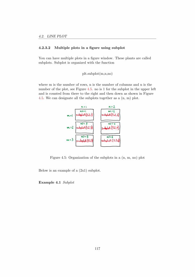
4.2. LINE PLOT
4.2.3.2 Multiple plots in a figure using subplot
You can have multiple plots in a figure window. These plants are calledsubplots. Subplot is organized with the function
plt.subplot(m,n,no)
where m is the number of rows, n is the number of columns and n is thenumber of the plot, see Figure 4.5. no is 1 for the subplot in the upper leftand is counted from there to the right and then down as shown in Figure4.5. We can designate all the subplots together as a (n, m) plot.
Figure 4.5: Organization of the subplots in a (n, m, no) plot
Below is an example of a (2x1) subplot.
Example 4.1 Subplot
117
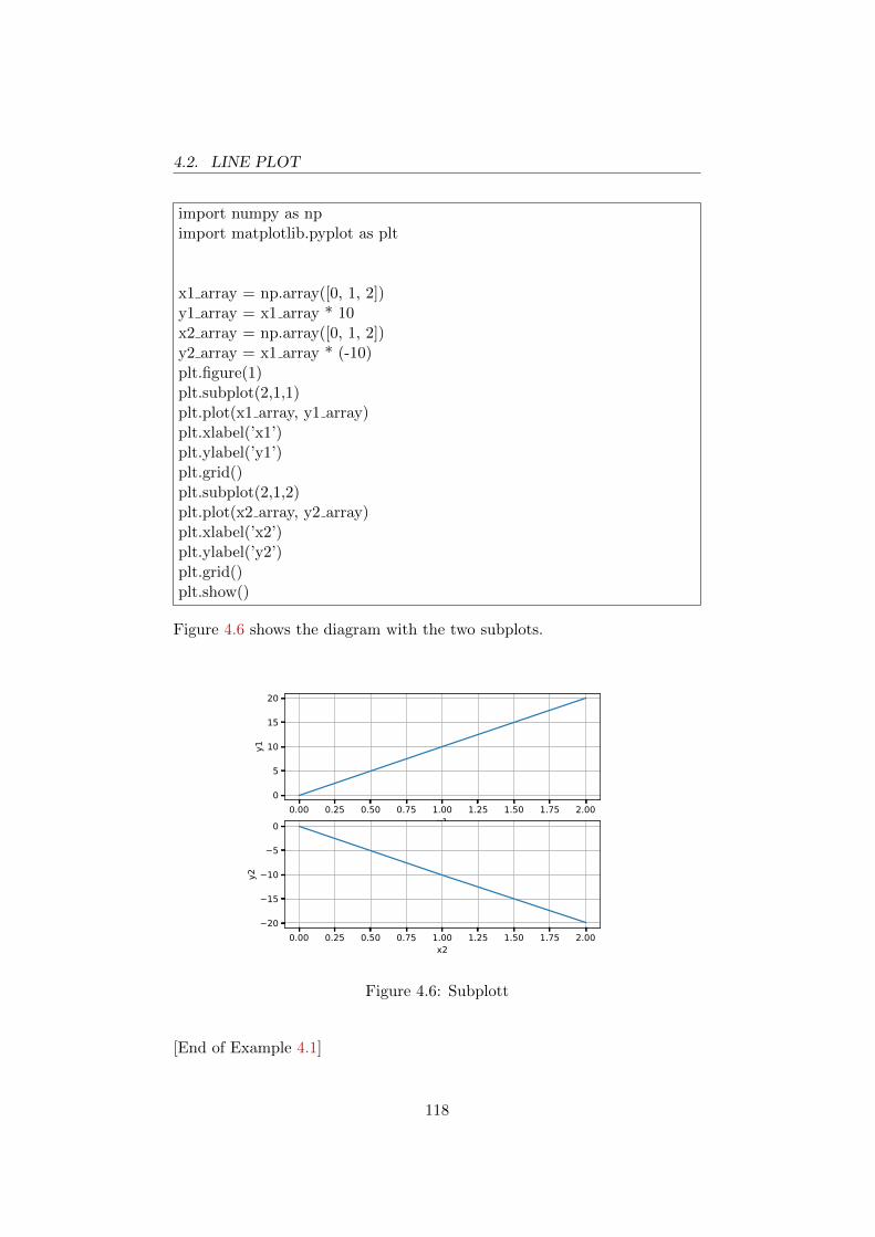
4.2. LINE PLOT
import numpy as npimport matplotlib.pyplot as plt
x1 array = np.array([0, 1, 2])y1 array = x1 array * 10x2 array = np.array([0, 1, 2])y2 array = x1 array * (-10)plt.figure(1)plt.subplot(2,1,1)plt.plot(x1 array, y1 array)plt.xlabel(’x1’)plt.ylabel(’y1’)plt.grid()plt.subplot(2,1,2)plt.plot(x2 array, y2 array)plt.xlabel(’x2’)plt.ylabel(’y2’)plt.grid()plt.show()
Figure 4.6 shows the diagram with the two subplots.
0.00 0.25 0.50 0.75 1.00 1.25 1.50 1.75 2.00x1
0
5
10
15
20
y1
0.00 0.25 0.50 0.75 1.00 1.25 1.50 1.75 2.00x2
20
15
10
5
0
y2
Figure 4.6: Subplott
[End of Example 4.1]
118

4.2. LINE PLOT
4.2.4 Mathematical symbols in chart title
You can include beautiful mathematical symbols in plt.title(), plt.xlabel()and plt.ylabel(). For this use codes from Latex, which is a text formattingsystem for books, scientific articles, etc. Example 4.2 demonstrates this.
Example 4.2 Latex-code in plt.title()
Some random data are plotted in the program shown below. Take a closelook at the relationship between the code in the plt.title() argument andthe plot shown in Figure 4.7. I guess you see how Latex code can be used(I won’t explain this in detail).
Note:
• The letter r is just before the text strings with Latex code, e.g. r ’$x {a 1} $’. r stands for "raw text". Without r, the Latex codes willnot work.
• The ’\ n’ text line (newline) is used to create more lines than one.
Programmets navn: prog plot latex.py
import numpy as npimport matplotlib.pyplot as plt
x array = np.array([0, 1, 2])y array = x array * 10plt.figure(1)plt.plot(x array, y array)plt.title(’Beautiful:’ + ’\n’
+ r’$x {a 1}$’+ ’ and ’ + r’$\sqrt{\alpha\beta\gamma\Omega\pi\theta\tau}$’+ ’ and ’ + r’$\int 0ˆt z d\tau$’+ ’ and finally ’ + r’$\sum {k=0}ˆ{N-1} y(k)$’)
plt.xlabel(’x’)plt.ylabel(’y’)plt.grid()plt.show()
119
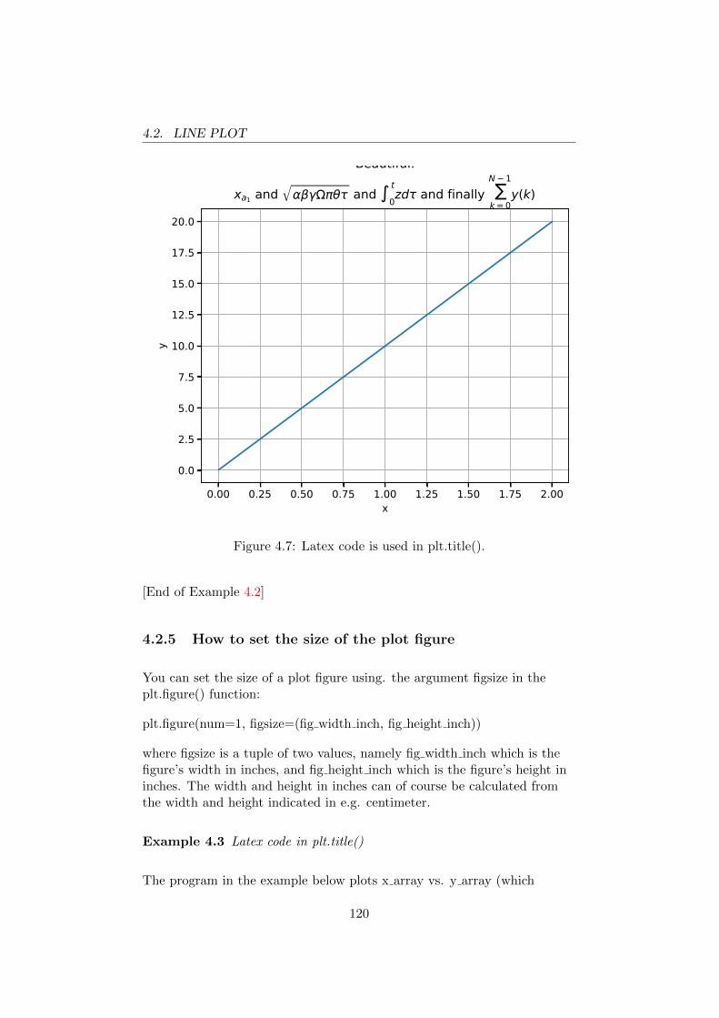
4.2. LINE PLOT
0.00 0.25 0.50 0.75 1.00 1.25 1.50 1.75 2.00x
0.0
2.5
5.0
7.5
10.0
12.5
15.0
17.5
20.0
yBeautiful:
xa1 and and t
0zd and finally N 1
k = 0y(k)
Figure 4.7: Latex code is used in plt.title().
[End of Example 4.2]
4.2.5 How to set the size of the plot figure
You can set the size of a plot figure using. the argument figsize in theplt.figure() function:
plt.figure(num=1, figsize=(fig width inch, fig height inch))
where figsize is a tuple of two values, namely fig width inch which is thefigure’s width in inches, and fig height inch which is the figure’s height ininches. The width and height in inches can of course be calculated fromthe width and height indicated in e.g. centimeter.
Example 4.3 Latex code in plt.title()
The program in the example below plots x array vs. y array (which
120

4.3. BAR CHARTS
consists of customs data) in a figure window with width 24 cm and height18 cm. (The figure itself does not appear here as it contains no interestinginformation.)
import numpy as npimport matplotlib.pyplot as plt
x array = np.array([0, 1, 2])y array = x array * 10
fig width cm = 24fig height cm = 18cm per inch = 2.54fig width inch = fig width cm/cm per inchfig height inch = fig height cm/cm per inch
plt.figure(num=1, figsize=(fig width inch, fig height inch))plt.plot(x array, y array)plt.title(’Tittel y vs. x’)plt.xlabel(’x’)plt.ylabel(’y’)plt.grid()plt.show()
[End of Example 4.3]
4.3 Bar charts
Example 4.4 demonstrates presenting data in a bar graph.
Example 4.4 Bar graph
The program below generates the bar graph shown in Figure 4.8.
121

4.3. BAR CHARTS
Alfa Beta GammaBank name
0
5
10
15
20
25
30
Debt
[MNO
K]
10
20
30Debt overview
Figure 4.8: Bar graph
Program name: prog bar graph.py.
122
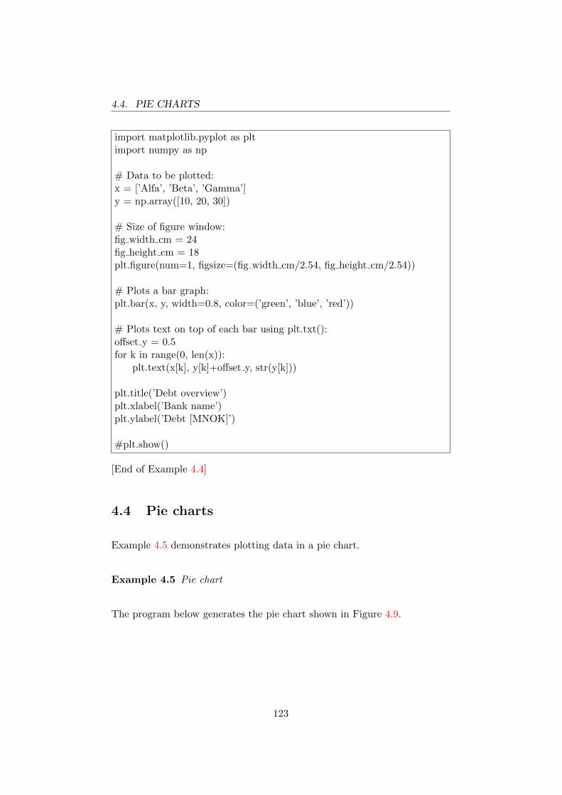
4.4. PIE CHARTS
import matplotlib.pyplot as pltimport numpy as np
# Data to be plotted:x = [’Alfa’, ’Beta’, ’Gamma’]y = np.array([10, 20, 30])
# Size of figure window:fig width cm = 24fig height cm = 18plt.figure(num=1, figsize=(fig width cm/2.54, fig height cm/2.54))
# Plots a bar graph:plt.bar(x, y, width=0.8, color=(’green’, ’blue’, ’red’))
# Plots text on top of each bar using plt.txt():offset y = 0.5for k in range(0, len(x)):
plt.text(x[k], y[k]+offset y, str(y[k]))
plt.title(’Debt overview’)plt.xlabel(’Bank name’)plt.ylabel(’Debt [MNOK]’)
#plt.show()
[End of Example 4.4]
4.4 Pie charts
Example 4.5 demonstrates plotting data in a pie chart.
Example 4.5 Pie chart
The program below generates the pie chart shown in Figure 4.9.
123

4.4. PIE CHARTS
Pi: 14.8%
Upsilon: 2
9.5%
Theta: 3
14.3%Eta: 4
19.0%
Omikron: 5
23.8%
Nu: 6
28.6%
Figure title
Figure 4.9: Pie chart
Program name: prog pie chart.py.
124
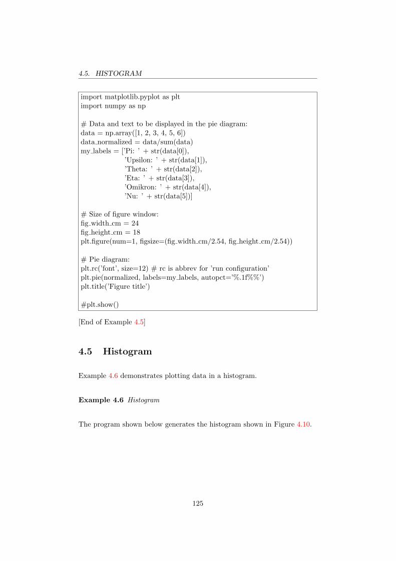
4.5. HISTOGRAM
import matplotlib.pyplot as pltimport numpy as np
# Data and text to be displayed in the pie diagram:data = np.array([1, 2, 3, 4, 5, 6])data normalized = data/sum(data)my labels = [’Pi: ’ + str(data[0]),
’Upsilon: ’ + str(data[1]),’Theta: ’ + str(data[2]),’Eta: ’ + str(data[3]),’Omikron: ’ + str(data[4]),’Nu: ’ + str(data[5])]
# Size of figure window:fig width cm = 24fig height cm = 18plt.figure(num=1, figsize=(fig width cm/2.54, fig height cm/2.54))
# Pie diagram:plt.rc(’font’, size=12) # rc is abbrev for ’run configuration’plt.pie(normalized, labels=my labels, autopct=’%.1f%%’)plt.title(’Figure title’)
#plt.show()
[End of Example 4.5]
4.5 Histogram
Example 4.6 demonstrates plotting data in a histogram.
Example 4.6 Histogram
The program shown below generates the histogram shown in Figure 4.10.
125

4.5. HISTOGRAM
4 3 2 1 0 1 2 3 40
200
400
600
800
1000
1200
1400
1600
Figure 4.10: Histogram
Program name: prog histogram.py
126

4.6. INTERACTIVE PLOTS
import numpy as npimport matplotlib.pyplot as plt
# Data to be plotted:n = 10000 # Number of random valuesx = np.random.randn(n) # The random valuesnum bins = 20 # Number of bins
# Size of figure window:fig width cm = 24fig height cm = 18plt.figure(num=1, figsize=(fig width cm/2.54, fig height cm/2.54))
# Plotting the histogram:plt.hist(x, num bins, color=’green’)plt.grid()
#plt.show()
[End of Example 4.6]
4.6 Interactive plots
Interactive plots are plots that are updated after the user has manipulatedthe user interface widgets in the figure window itself. You can createinteractive plots in Matplotlib.
Typical user interface elements – often called GUI-elementes (GUI =Graphical User Interface) – are:
• Text in textboxes, which are interpreted as numbers (pytonsk:textboxes)
• Buttons
• Radio buttons
• Sliders
These GUI elements are objects that have methods (functions) thatrespond to – or are fired by – events such as value change, button click andpress the Enter key. And these methods can be used to call any function
127

4.6. INTERACTIVE PLOTS
that we have created ourselves, e.g. a function to update a function valueand plot the new value. Here is a small taste of Example 4.7:
textbox a.on submit(fun submit a)
there:
• textbox a is a textbox object that represents a textbox that isembedded in the character window itself.
• on submit is a method associated with the textbox object. Themethod "fires off" or is activated by an "on submit" event, which isthat the user has pressed the Enter key after a new value is enteredin the text box. When firing, the method calls a user-defined functionwhich here is assumed to have the name fun submit a, which doesone or the other, e.g. performs a calculation or updates a plot.
• fun submit a is the name of the user-defined function.
We shall now study an example where a curve with two parameters, a andb, is plotted. When we change a or b via the respective text boxes in thefigure window, the plot changes immediately.
Example 4.7 Interactive plot with adjustable numbers in textboxes
Program name: prog interactive plot textbox.py
The curve to be plotted is given by the following function:
y = ax + b (4.1)
where x is in the range [0, 2] of solution 0.001. The default values area = 1 og b = 0. Figure 4.11 shows a plot of (4.1) with these default values,and Figure 4.6 shows a plot after that a and b has been changed to a = −1respectively b = 1 via the textboxes in the figure window.
128

4.6. INTERACTIVE PLOTS
0.00 0.25 0.50 0.75 1.00 1.25 1.50 1.75 2.002.0
1.5
1.0
0.5
0.0
0.5
1.0
1.5
2.0
a = 1.0
b = 0.0
Figure 4.11: Plot of (4.1) with a = 1 and b = 0
0.00 0.25 0.50 0.75 1.00 1.25 1.50 1.75 2.002.0
1.5
1.0
0.5
0.0
0.5
1.0
1.5
2.0
a = -1.0
b = 1.0
Figure 4.12: Plot of (4.1) with a = −1 and b = 1
The program that realizes this is shown below.3
3The program is based on the program https://matplotlib.org/gallery/widgets/textbox.html#sphx-glr-gallery-widgets-textbox-py, which I have modified so that there are two text boxesinstead of one.
129
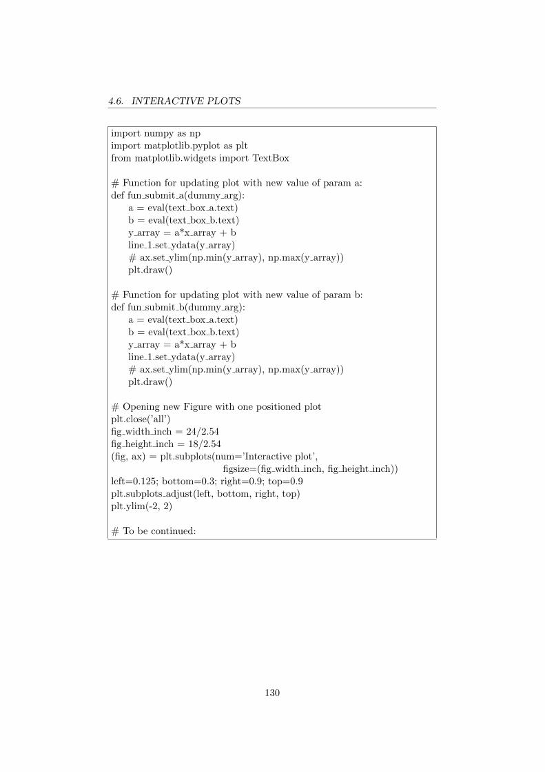
4.6. INTERACTIVE PLOTS
import numpy as npimport matplotlib.pyplot as pltfrom matplotlib.widgets import TextBox
# Function for updating plot with new value of param a:def fun submit a(dummy arg):
a = eval(text box a.text)b = eval(text box b.text)y array = a*x array + bline 1.set ydata(y array)# ax.set ylim(np.min(y array), np.max(y array))plt.draw()
# Function for updating plot with new value of param b:def fun submit b(dummy arg):
a = eval(text box a.text)b = eval(text box b.text)y array = a*x array + bline 1.set ydata(y array)# ax.set ylim(np.min(y array), np.max(y array))plt.draw()
# Opening new Figure with one positioned plotplt.close(’all’)fig width inch = 24/2.54fig height inch = 18/2.54(fig, ax) = plt.subplots(num=’Interactive plot’,
figsize=(fig width inch, fig height inch))left=0.125; bottom=0.3; right=0.9; top=0.9plt.subplots adjust(left, bottom, right, top)plt.ylim(-2, 2)
# To be continued:
130

4.6. INTERACTIVE PLOTS
# Continued:
# Generating and plotting y array using initial values of a and b:x array = np.arange(0.0, 2.0, 0.001)a = 1b = 0y array = a*x array + b(line 1, ) = plt.plot(x array, y array)plt.grid(which=’both’, color=’grey’)
# Generating textboxes for a and b:left a=0.1; bottom a=0.15; width a=0.1; height a=0.05left b=0.1; bottom b=0.05; width b=0.1; height b=0.05axbox a = plt.axes([left a, bottom a, width a, height a])axbox b = plt.axes([left b, bottom b, width b, height b])caption a = ’a = ’caption b = ’b = ’initial text a = "1.0"initial text b = "0.0"text box a = TextBox(axbox a, caption a, initial text a)text box b = TextBox(axbox b, caption b, initial text b)
# Invoking the functions named fun submit a() or fun submit b()# on click on Enter button of a or b:text box a.on submit(fun submit a)text box b.on submit(fun submit b)
plt.show()
Comments on the program (but only comments regarding the realizationof interactive plot with textbox):
• Code line from matplotlib.widgets import TextBox imports thetextbox object.
• The code line def fun submit a (dummy arg): is the beginning of thedefinition of the function fun submit a(). This function uses theupdated values of a and b to calculate the updated value of y arrayand plot y array vs. x array. The fun submit a() function is calledonly when the user has entered a new value in the text box forparameter a (not b). dummy arg is an argument that is not used,but Python returns an error message if that argument is dropped.
• The code line a = eval (text box a.text) interprets the text
131

4.6. INTERACTIVE PLOTS
text box a.text, which is the text in the text box element forparameter a, as a number.
• The code line b = eval (text box b.text) is like the code line above,but for parameter b.
• The code line line 1.set ydata (y array) updates the plot identifiedwith the object called line 1. This identification occurs in the codeline (line 1,) = plt.plot (x array, y array) in the main part of theprogram.
• The code line # ax.set ylim (np.min (y array), np.max (y array)) isactually "commented away", but I’ve included it to show how youcan adjust the value range along the y axis to the updated value ofy array.
• The plt.draw() code line ensures that the plot is updated.
• The code line def fun submit b (dummy arg): is the beginning of thedefinition of the function fun submit b(). The comments here are asfor the fun submit a() function.
• The code line under # Opening new Figure with one positioned plotopens a figure window with a plot figure of specified size and location:
– The size is indicated by the figsize argument.
– The location is specified with the code plt.subplots adjust (left,bottom, right, top) where the unit for the four parameters is theheight and width of the figure window. You can count to get thedesired size and position, but a little trial and error willprobably work well.
• The code under # Generating and plotting y array based on initialvalues of a and b: generates an initial plot. The plot is updated ifthe user sets new values for parameters a and b in the respective textboxes.
• The code line line 1, = plt.plot (x array, y array) creates an objectcalled line 1, which is used as a reference to the plot Figure in thefunctions fun submit a and fun submit b.
• The code under # Generating textboxes for a and b: generates thetext boxes for parameters a and b. The unit for left a, bottom a, etc.is the height and width of the figure window. Trial and error to getusable size and placement of text boxes works well.
• Code line text box a.on submit (fun submit a):
132

4.6. INTERACTIVE PLOTS
– text box a is the object that represents the text box forparameter a.
– on submit is a method of the text box a object. When the userpresses the Enter key in the text box, the function is calledfun submit a, which the user has defined (see comment on thisfunction further up in this comment list). Actually, the text inthe text box is transferred to this function, but I have chosennot to use this text in the fun submit a() function. Instead, Imake sure to read the value of the text attribute of thetext box a object, as well as the text attribute of the text box bobject, in the fun submit a() function. Thus, the fun submit a()function will use the updated values of both a and b wheneverthe y array is updated.
• Code line text box b.on submit (fun submit b): Here the commentsare exactly the same as for the code line text box a.on submit(fun submit a) above.
[End of Example 4.7]
133
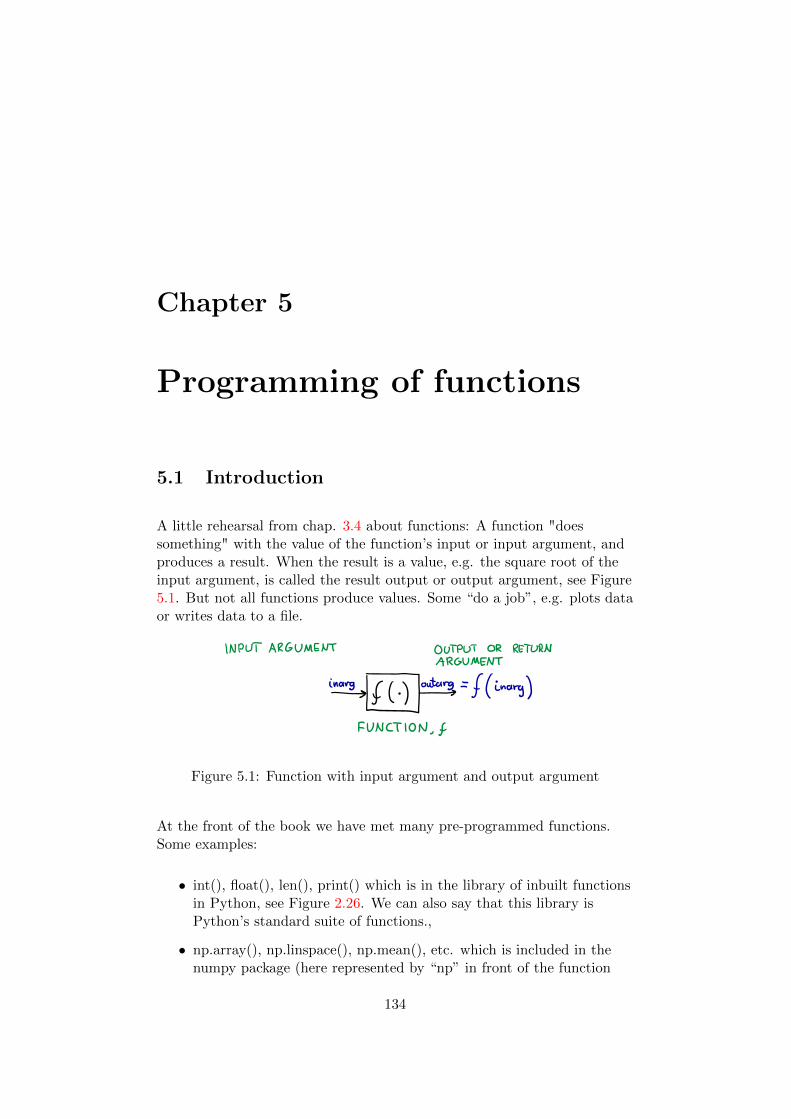
Chapter 5
Programming of functions
5.1 Introduction
A little rehearsal from chap. 3.4 about functions: A function "doessomething" with the value of the function’s input or input argument, andproduces a result. When the result is a value, e.g. the square root of theinput argument, is called the result output or output argument, see Figure5.1. But not all functions produce values. Some “do a job”, e.g. plots dataor writes data to a file.
Figure 5.1: Function with input argument and output argument
At the front of the book we have met many pre-programmed functions.Some examples:
• int(), float(), len(), print() which is in the library of inbuilt functionsin Python, see Figure 2.26. We can also say that this library isPython’s standard suite of functions.,
• np.array(), np.linspace(), np.mean(), etc. which is included in thenumpy package (here represented by “np” in front of the function
134

5.2. HOW TO PROGRAM FUNCTIONS
name itself).
• plt.plot(), plt.xlabel(), plt.grid() which is included in the pyplotmodule in the matplotlib package (pyplot is represented here with"plt" in front of the function name).
Why are these functions made? Some important reasons are:
• Support for reuse: The functions perform a well-defined task andcan be used by all programmers and in many different applications.
• Good program structure: The functions give the programs asimpler and more transparent structure by solving sub-tasks using. asingle function call. For example, the np.mean() function calculatesthe mean of a data series with one function call, and you do not haveto write program code for this from scratch.
• Less chance of error coding: Programming a program part witha given functionality from scratch every time you need thefunctionality increases the chance of error coding compared tocreating a function (which hopefully is flawless) and reusing it.
It is likely that in our programs we will need functionality that is not fullycovered by any of the completed functions. Python allows us to createfunctions ourselves, and the reasons for doing so are exactly the same asmentioned above.
5.2 How to program functions
5.2.1 Basic function definition
As an example, let’s create a function that calculates the value of yaccording to. the mathematical formula (function)
y = ax + b (5.1)
There a and b are parameters (constants). x is input variable orindependent variable. y is the output variable or dependent variable. Theprogram below contains definition of the function and code that uses thefunction. The part of the program that is outside the function definition isoften called the main program.
135

5.2. HOW TO PROGRAM FUNCTIONS
Example 5.1 Programming of function
Program name: prog fun intro.py
def fun lin(x, a, b):y = a*x + breturn y
p0 = 2.5p1 = 3.0inn = 10.0out = fun lin(in, p0, p1)print(’Result = ’, out)
Running the program:
Result = 28.0
Comments:
• I have named the function fun lin. In general, you are quite free tochoose file names, but cf. 3.3.3.
• The definition of the function starts with the command def followedby the file name and the function’s arguments, which are the threearguments x, a and b, separated by a comma in parentheses.
• It is necessary that the definition is before the function is used (inthe program). I have – as usual – written the definition of thefunction at the beginning of the program, after the comments aboutthe program itself indicated at the very top of the program.1
• The three input arguments x, a and b are used as variables in thefunction’s program code, which is the program code that expresseswhat the function does. These three variables are local to thefunction – or belong to the function namespace, which means thatthey (local variables) do not exist for use outside the function.Which namespaces that variables belong to, we look at in more detailin Chap. 5.3. The local variables are also called the function’sso-called formal parameters.
1If you know MATLAB programming, you know that functions must be defined therein the end of the program.
136
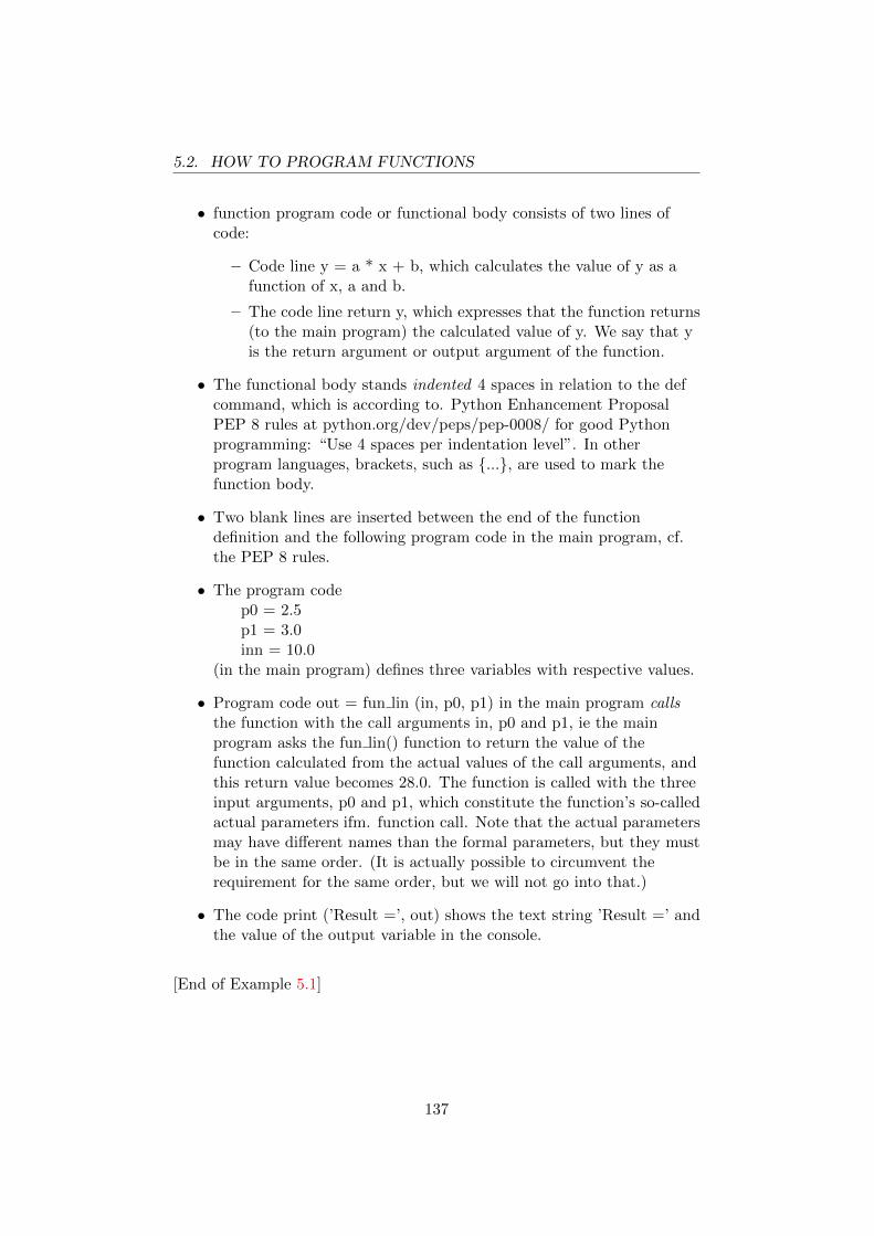
5.2. HOW TO PROGRAM FUNCTIONS
• function program code or functional body consists of two lines ofcode:
– Code line y = a * x + b, which calculates the value of y as afunction of x, a and b.
– The code line return y, which expresses that the function returns(to the main program) the calculated value of y. We say that yis the return argument or output argument of the function.
• The functional body stands indented 4 spaces in relation to the defcommand, which is according to. Python Enhancement ProposalPEP 8 rules at python.org/dev/peps/pep-0008/ for good Pythonprogramming: “Use 4 spaces per indentation level”. In otherprogram languages, brackets, such as {...}, are used to mark thefunction body.
• Two blank lines are inserted between the end of the functiondefinition and the following program code in the main program, cf.the PEP 8 rules.
• The program codep0 = 2.5p1 = 3.0inn = 10.0
(in the main program) defines three variables with respective values.
• Program code out = fun lin (in, p0, p1) in the main program callsthe function with the call arguments in, p0 and p1, ie the mainprogram asks the fun lin() function to return the value of thefunction calculated from the actual values of the call arguments, andthis return value becomes 28.0. The function is called with the threeinput arguments, p0 and p1, which constitute the function’s so-calledactual parameters ifm. function call. Note that the actual parametersmay have different names than the formal parameters, but they mustbe in the same order. (It is actually possible to circumvent therequirement for the same order, but we will not go into that.)
• The code print (’Result =’, out) shows the text string ’Result =’ andthe value of the output variable in the console.
[End of Example 5.1]
137

5.2. HOW TO PROGRAM FUNCTIONS
5.2.2 How to return more than one value
In the example above, the function fun lin() has a return argument whichhas one value, namely the floating point y from the formula or functiony = ax + b. But in general, it is curant to create functions that returnmultiple values: Just make sure that the function returns e.g. a tuple orlist or array, which are data types that can consist of multiple elements.
Below is an example of a program where the function returns two valuestogether in one tuple. The program is a modified version of the programfun intro.py, see page 5.2.1.
Example 5.2 Function that returns multiple values with tuple
Program name: prog fun tuppel retur.py.
def fun value and slope(x, a, b):y = a*x + bdy = areturn (y, dy)
p0 = 2.5p1 = 3.0x value = 10.0(value, slope) = fun value and slope(x value, p0, p1)print(Function value = ’, value)print(Slope = ’, slope)
Running the program gives the following results:
Function value = 28.0Slope = 2.5
Comments:
• The function fun value and slope now returns both the functionvalue y = ax + b and the slope of the function dy = a (agree, thelatter operation is pretty trivial), collected in the tuple (y, dy).
• The tuple (value, slope) gets a value equal to the returned tuplevalue.
[End of Example 5.2]
138

5.2. HOW TO PROGRAM FUNCTIONS
5.2.3 Default value function arguments
A function input argument can be defined with a default value. If for anyreason the user has chosen to not enter this argument in the function call,the function uses the argument’s default value.
Below is an example of a function with a default value argument. Theprogram is a modified version of the program prog fun intro.py, see page5.2.1.
Example 5.3 Function with an argument with default value
Program name: prog fun default arg.py.
def fun lin(x, a, b=5.0):y = a*x + breturn y
x value = 10.0p0 = 2.5p1 = 3.0
out = fun lin(x value, p0)print(’Resultat = ’, out)
Running the program gives the following results:
Resultat = 30.0
Comments:
• In the function definition, ie in the expression def fun lin (x, a, b =5.0), the argument b is defined with a default value 5.0.
• In the function shell, ie in the expression out = fun lin (in, p0),values are specified for the first two arguments. Since the value of thethird argument (b) is omitted in the function call, Python uses thedefault value of b.
• The default value arguments must follow the non-standard valuearguments in the function definition. For example, the functiondefinition def fun lin (x, a = 4.0, b) is incorrect because b standsafter a = 4.0.
139

5.2. HOW TO PROGRAM FUNCTIONS
[End of Example 5.3]
5.2.4 Function call using keyword argument
You can call a function with explicitly naming of the names of the formalfunction arguments. This is called function calling with keywordarguments as actual arguments.
In function calls with keyword arguments, the order of the arguments doesnot matter, which is natural since the arguments are crystal-clear in thatthe formal argument names are used.
We continue with the example above (the prog fun default arg.pyprogram), but now add two different ways to call the function - with andwithout keyword arguments.
Example 5.4 Function with a keyword argument
Program name: prog fun keyword arg.py.
def fun lin(x, a, b):y = a*x + breturn y
x in = 10.0p0 = 2.5p1 = 3.0
out1 = fun lin(in, p0, p1)out2 = fun lin(a=p0, b=p1, x=x in)
print(’out1 = ’, out1)print(’out2 = ’, out2)
Running the program gives the following results:
out1 = 28.0out2 = 28.0
Comments:
• Function calls without keyword arguments:
140

5.2. HOW TO PROGRAM FUNCTIONS
out1 = fun lin(in, p0, p1)that produces results 28.0.
• Function calls with keyword arguments:out2 = fun lin(a=p0, b=p1, x=in)Here I deliberately changed the order of the actual arguments tobecome different from the order of the formal arguments. The resultis 28.0, the same.
[End of Example 5.4]
5.2.5 * args and ** kwargs
*args and **kwargs may almost look like a curse, but stands here forPython’s functional arguments of a slightly special kind.
Many pre-made functions have *args (abbreviation for arguments) and /or **kwargs (abbreviation for keyword arguments) among its formalarguments. The two arguments have in common that they represent oneany number arguments, ie it is up to the user of the functions to determinethe number of arguments.
* args arguments are, in principle, just a list of individual arguments thatcan be in the form of values – without names. You can consider this listingas a Python list.
** kwargs are arguments where each argument is specified by name andvalue.
Here we will only look at an example of * args.
Example 5.5 Functions with *args
Program name: prog fun args.py.
import numpy as np
def fun arg test(k, *args):y = np.sum(args) * kreturn y
y = fun arg test(1000, 1, 2, 3)print(’y = ’, y)
141

5.2. HOW TO PROGRAM FUNCTIONS
Running the program gives the following results:
y = 6000
because the sum of 1, 2 and 3 is 6, which is multiplied by 1000, giving 6000.
Comments:
• The function definition is:def fun arg test(k, *args)k is a “normal” argument, while * args represents all arguments(often considered a list) following the argument named factor.
• Code line:y = np.sum(args) * kInside the function, the sum of the elements in the list, ismultiplied,with k.
• Function call:y = fun arg test(1000, 1, 2, 3)1000 is a current argument assigned to the formal argument namedk, while the sequence 1, 2, 3 is a actual argument that can beconsidered as a list assigned to the formal argument * args. Theelements in this list are summed in the code np.sum (args).
[End of Example 5.5]
5.2.6 Documentation text (docstring)
You can enter docstring in functions that you create. Documentation textis text where you can describe the function’s structure, its input andoutput arguments and their data types, and what the function does. Thedocumentation text can be displayed, among other things, using the codehelp (the function name), as demonstrated below.
A distinction is often made between so-called single-line and multi-linedocumentation.2 Both types are demonstrated below.
One-line documentation text
In the program below I have entered a one-line documentation text withinthe function fun lin.
2Guidelines for designing documentation text can be found in the document PEP 257pahttps://www.python.org/dev/peps/pep-0257.
142
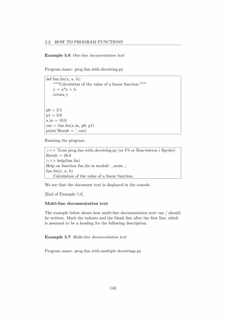
5.2. HOW TO PROGRAM FUNCTIONS
Example 5.6 One-line documentation text
Program name: prog fun with docstring.py
def fun lin(x, a, b):"""Calculation of the value of a linear function."""y = a*x + breturn y
p0 = 2.5p1 = 3.0x in = 10.0out = fun lin(x in, p0, p1)print(’Result = ’, out)
Running the program:
>>> %run prog fun with docstring.py (or F5 or Run-button i Spyder)Result = 28.0>>> help(fun lin)Help on function fun lin in module main :fun lin(x, a, b)
Calculation of the value of a linear function.
We see that the document text is displayed in the console.
[End of Example 5.6]
Multi-line documentation text
The example below shows how multi-line documentation text can / shouldbe written. Mark the indents and the blank line after the first line, whichis assumed to be a heading for the following description.
Example 5.7 Multi-line documentation text
Program name: prog fun with multiple docstrings.py
143

5.3. NAMESPACE
def fun lin(x, a, b):"""Calculation of the value of a linear function.
x (float) is an independent variable or input variable.a and b (float) are parameters.y (float) is a dependent variable or output variable."""y = a*x + breturn y
p0 = 2.5p1 = 3.0x in = 10.0out = fun lin(x in, p0, p1)print(’Result = ’, out)
The result of running the above program is not shown here.
[End of Example 5.7]
5.3 Namespace
When we create functions, it is important to know the term namespace.All variables belong to or exist in a namespace, but not outside thenamespace. The relationship between variables and namespaces can be oneof the following:
• The variable is both readable and writable (writable means the valuecan be changed) in the namespace.
• The variable is readable only (ie the value can be read but notchanged) in the namespace.
• The variable is neither readable nor writable, ie it does not exist inthe namespace.
Functions define namespaces, see Figure 5.2. (The variable namesglobalvar1 and localvar1 are here “random, ie they can generally havedifferent names.)
144

5.3. NAMESPACE
Figure 5.2: Navnerom
Note:
• locvar1 is readable and writable only within the function (itsnamespace), ie not outside. If you try to use localvar1 in acalculation in your main program, outside of the function, Pythonwill give an (incorrect) message that the variable does not exist.
• globalvar1 is readable, but not writable, within the function. Thus,you cannot change the value of globalvar1 with code that you enteredin the function.
The program in the example below demonstrates the difference betweendifferent namespaces.
Example 5.8 Navnerom
The program is based on the program fun intro.py shown on page 136.print() functions are used to check the existence of the two variables x andin that belong in namespace like:
• x is a local variable in the fun intro function, which defines thenamespace of x.
• inn is a global variable in the main program, which defines thenamespace to inn.
145
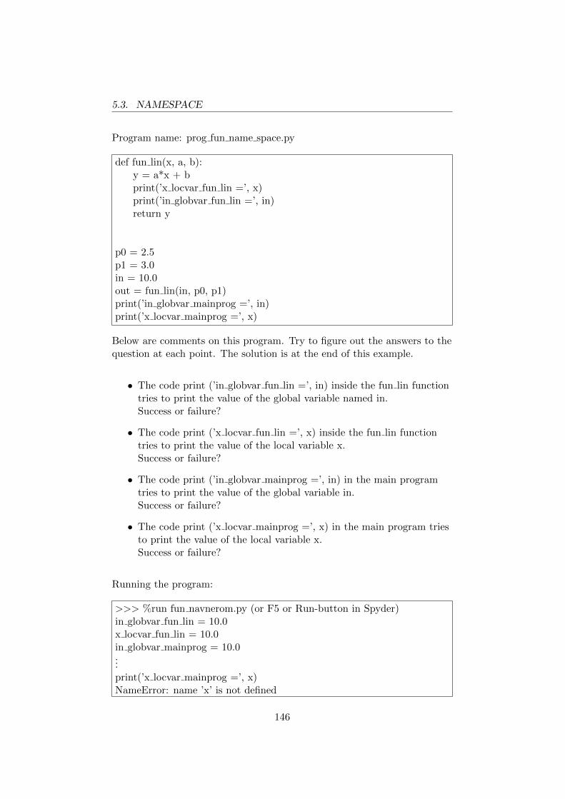
5.3. NAMESPACE
Program name: prog fun name space.py
def fun lin(x, a, b):y = a*x + bprint(’x locvar fun lin =’, x)print(’in globvar fun lin =’, in)return y
p0 = 2.5p1 = 3.0in = 10.0out = fun lin(in, p0, p1)print(’in globvar mainprog =’, in)print(’x locvar mainprog =’, x)
Below are comments on this program. Try to figure out the answers to thequestion at each point. The solution is at the end of this example.
• The code print (’in globvar fun lin =’, in) inside the fun lin functiontries to print the value of the global variable named in.Success or failure?
• The code print (’x locvar fun lin =’, x) inside the fun lin functiontries to print the value of the local variable x.Success or failure?
• The code print (’in globvar mainprog =’, in) in the main programtries to print the value of the global variable in.Success or failure?
• The code print (’x locvar mainprog =’, x) in the main program triesto print the value of the local variable x.Success or failure?
Running the program:
>>> %run fun navnerom.py (or F5 or Run-button in Spyder)in globvar fun lin = 10.0x locvar fun lin = 10.0in globvar mainprog = 10.0...print(’x locvar mainprog =’, x)NameError: name ’x’ is not defined
146
5.4. PROGRAMMING OF MODULES
Conclusion: Success! Success! Success! Failure!
[End of Example 5.8]
We can conclude this subchapter as follows:
• Local variables defined in functions cannot be used outside thefunction. If their value is to be used outside the function (in themain program), they must be passed there as a return variable fromthe function.
• Global variables are directly available for reading (not writing)within functions. But it is considered rather poor program techniqueto read global variables inside functions, since the function’s interfacewith the main program is then not well defined. The interface is welldefined if all data exchange with the main program takes place viaarguments in the function shell, so this is the recommended way totransfer data.
5.4 Programming of modules
One module is a script that contains functions and / or variables. You canuse these functions and variables in a main program after importing themodule into the program. Figure 5.3 illustrates the relationship between amodule and main applications.
147
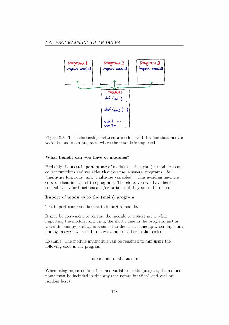
5.4. PROGRAMMING OF MODULES
Figure 5.3: The relationship between a module with its functions and/orvariables and main programs where the module is imported
What benefit can you have of modules?
Probably the most important use of modules is that you (in modules) cancollect functions and variables that you use in several programs – ie“multi-use functions” and “multi-use variables” – thus avoiding having acopy of them in each of the programs. Therefore, you can have bettercontrol over your functions and/or variables if they are to be reused.
Import of modules to the (main) program
The import command is used to import a module.
It may be convenient to rename the module to a short name whenimporting the module, and using the short name in the program, just aswhen the numpy package is renamed to the short name np when importingnumpy (as we have seen in many examples earlier in the book).
Example: The module my module can be renamed to mm using thefollowing code in the program:
import min modul as mm
When using imported functions and variables in the program, the modulename must be included in this way (the names function1 and var1 arerandom here):
148

5.4. PROGRAMMING OF MODULES
mm.funksjon1
and
mm.var1
Example 5.9 Import of our own module
This example works the same way as the prog fun intro.py program, seepage 136, but we will now define our own developed function fun lin() in amodule and not directly in the program. The variables p0 and p1 mustalso be defined in this module. The function and the two variables aremade available in the program by importing the module.
The main program is shown in the box below.
Program name: prog module.py.
import my module as mm
x in = 10.0out = mm.fun lin(x in, mm.p0, mm.p1)print(’Result = ’, out)
The module is shown in the box below.
Module name: my module.py.
def fun lin(x, a, b):y = a*x + breturn y
p0 = 2.5p1 = 3.0
The result of running the main program is:
Reloaded modules: my modulResult = 28.0
[End of Example 5.4]
149
5.5. LAMBDA FUNCTIONS
5.5 Lambda functions
Lambda functions is a special type of functions in Python that can be usedto solve simple calculations. Some important characteristics:
• They are not defined with the def command.
• They have no local variables.
• They are usually written on one line of code.
Lambda functions can be used as a kind of calculator based on a formula.Lambda functions are not assigned a name, which is why they are alsocalled anonymous functions.
The syntax is shown in the following example where we create a lambdafunction to calculate
y = a*x + b
where x, a and b are arguments, and y is arguments. (The Lambdafunction in the example below does the same job as the regular functionthat we developed in Chap. 5.2.1.)
Example 5.10 Lambda functions
y = lambda x, a, b: a * x + bout = y(10, 2.5, 3)print(’out = ’, out)
We see that the Lambda function is defined in only one line:
y = lambda x, a, b: a * x + b
there:
• The input arguments are x, a and b, which are listed, separated bycommas.
• The function (formula) is a * x + b that uses the arguments.
150

5.5. LAMBDA FUNCTIONS
• The output argument is y, which is calculated by the function(formula).
The actual call of the lambda function is
out = y(10, 2.5, 3)
Running the program gives the result:
out = 28.0
[End of Example 5.10]
151
Chapter 6
Testing your own code
6.1 Introduction
Don’t trust yourself completely. The programs you develop will probablyhave errors.
There are two main types of errors:
• Syntax Error, which are purely “technical” errors, e.g. that you haveforgotten a parenthesis or entered a function name incorrectly or thelike. The programming environment that you are using will indicatesyntax errors in some way. For example, Spyder provides goodinformation about syntax errors, cf. 2.2.4.
• Functional errors, which are errors in the program logic oralgorithms. Functional errors can be very difficult to find!
In this chapter, we will concentrate on testing with the aim of finding anyfunctional errors.
Who should test?
• You (the programmer)?
• A test user?
• The end user, who expects to get a program that works correctly?
152
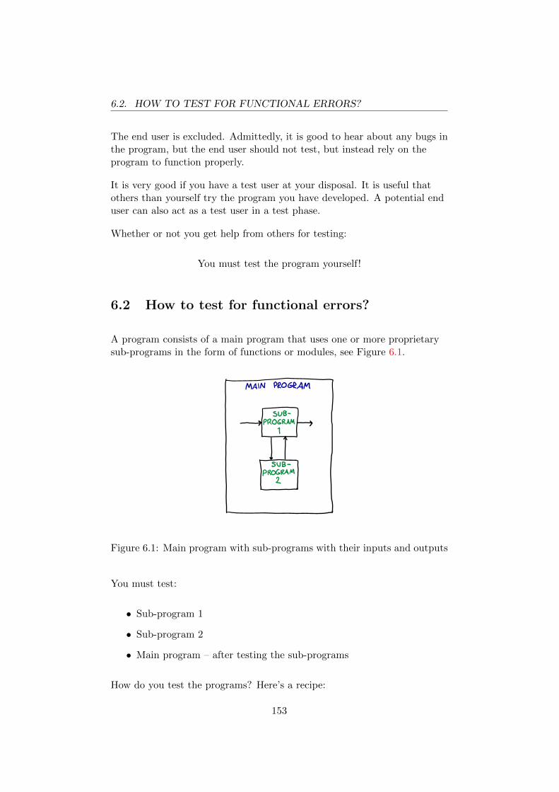
6.2. HOW TO TEST FOR FUNCTIONAL ERRORS?
The end user is excluded. Admittedly, it is good to hear about any bugs inthe program, but the end user should not test, but instead rely on theprogram to function properly.
It is very good if you have a test user at your disposal. It is useful thatothers than yourself try the program you have developed. A potential enduser can also act as a test user in a test phase.
Whether or not you get help from others for testing:
You must test the program yourself!
6.2 How to test for functional errors?
A program consists of a main program that uses one or more proprietarysub-programs in the form of functions or modules, see Figure 6.1.
Figure 6.1: Main program with sub-programs with their inputs and outputs
You must test:
• Sub-program 1
• Sub-program 2
• Main program – after testing the sub-programs
How do you test the programs? Here’s a recipe:
153
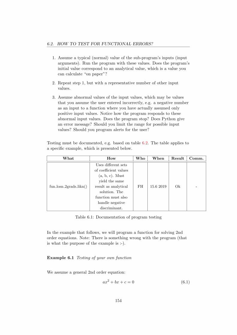
6.2. HOW TO TEST FOR FUNCTIONAL ERRORS?
1. Assume a typical (normal) value of the sub-program’s inputs (inputarguments). Run the program with these values. Does the program’sinitial value correspond to an analytical value, which is a value youcan calculate “on paper”?
2. Repeat step 1, but with a representative number of other inputvalues.
3. Assume abnormal values of the input values, which may be valuesthat you assume the user entered incorrectly, e.g. a negative numberas an input to a function where you have actually assumed onlypositive input values. Notice how the program responds to theseabnormal input values. Does the program stop? Does Python givean error message? Should you limit the range for possible inputvalues? Should you program alerts for the user?
Testing must be documented, e.g. based on table 6.2. The table applies toa specific example, which is presented below.
What How Who When Result Comm.
fun losn 2grads likn()
Uses different sets
of coefficient values
(a, b, c). Must
yield the same
result as analytical
solution. The
function must also
handle negative
discriminant.
FH 15.6 2019 Ok -
Table 6.1: Documentation of program testing
In the example that follows, we will program a function for solving 2ndorder equations. Note: There is something wrong with the program (thatis what the purpose of the example is :-).
Example 6.1 Testing of your own function
We assume a general 2nd order equation:
ax2 + bx + c = 0 (6.1)
154

6.2. HOW TO TEST FOR FUNCTIONAL ERRORS?
I think that the two solutions are1
x1 =b +√b2 − 4ac
2a(6.2)
and
x2 =−b +
√b2 − 4ac
2a(6.3)
and that any concurrent solution yields discriminant equal to zero:
D = b2 − 4ac = 0 (6.4)
The program is shown below.
Program name:
import numpy as np
def fun losn 2grads likn(a, b, c):x1 = (b + np.sqrt(b*b - 4*a*c))/(2*a)x2 = (-b + np.sqrt(b*b - 4*a*c))/(2*a)return (x1, x2)
a = 1.0b = 0.0c = -4.0(x1, x2) = fun losn 2grads likn(a, b, c)print(’x1 =’, x1)print(’x2= ’, x2)
The result is:
x1 = 2.0x2= 2.0
The fact that the solutions are “something with 2” seems reasonable basedon the given coefficient values, so it is tempting to conclude that theprogram gives the correct answer.
1;-)
155
6.2. HOW TO TEST FOR FUNCTIONAL ERRORS?
But, let’s test the program:
Test 1
Let’s put the solutions into the given equation and see if the right sidevalue really becomes zero, which is specified. For such a calculation we cancreate a program that calculates the value of the right-hand side, but hereit is easier to do the hand calculation. The two solutions are the same, sowe set x1 = x2 = 2.0 in for x i (6.1) and get
1 · 2.02 + 0 · 2.0− 4.0 = 0 (6.5)
that’s right! Thus, 2.0 is a solution. So far, nothing indicates thatsomething is wrong. But you may remember that with two concurrentsolutions, the discriminator equals zero.
Test 2
We calculate the discriminant, D:
D = b2 − 4ac = 02 + 4 · 1 · (−4) = −16 (6.6)
which is different from zero!
Since the program failed both tests, we must conclude that the programhas one or more errors.
We therefore review the program code once again. The code is correct inthat it implements the solution formulas (6.2) and (6.3). So then theremust be something wrong with one or both of the solution formulas. Thereare actually errors in both formulas. The correct ones are
x1 =−b +
√b2 − 4ac
2a(6.7)
and
x2 =−b−
√b2 − 4ac
2a(6.8)
Once we have fixed the errors, we run the tests again. (The result of this isnot shown here.)
Test 3
In the testing above, we used examples of coefficient values (a, b, c) whichdid not create problems in relation to the sign of the discriminant, D, ie D
156

6.3. HOW TO RUN ONLY PART OF THE PROGRAM?
was not negative. But let’s assume that it is conceivable that the user ofthe program will enter values that give negative D. For negative D thereare no real solutions of the 2nd degree equation; The solutions are complexnumbers. How our program responds to the negative D? Let’s try
a = 1, b = 0, c =4
The result is Python for Python (nan stands for not-a-number):
x1 = nanx2 = nanC:/techteach.no/publications/python/scripts/prog losn 2grads likn.py:14:RuntimeWarning: invalid value encountered in sqrt x1 = (-b + np.sqrt(b*b- 4*a*c))/(2*a)C:/techteach.no/publications/python/scripts/prog losn 2grads likn.py:15:RuntimeWarning: invalid value encountered in sqrt x2 = (-b - np.sqrt(b*b- 4*a*c))/(2*a)
It appears that the np.sqrt() function is unable to calculate complexsolutions. That’s a bit stubborn, I think, but we have to accept it, ofcourse. Then we have two options:
1. Find a function, as an alternative to np.sqrt(), that is capable ofcalculating complex solutions.
2. Continue using np.sqrt() in the program, but notify the user thatthere are no real solutions to the specified coefficient values if thediscriminator is negative.
I stop the example her, but you may try the above two options.
[End of Example 6.1]
6.3 How to run only part of the program?
Sometimes we want to run only part of the program code to see if it works.In Spyder, it can be done as follows:
1. Select the current program section.
2. Run the program section by making one of the following choices:
157

6.3. HOW TO RUN ONLY PART OF THE PROGRAM?
(a) The Run / Run selection or current line menu option
(b) Menu button Run / Run selection or current line
(c) F9 key on the keyboard
Of course, it is necessary that variables included in the program part to berun are already defined, ie are in the workspace.
158
Chapter 7
Conditional programexecution with if-structures
7.1 if-else
With an if-program structure we can control the program execution, seeFigure 7.1. If the if condition has a Boolean value of True, the programpart is executed in the if branch. I have called this code section forCODE IF. Otherwise, ie if the if condition has a Boolean value of False,the program part is executed in the else branch, ie the code inCODE ELSE. Of course, it is up to us to enter Python code into these twoalternative code sections.
159

7.1. IF-ELSE
Figure 7.1: If-else structure
The program execution is therefore governed by the boolean (logical) valueof the if condition. We construct the if condition with logical operatorsand comparison operators, cf. 3.8.
The program code below demonstrates programming with the if structure.The program has an if branch and an else branch. The comparisonexpression (x> y), where x and y are numbers, determines which branch isrun, cf. the detailed comments below.
Program name: prog if else.py
x = 10y = 0if (x > y):
print(’(x > y) =’, (x > y))print(’The If branch is active.’)
else:print(’(x > y) =’, (x > y))print(’The Else branch is active.’)
print(’This is the first code line after the if structure.’)
As demonstrated in the program above:
• The code lines according to the if condition must be indented. Thesame applies to the code lines according to the else condition. The
160

7.2. WITHOUT ELSE
Python standard is indented with 4 spaces.
• There should (not must) be a blank line between the last code line inthe if structure and subsequent code lines.
The box below shows the result of the run with the values x = 10 and y =0. The comparison expression (x> y) then has a Boolean value True, whichmeans that the if branch is active. The code that is then executed, ieCODE IF in Figure 7.1, are the following two calls of the print() function:
• The code print (’(x> y) =’, (x> y)) which prints the text ’(x> y) =’and the boolean value of the comparison expression (x> y).
• The code print (’if branch is active.’).
(x > y) = Trueif branch is active.This is the first code line after the if structure.
The box below shows the result of the run with the values x = –10 and y= 0. The expression (x> y) then has a Boolean value False, which meansthat the else branch is active. The code being executed, ie CODE ELSE inFigure 7.1, are two calls of the print() function (not reproduced here).
(x > y) = Falseelse branch is active.This is the first code line after the if structure.
7.2 Without else
The if structure doesn’t really need to include anything else, see Figure7.2. If the if condition has the value False, the program skips all codecontained within the if structure.
161

7.2. WITHOUT ELSE
Figure 7.2: Program flowchart for an if structure without else
The program code below demonstrates programming an if structurewithout else.
Program name: prog if.py.
x = 10y = 0if (x > y):
print(’(x > y) =’, (x > y))print(’if branch is active.’)
print(’This is the first code line after the if structure.’)
The box below shows the result of the run with the values x = 10 and y =0. The comparison expression (x> y) then has a Boolean value of True,which means that the if branch is active.
(x > y) = Trueif branch is active.This is the first code line after the if structure.
The box below shows the result of the run with the values x = –10 and y= 0. The comparison expression (x> y) then has a Boolean value False,which means that the if branch is inactive. And since there is no otherbranch here, the program goes straight to the code line after the ifstructure, which is print (’This is the first code line after the if structure.’).
162

7.3. ELIF
This is the first code line after the if structure.
7.3 elif
And so we have elif. Both elif and else are used to define code that is run ifthe if condition is False. But elif is narrower than else. You can specifyyour own elif condition (while you do not specify your own else condition).This is demonstrated in the program below.
Program name: prog elif.py.
x = 0y = 0if (x > y):
print(’if branch is active.’)elif (x == y):
print(’elif branch is active.’)else:
print(’else branch is active.’)
print(’This is the first code line after the if structure.’)
The box below shows the result of the run, where x = 0 and y = 0, whichmeans that the elif condition (x == y) is True, which makes the elifbranch active.
elif branch is active.This is the first code line after the if structure.
163
Chapter 8
Iterated program runs withfor loops and while loops
8.1 Introduction
Loops are very useful program structures. With loops, you can iterate(repeat) program code as many times as you like – automatically!
Loops are used in a variety of contexts, including:
• Mathematical operations on arrays and lists, etc. where the loopiterates the operations on the elements
• Solving equations with an iterative method (until the solution isfound with sufficient accuracy)
• Optimization (find the maximum or minimum of a function) with aniterative method (until the optimal value is found with sufficientaccuracy)
• Simulation where the mathematical model equations are solved foreach time in the simulation interval
The present version of this book does not cover the above applications. Iassume that you are to work on such applications in other contexts(courses or projects). Here and now my aim is only to describe loopingtechniques in Python.
164

8.2. FOR LOOPS
In this chapter we will take a closer look at the two main types of loops inPython:
• For loops, which are loops that iterate a predetermined number oftimes, e.g. as many times as there are elements in a given array onwhich the loop should operate. (Chap. 8.2.)
• While loops, which are loops that iterate as long as a continuecondition is satisfied. In principle, the number of iterations is inwhile loops not known in advance, which is a significant differencefrom for-loops where the number of iterations is determined beforestarting the loop. (Chap. 8.3.)
Figure 8.1 illustrates for-loops and while-loops with program flow charts.The for loop runs a predetermined number (N) times.
Figure 8.1: Program loop charts for for loop and while loop: Program loopsare used to iterate program code execution.
8.2 For loops
8.2.1 Basic programming of for loops
The program code below demonstrates basic programming of for-loops.
Example 8.1 For loops
Symbol use in the program code:
165

8.2. FOR LOOPS
• k is the iteration index of the loop. k is 0 at the first iteration of theloop.
• E represents the current element in the array.
Program name: prog for loop read.py
import numpy as np
A = np.array([5, 10, 15])k = 0
for E in A:print(’k =’, k)k = k + 1print(’E =’, E)print(’-----------------’)
print(’This is the first code line executed after the loop has stopped.’)
The result of the run:
k = 0E = 5-----------------k = 1E = 10-----------------k = 2E = 15-----------------This is the first code line executed after the loop has stopped.
Comments:
• The for loop iterates as many times as there are elements in thearray A, starting with the first element in the array.
• For each iteration of the loop, we can access the relevant element (E)in the array (A). In this example, I use the print() function todisplay the value of E in the console.
• At each iteration of the for loop, the loop index k is equal to thevalue of the number of times the for loop has iterated.
166
8.2. FOR LOOPS
A technicality: I implemented the update of k at each iteration withthe code: k = k + 1, which increases the previous value of k by 1.Alternative code is: k + = 1.
• The code inside the for loop must be indented (python: indented). Itis a Python standard with 4 space indents.1
• The code line print (’-----------------’) is for cosmetic reasons only.
• The very last line of code, ie the code line print ("This is the firstcode line executed after the loop has stopped."), is here displayed todemonstrate that there should (not must) be a blank line betweenthe last line of code in the for loop and subsequent code lines.
• In this example, I have used array (A) as the so-called iterationelement, but also other data types consisting of a sequence or seriesof data can be used, as lists and tuples.
[End of Example 8.1]
8.2.2 How to write to array elements in a for loop
In the program example above, the elements of an array are read as the forloop iterates. We can also write values to array elements, as shown in theexample below, to write values to an array that has 10 elements.
Example 8.2 For loop
Note: In this example, the array to which values are to be written iscreated in advance, ie before the for-loop starts. This is so-calledpreallocation of the array. Preallocation is a good programming techniquesince it can make the program spend far less time running than withoutpreallocation. Running times with and without preallocation are shown inthe example 8.3.
Program name: prog for loop write.py
1In other program languages, it is common to use parentheses to mark the start andend of the program code inside loops, but in Python, indentation is used. Indentationhelps to make the program appear structured and clearly cosmetic (but the logic of theprogram may just as well be unclear).
167
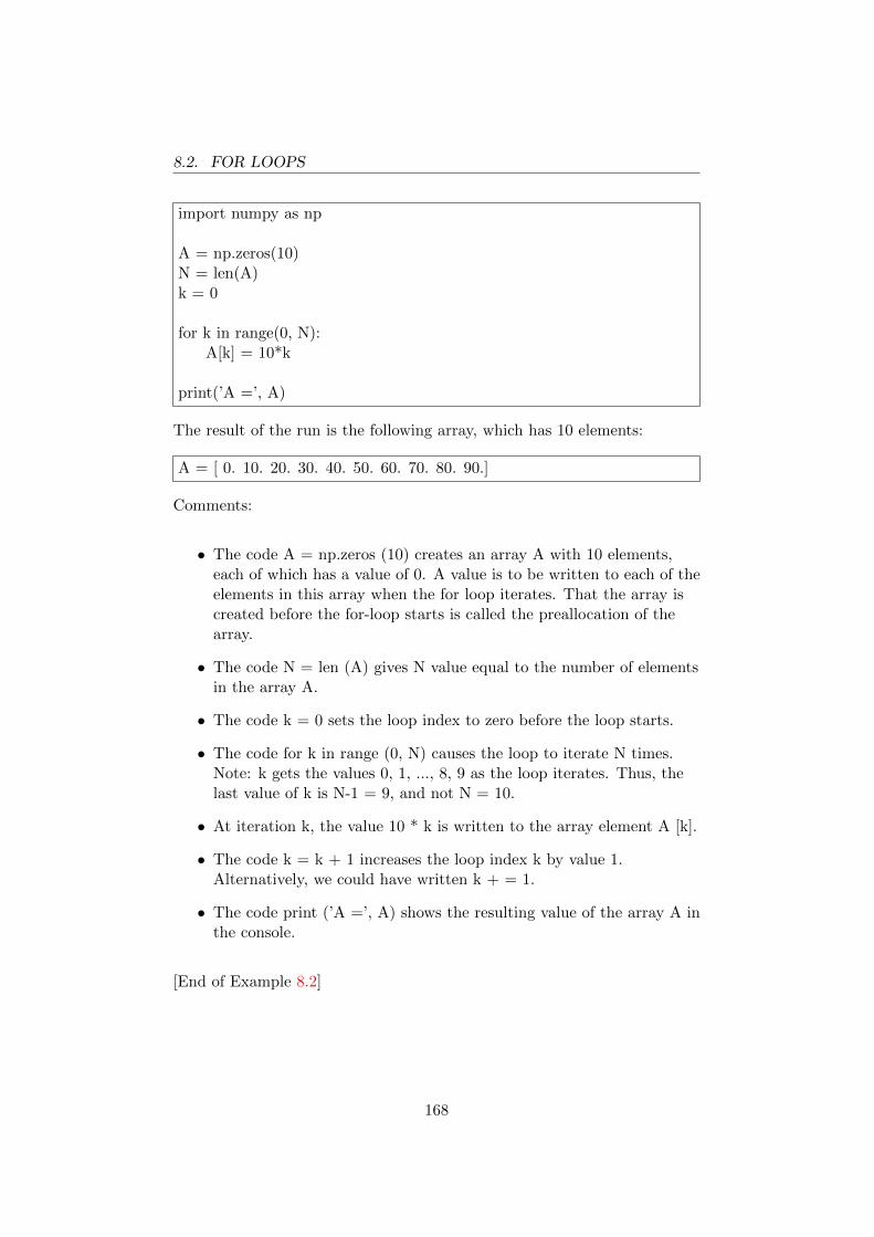
8.2. FOR LOOPS
import numpy as np
A = np.zeros(10)N = len(A)k = 0
for k in range(0, N):A[k] = 10*k
print(’A =’, A)
The result of the run is the following array, which has 10 elements:
A = [ 0. 10. 20. 30. 40. 50. 60. 70. 80. 90.]
Comments:
• The code A = np.zeros (10) creates an array A with 10 elements,each of which has a value of 0. A value is to be written to each of theelements in this array when the for loop iterates. That the array iscreated before the for-loop starts is called the preallocation of thearray.
• The code N = len (A) gives N value equal to the number of elementsin the array A.
• The code k = 0 sets the loop index to zero before the loop starts.
• The code for k in range (0, N) causes the loop to iterate N times.Note: k gets the values 0, 1, ..., 8, 9 as the loop iterates. Thus, thelast value of k is N-1 = 9, and not N = 10.
• At iteration k, the value 10 * k is written to the array element A [k].
• The code k = k + 1 increases the loop index k by value 1.Alternatively, we could have written k + = 1.
• The code print (’A =’, A) shows the resulting value of the array A inthe console.
[End of Example 8.2]
168

8.2. FOR LOOPS
8.2.3 Preallocation of arrays to save execution time
As mentioned, it can be a lot of time to save on preallocating arrays towrite values to iteratively (in a loop). Figure 8.2 illustrates two principlesfor iterative data writing in an array:
• Continuous expansion of an array with the np.append() function
• Writing to a preallocated array.
Python spends relatively much time expanding an existing array of newelements. That is why we should have as few such operations as possible inour programs. We can save a lot of execution time by creating the arraywith the sufficient number of elements in advance, perhaps with a value of0 in all the elements,and then write values to the elements in that array (inthe loop). This is preallocation of the array.
Figure 8.2: Illustration of two principles for iterative writing of data inarray: (1) Continuous expansion of an array with np.append() function and(2) writing to the preallocated array.
Here is an example that demonstrates the time savings that preallocationcan provide.
Example 8.3 The importance of preallocation
169
8.2. FOR LOOPS
Some comments on the program shown below:
• The program writes values to two arrays with 100,000 elements. Thevalue written to element # k is 10 * k.
• For one array, called dyn array, values are written using. np.append()- function. dyn array is not preallocated and is expanded with theappend() function for each iteration of the for-loop.
• For the second array, called preallok array, values are written at eachiteration through accessing the current element of the array.preallok array is preallocated, ie created before the for loop starts.
• The time to run the relevant program sections is measured using.function time() in the time packet, which is imported with the codeimport time at the top of the program.
• At the end of the program, the resulting running times withoutpreallocation and with preallocation are compared.
Here is the program:
Program name: prog time preallocation array.py
170

8.2. FOR LOOPS
# ----------------------------------------------------------# Import:
import numpy as npimport time
# ----------------------------------------------------------# Initialisering:
N = 100000dyn array = np.array([])preallok array = np.zeros(N)# ----------------------------------------------------------# append:
tic = time.time()for k in range(0, N):dyn array = np.append(dyn array, 10*k)toc = time.time()t elapsed append = toc - tic# ----------------------------------------------------------# preallok:
tic = time.time()for k in range(0, N):preallok array[k] = 10*ktoc = time.time()t elapsed preallok = toc - tic# ----------------------------------------------------------# Sammenlikning:
ratio append preallok = t elapsed append/t elapsed preallokprint(’------------------------------------------------’)print(’N =’, N)print(’t elapsed append [s] = ’,t elapsed append)print(’t elapsed preallok [s] =’, t elapsed preallok)print(’t elapsed append/t elapsed preallok =’, ratio append preallok)print(’------------------------------------------------’)
Result of a run (rounded numbers):
171

8.3. WHILE LOOPS
N = 100000t elapsed append [s] = 4.982t elapsed preallok [s] = 0.03000t elapsed append/t elapsed preallok = 166.1
Comments:
• The preallocation program of the array to which data is written runsapproximately. 166 times less time than without preallocation (withnp.append() function). Actually, there may be a lot of real time tosave: Suppose that in another case, with the ratio of run time as inour original example, it takes 1 minute to run the program withpreallocation. It will then take 166 minutes, ie not far from 3 hours,to run the program without preallocation. Assume you need theresult of the loop in some subsequent task... You can draw theconclusion about selecting between preallocation and nopreallocation yourself.
• Of course, the ratio 166 applies only to this test, but I have seensignificant time savings in other examples as well.
[End of Example 8.3]
8.3 While loops
While loops are loops that iterate as long as a given continue condition issatisfied. Figure 8.1 illustrates while loop with a program flowchart.
In principle, the number of iterations in while loops is not known inadvance. In Chap. 8.2.3 we saw that the preallocation of arrays cangreatly save the run time of a program where values are written to thearray inside the for loop. Since the number of iterations in while loops isnot known in advance, it may be more difficult to implement thepreallocation of arrays in the context of while loops. But preallocation canstill be realized if one knows an upper limit on the number of times theloop will be iterated. After all, it’s only possible to preallocate an array oflength equal to this greatest number of times.
The continue condition shown in Figure 8.1 is, in the python-technicalsense, a logical expression that has either the value True or False:
• If the value is True, the while loop continues to iterate.
172

8.3. WHILE LOOPS
• If the value is False, the iteration stops and Python continues to runthe program code after the while loop.
We construct the continue condition with logical operators and comparisonoperators, cf. 3.8.
The program code below demonstrates basic programming of while loops.
Program name: prog while loop.py
k = 0while (k < 5):
print(k)k = k + 1 #Alternatively: k += 1
print(’This is the first code line executed after the loop has stopped.’)
The result of the run:
01234This is the first code line executed after the loop has stopped.
Comments:
• The while loop is iterated as long as the continue condition (k <5) issatisfied.
• In each iteration, the following occurs:
– The value of k is written to the console with the print()command.
– The value of k is increased by 1 with the code k = k + 1, whichcan alternatively be written k + = 1.
• When k becomes 5, the continue condition is not satisfied and theloop stops. The program then goes to the program code that appearsafter the (below) while loop, ie the code: print(’This is the first codeline executed after the loop has stopped.’).
• In the continue condition, the comparison operator < is used, cf.
173
8.3. WHILE LOOPS
Table 3.4. You can drop the parentheses around k <5.2
• The code inside the while loop must be indented (python: indented).It is a Python standard (the PEP 8 guidelines) with 4 space indents(as for the for loops).
• The very last line of code, ie the code line print ("This is the firstcode line executed after the loop has stopped."), is here displayed todemonstrate that there should (not must) be a blank line betweenthe last line of code in the while loop and subsequent code lines.
2I myself prefer to include this unnecessary parenthesis because the code is then easierto read.
174

Chapter 9
Write and read file data
9.1 Introduction
Suppose you have useful numerical data from a calculation or a simulationor an experiment. You may want to write the data to (save the data on) afile so that you can read it later for plotting or analysis or datamanipulation, or send it to someone else who can use the data.
In this chapter we will see how we can write and read data files.
9.2 File Formats
The numeric data can be stored on file in two alternative formats:
• Textual data files
• Binary data files
Let’s take a closer look at these two file formats.
9.2.1 Textual data files
Textual data files are files where the data is in the form of numbers whichare strictly text and which you can therefore read yourself, eg. 1.2 and-18.57 with decimal point or 1.2 and -18.57 with decimal point. In this
175
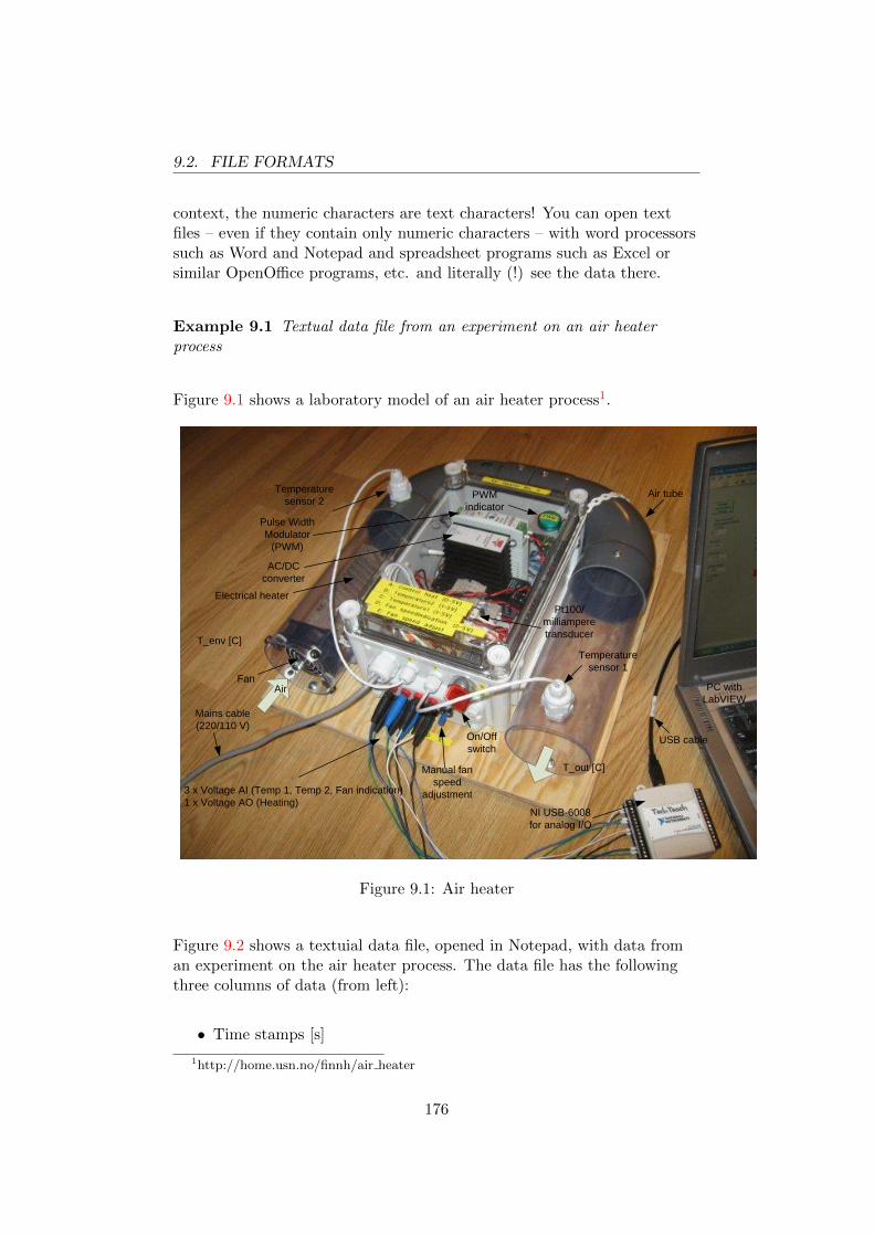
9.2. FILE FORMATS
context, the numeric characters are text characters! You can open textfiles – even if they contain only numeric characters – with word processorssuch as Word and Notepad and spreadsheet programs such as Excel orsimilar OpenOffice programs, etc. and literally (!) see the data there.
Example 9.1 Textual data file from an experiment on an air heaterprocess
Figure 9.1 shows a laboratory model of an air heater process1.
Temperature
sensor 1
Temperature
sensor 2
NI USB-6008
for analog I/O
Manual fan
speed
adjustment
On/Off
switch
PC with
LabVIEW
USB cable
Electrical heater
Fan
Mains cable
(220/110 V)
3 x Voltage AI (Temp 1, Temp 2, Fan indication)
1 x Voltage AO (Heating)
Air
Pulse Width
Modulator
(PWM)
PWM
indicator
AC/DC
converter
Pt100/
milliampere
transducer
Air tube
T_out [C]
T_env [C]
Figure 9.1: Air heater
Figure 9.2 shows a textuial data file, opened in Notepad, with data froman experiment on the air heater process. The data file has the followingthree columns of data (from left):
• Time stamps [s]
1http://home.usn.no/finnh/air heater
176
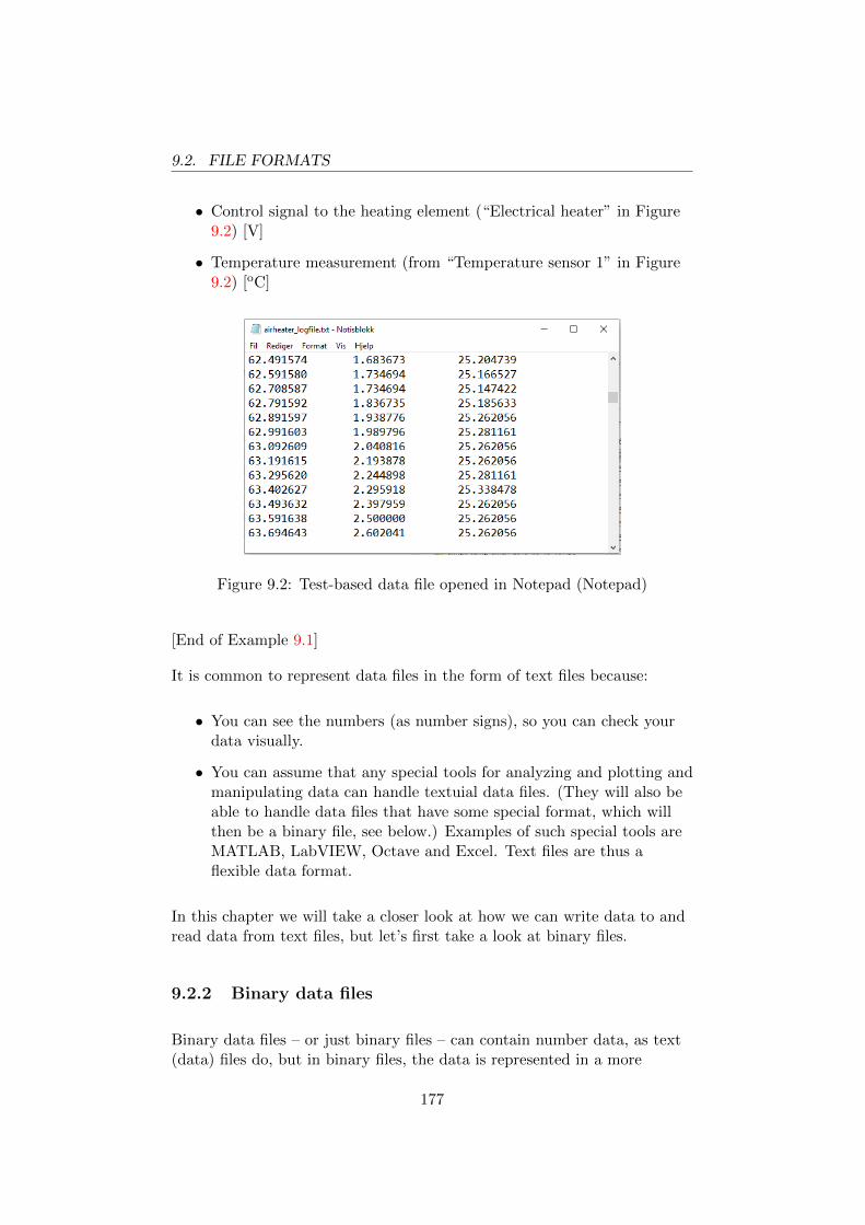
9.2. FILE FORMATS
• Control signal to the heating element (“Electrical heater” in Figure9.2) [V]
• Temperature measurement (from “Temperature sensor 1” in Figure9.2) [oC]
Figure 9.2: Test-based data file opened in Notepad (Notepad)
[End of Example 9.1]
It is common to represent data files in the form of text files because:
• You can see the numbers (as number signs), so you can check yourdata visually.
• You can assume that any special tools for analyzing and plotting andmanipulating data can handle textuial data files. (They will also beable to handle data files that have some special format, which willthen be a binary file, see below.) Examples of such special tools areMATLAB, LabVIEW, Octave and Excel. Text files are thus aflexible data format.
In this chapter we will take a closer look at how we can write data to andread data from text files, but let’s first take a look at binary files.
9.2.2 Binary data files
Binary data files – or just binary files – can contain number data, as text(data) files do, but in binary files, the data is represented in a more
177

9.3. WRITE DATA TO FILE
compact form than in text files and in some code that people cannot read.Only special tools (programs) can read the information in binary files.
Figure 9.3 shows an example of a binary file, namely a mat file (generatedin the MATLAB software) opened in Notepad. The data in the file aremeasured values from a biogas reactor: temperature, biogas flow, methaneconcentration, etc. Except for information about the file itself at the top ofthe file, the content is not readable to us. But the content is fully readablein MATLAB.
Figure 9.3: A binary file opened in Notepad
We can store data in the form of binary files in Python, but I will not gointo this further since text data files are far more convenient, even thoughthey are typically larger than binary files with the same informationcontent.
9.3 Write data to file
The open() function available in Python’s standard package, see Ch. 2.6.2,can be used to write data of different types to file. open() is thus a generalfunction. This book focuses on using Python for calculations, and the datais then typical numbers, most often floating numbers. The Numpy libraryhas the savetxt() function tailored to our purpose: “Save an array to a textfile”, cf. documentation on
https://docs.scipy.org/doc/numpy/reference/generated/numpy.savetxt.html
178

9.3. WRITE DATA TO FILE
It seems easier – at least to me – using savetxt() rather than open() towrite numeric data to text file. I therefore concentrate on savetxt() in thischapter.
When using savetxt() in a program, we need to type np.savetxt() if wehave imported the numpy package with the command
import numpy as np
np.savetxt() has a number of arguments, but for many of the argumentsthe default values will be ok, so we do not need to give explicit values tothese arguments. I guess the most current use of np.savetxt() is:
np.savetxt(fname, X, fmt=’%.18e’, delimiter=’ ’)
Here is a description of the individual arguments:
• fname (file name) is the name you give the file, quoted in quotationmarks, e.g. ’Eksperiment1.txt’.
• X represents the name of the variable to be stored, e.g. sensordata1.The variable must have data type array, either 1D array or 2D array.
• fmt (format) determines the format by which the numbers are storedin the file. The default value is ’% .18e’, which means that thenumbers are stored in exponential form by 18 digits after the decimalpoint, e.g. 1.123456789123456789e + 02 where e + 02 means 10 ˆ{2}. The number before the decimal point will be an integer in therange 1 - 9. It is possibly overkill to have 18 digits after the decimalpoint. A proposal is 3, which means that 4 digits determine thenumber in addition to the 10’s exponent.
• delimiter = ” (note: there are spaces between quotes) indicates thatspaces are used to separate the columns in the file. Space is thus thedefault value. You may use a comma, and then use delimiter = ’,’.
Here’s an example where we’re going to create a 2D array of columns equalto two given 1D arrays and then write the 2D array to file.
Example 9.2 Writing 2D array to np.savetxt file()
179

9.4. READ DATA FROM FILE
I hope the code in the box below is self-explanatory.
Program name: prog savetxt.py
Note that the two 1D arrays turn into columns in the 2D array, which isrealized with the transpose method (T) of the np.array array object ([A1,A2]), cf. Example 3.33 on page 96.
import numpy as np
A1 = np.linspace(0, 1, 7)A2 = np.linspace(0, 2, 7)M = np.array([A1, A2]).Tnp.savetxt(’datafil 1.txt’, M, fmt=’%.3e’, delimiter=’ ’)
Figure 9.4 shows the file datafil 1.txt opened in the Notepad program.
Figure 9.4: Datafile datafil 1.txt opened in Notepad
[End of Example 9.2]
9.4 Read data from file
The function open() in Python’s standard package, see chap. 2.6.2, can beused to read data from files, but for the same reason as for writing data tofile, cf. Section 9.3, I recommend using instead the loadtxt() Numpyfunction, which reads the numeric data in a text file and save it as anarray in the Python workspace.
Documentation of loadtxt() is available at
180

9.4. READ DATA FROM FILE
https://docs.scipy.org/doc/numpy/reference/generated/numpy.loadtxt.html
When we use loadtxt() in a program, we must type np.loadtxt() if we haveimported the numpy package with the command
import numpy as np
np.loadtxt() has a number of arguments, but for many of the arguments,the default values will be ok, so we do not need to give explicit values tothese arguments. I guess the most current use of np.loadtxt() is:
np.loadtxt(fname, delimiter=’ ’)
Here is a description of the individual arguments:
• fname (file name) is the name you give the file, quoted in quotationmarks, e.g. ’Eksperiment1.txt’.
• delimiter = ” (note: there are spaces between quotes) indicates thatspaces are used to separate the columns in the file. Space is thus thedefault value. If instead a comma is used to separate the columns inthe file, use delimiter = ’,’.
Here is an example of using np.loadtxt().
Example 9.3 Read 2D array from file with np.loadtxt()
The program below reads the number data stored in datafil 1.txt, which wecreated in the example 9.2, and returns the data as a 2D array here calledM. Two 1D arrays A1 and A2 are extracted from respective columns in M.
import numpy as np
M = np.loadtxt(’datafil 1.txt’, delimiter=’ ’)A1 = M[:, 0]A2 = M[:, 1]
print(’M =’, M)print(’A1 =’, A1)print(’A2 =’, A2)
181
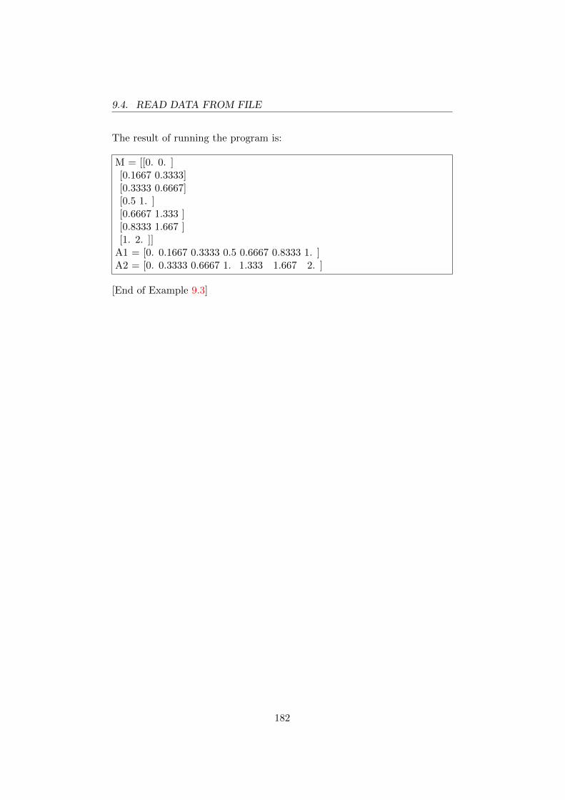
9.4. READ DATA FROM FILE
The result of running the program is:
M = [[0. 0. ][0.1667 0.3333][0.3333 0.6667][0.5 1. ][0.6667 1.333 ][0.8333 1.667 ][1. 2. ]]
A1 = [0. 0.1667 0.3333 0.5 0.6667 0.8333 1. ]A2 = [0. 0.3333 0.6667 1. 1.333 1.667 2. ]
[End of Example 9.3]
182
Bibliography
Haugen, F. A. (2019), Automatic Control, ’home.usn.no/finnh/books’.
Langtangen, H. P. (2016), A Primer on Scientific Programming withPython, Springer.
Linge, S. & Langtangen, H. P. (2016), Programming for Computations -Python, Springer (Open Access).
183
Index
**kwargs, 141
*args, 141
A
aksessere, 72
Anaconda distribution, 17
and, 66
anonymous functions, 150
args, 141
B
bar charts, 106
bar graph, 121
binary files, 177
block comments, 10
boolean variable, 66
built-in functions, 43
C
cancel, 23
casting, 62
Checkpoint, 33
command, 21
concatenate, 61
conda, 42
D
dashboard, 31
datatype casting, 62
default value, 139
del, 76
delete, 76
dictionary, 79
docstring, 142
E
editoren, 19
element-wise, 104
elif, 163
events, 127
execute, 21
F
filekstensjon, 32
floting point number, 57
format, 57
formelle parametre, 136
function, 22
functional errors, 152
funksjoner, 55
funksjonskropp, 137
G
Graphical User Interface, 127
GUI, 127
H
head, 10
histogram, 125
histograms, 106
hjelp, 27
Hjelp-vinduet, 20
I
if, 159
import, 42, 46
inline comments, 10
input argument, 22
input(), 63
integer, 57
interactive plots, 127
IPython console, 20
iterables, 70
184
INDEX
J
Jupyter Notebook, 30
K
kernel, 30
key, 79
keyword arguments, 140
kolonnevektorer, 93
konsollen, 20
konvertere, 62
kwargs, 141
L
Lambda functions, 150
legend, 113
line plots, 106
liste, 69
localhost, 32
logical operators, 66
logical variable, 66
loops, 164
M
magic command, 25, 110
main program, 135
matplotlib, 106
matrix object, 97
matrixes, 86, 96
modul, 147
moduler, 47
N
namespace, 144
not, 66
O
objects, 56
or, 66
P
packages, 41
PEP 8, 11
pie chart, 123
pie charts, 106
pip, 42
plottfigur, 110
preallocation, 167, 169
preallokering, 102
print(), 57
programflytdiagram, 65
programflytdiagrammer, 165
prompt, 50
PSF, 6
PyPA, 42
pyplot, 108
Python Packaging Authority, 42
Python Software Foundation, 6
R
radvektorer, 93
returargument, 137
return argument, 138
run, 21
Run file, 21
S
script, 20, 23
sequences, 70
slicing, 72
standard package, 44
STEM, 14
strings, 61
subplott, 117
syntaksfeil i Spyder, 28
T
text strings, 61
textbox, 127
textual data files, 175
three-dimentional, 86
transpose, 94
truth tables, 67
tuples, 77
two-dimentional, 86
typekonvertering, 62
U
underscore variable, 52
user interface, 127
185
INDEX
V
value, 79
variabel, 51
vectorized multiplication, 104
vectors, 96
vektorisering, 101
vektors, 86
Visual Studio Code, 36
W
while loop, 172
widgets, 127
workspace, 12, 51
186