python geospatial development (2010)
TRANSCRIPT
Python Geospatial Development
Build a complete and sophisticated mapping application from scratch using Python tools for GIS development
Erik Westra
BIRMINGHAM - MUMBAI
Python Geospatial Development
Copyright © 2010 Packt Publishing
All rights reserved. No part of this book may be reproduced, stored in a retrieval system, or transmitted in any form or by any means, without the prior written permission of the publisher, except in the case of brief quotations embedded in critical articles or reviews.
Every effort has been made in the preparation of this book to ensure the accuracy of the information presented. However, the information contained in this book is sold without warranty, either express or implied. Neither the author, nor Packt Publishing, and its dealers and distributors will be held liable for any damages caused or alleged to be caused directly or indirectly by this book.
Packt Publishing has endeavored to provide trademark information about all of the companies and products mentioned in this book by the appropriate use of capitals. However, Packt Publishing cannot guarantee the accuracy of this information.
First published: December 2010
Production Reference: 1071210
Published by Packt Publishing Ltd. 32 Lincoln Road Olton Birmingham, B27 6PA, UK.
ISBN 978-1-849511-54-4
www.packtpub.com
Cover Image by Asher Wishkerman ([email protected])

Credits
AuthorErik Westra
ReviewersTomi Juhola
Silas Toms
Acquisition EditorSteven Wilding
Development EditorHyacintha D'Souza
Technical EditorKartikey Pandey
IndexersHemangini Bari
Tejal Daruwale
Editorial Team LeaderMithun Sehgal
Project Team LeaderPriya Mukherji
Project CoordinatorJovita Pinto
ProofreaderJonathan Todd
GraphicsNilesh R. Mohite
Production Coordinator Kruthika Bangera
Cover WorkKruthika Bangera

About the Author
Erik Westra has been a professional software developer for over 25 years, and has worked almost exclusively in Python for the past decade. Erik's early interest in graphical user-interface design led to the development of one of the most advanced urgent courier dispatch systems used by messenger and courier companies worldwide. In recent years, Erik has been involved in the design and implementation of systems matching seekers and providers of goods and services across a range of geographical areas. This work has included the creation of real-time geocoders and map-based views of constantly changing data. Erik is based in New Zealand, and works for companies worldwide.
"For Ruth,
The love of my life."

About the Reviewers
Tomi Juhola is a software development professional from Finland. He has a wide range of development experience from embedded systems to modern distributed enterprise systems in various roles, such as tester, developer, consultant, and trainer.
Currently, he works in a company called Lindorff and shares this time between development lead duties and helping other projects to adopt Scrum and agile methodologies. He likes to spend his free time with new and interesting development languages and frameworks.
Silas Toms is a GIS Analyst for ICF International, working at the San Francisco and San Jose offices. His undergraduate degree is in Geography (from Humboldt State University), and he is currently finishing a thesis for an MS in GIS at San Francisco State University. He has been a GIS professional for four years, working with many local and regional governments before taking his current position. Python experience was gained through classes at SFSU and professional experience. This is the first book he has helped review.
I would like to thank everyone at Packt Publishing for allowing me to help review this book and putting up with my ever-shifting schedule. I would also like to thank my family for being supportive in my quest to master this somewhat esoteric field, and for never asking if I am going to teach with this degree.
www.PacktPub.com
Support files, eBooks, discount offers and moreYou might want to visit www.PacktPub.com for support files and downloads related to your book.
Did you know that Packt offers eBook versions of every book published, with PDF and ePub files available? You can upgrade to the eBook version at www.PacktPub.com and as a print book customer, you are entitled to a discount on the eBook copy. Get in touch with us at [email protected] for more details.
At www.PacktPub.com, you can also read a collection of free technical articles, sign up for a range of free newsletters, and receive exclusive discounts and offers on Packt books and eBooks.
http://PacktLib.PacktPub.com
Do you need instant solutions to your IT questions? PacktLib is Packt's online digital book library. Here, you can access, read, and search across Packt's entire library of books.

Why Subscribe?• Fully searchable across every book published by Packt• Copy and paste, print, and bookmark content• On demand and accessible via web browser
Free Access for Packt account holdersIf you have an account with Packt at www.PacktPub.com, you can use this to access PacktLib today and view nine entirely free books. Simply use your login credentials for immediate access.

Table of ContentsPreface 1Chapter 1: Geo-Spatial Development Using Python 7
Python 7Geo-spatial development 9Applications of geo-spatial development 11
Analyzing geo-spatial data 12Visualizing geo-spatial data 13Creating a geo-spatial mash-up 16
Recent developments 17Summary 19
Chapter 2: GIS 21Core GIS concepts 21
Location 22Distance 25Units 27Projections 28
Cylindrical projections 29Conic projections 31Azimuthal projections 31The nature of map projections 32
Coordinate systems 32Datums 35Shapes 36
GIS data formats 37Working with GIS data manually 39Summary 46
Table of Contents
[ ii ]
Chapter 3: Python Libraries for Geo-Spatial Development 47Reading and writing geo-spatial data 47
GDAL/OGR 48GDAL design 48GDAL example code 50OGR design 51OGR example code 52
Documentation 53Availability 53
Dealing with projections 54pyproj 54Design 54
Proj 55Geod 56
Example code 57Documentation 58Availability 58
Analyzing and manipulating geo-spatial data 59Shapely 59Design 60Example code 61Documentation 62Availability 62
Visualizing geo-spatial data 63Mapnik 63Design 64Example code 66Documentation 67Availability 68
Summary 68Chapter 4: Sources of Geo-Spatial Data 71
Sources of geo-spatial data in vector format 72OpenStreetMap 72
Data format 73Obtaining and using OpenStreetMap data 74
TIGER 76Data format 77Obtaining and using TIGER data 78
Digital Chart of the World 79Data format 80Available layers 80Obtaining and using DCW data 80
Table of Contents
[ iii ]
GSHHS 82Data format 83Obtaining the GSHHS database 84
World Borders Dataset 84Data format 85Obtaining the World Borders Dataset 85
Sources of geo-spatial data in raster format 85Landsat 86
Data format 86Obtaining Landsat imagery 87
GLOBE 90Data format 90Obtaining and using GLOBE data 91
National Elevation Dataset 92Data format 92Obtaining and using NED data 93
Sources of other types of geo-spatial data 94GEOnet Names Server 94
Data format 95Obtaining and using GEOnet Names Server data 95
GNIS 96Data format 97Obtaining and using GNIS data 97
Summary 98Chapter 5: Working with Geo-Spatial Data in Python 101
Prerequisites 101Reading and writing geo-spatial data 102
Task: Calculate the bounding box for each country in the world 102Task: Save the country bounding boxes into a Shapefile 104Task: Analyze height data using a digital elevation map 108
Changing datums and projections 115Task: Change projections to combine Shapefiles using geographic and UTM coordinates 115Task: Change datums to allow older and newer TIGER data to be combined 119
Representing and storing geo-spatial data 122Task: Calculate the border between Thailand and Myanmar 123Task: Save geometries into a text file 126
Working with Shapely geometries 127Task: Identify parks in or near urban areas 128
Converting and standardizing units of geometry and distance 132Task: Calculate the length of the Thai-Myanmar border 133Task: Find a point 132.7 kilometers west of Soshone, California 139
Table of Contents
[ iv ]
Exercises 141Summary 143
Chapter 6: GIS in the Database 145Spatially-enabled databases 145Spatial indexes 146Open source spatially-enabled databases 149
MySQL 149PostGIS 152
Installing and configuring PostGIS 152Using PostGIS 155Documentation 157Advanced PostGIS features 157
SpatiaLite 158Installing SpatiaLite 158Installing pysqlite 159Accessing SpatiaLite from Python 160Documentation 160Using SpatiaLite 161SpatiaLite capabilities 163
Commercial spatially-enabled databases 164Oracle 164MS SQL Server 165
Recommended best practices 165Use the database to keep track of spatial references 166Use the appropriate spatial reference for your data 168
Option 1: Use a database that supports geographies 169Option 2: Transform features as required 169Option 3: Transform features from the outset 169When to use unprojected coordinates 170
Avoid on-the-fly transformations within a query 170Don't create geometries within a query 171Use spatial indexes appropriately 172Know the limits of your database's query optimizer 173
MySQL 174PostGIS 175SpatiaLite 177
Working with geo-spatial databases using Python 178
Prerequisites 179Working with MySQL 179Working with PostGIS 182Working with SpatiaLite 184Speed comparisons 188
Summary 189
Table of Contents
[ v ]
Chapter 7: Working with Spatial Data 191About DISTAL 191Designing and building the database 195Downloading the data 199
World Borders Dataset 200GSHHS 200Geonames 200GEOnet Names Server 200
Importing the data 201World Borders Dataset 201GSHHS 203US placename data 205Worldwide placename data 208
Implementing the DISTAL application 210The "Select Country" script 212The "Select Area" script 214
Calculating the bounding box 215Calculating the map's dimensions 216Setting up the datasource 218Rendering the map image 220
The "Show Results" script 223Identifying the clicked-on point 223Identifying features by distance 225Displaying the results 233
Application review and improvements 235Usability 236Quality 237
Placename issues 237Lat/Long coordinate problems 238
Performance 239Finding the problem 240Improving performance 242Calculating the tiled shorelines 244Using the tiled shorelines 250Analyzing the performance improvement 252Further performance improvements 252
Scalability 253Summary 257
Chapter 8: Using Python and Mapnik to Generate Maps 259Introducing Mapnik 260Creating an example map 265Mapnik in depth 269
Data sources 269Shapefile 270
Table of Contents
[ vi ]
PostGIS 270GDAL 272OGR 273SQLite 274OSM 275PointDatasource 276
Rules, filters, and styles 277Filters 277Scale denominators 279"Else" rules 280
Symbolizers 281Drawing lines 281Drawing polygons 287Drawing labels 289Drawing points 298Drawing raster images 301Using colors 303
Maps and layers 304Map attributes and methods 305Layer attributes and methods 306
Map rendering 307MapGenerator revisited 309
The MapGenerator's interface 309Creating the main map layer 310Displaying points on the map 312Rendering the map 313What the map generator teaches us 313
Map definition files 314Summary 317
Chapter 9: Web Frameworks for Python Geo-Spatial Development 321
Web application concepts 322Web application architecture 322
A bare-bones approach 322Web application stacks 323Web application frameworks 324Web services 325
Map rendering 327Tile caching 327Web servers 330User interface libraries 331The "slippy map" stack 332The geo-spatial web application stack 334
Table of Contents
[ vii ]
Protocols 334The Web Map Service (WMS) protocol 334
WMS-C 337The Web Feature Service (WFS) protocol 337The TMS (Tile Map Service) protocol 339
Tools 344Tile caching 344
TileCache 345mod_tile 346TileLite 347
User interface libraries 347OpenLayers 348Mapiator 351
Web application frameworks 353GeoDjango 353MapFish 356TurboGears 357
Summary 359Chapter 10: Putting it All Together: A Complete Mapping Application 363
About the ShapeEditor 363Designing the application 367
Importing a Shapefile 367Selecting a feature 369Editing a feature 370Exporting a Shapefile 371
Prerequisites 371The structure of a Django application 372
Models 374Views 374Templates 377
Setting up the database 379Setting up the GeoDjango project 380Setting up the ShapeEditor application 382Defining the data models 383
Shapefile 383Attribute 384Feature 384AttributeValue 385The models.py file 385
Playing with the admin system 388Summary 395
Table of Contents
[ viii ]
Chapter 11: ShapeEditor: Implementing List View, Import, and Export 397
Implementing the "List Shapefiles" view 397Importing Shapefiles 401
The "import shapefile" form 402Extracting the uploaded Shapefile 405Importing the Shapefile's contents 408
Open the Shapefile 408Add the Shapefile object to the database 409Define the Shapefile's attributes 410Store the Shapefile's features 411Store the Shapefile's attributes 413
Cleaning up 416Exporting Shapefiles 417
Define the OGR Shapefile 418Saving the features into the Shapefile 419Saving the attributes into the Shapefile 420Compressing the Shapefile 422Deleting temporary files 422Returning the ZIP archive to the user 423
Summary 424Chapter 12: ShapeEditor: Selecting and Editing Features 425
Selecting a feature to edit 426Implementing the Tile Map Server 426
Setting up the base map 435Tile rendering 437
Using OpenLayers to display the map 442Intercepting mouse clicks 447Implementing the "find feature" view 451
Editing features 457Adding features 464Deleting features 467Deleting Shapefiles 468Using ShapeEditor 470Further improvements and enhancements 470Summary 471
Index 473
PrefaceOpen Source GIS (Geographic Information Systems) is a growing area with the explosion of Google Maps-based websites and spatially-aware devices and applications. The GIS market is growing rapidly, and as a Python developer you can't afford to be left behind. In today's location-aware world, all commercial Python developers can benefit from an understanding of GIS concepts and development techniques.
Working with geo-spatial data can get complicated because you are dealing with mathematical models of the Earth's surface. Since Python is a powerful programming language with high-level toolkits, it is well-suited to GIS development. This book will familiarize you with the Python tools required for geo-spatial development. It introduces GIS at the basic level with a clear, detailed walkthrough of the key GIS concepts such as location, distance, units, projections, datums, and GIS data formats. We then examine a number of Python libraries and combine these with geo-spatial data to accomplish a variety of tasks. The book provides an in-depth look at the concept of storing spatial data in a database and how you can use spatial databases as tools to solve a variety of geo-spatial problems.
It goes into the details of generating maps using the Mapnik map-rendering toolkit, and helps you to build a sophisticated web-based geo-spatial map editing application using GeoDjango, Mapnik, and PostGIS. By the end of the book, you will be able to integrate spatial features into your applications and build a complete mapping application from scratch.
This book is a hands-on tutorial, teaching you how to access, manipulate, and display geo-spatial data efficiently using a range of Python tools for GIS development.
Preface
[ 2 ]
What this book coversChapter 1, Geo-Spatial Development Using Python, introduces the Python programming language and the main concepts behind geo-spatial development
Chapter 2, GIS, discusses many of the core concepts that underlie GIS development. It examines the common GIS data formats, and gets our hands dirty exploring U.S. state maps downloaded from the U.S. Census Bureau website
Chapter 3, Python Libraries for Geo-Spatial Development, looks at a number of important libraries for developing geo-spatial applications using Python
Chapter 4, Sources of Geo-Spatial Data, covers a number of sources of freely-available geo-spatial data. It helps you to obtain map data, images, elevations, and place names for use in your geo-spatial applications
Chapter 5, Working with Geo-Spatial Data in Python, deals with various techniques for using OGR, GDAL, Shapely, and pyproj within Python programs to solve real-world problems
Chapter 6, GIS in the Database, takes an in-depth look at the concept of storing spatial data in a database, and examines three of the principal open source spatial databases
Chapter 7, Working with Spatial Data, guides us to implement, test, and make improvements to a simple web-based application named DISTAL. This application displays shorelines, towns, and lakes within a given radius of a starting point. We will use this application as the impetus for exploring a number of important concepts within geo-spatial application development
Chapter 8, Using Python and Mapnik to Generate Maps, helps us to explore the Mapnik map-generation toolkit in depth
Chapter 9, Web Frameworks for Python Geo-Spatial Development, discusses the geo-spatial web development landscape, examining the major concepts behind geo-spatial web application development, some of the main open protocols used by geo-spatial web applications, and a number of Python-based tools for implementing geo-spatial applications that run over the Internet
Chapter 10, Putting it all Together: a Complete Mapping Application, along with the final two chapters, brings together all the topics discussed in previous chapters to implement a sophisticated web-based mapping application called ShapeEditor
Chapter 11, ShapeEditor: Implementing List View, Import, and Export, continues with implementation of the ShapeEditor by adding a "list" view showing the imported Shapefiles, along with the ability to import and export Shapefiles
Preface
[ 3 ]
Chapter 12, ShapeEditor: Selecting and Editing Features, adds map-based editing and feature selection capabilities, completing the implementation of the ShapeEditor application
What you need for this bookTo follow through the various examples, you will need to download and install the following software:
• Python version 2.x (minimum version 2.5)• GDAL/OGR version 1.7.1 or later• GEOS version 3.2.2 or later• Shapely version 1.2 or later• Proj version 4.7 or later• pyproj version 1.8.6 or later• MySQL version 5.1 or later• MySQLdb version 1.2 or later• SpatiaLite version 2.3 or later• pysqlite version 2.6 or later• PostgreSQL version 8.4 or later• PostGIS version 1.5.1 or later• psycopg2 version 2.2.1 or later• Mapnik version 0.7.1 or later• Django version 1.2 or later
With the exception of Python itself, the procedure for downloading, installing, and using all of these tools is covered in the relevant chapters of this book.
Who this book is forThis book is useful for Python developers who want to get up to speed with open source GIS in order to build GIS applications or integrate geo-spatial features into their applications.
Preface
[ 4 ]
ConventionsIn this book, you will find a number of styles of text that distinguish between different kinds of information. Here are some examples of these styles, and an explanation of their meaning.
Code words in text are shown as follows: "We can then convert these to Shapely geometric objects using the shapely.wkt module."
A block of code is set as follows:
import osgeo.ogr
shapefile = osgeo.ogr.Open("TM_WORLD_BORDERS-0.3.shp")layer = shapefile.GetLayer(0)
When we wish to draw your attention to a particular part of a code block, the relevant lines or items are set in bold:
from pysqlite2 import dbapi as sqlite
conn = sqlite.connect("...")conn.enable_load_extension(True)conn.execute('SELECT load_extension("libspatialite-2.dll")')curs = conn.cursor()
Any command-line input or output is written as follows:
>>> import sqlite3
>>> conn = sqlite3.connect(":memory:")
>>> conn.enable_load_extension(True)
New terms and important words are shown in bold. Words that you see on the screen, in menus or dialog boxes for example, appear in the text like this: "If you want, you can change the format of the downloaded data by clicking on the Modify Data Request hyperlink".
Warnings or important notes appear in a box like this.
Tips and tricks appear like this.

Preface
[ 5 ]
Reader feedbackFeedback from our readers is always welcome. Let us know what you think about this book—what you liked or may have disliked. Reader feedback is important for us to develop titles that you really get the most out of.
To send us general feedback, simply send an e-mail to [email protected], and mention the book title via the subject of your message.
If there is a book that you need and would like to see us publish, please send us a note in the SUGGEST A TITLE form on www.packtpub.com or e-mail [email protected].
If there is a topic that you have expertise in and you are interested in either writing or contributing to a book, see our author guide on www.packtpub.com/authors.
Customer supportNow that you are the proud owner of a Packt book, we have a number of things to help you to get the most from your purchase.
Downloading the example code for this bookYou can download the example code files for all Packt books you have purchased from your account at http://www.PacktPub.com. If you purchased this book elsewhere, you can visit http://www.PacktPub.com/support and register to have the files e-mailed directly to you.
ErrataAlthough we have taken every care to ensure the accuracy of our content, mistakes do happen. If you find a mistake in one of our books—maybe a mistake in the text or the code—we would be grateful if you would report this to us. By doing so, you can save other readers from frustration and help us improve subsequent versions of this book. If you find any errata, please report them by visiting http://www.packtpub.com/support, selecting your book, clicking on the errata submission form link, and entering the details of your errata. Once your errata are verified, your submission will be accepted and the errata will be uploaded on our website, or added to any list of existing errata, under the Errata section of that title. Any existing errata can be viewed by selecting your title from http://www.packtpub.com/support.

Preface
[ 6 ]
PiracyPiracy of copyright material on the Internet is an ongoing problem across all media. At Packt, we take the protection of our copyright and licenses very seriously. If you come across any illegal copies of our works, in any form, on the Internet, please provide us with the location address or website name immediately so that we can pursue a remedy.
Please contact us at [email protected] with a link to the suspected pirated material.
We appreciate your help in protecting our authors, and our ability to bring you valuable content.
QuestionsYou can contact us at [email protected] if you are having a problem with any aspect of the book, and we will do our best to address it.
Geo-Spatial Development Using Python
This chapter provides an overview of the Python programming language and geo-spatial development. Please note that this is not a tutorial on how to use the Python language; Python is easy to learn, but the details are beyond the scope of this book.
In this chapter, we will cover:
• What the Python programming language is, and how it differs from other languages
• An introduction to the Python Standard Library and the Python Package Index
• What the terms "geo-spatial data" and "geo-spatial development" refer to• An overview of the process of accessing, manipulating, and displaying
geo-spatial data• Some of the major applications for geo-spatial development• Some of the recent trends in the field of geo-spatial development
PythonPython (http://python.org) is a modern, high-level language suitable for a wide variety of programming tasks. Technically, it is often referred to as a "scripting" language, though this distinction isn't very important nowadays. Python has been used for writing web-based systems, desktop applications, games, scientific programming, and even utilities and other higher-level parts of various operating systems.
Geo-Spatial Development Using Python
[ 8 ]
Python supports a wide range of programming idioms, from straightforward procedural programming to object-oriented programming and functional programming.
While Python is generally considered to be an "interpreted" language, and is occasionally criticized for being slow compared to "compiled" languages such as C, the use of byte-compilation and the fact that much of the heavy lifting is done by library code means that Python's performance is often surprisingly good.
Open source versions of the Python interpreter are freely available for all major operating systems. Python is eminently suitable for all sorts of programming, from quick one-off scripts to building huge and complex systems. It can even be run in interactive (command-line) mode, allowing you to type in commands and immediately see the results. This is ideal for doing quick calculations or figuring out how a particular library works.
One of the first things a developer notices about Python compared with other languages such as Java or C++ is how expressive the language is—what may take 20 or 30 lines of code in Java can often be written in half a dozen lines of code in Python. For example, imagine that you have an array of latitude and longitude values you wish to process one at a time. In Python, this is trivial:
for lat,long in coordinates: ...
Compare this with how much work a programmer would have to do in Java to achieve the same result:
for (int i=0; i < coordinates.length; i++) { float lat = coordinates[i][0]; float long = coordinates[i][1];...}
While the Python language itself makes programming quick and easy, allowing you to focus on the task at hand, the Python Standard Libraries make programming even more efficient. These libraries make it easy to do things such as converting date and time values, manipulating strings, downloading data from websites, performing complex maths, working with e-mail messages, encoding and decoding data, XML parsing, data encryption, file manipulation, compressing and decompressing files, working with databases—the list goes on. What you can do with the Python Standard Libraries is truly amazing.
Chapter 1
[ 9 ]
As well as the built-in modules in the Python Standard Libraries, it is easy to download and install custom modules, which can be written in either Python or C. The Python Package Index (http://pypi.python.org) provides thousands of additional modules that you can download and install. And, if that isn't enough, many other systems provide python bindings to allow you to access them directly from within your programs. We will be making heavy use of Python bindings in this book.
It should be pointed out that there are different versions of Python available. Python 2.x is the most common version in use today, while the Python developers have been working for the past several years on a completely new, non-backwards-compatible version called Python 3. Eventually, Python 3 will replace Python 2.x, but at this stage most of the third-party libraries (including all the GIS tools we will be using) only work with Python 2.x. For this reason, we won't be using Python 3 in this book.
Python is in many ways an ideal programming language. Once you are familiar with the language itself and have used it a few times, you'll find it incredibly easy to write programs to solve various tasks. Rather than getting buried in a morass of type-definitions and low-level string manipulation, you can simply concentrate on what you want to achieve. You end up almost thinking directly in Python code. Programming in Python is straightforward, efficient and, dare I say it, fun.
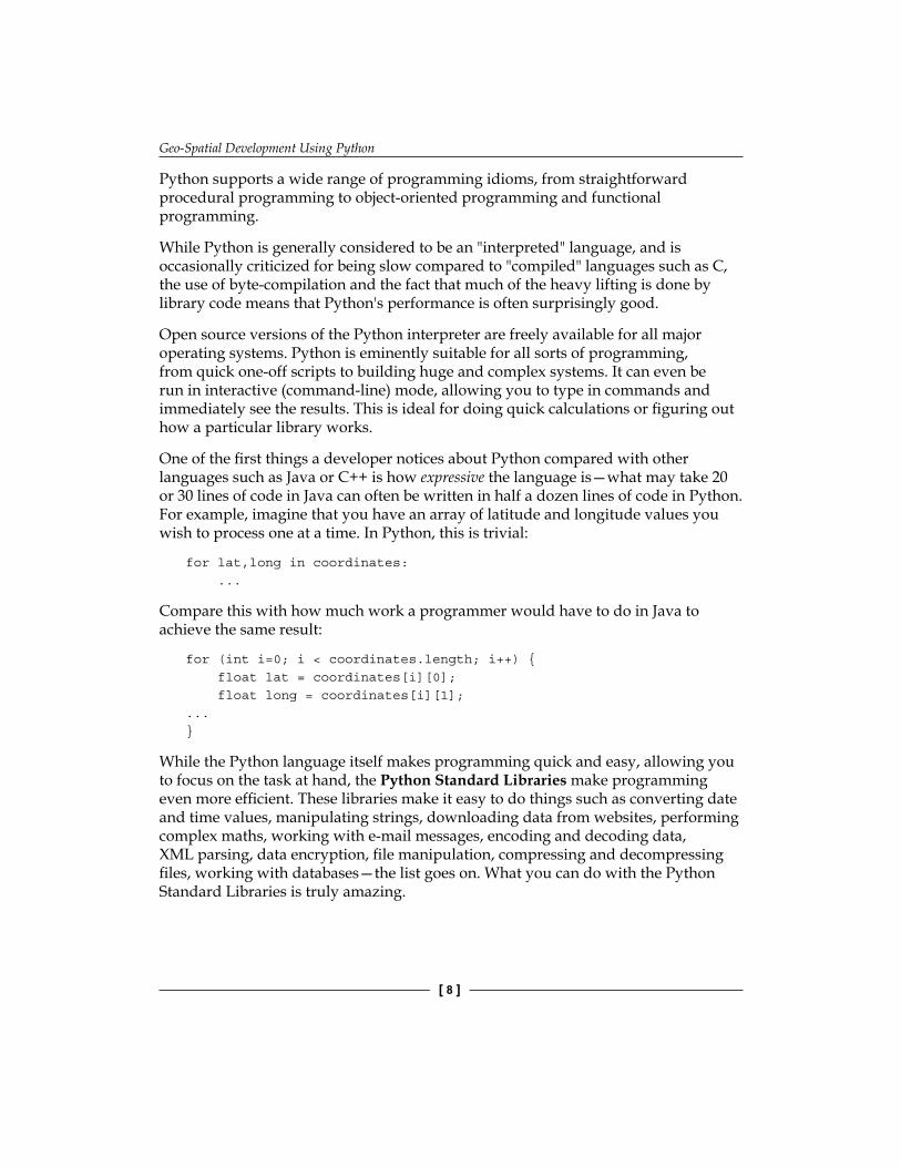
Geo-spatial developmentThe term Geo-spatial refers to information that is located on the Earth's surface using coordinates. This can include, for example, the position of a cell phone tower, the shape of a road, or the outline of a country:
Geo-Spatial Development Using Python
[ 10 ]
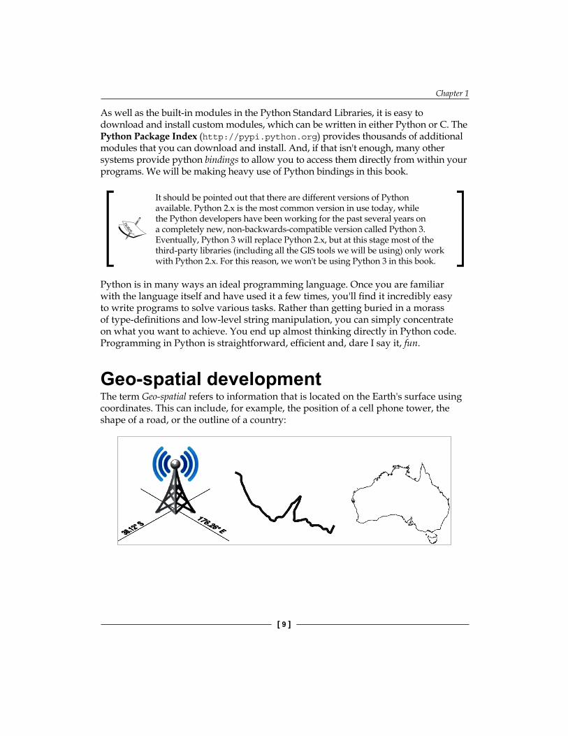
Geo-spatial data often associates some piece of information with a particular location. For example, here is a map of Afghanistan from the http://afghanistanelectiondata.org website showing the number of votes cast in each location in the 2009 elections:
Geo-spatial development is the process of writing computer programs that can access, manipulate, and display this type of information.
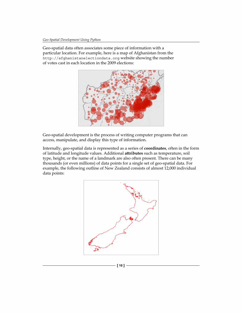
Internally, geo-spatial data is represented as a series of coordinates, often in the form of latitude and longitude values. Additional attributes such as temperature, soil type, height, or the name of a landmark are also often present. There can be many thousands (or even millions) of data points for a single set of geo-spatial data. For example, the following outline of New Zealand consists of almost 12,000 individual data points:
Chapter 1
[ 11 ]
Because so much data is involved, it is common to store geo-spatial information within a database. A large part of this book will be concerned with how to store your geo-spatial information in a database, and how to access it efficiently.
Geo-spatial data comes in many different forms. Different GIS (Geographical Information System) vendors have produced their own file formats over the years, and various organizations have also defined their own standards. It's often necessary to use a Python library to read files in the correct format when importing geo-spatial data into your database.
Unfortunately, not all geo-spatial data points are compatible. Just like a distance value of 2.8 can have a very different meaning depending on whether you are using kilometers or miles, a given latitude and longitude value can represent any number of different points on the Earth's surface, depending on which projection has been used.
A projection is a way of representing the Earth's surface in two dimensions. We will look at projections in more detail in Chapter 2, GIS, but for now just keep in mind that every piece of geo-spatial data has a projection associated with it. To compare or combine two sets of geo-spatial data, it is often necessary to convert the data from one projection to another.
Latitude and longitude values are sometimes referred to as unprojected coordinates. We'll learn more about this in the next chapter.
In addition to the prosaic tasks of importing geo-spatial data from various external file formats and translating data from one projection to another, geo-spatial data can also be manipulated to solve various interesting problems. Obvious examples include the task of calculating the distance between two points, calculating the length of a road, or finding all data points within a given radius of a selected point. We will be using Python libraries to solve all of these problems, and more.
Finally, geo-spatial data by itself is not very interesting. A long list of coordinates tells you almost nothing; it isn't until those numbers are used to draw a picture that you can make sense of it. Drawing maps, placing data points onto a map, and allowing users to interact with maps are all important aspects of geo-spatial development. We will be looking at all of these in later chapters.
Applications of geo-spatial developmentLet's take a brief look at some of the more common geo-spatial development tasks you might encounter.
Geo-Spatial Development Using Python
[ 12 ]
Analyzing geo-spatial dataImagine that you have a database containing a range of geo-spatial data for San Francisco. This database might include geographical features, roads and the location of prominent buildings and other man-made features such as bridges, airports, and so on.
Such a database can be a valuable resource for answering various questions. For example:
• What's the longest road in Sausalito?• How many bridges are there in Oakland?• What is the total area of the Golden Gate Park?• How far is it from Pier 39 to the Moscone Center?
Many of these types of problems can be solved using tools such as the PostGIS spatially-enabled database. For example, to calculate the total area of the Golden Gate Park, you might use the following SQL query:
select ST_Area(geometry) from features where name = "Golden Gate Park";
To calculate the distance between two places, you first have to geocode the locations to obtain their latitude and longitude. There are various ways to do this; one simple approach is to use a free geocoding web service such as this:
http://tinygeocoder.com/create-api.php?q=Pier 39,San Francisco,CA
This returns a latitude value of 37.809662 and a longitude value of -122.410408.
These latitude and longitude values are in decimal degrees. If you don't know what these are, don't worry; we'll talk about decimal degrees in Chapter 2, GIS.
Similarly, we can find the location of the Moscone Center using this query:
http://tinygeocoder.com/create-api.php?q=Moscone Center, San Francisco, CA
This returns a latitude value of 37.784161 and a longitude value of -122.401489.
Now that we have the coordinates for the two desired locations, we can calculate the distance between them using the pyproj Python library:
Chapter 1
[ 13 ]
import pyproj
lat1,long1 = (37.809662,-122.410408)lat2,long2 = (37.784161,-122.401489)
geod = pyproj.Geod(ellps="WGS84")angle1,angle2,distance = geod.inv(long1, lat1, long2, lat2)
print "Distance is %0.2f meters" % distance
This prints the distance between the two points:
Distance is 2937.41 meters
Don't worry about the "WGS84" reference at this stage; we'll look at what this means in Chapter 2, GIS.
Of course, you wouldn't normally do this sort of analysis on a one-off basis like this—it's much more common to create a Python program that will answer these sorts of questions for any desired set of data. You might, for example, create a web application that displays a menu of available calculations. One of the options in this menu might be to calculate the distance between two points; when this option is selected, the web application would prompt the user to enter the two locations, attempt to geocode them by calling an appropriate web service (and display an error message if a location couldn't be geocoded), then calculate the distance between the two points using Proj, and finally display the results to the user.
Alternatively, if you have a database containing useful geo-spatial data, you could let the user select the two locations from the database rather than typing in arbitrary location names or street addresses.
However you choose to structure it, performing calculations like this will usually be a major part of your geo-spatial application.
Visualizing geo-spatial dataImagine that you wanted to see which areas of a city are typically covered by a taxi during an average working day. You might place a GPS recorder into a taxi and leave it to record the taxi's position over several days. The results would be a series of timestamp, latitude and longitude values like the following:
2010-03-21 9:15:23 -38.16614499 176.23366262010-03-21 9:15:27 -38.16608632 176.23356352010-03-21 9:15:34 -38.16604198 176.23347712010-03-21 9:15:39 -38.16601507 176.2333958...
Geo-Spatial Development Using Python
[ 14 ]
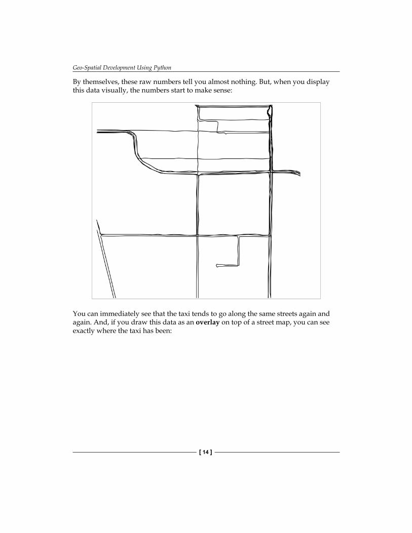
By themselves, these raw numbers tell you almost nothing. But, when you display this data visually, the numbers start to make sense:
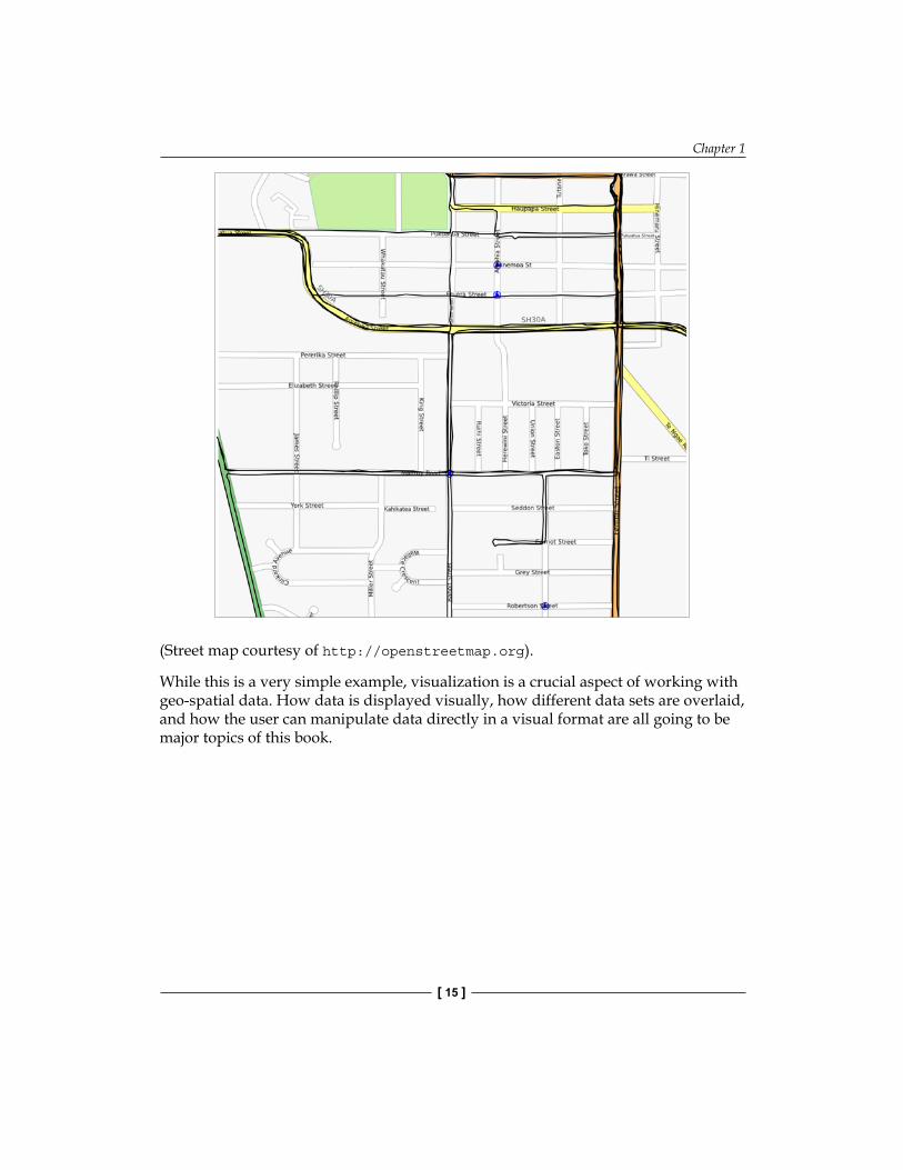
You can immediately see that the taxi tends to go along the same streets again and again. And, if you draw this data as an overlay on top of a street map, you can see exactly where the taxi has been:
Chapter 1
[ 15 ]
(Street map courtesy of http://openstreetmap.org).
While this is a very simple example, visualization is a crucial aspect of working with geo-spatial data. How data is displayed visually, how different data sets are overlaid, and how the user can manipulate data directly in a visual format are all going to be major topics of this book.
Geo-Spatial Development Using Python
[ 16 ]
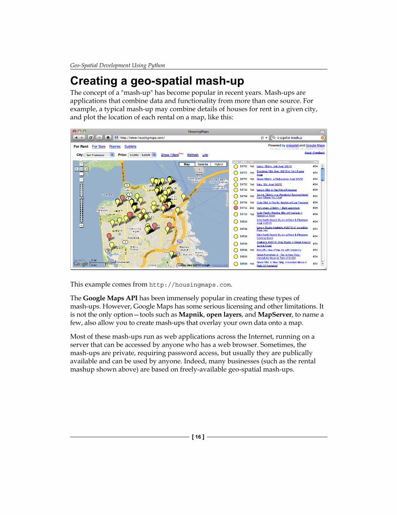
Creating a geo-spatial mash-upThe concept of a "mash-up" has become popular in recent years. Mash-ups are applications that combine data and functionality from more than one source. For example, a typical mash-up may combine details of houses for rent in a given city, and plot the location of each rental on a map, like this:
This example comes from http://housingmaps.com.
The Google Maps API has been immensely popular in creating these types of mash-ups. However, Google Maps has some serious licensing and other limitations. It is not the only option—tools such as Mapnik, open layers, and MapServer, to name a few, also allow you to create mash-ups that overlay your own data onto a map.
Most of these mash-ups run as web applications across the Internet, running on a server that can be accessed by anyone who has a web browser. Sometimes, the mash-ups are private, requiring password access, but usually they are publically available and can be used by anyone. Indeed, many businesses (such as the rental mashup shown above) are based on freely-available geo-spatial mash-ups.
Chapter 1
[ 17 ]
Recent developmentsA decade ago, geo-spatial development was vastly more limited than it is today. Professional (and hugely expensive) Geographical Information Systems were the norm for working with and visualizing geo-spatial data. Open source tools, where they were available, were obscure and hard to use. What is more, everything ran on the desktop—the concept of working with geo-spatial data across the Internet was no more than a distant dream.
In 2005, Google released two products that completely changed the face of geo-spatial development: Google Maps and Google Earth made it possible for anyone with a web browser or a desktop computer to view and work with geo-spatial data. Instead of requiring expert knowledge and years of practice, even a four year-old could instantly view and manipulate interactive maps of the world.
Google's products are not perfect—the map projections are deliberately simplified, leading to errors and problems with displaying overlays; these products are only free for non-commercial use; and they include almost no ability to perform geo-spatial analysis. Despite these limitations, they have had a huge effect on the field of geo-spatial development. People became aware of what was possible, and the use of maps and their underlying geo-spatial data has become so prevalent that even cell phones now commonly include built-in mapping tools.
The Global Positioning System (GPS) has also had a major influence on geo-spatial development. Geo-spatial data for streets and other man-made and natural features used to be an expensive and tightly controlled resource, often created by scanning aerial photographs and then manually drawing an outline of a street or coastline over the top to digitize the required features. With the advent of cheap and readily-available portable GPS units, anyone who wishes to can now capture their own geo-spatial data. Indeed, many people have made a hobby of recording, editing, and improving the accuracy of street and topological data, which are then freely shared across the Internet. All this means that you're not limited to recording your own data, or purchasing data from a commercial organization; volunteered information is now often as accurate and useful as commercially-available data, and may well be suitable for your geo-spatial application.
The open source software movement has also had a major influence on geo-spatial development. Instead of relying on commercial toolsets, it is now possible to build complex geo-spatial applications entirely out of freely-available tools and libraries. Because the source code for these tools is often available, developers can improve and extend these toolkits, fixing problems and adding new features for the benefit of everyone. Tools such as PROJ.4, PostGIS, OGR, and Mapnik are all excellent geo-spatial toolkits that are benefactors of the open source movement. We will be making use of all these tools throughout this book.
Geo-Spatial Development Using Python
[ 18 ]
As well as standalone tools and libraries, a number of geo-spatial-related Application Programming Interfaces (APIs) have become available. Google has provided a number of APIs that can be used to include maps and perform limited geo-spatial analysis within a website. Other services such as tinygeocoder.com and geoapi.com allow you to perform various geo-spatial tasks that would be difficult to do if you were limited to using your own data and programming resources.
As more and more geo-spatial data becomes available from an increasing number of sources, and as the number of tools and systems that can work with this data also increases, it has become essential to define standards for geo-spatial data. The Open Geospatial Consortium, often abbreviated to OGC (http://www.opengeospatial.org), is an international standards organization that aims to do precisely this: to provide a set of standard formats and protocols for sharing and storing geo-spatial data. These standards, including GML, KML, GeoRSS, WMS, WFS, and WCS, provide a shared "language" in which geo-spatial data can be expressed. Tools such as commercial and open source GIS systems, Google Earth, web-based APIs, and specialized geo-spatial toolkits such as OGR are all able to work with these standards. Indeed, an important aspect of a geo-spatial toolkit is the ability to understand and translate data between these various formats.
As GPS units have become more ubiquitous, it has become possible to record your location data as you are performing another task. Geolocation, the act of recording your location as you are doing something, is becoming increasingly common. The Twitter social networking service, for example, now allows you to record and display your current location as you enter a status update. As you approach your office, sophisticated To-do list software can now automatically hide any tasks that can't be done at that location. Your phone can also tell you which of your friends are nearby, and search results can be filtered to only show nearby businesses.
All of this is simply the continuation of a trend that started when GIS systems were housed on mainframe computers and operated by specialists who spent years learning about them. Geo-spatial data and applications have been democratized over the years, making them available in more places, to more people. What was possible only in a large organization can now be done by anyone using a handheld device. As technology continues to improve, and the tools become more powerful, this trend is sure to continue.
Chapter 1
[ 19 ]
SummaryIn this chapter, we briefly introduced the Python programming language and the main concepts behind geo-spatial development. We have seen:
• That Python is a very high-level language eminently suited to the task of geo-spatial development.
• That there are a number of libraries that can be downloaded to make it easier to perform geo-spatial development work in Python.
• That the term "geo-spatial data" refers to information that is located on the Earth's surface using coordinates.
• That the term "geo-spatial development" refers to the process of writing computer programs that can access, manipulate, and display geo-spatial data.
• That the process of accessing geo-spatial data is non-trivial, thanks to differing file formats and data standards.
• What types of questions can be answered by analyzing geo-spatial data.• How geo-spatial data can be used for visualization.• How mash-ups can be used to combine data (often geo-spatial data) in useful
and interesting ways.• How Google Maps, Google Earth, and the development of cheap and
portable GPS units have "democratized" geo-spatial development.• The influence the open source software movement has had on the availability
of high quality, freely-available tools for geo-spatial development.• How various standards organizations have defined formats and protocols for
sharing and storing geo-spatial data.• The increasing use of geolocation to capture and work with geo-spatial data
in surprising and useful ways.
In the next chapter, we will look in more detail at traditional Geographic Information Systems (GIS), including a number of important concepts that you need to understand in order to work with geo-spatial data. Different geo-spatial formats will be examined, and we will finish by using Python to perform various calculations using geo-spatial data.

GISThe term GIS generally refers to Geographical Information Systems, which are complex computer systems for storing, manipulating, and displaying geo-spatial data. GIS can also be used to refer to the more general Geographic Information Sciences, which is the science surrounding the use of GIS systems.
In this chapter, we will look at:
• The central GIS concepts you will have to become familiar with: location, distance, units, projections, coordinate systems, datums and shapes
• Some of the major data formats you are likely to encounter when working with geo-spatial data
• Some of the processes involved in working directly with geo-spatial data
Core GIS conceptsWorking with geo-spatial data is complicated because you are dealing with mathematical models of the Earth's surface. In many ways, it is easy to think of the Earth as a sphere on which you can place your data. That might be easy, but it isn't accurate—the Earth is an oblate spheroid rather than a perfect sphere. This difference, as well as other mathematical complexities we won't get into here, means that representing points, lines, and areas on the surface of the Earth is a rather complicated process.
Let's take a look at some of the key GIS concepts you will become familiar with as you work with geo-spatial data.
GIS
[ 22 ]
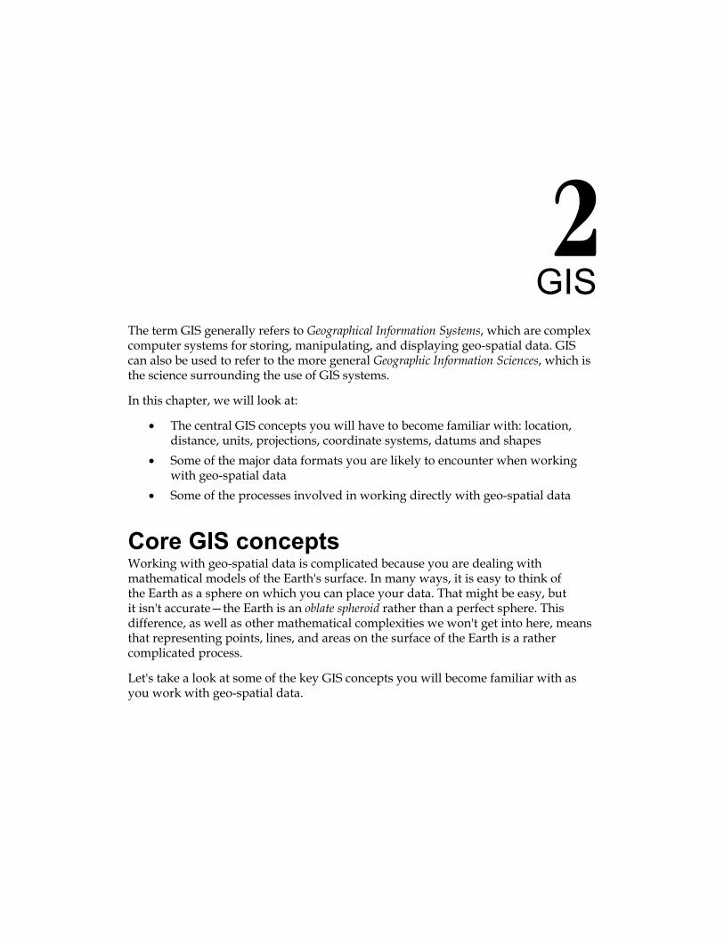
LocationLocations represent points on the surface of the Earth. One of the most common ways to measure location is through the use of latitude and longitude coordinates. For example, my current location (as measured by a GPS receiver) is 38.167446 degrees south and 176.234436 degrees east. What do these numbers mean and how are they useful?
Think of the Earth as a hollow sphere with an axis drawn through its middle:
For any given point on the Earth's surface, you can draw a line that connects that point with the centre of the Earth, as shown in the following image:
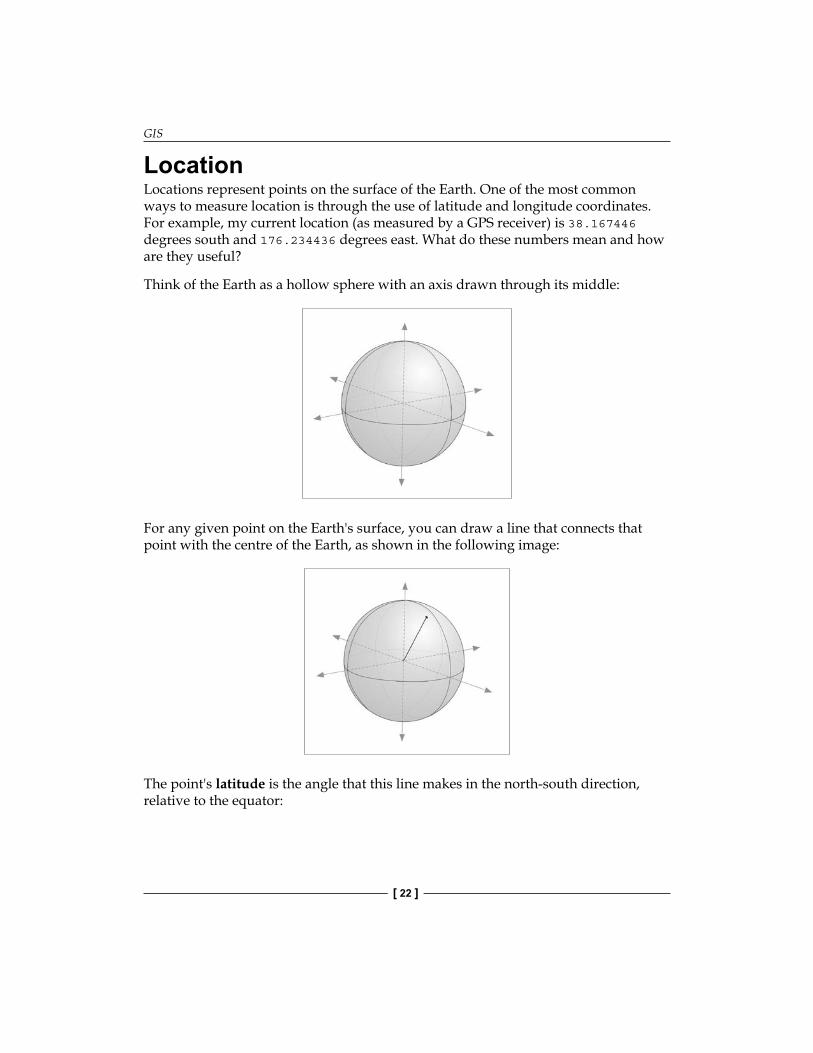
The point's latitude is the angle that this line makes in the north-south direction, relative to the equator:
Chapter 2
[ 23 ]
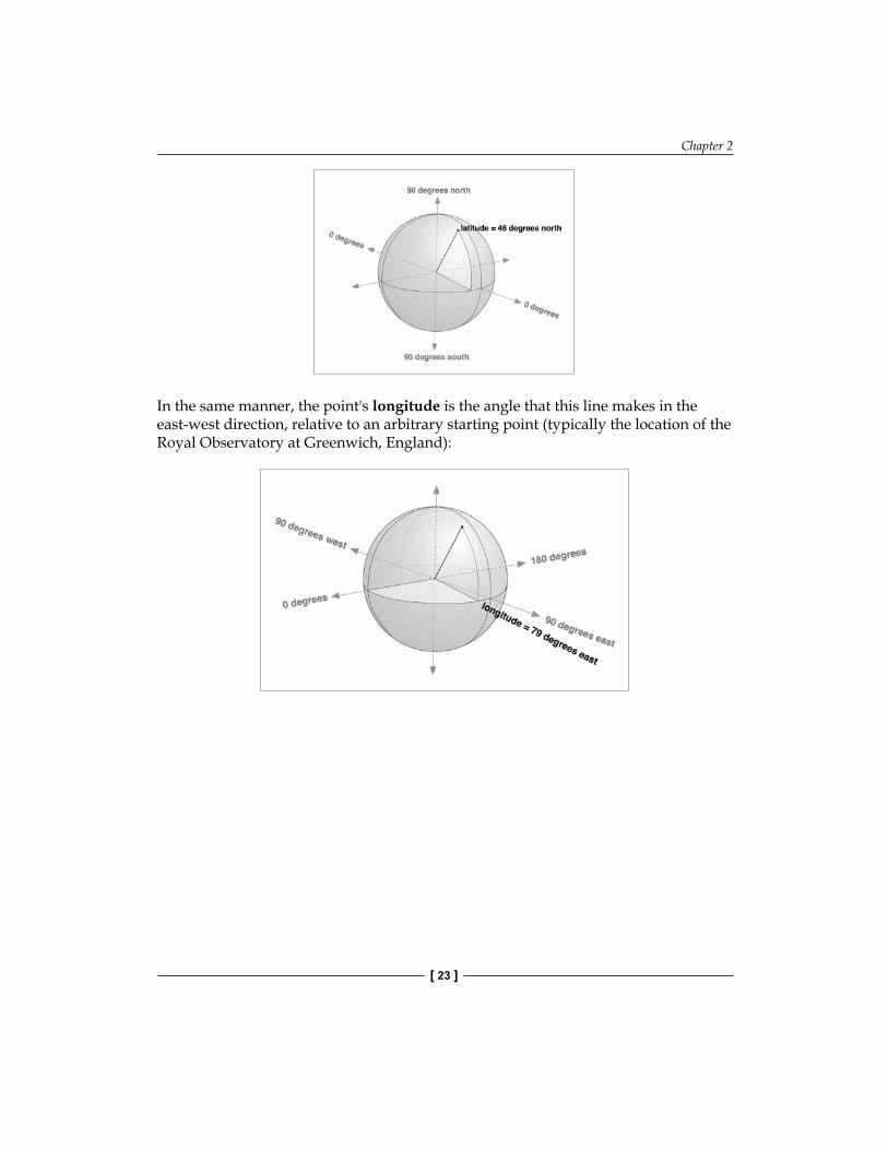
In the same manner, the point's longitude is the angle that this line makes in the east-west direction, relative to an arbitrary starting point (typically the location of the Royal Observatory at Greenwich, England):
GIS
[ 24 ]
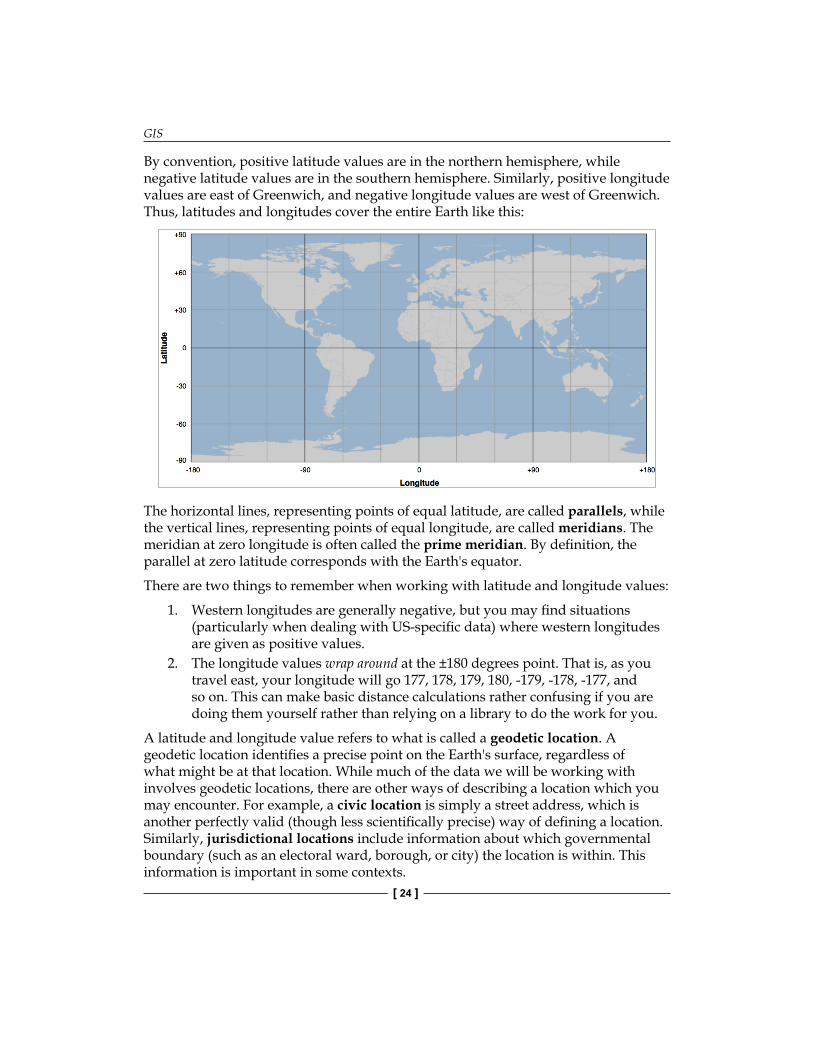
By convention, positive latitude values are in the northern hemisphere, while negative latitude values are in the southern hemisphere. Similarly, positive longitude values are east of Greenwich, and negative longitude values are west of Greenwich. Thus, latitudes and longitudes cover the entire Earth like this:
The horizontal lines, representing points of equal latitude, are called parallels, while the vertical lines, representing points of equal longitude, are called meridians. The meridian at zero longitude is often called the prime meridian. By definition, the parallel at zero latitude corresponds with the Earth's equator.
There are two things to remember when working with latitude and longitude values:
1. Western longitudes are generally negative, but you may find situations (particularly when dealing with US-specific data) where western longitudes are given as positive values.
2. The longitude values wrap around at the ±180 degrees point. That is, as you travel east, your longitude will go 177, 178, 179, 180, -179, -178, -177, and so on. This can make basic distance calculations rather confusing if you are doing them yourself rather than relying on a library to do the work for you.
A latitude and longitude value refers to what is called a geodetic location. A geodetic location identifies a precise point on the Earth's surface, regardless of what might be at that location. While much of the data we will be working with involves geodetic locations, there are other ways of describing a location which you may encounter. For example, a civic location is simply a street address, which is another perfectly valid (though less scientifically precise) way of defining a location. Similarly, jurisdictional locations include information about which governmental boundary (such as an electoral ward, borough, or city) the location is within. This information is important in some contexts.
Chapter 2
[ 25 ]
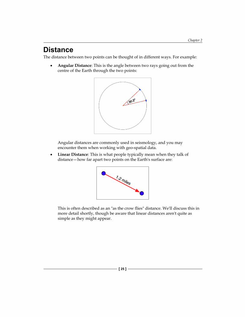
DistanceThe distance between two points can be thought of in different ways. For example:
• Angular Distance: This is the angle between two rays going out from the centre of the Earth through the two points:
Angular distances are commonly used in seismology, and you may encounter them when working with geo-spatial data.
• Linear Distance: This is what people typically mean when they talk of distance—how far apart two points on the Earth's surface are:
This is often described as an "as the crow flies" distance. We'll discuss this in more detail shortly, though be aware that linear distances aren't quite as simple as they might appear.
GIS
[ 26 ]
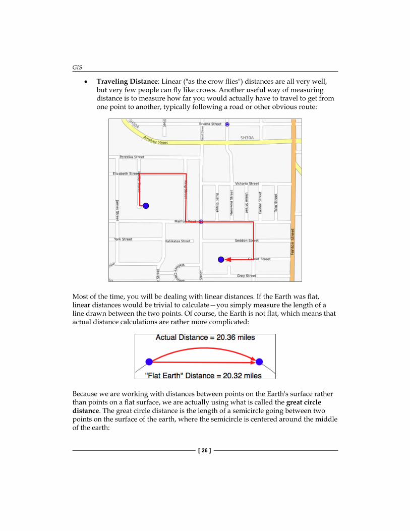
• Traveling Distance: Linear ("as the crow flies") distances are all very well, but very few people can fly like crows. Another useful way of measuring distance is to measure how far you would actually have to travel to get from one point to another, typically following a road or other obvious route:
Most of the time, you will be dealing with linear distances. If the Earth was flat, linear distances would be trivial to calculate—you simply measure the length of a line drawn between the two points. Of course, the Earth is not flat, which means that actual distance calculations are rather more complicated:
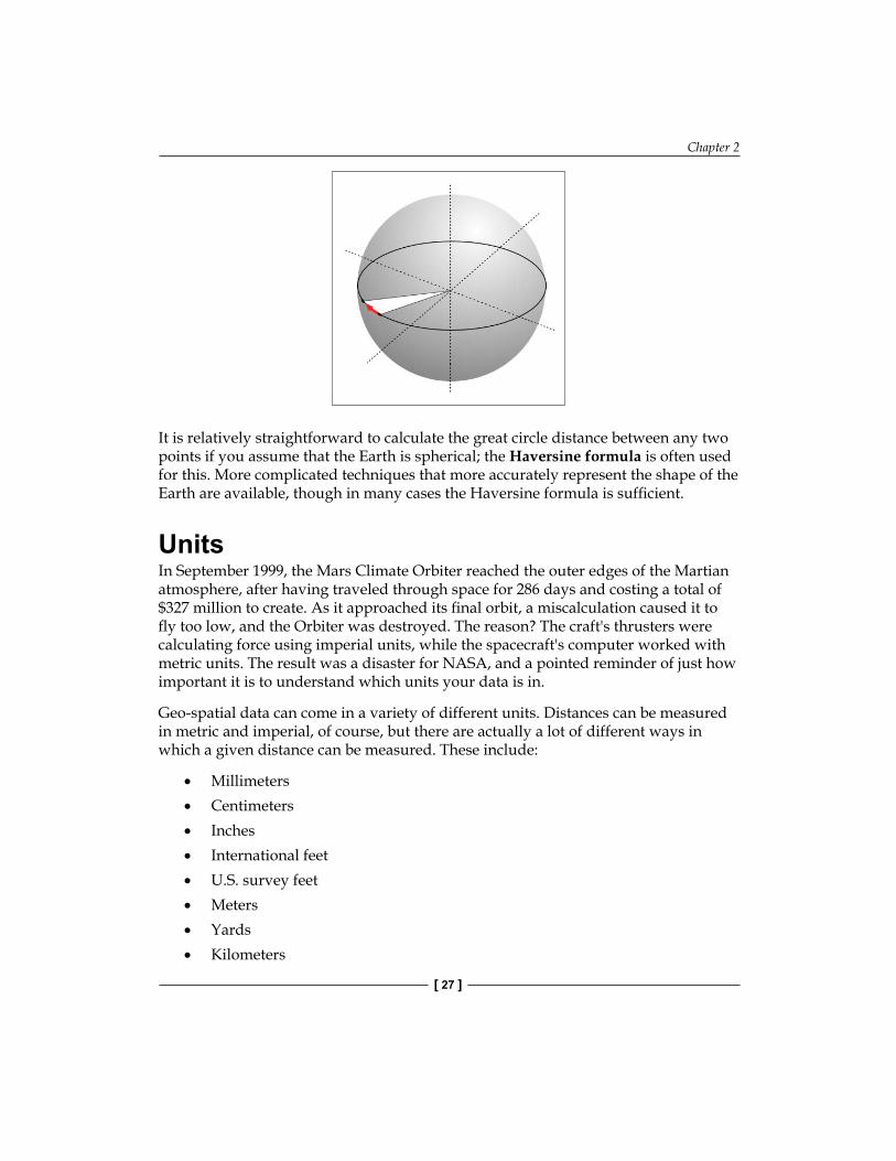
Because we are working with distances between points on the Earth's surface rather than points on a flat surface, we are actually using what is called the great circle distance. The great circle distance is the length of a semicircle going between two points on the surface of the earth, where the semicircle is centered around the middle of the earth:
Chapter 2
[ 27 ]
It is relatively straightforward to calculate the great circle distance between any two points if you assume that the Earth is spherical; the Haversine formula is often used for this. More complicated techniques that more accurately represent the shape of the Earth are available, though in many cases the Haversine formula is sufficient.
UnitsIn September 1999, the Mars Climate Orbiter reached the outer edges of the Martian atmosphere, after having traveled through space for 286 days and costing a total of $327 million to create. As it approached its final orbit, a miscalculation caused it to fly too low, and the Orbiter was destroyed. The reason? The craft's thrusters were calculating force using imperial units, while the spacecraft's computer worked with metric units. The result was a disaster for NASA, and a pointed reminder of just how important it is to understand which units your data is in.
Geo-spatial data can come in a variety of different units. Distances can be measured in metric and imperial, of course, but there are actually a lot of different ways in which a given distance can be measured. These include:
• Millimeters• Centimeters• Inches• International feet• U.S. survey feet• Meters• Yards• Kilometers
GIS
[ 28 ]
• International miles• U.S. survey (statute) miles• Nautical miles
Whenever you are working with distance data, it's important that you know which units those distances are in. You will also often find it necessary to convert data from one unit of measurement to another.
Angular measurements can also be in different units: degrees or radians. Once again, you will often have to convert from one to the other.
While these are not strictly speaking different units, you will often need to convert longitude and latitude values because of the various ways these values can be represented. Traditionally, longitude and latitude values have been written using "degrees, minutes, and seconds" notation, like this:
176° 14' 4''
Another possible way of writing these numbers is to use "degrees and decimal minutes" notation:
176° 14.066'
Finally, there is the "decimal degrees" notation:
176.234436°
Decimal degrees are quite common now, mainly because these are simply floating-point numbers you can put directly into your programs, but you may also need to convert longitude and latitude values from other formats before you can use them.
Another possible issue with longitude and latitude values is that the quadrant (east, west, north, south) can sometimes be given as a separate value rather than using positive or negative values. For example:
176.234436° E
Fortunately, all these conversions are relatively straightforward. But it is important to know which units, and in which format your data is in—your software may not crash a spacecraft, but it will produce some very strange and incomprehensible results if you aren't careful.
ProjectionsCreating a two-dimensional map from the three-dimensional shape of the Earth is a process known as projection. A projection is a mathematical transformation that unwraps the three-dimensional shape of the Earth and places it onto a two-dimensional plane.
Chapter 2
[ 29 ]
Hundreds of different projections have been developed, but none of them are perfect. Indeed, it is mathematically impossible to represent the three-dimensional Earth's surface on a two-dimensional plane without introducing some sort of distortion; the trick is to choose a projection where the distortion doesn't matter for your particular use. For example, some projections represent certain areas of the Earth's surface accurately while adding major distortion to other parts of the Earth; these projections are useful for maps in the accurate portion of the Earth, but not elsewhere. Other projections distort the shape of a country while maintaining its area, while yet other projections do the opposite.
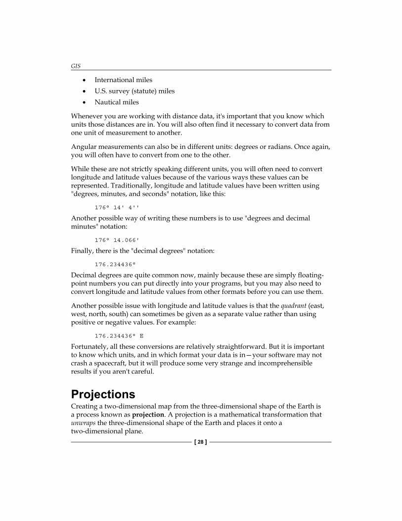
There are three main groups of projections: cylindrical, conical, and azimuthal. Let's look at each of these briefly.
Cylindrical projectionsAn easy way to understand cylindrical projections is to imagine that the Earth is like a spherical Chinese lantern, with a candle in the middle:
GIS
[ 30 ]
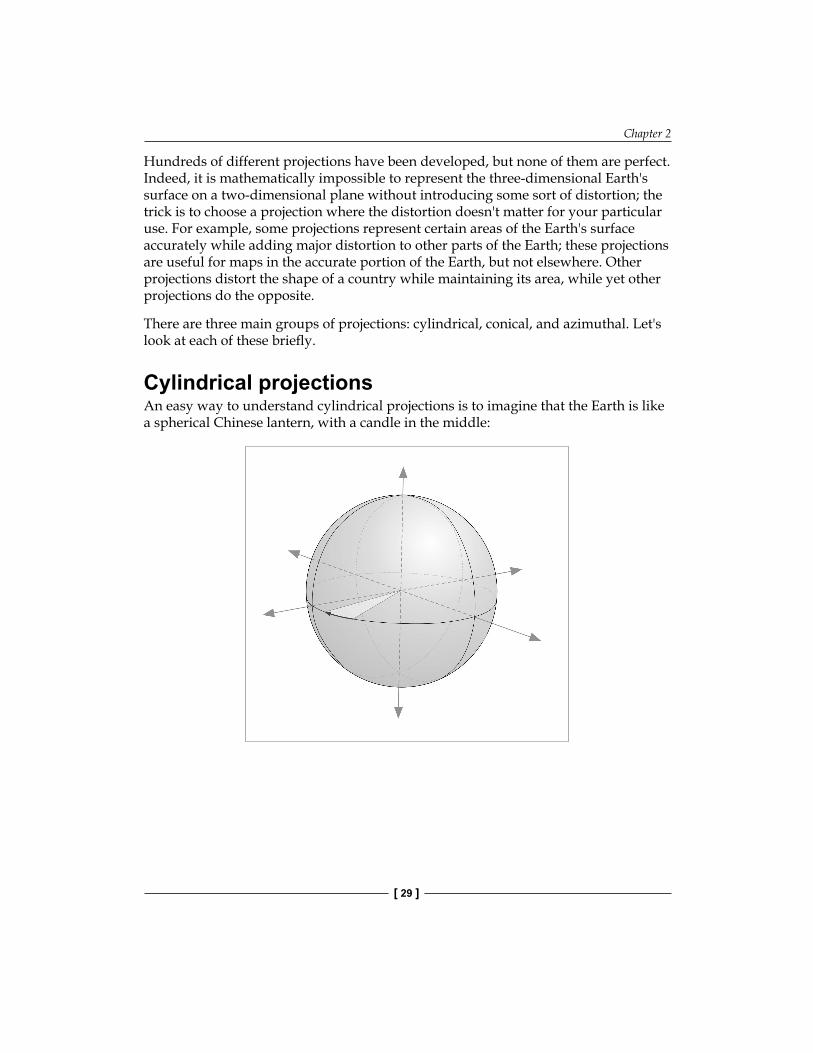
If you placed this lantern-Earth inside a paper cylinder, the candle would "project" the surface of the Earth onto the inside of the cylinder:
You can then "unwrap" this cylinder to obtain a two-dimensional image of the Earth:
Of course, this is a simplification—in reality, map projections don't actually use light sources to project the Earth's surface onto a plane, but instead use sophisticated mathematical transformations that result in less distortion. But the concept is the same.
Chapter 2
[ 31 ]
Some of the main types of cylindrical projections include the Mercator Projection, the Equal-Area Cylindrical Projection, and the Universal Transverse Mercator Projection.
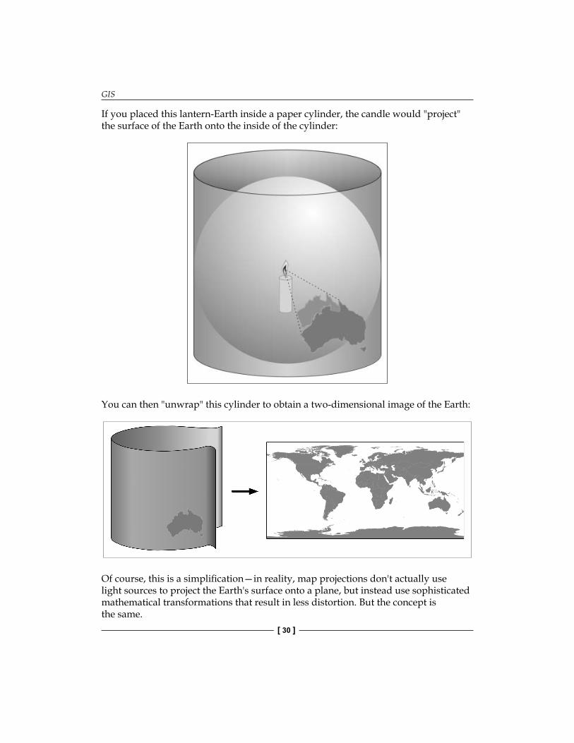
Conic projectionsA conic projection is obtained by projecting the Earth's surface onto a cone:
Some of the more common types of conic projections include the Albers Equal-Area Projection, the Lambert Conformal Conic Projection, and the Equidistant Projection.
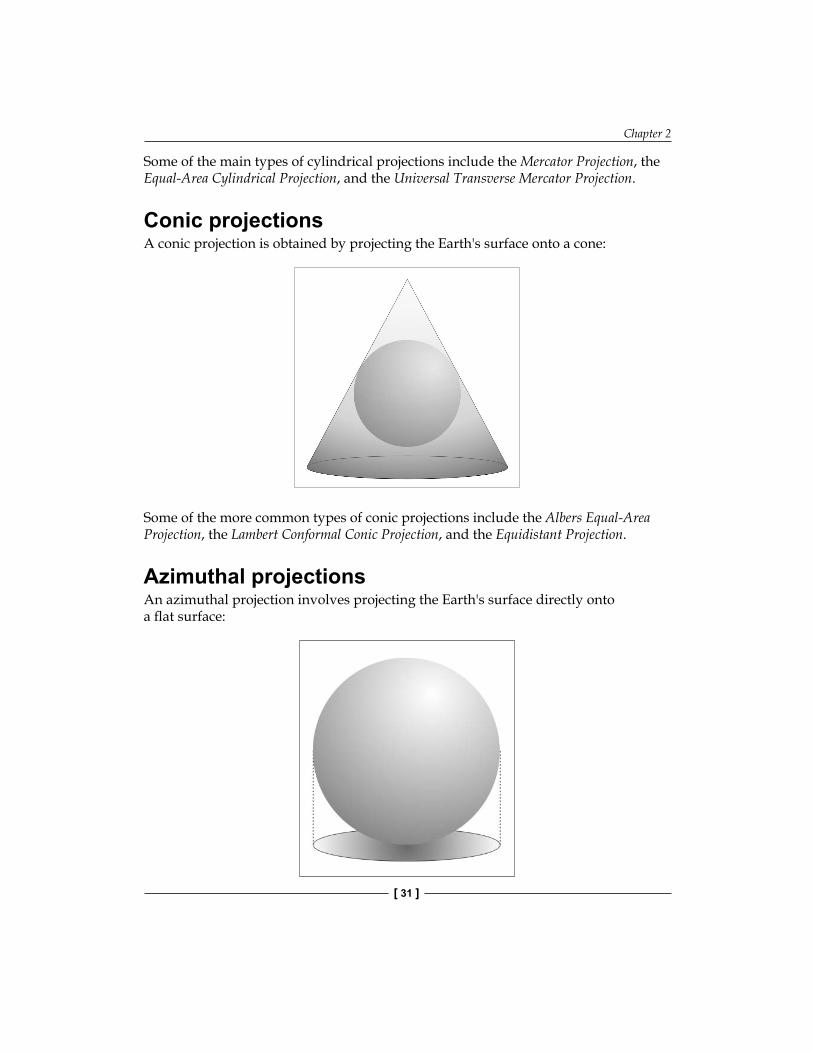
Azimuthal projectionsAn azimuthal projection involves projecting the Earth's surface directly onto a flat surface:
GIS
[ 32 ]
Azimuthal projections are centered around a single point, and don't generally show the entire Earth's surface. They do, however, emphasize the spherical nature of the Earth. In many ways, azimuthal projections depict the Earth as it would be seen from space.
Some of the main types of azimuthal projections include the Gnomonic Projection, the Lambert Equal-Area Azimuthal Projection, and the Orthographic Projection.
The nature of map projectionsAs mentioned earlier, there is no such thing as a perfect projection—every projection distorts the Earth's surface in some way. Indeed, the mathematician Carl Gausse proved that it is mathematically impossible to project a three-dimensional shape such as a sphere onto a flat plane without introducing some sort of distortion. This is why there are so many different types of projections—some projections are more suited to a given purpose, but no projection can do everything.
Whenever you create or work with geo-spatial data, it is essential that you know which projection has been used to create that data. Without knowing the projection, you won't be able to plot data or perform accurate calculations.
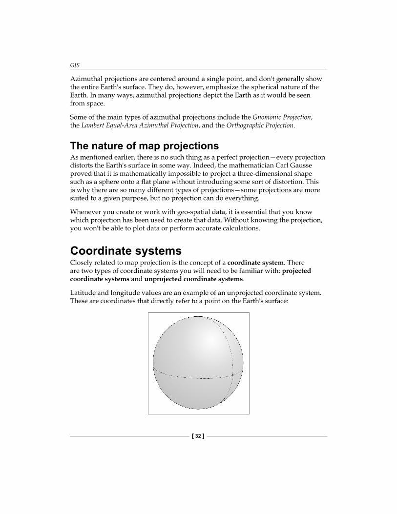
Coordinate systemsClosely related to map projection is the concept of a coordinate system. There are two types of coordinate systems you will need to be familiar with: projected coordinate systems and unprojected coordinate systems.
Latitude and longitude values are an example of an unprojected coordinate system. These are coordinates that directly refer to a point on the Earth's surface:
Chapter 2
[ 33 ]
Unprojected coordinates are useful because they can accurately represent a desired point on the Earth's surface, but they also make it very difficult to perform distance and other geo-spatial calculations.
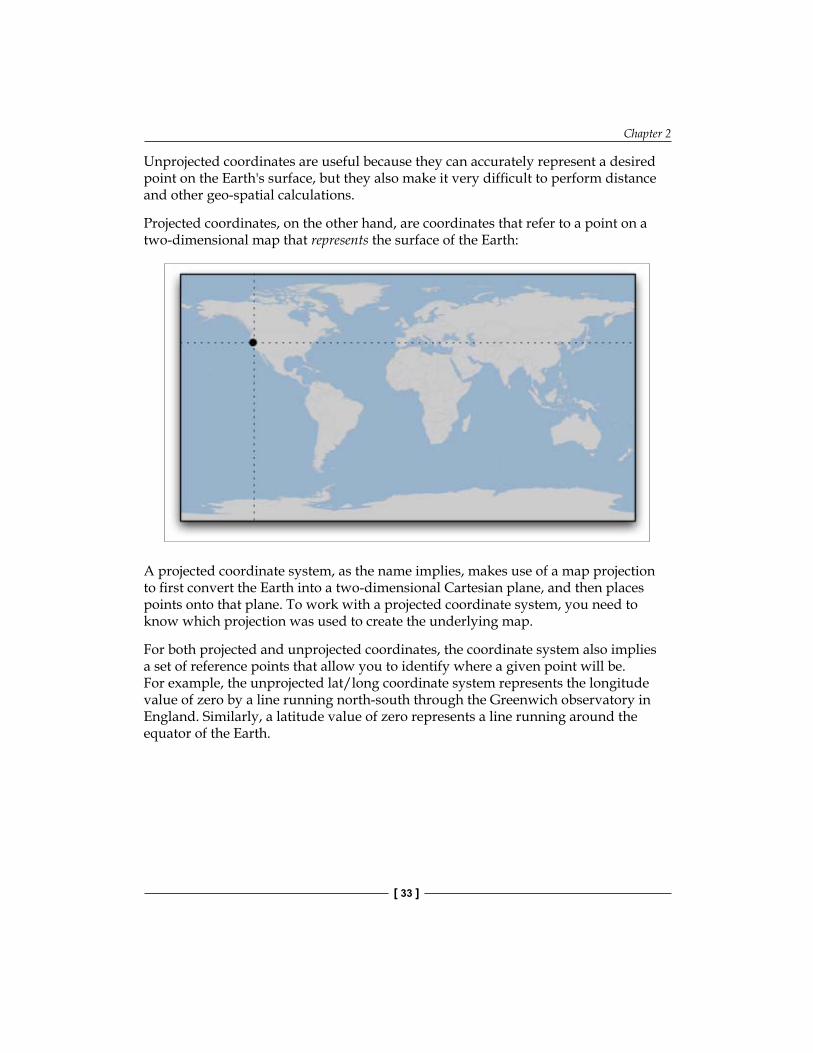
Projected coordinates, on the other hand, are coordinates that refer to a point on a two-dimensional map that represents the surface of the Earth:
A projected coordinate system, as the name implies, makes use of a map projection to first convert the Earth into a two-dimensional Cartesian plane, and then places points onto that plane. To work with a projected coordinate system, you need to know which projection was used to create the underlying map.
For both projected and unprojected coordinates, the coordinate system also implies a set of reference points that allow you to identify where a given point will be. For example, the unprojected lat/long coordinate system represents the longitude value of zero by a line running north-south through the Greenwich observatory in England. Similarly, a latitude value of zero represents a line running around the equator of the Earth.
GIS
[ 34 ]
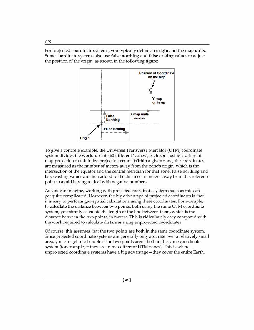
For projected coordinate systems, you typically define an origin and the map units. Some coordinate systems also use false northing and false easting values to adjust the position of the origin, as shown in the following figure:
To give a concrete example, the Universal Transverse Mercator (UTM) coordinate system divides the world up into 60 different "zones", each zone using a different map projection to minimize projection errors. Within a given zone, the coordinates are measured as the number of meters away from the zone's origin, which is the intersection of the equator and the central meridian for that zone. False northing and false easting values are then added to the distance in meters away from this reference point to avoid having to deal with negative numbers.
As you can imagine, working with projected coordinate systems such as this can get quite complicated. However, the big advantage of projected coordinates is that it is easy to perform geo-spatial calculations using these coordinates. For example, to calculate the distance between two points, both using the same UTM coordinate system, you simply calculate the length of the line between them, which is the distance between the two points, in meters. This is ridiculously easy compared with the work required to calculate distances using unprojected coordinates.
Of course, this assumes that the two points are both in the same coordinate system. Since projected coordinate systems are generally only accurate over a relatively small area, you can get into trouble if the two points aren't both in the same coordinate system (for example, if they are in two different UTM zones). This is where unprojected coordinate systems have a big advantage—they cover the entire Earth.
Chapter 2
[ 35 ]
DatumsRoughly speaking, a datum is a mathematical model of the Earth used to describe locations on the Earth's surface. A datum consists of a set of reference points, often combined with a model of the shape of the Earth. The reference points are used to describe the location of other points on the Earth's surface, while the model of the Earth's shape is used when projecting the Earth's surface onto a two-dimensional plane. Thus, datums are used by both map projections and coordinate systems.
While there are hundreds of different datums in use throughout the world, most of these only apply to a localized area. There are three main reference datums that cover larger areas and which you are likely to encounter when working with geo-spatial data:
• NAD 27: This is the North American datum of 1927. It includes a definition of the Earth's shape (using a model called the Clarke Spheroid of 1866) and a set of reference points centered around Meades Ranch in Kansas. NAD 27 can be thought of as a local datum covering North America.
• NAD 83: The North American datum of 1983. This datum makes use of a more complex model of the Earth's shape (the 1980 Geodetic Reference System, GRS 80). NAD 83 can be thought of as a local datum covering the United States, Canada, Mexico, and Central America.
• WGS 84: The World geodetic system of 1984. This is a global datum covering the entire Earth. It makes use of yet another model of the Earth's shape (the Earth Gravitational Model of 1996, EGM 96) and uses reference points based on the IERS International Reference Meridian. WGS 84 is a very popular datum. When dealing with geo-spatial data covering the United States, WGS 84 is basically identical to NAD 83. WGS 84 also has the distinction of being used by Global Positioning System satellites, so all data captured by GPS units will use this datum.
While WGS 84 is the most common datum in use today, a lot of geo-spatial data makes use of other datums. Whenever you are dealing with a coordinate value, it is important to know which datum was used to calculate that coordinate. A given point in NAD 27, for example, may be several hundred feet away from that same coordinate expressed in WGS 84. Thus, it is vital that you know which datum is being used for a given set of geo-spatial data, and convert to a different datum where necessary.
GIS
[ 36 ]
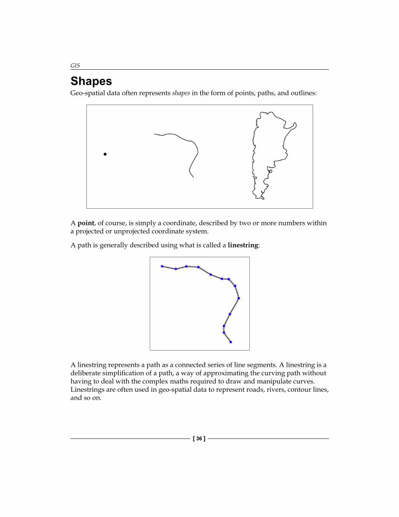
ShapesGeo-spatial data often represents shapes in the form of points, paths, and outlines:
A point, of course, is simply a coordinate, described by two or more numbers within a projected or unprojected coordinate system.
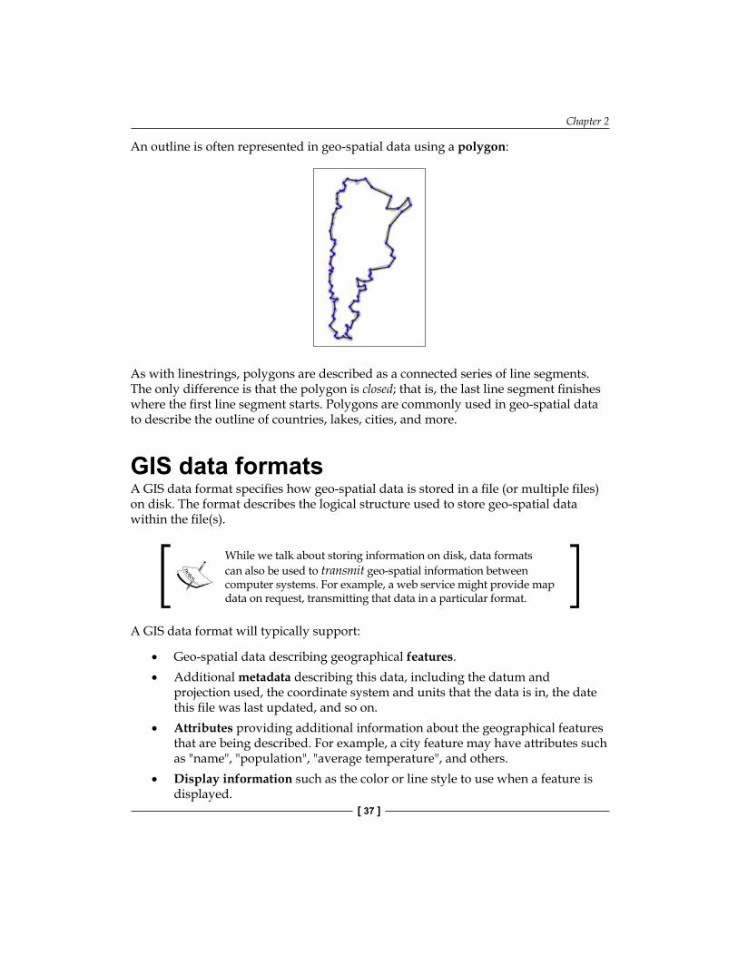
A path is generally described using what is called a linestring:
A linestring represents a path as a connected series of line segments. A linestring is a deliberate simplification of a path, a way of approximating the curving path without having to deal with the complex maths required to draw and manipulate curves. Linestrings are often used in geo-spatial data to represent roads, rivers, contour lines, and so on.
Chapter 2
[ 37 ]
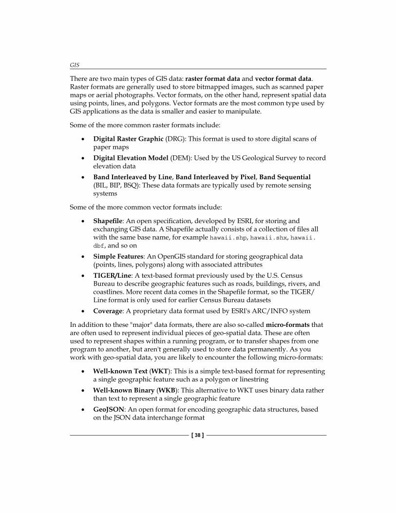
An outline is often represented in geo-spatial data using a polygon:
As with linestrings, polygons are described as a connected series of line segments. The only difference is that the polygon is closed; that is, the last line segment finishes where the first line segment starts. Polygons are commonly used in geo-spatial data to describe the outline of countries, lakes, cities, and more.
GIS data formatsA GIS data format specifies how geo-spatial data is stored in a file (or multiple files) on disk. The format describes the logical structure used to store geo-spatial data within the file(s).
While we talk about storing information on disk, data formats can also be used to transmit geo-spatial information between computer systems. For example, a web service might provide map data on request, transmitting that data in a particular format.
A GIS data format will typically support:
• Geo-spatial data describing geographical features.• Additional metadata describing this data, including the datum and
projection used, the coordinate system and units that the data is in, the date this file was last updated, and so on.
• Attributes providing additional information about the geographical features that are being described. For example, a city feature may have attributes such as "name", "population", "average temperature", and others.
• Display information such as the color or line style to use when a feature is displayed.
GIS
[ 38 ]
There are two main types of GIS data: raster format data and vector format data. Raster formats are generally used to store bitmapped images, such as scanned paper maps or aerial photographs. Vector formats, on the other hand, represent spatial data using points, lines, and polygons. Vector formats are the most common type used by GIS applications as the data is smaller and easier to manipulate.
Some of the more common raster formats include:
• Digital Raster Graphic (DRG): This format is used to store digital scans of paper maps
• Digital Elevation Model (DEM): Used by the US Geological Survey to record elevation data
• Band Interleaved by Line, Band Interleaved by Pixel, Band Sequential (BIL, BIP, BSQ): These data formats are typically used by remote sensing systems
Some of the more common vector formats include:
• Shapefile: An open specification, developed by ESRI, for storing and exchanging GIS data. A Shapefile actually consists of a collection of files all with the same base name, for example hawaii.shp, hawaii.shx, hawaii.dbf, and so on
• Simple Features: An OpenGIS standard for storing geographical data (points, lines, polygons) along with associated attributes
• TIGER/Line: A text-based format previously used by the U.S. Census Bureau to describe geographic features such as roads, buildings, rivers, and coastlines. More recent data comes in the Shapefile format, so the TIGER/Line format is only used for earlier Census Bureau datasets
• Coverage: A proprietary data format used by ESRI's ARC/INFO system
In addition to these "major" data formats, there are also so-called micro-formats that are often used to represent individual pieces of geo-spatial data. These are often used to represent shapes within a running program, or to transfer shapes from one program to another, but aren't generally used to store data permanently. As you work with geo-spatial data, you are likely to encounter the following micro-formats:
• Well-known Text (WKT): This is a simple text-based format for representing a single geographic feature such as a polygon or linestring
• Well-known Binary (WKB): This alternative to WKT uses binary data rather than text to represent a single geographic feature
• GeoJSON: An open format for encoding geographic data structures, based on the JSON data interchange format
Chapter 2
[ 39 ]
• Geography Markup Language (GML): An XML-based open standard for exchanging GIS data
Whenever you work with geo-spatial data, you need to know which format the data is in so that you can extract the information you need from the file(s), and where necessary transform the data from one format to another.
Working with GIS data manuallyLet's take a brief look at the process of working with GIS data manually. Before we can begin, there are two things you need to do:
• Obtain some GIS data• Install the GDAL Python library so that you can read the necessary data files
Let's use the U.S. Census Bureau's website to download a set of vector maps for the various U.S. states. The main site for obtaining GIS data from the U.S. Census Bureau can be found at:
http://www.census.gov/geo/www/tiger
To make things simpler, though, let's bypass the website and directly download the file we need:
http://www2.census.gov/geo/tiger/TIGER2009/tl_2009_us_state.zip
The resulting file, tl_2009_us_state.zip, should be a ZIP-format archive. After uncompressing the archive, you should have the following files:
tl_2009_us_state.dbf
tl_2009_us_state.prj
tl_2009_us_state.shp
tl_2009_us_state.shp.xml
tl_2009_us_state.shx
These files make up a Shapefile containing the outlines of all the U.S. states. Place these files together in a convenient directory.
We next have to download the GDAL Python library. The main website for GDAL can be found at:
http://gdal.org
GIS
[ 40 ]
The easiest way to install GDAL onto a Windows or Unix machine is to use the FWTools installer, which can be downloaded from the following site:
http://fwtools.maptools.org
If you are running Mac OS X, you can find a complete installer for GDAL at:
http://www.kyngchaos.com/software/frameworks
After installing GDAL, you can check that it works by typing import osgeo into the Python command prompt; if the Python command prompt reappears with no error message, GDAL was successfully installed and you are all set to go:
>>> import osgeo
>>>
Now that we have some data to work with, let's take a look at it. You can either type the following directly into the command prompt, or else save it as a Python script so you can run it whenever you wish (let's call this analyze.py):
import osgeo.ogr
shapefile = osgeo.ogr.Open("tl_2009_us_state.shp")numLayers = shapefile.GetLayerCount()
print "Shapefile contains %d layers" % numLayersprint
for layerNum in range(numLayers): layer = shapefile.GetLayer (layerNum) spatialRef = layer.GetSpatialRef().ExportToProj4() numFeatures = layer.GetFeatureCount() print "Layer %d has spatial reference %s" % (layerNum, spatialRef) print "Layer %d has %d features:" % (layerNum, numFeatures) print
for featureNum in range(numFeatures): feature = layer.GetFeature(featureNum) featureName = feature.GetField("NAME")
print "Feature %d has name %s" % (featureNum, featureName)
This gives us a quick summary of how the Shapefile's data is structured:
Shapefile contains 1 layers
Layer 0 has spatial reference +proj=longlat +ellps=GRS80 +datum=NAD83 +no_defs
Layer 0 has 56 features:
Feature 0 has name American Samoa
Chapter 2
[ 41 ]
Feature 1 has name Nevada
Feature 2 has name Arizona
Feature 3 has name Wisconsin
...
Feature 53 has name California
Feature 54 has name Ohio
Feature 55 has name Texas
This shows us that the data we downloaded consists of one layer, with 56 individual features corresponding to the various states and protectorates in the U.S. It also tells us the "spatial reference" for this layer, which tells us that the coordinates are stored as latitude and longitude values, using the GRS80 ellipsoid and the NAD83 datum.
As you can see from the above example, using GDAL to extract data from Shapefiles is quite straightforward. Let's continue with another example. This time, we'll look at the details for feature 2, Arizona:
import osgeo.ogr
shapefile = osgeo.ogr.Open("tl_2009_us_state.shp")layer = shapefile.GetLayer(0)feature = layer.GetFeature(2)
print "Feature 2 has the following attributes:"print
attributes = feature.items()
for key,value in attributes.items(): print " %s = %s" % (key, value) print
geometry = feature.GetGeometryRef()geometryName = geometry.GetGeometryName()
print "Feature's geometry data consists of a %s" % geometryName
Running this produces the following:
Feature 2 has the following attributes:
DIVISION = 8
INTPTLAT = +34.2099643
NAME = Arizona
STUSPS = AZ
FUNCSTAT = A
REGION = 4
GIS
[ 42 ]
LSAD = 00
AWATER = 1026257344.0
STATENS = 01779777
MTFCC = G4000
INTPTLON = -111.6024010
STATEFP = 04
ALAND = 294207737677.0
Feature's geometry data consists of a POLYGON
The meaning of the various attributes is described on the U.S. Census Bureau's website, but what interests us right now is the feature's geometry. A Geometry object is a complex structure that holds some geo-spatial data, often using nested Geometry objects to reflect the way the geo-spatial data is organized. So far, we've discovered that Arizona's geometry consists of a polygon. Let's now take a closer look at this polygon:
import osgeo.ogr
def analyzeGeometry(geometry, indent=0): s = [] s.append(" " * indent) s.append(geometry.GetGeometryName()) if geometry.GetPointCount() > 0: s.append(" with %d data points" % geometry.GetPointCount()) if geometry.GetGeometryCount() > 0: s.append(" containing:")
print "".join(s)
for i in range(geometry.GetGeometryCount()): analyzeGeometry(geometry.GetGeometryRef(i), indent+1)
shapefile = osgeo.ogr.Open("tl_2009_us_state.shp")layer = shapefile.GetLayer(0)feature = layer.GetFeature(2)geometry = feature.GetGeometryRef()
analyzeGeometry(geometry)
The analyzeGeometry() function gives a useful idea of how the geometry has been structured:
POLYGON containing:
LINEARRING with 10168 data points
In GDAL (or more specifically the OGR Simple Feature library we are using here), polygons are defined as a single outer "ring" with optional inner rings that define "holes" in the polygon (for example, to show the outline of a lake).
Chapter 2
[ 43 ]
Arizona is a relatively simple feature in that it consists of only one polygon. If we ran the same program over California (feature 53 in our Shapefile), the output would be somewhat more complicated:
MULTIPOLYGON containing:
POLYGON containing:
LINEARRING with 93 data points
POLYGON containing:
LINEARRING with 77 data points
POLYGON containing:
LINEARRING with 191 data points
POLYGON containing:
LINEARRING with 152 data points
POLYGON containing:
LINEARRING with 393 data points
POLYGON containing:
LINEARRING with 121 data points
POLYGON containing:
LINEARRING with 10261 data points
As you can see, California is made up of seven distinct polygons, each defined by a single linear ring. This is because California is on the coast, and includes six outlying islands as well as the main inland body of the state.
Let's finish this analysis of the U.S. state Shapefile by answering a simple question: what is the distance from the northernmost point to the southernmost point in California? There are various ways we could answer this question, but for now we'll do it by hand. Let's start by identifying the northernmost and southernmost points in California:
import osgeo.ogr
def findPoints(geometry, results): for i in range(geometry.GetPointCount()): x,y,z = geometry.GetPoint(i) if results['north'] == None or results['north'][1] < y: results['north'] = (x,y) if results['south'] == None or results['south'][1] > y: results['south'] = (x,y)
for i in range(geometry.GetGeometryCount()): findPoints(geometry.GetGeometryRef(i), results)
shapefile = osgeo.ogr.Open("tl_2009_us_state.shp")
GIS
[ 44 ]
layer = shapefile.GetLayer(0)feature = layer.GetFeature(53)geometry = feature.GetGeometryRef()
results = {'north' : None, 'south' : None}
findPoints(geometry, results)
print "Northernmost point is (%0.4f, %0.4f)" % results['north']print "Southernmost point is (%0.4f, %0.4f)" % results['south']
The findPoints() function recursively scans through a geometry, extracting the individual points and identifying the points with the highest and lowest y (latitude) values, which are then stored in the results dictionary so that the main program can use it.
As you can see, GDAL makes it easy to work with the complex Geometry data structure. The code does require recursion, but is still trivial compared with trying to read the data directly. If you run the above program, the following will be displayed:
Northernmost point is (-122.3782, 42.0095)
Southernmost point is (-117.2049, 32.5288)
Now that we have these two points, we next want to calculate the distance between them. As described earlier, we have to use a great circle distance calculation here to allow for the curvature of the Earth's surface. We'll do this manually, using the Haversine formula:
import math
lat1 = 42.0095long1 = -122.3782
lat2 = 32.5288long2 = -117.2049
rLat1 = math.radians(lat1)rLong1 = math.radians(long1)rLat2 = math.radians(lat2)rLong2 = math.radians(long2)
dLat = rLat2 - rLat1dLong = rLong2 - rLong1a = math.sin(dLat/2)**2 + math.cos(rLat1) * math.cos(rLat2) \ * math.sin(dLong/2)**2c = 2 * math.atan2(math.sqrt(a), math.sqrt(1-a))distance = 6371 * c
print "Great circle distance is %0.0f kilometers" % distance
Chapter 2
[ 45 ]
Don't worry about the complex maths involved here; basically, we are converting the latitude and longitude values to radians, calculating the difference in latitude/longitude values between the two points, and then passing the results through some trigonometric functions to obtain the great circle distance. The value of 6371 is the radius of the Earth in kilometers.
More details about the Haversine formula and how it is used in the above example can be found at http://mathforum.org/library/drmath/view/51879.html.
If you run the above program, your computer will tell you the distance from the northernmost point to the southernmost point in California:
Great circle distance is 1149 kilometers
There are, of course, other ways of calculating this. You wouldn't normally type the Haversine formula directly into your program as there are libraries that will do this for you. But we deliberately did the calculation this way to show just how it can be done.
If you would like to explore this further, you might like to try writing programs to calculate the following:
• The easternmost and westernmost points in California.• The midpoint in California. Hint: you can calculate the midpoint's longitude
by taking the average of the easternmost and westernmost longitude.• The midpoint in Arizona.• The distance between the middle of California and the middle of Arizona.
As you can see, working with GIS data manually isn't too troublesome. While the data structures and maths involved can be rather complex, using tools such as GDAL make your data accessible and easy to work with.
GIS
[ 46 ]
SummaryIn this chapter, we discussed many of the core concepts that underlie GIS development, looked briefly at the history of GIS, examined some of the more common GIS data formats, and got our hands dirty exploring U.S. state maps downloaded from the U.S. Census Bureau website. We have seen that:
• Locations are often, but not always, represented using coordinates.• Calculating the distance between two points requires you to take into
account the curvature of the Earth's surface.• You must be aware of the units used in geo-spatial data.• Map projections represent the three-dimensional shape of the Earth's surface
as a two-dimensional map.• There are three main classes of map projections: cylindrical, conic, and
azimuthal.• Datums are mathematical models of the Earth's shape.• The three most common datums in use are called NAD 27, NAD 83, and
WGS 84.• Coordinate systems describe how coordinates relate to a given point on the
Earth's surface.• Unprojected coordinate systems directly represent points on the Earth's
surface.• Projected coordinate systems use a map projection to represent the Earth as a
two-dimensional Cartesian plane, onto which coordinates are then placed.• Geo-spatial data can represent shapes in the form of points, linestrings, and
polygons.• There are a number of standard GIS data formats you might encounter. Some
data formats work with raster data, while others use vector data.• How to download map data from the U.S. Census site.• How to install and run GDAL.• How to analyze downloaded Shapefile data.• How Shapefile data is organized into geometries.• How to use the Haversine formula to manually calculate the great circle
distance between two points.
In the next chapter, we will look in more detail at the various Python libraries that can be used for working with geo-spatial data.
Python Libraries for Geo-Spatial Development
This chapter examines a number of libraries and other tools that can be used for geo-spatial development in Python.
More specifically, we will cover:
• Python libraries for reading and writing geo-spatial data• Python libraries for dealing with map projections• Libraries for analyzing and manipulating geo-spatial data directly within
your Python programs• Tools for visualizing geo-spatial data
Note that there are two types of geo-spatial tools that are not discussed in this chapter: geo-spatial databases and geo-spatial web toolkits. Both of these will be examined in detail later in this book.
Reading and writing geo-spatial dataWhile you could in theory write your own parser to read a particular geo-spatial data format, it is much easier to use an existing Python library to do this. We will look at two popular libraries for reading and writing geo-spatial data: GDAL and OGR.
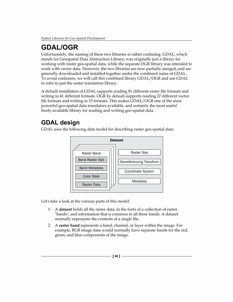
Python Libraries for Geo-Spatial Development
[ 48 ]
GDAL/OGRUnfortunately, the naming of these two libraries is rather confusing. GDAL, which stands for Geospatial Data Abstraction Library, was originally just a library for working with raster geo-spatial data, while the separate OGR library was intended to work with vector data. However, the two libraries are now partially merged, and are generally downloaded and installed together under the combined name of GDAL. To avoid confusion, we will call this combined library GDAL/OGR and use GDAL to refer to just the raster translation library.
A default installation of GDAL supports reading 81 different raster file formats and writing to 41 different formats. OGR by default supports reading 27 different vector file formats and writing to 15 formats. This makes GDAL/OGR one of the most powerful geo-spatial data translators available, and certainly the most useful freely-available library for reading and writing geo-spatial data.
GDAL designGDAL uses the following data model for describing raster geo-spatial data:
Let's take a look at the various parts of this model:
1. A dataset holds all the raster data, in the form of a collection of raster "bands", and information that is common to all these bands. A dataset normally represents the contents of a single file.
2. A raster band represents a band, channel, or layer within the image. For example, RGB image data would normally have separate bands for the red, green, and blue components of the image.
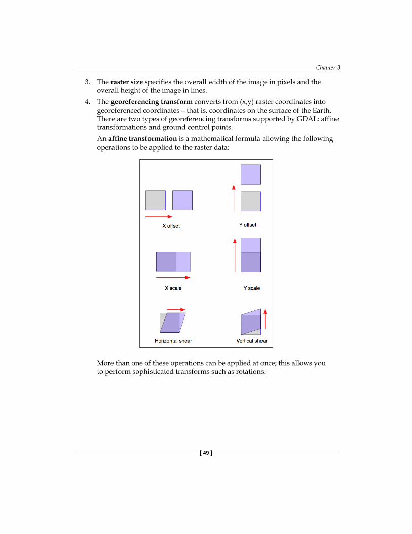
Chapter 3
[ 49 ]
3. The raster size specifies the overall width of the image in pixels and the overall height of the image in lines.
4. The georeferencing transform converts from (x,y) raster coordinates into georeferenced coordinates—that is, coordinates on the surface of the Earth. There are two types of georeferencing transforms supported by GDAL: affine transformations and ground control points.An affine transformation is a mathematical formula allowing the following operations to be applied to the raster data:
More than one of these operations can be applied at once; this allows you to perform sophisticated transforms such as rotations.
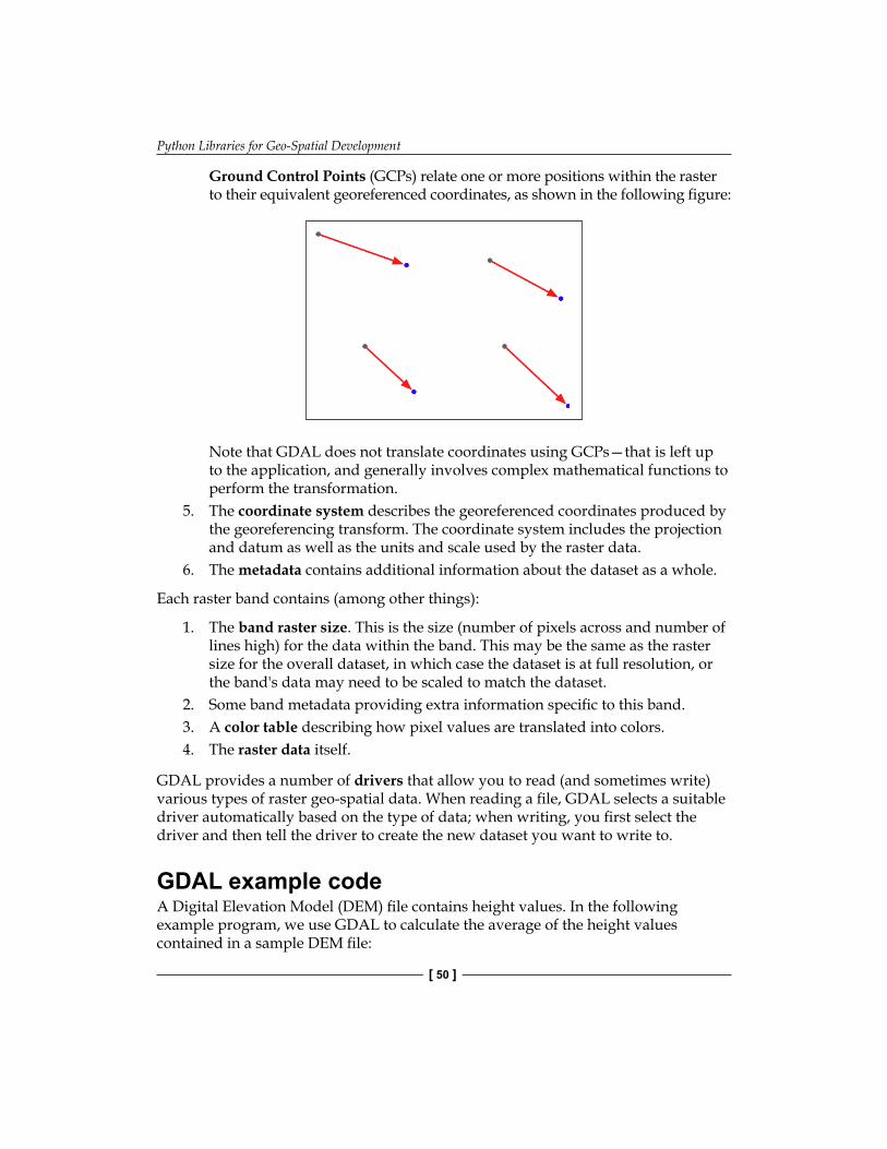
Python Libraries for Geo-Spatial Development
[ 50 ]
Ground Control Points (GCPs) relate one or more positions within the raster to their equivalent georeferenced coordinates, as shown in the following figure:
Note that GDAL does not translate coordinates using GCPs—that is left up to the application, and generally involves complex mathematical functions to perform the transformation.
5. The coordinate system describes the georeferenced coordinates produced by the georeferencing transform. The coordinate system includes the projection and datum as well as the units and scale used by the raster data.
6. The metadata contains additional information about the dataset as a whole.
Each raster band contains (among other things):
1. The band raster size. This is the size (number of pixels across and number of lines high) for the data within the band. This may be the same as the raster size for the overall dataset, in which case the dataset is at full resolution, or the band's data may need to be scaled to match the dataset.
2. Some band metadata providing extra information specific to this band.3. A color table describing how pixel values are translated into colors.4. The raster data itself.
GDAL provides a number of drivers that allow you to read (and sometimes write) various types of raster geo-spatial data. When reading a file, GDAL selects a suitable driver automatically based on the type of data; when writing, you first select the driver and then tell the driver to create the new dataset you want to write to.
GDAL example codeA Digital Elevation Model (DEM) file contains height values. In the following example program, we use GDAL to calculate the average of the height values contained in a sample DEM file:
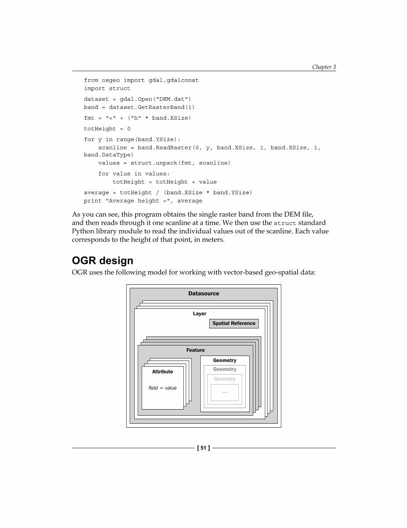
Chapter 3
[ 51 ]
from osgeo import gdal,gdalconstimport struct
dataset = gdal.Open("DEM.dat")band = dataset.GetRasterBand(1)
fmt = "<" + ("h" * band.XSize)
totHeight = 0
for y in range(band.YSize): scanline = band.ReadRaster(0, y, band.XSize, 1, band.XSize, 1, band.DataType) values = struct.unpack(fmt, scanline)
for value in values: totHeight = totHeight + value
average = totHeight / (band.XSize * band.YSize)print "Average height =", average
As you can see, this program obtains the single raster band from the DEM file, and then reads through it one scanline at a time. We then use the struct standard Python library module to read the individual values out of the scanline. Each value corresponds to the height of that point, in meters.
OGR designOGR uses the following model for working with vector-based geo-spatial data:
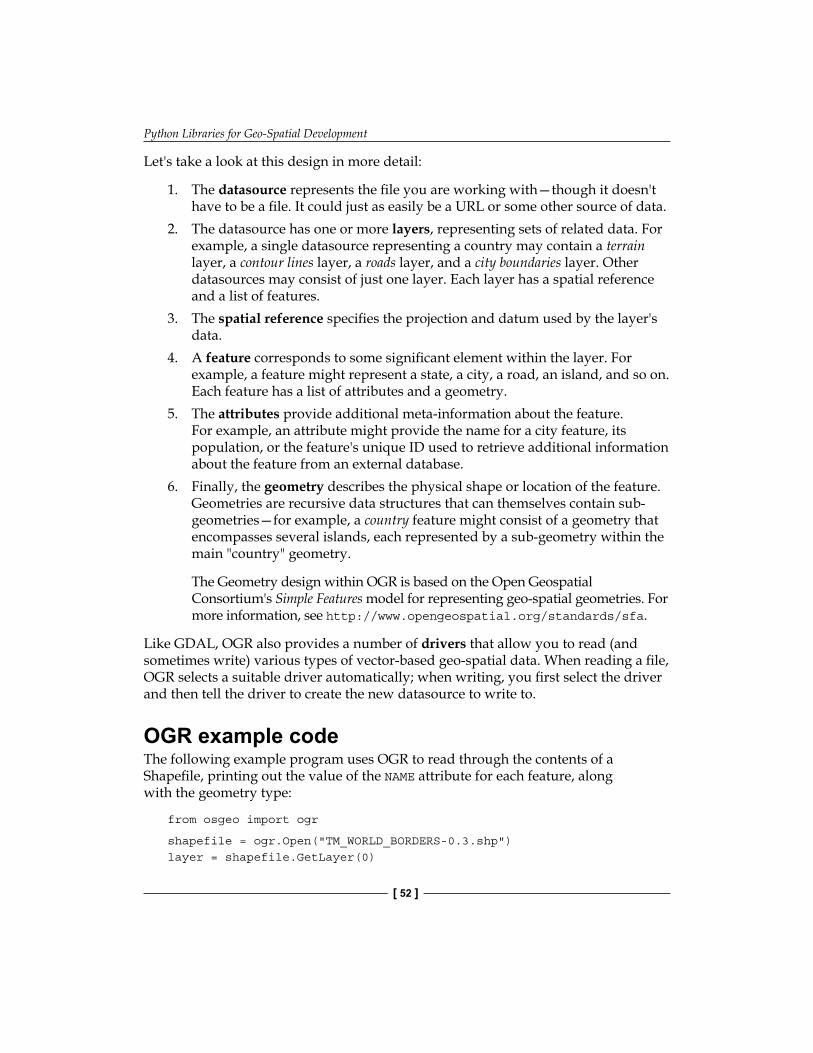
Python Libraries for Geo-Spatial Development
[ 52 ]
Let's take a look at this design in more detail:
1. The datasource represents the file you are working with—though it doesn't have to be a file. It could just as easily be a URL or some other source of data.
2. The datasource has one or more layers, representing sets of related data. For example, a single datasource representing a country may contain a terrain layer, a contour lines layer, a roads layer, and a city boundaries layer. Other datasources may consist of just one layer. Each layer has a spatial reference and a list of features.
3. The spatial reference specifies the projection and datum used by the layer's data.
4. A feature corresponds to some significant element within the layer. For example, a feature might represent a state, a city, a road, an island, and so on. Each feature has a list of attributes and a geometry.
5. The attributes provide additional meta-information about the feature. For example, an attribute might provide the name for a city feature, its population, or the feature's unique ID used to retrieve additional information about the feature from an external database.
6. Finally, the geometry describes the physical shape or location of the feature. Geometries are recursive data structures that can themselves contain sub-geometries—for example, a country feature might consist of a geometry that encompasses several islands, each represented by a sub-geometry within the main "country" geometry.
The Geometry design within OGR is based on the Open Geospatial Consortium's Simple Features model for representing geo-spatial geometries. For more information, see http://www.opengeospatial.org/standards/sfa.
Like GDAL, OGR also provides a number of drivers that allow you to read (and sometimes write) various types of vector-based geo-spatial data. When reading a file, OGR selects a suitable driver automatically; when writing, you first select the driver and then tell the driver to create the new datasource to write to.
OGR example codeThe following example program uses OGR to read through the contents of a Shapefile, printing out the value of the NAME attribute for each feature, along with the geometry type:
from osgeo import ogr
shapefile = ogr.Open("TM_WORLD_BORDERS-0.3.shp")layer = shapefile.GetLayer(0)
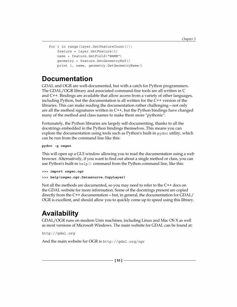
Chapter 3
[ 53 ]
for i in range(layer.GetFeatureCount()): feature = layer.GetFeature(i) name = feature.GetField("NAME") geometry = feature.GetGeometryRef() print i, name, geometry.GetGeometryName()
DocumentationGDAL and OGR are well-documented, but with a catch for Python programmers. The GDAL/OGR library and associated command-line tools are all written in C and C++. Bindings are available that allow access from a variety of other languages, including Python, but the documentation is all written for the C++ version of the libraries. This can make reading the documentation rather challenging—not only are all the method signatures written in C++, but the Python bindings have changed many of the method and class names to make them more "pythonic".
Fortunately, the Python libraries are largely self-documenting, thanks to all the docstrings embedded in the Python bindings themselves. This means you can explore the documentation using tools such as Python's built-in pydoc utility, which can be run from the command line like this:
pydoc -g osgeo
This will open up a GUI window allowing you to read the documentation using a web browser. Alternatively, if you want to find out about a single method or class, you can use Python's built-in help() command from the Python command line, like this:
>>> import osgeo.ogr
>>> help(osgeo.ogr.Datasource.CopyLayer)
Not all the methods are documented, so you may need to refer to the C++ docs on the GDAL website for more information. Some of the docstrings present are copied directly from the C++ documentation—but, in general, the documentation for GDAL/OGR is excellent, and should allow you to quickly come up to speed using this library.
AvailabilityGDAL/OGR runs on modern Unix machines, including Linux and Mac OS X as well as most versions of Microsoft Windows. The main website for GDAL can be found at:
http://gdal.org
And the main website for OGR is http://gdal.org/ogr

Python Libraries for Geo-Spatial Development
[ 54 ]
To download GDAL/OGR, follow the Downloads link on the main GDAL website. Windows users may find the "FWTools" package useful as it provides a wide range of geo-spatial software for win32 machines, including GDAL/OGR and its Python bindings. FWTools can be found at:
http://fwtools.maptools.org
For those running Mac OS X, pre-built binaries for GDAL/OGR can be obtained from:
http://www.kyngchaos.com/software/frameworks
Make sure that you install GDAL version 1.7 or later as you will need this version to work through the examples in this book.
Being an open source package, the complete source code for GDAL/OGR is available from the website, so you can compile it yourself. Most people, however, will simply want to use a pre-built binary version.
Dealing with projectionsOne of the challenges of working with geo-spatial data is that geodetic locations (points on the Earth's surface) are mapped into a two-dimensional cartesian plane using a cartographic projection. We looked at projections in the previous chapter—whenever you have some geo-spatial data, you need to know which projection that data uses. You also need to know the datum (model of the Earth's shape) assumed by the data.
A common challenge when dealing with geo-spatial data is that you have to convert data from one projection/datum to another. Fortunately, there is a Python library that makes this task easy: pyproj.
pyprojpyproj is a Python wrapper around another library called PROJ.4. PROJ.4 is an abbreviation for version 4 of the PROJ library. PROJ was originally written by the U.S. Geological Survey for dealing with map projections, and has been widely used by geo-spatial software for many years. The pyproj library makes it possible to access the functionality of PROJ.4 from within your Python programs.
DesignThe pyproj library consists of the following pieces:
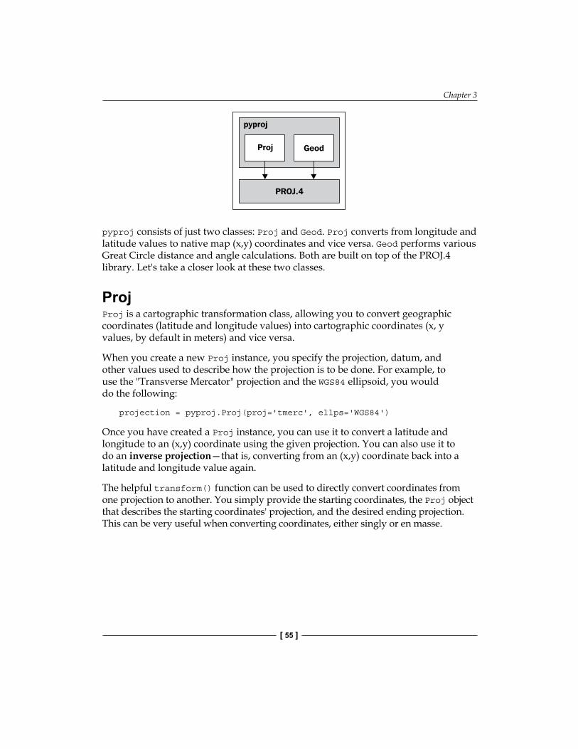
Chapter 3
[ 55 ]
pyproj consists of just two classes: Proj and Geod. Proj converts from longitude and latitude values to native map (x,y) coordinates and vice versa. Geod performs various Great Circle distance and angle calculations. Both are built on top of the PROJ.4 library. Let's take a closer look at these two classes.
ProjProj is a cartographic transformation class, allowing you to convert geographic coordinates (latitude and longitude values) into cartographic coordinates (x, y values, by default in meters) and vice versa.
When you create a new Proj instance, you specify the projection, datum, and other values used to describe how the projection is to be done. For example, to use the "Transverse Mercator" projection and the WGS84 ellipsoid, you would do the following:
projection = pyproj.Proj(proj='tmerc', ellps='WGS84')
Once you have created a Proj instance, you can use it to convert a latitude and longitude to an (x,y) coordinate using the given projection. You can also use it to do an inverse projection—that is, converting from an (x,y) coordinate back into a latitude and longitude value again.
The helpful transform() function can be used to directly convert coordinates from one projection to another. You simply provide the starting coordinates, the Proj object that describes the starting coordinates' projection, and the desired ending projection. This can be very useful when converting coordinates, either singly or en masse.
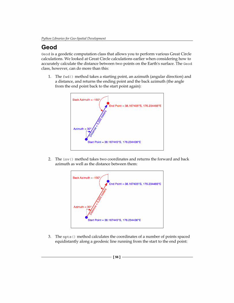
Python Libraries for Geo-Spatial Development
[ 56 ]
GeodGeod is a geodetic computation class that allows you to perform various Great Circle calculations. We looked at Great Circle calculations earlier when considering how to accurately calculate the distance between two points on the Earth's surface. The Geod class, however, can do more than this:
1. The fwd() method takes a starting point, an azimuth (angular direction) and a distance, and returns the ending point and the back azimuth (the angle from the end point back to the start point again):
2. The inv() method takes two coordinates and returns the forward and back azimuth as well as the distance between them:
3. The npts() method calculates the coordinates of a number of points spaced equidistantly along a geodesic line running from the start to the end point:
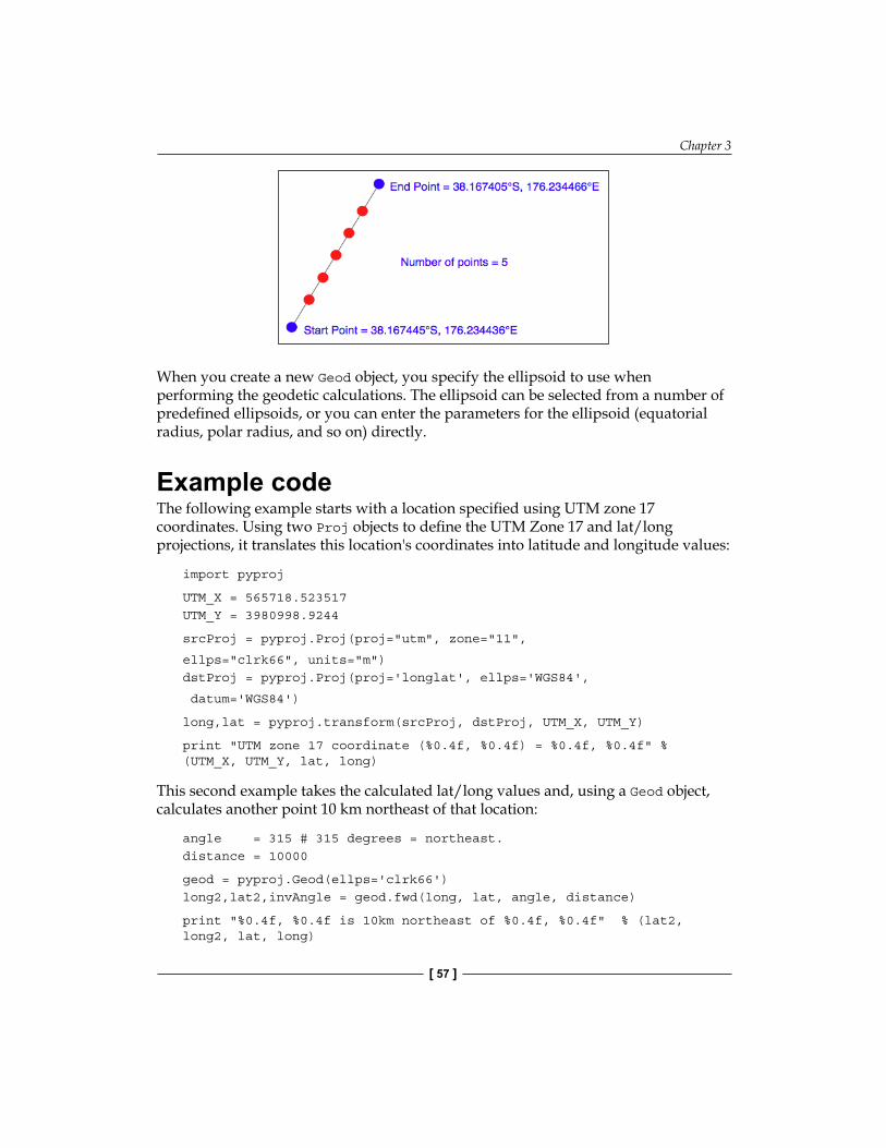
Chapter 3
[ 57 ]
When you create a new Geod object, you specify the ellipsoid to use when performing the geodetic calculations. The ellipsoid can be selected from a number of predefined ellipsoids, or you can enter the parameters for the ellipsoid (equatorial radius, polar radius, and so on) directly.
Example codeThe following example starts with a location specified using UTM zone 17 coordinates. Using two Proj objects to define the UTM Zone 17 and lat/long projections, it translates this location's coordinates into latitude and longitude values:
import pyproj
UTM_X = 565718.523517UTM_Y = 3980998.9244
srcProj = pyproj.Proj(proj="utm", zone="11",
ellps="clrk66", units="m")dstProj = pyproj.Proj(proj='longlat', ellps='WGS84',
datum='WGS84')
long,lat = pyproj.transform(srcProj, dstProj, UTM_X, UTM_Y)
print "UTM zone 17 coordinate (%0.4f, %0.4f) = %0.4f, %0.4f" % (UTM_X, UTM_Y, lat, long)
This second example takes the calculated lat/long values and, using a Geod object, calculates another point 10 km northeast of that location:
angle = 315 # 315 degrees = northeast.distance = 10000
geod = pyproj.Geod(ellps='clrk66')long2,lat2,invAngle = geod.fwd(long, lat, angle, distance)
print "%0.4f, %0.4f is 10km northeast of %0.4f, %0.4f" % (lat2, long2, lat, long)
Python Libraries for Geo-Spatial Development
[ 58 ]
DocumentationThe documentation available on the pyproj website and in the README file provided with the source code is excellent as far as it goes. It describes how to use the various classes and methods, what they do, and what parameters are required. However, the documentation is rather sparse when it comes to the parameters used when creating a new Proj object.
According to the documentation, a Proj class instance is initialized with proj map projection control parameter key/value pairs. The key/value pairs can either be passed in a dictionary, or as keyword arguments, or as a proj4 string (compatible with the proj command).
The documentation does provide a link to a website listing a number of standard map projections and their associated parameters, but understanding what these parameters mean generally requires you to delve into the PROJ documentation itself. The documentation for PROJ is dense and confusing, even more so because the main manual is written for PROJ version 3, with addendums for version 4 and version 4.3. Attempting to make sense of all this can be quite challenging.
Fortunately, in most cases you won't need to refer to the PROJ documentation at all. When working with geo-spatial data using GDAL or OGR, you can easily extract the projection as a "proj4 string" that can be passed directly to the Proj initializer. If you want to hardwire the projection, you can generally choose a projection and ellipsoid using the proj="..." and ellps="..." parameters respectively. If you want to do more than this, though, you will need to refer to the PROJ documentation for more details.
To find out more about PROJ and to read the original documentation, you can find everything you need at: http://trac.osgeo.org/proj.
Availabilitypyproj is available for MS Windows, Mac OS X, and any POSIX-based operating system. The main web page for pyproj can be found at:
http://code.google.com/p/pyproj
Chapter 3
[ 59 ]
The download link on this page will allow you to download either a Windows installer for pyproj, or the source code. Note, however, that the source code requires you to have installed a version of PROJ.4 before you can build pyproj. For Linux machines, you can generally obtain PROJ.4 as an RPM or source tarball that you can then compile yourself. For Mac OS X, you will probably find it easier to install a compiled version of the PROJ framework, either as part of a complete GDAL installation, or by just installing the PROJ framework itself. Either is available at:
http://www.kyngchaos.com/software/frameworks
Make sure that you install version 1.8.6 or later of the pyproj library. This version is required to follow the examples in this book.
Analyzing and manipulating geo-spatial dataBecause geo-spatial data works with geometrical features such as points, lines, and polygons, you often need to perform various calculations using these geometrical features. Fortunately, there are some very powerful tools for doing exactly this. The library of choice for performing this type of computational geometry is named Shapely.
ShapelyShapely is a Python package for the manipulation and analysis of two-dimensional geo-spatial geometries. Shapely is based on the GEOS library, which implements a wide range of geo-spatial data manipulations in C++. GEOS is itself based on a library called the "Java Topology Suite", which provides the same functionality for Java programmers. Shapely provides a Pythonic interface to GEOS that makes it easy to use these manipulations directly from your Python programs.
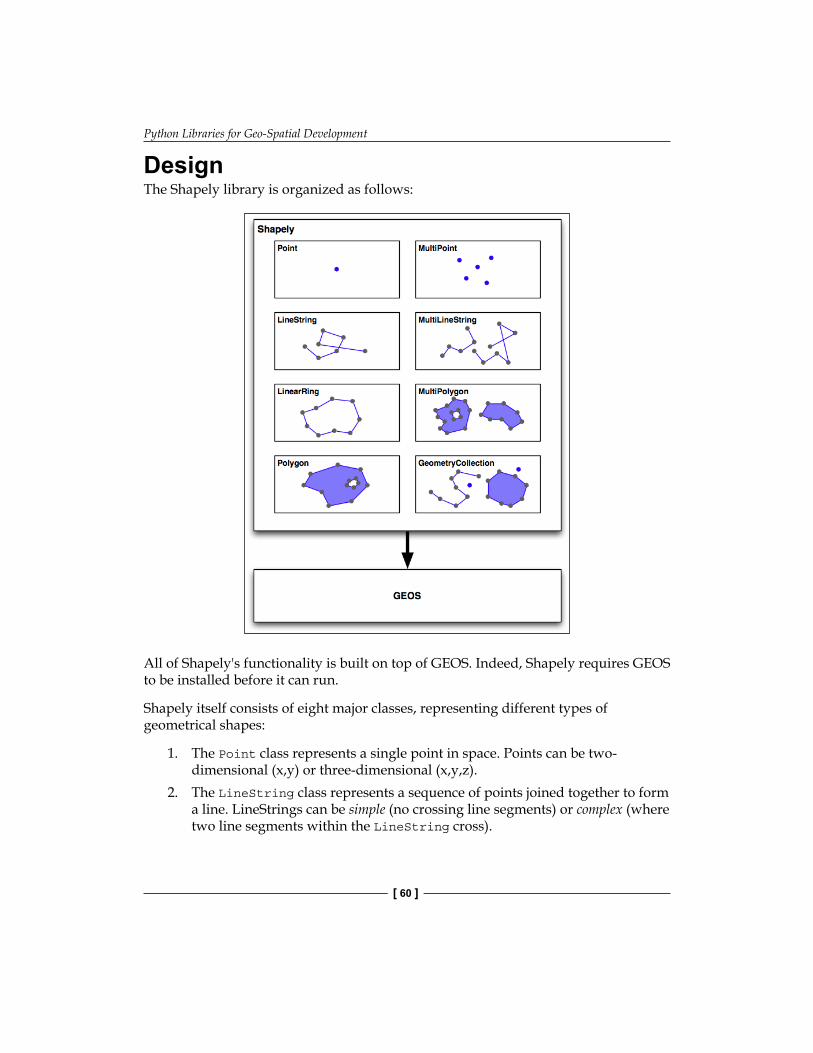
Python Libraries for Geo-Spatial Development
[ 60 ]
DesignThe Shapely library is organized as follows:
All of Shapely's functionality is built on top of GEOS. Indeed, Shapely requires GEOS to be installed before it can run.
Shapely itself consists of eight major classes, representing different types of geometrical shapes:
1. The Point class represents a single point in space. Points can be two-dimensional (x,y) or three-dimensional (x,y,z).
2. The LineString class represents a sequence of points joined together to form a line. LineStrings can be simple (no crossing line segments) or complex (where two line segments within the LineString cross).
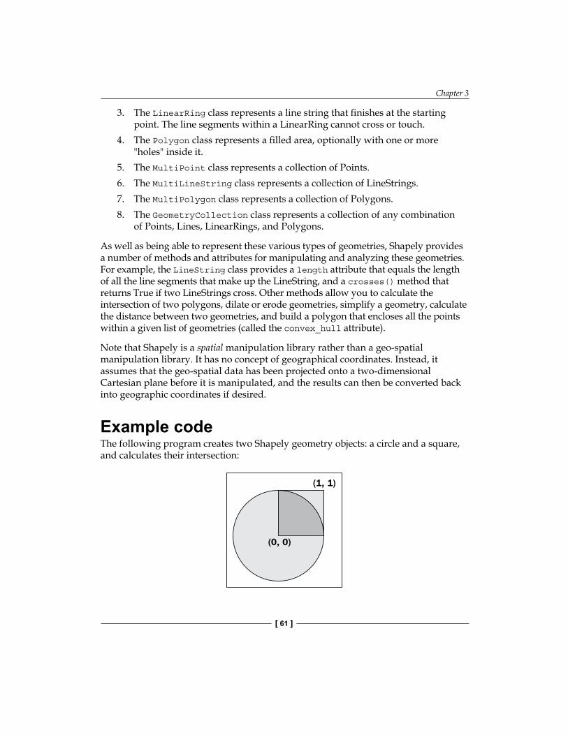
Chapter 3
[ 61 ]
3. The LinearRing class represents a line string that finishes at the starting point. The line segments within a LinearRing cannot cross or touch.
4. The Polygon class represents a filled area, optionally with one or more "holes" inside it.
5. The MultiPoint class represents a collection of Points.6. The MultiLineString class represents a collection of LineStrings.7. The MultiPolygon class represents a collection of Polygons.8. The GeometryCollection class represents a collection of any combination
of Points, Lines, LinearRings, and Polygons.
As well as being able to represent these various types of geometries, Shapely provides a number of methods and attributes for manipulating and analyzing these geometries. For example, the LineString class provides a length attribute that equals the length of all the line segments that make up the LineString, and a crosses() method that returns True if two LineStrings cross. Other methods allow you to calculate the intersection of two polygons, dilate or erode geometries, simplify a geometry, calculate the distance between two geometries, and build a polygon that encloses all the points within a given list of geometries (called the convex_hull attribute).
Note that Shapely is a spatial manipulation library rather than a geo-spatial manipulation library. It has no concept of geographical coordinates. Instead, it assumes that the geo-spatial data has been projected onto a two-dimensional Cartesian plane before it is manipulated, and the results can then be converted back into geographic coordinates if desired.
Example codeThe following program creates two Shapely geometry objects: a circle and a square, and calculates their intersection:
Python Libraries for Geo-Spatial Development
[ 62 ]
The intersection will be a polygon in the shape of a semicircle, as shown above.
import shapely.geometry
pt = shapely.geometry.Point(0, 0)circle = pt.buffer(1.0)
square = shapely.geometry.Polygon([(0, 0), (1, 0), (1, 1), (0, 1), (0, 0)])
intersect = circle.intersection(square)for x,y in intersect.exterior.coords: print x,y
Notice how the circle is constructed by taking a Point geometry and using the buffer() method to create a Polygon representing the outline of a circle.
DocumentationShapely version 1.0 includes a fairly straightforward manual that gives a brief description of each class, method, and attribute, along with sample code showing how to use it. However, the manual for Shapely version 1.2 is far more extensive, with detailed descriptions, extended code samples, and many illustrations that clearly show how the various classes, methods, and attributes work. The Shapely 1.2 manual is worth reading even if you are using an earlier version.
The Shapely documentation is entirely self-contained; there is no need to refer to the GEOS documentation, or to the Java Topology Suite it is based on, unless you particularly want to see how things are done in these libraries. The only exception is that you may need to refer to the GEOS documentation if you are compiling GEOS from source, and are having problems getting it to work.
AvailabilityShapely will run on all major operating systems, including MS Windows, Mac OS X, and Linux. Shapely's main website can be found at:
http://trac.gispython.org/lab/wiki/Shapely
The website has everything you need, including the documentation and downloads for the Shapely library, in both source code form and pre-built binaries for MS Windows.
If you are installing Shapely on a Windows computer, the pre-built binaries include the GEOS library built-in. Otherwise, you will be responsible for installing GEOS before you can use Shapely.
Chapter 3
[ 63 ]
Make sure that you install Shapely version 1.2 or later; you will need this version to work through the examples in this book.
The GEOS library's website is at:
http://trac.osgeo.org/geos
To install GEOS in a Unix-based computer, you can either download the source code from the GEOS website and compile it yourself, or you can install a suitable RPM or APT package that includes GEOS. If you are running Mac OS X, you can either try to download and build GEOS yourself, or you can install the pre-built GEOS framework, which is available from the following website:
http://www.kyngchaos.com/software/frameworks
Visualizing geo-spatial dataIt's very hard, if not impossible, to understand geo-spatial data unless it is turned into a visual form—that is, until it is rendered as an image of some sort. Converting geo-spatial data into images requires a suitable toolkit. While there are several such toolkits available, we will look at one in particular: Mapnik.
MapnikMapnik is a freely-available toolkit for building mapping applications. Mapnik takes geo-spatial data from a PostGIS database, Shapefile, or any other format supported by GDAL/OGR, and turns it into clearly-rendered, good-looking images.
There are a lot of complex issues involved in rendering images well, and Mapnik does a good job of allowing the application developer to control the rendering process. Rules control which features should appear on the map, while Symbolizers control the visual appearance of these features.
Mapnik allows developers to create XML stylesheets that control the map-creation process. Just as with CSS stylesheets, Mapnik's stylesheets give you complete control over the way geo-spatial data is rendered. Alternatively, you can create your styles by hand if you prefer.
Mapnik itself is written in C++, though bindings are included that allow access to almost all of the Mapnik functionality via Python. Because these bindings are included in the main code base rather than being added by a third-party developer, support for Python is built right into Mapnik. This makes Python eminently suited to developing Mapnik-based applications.

Python Libraries for Geo-Spatial Development
[ 64 ]
Mapnik is heavily used by Open Street Map (http://openstreetmap.org) and EveryBlock (http://everyblock.com) among others. Since the output of Mapnik is simply an image, it is easy to include Mapnik as part of a web-based application, or you can display the output directly in a window as part of a desktop-based application. Mapnik works equally well on the desktop and on the web.
DesignWhen using Mapnik, the main object you are dealing with is called the Map. A Map object has the following parts:
When creating a Map object, you tell it:
1. The overall width and height of the map, in pixels.2. The spatial reference to use for the map.3. The background color to draw behind the contents of the map.
Chapter 3
[ 65 ]
You then define one or more Layers that hold the map's contents. Each Layer has:
1. A name.2. A Datasource object defining where to get the data for this layer from. The
datasource can be a reference to a database, or it can be a Shapefile or other GDAL/OGR datasource.
3. A spatial reference to use for this layer. This can be different from the spatial reference used by the map as a whole, if appropriate.
4. A list of styles to apply to this layer. Each style is referred to by name, since the styles are actually defined elsewhere (often in an XML stylesheet).
Finally, you define one or more Styles that tell Mapnik how to draw the various layers. Each Style has a name and a list of Rules that make up the main part of the style's definition. Each Rule has:
1. A minimum scale and maximum scale value (called the "scale denominator"). The Rule will only apply if the map's scale is within this range.
2. A filter expression. The Rule will only apply to those features that match this filter expression.
3. A list of Symbolizers. These define how the matching features will be drawn onto the map.
There are a number of different types of Symbolizers implemented by Mapnik:
1. LineSymbolizer is used to draw a "stroke" along a line, a linear ring, or around the outside of a polygon.
2. LinePatternSymbolizer uses the contents of an image file (specified by name) to draw the "stroke" along a line, a linear ring, or around the outside of a polygon.
3. PolygonSymbolizer is used to draw the interior of a polygon.4. PolygonPatternSymbolizer uses the contents of an image file (again
specified by name) to draw the interior of a polygon.5. PointSymbolizer uses the contents of an image file (specified by name) to
draw a symbol at a point.6. TextSymbolizer draws a feature's text. The text to be drawn is taken from
one of the feature's attributes, and there are numerous options to control how the text is to be drawn.
7. RasterSymbolizer is used to draw raster data taken from any GDAL dataset.
Python Libraries for Geo-Spatial Development
[ 66 ]
8. ShieldSymbolizer draws a textual label and a point together. This is similar to the use of a PointSymbolizer to draw the image and a TextSymbolizer to draw the label, except that it ensures that both the text and the image are drawn together.
9. BuildingSymbolizer uses a pseudo-3D effect to draw a polygon, to make it appear that the polygon is a three-dimensional building.
10. Finally, MarkersSymbolizer draws blue directional arrows following the direction of polygon and line geometries. This is experimental, and is intended to be used to draw one-way streets onto a street map.
When you instantiate a Symbolizer and add it to a style (either directly in code, or via an XML stylesheet), you provide a number of parameters that define how the Symbolizer should work. For example, when using the PolygonSymbolizer, you can specify the fill color, the opacity, and a "gamma" value that helps draw adjacent polygons of the same color without the boundary being shown:
p = mapnik.PolygonSymbolizer(mapnik.Color(127, 127, 0))p.fill_opacity = 0.8p.gamma = 0.65
If the Rule that uses this Symbolizer matches one or more polygons, those polygons will be drawn using the given color, opacity, and gamma value.
Different Rules can, of course, have different Symbolizers, as well as different filter values. For example, you might set up Rules that draw countries in different colors depending on their population.
Example codeThe following example program displays a simple world map using Mapnik:
import mapnik
symbolizer = mapnik.PolygonSymbolizer(mapnik.Color("darkgreen"))
rule = mapnik.Rule()rule.symbols.append(symbolizer)
style = mapnik.Style()style.rules.append(rule)
layer = mapnik.Layer("mapLayer")layer.datasource = mapnik.Shapefile(file="TM_WORLD_BORDERS-0.3.shp")layer.styles.append("mapStyle")
map = mapnik.Map(800, 400)
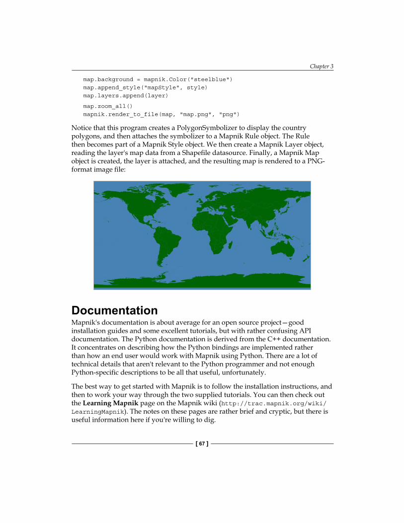
Chapter 3
[ 67 ]
map.background = mapnik.Color("steelblue")map.append_style("mapStyle", style)map.layers.append(layer)
map.zoom_all()mapnik.render_to_file(map, "map.png", "png")
Notice that this program creates a PolygonSymbolizer to display the country polygons, and then attaches the symbolizer to a Mapnik Rule object. The Rule then becomes part of a Mapnik Style object. We then create a Mapnik Layer object, reading the layer's map data from a Shapefile datasource. Finally, a Mapnik Map object is created, the layer is attached, and the resulting map is rendered to a PNG-format image file:
DocumentationMapnik's documentation is about average for an open source project—good installation guides and some excellent tutorials, but with rather confusing API documentation. The Python documentation is derived from the C++ documentation. It concentrates on describing how the Python bindings are implemented rather than how an end user would work with Mapnik using Python. There are a lot of technical details that aren't relevant to the Python programmer and not enough Python-specific descriptions to be all that useful, unfortunately.
The best way to get started with Mapnik is to follow the installation instructions, and then to work your way through the two supplied tutorials. You can then check out the Learning Mapnik page on the Mapnik wiki (http://trac.mapnik.org/wiki/LearningMapnik). The notes on these pages are rather brief and cryptic, but there is useful information here if you're willing to dig.
Python Libraries for Geo-Spatial Development
[ 68 ]
It is worth looking at the Python API documentation, despite its limitations. The main page lists the various classes that are available and a number of useful functions, many of which are documented. The classes themselves list the methods and properties (attributes) you can access, and even though many of these lack Python-specific documentation, you can generally guess what they do.
Chapter 8 includes a comprehensive description of Mapnik; you may find this useful in lieu of any other Python-based documentation.
AvailabilityMapnik runs on all major operating systems, including MS Windows, Mac OS X, and Linux. The main Mapnik website can be found at:
http://mapnik.org
Download links are provided for downloading the Mapnik source code, which can be readily compiled if you are running on a Unix machine, and you can also download pre-built binaries for Windows computers. For those running Mac OS X, pre-built binaries are available at:
http://dbsgeo.com/downloads
Make sure that you install Mapnik version 1.7.1 or later; you will need to use this version as you work through the examples in this book.
SummaryIn this chapter, we looked at a number of important libraries for developing geo-spatial applications using Python. We learned that:
• GDAL is a C++ library for reading (and sometimes writing) raster-based geo-spatial data.
• OGR is a C++ library for reading (and sometimes writing) vector-based geo-spatial data.
• GDAL and OGR include Python bindings that are easy to use, and support a large number of data formats.
• The PROJ.4 library and its Pythonic pyproj wrapper allow you to convert between geographic coordinates (points on the Earth's surface) and cartographic coordinates (x,y coordinates on a two-dimensional plane) using any desired map projection and ellipsoid.
Chapter 3
[ 69 ]
• The pyproj Geod class allows you to perform various geodetic calculations based on points on the Earth's surface, a given distance, and a given angle (azimuth).
• A geo-spatial data manipulation library called the Java Topology Suite was originally developed for Java. This was then rewritten in C++ under the name GEOS, and there is now a Python interface to GEOS called Shapely.
• Shapely makes it easy to represent geo-spatial data in the form of Points, LineStrings, LinearRings, Polygons, MultiPoints, MultiLineStrings, MultiPolygons, and GeometryCollections.
• As well as representing geo-spatial data, these classes allow you to perform a variety of geo-spatial calculations.
• Mapnik is a tool for producing good-looking maps based on geo-spatial data.• Mapnik can use an XML stylesheet to control which elements appear on the
map, and how they are formatted. Styles can also be created by hand if you prefer.
• Each Mapnik style has a list of Rules that are used to identify features to draw onto the map.
• Each Mapnik Rule has a list of Symbolizers that control how the selected features are drawn.
While these tools are very powerful, you can't do anything with them unless you have some geo-spatial data to work with. Unless you are lucky enough to have access to your own source of data, or are willing to pay large sums to purchase data commercially, your only choice is to make use of the geo-spatial data that is freely-available on the Internet. These freely-available sources of geo-spatial data are the topic of the next chapter.

Sources of Geo-Spatial DataWhen creating a geo-spatial application, the data you use will be just as important as the code you write. Good quality geo-spatial data, and in particular base maps and imagery, will be the cornerstone of your application. If your maps don't look good then your application will be treated as the work of an amateur, no matter how well you write the rest of your program.
Traditionally, geo-spatial data has been treated as a valuable and scarce resource, being sold commercially for many thousands of dollars and with strict licensing constraints. Fortunately, as with the trend towards democratizing geo-spatial tools, geo-spatial data is now becoming increasingly available for free and with little or no restriction on its use. There are still situations where you may have to pay for data, but often it is now just a case of downloading the data you need from a suitable web site.
This chapter provides an overview of some of these major sources of freely-available geo-spatial data. This is not intended to be an exhaustive list, but rather to provide information on the sources which are likely to be most useful to the Python geo-spatial developer.
In this chapter, we will cover:
• Some of the major freely-available sources of vector-format geo-spatial data• Some of the main freely-available sources of raster geo-spatial data• Sources of other types of freely-available geo-spatial data, concentrating on
databases of city and other placenames
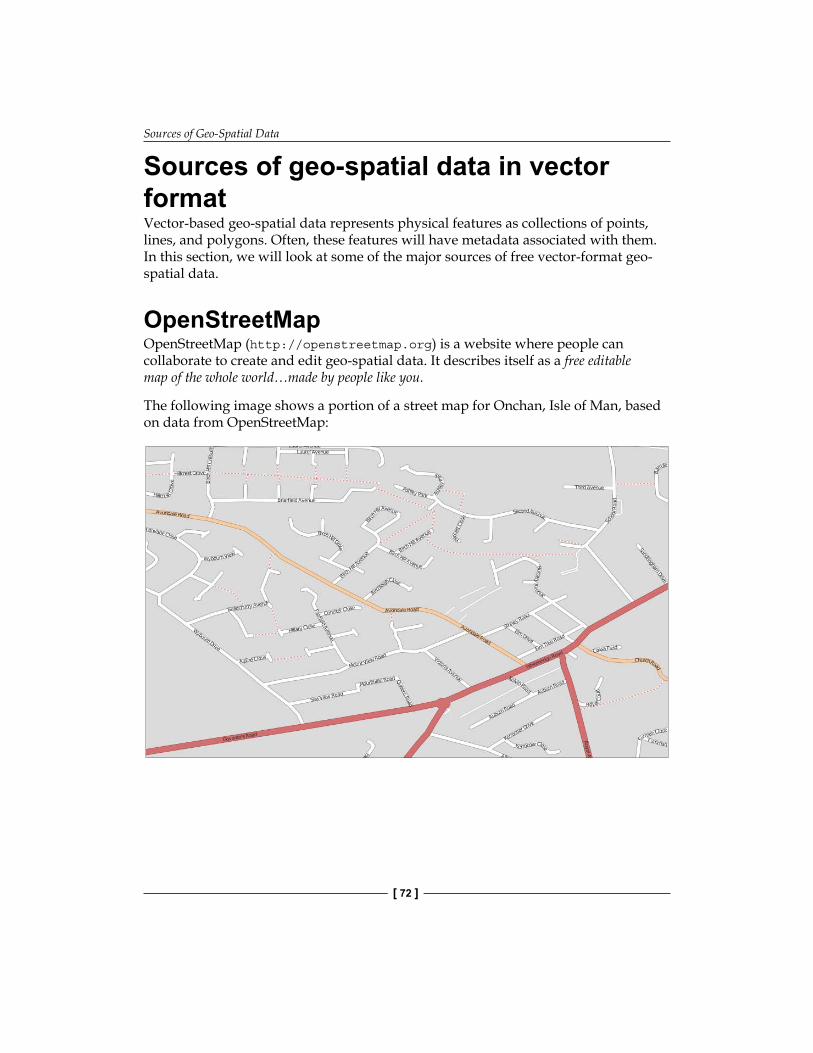
Sources of Geo-Spatial Data
[ 72 ]
Sources of geo-spatial data in vector formatVector-based geo-spatial data represents physical features as collections of points, lines, and polygons. Often, these features will have metadata associated with them. In this section, we will look at some of the major sources of free vector-format geo-spatial data.
OpenStreetMapOpenStreetMap (http://openstreetmap.org) is a website where people can collaborate to create and edit geo-spatial data. It describes itself as a free editable map of the whole world…made by people like you.
The following image shows a portion of a street map for Onchan, Isle of Man, based on data from OpenStreetMap:
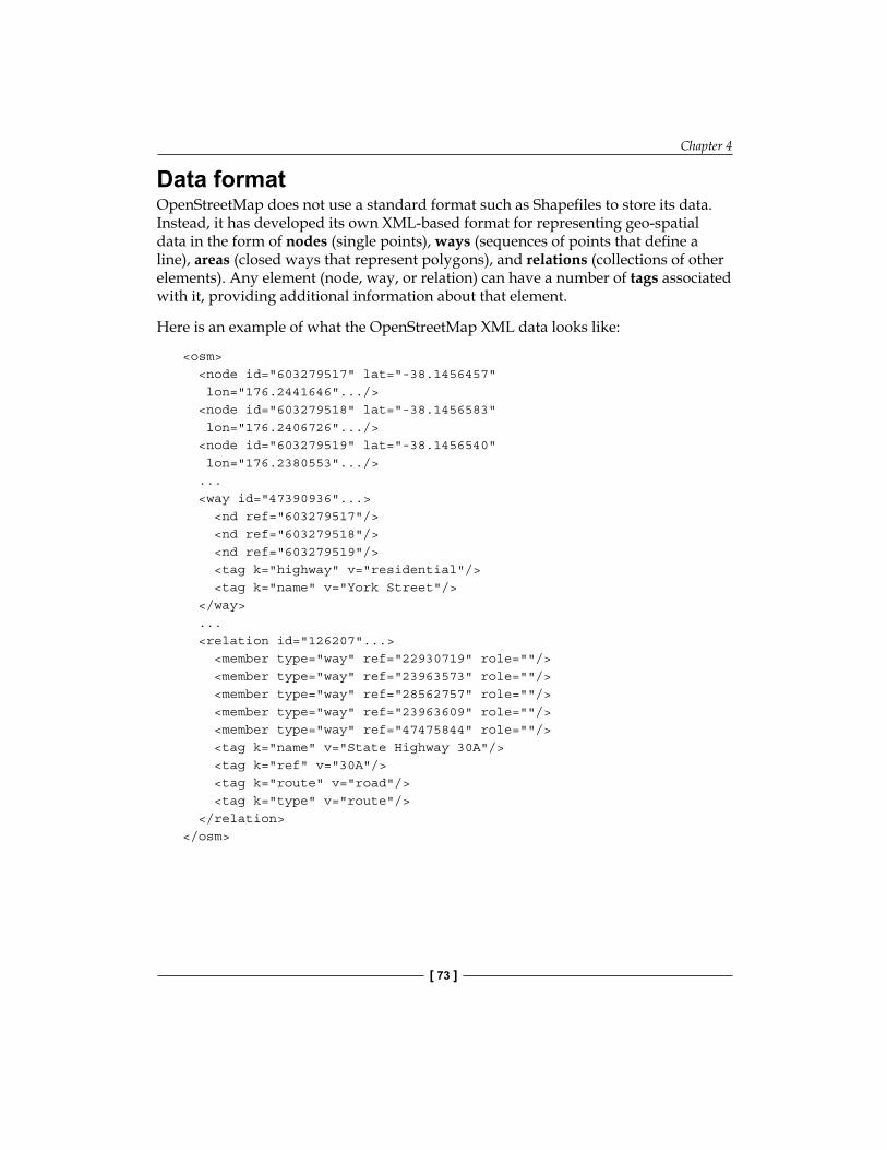
Chapter 4
[ 73 ]
Data formatOpenStreetMap does not use a standard format such as Shapefiles to store its data. Instead, it has developed its own XML-based format for representing geo-spatial data in the form of nodes (single points), ways (sequences of points that define a line), areas (closed ways that represent polygons), and relations (collections of other elements). Any element (node, way, or relation) can have a number of tags associated with it, providing additional information about that element.
Here is an example of what the OpenStreetMap XML data looks like:
<osm> <node id="603279517" lat="-38.1456457" lon="176.2441646".../> <node id="603279518" lat="-38.1456583" lon="176.2406726".../> <node id="603279519" lat="-38.1456540" lon="176.2380553".../> ... <way id="47390936"...> <nd ref="603279517"/> <nd ref="603279518"/> <nd ref="603279519"/> <tag k="highway" v="residential"/> <tag k="name" v="York Street"/> </way> ... <relation id="126207"...> <member type="way" ref="22930719" role=""/> <member type="way" ref="23963573" role=""/> <member type="way" ref="28562757" role=""/> <member type="way" ref="23963609" role=""/> <member type="way" ref="47475844" role=""/> <tag k="name" v="State Highway 30A"/> <tag k="ref" v="30A"/> <tag k="route" v="road"/> <tag k="type" v="route"/> </relation></osm>
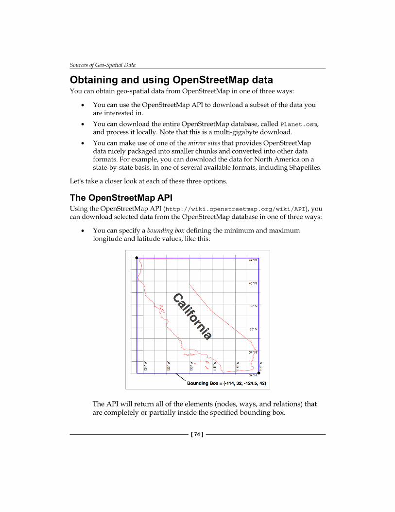
Sources of Geo-Spatial Data
[ 74 ]
Obtaining and using OpenStreetMap dataYou can obtain geo-spatial data from OpenStreetMap in one of three ways:
• You can use the OpenStreetMap API to download a subset of the data you are interested in.
• You can download the entire OpenStreetMap database, called Planet.osm, and process it locally. Note that this is a multi-gigabyte download.
• You can make use of one of the mirror sites that provides OpenStreetMap data nicely packaged into smaller chunks and converted into other data formats. For example, you can download the data for North America on a state-by-state basis, in one of several available formats, including Shapefiles.
Let's take a closer look at each of these three options.
The OpenStreetMap APIUsing the OpenStreetMap API (http://wiki.openstreetmap.org/wiki/API), you can download selected data from the OpenStreetMap database in one of three ways:
• You can specify a bounding box defining the minimum and maximum longitude and latitude values, like this:
The API will return all of the elements (nodes, ways, and relations) that are completely or partially inside the specified bounding box.
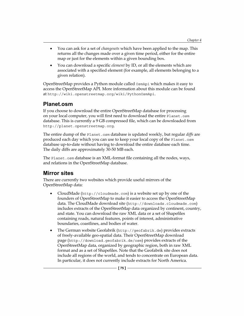
Chapter 4
[ 75 ]
• You can ask for a set of changesets which have been applied to the map. This returns all the changes made over a given time period, either for the entire map or just for the elements within a given bounding box.
• You can download a specific element by ID, or all the elements which are associated with a specified element (for example, all elements belonging to a given relation).
OpenStreetMap provides a Python module called OsmApi which makes it easy to access the OpenStreetMap API. More information about this module can be found at http://wiki.openstreetmap.org/wiki/PythonOsmApi.
Planet.osmIf you choose to download the entire OpenStreetMap database for processing on your local computer, you will first need to download the entire Planet.osm database. This is currently a 9 GB compressed file, which can be downloaded from http://planet.openstreetmap.org.
The entire dump of the Planet.osm database is updated weekly, but regular diffs are produced each day which you can use to keep your local copy of the Planet.osm database up-to-date without having to download the entire database each time. The daily diffs are approximately 30-50 MB each.
The Planet.osm database is an XML-format file containing all the nodes, ways, and relations in the OpenStreetMap database.
Mirror sitesThere are currently two websites which provide useful mirrors of the OpenStreetMap data:
• CloudMade (http://cloudmade.com) is a website set up by one of the founders of OpenStreetMap to make it easier to access the OpenStreetMap data. The CloudMade download site (http://downloads.cloudmade.com) includes extracts of the OpenStreetMap data organized by continent, country, and state. You can download the raw XML data or a set of Shapefiles containing roads, natural features, points of interest, administrative boundaries, coastlines, and bodies of water.
• The German website Geofabrik (http://geofabrik.de) provides extracts of freely-available geo-spatial data. Their OpenStreetMap download page (http://download.geofabrik.de/osm) provides extracts of the OpenStreetMap data, organized by geographic region, both in raw XML format and as a set of Shapefiles. Note that the Geofabrik site does not include all regions of the world, and tends to concentrate on European data. In particular, it does not currently include extracts for North America.
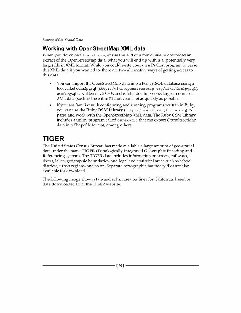
Sources of Geo-Spatial Data
[ 76 ]
Working with OpenStreetMap XML dataWhen you download Planet.osm, or use the API or a mirror site to download an extract of the OpenStreetMap data, what you will end up with is a (potentially very large) file in XML format. While you could write your own Python program to parse this XML data if you wanted to, there are two alternative ways of getting access to this data:
• You can import the OpenStreetMap data into a PostgreSQL database using a tool called osm2pgsql (http://wiki.openstreetmap.org/wiki/Osm2pgsql). osm2pgsql is written in C/C++, and is intended to process large amounts of XML data (such as the entire Planet.osm file) as quickly as possible.
• If you are familiar with configuring and running programs written in Ruby, you can use the Ruby OSM Library (http://osmlib.rubyforge.org) to parse and work with the OpenStreetMap XML data. The Ruby OSM Library includes a utility program called osmexport that can export OpenStreetMap data into Shapefile format, among others.
TIGERThe United States Census Bureau has made available a large amount of geo-spatial data under the name TIGER (Topologically Integrated Geographic Encoding and Referencing system). The TIGER data includes information on streets, railways, rivers, lakes, geographic boundaries, and legal and statistical areas such as school districts, urban regions, and so on. Separate cartographic boundary files are also available for download.
The following image shows state and urban area outlines for California, based on data downloaded from the TIGER website:
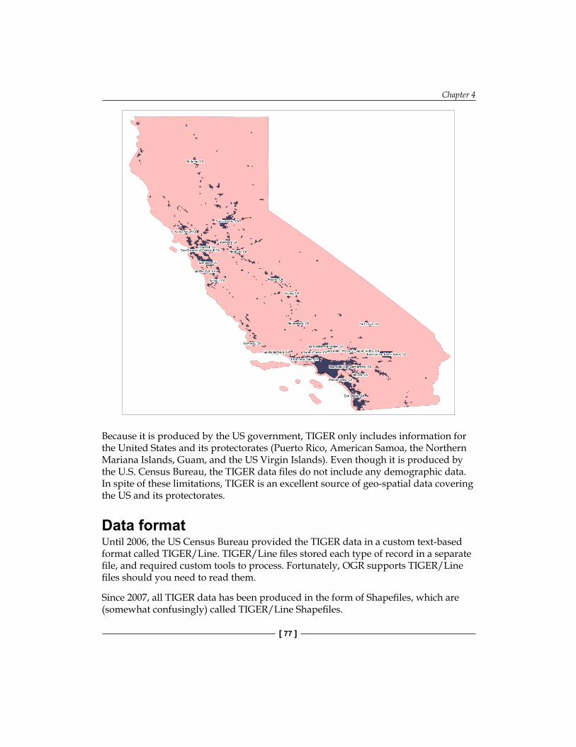
Chapter 4
[ 77 ]
Because it is produced by the US government, TIGER only includes information for the United States and its protectorates (Puerto Rico, American Samoa, the Northern Mariana Islands, Guam, and the US Virgin Islands). Even though it is produced by the U.S. Census Bureau, the TIGER data files do not include any demographic data. In spite of these limitations, TIGER is an excellent source of geo-spatial data covering the US and its protectorates.
Data formatUntil 2006, the US Census Bureau provided the TIGER data in a custom text-based format called TIGER/Line. TIGER/Line files stored each type of record in a separate file, and required custom tools to process. Fortunately, OGR supports TIGER/Line files should you need to read them.
Since 2007, all TIGER data has been produced in the form of Shapefiles, which are (somewhat confusingly) called TIGER/Line Shapefiles.
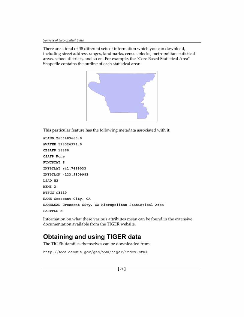
Sources of Geo-Spatial Data
[ 78 ]
There are a total of 38 different sets of information which you can download, including street address ranges, landmarks, census blocks, metropolitan statistical areas, school districts, and so on. For example, the "Core Based Statistical Area" Shapefile contains the outline of each statistical area:
This particular feature has the following metadata associated with it:
ALAND 2606489666.0
AWATER 578526971.0
CBSAFP 18860
CSAFP None
FUNCSTAT S
INTPTLAT +41.7499033
INTPTLON -123.9809983
LSAD M2
MEMI 2
MTFCC G3110
NAME Crescent City, CA
NAMELSAD Crescent City, CA Micropolitan Statistical Area
PARTFLG N
Information on what these various attributes mean can be found in the extensive documentation available from the TIGER website.
Obtaining and using TIGER dataThe TIGER datafiles themselves can be downloaded from:
http://www.census.gov/geo/www/tiger/index.html
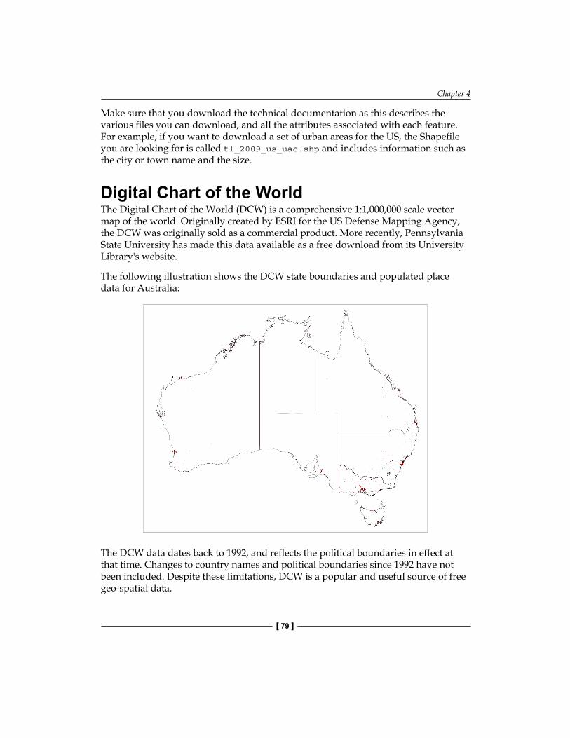
Chapter 4
[ 79 ]
Make sure that you download the technical documentation as this describes the various files you can download, and all the attributes associated with each feature. For example, if you want to download a set of urban areas for the US, the Shapefile you are looking for is called tl_2009_us_uac.shp and includes information such as the city or town name and the size.
Digital Chart of the WorldThe Digital Chart of the World (DCW) is a comprehensive 1:1,000,000 scale vector map of the world. Originally created by ESRI for the US Defense Mapping Agency, the DCW was originally sold as a commercial product. More recently, Pennsylvania State University has made this data available as a free download from its University Library's website.
The following illustration shows the DCW state boundaries and populated place data for Australia:
The DCW data dates back to 1992, and reflects the political boundaries in effect at that time. Changes to country names and political boundaries since 1992 have not been included. Despite these limitations, DCW is a popular and useful source of free geo-spatial data.
Sources of Geo-Spatial Data
[ 80 ]
Data formatThe Digital Chart of the World is available in ARC/INFO Interchange format, also known as E00 format. This is an ASCII file format used to export data out of ARC/Info GIS systems.
While it is possible to process an E00 file manually, it is much easier to use tools such as OGR to parse the file. We will look at how you can do this shortly.
Available layersWhen downloading data from the DCW, you can choose which layers of data to include. The available layers are:
• Country boundaries• Populated places (urban areas and points)• Railway lines• Roads• Utilities• Drainage• Elevation data (called Hypsography)• Land cover• Ocean features• Aeronautical features• Cultural landmarks• Transportation structures
Note that not all of this information is available for every location. Because of the file format used by the DCW data, there are no attributes or other metadata included; all you get is the raw geo-spatial data itself.
Obtaining and using DCW dataThe E00 files that make up the DCW data can be downloaded from Pennsylvania State University's website:
http://maproom.dlt.psu.edu/dcw
Unfortunately, the web interface is rather awkward to use, and you can't just download all the files at once. Instead, you have to wend your way through the interface one step at a time:
Chapter 4
[ 81 ]
1. Click on the continent you want to download data for2. Select the individual country or state you are looking for and click Continue3. Click on the Download Data button4. Select the layer(s) you want to download and click on Continue5. Choose the type of data compression you want and then click on the
Compute Data button6. Finally, click on the FTP or HTTP hyperlink to download the generated
datafile
If you want to download data for a number of locations (for example, all the US states), this can be extremely tedious. Unfortunately, there is no way around this short of writing a custom download script, which would probably take longer than just downloading the data by hand.
Once you have the necessary datafiles, you can read them using OGR in the usual way:
import osgeo.ogrdatasource = osgeo.ogr.Open("wyoming.e00")
Because you are importing an ARC/Info E00 format file, the resulting OGR datasource will consist of four separate layers, named ARC, CNT, LAB, and PAL. These correspond to the individual ARC files that were used to originally construct the data:
• The ARC (arc coordinates and topology) layer contains the actual geo-spatial data you need, in the form of linestrings and polygons.
• The CNT (polygon centroid coordinates) layer contains the centroid point for the entire geographical area covered by the file.
• The LAB (label points) layer appears to contain information about the positioning of labels onto the map. Unfortunately, it does not include the labels themselves.
• The PAL (polygon topology) layer includes more information about the area covered by the file, including the bounding box for the entire area.
In most cases, all the information you need will be in the first (ARC) layer. If you want to find out more about the ARC/Info E00 file format and what information may be included in these various layers, an unofficial reference for the E00 format can be found at:
http://avce00.maptools.org/docs/v7_e00_cover.html
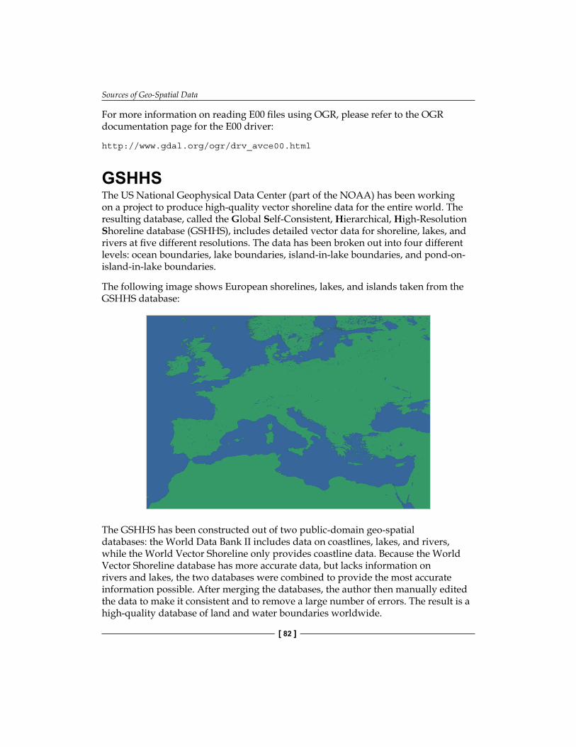
Sources of Geo-Spatial Data
[ 82 ]
For more information on reading E00 files using OGR, please refer to the OGR documentation page for the E00 driver:
http://www.gdal.org/ogr/drv_avce00.html
GSHHSThe US National Geophysical Data Center (part of the NOAA) has been working on a project to produce high-quality vector shoreline data for the entire world. The resulting database, called the Global Self-Consistent, Hierarchical, High-Resolution Shoreline database (GSHHS), includes detailed vector data for shoreline, lakes, and rivers at five different resolutions. The data has been broken out into four different levels: ocean boundaries, lake boundaries, island-in-lake boundaries, and pond-on-island-in-lake boundaries.
The following image shows European shorelines, lakes, and islands taken from the GSHHS database:
The GSHHS has been constructed out of two public-domain geo-spatial databases: the World Data Bank II includes data on coastlines, lakes, and rivers, while the World Vector Shoreline only provides coastline data. Because the World Vector Shoreline database has more accurate data, but lacks information on rivers and lakes, the two databases were combined to provide the most accurate information possible. After merging the databases, the author then manually edited the data to make it consistent and to remove a large number of errors. The result is a high-quality database of land and water boundaries worldwide.
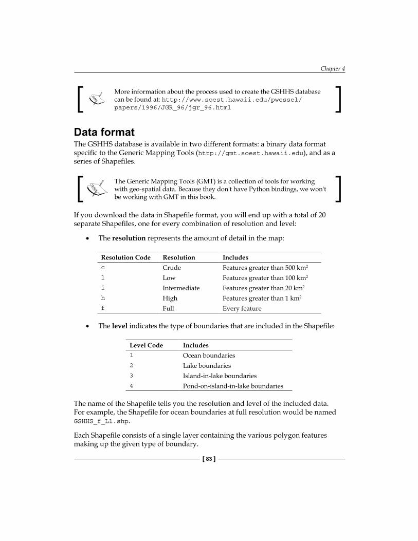
Chapter 4
[ 83 ]
More information about the process used to create the GSHHS database can be found at: http://www.soest.hawaii.edu/pwessel/papers/1996/JGR_96/jgr_96.html
Data formatThe GSHHS database is available in two different formats: a binary data format specific to the Generic Mapping Tools (http://gmt.soest.hawaii.edu), and as a series of Shapefiles.
The Generic Mapping Tools (GMT) is a collection of tools for working with geo-spatial data. Because they don't have Python bindings, we won't be working with GMT in this book.
If you download the data in Shapefile format, you will end up with a total of 20 separate Shapefiles, one for every combination of resolution and level:
• The resolution represents the amount of detail in the map:
Resolution Code Resolution Includesc Crude Features greater than 500 km2
l Low Features greater than 100 km2
i Intermediate Features greater than 20 km2
h High Features greater than 1 km2
f Full Every feature
• The level indicates the type of boundaries that are included in the Shapefile:
Level Code Includes1 Ocean boundaries2 Lake boundaries3 Island-in-lake boundaries4 Pond-on-island-in-lake boundaries
The name of the Shapefile tells you the resolution and level of the included data. For example, the Shapefile for ocean boundaries at full resolution would be named GSHHS_f_L1.shp.
Each Shapefile consists of a single layer containing the various polygon features making up the given type of boundary.
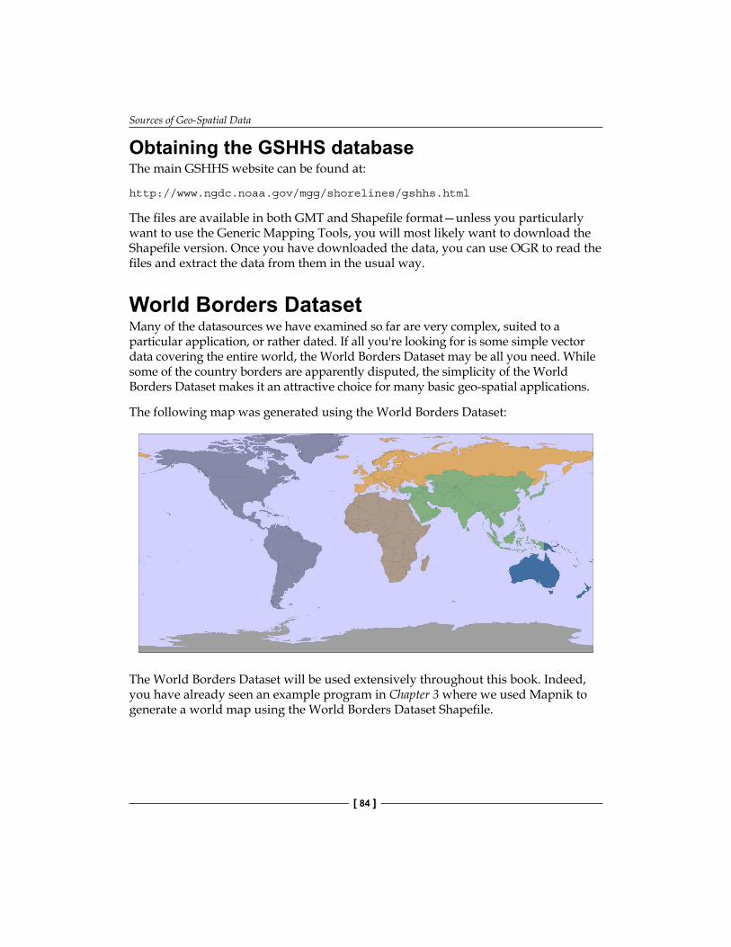
Sources of Geo-Spatial Data
[ 84 ]
Obtaining the GSHHS databaseThe main GSHHS website can be found at:
http://www.ngdc.noaa.gov/mgg/shorelines/gshhs.html
The files are available in both GMT and Shapefile format—unless you particularly want to use the Generic Mapping Tools, you will most likely want to download the Shapefile version. Once you have downloaded the data, you can use OGR to read the files and extract the data from them in the usual way.
World Borders DatasetMany of the datasources we have examined so far are very complex, suited to a particular application, or rather dated. If all you're looking for is some simple vector data covering the entire world, the World Borders Dataset may be all you need. While some of the country borders are apparently disputed, the simplicity of the World Borders Dataset makes it an attractive choice for many basic geo-spatial applications.
The following map was generated using the World Borders Dataset:
The World Borders Dataset will be used extensively throughout this book. Indeed, you have already seen an example program in Chapter 3 where we used Mapnik to generate a world map using the World Borders Dataset Shapefile.
Chapter 4
[ 85 ]
Data formatThe World Borders Dataset is available in the form of a Shapefile with a single layer, and one feature for each country or area. For each country/area, the feature has one or more polygons that define the country's boundary, along with useful attributes including the name of the country or area, various ISO, FIPS, and UN codes identifying the country, a region and sub-region classification, the country's population, land area, and latitude/longitude.
The various codes make it easy to match the features against your own country-specific data, and you can also use information such as the population and area to highlight different countries on the map. For example, the illustration above uses the "region" field to draw each geographic region using a different color.
Obtaining the World Borders DatasetThe World Borders Dataset can be downloaded from:
http://thematicmapping.org/downloads/world_borders.php
This website also provides more details on the contents of the dataset, including links to the United Nations' website where the region and sub-region codes are listed.
Sources of geo-spatial data in raster formatOne of the most enthralling aspects of programs such as Google Earth is the ability to see the Earth as you appear to fly above it. This is achieved by displaying satellite and aerial photographs carefully stitched together to provide the illusion that you are viewing the Earth's surface from above.
While writing your own version of Google Earth would be an almost impossible task, it is possible to obtain free satellite imagery in the form of raster format geo-spatial data, which you can then use in your own geo-spatial applications.
Raster data is not just limited to images of the Earth's surface, however. Other useful information can be found in raster format—for example, Digital Elevation Map (DEM) files contain the height of each point on the Earth's surface, which can then be used to calculate the elevation of any desired point. DEM data can also be used to generate pseudo-3D images by using different colors to represent different heights.
In this section, we will look at both an extremely comprehensive source of satellite imagery, and some freely-available sources of digital elevation data.
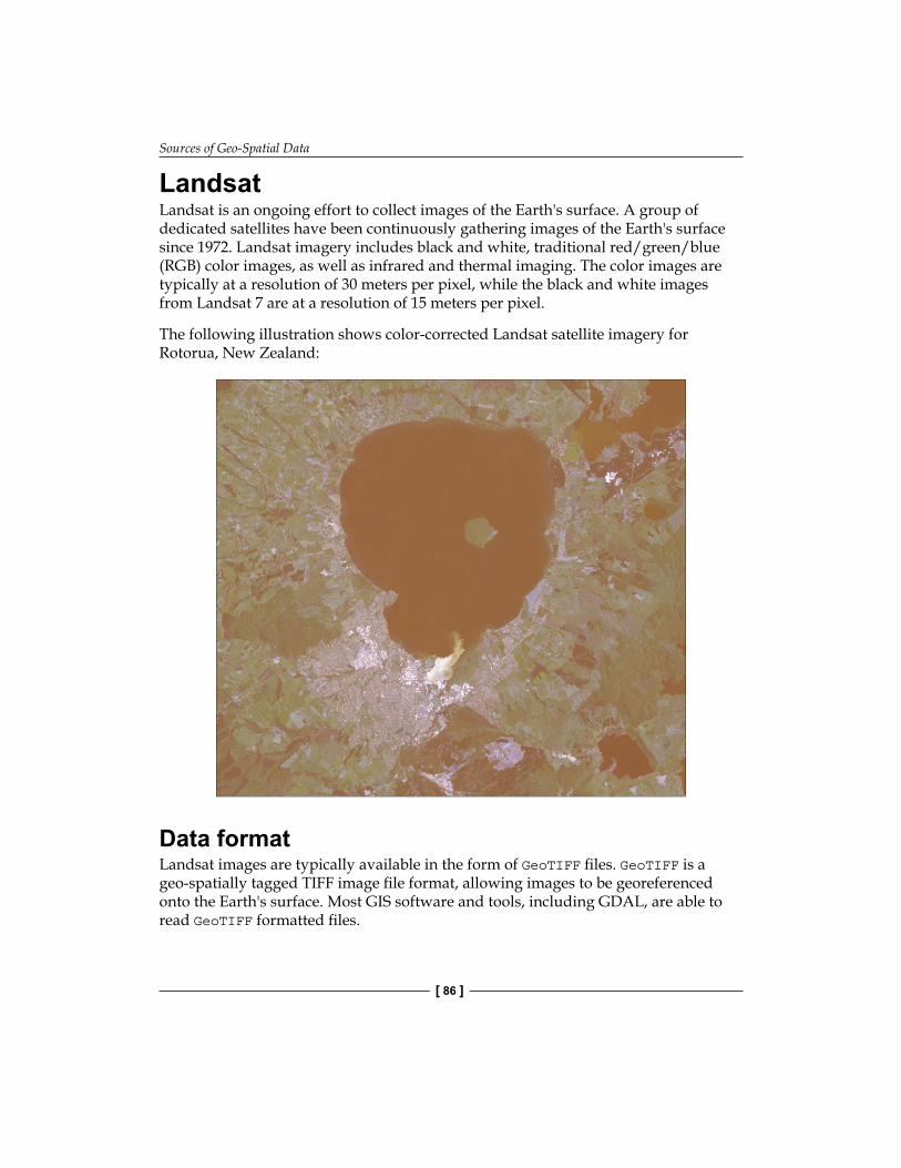
Sources of Geo-Spatial Data
[ 86 ]
LandsatLandsat is an ongoing effort to collect images of the Earth's surface. A group of dedicated satellites have been continuously gathering images of the Earth's surface since 1972. Landsat imagery includes black and white, traditional red/green/blue (RGB) color images, as well as infrared and thermal imaging. The color images are typically at a resolution of 30 meters per pixel, while the black and white images from Landsat 7 are at a resolution of 15 meters per pixel.
The following illustration shows color-corrected Landsat satellite imagery for Rotorua, New Zealand:
Data formatLandsat images are typically available in the form of GeoTIFF files. GeoTIFF is a geo-spatially tagged TIFF image file format, allowing images to be georeferenced onto the Earth's surface. Most GIS software and tools, including GDAL, are able to read GeoTIFF formatted files.
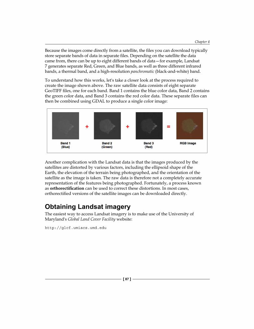
Chapter 4
[ 87 ]
Because the images come directly from a satellite, the files you can download typically store separate bands of data in separate files. Depending on the satellite the data came from, there can be up to eight different bands of data—for example, Landsat 7 generates separate Red, Green, and Blue bands, as well as three different infrared bands, a thermal band, and a high-resolution panchromatic (black-and-white) band.
To understand how this works, let's take a closer look at the process required to create the image shown above. The raw satellite data consists of eight separate GeoTIFF files, one for each band. Band 1 contains the blue color data, Band 2 contains the green color data, and Band 3 contains the red color data. These separate files can then be combined using GDAL to produce a single color image:
Another complication with the Landsat data is that the images produced by the satellites are distorted by various factors, including the ellipsoid shape of the Earth, the elevation of the terrain being photographed, and the orientation of the satellite as the image is taken. The raw data is therefore not a completely accurate representation of the features being photographed. Fortunately, a process known as orthorectification can be used to correct these distortions. In most cases, orthorectified versions of the satellite images can be downloaded directly.
Obtaining Landsat imageryThe easiest way to access Landsat imagery is to make use of the University of Maryland's Global Land Cover Facility website:
http://glcf.umiacs.umd.edu
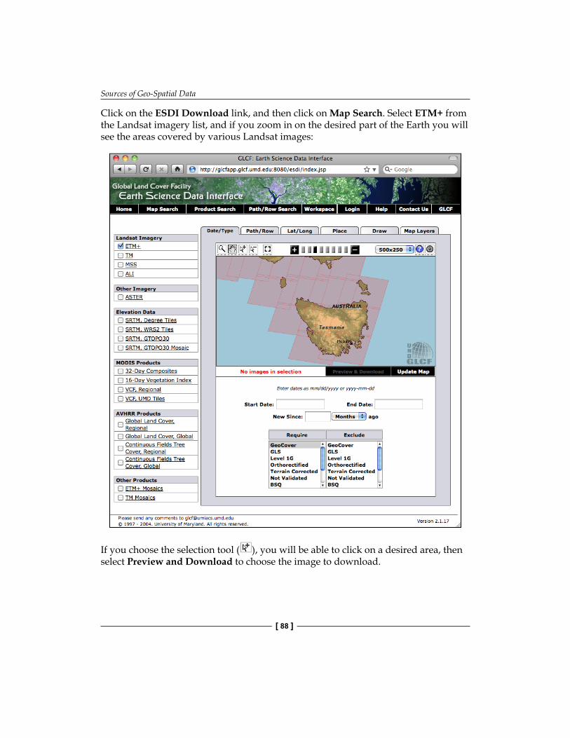
Sources of Geo-Spatial Data
[ 88 ]
Click on the ESDI Download link, and then click on Map Search. Select ETM+ from the Landsat imagery list, and if you zoom in on the desired part of the Earth you will see the areas covered by various Landsat images:
If you choose the selection tool ( ), you will be able to click on a desired area, then select Preview and Download to choose the image to download.
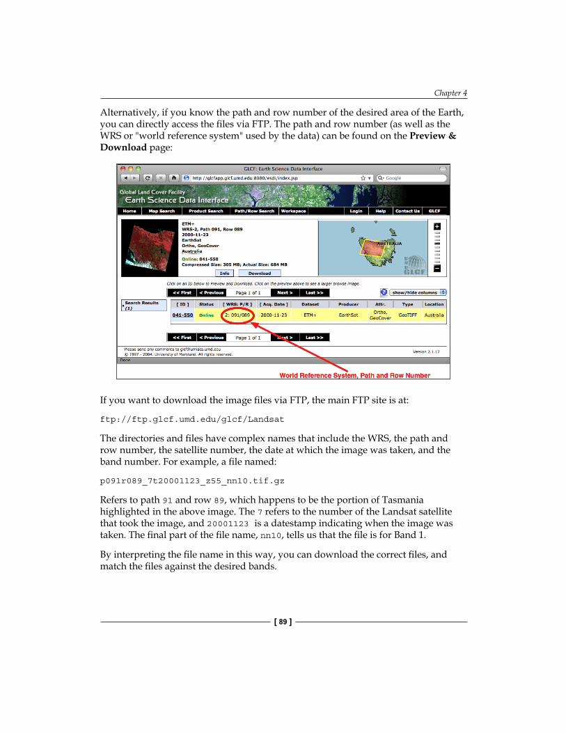
Chapter 4
[ 89 ]
Alternatively, if you know the path and row number of the desired area of the Earth, you can directly access the files via FTP. The path and row number (as well as the WRS or "world reference system" used by the data) can be found on the Preview & Download page:
If you want to download the image files via FTP, the main FTP site is at:
ftp://ftp.glcf.umd.edu/glcf/Landsat
The directories and files have complex names that include the WRS, the path and row number, the satellite number, the date at which the image was taken, and the band number. For example, a file named:
p091r089_7t20001123_z55_nn10.tif.gz
Refers to path 91 and row 89, which happens to be the portion of Tasmania highlighted in the above image. The 7 refers to the number of the Landsat satellite that took the image, and 20001123 is a datestamp indicating when the image was taken. The final part of the file name, nn10, tells us that the file is for Band 1.
By interpreting the file name in this way, you can download the correct files, and match the files against the desired bands.
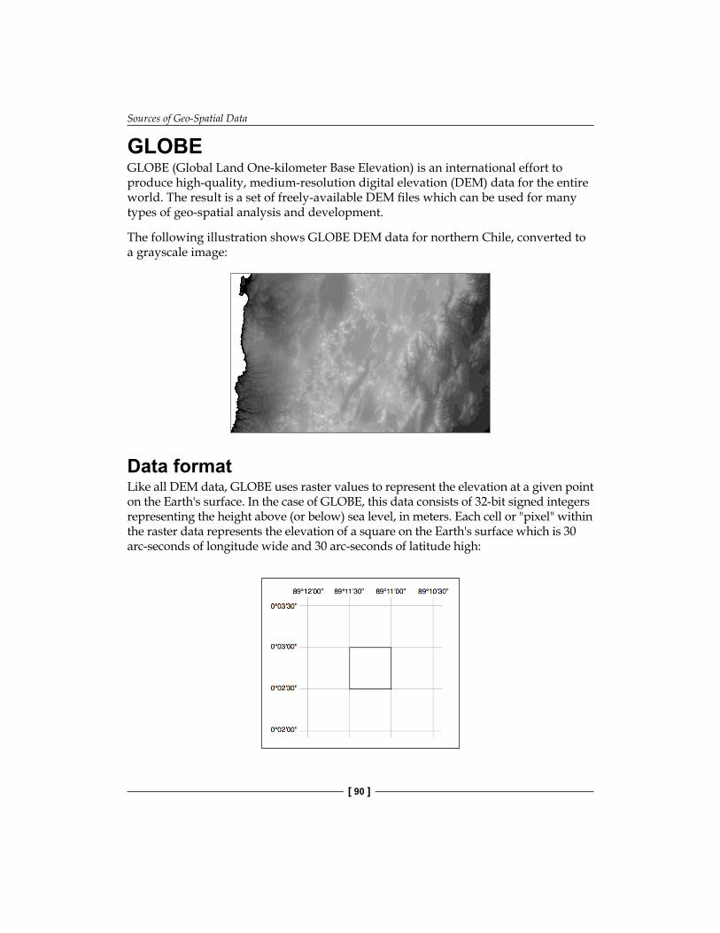
Sources of Geo-Spatial Data
[ 90 ]
GLOBEGLOBE (Global Land One-kilometer Base Elevation) is an international effort to produce high-quality, medium-resolution digital elevation (DEM) data for the entire world. The result is a set of freely-available DEM files which can be used for many types of geo-spatial analysis and development.
The following illustration shows GLOBE DEM data for northern Chile, converted to a grayscale image:
Data formatLike all DEM data, GLOBE uses raster values to represent the elevation at a given point on the Earth's surface. In the case of GLOBE, this data consists of 32-bit signed integers representing the height above (or below) sea level, in meters. Each cell or "pixel" within the raster data represents the elevation of a square on the Earth's surface which is 30 arc-seconds of longitude wide and 30 arc-seconds of latitude high:
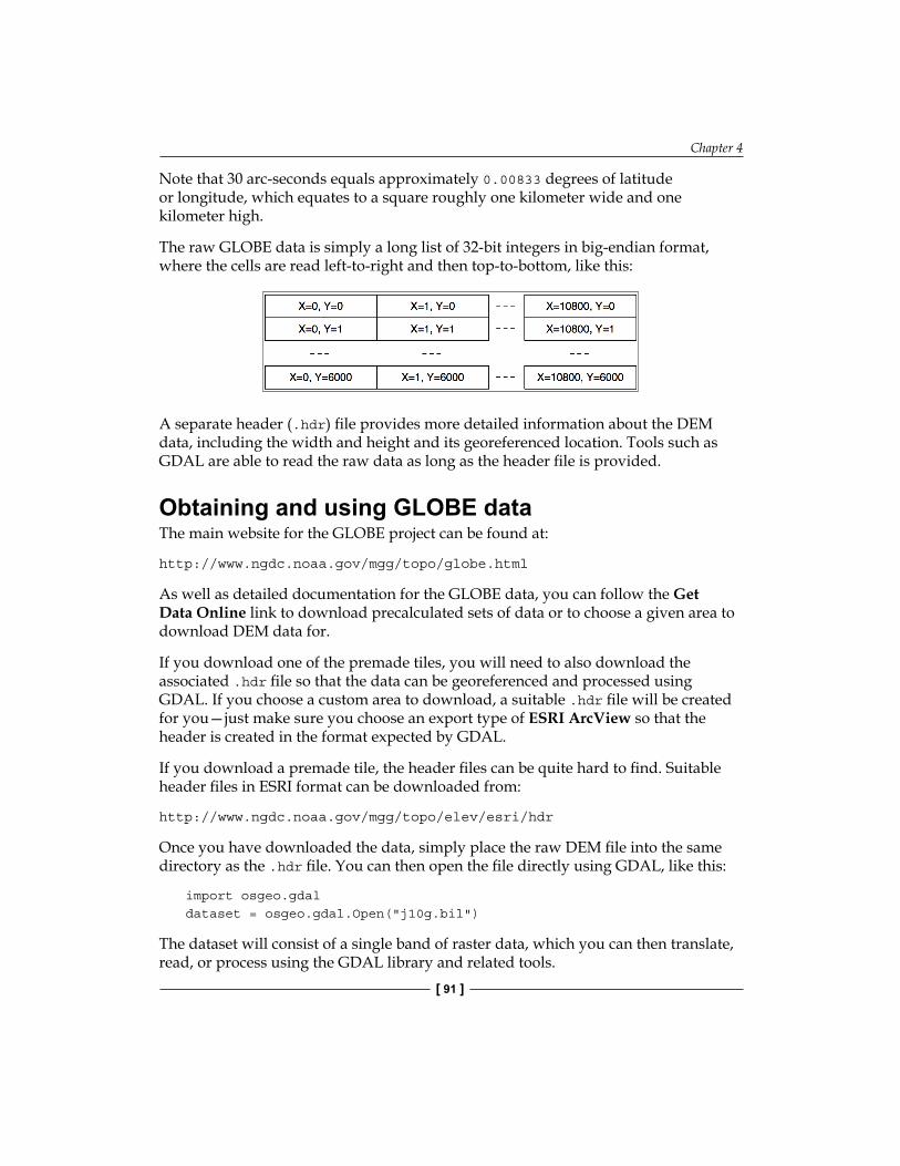
Chapter 4
[ 91 ]
Note that 30 arc-seconds equals approximately 0.00833 degrees of latitude or longitude, which equates to a square roughly one kilometer wide and one kilometer high.
The raw GLOBE data is simply a long list of 32-bit integers in big-endian format, where the cells are read left-to-right and then top-to-bottom, like this:
A separate header (.hdr) file provides more detailed information about the DEM data, including the width and height and its georeferenced location. Tools such as GDAL are able to read the raw data as long as the header file is provided.
Obtaining and using GLOBE dataThe main website for the GLOBE project can be found at:
http://www.ngdc.noaa.gov/mgg/topo/globe.html
As well as detailed documentation for the GLOBE data, you can follow the Get Data Online link to download precalculated sets of data or to choose a given area to download DEM data for.
If you download one of the premade tiles, you will need to also download the associated .hdr file so that the data can be georeferenced and processed using GDAL. If you choose a custom area to download, a suitable .hdr file will be created for you—just make sure you choose an export type of ESRI ArcView so that the header is created in the format expected by GDAL.
If you download a premade tile, the header files can be quite hard to find. Suitable header files in ESRI format can be downloaded from:
http://www.ngdc.noaa.gov/mgg/topo/elev/esri/hdr
Once you have downloaded the data, simply place the raw DEM file into the same directory as the .hdr file. You can then open the file directly using GDAL, like this:
import osgeo.gdaldataset = osgeo.gdal.Open("j10g.bil")
The dataset will consist of a single band of raster data, which you can then translate, read, or process using the GDAL library and related tools.
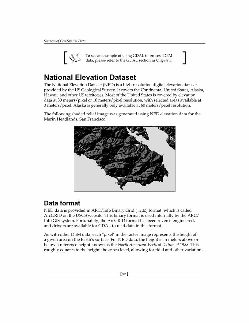
Sources of Geo-Spatial Data
[ 92 ]
To see an example of using GDAL to process DEM data, please refer to the GDAL section in Chapter 3.
National Elevation DatasetThe National Elevation Dataset (NED) is a high-resolution digital elevation dataset provided by the US Geological Survey. It covers the Continental United States, Alaska, Hawaii, and other US territories. Most of the United States is covered by elevation data at 30 meters/pixel or 10 meters/pixel resolution, with selected areas available at 3 meters/pixel. Alaska is generally only available at 60 meters/pixel resolution.
The following shaded relief image was generated using NED elevation data for the Marin Headlands, San Francisco:
Data formatNED data is provided in ARC/Info Binary Grid (.adf) format, which is called ArcGRID on the USGS website. This binary format is used internally by the ARC/Info GIS system. Fortunately, the ArcGRID format has been reverse-engineered, and drivers are available for GDAL to read data in this format.
As with other DEM data, each "pixel" in the raster image represents the height of a given area on the Earth's surface. For NED data, the height is in meters above or below a reference height known as the North American Vertical Datum of 1988. This roughly equates to the height above sea level, allowing for tidal and other variations.
Chapter 4
[ 93 ]
Obtaining and using NED dataNED data can be downloaded from the main NED website:
http://ned.usgs.gov
There are two options for downloading the elevation data:
• Choosing a prepackaged set of tiles by selecting the desired state and county or minimum and maximum lat/long values
• Using the National Map Seamless Server applet
Either option will work—the prepackaged tiles have the disadvantage that they are split into separate tiles, and include a six-pixel overlap at the edges of each tile. Using the Seamless Server returns all the data in one chunk, though the interface is a bit awkward to use and is limited in the amount of information that can be downloaded at any one time.
To download data using the Seamless Server, you first have to do the following:
1. Pan and zoom to display the area you want to download DEM data for.2. Click on the Download link in the upper-right corner and choose the
resolution for the elevation data you want to download.3. You then click on the Define Rectangular Download Area tool ( ) and drag
a box around the area you want to download data for.4. A separate window then appears showing you the area you have selected.
If you want, you can change the format of the downloaded data by clicking on the Modify Data Request hyperlink. The interface is quite confusing, but allows you to choose which format the data should be downloaded in, as well as compression and metadata options.
5. Finally, click on the Download button and your web browser will download the selected data once it has been extracted.
If you use the default download options, you will receive a ZIP file containing more than 20 separate files. Many of these files contain metadata and documentation; the ArcGRID files that contain the actual elevation data all end with the suffix .adf. Move these files into a separate directory, making sure to place all the .adf files in the same directory, and you will be able to read the elevation data from these files using GDAL.
Sources of Geo-Spatial Data
[ 94 ]
On non-Windows machines, you may need to remove the backslashes from the filenames before GDAL will recognize them
Once you have the ArcGRID datafiles, you can open them in GDAL just like you would open any other dataset:
import osgeo.gdaldataset = osgeo.gdal.Open("hdr.adf")
Finally, if you are working with DEM data, you might like to check out the gdaldem utility which is included as part of the GDAL download. This program makes it easy to view and manipulate DEM raster data. The shaded relief image shown above was created using this utility, like this:
gdaldem hillshade hdr.adf hillshade.tiff
Sources of other types of geo-spatial dataThe vector and raster geo-spatial data we have looked at so far is generally used to provide images or information about the Earth itself. However, geo-spatial applications often have to place data onto the surface of the Earth—that is, georeference something such as a place or event. In this section, we will look at two additional sources of geo-spatial data, in this case databases which place cities, towns, natural features, and points of interest onto the surface of the Earth.
This data can be used in two important ways. First, it can be used to label features—for example, to place the label London onto a georeferenced image of southern England. Secondly, this data can be used to locate something by name, for example by allowing the user to choose a city from a drop-down list and then draw a map centered around that city.
GEOnet Names ServerThe GEOnet Names Server (GNS) provides a large database of placenames. It is an official repository of non-American placenames, as decided by the US Board on Geographic Names.
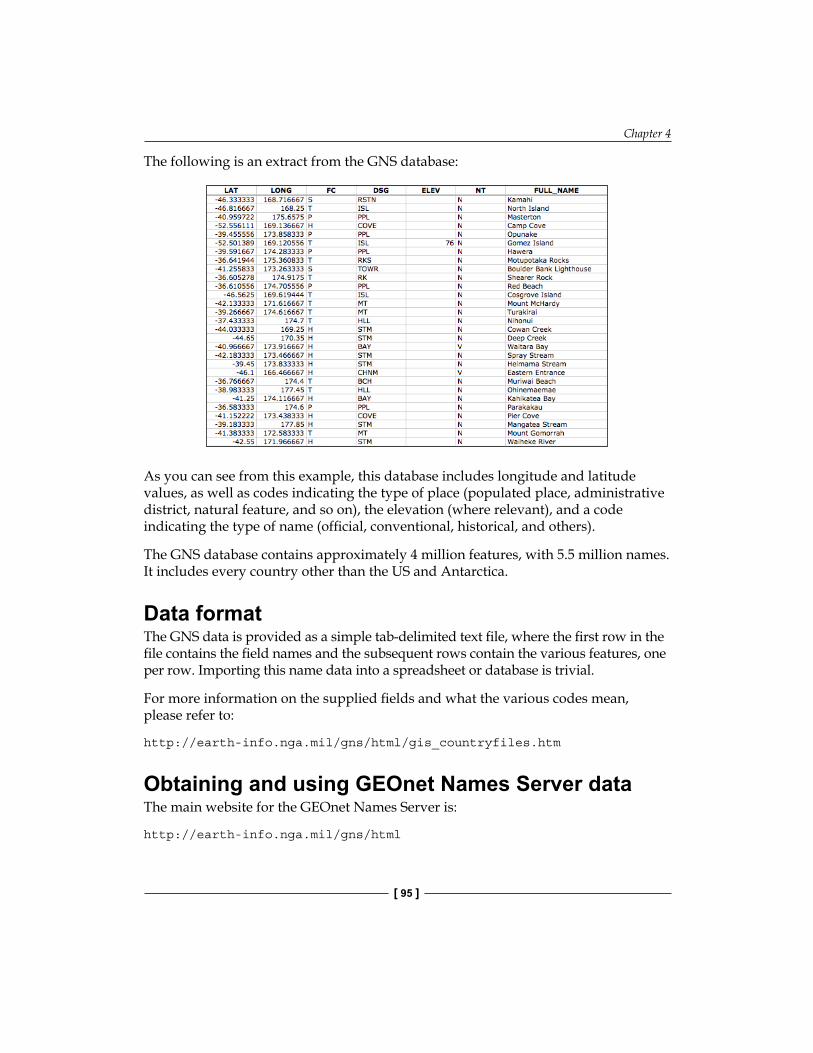
Chapter 4
[ 95 ]
The following is an extract from the GNS database:
As you can see from this example, this database includes longitude and latitude values, as well as codes indicating the type of place (populated place, administrative district, natural feature, and so on), the elevation (where relevant), and a code indicating the type of name (official, conventional, historical, and others).
The GNS database contains approximately 4 million features, with 5.5 million names. It includes every country other than the US and Antarctica.
Data formatThe GNS data is provided as a simple tab-delimited text file, where the first row in the file contains the field names and the subsequent rows contain the various features, one per row. Importing this name data into a spreadsheet or database is trivial.
For more information on the supplied fields and what the various codes mean, please refer to:
http://earth-info.nga.mil/gns/html/gis_countryfiles.htm
Obtaining and using GEOnet Names Server dataThe main website for the GEOnet Names Server is:
http://earth-info.nga.mil/gns/html
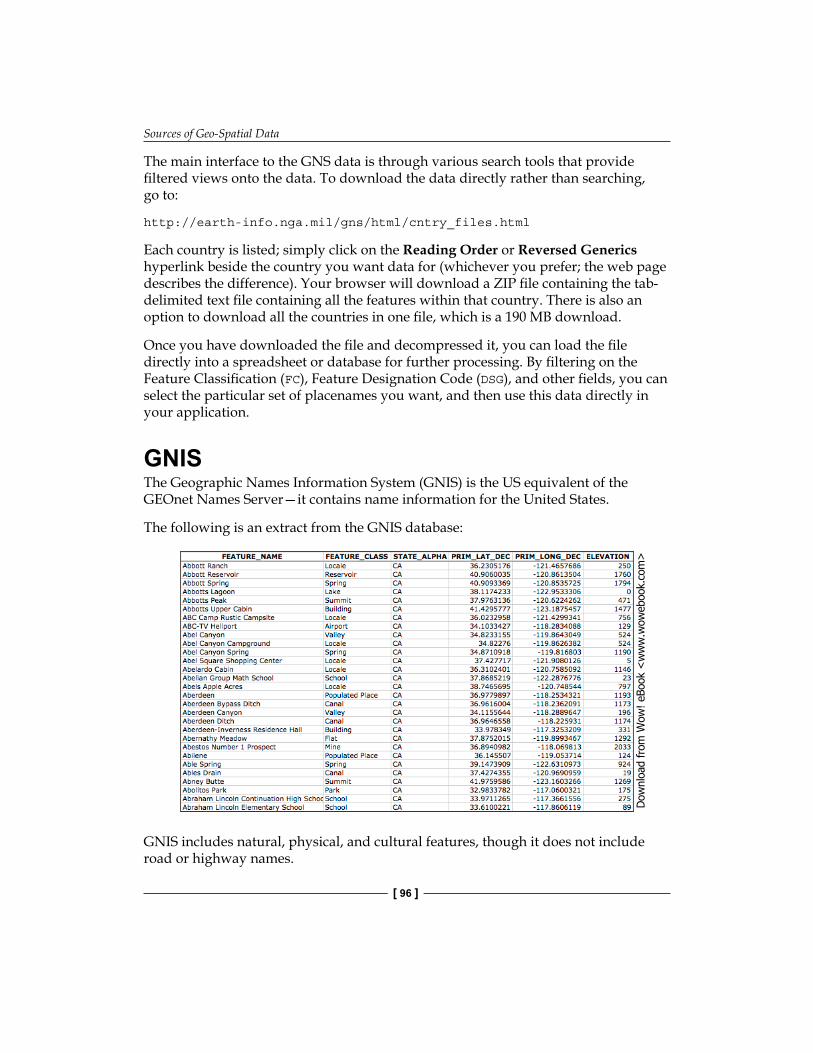
Sources of Geo-Spatial Data
[ 96 ]
The main interface to the GNS data is through various search tools that provide filtered views onto the data. To download the data directly rather than searching, go to:
http://earth-info.nga.mil/gns/html/cntry_files.html
Each country is listed; simply click on the Reading Order or Reversed Generics hyperlink beside the country you want data for (whichever you prefer; the web page describes the difference). Your browser will download a ZIP file containing the tab-delimited text file containing all the features within that country. There is also an option to download all the countries in one file, which is a 190 MB download.
Once you have downloaded the file and decompressed it, you can load the file directly into a spreadsheet or database for further processing. By filtering on the Feature Classification (FC), Feature Designation Code (DSG), and other fields, you can select the particular set of placenames you want, and then use this data directly in your application.
GNISThe Geographic Names Information System (GNIS) is the US equivalent of the GEOnet Names Server—it contains name information for the United States.
The following is an extract from the GNIS database:
GNIS includes natural, physical, and cultural features, though it does not include road or highway names.
Dow
nlo
ad fro
m W
ow
! eBook
<w
ww
.wow
ebook.
com
>
Chapter 4
[ 97 ]
As with the GEOnames database, the GNIS database contains the official names used by the US Government, as decided by the US Board on Geographic Names. GEOnames is run by the US Geological Survey, and currently contains over 2.1 million features.
Data formatGNIS names are available for download as pipe-delimited compressed text files. This format uses the "pipe" character (|) to separate the various fields:
FEATURE_ID|FEATURE_NAME|FEATURE_CLASS|...1397658|Ester|Populated Place|...1397926|Afognak|Populated Place|...
The first line contains the field names, and subsequent lines contain the various features. The available information includes the name of the feature, its type, elevation, the county and state the feature is in, the lat/long coordinate of the feature itself, and the lat/long coordinate for the "source" of the feature (for streams, valleys, and so on).
Obtaining and using GNIS dataThe main GNIS website can be found at:
http://geonames.usgs.gov/domestic
Click on the Download Domestic Names hyperlink and you will be given options to download all the GNIS data on a state-by-state basis, or all the features in a single large download. You can also download topical gazetteers that include selected subsets of the data—all populated places, all historical places, and so on.
If you click on the File Format hyperlinks, a pop up window will appear describing the structure of the files in more detail.
Once you have downloaded the data you want, you can simply import the file into a database or spreadsheet. To import into a spreadsheet, use the Delimited format and enter "|" as the custom delimiter character. You can then sort or filter the data in whatever way you want so that you can use it in your application.
Sources of Geo-Spatial Data
[ 98 ]
SummaryIn this chapter, we have surveyed a number of sources of freely-available geo-spatial data. If you wish to obtain map data, images, elevations, or placenames for use in your geo-spatial applications, the sources we have covered should give you everything you need. Of course, this is not an exhaustive list—other sources of data are available, and can be found using a search engine or sites such as http://freegis.org.
The following table lists the various requirements you may have for geo-spatial data in your application development, and which datasource(s) may be most appropriate in each case:
Requirement Suitable DatasourcesSimple base map World Borders DatasetShaded relief (pseudo-3D) maps GLOBE or NED data processed using gdaldemStreet map OpenStreetMapCity outlines TIGER (US), Digital Chart of the WorldDetailed country outlines GSHHS Level 1Photorealistic images of the earth LandsatLists of city and placenames GNIS (US) or Geonet Names Server (elsewhere)
To recap:
• OpenStreetMap is a collaborative website where people can create and edit vector maps worldwide.
• TIGER is a service of the US Geological Survey providing geo-spatial data on streets, railways, rivers, lakes, geographic boundaries, and legal and statistical entities such as school districts and urban regions.
• The Digital Chart of the World is a somewhat dated database providing country boundaries, urban areas, elevation data, and so on for the entire world.
• GSHHS is a high-resolution shoreline database containing detailed vector data for shorelines, lakes, and rivers worldwide.
• The World Borders Dataset is a simple vector datasource containing country borders and related data for the entire world bundled into one convenient package.
• Landsat provides detailed raster satellite imagery of all land masses on the Earth.
• GLOBE provides medium-resolution digital elevation (DEM) data for the entire world.

Chapter 4
[ 99 ]
• The National Elevation Dataset includes high-resolution digital elevation (DEM) data for the Continental United States, Alaska, Hawaii, and other US territories.
• The GEOnet Names Server provides information on official placenames for every country other than the US and Antarctica.
• GNIS provides official placenames for the United States.
In the next chapter, we will use the Python toolkits described in Chapter 3 to work with some of this geo-spatial data in interesting and useful ways.

Working with Geo-Spatial Data in Python
In this chapter, we combine the Python libraries and geo-spatial data covered earlier to accomplish a variety of tasks. These tasks have been chosen to demonstrate various techniques for working with geo-spatial data in your Python programs; while in some cases there are quicker and easier ways to achieve these results (for example, using command-line utilities), we will create these solutions in Python so you can learn how to work with geo-spatial data in your own Python programs.
This chapter will cover:
• Reading and writing geo-spatial data in both vector and raster format• Changing the datums and projections used by geo-spatial data• Representing and storing geo-spatial data within your Python programs• Using Shapely to work with points, lines, and polygons• Converting and standardizing units of geometry and distance
This chapter is formatted like a cookbook, detailing various real-world tasks you might want to perform and providing "recipes" for accomplishing them.
PrerequisitesIf you want to follow through the examples in this chapter, make sure you have the following Python libraries installed on your computer:
• GDAL/OGR version 1.7 or later (http://gdal.org)• pyproj version 1.8.6 or later (http://code.google.com/p/pyproj)• Shapely version 1.2 or later (http://trac.gispython.org/lab/wiki/
Shapely)
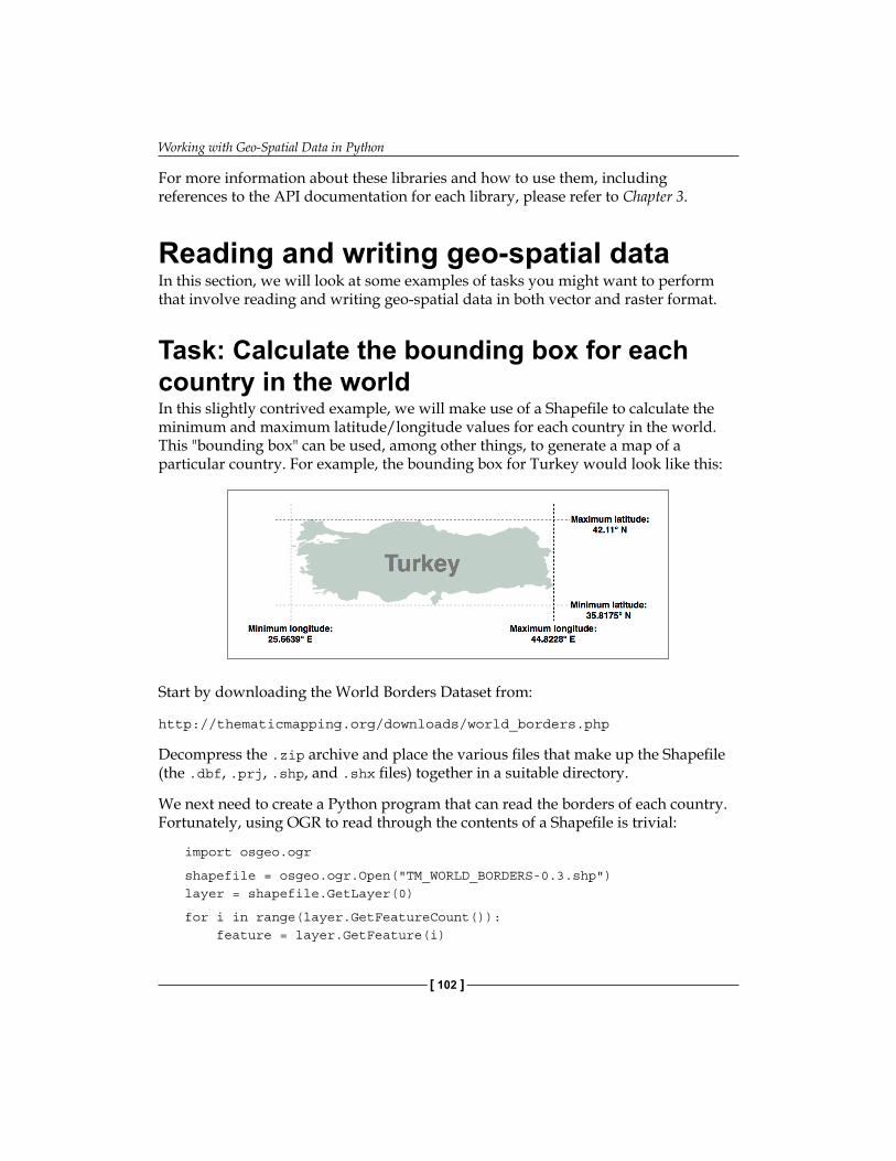
Working with Geo-Spatial Data in Python
[ 102 ]
For more information about these libraries and how to use them, including references to the API documentation for each library, please refer to Chapter 3.
Reading and writing geo-spatial dataIn this section, we will look at some examples of tasks you might want to perform that involve reading and writing geo-spatial data in both vector and raster format.
Task: Calculate the bounding box for each country in the worldIn this slightly contrived example, we will make use of a Shapefile to calculate the minimum and maximum latitude/longitude values for each country in the world. This "bounding box" can be used, among other things, to generate a map of a particular country. For example, the bounding box for Turkey would look like this:
Start by downloading the World Borders Dataset from:
http://thematicmapping.org/downloads/world_borders.php
Decompress the .zip archive and place the various files that make up the Shapefile (the .dbf, .prj, .shp, and .shx files) together in a suitable directory.
We next need to create a Python program that can read the borders of each country. Fortunately, using OGR to read through the contents of a Shapefile is trivial:
import osgeo.ogr
shapefile = osgeo.ogr.Open("TM_WORLD_BORDERS-0.3.shp")layer = shapefile.GetLayer(0)
for i in range(layer.GetFeatureCount()): feature = layer.GetFeature(i)
Chapter 5
[ 103 ]
The feature consists of a geometry and a set of fields. For this data, the geometry is a polygon that defines the outline of the country, while the fields contain various pieces of information about the country. According to the Readme.txt file, the fields in this Shapefile include the ISO-3166 three-letter code for the country (in a field named ISO3) as well as the name for the country (in a field named NAME). This allows us to obtain the country code and name like this:
countryCode = feature.GetField("ISO3")countryName = feature.GetField("NAME")
We can also obtain the country's border polygon using:
geometry = feature.GetGeometryRef()
There are all sorts of things we can do with this geometry, but in this case we want to obtain the bounding box or envelope for the polygon:
minLong,maxLong,minLat,maxLat = geometry.GetEnvelope()
Let's put all this together into a complete working program:
# calcBoundingBoxes.py
import osgeo.ogr
shapefile = osgeo.ogr.Open("TM_WORLD_BORDERS-0.3.shp")layer = shapefile.GetLayer(0)
countries = [] # List of (code,name,minLat,maxLat, # minLong,maxLong) tuples.
for i in range(layer.GetFeatureCount()): feature = layer.GetFeature(i) countryCode = feature.GetField("ISO3") countryName = feature.GetField("NAME") geometry = feature.GetGeometryRef() minLong,maxLong,minLat,maxLat = geometry.GetEnvelope()
countries.append((countryName, countryCode, minLat, maxLat, minLong, maxLong))
countries.sort()for name,code,minLat,maxLat,minLong,maxLong in countries: print "%s (%s) lat=%0.4f..%0.4f, long=%0.4f..%0.4f" \% (name, code,minLat, maxLat,minLong, maxLong)
Running this program produces the following output:
% python calcBoundingBoxes.py
Afghanistan (AFG) lat=29.4061..38.4721, long=60.5042..74.9157
Albania (ALB) lat=39.6447..42.6619, long=19.2825..21.0542
Algeria (DZA) lat=18.9764..37.0914, long=-8.6672..11.9865
...
Working with Geo-Spatial Data in Python
[ 104 ]
Task: Save the country bounding boxes into a ShapefileWhile the previous example simply printed out the latitude and longitude values, it might be more useful to draw the bounding boxes onto a map. To do this, we have to convert the bounding boxes into polygons, and save these polygons into a Shapefile.
Creating a Shapefile involves the following steps:
1. Define the spatial reference used by the Shapefile's data. In this case, we'll use the WGS84 datum and unprojected geographic coordinates (that is, latitude and longitude values). This is how you would define this spatial reference using OGR:import osgeo.osr
spatialReference = osgeo.osr.SpatialReference()
spatialReference.SetWellKnownGeogCS('WGS84')
We can now create the Shapefile itself using this spatial reference:import osgeo.ogr
driver = osgeo.ogr.GetDriverByName("ESRI Shapefile")
dstFile = driver.CreateDataSource("boundingBoxes.shp"))
dstLayer = dstFile.CreateLayer("layer", spatialReference)
2. After creating the Shapefile, you next define the various fields that will hold the metadata for each feature. In this case, let's add two fields to store the country name and its ISO-3166 code:fieldDef = osgeo.ogr.FieldDefn("COUNTRY", osgeo.ogr.OFTString)
fieldDef.SetWidth(50)
dstLayer.CreateField(fieldDef)
fieldDef = osgeo.ogr.FieldDefn("CODE", osgeo.ogr.OFTString)
fieldDef.SetWidth(3)
dstLayer.CreateField(fieldDef)
3. We now need to create the geometry for each feature—in this case, a polygon defining the country's bounding box. A polygon consists of one or more linear rings; the first linear ring defines the exterior of the polygon, while additional rings define "holes" inside the polygon. In this case, we want a simple polygon with a square exterior and no holes:linearRing = osgeo.ogr.Geometry(osgeo.ogr.wkbLinearRing)
linearRing.AddPoint(minLong, minLat)
linearRing.AddPoint(maxLong, minLat)
linearRing.AddPoint(maxLong, maxLat)
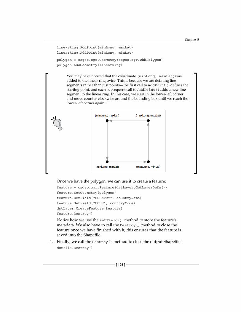
Chapter 5
[ 105 ]
linearRing.AddPoint(minLong, maxLat)
linearRing.AddPoint(minLong, minLat)
polygon = osgeo.ogr.Geometry(osgeo.ogr.wkbPolygon)
polygon.AddGeometry(linearRing)
You may have noticed that the coordinate (minLong, minLat)was added to the linear ring twice. This is because we are defining line segments rather than just points—the first call to AddPoint()defines the starting point, and each subsequent call to AddPoint()adds a new line segment to the linear ring. In this case, we start in the lower-left corner and move counter-clockwise around the bounding box until we reach the lower-left corner again:
Once we have the polygon, we can use it to create a feature:feature = osgeo.ogr.Feature(dstLayer.GetLayerDefn())
feature.SetGeometry(polygon)
feature.SetField("COUNTRY", countryName)
feature.SetField("CODE", countryCode)
dstLayer.CreateFeature(feature)
feature.Destroy()
Notice how we use the setField() method to store the feature's metadata. We also have to call the Destroy() method to close the feature once we have finished with it; this ensures that the feature is saved into the Shapefile.
4. Finally, we call the Destroy() method to close the output Shapefile:dstFile.Destroy()
Working with Geo-Spatial Data in Python
[ 106 ]
5. Putting all this together, and combining it with the code from the previous recipe to calculate the bounding boxes for each country in the World Borders Dataset Shapefile, we end up with the following complete program:
# boundingBoxesToShapefile.py
import os, os.path, shutil
import osgeo.ogr
import osgeo.osr
# Open the source shapefile.
srcFile = osgeo.ogr.Open("TM_WORLD_BORDERS-0.3.shp")
srcLayer = srcFile.GetLayer(0)
# Open the output shapefile.
if os.path.exists("bounding-boxes"):
shutil.rmtree("bounding-boxes")
os.mkdir("bounding-boxes")
spatialReference = osgeo.osr.SpatialReference()
spatialReference.SetWellKnownGeogCS('WGS84')
driver = osgeo.ogr.GetDriverByName("ESRI Shapefile")
dstPath = os.path.join("bounding-boxes", "boundingBoxes.shp")
dstFile = driver.CreateDataSource(dstPath)
dstLayer = dstFile.CreateLayer("layer", spatialReference)
fieldDef = osgeo.ogr.FieldDefn("COUNTRY", osgeo.ogr.OFTString)
fieldDef.SetWidth(50)
dstLayer.CreateField(fieldDef)
fieldDef = osgeo.ogr.FieldDefn("CODE", osgeo.ogr.OFTString)
fieldDef.SetWidth(3)
dstLayer.CreateField(fieldDef)
# Read the country features from the source shapefile.
for i in range(srcLayer.GetFeatureCount()):
feature = srcLayer.GetFeature(i)
countryCode = feature.GetField("ISO3")
countryName = feature.GetField("NAME")
geometry = feature.GetGeometryRef()
minLong,maxLong,minLat,maxLat = geometry.GetEnvelope()
# Save the bounding box as a feature in the output
# shapefile.
Chapter 5
[ 107 ]
linearRing = osgeo.ogr.Geometry(osgeo.ogr.wkbLinearRing)
linearRing.AddPoint(minLong, minLat)
linearRing.AddPoint(maxLong, minLat)
linearRing.AddPoint(maxLong, maxLat)
linearRing.AddPoint(minLong, maxLat)
linearRing.AddPoint(minLong, minLat)
polygon = osgeo.ogr.Geometry(osgeo.ogr.wkbPolygon)
polygon.AddGeometry(linearRing)
feature = osgeo.ogr.Feature(dstLayer.GetLayerDefn())
feature.SetGeometry(polygon)
feature.SetField("COUNTRY", countryName)
feature.SetField("CODE", countryCode)
dstLayer.CreateFeature(feature)
feature.Destroy()
# All done.
srcFile.Destroy()
dstFile.Destroy()
The only unexpected twist in this program is the use of a sub-directory called bounding-boxes to store the output Shapefile. Because a Shapefile is actually made up of multiple files on disk (a .dbf file, a .prj file, a .shp file, and a .shx file), it is easier to place these together in a sub-directory. We use the Python Standard Library module shutil to delete the previous contents of this directory, and then os.mkdir() to create it again.
If you aren't storing the TM_WORLD_BORDERS-0.3.shp Shapefile in the same directory as the script itself, you will need to add the directory where the Shapefile is stored to your osgeo.ogr.Open() call. You can also store the boundingBoxes.shp Shapefile in a different directory if you prefer, by changing the path where this Shapefile is created.
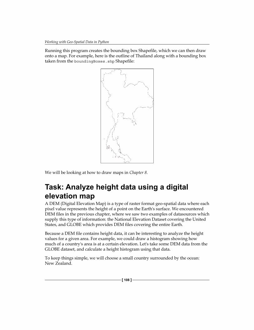
Working with Geo-Spatial Data in Python
[ 108 ]
Running this program creates the bounding box Shapefile, which we can then draw onto a map. For example, here is the outline of Thailand along with a bounding box taken from the boundingBoxes.shp Shapefile:
We will be looking at how to draw maps in Chapter 8.
Task: Analyze height data using a digital elevation mapA DEM (Digital Elevation Map) is a type of raster format geo-spatial data where each pixel value represents the height of a point on the Earth's surface. We encountered DEM files in the previous chapter, where we saw two examples of datasources which supply this type of information: the National Elevation Dataset covering the United States, and GLOBE which provides DEM files covering the entire Earth.
Because a DEM file contains height data, it can be interesting to analyze the height values for a given area. For example, we could draw a histogram showing how much of a country's area is at a certain elevation. Let's take some DEM data from the GLOBE dataset, and calculate a height histogram using that data.
To keep things simple, we will choose a small country surrounded by the ocean: New Zealand.
Chapter 5
[ 109 ]
We're using a small country so that we don't have too much data to work with, and we're using a country surrounded by ocean so that we can check all the points within a bounding box rather than having to use a polygon to exclude points outside of the country's boundaries.
To download the DEM data, go to the GLOBE website (http://www.ngdc.noaa.gov/mgg/topo/globe.html) and click on the Get Data Online hyperlink. We're going to use the data already calculated for this area of the world, so click on the Any or all 16 "tiles" hyperlink. New Zealand is in tile L, so click on this tile to download it.
The file you download will be called l10g.gz. If you decompress it, you will end up with a file l10g containing the raw elevation data.
By itself, this file isn't very useful—it needs to be georeferenced onto the Earth's surface so that you can match up a height value with its position on the Earth. To do this, you need to download the associated header file. Unfortunately, the GLOBE website makes this rather difficult; the header files for the premade tiles can be found at:
http://www.ngdc.noaa.gov/mgg/topo/elev/esri/hdr
Download the file named l10g.hdr and place it into the same directory as the l10g file you downloaded earlier. You can then read the DEM file using GDAL:
import osgeo.gdal
dataset = osgeo.gdal.Open("l10g")
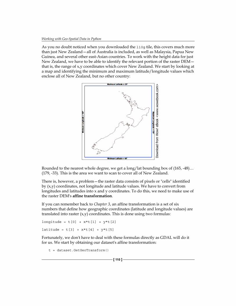
Working with Geo-Spatial Data in Python
[ 110 ]
As you no doubt noticed when you downloaded the l10g tile, this covers much more than just New Zealand—all of Australia is included, as well as Malaysia, Papua New Guinea, and several other east-Asian countries. To work with the height data for just New Zealand, we have to be able to identify the relevant portion of the raster DEM—that is, the range of x,y coordinates which cover New Zealand. We start by looking at a map and identifying the minimum and maximum latitude/longitude values which enclose all of New Zealand, but no other country:
Rounded to the nearest whole degree, we get a long/lat bounding box of (165, -48)…(179, -33). This is the area we want to scan to cover all of New Zealand.
There is, however, a problem—the raster data consists of pixels or "cells" identified by (x,y) coordinates, not longitude and latitude values. We have to convert from longitudes and latitudes into x and y coordinates. To do this, we need to make use of the raster DEM's affine transformation.
If you can remember back to Chapter 3, an affine transformation is a set of six numbers that define how geographic coordinates (latitude and longitude values) are translated into raster (x,y) coordinates. This is done using two formulas:
longitude = t[0] + x*t[1] + y*t[2]
latitude = t[3] + x*t[4] + y*t[5]
Fortunately, we don't have to deal with these formulas directly as GDAL will do it for us. We start by obtaining our dataset's affine transformation:
t = dataset.GetGeoTransform()
Dow
nlo
ad fro
m W
ow
! eBook
<w
ww
.wow
ebook.
com
>
Chapter 5
[ 111 ]
Using this transformation, we could convert an x,y coordinate into its associated latitude and longitude value. In this case, however, we want to do the opposite—we want to take a latitude and longitude, and calculate the associated x,y coordinate.
To do this, we have to invert the affine transformation. Once again, GDAL will do this for us:
success,tInverse = gdal.InvGeoTransform(t)if not success: print "Failed!" sys.exit(1)
There are some cases where an affine transformation can't be inverted. This is why gdal.InvGeoTransform() returns a success flag as well as the inverted transformation. With this DEM data, however, the affine transformation should always be invertible.
Now that we have the inverse affine transformation, it is possible to convert from a latitude and longitude into an x,y coordinate by using:
x,y = gdal.ApplyGeoTransform(tInverse, longitude, latitude)
Using this, it's easy to identify the minimum and maximum x,y coordinates that cover the area we are interested in:
x1,y1 = gdal.ApplyGeoTransform(tInverse, minLong, minLat)x2,y2 = gdal.ApplyGeoTransform(tInverse, maxLong, maxLat)
minX = int(min(x1, x2))maxX = int(max(x1, x2))minY = int(min(y1, y2))maxY = int(max(y1, y2))
Now that we know the x,y coordinates for the portion of the DEM that we're interested in, we can use GDAL to read in the individual height values. We start by obtaining the raster band that contains the DEM data:
band = dataset.GetRasterBand(1)
GDAL band numbers start at one. There is only one raster band in the DEM data we're using.
Now that we have the raster band, we can use the band.ReadRaster() method to read the raw DEM data. This is what the ReadRaster() method looks like:
ReadRaster(x, y, width, height, dWidth, dHeight, pixelType)
Working with Geo-Spatial Data in Python
[ 112 ]
Where:
• x is the number of pixels from the left side of the raster band to the left side of the portion of the band to read from
• y is the number of pixels from the top of the raster band to the top of the portion of the band to read from
• width is the number of pixels across to read• height is the number of pixels down to read• dWidth is the width of the resulting data• dHeight is the height of the resulting data• pixelType is a constant defining how many bytes of data there are for each
pixel value, and how that data is to be interpreted
Normally, you would set dWidth and dHeight to the same value as width and height; if you don't do this, the raster data will be scaled up or down when it is read.
The ReadRaster() method returns a string containing the raster data as a raw sequence of bytes. You can then read the individual values from this string using the struct standard library module:
values = struct.unpack("<" + ("h" * width), data)
Putting all this together, we can use GDAL to open the raster datafile and read all the pixel values within the bounding box surrounding New Zealand:
import sys, structfrom osgeo import gdalfrom osgeo import gdalconst
minLat = -48maxLat = -33minLong = 165maxLong = 179
dataset = gdal.Open("l10g")band = dataset.GetRasterBand(1)
t = dataset.GetGeoTransform()success,tInverse = gdal.InvGeoTransform(t)if not success: print "Failed!" sys.exit(1)
x1,y1 = gdal.ApplyGeoTransform(tInverse, minLong, minLat)
Chapter 5
[ 113 ]
x2,y2 = gdal.ApplyGeoTransform(tInverse, maxLong, maxLat)
minX = int(min(x1, x2))maxX = int(max(x1, x2))minY = int(min(y1, y2))maxY = int(max(y1, y2))
width = (maxX - minX) + 1fmt = "<" + ("h" * width)
for y in range(minY, maxY+1): scanline = band.ReadRaster(minX, y,width, 1, width, 1, gdalconst.GDT_Int16) values = struct.unpack(fmt, scanline)
for value in values: ...
Don't forget to add a directory path to the gdal.Open()statement if you placed the l10g file in a different directory.
Let's replace the ... with some code that does something useful with the pixel values. We will calculate a histogram:
histogram = {} # Maps height to # pixels with that height.
...
for value in values: try: histogram[value] += 1 except KeyError: histogram[value] = 1
for height in sorted(histogram.keys()): print height,histogram[height]
If you run this, you will see a list of heights (in meters) and how many pixels there are at that height:
-500 2607581
1 6641
2 909
3 1628
...
3097 1
3119 2
3173 1
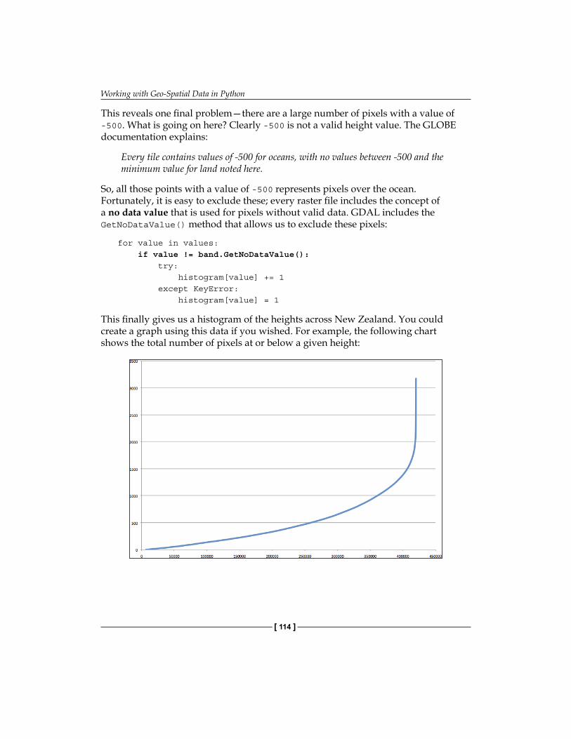
Working with Geo-Spatial Data in Python
[ 114 ]
This reveals one final problem—there are a large number of pixels with a value of -500. What is going on here? Clearly -500 is not a valid height value. The GLOBE documentation explains:
Every tile contains values of -500 for oceans, with no values between -500 and the minimum value for land noted here.
So, all those points with a value of -500 represents pixels over the ocean. Fortunately, it is easy to exclude these; every raster file includes the concept of a no data value that is used for pixels without valid data. GDAL includes the GetNoDataValue() method that allows us to exclude these pixels:
for value in values: if value != band.GetNoDataValue(): try: histogram[value] += 1 except KeyError: histogram[value] = 1
This finally gives us a histogram of the heights across New Zealand. You could create a graph using this data if you wished. For example, the following chart shows the total number of pixels at or below a given height:
Chapter 5
[ 115 ]
Changing datums and projectionsIf you can remember from Chapter 2, a datum is a mathematical model of the Earth's shape, while a projection is a way of translating points on the Earth's surface into points on a two-dimensional map. There are a large number of available datums and projections—whenever you are working with geo-spatial data, you must know which datum and which projection (if any) your data uses. If you are combining data from multiple sources, you will often have to change your geo-spatial data from one datum to another, or from one projection to another.
Task: Change projections to combine Shapefiles using geographic and UTM coordinatesHere, we will work with two Shapefiles that have different projections. We haven't yet encountered any geo-spatial data that uses a projection—all the data we've seen so far uses geographic (unprojected) latitude and longitude values. So, let's start by downloading some geo-spatial data in UTM (Universal Transverse Mercator) projection.
The WebGIS website (http://webgis.com) provides Shapefiles describing land-use and land-cover, called LULC datafiles. For this example, we will download a Shapefile for southern Florida (Dade County, to be exact) which uses the Universal Transverse Mercator projection.
You can download this Shapefile from the following URL:
http://webgis.com/MAPS/fl/lulcutm/miami.zip
The uncompressed directory contains the Shapefile, called miami.shp, along with a datum_reference.txt file describing the Shapefile's coordinate system. This file tells us the following:
The LULC shape file was generated from the original USGS GIRAS LULC file by Lakes Environmental Software.Datum: NAD83Projection: UTMZone: 17Data collection date by U.S.G.S.: 1972Reference: http://edcwww.cr.usgs.gov/products/landcover/lulc.html
So, this particular Shapefile uses UTM Zone 17 projection, and a datum of NAD83.
Working with Geo-Spatial Data in Python
[ 116 ]
Let's take a second Shapefile, this time in geographic coordinates. We'll use the GSHHS shoreline database, which uses the WGS84 datum and geographic (latitude/longitude) coordinates.
You don't need to download the GSHHS database for this example; while we will display a map overlaying the LULC data over the top of the GSHHS data, you only need the LULC Shapefile to complete this recipe. Drawing maps such as the one shown below will be covered in Chapter 8.
Combining these two Shapefiles as they are would be impossible—the LULC Shapefile has coordinates measured in UTM (that is, in meters from a given reference line), while the GSHHS Shapefile has coordinates in latitude and longitude values (in decimal degrees):
LULC: x=485719.47, y=2783420.62
x=485779.49,y=2783380.63
x=486129.65, y=2783010.66
...
GSHHS: x=180.0000,y=68.9938
x=180.0000,y=65.0338
x=179.9984, y=65.0337
...
Before we can combine these two Shapefiles, we first have to convert them to use the same projection. We'll do this by converting the LULC Shapefile from UTM-17 to geographic projection. Doing this requires us to define a coordinate transformation and then apply that transformation to each of the features in the Shapefile.
Here is how you can define a coordinate transformation using OGR:
from osgeo import osr
srcProjection = osr.SpatialReference()srcProjection.SetUTM(17)
dstProjection = osr.SpatialReference()dstProjection.SetWellKnownGeogCS('WGS84') # Lat/long.
transform = osr.CoordinateTransformation(srcProjection, dstProjection)
Chapter 5
[ 117 ]
Using this transformation, we can transform each of the features in the Shapefile from UTM projection back into geographic coordinates:
for i in range(layer.GetFeatureCount()): feature = layer.GetFeature(i) geometry = feature.GetGeometryRef() geometry.Transform(transform) ...
Putting all this together with the techniques we explored earlier for copying the features from one Shapefile to another, we end up with the following complete program:
# changeProjection.py
import os, os.path, shutilfrom osgeo import ogrfrom osgeo import osrfrom osgeo import gdal
# Define the source and destination projections, and a# transformation object to convert from one to the other.
srcProjection = osr.SpatialReference()srcProjection.SetUTM(17)
dstProjection = osr.SpatialReference()dstProjection.SetWellKnownGeogCS('WGS84') # Lat/long.
transform = osr.CoordinateTransformation(srcProjection, dstProjection)
# Open the source shapefile.
srcFile = ogr.Open("miami/miami.shp")srcLayer = srcFile.GetLayer(0)
# Create the dest shapefile, and give it the new projection.
if os.path.exists("miami-reprojected"): shutil.rmtree("miami-reprojected")os.mkdir("miami-reprojected")
driver = ogr.GetDriverByName("ESRI Shapefile")dstPath = os.path.join("miami-reprojected", "miami.shp")dstFile = driver.CreateDataSource(dstPath)dstLayer = dstFile.CreateLayer("layer", dstProjection)
# Reproject each feature in turn.
for i in range(srcLayer.GetFeatureCount()): feature = srcLayer.GetFeature(i) geometry = feature.GetGeometryRef()
Working with Geo-Spatial Data in Python
[ 118 ]
newGeometry = geometry.Clone() newGeometry.Transform(transform)
feature = ogr.Feature(dstLayer.GetLayerDefn()) feature.SetGeometry(newGeometry) dstLayer.CreateFeature(feature) feature.Destroy()
# All done.
srcFile.Destroy()dstFile.Destroy()
Note that this example doesn't copy field values into the new Shapefile; if your Shapefile has metadata, you will want to copy the fields across as you create each new feature. Also, the above code assumes that the miami.shp Shapefile has been placed into a miami sub-directory; you'll need to change the ogr.Open() statement to use the appropriate path name if you've stored this Shapefile in a different place.
After running this program over the miami.shp Shapefile, the coordinates for all the features in the Shapefile will have been converted from UTM-17 into geographic coordinates:
Before reprojection: x=485719.47, y=2783420.62
x=485779.49, y=2783380.63
x=486129.65, y=2783010.66
...
After reprojection: x=-81.1417, y=25.1668
x=-81.1411, y=25.1664
x=-81.1376, y=25.1631
...
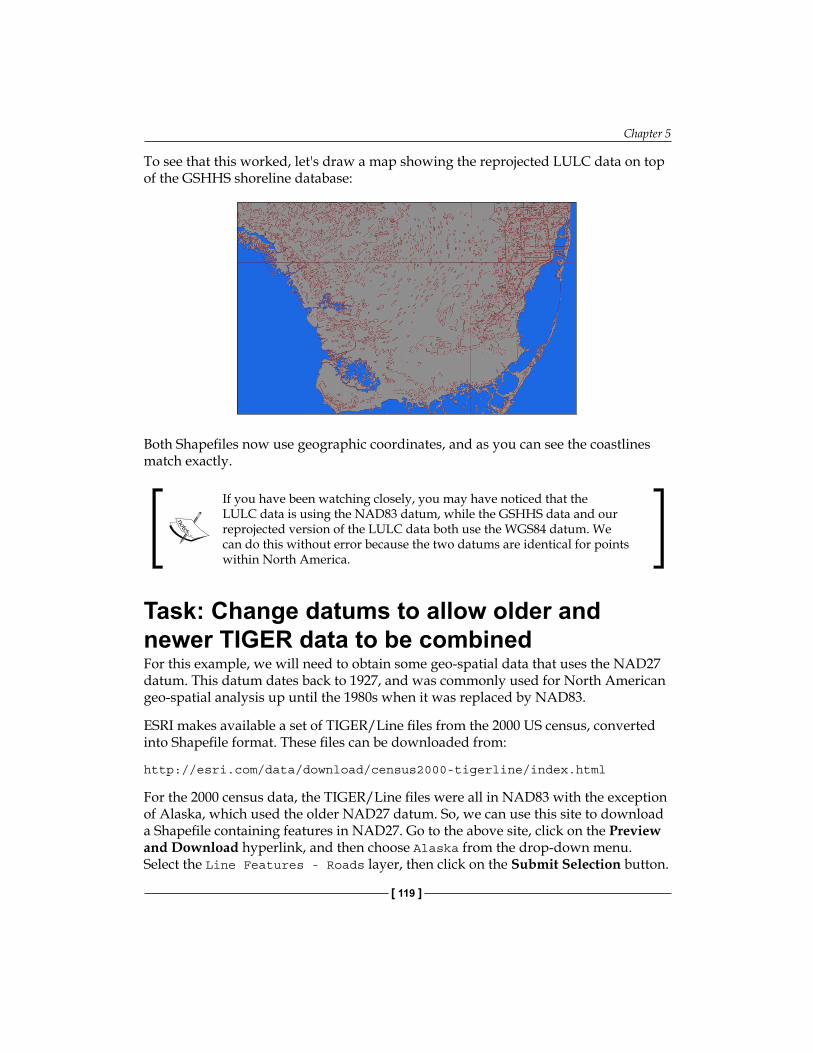
Chapter 5
[ 119 ]
To see that this worked, let's draw a map showing the reprojected LULC data on top of the GSHHS shoreline database:
Both Shapefiles now use geographic coordinates, and as you can see the coastlines match exactly.
If you have been watching closely, you may have noticed that the LULC data is using the NAD83 datum, while the GSHHS data and our reprojected version of the LULC data both use the WGS84 datum. We can do this without error because the two datums are identical for points within North America.
Task: Change datums to allow older and newer TIGER data to be combinedFor this example, we will need to obtain some geo-spatial data that uses the NAD27 datum. This datum dates back to 1927, and was commonly used for North American geo-spatial analysis up until the 1980s when it was replaced by NAD83.
ESRI makes available a set of TIGER/Line files from the 2000 US census, converted into Shapefile format. These files can be downloaded from:
http://esri.com/data/download/census2000-tigerline/index.html
For the 2000 census data, the TIGER/Line files were all in NAD83 with the exception of Alaska, which used the older NAD27 datum. So, we can use this site to download a Shapefile containing features in NAD27. Go to the above site, click on the Preview and Download hyperlink, and then choose Alaska from the drop-down menu. Select the Line Features - Roads layer, then click on the Submit Selection button.
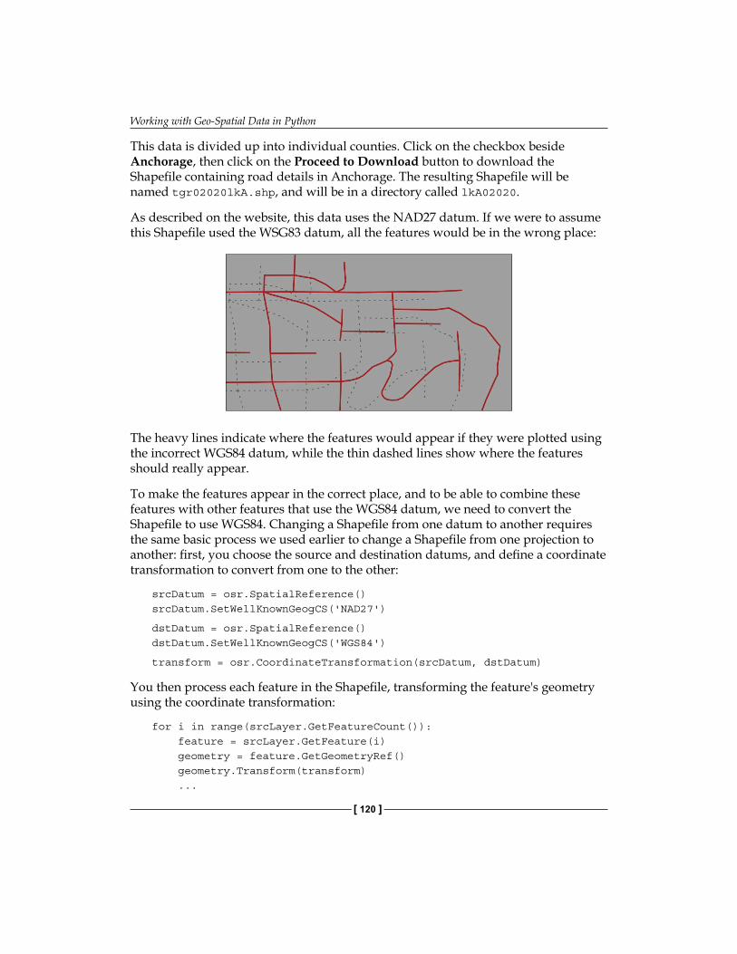
Working with Geo-Spatial Data in Python
[ 120 ]
This data is divided up into individual counties. Click on the checkbox beside Anchorage, then click on the Proceed to Download button to download the Shapefile containing road details in Anchorage. The resulting Shapefile will be named tgr02020lkA.shp, and will be in a directory called lkA02020.
As described on the website, this data uses the NAD27 datum. If we were to assume this Shapefile used the WSG83 datum, all the features would be in the wrong place:
The heavy lines indicate where the features would appear if they were plotted using the incorrect WGS84 datum, while the thin dashed lines show where the features should really appear.
To make the features appear in the correct place, and to be able to combine these features with other features that use the WGS84 datum, we need to convert the Shapefile to use WGS84. Changing a Shapefile from one datum to another requires the same basic process we used earlier to change a Shapefile from one projection to another: first, you choose the source and destination datums, and define a coordinate transformation to convert from one to the other:
srcDatum = osr.SpatialReference()srcDatum.SetWellKnownGeogCS('NAD27')
dstDatum = osr.SpatialReference()dstDatum.SetWellKnownGeogCS('WGS84')
transform = osr.CoordinateTransformation(srcDatum, dstDatum)
You then process each feature in the Shapefile, transforming the feature's geometry using the coordinate transformation:
for i in range(srcLayer.GetFeatureCount()): feature = srcLayer.GetFeature(i) geometry = feature.GetGeometryRef() geometry.Transform(transform) ...
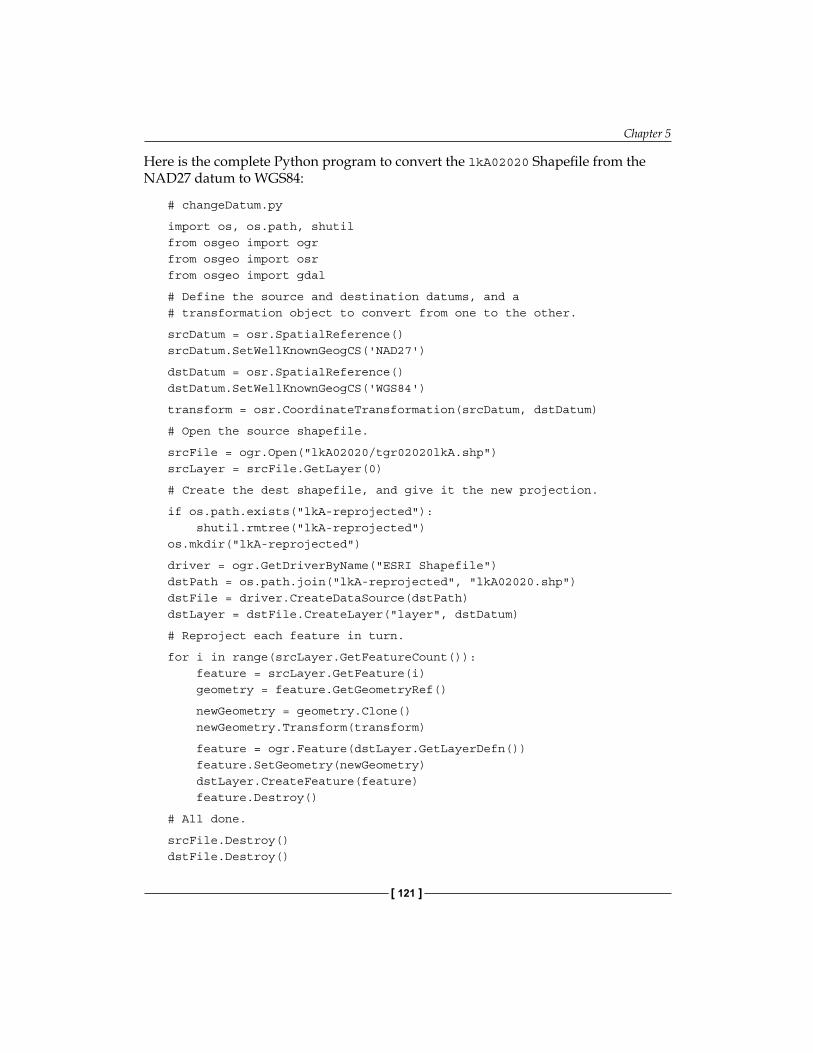
Chapter 5
[ 121 ]
Here is the complete Python program to convert the lkA02020 Shapefile from the NAD27 datum to WGS84:
# changeDatum.py
import os, os.path, shutilfrom osgeo import ogrfrom osgeo import osrfrom osgeo import gdal
# Define the source and destination datums, and a# transformation object to convert from one to the other.
srcDatum = osr.SpatialReference()srcDatum.SetWellKnownGeogCS('NAD27')
dstDatum = osr.SpatialReference()dstDatum.SetWellKnownGeogCS('WGS84')
transform = osr.CoordinateTransformation(srcDatum, dstDatum)
# Open the source shapefile.
srcFile = ogr.Open("lkA02020/tgr02020lkA.shp")srcLayer = srcFile.GetLayer(0)
# Create the dest shapefile, and give it the new projection.
if os.path.exists("lkA-reprojected"): shutil.rmtree("lkA-reprojected")os.mkdir("lkA-reprojected")
driver = ogr.GetDriverByName("ESRI Shapefile")dstPath = os.path.join("lkA-reprojected", "lkA02020.shp")dstFile = driver.CreateDataSource(dstPath)dstLayer = dstFile.CreateLayer("layer", dstDatum)
# Reproject each feature in turn.
for i in range(srcLayer.GetFeatureCount()): feature = srcLayer.GetFeature(i) geometry = feature.GetGeometryRef()
newGeometry = geometry.Clone() newGeometry.Transform(transform)
feature = ogr.Feature(dstLayer.GetLayerDefn()) feature.SetGeometry(newGeometry) dstLayer.CreateFeature(feature) feature.Destroy()
# All done.
srcFile.Destroy()dstFile.Destroy()
Working with Geo-Spatial Data in Python
[ 122 ]
The above code assumes that the lkA02020 folder is in the same directory as the Python script itself. If you've placed this folder somewhere else, you'll need to change the ogr.Open() statement to use the appropriate directory path.
If we now plot the reprojected features using the WGS84 datum, the features will appear in the correct place:
The thin dashed lines indicate where the original projection would have placed the features, while the heavy lines show the correct positions using the reprojected data.
Representing and storing geo-spatial dataWhile geo-spatial data is often supplied in the form of vector-format files such as Shapefiles, there are situations where Shapefiles are unsuitable or inefficient. One such situation is where you need to take geo-spatial data from one library and use it in a different library. For example, imagine that you have read a set of geometries out of a Shapefile and want to store them in a database, or work with them using the Shapely library. Because the different Python libraries all use their own private classes to represent geo-spatial data, you can't just take an OGR Geometry object and pass it to Shapely, or use a GDAL SpatialReference object to define the datum and projection to use for data stored in a database.
In these situations, you need to have an independent format for representing and storing geo-spatial data that isn't limited to just one particular Python library. This format, the lingua franca for vector-format geo-spatial data, is called Well-Known Text or WKT.
Chapter 5
[ 123 ]
WKT is a compact text-based description of a geo-spatial object such as a point, a line, or a polygon. For example, here is a geometry defining the boundary of the Vatican City in the World Borders Dataset, converted into a WKT string:
POLYGON ((12.445090330888604 41.90311752178485,
12.451653339580503 41.907989033391232,
12.456660170953796 41.901426024699163,
12.445090330888604 41.90311752178485))
As you can see, the WKT string contains a straightforward text description of a geometry—in this case, a polygon consisting of four x,y coordinates. Obviously, WKT text strings can be far more complex than this, containing many thousands of points and storing multipolygons and collections of different geometries. No matter how complex the geometry is, it can still be represented as a simple text string.
There is an equivalent binary format called Well-Known Binary (WKB) that stores the same information as binary data. WKB is often used to store geo-spatial data into a database.
WKT strings can also be used to represent a spatial reference encompassing a projection, a datum, and/or a coordinate system. For example, here is an osgeo.osr.SpatialReference object representing a geographic coordinate system using the WGS84 datum, converted into a WKT string:
GEOGCS["WGS 84",DATUM["WGS_1984",SPHEROID["WGS 84",6378137,298.257223563,AUTHORITY["EPSG","7030"]],TOWGS84[0,0,0,0,0,0, 0],AUTHORITY["EPSG","6326"]],PRIMEM["Greenwich",0,AUTHORITY["EPSG","8901 "]],UNIT["degree",0.0174532925199433,AUTHORITY["EPSG","9108"]],AUTHORITY ["EPSG","4326"]]
As with geometry representations, spatial references in WKT format can be used to pass a spatial reference from one Python library to another.
Task: Calculate the border between Thailand and MyanmarIn this recipe, we will make use of the World Borders Dataset to obtain polygons defining the borders of Thailand and Myanmar. We will then transfer these polygons into Shapely, and use Shapely's capabilities to calculate the common border between these two countries.
If you haven't already done so, download the World Borders Dataset from the Thematic Mapping website:
http://thematicmapping.org/downloads/world_borders.php
Working with Geo-Spatial Data in Python
[ 124 ]
The World Borders Dataset conveniently includes ISO 3166 two-character country codes for each feature, so we can identify the features corresponding to Thailand and Myanmar as we read through the Shapefile:
import osgeo.ogr
shapefile = osgeo.ogr.Open("TM_WORLD_BORDERS-0.3.shp")layer = shapefile.GetLayer(0)
for i in range(layer.GetFeatureCount()): feature = layer.GetFeature(i) if feature.GetField("ISO2") == "TH": ... elif feature.GetField("ISO2") == "MM": ...
This code assumes that you have placed the TM_WORLD_BORDERS-0.3.shp Shapefile in the same directory as the Python script. If you've placed it into a different directory, you'll need to adjust the osgeo.ogr.Open() statement to match.
Once we have identified the features we want, it is easy to extract the features' geometries as WKT strings:
geometry = feature.GetGeometryRef()wkt = geometry.ExportToWkt()
We can then convert these to Shapely geometry objects using the shapely.wkt module:
import shapely.wkt...border = shapely.wkt.loads(wkt)
Now that we have the objects in Shapely, we can use Shapely's computational geometry capabilities to calculate the common border between these two countries:
commonBorder = thailandBorder.intersection(myanmarBorder)
The result will be a LineString (or a MultiLineString if the border is broken up into more than one part). If we wanted to, we could then convert this Shapely object back into an OGR geometry, and save it into a Shapefile again:
wkt = shapely.wkt.dumps(commonBorder)
feature = osgeo.ogr.Feature(dstLayer.GetLayerDefn())feature.SetGeometry(osgeo.ogr.CreateGeometryFromWkt(wkt))dstLayer.CreateFeature(feature)feature.Destroy()
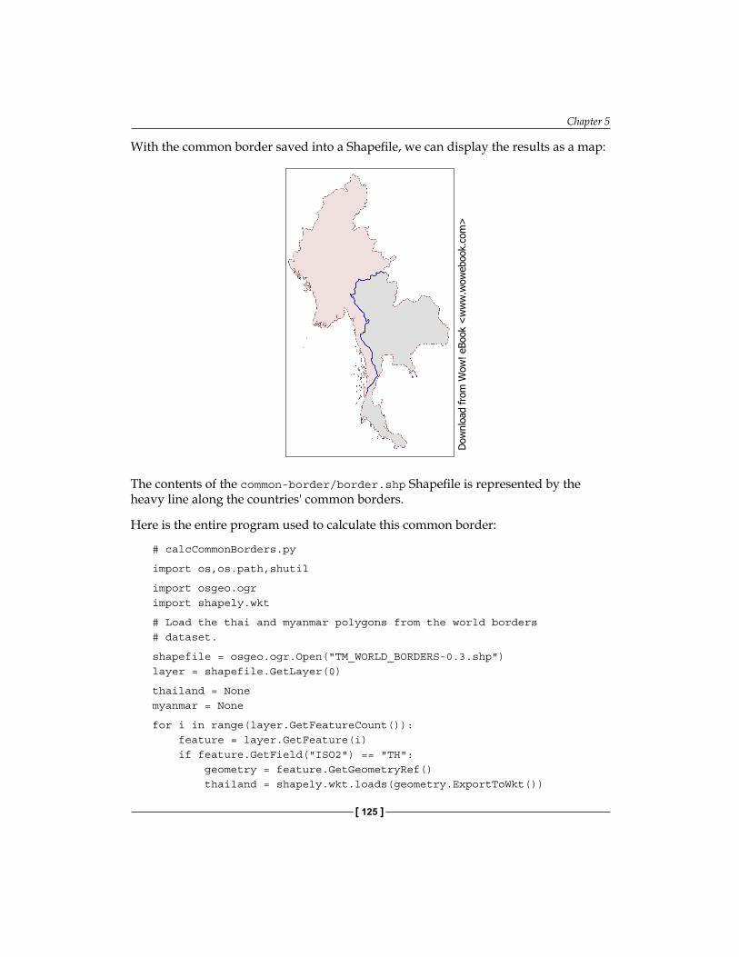
Chapter 5
[ 125 ]
With the common border saved into a Shapefile, we can display the results as a map:
The contents of the common-border/border.shp Shapefile is represented by the heavy line along the countries' common borders.
Here is the entire program used to calculate this common border:
# calcCommonBorders.py
import os,os.path,shutil
import osgeo.ogrimport shapely.wkt
# Load the thai and myanmar polygons from the world borders# dataset.
shapefile = osgeo.ogr.Open("TM_WORLD_BORDERS-0.3.shp")layer = shapefile.GetLayer(0)
thailand = Nonemyanmar = None
for i in range(layer.GetFeatureCount()): feature = layer.GetFeature(i) if feature.GetField("ISO2") == "TH": geometry = feature.GetGeometryRef() thailand = shapely.wkt.loads(geometry.ExportToWkt())
Dow
nlo
ad fro
m W
ow
! eBook
<w
ww
.wow
ebook.
com
>
Working with Geo-Spatial Data in Python
[ 126 ]
elif feature.GetField("ISO2") == "MM": geometry = feature.GetGeometryRef() myanmar = shapely.wkt.loads(geometry.ExportToWkt())
# Calculate the common border.
commonBorder = thailand.intersection(myanmar)
# Save the common border into a new shapefile.
if os.path.exists("common-border"): shutil.rmtree("common-border")os.mkdir("common-border")
spatialReference = osgeo.osr.SpatialReference()spatialReference.SetWellKnownGeogCS('WGS84')
driver = osgeo.ogr.GetDriverByName("ESRI Shapefile")dstPath = os.path.join("common-border", "border.shp")dstFile = driver.CreateDataSource(dstPath)dstLayer = dstFile.CreateLayer("layer", spatialReference)
wkt = shapely.wkt.dumps(commonBorder)
feature = osgeo.ogr.Feature(dstLayer.GetLayerDefn())feature.SetGeometry(osgeo.ogr.CreateGeometryFromWkt(wkt))dstLayer.CreateFeature(feature)feature.Destroy()
dstFile.Destroy()
If you've placed your TM_WORLD_BORDERS-0.3.shp Shapefile into a different directory, change the osgeo.ogr.Open() statement to include a suitable directory path.
We will use this Shapefile later in this chapter to calculate the length of the Thai-Myanmar border, so make sure you generate and keep a copy of the common-borders/border.shp Shapefile.
Task: Save geometries into a text fileWKT is not only useful for transferring geometries from one Python library to another. It can also be a useful way of storing geo-spatial data without having to deal with the complexity and constraints imposed by using Shapefiles.
Chapter 5
[ 127 ]
In this example, we will read a set of polygons from the World Borders Dataset, convert them to WKT format, and save them as text files:
# saveAsText.py
import os,os.path,shutil
import osgeo.ogr
if os.path.exists("country-wkt-files"): shutil.rmtree("country-wkt-files")os.mkdir("country-wkt-files")
shapefile = osgeo.ogr.Open("TM_WORLD_BORDERS-0.3.shp")layer = shapefile.GetLayer(0)
for i in range(layer.GetFeatureCount()): feature = layer.GetFeature(i) name = feature.GetField("NAME") geometry = feature.GetGeometryRef()
f = file(os.path.join("country-wkt-files", name + ".txt"), "w") f.write(geometry.ExportToWkt()) f.close()
As usual, you'll need to change the osgeo.ogr.Open() statement to include a directory path if you've stored the Shapefile in a different directory.
You might be wondering why you want to do this, rather than creating a Shapefile to store your geo-spatial data. Well, Shapefiles are limited in that all the features in a single Shapefile must have the same geometry type. Also, the complexity of setting up metadata and saving geometries can be overkill for some applications. Sometimes, dealing with plain text is just easier.
Working with Shapely geometriesShapely is a very capable library for performing various calculations on geo-spatial data. Let's put it through its paces with a complex, real-world problem.
Working with Geo-Spatial Data in Python
[ 128 ]
Task: Identify parks in or near urban areasThe U.S. Census Bureau makes available a Shapefile containing something called Core Based Statistical Areas (CBSAs), which are polygons defining urban areas with a population of 10,000 or more. At the same time, the GNIS website provides lists of placenames and other details. Using these two datasources, we will identify any parks within or close to an urban area.
Because of the volume of data we are potentially dealing with, we will limit our search to California. Feel free to download the larger data sets if you want, though you will have to optimize the code or your program will take a very long time to check all the CBSA polygon/placename combinations.
1. Let's start by downloading the necessary data. Go to the TIGER website at http://census.gov/geo/www/tiger
2. Click on the 2009 TIGER/Line Shapefiles Main Page link, then follow the Download the 2009 TIGER/Line Shapefiles now link.
3. Choose California from the pop-up menu on the right, and click on Submit. A list of the California Shapefiles will be displayed; the Shapefile you want is labelled Metropolitan/Micropolitan Statistical Area. Click on this link, and you will download a file named tl_2009_06_cbsa.zip. Once the file has downloaded, uncompress it and place the resulting Shapefile into a convenient location so that you can work with it.
4. You now need to download the GNIS placename data for California. Go to the GNIS website:http://geonames.usgs.gov/domestic
5. Click on the Download Domestic Names hyperlink, and then choose California from the pop-up menu. You will be prompted to save the CA_Features_XXX.zip file. Do so, then decompress it and place the resulting CA_Features_XXX.txt file into a convenient place.
The XXX in the above file name is a date stamp, and will vary depending on when you download the data. Just remember the name of the file as you'll need to refer to it in your source code.
6. We're now ready to write the code. Let's start by reading through the CBSA urban area Shapefile and extracting the polygons that define the boundary of each urban area:shapefile = osgeo.ogr.Open("tl_2009_06_cbsa.shp")
layer = shapefile.GetLayer(0)
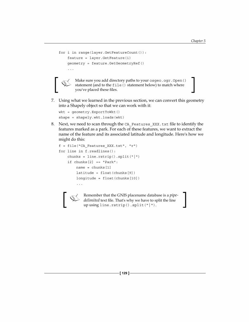
Chapter 5
[ 129 ]
for i in range(layer.GetFeatureCount()):
feature = layer.GetFeature(i)
geometry = feature.GetGeometryRef()
...
Make sure you add directory paths to your osgeo.ogr.Open() statement (and to the file() statement below) to match where you've placed these files.
7. Using what we learned in the previous section, we can convert this geometry into a Shapely object so that we can work with it:wkt = geometry.ExportToWkt()
shape = shapely.wkt.loads(wkt)
8. Next, we need to scan through the CA_Features_XXX.txt file to identify the features marked as a park. For each of these features, we want to extract the name of the feature and its associated latitude and longitude. Here's how we might do this:f = file("CA_Features_XXX.txt", "r")
for line in f.readlines():
chunks = line.rstrip().split("|")
if chunks[2] == "Park":
name = chunks[1]
latitude = float(chunks[9])
longitude = float(chunks[10])
...
Remember that the GNIS placename database is a pipe-delimited text file. That's why we have to split the line up using line.rstrip().split("|").
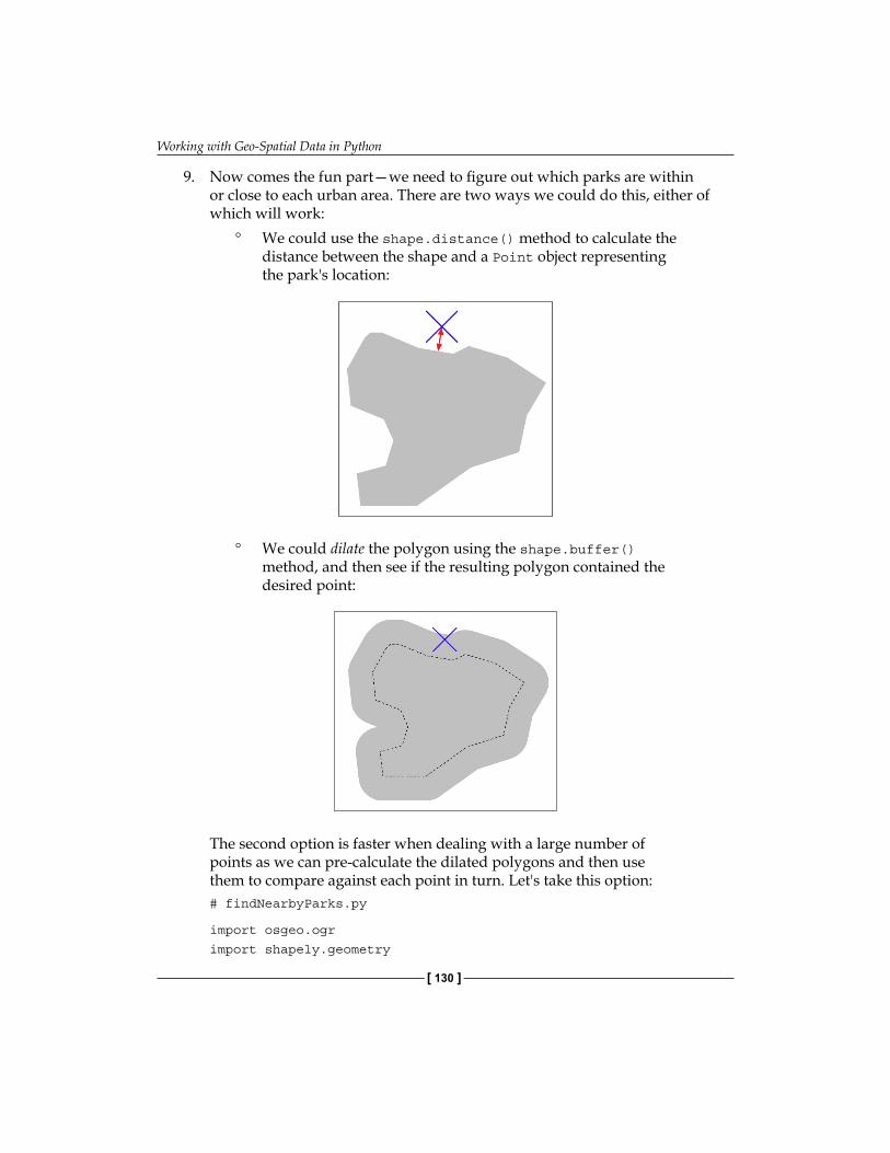
Working with Geo-Spatial Data in Python
[ 130 ]
9. Now comes the fun part—we need to figure out which parks are within or close to each urban area. There are two ways we could do this, either of which will work:
° We could use the shape.distance() method to calculate the distance between the shape and a Point object representing the park's location:
° We could dilate the polygon using the shape.buffer() method, and then see if the resulting polygon contained the desired point:
The second option is faster when dealing with a large number of points as we can pre-calculate the dilated polygons and then use them to compare against each point in turn. Let's take this option:# findNearbyParks.py
import osgeo.ogr
import shapely.geometry
Chapter 5
[ 131 ]
import shapely.wkt
MAX_DISTANCE = 0.1 # Angular distance; approx 10 km.
print "Loading urban areas..."
urbanAreas = {} # Maps area name to Shapely polygon.
shapefile = osgeo.ogr.Open("tl_2009_06_cbsa.shp")
layer = shapefile.GetLayer(0)
for i in range(layer.GetFeatureCount()):
feature = layer.GetFeature(i)
name = feature.GetField("NAME")
geometry = feature.GetGeometryRef()
shape = shapely.wkt.loads(geometry.ExportToWkt())
dilatedShape = shape.buffer(MAX_DISTANCE)
urbanAreas[name] = dilatedShape
print "Checking parks..."
f = file("CA_Features_XXX.txt", "r")
for line in f.readlines():
chunks = line.rstrip().split("|")
if chunks[2] == "Park":
parkName = chunks[1]
latitude = float(chunks[9])
longitude = float(chunks[10])
pt = shapely.geometry.Point(longitude, latitude)
for urbanName,urbanArea in urbanAreas.items():
if urbanArea.contains(pt):
print parkName + " is in or near " + urbanName
f.close()
Don't forget to change the name of the CA_Features_XXX.txt file to match the actual name of the file you downloaded. You may also need to change the path names to the tl_2009_06_CBSA.shp file and the CA_Features file if you placed them in a different directory.
If you run this program, you will get a master list of all the parks that are in or close to an urban area:
% python findNearbyParks.py
Loading urban areas...
Checking parks...
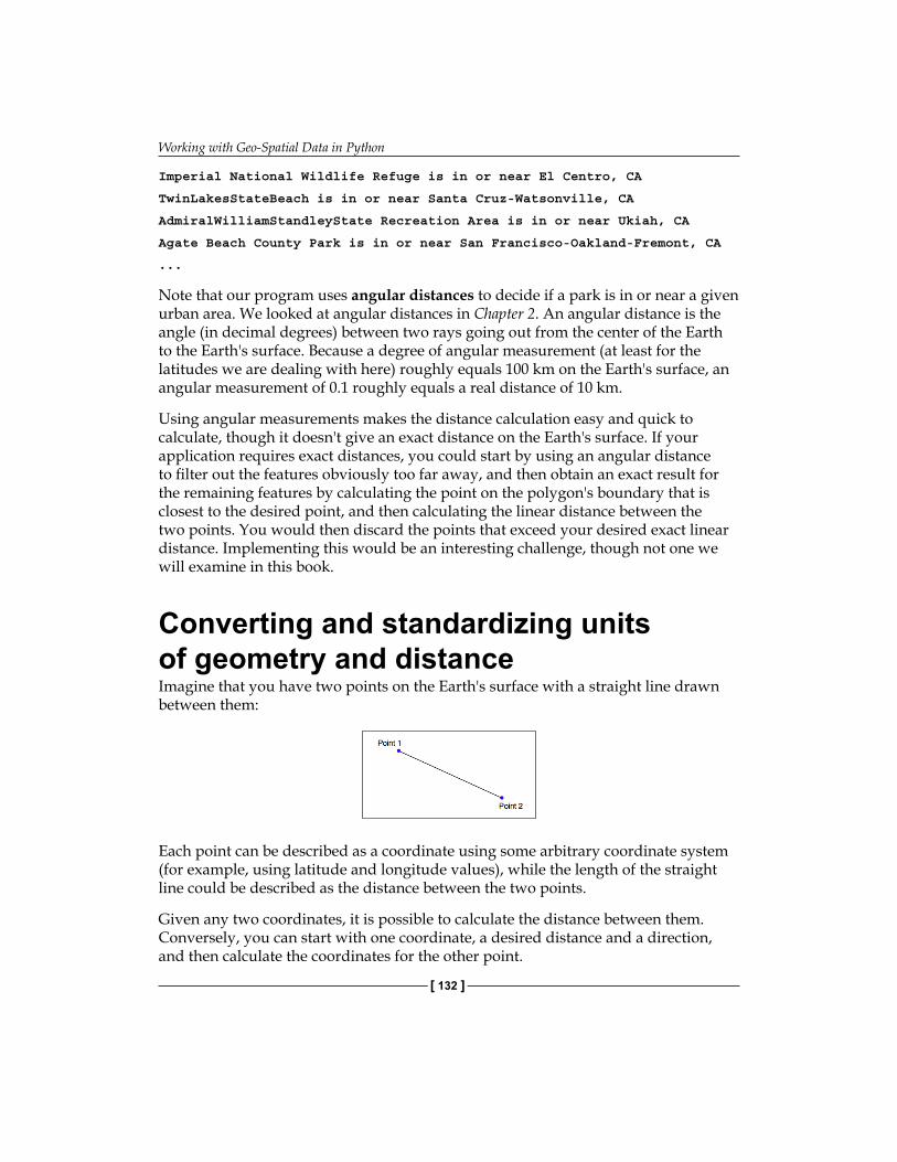
Working with Geo-Spatial Data in Python
[ 132 ]
Imperial National Wildlife Refuge is in or near El Centro, CA
TwinLakesStateBeach is in or near Santa Cruz-Watsonville, CA
AdmiralWilliamStandleyState Recreation Area is in or near Ukiah, CA
Agate Beach County Park is in or near San Francisco-Oakland-Fremont, CA
...
Note that our program uses angular distances to decide if a park is in or near a given urban area. We looked at angular distances in Chapter 2. An angular distance is the angle (in decimal degrees) between two rays going out from the center of the Earth to the Earth's surface. Because a degree of angular measurement (at least for the latitudes we are dealing with here) roughly equals 100 km on the Earth's surface, an angular measurement of 0.1 roughly equals a real distance of 10 km.
Using angular measurements makes the distance calculation easy and quick to calculate, though it doesn't give an exact distance on the Earth's surface. If your application requires exact distances, you could start by using an angular distance to filter out the features obviously too far away, and then obtain an exact result for the remaining features by calculating the point on the polygon's boundary that is closest to the desired point, and then calculating the linear distance between the two points. You would then discard the points that exceed your desired exact linear distance. Implementing this would be an interesting challenge, though not one we will examine in this book.
Converting and standardizing units of geometry and distanceImagine that you have two points on the Earth's surface with a straight line drawn between them:
Each point can be described as a coordinate using some arbitrary coordinate system (for example, using latitude and longitude values), while the length of the straight line could be described as the distance between the two points.
Given any two coordinates, it is possible to calculate the distance between them. Conversely, you can start with one coordinate, a desired distance and a direction, and then calculate the coordinates for the other point.
Chapter 5
[ 133 ]
Of course, because the Earth's surface is not flat, we aren't really dealing with straight lines at all. Rather, we are calculating geodetic or Great Circle distances across the surface of the Earth.
The pyproj Python library allows you to perform these types of calculations for any given datum. You can also use pyproj to convert from projected coordinates back to geographic coordinates, and vice versa, allowing you to perform these sorts of calculations for any desired datum, coordinate system, and projection.
Ultimately, a geometry such as a line or a polygon consists of nothing more than a list of connected points. This means that, using the above process, you can calculate the geodetic distance between each of the points in any polygon and total the results to get the actual length for any geometry. Let's use this knowledge to solve a real-world problem.
Task: Calculate the length of the Thai-Myanmar borderTo solve this problem, we will make use of the common-borders/border.shp Shapefile we created earlier. This Shapefile contains a single feature, which is a LineString defining the border between the two countries. Let's start by taking a look at the individual line segments that make up this feature's geometry:
import os.pathimport osgeo.ogr
def getLineSegmentsFromGeometry(geometry): segments = [] if geometry.GetPointCount() > 0: segment = [] for i in range(geometry.GetPointCount()): segment.append(geometry.GetPoint_2D(i)) segments.append(segment) for i in range(geometry.GetGeometryCount()): subGeometry = geometry.GetGeometryRef(i) segments.extend(getLineSegmentsFromGeometry(subGeometry)) return segments
filename = os.path.join("common-border", "border.shp")shapefile = osgeo.ogr.Open(filename)layer = shapefile.GetLayer(0)feature = layer.GetFeature(0)geometry = feature.GetGeometryRef()
segments = getLineSegmentsFromGeometry(geometry)
print segments
Working with Geo-Spatial Data in Python
[ 134 ]
Don't forget to change the os.path.join() statement to match the location of your border.shp Shapefile.
Note that we use a recursive function, getLineSegmentsFromGeometry(), to pull the individual coordinates for each line segment out of the geometry. Because geometries are recursive data structures, we have to pull out the individual line segments before we can work with them.
Running this program produces a long list of points that make up the various line segments defining the border between these two countries:
% python calcBorderLength.py
[[(100.08132200000006, 20.348840999999936),
(100.08943199999999, 20.347217999999941)],
[(100.08943199999999, 20.347217999999941),
(100.0913700000001, 20.348606000000075)], ...]
Each line segment consists of a list of points—in this case, you'll notice that each segment has only two points—and if you look closely you will notice that each segment starts at the same point as the previous segment ended. There are a total of 459 segments defining the border between Thailand and Myanmar—that is, 459 point pairs that we can calculate the geodetic distance for.
A geodetic distance is a distance measured on the surface of the Earth.
Let's see how we can use pyproj to calculate the geodetic distance between any two points. We first create a Geod instance:
geod = pyproj.Geod(ellps='WGS84')
Geod is the pyproj class that performs geodetic calculations. Note that we have to provide it with details of the datum used to describe the shape of the Earth. Once our Geod instance has been set up, we can calculate the geodetic distance between any two points by calling geod.inv(), the inverse geodetic transformation method:
angle1,angle2,distance = geod.inv(long1, lat1, long2, lat2)
angle1 will be the angle from the first point to the second, measured in decimal degrees; angle2 will be the angle from the second point back to the first (again in degrees); and distance will be the Great Circle distance between the two points, in meters.
Chapter 5
[ 135 ]
Using this, we can iterate over the line segments, calculate the distance from one point to another, and total up all the distances to obtain the total length of the border:
geod = pyproj.Geod(ellps='WGS84')
totLength = 0.0for segment in segments: for i in range(len(segment)-1): pt1 = segment[i] pt2 = segment[i+1]
long1,lat1 = pt1 long2,lat2 = pt2
angle1,angle2,distance = geod.inv(long1, lat1, long2, lat2) totLength += distance
Upon completion, totLength will be the total length of the border, in meters.
Putting all this together, we end up with a complete Python program to read the border.shp Shapefile, and calculate and then display the total length of the common border:
# calcBorderLength.py
import os.pathimport osgeo.ogrimport pyproj
def getLineSegmentsFromGeometry(geometry): segments = [] if geometry.GetPointCount() > 0: segment = [] for i in range(geometry.GetPointCount()): segment.append(geometry.GetPoint_2D(i)) segments.append(segment) for i in range(geometry.GetGeometryCount()): subGeometry = geometry.GetGeometryRef(i) segments.extend( getLineSegmentsFromGeometry(subGeometry)) return segments
filename = os.path.join("common-border", "border.shp")shapefile = osgeo.ogr.Open(filename)layer = shapefile.GetLayer(0)feature = layer.GetFeature(0)geometry = feature.GetGeometryRef()segments = getLineSegmentsFromGeometry(geometry)
Working with Geo-Spatial Data in Python
[ 136 ]
geod = pyproj.Geod(ellps='WGS84')
totLength = 0.0for segment in segments: for i in range(len(segment)-1): pt1 = segment[i] pt2 = segment[i+1]
long1,lat1 = pt1 long2,lat2 = pt2
angle1,angle2,distance = geod.inv(long1, lat1, long2, lat2) totLength += distance
print "Total border length = %0.2f km" % (totLength/1000)
Running this tells us the total calculated length of the Thai-Myanmar border:
% python calcBorderLength.py
Total border length = 1730.55 km
In this program, we have assumed that the Shapefile is in geographic coordinates using the WGS84 ellipsoid, and only contains a single feature. Let's extend our program to deal with any supplied projection and datum, and at the same time process all the features in the Shapefile rather than just the first. This will make our program more flexible, and allow it to work with any arbitrary Shapefile rather than just the common-border Shapefile we created earlier.
Let's deal with the projection and datum first. We could change the projection and datum for our Shapefile before we process it, just as we did with the LULC and lkA02020 Shapefiles earlier in this chapter. That would work, but it would require us to create a temporary Shapefile just to calculate the length, which isn't very efficient. Instead, let's make use of pyproj directly to reproject the Shapefile's contents back into geographic coordinates if necessary. We can do this by querying the Shapefile's spatial reference:
shapefile = ogr.Open(filename)layer = shapefile.GetLayer(0)spatialRef = layer.GetSpatialRef()if spatialRef == None: print "Shapefile has no spatial reference, using WGS84." spatialRef = osr.SpatialReference() spatialRef.SetWellKnownGeogCS('WGS84')
Once we have the spatial reference, we can see if the spatial reference is projected, and if so use pyproj to turn the projected coordinates back into lat/long values again, like this:
Chapter 5
[ 137 ]
if spatialRef.IsProjected(): # Convert projected coordinates back to lat/long values.srcProj = pyproj.Proj(spatialRef.ExportToProj4())dstProj = pyproj.Proj(proj='longlat', ellps='WGS84', datum='WGS84')...long,lat = pyproj.transform(srcProj, dstProj, x, y)
Using this, we can rewrite our program to accept data using any projection and datum. At the same time, we'll change it to calculate the overall length of every feature in the file, rather than just the first, and also to accept the name of the Shapefile from the command line. Finally, we'll add some error-checking. Let's call the results calcFeatureLengths.py.
We'll start by copying the getLineSegmentsFromGeometry() function we used earlier:
import sysfrom osgeo import ogr, osrimport pyproj
def getLineSegmentsFromGeometry(geometry): segments = [] if geometry.GetPointCount() > 0: segment = [] for i in range(geometry.GetPointCount()): segment.append(geometry.GetPoint_2D(i)) segments.append(segment) for i in range(geometry.GetGeometryCount()): subGeometry = geometry.GetGeometryRef(i) segments.extend( getLineSegmentsFromGeometry(subGeometry)) return segments
Next, we'll get the name of the Shapefile to open from the command line:
if len(sys.argv) != 2: print "Usage: calcFeatureLengths.py <shapefile>" sys.exit(1)
filename = sys.argv[1]
We'll then open the Shapefile and obtain its spatial reference, using the code we wrote earlier:
shapefile = ogr.Open(filename)layer = shapefile.GetLayer(0)spatialRef = layer.GetSpatialRef()if spatialRef == None:
Working with Geo-Spatial Data in Python
[ 138 ]
print "Shapefile lacks a spatial reference, using WGS84." spatialRef = osr.SpatialReference() spatialRef.SetWellKnownGeogCS('WGS84')
We'll then get the source and destination projections, again using the code we wrote earlier. Note that we only need to do this if we're using projected coordinates:
if spatialRef.IsProjected(): srcProj = pyproj.Proj(spatialRef.ExportToProj4()) dstProj = pyproj.Proj(proj='longlat', ellps='WGS84', datum='WGS84')
We are now ready to start processing the Shapefile's features:
for i in range(layer.GetFeatureCount()): feature = layer.GetFeature(i)
Now that we have the feature, we can borrow the code we used earlier to calculate the total length of that feature's line segments:
geometry = feature.GetGeometryRef() segments = getLineSegmentsFromGeometry(geometry)
geod = pyproj.Geod(ellps='WGS84')
totLength = 0.0 for segment in segments: for j in range(len(segment)-1): pt1 = segment[j] pt2 = segment[j+1]
long1,lat1 = pt1 long2,lat2 = pt2
The only difference is that we need to transform the coordinates back to WGS84 if we are using a projected coordinate system:
if spatialRef.IsProjected(): long1,lat1 = pyproj.transform(srcProj, dstProj, long1, lat1) long2,lat2 = pyproj.transform(srcProj, dstProj, long2, lat2)
We can then use pyproj to calculate the distance between the two points, as we did in our earlier example. This time, though, we'll wrap it in a try...except statement so that any failure to calculate the distance won't crash the program:
try: angle1,angle2,distance = geod.inv(long1, lat1,
Chapter 5
[ 139 ]
long2, lat2) except ValueError: print "Unable to calculate distance from " \ + "%0.4f,%0.4f to %0.4f,%0.4f" \ % (long1, lat1, long2, lat2) distance = 0.0 totLength += distance
The geod.inv() call can raise a ValueError if the two coordinates are in a place where an angle can't be calculated—for example, if the two points are at the poles.
And finally, we can print out the feature's total length, in kilometers:
print "Total length of feature %d is %0.2f km" \ % (i, totLength/1000)
This program can be run over any Shapefile. For example, you could use it to calculate the border length for every country in the world by running it over the World Borders Dataset:
% python calcFeatureLengths.py TM_WORLD_BORDERS-0.3.shp
Total length of feature 0 is 127.28 km
Total length of feature 1 is 7264.69 km
Total length of feature 2 is 2514.76 km
Total length of feature 3 is 968.86 km
Total length of feature 4 is 1158.92 km
Total length of feature 5 is 6549.53 km
Total length of feature 6 is 119.27 km
...
This program is an example of converting geometry coordinates into distances. Let's take a look at the inverse calculation: using distances to calculate new geometry coordinates.
Task: Find a point 132.7 kilometers west of Soshone, CaliforniaUsing the CA_Features_XXX.txt file we downloaded earlier, it is possible to find the latitude and longitude of Shoshone, a small town in California east of Las Vegas:
Working with Geo-Spatial Data in Python
[ 140 ]
f = file("CA_Features_20100607.txt", "r")for line in f.readlines(): chunks = line.rstrip().split("|") if chunks[1] == "Shoshone" and \ chunks[2] == "Populated Place": latitude = float(chunks[9]) longitude = float(chunks[10]) ...
Given this coordinate, we can use pyproj to calculate the coordinate of a point a given distance away, at a given angle:
geod = pyproj.Geod(ellps="WGS84")newLong,newLat,invAngle = geod.fwd(latitude, longitude, angle, distance)
For this task, we are given the desired distance and we know that the angle we want is "due west". pyproj uses azimuth angles, which are measured clockwise from North. Thus, due west would correspond to an angle of 270 degrees.
Putting all this together, we can calculate the coordinates of the desired point:
# findShoshone.py
import pyproj
distance = 132.7 * 1000angle = 270.0
f = file("CA_Features_20100607.txt", "r")for line in f.readlines(): chunks = line.rstrip().split("|") if chunks[1] == "Shoshone" and \ chunks[2] == "Populated Place": latitude = float(chunks[9]) longitude = float(chunks[10])
geod = pyproj.Geod(ellps='WGS84') newLong,newLat,invAngle = geod.fwd(longitude, latitude, angle, distance)
print "Shoshone is at %0.4f,%0.4f" % (latitude, longitude) print "The point %0.2f km west of Shoshone " \ % (distance/1000.0) \ + "is at %0.4f, %0.4f" % (newLat, newLong)
f.close()
Chapter 5
[ 141 ]
Running this program gives us the answer we want:
% python findShoshone.py
Shoshone is at 35.9730,-116.2711
The point 132.70 km west of Shoshone is at 35.9640,
-117.7423
ExercisesIf you are interested in exploring the techniques used in this chapter further, you might like to challenge yourself with the following tasks:
• Change the "Calculate Bounding Box" calculation to exclude outlying islands.
HintYou can split each country's MultiPolygon into individual Polygon objects, and then check the area of each polygon to exclude those that are smaller than a given total value.
• Use the World Borders Dataset to create a new Shapefile, where each country is represented by a single "Point" geometry containing the geographical middle of each country.
HintYou can start with the country bounding boxes we calculated earlier, and then simply calculate the midpoint using:midLat = (minLat + maxLat) / 2
midLong = (minLong + maxLong) / 2
This won't be exact, but it gives a reasonable mid-point value for you to use.
• Extend the histogram example given above to only include height values that fall inside a selected country's outline.
HintImplementing this in an efficient way can be difficult. A good approach would be to identify the bounding box for each of the polygons that make up the country's outline, and then iterate over the DEM coordinates within that bounding box. You could then check to see if a given coordinate is actually inside the country's outline using polygon.contains(point), and only add the height to the histogram if the point is indeed within the country's outline.
Working with Geo-Spatial Data in Python
[ 142 ]
• Optimize the "identify nearby parks" example given earlier so that it can work quickly with larger data sets.
HintOne possibility might be to calculate the rectangular bounding box around each park, and then expand that bounding box north, south, east, and west by the desired angular distance. You could then quickly exclude all the points that aren't in that bounding box before making the time-consuming call to polygon.contains(point).
• Calculate the total length of the coastline of the United Kingdom.
HintRemember that a country outline is a MultiPolygon, where each Polygon in the MultiPolygon represents a single island. You will need to extract the exterior ring from each of these individual island polygons, and calculate the total length of the line segments within that exterior ring. You can then total the length of each individual island to get the length of the entire country's coastline.
• Design your own reusable library of geo-spatial functions that build on OGR, GDAL, Shapely, and pyproj to perform common operations such as those discussed in this chapter.
HintWriting your own reusable library modules is a common programming tactic. Think about the various tasks we have solved in this chapter, and how they can be turned into generic library functions. For example, you might like to write a function named calcLineStringLength() that takes a LineString and returns the total length of the LineString's segments, optionally transforming the LineString's coordinates into lat/long values before calling geod.inv(). You could then write a calcPolygonOutlineLength()function that uses calcLineStringLength() to calculate the length of a polygon's outer ring.
• You could then write a calcPolygonOutlineLength()function that uses calcLineStringLength() to calculate the length of a polygon's outer ring.
Chapter 5
[ 143 ]
SummaryIn this chapter, we have looked at various techniques for using OGR, GDAL, Shapely, and pyproj within Python programs to solve real-world problems. We have learned:
• How to read from and write to vector-format geo-spatial data in Shapefiles.• How to read and analyze raster-format geo-spatial data.• How to change the datum and projection used by a Shapefile.• That the Well-Known Text (WKT) format can be used to represent geo-spatial
features and spatial references in plain text.• That WKT can be used to transfer geo-spatial data from one Python library
to another.• That WKT can be used to store geo-spatial data in plain text format.• That you can use the Shapely library to perform various geo-spatial
calculations on geometries, including distance calculations, dilation, and intersections.
• That you can use the pyproj.Proj class to convert coordinates from one projection and datum to another.
• That you can use the pyproj.Geod class to convert from geometry coordinates to distances, and vice versa.
Up to now, we have written programs that work directly with Shapefiles and other datasources to load and then process geo-spatial data. In the next chapter, we will look at ways that databases can be used to store and work with geo-spatial data. This is much faster and more scalable than storing geo-spatial data in files that have to be imported each time.

GIS in the DatabaseThis chapter examines the various open source options for storing geo-spatial data in a database. More specifically, we will cover:
• The concept of a spatially-enabled database• Spatial indexes and how they work• A summary of the major open source spatial databases• Recommended best practices for storing spatial data in a database• How to work with geo-spatial databases using Python
This chapter is intended to be an introduction to using databases in a geo-spatial application; Chapter 7 will build on this to perform powerful spatial queries not possible using Shapefiles and other geo-spatial datafiles.
Spatially-enabled databasesIn a sense, almost any database can be used to store geo-spatial data—simply convert a geometry to WKT format and store the results in a text column. But, while this would allow you to store geo-spatial data in a database, it wouldn't let you query it in any useful way. All you could do is retrieve the raw WKT text and convert it back to a geometry object one record at a time.
A spatially-enabled database, on the other hand, is aware of the notion of space, and allows you to work with spatial objects and concepts directly. In particular, a spatially-enabled database allows you to:
• Store spatial data types (points, lines, polygons, and so on) directly in the database, in the form of a geometry column.
• Perform spatial queries on your data. For example: select all landmarks within 10 km of the city named "San Francisco".
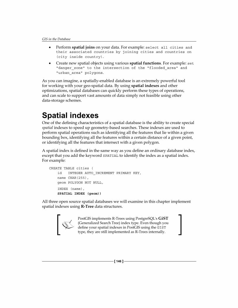
GIS in the Database
[ 146 ]
• Perform spatial joins on your data. For example: select all cities and their associated countries by joining cities and countries on (city inside country).
• Create new spatial objects using various spatial functions. For example: set "danger_zone" to the intersection of the "flooded_area" and "urban_area" polygons.
As you can imagine, a spatially-enabled database is an extremely powerful tool for working with your geo-spatial data. By using spatial indexes and other optimizations, spatial databases can quickly perform these types of operations, and can scale to support vast amounts of data simply not feasible using other data-storage schemes.
Spatial indexesOne of the defining characteristics of a spatial database is the ability to create special spatial indexes to speed up geometry-based searches. These indexes are used to perform spatial operations such as identifying all the features that lie within a given bounding box, identifying all the features within a certain distance of a given point, or identifying all the features that intersect with a given polygon.
A spatial index is defined in the same way as you define an ordinary database index, except that you add the keyword SPATIAL to identify the index as a spatial index. For example:
CREATE TABLE cities ( id INTEGER AUTO_INCREMENT PRIMARY KEY, name CHAR(255), geom POLYGON NOT NULL,
INDEX (name), SPATIAL INDEX (geom))
All three open source spatial databases we will examine in this chapter implement spatial indexes using R-Tree data structures.
PostGIS implements R-Trees using PostgreSQL's GiST (Generalized Search Tree) index type. Even though you define your spatial indexes in PostGIS using the GIST type, they are still implemented as R-Trees internally.
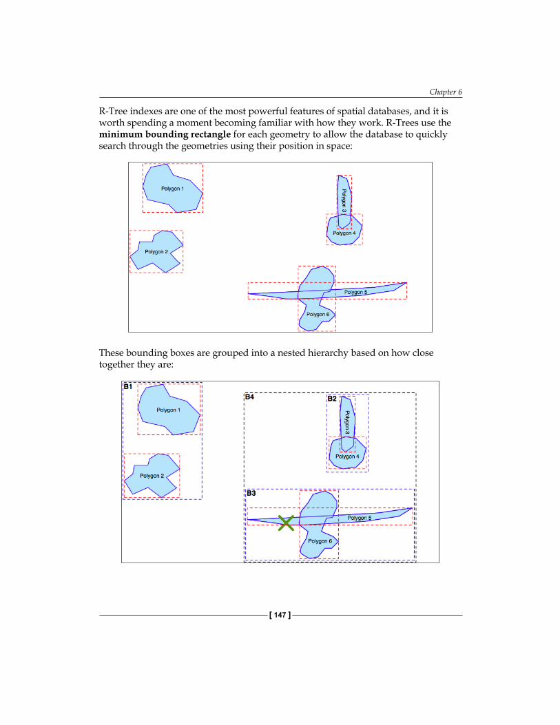
Chapter 6
[ 147 ]
R-Tree indexes are one of the most powerful features of spatial databases, and it is worth spending a moment becoming familiar with how they work. R-Trees use the minimum bounding rectangle for each geometry to allow the database to quickly search through the geometries using their position in space:
These bounding boxes are grouped into a nested hierarchy based on how close together they are:
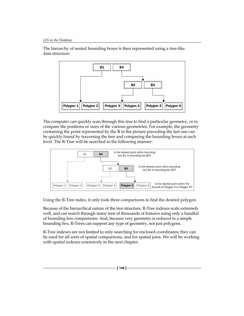
GIS in the Database
[ 148 ]
The hierarchy of nested bounding boxes is then represented using a tree-like data structure:
The computer can quickly scan through this tree to find a particular geometry, or to compare the positions or sizes of the various geometries. For example, the geometry containing the point represented by the X in the picture preceding the last one can be quickly found by traversing the tree and comparing the bounding boxes at each level. The R-Tree will be searched in the following manner:
Using the R-Tree index, it only took three comparisons to find the desired polygon.
Because of the hierarchical nature of the tree structure, R-Tree indexes scale extremely well, and can search through many tens of thousands of features using only a handful of bounding box comparisons. And, because very geometry is reduced to a simple bounding box, R-Trees can support any type of geometry, not just polygons.
R-Tree indexes are not limited to only searching for enclosed coordinates; they can be used for all sorts of spatial comparisons, and for spatial joins. We will be working with spatial indexes extensively in the next chapter.
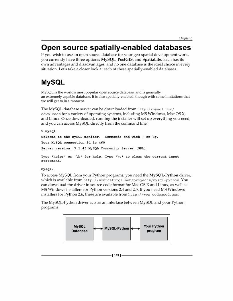
Chapter 6
[ 149 ]
Open source spatially-enabled databasesIf you wish to use an open source database for your geo-spatial development work, you currently have three options: MySQL, PostGIS, and SpatiaLite. Each has its own advantages and disadvantages, and no one database is the ideal choice in every situation. Let's take a closer look at each of these spatially-enabled databases.
MySQLMySQL is the world's most popular open source database, and is generally an extremely capable database. It is also spatially-enabled, though with some limitations that we will get to in a moment.
The MySQL database server can be downloaded from http://mysql.com/downloads for a variety of operating systems, including MS Windows, Mac OS X, and Linux. Once downloaded, running the installer will set up everything you need, and you can access MySQL directly from the command line:
% mysql
Welcome to the MySQL monitor. Commands end with ; or \g.
Your MySQL connection id is 460
Server version: 5.1.43 MySQL Community Server (GPL)
Type 'help;' or '\h' for help. Type '\c' to clear the current input statement.
mysql>
To access MySQL from your Python programs, you need the MySQL-Python driver, which is available from http://sourceforge.net/projects/mysql-python. You can download the driver in source-code format for Mac OS X and Linux, as well as MS Windows installers for Python versions 2.4 and 2.5. If you need MS Windows installers for Python 2.6, these are available from http://www.codegood.com.
The MySQL-Python driver acts as an interface between MySQL and your Python programs:
GIS in the Database
[ 150 ]
Once you have installed the MySQL-Python driver, it will be available as a module named MySQLdb. Here is an example of how you might use this module from within your Python programs:
import MySQLdb
connection = MySQLdb.connect(user="...", passwd="...")cursor = connection.cursor()cursor.execute("USE myDatabase")
The cursor.execute() method lets you execute any MySQL command, just as if you were using the MySQL command-line client. MySQLdb is also completely compatible with the Python Database API specification (http://www.python.org/dev/peps/pep-0249), allowing you to access all of MySQL's features from within your Python programs.
Learning how to use databases within Python is beyond the scope of this book. If you haven't used a DB-API compatible database from Python before, you may want to check out one of the many available tutorials on the subject, for example http://tutorialspoint.com/python/python_database_access.htm. Also, the Python Database Programming wiki page (http://wiki.python.org/moin/DatabaseProgramming) has useful information, as does the user's guide for MySQLdb (http://mysql-python.sourceforge.net/MySQLdb.html).
MySQL comes with spatial capabilities built-in. For example, the following MySQL command creates a new database table that contains a polygon:
CREATE TABLE cities ( id INTEGER AUTO_INCREMENT PRIMARY KEY, name CHAR(255), outline POLYGON NOT NULL,
INDEX (name), SPATIAL INDEX (outline))
Notice that POLYGON is a valid column type, and that you can directly create a spatial index on a geometry. This allows you to issue queries such as:
SELECT name FROM cities WHERE MBRContains(outline, myLocation)
This will return all the cities where the MBRContains() function determines that the given location is within the city's outline.
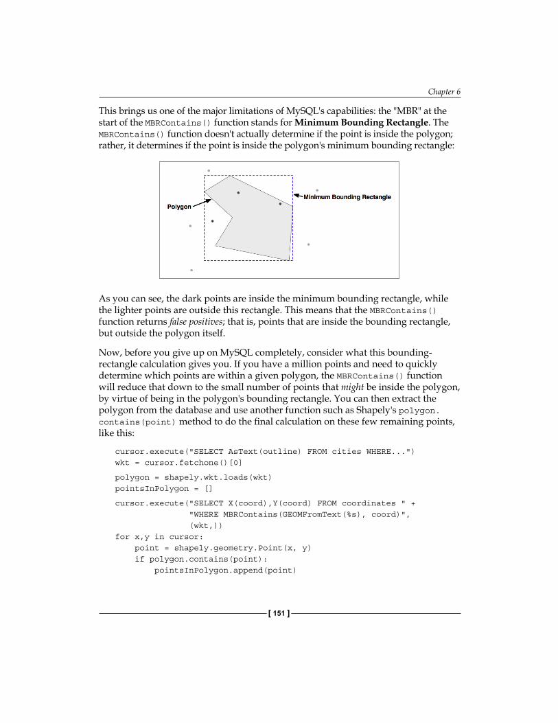
Chapter 6
[ 151 ]
This brings us one of the major limitations of MySQL's capabilities: the "MBR" at the start of the MBRContains() function stands for Minimum Bounding Rectangle. The MBRContains() function doesn't actually determine if the point is inside the polygon; rather, it determines if the point is inside the polygon's minimum bounding rectangle:
As you can see, the dark points are inside the minimum bounding rectangle, while the lighter points are outside this rectangle. This means that the MBRContains() function returns false positives; that is, points that are inside the bounding rectangle, but outside the polygon itself.
Now, before you give up on MySQL completely, consider what this bounding-rectangle calculation gives you. If you have a million points and need to quickly determine which points are within a given polygon, the MBRContains() function will reduce that down to the small number of points that might be inside the polygon, by virtue of being in the polygon's bounding rectangle. You can then extract the polygon from the database and use another function such as Shapely's polygon.contains(point) method to do the final calculation on these few remaining points, like this:
cursor.execute("SELECT AsText(outline) FROM cities WHERE...") wkt = cursor.fetchone()[0]
polygon = shapely.wkt.loads(wkt)pointsInPolygon = []
cursor.execute("SELECT X(coord),Y(coord) FROM coordinates " + "WHERE MBRContains(GEOMFromText(%s), coord)", (wkt,))for x,y in cursor: point = shapely.geometry.Point(x, y) if polygon.contains(point): pointsInPolygon.append(point)
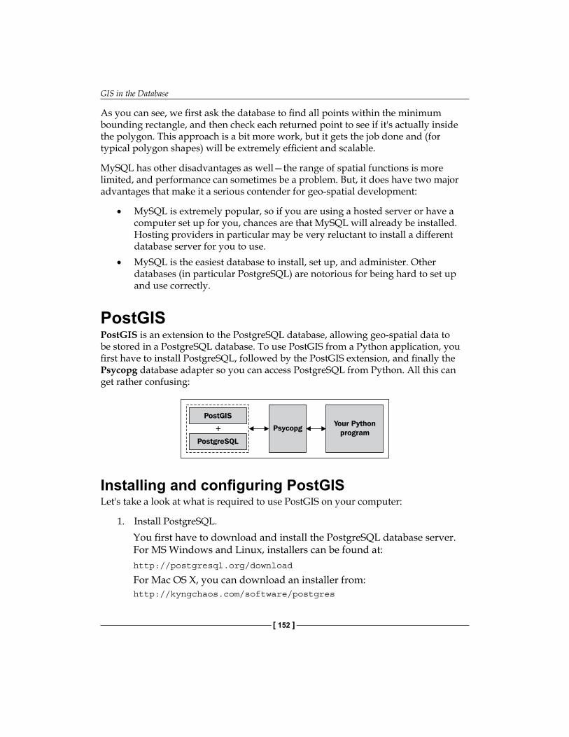
GIS in the Database
[ 152 ]
As you can see, we first ask the database to find all points within the minimum bounding rectangle, and then check each returned point to see if it's actually inside the polygon. This approach is a bit more work, but it gets the job done and (for typical polygon shapes) will be extremely efficient and scalable.
MySQL has other disadvantages as well—the range of spatial functions is more limited, and performance can sometimes be a problem. But, it does have two major advantages that make it a serious contender for geo-spatial development:
• MySQL is extremely popular, so if you are using a hosted server or have a computer set up for you, chances are that MySQL will already be installed. Hosting providers in particular may be very reluctant to install a different database server for you to use.
• MySQL is the easiest database to install, set up, and administer. Other databases (in particular PostgreSQL) are notorious for being hard to set up and use correctly.
PostGISPostGIS is an extension to the PostgreSQL database, allowing geo-spatial data to be stored in a PostgreSQL database. To use PostGIS from a Python application, you first have to install PostgreSQL, followed by the PostGIS extension, and finally the Psycopg database adapter so you can access PostgreSQL from Python. All this can get rather confusing:
Installing and configuring PostGISLet's take a look at what is required to use PostGIS on your computer:
1. Install PostgreSQL.You first have to download and install the PostgreSQL database server. For MS Windows and Linux, installers can be found at:http://postgresql.org/download
For Mac OS X, you can download an installer from:http://kyngchaos.com/software/postgres
Chapter 6
[ 153 ]
Be warned that installing PostgreSQL can be complicated, and you may well need to configure or debug the server before it will work. The PostgreSQL documentation (http://postgresql.org/docs) can help, and remember that Google is your friend if you encounter any problems.
Take note of where PostgreSQL has been installed on your computer. You will need to refer to files in the pgsql directory when you set up your spatially-enabled database.
2. Install the PostGIS ExtensionThe PostGIS spatial extension to PostgreSQL, along with full documentation, can be downloaded from:http://postgis.refractions.net
Make sure you install the correct version of PostGIS to match the version of PostgreSQL you are using.
3. Install PsycopgPsycopg allows you to access PostgreSQL (and PostGIS) databases from Python. The Psycopg database adapter can be found at:http://initd.org/psycopg
Make sure you use version 2 and not the outdated version 1 of Psycopg. For Windows, you can download a pre-built version of Psycopg; for Linux and Mac OS X, you need to download the source code and build it yourself in the usual way:% cd psycopg2
% python setup.py build
% python setup.py install
Mac OS X users: if you are building Psycopg to run with the Kyngchaos version of PostgreSQL, type the following into the terminal window before you attempt to build Psycopg:
% export PATH="/usr/local/pgsql/bin:$PATH"
% export ARCHFLAGS="-arch i386"
GIS in the Database
[ 154 ]
4. Set up a new PostgreSQL User and databaseBefore you can use PostgreSQL, you need to have a user (sometimes called a "role" in the PostgreSQL manuals) that owns the database you create. While you might have a user account on your computer that you use for logging in and out, the PostgreSQL user is completely separate from this account, and is used only within PostgreSQL. You can set up a PostgreSQL user with the same name as your computer username, or you can give it a different name if you prefer.To create a new PostgreSQL user, type the following command:% pgsql/bin/createuser -s <username>
Obviously, replace <username> with whatever name you want to use for your new user.
Once you have set up a new PostgreSQL user, you can create a new database to work with:% pgsql/bin/createdb -U <username> <dbname>
Once again, replace <username> and <dbname> with the appropriate names for the user and database you wish to set up.
Note that we are keeping this as simple as possible. Setting up and administering a properly-configured PostgreSQL database is a major undertaking, and is way beyond the scope of this book. The above commands, however, should be enough to get you up and running.
5. Spatially enable your new databaseSo far, you have created a plain-vanilla PostgreSQL database. To turn this into a spatially-enabled database, you will need to configure the database to use PostGIS. Doing this is a two-step process; first, type the following:% pgsql/bin/createlang plpgsql <dbname>
This enables the PL/pgSQL language used by PostGIS. You then load the PostGIS functions and data types into your database by typing (all on one line):% pgsql/bin/psql -d <dbname>
-f pgsql/share/contrib/postgis-1.5/postgis.sql
Chapter 6
[ 155 ]
6. Import the spatial reference table into your databasePostGIS comes with a complete list of more than 3,000 spatial references (projections, datums, coordinate systems) that you can import into your spatial database. With this table installed, you can tell PostGIS which spatial reference each piece of spatial data uses, and perform on-the-fly reprojections from one spatial reference to another.To import the spatial_ref_sys table into your database, use the following command (again, all on one line):% pgsql/bin/psql -d <dbname>
-f pgsql/share/contrib/postgis-1.5/spatial_ref_sys.sql
We will talk more about the use of spatial reference systems in the section on Recommended best practices later.
Using PostGISOnce you have installed the various pieces of software, and have set up a spatially-enabled database, you can use the Psycopg database adapter in much the same way as you would use MySQLdb to access a MySQL database:
import psycopg2
connection = psycopg2.connect("dbname=... user=...")cursor = connection.cursor()cursor.execute("SELECT id,name FROM cities WHERE pop>100000")for row in cursor: print row[0],row[1]
Because Psycopg conforms to Python's DB-API specification, using PostgreSQL from Python is relatively straightforward, especially if you have used databases from Python before.
Here is how you might create a new spatially-enabled table using PostGIS:
import psycopg2
connection = psycopg2.connect("dbname=... user=...")cursor = connection.cursor()
cursor.execute("DROP TABLE IF EXISTS cities")cursor.execute("CREATE TABLE cities (id INTEGER," + "name VARCHAR(255), PRIMARY KEY (id))")cursor.execute("SELECT AddGeometryColumn('cities', 'geom', " + "-1, 'POLYGON', 2)")cursor.execute("CREATE INDEX cityIndex ON cities " +
GIS in the Database
[ 156 ]
"USING GIST (geom)")connection.commit()
Let's take a look at each of these steps in more detail. We first get a cursor object to access the database, and then create the non-spatial parts of our table using standard SQL statements:
connection = psycopg2.connect("dbname=... user=...")cursor = connection.cursor()
cursor.execute("DROP TABLE IF EXISTS cities")cursor.execute("CREATE TABLE cities (id INTEGER," + "name VARCHAR(255), PRIMARY KEY (id))")
Once the table itself has been created, we have to use a separate PostGIS function called AddGeometryColumn() to define the spatial columns within our table:
cursor.execute("SELECT AddGeometryColumn('cities', 'geom', " + "-1, 'POLYGON', 2)")
Recent versions of PostGIS support two distinct types of geo-spatial data, called geometries and geographies. The geometry type (that we are using here) uses cartesian coordinates to place features onto a plane, and all calculations are done using cartesian (x,y) coordinates. The geography type, on the other hand, identifies geo-spatial features using angular coordinates (latitudes and longitudes), positioning the features onto a spheroid model of the Earth.The geography type is relatively new, much slower to use, and doesn't yet support all the functions that are available for the geometry type. Despite having the advantages of being able to accurately calculate distances that cover a large portion of the Earth and not requiring knowledge of projections and spatial references, we will not be using the geography type in this book.
Finally, we create a spatial index so that we can efficiently search using the new geometry column:
cursor.execute("CREATE INDEX cityIndex ON cities " + "USING GIST (geom)")
Once you have created your database, you can insert geometry features into it using the ST_GeomFromText() function, like this:
cursor.execute("INSERT INTO cities (name,geom) VALUES " + "(%s, ST_GeomFromText(%s)", (cityName, wkt))
Chapter 6
[ 157 ]
Conversely, you can retrieve a geometry from the database in WKT format using the ST_AsText() function:
cursor.execute("select name,ST_AsText(geom) FROM cities")for name,wkt in cursor: ...
DocumentationBecause PostGIS is an extension to PostgreSQL, and you use Psycopg to access it, there are three separate sets of documentation you will need to refer to:
• The PostgreSQL manual: http://postgresql.org/docs• The PostGIS manual: http://postgis.refractions.net/docs• The Psycopg documentation: http://initd.org/psycopg/docs
Of these, the PostGIS manual is probably going to be the most useful, and you will also need to refer to the Psycopg documentation to find out the details of using PostGIS from Python. You will probably also need to refer to the PostgreSQL manual to learn the non-spatial aspects of using PostGIS, though be aware that this manual is huge and extremely complex, reflecting the complexity of PostgreSQL itself.
Advanced PostGIS featuresPostGIS supports the following features not available with MySQL:
• On-the-fly transformations of geometries from one spatial reference to another.
• The ability to edit geometries by adding, changing, and removing points, and by rotating, scaling, and shifting entire geometries.
• The ability to read and write geometries in GeoJSON, GML, KML, and SVG formats, in addition to WKT and WKB.
• A complete range of bounding-box comparisons, including A overlaps B, A contains B, A is to the left of B, and so on. These comparison operators make use of spatial indexes to identify matching features extremely quickly.
• Proper spatial comparisons between geometries, including intersection, containment, crossing, equality, overlap, touching, and so on. These comparisons are done using the true geometry rather than just their bounding boxes.
• Spatial functions to calculate information such as the area, centroid, closest point, distance, length, perimeter, shortest connecting line, and more. These functions take into account the geometry's spatial reference, if known.
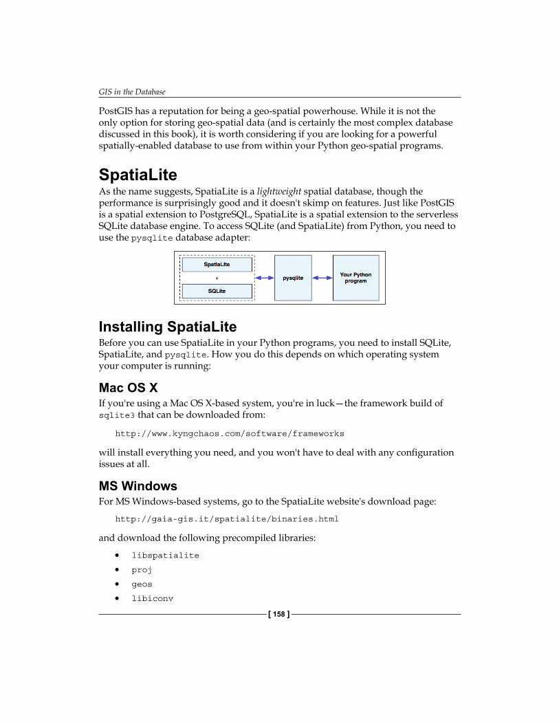
GIS in the Database
[ 158 ]
PostGIS has a reputation for being a geo-spatial powerhouse. While it is not the only option for storing geo-spatial data (and is certainly the most complex database discussed in this book), it is worth considering if you are looking for a powerful spatially-enabled database to use from within your Python geo-spatial programs.
SpatiaLiteAs the name suggests, SpatiaLite is a lightweight spatial database, though the performance is surprisingly good and it doesn't skimp on features. Just like PostGIS is a spatial extension to PostgreSQL, SpatiaLite is a spatial extension to the serverless SQLite database engine. To access SQLite (and SpatiaLite) from Python, you need to use the pysqlite database adapter:
Installing SpatiaLiteBefore you can use SpatiaLite in your Python programs, you need to install SQLite, SpatiaLite, and pysqlite. How you do this depends on which operating system your computer is running:
Mac OS XIf you're using a Mac OS X-based system, you're in luck—the framework build of sqlite3 that can be downloaded from:
http://www.kyngchaos.com/software/frameworks
will install everything you need, and you won't have to deal with any configuration issues at all.
MS WindowsFor MS Windows-based systems, go to the SpatiaLite website's download page:
http://gaia-gis.it/spatialite/binaries.html
and download the following precompiled libraries:
• libspatialite
• proj
• geos
• libiconv
Chapter 6
[ 159 ]
Once you have decompressed them, you will end up with a series of DLLs. Because the DLLs are dependent on each other, make sure you place these on the system path so they can be found when SpatiaLite is loaded.
LinuxFor Linux, you can download a prebuilt version of libspatialite from the SpatiaLite website:
http://gaia-gis.it/spatialite/binaries.html
You will, however, have to install PROJ, GEOS, and libiconv before libspatialite will work. These libraries can be found at:
• http://trac.osgeo.org/proj
• http://trac.osgeo.org/geos
• http://gnu.org/software/libiconv
Either install a suitable binary distribution, or compile the libraries yourself from source.
Installing pysqliteAfter installing the libspatialite library and its dependencies, you now need to make sure you have a workable version of pysqlite, the Python database adapter for SQLite.
Mac users are once again in luck: the sqlite3 framework you downloaded already includes a suitable version of pysqlite, so you can ignore this section.
A version of pysqlite comes bundled with Python version 2.5 and later, in the form of a standard library module named sqlite3. This standard library module, however, may not work with SpatiaLite. Because SpatiaLite is an extension to SQLite, the pysqlite library must be able to load extensions—a feature that was only introduced in pysqlite version 2.5, and is often disabled by default. To see if your version of Python includes a usable version of sqlite3, type the following into the Python command line:
>>> import sqlite3
>>> conn = sqlite3.connect(":memory:")
>>> conn.enable_load_extension(True)
If you get an AttributeError, your built-in version of sqlite3 does not support loading extensions, and you will have to download and install a different version.
GIS in the Database
[ 160 ]
The main website for pysqlite is:
http://code.google.com/p/pysqlite
You can download binary versions for MS Windows, and source code packages that you can compile yourself for Linux.
Accessing SpatiaLite from PythonNow that you have all the libraries installed, you are ready to start using pysqlite to access and work with SpatiaLite databases. There is, however, one final thing to be aware of: because pysqlite is a database adapter for SQLite rather than SpatiaLite, you will need to load the libspatialite extension before you can use any of the SpatiaLite functionality in your Python program.
Mac users don't need to do this because the version of sqlite3 you downloaded comes with the libspatialite extension built-in.
To load the libspatialite extension, add the following highlighted statements to your Python program:
from pysqlite2 import dbapi as sqlite
conn = sqlite.connect("...")conn.enable_load_extension(True)conn.execute('SELECT load_extension("libspatialite-2.dll")')curs = conn.cursor()...
For Linux users, make sure you use the correct name for the libspatialite extension. You may also need to change the name of the pysqlite2 module you're importing depending on which version you downloaded.
DocumentationWith all these different packages, it can be quite confusing knowing where to look for more information. First off, you can learn more about the SQL syntax supported by SQLite (and SpatiaLite) by looking at the SQL as Understood by SQLite page:
http://sqlite.org/lang.html
Then, to learn more about SpatiaLite itself, check out the SpatiaLite Manual, which can be found at:
http://gaia-gis.it/spatialite/docs.html
Chapter 6
[ 161 ]
There are also tutorials available from the above link, but they aren't that useful if you are using SpatiaLite from Python.
Finally, to learn more about using pysqlite to access SQLite and SpatiaLite from Python, see:
http://pysqlite.googlecode.com/svn/doc/sqlite3.html
Using SpatiaLiteIn many ways, SpatiaLite has been modeled after PostGIS. Before using SpatiaLite for your database, you need to load an "initialization file" into the database, and you also need to explicitly define your spatial columns by calling the AddGeometryColumn() function, just like you do in PostGIS. Let's see how all this works by creating a SpatiaLite database and creating an example database table.
As described above, the first step in using SpatiaLite is to connect to the database and load the SpatiaLite extension, like this:
from pysqlite2 import dbapi2 as sqlite
db = sqlite.connect("myDatabase.db")
db.enable_load_extension(True)
db.execute('SELECT load_extension("libspatialite.dll")')
Note that because SQLite is a serverless database, the myDatabase.db database is simply a file on your hard disk. Also, if you are running on Mac OS X, you can skip the enable_load_extension / load_extension dance and remove or comment out the last two lines.
You next need to load the SpatiaLite tables into your database. This can be done by downloading the initialization file from:
http://gaia-gis.it/spatialite/resources.html
For the current version of SpatiaLite at the time this book was written, the file you need is named init_spatialite-2.3.sql. The version number may have changed, so download the appropriate initialization file for your version of SpatiaLite.
This file contains a series of SQL commands that prepare your database to use with SpatiaLite. If you have the SQLite command-line client installed on your computer, you can load the initialization file directly into your database, like this:
% sqlite3 myDatabase.db < init_spatialite-2.3.sql
GIS in the Database
[ 162 ]
Alternatively, if you don't have the SQLite command-line client installed, you can use the following Python code to read the initialization file into memory and execute it using pysqlite:
from pysqlite2 import dbapi2 as sqlite
db = sqlite.connect("test.db")db.enable_load_extension(True)db.execute('SELECT load_extension("libspatialite.dll")')cursor = db.cursor()
f = file("init_spatialite-2.3.sql", "r")lines = []for line in f.readlines(): line = line.rstrip() if len(line) == 0: continue if line.startswith("--"): continue if line.startswith("BEGIN"): continue if line.startswith("COMMIT"): continue lines.append(line)f.close()cmds = ("".join(lines)).split(";")for cmd in cmds: cursor.execute(cmd)db.commit()
Mac users can skip the db.enable_load_extension(...) and db.execute('SELECT load_extension(...)') statements.
Note that this code removes comments (lines starting with --), and also strips out the BEGIN and COMMIT instructions as these can't be executed using pysqlite.
Running the initialization script will create the internal database tables needed by SpatiaLite, and will also load the master list of spatial references into the database so you can use SRID values to assign a spatial reference to your features.
After running the initialization script, you can create a new database table to hold your geo-spatial data. As with PostGIS, this is a two-step process; you first create the non-spatial parts of your table using standard SQL statements:
cursor.execute("DROP TABLE IF EXISTS cities")cursor.execute("CREATE TABLE cities (" + "id INTEGER PRIMARY KEY AUTOINCREMENT, " + "name CHAR(255))")
Chapter 6
[ 163 ]
You then use the SpatiaLite function AddGeometryColumn() to define the spatial column(s) in your table:
cursor.execute("SELECT AddGeometryColumn('cities', 'geom', " + "4326, 'POLYGON', 2)")
The number 4326 is the spatial reference ID (SRID) used to identify the spatial reference this column's features will use. The SRID number 4326 refers to a spatial reference using latitude and longitude values and the WGS84 datum; we will look at SRID values in more detail in the Recommended best practices section, later.
You can then create a spatial index on your geometries using the CreateSpatialIndex() function, like this:
cursor.execute("SELECT CreateSpatialIndex('cities', 'geom')")
Now that you have set up your database table, you can insert geometry features into it using the GeomFromText() function:
cursor.execute("INSERT INTO cities (name, geom)" + " VALUES (?, GeomFromText(?, 4326))", (city, wkt))
And, you can retrieve geometries from the database in WKT format using the AsText() function:
cursor.execute("select name,AsText(geom) FROM cities")for name,wkt in cursor: ...
SpatiaLite capabilitiesSome highlights of SpatiaLite include:
• The ability to handle all the major geometry types, including Point, LineString, Polygon, MultiPoint, MultiLineString, MultiPolygon, and GeometryCollection.
• Every geometry feature has a spatial reference identifier (SRID) which tells you the spatial reference used by this feature.
• Geometry columns are constrained to a particular type of geometry and a particular SRID. This prevents you from accidentally storing the wrong type of geometry, or a geometry with the wrong spatial reference, into a database table.
GIS in the Database
[ 164 ]
• Support for translating geometries to and from WKT and WKB format.• Support for Geometry functions to do things like calculate the area of a
polygon, to simplify polygons and linestrings, to calculate the distance between two geometries, and to calculate intersections, differences, and buffers.
• Functions to transform geometries from one spatial reference to another, and to shift, scale, and rotate geometries.
• Support for fast spatial relationship calculations using minimum bounding rectangles.
• Support for complete spatial relationship calculations (equals, touches, intersects, and so on) using the geometry itself rather than just the bounding rectangle.
• The use of R-Tree indexes that can (if you use them correctly) produce impressive results when performing spatial queries. Calculating the intersection of 500,000 linestrings with 380,000 polygons took just nine seconds, according to one researcher.
• An alternative way of implementing spatial indexes, using in-memory MBR caching. This can be an extremely fast way of indexing features using minimum bounding rectangles, though it is limited by the amount of available RAM and so isn't suitable for extremely large datasets.
While SpatiaLite is considered to be a lightweight database, it is indeed surprisingly capable. Depending on your application, SpatiaLite may well be an excellent choice for your Python geo-spatial programming needs.
Commercial spatially-enabled databasesWhile we will be concentrating on the use of open source databases in this book, it's worth spending a moment exploring the commercial alternatives. There are two major commercial databases that support spatial operations: Oracle and Microsoft's SQL Server.
OracleOracle provides one of the world's most powerful and popular commercial database systems. Spatial extensions to the Oracle database are available in two flavors: Oracle Spatial provides a large range of geo-spatial database features, including spatial data types, spatial indexes, the ability to perform spatial queries and joins, and a range of spatial functions. Oracle Spatial also supports linear referencing systems, spatial analysis and data-mining functions, geocoding, and support for raster-format data.

Chapter 6
[ 165 ]
While Oracle Spatial is only available for the Enterprise edition of the Oracle database, it is one of the most powerful spatially-enabled databases available anywhere.
A subset of the Oracle Spatial functionality, called Oracle Locator, is available for the Standard edition of the Oracle database. Oracle Locator does not support common operations such as unions and buffers, intersections, and area and length calculations. It also excludes support for more advanced features such as linear referencing systems, spatial analysis functions, geocoding, and raster-format data.
While being extremely capable, Oracle does have the disadvantage of using a somewhat non-standard syntax compared with other SQL databases. It also uses non-standard function names for its spatial extensions, making it difficult to switch database engines or use examples written for other databases.
MS SQL ServerMicrosoft's SQL Server is another widely-used and powerful commercial database system. SQL Server supports a full range of geo-spatial operations, including support for both geometry and geography data types, and all of the standard geo-spatial functions and operators.
Because Microsoft has followed the Open Geospatial Consortium's standards, the data types and function names used by SQL Server match those used by the open source databases we have already examined. The only difference stems from SQL Server's own internal object-oriented nature; for example, rather than ST_Intersects(geom, pt), SQL Server uses geom.STIntersects(pt).
Unlike Oracle, all of Microsoft's spatial extensions are included in every edition of the SQL Server; there is no need to obtain the Enterprise Edition to get the full range of spatial capabilities.
There are two limitations with MS SQL Server that may limit its usefulness as a spatially-enabled database. Firstly, SQL Server only runs on Microsoft Windows-based computers. This limits the range of servers it can be installed on. Also, SQL Server does not support transforming data from one spatial reference system to another.
Recommended best practicesIn this section, we will look at a number of practical things you can do to ensure your geo-spatial databases work as efficiently and effectively as possible.
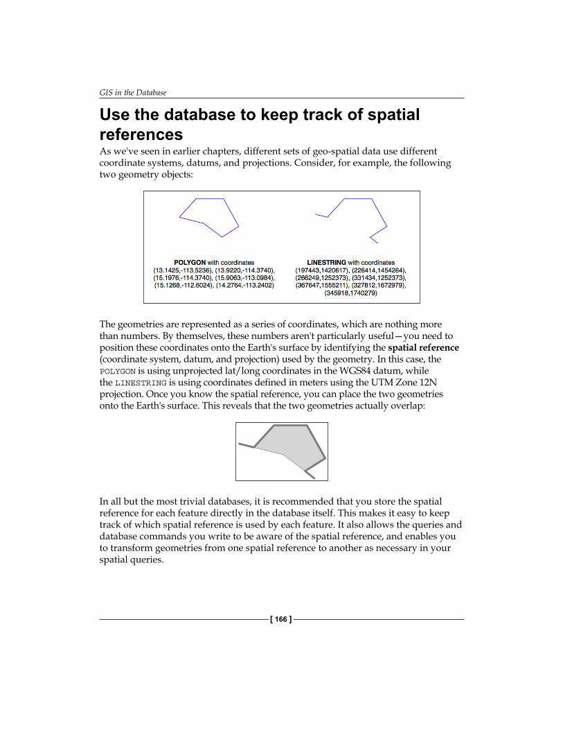
GIS in the Database
[ 166 ]
Use the database to keep track of spatial referencesAs we've seen in earlier chapters, different sets of geo-spatial data use different coordinate systems, datums, and projections. Consider, for example, the following two geometry objects:
The geometries are represented as a series of coordinates, which are nothing more than numbers. By themselves, these numbers aren't particularly useful—you need to position these coordinates onto the Earth's surface by identifying the spatial reference (coordinate system, datum, and projection) used by the geometry. In this case, the POLYGON is using unprojected lat/long coordinates in the WGS84 datum, while the LINESTRING is using coordinates defined in meters using the UTM Zone 12N projection. Once you know the spatial reference, you can place the two geometries onto the Earth's surface. This reveals that the two geometries actually overlap:
In all but the most trivial databases, it is recommended that you store the spatial reference for each feature directly in the database itself. This makes it easy to keep track of which spatial reference is used by each feature. It also allows the queries and database commands you write to be aware of the spatial reference, and enables you to transform geometries from one spatial reference to another as necessary in your spatial queries.
Chapter 6
[ 167 ]
Spatial references are generally referred to using a simple integer value called a Spatial Reference Identifier or SRID. While you could choose arbitrary SRID values to represent various spatial references, it is strongly recommended that you use the European Petroleum Survey Group (EPSG) numbers as standard SRID values. Using this internationally-recognized standard makes your data interchangeable with other databases, and allows tools such as OGR and Mapnik to identify the spatial reference used by your data.
To learn more about EPSG numbers, and SRID values in general, please refer to:
http://epsg-registry.org
You have seen SRID values before. For example, in the Using SpatiaLite section of this chapter, we encountered the following SQL statement:
SELECT AddGeometryColumn('cities','geom',4326,'POLYGON',2)
The value 4326 is the SRID used to identify a particular spatial reference, in this case the WGS84 Long Lat reference (unprojected lat/long coordinates using the WGS84 datum).
Both PostGIS and SpatiaLite add a special table to your spatially-enabled database called spatial_ref_sys. This table comes pre-loaded with a list of over 3,000 commonly-used spatial references, all identified by EPSG number. Because the SRID value is the primary key into this table, tools that access the database can refer to this table to perform on-the-fly coordinate transformations using the PROJ.4 library. Even if you are using MySQL, which doesn't provide a spatial_ref_sys table or other direct support for coordinate transformations, you should be using standard EPSG numbers for your spatial references.
Note that all three open source spatial databases allow you to associate an SRID value with a geometry when importing from WKT:
• MySQL: GeometryFromText(wkt, [srid])• PostGIS: ST_GeometryFromText(wkt, [srid])• SpatiaLite: GeometryFromText(wkt, [srid])
While the SRID value is optional, you should use this wherever possible to tell the database which spatial reference your geometry is using. In fact, both PostGIS and SpatiaLite require you to use the correct SRID value if a column has been set up to use a particular SRID. This prevents you from mixing the spatial references within a table.
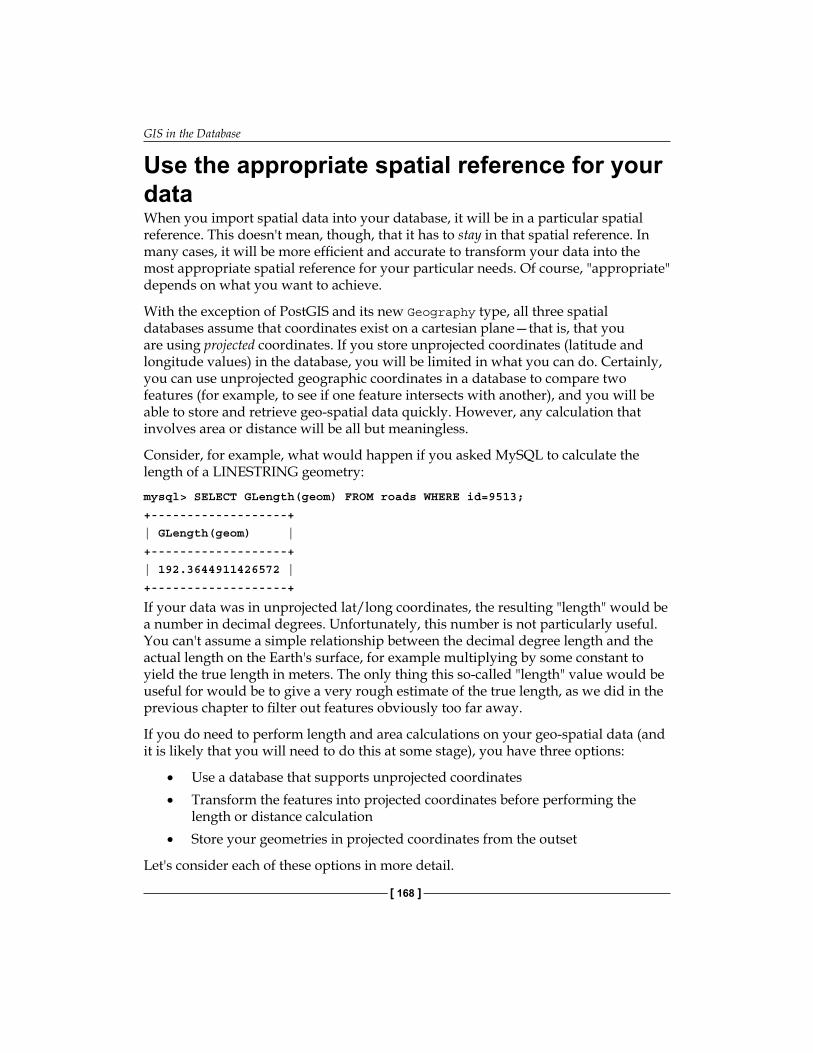
GIS in the Database
[ 168 ]
Use the appropriate spatial reference for your dataWhen you import spatial data into your database, it will be in a particular spatial reference. This doesn't mean, though, that it has to stay in that spatial reference. In many cases, it will be more efficient and accurate to transform your data into the most appropriate spatial reference for your particular needs. Of course, "appropriate" depends on what you want to achieve.
With the exception of PostGIS and its new Geography type, all three spatial databases assume that coordinates exist on a cartesian plane—that is, that you are using projected coordinates. If you store unprojected coordinates (latitude and longitude values) in the database, you will be limited in what you can do. Certainly, you can use unprojected geographic coordinates in a database to compare two features (for example, to see if one feature intersects with another), and you will be able to store and retrieve geo-spatial data quickly. However, any calculation that involves area or distance will be all but meaningless.
Consider, for example, what would happen if you asked MySQL to calculate the length of a LINESTRING geometry:
mysql> SELECT GLength(geom) FROM roads WHERE id=9513;
+-------------------+
| GLength(geom) |
+-------------------+
| 192.3644911426572 |
+-------------------+
If your data was in unprojected lat/long coordinates, the resulting "length" would be a number in decimal degrees. Unfortunately, this number is not particularly useful. You can't assume a simple relationship between the decimal degree length and the actual length on the Earth's surface, for example multiplying by some constant to yield the true length in meters. The only thing this so-called "length" value would be useful for would be to give a very rough estimate of the true length, as we did in the previous chapter to filter out features obviously too far away.
If you do need to perform length and area calculations on your geo-spatial data (and it is likely that you will need to do this at some stage), you have three options:
• Use a database that supports unprojected coordinates• Transform the features into projected coordinates before performing the
length or distance calculation• Store your geometries in projected coordinates from the outset
Let's consider each of these options in more detail.
Chapter 6
[ 169 ]
Option 1: Use a database that supports geographiesOf the open source databases we are considering, only PostGIS has the ability to work directly with unprojected coordinates, through the use of the relatively-new Geography type. Unfortunately, the Geography type has some major limitations that make this a less than ideal solution:
• Performing calculations on unprojected coordinates takes approximately an order of magnitude longer than performing the same calculations using projected (cartesian) coordinates
• The Geography type only supports lat/long values on the WGS84 datum (SRID 4326)
• Many of the functions available for projected coordinates are not yet supported by the Geography type
For these reasons, as well as the fact that the they are only supported by PostGIS, we will not be using Geography columns in this book.
Option 2: Transform features as requiredAnother possibility is to store your data in unprojected lat/long coordinates, and transform the coordinates into a projected coordinate system before you calculate the distance or area. While this will work, and will give you accurate results, you should beware of doing this because you may well forget to transform into a projected coordinate system before making the calculation. Also, performing on-the-fly transformations of large numbers of geometries is very time-consuming.
Despite these problems, there are situations where storing unprojected coordinates makes sense. We will look at this shortly.
Option 3: Transform features from the outsetBecause transforming features from one spatial reference to another is rather time-consuming, it often makes sense to do this once, at the time you import your data, and store it in the database already converted to a projected coordinate system.
Doing this, you will be able to perform your desired spatial calculations quickly and accurately. However, there are situations where this is not the best option, as we will see in the next section.
GIS in the Database
[ 170 ]
When to use unprojected coordinatesAs we saw in Chapter 2, projecting features from the three-dimensional surface of the Earth onto a two-dimensional cartesian plane can never be done perfectly. It is a mathematical truism that there will always be errors in any projection.
Different map projections are generally chosen to preserve values such as distance or area for a particular portion of the Earth's surface. For example, the Mercator projection is accurate at the tropics, but distorts features closer to the Poles.
Because of this inevitable distortion, projected coordinates work best when your geo-spatial data only covers a part of the Earth's surface. If you are only dealing with data for Austria, then a projected coordinate system will work very well indeed. But, if your data includes features in both Austria and Australia, then using the same projected coordinates for both sets of features will once again produce inaccurate results.
For this reason, it is generally best to use a projected coordinate system for data that covers only part of the Earth's surface, but unprojected coordinates will work best if you need to store data covering large parts of the Earth.
Of course, using unprojected coordinates leads to problems of its own, as discussed above. This is why it's recommended that you use the appropriate spatial reference for your particular needs; what is appropriate for you depends on what data you need to store and how you intend to use it.
The best way to find out what is appropriate would be to experiment; try importing your data in both spatial references, and write some test programs to work with the imported data. That will tell you which is the fastest and easiest spatial reference to work with, rather than having to guess.
Avoid on-the-fly transformations within a queryImagine that you have a cities table with a geom column containing POLYGON geometries in UTM 12N projection (EPSG number 32612). Being a competent geo-spatial developer, you have set up a spatial index on this column.
Now, imagine that you have a variable named pt that holds a POINT geometry in unprojected WGS84 coordinates (EPSG number 4326). You might want to find the city that contains this point, so you issue the following reasonable-looking query:
SELECT * FROM cities WHERE Contains(Transform(geom, 4326), pt);
Chapter 6
[ 171 ]
This will give you the right answer, but it will take an extremely long time. Why? Because the Transform(geom, 4326) expression is converting every geometry in the table from UTM 12N to long-lat WGS84 coordinates before the database can check to see if the point is inside the geometry. The spatial index is completely ignored as it is in the wrong coordinate system.
Compare this with the following query:
SELECT * FROM cities WHERE Contains(geom, Transform(pt, 32612));
A very minor change, but a dramatically different result. Instead of taking hours, the answer should come back almost immediately. Can you see why? The transformation is being done on a variable that does not change from one record to the next, so the Transform(pt, 32612) expression is being called just once, and the Contains() call can make use of your spatial index to quickly find the matching city.
The lesson here is simple—be aware of what you are asking the database to do, and make sure you structure your queries to avoid on-the-fly transformations of large numbers of geometries.
Don't create geometries within a queryWhile we are discussing database queries that can cause the database to perform a huge amount of work, consider the following (where poly is a polygon):
SELECT * FROM cities WHERE
NOT ST_IsEmpty(ST_Intersection(outline, poly));
In a sense, this is perfectly reasonable: identify all cities that have a non-empty intersection between the city's outline and the given polygon. And, the database will indeed be able to answer this query—it will just take an extremely long time to do so. Hopefully, you can see why: the ST_Intersection() function creates a new geometry out of two existing geometries. This means that for every row in the database table, a new geometry is created, and is then passed to ST_IsEmpty(). As you can imagine, these types of operations are extremely inefficient. To avoid creating a new geometry each time, you can rephrase your query like this:
SELECT * FROM cities WHERE ST_Intersects(outline, poly);
While this example may seem obvious, there are many cases where spatial developers have forgotten this rule, and have wondered why their queries were taking so long to complete. A common example is to use the ST_Buffer() function to see if a point is within a given distance of a polygon, like this:
SELECT * FROM cities WHERE
ST_Contains(ST_Buffer(outline, 100), pt);
GIS in the Database
[ 172 ]
Once again, this query will work, but will be painfully slow. A much better approach would be to use the ST_DWithin() function:
SELECT * FROM cities WHERE ST_DWithin(outline, pt, 100);
As a general rule, remember that you never want to call any function that returns a Geometry object (or one of its subclasses) within the WHERE portion of a SELECT statement.
Use spatial indexes appropriatelyJust like ordinary database indexes can make an immense difference to the speed and efficiency of your database, spatial indexes are also an extremely powerful tool for speeding up your database queries. Like all powerful tools, though, they have their limits:
• If you don't explicitly define a spatial index, the database can't use it. Conversely, if you have too many spatial indexes, the database will slow down because each index needs to be updated every time a record is added, updated, or deleted. Thus, it is crucial that you define the right set of spatial indexes: index the information you are going to search on, and nothing more.
• Because spatial indexes work on the geometries' bounding boxes, the index itself can only tell you which bounding boxes actually overlap or intersect; they can't tell you if the underlying points, lines, or polygons have this relationship. Thus, they are really only the first step in searching for the information you want. With PostGIS and SpatiaLite, the database itself can further refine the search by comparing the individual geometries for you; with MySQL, you have to do this yourself, as we saw earlier.
• Spatial indexes are most efficient when dealing with lots of relatively small geometries. If you have large polygons consisting of many thousands of vertices, the polygon's bounding box is going to be so large that it will intersect with lots of other geometries, and the database will have to revert to doing full polygon calculations rather than just the bounding box. If your geometries are huge, these calculations can be very slow indeed—the entire polygon will have to be loaded into memory and processed one vertex at a time. If possible, it is generally better to split large polygons (and in particular large multipolygons) into smaller pieces so that the spatial index can work with them more efficiently.
Chapter 6
[ 173 ]
Know the limits of your database's query optimizerWhen you send a query to the database, it automatically attempts to optimize the query to avoid unnecessary calculations and to make use of any available indexes. For example, if you issued the following (non-spatial) query:
SELECT * FROM people WHERE name=Concat("John ","Doe");
The database would know that Concat("John ","Doe") yields a constant, and so would only calculate it once before issuing the query. It would also look for a database index on the name column, and use it to speed up the operation.
This type of query optimization is very powerful, and the logic behind it is extremely complex. In a similar way, spatial databases have a spatial query optimizer that looks for ways to pre-calculate values and make use of spatial indexes to speed up the query. For example, consider this spatial query from the previous section:
select * from cities where ST_DWithin(outline, pt, 12.5);
In this case, the PostGIS function ST_DWithin() is given one geometry taken from a table (outline), and a second geometry that is specified as a fixed value (pt), along with a desired distance (12.5 "units", whatever that means in the geometry's spatial reference). The query optimizer knows how to handle this efficiently, by first pre-calculating the bounding box for the fixed geometry plus the desired distance (pt ±12.5), and then using a spatial index to quickly identify the records that may have their outline geometry within that extended bounding box.
While there are times when the database's query optimizer seems to be capable of magic, there are many other times when it is incredibly stupid. Part of the art of being a good database developer is to have a keen sense of how your database's query optimizer works, when it doesn't—and what to do about it.
Let's see how you can find out more about the query optimization process in each of our three spatial databases.
GIS in the Database
[ 174 ]
MySQLMySQL provides a command, EXPLAIN SELECT, that tells you how the query optimizer has tried to process your query. For example:
mysql> EXPLAIN SELECT * FROM cities
WHERE MBRContains(geom,
GeomFromText(pt))\G
*********************** 1. row ***********************
id: 1
select_type: SIMPLE
table: cities
type: range
possible_keys: geom
key: geom
key_len: 34
ref: NULL
rows: 1
Extra: Using where
1 row in set (0.00 sec)
Don't worry about the \G at the end of the command; this just formats the output in a way that makes it easier to read.
This command tells you that this query involves a simple search against the cities table, searching for a range of records using the geom spatial index to speed up the results. The rows:1 tells you that the query optimizer thinks it only needs to read a single row from the table to find the results.
This is good. Compare it with:
mysql> EXPLAIN SELECT * FROM cities
WHERE MBRContains(Envelope(geom),
GeomFromText(pt))\G
*********************** 1. row ***********************
id: 1
select_type: SIMPLE
table: cities
Chapter 6
[ 175 ]
type: ALL
possible_keys: NULL
key: NULL
key_len: NULL
ref: NULL
rows: 34916
Extra: Using where
1 row in set (0.00 sec)
This query uses the Envelope() function to create a new geometry, which is then checked to see if it contains the given point. As explained in the Don't Create Geometries Within a Query section, previously, the database has to create a new geometry for every row in the table. In this case, the query optimizer cannot use an index, as shown by the NULL value for possible_keys and key. It also tells you that it would have to scan through 34,916 records to find the matching points—not exactly an efficient query. Indeed, running this query could take several minutes to complete.
PostGISMySQL uses a theoretical approach to query optimization, looking only at the query itself to see how it could be optimized. PostGIS, on the other hand, takes into account the amount of information in the database and how it is distributed. In order to work well, the PostGIS query optimizer needs to have up-to-date statistics on the database's contents. It then uses a sophisticated genetic algorithm to determine the most effective way to run a particular query.
Because of this approach, you need to regularly run the VACUUM ANALYZE command, which gathers statistics on the database so that the query optimizer can work as effectively as possible. If you don't run VACUUM ANALYZE, the optimizer simply won't be able to work.
Here is how you can run the VACUUM ANALYZE command from Python:
import psycopg2
connection = psycopg2.connect("dbname=... user=...")cursor = connection.cursor()
old_level = connection.isolation_levelconnection.set_isolation_level(0)cursor.execute("VACUUM ANALYZE")connection.set_isolation_level(old_level)
GIS in the Database
[ 176 ]
Don't worry about the isolation_level logic here; that just allows you to run the VACUUM ANALYZE command from Python using the transaction-based psycopg2 adapter.
It is possible to set up an autovacuum daemon that runs automatically after a given period of time, or after a table's contents has changed enough to warrant another vacuum. Setting up an autovacuum daemon is beyond the scope of this book.
Once you have run the VACUUM ANALYZE command, the query optimizer will be able to start optimizing your queries. As with MySQL, you can see how the query optimizer works using the EXPLAIN SELECT command:
psql> EXPLAIN SELECT * FROM cities
WHERE ST_Contains(geom,pt);
QUERY PLAN
--------------------------------------------------------
Seq Scan on cities (cost=0.00..7.51 rows=1 width=2619)
Filter: ((geom && '010100000000000000000000000000000000000000'::geometry) AND _st_contains(geom, '010100000000000000000000000000000000000000'::geometry))
(2 rows)
Don't worry about the Seq Scan part; there are only a few records in this table, so PostGIS knows that it can do a sequential scan of the entire table faster than it can read through an index. When the database gets bigger, it will automatically start using the index to quickly identify the desired records.
The cost= part is an indication of how much this query will "cost", measured in arbitrary units that by default are relative to how long it takes to read a page of data from disk. The two numbers represent the "start up cost" (how long it takes before the first row can be processed), and the estimated total cost (how long it would take to process every record in the table). Since reading a page of data from disk is quite fast, a total cost of 7.51 is very quick indeed.
The most interesting part of this explanation is the Filter. Let's take a closer look at what the EXPLAIN SELECT command tells us about how PostGIS will filter this query. The first part:
(geom && '010100000000000000000000000000000000000000'::geometry)
makes use of the && operator, which searches for matching records using the bounding box defined in the spatial index. The second part of the filter condition:
Chapter 6
[ 177 ]
_st_contains(geom, '010100000000000000000000000000000000000000'::geometry)
uses the ST_Contains() function to identify the exact geometries that actually contain the desired point. This two-step process (first filtering by bounding box, then by the geometry itself) is exactly what we had to implement manually when using MySQL. As you can see, PostGIS does this for us automatically, resulting in a quick but also accurate search for geometries that contain a given point.
SpatiaLiteOne of the disadvantages of using a lightweight database such as SpatiaLite is that the query optimizer is rather naïve. In particular, the SpatiaLite query optimizer will only make use of B*Tree indexes; you can create a spatial R-Tree index, but it won't be used unless you explicitly include it in your query.
For example, consider the following SQL statements:
CREATE TABLE cities (id INTEGER PRIMARY KEY AUTOINCREMENT,
name CHAR(255));
SELECT AddGeometryColumn('cities','geom',4326,'POLYGON',2);
INSERT INTO cities (name,geom)
VALUES ('London', GeomFromText(wkt, 4326);
This creates a cities table, defines a spatial index, and inserts a record into the table. Because SpatiaLite uses triggers to automatically update the spatial index as records are added, updated, or deleted, the above statements would correctly create the spatial index and update it as the new record is inserted. However, if we then issue the following query:
SELECT * FROM cities WHERE Contains(geom, pt);
The SpatiaLite query optimizer won't know about the spatial index, and so will ignore it. We can confirm this using the EXPLAIN QUERY PLAN command, which shows the indexes used by the query:
sqlite> EXPLAIN QUERY PLAN SELECT * FROM cities
WHERE id < 100;
0|0|TABLE cities USING PRIMARY KEY
sqlite> EXPLAIN QUERY PLAN SELECT * FROM cities
WHERE Contains(geom, pt);
0|0|TABLE cities
GIS in the Database
[ 178 ]
The first query (WHERE id < 100) makes use of a B*Tree index, and so the query optimizer knows to use the primary key to index the query. The second query (WHERE Contains(geom, pt)) uses the spatial index that the query optimizer doesn't know about. In this case, the cities table will be scanned sequentially, without any index at all. This will be acceptable for small numbers of records, but for large databases this will be very slow indeed.
To use the spatial index, we have to include it directly in the query:
SELECT * FROM cities WHERE id IN
(SELECT pkid FROM idx_cities_geom WHERE xmin <= X(pt)
AND X(pt) <= xmax AND ymin <= Y(pt) AND Y(pt) <= ymax);
The EXPLAIN QUERY PLAN command tells us that this query would indeed use the database indexes to speed up the query:
sqlite> EXPLAIN QUERY PLAN SELECT * FROM cities
WHERE id IN (SELECT pkid FROM idx_cities_geom
WHERE xmin <= X(pt) AND X(pt) <= xmax
AND ymin <= Y(pt) AND Y(pt) <= ymax);
0|0|TABLE cities USING PRIMARY KEY
0|0|TABLE idx_cities_geom VIRTUAL TABLE INDEX 2:BaDbBcDd
This is an unfortunate consequence of using SpatiaLite—you have to include the indexes explicitly in every spatial query you make, or they won't be used at all. This can make creating your spatial queries more complicated, though the performance of the end result will be excellent.
Working with geo-spatial databases using PythonIn this section, we will build on what we've learned so far by writing a short program to:
1. Create a geo-spatial database.2. Import data from a Shapefile.3. Query that data.4. Save the results in WKT format.
We will write the same program using each of the three databases we have explored in this chapter so that you can see the differences and issues involved with using each particular database.
Chapter 6
[ 179 ]
PrerequisitesBefore you can run these examples, you will need to do the following:
1. If you haven't already done so, follow the instructions earlier in this chapter to install MySQL, PostGIS, and SpatiaLite onto your computer.
2. We will be working with the GSHHS shoreline dataset from Chapter 4. If you haven't already downloaded this dataset, you can download the Shapefiles from:http://www.ngdc.noaa.gov/mgg/shorelines/gshhs.html
3. Take a copy of the l (low-resolution) Shapefiles from the GSHHS shoreline dataset and place them in a convenient directory (we will call this directory GSHHS_l in the code samples shown here).
We will use the low-resolution Shapefiles to keep the amount of data manageable, and to avoid problems with large polygons triggering a max_allowed_packet error in MySQL. Large polygons are certainly supported by MySQL (by increasing the max_allowed_packet setting), but doing this is beyond the scope of this chapter.
4. Finally, make sure you have a copy of the init_spatialite-2.3.sql file as we will need it to set up the SpatiaLite database.
Working with MySQLWe have already seen how to connect to MySQL and create a database table:
import MySQLdb
connection = MySQLdb.connect(user="..." passwd="...")cursor = connection.cursor()
cursor.execute("USE myDatabase")
cursor.execute("""CREATE TABLE gshhs ( id INTEGER AUTO_INCREMENT, level INTEGER, geom POLYGON NOT NULL,
PRIMARY KEY (id) INDEX (level), SPATIAL INDEX (geom)) """)connection.commit()
GIS in the Database
[ 180 ]
We next need to read the features from the GSHHS Shapefiles and insert them into the database:
import os.pathfrom osgeo import ogr
for level in [1, 2, 3, 4]: fName = os.path.join("GSHHS_l", "GSHHS_l_L"+str(level)+".shp") shapefile = ogr.Open(fName) layer = shapefile.GetLayer(0) for i in range(layer.GetFeatureCount()): feature = layer.GetFeature(i) geometry = feature.GetGeometryRef() wkt = geometry.ExportToWkt()
cursor.execute("INSERT INTO gshhs (level, geom) " + "VALUES (%s, GeomFromText(%s, 4326))", (level, wkt)) connection.commit()
Note that we are assigning an SRID value (4326) to the features as we import them into the database. Even though we don't have a spatial_ref_sys table in MySQL, we are following the best practices by storing SRID values in the database.
We now want to query the database to find the shoreline information we want. In this case, we'll take the coordinate for London and search for a level 1 (ocean boundary) polygon that contains this point. This will give us the shoreline for the United Kingdom:
import shapely.wkt
LONDON = 'POINT(-0.1263 51.4980)'
cursor.execute("SELECT id,AsText(geom) FROM gshhs " + "WHERE (level=%s) AND " + "(MBRContains(geom, GeomFromText(%s, 4326)))", (1, LONDON))
shoreline = Nonefor id,wkt in cursor: polygon = shapely.wkt.loads(wkt) point = shapely.wkt.loads(LONDON) if polygon.contains(point): shoreline = wkt
Chapter 6
[ 181 ]
Remember that MySQL only supports bounding-rectangle queries, so we have to use Shapely to identify if the point is actually within the polygon, rather than just within its minimum bounding rectangle.
To check that this query can be run efficiently, we will follow the recommended best practice of asking the MySQL Query Optimizer what it will do with the query:
% /usr/local/mysql/bin/mysql
mysql> use myDatabase;
mysql> EXPLAIN SELECT id,AsText(geom) FROM gshhs
WHERE (level=1) AND (MBRContains(geom,
GeomFromText('POINT(-0.1263 51.4980)',
4326)))\G
*********************** 1. row ***********************
id: 1
select_type: SIMPLE
table: gshhs
type: range
possible_keys: level,geom
key: geom
key_len: 34
ref: NULL
rows: 1
Extra: Using where
1 row in set (0.00 sec)
As you can see, we simply retyped the query, adding the word EXPLAIN to the front and filling in the parameters to make a valid SQL statement. The result tells us that the SELECT query is indeed using the indexed geom column, allowing it to quickly find the desired feature.
Now that we have a working program that can quickly retrieve the desired geometry, let's save the UK shoreline polygon to a text file:
f = file("uk-shoreline.wkt", "w")f.write(shoreline)f.close()
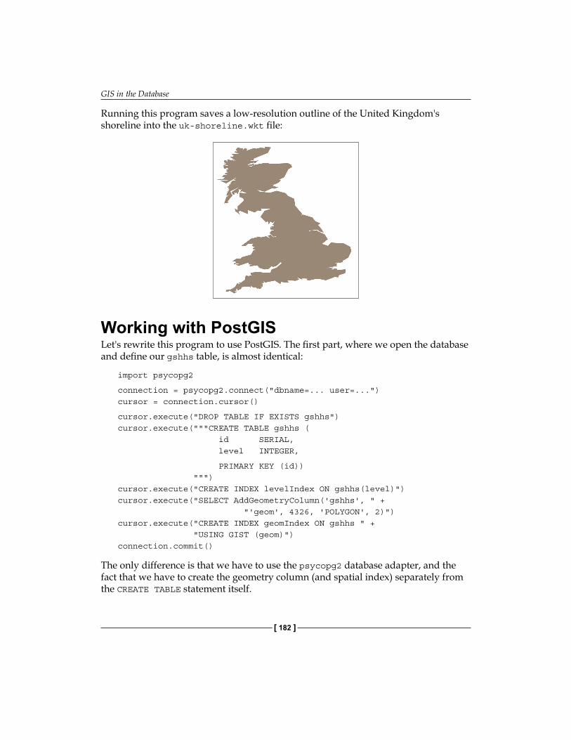
GIS in the Database
[ 182 ]
Running this program saves a low-resolution outline of the United Kingdom's shoreline into the uk-shoreline.wkt file:
Working with PostGISLet's rewrite this program to use PostGIS. The first part, where we open the database and define our gshhs table, is almost identical:
import psycopg2
connection = psycopg2.connect("dbname=... user=...")cursor = connection.cursor()
cursor.execute("DROP TABLE IF EXISTS gshhs")cursor.execute("""CREATE TABLE gshhs ( id SERIAL, level INTEGER,
PRIMARY KEY (id)) """)cursor.execute("CREATE INDEX levelIndex ON gshhs(level)")cursor.execute("SELECT AddGeometryColumn('gshhs', " + "'geom', 4326, 'POLYGON', 2)")cursor.execute("CREATE INDEX geomIndex ON gshhs " + "USING GIST (geom)")connection.commit()
The only difference is that we have to use the psycopg2 database adapter, and the fact that we have to create the geometry column (and spatial index) separately from the CREATE TABLE statement itself.
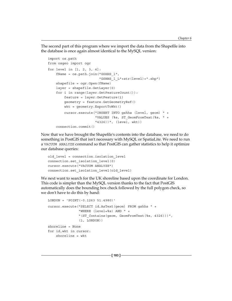
Chapter 6
[ 183 ]
The second part of this program where we import the data from the Shapefile into the database is once again almost identical to the MySQL version:
import os.pathfrom osgeo import ogr
for level in [1, 2, 3, 4]: fName = os.path.join("GSHHS_l", "GSHHS_l_L"+str(level)+".shp") shapefile = ogr.Open(fName) layer = shapefile.GetLayer(0) for i in range(layer.GetFeatureCount()): feature = layer.GetFeature(i) geometry = feature.GetGeometryRef() wkt = geometry.ExportToWkt()
cursor.execute("INSERT INTO gshhs (level, geom) " + "VALUES (%s, ST_GeomFromText(%s, " + "4326))", (level, wkt)) connection.commit()
Now that we have brought the Shapefile's contents into the database, we need to do something in PostGIS that isn't necessary with MySQL or SpatiaLite. We need to run a VACUUM ANALYZE command so that PostGIS can gather statistics to help it optimize our database queries:
old_level = connection.isolation_levelconnection.set_isolation_level(0)cursor.execute("VACUUM ANALYZE")connection.set_isolation_level(old_level)
We next want to search for the UK shoreline based upon the coordinate for London. This code is simpler than the MySQL version thanks to the fact that PostGIS automatically does the bounding box check followed by the full polygon check, so we don't have to do this by hand:
LONDON = 'POINT(-0.1263 51.4980)'
cursor.execute("SELECT id,AsText(geom) FROM gshhs " + "WHERE (level=%s) AND " + "(ST_Contains(geom, GeomFromText(%s, 4326)))", (1, LONDON))
shoreline = Nonefor id,wkt in cursor: shoreline = wkt
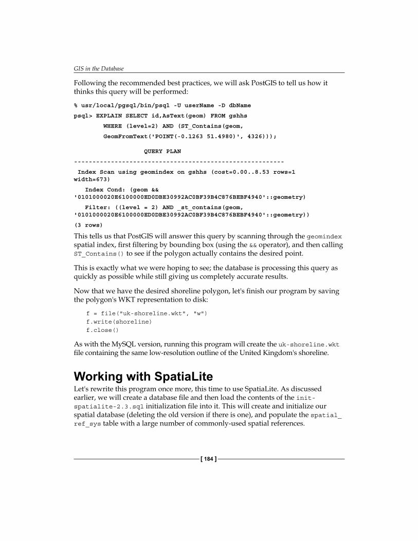
GIS in the Database
[ 184 ]
Following the recommended best practices, we will ask PostGIS to tell us how it thinks this query will be performed:
% usr/local/pgsql/bin/psql -U userName -D dbName
psql> EXPLAIN SELECT id,AsText(geom) FROM gshhs
WHERE (level=2) AND (ST_Contains(geom,
GeomFromText('POINT(-0.1263 51.4980)', 4326)));
QUERY PLAN
---------------------------------------------------------
Index Scan using geomindex on gshhs (cost=0.00..8.53 rows=1 width=673)
Index Cond: (geom && '0101000020E6100000ED0DBE30992AC0BF39B4C876BEBF4940'::geometry)
Filter: ((level = 2) AND _st_contains(geom, '0101000020E6100000ED0DBE30992AC0BF39B4C876BEBF4940'::geometry))
(3 rows)
This tells us that PostGIS will answer this query by scanning through the geomindex spatial index, first filtering by bounding box (using the && operator), and then calling ST_Contains() to see if the polygon actually contains the desired point.
This is exactly what we were hoping to see; the database is processing this query as quickly as possible while still giving us completely accurate results.
Now that we have the desired shoreline polygon, let's finish our program by saving the polygon's WKT representation to disk:
f = file("uk-shoreline.wkt", "w")f.write(shoreline)f.close()
As with the MySQL version, running this program will create the uk-shoreline.wkt file containing the same low-resolution outline of the United Kingdom's shoreline.
Working with SpatiaLiteLet's rewrite this program once more, this time to use SpatiaLite. As discussed earlier, we will create a database file and then load the contents of the init-spatialite-2.3.sql initialization file into it. This will create and initialize our spatial database (deleting the old version if there is one), and populate the spatial_ref_sys table with a large number of commonly-used spatial references.
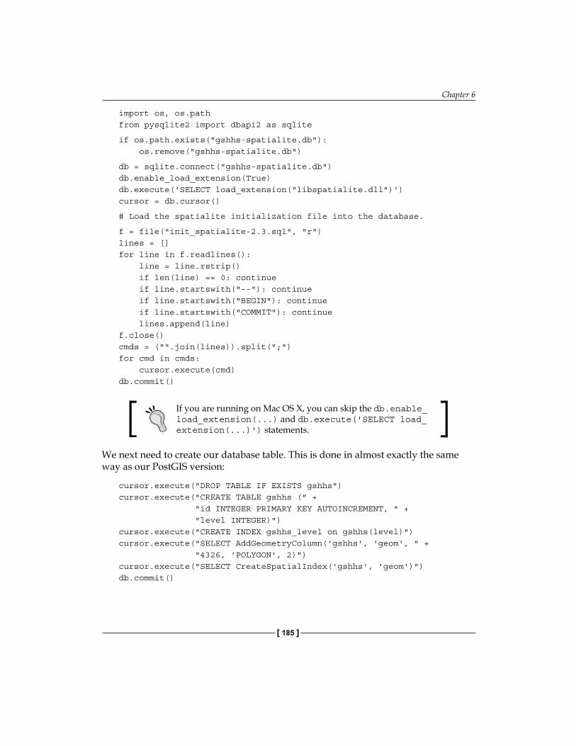
Chapter 6
[ 185 ]
import os, os.pathfrom pysqlite2 import dbapi2 as sqlite
if os.path.exists("gshhs-spatialite.db"): os.remove("gshhs-spatialite.db")
db = sqlite.connect("gshhs-spatialite.db")db.enable_load_extension(True)db.execute('SELECT load_extension("libspatialite.dll")')cursor = db.cursor()
# Load the spatialite initialization file into the database.
f = file("init_spatialite-2.3.sql", "r")lines = []for line in f.readlines(): line = line.rstrip() if len(line) == 0: continue if line.startswith("--"): continue if line.startswith("BEGIN"): continue if line.startswith("COMMIT"): continue lines.append(line)f.close()cmds = ("".join(lines)).split(";")for cmd in cmds: cursor.execute(cmd)db.commit()
If you are running on Mac OS X, you can skip the db.enable_load_extension(...) and db.execute('SELECT load_extension(...)') statements.
We next need to create our database table. This is done in almost exactly the same way as our PostGIS version:
cursor.execute("DROP TABLE IF EXISTS gshhs")cursor.execute("CREATE TABLE gshhs (" + "id INTEGER PRIMARY KEY AUTOINCREMENT, " + "level INTEGER)")cursor.execute("CREATE INDEX gshhs_level on gshhs(level)")cursor.execute("SELECT AddGeometryColumn('gshhs', 'geom', " + "4326, 'POLYGON', 2)")cursor.execute("SELECT CreateSpatialIndex('gshhs', 'geom')")db.commit()
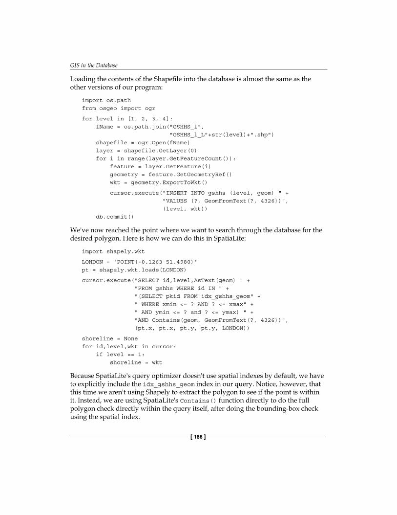
GIS in the Database
[ 186 ]
Loading the contents of the Shapefile into the database is almost the same as the other versions of our program:
import os.pathfrom osgeo import ogr
for level in [1, 2, 3, 4]: fName = os.path.join("GSHHS_l", "GSHHS_l_L"+str(level)+".shp") shapefile = ogr.Open(fName) layer = shapefile.GetLayer(0) for i in range(layer.GetFeatureCount()): feature = layer.GetFeature(i) geometry = feature.GetGeometryRef() wkt = geometry.ExportToWkt()
cursor.execute("INSERT INTO gshhs (level, geom) " + "VALUES (?, GeomFromText(?, 4326))", (level, wkt)) db.commit()
We've now reached the point where we want to search through the database for the desired polygon. Here is how we can do this in SpatiaLite:
import shapely.wkt
LONDON = 'POINT(-0.1263 51.4980)'pt = shapely.wkt.loads(LONDON)
cursor.execute("SELECT id,level,AsText(geom) " + "FROM gshhs WHERE id IN " + "(SELECT pkid FROM idx_gshhs_geom" + " WHERE xmin <= ? AND ? <= xmax" + " AND ymin <= ? and ? <= ymax) " + "AND Contains(geom, GeomFromText(?, 4326))", (pt.x, pt.x, pt.y, pt.y, LONDON))
shoreline = Nonefor id,level,wkt in cursor: if level == 1: shoreline = wkt
Because SpatiaLite's query optimizer doesn't use spatial indexes by default, we have to explicitly include the idx_gshhs_geom index in our query. Notice, however, that this time we aren't using Shapely to extract the polygon to see if the point is within it. Instead, we are using SpatiaLite's Contains() function directly to do the full polygon check directly within the query itself, after doing the bounding-box check using the spatial index.
Chapter 6
[ 187 ]
This query is complex, but in theory should produce a fast and accurate result. Following the recommended best practice, we want to check our query by asking SpatiaLite's query optimizer how the query will be processed. This will tell us if we have written the query correctly.
Unfortunately, depending on how your copy of SpatiaLite was installed, you may not have access to the SQLite command line. So, instead, let's call the EXPLAIN QUERY PLAN command from Python:
cursor.execute("EXPLAIN QUERY PLAN " + "SELECT id,level,AsText(geom) " + "FROM gshhs WHERE id IN " + "(SELECT pkid FROM idx_gshhs_geom" + " WHERE xmin <= ? AND ? <= xmax" + " AND ymin <= ? and ? <= ymax) " + "AND Contains(geom, GeomFromText(?, 4326))", (pt.x, pt.x, pt.y, pt.y, LONDON))for row in cursor: print row
Running this tells us that the SpatiaLite query optimizer will use the spatial index (along with the table's primary key) to quickly identify the features that match by bounding box:
(0, 0, 'TABLE gshhs USING PRIMARY KEY')
(0, 0, 'TABLE idx_gshhs_geom VIRTUAL TABLE INDEX 2:BaDbBcDd')
Note that there is a bug in SpatiaLite that prevents it from using both a spatial index and an ordinary B*Tree index in the same query. This is why our Python program asks SpatiaLite to return the level value, and then checks for the level explicitly before identifying the shoreline, rather than simply embedding AND (level=1) in the query itself.
Now that we have the shoreline, saving it to a text file is again trivial:
f = file("uk-shoreline.wkt", "w")f.write(shoreline)f.close()
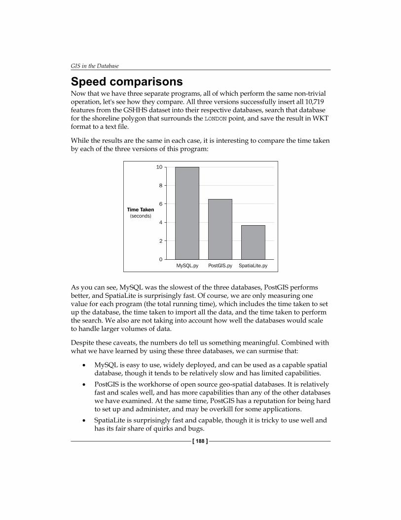
GIS in the Database
[ 188 ]
Speed comparisonsNow that we have three separate programs, all of which perform the same non-trivial operation, let's see how they compare. All three versions successfully insert all 10,719 features from the GSHHS dataset into their respective databases, search that database for the shoreline polygon that surrounds the LONDON point, and save the result in WKT format to a text file.
While the results are the same in each case, it is interesting to compare the time taken by each of the three versions of this program:
As you can see, MySQL was the slowest of the three databases, PostGIS performs better, and SpatiaLite is surprisingly fast. Of course, we are only measuring one value for each program (the total running time), which includes the time taken to set up the database, the time taken to import all the data, and the time taken to perform the search. We also are not taking into account how well the databases would scale to handle larger volumes of data.
Despite these caveats, the numbers do tell us something meaningful. Combined with what we have learned by using these three databases, we can surmise that:
• MySQL is easy to use, widely deployed, and can be used as a capable spatial database, though it tends to be relatively slow and has limited capabilities.
• PostGIS is the workhorse of open source geo-spatial databases. It is relatively fast and scales well, and has more capabilities than any of the other databases we have examined. At the same time, PostGIS has a reputation for being hard to set up and administer, and may be overkill for some applications.
• SpatiaLite is surprisingly fast and capable, though it is tricky to use well and has its fair share of quirks and bugs.
Chapter 6
[ 189 ]
Which database you choose to use, of course, depends on what you are trying to achieve, as well as factors such as which tools you have access to on your particular server, and your personal preference for which of these databases you want to work with. Whichever database you choose, you can be confident that it is more than capable of meeting your spatial database needs.
SummaryIn this chapter, we have taken an in-depth look at the concept of storing spatial data in a database, and examined three of the principal open source spatial databases. We have seen:
• That spatial databases differ from ordinary relational databases in that they directly support spatial data types, spatial queries, and spatial joins.
• That spatial indexes generally make use of R-Tree data structures to represent nested hierarchies of bounding boxes.
• That spatial indexes can be used to quickly find geometries based on their position in space, as well as for performing spatial comparisons between geometries based on their bounding boxes.
• That MySQL, the world's most popular open source database, has spatial capabilities built-in, though with some limitations.
• That PostGIS is considered to be the powerhouse of spatial databases, built on top of the PostgreSQL open source database engine.
• That SpatiaLite is an extension to the SQLite serverless database, with a large number of spatial capabilities built-in.
• That it is important to store the spatial reference for a feature, in the form of an SRID value, directly in the database.
• That you need to choose the appropriate spatial reference for your data, depending on how much the Earth's surface your data will cover, and what you intend to do with it.
• That you should avoid creating geometries and performing transformations on-the-fly as these kill the performance of your database queries.
• That you need to be clever in the way you use spatial indexes to speed up your queries.
• That you need to have an intimate understanding of your database's query optimizer, as well as any quirks or bugs in your database that may affect the way queries are executed.
GIS in the Database
[ 190 ]
• That you can use the EXPLAIN command to see how your database will actually go about performing a given query, and to ensure that your query is structured correctly to make use of the available indexes.
• That PostGIS needs to have the VACUUM ANALYZE command run periodically on the database so that the query optimizer can choose the best approach to take for a given query.
• That SpatiaLite does not automatically use a spatial index, though it can be used explicitly in your queries to great effect.
• That MySQL tends to be the slowest but easiest-to-use of the spatial databases, PostGIS is a workhorse that scales well, and SpatiaLite can be surprisingly fast, but is quirky and suffers from bugs.
• That all three spatial databases are powerful enough to use in complex, real-world geo-spatial applications, and that the choice of which database to use often comes down to personal preference and availability.
In the next chapter, we will look at how we can use spatial databases to solve a variety of geo-spatial problems while building a sophisticated geo-spatial application.
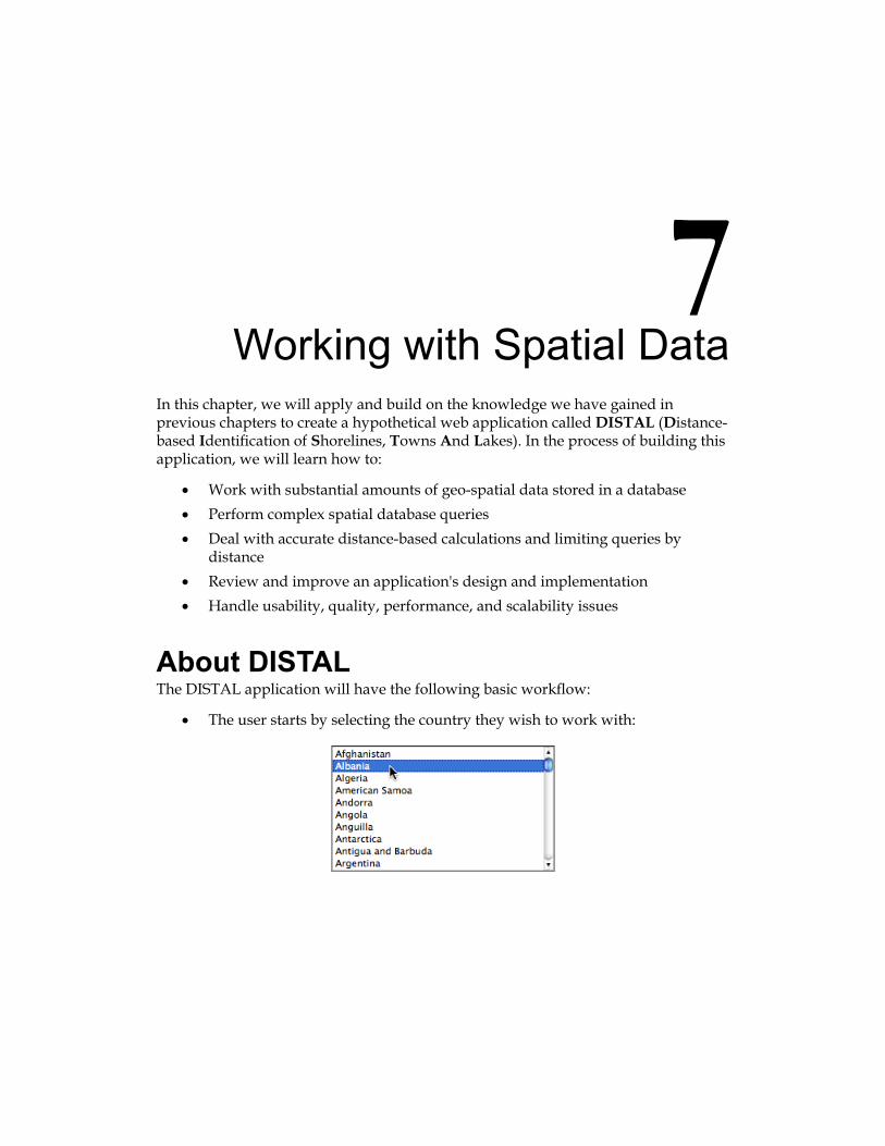
Working with Spatial DataIn this chapter, we will apply and build on the knowledge we have gained in previous chapters to create a hypothetical web application called DISTAL (Distance-based Identification of Shorelines, Towns And Lakes). In the process of building this application, we will learn how to:
• Work with substantial amounts of geo-spatial data stored in a database• Perform complex spatial database queries• Deal with accurate distance-based calculations and limiting queries by
distance• Review and improve an application's design and implementation• Handle usability, quality, performance, and scalability issues
About DISTALThe DISTAL application will have the following basic workflow:
• The user starts by selecting the country they wish to work with:
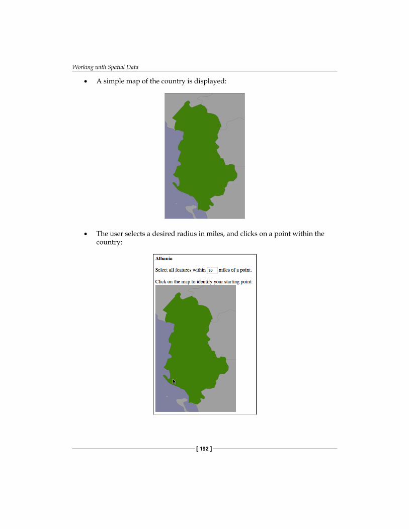
Working with Spatial Data
[ 192 ]
• A simple map of the country is displayed:
• The user selects a desired radius in miles, and clicks on a point within the country:
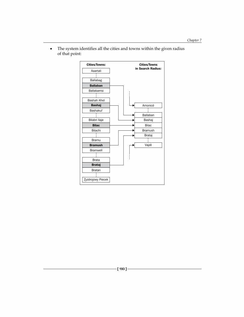
Chapter 7
[ 193 ]
• The system identifies all the cities and towns within the given radius of that point:
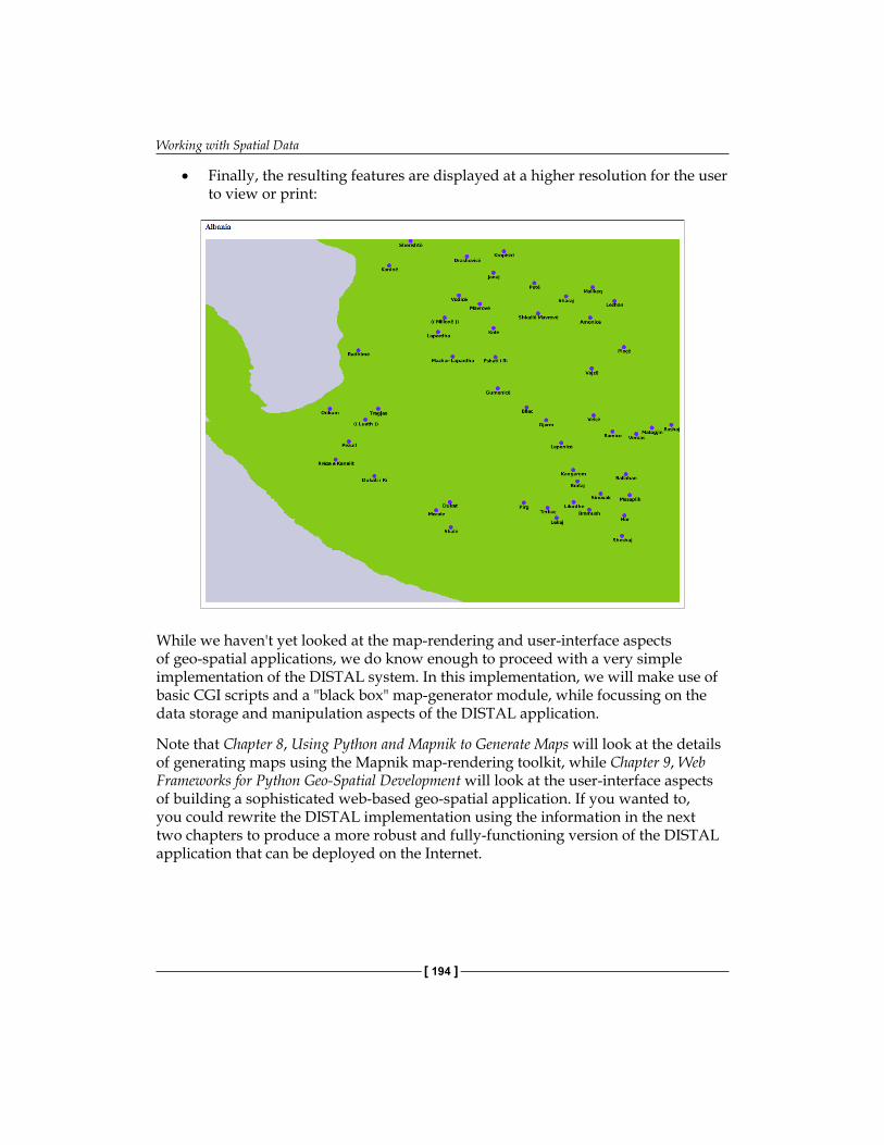
Working with Spatial Data
[ 194 ]
• Finally, the resulting features are displayed at a higher resolution for the user to view or print:
While we haven't yet looked at the map-rendering and user-interface aspects of geo-spatial applications, we do know enough to proceed with a very simple implementation of the DISTAL system. In this implementation, we will make use of basic CGI scripts and a "black box" map-generator module, while focussing on the data storage and manipulation aspects of the DISTAL application.
Note that Chapter 8, Using Python and Mapnik to Generate Maps will look at the details of generating maps using the Mapnik map-rendering toolkit, while Chapter 9, Web Frameworks for Python Geo-Spatial Development will look at the user-interface aspects of building a sophisticated web-based geo-spatial application. If you wanted to, you could rewrite the DISTAL implementation using the information in the next two chapters to produce a more robust and fully-functioning version of the DISTAL application that can be deployed on the Internet.
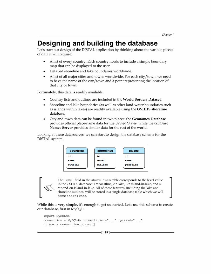
Chapter 7
[ 195 ]
Designing and building the databaseLet's start our design of the DISTAL application by thinking about the various pieces of data it will require:
• A list of every country. Each country needs to include a simple boundary map that can be displayed to the user.
• Detailed shoreline and lake boundaries worldwide.• A list of all major cities and towns worldwide. For each city/town, we need
to have the name of the city/town and a point representing the location of that city or town.
Fortunately, this data is readily available:
• Country lists and outlines are included in the World Borders Dataset.• Shoreline and lake boundaries (as well as other land-water boundaries such
as islands within lakes) are readily available using the GSHHS shoreline database.
• City and town data can be found in two places: the Geonames Database provides official place-name data for the United States, while the GEOnet Names Server provides similar data for the rest of the world.
Looking at these datasources, we can start to design the database schema for the DISTAL system:
The level field in the shorelines table corresponds to the level value in the GSHHS database: 1 = coastline, 2 = lake, 3 = island-in-lake, and 4 = pond-on-island-in-lake. All of these features, including the lake and shoreline outlines, will be stored in a single database table which we will name shorelines.
While this is very simple, it's enough to get us started. Let's use this schema to create our database, first in MySQL:
import MySQLdbconnection = MySQLdb.connect(user="...", passwd="...")cursor = connection.cursor()
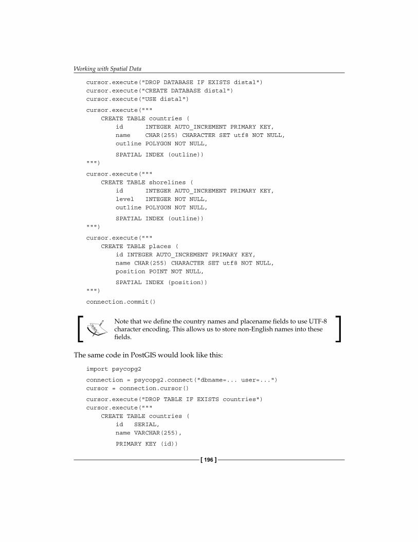
Working with Spatial Data
[ 196 ]
cursor.execute("DROP DATABASE IF EXISTS distal")cursor.execute("CREATE DATABASE distal")cursor.execute("USE distal")
cursor.execute(""" CREATE TABLE countries ( id INTEGER AUTO_INCREMENT PRIMARY KEY, name CHAR(255) CHARACTER SET utf8 NOT NULL, outline POLYGON NOT NULL,
SPATIAL INDEX (outline))""")
cursor.execute(""" CREATE TABLE shorelines ( id INTEGER AUTO_INCREMENT PRIMARY KEY, level INTEGER NOT NULL, outline POLYGON NOT NULL,
SPATIAL INDEX (outline))""")
cursor.execute(""" CREATE TABLE places ( id INTEGER AUTO_INCREMENT PRIMARY KEY, name CHAR(255) CHARACTER SET utf8 NOT NULL, position POINT NOT NULL,
SPATIAL INDEX (position))""")
connection.commit()
Note that we define the country names and placename fields to use UTF-8 character encoding. This allows us to store non-English names into these fields.
The same code in PostGIS would look like this:
import psycopg2
connection = psycopg2.connect("dbname=... user=...")cursor = connection.cursor()
cursor.execute("DROP TABLE IF EXISTS countries")cursor.execute(""" CREATE TABLE countries ( id SERIAL, name VARCHAR(255),
PRIMARY KEY (id))
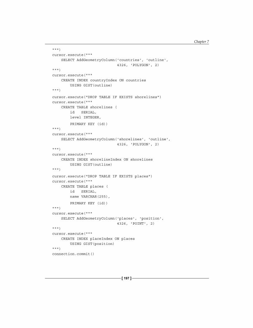
Chapter 7
[ 197 ]
""")cursor.execute(""" SELECT AddGeometryColumn('countries', 'outline', 4326, 'POLYGON', 2)""")cursor.execute(""" CREATE INDEX countryIndex ON countries USING GIST(outline)""")
cursor.execute("DROP TABLE IF EXISTS shorelines")cursor.execute(""" CREATE TABLE shorelines ( id SERIAL, level INTEGER,
PRIMARY KEY (id))""")cursor.execute(""" SELECT AddGeometryColumn('shorelines', 'outline', 4326, 'POLYGON', 2)""")cursor.execute(""" CREATE INDEX shorelineIndex ON shorelines USING GIST(outline)""")
cursor.execute("DROP TABLE IF EXISTS places")cursor.execute(""" CREATE TABLE places ( id SERIAL, name VARCHAR(255),
PRIMARY KEY (id))""")cursor.execute(""" SELECT AddGeometryColumn('places', 'position', 4326, 'POINT', 2)""")cursor.execute(""" CREATE INDEX placeIndex ON places USING GIST(position)""")connection.commit()

Working with Spatial Data
[ 198 ]
Notice how the PostGIS version allows us to specify the SRID value for the geometry columns. We'll be using the WG84 datum and unprojected lat/long coordinates for all our spatial data, which is why we specified SRID 4326 when we created our geometries.
And, finally, using SpatiaLite:
from pysqlite2 import dbapi2 as sqlite
if os.path.exists("distal.db"): os.remove("distal.db")
db = sqlite.connect("distal.db")db.enable_load_extension(True)db.execute('SELECT load_extension("...")')cursor = db.cursor()
# Load the SpatiaLite init file into our database.
f = file("init_spatialite-2.3.sql", "r")lines = []for line in f.readlines(): line = line.rstrip() if len(line) == 0: continue if line.startswith("--"): continue if line.startswith("BEGIN"): continue if line.startswith("COMMIT"): continue lines.append(line)f.close()cmds = ("".join(lines)).split(";")for cmd in cmds: cursor.execute(cmd)db.commit()
# Create the database tables.
cursor.execute("DROP TABLE IF EXISTS countries")cursor.execute(""" CREATE TABLE countries ( id INTEGER PRIMARY KEY AUTOINCREMENT, name CHAR(255))""")cursor.execute(""" SELECT AddGeometryColumn('countries', 'outline', 4326, 'POLYGON', 2)""")cursor.execute("""
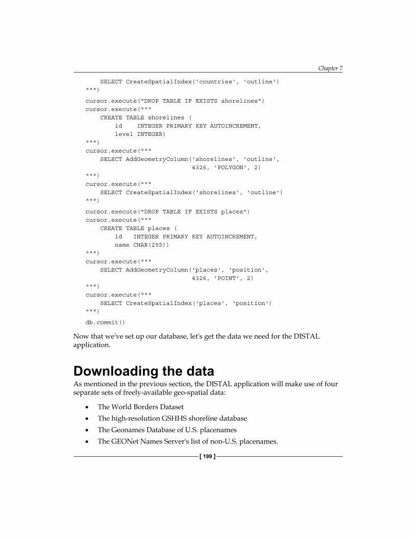
Chapter 7
[ 199 ]
SELECT CreateSpatialIndex('countries', 'outline')""")
cursor.execute("DROP TABLE IF EXISTS shorelines")cursor.execute(""" CREATE TABLE shorelines ( id INTEGER PRIMARY KEY AUTOINCREMENT, level INTEGER)""")cursor.execute(""" SELECT AddGeometryColumn('shorelines', 'outline', 4326, 'POLYGON', 2)""")cursor.execute(""" SELECT CreateSpatialIndex('shorelines', 'outline')""")
cursor.execute("DROP TABLE IF EXISTS places")cursor.execute(""" CREATE TABLE places ( id INTEGER PRIMARY KEY AUTOINCREMENT, name CHAR(255))""")cursor.execute(""" SELECT AddGeometryColumn('places', 'position', 4326, 'POINT', 2)""")cursor.execute(""" SELECT CreateSpatialIndex('places', 'position')""")
db.commit()
Now that we've set up our database, let's get the data we need for the DISTAL application.
Downloading the dataAs mentioned in the previous section, the DISTAL application will make use of four separate sets of freely-available geo-spatial data:
• The World Borders Dataset• The high-resolution GSHHS shoreline database• The Geonames Database of U.S. placenames• The GEONet Names Server's list of non-U.S. placenames.
Working with Spatial Data
[ 200 ]
For more information on these sources of data, please refer to Chapter 4, Sources of Geo-Spatial Data
To keep track of the data as we download it, create a directory named something like DISTAL-data. Then, it's time to download the information we need.
World Borders DatasetIf you haven't already done so, download the World Borders Dataset from:
http://thematicmapping.org/downloads/world_borders.php
When you decompress the TM_WORLD_BORDERS-0.3.zip archive, you will end up with a folder containing the World Borders Dataset in Shapefile format. Move this folder into your DISTAL-data directory.
GSHHSWe next need to download the GSHHS shoreline database in Shapefile format. If you haven't already downloaded it, the database can be found at:
http://www.ngdc.noaa.gov/mgg/shorelines/gshhs.html
Decompress the ZIP format archive and move the resulting GSHHS_shp folder (which itself contains 20 separate Shapefiles) into your DISTAL-data directory.
GeonamesFor the database of US placenames, go to: http://geonames.usgs.gov/domestic
Click on the Download Domestic Names hyperlink, and choose the download all national features in one .zip file option. This will download a file named NationalFile_YYYYMMDD.zip, where YYYYMMDD is the datestamp identifying when the file was last updated. Once again, decompress the resulting ZIP format archive and move the NationalFile_YYYYMMDD.txt file into your DISTAL-data directory.
GEOnet Names ServerFinally, to download the database of non-US placenames, go to:
http://earth-info.nga.mil/gns/html/cntry_files.html
Chapter 7
[ 201 ]
Click on the option to download a single compressed ZIP file that contains the entire country files dataset. This is a large download (300 MB compressed) that contains all the placename information we need worldwide. The resulting file will be named geonames_dd_dms_date_YYYYMMDD.zip, where once again YYYMMDD is the datestamp identifying when the file was last updated.
Don't get confused by names here: we go to the Geonames website to download a file named NationalFile, and to the GEOnet Names Server to download a file named geonames. From now on, we'll refer to the name of the file rather than the website it came from.
Decompress the ZIP format archive, and move the resulting geonames_dd_dms_date_YYYYMMDD.txt file into the DISTAL-data directory.
Importing the dataWe are now ready to import our four sets of data into the DISTAL database. We will be using the techniques discussed in Chapter 3, Python Libraries for Geo-Spatial Development and Chapter 5, Working with Geo-Spatial Data in Python to read the data from these data sets, and then insert them into the database using the techniques we discussed in Chapter 6, GIS in the Database.
Let's work through each of these files in turn.
World Borders DatasetThe World Borders Dataset consists of a Shapefile containing the outline of each country along with a variety of metadata, including the country's name in Latin-1 character encoding. We can import this directly into our countries table using the following Python code for MySQL:
import os.pathimport MySQLdbimport osgeo.ogr
connection = MySQLdb.connect(user="...", passwd="...")cursor = connection.cursor()
cursor.execute("USE distal")cursor.execute("DELETE FROM countries")cursor.execute("SET GLOBAL max_allowed_packet=50000000")
srcFile = os.path.join("DISTAL-data", "TM_WORLD_BORDERS-0.3", "TM_WORLD_BORDERS-0.3.shp")shapefile = osgeo.ogr.Open(srcFile)layer = shapefile.GetLayer(0)
Working with Spatial Data
[ 202 ]
for i in range(layer.GetFeatureCount()): feature = layer.GetFeature(i) name = feature.GetField("NAME").decode("Latin-1") wkt = feature.GetGeometryRef().ExportToWkt()
cursor.execute("INSERT INTO countries (name,outline) " + "VALUES (%s, PolygonFromText(%s, 4326))", (name.encode("utf8"), wkt))
connection.commit()
The only unusual thing here is the SET GLOBAL max_allowed_packet instruction. This command (which works with MySQL versions 5.1 and later) allows us to insert larger geometries into the database. If you are using an earlier version of MySQL, you will have to edit the my.cnf file and set this variable manually before running the program.
Notice that we are following the recommended best practice of associating the spatial reference with the polygon. In most cases, we will be dealing with unprojected coordinates on the WGS84 datum (SRID 4326), though stating this explicitly can save us some trouble when we come to dealing with data that uses other spatial references.
Here is what the equivalent code would look like for PostGIS:
import os.pathimport psycopg2import osgeo.ogr
connection = psycopg2.connect("dbname=... user=...")cursor = connection.cursor()
cursor.execute("DELETE FROM countries")
srcFile = os.path.join("DISTAL-data", "TM_WORLD_BORDERS-0.3", "TM_WORLD_BORDERS-0.3.shp")shapefile = osgeo.ogr.Open(srcFile)layer = shapefile.GetLayer(0)
for i in range(layer.GetFeatureCount()): feature = layer.GetFeature(i) name = feature.GetField("NAME").decode("Latin-1") wkt = feature.GetGeometryRef().ExportToWkt()
cursor.execute("INSERT INTO countries (name,outline) " + "VALUES (%s, ST_PolygonFromText(%s, " + "4326))", (name.encode("utf8"), wkt))
connection.commit()
Chapter 7
[ 203 ]
And for SpatiaLite:
import os, os.pathfrom pysqlite2 import dbapi2 as sqliteimport osgeo.ogr
db = sqlite.connect("distal.db")db.enable_load_extension(True)db.execute('SELECT load_extension("...")')cursor = db.cursor()
cursor.execute("DELETE FROM countries")
srcFile = os.path.join("DISTAL-data", "TM_WORLD_BORDERS-0.3", "TM_WORLD_BORDERS-0.3.shp")shapefile = osgeo.ogr.Open(srcFile)layer = shapefile.GetLayer(0)
for i in range(layer.GetFeatureCount()): feature = layer.GetFeature(i) name = feature.GetField("NAME").decode("Latin-1") wkt = feature.GetGeometryRef().ExportToWkt()
cursor.execute("INSERT INTO countries (name,outline) " + "VALUES (?, ST_PolygonFromText(?, " + "4326))", (name, wkt))
db.commit()
SpatiaLite doesn't know about UTF-8 encoding, so in this case we store the country names directly as Unicode strings.
GSHHSThe GSHHS shoreline database consists of five separate Shapefiles defining the land/water boundary at five different resolutions. For the DISTAL application, we want to import the four levels of GSHHS data (coastline, lake, island-in-lake, pond-in-island-in-lake) at full resolution. We can directly import these Shapefiles into the shorelines table within our DISTAL database.
For MySQL, we use the following code:
import os.pathimport MySQLdbimport osgeo.ogr
connection = MySQLdb.connect(user="...", passwd="...")cursor = connection.cursor()
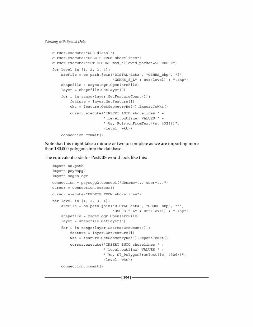
Working with Spatial Data
[ 204 ]
cursor.execute("USE distal")cursor.execute("DELETE FROM shorelines")cursor.execute("SET GLOBAL max_allowed_packet=50000000")
for level in [1, 2, 3, 4]: srcFile = os.path.join("DISTAL-data", "GSHHS_shp", "f", "GSHHS_f_L" + str(level) + ".shp") shapefile = osgeo.ogr.Open(srcFile) layer = shapefile.GetLayer(0)
for i in range(layer.GetFeatureCount()): feature = layer.GetFeature(i) wkt = feature.GetGeometryRef().ExportToWkt()
cursor.execute("INSERT INTO shorelines " + "(level,outline) VALUES " + "(%s, PolygonFromText(%s, 4326))", (level, wkt))
connection.commit()
Note that this might take a minute or two to complete as we are importing more than 180,000 polygons into the database.
The equivalent code for PostGIS would look like this:
import os.pathimport psycopg2import osgeo.ogr
connection = psycopg2.connect("dbname=... user=...")cursor = connection.cursor()
cursor.execute("DELETE FROM shorelines")
for level in [1, 2, 3, 4]: srcFile = os.path.join("DISTAL-data", "GSHHS_shp", "f", "GSHHS_f_L" + str(level) + ".shp") shapefile = osgeo.ogr.Open(srcFile) layer = shapefile.GetLayer(0)
for i in range(layer.GetFeatureCount()): feature = layer.GetFeature(i) wkt = feature.GetGeometryRef().ExportToWkt()
cursor.execute("INSERT INTO shorelines " + "(level,outline) VALUES " + "(%s, ST_PolygonFromText(%s, 4326))", (level, wkt))
connection.commit()
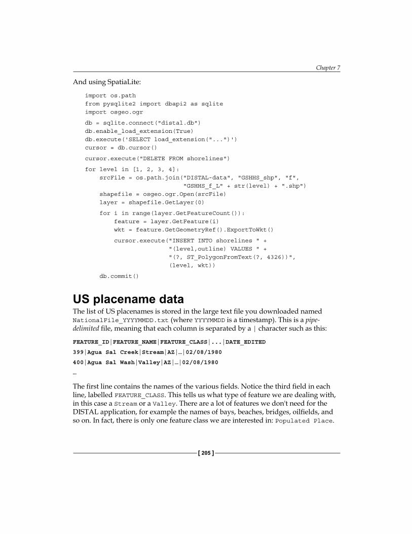
Chapter 7
[ 205 ]
And using SpatiaLite:
import os.pathfrom pysqlite2 import dbapi2 as sqliteimport osgeo.ogr
db = sqlite.connect("distal.db")db.enable_load_extension(True)db.execute('SELECT load_extension("...")')cursor = db.cursor()
cursor.execute("DELETE FROM shorelines")
for level in [1, 2, 3, 4]: srcFile = os.path.join("DISTAL-data", "GSHHS_shp", "f", "GSHHS_f_L" + str(level) + ".shp") shapefile = osgeo.ogr.Open(srcFile) layer = shapefile.GetLayer(0)
for i in range(layer.GetFeatureCount()): feature = layer.GetFeature(i) wkt = feature.GetGeometryRef().ExportToWkt()
cursor.execute("INSERT INTO shorelines " + "(level,outline) VALUES " + "(?, ST_PolygonFromText(?, 4326))", (level, wkt))
db.commit()
US placename dataThe list of US placenames is stored in the large text file you downloaded named NationalFile_YYYYMMDD.txt (where YYYYMMDD is a timestamp). This is a pipe-delimited file, meaning that each column is separated by a | character such as this:
FEATURE_ID|FEATURE_NAME|FEATURE_CLASS|...|DATE_EDITED
399|Agua Sal Creek|Stream|AZ|…|02/08/1980
400|Agua Sal Wash|Valley|AZ|…|02/08/1980
…
The first line contains the names of the various fields. Notice the third field in each line, labelled FEATURE_CLASS. This tells us what type of feature we are dealing with, in this case a Stream or a Valley. There are a lot of features we don't need for the DISTAL application, for example the names of bays, beaches, bridges, oilfields, and so on. In fact, there is only one feature class we are interested in: Populated Place.
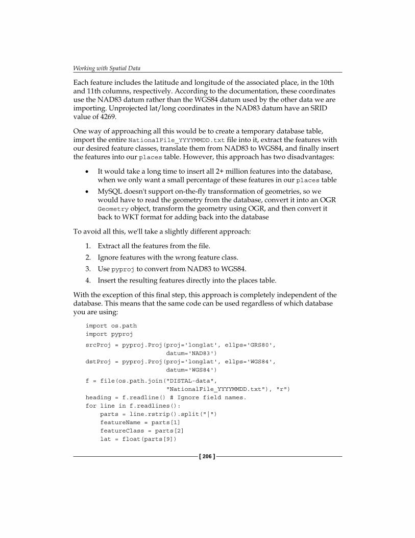
Working with Spatial Data
[ 206 ]
Each feature includes the latitude and longitude of the associated place, in the 10th and 11th columns, respectively. According to the documentation, these coordinates use the NAD83 datum rather than the WGS84 datum used by the other data we are importing. Unprojected lat/long coordinates in the NAD83 datum have an SRID value of 4269.
One way of approaching all this would be to create a temporary database table, import the entire NationalFile_YYYYMMDD.txt file into it, extract the features with our desired feature classes, translate them from NAD83 to WGS84, and finally insert the features into our places table. However, this approach has two disadvantages:
• It would take a long time to insert all 2+ million features into the database, when we only want a small percentage of these features in our places table
• MySQL doesn't support on-the-fly transformation of geometries, so we would have to read the geometry from the database, convert it into an OGR Geometry object, transform the geometry using OGR, and then convert it back to WKT format for adding back into the database
To avoid all this, we'll take a slightly different approach:
1. Extract all the features from the file.2. Ignore features with the wrong feature class.3. Use pyproj to convert from NAD83 to WGS84.4. Insert the resulting features directly into the places table.
With the exception of this final step, this approach is completely independent of the database. This means that the same code can be used regardless of which database you are using:
import os.pathimport pyproj
srcProj = pyproj.Proj(proj='longlat', ellps='GRS80', datum='NAD83')dstProj = pyproj.Proj(proj='longlat', ellps='WGS84', datum='WGS84')
f = file(os.path.join("DISTAL-data", "NationalFile_YYYYMMDD.txt"), "r")heading = f.readline() # Ignore field names.for line in f.readlines(): parts = line.rstrip().split("|") featureName = parts[1] featureClass = parts[2] lat = float(parts[9])
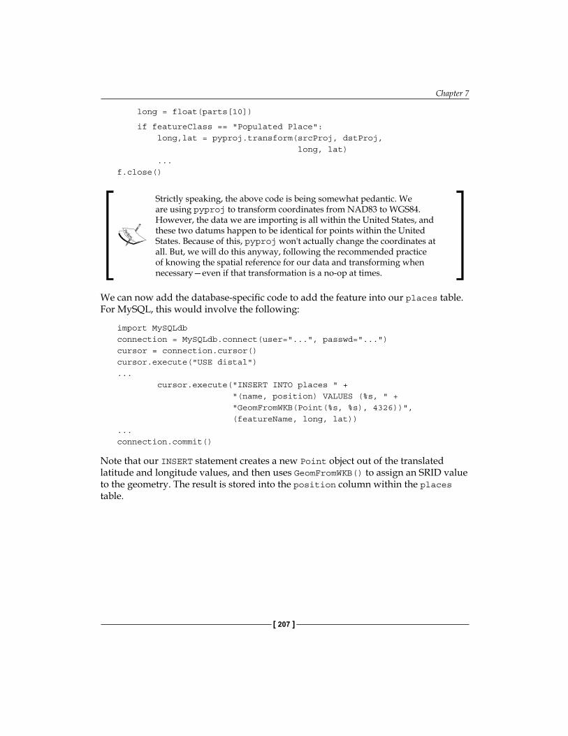
Chapter 7
[ 207 ]
long = float(parts[10])
if featureClass == "Populated Place": long,lat = pyproj.transform(srcProj, dstProj, long, lat) ...f.close()
Strictly speaking, the above code is being somewhat pedantic. We are using pyproj to transform coordinates from NAD83 to WGS84. However, the data we are importing is all within the United States, and these two datums happen to be identical for points within the United States. Because of this, pyproj won't actually change the coordinates at all. But, we will do this anyway, following the recommended practice of knowing the spatial reference for our data and transforming when necessary—even if that transformation is a no-op at times.
We can now add the database-specific code to add the feature into our places table. For MySQL, this would involve the following:
import MySQLdbconnection = MySQLdb.connect(user="...", passwd="...")cursor = connection.cursor()cursor.execute("USE distal")... cursor.execute("INSERT INTO places " + "(name, position) VALUES (%s, " + "GeomFromWKB(Point(%s, %s), 4326))", (featureName, long, lat))...connection.commit()
Note that our INSERT statement creates a new Point object out of the translated latitude and longitude values, and then uses GeomFromWKB() to assign an SRID value to the geometry. The result is stored into the position column within the places table.
Working with Spatial Data
[ 208 ]
The same code using PostGIS would look like this:
import psycopg2connection = psycopg2.connect("dbname=... user=...")cursor = connection.cursor()cursor.execute("SET NAMES 'utf8'")... cursor.execute("INSERT INTO places " + "(name, position) VALUES (%s, " + "ST_MakePoint(%s,%s, 4326)", (featureName, long, lat))...connection.commit()
Because the PostGIS function ST_MakePoint()allows us to specify an SRID value directly, we don't need to use GeomFromWKB to add the SRID after the geometry has been created.
Finally, the SpatiaLite version would look like this:
from pysqlite2 import dbapi2 as sqlitedb = sqlite.connect("distal.db")db.enable_load_extension(True)db.execute('SELECT load_extension("...")')cursor = db.cursor()... cursor.execute("INSERT INTO places " + "(name, position) VALUES " "(?, MakePoint(?, ?, 4326))", (featureName, long, lat))...db.commit()
Worldwide placename dataThe list of non-US placenames is stored in the geonames_dd_dms_date_YYYYMMDD file you downloaded earlier. This is a tab-delimited text file in UTF-8 character encoding, and will look something like this:
RC UFI ... FULL_NAME_ND_RG NOTE MODIFY_DATE
1 -1307834 ... Pavia 1993-12-21
1 -1307889 ... Santa Anna gjgscript 1993-12-21
...
Chapter 7
[ 209 ]
As with the US placename data, there are many more features here than we need for the DISTAL application. Since we are only interested in the official names for towns and cities, we need to filter this data in the following way:
• The FC (Feature Classification) field tells us what type of feature we are dealing with. We want features with an FC value of P (populated place).
• The NT (Name Type) field tells us the status of this feature's name. We want names with an NT value of N (approved name).
• The DSG (Feature Designation Code) field tells us the type of feature, in more detail than the FC field. A full list of all the feature designation codes can be found at http://geonames.nga.mil/ggmagaz/feadesgsearchhtml.asp. We are interested in features with a DSG value of PPL (populated place), PPLA (administrative capital), or PPLC (capital city).
There are also several different versions of each placename; we want the full name in normal reading order, which is in the field named FULL_NAME_RO. Knowing this, we can write some Python code to extract the features we want from the file:
f = file(os.path.join("DISTAL-data", "geonames_dd_dms_date_YYYYMMDD.txt"), "r")heading = f.readline() # Ignore field names.for line in f.readlines(): parts = line.rstrip().split("\t") lat = float(parts[3]) long = float(parts[4]) featureClass = parts[9] featureDesignation = parts[10] nameType = parts[17] featureName = parts[22]
if (featureClass == "P" and nameType == "N" and featureDesignation in ["PPL", "PPLA", "PPLC"]): ...f.close()
Now that we have the name, latitude, and longitude for each of the features we want, we can re-use the code from the previous section to insert these features into the database. For example, for MySQL we would do the following:
import MySQLdbconnection = MySQLdb.connect(user="...", passwd="...")cursor = connection.cursor()cursor.execute("USE distal")...

Working with Spatial Data
[ 210 ]
cursor.execute("INSERT INTO places " + "(name, position) VALUES (%s, " + "GeomFromWKB(Point(%s, %s), 4326))", (featureName, long, lat))...connection.commit()
Because we are dealing with worldwide data here, the lat/long values already use the WGS84 datum, so there is no need to translate the coordinates before adding them to the database.
If you are using PostGIS or SpatiaLite, simply copy the equivalent code from the previous section. Note that, because there are over two million features we want to add to the database, it can take several minutes for this program to complete.
Implementing the DISTAL applicationNow that we have the data, we can start to implement the DISTAL application itself. To keep things simple, we will use CGI scripts to implement the user-interface.
CGI scripts aren't the only way we could implement the DISTAL application. Other possible approaches include using web application frameworks such as TurboGears or Django, using AJAX to write your own dynamic web application, or even using tools such as Pyjamas (http://pyjs.org) to compile Python code into JavaScript. All of these approaches, however, are more complicated than CGI, and we will be making use of CGI scripts in this chapter to keep the code as straightforward as possible.
Let's take a look at how our CGI scripts will implement the DISTAL application's workflow:
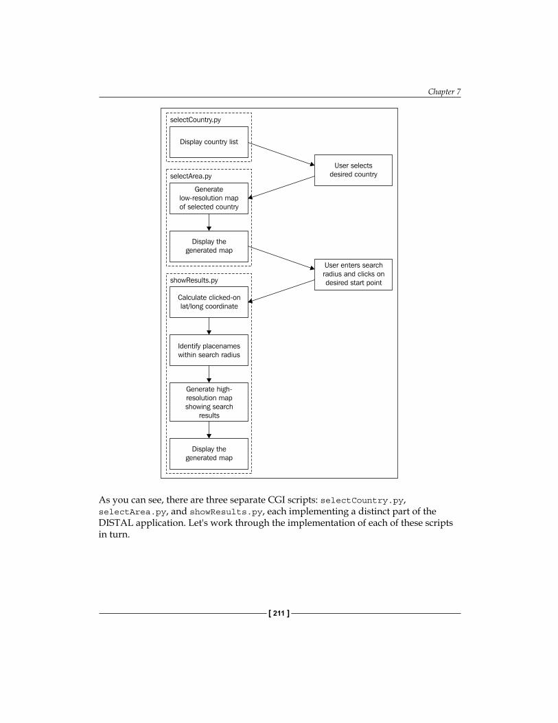
Chapter 7
[ 211 ]
As you can see, there are three separate CGI scripts: selectCountry.py, selectArea.py, and showResults.py, each implementing a distinct part of the DISTAL application. Let's work through the implementation of each of these scripts in turn.
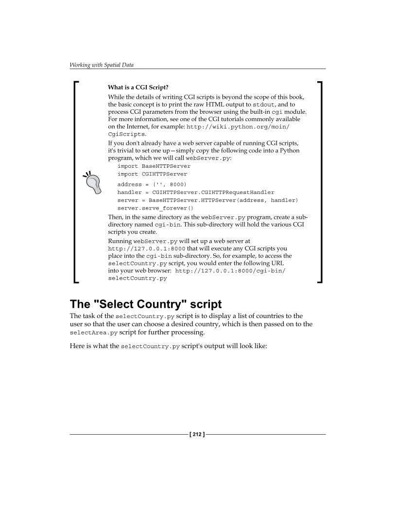
Working with Spatial Data
[ 212 ]
What is a CGI Script?While the details of writing CGI scripts is beyond the scope of this book, the basic concept is to print the raw HTML output to stdout, and to process CGI parameters from the browser using the built-in cgi module. For more information, see one of the CGI tutorials commonly available on the Internet, for example: http://wiki.python.org/moin/CgiScripts. If you don't already have a web server capable of running CGI scripts, it's trivial to set one up—simply copy the following code into a Python program, which we will call webServer.py:
import BaseHTTPServerimport CGIHTTPServer
address = ('', 8000)handler = CGIHTTPServer.CGIHTTPRequestHandlerserver = BaseHTTPServer.HTTPServer(address, handler)server.serve_forever()
Then, in the same directory as the webServer.py program, create a sub-directory named cgi-bin. This sub-directory will hold the various CGI scripts you create.Running webServer.py will set up a web server at http://127.0.0.1:8000 that will execute any CGI scripts you place into the cgi-bin sub-directory. So, for example, to access the selectCountry.py script, you would enter the following URL into your web browser: http://127.0.0.1:8000/cgi-bin/selectCountry.py
The "Select Country" scriptThe task of the selectCountry.py script is to display a list of countries to the user so that the user can choose a desired country, which is then passed on to the selectArea.py script for further processing.
Here is what the selectCountry.py script's output will look like:
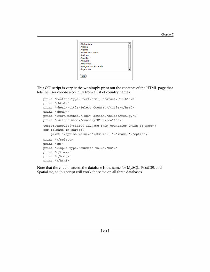
Chapter 7
[ 213 ]
This CGI script is very basic: we simply print out the contents of the HTML page that lets the user choose a country from a list of country names:
print 'Content-Type: text/html; charset=UTF-8\n\n'print '<html>'print '<head><title>Select Country</title></head>'print '<body>'print '<form method="POST" action="selectArea.py">'print '<select name="countryID" size="10">'
cursor.execute("SELECT id,name FROM countries ORDER BY name")for id,name in cursor: print '<option value="'+str(id)+'">'+name+'</option>'
print '</select>'print '<p>'print '<input type="submit" value="OK">'print '</form>'print '</body>'print '</html>'
Note that the code to access the database is the same for MySQL, PostGIS, and SpatiaLite, so this script will work the same on all three databases.
Working with Spatial Data
[ 214 ]
A Crash Course in HTML FormsIf you haven't used HTML forms before, don't panic. They are quite straightforward, and if you want you can just copy the code from the examples given here. The following brief overview may also help you to understand how these forms work.An HTML form is surrounded by <form> and </form> tags defining the start and end of the form's definition. The action="..." attribute tells the browser where to send the submitted data, and the method="..." attribute tells the browser how to submit the data. In this case, we are setting up a form that will use an HTTP POST request to send the submitted form parameters to a CGI script named selectArea.py.The contents of a form are made up of ordinary HTML elements, such as textual labels and images, combined with special form-specific elements. There are two types of form-specific elements we are interested in here: the <select> element, which displays a list of the available countries, and the <input> element, which in this case displays an OK button.For each country, the <select> element includes an <option> element listing the name of the country and its associated record ID. When the user selects a country (by choosing that country's name from the list), the associated record ID will be submitted as a parameter named countryID when the user clicks on the OK button.
The "Select Area" scriptThe next part of the DISTAL application is selectArea.py. This script generates a web page that displays a simple map of the selected country. The user can enter a desired search radius and click on the map to identify the starting point for the DISTAL search:
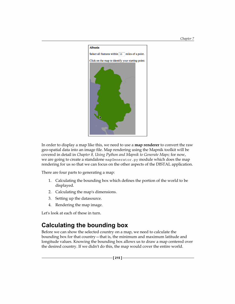
Chapter 7
[ 215 ]
In order to display a map like this, we need to use a map renderer to convert the raw geo-spatial data into an image file. Map rendering using the Mapnik toolkit will be covered in detail in Chapter 8, Using Python and Mapnik to Generate Maps; for now, we are going to create a standalone mapGenerator.py module which does the map rendering for us so that we can focus on the other aspects of the DISTAL application.
There are four parts to generating a map:
1. Calculating the bounding box which defines the portion of the world to be displayed.
2. Calculating the map's dimensions.3. Setting up the datasource.4. Rendering the map image.
Let's look at each of these in turn.
Calculating the bounding boxBefore we can show the selected country on a map, we need to calculate the bounding box for that country—that is, the minimum and maximum latitude and longitude values. Knowing the bounding box allows us to draw a map centered over the desired country. If we didn't do this, the map would cover the entire world.
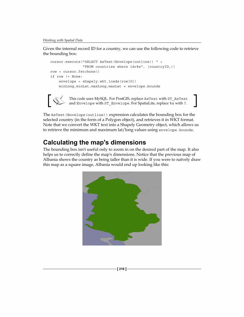
Working with Spatial Data
[ 216 ]
Given the internal record ID for a country, we can use the following code to retrieve the bounding box:
cursor.execute("SELECT AsText(Envelope(outline)) " + "FROM countries where id=%s", (countryID,))row = cursor.fetchone()if row != None: envelope = shapely.wkt.loads(row[0]) minLong,minLat,maxLong,maxLat = envelope.bounds
This code uses MySQL. For PostGIS, replace AsText with ST_AsText and Envelope with ST_Envelope. For SpatiaLite, replace %s with ?.
The AsText(Envelope(outline)) expression calculates the bounding box for the selected country (in the form of a Polygon object), and retrieves it in WKT format. Note that we convert the WKT text into a Shapely Geometry object, which allows us to retrieve the minimum and maximum lat/long values using envelope.bounds.
Calculating the map's dimensionsThe bounding box isn't useful only to zoom in on the desired part of the map. It also helps us to correctly define the map's dimensions. Notice that the previous map of Albania shows the country as being taller than it is wide. If you were to naïvely draw this map as a square image, Albania would end up looking like this:
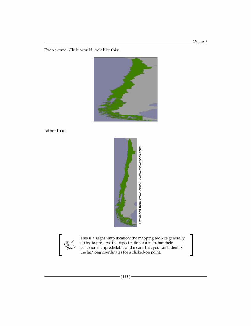
Chapter 7
[ 217 ]
Even worse, Chile would look like this:
rather than:
This is a slight simplification; the mapping toolkits generally do try to preserve the aspect ratio for a map, but their behavior is unpredictable and means that you can't identify the lat/long coordinates for a clicked-on point.
Dow
nlo
ad fro
m W
ow
! eBook
<w
ww
.wow
ebook.
com
>
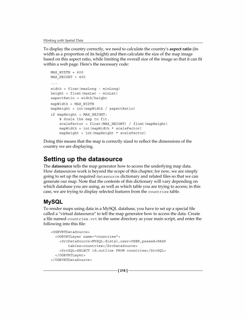
Working with Spatial Data
[ 218 ]
To display the country correctly, we need to calculate the country's aspect ratio (its width as a proportion of its height) and then calculate the size of the map image based on this aspect ratio, while limiting the overall size of the image so that it can fit within a web page. Here's the necessary code:
MAX_WIDTH = 600MAX_HEIGHT = 400
...
width = float(maxLong - minLong)height = float(maxLat - minLat)aspectRatio = width/height
mapWidth = MAX_WIDTHmapHeight = int(mapWidth / aspectRatio)
if mapHeight > MAX_HEIGHT: # Scale the map to fit. scaleFactor = float(MAX_HEIGHT) / float(mapHeight) mapWidth = int(mapWidth * scaleFactor) mapHeight = int(mapHeight * scaleFactor)
Doing this means that the map is correctly sized to reflect the dimensions of the country we are displaying.
Setting up the datasourceThe datasource tells the map generator how to access the underlying map data. How datasources work is beyond the scope of this chapter; for now, we are simply going to set up the required datasource dictionary and related files so that we can generate our map. Note that the contents of this dictionary will vary depending on which database you are using, as well as which table you are trying to access; in this case, we are trying to display selected features from the countries table.
MySQLTo render maps using data in a MySQL database, you have to set up a special file called a "virtual datasource" to tell the map generator how to access the data. Create a file named countries.vrt in the same directory as your main script, and enter the following into this file:
<OGRVRTDataSource> <OGRVRTLayer name="countries"> <SrcDataSource>MYSQL:distal,user=USER,passwd=PASS tables=countries</SrcDataSource> <SrcSQL>SELECT id,outline FROM countries</SrcSQL> </OGRVRTLayer></OGRVRTDataSource>
Chapter 7
[ 219 ]
Don't forget to replace USER with the username and PASS with the password used to access your MySQL database. Also, make sure all the text from <SrcDataSource> to </SrcDataSource> is on a single line.
Now that we have the virtual datasource file, we can go ahead and set up the MySQL datasource dictionary using the following code:
vrtFile = os.path.join(os.path.dirname(__file__), "countries.vrt")
datasource = {'type' : "OGR", 'file' : vrtFile, 'layer' : "countries"}
Note that we use Python's __file__ global to avoid having to hardwire paths into the script. This assumes that the countries.vrt file is in the same directory as the CGI script.
PostGISSetting up the datasource dictionary for a PostGIS database is straightforward:
datasource = {'type' : "PostGIS", 'dbname' : "distal", 'table' : "countries", 'user' : "USER", 'password' : "PASS"}
Obviously, you should replace USER and PASS with the username and password used to access your PostGIS database.
SpatiaLiteObtaining map data from a SpatiaLite database is also straightforward. The only trick is that we have to include the full path to the SpatiaLite database file, so we use __file__ to avoid hardcoding path names into our script:
dbFile = os.path.join(os.path.dirname(__file__), "distal.db")
datasource = {'type' : "SQLite", 'file' : dbFile, 'table' : "countries", 'geometry_field' : "outline", 'key_field' : "id"}
Working with Spatial Data
[ 220 ]
Rendering the map imageWith the bounding box, the map's dimensions, and the datasource all set up, we are finally ready to render the map into an image file. This is done using a single function call:
imgFile = mapGenerator.generateMap(datasource, minLong, minLat, maxLong, maxLat, mapWidth, mapHeight, "[id] = "+str(countryID))
Note that our datasource has been set up to display features from the countries table, and that "[id] = "+str(countryID) is a "highlight expression" used to visually highlight the country with the given ID.
The mapGenerator.generateMap() function returns a reference to a PNG-format image file containing the generated map. This image file is stored in a temporary directory, and the file's relative pathname is returned to the caller. This allows us to use the returned imgFile directly within our CGI script, like this:
print 'Content-Type: text/html; charset=UTF-8\n\n'print '<html>'print '<head><title>Select Area</title></head>'print '<body>"print '<b>' + name + '</b>'print '<p>'print '<form method="POST" action="...">'print 'Select all features within'print '<input type="text" name="radius" value="10" size="2">'print 'miles of a point.'print '<p>'print 'Click on the map to identify your starting point:'print '<br>'print '<input type="image" src="' + imgFile + '" ismap>'print '<input type="hidden" name="countryID"'print ' value="' + str(countryID) + '">'print '<input type="hidden" name="mapWidth"'print ' value="' + str(mapWidth) + '">'print '<input type="hidden" name="mapHeight"'print ' value="' + str(mapHeight) + '">'print '</form>'print '</body></html>'
Chapter 7
[ 221 ]
The <input type="hidden"> lines define "hidden form fields" that pass information on to the next CGI script. We'll discuss how this information is used in the next section.
The use of <input type="image" src="..." ismap> in this CGI script has the interesting effect of making the map clickable: when the user clicks on the image, the enclosing HTML form will be submitted with two extra parameters named x and y. These contain the coordinate within the image that the user clicked on.
This completes the selectArea.py CGI script. Before it will run, you will also need to download or type in the mapGenerator.py module, the source code of which is given below:
# mapGenerator.py
import os, os.path, sys, tempfileimport mapnik
def generateMap(datasource, minX, minY, maxX, maxY, mapWidth, mapHeight, hiliteExpr=None, background="#8080a0", hiliteLine="#000000", hiliteFill="#408000", normalLine="#404040", normalFill="#a0a0a0", points=None): srcType = datasource['type'] del datasource['type']
if srcType == "OGR": source = mapnik.Ogr(**datasource) elif srcType == "PostGIS": source = mapnik.PostGIS(**datasource) elif srcType == "SQLite": source = mapnik.SQLite(**datasource)
layer = mapnik.Layer("Layer") layer.datasource = source
map = mapnik.Map(mapWidth, mapHeight, '+proj=longlat +datum=WGS84') map.background = mapnik.Color(background)
style = mapnik.Style()
rule = mapnik.Rule() if hiliteExpr != None: rule.filter = mapnik.Filter(hiliteExpr)
rule.symbols.append(mapnik.PolygonSymbolizer( mapnik.Color(hiliteFill)))
Working with Spatial Data
[ 222 ]
rule.symbols.append(mapnik.LineSymbolizer( mapnik.Stroke(mapnik.Color(hiliteLine), 0.1)))
style.rules.append(rule)
rule = mapnik.Rule() rule.set_else(True)
rule.symbols.append(mapnik.PolygonSymbolizer( mapnik.Color(normalFill))) rule.symbols.append(mapnik.LineSymbolizer( mapnik.Stroke(mapnik.Color(normalLine), 0.1)))
style.rules.append(rule)
map.append_style("Map Style", style) layer.styles.append("Map Style") map.layers.append(layer)
if points != None: pointDatasource = mapnik.PointDatasource() for long,lat,name in points: pointDatasource.add_point(long, lat, "name", name)
layer = mapnik.Layer("Points") layer.datasource = pointDatasource
style = mapnik.Style() rule = mapnik.Rule()
pointImgFile = os.path.join(os.path.dirname(__file__), "point.png")
shield = mapnik.ShieldSymbolizer( "name", "DejaVu Sans Bold", 10, mapnik.Color("#000000"), pointImgFile, "png", 9, 9) shield.displacement(0, 7) shield.unlock_image = True rule.symbols.append(shield)
style.rules.append(rule)
map.append_style("Point Style", style) layer.styles.append("Point Style")
map.layers.append(layer)
map.zoom_to_box(mapnik.Envelope(minX, minY, maxX, maxY))
scriptDir = os.path.dirname(__file__) cacheDir = os.path.join(scriptDir, "..", "mapCache") if not os.path.exists(cacheDir): os.mkdir(cacheDir)
Chapter 7
[ 223 ]
fd,filename = tempfile.mkstemp(".png", dir=cacheDir) os.close(fd)
mapnik.render_to_file(map, filename, "png")
return "../mapCache/" + os.path.basename(filename)
We won't be explaining how this module works here. For more information on Mapnik, please refer to Chapter 8, Using Python and Mapnik to Generate Maps.
Before you can run this CGI script, you need to have Mapnik installed. The Mapnik toolkit can be found at: http://mapnik.org
If you are running Mac OS X and don't wish to compile Mapnik yourself from source, a pre-built version can be downloaded from: http://dbsgeo.com/downloads
You will also need to have a small image file, named point.png, which is used to mark placenames on the map. This 9 x 9 pixel image looks like this:
Place this file into the same directory as the mapGenerator.py module itself.
The "Show Results" scriptThe final CGI script is where all the work is done. We take the (x,y) coordinate the user clicked on, along with the entered search radius, convert the (x,y) coordinate into a longitude and latitude, and identify all the placenames within the specified search radius. We then generate a high-resolution map showing the shorelines and placenames within the search radius, and display that map to the user.
Let's examine each of these steps in turn.
Identifying the clicked-on pointThe selectArea.py script generated an HTML form that was submitted when the user clicked on the low-resolution country map. The showResults.py script then receives the form parameters, including the x and y coordinates of the point the user clicked on.
By itself, this coordinate isn't very useful as it is the pixel coordinate within the map image. We need to translate the submitted (x,y) pixel coordinate into a latitude and longitude value corresponding to the clicked-on point on the Earth's surface.
Working with Spatial Data
[ 224 ]
To do this, we need to have the following information:
• The map's bounding box in geographic coordinates: minLong, minLat, maxLong, and maxLat
• The map's size in pixels: mapWidth and mapHeight
These variables were all calculated in the previous section and passed to us using hidden form variables, along with the country ID, the desired search radius, and the (x,y) coordinate of the clicked-on point. We can retrieve all of these using the cgi module:
import cgi
form = cgi.FieldStorage()
countryID = int(form['countryID'].value)radius = int(form['radius'].value)x = int(form['x'].value)y = int(form['y'].value)mapWidth = int(form['mapWidth'].value)mapHeight = int(form['mapHeight'].value)
With this information, we can now calculate the latitude and longitude that the user clicked on. To do this, we first calculate how far across the image the user clicked, as a number in the range 0..1:
xFract = float(x)/float(mapWidth)
An xFract value of 0.0 corresponds to the left side of the image, while an xFract value of 1.0 corresponds to the right side of the image. We then combine this with the minimum and maximum longitude values to calculate the longitude of the clicked-on point:
longitude = minLong + xFract * (maxLong-minLong)
We then do the same to convert the Y coordinate into a latitude value:
yFract = float(y)/float(mapHeight)latitude = minLat + (1-yFract) * (maxLat-minLat)
Note that we are using (1-yFract) rather than yFract in the above calculation. This is because the minLat value refers to the latitude of the bottom of the image, while a yFract value of 0.0 corresponds to the top of the image. By using (1-yFract), we flip the values vertically so that the latitude is calculated correctly.
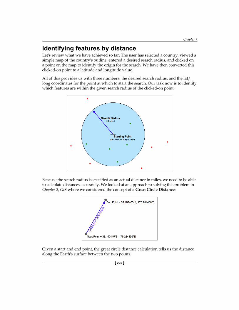
Chapter 7
[ 225 ]
Identifying features by distanceLet's review what we have achieved so far. The user has selected a country, viewed a simple map of the country's outline, entered a desired search radius, and clicked on a point on the map to identify the origin for the search. We have then converted this clicked-on point to a latitude and longitude value.
All of this provides us with three numbers: the desired search radius, and the lat/long coordinates for the point at which to start the search. Our task now is to identify which features are within the given search radius of the clicked-on point:
Because the search radius is specified as an actual distance in miles, we need to be able to calculate distances accurately. We looked at an approach to solving this problem in Chapter 2, GIS where we considered the concept of a Great Circle Distance:
Given a start and end point, the great circle distance calculation tells us the distance along the Earth's surface between the two points.
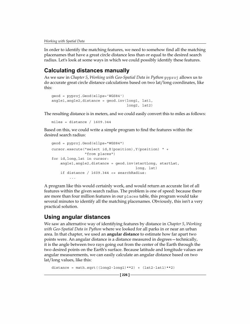
Working with Spatial Data
[ 226 ]
In order to identify the matching features, we need to somehow find all the matching placenames that have a great circle distance less than or equal to the desired search radius. Let's look at some ways in which we could possibly identify these features.
Calculating distances manuallyAs we saw in Chapter 5, Working with Geo-Spatial Data in Python pyproj allows us to do accurate great circle distance calculations based on two lat/long coordinates, like this:
geod = pyproj.Geod(ellps='WGS84')angle1,angle2,distance = geod.inv(long1, lat1, long2, lat2)
The resulting distance is in meters, and we could easily convert this to miles as follows:
miles = distance / 1609.344
Based on this, we could write a simple program to find the features within the desired search radius:
geod = pyproj.Geod(ellps="WGS84")
cursor.execute("select id,X(position),Y(position) " + "from places")for id,long,lat in cursor: angle1,angle2,distance = geod.inv(startLong, startLat, long, lat) if distance / 1609.344 <= searchRadius: ...
A program like this would certainly work, and would return an accurate list of all features within the given search radius. The problem is one of speed: because there are more than four million features in our places table, this program would take several minutes to identify all the matching placenames. Obviously, this isn't a very practical solution.
Using angular distancesWe saw an alternative way of identifying features by distance in Chapter 5, Working with Geo-Spatial Data in Python where we looked for all parks in or near an urban area. In that chapter, we used an angular distance to estimate how far apart two points were. An angular distance is a distance measured in degrees—technically, it is the angle between two rays going out from the center of the Earth through the two desired points on the Earth's surface. Because latitude and longitude values are angular measurements, we can easily calculate an angular distance based on two lat/long values, like this:
distance = math.sqrt((long2-long1)**2) + (lat2-lat1)**2)
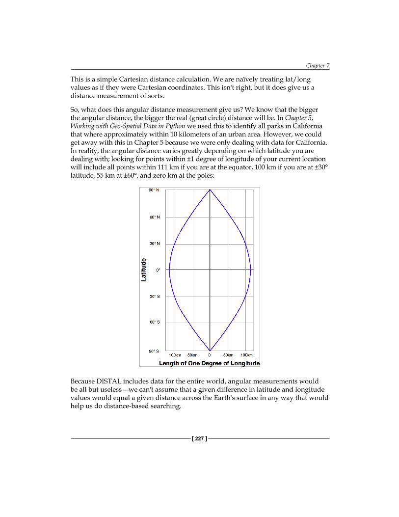
Chapter 7
[ 227 ]
This is a simple Cartesian distance calculation. We are naïvely treating lat/long values as if they were Cartesian coordinates. This isn't right, but it does give us a distance measurement of sorts.
So, what does this angular distance measurement give us? We know that the bigger the angular distance, the bigger the real (great circle) distance will be. In Chapter 5, Working with Geo-Spatial Data in Python we used this to identify all parks in California that where approximately within 10 kilometers of an urban area. However, we could get away with this in Chapter 5 because we were only dealing with data for California. In reality, the angular distance varies greatly depending on which latitude you are dealing with; looking for points within ±1 degree of longitude of your current location will include all points within 111 km if you are at the equator, 100 km if you are at ±30° latitude, 55 km at ±60°, and zero km at the poles:
Because DISTAL includes data for the entire world, angular measurements would be all but useless—we can't assume that a given difference in latitude and longitude values would equal a given distance across the Earth's surface in any way that would help us do distance-based searching.
Working with Spatial Data
[ 228 ]
Using projected coordinatesAnother way of finding all points within a given distance is to use a projected coordinate system that accurately represents distance as differences between coordinate values. For example, the Universal Transverse Mercator projection defines Y coordinates as a number of meters north or south of the equator, and X coordinates as a number of meters east or west of a given reference point. Using the UTM projection, it would be easy to identify all points within a given distance by using the Cartesian distance formula:
distance = math.sqrt((x2-x1)**2 + (y2-y1)**2)if distance < searchRadius: ...
Unfortunately, projected coordinate systems such as UTM are only accurate for data that covers a small portion of the Earth's surface. The UTM coordinate system is actually a large number of different projections, dividing the world up into 60 separate "zones", each six degrees of longitude wide. You need to use the correct UTM zone for your particular data: California's coordinates belong in UTM zone 10, and attempting to project them into UTM zone 20 would cause your distance measurements to be very inaccurate.
If you had data that covered only a small area of the Earth's surface, using a projected coordinate system would have great advantages. Not only could you calculate distances using Cartesian coordinates, you could also make use of database functions such as PostGIS' ST_DWithin() function to quickly find all points within a given physical distance of a central point.
Unfortunately, the DISTAL application makes use of data covering the entire Earth. For this reason, we can't use projected coordinates for this application, and have to find some other way of solving this problem.
Of course, the DISTAL application was deliberately designed to include worldwide data, for precisely this reason. Being able to use a single UTM zone for all the data would be too convenient.
Actually, there is a way in which DISTAL could use projected UTM coordinates, but it's rather complicated. Because every feature in a given database table has to have the same spatial reference, it isn't possible to have different features in a table belonging to different UTM zones—the only way we could store worldwide data in UTM projections would be to have a separate database table for each UTM zone. This would require 60 separate database tables! To identify the points within a given distance, you would first have to figure out which UTM zone the starting point was in, and then check the features within that database table. You would also have to deal with searches that extend out beyond the edge of a single UTM zone.
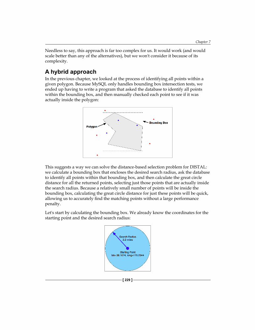
Chapter 7
[ 229 ]
Needless to say, this approach is far too complex for us. It would work (and would scale better than any of the alternatives), but we won't consider it because of its complexity.
A hybrid approachIn the previous chapter, we looked at the process of identifying all points within a given polygon. Because MySQL only handles bounding box intersection tests, we ended up having to write a program that asked the database to identify all points within the bounding box, and then manually checked each point to see if it was actually inside the polygon:
This suggests a way we can solve the distance-based selection problem for DISTAL: we calculate a bounding box that encloses the desired search radius, ask the database to identify all points within that bounding box, and then calculate the great circle distance for all the returned points, selecting just those points that are actually inside the search radius. Because a relatively small number of points will be inside the bounding box, calculating the great circle distance for just these points will be quick, allowing us to accurately find the matching points without a large performance penalty.
Let's start by calculating the bounding box. We already know the coordinates for the starting point and the desired search radius:
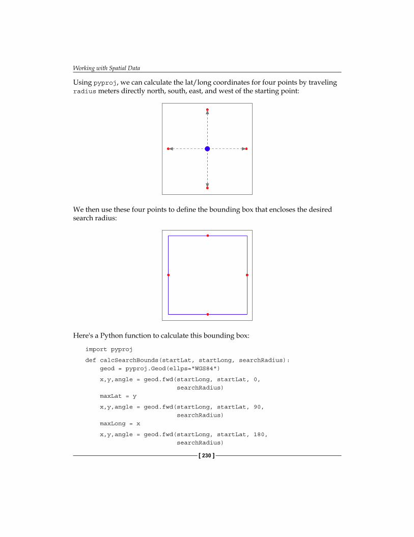
Working with Spatial Data
[ 230 ]
Using pyproj, we can calculate the lat/long coordinates for four points by traveling radius meters directly north, south, east, and west of the starting point:
We then use these four points to define the bounding box that encloses the desired search radius:
Here's a Python function to calculate this bounding box:
import pyproj
def calcSearchBounds(startLat, startLong, searchRadius): geod = pyproj.Geod(ellps="WGS84")
x,y,angle = geod.fwd(startLong, startLat, 0, searchRadius) maxLat = y
x,y,angle = geod.fwd(startLong, startLat, 90, searchRadius) maxLong = x
x,y,angle = geod.fwd(startLong, startLat, 180, searchRadius)
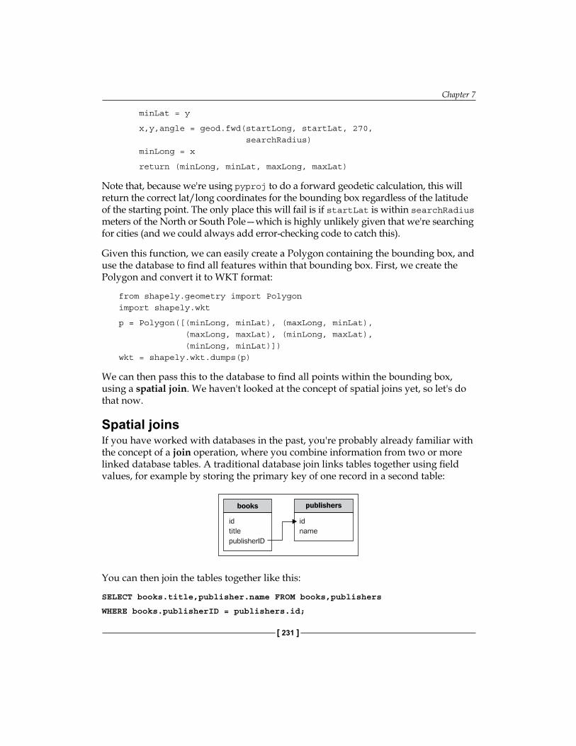
Chapter 7
[ 231 ]
minLat = y
x,y,angle = geod.fwd(startLong, startLat, 270, searchRadius) minLong = x
return (minLong, minLat, maxLong, maxLat)
Note that, because we're using pyproj to do a forward geodetic calculation, this will return the correct lat/long coordinates for the bounding box regardless of the latitude of the starting point. The only place this will fail is if startLat is within searchRadius meters of the North or South Pole—which is highly unlikely given that we're searching for cities (and we could always add error-checking code to catch this).
Given this function, we can easily create a Polygon containing the bounding box, and use the database to find all features within that bounding box. First, we create the Polygon and convert it to WKT format:
from shapely.geometry import Polygonimport shapely.wkt
p = Polygon([(minLong, minLat), (maxLong, minLat), (maxLong, maxLat), (minLong, maxLat), (minLong, minLat)])wkt = shapely.wkt.dumps(p)
We can then pass this to the database to find all points within the bounding box, using a spatial join. We haven't looked at the concept of spatial joins yet, so let's do that now.
Spatial joinsIf you have worked with databases in the past, you're probably already familiar with the concept of a join operation, where you combine information from two or more linked database tables. A traditional database join links tables together using field values, for example by storing the primary key of one record in a second table:
You can then join the tables together like this:
SELECT books.title,publisher.name FROM books,publishers
WHERE books.publisherID = publishers.id;
Working with Spatial Data
[ 232 ]
A spatial join works in the same way, except that you connect the records using spatial predicates like MBRIntersects(), ST_Contains(), or ST_DWithin(). These predicates identify records that are related in some way spatially, for example by having overlapping bounding boxes or being within a given distance of each other.
In this case, we want to use a spatial join to identify all the places within the calculated lat/long bounding box. To do this using MySQL, we would write the following:
connection = MySQLdb.connect(user="...", passwd="...")cursor = connection.cursor()
cursor.execute("USE distal")
cursor.execute("SELECT id,name,X(position),Y(position) " + "FROM places WHERE MBRContains(" + "GeomFromText(%s), position)", (wkt,))for row in cursor: ...
Using PostGIS:
connection = psycopg2.connect("dbname=... user=...")cursor = connection.cursor()cursor.execute("SET NAMES 'utf8'")
cursor.execute("SELECT id,name,X(position),Y(position) " + "FROM places WHERE ST_Contains(" + "GeomFromText(%s, 4326), position)", (wkt,)) for row in cursor: ...
Remember that SpatiaLite doesn't automatically use a spatial index for queries. To make this code efficient in SpatiaLite, we have to check the spatial index directly:
db = sqlite.connect("distal.db")db.enable_load_extension(True)db.execute('SELECT load_extension("...")')cursor = db.cursor()
cursor.execute("SELECT id,name,X(position),Y(position) " + "FROM places WHERE id in (SELECT pkid " + "FROM idx_places_position " + "WHERE xmin >= ? AND xmax <= ? " + "AND ymin >= ? and ymax <= ?)", (minLong, maxLong, minLat, maxLat))for row in cursor: ...
Chapter 7
[ 233 ]
Obviously, spatial joins work best if the database includes spatial indexes that can be used to join together the two tables. One of the challenges of developing spatial queries is to make sure that the database can and does use your spatial indexes; using the techniques described in the previous chapter, you can analyze your queries, and modify them if necessary, to ensure that your spatial indexes are used.
Identifying points by true distanceNow that we have identified all the points within the bounding box, we can check the Great Circle distance and discard those points that are inside the bounding box, but outside the search radius:
...
geod = pyproj.Geod(ellps="WGS84")
for row in cursor: id,name,long,lat = row angle1,angle2,distance = geod.inv(startLong, startLat, long, lat) if distance > searchRadius: continue
...
Using this logic, we can achieve a 100 percent accurate distance-based lookup on placenames, with the results taking only a fraction of a second to calculate.
Displaying the resultsNow that we have calculated the list of placenames within the desired search radius, we can use the mapGenerator.py module to display them. To do this, we first set up a list of all the matching placenames:
placenames = [] # List of (long, lat, name) tuples.
for row in cursor: id,name,long,lat = row angle1,angle2,distance = geod.inv(startLong, startLat, long, lat) if distance > searchRadius: continue
placenames.append([long, lat, name])
We then set up our datasource to access the shorelines table. For MySQL, we set up a shorelines.vrt file like this:
<OGRVRTDataSource> <OGRVRTLayer name="shorelines"> <SrcDataSource>MYSQL:distal,user=USER,passwd=PASS,
Working with Spatial Data
[ 234 ]
tables=shorelines</SrcDataSource> <SrcSQL> SELECT id,outline FROM shorelines where level=1 </SrcSQL> </OGRVRTLayer></OGRVRTDataSource>
and then define our datasource dictionary as follows:
vrtFile = os.path.join(os.path.dirname(__file__), "shorelines.vrt")
datasource = {'type' : "OGR", 'file' : vrtFile, 'layer' : "shorelines"}
Notice that the SrcSQL statement in our .VRT file only includes shoreline data where level = 1. This means that we’re only displaying the coastlines, and not the lakes, islands-on-lakes, and so on. Because the mapGenerator.py module doesn’t support multiple datasources, we aren’t able to draw lakes in this version of the DISTAL system. Extending mapGenerator.py to support multiple datasources is possible, but is too complicated for this chapter. For now we’ll just have to live with this limitation
Using PostGIS, we set up the datasource dictionary like this:
datasource = {'type' : "PostGIS", 'dbname' : "distal", 'table' : "shorelines", 'user' : "...", 'password' : "..."}
And for SpatiaLite, we use the following code:
dbFile = os.path.join(os.path.dirname(__file__), "distal.db")
datasource = {'type' : "SQLite", 'file' : dbFile, 'table' : "shorelines", 'geometry_field' : "outline", 'key_field' : "id"}
Chapter 7
[ 235 ]
We can then call mapGenerator.generateMap to generate an image file containing the map:
imgFile = mapGenerator.generateMap(datasource, minLong, minLat, maxLong, maxLat, mapWidth, mapHeight, points=placenames)
When we called the map generator previously, we used a filter expression to highlight particular features. In this case, we don't need to highlight anything. Instead, we pass it the list of placenames to display on the map in the keyword parameter named points.
The map generator creates a PNG-format file, and returns a reference to that file that we can then display to the user:
print 'Content-Type: text/html; charset=UTF-8\n\n'print '<html>'print '<head><title>Search Results</title></head>'print '<body>"print '<b>' + countryName + '</b>'print '<p>'print '<img src="' + imgFile + '">'print '</body>'print '</html>'
This completes our first version of the showResults.py CGI script.
Application review and improvementsAt this stage, we have a complete implementation of the DISTAL system that works as advertized: a user can choose a country, enter a search radius in miles, click on a starting point, and see a high-resolution map showing all the placenames within the desired search radius. We have solved the distance problem, and have all the data needed to search for placenames anywhere in the world.
Of course, we aren't finished yet. There are several areas where our DISTAL application doesn't work as well as it should, including:
• Usability• Quality• Performance• Scalability
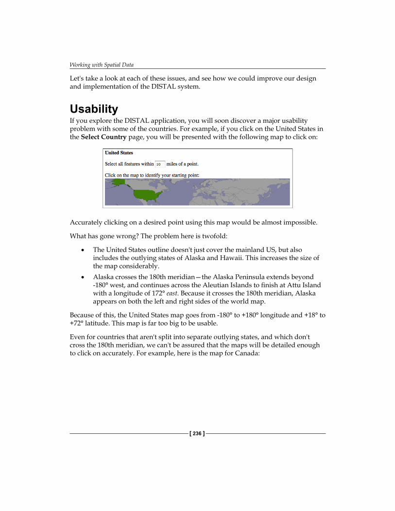
Working with Spatial Data
[ 236 ]
Let's take a look at each of these issues, and see how we could improve our design and implementation of the DISTAL system.
UsabilityIf you explore the DISTAL application, you will soon discover a major usability problem with some of the countries. For example, if you click on the United States in the Select Country page, you will be presented with the following map to click on:
Accurately clicking on a desired point using this map would be almost impossible.
What has gone wrong? The problem here is twofold:
• The United States outline doesn't just cover the mainland US, but also includes the outlying states of Alaska and Hawaii. This increases the size of the map considerably.
• Alaska crosses the 180th meridian—the Alaska Peninsula extends beyond -180° west, and continues across the Aleutian Islands to finish at Attu Island with a longitude of 172° east. Because it crosses the 180th meridian, Alaska appears on both the left and right sides of the world map.
Because of this, the United States map goes from -180° to +180° longitude and +18° to +72° latitude. This map is far too big to be usable.
Even for countries that aren't split into separate outlying states, and which don't cross the 180th meridian, we can't be assured that the maps will be detailed enough to click on accurately. For example, here is the map for Canada:
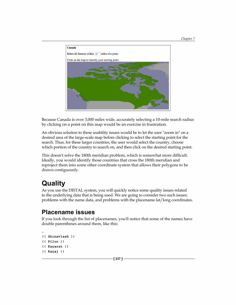
Chapter 7
[ 237 ]
Because Canada is over 3,000 miles wide, accurately selecting a 10-mile search radius by clicking on a point on this map would be an exercise in frustration.
An obvious solution to these usability issues would be to let the user "zoom in" on a desired area of the large-scale map before clicking to select the starting point for the search. Thus, for these larger countries, the user would select the country, choose which portion of the country to search on, and then click on the desired starting point.
This doesn't solve the 180th meridian problem, which is somewhat more difficult. Ideally, you would identify those countries that cross the 180th meridian and reproject them into some other coordinate system that allows their polygons to be drawn contiguously.
QualityAs you use the DISTAL system, you will quickly notice some quality issues related to the underlying data that is being used. We are going to consider two such issues: problems with the name data, and problems with the placename lat/long coordinates.
Placename issuesIf you look through the list of placenames, you'll notice that some of the names have double parentheses around them, like this:
…
(( Shinavlash ))
(( Pilur ))
(( Kaçarat ))
(( Kaçaj ))
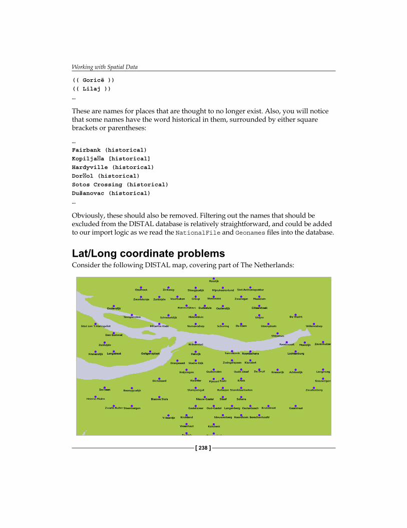
Working with Spatial Data
[ 238 ]
(( Goricë ))
(( Lilaj ))
…
These are names for places that are thought to no longer exist. Also, you will notice that some names have the word historical in them, surrounded by either square brackets or parentheses:
…
Fairbank (historical)
Kopiljača [historical]
Hardyville (historical)
Dorčol (historical)
Sotos Crossing (historical)
Dušanovac (historical)
…
Obviously, these should also be removed. Filtering out the names that should be excluded from the DISTAL database is relatively straightforward, and could be added to our import logic as we read the NationalFile and Geonames files into the database.
Lat/Long coordinate problemsConsider the following DISTAL map, covering part of The Netherlands:
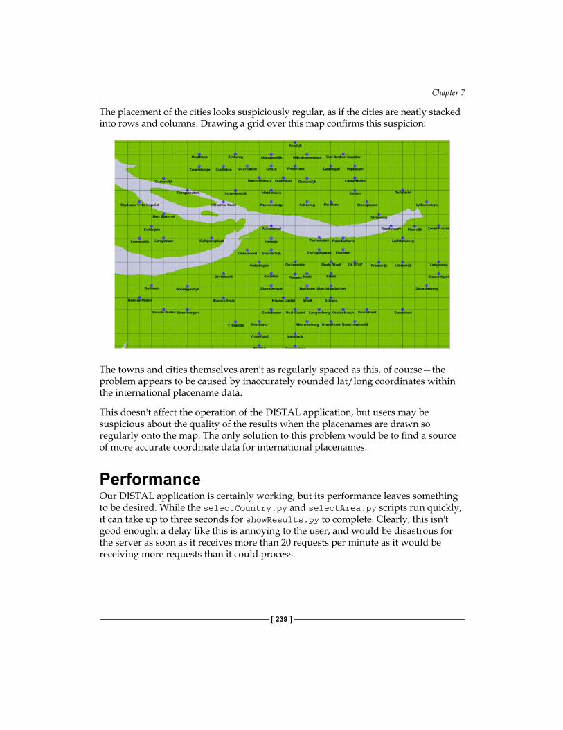
Chapter 7
[ 239 ]
The placement of the cities looks suspiciously regular, as if the cities are neatly stacked into rows and columns. Drawing a grid over this map confirms this suspicion:
The towns and cities themselves aren't as regularly spaced as this, of course—the problem appears to be caused by inaccurately rounded lat/long coordinates within the international placename data.
This doesn't affect the operation of the DISTAL application, but users may be suspicious about the quality of the results when the placenames are drawn so regularly onto the map. The only solution to this problem would be to find a source of more accurate coordinate data for international placenames.
PerformanceOur DISTAL application is certainly working, but its performance leaves something to be desired. While the selectCountry.py and selectArea.py scripts run quickly, it can take up to three seconds for showResults.py to complete. Clearly, this isn't good enough: a delay like this is annoying to the user, and would be disastrous for the server as soon as it receives more than 20 requests per minute as it would be receiving more requests than it could process.
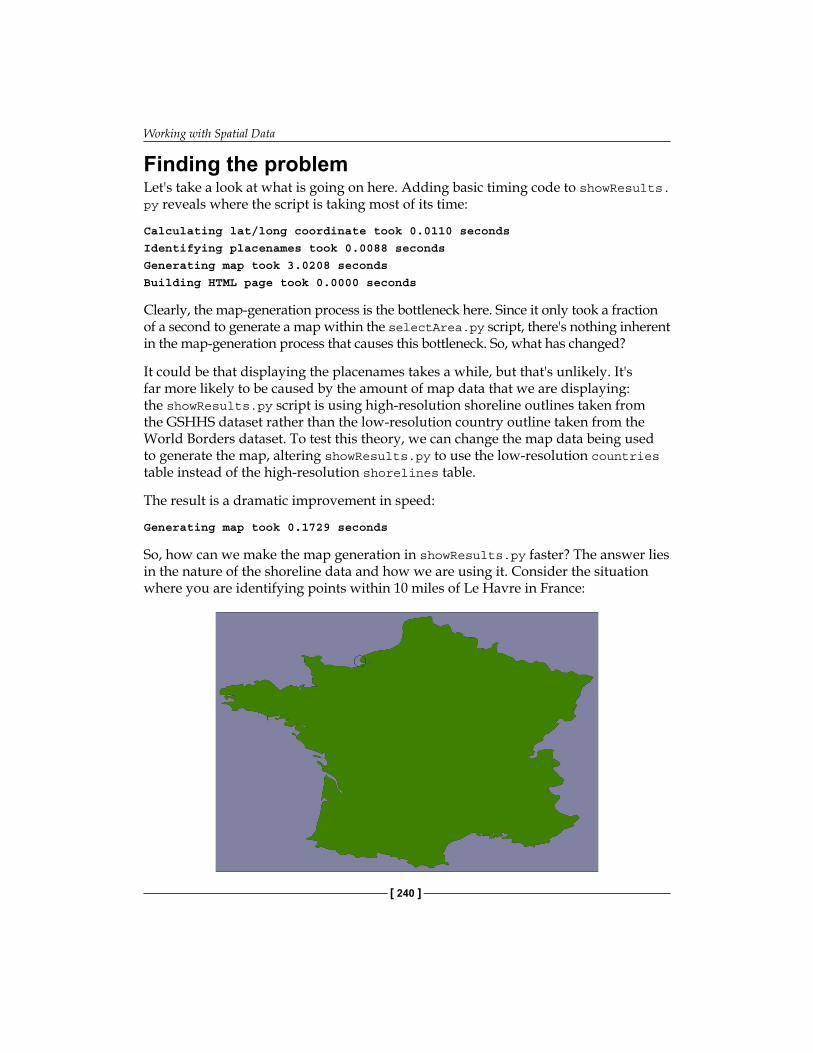
Working with Spatial Data
[ 240 ]
Finding the problemLet's take a look at what is going on here. Adding basic timing code to showResults.py reveals where the script is taking most of its time:
Calculating lat/long coordinate took 0.0110 seconds
Identifying placenames took 0.0088 seconds
Generating map took 3.0208 seconds
Building HTML page took 0.0000 seconds
Clearly, the map-generation process is the bottleneck here. Since it only took a fraction of a second to generate a map within the selectArea.py script, there's nothing inherent in the map-generation process that causes this bottleneck. So, what has changed?
It could be that displaying the placenames takes a while, but that's unlikely. It's far more likely to be caused by the amount of map data that we are displaying: the showResults.py script is using high-resolution shoreline outlines taken from the GSHHS dataset rather than the low-resolution country outline taken from the World Borders dataset. To test this theory, we can change the map data being used to generate the map, altering showResults.py to use the low-resolution countries table instead of the high-resolution shorelines table.
The result is a dramatic improvement in speed:
Generating map took 0.1729 seconds
So, how can we make the map generation in showResults.py faster? The answer lies in the nature of the shoreline data and how we are using it. Consider the situation where you are identifying points within 10 miles of Le Havre in France:
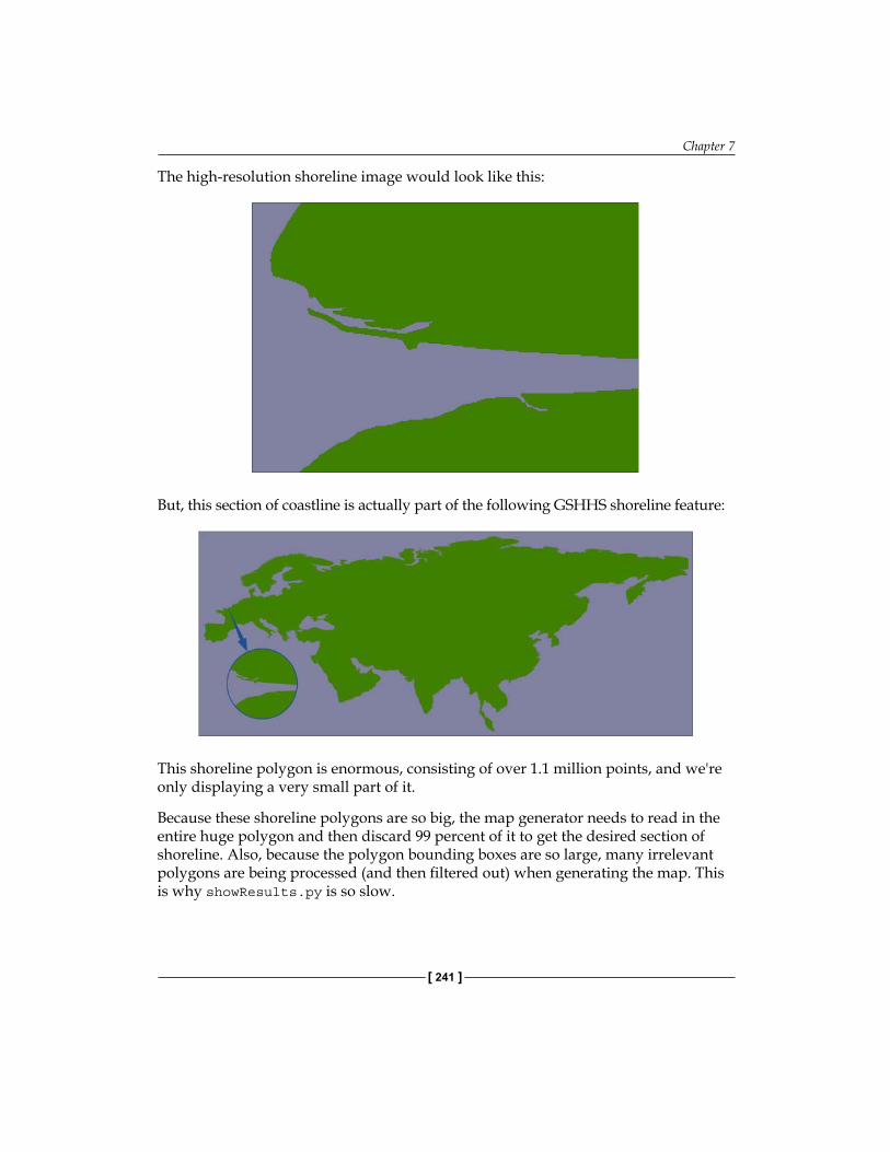
Chapter 7
[ 241 ]
The high-resolution shoreline image would look like this:
But, this section of coastline is actually part of the following GSHHS shoreline feature:
This shoreline polygon is enormous, consisting of over 1.1 million points, and we're only displaying a very small part of it.
Because these shoreline polygons are so big, the map generator needs to read in the entire huge polygon and then discard 99 percent of it to get the desired section of shoreline. Also, because the polygon bounding boxes are so large, many irrelevant polygons are being processed (and then filtered out) when generating the map. This is why showResults.py is so slow.
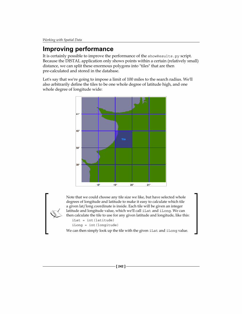
Working with Spatial Data
[ 242 ]
Improving performanceIt is certainly possible to improve the performance of the showResults.py script. Because the DISTAL application only shows points within a certain (relatively small) distance, we can split these enormous polygons into "tiles" that are then pre-calculated and stored in the database.
Let's say that we're going to impose a limit of 100 miles to the search radius. We'll also arbitrarily define the tiles to be one whole degree of latitude high, and one whole degree of longitude wide:
Note that we could choose any tile size we like, but have selected whole degrees of longitude and latitude to make it easy to calculate which tile a given lat/long coordinate is inside. Each tile will be given an integer latitude and longitude value, which we'll call iLat and iLong. We can then calculate the tile to use for any given latitude and longitude, like this:
iLat = int(latitude)iLong = int(longitude)
We can then simply look up the tile with the given iLat and iLong value.
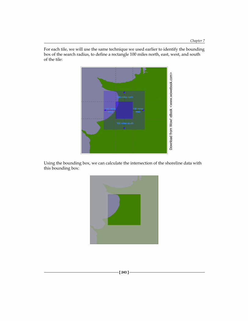
Chapter 7
[ 243 ]
For each tile, we will use the same technique we used earlier to identify the bounding box of the search radius, to define a rectangle 100 miles north, east, west, and south of the tile:
Using the bounding box, we can calculate the intersection of the shoreline data with this bounding box:
Dow
nlo
ad fro
m W
ow
! eBook
<w
ww
.wow
ebook.
com
>
Working with Spatial Data
[ 244 ]
Any search done within the tile's boundary, up to a maximum of 100 miles in any direction, will only display shorelines within this bounding box. We simply store this intersected shoreline into the database, along with the lat/long coordinates for the tile, and tell the map generator to use the appropriate tile's outline to display the desired shoreline.
Calculating the tiled shorelinesLet's write the code that calculates these tiled shorelines. First off, we'll define a function that calculates the tile bounding boxes. This function, expandRect(), takes a rectangle defined using lat/long coordinates, and expands it in each direction by a given number of meters:
def expandRect(minLat, minLong, maxLat, maxLong, distance):
geod = pyproj.Geod(ellps="WGS84") midLat = (minLat + maxLat) / 2.0 midLong = (minLong + maxLong) / 2.0
try: availDistance = geod.inv(midLong, maxLat, midLong, +90)[2] if availDistance >= distance: x,y,angle = geod.fwd(midLong, maxLat, 0, distance) maxLat = y else: maxLat = +90 except: maxLat = +90 # Can't expand north.
try: availDistance = geod.inv(maxLong, midLat, +180, midLat)[2] if availDistance >= distance: x,y,angle = geod.fwd(maxLong, midLat, 90, distance) maxLong = x else: maxLong = +180 except: maxLong = +180 # Can't expand east.
try: availDistance = geod.inv(midLong, minLat, midLong, -90)[2] if availDistance >= distance: x,y,angle = geod.fwd(midLong, minLat, 180,
Chapter 7
[ 245 ]
distance) minLat = y else: minLat = -90 except: minLat = -90 # Can't expand south.
try: availDistance = geod.inv(maxLong, midLat, -180, midLat)[2] if availDistance >= distance: x,y,angle = geod.fwd(minLong, midLat, 270, distance) minLong = x else: minLong = -180 except: minLong = -180 # Can't expand west.
return (minLat, minLong, maxLat, maxLong)
Notice that we've added error-checking here, to allow for rectangles close to the North or South Pole.
Using this function, we can calculate the bounding rectangle for a given tile as follows:
minLat,minLong,maxLat,maxLong = expandRect(iLat, iLong, iLat+1, iLong+1, MAX_DISTANCE)
We are now ready to load our shoreline polygons into memory:
shorelinePolys = []
cursor.execute("SELECT AsText(outline) FROM shorelines " + "WHERE level=1")for row in cursor: outline = shapely.wkt.loads(row[0]) shorelinePolys.append(outline)
This implementation of the shoreline tiling algorithm uses a lot of memory. If your computer has less than 2 GB of RAM, you may need to store temporary results in the database. Doing this will of course slow down the tiling process, but it will still work.
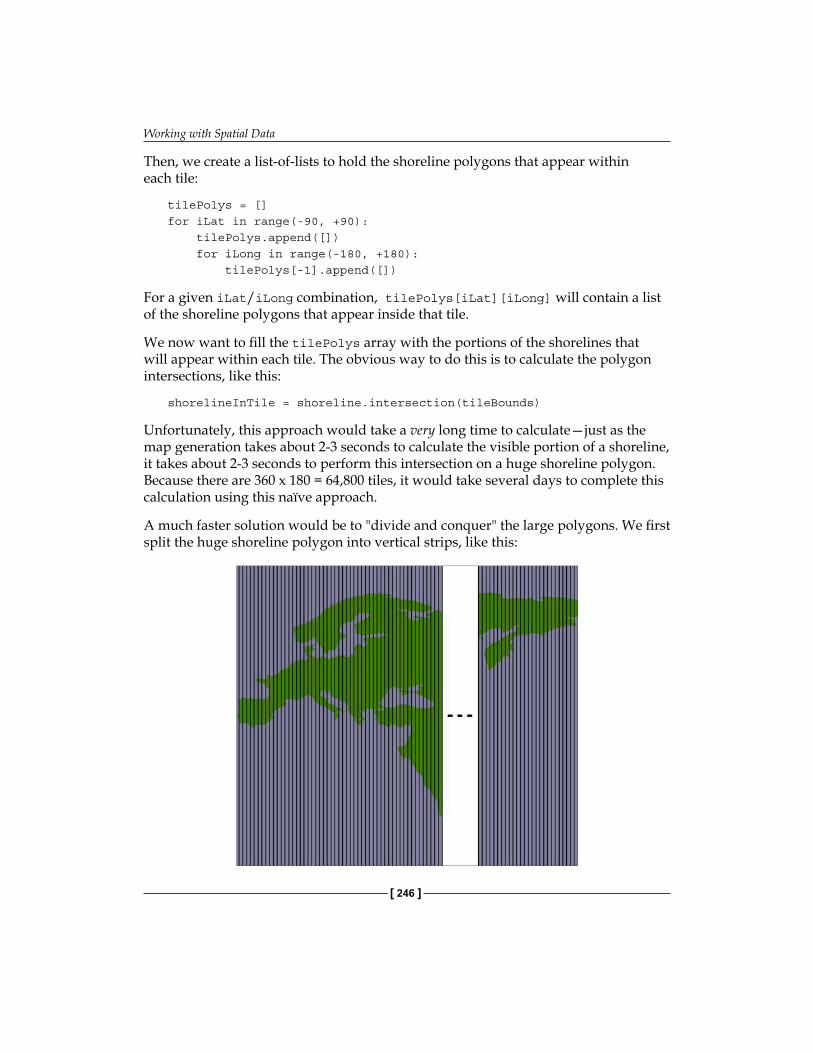
Working with Spatial Data
[ 246 ]
Then, we create a list-of-lists to hold the shoreline polygons that appear within each tile:
tilePolys = []for iLat in range(-90, +90): tilePolys.append([]) for iLong in range(-180, +180): tilePolys[-1].append([])
For a given iLat/iLong combination, tilePolys[iLat][iLong] will contain a list of the shoreline polygons that appear inside that tile.
We now want to fill the tilePolys array with the portions of the shorelines that will appear within each tile. The obvious way to do this is to calculate the polygon intersections, like this:
shorelineInTile = shoreline.intersection(tileBounds)
Unfortunately, this approach would take a very long time to calculate—just as the map generation takes about 2-3 seconds to calculate the visible portion of a shoreline, it takes about 2-3 seconds to perform this intersection on a huge shoreline polygon. Because there are 360 x 180 = 64,800 tiles, it would take several days to complete this calculation using this naïve approach.
A much faster solution would be to "divide and conquer" the large polygons. We first split the huge shoreline polygon into vertical strips, like this:

Chapter 7
[ 247 ]
We then split each vertical strip horizontally to give us the individual parts of the polygon that can be merged into the individual tiles:
By dividing the huge polygons into strips, and then further dividing each strip, the intersection process is much faster. Here is the code which performs this intersection; we start by iterating over each shoreline polygon and calculating the polygon's bounds:
for shoreline in shorelinePolys: minLong,minLat,maxLong,maxLat = shoreline.bounds minLong = int(math.floor(minLong)) minLat = int(math.floor(minLat)) maxLong = int(math.ceil(maxLong)) maxLat = int(math.ceil(maxLat))
We then split the polygon into vertical strips:
vStrips = [] for iLong in range(minLong, maxLong+1):
stripMinLat = minLat stripMaxLat = maxLat stripMinLong = iLong stripMaxLong = iLong + 1
bMinLat,bMinLong,bMaxLat,bMaxLong = \ expandRect(stripMinLat, stripMinLong, stripMaxLat, stripMaxLong,
Working with Spatial Data
[ 248 ]
MAX_DISTANCE)
bounds = Polygon([(bMinLong, bMinLat), (bMinLong, bMaxLat), (bMaxLong, bMaxLat), (bMaxLong, bMinLat), (bMinLong, bMinLat)])
strip = shoreline.intersection(bounds) vStrips.append(strip)
Next, we process each vertical strip, splitting the strip into tile-sized blocks and storing it into tilePolys:
stripNum = 0 for iLong in range(minLong, maxLong+1): vStrip = vStrips[stripNum] stripNum = stripNum + 1
for iLat in range(minLat, maxLat+1): bMinLat,bMinLong,bMaxLat,bMaxLong = \ expandRect(iLat, iLong, iLat+1, iLong+1, MAX_DISTANCE)
bounds = Polygon([(bMinLong, bMinLat), (bMinLong, bMaxLat), (bMaxLong, bMaxLat), (bMaxLong, bMinLat), (bMinLong, bMinLat)])
polygon = vStrip.intersection(bounds) if not polygon.is_empty: tilePolys[iLat][iLong].append(polygon)
We're now ready to save the tiled shorelines into the database. Before we do this, we have to create the necessary database table. Using MySQL:
cursor.execute(""" CREATE TABLE IF NOT EXISTS tiled_shorelines ( intLat INTEGER, intLong INTEGER, outline POLYGON,
PRIMARY KEY (intLat, intLong))""")
Using PostGIS:
cursor.execute("DROP TABLE IF EXISTS tiled_shorelines")cursor.execute(""" CREATE TABLE tiled_shorelines ( intLat INTEGER,
Chapter 7
[ 249 ]
intLong INTEGER,
PRIMARY KEY (intLat, intLong))""")cursor.execute(""" SELECT AddGeometryColumn('tiled_shorelines', 'outline', 4326, 'POLYGON', 2)""")cursor.execute(""" CREATE INDEX tiledShorelineIndex ON tiled_shorelines USING GIST(outline)""")
And using SpatiaLite:
cursor.execute("DROP TABLE IF EXISTS tiled_shorelines")cursor.execute(""" CREATE TABLE tiled_shorelines ( intLat INTEGER, intLong INTEGER, PRIMARY KEY (intLat, intLong))""")cursor.execute(""" SELECT AddGeometryColumn('tiled_shorelines', 'outline', 4326, 'POLYGON', 2)""")cursor.execute(""" SELECT CreateSpatialIndex('tiled_shorelines', 'outline')""")
We can now combine each tile's shoreline polygons into a single MultiPolygon, and save the results into the database:
for iLat in range(-90, +90): for iLong in range(-180, +180): polygons = tilePolys[iLat][iLong] if len(polygons) == 0: outline = Polygon() else: outline = shapely.ops.cascaded_union(polygons) wkt = shapely.wkt.dumps(outline)
cursor.execute("INSERT INTO tiled_shorelines " + "(intLat, intLong, outline) " + "VALUES (%s, %s, GeomFromText(%s))", (iLat, iLong, wkt)) connection.commit()
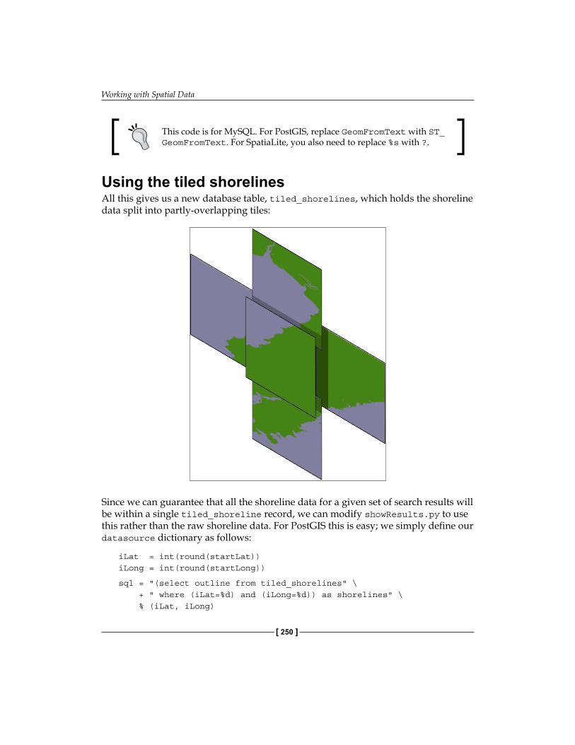
Working with Spatial Data
[ 250 ]
This code is for MySQL. For PostGIS, replace GeomFromText with ST_GeomFromText. For SpatiaLite, you also need to replace %s with ?.
Using the tiled shorelinesAll this gives us a new database table, tiled_shorelines, which holds the shoreline data split into partly-overlapping tiles:
Since we can guarantee that all the shoreline data for a given set of search results will be within a single tiled_shoreline record, we can modify showResults.py to use this rather than the raw shoreline data. For PostGIS this is easy; we simply define our datasource dictionary as follows:
iLat = int(round(startLat))iLong = int(round(startLong))
sql = "(select outline from tiled_shorelines" \ + " where (iLat=%d) and (iLong=%d)) as shorelines" \ % (iLat, iLong)
Chapter 7
[ 251 ]
datasource = {'type' : "PostGIS", 'dbname' : "distal", 'table' : sql, 'user' : "...", 'password' : "..."}
Notice that we're replacing the table name with an SQL sub-selection that directly loads the desired shoreline data from the selected tile.
For SpatiaLite, the code is almost identical:
iLat = int(round(startLat))iLong = int(round(startLong))
dbFile = os.path.join(os.path.dirname(__file__), "distal.db")
sql = "(select outline from tiled_shorelines" \ + " where (iLat=%d) and (iLong=%d)) as shorelines" \ % (iLat, iLong)
datasource = {'type' : "SQLite", 'file' : dbFile, 'table' : sql, 'geometry_field' : "outline", 'key_field' : "id"}
MySQL is a bit more tricky because we have to use a .VRT file to store the details of the datasource. To do this, we create a temporary file, write the contents of the .VRT file, and then delete the file once we're done:
iLat = int(round(startLat))iLong = int(round(startLong))
fd,filename = tempfile.mkstemp(".vrt", dir=os.path.dirname(__file__))os.close(fd)
vrtFile = os.path.join(os.path.dirname(__file__), filename)
f = file(vrtFile, "w")f.write('<OGRVRTDataSource>\n')f.write(' <OGRVRTLayer name="shorelines">\n')f.write(' <SrcDataSource>MYSQL:distal,user=USER,' + 'pass=PASS,tables=tiled_shorelines' + '</SrcDataSource>\n')f.write(' <SrcSQL>\n')f.write(' SELECT outline FROM tiled_shorelines WHERE ' + '(intLat=%d) AND (intLong=%d)\n' % (iLat, iLong)
Working with Spatial Data
[ 252 ]
f.write(' </SrcSQL>\n')f.write(' </OGRVRTLayer>\n')f.write('</OGRVRTDataSource>')f.close()
datasource = {'type' : "OGR", 'file' : vrtFile, 'layer' : "shorelines"}
imgFile = mapGenerator.generateMap(...)
os.remove(vrtFile)
With these changes in place, the showResults.py script will use the tiled shorelines rather than the full shoreline data downloaded from GSHHS. Let's now take a look at how much of a performance improvement these tiled shorelines give us.
Analyzing the performance improvementAs soon as you run this new version of the DISTAL application, you'll notice a huge improvement in speed: showResults.py now seems to return its results almost instantly. Where before the map generator was taking 2-3 seconds to generate the high-resolution maps, it's now only taking a fraction of a second:
Generating map took 0.1705 seconds
That's a dramatic improvement in performance: the map generator is now 15-20 times faster than it was, and the total time taken by the showResults.py script is now less than a quarter of a second. That's not bad for a relatively simple change to our underlying map data!
Further performance improvementsIf changing the way the underlying map data is structured made such a difference to the performance of the system, you might wonder what other performance improvements could be made. In general, improving performance is all about making your code more efficient (removing bottlenecks), and reducing the amount of work that your code has to do (precalculating and caching data).
There aren't any real bottlenecks in our DISTAL CGI scripts. All the data is static, and we don't have any complex loops in our scripts that could be optimized. There is, however, one further operation that could possibly benefit from precalculations: the process of identifying all placenames in a given area.
Chapter 7
[ 253 ]
At present, our entire database of placenames is being checked for each search query. Of course, we're using a spatial index, which makes this process fast, but we could in theory eke some more performance gains out of our code by grouping placenames into tiles, just as we did with the shoreline data, and then only checking those placenames that are in the current tile rather than the entire database of several million placenames.
Before we go down this route, though, we need to do a reality check: is it really worth implementing this optimization? If you look back at the timing results earlier in this chapter, you'll see that the placename identification is already very fast:
Identifying placenames took 0.0088 seconds
Even if we were to group placenames by tile and limit the placename searching to just one tile, it's unlikely that we'd improve the time taken. In fact, it could easily get worse. Remember:
"Premature Optimization is the Root of All Evil." - Donald Knuth.
Geo-spatial applications often make use of a caching tile server to avoid unnecessarily rendering the same maps over and over. This isn't suitable for the DISTAL application; because the user clicks on a point to identify the search circle, the generated map will be different each time, and there is no real possibility of caching and re-using the rendered maps. We will look at caching tile servers in Chapter 9, Web Frameworks for Python Geo-Spatial Development as they are very useful for other types of geo-spatial applications.
ScalabilityReducing the processing time from 3.0 to 0.2 seconds means that your application could handle up to 250 requests per minute instead of 20 requests per minute. But, what if you wanted to make DISTAL available on the Internet and had to support up to 25,000 requests per minute? Obviously, improving performance won't be enough, no matter how much you optimize your code.
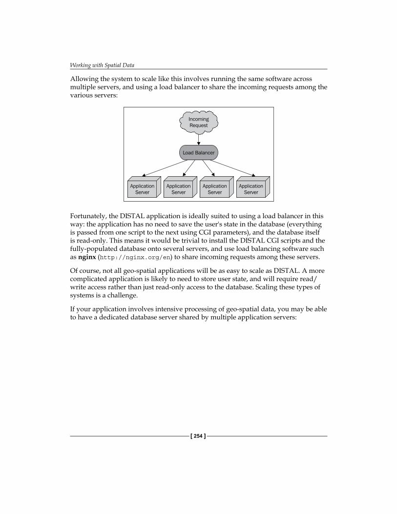
Working with Spatial Data
[ 254 ]
Allowing the system to scale like this involves running the same software across multiple servers, and using a load balancer to share the incoming requests among the various servers:
Fortunately, the DISTAL application is ideally suited to using a load balancer in this way: the application has no need to save the user's state in the database (everything is passed from one script to the next using CGI parameters), and the database itself is read-only. This means it would be trivial to install the DISTAL CGI scripts and the fully-populated database onto several servers, and use load balancing software such as nginx (http://nginx.org/en) to share incoming requests among these servers.
Of course, not all geo-spatial applications will be as easy to scale as DISTAL. A more complicated application is likely to need to store user state, and will require read/write access rather than just read-only access to the database. Scaling these types of systems is a challenge.
If your application involves intensive processing of geo-spatial data, you may be able to have a dedicated database server shared by multiple application servers:
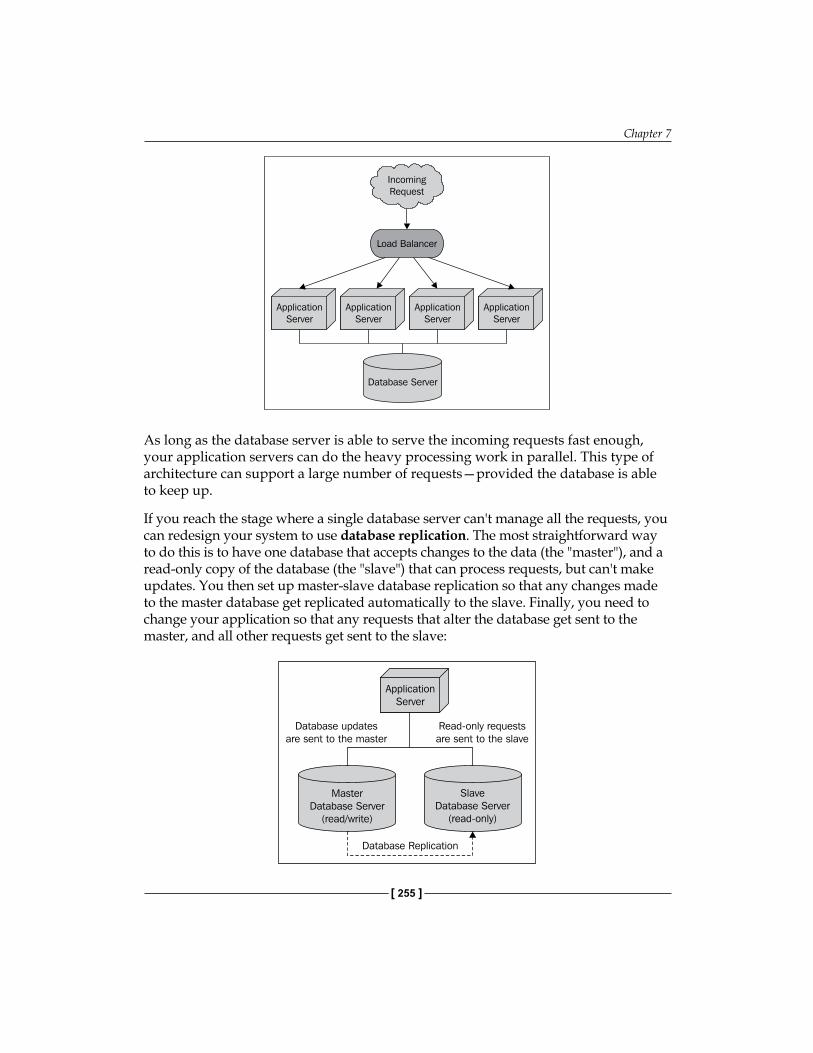
Chapter 7
[ 255 ]
As long as the database server is able to serve the incoming requests fast enough, your application servers can do the heavy processing work in parallel. This type of architecture can support a large number of requests—provided the database is able to keep up.
If you reach the stage where a single database server can't manage all the requests, you can redesign your system to use database replication. The most straightforward way to do this is to have one database that accepts changes to the data (the "master"), and a read-only copy of the database (the "slave") that can process requests, but can't make updates. You then set up master-slave database replication so that any changes made to the master database get replicated automatically to the slave. Finally, you need to change your application so that any requests that alter the database get sent to the master, and all other requests get sent to the slave:
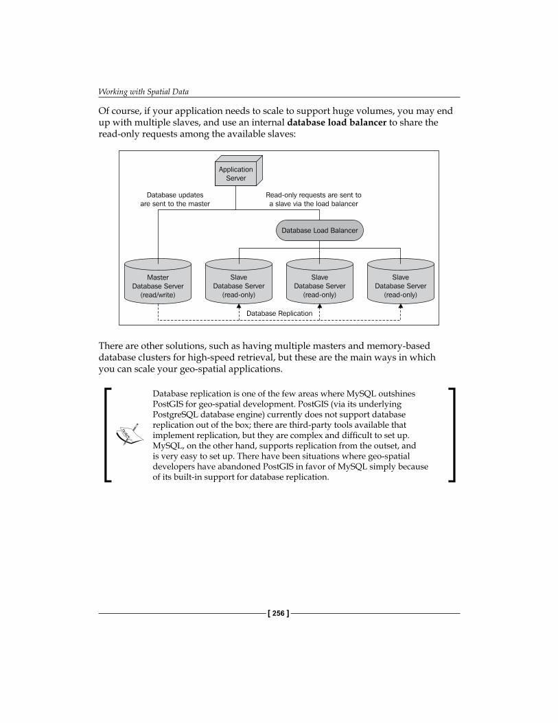
Working with Spatial Data
[ 256 ]
Of course, if your application needs to scale to support huge volumes, you may end up with multiple slaves, and use an internal database load balancer to share the read-only requests among the available slaves:
There are other solutions, such as having multiple masters and memory-based database clusters for high-speed retrieval, but these are the main ways in which you can scale your geo-spatial applications.
Database replication is one of the few areas where MySQL outshines PostGIS for geo-spatial development. PostGIS (via its underlying PostgreSQL database engine) currently does not support database replication out of the box; there are third-party tools available that implement replication, but they are complex and difficult to set up. MySQL, on the other hand, supports replication from the outset, and is very easy to set up. There have been situations where geo-spatial developers have abandoned PostGIS in favor of MySQL simply because of its built-in support for database replication.
Chapter 7
[ 257 ]
SummaryIn this chapter, we have implemented, tested, and made improvements to a simple web-based application that displays shorelines, towns, and lakes within a given radius of a starting point. This application was the impetus for exploring a number of important concepts within geo-spatial application development, including:
• The creation of a simple, but complete web-based geo-spatial application.• Using databases to store and work with large amounts of geo-spatial data.• Using a "black-box" map rendering module to create maps using spatial data
selected from a database.• Examining the issues involved in identifying features based on their true
distance rather than using a lat/long approximation.• Learning how to use spatial joins effectively.• Exploring usability issues in a prototype implementation.• Dealing with issues of data quality.• Learning how to pre-calculate data to improve performance.• Exploring how a geo-spatial application might be scaled to handle vast
numbers of users and requests.
As a result of our development efforts, we have learned:
• How to set up a database and import large quantities of data from Shapefiles and other datasources.
• How to design and structure a simple web-based application to display maps and respond to user input.
• That there are three steps in displaying a map: calculating the lat/long bounding box, calculating the pixel size of the map image, and telling the map renderer which tables to get its data from.
• Given the (x,y) coordinate of a point the user clicked on within a map, how to translate this point into the equivalent latitude and longitude value.
• Various ways in which true distance calculations, and selection of features by distance, can be performed.
• That manually calculating distance for every point using the Great Circle distance formula is accurate, but very slow.
• That angular distances (that is, differences in lat/long coordinates) is an easy approximation of distance but doesn't relate in any useful way to true distances across the Earth's surface.
Working with Spatial Data
[ 258 ]
• That using projected coordinates makes true distance calculations easy, but is limited to data covering only part of the Earth's surface.
• That we can use a hybrid approach to accurately and quickly identify features by distance, by calculating a lat/long bounding box to identify potential features and then doing a Great Circle distance calculation on these features to weed out the false positives.
• How to set up a datasource to access and retrieve data from MySQL, PostGIS and SpatiaLite databases.
• That displaying a country's outline and asking the user to click on a desired point works when the country is relatively small and compact, but breaks down for larger countries.
• That issues of data quality can affect the overall usefulness of your geo-spatial application.
• That you cannot assume that geo-spatial data comes in the best form for use in your application.
• That very large polygons can degrade performance, and can often be split into smaller sub-polygons, resulting in dramatic improvements in performance.
• That a divide-and-conquer approach to splitting large polygons is much faster than simply calculating the intersection using the full polygon each time.
• That just because you can think of an optimization doesn't mean that you should do it. Only optimize after you have identified your application's true bottlenecks.
• Making your code faster is worthwhile, but to achieve true scalability requires running multiple instances of your application on separate servers.
• That you can use a load balancer to spread requests among your application servers.
• That a dedicated database server will often meet the needs of multiple application servers.
• That you can go beyond the capacity of a single database server by using database replication and separating out the read/write requests from the read-only requests, and using different servers for each one.
• That the database replication capabilities of MySQL are much easier and often more stable than the equivalent PostGIS capabilities, which are not built in and require complex third-party support.
In the next chapter, we will explore the details of using the Mapnik library to convert raw geo-spatial data into map images.
Using Python and Mapnik to Generate Maps
Because geo-spatial data is almost impossible to understand until it is displayed, the creation of maps to visually represent spatial data is an extremely important topic. In this chapter, we will look at Mapnik, a powerful Python library for generating maps out of geo-spatial data.
This chapter will cover:
• The underlying concepts used by Mapnik to generate maps• How to create a simple map using the contents of a Shapefile• The different datasources that Mapnik support• How to use rules, filters, and styles to control the map-generation process• How to use symbolizers to draw lines, polygons, labels, points, and raster
images onto your map• How to define the colors used on a map• How to work with maps and layers• Your options for rendering a map image• How the mapGenerator.py module, introduced in the previous chapter,
uses Mapnik to generate maps• Using map definition files to control and simplify the map-generation process
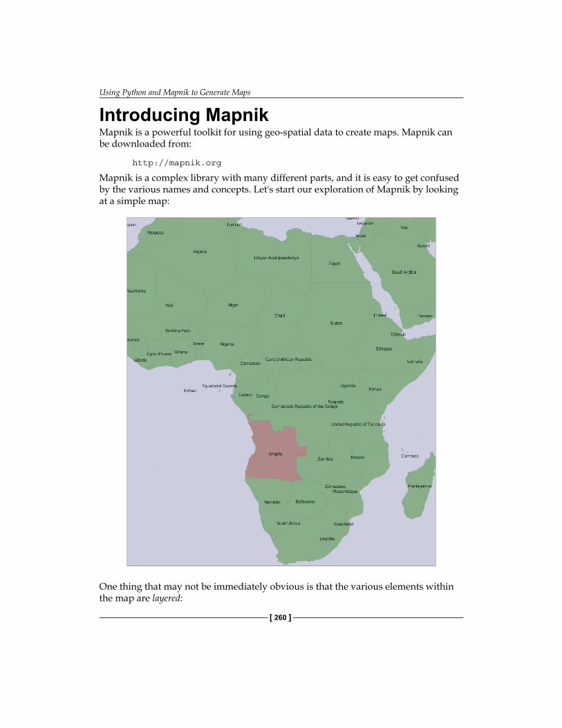
Using Python and Mapnik to Generate Maps
[ 260 ]
Introducing MapnikMapnik is a powerful toolkit for using geo-spatial data to create maps. Mapnik can be downloaded from:
http://mapnik.org
Mapnik is a complex library with many different parts, and it is easy to get confused by the various names and concepts. Let's start our exploration of Mapnik by looking at a simple map:
One thing that may not be immediately obvious is that the various elements within the map are layered:
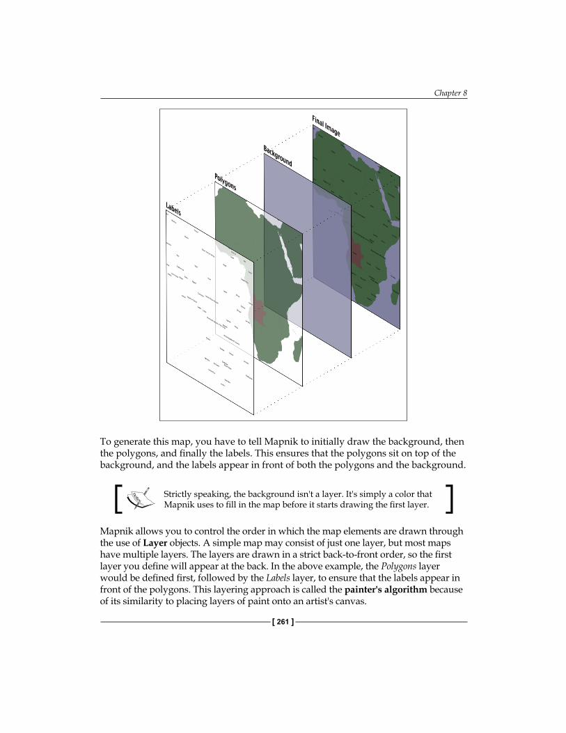
Chapter 8
[ 261 ]
To generate this map, you have to tell Mapnik to initially draw the background, then the polygons, and finally the labels. This ensures that the polygons sit on top of the background, and the labels appear in front of both the polygons and the background.
Strictly speaking, the background isn't a layer. It's simply a color that Mapnik uses to fill in the map before it starts drawing the first layer.
Mapnik allows you to control the order in which the map elements are drawn through the use of Layer objects. A simple map may consist of just one layer, but most maps have multiple layers. The layers are drawn in a strict back-to-front order, so the first layer you define will appear at the back. In the above example, the Polygons layer would be defined first, followed by the Labels layer, to ensure that the labels appear in front of the polygons. This layering approach is called the painter's algorithm because of its similarity to placing layers of paint onto an artist's canvas.
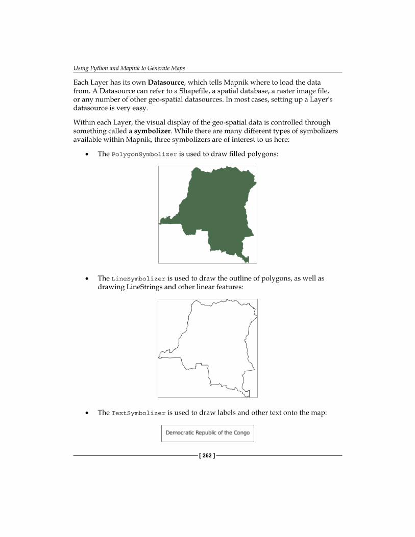
Using Python and Mapnik to Generate Maps
[ 262 ]
Each Layer has its own Datasource, which tells Mapnik where to load the data from. A Datasource can refer to a Shapefile, a spatial database, a raster image file, or any number of other geo-spatial datasources. In most cases, setting up a Layer's datasource is very easy.
Within each Layer, the visual display of the geo-spatial data is controlled through something called a symbolizer. While there are many different types of symbolizers available within Mapnik, three symbolizers are of interest to us here:
• The PolygonSymbolizer is used to draw filled polygons:
• The LineSymbolizer is used to draw the outline of polygons, as well as drawing LineStrings and other linear features:
• The TextSymbolizer is used to draw labels and other text onto the map:
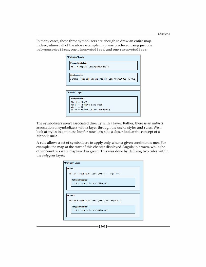
Chapter 8
[ 263 ]
In many cases, these three symbolizers are enough to draw an entire map. Indeed, almost all of the above example map was produced using just one PolygonSymbolizer, one LineSymbolizer, and one TextSymbolizer:
The symbolizers aren't associated directly with a layer. Rather, there is an indirect association of symbolizers with a layer through the use of styles and rules. We'll look at styles in a minute, but for now let's take a closer look at the concept of a Mapnik Rule.
A rule allows a set of symbolizers to apply only when a given condition is met. For example, the map at the start of this chapter displayed Angola in brown, while the other countries were displayed in green. This was done by defining two rules within the Polygons layer:
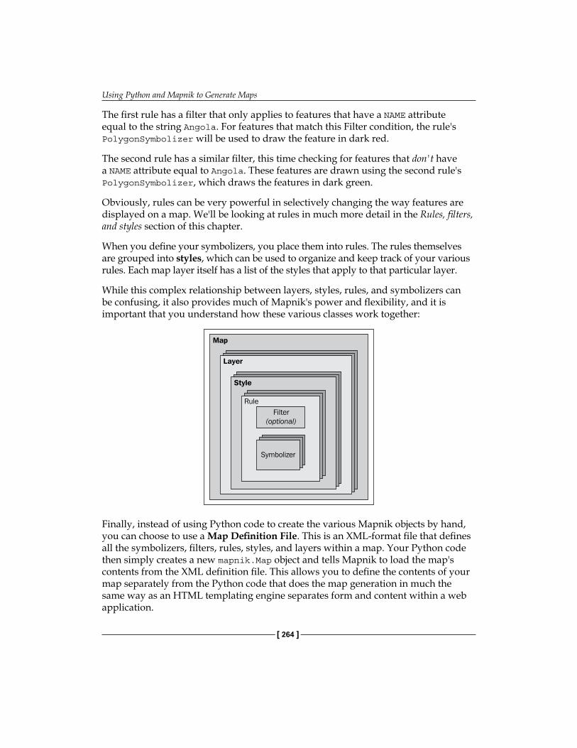
Using Python and Mapnik to Generate Maps
[ 264 ]
The first rule has a filter that only applies to features that have a NAME attribute equal to the string Angola. For features that match this Filter condition, the rule's PolygonSymbolizer will be used to draw the feature in dark red.
The second rule has a similar filter, this time checking for features that don't have a NAME attribute equal to Angola. These features are drawn using the second rule's PolygonSymbolizer, which draws the features in dark green.
Obviously, rules can be very powerful in selectively changing the way features are displayed on a map. We'll be looking at rules in much more detail in the Rules, filters, and styles section of this chapter.
When you define your symbolizers, you place them into rules. The rules themselves are grouped into styles, which can be used to organize and keep track of your various rules. Each map layer itself has a list of the styles that apply to that particular layer.
While this complex relationship between layers, styles, rules, and symbolizers can be confusing, it also provides much of Mapnik's power and flexibility, and it is important that you understand how these various classes work together:
Finally, instead of using Python code to create the various Mapnik objects by hand, you can choose to use a Map Definition File. This is an XML-format file that defines all the symbolizers, filters, rules, styles, and layers within a map. Your Python code then simply creates a new mapnik.Map object and tells Mapnik to load the map's contents from the XML definition file. This allows you to define the contents of your map separately from the Python code that does the map generation in much the same way as an HTML templating engine separates form and content within a web application.
Chapter 8
[ 265 ]
Creating an example mapTo better understand how the various parts of Mapnik work together, let's write a simple Python program that generates the map shown at the start of this chapter. This map makes use of the World Borders Dataset that you downloaded in an earlier chapter; copy the TM_WORLD_BORDERS-0.3 Shapefile directory into a convenient place, and create a new Python script in the same place. We'll call this program createExampleMap.py.
Obviously, if you've gotten this far without downloading and installing Mapnik, you need to do so now. Mapnik can be found at: http://mapnik.org.
We'll start by importing the Mapnik toolkit and defining some constants that the program will need:
import mapnik
MIN_LAT = -35MAX_LAT = +35MIN_LONG = -12MAX_LONG = +50
MAP_WIDTH = 700MAP_HEIGHT = 800
The MIN_LAT, MAX_LAT, MIN_LONG and MAX_LONG constants define the lat/long coordinates for the portion of the world to display on the map, while the MAP_WIDTH and MAP_HEIGHT constants define the size of the generated map image, in pixels. Obviously, you can change these if you want.
We're now ready to define the contents of the map. This map will have two layers: one for drawing the polygons and another for drawing the labels, so we'll define a Mapnik Style object for each of these two layers. Let's start with the style for the Polygons layer:
polygonStyle = mapnik.Style()
As we discussed in the previous section, a Filter object lets you choose which particular features a rule will apply to. In this case, we want to set up two rules: one to draw Angola in dark red, and another to draw all the other countries in dark green:
rule = mapnik.Rule()rule.filter = mapnik.Filter("[NAME] = 'Angola'")symbol = mapnik.PolygonSymbolizer(mapnik.Color("#604040"))rule.symbols.append(symbol)
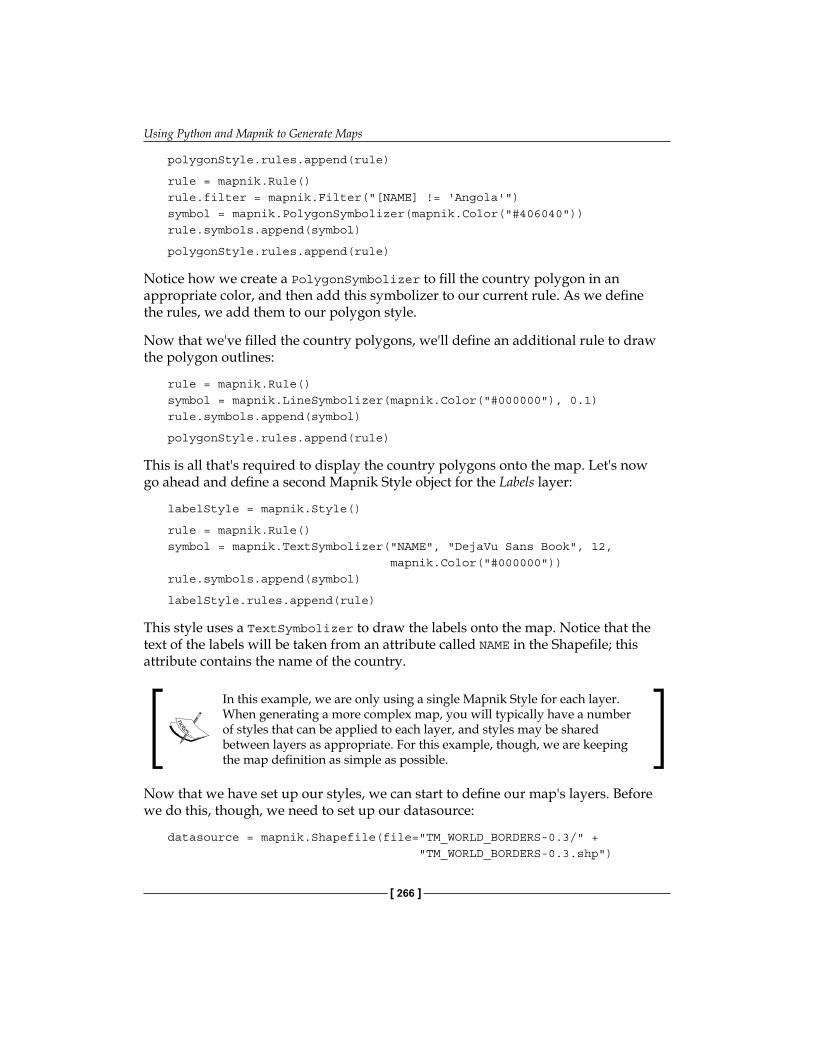
Using Python and Mapnik to Generate Maps
[ 266 ]
polygonStyle.rules.append(rule)
rule = mapnik.Rule()rule.filter = mapnik.Filter("[NAME] != 'Angola'")symbol = mapnik.PolygonSymbolizer(mapnik.Color("#406040"))rule.symbols.append(symbol)
polygonStyle.rules.append(rule)
Notice how we create a PolygonSymbolizer to fill the country polygon in an appropriate color, and then add this symbolizer to our current rule. As we define the rules, we add them to our polygon style.
Now that we've filled the country polygons, we'll define an additional rule to draw the polygon outlines:
rule = mapnik.Rule()symbol = mapnik.LineSymbolizer(mapnik.Color("#000000"), 0.1)rule.symbols.append(symbol)
polygonStyle.rules.append(rule)
This is all that's required to display the country polygons onto the map. Let's now go ahead and define a second Mapnik Style object for the Labels layer:
labelStyle = mapnik.Style()
rule = mapnik.Rule()symbol = mapnik.TextSymbolizer("NAME", "DejaVu Sans Book", 12, mapnik.Color("#000000"))rule.symbols.append(symbol)
labelStyle.rules.append(rule)
This style uses a TextSymbolizer to draw the labels onto the map. Notice that the text of the labels will be taken from an attribute called NAME in the Shapefile; this attribute contains the name of the country.
In this example, we are only using a single Mapnik Style for each layer. When generating a more complex map, you will typically have a number of styles that can be applied to each layer, and styles may be shared between layers as appropriate. For this example, though, we are keeping the map definition as simple as possible.
Now that we have set up our styles, we can start to define our map's layers. Before we do this, though, we need to set up our datasource:
datasource = mapnik.Shapefile(file="TM_WORLD_BORDERS-0.3/" + "TM_WORLD_BORDERS-0.3.shp")
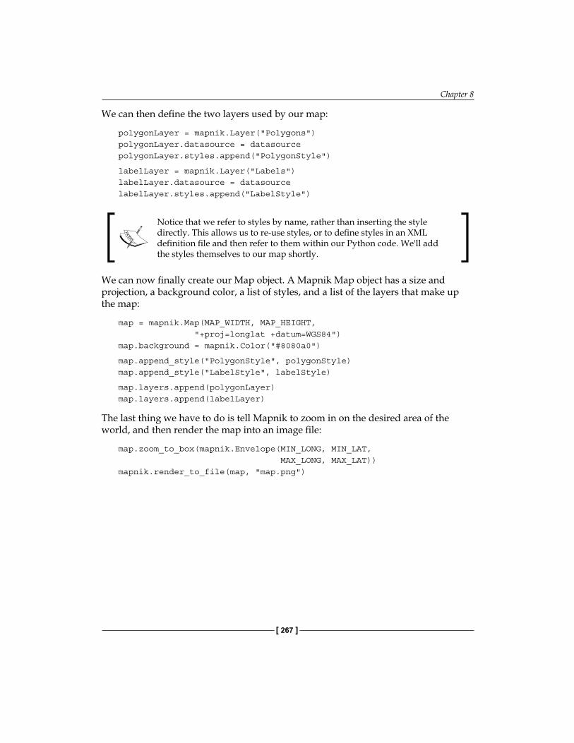
Chapter 8
[ 267 ]
We can then define the two layers used by our map:
polygonLayer = mapnik.Layer("Polygons")polygonLayer.datasource = datasourcepolygonLayer.styles.append("PolygonStyle")
labelLayer = mapnik.Layer("Labels")labelLayer.datasource = datasourcelabelLayer.styles.append("LabelStyle")
Notice that we refer to styles by name, rather than inserting the style directly. This allows us to re-use styles, or to define styles in an XML definition file and then refer to them within our Python code. We'll add the styles themselves to our map shortly.
We can now finally create our Map object. A Mapnik Map object has a size and projection, a background color, a list of styles, and a list of the layers that make up the map:
map = mapnik.Map(MAP_WIDTH, MAP_HEIGHT, "+proj=longlat +datum=WGS84")map.background = mapnik.Color("#8080a0")
map.append_style("PolygonStyle", polygonStyle)map.append_style("LabelStyle", labelStyle)
map.layers.append(polygonLayer)map.layers.append(labelLayer)
The last thing we have to do is tell Mapnik to zoom in on the desired area of the world, and then render the map into an image file:
map.zoom_to_box(mapnik.Envelope(MIN_LONG, MIN_LAT, MAX_LONG, MAX_LAT))mapnik.render_to_file(map, "map.png")
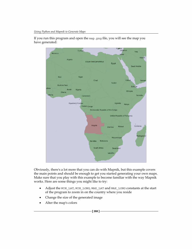
Using Python and Mapnik to Generate Maps
[ 268 ]
If you run this program and open the map.png file, you will see the map you have generated:
Obviously, there's a lot more that you can do with Mapnik, but this example covers the main points and should be enough to get you started generating your own maps. Make sure that you play with this example to become familiar with the way Mapnik works. Here are some things you might like to try:
• Adjust the MIN_LAT, MIN_LONG, MAX_LAT and MAX_LONG constants at the start of the program to zoom in on the country where you reside
• Change the size of the generated image• Alter the map's colors
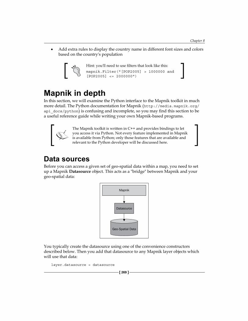
Chapter 8
[ 269 ]
• Add extra rules to display the country name in different font sizes and colors based on the country's population
Hint: you'll need to use filters that look like this:mapnik.Filter("[POP2005] > 1000000 and [POP2005] <= 2000000")
Mapnik in depthIn this section, we will examine the Python interface to the Mapnik toolkit in much more detail. The Python documentation for Mapnik (http://media.mapnik.org/api_docs/python) is confusing and incomplete, so you may find this section to be a useful reference guide while writing your own Mapnik-based programs.
The Mapnik toolkit is written in C++ and provides bindings to let you access it via Python. Not every feature implemented in Mapnik is available from Python; only those features that are available and relevant to the Python developer will be discussed here.
Data sourcesBefore you can access a given set of geo-spatial data within a map, you need to set up a Mapnik Datasource object. This acts as a "bridge" between Mapnik and your geo-spatial data:
You typically create the datasource using one of the convenience constructors described below. Then you add that datasource to any Mapnik layer objects which will use that data:
layer.datasource = datasource
Using Python and Mapnik to Generate Maps
[ 270 ]
A single datasource object can be shared by multiple layers, or it can be used by just one layer.
There are many different types of datasources supported by Mapnik, some of which are experimental or access data in commercial databases. Let's take a closer look at the types of datasources you are likely to find useful.
ShapefileIt is easy to use a Shapefile as a Mapnik datasource. All you need to do is supply the name and directory path for the desired Shapefile to the mapnik.Shapefile() convenience constructor:
import mapnik...datasource = mapnik.Shapefile(file="shapefile.shp")
If the Shapefile is in a different directory, you can use os.path.join() to define the full path. For example, you can open a Shapefile in a directory relative to your Python program like this:
datasource = mapnik.Shapefile(file=os.path.join("..", "data", "shapes.shp"))
When you open a Shapefile datasource, the Shapefile's attributes can be used within a filter expression, and as fields to be displayed by a TextSymbolizer. By default, all text within the Shapefile will be assumed to be in UTF-8 character encoding; if you need to use a different character encoding, you can use the encoding parameter, like this:
datasource = mapnik.Shapefile(file="shapefile.shp", encoding="latin1")
PostGISThis datasource allows you to use data from a PostGIS database on your map. The basic usage of the PostGIS datasource is like this:
import mapnik...datasource = mapnik.PostGIS(user="..." password="...", dbname="...", table="...")
Chapter 8
[ 271 ]
You simply supply the username and password used to access the PostGIS database, the name of the database, and the name of the table that contains the spatial data you want to include on your map. As with the Shapefiles, the fields in the database table can be used inside a filter expression, and as fields to be displayed using a TextSymbolizer.
There are some performance issues to be aware of when retrieving data from a PostGIS database. Imagine that we're accessing a large database table, and use the following to generate our map's layer:
datasource = mapnik.PostGIS(user="...", password="...", dbname="...", table="myBigTable")
layer = mapnik.Layer("myLayer")layer.datasource = datasourcelayer.styles.append("myLayerStyle")
symbol = mapnik.PolygonSymbolizer(mapnik.Color("#406080"))
rule = mapnik.Rule()rule.filter = mapnik.Filter("[level] = 1")rule.symbols.append(symbol)
style = mapnik.Style()style.rules.append(rule)
map.append_style("myLayerStyle", style)
Notice how the datasource refers to the myBigTable table within the PostGIS database, and we use a filter expression ([level] = 1) to select the particular records within that database table to be displayed using our PolygonSymbolizer.
When rendering this map layer, Mapnik will scan through every record in the table, apply the filter expression to each record in turn, and then use the PolygonSymbolizer to draw the record's polygon if, and only if, the record matches the filter expression. This is fine if there aren't many records in the table, or if most of the records will match the filter expression. But, imagine that the myBigTable table contains a million records, with only 10,000 records having a level value of 1. In this case, Mapnik will scan through the entire table and discard ninety-nine percent of the records. Only the remaining one percent will actually be drawn.
As you can imagine, this is extremely inefficient. Mapnik will waste a lot of time filtering the records in the database when PostGIS itself is much better suited to the task. In situations like this, you can make use of a sub-select query so that the database itself will do the filtering before the data is received by Mapnik. We actually used a sub-select query in the previous chapter, where we retrieved tiled shoreline data from our PostGIS database, though we didn't explain how it worked in any depth.
Using Python and Mapnik to Generate Maps
[ 272 ]
To use a sub-select query, you replace the table name with an SQL select statement that does the filtering and returns the fields needed by Mapnik to generate the map's layer. Here is an updated version of the last example, which uses a sub-select query:
query = "(select geom from myBigTable where level=1) as data"datasource = mapnik.PostGIS(user="...", password="...", dbname="...", table=query)
layer = mapnik.Layer("myLayer")layer.datasource = datasourcelayer.styles.append("myLayerStyle")
symbol = mapnik.PolygonSymbolizer(mapnik.Color("#406080"))
rule = mapnik.Rule()rule.symbols.append(symbol)
style = mapnik.Style()style.rules.append(rule)
map.append_style("myLayerStyle", style)
We've replaced the table name with a PostGIS sub-select statement that filters out all records with a level value not equal to 1 and returns just the geom field for the matching records back to Mapnik. We've also removed the rule.filter = line in our code as the datasource will only ever return records that already match that filter expression.
Note that the sub-select statement ends with ...as data. We have to give the results of the sub-select statement a name, even though that name is ignored. In this case, we've called the results data, though you can use any name you like.
If you use a sub-select, it is important that you include all the fields used by your filter expressions and symbolizers. If you don't include a field in the sub-select statement, it won't be available for Mapnik to use.
GDALThe GDAL datasource allows you to include any GDAL-compatible raster image datafile within your map. The GDAL datasource is straightforward to use:
datasource = mapnik.Gdal(file="myRasterImage.tiff")
Once you have a GDAL datasource, you need to use a RasterSymbolizer to draw it onto the map:
Chapter 8
[ 273 ]
layer = mapnik.Layer("myLayer")layer.datasource = datasourcelayer.styles.append("myLayerStyle")
symbol = mapnik.RasterSymbolizer()
rule = mapnik.Rule()rule.symbols.append(symbol)
style = mapnik.Style()style.rules.append(rule)
map.append_style("myLayerStyle", style)
Mapnik provides another way of reading TIFF-format raster images, using the Raster datasource. In general, using the GDAL datasource is more flexible and easier than using Raster.
OGRThe OGR datasource lets you display any OGR-compatible vector data on your map. The convenience constructor for an OGR datasource requires at least two named parameters:
datasource = mapnik.Ogr(file="...", layer="...")
The file parameter is the name of an OGR-compatible datafile, while layer is the name of the desired layer within that datafile. You could use this, for example, to read a Shapefile via the OGR driver:
datasource = mapnik.Ogr(file="shapefile.shp", layer="shapefile")
More usefully, you can use this to load data from any vector-format datafile supported by OGR. The various supported formats are listed on the following web page:
http://www.gdal.org/ogr/ogr_formats.html
Of particular interest to us is the Virtual Datasource (VRT) format. The VRT format is an XML-formatted file which allows you to set up an OGR datasource that isn't stored in a simple file on disk. We saw in the previous chapter how this can be used to display data from a MySQL database on a map, despite the fact that Mapnik itself does not implement a MySQL datasource.
Using Python and Mapnik to Generate Maps
[ 274 ]
The VRT file format is relatively complex, though it is explained fully on the OGR website. Here is an example of how you can use a VRT file to set up a MySQL virtual datasource:
<OGRVRTDataSource> <OGRVRTLayer name="myLayer"> <SrcDataSource>MYSQL:mydb,user=user,password=pass, tables=myTable</SrcDataSource> <SrcSQL> SELECT name,geom FROM myTable </SrcSQL> </OGRVRTLayer></OGRVRTDataSource>
The <SrcDataSource> element contains a string that sets up the OGR MySQL datasource. This string is of the format:
MySQL:«dbName»,user=«username»,password=«pass»,tables=«tables»
You need to replace «dbName» with the name of your database, «username» and «pass» with the username and password used to access your MySQL database, and «tables» with a list of the database tables you want to retrieve your data from. If you are retrieving data from multiple tables, you need to separate the table names with a semicolon, such as:
tables=lakes;rivers;coastlines
Note that all the text between <SrcDataSource> and </SrcDataSource> must be on a single line.
The text inside the <SrcSQL> element should be a MySQL select statement that retrieves the desired information from the database table(s). As with the PostGIS datasource, you can use this to filter out unwanted records before they are passed to Mapnik, which will significantly improve performance.
The VRT file should be saved to disk. For example, the above virtual file definition might be saved to a file named myLayer.vrt. You would then use this file to define your OGR datasource, such as:
datasource = mapnik.Ogr(file="myLayer.vrt", layer="myLayer")
SQLiteThe SQLite datasource allows you to include data from an SQLite (or SpatiaLite) database on a map. The mapnik.SQLite() convenience constructor accepts a number of keyword parameters; the ones most likely to be useful are:
Chapter 8
[ 275 ]
• file="...": The name and optional path to the SQLite database file• table="...": The name of the desired table within this database• geometry_field="...": The name of a field within this table that holds the
geometry to be displayed• key_field="...": The name of the primary key field within the table
For example, to access a table named countries in a SpatiaLite database named mapData.db, you might use the following:
datasource = mapnik.SQLite(file="mapData.db", table="countries", geometry_field="outline", key_field="id")
All of the fields within the countries table will be available for use in Mapnik filters and for display using a TextSymbolizer. The various symbolizers will use the geometry stored in the outline field for drawing lines, polygons, and so on.
OSMThe OSM datasource allows you to include OpenStreetMap data onto a map. The OpenStreetMap data is stored in .OSM format, which is an XML format containing the underlying nodes, ways, and relations used by OpenStreetMap. The OpenStreetMap data format, and options for downloading .OSM files, can be found at:
http://wiki.openstreetmap.org/wiki/.osm
If you have downloaded a .OSM file and want to access it locally, you can set up your datasource by using:
datasource = mapnik.OSM(file="myData.osm")
If you wish to use an OpenStreetMap API call to retrieve the OSM data on the fly, you can do this by supplying a URL to read the data from, along with a bounding box to identify which set of data you want to download. For example:
osmURL = "http://api.openstreetmap.org/api/0.6/map"bounds = "176.193,-38.172,176.276,-38.108"datasource = mapnik.OSM(url=osmURL, bbox=bounds)
The bounding box is a string containing the left, bottom, right, and top coordinates for the desired bounding box, respectively.
Using Python and Mapnik to Generate Maps
[ 276 ]
PointDatasourceThe PointDatasource is a relatively recent addition to Mapnik. It allows you to manually define a set of data points that will appear on your map.
Setting up a point datasource is easy; you simply create the PointDatasource object:
datasource = mapnik.PointDatasource()
You then use the PointDatasource's add_point() method to add the individual points to the datasource. This method takes four parameters:
• long: The point's longitude• lat: The point's latitude• key: The name of the attribute for this point• value: The value of the attribute for this point
You would normally use the same key for each data point, and set the value to some appropriate string that you can then display on your map. For example, the following code combines a PointDatasource with a TextSymbolizer to place labels onto a map at specific lat/long coordinates:
datasource = mapnik.PointDatasource()
datasource.add_point(-0.126, 51.513, "label", "London")datasource.add_point(-2.591, 51.461, "label", "Bristol")datasource.add_point(1.2964, 52.630, "label", "Norwich")...
layer = mapnik.Layer("points")layer.datasource = datasourcelayer.styles.append("pointStyle")
symbol = mapnik.TextSymbolizer("label", "DejaVu Sans Bold", 10, mapnik.Color("#000000"))
rule = mapnik.Rule()rule.symbols.append(symbol)
style = mapnik.Style()style.rules.append(rule)
map.append_style("pointStyle", style)
Chapter 8
[ 277 ]
Rules, filters, and stylesAs we saw earlier in this chapter, Mapnik uses rules to specify which particular symbolizers will be used to render a given feature. Rules are grouped together into a style, and the various styles are added to your map and then referred to by name when you set up your Layer. In this section, we will examine the relationship between rules, filters, and styles, and see just what can be done with these various Mapnik classes.
Let's take a closer look at Mapnik's Rule class. A Mapnik rule has two parts: a set of conditions, and a list of symbolizers. If the rule's conditions are met then the symbolizers will be used to draw the matching features onto the map.
There are three types of conditions supported by a rule:
1. A Mapnik filter can be used to specify an expression that must be met by the feature if it is to be drawn.
2. The rule itself can specify minimum and maximum scale denominators that must apply. This can be used to set up rules that are only used if the map is drawn at a given scale.
3. The rule can have an else condition, which means that the rule will only be applied if no other rule in the style has had its conditions met.
If all the conditions for a rule are met then the associated list of symbolizers will be used to render the feature onto the map.
Let's take a look at these conditions in more detail.
FiltersMapnik's Filter() constructor takes a single parameter: a string defining an expression that the feature must match if the rule is to apply. You then store the returned filter object into the rule's filter attribute:
rule.filter = mapnik.Filter("...")
Let's consider a very simple filter expression, comparing a field or attribute against a specific value:
filter = mapnik.Filter("[level] = 1")
String values can be compared by putting single quote marks around the value, such as:
filter = mapnik.Filter("[type] = 'CITY'")

Using Python and Mapnik to Generate Maps
[ 278 ]
Note that the field name and value are both case-sensitive, and that you must surround the field or attribute name with square brackets.
Of course, simply comparing a field with a value is the most basic type of comparison you can do. Filter expressions have their own powerful and flexible syntax for defining conditions, similar in concept to an SQL where expression. The following syntax diagram describes all the options for writing filter expression strings:
Mapnik filters also support the spatial operators Equals, Disjoint, Touches, Within, Overlaps, Crosses, Intersects, Contains, DWithin, Beyond, and BBOX. However, these operators are undocumented and it is not clear how they can be used, so we won't discuss them here.
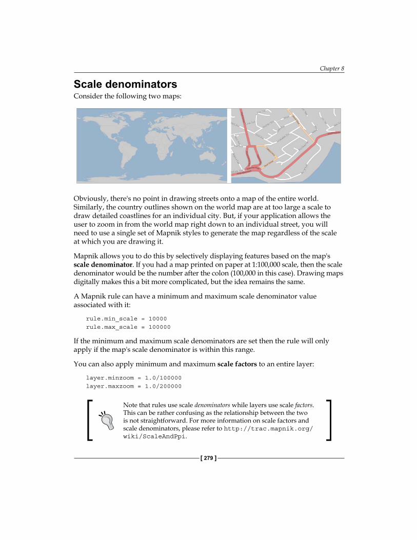
Chapter 8
[ 279 ]
Scale denominatorsConsider the following two maps:
Obviously, there's no point in drawing streets onto a map of the entire world. Similarly, the country outlines shown on the world map are at too large a scale to draw detailed coastlines for an individual city. But, if your application allows the user to zoom in from the world map right down to an individual street, you will need to use a single set of Mapnik styles to generate the map regardless of the scale at which you are drawing it.
Mapnik allows you to do this by selectively displaying features based on the map's scale denominator. If you had a map printed on paper at 1:100,000 scale, then the scale denominator would be the number after the colon (100,000 in this case). Drawing maps digitally makes this a bit more complicated, but the idea remains the same.
A Mapnik rule can have a minimum and maximum scale denominator value associated with it:
rule.min_scale = 10000rule.max_scale = 100000
If the minimum and maximum scale denominators are set then the rule will only apply if the map's scale denominator is within this range.
You can also apply minimum and maximum scale factors to an entire layer:
layer.minzoom = 1.0/100000layer.maxzoom = 1.0/200000
Note that rules use scale denominators while layers use scale factors. This can be rather confusing as the relationship between the two is not straightforward. For more information on scale factors and scale denominators, please refer to http://trac.mapnik.org/wiki/ScaleAndPpi.
Using Python and Mapnik to Generate Maps
[ 280 ]
The whole layer will only be displayed when the map's current scale factor is within this range. This is useful if you have a datasource that should only be used when displaying the map at a certain scale—for example, only using high-resolution shoreline data when the user has zoomed in.
Scale denominators can be used intuitively. For example, a scale denominator value of 200,000 represents a map drawn at roughly 1:200,000 scale. But, this is only an approximation; the actual calculation of a scale denominator has to take into account two important factors:
1. Because Mapnik renders a map as a bitmapped image, the size of the individual pixels within the image comes into play. Since bitmapped images can be displayed on a variety of different computer screens with different pixel sizes, Mapnik uses a standardized rendering pixel size as defined by the Open Geospatial Consortium to define how big a pixel is going to be. This value is 0.28 mm, and is approximately the size of a pixel on modern video displays.
2. The map projection being used can have a huge effect on the calculated scale denominator. Map projections always distort true distances, and a projection that is accurate at the equator may be wildly inaccurate closer to the Poles.
Depending on the projection being used, the formula Mapnik uses to calculate the scale denominator can get rather complicated. Rather than worrying about the formulas, it is much easier just to ask Mapnik to calculate the scale denominator and scale factor for us:
map = mapnik.Map(width, height, projection)map.zoom_to_box(bounds)print map.scale_denominator(), map.scale()
You can then zoom the map to your desired scale and see what the scale factor and denominator are, which you can then plug into your styles to choose which features should be displayed at a given scale denominator range.
Be careful if you are working with multiple projections. A scale denominator that works for one projection may need to be adjusted if you switch projections.
"Else" rulesImagine that you want to draw some features in one color, and all other features in a different color. One way to achieve this is to use Mapnik rules, as shown here:
rule1.filter = mapnik.Filter("[level] = 1")...rule2.filter = mapnik.Filter("[level] != 1")
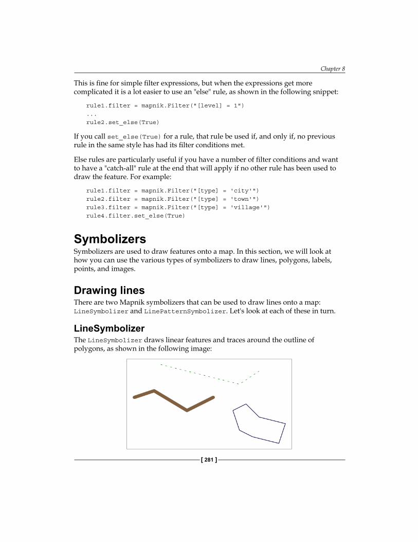
Chapter 8
[ 281 ]
This is fine for simple filter expressions, but when the expressions get more complicated it is a lot easier to use an "else" rule, as shown in the following snippet:
rule1.filter = mapnik.Filter("[level] = 1")...rule2.set_else(True)
If you call set_else(True) for a rule, that rule be used if, and only if, no previous rule in the same style has had its filter conditions met.
Else rules are particularly useful if you have a number of filter conditions and want to have a "catch-all" rule at the end that will apply if no other rule has been used to draw the feature. For example:
rule1.filter = mapnik.Filter("[type] = 'city'")rule2.filter = mapnik.Filter("[type] = 'town'")rule3.filter = mapnik.Filter("[type] = 'village'")rule4.filter.set_else(True)
SymbolizersSymbolizers are used to draw features onto a map. In this section, we will look at how you can use the various types of symbolizers to draw lines, polygons, labels, points, and images.
Drawing linesThere are two Mapnik symbolizers that can be used to draw lines onto a map: LineSymbolizer and LinePatternSymbolizer. Let's look at each of these in turn.
LineSymbolizerThe LineSymbolizer draws linear features and traces around the outline of polygons, as shown in the following image:
Using Python and Mapnik to Generate Maps
[ 282 ]
The LineSymbolizer is one of the most useful of the Mapnik symbolizers. Here is the Python code that created the LineSymbolizer used to draw the dashed line in the last example:
stroke = mapnik.Stroke()stroke.color = mapnik.Color("#008000")stroke.width = 1.0stroke.add_dash(5, 10)symbolizer = mapnik.LineSymbolizer(stroke)
As you can see, the LineSymbolizer uses a Mapnik Stroke object to define how the line will be drawn. To use a LineSymbolizer, you first create the stroke object and set the various options for how you want the line to be drawn. You then create your LineSymbolizer, passing the stroke object to the LineSymbolizer's constructor:
symbolizer = mapnik.LineSymbolizer(stroke)
Let's take a closer look at the various line-drawing options provided by the stroke object.
Line colorBy default, lines are drawn in black. You can change this by setting the stroke's color attribute to a Mapnik color object:
stroke.color = mapnik.Color("red")
For more information about the Mapnik color object, and the various ways in which you can specify a color, please refer to the Using Colors section later in this chapter.
Line widthThe line drawn by a LineSymbolizer will be one pixel wide by default. To change this, set the stroke's width attribute to the desired width, in pixels:
stroke.width = 1.5
Note that you can use fractional line widths for fine-grained control of your line widths.
OpacityYou can change how opaque or transparent the line is by setting the stroke's opacity attribute:
stroke.opacity = 0.8
The opacity can range from 0.0 (completely transparent) to 1.0 (completely opaque). If the opacity is not specified, the line will be completely opaque.
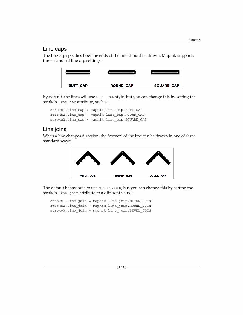
Chapter 8
[ 283 ]
Line capsThe line cap specifies how the ends of the line should be drawn. Mapnik supports three standard line cap settings:
By default, the lines will use BUTT_CAP style, but you can change this by setting the stroke's line_cap attribute, such as:
stroke1.line_cap = mapnik.line_cap.BUTT_CAPstroke2.line_cap = mapnik.line_cap.ROUND_CAPstroke3.line_cap = mapnik.line_cap.SQUARE_CAP
Line joinsWhen a line changes direction, the "corner" of the line can be drawn in one of three standard ways:
The default behavior is to use MITER_JOIN, but you can change this by setting the stroke's line_join attribute to a different value:
stroke1.line_join = mapnik.line_join.MITER_JOINstroke2.line_join = mapnik.line_join.ROUND_JOINstroke3.line_join = mapnik.line_join.BEVEL_JOIN
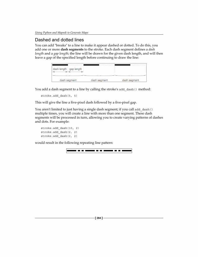
Using Python and Mapnik to Generate Maps
[ 284 ]
Dashed and dotted linesYou can add "breaks" to a line to make it appear dashed or dotted. To do this, you add one or more dash segments to the stroke. Each dash segment defines a dash length and a gap length; the line will be drawn for the given dash length, and will then leave a gap of the specified length before continuing to draw the line:
You add a dash segment to a line by calling the stroke's add_dash() method:
stroke.add_dash(5, 5)
This will give the line a five-pixel dash followed by a five-pixel gap.
You aren't limited to just having a single dash segment; if you call add_dash() multiple times, you will create a line with more than one segment. These dash segments will be processed in turn, allowing you to create varying patterns of dashes and dots. For example:
stroke.add_dash(10, 2)stroke.add_dash(2, 2)stroke.add_dash(2, 2)
would result in the following repeating line pattern:
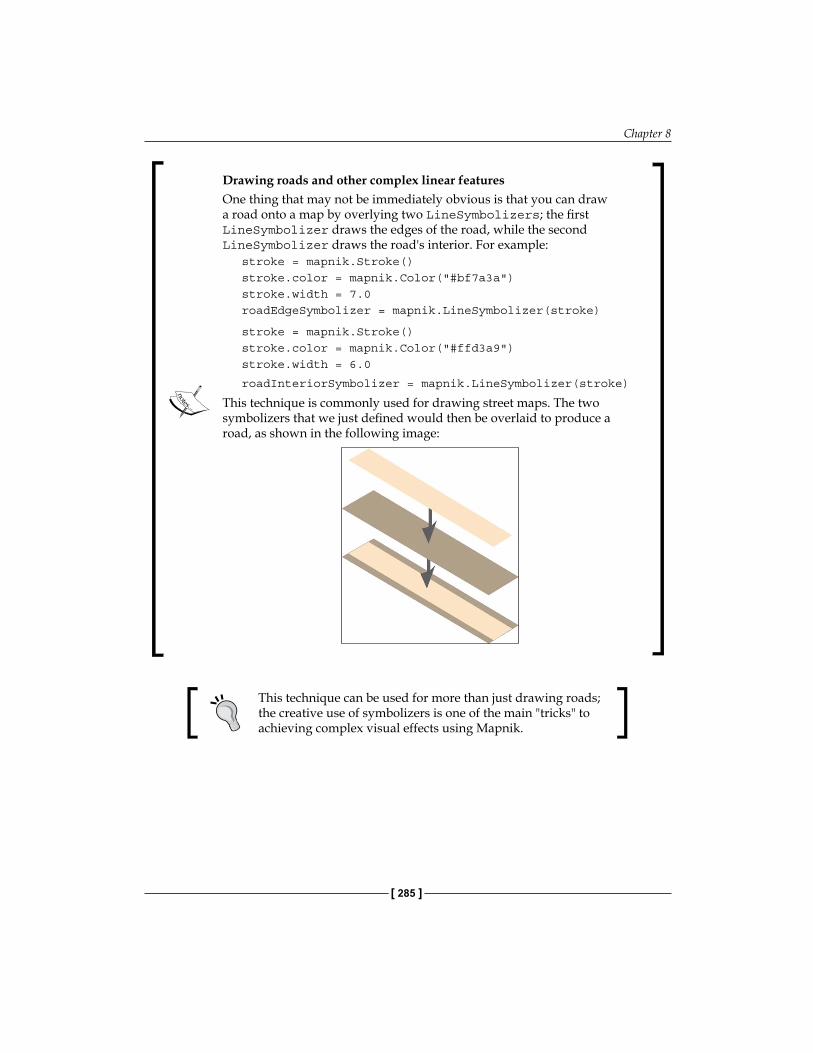
Chapter 8
[ 285 ]
Drawing roads and other complex linear featuresOne thing that may not be immediately obvious is that you can draw a road onto a map by overlying two LineSymbolizers; the first LineSymbolizer draws the edges of the road, while the second LineSymbolizer draws the road's interior. For example:
stroke = mapnik.Stroke()stroke.color = mapnik.Color("#bf7a3a")stroke.width = 7.0roadEdgeSymbolizer = mapnik.LineSymbolizer(stroke)
stroke = mapnik.Stroke()stroke.color = mapnik.Color("#ffd3a9")stroke.width = 6.0
roadInteriorSymbolizer = mapnik.LineSymbolizer(stroke)
This technique is commonly used for drawing street maps. The two symbolizers that we just defined would then be overlaid to produce a road, as shown in the following image:
This technique can be used for more than just drawing roads; the creative use of symbolizers is one of the main "tricks" to achieving complex visual effects using Mapnik.
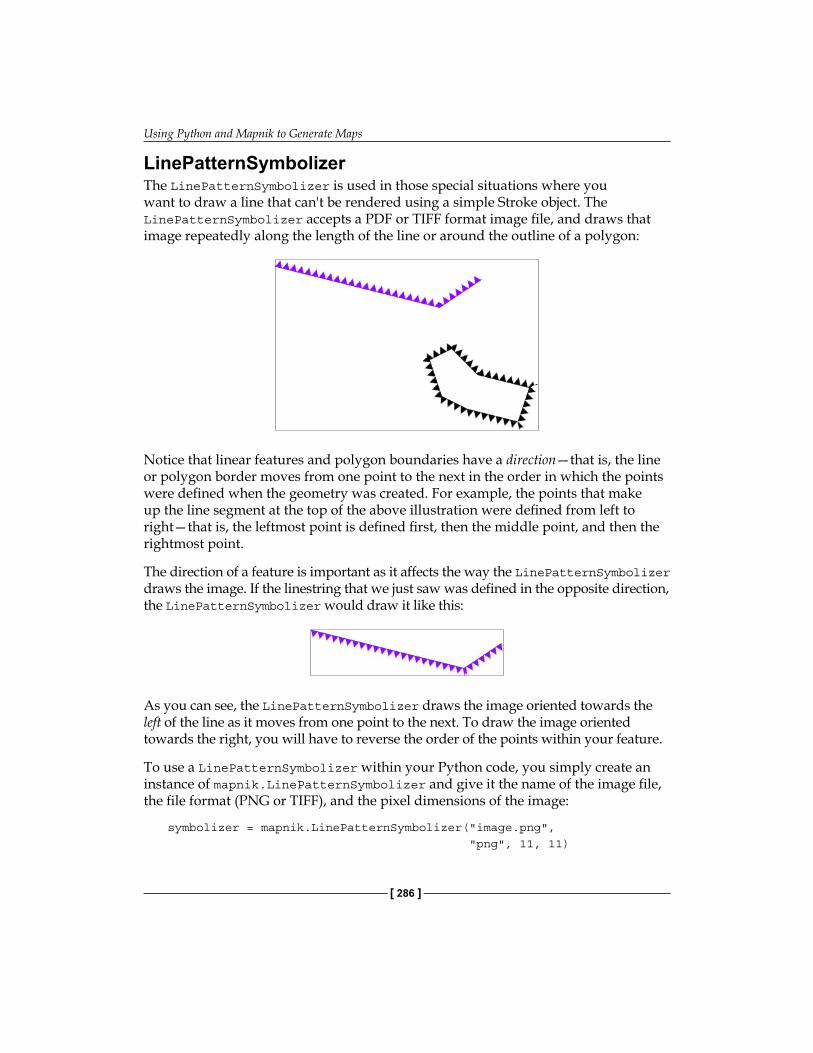
Using Python and Mapnik to Generate Maps
[ 286 ]
LinePatternSymbolizerThe LinePatternSymbolizer is used in those special situations where you want to draw a line that can't be rendered using a simple Stroke object. The LinePatternSymbolizer accepts a PDF or TIFF format image file, and draws that image repeatedly along the length of the line or around the outline of a polygon:
Notice that linear features and polygon boundaries have a direction—that is, the line or polygon border moves from one point to the next in the order in which the points were defined when the geometry was created. For example, the points that make up the line segment at the top of the above illustration were defined from left to right—that is, the leftmost point is defined first, then the middle point, and then the rightmost point.
The direction of a feature is important as it affects the way the LinePatternSymbolizer draws the image. If the linestring that we just saw was defined in the opposite direction, the LinePatternSymbolizer would draw it like this:
As you can see, the LinePatternSymbolizer draws the image oriented towards the left of the line as it moves from one point to the next. To draw the image oriented towards the right, you will have to reverse the order of the points within your feature.
To use a LinePatternSymbolizer within your Python code, you simply create an instance of mapnik.LinePatternSymbolizer and give it the name of the image file, the file format (PNG or TIFF), and the pixel dimensions of the image:
symbolizer = mapnik.LinePatternSymbolizer("image.png", "png", 11, 11)
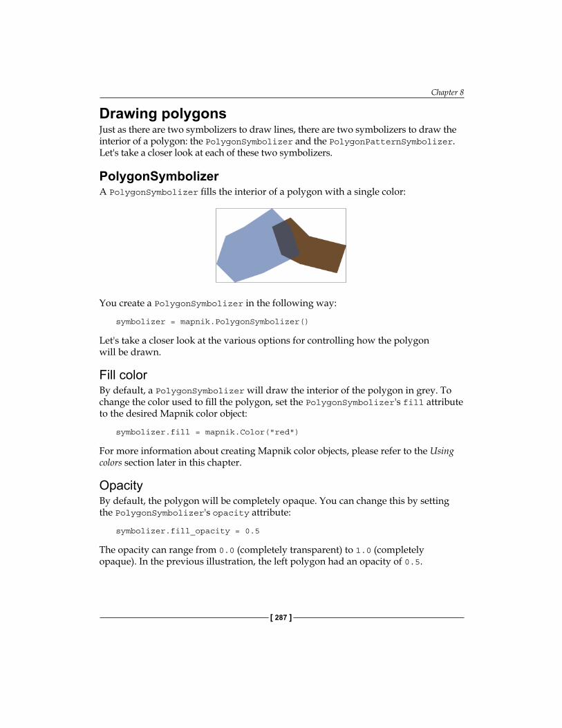
Chapter 8
[ 287 ]
Drawing polygonsJust as there are two symbolizers to draw lines, there are two symbolizers to draw the interior of a polygon: the PolygonSymbolizer and the PolygonPatternSymbolizer. Let's take a closer look at each of these two symbolizers.
PolygonSymbolizerA PolygonSymbolizer fills the interior of a polygon with a single color:
You create a PolygonSymbolizer in the following way:
symbolizer = mapnik.PolygonSymbolizer()
Let's take a closer look at the various options for controlling how the polygon will be drawn.
Fill colorBy default, a PolygonSymbolizer will draw the interior of the polygon in grey. To change the color used to fill the polygon, set the PolygonSymbolizer's fill attribute to the desired Mapnik color object:
symbolizer.fill = mapnik.Color("red")
For more information about creating Mapnik color objects, please refer to the Using colors section later in this chapter.
OpacityBy default, the polygon will be completely opaque. You can change this by setting the PolygonSymbolizer's opacity attribute:
symbolizer.fill_opacity = 0.5
The opacity can range from 0.0 (completely transparent) to 1.0 (completely opaque). In the previous illustration, the left polygon had an opacity of 0.5.
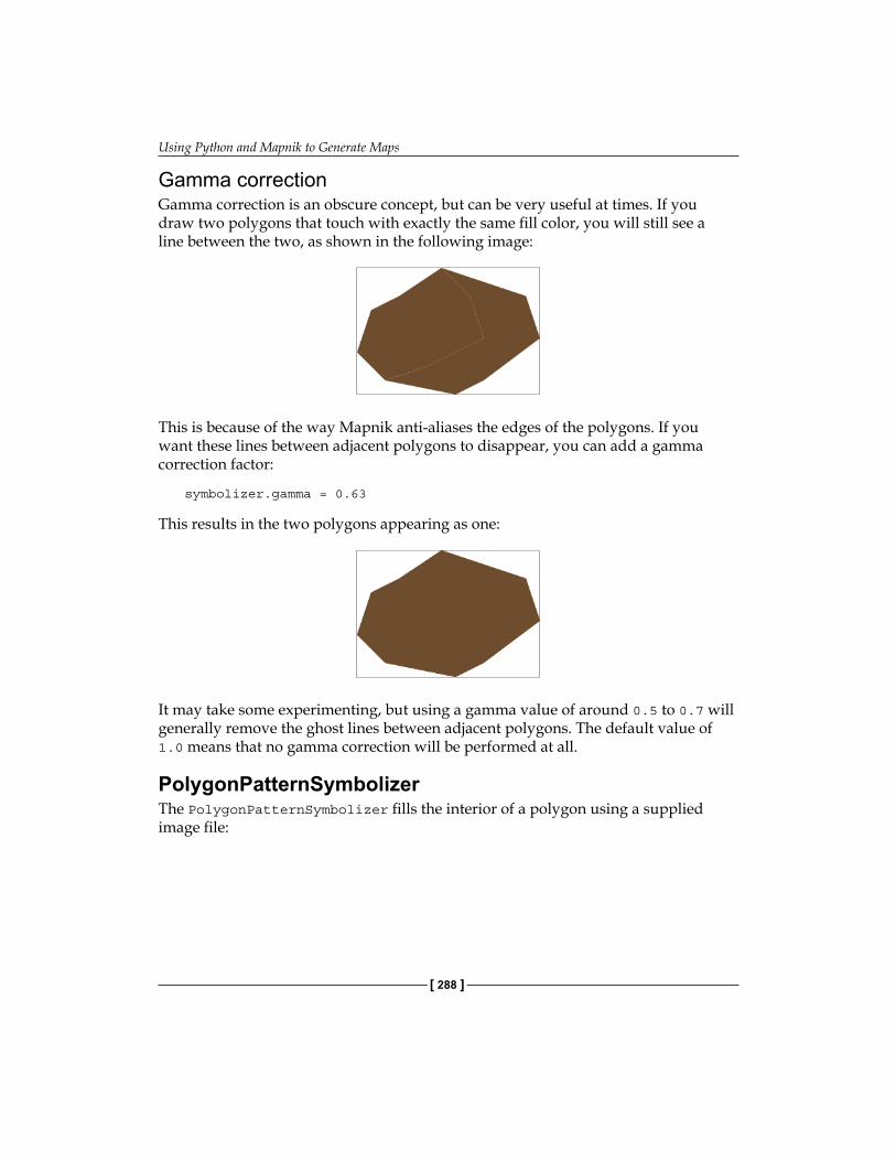
Using Python and Mapnik to Generate Maps
[ 288 ]
Gamma correctionGamma correction is an obscure concept, but can be very useful at times. If you draw two polygons that touch with exactly the same fill color, you will still see a line between the two, as shown in the following image:
This is because of the way Mapnik anti-aliases the edges of the polygons. If you want these lines between adjacent polygons to disappear, you can add a gamma correction factor:
symbolizer.gamma = 0.63
This results in the two polygons appearing as one:
It may take some experimenting, but using a gamma value of around 0.5 to 0.7 will generally remove the ghost lines between adjacent polygons. The default value of 1.0 means that no gamma correction will be performed at all.
PolygonPatternSymbolizerThe PolygonPatternSymbolizer fills the interior of a polygon using a supplied image file:
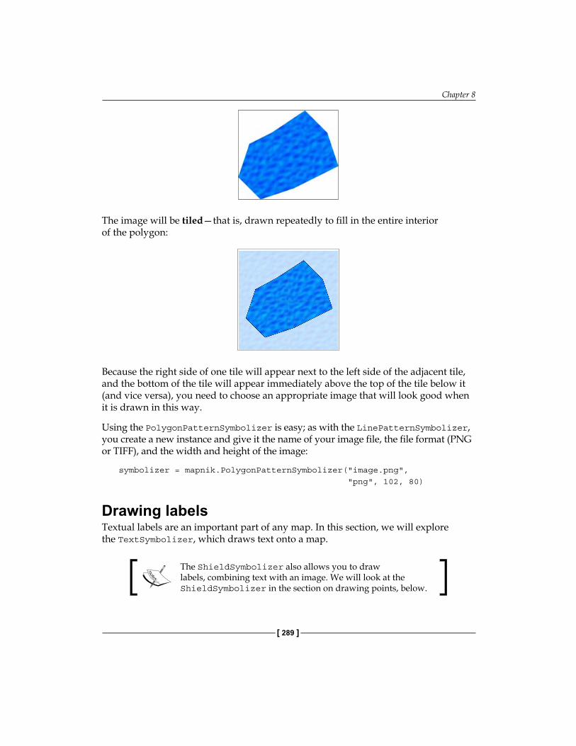
Chapter 8
[ 289 ]
The image will be tiled—that is, drawn repeatedly to fill in the entire interior of the polygon:
Because the right side of one tile will appear next to the left side of the adjacent tile, and the bottom of the tile will appear immediately above the top of the tile below it (and vice versa), you need to choose an appropriate image that will look good when it is drawn in this way.
Using the PolygonPatternSymbolizer is easy; as with the LinePatternSymbolizer, you create a new instance and give it the name of your image file, the file format (PNG or TIFF), and the width and height of the image:
symbolizer = mapnik.PolygonPatternSymbolizer("image.png", "png", 102, 80)
Drawing labelsTextual labels are an important part of any map. In this section, we will explore the TextSymbolizer, which draws text onto a map.
The ShieldSymbolizer also allows you to draw labels, combining text with an image. We will look at the ShieldSymbolizer in the section on drawing points, below.
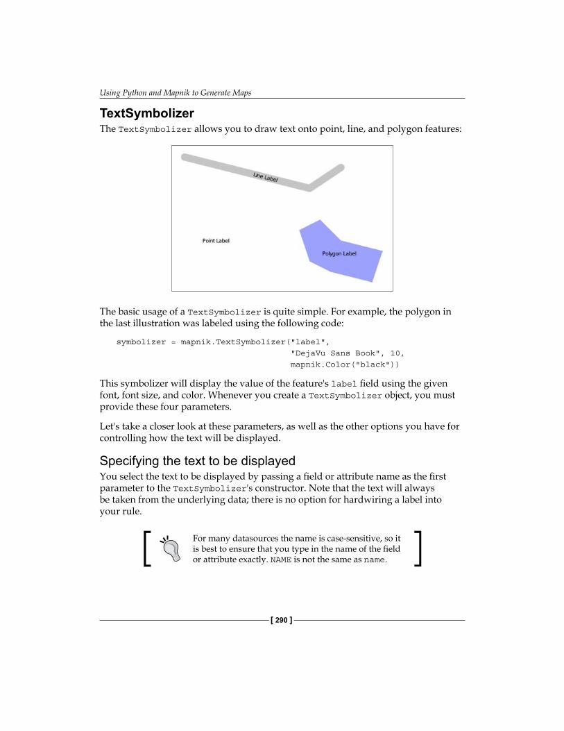
Using Python and Mapnik to Generate Maps
[ 290 ]
TextSymbolizerThe TextSymbolizer allows you to draw text onto point, line, and polygon features:
The basic usage of a TextSymbolizer is quite simple. For example, the polygon in the last illustration was labeled using the following code:
symbolizer = mapnik.TextSymbolizer("label", "DejaVu Sans Book", 10, mapnik.Color("black"))
This symbolizer will display the value of the feature's label field using the given font, font size, and color. Whenever you create a TextSymbolizer object, you must provide these four parameters.
Let's take a closer look at these parameters, as well as the other options you have for controlling how the text will be displayed.
Specifying the text to be displayedYou select the text to be displayed by passing a field or attribute name as the first parameter to the TextSymbolizer's constructor. Note that the text will always be taken from the underlying data; there is no option for hardwiring a label into your rule.
For many datasources the name is case-sensitive, so it is best to ensure that you type in the name of the field or attribute exactly. NAME is not the same as name.
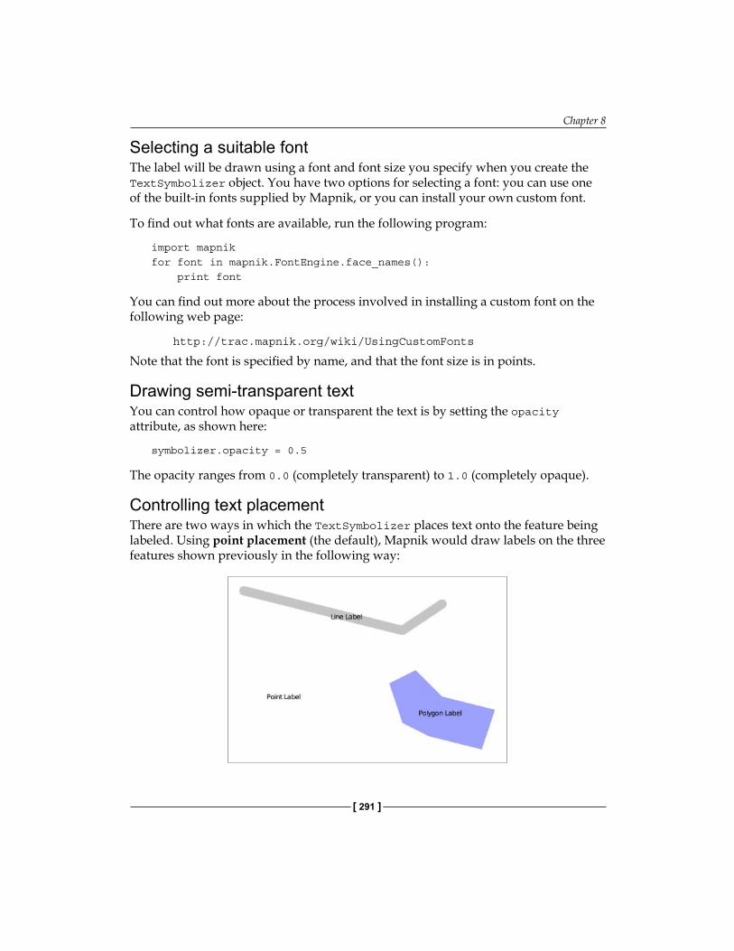
Chapter 8
[ 291 ]
Selecting a suitable fontThe label will be drawn using a font and font size you specify when you create the TextSymbolizer object. You have two options for selecting a font: you can use one of the built-in fonts supplied by Mapnik, or you can install your own custom font.
To find out what fonts are available, run the following program:
import mapnikfor font in mapnik.FontEngine.face_names(): print font
You can find out more about the process involved in installing a custom font on the following web page:
http://trac.mapnik.org/wiki/UsingCustomFonts
Note that the font is specified by name, and that the font size is in points.
Drawing semi-transparent textYou can control how opaque or transparent the text is by setting the opacity attribute, as shown here:
symbolizer.opacity = 0.5
The opacity ranges from 0.0 (completely transparent) to 1.0 (completely opaque).
Controlling text placementThere are two ways in which the TextSymbolizer places text onto the feature being labeled. Using point placement (the default), Mapnik would draw labels on the three features shown previously in the following way:
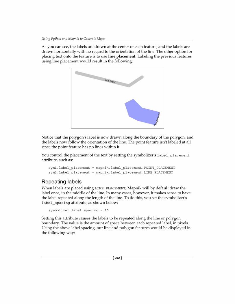
Using Python and Mapnik to Generate Maps
[ 292 ]
As you can see, the labels are drawn at the center of each feature, and the labels are drawn horizontally with no regard to the orientation of the line. The other option for placing text onto the feature is to use line placement. Labeling the previous features using line placement would result in the following:
Notice that the polygon's label is now drawn along the boundary of the polygon, and the labels now follow the orientation of the line. The point feature isn't labeled at all since the point feature has no lines within it.
You control the placement of the text by setting the symbolizer's label_placement attribute, such as:
sym1.label_placement = mapnik.label_placement.POINT_PLACEMENTsym2.label_placement = mapnik.label_placement.LINE_PLACEMENT
Repeating labelsWhen labels are placed using LINE_PLACEMENT, Mapnik will by default draw the label once, in the middle of the line. In many cases, however, it makes sense to have the label repeated along the length of the line. To do this, you set the symbolizer's label_spacing attribute, as shown below:
symbolizer.label_spacing = 30
Setting this attribute causes the labels to be repeated along the line or polygon boundary. The value is the amount of space between each repeated label, in pixels. Using the above label spacing, our line and polygon features would be displayed in the following way:
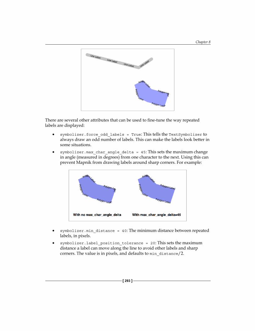
Chapter 8
[ 293 ]
There are several other attributes that can be used to fine-tune the way repeated labels are displayed:
• symbolizer.force_odd_labels = True: This tells the TextSymbolizer to always draw an odd number of labels. This can make the labels look better in some situations.
• symbolizer.max_char_angle_delta = 45: This sets the maximum change in angle (measured in degrees) from one character to the next. Using this can prevent Mapnik from drawing labels around sharp corners. For example:
• symbolizer.min_distance = 40: The minimum distance between repeated labels, in pixels.
• symbolizer.label_position_tolerance = 20: This sets the maximum distance a label can move along the line to avoid other labels and sharp corners. The value is in pixels, and defaults to min_distance/2.
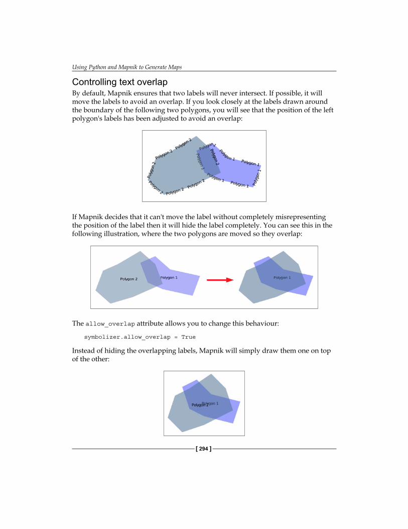
Using Python and Mapnik to Generate Maps
[ 294 ]
Controlling text overlapBy default, Mapnik ensures that two labels will never intersect. If possible, it will move the labels to avoid an overlap. If you look closely at the labels drawn around the boundary of the following two polygons, you will see that the position of the left polygon's labels has been adjusted to avoid an overlap:
If Mapnik decides that it can't move the label without completely misrepresenting the position of the label then it will hide the label completely. You can see this in the following illustration, where the two polygons are moved so they overlap:
The allow_overlap attribute allows you to change this behaviour:
symbolizer.allow_overlap = True
Instead of hiding the overlapping labels, Mapnik will simply draw them one on top of the other:
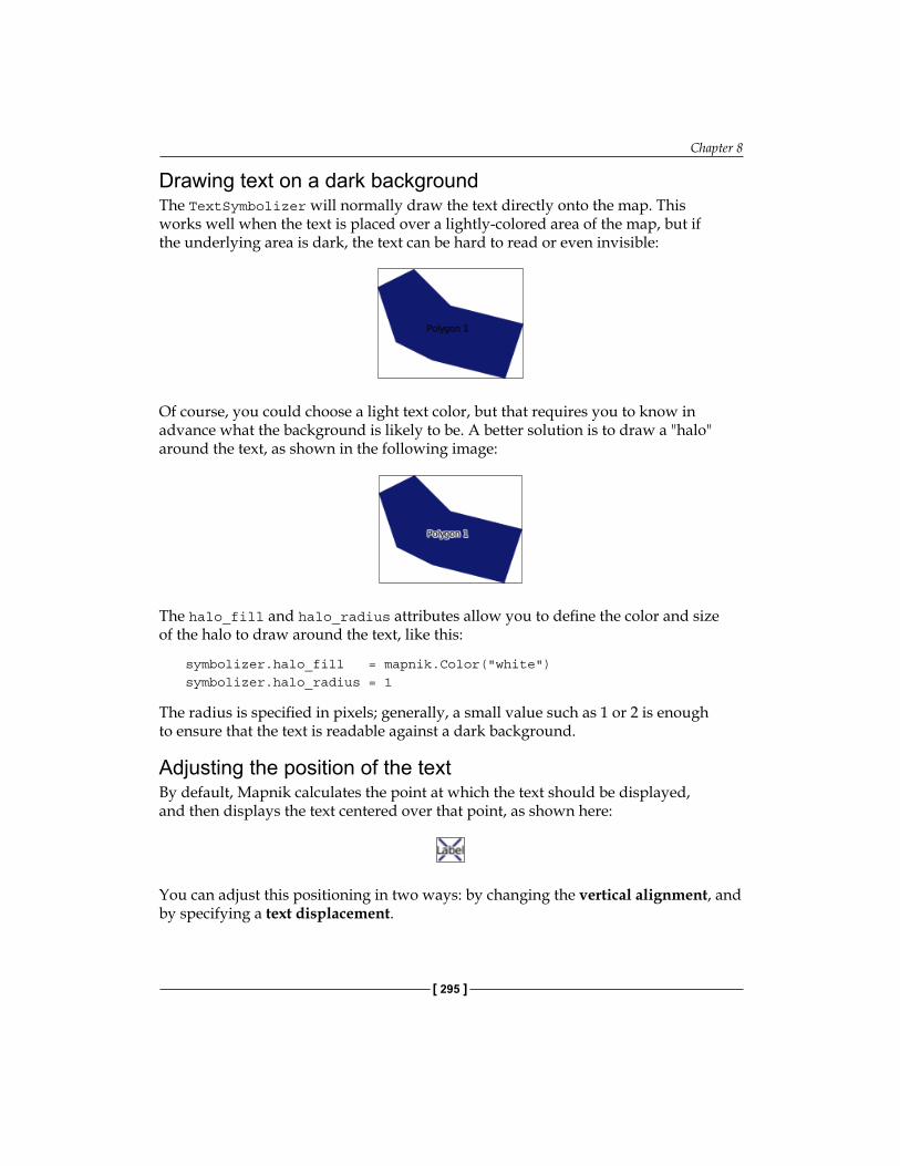
Chapter 8
[ 295 ]
Drawing text on a dark backgroundThe TextSymbolizer will normally draw the text directly onto the map. This works well when the text is placed over a lightly-colored area of the map, but if the underlying area is dark, the text can be hard to read or even invisible:
Of course, you could choose a light text color, but that requires you to know in advance what the background is likely to be. A better solution is to draw a "halo" around the text, as shown in the following image:
The halo_fill and halo_radius attributes allow you to define the color and size of the halo to draw around the text, like this:
symbolizer.halo_fill = mapnik.Color("white")symbolizer.halo_radius = 1
The radius is specified in pixels; generally, a small value such as 1 or 2 is enough to ensure that the text is readable against a dark background.
Adjusting the position of the textBy default, Mapnik calculates the point at which the text should be displayed, and then displays the text centered over that point, as shown here:
You can adjust this positioning in two ways: by changing the vertical alignment, and by specifying a text displacement.
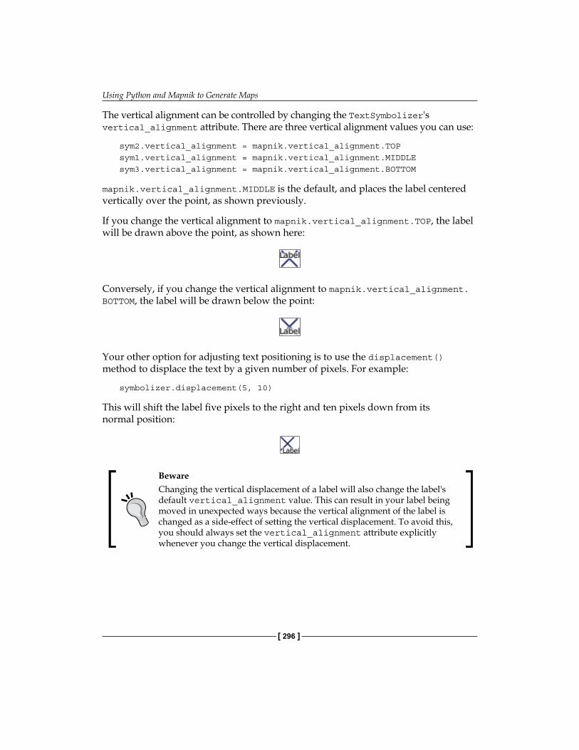
Using Python and Mapnik to Generate Maps
[ 296 ]
The vertical alignment can be controlled by changing the TextSymbolizer's vertical_alignment attribute. There are three vertical alignment values you can use:
sym2.vertical_alignment = mapnik.vertical_alignment.TOPsym1.vertical_alignment = mapnik.vertical_alignment.MIDDLEsym3.vertical_alignment = mapnik.vertical_alignment.BOTTOM
mapnik.vertical_alignment.MIDDLE is the default, and places the label centered vertically over the point, as shown previously.
If you change the vertical alignment to mapnik.vertical_alignment.TOP, the label will be drawn above the point, as shown here:
Conversely, if you change the vertical alignment to mapnik.vertical_alignment.BOTTOM, the label will be drawn below the point:
Your other option for adjusting text positioning is to use the displacement() method to displace the text by a given number of pixels. For example:
symbolizer.displacement(5, 10)
This will shift the label five pixels to the right and ten pixels down from its normal position:
BewareChanging the vertical displacement of a label will also change the label's default vertical_alignment value. This can result in your label being moved in unexpected ways because the vertical alignment of the label is changed as a side-effect of setting the vertical displacement. To avoid this, you should always set the vertical_alignment attribute explicitly whenever you change the vertical displacement.
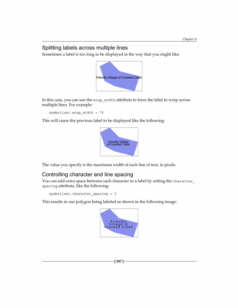
Chapter 8
[ 297 ]
Splitting labels across multiple linesSometimes a label is too long to be displayed in the way that you might like:
In this case, you can use the wrap_width attribute to force the label to wrap across multiple lines. For example:
symbolizer.wrap_width = 70
This will cause the previous label to be displayed like the following:
The value you specify is the maximum width of each line of text, in pixels.
Controlling character and line spacingYou can add extra space between each character in a label by setting the character_spacing attribute, like the following:
symbolizer.character_spacing = 3
This results in our polygon being labeled as shown in the following image:
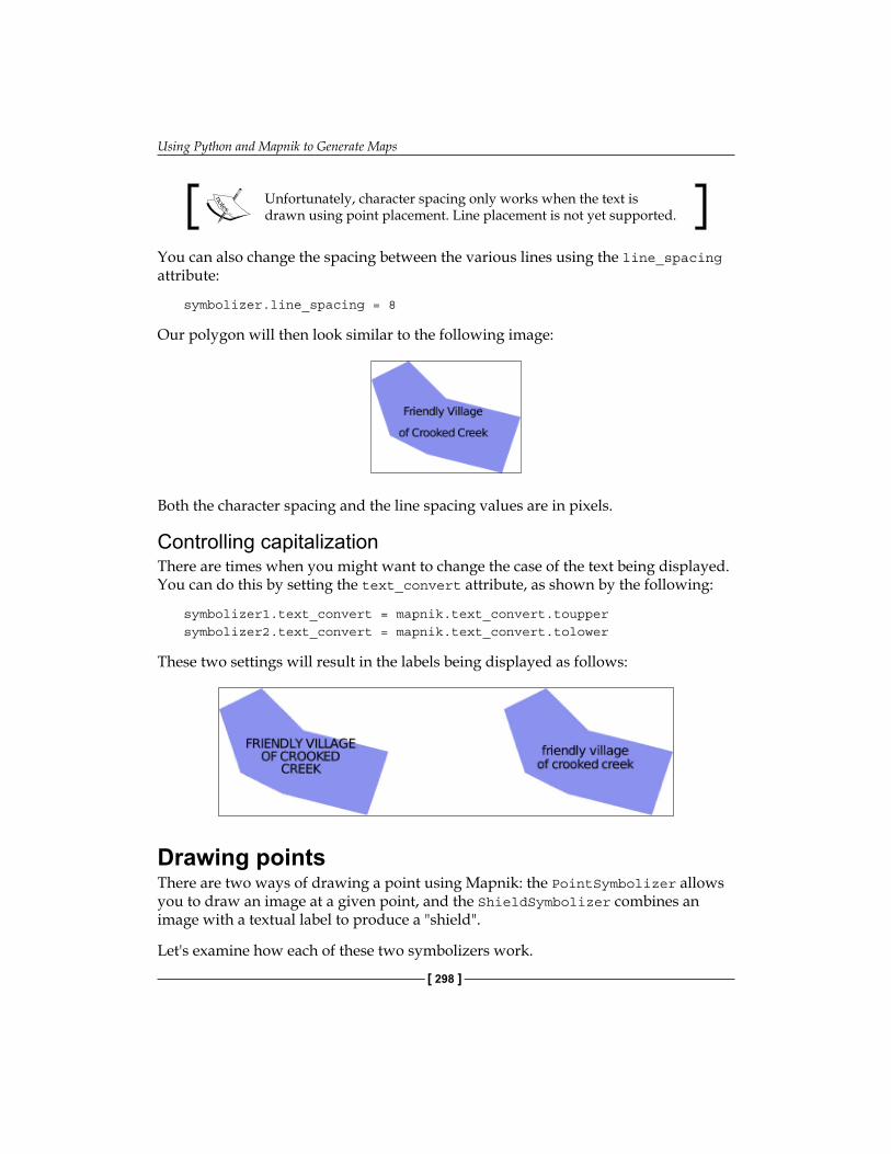
Using Python and Mapnik to Generate Maps
[ 298 ]
Unfortunately, character spacing only works when the text is drawn using point placement. Line placement is not yet supported.
You can also change the spacing between the various lines using the line_spacing attribute:
symbolizer.line_spacing = 8
Our polygon will then look similar to the following image:
Both the character spacing and the line spacing values are in pixels.
Controlling capitalizationThere are times when you might want to change the case of the text being displayed. You can do this by setting the text_convert attribute, as shown by the following:
symbolizer1.text_convert = mapnik.text_convert.touppersymbolizer2.text_convert = mapnik.text_convert.tolower
These two settings will result in the labels being displayed as follows:
Drawing pointsThere are two ways of drawing a point using Mapnik: the PointSymbolizer allows you to draw an image at a given point, and the ShieldSymbolizer combines an image with a textual label to produce a "shield".
Let's examine how each of these two symbolizers work.
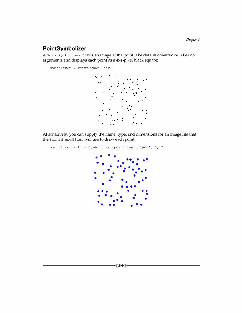
Chapter 8
[ 299 ]
PointSymbolizerA PointSymbolizer draws an image at the point. The default constructor takes no arguments and displays each point as a 4x4-pixel black square:
symbolizer = PointSymbolizer()
Alternatively, you can supply the name, type, and dimensions for an image file that the PointSymbolizer will use to draw each point:
symbolizer = PointSymbolizer("point.png", "png", 9, 9)
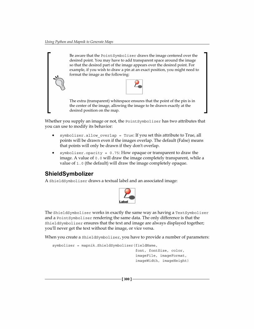
Using Python and Mapnik to Generate Maps
[ 300 ]
Be aware that the PointSymbolizer draws the image centered over the desired point. You may have to add transparent space around the image so that the desired part of the image appears over the desired point. For example, if you wish to draw a pin at an exact position, you might need to format the image as the following:
The extra (transparent) whitespace ensures that the point of the pin is in the center of the image, allowing the image to be drawn exactly at the desired position on the map.
Whether you supply an image or not, the PointSymbolizer has two attributes that you can use to modify its behavior:
• symbolizer.allow_overlap = True: If you set this attribute to True, all points will be drawn even if the images overlap. The default (False) means that points will only be drawn if they don't overlap.
• symbolizer.opacity = 0.75: How opaque or transparent to draw the image. A value of 0.0 will draw the image completely transparent, while a value of 1.0 (the default) will draw the image completely opaque.
ShieldSymbolizerA ShieldSymbolizer draws a textual label and an associated image:
The ShieldSymbolizer works in exactly the same way as having a TextSymbolizer and a PointSymbolizer rendering the same data. The only difference is that the ShieldSymbolizer ensures that the text and image are always displayed together; you'll never get the text without the image, or vice versa.
When you create a ShieldSymbolizer, you have to provide a number of parameters:
symbolizer = mapnik.ShieldSymbolizer(fieldName, font, fontSize, color, imageFile, imageFormat, imageWidth, imageHeight)
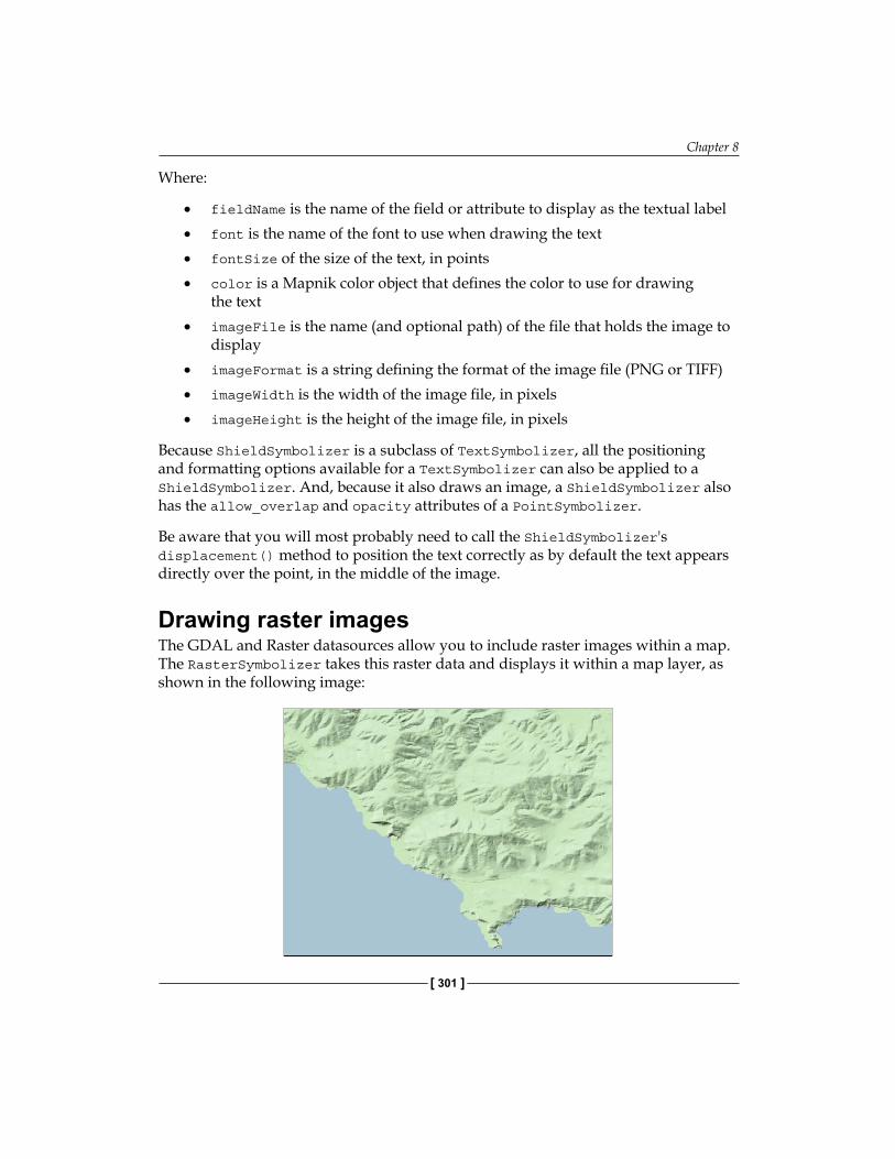
Chapter 8
[ 301 ]
Where:
• fieldName is the name of the field or attribute to display as the textual label• font is the name of the font to use when drawing the text• fontSize of the size of the text, in points• color is a Mapnik color object that defines the color to use for drawing
the text• imageFile is the name (and optional path) of the file that holds the image to
display• imageFormat is a string defining the format of the image file (PNG or TIFF)• imageWidth is the width of the image file, in pixels• imageHeight is the height of the image file, in pixels
Because ShieldSymbolizer is a subclass of TextSymbolizer, all the positioning and formatting options available for a TextSymbolizer can also be applied to a ShieldSymbolizer. And, because it also draws an image, a ShieldSymbolizer also has the allow_overlap and opacity attributes of a PointSymbolizer.
Be aware that you will most probably need to call the ShieldSymbolizer's displacement() method to position the text correctly as by default the text appears directly over the point, in the middle of the image.
Drawing raster imagesThe GDAL and Raster datasources allow you to include raster images within a map. The RasterSymbolizer takes this raster data and displays it within a map layer, as shown in the following image:
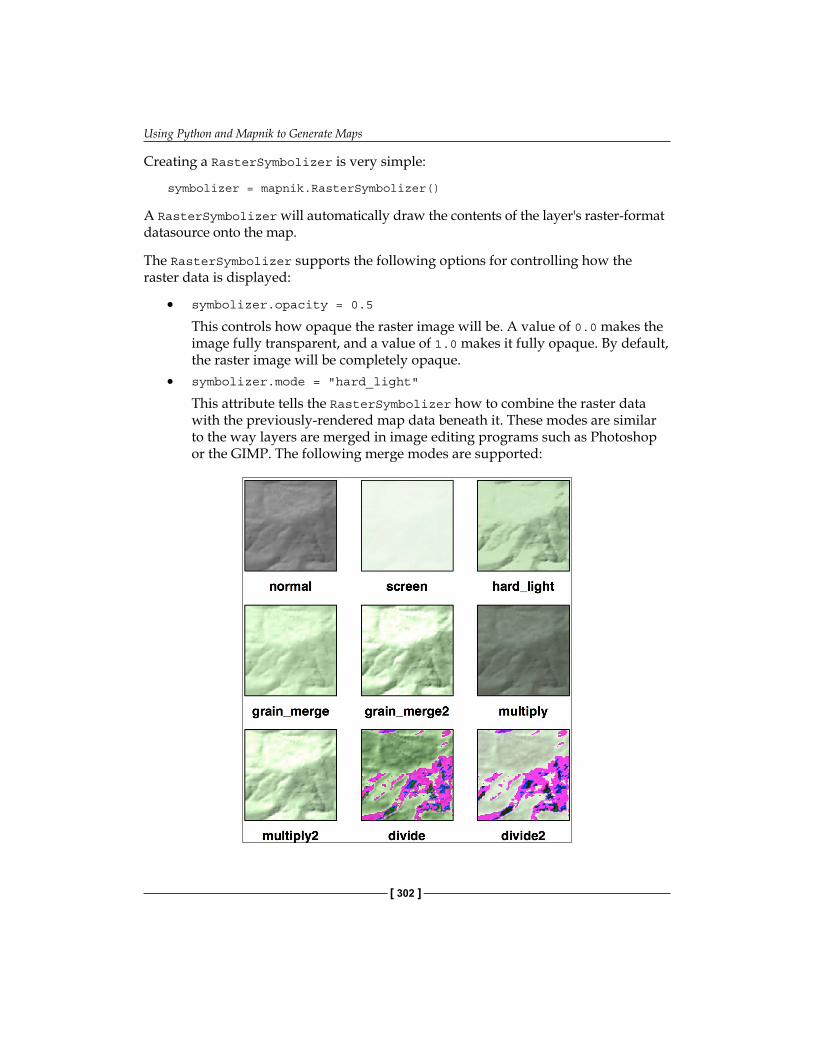
Using Python and Mapnik to Generate Maps
[ 302 ]
Creating a RasterSymbolizer is very simple:
symbolizer = mapnik.RasterSymbolizer()
A RasterSymbolizer will automatically draw the contents of the layer's raster-format datasource onto the map.
The RasterSymbolizer supports the following options for controlling how the raster data is displayed:
• symbolizer.opacity = 0.5
This controls how opaque the raster image will be. A value of 0.0 makes the image fully transparent, and a value of 1.0 makes it fully opaque. By default, the raster image will be completely opaque.
• symbolizer.mode = "hard_light"
This attribute tells the RasterSymbolizer how to combine the raster data with the previously-rendered map data beneath it. These modes are similar to the way layers are merged in image editing programs such as Photoshop or the GIMP. The following merge modes are supported:
Chapter 8
[ 303 ]
• symbolizer.scaling = "fast"
This allows you to control the algorithm used to scale the raster image data. The available options are: fast (uses the nearest-neighbor algorithm), bilinear (uses bilinear interpolation across all four color channels), and bilinear8 (uses bilinear interpolation for just a single color channel).
Mapnik does not currently support on-the-fly reprojection of raster data. If you need to generate a map using a projection that is different from the raster data's projection, you will need to reproject the raster data before it can be displayed, for example by using gdalwarp.
One of the main uses for a RasterSymbolizer is to display a shaded relief background such as the one shown previously. This gives the viewer a good impression of the underlying terrain.
The previous image was created using a Digital Elevation Map (DEM-format) data file taken from the National Elevation Dataset. This file was processed using the gdaldem utility with the hillshade option to create a shaded relief grayscale image. This image was then displayed using a RasterSymbolizer set to hard_light mode, laid on top of a pale green background with the coastline defined from the GSHHS shoreline database. You may find this process useful if you want to display a shaded relief image as a background for your map.
Using colorsMany of the Mapnik symbolizers require you to supply a color value. These color values are defined using the mapnik.Color class. Instances of mapnik.Color can be created in one of four ways:
• mapnik.Color(r, g, b, a)
Creates a color object by supplying separate red, green, blue, and alpha (opacity) values. Each of these values should be in the range 0 to 255.
• mapnik.Color(r, g, b)
Creates a color object by supplying red, green, and blue components. Each value should be in the range 0 to 255. The resulting object will be completely opaque.
• mapnik.Color(colorName)
Creates a color object by specifying a standard CSS color name. A complete list of the available color names can be found at: http://www.w3.org/TR/css3-color/#svg-color.
Using Python and Mapnik to Generate Maps
[ 304 ]
• mapnik.Color(colorCode)
Creates a color object using an HTML color code. For example, #806040 is medium brown.
Maps and layersOnce you have set up your datasources, symbolizers, rules, and styles, you can combine them into Mapnik layers and place the various layers together onto a map. To do this, you first create a mapnik.Map object to represent the map as a whole:
map = mapnik.Map(width, height, srs)
You supply the width and height of the map image you want to generate, in pixels, and an optional Proj 4 format initialization string in srs. If you do not specify a spatial reference system, the map will use +proj=latlong +datum=WGS84 (unprojected lat/long coordinates on the WGS84 datum).
After creating the map, you set the map's background color, and add your various styles to the map by calling the map.append_style() method:
map.background = mapnik.Color('white')
map.append_style("countryStyle", countryStyle)map.append_style("roadStyle", roadStyle)map.append_style("pointStyle", pointStyle)map.append_style("rasterStyle", rasterStyle)...
You also need to create the various layers within the map. To do this, you create a mapnik.Layer object to represent each map layer:
layer = mapnik.Layer(layerName, srs)
Each layer is given a unique name, and can optionally have a spatial reference associated with it. The srs string is a Proj.4 format initialization string; if no spatial reference is given, the layer will use +proj=latlong +datum=WGS84.
Once you have created your map layer, you assign it a datasource and choose the style(s) that will apply to that layer, identifying each style by name:
layer.datasource = myDatasource
layer.styles.append("countryStyle")layer.styles.append("rasterStyle")...
Chapter 8
[ 305 ]
Finally, you add your new layer to the map:
map.layers.append(layer)
Let's take a closer look at some of the optional methods and attributes of the Mapnik Map and Layer objects. These can be useful when manipulating map layers, and for setting up rules and layers which selectively apply based on the map's current scale factor.
Map attributes and methodsThe mapnik.Map class provides several additional methods and attributes that you may find useful:
• map.envelope()
This method returns a mapnik.Envelope object representing the area of the map that is to be displayed. The mapnik.Envelope object supports a number of useful methods and attributes, but most importantly includes minx, miny, maxx, and maxy attributes. These define the map's bounding box in map coordinates.
• map.aspect_fix_mode = mapnik.aspect_fix.GROW_CANVAS
This controls how Mapnik adjusts the map if the aspect ratio of the map's bounds does not match the aspect ratio of the rendered map image. The following values are supported:
° GROW_BBOX expands the map's bounding box to match the aspect ratio of the generated image. This is the default behavior.
° GROW_CANVAS expands the generated image to match the aspect ratio of the bounding box.
° SHRINK_BBOX shrinks the map's bounding box to match the aspect ratio of the generated image.
° SHRINK_CANVAS shrinks the generated image to match the aspect ratio of the map's bounding box.
° ADJUST_BBOX_HEIGHT expands or shrinks the height of the map's bounding box, while keeping the width constant, to match the aspect ratio of the generated image.
° ADJUST_BBOX_WIDTH expands or shrinks the width of the map's bounding box, while keeping the height constant, to match the aspect ratio of the generated image.
° ADJUST_CANVAS_HEIGHT expands or shrinks the height of the generated image, while keeping the width constant, to match the aspect ratio of the map's bounding box.
Using Python and Mapnik to Generate Maps
[ 306 ]
° ADJUST_CANVAS_WIDTH expands or shrinks the width of the generated image, while keeping the height constant, to match the aspect ratio of the map's bounding box.
• map.scale_denominator()
Returns the current scale denominator used to generate the map. The scale denominator depends on the map's bounds and the size of the rendered image.
• map.scale()
Returns the current scale factor used by the map. The scale factor depends on the map's bounds and the size of the rendered image.
• map.zoom_all()
Sets the map's bounding box to encompass the bounding box of each of the map's layers. This ensures that all the map data will appear on the map.
• map.zoom_to_box(mapnik.Envelope(minX, minY, maxX, maxY))
Sets the map's bounding box to the given values. Note that minX, minY, maxX, and maxY are all in the map's coordinate system.
Layer attributes and methodsThe mapnik.Layer class has the following useful attributes and methods:
• layer.envelope()
This method returns a mapnik.Envelope object representing the rectangular area of the map that encompasses all the layer's data. The mapnik.Envelope object supports a number of useful methods and attributes, but most importantly includes minx, miny, maxx, and maxy attributes.
• layer.active = False
This can be used to hide a layer within the map.• layer.minzoom = 1.0/100000
This sets the minimum scale factor that must apply if the layer is to appear within the map. If this is not set, the layer will not have a minimum scale factor.
• layer.maxzoom = 1.0/10000
This sets the maximum scale factor that must apply if the layer is to be drawn onto the map. If this is not set, the layer will not have a maximum scale factor.
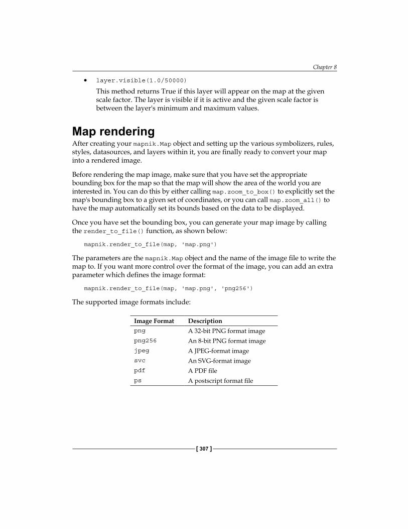
Chapter 8
[ 307 ]
• layer.visible(1.0/50000)
This method returns True if this layer will appear on the map at the given scale factor. The layer is visible if it is active and the given scale factor is between the layer's minimum and maximum values.
Map renderingAfter creating your mapnik.Map object and setting up the various symbolizers, rules, styles, datasources, and layers within it, you are finally ready to convert your map into a rendered image.
Before rendering the map image, make sure that you have set the appropriate bounding box for the map so that the map will show the area of the world you are interested in. You can do this by either calling map.zoom_to_box() to explicitly set the map's bounding box to a given set of coordinates, or you can call map.zoom_all() to have the map automatically set its bounds based on the data to be displayed.
Once you have set the bounding box, you can generate your map image by calling the render_to_file() function, as shown below:
mapnik.render_to_file(map, 'map.png')
The parameters are the mapnik.Map object and the name of the image file to write the map to. If you want more control over the format of the image, you can add an extra parameter which defines the image format:
mapnik.render_to_file(map, 'map.png', 'png256')
The supported image formats include:
Image Format Descriptionpng A 32-bit PNG format imagepng256 An 8-bit PNG format imagejpeg A JPEG-format imagesvc An SVG-format imagepdf A PDF fileps A postscript format file
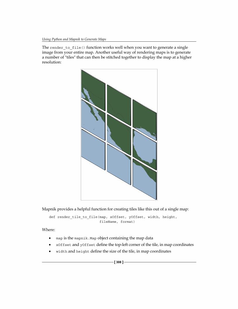
Using Python and Mapnik to Generate Maps
[ 308 ]
The render_to_file() function works well when you want to generate a single image from your entire map. Another useful way of rendering maps is to generate a number of "tiles" that can then be stitched together to display the map at a higher resolution:
Mapnik provides a helpful function for creating tiles like this out of a single map:
def render_tile_to_file(map, xOffset, yOffset, width, height, fileName, format)
Where:
• map is the mapnik.Map object containing the map data• xOffset and yOffset define the top-left corner of the tile, in map coordinates• width and height define the size of the tile, in map coordinates
Chapter 8
[ 309 ]
• fileName is the name of the file to save the tiled image into• format is the file format to use for saving this tile
You can simply call this function repeatedly to create the individual tiles for your map. For example:
for x in range(NUM_TILES_ACROSS): for y in range(NUM_TILES_DOWN): xOffset = TILE_SIZE * x yOffset = TILE_SIZE * y tileName = "tile_%d_%d.png" % (x, y) mapnik.render_tile_to_file(map, xOffset, yOffset, TILE_SIZE, TILE_SIZE, tileName, "png")
Another way of rendering a map is to use a Mapnik.Image object to hold the rendered map data in memory. You can then extract the raw image data from the Image object, such as:
image = mapnik.Image(MAP_WIDTH, MAP_HEIGHT)mapnik.render(map, image)imageData = image.tostring('png')
MapGenerator revisitedNow that we have examined the Python interface to Mapnik, let's use this knowledge to take a closer look at the mapGenerator.py module used in Chapter 7. As well as being a more comprehensive example of creating maps programmatically, the mapGenerator.py module suggests ways in which you can write your own wrapper around Mapnik to simplify the creation of a map using Python code.
The MapGenerator's interfaceThe mapGenerator.py module defines just one function, generateMap(), which allows you to create a simple map that is stored in a temporary file on disk. The method signature for the generateMap() function looks like this:
def generateMap(datasource, minX, minY, maxX, maxY, mapWidth, mapHeight, hiliteExpr=None, background="#8080a0", hiliteLine="#000000", hiliteFill="#408000", normalLine="#404040", normalFill="#a0a0a0", points=None)
Using Python and Mapnik to Generate Maps
[ 310 ]
The parameters are as follows:
• datasource is a dictionary defining the datasource to use for this map. This dictionary should have at least one entry, type, which defines the type of datasource. The following datasource types are supported: OGR, PostGIS, and SQLite. Any additional entries in this dictionary will be passed as keyword parameters to the datasource initializer.
• minX, minY, maxX, and maxY define the bounding box for the area to display, in map coordinates.
• mapWidth and mapHeight are the width and height of the image to generate, in pixels.
• hiliteExpr is a Mapnik filter expression to use to identify the feature(s) to be highlighted.
• background is the HTML color code to use for the background of the map.• hiliteLine and hiliteFill are the HTML color codes to use for the line
and fill for the highlighted features.• normalLine and normalFill are the HTML color codes to use for the line
and fill for the non-highlighted features.• points, if defined, should be a list of (long, lat, name) tuples identifying
points to display on the map.
Because many of these keyword parameters have default values, creating a simple map only requires the datasource, bounding box, and map dimensions to be specified. Everything else is optional.
The generateMap() function creates a new map based on the given parameters, and stores the result as a PNG format image file in a temporary map cache directory. Upon completion, it returns the name and relative path to the newly-rendered image file.
So much for the public interface to the mapGenerator.py module. Let's take a look inside to see how it works.
Creating the main map layerThe module starts by creating a mapnik.Map object to hold the generated map. We set the background color at the same time:
map = mapnik.Map(mapWidth, mapHeight, '+proj=longlat +datum=WGS84')map.background = mapnik.Color(background)
Chapter 8
[ 311 ]
We next have to set up the Mapnik datasource to load our map data from. To simplify the job of accessing a datasource, the datasource parameter includes the type of datasource, as well as any additional entries which are passed as keyword parameters directly to the Mapnik datasource initializer:
srcType = datasource['type']del datasource['type']
if srcType == "OGR": source = mapnik.Ogr(**datasource)elif srcType == "PostGIS": source = mapnik.PostGIS(**datasource)elif srcType == "SQLite": source = mapnik.SQLite(**datasource)
We then create our Layer object, and start defining the style that is used to draw the map data onto the map:
layer = mapnik.Layer("Layer")layer.datasource = source
style = mapnik.Style()
We next set up a rule that only applies to the highlighted features:
rule = mapnik.Rule()if hiliteExpr != None: rule.filter = mapnik.Filter(hiliteExpr)
This rule will use the "highlight" line and fill colors:
rule.symbols.append(mapnik.PolygonSymbolizer( mapnik.Color(hiliteFill)))rule.symbols.append(mapnik.LineSymbolizer( mapnik.Stroke(mapnik.Color(hiliteLine), 0.1)))
We then add this rule to the style, and create another rule that only applies to the non-highlighted features:
style.rules.append(rule)
rule = mapnik.Rule()rule.set_else(True)
This rule will use the "normal" line and fill colors:
rule.symbols.append(mapnik.PolygonSymbolizer( mapnik.Color(normalFill)))rule.symbols.append(mapnik.LineSymbolizer( mapnik.Stroke(mapnik.Color(normalLine), 0.1)))
Using Python and Mapnik to Generate Maps
[ 312 ]
We then add this rule to the style, and add the style to the map and layer:
style.rules.append(rule) map.append_style("Map Style", style)layer.styles.append("Map Style")
Finally, the layer is added to the map:
map.layers.append(layer)
Displaying points on the mapOne of the features of the generateMap() function is that it can take a list of points and display them directly onto the map without having to store those points into a database. This is done through the use of a PointDataSource datasource and a ShieldSymbolizer to draw the points onto the map:
if points != None: pointDatasource = mapnik.PointDatasource() for long,lat,name in points: pointDatasource.add_point(long, lat, "name", name)
layer = mapnik.Layer("Points") layer.datasource = pointDatasource
style = mapnik.Style() rule = mapnik.Rule()
pointImgFile = os.path.join(os.path.dirname(__file__), "point.png")
shield = mapnik.ShieldSymbolizer( "name", "DejaVu Sans Bold", 10, mapnik.Color("#000000"), pointImgFile, "png", 9, 9) shield.displacement(0, 7) shield.unlock_image = True rule.symbols.append(shield)
style.rules.append(rule)
map.append_style("Point Style", style) layer.styles.append("Point Style")
map.layers.append(layer)
Chapter 8
[ 313 ]
Notice that the path to the point.png file is calculated as an absolute path based on the location of the mapGenerator.py module itself (via the __file__ global). This is done because the module can be called as part of a CGI script, and CGI scripts do not have a current working directory.
Rendering the mapBecause the mapGenerator.py module is designed to be used within a CGI script, the module makes use of a temporary map cache to hold the generated image files. Before it can render the map image, the generateMap() function has to create the map cache if it doesn't already exist, and create a temporary file within the cache directory to hold the generated map:
scriptDir = os.path.dirname(__file__)cacheDir = os.path.join(scriptDir, "..", "mapCache")if not os.path.exists(cacheDir): os.mkdir(cacheDir)fd,filename = tempfile.mkstemp(".png", dir=cacheDir)os.close(fd)
Finally, we are ready to render the map into an image file, and return back to the caller the relative path to the generated map file:
map.zoom_to_box(mapnik.Envelope(minX, minY, maxX, maxY))mapnik.render_to_file(map, filename, "png")
return "../mapCache/" + os.path.basename(filename)
What the map generator teaches usWhile in many ways the mapGenerator.py module is quite simplistic and designed specifically to meet the needs of the DISTAL application presented in the previous chapter, it is worth examining this module in depth because it shows how the principle of encapsulation can be used to hide Mapnik's complexity and simplify the process of map generation. Using the generateMap() function is infinitely easier than creating all the datasources, layers, symbolizers, rules, and styles each time a map has to be generated.
Using Python and Mapnik to Generate Maps
[ 314 ]
It would be a relatively easy task to design a more generic map generator that could handle a variety of datasources and map layers, as well as various ways of returning the results, without having to exhaustively define every object by hand. Designing and implementing such a module would be very worthwhile if you want to use Mapnik extensively from your Python programs. Hopefully, this section has given you some ideas about how you can proceed with implementing your own high-level Mapnik wrapper module.
Map definition filesThere is one final approach to using Mapnik that is worth examining. In addition to creating your symbolizers, rules, styles, and layers programmatically, Mapnik allows you to store all of this information using a map definition file. This is an XML-format file that defines the various Mapnik objects used to generate a map. For example, consider the following Python program to create a simple world map using the World Borders Dataset:
import mapnik
map = mapnik.Map(800, 400)map.background = mapnik.Color("steelblue")
style = mapnik.Style()rule = mapnik.Rule()polySymbolizer = mapnik.PolygonSymbolizer()polySymbolizer.fill = mapnik.Color("ghostwhite")
stroke = mapnik.Stroke()stroke.color = mapnik.Color("gray")stroke.width = 0.1lineSymbolizer = mapnik.LineSymbolizer(stroke)
rule.symbols.append(polySymbolizer)rule.symbols.append(lineSymbolizer)style.rules.append(rule)map.append_style("My Style", style)
datasource = mapnik.Shapefile(file="TM_WORLD_BORDERS-0.3/" + "TM_WORLD_BORDERS-0.3.shp")
layer = mapnik.Layer("layer")layer.datasource = datasourcelayer.styles.append("My Style")
map.layers.append(layer)
map.zoom_to_box(mapnik.Envelope(-180, -90, +180, +90))mapnik.render_to_file(map, "map.png")
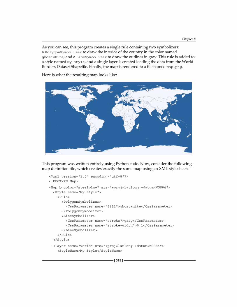
Chapter 8
[ 315 ]
As you can see, this program creates a single rule containing two symbolizers: a PolygonSymbolizer to draw the interior of the country in the color named ghostwhite, and a LineSymbolizer to draw the outlines in gray. This rule is added to a style named My Style, and a single layer is created loading the data from the World Borders Dataset Shapefile. Finally, the map is rendered to a file named map.png.
Here is what the resulting map looks like:
This program was written entirely using Python code. Now, consider the following map definition file, which creates exactly the same map using an XML stylesheet:
<?xml version="1.0" encoding="utf-8"?><!DOCTYPE Map>
<Map bgcolor="steelblue" srs="+proj=latlong +datum=WGS84"> <Style name="My Style"> <Rule> <PolygonSymbolizer> <CssParameter name="fill">ghostwhite</CssParameter> </PolygonSymbolizer> <LineSymbolizer> <CssParameter name="stroke">gray</CssParameter> <CssParameter name="stroke-width">0.1</CssParameter> </LineSymbolizer> </Rule> </Style>
<Layer name="world" srs="+proj=latlong +datum=WGS84"> <StyleName>My Style</StyleName>
Using Python and Mapnik to Generate Maps
[ 316 ]
<Datasource> <Parameter name="type">shape</Parameter> <Parameter name="file">TM_WORLD_BORDERS-0.3/TM_WORLD_BORDERS- 0.3.shp</Parameter> </Datasource> </Layer></Map>
To use this stylesheet, you call the load_map() function to load the contents of the map definition file into a Mapnik Map object before rendering it, as shown here:
map = mapnik.Map(800, 400)mapnik.load_map(map, "mapDefinition.xml")map.zoom_to_box(mapnik.Envelope(-180, -90, +180, +90))mapnik.render_to_file(map, "map.png")
Either approach is perfectly valid. You may prefer to do all your coding in Python (with or without a wrapper module), or you might like the more compact XML stylesheet definition. With only a few exceptions, anything you can do in Python can be done with the XML stylesheets, and vice versa.
Unlike the Python bindings, the format for the XML definition file is thoroughly documented. More information on the syntax of the map definition file can be found at:
http://trac.mapnik.org/wiki/XMLConfigReference
You don't have to choose between doing all your map definition in the XML or doing it all in Python; Mapnik supports a hybrid approach where you can define as much or as little in the XML file, and use Python to do the rest. For example, you might like to define your Mapnik styles in the XML file, and use Python to define the datasources and map layers. To do this, you would set up your map definition file, as shown here:
<?xml version="1.0" encoding="utf-8"?><!DOCTYPE Map>
<Map bgcolor="steelblue" srs="+proj=latlong +datum=WGS84"> <Style name="My Style"> <Rule> <PolygonSymbolizer> <CssParameter name="fill">ghostwhite</CssParameter> </PolygonSymbolizer> <LineSymbolizer> <CssParameter name="stroke">gray</CssParameter> <CssParameter name="stroke-width">0.1</CssParameter> </LineSymbolizer> </Rule> </Style></Map>
Chapter 8
[ 317 ]
Your Python code would then look like this:
import mapnik
map = mapnik.Map(800, 400)mapnik.load_map(map, "sampleXMLStylesheet.xml")
datasource = mapnik.Shapefile(file="TM_WORLD_BORDERS-0.3/" + "TM_WORLD_BORDERS-0.3.shp")
layer = mapnik.Layer("layer")layer.datasource = datasourcelayer.styles.append("My Style")
map.layers.append(layer)
map.zoom_to_box(mapnik.Envelope(-180, -90, +180, +90))mapnik.render_to_file(map, "map.png")
Notice how we simply exclude the <Layer> section from the XML file, and then create our map layers using Python.
This hybrid approach has the advantage of separating out the visual representation of the map from the code used to generate it: the XML file defines the various styles to use for rendering the map, but doesn't include any map-generation logic itself. Indeed, you can completely change the appearance of the map just by changing the XML stylesheet, without having to change a single line of code in your program. This is very similar to the way HTML templating engines separate form and function within a web application.
SummaryIn this chapter, we have explored the Mapnik map-generation toolkit in depth. We learned:
• That Mapnik is a powerful and flexible toolkit for generating a variety of maps• That Mapnik uses the painter's algorithm to draw the various parts of a map in
the correct order• That rendering a map requires you to set up map layers and their associated
datasources, in the order in which they will appear on the map.• That datasources act as a "bridge" between Mapnik and your geo-spatial data• That Mapnik can directly use Shapefiles, PostGIS databases, GDAL-
compatible raster image files, OGR-compatible vector data, SQLite/SpatiaLite databases, and OpenStreetMap files as datasources
• That OGR's virtual datasource (VRT) format can be used by Mapnik to read data from a MySQL database
Using Python and Mapnik to Generate Maps
[ 318 ]
• That the PointDatasource allows you to manually create a set of data points and place them onto a map, without having to store them in a database or shapefile
• That each layer has one or more styles associated with it• That each style consists of one or more rules• That each rule has a list of symbolizers telling Mapnik how to draw the layer's
features onto the map• That a rule can have an optional filter that selects the features the rule
applies to• That you can selectively enable or disable rules and layers based on the
map's scale• That the LineSymbolizer allows you to draw solid and dotted lines onto a
map, following linear features and the boundaries of polygons• That the LinePatternSymbolizer uses an image file to draw more complex
images along the length of a line or polygon boundary• That the PolygonSymbolizer draws the interior of a polygon with a solid
color• That the PolygonPatternSymbolizer allows you to fill the interior of a
polygon with a repeating image• That the TextSymbolizer can be used to draw labels onto point, line, and
polygon features• That the PointSymbolizer draws images onto the map at coordinates
specified by point features• That the ShieldSymbolizer combines the features of a TextSymbolizer
with a PointSymbolizer to draw an image and label together• That the RasterSymbolizer can be used to draw raster-format images onto
a map• That once you have set up your various datasources, symbolizers, rules, and
styles, you combine them into Layer objects and place the various layers together onto a Map object
• That a layer's styles are referred to by name, with the style definitions themselves being stored in the map
• That you tell the map which area of the world to display, typically by calling the map.zoom_to_box() method, and then call mapnik.render_to_file() to render the map into an image file
Chapter 8
[ 319 ]
• That you can use the render_tile_to_file() function to create multiple high-resolution tiles out of a single map
• That you can use a Mapnik.Image object to work with a rendered map image in memory rather than having to store it on disk
• That the mapGenerator.py module defined in Chapter 7 is an example of a higher-level wrapper that can hide Mapnik's complexity and make it easier to use
• That you can use a map definition file as a simpler way of creating maps without having to define all the symbolizers, rules, styles, datasources, and layers in Python
• That you can use a map definition file as a stylesheet, separating the logic of building a map from the way it is formatted, in the same way that an HTML templating engine separates form and content in a web application
In the next chapter, we will explore some of the frameworks available for creating web-based geo-spatial applications.


Web Frameworks for Python Geo-Spatial Development
In this chapter, we will examine various options for developing web-based geo-spatial applications. We will explore a number of important concepts used by web applications, and geo-spatial web applications in particular, as well as studying some of the important open protocols used by these applications and a number of tools that you can use to implement your own web-based geo-spatial systems.
In particular, we will:
• Examine the architecture used by web applications• Learn about web application stacks• Explore the concept of a "full stack" web application framework• Learn about web services• See how map rendering can be implemented as a standalone web service• Learn how tile caching can be used to improve performance• See how web servers act as a frontend to a web application• Explore how JavaScript user interface libraries can enhance a web
application's user interface• See how "slippy maps" can be created using an application stack• Examine the web frameworks available for developing geo-spatial
applications• Learn about some of the important open protocols for working with geo-
spatial data within a web application• Explore some of the major tools and frameworks available for building your
own geo-spatial web applications
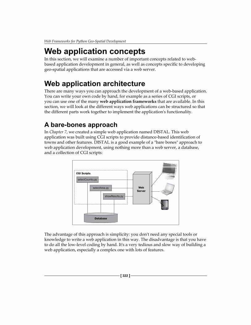
Web Frameworks for Python Geo-Spatial Development
[ 322 ]
Web application conceptsIn this section, we will examine a number of important concepts related to web-based application development in general, as well as concepts specific to developing geo-spatial applications that are accessed via a web server.
Web application architectureThere are many ways you can approach the development of a web-based application. You can write your own code by hand, for example as a series of CGI scripts, or you can use one of the many web application frameworks that are available. In this section, we will look at the different ways web applications can be structured so that the different parts work together to implement the application's functionality.
A bare-bones approachIn Chapter 7, we created a simple web application named DISTAL. This web application was built using CGI scripts to provide distance-based identification of towns and other features. DISTAL is a good example of a "bare bones" approach to web application development, using nothing more than a web server, a database, and a collection of CGI scripts:
The advantage of this approach is simplicity: you don't need any special tools or knowledge to write a web application in this way. The disadvantage is that you have to do all the low-level coding by hand. It's a very tedious and slow way of building a web application, especially a complex one with lots of features.
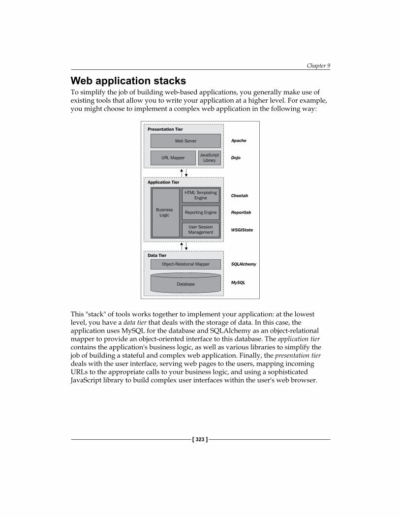
Chapter 9
[ 323 ]
Web application stacksTo simplify the job of building web-based applications, you generally make use of existing tools that allow you to write your application at a higher level. For example, you might choose to implement a complex web application in the following way:
This "stack" of tools works together to implement your application: at the lowest level, you have a data tier that deals with the storage of data. In this case, the application uses MySQL for the database and SQLAlchemy as an object-relational mapper to provide an object-oriented interface to this database. The application tier contains the application's business logic, as well as various libraries to simplify the job of building a stateful and complex web application. Finally, the presentation tier deals with the user interface, serving web pages to the users, mapping incoming URLs to the appropriate calls to your business logic, and using a sophisticated JavaScript library to build complex user interfaces within the user's web browser.
Web Frameworks for Python Geo-Spatial Development
[ 324 ]
Different terms are sometimes used for these three tiers. For example, the data tier is sometimes called the data access layer, and the application tier is sometimes called the business logic layer. The concept is the same, however.
Don't be too concerned about the details of this particular application's architecture—the main thing to realize is that there is a "stack" of tools all working together, where each tool makes use of the tools below it. Also, notice the complexity of this system: this application depends on a lot of different tools and libraries. Developing, deploying, and upgrading an application like this can be challenging because it has so many different parts.
Web application frameworksTo avoid the complexity of mixing and matching so many different parts, web developers have created various frameworks that combine tools to provide a complete web development system. Instead of having to select, install, and deploy ten different libraries, you can simply choose a complete framework that brings a known good set of libraries together, and adds its own logic to provide a complete "batteries included" web development experience. Most of these toolkits provide you with built-in logic to handle tasks such as:
• Defining and migrating your database schema• Keeping track of user sessions, and handling user authentication• Building sophisticated user interfaces, often using AJAX to handle complex
widgets within the user's browser• Automatically allowing users to create, read, update, and delete records in
the database (the so-called CRUD interface)• Simplifying the creation of database-driven applications through standard
templates and recipes
There is a lot more to these frameworks, but the important thing to remember is that they aim to provide a "full stack" of features to allow developers to quickly implement the most common aspects of a web application with a minimum of fuss. They aim to provide rapid application development (RAD) for web-based systems.
There are a number of Python-based web application frameworks available, including TurboGears, Django, Zope, Web2py, and Webware. Some of these frameworks also include extensions for developing geo-spatial web applications.

Chapter 9
[ 325 ]
Web servicesA web service is a piece of software that has an application programming interface (API) that is accessed via the HTTP protocol. Web services generally implement the behind-the-scenes functionality used by other systems; they don't generally have an interface that allows end users to access them directly.
Web services are accessed via a URL; other parts of the system send a request to this URL and receive back a response, often in the form of XML or JSON encoded data, which is then used for further processing.
Types of web servicesThere are two main types of web services you are likely to encounter: RESTful web services, which use parts of the URL itself to tell the web service what to do, and "big web services" that typically use the SOAP protocol to communicate with the outside world.REST stands for REpresentational State Transfer. This protocol uses sub-paths within the URL to define the request to be made. For example, a web service might use the following URL to return information about a customer:http://myserver.com/webservice/customer/123
In this example, customer defines what type of information you want, and 123 is the internal ID of the desired customer. RESTful web services are very easy to implement and use, and are becoming increasingly popular with web application developers.A "big web service", on the other hand, has just one URL for the entire web service. A request is sent to this URL as an XML-format message, and the response is sent back, also as an XML-formatted message. The SOAP protocol is often used to describe the message format and how the web service should behave. Big web services are popular in large commercial systems, despite being more complex than their RESTful equivalent.
Let's take a look at a simple but useful web service. This CGI script, called greatCircleDistance.py, calculates and returns the great-circle distance between two coordinates on the Earth's surface. Here is the full source code for this web service:
#!/usr/bin/python
import cgiimport pyproj
form = cgi.FieldStorage()
lat1 = float(form['lat1'].value)long1 = float(form['long1'].value)
Web Frameworks for Python Geo-Spatial Development
[ 326 ]
lat2 = float(form['lat2'].value)long2 = float(form['long2'].value)
geod = pyproj.Geod(ellps="WGS84")angle1,angle2,distance = geod.inv(long1, lat1, long2, lat2)
print 'Content-Type: text/plain'printprint distance
Because this is intended to be used by other systems rather than end users, the two coordinates are passed as query parameters, and the resulting distance (in meters) is returned as the body of the HTTP response. Because the returned value is a single number, there is no need to encode the results using XML or JSON; instead, the distance is returned as plain text.
Let's now look at a simple Python program that calls this web service:
import urllib
URL = "http://127.0.0.1:8000/cgi-bin/greatCircleDistance.py"
params = urllib.urlencode({'lat1' : 53.478948, # Manchester. 'long1' : -2.246017, 'lat2' : 53.411142, # Liverpool. 'long2' : -2.977638})
f = urllib.urlopen(URL, params)response = f.read()f.close()
print response
Running this program tells us the distance in meters between these two coordinates, which happen to be the locations of Manchester and Liverpool in England:
% python callWebService.py
49194.46315
While this might not seem very exciting, web services are an extremely important part of web-based development. When developing your own web-based geo-spatial applications, you may well make use of existing web services, and potentially implement your own web services as part of your web application.
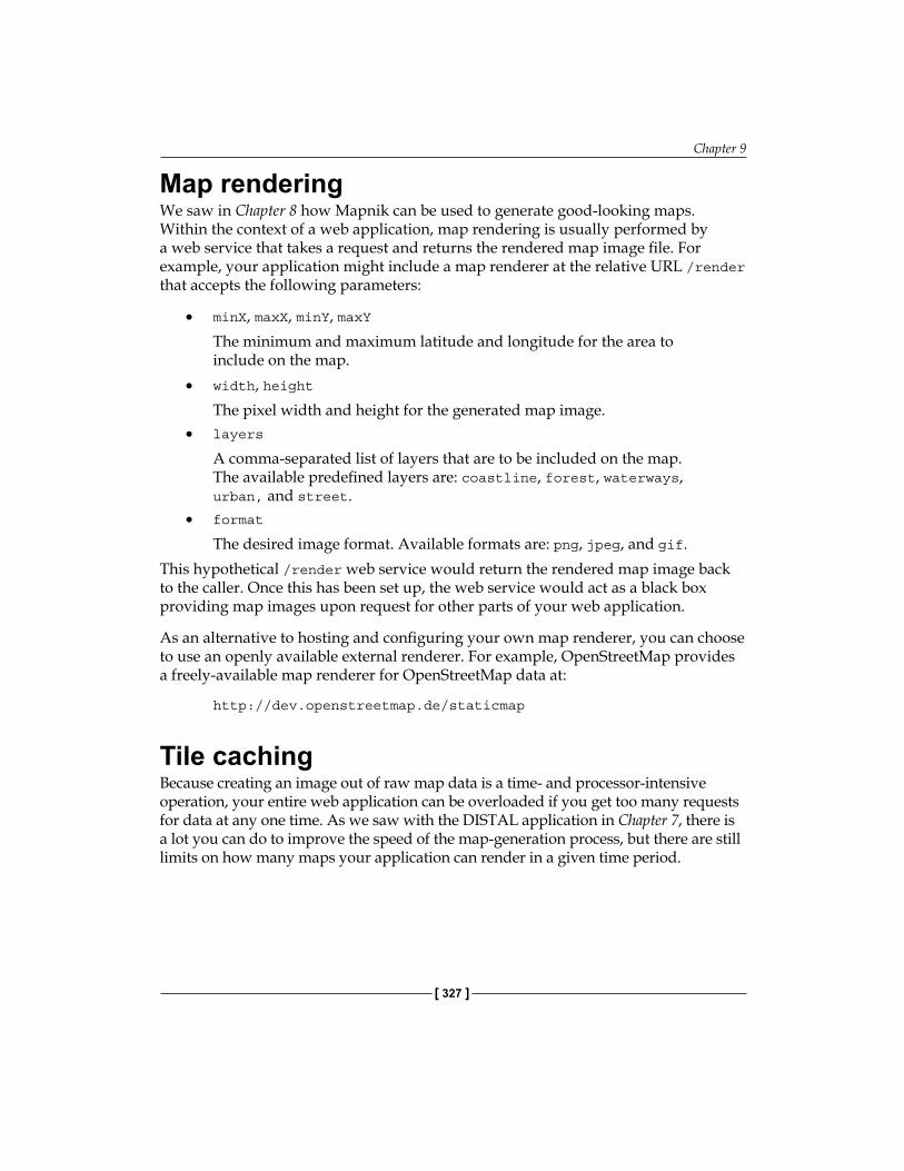
Chapter 9
[ 327 ]
Map renderingWe saw in Chapter 8 how Mapnik can be used to generate good-looking maps. Within the context of a web application, map rendering is usually performed by a web service that takes a request and returns the rendered map image file. For example, your application might include a map renderer at the relative URL /render that accepts the following parameters:
• minX, maxX, minY, maxYThe minimum and maximum latitude and longitude for the area to include on the map.
• width, heightThe pixel width and height for the generated map image.
• layers
A comma-separated list of layers that are to be included on the map. The available predefined layers are: coastline, forest, waterways, urban, and street.
• format
The desired image format. Available formats are: png, jpeg, and gif.This hypothetical /render web service would return the rendered map image back to the caller. Once this has been set up, the web service would act as a black box providing map images upon request for other parts of your web application.
As an alternative to hosting and configuring your own map renderer, you can choose to use an openly available external renderer. For example, OpenStreetMap provides a freely-available map renderer for OpenStreetMap data at:
http://dev.openstreetmap.de/staticmap
Tile cachingBecause creating an image out of raw map data is a time- and processor-intensive operation, your entire web application can be overloaded if you get too many requests for data at any one time. As we saw with the DISTAL application in Chapter 7, there is a lot you can do to improve the speed of the map-generation process, but there are still limits on how many maps your application can render in a given time period.
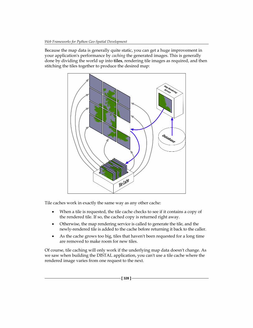
Web Frameworks for Python Geo-Spatial Development
[ 328 ]
Because the map data is generally quite static, you can get a huge improvement in your application's performance by caching the generated images. This is generally done by dividing the world up into tiles, rendering tile images as required, and then stitching the tiles together to produce the desired map:
Tile caches work in exactly the same way as any other cache:
• When a tile is requested, the tile cache checks to see if it contains a copy of the rendered tile. If so, the cached copy is returned right away.
• Otherwise, the map rendering service is called to generate the tile, and the newly-rendered tile is added to the cache before returning it back to the caller.
• As the cache grows too big, tiles that haven't been requested for a long time are removed to make room for new tiles.
Of course, tile caching will only work if the underlying map data doesn't change. As we saw when building the DISTAL application, you can't use a tile cache where the rendered image varies from one request to the next.
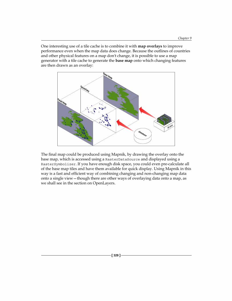
Chapter 9
[ 329 ]
One interesting use of a tile cache is to combine it with map overlays to improve performance even when the map data does change. Because the outlines of countries and other physical features on a map don't change, it is possible to use a map generator with a tile cache to generate the base map onto which changing features are then drawn as an overlay:
The final map could be produced using Mapnik, by drawing the overlay onto the base map, which is accessed using a RasterDataSource and displayed using a RasterSymbolizer. If you have enough disk space, you could even pre-calculate all of the base map tiles and have them available for quick display. Using Mapnik in this way is a fast and efficient way of combining changing and non-changing map data onto a single view—though there are other ways of overlaying data onto a map, as we shall see in the section on OpenLayers.

Web Frameworks for Python Geo-Spatial Development
[ 330 ]
Web serversIn many ways, a web server is the least interesting part of a web application: the web server listens for incoming HTTP requests from web browsers and returns either static content or the dynamic output of a program in response to these requests:
There are many different types of web servers, ranging from the pure-Python SimpleHTTPServer included in the Python Standard Library, through more fully-featured servers such as CherryPy, and of course the most popular industrial-strength web server of them all: Apache.
One of the main consequences of your choice of web server is how fast your application will run. Obviously, a pure-Python web server will be slower than a compiled high-performance server such as Apache. In addition, writing CGI scripts in Python will cause the entire Python interpreter to be started up every time a request is received—so, even if you are running a high performance web server, your application can still run slowly if you don't structure your application correctly. A slow web server doesn't just affect your application's responsiveness: if your server runs slowly, it won't take many requests to overload the server.
Another consequence of your choice of web server is how your application's code interacts with the end user. The HTTP protocol itself is stateless—that is, each incoming request is completely separate, and a web page handler has no way of knowing what the user has done previously unless you explicitly code your pages in such a way that the application's state is passed from one request to the next (for example, using hidden HTML form fields as we did in our implementation of the DISTAL application in Chapter 7).
Because some web servers run your Python code only when a request comes in, there is often no way of having a long-running process sitting in the background that keeps track of the user's state or performs other capabilities for your web page handlers. For example, an in-memory cache might be used to improve performance, but you can't easily use such a cache with CGI scripts as the entire interpreter is restarted for every incoming HTTP request.

Chapter 9
[ 331 ]
One of the big advantages of using a web application framework is that you don't need to worry about these sorts of issues: in many cases, the web framework itself will include a simple web server you can use for development, and provides a standard way of using industry-standard web servers when you deploy your application. The challenges of performance, keeping track of the user's state, and using long-running processes will all have been solved for you by the web framework. It is, however, worthwhile to understand some of the issues involved in the choice of a web server, and to know where the web server fits within the overall web application. This will help you to understand what your web framework is doing, and how to configure and deploy it to achieve the best possible performance.
User interface librariesWhile it is easy to build a simple web-based interface in HTML, users are increasingly expecting web applications to compete with desktop applications in terms of their user interface. Selecting objects by clicking on them, drawing images with the mouse, and dragging-and-dropping are no longer actions restricted to desktop applications.
AJAX (Asynchronous JavaScript and XML) is the technology typically used to build complex user interfaces in a web application. In particular, running JavaScript code on the user's web browser allows the application to dynamically respond to user actions, and make the web page behave in ways that simply can't be achieved with static HTML pages.
While JavaScript is ubiquitous, it is also hard to program in. The various web browsers in which the JavaScript code can run all have their own quirks and limitations, making it hard to write code that runs the same way on every browser. JavaScript code is also very low level, requiring detailed manipulation of the web page contents to achieve a given effect. For example, implementing a pop-up menu requires the creation of a <DIV> element that contains the menu, formatting it appropriately (typically using CSS), and making it initially invisible. When the user clicks on the page, the pop-up menu should be shown by making the associated <div> element visible. You then need to respond to the user mousing over each item in the menu by visually highlighting that item and un-highlighting the previously-highlighted item. Then, when the user clicks, you have to hide the menu again before responding to the user's action.
All this detailed low-level coding can take weeks to get right—especially when dealing with multiple types of browsers and different browser versions. Since all you want to do in this case is have a pop-up menu that allows the user to choose an action, it just isn't worth doing all this low-level work yourself. Instead, you would typically make use of one of the available user interface libraries to do all the hard work for you.
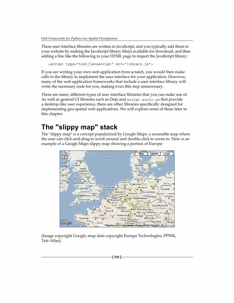
Web Frameworks for Python Geo-Spatial Development
[ 332 ]
These user interface libraries are written in JavaScript, and you typically add them to your website by making the JavaScript library file(s) available for download, and then adding a line like the following to your HTML page to import the JavaScript library:
<script type="text/javascript" src="library.js">
If you are writing your own web application from scratch, you would then make calls to the library to implement the user interface for your application. However, many of the web application frameworks that include a user interface library will write the necessary code for you, making even this step unnecessary.
There are many different types of user interface libraries that you can make use of. As well as general UI libraries such as Dojo and script.aculo.us that provide a desktop-like user experience, there are other libraries specifically designed for implementing geo-spatial web applications. We will explore some of these later in this chapter.
The "slippy map" stackThe "slippy map" is a concept popularized by Google Maps: a zoomable map where the user can click-and-drag to scroll around and double-click to zoom in. Here is an example of a Google Maps slippy map showing a portion of Europe:
(Image copyright Google; map data copyright Europa Technologies, PPWK, Tele Atlas).
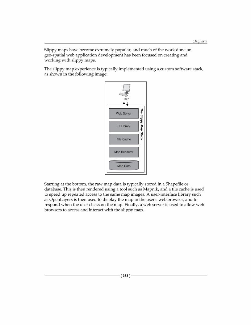
Chapter 9
[ 333 ]
Slippy maps have become extremely popular, and much of the work done on geo-spatial web application development has been focused on creating and working with slippy maps.
The slippy map experience is typically implemented using a custom software stack, as shown in the following image:
Starting at the bottom, the raw map data is typically stored in a Shapefile or database. This is then rendered using a tool such as Mapnik, and a tile cache is used to speed up repeated access to the same map images. A user-interface library such as OpenLayers is then used to display the map in the user's web browser, and to respond when the user clicks on the map. Finally, a web server is used to allow web browsers to access and interact with the slippy map.
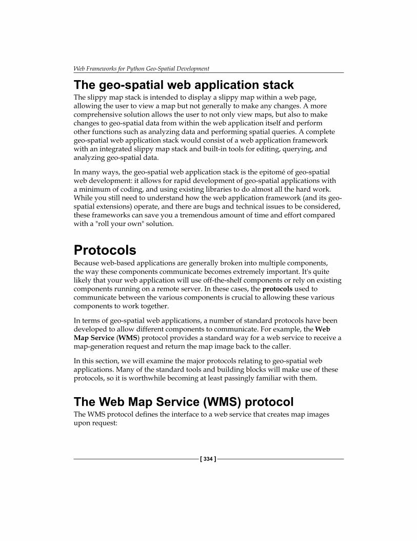
Web Frameworks for Python Geo-Spatial Development
[ 334 ]
The geo-spatial web application stackThe slippy map stack is intended to display a slippy map within a web page, allowing the user to view a map but not generally to make any changes. A more comprehensive solution allows the user to not only view maps, but also to make changes to geo-spatial data from within the web application itself and perform other functions such as analyzing data and performing spatial queries. A complete geo-spatial web application stack would consist of a web application framework with an integrated slippy map stack and built-in tools for editing, querying, and analyzing geo-spatial data.
In many ways, the geo-spatial web application stack is the epitomé of geo-spatial web development: it allows for rapid development of geo-spatial applications with a minimum of coding, and using existing libraries to do almost all the hard work. While you still need to understand how the web application framework (and its geo-spatial extensions) operate, and there are bugs and technical issues to be considered, these frameworks can save you a tremendous amount of time and effort compared with a "roll your own" solution.
ProtocolsBecause web-based applications are generally broken into multiple components, the way these components communicate becomes extremely important. It's quite likely that your web application will use off-the-shelf components or rely on existing components running on a remote server. In these cases, the protocols used to communicate between the various components is crucial to allowing these various components to work together.
In terms of geo-spatial web applications, a number of standard protocols have been developed to allow different components to communicate. For example, the Web Map Service (WMS) protocol provides a standard way for a web service to receive a map-generation request and return the map image back to the caller.
In this section, we will examine the major protocols relating to geo-spatial web applications. Many of the standard tools and building blocks will make use of these protocols, so it is worthwhile becoming at least passingly familiar with them.
The Web Map Service (WMS) protocolThe WMS protocol defines the interface to a web service that creates map images upon request:
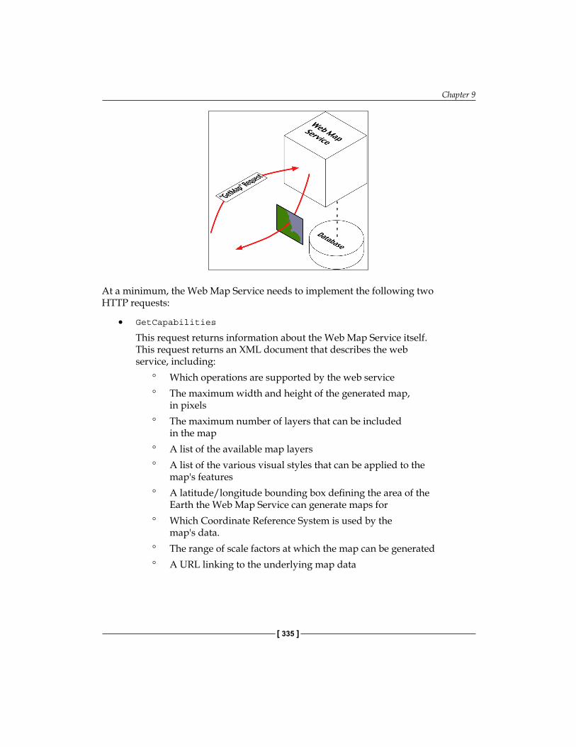
Chapter 9
[ 335 ]
At a minimum, the Web Map Service needs to implement the following two HTTP requests:
• GetCapabilities
This request returns information about the Web Map Service itself. This request returns an XML document that describes the web service, including:
° Which operations are supported by the web service° The maximum width and height of the generated map,
in pixels° The maximum number of layers that can be included
in the map° A list of the available map layers° A list of the various visual styles that can be applied to the
map's features° A latitude/longitude bounding box defining the area of the
Earth the Web Map Service can generate maps for° Which Coordinate Reference System is used by the
map's data.° The range of scale factors at which the map can be generated° A URL linking to the underlying map data
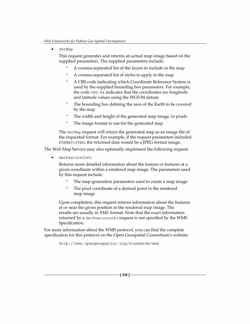
Web Frameworks for Python Geo-Spatial Development
[ 336 ]
• GetMap
This request generates and returns an actual map image based on the supplied parameters. The supplied parameters include:
° A comma-separated list of the layers to include in the map° A comma-separated list of styles to apply to the map° A CRS code indicating which Coordinate Reference System is
used by the supplied bounding box parameters. For example, the code CRS:84 indicates that the coordinates are longitude and latitude values using the WGS 84 datum
° The bounding box defining the area of the Earth to be covered by the map
° The width and height of the generated map image, in pixels° The image format to use for the generated map
The GetMap request will return the generated map as an image file of the requested format. For example, if the request parameters included FORMAT=JPEG, the returned data would be a JPEG-format image.
The Web Map Service may also optionally implement the following request:
• GetFeatureInfo
Returns more detailed information about the feature or features at a given coordinate within a rendered map image. The parameters used by this request include:
° The map-generation parameters used to create a map image° The pixel coordinate of a desired point in the rendered
map image
Upon completion, this request returns information about the features at or near the given position in the rendered map image. The results are usually in XML format. Note that the exact information returned by a GetFeatureInfo request is not specified by the WMS Specification.
For more information about the WMS protocol, you can find the complete specification for this protocol on the Open Geospatial Consortium's website:
http://www.opengeospatial.org/standards/wms
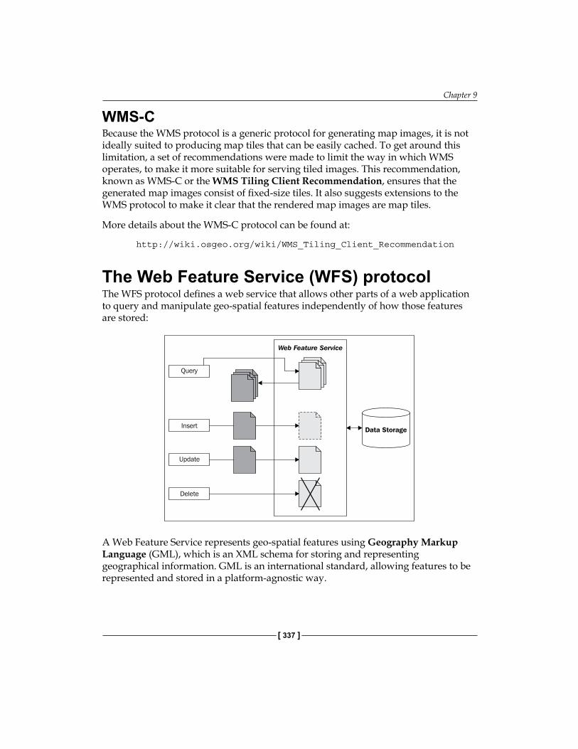
Chapter 9
[ 337 ]
WMS-CBecause the WMS protocol is a generic protocol for generating map images, it is not ideally suited to producing map tiles that can be easily cached. To get around this limitation, a set of recommendations were made to limit the way in which WMS operates, to make it more suitable for serving tiled images. This recommendation, known as WMS-C or the WMS Tiling Client Recommendation, ensures that the generated map images consist of fixed-size tiles. It also suggests extensions to the WMS protocol to make it clear that the rendered map images are map tiles.
More details about the WMS-C protocol can be found at:
http://wiki.osgeo.org/wiki/WMS_Tiling_Client_Recommendation
The Web Feature Service (WFS) protocolThe WFS protocol defines a web service that allows other parts of a web application to query and manipulate geo-spatial features independently of how those features are stored:
A Web Feature Service represents geo-spatial features using Geography Markup Language (GML), which is an XML schema for storing and representing geographical information. GML is an international standard, allowing features to be represented and stored in a platform-agnostic way.

Web Frameworks for Python Geo-Spatial Development
[ 338 ]
At a minimum, a Web Feature Service needs to support the following requests, which allow client systems to query the WFS and retrieve features:
• GetCapabilities
This request returns information about the Web Feature Service itself. This request returns an XML document that describes the web service, including:
° Which operations are supported by the web service° Which types of features can be stored and retrieved by the
web service° Which operations are supported by each type of feature
• DescribeFeatureType
This request returns an XML document describing the structure of one or more types of features. This provides information about the attributes stored for each feature, as well as the way in which the feature itself is represented in the datastore.
• GetFeature
This request queries the WFS, returning features that match certain criteria. The caller can request which properties to retrieve and a maximum number of matching features to return, as well as both spatial and non-spatial query parameters.
The Web Feature Service may also allow client systems to add, update and delete features. This can be done in one of two ways: by allowing the client to lock one or more features before making a series of changes and then unlocking the features again, or simply by making the updates one at a time. The locking approach ensures that two processes don't both update the same feature at the same time, though not all Web Feature Services support locking.
The following requests support locking and non-locking changes to the datastore:
• LockFeature
Lock one or more features so that other processes cannot make any changes to those features.
• GetFeatureWithLock
Retrieve one or more features, and immediately lock the retrieved features.
Chapter 9
[ 339 ]
• Transaction
This request is used to add, update, and delete features. It also allows previously-locked features to be unlocked, allowing other processes to make changes to those features.
Finally, the Web Feature Service can optionally support external linking, where features (possibly stored in different Web Feature Services) can be linked together. This is done through supporting the retrieval of nested features within the GetFeature request, and the separate GetGmlObject request that returns a given feature referred to by an XLink ID.
Web Feature Services are intended to abstract the storage and retrieval away from other parts of a web application, allowing different datastores to be used, and to allow information stored in separate places (possibly on separate servers) to be seamlessly combined. Unfortunately, the WFS protocol is quite complicated, relying heavily on complex XML schemas, which makes accessing and using a Web Feature Service somewhat challenging. Despite this, the open and scalable nature of the WFS protocol does make it worthwhile. Depending on your requirements, you may wish to make use of this protocol in your applications—especially if you are trying to access or manipulate data stored externally.
More information about Web Feature Services, including a complete specification for the WFS protocol, can be found at:
http://www.opengeospatial.org/standards/wfs
The TMS (Tile Map Service) protocolThe TMS protocol defines the interface to a web service that returns map tile images upon request. The TMS protocol is similar to WMS, except that it is simpler and more oriented towards the storage and retrieval of map tiles rather than arbitrarily-specified complete maps.
The TMS protocol uses RESTful (REpresentational State Transfer) principles, which means that the URL used to access the web service includes all of the information needed to complete a request. Unlike WMS, there is no need to create and submit complex XML documents to retrieve a map tile—all of the information is contained within the URL itself.
Within the TMS protocol, a Tile Map Service is a mechanism for providing access to rendered map images at a given set of scale factors and using a predetermined set of spatial reference systems.
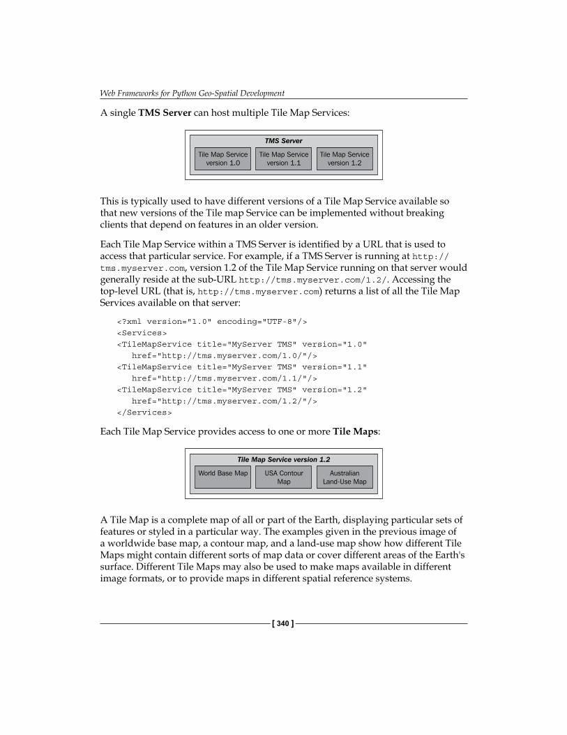
Web Frameworks for Python Geo-Spatial Development
[ 340 ]
A single TMS Server can host multiple Tile Map Services:
This is typically used to have different versions of a Tile Map Service available so that new versions of the Tile map Service can be implemented without breaking clients that depend on features in an older version.
Each Tile Map Service within a TMS Server is identified by a URL that is used to access that particular service. For example, if a TMS Server is running at http://tms.myserver.com, version 1.2 of the Tile Map Service running on that server would generally reside at the sub-URL http://tms.myserver.com/1.2/. Accessing the top-level URL (that is, http://tms.myserver.com) returns a list of all the Tile Map Services available on that server:
<?xml version="1.0" encoding="UTF-8"/><Services><TileMapService title="MyServer TMS" version="1.0" href="http://tms.myserver.com/1.0/"/><TileMapService title="MyServer TMS" version="1.1" href="http://tms.myserver.com/1.1/"/><TileMapService title="MyServer TMS" version="1.2" href="http://tms.myserver.com/1.2/"/></Services>
Each Tile Map Service provides access to one or more Tile Maps:
A Tile Map is a complete map of all or part of the Earth, displaying particular sets of features or styled in a particular way. The examples given in the previous image of a worldwide base map, a contour map, and a land-use map show how different Tile Maps might contain different sorts of map data or cover different areas of the Earth's surface. Different Tile Maps may also be used to make maps available in different image formats, or to provide maps in different spatial reference systems.
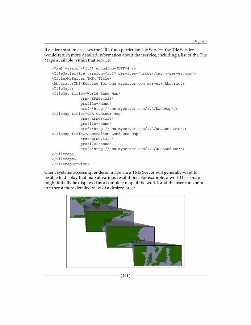
Chapter 9
[ 341 ]
If a client system accesses the URL for a particular Tile Service, the Tile Service would return more detailed information about that service, including a list of the Tile Maps available within that service:
<?xml version="1.0" encoding="UTF-8"/><TileMapService version="1.2" services="http://tms.myserver.com"><Title>MyServer TMS</Title><Abstract>TMS Service for the myserver.com server</Abstract><TileMaps><TileMap title="World Base Map" srs="EPSG:4326" profile="none" href="http://tms.myserver.com/1.2/baseMap"/><TileMap title="USA Contour Map" srs="EPSG:4326" profile="none" href="http://tms.myserver.com/1.2/usaContours"/><TileMap title="Australian Land-Use Map" srs="EPSG:4326" profile="none" href="http://tms.myserver.com/1.2/ausLandUse"/></TileMap></TileMaps></TileMapService>
Client systems accessing rendered maps via a TMS Server will generally want to be able to display that map at various resolutions. For example, a world base map might initially be displayed as a complete map of the world, and the user can zoom in to see a more detailed view of a desired area:
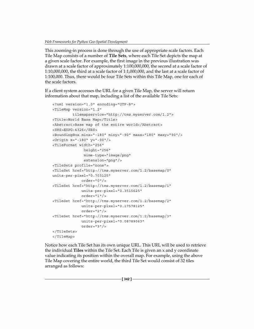
Web Frameworks for Python Geo-Spatial Development
[ 342 ]
This zooming-in process is done through the use of appropriate scale factors. Each Tile Map consists of a number of Tile Sets, where each Tile Set depicts the map at a given scale factor. For example, the first image in the previous illustration was drawn at a scale factor of approximately 1:100,000,000, the second at a scale factor of 1:10,000,000, the third at a scale factor of 1:1,000,000, and the last at a scale factor of 1:100,000. Thus, there would be four Tile Sets within this Tile Map, one for each of the scale factors.
If a client system accesses the URL for a given Tile Map, the server will return information about that map, including a list of the available Tile Sets:
<?xml version="1.0" encoding="UTF-8"><TileMap version="1.2" tilemapservice="http://tms.myserver.com/1.2"><Title>World Base Map</Title><Abstract>Base map of the entire world</Abstract><SRS>ESPG:4326</SRS><BoundingBox minx="-180" miny="-90" maxx="180" maxy="90"/><Origin x="-180" y="-90"/><TileFormat width="256" height="256" mime-type="image/png" extension="png"/><TileSets profile="none"><TileSet href="http://tms.myserver.com/1.2/basemap/0"units-per-pixel="0.703125" order="0"/><TileSet href="http://tms.myserver.com/1.2/basemap/1" units-per-pixel="0.3515625" order="1"/><TileSet href="http://tms.myserver.com/1.2/basemap/2" units-per-pixel="0.17578125" order="2"/><TileSet href="http://tms.myserver.com/1.2/basemap/3" units-per-pixel="0.08789063" order="3"/></TileSets></TileMap>
Notice how each Tile Set has its own unique URL. This URL will be used to retrieve the individual Tiles within the Tile Set. Each Tile is given an x and y coordinate value indicating its position within the overall map. For example, using the above Tile Map covering the entire world, the third Tile Set would consist of 32 tiles arranged as follows:
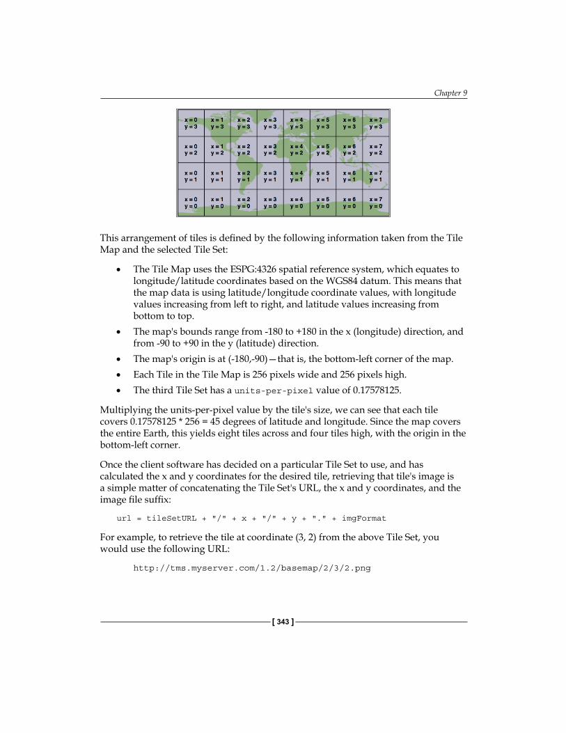
Chapter 9
[ 343 ]
This arrangement of tiles is defined by the following information taken from the Tile Map and the selected Tile Set:
• The Tile Map uses the ESPG:4326 spatial reference system, which equates to longitude/latitude coordinates based on the WGS84 datum. This means that the map data is using latitude/longitude coordinate values, with longitude values increasing from left to right, and latitude values increasing from bottom to top.
• The map's bounds range from -180 to +180 in the x (longitude) direction, and from -90 to +90 in the y (latitude) direction.
• The map's origin is at (-180,-90)—that is, the bottom-left corner of the map.• Each Tile in the Tile Map is 256 pixels wide and 256 pixels high.• The third Tile Set has a units-per-pixel value of 0.17578125.
Multiplying the units-per-pixel value by the tile's size, we can see that each tile covers 0.17578125 * 256 = 45 degrees of latitude and longitude. Since the map covers the entire Earth, this yields eight tiles across and four tiles high, with the origin in the bottom-left corner.
Once the client software has decided on a particular Tile Set to use, and has calculated the x and y coordinates for the desired tile, retrieving that tile's image is a simple matter of concatenating the Tile Set's URL, the x and y coordinates, and the image file suffix:
url = tileSetURL + "/" + x + "/" + y + "." + imgFormat
For example, to retrieve the tile at coordinate (3, 2) from the above Tile Set, you would use the following URL:
http://tms.myserver.com/1.2/basemap/2/3/2.png
Web Frameworks for Python Geo-Spatial Development
[ 344 ]
Notice how this URL (and indeed, every URL used by the TMS protocol) looks as if it is simply retrieving a file from the server. Behind the scenes, the TMS Server may indeed be running a complex set of map-generation and map-caching code to generate these tiles on demand—but the entire TMS Server could just as easily be defined by a series of hardwired XML files and a number of directories containing pre-generated image files.
This notion of a Static Tile Map Server is a deliberate design feature of the TMS protocol. If you don't need to generate too many map tiles, or if you have a particularly large hard disk, you could easily pre-generate all the tile images and create a static TMS server by creating a few XML files and serving the whole thing behind a standard web server such as Apache.
While you might not implement your own dynamic TMS Server from scratch, you may well wish to make use of TMS servers in your own web applications, either by creating a Static Tile Map Server, or by using an existing software library that implements the TMS protocol such as the open-source TileCache server. TileCache will be discussed in the next section of this chapter.
The full specification for the TMS protocol can be found at:
http://wiki.osgeo.org/wiki/Tile_Map_Service_Specification
ToolsWhen discussing tools for developing geo-spatial web applications, it is worth remembering that all of the libraries and toolkits we have discussed in earlier chapters (SpatiaLite, MySQL, PostGIS, Mapnik, OGR, GDAL, Proj, Shapely, and so on) can also be used for web applications. In this section, we will add to this collection by examining some of the major Python libraries available for implementing tile caching and slippy maps. We will also look at some of the web application frameworks that support geo-spatial development.
Tile cachingThere are three main tools for implementing tile caching within a Python geo-spatial web application: TileCache, mod_tile, and TileLite. Let's take a closer look at each of these.
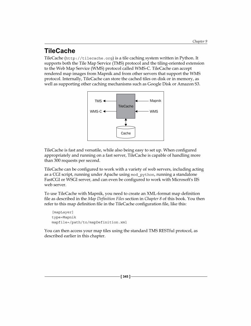
Chapter 9
[ 345 ]
TileCacheTileCache (http://tilecache.org) is a tile caching system written in Python. It supports both the Tile Map Service (TMS) protocol and the tiling-oriented extension to the Web Map Service (WMS) protocol called WMS-C. TileCache can accept rendered map images from Mapnik and from other servers that support the WMS protocol. Internally, TileCache can store the cached tiles on disk or in memory, as well as supporting other caching mechanisms such as Google Disk or Amazon S3.
TileCache is fast and versatile, while also being easy to set up. When configured appropriately and running on a fast server, TileCache is capable of handling more than 300 requests per second.
TileCache can be configured to work with a variety of web servers, including acting as a CGI script, running under Apache using mod_python, running a standalone FastCGI or WSGI server, and can even be configured to work with Microsoft's IIS web server.
To use TileCache with Mapnik, you need to create an XML-format map definition file as described in the Map Definition Files section in Chapter 8 of this book. You then refer to this map definition file in the TileCache configuration file, like this:
[mapLayer]type=Mapnikmapfile=/path/to/mapDefinition.xml
You can then access your map tiles using the standard TMS RESTful protocol, as described earlier in this chapter.
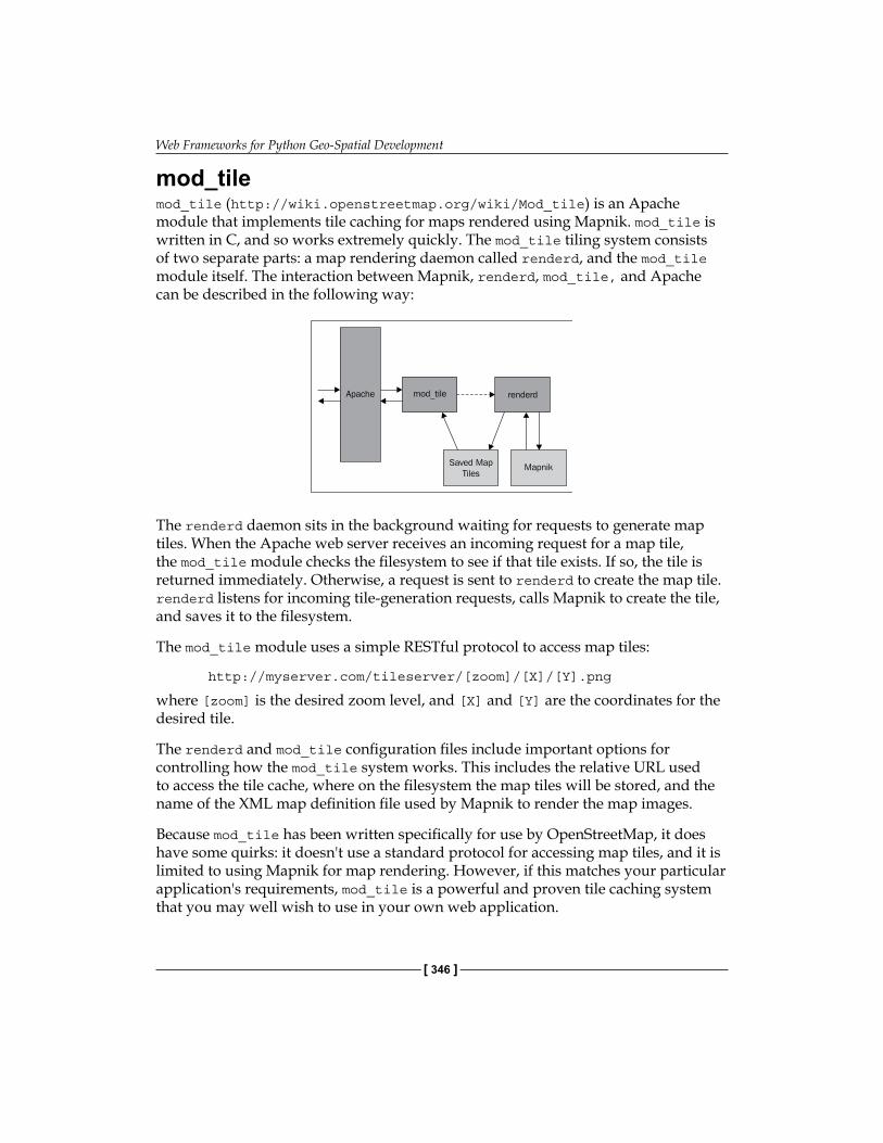
Web Frameworks for Python Geo-Spatial Development
[ 346 ]
mod_tilemod_tile (http://wiki.openstreetmap.org/wiki/Mod_tile) is an Apache module that implements tile caching for maps rendered using Mapnik. mod_tile is written in C, and so works extremely quickly. The mod_tile tiling system consists of two separate parts: a map rendering daemon called renderd, and the mod_tile module itself. The interaction between Mapnik, renderd, mod_tile, and Apache can be described in the following way:
The renderd daemon sits in the background waiting for requests to generate map tiles. When the Apache web server receives an incoming request for a map tile, the mod_tile module checks the filesystem to see if that tile exists. If so, the tile is returned immediately. Otherwise, a request is sent to renderd to create the map tile. renderd listens for incoming tile-generation requests, calls Mapnik to create the tile, and saves it to the filesystem.
The mod_tile module uses a simple RESTful protocol to access map tiles:
http://myserver.com/tileserver/[zoom]/[X]/[Y].png
where [zoom] is the desired zoom level, and [X] and [Y] are the coordinates for the desired tile.
The renderd and mod_tile configuration files include important options for controlling how the mod_tile system works. This includes the relative URL used to access the tile cache, where on the filesystem the map tiles will be stored, and the name of the XML map definition file used by Mapnik to render the map images.
Because mod_tile has been written specifically for use by OpenStreetMap, it does have some quirks: it doesn't use a standard protocol for accessing map tiles, and it is limited to using Mapnik for map rendering. However, if this matches your particular application's requirements, mod_tile is a powerful and proven tile caching system that you may well wish to use in your own web application.
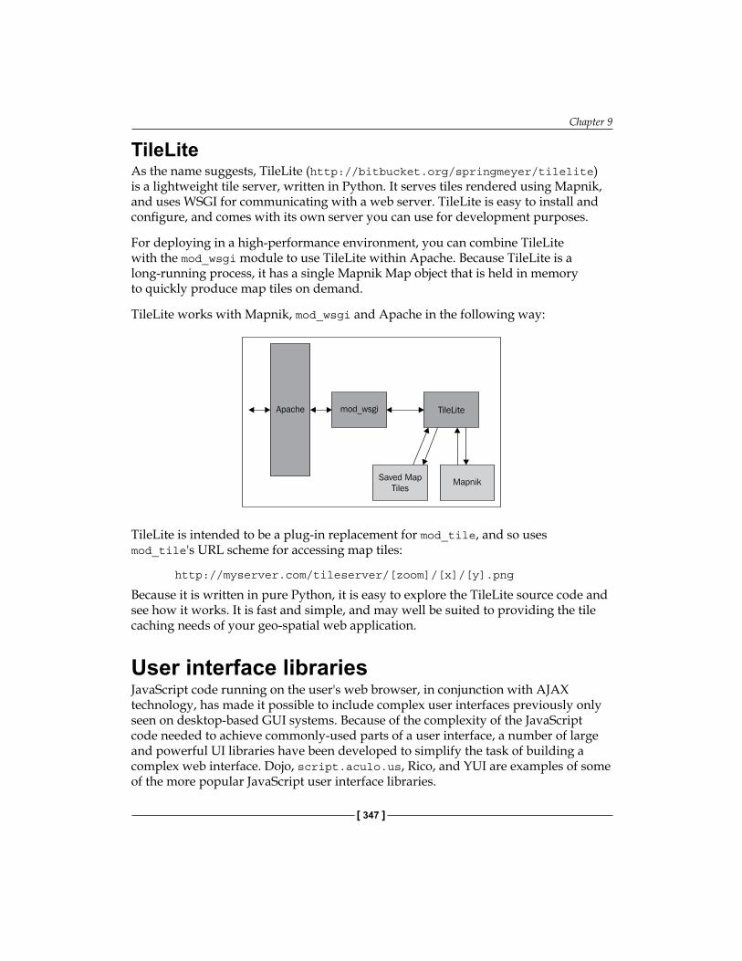
Chapter 9
[ 347 ]
TileLiteAs the name suggests, TileLite (http://bitbucket.org/springmeyer/tilelite) is a lightweight tile server, written in Python. It serves tiles rendered using Mapnik, and uses WSGI for communicating with a web server. TileLite is easy to install and configure, and comes with its own server you can use for development purposes.
For deploying in a high-performance environment, you can combine TileLite with the mod_wsgi module to use TileLite within Apache. Because TileLite is a long-running process, it has a single Mapnik Map object that is held in memory to quickly produce map tiles on demand.
TileLite works with Mapnik, mod_wsgi and Apache in the following way:
TileLite is intended to be a plug-in replacement for mod_tile, and so uses mod_tile's URL scheme for accessing map tiles:
http://myserver.com/tileserver/[zoom]/[x]/[y].png
Because it is written in pure Python, it is easy to explore the TileLite source code and see how it works. It is fast and simple, and may well be suited to providing the tile caching needs of your geo-spatial web application.
User interface librariesJavaScript code running on the user's web browser, in conjunction with AJAX technology, has made it possible to include complex user interfaces previously only seen on desktop-based GUI systems. Because of the complexity of the JavaScript code needed to achieve commonly-used parts of a user interface, a number of large and powerful UI libraries have been developed to simplify the task of building a complex web interface. Dojo, script.aculo.us, Rico, and YUI are examples of some of the more popular JavaScript user interface libraries.
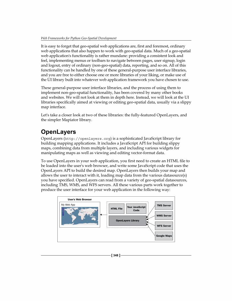
Web Frameworks for Python Geo-Spatial Development
[ 348 ]
It is easy to forget that geo-spatial web applications are, first and foremost, ordinary web applications that also happen to work with geo-spatial data. Much of a geo-spatial web application's functionality is rather mundane: providing a consistent look and feel, implementing menus or toolbars to navigate between pages, user signup, login and logout, entry of ordinary (non-geo-spatial) data, reporting, and so on. All of this functionality can be handled by one of these general-purpose user interface libraries, and you are free to either choose one or more libraries of your liking, or make use of the UI library built into whatever web application framework you have chosen to use.
These general-purpose user interface libraries, and the process of using them to implement non-geo-spatial functionality, has been covered by many other books and websites. We will not look at them in depth here. Instead, we will look at the UI libraries specifically aimed at viewing or editing geo-spatial data, usually via a slippy map interface.
Let's take a closer look at two of these libraries: the fully-featured OpenLayers, and the simpler Mapiator library.
OpenLayersOpenLayers (http://openlayers.org) is a sophisticated JavaScript library for building mapping applications. It includes a JavaScript API for building slippy maps, combining data from multiple layers, and including various widgets for manipulating maps as well as viewing and editing vector-format data.
To use OpenLayers in your web application, you first need to create an HTML file to be loaded into the user's web browser, and write some JavaScript code that uses the OpenLayers API to build the desired map. OpenLayers then builds your map and allows the user to interact with it, loading map data from the various datasource(s) you have specified. OpenLayers can read from a variety of geo-spatial datasources, including TMS, WMS, and WFS servers. All these various parts work together to produce the user interface for your web application in the following way:
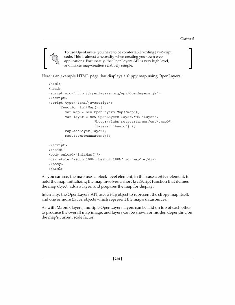
Chapter 9
[ 349 ]
To use OpenLayers, you have to be comfortable writing JavaScript code. This is almost a necessity when creating your own web applications. Fortunately, the OpenLayers API is very high level, and makes map-creation relatively simple.
Here is an example HTML page that displays a slippy map using OpenLayers:
<html><head><script src="http://openlayers.org/api/OpenLayers.js"></script><script type="text/javascript"> function initMap() { var map = new OpenLayers.Map("map"); var layer = new OpenLayers.Layer.WMS("Layer", "http://labs.metacarta.com/wms/vmap0", {layers: 'basic'} ); map.addLayer(layer); map.zoomToMaxExtent(); }</script></head><body onload="initMap()"><div style="width:100%; height:100%" id="map"></div></body></html>
As you can see, the map uses a block-level element, in this case a <div> element, to hold the map. Initializing the map involves a short JavaScript function that defines the map object, adds a layer, and prepares the map for display.
Internally, the OpenLayers API uses a Map object to represent the slippy map itself, and one or more Layer objects which represent the map's datasources.
As with Mapnik layers, multiple OpenLayers layers can be laid on top of each other to produce the overall map image, and layers can be shown or hidden depending on the map's current scale factor.
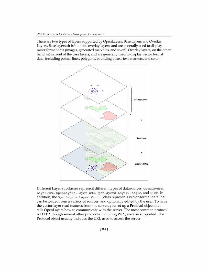
Web Frameworks for Python Geo-Spatial Development
[ 350 ]
There are two types of layers supported by OpenLayers: Base Layers and Overlay Layers. Base layers sit behind the overlay layers, and are generally used to display raster format data (images, generated map tiles, and so on). Overlay layers, on the other hand, sit in front of the base layers, and are generally used to display vector format data, including points, lines, polygons, bounding boxes, text, markers, and so on:
Different Layer subclasses represent different types of datasources: OpenLayers.Layer.TMS, OpenLayers.Layer.WMS, OpenLayers.Layer.Google, and so on. In addition, the OpenLayers.Layer.Vector class represents vector-format data that can be loaded from a variety of sources, and optionally edited by the user. To have the vector layer read features from the server, you set up a Protocol object that tells OpenLayers how to communicate with the server. The most common protocol is HTTP, though several other protocols, including WFS, are also supported. The Protocol object usually includes the URL used to access the server.
Chapter 9
[ 351 ]
As well as setting the protocol, you also supply the Format used to read and write data. Supported formats include GML, GeoJSON, GeoRSS, OSM, and WKT, among others. Format objects also support on-the-fly reprojection of vector data so that data from different sources, using different map projections, can be combined onto a single map.
In addition to the map itself, OpenLayers allows you to use various Control objects, either embedded within the map or shown elsewhere on the web page. Control objects include simple push-buttons, controls for panning and zooming the map, controls that display the map's current scale, controls for showing and hiding layers, and various controls for selecting, adding, and editing vector features. There are also invisible controls that change the behavior of the map itself. For example, the Navigation control allows the user to pan and zoom by clicking-and-dragging on the map, and the ArgParser control tells OpenLayers to scan the URL's query string during page load for arguments that adjust how the map is initially displayed.
OpenLayers is a very powerful tool for building geo-spatial web interfaces. Even if you don't use it directly in your own code, many of the web application frameworks that support geo-spatial web development (including TurboGears, Mapfish, and GeoDjango) use OpenLayers internally to display and edit map data.
MapiatorMapiator (http://pdietrich.github.com/mapiator) is a simple JavaScript library for including slippy maps within a web application. The main benefits of Mapiator are that it is small and easy to use: simply load the Mapiator.js library into your web page and add a few lines of JavaScript code to set up and display your map. For example, the following HTML page:
<html><head><title>My Map</title><script type="text/javascript" src="Mapiator.js"></script><script type="text/javascript"> function onLoad() { var map = new Mapiator.Map("mapID"); map.setZoomLevel(3); map.setCenter(48.0, 10.0); map.redraw(); }</script></head><body onload="onLoad()">
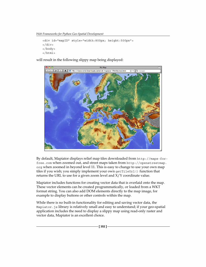
Web Frameworks for Python Geo-Spatial Development
[ 352 ]
<div id="mapID" style="width:800px; height:500px"></div></body></html>
will result in the following slippy map being displayed:
By default, Mapiator displays relief map tiles downloaded from http://maps-for-free.com when zoomed out, and street maps taken from http://openstreetmap.org when zoomed in beyond level 11. This is easy to change to use your own map tiles if you wish; you simply implement your own getTileUrl() function that returns the URL to use for a given zoom level and X/Y coordinate value.
Mapiator includes functions for creating vector data that is overlaid onto the map. These vector elements can be created programmatically, or loaded from a WKT format string. You can also add DOM elements directly to the map image, for example to display buttons or other controls within the map.
While there is no built-in functionality for editing and saving vector data, the Mapiator.js library is relatively small and easy to understand; if your geo-spatial application includes the need to display a slippy map using read-only raster and vector data, Mapiator is an excellent choice.
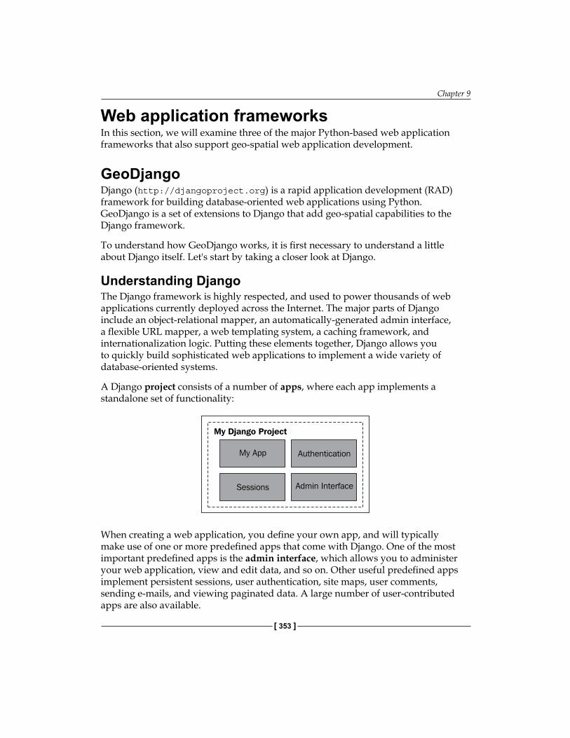
Chapter 9
[ 353 ]
Web application frameworksIn this section, we will examine three of the major Python-based web application frameworks that also support geo-spatial web application development.
GeoDjangoDjango (http://djangoproject.org) is a rapid application development (RAD) framework for building database-oriented web applications using Python. GeoDjango is a set of extensions to Django that add geo-spatial capabilities to the Django framework.
To understand how GeoDjango works, it is first necessary to understand a little about Django itself. Let's start by taking a closer look at Django.
Understanding DjangoThe Django framework is highly respected, and used to power thousands of web applications currently deployed across the Internet. The major parts of Django include an object-relational mapper, an automatically-generated admin interface, a flexible URL mapper, a web templating system, a caching framework, and internationalization logic. Putting these elements together, Django allows you to quickly build sophisticated web applications to implement a wide variety of database-oriented systems.
A Django project consists of a number of apps, where each app implements a standalone set of functionality:
When creating a web application, you define your own app, and will typically make use of one or more predefined apps that come with Django. One of the most important predefined apps is the admin interface, which allows you to administer your web application, view and edit data, and so on. Other useful predefined apps implement persistent sessions, user authentication, site maps, user comments, sending e-mails, and viewing paginated data. A large number of user-contributed apps are also available.
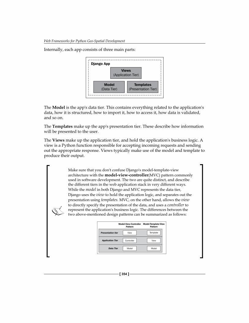
Web Frameworks for Python Geo-Spatial Development
[ 354 ]
Internally, each app consists of three main parts:
The Model is the app's data tier. This contains everything related to the application's data, how it is structured, how to import it, how to access it, how data is validated, and so on.
The Templates make up the app's presentation tier. These describe how information will be presented to the user.
The Views make up the application tier, and hold the application's business logic. A view is a Python function responsible for accepting incoming requests and sending out the appropriate response. Views typically make use of the model and template to produce their output.
Make sure that you don't confuse Django's model-template-view architecture with the model-view-controller(MVC) pattern commonly used in software development. The two are quite distinct, and describe the different tiers in the web application stack in very different ways. While the model in both Django and MVC represents the data tier, Django uses the view to hold the application logic, and separates out the presentation using templates. MVC, on the other hand, allows the view to directly specify the presentation of the data, and uses a controller to represent the application's business logic. The differences between the two above-mentioned design patterns can be summarized as follows:
Chapter 9
[ 355 ]
There is a lot more to Django than can be covered in this brief introduction, but this is enough to understand how GeoDjango extends the Django framework.
GeoDjangoThe GeoDjango extension builds on Django's capabilities to add complete support for building geo-spatial web applications. In particular, it extends the following parts of the Django system:
1. The Model° The Django model is extended to support geo-spatial data
types and spatial queries.° As geo-spatial features are read from the database, the object-
relational mapper automatically converts them into GEOS objects, providing methods for querying and manipulating these features in a sophisticated way similar to the interface provided by Shapely.
° The Model can import data from any OGR-supported vector datasource into the GeoDjango database.
° GeoDjango can use introspection to see which attributes are available in a given OGR datasource, and automatically set up the model to store and import these attributes.
2. The Template° Django's templating system is extended to allow for the
display of geo-spatial data using an embedded OpenLayers slippy map.
3. The Admin Interface° Django's admin interface is extended to allow the user to
create and edit geo-spatial data using OpenLayers. The vector data is displayed on top of a base map using either OpenStreetMap data or a less detailed WMS source called Vector Map Level 0.
All told, the GeoDjango extension makes Django an excellent choice for developing geo-spatial web applications. We will be working with GeoDjango in much more detail in the remaining chapters of this book.
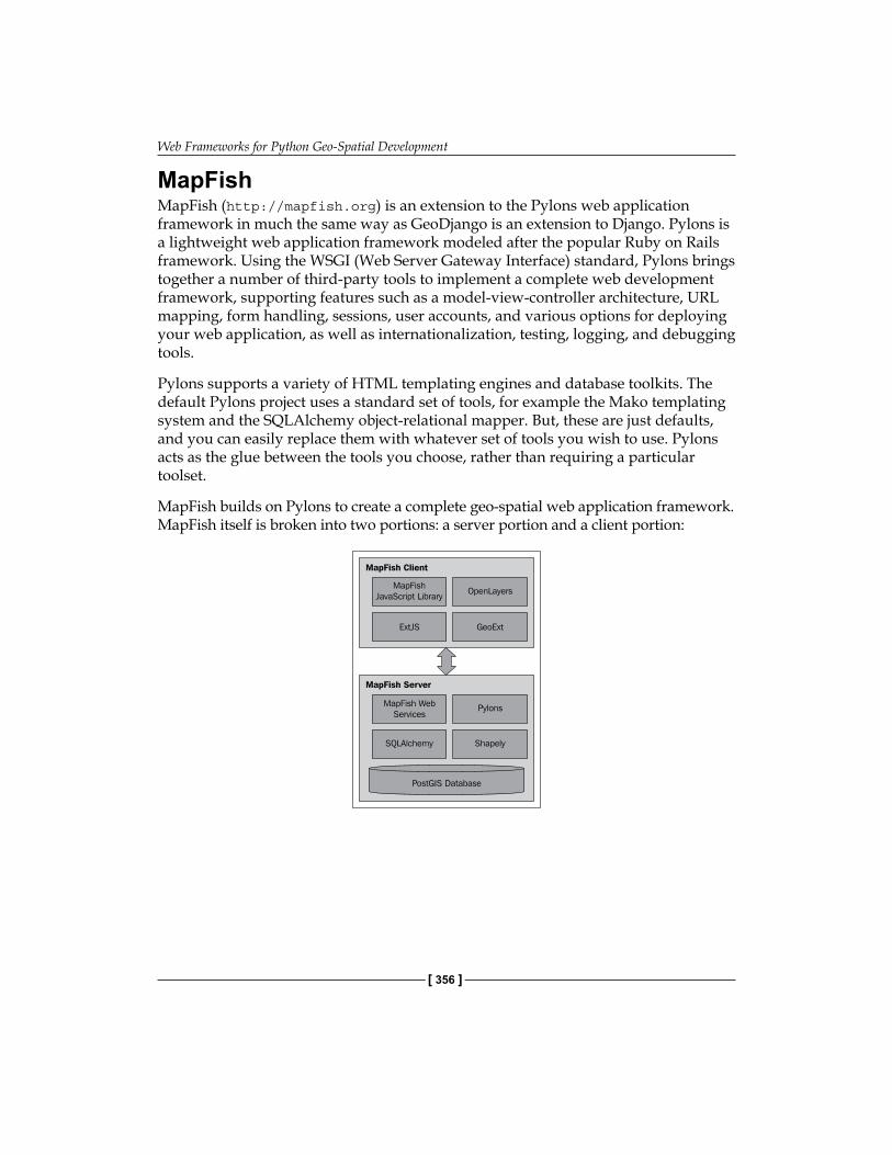
Web Frameworks for Python Geo-Spatial Development
[ 356 ]
MapFishMapFish (http://mapfish.org) is an extension to the Pylons web application framework in much the same way as GeoDjango is an extension to Django. Pylons is a lightweight web application framework modeled after the popular Ruby on Rails framework. Using the WSGI (Web Server Gateway Interface) standard, Pylons brings together a number of third-party tools to implement a complete web development framework, supporting features such as a model-view-controller architecture, URL mapping, form handling, sessions, user accounts, and various options for deploying your web application, as well as internationalization, testing, logging, and debugging tools.
Pylons supports a variety of HTML templating engines and database toolkits. The default Pylons project uses a standard set of tools, for example the Mako templating system and the SQLAlchemy object-relational mapper. But, these are just defaults, and you can easily replace them with whatever set of tools you wish to use. Pylons acts as the glue between the tools you choose, rather than requiring a particular toolset.
MapFish builds on Pylons to create a complete geo-spatial web application framework. MapFish itself is broken into two portions: a server portion and a client portion:
Chapter 9
[ 357 ]
The MapFish Server uses PostGIS, SQLAlchemy, and Shapely to provide an object-oriented layer on top of your geo-spatial data as part of a Pylons application. The server also implements a number of RESTful web services, using a custom protocol known as the MapFish Protocol. These allow the client software to view and make changes to the underlying geo-spatial data.
The MapFish Client software consists of a JavaScript library that provides the user interface for a MapFish application. The MapFish JavaScript library builds on OpenLayers to produce a slippy map, along with the ExtJS and GeoExt libraries to provide user-interface widgets and common behaviors such as feature selection and editing, searching, enabling and disabling layers, and so on.
Putting all this together, MapFish allows developers to build complex user interfaces for geo-spatial web applications, along with server-side components to implement features such as geocoding, spatial analysis, and editing geo-spatial features.
TurboGearsJust like GeoDjango is an extension to the existing Django web framework and MapFish is an extension to Pylons, the TurboGears web framework (http://turbogears.org) also has an extension designed to make it easy to implement your own geo-spatial web applications. This extension is named tgext.geo, and comes bundled with TurboGears.
TurboGears is a sophisticated and extremely popular web application framework built upon Pylons and using a number of standard components, including the SQLAlchemy object-relational mapper, the Genshi templating system, and the ToscaWidgets user interface library. TurboGears also uses the MVC architecture to separate the application's data, business logic, and presentation.
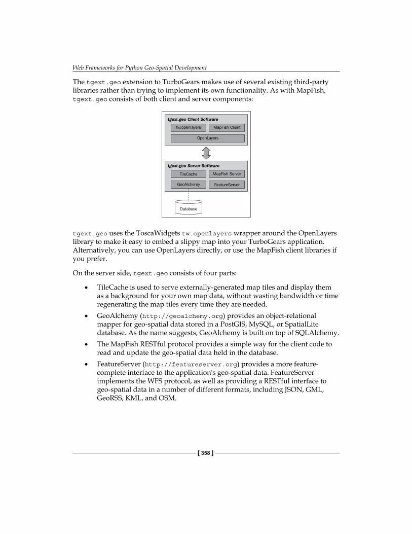
Web Frameworks for Python Geo-Spatial Development
[ 358 ]
The tgext.geo extension to TurboGears makes use of several existing third-party libraries rather than trying to implement its own functionality. As with MapFish, tgext.geo consists of both client and server components:
tgext.geo uses the ToscaWidgets tw.openlayers wrapper around the OpenLayers library to make it easy to embed a slippy map into your TurboGears application. Alternatively, you can use OpenLayers directly, or use the MapFish client libraries if you prefer.
On the server side, tgext.geo consists of four parts:
• TileCache is used to serve externally-generated map tiles and display them as a background for your own map data, without wasting bandwidth or time regenerating the map tiles every time they are needed.
• GeoAlchemy (http://geoalchemy.org) provides an object-relational mapper for geo-spatial data stored in a PostGIS, MySQL, or SpatialLite database. As the name suggests, GeoAlchemy is built on top of SQLAlchemy.
• The MapFish RESTful protocol provides a simple way for the client code to read and update the geo-spatial data held in the database.
• FeatureServer (http://featureserver.org) provides a more feature-complete interface to the application's geo-spatial data. FeatureServer implements the WFS protocol, as well as providing a RESTful interface to geo-spatial data in a number of different formats, including JSON, GML, GeoRSS, KML, and OSM.
Chapter 9
[ 359 ]
The tgext.geo extension to TurboGears makes it possible to quickly build complete and complex geo-spatial applications on top of these components using the TurboGears framework.
SummaryIn this chapter, we have surveyed the geo-spatial web development landscape, examining the major concepts behind geo-spatial web application development, some of the main open protocols used by geo-spatial web applications, and a number of Python-based tools for implementing geo-spatial applications that run over the Internet.
We have seen:
• That a web application stack allows you to build complex, but highly structured web applications using off-the-shelf components.
• That a web application framework supports rapid development of web-based applications, providing a "batteries included" or "full stack" development experience.
• That web services make functionality available to other software components via an HTTP-based API.
• That a map renderer such as Mapnik can be used to build a web service that provides map-rendering services to other parts of a web application.
• That tile caching dramatically improves the performance of a web application by holding previously-generated map tiles, and only generating new tiles as they are needed.
• That tile caching is often used to provide a base map onto which your own geo-spatial data is displayed using overlays.
• That web servers provide the interface between your web application and the outside world.
• That a user-interface library, generally using AJAX technology, runs in the user's web browser and provides a sophisticated user interface not possible with traditional HTML web pages.
• That the slippy map, popularized by Google Maps, is the ubiquitous interface for viewing and manipulating geo-spatial data.
• That slippy maps are generally implemented using a custom application stack that combines map data, a renderer, a tile cache, and a UI library, all sitting behind a web server.
Web Frameworks for Python Geo-Spatial Development
[ 360 ]
• That complete geo-spatial web application stacks, developed using web application frameworks, can implement sophisticated geo-spatial features, including data manipulation, searching, and analysis with far less development effort than would be required using a "roll your own" solution.
• That geo-spatial web protocols allow different components to communicate in a standard way.
• That the Web Map Service (WMS) is an XML-based protocol for generating map images on demand.
• That the WMS-C protocol is a suggested extension to WMS suited to the generation of map tiles.
• That the Web Feature Service (WFS) protocol allows for querying, retrieving, and updating geo-spatial data using a web-based API.
• That the Tile Map Service (TMS) is a simpler, RESTful protocol for retrieving map tiles without having to use XML or deal with the complexity of the WMS protocol.
• That TileCache is a Python-based tile caching system supporting both the TMS and WMS-C protocols.
• That mod_tile is an Apache module for caching map tiles, using a custom interface protocol and rendering tiles using Mapnik.
• That TileLite is a lightweight tile server, written in Python, that is designed to be a fast, easy-to-use, and flexible alternative to mod_tile.
• That existing general-purpose user interface libraries such as Dojo, script.aculo.us, Rico, and YUI can all be used in geo-spatial applications to implement the non-spatial portions of the user interface.
• The OpenLayers is a major JavaScript library for implementing slippy maps, allowing the user to view and edit geo-spatial data.
• That Mapiator is a simpler JavaScript library implementing a slippy map interface for viewing, but not editing, geo-spatial data.
• That GeoDjango is a powerful extension to the popular Django web application framework that provides a complete geo-spatial web application development environment, including an automatically-generated admin interface for viewing and editing geo-spatial data.
• That MapFish is an extension to the Pylons web application framework, making it possible to build complex geo-spatial web applications on top of Pylons.
Chapter 9
[ 361 ]
• That the tgext.geo extension to TurboGears supports geo-spatial web application development by integrating OpenLayers, MapFish, and TileCache, as well as supporting an object-relational mapper for geo-spatial data and a WMS-compatible feature server, all within the TurboGears framework.
In the next chapter, we will start to build a complete mapping application using PostGIS, Mapnik, and GeoDjango.

Putting it All Together: A Complete Mapping
ApplicationIn the final three chapters of this book, we will bring together all the topics discussed in previous chapters to implement a sophisticated web-based mapping application called ShapeEditor. In this chapter, we will cover:
• How to design a geo-spatial application, and then translate that design into code
• How Django web applications are structured• How to set up a new Django project and application• How Django represents data structures as objects• How to use GeoDjango's built-in "admin" system to view and edit
geo-spatial data
About the ShapeEditorAs we have seen, Shapefiles are commonly used to store, make available, and transfer geo-spatial data. We have worked with Shapefiles extensively in this book, obtaining freely-available geo-spatial data in Shapefile format, writing programs to load data from a Shapefile, and creating Shapefiles programmatically.
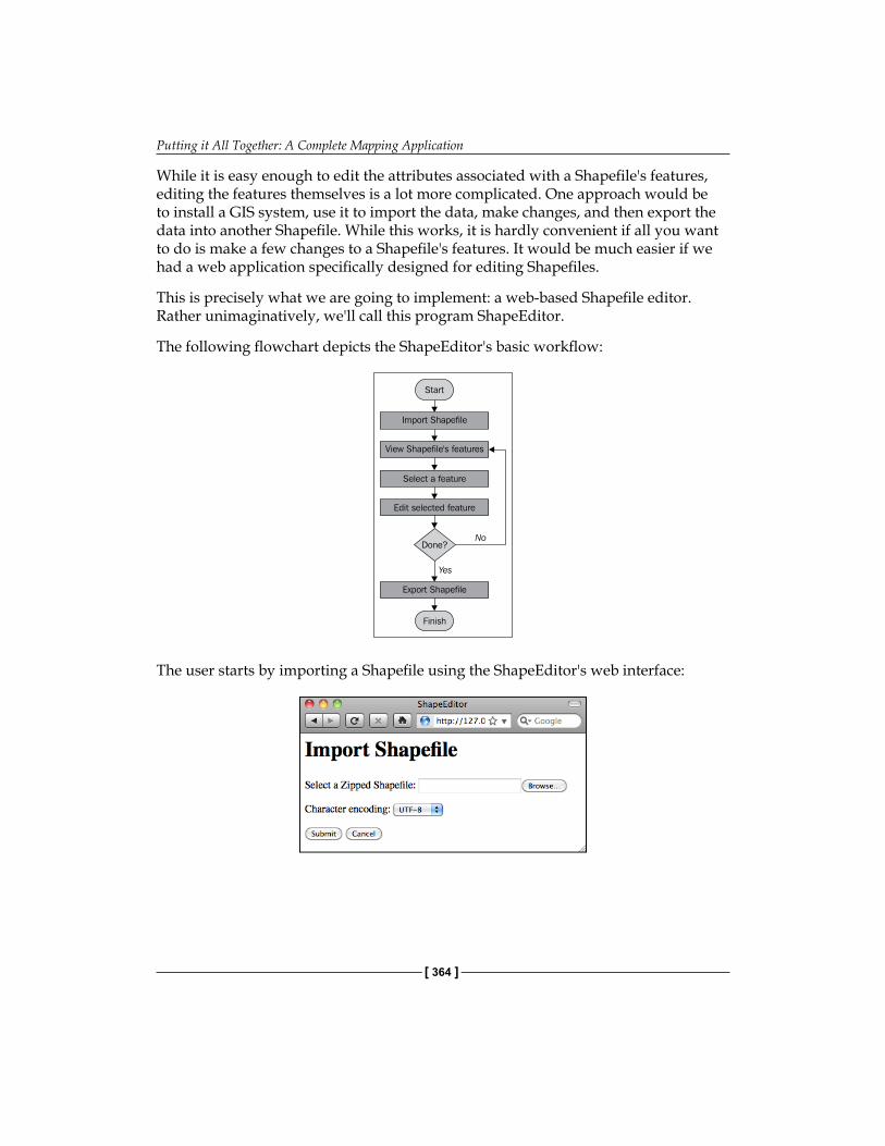
Putting it All Together: A Complete Mapping Application
[ 364 ]
While it is easy enough to edit the attributes associated with a Shapefile's features, editing the features themselves is a lot more complicated. One approach would be to install a GIS system, use it to import the data, make changes, and then export the data into another Shapefile. While this works, it is hardly convenient if all you want to do is make a few changes to a Shapefile's features. It would be much easier if we had a web application specifically designed for editing Shapefiles.
This is precisely what we are going to implement: a web-based Shapefile editor. Rather unimaginatively, we'll call this program ShapeEditor.
The following flowchart depicts the ShapeEditor's basic workflow:
The user starts by importing a Shapefile using the ShapeEditor's web interface:
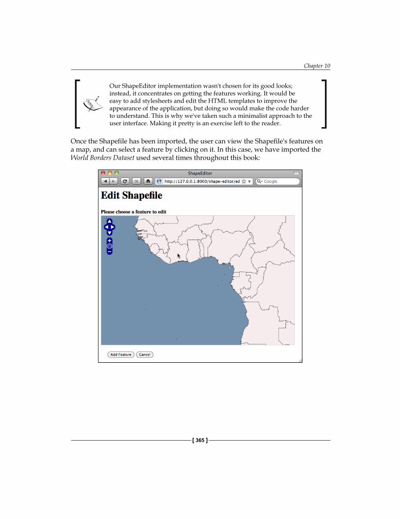
Chapter 10
[ 365 ]
Our ShapeEditor implementation wasn't chosen for its good looks; instead, it concentrates on getting the features working. It would be easy to add stylesheets and edit the HTML templates to improve the appearance of the application, but doing so would make the code harder to understand. This is why we've taken such a minimalist approach to the user interface. Making it pretty is an exercise left to the reader.
Once the Shapefile has been imported, the user can view the Shapefile's features on a map, and can select a feature by clicking on it. In this case, we have imported the World Borders Dataset used several times throughout this book:
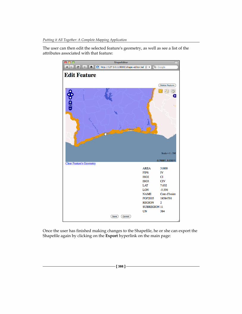
Putting it All Together: A Complete Mapping Application
[ 366 ]
The user can then edit the selected feature's geometry, as well as see a list of the attributes associated with that feature:
Once the user has finished making changes to the Shapefile, he or she can export the Shapefile again by clicking on the Export hyperlink on the main page:
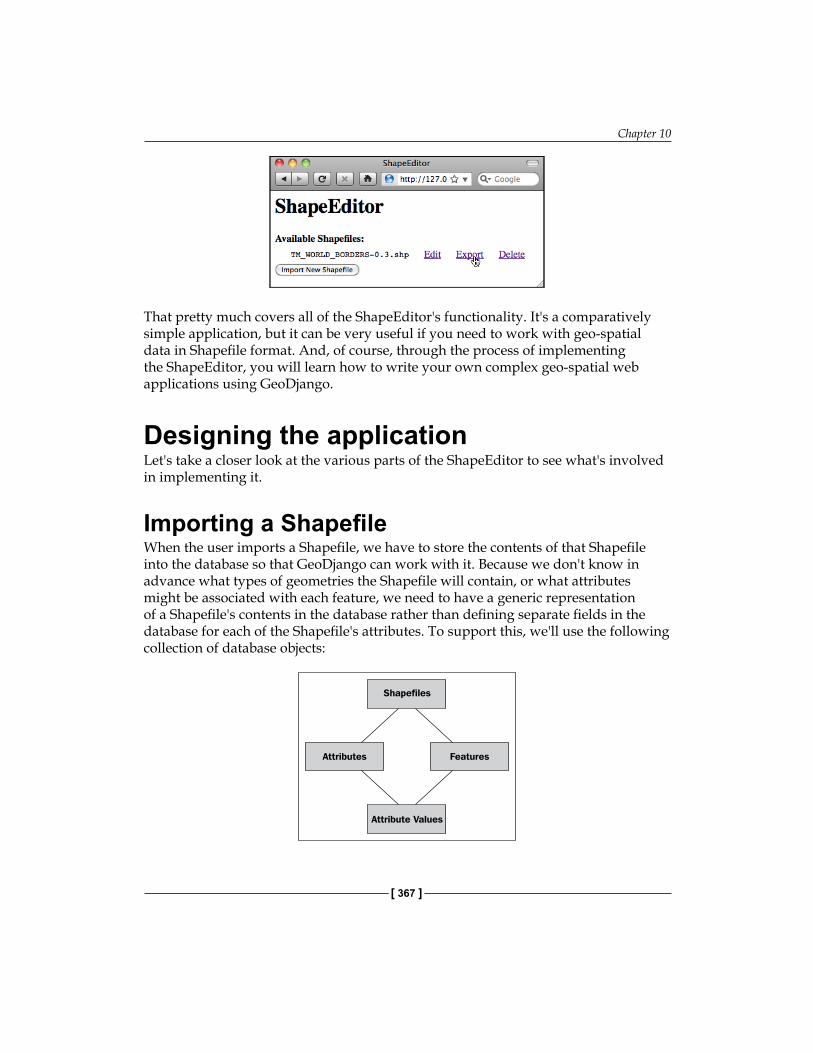
Chapter 10
[ 367 ]
That pretty much covers all of the ShapeEditor's functionality. It's a comparatively simple application, but it can be very useful if you need to work with geo-spatial data in Shapefile format. And, of course, through the process of implementing the ShapeEditor, you will learn how to write your own complex geo-spatial web applications using GeoDjango.
Designing the applicationLet's take a closer look at the various parts of the ShapeEditor to see what's involved in implementing it.
Importing a ShapefileWhen the user imports a Shapefile, we have to store the contents of that Shapefile into the database so that GeoDjango can work with it. Because we don't know in advance what types of geometries the Shapefile will contain, or what attributes might be associated with each feature, we need to have a generic representation of a Shapefile's contents in the database rather than defining separate fields in the database for each of the Shapefile's attributes. To support this, we'll use the following collection of database objects:
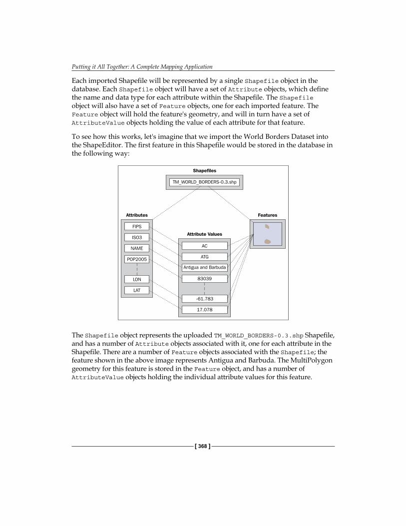
Putting it All Together: A Complete Mapping Application
[ 368 ]
Each imported Shapefile will be represented by a single Shapefile object in the database. Each Shapefile object will have a set of Attribute objects, which define the name and data type for each attribute within the Shapefile. The Shapefile object will also have a set of Feature objects, one for each imported feature. The Feature object will hold the feature's geometry, and will in turn have a set of AttributeValue objects holding the value of each attribute for that feature.
To see how this works, let's imagine that we import the World Borders Dataset into the ShapeEditor. The first feature in this Shapefile would be stored in the database in the following way:
The Shapefile object represents the uploaded TM_WORLD_BORDERS-0.3.shp Shapefile, and has a number of Attribute objects associated with it, one for each attribute in the Shapefile. There are a number of Feature objects associated with the Shapefile; the feature shown in the above image represents Antigua and Barbuda. The MultiPolygon geometry for this feature is stored in the Feature object, and has a number of AttributeValue objects holding the individual attribute values for this feature.
Chapter 10
[ 369 ]
While this is a somewhat roundabout way of storing Shapefile data in a database (it would be more common to use the ogrinspect.py utility to create a static GeoDjango model out of the Shapefile's features), we have to do this because we don't know the Shapefile's structure ahead of time, and don't want to be constantly adding a new database table whenever a Shapefile is imported.
With this basic model in place to store a Shapefile's data in the database, we can continue designing the rest of the "Import Shapefile" logic.
Because Shapefiles are represented on disk by a number of separate files, we will expect the user to create a ZIP archive out of the Shapefile and upload the zipped Shapefile. This saves us having to handle multiple file uploads for a single Shapefile, and makes things more convenient for the user as Shapefiles often come in ZIP format already.
Once the ZIP archive has been uploaded, our code will need to decompress the archive and extract the individual files that make up the Shapefile. We'll then have to read through the Shapefile to find its attributes, create the appropriate Attribute objects, and then process the Shapefile's features one at a time, creating Feature and AttributeValue objects as we go. All of this will be quite straightforward to implement.
Selecting a featureBefore the user can edit a feature, we have to let the user select the desired feature. Unfortunately, this is an area where GeoDjango's built-in editing code lets us down: the GeoDjango admin module displays a text-based list of the features, and only shows a map once a particular feature has been selected. This is because GeoDjango can only display a single feature on a map at once thanks to the way GeoDjango's geometry editor has been implemented.
This isn't really suitable for the ShapeEditor as we have no useful information to display to the user, and simply seeing a list of attribute values isn't going to be very helpful. Instead, we will bypass GeoDjango's built-in editor and instead use OpenLayers directly to display a map showing all the features in the imported Shapefile. We'll then let the user click on a feature to select it for editing.
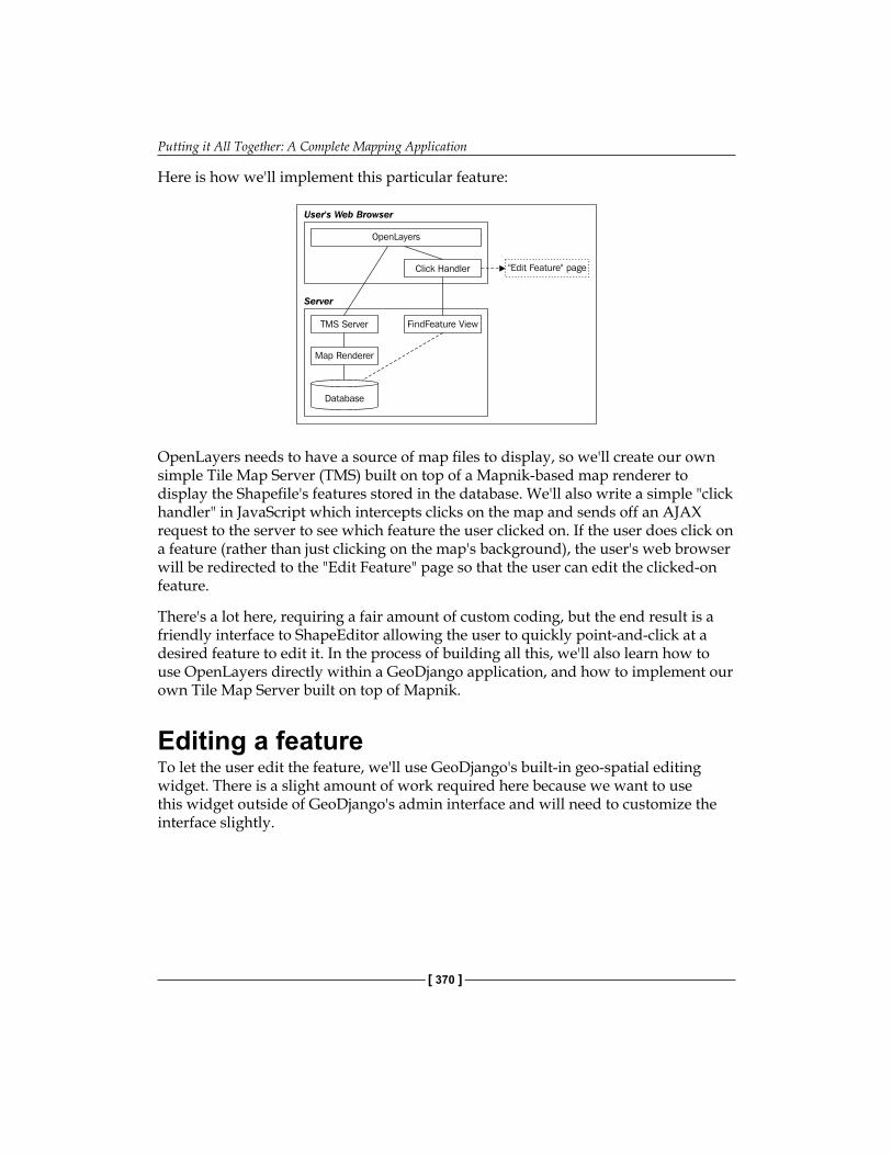
Putting it All Together: A Complete Mapping Application
[ 370 ]
Here is how we'll implement this particular feature:
OpenLayers needs to have a source of map files to display, so we'll create our own simple Tile Map Server (TMS) built on top of a Mapnik-based map renderer to display the Shapefile's features stored in the database. We'll also write a simple "click handler" in JavaScript which intercepts clicks on the map and sends off an AJAX request to the server to see which feature the user clicked on. If the user does click on a feature (rather than just clicking on the map's background), the user's web browser will be redirected to the "Edit Feature" page so that the user can edit the clicked-on feature.
There's a lot here, requiring a fair amount of custom coding, but the end result is a friendly interface to ShapeEditor allowing the user to quickly point-and-click at a desired feature to edit it. In the process of building all this, we'll also learn how to use OpenLayers directly within a GeoDjango application, and how to implement our own Tile Map Server built on top of Mapnik.
Editing a featureTo let the user edit the feature, we'll use GeoDjango's built-in geo-spatial editing widget. There is a slight amount of work required here because we want to use this widget outside of GeoDjango's admin interface and will need to customize the interface slightly.
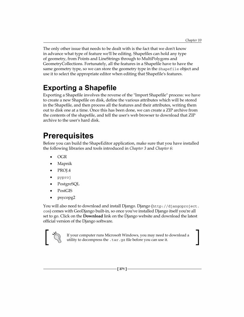
Chapter 10
[ 371 ]
The only other issue that needs to be dealt with is the fact that we don't know in advance what type of feature we'll be editing. Shapefiles can hold any type of geometry, from Points and LineStrings through to MultiPolygons and GeometryCollections. Fortunately, all the features in a Shapefile have to have the same geometry type, so we can store the geometry type in the Shapefile object and use it to select the appropriate editor when editing that Shapefile's features.
Exporting a ShapefileExporting a Shapefile involves the reverse of the "Import Shapefile" process: we have to create a new Shapefile on disk, define the various attributes which will be stored in the Shapefile, and then process all the features and their attributes, writing them out to disk one at a time. Once this has been done, we can create a ZIP archive from the contents of the shapefile, and tell the user's web browser to download that ZIP archive to the user's hard disk.
PrerequisitesBefore you can build the ShapeEditor application, make sure that you have installed the following libraries and tools introduced in Chapter 3 and Chapter 6:
• OGR• Mapnik• PROJ.4• pyproj
• PostgreSQL• PostGIS• psycopg2
You will also need to download and install Django. Django (http://djangoproject.com) comes with GeoDjango built-in, so once you've installed Django itself you're all set to go. Click on the Download link on the Django website and download the latest official version of the Django software.
If your computer runs Microsoft Windows, you may need to download a utility to decompress the .tar.gz file before you can use it.
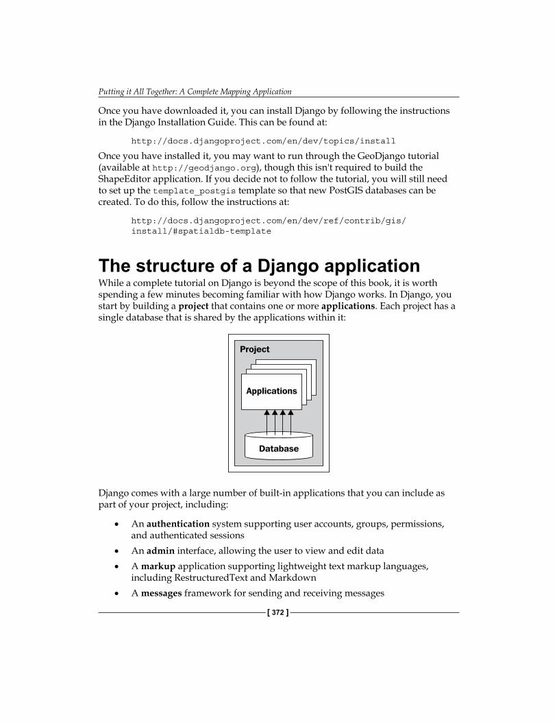
Putting it All Together: A Complete Mapping Application
[ 372 ]
Once you have downloaded it, you can install Django by following the instructions in the Django Installation Guide. This can be found at:
http://docs.djangoproject.com/en/dev/topics/install
Once you have installed it, you may want to run through the GeoDjango tutorial (available at http://geodjango.org), though this isn't required to build the ShapeEditor application. If you decide not to follow the tutorial, you will still need to set up the template_postgis template so that new PostGIS databases can be created. To do this, follow the instructions at:
http://docs.djangoproject.com/en/dev/ref/contrib/gis/install/#spatialdb-template
The structure of a Django applicationWhile a complete tutorial on Django is beyond the scope of this book, it is worth spending a few minutes becoming familiar with how Django works. In Django, you start by building a project that contains one or more applications. Each project has a single database that is shared by the applications within it:
Django comes with a large number of built-in applications that you can include as part of your project, including:
• An authentication system supporting user accounts, groups, permissions, and authenticated sessions
• An admin interface, allowing the user to view and edit data• A markup application supporting lightweight text markup languages,
including RestructuredText and Markdown• A messages framework for sending and receiving messages
Chapter 10
[ 373 ]
• A sessions system for keeping track of anonymous (non-authenticated) sessions
• A sitemaps framework for generating site maps• A syndication system for generating RSS and ATOM feeds
The GeoDjango extension is implemented as another application within Django that you turn on when you wish to use it.
The project has a settings file that you to use to configure the project as a whole. These settings include a list of the applications you want to include in the project, which database to use, as well as various other project- and application-specific settings.
As we saw in the previous chapter, a Django application has three main components:
The models define your application's data structures, the views contain your application's business logic, and the templates are used to control how information is presented to the user. These correspond to the data, application, and presentation tiers within a traditional web application stack. Let's take a closer look at each of these in turn.
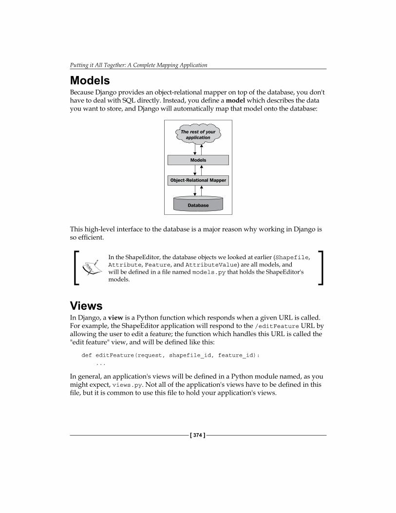
Putting it All Together: A Complete Mapping Application
[ 374 ]
ModelsBecause Django provides an object-relational mapper on top of the database, you don't have to deal with SQL directly. Instead, you define a model which describes the data you want to store, and Django will automatically map that model onto the database:
This high-level interface to the database is a major reason why working in Django is so efficient.
In the ShapeEditor, the database objects we looked at earlier (Shapefile, Attribute, Feature, and AttributeValue) are all models, and will be defined in a file named models.py that holds the ShapeEditor's models.
ViewsIn Django, a view is a Python function which responds when a given URL is called. For example, the ShapeEditor application will respond to the /editFeature URL by allowing the user to edit a feature; the function which handles this URL is called the "edit feature" view, and will be defined like this:
def editFeature(request, shapefile_id, feature_id): ...
In general, an application's views will be defined in a Python module named, as you might expect, views.py. Not all of the application's views have to be defined in this file, but it is common to use this file to hold your application's views.
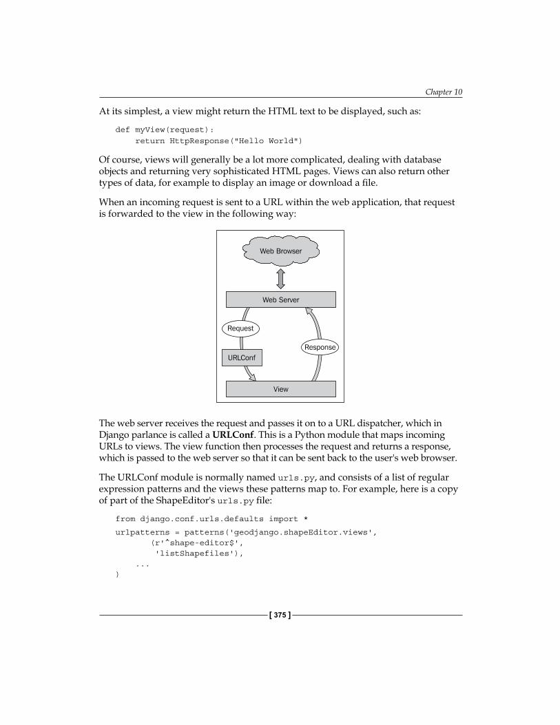
Chapter 10
[ 375 ]
At its simplest, a view might return the HTML text to be displayed, such as:
def myView(request): return HttpResponse("Hello World")
Of course, views will generally be a lot more complicated, dealing with database objects and returning very sophisticated HTML pages. Views can also return other types of data, for example to display an image or download a file.
When an incoming request is sent to a URL within the web application, that request is forwarded to the view in the following way:
The web server receives the request and passes it on to a URL dispatcher, which in Django parlance is called a URLConf. This is a Python module that maps incoming URLs to views. The view function then processes the request and returns a response, which is passed to the web server so that it can be sent back to the user's web browser.
The URLConf module is normally named urls.py, and consists of a list of regular expression patterns and the views these patterns map to. For example, here is a copy of part of the ShapeEditor's urls.py file:
from django.conf.urls.defaults import *
urlpatterns = patterns('geodjango.shapeEditor.views', (r'^shape-editor$', 'listShapefiles'), ...)
Putting it All Together: A Complete Mapping Application
[ 376 ]
This tells Django that any URL that matches the pattern ^shape-editor$ (that is, a URL consisting only of the text shape-editor) will be mapped to the listShapefiles function, which can be found in the geodjango.shapeEditor.views module.
This is a slight simplification: the geodjango.shapeEditor.views entry in the above code example is actually a prefix that is applied to the view name. Prefixes can be anything you like; they don't have to be module names.
As well as simply mapping URLs to view functions, the URLConf module also lets you define parameters to be passed to the view function. Take, for example, the following URL mapping:
(r'^shape-editor/edit/(?P<shapefile_id>\d+)$', 'editShapefile'),
The syntax is a bit complicated thanks to the use of regular expression patterns, but the basic idea is that the URL mapping will accept any URL of the form
shape-editor/edit/NNNN
where NNNN is a sequence of one or more digits. The actual text used for NNNN will be passed to the editShapefile() view function as an extra keyword parameter named shapefile_id. This means that the view function would be defined like this:
def editShapefile(request, shapefile_id): ...
While the URL mapping does require you to be familiar with regular expressions, it is extremely flexible and allows you to define exactly which view will be called for any given incoming URL, as well as allowing you to include parts of the URL as parameters to the view function.
Remember that Django allows multiple applications to exist within a single project. Because of this, the URLConf module belongs to the project, and contains mappings for all the project's applications in one place.
Chapter 10
[ 377 ]
TemplatesTo simplify the creation of complex HTML pages, Django provides a sophisticated templating system. A template is a text file that is processed to generate a web page by taking variables from the view and processing them to generate the page dynamically. For example, here is a snippet from the listShapefiles.html template used by the ShapeEditor:
<b>Available Shapefiles:</b><table> {% for shapefile in shapefiles %} <tr> <td>{{ shapefile.filename }}</td> ... </tr> {% endfor %}</table>
As you can see, most of the template is simply HTML, with a few programming constructs added. In this case, we loop through the shapefiles list, creating a table row for each Shapefile, and display (among other things) the Shapefile's file name.
To use this template, the view might look something like this:
def myView(request): shapefiles = ... return render_to_response("listShapefiles.html", {'shapefiles' : shapefiles})
As you can see, the render_to_response() function takes the name of the template, and a dictionary containing the variables to use when processing the template. The result is an HTML page which will be displayed.
All of the templates for an application are generally stored in a directory named templates within the application's directory.
Django also includes a library for working with data-entry forms. A form is a Python class defining the various fields to be entered, along with data-validation and other behaviors associated with the form. For example, here is the "import Shapefile" form used by the ShapeEditor:
class ImportShapefileForm(forms.Form): import_file = forms.FileField(label="Select a Shapefile") character_encoding = forms.ChoiceField(...)
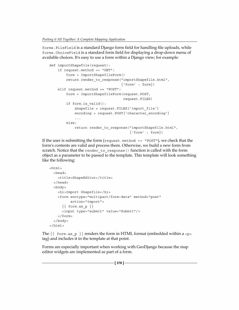
Putting it All Together: A Complete Mapping Application
[ 378 ]
forms.FileField is a standard Django form field for handling file uploads, while forms.ChoiceField is a standard form field for displaying a drop-down menu of available choices. It's easy to use a form within a Django view; for example:
def importShapefile(request): if request.method == "GET": form = ImportShapefileForm() return render_to_response("importShapefile.html", {'form' : form}) elif request.method == "POST": form = ImportShapefileForm(request.POST, request.FILES) if form.is_valid(): shapefile = request.FILES['import_file'] encoding = request.POST['character_encoding'] ... else: return render_to_response("importShapefile.html", {'form' : form})
If the user is submitting the form (request.method == "POST"), we check that the form's contents are valid and process them. Otherwise, we build a new form from scratch. Notice that the render_to_response() function is called with the form object as a parameter to be passed to the template. This template will look something like the following:
<html> <head> <title>ShapeEditor</title> </head> <body> <h1>Import Shapefile</h1> <form enctype="multipart/form-data" method="post" action="import"> {{ form.as_p }} <input type="submit" value="Submit"/> </form> </body></html>
The {{ form.as_p }} renders the form in HTML format (embedded within a <p> tag) and includes it in the template at that point.
Forms are especially important when working with GeoDjango because the map editor widgets are implemented as part of a form.
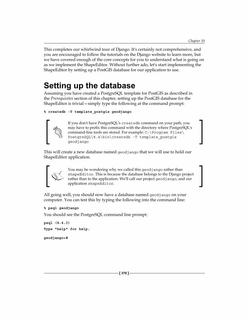
Chapter 10
[ 379 ]
This completes our whirlwind tour of Django. It's certainly not comprehensive, and you are encouraged to follow the tutorials on the Django website to learn more, but we have covered enough of the core concepts for you to understand what is going on as we implement the ShapeEditor. Without further ado, let's start implementing the ShapeEditor by setting up a PostGIS database for our application to use.
Setting up the databaseAssuming you have created a PostgreSQL template for PostGIS as described in the Prerequisites section of this chapter, setting up the PostGIS database for the ShapeEditor is trivial—simply type the following at the command prompt:
% createdb -T template_postgis geodjango
If you don't have PostgreSQL's createdb command on your path, you may have to prefix this command with the directory where PostgreSQL's command-line tools are stored. For example: C:\Program Files\PostgreSQL\8.4\bin\createdb -T template_postgis geodjango
This will create a new database named geodjango that we will use to hold our ShapeEditor application.
You may be wondering why we called this geodjango rather than shapeEditor. This is because the database belongs to the Django project rather than to the application. We'll call our project geodjango, and our application shapeEditor.
All going well, you should now have a database named geodjango on your computer. You can test this by typing the following into the command line:
% psql geodjango
You should see the PostgreSQL command line prompt:
psql (8.4.3)
Type "help" for help.
geodjango=#
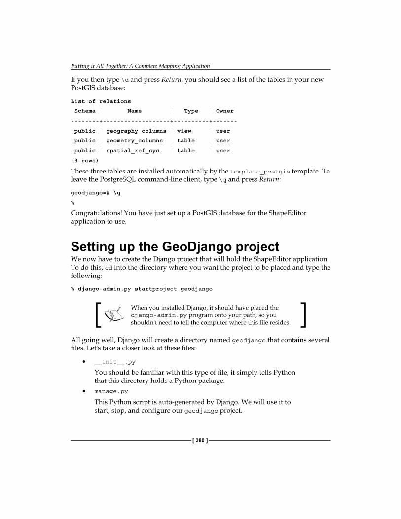
Putting it All Together: A Complete Mapping Application
[ 380 ]
If you then type \d and press Return, you should see a list of the tables in your new PostGIS database:
List of relations
Schema | Name | Type | Owner
--------+-------------------+----------+-------
public | geography_columns | view | user
public | geometry_columns | table | user
public | spatial_ref_sys | table | user
(3 rows)
These three tables are installed automatically by the template_postgis template. To leave the PostgreSQL command-line client, type \q and press Return:
geodjango=# \q
%
Congratulations! You have just set up a PostGIS database for the ShapeEditor application to use.
Setting up the GeoDjango projectWe now have to create the Django project that will hold the ShapeEditor application. To do this, cd into the directory where you want the project to be placed and type the following:
% django-admin.py startproject geodjango
When you installed Django, it should have placed the django-admin.py program onto your path, so you shouldn't need to tell the computer where this file resides.
All going well, Django will create a directory named geodjango that contains several files. Let's take a closer look at these files:
• __init__.py
You should be familiar with this type of file; it simply tells Python that this directory holds a Python package.
• manage.py
This Python script is auto-generated by Django. We will use it to start, stop, and configure our geodjango project.
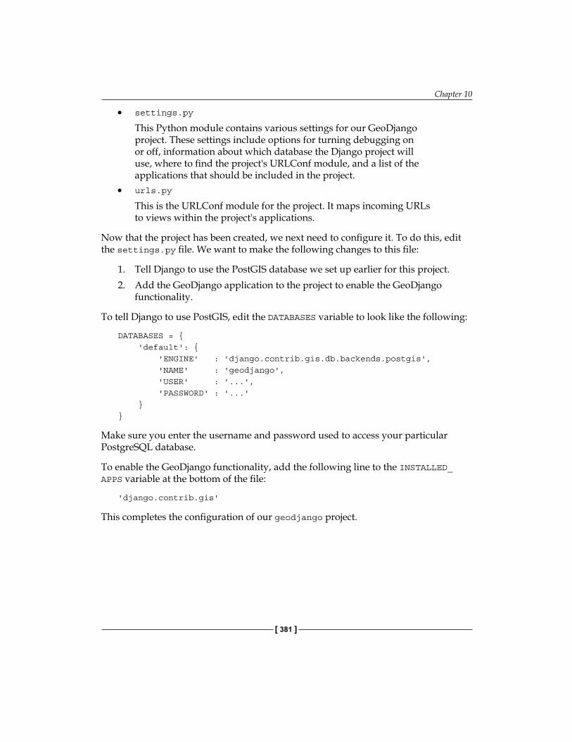
Chapter 10
[ 381 ]
• settings.py
This Python module contains various settings for our GeoDjango project. These settings include options for turning debugging on or off, information about which database the Django project will use, where to find the project's URLConf module, and a list of the applications that should be included in the project.
• urls.py
This is the URLConf module for the project. It maps incoming URLs to views within the project's applications.
Now that the project has been created, we next need to configure it. To do this, edit the settings.py file. We want to make the following changes to this file:
1. Tell Django to use the PostGIS database we set up earlier for this project.2. Add the GeoDjango application to the project to enable the GeoDjango
functionality.
To tell Django to use PostGIS, edit the DATABASES variable to look like the following:
DATABASES = { 'default': { 'ENGINE' : 'django.contrib.gis.db.backends.postgis', 'NAME' : 'geodjango', 'USER' : '...', 'PASSWORD' : '...' }}
Make sure you enter the username and password used to access your particular PostgreSQL database.
To enable the GeoDjango functionality, add the following line to the INSTALLED_APPS variable at the bottom of the file:
'django.contrib.gis'
This completes the configuration of our geodjango project.
Putting it All Together: A Complete Mapping Application
[ 382 ]
Setting up the ShapeEditor applicationWe next need to create the ShapeEditor application itself. Remember that applications exist inside a project—to create our application, cd into the geodjango project directory, and type the following:
python manage.py startapp shapeEditor
This will create a new directory within the geodjango directory named shapeEditor. This application directory will be set up with the following files:
• __init__.py
This is another Python package initialization file, telling Python that the shapeEditor directory holds a Python package.
• models.py
This Python module will hold the ShapeEditor's data models.• tests.py
This Python module holds various unit tests for your application. We won't be using this.
• views.py
This Python module will hold various views for the ShapeEditor application.
Now that we have created the application itself, let's add it to our project. Edit the settings.py file again, and add the following entry to the INSTALLED_APPS list:
'shapeEditor'
While we're editing the settings.py file, let's make one more change that will save us some trouble down the track. Go to the MIDDLEWARE_CLASSES setting, and comment out the django.middleware.csrf.CsrfViewMiddleware line. This entry tells Django to perform extra error checking when processing forms to prevent cross-site request forgery. Implementing CSRF support requires adding extra code to our form templates, which we won't be doing here to keep things simple.
If you deploy your own applications on the Internet, you should read the CSRF documentation on the Django website and enable CSRF support. Otherwise, your application will be susceptable to cross-site request forgery attacks.
That's all we have to do to create the basic framework for our ShapeEditor application. Now, let's tell Django what data we need to work with.
Chapter 10
[ 383 ]
Defining the data modelsWe already know which database objects we are going to need to store the uploaded Shapefiles:
• The Shapefile object will represent a single uploaded Shapefile.• Each Shapefile will have a number of Attribute objects, giving the name,
data type, and other information about each attribute within the Shapefile• Each Shapefile will have a number of Feature objects, which hold the
geometry for each of the Shapefile's features• Each feature will have a set of AttributeValue objects, which hold the value
for each of the feature's attributes
Let's look at each of these in more detail, and think about exactly what information will need to be stored in each object.
ShapefileWhen we import a Shapefile, there are a few things we are going to need to remember:
• The original name of the uploaded file. We will display this in the "list Shapefiles" view so that the user can identify the Shapefile within this list.
• Which spatial reference system the Shapefile's data was in. When we import the Shapefile, we will convert it to use latitude and longitude coordinates using the WGS84 datum (EPSG 4326), but we need to remember the Shapefile's spatial reference system so that we can use it again when exporting the features. For simplicity, we're going to store the spatial reference system in WKT format.
• What type of geometry was stored in the Shapefile. We'll need this to know which field in the Feature object holds the geometry.
• The character encoding to use for the Shapefile's attributes. Shapefiles do not always come in UTF-8 character encoding, and while we'll convert the attribute values to Unicode when importing the data, we do need to know which character encoding the file was in, so we'll store this information in the Shapefile object as well. This allows us to use the same character encoding when exporting the Shapefile again.
Putting it All Together: A Complete Mapping Application
[ 384 ]
AttributeWhen we export a Shapefile, it has to have the same attributes as the original imported file. Because of this, we have to remember the Shapefile's attributes. That is what the Attribute object does. We will need to remember the following information for each attribute:
• Which Shapefile the attribute belongs to• The name of the attribute• The type of data stored in this attribute (string, floating-point number,
and so on)• The field width of the attribute, in characters• For floating-point attributes, the number of digits to display after
the decimal point
All of this information comes directly from the Shapefile's layer definition.
FeatureEach feature in the imported Shapefile will need to be stored in the database. Because PostGIS (and GeoDjango) uses different field types for different types of geometries, we need to define separate fields for each geometry type. Because of this, the Feature object will need to store the following information:
• Which Shapefile the feature belongs to• The Point geometry, if the Shapefile stores this type of geometry• The MultiPoint geometry, if the Shapefile stores this type of geometry• The MultiLineString geometry, if the Shapefile stores this type of geometry• The MultiPolygon geometry, if the Shapefile stores this type of geometry• The GeometryCollection geometry, if the Shapefile stores this type of geometry
Chapter 10
[ 385 ]
Isn't something missing?If you've been paying attention, you've probably noticed that some of the geometry types are missing. What about Polygons or LineStrings? Because of the way data is stored in a Shapefile, it is impossible to know in advance whether a Shapefile holds Polygons or MultiPolygons, and similarly if it holds LineStrings or MultiLineStrings. The Shapefile's internal structure makes no distinction between these geometry types. Because of this, a Shapefile may claim to store Polygons when it really contains MultiPolygons, and similarly for LineString geometries. For more information, see http://code.djangoproject.com/ticket/7218.To work around this limitation, we store all Polygons as MultiPolygons, and all LineStrings as MultiLineStrings. This is why we don't need Polygon or LineString fields in the Feature object.
AttributeValueThe AttributeValue object holds the value for each of the feature's attributes. This object is quite straightforward, storing the following information:
• Which feature the attribute value is for• Which attribute this value is for• The attribute's value, as a string
For simplicity, we'll be storing all attribute values as strings.
The models.py fileNow that we know what information we want to store in our database, it's easy to define our various model objects. To do this, edit the models.py file in the shapeEditor directory, and make sure it looks like this:
from django.contrib.gis.db import models
class Shapefile(models.Model): filename = models.CharField(max_length=255) srs_wkt = models.CharField(max_length=255) geom_type = models.CharField(max_length=50) encoding = models.CharField(max_length=20)
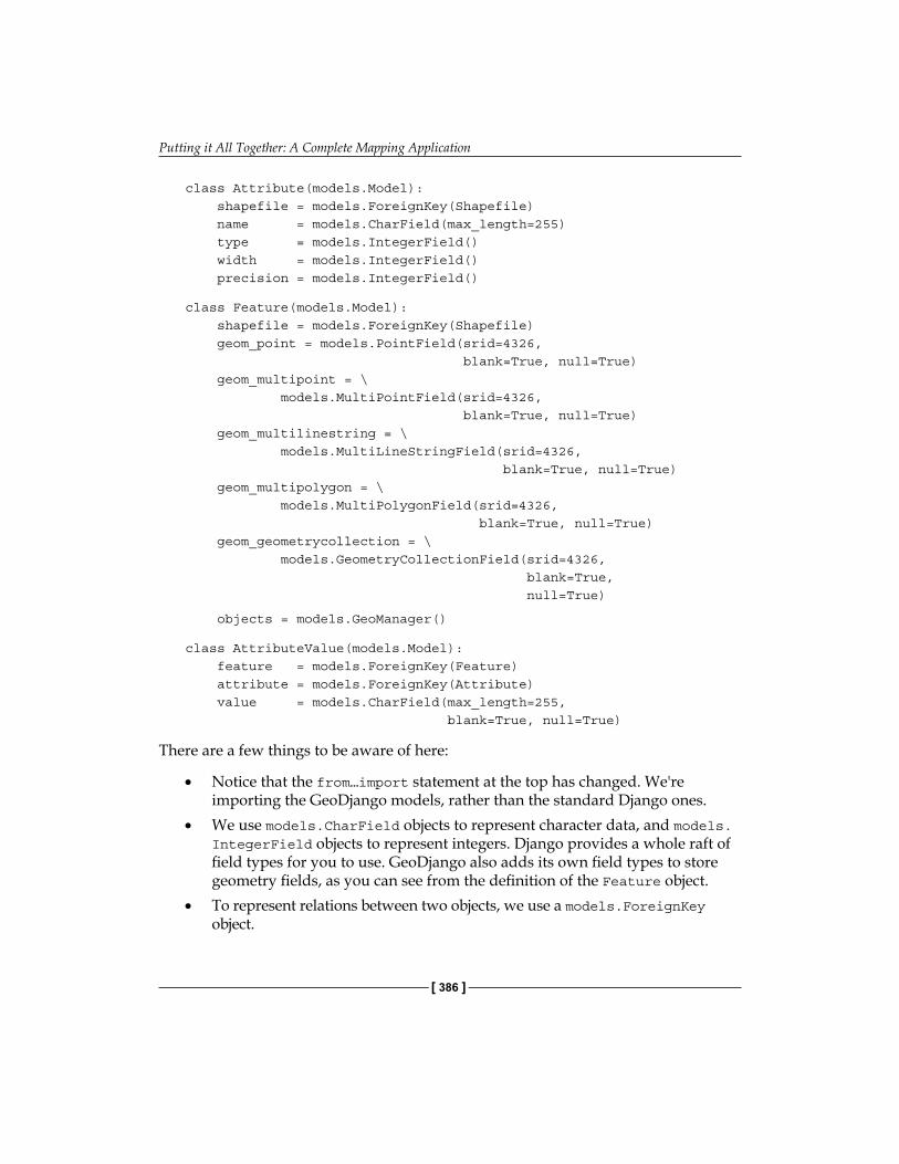
Putting it All Together: A Complete Mapping Application
[ 386 ]
class Attribute(models.Model): shapefile = models.ForeignKey(Shapefile) name = models.CharField(max_length=255) type = models.IntegerField() width = models.IntegerField() precision = models.IntegerField()
class Feature(models.Model): shapefile = models.ForeignKey(Shapefile) geom_point = models.PointField(srid=4326, blank=True, null=True) geom_multipoint = \ models.MultiPointField(srid=4326, blank=True, null=True) geom_multilinestring = \ models.MultiLineStringField(srid=4326, blank=True, null=True) geom_multipolygon = \ models.MultiPolygonField(srid=4326, blank=True, null=True) geom_geometrycollection = \ models.GeometryCollectionField(srid=4326, blank=True, null=True)
objects = models.GeoManager()
class AttributeValue(models.Model): feature = models.ForeignKey(Feature) attribute = models.ForeignKey(Attribute) value = models.CharField(max_length=255, blank=True, null=True)
There are a few things to be aware of here:
• Notice that the from…import statement at the top has changed. We're importing the GeoDjango models, rather than the standard Django ones.
• We use models.CharField objects to represent character data, and models.IntegerField objects to represent integers. Django provides a whole raft of field types for you to use. GeoDjango also adds its own field types to store geometry fields, as you can see from the definition of the Feature object.
• To represent relations between two objects, we use a models.ForeignKey object.
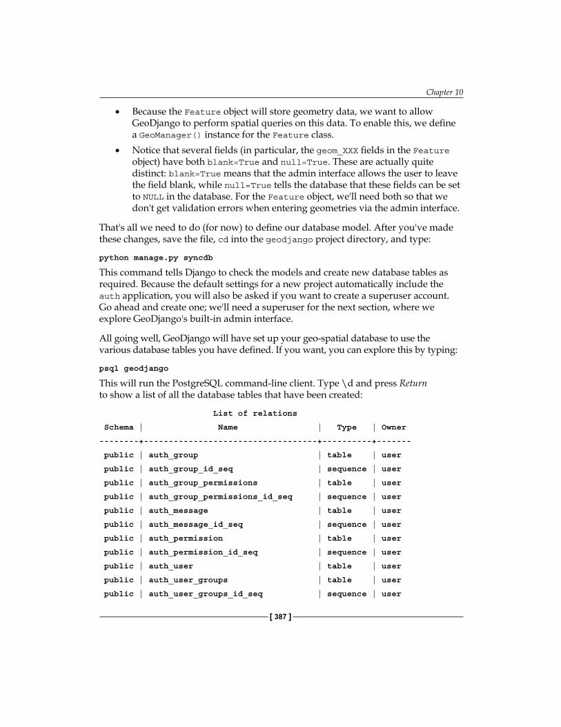
Chapter 10
[ 387 ]
• Because the Feature object will store geometry data, we want to allow GeoDjango to perform spatial queries on this data. To enable this, we define a GeoManager() instance for the Feature class.
• Notice that several fields (in particular, the geom_XXX fields in the Feature object) have both blank=True and null=True. These are actually quite distinct: blank=True means that the admin interface allows the user to leave the field blank, while null=True tells the database that these fields can be set to NULL in the database. For the Feature object, we'll need both so that we don't get validation errors when entering geometries via the admin interface.
That's all we need to do (for now) to define our database model. After you've made these changes, save the file, cd into the geodjango project directory, and type:
python manage.py syncdb
This command tells Django to check the models and create new database tables as required. Because the default settings for a new project automatically include the auth application, you will also be asked if you want to create a superuser account. Go ahead and create one; we'll need a superuser for the next section, where we explore GeoDjango's built-in admin interface.
All going well, GeoDjango will have set up your geo-spatial database to use the various database tables you have defined. If you want, you can explore this by typing:
psql geodjango
This will run the PostgreSQL command-line client. Type \d and press Return to show a list of all the database tables that have been created:
List of relations
Schema | Name | Type | Owner
--------+-----------------------------------+----------+-------
public | auth_group | table | user
public | auth_group_id_seq | sequence | user
public | auth_group_permissions | table | user
public | auth_group_permissions_id_seq | sequence | user
public | auth_message | table | user
public | auth_message_id_seq | sequence | user
public | auth_permission | table | user
public | auth_permission_id_seq | sequence | user
public | auth_user | table | user
public | auth_user_groups | table | user
public | auth_user_groups_id_seq | sequence | user
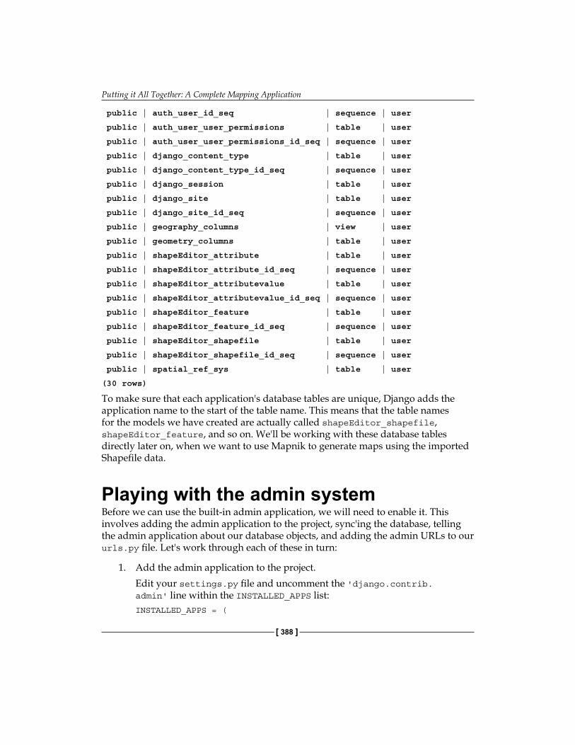
Putting it All Together: A Complete Mapping Application
[ 388 ]
public | auth_user_id_seq | sequence | user
public | auth_user_user_permissions | table | user
public | auth_user_user_permissions_id_seq | sequence | user
public | django_content_type | table | user
public | django_content_type_id_seq | sequence | user
public | django_session | table | user
public | django_site | table | user
public | django_site_id_seq | sequence | user
public | geography_columns | view | user
public | geometry_columns | table | user
public | shapeEditor_attribute | table | user
public | shapeEditor_attribute_id_seq | sequence | user
public | shapeEditor_attributevalue | table | user
public | shapeEditor_attributevalue_id_seq | sequence | user
public | shapeEditor_feature | table | user
public | shapeEditor_feature_id_seq | sequence | user
public | shapeEditor_shapefile | table | user
public | shapeEditor_shapefile_id_seq | sequence | user
public | spatial_ref_sys | table | user
(30 rows)
To make sure that each application's database tables are unique, Django adds the application name to the start of the table name. This means that the table names for the models we have created are actually called shapeEditor_shapefile, shapeEditor_feature, and so on. We'll be working with these database tables directly later on, when we want to use Mapnik to generate maps using the imported Shapefile data.
Playing with the admin systemBefore we can use the built-in admin application, we will need to enable it. This involves adding the admin application to the project, sync'ing the database, telling the admin application about our database objects, and adding the admin URLs to our urls.py file. Let's work through each of these in turn:
1. Add the admin application to the project.Edit your settings.py file and uncomment the 'django.contrib.admin' line within the INSTALLED_APPS list:INSTALLED_APPS = (
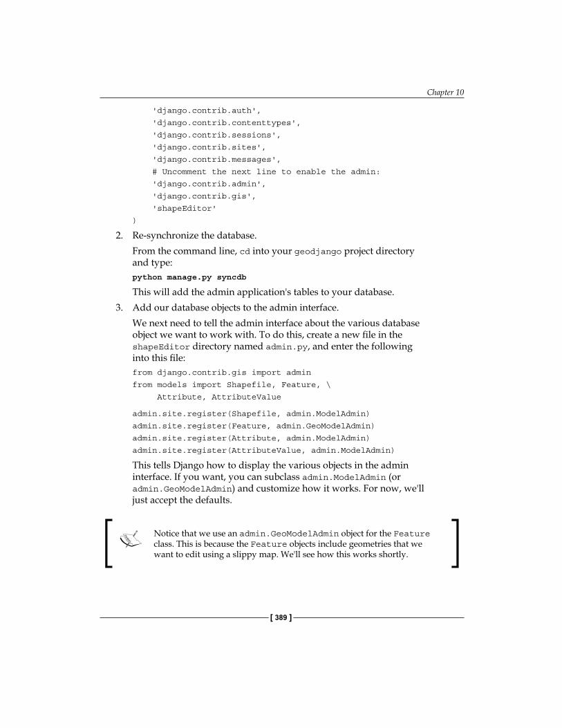
Chapter 10
[ 389 ]
'django.contrib.auth',
'django.contrib.contenttypes',
'django.contrib.sessions',
'django.contrib.sites',
'django.contrib.messages',
# Uncomment the next line to enable the admin:
'django.contrib.admin',
'django.contrib.gis',
'shapeEditor'
)
2. Re-synchronize the database.From the command line, cd into your geodjango project directory and type:python manage.py syncdb
This will add the admin application's tables to your database.3. Add our database objects to the admin interface.
We next need to tell the admin interface about the various database object we want to work with. To do this, create a new file in the shapeEditor directory named admin.py, and enter the following into this file:from django.contrib.gis import admin
from models import Shapefile, Feature, \
Attribute, AttributeValue
admin.site.register(Shapefile, admin.ModelAdmin)
admin.site.register(Feature, admin.GeoModelAdmin)
admin.site.register(Attribute, admin.ModelAdmin)
admin.site.register(AttributeValue, admin.ModelAdmin)
This tells Django how to display the various objects in the admin interface. If you want, you can subclass admin.ModelAdmin (or admin.GeoModelAdmin) and customize how it works. For now, we'll just accept the defaults.
Notice that we use an admin.GeoModelAdmin object for the Feature class. This is because the Feature objects include geometries that we want to edit using a slippy map. We'll see how this works shortly.
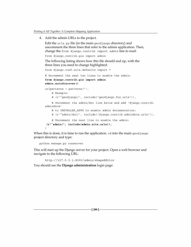
Putting it All Together: A Complete Mapping Application
[ 390 ]
4. Add the admin URLs to the project.Edit the urls.py file (in the main geodjango directory) and uncomment the three lines that refer to the admin application. Then, change the from django.contrib import admin line to read:from django.contrib.gis import admin
The following listing shows how this file should end up, with the three lines you need to change highlighted:from django.conf.urls.defaults import *
# Uncomment the next two lines to enable the admin:
from django.contrib.gis import adminadmin.autodiscover()
urlpatterns = patterns('',
# Example:
# (r'^geodjango/', include('geodjango.foo.urls')),
# Uncomment the admin/doc line below and add 'django.contrib.admindocs'
# to INSTALLED_APPS to enable admin documentation:
# (r'^admin/doc/', include('django.contrib.admindocs.urls')),
# Uncomment the next line to enable the admin:
(r'^admin/', include(admin.site.urls)),)
When this is done, it is time to run the application. cd into the main geodjango project directory and type:
python manage.py runserver
This will start up the Django server for your project. Open a web browser and navigate to the following URL:
http://127.0.0.1:8000/admin/shapeEditor
You should see the Django administration login page:
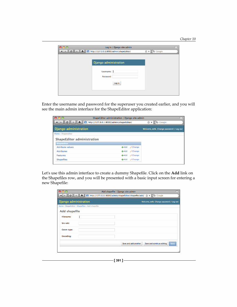
Chapter 10
[ 391 ]
Enter the username and password for the superuser you created earlier, and you will see the main admin interface for the ShapeEditor application:
Let's use this admin interface to create a dummy Shapefile. Click on the Add link on the Shapefiles row, and you will be presented with a basic input screen for entering a new Shapefile:
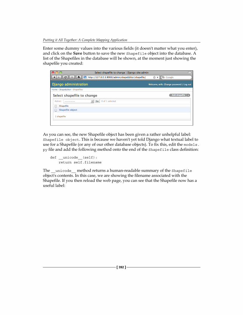
Putting it All Together: A Complete Mapping Application
[ 392 ]
Enter some dummy values into the various fields (it doesn't matter what you enter), and click on the Save button to save the new Shapefile object into the database. A list of the Shapefiles in the database will be shown, at the moment just showing the shapefile you created:
As you can see, the new Shapefile object has been given a rather unhelpful label: Shapefile object. This is because we haven't yet told Django what textual label to use for a Shapefile (or any of our other database objects). To fix this, edit the models.py file and add the following method onto the end of the Shapefile class definition:
def __unicode__(self): return self.filename
The __unicode__ method returns a human-readable summary of the Shapefile object's contents. In this case, we are showing the filename associated with the Shapefile. If you then reload the web page, you can see that the Shapefile now has a useful label:
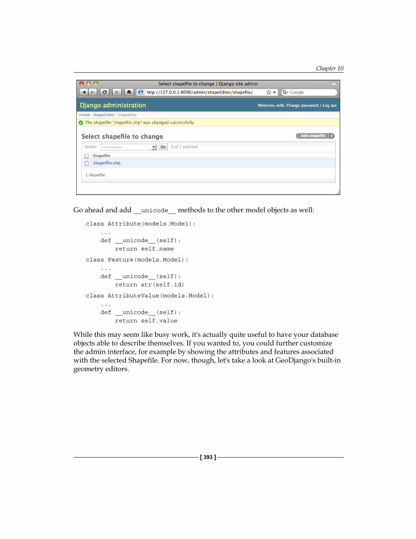
Chapter 10
[ 393 ]
Go ahead and add __unicode__ methods to the other model objects as well:
class Attribute(models.Model): ... def __unicode__(self): return self.name
class Feature(models.Model): ... def __unicode__(self): return str(self.id)
class AttributeValue(models.Model): ... def __unicode__(self): return self.value
While this may seem like busy work, it's actually quite useful to have your database objects able to describe themselves. If you wanted to, you could further customize the admin interface, for example by showing the attributes and features associated with the selected Shapefile. For now, though, let's take a look at GeoDjango's built-in geometry editors.
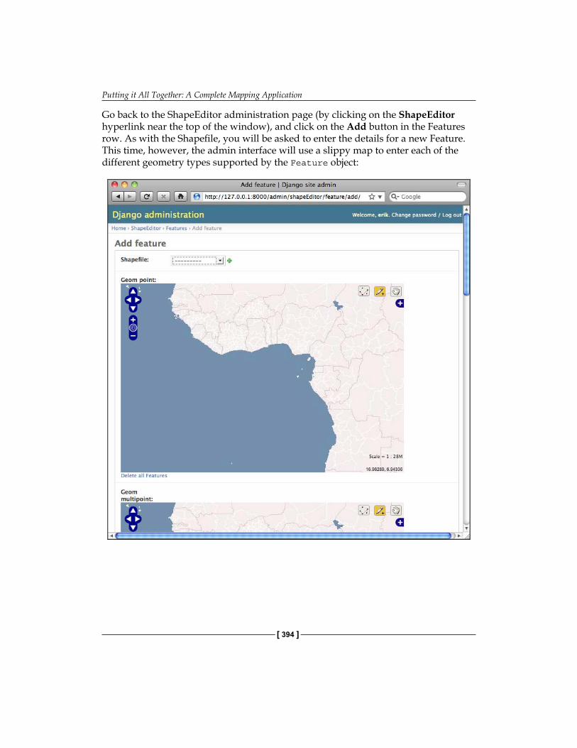
Putting it All Together: A Complete Mapping Application
[ 394 ]
Go back to the ShapeEditor administration page (by clicking on the ShapeEditor hyperlink near the top of the window), and click on the Add button in the Features row. As with the Shapefile, you will be asked to enter the details for a new Feature. This time, however, the admin interface will use a slippy map to enter each of the different geometry types supported by the Feature object:
Chapter 10
[ 395 ]
Obviously, having multiple slippy maps like this isn't quite what we want, and if we wanted to we could set up a custom GeoModelAdmin subclass to avoid this, but that's not important right now. Instead, try selecting the Shapefile to associate this feature with by choosing your Shapefile from the pop up menu, and then scroll down to the Geom Multipolygon field and try adding a couple of polygons to the map. Then, use the Edit Polygon tool ( ) to make changes to the polygons; the interface should be fairly obvious once you play with it for a minute or two.
When you're done, click on Save to save your new feature. If you edit it again, you'll see your saved geometry (or geometries) once again on the slippy maps.
That completes our tour of the admin interface. We won't be using this for end users as we don't want to require users to log in before making changes to the Shapefile data. We will, however, be borrowing some code from the admin application so that end users can edit their Shapefile features using a slippy map.
SummaryYou have now finished implementing the first part of the ShapeEditor application. Even at this early stage, you have made good progress, learning how GeoDjango works, designing the application, and laying the foundations for the functionality you will implement in the next two chapters.
In this chapter, you have learned:
• That the GeoDjango extension to Django can be used to build sophisticated geo-spatial web applications.
• That a Django project consists of a single database and multiple Django applications.
• That Django uses objects to represent records in the database.• That a Django view is a Python function that responds when a given URL
is called.• That the mapping from URLs to views is controlled by a URLConf module
named urls.py defined at the project level.• That Django uses a powerful templating system to simplify the creation of
complex HTML pages.• That Django allows you to define forms for handling the input of data• That Django form fields make it easy to accept and validate a variety of
different types of data.
Putting it All Together: A Complete Mapping Application
[ 396 ]
• That GeoDjango provides its own set of form fields for editing geo-spatial data.• That an application's data objects are defined in a file called models.py.• That GeoDjango's built-in "admin" system allows you to view and edit
geo-spatial data using slippy maps.
In Chapter 11, we will implement a view to show the available Shapefiles, as well as writing the rather complex code for importing and exporting Shapefiles.
ShapeEditor: Implementing List View, Import, and Export
In this chapter, we will continue our implementation of the ShapeEditor application. We will start by implementing a "list" view to show the available Shapefiles, and then work through the details of importing and exporting Shapefiles via a web interface.
In this chapter, we will learn:
• How to display a list of records using a Django template• How to deal with the complexities of Shapefile data, including issues with
geometries and attribute data types• How to import a Shapefile's data using a web interface• How to export a Shapefile using a web interface
Implementing the "List Shapefiles" viewWhen the user first opens the ShapeEditor application, we want them to see a list of the previously-uploaded Shapefiles, with import, edit, export, and delete options. Let's build this list view, which acts as the starting point for the entire ShapeEditor application.
We'll start by tidying up the urls.py module so that we can add more URLs as we need them. Edit the urls.py file to look like this:
from django.conf.urls.defaults import *from django.contrib.gis import adminadmin.autodiscover()
urlpatterns = patterns('geodjango.shapeEditor.views',
ShapeEditor: Implementing List View, Import, and Export
[ 398 ]
(r'^shape-editor$', 'listShapefiles'),)
urlpatterns += patterns('', (r'^admin/', include(admin.site.urls)),)
Notice that we've now got two separate sets of URL patterns: one accessing functions within the geodjango.shapeEditor.views module, and the other for the admin interface. Splitting the URLs up like this is convenient as it lets us group the URLs logically by which module the views are defined in.
Let's take a closer look at the first URL pattern definition:
urlpatterns = patterns('geodjango.shapeEditor.views', (r'^shape-editor$', 'listShapefiles'),)
This tells Django that any incoming URL that has a path name equal to / shape-editor should be mapped to the geodjango.shapeEditor.views.listShapefiles() function. This is the top-level URL for our entire application. Notice that we use regular expressions (and the r'...' syntax convention) to define the URL to match against.
Now that we've set up our URL, let's write the view to go with it. We'll start by creating a very simple implementation of the listShapefiles() view, just to make sure it works. Open the views.py module in the shapeEditor directory and edit the file to look like this:
from django.http import HttpResponse
def listShapefiles(request): return HttpResponse("in listShapefiles")
If it isn't already running, start up the GeoDjango web server. To do this, open a command-line window, cd into the geodjango project directory, and type:
python manage.py runserver
Then, open your web browser and navigate to the following URL:
http://127.0.0.1:8000/shape-editor
All going well, you should see in listShapefiles appear on the web page. This tells us that we've created the listShapefiles() view function and have successfully set up the URL mapping to point to this view.
Chapter 11
[ 399 ]
We now want to create the view which will display the list of Shapefiles. To do so, we'll make use of a Django template. Start by editing the views.py module, and change the module's contents to look like this:
from django.http import HttpResponsefrom django.shortcuts import render_to_responsefrom geodjango.shapeEditor.models import Shapefile
def listShapefiles(request): shapefiles = Shapefile.objects.all().order_by('filename') return render_to_response("listShapefiles.html", {'shapefiles' : shapefiles})
The listShapefiles() view function now does two things:
1. It loads the list of all Shapefile objects from the database into memory, sorted by filename.
2. It passes this list to a Django template (in the file listShapefiles.html), which is rendered into an HTML web page and returned back to the caller.
Let's go ahead and create the listShapefiles.html template. Create a directory called templates within the shapeEditor directory, and create a new file in this directory named listShapefiles.html. This file should have the following contents:
<html> <head> <title>ShapeEditor</title> </head> <body> <h1>ShapeEditor</h1> {% if shapefiles %} <b>Available Shapefiles:</b> <table border="0" cellspacing="0" cellpadding="5" style="padding-left:20px"> {% for shapefile in shapefiles %} <tr> <td><font style="font-family:monospace">{{ shapefile.filename }}</font></td> <td> </td> <td> <a href="/shape-editor/edit/{{ shapefile.id }}"> Edit </a> </td> <td> </td> <td>
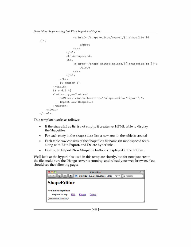
ShapeEditor: Implementing List View, Import, and Export
[ 400 ]
<a href="/shape-editor/export/{{ shapefile.id }}"> Export </a> </td> <td> </td> <td> <a href="/shape-editor/delete/{{ shapefile.id }}"> Delete </a> </td> </tr> {% endfor %} </table> {% endif %} <button type="button" onClick='window.location="/shape-editor/import";'> Import New Shapefile </button> </body></html>
This template works as follows:
• If the shapefiles list is not empty, it creates an HTML table to display the Shapefiles
• For each entry in the shapefiles list, a new row in the table is created• Each table row consists of the Shapefile's filename (in monospaced text),
along with Edit, Export, and Delete hyperlinks• Finally, an Import New Shapefile button is displayed at the bottom
We'll look at the hyperlinks used in this template shortly, but for now just create the file, make sure the Django server is running, and reload your web browser. You should see the following page:
Chapter 11
[ 401 ]
As you can see, the Shapefile we created earlier in the admin interface is shown, along with the relevant hyperlinks and buttons to access the rest of the ShapeEditor's functionality:
• The Edit hyperlink will take the user to the /shape-editor/edit/1 URL, which will let the user edit the Shapefile with the given record ID
• The Export hyperlink will take the user to the /shape-editor/export/1 URL, which will let the user download a copy of the Shapefile with the given ID
• The Delete hyperlink will take the user to the /shape-editor/delete/1 URL, which will let the user delete the given Shapefile
• The Import New Shapefile button will take the user to the /shape-editor/import URL, which will let the user upload a new Shapefile
You can explore these URLs by clicking on them if you want—they won't do anything other than display an error page, but you can see how the URLs link the various parts of the ShapeEditor's functionality together. You can also take a detailed look at the Django error page, which can be quite helpful in tracking down bugs.
Now that we have a working first page, let's start implementing the core functionality of the ShapeEditor application. We'll start with the logic required to import a Shapefile.
Importing ShapefilesThe process of importing a Shapefile involves the following steps:
1. Display a form prompting the user to upload the Shapefile's ZIP archive.2. Decompress the ZIP file to extract the uploaded Shapefile.3. Open the Shapefile and read the data out of it into the database.4. Delete the temporary files we have created.
Let's work through each of these steps in turn.
ShapeEditor: Implementing List View, Import, and Export
[ 402 ]
The "import shapefile" formLet's start by creating a placeholder for the "import shapefile" view. Edit the urls.py module and add a second entry to the geodjango.shapeEditor.views pattern list:
urlpatterns = patterns('geodjango.shapeEditor.views', (r'^shape-editor$', 'listShapefiles'), (r'^shape-editor/import$', 'importShapefile'),)
Then, edit the views.py module and add a dummy importShapefile() view function to respond to this URL:
def importShapefile(request): return HttpResponse("More to come")
You can test this if you want: run the Django server, go to the main page, and click on the Import New Shapefile button. You should see the More to come message.
To let the user enter data, we're going to use a Django form. Forms are custom classes that define the various fields that will appear on the web page. In this case, our form will have two fields: one to accept the uploaded file, and the other to select the character encoding from a pop up menu. We're going to store this form in a file named forms.py in the shapeEditor directory; go ahead and create this file, and then edit it to look like this:
from django import forms
CHARACTER_ENCODINGS = [("ascii", "ASCII"), ("latin1", "Latin-1"), ("utf8", "UTF-8")]
class ImportShapefileForm(forms.Form): import_file = forms.FileField(label="Select a Zipped Shapefile") character_encoding = forms.ChoiceField(choices=CHARACTER_ENCODINGS, initial="utf8")
The first field is a FileField which accepts uploaded files. We give this field a custom label which will be displayed in the web page. For the second field, we'll use a ChoiceField, which displays a pop up menu. Notice that the CHARACTER_ENCODINGS list shows the various choices to display in the pop up menu; each entry in this list is a (value, label) tuple, where label is the string to be displayed and value is the actual value to use for that field when the user chooses this item from the list.
Now that we have created the form, go back to views.py and change the definition of the importShapefile() view function to look like this:
Chapter 11
[ 403 ]
def importShapefile(request): if request.method == "GET": form = ImportShapefileForm() return render_to_response("importShapefile.html", {'form' : form}) elif request.method == "POST": form = ImportShapefileForm(request.POST, request.FILES) if form.is_valid(): shapefile = request.FILES['import_file'] encoding = request.POST['character_encoding'] # More to come... return HttpResponseRedirect("/shape-editor")
return render_to_response("importShapefile.html", {'form' : form})
Also, add these two import statements to the top of the module:
from django.http import HttpResponseRedirectfrom geodjango.shapeEditor.forms import ImportShapefileForm
Let's take a look at what is happening here. The importShapefile() function will initially be called with an HTTP GET request; this will cause the function to create a new ImportShapefileForm object, and then call render_to_response() to display that form to the user. When the form is submitted, the importShapefile() function will be called with an HTTP POST request. In this case, the ImportShapefileForm will be created with the submitted data (request.POST and request.FILES), and the form will be checked to see that the entered data is valid. If so, we extract the uploaded Shapefile and the selected character encoding.
At this point, because we haven't implemented the actual importing code, we simply redirect the user back to the main /shape-editor page again. As the comment says, we'll add more code here shortly.
If the form was not valid, we once again call render_to_response() to display the form to the user. In this case, Django will automatically display the error message(s) associated with the form so the user can see why the validation failed.
To display the form, we'll use a Django template and pass the form object as a parameter. Let's create that template now; add a new file named importShapefile.html in the templates directory and enter the following text into this file:
<html> <head> <title>ShapeEditor</title> </head>
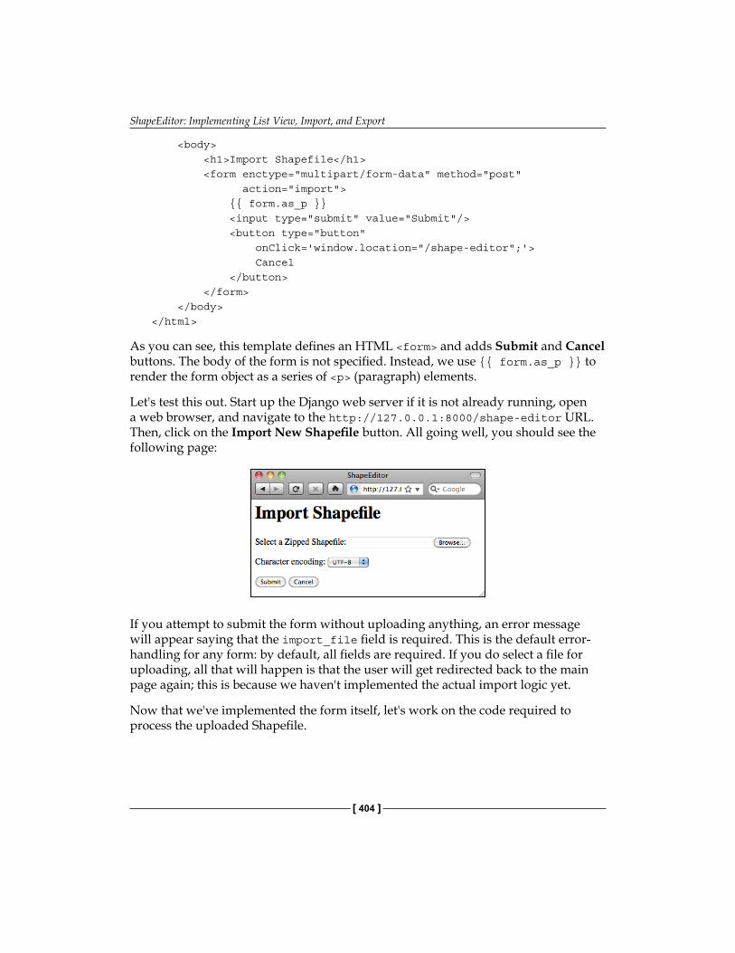
ShapeEditor: Implementing List View, Import, and Export
[ 404 ]
<body> <h1>Import Shapefile</h1> <form enctype="multipart/form-data" method="post" action="import"> {{ form.as_p }} <input type="submit" value="Submit"/> <button type="button" onClick='window.location="/shape-editor";'> Cancel </button> </form> </body></html>
As you can see, this template defines an HTML <form> and adds Submit and Cancel buttons. The body of the form is not specified. Instead, we use {{ form.as_p }} to render the form object as a series of <p> (paragraph) elements.
Let's test this out. Start up the Django web server if it is not already running, open a web browser, and navigate to the http://127.0.0.1:8000/shape-editor URL. Then, click on the Import New Shapefile button. All going well, you should see the following page:
If you attempt to submit the form without uploading anything, an error message will appear saying that the import_file field is required. This is the default error-handling for any form: by default, all fields are required. If you do select a file for uploading, all that will happen is that the user will get redirected back to the main page again; this is because we haven't implemented the actual import logic yet.
Now that we've implemented the form itself, let's work on the code required to process the uploaded Shapefile.
Chapter 11
[ 405 ]
Extracting the uploaded ShapefileBecause the process of importing data is going to be rather involved, we'll put this code into a separate module. Create a new file named shapefileIO.py within the shapeEditor directory and add the following text to this file:
def importData(shapefile, characterEncoding): return "More to come..."
Since it's quite possible for the process of importing a Shapefile to fail (for example, if the user uploads a file that isn't a ZIP archive), our importData() function is going to return an error message if something goes wrong. Let's go back and change our view (and template) to call this importData() function and display the returned error message, if any.
Edit the views.py module, and add the following highlighted lines to the importShapefile() view function:
def importShapefile(request): if request.method == "GET": form = ImportShapefileForm() return render_to_response("importShapefile.html", {'form' : form, 'errMsg' : None}) elif request.method == "POST": errMsg = None # initially.
form = ImportShapefileForm(request.POST, request.FILES) if form.is_valid(): shapefile = request.FILES['import_file'] encoding = request.POST['character_encoding'] errMsg = shapefileIO.importData(shapefile, encoding) if errMsg == None: return HttpResponseRedirect("/shape-editor")
return render_to_response("importShapefile.html", {'form' : form, 'errMsg' : errMsg})
You'll also need to add import shapefileIO to the top of the file.
Now, edit the importShapefile.html template, and add the following lines to the file immediately below the <h1>Import Shapefile<h1> line:
{% if errMsg %}<b><i>{{ errMsg }}</i></b>{% endif %}
ShapeEditor: Implementing List View, Import, and Export
[ 406 ]
This will display the error message to the user if it is not None.
Go ahead and try out your changes: click on the Import New Shapefile button, select a ZIP archive, and click on Submit. You should see the text More to come... appear at the top of the form, which is the error text returned by our dummy importData() function.
We're now ready to start implementing the import logic. Edit the shapefileIO.py module again and get ready to write the body of the importData() function. We'll take this one step at a time.
When we set up a form that includes a FileField, Django returns to us an UploadedFile object representing the uploaded file. Our first task is to read the contents of the UploadedFile object and store it into a temporary file on disk so that we can work with it. Add the following to your importData() function:
fd,fname = tempfile.mkstemp(suffix=".zip") os.close(fd)
f = open(fname, "wb") for chunk in shapefile.chunks(): f.write(chunk) f.close()
As you can see, we use the tempfile module from the Python standard library to create a temporary file, and then copy the contents of the Shapefile object into it.
Because tempfile.mkstemp() returns both a file descriptor and a filename, we call os.close(fd) to close the file descriptor. This allows us to re-open the file using open() and write to it in the normal way.
We're now ready to open the temporary file and check that it is indeed a ZIP archive containing the files that make up a Shapefile. Here is how we can do this:
if not zipfile.is_zipfile(fname): os.remove(fname) return "Not a valid zip archive."
zip = zipfile.ZipFile(fname)
required_suffixes = [".shp", ".shx", ".dbf", ".prj"] hasSuffix = {} for suffix in required_suffixes: hasSuffix[suffix] = False
for info in zip.infolist(): extension = os.path.splitext(info.filename)[1].lower() if extension in required_suffixes:
Chapter 11
[ 407 ]
hasSuffix[extension] = True
for suffix in required_suffixes: if not hasSuffix[suffix]: zip.close() os.remove(fname) return "Archive missing required "+suffix+" file."
Notice that we use the Python standard library's zipfile module to check the contents of the uploaded ZIP archive and return a suitable error message if something is wrong. We also delete the temporary file before returning an error message so that we don't leave temporary files lying around.
Finally, now that we know that the uploaded file is a valid ZIP archive containing the files that make up a Shapefile, we can extract these files and store them into a temporary directory:
zip = zipfile.ZipFile(fname) shapefileName = None dirname = tempfile.mkdtemp() for info in zip.infolist(): if info.filename.endswith(".shp"): shapefileName = info.filename
dstFile = os.path.join(dirname, info.filename) f = open(dstFile, "wb") f.write(zip.read(info.filename)) f.close() zip.close()
Notice that we create a temporary directory to hold the extracted files before copying the files into this directory. At the same time, we remember the name of the main .shp file from the archive as we'll need to use this name when we add the Shapefile into the database.
Because we've used some of the Python standard library modules in this code, you'll also need to add the following to the top of the module:
import os, os.path, tempfile, zipfile
ShapeEditor: Implementing List View, Import, and Export
[ 408 ]
Importing the Shapefile's contentsNow that we've extracted the Shapefile's files out of the ZIP archive, we are ready to import the data from the uploaded Shapefile. The process of importing the Shapefile's contents involves the following steps:
1. Open the Shapefile.2. Add the Shapefile object to the database.3. Define the Shapefile's attributes.4. Store the Shapefile's features.5. Store the Shapefile's attributes.
Let's work through these steps one at a time.
Open the ShapefileWe will use the OGR library to open the Shapefile:
try: datasource = ogr.Open(os.path.join(dirname, shapefileName)) layer = datasource.GetLayer(0) shapefileOK = True except: traceback.print_exc() shapefileOK = False
if not shapefileOK: os.remove(fname) shutil.rmtree(dirname) return "Not a valid shapefile."
Once again, if something goes wrong we clean up our temporary files and return a suitable error message. We're also using the traceback library module to display debugging information in the web server's log, while returning a friendly error message that will be shown to the user.
In this program, we will be using OGR directly to read and write Shapefiles. GeoDjango provides its own Python interface to OGR in the contrib.gis.gdal package, but unfortunately GeoDjango's version doesn't implement writing to Shapefiles. Because of this, we will use the OGR Python bindings directly, and require you to install OGR separately.
Chapter 11
[ 409 ]
Because this code uses a couple of standard library modules, as well as the OGR library, we'll have to add the following import statements to the top of the shapefileIO.py module:
import shutil, tracebackfrom osgeo import ogr
Add the Shapefile object to the databaseNow that we've successfully opened the Shapefile, we are ready to read the data out of it. First off, we'll create the Shapefile object to represent this imported Shapefile:
srcSpatialRef = layer.GetSpatialRef() shapefile = Shapefile(filename=shapefileName, srs_wkt=srcSpatialRef.ExportToWkt(), geom_type="More to come", encoding=characterEncoding) shapefile.save()
As you can see, we get the spatial reference from the Shapefile's layer, and then store the Shapefile's name, spatial reference, and encoding into a Shapefile object, which we then save into the database. There's only one glitch: what value are we going to store into the geom_type field?
The geom_type field is supposed to hold the name of the geometry type that this Shapefile holds. While OGR is able to tell us the geometry type as a numeric constant, the OGRGeometryTypeToName() function in OGR is not exposed by the Python bindings, so we can't get the name of the geometry directly using OGR.
To work around this, we'll implement our own version of OGRGeometryTypeToName(). Because we're going to have a number of these sorts of functions, we'll store this in a separate module, which we'll call utils.py. Create the utils.py file inside the shapeEditor directory, and then add the following code to this module:
from osgeo import ogr
def ogrTypeToGeometryName(ogrType): return {ogr.wkbUnknown : 'Unknown', ogr.wkbPoint : 'Point', ogr.wkbLineString : 'LineString', ogr.wkbPolygon : 'Polygon', ogr.wkbMultiPoint : 'MultiPoint', ogr.wkbMultiLineString : 'MultiLineString', ogr.wkbMultiPolygon : 'MultiPolygon', ogr.wkbGeometryCollection : 'GeometryCollection', ogr.wkbNone : 'None', ogr.wkbLinearRing : 'LinearRing'}.get(ogrType)
ShapeEditor: Implementing List View, Import, and Export
[ 410 ]
Every self-respecting Python program should have a utils.py module; it's about time we added one in the ShapeEditor.
Now that we have our own version of OGRGeometryTypeToName(), we can use this to set the geom_type field in the Shapefile object. Go back to the shapefileIO.py module and make the following changes to the end of your importData() function:
srcSpatialRef = layer.GetSpatialRef()
geometryType = layer.GetLayerDefn().GetGeomType() geometryName = \ utils.ogrTypeToGeometryName(geometryType)
shapefile = Shapefile(filename=shapefileName, srs_wkt=srcSpatialRef.ExportToWkt(), geom_type=geometryName, encoding=characterEncoding) shapefile.save()
To make this code work, we'll have to add the following import statements to the top of the shapefileIO.py module:
from geodjango.shapeEditor.models import Shapefileimport utils
Define the Shapefile's attributesNow that we've created the Shapefile object to represent the imported Shapefile, our next task is to create Attribute objects describing the Shapefile's attributes. We can do this by querying the OGR Shapefile; add the following code to the end of the importData() function:
attributes = [] layerDef = layer.GetLayerDefn() for i in range(layerDef.GetFieldCount()): fieldDef = layerDef.GetFieldDefn(i) attr = Attribute(shapefile=shapefile, name=fieldDef.GetName(), type=fieldDef.GetType(), width=fieldDef.GetWidth(), precision=fieldDef.GetPrecision()) attr.save() attributes.append(attr)
Chapter 11
[ 411 ]
Notice that as well as saving the Attribute objects into a database, we also create a separate list of these attributes in a variable named attributes. We'll use this later on when we import the attribute values for each feature.
Don't forget to add the following import statement to the top of the module:
from geodjango.shapeEditor.models import Attribute
Store the Shapefile's featuresOur next task is to extract the Shapefile's features and store them as Feature objects in the database. Because the Shapefile's features can be in any spatial reference, we need to transform them into our internal spatial reference system (EPSG 4326, unprojected latitude and longitude values) before we can store them. To do this, we'll use an OGR CoordinateTransformation() object.
Here is how we're going to scan through the Shapefile's features, extract the geometry from each feature, transform it into the EPSG 4326 spatial reference, and convert it into a GeoDjango GEOS geometry object so that we can store it into the database:
dstSpatialRef = osr.SpatialReference() dstSpatialRef.ImportFromEPSG(4326)
coordTransform = osr.CoordinateTransformation(srcSpatialRef, dstSpatialRef)
for i in range(layer.GetFeatureCount()): srcFeature = layer.GetFeature(i) srcGeometry = srcFeature.GetGeometryRef() srcGeometry.Transform(coordTransform) geometry = GEOSGeometry(srcGeometry.ExportToWkt())
So far, so good. Unfortunately, we're now faced with a couple of problems: firstly, the inability of Shapefiles to distinguish between Polygons and MultiPolygons (and between LineStrings and MultiLineStrings) as described in the previous chapter means that we have to wrap a Polygon geometry inside a MultiPolygon, and a LineString geometry inside a MultiLineString, so that all the features in the Shapefile will have the same geometry type. This is kind of messy, so we'll write a utils.py function to do this. Add the following line to the end of your importData() function (along with the code we have just seen, if you haven't already typed this in) to wrap the geometry:
geometry = utils.wrapGEOSGeometry(geometry)
The second problem we have is that we need to decide which particular field within the Feature object will hold our geometry. When we defined the Feature object, we had to create separate geometry fields for each of the geometry types; we now need to decide which of these fields will be used to store a given type of geometry.
ShapeEditor: Implementing List View, Import, and Export
[ 412 ]
Because we sometimes have to wrap up geometries, we can't simply use the geometry name to identify the field. This is another messy function that we'll implement in utils.py. For now, just add the following line to the end of your importData() function:
geometryField = utils.calcGeometryField(geometryName)
Now that we've sorted out these problems, we're finally ready to store the feature's geometry into a Feature object within the database:
args = {} args['shapefile'] = shapefile args[geometryField] = geometry feature = Feature(**args) feature.save()
Notice that we use keyword arguments (**args) to create the Feature object. This lets us store the geometry into the correct field of the Feature object with a minimum of fuss. The alternative, using a series of if...elif...elif statements, would have been much more tedious.
Before we move on, we'd better implement those two extra functions in the utils.py module. Here is the implementation for the wrapGEOSGeometry() function:
def wrapGEOSGeometry(geometry): if geometry.geom_type == "Polygon": return MultiPolygon(geometry) elif geometry.geom_type == "LineString": return MultiLineString(geometry) else: return geometry
and here is the implementation for the calcGeometryField() function:
def calcGeometryField(geometryType): if geometryType == "Polygon": return "geom_multipolygon" elif geometryType == "LineString": return "geom_multilinestring" else: return "geom_" + geometryType.lower()
Chapter 11
[ 413 ]
You're also going to have to add the following import statement to the top of the utils.py module:
from django.contrib.gis.geos.collections \ import MultiPolygon, MultiLineString
Finally, in the shapefileIO.py module, you'll have to add the following import statements:
from django.contrib.gis.geos.geometry import GEOSGeometryfrom osgeo import osrfrom geodjango.shapeEditor.models import Feature
Store the Shapefile's attributesNow that we've dealt with the feature's geometry, we can look at importing the feature's attributes. The basic process involves iterating over the attributes, extracting the attribute value from the OGR feature, creating an AttributeValue object to store the value, and then saving it into the database:
for attr in attributes: value = ... attrValue = AttributeValue(feature=feature, attribute=attr, value=value) attrValue.save()
The challenge is to extract the attribute value from the feature. Because the OGR Feature object has different methods to call to extract different types of field values, we are going to have to check for the different field types, call the appropriate GetFieldAs() method, convert the resulting value to a string, and then store this string into the AttributeValue object. NULL values will also have to be handled appropriately. In addition, we have to deal with character encoding: any strings values will have to be converted from the Shapefile's character encoding into Unicode text so that they can be saved into the database. Because of all this complexity, we'll define a new utils.py function to do the hard work, and simply call that function from importData().
Note that because the user might have selected the wrong character encoding for the Shapefile, the process of extracting the attribute value can actually fail. Because of this, we have to add error-handling to our code. To support error-handling, our utility function, getOGRFeatureAttribute(), will return a (success, result) tuple, where success will be True if, and only if, the attribute was successfully extracted, and result will either be the extracted attribute value (as a string), or an error message explaining why the operation failed.
ShapeEditor: Implementing List View, Import, and Export
[ 414 ]
Let's add the necessary code to our importData() function to store the attribute values into the database and gracefully handle any conversion errors that might occur:
for attr in attributes: success,result = utils.getOGRFeatureAttribute( attr, srcFeature, characterEncoding) if not success: os.remove(fname) shutil.rmtree(dirname) shapefile.delete() return result
attrValue = AttributeValue(feature=feature, attribute=attr, value=result) attrValue.save()
Notice that we pass the Attribute object, the OGR feature, and the character encoding to the getOGRFeatureAttribute() function. If an error occurs, we clean up the temporary files, delete the Shapefile object we created earlier, and return the error message back to the caller. If the attribute was successfully extracted, we create a new AttributeValue object with the attribute's value, and save it into the database.
Note that we use shapefile.delete() to remove the partially-imported Shapefile from the database. By default, Django will also automatically delete any records that are related to the record being deleted through a ForeignKey field. This means that the Shapefile object will be deleted, along with all the related Attribute, Feature, and AttributeValue objects. With one line of code, we can completely remove all references to the Shapefile's data.
Now, let's implement that getOGRFeatureAttribute() function. Add the following to utils.py:
def getOGRFeatureAttribute(attr, feature, encoding): attrName = str(attr.name)
if not feature.IsFieldSet(attrName): return (True, None)
needsEncoding = False if attr.type == ogr.OFTInteger: value = str(feature.GetFieldAsInteger(attrName)) elif attr.type == ogr.OFTIntegerList: value = repr(feature.GetFieldAsIntegerList(attrName)) elif attr.type == ogr.OFTReal:
Chapter 11
[ 415 ]
value = feature.GetFieldAsDouble(attrName) value = "%*.*f" % (attr.width, attr.precision, value) elif attr.type == ogr.OFTRealList: values = feature.GetFieldAsDoubleList(attrName) sValues = [] for value in values: sValues.append("%*.*f" % (attr.width, attr.precision, value)) value = repr(sValues) elif attr.type == ogr.OFTString: value = feature.GetFieldAsString(attrName) needsEncoding = True elif attr.type == ogr.OFTStringList: value = repr(feature.GetFieldAsStringList(attrName)) needsEncoding = True elif attr.type == ogr.OFTDate: parts = feature.GetFieldAsDateTime(attrName) year,month,day,hour,minute,second,tzone = parts value = "%d,%d,%d,%d" % (year,month,day,tzone) elif attr.type == ogr.OFTTime: parts = feature.GetFieldAsDateTime(attrName) year,month,day,hour,minute,second,tzone = parts value = "%d,%d,%d,%d" % (hour,minute,second,tzone) elif attr.type == ogr.OFTDateTime: parts = feature.GetFieldAsDateTime(attrName) year,month,day,hour,minute,second,tzone = parts value = "%d,%d,%d,%d,%d,%d,%d,%d" % (year,month,day, hour,minute, second,tzone) else: return (False, "Unsupported attribute type: " + str(attr.type))
if needsEncoding: try: value = value.decode(encoding) except UnicodeDecodeError: return (False, "Unable to decode value in " + repr(attrName) + " attribute. " + "Are you sure you're using the right " + "character encoding?")
return (True, value)
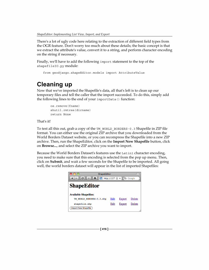
ShapeEditor: Implementing List View, Import, and Export
[ 416 ]
There's a lot of ugly code here relating to the extraction of different field types from the OGR feature. Don't worry too much about these details; the basic concept is that we extract the attribute's value, convert it to a string, and perform character encoding on the string if necessary.
Finally, we'll have to add the following import statement to the top of the shapefileIO.py module:
from geodjango.shapeEditor.models import AttributeValue
Cleaning upNow that we've imported the Shapefile's data, all that's left is to clean up our temporary files and tell the caller that the import succeeded. To do this, simply add the following lines to the end of your importData() function:
os.remove(fname) shutil.rmtree(dirname) return None
That's it!
To test all this out, grab a copy of the TM_WORLD_BORDERS-0.3 Shapefile in ZIP file format. You can either use the original ZIP archive that you downloaded from the World Borders Dataset website, or you can recompress the Shapefile into a new ZIP archive. Then, run the ShapeEditor, click on the Import New Shapefile button, click on Browse..., and select the ZIP archive you want to import.
Because the World Borders Dataset's features use the Latin1 character encoding, you need to make sure that this encoding is selected from the pop up menu. Then, click on Submit, and wait a few seconds for the Shapefile to be imported. All going well, the world borders dataset will appear in the list of imported Shapefiles:
Chapter 11
[ 417 ]
If a problem occurs, check the error message to see what might be wrong. Also, go back and make sure you have typed the code in exactly as described. If it works, congratulations! You have just implemented the most difficult part of the ShapeEditor. It gets easier from here.
Exporting ShapefilesWe next need to implement the ability to export a Shapefile. The process of exporting a Shapefile is basically the reverse of the import logic, and involves the following steps:
1. Create an OGR Shapefile to receive the exported data.2. Save the features into the Shapefile.3. Save the attributes into the Shapefile.4. Compress the shapefile into a ZIP archive.5. Delete our temporary files.
6. Send the ZIP file back to the user's web browser.
All this work will take place in the shapefileIO.py module, with help from some utils.py functions. Before we begin, let's define the exportData() function so that we have somewhere to place our code. Edit shapefileIO.py, and add the following new function:
def exportData(shapefile): return "More to come..."
While we're at it, let's create the "export shapefile" view function. This will call the exportData() function to do all the hard work. Edit views.py and add the following new function:
def exportShapefile(request, shapefile_id): try: shapefile = Shapefile.objects.get(id=shapefile_id) except Shapefile.DoesNotExist: raise Http404
return shapefileIO.exportData(shapefile)
This is all pretty straightforward. Then, edit urls.py and add the following entry to the geodjango.shapeEditor.views URL pattern list:
(r'^shape-editor/export/(?P<shapefile_id>\d+)$', 'exportShapefile'),
ShapeEditor: Implementing List View, Import, and Export
[ 418 ]
We've already got the /export URL defined in our "list shapefiles" view, so the user can click on the Export hyperlink to call our view function. This in turn will call shapefileIO.exportData() to do the actual exporting. Let's start implementing that exportData() function.
Define the OGR ShapefileWe'll use OGR to create the new Shapefile that will hold the exported features. Let's start by creating a temporary directory to hold the Shapefile's contents; replace your placeholder version of exportData() with the following:
def exportData(shapefile): dstDir = tempfile.mkdtemp() dstFile = str(os.path.join(dstDir, shapefile.filename))
Now that we've got somewhere to store the Shapefile (and a filename for it), we'll create a spatial reference for the Shapefile to use, and set up the Shapefile's datasource and layer:
dstSpatialRef = osr.SpatialReference() dstSpatialRef.ImportFromWkt(shapefile.srs_wkt)
driver = ogr.GetDriverByName("ESRI Shapefile") datasource = driver.CreateDataSource(dstFile) layer = datasource.CreateLayer(str(shapefile.filename), dstSpatialRef)
Notice that we're using str() to convert the Shapefile's filename to an ASCII string. This is because Django uses Unicode strings, but OGR can't handle unicode filenames. We'll need to do the same thing for the attribute names.
Now that we've created the Shapefile itself, we next need to define the various fields which will hold the Shapefile's attributes:
for attr in shapefile.attribute_set.all(): field = ogr.FieldDefn(str(attr.name), attr.type) field.SetWidth(attr.width) field.SetPrecision(attr.precision) layer.CreateField(field)
Notice how the information needed to define the field is taken directly from the Attribute object; Django makes iterating over the Shapefile's attributes easy.
That completes the definition of the Shapefile. We're now ready to start saving the Shapefile's features.
Chapter 11
[ 419 ]
Saving the features into the ShapefileBecause the Shapefile can use any valid spatial reference, we'll need to transform the Shapefile's features from the spatial reference used internally (EPSG 4326) into the Shapefile's own spatial reference. Before we can do this, we'll need to set up an osr.CoordinateTransformation object to do the transformation:
srcSpatialRef = osr.SpatialReference() srcSpatialRef.ImportFromEPSG(4326)
coordTransform = osr.CoordinateTransformation(srcSpatialRef, dstSpatialRef)
We'll also need to know which geometry field in the Feature object holds the feature's geometry data:
geomField = utils.calcGeometryField(shapefile.geom_type)
With this information, we're ready to start exporting the Shapefile's features:
for feature in shapefile.feature_set.all(): geometry = getattr(feature, geomField)
Right away, however, we encounter a problem. If you remember when we imported the Shapefile, we had to wrap a Polygon or a LineString geometry into a MultiPolygon or MultiLineString so that the geometry types would be consistent in the database. Now that we're exporting the Shapefile, we need to unwrap the geometry so that features that had only one Polygon or LineString in their geometries are saved as Polygons and LineStrings rather than MultiPolygons and MultiLineStrings. We'll use a utils.py function to do this unwrapping:
geometry = utils.unwrapGEOSGeometry(geometry)
We'll implement this utils.py function shortly.
Now that we've unwrapped the feature's geometry, we can go ahead and convert it back into an OGR geometry again, transform it into the Shapefile's own spatial reference system, and create an OGR feature using that geometry:
dstGeometry = ogr.CreateGeometryFromWkt(geometry.wkt) dstGeometry.Transform(coordTransform)
dstFeature = ogr.Feature(layer.GetLayerDefn()) dstFeature.SetGeometry(dstGeometry)
ShapeEditor: Implementing List View, Import, and Export
[ 420 ]
Finally, we need to add the feature to the layer and call the Destroy() method to save the feature (and then the layer) into the Shapefile:
layer.CreateFeature(dstFeature) dstFeature.Destroy()
datasource.Destroy()
Before we move on, let's add our new unwrapGEOSGeometry() function to utils.py. This code is quite straightforward, pulling a single Polygon or LineString object out of a MultiPolygon or MultiLineString if they contain only one geometry:
def unwrapGEOSGeometry(geometry): if geometry.geom_type in ["MultiPolygon", "MultiLineString"]: if len(geometry) == 1: geometry = geometry[0] return geometry
So far, so good: we've created the OGR feature, unwrapped the feature's geometry, and stored everything into the Shapefile. Now, we're ready to save the feature's attribute values.
Saving the attributes into the ShapefileOur next task is to save the attribute values associated with each feature. When we imported the Shapefile, we extracted the attribute values from the various OGR data types and converted them into strings so they could be stored into the database. This was done using the utils.getOGRFeatureAttribute() function. We now have to do the opposite: storing the string value into the OGR attribute field. As before, we'll use a utils.py function to do the hard work; add the following highlighted lines to the bottom of your exportData() function:
...
dstFeature = ogr.Feature(layer.GetLayerDefn()) dstFeature.SetGeometry(dstGeometry)
for attrValue in feature.attributevalue_set.all(): utils.setOGRFeatureAttribute(attrValue.attribute, attrValue.value, dstFeature, shapefile.encoding)
layer.CreateFeature(dstFeature) dstFeature.Destroy()
datasource.Destroy()
Chapter 11
[ 421 ]
Now, let's implement the setOGRFeatureAttribute() function within utils.py. As with the getOGRFeatureAttribute() function, setOGRFeatureAttribute() is rather tedious, but straightforward: we have to deal with each OGR data type in turn, processing the string representation of the attribute value and calling the appropriate SetField() method to set the field's value. Here is the relevant code:
def setOGRFeatureAttribute(attr, value, feature, encoding): attrName = str(attr.name)
if value == None: feature.UnsetField(attrName) return
if attr.type == ogr.OFTInteger: feature.SetField(attrName, int(value)) elif attr.type == ogr.OFTIntegerList: integers = eval(value) feature.SetFieldIntegerList(attrName, integers) elif attr.type == ogr.OFTReal: feature.SetField(attrName, float(value)) elif attr.type == ogr.OFTRealList: floats = [] for s in eval(value): floats.append(eval(s)) feature.SetFieldDoubleList(attrName, floats) elif attr.type == ogr.OFTString: feature.SetField(attrName, value.encode(encoding)) elif attr.type == ogr.OFTStringList: strings = [] for s in eval(value): strings.append(s.encode(encoding)) feature.SetFieldStringList(attrName, strings) elif attr.type == ogr.OFTDate: parts = value.split(",") year = int(parts[0]) month = int(parts[1]) day = int(parts[2]) tzone = int(parts[3]) feature.SetField(attrName, year, month, day, 0, 0, 0, tzone) elif attr.type == ogr.OFTTime: parts = value.split(",") hour = int(parts[0]) minute = int(parts[1]) second = int(parts[2]) tzone = int(parts[3])
ShapeEditor: Implementing List View, Import, and Export
[ 422 ]
feature.SetField(attrName, 0, 0, 0, hour, minute, second, tzone) elif attr.type == ogr.OFTDateTime: parts = value.split(",") year = int(parts[0]) month = int(parts[1]) day = int(parts[2]) hour = int(parts[3]) minute = int(parts[4]) second = int(parts[5]) tzone = int(parts[6]) feature.SetField(attrName, year, month, day, hour, minute, second, tzone)
Compressing the ShapefileNote that we use a temporary file object, named temp, to store the ZIP archive's contents. Go back to the shapefileIO.py module and add the following to the end of your exportData() function:
temp = tempfile.TemporaryFile() zip = zipfile.ZipFile(temp, 'w', zipfile.ZIP_DEFLATED)
shapefileBase = os.path.splitext(dstFile)[0] shapefileName = os.path.splitext(shapefile.filename)[0]
for fName in os.listdir(dstDir): zip.write(os.path.join(dstDir, fName), fName)
zip.close()
Note that we use a temporary file, named temp, to store the ZIP archive's contents. We'll be returning temp to the user's web browser once the export process has finished.
Deleting temporary filesWe next have to clean up after ourselves by deleting the Shapefile that we created earlier:
shutil.rmtree(dstDir)
Notice that we don't have to remove the temporary ZIP archive as that's done automatically for us by the tempfile module when the file is closed.
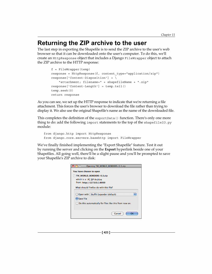
Chapter 11
[ 423 ]
Returning the ZIP archive to the userThe last step in exporting the Shapefile is to send the ZIP archive to the user's web browser so that it can be downloaded onto the user's computer. To do this, we'll create an HttpResponse object that includes a Django FileWrapper object to attach the ZIP archive to the HTTP response:
f = FileWrapper(temp) response = HttpResponse(f, content_type="application/zip") response['Content-Disposition'] = \ "attachment; filename=" + shapefileName + ".zip" response['Content-Length'] = temp.tell() temp.seek(0) return response
As you can see, we set up the HTTP response to indicate that we're returning a file attachment. This forces the user's browser to download the file rather than trying to display it. We also use the original Shapefile's name as the name of the downloaded file.
This completes the definition of the exportData() function. There's only one more thing to do: add the following import statements to the top of the shapefileIO.py module:
from django.http import HttpResponsefrom django.core.servers.basehttp import FileWrapper
We've finally finished implementing the "Export Shapefile" feature. Test it out by running the server and clicking on the Export hyperlink beside one of your Shapefiles. All going well, there'll be a slight pause and you'll be prompted to save your Shapefile's ZIP archive to disk:
ShapeEditor: Implementing List View, Import, and Export
[ 424 ]
SummaryIn this chapter, we continued our implementation of the ShapeEditor by adding three important functions: the "list" view, and the ability to import and export Shapefiles. While these aren't very exciting features, they are a crucial part of the ShapeEditor.
In the process of implementing these features, we have learned:
• How to use Django's templating language to display a list of records within a web page.
• How you can use the zipfile standard library module to extract the contents of an uploaded Shapefile before opening that Shapefile using OGR.
• That you need to wrap Polygon and LineString geometries when importing data from a Shapefile into a PostGIS database to avoid problems caused by a Shapefile's inability to distinguish between Polygons and MultiPolygons, and between LineStrings and MultiLineStrings.
• That when you call the object.delete() method, Django automatically deletes all the linked records for you, simplifying the process of removing a record and all its associated data.
• That you can use OGR to create a new Shapefile, and the zipfile library module to compress it, so that you can export geo-spatial data using a web interface.
With this functionality out of the way, we can now turn our attention to the most interesting parts of the ShapeEditor: the code which displays and lets the user edit geometries using a slippy map interface. This will be the main focus for the final chapter of this book.
ShapeEditor: Selecting and Editing Features
In this final chapter, we will implement the remaining features of the ShapeEditor application. A large part of this chapter will involve the use of OpenLayers and the creation of a Tile Map Server so that we can display a map with all the Shapefile's features on it, and allow the user to click on a feature to select it. We'll also implement the the ability to add, edit, and delete features, and conclude with an exploration of how the ShapeEditor can be used to work with geo-spatial data, and how it can serve as the springboard for your own geo-spatial development efforts.
In this chapter, we will learn:
• How to implement a Tile Map Server using Mapnik and GeoDjango• How to use OpenLayers to display a slippy map on a web page• How to write a custom "click" handler for OpenLayers• How to use AJAX requests within OpenLayers• How to perform spatial queries using GeoDjango• How to use GeoDjango's built-in editing widgets in your own application• How to edit geo-spatial data using GeoDjango's built-in editing widgets• How to customize the interface for GeoDjango's editing widgets• How to add and delete records in a Django web application
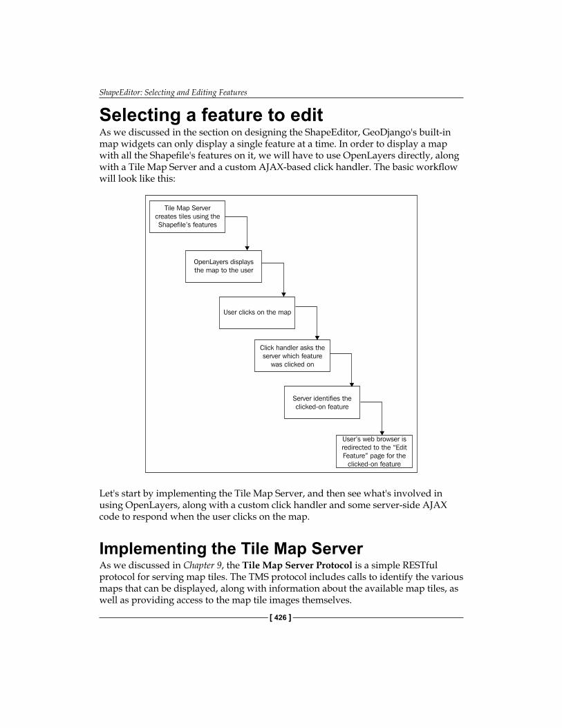
ShapeEditor: Selecting and Editing Features
[ 426 ]
Selecting a feature to editAs we discussed in the section on designing the ShapeEditor, GeoDjango's built-in map widgets can only display a single feature at a time. In order to display a map with all the Shapefile's features on it, we will have to use OpenLayers directly, along with a Tile Map Server and a custom AJAX-based click handler. The basic workflow will look like this:
Let's start by implementing the Tile Map Server, and then see what's involved in using OpenLayers, along with a custom click handler and some server-side AJAX code to respond when the user clicks on the map.
Implementing the Tile Map ServerAs we discussed in Chapter 9, the Tile Map Server Protocol is a simple RESTful protocol for serving map tiles. The TMS protocol includes calls to identify the various maps that can be displayed, along with information about the available map tiles, as well as providing access to the map tile images themselves.
Chapter 12
[ 427 ]
Let's briefly review the terminology used by the TMS protocol:
• A Tile Map Server is the overall web server that is implementing the TMS protocol.
• A Tile Map Service provides access to a particular set of maps. There can be multiple Tile Map Services hosted by a single Tile Map Server.
• A Tile Map is a complete map of all or part of the Earth's surface, displaying a particular set of features or styled in a particular way. A Tile Map Service can provide access to more than one Tile Map.
• A Tile Set consists of a set of tiles displaying a given Tile Map at a given zoom level.
• A Tile is a single map image representing a small portion of the map being displayed by the Tile Set.
This may sound confusing, but it's actually not too bad. We'll be implementing a Tile Map Server with just one Tile Map Service, which we'll call the "ShapeEditor Tile Map Service". There will be one Tile Map for each Shapefile that has been uploaded, and we'll support Tile Sets for a standard range of zoom levels. Finally, we'll use Mapnik to render the individual Tiles within the Tile Set.
We'll create a separate module, tms.py, for our Tile Map Server's code. Create this file (inside the shapeEditor directory), and enter the following:
from django.http import HttpResponse
def root(request): return HttpResponse("Tile Map Server")
def service(request, version): return HttpResponse("Tile Map Service")
def tileMap(request, version, shapefile_id): return HttpResponse("Tile Map")
def tile(request, version, shapefile_id, zoom, x, y): return HttpResponse("Tile")
Obviously, these are only placeholders, but they give us the basic structure for our Tile Map Server, and let us set up the URL mappings we will need. Now, go back and edit the urls.py module, adding the following code to the end of the module:
urlpatterns += patterns('geodjango.shapeEditor.tms', (r'^shape-editor/tms$', 'root'), # "shape-editor/tms" calls root() (r'^shape-editor/tms/(?P<version>[0-9.]+)$', 'service'), # eg, "shape-editor/tms/1.0" calls service(version=1.0)
ShapeEditor: Selecting and Editing Features
[ 428 ]
(r'^shape-editor/tms/(?P<version>[0-9.]+)/' + r'(?P<shapefile_id>\d+)$', 'tileMap'), # eg, "shape-editor/tms/1.0/2" calls # tileMap(version=1.0, shapefile_id=2) (r'^shape-editor/tms/(?P<version>[0-9.]+)/' + r'(?P<shapefile_id>\d+)/(?P<zoom>\d+)/' + r'(?P<x>\d+)/(?P<y>\d+)\.png$', 'tile'), # eg, "shape-editor/tms/1.0/2/3/4/5" calls # tile(version=1.0, shapefile_id=2, zoom=3, x=4, y=5))
Each of these URL patterns maps an incoming RESTful URL to the appropriate view function within our new tms.py module. The included comments give an example of how the regular expressions map URLs to the view functions.
To test that this works, run the GeoDjango server and point your web browser to http://127.0.0.1:8000/shape-editor/tms. You should see the text you entered into your placeholder root() view function.
Let's make that top-level view function do something useful. Go back to the tms.py module, and change the root() function to look like this:
def root(request): try: baseURL = request.build_absolute_uri() xml = [] xml.append('<?xml version="1.0" encoding="utf-8" ?>') xml.append('<Services>') xml.append(' <TileMapService ' + 'title="ShapeEditor Tile Map Service" ' + 'version="1.0" href="' + baseURL + '/1.0"/>') xml.append('</Services>') return HttpResponse("\n".join(xml), mimetype="text/xml") except: traceback.print_exc() return HttpResponse("")
You'll also need to add the following import statement to the top of the module:
import traceback
This view function returns an XML-format response describing the one-and-only Tile Map Service supported by our TMS server. This Tile Map Service is identified by a version number, 1.0 (Tile Map Services are typically identified by version number). If you now go to http://127.0.0.1:8000/shape-editor/tms, you'll see the TMS response displayed in your web browser:
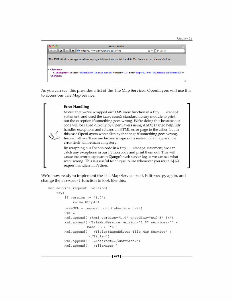
Chapter 12
[ 429 ]
As you can see, this provides a list of the Tile Map Services. OpenLayers will use this to access our Tile Map Service.
Error HandlingNotice that we've wrapped our TMS view function in a try...except statement, and used the traceback standard library module to print out the exception if something goes wrong. We're doing this because our code will be called directly by OpenLayers using AJAX; Django helpfully handles exceptions and returns an HTML error page to the caller, but in this case OpenLayers won't display that page if something goes wrong. Instead, all you'll see are broken image icons instead of a map, and the error itself will remain a mystery.By wrapping our Python code in a try...except statement, we can catch any exceptions in our Python code and print them out. This will cause the error to appear in Django's web server log so we can see what went wrong. This is a useful technique to use whenever you write AJAX request handlers in Python.
We're now ready to implement the Tile Map Service itself. Edit tms.py again, and change the service() function to look like this:
def service(request, version): try: if version != "1.0": raise Http404
baseURL = request.build_absolute_uri() xml = [] xml.append('<?xml version="1.0" encoding="utf-8" ?>') xml.append('<TileMapService version="1.0" services="' + baseURL + '">') xml.append(' <Title>ShapeEditor Tile Map Service' + '</Title>') xml.append(' <Abstract></Abstract>') xml.append(' <TileMaps>')
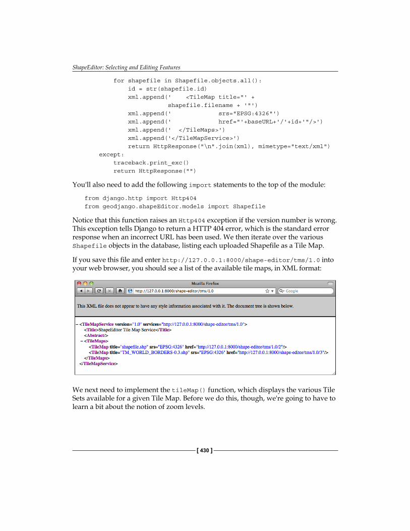
ShapeEditor: Selecting and Editing Features
[ 430 ]
for shapefile in Shapefile.objects.all(): id = str(shapefile.id) xml.append(' <TileMap title="' + shapefile.filename + '"') xml.append(' srs="EPSG:4326"') xml.append(' href="'+baseURL+'/'+id+'"/>') xml.append(' </TileMaps>') xml.append('</TileMapService>') return HttpResponse("\n".join(xml), mimetype="text/xml") except: traceback.print_exc() return HttpResponse("")
You'll also need to add the following import statements to the top of the module:
from django.http import Http404from geodjango.shapeEditor.models import Shapefile
Notice that this function raises an Http404 exception if the version number is wrong. This exception tells Django to return a HTTP 404 error, which is the standard error response when an incorrect URL has been used. We then iterate over the various Shapefile objects in the database, listing each uploaded Shapefile as a Tile Map.
If you save this file and enter http://127.0.0.1:8000/shape-editor/tms/1.0 into your web browser, you should see a list of the available tile maps, in XML format:
We next need to implement the tileMap() function, which displays the various Tile Sets available for a given Tile Map. Before we do this, though, we're going to have to learn a bit about the notion of zoom levels.
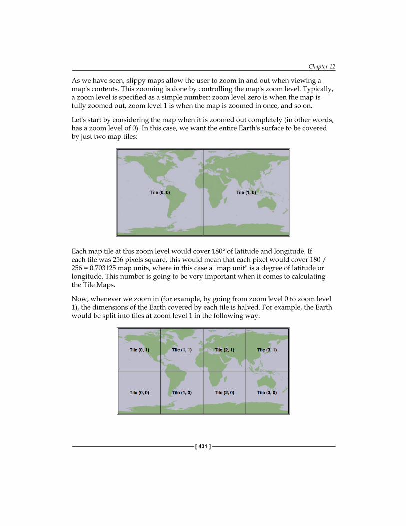
Chapter 12
[ 431 ]
As we have seen, slippy maps allow the user to zoom in and out when viewing a map's contents. This zooming is done by controlling the map's zoom level. Typically, a zoom level is specified as a simple number: zoom level zero is when the map is fully zoomed out, zoom level 1 is when the map is zoomed in once, and so on.
Let's start by considering the map when it is zoomed out completely (in other words, has a zoom level of 0). In this case, we want the entire Earth's surface to be covered by just two map tiles:
Each map tile at this zoom level would cover 180° of latitude and longitude. If each tile was 256 pixels square, this would mean that each pixel would cover 180 / 256 = 0.703125 map units, where in this case a "map unit" is a degree of latitude or longitude. This number is going to be very important when it comes to calculating the Tile Maps.
Now, whenever we zoom in (for example, by going from zoom level 0 to zoom level 1), the dimensions of the Earth covered by each tile is halved. For example, the Earth would be split into tiles at zoom level 1 in the following way:
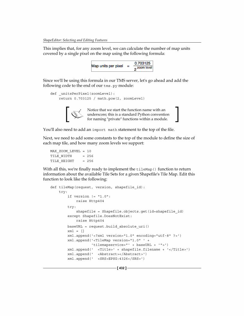
ShapeEditor: Selecting and Editing Features
[ 432 ]
This implies that, for any zoom level, we can calculate the number of map units covered by a single pixel on the map using the following formula:
Since we'll be using this formula in our TMS server, let's go ahead and add the following code to the end of our tms.py module:
def _unitsPerPixel(zoomLevel): return 0.703125 / math.pow(2, zoomLevel)
Notice that we start the function name with an underscore; this is a standard Python convention for naming "private" functions within a module.
You'll also need to add an import math statement to the top of the file.
Next, we need to add some constants to the top of the module to define the size of each map tile, and how many zoom levels we support:
MAX_ZOOM_LEVEL = 10TILE_WIDTH = 256TILE_HEIGHT = 256
With all this, we're finally ready to implement the tileMap() function to return information about the available Tile Sets for a given Shapefile's Tile Map. Edit this function to look like the following:
def tileMap(request, version, shapefile_id): try: if version != "1.0": raise Http404
try: shapefile = Shapefile.objects.get(id=shapefile_id) except Shapefile.DoesNotExist: raise Http404
baseURL = request.build_absolute_uri() xml = [] xml.append('<?xml version="1.0" encoding="utf-8" ?>') xml.append('<TileMap version="1.0" ' + 'tilemapservice="' + baseURL + '">') xml.append(' <Title>' + shapefile.filename + '</Title>') xml.append(' <Abstract></Abstract>') xml.append(' <SRS>EPSG:4326</SRS>')
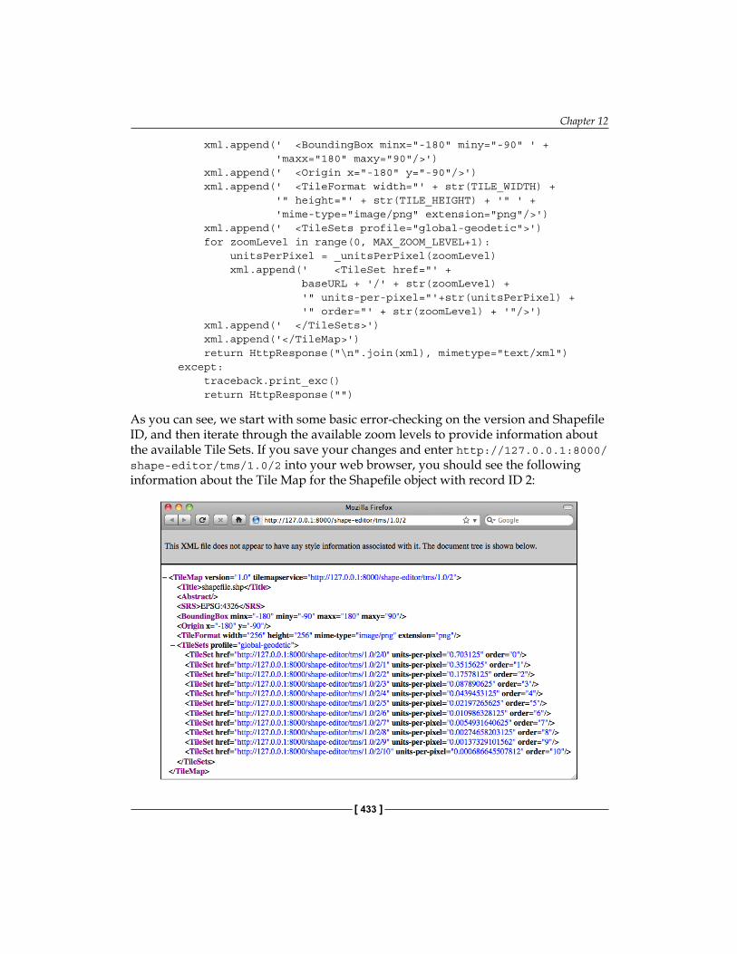
Chapter 12
[ 433 ]
xml.append(' <BoundingBox minx="-180" miny="-90" ' + 'maxx="180" maxy="90"/>') xml.append(' <Origin x="-180" y="-90"/>') xml.append(' <TileFormat width="' + str(TILE_WIDTH) + '" height="' + str(TILE_HEIGHT) + '" ' + 'mime-type="image/png" extension="png"/>') xml.append(' <TileSets profile="global-geodetic">') for zoomLevel in range(0, MAX_ZOOM_LEVEL+1): unitsPerPixel = _unitsPerPixel(zoomLevel) xml.append(' <TileSet href="' + baseURL + '/' + str(zoomLevel) + '" units-per-pixel="'+str(unitsPerPixel) + '" order="' + str(zoomLevel) + '"/>') xml.append(' </TileSets>') xml.append('</TileMap>') return HttpResponse("\n".join(xml), mimetype="text/xml") except: traceback.print_exc() return HttpResponse("")
As you can see, we start with some basic error-checking on the version and Shapefile ID, and then iterate through the available zoom levels to provide information about the available Tile Sets. If you save your changes and enter http://127.0.0.1:8000/shape-editor/tms/1.0/2 into your web browser, you should see the following information about the Tile Map for the Shapefile object with record ID 2:
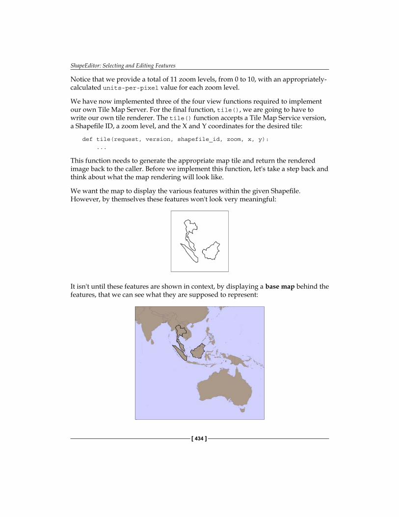
ShapeEditor: Selecting and Editing Features
[ 434 ]
Notice that we provide a total of 11 zoom levels, from 0 to 10, with an appropriately-calculated units-per-pixel value for each zoom level.
We have now implemented three of the four view functions required to implement our own Tile Map Server. For the final function, tile(), we are going to have to write our own tile renderer. The tile() function accepts a Tile Map Service version, a Shapefile ID, a zoom level, and the X and Y coordinates for the desired tile:
def tile(request, version, shapefile_id, zoom, x, y): ...
This function needs to generate the appropriate map tile and return the rendered image back to the caller. Before we implement this function, let's take a step back and think about what the map rendering will look like.
We want the map to display the various features within the given Shapefile. However, by themselves these features won't look very meaningful:
It isn't until these features are shown in context, by displaying a base map behind the features, that we can see what they are supposed to represent:
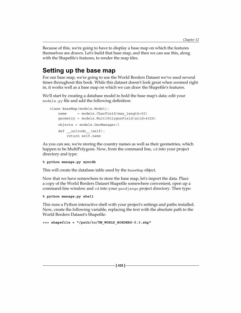
Chapter 12
[ 435 ]
Because of this, we're going to have to display a base map on which the features themselves are drawn. Let's build that base map, and then we can use this, along with the Shapefile's features, to render the map tiles.
Setting up the base mapFor our base map, we're going to use the World Borders Dataset we've used several times throughout this book. While this dataset doesn't look great when zoomed right in, it works well as a base map on which we can draw the Shapefile's features.
We'll start by creating a database model to hold the base map's data: edit your models.py file and add the following definition:
class BaseMap(models.Model): name = models.CharField(max_length=50) geometry = models.MultiPolygonField(srid=4326)
objects = models.GeoManager()
def __unicode__(self): return self.name
As you can see, we're storing the country names as well as their geometries, which happen to be MultiPolygons. Now, from the command line, cd into your project directory and type:
% python manage.py syncdb
This will create the database table used by the BaseMap object.
Now that we have somewhere to store the base map, let's import the data. Place a copy of the World Borders Dataset Shapefile somewhere convenient, open up a command-line window and cd into your geodjango project directory. Then type:
% python manage.py shell
This runs a Python interactive shell with your project's settings and paths installed. Now, create the following variable, replacing the text with the absolute path to the World Borders Dataset's Shapefile:
>>> shapefile = "/path/to/TM_WORLD_BORDERS-0.3.shp"
ShapeEditor: Selecting and Editing Features
[ 436 ]
Then type the following:
>>> from django.contrib.gis.utils import LayerMapping
>>> from geodjango.shapeEditor.models import BaseMap
>>> mapping = LayerMapping(BaseMap, shapefile, {'name' : "NAME", 'geometry' : "MULTIPOLYGON"}, transform=False, encoding="iso-8859-1")
>>> mapping.save(strict=True, verbose=True)
We're using GeoDjango's LayerMapping module to import the data from this Shapefile into our database. The various countries will be displayed as they are imported, which will take a few seconds.
Once this has been done, you can check the imported data by typing commands into the interactive shell. For example:
>>> print BaseMap.objects.count()
246
>>> print BaseMap.objects.all()
[<BaseMap: Antigua and Barbuda>, <BaseMap: Algeria>, <BaseMap: Azerbaijan>, <BaseMap: Albania>, <BaseMap: Armenia>, <BaseMap: Angola>, <BaseMap: American Samoa>, <BaseMap: Argentina>, <BaseMap: Australia>, <BaseMap: Bahrain>, <BaseMap: Barbados>, <BaseMap: Bermuda>, <BaseMap: Bahamas>, <BaseMap: Bangladesh>, <BaseMap: Belize>, <BaseMap: Bosnia and Herzegovina>, <BaseMap: Bolivia>, <BaseMap: Burma>, <BaseMap: Benin>, <BaseMap: Solomon Islands>, '...(remaining elements truncated)...']
Feel free to play some more if you want; the Django tutorial includes several examples of exploring your data objects using the interactive shell.
Because this base map is going to be part of the ShapeEditor application itself (the application won't run without it), it would be good if Django could treat that data as part of the application's source code. That way, if we ever had to rebuild the database from scratch, the base map would be reinstalled automatically.
Django allows you to do this by creating a fixture. A fixture is a set of data that can be loaded into the database on demand, either manually or automatically when the database is initialized. We'll save our base map data into a fixture so that Django can reload that data as required.
Create a directory named fixtures within the shapeEditor application directory. Then, in a terminal window, cd into the geodjango project directory and type:
% python manage.py dumpdata shapeEditor shapeEditor.BaseMap > shapeEditor/fixtures/initial_data.json
Chapter 12
[ 437 ]
This will create a fixture named initial_data.json. As the name suggests, the contents of this fixture will be loaded automatically if Django ever has to re-initialize the database.
Now that we have a base map, let's use it to implement our tile rendering code.
Tile renderingUsing our knowledge of Mapnik, we're going to implement the TMS server's tile() function. Our generated map will consist of two layers: a base layer showing the base map, and a feature layer showing the features in the imported Shapefile. Since all our data is stored in a PostGIS database, we'll be using a mapnik.PostGIS datasource for both layers.
Our tile() function can be broken down into five steps:
1. Parse the query parameters.2. Set up the map.3. Define the base layer.4. Define the feature layer.5. Render the map.
Let's work through each of these in turn.
Parsing the query parametersEdit the tms.py module, and delete the dummy code we had in the tile() function. We'll add our parsing code one step at a time, starting with some basic error-checking code to ensure the version number is correct and that the Shapefile exists, and once again wrap our entire view function in a try...except statement to catch typos and other errors:
try: if version != "1.0": raise Http404
try: shapefile = Shapefile.objects.get(id=shapefile_id) except Shapefile.DoesNotExist: raise Http404
ShapeEditor: Selecting and Editing Features
[ 438 ]
We now need to convert the query parameters (which Django passes to us as strings) into integers so that we can work with them:
zoom = int(zoom) x = int(x) y = int(y)
We can now check that the zoom level is correct:
if zoom < 0 or zoom > MAX_ZOOM_LEVEL: raise Http404
Our next step is to convert the supplied x and y parameters into the minimum and maximum latitude and longitude values covered by the tile. This requires us to use the _unitsPerPixel() function we defined earlier to calculate the amount of the Earth's surface covered by the tile for the current zoom level:
xExtent = _unitsPerPixel(zoom) * TILE_WIDTH yExtent = _unitsPerPixel(zoom) * TILE_HEIGHT
minLong = x * xExtent - 180.0 minLat = y * yExtent - 90.0 maxLong = minLong + xExtent maxLat = minLat + yExtent
Finally, we can add some rudimentary error-checking to ensure that the tile's coordinates are valid:
if (minLong < -180 or maxLong > 180 or minLat < -90 or maxLat > 90): raise Http404
Setting up the mapWe're now ready to create the mapnik.Map object to represent the map. This is trivial:
map = mapnik.Map(TILE_WIDTH, TILE_HEIGHT, "+proj=longlat +datum=WGS84") map.background = mapnik.Color("#7391ad")
Defining the base layerWe now want to define the layer that draws our base map. To do this, we have to set up a mapnik.PostGIS datasource for the layer:
dbSettings = settings.DATABASES['default'] datasource = \ mapnik.PostGIS(user=dbSettings['USER'], password=dbSettings['PASSWORD'],
Chapter 12
[ 439 ]
dbname=dbSettings['NAME'], table='"shapeEditor_basemap"', srid=4326, geometry_field="geometry", geometry_table='"shapeEditor_basemap"')
As you can see, we get the name of the database, the username, and the password from our project's settings module. We then set up a PostGIS datasource using these settings.
There is one surprising thing here: notice how the table and geometry_table parameters have extra quotes within the string. This is because of a quirk in the way PostgreSQL works: unless you put quotes around a field or table name, PostgreSQL helpfully converts that name to lowercase. Most of the time you won't even notice this, but because we're using the database directly rather than going through Django's object-relational mapper, we will get an error if we don't add extra quotes to these table names.
An alternative would have been to keep the name of the Django application entirely in lowercase, but shapeeditor is much harder to read than shapeEditor. These extra quotes are a minor price to pay for having a good-looking application name.
Now that we have set up our datasource, let's create the base layer itself:
baseLayer = mapnik.Layer("baseLayer") baseLayer.datasource = datasource baseLayer.styles.append("baseLayerStyle")
We now need to set up the layer's style. In this case, we'll use a single rule with two symbolizers: a PolygonSymbolizer that draws the interior of the base map's polygons, and a LineSymbolizer to draw the polygon outlines:
rule = mapnik.Rule()
rule.symbols.append( mapnik.PolygonSymbolizer(mapnik.Color("#b5d19c"))) rule.symbols.append( mapnik.LineSymbolizer(mapnik.Color("#404040"), 0.2))
style = mapnik.Style() style.rules.append(rule)
Finally, we can add the base layer and its style to the map:
map.append_style("baseLayerStyle", style) map.layers.append(baseLayer)
ShapeEditor: Selecting and Editing Features
[ 440 ]
Defining the feature layerOur next task is to add another layer to draw the Shapefile's features onto the map. Once again, we'll set up a mapnik.PostGIS datasource for the new layer:
geometryField = utils.calcGeometryField(shapefile.geom_type)
query = '(select ' + geometryField \ + ' from "shapeEditor_feature" where' \ + ' shapefile_id=' + str(shapefile.id) + ') as geom'
datasource = \ mapnik.PostGIS(user=dbSettings['USER'], password=dbSettings['PASSWORD'], dbname=dbSettings['NAME'], table=query, srid=4326, geometry_field=geometryField, geometry_table='"shapeEditor_feature"')
In this case, we are calling utils.calcGeometryField() to see which field in the shapeEditor_feature table contains the geometry we're going to display. Once again, we're adding extra quotes to the table name to avoid PostgreSQL's annoying tendency to convert unquoted names to lowercase.
We're now ready to create the new layer itself:
featureLayer = mapnik.Layer("featureLayer") featureLayer.datasource = datasource featureLayer.styles.append("featureLayerStyle")
Next, we want to define the styles used by the feature layer. As before, we'll have just a single rule, but in this case we'll use different symbolizers depending on the type of feature we are displaying:
rule = mapnik.Rule()
if shapefile.geom_type in ["Point", "MultiPoint"]: rule.symbols.append(mapnik.PointSymbolizer()) elif shapefile.geom_type in ["LineString", "MultiLineString"]: rule.symbols.append( mapnik.LineSymbolizer(mapnik.Color("#000000"), 0.5)) elif shapefile.geom_type in ["Polygon", "MultiPolygon"]: rule.symbols.append( mapnik.PolygonSymbolizer(mapnik.Color("#f7edee"))) rule.symbols.append( mapnik.LineSymbolizer(mapnik.Color("#000000"), 0.5))
style = mapnik.Style() style.rules.append(rule)
Chapter 12
[ 441 ]
Finally, we can add our new feature layer to the map:
map.append_style("featureLayerStyle", style) map.layers.append(featureLayer)
Rendering the Map TileWe've looked at using Mapnik to render map images in Chapter 9. The basic process of rendering a map tile is the same, except that we won't be storing the results into an image file on disk. Instead, we'll create a mapnik.Image object, use it to extract the raw image data in PNG format, and return that data back to the caller using an HttpResponse object:
map.zoom_to_box(mapnik.Envelope(minLong, minLat, maxLong, maxLat)) image = mapnik.Image(TILE_WIDTH, TILE_HEIGHT) mapnik.render(map, image) imageData = image.tostring('png')
return HttpResponse(imageData, mimetype="image/png")
All that's left now is to add our error-catching code to the end of the function:
except: traceback.print_exc() return HttpResponse("")
That completes the implementation of our Tile Map Server's tile() function. Let's tidy up and do some testing.
Completing the Tile Map ServerBecause we've referred to some new modules in our tms.py module, we'll have to add some extra import statements to the top of the file:
from django.conf import settingsimport mapnikimport utils
In theory, our Tile Map Server should now be ready to go. Let's test it by running the GeoDjango server. If you don't currently have the GeoDjango web server running, cd into the geodjango project directory and type:
% python manage.py runserver
Start up your web browser and enter the following URL into your browser's address bar:
http://127.0.0.1:8000/shape-editor/tms/1.0/2/0/0/0.png
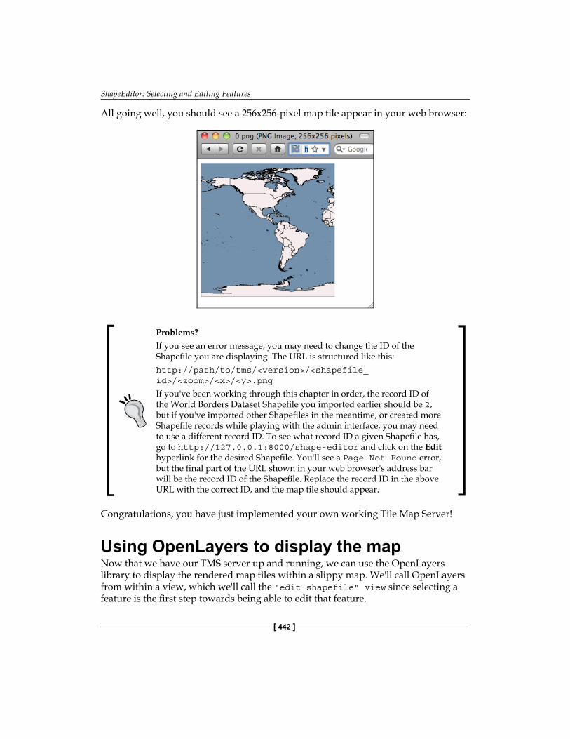
ShapeEditor: Selecting and Editing Features
[ 442 ]
All going well, you should see a 256x256-pixel map tile appear in your web browser:
Problems?If you see an error message, you may need to change the ID of the Shapefile you are displaying. The URL is structured like this:http://path/to/tms/<version>/<shapefile_id>/<zoom>/<x>/<y>.png
If you've been working through this chapter in order, the record ID of the World Borders Dataset Shapefile you imported earlier should be 2, but if you've imported other Shapefiles in the meantime, or created more Shapefile records while playing with the admin interface, you may need to use a different record ID. To see what record ID a given Shapefile has, go to http://127.0.0.1:8000/shape-editor and click on the Edit hyperlink for the desired Shapefile. You'll see a Page Not Found error, but the final part of the URL shown in your web browser's address bar will be the record ID of the Shapefile. Replace the record ID in the above URL with the correct ID, and the map tile should appear.
Congratulations, you have just implemented your own working Tile Map Server!
Using OpenLayers to display the mapNow that we have our TMS server up and running, we can use the OpenLayers library to display the rendered map tiles within a slippy map. We'll call OpenLayers from within a view, which we'll call the "edit shapefile" view since selecting a feature is the first step towards being able to edit that feature.
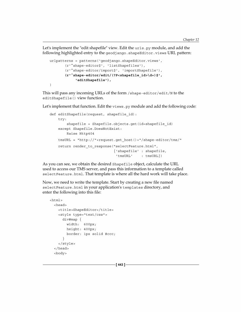
Chapter 12
[ 443 ]
Let's implement the "edit shapefile" view. Edit the urls.py module, and add the following highlighted entry to the geodjango.shapeEditor.views URL pattern:
urlpatterns = patterns('geodjango.shapeEditor.views', (r'^shape-editor$', 'listShapefiles'), (r'^shape-editor/import$', 'importShapefile'), (r'^shape-editor/edit/(?P<shapefile_id>\d+)$', 'editShapefile'),)
This will pass any incoming URLs of the form /shape-editor/edit/N to the editShapefile() view function.
Let's implement that function. Edit the views.py module and add the following code:
def editShapefile(request, shapefile_id): try: shapefile = Shapefile.objects.get(id=shapefile_id) except Shapefile.DoesNotExist: Raise Http404
tmsURL = "http://"+request.get_host()+"/shape-editor/tms/"
return render_to_response("selectFeature.html", {'shapefile' : shapefile, 'tmsURL' : tmsURL})
As you can see, we obtain the desired Shapefile object, calculate the URL used to access our TMS server, and pass this information to a template called selectFeature.html. That template is where all the hard work will take place.
Now, we need to write the template. Start by creating a new file named selectFeature.html in your application's templates directory, and enter the following into this file:
<html> <head> <title>ShapeEditor</title> <style type="text/css"> div#map { width: 600px; height: 400px; border: 1px solid #ccc; } </style> </head> <body>
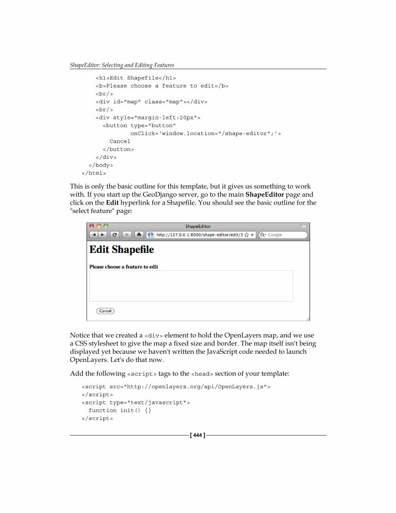
ShapeEditor: Selecting and Editing Features
[ 444 ]
<h1>Edit Shapefile</h1> <b>Please choose a feature to edit</b> <br/> <div id="map" class="map"></div> <br/> <div style="margin-left:20px"> <button type="button" onClick='window.location="/shape-editor";'> Cancel </button> </div> </body></html>
This is only the basic outline for this template, but it gives us something to work with. If you start up the GeoDjango server, go to the main ShapeEditor page and click on the Edit hyperlink for a Shapefile. You should see the basic outline for the "select feature" page:
Notice that we created a <div> element to hold the OpenLayers map, and we use a CSS stylesheet to give the map a fixed size and border. The map itself isn't being displayed yet because we haven't written the JavaScript code needed to launch OpenLayers. Let's do that now.
Add the following <script> tags to the <head> section of your template:
<script src="http://openlayers.org/api/OpenLayers.js"></script><script type="text/javascript"> function init() {}</script>
Chapter 12
[ 445 ]
Also, change the <body> tag definition to look like this:
<body onload="init()">
Notice that there are two <script> tags: the first loads the OpenLayers.js library from the http://openlayers.org website, while the second will hold the JavaScript code that we'll write to create the map. We've also defined a JavaScript function called init() which will be called when the page is loaded.
Let's implement that initialization function. Replace the line which says function init() {} with the following:
function init() { map = new OpenLayers.Map('map', {maxResolution: 0.703125, numZoomLevels: 11}); layer = new OpenLayers.Layer.TMS('TMS', "{{ tmsURL }}", {serviceVersion: "1.0", layername: "{{ shapefile.id }}", type: 'png'}); map.addLayer(layer); map.zoomToMaxExtent(); }
Even if you haven't used JavaScript before, this code should be quite straightforward: the first instruction creates an OpenLayers.Map object representing the slippy map. We then create an OpenLayers.Layer.TMS object to represent a map layer that takes data from a TMS server. Then, we add the layer to the map, and zoom the map out as far as possible so that the user sees the entire world when the map is first displayed.
Notice that the Map object accepts the ID of the <div> tag in which to place the map, along with a dictionary of options. The maxResolution option defines the maximum resolution to use for the map, and the numZoomLevels option tells OpenLayers how many zoom levels the map should support.
For the Layer.TMS object, we pass in the URL used to access the Tile Map Server (which is a parameter passed to the template from our Python view), along with the version of the Tile Map Service to use and the name of the layer—which in our Tile Map Server is the record ID of the Shapefile to display the features for.
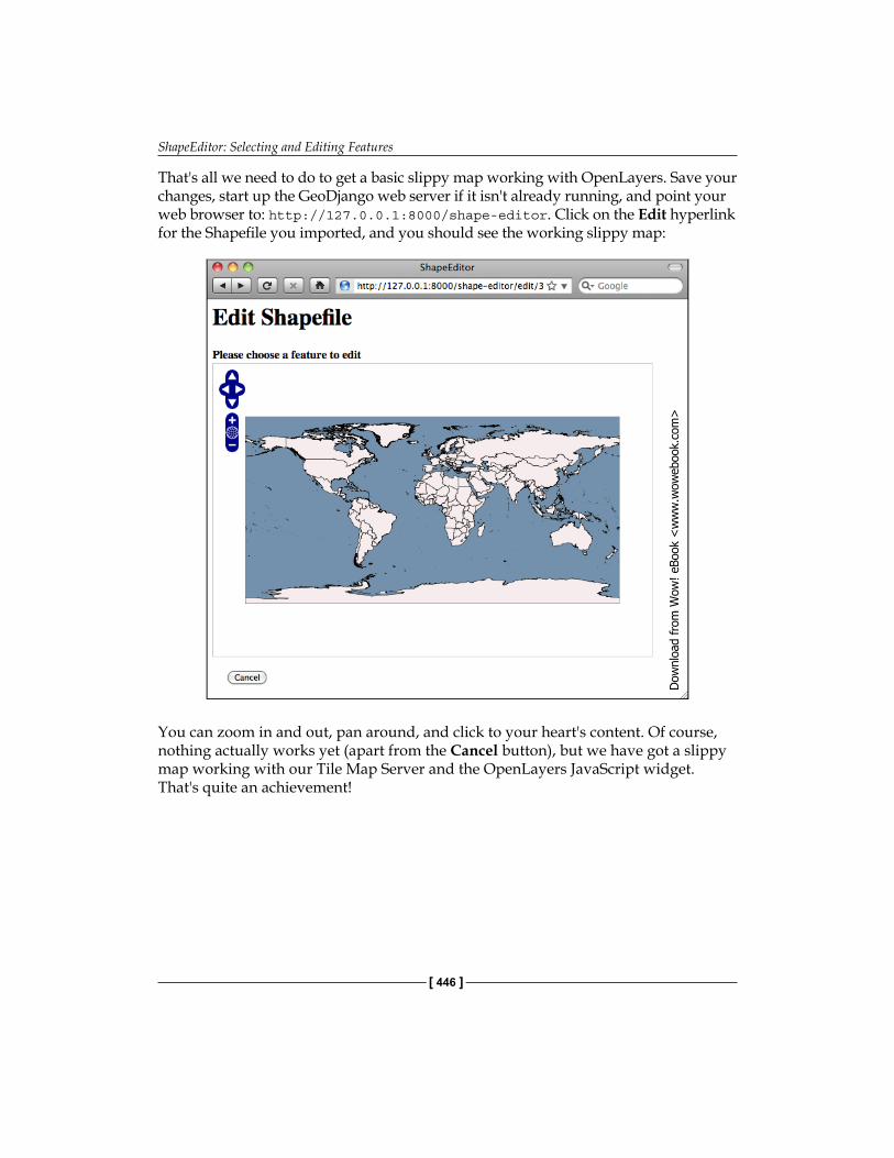
ShapeEditor: Selecting and Editing Features
[ 446 ]
That's all we need to do to get a basic slippy map working with OpenLayers. Save your changes, start up the GeoDjango web server if it isn't already running, and point your web browser to: http://127.0.0.1:8000/shape-editor. Click on the Edit hyperlink for the Shapefile you imported, and you should see the working slippy map:
You can zoom in and out, pan around, and click to your heart's content. Of course, nothing actually works yet (apart from the Cancel button), but we have got a slippy map working with our Tile Map Server and the OpenLayers JavaScript widget. That's quite an achievement!
Dow
nlo
ad fro
m W
ow
! eBook
<w
ww
.wow
ebook.
com
>
Chapter 12
[ 447 ]
What if it doesn't work?If the map isn't being shown for some reason, there are several possible causes. First, check the Django web server log as we are printing any Python exceptions there. If that doesn't reveal the problem, look at your web browser's Error Console window to see if there are any errors at the JavaScript level. Because we are now writing JavaScript code, error messages will appear within the web browser rather than in Django's server log. In FireFox, you can view JavaScript errors by selecting the Error Console item from the Tools menu. Other browsers have similar windows for showing JavaScript errors.JavaScript debugging can be quite tricky, even for people experienced with developing web-based applications. If you do get stuck, you may find the following article helpful: http://www.webmonkey.com/2010/02/javascript_debugging_for_beginners
Intercepting mouse clicksWhen the user clicks on the map, we want to intercept that mouse click, identify the map coordinate that the user clicked on, and then ask the server to identify the clicked-on feature (if any). To intercept mouse clicks, we will need to create a custom OpenLayers.Control subclass. We'll follow the OpenLayers convention of adding the subclass to the OpenLayers namespace by calling our new control OpenLayers.Control.Click. Once we've defined our new control, we can create an instance of the control and add it to the map so that the control can respond to mouse clicks.
All of this has to be done in JavaScript. The code can be a bit confusing, so let's take this one step at a time. Edit your selectFeature.html file and add the following code to the <script> tag, immediately before your init() function:
OpenLayers.Control.Click = OpenLayers.Class( OpenLayers.Control, { defaultHandlerOptions: { 'single' : true, 'double' : false, 'pixelTolerance' : 0, 'stopSingle' : false, 'stopDouble' : false },
initialize: function(options) { this.handlerOptions = OpenLayers.Util.extend( {}, this.defaultHandlerOptions); OpenLayers.Control.prototype.initialize.apply( this, arguments);
ShapeEditor: Selecting and Editing Features
[ 448 ]
this.handler = new OpenLayers.Handler.Click( this, {'click' : this.onClick}, this.handlerOptions); },
onClick: function(e) { alert("click") }, });
Don't worry too much about the details here—the initialize() function is a bit of black magic that creates a new OpenLayers.Control.Click instance and sets it up to run as an OpenLayers control. What is interesting to us are the defaultHandlerOptions dictionary and the onClick() function.
The defaultHandlerOptions dictionary tells OpenLayers how you want the click handler to respond to mouse clicks. In this case, we want to respond to single clicks, but not double-clicks (as these are used to zoom further in to the map).
The onClick() function is actually a JavaScript method for our OpenLayers.Control.Click class. This method will be called when the user clicks on the map—at the moment, all we're doing is displaying an alert box with the message "click", but that's enough to ensure that the click control is working.
Now that we've defined our new click control, let's add it to the map. Add the following lines immediately before the closing } for the init() function:
var click = new OpenLayers.Control.Click();map.addControl(click);click.activate();
As you can see, we create a new instance of our OpenLayers.Control.Click class, add it to the map, and activate it.
With all this code written, we can now reload the Select Feature web page and see what happens when the user clicks on a map:
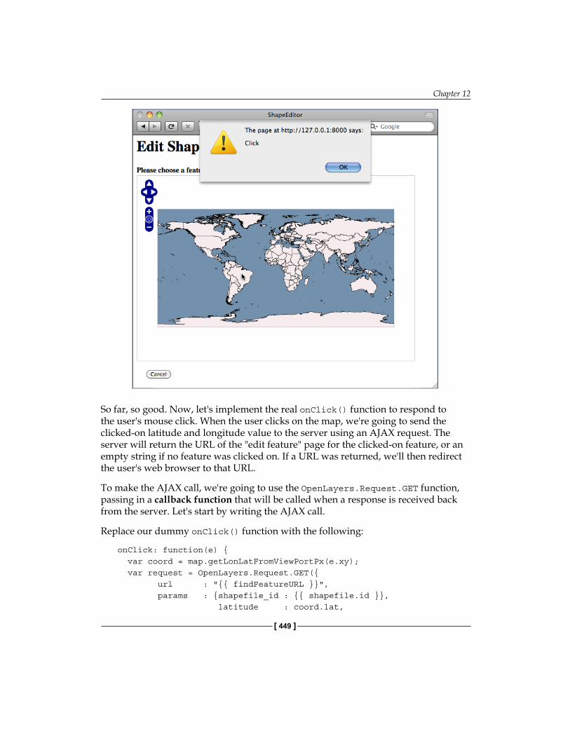
Chapter 12
[ 449 ]
So far, so good. Now, let's implement the real onClick() function to respond to the user's mouse click. When the user clicks on the map, we're going to send the clicked-on latitude and longitude value to the server using an AJAX request. The server will return the URL of the "edit feature" page for the clicked-on feature, or an empty string if no feature was clicked on. If a URL was returned, we'll then redirect the user's web browser to that URL.
To make the AJAX call, we're going to use the OpenLayers.Request.GET function, passing in a callback function that will be called when a response is received back from the server. Let's start by writing the AJAX call.
Replace our dummy onClick() function with the following:
onClick: function(e) { var coord = map.getLonLatFromViewPortPx(e.xy); var request = OpenLayers.Request.GET({ url : "{{ findFeatureURL }}", params : {shapefile_id : {{ shapefile.id }}, latitude : coord.lat,
ShapeEditor: Selecting and Editing Features
[ 450 ]
longitude : coord.lon}, callback : this.handleResponse });}
This function does two things: it obtains the map coordinate that corresponds to the clicked-on point (by calling the map.getLonLatFromViewPortPx() method), and then creates an OpenLayers.Request.GET AJAX call to send the request to the server and call the handleResponse() callback function when the response is received.
Notice that the OpenLayers.Request.GET() function accepts a set of query parameters (in the params entry), as well as a URL to send the request to (in the url entry), and a callback function to call when the response is received (in the callback entry). We're using a template parameter, {{ findFeatureURL }}, to select the URL to send the request to. This will be provided by our editShapeFile() view function when the template is loaded. When we make the request, the query parameters will consist of the record ID of the Shapefile and the clicked-on latitude and longitude values.
While we're editing the selectFeature.html template, let's go ahead and implement the callback function. Add the following function to the end of the OpenLayers.Control.Click class definition (immediately below the closing } for the onClick() function):
handleResponse: function(request) { if (request.status != 200) { alert("Server returned a "+request.status+" error"); return; }; if (request.responseText != "") { window.location.href = request.responseText; };}
You will also need to add a comma after the onClick() function's closing parenthesis, or you'll get a JavaScript error. Just like with Python, you need to add commas to separate dictionary entries in JavaScript.
Even if you're not familiar with JavaScript, this function should be easy to understand: if the response didn't have a status value of 200, an error message is displayed. Otherwise, we check that the response text is not blank, and if so we redirect the user's web browser to that URL.
Chapter 12
[ 451 ]
Now that we've implemented our callback function, let's go back to our view module and define the findFeatureURL parameter that will get passed to the template we've created. Edit the view.py module to add the following highlighted lines to the editShapefile() function:
def editShapefile(request, shapefile_id): try: shapefile = Shapefile.objects.get(id=shapefile_id) except Shapefile.DoesNotExist: raise Http404
tmsURL = "http://"+request.get_host()+"/shape-editor/tms/" findFeatureURL = "http://" + request.get_host() \ + "/shape-editor/findFeature"
return render_to_response("selectFeature.html", {'shapefile' : shapefile, 'findFeatureURL' : findFeatureURL, 'tmsURL' : tmsURL})
This parameter will contain the URL the click handler will send its AJAX request to. This URL will look something like this:
http://127.0.0.1:8000/shape-editor/findFeature
Our onClick() function will add shapefile_id, latitude and longitude query parameters to this request, so the AJAX request sent to the server will look something like this:
http://127.0.0.1:8000/shape-editor/findFeature?shapefile_id=1
&latitude=-38.1674&longitude=176.2344
With our click handler up and running, we're now ready to start implementing the findFeature() view function to respond to these AJAX requests.
Implementing the "find feature" viewWe now need to write the view function that receives the AJAX request, checks to see which feature was clicked on (if any), and returns a suitable URL to use to redirect the user's web browser to the "edit" page for that clicked-on feature. To implement this, we're going to make use of GeoDjango's spatial query functions.
Let's start by adding the findFeature view itself. To do this, edit views.py and add the following placeholder code:
def findFeature(request): return HttpResponse("")
ShapeEditor: Selecting and Editing Features
[ 452 ]
Returning an empty string tells our AJAX callback function that no feature was clicked on. We'll replace this with some proper spatial queries shortly. First, though, we need to add a URL pattern so that incoming requests will get forwarded to the findFeature() view function. Edit urls.py and add the following entry to the geodjango.shapeEditor.views URL pattern list:
(r'^shape-editor/findFeature$', 'findFeature'),
You should now be able to run the ShapeEditor, click on the Edit hyperlink for an uploaded Shapefile, see a map showing the various features within the Shapefile, and click somewhere on the map. In response, the system should do—absolutely nothing! This is because our findFeature() function is returning an empty string, so the system thinks that the user didn't click on a feature and so ignores the mouse click.
In this case, "absolutely nothing" is good news. As long as no error messages are being displayed, either at the Python or JavaScript level, this tells us that the AJAX code is running correctly. So, go ahead and try this, even though nothing happens, just to make sure that you haven't got any bugs in your code. You should see the AJAX calls in the list of incoming HTTP requests being received by the server.
Before we implement the findFeature() function, let's take a step back and think what it means for the user to "click on" a feature's geometry. The ShapeEditor supports a complete range of possible geometry types: Point, LineString, Polygon, MultiPoint, MultiLineString, MultiPolygon, and GeometryCollection. Checking if the user clicked on a Polygon or MultiPolygon feature is straightforward enough—we simply see if the clicked-on point is inside the polygon's bounds. But, because lines and points have no interior (their area will always be zero), a given coordinate could never be "inside" a Point or a LineString geometry. It might get infinitely close, but in all practical terms the user can never click inside a Point or a LineString.
This means that a spatial query of the form:
SELECT * FROM features WHERE ST_Contains(feature.geometry, clickPt)
is not going to work. Instead, we have to allow for the user clicking close to the feature rather than within it. To do this, we'll calculate a search radius, in map units, and then use the DWithin() spatial query function to find all features within the given search radius of the clicked-on point.
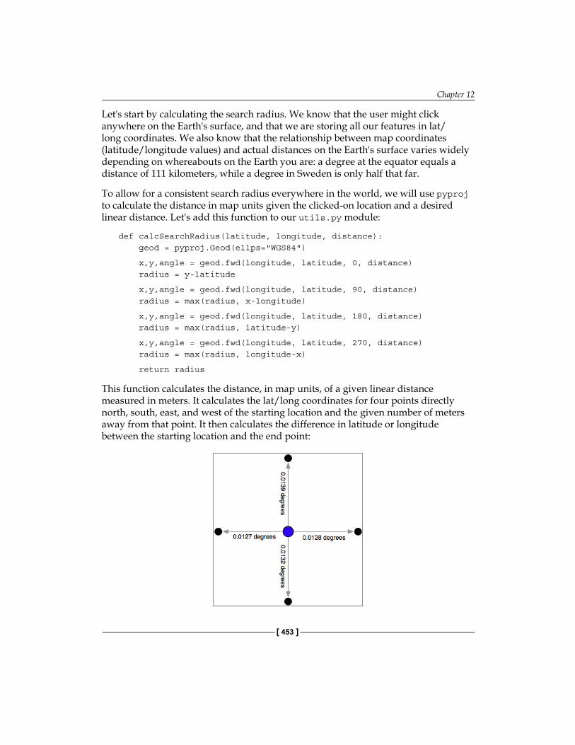
Chapter 12
[ 453 ]
Let's start by calculating the search radius. We know that the user might click anywhere on the Earth's surface, and that we are storing all our features in lat/long coordinates. We also know that the relationship between map coordinates (latitude/longitude values) and actual distances on the Earth's surface varies widely depending on whereabouts on the Earth you are: a degree at the equator equals a distance of 111 kilometers, while a degree in Sweden is only half that far.
To allow for a consistent search radius everywhere in the world, we will use pyproj to calculate the distance in map units given the clicked-on location and a desired linear distance. Let's add this function to our utils.py module:
def calcSearchRadius(latitude, longitude, distance): geod = pyproj.Geod(ellps="WGS84")
x,y,angle = geod.fwd(longitude, latitude, 0, distance) radius = y-latitude
x,y,angle = geod.fwd(longitude, latitude, 90, distance) radius = max(radius, x-longitude)
x,y,angle = geod.fwd(longitude, latitude, 180, distance) radius = max(radius, latitude-y)
x,y,angle = geod.fwd(longitude, latitude, 270, distance) radius = max(radius, longitude-x)
return radius
This function calculates the distance, in map units, of a given linear distance measured in meters. It calculates the lat/long coordinates for four points directly north, south, east, and west of the starting location and the given number of meters away from that point. It then calculates the difference in latitude or longitude between the starting location and the end point:
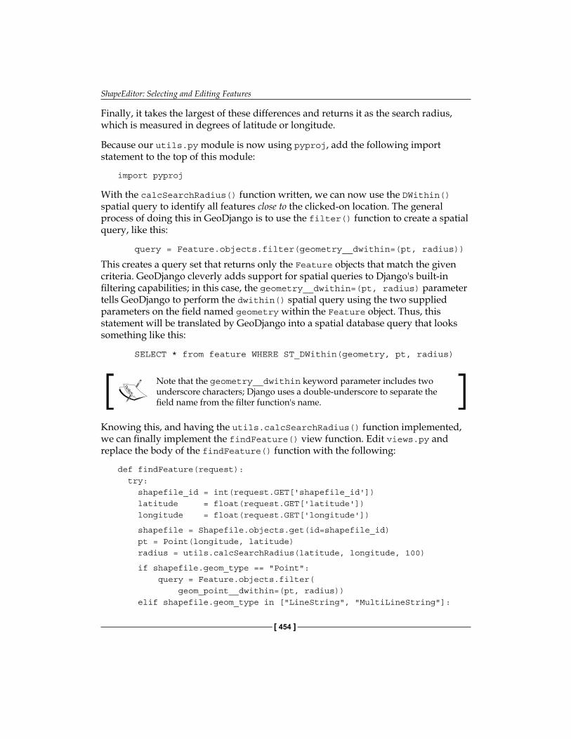
ShapeEditor: Selecting and Editing Features
[ 454 ]
Finally, it takes the largest of these differences and returns it as the search radius, which is measured in degrees of latitude or longitude.
Because our utils.py module is now using pyproj, add the following import statement to the top of this module:
import pyproj
With the calcSearchRadius() function written, we can now use the DWithin() spatial query to identify all features close to the clicked-on location. The general process of doing this in GeoDjango is to use the filter() function to create a spatial query, like this:
query = Feature.objects.filter(geometry__dwithin=(pt, radius))
This creates a query set that returns only the Feature objects that match the given criteria. GeoDjango cleverly adds support for spatial queries to Django's built-in filtering capabilities; in this case, the geometry__dwithin=(pt, radius) parameter tells GeoDjango to perform the dwithin() spatial query using the two supplied parameters on the field named geometry within the Feature object. Thus, this statement will be translated by GeoDjango into a spatial database query that looks something like this:
SELECT * from feature WHERE ST_DWithin(geometry, pt, radius)
Note that the geometry__dwithin keyword parameter includes two underscore characters; Django uses a double-underscore to separate the field name from the filter function's name.
Knowing this, and having the utils.calcSearchRadius() function implemented, we can finally implement the findFeature() view function. Edit views.py and replace the body of the findFeature() function with the following:
def findFeature(request): try: shapefile_id = int(request.GET['shapefile_id']) latitude = float(request.GET['latitude']) longitude = float(request.GET['longitude'])
shapefile = Shapefile.objects.get(id=shapefile_id) pt = Point(longitude, latitude) radius = utils.calcSearchRadius(latitude, longitude, 100)
if shapefile.geom_type == "Point": query = Feature.objects.filter( geom_point__dwithin=(pt, radius)) elif shapefile.geom_type in ["LineString", "MultiLineString"]:
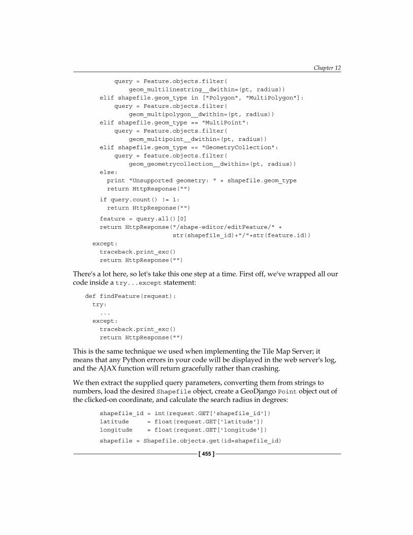
Chapter 12
[ 455 ]
query = Feature.objects.filter( geom_multilinestring__dwithin=(pt, radius)) elif shapefile.geom_type in ["Polygon", "MultiPolygon"]: query = Feature.objects.filter( geom_multipolygon__dwithin=(pt, radius)) elif shapefile.geom_type == "MultiPoint": query = Feature.objects.filter( geom_multipoint__dwithin=(pt, radius)) elif shapefile.geom_type == "GeometryCollection": query = feature.objects.filter( geom_geometrycollection__dwithin=(pt, radius)) else: print "Unsupported geometry: " + shapefile.geom_type return HttpResponse("")
if query.count() != 1: return HttpResponse("")
feature = query.all()[0] return HttpResponse("/shape-editor/editFeature/" + str(shapefile_id)+"/"+str(feature.id)) except: traceback.print_exc() return HttpResponse("")
There's a lot here, so let's take this one step at a time. First off, we've wrapped all our code inside a try...except statement:
def findFeature(request): try: ... except: traceback.print_exc() return HttpResponse("")
This is the same technique we used when implementing the Tile Map Server; it means that any Python errors in your code will be displayed in the web server's log, and the AJAX function will return gracefully rather than crashing.
We then extract the supplied query parameters, converting them from strings to numbers, load the desired Shapefile object, create a GeoDjango Point object out of the clicked-on coordinate, and calculate the search radius in degrees:
shapefile_id = int(request.GET['shapefile_id']) latitude = float(request.GET['latitude']) longitude = float(request.GET['longitude'])
shapefile = Shapefile.objects.get(id=shapefile_id)
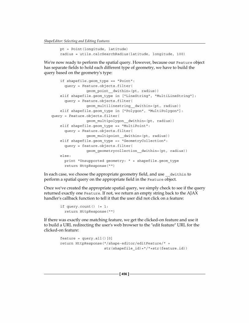
ShapeEditor: Selecting and Editing Features
[ 456 ]
pt = Point(longitude, latitude) radius = utils.calcSearchRadius(latitude, longitude, 100)
We're now ready to perform the spatial query. However, because our Feature object has separate fields to hold each different type of geometry, we have to build the query based on the geometry's type:
if shapefile.geom_type == "Point": query = Feature.objects.filter( geom_point__dwithin=(pt, radius)) elif shapefile.geom_type in ["LineString", "MultiLineString"]: query = Feature.objects.filter( geom_multilinestring__dwithin=(pt, radius)) elif shapefile.geom_type in ["Polygon", "MultiPolygon"]:query = Feature.objects.filter( geom_multipolygon__dwithin=(pt, radius)) elif shapefile.geom_type == "MultiPoint": query = Feature.objects.filter( geom_multipoint__dwithin=(pt, radius)) elif shapefile.geom_type == "GeometryCollection": query = feature.objects.filter( geom_geometrycollection__dwithin=(pt, radius)) else: print "Unsupported geometry: " + shapefile.geom_type return HttpResponse("")
In each case, we choose the appropriate geometry field, and use __dwithin to perform a spatial query on the appropriate field in the Feature object.
Once we've created the appropriate spatial query, we simply check to see if the query returned exactly one Feature. If not, we return an empty string back to the AJAX handler's callback function to tell it that the user did not click on a feature:
if query.count() != 1: return HttpResponse("")
If there was exactly one matching feature, we get the clicked-on feature and use it to build a URL redirecting the user's web browser to the "edit feature" URL for the clicked-on feature:
feature = query.all()[0] return HttpResponse("/shape-editor/editFeature/" + str(shapefile_id)+"/"+str(feature.id))
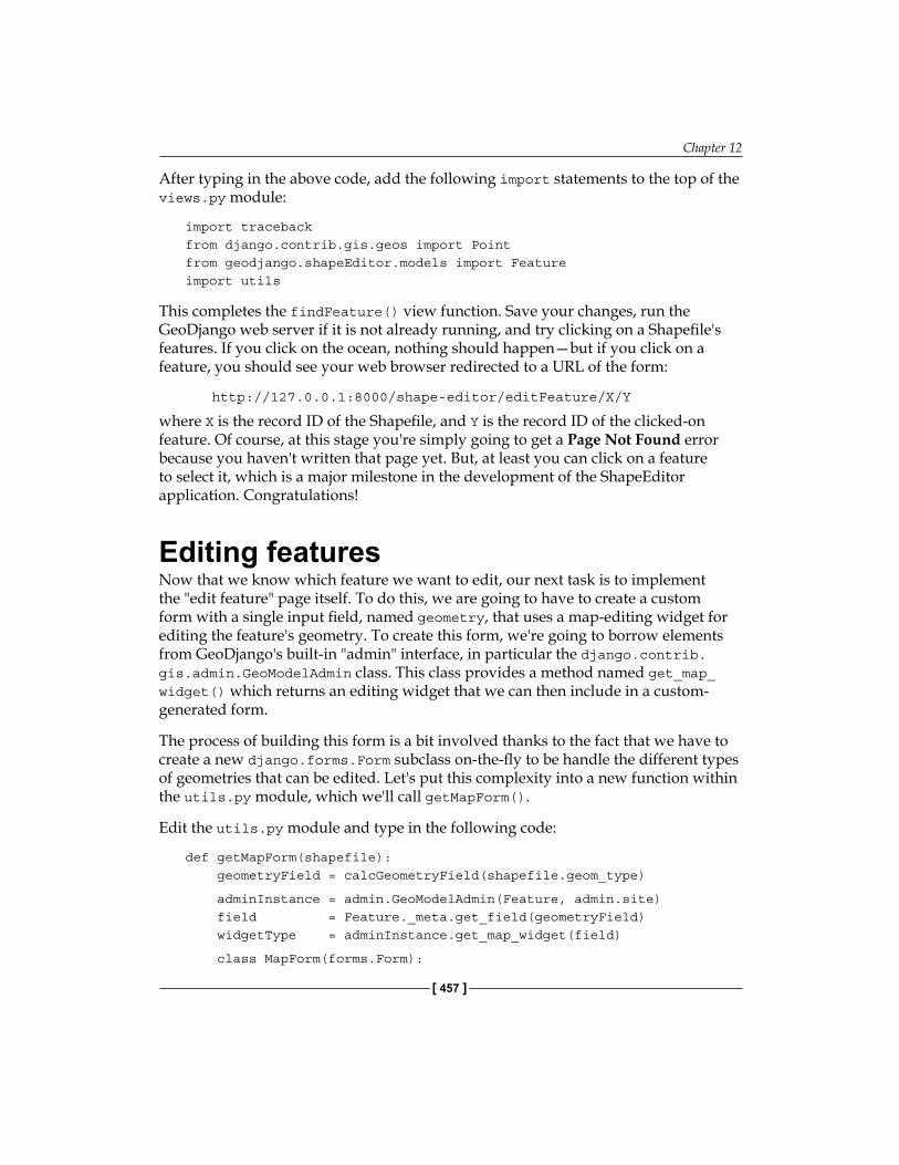
Chapter 12
[ 457 ]
After typing in the above code, add the following import statements to the top of the views.py module:
import tracebackfrom django.contrib.gis.geos import Pointfrom geodjango.shapeEditor.models import Featureimport utils
This completes the findFeature() view function. Save your changes, run the GeoDjango web server if it is not already running, and try clicking on a Shapefile's features. If you click on the ocean, nothing should happen—but if you click on a feature, you should see your web browser redirected to a URL of the form:
http://127.0.0.1:8000/shape-editor/editFeature/X/Y
where X is the record ID of the Shapefile, and Y is the record ID of the clicked-on feature. Of course, at this stage you're simply going to get a Page Not Found error because you haven't written that page yet. But, at least you can click on a feature to select it, which is a major milestone in the development of the ShapeEditor application. Congratulations!
Editing featuresNow that we know which feature we want to edit, our next task is to implement the "edit feature" page itself. To do this, we are going to have to create a custom form with a single input field, named geometry, that uses a map-editing widget for editing the feature's geometry. To create this form, we're going to borrow elements from GeoDjango's built-in "admin" interface, in particular the django.contrib.gis.admin.GeoModelAdmin class. This class provides a method named get_map_widget() which returns an editing widget that we can then include in a custom-generated form.
The process of building this form is a bit involved thanks to the fact that we have to create a new django.forms.Form subclass on-the-fly to be handle the different types of geometries that can be edited. Let's put this complexity into a new function within the utils.py module, which we'll call getMapForm().
Edit the utils.py module and type in the following code:
def getMapForm(shapefile): geometryField = calcGeometryField(shapefile.geom_type)
adminInstance = admin.GeoModelAdmin(Feature, admin.site) field = Feature._meta.get_field(geometryField) widgetType = adminInstance.get_map_widget(field)
class MapForm(forms.Form):
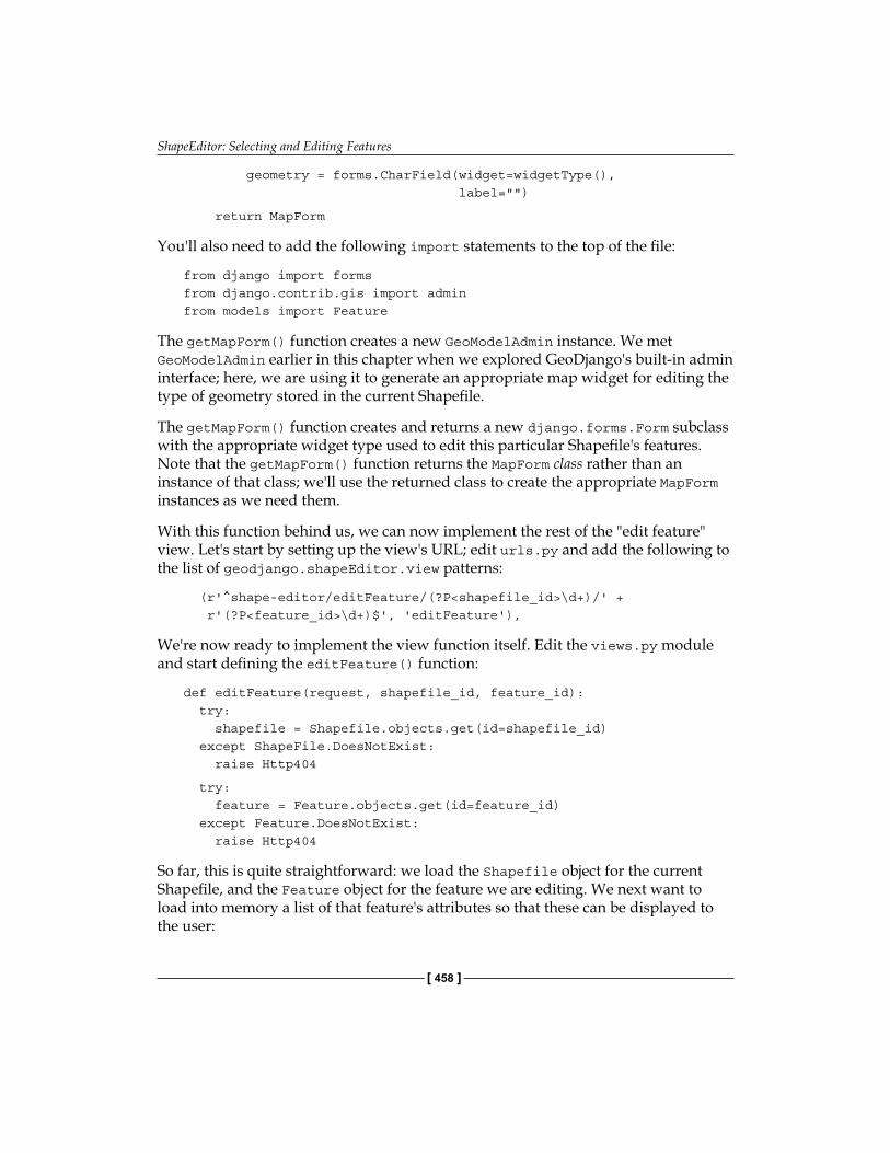
ShapeEditor: Selecting and Editing Features
[ 458 ]
geometry = forms.CharField(widget=widgetType(), label="")
return MapForm
You'll also need to add the following import statements to the top of the file:
from django import formsfrom django.contrib.gis import adminfrom models import Feature
The getMapForm() function creates a new GeoModelAdmin instance. We met GeoModelAdmin earlier in this chapter when we explored GeoDjango's built-in admin interface; here, we are using it to generate an appropriate map widget for editing the type of geometry stored in the current Shapefile.
The getMapForm() function creates and returns a new django.forms.Form subclass with the appropriate widget type used to edit this particular Shapefile's features. Note that the getMapForm() function returns the MapForm class rather than an instance of that class; we'll use the returned class to create the appropriate MapForm instances as we need them.
With this function behind us, we can now implement the rest of the "edit feature" view. Let's start by setting up the view's URL; edit urls.py and add the following to the list of geodjango.shapeEditor.view patterns:
(r'^shape-editor/editFeature/(?P<shapefile_id>\d+)/' + r'(?P<feature_id>\d+)$', 'editFeature'),
We're now ready to implement the view function itself. Edit the views.py module and start defining the editFeature() function:
def editFeature(request, shapefile_id, feature_id): try: shapefile = Shapefile.objects.get(id=shapefile_id) except ShapeFile.DoesNotExist: raise Http404
try: feature = Feature.objects.get(id=feature_id) except Feature.DoesNotExist: raise Http404
So far, this is quite straightforward: we load the Shapefile object for the current Shapefile, and the Feature object for the feature we are editing. We next want to load into memory a list of that feature's attributes so that these can be displayed to the user:
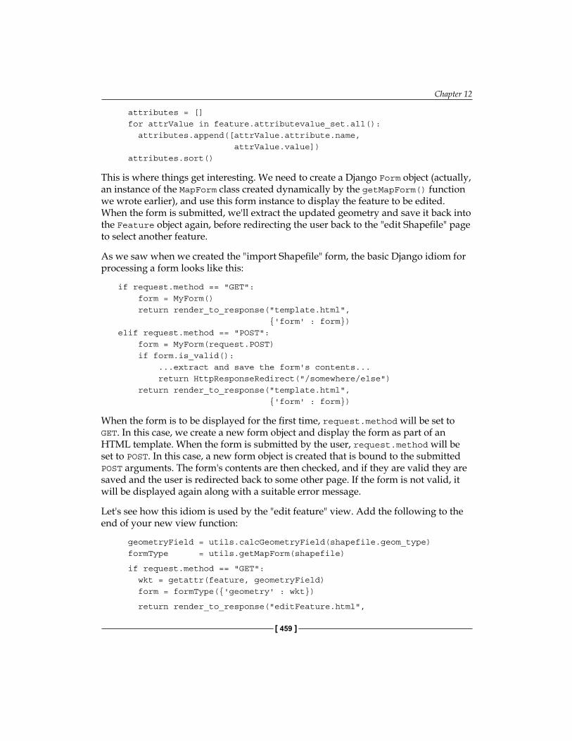
Chapter 12
[ 459 ]
attributes = [] for attrValue in feature.attributevalue_set.all(): attributes.append([attrValue.attribute.name, attrValue.value]) attributes.sort()
This is where things get interesting. We need to create a Django Form object (actually, an instance of the MapForm class created dynamically by the getMapForm() function we wrote earlier), and use this form instance to display the feature to be edited. When the form is submitted, we'll extract the updated geometry and save it back into the Feature object again, before redirecting the user back to the "edit Shapefile" page to select another feature.
As we saw when we created the "import Shapefile" form, the basic Django idiom for processing a form looks like this:
if request.method == "GET": form = MyForm() return render_to_response("template.html", {'form' : form})elif request.method == "POST": form = MyForm(request.POST) if form.is_valid(): ...extract and save the form's contents... return HttpResponseRedirect("/somewhere/else") return render_to_response("template.html", {'form' : form})
When the form is to be displayed for the first time, request.method will be set to GET. In this case, we create a new form object and display the form as part of an HTML template. When the form is submitted by the user, request.method will be set to POST. In this case, a new form object is created that is bound to the submitted POST arguments. The form's contents are then checked, and if they are valid they are saved and the user is redirected back to some other page. If the form is not valid, it will be displayed again along with a suitable error message.
Let's see how this idiom is used by the "edit feature" view. Add the following to the end of your new view function:
geometryField = utils.calcGeometryField(shapefile.geom_type) formType = utils.getMapForm(shapefile)
if request.method == "GET": wkt = getattr(feature, geometryField) form = formType({'geometry' : wkt})
return render_to_response("editFeature.html",
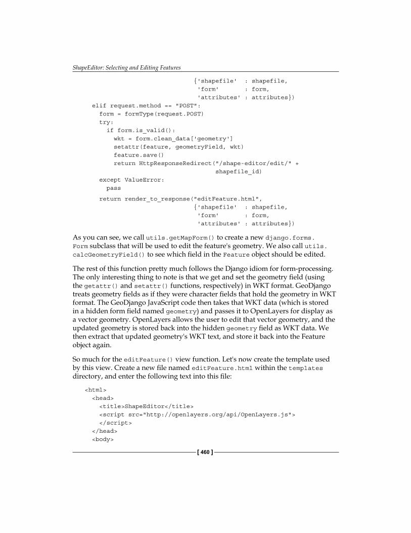
ShapeEditor: Selecting and Editing Features
[ 460 ]
{'shapefile' : shapefile, 'form' : form, 'attributes' : attributes}) elif request.method == "POST": form = formType(request.POST) try: if form.is_valid(): wkt = form.clean_data['geometry'] setattr(feature, geometryField, wkt) feature.save() return HttpResponseRedirect("/shape-editor/edit/" + shapefile_id) except ValueError: pass
return render_to_response("editFeature.html", {'shapefile' : shapefile, 'form' : form, 'attributes' : attributes})
As you can see, we call utils.getMapForm() to create a new django.forms.Form subclass that will be used to edit the feature's geometry. We also call utils.calcGeometryField() to see which field in the Feature object should be edited.
The rest of this function pretty much follows the Django idiom for form-processing. The only interesting thing to note is that we get and set the geometry field (using the getattr() and setattr() functions, respectively) in WKT format. GeoDjango treats geometry fields as if they were character fields that hold the geometry in WKT format. The GeoDjango JavaScript code then takes that WKT data (which is stored in a hidden form field named geometry) and passes it to OpenLayers for display as a vector geometry. OpenLayers allows the user to edit that vector geometry, and the updated geometry is stored back into the hidden geometry field as WKT data. We then extract that updated geometry's WKT text, and store it back into the Feature object again.
So much for the editFeature() view function. Let's now create the template used by this view. Create a new file named editFeature.html within the templates directory, and enter the following text into this file:
<html> <head> <title>ShapeEditor</title> <script src="http://openlayers.org/api/OpenLayers.js"> </script> </head> <body>
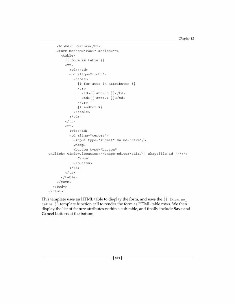
Chapter 12
[ 461 ]
<h1>Edit Feature</h1> <form method="POST" action=""> <table> {{ form.as_table }} <tr> <td></td> <td align="right"> <table> {% for attr in attributes %} <tr> <td>{{ attr.0 }}</td> <td>{{ attr.1 }}</td> </tr> {% endfor %} </table> </td> </tr> <tr> <td></td> <td align="center"> <input type="submit" value="Save"/> <button type="button" onClick='window.location="/shape-editor/edit/{{ shapefile.id }}";'> Cancel </button> </td> </tr> </table> </form> </body></html>
This template uses an HTML table to display the form, and uses the {{ form.as_table }} template function call to render the form as HTML table rows. We then display the list of feature attributes within a sub-table, and finally include Save and Cancel buttons at the bottom.
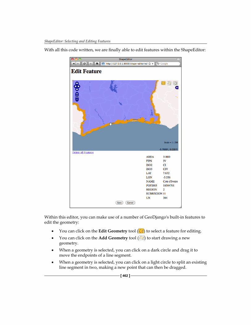
ShapeEditor: Selecting and Editing Features
[ 462 ]
With all this code written, we are finally able to edit features within the ShapeEditor:
Within this editor, you can make use of a number of GeoDjango's built-in features to edit the geometry:
• You can click on the Edit Geometry tool ( ) to select a feature for editing.• You can click on the Add Geometry tool ( ) to start drawing a new
geometry.• When a geometry is selected, you can click on a dark circle and drag it to
move the endpoints of a line segment.• When a geometry is selected, you can click on a light circle to split an existing
line segment in two, making a new point that can then be dragged.
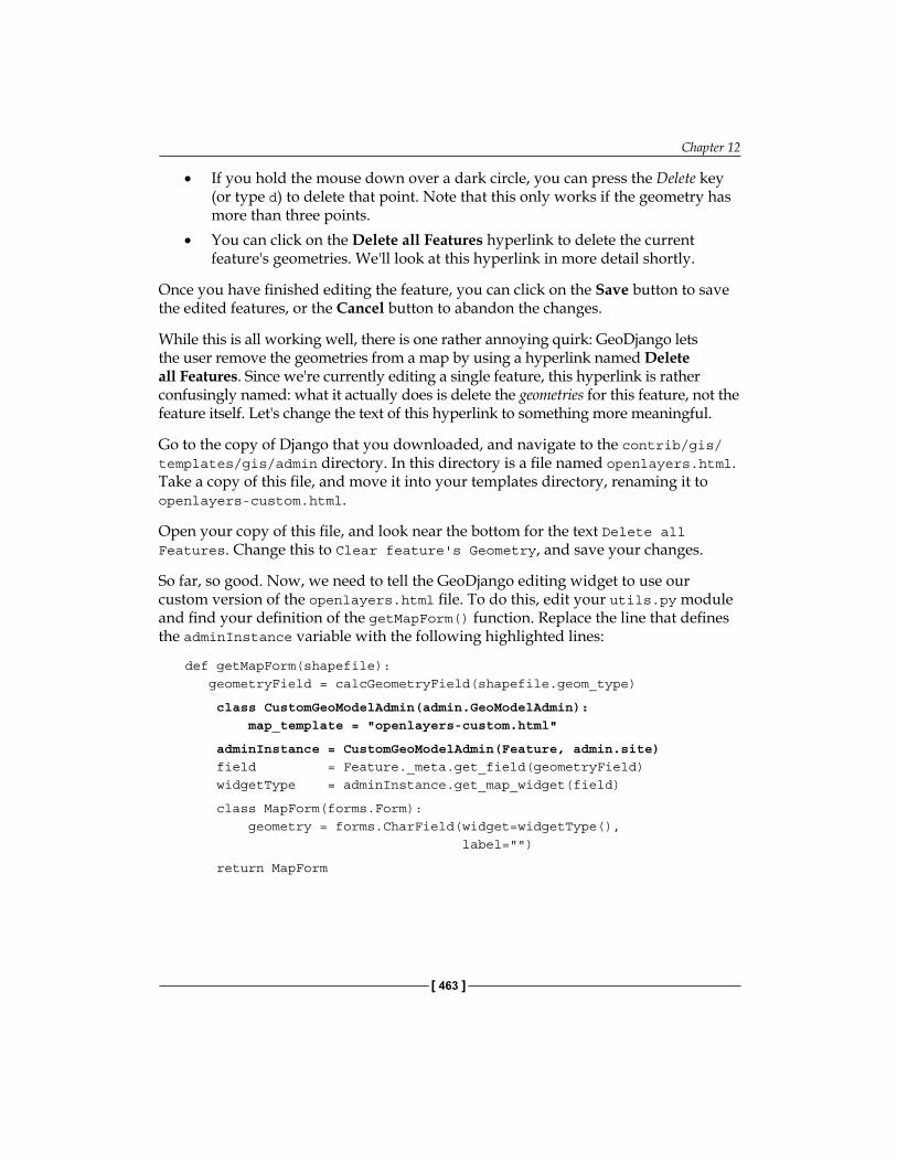
Chapter 12
[ 463 ]
• If you hold the mouse down over a dark circle, you can press the Delete key (or type d) to delete that point. Note that this only works if the geometry has more than three points.
• You can click on the Delete all Features hyperlink to delete the current feature's geometries. We'll look at this hyperlink in more detail shortly.
Once you have finished editing the feature, you can click on the Save button to save the edited features, or the Cancel button to abandon the changes.
While this is all working well, there is one rather annoying quirk: GeoDjango lets the user remove the geometries from a map by using a hyperlink named Delete all Features. Since we're currently editing a single feature, this hyperlink is rather confusingly named: what it actually does is delete the geometries for this feature, not the feature itself. Let's change the text of this hyperlink to something more meaningful.
Go to the copy of Django that you downloaded, and navigate to the contrib/gis/templates/gis/admin directory. In this directory is a file named openlayers.html. Take a copy of this file, and move it into your templates directory, renaming it to openlayers-custom.html.
Open your copy of this file, and look near the bottom for the text Delete all Features. Change this to Clear feature's Geometry, and save your changes.
So far, so good. Now, we need to tell the GeoDjango editing widget to use our custom version of the openlayers.html file. To do this, edit your utils.py module and find your definition of the getMapForm() function. Replace the line that defines the adminInstance variable with the following highlighted lines:
def getMapForm(shapefile): geometryField = calcGeometryField(shapefile.geom_type)
class CustomGeoModelAdmin(admin.GeoModelAdmin): map_template = "openlayers-custom.html"
adminInstance = CustomGeoModelAdmin(Feature, admin.site) field = Feature._meta.get_field(geometryField) widgetType = adminInstance.get_map_widget(field)
class MapForm(forms.Form): geometry = forms.CharField(widget=widgetType(), label="")
return MapForm
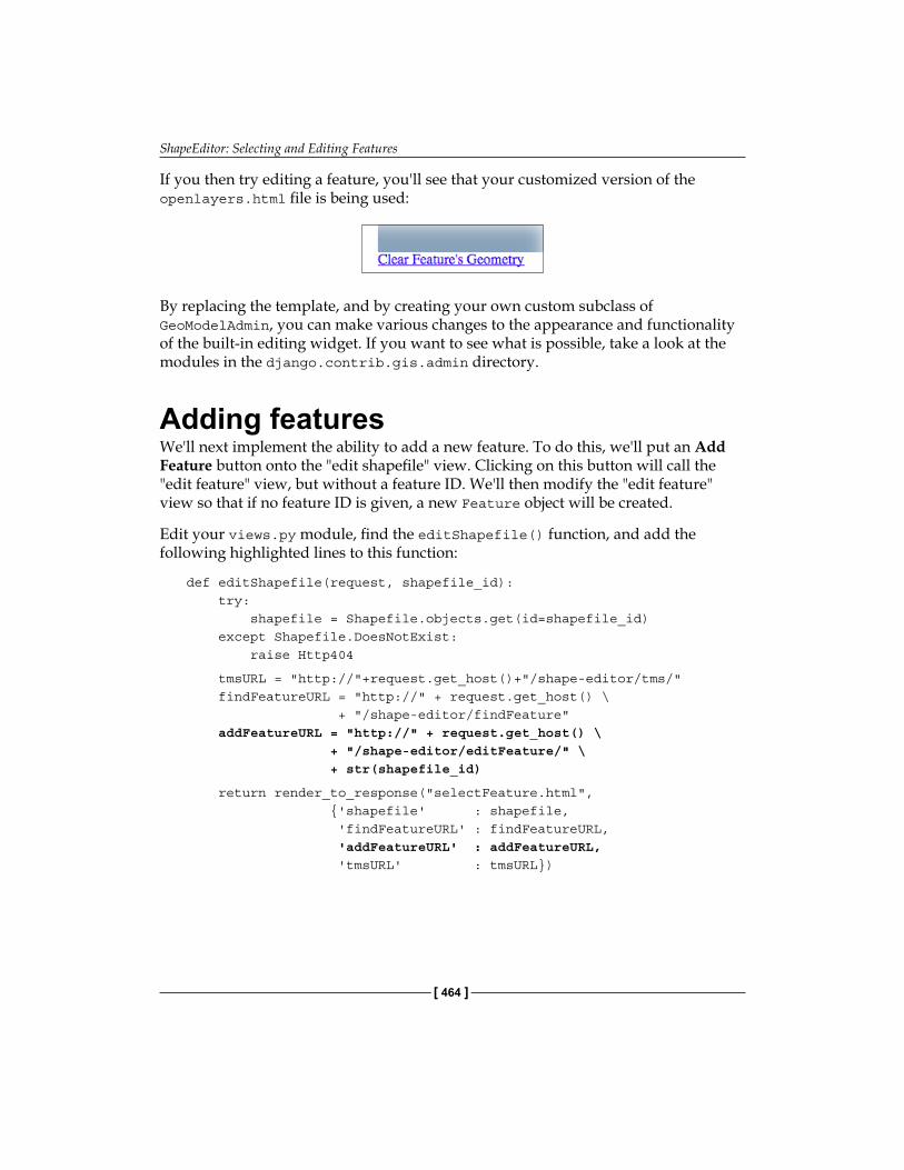
ShapeEditor: Selecting and Editing Features
[ 464 ]
If you then try editing a feature, you'll see that your customized version of the openlayers.html file is being used:
By replacing the template, and by creating your own custom subclass of GeoModelAdmin, you can make various changes to the appearance and functionality of the built-in editing widget. If you want to see what is possible, take a look at the modules in the django.contrib.gis.admin directory.
Adding featuresWe'll next implement the ability to add a new feature. To do this, we'll put an Add Feature button onto the "edit shapefile" view. Clicking on this button will call the "edit feature" view, but without a feature ID. We'll then modify the "edit feature" view so that if no feature ID is given, a new Feature object will be created.
Edit your views.py module, find the editShapefile() function, and add the following highlighted lines to this function:
def editShapefile(request, shapefile_id): try: shapefile = Shapefile.objects.get(id=shapefile_id) except Shapefile.DoesNotExist: raise Http404
tmsURL = "http://"+request.get_host()+"/shape-editor/tms/" findFeatureURL = "http://" + request.get_host() \ + "/shape-editor/findFeature" addFeatureURL = "http://" + request.get_host() \ + "/shape-editor/editFeature/" \ + str(shapefile_id)
return render_to_response("selectFeature.html", {'shapefile' : shapefile, 'findFeatureURL' : findFeatureURL, 'addFeatureURL' : addFeatureURL, 'tmsURL' : tmsURL})
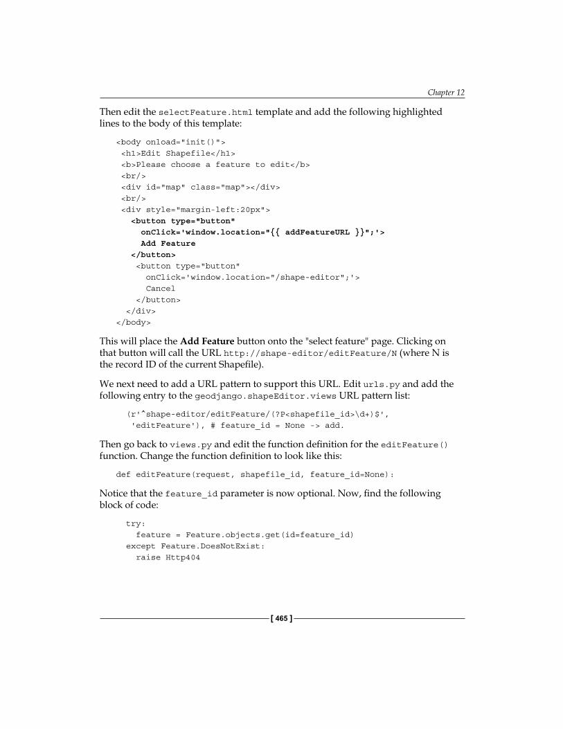
Chapter 12
[ 465 ]
Then edit the selectFeature.html template and add the following highlighted lines to the body of this template:
<body onload="init()"> <h1>Edit Shapefile</h1> <b>Please choose a feature to edit</b> <br/> <div id="map" class="map"></div> <br/> <div style="margin-left:20px"> <button type="button" onClick='window.location="{{ addFeatureURL }}";'> Add Feature </button> <button type="button" onClick='window.location="/shape-editor";'> Cancel </button> </div></body>
This will place the Add Feature button onto the "select feature" page. Clicking on that button will call the URL http://shape-editor/editFeature/N (where N is the record ID of the current Shapefile).
We next need to add a URL pattern to support this URL. Edit urls.py and add the following entry to the geodjango.shapeEditor.views URL pattern list:
(r'^shape-editor/editFeature/(?P<shapefile_id>\d+)$', 'editFeature'), # feature_id = None -> add.
Then go back to views.py and edit the function definition for the editFeature() function. Change the function definition to look like this:
def editFeature(request, shapefile_id, feature_id=None):
Notice that the feature_id parameter is now optional. Now, find the following block of code:
try: feature = Feature.objects.get(id=feature_id) except Feature.DoesNotExist: raise Http404
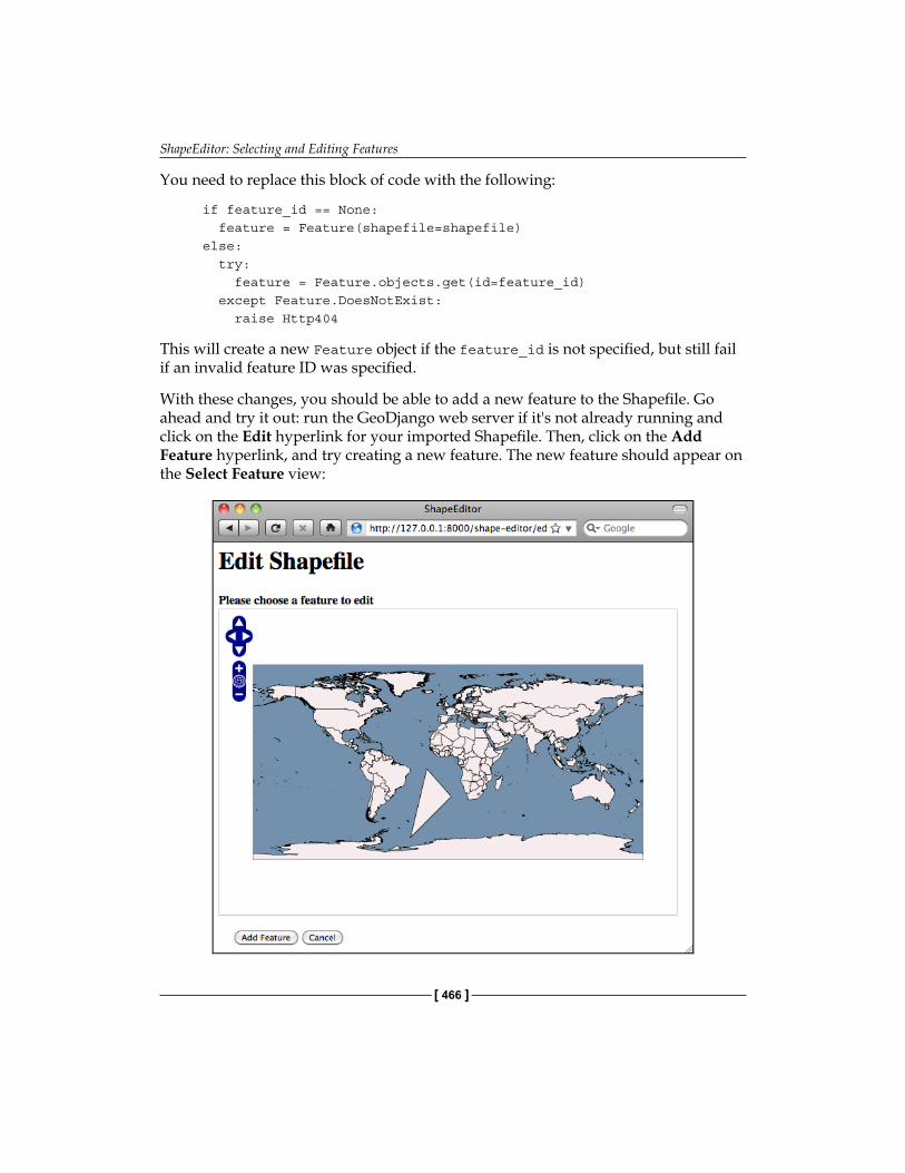
ShapeEditor: Selecting and Editing Features
[ 466 ]
You need to replace this block of code with the following:
if feature_id == None: feature = Feature(shapefile=shapefile) else: try: feature = Feature.objects.get(id=feature_id) except Feature.DoesNotExist: raise Http404
This will create a new Feature object if the feature_id is not specified, but still fail if an invalid feature ID was specified.
With these changes, you should be able to add a new feature to the Shapefile. Go ahead and try it out: run the GeoDjango web server if it's not already running and click on the Edit hyperlink for your imported Shapefile. Then, click on the Add Feature hyperlink, and try creating a new feature. The new feature should appear on the Select Feature view:
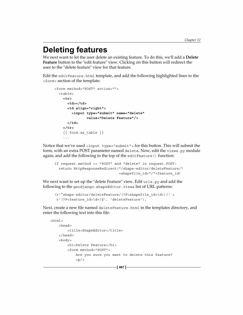
Chapter 12
[ 467 ]
Deleting featuresWe next want to let the user delete an existing feature. To do this, we'll add a Delete Feature button to the "edit feature" view. Clicking on this button will redirect the user to the "delete feature" view for that feature.
Edit the editFeature.html template, and add the following highlighted lines to the <form> section of the template:
<form method="POST" action=""> <table> <tr> <td></td> <td align="right"> <input type="submit" name="delete" value="Delete Feature"/> </td> </tr> {{ form.as_table }} ...
Notice that we've used <input type="submit"> for this button. This will submit the form, with an extra POST parameter named delete. Now, edit the views.py module again, and add the following to the top of the editFeature() function:
if request.method == "POST" and "delete" in request.POST: return HttpResponseRedirect("/shape-editor/deleteFeature/" +shapefile_id+"/"+feature_id)
We next want to set up the "delete Feature" view. Edit urls.py and add the following to the geodjango.shapeEditor.views list of URL patterns:
(r'^shape-editor/deleteFeature/(?P<shapefile_id>\d+)/' + r'(?P<feature_id>\d+)$', 'deleteFeature'),
Next, create a new file named deleteFeature.html in the templates directory, and enter the following text into this file:
<html> <head> <title>ShapeEditor</title> </head> <body> <h1>Delete Feature</h1> <form method="POST"> Are you sure you want to delete this feature? <p/>
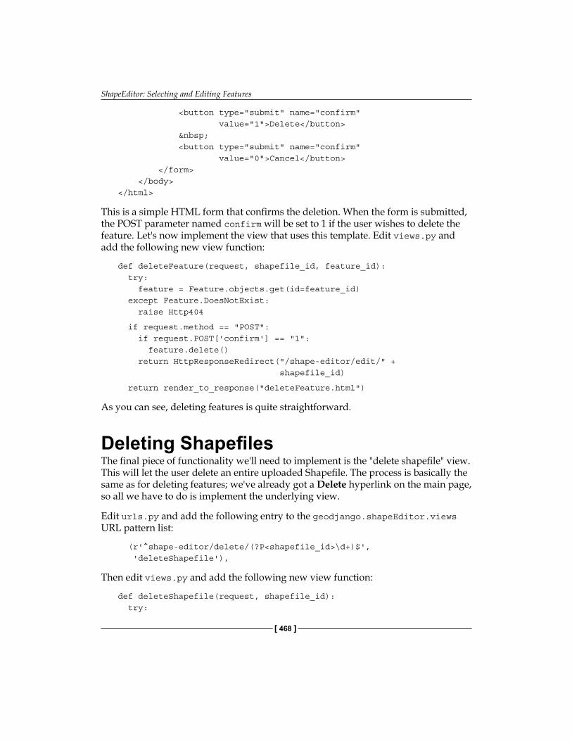
ShapeEditor: Selecting and Editing Features
[ 468 ]
<button type="submit" name="confirm" value="1">Delete</button> <button type="submit" name="confirm" value="0">Cancel</button> </form> </body></html>
This is a simple HTML form that confirms the deletion. When the form is submitted, the POST parameter named confirm will be set to 1 if the user wishes to delete the feature. Let's now implement the view that uses this template. Edit views.py and add the following new view function:
def deleteFeature(request, shapefile_id, feature_id): try: feature = Feature.objects.get(id=feature_id) except Feature.DoesNotExist: raise Http404
if request.method == "POST": if request.POST['confirm'] == "1": feature.delete() return HttpResponseRedirect("/shape-editor/edit/" + shapefile_id)
return render_to_response("deleteFeature.html")
As you can see, deleting features is quite straightforward.
Deleting ShapefilesThe final piece of functionality we'll need to implement is the "delete shapefile" view. This will let the user delete an entire uploaded Shapefile. The process is basically the same as for deleting features; we've already got a Delete hyperlink on the main page, so all we have to do is implement the underlying view.
Edit urls.py and add the following entry to the geodjango.shapeEditor.views URL pattern list:
(r'^shape-editor/delete/(?P<shapefile_id>\d+)$', 'deleteShapefile'),
Then edit views.py and add the following new view function:
def deleteShapefile(request, shapefile_id): try:
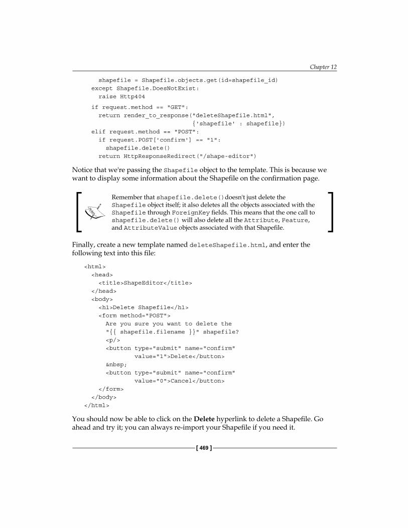
Chapter 12
[ 469 ]
shapefile = Shapefile.objects.get(id=shapefile_id) except Shapefile.DoesNotExist: raise Http404
if request.method == "GET": return render_to_response("deleteShapefile.html", {'shapefile' : shapefile}) elif request.method == "POST": if request.POST['confirm'] == "1": shapefile.delete() return HttpResponseRedirect("/shape-editor")
Notice that we're passing the Shapefile object to the template. This is because we want to display some information about the Shapefile on the confirmation page.
Remember that shapefile.delete()doesn't just delete the Shapefile object itself; it also deletes all the objects associated with the Shapefile through ForeignKey fields. This means that the one call to shapefile.delete() will also delete all the Attribute, Feature, and AttributeValue objects associated with that Shapefile.
Finally, create a new template named deleteShapefile.html, and enter the following text into this file:
<html> <head> <title>ShapeEditor</title> </head> <body> <h1>Delete Shapefile</h1> <form method="POST"> Are you sure you want to delete the "{{ shapefile.filename }}" shapefile? <p/> <button type="submit" name="confirm" value="1">Delete</button> <button type="submit" name="confirm" value="0">Cancel</button> </form> </body></html>
You should now be able to click on the Delete hyperlink to delete a Shapefile. Go ahead and try it; you can always re-import your Shapefile if you need it.
ShapeEditor: Selecting and Editing Features
[ 470 ]
Using ShapeEditorCongratulations! You have just finished implementing the last of the ShapeEditor's features, and you now have a complete working geo-spatial application built using GeoDjango. Using the ShapeEditor, you can import Shapefiles, view their features and the feature attributes, make changes to the feature geometries, add and delete features, and then export the Shapefile again.
This is certainly a useful application. Even if you don't have a full-blown GIS system installed, you can now make quick and easy changes to a Shapefile's contents using the ShapeEditor. And, of course, the ShapeEditor is a great starting point for the development of your own geo-spatial applications.
Further improvements and enhancementsAs with any new application, there are a number of ways in which the ShapeEditor could be improved. For example:
• Adding user signup and login so that each user has his or her own private set of Shapefiles rather than every user seeing the entire list of all the uploaded Shapefiles.
• Adding the ability to edit a feature's attribute values.• Using a higher resolution base map. An obvious candidate for this would be
the GSHHS high-resolution shoreline database.• Adding a tile cache for our TMS server.• Using JavaScript to add a "please wait" pop up message while a Shapefile is
being imported or exported.• Improving the reusability of the ShapeEditor's codebase. We've concentrated
on learning how to use GeoDjango to build a working system, but with a suitable redesign the code could be made much more generic so that it can be used in other applications as well.
Feel free to make these improvements; you will learn a lot more about GeoDjango, and about geo-spatial development in general, if you take the time to implement these features. As you work with the ShapeEditor, you'll probably come up with your own list of things you'd like to improve.
Chapter 12
[ 471 ]
SummaryIn this chapter, we finished implementing a sophisticated geo-spatial web application using GeoDjango, Mapnik, PostGIS, OGR, and pyproj. This application is useful in its own right, as well as being a springboard to developing your own geo-spatial web applications.
We have learned:
• That we can easily create our own Tile Map Server using Mapnik and GeoDjango.
• That we can include OpenLayers on our own web pages, independent of GeoDjango, and display map data from our Tile Map Server.
• How we can create a custom "click handler" to respond to mouse clicks within an OpenLayers map.
• That we can use AJAX calls to have the server respond to events within the web browser.
• That GeoDjango provides a powerful query language for performing spatial queries without writing a single line of SQL.
• How to "borrow"geometry editing widgets from GeoDjango and use them within your own web application.
• That you can create your own GeoModelAdmin subclass to change the appearance and functionality of GeoDjango's geometry editing widgets.
• That you can use a simple HTML form to confirm the deletion of a record.
This completes our exploration of GeoDjango, and also completes this book. Hopefully, you have learned a lot about geo-spatial development, and how to create geo-spatial applications using Python. With these tools at your disposal, you are now ready to start developing your own complex geo-spatial applications. Have fun!

IndexSymbols<SrcDataSource> element 274
AAddGeometryColumn() function 156, 161add_point() method 276AddPoint() method 105affine transformation 49, 110AJAX 331analyzeGeometry() function 42angular distance 25, 132, 226application, designing
about 367feature, editing 370, 371feature, selecting 369Shapefile, exporting 371Shapefile, importing 367, 368
Application Programming Interfaces (APIs) 18
ArcGRID 92ARC/Info Binary Grid (.adf) format. See
ArcGRIDARC/INFO Interchange format 80areas 73Asynchronous JavaScript and XML. See
AJAXAttribute object 384AttributeValue object 385, 413, 414azimuthal projection
types 32
BBand Interleaved by Line (BIL) format 38Band Interleaved by Pixel (BIP) format 38
Band Sequential (BSQ) format 38bare-bones approach
about 322advantages 322disadvantages 322
base layerabout 350defining 438, 439
base mapsetting up 435, 436
big web service 325border, calculating
between Thailand and Myanmar 123-126bounding box
calculating, for country 102, 103saving, into Shapefile 104-108
bounding box, selectArea.py scriptcalculating 215, 216
buffer() method 62BuildingSymbolizer 66built-in admin application
using 388-395built-in applications, Django
about 372admin interface 372authentication system 372markup application 372messages framework 372sessions system 373sitemaps framework 373syndication system 373
CcalcGeometryField() function 412callback function 449CBSA 128
[ 474 ]
CGI scriptsabout 211selectArea.py script 214, 215selectCountry.py script 212, 213showResults.py script 223
civic location 24CloudMade
about 75URL 75
colorsusing 303
commercial database, geo-spatialabout 164MS SQL Server 165Oracle 164, 165
complex linear featuresdrawing 285
components, Django applicationmodel 374template 377, 378view 374, 376
conic projectionabout 31types 31
coordinates 10coordinates systems
projected coordinate systems 33unprojected coordinate system 33
CoordinateTransformation() object 411Core Based Statistical Area. See CBSACreateSpatialIndex() function 163cursor.execute() method 150cylindrical projections
about 29example 30types 31
Ddatabase
setting up 379, 380database, DISTAL application
building 195-199designing 195-199
database load balancer 256database objects
using 368database replication 255
data, DISTAL applicationdownloading 199importing 201
data download, DISTAL applicationGeonames, downloading 200GEOnet Names Server, downloading 200GSHHS shoreline database, downloading
200World Borders Dataset, downloading 200
data format, DCW 80data format, GLOBE 90, 91data format, Landsat 86data format, OpenStreetMap 73data format, TIGER 77, 78data importing, DISTAL application
GSHHS 203, 204US placename data 205-207World Borders Dataset 201-203Worldwide placename data 208, 210
data model, GDALdataset 48raster band 48raster size 49
data modelsdefining 383-387
dataset 48datasource, selectArea.py script
MySQL 218PostGIS 219setting up 218SpatiaLite 219
datasources, Mapnikabout 269, 270GDAL 272, 273OGR 273, 274OSM 275PointDatasource 276PostGIS 270-272Shapefile 270SQLite 274, 275
datumabout 35, 115changing 119-122reference datums 35
DCWabout 79data format 80
[ 475 ]
DCW dataobtaining 80, 81using 80, 81
defaultHandlerOptions dictionary 448def render_tile_to_file() function 308DescribeFeatureType request 338Destroy() method 105, 420Digital Chart of the World. See DCWDigital Elevation Map (DEM-format)
about 38, 85, 108, 303height data, analyzing 108-114
Digital Raster Graphic (DRG) 38DISTAL 191, 322DISTAL application
CGI scripts 210database, building 195-199database, designing 195-199data, downloading 199data, importing 201implementing 210issues 235workflow 191-194, 210
distanceabout 25angular distance 25linear distance 25traveling distance 26
distance calculations, showResults.py scriptabout 225angular distances, using 226, 227hybrid approach 229-231manual 226points, identifying 233projected coordinates, using 228Spatial Joins 231, 232
Djangoabout 353admin interface 355model 355templating system 355
Django applicationcomponents 373structure 372
Django application, componentsmodel 374template 377, 378view 374, 376
django.forms.Form subclasscreating 457
Django framework 353Django model 355documentation, PostGIS 157documentation, SpatiaLite 160
EE00 format 80else rule
about 280using 281
Envelope() function 175EPSG 167error handling 429ESRI 119European Petroleum Survey Group.
See EPSGEveryBlock
URL 64EXPLAIN QUERY PLAN command 178exportData() function 417external linking 339
Ffalse easting 34false northing 34feature layer
defining 440, 441Feature object 384, 411features
adding 464-466deleting 467, 468editing 370, 371, 457-463selecting 369selecting, for edit 426
features, PostGIS 157fields 103filters
about 277example 278
findFeature() function 452findFeatureURL parameter 451findFeature view
implementing 451findPoints() function 44
[ 476 ]
fixture 436fwd() method 56FWTools
URL 54
Ggamma correction 288GDAL
about 17, 48data model 48-50documentation 53example code 50, 51resources 53URL 53
GDAL datasource 272, 273gdaldem utility 94Generalized Search Tree index type. See
GiSTgenerateMap() function
about 309parameters 310using 313
generateMap() function, parametersbackground 310datasource 310hiliteExpr 310hiliteFill 310hiliteLine 310mapHeight 310mapWidth 310maxX 310maxY 310minX 310minY 310normalFill 310normalLine 310points 310
Generic Mapping Tools (GMT) 83geocode 12Geod class
about 56methods 56
geodetic distance 134geodetic location 24GeoDjango
about 353
spatial queries, performing 451-455TMS protocol, implementing with 428
GeoDjango projectsetting up 380, 381
geodjango project directory 435Geofabrik
about 75URL 75
Geographical Information Systems. See GISGeographic Names Information System. See
GNISgeographies 156Geography Markup Language. See GMLGeoJSON 38geolocation 18geometries
about 103, 156saving, into text file 126
GeometryCollection class 61Geometry object 122geom_type field 409Geonames
downloading 200GEOnet Names Server. See GNSgeoreferencing transform 49GEOS library
URL 63geo-spatial, commercial databases
about 164MS SQL Server 165Oracle 164, 165
geo-spatial dataabout 71analyzing 12, 13, 59attributes 10coordinates 10manipulating 59raster format sources 85reading 47, 102representing 122, 123storing 122, 123vector based sources 72visualizing 13-15, 63writing 47, 102
Geospatial Data Abstraction Library. See GDAL
[ 477 ]
geo-spatial databasesbest practices 165-173
geo-spatial databases, best practices 165-173geo-spatial data, examples
prerequisites 101geo-spatial development
about 9applications 11example 9, 10working 10
geo-spatial development, applicationsgeo-spatial data, analyzing 12, 13geo-spatial data, visualizing 13-15geo-spatial mash-up, creating 16
geo-spatial mash-upcreating 16
geo-spatial, open source databasesabout 149MySQL 149-152PostGIS 152-158SpatiaLite 158-164
geo-spatial web applicationsprotocols 334tools 344
geo-spatial web application stack 334GeoTIFF files 86GetCapabilities request 335, 338GetFeatureInfo request 336GetFeature request 338GetFeatureWithLock request 338GetFieldAs() method 413getLineSegmentsFromGeometry()
function 134getMapForm() function 458GetMap request 336GetNoDataValue() method 114getOGRFeatureAttribute()
function 413, 414, 421GIS
about 21data format 37
GIS, conceptsabout 21coordinate system 32, 34datums 35distance 25, 26location 22, 24
projections 28, 29shapes 36units 27, 28
GIS dataworking with, manually 39-45
GIS data formatabout 37Band Interleaved by Line (BIL) 38Band Interleaved by Pixel (BIP) 38coverage 38Digital Elevation Model (DEM) 38Digital Raster Graphic (DRG) 38Geography Markup Language (GML) 39GeoJSON 38micro-formats 38shapefile 38simple features 38TIGER/Line 38Well-known Binary (WKB) 38Well-known Text (WKT) 38
GiST 146Global Land One-kilometer Base Elevation.
See GLOBEGlobal Positioning System. See GPSGlobal Self-Consistent, Hierarchical,
High-Resolution Shoreline. See GSHHS
GLOBEabout 90data format 90, 91
GLOBE dataobtaining 91using 91
GML 337GNIS
about 96database 96
GNIS dataabout 96, 97obtaining 97using 97
GNSabout 94database 95downloading 200obtaining 95using 95
[ 478 ]
GNS databaseabout 95
GoogleGoogle Earth 17Google Maps 17products, limitations 17
Google Earth 17Google Maps 17Google Maps slippy map example 332GPS 17GPS receiver 22great circle distance 26Great Circle Distance concept 225Ground Control Points (GCPs) 50GSHHS
about 82downloading 200importing 203, 204
GSHHS databaseabout 83obtaining 84
HHaversine formula 27height data
analyzing, digital elevation map (DEM) used 108-114
help() command 53Http404 exception 430
IimportData() function 405, 406, 414ImportShapefileForm object 403importShapefile() function 403importShapefile() view function 402, 405initialize() function 448installation, PostGIS 152, 154installation, Psycopg 153installation, pysqlite 159installation, SpatiaLite
about 158for Linux 159for Mac OS X 158for MS Windows 158
interpreted language 8inverse projection 55
inv() method 56issues, DISTAL application
performance 239quality 237scalability 253-256usability 236, 237
JJava
comparing, with Python 8jurisdictional locations 24
Llabels
drawing 289Labels layer 261Landsat
about 86data format 86
Landsat imageryabout 86obtaining 87-89
latitude 22LayerMapping module
data, importing from ShapeFile 436layers, Mapnik
about 304creating 304
lengthcalculating, for Thai-Myanmar
border 133-138linear distance 25LinearRing class 61linear rings 104LinePatternSymbolizer
about 65, 286working 286
line placementabout 292allow_overlap attribute 294labels, repeating 292text, drawing on dark background 295text overlap, controlling 294
linesdrawing 281
linestring 36
[ 479 ]
LineString class 60LineSymbolizer
about 65, 262, 281, 439color attribute, setting 282line_cap attribute, setting 283line color, setting 282line_join attribute, setting 283opacity, setting 282working 282
LinuxSpatiaLite, installing on 159
listShapefiles() function 398List Shapefiles view
implementing 397-401listShapefiles() view function 398, 399load_map() function 316location
about 22civic location 24example 22, 24geodetic location 24jurisdictional locations 24measuring 22, 24
LockFeature request 338longitude 23
MMac OS X
SpatiaLite, installing on 158main map layer
creating 310-312map
base layer, defining 438, 439displaying, OpenLayers used 442-445feature layer, defining 440, 441generating 261rendering 313zoom levels 431, 432
map.append_style() method 304map definition file
about 264, 314example 314using 314
map dimensions, selectArea.py scriptcalculating 216-218
Mapfishabout 356URL 356working 357
MapGeneratormind map layer, creating 310-312points, displaying on map 312, 313
map.getLonLatFromViewPortPx() method 450
Mapiatorabout 351working 352
map image, selectArea.py scriptrendering 220-223
Mapnikabout 63, 260datasources 269, 270design 64, 65documentation 67else rule 280, 281example code 66, 67features 63filters 277, 278layers 304map, generating 261, 265map rendering 307resources 68scale denominators 279, 280symbolizers 65, 66, 281TMS protocol, implementing with 427, 428URL 68, 260working 63, 261, 268world map, displaying 66, 67
mapnik.Color classinstances, creating ways 303
mapnik.Layer class 306mapnik.Layer class, methods
layer.envelope() 306layer.visible() 307
mapnik.Map classabout 305methods 305
mapnik.Map class, methodsmap.envelope() 305map.scale() 306map.scale_denominator() 306map.zoom_all() 306
[ 480 ]
map.zoom_to_box() 306mapnik.Map object
creating 438mapnik.PostGIS datasource
setting up 438, 440Mapnik rule 263
conditions 277mapnik.Shapefile() constructor 270mapnik.SQLite() constructor 274mapnik tool 16Mapnik toolkit 269
importing 265Mapnik wiki
URL 67map object
about 64creating 64, 267
map renderer 215map rendering
about 327example 327about 307
MapServer tool 16Map Tile
rendering 441MarkersSymbolizer 66mash-ups
about 16example 16
maxResolution option 445MBRContains() function 151meridians 24micro-formats 38minimum bounding rectangle 147mirror sites, OpenStreetMap data
about 75CloudMade 75Geofabrik 75
model 374models.py file
about 385editing 386
model-view-controller pattern. See MVCmod_tile module
about 346working 346
mod_wsgi module 347
mouse clicksintercepting 447-451
MS SQL Serverabout 165limitations 165
MS WindowsSpatiaLite, installing on 158
MultiLineString class 61MultiPoint class 61MultiPolygon class 61MVC 354MySQL
about 149, 188, 323accessing, from Python programs 149, 150advantages 152query optimization process 174, 175working with 179-182
MySQL database 218MySQLdb module 150MySQL-Python driver 149
NNAD 27 35NAD 83 35National Elevation Dataset. See NEDNED 92NED data
about 92obtaining 93using 93
nginx about 254URL 254
nodes 73npts() method 56numZoomLevels option 445
Ooblate spheroid 21OGC
about 18URL 18
OGR about 17, 48, 77design 51, 52documentation 53
[ 481 ]
example code 52resources 53
OGR Datasource 273, 274OGRGeometryTypeToName() function 409ogrinspect.py utility 369OGR library. See OGRonClick() function 448Open Geospatial Consortium. See OGCOpenLayers
about 348example 349maps, displaying 442-445types 350URL 348using 348-351
OpenLayers.Control class 447OpenLayers.Control.Click class 448OpenLayers.Layer.TMS object 445OpenLayers.Map object 445OpenLayers.Request.GET function 449OpenLayers.Request.GET() function 450open source databases, geo-spatial
about 149MySQL 149-152PostGIS 152-158SpatiaLite 158-164
OpenStreetMapabout 72data format 73URL 15
OpenStreetMap APIusing 74, 75
OpenStreetMap dataobtaining 74using 74
OpenStreetMap XML dataexample 73working with 76
Oracle 164Oracle Locator 165Oracle Spatial 164orthorectification 87osm2pgsql tool 76OsmApi module 75OSM datasource 275osmexport utility 76os.path.join() function 270
other source types, geo-spatial dataabout 94GNS 94, 95
overlay 14Overlay Layers 350
Ppainter's algorithm 261parallels 24parks
identifying, near urban areas 128-132performance, DISTAL application issues
about 239improving 242-244performance improvement, analyzing 252,
253problem finding 240, 241tiled shorelines, calculating 244-249tiled shorelines, using 250-252
pipe-delimited compressed text files 97Planet.osm database 75point
about 36coordinate, calculating for 139, 141
Point class 60PointDatasource
about 276setting up 276
point placement 291points
displaying, on map 312, 313drawing 298
PointSymbolizer 65, 299, 300polygon 37Polygon class 61polygon.contains(point) method 151PolygonPatternSymbolizer 65, 288polygons
drawing 287Polygons layer 261PolygonSymbolizer
about 65, 262, 287, 439color, setting for polygon 287gamma correction 288opacity, setting for polygon 287using 264
[ 482 ]
PostGIS about 12, 17, 152, 188documentation 157features 157installing 152, 154query optimization process 175, 176using 155working with 182, 184
PostGIS database 219PostGIS datasource 270-272PostGIS, installing
about 152requisites 152, 154
PostGIS manualURL 157
PostgreSQL manualURL 157
prime meridian 24PROJ.4 17Proj class
about 55working 55
projected coordinate systemsabout 33map units 34origin 34working 33
projection 11about 28, 54, 115azimuthal projection 31changing, geographic and UTM coordinates
used 115-119conic projection 31cylindrical projection 29, 30pyproj library 54
Proj Python library 12protocols, geo-spatial web applications
about 334TMS 339-344WFS 337-339WMS 334, 335
Psycopgabout 152, 153installing 153
Psycopg documentationURL 157
Pylons 356
pyproj libraryabout 54classes 55design 55documentation 58example code 57resources 58
pyproj library, classesGeod 56Proj 55
pyproj Python library 133pysqlite
installing 159pysqlite database adapter 158pysqlite, installing 159Python
about 7comparing, with Java 8features 8, 9geo-spatial databases, working 178geo-spatial development 9SpatiaLite, accessing from 160URL 7versions 9
Python Database API specification 150Python, libraries
GDAL 48OGR 48
Python Package Indexabout 9URL 9
Python programsMySQL, accessing from 149, 150
Python Standard Libraries 8
Qquality, DISTAL application issues
about 237lat/long coordinate problems 238, 239placename issues 237
query optimization process, MySQLabout 174example 174, 175
query optimization process, PostGISabout 175example 176
[ 483 ]
query optimization process, SpatiaLiteabout 177example 178
query parametersparsing 437, 438
Rraster band
about 48contents 50
raster format sources, geo-spatial dataabout 85GLOBE 90Landsat 86-89NED 92
raster imagesdrawing 301-303
raster size 49RasterSymbolizer
about 65, 301benefits 303working 302
ReadRaster() method 112reference datums
NAD 27 35NAD 83 35WGS 84 35
relations 73rendered daemon 346render_to_file() function 307, 308render_to_response() function 403REpresentational State Transfer. See RESTREST 325RESTful web services 325R-Tree indexes
about 147using 147, 148
Ruby OSM Library 76rules 277
Sscalability, DISTAL application issues 253-
256scale denominators
about 279using 279, 280
scripting language 7search radius 452selectArea.py script
about 214, 215bounding box, calculating 215, 216datasource, setting up 218map dimensions, calculating 216-218map image, rendering 220-223map renderer, using 215
selectCountry.py script 212, 213select statement 272service() function 429setField() method 105SetField() method 421setOGRFeatureAttribute() function 421shape.buffer() method 130ShapeEditor
basic workflow 364, 366further enhancements 470further improvements 470using 470
ShapeEditor applicationrequisites 371setting up 382features, adding 464-466features, deleting 467, 468features, editing 457-463features, selecting for edit 426List Shapefiles view, implementing 397-401Shapefiles, exporting 417Shapefiles, importing 401TMS prototcol, implementing 426, 427
Shapefileabout 38, 39, 363bounding box, saving into 104-108deleting 468, 469exporting 371, 417importing 367, 368, 401importing, tips 383
Shapefile datasource 270shapefileIO.py module 422shapefile object 406Shapefile's contents, importing
Shapefile object, adding to database 409, 410
Shapefile, opening 408Shapefile's attributes, defining 410
[ 484 ]
Shapefile's attributes, storing 413-416Shapefile's features, storing 411, 412steps 408
Shapefiles, exportingattributes, saving into Shapefile 420, 421features, saving into Shapefile 419OGR Shapefile, defining 418Shapefile, compressing 422steps 417temporary files, deleting 422ZIP archive, returning to user 423
Shapefiles, importingimport Shapefile form 402-404Shapefile's contents, importing 408temporary files, cleaning up 416, 417uploaded Shapefile, extracting 405-407
Shapely 127Shapely library
about 59classes 60, 61design 60documentation 62example code 61, 62resources 62
Shapely library, classesGeometryCollection 61LinearRing 61LineString 60MultiLineString 61MultiPoint 61MultiPolygon 61Point 60Polygon 61
shapesabout 36linestring 36point 36polygon 37
ShieldSymbolizer about 66, 289, 300parameters 300working 300
ShieldSymbolizer, parameterscolor 301fieldName 301font 301fontSize 301
imageFile 301imageFormat 301imageHeight 301imageWidth 301
showResults.py scriptabout 223clicked-on point, identifying 223, 224features, identifying by distance 225results, displaying 233-235
SimpleHTTPServer 330simple world map
creating, World Borders Dataset used 314, 315
slippy map 332, 333, 431spatial data types 145spatial functions 146spatial indexes
about 146using, guidelines 172
SpatiaLiteabout 158, 188accessing, from Python 160capabilities 163, 164documentation 160installing 158installing, on Linux 159installing, on Mac OS X 158installing, on MS Windows 158query optimization process 177, 178using 161-163working with 184, 186, 187
SpatiaLite database 219SpatiaLite, installing
about 158on Linux 159on Mac OS X 158on MS Windows 158
spatial join 146, 231SPATIAL keyword 146spatially-enabled database
about 145speed, comparing 188
spatial queriesabout 145performing, GeoDjango used 451-455
spatial query functions 451spatial reference 104
[ 485 ]
Spatial Reference Identifier. See SRIDSpatialReference object 122SQLAlchemy 323SQLite datasource 274, 275SRID 167ST_AsText() function 157Static Tile Map Server 344ST_Buffer() function 171ST_DWithin() function 172, 228ST_GeomFromText() function 156ST_Intersection() function 171ST_IsEmpty() function 171styles 277sub-select query 271symbolizers, Mapnik
about 262, 281BuildingSymbolizer 66LinePatternSymbolizer 65, 281, 286LineSymbolizer 65, 262, 263, 281MarkersSymbolizer 66PointSymbolizer 65, 299, 300PolygonPatternSymbolizer 65, 288PolygonSymbolizer 65, 262, 263, 287RasterSymbolizer 65, 301, 302, 303ShieldSymbolizer 66, 300TextSymbolizer 65, 262, 290
Ttags 73tempfile module 406, 422template
about 377using 377, 378
textdrawing, on dark background 295
text column 145text file
geometries, saving 126TextSymbolizer
about 65, 262, 290capitalization, controlling 298character spacing, controlling 297font, selecting 291labels, drawing on map 266labels, splitting 297line spacing, controlling 297
semi-transparent text, drawing 291text placement, controlling 291text position, adjusting 295
tgext.geo extensionabout 358parts 358
TIGERabout 76, 77data format 77, 78
TIGER dataobtaining 78, 79using 78, 79
TIGER/Line 38TIGER/Line Shapefiles 77Tile 427TileCache
about 345features 345mod_tile module 346URL 345
tile cachingabout 327, 344TileCache 345TileLite 347working 328, 329
tile() function 434, 437TileLite 347Tile Map 427tileMap() function
about 430, 432implementing 433
Tile Map Servercompleting 441, 442
Tile Map Server (TMS) 370, 427Tile Map Service
about 339, 427implementing 429, 430
Tile Map Service protocol. See TMS protocol
tile rendering 437Tile Set 427TMS protocol
about 339-341, 426implementing 427Tile 427Tile Map 427Tile Map Server (TMS) 427
[ 486 ]
Tile Map Service 427Tile Set 427working 342, 344
tms.py module 432tools, geo-spatial web applications
about 344tile caching 344user interface libraries 347, 348
Topologically Integrated Geographic En-coding, and Referencing System. See TIGER
Transaction request 339transform() function 55traveling distance 26triggers 177try...except statement 429TurboGears
about 357tgext.geo extension 358URL 357
Uunits
about 27converting 132, 133standardizing 132, 133
Universal Transverse Mercator (UTM) coordinate system 34
unprojected coordinates 11unprojected coordinate systems 33unwrapGEOSGeometry() function 420UploadedFile object 406URLConf module 375urls.py module 402usability, DISTAL application
issues 236, 237user interface libraries
about 331, 347Mapiator 351, 352OpenLayers 348-351
US placename dataimporting 205-207
utils.getOGRFeatureAttribute() function 420
VVACUUM ANALYZE command 175vector based sources, geo-spatial data
about 72DCW 79-81GSHHS 82, 83OpenStreetMap 72, 74TIGER 76, 77, 78World Borders Dataset 84, 85
view 374, 376views module 398views.py module 399virtual datasource 218
Wways 73web application architecture
about 322bare-bones approach 322web application frameworks 324web application stacks 323web services 325, 326
web application frameworksabout 324, 353advantages 331GeoDjango 353, 354Mapfish 356, 357TurboGears 357, 358
web application stacks 323Web Features Service protocol.
See WFS protocolWebGIS website
URL 115Web Map Service protocol.
See WMS protocolweb servers
about 330selecting, consequences 330types 330
web serviceabout 325example 325, 326types 325
[ 487 ]
web service, typesabout 325big web service 325RESTful 325
Well-Known Binary. See WKBWell-Known Text. See WKTWFS protocol
about 337DescribeFeatureType request,
implementing 338GetCapabilities request, implementing 338GetFeature request, implementing 338GetFeatureWithLock request 338LockFeature request 338Transaction request 339
WGS 84 35WKB 123WKT 123WMS-C protocol 337WMS protocol
about 334
GetCapabilities request, implementing 335GetFeatureInfo request, implementing 336GetMap request, implementing 336WMS-C 337
WMS Tiling Client Recommendation. See WMS-C protocol
World Borders Dataseterror, for downloading 102using 123-126about 84downloading 200importing 201-203obtaining 85
Worldwide placename dataimporting 208, 209
wrapGEOSGeometry() function 412
Zzipfile module 407

Thank you for buying Python Geospatial Development
About Packt PublishingPackt, pronounced 'packed', published its first book "Mastering phpMyAdmin for Effective MySQL Management" in April 2004 and subsequently continued to specialize in publishing highly focused books on specific technologies and solutions.
Our books and publications share the experiences of your fellow IT professionals in adapting and customizing today's systems, applications, and frameworks. Our solution based books give you the knowledge and power to customize the software and technologies you're using to get the job done. Packt books are more specific and less general than the IT books you have seen in the past. Our unique business model allows us to bring you more focused information, giving you more of what you need to know, and less of what you don't.
Packt is a modern, yet unique publishing company, which focuses on producing quality, cutting-edge books for communities of developers, administrators, and newbies alike. For more information, please visit our website: www.packtpub.com.
About Packt Open SourceIn 2010, Packt launched two new brands, Packt Open Source and Packt Enterprise, in order to continue its focus on specialization. This book is part of the Packt Open Source brand, home to books published on software built around Open Source licences, and offering information to anybody from advanced developers to budding web designers. The Open Source brand also runs Packt's Open Source Royalty Scheme, by which Packt gives a royalty to each Open Source project about whose software a book is sold.
Writing for PacktWe welcome all inquiries from people who are interested in authoring. Book proposals should be sent to [email protected]. If your book idea is still at an early stage and you would like to discuss it first before writing a formal book proposal, contact us; one of our commissioning editors will get in touch with you. We're not just looking for published authors; if you have strong technical skills but no writing experience, our experienced editors can help you develop a writing career, or simply get some additional reward for your expertise.
Matplotlib for Python DevelopersISBN: 978-1-847197-90-0 Paperback: 308 pages
Build remarkable publication-quality plots the easy way
1. Create high quality 2D plots by using Matplotlib productively
2. Incremental introduction to Matplotlib, from the ground up to advanced levels
3. Embed Matplotlib in GTK+, Qt, and wxWidgets applications as well as web sites to utilize them in Python applications
Python 3 Object Oriented ProgrammingISBN: 978-1-849511-26-1 Paperback: 404 pages
Harness the power of Python 3 objects
1. Learn how to do Object Oriented Programming in Python using this step-by-step tutorial
2. Design public interfaces using abstraction, encapsulation, and information hiding
3. Turn your designs into working software by studying the Python syntax
Please check www.PacktPub.com for information on our titles

Agile Web Application Development with Yii1.1 and PHP5ISBN: 978-1-847199-58-4 Paperback: 368 pages
Fast-track your Web application development by harnessing the power of the Yii PHP framework
1. A step-by-step guide to creating a modern, sophisticated web application using an incremental and iterative approach to software development
2. Build a real-world, user-based, database-driven project task management application using the Yii development framework
Django 1.1 Testing and DebuggingISBN: 978-1-847197-56-6 Paperback: 436 pages
Building rigorously tested and bug-free Django applications
1. Develop Django applications quickly with fewer bugs through effective use of automated testing and debugging tools.
2. Ensure your code is accurate and stable throughout development and production by using Django's test framework.
3. Understand the working of code and its generated output with the help of debugging tools.
Please check www.PacktPub.com for information on our titles