an investigation of stride interval stationarity in a paediatric population

Human Movement Science 29 (2010) 125–136

Contents lists available at ScienceDirect

Human Movement Science

journal homepage: www.elsevier .com/locate/humov

An investigation of stride interval stationarityin a paediatric population

Jillian A. Fairley a,b, Ervin Sejdic a,b, Tom Chau a,b,*

a Institute of Biomaterials and Biomedical Engineering, University of Toronto, Toronto, Ontario, Canadab Bloorview Research Institute, Bloorview Kids Rehab, Toronto, Ontario, Canada

a r t i c l e i n f o a b s t r a c t

Article history:Available online 8 January 2010

PsycINFO classification:22402330

Keywords:Statistical testsWalkingLocomotion

0167-9457/$ - see front matter � 2009 Elsevier B.doi:10.1016/j.humov.2009.09.002

* Corresponding author. Address: Bloorview Res416 425 6220x3515; fax: +1 416 425 1634.

E-mail address: [email protected] (T. Chau

Fluctuations in the stride interval of human gait have been foundto exhibit statistical persistence over hundreds of strides, theextent of which changes with age, pathology, and speed-con-strained walking. Thus, recent investigations have focused onquantifying this scaling behavior in order to gain insight into loco-motor control. While the ability of a given analysis technique toprovide an accurate scaling estimate depends largely on the sta-tionary properties of the given series, direct investigation of strideinterval stationarity has been largely overlooked. In the presentstudy we test the stride interval time series obtained from able-bodied children for weak stationarity. Specifically, we analyze sig-nals obtained during three distinct modes of self-paced locomo-tion: (i) overground walking, (ii) unsupported (hands-free)treadmill walking, and (iii) handrail-supported treadmill walking.Using the reverse arrangements test, we identify non-stationarysignals in all three walking conditions and find the major knowncause to be due to time-varying first and second moments. We fur-ther discuss our findings in terms of locomotor control and the dif-ferences between the locomotor modalities investigated. Overall,our results advocate against scaling analysis techniques thatassume stationarity.

� 2009 Elsevier B.V. All rights reserved.

V. All rights reserved.

earch Institute, 150 Kilgour Road, Toronto, Ont., Canada M4G 1R8. Tel.: +1

).

http://dx.doi.org/10.1016/j.humov.2009.09.002

mailto:[email protected]

http://www.sciencedirect.com/science/journal/01679457

http://www.elsevier.com/locate/humov

126 J.A. Fairley et al. / Human Movement Science 29 (2010) 125–136

1. Introduction

The stride interval, defined as the time between consecutive heel strikes of the same foot, has beenincreasingly studied in recent years. In particular, much interest has lied in quantifying the statisticalpersistence of stride interval time series which are known to be correlated up to thousands of strides(Hausdorff et al., 1996). Since the original discovery of these persistent fluctuations (Hausdorff, Peng,Ladin, Wei, & Goldberger, 1995), scaling estimates have shown sensitivity to ageing, pathology, andspeed-constrained gait, as well as the potential to differentiate between fallers and non-fallers (Chau& Rizvi, 2002; Hausdorff et al., 2000; Hausdorff et al., 1997; Hausdorff, Zemany, Peng, & Goldberger,1999; Herman, Giladi, Gurevich, & Hausdorff, 2005; Jordan, Challis, & Newell, 2007). Thus, throughcareful quantification of the underlying scaling behavior, stride interval analysis may provide us witha deeper understanding of the locomotor control system and could eventually become a useful clinicaltool.

The ability of a particular analysis technique to provide an accurate scaling estimate depends lar-gely on the nature of the given series. When dealing with fractal processes, typically assumed a priorito describe stride interval time series (Delignières & Torre, 2009), it is first necessary to classify signalsas either fractional Gaussian noise (fGn) or fractional Brownian motion (fBm) to ensure that the mostrelevant analysis technique can be applied (Eke, Herman, Kocsis, & Kozak, 2002). Indeed, the differentproperties of fGn and fBm processes, where the first is stationary and the second is non-stationary,necessarily require the application of different estimation techniques to ensure meaningful scalingestimates (Delignières et al., 2006). Unfortunately, matters are further complicated when dealing withseries at the 1=f boundary, where it becomes difficult to distinguish between fGn and fBm processesusing current methods (Delignières et al., 2006; Eke et al., 2000).

Until recently, investigators were unaware of this need to classify signals as either fGn or fBm priorto the application of scaling techniques. Thus, the interpretation of previous work must be approachedwith caution (Delignières et al., 2006). To this end, it would appear that the stationarity of stride inter-val time series has not been directly and systematically analyzed to date, even though such knowledgewould enable a more informed choice of scaling method. Instead, the use of detrended fluctuationanalysis (DFA) to quantify the statistical persistence in stride interval time series has seemingly be-come an automatic and habitual practice, likely due to the earliest reports which made use of thistechnique (Hausdorff et al., 1995, 1996). Fortunately, DFA does offer the advantage that it is less af-fected by non-stationarities (Peng et al., 1994) (i.e., time-varying changes in the statistical propertiesof a process), known to be common in physiological data (Stanley et al., 1999), than alternative meth-ods sometimes adopted such as spectral analysis and rescaled range analysis (Peng, Hausdorff, & Gold-berger, 2000). Nonetheless, careful quantification of stride interval stationarity may provide insight toeither justify or refute the choice of DFA as the most appropriate analysis technique for estimatingstride interval persistence.

Some qualitative observations have been made surrounding the stationarity of gait. Hausdorff et al.(1995) observed that stride intervals recorded over 3500 strides remained quite stationary, falling be-tween 1.0 and 1.2 s for an entire hour-long walking trial. On the other hand, a subsequent investiga-tion by the same group (Hausdorff et al., 1996) revealed the appearance of ‘‘variations in the localaverage with time” for certain individual time series. They further suggested that these apparentnon-stationarities may be the result of a loss of focus on the walking task at hand, or due to the ab-sence of external constraints that might otherwise regulate stride interval behavior. In support of thislatter idea, a stationarity analysis of human gait kinematics performed by Dingwell and Cusumano(2000) identified mild non-stationarities in the lower extremity joint angles of some individuals dur-ing overground walking, but found them to largely disappear during subsequent treadmill walking.The authors attributed suppression of the non-stationarities, identified as very low frequency drifting,to the externally imposed speed constraint that is inherent in treadmill walking.

Analysis of stride interval data from a paediatric population is of particular interest since the sta-tistical persistence present in the stride interval time series of children have been largely unexplored.An initial study by Hausdorff et al. (1999) suggested that quantification of the stride-to-stride fluctu-ations of children may serve to improve the ‘‘early detection and classification of gait disorders in

J.A. Fairley et al. / Human Movement Science 29 (2010) 125–136 127

children”. In support of this idea, an investigation by Chau and Rizvi (2002) revealed decreased strideinterval correlations in children with spastic diplegia when compared to the able-bodied children, ofsimilar age, reported on by Hausdorff et al. (1999). Therefore, in line with the overall effort to establishthe quantitative assessment of stride interval persistence for clinical purposes, we investigate the sta-tionarity of paediatric stride interval time series as an important first step.

In particular, we investigate series obtained in two distinctly different gait environments. We ana-lyze stride interval time series emerging from overground walking in a level hallway; a gait environ-ment similar to that of everyday walking where the individual is free to modulate his or her walkingpattern at will. For completeness and comparison, we also analyze time series obtained from treadmillwalking (both with and without handrail support). This locomotor modality, often implemented inclinical and research settings, imposes external constraints including constant optic flow feedbackand speed fixation, the latter of which has been suggested to suppress non-stationarities in gait kine-matics (Dingwell & Cusumano, 2000).

2. Methodology

2.1. Data collection

Stride interval time series were obtained from 31 asymptomatic children (20 female, 11 male) witha mean age of 7:0� 1:6 years. Each child completed a total of three, 10 min walking trials including: (i)overground walking (OW), (ii) unsupported treadmill walking (UTW) (without handrail support) and(iii) supported treadmill walking (STW) (with side-handrail support). Condition sequences were pseu-do-randomized, ensuring that each of the six possible permutations was completed once every sixparticipants. Subjects rested for at least seven minutes before each walking trial. Furthermore, sub-jects were instructed to walk at their own comfortable walking speed as if ‘‘walking to school” or‘‘going for a walk in the park”. The preferred UTW and STW speeds were established after the rest per-iod, immediately prior to the start of each respective trial. With the subject walking on the treadmill(GK200T, Mobility Research, USA) at a relatively slow speed, the speed was increased in 0.1 mph incre-ments until the subject reported that his or her preferred speed had been reached. The speed was thenincreased by at least 0.5 mph and subsequently decreased in 0.1 mph increments until the subjectagain reported that his or her preferred speed had been reached. This procedure was then repeatedand the mean of the four reported speeds was taken as the preferred walking speed for the giventreadmill walking condition.

Prior to data collection, subjects were given at least five minutes to become accustomed to tread-mill walking and the measurement equipment. This practice period continued until the child reportedfeeling comfortable with the setup and visually appeared to be walking naturally. Children were re-cruited through the staff and community programs of Bloorview Kids Rehab (located in Toronto, On-tario, Canada) and the institutional Research Ethics Board approved the study.

During walking trials, heel strike was measured bilaterally via two ultra-thin, force sensitive resis-tors (Model 406, Interlink Electronics, USA) fastened to the sole of the subject’s shoe underneath theheel. Heel contact with the walking surface was reflected by a change in voltage which was sampled at250 Hz and recorded to the data acquisition card (CF-6004, National Instruments, USA) of a personaldigital assistant (Axim x51v, Dell, USA) worn on the subject’s abdomen via a waist harness.1

For each walking trial, data collection was initiated (pre-walk) and terminated (post-walk) whilethe subject was standing still. Given that the protocol called for analysis of a 10 min walking period,approximately 10.5 min of data were recorded for each trial. This served to ensure that, after removalof start-up and ending effects, full 10 min gait recordings would be available for analysis.

1 During treadmill walking trials subjects were attached to an overhead safety support (LGJr200, Mobility Research, USA) butwere fully weight bearing. Participants also wore a portable metabolic cart (K4b2, Cosmed, Italy) throughout the duration of thetrials as part of a separate investigation. This system includes a face mask, heart rate monitor, data collection unit and battery, thelatter two of which were attached to the subject’s back via the waist harness. The total weight of the study equipment worn bysubjects was 2.5 kg.


2.2. Stationarity

2.2.1. Stationary seriesAssume that Xt is a real-valued random variable representing the observation made at stride inter-

val t and that a series fXtg denotes a family of these real-valued random variables. Without loss of gen-erality, we index the observations such that t 2 Z, where Z is the set of integers. A series fXtg isconsidered to be strongly (or strict-sense) stationary if its statistical properties are shift-invariant(Papoulis, 1991), i.e.,

fXt1;Xt2

; . . . ;Xtnðx1; x2; . . . ; xnÞ ¼ fXt1þh

;Xt2þh; . . . ;Xtnþh

ðx1; x2; . . . ; xnÞ; ð1Þ

where xi denotes a particular realization of the random variable Xti; i ¼ 1;2; . . . ;n and h 2 Z. More gen-

erally, a series is weakly (or wide-sense) stationary if only its first two moments do not vary with time,such that the mean is constant, i.e.,

EðXt1 Þ ¼ EðXt1þhÞ ð2Þ

and the covariance between two observations made at different times depends only on their time lagand not on their temporal location, i.e.,

CovðXt1 ;Xt2 Þ ¼ CovðXt1þh;Xt2þh

Þ: ð3Þ

2.2.2. Reverse arrangements testThe reverse arrangements test (RAT) is a non-parametric test used to evaluate the weak stationa-

rity of a time series (Bendat & Piersol, 2000). Specifically, the test searches for monotonic trends in themean square values that are calculated along non-overlapping intervals of a particular signal of inter-est. The mean square value, given by,

EðX2Þ ¼ EðXÞ2 þ VarðXÞ ð4Þ

captures the first two moments of the time series for assessment of weak stationarity. The RAT is oftenused to evaluate the weak stationarity of physiological and biomedical signals (Alves & Chau, 2008;Bilodeau, Cincera, Arsenault, & Gravel, 1997; Chau, Chau, Casas, Berall, & Kenny, 2005; Hampson,Munro, Paterson, & Dainty, 2005; Harris, Riedel, Matesi, & Smith, 1993; Nhan & Chau, 2009; Novak,Honos, & Schondorf, 1996).

Considering a sample realization of the previously defined time series, fx1; x2; . . . ; xNg, the reversearrangements test is implemented as follows:

(1) The sample is divided into M equal and non-overlapping intervals, Ii, where i ¼ 1;2; . . . ;M.(2) For each interval, the mean square value yi is calculated, i.e., yi ¼ ð1=nÞ

Pk�Ii

x2k , where n is the

number of points within each interval and k ¼ 1;2; . . . n.(3) The total number of reverse arrangements, A, present within the sequence of mean square val-ues y1; y2; . . . ; yM , are counted. A reverse arrangement occurs when one mean square value isgreater than a subsequent mean square value, i.e., when yi > yj for i < j.(4) The resulting value, A, is compared to the value that would be expected from a realization of aweakly stationary random process. In the case that the sample time series under consideration isweakly stationary, the expected value of A has a normal distribution with mean lA ¼ NðN � 1Þ=4and variance r2

A ¼ NðN � 1Þð2N þ 5Þ=72 (Bendat & Piersol, 2000). The null hypothesis that fyig isweakly stationary is rejected if A falls outside the critical values defined by a significance level of a.

The critical values can be determined from calculation of the stationarity test statistic, zA, where,

zA ¼A� lA

rAð5Þ

and zA � Nð0;1Þ. At a significance level a, the critical values are given by za=2 and z1�a=2 such that, fora standard normal deviate at a 5% level of significance, we have za=2 ¼ �1:96 and z1�a=2 ¼ 1:96.


Comparison of the stationarity test statistic with the critical values at the significance level of interestshould be interpreted as follows:

� jzAj < z1�a=2. The null hypothesis that the time series is weakly stationary is accepted.� zA 6 za=2. The number of reverse arrangements is less than the number expected of a stationary sig-

nal, implying that an upward trend in mean square sequence is present.� zA P z1�a=2. The number of reverse arrangements is greater than the number expected of a station-

ary signal, implying that a downward trend in the mean square sequence is present.

2.3. Data analysis

2.3.1. Stride interval analysisTo extract stride intervals from the heel strike recordings, the initiation and completion of each

walking trial was manually selected to remove the extraneous static portion of the recordings (i.e.,when the subject was standing stationary). The first 10 s of each trial was then eliminated to ensurethat the subject had finished accelerating from rest to his or her preferred walking speed and the sub-sequent 10 min of data were used for analysis.

A step function of zeroes and ones, denoting heel contact and heel off respectively, was then gen-erated from each of the voltage signals. Stride intervals were isolated based on an automatic strideinterval extraction algorithm adapted from Chau and Rizvi (2002). Briefly, this involved identifyingcandidate stride times (i.e., all changes in the step function from 1 to 0) and then selecting the mostprobable event times based on a mean stride estimate. The mean stride estimate is taken as the meanstride interval from a subset of stride intervals, after having eliminated the outliers that may other-wise skew the mean calculation.

From the set of probabilistic stride intervals extracted, we subsequently eliminated the strides thatfell outside 0.01% and 99.99% of a gamma distribution fit, considering these strides as unphysiologi-cally long or short. Ultimately, the number of stride intervals comprising each time series ranged be-tween 446 and 706, depending on the cadence of the participant.

2.3.2. Stationarity testingGiven that results of the reverse arrangements test are sensitive to window size, M, we tested the

stationarity at window sizes ranging from 10 to 45 strides, in five stride increments. The minimumwindow size was constrained to include at least 10 stride intervals and the maximum window sizewas constrained to include at least 10 windows (for all series but one). In this way, we maintainedan adequate number of data points as required to estimate a single statistical parameter (Chauet al., 2005) when calculating both the mean squared value within each interval and the total numberof reverse arrangements.

In general, time series lengths were not exact multiples of the chosen window sizes. Therefore,strides that were not included within the intervals for analysis were equally omitted from both endsof the signal. After selecting an appropriate window size for further analysis, we subsequently exam-ined the effect of our choice of trimming location by comparing results when trimming the outstand-ing stride intervals from the beginning, the end and equally from both ends, of the signals.

To determine which, if either, of the first two moments could be identified as possible contributorsto the identified non-stationary signal, we divided the signal into non-overlapping intervals of thechosen length, and computed the mean and variance of the time series within each of these windows.The null hypothesis of time invariance was then tested with regression analysis. Finally, time series forwhich time-varying means and/or variances were identified were further classified as either having anincreasing or decreasing trend. In this case, rejection of the null hypothesis due to a significantly non-zero positive or negative slope indicated the presence of an increasing or decreasing trend,respectively.

Unless indicated, all tests were performed at a 5% level of significance and left and right foot datawere considered separately.


3. Results

3.1. Effect of window size

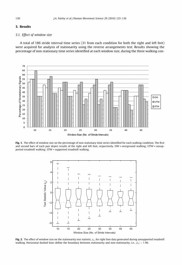
A total of 186 stride interval time series (31 from each condition for both the right and left feet)were acquired for analysis of stationarity using the reverse arrangements test. Results showing thepercentage of non-stationary time series identified at each window size, during the three walking con-

Fig. 1. The effect of window size on the percentage of non-stationary time series identified for each walking condition. The firstand second bars of each pair depict results of the right and left foot, respectively. OW = overground walking; UTW = unsup-ported treadmill walking; STW = supported treadmill walking.

10 15 20 25 30 35 40 45

−6

−4

−2

0

2

4

6

Test

Sta

tistic

Val

ue ( z

α)

Window Size (No. of Stride Intervals)

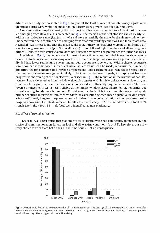
Fig. 2. The effect of window size on the stationarity test statistic, za , for right foot data generated during unsupported treadmillwalking. Horizontal dashed lines define the boundary between stationarity and non-stationarity, i.e., jzaj < 1:96.


ditions under study, are presented in Fig. 1. In general, the least number of non-stationary signals wereidentified during STW while the most non-stationary signals were identified during UTW.

A representative boxplot showing the distribution of test statistic values for all right foot time ser-ies emerging from UTW trials is presented in Fig. 2. The median of the test statistic values clearly fellwithin the stationary range (i.e., jzaj < 1:96) and were essentially the same for the given window sizes.The same result held for time series emerging from treadmill walking conditions and for left foot data.A Kruskal–Wallis test found that the mean ranks of stationary test statistics were not significantly dif-ferent among window sizes ðp > :96Þ in all cases (i.e., for left and right foot data and all walking con-ditions). Thus, the test statistic alone does not suggest a window size preference for further analysis.

As evident in Fig. 1, the percentage of non-stationary time series identified in each walking condi-tion tends to decrease with increasing window size. Since at larger window sizes a given time series isdivided into fewer segments, a shorter mean square sequence is generated. With a shorter sequence,fewer comparisons between subsequent mean square values can be made, reducing the number ofopportunities for detection of a reverse arrangement. This constraint also reduces the variation inthe number of reverse arrangements likely to be identified between signals, as is apparent from theprogressive shortening of the boxplot whiskers seen in Fig. 2. The reduction in the number of non-sta-tionary signals detected at larger window sizes also agrees with intuition, since even a slow varyingtrend would begin to appear stationary when observed at sufficiently large window sizes. Thus, thereverse arrangements test is least reliable at the largest window sizes, where non-stationarities dueto fast varying trends may be masked. Considering the tradeoff between maintaining an adequatenumber of stride intervals within each window for calculation of each mean square value and gener-ating a sufficiently long mean square sequence for identification of non-stationarities, we chose a mid-range window size of 25 stride intervals for all subsequent analysis. At this window size, a total of 74signals (36 – right foot, 38 – left foot) were identified as non-stationary.

3.2. Effect of trimming location

A Kruskal–Wallis test found that stationarity test statistics were not significantly influenced by thechoice of trimming location for either foot and all walking conditions ðp > :74Þ. Therefore, our arbi-trary choice to trim from both ends of the time series is of no consequence.

Mean Only Variance Only Mean + Variance Unknown0

10

20

30

40

50

60

70

80

90

100

Perc

enta

ge o

f Non

stat

iona

ry S

igna

ls

Source

OWUTWSTW

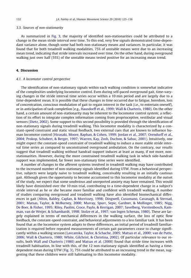
Fig. 3. Sources contributing to non-stationarity of the time series, as a percentage of the non-stationary signals identifiedwithin each particular walking condition. Data presented is for the right foot. OW = overground walking; UTW = unsupportedtreadmill walking; STW = supported treadmill walking.


3.3. Sources of non-stationarity

As summarized in Fig. 3, the majority of identified non-stationarities could be attributed to achange in the mean stride interval over time. To this end, very few signals demonstrated time-depen-dant variance alone, though some had both non-stationary means and variances. In particular, it wasfound that for both treadmill walking modalities, 75% of unstable means were due to an increasingmean trend, indicating that stride intervals increased over time. On the other hand, during overgroundwalking just over half (55%) of the unstable means tested positive for an increasing mean trend.

4. Discussion

4.1. A locomotor control perspective

The identification of non-stationary signals within each walking condition is somewhat indicativeof the complexities underlying locomotor control. Even during self-paced overground gait, time-vary-ing changes in the stride interval time series occur within a 10 min period and are largely due to atime-dependent mean. It is possible that these changes in time occurred due to fatigue, boredom, lossof concentration, conscious modulation of gait to regain interest in the task (i.e., to entertain oneself),or in anticipation of task completion (e.g., Hausdorff et al., 1999; Wall & Charteris, 1980). On the otherhand, a certain amount of non-stationarity may be inherent to the locomotor control system; a reflec-tion of its effort to integrate complex information coming from proprioceptive, vestibular and visualsensors (Dietz, 2002). Some support to this second possibility is provided through the identification ofnon-stationary signals during treadmill walking. This locomotor modality is characterized by a con-stant-speed constraint and static visual feedback, two external cues that are known to influence hu-man locomotor control (Hirasaki, Moore, Raphan, & Cohen, 1999; Jordan et al., 2007; Orendurff et al.,2004; Prokop, Schubert, & Berger, 1997; Warren, Kay, Zosh, Duchon, & Sahuc, 2001). Intuitively, onemight expect the constant-speed constraint of treadmill walking to induce a more stable stride inter-val time series as compared to unconstrained overground ambulation. On the contrary, our resultssuggest that treadmill walking without handrail support induces at least as many, if not more, non-stationarities. However, during the more constrained treadmill walking task in which side-handrailsupport was implemented, far fewer non-stationary time series were identified.

A number of changes to the afferent systems involved in treadmill walking may have contributedto the increased number of non-stationary signals identified during UTW. From a behavioral perspec-tive, subjects were largely naive to treadmill walking, conceivably resulting in an initially cautiousgait. Although given the opportunity to become accustomed to this locomotor modality at the outsetof the study, we expect that some unobvious and unreported anxiety may have remained. This wouldlikely have diminished over the 10 min trial, contributing to a time-dependent change in a subject’sstride interval as he or she became more familiar and confident with treadmill walking. A numberof studies comparing overground and treadmill walking have also identified biomechanical differ-ences in gait (Alton, Baldey, Caplan, & Morrissey, 1998; Dingwell, Cusumano, Cavanagh, & Sternad,2001; Matsas, Taylor, & McBurney, 2000; Murray, Spurr, Sepic, Gardner, & Mollinger, 1985; Nigg,De Boer, & Fisher, 1995; Riley, Paolini, Croce, Paylo, & Kerrigan, 2007; Savelberg, Vorstenbosch, Kam-man, van de Weijer, & Schambardt, 1998; Stolze et al., 1997; van Ingen Schenau, 1980). These are lar-gely explained in terms of mechanical differences in the walking surface, the loss of optic flowfeedback, the constant-speed constraint, and behavioral adjustments to a less familiar task. It has beenfound that as the locomotor system adapts to these differences, an initial period of treadmill familiar-ization is required before repeated measurements of certain gait parameters cease to change signifi-cantly within a walking session (Lavcanska, Taylor, & Schache, 2005; Matsas et al., 2000; van de Putte,2006; Wall & Charteris, 1980; White, Gilchrist, & Christina, 2002). Of particular relevance to our re-sults, both Wall and Charteris (1980) and Matsas et al. (2000) found that stride time increases withtreadmill habituation. In line with this, of the 12 non-stationary signals identified as having a time-dependent mean during UTW (Fig. 3), 75% could be attributed to an increasing trend in the mean, sug-gesting that these children were still habituating to this locomotor modality.


The reduction in the number of non-stationary signals identified during STW likely occurred due tothe additional proprioceptive information available for regulation of locomotor control. In line withthis result, Dickstein and Laufer (2004) found that additional somatosensory input provided by lightfingertip touch during treadmill walking facilitates spatial orientation and reduces body sway. From apurely anthropometric perspective, by grasping the handrails, the reasonable range for each child’sfoot placement (and hence stride length) is effectively reduced, restricted by the extent of his orher arm reach. This limitation on stride length imposes an additional constraint on the user’s strideinterval on top of the constant-speed constraint of the treadmill. Seemingly, the handrails act to some-what anchor somatosensory feedback, perhaps contributing to fewer non-stationary signals duringsupported treadmill walking.

We also consider the influence of gait maturity on our results. Since the various afferent systemscontributing to regulation of locomotor control may not have reached full maturity in children, thecapacity of these systems to efficiently generate stable movement patterns may be reduced (Stolzeet al., 1997). This idea may also have contributed to the identification of more non-stationary signalsduring UTW than during OW in our paediatric study. Conversely, during STW, the additional locomo-tor constraints discussed above may have sufficiently augmented locomotor regulation so as to over-come the suggested age-sensitivity to treadmill walking. To this end, it would be interesting to assesswhether or not the same trend, suggesting an increased number of non-stationary signals during UTW,would also appear in an investigation of stride interval stationarity in an adult population.

4.2. Relevance to analysis of stride interval dynamics

This investigation reveals that the stride interval time series emerging from paediatric gait undervarying degrees of locomotor constraint is often, though not always, non-stationary. While the strideinterval time series of 11 children (age range 5–9 years old; 5 males) were found to be weakly station-ary for all walking trials, other children produced non-stationary signals under at least one walkingcondition and two children (ages 5 and 8 years; both male) produced non-stationary series for allthree walks. Finally, considering the possibility of maturation effects within our sample population,we also note that non-stationary signals were identified in at least one walking condition acrossthe entire age spectrum under analysis. Thus, we have confirmed, at least for a paediatric population,the often assumed notion that stride interval time series exhibit non-stationary behavior in manycases. Given this finding, when estimating the fractal behavior of gait, we emphasize the importanceof implementing scaling analysis techniques that are robust to non-stationarities.

DFA is one method that was developed to account for the non-stationary behavior of series gener-ated from certain DNA sequences (Peng et al., 1994). This method, often applied to stride interval timeseries and other physiological processes, has since been tested with simulated fGn and fBm data,alongside numerous alternative techniques, with findings depending largely on the nature and lengthof the series under analysis (Delignières et al., 2006; Eke et al., 2000). While other methods seem toproduce more accurate estimates when dealing strictly with fGn or fBm processes, DFA or a modifiedpower spectral density approach typically provide more robust estimates for series near the 1=fboundary (Delignières et al., 2006). Considering that the scaling behavior of human stride intervaltime series is generally considered to fall within this range (Hausdorff et al., 1995), and given the iden-tification of both stationary and non-stationary signals in this investigation, DFA and modified powerspectral density would seem to hold the most promise for estimation of statistical persistence withinstride interval data.

Nonetheless, both methods still present considerable challenges to gait researchers. While Delig-nières et al. (2006) fittingly suggest that the low variability associated with the modified power spec-tral density method render it most appropriate for comparisons between mean scaling exponents, thisvariability is significantly increased for series containing less than 512 data points. Within the scien-tific and rehabilitation communities where stride interval quantification is of interest, it is not uncom-mon for the population under study to have gait difficulty, rendering acquisition of a sufficiently longtime series frequently impossible. When considering DFA analysis, seemingly most appropriate whenthe goal is not to compare but rather to quantify the persistence of a series sample (due to its lowbias), there are other issues to consider. For example, depending on the signal’s underlying correlation


properties, certain non-stationarities are still known to influence the scaling estimate (Chen, Ivanov,Hu, & Stanley, 2002; Hu, Ivanov, Chen, Carpena, & Stanley, 2001). In addition, use of DFA requires thatthe investigator choose a box size fitting range to be used in the analysis; a choice that can have a sig-nificant influence on the scaling estimate. These issues are often handled differently by researchers,complicating the interpretation of results and the ability to draw comparative conclusions across stud-ies (Hausdorff, 2007) and highlighting the need for a widely-acceptable and standardized approach foruse in the gait literature.

It has been suggested that an integrated approach be adopted for scaling analysis, in which multi-ple methods be consistently implemented (Rangarajan & Ding, 2000). This approach would not onlyfacilitate comparison between studies, but may also improve within study estimates. Where the re-sults of one method may otherwise lead to false conclusions, inconsistencies revealed by another tech-nique would enable one to more accurately determine the true scaling behavior of a given time series(Rangarajan & Ding, 2000). Of course, such an approach is only of use if the scaling methods are appro-priately chosen based on the underlying signal properties, and only then if the associated user-se-lected parameters are consistently implemented. For example, when evaluating the statisticalpersistence of stride interval fluctuations, the pair of estimators most commonly compared are thosederived from DFA and spectral analysis (Hausdorff et al., 1995; Hausdorff et al., 1996). Given that spec-tral analysis is sensitive to non-stationarities, we question the utility of making such a comparison andsuggest instead the use of alternative techniques that, like DFA, are less affected by non-stationarybehavior.

5. Conclusion

In order to better understand the human locomotor control system, it is important to carefullycharacterize gait dynamics. In particular, to determine the appropriateness of various scaling analysistechniques for quantification of the correlation properties of stride interval time series, it is importantto know the extent to which the signal of interest is stationary. This study assesses for the first timethe extent to which stride interval time series, obtained from a paediatric population, are weakly sta-tionary. We reveal non-stationary signals in all walking conditions, including the most constrainedlocomotor modality in which children walked on a treadmill with handrail support. We have thus con-firmed that, as is true for many physiological signals, paediatric stride interval time series are oftennon-stationary. Therefore, when seeking to quantify the statistical persistence of stride interval fluc-tuations, scaling analysis techniques that are less affected by non-stationarities should be imple-mented. To this end, much has been done as of late to facilitate the selection and implementationof these techniques when dealing with physiological data. However, this body of work has largely fo-cused on simulated data and other physiological processes, with little empirical investigation of strideinterval time series specifically. Evidently, if scaling analysis of stride interval time series is to gaintrue clinical value, a methodological effort to standardize approaches is needed.

Acknowledgements

The authors would like to acknowledge the support provided by the Natural Sciences and Engineer-ing Research Council of Canada, the Hilda and William Courtney Clayton Paediatric Research Fund, theBloorview Children’s Hospital Foundation and the Canada Research Chairs Program.

References

Alton, F., Baldey, L., Caplan, S., & Morrissey, M. (1998). A kinematic comparison of overground and treadmill walking. ClinicalBiomechanics, 13, 434–440.

Alves, N., & Chau, T. (2008). Stationarity distributions of mechanomyogram signals from isometric contractions of extrinsic handmuscles during functional grasping. Journal of Electromyography and Kinesiology, 18, 509–515.

Bendat, J., & Piersol, A. (2000). Random data: Analysis and measurement procedures (3rd ed.). New York, NY: Wiley.Bilodeau, M., Cincera, M., Arsenault, A., & Gravel, D. (1997). Normality and stationarity of EMG signals of elbow flexor muscles

during ramp and step isometric contractions. Journal of Electromyography and Kinesiology, 7, 87–96.Chau, T., Chau, D., Casas, M., Berall, G., & Kenny, D. J. (2005). Investigating the stationarity of paediatric aspiration signals. IEEE

Transactions on Neural Systems and Rehabilitation Engineering, 13, 99–105.


Chau, T., & Rizvi, S. (2002). Automatic stride interval extraction from long, highly variable and noisy gait timing signals. HumanMovement Science, 21, 495–514.

Chen, Z., Ivanov, P., Hu, K., & Stanley, H. (2002). Effect of nonstationarities on detrended fluctuation analysis. Physical Review E,65, 41107-1–41107-15.

Delignières, D., Ramdani, S., Lemoine, L., Torre, K., Fortes, M., & Ninot, G. (2006). Fractal analyses for short time series: A re-assessment of classical methods. Journal of Mathematical Psychology, 50, 525–544.

Delignières, D., & Torre, K. (2009). Fractal dynamics of human gait: A reassessment of the 1996 data of Hausdorff et al.. Journal ofApplied Physiology, 106, 1272–1279.

Dickstein, R., & Laufer, Y. (2004). Light touch and center of mass stability during treadmill locomotion. Gait and Posture, 20,41–47.

Dietz, V. (2002). Proprioception and locomotor disorders. Nature Reviews Neuroscience, 3, 781–790.Dingwell, J., & Cusumano, J. (2000). Nonlinear time series analysis of normal and pathological human walking. Chaos: An

Interdisciplinary Journal of Nonlinear Science, 10, 848–863.Dingwell, J. B., Cusumano, J. P., Cavanagh, P. R., & Sternad, D. (2001). Local dynamic stability versus kinematic variability of

continuous overground and treadmill walking. Journal of Biomechanical Engineering, 123, 27–32.Eke, A., Herman, P., Bassingthwaighte, J., Raymond, G., Percival, D., Cannon, M., et al (2000). Physiological time series:

Distinguishing fractal noises from motions. Pflügers Archive European Journal of Physiology, 439, 403–415.Eke, A., Herman, P., Kocsis, L., & Kozak, L. (2002). Fractal characterization of complexity in temporal physiological signals.

Physiological Measurement, 23, R1–R38.Hampson, K., Munro, I., Paterson, C., & Dainty, C. (2005). Weak correlation between the aberration dynamics of the human eye

and the cardiopulmonary system. Journal of the Optical Society of America A, 22, 1241–1250.Harris, G. F., Riedel, S. A., Matesi, D., & Smith, P. (1993). Standing postural stability assessment and signal stationarity in children

with cerebral palsy. IEEE Transactions on Rehabilitation Engineering, 1, 35–42.Hausdorff, J. (2007). Gait dynamics, fractals and falls: Finding meaning in the stride-to-stride fluctuations of human walking.

Human Movement Science, 26, 555–589.Hausdorff, J. M., Lertratanakul, A., Cudkowicz, M. E., Peterson, A. L., Kaliton, D., & Goldberger, A. L. (2000). Dynamic markers of

altered gait rhythm in amyotrophic lateral sclerosis. Journal of Applied Physiology, 88, 2045–2053.Hausdorff, J. M., Mitchell, S. L., Firtion, R., Peng, C. K., Cudkowicz, M. E., Wei, J. Y., et al (1997). Altered fractal dynamics of gait:

Reduced stride-interval correlations with aging and Huntington’s disease. Journal of Applied Physiology, 82, 262–269.Hausdorff, J. M., Peng, C. K., Ladin, Z., Wei, J. Y., & Goldberger, A. L. (1995). Is walking a random walk? Evidence for long-range

correlations in stride interval of human gait. Journal of Applied Physiology, 78, 349–358.Hausdorff, J. M., Purdon, P. L., Peng, C. K., Ladin, Z., Wei, J. Y., & Goldberger, A. L. (1996). Fractal dynamics of human gait: Stability

of long-range correlations in stride interval fluctuations. Journal of Applied Physiology, 80, 1448–1457.Hausdorff, J. M., Zemany, L., Peng, C. K., & Goldberger, A. L. (1999). Maturation of gait dynamics: Stride-to-stride variability and

its temporal organization in children. Journal of Applied Physiology, 86, 1040–1047.Herman, T., Giladi, N., Gurevich, T., & Hausdorff, J. M. (2005). Gait instability and fractal dynamics of older adults with a

‘‘cautious” gait: Why do certain older adults walk fearfully? Gait and Posture, 21, 178–185.Hirasaki, E., Moore, S., Raphan, T., & Cohen, B. (1999). Effects of walking velocity on vertical head and body movements during

locomotion. Experimental Brain Research, 127, 117–130.Hu, K., Ivanov, P., Chen, Z., Carpena, P., & Stanley, H. (2001). Effect of trends on detrended fluctuation analysis. Physical Review E,

64, 011114-1–011114-19.Jordan, K., Challis, J., & Newell, K. (2007). Walking speed influences on gait cycle variability. Gait and Posture, 26, 128–134.Lavcanska, V., Taylor, N., & Schache, A. (2005). Familiarization to treadmill running in young unimpaired adults. Human

Movement Science, 24, 544–557.Matsas, A., Taylor, N., & McBurney, H. (2000). Knee joint kinematics from familiarised treadmill walking can be generalised to

overground walking in young unimpaired subjects. Gait and Posture, 11, 46–53.Murray, M. P., Spurr, G. B., Sepic, S. B., Gardner, G. M., & Mollinger, L. A. (1985). Treadmill vs. floor walking: Kinematics,

electromyogram, and heart rate. Journal of Applied Physiology, 59, 87–91.Nhan, B. R., & Chau, T. (2009). Infrared thermal imaging as a physiological access pathway: A study of the baseline

characteristics of facial skin temperatures. Physiological Measurement, 30, N23–N35.Nigg, B., De Boer, R., & Fisher, V. (1995). A kinematic comparison of overground and treadmill running. Medicine and Science in

Sports and Exercise, 27, 98–105.Novak, V., Honos, G., & Schondorf, R. (1996). Is the heart ‘empty’ at syncope? Journal of the Autonomic Nervous System, 60, 83–92.Orendurff, M., Segal, A., Klute, G., Berge, J., Rohr, E., & Kadel, N. (2004). The effect of walking speed on center of mass

displacement. Journal of Rehabilitation Research and Development, 41, 829–834.Papoulis, A. (1991). Probability, random variables, and stochastic processes (3rd ed.). New York, NY: McGraw-Hill.Peng, C., Buldyrev, S. V., Havlin, S., Simons, M., Stanley, H. E., & Goldberger, A. L. (1994). Mosaic organization of DNA nucleotides.

Physical Review E, 49, 1685–1689.Peng, C. K., Hausdorff, J. M., & Goldberger, A. L. (2000). Fractal mechanisms in neural control: Human heartbeat and gait

dynamics in health and disease. In J. Walleczek (Ed.), Self-organized biological dynamics and nonlinear control: Towardunderstanding complexity. Chaos, and emergent function in living systems (pp. 66–96). New York, NY: Cambridge UniversityPress.

Prokop, T., Schubert, M., & Berger, W. (1997). Visual influence on human locomotion modulation to changes in optic flow.Experimental Brain Research, 114, 63–70.

Rangarajan, G., & Ding, M. Z. (2000). Integrated approach to the assessment of long range correlation in time series data. PhysicalReview E, 61, 4991–5001.

Riley, P., Paolini, G., Croce, U., Paylo, K., & Kerrigan, D. (2007). A kinematic and kinetic comparison of overground and treadmillwalking in healthy subjects. Gait and Posture, 26, 17–24.

Savelberg, H., Vorstenbosch, M., Kamman, E., van de Weijer, J., & Schambardt, H. (1998). Intra-stride belt-speed variation affectstreadmill locomotion. Gait and Posture, 7, 26–34.


Stanley, H. E., Amaral, L. A. N., Goldberger, A. L., Havlin, S., Ivanov, P., & Peng, C. K. (1999). Statistical physics and physiology:Monofractal and multifractal approaches. Physica A, 270, 309–324.

Stolze, H., Kuhtz-Buschbeck, J. P., Mondwurf, C., Boczek-Funcke, A., Johnk, K., Deuschl, G., et al (1997). Gait analysis duringtreadmill and overground locomotion in children and adults. Electromyography and Motor Control – Electroencephalographyand Clinical Neurophysiology, 105, 490–497.

van de Putte, M. (2006). Habituation to treadmill walking. Bio-Medical Materials and Engineering, 16, 43–52.van Ingen Schenau, G. (1980). Some fundamental aspects of the biomechanics of overground versus treadmill locomotion.

Medicine and Science in Sports and Exercise, 12, 257–261.Wall, J. C., & Charteris, J. (1980). The process of habituation to treadmill walking at different velocities. Ergonomics, 23, 425–435.Warren, W., Kay, B., Zosh, W., Duchon, A., & Sahuc, S. (2001). Optic flow is used to control human walking. Nature Neuroscience,

4, 213–216.White, S., Gilchrist, L., & Christina, K. (2002). Within-day accommodation effects on vertical reaction forces for treadmill

running. Journal of Applied Biomechanics, 18, 74–82.

an investigation of stride interval stationarity in a paediatric population

Documents