local stationarity for spatial data
TRANSCRIPT
Local stationarity for spatial data
Vom Fachbereich Mathematikder Technischen Universität Kaiserslauternzur Verleihung des akademischen Grades
Doktor der Naturwissenschaften(Doctor rerum naturalium, Dr. rer. nat.)
genehmigte Dissertation
von
Danilo Pezo Villar
1. Gutachter: Prof. Dr. Jürgen Franke, TU Kaiserslautern2. Gutachter: Prof. Dr. Rainer Dahlhaus, Universität Heidelberg
Datum der Disputation: 20. Dezember 2017
D386


To my wife Dafne and my son Felipe
iii


Abstract
Following the ideas presented in Dahlhaus (2000) and Dahlhaus and Sahm (2000) fortime series, we build a Whittle-type approximation of the Gaussian likelihood for lo-cally stationary random fields. To achieve this goal, we extend a Szegö-type formula,for the multidimensional and local stationary case and secondly we derived a set ofmatrix approximations using elements of the spectral theory of stochastic processes.The minimization of the Whittle likelihood leads to the so-called Whittle estima-tor θT . For the sake of simplicity we assume known mean (without loss of generalityzero mean), and hence θT estimates the parameter vector of the covariance matrix Σθ.
We investigate the asymptotic properties of the Whittle estimate, in particular uni-form convergence of the likelihoods, and consistency and Gaussianity of the estimator.A main point is a detailed analysis of the asymptotic bias which is considerably moredifficult for random fields than for time series. Furthemore, we prove in case of modelmisspecification that the minimum of our Whittle likelihood still converges, where thelimit is the minimum of the Kullback-Leibler information divergence.
Finally, we evaluate the performance of the Whittle estimator through computationalsimulations and estimation of conditional autoregressive models, and a real data ap-plication.
v


Zusammenfassung
Aufbauend auf den Ansätzen von Dahlhaus (2000) und Dahlhaus and Sahm (2000)für Zeitreihen konstruieren wir eine Approximation vom Whittle-Typ für die Gauß-sche Likelihoodfunktion lokal-stationärer Zufallsfelder. Als wesentliche Bausteine ver-allgemeinern wir einerseits die Szegö-Formel auf den mehrdimensionalen und lokal-stationären Fall und leiten andererseits eine Reihe von Matrixapproximationen unterVerwendung der Spektraltheorie stochastischer Prozesse her. Die Minimierung derWhittle-Likelihood führt dann zum so-genannten Whittle-Schätzer θT . Der Einfach-heit halber nehmen wir an, dass der Mittelwert bekannt (ohne Beschränkung der All-gemeinheit = 0) ist, so dass θT den Parametervektor der Kovarianzmatrix Σθ schätzt.
Wir untersuchen die asymptotischen Eigenschaften des Whittle-Schätzers, insbeson-dere die uniforme Konvergenz der Likelihoodfunktionen sowie die Konsistenz undasymptotische Normalität des Schätzers. Ein Hauptaspekt ist eine detaillierte Unter-suchung des asymptotischen Bias, die für Zufallsfelder deutlich problematischer alsfür Zeitreihen ausfällt. Weiterhin zeigen wir, dass bei Vorliegen eines missspezifizier-ten Modells das Minimum der Whittle-Likelihood immer noch konvergiert, und zwargegen das Minimum der Kullback-Leibler Informationsdivergenz.
Schließlich untersuchen wir die praktische Qualität des Whittle-Schätzers durch dieAnwendung auf simulierte Daten und einen realen Datensatz.
vii


Acknowledgements
I would like to express my gratitude to Prof. Dr. Jürgen Franke for his invaluablehelp and encouragement regarding my research along these three years. My gratitudealso goes to Prof. Dr. Rainer Dahlhaus for providing with the draft of a paper on thetopic, which was unfinished due to gaps in the proofs.I would like to thank to Prof. Dr. Claudia Redenbach for her support regarding mywork, specially for allowing me to participate in the Ph.D. seminar in spite of thedifferent research areas.My gratitude to the Deutscher Akademischer Austauschdienst (DAAD) for awardingme with the funds that made this project possible, to Ms. Birgitt Skailes for heralways prompt answer to every request, and to Dr. Falk Triebsch for supporting usas Ph.D. students as much as his position allows him.I will never forget my friends and colleagues from the mathematics department andFraunhofer Institut ITWM who always made me feel at home. Dr. Euna Nyarige, Dr.Rumana Rois, Pak Lo, Yolanda Rodríguez, Martina Sormani, Dr. Prakash Easwaran,Ms. Beate Seagler, Jessica Borsche among others, thanks to you the Uni was like asecond home where I could profit from your knowledge and friendship.I am deeply grateful to Dr. Katja Schladitz, who selflessly offered me help with thelanguage. Thanks because every time we met, I received your advices and commentswhich enriched my perspectives, thanks for helping me “open my horizons” as youonce mentioned it.I know that this dream made my family in Chile to miss me and pray that everythinggoes fine. I just thank you mom for all your prayers, for God was always and still isby me side.I am absolutely sure, that even receiving all the support and advice from the peopleabove, I would not have succeeded without the love and company of my dear wife andson. From the bottom of my heart I thank you, Dafne and Felipe, you are my mostprecious God’s gift.
ix

Contents
Abstract v
Acknowledgements ix
Lists xiii
Introduction xv
1 Locally Stationary Random Fields 11.1 Basic Definitions . . . . . . . . . . . . . . . . . . . . . . . . . . . . . . 11.2 Locally Stationary Random Fields . . . . . . . . . . . . . . . . . . . . 2
2 Whittle Estimator 72.1 Whittle Estimator for Stationary Random Fields . . . . . . . . . . . . 72.2 Whittle Estimator for Locally Stationary Random Fields . . . . . . . . 102.3 Appendix: Technical Results . . . . . . . . . . . . . . . . . . . . . . . 28
3 Asymptotic Properties 413.1 Consistency . . . . . . . . . . . . . . . . . . . . . . . . . . . . . . . . . 423.2 Gaussianity . . . . . . . . . . . . . . . . . . . . . . . . . . . . . . . . . 50
4 Simulations and a Real Data Application 574.1 Simulations . . . . . . . . . . . . . . . . . . . . . . . . . . . . . . . . . 574.2 Real Data Application . . . . . . . . . . . . . . . . . . . . . . . . . . . 674.3 Discussion . . . . . . . . . . . . . . . . . . . . . . . . . . . . . . . . . . 71
Conclusion 73
References 75
Lebenslauf 77
Erklärung 79
xi

Lists
Figures4.1 Function α(s, t) . . . . . . . . . . . . . . . . . . . . . . . . . . . . . . . 644.2 Non-tapered data, α quadratic, β constant . . . . . . . . . . . . . . . . 654.3 Non-tapered data, α cubic, β linear . . . . . . . . . . . . . . . . . . . . 654.4 Tapered data, α quadratic, β constant . . . . . . . . . . . . . . . . . . 654.5 Tapered data, α cubic, β linear . . . . . . . . . . . . . . . . . . . . . . 664.6 Mercer and Hall (1911) (own elaboration) . . . . . . . . . . . . . . . . 674.7 Spatial Correlation Wheat-Yield data (own elaboration). Regarding
what the “naive” term means, see Dahlhaus and Künsch (1987) andthe distinctions made therein. . . . . . . . . . . . . . . . . . . . . . . . 68
4.8 Level plots of estimated functions α and β using the non-tapered wheatyield data . . . . . . . . . . . . . . . . . . . . . . . . . . . . . . . . . . 69
Tables4.1 Parameter estimation for model (4.1) under stationarity assumption
using simulated data . . . . . . . . . . . . . . . . . . . . . . . . . . . . 584.2 Parameter estimation for model (4.1) with |α|+ |β| ≈ 1 using simulated
data . . . . . . . . . . . . . . . . . . . . . . . . . . . . . . . . . . . . . 594.3 Parameter estimation for model (4.1) with α and β given by (4.5) and
(4.6), respectively, and εs,t ∼ N (0, 1). . . . . . . . . . . . . . . . . . . 634.4 Parameter estimation for model (4.1) with α and β given by (4.5) and
(4.6), respectively, and εs,t ∼ Unif(−√
3,√
3). . . . . . . . . . . . . . . 634.5 Parameter estimation for function β . . . . . . . . . . . . . . . . . . . 664.6 Parameter estimation of model (4.7) under stationarity assumption
using wheat-yield data set . . . . . . . . . . . . . . . . . . . . . . . . . 68
xiii

Introduction
Stationarity is an ubiquitous concepts in stochastics. By its very definition (unchangedprobabilistic structure, roughly speaking), it draws a framework where asymptoticresults are possible and meaningful. Nevertheless, in real-world applications such as-sumption often does not fit well. In many situations the probabilistic properties ofdata change along time or space in unknown way making the modelling process ratherdifficult. In other words, increasing data does not necessarily give additional informa-tion about the overall properties as it typically does in the stationary world and thereason is simple: the probabilistic structure changes along the index set.
Unfortunately there is no unique natural way how to extend the definition of stationa-rity in a general and still useful form. In this research we, therefore, have used a spe-cial, but wide enough class of processes introduced in Dahlhaus (1997) and Dahlhausand Sahm (2000) for time series and random fields respectively, which comprises anatural nonstationary extension of many classical (linear) stationary processes usedin practice, like autoregressive, moving average, conditional autoregressive and so on,by allowing them to behave only locally as stationary.
The class of locally stationary random field processes contains many of the typicalprocesses for stationary random fields such as CAR or SAR, turning into a very na-tural nonstationary extension of some stationary process. Thus, a crucial problem inthis regard corresponds to the parametric estimation of a locally stationary model. Inthe stationary setting the Whittle estimator (Whittle (1954), originally for data onthe plane but easily extended to any dimension, see Dahlhaus and Künsch (1987)) hasturned into a simple and fast method of estimation which takes place in the spectraldomain, i.e. using the parametric spectral density of the model and the periodogram,which makes calculations faster by means of the FFT algorithm.
Following the ideas presented in Dahlhaus (2000) for time series, we build a Whittle-type approximation (Whittle likelihood) of the Gaussian likelihood for locally statio-nary random fields. The minimization of the Whittle likelihood leads to the so-calledWhittle estimator θT . For the sake of simplicity we assume known mean (withoutloss of generality zero mean), and hence θT estimates the parameter vector of the co-variance matrix Σθ. We investigate some of its asymptotic properties, namely consis-tency and Gaussianity. Finally, we evaluate the performance of the estimator throughcomputational simulations and a real data application.
The structure of this work is as follows:
xv

Introduction
In Chapter 1 we make the notion of locally stationary random field and its relationwith linear process precise. Notation and a few conventions to be used areintroduced.
In Chapter 2 we construct the Whittle likelihood LT (θ), and thus our Whittle estima-tor. This is done mainly through an approximation of the Gaussian likelihoodusing and extension of the Szegö’s theorem. The score function of LT (θ) isproved to be biased, we identify the source of this problem and discuss ways toreduce it.
In Chapter 3 we prove consistency and a modified Gaussian law for both, the taperedWhittle estimator and the exact Gaussian estimator. This is achieved by provingasymptotic properties of the likelihoods involved.
In Chapter 4 we present a simulation study considering a 2 dimensional autoregressiveprocess of order one. We estimate the parameter vector using tapered andnon tapered Whittle likelihoods, together with different set of parameters andassumptions. We model the classical wheat-yield data set of Mercer and Hall(1911) using a local stationary SAR model.
Finally, we present conclusions and possible directions of future research.
xvi


1 Locally Stationary Random Fields
In this chapter we introduce the definition of a locally stationary random field anddiscuss some implication of it. We begin this exposition giving some basic definitionscoming from the stationary setting to motivate and link the locally stationary case.Some assumptions and notation are introduced as well.
1.1 Basic DefinitionsDefinition 1.1.1 (Random field). Let (Ω,F , P ) be a probability space. Given d, δ ∈ N,we say that a function X:
X : Ω× Zd → Rδ
is a Random Field if and only if ∀t ∈ Zd, the function:
Xt : Ω→ Rδ
ω → X(ω, t)
is F − B(Rδ)-measurable; where B denotes the Borel σ-algebra.
We will assume henceforth only univariate random fields, i.e. δ = 1. A random fieldXt, t ∈ Zd is described by its finite dimensional distributions
FXt1 ,...,Xtk (x1, . . . , xk) = P(Xt1 ≤ x1, . . . , Xtk ≤ xk)
where the next two consistency conditions must be fulfilled, i.e.
Symmetry: FXt1 ,...,Xtk (x1, . . . , xk) = FXπ1,...,Xπk(xπ1, . . . , xπk), where π is a permuta-tion.
Compatibility: FXt1 ,...,Xtk (x1, . . . , xk−1) = FXt1 ,...,Xtk−1 ,Xtk(x1, . . . , xk−1,∞).
Definition 1.1.2 (Gaussian random field). A random field Xt, t ∈ Zd is calledGaussian if FXt1 ,...,Xtk are multivariate Gaussian distributions for any choice of kand (t1, . . . , tk) ∈ Zd.
Since a multivariate Gaussian distribution is completely specified by its mean µ andcovariance matrix Σ, if we restrict the class of random fields to those with constantmean and positive definite Σ, then we speak of a stationary random field.
Definition 1.1.3 (Stationarity). A random field is called (weakly) stationary if EXt =µ and Σr,s = Cov (Xr, Xs) = Cov (Xr−s, X0) for all t, r, s ∈ Zd.
1
1 Locally Stationary Random Fields
The Cramér spectral representation theorem guarantees that assuming µ = 0 and thesummability of the entries Σr,s, the stationary process Xt can be represented as
Xt =∫
Πd
A(λ) exp(i〈λ, t〉) dξ(λ), (1.1)
where ξ(λ) is an orthogonal process, A(λ) is the transfer function of the process,〈λ, t〉 =
∑di=1 λiti and Πd = (−π, π]d. In other words, the process Xt can be repre-
sented as a continuous superposition of sinusoids with random amplitudes (for furtherdetails see Brillinger (1981)). In the next section we define the locally stationary caseby an extension of (1.1).
1.2 Locally Stationary Random FieldsThe concept of stationarity describes essentially the situation where the statisticalproperties of a stochastic process do not change as it moves in the index set (usuallytime or space). This implies that more observations improve the knowledge about thestructure of the overall process. Unfortunately, in the general nonstationary framethis is clearly not the case. In time series, for instance, looking into the future givesnot necessarily information about the current state of the process.
To overcome this problem, Dahlhaus (1997) has proposed an asymptotic approachsimilar to nonparametric regression. To exemplify it let us assume a time-varyingAR(1)
Xt = g(t; θ)Xt−1 + εt, εt ∼iid N (0, σ2),
with |g(t; θ)| < 1 for t = 1, . . . , T and parameter vector θ. Depending on the func-tional form of g(t; θ), this might not behave as stationary for times bigger than T ,giving no useful information about its parameters. Therefore, instead of looking intothe future when T → ∞, we rescale the function g, i.e. g(t/T ), obtaining more andmore realizations of the local process as T increases. This does not mean to havea higher sampled continuous process, but only an abstract setting where statisticalinference over the parameter vector θ is possible. This idea will allow us to find Quasi-ML estimators and their asymptotic properties in the next chapters. Notice that inthis setting we do not have a sequence X1, . . . , XT any more, but a triangular arrayX1,T , . . . , XT,T indexed by T .
To keep notation simple, we will only consider processes on the cubeDT = 1, . . . , Td,however the results are still valid for other cuboids, provided that the side lengthincreases proportionally as we consider more and more data points (see Guyon (1995)).The next definition corresponds to the definition of locally stationary random fieldintroduced in Dahlhaus and Sahm (2000).
Definition 1.2.1 (Locally Stationary Random Field). A sequence of stochastic pro-cesses (Xt,T )t∈DT is called locally stationary with transfer function A0 and mean
2
1.2 Locally Stationary Random Fields
function µ, if there is a representation
Xt,T = µ( t−1/2
T
)+∫
Πd
A0t,T (λ) exp(i〈λ, t〉) dξ(λ), (1.2)
such that
(i) ξ(λ) is a stochastic process on Πd with orthogonal increments and ξ(λ) = ξ(−λ)for all λ ∈ Πd and
Cum (dξ(λ1), . . . ,dξ(λk)) = η( k∑j=1
λj)hk(λ1, . . . , λk−1) dλ1 · · · dλk,
where Cum (. . .) denotes the cumulant of kth order, h1 = 0, h2(λ) = 1,|hk(λ1, . . . , λk−1)| ≤ constk for all k and η(λ) =
∑+∞j=−∞ δ(λ + 2πj) represents
the Dirac comb.
(ii) There is a constant K and a function A : [0, 1]d × Πd → C with A(u, λ) =A(u,−λ) such that
supt,λ
∣∣A0t,T (λ)−A
( t−1/2T , λ
)∣∣ ≤ K
T. (1.3)
Under some regularity conditions on A(u, λ) as a function of the spatial component udefined as u = t−1/2
T , it can be proved that the space varying spectrum fT (u, λ) (seeMartin and Flandrin (1985) in the time series case) converges in L2(Πd) to f(u, λ).Consequently, f(u, λ) = |A(u, λ)|2 is called the varying spectral density of the field.
We shall shift the points t ∈ DT by 1/2 in order to avoid an additional edge effect.Henceforth, we assume that Xt,T is Gaussian, i.e. hk(λ) = 0 for all k ≥ 3, and forthe sake of simplicity µ will be known (without loss of generality µ ≡ 0), neverthelessall the results are easily extendable for the unknown mean case. The condition (1.3)is needed because of two reasons: First, in order to have a tractable mathematicalframework we need some degree of smoothness in the spatial component u, whichis guaranteed by the regularity of the function A(u, λ). Second, an assumption ofequality (A0
t,T (λ) = A( t−1/2
T , λ)) would be too restrictive since important families of
models, like CAR or AR, would remain excluded. We will return to this point later.Let us discuss the close connection between the representations (1.2)-(1.3) of Xt,T anda MA(∞) representation.
Let us define the Fourier coefficients of A0t,T (λ) and A(u, λ) as
at,T,k :=∫
Πd
A0t,T (λ) exp(i〈λ, k〉) dλ, (1.4)
ak(u) :=∫
Πd
A(u, λ) exp(i〈λ, k〉) dλ, (1.5)
3
1 Locally Stationary Random Fields
respectively, and
εt :=∫
Πd
exp(i〈λ, t〉) dξ(λ).
The orthogonality of the process ξ(λ) implies E εt = 0 and E εt1εt2 = (2π)dδ(t1 − t2).Inverting expressions (1.4) and (1.5) we obtain
A0t,T (λ) = 1
(2π)d∑k∈Zd
at,T,k exp(−i〈λ, k〉),
A(u, λ) = 1(2π)d
∑k∈Zd
ak(u) exp(−i〈λ, k〉),
then
Xt,T =∫
Πd
A0t,T (λ) exp(i〈λ, t〉) dξ(λ)
= 1(2π)d
∑k∈Zd
at,T,k
∫Πd
exp(i〈λ, t− k〉) dξ(λ)
= 1(2π)d
∑k∈Zd
at,T,kεt−k, (1.6)
i.e. Xt,T can be expressed as a linear process. This connection has also been reportedin the case of time series (see Dahlhaus (2000)). Inequality (1.3) implies
supt|at,T,k − ak( t−1/2
T )| ≤ (2π)d supt,λ|A0
t,T (λ)−A( t−1/2T , λ)| = O(T−1).
Conversely, if we assume that the representation (1.6) holds, then we can easily obtainthe representation (1.2). On the other hand, if
supt
∑k∈Zd|at,T,k − a( t−1/2
T )| = O(T−1)
holds, then
supt,k|A0
t,T (λ)−A( t−1/2T , λ)| ≤ sup
t
1(2π)d
∑k∈Zd|at,T,k − ak( t−1/2
T )| = O(T−1),
and hence, the condition (1.3) is fulfilled too. Taking into account this connectionbetween (1.2) and MA(∞) processes, it is easier to understand the necessity of thebound (1.3). We may consider, for instance, a 2D space-varying AR(1), i.e.
Xr,s;T = α( r−1/2T , s−1/2
T )Xr−1,s;T + β( r−1/2T , s−1/2
T )Xr,s−1;T + σεr,s.
4
1.2 Locally Stationary Random Fields
After some manipulations we verify from the MA(∞) representation that
A0t,T (λ) 6= A(u, λ)
= σ
2π(1− α(u1, u2) exp(−iλ1)− β(u1, u2) exp(−iλ2)) , (1.7)
butA0t,T (λ) = A(u, λ) + 1
TB(u, λ) +O(T−2),
with u = (u1, u2) = ( r−1/2T , s−1/2
T ), λ = (λ1, λ2) and where B(u, λ) is usually not zero(see Dahlhaus and Sahm (2000) for a closed-form expression). Making the bound(1.3) stricter, we would need to find the higher order terms in the Taylor expansionin order to fulfil the desired precision, which can be very hard for some families ofmodels. Nevertheless, the simulations conducted in the Chapter 4 showed a goodenough performance, considering a transfer function of order one, i.e. satisfying (1.3).
Regarding the covariance, straightforward calculations using equation (1.2) yield
ΣT (A0)r,s =∫
Πd
A0r,T (λ)A0
s,T (λ) exp(i〈λ, r − s〉) dλ.
The bound (1.3) implies that A0t,T (λ) = A( t−1/2
T , λ) +O(T−1). Thus replacing in thelast equation we obtain
ΣT (A0)r,s = Cov (Xr,T , Xs,T )
=∫
Πd
A( r−1/2
T , λ)A( s−1/2
T , λ)
exp(i〈λ, r − s〉) dλ+O(T−1) (1.8)
= ΣT (A)r,s +O(T−1).
The mean value theorem guarantees for some ξ1 and ξ2 that
A( r−1/2T , λ) = A( r+s−1
2T , λ) + 12T (r − s)′∇uA(u, λ)|u=ξ1 ,
A( s−1/2T ,−λ) = A( r+s−1
2T ,−λ) + 12T (s− r)′∇uA(u,−λ)|u=ξ2 ,
which by multiplication and integration yields∫Πd
A( r−1/2T , λ)A( s−1/2
T ,−λ) exp(i〈λ, r − s〉) dλ =
∫Πd
|A( r+s−12T , λ)|2 exp(i〈λ, r − s〉) dλ+O(T−1). (1.9)
This implies that up to an error term of order O(T−1) (due to the local stationarity)and recalling that f(u, λ) = |A(u, λ)|2, the right hand side of the equation (1.9) is∫
Πd
f( r+s−12T , λ) exp(i〈λ, r − s〉) dλ, (1.10)
5

1 Locally Stationary Random Fields
which corresponds to the natural approximation of the covariances ΣT (A0)r,s. Wewill return to this point in the Chapter 2.Following the arguments in the 1D stationary case (see Dzhaparidze (1986)), we mayuse the matrix ∫
Πd
f( r+s−12T , λ)−1 exp(i〈λ, r − s〉) dλ
r,s∈DT
(1.11)
as an approximation of Σ−1T (A0). It will be shown later that by using the matrix
UT ((2π)−2df−1) where
UT (φ)r,s =∫
Πd
φ( 1T [ r+s2 ]− 1
2T , λ) exp(i〈λ, r − s〉) dλ, r, s ∈ DT (1.12)
([x] denotes the smaller integer smaller than or equal to x componentwise for thevector x), can be obtained an easier interpretable formula.
6
2 Whittle Estimator
In Chapter 1 we introduced the definition of a locally stationary random field (LSRF)following Dahlhaus and Sahm (2000). In this chapter we consider the problem ofestimation, i.e., given zero-mean Gaussian observations Xt,T , t ∈ DT coming from alocally stationary process, we want to fit a parametric model with parameter vector θ ∈Θ. Due to the computational burden implied from the exact Gaussian log-likelihood,a common approach to overcome this problem consists in using the Whittle estimator(Whittle (1954)). For the sake of clarity in the exposition, we start presenting thisestimator for the much simpler stationary case. The construction of the Whittlelikelihood for LSRFs is much more involved as it makes use of an extension of theSzegö formula and a matrix approximation (see (1.12)). We will show that the scorefunction of our Whittle likelihood has a bias of order O(T−1) whose sources will beidentified. Since the bias is transferred to the Whittle estimator (see Proposition2.3.1), some modification are introduced in the Whittle likelihood in order to decreasethe bias order.
2.1 Whittle Estimator for Stationary Random Fields
Let Πd = (−π, π]d. Suppose a zero-mean stationary random processXt, t = (t1, . . . , td)∈ Zd with spectral density f(λ), λ = (λ1, . . . , λd) ∈ Πd such that
(a) log f ∈ L1(Πd).
This implies that log f(λ) has a Fourier expansion, and therefore, f(λ) may be repre-sented as
f(z1, . . . , zd) = exp( ∑k∈Zd
ak1,...,kdzk11 · · · z
kdd
), (2.1)
where zj := exp(iλj) and k := (k1, . . . , kd). Defining
P (z1, . . . , zd) = exp(−(a0,...,0
2 +∞∑
kd=1a0,...kdz
kdd +
∞∑kd−1=1
∞∑kd=−∞
a0,...,kd−1,kdzkd−1d−1 z
kdd +
. . .+∞∑k1=1
∞∑k2=−∞
· · ·∞∑
kd=−∞ak1,...,kdz
k11 · · · z
kdd
))(2.2)
7
2 Whittle Estimator
after some algebra, we observe that
f(z1, . . . , zd) = 1P (z1, . . . , zd)P (z−1
1 , . . . , z−1d )
= 1|P (z1, . . . , zd)|2
. (2.3)
Assuming additionally that
(b) P (z1, . . . , zd) has a Fourier expansion,
the model
P (Bt1 , . . . , Btd)Xt = εt, σ2(ε) = 1, (2.4)has associated the spectral density function f(λ), where Btj , j = 1, . . . , d are forwardshift operators, i.e. Bl
tjXt1,...,td = Xt1,...,tj+l,...,td .
As it was pointed out in Whittle (1954), conditions (a) and (b) are enough for a pro-cess to be found which generates a given set of autocorrelations and in which Xt isexpressed as an autoregression upon Xu where u < t in terms of lexicographic orderover half-hyperplane.
The next theorem uses this unilateral representation to obtain the Whittle likelihood,which results in a more tractable expression than the exact Gaussian log-likelihood,and consequently it allows to get asymptotic ml-estimators.
Theorem 2.1.1 (Whittle (1954)). Let Xt, t ∈ DT , be a sequence of observationsfrom a zero-mean stationary Gaussian random field with spectral density functionfθ(λ), λ ∈ Πd, θ ∈ Θ. Then the joint likelihood is given, apart from boundary-effects,by the expression
pX(x) = 1(2πV )T d/2
exp(− T d
2(2π)d∫
Πd
I(λ)fθ(λ) dλ
),
whereV = exp
( 1(2π)d
∫Πd
log fθ(λ) dλ).
Taking logarithm, approximated ml-estimates of θ are obtained minimizing
L(θ) = 1(2π)d
∫Πd
[log fθ(λ) + I(λ)
fθ(λ)
]dλ, (2.5)
where I(λ) corresponds to the periodogram, defined by
I(λ) =∑k∈Zd
Ck exp(−i〈λ, k〉),
withCk = 1
T d
∑t∈DT
Xt1,...,tdXt1+k1,...,td+kd .
8
2.1 Whittle Estimator for Stationary Random Fields
Proof. Suppose the process has a unilateral representation (2.4). The joint densityfunction of the T d residuals εt is
p(ε) = 1(2π)T d/2
exp(− 1
2∑t∈DT
ε2t
).
We can write
P (Bt1 , . . . , Btd)Xt = exp(−a0,...,0/2)Q(Bt1 , . . . , Btd)Xt = εt
and therefore Q(Bt1 , . . . , Btd)Xt = exp(a0,...,0/2)εt = ε′t where ε′t ∼ N (0, exp(a0,...,0)).Therefore, we define the constant A = exp(−a0,...,0/2). Neglecting boundary-effects,we obtain
p(ε) = ATd
(2π)T d/2exp
(− 1
2∑t∈DT
(P (Bt1 , . . . , Btd)Xt)2)
(2.6)
using (2.3) the argument of the exponential can be inverted as
−12∑t∈DT
1fθ(Bt1 , . . . , Btd)
Xt ·Xt (2.7)
The assumption of unilateral representation implies that fθ(λ) has a Fourier expan-sion, thus
1fθ(Bt1 , . . . , Btd)
Xt =∑k∈Zd
ck1,...,kdBk1t1 · · ·B
kdtdXt =
∑k∈Zd
ck1,...,kdXt1+k1,...,td+kd (2.8)
plugging this in (2.7) and interchanging the order of summation, we obtain
−Td
2∑k∈Zd
ck1,...,kd
( 1T d
∑t∈DT
Xt1,...,tdXt1+k1,...,td+kd
).
Neglecting edge-effects, the above expression is approximately
≈ −Td
2∑k∈Zd
ckCk. (2.9)
Using (2.8)1
fθ(λ) =∑k∈Zd
ck exp(i〈λ, k〉),
thenI(λ)fθ(λ) =
∑k∈Zd
∑k∗∈Zd
ckCk∗ exp(i〈λ, k − k∗〉).
Integrating in Πd we obtain∫Πd
I(λ)fθ(λ) dλ = (2π)d
∑k∈Zd
ckCk.
9
2 Whittle Estimator
Consequently, (2.9) is approximately
− T d
2(2π)d∫
Πd
I(λ)fθ(λ) dλ.
Finally, taking logarithm and integrating in (2.1), we obtain in our case
a0,...,0 = 1(2π)d
∫Πd
log fθ(λ) dλ. (2.10)
Replacing (2.10) in (2.6) and building − 1T d
log p(ε) we get (2.5) up to a constant.
The periodogram involves a bias from the edge effects in the calculation of the co-variance estimator. In order to get an efficient, consistent and asymptotic Gaussianestimator of θ, Dahlhaus and Künsch (1987) introduce data tapers. In the next sectionwe use this idea and build the Whittle likelihood using a particular Szegö-type for-mula for the locally stationary spectral density. This is done through some technicallemmas which will be used in the chapter on asymptotic properties as well.
2.2 Whittle Estimator for Locally Stationary Random FieldsLet Xt,T , t ∈ DT be a zero mean locally stationary Gaussian random field from aparametric class Θ ⊂ Rp. We denote X = (X1,T , . . . , XT d,T ) the vectorization of therandom field. Its log-likelihood can be written as
−2l(θ;X)T d
= log(2π) + 1T d
log det Σθ + 1T dX ′Σ−1
θ X, θ ∈ Θ,
where Σθ is the parametric covariance matrix of X. As the constant log(2π) does notcontribute to find the minimum, we consider only the essential component, denotedby
L(ex)T (θ) = 1
T d[log det Σθ +X ′Σ−1
θ X], (2.11)
where (ex) stands for exact Gaussian likelihood. The exact estimator will be denotedby
θT := arg minθ∈Θ
L(ex)T (θ). (2.12)
The calculation of the inverse and determinant in (2.11) implies typically O(T 3d) op-erations which can be computationally burdensome for large random fields. The pro-blem involved in the calculation of (2.12) within a reasonable time has been partiallysolved by using spectral methods. As shown in the previous section, the minimizationof the Whittle likelihood involves the calculation of the periodogram which can bedone efficiently by means of the Fast Fourier Transform algorithm, which typicallyinvolves only O(dT d log2 T ) operations.
10
2.2 Whittle Estimator for Locally Stationary Random Fields
These ideas suggest the use of a Whittle estimator, denoted by
θT := arg minθ∈Θ
LT (θ),
where LT (θ) corresponds to the Whittle approximation of the exact likelihood (2.11).In this section we build this Whittle approximation. The technical difficulties arehigher given the local stationarity. Unfortunately, our approximation leads to a bi-ased estimator. Though the bias vanishes asymptotically, this complicates the findingof an asymptotic Gaussian law as it will be discussed in Chapter 3.
We start by introducing notation, a set of assumptions and some technical lemmas.In order to maintain the discussion streamlined some of the proofs are relegated tothe technical section (Section 2.3) at the end of this chapter.
Assumptions:
We define: ∇i = ∂∂θi
, ∇2ij = ∂2
∂θi∂θjand so on, and
k1(r) =d∏j=1
1(|rj |+ 1)3 , r ∈ Zd. (2.13)
In the following, the functions A = A(u, λ) and Aθ = Aθ(u, λ) are defined satisfyingthe conditions given in (1.3). The expression L(h)
T (θ) stands for the discretized versionof the tapered Whittle likelihood. Further details are given later.
(A1) LetXt, t ∈ DT be a realization of a locally stationary centered Gaussian randomfield with transfer function A0 and fast decaying covariance Cov(Xt,T , Xs,T ) =O((|ti − si| + 1)−3), i = 1, . . . , d. We fit a class of locally stationary centeredGaussian process with transfer function A0
θ, θ ∈ Θ ⊂ Rp, Θ compact.
(A2) θ0 = arg minθ∈Θ
L(h)(θ) where L(h)(θ) = limT→∞
L(h)T (θ) exists, is unique and lies in
the interior of Θ. This is also valid when the taper function h tends to one, i.e.a non tapered likelihood L(θ).
(A3) The spectral densities f(u, λ) = |A(u, λ)|2, fθ(u, λ) = |Aθ(u, λ)|2 are boundedfrom above and away from zero uniformly in θ, u and λ.
(A4) The Fourier coefficients (fθ)n of fθ(u, λ) are O(k1(|n|)) in frequency directionand uniformly in u and θ.
(A5) A(u, λ) is differentiable with respect to u and λ with uniform continuous deriva-tives ∂2
∂u2∂2
∂λ2A(u, λ). Aθ(u, λ) is differentiable with respect to θ, u and λ withuniformly continuous derivatives ∇ijk ∂2
∂u2∂2
∂λ2Aθ(u, λ).
(A6) Let h(u) be a taper function such that h(0) = h′(0) = 0 and supu |h′(u)2|,supu h′′(u) = O(ρ−2), where ρ stands for the proportion of tapered data.
11
2 Whittle Estimator
Henceforth the notation φ−1 stands for the reciprocal of the function φ, not for itsinverse, unless the contrary is explicitly said. Considering the matrices ΣT (A) andUT (φ) introduced in (1.12) and (1.8) respectively, we have the following lemmas.
Lemma 2.2.1. If A and f fulfil assumptions (A3) and (A5), then the matrices ΣT (A),Σ−1T (A), UT (f) and U−1
T (f) are bounded with respect to the operator norm for matrices
(i) ‖ΣT (A)‖op ≤ (2π)d sup(u,λ)∈[0,1]d×Πd
|A(u, λ)|2 + o(1).
(ii) ‖Σ−1T (A)‖op ≤ (2π)−d sup
(u,λ)∈[0,1]d×Πd|A(u, λ)|−2 + o(1).
(iii) ‖UT (f)‖op ≤ (2π)d sup(u,λ)∈[0,1]d×Πd
f(u, λ) + o(1).
(iv) ‖U−1T (f)‖op ≤ (2π)−d sup
(u,λ)∈[0,1]d×Πdf−1(u, λ) + o(1).
Proof. A proof of this result can be found in Dahlhaus (1996), Lemma 4.4 for theunivariate locally stationary time series case. The proof for locally stationary randomfields is completely analogous and we do not give details here.
The next two lemmas form the core of the technical arguments for both, establishingthe Whittle estimator and its asymptotic properties. Next, we use the functions Akand φk which are analogous to A and φ.
Lemma 2.2.2. Let Ak and φk, k = 1, . . . , n fulfil assumptions (A3), (A4) and (A5).Furthermore let
Ck = ΣT (Ak), ψk(u, λ) = (2π)d|Ak(u, λ)|2.Ck = UT (φk), ψk(u, λ) = (2π)dφk(u, λ).
Then1T d
tr[ n∏k=1
Ck]
= 1(2π)d
∫[0,1]d
∫Πd
n∏k=1
ψk(u, λ) dλ du+O(T−1). (2.14)
Proof. See proof in Section 2.3 on page 31.
Lemma 2.2.3. Let Ak and φk, k = 1, . . . , n fulfil assumptions (A3), (A4) and (A5).Furthermore, let
Ck = ΣT (Ak), ψk(u, λ) = (2π)d|Ak(u, λ)|2 orCk = Σ−1
T (Ak), ψk(u, λ) = (2π)−d|Ak(u, λ)|−2 orCk = UT (φk), ψk(u, λ) = (2π)dφk(u, λ) orCk = U−1
T (φk), ψk(u, λ) = (2π)−dφ−1k (u, λ).
12
2.2 Whittle Estimator for Locally Stationary Random Fields
Then, in each of these cases
1T d
tr[ n∏k=1
Ck]
= 1(2π)d
∫[0,1]d
∫Πd
n∏k=1
ψk(u, λ) dλ du+O(T−1). (2.15)
Proof. See proof in Section 2.3 on page 36.
Proposition 2.2.1 (Szegö-type Formula). Suppose assumptions (A3), (A4) and (A5)hold, then
1T d
log det ΣT (A) = 1(2π)d
∫[0,1]d
∫Πd
log[(2π)df(u, λ)] dλ du+O(T−1) (2.16)
Proof. Consider the matrix UT (φ) introduced in (1.12), with φ(u, λ) = f(u, λ) andf(u, λ) = |A(u, λ)|2. Using Lemma 2.3.1(i) below we get
log detUT (f)− log det ΣT (A) = log detUT (f)Σ−1T (A)
≤ tr(UT (f)Σ−1T (A)− I).
We divide by T d and Lemma 2.2.3 yields1T d
log det ΣT (A) = 1T d
log detUT (f) +O(T−1). (2.17)
Notice that UT (1)r,r = (2π)d, log detUT (1) = T d log(2π)d, and let us consider thefunction fx, ∀x ∈ [0, 1]. From Lemma 2.3.1(ii) below
1T d
log detUT (f) = 1T d
1∫0
∂
∂xlog detUT (fx) dx+ log(2π)d
= 1T d
1∫0
tr(U−1T (fx) ∂
∂xUT (fx)) dx+ log(2π)d. (2.18)
The dominated convergence theorem yields
∂
∂xUT (fx)r,s = 1
(2π)d∫
Πd
exp(i〈λ, r − s〉)fx log f dλ = UT (fx log f)r,s. (2.19)
Thus, plugging this into (2.18) and using again Lemma 2.2.3 we obtain
1T d
log detUT (f) = 1T d
1∫0
tr(U−1T (fx)UT (fx log f)) dx+ log(2π)d
= 1(2π)d
∫[0,1]d
∫Πd
log[(2π)df(u, λ)] dλ du+O(T−1).
The result follows using the expression above in (2.17)
13
2 Whittle Estimator
The proof of Lemma 2.2.2 implies that the result above is uniform in θ, when f(u, λ) =fθ(u, λ). Additionally, we need to find an approximation for Σ−1
T (A) easier to calculate.This is achieved in the next proposition.
Proposition 2.2.2. Let φ(u, λ) = (2π)−2df−1(u, λ) where (A3), (A4) and (A5) hold,then
1T d‖Σ−1
T (A)− UT (φ)‖2E = O(T−1), (2.20)
where ‖ · ‖E corresponds to the Euclidean norm (see Definition 2.3.1).
Proof. We make notation shorter by writing ΣT := ΣT (A) and UT := UT (φ)
‖Σ−1T − UT ‖E = ‖Σ−1/2
T (I − Σ1/2T UTΣ1/2
T )Σ−1/2T ‖E
= tr((I − Σ1/2T UTΣ1/2
T )Σ−1T (I − Σ1/2
T UTΣ1/2T )∗Σ−1∗
T )
= ‖(I − Σ1/2T UTΣ1/2
T )Σ−1T ‖
2E
≤ ‖I − Σ1/2T UTΣ1/2
T ‖2E‖Σ−1
T ‖2op,
where ∗ denotes conjugate and ‖ · ‖op corresponds to the operator norm. Lemma 2.2.1ensures ‖Σ−1
T ‖2op = O(1), therefore it is enough to analyse the first norm in the lastinequality. After some algebra we obtain
‖I − Σ1/2T UTΣ1/2
T ‖2E = tr(I − 2UTΣT + UTΣTUTΣT ).
Consequently
1T d‖Σ−1
T − UT ‖2E ≤ (1− 2
T dtr(UTΣT ) + 1
T dtr(UTΣTUTΣT ))O(1).
Applying Lemma 2.2.2 two times we get the desired result.
Before presenting the deduction of the Whittle likelihood we need the next proposition.
Proposition 2.2.3. Let g : [0, 1]d → R be a Lipschitz continuous function with cons-tant L, then ∣∣∣ 1
T d
∑t∈DT
g( t−1/2T )−
∫[0,1]d
g(u) du∣∣∣ = O(LT ), (2.21)
where DT = 1, . . . , Td.
Proof. There exist a ξt ∈ [ t−1T , tT ] such that the left-hand side of (2.21) can be written
14
2.2 Whittle Estimator for Locally Stationary Random Fields
as
1T d
∣∣∣ ∑t∈DT
g( t−1/2
T )− g(ξt)∣∣∣ ≤ 1
T d
∑t∈DT
|g( t−1/2T )− g(ξt)|
≤ L
T d
∑t∈DT
‖ t−1/2T − ξt‖
≤ L
T d
∑t∈DT
√d
T
= O(LT ).
Proposition 2.2.4 (Whittle Likelihood). Suppose assumptions (A1), (A3), (A4) and(A5) hold. Then, the Whittle-type approximation of the likelihood (2.11) is
LT (θ) = 1(2πT )d
∑t∈DT
∫Πd
log[(2π)dfθ( t−1/2
T , λ)] +JT ( t−1/2
T , λ)fθ( t−1/2
T , λ)
dλ, (2.22)
where
JT(t−1/2T , λ
)= 1
(2π)d∑
k∈DT−DT :[t±k/2]∈DT
X[t+k/2],TX[t−k/2],T exp(i〈λ, k〉), (2.23)
is called preperiodogram.
Proof. Given Proposition 2.2.3, the error involved in the Szegö-type formula whendiscretized has order O(T−1). Therefore, assuming a Gaussian model Σθ := ΣT (Aθ)for ΣT (A) we obtain
1T d
log det Σθ = 1(2π)d
∫[0,1]d
∫Πd
log[(2π)dfθ(u, λ)] dλ du+O(T−1)
= 1(2πT )d
∑t∈DT
∫Πd
log[(2π)dfθ( t−1/2T , λ)] dλ du (2.24)
+O(T−1).
Proposition 2.2.2 implies the asymptotic equivalence between the matrices Σ−1θ and
UT ((2π)−2df−1θ ). Thus, we can approximate X ′Σ−1
θ X by X ′UT ((2π)−2df−1θ )X.
1T dX ′UT ((2π)−2df−1
θ )X = 1(2π)2dT d
∑r,s∈DT
Xr,TXs,T
×∫
Πd
f−1θ
([(r+s)/2]−1/2
T , λ)
exp(i〈λ, r − s〉) dλ,
15
2 Whittle Estimator
where [·] is the floor function. The change of variable s→ t, r − s→ k implies
= 1(2π)2dT d
∑k∈DT−DT
∑t∈(DT−k)∩DT
∫ΠdXt+k,TXt,T f
−1θ
([t+k/2]−1/2
T , λ)
exp(i〈λ, k〉) dλ.
Making a shift equal to k in the second summation we get rid of the dependency onk and the order of summation can be exchanged
= 1(2π)2dT d
∑t∈DT
∑k∈DT−DT :[(t−k)∈DT ]
∫ΠdXt,TXt−k,T f
−1θ
([t−k/2]−1/2
T , λ)
exp(i〈λ, k〉) dλ.
Notice the elements involving t are indexed in the sequence t − k, [t − k/2] and t,therefore, we can rearrange them in the sequence [t − k/2], t and [t + k/2] using thesymmetry of the set DT −DT . This yields
1(2π)2dT d
∑t∈DT
∑k∈DT−DT :[t±k/2]∈DT
∫ΠdX[t+k/2],TX[t−k/2],T f
−1θ
(t−1/2T , λ
)exp(i〈λ, k〉) dλ,
which can be written as1
(2πT )d∑t∈DT
∫Πd
JT(t−1/2T , λ
)f−1θ
(t−1/2T , λ
)dλ
where
JT(t−1/2T , λ
)= 1
(2π)d∑
k∈DT−DT :[t±k/2]∈DT
X[t+k/2],TX[t−k/2],T exp(i〈λ, k〉). (2.25)
In short we can write
1T dX ′UTX = 1
(2πT )d∑t∈DT
∫Πd
JT ( t−1/2T , λ)
fθ( t−1/2T , λ)
dλ. (2.26)
The result follows combining (2.24) and (2.26).
Summarizing, we obtained the discretized version of the Whittle likelihood for locallystationary Gaussian random fields of dimension d.
LT (θ) = 1(2πT )d
∑t∈DT
∫Πd
log[(2π)dfθ( t−1/2
T , λ)] +JT ( t−1/2
T , λ)fθ( t−1/2
T , λ)
dλ. (2.27)
We have assumed the true process to be Gaussian. We might ask what happens if themodel fitted fθ is not the right one. We can address this problem by considering theKullback-Leibler information divergence.
16
2.2 Whittle Estimator for Locally Stationary Random Fields
Proposition 2.2.5. Let X = Xt,T , t ∈ DT be a locally stationary Gaussian randomfield with density g(X) and spectral density f(u, λ) = |A(u, λ)|2. Furthermore, wewill consider a parametric model with density gθ(X) and spectral density fθ(u, λ).Suppose additionally that the assumptions (A1), (A3), (A4) and (A5) hold. Then,the Kullback-Leibler information divergence corresponds to
D(fθ, f) = 12L(θ) + const.
where the constant does not depend on θ.
Proof. By definition
D(fθ, f) = limT→∞
1T d
E g log g
gθ
= limT→∞
1T d
∫Rd
log g(X)− log gθ(X)g(X) dX
= limT→∞
12T d
∫Rd
log det Σθ − log det Σ(A)g(X) dX
+ limT→∞
12T d
∫Rd
X ′Σ−1θ X −X ′Σ(A)Xg(X) dX
= limT→∞
12T d log det Σθ − log det Σ(A)
+ 12 limT→∞
1T dE gX
′Σ−1θ X − E gX
′Σ−1(A)X
Proposition 2.2.1 implies
= 12 limT→∞
1(2π)d
∫[0,1]d
∫Πd
log fθ(u, λ)f(u, λ) dλdu+O(T−1)
+ 12 limT→∞
1T dtr(Σ−1
θ Σ(A))− tr(Σ−1(A)Σ(A))
by using Lemma 2.2.3 we obtain
= 12(2π)d
∫[0,1]d
∫Πd
log fθ(u, λ)
f(u, λ) + f(u, λ)fθ(u, λ) − 1
dλ du
= 12(2π)d
∫[0,1]d
∫Πd
log[(2π)dfθ(u, λ)] + f(u, λ)fθ(u, λ) dλ du
− 12(2π)d
∫[0,1]d
∫Πd
log[(2π)df(u, λ)] + 1 dλdu
= 12L(θ) + const.
17
2 Whittle Estimator
The parameter θ0, which minimizes L(θ) will also minimizeD(fθ, f) and hence fθ0(u, λ)is the best approximation of the true f(u, λ) in the sense of the Kullback-Leibler infor-mation divergence. In Chapter 4, we present a simulation where the true parameterfunction is given by an exponential function of location. Assuming an unknown func-tional form of the parameter function, we use polynomials of different order, i.e. weonly have an approximating model of the true one (see Figures 4.2 - 4.5). It is worthnoticing how the polynomials approximate quite well the exponential as we increasethe order, reflecting what the result above tells us.
A non Gaussian case is much more technical and it is not considered here. Neverthe-less, in Chapter 4 we consider briefly a simulation with uniform innovations, givingresults quite similar to, in some cases even better than, the Gaussian case.
We return now to the result proved in Proposition 2.2.4. Because of rounding, i.e.the use of floor functions, we have artificially introduced a bias. Next, we study thisand other sources of bias and consider alternatives to reduce it.
Let ST (θ) be the score function of the Whittle likelihood LT (θ), i.e. the gradient w.r.t.the parameter θ. Departures of its expectation from zero imply that the estimatoris biased (see Proposition 2.3.1). Below we calculate the expectation of the scorefunction and identify the sources of bias. In order to avoid cumbersome notation, thevariable θ will represent θi for i = 1, . . . , p.
Proposition 2.2.6. Under conditions of Proposition 2.2.4 and considering fθ(u, λ) =|Aθ(u, λ)|2 as the true model, it holds that
E θ[ST (θ)] = O(T−1).
Proof.
E θ[ST (θ)] = E θ
[ ∇θ(2πT )d
∑t∈DT
∫Πd
log[(2π)dfθ( t−1/2
T , λ)] +JT ( t−1/2
T , λ)fθ( t−1/2
T , λ)
dλ]
= 1(2πT )d tr
[UT(∇θfθfθ
)]+ 1
(2πT )dE θ
[ ∑t∈DT
∫Πd
JT ( t−1/2T , λ)∇θf−1
θ ( t−1/2T , λ) dλ
].
The second term can be written as
1(2πT )d
∑t∈DT
∫Πd
1(2π)d
∑k
E θ[X[t+k/2],TX[t−k/2],T ] exp(i〈λ, k〉)∇θf−1θ ( t−1/2
T , λ) dλ
= 1(2πT )d
∑r,s∈DT
∫Πd
1(2π)d∇θf
−1θ ( 1
T [ r+s2 ]− 12T , λ)E θ[Xs,TXr,T ] exp(i〈λ, r − s〉) dλ
18
2.2 Whittle Estimator for Locally Stationary Random Fields
= 1(2π)2dT d
∑r,s∈DT
∫Πd
∇θf−1θ ( 1
T [ r+s2 ]− 12T , λ1) exp(i〈λ1, r − s〉) dλ1
×∫
Πd
Aθ( s−1/2T , λ2)Aθ( r−1/2
T , λ2) exp(i〈λ2, s− r〉) dλ2
= 1(2πT )d
∑r,s∈DT
UT ((2π)−d∇θf−1θ )r,sΣT (Aθ)s,r
= 1(2πT )d tr
[UT ((2π)−d∇θf−1
θ )ΣT (Aθ)].
Therefore, the expectation of the score function takes the form
E θ[ST (θ)] = 1(2π)d
1T d
tr[UT (∇θfθfθ
)]
+ 1T d
tr[UT ((2π)−d∇θf−1
θ )ΣT (Aθ)]. (2.28)
The result follows applying Lemma 2.2.2 to the two right-hand side terms in (2.28).
Proposition 2.3.1 (see Section 2.3) implies that our Whittle estimator has a bias oforder O(T−1). We distinguish at least three sources: 1) The skewed definition of thepreperiodogram, 2) Non-stationarity and 3) Edge-effects.
1) Skewed preperiodogram:
From equations (1.9) and (1.10), the natural approximation matrix of ΣT (Aθ) corres-ponds to
UT (f)r,s =∫
Πd
fθ( r+s−12T , λ) exp(i〈λ, r − s〉) dλ, (2.29)
where fθ(u, λ) = |Aθ(u, λ)|2. The reason not to use (2.29) but UT (f) lies in that theresulting formula for the preperiodogram is closely related to the Wigner-Wille spec-trum, and therefore it can be interpreted as a natural generalization of the spectrumfor non-stationary processes (see Martin and Flandrin (1985)). This nice relationshipis not possible using (2.29), in fact the likelihood approximation in this case turns outto be
LT (θ) = 1(2πT )d
tr[UT (log[(2π)dfθ])
]+X
′UT ((2π)−df−1
θ )X, (2.30)
where technically, the second term cannot be written in terms of a preperiodogram.
However, the use of UT introduces a bias due to the floor functions involved. Toovercome this problem, we can modify slightly the preperiodogram in the followingform
JT ( t−1/2T , λ) := 1
(2π)d∑k
(X[t−k/2],TX[t+k/2],T+X[t−k/2]∗,TX[t+k/2]∗,T
2
)(2.31)
× exp(i〈λ, k〉),
19
2 Whittle Estimator
where [·]∗ denotes the ceiling function. In order to verify the magnitude of the bias re-duction we need to analyse the difference between the score expectations, using LT (θ)and the likelihood LT (θ) derived from using (2.31).
Note that the first term in brackets in (2.30) involves the elements of the diagonal ofUT and therefore no difference exist when compared with UT , hence we stick to thedifference of the second terms.
Using (2.31) it is straightforward to verify that
1(2πT )d
∑t∈DT
∫Πd
JT ( t−1/2T , λ)
fθ( t−1/2T , λ)
dλ = 1(2π)2dT d
∑r,s∈DT
Xr,TXs,T
×∫
Πd
12(f−1θ ( 1
T [ r+s2 ]− 12T , λ) + f−1
θ ( 1T [ r+s2 ]∗ − 1
2T , λ))
exp(i〈λ, r − s〉) dλ.
For the sake of simplicity, let us denote this expression as
1(2πT )dX
′UT ((2π)−df−1
θ )X. (2.32)
Thus, using same arguments as above
1(2πT )d
∣∣∣E θ∇θ[X′UT ((2π)−df−1
θ )X −X ′UT ((2π)−df−1θ )X
]∣∣∣= 1
(2π)2dT d
∣∣∣ ∑r,s∈DT
∫Πd
∇θf−1θ ( r+s−1
2T , λ1)− 12(f−1
θ ( 1T [ r+s2 ]− 1
2T , λ1)
+f−1θ ( 1
T [ r+s2 ]∗ − 12T , λ1))
exp(i〈λ1, r − s〉) dλ1
×∫
Πd
Aθ( s−1/2T , λ2)Aθ( r−1/2
T , λ2) exp(i〈λ2, s− r〉) dλ2∣∣∣.
Due to the Lipschitz continuity of ∇θfθ(u, λ) in u we can make the following appro-ximation for each θ
∇θf−1θ ( 1
T [ r+s2 ]− 12T , λ1) = ∇θf−1
θ ( r+s−12T , λ1) + ~v1 · LTO(‖ r+s2T −
1T [ r+s2 ]‖)
where ~v1 is a unit vector and L is the Lipschitz constant. The same can be donearound 1
T [ r+s2 ]∗ − 12T with a given ~v2. Thus, the term
∇θf−1θ ( r+s−1
2T , λ1)− 12(∇θf−1
θ ( 1T [ r+s2 ]− 1
2T , λ1) +∇θf−1θ ( 1
T [ r+s2 ]∗ − 12T , λ1)
)can be approximated as
− L
2T~v1O(‖ r+s2T −
1T [ r+s2 ]‖) + ~v2O(‖ r+s2T −
1T [ r+s2 ]∗‖)
= O(T−2).
20
2.2 Whittle Estimator for Locally Stationary Random Fields
Obviously the estimator based on UT (f) has no bias associated to floor functions inthe preperiodogram, thus the difference of bias of the score functions just calculatedimplies a reduction of bias from O(T−1) to O(T−2) by incorporating the local average
12(X[t−k/2],TX[t+k/2],T +X[t−k/2]∗,TX[t+k/2]∗,T ). (2.33)
As pointed out in Dahlhaus (2000) while the periodogram corresponds to the Fouriertransform of the covariance estimator of lag k over the whole field, the preperiodogramJT ( t−1/2
T , λ) uses (2.33) as some kind of local estimator of the covariance of lag k atpoint t− 1/2.
2) Non-stationarity:
The second source of bias comes from the approximation A0t,T (λ) ≈ A( t−1/2
T , λ) wherethe error is at most O(T−1) (see (1.3)). Assuming equality in this approximationwould imply leaving out some important models as those used in Chapter 4 from ourconsiderations, and therefore this bias cannot be avoided. However, if it is possible toget a second order approximation B( t−1/2
T , λ), i.e.
A0t,T (λ) ≈ A( t−1/2
T , λ) + 1TB( t−1/2
T , λ),
then it would be possible to reduce the bias to an order O(T−2). Let us look closerhow.The contribution to this bias will be given through the matrix ΣT (A) by the appro-ximation of the transfer function A. This contribution to the overall bias arises inthe term containing ΣT (A) in equation (2.28). To measure how big it is, notice thatLemma 2.2.2 implies
1T d| tr(UT ((2π)−d∇θf−1
θ )ΣT (Aθ))− tr(UT ((2π)−d∇θf−1θ )ΣT (Aθ))|
= 2T
∫[0,1]d
∫Πd
Re(A(u, λ)B(u, λ))∇θf−1θ (u, λ) dλ du+O(T−2),
where Aθ(u, λ) = A(u, λ) + 1TB(u, λ) +O(T−2) and Aθ(u, λ) = A(u, λ) correspond to
the transfer functions associated to ΣT (Aθ) and ΣT (Aθ) respectively, Re correspondsto the real part and UT corresponds to the matrix used in (2.32) which incorporates thebias correction for skewness. Repeating the calculations but considering our secondorder approximation Aθ(u, λ) = A(u, λ) + 1
TB(u, λ) associated to the matrix ΣT (Aθ),the result turns out to be
1T d| tr(UT ((2π)−d∇θf−1
θ )ΣT (Aθ))− tr(UT ((2π)−d∇θf−1θ )ΣT (Aθ))|
= O(T−2)∫
[0,1]d
∫Πd
2Re(A(u, λ))∇θf−1θ (u, λ) dλ du,
21
2 Whittle Estimator
which shows our assertion.
3) Edge-effects:
Close to the edges, the preperiodogram (2.23) involves few observations in comparisonto, for instance, the center of the field, causing an important bias. In one dimension,the edge effect vanishes as the number of observations increases. In higher dimen-sions the proportion of points at the edges with respect to the whole field has orderO(T−1). This implies a biased preperiodogram with bias of the same order. Below weuse ideas of Dahlhaus and Künsch (1987) by introducing taper functions to overcomethis problem.
Definition 2.2.1 (Taper function). A twice differentiable function hρ : [0, 1]→ [0, 1]is called taper of proportion ρ if hρ(0) = hρ(1) = h′ρ(0) = h′ρ(1) = 0, hρ(x) = 1 forx ∈ [ρ/2, 1− ρ/2] and monotone on [0, 1/2] and [1/2, 1]
In dimension d, the standardized hρ(u) taper is, then, defined as
hρ(u) =( 1∫
0
h2ρ(x) dx
)−d/2 d∏j=1
hρ(uj).
One common example of a taper function that will be used in Chapter 4 is the Tukey-Hanning taper defined as follows: Let hc(u) = 1
2(1− cos(πu)),
hρ(u) =
hc(2u/ρ) 0 ≤ u < ρ/21 ρ/2 ≤ u ≤ 1/2hρ(1− u) 1/2 < u ≤ 1
(2.34)
This case exemplify how a taper function downweighs the data at the edges, makingthe data contribution from this source less important.
Remark 2.2.1. A couple of results to be used later are
1) Using Cauchy-Schwarz inequality it can be easily shown that
1∫0
hρ(u) du ≤ 1 ≤1∫
0
h4ρ(u) du, (2.35)
2) For a constant k ∈ (0, 1) ∫[0,1]
hρ(u) du = 1− (1− k)ρ.
22
2.2 Whittle Estimator for Locally Stationary Random Fields
Consequently, the normalizing term is approximately
1∫0
h2ρ(u) du
−d/2 ≈ 1 + d
2(1− k)ρ,
which implies∫[0,1]d
hρ(u) du ≈ (1− d
2(1− k)ρ)(1 + d
2(1 +K)ρ) = 1 +O(ρ), (2.36)
with K > k.
From now on, we drop the index ρ in hρ(u) to shorten notation. Considering the dataXt,T , t ∈ DT , its tapered version will be denoted as
X(h)t,T =
1T d
∑t∈DT
d∏i=1
h2ρ
(ti−1/2T
)−1/2(d∏i=1
hρ(ti−1/2T
))Xt,T = h( t−1/2
T )Xt,T .
Replacing Xt,T in (2.25) by its tapered version X(h)t,T we obtain the tapered preperio-
dogram J(h)T . Notice that when ρ = 0 we recover the classical non-tapered case.
In the following proposition, we modify the expectation of the score function by intro-ducing a taper. A bias reduction to an order O(T−2) is proved. To avoid additionalbias sources (skew preperiodogram), we use UT as an approximating matrix. The aimis measuring only the source that comes up from edge-effects.
Proposition 2.2.7. Let fθ(u, λ) fulfil (A3), (A4), (A5) and h(u) fulfil (A6). Fur-thermore, we assume ρ = O(T−β), with a suitable β ≥ 0 then
1T d
∣∣∣ tr [UT (h2∇θfθfθ
)]
+ tr[UT ((2π)−d∇θf−1
θ )UT (h2fθ)]∣∣∣ = O(T−2).
Proof. For a shorter notation we abbreviate: g(u, λ) = (2π)−d∇θf−1θ (u, λ) and f(u, λ)
= fθ(u, λ) = |Aθ(u, λ)|2 and consequently fn(u) and gn(u) denote the n-th Fouriercoefficient of f(u, λ) and g(u, λ), respectively.
tr(UT (h2f)UT (g)) =∑
r,s∈DT
h2( r+s−12T )fr−s( r+s−1
2T )gr−s( r+s−12T ).
We use the following change of variable: n = r−s andm = (r+s)/2. Each componentof r and s are integers. This must be reflected on the domain of n and m. After somecalculations, we can summarize this with the conditions m ≡ ±n
2 mod 1. Notice thateach component of r and s lies between 1 and T , hence there exist a second condition
23
2 Whittle Estimator
for n and m, and this is 1 + |n|2 ≤ m ≤ T − |n|2 , which is valid component-wise. The
last summation can be written as∑n∈DT−DT
∑1+ |n|2 ≤m≤T−
|n|2
m≡±n2 mod 1
h2(mT −1
2T )fn(mT −1
2T )gn(mT −1
2T ). (2.37)
Shifting and rearranging terms, the summation is
T d( ∑n∈DT−DT
1T d
∑1≤m≤T−|n|m≡±n2 mod 1
h2( |n|2T −1
2T + (1− |n|T ) mT−|n|)fn( |n|2T −
12T + (1− |n|T ) m
T−|n|)
× g−n( |n|2T −1
2T + (1− |n|T ) mT−|n|)
).
For the sake of ease of notation, the indices in the inner summation represent d sums(each component of the vector m). Notice that this is a Riemann sum. The domainof the outer summation can be split into two sets, namely
C1 : n ∈ DT −DT : |ni| ≥ δTα, for at least one i = 1, . . . , d, δ > 0, 0 < α < 1C2 : n ∈ DT −DT : |ni| < δTα,∀i,
then the last sum can be written as
T d( ∑n∈C1
∑1≤m≤T−|n|m≡±n2 mod 1
bn(mT + |n|2T −
12T ) 1
T d+∑n∈C2
∑1≤m≤T−|n|m≡±n2 mod 1
bn(mT + |n|2T −
12T ) 1
T d
),
where we have abbreviated the function h2(·)fn(·)g−n(·) by bn(·). We analyse bothsummations separately. The Proposition 2.3.2 and the remark after imply for the firstsummation
∑n∈C1
∑1≤m≤T−|n|m≡±n2 mod 1
bn(mT + |n|2T −
12T ) 1
T d=∑n∈C1
∫
[ |n|2T −1
2T ,1−|n|2T −
12T ]
bn(u) du (2.38)
+O(T−1)∫
[ |n|2T −1
2T ,1−|n|2T −
12T ]
d∑i=1
∂bn∂ui
du1 · · · dud +O(LnT 2 )
.Since Ln = 2M√
dk1(n) for a M > 0,
∑n∈C1
O(k1(n)T 2 ) = O(T−2).
With a bit more effort, this rate might be improved, but it is not necessary. Theassumption over the rate of decay of fn(u) implies that bn(u) = O(k2
1(n)) uniformlyin u, thus
O(T−1)∑n∈C1
O(k21(n)) ≈ CO(T−1)
∑n∈C1
d∏j=1
1(1 + |nj |)6 .
24
2.2 Whittle Estimator for Locally Stationary Random Fields
Without loss of generality we may consider only the points n ∈ DT −DT such that|n1| ≥ δTα. Then the right term of the last summation turns out to be
= dCO(T−1)∑
|n1|≥δTα
∑|n(1)|∈DT−DT
d∏j=1
1(1 + |nj |)6
= dCO(T−1)∑
|n1|≥δTα
1(1 + |n1|)6
∑|n(1)|∈DT−DT
d∏j=2
1(1 + |nj |)6
≤ dCO(T−1) · T · 1(1 + δTα)6 · O(1)
= O(T−6α),
where n(1) corresponds to n with the first component being omitted. If 1/3 ≤ α ≤ 1,then the desired rate (at least −2) is achieved. The first summation turns out to be
∑n∈C1
∑1≤m≤T−|n|m≡±n2 mod 1
bn(mT + |n|2T −1
2T ) 1T d
=∑n∈C1
∫[ |n|2T −
12T ,1−
|n|2T −
12T ]
bn(u) du+O(T−2). (2.39)
The arguments needed in order to bound the summation over C2 are similar to theprevious case. Let Ωi = [ |n
(i)|2T −
12T , 1−
|n(i)|2T −
12T ], i = 0, . . . , d, and Ω0 be the original
domain. Without loss of generality we obtain∫Ω0
∂bn∂u1
du =∫
Ω1
bn(1− |n|2T −1
2T , u2, . . . , ud)− bn( |n|2T −1
2T , u2, . . . , ud) du2 · · · dud.
(2.40)Since |fn(u)g−n(u)| = O(k2
1(n)), (2.40) is bounded by
D∫
Ω1
h2(1− |n|2T −1
2T , u2, . . . , ud) du2 · · · dud +∫
Ω1
h2( |n|2T −1
2T , u2, . . . , ud) du2 · · · dud,
(2.41)with D > 0. The second integral can be decomposed as
h2( |n1|2T −
12T )
∫Ω1
h2(u2, . . . , ud) du2 . . . dud
︸ ︷︷ ︸O(1)
.
Since |n1| < δTα, |n1|2T −
12T = O(Tα−1). A Taylor expansion of h(u) about u = 0
yields h(u) ≈ h′′(u)u2/2. From assumption (A6), h′′(u) = O(ρ−2) and hence h(u) =O(ρ−2u2). We have assumed that ρ = O(T−β) obtaining
h2( |n1|2T −
12T ) = O(T 4(α+β−1)), (2.42)
25
2 Whittle Estimator
the same is valid for the first integral in (2.41). In order to fulfil the minimum rate of−2 the exponent must fulfil α + β ≤ 1/2. Since 1/3 ≤ α ≤ 1 we choose α = 1/3 andβ = 1/6. Thus, we obtain∑n∈C2
∑1≤m≤T−|n|m≡±n2 mod 1
bn(mT + |n|2T −1
2T ) 1T d
=∑n∈C2
∫[ |n|2T −
12T ,1−
|n|2T −
12T ]
bn(u) du+O(T−2). (2.43)
The equations (2.39) and (2.43) imply that (2.37) is equivalent to
T d[ ∑n∈DT−DT
∫[ |n|2T ,1−
|n|2T ]
h2(u)fn(u)g−n(u) du+O(T−2)],
where the domain has been shifted by 1/2T producing an error at most of orderO(T−2) as well. The last term can be decomposed as∑
n∈DT−DT
∫[ |n|2T ,1−
|n|2T ]
h2(u)fn(u)g−n(u) du =∑n∈Zd
∫[0,1]d
h2(u)fn(u)g−n(u) du
−∑
n∈DT−DT
∫[0,1]d−[ |n|2T ,1−
|n|2T ]
h2(u)fn(u)g−n(u) du
︸ ︷︷ ︸R1
−∑
n/∈DT−DT
∫[0,1]d
h2(u)fn(u)g−n(u) du
︸ ︷︷ ︸R2
.
The first summation on the right-hand side turns out to be∑n∈Zd
∫[0,1]d
h2(u)fn(u)g−n(u) du
=∫
[0,1]d
h2(u)∑n∈Zd
∫Πd
∫Πd
fθ(u, λ1)(2π)−d∇θf−1θ (u, λ2) exp(i〈λ1 − λ2, n〉) dλ1 dλ2
=∫
[0,1]d
h2(u)∫
Πd
∫Πd
fθ(u, λ1)(2π)−d∇θf−1θ (u, λ2)
∑n∈Zd
exp(i〈λ1 − λ2, n〉) dλ1 dλ2
=∫
[0,1]d
h2(u)∫
Πd
∫Πd
fθ(u, λ1)(2π)−d∇θf−1θ (u, λ2)(2π)dδ(λ1 − λ2) dλ1 dλ2
=∫
[0,1]d
∫Πd
h2(u)fθ(u, λ)∇θf−1θ (u, λ) dλ
=∫
[0,1]d
∫Πd
−h2(u)∇θfθ(u, λ)fθ(u, λ) dλ
26
2.2 Whittle Estimator for Locally Stationary Random Fields
= 1T d
tr[UT (−h2∇θfθ
fθ)].
From assumption (A4) we obtain
|R2| ≤∑
n/∈DT−DT
∫[ |n|2T ,1−
|n|2T ]
h2(u)|fn(u)||g−n(u)|du
≤∑
n/∈DT−DT
∫[0,1]d
h2(u)|fn(u)||g−n(u)| du
=∑
n/∈DT−DT
O(k21(n))
= O(T−5d).
Regarding R1
|R1| ≤∑
n∈DT−DT
d∑j=1
∫[0,1]d−1
∣∣∣ ∫[0,1]−[
|nj |2T ,1−
|nj |2T ]
bn(u(j), uj) duj∣∣∣ du(j)
≤ 2d∑
n∈DT−DT
∫[0,1]d−1
∣∣∣ ∫[0,|nj |2T ]
bn(u(1), u1) du1∣∣∣ du(1),
where u(j) represents a vector u ∈ [0, 1]d with the jth component omitted, and wherew.l.o.g. we have assumed that u(1) contributes mostly to the sum. Consequently, wecarry out a second order Taylor expansion of the variable u1 around 0. Consideringthe assumption (A6) regarding the taper function we obtain
bn(u(1), u1) = u21
2∂2bn∂u1
(u(1), ξ)
≤ 2d∑
n∈DT−DT
∫[0,1]d−1
∣∣∣∣∣∫
[0, |n1|2T ]
supξ∈[0,n1
2T ]
∣∣∣ξ2
2∂2bn∂u1
(u(1), ξ)∣∣∣ du1
∣∣∣∣∣ du(1)
= 2d∑
n∈DT−DT
∫[0,1]d−1
|n1|2T sup
ξ∈[0,n12T ]
∣∣∣ξ2
2∂2bn∂u1
(u(1), ξ)∣∣∣ du(1)
≤ 2d∑
n∈DT−DT
|n1|3
16T 3 supu∈[0,1]d
∣∣∣∂2bn∂u2 (u)
∣∣∣= O(T−3)
∑n∈DT−DT
|n1|3 supu∈[0,1]d
∣∣∣∂2bn∂u2 (u)
∣∣∣= O(T−3)O(ρ−2)
∑n∈DT−DT
|n1|3 supu∈[0,1]d
∣∣∣ ∂2
∂u1(fn(u)gn(u))
∣∣∣︸ ︷︷ ︸
O(1)
27
2 Whittle Estimator
= O(T−3ρ−2), (2.44)
where we have used the conditions (A4) and (A5) on f(u, λ) and g(u, λ) to prove theconvergence of the sum. Recall that we have assumed β = 1/6 and ρ = O(T−β),thus the last rate is O(T−3+2β) which is smaller than O(T−2), which proves ourassertion.
Using Lemmas 2.2.2 and 2.3.4 the variance of the score function for tapered data is
Var (S(h)T (θ)) = 1
(2πT )2dVar X′U
(h)T ((2π)−d∇θf−1
θ )X
= 2(2πT )2d tr(ΣT (Aθ)U
(h)T ((2π)−d∇θf−1
θ )ΣT (Aθ)U(h)T ((2π)−d∇θf−1
θ ))
= 2(2πT )d
( ∫[0,1]d
∫Πd
h4(u)∇θfθ
fθ
2dλ du+O(T−1)
).
If∫
Πd fθ(u, λ) dλ ≈ gθ, i.e. the process Xt,T has approximately the same variance(total power) on each point t−1/2
T , then from (2.35) we obtain
Var (S(h)T (θ))/Var (ST (θ)) ≈
∫[0,1]d
h4ρ(u) du ≈ 1 + 9
4ρd,
when T →∞. Thus, in order to achieve an asymptotically efficient estimator we needto chose ρ = o(1), but not so fast such that the bias term in (2.44) tends to zero aswell. In Chapter 4 we have used ρ of order T−1/6 for simulations and the real dataapplication.The last proposition (and previous bias sources) implies that the Whittle likelihoodmust be modified in order to achieve the above mentioned bias reductions. Therefore,the resulting Whittle likelihood turns out to be
L(h)T (θ) = 1
(2πT )d∑t∈DT
∫Πd
h2( t−1/2
T ) log[(2π)dfθ( t−1/2T , λ)] +
J(h)T ( t−1/2
T , λ)fθ( t−1/2
T , λ)
dλ,
where the tapered preperiodogram corrected for skewness is
J(h)T ( t−1/2
T , λ) := 1(2π)d
∑k
(X(h)[t−k/2],TX
(h)[t+k/2],T+X(h)
[t−k/2]∗,TX(h)[t+k/2]∗,T
2
)× exp(i〈λ, k〉).
2.3 Appendix: Technical ResultsIn this section we present technical results needed for proving the propositions andlemmas of this and the next chapter. Some results (Lemmas 2.3.1, 2.3.4 and Propo-sition 2.3.2) are classical and their proofs can be found in the standard literature.Others correspond to the proofs of technical lemmas needed specifically for our work.
28
2.3 Appendix: Technical Results
Definition 2.3.1. Let A be an n × n matrix. We define the operator (spectral) andEuclidean norm respectively
‖A‖op = supx∈Cn
|Ax||x|
= supx∈Cn
(x∗A∗Axx∗x
)1/2
= [maximum characteristic root of A∗A]1/2.
where A∗ denotes the conjugate transpose of A, and
‖A‖E = [tr(AA∗)]1/2.
Lemma 2.3.1. Let A,B be n × n matrices, and Id denotes the n × n unit matrix.Then
(i) log detA ≤ tr(A− Id) for a positive n× n matrix A
(ii) ∂∂x log detA = tr(A−1 ∂
∂xA) if all elements of A are differentiable functions ofx ∈ R.
(iii) ‖A‖2op ≤ (supi
n∑j=1|aij |)(sup
j
n∑i=1|aij |)
(iv) | tr(AB)| ≤ ‖A‖E‖B‖E
(v) ‖AB‖op ≤ ‖A‖op‖B‖E
(vi) ‖AB‖E ≤ ‖A‖E‖B‖op
(vii) ‖AB‖op ≤ ‖A‖op‖B‖op
Proof. (i) Let λini=1 be the eigenvalues of A. Since A > 0, λi > 0 ∀i, then fromthe concavity of logarithm
log detA = logn∏i=1
λi =n∑i=1
log λi ≤n∑i=1
(λi − 1) = tr(A)− tr(Id).
(ii) The Jacobi’s formula yields ddx log detA = 1
detA tr(adj(A)dAdx ). Thus, the result
follows considering that 1detA = A−1 adj−1(A).
(iii) Given λ and x eigenvalue and eigenvector of A respectively, |λ|‖x‖ = ‖λx‖ =‖Ax‖ ≤ ‖A‖‖x‖, hence ρ(A) ≤ ‖A‖, with ρ(·) spectral radius. Finally ‖A‖2op =ρ(A∗A) ≤ ‖A∗A‖1 ≤ ‖A∗‖1‖A‖1 = ‖A‖∞‖A‖1.
(iv) Using Cauchy-Schwarz inequality
tr2(AB) = (n∑
i,j=1aijbji)2 ≤ (
n∑i,j=1
a2ij)(
n∑i,j=1
b2ji) = tr(AA∗) tr(BB∗) = ‖A‖2E‖B‖2E .
29
2 Whittle Estimator
(v) We denote ‖A‖op = [λ(n)A ]1/2 the maximum eigenvalue of A∗A, then
det(A∗AB∗B) = det(A∗A) det(B∗B) =n∏i=1
λ(i)A λ
(i)B ,
hence‖AB‖2op = λ
(n)AB = λ
(n)A λ
(n)B = ‖A‖2opλ
(n)B .
The result follows noting that λ(n)B ≤
∑ni=1 λ
(i)B = tr(BB∗) = ‖B‖2E
(vi) By definition
‖AB‖E = [tr(ABB∗A∗)]1/2 = tr(A∗ABB∗)1/2 = (n∑i=1
λA∗ABB∗
i )1/2.
The right-hand side of the last equation can be bounded as
(n∑i=1
λA∗A
i λBB∗
i )1/2 ≤ (n∑i=1
λA∗A
i max1≤i≤n
λBB∗
i )1/2 = ‖A‖E‖B‖op.
(vii) Take x with ‖x‖2 = 1 then notice
‖ABx‖2 ≤ ‖A(Bx)‖2 ≤ ‖A‖2‖Bx‖2 ≤ ‖A‖2‖B‖2‖x‖2.
The result follows taking supremum over ‖x‖2 = 1.
In (2.13) we defined the function k1(r). Additionally, we define k2(r, s, T ) as
k2(r, s, T ) =d∏j=1
( 1r3j s
3j
+ 1(T + 1− rj)3(T + 1− sj)3
), (2.45)
where r, s ∈ DT , T ∈ N.
Lemma 2.3.2. The functions k1 and k2 satisfy the following relations
(i) 1T d
∑r∈DT
O(k2(r, r, T )) = O(T−d)
(ii)∑t∈DT
k1(|r − t|)k1(|t− s|) = O(k1(|r − s|))
(iii)∑t∈DT
k2(r, t, T )k1(|t− s|) = O(k2(r, s, T ))
(iv)∑t∈DT
k1(|r − t|)k1(|t− s|) = O(k2(r, s, T ))
Proof. (i) It is enough to notice that
1T d
∑r∈DT
O(k2(r, r, T )) = 1T dO([∑
rj
( 1r6j
+ 1(T+1−rj)6 )
]d)= T−dO(1)
30
2.3 Appendix: Technical Results
(ii) The triangular inequality yields
∑t∈DT
k1(|r − t|)k1(|t− s|) ≤∑t∈DT
d∏j=1
1(|rj − tj ||tj − sj |+ |rj − sj |+ 1)3
=∑t∈DT
d∏j=1
1(|rj − sj |+ 1)3
d∏j=1
(|rj − sj |+ 1
|rj − tj ||tj − sj |+ |rj − sj |+ 1
)3
= k1(|r − s|)∑t1
( |r1 − s1|+ 1|r1 − t1||t1 − s1|+ |r1 − s1|+ 1
)3×
· · · ×∑td
( |rd − sd|+ 1|rd − td||td − sd|+ |rd − sd|+ 1
)3
The result follows noticing that each sum is convergent for any T .
(iii) The sum can be written like
k2(r, s, T )∑t∈DT
d∏j=1
(s3j (T + 1− rj)3(T + 1− sj)3
t3j (|tj − sj |+ 1)3(r3j s
3j + (T + 1− rj)3(T + 1− sj)3)
+r3j s
3j (T + 1− sj)3
(T + 1− tj)3(|tj − sj |+ 1)3(r3j s
3j + (T + 1− rj)3(T + 1− sj)3)
)
which is equal to k2(r, s, T )O(1) since by comparison test with∑
(1/t3) can beverified that each of the d sums are bounded.
(iv) The result is obtained analogously to the previous case by comparing with∑(1/t6).
Proof of Lemma 2.2.2. The key to this result are the following two approximationsfor the involved matrices: [ n∏
k=1Ck]r,s
= O(k1(|r − s|)) (2.46)
and [ n∏k=1
Ck]r,s
=(UT( n∏k=1
ψk))
r,s+O(T−1) +O(k2(r, s, T )) (2.47)
∀r, s ∈ DT , where UT is defined as(UT (φ)
)r,s
= 1(2π)d
∫Πd
φ( r+s−12T , λ) exp(i〈λ, r − s〉) dλ
From (2.47) the assertion follows with:
1T d
∑r∈DT
( n∏k=1
Ck)r,r
= 1T d
∑r∈DT
(UT (
n∏k=1
ψk))r,r
31
2 Whittle Estimator
+ 1T d
∑r∈DT
O(T−1) + 1T d
∑r∈DT
O(k2(r, r, T )).
Using Lemma 2.3.2 (i)
1T d
∑r∈DT
( n∏k=1
Ck)r,r
= 1T d
∑r∈DT
(UT( n∏k=1
ψk))
r,r+O(T−1)
= 1T d
[ ∑r∈DT
1(2π)d
∫Πd
n∏k=1
ψk(r−1/2T , λ
)dλ]
+O(T−1)
= 1(2π)d
∫[0,1]d
∫Πd
n∏k=1
ψk(u, k) dλ du+O(T−1).
The properties (2.46) and (2.47) are proved by induction over n. Let us assume thatCn = ΣT (An).For n = 1 we have by assumption (A1) on the covariances
(C1)r,s =∫
Πd
A0r,T (λ)A0
s,T (λ) exp(i〈λ, r − s〉) dλ
= Cov(Xr,T , Xs,T )= O(k1(|r − s|)).
Furthermore, the regularity imposed in (A5) implies
(C1)r,s =∫
Πd
A0r,T (λ)A0
s,T (λ) exp(i〈λ, r − s〉) dλ
=∫
Πd
A( r−1/2
T , λ)A( s−1/2
T , λ)
exp(i〈λ, r − s〉) dλ+O(T−1)
=∫
Πd
∣∣A( r+s−12T , λ
)∣∣2 exp(i〈λ, r − s〉) dλ+O(T−1)
=(UT ((2π)d|A|2)
)r,s
+O(T−1),
using (1.3) and (1.9). We assume the properties (2.46) and (2.47) are proved for alln ≤ m− 1 and let n = m
( n∏k=1
Ck)r,s
=(( n−1∏
k=1Ck)Cn)r,s,
which is equivalent to multiplying the rth row of (∏n−1k=1 Ck) and the sth column of
Cn. Using the induction hypothesis, we know that the elements of the rth row of
32
2.3 Appendix: Technical Results
(∏n−1k=1 Ck) have orders: O(k1(|r− sj |)) with sj running over DT and the orders of Cn
are O(k1(|rj − s|)) with rj running over DT therefore
(( n−1∏k=1
Ck)Cn)r,s
=T d∑j=1
( n−1∏k=1
Ck)r,j
(Cn)j,s
=∑t∈DT
( n−1∏k=1
Ck)r,t
(Cn)t,s
=∑t∈DT
k1(|r − t|)k1(|t− s|)
= O(k1(|r − s|)),
by using Lemma 2.3.2 (ii). On the other hand
( n∏k=1
Ck)r,s
=∑t∈DT
( n−1∏k=1
Ck)r,t
(Cn)t,s
=∑t∈DT
(UT (
n−1∏k=1
ψk))r,t
+O(T−1) +O(k2(r, t, T ))
×ΣT (An)t,s. (2.48)
Note that ∑t∈DT
ΣT (An)t,s =∑t∈DT
O(k1(|t− s|))
= M∑t∈DT
d∏j=1
1(|tj−sj |+1)3
= M∑t1
1(|t1−s1|+1)3 · · ·
∑td
1(|td−sd|+1)3
= O(1),
for some M > 0. From Lemma 2.3.2 (iii) and the induction hypothesis ΣT (An)t,s =O(k1|t− s|), (2.48) yields
=∑t∈DT
(UT (
n−1∏k=1
ψk))r,t
ΣT (An)t,s +O(T−1)O(1) +O(k2(r, s, T ))
=∑t∈DT
1(2π)d
∫Πd
n−1∏k=1
ψk( r+t−12T , λ) exp(i〈λ, r − t〉) dλ
×∫
Πd
A0t,T (λ)A0
s,T (λ) exp(i〈λ, t− s〉) dλ+O(T−1) +O(k2(r, s, T ))
33
2 Whittle Estimator
We let g(u, λ) =∏n−1k=1 ψk(u, λ) and h(u, λ) = ψn(u, λ) and let gn and hn the nth
coefficient of the Fourier expansion of g(u, λ) and h(u, λ) respectively in frequencydirection. Then, the last expression is
= 1(2π)d
∑t∈DT
gr−t( r+t−12T )
∫Πd
exp(i〈λ, t− s〉)A0t,T (λ)A0
s,T (λ) dλ
+O(T−1) +O(k2(r, s, T ))
From (1.3) we replace A0t,T (λ) and A0
s,T (λ) by the respective estimates and get
= 1(2π)d
∑t∈DT
gr−t( r+t−12T )
∫Πd
exp(i〈λ, t− s〉)A(2t−1
2T , λ)A(2s−1
2T , λ)
dλ
+O(T−1) +O(k2(r, s, T )),
and using (1.9) we have
= 1(2π)d
∑t∈DT
gr−t( r+t−12T )
∫Πd
exp(i〈λ, t− s〉)∣∣A( t+s−1
2T , λ)∣∣2 dλ (2.49)
+O(T−1) +O(k2(r, s, T ))
= 1(2π)2d
∑t∈DT
gr−t( r+t−12T )ht−s( t+s−1
2T ) +O(T−1) +O(k2(r, s, T )). (2.50)
(A4) and Lemma 2.2.1 (iv) imply for the sum above∑t∈DT
gr−t( r+t−12T )ht−s( t+s−1
2T ) =∑t∈DT
gr−t( r+s−12T ) +O(k1(|r − t|))
× ht−s( r+s−12T ) +O(k1(|t− s|))
=∑t∈DT
gr−t( r+s−12T )ht−s( r+s−1
2T ) +O(k2(r, s, T ))
We denote D0T := −T, . . . , Td. Hence (2.49) can be written as
1(2π)2d
∑t∈Zd
gr−t( r+s−12T )ht−s( r+s−1
2T )− 1(2π)2d
∑t/∈DT
O(k1(|r − t|)k1(|t− s|))
+O(T−1) +O(k2(r, s, T ))
= 1(2π)2d
∑t∈Zd
gr−t( r+s−12T )ht−s( r+s−1
2T )−O(k2(r, s, T )) +O(T−1) +O(k2(r, s, T ))
= limT→∞
1(2π)2d
∑t∈D0
T
gr−t( r+s−12T )ht−s( r+s−1
2T ) +O(T−1) +O(k2(r, s, T ))
= limT→∞
1(2π)2d
∑t∈D0
T
∫Πd
∫Πd
g( r+s−12T , λ1)h( r+s−1
2T , λ2)
34
2.3 Appendix: Technical Results
× exp(i〈λ1, r − t〉+ i〈λ2, t− s〉) dλ1 dλ2 +O(T−1) +O(k2(r, s, T ))
= limT→∞
1(2π)2d
∫Πd
∫Πd
g( r+s−12T , λ1)h( r+s−1
2T , λ2) exp(i〈λ1, r〉 − i〈λ2, s〉)
×∑t∈D0
T
exp(i〈λ2 − λ1, t〉) dλ1 dλ2 +O(T−1) +O(k2(r, s, T )) (2.51)
The sum corresponds to the Fejér kernel in d dimensions. Letting T →∞ we obtainthe Dirac delta function. Thus, the last equation turns out be
= 1(2π)2d
∫Πd
∫Πd
g( r+s−12T , λ1)h( r+s−1
2T , λ2)
× exp(i〈λ1, r〉 − i〈λ2, s〉)(2π)dδ(λ2 − λ1) dλ1 dλ2 +O(T−1) +O(k2(r, s, T ))
= 1(2π)d
∫Πd
g( r+s−12T , λ)h( r+s−1
2T , λ) exp(i〈λ, r − s〉) dλ+O(T−1) +O(k2(r, s, T ))
= 1(2π)d
∫Πd
(gh)( r+s−12T , λ) exp(i〈λ, r − s〉) dλ+O(T−1) +O(k2(r, s, T ))
=(UT (
n∏k=1
ψk))r,s
+O(T−1) +O(k2(r, s, T ))
Finally, the proof in the case Cn = UT (φ) turns out to be simpler. We prove thecase for n = 1. The general case follows analogously to what we have done withCn = ΣT (An).
Since φ(u, λ) satisfies (A4) we obtain immediately (C1)r,s = O(k1(|r− s|)). The sameassumption implies Lipschitz continuity in u, thus
|φ( 1T [ r+s2 ]− 1
2T , λ)− φ( r+s−12T , λ)| ≤ L
T|[ r+s2 ]− r+s
2 | = O(T−1)
therefore
(C1)r,s =∫
Πd
φ( 1T [ r+s2 ]− 1
2T , λ) exp(i〈λ, r − s〉) dλ
=∫
Πd
φ( r+s−12T , λ) exp(i〈λ, r − s〉) dλ+O(T−1)
=(UT ((2π)dφ)
)r,s
+O(T−1)
Lemma 2.3.3. If A(u, λ) and f(u, λ) fulfil assumptions (A3), (A4), (A5), then
1T d‖UT ((2π)−2d|A|−2)− Σ−1
T (A)‖2E = O(T−1) (2.52)
35
2 Whittle Estimator
1T d‖UT ((2π)−2df−1)− U−1
T (f)‖2E = O(T−1) (2.53)1T d‖UT (|A|2)− ΣT (A)‖2E = O(T−1) (2.54)
Proof. (i) Lemma 2.3.1(i) and lemma 2.2.1 yield
‖UT ((2π)−2d|A|−2)− Σ−1T (A)‖2E ≤ ‖UT ((2π)−2d|A|−2)ΣT (A)− Id‖2E
×‖Σ−1T (A)‖2op
= ‖UT ((2π)−2d|A|−2)ΣT (A)− Id‖2EO(1)
By using Lemma 2.2.2, the last norm above can be bounded as
‖UT ((2π)−2d|A|−2)ΣT (A)− Id‖2E = tr(U2T ((2π)−2d|A|−2)Σ2
T (A))− 2 tr(UT ((2π)−2d|A|−2)ΣT (A)) + tr(Id)
= T d +O(T d−1)− 2T d +O(T d−1) + T d
= O(T d−1)
(ii) The result follows using same arguments as in (i)
(iii) We applied two times the factorization in (i) obtaining
‖UT (|A|2)− ΣT (A)‖2E ≤ ‖UT (|A|2)‖2op‖ΣT (A)‖2op‖U−1T (|A|2)− Σ−1
T (A)‖2E= O(1)‖U−1
T (|A|2)− Σ−1T (A)‖2E
≤ O(1)‖U−1T (|A|2)− UT ((2π)−2d|A|−2)‖2E
+O(1)‖UT ((2π)−2d|A|−2)− Σ−1T (A)‖2E ,
therefore from (i) and (ii), we obtain the desired result.
Proof of Lemma 2.2.3. From Lemma 2.2.2 we get
∣∣∣ 1T d
tr[ n∏k=1
Ck]− 1
(2π)d∫
[0,1]d
∫Πd
n∏k=1
ψk(u, λ) dλ du∣∣∣
≤ 1T d
∣∣∣ tr [ n∏k=1
Ck]− tr
[ n∏k=1
UT (φk)]∣∣∣
+∣∣∣ 1T d
tr[ n∏k=1
UT (φk)]− 1
(2π)d∫
[0,1]d
∫Πd
n∏k=1
ψk(u, λ) dλ du∣∣∣
= 1T d
∣∣∣ tr [ n∏k=1
Ck]− tr
[ n∏k=1
UT (φk)]∣∣∣+O(T−1)
36
2.3 Appendix: Technical Results
We define the set
K := k; 1 ≤ k ≤ n such that Ck ∈ ΣT (Ak)−1, UT (φk)−1
We prove that1T d
∣∣∣ tr [ n∏k=1
Ck]− tr
[ n∏k=1
UT (φk)]∣∣∣ = O(T−1) (2.55)
by induction over |K| (cardinality of K). If |K| = 0, then Ck ∈ ΣT (Ak), UT (φk) forall 1 ≤ k ≤ n; therefore Lemma 2.2.2 applies and shows (2.55). Now we assume that(2.55) is proved for all |K| ≤ m and let |K| = m + 1. Without loss of generality wemay assume n ∈ K, furthermore, let us assume Cn = Σ−1
T (An).
1T d
∣∣∣ tr [ n∏k=1
Ck]− tr
[ n∏k=1
UT (φk)]∣∣∣ ≤ 1
T d
∣∣∣ tr [ n∏k=1
Ck]− tr
[( n−1∏k=1
Ck)UT (φn)
]∣∣∣+ 1T d
∣∣∣ tr [( n−1∏k=1
Ck)UT (φn)
]− tr
[ n∏k=1
UT (φk)]∣∣∣,
where the second term above has order O(T−1) by the induction hypothesis. The firstterm can be bounded as
1T d
∣∣∣ tr [ n∏k=1
Ck]− 2 tr
[( n−1∏k=1
Ck)UT (φn)
]+ tr
[( n−1∏k=1
Ck)UT (φn)C−1
n UT (φn)]∣∣∣
+ 1T d
∣∣∣ tr [( n−1∏k=1
Ck)UT (φn)
]− tr
[( n−1∏k=1
Ck)UT (φn)C−1
n UT (φn)]∣∣∣.
Regarding the second term, we can approximate the matrix Σ−1T (An) by UT (φn) where
φn(u, λ) = (2π)−2d|An(u, λ)|−2 (see Lemma 2.3.3). Thus, the induction hypothesisimplies
1T d
tr[( n−1∏
k=1Ck)UT (φn)
]= 1
(2π)2d
∫[0,1]d
∫Πd
n−1∏k=1
ψk(u, λ)|An(u, λ)|−2 dλ du+O(T−1)
= 1T d
tr[( n−1∏
k=1Ck)UT (φn)C−1
n UT (φn)],
and hence this second term has order O(T−1) such that
= 1T d
∣∣∣ tr [( n−1∏k=1
Ck)(Cn − 2UT (φn) + UT (φn)C−1
n UT (φn))]∣∣∣+O(T−1)
= 1T d
∣∣∣ tr [( n−1∏k=1
Ck)(Cn − UT (φn))C−1
n (Cn − UT (φn))]∣∣∣+O(T−1).
37
2 Whittle Estimator
Using Lemmas 2.3.1 (iv), (vi), (vii), 2.2.1 and 2.3.3 we can bound the last expressionby
≤ 1T d‖(Cn − UT (φn))
( n−1∏k=1
Ck)‖E‖(Cn − UT (φn))C−1
n ‖E
≤ 1T d‖Cn − UT (φn)‖E
∥∥∥ n−1∏k=1
Ck∥∥∥op‖Cn − UT (φn)‖E‖C−1
n ‖op
≤ 1T d
( n−1∏k=1‖Ck‖op
)‖C−1
n ‖op‖Cn − UT (φn)‖2E
= O(1)O(T−1).
In case Cn = U−1T (φn) we may use Lemma 2.3.3 to approximate the inverse. The rest
of the proof follows analogously.
Proposition 2.3.1. Suppose (A1)-(A5) hold, then
O(bias θT ) = O(bias ST (θ)).
where θT := arg minθ∈Θ LT (θ), LT (θ) is the Whittle likelihood and ST (θ) is its scorefunction.
Proof. By Taylor expansion
0 = ∇θLT (θ) = ∇θLT (θ0) +∇2θLT (θT )(θT − θ0) (2.56)
where θT lies between θ0 and θT , i.e. |θT − θ0| ≤ |θT − θ0| and therefore the assump-tions, together with Theorem 3.1.2, imply θT
p−→ θ0 then θTp−→ θ0. From (2.56) we
obtain
θT − θ0 = −∇2θLT (θT )−1∇θLT (θ0),
E θ0 θT − θ0 = −E θ0∇2θLT (θT )−1∇θLT (θ0),
by Theorem 3.1.1, ∇2θLT (θT ) p−→ Γ−1
1 , such that we decompose
= −Γ−11 E θ0∇θLT (θ0)− E θ0[∇2
θLT (θT )]−1 − Γ−11 ∇θLT (θ0),
and we get by Slutsky’s theorem
= −Γ−11 E θ0∇θLT (θ0)− o(1)E θ0∇θLT (θ0).
Therefore,
O(bias θT ) = O(bias ∇θLT (θ0)).
38
2.3 Appendix: Technical Results
Lemma 2.3.4. Let A and B be two symmetric matrices and X a Gaussian vectorwith EX = µ and CovX = Σ = CC ′ then
(i) E (X ′AX) = tr(AΣ) + µ′Aµ.
If additionally C ′AC 6= 0 and C ′BC 6= 0 then
(ii) Cov (X ′AX,X ′BX) = 2 tr(AΣBΣ) + 4µ′AΣBµ
Proof. (i) Notice that X ′AX is a 1× 1 matrix and hence
E (X ′AX) = trE (X ′AX) = E tr(AXX ′)= trA(Σ + µµ′)= trAΣ + tr(Aµµ′)= trAΣ + trµ′Aµ= trAΣ + µ′Aµ.
(ii) This proof is much more involved than (i) and it is not given here (see Theorem3.2d.3 in Mathai and Provost (1992))
Proposition 2.3.2. Let m : [a, b]d → R differentiable with gradient ∇m Lipschitzcontinuous, i.e. for some L > 0
‖∇m(x)−∇m(y)‖ ≤ L‖x− y‖, x, y ∈ [a, b]d
then∣∣∣ ∫(a,b]d
m(x) dx−(b− a
T
)d T∑k1,...,kd=1
m(xk1 , . . . , xkd)∣∣∣ = O(T−1)
∫(a,b]d
d∑i=1
∂m
∂xidx+O( L
T 2 ),
where we have used x = (x1, . . . , xd) and dx = dx1 · · · dxd.
Proof. Let (x1k1 , x2k2 , . . . , xdkd), 1 ≤ k1, . . . , kd ≤ T be an equidistant grid in (a, b]dand let Ik1···kd = (xk1−1, xk1 ]× · · · × (xkd−1, xkd ]
xkj = a+ kj(b− a)T
, ∀ j = 1, . . . , d
The term Ik1···kd , 1 ≤ k1, . . . , kd ≤ T denotes a partition of (a, b]d which coincidesLebesgue a.e. with (a, b]d. We want to approximate
∫(a,b]dm(x)dx by a Riemann sum:
(b− aT
)d T∑k1,...,kd=1
m(xk1 , . . . , xkd)
=T∑
k1,...,kd=1
∫Ik1···kd
m(xk1 , . . . , xkd) dx1 · · · dxd. (2.57)
39
2 Whittle Estimator
By mean-value theorem and the Lipschitz continuity of ∇m
m(x) ≤ m(y) +∇m(y)′(x− y) + L
2 ‖x− y‖2
then∣∣∣ ∫Ik
(m(x)−m(xk)) dx∣∣∣ ≤ ∣∣∣ ∫
Ik
∇m(xk)′(x− xk) dx∣∣∣+ L
2
∫Ik
‖x− xk‖2 dx. (2.58)
With the change of variable u = x− xk (ui = xi − xki), (2.58) can be bounded as∣∣∣(−1)d∫
(0, b−aT
]d
∇m(xk)′udu∣∣∣+ dL(b− a)2
2T 2
∫Ik
dx.
Aditionally ∫(0, b−a
T]d
∇m(xk)′u du = 12(b− a
T
)d+1 d∑i=1
∂m(xk)∂xi
.
Putting all this together
∣∣∣ ∫Ik
(m(x)−m(xk)) dx∣∣∣ ≤ 1
2(b− a
T
)d+1 d∑i=1
∂m(xk)∂xi
+ dL
2(b− a
T
)2 ∫Ik
dx,
and using (2.57), we sum over k = (k1, . . . , kd)∣∣∣ ∫(a,b]d
m(x) dx−(b− a
T
)d T∑k1,...,kd=1
m(xk1 , . . . , xkd)∣∣∣ ≤ 1
2(b− a
T
)d+1∑k
d∑i=1
∂m(xk)∂xi
+dL
2(b− a
T
)2(b− a)d.
By Lipschitz continuity of m, we have
(b− aT
)d∑k
d∑i=1
∂m(xk)∂xi
=∫
(a,b]d
d∑i=1
∂m
∂xidx+O(L
T).
Finally,
∣∣∣ ∫(a,b]d
m(x) dx−(b− a
T
)d T∑k1,...,kd=1
m(xk1 , . . . , xkd)∣∣∣ = O(T−1)
∫(a,b]d
d∑i=1
∂m
∂xidx+O( L
T 2 ).
Remark: If additionally |mn(x)| ≤ Mk1(n) is uniform in x with M > 0, then‖∇mn(x)‖ ≤ Mk1(n). This implies, for a Lipschitz constant Ln, that ‖∇mn(x) −∇mn(y)‖ ≤ Ln‖x − y‖ ≤ Ln
√d. Besides, ‖∇mn(x) − ∇mn(y)‖ ≤ ‖∇mn(x)‖ +
‖∇mn(y)‖ ≤ 2Mk1(n), we equal both bounds obtaining Ln = 2Mk1(n)/√d.
40
3 Asymptotic Properties
In this chapter we derive asymptotic properties of the tapered Whittle estimator
θ(h)T := arg min
θ∈ΘL(h)T (θ),
where
L(h)T (θ) := 1
(2πT )d∑t∈DT
∫Πd
h2( t−1/2
T ) log[(2π)dfθ( t−1/2T , λ)] +
J(h)T ( t−1/2
T , λ)fθ( t−1/2
T , λ)
dλ,
with J (h)T corrected for skewness, and of the estimator
θT := arg minθ∈Θ
L(ex)T (θ),
where the exact Gaussian log-likelihood is given by
L(ex)T (θ) := 1
T dlog det Σθ + 1
T dX ′Σ−1
θ X.
We prove consistency of these estimators, i.e.
θ(h)T
p−→ θ0 and θTp−→ θ0,
whereθ0 := arg min
θ∈ΘL(h)(θ)
with
L(h)(θ) := 1(2π)d
∫[0,1]d
h2(u)∫
Πd
log[(2π)dfθ(u, λ)] + f(u, λ)
fθ(u, λ)
dλ du,
and Gaussianity (in the case of the exact estimator, θT , the convergence holds as-suming h(u) = 1 in L(h)(θ)) . We keep the convention of Chapter 2 by droppingρ from hρ, i.e hρ(u) = h(u). Regarding the first property, we prove equicontinuityand uniform convergence of the likelihoods and their derivatives (up to order two).In order to prove the second property we use cumulants. We conclude this chaptercommenting on some aspects of the Gaussian law in the presence of bias. We useideas presented in Dahlhaus (2000).
41
3 Asymptotic Properties
3.1 ConsistencyDefinition 3.1.1 (Equicontinuity). A sequence of random variables ZT (θ), θ ∈ Θ isequicontinuous in probability, if for each η > 0 and ε > 0 there exists a δ > 0 suchthat
limT→∞
P( sup|θ1−θ2|≤δ
|ZT (θ1)− ZT (θ2)| > η) < ε.
Lemma 3.1.1. Suppose assumptions (A1), (A3), (A4) and (A5) hold, then L(h)T (θ),
∇L(h)T (θ), ∇2L(h)
T (θ), L(ex)T (θ), ∇L(ex)
T (θ) and ∇2L(ex)T (θ) are equicontinuous in pro-
bability.
Proof. The mean value theorem guarantees that for θ = αθ1 + (1 − α)θ2, for someα ∈ [0, 1]
LT (θ2)− LT (θ1) = (θ2 − θ1)′∇LT (θ), (3.1)
where LT (θ) corresponds to the tapered Whittle or the exact likelihood. What needsto be shown is that the gradient ∇LT is bounded in probability, which is equivalentto prove it for each partial derivative ∇i, i = 1, . . . , p.Let us start examining the tapered Whittle likelihood case. Straightforward calcula-tions yield
∇iL(h)T (θ) = 1
(2πT )d trUT (h2f−1θ ∇ifθ) + 1
(2πT )dX′U
(h)T ((2π)−d∇if−1
θ )X. (3.2)
The uniform continuity and non-randomness of fθ guarantee that the first term in theright-hand side of (3.2) exists and it is bounded in probability. Regarding the secondterm we obtain
1(2πT )dX
′U(h)T ((2π)−d∇if−1
θ )X ≤ 1(2πT )dX
′X‖U (h)T ((2π)−d∇if−1
θ )‖op.
Using Lemma 2.2.1 we get
‖U (h)T ((2π)−d∇if−1
θ )‖op = ‖UT ((2π)−dh2∇if−1θ )‖op
≤ sup(u,λ)∈[0,1]d×Πd
|h2(u)∇if−1θ (u, λ)|+ o(1).
The boundedness follows from the differentiability assumptions with respect to θ.Regarding the quantity 1
(2πT )dX′X, we note that
1(2πT )dEX
′X = 1(2πT )d trEX ′X
= 1(2πT )d tr Σ
=∫
[0,1]d
∫Πd
f(u, λ) dλ du+O(T−1), (3.3)
42
3.1 Consistency
and for the variance
Var ( 1(2πT )dX
′X) = 1(2πT )2dVar (X ′X)
= 1(2πT )2d tr(Σ2)
= 1(2πT )d
[ ∫[0,1]d
∫Πd
f2(u, λ) dλ du+O(T−1)]. (3.4)
where we have used Lemma 2.3.4. Summarizing, the expectation is bounded andthe variance converge to zero, therefore 1
(2πT )dX′X is bounded in probability (see
Proposition 3.1.1). Taking supremum in (3.1) we obtain
sup|θ1−θ2|≤δ
|LT (θ2)− LT (θ1)| ≤ δ(K1 + K2
T dX ′X
), (3.5)
with K1,K2 constants. Thus, the equicontinuity of L(h)T is proved. For proving
equicontinuity of the exact likelihood and their first derivatives (including first deriva-tive of the Whittle likelihood) the argument is basically the same, we only have toverify the boundedness of the derivative on the right-hand side of (3.1).Using Lemma 2.3.1 (ii), the derivative of the exact likelihood with respect to θi is
∇iL(ex)T (θ) = 1
T d
[trΣ−1
θ ∇iΣθ+X ′∇iΣ−1θ X
].
Regarding the first term, from Lemma 2.2.3 this is equal to
1T d
tr
Σ−1θ Σθ(∇ifθ)
= 1
(2π)d∫
[0,1]d
∫Πd
f−1θ ∇ifθ dλ du+O(T−1),
which is bounded because of the regularity assumptions. The second term can bebounded as
1T dX ′∇iΣ−1
θ X ≤ 1T dX ′X‖∇iΣ−1
θ ‖op.
Using Lemma 2.3.1 (vii), Lemma 2.2.2, Lemma 2.2.1 the norm on the right-hand sidecan be written as
‖∇iΣ−1θ ‖op = ‖ − Σ−1
θ ∇iΣθΣ−1θ ‖op = ‖Σ−1
θ Σθ(∇ifθ)Σ−1θ ‖op
≤ ‖Σ−1θ ‖
2op‖Σθ(∇ifθ)‖op
< ∞.
Hence the equicontinuity follows from (3.3) and (3.4). The results of equicontinuityfor ∇L(h)
T (θ) and ∇L(ex)T (θ) follows exactly in the same way given the second order
differentiablity and uniform continuity conditions assumed.In order to prove the equicontinuity of ∇2
ijL(h)T (θ) we follow a different approach since
43
3 Asymptotic Properties
we have assumed only second order continuous differentiability. It is enough to verifythe equicontinuity of each term separately. Differentiating in (3.2) we obtain
∇2ijL
(h)T (θ) = 1
(2πT )d[trUT (h2∇if−1
θ ∇jfθ) + trUT (h2f−1θ ∇
2ijfθ)
+X ′U (h)T ((2π)−d∇2
ijf−1θ )X
]. (3.6)
The first two terms in brackets are deterministic and uniformly continuous in θ, henceequicontinuous in probability. We study now the third term. Its equicontinuity wouldimply the equicontinuity of the second derivative.
1(2πT )d |X
′U(h)T ((2π)−d∇2
ijf−1θ1
)X −X ′U (h)T ((2π)−d∇2
ijf−1θ2
)X| ≤ 1(2πT )dX
′X
×‖U (h)T ((2π)−d∇2
ijf−1θ1
)− U (h)T ((2π)−d∇2
ijf−1θ2
)‖op.
About the normed term, the Lemma 2.2.1 implies
‖UT ((2π)−dh2∇2ij(f−1
θ1− f−1
θ2))‖op ≤ sup
(u,λ)∈[0,1]d×Πd|h2∇2
ij(f−1θ1− f−1
θ2)|+ o(1).
The regularity assumptions with respect to θ imply that for ε > 0, there exists a T0and δ such that
sup|θ1−θ2|<δ
‖UT ((2π)−dh2∇2ij(f−1
θ1− f−1
θ2))‖op
≤ sup|θ1−θ2|<δ
sup(u,λ)∈[0,1]d×Πd
|h2∇2ij(f−1
θ1− f−1
θ2)|+ o(1)
< ε ∀T ≥ T0
since the term o(1) depends on T (see Lemma 2.2.1). We have proved before thatX ′X/(2πT )d is bounded in probability which implies finally the equicontinuity of thethird term, and hence of ∇2
ijL(h)T (θ).
The arguments to prove equicontinuity of ∇2ijL
(ex)T (θ) are the same as before, we only
need to show the boundedness of the difference of derivatives evaluated in θ1 and θ2.It is easy to verify that
∇jL(ex)T (θ) = 1
T d
[tr
Σ−1θ Σθ(∇jfθ)
−X ′Σ−1
θ Σθ(∇jfθ)Σ−1θ X
](3.7)
Applying Lemma 2.2.3 to the derivative of the first term with respect to θi we obtain
∇i1T d
tr(Σ−1θ Σθ(∇jfθ)
)= 1
(2π)d∫
[0,1]d
∫Πd
(∇if−1θ ∇jfθ + f−1
θ ∇2ijfθ) dλ du.
Again, its equicontinuity is a consequence of the regularity conditions imposed on fθ.The derivative of the second term yields
∇i(X ′Σ−1θ Σθ(∇jfθ)Σ−1
θ X) = X ′(−Σ−1
θ Σθ(∇ifθ)Σ−1θ Σθ(∇jfθ)Σ−1
θ
44
3.1 Consistency
+Σ−1θ Σθ(∇2
ijfθ)Σ−1θ − Σ−1
θ Σθ(∇jfθ)Σ−1θ Σθ(∇ifθ)Σ−1
θ
)X.
We denote this expression as DL(θ). Thus,
1T d|DL(θ1)−DL(θ2)| ≤ 1
T dX ′X
∥∥∥Σ−1θ1
Σθ(∇ifθ1)Σ−1θ1
Σθ(∇jfθ1)Σ−1θ1
−Σ−1θ2
Σθ(∇ifθ2)Σθ2Σθ(∇jfθ2)Σ−1θ2
∥∥∥op
+‖Σ−1θ1
Σθ(∇2ijfθ1)Σ−1
θ1− Σ−1
θ2Σθ(∇2
ijfθ2)Σ−1θ2‖op
+∥∥∥Σ−1
θ1Σθ(∇jfθ1)Σ−1
θ1Σθ(∇ifθ1)Σ−1
θ1
−Σ−1θ2
Σθ(∇jfθ2)Σ−1θ2
Σθ(∇ifθ2)Σ−1θ2
∥∥∥op
.
The expression in curly brackets turns out to be bounded by applying several timesthe triangular inequality, Lemma 2.2.1 and the regularity assumptions. Finally, theresult follows from the boundedness of |X ′X|/(2πT )d in probability.
Proposition 3.1.1. If EXn → µ and VarXn → 0, then Xnp−→ µ
Proof. Let ε > 0. Chebyshev’s inequality yields
P(|Xn − µ| > ε) ≤ VarXn
ε2+ (EXn − µ)2
ε2,
which shows the assertion when n→∞.
Theorem 3.1.1. Suppose assumptions (A1), (A3), (A4) and (A5) hold, then we havefor k = 0, 1, 2
(i) supθ∈Θ|∇k(L(h)
T (θ)− L(h)(θ))| p−→ 0
(ii) supθ∈Θ|∇k(L(ex)
T (θ)− L(1)(θ))| p−→ 0
(iii) If h(u) = hT (u)→ 1 for u ∈ [0, 1]d, then
supθ∈Θ|∇k(L(ex)
T (θ)− L(h)(θ))| p−→ 0
Proof. In the following we use Proposition 3.1.1 to prove the pointwise consistencyof the likelihoods and their derivatives. We have already proved in Lemma 3.1.1the equicontinuity of the likelihoods and their derivatives which in addition yieldsthe desired result. Summarizing, we need to show that the expectation of everynon-deterministic likelihood converges to its deterministic counterpart and that theirrespective variance vanishes for T →∞. The same steps are valid for the derivatives.
45
3 Asymptotic Properties
(i) Let k = 0.
Recall that
L(h)T (θ) = 1
(2πT )d∑t∈DT
∫Πd
h2( t−1/2
T ) log[(2π)dfθ( t−1/2T , λ)] +
J(h)T ( t−1/2
T , λ)fθ( t−1/2
T , λ)
dλ
L(h)(θ) = 1(2π)d
∫[0,1]d
h2(u)∫
Πd
log[(2π)dfθ(u, λ)] + f(u, λ)
fθ(u, λ)
dλ du
The term L(h)T (θ)−L(h)(θ) consists of two differences, the logarithmic and preperiodo-
gram terms. Assumption (A3), (A5) and Proposition (2.2.3) guarantee the first termto have a rate O(T−1). From Chapter 2 we know that
1(2πT )d
∑t∈DT
∫Πd
J(h)T ( t−1/2
T , λ)fθ( t−1/2
T , λ)dλ = 1
(2πT )dX′U
(h)T ((2π)−df−1
θ )X.
The expectation of this term is
1(2πT )dEX
′U(h)T ((2π)−df−1
θ )X = 1(2πT )d tr U (h)
T ((2π)−df−1θ )Σ(A)
= 1(2π)d
∫[0,1]d
∫Πd
h2(u) f(u, λ)fθ(u, λ) dλ du+O(T−1),
where we have used Lemma 2.2.2. Consequently, EL(h)T (θ) = L(h)(θ) + O(T−1). In
order to calculate the variance it is enough to invoke Lemmas 2.3.4 and 2.2.2 as follows
Var[ 1(2πT )dX
′U(h)T ((2π)−df−1
θ )X]
= 2(2πT )2d tr
[Σ(A)U (h)
T ((2π)−df−1θ )
]2= 2
(2πT )d[ ∫[0,1]d
∫Πd
h4(u)f2(u, λ)f2θ (u, λ)
dλ du+O(T−1)].
Since the first part of L(h)T (θ) is deterministic, its variance turns out to be
VarL(h)T (θ) = O(T−d).
The regularity conditions imposed on f(u, λ) and fθ(u, λ) guarantee the uniform conti-nuity of L(h)(θ). Moreover this term is deterministic and hence equicontinuous, whichconcludes our proof for k = 0.
For k = 1 we take derivatives of L(h)T (θ) and expectations, then
E∇iL(h)T (θ) = 1
(2πT )d trU(h)T (∇ifθfθ
) + tr U (h)T ((2π)−d∇if−1
θ )Σ(A)
46
3.1 Consistency
= 1(2π)d
[ ∫[0,1]d
∫Πd
h2(u)∇ifθfθ
dλ du+∫
[0,1]d
∫Πd
h2(u)∇if(u, λ)fθ(u, λ) dλ du+O(T−1)
]= ∇iL(h)(θ) +O(T−1).
Using the same arguments as for the case k = 0, we obtain
Var∇iL(h)T (θ) = 1
(2πT )d[ ∫[0,1]d
∫Πd
h2(u)f(u, λ)∇if−1θ
2 dλdu+O(T−1)]
= O(T−d).
Regarding the case k = 2 we calculate first the second derivatives with respect toθi, θj .
∇2ijL
(h)T (θ) = 1
(2πT )d[trUT (h2∇if−1
θ ∇jf−1θ ) + trUT (h2f−1
θ ∇ijfθ)
+X ′UT (h2(2π)−d∇2ijf−1θ )X
].
We calculate the expectation only of the third term in brackets (the other two aredeterministic) obtaining
1(2πT )dEX
′UT (h2(2π)−d∇2ijf−1θ )X = 1
(2πT )d trUT (h2(2π)−d∇2ijf−1θ )Σ(A)
= 1(2π)d
∫[0,1]d
∫Πd
h2(u)f(u, λ)∇2ijf−1θ (u, λ) dλ du
+O(T−1).
Thus, E∇2ijL
(h)T (θ) = ∇2
ijL(h)(θ) +O(T−1).Finally, we calculate the variance of the third term analogously to the case k = 0obtaining
Var∇2ijL
(h)T (θ) = 1
(2πT )d[ ∫[0,1]d
∫Πd
h4(u)f(u, λ)∇2ijfθ(u, λ)2 dλ du+O(T−1)
]= O(T−d).
(ii) Let k = 0.
Recall that
L(ex)T (θ) = 1
T d[log det Σθ +X ′Σ−1
θ X]
L(1)(θ) = 1(2π)d
∫[0,1]d
∫Πd
log[(2π)dfθ(u, λ)] + f(u, λ)
fθ(u, λ)
dλ du
47
3 Asymptotic Properties
The Proposition 2.2.1 yields
1T d
log det Σθ −1
(2π)d∫
[0,1]d
∫Πd
log[(2π)dfθ(u, λ)] dλ du = O(T−1). (3.8)
Consider the matrix UT ((2π)−2df−1θ ). Using Lemma 2.2.2, we note that
E 1T dX ′UT ((2π)−2df−1
θ )X = 1T d
trUT ((2π)−2df−1θ )Σ(A)
= 1(2π)d
∫[0,1]d
∫Πd
f(u, λ)fθ(u, λ) dλ du+O(T−1). (3.9)
Combining expressions (3.8) and (3.9), the following expectation yields
E(L(ex)T (θ)− L(1)(θ)
)= E 1
T dX ′Σ−1
θ − UT ((2π)−2df−1θ )X +O(T−1)
= 1T d
tr Σ−1θ Σ(A)− 1
T dtrUT ((2π)−2df−1
θ )Σ(A) +O(T−1)
= O(T−1).
where we have used Lemmas 2.2.2 and 2.2.3 in the second line. Thus, EL(ex)T (θ) =
L(1)(θ) +O(T−1). Analogously, the variance turns out to be
Var(L(ex)T (θ)− L(1)(θ)
)= 1
T 2dVarX′Σ−1
θ − UT ((2π)−2df−1θ )X
= 1T 2d tr
(Σ−1
θ − UT ((2π)−2df−1θ )Σ(A)
)2
= O(T−d−1).
We move on to the case k = 1. Lemma 2.3.1 (ii) yields an expression for the derivativeof a determinant, thus
∇iL(ex)T = 1
T d[tr Σ−1
θ ∇iΣθ +X ′∇iΣ−1θ X].
Applying Lemma 2.2.3, the first term in brackets yields
1T d
trΣ−1θ ∇iΣθ = 1
T dtrΣ−1
θ Σθ(∇ifθ)
= 1(2π)d
∫[0,1]d
∫Πd
f−1θ (u, λ)∇ifθ(u, λ) dλdu+O(T−1),
and so
∇iL(ex)T (θ)−∇iL(1)(θ) = 1
T dX ′∇iΣ−1
θ X − 1(2π)d
∫[0,1]d
∫Πd
f(u, λ)∇if−1θ (u, λ) dλdu
48
3.1 Consistency
+O(T−1).
The non-deterministic term in the right-hand side of this equation has expectationgiven by
E 1T dX ′∇iΣ−1
θ X = − 1T d
tr Σ−1θ Σθ(∇ifθ)Σ−1
θ Σ(A)
= − 1(2π)d
∫[0,1]d
∫Πd
f−2θ (u, λ)∇ifθ(u, λ)f(u, λ) dλ du+O(T−1).
Note that ∇if−1θ = −f−2
θ ∇ifθ, therefore E∇iL(ex)T (θ) = ∇iL(1)(θ) +O(T−1). Finally
we calculate the variance
Var(∇iL(ex)
T (θ)−∇iL(1)(θ))
= 1T 2dVarX
′∇iΣ−1θ X
= 1T 2d tr
(Σ−1θ Σθ(∇ifθ)Σ−1
θ Σ(A))2
= 1T d
[ 1(2π)d
∫[0,1]d
∫Πd
f2(u, λ)f−4θ (u, λ)(∇ifθ(u, λ))2 dλdu+O(T−1)
]= O(T−d).
As before, the equicontinuity of L(ex)T and L(1) imply the uniform consistency. The
result for k = 2 follows in the same way.
(iii) Triangular inequality yields for k = 0, 1, 2
|∇k(L(ex)T (θ)− L(h)(θ))| ≤ |∇k(L(ex)
T (θ)− L(1)(θ))|+ |∇k(L(1)(θ)− L(h)(θ))|. (3.10)
The item (ii) above yields the convergence in probability of the first term on theright-hand side of (3.10). Particularly for k = 0, the second term can be bounded asfollows
|L(h) − L(1)| ≤ 1(2π)d sup
u∈[0,1]d
∫Πd
∣∣∣ log[(2π)dfθ(u, λ)] + f(u, λ)fθ(u, λ)
∣∣∣ dλ ∫[0,1]d
|h(u)− 1|du
From the assumptions on f(u, λ) and fθ(u, λ) the first integral is bounded. In order toreduce the variance and control the bias, in Chapter 2 we assumed a relation betweenρ and T , namely ρ = O(T−β), β ∈ (0, 1/6]. From (2.36) follows that∫
[0,1]d
|h(u)− 1|du = O(ρ),
which implies L(h) = L(1) +O(T−β), and consequently EL(ex)T = L(h) +O(T−β). The
result follows from the convergence of the variance of L(ex)T to 0 proved in (ii). The
arguments for the cases k = 1, 2 are the same.
49
3 Asymptotic Properties
From Lemma 3.1.1 and Theorem 3.1.1, the consistency follows straightforwardly.
Theorem 3.1.2 (Consistency). We assume the conditions (A1), (A2), (A3), (A4)and (A5) hold. Additionally, assume that the taper function h(u) = hT (u) convergeto one, then
θ(h)T
p−→ θ0 and θTp−→ θ0.
Proof. To shorten notation let L(θ) := L(1)(θ). It is straightforward to note that
L(θ(h)T )− L(θ0) ≥ 0
L(h)T (θ0)− L(h)
T (θ(h)T ) ≥ 0.
Therefore,
|L(θ(h)T )− L(θ0)| ≤ |L(θ(h)
T )− L(h)T (θ(h)
T )|+ |L(h)T (θ0)− L(θ0)|. (3.11)
Since h(u) = hT (u) → 1 as T → ∞, Theorem 3.1.1 guarantees that each term onthe right hand side (3.11) converges to zero. Therefore, the result follows from thecompactness assumption on Θ. The consistency of θT follows analogously.
3.2 Gaussianity
In the last section we have proved the consistency of θ(h)T and θT . Now we move on
to verify the Gaussianity of these estimators. In Chapter 2 we proved that the scorefunction of L(h)
T (θ) has a bias of order O(T−1) which implies that our estimator θ(h)T
has also a bias of the same order. Furthermore, the bias has three different sources,two of which can be reduced to O(T−2) by a simple change in the preperiodogramand by introducing taper functions. However, the bias produced by the approximation(1.3) persists but it might be reduced by considering a more precise approximation ofA0t,T (λ), e.g. A(u, λ) + 1
TB(u, λ), as exemplified in Chapter 1. Unfortunately, gettingan expression for B(u, λ) can be hard in practice and so an according bias correctionwould be difficult to implement. Taking this bias into account we prove a version ofa Gaussian law, namely
T d/2(θ(h)T − E θ(h)
T ) D−→ N (0,Γ−1h VhΓ−1
h ),
where we center around the expectation instead of the limit parameter. The chosentechnique for proving Gaussianity involves cumulants. In what follows we present thisdefinition, some properties and a couple of results which play a crucial role in ourproof.
Definition 3.2.1 (Cumulant). The rth order joint cumulant, Cum (Y1, . . . , Yr), isgiven by the coefficient of irt1 · · · tr in the Taylor series expansion of log(φY (t1, . . . , tr))about the origin, where
φY (t1, . . . , tr) = E exp(ir∑j=1
Yjtj)
50
3.2 Gaussianity
corresponds to the joint characteristic function of (Y1, . . . , Yr).
It is a well known fact that the joint characteristic function of a Gaussian vector withparameters µ and Σ is
φY (t) = exp(it′µ− 12 t′Σt),
therefore, from the definition, the joint cumulants of order higher than 2 vanish. Theopposite claim is also true, i.e. the only distribution with vanishing higher order jointcumulants is the Gaussian (see Jammalamadaka et al. (2006)).We list, without proof, some of the properties to be used (for details see Brillinger(1981), p. 19)
Properties 3.2.1. Let µ, a1, . . . , al be constants.
(i) Cum (a1Y1, . . . , alYl) = a1 · · · alCum (Y1, . . . , Yl).
(ii) For the random vector (Z1, Y1, . . . , Yl),
Cum (Y1 + Z1, Y2, . . . , Yl) = Cum (Y1, Y2, . . . , Yl) + Cum (Z1, Y2, . . . , Yl)
.
(iii) For l = 2, 3, . . ., it holds that Cum (Y1 + µ, . . . , Yl) = Cum (Y1, . . . , Yl).
(iv) Cum (Y1, . . . , Yl) is symmetric in its arguments.
Definition 3.2.2 (hook, communicate, indecomposable, Brillinger (1981)). Considera (not necessarily rectangular) two-way table
(1, 1) · · · (1, J1)...
...(I, 1) · · · (I, JI)
and a partition P1 ∪ · · · ∪ PM of its entries. We shall say that sets Pm′ , Pm′′, of thepartition, hook if there exist (i1, j1) ∈ Pm′ and (i2, j2) ∈ Pm′′ such that i1 = i2.We shall say that the sets Pm′ and Pm′′ communicate if there exists a sequenceof sets Pm1 = Pm′, Pm2 , . . . , PmN = Pm′′ such that Pmn and Pmn+1 hook for n =1, 2, . . . , N − 1. A partition is said to be indecomposable if all sets communicate.
Theorem 3.2.1. Consider a two-way array of random variables Xij; j = 1, . . . , Ji;i = 1, . . . , I. Consider the I random variables
Yi =Ji∏j=1
Xij , i = 1, . . . , I.
The joint cumulant Cum (Y1, . . . , YI) is then given by∑ν
Cum (Xij ; (i, j) ∈ ν1) · · ·Cum (Xij ; (i, j) ∈ νp),
where the summation is over all indecomposable partitions ν = ν1 ∪ · · · ∪ νp.
51
3 Asymptotic Properties
Proof. See proof of Theorem 2.3.2 in Brillinger (1981), pag. 392-393.
Theorem 3.2.2 (Gaussian Law). Suppose assumptions (A1), (A2), (A3), (A4) and(A5) hold, then we have
(i) T d/2(θ(h)T − E θ(h)
T ) D−→ N (0,Γ−1h VhΓ−1
h ),
(ii) T d/2(θT − E θT ) D−→ N (0,Γ−11 V1Γ−1
1 ),
where
(Vh)ij = 2(2π)d
∫[0,1]d
∫Πd
h4(u)f2(u, λ)∇if−1θ0
(u, λ)∇jf−1θ0
(u, λ) dλdu,
(Γh)ij = 1(2π)d
∫[0,1]d
∫Πd
h2(u)
(f − fθ0)∇2ijf−1θ0
+ f2θ0∇if
−1θ0∇jf−1
θ0
dλ du.
V1 and Γ1 corresponds to the nontapered versions of Vh and Γh respectively.
Proof. The mean value theorem guarantees
∇iL(h)T (θ(h)
T )−∇iL(h)T (θ0) = ∇2L(h)
T (θ(i)T )(θ(h)
T − θ0)i, (3.12)
for some θ(i)T with |θ(i)
T − θ0| ≤ |θ(h)T − θ0|, i = 1, . . . , p. Notice that if θ(h)
T lies in theinterior of Θ, then ∇L(h)
T (θ(h)T ) = 0. On the other hand, if θ(h)
T lies on the boundary ofΘ, then for some δ > 0, |θ(h)
T −θ0| ≥ δ, hence P(T d/2|∇L(h)T (θ(h)
T )| ≥ ε) ≤ P(|θ(h)T −θ0| ≥
δ) → 0 when T increases for all ε > 0. Thus the term ∇iL(h)T (θ(h)
T ) = 0 for a largeenough T . We obtain the result by proving
(i) ∇2L(h)T (θ(i)
T )−∇2L(h)T (θ0) p−→ 0,
(ii) ∇2L(h)T (θ0) p−→ ∇2L(h)(θ0) and Γh = ∇2L(h)(θ0),
(iii) T d/2(∇L(h)T (θ0)− E∇L(h)
T (θ0)) D−→ N (0, Vh).
From the consistency of θ(h)T we obtain that θ(i)
Tp−→ θ0, thus, the result (i) follows from
the equicontinuity of ∇2L(h)T (θ) proved in Lemma 3.1.1. The item (ii) is consequence
of the uniform convergence of L(h)T (θ) proved in Proposition 3.1.1. The matrix Γh is
obtained by simply differentiating L(h)(θ) and rearranging terms. In order to prove(iii) we use the method of cumulants. The difference in (iii) has zero expectation.Thus, let us examine the covariance term.
Cov [T d/2(∇iL(h)T (θ0)− E∇iL(h)
T (θ0)), T d/2(∇jL(h)T (θ0)− E∇jL(h)
T (θ0))]
= T dCov [∇iL(h)T (θ0),∇jL(h)
T (θ0)].
52
3.2 Gaussianity
Recall that from the definition of L(h)T and (2.32), ∇iL(h)
T (θ0) can be written as
∇iL(h)T (θ0) = 1
(2πT )d trUT (h2fθ0∇ifθ0) + 1(2πT )dX
′U(h)T ((2π)−d∇if−1
θ0)X.
Then the covariance turns out to be
T dCov [ 1(2πT )dX
′U(h)T ((2π)−d∇if−1
θ0)X, 1
(2πT )dX′U
(h)T ((2π)−d∇jf−1
θ0)X]
= 2(2π)2d
1T d
tr[U (h)T ((2π)−d∇if−1
θ0)Σ(A)U (h)
T ((2π)−d∇jf−1θ0
)Σ(A)]
= 2(2π)d
∫[0,1]d
∫Πd
h4(u)f2(u, λ)∇if−1θ0
(u, λ)∇jf−1θ0
(u, λ) dλdu+O(T−1)
where we have used Lemmas 2.3.4 and 2.2.2. We examine now the joint cumulants oforder higher than 2. Using Properties 3.2.1 (i) and (iii) note
Cum (T d/2(∇i1L(h)T (θ0)− E∇i1L
(h)T (θ0)), . . . , T d/2(∇ilL
(h)T (θ0)− E∇ilL
(h)T (θ0)))
= T dl/2Cum (∇i1L(h)T (θ0), . . . ,∇ilL
(h)T (θ0)). (3.13)
Since ∇iL(h)T (θ0) = 1
(2πT )dX′U
(h)T ((2π)−d∇if−1
θ0)X + C, with C a constant, the Pro-
perty 3.2.1 (iii) implies that (3.13) is equal to
T dl/2Cum( 1
(2πT )dX′U
(h)T ((2π)−d∇i1f−1
θ0)X, . . . , 1
(2πT )dX′U
(h)T ((2π)−d∇ilf
−1θ0
)X)
= 1(2π)dlT
−dl/2Cum (X ′U (h)T ((2π)−d∇i1f−1
θ0)X, . . . ,X ′U (h)
T ((2π)−d∇ilf−1θ0
)X).
Notice that each term in the cumulant corresponds to a quadratic form X ′AjX,j = 1, . . . , l. Using Theorem 3.2.1 and Properties 3.2.1 we can reduce the cumulantto an expression involving traces of product of matrices, which can be bounded easilyby means of Lemma 2.2.2.In order to make the argument clear enough, let us consider the following example:Suppose we want to calculate Cum (X ′AX,X ′BX,X ′CX) where each matrix, A,Band C, is (n× n)-symmetric and X ∼ Nn(0,Σ) like in our case. The Properties 3.2.1yield
Cum (X ′AX,X ′BX,X ′CX) =∑i,j
∑k,l
∑m,n
aijbklcmnCum (XiXj , XkXl, XmXn),
where aij , bkl and cmn are the entries of the matrices A,B and C respectively. Whenusing Theorem 3.2.1 over Cum (XiXj , XkXl, XmXn) we observe that many indecom-posable partitions of the table
Xi Xj
Xk Xl
Xm Xn
53

3 Asymptotic Properties
generate vanishing cumulants, namely all Cum (X1, . . . , Xl) for l > 2 (since the Xi
are Gaussian) and for all i = 1, . . . , n, Cum (Xi) = EXi = 0. Thus,
Cum (XiXj , XkXl, XmXn)=∑ν
Cum (Xij ; (i, j) ∈ ν1)Cum (Xkl; (k, l) ∈ ν2)Cum (Xmn; (m,n) ∈ ν3)
where each set ν1, ν2, ν3 of the partition ν contains only two indices. Writing this byextension we obtain
Cum (X ′AX,X ′BX,X ′CX)=
∑i,j
∑k,l
∑m,n
aijbklcmnCum (Xi, Xk)Cum (Xj , Xm)Cum (Xl, Xn)
+∑i,j
∑k,l
∑m,n
aijbklcmnCum (Xi, Xk)Cum (Xj , Xn)Cum (Xl, Xm)
+∑i,j
∑k,l
∑m,n
aijbklcmnCum (Xi, Xl)Cum (Xj , Xm)Cum (Xk, Xn)
+∑i,j
∑k,l
∑m,n
aijbklcmnCum (Xi, Xl)Cum (Xj , Xn)Cum (Xk, Xm)
+∑i,j
∑k,l
∑m,n
aijbklcmnCum (Xi, Xm)Cum (Xj , Xk)Cum (Xl, Xn)
+∑i,j
∑k,l
∑m,n
aijbklcmnCum (Xi, Xm)Cum (Xj , Xl)Cum (Xk, Xn)
+∑i,j
∑k,l
∑m,n
aijbklcmnCum (Xi, Xn)Cum (Xj , Xk)Cum (Xl, Xm)
+∑i,j
∑k,l
∑m,n
aijbklcmnCum (Xi, Xn)Cum (Xj , Xl)Cum (Xk, Xm)
=∑i,j
∑k,l
∑m,n
aijCum (Xj , Xm)cmnCum (Xn, Xl)blkCum (Xk, Xi)
+∑i,j
∑k,l
∑m,n
aijCum (Xj , Xn)cnmCum (Xm, Xl)blkCum (Xk, Xi)
+∑i,j
∑k,l
∑m,n
aijCum (Xj , Xm)cmnCum (Xn, Xk)bklCum (Xl, Xi)
+∑i,j
∑k,l
∑m,n
aijCum (Xj , Xn)cnmCum (Xm, Xk)bklCum (Xl, Xi)
+∑i,j
∑k,l
∑m,n
aijCum (Xj , Xk)bklCum (Xl, Xn)cnmCum (Xm, Xi)
+∑i,j
∑k,l
∑m,n
aijCum (Xj , Xl)blkCum (Xk, Xn)cnmCum (Xm, Xi)
+∑i,j
∑k,l
∑m,n
aijCum (Xj , Xk)bklCum (Xl, Xm)cmnCum (Xn, Xi)
+∑i,j
∑k,l
∑m,n
aijCum (Xj , Xl)blkCum (Xk, Xm)cmnCum (Xn, Xi)
54
3.2 Gaussianity
= 4 tr(AΣCΣBΣ) + 4 tr(AΣBΣCΣ),
where we have used the symmetry of the matrices, Properties 3.2.1 (iv), the propertiesof trace of products of matrices and that Cum (Xi, Xj) = Cov (Xi, Xj). The numberof indecomposable partitions can easily be proved to be 2l−1(l − 1)! with l being thenumber of quadratic forms. Using this fact in our problem, the lth joint cumulant ofthe quadratic forms takes the form
T dl/2Cum (∇i1L(h)T (θ0), . . . ,∇ilL
(h)T (θ0))
= T−dl/2∑ν
∑jk∈σ(i1,...,il)
trl∏
k=1U
(h)T ((2π)−d∇jkf
−1θ0
)Σ(A),
where ν runs over all indecomposable partitions of the table
Xi1 Xj1...
...Xil Xjl
and σ denotes in this case the set of permutations of a sequence. Consequently this is
= T−dl/2+d∑ν
∑jk∈σ(i1,...,il)
1T d
trl∏
k=1U
(h)T ((2π)−d∇jkf
−1θ0
)Σ(A),
which is bounded given Lemma 2.2.2. Therefore the whole expression for the cumulanthas orderO(T−dl/2+d), i.e. the cumulants vanish for l > 2 when T →∞, which impliesfinally the Gaussianity in (iii).From the Taylor expansion in (3.12) we have
θ(h)T = θ0 − Γ−1
h,T∇L(h)T (θ0),
E θ(h)T = θ0 − EΓ−1
h,T∇L(h)T (θ0),
where Γ−1h,T := ∇2L(h)
T (θ(∗)T )−1. Thus,
T d/2(θ(h)T − E θ(h)
T ) = −T d/2(Γ−1h,T∇L
(h)T (θ0)− EΓ−1
h,T∇L(h)T (θ0)). (3.14)
Step (ii) from above implies that Γ−1h,T
p−→ Γ−1h . Finally, the desired result follows
applying Slutski’s theorem and the Gaussianity proved above, in the right-hand sideof (3.14), i.e.
T d/2Γ−1h (∇L(h)
T (θ0)− E∇L(h)T (θ0)) D−→ N (0,Γ−1
h VhΓ−1h ). (3.15)
The Gaussianity of θT follows by similar steps. The presence of Σ−1θ in the expression
for ∇L(ex)T (θ) implies the use of Lemma 2.2.3 in order to calculate the cumulants.
Further steps in the proof are similar to the one above.
55
3 Asymptotic Properties
Remark 3.2.1. Notice that the Gaussian distribution of θ(h)T −E θ(h)
T depends on thetrue parameter θ0. In practice we may approximate this by plugging our estimatorθ
(h)T in θ0 which, given the asymptotic vanishing bias, yields reasonable estimates ofthe Gaussian parameters.
The crucial problem to obtain a Gaussian law centered in the true parameter vector θ0is the bias of θ(h)
T . As we have seen, its sources are the skew periodogram, edge effectsand local stationarity. We were able to tackle the first two, yet the third source cannotbe remove because of the very definition of a local stationary process. Nevertheless, inDahlhaus and Sahm (2000) the authors propose to find a second order approximationof the transfer function, namely A0
t,T (λ) = A(u, λ) + 1TB(u, λ) +O(T−2). This would
imply a biased score function of order O(T−2) and therefore an asymptotic Gaussianlaw for the dimensions 1, 2 and 3. Unfortunately, a second order approximation israther cumbersome to find as well as to implement, which contradicts the spirit of ourestimator.
56
4 Simulations and a Real Data ApplicationIn this chapter we present the results of some simulations and an application of ourmethod to the wheat-yield dataset of Mercer and Hall (1911). We divided the simu-lations in two steps: stationary and locally stationary. In the first case we simulateddata using a backward substitution formula for the case of a 2D AR-process. Theestimation was carried out using the ideas in Dahlhaus and Künsch (1987). In thesecond case the data was simulated using the infill asymptotic property and the esti-mation was carried out through our method. The results turned out to be quit gooddespite the small sample size in some cases. Concerning the real data application,we estimated a non-causal model using tapered and non-tapered estimators. Theresults in the non-tapered stationary case confirmed those of Whittle (1954), whilethe tapered estimator yielded results slightly different, as it was expected. Finally,we implemented the Whittle estimator for this model and fitted a model with affinefunctions as the corresponding parameters.
4.1 Simulations4.1.1 Stationary CaseWe consider a 2D causal AR(1)-process on the lattice DT = 1, . . . , T2 given by
Xs,t = αXs−1,t + βXs,t−1 + εs,t, (4.1)εs,t ∼ N (0, 1).
In terms of backward operators, the model (4.1) can be written as
(1− αT−1s − βT−1
t )Xs,t = εs,t.
Using (2.4) and (2.3) we obtain the spectral density of the process
fθ(λ) = 1(2π)2(1 + α2 + β2 − 2α cos(λ1)− 2β cos(λ2) + 2αβ cos(λ2 − λ1)) , (4.2)
where λ = (λ1, λ2) and θ = (α, β, 1). Performing n steps of backward substitution inmodel (4.1) we obtain
Xs,t = (αT−1s + βT−1
t )nXs,t +n−1∑j=0
(αT−1s + βT−1
t )jεs,t.
If we assume E|Xs−n+k,t−k| < M < ∞, ∀k, n with 0 ≤ k ≤ n, a sufficient conditionfor stationarity to hold is |α| + |β| < 1, and hence, the first term of the right hand
57
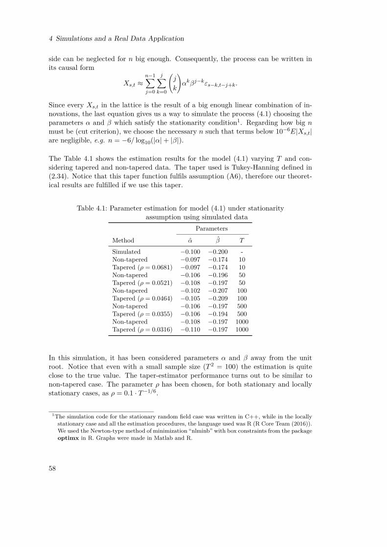
4 Simulations and a Real Data Application
side can be neglected for n big enough. Consequently, the process can be written inits causal form
Xs,t ≈n−1∑j=0
j∑k=0
(j
k
)αkβj−kεs−k,t−j+k.
Since every Xs,t in the lattice is the result of a big enough linear combination of in-novations, the last equation gives us a way to simulate the process (4.1) choosing theparameters α and β which satisfy the stationarity condition1. Regarding how big nmust be (cut criterion), we choose the necessary n such that terms below 10−6E|Xs,t|are negligible, e.g. n = −6/ log10(|α|+ |β|).
The Table 4.1 shows the estimation results for the model (4.1) varying T and con-sidering tapered and non-tapered data. The taper used is Tukey-Hanning defined in(2.34). Notice that this taper function fulfils assumption (A6), therefore our theoret-ical results are fulfilled if we use this taper.
Table 4.1: Parameter estimation for model (4.1) under stationarityassumption using simulated data
Parameters
Method α β T
Simulated −0.100 −0.200 -Non-tapered −0.097 −0.174 10Tapered (ρ = 0.0681) −0.097 −0.174 10Non-tapered −0.106 −0.196 50Tapered (ρ = 0.0521) −0.108 −0.197 50Non-tapered −0.102 −0.207 100Tapered (ρ = 0.0464) −0.105 −0.209 100Non-tapered −0.106 −0.197 500Tapered (ρ = 0.0355) −0.106 −0.194 500Non-tapered −0.108 −0.197 1000Tapered (ρ = 0.0316) −0.110 −0.197 1000
In this simulation, it has been considered parameters α and β away from the unitroot. Notice that even with a small sample size (T 2 = 100) the estimation is quiteclose to the true value. The taper-estimator performance turns out to be similar tonon-tapered case. The parameter ρ has been chosen, for both stationary and locallystationary cases, as ρ = 0.1 · T−1/6.
1The simulation code for the stationary random field case was written in C++, while in the locallystationary case and all the estimation procedures, the language used was R (R Core Team (2016)).We used the Newton-type method of minimization “nlminb” with box constraints from the packageoptimx in R. Graphs were made in Matlab and R.
58
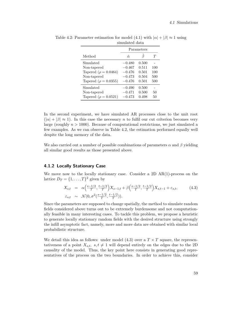
4.1 Simulations
Table 4.2: Parameter estimation for model (4.1) with |α|+ |β| ≈ 1 usingsimulated data
Parameters
Method α β T
Simulated −0.480 0.500 -Non-tapered −0.467 0.511 100Tapered (ρ = 0.0464) −0.476 0.501 100Non-tapered −0.473 0.504 500Tapered (ρ = 0.0355) −0.476 0.501 500
Simulated −0.490 0.500 -Non-tapered −0.471 0.500 50Tapered (ρ = 0.0521) −0.473 0.498 50
In the second experiment, we have simulated AR processes close to the unit root(|α| + |β| ≈ 1). In this case the necessary n to fulfil our cut criterion becomes verylarge (roughly n > 1000). Because of computational restrictions, we just simulated afew examples. As we can observe in Table 4.2, the estimation performed equally welldespite the long memory of the data.
We also carried out a number of possible combinations of parameters α and β yieldingall similar good results as those presented above.
4.1.2 Locally Stationary CaseWe move now to the locally stationary case. Consider a 2D AR(1)-process on thelattice DT = 1, . . . , T2 given by
Xs,t = α(s−1/2T , t−1/2
T
)Xs−1,t + β
(s−1/2T , t−1/2
T
)Xs,t−1 + εs,t, (4.3)
εs,t ∼ N (0, σ2( s−1/2T , t−1/2
T )).
Since the parameters are supposed to change spatially, the method to simulate randomfields considered above turns out to be extremely burdensome and not computation-ally feasible in many interesting cases. To tackle this problem, we propose a heuristicto generate locally stationary random fields with the desired structure using stronglythe infill asymptotic fact, namely, more and more data are obtained with similar localprobabilistic structure.
We detail this idea as follows: under model (4.3) over a T × T square, the represen-tativeness of a point Xs,t, s, t 6= 1 will depend entirely on the edges due to the 2Dcausality of the model. Thus, the key point here consists in generating good repre-sentatives of the process on the two boundaries. In order to achieve this, consider
59
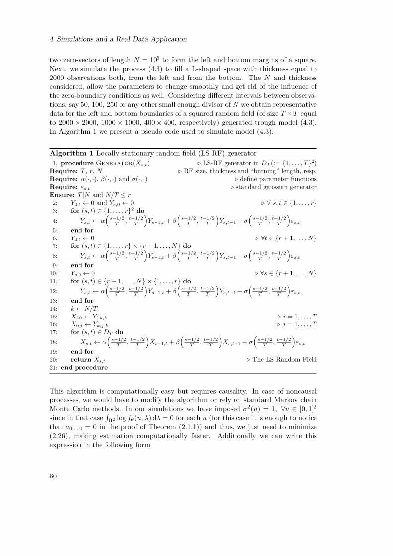
4 Simulations and a Real Data Application
two zero-vectors of length N = 105 to form the left and bottom margins of a square.Next, we simulate the process (4.3) to fill a L-shaped space with thickness equal to2000 observations both, from the left and from the bottom. The N and thicknessconsidered, allow the parameters to change smoothly and get rid of the influence ofthe zero-boundary conditions as well. Considering different intervals between observa-tions, say 50, 100, 250 or any other small enough divisor of N we obtain representativedata for the left and bottom boundaries of a squared random field (of size T ×T equalto 2000 × 2000, 1000 × 1000, 400 × 400, respectively) generated trough model (4.3).In Algorithm 1 we present a pseudo code used to simulate model (4.3).
Algorithm 1 Locally stationary random field (LS-RF) generator1: procedure Generator(Xs,t) . LS-RF generator in DT (:= 1, . . . , T2)Require: T , r, N . RF size, thickness and “burning” length, resp.Require: α(·, ·), β(·, ·) and σ(·, ·) . define parameter functionsRequire: εs,t . standard gaussian generatorEnsure: T |N and N/T ≤ r2: Y0,t ← 0 and Ys,0 ← 0 . ∀ s, t ∈ 1, . . . , r3: for (s, t) ∈ 1, . . . , r2 do4: Ys,t ← α
(s−1/2
T , t−1/2T
)Ys−1,t + β
(s−1/2
T , t−1/2T
)Ys,t−1 + σ
(s−1/2
T , t−1/2T
)εs,t
5: end for6: Y0,t ← 0 . ∀t ∈ r + 1, . . . , N7: for (s, t) ∈ 1, . . . , r × r + 1, . . . , N do8: Ys,t ← α
(s−1/2
T , t−1/2T
)Ys−1,t + β
(s−1/2
T , t−1/2T
)Ys,t−1 + σ
(s−1/2
T , t−1/2T
)εs,t
9: end for10: Ys,0 ← 0 . ∀s ∈ r + 1, . . . , N11: for (s, t) ∈ r + 1, . . . , N × 1, . . . , r do12: Ys,t ← α
(s−1/2
T , t−1/2T
)Ys−1,t + β
(s−1/2
T , t−1/2T
)Ys,t−1 + σ
(s−1/2
T , t−1/2T
)εs,t
13: end for14: k ← N/T15: Xi,0 ← Yi·k,k . i = 1, . . . , T16: X0,j ← Yk,j·k . j = 1, . . . , T17: for (s, t) ∈ DT do18: Xs,t ← α
(s−1/2
T , t−1/2T
)Xs−1,t + β
(s−1/2
T , t−1/2T
)Xs,t−1 + σ
(s−1/2
T , t−1/2T
)εs,t
19: end for20: return Xs,t . The LS Random Field21: end procedure
This algorithm is computationally easy but requires causality. In case of noncausalprocesses, we would have to modify the algorithm or rely on standard Markov chainMonte Carlo methods. In our simulations we have imposed σ2(u) = 1, ∀u ∈ [0, 1]2since in that case
∫Π2 log fθ(u, λ) dλ = 0 for each u (for this case it is enough to notice
that a0,...,0 = 0 in the proof of Theorem (2.1.1)) and thus, we just need to minimize(2.26), making estimation computationally faster. Additionally we can write thisexpression in the following form
60
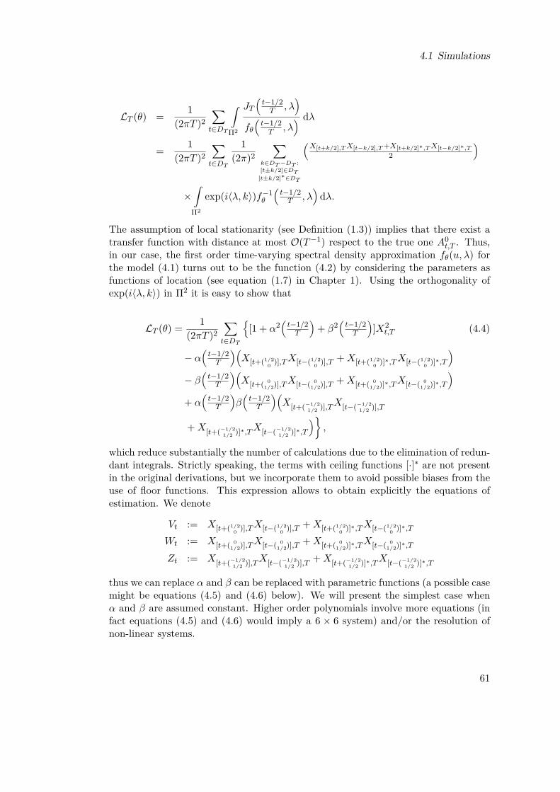
4.1 Simulations
LT (θ) = 1(2πT )2
∑t∈DT
∫Π2
JT(t−1/2T , λ
)fθ(t−1/2T , λ
) dλ
= 1(2πT )2
∑t∈DT
1(2π)2
∑k∈DT−DT :[t±k/2]∈DT
[t±k/2]∗∈DT
(X[t+k/2],TX[t−k/2],T+X[t+k/2]∗,TX[t−k/2]∗,T
2
)
×∫
Π2
exp(i〈λ, k〉)f−1θ
(t−1/2T , λ
)dλ.
The assumption of local stationarity (see Definition (1.3)) implies that there exist atransfer function with distance at most O(T−1) respect to the true one A0
t,T . Thus,in our case, the first order time-varying spectral density approximation fθ(u, λ) forthe model (4.1) turns out to be the function (4.2) by considering the parameters asfunctions of location (see equation (1.7) in Chapter 1). Using the orthogonality ofexp(i〈λ, k〉) in Π2 it is easy to show that
LT (θ) = 1(2πT )2
∑t∈DT
[1 + α2
(t−1/2T
)+ β2
(t−1/2T
)]X2
t,T (4.4)
− α(t−1/2T
)(X[t+(1/2
0 )],TX[t−(1/20 )],T +X[t+(1/2
0 )]∗,TX[t−(1/20 )]∗,T
)− β
(t−1/2T
)(X[t+( 0
1/2)],TX[t−( 01/2)],T +X[t+( 0
1/2)]∗,TX[t−( 01/2)]∗,T
)+ α
(t−1/2T
)β(t−1/2T
)(X[t+(−1/2
1/2 )],TX[t−(−1/21/2 )],T
+X[t+(−1/21/2 )]∗,TX[t−(−1/2
1/2 )]∗,T
),
which reduce substantially the number of calculations due to the elimination of redun-dant integrals. Strictly speaking, the terms with ceiling functions [·]∗ are not presentin the original derivations, but we incorporate them to avoid possible biases from theuse of floor functions. This expression allows to obtain explicitly the equations ofestimation. We denote
Vt := X[t+(1/20 )],TX[t−(1/2
0 )],T +X[t+(1/20 )]∗,TX[t−(1/2
0 )]∗,T
Wt := X[t+( 01/2)],TX[t−( 0
1/2)],T +X[t+( 01/2)]∗,TX[t−( 0
1/2)]∗,T
Zt := X[t+(−1/21/2 )],TX[t−(−1/2
1/2 )],T +X[t+(−1/21/2 )]∗,TX[t−(−1/2
1/2 )]∗,T
thus we can replace α and β can be replaced with parametric functions (a possible casemight be equations (4.5) and (4.6) below). We will present the simplest case whenα and β are assumed constant. Higher order polynomials involve more equations (infact equations (4.5) and (4.6) would imply a 6 × 6 system) and/or the resolution ofnon-linear systems.
61
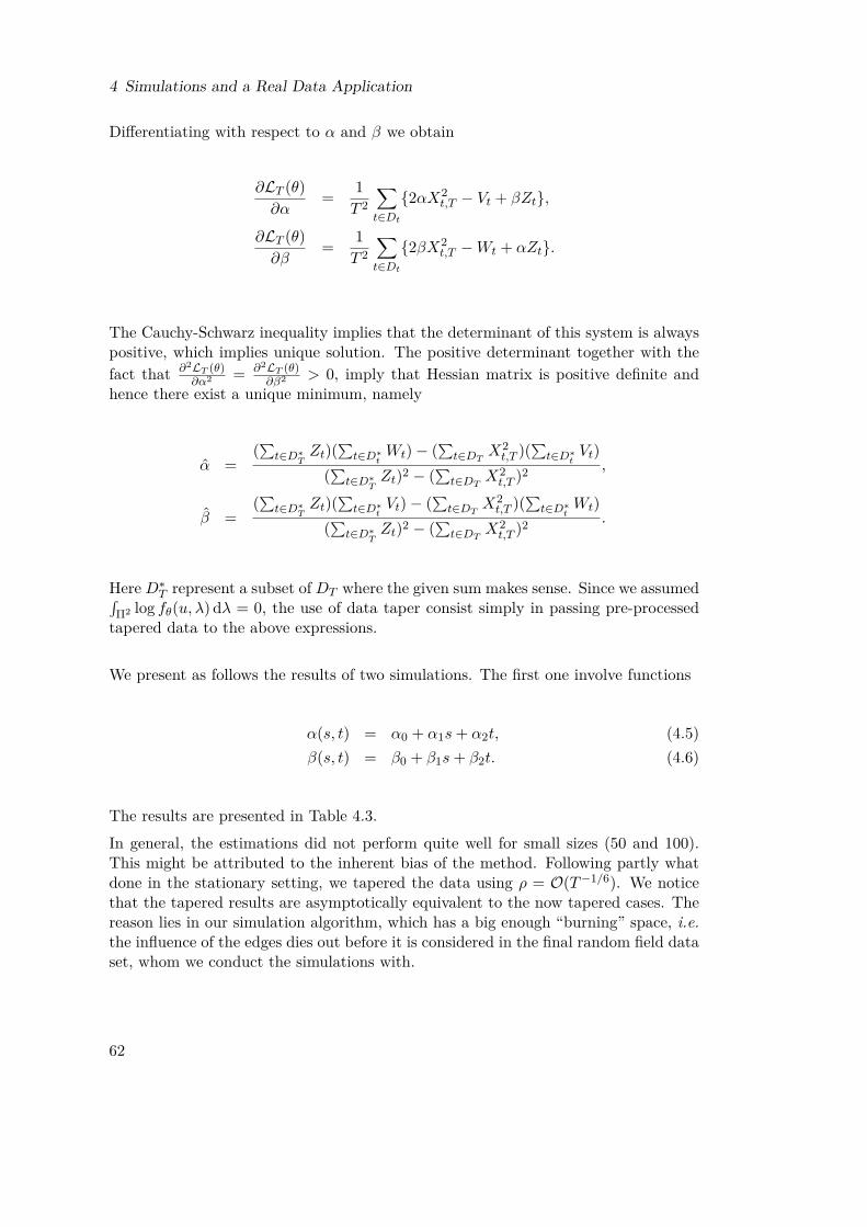
4 Simulations and a Real Data Application
Differentiating with respect to α and β we obtain
∂LT (θ)∂α
= 1T 2
∑t∈Dt2αX2
t,T − Vt + βZt,
∂LT (θ)∂β
= 1T 2
∑t∈Dt2βX2
t,T −Wt + αZt.
The Cauchy-Schwarz inequality implies that the determinant of this system is alwayspositive, which implies unique solution. The positive determinant together with thefact that ∂2LT (θ)
∂α2 = ∂2LT (θ)∂β2 > 0, imply that Hessian matrix is positive definite and
hence there exist a unique minimum, namely
α =(∑t∈D∗T
Zt)(∑t∈D∗t Wt)− (
∑t∈DT X
2t,T )(
∑t∈D∗t Vt)
(∑t∈D∗T
Zt)2 − (∑t∈DT X
2t,T )2 ,
β =(∑t∈D∗T
Zt)(∑t∈D∗t Vt)− (
∑t∈DT X
2t,T )(
∑t∈D∗t Wt)
(∑t∈D∗T
Zt)2 − (∑t∈DT X
2t,T )2 .
Here D∗T represent a subset of DT where the given sum makes sense. Since we assumed∫Π2 log fθ(u, λ) dλ = 0, the use of data taper consist simply in passing pre-processedtapered data to the above expressions.
We present as follows the results of two simulations. The first one involve functions
α(s, t) = α0 + α1s+ α2t, (4.5)β(s, t) = β0 + β1s+ β2t. (4.6)
The results are presented in Table 4.3.In general, the estimations did not perform quite well for small sizes (50 and 100).This might be attributed to the inherent bias of the method. Following partly whatdone in the stationary setting, we tapered the data using ρ = O(T−1/6). We noticethat the tapered results are asymptotically equivalent to the now tapered cases. Thereason lies in our simulation algorithm, which has a big enough “burning” space, i.e.the influence of the edges dies out before it is considered in the final random field dataset, whom we conduct the simulations with.
62
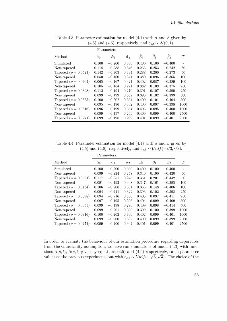
4.1 Simulations
Table 4.3: Parameter estimation for model (4.1) with α and β given by(4.5) and (4.6), respectively, and εs,t ∼ N (0, 1).
Parameters
Method α0 α1 α2 β0 β1 β2 T
Simulated 0.100 −0.200 0.300 0.400 0.100 −0.400 -Non-tapered 0.118 −0.288 0.346 0.233 0.253 −0.242 50Tapered (ρ = 0.0521) 0.142 −0.303 0.334 0.288 0.200 −0.273 50Non-tapered 0.050 −0.160 0.341 0.380 0.096 −0.365 100Tapered (ρ = 0.0464) 0.065 −0.167 0.321 0.402 0.087 −0.389 100Non-tapered 0.105 −0.184 0.271 0.382 0.109 −0.375 250Tapered (ρ = 0.0398) 0.112 −0.194 0.270 0.391 0.107 −0.390 250Non-tapered 0.099 −0.199 0.302 0.396 0.102 −0.399 500Tapered (ρ = 0.0355) 0.100 −0.202 0.304 0.400 0.101 −0.404 500Non-tapered 0.095 −0.196 0.302 0.400 0.097 −0.398 1000Tapered (ρ = 0.0316) 0.096 −0.199 0.304 0.403 0.095 −0.400 1000Non-tapered 0.099 −0.197 0.299 0.400 0.099 −0.400 2500Tapered (ρ = 0.0271) 0.099 −0.198 0.299 0.401 0.099 −0.401 2500
Table 4.4: Parameter estimation for model (4.1) with α and β given by(4.5) and (4.6), respectively, and εs,t ∼ Unif(−
√3,√
3).Parameters
Method α0 α1 α2 β0 β1 β2 T
Simulated 0.100 −0.200 0.300 0.400 0.100 −0.400 -Non-tapered 0.099 −0.224 0.258 0.340 0.190 −0.420 50Tapered (ρ = 0.0521) 0.117 −0.251 0.245 0.351 0.201 −0.442 50Non-tapered 0.091 −0.192 0.308 0.347 0.161 −0.395 100Tapered (ρ = 0.0464) 0.106 −0.208 0.301 0.363 0.148 −0.406 100Non-tapered 0.094 −0.211 0.322 0.393 0.102 −0.398 250Tapered (ρ = 0.0398) 0.094 −0.216 0.330 0.405 0.097 −0.411 250Non-tapered 0.097 −0.195 0.296 0.404 0.099 −0.409 500Tapered (ρ = 0.0355) 0.099 −0.198 0.296 0.409 0.098 −0.414 500Non-tapered 0.099 −0.201 0.300 0.399 0.100 −0.399 1000Tapered (ρ = 0.0316) 0.100 −0.202 0.300 0.402 0.099 −0.401 1000Non-tapered 0.099 −0.200 0.302 0.400 0.099 −0.399 2500Tapered (ρ = 0.0271) 0.099 −0.200 0.302 0.401 0.099 −0.401 2500
In order to evaluate the behaviour of our estimation procedure regarding departuresfrom the Gaussianity assumption, we have run simulations of model (4.3) with func-tions α(s, t), β(s, t) given by equations (4.5) and (4.6) respectively, same parametervalues as the previous experiment, but with εs,t ∼ Unif(−
√3,√
3). The choice of the
63
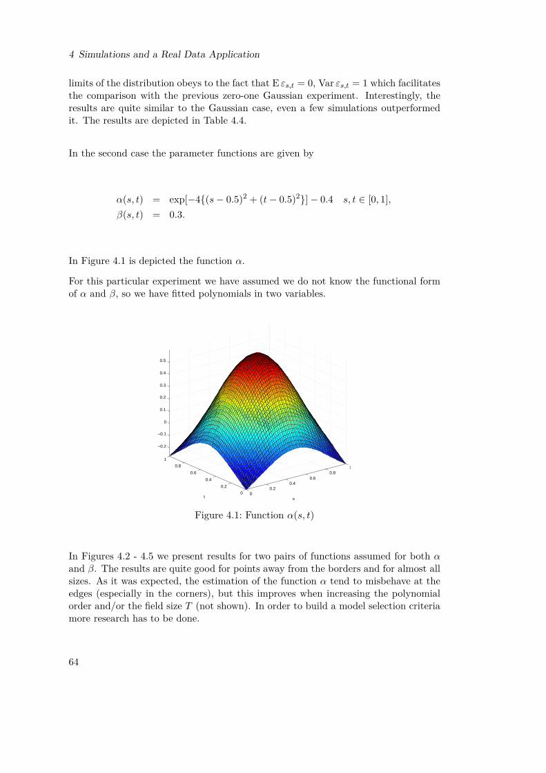
4 Simulations and a Real Data Application
limits of the distribution obeys to the fact that E εs,t = 0, Var εs,t = 1 which facilitatesthe comparison with the previous zero-one Gaussian experiment. Interestingly, theresults are quite similar to the Gaussian case, even a few simulations outperformedit. The results are depicted in Table 4.4.
In the second case the parameter functions are given by
α(s, t) = exp[−4(s− 0.5)2 + (t− 0.5)2]− 0.4 s, t ∈ [0, 1],β(s, t) = 0.3.
In Figure 4.1 is depicted the function α.
For this particular experiment we have assumed we do not know the functional formof α and β, so we have fitted polynomials in two variables.
00.2
0.40.6
0.81
0
0.2
0.4
0.6
0.8
1
−0.2
−0.1
0
0.1
0.2
0.3
0.4
0.5
st
Figure 4.1: Function α(s, t)
In Figures 4.2 - 4.5 we present results for two pairs of functions assumed for both αand β. The results are quite good for points away from the borders and for almost allsizes. As it was expected, the estimation of the function α tend to misbehave at theedges (especially in the corners), but this improves when increasing the polynomialorder and/or the field size T (not shown). In order to build a model selection criteriamore research has to be done.
64
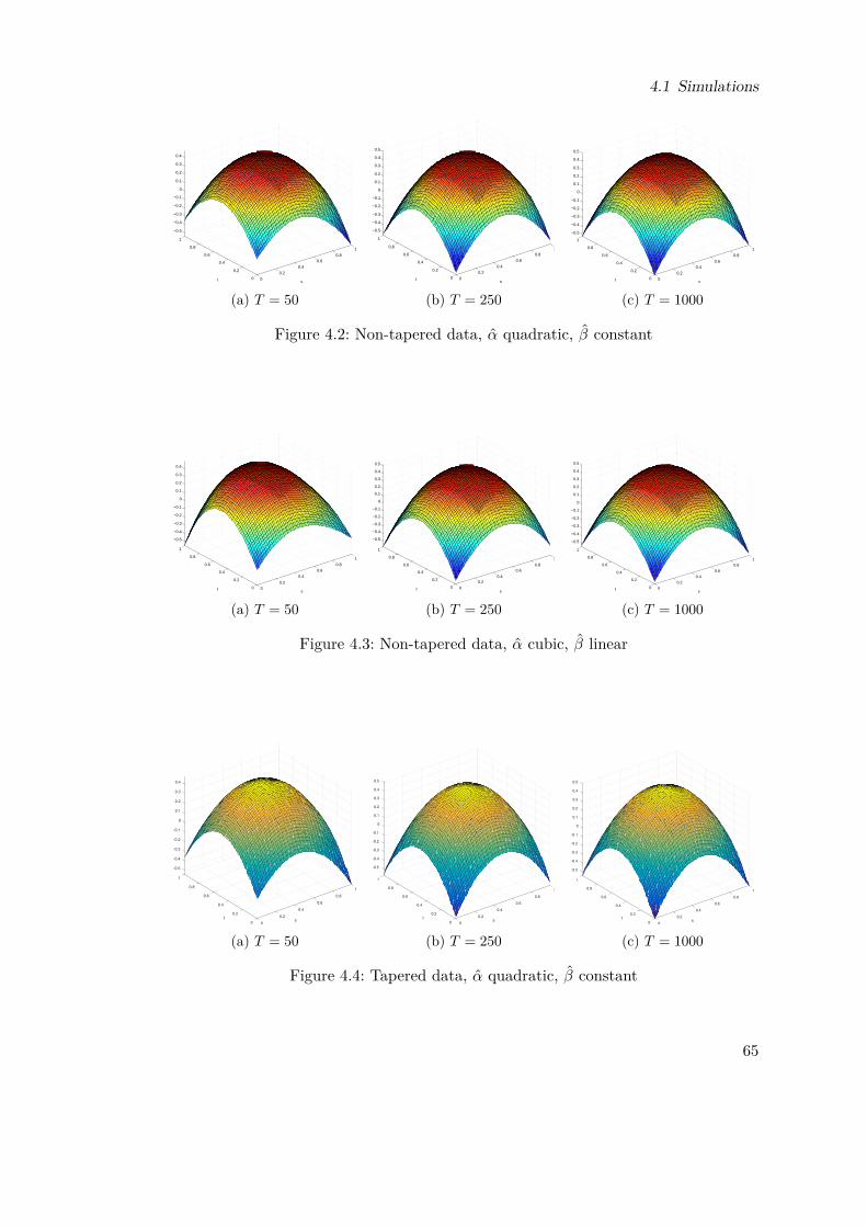
4.1 Simulations
00.2
0.40.6
0.81
0
0.2
0.4
0.6
0.8
1
−0.5
−0.4
−0.3
−0.2
−0.1
0
0.1
0.2
0.3
0.4
st
(a) T = 500
0.20.4
0.60.8
1
0
0.2
0.4
0.6
0.8
1
−0.5
−0.4
−0.3
−0.2
−0.1
0
0.1
0.2
0.3
0.4
0.5
st
(b) T = 2500
0.20.4
0.60.8
1
0
0.2
0.4
0.6
0.8
1
−0.5
−0.4
−0.3
−0.2
−0.1
0
0.1
0.2
0.3
0.4
0.5
st
(c) T = 1000
Figure 4.2: Non-tapered data, α quadratic, β constant
00.2
0.40.6
0.81
0
0.2
0.4
0.6
0.8
1
−0.5
−0.4
−0.3
−0.2
−0.1
0
0.1
0.2
0.3
0.4
st
(a) T = 500
0.20.4
0.60.8
1
0
0.2
0.4
0.6
0.8
1
−0.5
−0.4
−0.3
−0.2
−0.1
0
0.1
0.2
0.3
0.4
0.5
st
(b) T = 2500
0.20.4
0.60.8
1
0
0.2
0.4
0.6
0.8
1
−0.5
−0.4
−0.3
−0.2
−0.1
0
0.1
0.2
0.3
0.4
0.5
st
(c) T = 1000
Figure 4.3: Non-tapered data, α cubic, β linear
-0.5
1
-0.4
-0.3
-0.2
0.8
-0.1
1
0
0.1
0.6 0.8
0.2
t
0.3
0.6
s
0.4
0.4
0.4
0.20.2
0 0
(a) T = 50
-0.5
1
-0.4
-0.3
-0.2
0.8
-0.1
1
0
0.1
0.6 0.8
0.2
t
0.3
0.6
0.4
s
0.4
0.5
0.4
0.20.2
0 0
(b) T = 250
-0.5
1
-0.4
-0.3
-0.2
0.8
-0.1
1
0
0.1
0.6 0.8
0.2
t
0.3
0.6
0.4
s
0.4
0.5
0.4
0.20.2
0 0
(c) T = 1000
Figure 4.4: Tapered data, α quadratic, β constant
65
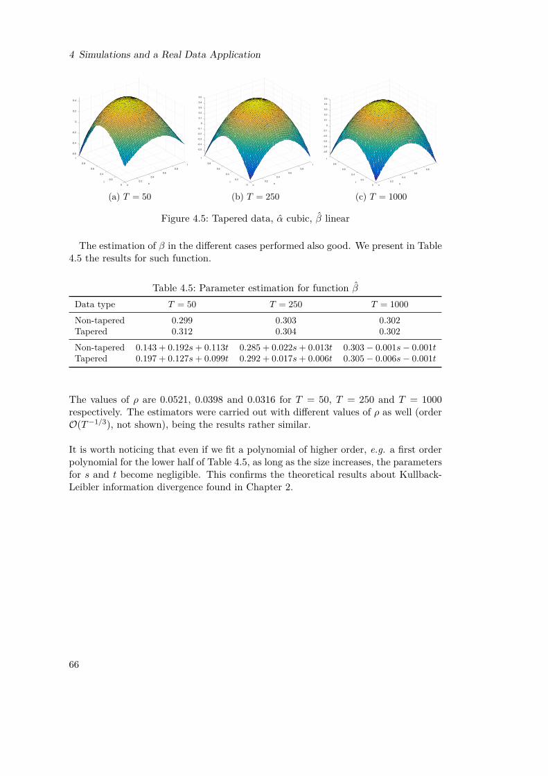
4 Simulations and a Real Data Application
-0.6
1
-0.4
-0.2
0.81
0
0.6 0.8
0.2
t
0.6
s
0.4
0.4
0.4
0.20.2
0 0
(a) T = 50
-0.5
1
-0.4
-0.3
-0.2
0.8
-0.1
1
0
0.1
0.6 0.8
0.2
t
0.3
0.6
0.4
s
0.4
0.5
0.4
0.20.2
0 0
(b) T = 250
-0.5
1
-0.4
-0.3
-0.2
0.8
-0.1
1
0
0.1
0.6 0.8
0.2
t
0.3
0.6
0.4
s
0.4
0.5
0.4
0.20.2
0 0
(c) T = 1000
Figure 4.5: Tapered data, α cubic, β linear
The estimation of β in the different cases performed also good. We present in Table4.5 the results for such function.
Table 4.5: Parameter estimation for function βData type T = 50 T = 250 T = 1000
Non-tapered 0.299 0.303 0.302Tapered 0.312 0.304 0.302
Non-tapered 0.143 + 0.192s+ 0.113t 0.285 + 0.022s+ 0.013t 0.303− 0.001s− 0.001tTapered 0.197 + 0.127s+ 0.099t 0.292 + 0.017s+ 0.006t 0.305− 0.006s− 0.001t
The values of ρ are 0.0521, 0.0398 and 0.0316 for T = 50, T = 250 and T = 1000respectively. The estimators were carried out with different values of ρ as well (orderO(T−1/3), not shown), being the results rather similar.
It is worth noticing that even if we fit a polynomial of higher order, e.g. a first orderpolynomial for the lower half of Table 4.5, as long as the size increases, the parametersfor s and t become negligible. This confirms the theoretical results about Kullback-Leibler information divergence found in Chapter 2.
66
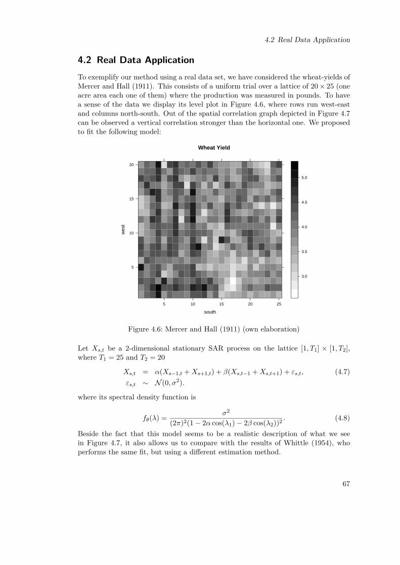
4.2 Real Data Application
4.2 Real Data ApplicationTo exemplify our method using a real data set, we have considered the wheat-yields ofMercer and Hall (1911). This consists of a uniform trial over a lattice of 20× 25 (oneacre area each one of them) where the production was measured in pounds. To havea sense of the data we display its level plot in Figure 4.6, where rows run west-eastand columns north-south. Out of the spatial correlation graph depicted in Figure 4.7can be observed a vertical correlation stronger than the horizontal one. We proposedto fit the following model:
Wheat Yield
south
wes
t
5
10
15
20
5 10 15 20 25
3.0
3.5
4.0
4.5
5.0
Figure 4.6: Mercer and Hall (1911) (own elaboration)
Let Xs,t be a 2-dimensional stationary SAR process on the lattice [1, T1] × [1, T2],where T1 = 25 and T2 = 20
Xs,t = α(Xs−1,t +Xs+1,t) + β(Xs,t−1 +Xs,t+1) + εs,t, (4.7)εs,t ∼ N (0, σ2).
where its spectral density function is
fθ(λ) = σ2
(2π)2(1− 2α cos(λ1)− 2β cos(λ2))2 . (4.8)
Beside the fact that this model seems to be a realistic description of what we seein Figure 4.7, it also allows us to compare with the results of Whittle (1954), whoperforms the same fit, but using a different estimation method.
67
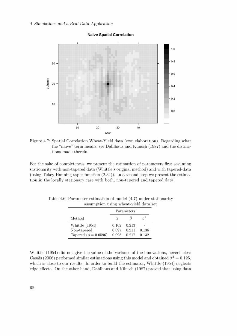
4 Simulations and a Real Data Application
Naive Spatial Correlation
row
colu
mn
10
20
30
10 20 30 40
0.0
0.2
0.4
0.6
0.8
1.0
Figure 4.7: Spatial Correlation Wheat-Yield data (own elaboration). Regarding whatthe “naive” term means, see Dahlhaus and Künsch (1987) and the distinc-tions made therein.
For the sake of completeness, we present the estimation of parameters first assumingstationarity with non-tapered data (Whittle’s original method) and with tapered-data(using Tukey-Hanning taper function (2.34)). In a second step we present the estima-tion in the locally stationary case with both, non-tapered and tapered data.
Table 4.6: Parameter estimation of model (4.7) under stationarityassumption using wheat-yield data set
Parameters
Method α β σ2
Whittle (1954) 0.102 0.213 -Non-tapered 0.097 0.211 0.136Tapered (ρ = 0.0596) 0.098 0.217 0.132
Whittle (1954) did not give the value of the variance of the innovations, neverthelessCasáis (2006) performed similar estimations using this model and obtained σ2 = 0.125,which is close to our results. In order to build the estimator, Whittle (1954) neglectsedge-effects. On the other hand, Dahlhaus and Künsch (1987) proved that using data
68
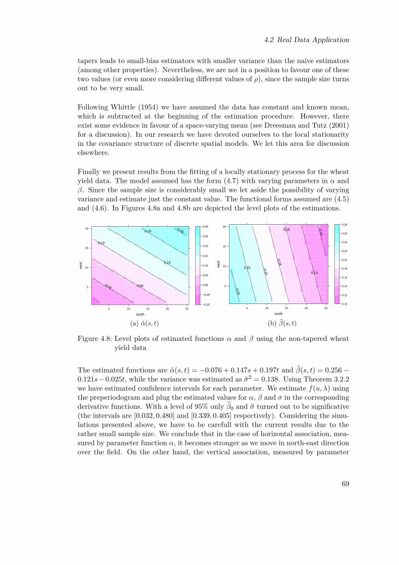
4.2 Real Data Application
tapers leads to small-bias estimators with smaller variance than the naive estimators(among other properties). Nevertheless, we are not in a position to favour one of thesetwo values (or even more considering different values of ρ), since the sample size turnsout to be very small.
Following Whittle (1954) we have assumed the data has constant and known mean,which is subtracted at the beginning of the estimation procedure. However, thereexist some evidence in favour of a space-varying mean (see Dreesman and Tutz (2001)for a discussion). In our research we have devoted ourselves to the local stationarityin the covariance structure of discrete spatial models. We let this area for discussionelsewhere.
Finally we present results from the fitting of a locally stationary process for the wheatyield data. The model assumed has the form (4.7) with varying parameters in α andβ. Since the sample size is considerably small we let aside the possibility of varyingvariance and estimate just the constant value. The functional forms assumed are (4.5)and (4.6). In Figures 4.8a and 4.8b are depicted the level plots of the estimations.
south
wes
t
5
10
15
20
5 10 15 20 25
0.00 0.05
0.10
0.15
0.200.25
−0.10
−0.05
0.00
0.05
0.10
0.15
0.20
0.25
0.30
(a) α(s, t)south
wes
t
5
10
15
20
5 10 15 20 25
0.12
0.14
0.16
0.18
0.20
0.22
0.24
0.10
0.12
0.14
0.16
0.18
0.20
0.22
0.24
0.26
0.28
(b) β(s, t)
Figure 4.8: Level plots of estimated functions α and β using the non-tapered wheatyield data
The estimated functions are α(s, t) = −0.076 + 0.147s+ 0.197t and β(s, t) = 0.256−0.121s−0.025t, while the variance was estimated as σ2 = 0.138. Using Theorem 3.2.2we have estimated confidence intervals for each parameter. We estimate f(u, λ) usingthe preperiodogram and plug the estimated values for α, β and σ in the correspondingderivative functions. With a level of 95% only β0 and σ turned out to be significative(the intervals are [0.032, 0.480] and [0.339, 0.405] respectively). Considering the simu-lations presented above, we have to be carefull with the current results due to therather small sample size. We conclude that in the case of horizontal association, mea-sured by parameter function α, it becomes stronger as we move in north-east directionover the field. On the other hand, the vertical association, measured by parameter
69

4 Simulations and a Real Data Application
function β, it becomes stronger as we move in direction east-west being the changesalong the level curves in vertical direction almost negligible. We also conducted esti-mations with tapered data obtaining essentially the same results for different valuesof ρ (not shown).
70
4.3 Discussion
4.3 DiscussionThe stationary simulations showed to perform better as the sample size T increases.Though not all depicted, we ran additional simulation whose posterior estimationyielded better results for decreasing ρ. According to our results, the chosen parame-ter values for each model played no role regarding estimation (see Table 4.2), but theyactually did in terms of computer data generation; those close to the unit root turnedout to be quit burdensome computationally. In the locally stationary case we facedthe problem of generating data with the desired properties. To tackle this problem,we proposed a fast and simple algorithm which make use of the infill asymptotic as-sumption. The estimation results confirmed the consistency of the data generatingalgorithm. The above two observations for the stationary case regarding T and ρ holdalso for the local stationary case. Nevertheless it is clear that reasonable results startfor bigger values of T (say between 100 and 250), considering that in this case thenumber of parameters increase as well. The use of a different distribution (in our caseuniform) did not represent any major change in the estimated parameter in compari-son with the Gaussian case. The estimations for the parametric non linear functionα(s, t) turned out to be also reasonable just by simple inspection, we do not have thenecessary tools to compare functions with different polynomial order. We let a modelselection criteria as a matter of future research.
The results obtained from the stationary estimation for the non tapered wheat-yielddata, turned out to be very similar with respect to those given in Whittle (1954),thus our method is consistent. The model assumed was a non causal SAR (eq. 4.7).In the locally stationary case, we just estimated affine functions for parameters αand β and constant σ2. Because of the small sample size data, we treat the resultscarefully. With a Gaussian law might be obtained an estimation of the error, andhence, weighing up rightly conclusions from the results.
71

Conclusion
In this work we have developed an estimator for centered Gaussian locally statio-nary random fields processes. We have applied, and in some cases extended the ideasof Prof. Dr. Rainer Dahlhaus (Dahlhaus (1996), Dahlhaus (2000)) who proposeda Whittle-type approximation of the Gaussian likelihood for locally stationary timeseries. This approach has motivated our research of the random field case taking asstarting point what has been presented in Dahlhaus and Sahm (2000). The Whittlelikelihood was obtained thanks to an extension of the Szegö’s theorem and an approxi-mation of the matrix Σ−1
T (Aθ). The score function of the Whittle likelihood proved tobe biased, which implies a bias of same order for the Whittle estimator θT . The biassources were identified (skewed preperiodogram, local stationarity and edge-effects),studied and some solutions were proposed. Yet, the bias coming from the local sta-tionarity remains. In order to get a Gaussian law we centered the estimator in E θ(h)
T ,obtaining a useful law in any dimension. Consistency of the estimator and uniformconvergence of likelihoods were proved as well.
Finally, we conducted some simulations under different sets of parameters, differentfield sizes, with tapered and non tapered data, considering linear and non linear pa-rameter functions and different distributions of innovations. In all cases the resultsperformed reasonably well, excepting for those with small amount of data. We fittedstationary and locally stationary SAR models to the well known wheat-yield data setof Mercer and Hall (1911). Our estimation of the stationary case (following Dahlhausand Künsch (1987)) turned out to be quite similar to what is found in the literature(see Whittle (1954)). From the results of the non stationary case we learned that aswe move in the south west - north east and east - west directions the horizontal andvertical association respectively get stronger.
Possible directions of future research are:
(a) Determine a model selection criteria.
(b) Incorporate a local stationary mean.
(c) Generalize this findings to higher dimension random fields (δ > 1, see Definition1.1.1).
(d) Build a test of non stationarity for random fields using this approach (see Pa-paroditis et al. (2009) for an analogous in the time series context).
73

References
Brillinger, D. (1981). Time Series: Data Analysis and Theory. Holden-Day, Inc.
Casáis, R. M. C. (2006). Contributions to spectral spatial statistics. Univ Santiagode Compostela.
Dahlhaus, R. (1996). On the Kullback-Leibler information divergence of locally sta-tionary processes. Stochastic Processes and their Applications 62, 139–168.
Dahlhaus, R. (1997). Fitting Time Series models to Nonstationary processes. TheAnnals of Statistics 25, 1–37.
Dahlhaus, R. (2000). A Likelihood Approximation for Locally Stationary Processes.The Annals of Statistics 28, 1762–1794.
Dahlhaus, R. and Künsch, H. (1987). Edge effects and efficient parameter estimationfor stationary random fields. Biometrika 74, 877–882.
Dahlhaus, R. and Sahm, M. (2000). Likelihood Methods for Nonstationary TimeSeries and Random Fields. Resenhas do Instituto de Matemática e Estatística daUniversidade de Sao Paulo 4, 457–477.
Dreesman, J. M. and Tutz, G. (2001). Non-Stationary Conditional Models for SpatialData Based on Varying Coefficients. Journal of the Royal Statistical Society: SeriesD (The Statistician) 50, 1–15.
Dzhaparidze, K. (1986). Parameter Estimation and Hypothesis Testing in SpectralAnalysis of Stationary Time Series. Springer Series in Statistics, Springer NewYork.
Guyon, X. (1995). Random fields on a network: modeling, statistics, and applications.Springer Science & Business Media.
Jammalamadaka, S. R., Rao, T. S. and Terdik, G. (2006). Higher Order Cumu-lants of Random Vectors and Applications to Statistical Inference and Time Series.Sankhya: The Indian Journal of Statistics (2003-2007) 68, 326–356.
Martin, W. and Flandrin, P. (1985). Wigner-Ville spectral analysis of nonstationaryprocesses. IEEE Transactions on Acoustics, Speech, and Signal Processing 33,1461–1470.
Mathai, A. M. and Provost, S. B. (1992). Quadratic forms in random variables: theoryand applications. Dekker.
75

References
Mercer, W. and Hall, A. (1911). The experimental error of field trials. The Journalof Agricultural Science 4, 107–132.
Paparoditis, E. et al. (2009). Testing temporal constancy of the spectral structure ofa time series. Bernoulli 15, 1190–1221.
R Core Team (2016). R: A Language and Environment for Statistical Computing. RFoundation for Statistical Computing Vienna, Austria.
Whittle, P. (1954). On Stationary Processes in the Plane. Biometrika 41, 434–449.
76
Lebenslauf
Persönliche DatenName: Danilo Alberto Pezo Villar
Ausbildung2001–2007,2011 Mathematikingenieur, mit Hauptfach Angewandte Statistik, Fach-
bereich Mathematik, Universidad Técnica Federico Santa María,Chile.
2008–2010,2013 M.Sc. Mathematik, Fachbereich Mathematik, Universidad TécnicaFederico Santa María, Chile.
2010–2012 B.A. Pädagogik, Universidad de Playa Ancha, Chile.
2014–2017 Doktorand, Fachbereich Mathematik, Technische Universität Kai-serslautern, Deutschland.
Berufserfahrungen2004–2007 Aushilfkraft in verschidenen Fächern, Fachbereich Mathematik,
Universidad Técnica Federico Santa María, Chile.
2008–2013 Dozent, Fachbereich Mathematik, Universidad Técnica FedericoSanta María, Chile.
2011–2014 Wissentschaftliche Mitarbeiter, Centro Interdisciplinario de Neu-rociencia de Valaparaíso, Chile.
2015–2017 Wissentschaftliche Hilfkraft, Fraunhofer-Institut für Techno- undWirtschaftsmathematik ITWM, Deutschland.
77


Erklärung
Hiermit erkläre ich, dass ich die vorliegende Arbeit selbstständig verfasst und keineanderen als die angegebenen Hilfsmittel benutzt habe. Die Stellen, die anderen Werkendem Wortlaut oder dem Sinn nach entnommen wurden, habe ich durch die Angabeder Quelle, auch der benutzten Sekundärliteratur, als Entlehnung kenntlich gemacht.
Kaiserslautern, den 09. Oktober 2017Danilo Pezo Villar
79