University of Rhode Island University of Rhode Island

DigitalCommons@URI DigitalCommons@URI

Open Access Master's Theses

2018

An Assessment of Holographic Microscopy for Quantifying An Assessment of Holographic Microscopy for Quantifying

Marine Particle Size and Concentration Marine Particle Size and Concentration

Noah L. Walcutt University of Rhode Island, noahw@uri.edu

Follow this and additional works at: https://digitalcommons.uri.edu/theses

Recommended Citation Recommended Citation Walcutt, Noah L., "An Assessment of Holographic Microscopy for Quantifying Marine Particle Size and Concentration" (2018). Open Access Master's Theses. Paper 1328. https://digitalcommons.uri.edu/theses/1328

This Thesis is brought to you for free and open access by DigitalCommons@URI. It has been accepted for inclusion in Open Access Master's Theses by an authorized administrator of DigitalCommons@URI. For more information, please contact digitalcommons@etal.uri.edu.

AN ASSESSMENT OF HOLOGRAPHIC MICROSCOPY

FOR QUANTIFYING MARINE PARTICLE SIZE AND

CONCENTRATION

BY

NOAH L. WALCUTT

A THESIS SUBMITTED IN PARTIAL FULFILLMENT OF THE

REQUIREMENTS FOR THE DEGREE OF

MASTER OF SCIENCE

IN

OCEANOGRAPHY

UNIVERSITY OF RHODE ISLAND

2018

MASTER OF SCIENCE

OF

NOAH L. WALCUTT

APPROVED:

Thesis Committee:

Major Professor Melissa Omand

Susanne Menden-Deuer

Jean-Yves Hervé

Nasser H. Zawia DEAN OF THE GRADUATE SCHOOL

UNIVERSITY OF RHODE ISLAND 2018

ABSTRACT

Achieving depth-resolved particle-specific data in sparse, highly variable oceanic

environments persists as a methodological challenge. Holography has emerged as a tool

for in-situ imaging of microscopic organisms and other particles in the marine

environment; appealing because of the relatively larger volume and simple optical

configuration compared to other imaging systems. The digital in-line holographic

microscope (DIHM) used in this study samples ~100× larger volumes than comparable

objective lens-based systems, and is deployable on CTD-rosette, flow-through, and

autonomous systems. However, it’s quantitative capabilities have so far, remained

uncertain. Here, the quantitative skill of the DIHM to evaluate size and concentration of

marine particles ranging from 5 to 1000 µm in diameter is assessed. Over one million

particles are analyzed using a custom image processing pipeline, which allows a precise

characterization of the three-dimensional volume sampled. These results are compared

with the FlowCam, the Imaging FlowCytobot and traditional microscope counts through

laboratory and field-based inter-calibration experiments. Based on this analysis,

recommendations for achieving quantitive size and concentration measurements from the

DIHM are suggested.

ACKNOWLEDGEMENTS

I would like to acknowledge my advisor, Melissa Omand, for continued guidance

and encouragement. Ben Knörlein and Tom Sgouros from Brown University developed

the CCV pipeline. A grant from the State of Rhode Island Technology Council supported

the development of the CCV Pipeline. Zrinka Ljubešić and Suncica Bosak completed

manual microscope counts. Colleen Mouw and Audrey Ciochetto provided training and

support on the Imaging FlowCytobot. Rodrigue Spinette ran samples and provided

training and support on the FlowCam. Megan Norato and Jack Flynn assisted with

manual hologram identification. Aimee Neeley and Ivona Cetinic ran samples on the FC

and IFCB. For work performed aboard the R/V Falkor, I am grateful to chief scientist

Ivona Cetinić, the ship’s crew and Schmidt Ocean Institute.

$iii

TABLE OF CONTENTS

ABSTRACT ii .......................................................................................................................

ACKNOWLEDGEMENTS iii ................................................................................................

TABLE OF CONTENTS iv ....................................................................................................

LIST OF FIGURES v .............................................................................................................

INTRODUCTION 1 ...............................................................................................................

METHODS 4 ..........................................................................................................................

RESULTS 19 ...........................................................................................................................

DISCUSSION 39 ....................................................................................................................

CONCLUSION 49 ..................................................................................................................

BIBLIOGRAPHY 50..............................................................................................................

$iv

LIST OF FIGURES

FIGURE PAGE

Figure 1. An example of unfocused v. focused holographic images. 4 .................................

Figure 2. Distance between Reconstruction Planes and Average Particles Observed. 6 ........

Figure 3. Schematic drawing of CCV hologram image processing pipeline. 9 ......................

Figure 4. Illustration of artifact removal steps. 12 ..................................................................

Figure 5. Schematic of DIHM for the Sample Collection types used for data collected. 14 ..

Figure 6. Illustration of the DIHM deployment for Environmental Samples. 15 ..................

Figure 7. Distribution of particles in the imaging volume (side view). 21 .............................

Figure 8. Distribution of particles in the imaging volume (axial view). 22 ............................

Figure 9. Model fit of ROI spatial distribution for concentration scaling coefficients. 23 .....

Figure 10. LogLog Size correction coefficient determination. 26 ..........................................

Figure 11. Environmental Sample Particle Size Distribution Intercomparison. 28 ................

Figure 12. Summary of size inter-comparison results. 30 ......................................................

Figure 13. Individual size inter-comparison results. 34 .........................................................

Figure 14. Measured Particle Concentration Inter-comparison. 38 ........................................

Figure 15. A hydrodynamic model of particle projections: DIHM v. IFCB. 43 .....................

Figure 16. Measured aspect ratio inter-comparison: DIHM v. IFCB. 45...............................

$v

INTRODUCTION

Quantitive particle measurements, such as size spectral shape and particle

concentration, provides insights into ecological community composition, abundance, and

diversity (Cavender-Bares et al. 2001). However, the discrete quantification of individual

microplankton organisms, marine snow and other detritus (herein referred to as marine

particles) over the depth and lateral expanse of the ocean persists as a methodological

challenge (Boss et al. 2015). Depth-resolved collection by nets and bottles that

concentrate small particles from seawater have been conducted extensively since the

early 20th century (Gutkowska et al. 2012), however, spatio-temporal sampling coverage

has been limited by time- and effort-intensive collection and analysis protocols which

often employed manual microscope analysis. Furthermore, this method can often damage

the more delicate forms. Aldridge (1972) circumvented this challenge through manual, in

situ measurements of marine particles using underwater photography by divers, however

implementing on broad scales is similarly prohibitive. In response to the need for better,

wider and easier particle-specific sampling, many in situ tools have emerged over the last

few decades. One of the first instruments for automated collection was the Continuous

Plankton Recorder, which dramatically increased spatio-temporal coverage by filtering

and preserving surface water phytoplankton while towed from ships. Measured particles

were limited to those <300 µm (Warner and Hays 1994), from upper 5-10 m of the water

column.

The in situ Video Plankton Recorder (Davis et al. 2005) and the Underwater

Vision Profiler (Picheral et al. 2010) sample larger particles, more than 1mm and more

$1

than 100 µm respectively, while using high throughput processing to measure and

classify objects. Imaging flow cytometers use a fixed focal plane, and sheath fluid to

capture particles at high sampling volume and resolution. Notably the Imaging

FlowCytobot (IFCB, Olson and Sosik 2007) and FlowCam (FC, Sieracki et al. 1998),

have led to rapid imaging and enumeration of particles at increased sampling volume and

smaller size classes (less than 300 µm) with much improved image quality.

Quantitive evaluation of commercially available, semi-automated particle-sizers is

important to the oceanographic community as it sheds light on the opportunities and

advantages of each system. An inter-comparison of the FlowCam with flow cytometry

and membrane filter direct counts has provided guidelines for monitoring discharged

ballast water (Steinberg et al. 2012). The IFCB offers the potential for continuous, long

term observations of plankton community structure (Olson and Sosik 2007).

In situ digital inline holographic microscopes (DIHM) have the potential to

capture a broad range of size classes simultaneously (Beers et al. 1970; Schnars and

Jüptner 2005), with no lenses or moving parts. For example, the DIHM used in this study

(manufactured by 4Deep, formerly Resolution Optics) resolves particles with diameters

that range from about 0.005 mm to 1 mm. (Zetsche et al. 2014; Bochdansky et al. 2016).

The broad size range is made possible because the image is not constrained by a depth-

of-field since image focusing occurs in post-processsing, and this allows for a ~100×

larger sample volume, than comparable imaging tools such as the FC. The trade-off is

that regions of interest (ROI) within the reconstructed images often contain artifacts and

the quantitative skill of this relatively new technique remains uncertain. An additional

$2

challenge is processing the large volume of data generated with each deployment: In the

near-surface open ocean, a sample rate of 16 frames per second, has typically yielded

about 200 regions of interest (ROI) per frame, resulting in over 10 million ROI per hour

of deployment. Manual analysis of this data is impractical, and so a custom image

processing pipeline was recently developed in collaboration with the Brown University

Center for Computation and Visualization.

Previous efforts to calibrate DIHM size measurements have utilized laboratory

experiments; previous efforts to calibrate DIHM concentration measurements have

utilized field observations (Bochdansky et al. 2013). Other efforts for quantitative sizing

and concentration performance of digital inline holography was previously assessed using

polystyrene beads in silicone oil (Guildenbecher et al. 2013). With our automated

method, we have expanded upon these previous efforts to calibrate the DIHM

(Bochdansky et al. 2013) by performing controlled laboratory experiments using

microspheres, four different cultures, environmental samples and then compared these

quantities with the IFCB, FC, and manual microscope counts.

This study expands our understanding of the advantages and limitations of in situ

holographic microscopy and makes two main recommendations for image analysis that

are critical for obtaining quantitative estimates of particle concentration and size with this

modern technology: (i) particle size estimates should be corrected as a non-linear

function of the distance from the laser source (Equation 1); and (ii) particle concentration

estimates should account for non-uniform spatial illumination bias via scaling

coefficients (Equation 2).

$3

METHODS

Digital Inline Holographic Microscopy (DIHM). The DIHM uses spherical waves

propagating from a point source to illuminate and image objects. This illumination (in our

case, a 360 nm pulsed laser) casts diffraction patterns around particles that intercept the

beam. A camera records the light intensities of the diffraction pattern in 2D, and this

pattern is later solved for wavefront intensity for all points in the 3D, conically-shaped

imaging volume. These solutions of point intensities require knowledge of the laser’s

wavelength and the distance from laser to camera, or path-length (Garcia-Sucerquia et al.

2006). Parsing the planes along the laser’s path (defined as the z-direction) in the 3D

imaging volume is similar to turning the focusing knob of a light microscope and yields

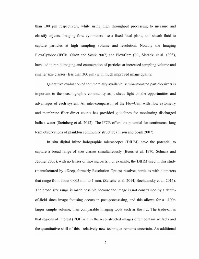
an in-focus ‘reconstructed’ plane at the z-location where the object was located (Figure

1).

$ $

Figure 1. An example of unfocused v. focused holographic images. Modification of the reconstruction plane in Octopus changes the spatial-point intensity values. The gradient of pixel intensity or sharpness of object edges can be used to determine whether it is in focus, so holograms are reconstructed at regular depth

$4

intervals, the sharpness scores are computed, and the objects with the highest scores are saved. Unfocused (left image), Focused (right image).

Region of Interest (ROI) detection algorithm. The CCV Holographic Image Processing

Pipeline (Figure 3, herein referred to as the CCV Pipeline, available for download:

https://github.com/BenKnorlein/Holograms) automates particle size and concentration

measurements for high-throughput hologram analysis. Background subtraction is applied

to raw holographic images before mathematical hologram reconstruction using software

supplied by the manufacturer (Octopus©, www.4-Deep.com). The background image is

constructed using the median pixel values from all raw images of the recorded sequence.

Octopus© uses the Kirchhoff- Helmholtz transform to solve point source wave front

intensities at the object focal plane (Xu et al. 2002). The CCV Pipeline saves slices of the

hologram (ie. focal planes) in user-specified µm increments across the 22 mm path

between the point source and the camera. We tested the results for reconstructed

holograms which recorded a Dunaliella tertliotecca monoculture (nominally 10µm in

diameter), and obtained comparisons from reconstructing planes at 25, 50, 100, and 500

µm increments (Figure 2).

$5

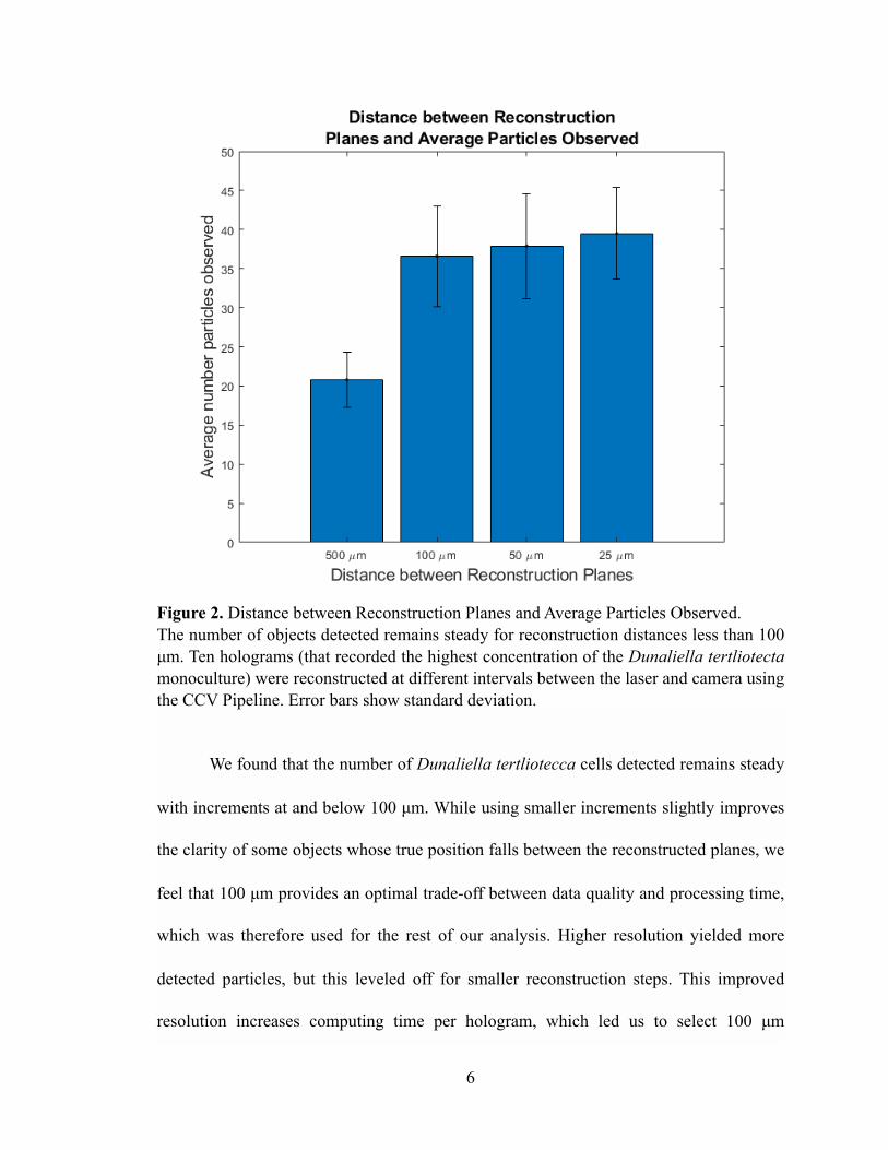
$ Figure 2. Distance between Reconstruction Planes and Average Particles Observed. The number of objects detected remains steady for reconstruction distances less than 100 µm. Ten holograms (that recorded the highest concentration of the Dunaliella tertliotecta monoculture) were reconstructed at different intervals between the laser and camera using the CCV Pipeline. Error bars show standard deviation.

We found that the number of Dunaliella tertliotecca cells detected remains steady

with increments at and below 100 µm. While using smaller increments slightly improves

the clarity of some objects whose true position falls between the reconstructed planes, we

feel that 100 µm provides an optimal trade-off between data quality and processing time,

which was therefore used for the rest of our analysis. Higher resolution yielded more

detected particles, but this leveled off for smaller reconstruction steps. This improved

resolution increases computing time per hologram, which led us to select 100 µm

$6

increments as the default setting for all processing. Qualitatively, the highest image

quality was that from the 25 µm increment reconstruction planes.

The processing pipeline then uses the OpenCV (www.opencv.org) image

processing library to first detect regions of interest in 2D image space, to determine for

each region the plane in which the object is the sharpest and finally to accurately segment

the sharp object. First, the highest sharpness score refers specifically to the Tenenbaum

Gradient computed for each individual pixel (Groen et al. 1985), where the sharpness

score (∇T) is the sum of the square of the change in pixel intensity in adjacent pixels for

the image’s horizontal (∇x) and vertical (∇y) axes (∇T = ∇x2 + ∇y2). A subset of these

image regions were selected for using an empirically determined sharpness score

threshold. After evaluating the overall results (in terms of image artifact to ROI ratio) for

the 90th, 95th, and 98th percentile sharpness scores, we found the best results (fewest

image artifacts) were given by selecting regions from the 95th percentile. Each image

was sharpened to remove noise by blurring with a 7×7 pixel mask. A feature map was

generated for each hologram slice by saving x-y position, slice number, and pixel score.

All binary feature maps were splatted into one image and connected regions were

identified using the FindContours function. Small objects (less than 5 pixels) were

thrown out and cropped contour boundaries were refined and saved using the GrabCut

function, where pixel values 190-250 were foreground, 75-190 were probably

foreground, 0-75 were probably background, and the border of the image was

background. This sequence results in a library of cropped ROIs (saved as .png files,

Figure 4) catalogued according to the hologram they were derived from. The ROI

$7

equivalent spherical diameter (ESD) and position were converted from pixel space to

physical dimensions in micrometers. Additional image analysis was performed using the

MatLab Image Processing toolbox (www.mathworths.com), for aspect ratio,

circumference, major/minor axis length and others. Finally, these holographic image

variables were in turn matched to the corresponding bio-optical and hydrographic

variables (by comparing synchronized time stamps) from quality-controlled CTD data at

full 16 Hz resolution (temperature, salinity, density, depth, dissolved oxygen,

photosynthetically active radiation, light attenuation, chlorophyll fluorescence, and

others) for later analysis.

$8

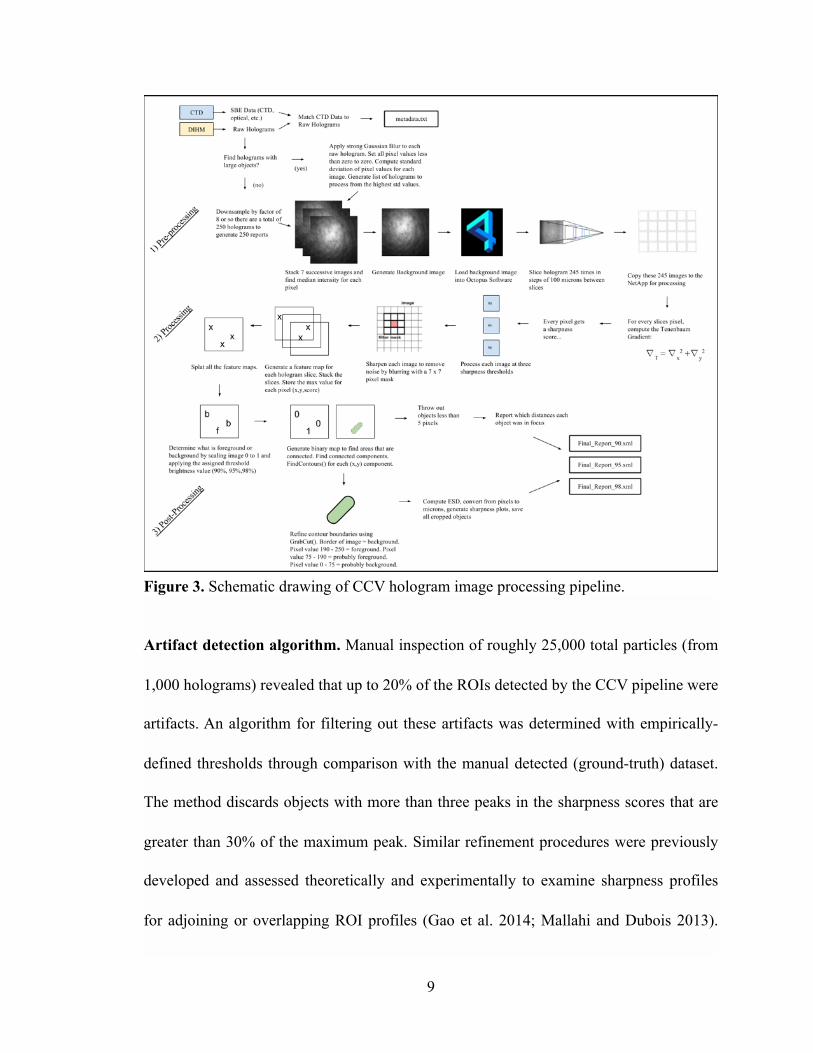
$ Figure 3. Schematic drawing of CCV hologram image processing pipeline.

Artifact detection algorithm. Manual inspection of roughly 25,000 total particles (from

1,000 holograms) revealed that up to 20% of the ROIs detected by the CCV pipeline were

artifacts. An algorithm for filtering out these artifacts was determined with empirically-

defined thresholds through comparison with the manual detected (ground-truth) dataset.

The method discards objects with more than three peaks in the sharpness scores that are

greater than 30% of the maximum peak. Similar refinement procedures were previously

developed and assessed theoretically and experimentally to examine sharpness profiles

for adjoining or overlapping ROI profiles (Gao et al. 2014; Mallahi and Dubois 2013).

$9

We developed and assessed our own user-defined thresholds to give the best results for

the data examined i.e. most artifacts detected while minimizing the number of ‘good’

objects discarded. The 25,000 particles in the ground-truth dataset detected by the CCV

Pipeline were were manually classified as either artifact or actual particle. The overall

rate of artifact prevalence in the datasets varied between 4% and 21.6% for the

environmental samples, microspheres, and the CTD-mounted deployment. Detection

performance of the artifact detection algorithm varied depending on the sample type.

Environmental sample bottles showed the greatest artifact detection performance,

reducing the overall percentage of artifacts by ~15%. Artifacts in the diluted microsphere

dataset could be reduced by around 9% using the algorithm. Overall rate of artifact

occurrence in CTD samples was low (around 4%), so detection rate in the CTD dataset

improved results minimally (2%).

After initial artifact removal in the DIHM data using the aforementioned features,

persistent artifacts were identified in all monoculture particle size distributions using a

Gaussian filter to define the apparent particle size distribution signal in 1 micron

increments. Size bins which exceeded the 90% confidence interval for the curve-to-bin fit

were adjusted to match the corresponding bin count for the Gaussian curve (Figure 9).

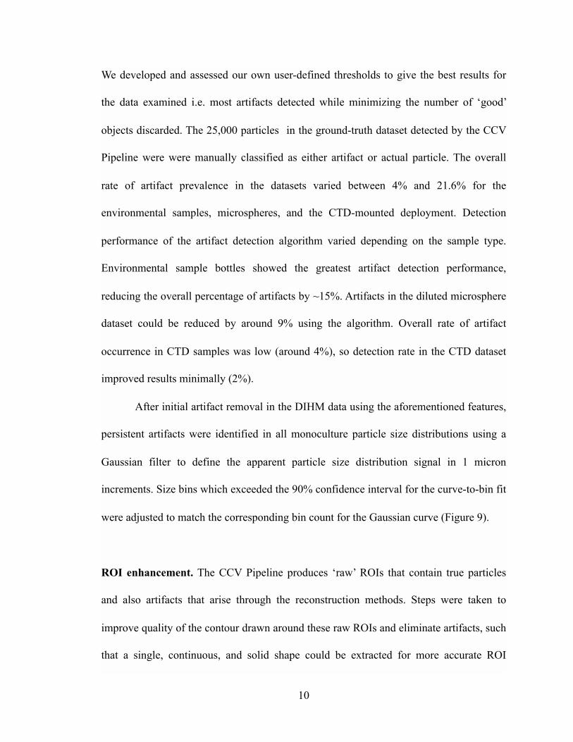
ROI enhancement. The CCV Pipeline produces ‘raw’ ROIs that contain true particles

and also artifacts that arise through the reconstruction methods. Steps were taken to

improve quality of the contour drawn around these raw ROIs and eliminate artifacts, such

that a single, continuous, and solid shape could be extracted for more accurate ROI

$10

statistics. First, the grayscale CCV contour was converted to a binary image using the

MatLab imbinarize.m function. Next, blobs (ie. discrete contours in the CCV binarized

image) with fewer than 20 pixels were eliminated. Next, the MatLab regionprops.m

function was applied to the largest remaining blob for extracting solidity (ie. the area of

the region divided by the smallest polygon that can contain the region), major axis, minor

axis, equivalent spherical diameter, area, and the number of blobs contained in each

contour. Next, ‘holes’ in the largest contour were filled in. Next, the ratio of the number

of largest contour perimeter pixels (ie. those coinciding with the ROI edge box) to the

total contour area (PA), and the ratio of the number of largest contour perimeter pixels to

the total ROI perimeter (PP) were computed. A graphical output enabled an assessment

of original image, the binarized image, and the ‘cleaned-up’ image with PA, PP, solidity,

and the number of blobs (Figure 4). Manual inspection of the these output provided

empirical thresholds from which to reduce artifacts. ROI had to have a solidity greater

than 0.8, the number of multi-blobs had to be fewer than 5, the fraction of the ROI

perimeter occupied by the contour had to be less than 0.15, and the fraction of the contour

area that was a ROI perimeter pixel had to be less than 0.08. The result of these ROI

enhancement steps was an improved calibration for the microspheres, reduced artifacts,

and improved estimates of the major and minor axes.

$11

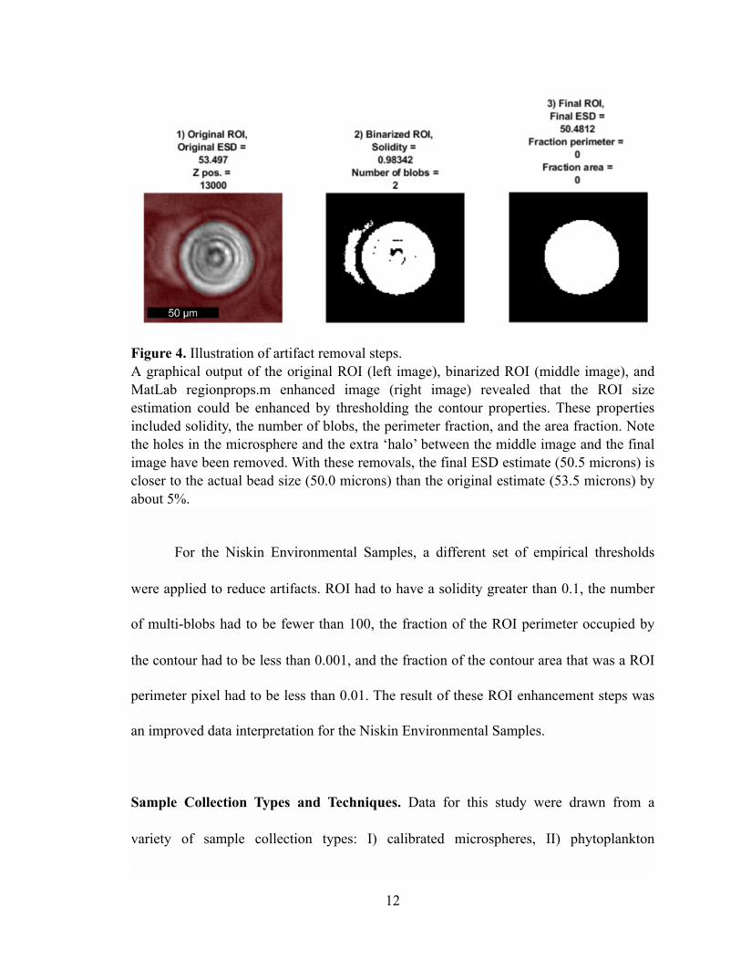
$ Figure 4. Illustration of artifact removal steps. A graphical output of the original ROI (left image), binarized ROI (middle image), and MatLab regionprops.m enhanced image (right image) revealed that the ROI size estimation could be enhanced by thresholding the contour properties. These properties included solidity, the number of blobs, the perimeter fraction, and the area fraction. Note the holes in the microsphere and the extra ‘halo’ between the middle image and the final image have been removed. With these removals, the final ESD estimate (50.5 microns) is closer to the actual bead size (50.0 microns) than the original estimate (53.5 microns) by about 5%.

For the Niskin Environmental Samples, a different set of empirical thresholds

were applied to reduce artifacts. ROI had to have a solidity greater than 0.1, the number

of multi-blobs had to be fewer than 100, the fraction of the ROI perimeter occupied by

the contour had to be less than 0.001, and the fraction of the contour area that was a ROI

perimeter pixel had to be less than 0.01. The result of these ROI enhancement steps was

an improved data interpretation for the Niskin Environmental Samples.

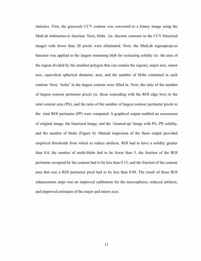
Sample Collection Types and Techniques. Data for this study were drawn from a

variety of sample collection types: I) calibrated microspheres, II) phytoplankton

$12

monocultures, III) environmental communities from Niskin bottles, IV) in situ

environmental communities when the DIHM was mounted to the CTD-rosette. Types I, II

and III were analyzed by wrapping and sealing the DIHM in Para-Film and injecting a

~75 mL sample media into the imaging volume (Figure 5).

$13

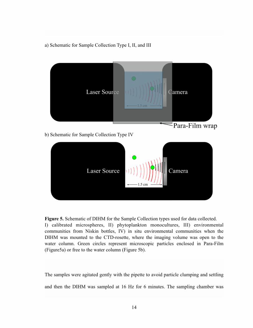
a) Schematic for Sample Collection Type I, II, and III

$ b) Schematic for Sample Collection Type IV

$

Figure 5. Schematic of DIHM for the Sample Collection types used for data collected. I) calibrated microspheres, II) phytoplankton monocultures, III) environmental communities from Niskin bottles, IV) in situ environmental communities when the DIHM was mounted to the CTD-rosette, where the imaging volume was open to the water column. Green circles represent microscopic particles enclosed in Para-Film (Figure5a) or free to the water column (Figure 5b).

The samples were agitated gently with the pipette to avoid particle clumping and settling

and then the DIHM was sampled at 16 Hz for 6 minutes. The sampling chamber was

$14

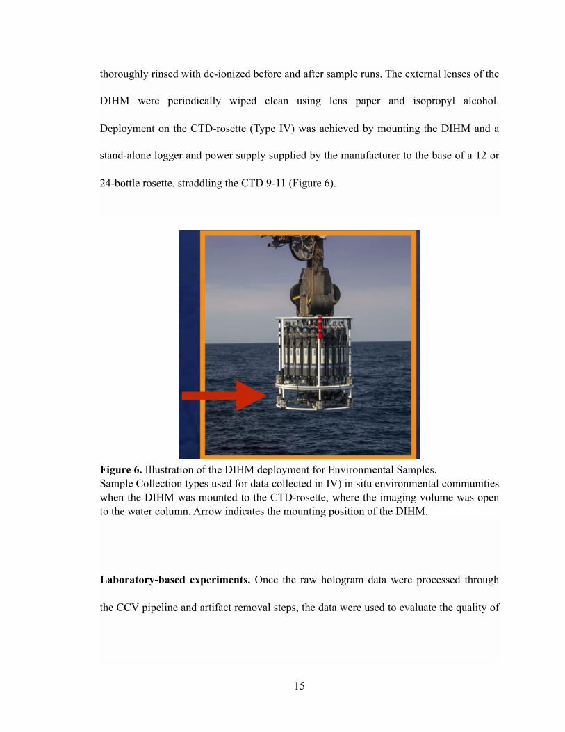
thoroughly rinsed with de-ionized before and after sample runs. The external lenses of the

DIHM were periodically wiped clean using lens paper and isopropyl alcohol.

Deployment on the CTD-rosette (Type IV) was achieved by mounting the DIHM and a

stand-alone logger and power supply supplied by the manufacturer to the base of a 12 or

24-bottle rosette, straddling the CTD 9-11 (Figure 6).

$ Figure 6. Illustration of the DIHM deployment for Environmental Samples. Sample Collection types used for data collected in IV) in situ environmental communities when the DIHM was mounted to the CTD-rosette, where the imaging volume was open to the water column. Arrow indicates the mounting position of the DIHM.

Laboratory-based experiments. Once the raw hologram data were processed through

the CCV pipeline and artifact removal steps, the data were used to evaluate the quality of

$15

high-throughput particle size and abundance measurements derived from the DIHM and

CCV pipeline processing routine.

Particle types and densities used for this study were selected to simulate those

found in the surface ocean for a wide range of environments. Oligotrophic gyres have

been observed to have particle concentrations of 10 particles/mL and comparatively small

cell sizes, ranging from 1 to 102 µm ESD (White et al. 2015). On the opposite end of the

spectrum, nearshore bloom conditions have been observed with particle concentrations as

high as 107 particles/mL and cell sizes and cell chain lengths ranging from 1 micron to

several millimeters (Karentz and Smayda 1998). To avoid the pitfalls of shape-specific

measurement bias, a variety of cell forms and sizes were selected including spherical,

elongate, and asymmetrical. Use of cosmopolitan representatives from major

phytoplankton groups—diatoms, dinoflagellates, and raphidophytes—further reduced the

possibility of any organism-specific size or concentration biases.

Several criteria were used to select the instruments used for inter-calibration.

Commercially available instruments for particle sizing utilize size estimates from direct

optical imaging (eg. the IFCB and FC), size estimates from bulk or single particle optical

properties (eg. the LISST), or changes in electrical impedance between micro channels

(eg. the Coulter Counter). Size estimates from optical imaging constrained measurement

inter-comparability variance to analogous sets of imaging challenges in digital

holography: CCD pixel to physical size ratio determination, ROI focussing, ROI

detection, and ROI contouring. The working size range and resolution of the FC and

IFCB was selected for particles with ESDs between 5 and 150 µm, a critical size range

$16

for suspended POC and the DIHM. Finally, instrument availability and ease of ship-side

deployment during the Schmidt Ocean Institute’s Sea to Space Particle Investigation were

also key considerations for the selection of the particle sizers used in this study.

For the FC and IFCB, concentration measurements are impacted by the

measurement protocols for each machine. Best practices were followed for each,

including (but not limited to) flow cell selection, manual focussing for optimal image

quality, de-bubbling at regular intervals, flow cell purging at regular intervals, and trigger

type selection. These parameters varied between culture type, but large modifications

were avoided between sample runs for a given culture.

FlowCam Visualization of particles. All samples were imaged with a 10X objective

lens and set to run in the instrument’s trigger mode setting. Manual focussing of the

objective on test run particles provided crisp contours for measurement. The flow cell

was selected to image particles that ranged from 1 - 100 µm, with a minimum distance

between particles of 1 µm. The flow rate was adjusted between 0.1 and 0.15 mL/min to

optimize particle detection from the light scattering and fluorescence triggers in the

instrument’s trigger mode, which minimized duplicate images from being recorded. The

frame rate varied between 0.04 fps and 1 fps. Care was taken to purge the flow cell and

flow cell tubing before beginning the next sample run, by pumping filtered seawater

through the system a minimum of three times, and manually inspecting the instrument’s

readout.

$17

Imaging FlowCytobot Visualization. All samples were imaged with a 10X objective

lens. After priming, optical focus of images is tested and manually focussed to provide

optimal clarity. Laser-induced fluorescence is used to generate a trigger for image

acquisition. The flow rate of the IFCB is fixed at 0.25 mL/min. The flow cell of the IFCB

enables imaging of particles between 3 and 300 µm. Care was taken to purge the flow cell

and flow cell plumbing before beginning each sample run, by priming the IFCB in the de-

bubbling mode a minimum of thee times, and manually inspecting the instrument’s read

out.

$18

RESULTS

The goal of this study was to assess holographic microscopy as a tool for

quantifying particle size and concentration. Our methodology for performing this

assessment focussed on laboratory and field-based inter-calibration with commercially

available particle sizers as well as with traditional microscope counting methods. Overall,

these results are instructive for improving size and concentration corrections for the

DIHM, and for estimating error in these measurements. After applying corrections, size

measurements tend to be 2% higher overall than the ensemble average size of those

measured by all instruments combined. Concentration measurements tend to be 5%

higher overall than the ensemble average size of those measured by all instruments

combined. These measurements are comparable to results by Guildenbecher (2013),

whose analysis resolved mean particle concentration and size to within 4% of the actual

value.

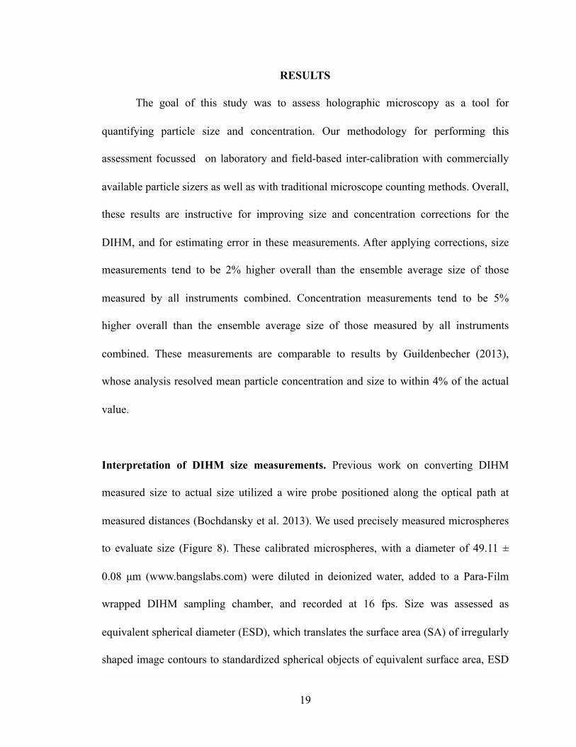
Interpretation of DIHM size measurements. Previous work on converting DIHM

measured size to actual size utilized a wire probe positioned along the optical path at

measured distances (Bochdansky et al. 2013). We used precisely measured microspheres

to evaluate size (Figure 8). These calibrated microspheres, with a diameter of 49.11 ±

0.08 µm (www.bangslabs.com) were diluted in deionized water, added to a Para-Film

wrapped DIHM sampling chamber, and recorded at 16 fps. Size was assessed as

equivalent spherical diameter (ESD), which translates the surface area (SA) of irregularly

shaped image contours to standardized spherical objects of equivalent surface area, ESD

$19

= 2 × √(SA / π) . We found the measured size (Sm) was correlated to the actual size (Scorr,

mm) as an exponential function of the distance from the laser source (Dm, mm):

[Equation 1]

Interpretation of DIHM concentration measurements. We performed a series of

experiments to quantify the correlation between particle concentrations measured by the

DIHM, Imaging FlowCytobot, FlowCam, and manual microscope counts. Suspended

media, including microspheres, environmental samples, and cultures of Dunaliella

tertiolecta, Akashiwo sanguinea, and Prorocentrum micans were processed by each of

these systems and the concentration was estimated. Manual microscope counts followed

the inverted Utermöhl technique outlined by Lund (1958), and were completed on

samples preserved in either Lugol’s solution (Akashiwo sanguinea and Prorocentrum

micans) or 36% formaldehyde solution (Dunaliella tertiolecta, environmental samples).

Sample preservation occurred rapidly after collection to avoid excess growth. Multiple

runs and counts on each sample provided statistical confidence and means for uncertainty

quantification.

However, in order to achieve a concentration estimate from the DIHM, the true

‘volume’ of water that the DIHM sees, needed to be quantified. This proved to be a non-

trivial problem, since for homogeneously mixed media, the probability distribution of

particle detection (for a given XYZ position) is non-uniform as a function of distance

from the laser (Figure 7) and radial position (Figure 8a,b). Qualitative similarity between

$20

Scorr = 0.121*Sm *Dm0.763

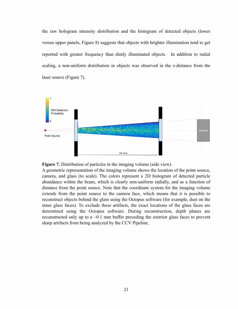
the raw hologram intensity distribution and the histogram of detected objects (lower

versus upper panels, Figure 8) suggests that objects with brighter illumination tend to get

reported with greater frequency than dimly illuminated objects. In addition to radial

scaling, a non-uniform distribution in objects was observed in the z-distance from the

laser source (Figure 7).

$ Figure 7. Distribution of particles in the imaging volume (side view). A geometric representation of the imaging volume shows the location of the point source, camera, and glass (to scale). The colors represent a 2D histogram of detected particle abundance within the beam, which is clearly non-uniform radially, and as a function of distance from the point source. Note that the coordinate system for the imaging volume extends from the point source to the camera face, which means that it is possible to reconstruct objects behind the glass using the Octopus software (for example, dust on the inner glass faces). To exclude these artifacts, the exact locations of the glass faces are determined using the Octopus software. During reconstruction, depth planes are reconstructed only up to a ~0.1 mm buffer preceding the exterior glass faces to prevent sharp artifacts from being analyzed by the CCV Pipeline.

$21

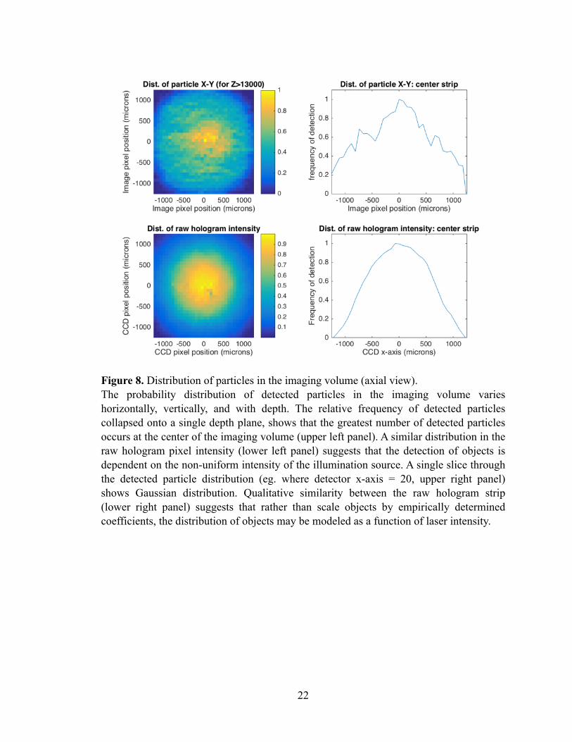
$Figure 8. Distribution of particles in the imaging volume (axial view). The probability distribution of detected particles in the imaging volume varies horizontally, vertically, and with depth. The relative frequency of detected particles collapsed onto a single depth plane, shows that the greatest number of detected particles occurs at the center of the imaging volume (upper left panel). A similar distribution in the raw hologram pixel intensity (lower left panel) suggests that the detection of objects is dependent on the non-uniform intensity of the illumination source. A single slice through the detected particle distribution (eg. where detector x-axis = 20, upper right panel) shows Gaussian distribution. Qualitative similarity between the raw hologram strip (lower right panel) suggests that rather than scale objects by empirically determined coefficients, the distribution of objects may be modeled as a function of laser intensity.

$22

�

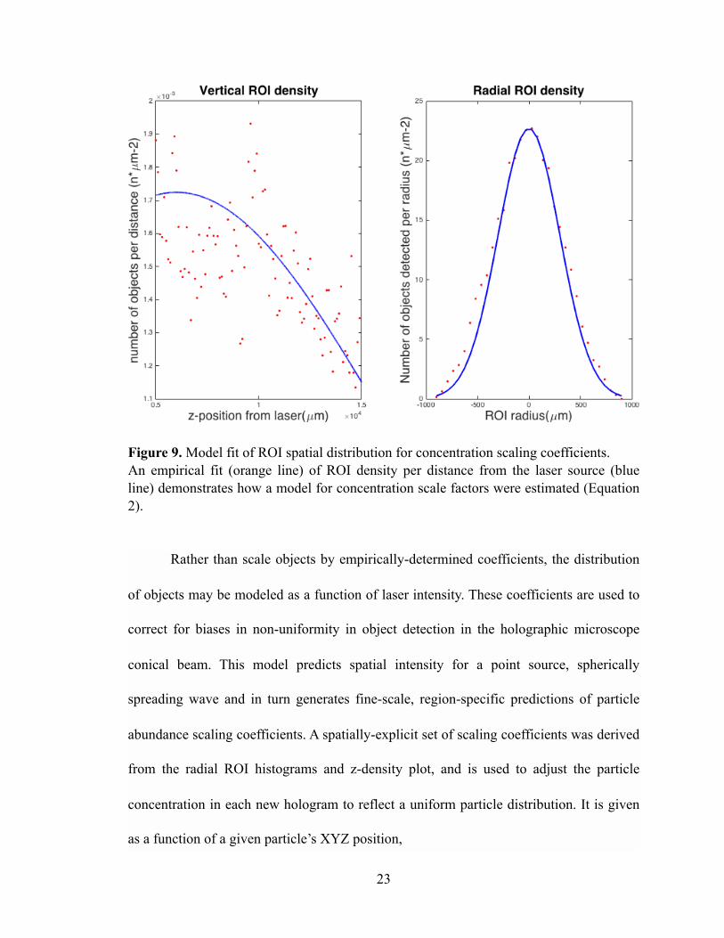
Figure 9. Model fit of ROI spatial distribution for concentration scaling coefficients. An empirical fit (orange line) of ROI density per distance from the laser source (blue line) demonstrates how a model for concentration scale factors were estimated (Equation 2).

Rather than scale objects by empirically-determined coefficients, the distribution

of objects may be modeled as a function of laser intensity. These coefficients are used to

correct for biases in non-uniformity in object detection in the holographic microscope

conical beam. This model predicts spatial intensity for a point source, spherically

spreading wave and in turn generates fine-scale, region-specific predictions of particle

abundance scaling coefficients. A spatially-explicit set of scaling coefficients was derived

from the radial ROI histograms and z-density plot, and is used to adjust the particle

concentration in each new hologram to reflect a uniform particle distribution. It is given

as a function of a given particle’s XYZ position,

$23

[Equation 2]

where the scaling coefficient C is a function of the distance from the laser source plane to

the particle (z) and the radial distance (r) from the source-to-camera axis. This distance z

is defined as the parallel offset plane, and r is the radial length from the source-camera

axis along this plane (r = √ (x2 + y2) ). The coefficients zo (8000 µm), γr (466 µm), and γz

(6400 µm) were determined by a best fit of these constituent distributions (Figure 9).

Size Estimates. Particle size was evaluated for 50 µm microsphere, Akashiwo sanguinea,

Prorocentrum micans, Dunaliella tertiolecta, and environmental samples. Overall, the

estimated ESD for the 50 µm microsphere by the DIHM, FC, and IFCB PSDs were

highly correlated, with the mean estimated size for all samples less than 2% of the actual

size. Although the correlation coefficient between all PSDs was a moderate 0.78, any

deficiency in this value is likely attributed to the variation in size-specific concentration,

which was high for the microspheres (see section below on Concentration Results). The

IFCB and DIHM showed the greatest similarity in size-specific concentration, with the

DIHM signal centered on the 50 µm bin, but of lower concentration.

Evaluation of size estimates for Microspheres.

The observed ESD measurements of microsphere increase as a function of

distance from the laser source for the DIHM (Figure 8). The measured size for each

object was normalized by the true size, as reported in the manufacturer supplied

C(x, y, z) = e−0.5 r

γ r

⎛⎝⎜

⎞⎠⎟

2

+ z−z°γ z

⎛⎝⎜

⎞⎠⎟

2⎛

⎝⎜⎜

⎞

⎠⎟⎟

$24

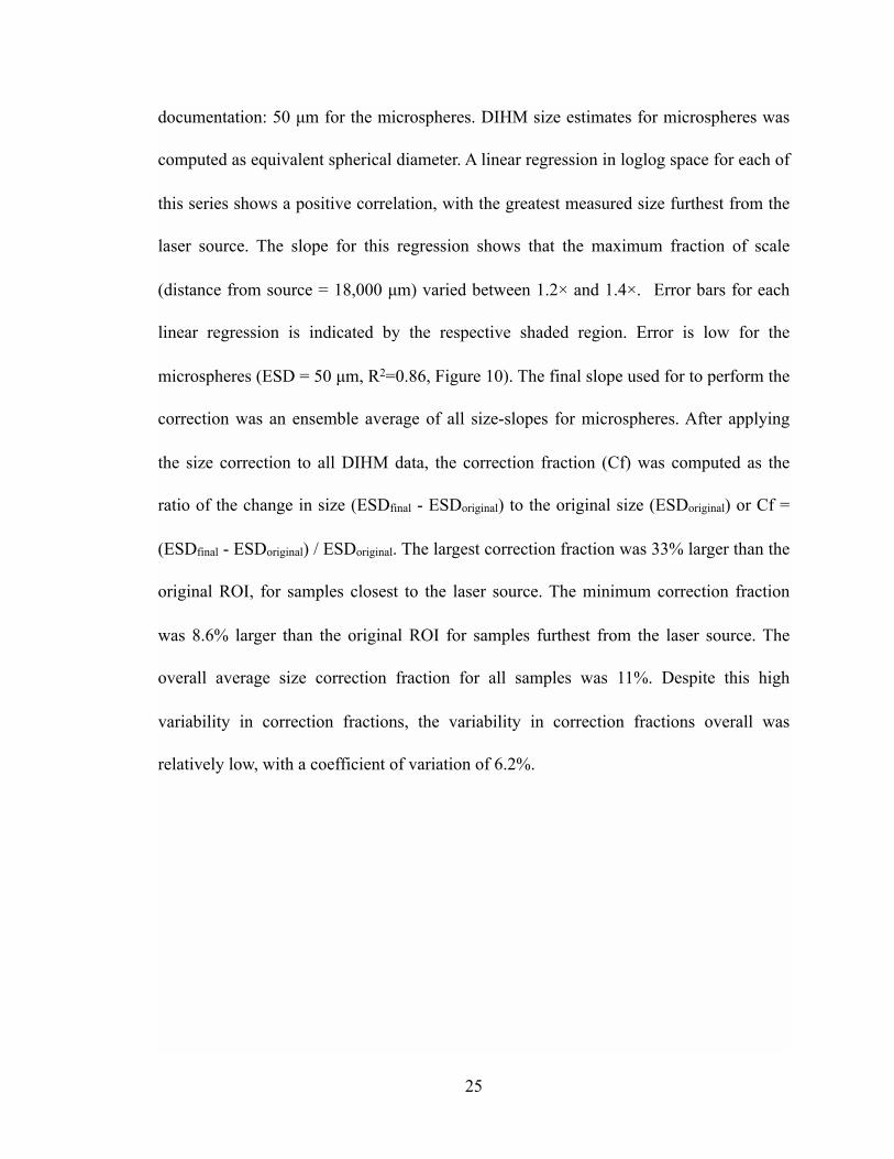
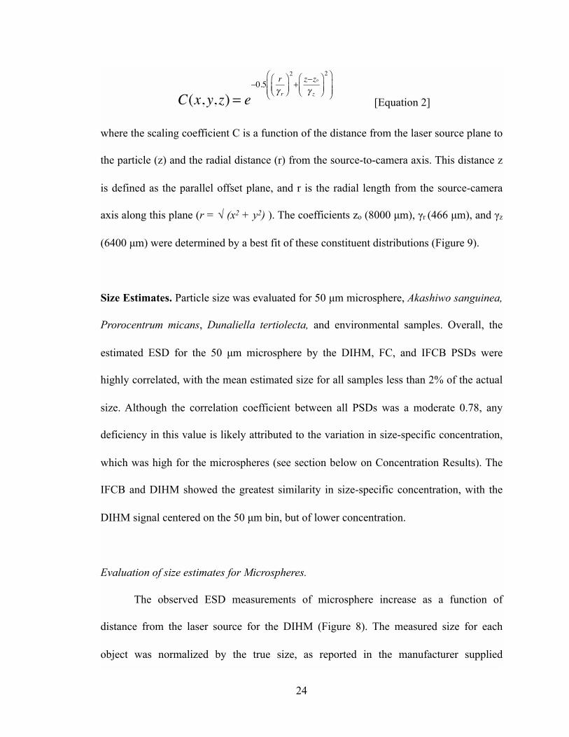
documentation: 50 µm for the microspheres. DIHM size estimates for microspheres was

computed as equivalent spherical diameter. A linear regression in loglog space for each of

this series shows a positive correlation, with the greatest measured size furthest from the

laser source. The slope for this regression shows that the maximum fraction of scale

(distance from source = 18,000 µm) varied between 1.2× and 1.4×. Error bars for each

linear regression is indicated by the respective shaded region. Error is low for the

microspheres (ESD = 50 µm, R2=0.86, Figure 10). The final slope used for to perform the

correction was an ensemble average of all size-slopes for microspheres. After applying

the size correction to all DIHM data, the correction fraction (Cf) was computed as the

ratio of the change in size (ESDfinal - ESDoriginal) to the original size (ESDoriginal) or Cf =

(ESDfinal - ESDoriginal) / ESDoriginal. The largest correction fraction was 33% larger than the

original ROI, for samples closest to the laser source. The minimum correction fraction

was 8.6% larger than the original ROI for samples furthest from the laser source. The

overall average size correction fraction for all samples was 11%. Despite this high

variability in correction fractions, the variability in correction fractions overall was

relatively low, with a coefficient of variation of 6.2%.

$25

$ Figure 10. LogLog Size correction coefficient determination. The observed (black dots) and modeled (blue dashed line) relationship between the measured 50 µm microsphere ESD and distance from the laser source. Blue shading represents the 95% confidence interval. The blue dashed line was used to model the true particle ESD as a function of observed particle ESD and distance from the source (Equation 1).

Evaluation of size estimates for field samples

The particle size distributions for the environmental samples show good

agreement according to both a linear fit (Figure 11) and correlation analysis between size-

bin specific measurements. The overall correlation coefficient for the DIHM Niskin PSD

and the averaged FC and DIHM PSDs was very high at 0.99. The size ranges captured for

each instrument for the environmental samples was 10 - 108 µm for the DIHM, 10 to 181

$26

µm for the IFCB, and 10 to 107 µm for the FC. ROI less than 10 µm were observed, but

filtered out for the sake of inter-comparison with the DIHM, which showed significant

numbers of artifacts in this size range. The best results for inter-comparison was attained

by avoiding the region specific scaling coefficients. This is notable, considering the

important role these scaling coefficients played in accurate concentration estimates for

the laboratory monocultures and microspheres. See Discussion section for additional

details on interpreting this result.

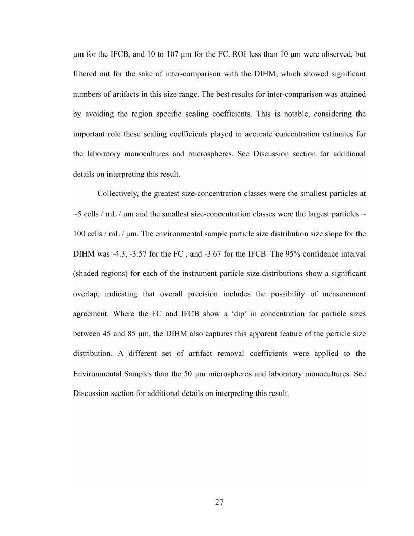
Collectively, the greatest size-concentration classes were the smallest particles at

~5 cells / mL / µm and the smallest size-concentration classes were the largest particles ~

100 cells / mL / µm. The environmental sample particle size distribution size slope for the

DIHM was -4.3, -3.57 for the FC , and -3.67 for the IFCB. The 95% confidence interval

(shaded regions) for each of the instrument particle size distributions show a significant

overlap, indicating that overall precision includes the possibility of measurement

agreement. Where the FC and IFCB show a ‘dip’ in concentration for particle sizes

between 45 and 85 µm, the DIHM also captures this apparent feature of the particle size

distribution. A different set of artifact removal coefficients were applied to the

Environmental Samples than the 50 µm microspheres and laboratory monocultures. See

Discussion section for additional details on interpreting this result.

$27

$ Figure 11. Environmental Sample Particle Size Distribution Intercomparison. Particle size distributions of Niskin bottles from the North Pacific for the DIHM (blue), FlowCam (red), and Imaging FlowCytobot (yellow) show good correlation.

Evaluation of size estimates for the laboratory-based experiments (cultures and beads)

After applying some corrections (see the following section), the particle size

distributions for the laboratory-based experiments (Figure 12) show reasonable

agreement according to two metrics: the correlation coefficients and coefficients of

variation. The correlation coefficient (CC) provides a quantitative measure of dependency

or relatedness of two random variables. It is computed from the covariance of the

variables divided by the product of the standard deviations. A correlation coefficient of

CC = 1 suggests complete linear relation between two vectors, and CC = 0 suggests no

$28

correlation. The average correlation coefficient between the DIHM particle size

distribution and averaged FC and IFCB PSDs was 0.82. A second metric called the

coefficient of variation (CV) provides a measure of relative variability or “broadness” of

a given particle size distribution for particles of uniform size. Here, a large CV is reflects

highly variable size measurements and a narrow CV indicates highly consistent size

measurements. CV is computed as the ratio of the standard deviation (σ) to the mean

(mu), CV = σ/µ. Overall, the size reported by the DIHM was 81% of the ensemble

average of the FC and IFCB. The overall coefficient of variation for the DIHM for all

measurements was 24%, compared with 19% for the FC and 15% for the IFCB,

suggesting that the DIHM measured a broader range of sizes. Explanations for this

pattern are explored in the Discussion section.

$29

$

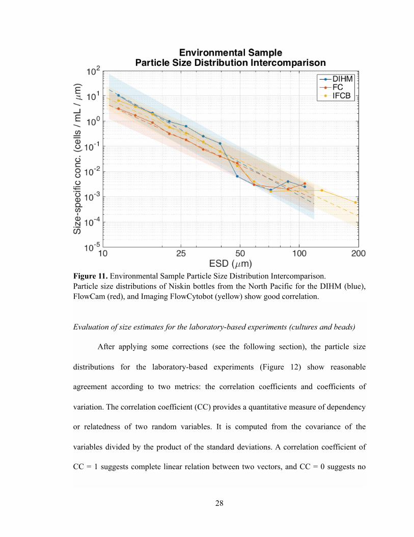
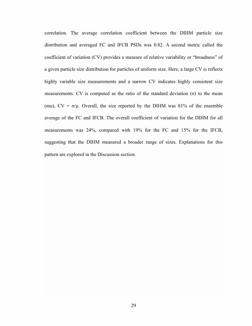
Figure 12. Summary of size inter-comparison results. Particle size distributions (PSD) after artifact-filtering for 50 µm microspheres, Dunaliella tertiolecta, Akashiwo sanguinea, and Prorocentrum micans for the DIHM (blue), Imaging FlowCytobot (red), and FlowCam (yellow). The dashed green line shows the weighted average of the artifact-filtered particle size distributions. Note that the y-axis limit is fixed for the Dunaliella tertiolecta, Akashiwo sanguinea, and Prorocentrum micans concentrations, but the y-axis limit is not fixed for the beads to show greater detail for the calibration object PSD.

$30

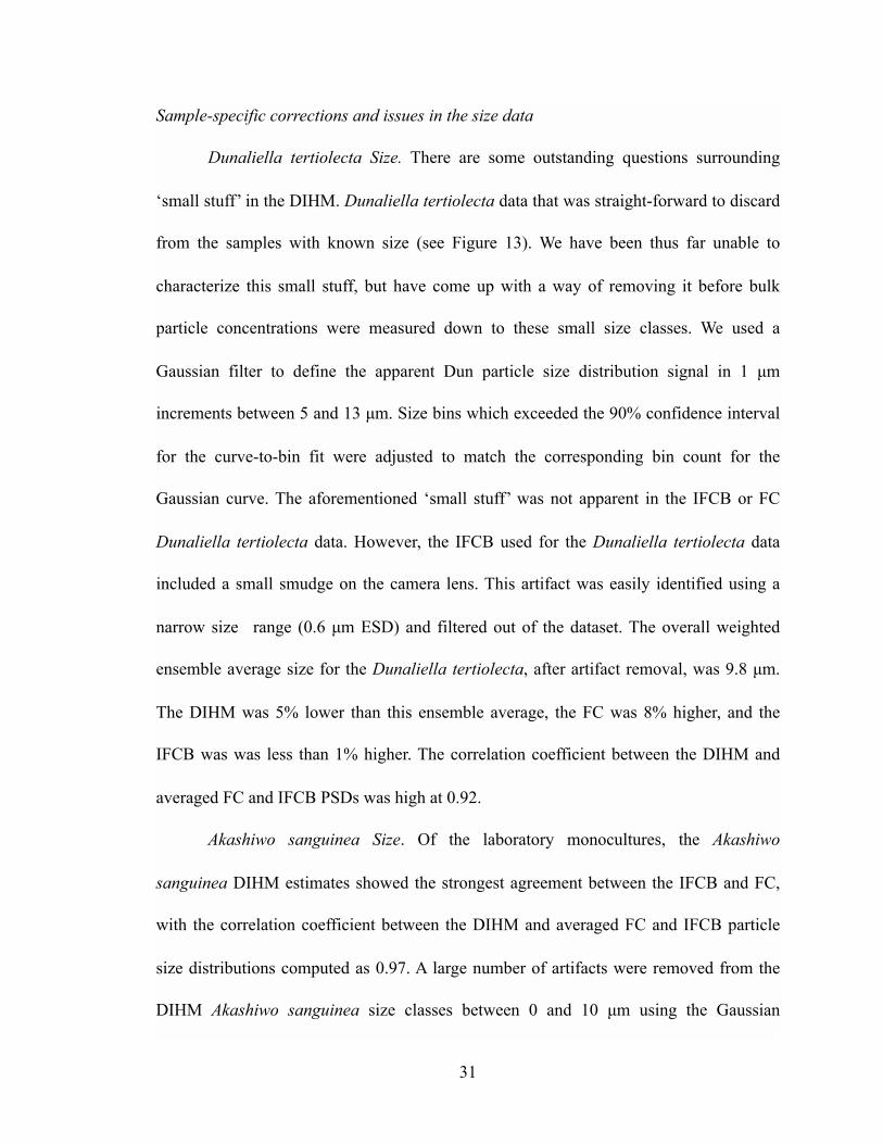
Sample-specific corrections and issues in the size data

Dunaliella tertiolecta Size. There are some outstanding questions surrounding

‘small stuff’ in the DIHM. Dunaliella tertiolecta data that was straight-forward to discard

from the samples with known size (see Figure 13). We have been thus far unable to

characterize this small stuff, but have come up with a way of removing it before bulk

particle concentrations were measured down to these small size classes. We used a

Gaussian filter to define the apparent Dun particle size distribution signal in 1 µm

increments between 5 and 13 µm. Size bins which exceeded the 90% confidence interval

for the curve-to-bin fit were adjusted to match the corresponding bin count for the

Gaussian curve. The aforementioned ‘small stuff’ was not apparent in the IFCB or FC

Dunaliella tertiolecta data. However, the IFCB used for the Dunaliella tertiolecta data

included a small smudge on the camera lens. This artifact was easily identified using a

narrow size range (0.6 µm ESD) and filtered out of the dataset. The overall weighted

ensemble average size for the Dunaliella tertiolecta, after artifact removal, was 9.8 µm.

The DIHM was 5% lower than this ensemble average, the FC was 8% higher, and the

IFCB was was less than 1% higher. The correlation coefficient between the DIHM and

averaged FC and IFCB PSDs was high at 0.92.

Akashiwo sanguinea Size. Of the laboratory monocultures, the Akashiwo

sanguinea DIHM estimates showed the strongest agreement between the IFCB and FC,

with the correlation coefficient between the DIHM and averaged FC and IFCB particle

size distributions computed as 0.97. A large number of artifacts were removed from the

DIHM Akashiwo sanguinea size classes between 0 and 10 µm using the Gaussian

$31

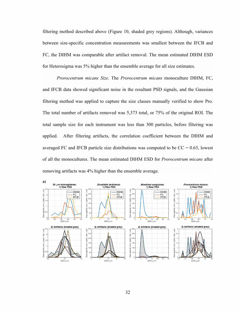
filtering method described above (Figure 10, shaded grey regions). Although, variances

between size-specific concentration measurements was smallest between the IFCB and

FC, the DIHM was comparable after artifact removal. The mean estimated DIHM ESD

for Heterosigma was 5% higher than the ensemble average for all size estimates.

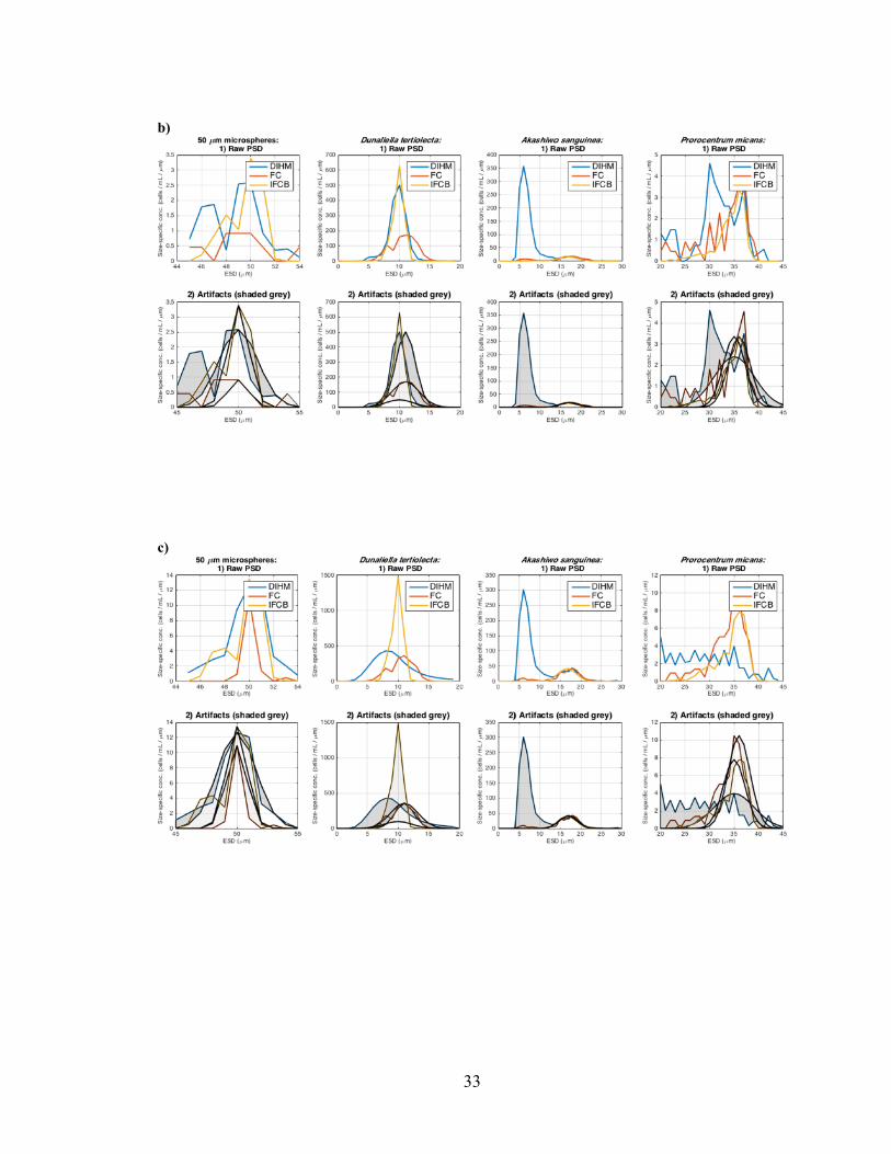
Prorocentrum micans Size. The Prorocentrum micans monoculture DIHM, FC,

and IFCB data showed significant noise in the resultant PSD signals, and the Gaussian

filtering method was applied to capture the size classes manually verified to show Pro.

The total number of artifacts removed was 5,373 total, or 75% of the original ROI. The

total sample size for each instrument was less than 300 particles, before filtering was

applied. After filtering artifacts, the correlation coefficient between the DIHM and

averaged FC and IFCB particle size distributions was computed to be CC = 0.63, lowest

of all the monocultures. The mean estimated DIHM ESD for Prorocentrum micans after

removing artifacts was 4% higher than the ensemble average.

a)

$

$32

b)

$

c)

$

$33

d)

$

e)

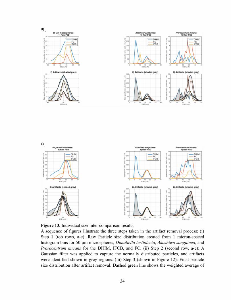
$ Figure 13. Individual size inter-comparison results. A sequence of figures illustrate the three steps taken in the artifact removal process: (i) Step 1 (top rows, a-e): Raw Particle size distribution created from 1 micron-spaced histogram bins for 50 µm microspheres, Dunaliella tertiolecta, Akashiwo sanguinea, and Prorocentrum micans for the DIHM, IFCB, and FC. (ii) Step 2 (second row, a-e): A Gaussian filter was applied to capture the normally distributed particles, and artifacts were identified shown in grey regions. (iii) Step 3 (shown in Figure 12): Final particle size distribution after artifact removal. Dashed green line shows the weighted average of

$34

the artifact-filtered particle size distributions. Each particle PSD shows the sample of highest concentration solution for each sample. For example, the microsphere results here are those from the highest concentration microsphere. a) Concentration 1, all samples b) Concentration 2, all samples c) Concentration 3, all samples d) concentration 4, for all samples except Dunaliella tertiolecta which did not have five concentrations e) concentration 5, for all samples except Dunaliella tertiolecta which did not have five concentrations.

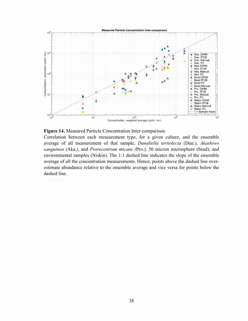
Concentration Estimates. DIHM concentration measurements for Akashiwo sanguinea,

Dunaliella tertiolecta, Prorocentrum micans, microspheres and environmental samples

followed a strong linear trend when compared to the ensemble average of all

measurements (Figure 14). The overall correlation of the DIHM concentration estimates

for all samples, for all methods (the manual counts, IFCB and FC) showed relatively

good agreement (CC = 0.69) despite relatively high variance (CV = 58.7%). The DIHM

tended to underestimate sample concentration for low concentration samples (less than

100 particles/mL), and tended to overestimate sample concentration for high

concentration samples (greater than 100 particles/mL). The greatest agreement in for all

samples were in intermediate sample concentrations, between 40 and 500 particles/mL.

Of all the measurement methods, the IFCB showed the highest overall correlation with

the DIHM measurements (CC = 0.57) compared to the FC (CC = 0.49) and the manual

counts (CC = 0.22). The IFCB and FC also showed considerably high correlation (CC =

0.76), as one might expect for two instruments similar in measurement mechanisms,

suggesting that the inter-comparability of the DIHM and IFCB (two instruments of

dissimilar measurement mechanisms) approaches the theoretical limit of relatedness.

$35

The concentration correction algorithm on average scaled particle densities by

2.3× (after artifact removal), where the minimum particle multiplier was 1× (applied to

46%) and the maximum multiplier was 7× (applied to fewer than 3% of all samples). Half

(50%) of all samples scaled by 2×. Overall, there was moderate variation in the scaling

factor applied (CV =72%) suggesting particle detection positions were variable.

Microsphere Concentration. The DIHM concentration estimates of the 50 µm

microspheres showed high correlation with the ensemble average of the manual counts,

IFCB and FC (CC = 0.90). Overall, the DIHM microsphere concentration estimates were

3% less than the ensemble average of all measurements. Sample sizes (n) for the

microsphere concentration sizes were notably low for the FC, with n=7 for Concentration

1 and n < 100 for all FC microsphere sample runs. Sample sizes for the DIHM and IFCB

were moderately improved, with 50 < n < 1000 for each instrument.

Dunaliella tertiolecta Concentration. The DIHM concentration estimates for

Dunaliella tertiolecta are overall 30% higher than the ensemble average, with relatively

high correlation (CC = 0.72). Sample sizes for the Dunaliella tertiolecta were higher than

all other instruments combined, with n > 5000 for all instruments.

Akashiwo sanguinea Concentration. The DIHM concentration estimates of the

Akashiwo sanguinea showed high correlation with the ensemble average of the manual

counts, IFCB and FC (CC = 0.94). These results follow strong correlation in the

Akashiwo sanguinea PSD, highlighting the strong inter-comparability for the Akashiwo

sanguinea samples overall. The DIHM Akashiwo sanguinea concentration estimates were

5% less than the ensemble average of all measurements.

$36

Environmental Sample Concentration. The DIHM concentration estimates of the

Environmental Samples showed the highest correlation with the ensemble average of the

manual counts, IFCB and FC (CC = 1.00). No Gaussian Filter was applied to the

Environmental sample Particle Size distribution, and a different set of artifact filters were

applied as noted in the Methods section. It is notable that the internal consistency of the

concentration estimates for each method are follow a relatively similar pattern, with each

depth sample (surface, deep chlorophyll maxima, and mixed layer depth) all showing

similar patterns in relationship.

Prorocentrum micans Concentration. The DIHM concentration estimates of the

Prorocentrum micans showed moderate correlation with the ensemble average of the

manual counts, IFCB and FC (CC = 0.66). The overall DIHM concentration estimates for

Prorocentrum micans were 39% less than the ensemble average of all measurements. It is

notable that the manual counting methods estimated the concentration as significantly

higher than the IFCB (by more than an order of magnitude), however the estimates from

the DIHM generally fall between these two extremes.

$37

$

Figure 14. Measured Particle Concentration Inter-comparison. Correlation between each measurement type, for a given culture, and the ensemble average of all measurement of that sample, Dunaliella tertiolecta (Dun.), Akashiwo sanguinea (Aka.), and Prorocentrum micans (Pro.), 50 micron microsphere (bead), and environmental samples (Niskin). The 1:1 dashed line indicates the slope of the ensemble average of all the concentration measurements. Hence, points above the dashed line over-estimate abundance relative to the ensemble average and vice versa for points below the dashed line.

$38

DISCUSSION

These series of experiments provide new insight into the inter-comparability of

quantitive particle size and concentration statistics observed by the IFCB, FC, traditional

microscope counts, and with the DIHM. Previous quantitive particle inter-comparison

analysis for the DIHM compared results with the Malvern Mastersizer 2000

(Guildenbecher et al. 2013). Here we have also made suggestions for correcting biases in

the observed DIHM size and concentration. We have attempted to provide broad

coverage in the parameters of particle density, shape, size, and use cell cultures and

environmental samples to assist in quantitative evaluation of populations in the laboratory

and field. However, significant challenges remain - particularly with respect to our

primary tool the DIHM. We did not find a universal correction for the various particles

types observed, and so applying these corrections to field samples remains elusive. In the

following paragraphs we discuss the sources of error and uncertainty within the DIHM

size and concentration measurements, and despite the challenges of applying these to

field measurements, we conclude with some recommended best practices for

interpretation.

DIHM Error. We have observed that illumination of the imaging volume has an impact

on the detection of objects and also the recorded size of objects, so the nature of the

interaction of the source illumination and particles merits some discussion. As light

intensity attenuates both radially and axially, objects at the periphery of the ROI detection

volume will receive less illumination than those objects closer to the closer to the central

$39

axis. Dimly illuminated objects will tend to be detected less frequently by the ROI

detection algorithm, which uses changes in pixel intensity to detect object edges. This

effect was previously described as a “shadow density” problem by Malek (2004). Hence,

detected object concentration changes as a function of light intensity. In addition,

geometric properties of the source-particle light interaction and the laser pinhole

geometry will also bias concentration measurements. The diffracted light patterns, upon

which the holographic reconstruction depends, tend to magnify across space.

The diffraction patterns cast by objects that are closer to the illumination source

will spread with greater distance on the camera face than those patterns cast by objects

close to the camera face. These far-traveling diffraction patterns can lead to information

loss from wave spreading (referred to here as the ‘antenna problem’). As diffraction

patterns propagate away from the object, some of this information will inevitably

propagate outside the camera viewing area. Thus we suspect that reconstructed objects

near the edges of the hologram experience a degraded image quality. Overall, we find that

there is a trade-off between optimal illumination and the geometric position of the object

in the illumination volume. Although the DIHM is capable of focussing many more focal

planes than a traditional microscope, there still exists a ‘sweet spot’ for maximum image

quality and size range detectable. The presence of degraded object detection regions can

be problematic for statistical calculations of particle concentration. We have attempted to

resolve this issue by scaling observations AFTER the object detection algorithm has

inadvertently removed this data. However, to account for the presence of these optimal

and non-optimal detection regions, future object detection algorithms might consider a

$40

region-specific weighted approach to ranking and saving contour scores BEFORE objects

are saved/discarded. For all these reasons, how the geometry of the imaging volume

biases measurements of larger size class objects merits discussion, but for the purposes of

this paper is out of scope.

Interpreting DIHM Data. The size corrections provided here are relevant to holographic

systems with point source illumination. The concentration corrections provided here may

be relevant to systems with both point source and columnated illumination (as in Katz et

al. 1999). These corrections were developed primarily in a laboratory setting with the

intent that they will improve the accuracy and precision of field-recorded data. This step,

essential for data interpretation, may introduce bias as laboratory monocultures are not

representative of field-recorded, mixed communities. Field-recorded data includes

particles of mixed shape and size, variable light field (which may affect image contrast),

and variable levels of dissolved media in the water (that impacts image quality). For this

reason, we have also included an inter-comparison of field recorded, environmental

samples collected via Niskin bottles.

Preferential Particle Orientation and Observed Size

Different particle sizing instruments have different systems for collecting images,

and these differences can directly affect the measured particle size. For the FlowCam and

Imaging FlowCytobot, which utilize laminar flow from a sheath fluid to fix the imaging

focal length, a trend in orientation was observed which tended to align the major axis in

$41

the direction of flow (Figure 15). This preferential orientation could lead to differences in

the measured size of the Dunaliella tertiolecta with these instruments and the DIHM. The

laboratory setup of the DIHM, for which the imaging fluid is closed, is likely to orient

objects randomly. The observed size for the DIHM hence followed a somewhat broader

range than for the IFCB. Practically speaking, this high variance in the DIHM size

measurements may be an informative measure for heterogeneous assessment of object

width and height. In other words, higher variance in the DIHM measurements may

provide more 3D insight into the object of interest.

$42

$

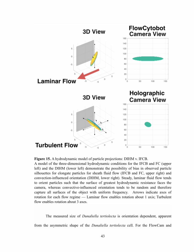
Figure 15. A hydrodynamic model of particle projections: DIHM v. IFCB. A model of the three-dimensional hydrodynamic conditions for the IFCB and FC (upper left) and the DIHM (lower left) demonstrate the possibility of bias in observed particle silhouettes for elongate particles for sheath fluid flow (IFCB and FC, upper right) and convection-influenced orientation (DIHM, lower right). Steady, laminar fluid flow tends to orient particles such that the surface of greatest hydrodynamic resistance faces the camera, whereas convective-influenced orientation tends to be random and therefore capture all surfaces of the object with uniform frequency. Arrows indicate axes of rotation for each flow regime — Laminar flow enables rotation about 1 axis; Turbulent flow enables rotation about 3 axes.

The measured size of Dunaliella tertiolecta is orientation dependent, apparent

from the asymmetric shape of the Dunaliella tertiolecta cell. For the FlowCam and

$43

Imaging FlowCytobot, which utilize laminar flow from a sheath fluid to fix the imaging

focal length, a trend in orientation was observed which tended to align the major axis in

the direction of flow. This preferential orientation likely led to bias in the measured size

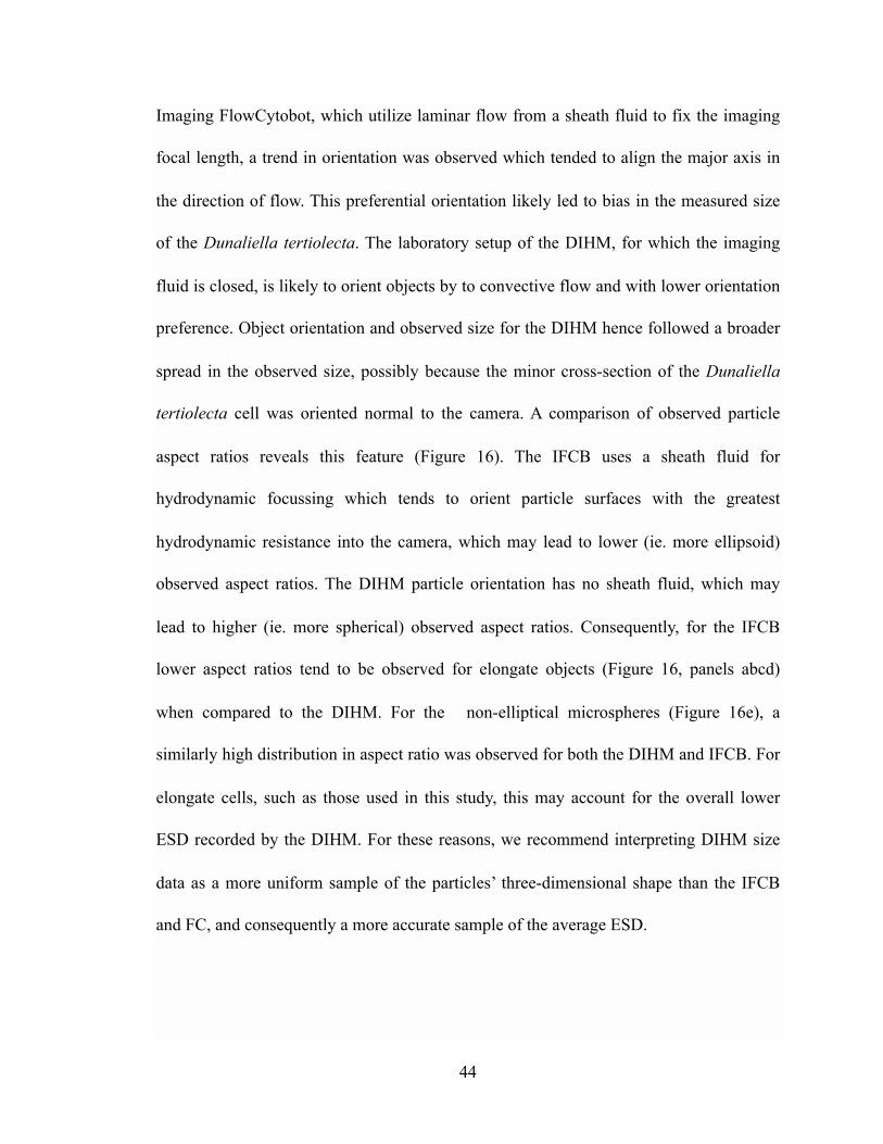
of the Dunaliella tertiolecta. The laboratory setup of the DIHM, for which the imaging

fluid is closed, is likely to orient objects by to convective flow and with lower orientation

preference. Object orientation and observed size for the DIHM hence followed a broader

spread in the observed size, possibly because the minor cross-section of the Dunaliella

tertiolecta cell was oriented normal to the camera. A comparison of observed particle

aspect ratios reveals this feature (Figure 16). The IFCB uses a sheath fluid for

hydrodynamic focussing which tends to orient particle surfaces with the greatest

hydrodynamic resistance into the camera, which may lead to lower (ie. more ellipsoid)

observed aspect ratios. The DIHM particle orientation has no sheath fluid, which may

lead to higher (ie. more spherical) observed aspect ratios. Consequently, for the IFCB

lower aspect ratios tend to be observed for elongate objects (Figure 16, panels abcd)

when compared to the DIHM. For the non-elliptical microspheres (Figure 16e), a

similarly high distribution in aspect ratio was observed for both the DIHM and IFCB. For

elongate cells, such as those used in this study, this may account for the overall lower

ESD recorded by the DIHM. For these reasons, we recommend interpreting DIHM size

data as a more uniform sample of the particles’ three-dimensional shape than the IFCB

and FC, and consequently a more accurate sample of the average ESD.

$44

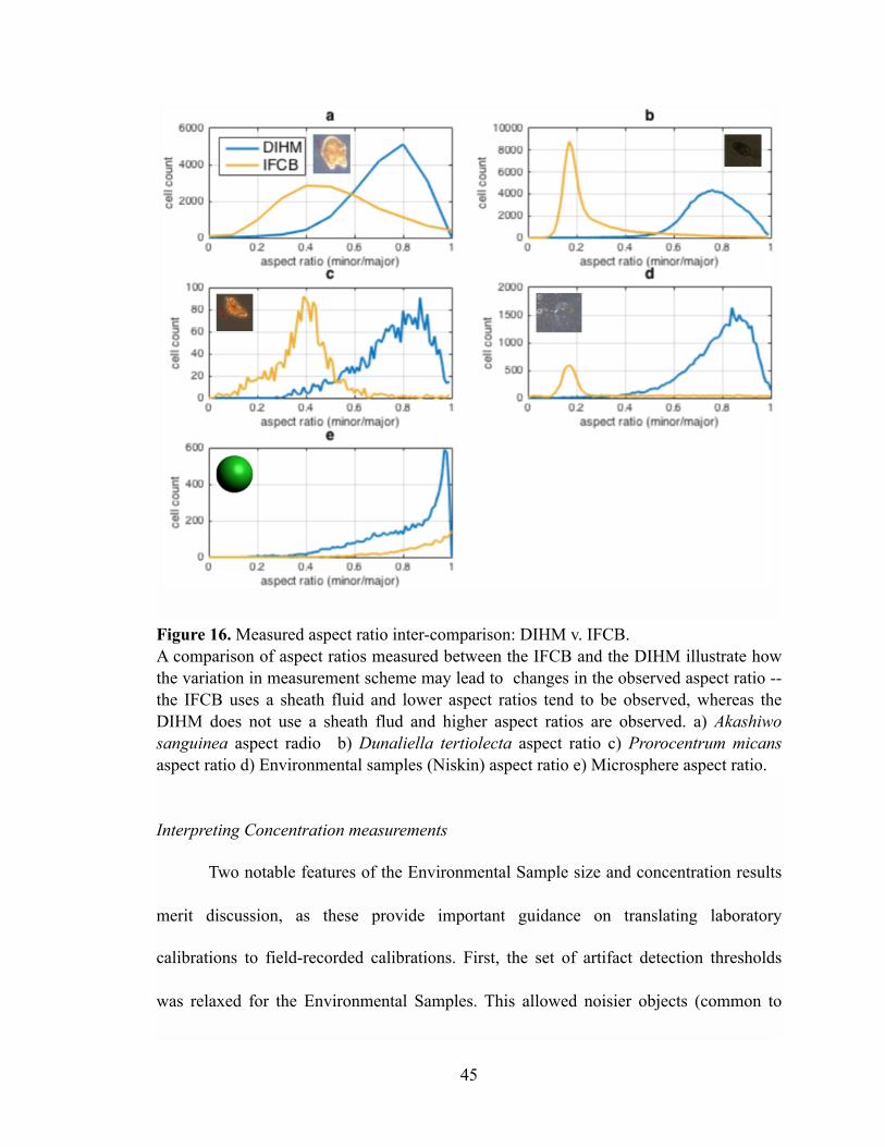
$ Figure 16. Measured aspect ratio inter-comparison: DIHM v. IFCB. A comparison of aspect ratios measured between the IFCB and the DIHM illustrate how the variation in measurement scheme may lead to changes in the observed aspect ratio --the IFCB uses a sheath fluid and lower aspect ratios tend to be observed, whereas the DIHM does not use a sheath flud and higher aspect ratios are observed. a) Akashiwo sanguinea aspect radio b) Dunaliella tertiolecta aspect ratio c) Prorocentrum micans aspect ratio d) Environmental samples (Niskin) aspect ratio e) Microsphere aspect ratio.

Interpreting Concentration measurements

Two notable features of the Environmental Sample size and concentration results

merit discussion, as these provide important guidance on translating laboratory

calibrations to field-recorded calibrations. First, the set of artifact detection thresholds

was relaxed for the Environmental Samples. This allowed noisier objects (common to

$45

larger particles) to be included in the analysis. Given the variability in size and shape for

the Environmental Samples, this resulted ultimately in better comparison with the FC and

IFCB. We recommend refining these thresholds for environmental samples, and also

improving image contouring techniques for best results. Second, the best results for the

Environmental Sample size inter-comparison between the FC and IFCB and FC were

obtained by omitting the region-specific particle abundance scaling step. This is a notable

result, considering these scaling coefficients were determined based on many

observations of laboratory monocultures. The results analyzed here are from three depths

from a single CTD cast. We recommend further data collection and analysis on a variety

of environmental samples to determine the extent to which region-specific scaling

coefficients impact concentration accuracy estimates.

Overall, it bears mentioning that enumeration of exact particle abundances and

fluid volumes for the laboratory monocultures and microspheres, for the definition of

exact sample concentrations, was prohibitive. Hence, the ideal metric of inter-comparison

the ratio of observed concentration to the exact, true concentration for each sample was

unknown. Therefore, we must resort to other metrics to evaluate which particle sizers

provide the best estimation of concentration. Strong agreement between two or more

measurements for a given sample may indicate convergence on true concentration

measurement, but not necessarily. For this reason, we interpret measurement agreement

as predictive of how relative concentrations of a given particle type would be observed.

An inter-comparison of measurement precision between sample runs provides insight into

reliability and variability. However, it should be noted that variability estimation requires

$46

uniform distribution of the suspended particles in the sample media. The DIHM acquires

samples directly from the water column, as opposed to the IFCB and FC which sample

using in intake pump. This difference in sampling scheme creates challenges in inter-

comparison, as these mechanisms bias samples in district hydrodynamic ways. For these

reasons, we recommend interpreting the DIHM concentration measurements as consistent

with IFCB and FC measurements, but not to be used interchangeably. Furthermore, we

recommend a side-by-side time-series field deployment (eg. IFCB deployed next to the

DIHM) to be completed before using the respective measurements interchangeably.

Interpreting size and concentration measurements of living cells

Although best efforts were taken to run samples in rapid succession, this was not

always feasible. Time delays of up to 12 hours between instruments sample runs likely

provided time for the living cells to grow and divide, or die. For this reason,

photosynthetic cultures not being processed immediately were stored in light-opaque

bottles to attempt to arrest growth. Cells to be processed by manual counts were

preserved using Lugol’s solution, however this preservation can cause cell shrinking or

swelling (Booth 1987; Menden-Deuer et al. 2001) and impact size estimation. Dead cells

and other detritus may have also played a role in biasing measurements. We recommend

some additional analysis and quantification of the organism-specific growth and mortality

rates to further close the error gap between the different instruments.

$47

Interpreting measurement variability

Efforts were taken to avoid spatial sample partitioning via gravitational settling

through resuspension of particles by stirring samples in between runs. However,

especially for low density samples, “patchiness” in particle distribution was inevitable.

This patchiness may account for some of the variance in the observed concentrations. The

remaining variability between instrument concentration measurements is ascribed to the

overall biases of the methods including, but not limited to, intake pump flow rates,

triggering mechanisms, flow-cell flow rates, and others. Buoyant or swimming of cells

may also have impacted fractionation in the sampling volume. Efforts were taken to

optimize the instrument settings for each individual culture. Flow cell re-alignment and

focussing in-between dilution runs was avoided. Finally, an ensemble average of all

measurements, where each component is weighted by sample size and variability,

provides a final metric to which concentration estimates from the DIHM can be assessed.

For these reasons, we recommend interpreting the results of this experiment as having

reasonable variability.

$48

CONCLUSION

Here we have developed a methodology for estimating marine particle size and

concentration using the DIHM, designed and executed a series of experiments to validate

these methods, and assessed the performance of these instrument inter-comparisons. We

have shown that these methods enable statistical accuracy with less than 5% error for

both size and concentration. These methods apply to both laboratory monocultures and

mixed-community environmental samples.

Although the direct application of this knowledge is in interpreting field-recorded

DIHM data, we’re hopeful that the utility of this application will extend beyond this

calibration. Preliminary comparison of particle aspect ratios with the IFCB (Figure 16)

suggest that the DIHM provides a truer representation of particle three-dimensionality.

Where the IFCB biases measurements along the surface of greatest hydrodynamic

resistance, the DIHM orients particles randomly and can sample all surfaces uniformly.

Additional analysis of these orientations and their corresponding camera silhouette,

compared to non-random orientations, may yield improved insights about particle bio-

volume estimation from the DIHM. For example, algorithms have been developed which

reconstruct a three-dimensional object mass from the set of its two dimension line

projections (Penczek 2010). Oceanographers are keen on improving these three-

dimensional estimates (see Saccà 2017) which, for example, can lead to improved

insights about carbon to volume relationships (Menden-Deuer et al. 2001). With

additional analysis, I’m hopeful that these results may provide new insights about

biogeochemical cycling and phytoplankton ecology.

$49

BIBLIOGRAPHY

Alldredge, A. L., T. J. Cowles, S. MacIntyre, and others. 2002. Occurrence and

mechanisms of formation of a dramatic thin layer of marine snow in a shallow

Pacific fjord. Marine Ecology Progress Series 233: 1–12. doi:10.3354/

meps233001

Bochdansky, A. B., M. A. Clouse, and G. J. Herndl. 2016. Dragon kings of the deep sea:

marine particles deviate markedly from the common number-size spectrum.

Scientific Reports 6. doi:10.1038/srep22633

Bochdansky, A. B., M. H. Jericho, and G. J. Herndl. 2013. Development and deployment

of a point-source digital inline holographic microscope for the study of plankton

and particles to a depth of 6000 m. Limnology and Oceanography: Methods 11:

28–40. doi:10.4319/lom.2013.11.28

Booth, B. C. 1987. The Use of Autofluorescence for Analyzing Oceanic Phytoplankton

Communities. Botanica Marina 30: 101–108. doi:10.1515/botm.1987.30.2.101

Boss, E., L. Guidi, M. J. Richardson, L. Stemmann, W. Gardner, J. K. B. Bishop, R. F.

Anderson, and R. M. Sherrell. 2015. Optical techniques for remote and in-situ

characterization of particles pertinent to GEOTRACES. Progress in

Oceanography 133: 43–54. doi:10.1016/j.pocean.2014.09.007

Cavender-Bares, K. K., A. Rinaldo, and S. W. Chisholm. 2001. Microbial size spectra

from natural and nutrient enriched ecosystems. Limnology and Oceanography 46:

778–789. doi:10.4319/lo.2001.46.4.0778

$50

Davis, C. S., F. T. Thwaites, S. M. Gallager, and Q. Hu. 2005. A three-axis fast-tow

digital Video Plankton Recorder for rapid surveys of plankton taxa and

hydrography. Limnology and Oceanography: Methods 3: 59–74. doi:10.4319/lom.

2005.3.59

Gao, J., D. R. Guildenbecher, L. Engvall, P. L. Reu, and J. Chen. 2014. Refinement of

particle detection by the hybrid method in digital in-line holography. Applied

Optics, AO 53: G130–G138. doi:10.1364/AO.53.00G130

Garcia-Sucerquia, J., W. Xu, S. K. Jericho, P. Klages, M. H. Jericho, and H. J. Kreuzer.

2006. Digital in-line holographic microscopy. Applied Optics, AO 45: 836–850.

doi:10.1364/AO.45.000836

Groen, F. C., I. T. Young, and G. Ligthart. 1985. A comparison of different focus

functions for use in autofocus algorithms. Cytometry 6: 81–91. doi:10.1002/cyto.

990060202

Guidi, L., S. Chaffron, L. Bittner, and others. 2016. Plankton networks driving carbon

export in the oligotrophic ocean. Nature 532: 465–470. doi:10.1038/nature16942

Guildenbecher, D. R., J. Gao, P. L. Reu, and J. Chen. 2013. Digital holography

simulations and experiments to quantify the accuracy of 3D particle location and

2D sizing using a proposed hybrid method. Applied Optics, AO 52: 3790–3801.

doi:10.1364/AO.52.003790

Gutkowska, A., E. Paturej, and E. Kowalska. 2012. Qualitative and quantitative methods

for sampling zooplankton in shallow coastal estuaries. Ecohydrology &

Hydrobiology 12: 253–263. doi:10.1016/S1642-3593(12)70208-2

$51

Hunter-Cevera, K. R., M. G. Neubert, R. J. Olson, A. R. Solow, A. Shalapyonok, and H.

M. Sosik. 2016. Physiological and ecological drivers of early spring blooms of a

coastal phytoplankter. Science 354: 326–329. doi:10.1126/science.aaf8536

Karentz, D., and T. J. Smayda. 1998. Temporal patterns and variations in phytoplankton

community organization and abundance in Narragansett Bay during 1959–1980.

Journal of Plankton Research 20: 145–168. doi:10.1093/plankt/20.1.145

Karp-Boss, L., L. Azevedo, and E. Boss. 2007. LISST-100 measurements of

phytoplankton size distribution: evaluation of the effects of cell shape. Limnology

and Oceanography: Methods 5: 396–406. doi:10.4319/lom.2007.5.396

Katz, J., P. L. Donaghay, J. Zhang, S. King, and K. Russell. 1999. Submersible

holocamera for detection of particle characteristics and motions in the ocean.

Deep Sea Research Part I: Oceanographic Research Papers 46: 1455–1481. doi:

10.1016/S0967-0637(99)00011-4

Lund, J. W. G., C. Kipling, and E. D. L. Cren. 1958. The inverted microscope method of

estimating algal numbers and the statistical basis of estimations by counting.

Hydrobiologia 11: 143–170. doi:10.1007/BF00007865

Malek, M., D. Allano, S. Coëtmellec, and D. Lebrun. 2004. Digital in-line holography:

influence of the shadow density on particle field extraction. Optics Express, OE

12: 2270–2279. doi:10.1364/OPEX.12.002270

Mallahi, A. E., and F. Dubois. 2013. Separation of overlapped particles in digital

holographic microscopy. Optics Express, OE 21: 6466–6479. doi:10.1364/OE.

21.006466

$52

Menden-Deuer, S., and E. J. Lessard. 2000. Carbon to volume relationships for

dinoflagellates, diatoms, and other protist plankton. Limnology and

Oceanography 45: 569–579. doi:10.4319/lo.2000.45.3.0569

Menden-Deuer, S., E. J. Lessard, and J. Satterberg. 2001. Effect of preservation on

dinoflagellate and diatom cell volume and consequences for carbon biomass

predictions. Marine Ecology Progress Series 222: 41–50. doi:10.3354/

meps222041

Olson, R. J., and H. M. Sosik. 2007. A submersible imaging-in-flow instrument to

analyze nano-and microplankton: Imaging FlowCytobot. Limnology and

Oceanography: Methods 5: 195–203. doi:10.4319/lom.2007.5.195

Penczek, P. A. 2010. Fundamentals of three-dimensional reconstruction from projections.

Methods Enzymology 482: 1–33. doi:10.1016/S0076-6879(10)82001-4

Picheral, M., L. Guidi, L. Stemmann, D. M. Karl, G. Iddaoud, and G. Gorsky. 2010. The

Underwater Vision Profiler 5: An advanced instrument for high spatial resolution

studies of particle size spectra and zooplankton. Limnology and Oceanography:

Methods 8: 462–473. doi:10.4319/lom.2010.8.462

Saccà, A. 2017. Methods for the estimation of the biovolume of microorganisms: A

critical review. Limnology and Oceanography: Methods 15: 337–348. doi:

10.1002/lom3.10162

Schnars, U., and W. Jüptner. 2005. Digital Holography: Digital Hologram Recording,

Numerical Reconstruction, and Related Techniques, Springer-Verlag.

$53

Sieracki, C. K., M. E. Sieracki, and C. S. Yentsch. 1998. An imaging-in-flow system for

automated analysis of marine microplankton. Marine Ecology Progress Series

285–296.

Steinberg, M. K., M. R. First, E. J. Lemieux, and others. 2012. Comparison of techniques

used to count single-celled viable phytoplankton. Journal of Applied Phycology

24: 751–758. doi:10.1007/s10811-011-9694-z

Warner, A. J., and G. C. Hays. 1994. Sampling by the continuous plankton recorder

survey. Progress in Oceanography 34: 237–256. doi:

10.1016/0079-6611(94)90011-6

White, A. E., R. M. Letelier, A. L. Whitmire, B. Barone, R. R. Bidigare, M. J. Church,

and D. M. Karl. 2015. Phenology of particle size distributions and primary

productivity in the North Pacific subtropical gyre (Station ALOHA): PARTICLE

SIZE IN THE NPSG. Journal of Geophysical Research: Oceans 120: 7381–7399.

doi:10.1002/2015JC010897

Xu, W., M. H. Jericho, I. A. Meinertzhagen, and H. J. Kreuzer. 2002. Digital in-line

holography of microspheres. Applied Optics, AO 41: 5367–5375. doi:10.1364/

AO.41.005367

Zetsche, E.-M., A. E. Mallahi, F. Dubois, C. Yourassowsky, J. C. Kromkamp, and F. J. R.

Meysman. 2014. Imaging-in-Flow: Digital holographic microscopy as a novel

tool to detect and classify nanoplanktonic organisms. Limnology and

Oceanography: Methods 12: 757–775. doi:10.4319/lom.2014.12.757

$54