digital holographic interferometry for radiation dosimetry
TRANSCRIPT
Department of Physics and Astronomy, University of Canterbury,Private Bag 4800, Christchurch, New Zealand
Digital Holographic Interferometry
for Radiation Dosimetry
Alicia Cavan
BSc(Hons)
A thesis submitted in partial fulfillment
of the requirements for the degree
of Doctor of Philosophy
March 2014
Supervisors: Assoc. Prof. Juergen Meyerand Assoc. Prof. Jon-Paul Wells

Abstract
A novel optical calorimetry approach is proposed for the dosimetry of therapeutic radiation,based on the optical technique of Digital Holographic Interferometry (DHI). This detectordetermines the radiation absorbed dose to water by measurement of the refractive index vari-ations arising from radiation induced temperature increases. The output consists of a timeseries of high resolution, two dimensional images of the spatial distribution of the projecteddose map across the water sample. This absorbed dose to water is measured directly, inde-pendently of radiation type, dose rate and energy, and without perturbation of the beam.These are key features which make DHI a promising technique for radiation dosimetry.
A prototype DHI detector was developed, with the aim of providing proof-of-principle of theapproach. The detector consists of an optical laser interferometer based on a lensless Fouriertransform digital holography (LFTDH) system, and the associated mathematical reconstruc-tion of the absorbed dose. The conceptual basis was introduced, and a full framework wasestablished for the measurement and analysis of the results. Methods were developed formathematical correction of the distortions introduced by heat diffusion within the system.Pilot studies of the dosimetry of a high dose rate Ir-192 brachytherapy source and a smallfield proton beam were conducted in order to investigate the dosimetric potential of the tech-nique. Results were validated against independent models of the expected radiation dosedistributions.
Initial measurements of absorbed dose demonstrated the ability of the DHI detector to resolvethe minuscule temperature changes produced by radiation in water to within experimentaluncertainty. Spatial resolution of approximately 0.03 mm/pixel was achieved, and the dosedistribution around the brachytherapy source was accurately measured for short irradiationtimes, to within the experimental uncertainty. The experimental noise for the prototypedetector was relatively large and combined with the occurrence of heat diffusion, means thatthe method is predominantly suitable for high dose rate applications.
The initial proof-of-principle results confirm that DHI dosimetry is a promising technique,with a range of potential benefits. Further development of the technique is warranted, toimprove on the limitations of the current prototype. A comprehensive analysis of the systemwas conducted to determine key requirements for future development of the DHI detectorto be a useful contribution to the dosimetric toolbox of a range of current and emerging ap-plications. The sources of measurement uncertainty are considered, and methods suggestedto mitigate these. Improvement of the signal-to-noise ratio, and further development of theheat transport corrections for high dose gradient regions are key areas of focus highlightedfor future development.

ii

Acknowledgements
I really can’t thank my supervisor Dr. Juergen Meyer enough. Firstly for the initial conver-sation many years ago which sparked my interest in medical physics, and then for everythingelse I have learnt from you about how to be a scientist and how to write about science (anyexcessive parenthesising or lack of conciseness in this thesis are my natural tendencies whichhe hasn’t quite managed to completely eradicate). Thank you for the continued discus-sions, planning, advice, reviewing, emailing and skyping, and for moving halfway around theworld to a facility with convenient access to a proton beam which I could test my detector on.
To my other supervisor Dr. Jon-Paul Wells for taking on a medical physics student andteaching me about optics. Thank you for the advice readily provided whenever I needed it,and for dealing with all the acronyms that a medical physics thesis inevitably includes. Also,thank you to Dr. Richard Watts for supervision at the start of my research and helping withthe initial development of the detector.
Thank you to the technical and support staff in the University of Canterbury Departmentof Physics and Astronomy - in particular, Graeme Kershaw for always being happy to buildme test cells and other components for the detector, Dr. Bob Hurst for advice and opticsideas and Dr. Orlon Peterson for rescuing me from computer illiteracy.
Love and thanks to Juergen’s family - Louise, Finn, Zoe and Pia for looking after me whileI visited Seattle and joined your family for extended periods of time.
A world of thanks to my partner Gert-Jan for looking after, pep-talking, feeding, listeningto and loving me throughout. Thank you to my mum Jillian, for diligently reading throughcountless pages of a topic you know nothing about, to catch all my misspellings of neccessaryand occurence. To both mum and dad, Sean, for everything! Thank you also to the rest ofmy friends and family who have been there for me, for your encouragement and for carefullynot asking me about my progress for the last 18 months.
Thank you to the Medical Physics and Bioengineering Department at the Canterbury Dis-trict Health Board for taking me on as a Registrar and allowing me the extra time requiredto complete my PhD concurrently. The experience that I gained in all aspects of radiationoncology physics has been invaluable for my research, and I also appreciate the financialsupport received to attend conferences and the access to the brachytherapy source.
Thank you very much to the team at the University of Washington Medical Centre SmallField Proton Facility for allowing me access to the beam line, and providing a wealth oftechnical support and experience. In particular, thank you to George Sandison, Eric Ford,Rob Emery and Steven Steininger.
I am grateful for financial support I have received allowing me to present my work at inter-national conferences, and travel to Seattle for proton beam experiments. Thank you to theRoyal Society of New Zealand Canterbury Branch for a travel scholarship, Universities NewZealand for a Claude McCarthy Fellowship, and the University of Canterbury Departmentof Physics and Astronomy for travel assistance.
iii

iv
Contents
Abstract i
Acknowledgements iii
1 Motivation 1
1.1 Introduction . . . . . . . . . . . . . . . . . . . . . . . . . . . . . . . . . . . . 1
1.2 Research Questions . . . . . . . . . . . . . . . . . . . . . . . . . . . . . . . 4
1.3 Outline of Thesis . . . . . . . . . . . . . . . . . . . . . . . . . . . . . . . . . 5
2 Introduction to Dosimetry 7
2.1 Principles of Radiation Dosimetry . . . . . . . . . . . . . . . . . . . . . . . . 7
2.1.1 Radiation Therapy . . . . . . . . . . . . . . . . . . . . . . . . . . . . 7
2.1.2 Radiation Dosimetry . . . . . . . . . . . . . . . . . . . . . . . . . . . 10
2.1.3 Properties of Dosimeters . . . . . . . . . . . . . . . . . . . . . . . . . 12
2.2 Calorimetry . . . . . . . . . . . . . . . . . . . . . . . . . . . . . . . . . . . . 15
2.3 Dosimetry for Specialised Radiation Therapy Approaches . . . . . . . . . . . 17
2.3.1 High Dose Rate Brachytherapy . . . . . . . . . . . . . . . . . . . . . 17
2.3.2 Proton Therapy . . . . . . . . . . . . . . . . . . . . . . . . . . . . . 27
2.3.3 Microbeam Radiation Therapy . . . . . . . . . . . . . . . . . . . . . 43
2.4 Concluding Remarks . . . . . . . . . . . . . . . . . . . . . . . . . . . . . . . 49
3 Principles of Digital Holographic Interferometry 51
3.1 Fundamental Concept of Optical Calorimetry . . . . . . . . . . . . . . . . . 51
3.2 Optical Interferometry . . . . . . . . . . . . . . . . . . . . . . . . . . . . . . 52
3.2.1 Basic Optics Principles . . . . . . . . . . . . . . . . . . . . . . . . . 52
3.3 Refractive Index Determination in Liquids . . . . . . . . . . . . . . . . . . . 57
3.3.1 Holographic Interferometry . . . . . . . . . . . . . . . . . . . . . . . . 58
3.3.2 Digital Holographic Interferometry . . . . . . . . . . . . . . . . . . . 60
3.3.3 Experimental Configurations . . . . . . . . . . . . . . . . . . . . . . 61
3.4 Historical Development of Interferometry for Radiation Dosimetry . . . . . . 69
3.4.1 Early Holographic Interferometry Studies . . . . . . . . . . . . . . . 69
3.5 Concluding Remarks . . . . . . . . . . . . . . . . . . . . . . . . . . . . . . . 75
iii
4 DHI Dosimeter 77
4.1 Design Considerations . . . . . . . . . . . . . . . . . . . . . . . . . . . . . . 77
4.2 Lensless Fourier Transform Digital Holography . . . . . . . . . . . . . . . . . 81
4.3 Prototype Detector . . . . . . . . . . . . . . . . . . . . . . . . . . . . . . . . 84
4.3.1 System Components . . . . . . . . . . . . . . . . . . . . . . . . . . . 84
4.3.2 Image Reconstruction and Dose Determination . . . . . . . . . . . . 89
4.3.3 Experimental Process . . . . . . . . . . . . . . . . . . . . . . . . . . 99
4.3.4 Graphical User Interface Design . . . . . . . . . . . . . . . . . . . . 104
4.4 Detector Progression and Characterisation . . . . . . . . . . . . . . . . . . . 106
4.4.1 Initial Holographic Interferometer . . . . . . . . . . . . . . . . . . . . 107
4.4.2 Non-Radiation Induced Heating Patterns . . . . . . . . . . . . . . . . 111
4.4.3 Absolute Temperature Measurements . . . . . . . . . . . . . . . . . 116
4.4.4 Fibre Optic Approach . . . . . . . . . . . . . . . . . . . . . . . . . . 120
4.5 Concluding Remarks . . . . . . . . . . . . . . . . . . . . . . . . . . . . . . . 122
5 Heat Transfer Modelling 125
5.1 Introduction to Heat Transfer . . . . . . . . . . . . . . . . . . . . . . . . . . 125
5.2 Heat Diffusion . . . . . . . . . . . . . . . . . . . . . . . . . . . . . . . . . . . 126
5.2.1 General Model of Heat Diffusion . . . . . . . . . . . . . . . . . . . . 127
5.2.2 Numerical Modelling . . . . . . . . . . . . . . . . . . . . . . . . . . . 133
5.2.3 Expansion to Multiple Dimensions . . . . . . . . . . . . . . . . . . . 136
5.3 Method 1: Forward Modelling . . . . . . . . . . . . . . . . . . . . . . . . . . 137
5.3.1 Application to Radiation Dose Distributions . . . . . . . . . . . . . . 140
5.3.2 Efficacy of the Method . . . . . . . . . . . . . . . . . . . . . . . . . . 151
5.4 Method 2: Quasi-Inverse Modelling . . . . . . . . . . . . . . . . . . . . . . . 151
5.4.1 Description of Approach . . . . . . . . . . . . . . . . . . . . . . . . . 152
5.4.2 Implementation of the Abel Transform . . . . . . . . . . . . . . . . . 153
5.4.3 Implementation of Method 2 . . . . . . . . . . . . . . . . . . . . . . . 155
5.4.4 Efficacy of Method . . . . . . . . . . . . . . . . . . . . . . . . . . . . 157
5.5 Concluding Remarks . . . . . . . . . . . . . . . . . . . . . . . . . . . . . . . 161
6 HDR Brachytherapy Source Measurements 163
6.1 Methods . . . . . . . . . . . . . . . . . . . . . . . . . . . . . . . . . . . . . . 163
6.1.1 Measurement . . . . . . . . . . . . . . . . . . . . . . . . . . . . . . . 163
6.1.2 Analysis . . . . . . . . . . . . . . . . . . . . . . . . . . . . . . . . . . 166
6.2 Results . . . . . . . . . . . . . . . . . . . . . . . . . . . . . . . . . . . . . . . 174
6.2.1 Pixel Size Calibration . . . . . . . . . . . . . . . . . . . . . . . . . . 176
6.2.2 Raw Data and Noise Filtering . . . . . . . . . . . . . . . . . . . . . . 176
6.2.3 Detector Sensitivity and Dosimetric Uncertainty . . . . . . . . . . . 178
6.2.4 Direct Comparison to BrachyVision Data . . . . . . . . . . . . . . . 183
6.2.5 Comparison via Radial Dose Function . . . . . . . . . . . . . . . . . 198
iv
6.2.6 Gamma Index Evaluation . . . . . . . . . . . . . . . . . . . . . . . . 199
6.3 Discussion . . . . . . . . . . . . . . . . . . . . . . . . . . . . . . . . . . . . 200
6.3.1 Potential for Contribution to HDR Brachytherapy Dosimetry . . . . 202
6.4 Concluding Remarks . . . . . . . . . . . . . . . . . . . . . . . . . . . . . . . 203
7 Proton Beam Measurements 205
7.1 Methods . . . . . . . . . . . . . . . . . . . . . . . . . . . . . . . . . . . . . . 205
7.1.1 Measurement . . . . . . . . . . . . . . . . . . . . . . . . . . . . . . . 205
7.1.2 Analysis . . . . . . . . . . . . . . . . . . . . . . . . . . . . . . . . . . 210
7.2 Results . . . . . . . . . . . . . . . . . . . . . . . . . . . . . . . . . . . . . . 215
7.2.1 Uncertainty Quantification and Image Post-Processing . . . . . . . . 215
7.2.2 Consistency of Image Series . . . . . . . . . . . . . . . . . . . . . . . 219
7.2.3 Analysis of DHI results . . . . . . . . . . . . . . . . . . . . . . . . . . 222
7.3 Discussion . . . . . . . . . . . . . . . . . . . . . . . . . . . . . . . . . . . . . 224
7.3.1 Beam Settings . . . . . . . . . . . . . . . . . . . . . . . . . . . . . . . 224
7.3.2 Monte Carlo Model . . . . . . . . . . . . . . . . . . . . . . . . . . . . 225
7.3.3 Detector Dosimetric Sensitivity . . . . . . . . . . . . . . . . . . . . . 226
7.3.4 Detector Sensitive Region . . . . . . . . . . . . . . . . . . . . . . . . 227
7.3.5 Experimental Process . . . . . . . . . . . . . . . . . . . . . . . . . . . 228
7.4 Concluding Remarks . . . . . . . . . . . . . . . . . . . . . . . . . . . . . . . 229
8 Discussion 231
8.1 Proof-of-principle Results . . . . . . . . . . . . . . . . . . . . . . . . . . . . . 231
8.1.1 Achievements . . . . . . . . . . . . . . . . . . . . . . . . . . . . . . . 232
8.1.2 Limitations . . . . . . . . . . . . . . . . . . . . . . . . . . . . . . . . 233
8.2 Impact of Heat Transport . . . . . . . . . . . . . . . . . . . . . . . . . . . . 234
8.2.1 Evaluation of Heat Diffusion Model . . . . . . . . . . . . . . . . . . 235
8.2.2 Consideration of Heat Convection . . . . . . . . . . . . . . . . . . . 239
8.2.3 Experimental Validation of Heat Transport Models . . . . . . . . . . 242
8.3 Analysis of Uncertainty Budget and Evaluation Metrics . . . . . . . . . . . 242
8.3.1 Positional Uncertainty . . . . . . . . . . . . . . . . . . . . . . . . . . 244
8.3.2 Dosimetric Uncertainty . . . . . . . . . . . . . . . . . . . . . . . . . . 245
8.3.3 Use of the Abel Transform . . . . . . . . . . . . . . . . . . . . . . . 249
8.3.4 Gamma Index as an Evaluation Metric . . . . . . . . . . . . . . . . . 251
8.4 Recommendations for Experimental Improvements . . . . . . . . . . . . . . 254
8.4.1 Independence from Ambient Conditions . . . . . . . . . . . . . . . . 254
8.4.2 Sensitivity Improvements . . . . . . . . . . . . . . . . . . . . . . . . . 259
8.4.3 Absolute Dosimetry . . . . . . . . . . . . . . . . . . . . . . . . . . . 265
8.4.4 Spatial Resolution and Sensitive Region Size . . . . . . . . . . . . . 266
8.4.5 Experimental Process . . . . . . . . . . . . . . . . . . . . . . . . . . 266
8.5 Considerations for Extension to Tomographic Acquisition . . . . . . . . . . 267
v
8.5.1 Tomography at Limited Projection Angles . . . . . . . . . . . . . . . 269
8.5.2 Tomography by Interferometer Rotation . . . . . . . . . . . . . . . . 272
8.5.3 Additional Considerations . . . . . . . . . . . . . . . . . . . . . . . . 273
8.6 Considerations for DHI Application to MRT Dosimetry . . . . . . . . . . . . 274
8.7 Other Proposed Future Applications . . . . . . . . . . . . . . . . . . . . . . 277
8.8 Concluding Remarks . . . . . . . . . . . . . . . . . . . . . . . . . . . . . . . 281
9 Conclusions 283
9.1 Review of Research Questions . . . . . . . . . . . . . . . . . . . . . . . . . . 284
9.1.1 Research Question One . . . . . . . . . . . . . . . . . . . . . . . . . . 284
9.1.2 Research Question Two . . . . . . . . . . . . . . . . . . . . . . . . . 284
9.1.3 Research Question Three . . . . . . . . . . . . . . . . . . . . . . . . . 285
9.1.4 Research Question Four . . . . . . . . . . . . . . . . . . . . . . . . . 287
Bibliography 289
A List of Abbreviations 317
B MATLAB Code 321
B.1 Graphical User Interface for Image Reconstruction . . . . . . . . . . . . . . 322
B.2 Heat Diffusion Calculations . . . . . . . . . . . . . . . . . . . . . . . . . . . 349
C Publications 355
C.1 Refereed Paper . . . . . . . . . . . . . . . . . . . . . . . . . . . . . . . . . . 355
C.2 Conference Proceedings . . . . . . . . . . . . . . . . . . . . . . . . . . . . . . 355
vi
Chapter 1
Motivation
1.1 Introduction
Cancer is one of the leading causes of death in New Zealand, with the disease responsible
for some 8,593 deaths in 2010 (29% of total deaths) [1, 2]. The total number of new cancer
registrations was 21,235 in 2010 [2]; with population growth and an ageing population these
numbers are set to increase in coming years [3]. The average survival rate across all types
of cancer five years after diagnosis was 63% in 2009 [4]. Radiation therapy, also referred to
as radiotherapy, is a treatment approach which uses ionising radiation to kill cancer cells.
It is one of the most effective and widely used tools for fighting cancer. In New Zealand
about 50% of people diagnosed with cancer receive radiotherapy treatment, with the choice
of treatment dependent on the type and stage of cancer [5, 6].
Radiation therapy exploits the biological effect of high energy ionising radiation on tissues
to preferentially destroy cancerous cells within a target volume in the body. This volume
consists of the tumour plus surrounding treatment margins to account for such influences as
microscopic tumour invasion, set-up error and motion during or between treatment fractions.
A radiotherapy treatment can be delivered with curative, known as radical, or palliative in-
tent. This choice affects how aggressively the cancer is treated, in order to balance the chance
of a cure with the quality of remaining life for terminally ill patients [7]. The paradox with
radiotherapy is that the ionising radiation which damages tumour cells is also damaging to
the healthy tissues surrounding them, and this causes the patient to experience various toxic
side effects. The acceptable dose to healthy tissue varies according to the critical morbidity
of the relevant tissues or organs, which depends on the response to radiation, called the
radiosensitivity of the tissue [8]. The aim of radiotherapy is to concentrate a lethal absorbed
dose of radiation to the tumour in order to optimise the probability of local tumour con-
trol, whilst minimising the dose received by the surrounding healthy tissue, to reduce the
1
incidence of complications. This goal is achieved by shaping the radiation dose to be as
conformal as possible to the shape of the tumour. Treatment is usually conducted using
the techniques of external beam radiation therapy (EBRT) or brachytherapy [9]. EBRT is
performed with a linear accelerator, which produces high energy beams of electron or photon
radiation which are then shaped by external collimating devices. These shaped fields are
then delivered to the patient at multiple beam angles coincident on the tumour location.
Brachytherapy is the use of sealed radiation sources (radionuclides) which are placed either
permanently or temporarily inside the body, adjacent to or within the tumour location. Due
to local radiation/tissue interactions and the inverse square law, the dose to tissue decreases
with distance from the source. Treatments using either method are typically delivered as
an accumulation of several smaller fractions of the prescribed dose [10]. Modern EBRT is
geometrically accurate to within a few millimetres, and the prescribed dose can be delivered
to within ±5% [11]. However any improvements which can be made in either geometric
or dosimetric accuracy have been demonstrably shown to improve outcomes for patients;
thus this is a field of widespread active research. Modern day advances in radiation therapy
treatments have seen a trend towards increasing the conformity of the delivered dose to the
tumour volume, and a reduction in treatment margins to decrease the amount of normal
tissue irradiated. For EBRT this often involves more complex treatment plans where a frac-
tion consists of many fields of even smaller doses, a technique called intensity modulated
radiation therapy (IMRT) [12], or a technique using continuous dose deposition, known as
volumetric modulated arc therapy (VMAT) [13, 14] or hypo-fractionated stereotactic radio-
therapy (SRT) treatments [15]. This trend towards more complex treatments has led to a
corresponding requirement for further improvements in dose quantification and localisation.
Radiation dosimetry is the calculation of the absorbed dose to some medium, typically wa-
ter or tissue, resulting from exposure to indirectly and/or directly ionising radiation. When
ionising radiation is incident on a medium, the interactions of the radiation with the atoms
within the medium causes energy to be transferred to the medium by various mechanisms
including Compton scattering, pair-production, the photoelectric effect and Coulombic inter-
actions such as Bremsstrahlung production [9]. The extent to which each effect contributes
to the dose to a specific type of tissue is dependent on the initial energy and type of the inci-
dent radiation, as well as the tissue composition. The biological impact of the radiation dose
in tissue is predominantly by means of DNA strand breaks, resulting in cell damage and/or
death. This biological impact is directly related to the energy transferred from the incident
radiation to the medium [10]. Due to the difficulties in consistently and safely measuring
2
biological effects, especially in actual human tissue, water has been used as a surrogate refer-
ence medium which approximates the response of human tissue to radiation in a consistent
and reproducible way [16]. Therapeutic radiation doses are therefore calculated in terms of
their reference absorbed dose to water, in units of Gray (Gy), where:
1 Gy = 1 J kg−1 (1.1)
Accurate and consistent measurements of radiation dose are fundamental to ensure that ra-
diotherapy clinical trial and treatment outcomes are comparable worldwide. Clinical trials
and treatment outcomes are all based on a consistent scale of dose so that they can be ac-
curately compared. Primary standards laboratories located throughout the world determine
the absolute dose values and regular intercomparisons are performed between these centres.
One of the roles of these laboratories is to provide a calibration service, which ensures there
is a traceable link between the field detectors used for quality assurance of radiation doses
delivered in individual hospital clinics back to the primary standard. Variation in dose by
more than ±5% from prescribed values has been shown to have measurable detrimental
effects on treatment outcomes for patients [11]. Therefore sources of uncertainty in the cal-
ibration chain must be kept as low as possible in order to ensure that the final dose can
be measured to within ±5% of the prescription dose. There are many varied methods for
quantifying absorbed dose to water (discussed further in Section 2.1.2) each with their own
advantages, limitations and influences on the accuracies and uncertainties of the delivered
dose.
Existing dosimetry techniques provide adequate solutions for the dosimetric needs of most
conventional radiation therapy treatments that are widely and effectively used throughout
the world today. Limitations arise from factors external to the irradiation and dosimetry
process, which include individual variations between patients, imaging and tumour/organ-
at-risk contouring uncertainties, patient set-up errors and misdiagnoses. However there are a
number of emerging delivery techniques in radiotherapy that provide challenges which classi-
cal dosimetry techniques are not always able to fully overcome. These techniques range from
new treatment modalities such as proton beams or heavier ion beams [17,18] or synchrotron
generated microbeams [19, 20], to increased use of small fields as part of IMRT or SBRT
techniques [21–23], with each presenting its own specific set of dosimetric challenges. These
methodologies are in various stages of development, from early pre-clinical studies to clinical
trials to increasing implementation in clinics worldwide. There is also additional focus on the
expansion of conventional treatment techniques to non-traditional tumour types and loca-
tions. In order to advance these new techniques to their full potential, dosimetry techniques
3
need to advance at the same or greater rate. This includes both the refinement and devel-
opment of existing dosimetry solutions, as well as the development of new approaches. An
introduction to some of these therapeutic modalities is provided in more detail in Chapter 3,
along with a discussion of their dosimetric limitations and potential approaches to overcome
these.
The aim of the present research is to adapt an optical metrology technique known as Digital
Holographic Interferometry (DHI) for application to radiation dosimetry. The fundamental
concept of the technique is to infer the absorbed dose to water from a source of radiation,
by measurement of the temperature increase induced by the transfer of energy from the
radiation to the water. This concept is the basis for calorimetry which is a fundamental
means of measuring radiation dose (see Section 2.2). DHI is a widely applied technique
in many optics applications, but in particular the technique can be used to measure small
changes in physical parameters of a transparent medium, such as the refractive index. Thus
an optical calorimetry approach can be developed, measuring absorbed dose to water by
exploiting the fact that temperature increases in water cause a predictable variation in the
refractive index. A similar method was first applied to radiation dosimetry in the 1970’s
by Hussmann [24, 25], and then Miller [26, 27] and is described in Section 3.4.1. They used
an analogue method of holographic interferometry to measure radiation dose from electron
beams. Hussmann and Miller’s detectors were ultimately limited by the technology they had
available to them and were superseded by alternative detectors of their day. The advent of
modern digital technology and the subsequent advances in optical interferometry mean that
digital holographic interferometry may again become a viable and useful tool for dosimetry,
with several properties that make it a desirable technique.
1.2 Research Questions
Advances in radiation therapy delivery have resulted in current detector technology being
a limiting factor for some emerging therapeutic approaches [17, 21, 23, 28]. There is a clear
need for advances in detector technology, including investigation into new methods, in order
to develop detectors which overcome the shortfalls of existing techniques with regard to a
range of new therapeutic options. Dosimetric limitations of radiotherapy techniques depend
on the parameters required for safe and effective treatment. These parameters cover a
broad range and include spatial resolution, beam perturbation, lack of charged particle
equilibrium, variations in stopping power ratios, dynamic range and linearity of response.
With the application of modern technology to the previously redundant dosimetry technique
4
of holographic interferometry there is now the potential to make advances in dosimetry in
areas as diverse as proton therapy, high dose rate brachytherapy, and microbeam radiation
therapy. The potential advantages are manifold, as the technique has the ability to provide
high resolution absolute dose measurements of absorbed dose to water directly, overcoming
several limitations of present detectors. This research applies DHI techniques to the field of
radiation dosimetry in order to develop a novel radiation detector, with the aim of answering
the following research questions:
1. Can the optical technique of digital holographic interferometry be successfully applied
to radiation dosimetry?
2. Is it possible to develop a digital dosimeter based on the fundamental principles of
calorimetry that is capable of measuring dose with high two dimensional spatial reso-
lution?
3. Will the application of modern digital technology allow for dosimetric results which
advance the early achievements of Hussmann and Miller?
4. Is there a justification for further work to explore the potential for such a detector
to be used to overcome the dosimetric problems associated with emerging radiation
therapy techniques?
1.3 Outline of Thesis
The aim of this work is to develop a novel DHI dosimeter to address the above research ques-
tions. This incorporates work across a variety of subject areas, from optical interferometry,
radiation dosimetry and medical physics, to image processing and mathematical modelling.
This thesis is written at a level which will provide a comprehensive introduction to each
of these areas in terms of their relevance to DHI dosimetry, to allow for an understanding
of the subject by those with limited background in one or more of these fields. Chapter 2
provides an introduction to radiation therapy and dosimetry with the aim of providing a
justification for the development of a new detector. In particular, some of the developing
areas of radiation treatment approaches are introduced. Each has specific dosimetry require-
ments, and the ways in which a DHI detector may overcome existing dosimetry problems
is proposed. Chapter 3 introduces the principles of digital holographic interferometry as an
optical calorimetry technique and reviews the available literature regarding previous appli-
cations of interferometry to this field. Chapter 4 progresses through the development stages
of a DHI detector to describe the working prototype that was used for the remainder of this
5
research. This includes a discussion of the potentially advantageous characteristics of this
approach to dosimetry. Chapter 5 discusses the impact and modelling of heat transport, in
particular diffusion, which is a phenomenon which is critical to consider in order to obtain
accurate interpretation of DHI dosimetry results. Two different approaches are proposed
and implemented to account for this effect. Chapters 6 and 7 present the application of the
detector to radiation measurement of a high dose rate (HDR) brachytherapy source and a
proton therapy beam, respectively. Chapter 8 discusses the outcomes of the research, consid-
ering the effectiveness of DHI as a radiation detector. The various benefits and limitations
are summarised and comprehensive recommendations are given in regard to the direction
of further research. Consideration is given to the potential for DHI as a detector for areas
such as absolute dosimetry, microbeam radiation therapy (MRT) and interface dosimetry.
Chapter 9 concludes the work by revisiting the research questions posed in Section 1.2 to
determine the extent to which they have been achieved. A list of all abbreviations used is
included in Appendix A, whilst Appendix B contains the MATLAB code for key parts of
the process. Appendix C lists the publications arising from this work.
6
Chapter 2
Introduction to Dosimetry
In this chapter a framework of the particular dosimetric requirements of various modern
radiation therapy treatment modalities and the array of dosimetry tools that are presently
used to achieve these is established. In doing so, a justification for the development of a
DHI detector will be covered, by demonstrating that there is a space within this framework
for investigation into new dosimetry techniques. Finally the principles of calorimetry as a
dosimetry technique is introduced separately in more detail, as this will serve as the basis
for a DHI approach.
2.1 Principles of Radiation Dosimetry
2.1.1 Radiation Therapy
Radiation Physics
Radiation therapy utilises ionising radiation to preferentially destroy cancerous cells within
a target volume. Ionising radiation is composed of photons or particles which individually
have enough kinetic energy to liberate an electron from an atom or molecule, thereby ion-
ising it. In cells, the interaction of the subsequent free radicals with the cells nucleic acids
(DNA) can result in DNA strand breaks which can ultimately lead to cell death. Ionising
radiation comprises two categories of particles: directly and indirectly ionising, depending on
their ionisation method. A directly ionising particle is a charged particle which can, if it has
sufficient energy, ionise atoms directly via Coulombic interactions. Directly ionising particles
include atomic nuclei (both alpha particles and heavier nuclei), electrons, muons, charged
pions, and protons. A single particle of these types can ionise a number of atoms along its
path through a medium until all of its kinetic energy is dissipated. High energy electrons
in matter can produce Bremsstrahlung X-ray radiation and secondary electrons, Delta rays
which can also go on to be ionising in turn. Indirectly ionising radiation includes photons
7
and neutrons. The photons are called gamma rays or X-rays, depending on their energy and
mode of production. Photons and neutrons are electrically neutral particles, which lose their
energy via interactions such as the photoelectric effect, pair production and/or the Compton
effect.
Radiation Biology
Irradiation of any biological system with ionising radiation results in a series of processes,
which can be divided into three phases [29]. The first is the physical phase, where the in-
teractions listed above occur between the radiation and the atoms that make up the tissue.
A high speed electron takes about 10−18 seconds to traverse the DNA molecule, and about
10−14 seconds to entirely cross a mammalian cell. Interactions occur mainly with orbital
electrons, ionising some and exciting others. Sufficiently energetic secondary electrons can
then excite or ionise surrounding atoms, leading to a cascade of ionisation events in the vicin-
ity of the original radiation track. For 1 Gy of absorbed radiation dose from a photon beam,
there are in excess of 105 ionisations within the volume of every cell of diameter 10 µm. The
next phase is the chemical phase, in which the damaged atoms and molecules undergo rapid
chemical reactions with other cellular components. Chemical bonds are broken and ionised,
extremely reactive, free radicals are formed. These undergo a succession of reactions, which
eventually lead to the restoration of the electronic charge equilibrium within the cell. Some
of these reactions are with scavenging compounds such as sulfhydryl compounds which inac-
tivate the free radicals, whilst others are fixation reactions which can lead to stable chemical
changes in molecules which are biologically important. This entire chemical phase occurs
within approximately 1 ms of radiation exposure. The biological phase is the third phase,
which begins with enzymatic reactions which repair the majority of the residual chemical
damage, for example in DNA. Occasional lesions fail to repair, which can eventually lead to
cell death after some time, even after a number of mitotic divisions. The cell deaths caused
by the radiation are seen in both the tumour and in the normal tissue that is unavoidably
included within the irradiated region. A tumour response of regression with regrowth not
occurring, or at least not occurring within the natural lifetime of the patient, is described as
local control.
The response of normal tissue to radiation damage from doses at therapeutic radiation ex-
posure levels ranges from mild discomfort to life threatening conditions. The speed at which
a response develops varies widely, and depends on the type of tissue, and on the dose that
8
each tissue receives. This varied response is key to the use of fractionation schemes, whereby
the prescribed dose to the tumour is divided into a number of fractions, whereby the differ-
entiated responses are exploited to allow for maximum detriment to the tumour and reduced
normal tissue detriment. The overall goal of radiotherapy is to maximize radiation dose to
the tumour while keeping the dose to the surrounding normal tissues below their respective
tolerance doses. The tolerance doses define an unacceptable level or likelihood of detriment.
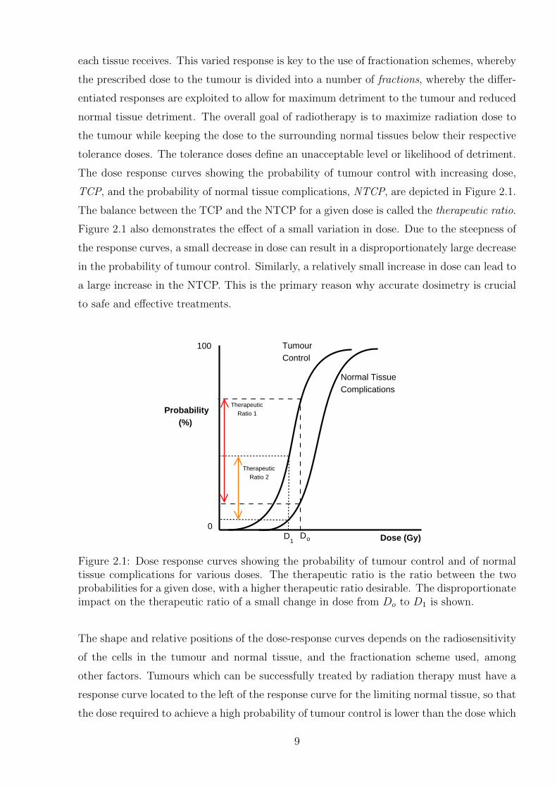
The dose response curves showing the probability of tumour control with increasing dose,
TCP, and the probability of normal tissue complications, NTCP, are depicted in Figure 2.1.
The balance between the TCP and the NTCP for a given dose is called the therapeutic ratio.
Figure 2.1 also demonstrates the effect of a small variation in dose. Due to the steepness of
the response curves, a small decrease in dose can result in a disproportionately large decrease
in the probability of tumour control. Similarly, a relatively small increase in dose can lead to
a large increase in the NTCP. This is the primary reason why accurate dosimetry is crucial
to safe and effective treatments.
Dose (Gy)
Probability (%)
100
0DD o1
Therapeutic Ratio 1
Therapeutic Ratio 2
TumourControl
Normal Tissue Complications
Figure 2.1: Dose response curves showing the probability of tumour control and of normaltissue complications for various doses. The therapeutic ratio is the ratio between the twoprobabilities for a given dose, with a higher therapeutic ratio desirable. The disproportionateimpact on the therapeutic ratio of a small change in dose from Do to D1 is shown.
The shape and relative positions of the dose-response curves depends on the radiosensitivity
of the cells in the tumour and normal tissue, and the fractionation scheme used, among
other factors. Tumours which can be successfully treated by radiation therapy must have a
response curve located to the left of the response curve for the limiting normal tissue, so that
the dose required to achieve a high probability of tumour control is lower than the dose which
9
produces an unacceptable number of complications in normal tissue. Successful radiotherapy
treatment is most probable when the two curves are widely separated and/or when the dose
to the tumour is higher than the dose to the surrounding organs at risk. Some examples
of types of cancer that have high therapeutic ratios and therefore generally respond well
to radiotherapy are lymphoma, early breast cancers, early lung tumours, prostate tumours,
cervical cancers, and head and neck cancers [10]. Many radiotherapy treatments are given
in conjunction with surgical or chemotherapy treatments.
Radiation Therapy Delivery Modalities
There are three principal routes for the administration of radiotherapy: external beam radio-
therapy (EBRT), sealed source therapy (brachytherapy) and unsealed source therapy (not
discussed here). EBRT is the most common form of radiotherapy and is normally performed
with high energy electron and photon beams produced by a linear accelerator, or by gamma
ray beams from Cobalt-60 units or lower energy X-ray beams. Further treatments using
cyclotron produced proton beams (covered in Section 2.3.2), neutron beams and heavier
ion beams, as well as the more experimental techniques of laser driven proton acceleration
(Section 2.3.2) and synchrotron generated X-ray microbeams (Section 2.3.3), are also in var-
ious stages of development or clinical implementation. Brachytherapy utilises sealed sources
placed inside the tumour volume, resulting in a more localized dose to the tumour, avoiding
surrounding healthy tissues (Section 2.3.1).
2.1.2 Radiation Dosimetry
As demonstrated in Figure 2.1, a small variation in dose can have a high impact on treatment
outcomes. In 1976 the ICRU recommended that the dose to the target volume should be
delivered within ±5%, given as one standard deviation [11]. This is to be seen as an overall
uncertainty on the dose received by the patient at the end of all the steps contributing to
radiation dosimetry, and has many contributing factors. The accuracy can be divided into
two categories, dosimetric accuracy and geometric accuracy. However the two are inextri-
cably linked. Dosimetric accuracy requires delivering a dose that is as close as possible to
the prescribed dose. However as dose is prescribed to a target volume, geometric accuracy
is also imperative, to ensure the dose is highly conformal to the target volume.
The absolute accuracy of basic dosimetry in the energy range used in radiotherapy is consid-
ered to be approximately 1-2% [30–32]. In itself, however, this uncertainty is not a problem
10
for a given modality, provided all centres use the same basic physical input data, and follow
compatible dosimetry protocols. The absorbed dose required to kill a tumour has been de-
termined empirically from many years of clinical data, thus the precision in measurements
is required to ensure that clinical experience from past patients and between centres can be
transferred with confidence. Theoretical calculations of required doses are also limited by
the accuracy of the experimental data used to validate the calculations. Thus any dosimeter
must be able to measure absorbed dose in a way that is in accordance with existing protocols
such as the International Atomic Energy Agency (IAEA) TRS-398, or American Associa-
tion of Physicists in Medicine (AAPM) TG51 [16, 33]. These recent protocols require the
determination of the absorbed dose in terms of absorbed dose to water at a reference point
in a beam, and doses within the beam relative to that point.
There is a distinction to be made between different types of dosimetry, each a vital link in the
chain to provide an accurate dosimetric characterisation of radiation delivered to patients in
the clinic. The determination of dose is initially done in what is called absolute dosimetry.
This directly yields the absorbed dose in standard units, and is based on a fundamental prop-
erty of absorbed radiation such as calorimetry, which measures energy deposited as heat, or
charge collected due to electrons released by ionisation. In order to facilitate accuracy and
consistency, some national and international standards organisations have highly accurate
absolute dosimeters which are then used as a primary calibration standard for other detec-
tors. Thus all treatment sites should have a chain of calibration resulting in a calibration
factor traceable directly back to this absolute dose measurement. Calibration measurements
are performed under reference conditions, which are reproducible conditions that are con-
sistently used for the radiation type being measured, and include such factors as ambient
temperature, pressure and humidity, as well as radiation specific parameters such as field
size, distance to the measurement point and detector parameters. This process is known as
reference dosimetry. Using a calibrated reference dosimeter, the absolute output dose to a
reference point under standard conditions can be determined for a clinical radiation situa-
tion. Relative dosimetry involves a comparison of two dosimeter readings to determine the
comparative dose under different conditions. In general, few conversion coefficients or cor-
rection factors are required in relative dosimetry. Relative dosimetry can be used to make
measurements which characterise a radiation source, including depth dose profiles, tissue
maximum ratios, output factors, axial profiles or patient specific factors. Depth dose profiles
are a key parameter for radiotherapy treatments, as they quantify the variation of dose with
depth in a medium, typically water. Two factors influence the shape of the depth dose curve:
11
attenuation of the radiation beam through dose deposition in the medium, and the inverse
square law where the radiation flux decreases with increasing distance from the radiation
source. Normalising the dose at each depth to the dose at a certain point results in a relative
dose scale, usually a percentage scale in terms of the maximum dose.
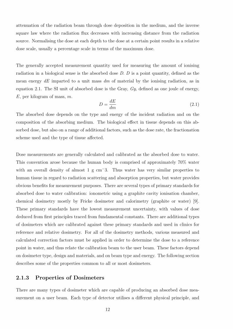
The generally accepted measurement quantity used for measuring the amount of ionising
radiation in a biological sense is the absorbed dose D. D is a point quantity, defined as the
mean energy dE imparted to a unit mass dm of material by the ionising radiation, as in
equation 2.1. The SI unit of absorbed dose is the Gray, Gy, defined as one joule of energy,
E, per kilogram of mass, m.
D =dE
dm(2.1)
The absorbed dose depends on the type and energy of the incident radiation and on the
composition of the absorbing medium. The biological effect in tissue depends on this ab-
sorbed dose, but also on a range of additional factors, such as the dose rate, the fractionation
scheme used and the type of tissue affected.
Dose measurements are generally calculated and calibrated as the absorbed dose to water.
This convention arose because the human body is comprised of approximately 70% water
with an overall density of almost 1 g cm−3. Thus water has very similar properties to
human tissue in regard to radiation scattering and absorption properties, but water provides
obvious benefits for measurement purposes. There are several types of primary standards for
absorbed dose to water calibration: ionometric using a graphite cavity ionisation chamber,
chemical dosimetry mostly by Fricke dosimeter and calorimetry (graphite or water) [9].
These primary standards have the lowest measurement uncertainty, with values of dose
deduced from first principles traced from fundamental constants. There are additional types
of dosimeters which are calibrated against these primary standards and used in clinics for
reference and relative dosimetry. For all of the dosimetry methods, various measured and
calculated correction factors must be applied in order to determine the dose to a reference
point in water, and thus relate the calibration beam to the user beam. These factors depend
on dosimeter type, design and materials, and on beam type and energy. The following section
describes some of the properties common to all or most dosimeters.
2.1.3 Properties of Dosimeters
There are many types of dosimeter which are capable of producing an absorbed dose mea-
surement on a user beam. Each type of detector utilises a different physical principle, and
12
possesses some of the properties of an ideal radiation detector, however each is also limited
by its physical principles and thus different detector types are better suited to different ap-
plications within radiation oncology. Detectors for the dosimetry of therapeutic radiation
must be able to measure a fundamental quality of the radiation and relate this to the abso-
lute value of the absorbed dose to water at a point. An ideal detector must also be able to
measure relative dose across a volume with high spatial resolution and be able to benchmark
all results against the relative dose. These properties result in the determination of a full
and accurate three dimensional characterisation of the dose produced at each point within
a water phantom. This detector would possess all of the properties listed below, resulting in
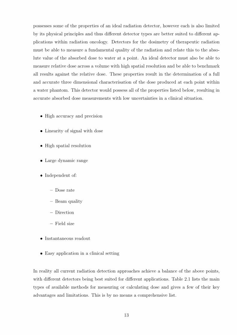
accurate absorbed dose measurements with low uncertainties in a clinical situation.
� High accuracy and precision
� Linearity of signal with dose
� High spatial resolution
� Large dynamic range
� Independent of:
– Dose rate
– Beam quality
– Direction
– Field size
� Instantaneous readout
� Easy application in a clinical setting
In reality all current radiation detection approaches achieve a balance of the above points,
with different detectors being best suited for different applications. Table 2.1 lists the main
types of available methods for measuring or calculating dose and gives a few of their key
advantages and limitations. This is by no means a comprehensive list.
13

Tab
le2.1:
Som
ekey
prop
ertiesof
comm
onaltern
ativedetectors
and
Mon
teC
arlom
odellin
g,w
ithad
vantages
that
DH
Ip
otentially
shares
coloured
redan
dlim
itations
DH
Ican
poten
tiallyovercom
e(or
isunaff
ectedby)
aresh
own
inblu
e.
Dete
ctor/
Model
Typ
eA
dvanta
ges
Lim
itatio
ns
Dim
.
High
accuracy
and
precision
Very
limited
spatial
resolution
Measu
resab
solute
dose
based
onits
fundam
ental
defi
ni-
tionSm
alltem
peratu
rerises
limit
use
torelatively
high
doses
Dose
ratein
dep
enden
tA
tlow
dose
ratesheat
leakageb
ecomes
more
signifi
cant
Calorim
etry
Energy
indep
enden
tN
otsu
itedfor
routin
eclin
icaluse
1D
High
accuracy
and
precision
Spatial
resolution
limited
by
sizeof
collectionvolu
me
Instan
tread
out
Man
ycorrection
factorsreq
uired
Able
tom
easure
absolu
tedose
Dep
enden
ton
beam
quality
Necessary
correctionfactors
well
understo
od
High
voltagesu
pply
required
(safetycon
cern)
Ionch
amb
ers
Easy
application
ina
clinical
setting
1D
High
2Dsp
atialresolu
tionL
owdynam
icran
geM
inim
alp
erturb
ationof
radiation
beam
(radio
chrom
icfilm
)E
nergy
dep
enden
ce(esp
eciallyat
lowen
ergies)
Can
be
archived
Quan
titativedosim
etryreq
uires
careful
calibration
Ease
ofuse
ina
clinical
setting
No
real-time
readou
tF
ilm
Relatively
insen
sitiveto
ambien
tcon
dition
sdurin
gm
ea-su
remen
t(w
ithcorrect
use
and
storage)R
epro
ducib
ilitydiffi
cult
(betw
eenbatch
esof
film
)
2D
High
dynam
icran
geSign
alerased
durin
gread
out
High
spatial
resolution
forp
oint
measu
remen
tsT
ime
consu
min
gcalib
rationan
dread
out
Reu
sable
Lab
our
inten
sivecalib
rationan
dhan
dlin
gT
LD
s
Can
be
reasonab
lytissu
eeq
uivalen
tN
otusefu
lfor
beam
calibration
1D
High
sensitiv
ityN
otusefu
lfor
beam
calibration
Dio
des
and
High
spatial
resolution
(due
tosm
allsize)
Chan
gein
sensitiv
ityw
ithaccu
mulated
dose
MO
SF
ET
sU
seful
forin
-vivo
measu
remen
tsV
ariationin
dose
respon
sew
ithtem
peratu
reL
owdose
ratedep
enden
ceShow
energy
dep
enden
ce,esp
eciallyat
lower
energies
Real-tim
eread
out
1D
Intrin
sicallyhigh
spatial
resolution
and
sensitiv
ityD
oes
not
necessarily
reflect
chan
gesin
system
param
etersM
onte
Carlo
Can
verifydose
with
inpatien
tgeom
etryV
alidation
ofaccu
racydiffi
cult
simulation
sO
nce
am
odel
isdevelop
edit
canb
eless
labou
rin
tensive
than
exp
erimen
talm
easurem
ents
Lon
gcom
putation
altim
es3D
14
2.2 Calorimetry
Calorimetry is the measurement of heat. Dosimetric calorimetry is a fundamental method of
measuring absorbed dose, because the irradiation of a medium and the subsequent transfer
of energy as heat causes a corresponding proportional temperature increase according to the
specific heat capacity of the medium [34]. The basic components of a radiation calorimeter
involve a medium which is irradiated, and one or more probes to measure the temperature
increase, all contained within a large thermally insulated and shielded container to isolate
the calorimeter from the effects of any external temperature changes. The container is im-
portant, because the temperature increase of water attributable to a 1 Gy absorbed dose of
radiation is just 0.00024 K. For this reason higher doses are used, and doses are integrated
across a volume, to infer a dose to a point. The specific heat capacity of graphite is six
times less than water, allowing for larger temperature rises for a given radiation dose and
thus more accurate measurements, but requiring conversion of the result from absorbed dose
in graphite to absorbed dose in water. Generally the measurement complexities involved in
isolating the irradiated sample from ambient temperature and pressure conditions, and the
high doses required to attain accurate calorimetric measurements mean that the technique
is not useful as a routine tool for dosimetry in a clinical environment, but rather is used
worldwide in standards laboratories as a means of absolute reference dosimetry [35]. Some
key features of calorimeters are described in Table 2.1.
There are different types of calorimeters used in various standards laboratories around the
world - historically graphite calorimeters have been used to establish the standards for ab-
sorbed dose, whilst now standards based on water calorimetry are available to a high degree
of accuracy (having a relative standard uncertainty of ∼ 0.5 − 1%) [35]. Water calorime-
try reduces some of the uncertainties associated with graphite calorimetry, especially for
high energy X-ray and electron beams. Types of calorimeters are distinguished by different
procedures, features or the medium used, such as the aqueous solution chosen, the use of
motionless versus stirred water, large gas space versus no gas space, low accumulated dose
versus high accumulated dose etc [36]. Whilst calorimetry is basically the gold standard for
absolute absorbed dose determination, there are various complicating factors which increase
the difficulty of the measurements, which are briefly covered below.
A key compounding factor for most calorimeters is the need for a probe to read the tem-
perature. If the probe and the medium have different radiation absorbing properties then it
is necessary to apply cavity theory corrections. This introduces several complications: 1) it
15
can be difficult to determine the variation of stopping power, especially if inhomogeneities
are present, as the radiation energy spectrum is degraded throughout the medium; 2) spatial
resolution is limited by probe dimensions; 3) sensor sensitivity may limit measurement of
high doses or dose rates; and 4) time resolution is limited by the thermal equilibration time
between the probe and the medium. This problem is overcome by either measuring inte-
grated doses across the whole calorimeter sensitive volume; or by the use of the absorbing
medium itself as a temperature sensitive body, in other words the measurement of a tem-
perature dependent property using a non-disturbing probe, such as in a DHI approach.
A factor which must be considered is heat transfer to and from the point of measurement [35].
Because the thermal diffusivity of water is small, heat transfer by conduction is low for most
irradiation conditions, although it must be calculated for more modulated beams and longer
irradiation times. For some irradiation conditions convection can be a serious concern and
various techniques have been used or proposed to reduce or eliminate the effects of convective
flow (e.g. stirring, which would require a transfer medium to give dose at a point), sealed
glass vessels acting as a convective barrier within larger phantoms, or low temperature op-
eration at 4◦C where the volume expansion coefficient of water is zero, but this increases the
technical complexity of the calorimeter. This factor is also a major consideration for DHI,
however it is possible that the use of optical calorimetry techniques may allow this effect to
be more readily quantified and accounted for, as discussed in Chapter 5.
Another consideration for radiation calorimetry is the possible occurrence of exothermic or
endothermic radiation-induced chemical reactions, which consume or release energy, thus
affecting the temperature change. This is corrected for with the use of a factor called the
heat defect [36]. The heat defect has various contributing mechanisms, depending on the
calorimeter material and radiation linear energy transfer (LET). For this reason, the absorb-
ing medium must be carefully selected to reduce the need for, or simplify the implementation
of heat defect corrections. In water the heat defect is highly influenced by the presence of
impurities in the water, which undergo radiation-induced chemical reactions. Nevertheless,
several different calorimeter designs using various aqueous systems have now demonstrated
results which are consistent, to 1% or better, with the absorbed dose to water obtained by
more conventional techniques [35]. Water quality is important, and modern water purifica-
tion is highly effective, even without distillation, but subsequent exposure to air or other
materials can introduce impurities which can affect the heat defect, which is generally con-
stant for the first 400 Gy [36]. This is also where graphite has an advantage as a calorimeter
16
material, as the stability of the covalent carbon bonds in graphite mean that the heat defect
is negligible.
2.3 Dosimetry for Specialised Radiation Therapy Ap-
proaches
The vast majority of radiotherapy treatments are conducted using radiotherapy approaches
that have well-characterised dosimetry, with well-established protocols which enable consis-
tent dosimetric measurement worldwide using existing detector technologies. There are a
large range of radiation detectors marketed by various companies, coming in a large range of
types, sizes and shapes. There are however specialized radiation therapy approaches where
current detector technology has some limitations. In these areas, there is a need for improved
dosimetric capabilities in order to fully exploit the therapeutic potential of the different ap-
proaches. High dose rate brachytherapy, proton therapy, in particular narrow field proton
beams and high dose rate pulsed beams, and microbeam radiation therapy are three such
areas, which are discussed in the following sections. For each, the main dosimetric require-
ments are described, along with the existing dosimetry options, from amongst the multitude
of radiation detectors marketed by various manufacturers.
2.3.1 High Dose Rate Brachytherapy
Brachytherapy is a type of radiotherapy where an encapsulated radioactive source is placed
on or inside the area to be treated. If the source is placed directly in the target tissue, such
as for breast or prostate treatments, this is called interstitial. Alternatively, the source may
be placed next to or in contact with the target tissue, either intracavitary as for the cervix,
uterus or vagina, intraluminal as for the trachea or oesophagus, intravascularly within a
blood vessel, or externally on a surface such as skin. The main advantage of brachytherapy
is the high dose delivered to the tumour with minimised damage to the surrounding healthy
tissues and a consequent reduction in side effects due to a rapid dose reduction with distance
from the source. Brachytherapy treatments are limited to cases in which the tumour is well
localized, relatively small and accessible by means of one of the brachytherapy approaches
listed above.
Brachytherapy photon emitter sources are available in a variety of cylindrical forms, includ-
ing needles, seeds and wires, but are generally sealed to prevent leakage and to provide
17
shielding against any undesired α and β radiation emitted. The dose from a brachyther-
apy source depends on the isotope used, which controls the energy spectrum and type of
radiation emitted, as well as the source strength, which is a measure of its specific activity.
Additionally, the shielding and the different construction of the sources affects the source
dose distribution, because of absorbance of radiation in the shielding material and within
the source itself. The dose can be delivered over one or more short treatment periods or
be permanently implanted until the source has completely decayed, depending on the dose
rate of the source and the treatment requirements. Brachytherapy treatments are classified
according to the dose rate of the source at a dose specification point, with high dose rate
sources (HDR) producing > 12 Gy/h or more. HDR brachytherapy has become the most
common form of brachytherapy, and this will be the focus of the rest of this section. The
most common HDR isotopes are mainly photon emitters Ir-192, Co-60 and Cs-137.
The dosimetry of brachytherapy sources is complicated because of the steep fall-off of dose
with distance, d, from the source, ranging from ∼ 1/d close to the source to ∼ 1/d2 at greater
distances [37]. This means that the dose gradient in the region immediately adjacent to the
source is very high, which presents considerable difficulties to most conventional radiation
detectors, which are generally impractical to use within 1 cm of the source [38]. This may be
due to the physical size of the source and the corresponding volume averaging effect, or due
to the energy or dose rate dependence which is more pronounced in this region. As such,
most dosimetric measurements have been performed at distances > 1 cm and dose values
closer than this simulated using Monte Carlo models or the AAPM TG-43 algorithm [39].
However uncertainties in the dose in close proximity to the source can create problems such
as hotspots in both the tumour volume and in the surrounding critical tissue. It is rec-
ommended that dose measurements be obtained at the smallest possible distance, ideally
offering adequate precision and reproducibility to allow for 1σ statistical uncertainty (Type
A) ≤ 5% and 1σ systematic uncertainty (Type B) < 7% [30,39].
This becomes particularly important with the increasing use of HDR brachytherapy for
endobronchial and intravascular treatments for both palliation and cure [38, 40–42]. In en-
dobronchial treatments hemoptysis is a common side effect, fatal in 7-32% of cases, which
can be reduced by better sparing of normal tissue [40]. For these treatments, doses are often
prescribed at 5 or 10 mm distances from the source, thus accurate knowledge of the dose
distributions on a scale of millimetres around the source is crucial. However the steep dose
gradients in this region are on the order of 40% per mm which necessitates a detector with
18
wide dynamic range, high positioning reproducibility and accuracy and high spatial resolu-
tion of less than 0.5 mm to avoid excessive volume averaging effects [37, 43].
There are a number of studies that have looked at the dose distributions around brachyther-
apy sources in this region, using a various detectors or models, with work ongoing in many
areas to achieve accurate, practical and reproducible dosimetry. The sections below intro-
duce some of the main areas of focus.
Source Models
Dose distributions for a given treatment configuration are generally calculated by models
which have been validated by experimental data. Conventional treatment planning system
(TPS) algorithms have high uncertainties in the near source region, with uncertainties being
as high as ±15− 20% of the dose [44]. This is largely due to the difficulty of measurements
in this region meaning that models have been extrapolated often without sufficient exper-
imental validation. A Monte Carlo algoritm is a computational tool which samples from
known probability distributions to determine the average behaviour of a system, and this
can be used to model radiation transport processes from HDR sources to determine dose dis-
tributions. Monte Carlo simulations are capable of higher accuracy than conventional TPS
algorithms, however they still require experimental validation. There are several Monte
Carlo codes which have been used to work on HDR source modelling, including BEAM,
EGSnrc, PENELOPE and GEANT4 [37,44,45]. With appropriate experimental validation,
Monte Carlo models can allow for calculation of dose distributions with unparalleled spatial
resolution at all distances and angles from the source, in both water as a reference medium,
and in tissue [37,46–48].
Monte Carlo models are also used to calculate the parameters required in the TG-43 dose
formulism for calculation of dose rate distributions around photon-emitting brachytherapy
sources. This code of practice stipulates that the dose calculations be divided into compo-
nents of geometry, attenuation, scattering and anisotropy, with dose distribution parameters
in water being the dose rate constant Λ, the geometry factor G(r, θ), the radial dose function
g(r), and the two dimensional anisotropy function F (r, θ) [39,44]. All of these are measured
factors, with the exception of the geometry factor, which is a calculated value.
19
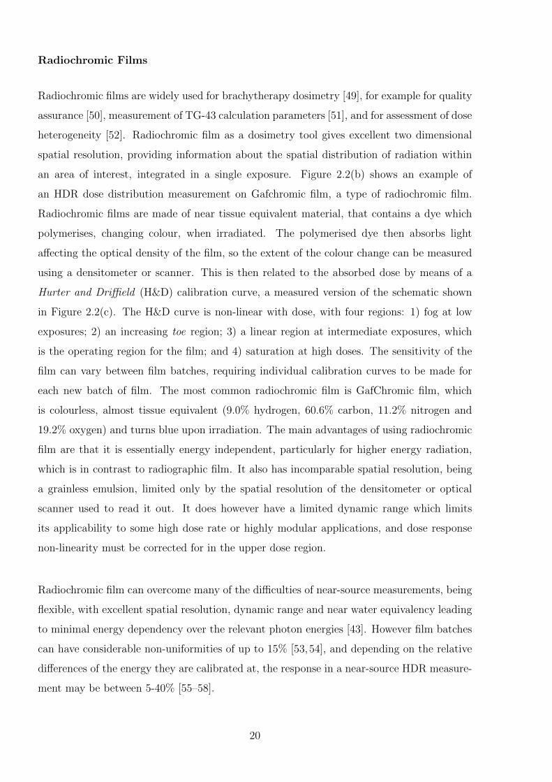
Radiochromic Films
Radiochromic films are widely used for brachytherapy dosimetry [49], for example for quality
assurance [50], measurement of TG-43 calculation parameters [51], and for assessment of dose
heterogeneity [52]. Radiochromic film as a dosimetry tool gives excellent two dimensional
spatial resolution, providing information about the spatial distribution of radiation within
an area of interest, integrated in a single exposure. Figure 2.2(b) shows an example of
an HDR dose distribution measurement on Gafchromic film, a type of radiochromic film.
Radiochromic films are made of near tissue equivalent material, that contains a dye which
polymerises, changing colour, when irradiated. The polymerised dye then absorbs light
affecting the optical density of the film, so the extent of the colour change can be measured
using a densitometer or scanner. This is then related to the absorbed dose by means of a
Hurter and Driffield (H&D) calibration curve, a measured version of the schematic shown
in Figure 2.2(c). The H&D curve is non-linear with dose, with four regions: 1) fog at low
exposures; 2) an increasing toe region; 3) a linear region at intermediate exposures, which
is the operating region for the film; and 4) saturation at high doses. The sensitivity of the
film can vary between film batches, requiring individual calibration curves to be made for
each new batch of film. The most common radiochromic film is GafChromic film, which
is colourless, almost tissue equivalent (9.0% hydrogen, 60.6% carbon, 11.2% nitrogen and
19.2% oxygen) and turns blue upon irradiation. The main advantages of using radiochromic
film are that it is essentially energy independent, particularly for higher energy radiation,
which is in contrast to radiographic film. It also has incomparable spatial resolution, being
a grainless emulsion, limited only by the spatial resolution of the densitometer or optical
scanner used to read it out. It does however have a limited dynamic range which limits
its applicability to some high dose rate or highly modular applications, and dose response
non-linearity must be corrected for in the upper dose region.
Radiochromic film can overcome many of the difficulties of near-source measurements, being
flexible, with excellent spatial resolution, dynamic range and near water equivalency leading
to minimal energy dependency over the relevant photon energies [43]. However film batches
can have considerable non-uniformities of up to 15% [53,54], and depending on the relative
differences of the energy they are calibrated at, the response in a near-source HDR measure-
ment may be between 5-40% [55–58].
20
(a)
−20 −10 0 10 200
0.2
0.4
0.6
0.8
1
Rel
ativ
e gr
eysc
ale
valu
es
Distance from central axis (mm)
(b)
log (Relative Exposure)
Optical Density
Fog density
Toe
Linear region
Shoulder Saturation
(c)
Figure 2.2: (a) A piece of Gafchromic film showing the exposure due to irradiation by anHDR source, (b) the scanned greyscale values along a horizontal (red) and vertical (blue)profile through the centre of the source, and (c) a schematic of a typical Hurter and Driffieldcalibration curve showing the characteristic regions of the curve.
Thermoluminescent Detectors
Thermoluminescent detectors (TLDs) are a type of detector which is considered by some to
provide an optimum compromise between being small enough to achieve adequate spatial res-
olution, but still achieve a sufficient sensitivity [47]. TLDs have been used for experimental
dosimetry across the entire energy range of brachytherapy sources to validate Monte Carlo
simulations. TLDs operate on the principle that when certain thermoluminescent phospho-
rous materials absorb radiation, the transferred energy causes excitation of electrons which
are then trapped in meta-stable states known as luminescence centres. At room tempera-
ture electrons can stay in these traps for extended periods of time. TLDs are then read by a
controlled heating pattern which imparts energy to the material, releasing the electrons back
to their ground state, resulting in the emission of light photons. This luminescence can be
measured with a photomultiplier tube which detects the photon fluence with time (and thus
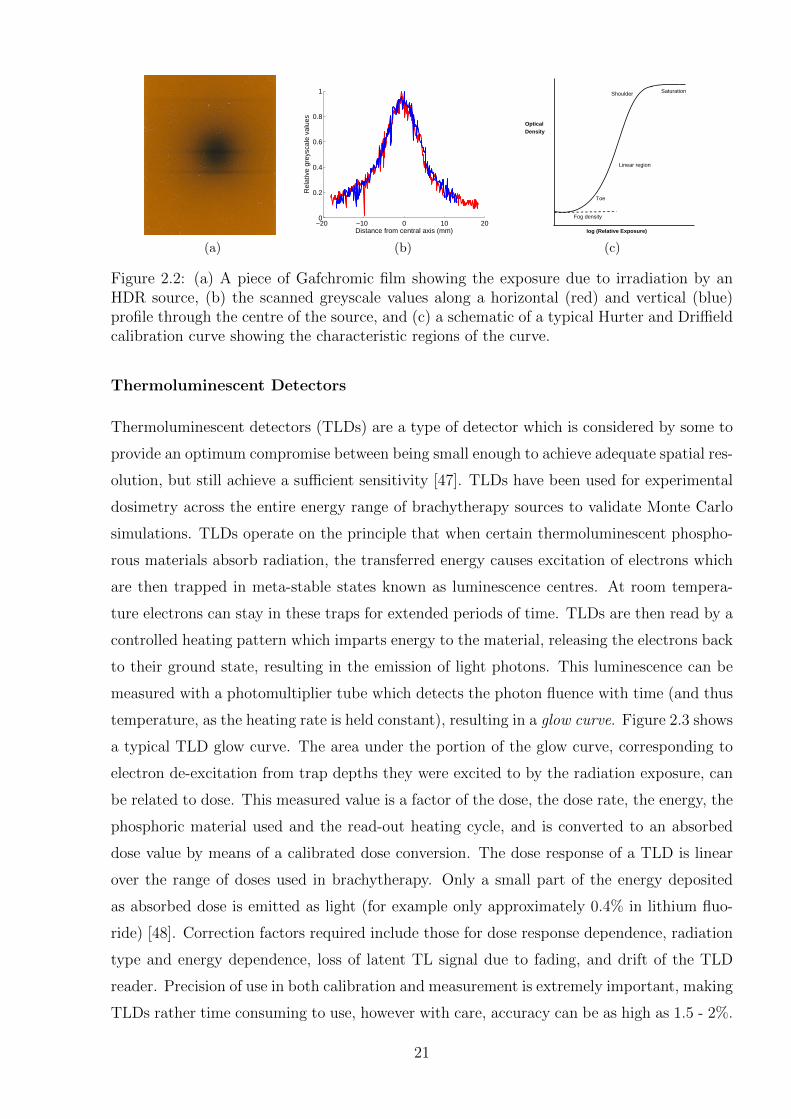
temperature, as the heating rate is held constant), resulting in a glow curve. Figure 2.3 shows
a typical TLD glow curve. The area under the portion of the glow curve, corresponding to
electron de-excitation from trap depths they were excited to by the radiation exposure, can
be related to dose. This measured value is a factor of the dose, the dose rate, the energy, the
phosphoric material used and the read-out heating cycle, and is converted to an absorbed
dose value by means of a calibrated dose conversion. The dose response of a TLD is linear
over the range of doses used in brachytherapy. Only a small part of the energy deposited
as absorbed dose is emitted as light (for example only approximately 0.4% in lithium fluo-
ride) [48]. Correction factors required include those for dose response dependence, radiation
type and energy dependence, loss of latent TL signal due to fading, and drift of the TLD
reader. Precision of use in both calibration and measurement is extremely important, making
TLDs rather time consuming to use, however with care, accuracy can be as high as 1.5 - 2%.
21
The two most commonly used phosphors for TLD dosimetry are lithium fluoride (high tissue
equivalence) and calcium fluoride (high sensitivity), doped with impurities to provide the
luminescence centres, used in the form of small chips, pellets or encapsulated powder. Due to
their extensive calibration requirements TLD detectors are often used as relative dosimeters,
most commonly in a brachytherapy sense for in-vivo dosimetry as routine quality assurance,
but also sometimes used as absolute dosimeters for dose monitoring in complex treatments.
The application of TLDs to near-source measurements has been relatively limited to date,
but Issa et al. have achieved good results using Ge-doped optical fibres used as TLDs [59].
They achieved sub-mm spatial resolution for source-dosimeter separations from as close as
0.1 cm, with quoted agreement to models of 2.3%± 0.3% along the transverse and perpen-
dicular axes, making this a potentially suitable option for this type of dosimetry. A potential
area of uncertainty is the lack of tissue equivalency of the SiO2 which makes up the fibres,
although this is suggested to be small.
Figure 2.3: A typical glow curve of LiF:Mg,Ti measured with a TLD reader at a low heatingrate. Figure reproduced from Podgorsak (2005) [9].
Gel Dosimeters
Polymer gels are fabricated out of radiosensitive chemicals which polymerize upon absorp-
tion of radiation. They are able to record a cumulative dose distribution in three dimensions
to relatively high spatial resolution. The ability to measure dose in two or three dimensions
is advantageous in high dose gradient situations and is useful for brachytherapy [60,61]. An
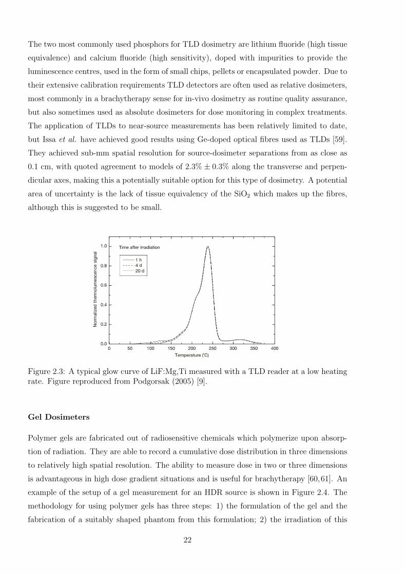
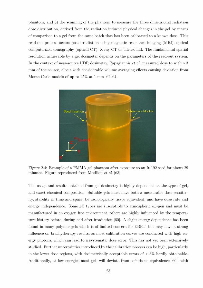
example of the setup of a gel measurement for an HDR source is shown in Figure 2.4. The
methodology for using polymer gels has three steps: 1) the formulation of the gel and the
fabrication of a suitably shaped phantom from this formulation; 2) the irradiation of this
22
phantom; and 3) the scanning of the phantom to measure the three dimensional radiation
dose distribution, derived from the radiation induced physical changes in the gel by means
of comparison to a gel from the same batch that has been calibrated to a known dose. This
read-out process occurs post-irradiation using magnetic resonance imaging (MRI), optical
computerized tomography (optical-CT), X-ray CT or ultrasound. The fundamental spatial
resolution achievable by a gel dosimeter depends on the parameters of the read-out system.
In the context of near-source HDR dosimetry, Papagiannis et al. measured dose to within 3
mm of the source, albeit with considerable volume averaging effects causing deviation from
Monte Carlo models of up to 25% at 1 mm [62–64].
Figure 2.4: Example of a PMMA gel phantom after exposure to an Ir-192 seed for about 29minutes. Figure reproduced from Masillon et al. [63].
The usage and results obtained from gel dosimetry is highly dependent on the type of gel,
and exact chemical composition. Suitable gels must have both a measurable dose sensitiv-
ity, stability in time and space, be radiologically tissue equivalent, and have dose rate and
energy independence. Some gel types are susceptible to atmospheric oxygen and must be
manufactured in an oxygen free environment, others are highly influenced by the tempera-
ture history before, during and after irradiation [60]. A slight energy-dependence has been
found in many polymer gels which is of limited concern for EBRT, but may have a strong
influence on brachytherapy results, as most calibration curves are conducted with high en-
ergy photons, which can lead to a systematic dose error. This has not yet been extensively
studied. Further uncertainties introduced by the calibration process can be high, particularly
in the lower dose regions, with dosimetrically acceptable errors of < 3% hardly obtainable.
Additionally, at low energies most gels will deviate from soft-tissue equivalence [60], with
23
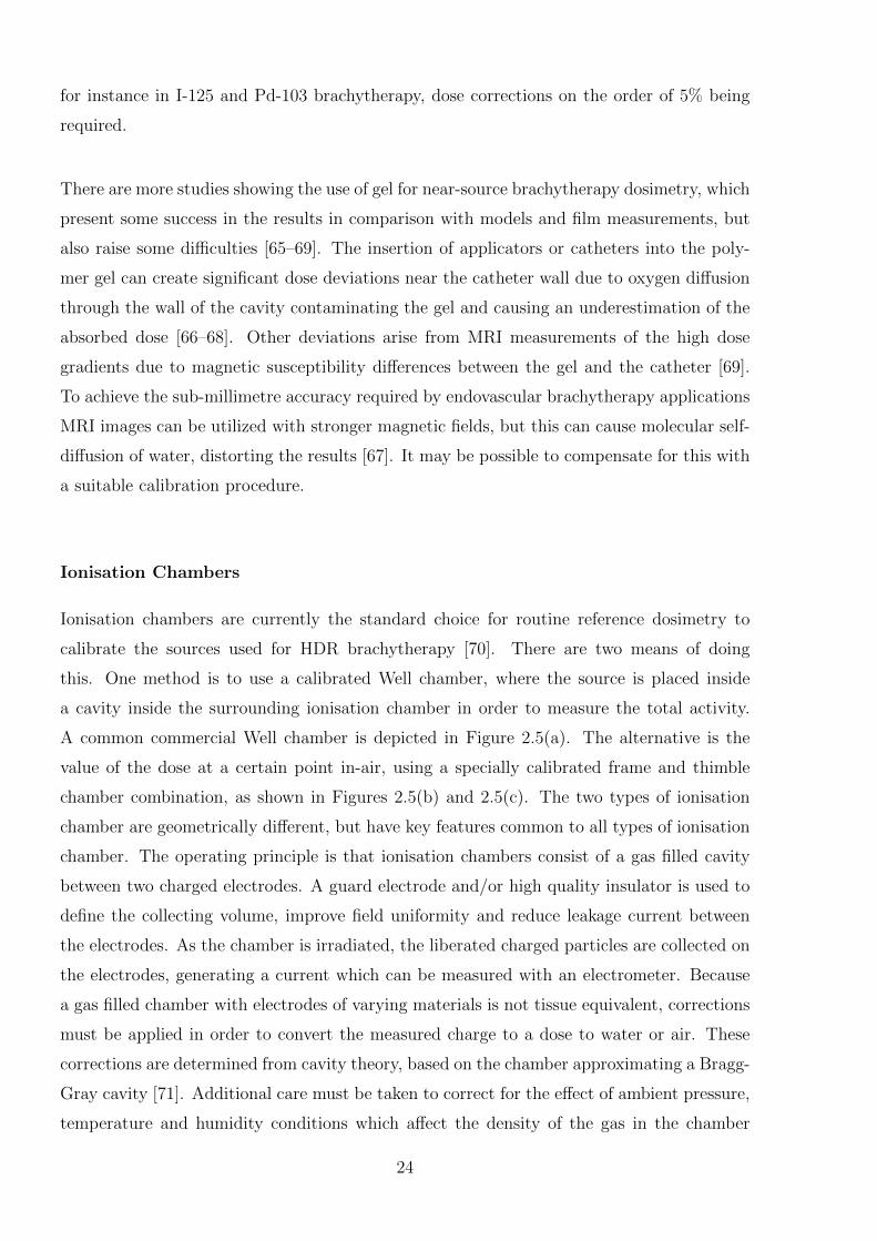
for instance in I-125 and Pd-103 brachytherapy, dose corrections on the order of 5% being
required.
There are more studies showing the use of gel for near-source brachytherapy dosimetry, which
present some success in the results in comparison with models and film measurements, but
also raise some difficulties [65–69]. The insertion of applicators or catheters into the poly-
mer gel can create significant dose deviations near the catheter wall due to oxygen diffusion
through the wall of the cavity contaminating the gel and causing an underestimation of the
absorbed dose [66–68]. Other deviations arise from MRI measurements of the high dose
gradients due to magnetic susceptibility differences between the gel and the catheter [69].
To achieve the sub-millimetre accuracy required by endovascular brachytherapy applications
MRI images can be utilized with stronger magnetic fields, but this can cause molecular self-
diffusion of water, distorting the results [67]. It may be possible to compensate for this with
a suitable calibration procedure.
Ionisation Chambers
Ionisation chambers are currently the standard choice for routine reference dosimetry to
calibrate the sources used for HDR brachytherapy [70]. There are two means of doing
this. One method is to use a calibrated Well chamber, where the source is placed inside
a cavity inside the surrounding ionisation chamber in order to measure the total activity.
A common commercial Well chamber is depicted in Figure 2.5(a). The alternative is the
value of the dose at a certain point in-air, using a specially calibrated frame and thimble
chamber combination, as shown in Figures 2.5(b) and 2.5(c). The two types of ionisation
chamber are geometrically different, but have key features common to all types of ionisation
chamber. The operating principle is that ionisation chambers consist of a gas filled cavity
between two charged electrodes. A guard electrode and/or high quality insulator is used to
define the collecting volume, improve field uniformity and reduce leakage current between
the electrodes. As the chamber is irradiated, the liberated charged particles are collected on
the electrodes, generating a current which can be measured with an electrometer. Because
a gas filled chamber with electrodes of varying materials is not tissue equivalent, corrections
must be applied in order to convert the measured charge to a dose to water or air. These
corrections are determined from cavity theory, based on the chamber approximating a Bragg-
Gray cavity [71]. Additional care must be taken to correct for the effect of ambient pressure,
temperature and humidity conditions which affect the density of the gas in the chamber
24
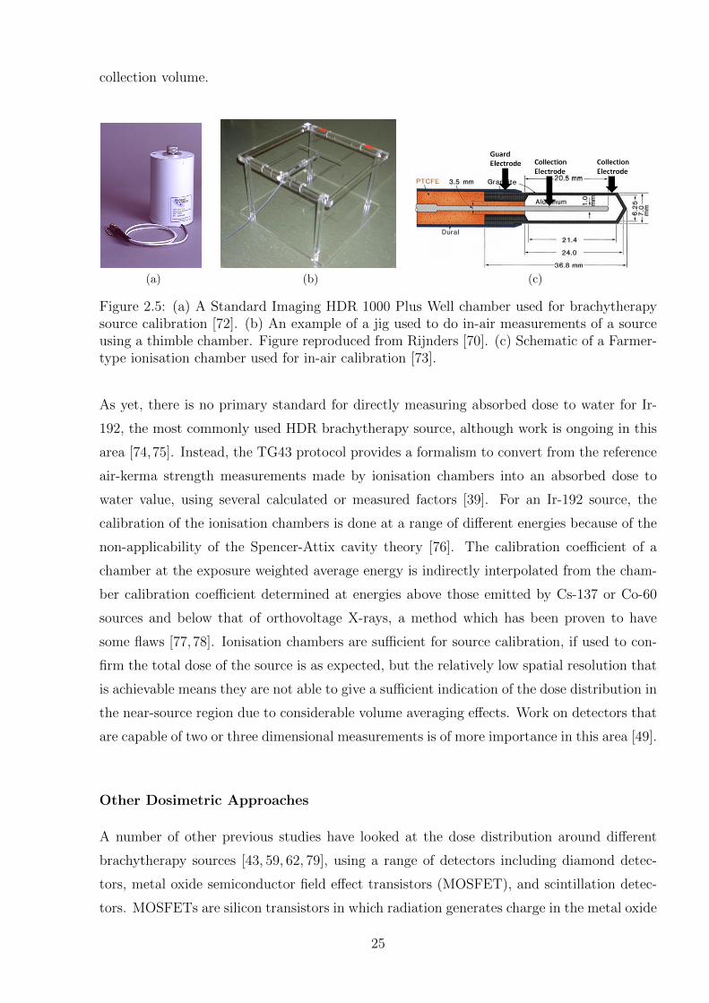
collection volume.
(a) (b) (c)
Figure 2.5: (a) A Standard Imaging HDR 1000 Plus Well chamber used for brachytherapysource calibration [72]. (b) An example of a jig used to do in-air measurements of a sourceusing a thimble chamber. Figure reproduced from Rijnders [70]. (c) Schematic of a Farmer-type ionisation chamber used for in-air calibration [73].
As yet, there is no primary standard for directly measuring absorbed dose to water for Ir-
192, the most commonly used HDR brachytherapy source, although work is ongoing in this
area [74,75]. Instead, the TG43 protocol provides a formalism to convert from the reference
air-kerma strength measurements made by ionisation chambers into an absorbed dose to
water value, using several calculated or measured factors [39]. For an Ir-192 source, the
calibration of the ionisation chambers is done at a range of different energies because of the
non-applicability of the Spencer-Attix cavity theory [76]. The calibration coefficient of a
chamber at the exposure weighted average energy is indirectly interpolated from the cham-
ber calibration coefficient determined at energies above those emitted by Cs-137 or Co-60
sources and below that of orthovoltage X-rays, a method which has been proven to have
some flaws [77, 78]. Ionisation chambers are sufficient for source calibration, if used to con-
firm the total dose of the source is as expected, but the relatively low spatial resolution that
is achievable means they are not able to give a sufficient indication of the dose distribution in
the near-source region due to considerable volume averaging effects. Work on detectors that
are capable of two or three dimensional measurements is of more importance in this area [49].
Other Dosimetric Approaches
A number of other previous studies have looked at the dose distribution around different
brachytherapy sources [43, 59, 62, 79], using a range of detectors including diamond detec-
tors, metal oxide semiconductor field effect transistors (MOSFET), and scintillation detec-
tors. MOSFETs are silicon transistors in which radiation generates charge in the metal oxide
25
layer which becomes permanently trapped, affecting the threshold voltage in the MOSFET.
The threshold voltage operates as a linear function of absorbed dose, and can be read out
in real time (with the detector connected to a bias voltage) and also following irradiation.
MOSFETs can be used for the full energy range of therapeutic photons and electrons al-
though for lower energy radiation the energy response can vary and needs correction. They
do not require correction for dose rate, but exhibit a small axial anisotropy (2% for 360◦) [79].
Many measurements using these detectors are however only made to a closest distance of 5 -
10 mm from the source. One study showed a diamond detector and MOSFET to have dose
rate dependence at distances closer than 50 mm, as did the MOSFET, lowering response by
up to 10% [79].
Absolute Dosimetry using Calorimetry
As mentioned in the section on ionisation chambers above, absolute dosimetry for brachyther-
apy sources is complicated by the lack of an absorbed dose to water standard for Ir-192, with
the existing air-kerma calibrations shown to have several shortcomings [80]. A direct cali-
bration in terms of absorbed dose to water of Ir-192 sources by means of calorimetry has
potential to reduce some of the basic reference dosimetry uncertainties [74,75]. As the basis
for the use of digital holographic interferometry, calorimetry has been described in more
depth in Section 2.2. The complicating factor for absolute dosimetry is the source self-
heating, which impairs reliable experimental determination of dose in the region closest to
the source. Positional uncertainties also increase in this region, whilst dose decreases with
distance, so the measurement conditions must find a balance between these competing ef-
fects. Sarfehnia et al. have proposed an absorbed dose to water standard for brachytherapy
which considers these effects [49, 74, 75], and suggests that an absolute dose measurement
with an accuracy of better than 5% is achievable at a distance of 2.5 - 5 cm from the source.
Whilst this is not in the relevant region for the near-field dosimetry discussed in the earlier
sections, it is possible that DHI dosimetry may also be useful for this application. The
German Standards Laboratory, Physikalisch-Technische Bundesanstalt (PTB), has recently
published proof-of-principle results for the use of water calorimetry as a primary standard
to determine the dose rate constant of an Ir-192 source, quoting measurement uncertain-
ties of 3.7% [81]. Additionally, Malyarenko et al. have successfully used a high resolution
ultrasonic thermometer for calorimetry [82], which could prove suitable for application to
absolute dosimetry of HDR sources, and they are considering the implementation of an op-
tical interferometric system to further improve these results [83].
26
2.3.2 Proton Therapy
Proton therapy is a type of radiation therapy where protons are typically accelerated in a
cyclotron or synchrotron to the required therapeutic energy range. A schematic showing the
key components of a cyclotron is shown in Figure 2.6(a), and a photograph of a commercial
cyclotron in Figure 2.6(b). Energies below 70 MeV are used for superficial tumours, with
energies of up to approximately 250 MeV used for deeper clinical targets. The application of
protons to radiation therapy was first proposed by Robert Wilson in 1946, due to the advan-
tageous dose distributions produced by a proton beam [84]. The interaction of proton beams
with matter results in an energy distribution which is characterized by a relatively low dose
in the shallow regions of their path, rising to a sharp peak near the end of the proton range,
named the Bragg peak, and then a rapid decrease to zero. This dose distribution arises
due to the nature of charged particle energy loss, where once the particles reach a certain
energy threshold, the interactions increase and the remaining energy is absorbed in a rela-
tively localised depth [85]. This dose distribution allows for the delivery of a high dose to a
tumour with a lower dose to the intervening normal tissues, and minimal dose to any normal
tissues deeper than the tumour. This results in an increased ability to safely treat tumours
located adjacent to sensitive structures such as the optical chiasm or spinal cord [17]. The
use of proton therapy is increasing rapidly, however is still not ubiquitous, in large part due
to the large capital expenditure required to set up new treatment centres. At the present
time there are approximately 40 particle accelerator facilities worldwide which are used for
proton therapy, with that number set to increase dramatically in coming years [86].
Treatment using a proton beam generally exploits the fact that the depth of the Bragg peak
is energy specific, and thus modifying the beam energy allows for variation in the treatment
location. Modulating the energy and intensity over a specific range can result in a spread
out Bragg peak (SOBP) which allows the treatment depth to cover a larger region than
a monochromatic beam, allowing better conformation to the cross-sectional depth of the
tumour [87]. Figure 2.7(a) shows an example of a SOBP achieved by combining beams of
several different energies so that the individual Bragg peaks combine. Figure 2.7(b) shows
the relative advantage in the dose distribution that can be achieved by a SOBP compared
to a photon beam. An additional benefit is that due to the relatively large mass of a proton
compared to electrons or photons, there is little lateral side scatter in tissue, resulting in
limited beam broadening. This further reduces the dose to normal tissue in comparison to
27
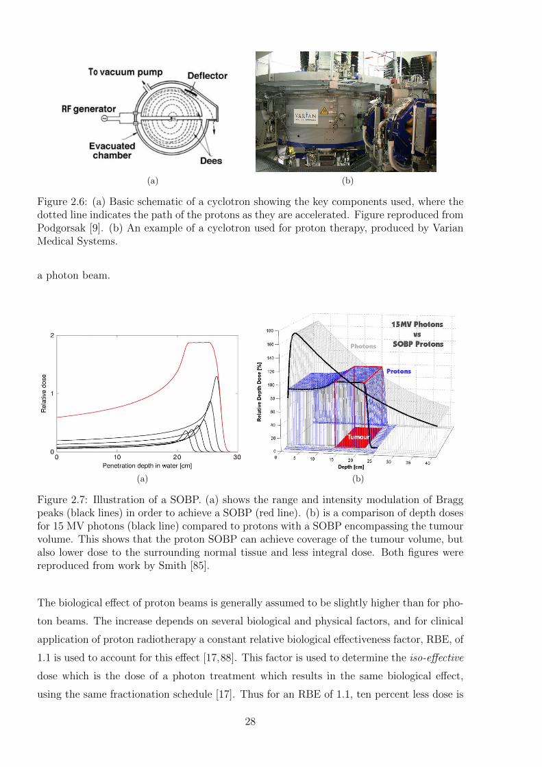
(a) (b)
Figure 2.6: (a) Basic schematic of a cyclotron showing the key components used, where thedotted line indicates the path of the protons as they are accelerated. Figure reproduced fromPodgorsak [9]. (b) An example of a cyclotron used for proton therapy, produced by VarianMedical Systems.
a photon beam.
(a) (b)
Figure 2.7: Illustration of a SOBP. (a) shows the range and intensity modulation of Braggpeaks (black lines) in order to achieve a SOBP (red line). (b) is a comparison of depth dosesfor 15 MV photons (black line) compared to protons with a SOBP encompassing the tumourvolume. This shows that the proton SOBP can achieve coverage of the tumour volume, butalso lower dose to the surrounding normal tissue and less integral dose. Both figures werereproduced from work by Smith [85].
The biological effect of proton beams is generally assumed to be slightly higher than for pho-
ton beams. The increase depends on several biological and physical factors, and for clinical
application of proton radiotherapy a constant relative biological effectiveness factor, RBE, of
1.1 is used to account for this effect [17,88]. This factor is used to determine the iso-effective
dose which is the dose of a photon treatment which results in the same biological effect,
using the same fractionation schedule [17]. Thus for an RBE of 1.1, ten percent less dose is
28
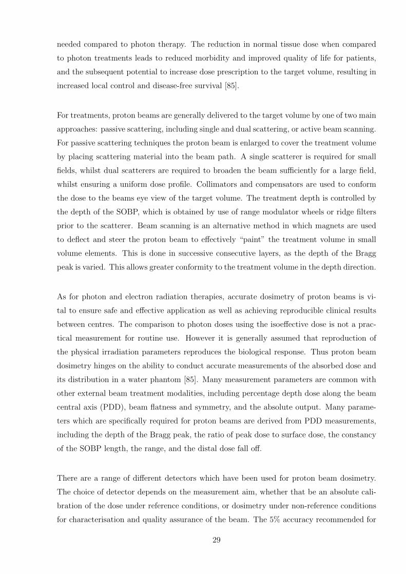
needed compared to photon therapy. The reduction in normal tissue dose when compared
to photon treatments leads to reduced morbidity and improved quality of life for patients,
and the subsequent potential to increase dose prescription to the target volume, resulting in
increased local control and disease-free survival [85].
For treatments, proton beams are generally delivered to the target volume by one of two main
approaches: passive scattering, including single and dual scattering, or active beam scanning.
For passive scattering techniques the proton beam is enlarged to cover the treatment volume
by placing scattering material into the beam path. A single scatterer is required for small
fields, whilst dual scatterers are required to broaden the beam sufficiently for a large field,
whilst ensuring a uniform dose profile. Collimators and compensators are used to conform
the dose to the beams eye view of the target volume. The treatment depth is controlled by
the depth of the SOBP, which is obtained by use of range modulator wheels or ridge filters
prior to the scatterer. Beam scanning is an alternative method in which magnets are used
to deflect and steer the proton beam to effectively “paint” the treatment volume in small
volume elements. This is done in successive consecutive layers, as the depth of the Bragg
peak is varied. This allows greater conformity to the treatment volume in the depth direction.
As for photon and electron radiation therapies, accurate dosimetry of proton beams is vi-
tal to ensure safe and effective application as well as achieving reproducible clinical results
between centres. The comparison to photon doses using the isoeffective dose is not a prac-
tical measurement for routine use. However it is generally assumed that reproduction of
the physical irradiation parameters reproduces the biological response. Thus proton beam
dosimetry hinges on the ability to conduct accurate measurements of the absorbed dose and
its distribution in a water phantom [85]. Many measurement parameters are common with
other external beam treatment modalities, including percentage depth dose along the beam
central axis (PDD), beam flatness and symmetry, and the absolute output. Many parame-
ters which are specifically required for proton beams are derived from PDD measurements,
including the depth of the Bragg peak, the ratio of peak dose to surface dose, the constancy
of the SOBP length, the range, and the distal dose fall off.
There are a range of different detectors which have been used for proton beam dosimetry.
The choice of detector depends on the measurement aim, whether that be an absolute cali-
bration of the dose under reference conditions, or dosimetry under non-reference conditions
for characterisation and quality assurance of the beam. The 5% accuracy recommended for
29
photon beam treatments [89] should in principle apply to the isoeffective dose, which, given
that the RBE contains inherent uncertainties, poses a serious challenge [17]. In fact this level
of accuracy is currently unrealistic, as the fixed value of 1.1 for the RBE has an uncertainty
in the region of 10-15% [90].
There is not yet a primary standard for absorbed dose measurement of proton beams. Dif-
ferent proton therapy centres rely on a range of dosimetry protocols and recommendations
which are relevant or specific to proton dosimetry, including but not limited to AAPM Re-
port 16 [91], the European Charged Heavy Particle Dosimetry (ECHED) protocols [92, 93],
ICRU Report 59 [94], and the more recent ICRU Report 78 [95]. The common recommen-
dation in most of the publications is the use of calorimetry for reference dosimetry, with
ionisation chambers for routine dosimetry. ICRU Report 78 recommends the use of the
IAEA TRS-398 protocol for absorbed dose to water measurements. The difference in cali-
bration varies between the different reports by up to 2%, depending on the chamber used [96].
There are however various complicating factors when it comes to the measurement of proton
beams compared to more commonly used treatment modalities. Key amongst these is the
high uncertainty in the stopping power water to air ratios which are required for ionisation
chamber measurements, in particular in the region of the Bragg peak [97]. Thus the use of
other detector types is still very much an area of active research, as there is considerable
room for development to improve on the dosimetric accuracy and measurement efficiency
achievable [17]. An overview of the key types of detectors used is given in the subsequent
sections, with a summary of their various advantages, disadvantages and applications.
Narrow beam proton fields
A particular subset of proton treatments is the use of narrow beam proton fields for use
in proton stereotactic radiosurgery (PSRS). The beams used in proton stereotactic radio-
surgery generally have a diameter of between 2-30 mm, with a diameter of 10 mm or less
considered narrow beams. Narrow beams experience a host of added difficulties in dosimetric
measurements [18]. The dose in a proton beam changes with depth due to three processes:
multiple Coulomb scattering (MCS), nuclear interactions and a changing rate of energy loss.
For beams with a large cross sectional area MCS is negligible, but for narrow beams this
becomes the major factor changing the gradient of the dose decrease at the end of the Bragg
peak. This is because for a narrower beam there is a lack of balance where more particles
30
are scattered out of each section of the beam path than into it, leading to a widening of
the penumbra with depth, maximised at the depth of the Bragg peak. Within the narrower
cross sectional area this causes a high degree of lateral proton disequilibrium and therefore
the whole width of the beam can become part of the penumbra. This results in lower than
expected dose values in the drop off after the Bragg peak. For beams with collimators of
less than 5 mm diameter, and below certain energies, any SOBP region is therefore not
maintained across the expected depth [18]. The result of these effects is that many of the
detectors routinely used for clinical proton dosimetry are not appropriate in narrow beams,
with the finite size of the detectors introducing perturbations which distort the dose distri-
bution [98, 99]. However this must be overcome, as accurate measurements are required to
input into treatment planning system models to validate treatment doses. Key parameters
are the central axis depth dose and localisation of the Bragg peak, and field size dependent
factors. Lateral off-axis profiles are also particularly important at varying depths near the
surface and near the peak, because at the surface the beam width, measured between the
positions of 50% dose level, is close to the size of the collimator with relatively consistent
penumbra, but at the depth of the Bragg peak there is a more complex relationship between
penumbra, beam width and collimator size, and beam energy [18]. A range of different de-
tectors are recommended to optimise the measurements of narrow beams, as there is no one
optimal choice for beam characterisation [18].
High Dose Rate Pulsed Proton Beams
Recent advancements in laser-driven ion acceleration (LDA) have shown the potential to
create proton sources of ultra high dose rate that may be suitable for therapeutic use [100].
The technique is in the very early stages of investigation of its potential for therapeutic
application. The major advantage of LDA is that treatment units could be extremely cost
effective and compact (table-top sized), compared to conventional proton accelerators. Early
investigations are ongoing into the radiobiological impact of delivering doses in extremely
short but intense pulses, on the order of nanoseconds [101, 102]. Dose rates can exceed 100
Gy/s, with 7 Gy deliverable in a single pulse [102]. This results in peak dose rates of up to
nine orders of magnitude greater than conventional treatments. Several studies have shown
the RBE of such a pulsed beam to be between 1.2 and 1.4 [101, 103], with no evidence for
substantially different radiobiology [101]. The maximum proton energy achievable to date
is 40 MeV [102], but emerging techniques may allow for this to be significantly increased [104].
Accurate dosimetry of these pulsed proton beams is crucial to radiobiological measurements,
31
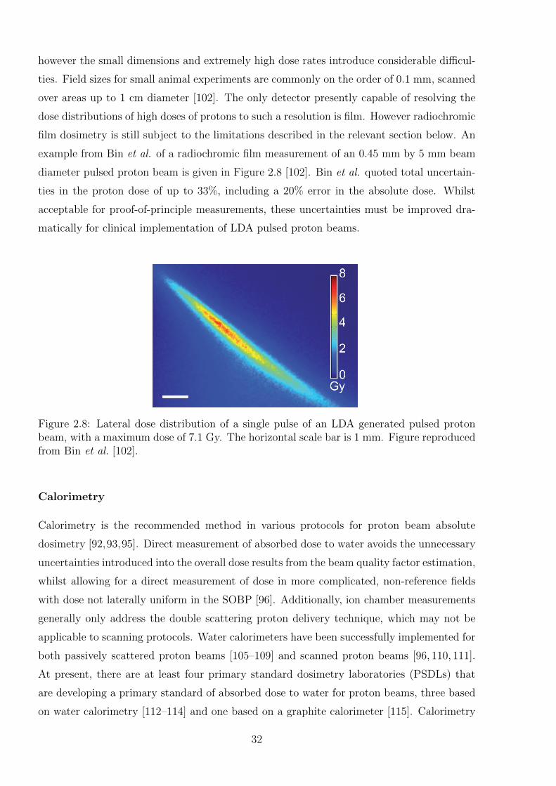
however the small dimensions and extremely high dose rates introduce considerable difficul-
ties. Field sizes for small animal experiments are commonly on the order of 0.1 mm, scanned
over areas up to 1 cm diameter [102]. The only detector presently capable of resolving the
dose distributions of high doses of protons to such a resolution is film. However radiochromic
film dosimetry is still subject to the limitations described in the relevant section below. An
example from Bin et al. of a radiochromic film measurement of an 0.45 mm by 5 mm beam
diameter pulsed proton beam is given in Figure 2.8 [102]. Bin et al. quoted total uncertain-
ties in the proton dose of up to 33%, including a 20% error in the absolute dose. Whilst
acceptable for proof-of-principle measurements, these uncertainties must be improved dra-
matically for clinical implementation of LDA pulsed proton beams.
Figure 2.8: Lateral dose distribution of a single pulse of an LDA generated pulsed protonbeam, with a maximum dose of 7.1 Gy. The horizontal scale bar is 1 mm. Figure reproducedfrom Bin et al. [102].
Calorimetry
Calorimetry is the recommended method in various protocols for proton beam absolute
dosimetry [92,93,95]. Direct measurement of absorbed dose to water avoids the unnecessary
uncertainties introduced into the overall dose results from the beam quality factor estimation,
whilst allowing for a direct measurement of dose in more complicated, non-reference fields
with dose not laterally uniform in the SOBP [96]. Additionally, ion chamber measurements
generally only address the double scattering proton delivery technique, which may not be
applicable to scanning protocols. Water calorimeters have been successfully implemented for
both passively scattered proton beams [105–109] and scanned proton beams [96, 110, 111].
At present, there are at least four primary standard dosimetry laboratories (PSDLs) that
are developing a primary standard of absorbed dose to water for proton beams, three based
on water calorimetry [112–114] and one based on a graphite calorimeter [115]. Calorimetry
32
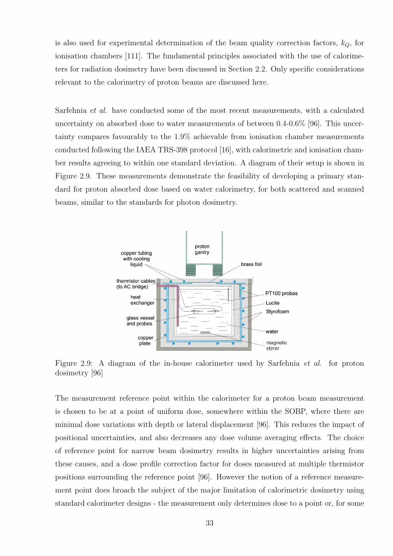
is also used for experimental determination of the beam quality correction factors, kQ, for
ionisation chambers [111]. The fundamental principles associated with the use of calorime-
ters for radiation dosimetry have been discussed in Section 2.2. Only specific considerations
relevant to the calorimetry of proton beams are discussed here.
Sarfehnia et al. have conducted some of the most recent measurements, with a calculated
uncertainty on absorbed dose to water measurements of between 0.4-0.6% [96]. This uncer-
tainty compares favourably to the 1.9% achievable from ionisation chamber measurements
conducted following the IAEA TRS-398 protocol [16], with calorimetric and ionisation cham-
ber results agreeing to within one standard deviation. A diagram of their setup is shown in
Figure 2.9. These measurements demonstrate the feasibility of developing a primary stan-
dard for proton absorbed dose based on water calorimetry, for both scattered and scanned
beams, similar to the standards for photon dosimetry.
Figure 2.9: A diagram of the in-house calorimeter used by Sarfehnia et al. for protondosimetry [96]
The measurement reference point within the calorimeter for a proton beam measurement
is chosen to be at a point of uniform dose, somewhere within the SOBP, where there are
minimal dose variations with depth or lateral displacement [96]. This reduces the impact of
positional uncertainties, and also decreases any dose volume averaging effects. The choice
of reference point for narrow beam dosimetry results in higher uncertainties arising from
these causes, and a dose profile correction factor for doses measured at multiple thermistor
positions surrounding the reference point [96]. However the notion of a reference measure-
ment point does broach the subject of the major limitation of calorimetric dosimetry using
standard calorimeter designs - the measurement only determines dose to a point or, for some
33
designs, several points. The energy of the beam and the subsequent depth of the Bragg peak
or SOBP must be well known so that the relevant positioning of the temperature probe to
this region is well understood. Thus whilst calorimeters are the recommended choice for
beam calibration, supplementary detectors are required for the full beam characterisation.
The main ways in which proton calorimetry differs from photon beam calorimetry are with
respect to corrections for the chemical heat defect and thermal heat conduction. The chemi-
cal heat defect is a correction for energy consumed by chemical reactions which prevents the
entire beam energy from being converted to a temperature increase. The chemical reactions
which occur are specific to proton beam irradiation, and have been both numerically sim-
ulated and experimentally investigated [96, 105, 107, 108, 111, 116–118]. For water saturated
with hydrogen a steady state of zero for the heat defect is reached after a certain dose accu-
mulation, whilst for nitrogen or argon saturated water there is some exothermic heat defect
of < 1%, which increases with increasing LET, to an extent slightly less than the heat defect
in a photon beam. With regard to the thermal heat conduction, the difference between
scattered or scanned proton beams versus photon beams is in terms of the depth dose curve,
where the influence of the Bragg peak results in more of an imbalance between the measured
heat distribution and the radiation dose distribution [96, 116]. This places a limit on the
maximum measurement time as a function of the distance between the measurement point
and the distal edge of the SOBP. For scanned beams the steep lateral dose gradients are in-
stantaneous, which results in a much larger influence of heat diffusion, especially in between
the planes of a scanned beam [117]. The presence of conductive heat transfer is limited. A
smaller heat conduction effect arises from the different heat constants of the walls of the mea-
surement vessel and temperature probes compared to that of water. The correction required
is similar to that of a photon beam, but has some small differences which depend on the con-
tinuous slowing down approximation range of protons to water in the wall material [108,116].
The alternative method of calorimetry is to use a solid material such as graphite for the
sensitive volume rather than water. This has the advantage of having a higher sensitivity
due to the lower specific heat capacity. The disadvantages are that the thermal conductiv-
ity is higher, and notably for proton beams, that the conversion of absorbed dose in the
calorimeter medium to that in water introduces relatively large uncertainties. Solid state
calorimeters have been used for proton beam reference dosimetry [119, 120] with absorbed
dose to water calculated by consideration of the variation in the energy spectrum at different
equivalent depths in graphite and water due to the production of secondary charged particles
34
in each medium. Additional uncertainties are introduced from radiative power dissipation,
measurement of the mass of the core and the physico-chemical heat defect [121].
An additional constraint on calorimetric measurements is the logistical effort required, in
part due to the high level of thermal isolation necessary.
Ionisation chambers
Ionisation chambers are the standard detectors for routine proton beam reference dosimetry
and beam monitoring, and commonly used in the acquisition of depth dose distributions
[17, 122–124]. The main advantages of ionisation chambers over other detector types is the
high accuracy and reproducibility under reference conditions, with a relatively small LET and
energy dependence, and the availability of a range of chamber types for different applications.
The disadvantages are the corrections required for any deviation from reference conditions,
which are specific to the chamber used, and which are not well characterised for proton
beams, resulting in the introduction of higher uncertainties compared to photon beams.
There are an array of ionisation chamber designs available, generally classified into two main
categories of cylindrical or thimble type chambers and plane parallel chambers. Cylindrical
chambers are recommended for reference dosimetry as the combined standard uncertainty
is lower than for plane parallel chambers [16]. For many commonly used thimble chambers
relatively high accuracy and reproducibility is achievable, however the sensitive volume is
often relatively large, often on the order of 0.05 cm3. This limits their suitability for mea-
surements in steep dose gradient regions such as the lateral edges of the beam, or near the
Bragg peak. This imposes the limitation that the SOBP width must begin at least 2 cm
deep, and span at least 2 cm in water, in order to achieve accurate measurements with
reduced volume averaging effects [17]. So this is only useful for the measurement of high
energy beams intended for deep seated tumours, rather than the lower 60-70 MeV proton
beams with SOBP widths of less than 2 cm, such as those used for eye treatments [17]. The
inaccuracies are exacerbated for narrow beams. Various pinpoint chambers with radii of less
than 1.5 mm and cavities on the order of 0.015 cm3 are available for narrow beams or beams
with high dose gradients. These can, however, still result in a widening of the penumbra
in steep dose gradient regions, whilst the reduced volume results in a lower sensitivity and
accuracy [18]. A common use for these is for the verification of treatment plans in a water
phantom. In general the use of ion chambers is restricted to beams with a diameter greater
than 10 mm [18].
35
Plane parallel chambers, such as the PTW-Roos, PTW-Markus, or IBA-NACP chambers [16]
can also be used for absorbed dose measurements but are used more commonly for depth
dose distributions. The diameters of the measurement cavities are typically between 5 and
20 mm, with a surrounding guard ring to ensure the secondary electron fluence is in lat-
eral equilibrium. The spacing of the electrodes is typically between 0.5 and 2 mm, which
allows for higher resolution of depth dose measurements than most thimble chambers, pro-
viding the field size is sufficiently large considering the cavity diameter, with a factor of
two recommended [16]. The limitation of depth dose measurements with a plane parallel
chamber is the requirement to scan the detector across the relevant depths in a water phan-
tom. To increase the measurement efficiency various multiple channel devices have been
developed incorporating a stack of plane parallel ion chambers [125–127]. These contain
an absorbing material between neighbouring chambers, allowing for the shape of the depth
dose distribution to be determined in a single measurement. Plane parallel chambers have
also been used in segmented designs allowing measurement of beam properties like flatness
or lateral profiles, with spatial resolution on the order of a few mm [97, 126, 128, 129], and
a stack of such detectors can achieve quasi-three dimensional dosimetric measurements [130].
A detector based on a similar approach to an ionisation chamber and which has been used
for proton measurements is a Faraday cup, which is a conductive metal cup which measures
the fluence of charged particles by catching them in a vacuum. The dose distribution is
then derived from the fluence by the relevant stopping power ratios. These have also been
used in stacked configurations for depth dose measurements [123]. They have been shown
to have decreased accuracy compared to ionisation chambers for lower energy beams, due to
low energy protons in the beam affecting the mass stopping power [18]. For larger field sizes
they also require an accurate knowledge of the cross sectional area of the beam, which intro-
duces uncertainties compared to ionisation chamber measurements [119, 131, 132]. However
this uncertainty disappears for narrow beam measurements, where the derived quality is the
laterally integrated dose [133,134].
There are several limitations regarding the use of ionisation chambers for proton beam
measurements, beyond the constraints imposed by their geometry. The main source of un-
certainty is in the ratio of the stopping power of the proton beam in water to that in air,
which is introduced in order to convert the dose measured in the air cavity to that in water.
The stopping powers have a strong dependence on the mean ionisation energies in water
36
and air. In a low energy region, such as for measurements in and around the Bragg peak,
a simple ratio of stopping powers is no longer valid [135]. This results in a deviation of the
stopping power ratio from those recommended in TRS-398 by up to 3% in this region. A
typical uncertainty achievable using TRS-398 protocol is 1.9%, which is already considerably
higher than that achievable with a calorimetric measurement. This may in actuality be even
higher if this effect is taken into account [96]. Additional uncertainty arises due to limited
knowledge regarding the chamber specific perturbation factors for proton beams of varying
energy [17]. Current research aims to improve the accuracy of ion chamber dosimetry by
reducing the uncertainty in these parameters by means of both experimental measurements,
and theoretical calculations.
The second main limitation of the use of ionisation chambers, is that except for the seg-
mented chambers mentioned above, they are only able to measure the doses from scattered
proton beams rather than scanned beams [17,97]. The correction factors given in protocols
such as TRS-398 are only valid for scattered beams. The limitation of a scanned beam is that
the dose is deposited in a cumulative fashion, which affects the measured ionisation current.
As scanned beams are becoming increasingly the modus operandi for proton therapies the
need for alternative detector systems is increased.
Radiochromic Film
Radiochromic film dosimetry using various film products has been shown to be possible for
both scattered and scanned proton beams, achieving high resolution measurements [136–139].
In fact film is considered by many to be the detector of choice for lateral beam profiles, es-
pecially for narrow proton beams [18]. Film is also used for measuring beam widths, and
quality assurance of field geometry and homogeneity. Commercially available radiochromic
films suitable for proton measurements include Gafchromic EBT or MD-V2-55 from ISP
Technologies (Wayne, New Jersey, USA). The resolution of most film measurements is on
the order of 85 µm, with the limiting factor being the digitisation of the film by the flatbed
scanner used for the analysis [139]. Radiochromic film has been shown to be a valid tool
for narrow beam geometries, except at the very distal part of the Bragg peak curve, and is
often considered the preferred tool for obtaining depth dose data of beams with a diameter
of less than 5 mm [18].
Radiochromic film has been shown to have an approximately linear response to dose for high
37
energy proton beams, which is a distinct advantage over radiographic beams. Studies have
shown this linearity to be approximately 4.5% for one standard deviation, except for the low
energy regions near the Bragg peak, where a 5-10% dose suppression is recorded [139]. The
complicating factor is that the optical density with dose is non-linear, and the film response
depends on beam quality in a more complicated fashion for proton beams as compared
to photon beams [17]. As the energy of the proton beam varies, the linear energy transfer,
LET, varies over a wide range, with each LET component leading to a different film response
[140]. Thus for mixed fields where the SOBP is created from beams of varying energies, to
reconstruct the dose from the optical density requires a knowledge of the exact composition
of the beam, as well as a dose response calibration curve for each beam component. It is
complex but possible to do this by modelling of the film response [140] or application of
relative effectiveness factors to measure depth dose profiles by quenching the film response
[137]. However most dosimetric measurements using film in proton beams are for lateral
measurements in mono-energetic beams. For a monoenergetic beam, a single calibration
curve can be used to evaluate films exposed at different depths in the beam [18]. These
measurements achieve relative dose distributions rather than absorbed dose to a reference
point within a SOBP.
Monte Carlo Beam Models
Monte Carlo modelling of many different types of radiation dosimetry problems is an area
of rapidly increasing importance, with many authors reporting work on the application of
Monte Carlo codes to proton therapy [141–143]. The Monte Carlo (MC) modelling tech-
nique is a computational algorithm which, in the context of radiation dosimetry, develops a
model of the radiation progression through a bulk medium. An MC model simulates random
trajectories of individual particles by using random numbers to sample from the probability
distributions which govern the individual interactions of electrons, photons and charged par-
ticles in materials. If physical quantities of interest are tracked over a sufficient number of
particles and their interactions (or histories), then a MC model is able to predict expected
values of macroscopic quantities such as energy deposition and therefore dose distribution.
Each MC simulation code has four main components: the cross-section data for all processes
considered, the algorithms used for particle transport, algorithms to specify the geometry
and the analysis to determine the physical quantities of interest. Some of the physical pro-
cesses considered include energy loss, straggling, multiple Coulomb scattering of primary
beam and secondary radiation and nuclear interactions [141]. The path of the radiation is
calculated from a modelled source, often assumed to have a Gaussian distribution, through
38
a complete simulation of the treatment head geometry including beam components such
as bending magnets, energy modulators and collimators, and into the irradiated material,
which may be homogeneous e.g. water or air, or heterogeneous, e.g. patient body compo-
sition obtained from computed tomography (CT) scans. The interactions at each point are
sampled, to calculate a resulting dose distribution within the medium. MC models can also
incorporate a detector such as an ionisation chamber or film, in order to compare modelled
and measured results directly. There are various MC algorithms used for radiation dosime-
try of proton beams, including GEANT4 [45], FLUKA [144] and MCNPX [145]. These all
use variations on the physical interaction models and transport algorithms, with their own
nuclear cross section libraries and the results of each model are often compared for validation
and improvement [146].
Most treatment planning systems are based on fast analytical pencil-beam dose calculation
algorithms which calculate dose distributions based on a water-equivalent path length [141].
A full MC model demonstrably improves on these, by considering the physical system in far
more detail [147–152].
MC models have a major limitation in that the accuracy of the model is limited by the
user-defined input parameters of the proton beam, and the data on the physical processes
which occur. Discrepancies in some MC models result from some of the input parameters
such as the irradiation geometry, or spectrum and flux of the radiation being too crude,
for example neglecting scattering within the collimators or divergence or polarisation of the
beam [153,154]. The input data relies heavily on the accuracy of vendor blueprints with re-
gard to component geometries and compositions, which may vary in actuality. Additionally,
the implementation of the physical interactions is via theoretical models or interpolation of
experimental data. The accuracies of these calculations can depend on the energy region
in question. Thus whilst modelling can produce a general model of each particular type
of radiation system, it may not incorporate the real life irregularities of the particular sys-
tem into the simulations. This makes MC very labour intensive, as the algorithm must be
specifically applied and validated for any given beamline. The calculations also tend to be
very computationally intensive, as the accuracy increases with the number of histories run.
MC codes may be underutilised for these reasons, although there has recently been some
development of more user-friendly interfaces such as TOPAS [155].
An MC algorithm which has been accurately implemented and validated does have many
39
advantages for proton beam dosimetry. This includes the fact that there is no fundamental
limit on spatial resolution, given sufficient accuracy of the input parameters [156]. There
is also inherently no uncertainty in the measurement position. Thus MC is a vital tool for
validating narrow beam measurements. Additionally, the ability to obtain multiple output
parameters, for example both dose and LET as a function of water depth can contribute to
the accuracy of other dosimetric tools such as film, which require additional knowledge of
the beam spectra to achieve high accuracy.
MC is therefore an extremely useful tool for dosimetry of proton beams, however it will never
be a standalone dosimetry method, as verification with experimental results will be required
across the entire range of applicable measurement conditions for any given system. Thus
there is still a strong need for accurate physical detectors for validation of the MC model.
Other Dosimetry Approaches
There are a variety of other detectors that have been applied to proton beam dosimetry.
Most of them are solid state detectors, which have the advantage of a higher signal due to
their higher ionisation density, allowing for a reduction in the sensitive volume and corre-
spondingly higher spatial resolution. This can result in signal saturation at the distal edge
of a Bragg peak [17]. The detectors can be broadly categorised based on their geometry
into point-like detectors such as silicon diodes, diamond detectors, TLDs and optically stim-
ulated luminescence detectors; two dimensional detectors such as scintillating screens; and
three dimensional detectors such as gel and sample activation detectors. Each of these is
briefly described.
Silicon diodes are detectors made of elemental semi-conductor material, which are based
on the principles of a P-N junction diode whereby radiation introduces electron-hole pairs
which diffuse into the depletion region, generating a current. A diode dosimeter is made
of p type silicon, counterdoped at the surface to produce a p-n junction diode. Radiation
produces electron-hole pairs throughout, including in the depletion layer, and then charges
produced in the body of the dosimeter within the diffusion length diffuse into the depletion
region. Here they come under the action of the electric field from the intrinsic potential,
and a reverse current is generated. Operated in the short circuit mode this exhibits a linear
relationship between measured charge and dose. The benefits of diodes are that they can be
40
made small in size with high spatial resolution but also high sensitivity. The disadvantages
are that they demonstrate a dependence on the proton beam LET, dose rate and energy [17].
Some diodes experience a significant over-response in the Bragg peak, whilst others experi-
ence an overall decrease in response with increasing dose of approximately 0.7% [157].
Diodes are commonly used for lateral profile measurements and determination of field fac-
tors, and are the detector of choice for determination of these in narrow beam geometries.
For instance the Scanditronix diode DB050 was designed for use in photon radiosurgery
beams and has a width of 0.6 mm, but has also been applied to narrow proton beams to
good agreement with ionisation chamber results for beams of 20-30 mm diameter, and was
effective for smaller beams down to 5 mm, although volume averaging effects can still be
observed [18].
Both diodes and MOSFETs are used as relative dosimeters, because they require regularly
updated calibration curves to obtain the absorbed dose from the current or threshold voltage.
Both detectors show a temperature dependence, and a non-linearity of response with their
radiation history, so they cannot be used for beam calibration. They are more sensitive
and smaller than ion chambers, with excellent spatial resolution and limited attenuation
of the beam. Diodes and MOSFETs are commonly used for in vivo and in phantom dose
measurements, including for routine patient dose verification, brachytherapy, total body
irradiation, intensity modulated radiotherapy and intraoperative radiotherapy. Because of
their small size they are useful in high dose gradient areas such as those found in stereotactic
radiosurgery, electron depth dose curves or the penumbral region of beams.
Diamond detectors are similar in many aspects to diodes, but radiation hard. The
PTW design diamond detectors function by attaching metal contacts to the edges of the
diamond [158]. A metal-semiconductor barrier creates a Schottky diode on the top metal
contact. Positive and negative charge carriers are generated by the incident radiation, and
because they are separated by the diode field a signal current is produced which can be mea-
sured with an electrometer, without the requirement for an external bias voltage. Diamond
can detect any type of radiation that generates electron-hole pairs as long as the exciting
radiation is of higher energy than the band gap, 5.5 eV. Chemical vapour deposition (CVD)
is used to produce diamond films with similar electrical and thermal properties to natural
diamond, reducing the cost and increasing the versatility.
41
As for diodes, diamond detectors achieve high spatial resolution with high sensitivity. They
often experience radiation type, dose rate and energy dependence [138, 159]. The dose rate
dependence is not dependent on the rate of linear energy transfer (LET), so values mea-
sured for photon beams can also be used for protons, but the energy dependence can be
substantial [18]. A recent study by Mandapaka et al. reported a commercially available
detector with 1 µm thickness and no energy dependence, for high energy beams ranging
between 155 and 250 MeV [160]. Diamond detectors have been shown to be useful in proton
beam calibration, and are used for lateral profile measurements for beams down to 10 mm
in diameter [138, 159, 160]. The tissue equivalency of diamond is an advantage over that of
the diode detector.
Thermoluminescence Detectors (TLDs) are used for proton beam dosimetry, even
though they exhibit supra-linearity with dose and substantial energy dependence [161,162].
The energy response can be corrected for by measuring the energy dependence of the differ-
ent glow curve peaks [163, 164]. They also require correction for the density being greater
than that of water. TLDs do achieve sufficient spatial resolution on the order of a millimetre,
and are useful for absorbed dose calibration in narrow beams, as the proton beam quality
correction factors are close to unity [18].
Optically Stimulated Luminescence (OSL) Detectors are based on the same prin-
ciple of operation as TLDs, except that the read out is via optical excitation. OSL is widely
used in personal dosimetry, but preliminary work has been reported on the use of carbon-
doped aluminium oxide crystals for proton dose measurements [165]. An under-response
in the Bragg peak region was reported at doses above 0.3 Gy, but they generally have a
linear response with dose to high fluences, and very good spatial resolution. OSLs will be
potentially useful for in-vivo dosimetry of proton beams.
Scintillating screens have been used for dosimetric purposes in a proton beam [166,167].
They consist of a plate coated with a scintillating material such as Gd2O2S:Tb, and the light
emitted when a proton strikes the detector is recorded by a CCD camera. They achieve
a high spatial resolution in two dimensions, a linear response over a large range of dose
rates, and dose rate independence, so are suitable for measuring field size and distribution,
including for narrow beams. They do experience some LET and energy dependence, so are
42
not suitable for depth dose measurements.
Gel dosimetry using ferrous sulphate gels to record the dose from a clinical proton beam
allows for the subsequent optical three dimensional reconstruction of the beam [168]. How-
ever as for most of the detectors mentioned, they exhibit an LET and energy dependence,
resulting in a lack of sensitivity in the Bragg peak region [169]. Polymeric gels such as
BANGR are somewhat less dependent on LET [170], whilst PRESAGE has the advantage
of being nearly water equivalent, relatively insensitive to oxygen and solid-state allowing the
detector shape to be customised more easily [171,172], however both have been reported to
still underestimate the dose in the Bragg peak by approximately 20% [173].
Sample activation measurements have also been used for proton dosimetry, whereby a
sample with a known number of C-12 atoms is irradiated and the proton fluence determined
from a subsequent measurement of the induced C-11 activity [174]. The advantage of this
method is that it can be used in high dose per pulse beams such as a synchrotron.
2.3.3 Microbeam Radiation Therapy
Microbeam radiation therapy (MRT) and its dosimetric challenges was the initial motivation
for developing a DHI detector for radiation dosimetry. No measurements of MRT radiation
have yet been made with the prototype DHI detector, however Chapter 8 includes a theoret-
ical consideration of the potential for DHI to measure microbeams, based on the experimen-
tal results achieved in the initial proof-of-principle measurements of an HDR brachytherapy
source and a proton beam. For this reason, a short introduction to MRT is included here,
with a focus on the dosimetric problems that it presents. Brief mention is made of some of
the alternative dosimetry options being explored, however this is not intended to provide a
thorough coverage of the field.
Microbeam radiation therapy is a technique which utilises the fact that normal tissue can
sustain very high radiation doses without notable functional damage, if the dose is limited
to a minuscule volume of tissue. This phenomenon was first discovered almost 40 years ago
at the Brookhaven National Laboratory in the US [153], and applied to the field of radiation
therapy about ten years ago.
43
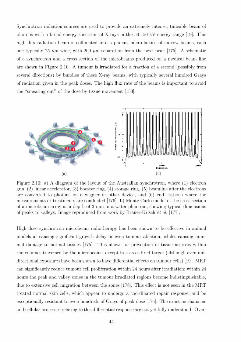
Synchrotron radiation sources are used to provide an extremely intense, tuneable beam of
photons with a broad energy spectrum of X-rays in the 50-150 kV energy range [19]. This
high flux radiation beam is collimated into a planar, micro-lattice of narrow beams, each
one typically 25 µm wide, with 200 µm separation from the next peak [175]. A schematic
of a synchrotron and a cross section of the microbeams produced on a medical beam line
are shown in Figure 2.10. A tumour is irradiated for a fraction of a second (possibly from
several directions) by bundles of these X-ray beams, with typically several hundred Grays
of radiation given in the peak doses. The high flux rate of the beams is important to avoid
the “smearing out” of the dose by tissue movement [153].
(a) (b)
Figure 2.10: a) A diagram of the layout of the Australian synchrotron, where (1) electrongun, (2) linear accelerator, (3) booster ring, (4) storage ring, (5) beamline after the electronsare converted to photons on a wiggler or other device, and (6) end stations where themeasurements or treatments are conducted [176]. b) Monte Carlo model of the cross sectionof a microbeam array at a depth of 3 mm in a water phantom, showing typical dimensionsof peaks to valleys. Image reproduced from work by Brauer-Krisch et al. [177].
High dose synchrotron microbeam radiotherapy has been shown to be effective in animal
models at causing significant growth delay or even tumour ablation, whilst causing mini-
mal damage to normal tissues [175]. This allows for prevention of tissue necrosis within
the volumes traversed by the microbeams, except in a cross-fired target (although even uni-
directional exposures have been shown to have differential effects on tumour cells) [19]. MRT
can significantly reduce tumour cell proliferation within 24 hours after irradiation; within 24
hours the peak and valley zones in the tumour irradiated regions become indistinguishable,
due to extensive cell migration between the zones [178]. This effect is not seen in the MRT
treated normal skin cells, which appear to undergo a coordinated repair response, and be
exceptionally resistant to even hundreds of Grays of peak dose [175]. The exact mechanisms
and cellular processes relating to this differential response are not yet fully understood. Over-
44
all, survival times are on a par with conventional radiotherapy, whilst there is considerably
less normal tissue damage, so therefore the therapeutic index is higher for MRT [178].
This technique may prove to be more effective than the best existing technique for several
intractable human malignancies, and therefore has the potential for therapeutic applica-
tion [179]. In particular, conventional radiotherapy has some limitations for treating brain
tumours - especially in children, as the radiation damage is intolerable to normal brain de-
velopment if applied before the age of around three years [154]. High-grade glioma is one of
the most common forms of child cancer, and MRT may be able to potentially overcome this
limitation, so for this reason alone it is well worth pursuing.
Synchrotron radiation sources are now found throughout the world, with MRT being most
actively studied at the European Synchrotron Radiation Facility (ESRF), and the National
Synchrotron Light Source (NSLS) in the USA, although other facilities also investigate this
area, including dedicated medical beamlines at SPring8 in Japan, and the Australian syn-
chrotron in Melbourne [19].
Dosimetry requirements for MRT
There are many questions to be answered before MRT’s potential can be fully estimated,
and before clinical application on humans. To answer most of these questions requires very
accurate dosimetry methods to determine the dose distribution throughout the irradiated
volume. There currently exist no commercial dosimetry systems capable of satisfactorily
measuring the dose distributions of MRT. Currently one of the main approaches has been
to model the dose using Monte Carlo simulations based on assumptions about the radia-
tion transport and dose deposition in water; however it is essential to have an independent,
measurement-based dosimetry system that can be used to verify these computer simulations
and measure day-to-day variations.
The primary problem is to quantify the relationship between the microbeam irradiation
parameters and the resultant tissue damage. This is important because the microbeam en-
hanced normal-tissue sparing effect is heavily dependent on the peak-to-valley dose ratio
(PVDR) and the irradiated volume [178, 180]. This correlation must be thoroughly under-
stood in order to determine the optimal geometric configurations for MRT treatments [181].
There is a certain width of the microbeams which should not be exceeded, and the valley
doses, which are proportional to the array size, subject size, tissue depth, and the increasing
45
ratio of beam thickness to spacing, must be minimised [180]. Therefore it is particularly
important to develop a reliable means to accurately determine the PVDRs.
Lower valley doses may be achieved by temporal spacing of dose fractions, by 1-3 days,
possibly at perpendicular angles, although the MRT spatial fractionation may be sufficient
in most cases [178]. This needs to be investigated, along with other questions such as the
extent to which the dose penetration is lower for microbeams, is there any dose build-up
at depth, what is the effect of the collimator on the beam quality (relating to the beam
penetration), further investigation of the bystander effect, as well as to assess the effect of
greater X-ray scattering in larger target volumes of humans rather than samples.
The nature of microbeam radiation creates some difficulties in accurately characterising the
dose. There are several factors to consider for MRT that are not a consideration for linac
produced broad beam radiation dosimetry. The key parameters for microbeam dosimetry
are:
� PVDR: The most crucial factor for the outcome of MRT treatments is the PVDR, as
this is the limiting biological factor for MRT [28,182]. However simultaneous measure-
ment of peak and valley doses has proven difficult for the typical MRT energy ranges
of 50-150 kV [28, 153, 183]. This can be attributed in part to the high dose gradients
(hundreds of Gray) that occur over very short distances of tens of µm.
� Spatial resolution: In order to have optimal use of the MRT benefits, it is important
to accurately localise the peaks and valley doses, particularly if multiple treatment
fractions are used. Due to the microscopic dimensions of the microbeam arrays this is
not a trivial consideration.
� Peak dose: The absolute peak dose must also be determined. This may be less cru-
cial than the PVDR, because when delivering hundreds of Grays of radiation (already
a lethal dose) a small percentage error is negligible. However, any dosimetry system
must still be able to resolve the very high dose rates, on the microscopic scale required.
� Spectral range: The system must be able to cope with the non-monochromatic na-
ture of the synchrotron beam. Some traditional dosimetry methods can encounter
46
difficulties arising from their use of absorption correction factors which vary with pho-
ton energy. Additionally, measurements should ideally be able to be made at different
depths within the irradiated material.
Monte Carlo simulations are used to calculate the MRT dose distributions within the
tissue. Because there is a lack of experimental dosimetry systems with sufficient resolu-
tion for MRT, MC has made up the majority of approaches to this dosimetry problem in
the past ten years, and has been vitally important to the development of MRT [182]. A
Monte Carlo approach will never be a stand-alone dosimetry method, as any model needs
verification with experimental measurements. Work by Crosbie et al. has shown large dif-
ferences between film measurements and a corresponding MC model, demonstrating the
need for empirical verification of MC models used for dosimetry purposes [28]. However,
these simulations are still crucial for the refinement of treatment planning for clinical trials
or other experiments [182]. Various MC algorithms are used, including PENELOPE [153],
PSI-Geant3, EGS4 [182], and GEANT-4 [45, 154]. These all use variations on the physical
interaction models and transport algorithms, and results of each model are often compared
for validation and improvement. There are a huge number of irradiation parameters and
physical processes which must be carefully simulated, to try and ensure the comparability of
the simulation models and experimental data. The primary mechanisms for dose deposition
are the Compton scattering and photoelectric events that set electrons in motion [180]. An
important factor is the models’ ability to deal with low energy electron transport, important
for dose calculations in the micron-sized ranges of MRT, because the low energy electrons
determine the dose scattered into the valley regions. Present discrepancies may be based on,
for example, too crude a model of the real irradiation geometries (e.g. many models neglect
the scattering in the collimators, or the divergence or polarisation of the beam [153, 154].
One of the main shortfalls of MC is that it is next to impossible to incorporate the real
life irregularities of the MRT system into the simulations. For example the collimators used
are not uniform (as in the MC calculations), actually the manufacturing process introduces
significant variations and curvature, which is exacerbated by the intrinsic divergence from
the wiggler on the synchrotron. One study found that for a collimator with average full
width half maximum apertures of 25 µm, the actual variation was between 19-39 µm, which
has a huge effect on the dose distribution [183].
Ionisation chambers are not well-suited for resolving the peak and valley doses for MRT
due to the low spatial resolution [28]. Additionally, because the irradiated volume is so small
47
it becomes hard to satisfy the condition of charged particle equilibrium, and the intensity
of the beam means that ion recombination becomes an unavoidable problem [20]. Despite
these difficulties, low energy free air ionisation chambers have been used to measure air kerma
rates and attenuation coefficients for the MRT beam at the Australian Synchrotron, with the
results showing agreement to calculations to within 3 % [184]. Further measurements using
graphite chambers have also shown promise for integrated absolute dose determination [185].
TLDs can come in two dimensional foils which have been used to measure microbeam
doses. These foils have limited spatial resolution due to the properties of the detectors, and
the light scattering within the detectors, so they are not really suited to this application.
Nonetheless, they have been considered a convenient tool for quality control and basic dose
measurement of X-ray microbeams [186].
Solid state detectors based on an epitaxial silicon detector are under development by
Lerch et al. to measure the lateral dose distribution of a microbeam array in high resolution
and real time [187]. Initial results have been shown to be reproducible to within 0.5%, but
with PVDRs a factor of 4.5 times less than expected due to charge recombination effects at
low bias voltages. Suggested improvements to this detector may result in potential for its
use for MRT in the future.
Radiographic films have been used for micro-dosimetry with reasonable accuracy, but
the precision of the dose measurements is limited due to the energy dependence, speed of
the film, slight changes in processing conditions, inter-film emulsion difference, conditions of
the densitometer, and the uncertainty from the calibration curve (for example the difference
between the energy spectra of the calibration versus the MRT radiation) [20]. Measurements
can have a tendency to underestimate the PVDR, possibly due to the point spread function
of the film [20].
Radiochromic film has a much weaker energy dependence than radiographic film, which
is important because synchrotron radiation is produced in a wide beam spectrum rather
than quasi-monochromatically [28, 153]. An example of radiochromic film which has been
used for MRT dosimetry is GafChromic film [28]. Aside from the calibration of the films,
one of the other primary difficulties is in recording the peak and the valley doses on the same
film. One study has sought to overcome this by using parallel sheets of two types of film
with different sensitivities, to record peak (low sensitivity film) and valley (high sensitivity
film) doses [28]. Film has the advantage of unparalleled spatial resolution - this is limited
48
by the microdensitometer used to read it, but film still provides sufficient spatial resolution
for microbeams.
2.4 Concluding Remarks
This chapter served as a general introduction to the field of dosimetry for radiation ther-
apy, and described the motivation behind the development of a new approach to radiation
dosimetry. Radiotherapy is a widespread and effective tool against many types of cancer,
and accurate measurements of dose distributions delivered to patients are critical to optimise
treatment efficacy and safety. Current detectors are adequate for conventional treatment ap-
proaches, however there are various new and existing treatment types which have particular
dosimetry requirements which are not fully realisable by existing technology. These include
HDR brachytherapy, narrow beam proton therapy, high dose rate proton beams and MRT.
The dosimetry requirements for each of these were introduced and discussed, along with the
main types of dosimeters currently used to approach these requirements. While each has its
own set of advantages, the fact that no dosimeter can in isolation fulfil all the requirements
of an ideal dosimeter means there will always be a motivation for further development to
achieve different combinations of beneficial features. The ways in which DHI may provide
some advantages over existing dosimetry techniques will be discussed further in the relevant
Chapters 6-8. In the next chapter, the optical technique of digital holographic interferometry
is introduced.
49

50
Chapter 3
Principles of Digital HolographicInterferometry
This chapter introduces the optical principles required for digital holographic interferometry
(DHI) and the history of DHI, and then includes a short discussion of the different types of
DHI interferometers available with a focus on which is the most applicable for the purpose
of dosimetry. The chapter concludes with a summary of the literature relating to previous
applications of interferometry to dosimetry.
3.1 Fundamental Concept of Optical Calorimetry
An optical calorimetry approach to dosimetry is based on the concept that irradiation of a
sample of water, or some other transparent tissue or near tissue equivalent medium, deposits
a dose of energy. Most of this energy is converted into heat energy, which increases the
temperature of the medium, depending on its specific heat capacity. Measurement of this
temperature increase means it is possible to then infer the absorbed dose to a high degree of
accuracy. This is the principle that calorimetry, which is used at several national standards
laboratories as a primary standard for determining absorbed dose, is based upon. Conven-
tional calorimetry techniques, however, whilst providing highly accurate measurements of
the temperature increase, generally provide limited information about spatial distribution.
Most calorimeters determine an integrated dose to the entire measurement volume of the
calorimeter. They also often rely on physical probes to detect the temperature, which can
perturb the radiation field and require a thermal equilibration time which limits the tempo-
ral resolution. These limitations to conventional calorimetry techniques can potentially be
overcome by the use of an optical technique such as holographic interferometry to probe the
temperature distribution within a test cell.
51
The key phenomenon that makes the use of optical interferometry possible for calorimetric
measurements is that the refractive index of water is temperature dependent. This means
that when the absorbed energy from irradiation of a water sample causes a temperature
increase, there is a corresponding decrease in the refractive index - a parameter which is
able to be quantified with an interferometer. An interferometer can measure the change in
refractive index because it is able to detect the variation in the path length of light travelling
through the water sample, which is a function of refractive index. These optical concepts
will be covered in more detail in Section 3.2.1. The result is that by means of a type
of interferometry known as holographic interferometry, it is possible to obtain information
regarding the spatial distribution of the temperature variation within a cell, and thus infer
the dose distribution. As this process involves no physical detector placed in the beam,
there is no perturbation of the radiation beam, and no intrinsic limitation on the spatial and
temporal resolution.
3.2 Optical Interferometry
The radiation induced graduated change in the refractive index of a water cell can be mea-
sured by means of optical interferometry. The refractive index variation and resultant vari-
ation in the optical path length of light passing through the water cell can be measured
using a coherent light source, such as a laser. The optical phase of the laser light passing
through the cell varies compared to light that does not pass through the cell. If the two
wavefronts interfere after the cell, they will produce a pattern of fringes that is related to
the path difference. Comparison of the fringe patterns formed before and after the cell is
irradiated gives a direct measurement of the absorbed dose in the water. The most basic
interferometric set-up is the Michelson interferometer [188], which was used by Hussmann
for the first interferometric measurements of radiation dose [24]. An example is shown in
Figure 3.1 along with an example of the type of fringe pattern that it produces. Many other
configurations of interferometer have since been developed, such as the Mach-Zehnder inter-
ferometer, which has proven to have a more usable geometry for many applications [189,190].
A number of interferometer configurations will be described in Section 3.3.3.
3.2.1 Basic Optics Principles
This section introduces some of the optics principles that are fundamental to the under-
standing of interferometric systems.
52
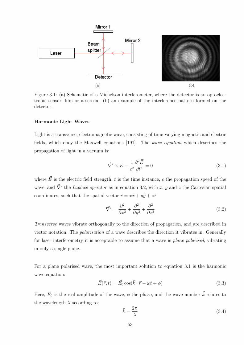
(a) (b)
Figure 3.1: (a) Schematic of a Michelson interferometer, where the detector is an optoelec-tronic sensor, film or a screen. (b) an example of the interference pattern formed on thedetector.
Harmonic Light Waves
Light is a transverse, electromagnetic wave, consisting of time-varying magnetic and electric
fields, which obey the Maxwell equations [191]. The wave equation which describes the
propagation of light in a vacuum is:
~∇2 × ~E − 1
c2
∂2 ~E
∂t2= 0 (3.1)
where ~E is the electric field strength, t is the time instance, c the propagation speed of the
wave, and ~∇2 the Laplace operator as in equation 3.2, with x, y and z the Cartesian spatial
coordinates, such that the spatial vector ~r = xx+ yy + zz.
~∇2 =∂2
∂x2+
∂2
∂y2+
∂2
∂z2(3.2)
Transverse waves vibrate orthogonally to the direction of propagation, and are described in
vector notation. The polarisation of a wave describes the direction it vibrates in. Generally
for laser interferometry it is acceptable to assume that a wave is plane polarised, vibrating
in only a single plane.
For a plane polarised wave, the most important solution to equation 3.1 is the harmonic
wave equation:
~E(~r, t) = ~E0 cos(~k · ~r − ωt+ φ) (3.3)
Here, ~E0 is the real amplitude of the wave, φ the phase, and the wave number ~k relates to
the wavelength λ according to:
~k =2π
λ(3.4)
53
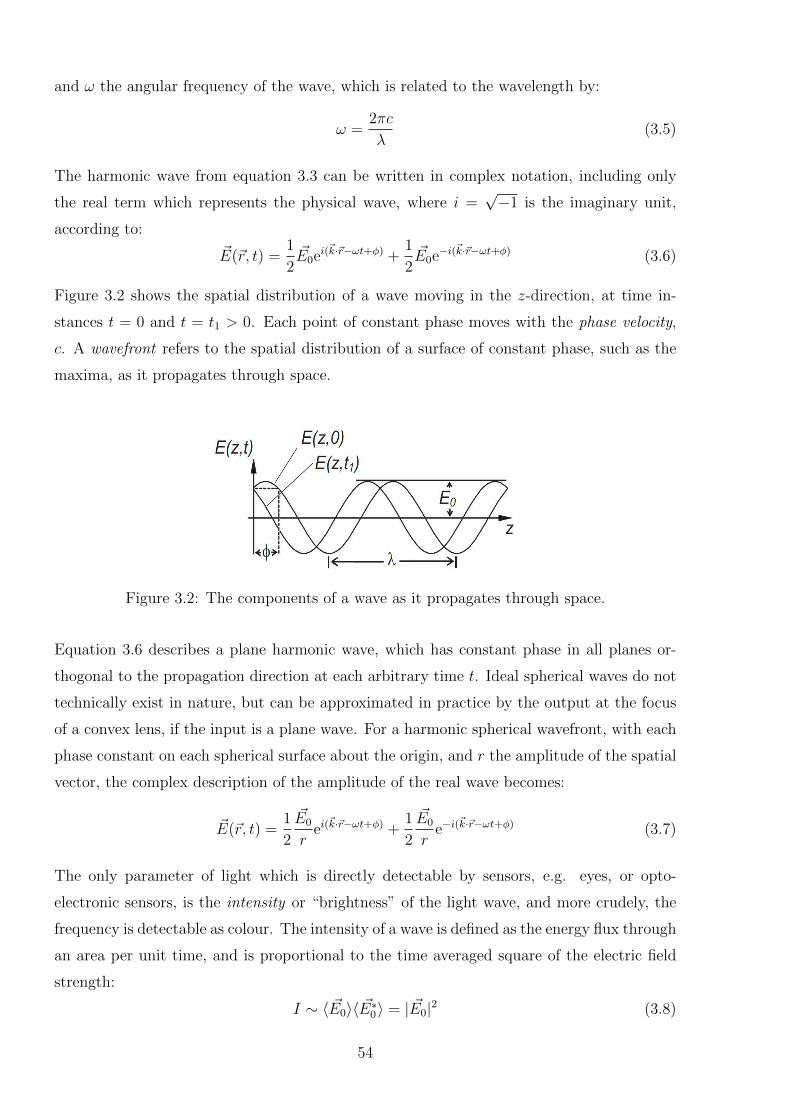
and ω the angular frequency of the wave, which is related to the wavelength by:
ω =2πc
λ(3.5)
The harmonic wave from equation 3.3 can be written in complex notation, including only
the real term which represents the physical wave, where i =√−1 is the imaginary unit,
according to:
~E(~r, t) =1
2~E0ei(
~k·~r−ωt+φ) +1
2~E0e−i(
~k·~r−ωt+φ) (3.6)
Figure 3.2 shows the spatial distribution of a wave moving in the z-direction, at time in-
stances t = 0 and t = t1 > 0. Each point of constant phase moves with the phase velocity,
c. A wavefront refers to the spatial distribution of a surface of constant phase, such as the
maxima, as it propagates through space.
Figure 3.2: The components of a wave as it propagates through space.
Equation 3.6 describes a plane harmonic wave, which has constant phase in all planes or-
thogonal to the propagation direction at each arbitrary time t. Ideal spherical waves do not
technically exist in nature, but can be approximated in practice by the output at the focus
of a convex lens, if the input is a plane wave. For a harmonic spherical wavefront, with each
phase constant on each spherical surface about the origin, and r the amplitude of the spatial
vector, the complex description of the amplitude of the real wave becomes:
~E(~r, t) =1
2
~E0
rei(~k·~r−ωt+φ) +
1
2
~E0
re−i(
~k·~r−ωt+φ) (3.7)
The only parameter of light which is directly detectable by sensors, e.g. eyes, or opto-
electronic sensors, is the intensity or “brightness” of the light wave, and more crudely, the
frequency is detectable as colour. The intensity of a wave is defined as the energy flux through
an area per unit time, and is proportional to the time averaged square of the electric field
strength:
I ∼ 〈 ~E0〉〈 ~E∗0〉 = | ~E0|2 (3.8)
54
Refractive Index
The refractive index, n, of a medium is defined as the ratio of the phase velocity of a given
wavelength of light in a vacuum, c, to that in the medium, v [191]. If a given medium has
a greater optical density, then it has a higher refractive index, and light moves more slowly
through it.
n =c
v(3.9)
This slowing down effect is caused by the electric and magnetic fields of the wave causing
disturbances in the charges of each atom, proportionate to the electric and magnetic sus-
ceptibility of the medium [191]. These disturbances contribute additional electromagnetic
waves and the light wave becomes the macroscopic superposition of all such contributions
in the material, typically resulting in a reduction in phase speed according to equation 3.5.
This results in a phase retardation of the wave, where the phase of the wave upon exiting
the material is retarded compared to that of a wave traversing the same distance with a
vacuum, or material of different refractive index.
To consider it in a slightly different way, the optical path length, OPL, of light propagating
through a medium is a product of the geometric distance of the path of the light and the
refractive index of the medium. In a vacuum, the optical path length is always equivalent
to the physical path length, or geometric distance. This can be determined according to
Fermat’s principle, which is that the path light takes between two points is always the path
that has the minimum optical path length. An optical path length difference ∆OPL is the
difference in the optical path length traversing between the same points along two different
paths or through mediums with differing properties. The optical path length traversed
determines which phase the light has at any given point.
∆OPL =λ∆φ
2π(3.10)
Alteration of the refractive index by external factors can thus be investigated by measuring
the change in phase of a wave passing a distance d through a medium.
∆φ =2πd∆n
λ(3.11)
Interference
The term interference refers to the redistribution of energy in space when two or more waves
overlap, resulting in a new wave consisting of the undisturbed superposition of the two
waves. The components of the waves in each direction superimpose independently, therefore
55
two waves travelling orthogonally to each other will not interfere. The combined intensity,
I, of two waves can be calculated from their descriptions in equation 3.6. In the simplest
case, it is assumed that the two interfering waves have the same frequency and polarisation,
resulting in a combined intensity of:
I ∼ | ~E1 + ~E2|2 (3.12)
= ( ~E1 + ~E2)( ~E1 + ~E2)∗ (3.13)
= ( ~E10)2 + ( ~E2
0)2 + 2 ~E10~E2
0 cos(φ1 − φ2) (3.14)
= I1 + I2 + 2√I1I2 cos ∆φ (3.15)
where I1 and I2 are the individual intensities of each wave, and ∆φ = φ1−φ2 is the difference
in phase between the two waves. The third term in equation 3.15 is the sinusoidal varying
term which governs the interference. This term is maximum, referred to as constructive
interference, when the two waves are in phase:
∆φ = 2nπ for n = 0, 1, 2 ... (3.16)
Destructive interference occurs when this term is minimum because the two waves are com-
pletely out of phase:
∆φ = (2n+ 1)π for n = 0, 1, 2 ... (3.17)
where n represents the order of the interference. Across any given plane through the inter-
section of the two light waves, this results in a pattern of alternating bright and dark bands
called interference fringes. These fringes are spaced according to the variation in phase be-
tween the two light waves. This is determined by the difference in optical path length each
has traversed to reach the observation point, a factor which depends on the wavelength, the
angle between the waves, and the geometric distance travelled in each medium with differing
refractive indices. Thus for the interference bands to be resolvable the angle between the
two light beams must be small.
If the two waves have the same intensity, I, then the interference pattern displays the max-
imum intensity modulation, from zero to 4I. As the intensities of the two waves become
increasingly different, the interference pattern has lower contrast C, where C is described
according to:
C =Imax − IminImax + Imin
(3.18)
In the above example calculating the intensity of an interfering wave, the waves are assumed
to have the same frequency and polarization. This is a factor of the coherence, or correlation
56
between the two light beams. Thus only two light beams which are sufficiently coherent
will display this interference effect. There are two aspects of coherence, temporal and spa-
tial. Temporal coherence describes the correlation of a wave with itself, at different time
instances - in other words whether there is frequency drift over time, proportional to the
distance travelled by the wave in a medium of given refractive index. A stabilized single-
mode laser emits nearly perfectly temporally coherent light. Spatial coherence describes
the mutual correlation of different parts of the same wavefront at a given distance from the
source, both longitudinal and cross-sectional. This is a property of the light wave and is
usually associated with the apparent size of the source as seen from the measurement point.
The spatial coherence of laser light is associated with the transverse mode structure of the
resonance cavity, so for lasers resonating in the fundamental transverse (TEM00) mode, all
points on the wavefront have essentially perfect spatial coherence. Thus for many inter-
ferometry experiments, a single laser possessing sufficient spatial and temporal coherence
is used, and divided into two beams which can then later be recombined after probing the
medium of interest.
3.3 Refractive Index Determination in Liquids
Interferometers have been developed in a large range of different designs, and been applied to
countless different applications in many fields of scientific research. The use of interferometry
is indicated by the occurrence of a physical process where the optical path length is modified
by various physical quantities. If this induced modification of the path length changes only
the phase of the light and has minimal effect on the lateral displacement then measurement
of the physical quantity is amenable to interferometry. For many years, a major application
of interferometry has been for non-destructive testing of mechanical components under load
or vibration; they must have diffusely reflecting opaque surfaces, such as turbine blades,
pressure transducers, aircraft and automotive parts etc [192–194]. Some of the additional
areas interferometry has been used for have been to investigate the propagation of bending
waves after an impact [195, 196], crack propagation in glass [197], flow visualisation in fluid
dynamics [198], mass distributions in mass transfer experiments [199] and measurement of
electron densities in plasma diagnostics [200].
Application of interferometry to radiation dosimetry exploits the use of interferometry as a
tool to non-intrusively provide temperature field visualisation and quantification in transpar-
ent gases and liquids. There are many optical techniques capable of utilising refractive index
57
variations in order to measure temperature fields in a liquid [201]. These include methods
based around the deflection of light rays from refraction effects, including laser speckle pho-
tography [202], Talbot interferometry [203] and quantitative Schlieren [204]. Other methods
infer the temperature field in a test liquid, known as a phase object, from measured phase
differences of light due to refractive index variation. These include classical interferometry,
shearing interferometry [205], and holographic interferometry [200, 206–208]. Holographic
interferometric techniques have some distinct advantages in certain applications, which will
be discussed in the following section.
3.3.1 Holographic Interferometry
Holography is a type of optical interferometry, whereby optical interferograms are created,
and then a three dimensional image of the object is reconstructed. This has traditionally
been done using holographic film as the recording medium, which is exposed by the interfer-
ing light waves, which consist of an unchanging reference beam and an object beam which
probes the phase object and thus varies with temperature. Following exposure, the film is
developed, and replaced precisely in the location where it was exposed, and re-illuminated
by the reference beam. This reference beam then interferes with the interference pattern
already developed on the film, causing a hologram to form - a three dimensional image of
the original object to be reconstructed, in its original location.
Holographic interferometry is a further extension of this process whereby it is possible to
make two holograms, which were recorded with different states of the phase object, interfere
with each other. This results in a reconstruction of the phase object which shows only the
changes in the object between the different states. Compared to classical interferometry,
this greatly simplifies the process of obtaining information regarding the refractive index
variations. For classical interferometry, variation of phase throughout the object is obtained
by analysis of the recorded fringe pattern, which shows only minor variations. Comparison
of two fringe patterns can allow for inference of the parameter of interest, i.e. the change in
the temperature field. However for holographic interferometry, instead of having to analyse
the fringe patterns directly, the reconstructed interferograms show a fringe pattern that cor-
responds only to the difference in phase, and therefore the temperature change.
The additional benefit of holographic interferometry over classical interferometry, is that less
precise and therefore cheaper, optical components may be used in the interferometer [209].
For classical interferometry, very high precision optical components are required in order
58
to produce a fringe field with minimal distortions. Each optical component, such as beam
splitters, mirrors, lenses etc. cause distortions in the wavefront which affects the uniformity
of the fringes in the resultant interference pattern. This greatly enhances the difficulty of the
analysis, reducing the accuracy achievable in the results. Reduction of this effect is achieved
with a reference beam with an ideal shape, such as flat or spherical, and all surfaces kept
optically flat to approximately one twentieth or less of the wavelength of light used, which
is difficult and therefore expensive to achieve [200]. In contrast, holographic interferometry
circumvents this problem by implementing a differential concept, because the output is a
reconstructed interferogram showing only the differences between the two interferograms,
and thus any distortions or non-uniformities effectively cancel out [209].
Holographic interferometry can be done using a real-time technique, as well as the traditional
double exposure technique which captures just one time instance. An interferogram in the
reference state of the object is captured, developed and re-illuminated by the interferometer
as the refractive index in the phase object is altered, by heat or some other means such as
varying the chemical composition. The fringe pattern of the resultant reconstructed holo-
graphic interferogram has bright fringes at the even integer multiples of π and so locations in
the object where there is no change in the phase, or a 2nπ change, will be in the centre of a
dark fringe in the reconstructed image. Quantitative evaluation of the holographic interfer-
ence patterns involves the pointwise determination of the numerical value of the optical path
length change at each point, and relating that back to the physical quantity which caused
it. Early techniques involved manually counting the fringes directly in the interferograms to
obtain an approximation to the interference phase distribution. In more modern techniques,
the resultant holograms are often captured by a camera either in video mode, or at specific
time instances. A consideration is the variation caused by the observation vector, which
is overcome by the observer projector theorem, which states that if the holographic inter-
ferometric fringes are localized off the object surface, they can be observed as if projected
onto the object surface radially from the centre of the aperture of the viewing system [200].
The captured images can be stored for later analysis. The manual counting of the fringes is
replaced by computerized techniques such as fringe skeletonising [210, 211]. These methods
assume that the local extrema of the intensity distribution correspond to maxima and min-
ima of the cosine function in equation 3.15 and that the phase at these pixels is therefore an
even or odd integer multiple of π. There are several types of fringe skeletonising methods,
including some based on fringe tracking, and some related to segmentation. A processing
scheme involves multiple steps, beginning with spatial and temporal filtering to improve
59
the signal-to-noise ratio and specification of the fringe pattern boundary, then extraction
of the raw skeleton by fringe tracking, pattern segmentation, or another method, and in-
teractive enhancement of this skeleton by removing artifacts, adding missing points, linking
interrupted lines and removing line crossings. The fringes are then given interference order
numbers, and the interference phase between the lines is interpolated, before the physical
values of what was being measured are determined at each point.
3.3.2 Digital Holographic Interferometry
Advances in optoelectronic sensor technology such as CCD (charge coupled devices) and
CMOS (complementary metal oxide semiconductor) technology, as well as in computer pro-
cessing power, have made it feasible to collect the interferograms digitally, and then use
numerical algorithms to reconstruct the holograms directly. This method is termed Digi-
tal Holographic Interferometry (DHI) and was first developed by Schnars and Juptner in
1994 [205, 212]. For each recorded state of the object, the intensity and the phase of the
object wave can be calculated during the reconstruction of the algorithm, and the interfer-
ence phase determined from the comparison of these individual phases. This eliminates the
technical challenges of using film, which requires a time consuming chemical development
process, as well as introducing potential uncertainties during the realignment of the film to
its exact previous location in the interferometer. The results of doing this process digitally
are reconstructed interferograms from which the phase information can be directly obtained,
at video frequency, having high resolution and contrast, with no need to consider the obser-
vation vector. Any state of the object can be used as a reference, being the initial conditions
of the object which all subsequent changes are compared to. This is a major advantage
compared to non-digital methods which require the exposure of a film with a reference inter-
ferogram at a single set time instance. Because the interferogram only provides information
on the evolution of the system since the reference conditions, the digital methods minimisa-
tion of the elapsed time between acquisition of the reference interferogram and later object
ones increases the reliability of the results. The integration of optical recording, numerical
reconstruction and evaluation into one system is also a major advantage as it simplifies and
streamlines the process.
The drawback of the digital method is the lower spatial resolution of optoelectronic arrays
compared to film. This means that the angle between the reference and object waves must
be limited to just a few degrees, in order to satisfy the Nyquist sampling theorem [213].
60
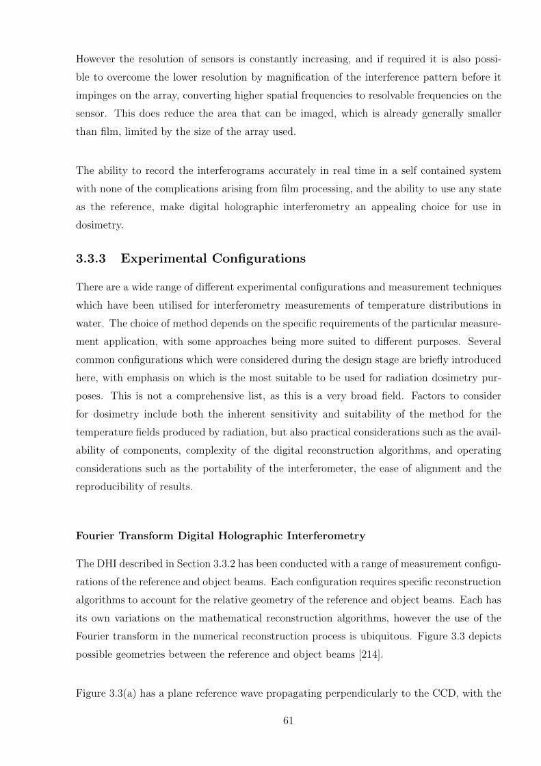
However the resolution of sensors is constantly increasing, and if required it is also possi-
ble to overcome the lower resolution by magnification of the interference pattern before it
impinges on the array, converting higher spatial frequencies to resolvable frequencies on the
sensor. This does reduce the area that can be imaged, which is already generally smaller
than film, limited by the size of the array used.
The ability to record the interferograms accurately in real time in a self contained system
with none of the complications arising from film processing, and the ability to use any state
as the reference, make digital holographic interferometry an appealing choice for use in
dosimetry.
3.3.3 Experimental Configurations
There are a wide range of different experimental configurations and measurement techniques
which have been utilised for interferometry measurements of temperature distributions in
water. The choice of method depends on the specific requirements of the particular measure-
ment application, with some approaches being more suited to different purposes. Several
common configurations which were considered during the design stage are briefly introduced
here, with emphasis on which is the most suitable to be used for radiation dosimetry pur-
poses. This is not a comprehensive list, as this is a very broad field. Factors to consider
for dosimetry include both the inherent sensitivity and suitability of the method for the
temperature fields produced by radiation, but also practical considerations such as the avail-
ability of components, complexity of the digital reconstruction algorithms, and operating
considerations such as the portability of the interferometer, the ease of alignment and the
reproducibility of results.
Fourier Transform Digital Holographic Interferometry
The DHI described in Section 3.3.2 has been conducted with a range of measurement configu-
rations of the reference and object beams. Each configuration requires specific reconstruction
algorithms to account for the relative geometry of the reference and object beams. Each has
its own variations on the mathematical reconstruction algorithms, however the use of the
Fourier transform in the numerical reconstruction process is ubiquitous. Figure 3.3 depicts
possible geometries between the reference and object beams [214].
Figure 3.3(a) has a plane reference wave propagating perpendicularly to the CCD, with the
61
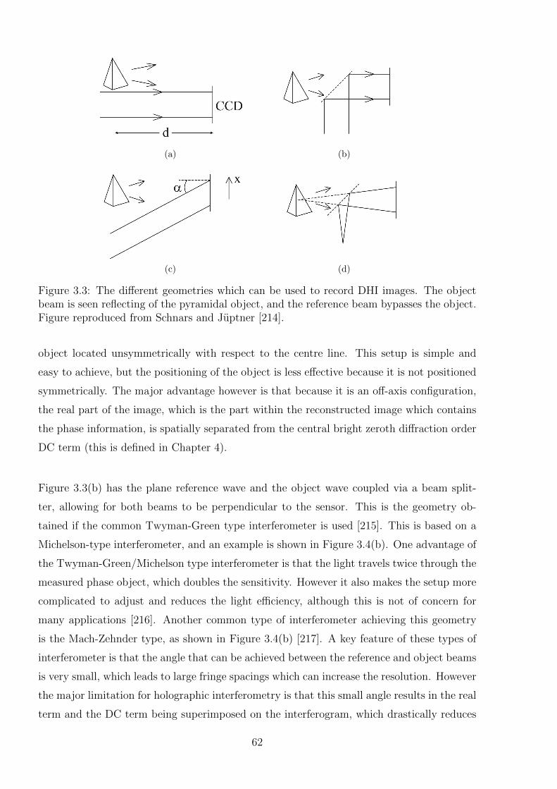
(a) (b)
(c) (d)
Figure 3.3: The different geometries which can be used to record DHI images. The objectbeam is seen reflecting of the pyramidal object, and the reference beam bypasses the object.Figure reproduced from Schnars and Juptner [214].
object located unsymmetrically with respect to the centre line. This setup is simple and
easy to achieve, but the positioning of the object is less effective because it is not positioned
symmetrically. The major advantage however is that because it is an off-axis configuration,
the real part of the image, which is the part within the reconstructed image which contains
the phase information, is spatially separated from the central bright zeroth diffraction order
DC term (this is defined in Chapter 4).
Figure 3.3(b) has the plane reference wave and the object wave coupled via a beam split-
ter, allowing for both beams to be perpendicular to the sensor. This is the geometry ob-
tained if the common Twyman-Green type interferometer is used [215]. This is based on a
Michelson-type interferometer, and an example is shown in Figure 3.4(b). One advantage of
the Twyman-Green/Michelson type interferometer is that the light travels twice through the
measured phase object, which doubles the sensitivity. However it also makes the setup more
complicated to adjust and reduces the light efficiency, although this is not of concern for
many applications [216]. Another common type of interferometer achieving this geometry
is the Mach-Zehnder type, as shown in Figure 3.4(b) [217]. A key feature of these types of
interferometer is that the angle that can be achieved between the reference and object beams
is very small, which leads to large fringe spacings which can increase the resolution. However
the major limitation for holographic interferometry is that this small angle results in the real
term and the DC term being superimposed on the interferogram, which drastically reduces
62
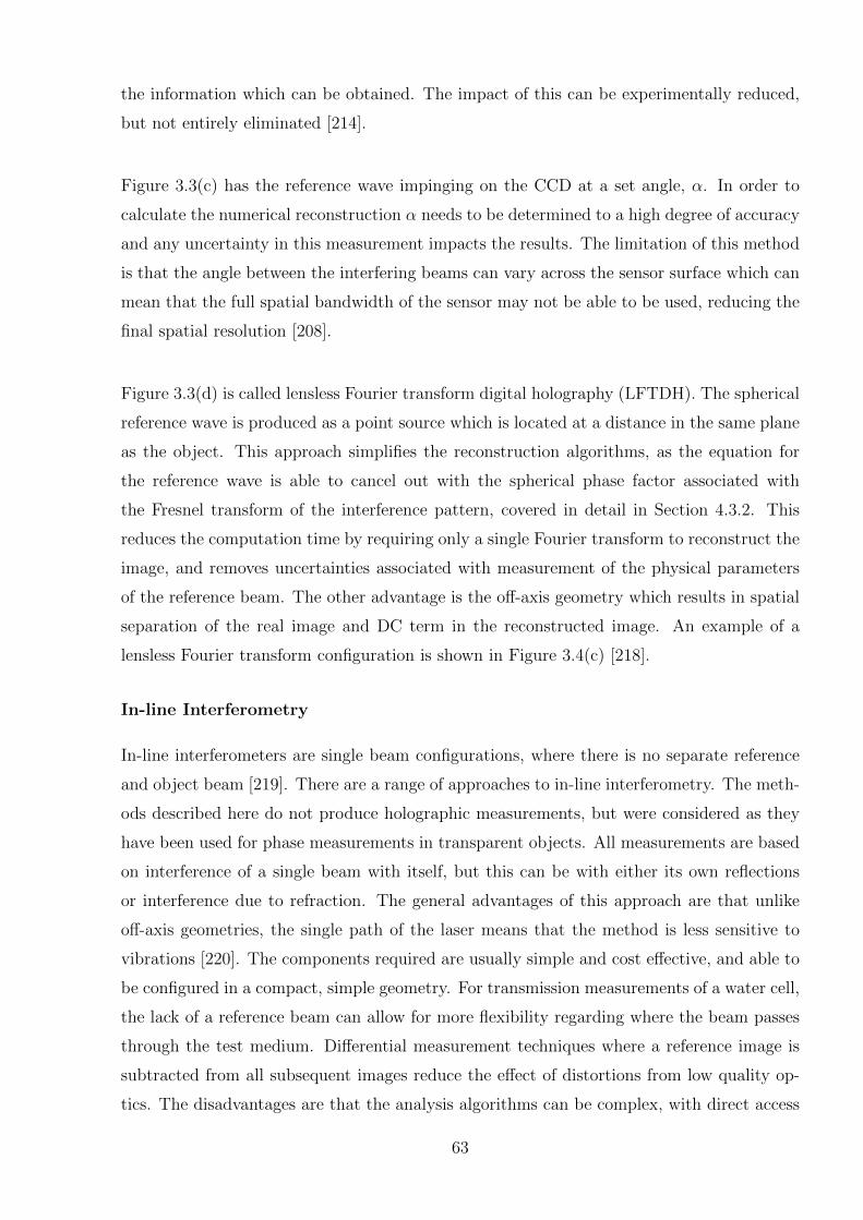
the information which can be obtained. The impact of this can be experimentally reduced,
but not entirely eliminated [214].
Figure 3.3(c) has the reference wave impinging on the CCD at a set angle, α. In order to
calculate the numerical reconstruction α needs to be determined to a high degree of accuracy
and any uncertainty in this measurement impacts the results. The limitation of this method
is that the angle between the interfering beams can vary across the sensor surface which can
mean that the full spatial bandwidth of the sensor may not be able to be used, reducing the
final spatial resolution [208].
Figure 3.3(d) is called lensless Fourier transform digital holography (LFTDH). The spherical
reference wave is produced as a point source which is located at a distance in the same plane
as the object. This approach simplifies the reconstruction algorithms, as the equation for
the reference wave is able to cancel out with the spherical phase factor associated with
the Fresnel transform of the interference pattern, covered in detail in Section 4.3.2. This
reduces the computation time by requiring only a single Fourier transform to reconstruct the
image, and removes uncertainties associated with measurement of the physical parameters
of the reference beam. The other advantage is the off-axis geometry which results in spatial
separation of the real image and DC term in the reconstructed image. An example of a
lensless Fourier transform configuration is shown in Figure 3.4(c) [218].
In-line Interferometry
In-line interferometers are single beam configurations, where there is no separate reference
and object beam [219]. There are a range of approaches to in-line interferometry. The meth-
ods described here do not produce holographic measurements, but were considered as they
have been used for phase measurements in transparent objects. All measurements are based
on interference of a single beam with itself, but this can be with either its own reflections
or interference due to refraction. The general advantages of this approach are that unlike
off-axis geometries, the single path of the laser means that the method is less sensitive to
vibrations [220]. The components required are usually simple and cost effective, and able to
be configured in a compact, simple geometry. For transmission measurements of a water cell,
the lack of a reference beam can allow for more flexibility regarding where the beam passes
through the test medium. Differential measurement techniques where a reference image is
subtracted from all subsequent images reduce the effect of distortions from low quality op-
tics. The disadvantages are that the analysis algorithms can be complex, with direct access
63
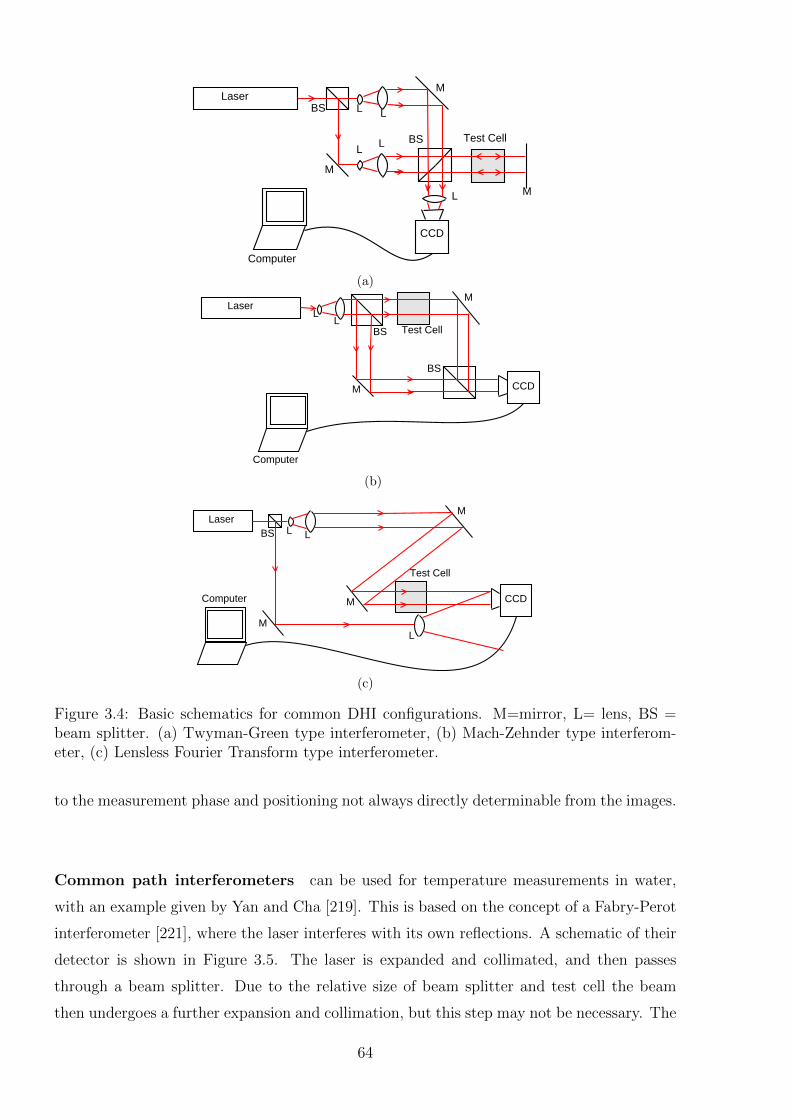
M
M
M
BS
BS
LaserL L
L
L
L
CCD
Computer
Test Cell
(a)
M
M
BS
BS
Laser
LL
CCD
Computer
Test Cell
(b)
M
M
BS
M
Laser
LL
CCDComputer
Test Cell
L
(c)
Figure 3.4: Basic schematics for common DHI configurations. M=mirror, L= lens, BS =beam splitter. (a) Twyman-Green type interferometer, (b) Mach-Zehnder type interferom-eter, (c) Lensless Fourier Transform type interferometer.
to the measurement phase and positioning not always directly determinable from the images.
Common path interferometers can be used for temperature measurements in water,
with an example given by Yan and Cha [219]. This is based on the concept of a Fabry-Perot
interferometer [221], where the laser interferes with its own reflections. A schematic of their
detector is shown in Figure 3.5. The laser is expanded and collimated, and then passes
through a beam splitter. Due to the relative size of beam splitter and test cell the beam
then undergoes a further expansion and collimation, but this step may not be necessary. The
64
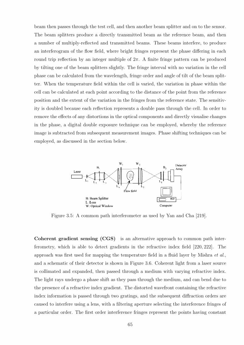
beam then passes through the test cell, and then another beam splitter and on to the sensor.
The beam splitters produce a directly transmitted beam as the reference beam, and then
a number of multiply-reflected and transmitted beams. These beams interfere, to produce
an interferogram of the flow field, where bright fringes represent the phase differing in each
round trip reflection by an integer multiple of 2π. A finite fringe pattern can be produced
by tilting one of the beam splitters slightly. The fringe interval with no variation in the cell
phase can be calculated from the wavelength, fringe order and angle of tilt of the beam split-
ter. When the temperature field within the cell is varied, the variation in phase within the
cell can be calculated at each point according to the distance of the point from the reference
position and the extent of the variation in the fringes from the reference state. The sensitiv-
ity is doubled because each reflection represents a double pass through the cell. In order to
remove the effects of any distortions in the optical components and directly visualise changes
in the phase, a digital double exposure technique can be employed, whereby the reference
image is subtracted from subsequent measurement images. Phase shifting techniques can be
employed, as discussed in the section below.
Figure 3.5: A common path interferometer as used by Yan and Cha [219].
Coherent gradient sensing (CGS) is an alternative approach to common path inter-
ferometry, which is able to detect gradients in the refractive index field [220, 222]. The
approach was first used for mapping the temperature field in a fluid layer by Mishra et al.,
and a schematic of their detector is shown in Figure 3.6. Coherent light from a laser source
is collimated and expanded, then passed through a medium with varying refractive index.
The light rays undergo a phase shift as they pass through the medium, and can bend due to
the presence of a refractive index gradient. The distorted wavefront containing the refractive
index information is passed through two gratings, and the subsequent diffraction orders are
caused to interfere using a lens, with a filtering aperture selecting the interference fringes of
a particular order. The first order interference fringes represent the points having constant
65
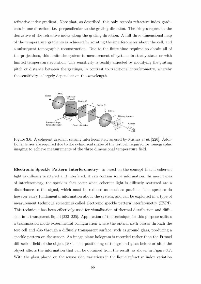
refractive index gradient. Note that, as described, this only records refractive index gradi-
ents in one direction, i.e. perpendicular to the grating direction. The fringes represent the
derivative of the refractive index along the grating direction. A full three dimensional map
of the temperature gradients is achieved by rotating the interferometer about the cell, and
a subsequent tomographic reconstruction. Due to the finite time required to obtain all of
the projections, this limits the system to measurement of systems in steady state, or with
limited temperature evolution. The sensitivity is readily adjusted by modifying the grating
pitch or distance between the gratings, in contrast to traditional interferometry, whereby
the sensitivity is largely dependent on the wavelength.
Figure 3.6: A coherent gradient sensing interferometer, as used by Mishra et al. [220]. Addi-tional lenses are required due to the cylindrical shape of the test cell required for tomographicimaging to achieve measurements of the three dimensional temperature field.
Electronic Speckle Pattern Interferometry is based on the concept that if coherent
light is diffusely scattered and interfered, it can contain some information. In most types
of interferometry, the speckles that occur when coherent light is diffusely scattered are a
disturbance to the signal, which must be reduced as much as possible. The speckles do
however carry fundamental information about the system, and can be exploited in a type of
measurement technique sometimes called electronic speckle pattern interferometry (ESPI).
This technique has been effectively used for visualisation of thermal distribution and diffu-
sion in a transparent liquid [223–225]. Application of the technique for this purpose utilises
a transmission mode experimental configuration where the optical path passes through the
test cell and also through a diffusely transparent surface, such as ground glass, producing a
speckle pattern on the sensor. An image plane hologram is recorded rather than the Fresnel
diffraction field of the object [200]. The positioning of the ground glass before or after the
object affects the information that can be obtained from the result, as shown in Figure 3.7.
With the glass placed on the sensor side, variations in the liquid refractive index variation
66
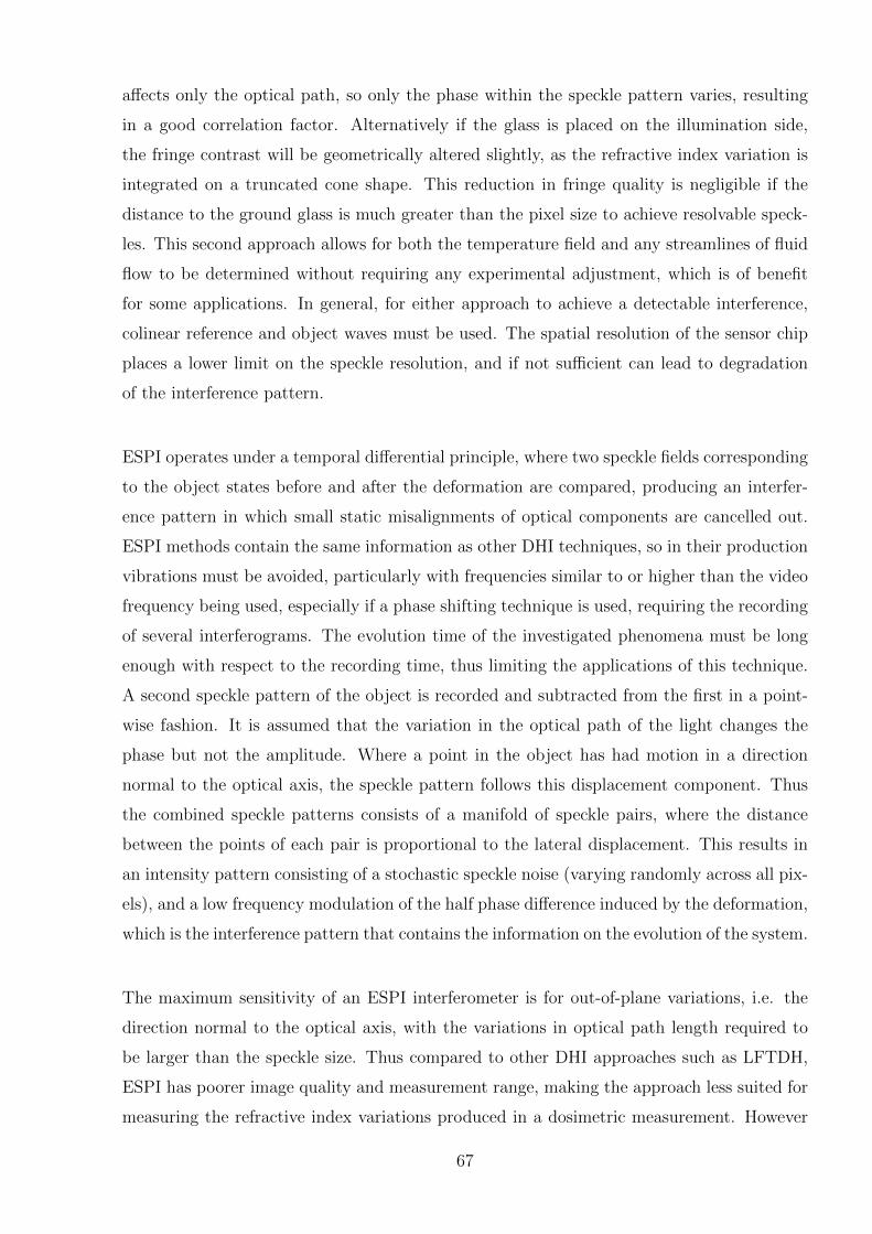
affects only the optical path, so only the phase within the speckle pattern varies, resulting
in a good correlation factor. Alternatively if the glass is placed on the illumination side,
the fringe contrast will be geometrically altered slightly, as the refractive index variation is
integrated on a truncated cone shape. This reduction in fringe quality is negligible if the
distance to the ground glass is much greater than the pixel size to achieve resolvable speck-
les. This second approach allows for both the temperature field and any streamlines of fluid
flow to be determined without requiring any experimental adjustment, which is of benefit
for some applications. In general, for either approach to achieve a detectable interference,
colinear reference and object waves must be used. The spatial resolution of the sensor chip
places a lower limit on the speckle resolution, and if not sufficient can lead to degradation
of the interference pattern.
ESPI operates under a temporal differential principle, where two speckle fields corresponding
to the object states before and after the deformation are compared, producing an interfer-
ence pattern in which small static misalignments of optical components are cancelled out.
ESPI methods contain the same information as other DHI techniques, so in their production
vibrations must be avoided, particularly with frequencies similar to or higher than the video
frequency being used, especially if a phase shifting technique is used, requiring the recording
of several interferograms. The evolution time of the investigated phenomena must be long
enough with respect to the recording time, thus limiting the applications of this technique.
A second speckle pattern of the object is recorded and subtracted from the first in a point-
wise fashion. It is assumed that the variation in the optical path of the light changes the
phase but not the amplitude. Where a point in the object has had motion in a direction
normal to the optical axis, the speckle pattern follows this displacement component. Thus
the combined speckle patterns consists of a manifold of speckle pairs, where the distance
between the points of each pair is proportional to the lateral displacement. This results in
an intensity pattern consisting of a stochastic speckle noise (varying randomly across all pix-
els), and a low frequency modulation of the half phase difference induced by the deformation,
which is the interference pattern that contains the information on the evolution of the system.
The maximum sensitivity of an ESPI interferometer is for out-of-plane variations, i.e. the
direction normal to the optical axis, with the variations in optical path length required to
be larger than the speckle size. Thus compared to other DHI approaches such as LFTDH,
ESPI has poorer image quality and measurement range, making the approach less suited for
measuring the refractive index variations produced in a dosimetric measurement. However
67
ESPI can be straightforward to use, as it does not require precise alignment of components,
meaning it is possible to automate the measurement process [224]. The most common use of
ESPI is in reflection rather than transmission mode, for deformation measurements of opaque
surfaces, and in fluid mechanics where fluids are seeded with reflective tracer particles.
(a) (b)
Figure 3.7: The effect of the positioning of the ground glass for an ESPI interferometer:(a) when the ground glass is placed between the cell and the camera, the refractive-indexvariation is integrated along a line, and (b) when the ground glass is located on the illumina-tion side of the cell, the refractive-index variation is integrated on a truncated cone. Figurereproduced from Dupont et al. [223].
Phase Shifting Measurement Acquisition
Phase shifting is a measurement approach that was developed to interpret the fringe patterns
on the reconstructed images obtained using film interferometric techniques [226, 227]. The
reconstructed film contains a fringe pattern consisting of light intensity maps, rather than
phase maps. Phase shifting allowed for the phase of the object beam to be determined from
the film. The process involves rotating one of the mirrors along the path of the reference
wave step-wise, causing the phase of the reference wave to shift. This results in a pattern of
parallel fringes on the recorded interferogram. The principle of phase shifting interferometry
is to record several (at least three) interferograms with added phase shifts between each. Any
change in the phase within the object beam results in a shift of these fringes, with the extent
of the shift proportional to the change in phase. Multiple phase shifts are required in order
to create sufficient points at which the phase can be analysed. The object phase can then be
calculated from these phase shifted interferograms via a range of available algorithms [200].
Phase shifting approaches can be applied to all of the interferometer configurations described
above.
For digital holographic techniques the advantage of access to the phase information is some-
what negligible, as the phase can be determined from the complex intensity wave that is
68
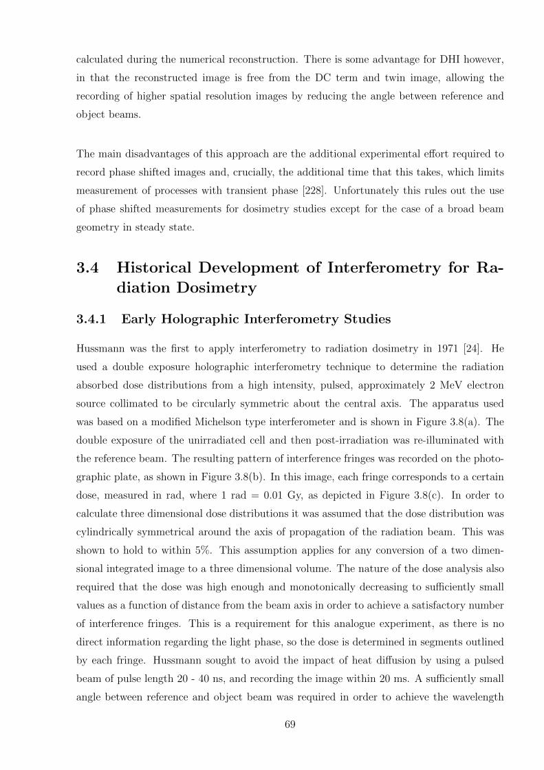
calculated during the numerical reconstruction. There is some advantage for DHI however,
in that the reconstructed image is free from the DC term and twin image, allowing the
recording of higher spatial resolution images by reducing the angle between reference and
object beams.
The main disadvantages of this approach are the additional experimental effort required to
record phase shifted images and, crucially, the additional time that this takes, which limits
measurement of processes with transient phase [228]. Unfortunately this rules out the use
of phase shifted measurements for dosimetry studies except for the case of a broad beam
geometry in steady state.
3.4 Historical Development of Interferometry for Ra-
diation Dosimetry
3.4.1 Early Holographic Interferometry Studies
Hussmann was the first to apply interferometry to radiation dosimetry in 1971 [24]. He
used a double exposure holographic interferometry technique to determine the radiation
absorbed dose distributions from a high intensity, pulsed, approximately 2 MeV electron
source collimated to be circularly symmetric about the central axis. The apparatus used
was based on a modified Michelson type interferometer and is shown in Figure 3.8(a). The
double exposure of the unirradiated cell and then post-irradiation was re-illuminated with
the reference beam. The resulting pattern of interference fringes was recorded on the photo-
graphic plate, as shown in Figure 3.8(b). In this image, each fringe corresponds to a certain
dose, measured in rad, where 1 rad = 0.01 Gy, as depicted in Figure 3.8(c). In order to
calculate three dimensional dose distributions it was assumed that the dose distribution was
cylindrically symmetrical around the axis of propagation of the radiation beam. This was
shown to hold to within 5%. This assumption applies for any conversion of a two dimen-
sional integrated image to a three dimensional volume. The nature of the dose analysis also
required that the dose was high enough and monotonically decreasing to sufficiently small
values as a function of distance from the beam axis in order to achieve a satisfactory number
of interference fringes. This is a requirement for this analogue experiment, as there is no
direct information regarding the light phase, so the dose is determined in segments outlined
by each fringe. Hussmann sought to avoid the impact of heat diffusion by using a pulsed
beam of pulse length 20 - 40 ns, and recording the image within 20 ms. A sufficiently small
angle between reference and object beam was required in order to achieve the wavelength
69
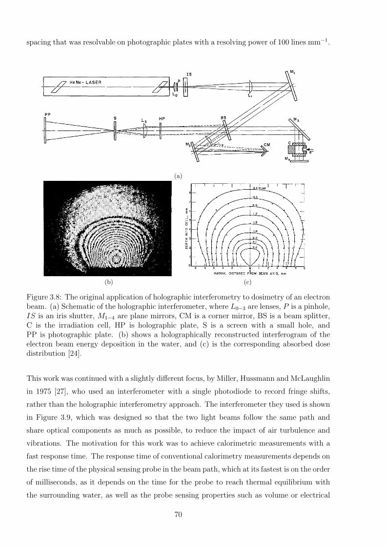
spacing that was resolvable on photographic plates with a resolving power of 100 lines mm−1.
(a)
(b) (c)
Figure 3.8: The original application of holographic interferometry to dosimetry of an electronbeam. (a) Schematic of the holographic interferometer, where L0−3 are lenses, P is a pinhole,IS is an iris shutter, M1−4 are plane mirrors, CM is a corner mirror, BS is a beam splitter,C is the irradiation cell, HP is holographic plate, S is a screen with a small hole, andPP is photographic plate. (b) shows a holographically reconstructed interferogram of theelectron beam energy deposition in the water, and (c) is the corresponding absorbed dosedistribution [24].
This work was continued with a slightly different focus, by Miller, Hussmann and McLaughlin
in 1975 [27], who used an interferometer with a single photodiode to record fringe shifts,
rather than the holographic interferometry approach. The interferometer they used is shown
in Figure 3.9, which was designed so that the two light beams follow the same path and
share optical components as much as possible, to reduce the impact of air turbulence and
vibrations. The motivation for this work was to achieve calorimetric measurements with a
fast response time. The response time of conventional calorimetry measurements depends on
the rise time of the physical sensing probe in the beam path, which at its fastest is on the order
of milliseconds, as it depends on the time for the probe to reach thermal equilibrium with
the surrounding water, as well as the probe sensing properties such as volume or electrical
70
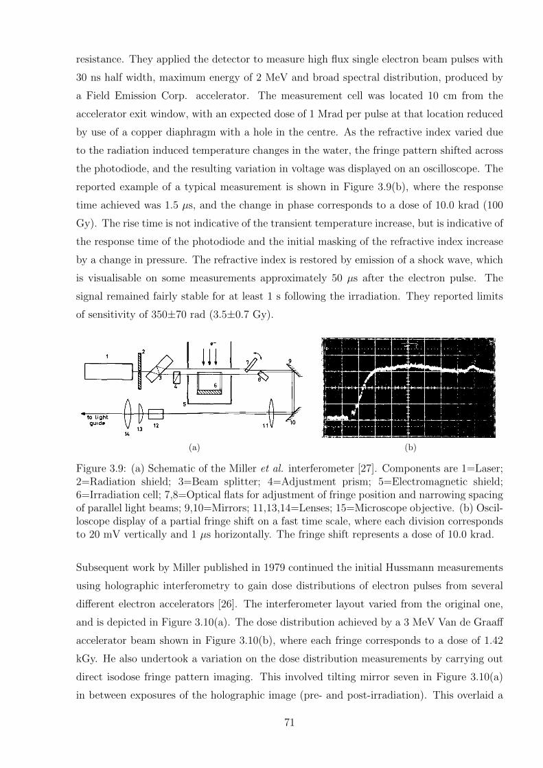
resistance. They applied the detector to measure high flux single electron beam pulses with
30 ns half width, maximum energy of 2 MeV and broad spectral distribution, produced by
a Field Emission Corp. accelerator. The measurement cell was located 10 cm from the
accelerator exit window, with an expected dose of 1 Mrad per pulse at that location reduced
by use of a copper diaphragm with a hole in the centre. As the refractive index varied due
to the radiation induced temperature changes in the water, the fringe pattern shifted across
the photodiode, and the resulting variation in voltage was displayed on an oscilloscope. The
reported example of a typical measurement is shown in Figure 3.9(b), where the response
time achieved was 1.5 µs, and the change in phase corresponds to a dose of 10.0 krad (100
Gy). The rise time is not indicative of the transient temperature increase, but is indicative of
the response time of the photodiode and the initial masking of the refractive index increase
by a change in pressure. The refractive index is restored by emission of a shock wave, which
is visualisable on some measurements approximately 50 µs after the electron pulse. The
signal remained fairly stable for at least 1 s following the irradiation. They reported limits
of sensitivity of 350±70 rad (3.5±0.7 Gy).
(a) (b)
Figure 3.9: (a) Schematic of the Miller et al. interferometer [27]. Components are 1=Laser;2=Radiation shield; 3=Beam splitter; 4=Adjustment prism; 5=Electromagnetic shield;6=Irradiation cell; 7,8=Optical flats for adjustment of fringe position and narrowing spacingof parallel light beams; 9,10=Mirrors; 11,13,14=Lenses; 15=Microscope objective. (b) Oscil-loscope display of a partial fringe shift on a fast time scale, where each division correspondsto 20 mV vertically and 1 µs horizontally. The fringe shift represents a dose of 10.0 krad.
Subsequent work by Miller published in 1979 continued the initial Hussmann measurements
using holographic interferometry to gain dose distributions of electron pulses from several
different electron accelerators [26]. The interferometer layout varied from the original one,
and is depicted in Figure 3.10(a). The dose distribution achieved by a 3 MeV Van de Graaff
accelerator beam shown in Figure 3.10(b), where each fringe corresponds to a dose of 1.42
kGy. He also undertook a variation on the dose distribution measurements by carrying out
direct isodose fringe pattern imaging. This involved tilting mirror seven in Figure 3.10(a)
in between exposures of the holographic image (pre- and post-irradiation). This overlaid a
71
pattern of equally spaced vertical fringes on the reconstructed image. These fringes were
distorted when the water was heated, with the degree of distortion at each point proportional
to the temperature rise. Thus the resulting image was representative of depth dose curves.
The equivalent 10 MeV Van de Graaff generated beam measurement using this method is
shown in Figure 3.10(c). This method was shown to improve the sensitivity, and simplify
the location of the region of maximum dose.
(a)
(b) (c)
Figure 3.10: (a) Schematic of the Miller interferometer [26]. Components are 1=Laser;2=Shutter; 3=Microscope objective; 4=Pinhole; 5=Lens; 6=Beamsplitter; 7=Movable mir-ror; 8=Irradiation cell; 9=Diffuser; 10=Holographic plate. (b) Holographic interferogram ofthe absorbed dose distribution, where each fringe represents an isodose curve correspondingto 1.42 kGy. (c) The same measurement, on a system with parallel fringes superimposed.The distortion of the fringes from vertical corresponds to the dose at each point.
Miller also undertook various measurements to understand the different dose absorption
properties of a range of transparent mediums. He also measured the effect of back scatter
from materials of different densities placed within the electron range, with results showing
an increase in dose just prior to the scatterer, compared to a cell containing only water.
He extended this to investigate the effect of beam perturbations around different shaped
inhomogeneities in the water, simulating the presence of bone within an irradiation volume
in the body. Figure 3.11 shows the aluminium rod used to perturb the dose in the cell, along
with the measured dose distribution and isodose map.
72
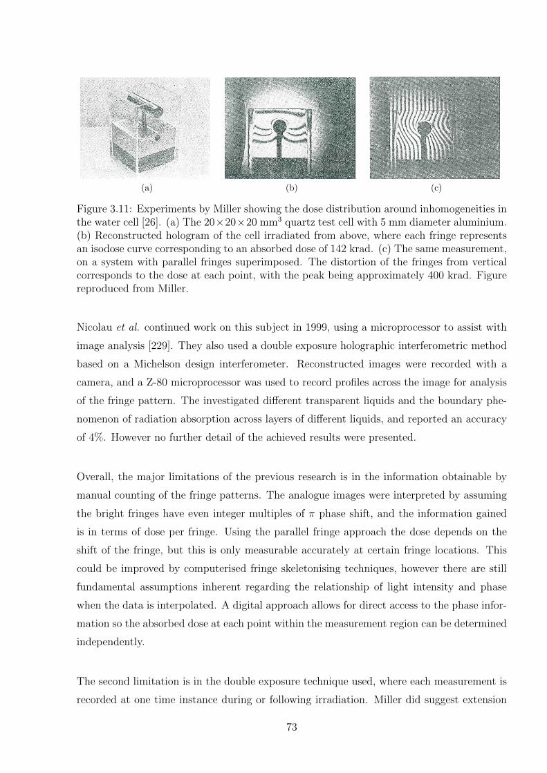
(a) (b) (c)
Figure 3.11: Experiments by Miller showing the dose distribution around inhomogeneities inthe water cell [26]. (a) The 20×20×20 mm3 quartz test cell with 5 mm diameter aluminium.(b) Reconstructed hologram of the cell irradiated from above, where each fringe representsan isodose curve corresponding to an absorbed dose of 142 krad. (c) The same measurement,on a system with parallel fringes superimposed. The distortion of the fringes from verticalcorresponds to the dose at each point, with the peak being approximately 400 krad. Figurereproduced from Miller.
Nicolau et al. continued work on this subject in 1999, using a microprocessor to assist with
image analysis [229]. They also used a double exposure holographic interferometric method
based on a Michelson design interferometer. Reconstructed images were recorded with a
camera, and a Z-80 microprocessor was used to record profiles across the image for analysis
of the fringe pattern. The investigated different transparent liquids and the boundary phe-
nomenon of radiation absorption across layers of different liquids, and reported an accuracy
of 4%. However no further detail of the achieved results were presented.
Overall, the major limitations of the previous research is in the information obtainable by
manual counting of the fringe patterns. The analogue images were interpreted by assuming
the bright fringes have even integer multiples of π phase shift, and the information gained
is in terms of dose per fringe. Using the parallel fringe approach the dose depends on the
shift of the fringe, but this is only measurable accurately at certain fringe locations. This
could be improved by computerised fringe skeletonising techniques, however there are still
fundamental assumptions inherent regarding the relationship of light intensity and phase
when the data is interpolated. A digital approach allows for direct access to the phase infor-
mation so the absorbed dose at each point within the measurement region can be determined
independently.
The second limitation is in the double exposure technique used, where each measurement is
recorded at one time instance during or following irradiation. Miller did suggest extension
73
to a real time holographic interferometry approach, however this was not implemented, and
does introduce further uncertainties from evolution of the system whilst the reference image
is developed. Digital holographic interferometry allows for video frequency recording of the
phase evolution, with any time instance able to be chosen for the reference time during data
analysis.
Reference Image Topography
Ackerley et al. revisited the idea of optical calorimetry, for the purposes of MRT dosimetry
in 2011 [230]. They proposed the concept of digital holographic interferometry, but due to
equipment availability they instead utilised a method based on a modified Schlieren approach
known as Reference Image Topography (RIT) [231, 232]. RIT also maps the variation in
refractive index across a test cell, based on the apparent motion of a speckle pattern projected
through the test cell and imaged on a camera. As the refractive index varies the speckles
appear to move, and the degree of apparent motion at each point in space can be analysed by
a cross-correlation approach like that used in particle image velocimetry processing [233], and
integrated to obtain the indicative temperature values. They made some preliminary proof-
of-principle measurements using a heated wire in a water bath in place of a radiation dose.
Despite the temperatures measured being two orders of magnitude greater than expected
MRT temperature changes, the conclusions they drew were positive regarding the potential
applicability of the method to MRT dosimetry, with RIT expected to be able to resolve
individual heat diffused synchrotron microbeams.
Ultrasonic Thermometry
Malyarenko et al. used an approach based on the same fundamental concept as optical
calorimetry: the use of a non-invasive system to measure temperature variations within a
calorimeter volume, thus eliminating the complexities associated with the presence of non-
water temperature sensing materials within the water phantom [82, 234]. Their approach
was not actually interferometric, comprising the use of ultrasonic thermometry. This tech-
nique determines temperature variations in a medium based on their impact on the speed
of sound, which is measured by detecting the variation in the time of flight of an ultrasound
pulse as it passes through the medium. Their initial work achieved temperature resolutions
on the order of 0.001 K, with a root mean square noise of 5 µK, averaged over a 60 cm
test cell [82]. Their work included a careful consideration of the influence quantities impact-
ing the measurement. Subsequent work extended the system to achieve spatially resolved
74
temperatures via tomographic measurements [234]. The detector used a 128-element trans-
ducer array covering a planar area of 230 mm x 230 mm, to acquire temperature maps by
a fan beam tomographic reconstruction algorithm, to a resolution of approximately 5 mm.
Measurements were achieved with a temporal resolution of four seconds. This is sufficiently
low that the temperature map degradation, for the broad beam geometries considered, due
to heat transport experiences blurring to less than 50% of the spatial resolution. Refine-
ments to the instrument to potentially improve the temporal, spatial and thermal resolutions
were suggested, however to some extent each suggested improvements favour one of these
parameters at the expense of the others. For instance expanding the number of channels
will increase spatial resolution, but also the overall acquisition time. They consider that a
spatial resolution of < 1 mm3 is required in order to make ultrasonic thermometry viable as
a reference standard for medical radiation dosimetry.
Preliminary work in the same research group has considered the use of a similar tomo-
graphic system but utilising an optical interferometry approach to the temperature deter-
mination [83]. The preliminary work is similar to the initial work by Hussmann, with shifts
in the interference pattern recorded by means of a photodiode [24]. Early experiments on
simulated heating patterns have indicated that an optical approach may result in higher
sensitivity temperature resolution than that achieved by ultrasonic thermometry.
3.5 Concluding Remarks
This chapter introduced the fundamental concept of an optical calorimetry approach to
dosimetry. The basic optical principles required to understand the process of digital holo-
graphic interferometry were introduced, including the wave equation for light, refractive
indices, and the process of interference. An introduction to the use of interferometry for
the determination of refractive index variations in water followed, with focus on holographic
interferometry, and the subsequent development of DHI. A selection of experimental config-
urations which were considered during the design phase of the DHI dosimeter are described,
and each has its relative advantages and disadvantages. The chapter concluded with an
historical overview of previous interferometry based approaches to dosimetry. In particular
is the early work by Hussmann and Miller et al. in the 1970s, of which developing this
work further with the application of modern digital technology was the inspiration behind
the present work. The next chapter describes the selection of a DHI approach, and its
subsequent development, including a full description of the completed prototype detector
75
and reconstruction algorithms implemented to interpret the recorded interferograms. The
chapter also describes the preliminary testing and characterisation of the detector that was
undertaken during the refinement process, prior to the eventual radiation measurements.
76
Chapter 4
DHI Dosimeter
This chapter focuses on the design, development and refinement of a prototype interferom-
eter for use as a radiation dosimeter. The design considerations for applying interferometry
to dosimetry are discussed, with the design of the prototype developed based on these re-
quirements. Following this, a complete description of the prototype dosimeter is presented,
along with the mathematical algorithms required for the reconstruction, and an outline of
the operating procedure for a series of measurements. The chapter concludes with examples
of some of the preliminary tests done on the interferometer during development and testing.
4.1 Design Considerations
The choice and design of the interferometer for application to radiation dosimetry has many
technical and practical considerations to take into account. The foremost of these is the
consideration of which particular interferometric approach will be capable of acquiring the
measurements required to a suitable standard. The key points for this choice have already
been introduced in Chapter 3. The next category of design considerations encompasses
the choice of equipment used to build the selected type of interferometer, including the
selection of a laser, camera and optical componentry. Correct selection of equipment is
required in order to optimise the results that can be obtained with a prototype detector,
whilst acknowledging that there are financial constraints. Thus in some cases tradeoffs may
be required to achieve an economical solution. Included within the choice of equipment is
the design of the test cell which is used as a water phantom for the measurements. Another
design consideration is the exact layout and construction of the interferometer to meet the
physical space requirements of some potential radiation applications. The final consideration
is the transportability and ease of operation of the prototype interferometer, for both initial
measurements, and with an eye to potential future clinical implementation. The choice of
an interferometry approach, and the exact design of the prototype dosimeter for this initial
77
proof-of-principle work does not rule out the use of a different design in the future if at that
point it would provide advantages. Suggestions for the improvement of the final design are
given in Chapter 8.
Some of the key considerations are introduced below, with a short description and discussion
of how to incorporate each point into the prototype.
� Choice of interferometry approach: The decision of which interferometry ap-
proach to select required consideration of the advantages and limitations of each tech-
nique as described in Section 3.3.3. Some key considerations which helped to distin-
guish between the possible approaches included the following items.
– The design must be able to achieve high spatial resolution and sensitivity in at
least two dimensions.
– The design must be capable of measuring transient processes, which rules out the
use of phase shifting approaches.
– To reduce the influence of external vibrations and turbulence, the design should
have the light beams share optical components where possible, or fit onto a single
breadboard.
– The measurement uncertainties should be minimised where possible.
– The design should have reconstruction algorithms with access to the interference
phase.
� Equipment considerations: Where possible, available equipment from the optics
laboratories in the Department of Physics and Astronomy, University of Canterbury
was utilised in order to reduce unnecessary expenditure. A limited amount of funding
was available to purchase equipment. The result of this was that some of the equip-
ment choices whilst fit for purpose, involved tradeoffs between cost and quality. The
main purpose of this work was to develop a prototype dosimeter as proof-of-principle
of a DHI approach, and it is anticipated that this will provide a basis for future fund-
ing applications to further develop the work and upgrade the equipment used. With
these funding constraints in mind, some of the design considerations for the equipment
selection are listed here.
– The laser chosen must have low amplitude noise, as the detection system is sensi-
tive to variations in the light intensity and phase, and have a stable power output.
78
– A shorter wavelength laser will increase the sensitivity because a change in refrac-
tive index induces a larger change in optical path length, however the absorbance
of the wavelength in the medium used must be negligible to avoid introduction of
extraneous temperature variations.
– The laser must be of sufficient power to provide enough illumination for the short
exposure times of the camera. The upper limit on the laser power is such that
the camera sensor is not oversaturated. However the ability to attenuate the light
beam makes this a less important requirement.
– The test medium should be water, or near water equivalent, and transparent, with
consideration given to minimisation of the impact of the heat defect. A medium
with a higher variation in refractive index with temperature than water could
be used to increase sensitivity, but this then introduces a further step to convert
absorbed dose to that in water.
– The test cell should have low thermal coefficient of expansion, although this is a
minor point as the temperatures involved are extremely low.
– The test cell must also have smooth, parallel faces, with negligible reflection.
The thickness must be small enough to have minimal impact on the radiation
beam, and the material used should have close to water equivalence for radiation
absorption.
– The width and depth of the test cell must be sufficient to allow the desired depth
of measurement for a given radiation source. This is constrained by where the
cell is located within the interferometer. Additionally, the distance across of the
test cell in the direction of the laser line-of-sight must be optimised to allow for
full measurement of the radiation, but reduce the reduction in sensitivity caused
by integration across a larger distance.
– Ideally the test cell should be large enough to completely absorb the beam, how-
ever this requirement is unlikely to be fully achieved. An approximation of it may
be possible for protons or low energy photons, but is unlikely for higher energy
photons and electrons. At this stage the uncertainty introduced by any scattered
radiation is likely to be negligible compared to the overall uncertainty.
– The camera resolution must be sufficient to resolve dosimetric features such as
the Bragg peak of a proton beam.
– The frame rate of the camera must be high enough to allow any phase changes
to be resolved to within an entire 2π shift in phase. This is only applicable for
79

potentially very high dose rates. The faster the frame rate achievable, the more
accurately corrections for heat diffusion can be made, which is key for highly
modulated radiation sources.
– The camera sensor size controls the size of the region that can be measured, so
as large as possible is desirable. For affordable cameras, this generally becomes a
trade-off between pixel number and pixel size.
� Layout and construction of the interferometer: There are countless variations in
the design of each type of interferometer, and the exact configuration must be designed
to be specific for the purpose of radiation measurement. Some of the considerations
involved in this are listed here.
– If possible there needs to be space available to incorporate shielding to protect
the electronics (camera and laser) from scatter radiation if this is likely to be
considerable.
– It must be possible to enclose the set-up within a box to isolate it as much as
possible from variations in ambient conditions/turbulent airflow etc. In practice,
this entails containing the interferometer on a single breadboard.
– There must be some way of damping vibrations. The use of a vibration isolated
table is not feasible for any measurements of a clinical radiation source, so some
other means must be considered.
– The location of the test cell must have enough space available to allow for different
depths of measurement and varying size test cells.
– The configuration must allow for irradiation of the test cell from the side and
from the top, for use in different beamlines.
� Ease of use: The ease of use of the interferometer and the workflow for radiation
measurements is a vital consideration. This is because most radiation measurements
will be in-situ in a clinical environment. Some points to consider in the design of the
interferometer are listed below.
– The interferometer must be transportable, which involves consideration of weight,
ease of set-up deconstruction, and fragility of the components.
– In a clinical situation most radiation sources are likely to have time constraints,
with limited beam time available for dosimetry experiments. Thus the workflow
for use of the interferometer must be straightforward and well planned, to reduce
80
measurement times required, and the chance of making unpredicted errors. The
interferometer must also be easy to realign in situ if required. Additionally, with
an eye to future clinical implementation, the interferometer should have the po-
tential to be developed to the point where specialised optics experience is not
required for its implementation.
– If tomographic measurements are to be considered at some point in the future this
would be relatively straightforward for vertical beam sources, but far more com-
plicated for a horizontal source (such as many proton beamlines or synchrotron
medical beamlines).
– The selected camera must easily interface with a computer for data acquisition.
The computer must be accessible from outside of any radiation shielding around
the radiation source. Software used must be able to facilitate a straightforward,
easy-to-use workflow.
– An easy to use graphical user interface should be developed to visualise and
analyse the results accurately and efficiently.
4.2 Lensless Fourier Transform Digital Holography
LFTDH was selected as the configuration of choice for the prototype DHI dosimeter. An
in-line configuration is also a potentially viable option, however LFTDH was preferentially
selected because the use of a digital holographic interferometry technique allows for direct
access to the phase information from the reconstructed images. The geometry of an LFTDH
interferometer with a spherical reference beam allows utilisation of the full spatial bandwidth
of the sensor and simplifies the reconstruction algorithms as the equation describing the ref-
erence beam cancels out. The off-axis relative positions of the reference and object beams
means the reconstructed images are easily interpreted, with the real image and DC terms able
to be spatially separated. This is believed to be more important for the proof-of-principle of
the system than the sensitivity increase which would be achieved by the double-pass config-
uration of a Twyman-Green or Michelson type interferometer. The system was thought to
be more influenced by vibrations than an in-line configuration would be, however LFTDH
has been shown by others to be suitable for measurement of small temperature variations
in water. Thus with sufficient damping of vibrations this is not believed to be of concern
at this stage and the benefits achieved from the direct access to the phase in the calculated
reconstructions outweigh this effect for early testing.
81
The geometry of the detector, whilst more complex and less flexible than an in-line config-
uration, is easy to adjust, and can be contained within a single breadboard. This ensures
the detector is easily transportable. The components required were all readily available.
Phase shifting approaches were not used for the preliminary work as the off-axis LFTDH
configuration voids the benefit attained from removing the DC term from the reconstruction.
Additionally, as the radiation sources used all experience high spatial and temporal variation
in the dose distribution, the experimental time required to obtain phase shifted measure-
ments would result in too high an uncertainty contribution arising from heat diffusion and
continued dose deposition.
The proposed system of holographic interferometry potentially overcomes or improves on
some of the problems associated with the alternative dosimetry systems, listed in Table 2.1
and discussed in Chapter 2. The following discusses the theoretical potential of the concept
of using DHI in terms of the list of desirable features of a dosimeter that was introduced in
Section 2.1.3. This theoretical potential of DHI justifies research into the development of DHI
for dosimetric purposes. The proof-of-principle work that follows will aim to experimentally
investigate the theoretical advantages and limitations given here, to determine whether DHI
is a viable dosimetric approach in practice.
� High accuracy and precision: The primary benefit of DHI as a dosimetry system is
that it is a calorimetric approach based on the direct measurement of absorbed dose
to water. Thus the fundamental quantity of dose is measured without the need for
correction factors (such as cavity theory corrections as required for ion chambers).
This is especially relevant for applications where the radiation energy spectrum is not
well characterised and correction factors are not yet thoroughly understood or readily
available, such as proton beams or synchrotron radiation spectra. Additionally, the
‘remote sensing’ of the temperature variation means that there is no perturbation of
the beam by a probe directly in the beam path, so no correction is required for non-
water equivalence of the detector. This means that with the appropriate experimental
set-up DHI has the potential to have very high accuracy, especially when validated by
cross-calibration with other measurement systems.
The precision will depend on the repeatability and reproducibility of the measurement
process and the ability to control the effects of external influence quantities such as
temperature. The considerations which apply to measurements using calorimeters will
be relevant to this. It should be possible to use the same approach as used for high
82
precision primary standards measurements to achieve similar high precision for DHI
measurements.
� Linearity of signal with dose: Because DHI is based on the measurement of tempera-
ture, the occurrence of heat transport within the test cell will impact on the linearity
of signal with dose. This will have minimal impact for the measurement of fields with
broad beam geometry. For smaller fields with high modulation and lower dose rates
or longer delivery times, the impact of heat diffusion and convection on the measured
temperature distribution may be considerable. This will affect the linearity of the
signal with dose. The effect can be experimentally reduced with careful experimental
planning, or the use of higher frame rate cameras, or theoretically accounted for to
different degrees of success by several different approaches, which are introduced in
Chapter 5.
� Adequate spatial resolution: The intrinsic resolution of this method is primarily de-
pendent on the resolution of the CCD camera used. It can be further increased by
magnification of the image before recording it, as long as the photon flux is high
enough to get a high signal-to-noise ratio, however this comes at the expense of a re-
duced field of view. The resolution of many standard scientific cameras is sufficient for
most dosimetric purposes, and may even achieve suitable resolution for MRT dosime-
try. Many of the advantages of calorimetry are shared, whilst also having the ability to
measure the dose distribution to a high spatial resolution. There is no limitation for the
measurement depth, any point in the cell can be measured, provided the appropriate
experimental configuration of laser reference and object beams is achievable.
The size of the camera sensor constrains the size of the sensitive region that can be
measured. For readily available sensors that are reasonably priced this is normally
on the order of 1 cm2, but higher pixel numbers are possible in the more advanced
models. Alternatively, additional experimental efforts involving focussing a larger sen-
sitive region onto a smaller sensor can overcome this limitation, with the corresponding
decrease in spatial resolution.
� Large dynamic range: There is no inherent constraint on the dynamic range of the
system, and measuring high dose and low dose regions simultaneously. There is a
caveat however, that for dose distributions with high dose modulation, heat diffusion
has a major impact. This can be modelled and accounted for but does provide a
limitation on the method.
83
� Independent of dose rate, beam energy and direction: The direct measurement of
absorbed dose to water calorimetrically means that DHI will be largely independent of
dose rate and beam energy, however as mentioned above, the impact of heat transport
can have a higher impact on measurements made of small fields at higher dose rates.
In terms of direction, the output of the interferometer is line-of-sight projections
through the medium, a similar concept to planar X-ray images. This results in mea-
surements which have no information regarding the distribution of temperature/ab-
sorbed dose in one direction perpendicular to the beam axis. In future this could be
potentially dealt with by tomographic reconstructions from different angles (for some
applications), or for symmetrical source symmetry by modelling the dose distribution
from the known information (refer to Chapter 6).
� Ease of application in a clinical setting: With a basic understanding of interferometry,
a DHI dosimeter can be easily set up, if time consuming to align accurately. However a
finalised version of the detector would probably be able to be constructed in a fashion
that requires limited adjustments, allowing for its fast and simple use.
Because it is a calorimetrically based method, external environmental fluctuations in
temperature, pressure and air flow can have an impact on the results for some applica-
tions of the detector. The sensitivity of the detector is directly related to the ability to
reduce or eliminate these influence factors. This will require an experimental enclosure
to isolate the detector from temperature and possibly pressure changes. Depending on
the application, this may prove prohibitive for an easily portable detector for routine
clinical usage, however still allow the use of DHI for more specialised measurements.
The following sections describe the components used in the prototype detector, the mathe-
matical reconstruction of the data, and the process of making an absorbed dose measurement.
4.3 Prototype Detector
4.3.1 System Components
Laser
The two key parameters for selection of the laser are the wavelength and the power. As
the wavelength of light increases, generally the absorbance in water also increases, as shown
in Figure 4.1. A 700 nm laser impinging on an area of 1 cm2 of a water cell will cause a
temperature increase of 1.49 × 10⁻⁶ K mW−1 cm−1 s−1 compared to 2.72 × 10⁻⁸ K mW−1
84
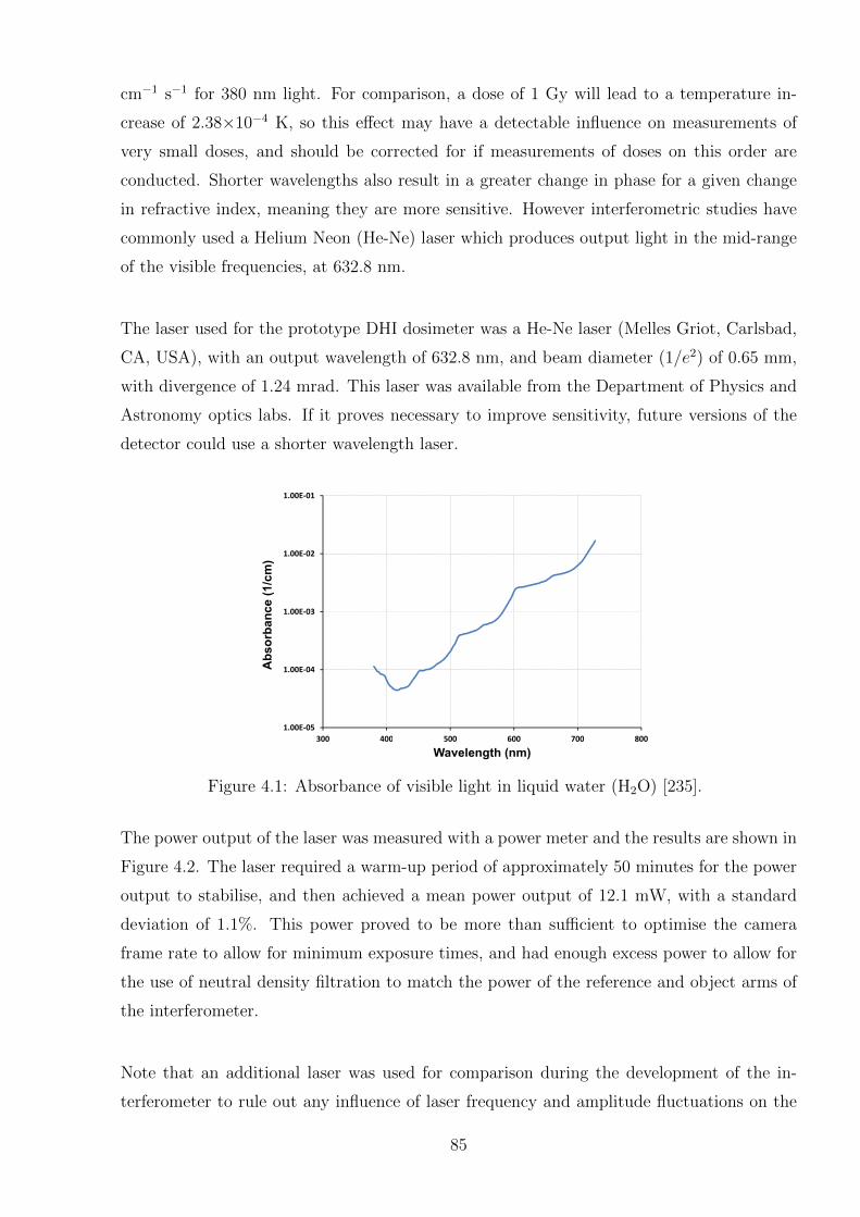
cm−1 s−1 for 380 nm light. For comparison, a dose of 1 Gy will lead to a temperature in-
crease of 2.38×10⁻⁴ K, so this effect may have a detectable influence on measurements of
very small doses, and should be corrected for if measurements of doses on this order are
conducted. Shorter wavelengths also result in a greater change in phase for a given change
in refractive index, meaning they are more sensitive. However interferometric studies have
commonly used a Helium Neon (He-Ne) laser which produces output light in the mid-range
of the visible frequencies, at 632.8 nm.
The laser used for the prototype DHI dosimeter was a He-Ne laser (Melles Griot, Carlsbad,
CA, USA), with an output wavelength of 632.8 nm, and beam diameter (1/e2) of 0.65 mm,
with divergence of 1.24 mrad. This laser was available from the Department of Physics and
Astronomy optics labs. If it proves necessary to improve sensitivity, future versions of the
detector could use a shorter wavelength laser.
1.00E-02
1.00E-01
Absorbance (1/cm)
1.00E-05
1.00E-04
1.00E-03
300 400 500 600 700 800
Absorbance (1/cm)
300 400 500 600 700 800
Wavelength (nm)
Figure 4.1: Absorbance of visible light in liquid water (H2O) [235].
The power output of the laser was measured with a power meter and the results are shown in
Figure 4.2. The laser required a warm-up period of approximately 50 minutes for the power
output to stabilise, and then achieved a mean power output of 12.1 mW, with a standard
deviation of 1.1%. This power proved to be more than sufficient to optimise the camera
frame rate to allow for minimum exposure times, and had enough excess power to allow for
the use of neutral density filtration to match the power of the reference and object arms of
the interferometer.
Note that an additional laser was used for comparison during the development of the in-
terferometer to rule out any influence of laser frequency and amplitude fluctuations on the
85
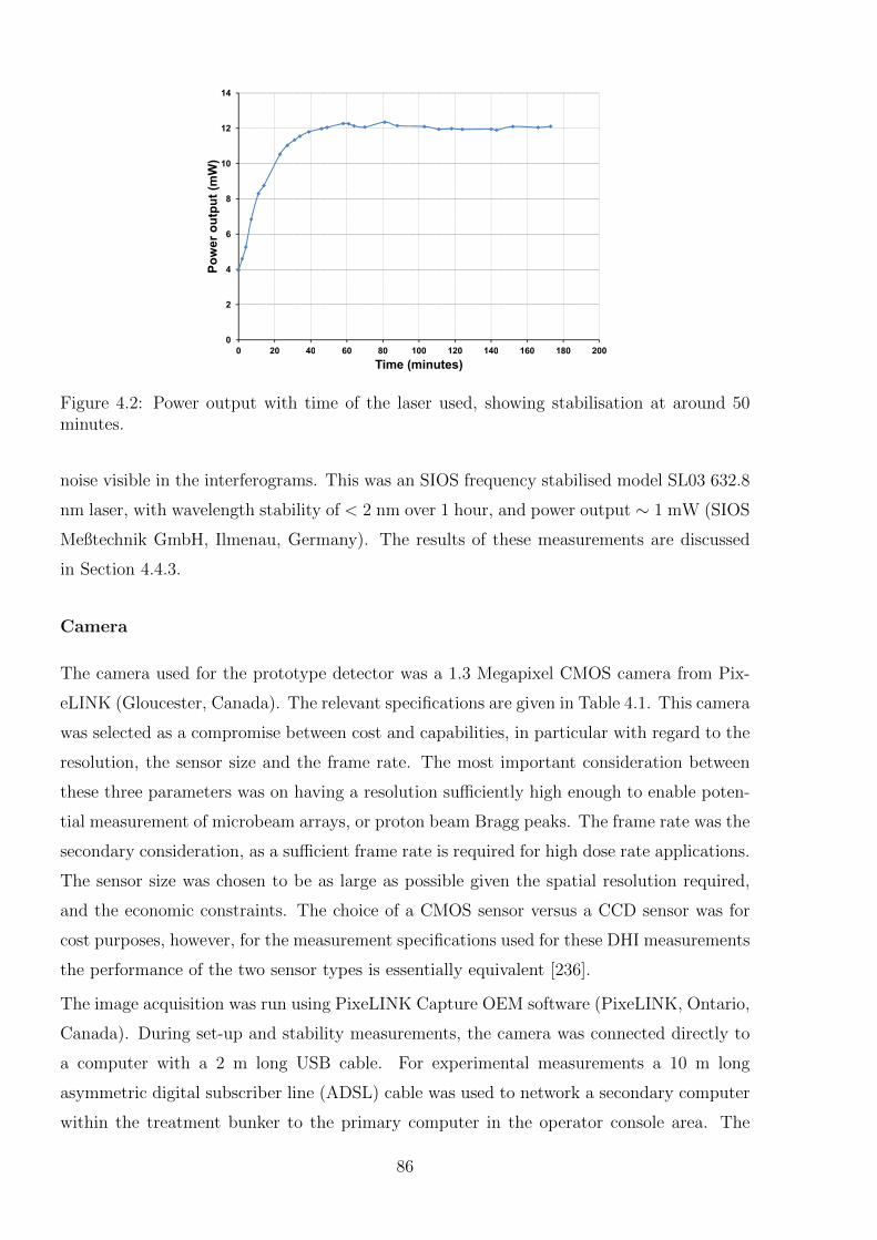
8
10
12
14
Power output (mW)
0
2
4
6
0 20 40 60 80 100 120 140 160 180 200
Power output (mW)
0 20 40 60 80 100 120 140 160 180 200
Time (minutes)
Figure 4.2: Power output with time of the laser used, showing stabilisation at around 50minutes.
noise visible in the interferograms. This was an SIOS frequency stabilised model SL03 632.8
nm laser, with wavelength stability of < 2 nm over 1 hour, and power output ∼ 1 mW (SIOS
Meßtechnik GmbH, Ilmenau, Germany). The results of these measurements are discussed
in Section 4.4.3.
Camera
The camera used for the prototype detector was a 1.3 Megapixel CMOS camera from Pix-
eLINK (Gloucester, Canada). The relevant specifications are given in Table 4.1. This camera
was selected as a compromise between cost and capabilities, in particular with regard to the
resolution, the sensor size and the frame rate. The most important consideration between
these three parameters was on having a resolution sufficiently high enough to enable poten-
tial measurement of microbeam arrays, or proton beam Bragg peaks. The frame rate was the
secondary consideration, as a sufficient frame rate is required for high dose rate applications.
The sensor size was chosen to be as large as possible given the spatial resolution required,
and the economic constraints. The choice of a CMOS sensor versus a CCD sensor was for
cost purposes, however, for the measurement specifications used for these DHI measurements
the performance of the two sensor types is essentially equivalent [236].
The image acquisition was run using PixeLINK Capture OEM software (PixeLINK, Ontario,
Canada). During set-up and stability measurements, the camera was connected directly to
a computer with a 2 m long USB cable. For experimental measurements a 10 m long
asymmetric digital subscriber line (ADSL) cable was used to network a secondary computer
within the treatment bunker to the primary computer in the operator console area. The
86
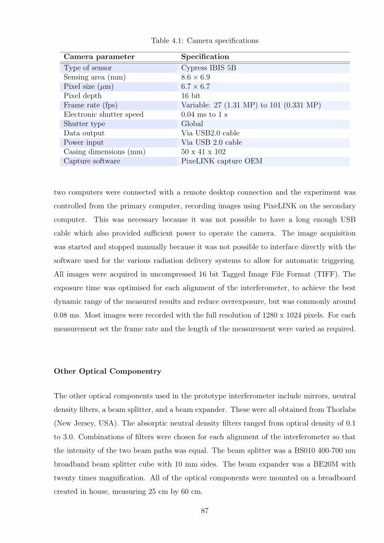
Table 4.1: Camera specifications
Camera parameter Specification
Type of sensor Cypress IBIS 5BSensing area (mm) 8.6× 6.9Pixel size (µm) 6.7× 6.7Pixel depth 16 bitFrame rate (fps) Variable: 27 (1.31 MP) to 101 (0.331 MP)Electronic shutter speed 0.04 ms to 1 sShutter type GlobalData output Via USB2.0 cablePower input Via USB 2.0 cableCasing dimensions (mm) 50 x 41 x 102Capture software PixeLINK capture OEM
two computers were connected with a remote desktop connection and the experiment was
controlled from the primary computer, recording images using PixeLINK on the secondary
computer. This was necessary because it was not possible to have a long enough USB
cable which also provided sufficient power to operate the camera. The image acquisition
was started and stopped manually because it was not possible to interface directly with the
software used for the various radiation delivery systems to allow for automatic triggering.
All images were acquired in uncompressed 16 bit Tagged Image File Format (TIFF). The
exposure time was optimised for each alignment of the interferometer, to achieve the best
dynamic range of the measured results and reduce overexposure, but was commonly around
0.08 ms. Most images were recorded with the full resolution of 1280 x 1024 pixels. For each
measurement set the frame rate and the length of the measurement were varied as required.
Other Optical Componentry
The other optical components used in the prototype interferometer include mirrors, neutral
density filters, a beam splitter, and a beam expander. These were all obtained from Thorlabs
(New Jersey, USA). The absorptic neutral density filters ranged from optical density of 0.1
to 3.0. Combinations of filters were chosen for each alignment of the interferometer so that
the intensity of the two beam paths was equal. The beam splitter was a BS010 400-700 nm
broadband beam splitter cube with 10 mm sides. The beam expander was a BE20M with
twenty times magnification. All of the optical components were mounted on a breadboard
created in house, measuring 25 cm by 60 cm.
87
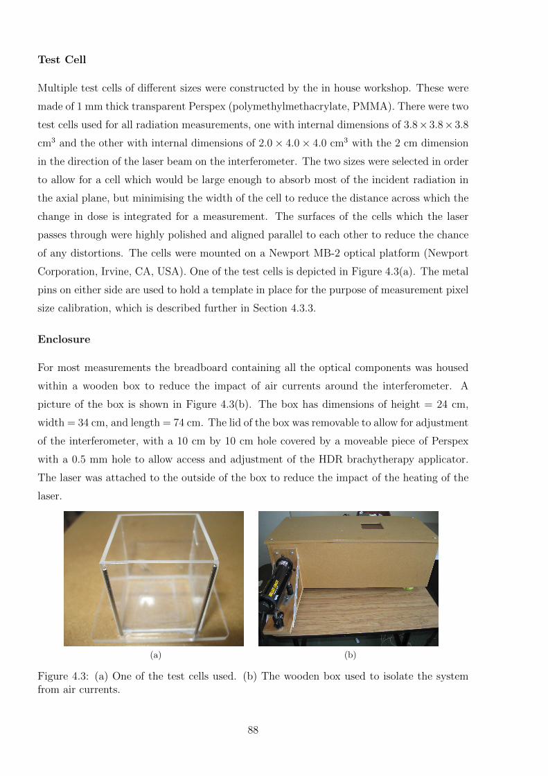
Test Cell
Multiple test cells of different sizes were constructed by the in house workshop. These were
made of 1 mm thick transparent Perspex (polymethylmethacrylate, PMMA). There were two
test cells used for all radiation measurements, one with internal dimensions of 3.8×3.8×3.8
cm3 and the other with internal dimensions of 2.0× 4.0× 4.0 cm3 with the 2 cm dimension
in the direction of the laser beam on the interferometer. The two sizes were selected in order
to allow for a cell which would be large enough to absorb most of the incident radiation in
the axial plane, but minimising the width of the cell to reduce the distance across which the
change in dose is integrated for a measurement. The surfaces of the cells which the laser
passes through were highly polished and aligned parallel to each other to reduce the chance
of any distortions. The cells were mounted on a Newport MB-2 optical platform (Newport
Corporation, Irvine, CA, USA). One of the test cells is depicted in Figure 4.3(a). The metal
pins on either side are used to hold a template in place for the purpose of measurement pixel
size calibration, which is described further in Section 4.3.3.
Enclosure
For most measurements the breadboard containing all the optical components was housed
within a wooden box to reduce the impact of air currents around the interferometer. A
picture of the box is shown in Figure 4.3(b). The box has dimensions of height = 24 cm,
width = 34 cm, and length = 74 cm. The lid of the box was removable to allow for adjustment
of the interferometer, with a 10 cm by 10 cm hole covered by a moveable piece of Perspex
with a 0.5 mm hole to allow access and adjustment of the HDR brachytherapy applicator.
The laser was attached to the outside of the box to reduce the impact of the heating of the
laser.
(a) (b)
Figure 4.3: (a) One of the test cells used. (b) The wooden box used to isolate the systemfrom air currents.
88
Interferometer Configuration
The final configuration that was used for the radiation measurements is shown in Figure 4.4.
This was an LFTDH set-up, with an object to sensor distance s = 26.5 cm, measured between
the camera sensor surface and the focal point of the reference beam. The test cell was aligned
such that the centre of the cell was in line with this focal point. This arrangement of mirrors
was determined with the first priority to optimise the size and position of the real image in
the reconstructed image. The secondary requirements were that the entire interferometer
was contained on one breadboard, excluding the laser, as well as ensuring that there was
sufficient horizontal space to allow for horizontal irradiation of the test cell when required.
The interferometer was disassembled for transportation, so the precise alignment of all the
components was adjusted before each individual set of measurements. Section 4.4 shows
some of the steps in the development of a working DHI interferometer for dosimetry, and
shows some of the different configurations used for earlier measurements.
4.3.2 Image Reconstruction and Dose Determination
In this section, the analysis of the images acquired by the interferometer is discussed. This
process is summarised in Figure 4.5. The process is split into two parts. The first part is
the use of the interferometer set-up and digital reconstruction algorithms to derive phase
information about laser light passing through the irradiated system (steps 1-4). This process
is not specific to dosimetry and can be applied to a wide range of applications. The second
part is specific to dosimetry, and involves the subsequent determination of the absorbed dose
from the phase information (steps 5-8). Figure 4.6 expands on steps 3 and 4 to outline the
process involved in obtaining interference phase information from the recorded interference
patterns. There are two possible paths for this process, in the first the phase information
is obtained from each image independently and then they are compared by modulo 2π sub-
traction, whereas in the second path the images are superimposed and a combined image
reconstructed, from which the interference phase can be derived. The first path was used in
the present work.
All of the analysis of the data was carried out in the MATLAB environment, using a spe-
cialised GUI written to streamline the process of obtaining the dose information. The GUI
is described in Section 4.3.4, with the code given in Appendix B.
89
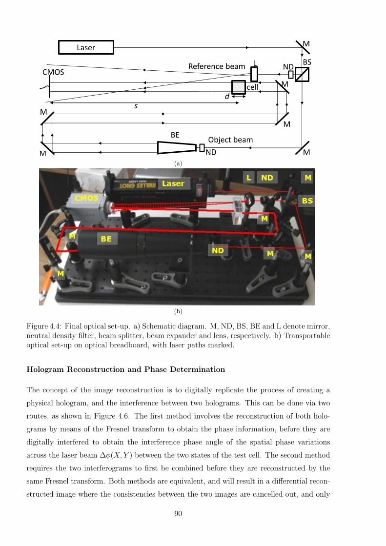
Laser M
BS
M
BE
M
M
M
M
L CMOS
Object beam
cell
s d
Reference beam ND
ND (a)
(b)
Figure 4.4: Final optical set-up. a) Schematic diagram. M, ND, BS, BE and L denote mirror,neutral density filter, beam splitter, beam expander and lens, respectively. b) Transportableoptical set-up on optical breadboard, with laser paths marked.
Hologram Reconstruction and Phase Determination
The concept of the image reconstruction is to digitally replicate the process of creating a
physical hologram, and the interference between two holograms. This can be done via two
routes, as shown in Figure 4.6. The first method involves the reconstruction of both holo-
grams by means of the Fresnel transform to obtain the phase information, before they are
digitally interfered to obtain the interference phase angle of the spatial phase variations
across the laser beam ∆φ(X, Y ) between the two states of the test cell. The second method
requires the two interferograms to first be combined before they are reconstructed by the
same Fresnel transform. Both methods are equivalent, and will result in a differential recon-
structed image where the consistencies between the two images are cancelled out, and only
90
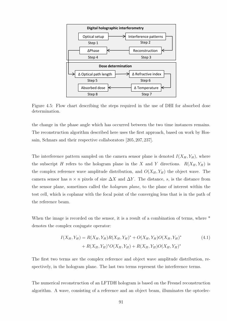
Optical setup Interference patterns
Digital holographic interferometry
Step 1 Step 2
Step 6
∆Phase
Step 3
Dose determination
∆ Temperature
∆ Refractive index ∆ Optical path length
Step 7 Step 8
Absorbed dose
Step 5
Reconstruction
Step 4
Figure 4.5: Flow chart describing the steps required in the use of DHI for absorbed dosedetermination.
the change in the phase angle which has occurred between the two time instances remains.
The reconstruction algorithm described here uses the first approach, based on work by Hos-
sain, Schnars and their respective collaborators [205,207,237].
The interference pattern sampled on the camera sensor plane is denoted I(XH , YH), where
the subscript H refers to the hologram plane in the X and Y directions. R(XH , YH) is
the complex reference wave amplitude distribution, and O(XH , YH) the object wave. The
camera sensor has n × n pixels of size ∆X and ∆Y . The distance, s, is the distance from
the sensor plane, sometimes called the hologram plane, to the plane of interest within the
test cell, which is coplanar with the focal point of the converging lens that is in the path of
the reference beam.
When the image is recorded on the sensor, it is a result of a combination of terms, where *
denotes the complex conjugate operator:
I(XH , YH) = R(XH , YH)R(XH , YH)∗ +O(XH , YH)O(XH , YH)∗ (4.1)
+R(XH , YH)∗O(XH , YH) +R(XH , YH)O(XH , YH)∗
The first two terms are the complex reference and object wave amplitude distribution, re-
spectively, in the hologram plane. The last two terms represent the interference terms.
The numerical reconstruction of an LFTDH hologram is based on the Fresnel reconstruction
algorithm. A wave, consisting of a reference and an object beam, illuminates the optoelec-
91
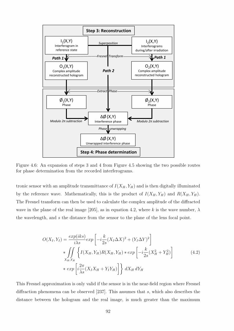
I1(X,Y) Interferogram in reference state
Step 3: Reconstruction
Step 4: Phase determination
I2(X,Y) Interferograms
during/after irradiation
Ø1(X,Y) Phase
Ø2(X,Y) Phase
ΔØ (X,Y) Interference phase
O1(X,Y) Complex amplitude
reconstructed hologram
O2(X,Y) Complex amplitude
reconstructed hologram
ΔØ (X,Y) Unwrapped interference phase
Superposition
Fresnel Transform
Extract Phase
Modulo 2π subtraction Modulo 2π subtraction
Phase unwrapping
Path 1 Path 1
Path 2
Figure 4.6: An expansion of steps 3 and 4 from Figure 4.5 showing the two possible routesfor phase determination from the recorded interferograms.
tronic sensor with an amplitude transmittance of I(XH , YH) and is then digitally illuminated
by the reference wave. Mathematically, this is the product of I(XH , YH) and R(XH , YH).
The Fresnel transform can then be used to calculate the complex amplitude of the diffracted
wave in the plane of the real image [205], as in equation 4.2, where k is the wave number, λ
the wavelength, and s the distance from the sensor to the plane of the lens focal point.
O(XI , YI) =exp(iks)
iλsexp
[−i k
2s(XI∆X)2 + (YI∆Y )2
]∗∫∫
XH ,YH
{I(XH , YH)R(XH , YH) ∗ exp
[−i k
2s(X2
H + Y 2H)
](4.2)
∗ exp[i2π
λs(XIXH + YIYH)
]}dXH dYH
This Fresnel approximation is only valid if the sensor is in the near-field region where Fresnel
diffraction phenomena can be observed [237]. This assumes that s, which also describes the
distance between the hologram and the real image, is much greater than the maximum
92
dimensions of the CCD chip, and thus the following condition must be obeyed:
s3 >>π
4λ
[(n∆X −XI)
2 + (n∆Y − YI)2]2
(4.3)
The maximum possible value of n∆X−XI and n∆Y −YI must therefore be considered. For
a λ = 632.8 nm and typical hologram dimensions of (n∆X−XI)2max = (n∆Y −YI)2
max = 0.5
cm, s must be greater than 14 cm.
This function is digitized into a discrete form, when sampled on an n×n matrix on a CMOS
sensor, where (XI , YI) and (XH , YH) run in discrete steps from 0 to n− 1, of width ∆X and
∆Y , respectively. This results in:
O(XI , YI) =exp(iks)
iλsexp
[−i k
2s(XI∆X)2 + (YI∆Y )2
]∗
n−1∑XH=0
n−1∑YH=0
{I(XH , YH)R(XH , YH) ∗ exp
[−i k
2s(X2
H + Y 2H)
](4.4)
∗ exp[i2π
λs(XIXH + YIYH)
]}This equation is a numerical representation of the Fresnel approximation, which can be
written in terms of a discrete inverse Fourier transformation. By using the Fourier transform
equation, 4.5, scaled by 1/λs (indicated further below in equation 4.8 by F−1λs ) this results
in equation 4.6 [238]:
F (u, v) =
∫∫ ∞−∞
f(x, y) exp (−2 i π(ux+ vy) dx dy (4.5)
O(XI , YI) =exp(iks)
iλsexp
[−i k
2s(XI∆X)2 + (YI∆Y )2
](4.6)
∗ F−1λs
{I(XH , YH)R(XH , YH) ∗ exp
[−i k
2s(X2
H + Y 2H)
]}Additionally, the use of a LFTDH set-up produces a spherical reference wave, described by
equation 4.7, where B is a constant which depends on the amplitude. Thus it is possible to
eliminate the effects of the reference wave spherical phase factor from equation 4.6, resulting
in a simplified equation for the reconstructed object, 4.8.
R(XH , YH) = B · exp[ik
2s(X2
H + Y 2H)
](4.7)
O(XI , YI) = B · exp(iks)iλs
exp
[−i k
2s(XI∆X)2 + (YI∆Y )2
]∗ F−1
λs {I(XH , YH)} (4.8)
93
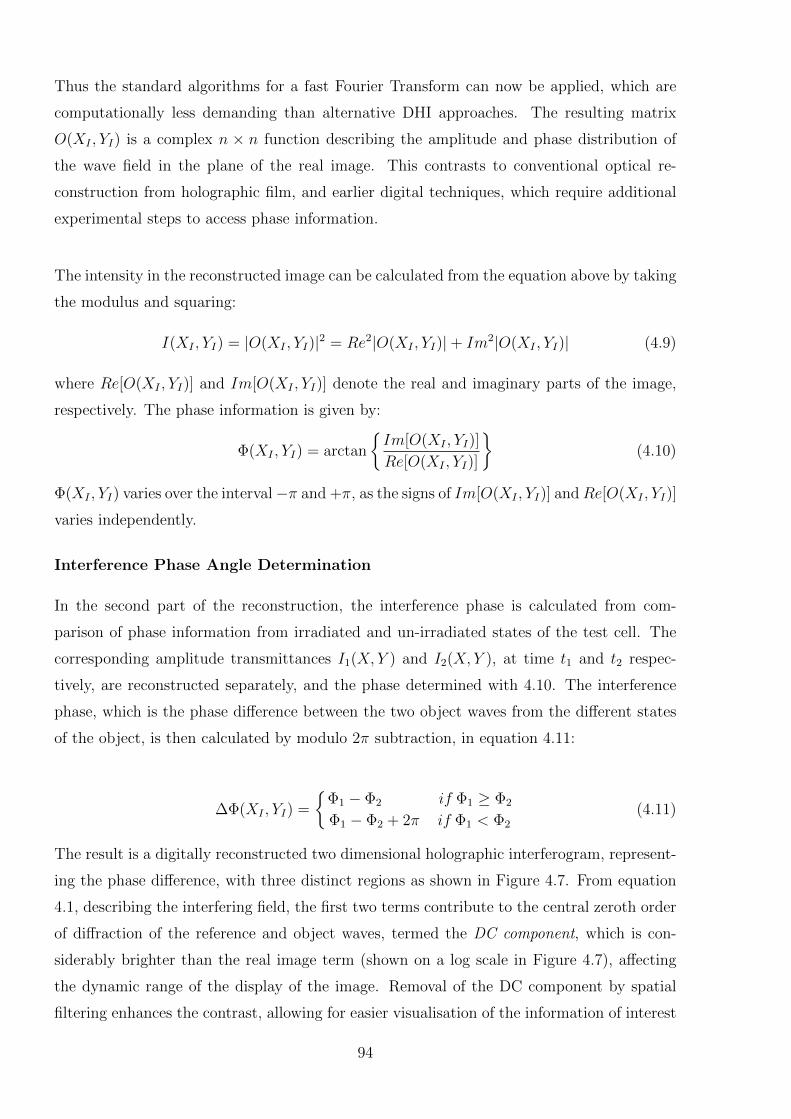
Thus the standard algorithms for a fast Fourier Transform can now be applied, which are
computationally less demanding than alternative DHI approaches. The resulting matrix
O(XI , YI) is a complex n × n function describing the amplitude and phase distribution of
the wave field in the plane of the real image. This contrasts to conventional optical re-
construction from holographic film, and earlier digital techniques, which require additional
experimental steps to access phase information.
The intensity in the reconstructed image can be calculated from the equation above by taking
the modulus and squaring:
I(XI , YI) = |O(XI , YI)|2 = Re2|O(XI , YI)|+ Im2|O(XI , YI)| (4.9)
where Re[O(XI , YI)] and Im[O(XI , YI)] denote the real and imaginary parts of the image,
respectively. The phase information is given by:
Φ(XI , YI) = arctan
{Im[O(XI , YI)]
Re[O(XI , YI)]
}(4.10)
Φ(XI , YI) varies over the interval−π and +π, as the signs of Im[O(XI , YI)] andRe[O(XI , YI)]
varies independently.
Interference Phase Angle Determination
In the second part of the reconstruction, the interference phase is calculated from com-
parison of phase information from irradiated and un-irradiated states of the test cell. The
corresponding amplitude transmittances I1(X, Y ) and I2(X, Y ), at time t1 and t2 respec-
tively, are reconstructed separately, and the phase determined with 4.10. The interference
phase, which is the phase difference between the two object waves from the different states
of the object, is then calculated by modulo 2π subtraction, in equation 4.11:
∆Φ(XI , YI) =
{Φ1 − Φ2 if Φ1 ≥ Φ2
Φ1 − Φ2 + 2π if Φ1 < Φ2
(4.11)
The result is a digitally reconstructed two dimensional holographic interferogram, represent-
ing the phase difference, with three distinct regions as shown in Figure 4.7. From equation
4.1, describing the interfering field, the first two terms contribute to the central zeroth order
of diffraction of the reference and object waves, termed the DC component, which is con-
siderably brighter than the real image term (shown on a log scale in Figure 4.7), affecting
the dynamic range of the display of the image. Removal of the DC component by spatial
filtering enhances the contrast, allowing for easier visualisation of the information of interest
94
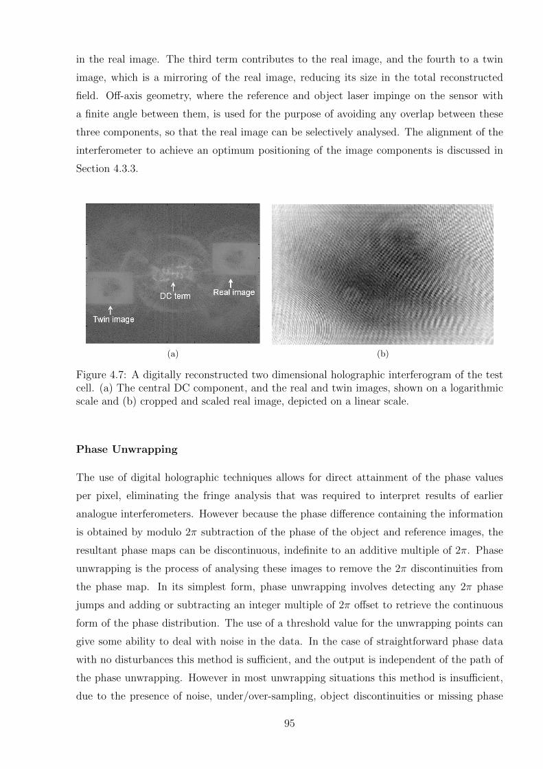
in the real image. The third term contributes to the real image, and the fourth to a twin
image, which is a mirroring of the real image, reducing its size in the total reconstructed
field. Off-axis geometry, where the reference and object laser impinge on the sensor with
a finite angle between them, is used for the purpose of avoiding any overlap between these
three components, so that the real image can be selectively analysed. The alignment of the
interferometer to achieve an optimum positioning of the image components is discussed in
Section 4.3.3.
(a) (b)
Figure 4.7: A digitally reconstructed two dimensional holographic interferogram of the testcell. (a) The central DC component, and the real and twin images, shown on a logarithmicscale and (b) cropped and scaled real image, depicted on a linear scale.
Phase Unwrapping
The use of digital holographic techniques allows for direct attainment of the phase values
per pixel, eliminating the fringe analysis that was required to interpret results of earlier
analogue interferometers. However because the phase difference containing the information
is obtained by modulo 2π subtraction of the phase of the object and reference images, the
resultant phase maps can be discontinuous, indefinite to an additive multiple of 2π. Phase
unwrapping is the process of analysing these images to remove the 2π discontinuities from
the phase map. In its simplest form, phase unwrapping involves detecting any 2π phase
jumps and adding or subtracting an integer multiple of 2π offset to retrieve the continuous
form of the phase distribution. The use of a threshold value for the unwrapping points can
give some ability to deal with noise in the data. In the case of straightforward phase data
with no disturbances this method is sufficient, and the output is independent of the path of
the phase unwrapping. However in most unwrapping situations this method is insufficient,
due to the presence of noise, under/over-sampling, object discontinuities or missing phase
95
information [239]. These disturbances can mean that different results are obtained depend-
ing on the order in which the pixels are unwrapped. In this case, more advanced methods
are required.
Most DHI images obtained during radiation measurements will have straightforward fringe
patterns because, with the exception of highly modulated dose distributions such as those
produced by MRT, the phase gradients are consistently changing in the same direction. This
means that fringe edges, or unwrapping points, are easily evident and the offset required dur-
ing the unwrapping process is always in the same direction. However at this stage the images
produced have a considerable noise component, as well as the potential to be influenced by
external factors such as atmospheric variations or vibrations, which can produce wrap points
in the image. For this reason the choice of phase unwrapping technique was carefully con-
sidered in order to implement the most robust phase unwrapper.
There are various approaches to solving the phase unwrapping problem for a range of ap-
plications, with varying degrees of accuracy and complexity [240]. These can be roughly
categorised into local or path-following phase-unwrapping algorithms, versus global unwrap-
ping algorithms. Local methods unwrap the phase map by following certain paths across
all the pixels in the phase map to reduce the chance of incorrect unwrapping propagating
around discontinuities. In these approaches, the choice of path is key to producing the most
accurate results. Global algorithms unwrap the phase by formulating the solution in terms
of minimisation of a global function to estimate the phase gradient, an approach which is
quite computationally intensive. Many authors have made their phase unwrapping codes
readily available for use by others, so it becomes a question of selecting a code which will be
effective for the type of dataset.
The unwrapper selected was obtained from Herraez et al.1, along with their paper describ-
ing the algorithm [241]. This unwrapper is described as a “Fast, two-dimensional phase-
unwrapping algorithm, based on sorting by reliability, following a non-continuous path (2D-
SRNCP).” The algorithm is a path-following phase unwrapper which chooses the order to
unwrap pixels in based on the quality of the pixels. Pixel quality is determined using the
second difference quality map technique, which effectively corresponds to the amount of noise
in the region of the discontinuity edge. High quality pixels are unwrapped before the lower
quality ones, minimising the incidence of error propagation. This method of unwrapping
1From the website of Liverpool John Moores University: http://www.ljmu.ac.uk/GERI/90207.htm
96
gives better results than a straightforward flood fill technique. The key feature distinguish-
ing this algorithm from similar path-following approaches is that the selected path is not
limited to a continuous path, which improves the reliability of the results in the presence
of discontinuities or noise, particularly where there are high local variations in the signal-
to-noise ratio (as is the case with the DHI data). In terms of the implementation, a MEX
file was written and compiled in MATLAB containing the C++ algorithm code and incor-
porated into the GUI, described in Section 4.3.4.
In the case of the DHI measurements, as the radiation delivery is not instantaneous, the
phase map changes dynamically with time. The ideal approach is to compare not only the
phase distribution across a two-dimensional region, but also the variation of this phase map
over the irradiation period. This would enable the measurement of absolute doses at each
point in the image, rather than being limited to a dose difference map at each point in time.
Thus the phase unwrapping problem becomes three dimensional, considering two spatial
directions and the temporal dimension. Two different approaches were compared for this.
The first involved the unwrapping of each image individually using the Herraez unwrapper,
then a subsequent basic phase unwrapping in the temporal direction of each point within
the image. This approach was adequate for some image sets, but for noisy data, the sec-
ondary unwrapping process seriously affected the previously unwrapped images at each time
point. The second approach was to utilise an extension of the Herraez unwrapper which
calculates the phase unwrapping in all three dimensions directly. The code was written by
Abdul-Rahman, a doctoral student from the same group, and is henceforth referred to as
the “Rahman unwrapper” [242]. This was more successful on most of the datasets, but still
resulted in a degradation of the quality of the individual images when compared to using the
two dimensional unwrapper. A contributing factor that would worsen this impact is that the
noise influences intra- versus inter-image are different, so the path-following route selection
is altered for the three dimensional unwrapper as compared to the two dimensional one.
At the current stage of the development of the DHI dosimeter, there are complications in ob-
taining consistent measurements in the time direction, as discussed further in Section 4.4.3.
This means that for some of the results analysis presented in this thesis the information from
the temporal direction is not used. In these situations, the primary purpose of the unwrapper
is for two dimensional analyses only, with incidental consideration of the third dimension.
Thus the Herraez unwrapper is used for the results presented in the remainder of this work,
unless stated otherwise. Future development of the detector to increase consistency, enabling
97
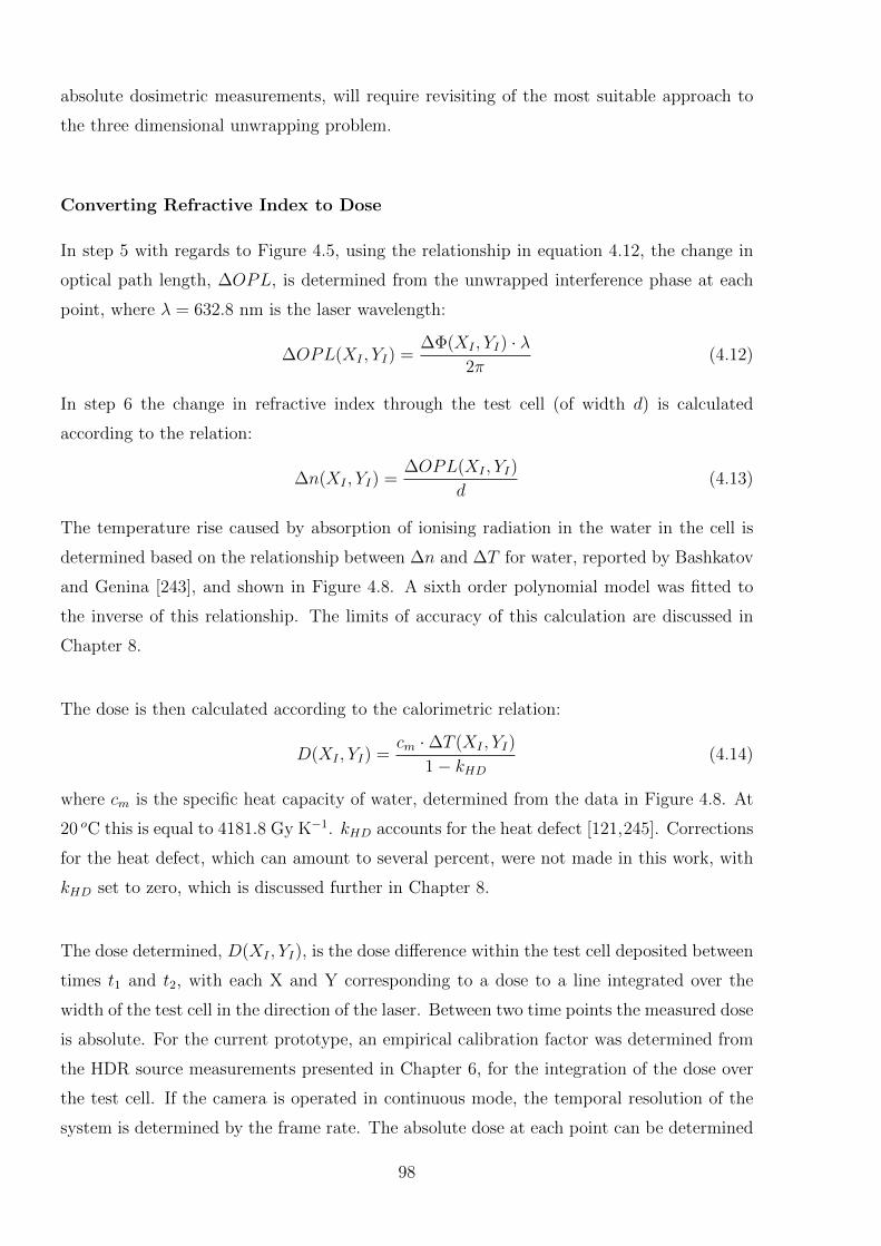
absolute dosimetric measurements, will require revisiting of the most suitable approach to
the three dimensional unwrapping problem.
Converting Refractive Index to Dose
In step 5 with regards to Figure 4.5, using the relationship in equation 4.12, the change in
optical path length, ∆OPL, is determined from the unwrapped interference phase at each
point, where λ = 632.8 nm is the laser wavelength:
∆OPL(XI , YI) =∆Φ(XI , YI) · λ
2π(4.12)
In step 6 the change in refractive index through the test cell (of width d) is calculated
according to the relation:
∆n(XI , YI) =∆OPL(XI , YI)
d(4.13)
The temperature rise caused by absorption of ionising radiation in the water in the cell is
determined based on the relationship between ∆n and ∆T for water, reported by Bashkatov
and Genina [243], and shown in Figure 4.8. A sixth order polynomial model was fitted to
the inverse of this relationship. The limits of accuracy of this calculation are discussed in
Chapter 8.
The dose is then calculated according to the calorimetric relation:
D(XI , YI) =cm ·∆T (XI , YI)
1− kHD(4.14)
where cm is the specific heat capacity of water, determined from the data in Figure 4.8. At
20 oC this is equal to 4181.8 Gy K−1. kHD accounts for the heat defect [121,245]. Corrections
for the heat defect, which can amount to several percent, were not made in this work, with
kHD set to zero, which is discussed further in Chapter 8.
The dose determined, D(XI , YI), is the dose difference within the test cell deposited between
times t1 and t2, with each X and Y corresponding to a dose to a line integrated over the
width of the test cell in the direction of the laser. Between two time points the measured dose
is absolute. For the current prototype, an empirical calibration factor was determined from
the HDR source measurements presented in Chapter 6, for the integration of the dose over
the test cell. If the camera is operated in continuous mode, the temporal resolution of the
system is determined by the frame rate. The absolute dose at each point can be determined
98

Figure 4.8: Empirical relationships between temperature and the refractive index of water(dashed) (reproduced using data obtained from [243]) and the specific heat capacity of water(solid) (reproduced using data from [244]).
by phase unwrapping in the time dimension, between adjacent images, to determine the
cumulative dose to each point. This process is susceptible to environmental variations such
as temperature, pressure and vibrational interferences, which, if significant, mean that the
absolute dose delivered between the two time instances cannot be determined with a high
degree of certainty. For completeness it should also be noted that if the dose variation
between frames causes a variation in phase of larger than 2π then the absolute dose may not
be able to be determined. However as 2π corresponds to a dose of approximately 1500 Gy this
limitation is unlikely to be encountered, except perhaps in a synchrotron MRT measurement.
Even in these two situations, the relative dose across the measurement region can still be
accurately measured. Thus the measured results achieve a series of two dimensional dose
difference maps at each point in time.
4.3.3 Experimental Process
The determination of absorbed dose for clinical purposes necessarily requires a high level
of accuracy. For this reason, achieving consistent and reproducible results is imperative for
any dosimeter, as well as a thorough awareness of exactly what the measurement parameters
are. For radiation measurement the complicating factor is that the measurement quantity
is not visible to the naked eye, which means that alignment of the dosimeter requires spe-
cial attention. The experimental process of taking a DHI dosimetry measurement with the
99
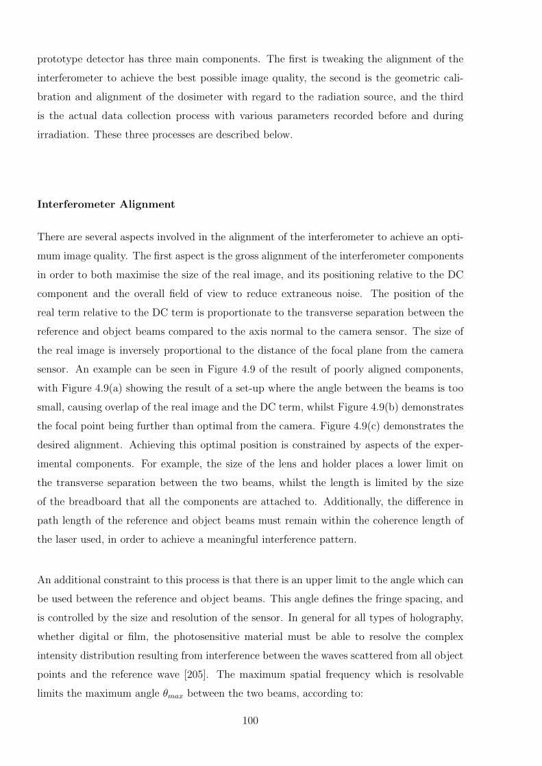
prototype detector has three main components. The first is tweaking the alignment of the
interferometer to achieve the best possible image quality, the second is the geometric cali-
bration and alignment of the dosimeter with regard to the radiation source, and the third
is the actual data collection process with various parameters recorded before and during
irradiation. These three processes are described below.
Interferometer Alignment
There are several aspects involved in the alignment of the interferometer to achieve an opti-
mum image quality. The first aspect is the gross alignment of the interferometer components
in order to both maximise the size of the real image, and its positioning relative to the DC
component and the overall field of view to reduce extraneous noise. The position of the
real term relative to the DC term is proportionate to the transverse separation between the
reference and object beams compared to the axis normal to the camera sensor. The size of
the real image is inversely proportional to the distance of the focal plane from the camera
sensor. An example can be seen in Figure 4.9 of the result of poorly aligned components,
with Figure 4.9(a) showing the result of a set-up where the angle between the beams is too
small, causing overlap of the real image and the DC term, whilst Figure 4.9(b) demonstrates
the focal point being further than optimal from the camera. Figure 4.9(c) demonstrates the
desired alignment. Achieving this optimal position is constrained by aspects of the exper-
imental components. For example, the size of the lens and holder places a lower limit on
the transverse separation between the two beams, whilst the length is limited by the size
of the breadboard that all the components are attached to. Additionally, the difference in
path length of the reference and object beams must remain within the coherence length of
the laser used, in order to achieve a meaningful interference pattern.
An additional constraint to this process is that there is an upper limit to the angle which can
be used between the reference and object beams. This angle defines the fringe spacing, and
is controlled by the size and resolution of the sensor. In general for all types of holography,
whether digital or film, the photosensitive material must be able to resolve the complex
intensity distribution resulting from interference between the waves scattered from all object
points and the reference wave [205]. The maximum spatial frequency which is resolvable
limits the maximum angle θmax between the two beams, according to:
100
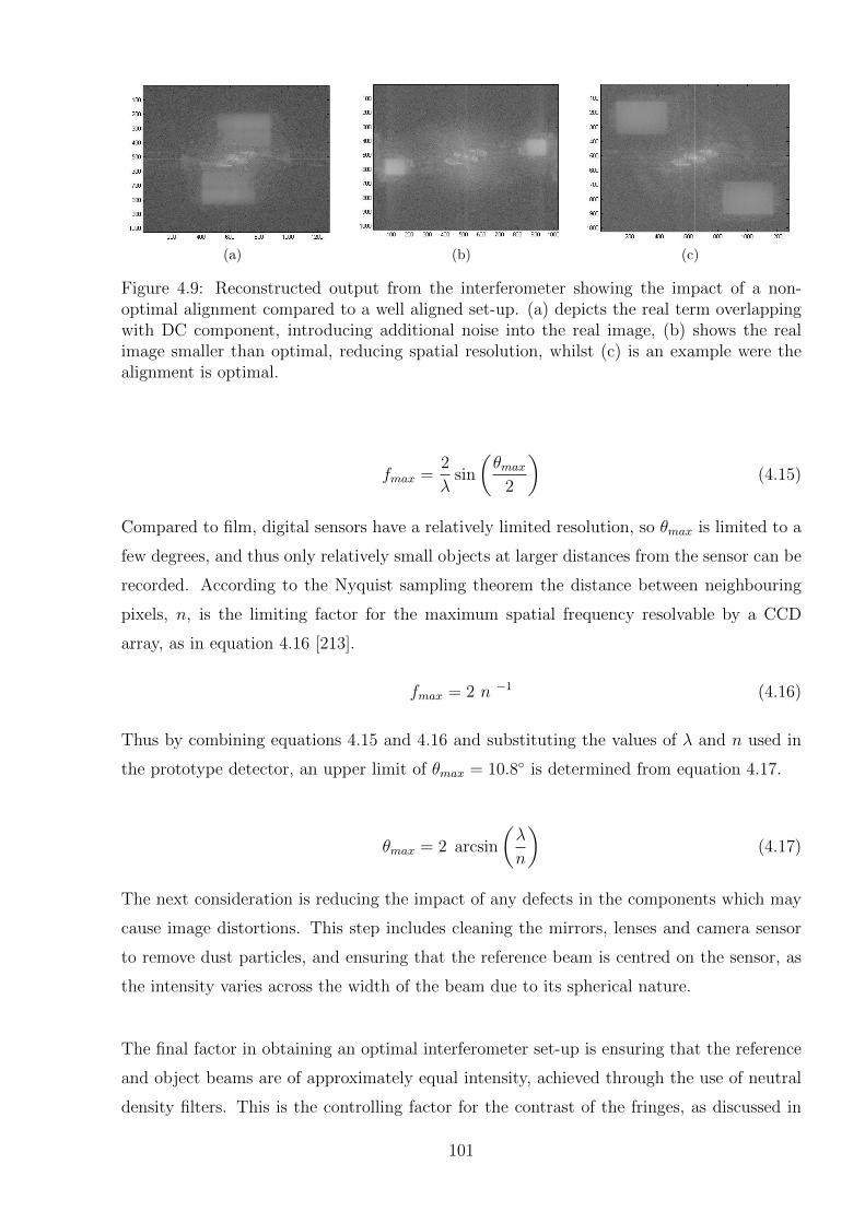
(a) (b) (c)
Figure 4.9: Reconstructed output from the interferometer showing the impact of a non-optimal alignment compared to a well aligned set-up. (a) depicts the real term overlappingwith DC component, introducing additional noise into the real image, (b) shows the realimage smaller than optimal, reducing spatial resolution, whilst (c) is an example were thealignment is optimal.
fmax =2
λsin
(θmax
2
)(4.15)
Compared to film, digital sensors have a relatively limited resolution, so θmax is limited to a
few degrees, and thus only relatively small objects at larger distances from the sensor can be
recorded. According to the Nyquist sampling theorem the distance between neighbouring
pixels, n, is the limiting factor for the maximum spatial frequency resolvable by a CCD
array, as in equation 4.16 [213].
fmax = 2 n −1 (4.16)
Thus by combining equations 4.15 and 4.16 and substituting the values of λ and n used in
the prototype detector, an upper limit of θmax = 10.8◦ is determined from equation 4.17.
θmax = 2 arcsin
(λ
n
)(4.17)
The next consideration is reducing the impact of any defects in the components which may
cause image distortions. This step includes cleaning the mirrors, lenses and camera sensor
to remove dust particles, and ensuring that the reference beam is centred on the sensor, as
the intensity varies across the width of the beam due to its spherical nature.
The final factor in obtaining an optimal interferometer set-up is ensuring that the reference
and object beams are of approximately equal intensity, achieved through the use of neutral
density filters. This is the controlling factor for the contrast of the fringes, as discussed in
101
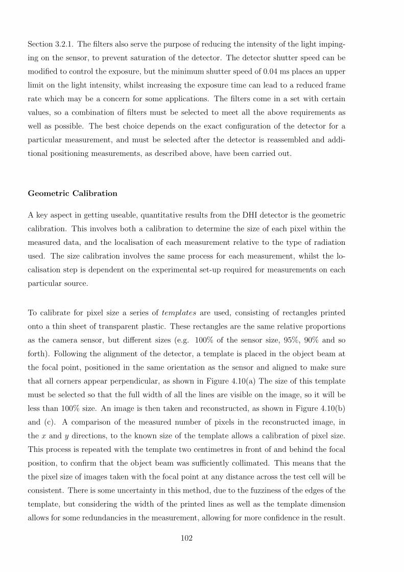
Section 3.2.1. The filters also serve the purpose of reducing the intensity of the light imping-
ing on the sensor, to prevent saturation of the detector. The detector shutter speed can be
modified to control the exposure, but the minimum shutter speed of 0.04 ms places an upper
limit on the light intensity, whilst increasing the exposure time can lead to a reduced frame
rate which may be a concern for some applications. The filters come in a set with certain
values, so a combination of filters must be selected to meet all the above requirements as
well as possible. The best choice depends on the exact configuration of the detector for a
particular measurement, and must be selected after the detector is reassembled and addi-
tional positioning measurements, as described above, have been carried out.
Geometric Calibration
A key aspect in getting useable, quantitative results from the DHI detector is the geometric
calibration. This involves both a calibration to determine the size of each pixel within the
measured data, and the localisation of each measurement relative to the type of radiation
used. The size calibration involves the same process for each measurement, whilst the lo-
calisation step is dependent on the experimental set-up required for measurements on each
particular source.
To calibrate for pixel size a series of templates are used, consisting of rectangles printed
onto a thin sheet of transparent plastic. These rectangles are the same relative proportions
as the camera sensor, but different sizes (e.g. 100% of the sensor size, 95%, 90% and so
forth). Following the alignment of the detector, a template is placed in the object beam at
the focal point, positioned in the same orientation as the sensor and aligned to make sure
that all corners appear perpendicular, as shown in Figure 4.10(a) The size of this template
must be selected so that the full width of all the lines are visible on the image, so it will be
less than 100% size. An image is then taken and reconstructed, as shown in Figure 4.10(b)
and (c). A comparison of the measured number of pixels in the reconstructed image, in
the x and y directions, to the known size of the template allows a calibration of pixel size.
This process is repeated with the template two centimetres in front of and behind the focal
position, to confirm that the object beam was sufficiently collimated. This means that the
the pixel size of images taken with the focal point at any distance across the test cell will be
consistent. There is some uncertainty in this method, due to the fuzziness of the edges of the
template, but considering the width of the printed lines as well as the template dimension
allows for some redundancies in the measurement, allowing for more confidence in the result.
102
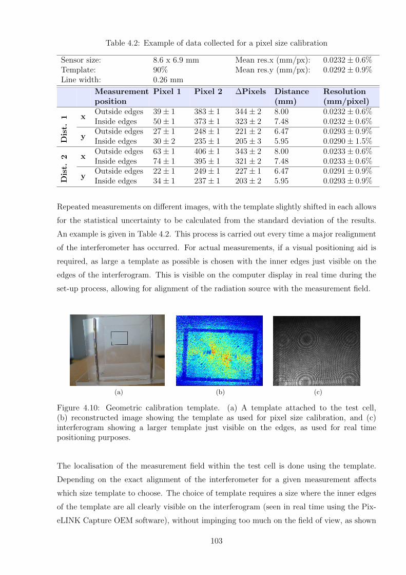
Table 4.2: Example of data collected for a pixel size calibration
Sensor size: 8.6 x 6.9 mm Mean res.x (mm/px): 0.0232± 0.6%Template: 90% Mean res.y (mm/px): 0.0292± 0.9%Line width: 0.26 mm
Measurementposition
Pixel 1 Pixel 2 ∆Pixels Distance(mm)
Resolution(mm/pixel)
xOutside edges 39± 1 383± 1 344± 2 8.00 0.0232± 0.6%Inside edges 50± 1 373± 1 323± 2 7.48 0.0232± 0.6%
yOutside edges 27± 1 248± 1 221± 2 6.47 0.0293± 0.9%
Dis
t.1
Inside edges 30± 2 235± 1 205± 3 5.95 0.0290± 1.5%
xOutside edges 63± 1 406± 1 343± 2 8.00 0.0233± 0.6%Inside edges 74± 1 395± 1 321± 2 7.48 0.0233± 0.6%
yOutside edges 22± 1 249± 1 227± 1 6.47 0.0291± 0.9%
Dis
t.2
Inside edges 34± 1 237± 1 203± 2 5.95 0.0293± 0.9%
Repeated measurements on different images, with the template slightly shifted in each allows
for the statistical uncertainty to be calculated from the standard deviation of the results.
An example is given in Table 4.2. This process is carried out every time a major realignment
of the interferometer has occurred. For actual measurements, if a visual positioning aid is
required, as large a template as possible is chosen with the inner edges just visible on the
edges of the interferogram. This is visible on the computer display in real time during the
set-up process, allowing for alignment of the radiation source with the measurement field.
(a) (b) (c)
Figure 4.10: Geometric calibration template. (a) A template attached to the test cell,(b) reconstructed image showing the template as used for pixel size calibration, and (c)interferogram showing a larger template just visible on the edges, as used for real timepositioning purposes.
The localisation of the measurement field within the test cell is done using the template.
Depending on the exact alignment of the interferometer for a given measurement affects
which size template to choose. The choice of template requires a size where the inner edges
of the template are all clearly visible on the interferogram (seen in real time using the Pix-
eLINK Capture OEM software), without impinging too much on the field of view, as shown
103
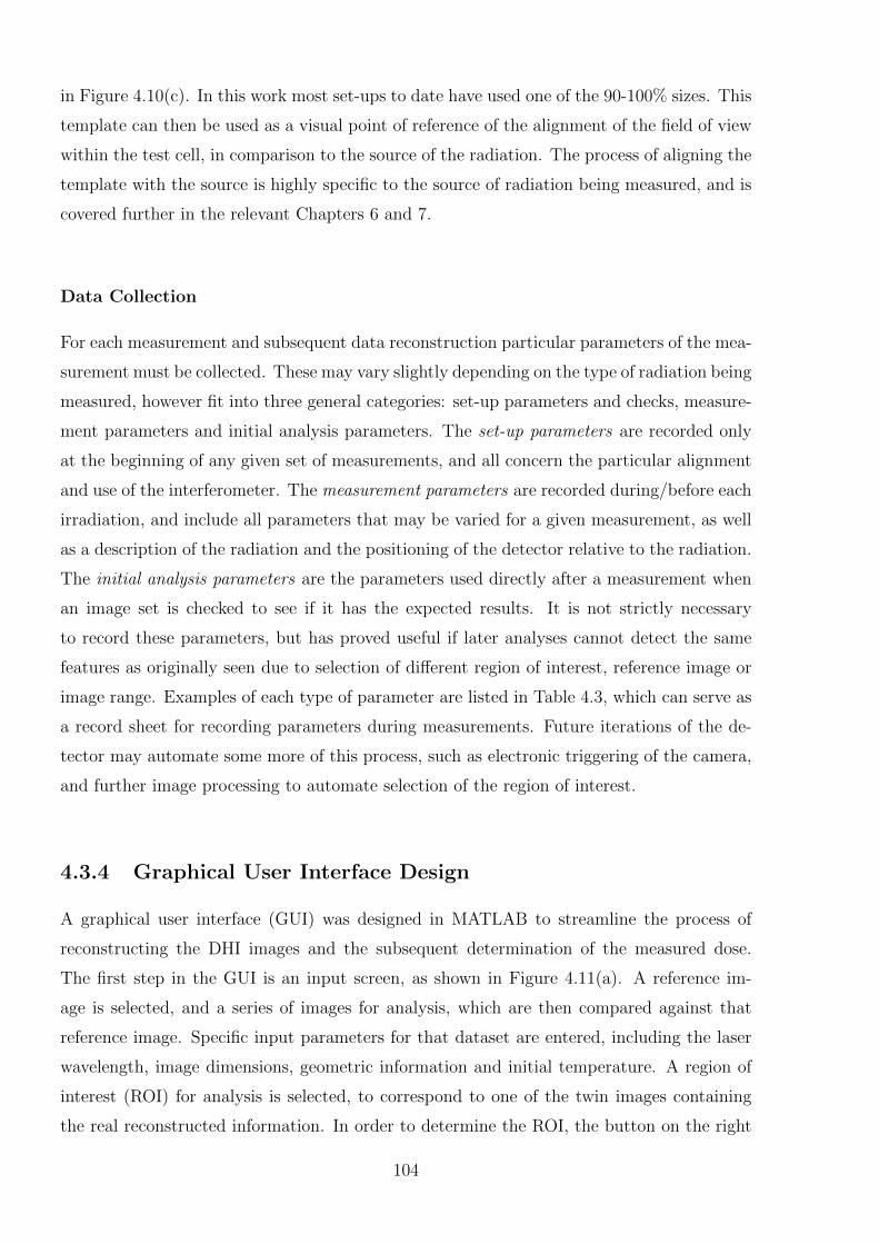
in Figure 4.10(c). In this work most set-ups to date have used one of the 90-100% sizes. This
template can then be used as a visual point of reference of the alignment of the field of view
within the test cell, in comparison to the source of the radiation. The process of aligning the
template with the source is highly specific to the source of radiation being measured, and is
covered further in the relevant Chapters 6 and 7.
Data Collection
For each measurement and subsequent data reconstruction particular parameters of the mea-
surement must be collected. These may vary slightly depending on the type of radiation being
measured, however fit into three general categories: set-up parameters and checks, measure-
ment parameters and initial analysis parameters. The set-up parameters are recorded only
at the beginning of any given set of measurements, and all concern the particular alignment
and use of the interferometer. The measurement parameters are recorded during/before each
irradiation, and include all parameters that may be varied for a given measurement, as well
as a description of the radiation and the positioning of the detector relative to the radiation.
The initial analysis parameters are the parameters used directly after a measurement when
an image set is checked to see if it has the expected results. It is not strictly necessary
to record these parameters, but has proved useful if later analyses cannot detect the same
features as originally seen due to selection of different region of interest, reference image or
image range. Examples of each type of parameter are listed in Table 4.3, which can serve as
a record sheet for recording parameters during measurements. Future iterations of the de-
tector may automate some more of this process, such as electronic triggering of the camera,
and further image processing to automate selection of the region of interest.
4.3.4 Graphical User Interface Design
A graphical user interface (GUI) was designed in MATLAB to streamline the process of
reconstructing the DHI images and the subsequent determination of the measured dose.
The first step in the GUI is an input screen, as shown in Figure 4.11(a). A reference im-
age is selected, and a series of images for analysis, which are then compared against that
reference image. Specific input parameters for that dataset are entered, including the laser
wavelength, image dimensions, geometric information and initial temperature. A region of
interest (ROI) for analysis is selected, to correspond to one of the twin images containing
the real reconstructed information. In order to determine the ROI, the button on the right
104
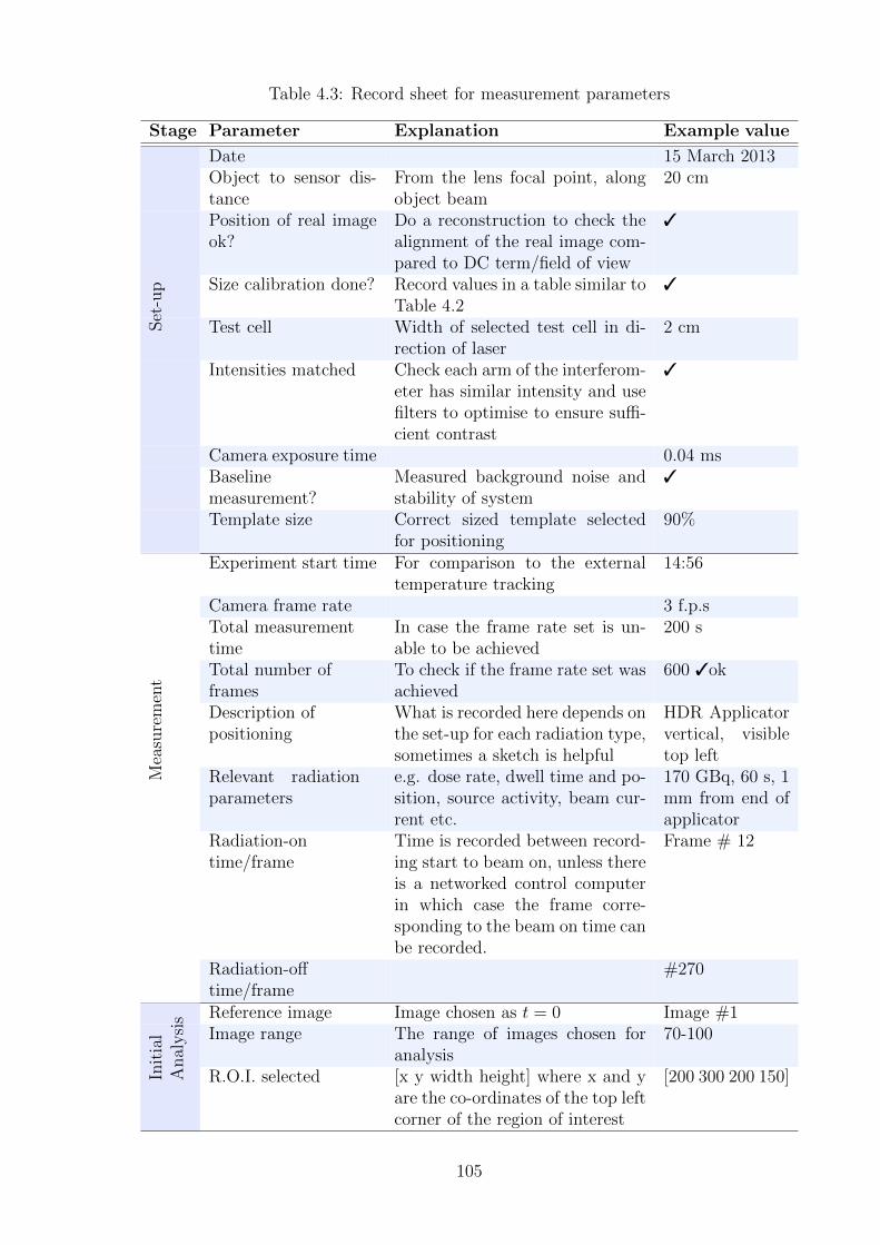
Table 4.3: Record sheet for measurement parameters
Stage Parameter Explanation Example value
Date 15 March 2013Object to sensor dis-tance
From the lens focal point, alongobject beam
20 cm
Position of real imageok?
Do a reconstruction to check thealignment of the real image com-pared to DC term/field of view
3
Size calibration done? Record values in a table similar toTable 4.2
3
Set
-up
Test cell Width of selected test cell in di-rection of laser
2 cm
Intensities matched Check each arm of the interferom-eter has similar intensity and usefilters to optimise to ensure suffi-cient contrast
3
Camera exposure time 0.04 msBaselinemeasurement?
Measured background noise andstability of system
3
Template size Correct sized template selectedfor positioning
90%
Experiment start time For comparison to the externaltemperature tracking
14:56
Camera frame rate 3 f.p.sTotal measurementtime
In case the frame rate set is un-able to be achieved
200 s
Total number offrames
To check if the frame rate set wasachieved
600 3ok
Description ofpositioning
What is recorded here depends onthe set-up for each radiation type,sometimes a sketch is helpful
HDR Applicatorvertical, visibletop left
Mea
sure
men
t
Relevant radiationparameters
e.g. dose rate, dwell time and po-sition, source activity, beam cur-rent etc.
170 GBq, 60 s, 1mm from end ofapplicator
Radiation-ontime/frame
Time is recorded between record-ing start to beam on, unless thereis a networked control computerin which case the frame corre-sponding to the beam on time canbe recorded.
Frame # 12
Radiation-offtime/frame
#270
Reference image Image chosen as t = 0 Image #1Image range The range of images chosen for
analysis70-100
Init
ial
Anal
ysi
s
R.O.I. selected [x y width height] where x and yare the co-ordinates of the top leftcorner of the region of interest
[200 300 200 150]
105
of Figure 4.11(a) can be selected, which opens a window showing the initial reconstruction
of the full image, as shown in Figure 4.11(b). From here the box can be adjusted to ex-
actly contain the ROI, which then automatically enters the parameters. Once all data is
correctly entered, the “Reconstruct” button is pushed. This reconstructs the full image se-
ries, and then displays the results for the ROI, in Figure 4.11(c). This display has several
components. The data can be depicted in various formats, using the drop down menu above
each graph: phase, two or three dimensional unwrapped phase, temperature and dose. The
left graph shows the reconstructed series of images, with a bar to scroll between images.
A horizontal or vertical line can be selected at any point within the image, with the data
in these profiles displayed in the central graph. The right graph shows the phase value at
the point of intersection of these profiles, across the whole image series. These plots allow
for a straightforward analysis of the data to determine any immediate trends visible, either
spatially or temporally. Further analysis of the results, for example quantitative sensitivity
or noise calculations, and comparison to a model dataset are conducted using the output
datasets from the GUI. These have not yet been included in the GUI as there is considerable
variation in the calculations required for different applications.
4.4 Detector Progression and Characterisation
The process of developing the prototype interferometer and digital reconstruction algorithm
involved several stages of interferometer design, with consequent testing on a series of heat-
ing patterns. The knowledge gained from each stage in this process informed the design and
use of the final prototype.
The first step in the process was the development of a system capable of doing digital holo-
graphic interferometry. This has two parts, the first is the experimental configuration, and
the second is the digital image processing for reconstructing the algorithms. The first at-
tempts focussed on a basic interferometer design based around a Michelson interferometer,
to produce interferograms which were used to develop preliminary reconstruction algorithms.
These were tested by producing reconstructed holograms visualising the absorption of the
object beam laser light in solid objects, and then phase objects (objects which induce a phase
change in the laser light without excessive absorption). Following this a set-up similar to
the design used for the prototype detector was developed and the sensitivity of the system
tested with the measurement of heat distributions using flames and drops of heated water.
This served to confirm the measured temperatures and temperature distributions approxi-
106
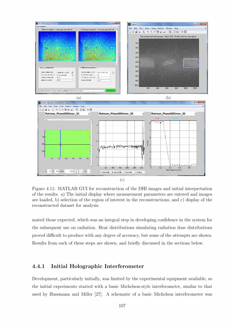
(a) (b)
(c)
Figure 4.11: MATLAB GUI for reconstruction of the DHI images and initial interpretationof the results. a) The initial display where measurement parameters are entered and imagesare loaded, b) selection of the region of interest in the reconstructions, and c) display of thereconstructed dataset for analysis.
mated those expected, which was an integral step in developing confidence in the system for
the subsequent use on radiation. Heat distributions simulating radiation dose distributions
proved difficult to produce with any degree of accuracy, but some of the attempts are shown.
Results from each of these steps are shown, and briefly discussed in the sections below.
4.4.1 Initial Holographic Interferometer
Development, particularly initially, was limited by the experimental equipment available, so
the initial experiments started with a basic Michelson-style interferometer, similar to that
used by Hussmann and Miller [27]. A schematic of a basic Michelson interferometer was
107
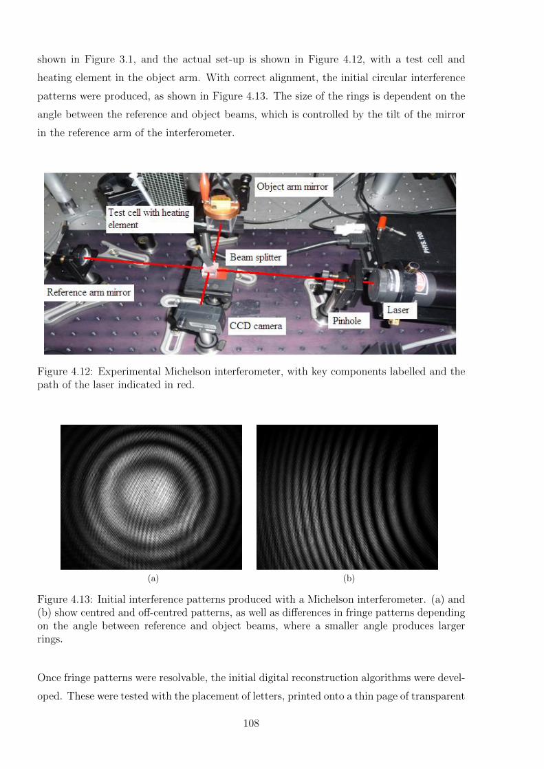
shown in Figure 3.1, and the actual set-up is shown in Figure 4.12, with a test cell and
heating element in the object arm. With correct alignment, the initial circular interference
patterns were produced, as shown in Figure 4.13. The size of the rings is dependent on the
angle between the reference and object beams, which is controlled by the tilt of the mirror
in the reference arm of the interferometer.
Figure 4.12: Experimental Michelson interferometer, with key components labelled and thepath of the laser indicated in red.
(a) (b)
Figure 4.13: Initial interference patterns produced with a Michelson interferometer. (a) and(b) show centred and off-centred patterns, as well as differences in fringe patterns dependingon the angle between reference and object beams, where a smaller angle produces largerrings.
Once fringe patterns were resolvable, the initial digital reconstruction algorithms were devel-
oped. These were tested with the placement of letters, printed onto a thin page of transparent
108
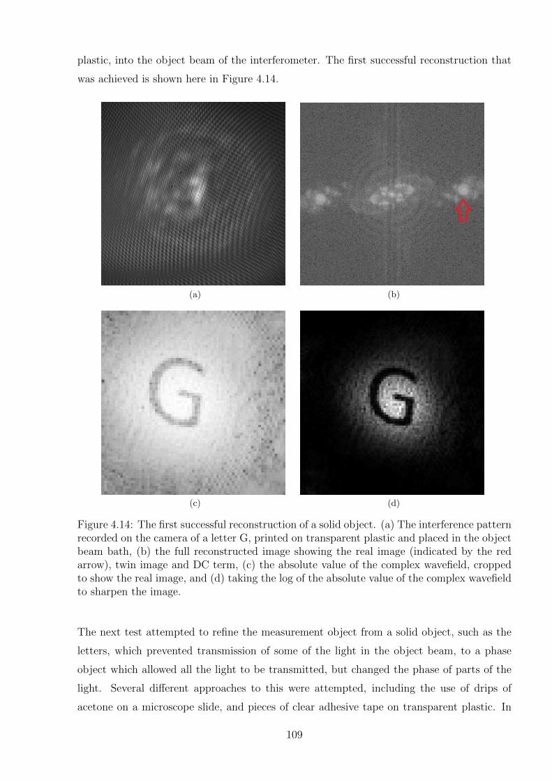
plastic, into the object beam of the interferometer. The first successful reconstruction that
was achieved is shown here in Figure 4.14.
(a) (b)
(c) (d)
Figure 4.14: The first successful reconstruction of a solid object. (a) The interference patternrecorded on the camera of a letter G, printed on transparent plastic and placed in the objectbeam bath, (b) the full reconstructed image showing the real image (indicated by the redarrow), twin image and DC term, (c) the absolute value of the complex wavefield, croppedto show the real image, and (d) taking the log of the absolute value of the complex wavefieldto sharpen the image.
The next test attempted to refine the measurement object from a solid object, such as the
letters, which prevented transmission of some of the light in the object beam, to a phase
object which allowed all the light to be transmitted, but changed the phase of parts of the
light. Several different approaches to this were attempted, including the use of drips of
acetone on a microscope slide, and pieces of clear adhesive tape on transparent plastic. In
109
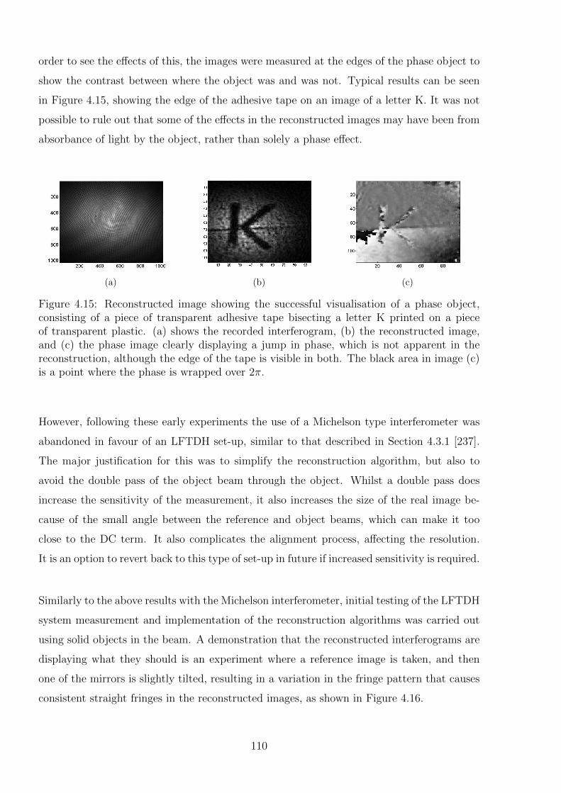
order to see the effects of this, the images were measured at the edges of the phase object to
show the contrast between where the object was and was not. Typical results can be seen
in Figure 4.15, showing the edge of the adhesive tape on an image of a letter K. It was not
possible to rule out that some of the effects in the reconstructed images may have been from
absorbance of light by the object, rather than solely a phase effect.
(a) (b) (c)
Figure 4.15: Reconstructed image showing the successful visualisation of a phase object,consisting of a piece of transparent adhesive tape bisecting a letter K printed on a pieceof transparent plastic. (a) shows the recorded interferogram, (b) the reconstructed image,and (c) the phase image clearly displaying a jump in phase, which is not apparent in thereconstruction, although the edge of the tape is visible in both. The black area in image (c)is a point where the phase is wrapped over 2π.
However, following these early experiments the use of a Michelson type interferometer was
abandoned in favour of an LFTDH set-up, similar to that described in Section 4.3.1 [237].
The major justification for this was to simplify the reconstruction algorithm, but also to
avoid the double pass of the object beam through the object. Whilst a double pass does
increase the sensitivity of the measurement, it also increases the size of the real image be-
cause of the small angle between the reference and object beams, which can make it too
close to the DC term. It also complicates the alignment process, affecting the resolution.
It is an option to revert back to this type of set-up in future if increased sensitivity is required.
Similarly to the above results with the Michelson interferometer, initial testing of the LFTDH
system measurement and implementation of the reconstruction algorithms was carried out
using solid objects in the beam. A demonstration that the reconstructed interferograms are
displaying what they should is an experiment where a reference image is taken, and then
one of the mirrors is slightly tilted, resulting in a variation in the fringe pattern that causes
consistent straight fringes in the reconstructed images, as shown in Figure 4.16.
110
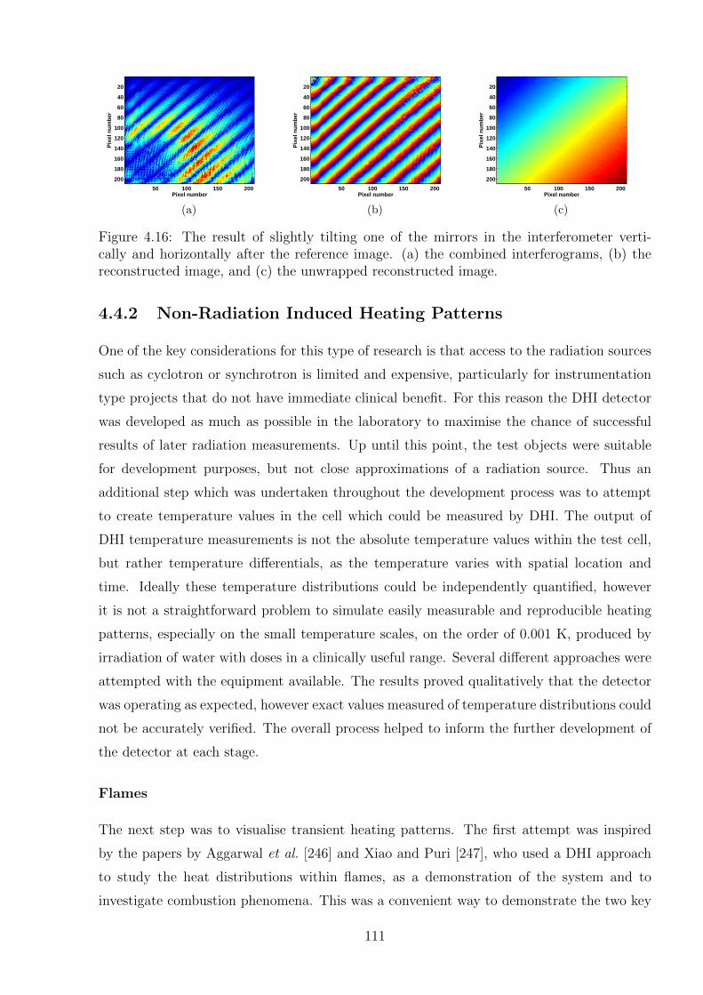
Pixel number
Pix
el n
um
ber
50 100 150 200
20
40
60
80
100
120
140
160
180
200
(a)
Pixel number
Pix
el n
um
ber
50 100 150 200
20
40
60
80
100
120
140
160
180
200
(b)
Pixel number
Pix
el n
um
ber
50 100 150 200
20
40
60
80
100
120
140
160
180
200
(c)
Figure 4.16: The result of slightly tilting one of the mirrors in the interferometer verti-cally and horizontally after the reference image. (a) the combined interferograms, (b) thereconstructed image, and (c) the unwrapped reconstructed image.
4.4.2 Non-Radiation Induced Heating Patterns
One of the key considerations for this type of research is that access to the radiation sources
such as cyclotron or synchrotron is limited and expensive, particularly for instrumentation
type projects that do not have immediate clinical benefit. For this reason the DHI detector
was developed as much as possible in the laboratory to maximise the chance of successful
results of later radiation measurements. Up until this point, the test objects were suitable
for development purposes, but not close approximations of a radiation source. Thus an
additional step which was undertaken throughout the development process was to attempt
to create temperature values in the cell which could be measured by DHI. The output of
DHI temperature measurements is not the absolute temperature values within the test cell,
but rather temperature differentials, as the temperature varies with spatial location and
time. Ideally these temperature distributions could be independently quantified, however
it is not a straightforward problem to simulate easily measurable and reproducible heating
patterns, especially on the small temperature scales, on the order of 0.001 K, produced by
irradiation of water with doses in a clinically useful range. Several different approaches were
attempted with the equipment available. The results proved qualitatively that the detector
was operating as expected, however exact values measured of temperature distributions could
not be accurately verified. The overall process helped to inform the further development of
the detector at each stage.
Flames
The next step was to visualise transient heating patterns. The first attempt was inspired
by the papers by Aggarwal et al. [246] and Xiao and Puri [247], who used a DHI approach
to study the heat distributions within flames, as a demonstration of the system and to
investigate combustion phenomena. This was a convenient way to demonstrate the two key
111
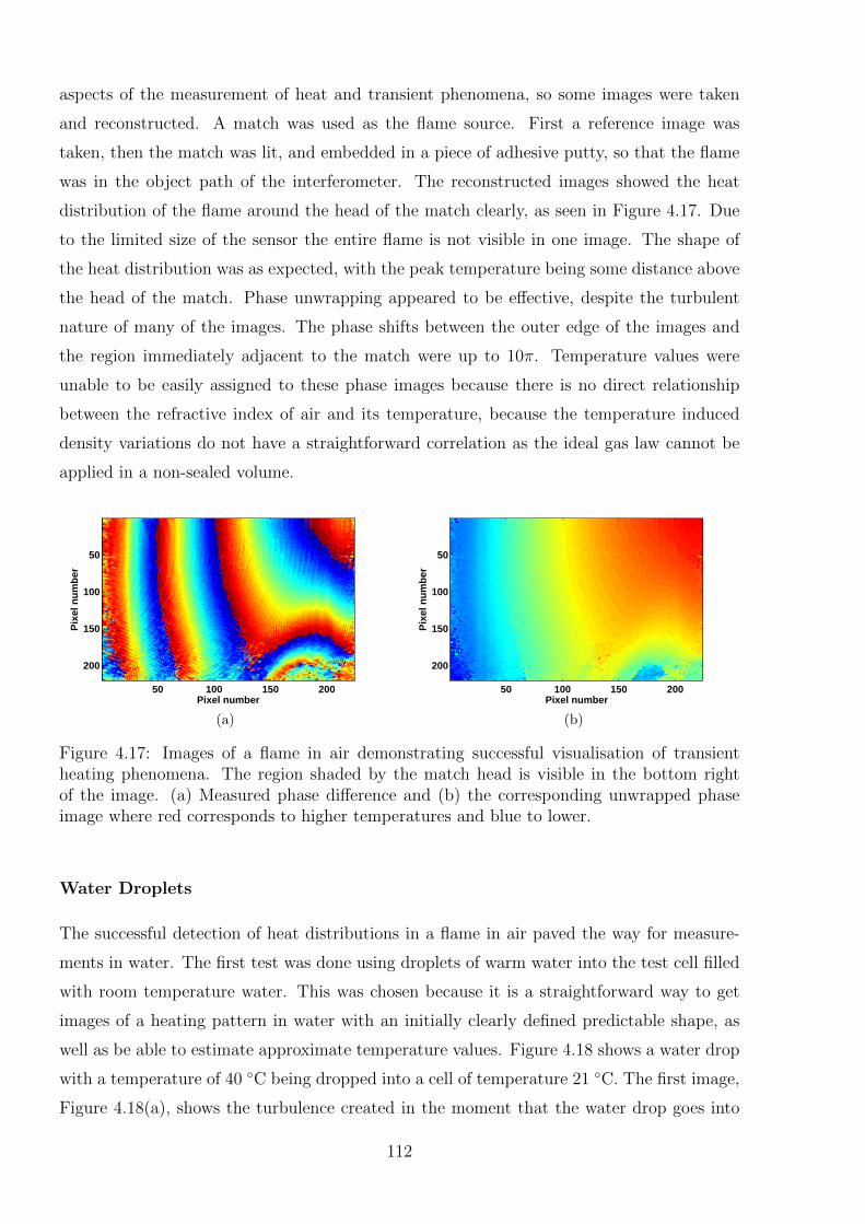
aspects of the measurement of heat and transient phenomena, so some images were taken
and reconstructed. A match was used as the flame source. First a reference image was
taken, then the match was lit, and embedded in a piece of adhesive putty, so that the flame
was in the object path of the interferometer. The reconstructed images showed the heat
distribution of the flame around the head of the match clearly, as seen in Figure 4.17. Due
to the limited size of the sensor the entire flame is not visible in one image. The shape of
the heat distribution was as expected, with the peak temperature being some distance above
the head of the match. Phase unwrapping appeared to be effective, despite the turbulent
nature of many of the images. The phase shifts between the outer edge of the images and
the region immediately adjacent to the match were up to 10π. Temperature values were
unable to be easily assigned to these phase images because there is no direct relationship
between the refractive index of air and its temperature, because the temperature induced
density variations do not have a straightforward correlation as the ideal gas law cannot be
applied in a non-sealed volume.
Pixel number
Pix
el n
um
ber
50 100 150 200
50
100
150
200
(a)
Pixel number
Pix
el n
um
ber
50 100 150 200
50
100
150
200
(b)
Figure 4.17: Images of a flame in air demonstrating successful visualisation of transientheating phenomena. The region shaded by the match head is visible in the bottom rightof the image. (a) Measured phase difference and (b) the corresponding unwrapped phaseimage where red corresponds to higher temperatures and blue to lower.
Water Droplets
The successful detection of heat distributions in a flame in air paved the way for measure-
ments in water. The first test was done using droplets of warm water into the test cell filled
with room temperature water. This was chosen because it is a straightforward way to get
images of a heating pattern in water with an initially clearly defined predictable shape, as
well as be able to estimate approximate temperature values. Figure 4.18 shows a water drop
with a temperature of 40 ◦C being dropped into a cell of temperature 21 ◦C. The first image,
Figure 4.18(a), shows the turbulence created in the moment that the water drop goes into
112
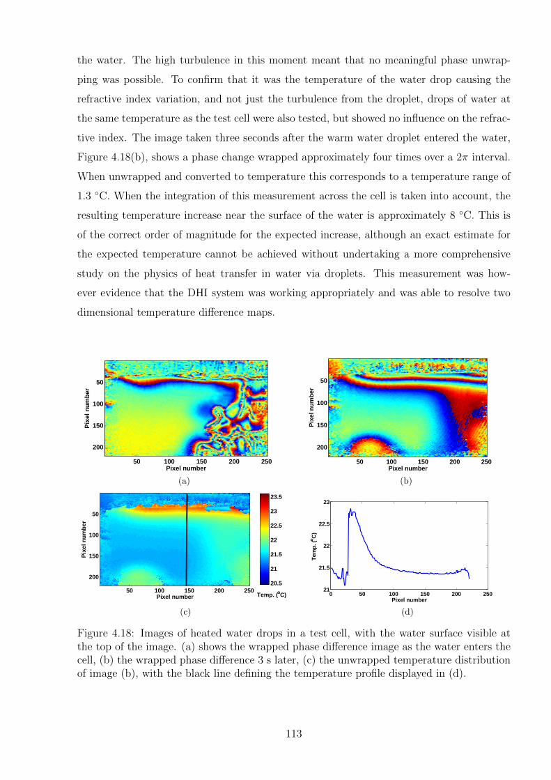
the water. The high turbulence in this moment meant that no meaningful phase unwrap-
ping was possible. To confirm that it was the temperature of the water drop causing the
refractive index variation, and not just the turbulence from the droplet, drops of water at
the same temperature as the test cell were also tested, but showed no influence on the refrac-
tive index. The image taken three seconds after the warm water droplet entered the water,
Figure 4.18(b), shows a phase change wrapped approximately four times over a 2π interval.
When unwrapped and converted to temperature this corresponds to a temperature range of
1.3 ◦C. When the integration of this measurement across the cell is taken into account, the
resulting temperature increase near the surface of the water is approximately 8 ◦C. This is
of the correct order of magnitude for the expected increase, although an exact estimate for
the expected temperature cannot be achieved without undertaking a more comprehensive
study on the physics of heat transfer in water via droplets. This measurement was how-
ever evidence that the DHI system was working appropriately and was able to resolve two
dimensional temperature difference maps.
Pixel number
Pix
el n
um
ber
50 100 150 200 250
50
100
150
200
(a)
Pixel number
Pix
el n
um
ber
50 100 150 200 250
50
100
150
200
(b)
Pixel number
Pix
el n
um
ber
50 100 150 200 250
50
100
150
20020.5
21
21.5
22
22.5
23
23.5
Temp. (oC)
(c)
0 50 100 150 200 25021
21.5
22
22.5
23
Pixel number
Tem
p. (
oC
)
(d)
Figure 4.18: Images of heated water drops in a test cell, with the water surface visible atthe top of the image. (a) shows the wrapped phase difference image as the water enters thecell, (b) the wrapped phase difference 3 s later, (c) the unwrapped temperature distributionof image (b), with the black line defining the temperature profile displayed in (d).
113
Modulated Heating Pattern
A final approach to creating measurable temperature variations in the laboratory was at-
tempted, with the creation of a more highly modulated temperature distribution. The idea
was that the resultant phase changes would be both more confidently determined on the
images, as well as provide some indication of the complexities that would be faced in at-
tempting to measure more modulated radiation dose distributions, such as that produced by
MRT radiation beams. An example of one such complexity is that the phase wrapping will
not be only in one direction, so this may reduce the effectiveness achieved by the unwrapping
algorithm. In order to simulate microbeams, the heat gradient must be high over a short
distance, and created on a short timescale. A heating element was manufactured in the form
of a copper heat sink with three parallel pins extruding from it, each of length 1 cm and
diameter 1 mm (depicted in Figure 4.19(a)). The pins were immersed in the water of the test
cell, and then resistively heated with a current of 0.5 A and 12 V voltage. A temperature
probe was inserted into the centre of the copper block in order to provide a temperature
value for comparison with the DHI measurements. An example of the result after a one
minute measurement is shown in Figure 4.19, progressing from the recorded interferogram,
to the image reconstruction, phase difference map and corresponding temperature difference
map. The temperature increase around the pins is clearly visible, and the profile lines shown
in Figure 4.19(e) clearly show the range of the temperatures around the heating elements.
The temperature probe in the copper block measured an increase in temperature over this
time period of 4.6 ◦C. The DHI measured temperature increase at the tip of the pins was
0.29±0.03 ◦C, however at 1 mm along the pins this rose to 0.81±0.04 ◦C. Additional mea-
surements, not depicted here, with more of the pins visible on the interferogram, showed
a temperature rise of up to 3.12±0.08 ◦C in the water immediately adjacent to the pins,
approximately 3 mm distally from the copper block. Thus it is evident that despite the
high thermal conductivity of copper, the temperature in the centre of the heat sink is not
equal to the temperatures along the pins. This effect is compounded by heat diffusion which
would occur over the minute-long heating up period allowing for faster transfer of heat away
from the pins because of their higher surface area compared to the heat sink. In this case,
the DHI measured values are on the order of magnitude that one might expect, especially
considering the occurrence of heat diffusion over the one minute.
114
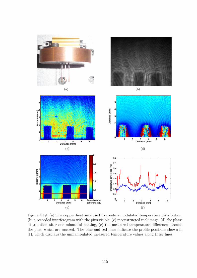
(a) (b)
Distance (mm)
Dis
tan
ce (
mm
)
1 2 3 4 5 6
5
4
3
2
1
0
(c)
Distance (mm)
Dis
tan
ce (
mm
)
1 2 3 4 5 6
5
4
3
2
1
0
(d)
Distance (mm)
Dis
tan
ce (
mm
)
1 2 3 4 5 6
5
4
3
2
1
0 0
0.2
0.4
0.6
0.8
1
Temperaturedifference (K)
(e)
0 1 2 3 4 5 60
0.1
0.2
0.3
0.4
0.5
0.6
0.7
0.8
Tem
per
atu
re d
iffe
ren
ce (o
C)
Distance (mm)
(f)
Figure 4.19: (a) The copper heat sink used to create a modulated temperature distribution,(b) a recorded interferogram with the pins visible, (c) reconstructed real image, (d) the phasedistribution after one minute of heating, (e) the measured temperature differences aroundthe pins, which are masked. The blue and red lines indicate the profile positions shown in(f), which displays the unmanipulated measured temperature values along these lines.
115
4.4.3 Absolute Temperature Measurements
The measurements presented in the previous sections are examples of relative measurements,
where the temperature variation within the field of view is considered at one time instance.
In situations where the induced temperature change does not reach all areas of the field of
view, then the absolute temperature change at each point compared to the reference image
can be determined. However in most situations, including most dosimetric measurements,
there may be an induced temperature rise in every pixel of the field of view. Thus each
image provides a measurement of only the temperature (or dose) difference at that point
in time and gives no indication of the cumulative temperature increase/absorbed dose to
each point. It is theoretically possible, by taking a series of measurements it is possible to
determine the cumulative temperature/dose increase at each point in the cell over the entire
irradiation period. This would result in a determination of the absolute dose value at each
point, but remains an area of further work.
As discussed in Section 4.3.2, the series of images measured can have phase values wrapped
in the time dimension, which also need to be unwrapped, using the Rahman unwrapper.
The complicating factor is that the noise from atmospheric temperature and pressure vari-
ations, and vibrations will have a greater effect inter-image than they do intra-image. For
instance, variation of the room temperature causes expansion or contraction of the optical
componentry, which can affect the measured phase values. Additionally, there is a degree of
heating induced in the water due to the laser, as calculated below. In order to do any kind
of absolute dosimetry, these influences need to be quantified to determine if it is possible
to correct for it. They have no impact on the individual images because, in a first order
approximation, variations in these quantities will affect each point in the image to the same
extent.
Laser Induced Heating
The extent to which the water in the test cell is heated by absorption of a laser in the water
can be calculated for a given configuration of the interferometer. The first step is to calculate
the transmittance, T , of the light through the sample, using the Beer-Lambert Law:
T = 10−A = 10−a·d (4.18)
where A is the absorbance of the medium for that wavelength of light, a is the absorption
coefficient, and d the depth of the test cell in the laser direction. The laser power absorbed
in the sample, PA, can then be calculated according to:
116
PA = PL ·BS ·ND · F · (1− T ) (4.19)
where PL is the mean power of the laser in steady state, BS is the fraction of light in the
object beam after passing through the beam splitter, ND is the fraction of the light passing
through the neutral density filters and F is the fraction of the light which reaches the test
cell and is not obscured by one or more of the mirrors. This last value of F involves an
approximation, however it proves to have relatively negligible influence on final measured
results. Additional assumptions are that the light from the laser as it comes out of the beam
splitter is of homogenous intensity, that the transduction efficiency is equal to one, that there
is no laser attenutaion in air, and thatany absorbance in the thin Perspex wall of the test
cell is ignored. These assumptions should be revisited in future if improved measurement
accuracy warrants this correction.
The rate of temperature rise of the test cell water in the path of the laser, is then calculated
from the heat capacity of the water, Cm, using the equation:
∆T =PACm
(4.20)
where the units are K s−1.
For a He-Ne laser, the absorption coefficient is a = 0.2995 m−1 [235, 244]. For a typical
measurement with the DHI dosimeter prototype, the laser had a mean power output of
PL = 12.1 mW, in an interferometer with a 50/50 beam splitter (BS = 0.5), neutral density
filters with optical density 0.4 and 0.2, and with F = 0.8. The beam was incident on a
cross-sectional area of the test cell of 1.57 cm2. Substituting these values into equations
4.18-4.20 gives an increase in temperature of approximately 0.4 mK s−1. This is compared
to a radiation induced temperature increase of approximately 0.24 mK G−1. Thus for a
dose of several hundred Gy, the impact is minimal, provided the dose rate is sufficient.
However, for lower dose measurements, and for heat diffusion calculations this effect may
become significant. At this stage, the projection of the dose means that the differential
heating of different portions of the cell by the laser is not visible on the final image, but in
future it should be included in the heat modelling, especially if low doses are to be measured.
117
Correlation of External Temperature Variation
Various so-called “flat field” measurements were taken, where there was no induced temper-
ature change in the water. In the absence of room temperature variations, this should result
in images that show only the small, consistent increase in temperature due to the optical
heating. However, variations in room temperature may have an impact on the path length of
the light passing through the interferometer. Ambient temperature increase causes decreased
air density and expansion of the metal parts of the interferometer, to a different extent on
the reference and object paths, thus causing a corresponding variation in the measured phase
shifts and resultant temperature measurements. A separate temperature logger with 0.1 ◦C
resolution was placed within the experimental box to record the atmospheric temperature
during the measurements, to attempt to correlate this effect. If a consistent value can be
achieved for the correlation of room temperature and measured temperature, then it may
be possible to account for this effect, and undertake absolute dosimetry measurements.
A series of flat field images was recorded over several measurement sessions on different
days. The measurement periods encompassed times when the ambient temperature in the
box was consistently increasing, decreasing or unchanging. The resulting DHI measurements
also showed a range of outcomes in terms of temperature variation. A sample of some of
these measurements is shown in Figure 4.20. In general, when the ambient temperature
increased or decreased there was a corresponding change in the measured phase difference
values, averaged across each image. This corresponds to an artificial change (in the opposite
direction to the phase) in the measured temperature values attributed to the water in the
test cell. However some measurements where the ambient temperature showed no variation
resulted in a decrease in phase measured by the detector, corresponding to apparent tem-
peratures of up to 0.34 K min−1. The source of this variation was unable to be determined
and, whilst generally consistent for the period of each measurement, varied between mea-
surements. The frequency stabilised laser described in Section 4.3.1 was used to rule out the
drift being caused by some instability in the laser frequency, with results also showing similar
inconsistencies. All other aspects of the interferometer were carefully considered, but at this
point no suitable explanation for these results has been determined. Given this unexplained
drift, a consistent correlation value between the ambient temperature values and the DHI
measurements was not determined. It may prove to be due to non-homogenous temperature
variation within the experimental box, or alternatively barometric variations which were not
measured.
118
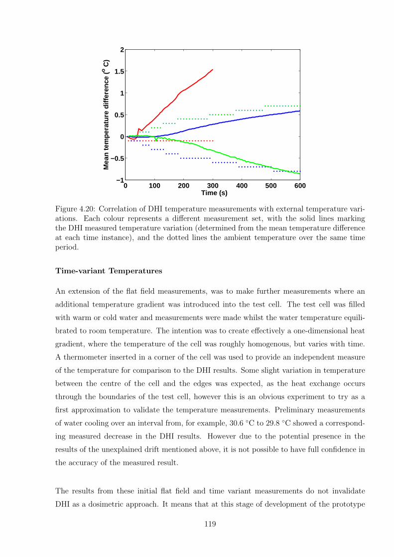
0 100 200 300 400 500 600−1
−0.5
0
0.5
1
1.5
2
Time (s)
Mea
n te
mpe
ratu
re d
iffer
ence
(o C
)
Figure 4.20: Correlation of DHI temperature measurements with external temperature vari-ations. Each colour represents a different measurement set, with the solid lines markingthe DHI measured temperature variation (determined from the mean temperature differenceat each time instance), and the dotted lines the ambient temperature over the same timeperiod.
Time-variant Temperatures
An extension of the flat field measurements, was to make further measurements where an
additional temperature gradient was introduced into the test cell. The test cell was filled
with warm or cold water and measurements were made whilst the water temperature equili-
brated to room temperature. The intention was to create effectively a one-dimensional heat
gradient, where the temperature of the cell was roughly homogenous, but varies with time.
A thermometer inserted in a corner of the cell was used to provide an independent measure
of the temperature for comparison to the DHI results. Some slight variation in temperature
between the centre of the cell and the edges was expected, as the heat exchange occurs
through the boundaries of the test cell, however this is an obvious experiment to try as a
first approximation to validate the temperature measurements. Preliminary measurements
of water cooling over an interval from, for example, 30.6 ◦C to 29.8 ◦C showed a correspond-
ing measured decrease in the DHI results. However due to the potential presence in the
results of the unexplained drift mentioned above, it is not possible to have full confidence in
the accuracy of the measured result.
The results from these initial flat field and time variant measurements do not invalidate
DHI as a dosimetric approach. It means that at this stage of development of the prototype
119
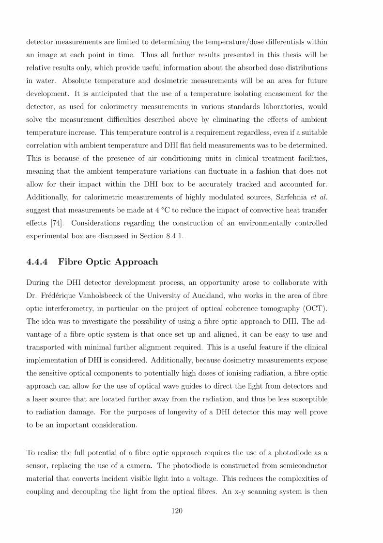
detector measurements are limited to determining the temperature/dose differentials within
an image at each point in time. Thus all further results presented in this thesis will be
relative results only, which provide useful information about the absorbed dose distributions
in water. Absolute temperature and dosimetric measurements will be an area for future
development. It is anticipated that the use of a temperature isolating encasement for the
detector, as used for calorimetry measurements in various standards laboratories, would
solve the measurement difficulties described above by eliminating the effects of ambient
temperature increase. This temperature control is a requirement regardless, even if a suitable
correlation with ambient temperature and DHI flat field measurements was to be determined.
This is because of the presence of air conditioning units in clinical treatment facilities,
meaning that the ambient temperature variations can fluctuate in a fashion that does not
allow for their impact within the DHI box to be accurately tracked and accounted for.
Additionally, for calorimetric measurements of highly modulated sources, Sarfehnia et al.
suggest that measurements be made at 4 ◦C to reduce the impact of convective heat transfer
effects [74]. Considerations regarding the construction of an environmentally controlled
experimental box are discussed in Section 8.4.1.
4.4.4 Fibre Optic Approach
During the DHI detector development process, an opportunity arose to collaborate with
Dr. Frederique Vanholsbeeck of the University of Auckland, who works in the area of fibre
optic interferometry, in particular on the project of optical coherence tomography (OCT).
The idea was to investigate the possibility of using a fibre optic approach to DHI. The ad-
vantage of a fibre optic system is that once set up and aligned, it can be easy to use and
transported with minimal further alignment required. This is a useful feature if the clinical
implementation of DHI is considered. Additionally, because dosimetry measurements expose
the sensitive optical components to potentially high doses of ionising radiation, a fibre optic
approach can allow for the use of optical wave guides to direct the light from detectors and
a laser source that are located further away from the radiation, and thus be less susceptible
to radiation damage. For the purposes of longevity of a DHI detector this may well prove
to be an important consideration.
To realise the full potential of a fibre optic approach requires the use of a photodiode as a
sensor, replacing the use of a camera. The photodiode is constructed from semiconductor
material that converts incident visible light into a voltage. This reduces the complexities of
coupling and decoupling the light from the optical fibres. An x-y scanning system is then
120
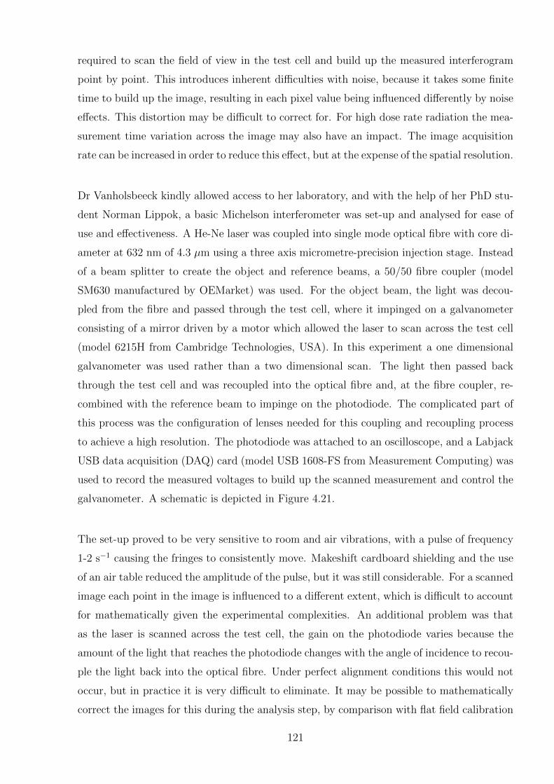
required to scan the field of view in the test cell and build up the measured interferogram
point by point. This introduces inherent difficulties with noise, because it takes some finite
time to build up the image, resulting in each pixel value being influenced differently by noise
effects. This distortion may be difficult to correct for. For high dose rate radiation the mea-
surement time variation across the image may also have an impact. The image acquisition
rate can be increased in order to reduce this effect, but at the expense of the spatial resolution.
Dr Vanholsbeeck kindly allowed access to her laboratory, and with the help of her PhD stu-
dent Norman Lippok, a basic Michelson interferometer was set-up and analysed for ease of
use and effectiveness. A He-Ne laser was coupled into single mode optical fibre with core di-
ameter at 632 nm of 4.3 µm using a three axis micrometre-precision injection stage. Instead
of a beam splitter to create the object and reference beams, a 50/50 fibre coupler (model
SM630 manufactured by OEMarket) was used. For the object beam, the light was decou-
pled from the fibre and passed through the test cell, where it impinged on a galvanometer
consisting of a mirror driven by a motor which allowed the laser to scan across the test cell
(model 6215H from Cambridge Technologies, USA). In this experiment a one dimensional
galvanometer was used rather than a two dimensional scan. The light then passed back
through the test cell and was recoupled into the optical fibre and, at the fibre coupler, re-
combined with the reference beam to impinge on the photodiode. The complicated part of
this process was the configuration of lenses needed for this coupling and recoupling process
to achieve a high resolution. The photodiode was attached to an oscilloscope, and a Labjack
USB data acquisition (DAQ) card (model USB 1608-FS from Measurement Computing) was
used to record the measured voltages to build up the scanned measurement and control the
galvanometer. A schematic is depicted in Figure 4.21.
The set-up proved to be very sensitive to room and air vibrations, with a pulse of frequency
1-2 s−1 causing the fringes to consistently move. Makeshift cardboard shielding and the use
of an air table reduced the amplitude of the pulse, but it was still considerable. For a scanned
image each point in the image is influenced to a different extent, which is difficult to account
for mathematically given the experimental complexities. An additional problem was that
as the laser is scanned across the test cell, the gain on the photodiode varies because the
amount of the light that reaches the photodiode changes with the angle of incidence to recou-
ple the light back into the optical fibre. Under perfect alignment conditions this would not
occur, but in practice it is very difficult to eliminate. It may be possible to mathematically
correct the images for this during the analysis step, by comparison with flat field calibration
121
1-axis galvanometer mirror
Test cell
Lens
Mirror
Photodiode
Mirror
Reference arm
Object arm
3-axis injection stage
Laser
Lens
50/50 fibre coupler
Figure 4.21: The schematic of the initial Michelson-type fibre optic set-up.
images. Additionally, the influence of vibrations of the optical fibres can have a considerable
effect on fibre optic interferometry. This can be mitigated to some extent by the use of a
vibration isolated table, but this is likely not to be available in a clinical dosimetry situation.
Following these early experiments, further work was done on this approach by Masters
student Kaidi Liang, under the co-supervision of Dr. Vanholsbeeck and Dr. Juergen Meyer
[248]. He achieved successful holographic reconstructions of two dimensional interferograms,
however did not achieve any conclusive temperature measurement results due to encountering
various experimental setbacks. The use of fibre optic interferometry therefore remains an
area to explore further for the sake of its potential advantages for transportability of a
DHI detector. This approach has more complexities than the standard non fibre approach
described in the rest of this chapter. There are many areas that would require consideration
for this to work, including the best method of coupling the light into the fibre by the test
cell, and experimental and image processing noise reduction.
4.5 Concluding Remarks
The purpose of this chapter was to fully describe the prototype DHI detector used for the
radiation dosimetry measurements, based on an LFTDH configuration. The various design
considerations and equipment choices were discussed in the context of how they influenced
the final prototype design. A complete description of the detector and the mathematical al-
gorithms developed to reconstruct the images and obtain measured dose values was included.
122
Further description of the entire measurement process was given in sufficient detail to allow
for all measurements to be independently replicated. Initial measurements of various heat
distributions were presented as part of the development process of the interferometer, and in
order to determine that it was operating as expected. The result of these measurements was
a prototype detector that successfully resolved various two dimensional temperature maps
and was ready for application to clinical radiation sources.
Consideration was given to measuring temperatures/doses in terms of absolute versus dose
difference distributions. Based on the absolute temperature experiments conducted to date,
the present prototype detector is limited to dose differential measurements. Future develop-
ment of an atmospheric controlled experimental enclosure may allow for absolute dosimetry
measurements at some later stage. Future work may also include further consideration of a
fibre optic interferometry approach.
The next chapter introduces the concept of heat transport within the test cell, which must
be considered in order to ensure the correct interpretation of measured temperature maps
when determining absorbed dose from irradiation.
123

124
Chapter 5
Heat Transfer Modelling
The impacts of heat transfer must be considered when undertaking any form of calorimetric
radiation dose measurements over a finite time interval. As absorbed doses are derived
directly from the temperature increases imparted by the radiation, any variations in the
temperature field can be a limiting factor on measurement accuracy. This chapter introduces
the basic forms of heat transfer, and their relevance to DHI dosimetry. Methods to account
for the effects of heat transfer in DHI dosimetry are developed and described.
5.1 Introduction to Heat Transfer
In this context, heat is considered to be thermal energy, which can transfer from one ther-
modynamic system to another. There are three fundamental modes of heat transfer which
are relevant to calorimetry: conduction, convection and radiation [249]. Conduction is the
direct microscopic exchange of kinetic energy of adjacent particles, and is also referred to as
diffusion in this work. A net flow of heat occurs when there is a temperature differential
between two points, in order to reach thermal equilibrium, as described by the second law
of thermodynamics. Convection is the transfer of energy due to fluid motion, as bulk flow
of a gas or liquid carries heat along with the flow of matter. This process is sometimes also
referred to as advection. In calorimetry the relevant type of convection is natural convection
where thermal expansion of the fluid in a heated region causes buoyancy forces, establishing
a circulation of heat away from the heated region. At times the term convection is used
to describe the transfer of heat by both advection and diffusion, as convective heat transfer
generally has an element of conduction associated with it. The third relevant type of heat
transfer is thermal radiation, which occurs through a vacuum or any transparent medium,
transferred by means of the absorption or emission of thermal photons in electromagnetic
waves. The electromagnetic waves are generated by the movement of the charged particles
(protons and electrons) within the atoms of a heated object.
125
The most relevant types of heat transfer for DHI dosimetry are heat diffusion and heat
convection [74]. The extent to which these phenomena impact the measurement results de-
pends on the specific application and measurement conditions. Ideally, to reduce the impact
of heat transport, doses should be delivered at as high a dose rate as possible, and measure-
ment taken concurrently or immediately subsequent to dose delivery. Sufficiently high dose
rates are however, depending on the radiation modality in question, not always achievable or
clinically relevant. Thus some consideration must be given to the extent of diffusion and con-
vection occurring, and corrections made for the impacts these effects may have on the results.
Radiative heat transfer in the case of DHI pertains to the energy losses at the sides of the
test cell. Considering the miniscule temperature increases expected, and the localisation of
measurement regions away from the edges of the test cell, for most DHI applications this
effect will have negligible impact on the total temperature distributions measured, so has
not been considered further in this work.
The next section describes a framework for modelling heat diffusion, and then describes two
different methods to account for heat diffusion in DHI radiation dosimetry measurements.
The impact of convection on the measurements is not considered, and the effects of this
omission will be discussed in Chapter 8.
5.2 Heat Diffusion
The occurrence of heat diffusion is unavoidable in DHI dosimetry of spatially varying dose
distributions, although in some applications there will be less of an impact than in others.
The rate of heat diffusion depends on the temperature gradient between two points, with
higher dose gradients resulting in a higher rate of heat diffusion down the temperature gra-
dient (towards temperature equilibrium between the two points). Thus, radiation modalities
where there is a higher modulation in the dose will be more affected by heat diffusion. The
most obvious example of this is MRT, where the key principle behind the approach is to
have highly modulated beams, with the array of microbeams being both extremely close
together and with high peak to valley dose ratios. The alleviating factor is that the dose
rate is extremely high, so measurements can be made on a short time scale. For a microbeam
array, the heating pattern generated by a radiation dose of hundreds of Gray in the peaks
has been calculated to dissipate entirely in less than a second. This will be discussed further
126
in Chapter 8. A therapeutic proton beam is another example that, in this context, could
be considered a highly modulated dose distribution, as the Bragg peak is a narrow region of
much higher dose than at the depths adjacent to it. A situation where heat diffusion would
have the least amount of impact would be an absolute dose measurement of a broadbeam
radiation geometry, where the irradiated region is much larger than the measurement region
of interest. In this case the temperature distribution will have limited variation over the
measurement volume, reducing the impact of diffusion.
Two different approaches are suggested for quantifying and correcting for the impact of heat
diffusion, displayed in Figure 5.1. The mathematical framework to describe heat diffusion in
three dimensions is common to both methods, which are outlined below in Sections 5.3 and
5.4. Each method has inherent advantages and limitations, which are discussed. Method
1 requires comparison of the measured dose to an independent model of the expected dose
distribution. The DHI detector test cell is then described by three dimensional heat equa-
tions, which are used to model the heat diffusion that has occurred in the system. These
equations are solved numerically, in order to correct the modelled dose data to the same state
as the measured data, enabling a “like with like” comparison of the two datasets. Method
2 requires deconvolution of the heat diffusion. This process has many complicating factors
that mean it is not possible to achieve to the level of accuracy required for dosimetry. An
alternative approach is proposed, involving determining the heat diffusion contribution to
each time instance by calculating the heat diffusion of the temperature distribution at the
previous time instance. This method is described and has been implemented on simulated
data.
5.2.1 General Model of Heat Diffusion
Heat diffusion in a medium is steady if the overall temperature does not vary with time at any
point in the medium, whilst transient heat diffusion displays a time dependence. The rate
of heat diffusion in a specified direction is proportional to the temperature gradient in that
direction [238,249]. The temperature gradient can be defined as the change in temperature
per unit length in a given direction. In general heat distribution within a medium is three
dimensional and time dependent, and can be written as the scalar quantity T = T (x, y, z, t).
The transfer of heat from any given point is a vector quantity named heat flux. In certain
situations the heat conduction in some dimensions is negligible, so this can result in one
dimensional, two dimensional or three dimensional heat diffusion problems. Solving heat
transport problems in one dimension has a much lower level of complexity so is generally
127
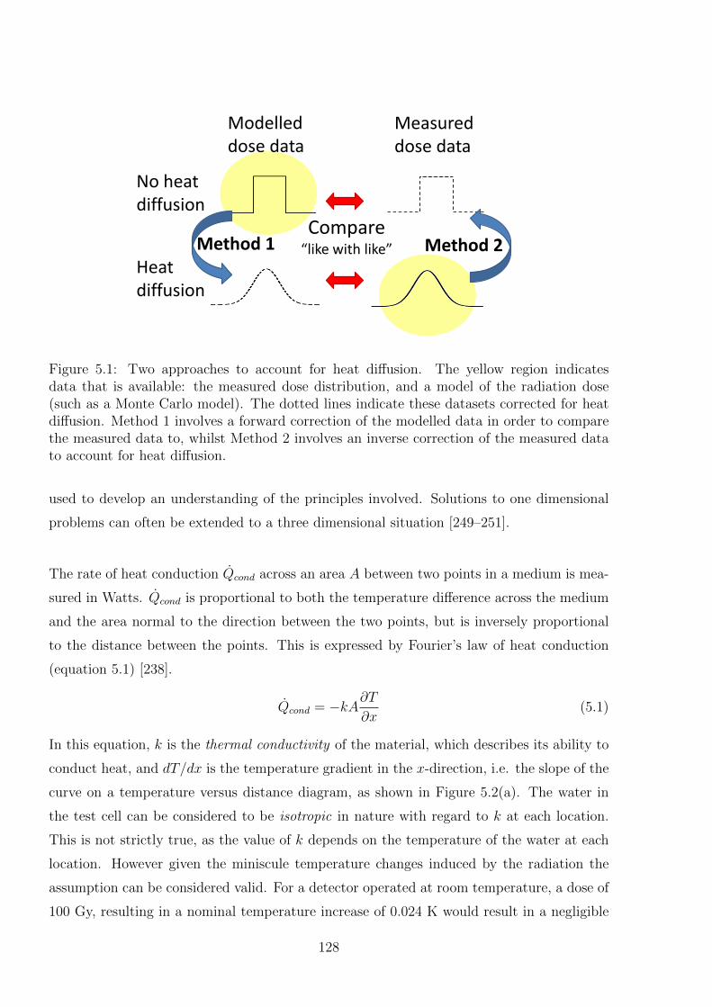
Compare “like with like” Method 1 Method 2
Modelled dose data
Measured dose data
No heat diffusion
Heat diffusion
Figure 5.1: Two approaches to account for heat diffusion. The yellow region indicatesdata that is available: the measured dose distribution, and a model of the radiation dose(such as a Monte Carlo model). The dotted lines indicate these datasets corrected for heatdiffusion. Method 1 involves a forward correction of the modelled data in order to comparethe measured data to, whilst Method 2 involves an inverse correction of the measured datato account for heat diffusion.
used to develop an understanding of the principles involved. Solutions to one dimensional
problems can often be extended to a three dimensional situation [249–251].
The rate of heat conduction Qcond across an area A between two points in a medium is mea-
sured in Watts. Qcond is proportional to both the temperature difference across the medium
and the area normal to the direction between the two points, but is inversely proportional
to the distance between the points. This is expressed by Fourier’s law of heat conduction
(equation 5.1) [238].
Qcond = −kA∂T∂x
(5.1)
In this equation, k is the thermal conductivity of the material, which describes its ability to
conduct heat, and dT/dx is the temperature gradient in the x-direction, i.e. the slope of the
curve on a temperature versus distance diagram, as shown in Figure 5.2(a). The water in
the test cell can be considered to be isotropic in nature with regard to k at each location.
This is not strictly true, as the value of k depends on the temperature of the water at each
location. However given the miniscule temperature changes induced by the radiation the
assumption can be considered valid. For a detector operated at room temperature, a dose of
100 Gy, resulting in a nominal temperature increase of 0.024 K would result in a negligible
128
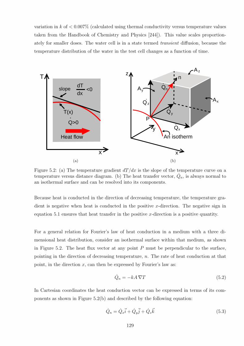
variation in k of < 0.007% (calculated using thermal conductivity versus temperature values
taken from the Handbook of Chemistry and Physics [244]). This value scales proportion-
ately for smaller doses. The water cell is in a state termed transient diffusion, because the
temperature distribution of the water in the test cell changes as a function of time.
x
.
T
Heat flow
Q>0
T(x)
slopedT
dx<0
(a)
z
x
y
An isotherm
PQ
Q
Q
A
A
n
A Q
x
x
y
y
n
z
z
.
.
.
.
(b)
Figure 5.2: (a) The temperature gradient dT/dx is the slope of the temperature curve on atemperature versus distance diagram. (b) The heat transfer vector, Qn, is always normal toan isothermal surface and can be resolved into its components.
Because heat is conducted in the direction of decreasing temperature, the temperature gra-
dient is negative when heat is conducted in the positive x-direction. The negative sign in
equation 5.1 ensures that heat transfer in the positive x-direction is a positive quantity.
For a general relation for Fourier’s law of heat conduction in a medium with a three di-
mensional heat distribution, consider an isothermal surface within that medium, as shown
in Figure 5.2. The heat flux vector at any point P must be perpendicular to the surface,
pointing in the direction of decreasing temperature, n. The rate of heat conduction at that
point, in the direction x, can then be expressed by Fourier’s law as:
Qn = −kA∇T (5.2)
In Cartesian coordinates the heat conduction vector can be expressed in terms of its com-
ponents as shown in Figure 5.2(b) and described by the following equation:
Qn = Qx~i+ Qy
~j + Qz~k (5.3)
129
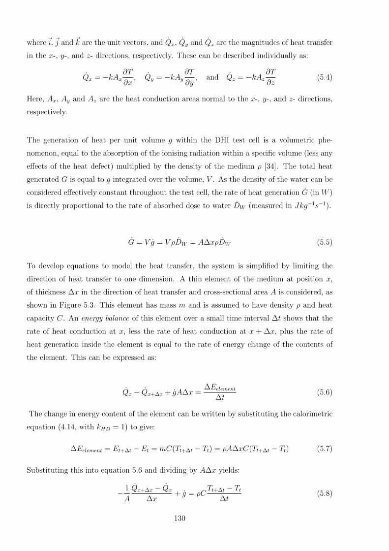
where~i, ~j and ~k are the unit vectors, and Qx, Qy and Qz are the magnitudes of heat transfer
in the x-, y-, and z- directions, respectively. These can be described individually as:
Qx = −kAx∂T
∂x, Qy = −kAy
∂T
∂y, and Qz = −kAz
∂T
∂z(5.4)
Here, Ax, Ay and Az are the heat conduction areas normal to the x-, y-, and z- directions,
respectively.
The generation of heat per unit volume g within the DHI test cell is a volumetric phe-
nomenon, equal to the absorption of the ionising radiation within a specific volume (less any
effects of the heat defect) multiplied by the density of the medium ρ [34]. The total heat
generated G is equal to g integrated over the volume, V . As the density of the water can be
considered effectively constant throughout the test cell, the rate of heat generation G (in W )
is directly proportional to the rate of absorbed dose to water DW (measured in Jkg−1s−1).
G = V g = V ρDW = A∆xρDW (5.5)
To develop equations to model the heat transfer, the system is simplified by limiting the
direction of heat transfer to one dimension. A thin element of the medium at position x,
of thickness ∆x in the direction of heat transfer and cross-sectional area A is considered, as
shown in Figure 5.3. This element has mass m and is assumed to have density ρ and heat
capacity C. An energy balance of this element over a small time interval ∆t shows that the
rate of heat conduction at x, less the rate of heat conduction at x + ∆x, plus the rate of
heat generation inside the element is equal to the rate of energy change of the contents of
the element. This can be expressed as:
Qx − Qx+∆x + gA∆x =∆Eelement
∆t(5.6)
The change in energy content of the element can be written by substituting the calorimetric
equation (4.14, with kHD = 1) to give:
∆Eelement = Et+∆t − Et = mC(Tt+∆t − Tt) = ρA∆xC(Tt+∆t − Tt) (5.7)
Substituting this into equation 5.6 and dividing by A∆x yields:
− 1
A
Qx+∆x − Qx
∆x+ g = ρC
Tt+∆t − Tt∆t
(5.8)
130
x
Volumeelement
AQx
.
0
Qx+ x
x+ xx
G
L
A =A =Ax+ xx
.
Figure 5.3: One dimensional heat conduction through a volume element.
Taking the limit as ∆x→ 0 and ∆t→ 0 gives:
1
A
∂
∂x
(kA
∂T
∂x
)+ g = ρC
∂T
∂t(5.9)
since, according to the definition of the derivative [252] and Fourier’s law of heat conduction
(equation 5.2),
limx→0
Qx+∆x − Qx
∆x=∂Q
∂x=
∂
∂x
(−kA∂T
∂x
)(5.10)
With constant values for k and A, equation 5.9 becomes:
∂2T
∂x2+g
k=
1
α
∂T
∂t(5.11)
where α = k/ρC is the thermal diffusivity of the medium, representing how fast heat prop-
agates through the material. This equation can be extended to three dimensions, with
coordinates as shown in Figure 5.4, and is then known as the Fourier-Biot equation [250]:
∂2T
∂x2+∂2T
∂y2+∂2T
∂z2+g
k=
1
α
∂T
∂t(5.12)
All the equations above were developed using an energy balance on all the interior ele-
ments of the medium. No consideration was paid to the thermal conditions on the surface,
however these will have an impact on the internal heat flux and temperature distribution.
When solving the Fourier-Biot equation for any given system, these surface conditions are
included in the calculation as boundary conditions. In general, to give a unique solution for
a system with heat transfer, two boundary conditions are required for each dimension of
heat transfer. This is equal to the number of arbitrary constants that would be present in
a general solution to the differential equation. There are various types of boundary condi-
tions, including specified temperature (for example T (x, y, z, 0) = f(x, y, z)), heat flux (with
131
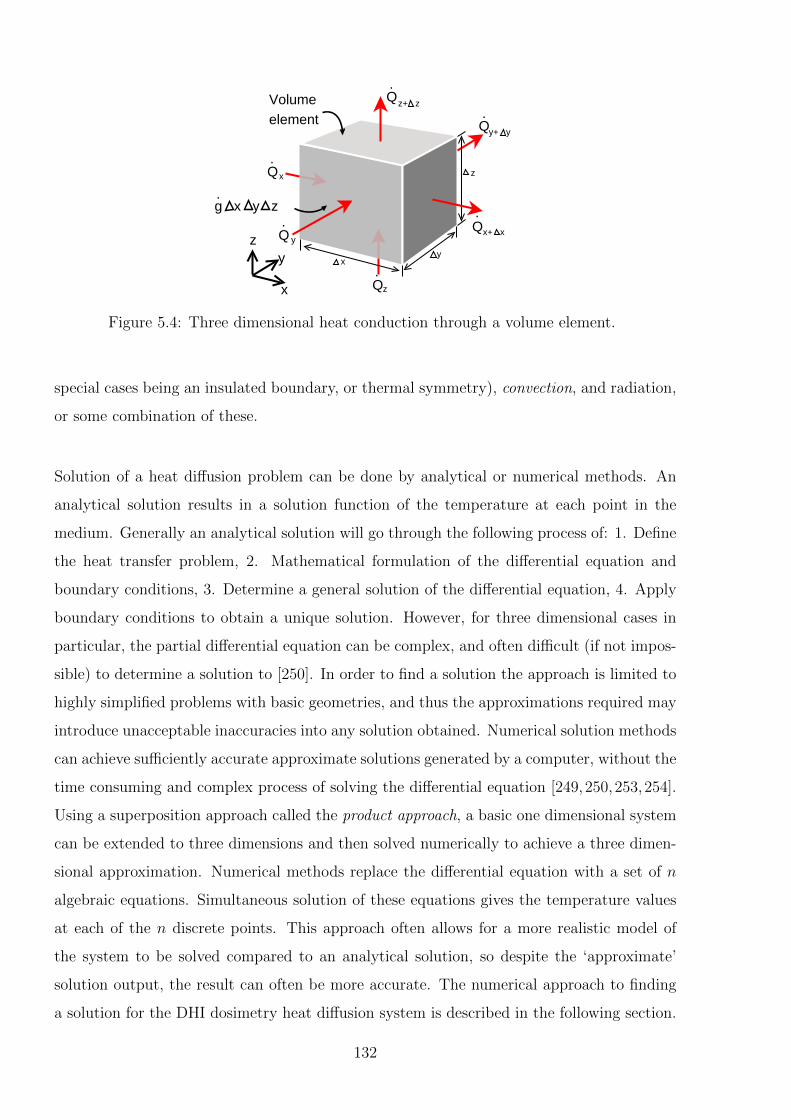
x
Volumeelement
Qx
.
Qx+ x
y+ y
yz Q
.y
Q
Q
Q
.
.
.
.
z+ z
z
y
z
x
g x y z.
Figure 5.4: Three dimensional heat conduction through a volume element.
special cases being an insulated boundary, or thermal symmetry), convection, and radiation,
or some combination of these.
Solution of a heat diffusion problem can be done by analytical or numerical methods. An
analytical solution results in a solution function of the temperature at each point in the
medium. Generally an analytical solution will go through the following process of: 1. Define
the heat transfer problem, 2. Mathematical formulation of the differential equation and
boundary conditions, 3. Determine a general solution of the differential equation, 4. Apply
boundary conditions to obtain a unique solution. However, for three dimensional cases in
particular, the partial differential equation can be complex, and often difficult (if not impos-
sible) to determine a solution to [250]. In order to find a solution the approach is limited to
highly simplified problems with basic geometries, and thus the approximations required may
introduce unacceptable inaccuracies into any solution obtained. Numerical solution methods
can achieve sufficiently accurate approximate solutions generated by a computer, without the
time consuming and complex process of solving the differential equation [249,250,253,254].
Using a superposition approach called the product approach, a basic one dimensional system
can be extended to three dimensions and then solved numerically to achieve a three dimen-
sional approximation. Numerical methods replace the differential equation with a set of n
algebraic equations. Simultaneous solution of these equations gives the temperature values
at each of the n discrete points. This approach often allows for a more realistic model of
the system to be solved compared to an analytical solution, so despite the ‘approximate’
solution output, the result can often be more accurate. The numerical approach to finding
a solution for the DHI dosimetry heat diffusion system is described in the following section.
132
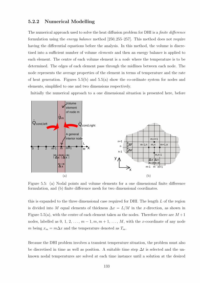
5.2.2 Numerical Modelling
The numerical approach used to solve the heat diffusion problem for DHI is a finite difference
formulation using the energy balance method [250, 255–257]. This method does not require
having the differential equations before the analysis. In this method, the volume is discre-
tised into a sufficient number of volume elements and then an energy balance is applied to
each element. The centre of each volume element is a node where the temperature is to be
determined. The edges of each element pass through the midlines between each node. The
node represents the average properties of the element in terms of temperature and the rate
of heat generation. Figures 5.5(b) and 5.5(a) show the co-ordinate system for nodes and
elements, simplified to one and two dimensions respectively.
Initially the numerical approach to a one dimensional situation is presented here, before
xm+1
x
mm-1210 M
L
x x
Q Q. .
cond,left cond,right
A general interior node
Volume element of node m
gm
.
(a)
x
y
y m,n
m,n+1
m+1,n
m,n-1
m-1,n
y
x x
n+1
n
n-1
m-1 m m+1
(b)
Figure 5.5: (a) Nodal points and volume elements for a one dimensional finite differenceformulation, and (b) finite difference mesh for two dimensional coordinates.
this is expanded to the three dimensional case required for DHI. The length L of the region
is divided into M equal elements of thickness ∆x = L/M in the x-direction, as shown in
Figure 5.5(a), with the centre of each element taken as the nodes. Therefore there are M +1
nodes, labelled as 0, 1, 2, . . . , m − 1,m,m + 1, . . . , M , with the x-coordinate of any node
m being xm = m∆x and the temperature denoted as Tm.
Because the DHI problem involves a transient temperature situation, the problem must also
be discretised in time as well as position. A suitable time step ∆t is selected and the un-
known nodal temperatures are solved at each time instance until a solution at the desired
133
time is achieved. As ∆t is reduced the solution becomes more accurate, however there is
a corresponding increase in computation time. The superscript i is used as an index of
time steps, with i = 0 corresponding to the initial state of the system and each time step
i corresponding to a time of t = i∆t. T im represents the temperature at node m at time step i.
Then a general difference equation for the interior nodes is obtained by considering the
element represented by the node m, and the neighbouring modes m+ 1 and m− 1. Taking
heat conduction into an element to be positive, the energy balance on the element during ∆t
can be expressed as the rate of heat conduction at the left surface (Qcond,left), plus that at
the right surface (Qcond,right), plus the rate of heat generation inside the element (Gelement),
which is set equal to the rate of change of the energy content of the element [249,250]. This
is expressed in the following equation:
Qcond,left + Qcond,right + Gelement =∆Eelement
∆t(5.13)
Using the equation for heat generation (5.5) and Fourier’s equation (5.2), the rate of heat
conduction towards the node m at the left and right surfaces can be expressed as:
Qcond,left = kATm−1 − Tm
∆xand Qcond,right = kA
Tm+1 − Tm∆x
(5.14)
The change of the energy content of the element is, similarly to the one dimensional case
(5.7),
∆Eelement = mC∆T = ρVelementC∆T (5.15)
where ρ is density and C is the heat capacity of the element.
Substituting equations 5.5, 5.14 and 5.15 into equation 5.13 gives the change in temperature
of the node between the time steps i and i+ 1:
kATm−1 − Tm
∆x+ kA
Tm+1 − Tm∆x
+ gmA∆x = ρVelementCT i+1m − T im
∆t(5.16)
Simplifying by cancelling the surface area A and multiplying through by ∆x/k results in:
Tm−1 − 2Tm + Tm+1 +gm∆x2
k=
∆x2
α∆t(T i+1
m − T im) (5.17)
This equation is based on the assumption that the temperature varies linearly across the
element, an approximation which becomes increasingly accurate as the distance between
134
nodes (∆x) and thus the size of the elements is reduced. Note that in the limiting case of
∆x approaching zero, the formulation becomes exact and becomes a differential equation.
For simplicity in the computations, the equation can be simplified further by describing a
dimensionless mesh Fourier number as:
τ =α∆t
∆x2(5.18)
As the nodal temperatures change during each time step, the temperatures from either the
previous time step i or the new time step i+ 1 can be used for the left hand side of equation
5.17, called the explicit and implicit methods respectively. Both methods result in approx-
imately the same values for the calculation of T i+1 values, however the explicit method is
easier to implement but has a time limit on the maximum size time step ∆T which can be
solved. The implicit method has no such time limit but requires all M + 1 equations to be
solved simultaneously. The explicit method is used in the following work, because for an
implicit approach, the large number of equations required (equal to the number of pixels
sampled) means that a direct method of solving the system of simultaneous equations is
computationally prohibitive.
Substituting Equation 5.18 into Equation 5.17, assuming no heat generation and rearranging
using the explicit approach to solve for T i+1m results in:
T i+1m = τ(T im−1 + T im+1) + (1− 2τ)T im (5.19)
Using an implicit solution, the result is:
(6kτ + 1)T i+1m − kτ(T i+1
m−1 + T i+1m+1) = T im (5.20)
This equation is applicable to each of the M−1 interior nodes. The two additional equations
for the elements at the boundaries (which are half sized) are obtained by using the boundary
conditions of the system, which can involve any of specified temperature, specified heat flux,
convection and radiation boundary conditions.
The choice of implicit versus explicit solution hinges on the stability criterion for the explicit
solution, which limits the largest permissible value of ∆t, in order to prevent the solutions
135
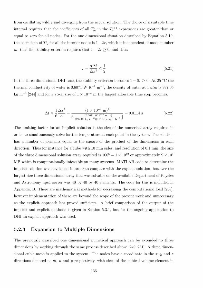
from oscillating wildly and diverging from the actual solution. The choice of a suitable time
interval requires that the coefficients of all T im in the T i+1m expressions are greater than or
equal to zero for all nodes. For the one dimensional situation described by Equation 5.19,
the coefficient of T im for all the interior nodes is 1−2τ , which is independent of mode number
m, thus the stability criterion requires that 1− 2τ ≥ 0, and thus:
τ =α∆t
∆x2≤ 1
2(5.21)
In the three dimensional DHI case, the stability criterion becomes 1− 6τ ≥ 0. At 25 ◦C the
thermal conductivity of water is 0.6071 W K−1 m−1, the density of water at 1 atm is 997.05
kg m−3 [244] and for a voxel size of 1× 10⁻⁴ m the largest allowable time step becomes:
∆t ≤ 1
6
∆x2
α=
(1× 10⁻⁴ m)2
6[ (0.6071 W K−1 m−1)
(997.05 kg m−3)(4181.8 J kg−1K−1)]
= 0.0114 s (5.22)
The limiting factor for an implicit solution is the size of the numerical array required in
order to simultaneously solve for the temperature at each point in the system. The solution
has a number of elements equal to the square of the product of the dimensions in each
direction. Thus for instance for a cube with 10 mm sides, and resolution of 0.1 mm, the size
of the three dimensional solution array required is 1006 = 1× 10¹² or approximately 9× 10⁵
MB which is computationally infeasible on many systems. MATLAB code to determine the
implicit solution was developed in order to compare with the explicit solution, however the
largest size three dimensional array that was solvable on the available Department of Physics
and Astronomy hpc1 server was 40 by 40 by 40 elements. The code for this is included in
Appendix B. There are mathematical methods for decreasing the computational load [258],
however implementation of these are beyond the scope of the present work and unnecessary
as the explicit approach has proved sufficient. A brief comparison of the output of the
implicit and explicit methods is given in Section 5.3.1, but for the ongoing application to
DHI an explicit approach was used.
5.2.3 Expansion to Multiple Dimensions
The previously described one dimensional numerical approach can be extended to three
dimensions by working through the same process described above [249–251]. A three dimen-
sional cubic mesh is applied to the system. The nodes have a coordinate in the x, y and z
directions denoted as m, n and p respectively, with sizes of the cubical volume element in
136
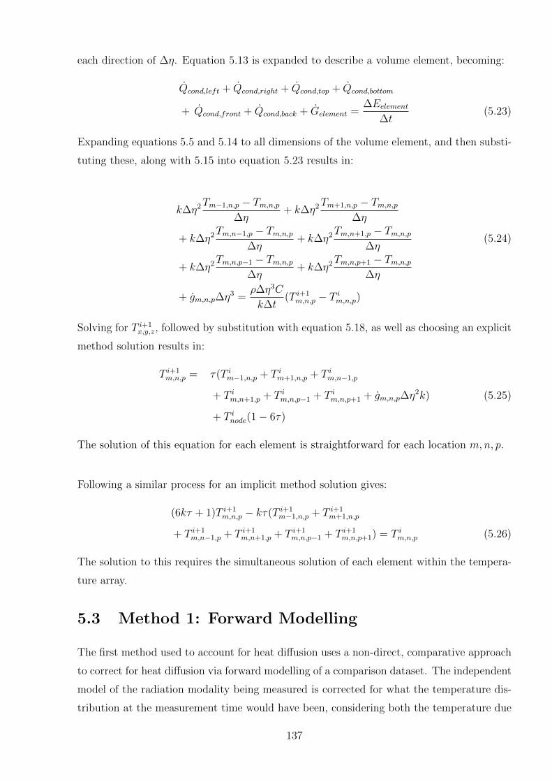
each direction of ∆η. Equation 5.13 is expanded to describe a volume element, becoming:
Qcond,left + Qcond,right + Qcond,top + Qcond,bottom
+ Qcond,front + Qcond,back + Gelement =∆Eelement
∆t(5.23)
Expanding equations 5.5 and 5.14 to all dimensions of the volume element, and then substi-
tuting these, along with 5.15 into equation 5.23 results in:
k∆η2Tm−1,n,p − Tm,n,p∆η
+ k∆η2Tm+1,n,p − Tm,n,p∆η
+ k∆η2Tm,n−1,p − Tm,n,p∆η
+ k∆η2Tm,n+1,p − Tm,n,p∆η
(5.24)
+ k∆η2Tm,n,p−1 − Tm,n,p∆η
+ k∆η2Tm,n,p+1 − Tm,n,p∆η
+ gm,n,p∆η3 =
ρ∆η3C
k∆t(T i+1
m,n,p − T im,n,p)
Solving for T i+1x,y,z, followed by substitution with equation 5.18, as well as choosing an explicit
method solution results in:
T i+1m,n,p = τ(T im−1,n,p + T im+1,n,p + T im,n−1,p
+ T im,n+1,p + T im,n,p−1 + T im,n,p+1 + gm,n,p∆η2k) (5.25)
+ T inode(1− 6τ)
The solution of this equation for each element is straightforward for each location m,n, p.
Following a similar process for an implicit method solution gives:
(6kτ + 1)T i+1m,n,p − kτ(T i+1
m−1,n,p + T i+1m+1,n,p
+ T i+1m,n−1,p + T i+1
m,n+1,p + T i+1m,n,p−1 + T i+1
m,n,p+1) = T im,n,p (5.26)
The solution to this requires the simultaneous solution of each element within the tempera-
ture array.
5.3 Method 1: Forward Modelling
The first method used to account for heat diffusion uses a non-direct, comparative approach
to correct for heat diffusion via forward modelling of a comparison dataset. The independent
model of the radiation modality being measured is corrected for what the temperature dis-
tribution at the measurement time would have been, considering both the temperature due
137
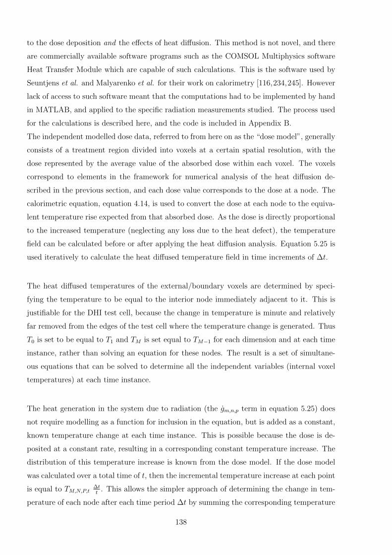
to the dose deposition and the effects of heat diffusion. This method is not novel, and there
are commercially available software programs such as the COMSOL Multiphysics software
Heat Transfer Module which are capable of such calculations. This is the software used by
Seuntjens et al. and Malyarenko et al. for their work on calorimetry [116,234,245]. However
lack of access to such software meant that the computations had to be implemented by hand
in MATLAB, and applied to the specific radiation measurements studied. The process used
for the calculations is described here, and the code is included in Appendix B.
The independent modelled dose data, referred to from here on as the “dose model”, generally
consists of a treatment region divided into voxels at a certain spatial resolution, with the
dose represented by the average value of the absorbed dose within each voxel. The voxels
correspond to elements in the framework for numerical analysis of the heat diffusion de-
scribed in the previous section, and each dose value corresponds to the dose at a node. The
calorimetric equation, equation 4.14, is used to convert the dose at each node to the equiva-
lent temperature rise expected from that absorbed dose. As the dose is directly proportional
to the increased temperature (neglecting any loss due to the heat defect), the temperature
field can be calculated before or after applying the heat diffusion analysis. Equation 5.25 is
used iteratively to calculate the heat diffused temperature field in time increments of ∆t.
The heat diffused temperatures of the external/boundary voxels are determined by speci-
fying the temperature to be equal to the interior node immediately adjacent to it. This is
justifiable for the DHI test cell, because the change in temperature is minute and relatively
far removed from the edges of the test cell where the temperature change is generated. Thus
T0 is set to be equal to T1 and TM is set equal to TM−1 for each dimension and at each time
instance, rather than solving an equation for these nodes. The result is a set of simultane-
ous equations that can be solved to determine all the independent variables (internal voxel
temperatures) at each time instance.
The heat generation in the system due to radiation (the gm,n,p term in equation 5.25) does
not require modelling as a function for inclusion in the equation, but is added as a constant,
known temperature change at each time instance. This is possible because the dose is de-
posited at a constant rate, resulting in a corresponding constant temperature increase. The
distribution of this temperature increase is known from the dose model. If the dose model
was calculated over a total time of t, then the incremental temperature increase at each point
is equal to TM,N,P,t∆tt
. This allows the simpler approach of determining the change in tem-
perature of each node after each time period ∆t by summing the corresponding temperature
138
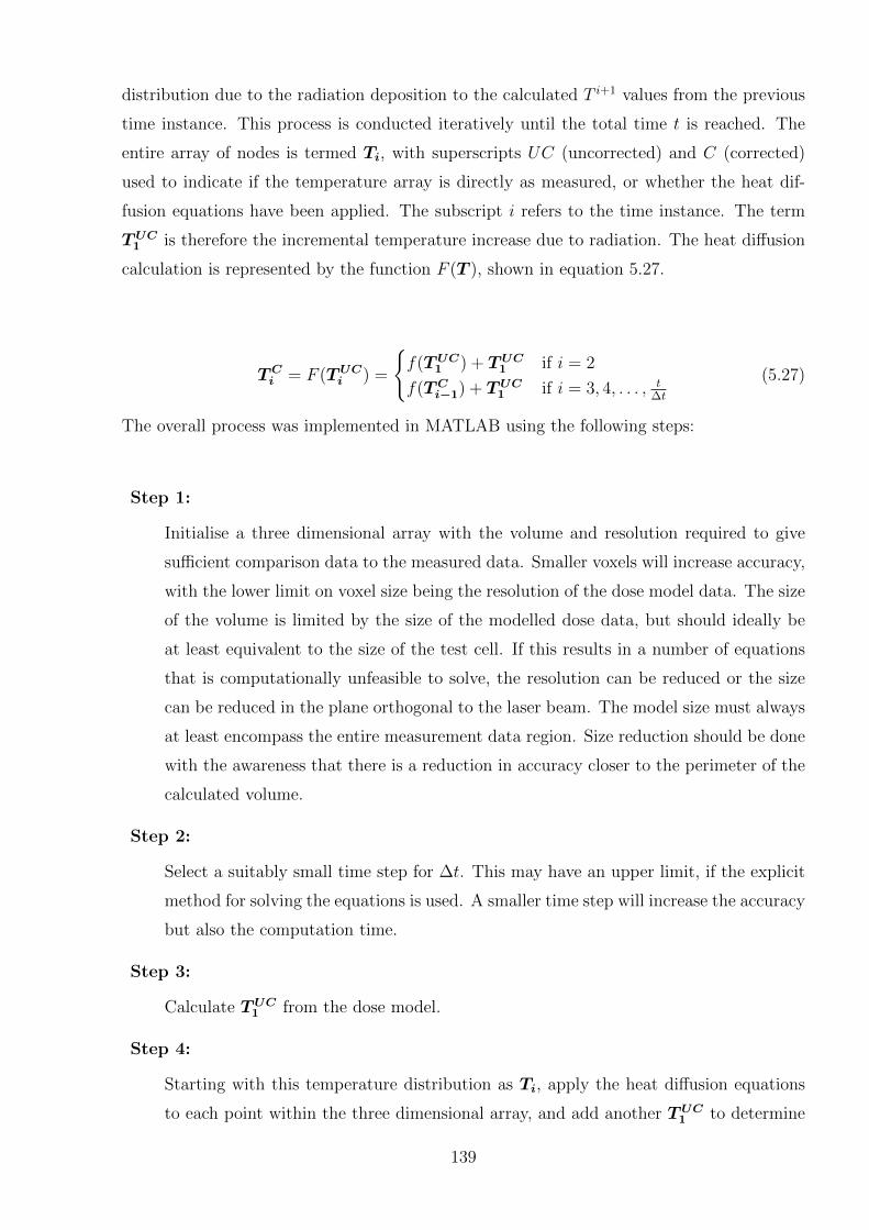
distribution due to the radiation deposition to the calculated T i+1 values from the previous
time instance. This process is conducted iteratively until the total time t is reached. The
entire array of nodes is termed Ti, with superscripts UC (uncorrected) and C (corrected)
used to indicate if the temperature array is directly as measured, or whether the heat dif-
fusion equations have been applied. The subscript i refers to the time instance. The term
TUC1 is therefore the incremental temperature increase due to radiation. The heat diffusion
calculation is represented by the function F (T ), shown in equation 5.27.
TCi = F (TUC
i ) =
{f(TUC
1 ) + TUC1 if i = 2
f(TCi−1) + TUC
1 if i = 3, 4, . . . , t∆t
(5.27)
The overall process was implemented in MATLAB using the following steps:
Step 1:
Initialise a three dimensional array with the volume and resolution required to give
sufficient comparison data to the measured data. Smaller voxels will increase accuracy,
with the lower limit on voxel size being the resolution of the dose model data. The size
of the volume is limited by the size of the modelled dose data, but should ideally be
at least equivalent to the size of the test cell. If this results in a number of equations
that is computationally unfeasible to solve, the resolution can be reduced or the size
can be reduced in the plane orthogonal to the laser beam. The model size must always
at least encompass the entire measurement data region. Size reduction should be done
with the awareness that there is a reduction in accuracy closer to the perimeter of the
calculated volume.
Step 2:
Select a suitably small time step for ∆t. This may have an upper limit, if the explicit
method for solving the equations is used. A smaller time step will increase the accuracy
but also the computation time.
Step 3:
Calculate TUC1 from the dose model.
Step 4:
Starting with this temperature distribution as Ti, apply the heat diffusion equations
to each point within the three dimensional array, and add another TUC1 to determine
139
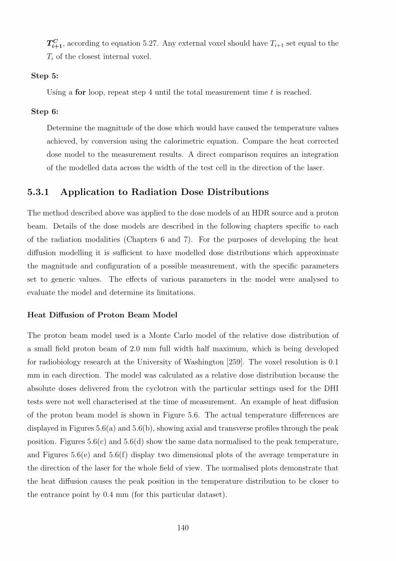
TCi+1, according to equation 5.27. Any external voxel should have Ti+1 set equal to the
Ti of the closest internal voxel.
Step 5:
Using a for loop, repeat step 4 until the total measurement time t is reached.
Step 6:
Determine the magnitude of the dose which would have caused the temperature values
achieved, by conversion using the calorimetric equation. Compare the heat corrected
dose model to the measurement results. A direct comparison requires an integration
of the modelled data across the width of the test cell in the direction of the laser.
5.3.1 Application to Radiation Dose Distributions
The method described above was applied to the dose models of an HDR source and a proton
beam. Details of the dose models are described in the following chapters specific to each
of the radiation modalities (Chapters 6 and 7). For the purposes of developing the heat
diffusion modelling it is sufficient to have modelled dose distributions which approximate
the magnitude and configuration of a possible measurement, with the specific parameters
set to generic values. The effects of various parameters in the model were analysed to
evaluate the model and determine its limitations.
Heat Diffusion of Proton Beam Model
The proton beam model used is a Monte Carlo model of the relative dose distribution of
a small field proton beam of 2.0 mm full width half maximum, which is being developed
for radiobiology research at the University of Washington [259]. The voxel resolution is 0.1
mm in each direction. The model was calculated as a relative dose distribution because the
absolute doses delivered from the cyclotron with the particular settings used for the DHI
tests were not well characterised at the time of measurement. An example of heat diffusion
of the proton beam model is shown in Figure 5.6. The actual temperature differences are
displayed in Figures 5.6(a) and 5.6(b), showing axial and transverse profiles through the peak
position. Figures 5.6(c) and 5.6(d) show the same data normalised to the peak temperature,
and Figures 5.6(e) and 5.6(f) display two dimensional plots of the average temperature in
the direction of the laser for the whole field of view. The normalised plots demonstrate that
the heat diffusion causes the peak position in the temperature distribution to be closer to
the entrance point by 0.4 mm (for this particular dataset).
140
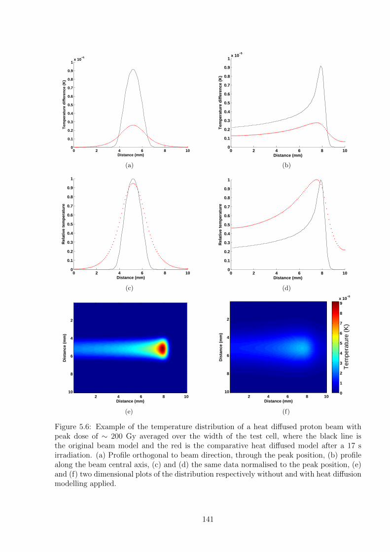
0 2 4 6 8 100
0.1
0.2
0.3
0.4
0.5
0.6
0.7
0.8
0.9
1x 10
−5
Distance (mm)
Tem
pera
ture
diff
eren
ce (
K)
(a)
0 2 4 6 8 100
0.1
0.2
0.3
0.4
0.5
0.6
0.7
0.8
0.9
1x 10
−5
Distance (mm)
Tem
pera
ture
diff
eren
ce (
K)
(b)
0 2 4 6 8 100
0.1
0.2
0.3
0.4
0.5
0.6
0.7
0.8
0.9
1
Distance (mm)
Rel
ativ
e te
mp
erat
ure
(c)
0 2 4 6 8 100
0.1
0.2
0.3
0.4
0.5
0.6
0.7
0.8
0.9
1
Distance (mm)
Rel
ativ
e te
mp
erat
ure
(d)
Distance (mm)
Dis
tan
ce (
mm
)
2 4 6 8 10
2
4
6
8
10
(e)
Distance (mm)
Dis
tanc
e (m
m)
2 4 6 8 10
2
4
6
8
10
Tem
pera
ture
(K
)
0
1
2
3
4
5
6
7
8
9x 10
−6
(f)
Figure 5.6: Example of the temperature distribution of a heat diffused proton beam withpeak dose of ∼ 200 Gy averaged over the width of the test cell, where the black line isthe original beam model and the red is the comparative heat diffused model after a 17 sirradiation. (a) Profile orthogonal to beam direction, through the peak position, (b) profilealong the beam central axis, (c) and (d) the same data normalised to the peak position, (e)and (f) two dimensional plots of the distribution respectively without and with heat diffusionmodelling applied.
141
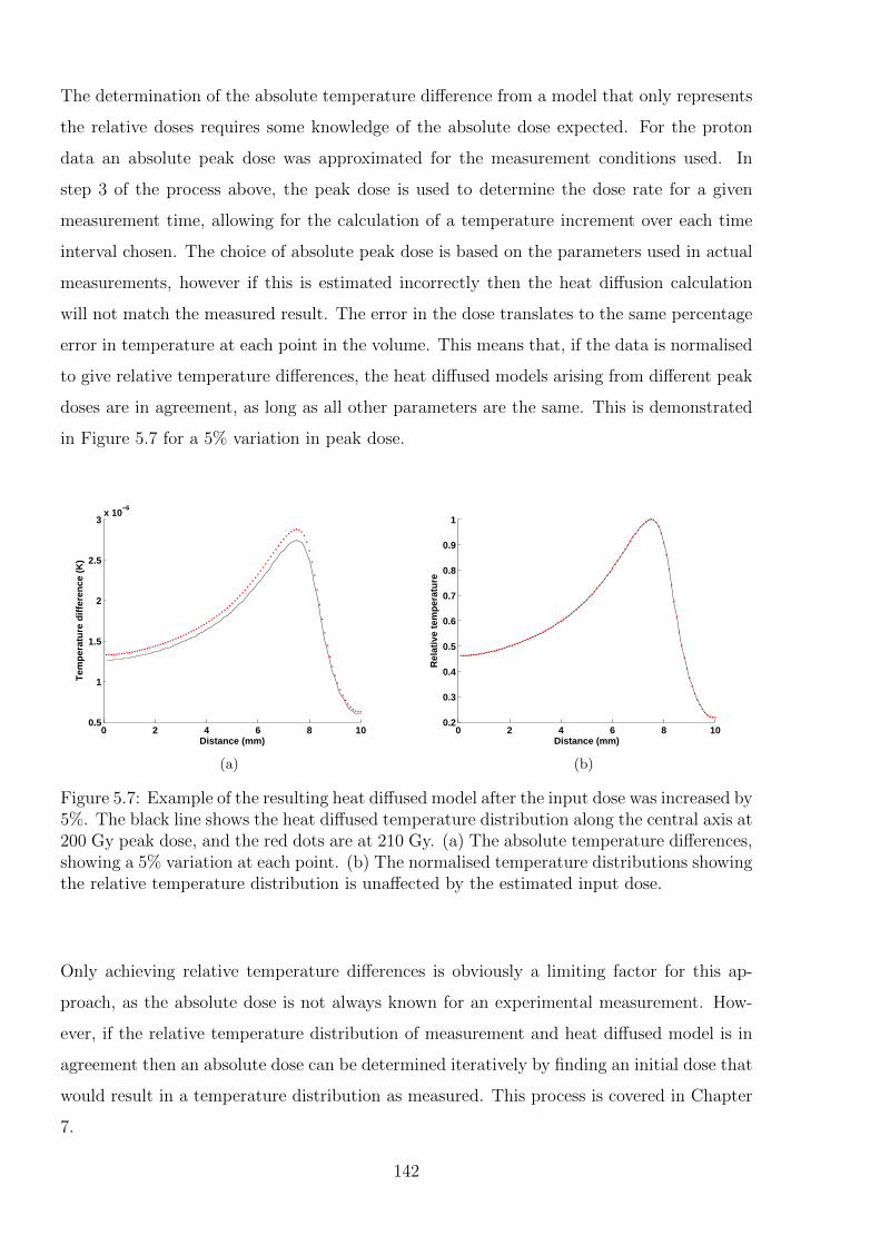
The determination of the absolute temperature difference from a model that only represents
the relative doses requires some knowledge of the absolute dose expected. For the proton
data an absolute peak dose was approximated for the measurement conditions used. In
step 3 of the process above, the peak dose is used to determine the dose rate for a given
measurement time, allowing for the calculation of a temperature increment over each time
interval chosen. The choice of absolute peak dose is based on the parameters used in actual
measurements, however if this is estimated incorrectly then the heat diffusion calculation
will not match the measured result. The error in the dose translates to the same percentage
error in temperature at each point in the volume. This means that, if the data is normalised
to give relative temperature differences, the heat diffused models arising from different peak
doses are in agreement, as long as all other parameters are the same. This is demonstrated
in Figure 5.7 for a 5% variation in peak dose.
0 2 4 6 8 100.5
1
1.5
2
2.5
3x 10
−6
Distance (mm)
Tem
pera
ture
diff
eren
ce (
K)
(a)
0 2 4 6 8 100.2
0.3
0.4
0.5
0.6
0.7
0.8
0.9
1
Distance (mm)
Rel
ativ
e te
mp
erat
ure
(b)
Figure 5.7: Example of the resulting heat diffused model after the input dose was increased by5%. The black line shows the heat diffused temperature distribution along the central axis at200 Gy peak dose, and the red dots are at 210 Gy. (a) The absolute temperature differences,showing a 5% variation at each point. (b) The normalised temperature distributions showingthe relative temperature distribution is unaffected by the estimated input dose.
Only achieving relative temperature differences is obviously a limiting factor for this ap-
proach, as the absolute dose is not always known for an experimental measurement. How-
ever, if the relative temperature distribution of measurement and heat diffused model is in
agreement then an absolute dose can be determined iteratively by finding an initial dose that
would result in a temperature distribution as measured. This process is covered in Chapter
7.
142
Heat Diffusion of HDR Source Model
The HDR brachytherapy source model used was the treatment planning system BrachyVisionTM
(Varian Medical Systems, Palo Alto, California, USA), with voxel resolution of 0.5 mm in
each direction. More details of the model are given in Chapter 6. The dose distributions pre-
dicted by the model were converted to temperatures using the calorimetric equation (4.14),
then the heat diffusion model was applied. For the initial proof of principle the influence of
the non-water materials in the applicator were not considered. For short irradiation times
this is not anticipated to have a large effect on the result, but should be considered in future
work. An example of heat diffusion of the model is shown in Figure 5.8(d) for a 20 second
irradiation by a source with activity 4.6 Ci. Unlike the proton beam, the absolute dose for a
given irradiation time is known to sufficient accuracy for the HDR source, so the dose/tem-
perature differences can be reported directly, rather than as values relative to some reference
point. As expected, the heat diffusion results in a greatly reduced peak dose, with increased
doses further from the peak. The radial distance away from the source at which the heat
diffused dose shifts from lower than the non-heat diffused dose to higher, depends on the
source activity and the irradiation time. In the example given in Figure 5.8(d) this occurs
at 2.3 mm from the centre of the source, or 0.7 mm outside of the applicator. It should be
noted that with a voxel resolution of 0.5 mm there is some considerable smoothing of the
dose from the real shape especially around the peak, which introduces some uncertainties to
this crossover point.
Sensitivity Analysis of Heat Diffusion Parameters
There are various parameters involved in the calculation of heat diffusion by the above
method, and potential areas where an incorrect selection of parameter value may cause un-
necessary uncertainty to be introduced to the result. These areas were investigated and are
presented here. The proton beam model is used to demonstrate these effects as the model is
known to higher resolution, thus small effects are more apparent and can be more accurately
quantified.
Time Step
The key parameter when calculating heat diffusion in this fashion is the size of the time step,
δt which is selected. The upper limit on the size of the time step when using an explicit
calculation method is given in equation 5.21. For the proton beam model data, with voxel
dimensions of 0.1 mm in each direction the maximum time step is 0.0114 s, as calculated in
equation 5.22. If a value larger than this is chosen, the result oscillates wildly, diverging from
143
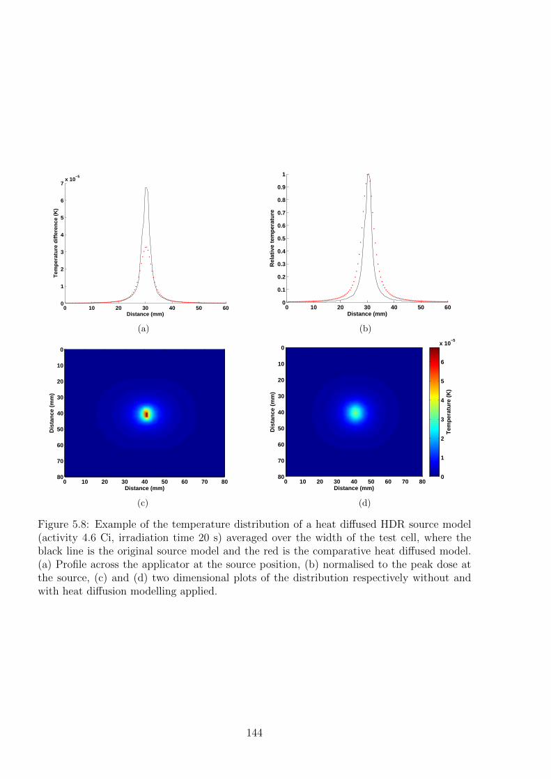
0 10 20 30 40 50 600
1
2
3
4
5
6
7x 10
−5
Distance (mm)
Tem
pera
ture
diff
eren
ce (
K)
(a)
0 10 20 30 40 50 600
0.1
0.2
0.3
0.4
0.5
0.6
0.7
0.8
0.9
1
Distance (mm)
Rel
ativ
e te
mp
erat
ure
(b)
Distance (mm)
Dis
tan
ce (
mm
)
0 10 20 30 40 50 60 70 80
0
10
20
30
40
50
60
70
80
(c)
Distance (mm)
Dis
tanc
e (m
m)
0 10 20 30 40 50 60 70 80
0
10
20
30
40
50
60
70
80
Tem
pera
ture
(K
)
0
1
2
3
4
5
6
x 10−5
(d)
Figure 5.8: Example of the temperature distribution of a heat diffused HDR source model(activity 4.6 Ci, irradiation time 20 s) averaged over the width of the test cell, where theblack line is the original source model and the red is the comparative heat diffused model.(a) Profile across the applicator at the source position, (b) normalised to the peak dose atthe source, (c) and (d) two dimensional plots of the distribution respectively without andwith heat diffusion modelling applied.
144
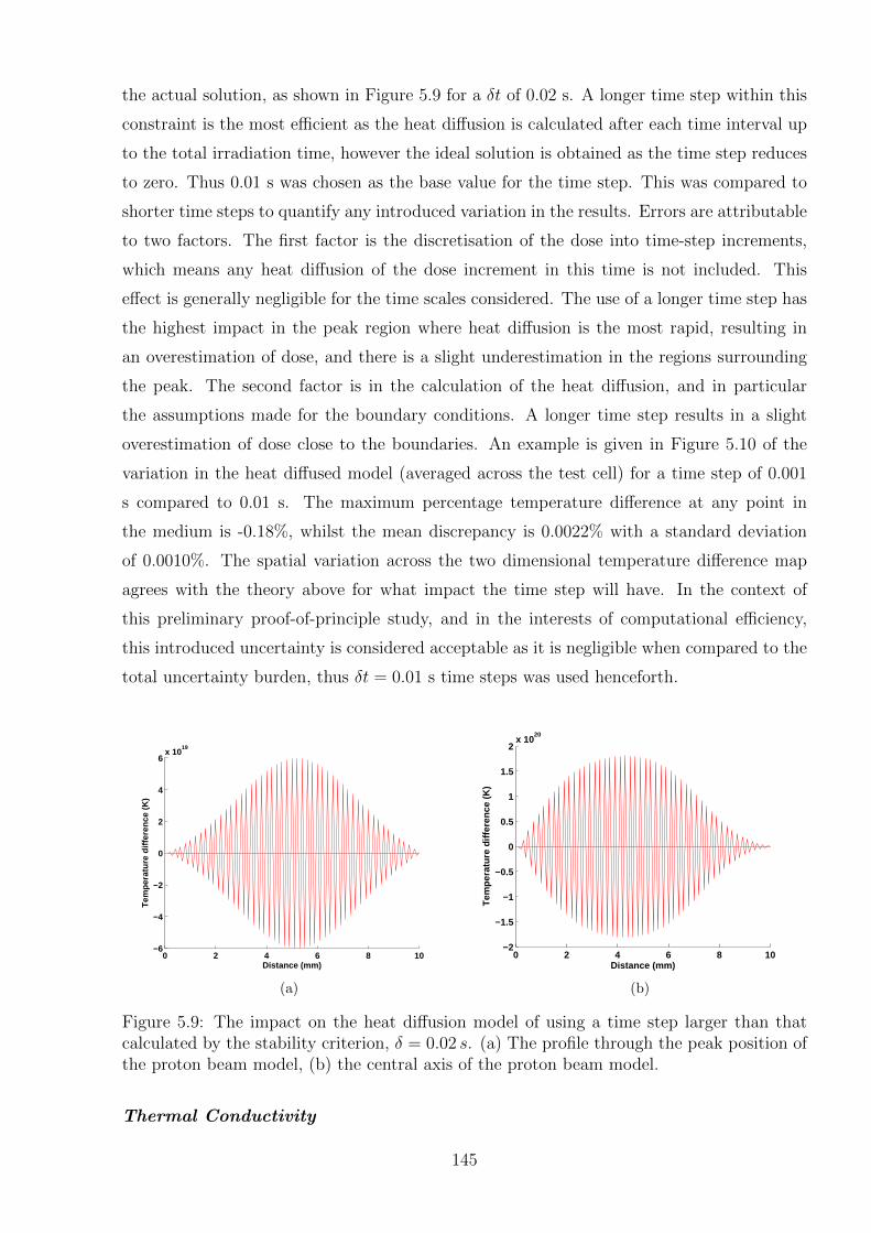
the actual solution, as shown in Figure 5.9 for a δt of 0.02 s. A longer time step within this
constraint is the most efficient as the heat diffusion is calculated after each time interval up
to the total irradiation time, however the ideal solution is obtained as the time step reduces
to zero. Thus 0.01 s was chosen as the base value for the time step. This was compared to
shorter time steps to quantify any introduced variation in the results. Errors are attributable
to two factors. The first factor is the discretisation of the dose into time-step increments,
which means any heat diffusion of the dose increment in this time is not included. This
effect is generally negligible for the time scales considered. The use of a longer time step has
the highest impact in the peak region where heat diffusion is the most rapid, resulting in
an overestimation of dose, and there is a slight underestimation in the regions surrounding
the peak. The second factor is in the calculation of the heat diffusion, and in particular
the assumptions made for the boundary conditions. A longer time step results in a slight
overestimation of dose close to the boundaries. An example is given in Figure 5.10 of the
variation in the heat diffused model (averaged across the test cell) for a time step of 0.001
s compared to 0.01 s. The maximum percentage temperature difference at any point in
the medium is -0.18%, whilst the mean discrepancy is 0.0022% with a standard deviation
of 0.0010%. The spatial variation across the two dimensional temperature difference map
agrees with the theory above for what impact the time step will have. In the context of
this preliminary proof-of-principle study, and in the interests of computational efficiency,
this introduced uncertainty is considered acceptable as it is negligible when compared to the
total uncertainty burden, thus δt = 0.01 s time steps was used henceforth.
0 2 4 6 8 10−6
−4
−2
0
2
4
6x 10
19
Distance (mm)
Tem
pera
ture
diff
eren
ce (
K)
(a)
0 2 4 6 8 10−2
−1.5
−1
−0.5
0
0.5
1
1.5
2x 10
20
Distance (mm)
Tem
pera
ture
diff
eren
ce (
K)
(b)
Figure 5.9: The impact on the heat diffusion model of using a time step larger than thatcalculated by the stability criterion, δ = 0.02 s. (a) The profile through the peak position ofthe proton beam model, (b) the central axis of the proton beam model.
Thermal Conductivity
145
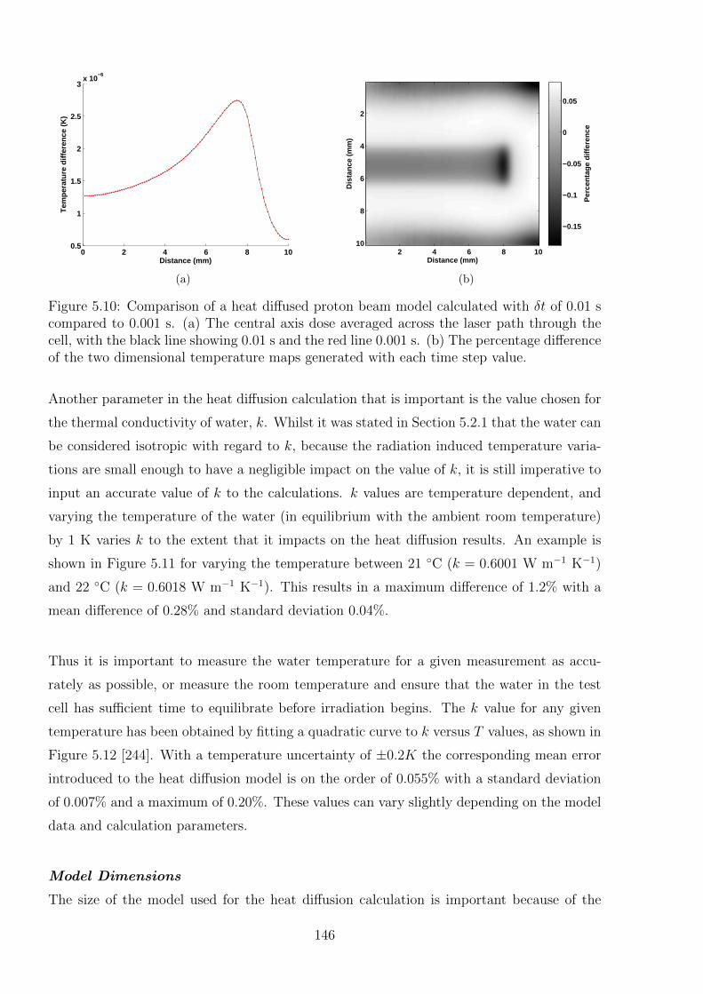
0 2 4 6 8 100.5
1
1.5
2
2.5
3x 10
−6
Distance (mm)
Tem
pera
ture
diff
eren
ce (
K)
(a)
Distance (mm)
Dis
tanc
e (m
m)
2 4 6 8 10
2
4
6
8
10
Per
cent
age
diffe
renc
e
−0.15
−0.1
−0.05
0
0.05
(b)
Figure 5.10: Comparison of a heat diffused proton beam model calculated with δt of 0.01 scompared to 0.001 s. (a) The central axis dose averaged across the laser path through thecell, with the black line showing 0.01 s and the red line 0.001 s. (b) The percentage differenceof the two dimensional temperature maps generated with each time step value.
Another parameter in the heat diffusion calculation that is important is the value chosen for
the thermal conductivity of water, k. Whilst it was stated in Section 5.2.1 that the water can
be considered isotropic with regard to k, because the radiation induced temperature varia-
tions are small enough to have a negligible impact on the value of k, it is still imperative to
input an accurate value of k to the calculations. k values are temperature dependent, and
varying the temperature of the water (in equilibrium with the ambient room temperature)
by 1 K varies k to the extent that it impacts on the heat diffusion results. An example is
shown in Figure 5.11 for varying the temperature between 21 ◦C (k = 0.6001 W m−1 K−1)
and 22 ◦C (k = 0.6018 W m−1 K−1). This results in a maximum difference of 1.2% with a
mean difference of 0.28% and standard deviation 0.04%.
Thus it is important to measure the water temperature for a given measurement as accu-
rately as possible, or measure the room temperature and ensure that the water in the test
cell has sufficient time to equilibrate before irradiation begins. The k value for any given
temperature has been obtained by fitting a quadratic curve to k versus T values, as shown in
Figure 5.12 [244]. With a temperature uncertainty of ±0.2K the corresponding mean error
introduced to the heat diffusion model is on the order of 0.055% with a standard deviation
of 0.007% and a maximum of 0.20%. These values can vary slightly depending on the model
data and calculation parameters.
Model Dimensions
The size of the model used for the heat diffusion calculation is important because of the
146
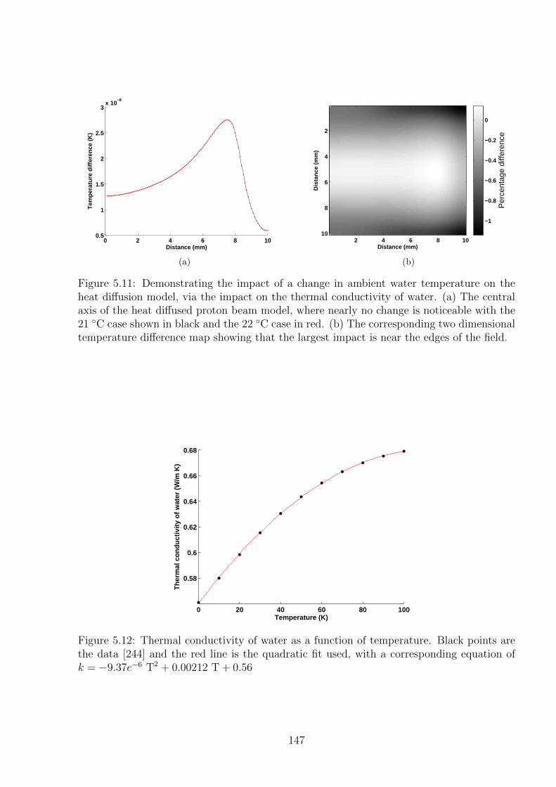
0 2 4 6 8 100.5
1
1.5
2
2.5
3x 10
−6
Distance (mm)
Tem
pera
ture
diff
eren
ce (
K)
(a)
Distance (mm)
Dis
tanc
e (m
m)
2 4 6 8 10
2
4
6
8
10
Per
cent
age
diffe
renc
e
−1
−0.8
−0.6
−0.4
−0.2
0
(b)
Figure 5.11: Demonstrating the impact of a change in ambient water temperature on theheat diffusion model, via the impact on the thermal conductivity of water. (a) The centralaxis of the heat diffused proton beam model, where nearly no change is noticeable with the21 ◦C case shown in black and the 22 ◦C case in red. (b) The corresponding two dimensionaltemperature difference map showing that the largest impact is near the edges of the field.
0 20 40 60 80 100
0.58
0.6
0.62
0.64
0.66
0.68
Temperature (K)
Th
erm
al c
on
du
ctiv
ity
of
wat
er (
W/m
K)
Figure 5.12: Thermal conductivity of water as a function of temperature. Black points arethe data [244] and the red line is the quadratic fit used, with a corresponding equation ofk = −9.37e−6 T2 + 0.00212 T + 0.56
147
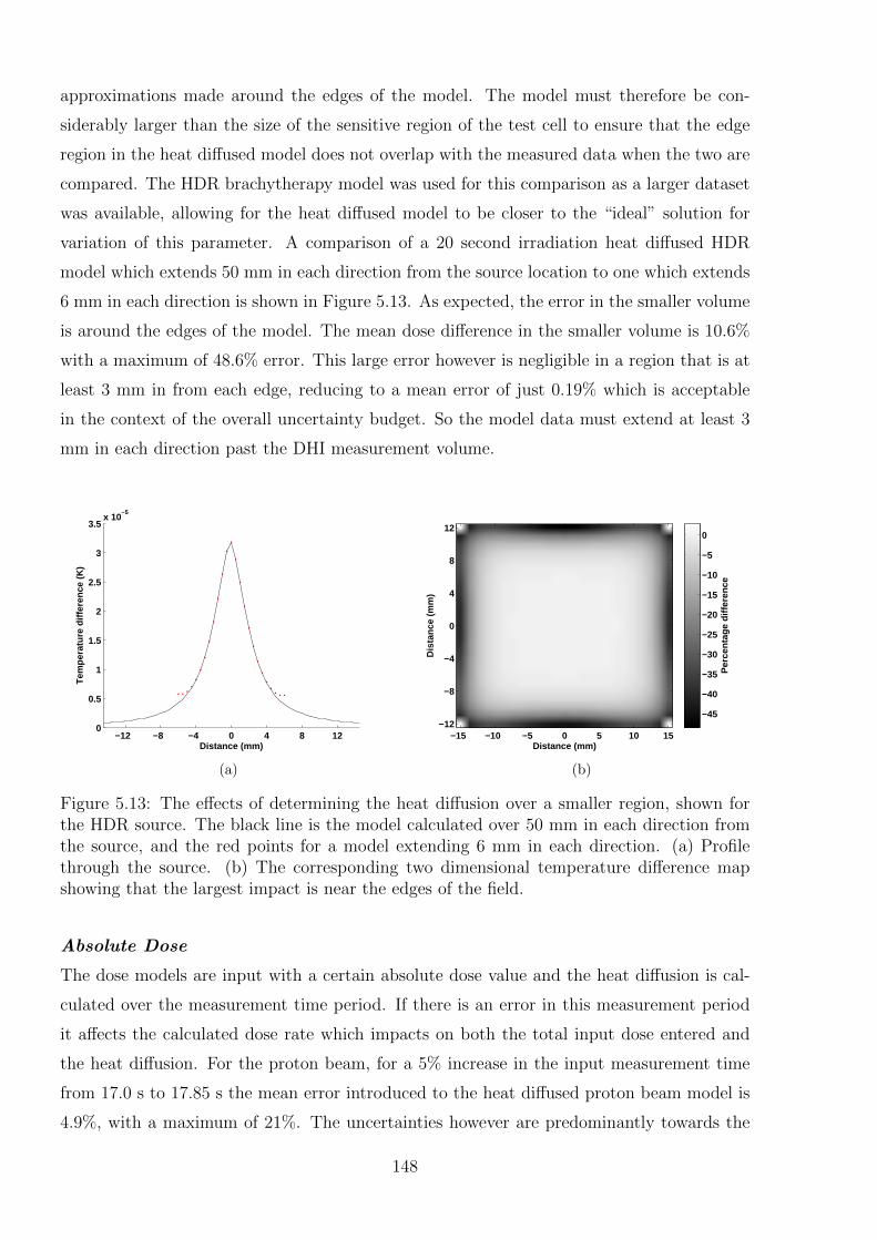
approximations made around the edges of the model. The model must therefore be con-
siderably larger than the size of the sensitive region of the test cell to ensure that the edge
region in the heat diffused model does not overlap with the measured data when the two are
compared. The HDR brachytherapy model was used for this comparison as a larger dataset
was available, allowing for the heat diffused model to be closer to the “ideal” solution for
variation of this parameter. A comparison of a 20 second irradiation heat diffused HDR
model which extends 50 mm in each direction from the source location to one which extends
6 mm in each direction is shown in Figure 5.13. As expected, the error in the smaller volume
is around the edges of the model. The mean dose difference in the smaller volume is 10.6%
with a maximum of 48.6% error. This large error however is negligible in a region that is at
least 3 mm in from each edge, reducing to a mean error of just 0.19% which is acceptable
in the context of the overall uncertainty budget. So the model data must extend at least 3
mm in each direction past the DHI measurement volume.
−12 −8 −4 0 4 8 120
0.5
1
1.5
2
2.5
3
3.5x 10
−5
Distance (mm)
Tem
pera
ture
diff
eren
ce (
K)
(a)
Distance (mm)
Dis
tanc
e (m
m)
−15 −10 −5 0 5 10 15
12
8
4
0
−4
−8
−12P
erce
ntag
e di
ffere
nce
−45
−40
−35
−30
−25
−20
−15
−10
−5
0
(b)
Figure 5.13: The effects of determining the heat diffusion over a smaller region, shown forthe HDR source. The black line is the model calculated over 50 mm in each direction fromthe source, and the red points for a model extending 6 mm in each direction. (a) Profilethrough the source. (b) The corresponding two dimensional temperature difference mapshowing that the largest impact is near the edges of the field.
Absolute Dose
The dose models are input with a certain absolute dose value and the heat diffusion is cal-
culated over the measurement time period. If there is an error in this measurement period
it affects the calculated dose rate which impacts on both the total input dose entered and
the heat diffusion. For the proton beam, for a 5% increase in the input measurement time
from 17.0 s to 17.85 s the mean error introduced to the heat diffused proton beam model is
4.9%, with a maximum of 21%. The uncertainties however are predominantly towards the
148
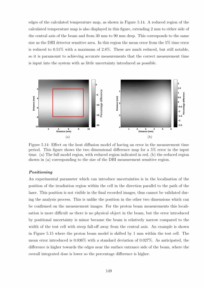
edges of the calculated temperature map, as shown in Figure 5.14. A reduced region of the
calculated temperature map is also displayed in this figure, extending 2 mm to either side of
the central axis of the beam and from 30 mm to 90 mm deep. This corresponds to the same
size as the DHI detector sensitive area. In this region the mean error from the 5% time error
is reduced to 0.51% with a maximum of 2.8%. These are much reduced, but still notable,
so it is paramount to achieving accurate measurements that the correct measurement time
is input into the system with as little uncertainty introduced as possible.
Distance (mm)
Dis
tanc
e (m
m)
2 4 6 8 10
2
4
6
8
10
Per
cent
age
diffe
renc
e
−20
−15
−10
−5
0
(a)
Distance (mm)
Dis
tanc
e (m
m)
1 2 3 4 5 6
1
2
3
4
Per
cent
age
diffe
renc
e
−2.5
−2
−1.5
−1
−0.5
0
0.5
1
1.5
2
(b)
Figure 5.14: Effect on the heat diffusion model of having an error in the measurement timeperiod. This figure shows the two dimensional difference map for a 5% error in the inputtime. (a) The full model region, with reduced region indicated in red, (b) the reduced regionshown in (a) corresponding to the size of the DHI measurement sensitive region.
Positioning
An experimental parameter which can introduce uncertainties is in the localisation of the
position of the irradiation region within the cell in the direction parallel to the path of the
laser. This position is not visible in the final recorded images, thus cannot be validated dur-
ing the analysis process. This is unlike the position in the other two dimensions which can
be confirmed on the measurement images. For the proton beam measurements this locali-
sation is more difficult as there is no physical object in the beam, but the error introduced
by positional uncertainty is minor because the beam is relatively narrow compared to the
width of the test cell with steep fall-off away from the central axis. An example is shown
in Figure 5.15 where the proton beam model is shifted by 1 mm within the test cell. The
mean error introduced is 0.036% with a standard deviation of 0.027%. As anticipated, the
difference is higher towards the edges near the surface entrance side of the beam, where the
overall integrated dose is lower so the percentage difference is higher.
149
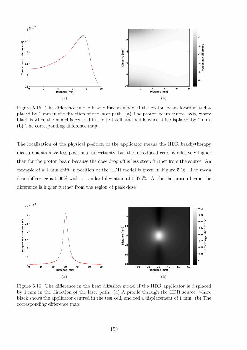
0 2 4 6 8 100.5
1
1.5
2
2.5
3x 10
−6
Distance (mm)
Tem
pera
ture
diff
eren
ce (
K)
(a)
Distance (mm)
Dis
tanc
e (m
m)
2 4 6 8 10
2
4
6
8
10
Per
cent
age
diffe
renc
e
−6
−5
−4
−3
−2
−1
(b)
Figure 5.15: The difference in the heat diffusion model if the proton beam location is dis-placed by 1 mm in the direction of the laser path. (a) The proton beam central axis, whereblack is when the model is centred in the test cell, and red is when it is displaced by 1 mm.(b) The corresponding difference map.
The localisation of the physical position of the applicator means the HDR brachytherapy
measurements have less positional uncertainty, but the introduced error is relatively higher
than for the proton beam because the dose drop off is less steep further from the source. An
example of a 1 mm shift in position of the HDR model is given in Figure 5.16. The mean
dose difference is 0.90% with a standard deviation of 0.075%. As for the proton beam, the
difference is higher further from the region of peak dose.
0 10 20 30 40 50 600
0.5
1
1.5
2
2.5
3
3.5x 10
−5
Distance (mm)
Tem
pera
ture
diff
eren
ce (
K)
(a)
Distance (mm)
Dis
tanc
e (m
m)
10 20 30 40 50 60
10
20
30
40
50
60
Per
cent
age
diffe
renc
e
−1
−0.9
−0.8
−0.7
−0.6
−0.5
−0.4
−0.3
−0.2
(b)
Figure 5.16: The difference in the heat diffusion model if the HDR applicator is displacedby 1 mm in the direction of the laser path. (a) A profile through the HDR source, whereblack shows the applicator centred in the test cell, and red a displacement of 1 mm. (b) Thecorresponding difference map.
150
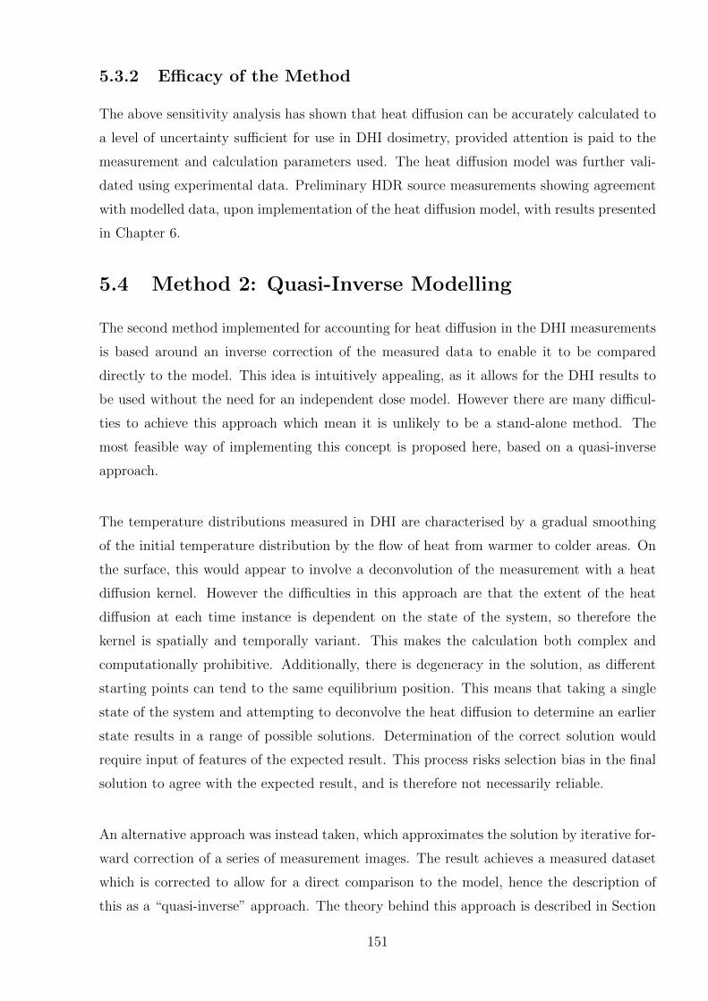
5.3.2 Efficacy of the Method
The above sensitivity analysis has shown that heat diffusion can be accurately calculated to
a level of uncertainty sufficient for use in DHI dosimetry, provided attention is paid to the
measurement and calculation parameters used. The heat diffusion model was further vali-
dated using experimental data. Preliminary HDR source measurements showing agreement
with modelled data, upon implementation of the heat diffusion model, with results presented
in Chapter 6.
5.4 Method 2: Quasi-Inverse Modelling
The second method implemented for accounting for heat diffusion in the DHI measurements
is based around an inverse correction of the measured data to enable it to be compared
directly to the model. This idea is intuitively appealing, as it allows for the DHI results to
be used without the need for an independent dose model. However there are many difficul-
ties to achieve this approach which mean it is unlikely to be a stand-alone method. The
most feasible way of implementing this concept is proposed here, based on a quasi-inverse
approach.
The temperature distributions measured in DHI are characterised by a gradual smoothing
of the initial temperature distribution by the flow of heat from warmer to colder areas. On
the surface, this would appear to involve a deconvolution of the measurement with a heat
diffusion kernel. However the difficulties in this approach are that the extent of the heat
diffusion at each time instance is dependent on the state of the system, so therefore the
kernel is spatially and temporally variant. This makes the calculation both complex and
computationally prohibitive. Additionally, there is degeneracy in the solution, as different
starting points can tend to the same equilibrium position. This means that taking a single
state of the system and attempting to deconvolve the heat diffusion to determine an earlier
state results in a range of possible solutions. Determination of the correct solution would
require input of features of the expected result. This process risks selection bias in the final
solution to agree with the expected result, and is therefore not necessarily reliable.
An alternative approach was instead taken, which approximates the solution by iterative for-
ward correction of a series of measurement images. The result achieves a measured dataset
which is corrected to allow for a direct comparison to the model, hence the description of
this as a “quasi-inverse” approach. The theory behind this approach is described in Section
151
5.4.1. The key mathematical algorithms required to implement it are introduced in Sec-
tion 5.4.2. In order to analyse the efficacy of this approach the method was implemented on
simulated data, and various limitations were determined, which are discussed in Section 5.4.3.
5.4.1 Description of Approach
The basic theory underlying Method 2 is to determine the rate of incremental dose deposi-
tion throughout the irradiation time. Accumulation of the incremental doses results in the
total dose and its distribution. This method is based on the theory that for any given time
instance tn the temperature map is a result of the heat diffusion of the temperature map at
some previous time instance tn−1 plus the dose deposited in the intervening time interval.
The aim is to separate these two components so that the absorbed dose can be isolated to
be quantified independently of the heat diffusion. By taking the image at tn−1 and forward
calculating the expected effects of heat diffusion, it is then possible to subtract this value
from the image at time tn, and obtain the incremental increase in temperature T1 for each
time period tn − tn−1.
The data consists of a series of reconstructed images which represent the temperature distri-
bution at each point in time. The shortest possible time interval tn− tn−1 should be used, in
order to reduce variation in the diffused temperature map due to dose deposited during the
intervening time. The minimum time interval achievable is dependent on the frequency of
image acquisition, f . This is a balance between the maximum frame rate achievable by the
sensor, and the need to achieve an acceptable signal to noise ratio, and should be carefully
selected. Adjacent images should then be analysed. Analysis using larger time intervals
can be achieved by examining two or more pictures that are multiple frames apart, in or-
der to estimate the extent of the errors induced by this discretisation approximation which
incompletely considers the conductive effects. Therefore the values of tn represent the time
instances of image n, where n = 1, 2, . . . t · f , where t is the total measurement time and
the actual time for each image is calculated by nf. The final temperature array is therefore
referred to as Tt.
The Method 2 function used for calculating heat diffusion is shown in equations 5.28 and
5.29. This method incorporates the heat diffusion function F from Method 1 equation 5.27.
Note that the subscripts C and UC for corrected and uncorrected temperature matrices refer
152
to correction of the measurement data rather than the model. So in contrast to Method 1,
TC refers to a temperature array which has been corrected for the effects of heat diffusion,
while TUC is the original measured temperature distribution.
T1 = TUCn − TC
n−1 = TUCn − F n
n−1(TUCi ) (5.28)
Tt =
t·f∑n=1
T1 (5.29)
To accurately calculate the effects of heat diffusion the three dimensional temperature distri-
bution must be known. However each image in the series of measured DHI images is the two
dimensional projection of the temperature distribution in the test cell. Thus in order to use
this approach, it is necessary to approximate a three dimensional temperature distribution
from each of the measured images in the series. This limits the approach to use in situations
where symmetry in the geometry of the radiation dose distribution allows for approximation
of three dimensions from a two dimensional map. Both of the approaches presented in this
work can be assumed to possess cylindrical symmetry about a central axis. Generally the
way that HDR sources are fabricated in terms of their core and encapsulation results in
effective cylindrical symmetry of the dose distribution to their longitudinal axis [37]. The
proton beam, after passing through a circular collimator, can be assumed to have cylindrical
symmetry about the central axis. Cylindrical symmetry allows for a mathematical formula-
tion called the Abel transform to be used to convert the projection map from two to three
dimensions [260].
5.4.2 Implementation of the Abel Transform
The Abel transform is an integral transform, which is often used for the analysis of spher-
ically or cylindrically symmetric functions [260]. The forward Abel transform is used to
project a symmetric three dimensional function onto a plane. The reverse Abel transform
is used to calculate the radial cross section from a projection across that area. This is the
process which is relevant to the current problem. In the case of cylindrical symmetry, the
function can be used in its two dimensional form, and applied to one line of the projection
image at a time, in order to build up an approximation of the full three dimensional function.
153
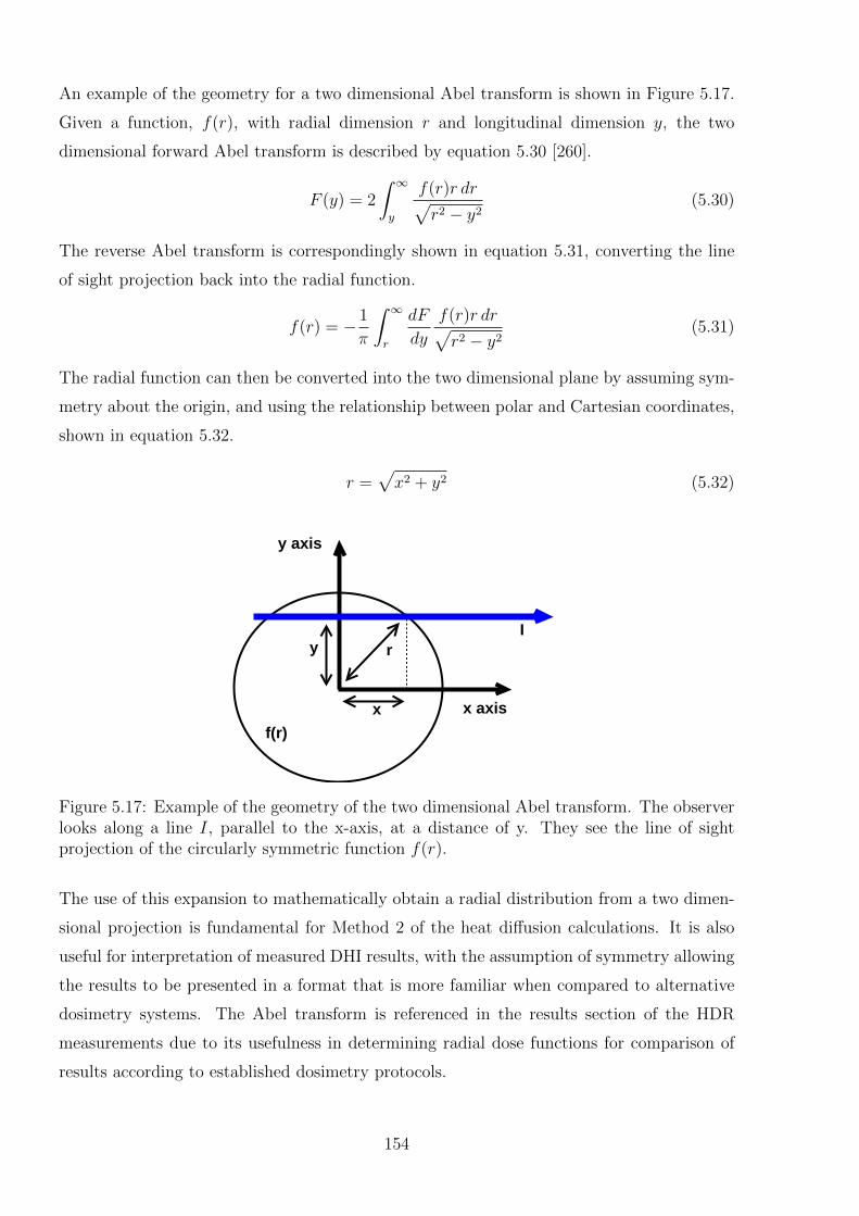
An example of the geometry for a two dimensional Abel transform is shown in Figure 5.17.
Given a function, f(r), with radial dimension r and longitudinal dimension y, the two
dimensional forward Abel transform is described by equation 5.30 [260].
F (y) = 2
∫ ∞y
f(r)r dr√r2 − y2
(5.30)
The reverse Abel transform is correspondingly shown in equation 5.31, converting the line
of sight projection back into the radial function.
f(r) = − 1
π
∫ ∞r
dF
dy
f(r)r dr√r2 − y2
(5.31)
The radial function can then be converted into the two dimensional plane by assuming sym-
metry about the origin, and using the relationship between polar and Cartesian coordinates,
shown in equation 5.32.
r =√x2 + y2 (5.32)
x axis
y axis
x
Iy r
f(r)
Figure 5.17: Example of the geometry of the two dimensional Abel transform. The observerlooks along a line I, parallel to the x-axis, at a distance of y. They see the line of sightprojection of the circularly symmetric function f(r).
The use of this expansion to mathematically obtain a radial distribution from a two dimen-
sional projection is fundamental for Method 2 of the heat diffusion calculations. It is also
useful for interpretation of measured DHI results, with the assumption of symmetry allowing
the results to be presented in a format that is more familiar when compared to alternative
dosimetry systems. The Abel transform is referenced in the results section of the HDR
measurements due to its usefulness in determining radial dose functions for comparison of
results according to established dosimetry protocols.
154
The numerical implementation of the inverse Abel transform is not straightforward, due to
the presence of the derivative of the projection function. Numerical differentiation tends to
amplify noise, which is of concern for the relatively noisy data achieved with the current
DHI detector. There are various methods of implementing this function to improve this.
A conventional approach is to convolve the derivative of a Gaussian with the function we
wish to differentiate and then perform an inverse transform to recover a smoothed numerical
derivative. A similar approach uses an iterative Fourier-Bessel expansion. MATLAB code
for both of these approaches was written and implemented on simulated test data. A third
approach, which was the selected approach for further work for DHI, was a Fourier-based
algorithm, as proposed by Pretzler [261,262]. This approach is based on fitting the measured
profile to a set of cosine-based expansion integrals. The Pretzler approach is less prone to
error in the determination of the object centre, and relatively insensitive to noise [262]. The
algorithm has already been implemented in MATLAB, with the code for the abel.m made
available through the MATLAB file sharing website www.mathworks.com [263]. These m-
files were checked against simulated data, and found to be operating correctly. The approach
was found to be more accurate than the other two at reproducing the original distribution
of simulated data.
The Pretzler approach incorporates a series expansion, with a lower frequency limit of 1,
and the upper frequency limit selected to control the level of noise filtering required. This
parameter defines the number of cosine expansions used. Lower values act as low pass filters,
reducing the noise, but also potential features of the image. Higher numbers also increase
the computation time. By analysis of the modelled proton beam data an upper frequency
of 20 was selected, however for noisy data this may need to be reduced.
5.4.3 Implementation of Method 2
The Method 2 approach for calculating the heat corrected temperature/dose distribution was
developed using simulated proton beam data. The Monte Carlo beam model was modelled
for heat diffusion as described in Method 1. The result was then converted into projections,
in the form that would be recorded by DHI measurements. This process has no noise intro-
duced, so it is an idealised dataset. It would be possible to add noise if further exploration
of the limits of accuracy in a controlled condition was to be explored. The calculation of
Method 2 equations 5.28 and 5.29 were applied in MATLAB, in an attempt to reproduce
the original MC model. The process is split into the following steps:
155
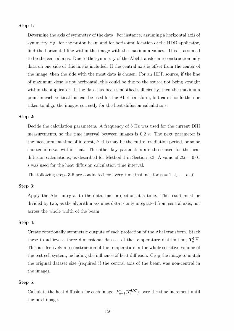
Step 1:
Determine the axis of symmetry of the data. For instance, assuming a horizontal axis of
symmetry, e.g. for the proton beam and for horizontal location of the HDR applicator,
find the horizontal line within the image with the maximum values. This is assumed
to be the central axis. Due to the symmetry of the Abel transform reconstruction only
data on one side of this line is included. If the central axis is offset from the center of
the image, then the side with the most data is chosen. For an HDR source, if the line
of maximum dose is not horizontal, this could be due to the source not being straight
within the applicator. If the data has been smoothed sufficiently, then the maximum
point in each vertical line can be used for the Abel transform, but care should then be
taken to align the images correctly for the heat diffusion calculations.
Step 2:
Decide the calculation parameters. A frequency of 5 Hz was used for the current DHI
measurements, so the time interval between images is 0.2 s. The next parameter is
the measurement time of interest, t: this may be the entire irradiation period, or some
shorter interval within that. The other key parameters are those used for the heat
diffusion calculations, as described for Method 1 in Section 5.3. A value of ∆t = 0.01
s was used for the heat diffusion calculation time interval.
The following steps 3-6 are conducted for every time instance for n = 1, 2, . . . , t · f .
Step 3:
Apply the Abel integral to the data, one projection at a time. The result must be
divided by two, as the algorithm assumes data is only integrated from central axis, not
across the whole width of the beam.
Step 4:
Create rotationally symmetric outputs of each projection of the Abel transform. Stack
these to achieve a three dimensional dataset of the temperature distribution, TUCn .
This is effectively a reconstruction of the temperature in the whole sensitive volume of
the test cell system, including the influence of heat diffusion. Crop the image to match
the original dataset size (required if the central axis of the beam was non-central in
the image).
Step 5:
Calculate the heat diffusion for each image, F nn−1(TUC
i ), over the time increment until
the next image.
156
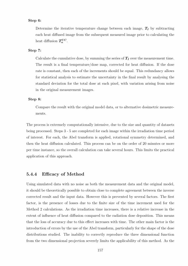
Step 6:
Determine the iterative temperature change between each image, TI by subtracting
each heat diffused image from the subsequent measured image prior to calculating the
heat diffusion TUCn .
Step 7:
Calculate the cumulative dose, by summing the series of TI over the measurement time.
The result is a final temperature/dose map, corrected for heat diffusion. If the dose
rate is constant, then each of the increments should be equal. This redundancy allows
for statistical analysis to estimate the uncertainty in the final result by analysing the
standard deviation for the total dose at each pixel, with variation arising from noise
in the original measurement images.
Step 8:
Compare the result with the original model data, or to alternative dosimetric measure-
ments.
The process is extremely computationally intensive, due to the size and quantity of datasets
being processed. Steps 3 - 5 are completed for each image within the irradiation time period
of interest. For each, the Abel transform is applied, rotational symmetry determined, and
then the heat diffusion calculated. This process can be on the order of 20 minutes or more
per time instance, so the overall calculation can take several hours. This limits the practical
application of this approach.
5.4.4 Efficacy of Method
Using simulated data with no noise as both the measurement data and the original model,
it should be theoretically possible to obtain close to complete agreement between the inverse
corrected result and the input data. However this is prevented by several factors. The first
factor, is the presence of losses due to the finite size of the time increment used for the
Method 2 calculations. As the irradiation time increases, there is a relative increase in the
extent of influence of heat diffusion compared to the radiation dose deposition. This means
that the loss of accuracy due to this effect increases with time. The other main factor is the
introduction of errors by the use of the Abel transform, particularly for the shape of the dose
distributions studied. The inability to correctly reproduce the three dimensional function
from the two dimensional projection severely limits the applicability of this method. As the
157
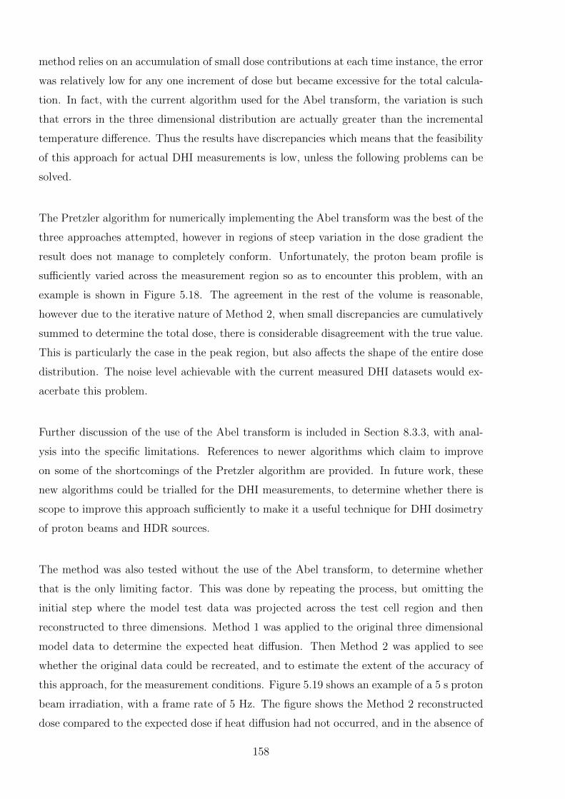
method relies on an accumulation of small dose contributions at each time instance, the error
was relatively low for any one increment of dose but became excessive for the total calcula-
tion. In fact, with the current algorithm used for the Abel transform, the variation is such
that errors in the three dimensional distribution are actually greater than the incremental
temperature difference. Thus the results have discrepancies which means that the feasibility
of this approach for actual DHI measurements is low, unless the following problems can be
solved.
The Pretzler algorithm for numerically implementing the Abel transform was the best of the
three approaches attempted, however in regions of steep variation in the dose gradient the
result does not manage to completely conform. Unfortunately, the proton beam profile is
sufficiently varied across the measurement region so as to encounter this problem, with an
example is shown in Figure 5.18. The agreement in the rest of the volume is reasonable,
however due to the iterative nature of Method 2, when small discrepancies are cumulatively
summed to determine the total dose, there is considerable disagreement with the true value.
This is particularly the case in the peak region, but also affects the shape of the entire dose
distribution. The noise level achievable with the current measured DHI datasets would ex-
acerbate this problem.
Further discussion of the use of the Abel transform is included in Section 8.3.3, with anal-
ysis into the specific limitations. References to newer algorithms which claim to improve
on some of the shortcomings of the Pretzler algorithm are provided. In future work, these
new algorithms could be trialled for the DHI measurements, to determine whether there is
scope to improve this approach sufficiently to make it a useful technique for DHI dosimetry
of proton beams and HDR sources.
The method was also tested without the use of the Abel transform, to determine whether
that is the only limiting factor. This was done by repeating the process, but omitting the
initial step where the model test data was projected across the test cell region and then
reconstructed to three dimensions. Method 1 was applied to the original three dimensional
model data to determine the expected heat diffusion. Then Method 2 was applied to see
whether the original data could be recreated, and to estimate the extent of the accuracy of
this approach, for the measurement conditions. Figure 5.19 shows an example of a 5 s proton
beam irradiation, with a frame rate of 5 Hz. The figure shows the Method 2 reconstructed
dose compared to the expected dose if heat diffusion had not occurred, and in the absence of
158
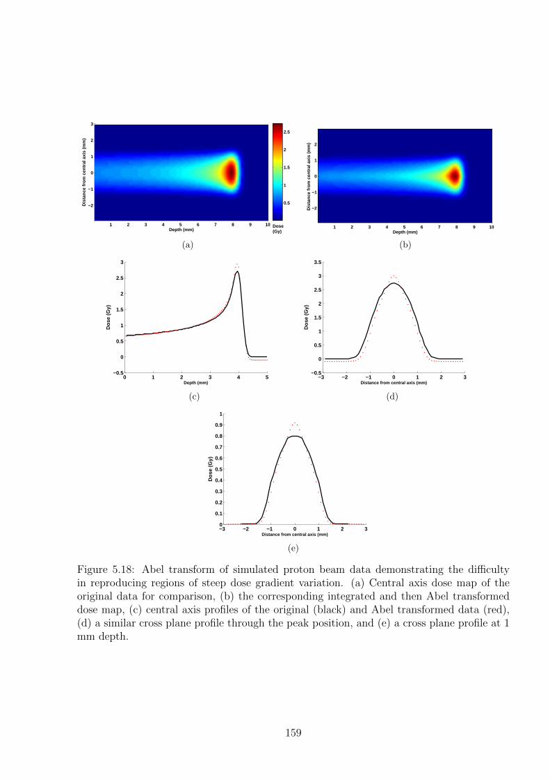
Depth (mm)
Dis
tanc
e fr
om c
entr
al a
xis
(mm
)
1 2 3 4 5 6 7 8 9 10
3
2
1
0
−1
−2 0.5
1
1.5
2
2.5
Dose(Gy)
(a)
Depth (mm)
Dis
tanc
e fr
om c
entr
al a
xis
(mm
)
1 2 3 4 5 6 7 8 9 10
2
1
0
−1
−2
(b)
0 1 2 3 4 5−0.5
0
0.5
1
1.5
2
2.5
3
Depth (mm)
Dos
e (G
y)
(c)
−3 −2 −1 0 1 2 3−0.5
0
0.5
1
1.5
2
2.5
3
3.5
Distance from central axis (mm)
Dos
e (G
y)
(d)
−3 −2 −1 0 1 2 30
0.1
0.2
0.3
0.4
0.5
0.6
0.7
0.8
0.9
1
Distance from central axis (mm)
Dos
e (G
y)
(e)
Figure 5.18: Abel transform of simulated proton beam data demonstrating the difficultyin reproducing regions of steep dose gradient variation. (a) Central axis dose map of theoriginal data for comparison, (b) the corresponding integrated and then Abel transformeddose map, (c) central axis profiles of the original (black) and Abel transformed data (red),(d) a similar cross plane profile through the peak position, and (e) a cross plane profile at 1mm depth.
159
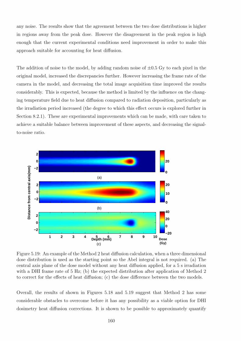
any noise. The results show that the agreement between the two dose distributions is higher
in regions away from the peak dose. However the disagreement in the peak region is high
enough that the current experimental conditions need improvement in order to make this
approach suitable for accounting for heat diffusion.
The addition of noise to the model, by adding random noise of ±0.5 Gy to each pixel in the
original model, increased the discrepancies further. However increasing the frame rate of the
camera in the model, and decreasing the total image acquisition time improved the results
considerably. This is expected, because the method is limited by the influence on the chang-
ing temperature field due to heat diffusion compared to radiation deposition, particularly as
the irradiation period increased (the degree to which this effect occurs is explored further in
Section 8.2.1). These are experimental improvements which can be made, with care taken to
achieve a suitable balance between improvement of these aspects, and decreasing the signal-
to-noise ratio.
2
0
−2
2
0
−2
Depth (mm)
Dis
tanc
e fr
om c
entr
al a
xis(
mm
)
Dose(Gy)
1 2 3 4 5 6 7 8 9 10
2
0
−2−20
0
20
40
0
20
0
10
20
(c)
(a)
(b)
Figure 5.19: An example of the Method 2 heat diffusion calculation, when a three dimensionaldose distribution is used as the starting point so the Abel integral is not required. (a) Thecentral axis plane of the dose model without any heat diffusion applied, for a 5 s irradiationwith a DHI frame rate of 5 Hz; (b) the expected distribution after application of Method 2to correct for the effects of heat diffusion; (c) the dose difference between the two models.
Overall, the results of shown in Figures 5.18 and 5.19 suggest that Method 2 has some
considerable obstacles to overcome before it has any possibility as a viable option for DHI
dosimetry heat diffusion corrections. It is shown to be possible to approximately quantify
160
the extent of heat diffusion in the measured results, however care must be taken with the
experimental situations to which this method is applied. Currently this approach is limited
to the measurement of dose distributions which do not have steep dose gradients. In these
situations however, heat diffusion has a lower influence on the measured temperature map.
The use of Method 2 could potentially improve accuracy for these conditions, if it proves
necessary. For situations with a more modulated dose, Method 2 will not currently allow
the true dose distribution to be accurately determined from the measurement. Varying the
experimental parameters as described above may help with this. Additionally, for highly
modulated doses, a mathematical algorithm which is more robust towards steep gradient
variations and noise than the Abel integral is required. Alternatively, to avoid this step, a
first order approximation could be used based on approximating the effects of heat diffusion
directly on the two dimensional projection images. This could be done by a two dimensional
heat transfer calculation and the use of a proportionality constant to account for contribu-
tions from out-of-plane regions. For data such as the HDR source, where the dose gradient is
predominantly in one direction, this approximation could have some degree of accuracy. This
would also avoid another uncertainty in the DHI HDR correction, where the sharp edge in
the image created by shading from the applicator results in an incorrect Abel reconstruction
in that region.
5.5 Concluding Remarks
Calorimetric based measurement processes must consider the impact of heat transfer on
the measured results. The basic mechanisms of heat transfer have been described, and the
mathematical formulations for considering the extent of heat diffusion were introduced.
Two different approaches were developed to account for heat diffusion in the DHI measure-
ment process. Method 1 is a forward correction of the model comparison data, to allow a
“like with like” comparison with the form of the measured data. This approach was success-
fully implemented, and was found to introduce a total uncertainty on the order of 0.75% to
the interpretation of DHI measurement results. The fundamental limitation of this approach
is that it relies on a set of model data to compare to, so measurements can only be used in
conjunction with a model or alternative measurement approach. Method 2 is based on an
inverse correction of the measured data to remove the effects of heat diffusion. The approach
was to iteratively determine the dose deposition rate by comparison of the calculated heat
diffusion in subsequent measurement images. This approach is appealing because it removes
161
the dependence on an alternative dosimetry system, which would increase the versatility
of the DHI results. However Method 2, whilst theoretically possible, was limited by the
constraints of the Abel integral and the cumulative nature of the calculation, with these
effects resulting in discrepancies that render this approach infeasible at this time for radia-
tion distributions with high variation in dose gradients. Improvements to the mathematical
algorithms used for reconstructing the three dimensional dose, experimental reduction of the
noise and increase in the image acquisition frequency may allow for reconsideration of this
method in the future. The implementation of a three dimensional measurement acquisition
method such as tomographic imaging would eliminate the need to approximate the temper-
ature distribution by means of the Abel transform, and the advantages and disadvantages
of this approach are also discussed.
The effects of heat convection have not been considered in the current work. The validity of
this assumption is also considered in Chapter 8.
162
Chapter 6
HDR Brachytherapy SourceMeasurements
HDR brachytherapy was selected as a suitable radiation source to test the DHI detector
prototype. These measurements were intended to demonstrate the feasibility of a DHI ap-
proach to radiation dosimetry by measuring the miniscule radiation induced temperature
variations. An HDR source was a practical choice for the initial measurements because of
the availability of a source at Christchurch Women’s Hospital. The source by definition has
a high dose rate, which is also highly spatially variant in the region close to the source. This
results in a high relative dose range and subsequent temperature variation, which should be
resolvable on each of the DHI images.
The primary aim was to provide an initial proof-of-principle of DHI as a radiation dosimetry
approach, characterise the dosimeter and identify issues for future improvements. The sec-
ondary aim was to investigate the potential for DHI to contribute to the field of near-source
dosimetry described in Section 2.3.1.
6.1 Methods
6.1.1 Measurement
All measurements were acquired according to the general process described in Section 4.3.3
and measurement parameters recorded as in Table 4.3. Details specific to the HDR mea-
surements are given below.
163
HDR Brachytherapy Source
The HDR source used in this study was an Ir-192 source supplied by Varian Medical Sys-
tems (Paolo Alto, USA), owned by Canterbury District Health Board (CDHB) and located at
Christchurch Womens’ Hospital (Christchurch, New Zealand). Ir-192 has a complex gamma
ray spectrum with energies ranging from 136 keV to 1.06 MeV and an average energy of 380
keV. The source consisted of a cylindrical Ir-192 pellet of length 3.5 mm and diameter 0.6
mm, housed within a stainless steel capsule of length 4.52 mm and diameter 0.9 mm. The
source was attached to a flexible stainless steel wire, housed within a Varian Medical Systems
GammaMed Plus afterloader. The manufacturer’s quoted specification for the positioning
accuracy of the wire is ±1 mm relative to the indexer. At the time of measurement the air
kerma rate of the source at 1 m distance was 18.7 mGy h−1. The corresponding activity was
170.1 GBq (4.597 Ci). A calibrated well chamber was used at the time of source installation
to validate the manufacturer’s quoted source strength source, achieving agreement to within
0.3%, well within the 2% tolerance required for clinical usage.
For all measurements the source was housed within a Perma-Doc Phantom Applicator (Var-
ian Medical Systems), which is a straight aluminium applicator of diameter 3 mm. The
distance between the external tip of the tandem and the source centre is 3.75 mm when the
source in the end dwell position. This relatively thick applicator was selected rather than the
much smaller plastic catheter used for source calibration in the well chamber, because it had
a much higher rigidity. The movement of the source from where it was housed in the after-
loader to the end of the applicator causes movement of the applicator. All measurements are
made comparatively by subtracting a reference image taken before the source was in place
from images taken during irradiation, thus if a non rigid applicator is used, any change in
position of the applicator due to source movement leads to inaccuracies in the results. With
the applicator that was used, the closest measurable point was 1.5 mm from the central axis
of the source. For closer measurements alternative applicators could be used if required.
DHI Detector
The DHI detector used was the configuration shown in Figure 4.4. The object-to-sensor
distance was 26.5 cm. The detector in situ is pictured in Figure 6.1, from one of the prelim-
inary measurements. The box which was used to isolate the detector from air flows is not
pictured, but was used during the subsequent measurements, results of which are presented
in this chapter. A burette stand was used to suspend the applicator in the test cell. Care
164
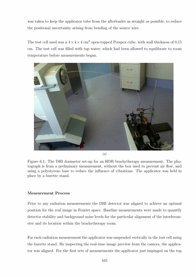
was taken to keep the applicator tube from the afterloader as straight as possible, to reduce
the positional uncertainty arising from bending of the source wire.
The test cell used was a 4×4×4 cm3 open-topped Perspex cube, with wall thickness of 0.15
cm. The test cell was filled with tap water, which had been allowed to equilibrate to room
temperature before measurements began.
(a)
Figure 6.1: The DHI dosimeter set-up for an HDR brachytherapy measurement. The pho-tograph is from a preliminary measurement, without the box used to prevent air flow, andusing a polystyrene base to reduce the influence of vibrations. The applicator was held inplace by a burette stand.
Measurement Process
Prior to any radiation measurements the DHI detector was aligned to achieve an optimal
position for the real image in Fourier space. Baseline measurements were made to quantify
detector stability and background noise levels for the particular alignment of the interferom-
eter and its location within the brachytherapy room.
For each radiation measurement the applicator was suspended vertically in the test cell using
the burette stand. By inspecting the real-time image preview from the camera, the applica-
tor was aligned. For the first sets of measurements the applicator just impinged on the top
165
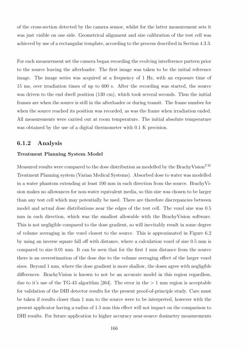
of the cross-section detected by the camera sensor, whilst for the latter measurement sets it
was just visible on one side. Geometrical alignment and size calibration of the test cell was
achieved by use of a rectangular template, according to the process described in Section 4.3.3.
For each measurement set the camera began recording the evolving interference pattern prior
to the source leaving the afterloader. The first image was taken to be the initial reference
image. The image series was acquired at a frequency of 1 Hz, with an exposure time of
15 ms, over irradiation times of up to 600 s. After the recording was started, the source
was driven to the end dwell position (130 cm), which took several seconds. Thus the initial
frames are when the source is still in the afterloader or during transit. The frame number for
when the source reached its position was recorded, as was the frame when irradiation ended.
All measurements were carried out at room temperature. The initial absolute temperature
was obtained by the use of a digital thermometer with 0.1 K precision.
6.1.2 Analysis
Treatment Planning System Model
Measured results were compared to the dose distribution as modelled by the BrachyVisionTM
Treatment Planning system (Varian Medical Systems). Absorbed dose to water was modelled
in a water phantom extending at least 100 mm in each direction from the source. BrachyVi-
sion makes no allowances for non-water equivalent media, so this size was chosen to be larger
than any test cell which may potentially be used. There are therefore discrepancies between
model and actual dose distributions near the edges of the test cell. The voxel size was 0.5
mm in each direction, which was the smallest allowable with the BrachyVision software.
This is not negligible compared to the dose gradient, so will inevitably result in some degree
of volume averaging in the voxel closest to the source. This is approximated in Figure 6.2
by using an inverse square fall off with distance, where a calculation voxel of size 0.5 mm is
compared to size 0.01 mm. It can be seen that for the first 1 mm distance from the source
there is an overestimation of the dose due to the volume averaging effect of the larger voxel
sizes. Beyond 1 mm, where the dose gradient is more shallow, the doses agree with negligible
differences. BrachyVision is known to not be an accurate model in this region regardless,
due to it’s use of the TG-43 algorithm [264]. The error in the > 1 mm region is acceptable
for validation of the DHI detector results for the present proof-of-principle study. Care must
be taken if results closer than 1 mm to the source were to be interpreted, however with the
present applicator having a radius of 1.5 mm this effect will not impact on the comparison to
DHI results. For future application to higher accuracy near-source dosimetry measurements
166
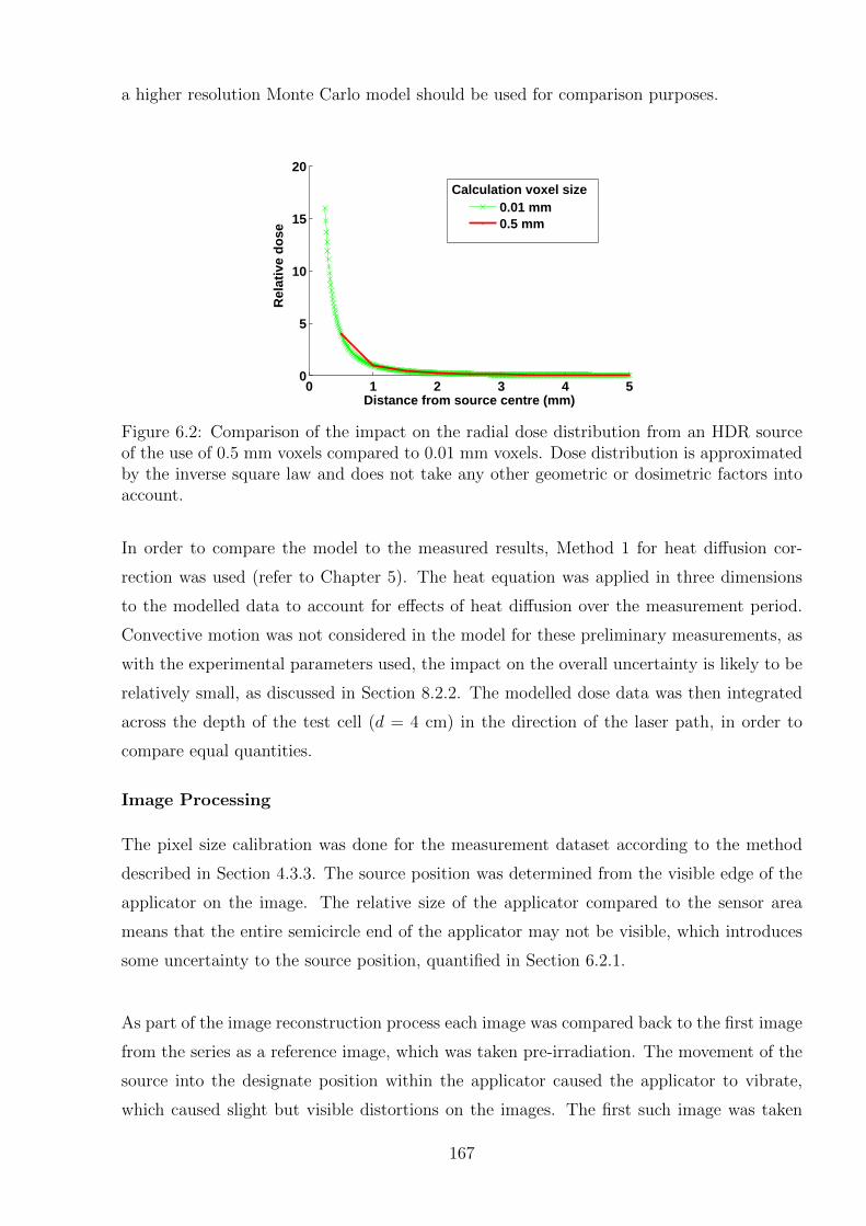
a higher resolution Monte Carlo model should be used for comparison purposes.
0 1 2 3 4 50
5
10
15
20
Distance from source centre (mm)
Rel
ativ
e d
ose
0.01 mm 0.5 mm
Calculation voxel size
Figure 6.2: Comparison of the impact on the radial dose distribution from an HDR sourceof the use of 0.5 mm voxels compared to 0.01 mm voxels. Dose distribution is approximatedby the inverse square law and does not take any other geometric or dosimetric factors intoaccount.
In order to compare the model to the measured results, Method 1 for heat diffusion cor-
rection was used (refer to Chapter 5). The heat equation was applied in three dimensions
to the modelled data to account for effects of heat diffusion over the measurement period.
Convective motion was not considered in the model for these preliminary measurements, as
with the experimental parameters used, the impact on the overall uncertainty is likely to be
relatively small, as discussed in Section 8.2.2. The modelled dose data was then integrated
across the depth of the test cell (d = 4 cm) in the direction of the laser path, in order to
compare equal quantities.
Image Processing
The pixel size calibration was done for the measurement dataset according to the method
described in Section 4.3.3. The source position was determined from the visible edge of the
applicator on the image. The relative size of the applicator compared to the sensor area
means that the entire semicircle end of the applicator may not be visible, which introduces
some uncertainty to the source position, quantified in Section 6.2.1.
As part of the image reconstruction process each image was compared back to the first image
from the series as a reference image, which was taken pre-irradiation. The movement of the
source into the designate position within the applicator caused the applicator to vibrate,
which caused slight but visible distortions on the images. The first such image was taken
167
to be the first time instance of irradiation, however only later images where the picture had
stabilised were used for analysis.
There are two types of noise inherent in the measurements made by the optical system.
These both cause the phase values measured on each sensor pixel to fluctuate with time
and/or position, in the absence of any irradiation. The first is ambient noise due to ambient
influence quantities, including air flow, temperature fluctuations, vibrations, and variation
of the temperature within the test cell. The impact of these was minimized by housing the
detector in a box to isolate it from air motion, with a rubber base to absorb vibrations.
However these influences could not be entirely eliminated for the prototype detector, and
impacted on the measurements. The second type of noise is intrinsic noise, which is a conse-
quence of the optical components used and their exact alignment. An example can be seen
in the ring pattern visible in the bottom left corner of Figure 6.4(a). Both types of noise
combine to influence the dose measurements. A low pass Gaussian filter was used to reduce
the impact of the noise in order to examine the dose distribution. Before applying the filter
the applicator was masked in the image, to avoid excessive influence by the arbitrary but
wildly fluctuating phase values which are seen in the region shaded by the applicator.
Direct Comparison to Model Results
The results presented later in Section 6.2.4 show the direct comparison of the measured
datasets to the BrachyVision model data, which has been corrected for heat diffusion and
integrated over the width of the test cell. The DHI measurement values showed the relative
dose difference between the different points in the sensitive region, plus some amount that
depended on the absolute phase of the measurements, which has an arbitrary value between
0 and 2π. The process used to normalise this dose difference is referred to as “difference
normalisation” throughout the remainder of this work. A normalisation point was chosen at
a point as far away as possible from the applicator. The exact distance achievable depended
on the location of the applicator within the field of view, whilst consideration was also given
to avoiding any visible distortions in the measured image. The measured dose value at this
difference normalisation point was then subtracted from every pixel in the image. However
the limited sensitive region of the present version of the prototype detector meant that, for
longer irradiations, even the most distant point of the image experienced a non-negligible
increase in temperature. Thus in order to benchmark the dose difference to a value that
allowed the results to be meaningfully compared to the model, the dose determined by the
168
model at the location of the distance normalisation point was added to the measured dataset,
so that the dose differences of the model and the measured data could be compared directly.
This approach is equivalent to also doing a difference normalisation of the model to the same
normalisation point, however allows for the values of the dose to be compared at the actual
dose values. This allows for more meaningful uncertainty metrics, with the percentage un-
certainty for instance being a valid tool to consider the agreement of measurement and model.
In Section 6.2.4 dose profiles along axial and longitudinal axes from the applicator are pre-
sented, at a range of distances from the source centre. Two dimensional dose distribution
maps at different time instances are shown. In order to quantify the results by calculating
dose difference maps of measured versus modelled data, the datasets must have the same
resolution. The conventional approach to this would be to resample the measured results
to match the lower resolution of the model, however this has a major downside in that it
loses the benefit of the higher resolution of the measured results in the region of the source
where the model may be less accurate. Additionally, the presence of the applicator distorts
the resampled results in this region. The alternative approach is to interpolate the model
data, using a MATLAB spline interpolant function, to have the same dose grid spacing as
the measured dataset. This approach allows for a better comparison of the data near the
source, as long as due consideration is accorded to the impact of interpolation on the model
dose profile in this region. Both approaches are compared in the results section.
Section 6.2.5 presents the results in a more conventional fashion by comparing radial dose
functions of the measured and modelled data. This is in contrast to the results in the rest of
the comparison, which are in terms of the integrated dose across the distance of the test cell,
which is not a metric which is commonly encountered in radiation dosimetry. The radial dose
function is a measure of the dose along any given profile in a radial direction from the source
longitudinal axis, and is required in the TG-43 algorithm [39]. The Abel transform, which
was introduced in Section 5.4.2 in the process of calculating the heat diffusion, can be used
to determine the three dimensional distribution of a cylindrically symmetric measurement.
This does not add any information to the measurements presented above, indeed it actually
risks losing some information about any asymmetries in the source positioning which may
be detected by the standard DHI measurements. It may however make the results of the
DHI detector more accessible by presenting them in a means that medical physicists may be
more familiar with.
169
Uncertainties
In order to determine the sensitivity of the detector, and quantify the accuracy of the dose
distribution measurements the uncertainty in the measurement parameters are determined.
There are various points in the experimental process where errors can be introduced, but
they can be divided into dosimetric uncertainties and positional uncertainties. Their impact
must be quantified in order to put a limit of accuracy on the results in order to determine the
sensitivity of the DHI dosimeter. The final values used for both dosimetric and positional
uncertainty are reported in Section 6.2.3. The methods of quantifying them are described
below.
A main contributing factor to the dosimetric uncertainties is noise in the measurement
system. The two types of noise already mentioned, ambient and intrinsic noise, are inherent
in the dosimetric uncertainty. At this point, both of these effects are grouped together in
order to estimate the total dosimetric uncertainty. As all dose measurements are determined
via a differential comparison with an initial reference image, an estimate of the noise in
the system can be obtained by quantifying the phase variation from the reference image,
for a series of images prior to each irradiation beginning, effectively giving flat-field null
measurements. As these measurements were only concerned with the dose difference maps
at each time instance, rather than absolute dose, the mean value of the arbitrary phase
difference of each image was subtracted from that image. This resulted in a series of null
images where the phase fluctuated across the image. The standard deviation of the calculated
dose values in each image was determined, and then the total standard deviation of the
image series determined by taking the square root of the sum of the variances of each image.
The data from the null images was analysed by several means to determine if it obeyed a
normal distribution. The first method was a straightforward visual comparison of a normal
distribution function with a relative frequency histogram of the data, using the Freedman-
Draconis rule [265], given in equation 6.1, to select a bin width of 0.413 Gy. This selects the
bin width based on a comparison of the interquartile range, IQR, of sample x to the number
of data points, n.
Bin size = 2 IQR(x)n−1/3 (6.1)
In order to give the visual method some degree of statistical significance, the chi-square
goodness of fit test against the null hypothesis that the data is normally distributed was
calculated, via the built-in MATLAB function chi2gof.m. This returns one if the test
rejects the null hypothesis at the 5% significance level, and zero otherwise. The test groups
data into N bins, and then calculates the chi-square test statistic to compare the observed,
170
O, and expected, E, counts for those bins according to:
χ2 =N∑i=1
(Oi − Ei)2
Ei(6.2)
If there was any uncertainty in these results then an additional test of normality was also
calculated by constructing a normal probability plot for the data, using the MATLAB func-
tion normplot.m, where if the points are linear then the data has a high positive correlation
to a normal distribution. In this test, the x-axis is transformed so that a cumulative normal
density function will be plotted as a straight line. Then the mean and standard deviation
are calculated from the data and transformed to the standard normal values, i.e. where the
mean is zero and the standard deviation is one. The data points are then plotted along the
fitted normal line.
If the results of this null testing for each individual irradiation measurement showed a suffi-
cient correlation with a normal distribution, then the dosimetric uncertainty arising from the
measurement influence quantities was taken to be the standard deviation, σ, of the calculated
dose values of the preliminary images, which corresponds to the 68.2% confidence interval.
Standard deviations from the individual images σi,were summed according to equation 6.3.
σ =√σ2
1 + σ22 + ...σ2
i (6.3)
The other contributing factor to the dosimetric uncertainty in the measured DHI results is
termed relative shift. This is the uncertainty that arises from the difference normalisation
process, where an absolute value is used to benchmark the dose difference distribution for
comparison to the model distribution. The uncertainty is dependent on the possible error due
to the relative positioning of the normalisation point on the measured versus the modelled
data. The normalisation point is chosen to be at the lowest possible dose value, in a region
where there are no evident distortions in the measured dose distribution. An estimate of the
uncertainty introduced is obtained by comparing the normalisation value from the model at
that point with the dose at a distance of 0.5 mm in either direction, to account for possible
positional errors between the measured and modelled data. The total dosimetric uncertainty
is the sum of the relative shift and the combined ambient and intrinsic noise.
The dosimetric uncertainty in the BrachyVision data was determined using the comparison
by Zourari et al. of the BrachyVision data with a state of the art Monte Carlo model [266]
in order to attest to the capability of BrachyVision to accurately account for the scatter-
ing conditions in any homogeneous geometry. They benchmarked the dose distributions
171
created by BrachyVision with Monte Carlo models, for single Ir-192 sources in homoge-
neous bounded water geometries, so their results are applicable to the DHI situation. They
found that at points close to the longitudinal source axis BrachyVision results present a
dose rate over-estimation of 1-3% which is statistically significant, although some of it can
be attributed to the Monte Carlo model statistical uncertainty. The remaining difference is
attributed to spatial discretisation. The rest of the points are within agreement to less than
1%, with BrachyVision slightly underestimating the dose. Based on these results, for the
proof-of-principle comparisons a conservative estimate of ±3% uncertainty was assumed on
the BrachyVision data. Future studies may investigate this further and possibly reduce this
estimate.
An additional dosimetric uncertainty arises from the temporal uncertainty. The time of the
HDR measurement was selected according to the current image numbers when the applica-
tor reached its end dwell position. For a measurement rate of 1 Hz, this has an inherent
uncertainty of ±0.5 s. This was incorporated in the dosimetric uncertainty for the model,
with the value proportionate to the length of the irradiation time. Thus for a twenty second
irradiation there is an additional 2.5% uncertainty, but this value decreases with longer ir-
radiation time. This is an influence which can be greatly reduced in future iterations of the
detector by automating the timing of the image acquisition by automatic triggering.
The heat diffusion calculations induce some uncertainties, which were discussed in Chapter
5. The relevant uncertainties for the HDR model heat diffusion calculations were summed,
with the total of 0.75% added to the above uncertainties. This number incorporates the
impact of applicator positional error when calculating the integrated dose, variation in am-
bient temperature from that used in the calculations, and the effects of timing error on the
heat diffusion calculation. The overall dosimetric uncertainty in the integrated, heat diffused
HDR model was thus 3% + 2.5% + 0.75% = 6.3%.
The other type of uncertainty to be considered is the positional uncertainty of the reported
distances for the model and the DHI results. For the model data, the resolution is 0.5 mm
in each direction, and so the presumed uncertainty is half of that, i.e. 0.25 mm. The uncer-
tainty in the positioning of the DHI measurements is determined during the pixel calibration,
and reported in Section 6.2.1.
172
Accuracy Determination via Gamma Analysis
The gamma test is a metric for considering the agreement between a pair of two or three
dimensional dose distributions. The gamma test was developed by Low et al. [267] from two
simpler approaches, the dose difference comparison (as used in the previous section) and the
distance-to-agreement (DTA) comparison. A dose distance comparison is a straightforward
comparison of the dose at the corresponding points in the two dose distributions under com-
parison. Generally a passing criteria is used, for example 5%, whereby if the absolute dose
difference at each point is less than the passing criterion then the measured dose distribu-
tion is considered to “pass” at that point. This approach has a major drawback in that it
is not robust in high gradient regions, where a small misalignment can cause a dispropor-
tionately large dose difference. An alternative method which is often used in conjunction is
the distance-to-agreement (DTA) method, where for each point, if the dose within a certain
radius matches the dose at the corresponding point in the model then that point passes.
This techniques is more robust against misalignments in high gradient regions, because the
matching dose will still be nearby, but is more prone to failure in low dose regions, where
small misalignments can require a large radius to find the matching dose level. In order to
overcome these limitations in the high and low gradient regions, these two tests are often
used in conjunction with each other, by evaluating them separately, and determining each
point to be sufficiently accurate if it passes either test [268,269]. The gamma test is a more
sophisticated combination of the two approaches, whereby they are combined into a more
abstract metric which resembles a distance.
The gamma test is implemented mathematically according to equations 6.4 and 6.5. Compar-
ison of two dose distributions is done pointwise, with a dose Da(ra) in the first distribution,
a, at point ra, and a dose Db(rb) at the corresponding point rb in the second dose distribu-
tion, b. The first term in the square root of equation 6.4 describes the DTA condition. A
threshold passing value, δDTA is defined, for example 2 mm. The DTA condition is fulfilled
when Da(ra) = Db(rb+ r) where r is an arbitrary point some distance |r| away from rb. This
describes an isodose contour in the second dose distribution around point rb. For a simple
DTA test, any value smaller than the threshold is considered a passing value. The gamma
test uses δDTA to normalise the DTA value, so that a normal passing value would become
unity. The second term in equation 6.4 describes the dose difference at the corresponding
points, |Da(ra) − Db(rb)|, with the use of a pass/fail threshold δDD to also normalise the
result of a normal passing value to unity. The DTA and dose difference terms are combined
by squaring them, summing them and then taking the square root, to achieve a distance-like
173
metric, Γ. Γ is only defined for values of r such that Da(ra) = Db(rb + r), which are those
values geometrically located along the DTA isodose contours.
The actual gamma index, γ is then determined as in equation 6.5 from the minimum value
of Γ by varying r, which corresponds to the point along the isodose contour where DTA is
the smallest. The convention is for a gamma test to pass when γ ≤ 1 and failing if γ > 1.
Γ =
√d2DTA((ra, rb) + r)
δ2DTA
+|Da(ra)−Db(rb)|2
δ2DD
(6.4)
γ(ra, rb) = min{Γ(ra, rb),∀r} (6.5)
The gamma test was applied to compare some of the measured data to the model, using
threshold passing values of ±10% and 2 mm. These criteria were chosen based on the per-
formance of the measured data, in order to gain an understanding of where improvements
are most necessary. The results are shown in Section 6.2.6 and the usefulness of the gamma
index as a metric for dose distribution evaluation for the purposes of DHI is discussed in
Section 8.3.4.
6.2 Results
The results presented in this Chapter are intended to be a representative sample of the
measurements. As such, results with the applicator in two different positions within the
cell are shown. Dataset 1 shows the applicator just impinging on the right hand side of the
image, and is an example of a measurement with generally high agreement between the mea-
sured and modelled dose distributions, over a relatively short irradiation period. Dataset
2 shows the applicator just impinging on the top of the image, and was chosen as it has
some more distortions in the measured dose distributions that were typical of many of the
measurements. Both datasets show increasing disagreement with the model as irradiation
periods increase. An example of the interferograms and subsequent reconstructed images
from measurements taken with the applicator in a central versus a lateral position are shown
in Figure 6.3. The calibration template is visible in these images, but for the analysis of the
measured results a smaller region of interest was selected just inside this outline.
174
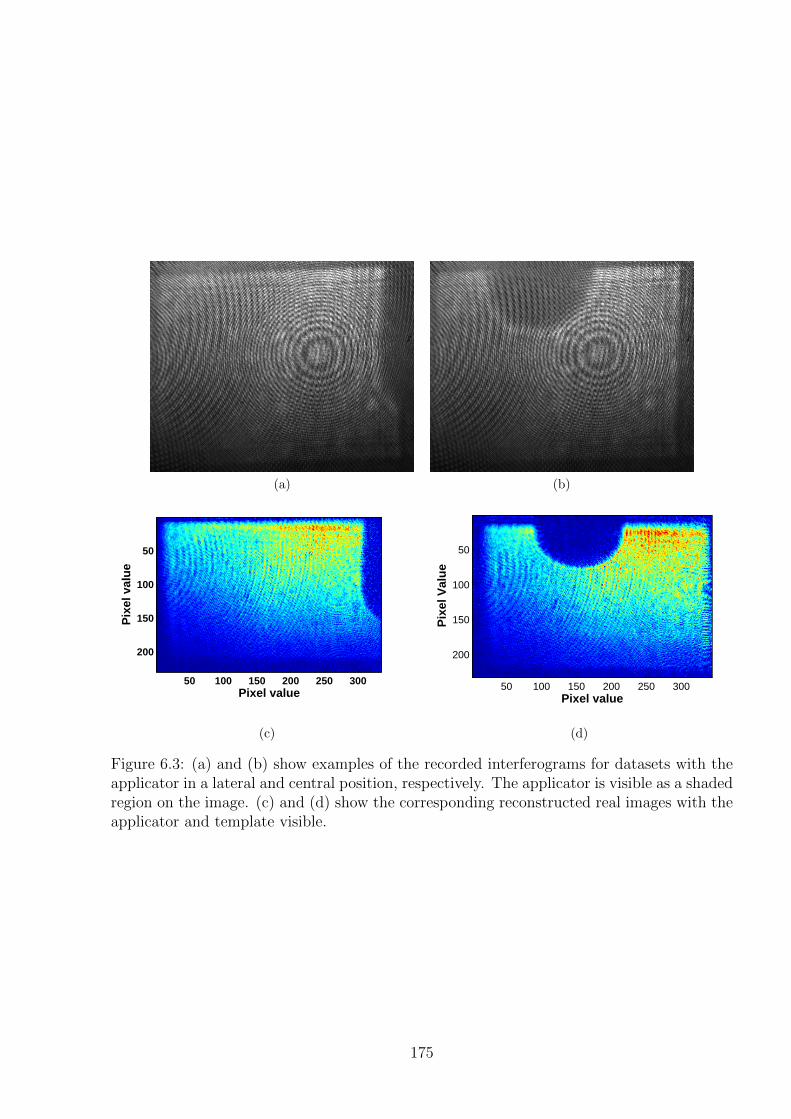
(a) (b)
Pixel value
Pix
el v
alu
e
50 100 150 200 250 300
50
100
150
200
(c)
Pixel value
Pix
el V
alu
e
50 100 150 200 250 300
50
100
150
200
(d)
Figure 6.3: (a) and (b) show examples of the recorded interferograms for datasets with theapplicator in a lateral and central position, respectively. The applicator is visible as a shadedregion on the image. (c) and (d) show the corresponding reconstructed real images with theapplicator and template visible.
175
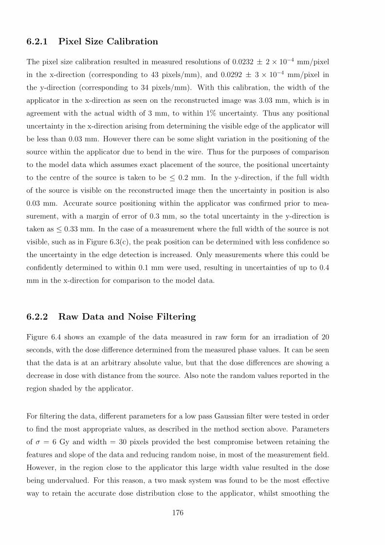
6.2.1 Pixel Size Calibration
The pixel size calibration resulted in measured resolutions of 0.0232 ± 2 × 10⁻⁴ mm/pixel
in the x-direction (corresponding to 43 pixels/mm), and 0.0292 ± 3 × 10⁻⁴ mm/pixel in
the y-direction (corresponding to 34 pixels/mm). With this calibration, the width of the
applicator in the x-direction as seen on the reconstructed image was 3.03 mm, which is in
agreement with the actual width of 3 mm, to within 1% uncertainty. Thus any positional
uncertainty in the x-direction arising from determining the visible edge of the applicator will
be less than 0.03 mm. However there can be some slight variation in the positioning of the
source within the applicator due to bend in the wire. Thus for the purposes of comparison
to the model data which assumes exact placement of the source, the positional uncertainty
to the centre of the source is taken to be ≤ 0.2 mm. In the y-direction, if the full width
of the source is visible on the reconstructed image then the uncertainty in position is also
0.03 mm. Accurate source positioning within the applicator was confirmed prior to mea-
surement, with a margin of error of 0.3 mm, so the total uncertainty in the y-direction is
taken as ≤ 0.33 mm. In the case of a measurement where the full width of the source is not
visible, such as in Figure 6.3(c), the peak position can be determined with less confidence so
the uncertainty in the edge detection is increased. Only measurements where this could be
confidently determined to within 0.1 mm were used, resulting in uncertainties of up to 0.4
mm in the x-direction for comparison to the model data.
6.2.2 Raw Data and Noise Filtering
Figure 6.4 shows an example of the data measured in raw form for an irradiation of 20
seconds, with the dose difference determined from the measured phase values. It can be seen
that the data is at an arbitrary absolute value, but that the dose differences are showing a
decrease in dose with distance from the source. Also note the random values reported in the
region shaded by the applicator.
For filtering the data, different parameters for a low pass Gaussian filter were tested in order
to find the most appropriate values, as described in the method section above. Parameters
of σ = 6 Gy and width = 30 pixels provided the best compromise between retaining the
features and slope of the data and reducing random noise, in most of the measurement field.
However, in the region close to the applicator this large width value resulted in the dose
being undervalued. For this reason, a two mask system was found to be the most effective
way to retain the accurate dose distribution close to the applicator, whilst smoothing the
176
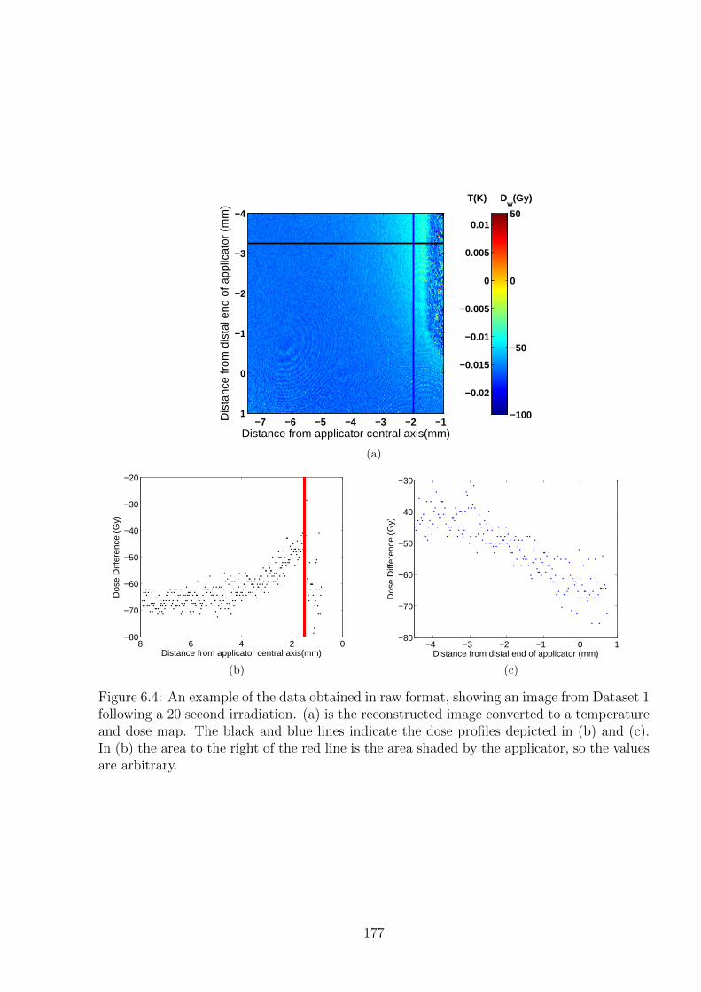
Dis
tanc
e fr
om d
ista
l end
of a
pplic
ator
(m
m)
Distance from applicator central axis(mm)
−7 −6 −5 −4 −3 −2 −1
−4
−3
−2
−1
0
1 −100
−50
0
50
−0.02
−0.015
−0.01
−0.005
0
0.005
0.01
T(K) Dw
(Gy)
(a)
−8 −6 −4 −2 0−80
−70
−60
−50
−40
−30
−20
Dos
e D
iffer
ence
(G
y)
Distance from applicator central axis(mm)
(b)
−4 −3 −2 −1 0 1−80
−70
−60
−50
−40
−30
Dos
e D
iffer
ence
(G
y)
Distance from distal end of applicator (mm)
(c)
Figure 6.4: An example of the data obtained in raw format, showing an image from Dataset 1following a 20 second irradiation. (a) is the reconstructed image converted to a temperatureand dose map. The black and blue lines indicate the dose profiles depicted in (b) and (c).In (b) the area to the right of the red line is the area shaded by the applicator, so the valuesare arbitrary.
177
noise sufficiently in the remainder of the image. This approach involved increasing the region
that was masked over the applicator, by ten pixels in each direction to create a perimeter
region around the applicator. Within this region the parameters for the Gaussian filter were
chosen as σ = 6 Gy and width = 10 pixels. The resultant filtered image was then combined
with the original filtered image of the whole region to produce the final result. An example
of the results after this process is depicted for two different positions of the applicator in
Figures 6.5 and 6.6. For the two datasets shown the mean residual between the smoothed
data and the raw data is -0.114 Gy and 0.559 Gy for Dataset 1 and Dataset 2, respectively.
6.2.3 Detector Sensitivity and Dosimetric Uncertainty
As described in Section 6.1.2, the uncertainty on each measurement point is made up of dosi-
metric and positional uncertainty. The initial sensitivity measurements which were taken as
the first few images pre-irradiation, in the image series of each irradiation, were analysed to
determine the noise contribution to the dosimetric uncertainty. This also allows an estima-
tion of the limits of the sensitivity of the prototype DHI detector.
Various tests were done in order to determine whether the noise fits a normal distribution.
An example is presented of the data from one of the HDR measurements, Dataset 1, with
the applicator at the right hand side of the sensitive region. An example of one of the flat
field reconstructed images, converted to dose, is shown in Figure 6.7(a), with the region
shaded by the applicator masked. Figure 6.7(b) shows a histogram of the data points, in
0.413 Gy bin widths, with the corresponding normal distribution displayed for comparison.
Figure 6.7(c) shows the normal probability plot of the data which compares the measured
data spread with the spread expected from a normal distribution. For the dataset shown, the
standard deviation was 2.90 Gy. The chi-square test confirmed agreement with the normal
distribution. The normal probability plot shows that there is some deviation from a normal
distribution, with the S-shape indicating that there was less variance than expected. This
means that the standard deviation was somewhat higher than the 68% confidence interval,
thus this was considered an acceptable estimate for the noise induced uncertainty in the
data. For each of the datasets the first five images were analysed and the total standard
deviation of the noise was calculated, according to equation 6.3. For Dataset 1 this resulted
in an uncertainty estimate of σ = ±3.01 Gy.
Determination of the relative shift uncertainty is shown in Figure 6.8. For a normalisa-
178
Dis
tanc
e fr
om d
ista
l end
of a
pplic
ator
(m
m)
Distance from applicator central axis (mm)
−8 −7 −6 −5 −4 −3 −2 −1
−4
−3
−2
−1
0
1−30
−20
−10
0
10
20
30
−6
−4
−2
0
2
4
6
8x 10
−3
T(K) Dw
(Gy)
(a)
Dis
tanc
e fr
om d
ista
l end
of a
pplic
ator
(m
m)
Distance from applicator central axis (mm)
−8 −7 −6 −5 −4 −3 −2 −1
−4
−3
−2
−1
0
1
(b)
Dis
tanc
e fr
om d
ista
l end
of a
pplic
ator
(m
m)
Distance from applicator central axis (mm)
−8 −7 −6 −5 −4 −3 −2 −1
−4
−3
−2
−1
0
1
(c)
−8 −6 −4 −2 00
5
10
15
20
25
30
35
Dos
e D
iffer
ence
(G
y)
Distance from applicator central axis (mm)
(d)
−5 −4 −3 −2 −1 0 10
5
10
15
20
25
30
35
Dos
e D
iffer
ence
(G
y)
Distance from distal end of applicator (mm)
(e)
−5 −4 −3 −2 −1 0 1
0
5
10
15
20
0
5
10
15
Dos
e D
iffer
ence
(G
y)
Distance from distal end of applicator (mm)
(f)
Figure 6.5: Data filtering, Dataset 1. (a) The raw temperature/dose data after 20 seconds ofirradiation, showing the mask applied over the applicator region. Profiles of interest markedin black and blue. (b) The same image after application of a Gaussian filter (σ = 6 Gy,width = 30 pixels), (c) the mask used for the region adjacent to the applicator where theGaussian filter had width = 10 pixels. (d) Blue points are the data points from a profileorthogonal to the applicator in the raw dataset (black line in (a)). The green line marksthe edge of the applicator, and signal to the right of this is arbitrary. The black line marksthe smoothed data without the additional region shown in (c), displaying how the valuesare lower than they should be near the applicator. The red line shows the smoothed datawith the two mask regions. (e) is the profile along the solid blue line from (a) and (f) is thedotted blue line.
179
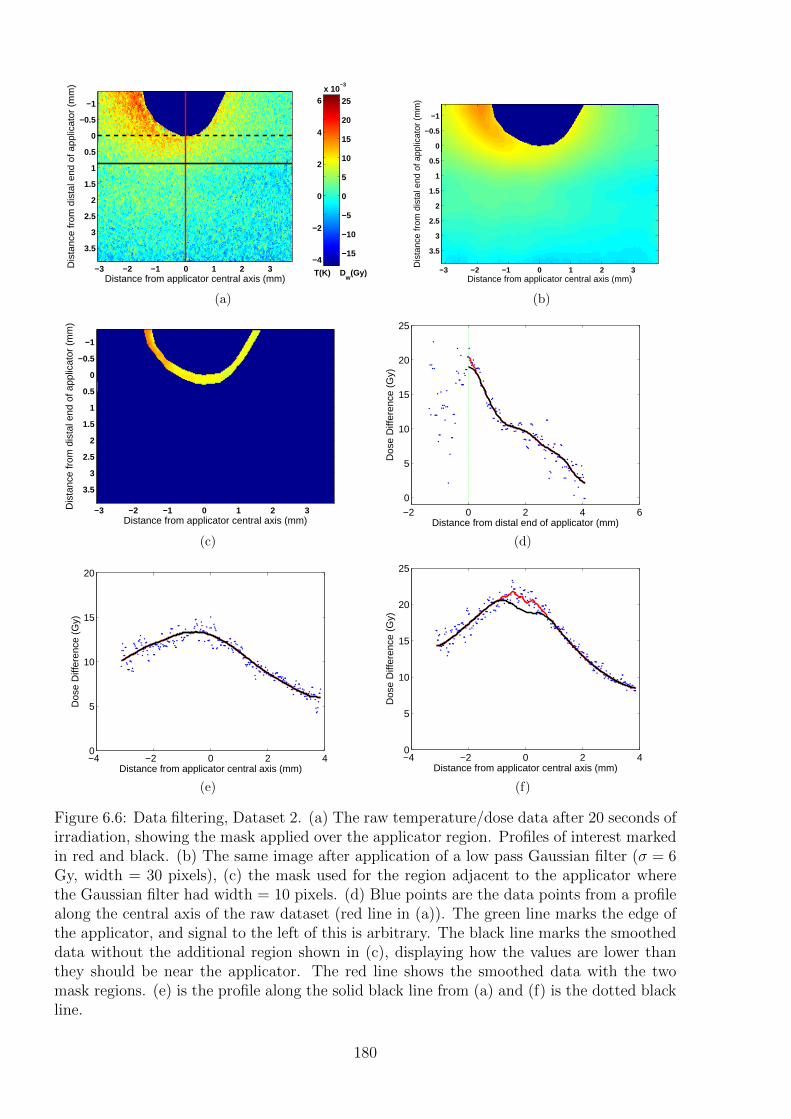
Dis
tanc
e fr
om d
ista
l end
of a
pplic
ator
(m
m)
Distance from applicator central axis (mm)
−3 −2 −1 0 1 2 3
−1
−0.5
0
0.5
1
1.5
2
2.5
3
3.5−15
−10
−5
0
5
10
15
20
25
−4
−2
0
2
4
6x 10
−3
T(K) Dw
(Gy)
(a)
Dis
tanc
e fr
om d
ista
l end
of a
pplic
ator
(m
m)
Distance from applicator central axis (mm)
−3 −2 −1 0 1 2 3
−1
−0.5
0
0.5
1
1.5
2
2.5
3
3.5
(b)
Dis
tanc
e fr
om d
ista
l end
of a
pplic
ator
(m
m)
Distance from applicator central axis (mm)
−3 −2 −1 0 1 2 3
−1
−0.5
0
0.5
1
1.5
2
2.5
3
3.5
(c)
−2 0 2 4 6
0
5
10
15
20
25
Dos
e D
iffer
ence
(G
y)
Distance from distal end of applicator (mm)
(d)
−4 −2 0 2 40
5
10
15
20
Dos
e D
iffer
ence
(G
y)
Distance from applicator central axis (mm)
(e)
−4 −2 0 2 40
5
10
15
20
25
Dos
e D
iffer
ence
(G
y)
Distance from applicator central axis (mm)
(f)
Figure 6.6: Data filtering, Dataset 2. (a) The raw temperature/dose data after 20 seconds ofirradiation, showing the mask applied over the applicator region. Profiles of interest markedin red and black. (b) The same image after application of a low pass Gaussian filter (σ = 6Gy, width = 30 pixels), (c) the mask used for the region adjacent to the applicator wherethe Gaussian filter had width = 10 pixels. (d) Blue points are the data points from a profilealong the central axis of the raw dataset (red line in (a)). The green line marks the edge ofthe applicator, and signal to the left of this is arbitrary. The black line marks the smootheddata without the additional region shown in (c), displaying how the values are lower thanthey should be near the applicator. The red line shows the smoothed data with the twomask regions. (e) is the profile along the solid black line from (a) and (f) is the dotted blackline.
180
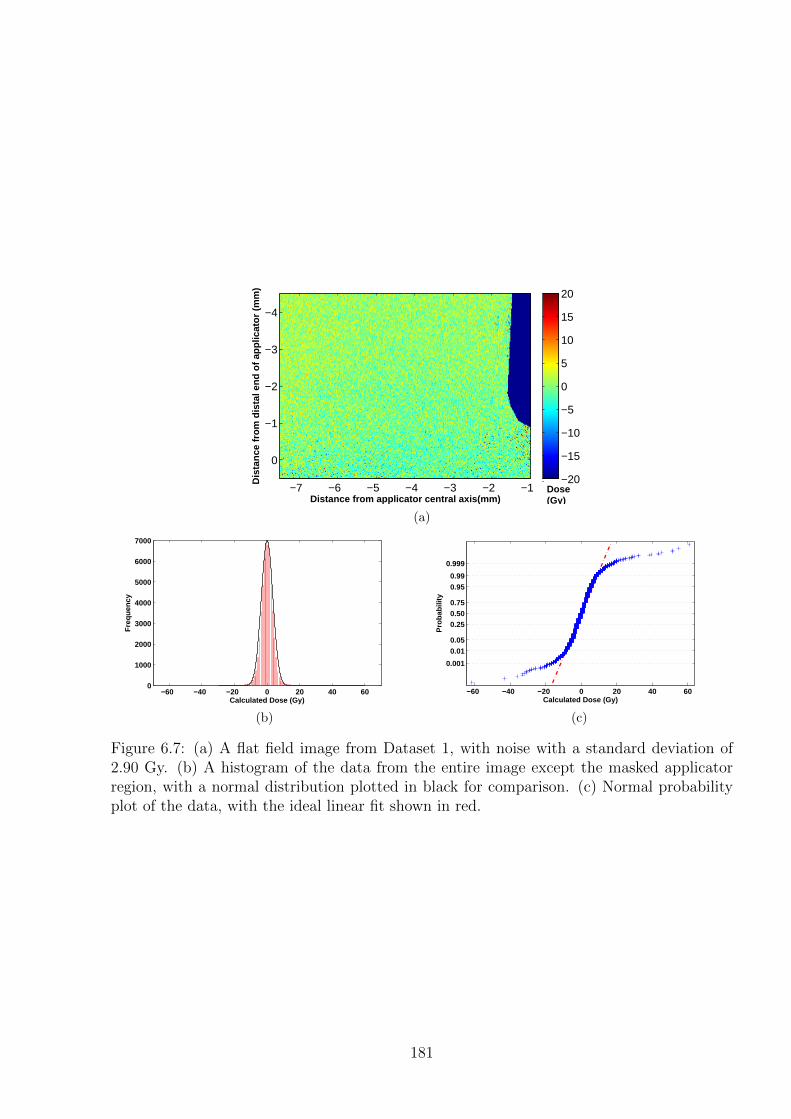
Distance from applicator central axis(mm)
Dis
tan
ce f
rom
dis
tal e
nd
of
app
licat
or
(mm
)
−7 −6 −5 −4 −3 −2 −1
−4
−3
−2
−1
0
−20
−15
−10
−5
0
5
10
15
20
Dose(Gy)
(a)
−60 −40 −20 0 20 40 600
1000
2000
3000
4000
5000
6000
7000
Calculated Dose (Gy)
Fre
quen
cy
(b)
−60 −40 −20 0 20 40 60
0.001
0.010.05
0.250.500.75
0.950.99
0.999
Calculated Dose (Gy)
Pro
babi
lity
(c)
Figure 6.7: (a) A flat field image from Dataset 1, with noise with a standard deviation of2.90 Gy. (b) A histogram of the data from the entire image except the masked applicatorregion, with a normal distribution plotted in black for comparison. (c) Normal probabilityplot of the data, with the ideal linear fit shown in red.
181
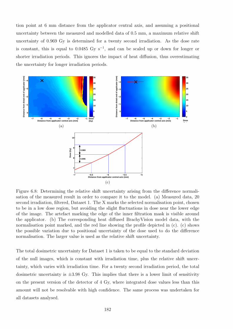
tion point at 6 mm distance from the applicator central axis, and assuming a positional
uncertainty between the measured and modelled data of 0.5 mm, a maximum relative shift
uncertainty of 0.969 Gy is determined for a twenty second irradiation. As the dose rate
is constant, this is equal to 0.0485 Gy s−1, and can be scaled up or down for longer or
shorter irradiation periods. This ignores the impact of heat diffusion, thus overestimating
the uncertainty for longer irradiation periods.
Distance from applicator central axis (mm)
Dis
tanc
e fr
om d
ista
l end
of a
pplic
ator
(m
m)
−7 −6 −5 −4 −3 −2 −1
−4
−3
−2
−1
0
0
5
10
15
20
25
30
35
Dose(Gy)
(a)
Distance from applicator central axis (mm)
Dis
tanc
e fr
om d
ista
l end
of a
pplic
ator
(m
m)
−7 −6 −5 −4 −3 −2 −1
−4
−3
−2
−1
0
0
5
10
15
20
25
30
35
Dose(Gy)
(b)
−7 −6.5 −6 −5.5 −5
7
8
9
10
Distance from applicator central axis (mm)
Dos
e (G
y) 0.969
0.806
(c)
Figure 6.8: Determining the relative shift uncertainty arising from the difference normali-sation of the measured result in order to compare it to the model. (a) Measured data, 20second irradiation, filtered, Dataset 1. The X marks the selected normalisation point, chosento be in a low dose region, but avoiding the slight fluctuations in dose near the lower edgeof the image. The artefact marking the edge of the inner filtration mask is visible aroundthe applicator. (b) The corresponding heat diffused BrachyVision model data, with thenormalisation point marked, and the red line showing the profile depicted in (c). (c) showsthe possible variation due to positional uncertainty of the dose used to do the differencenormalisation. The larger value is used as the relative shift uncertainty.
The total dosimetric uncertainty for Dataset 1 is taken to be equal to the standard deviation
of the null images, which is constant with irradiation time, plus the relative shift uncer-
tainty, which varies with irradiation time. For a twenty second irradiation period, the total
dosimetric uncertainty is ±3.98 Gy. This implies that there is a lower limit of sensitivity
on the present version of the detector of 4 Gy, where integrated dose values less than this
amount will not be resolvable with high confidence. The same process was undertaken for
all datasets analysed.
182
The total uncertainties for Dataset 1 and its comparison to the BrachyVision model consist of
a dosimetric uncertainty on the DHI results of ±3.98 Gy for a 20 s measurement, and ±5.92
Gy for a 60 s measurement, with a positional uncertainty of ±0.33 mm for measurements
where the full width of the source was visible, and ±0.40 mm if it was obscured to some
extent. The corresponding percentage uncertainty depends on which region of the curve is
considered, as the dose difference at each point varies. The model data had a dosimetric
uncertainty of ± 6.25% for a 20 second measurement, with a positional uncertainty of ±0.25
mm. The uncertainty for other datasets were calculated in a similar fashion to that described
for Dataset 1. Dataset 2 had a dosimetric uncertainty on the DHI results of ±3.94 Gy and
±5.88 Gy for the 20 s and 60 s irradiations, respectively.
6.2.4 Direct Comparison to BrachyVision Data
The DHI measured results were compared to the BrachyVision model data, corrected for heat
diffusion, and integrated over a width equivalent to the test cell. Figures 6.9-6.11 present the
results from Dataset 1 after 20 seconds of irradiation. The measured dose distribution image
is shown, along with the corresponding modelled dose distribution for comparison. The one
dimensional dose profiles along different lines from the two dimensional maps are shown
in more detail. The profiles shown were selected to show the dose in both the radial and
axial directions, adjacent and relatively distant to the source position. The top horizontal
profile was chosen to be the closest position to the centre of the source, constrained by the
resolution of the model data to 0.5 mm intervals. The source centre is located 3.75 mm from
the distal end of the applicator, whilst the profile shown is at 3.5 mm. The lower horizontal
profile was selected to be in line with the end of the applicator. The vertical profiles were
chosen as 2 mm and 6 mm away from the centre of the applicator, thus 0.5 mm and 4.5 mm
respectively from the visible edge of the applicator.
From the profiles shown in Figures 6.9(c)-(f), it can be seen that there is excellent agreement
between the dose differences in the measured and modelled data. All points in the image
agree to within the experimental uncertainty values, except for a region to the lower left of
the image, >5 mm from the applicator, where the doses are slightly higher than expected.
As described in Section 6.2.2 the filtering of the measured data means that the dose is under-
reported next to the applicator, which is visible in Figure 6.9(c).
Figures 6.10 and 6.11 inspect the relative dose distributions across the image in more detail.
183
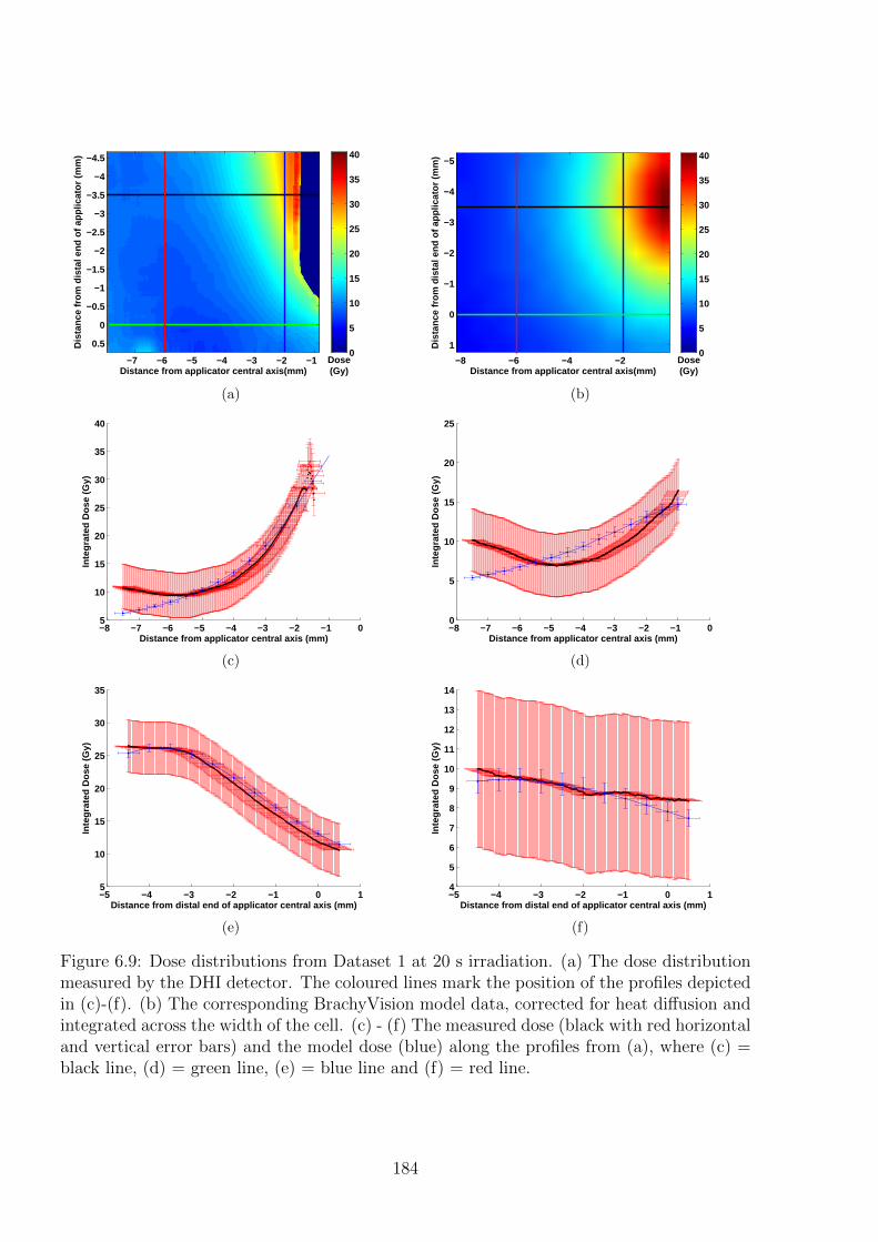
Dis
tanc
e fr
om d
ista
l end
of a
pplic
ator
(m
m)
Distance from applicator central axis(mm)
−7 −6 −5 −4 −3 −2 −1
−4.5
−4
−3.5
−3
−2.5
−2
−1.5
−1
−0.5
0
0.5
Dose(Gy)
0
5
10
15
20
25
30
35
40
(a)
Distance from applicator central axis(mm)
Dis
tanc
e fr
om d
ista
l end
of a
pplic
ator
(m
m)
−8 −6 −4 −2
−5
−4
−3
−2
−1
0
1
Dose(Gy)
0
5
10
15
20
25
30
35
40
(b)
−8 −7 −6 −5 −4 −3 −2 −1 05
10
15
20
25
30
35
40
Inte
grat
ed D
ose
(Gy)
Distance from applicator central axis (mm)
(c)
−8 −7 −6 −5 −4 −3 −2 −1 00
5
10
15
20
25In
tegr
ated
Dos
e (G
y)
Distance from applicator central axis (mm)
(d)
−5 −4 −3 −2 −1 0 15
10
15
20
25
30
35
Inte
grat
ed D
ose
(Gy)
Distance from distal end of applicator central axis (mm)
(e)
−5 −4 −3 −2 −1 0 14
5
6
7
8
9
10
11
12
13
14
Inte
grat
ed D
ose
(Gy)
Distance from distal end of applicator central axis (mm)
(f)
Figure 6.9: Dose distributions from Dataset 1 at 20 s irradiation. (a) The dose distributionmeasured by the DHI detector. The coloured lines mark the position of the profiles depictedin (c)-(f). (b) The corresponding BrachyVision model data, corrected for heat diffusion andintegrated across the width of the cell. (c) - (f) The measured dose (black with red horizontaland vertical error bars) and the model dose (blue) along the profiles from (a), where (c) =black line, (d) = green line, (e) = blue line and (f) = red line.
184
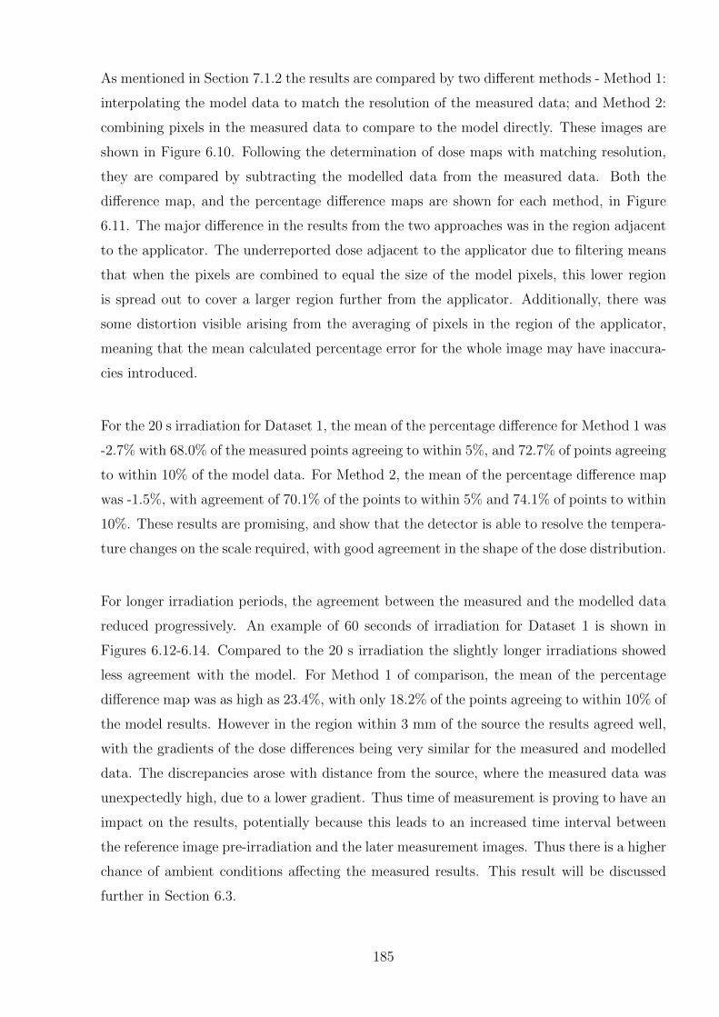
As mentioned in Section 7.1.2 the results are compared by two different methods - Method 1:
interpolating the model data to match the resolution of the measured data; and Method 2:
combining pixels in the measured data to compare to the model directly. These images are
shown in Figure 6.10. Following the determination of dose maps with matching resolution,
they are compared by subtracting the modelled data from the measured data. Both the
difference map, and the percentage difference maps are shown for each method, in Figure
6.11. The major difference in the results from the two approaches was in the region adjacent
to the applicator. The underreported dose adjacent to the applicator due to filtering means
that when the pixels are combined to equal the size of the model pixels, this lower region
is spread out to cover a larger region further from the applicator. Additionally, there was
some distortion visible arising from the averaging of pixels in the region of the applicator,
meaning that the mean calculated percentage error for the whole image may have inaccura-
cies introduced.
For the 20 s irradiation for Dataset 1, the mean of the percentage difference for Method 1 was
-2.7% with 68.0% of the measured points agreeing to within 5%, and 72.7% of points agreeing
to within 10% of the model data. For Method 2, the mean of the percentage difference map
was -1.5%, with agreement of 70.1% of the points to within 5% and 74.1% of points to within
10%. These results are promising, and show that the detector is able to resolve the tempera-
ture changes on the scale required, with good agreement in the shape of the dose distribution.
For longer irradiation periods, the agreement between the measured and the modelled data
reduced progressively. An example of 60 seconds of irradiation for Dataset 1 is shown in
Figures 6.12-6.14. Compared to the 20 s irradiation the slightly longer irradiations showed
less agreement with the model. For Method 1 of comparison, the mean of the percentage
difference map was as high as 23.4%, with only 18.2% of the points agreeing to within 10% of
the model results. However in the region within 3 mm of the source the results agreed well,
with the gradients of the dose differences being very similar for the measured and modelled
data. The discrepancies arose with distance from the source, where the measured data was
unexpectedly high, due to a lower gradient. Thus time of measurement is proving to have an
impact on the results, potentially because this leads to an increased time interval between
the reference image pre-irradiation and the later measurement images. Thus there is a higher
chance of ambient conditions affecting the measured results. This result will be discussed
further in Section 6.3.
185
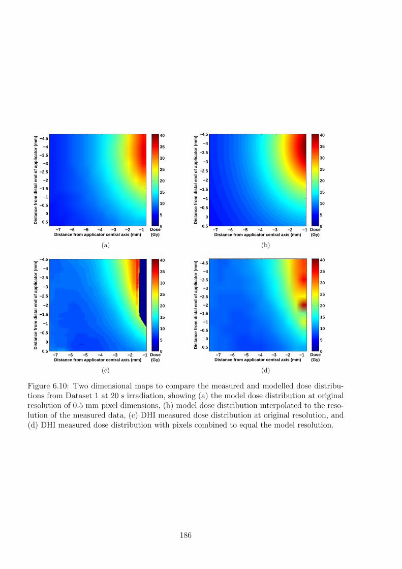
Dis
tanc
e fr
om d
ista
l end
of a
pplic
ator
(m
m)
Distance from applicator central axis (mm)
−7 −6 −5 −4 −3 −2 −1
−4.5
−4
−3.5
−3
−2.5
−2
−1.5
−1
−0.5
0
0.5
Dose(Gy)
0
5
10
15
20
25
30
35
40
(a)
Dis
tanc
e fr
om d
ista
l end
of a
pplic
ator
(m
m)
Distance from applicator central axis (mm)
−7 −6 −5 −4 −3 −2 −1
−4.5
−4
−3.5
−3
−2.5
−2
−1.5
−1
−0.5
0
0.5Dose(Gy)
0
5
10
15
20
25
30
35
40
(b)
Dis
tanc
e fr
om d
ista
l end
of a
pplic
ator
(m
m)
Distance from applicator central axis (mm)
−7 −6 −5 −4 −3 −2 −1
−4.5
−4
−3.5
−3
−2.5
−2
−1.5
−1
−0.5
0
0.5Dose(Gy)
0
5
10
15
20
25
30
35
40
(c)
Dis
tanc
e fr
om d
ista
l end
of a
pplic
ator
(m
m)
Distance from applicator central axis (mm)
−7 −6 −5 −4 −3 −2 −1
−4.5
−4
−3.5
−3
−2.5
−2
−1.5
−1
−0.5
0
0.5
Dose(Gy)
0
5
10
15
20
25
30
35
40
(d)
Figure 6.10: Two dimensional maps to compare the measured and modelled dose distribu-tions from Dataset 1 at 20 s irradiation, showing (a) the model dose distribution at originalresolution of 0.5 mm pixel dimensions, (b) model dose distribution interpolated to the reso-lution of the measured data, (c) DHI measured dose distribution at original resolution, and(d) DHI measured dose distribution with pixels combined to equal the model resolution.
186
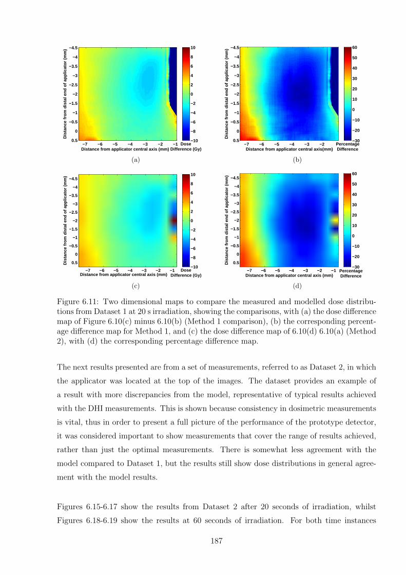
Dis
tanc
e fr
om d
ista
l end
of a
pplic
ator
(m
m)
Distance from applicator central axis (mm)
−7 −6 −5 −4 −3 −2 −1
−4.5
−4
−3.5
−3
−2.5
−2
−1.5
−1
−0.5
0
0.5Dose
Difference (Gy)
−10
−8
−6
−4
−2
0
2
4
6
8
10
(a)
Dis
tanc
e fr
om d
ista
l end
of a
pplic
ator
(m
m)
Distance from applicator central axis(mm)
−7 −6 −5 −4 −3 −2
−4.5
−4
−3.5
−3
−2.5
−2
−1.5
−1
−0.5
0
0.5PercentageDifference
−30
−20
−10
0
10
20
30
40
50
60
(b)
Dis
tanc
e fr
om d
ista
l end
of a
pplic
ator
(m
m)
Distance from applicator central axis (mm)
−7 −6 −5 −4 −3 −2 −1
−4.5
−4
−3.5
−3
−2.5
−2
−1.5
−1
−0.5
0
0.5
DoseDifference (Gy)
−10
−8
−6
−4
−2
0
2
4
6
8
10
(c)
Dis
tanc
e fr
om d
ista
l end
of a
pplic
ator
(m
m)
Distance from applicator central axis (mm)
−7 −6 −5 −4 −3 −2 −1
−4.5
−4
−3.5
−3
−2.5
−2
−1.5
−1
−0.5
0
0.5
PercentageDifference
−30
−20
−10
0
10
20
30
40
50
60
(d)
Figure 6.11: Two dimensional maps to compare the measured and modelled dose distribu-tions from Dataset 1 at 20 s irradiation, showing the comparisons, with (a) the dose differencemap of Figure 6.10(c) minus 6.10(b) (Method 1 comparison), (b) the corresponding percent-age difference map for Method 1, and (c) the dose difference map of 6.10(d) 6.10(a) (Method2), with (d) the corresponding percentage difference map.
The next results presented are from a set of measurements, referred to as Dataset 2, in which
the applicator was located at the top of the images. The dataset provides an example of
a result with more discrepancies from the model, representative of typical results achieved
with the DHI measurements. This is shown because consistency in dosimetric measurements
is vital, thus in order to present a full picture of the performance of the prototype detector,
it was considered important to show measurements that cover the range of results achieved,
rather than just the optimal measurements. There is somewhat less agreement with the
model compared to Dataset 1, but the results still show dose distributions in general agree-
ment with the model results.
Figures 6.15-6.17 show the results from Dataset 2 after 20 seconds of irradiation, whilst
Figures 6.18-6.19 show the results at 60 seconds of irradiation. For both time instances
187
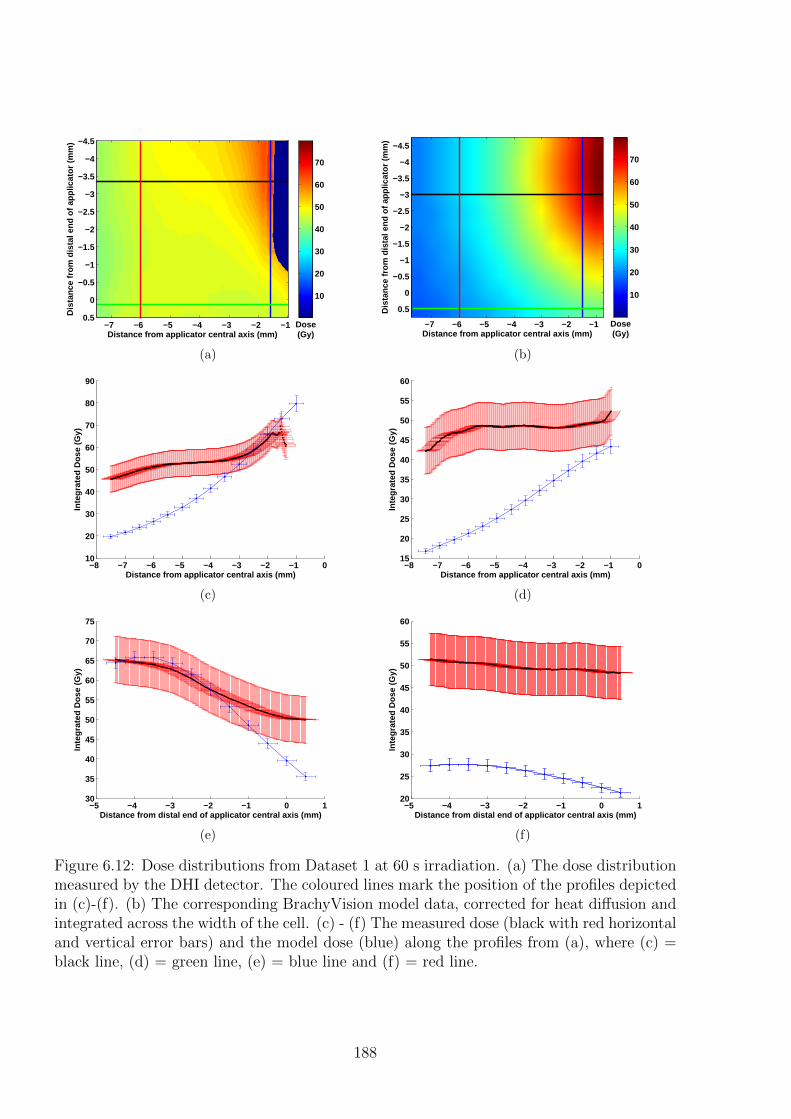
Dis
tanc
e fr
om d
ista
l end
of a
pplic
ator
(m
m)
Distance from applicator central axis (mm)
−7 −6 −5 −4 −3 −2 −1
−4.5
−4
−3.5
−3
−2.5
−2
−1.5
−1
−0.5
0
0.5Dose(Gy)
10
20
30
40
50
60
70
(a)
Dis
tanc
e fr
om d
ista
l end
of a
pplic
ator
(m
m)
Distance from applicator central axis (mm)
−7 −6 −5 −4 −3 −2 −1
−4.5
−4
−3.5
−3
−2.5
−2
−1.5
−1
−0.5
0
0.5
Dose(Gy)
10
20
30
40
50
60
70
(b)
−8 −7 −6 −5 −4 −3 −2 −1 010
20
30
40
50
60
70
80
90
Inte
grat
ed D
ose
(Gy)
Distance from applicator central axis (mm)
(c)
−8 −7 −6 −5 −4 −3 −2 −1 015
20
25
30
35
40
45
50
55
60In
tegr
ated
Dos
e (G
y)
Distance from applicator central axis (mm)
(d)
−5 −4 −3 −2 −1 0 130
35
40
45
50
55
60
65
70
75
Inte
grat
ed D
ose
(Gy)
Distance from distal end of applicator central axis (mm)
(e)
−5 −4 −3 −2 −1 0 120
25
30
35
40
45
50
55
60
Inte
grat
ed D
ose
(Gy)
Distance from distal end of applicator central axis (mm)
(f)
Figure 6.12: Dose distributions from Dataset 1 at 60 s irradiation. (a) The dose distributionmeasured by the DHI detector. The coloured lines mark the position of the profiles depictedin (c)-(f). (b) The corresponding BrachyVision model data, corrected for heat diffusion andintegrated across the width of the cell. (c) - (f) The measured dose (black with red horizontaland vertical error bars) and the model dose (blue) along the profiles from (a), where (c) =black line, (d) = green line, (e) = blue line and (f) = red line.
188
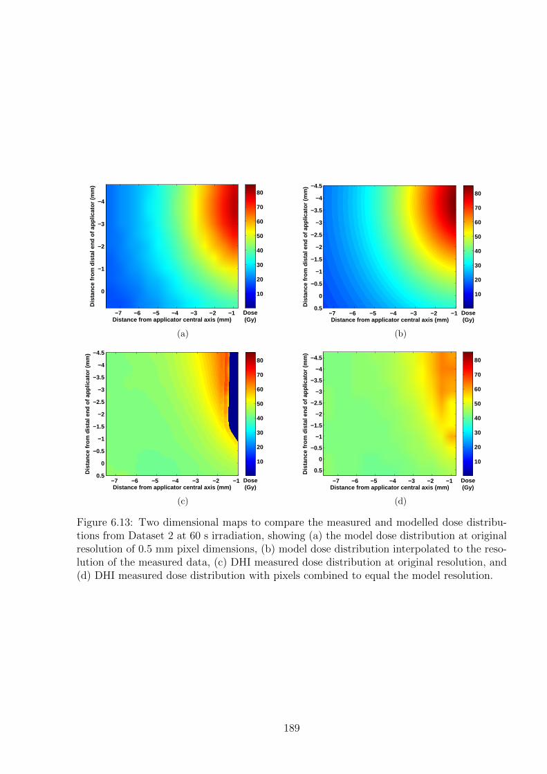
Dis
tanc
e fr
om d
ista
l end
of a
pplic
ator
(m
m)
Distance from applicator central axis (mm)
−7 −6 −5 −4 −3 −2 −1
−4
−3
−2
−1
0
Dose(Gy)
10
20
30
40
50
60
70
80
(a)
Dis
tanc
e fr
om d
ista
l end
of a
pplic
ator
(m
m)
Distance from applicator central axis (mm)
−7 −6 −5 −4 −3 −2 −1
−4.5
−4
−3.5
−3
−2.5
−2
−1.5
−1
−0.5
0
0.5Dose(Gy)
10
20
30
40
50
60
70
80
(b)
Dis
tanc
e fr
om d
ista
l end
of a
pplic
ator
(m
m)
Distance from applicator central axis (mm)
−7 −6 −5 −4 −3 −2 −1
−4.5
−4
−3.5
−3
−2.5
−2
−1.5
−1
−0.5
0
0.5Dose(Gy)
10
20
30
40
50
60
70
80
(c)
Dis
tanc
e fr
om d
ista
l end
of a
pplic
ator
(m
m)
Distance from applicator central axis (mm)
−7 −6 −5 −4 −3 −2 −1
−4.5
−4
−3.5
−3
−2.5
−2
−1.5
−1
−0.5
0
0.5
Dose(Gy)
10
20
30
40
50
60
70
80
(d)
Figure 6.13: Two dimensional maps to compare the measured and modelled dose distribu-tions from Dataset 2 at 60 s irradiation, showing (a) the model dose distribution at originalresolution of 0.5 mm pixel dimensions, (b) model dose distribution interpolated to the reso-lution of the measured data, (c) DHI measured dose distribution at original resolution, and(d) DHI measured dose distribution with pixels combined to equal the model resolution.
189
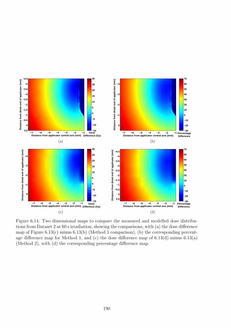
Dis
tanc
e fr
om d
ista
l end
of a
pplic
ator
(m
m)
Distance from applicator central axis (mm)
−7 −6 −5 −4 −3 −2 −1
−4.5
−4
−3.5
−3
−2.5
−2
−1.5
−1
−0.5
0
0.5Dose
Difference (Gy)
−15
−10
−5
0
5
10
15
20
25
30
(a)
Dis
tanc
e fr
om d
ista
l end
of a
pplic
ator
(m
m)
Distance from applicator central axis (mm)
−7 −6 −5 −4 −3 −2 −1
−4
−3
−2
−1
0
PercentageDifference
−30
−20
−10
0
10
20
30
40
50
60
70
(b)
Dis
tanc
e fr
om d
ista
l end
of a
pplic
ator
(m
m)
Distance from applicator central axis (mm)
−7 −6 −5 −4 −3 −2 −1
−4
−3
−2
−1
0
DoseDifference (Gy)
−15
−10
−5
0
5
10
15
20
25
30
(c)
Dis
tanc
e fr
om d
ista
l end
of a
pplic
ator
(m
m)
Distance from applicator central axis (mm)
−7 −6 −5 −4 −3 −2 −1
−4.5
−4
−3.5
−3
−2.5
−2
−1.5
−1
−0.5
0
0.5
PercentageDifference
−30
−20
−10
0
10
20
30
40
50
60
70
(d)
Figure 6.14: Two dimensional maps to compare the measured and modelled dose distribu-tions from Dataset 2 at 60 s irradiation, showing the comparisons, with (a) the dose differencemap of Figure 6.13(c) minus 6.13(b) (Method 1 comparison), (b) the corresponding percent-age difference map for Method 1, and (c) the dose difference map of 6.13(d) minus 6.13(a)(Method 2), with (d) the corresponding percentage difference map.
190
the dose difference in the region close to the applicator agrees reasonably well to the model
values. However it is clear that there is some distortion in the lower part of the images
at increasing distance from the applicator, which is clearly visible on the dose map. In
particular, Figure 6.15(e) clearly shows a distortion in the dose attenuation curve. The
distortion results in the dose values measured by DHI being lower than expected from the
model. For the 20 second measurement only 57% of the points agree to within 10% of the
model, with discrepancies mostly beyond a 2-3 mm radius of the applicator. It should be
noted that the dose values are small in this region, thus a high percentage uncertainty is
actually a low absolute uncertainty. This effect worsens with time, as seen in the results
from the 60 s irradiation, shown in Figures 6.18 and 6.19. This disagreement is surmised to
be due to variations in the ambient conditions, and possibly the effects of heat convection
which have not yet been incorporated into the model. This is discussed further in Section 6.3.
In Figure 6.15(a) it appears that there is some asymmetry of the dose distribution around
the visible end of the applicator, with a slightly higher dose occurring on the left hand side
of the image adjacent to the applicator. It is possible that the source was not perfectly
centred inside the applicator tube during this particular measurement. This detection of
such a misalignment serves to underscore the need to experimentally validate modelled dose
distributions. The ability to detect this to high spatial resolution is a useful outcome of the
DHI measurements, although this is limited to situations where the error has some compo-
nent in a direction perpendicular to the laser path.
It is obvious from Figures 6.16(d), 6.17(c), and 6.17(d), that Method 2 for comparing the
two dose distributions, which involved the reduction of the measured resolution to match
the model, is not appropriate in all situations. The way the applicator protrudes into the
image and is masked when the data is filtered, means that there are a large number of pix-
els where the average dose cannot be determined to any degree of accuracy. This means
that the comparison doses will result in an artificially lower agreement than using Method
1, and much information about the agreement of the measured and modelled data is lost,
particularly in the important region in the vicinity of the source. Thus despite the obvious
shortcomings of interpolating the model data, this method is preferred for the comparisons.
191
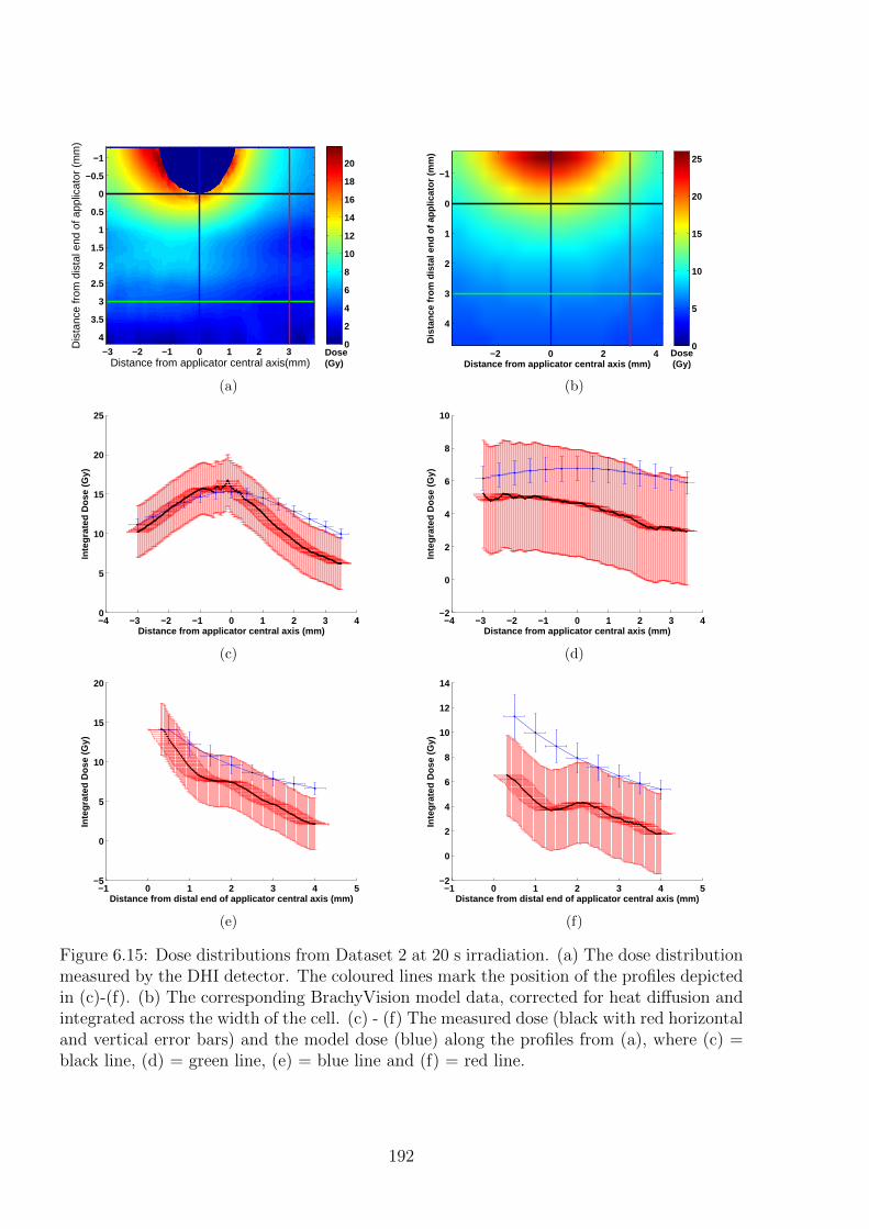
Dis
tanc
e fr
om d
ista
l end
of a
pplic
ator
(m
m)
Distance from applicator central axis(mm)
−3 −2 −1 0 1 2 3
−1
−0.5
0
0.5
1
1.5
2
2.5
3
3.5
40
2
4
6
8
10
12
14
16
18
20
Dose(Gy)
(a)
Dis
tanc
e fr
om d
ista
l end
of a
pplic
ator
(m
m)
Distance from applicator central axis (mm)
−2 0 2 4
−1
0
1
2
3
4
Dose(Gy)
0
5
10
15
20
25
(b)
−4 −3 −2 −1 0 1 2 3 40
5
10
15
20
25
Inte
grat
ed D
ose
(Gy)
Distance from applicator central axis (mm)
(c)
−4 −3 −2 −1 0 1 2 3 4−2
0
2
4
6
8
10In
tegr
ated
Dos
e (G
y)
Distance from applicator central axis (mm)
(d)
−1 0 1 2 3 4 5−5
0
5
10
15
20
Inte
grat
ed D
ose
(Gy)
Distance from distal end of applicator central axis (mm)
(e)
−1 0 1 2 3 4 5−2
0
2
4
6
8
10
12
14
Inte
grat
ed D
ose
(Gy)
Distance from distal end of applicator central axis (mm)
(f)
Figure 6.15: Dose distributions from Dataset 2 at 20 s irradiation. (a) The dose distributionmeasured by the DHI detector. The coloured lines mark the position of the profiles depictedin (c)-(f). (b) The corresponding BrachyVision model data, corrected for heat diffusion andintegrated across the width of the cell. (c) - (f) The measured dose (black with red horizontaland vertical error bars) and the model dose (blue) along the profiles from (a), where (c) =black line, (d) = green line, (e) = blue line and (f) = red line.
192
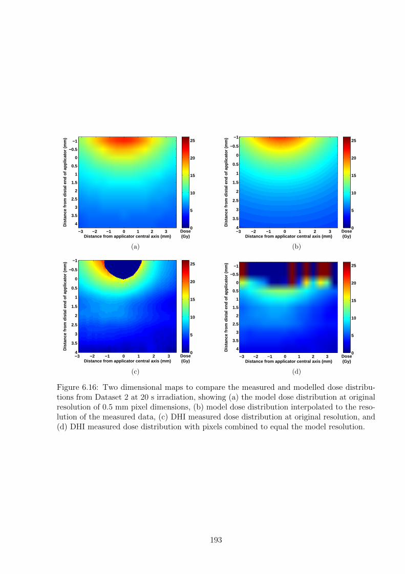
Dis
tanc
e fr
om d
ista
l end
of a
pplic
ator
(m
m)
Distance from applicator central axis (mm)
−3 −2 −1 0 1 2 3
−1
−0.5
0
0.5
1
1.5
2
2.5
3
3.5
4
Dose(Gy)
0
5
10
15
20
25
(a)
Dis
tanc
e fr
om d
ista
l end
of a
pplic
ator
(m
m)
Distance from applicator central axis (mm)
−3 −2 −1 0 1 2 3
−1
−0.5
0
0.5
1
1.5
2
2.5
3
3.5
4Dose(Gy)
0
5
10
15
20
25
(b)
Dis
tanc
e fr
om d
ista
l end
of a
pplic
ator
(m
m)
Distance from applicator central axis (mm)
−3 −2 −1 0 1 2 3
−1
−0.5
0
0.5
1
1.5
2
2.5
3
3.5
4Dose(Gy)
0
5
10
15
20
25
(c)
Dis
tanc
e fr
om d
ista
l end
of a
pplic
ator
(m
m)
Distance from applicator central axis (mm)
−3 −2 −1 0 1 2 3
−1
−0.5
0
0.5
1
1.5
2
2.5
3
3.5
4
Dose(Gy)
0
5
10
15
20
25
(d)
Figure 6.16: Two dimensional maps to compare the measured and modelled dose distribu-tions from Dataset 2 at 20 s irradiation, showing (a) the model dose distribution at originalresolution of 0.5 mm pixel dimensions, (b) model dose distribution interpolated to the reso-lution of the measured data, (c) DHI measured dose distribution at original resolution, and(d) DHI measured dose distribution with pixels combined to equal the model resolution.
193
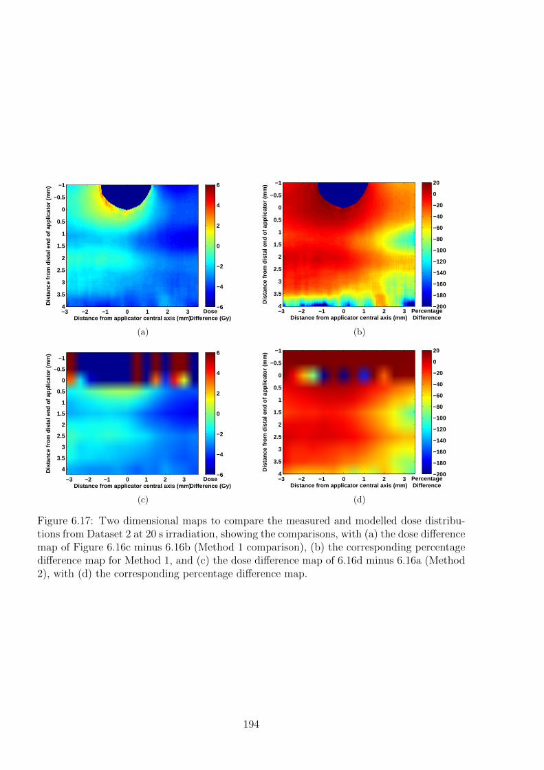
Dis
tanc
e fr
om d
ista
l end
of a
pplic
ator
(m
m)
Distance from applicator central axis (mm)
−3 −2 −1 0 1 2 3
−1
−0.5
0
0.5
1
1.5
2
2.5
3
3.5
4Dose
Difference (Gy)
−6
−4
−2
0
2
4
6
(a)
Dis
tanc
e fr
om d
ista
l end
of a
pplic
ator
(m
m)
Distance from applicator central axis (mm)
−3 −2 −1 0 1 2 3
−1
−0.5
0
0.5
1
1.5
2
2.5
3
3.5
4PercentageDifference
−200
−180
−160
−140
−120
−100
−80
−60
−40
−20
0
20
(b)
Dis
tanc
e fr
om d
ista
l end
of a
pplic
ator
(m
m)
Distance from applicator central axis (mm)
−3 −2 −1 0 1 2 3
−1
−0.5
0
0.5
1
1.5
2
2.5
3
3.5
4
DoseDifference (Gy)
−6
−4
−2
0
2
4
6
(c)
Dis
tanc
e fr
om d
ista
l end
of a
pplic
ator
(m
m)
Distance from applicator central axis (mm)
−3 −2 −1 0 1 2 3
−1
−0.5
0
0.5
1
1.5
2
2.5
3
3.5
4PercentageDifference
−200
−180
−160
−140
−120
−100
−80
−60
−40
−20
0
20
(d)
Figure 6.17: Two dimensional maps to compare the measured and modelled dose distribu-tions from Dataset 2 at 20 s irradiation, showing the comparisons, with (a) the dose differencemap of Figure 6.16c minus 6.16b (Method 1 comparison), (b) the corresponding percentagedifference map for Method 1, and (c) the dose difference map of 6.16d minus 6.16a (Method2), with (d) the corresponding percentage difference map.
194
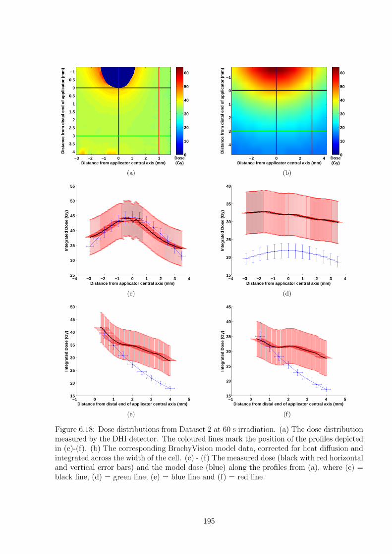
Dis
tanc
e fr
om d
ista
l end
of a
pplic
ator
(m
m)
Distance from applicator central axis (mm)
−3 −2 −1 0 1 2 3
−1
−0.5
0
0.5
1
1.5
2
2.5
3
3.5
4Dose(Gy)
0
10
20
30
40
50
60
(a)
Dis
tanc
e fr
om d
ista
l end
of a
pplic
ator
(m
m)
Distance from applicator central axis (mm)
−2 0 2 4
−1
0
1
2
3
4
Dose(Gy)
0
10
20
30
40
50
60
(b)
−4 −3 −2 −1 0 1 2 3 425
30
35
40
45
50
55
Inte
grat
ed D
ose
(Gy)
Distance from applicator central axis (mm)
(c)
−4 −3 −2 −1 0 1 2 3 415
20
25
30
35
40
Inte
grat
ed D
ose
(Gy)
Distance from applicator central axis (mm)
(d)
−1 0 1 2 3 4 515
20
25
30
35
40
45
50
Inte
grat
ed D
ose
(Gy)
Distance from distal end of applicator central axis (mm)
(e)
−1 0 1 2 3 4 515
20
25
30
35
40
45
Inte
grat
ed D
ose
(Gy)
Distance from distal end of applicator central axis (mm)
(f)
Figure 6.18: Dose distributions from Dataset 2 at 60 s irradiation. (a) The dose distributionmeasured by the DHI detector. The coloured lines mark the position of the profiles depictedin (c)-(f). (b) The corresponding BrachyVision model data, corrected for heat diffusion andintegrated across the width of the cell. (c) - (f) The measured dose (black with red horizontaland vertical error bars) and the model dose (blue) along the profiles from (a), where (c) =black line, (d) = green line, (e) = blue line and (f) = red line.
195
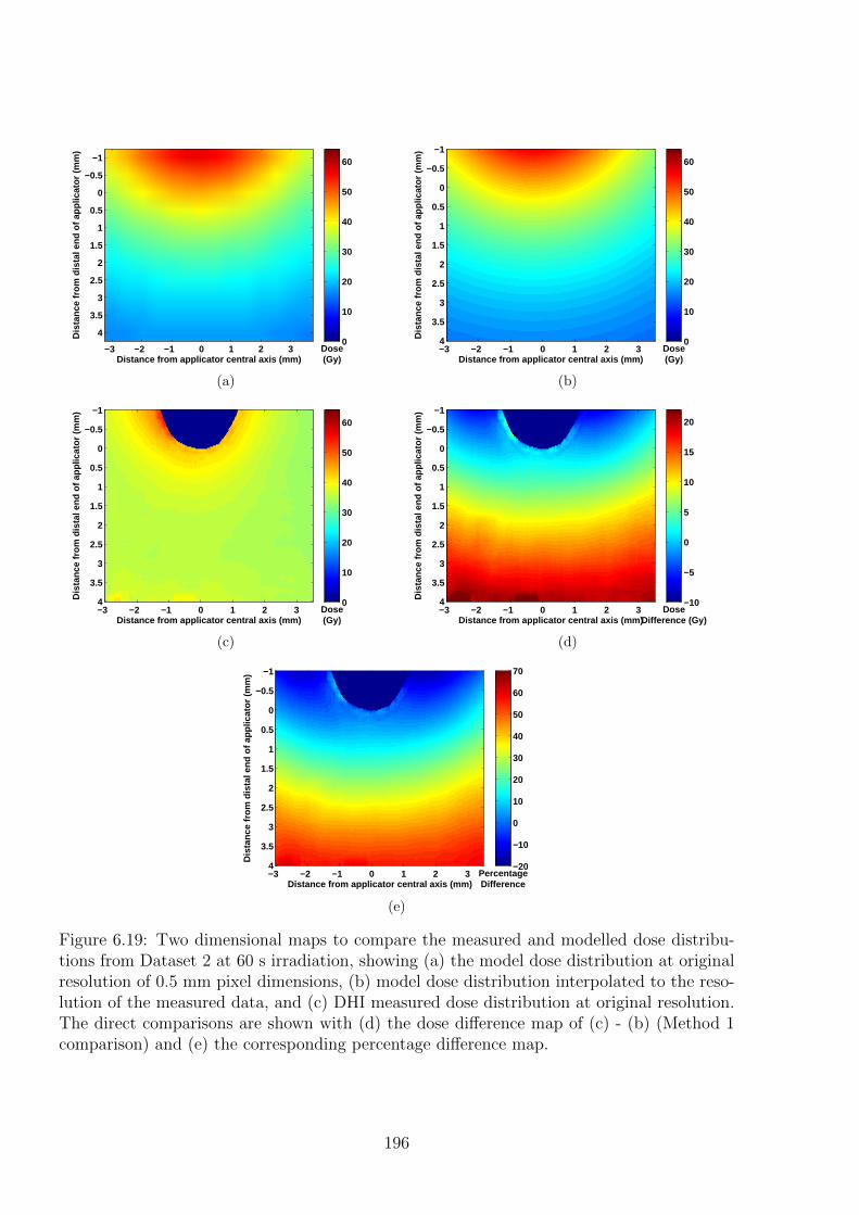
Dis
tanc
e fr
om d
ista
l end
of a
pplic
ator
(m
m)
Distance from applicator central axis (mm)
−3 −2 −1 0 1 2 3
−1
−0.5
0
0.5
1
1.5
2
2.5
3
3.5
4
Dose(Gy)
0
10
20
30
40
50
60
(a)
Dis
tanc
e fr
om d
ista
l end
of a
pplic
ator
(m
m)
Distance from applicator central axis (mm)
−3 −2 −1 0 1 2 3
−1
−0.5
0
0.5
1
1.5
2
2.5
3
3.5
4Dose(Gy)
0
10
20
30
40
50
60
(b)
Dis
tanc
e fr
om d
ista
l end
of a
pplic
ator
(m
m)
Distance from applicator central axis (mm)
−3 −2 −1 0 1 2 3
−1
−0.5
0
0.5
1
1.5
2
2.5
3
3.5
4Dose(Gy)
0
10
20
30
40
50
60
(c)
Dis
tanc
e fr
om d
ista
l end
of a
pplic
ator
(m
m)
Distance from applicator central axis (mm)
−3 −2 −1 0 1 2 3
−1
−0.5
0
0.5
1
1.5
2
2.5
3
3.5
4Dose
Difference (Gy)
−10
−5
0
5
10
15
20
(d)
Dis
tanc
e fr
om d
ista
l end
of a
pplic
ator
(m
m)
Distance from applicator central axis (mm)
−3 −2 −1 0 1 2 3
−1
−0.5
0
0.5
1
1.5
2
2.5
3
3.5
4PercentageDifference
−20
−10
0
10
20
30
40
50
60
70
(e)
Figure 6.19: Two dimensional maps to compare the measured and modelled dose distribu-tions from Dataset 2 at 60 s irradiation, showing (a) the model dose distribution at originalresolution of 0.5 mm pixel dimensions, (b) model dose distribution interpolated to the reso-lution of the measured data, and (c) DHI measured dose distribution at original resolution.The direct comparisons are shown with (d) the dose difference map of (c) - (b) (Method 1comparison) and (e) the corresponding percentage difference map.
196
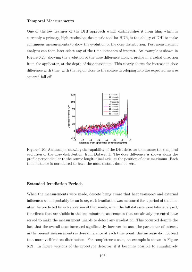
Temporal Measurements
One of the key features of the DHI approach which distinguishes it from film, which is
currently a primary, high resolution, dosimetric tool for HDR, is the ability of DHI to make
continuous measurements to show the evolution of the dose distribution. Post measurement
analysis can then later select any of the time instances of interest. An example is shown in
Figure 6.20, showing the evolution of the dose difference along a profile in a radial direction
from the applicator, at the depth of dose maximum. This clearly shows the increase in dose
difference with time, with the region close to the source developing into the expected inverse
squared fall off.
−8 −7 −6 −5 −4 −3 −2 −1−25
0
25
50
75
100
125
Dos
e D
iffer
ence
(G
y)
Distance from applicator central axis(mm)
0 seconds10 seconds20 seconds 30 seconds40 seconds50 seconds60 seconds70 seconds80 seconds
Figure 6.20: An example showing the capability of the DHI detector to measure the temporalevolution of the dose distribution, from Dataset 1. The dose difference is shown along theprofile perpendicular to the source longitudinal axis, at the position of dose maximum. Eachtime instance is normalised to have the most distant dose be zero.
Extended Irradiation Periods
When the measurements were made, despite being aware that heat transport and external
influences would probably be an issue, each irradiation was measured for a period of ten min-
utes. As predicted by extrapolation of the trends, when the full datasets were later analysed,
the effects that are visible in the one minute measurements that are already presented have
served to make the measurement unable to detect any irradiation. This occurred despite the
fact that the overall dose increased significantly, however because the parameter of interest
in the present measurements is dose difference at each time point, this increase did not lead
to a more visible dose distribution. For completeness sake, an example is shown in Figure
6.21. In future versions of the prototype detector, if it becomes possible to cumulatively
197
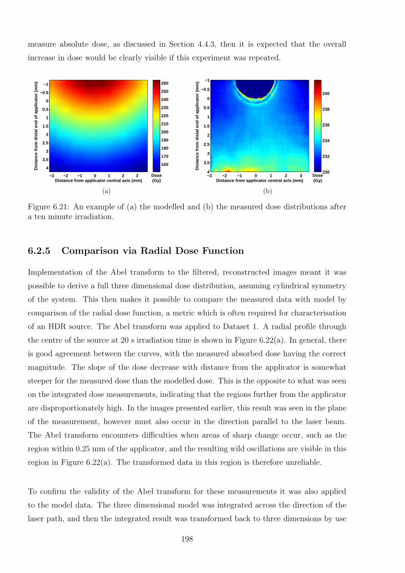
measure absolute dose, as discussed in Section 4.4.3, then it is expected that the overall
increase in dose would be clearly visible if this experiment was repeated.
Dis
tanc
e fr
om d
ista
l end
of a
pplic
ator
(m
m)
Distance from applicator central axis (mm)
−3 −2 −1 0 1 2 3
−1
−0.5
0
0.5
1
1.5
2
2.5
3
3.5
4
Dose(Gy)
160
170
180
190
200
210
220
230
240
250
260
(a)D
ista
nce
from
dis
tal e
nd o
f app
licat
or (
mm
)
Distance from applicator central axis (mm)
−3 −2 −1 0 1 2 3
−1
−0.5
0
0.5
1
1.5
2
2.5
3
3.5
4Dose(Gy)
230
232
234
236
238
240
(b)
Figure 6.21: An example of (a) the modelled and (b) the measured dose distributions aftera ten minute irradiation.
6.2.5 Comparison via Radial Dose Function
Implementation of the Abel transform to the filtered, reconstructed images meant it was
possible to derive a full three dimensional dose distribution, assuming cylindrical symmetry
of the system. This then makes it possible to compare the measured data with model by
comparison of the radial dose function, a metric which is often required for characterisation
of an HDR source. The Abel transform was applied to Dataset 1. A radial profile through
the centre of the source at 20 s irradiation time is shown in Figure 6.22(a). In general, there
is good agreement between the curves, with the measured absorbed dose having the correct
magnitude. The slope of the dose decrease with distance from the applicator is somewhat
steeper for the measured dose than the modelled dose. This is the opposite to what was seen
on the integrated dose measurements, indicating that the regions further from the applicator
are disproportionately high. In the images presented earlier, this result was seen in the plane
of the measurement, however must also occur in the direction parallel to the laser beam.
The Abel transform encounters difficulties when areas of sharp change occur, such as the
region within 0.25 mm of the applicator, and the resulting wild oscillations are visible in this
region in Figure 6.22(a). The transformed data in this region is therefore unreliable.
To confirm the validity of the Abel transform for these measurements it was also applied
to the model data. The three dimensional model was integrated across the direction of the
laser path, and then the integrated result was transformed back to three dimensions by use
198
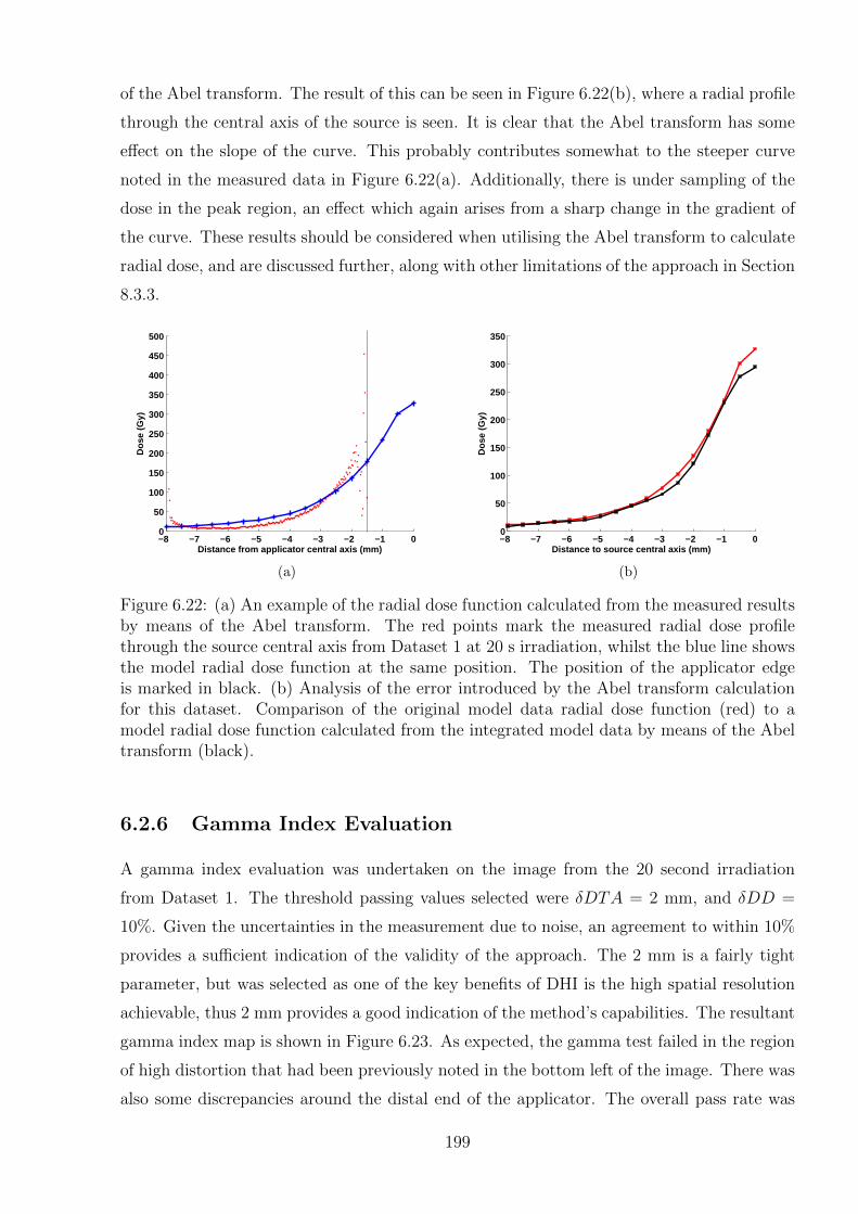
of the Abel transform. The result of this can be seen in Figure 6.22(b), where a radial profile
through the central axis of the source is seen. It is clear that the Abel transform has some
effect on the slope of the curve. This probably contributes somewhat to the steeper curve
noted in the measured data in Figure 6.22(a). Additionally, there is under sampling of the
dose in the peak region, an effect which again arises from a sharp change in the gradient of
the curve. These results should be considered when utilising the Abel transform to calculate
radial dose, and are discussed further, along with other limitations of the approach in Section
8.3.3.
−8 −7 −6 −5 −4 −3 −2 −1 00
50
100
150
200
250
300
350
400
450
500
Distance from applicator central axis (mm)
Dos
e (G
y)
(a)
−8 −7 −6 −5 −4 −3 −2 −1 00
50
100
150
200
250
300
350
Distance to source central axis (mm)
Dos
e (G
y)
(b)
Figure 6.22: (a) An example of the radial dose function calculated from the measured resultsby means of the Abel transform. The red points mark the measured radial dose profilethrough the source central axis from Dataset 1 at 20 s irradiation, whilst the blue line showsthe model radial dose function at the same position. The position of the applicator edgeis marked in black. (b) Analysis of the error introduced by the Abel transform calculationfor this dataset. Comparison of the original model data radial dose function (red) to amodel radial dose function calculated from the integrated model data by means of the Abeltransform (black).
6.2.6 Gamma Index Evaluation
A gamma index evaluation was undertaken on the image from the 20 second irradiation
from Dataset 1. The threshold passing values selected were δDTA = 2 mm, and δDD =
10%. Given the uncertainties in the measurement due to noise, an agreement to within 10%
provides a sufficient indication of the validity of the approach. The 2 mm is a fairly tight
parameter, but was selected as one of the key benefits of DHI is the high spatial resolution
achievable, thus 2 mm provides a good indication of the method’s capabilities. The resultant
gamma index map is shown in Figure 6.23. As expected, the gamma test failed in the region
of high distortion that had been previously noted in the bottom left of the image. There was
also some discrepancies around the distal end of the applicator. The overall pass rate was
199
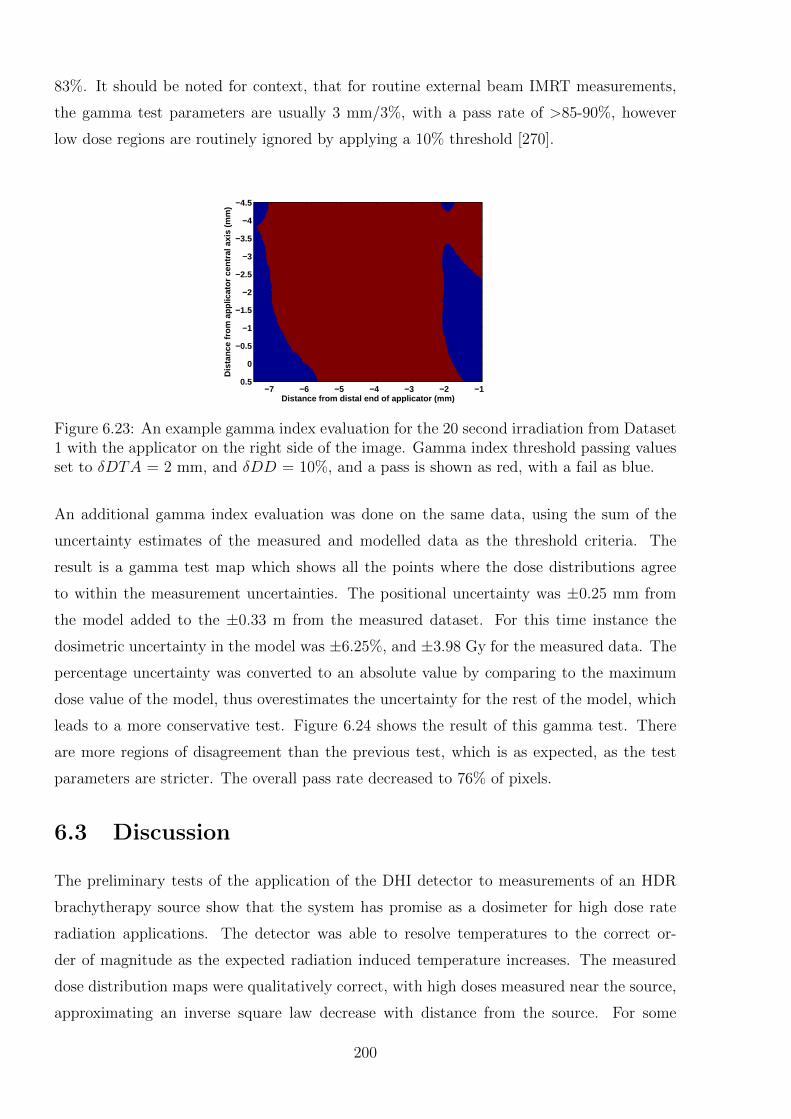
83%. It should be noted for context, that for routine external beam IMRT measurements,
the gamma test parameters are usually 3 mm/3%, with a pass rate of >85-90%, however
low dose regions are routinely ignored by applying a 10% threshold [270].
Distance from distal end of applicator (mm)
Dis
tanc
e fr
om a
pplic
ator
cen
tral
axi
s (m
m)
−7 −6 −5 −4 −3 −2 −1
−4.5
−4
−3.5
−3
−2.5
−2
−1.5
−1
−0.5
0
0.5
Figure 6.23: An example gamma index evaluation for the 20 second irradiation from Dataset1 with the applicator on the right side of the image. Gamma index threshold passing valuesset to δDTA = 2 mm, and δDD = 10%, and a pass is shown as red, with a fail as blue.
An additional gamma index evaluation was done on the same data, using the sum of the
uncertainty estimates of the measured and modelled data as the threshold criteria. The
result is a gamma test map which shows all the points where the dose distributions agree
to within the measurement uncertainties. The positional uncertainty was ±0.25 mm from
the model added to the ±0.33 m from the measured dataset. For this time instance the
dosimetric uncertainty in the model was ±6.25%, and ±3.98 Gy for the measured data. The
percentage uncertainty was converted to an absolute value by comparing to the maximum
dose value of the model, thus overestimates the uncertainty for the rest of the model, which
leads to a more conservative test. Figure 6.24 shows the result of this gamma test. There
are more regions of disagreement than the previous test, which is as expected, as the test
parameters are stricter. The overall pass rate decreased to 76% of pixels.
6.3 Discussion
The preliminary tests of the application of the DHI detector to measurements of an HDR
brachytherapy source show that the system has promise as a dosimeter for high dose rate
radiation applications. The detector was able to resolve temperatures to the correct or-
der of magnitude as the expected radiation induced temperature increases. The measured
dose distribution maps were qualitatively correct, with high doses measured near the source,
approximating an inverse square law decrease with distance from the source. For some
200
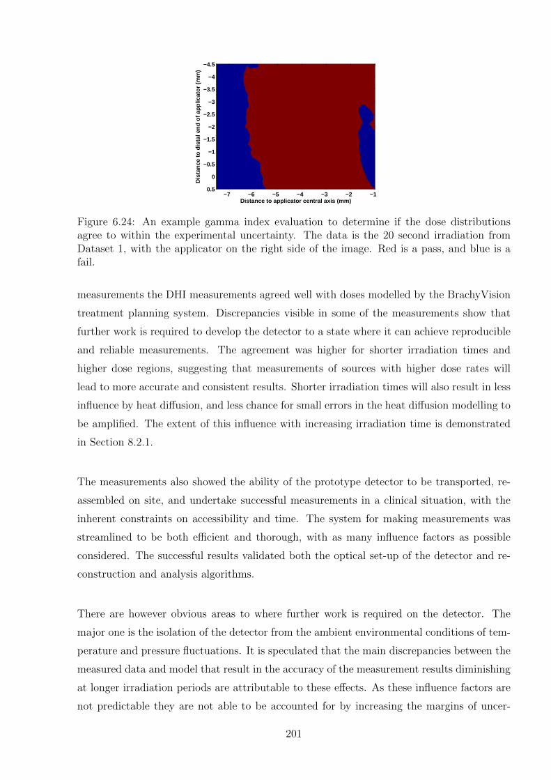
Distance to applicator central axis (mm)D
ista
nce
to d
ista
l end
of a
pplic
ator
(m
m)
−7 −6 −5 −4 −3 −2 −1
−4.5
−4
−3.5
−3
−2.5
−2
−1.5
−1
−0.5
0
0.5
Figure 6.24: An example gamma index evaluation to determine if the dose distributionsagree to within the experimental uncertainty. The data is the 20 second irradiation fromDataset 1, with the applicator on the right side of the image. Red is a pass, and blue is afail.
measurements the DHI measurements agreed well with doses modelled by the BrachyVision
treatment planning system. Discrepancies visible in some of the measurements show that
further work is required to develop the detector to a state where it can achieve reproducible
and reliable measurements. The agreement was higher for shorter irradiation times and
higher dose regions, suggesting that measurements of sources with higher dose rates will
lead to more accurate and consistent results. Shorter irradiation times will also result in less
influence by heat diffusion, and less chance for small errors in the heat diffusion modelling to
be amplified. The extent of this influence with increasing irradiation time is demonstrated
in Section 8.2.1.
The measurements also showed the ability of the prototype detector to be transported, re-
assembled on site, and undertake successful measurements in a clinical situation, with the
inherent constraints on accessibility and time. The system for making measurements was
streamlined to be both efficient and thorough, with as many influence factors as possible
considered. The successful results validated both the optical set-up of the detector and re-
construction and analysis algorithms.
There are however obvious areas to where further work is required on the detector. The
major one is the isolation of the detector from the ambient environmental conditions of tem-
perature and pressure fluctuations. It is speculated that the main discrepancies between the
measured data and model that result in the accuracy of the measurement results diminishing
at longer irradiation periods are attributable to these effects. As these influence factors are
not predictable they are not able to be accounted for by increasing the margins of uncer-
201
tainty. Indeed, the variation in the results that would be induced by incorporating it into the
uncertainties would result in a loss of profile shape information. Chapter 8 includes a more
thorough analysis of the uncertainty budgets, discusses the use of the radial dose function
and gamma index as evaluation metrics, and discusses in further details the impact of heat
transport.
6.3.1 Potential for Contribution to HDR Brachytherapy Dosime-try
The primary aim of these measurements was validation of the detector rather than demon-
strating its use for accurate HDR dosimetry. However, some consideration was given to the
potential of DHI to contribute to the limitations in the present array of HDR dosimetry op-
tions that were introduced in section 2.3.1. A full understanding of the potential of DHI in
this field will require improvements to the detector, which are recommended in Section 8.4,
however based on the preliminary results some indication of a more developed DHI detectors
usefulness can be conjectured.
The key area of focus where DHI may be able to contribute is in the field of near source
dosimetry, where measurements down to 1 mm spatial resolution are required. The prelimi-
nary measurements with the prototype detector have achieved a resolution of approximately
0.03 mm or better, with potential for improvement. This is a very high spatial resolution
compared to most alternative dosimetry options, which is only surpassed by the spatial res-
olution achievable using film. The measurement shown in Figure 6.13 where some slight
asymmetry in the source positioning is visible indicates the potential for DHI to be used to
validate various parameters of Monte Carlo models in the near source region.
The estimated uncertainties in the present measurements are higher than those achievable
by alternative approaches such as measurements using film or gel dosimetry. The uncertain-
ties assumed in this work are discussed further in Section 8.3 and it is expected that with
careful experimental design and implementation these values will be able to be much reduced.
The fact that DHI dosimetry is directly measuring the absorbed dose to water, and has
no inherent energy or dose dependence is a favourable aspect in comparison to measure-
ments using most other detector types. It is feasible therefore that a future iteration of the
detector could contribute to the field of absolute and standards dosimetry for HDR, in a sim-
202
ilar fashion to the development of the ultrasound thermometry by the NIST laboratories [82].
The major limitation at this stage is the lack of a sufficient method to account for heat
diffusion directly in the experimental results. At this stage all measurements are relevant
only in terms of comparison to a heat diffused model of the source, integrated across the
width of the test cell. With continued work on the inverse modelling of heat diffusion that
was suggested in Chapter 5, this may be able to be overcome, allowing a more versatile use
of DHI for HDR brachytherapy measurements.
6.4 Concluding Remarks
This chapter covered the application of the prototype DHI detector to the dosimetry of
an HDR brachytherapy source, in measurements intended to provide a proof-of-principle of
the DHI approach. A series of measurements were taken, with results from two of them
fully analysed and presented in this chapter. The measurements presented were chosen in
order to provide a fair indication of the capabilities and limitations of the detector. A full
analysis of the measurement uncertainties was included, with all areas of potential error
considered and if appropriate incorporated into the results. The process of filtering the
data to reduce the excess noise in the images was described, including means of reducing
the dose underestimation near the source due to volume averaging effects. The data was
compared to a model produced by the commercial treatment planning system BrachyVision.
Some of the measurements were in relatively good agreement with the model, within the
range of experimental uncertainties. Other measurements displayed clear distortions in the
recorded images, and further experimental work will be required to reduce the impact of
these effects. Overall, the results were promising, with the measured dose differences for
irradiations of limited duration clearly displaying a dose distribution similar to that predicted
by the model, however with some areas of discrepancy. Improvements to the experimental
process are suggested in Chapter 8 which aim to increase the accuracy and reproducibility
of the measurements in order to improve the quantitative agreement of the DHI results to
the model. The next chapter presents the results from application of the DHI detector to
the dosimetry of a small field proton beam.
203

204
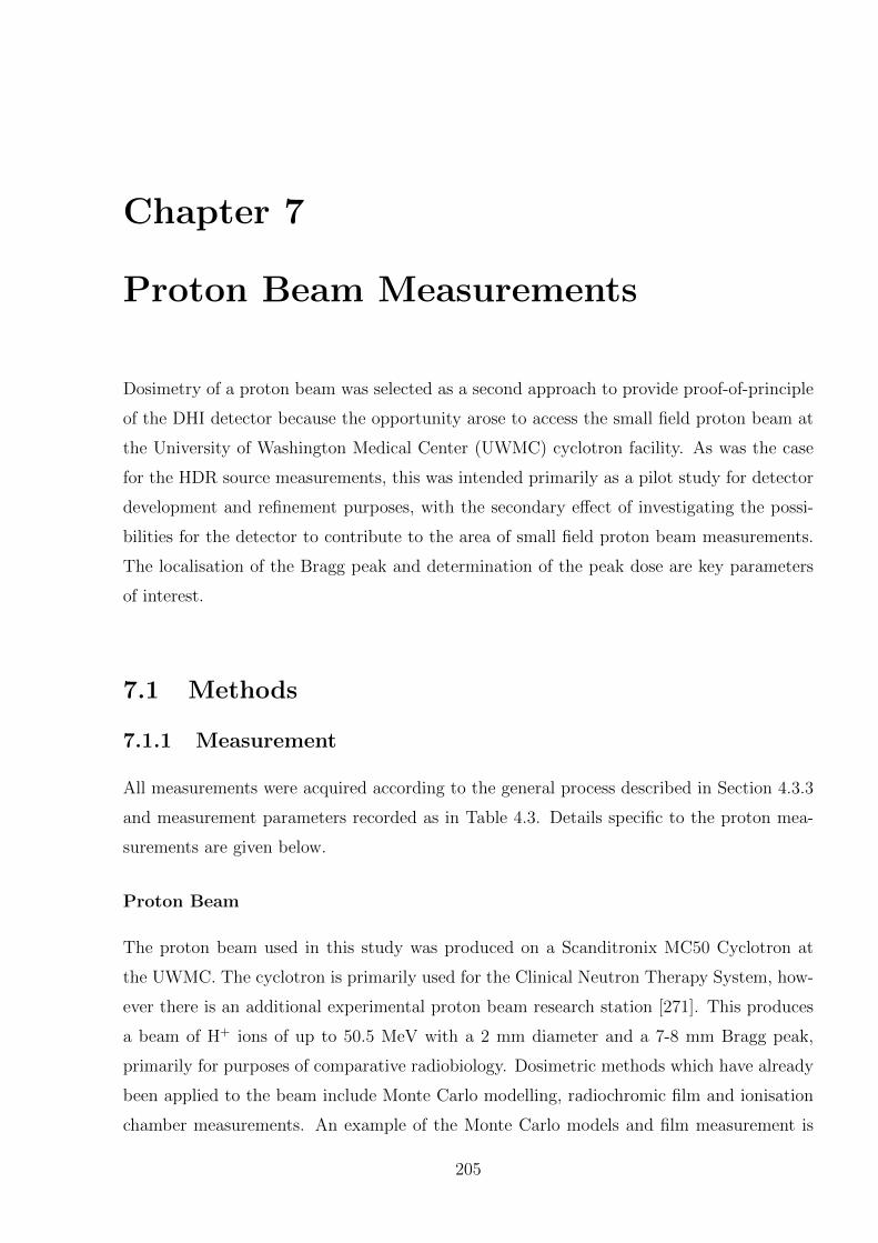
Chapter 7
Proton Beam Measurements
Dosimetry of a proton beam was selected as a second approach to provide proof-of-principle
of the DHI detector because the opportunity arose to access the small field proton beam at
the University of Washington Medical Center (UWMC) cyclotron facility. As was the case
for the HDR source measurements, this was intended primarily as a pilot study for detector
development and refinement purposes, with the secondary effect of investigating the possi-
bilities for the detector to contribute to the area of small field proton beam measurements.
The localisation of the Bragg peak and determination of the peak dose are key parameters
of interest.
7.1 Methods
7.1.1 Measurement
All measurements were acquired according to the general process described in Section 4.3.3
and measurement parameters recorded as in Table 4.3. Details specific to the proton mea-
surements are given below.
Proton Beam
The proton beam used in this study was produced on a Scanditronix MC50 Cyclotron at
the UWMC. The cyclotron is primarily used for the Clinical Neutron Therapy System, how-
ever there is an additional experimental proton beam research station [271]. This produces
a beam of H+ ions of up to 50.5 MeV with a 2 mm diameter and a 7-8 mm Bragg peak,
primarily for purposes of comparative radiobiology. Dosimetric methods which have already
been applied to the beam include Monte Carlo modelling, radiochromic film and ionisation
chamber measurements. An example of the Monte Carlo models and film measurement is
205
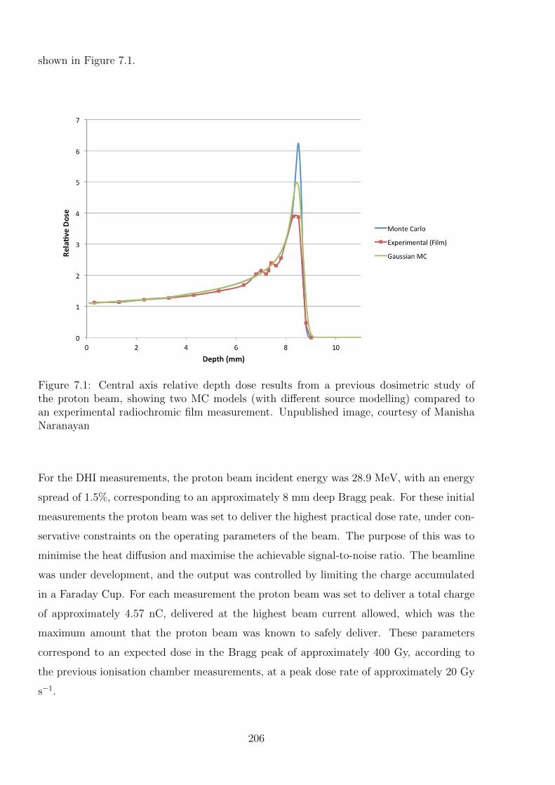
shown in Figure 7.1.
Figure 7.1: Central axis relative depth dose results from a previous dosimetric study ofthe proton beam, showing two MC models (with different source modelling) compared toan experimental radiochromic film measurement. Unpublished image, courtesy of ManishaNaranayan
For the DHI measurements, the proton beam incident energy was 28.9 MeV, with an energy
spread of 1.5%, corresponding to an approximately 8 mm deep Bragg peak. For these initial
measurements the proton beam was set to deliver the highest practical dose rate, under con-
servative constraints on the operating parameters of the beam. The purpose of this was to
minimise the heat diffusion and maximise the achievable signal-to-noise ratio. The beamline
was under development, and the output was controlled by limiting the charge accumulated
in a Faraday Cup. For each measurement the proton beam was set to deliver a total charge
of approximately 4.57 nC, delivered at the highest beam current allowed, which was the
maximum amount that the proton beam was known to safely deliver. These parameters
correspond to an expected dose in the Bragg peak of approximately 400 Gy, according to
the previous ionisation chamber measurements, at a peak dose rate of approximately 20 Gy
s−1.
206
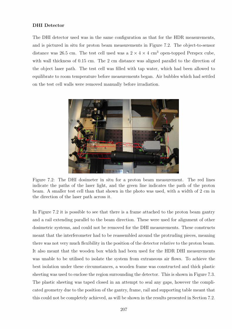
DHI Detector
The DHI detector used was in the same configuration as that for the HDR measurements,
and is pictured in situ for proton beam measurements in Figure 7.2. The object-to-sensor
distance was 26.5 cm. The test cell used was a 2 × 4 × 4 cm3 open-topped Perspex cube,
with wall thickness of 0.15 cm. The 2 cm distance was aligned parallel to the direction of
the object laser path. The test cell was filled with tap water, which had been allowed to
equilibrate to room temperature before measurements began. Air bubbles which had settled
on the test cell walls were removed manually before irradiation.
Figure 7.2: The DHI dosimeter in situ for a proton beam measurement. The red linesindicate the paths of the laser light, and the green line indicates the path of the protonbeam. A smaller test cell than that shown in the photo was used, with a width of 2 cm inthe direction of the laser path across it.
In Figure 7.2 it is possible to see that there is a frame attached to the proton beam gantry
and a rail extending parallel to the beam direction. These were used for alignment of other
dosimetric systems, and could not be removed for the DHI measurements. These constructs
meant that the interferometer had to be reassembled around the protruding pieces, meaning
there was not very much flexibility in the position of the detector relative to the proton beam.
It also meant that the wooden box which had been used for the HDR DHI measurements
was unable to be utilised to isolate the system from extraneous air flows. To achieve the
best isolation under these circumstances, a wooden frame was constructed and thick plastic
sheeting was used to enclose the region surrounding the detector. This is shown in Figure 7.3.
The plastic sheeting was taped closed in an attempt to seal any gaps, however the compli-
cated geometry due to the position of the gantry, frame, rail and supporting table meant that
this could not be completely achieved, as will be shown in the results presented in Section 7.2.
207
(a) (b)
Figure 7.3: The makeshift cover used to isolate the DHI detector from air flow duringproton measurements. (a) With an opening for adjustment of the interferometer, and (b)fully enclosed for measurement.
Measurement Process
Prior to any radiation measurements the DHI detector was aligned to achieve an optimal
position for the real image in Fourier space. Baseline measurements were made to quantify
detector stability and background noise levels for the particular alignment of the interferom-
eter and its location within the proton room.
The relative positioning of the proton beam within the test cell of the detector was some-
what more complex than for the HDR measurements, as the lack of an applicator within
the sensitive region meant that there was no inherent reference point common to both sets
of data. Geometrical alignment and size calibration of the test cell was achieved by use of a
rectangular template, according to the process described in Section 4.3.3. By inspecting the
real-time image preview from the camera, the transparent rectangular template was then
used to localise the measurement region within the cell. The distance from the edge of the
test cell to the edge of the template was recorded, in order to determine the horizontal depth
of the measurement region within the test cell. The distance from the proton beam nozzle
to the test cell was approximately 16 cm. This value varied slightly in accordance with the
position of the test cell and subsequent depth of the measurement region in the test cell, as
the rail and frame around the proton beam meant the interferometer could not be reposi-
tioned. This is not considered to be an issue, as the source to surface distance has minimal
impact on the depth dose distribution of a proton beam.
208
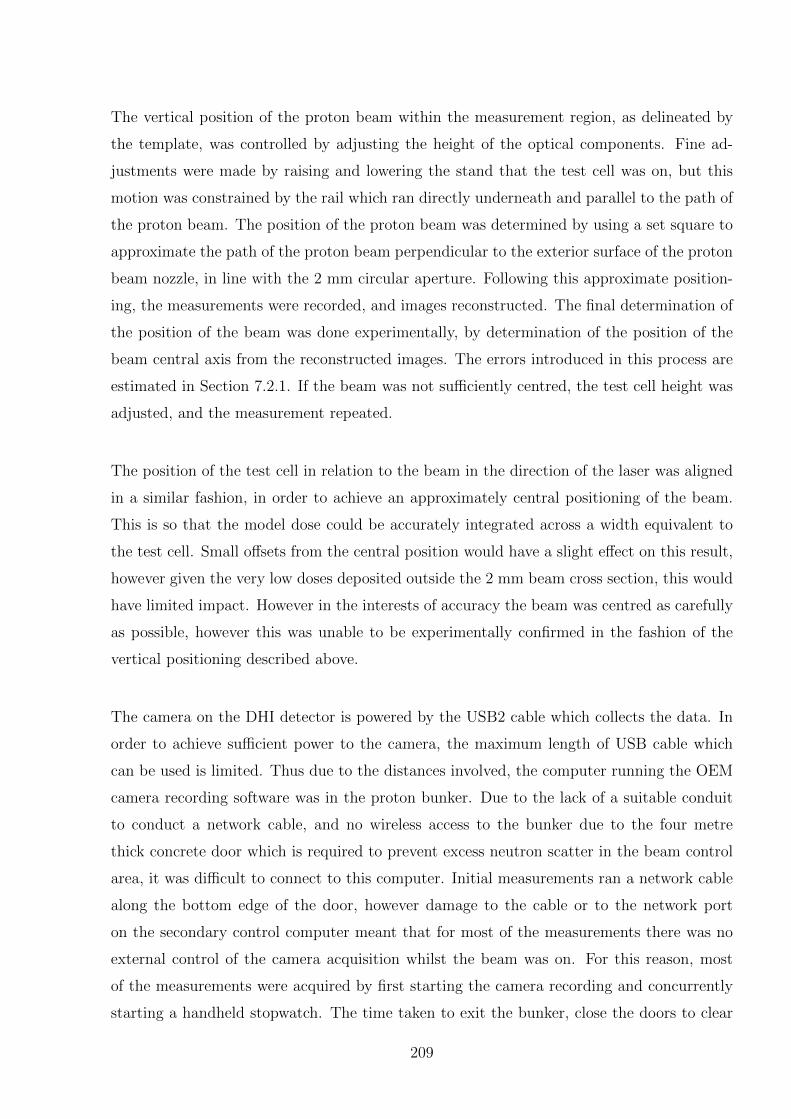
The vertical position of the proton beam within the measurement region, as delineated by
the template, was controlled by adjusting the height of the optical components. Fine ad-
justments were made by raising and lowering the stand that the test cell was on, but this
motion was constrained by the rail which ran directly underneath and parallel to the path of
the proton beam. The position of the proton beam was determined by using a set square to
approximate the path of the proton beam perpendicular to the exterior surface of the proton
beam nozzle, in line with the 2 mm circular aperture. Following this approximate position-
ing, the measurements were recorded, and images reconstructed. The final determination of
the position of the beam was done experimentally, by determination of the position of the
beam central axis from the reconstructed images. The errors introduced in this process are
estimated in Section 7.2.1. If the beam was not sufficiently centred, the test cell height was
adjusted, and the measurement repeated.
The position of the test cell in relation to the beam in the direction of the laser was aligned
in a similar fashion, in order to achieve an approximately central positioning of the beam.
This is so that the model dose could be accurately integrated across a width equivalent to
the test cell. Small offsets from the central position would have a slight effect on this result,
however given the very low doses deposited outside the 2 mm beam cross section, this would
have limited impact. However in the interests of accuracy the beam was centred as carefully
as possible, however this was unable to be experimentally confirmed in the fashion of the
vertical positioning described above.
The camera on the DHI detector is powered by the USB2 cable which collects the data. In
order to achieve sufficient power to the camera, the maximum length of USB cable which
can be used is limited. Thus due to the distances involved, the computer running the OEM
camera recording software was in the proton bunker. Due to the lack of a suitable conduit
to conduct a network cable, and no wireless access to the bunker due to the four metre
thick concrete door which is required to prevent excess neutron scatter in the beam control
area, it was difficult to connect to this computer. Initial measurements ran a network cable
along the bottom edge of the door, however damage to the cable or to the network port
on the secondary control computer meant that for most of the measurements there was no
external control of the camera acquisition whilst the beam was on. For this reason, most
of the measurements were acquired by first starting the camera recording and concurrently
starting a handheld stopwatch. The time taken to exit the bunker, close the doors to clear
209
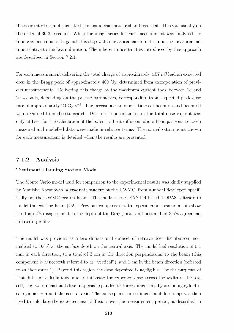
the door interlock and then start the beam, was measured and recorded. This was usually on
the order of 30-35 seconds. When the image series for each measurement was analysed the
time was benchmarked against this stop watch measurement to determine the measurement
time relative to the beam duration. The inherent uncertainties introduced by this approach
are described in Section 7.2.1.
For each measurement delivering the total charge of approximately 4.57 nC had an expected
dose in the Bragg peak of approximately 400 Gy, determined from extrapolation of previ-
ous measurements. Delivering this charge at the maximum current took between 18 and
20 seconds, depending on the precise parameters, corresponding to an expected peak dose
rate of approximately 20 Gy s−1. The precise measurement times of beam on and beam off
were recorded from the stopwatch. Due to the uncertainties in the total dose value it was
only utilised for the calculation of the extent of heat diffusion, and all comparisons between
measured and modelled data were made in relative terms. The normalisation point chosen
for each measurement is detailed when the results are presented.
7.1.2 Analysis
Treatment Planning System Model
The Monte Carlo model used for comparison to the experimental results was kindly supplied
by Manisha Naranayan, a graduate student at the UWMC, from a model developed specif-
ically for the UWMC proton beam. The model uses GEANT-4 based TOPAS software to
model the existing beam [259]. Previous comparison with experimental measurements show
less than 2% disagreement in the depth of the Bragg peak and better than 3.5% agreement
in lateral profiles.
The model was provided as a two dimensional dataset of relative dose distribution, nor-
malised to 100% at the surface depth on the central axis. The model had resolution of 0.1
mm in each direction, to a total of 3 cm in the direction perpendicular to the beam (this
component is henceforth referred to as “vertical”), and 1 cm in the beam direction (referred
to as “horizontal”). Beyond this region the dose deposited is negligible. For the purposes of
heat diffusion calculations, and to integrate the expected dose across the width of the test
cell, the two dimensional dose map was expanded to three dimensions by assuming cylindri-
cal symmetry about the central axis. The consequent three dimensional dose map was then
used to calculate the expected heat diffusion over the measurement period, as described in
210
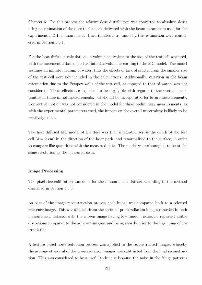
Chapter 5. For this process the relative dose distribution was converted to absolute doses
using an estimation of the dose to the peak delivered with the beam parameters used for the
experimental DHI measurement. Uncertainties introduced by this estimation were consid-
ered in Section 5.3.1.
For the heat diffusion calculations, a volume equivalent to the size of the test cell was used,
with the incremental dose deposited into this volume according to the MC model. The model
assumes an infinite medium of water, thus the effects of lack of scatter from the smaller size
of the test cell were not included in the calculations. Additionally, variation in the beam
attenuation due to the Perspex walls of the test cell, as opposed to that of water, was not
considered. These effects are expected to be negligible with regards to the overall uncer-
tainties in these initial measurements, but should be incorporated for future measurements.
Convective motion was not considered in the model for these preliminary measurements, as
with the experimental parameters used, the impact on the overall uncertainty is likely to be
relatively small.
The heat diffused MC model of the dose was then integrated across the depth of the test
cell (d = 2 cm) in the direction of the laser path, and renormalised to the surface, in order
to compare like quantities with the measured data. The model was subsampled to be at the
same resolution as the measured data.
Image Processing
The pixel size calibration was done for the measurement dataset according to the method
described in Section 4.3.3.
As part of the image reconstruction process each image was compared back to a selected
reference image. This was selected from the series of pre-irradiation images recorded in each
measurement dataset, with the chosen image having low random noise, no repeated visible
distortions compared to the adjacent images, and being shortly prior to the beginning of the
irradiation.
A feature based noise reduction process was applied to the reconstructed images, whereby
the average of several of the pre-irradiation images was subtracted from the final reconstruc-
tion. This was considered to be a useful technique because the noise in the fringe patterns
211
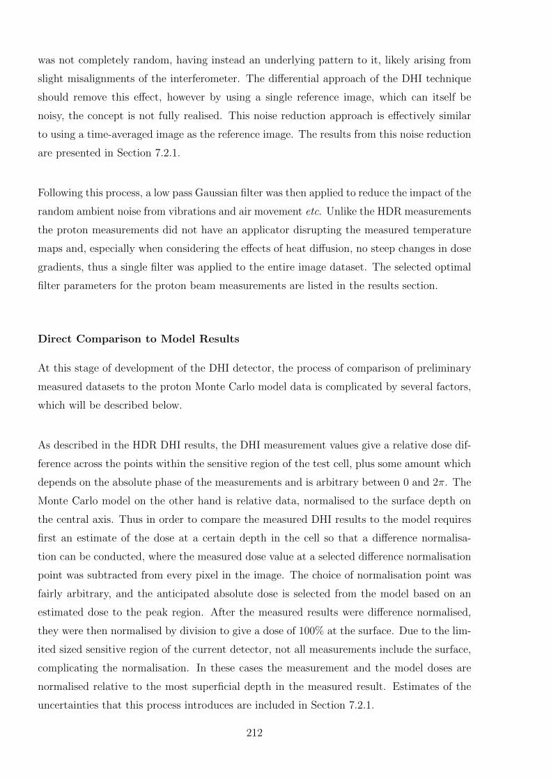
was not completely random, having instead an underlying pattern to it, likely arising from
slight misalignments of the interferometer. The differential approach of the DHI technique
should remove this effect, however by using a single reference image, which can itself be
noisy, the concept is not fully realised. This noise reduction approach is effectively similar
to using a time-averaged image as the reference image. The results from this noise reduction
are presented in Section 7.2.1.
Following this process, a low pass Gaussian filter was then applied to reduce the impact of the
random ambient noise from vibrations and air movement etc. Unlike the HDR measurements
the proton measurements did not have an applicator disrupting the measured temperature
maps and, especially when considering the effects of heat diffusion, no steep changes in dose
gradients, thus a single filter was applied to the entire image dataset. The selected optimal
filter parameters for the proton beam measurements are listed in the results section.
Direct Comparison to Model Results
At this stage of development of the DHI detector, the process of comparison of preliminary
measured datasets to the proton Monte Carlo model data is complicated by several factors,
which will be described below.
As described in the HDR DHI results, the DHI measurement values give a relative dose dif-
ference across the points within the sensitive region of the test cell, plus some amount which
depends on the absolute phase of the measurements and is arbitrary between 0 and 2π. The
Monte Carlo model on the other hand is relative data, normalised to the surface depth on
the central axis. Thus in order to compare the measured DHI results to the model requires
first an estimate of the dose at a certain depth in the cell so that a difference normalisa-
tion can be conducted, where the measured dose value at a selected difference normalisation
point was subtracted from every pixel in the image. The choice of normalisation point was
fairly arbitrary, and the anticipated absolute dose is selected from the model based on an
estimated dose to the peak region. After the measured results were difference normalised,
they were then normalised by division to give a dose of 100% at the surface. Due to the lim-
ited sized sensitive region of the current detector, not all measurements include the surface,
complicating the normalisation. In these cases the measurement and the model doses are
normalised relative to the most superficial depth in the measured result. Estimates of the
uncertainties that this process introduces are included in Section 7.2.1.
212
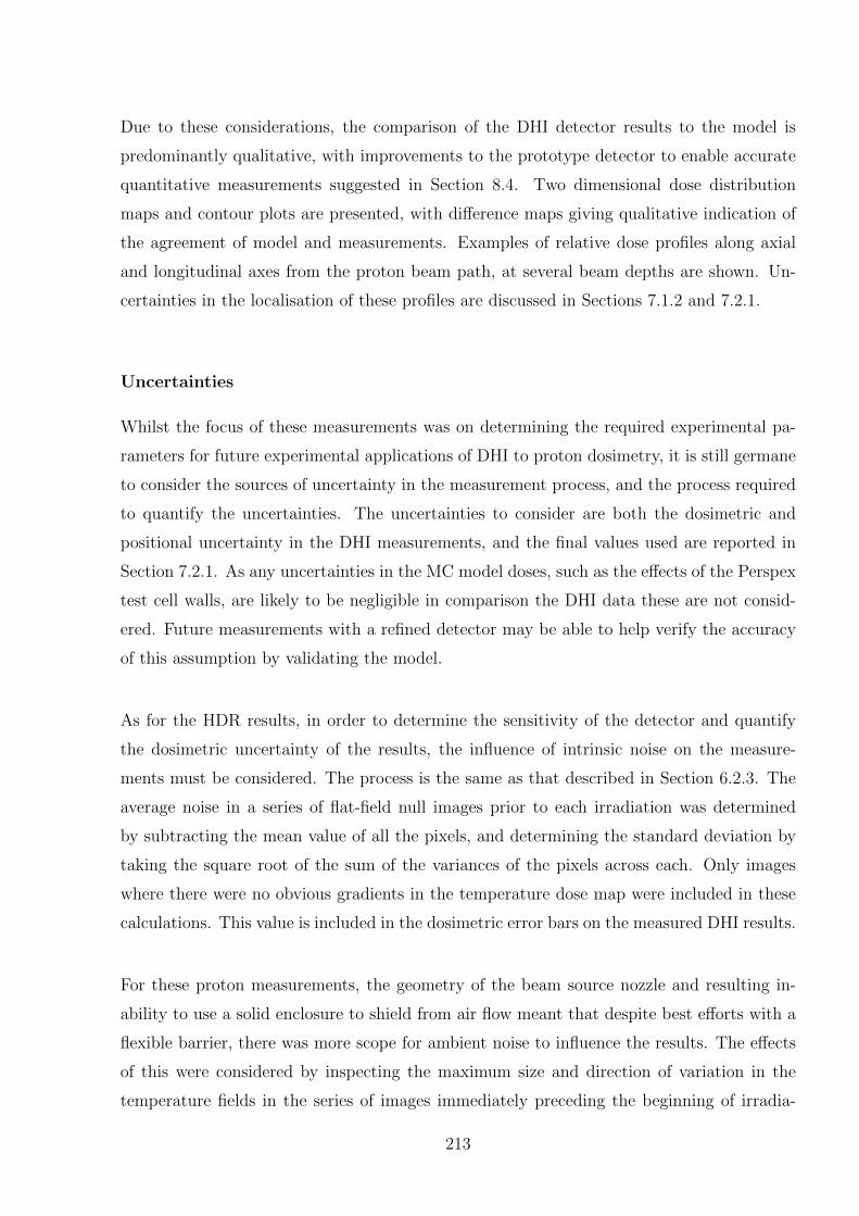
Due to these considerations, the comparison of the DHI detector results to the model is
predominantly qualitative, with improvements to the prototype detector to enable accurate
quantitative measurements suggested in Section 8.4. Two dimensional dose distribution
maps and contour plots are presented, with difference maps giving qualitative indication of
the agreement of model and measurements. Examples of relative dose profiles along axial
and longitudinal axes from the proton beam path, at several beam depths are shown. Un-
certainties in the localisation of these profiles are discussed in Sections 7.1.2 and 7.2.1.
Uncertainties
Whilst the focus of these measurements was on determining the required experimental pa-
rameters for future experimental applications of DHI to proton dosimetry, it is still germane
to consider the sources of uncertainty in the measurement process, and the process required
to quantify the uncertainties. The uncertainties to consider are both the dosimetric and
positional uncertainty in the DHI measurements, and the final values used are reported in
Section 7.2.1. As any uncertainties in the MC model doses, such as the effects of the Perspex
test cell walls, are likely to be negligible in comparison the DHI data these are not consid-
ered. Future measurements with a refined detector may be able to help verify the accuracy
of this assumption by validating the model.
As for the HDR results, in order to determine the sensitivity of the detector and quantify
the dosimetric uncertainty of the results, the influence of intrinsic noise on the measure-
ments must be considered. The process is the same as that described in Section 6.2.3. The
average noise in a series of flat-field null images prior to each irradiation was determined
by subtracting the mean value of all the pixels, and determining the standard deviation by
taking the square root of the sum of the variances of the pixels across each. Only images
where there were no obvious gradients in the temperature dose map were included in these
calculations. This value is included in the dosimetric error bars on the measured DHI results.
For these proton measurements, the geometry of the beam source nozzle and resulting in-
ability to use a solid enclosure to shield from air flow meant that despite best efforts with a
flexible barrier, there was more scope for ambient noise to influence the results. The effects
of this were considered by inspecting the maximum size and direction of variation in the
temperature fields in the series of images immediately preceding the beginning of irradia-
213
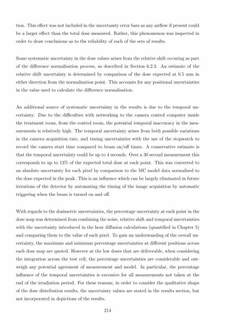
tion. This effect was not included in the uncertainty error bars as any airflow if present could
be a larger effect than the total dose measured. Rather, this phenomenon was inspected in
order to draw conclusions as to the reliability of each of the sets of results.
Some systematic uncertainty in the dose values arises from the relative shift occuring as part
of the difference normalisation process, as described in Section 6.2.3. An estimate of the
relative shift uncertainty is determined by comparison of the dose expected at 0.5 mm in
either direction from the normalisation point. This accounts for any positional uncertainties
in the value used to calculate the difference normalisation.
An additional source of systematic uncertainty in the results is due to the temporal un-
certainty. Due to the difficulties with networking to the camera control computer inside
the treatment room, from the control room, the potential temporal inaccuracy in the mea-
surements is relatively high. The temporal uncertainty arises from both possible variations
in the camera acquisition rate, and timing uncertainties with the use of the stopwatch to
record the camera start time compared to beam on/off times. A conservative estimate is
that the temporal uncertainty could be up to 4 seconds. Over a 30 second measurement this
corresponds to up to 13% of the expected total dose at each point. This was converted to
an absolute uncertainty for each pixel by comparison to the MC model data normalised to
the dose expected in the peak. This is an influence which can be largely eliminated in future
iterations of the detector by automating the timing of the image acquisition by automatic
triggering when the beam is turned on and off.
With regards to the dosimetric uncertainties, the percentage uncertainty at each point in the
dose map was determined from combining the noise, relative shift and temporal uncertainties
with the uncertainty introduced in the heat diffusion calculations (quantified in Chapter 5)
and comparing them to the value of each pixel. To gain an understanding of the overall un-
certainty, the maximum and minimum percentage uncertainties at different positions across
each dose map are quoted. However at the low doses that are deliverable, when considering
the integration across the test cell, the percentage uncertainties are considerable and out-
weigh any potential agreement of measurement and model. In particular, the percentage
influence of the temporal uncertainties is excessive for all measurements not taken at the
end of the irradiation period. For these reasons, in order to consider the qualitative shape
of the dose distribution results, the uncertainty values are stated in the results section, but
not incorporated in depictions of the results.
214
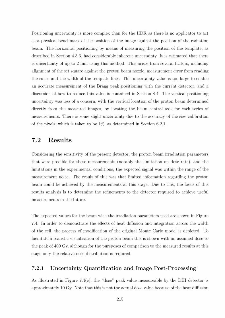
Positioning uncertainty is more complex than for the HDR as there is no applicator to act
as a physical benchmark of the position of the image against the position of the radiation
beam. The horizontal positioning by means of measuring the position of the template, as
described in Section 4.3.3, had considerable inherent uncertainty. It is estimated that there
is uncertainty of up to 2 mm using this method. This arises from several factors, including
alignment of the set square against the proton beam nozzle, measurement error from reading
the ruler, and the width of the template lines. This uncertainty value is too large to enable
an accurate measurement of the Bragg peak positioning with the current detector, and a
discussion of how to reduce this value is contained in Section 8.4. The vertical positioning
uncertainty was less of a concern, with the vertical location of the proton beam determined
directly from the measured images, by locating the beam central axis for each series of
measurements. There is some slight uncertainty due to the accuracy of the size calibration
of the pixels, which is taken to be 1%, as determined in Section 6.2.1.
7.2 Results
Considering the sensitivity of the present detector, the proton beam irradiation parameters
that were possible for these measurements (notably the limitation on dose rate), and the
limitations in the experimental conditions, the expected signal was within the range of the
measurement noise. The result of this was that limited information regarding the proton
beam could be achieved by the measurements at this stage. Due to this, the focus of this
results analysis is to determine the refinements to the detector required to achieve useful
measurements in the future.
The expected values for the beam with the irradiation parameters used are shown in Figure
7.4. In order to demonstrate the effects of heat diffusion and integration across the width
of the cell, the process of modification of the original Monte Carlo model is depicted. To
facilitate a realistic visualisation of the proton beam this is shown with an assumed dose to
the peak of 400 Gy, although for the pursposes of comparison to the measured results at this
stage only the relative dose distribution is required.
7.2.1 Uncertainty Quantification and Image Post-Processing
As illustrated in Figure 7.4(e), the “dose” peak value measureable by the DHI detector is
approximately 10 Gy. Note that this is not the actual dose value because of the heat diffusion
215
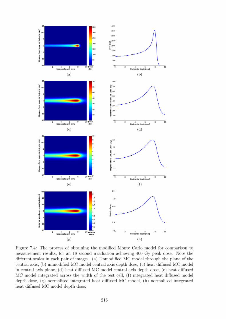
Dis
tanc
e fr
om b
eam
cen
tral
axi
s (m
m)
Horizontal depth (mm)
2 4 6 8 10
−15
−10
−5
0
5
10
15Dose(Gy)
0
50
100
150
200
250
300
350
(a)
0 2 4 6 8 100
50
100
150
200
250
300
350
400
Do
se (
Gy)
Horizontal depth (mm)
(b)
Dis
tanc
e fr
om b
eam
cen
tral
axi
s (m
m)
Horizontal depth (mm)
2 4 6 8 10
−15
−10
−5
0
5
10
15Dose(Gy)
10
20
30
40
50
60
70
(c)
0 2 4 6 8 100
10
20
30
40
50
60
70
80
Hea
t D
iffu
sed
Cen
tral
Axi
s D
ose
(G
y)
Horizontal depth (mm)
(d)
Dis
tanc
e fr
om b
eam
cen
tral
axi
s (m
m)
Horizontal depth (mm)
2 4 6 8 10
−15
−10
−5
0
5
10
15Dose(Gy)
0
1
2
3
4
5
6
7
8
9
10
(e)
0 2 4 6 8 100
2
4
6
8
10
Inte
gra
ted
Hea
t D
iffu
sed
Do
se (
Gy)
Horizontal depth (mm)
(f)
Dis
tanc
e fr
om b
eam
cen
tral
axi
s (m
m)
Horizontal depth (mm)
2 4 6 8 10
−15
−10
−5
0
5
10
15Relative
Dose
0
0.2
0.4
0.6
0.8
1
1.2
1.4
1.6
1.8
2
(g)
0 2 4 6 8 100
0.5
1
1.5
2
2.5
Rel
ativ
e D
ose
Horizontal depth (mm)
(h)
Figure 7.4: The process of obtaining the modified Monte Carlo model for comparison tomeasurement results, for an 18 second irradiation achieving 400 Gy peak dose. Note thedifferent scales in each pair of images. (a) Unmodified MC model through the plane of thecentral axis, (b) unmodified MC model central axis depth dose, (c) heat diffused MC modelin central axis plane, (d) heat diffused MC model central axis depth dose, (e) heat diffusedMC model integrated across the width of the test cell, (f) integrated heat diffused modeldepth dose, (g) normalised integrated heat diffused MC model, (h) normalised integratedheat diffused MC model depth dose.
216
and integration across the test cell, however for the sake of simplicity it will be referred to as
the “measured dose” for the remainder of this chapter. Given the small sensitive region of
the detector, the maximum dose difference that can be detected along a depth dose profile is
approximately 7.5 Gy. This value is not significantly greater than the dosimetric uncertainty
on each point in the images, which is calculated next.
In the same fashion as for the HDR results, the inherent noise contribution to the dosimetric
uncertainty in the image series for this set-up of the detector was determined by analysing
the null images from the beginning of each measurement set. For one of the measurement
sets presented in this section, the standard deviation of the noise over the first six images
was 3.7 Gy. This number is typical of the results achieved for all the datasets, and is an
estimate of the sensitivity of the detector for relative dose measurements. The uncertainty
in the heat diffusion calculations of approximately 0.75% also impacts on the relative dose
distribution. This 0.75% results in a maximum uncertainty in the peak of 0.1 Gy. The
relative shift uncertainty was determined from the variation in dose across the positional
uncertainty of 2 mm, at the difference normalisation point. As the difference normalisation
point was usually in the low gradient pre-Bragg peak region of the curve this value was
relatively low, and was taken to be 0.5 Gy for all measurements. The temporal uncertainty
is up to 13% of the dose at each point. Combining all of these uncertainties results in an
absolute uncertainty for the measured value of each pixel of between 4.2 - 5.6 Gy.
Thus from the above values it is evident that with the present sensitivity of the detector,
and the limitation on deliverable dose rate, limited interpretation of the measured results is
possible.
In an attempt to maximise the information that can be achieved from these DHI proton
measurements, post-processing of the images to reduce the noise contribution to the dosi-
metric uncertainty by means of feature based analysis was conducted. This process was
based on the observation that the noise in each image does not appear completely random,
but rather some component is attributable to some significant artifacts which are visible
across the series of images. By combining null images and subtracting the mean of the
combined images from each image, a slight reduction of artifacts was achieved. A repeat
calculation of the standard deviation within each image was then calculated. Some image
series showed no improvement, and some showed noise uncertainty in the dosimetric values
reduced by up to 1 Gy. This value is relatively small, in agreement with the assumption
217
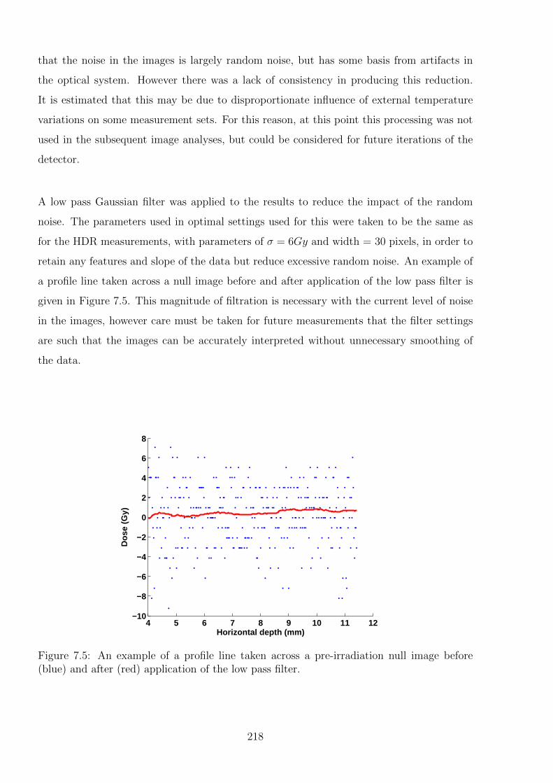
that the noise in the images is largely random noise, but has some basis from artifacts in
the optical system. However there was a lack of consistency in producing this reduction.
It is estimated that this may be due to disproportionate influence of external temperature
variations on some measurement sets. For this reason, at this point this processing was not
used in the subsequent image analyses, but could be considered for future iterations of the
detector.
A low pass Gaussian filter was applied to the results to reduce the impact of the random
noise. The parameters used in optimal settings used for this were taken to be the same as
for the HDR measurements, with parameters of σ = 6Gy and width = 30 pixels, in order to
retain any features and slope of the data but reduce excessive random noise. An example of
a profile line taken across a null image before and after application of the low pass filter is
given in Figure 7.5. This magnitude of filtration is necessary with the current level of noise
in the images, however care must be taken for future measurements that the filter settings
are such that the images can be accurately interpreted without unnecessary smoothing of
the data.
4 5 6 7 8 9 10 11 12−10
−8
−6
−4
−2
0
2
4
6
8
Dos
e (G
y)
Horizontal depth (mm)
Figure 7.5: An example of a profile line taken across a pre-irradiation null image before(blue) and after (red) application of the low pass filter.
218
7.2.2 Consistency of Image Series
The results from the proton beam measurements were more affected by inconsistencies across
and between the images than the previous HDR source measurements. This can partly be
attributed to the difficulties encountered in creating a sealed enclosure around the detector
to reduce air flow. The other factor is that the limit on the proton beam dose rate meant
that high dose gradients were not achievable, so therefore fluctuations in the measurement
of several Gy were of much higher significance when interpreting the results. Ideally these
inconsistencies would be eliminated for measurements, high dose gradient or not, however
if they are unable to be eliminated then a metric needs to be introduced to quantify the
influence that they have. This is complicated by the fact that the very nature of the in-
consistencies means that they are not necessarily predictable, and measuring the variations
at one point in time does not necessarily correlate with what is occuring during the actual
irradiation period. The proton beam measurements do however have a relatively large set of
images from pre-irradiation compared to during irradiation, necessitated by the difficulty in
networking the control computer and the long time taken for the proton room door to close
before measurement could begin. Thus by examining the fluctuations in the series of pre-
irradiation images, any trends can be extrapolated to estimate the impact of non-radiation
induced variations on the measurement data.
The smoothed null images were inspected for any kind of gradient in the measurement field.
The maximum gradient in each image was determined from the maximum and minimum
points, and quantified as a percentage of the expected measurement value for a given time
instance. This allows for an estimation of the impact of this effect on the validity of any
measured results. Additionally, the direction of the gradient between those points was quan-
tified in order to give an indication of the variability with time, whether the effect was just
a drift in one direction, and how constant the variation was.
An example of an image series recorded at one second intervals is shown in Figure 7.6 to
give an indication of the variation in the results. The long term drifts from serval datasets
are presented in Figure 7.7. This figure presents the size of the maximum dose gradient,
and it’s direction for each image in a 40 second series prior to the irradiation of each of the
actual measurement datasets. It was found that the influence was predominantly a vertical
temperature gradient, with very little variation across the horizontal plane. The fluctuations
were relatively unpredictable, oscillating between approximately 0 and 10 Gy deviation from
the intial reference image at most time points, but with occasional sections of larger devi-
219
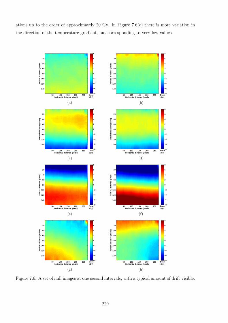
ations up to the order of approximately 20 Gy. In Figure 7.6(c) there is more variation in
the direction of the temperature gradient, but corresponding to very low values.
Horizontal distance (pixels)
Ver
tical
dis
tanc
e (p
ixel
s)
50 100 150 200 250
20
40
60
80
100
120
140
Dose(Gy)
−8
−6
−4
−2
0
2
4
6
8
(a)
Horizontal distance (pixels)
Ver
tical
dis
tanc
e (p
ixel
s)
50 100 150 200 250
20
40
60
80
100
120
140
Dose(Gy)
−8
−6
−4
−2
0
2
4
6
8
(b)
Horizontal distance (pixels)
Ver
tical
dis
tanc
e (p
ixel
s)
50 100 150 200 250
20
40
60
80
100
120
140
Dose(Gy)
−8
−6
−4
−2
0
2
4
6
8
(c)
Horizontal distance (pixels)
Ver
tical
dis
tanc
e (p
ixel
s)
50 100 150 200 250
20
40
60
80
100
120
140
Dose(Gy)
−8
−6
−4
−2
0
2
4
6
8
(d)
Horizontal distance (pixels)
Ver
tical
dis
tanc
e (p
ixel
s)
50 100 150 200 250
20
40
60
80
100
120
140
Dose(Gy)
−8
−6
−4
−2
0
2
4
6
8
(e)
Horizontal distance (pixels)
Ver
tical
dis
tanc
e (p
ixel
s)
50 100 150 200 250
20
40
60
80
100
120
140
Dose(Gy)
−8
−6
−4
−2
0
2
4
6
8
(f)
Horizontal distance (pixels)
Ver
tical
dis
tanc
e (p
ixel
s)
50 100 150 200 250
20
40
60
80
100
120
140
Dose(Gy)
−8
−6
−4
−2
0
2
4
6
8
(g)
Horizontal distance (pixels)
Ver
tical
dis
tanc
e (p
ixel
s)
50 100 150 200 250
20
40
60
80
100
120
140
Dose(Gy)
−8
−6
−4
−2
0
2
4
6
8
(h)
Figure 7.6: A set of null images at one second intervals, with a typical amount of drift visible.
220
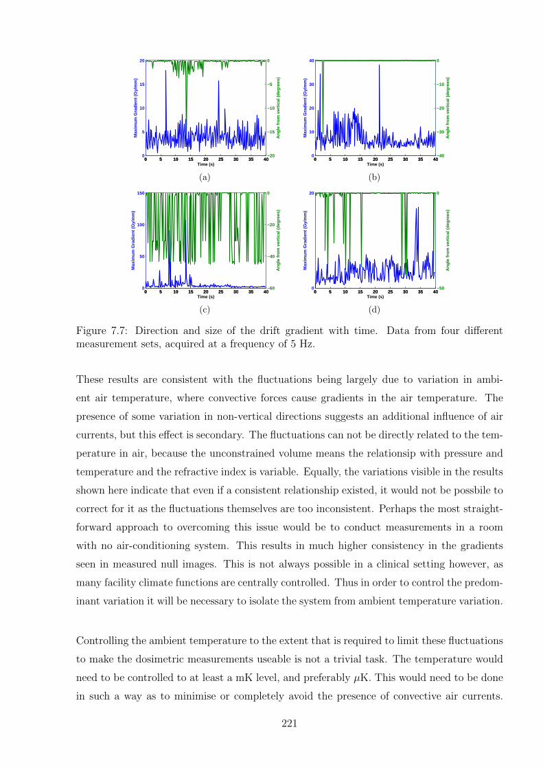
0 5 10 15 20 25 30 35 400
5
10
15
20
Max
imum
Gra
dien
t (G
y/m
m)
0 5 10 15 20 25 30 35 40−20
−15
−10
−5
0
Ang
le fr
om v
ertic
al (
degr
ees)
Time (s)
(a)
0 5 10 15 20 25 30 35 400
10
20
30
40
Max
imum
Gra
dien
t (G
y/m
m)
0 5 10 15 20 25 30 35 40−40
−30
−20
−10
0
Ang
le fr
om v
ertic
al (
degr
ees)
Time (s)
(b)
0 5 10 15 20 25 30 35 400
50
100
150
Max
imum
Gra
dien
t (G
y/m
m)
0 5 10 15 20 25 30 35 40−60
−40
−20
0
Ang
le fr
om v
ertic
al (
degr
ees)
Time (s)
(c)
0 5 10 15 20 25 30 35 400
20
Max
imum
Gra
dien
t (G
y/m
m)
0 5 10 15 20 25 30 35 40−50
0
Ang
le fr
om v
ertic
al (
degr
ees)
Time (s)
(d)
Figure 7.7: Direction and size of the drift gradient with time. Data from four differentmeasurement sets, acquired at a frequency of 5 Hz.
These results are consistent with the fluctuations being largely due to variation in ambi-
ent air temperature, where convective forces cause gradients in the air temperature. The
presence of some variation in non-vertical directions suggests an additional influence of air
currents, but this effect is secondary. The fluctuations can not be directly related to the tem-
perature in air, because the unconstrained volume means the relationsip with pressure and
temperature and the refractive index is variable. Equally, the variations visible in the results
shown here indicate that even if a consistent relationship existed, it would not be possbile to
correct for it as the fluctuations themselves are too inconsistent. Perhaps the most straight-
forward approach to overcoming this issue would be to conduct measurements in a room
with no air-conditioning system. This results in much higher consistency in the gradients
seen in measured null images. This is not always possible in a clinical setting however, as
many facility climate functions are centrally controlled. Thus in order to control the predom-
inant variation it will be necessary to isolate the system from ambient temperature variation.
Controlling the ambient temperature to the extent that is required to limit these fluctuations
to make the dosimetric measurements useable is not a trivial task. The temperature would
need to be controlled to at least a mK level, and preferably µK. This would need to be done
in such a way as to minimise or completely avoid the presence of convective air currents.
221
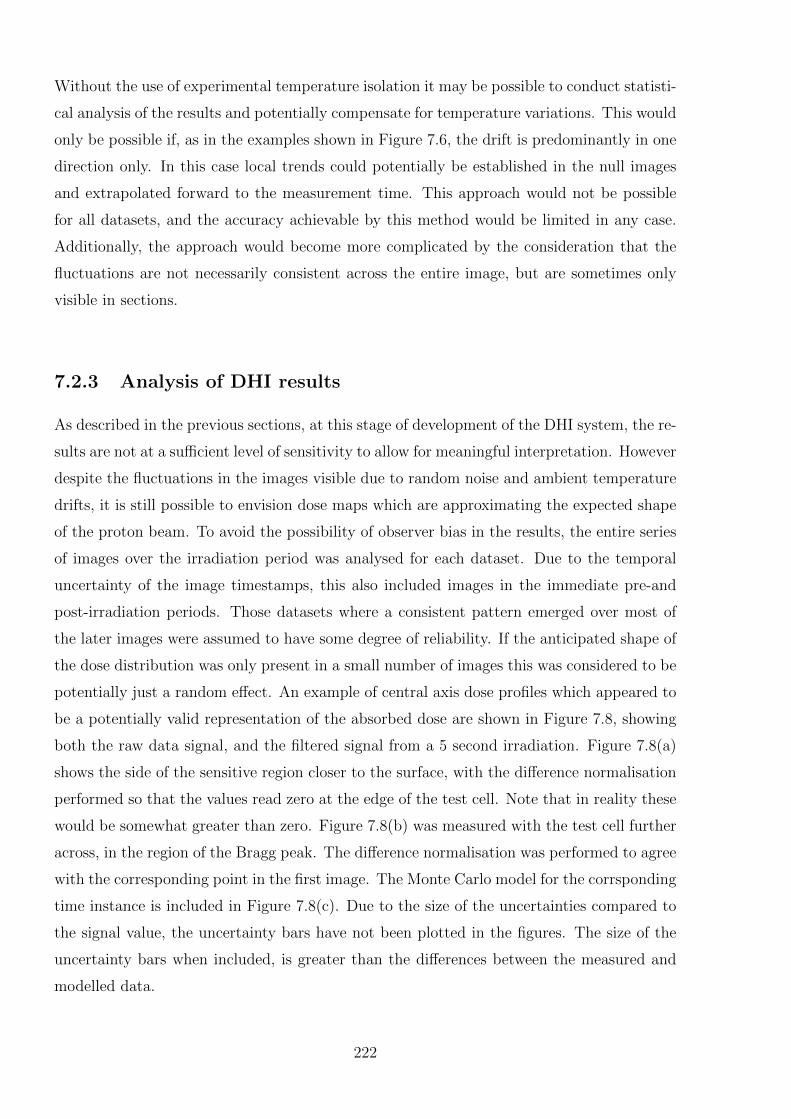
Without the use of experimental temperature isolation it may be possible to conduct statisti-
cal analysis of the results and potentially compensate for temperature variations. This would
only be possible if, as in the examples shown in Figure 7.6, the drift is predominantly in one
direction only. In this case local trends could potentially be established in the null images
and extrapolated forward to the measurement time. This approach would not be possible
for all datasets, and the accuracy achievable by this method would be limited in any case.
Additionally, the approach would become more complicated by the consideration that the
fluctuations are not necessarily consistent across the entire image, but are sometimes only
visible in sections.
7.2.3 Analysis of DHI results
As described in the previous sections, at this stage of development of the DHI system, the re-
sults are not at a sufficient level of sensitivity to allow for meaningful interpretation. However
despite the fluctuations in the images visible due to random noise and ambient temperature
drifts, it is still possible to envision dose maps which are approximating the expected shape
of the proton beam. To avoid the possibility of observer bias in the results, the entire series
of images over the irradiation period was analysed for each dataset. Due to the temporal
uncertainty of the image timestamps, this also included images in the immediate pre-and
post-irradiation periods. Those datasets where a consistent pattern emerged over most of
the later images were assumed to have some degree of reliability. If the anticipated shape of
the dose distribution was only present in a small number of images this was considered to be
potentially just a random effect. An example of central axis dose profiles which appeared to
be a potentially valid representation of the absorbed dose are shown in Figure 7.8, showing
both the raw data signal, and the filtered signal from a 5 second irradiation. Figure 7.8(a)
shows the side of the sensitive region closer to the surface, with the difference normalisation
performed so that the values read zero at the edge of the test cell. Note that in reality these
would be somewhat greater than zero. Figure 7.8(b) was measured with the test cell further
across, in the region of the Bragg peak. The difference normalisation was performed to agree
with the corresponding point in the first image. The Monte Carlo model for the corrsponding
time instance is included in Figure 7.8(c). Due to the size of the uncertainties compared to
the signal value, the uncertainty bars have not been plotted in the figures. The size of the
uncertainty bars when included, is greater than the differences between the measured and
modelled data.
222
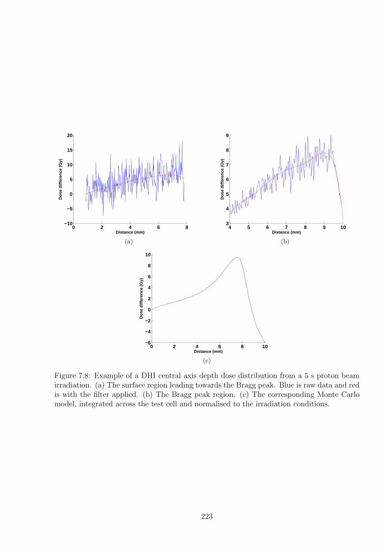
0 2 4 6 8−10
−5
0
5
10
15
20
Distance (mm)
Dos
e di
ffere
nce
(Gy)
(a)
4 5 6 7 8 9 103
4
5
6
7
8
9
Distance (mm)
Do
se d
iffe
ren
ce (
Gy)
(b)
0 2 4 6 8 10−6
−4
−2
0
2
4
6
8
10
Distance (mm)
Dos
e di
ffere
nce
(Gy)
(c)
Figure 7.8: Example of a DHI central axis depth dose distribution from a 5 s proton beamirradiation. (a) The surface region leading towards the Bragg peak. Blue is raw data and redis with the filter applied. (b) The Bragg peak region. (c) The corresponding Monte Carlomodel, integrated across the test cell and normalised to the irradiation conditions.
223
Radial dose functions of the proton beam data are not presented at this stage, as the limi-
tations of the present detector did not allow for sufficiently accurate results to warrant this
level of comparison. This analytic would be possible to use in the same fashion as for the
HDR measurements, assuming cylindrical symmetry about the central axis.
It was evident from some of the more reliable datasets obtained that the measured reading
was too high in the penumbral regions of the beam. This may be attributable to discrep-
ancies due to the extremely low signal to noise ratio, or possibly incorrect heat diffusion
equations underestimating the extent of heat flow.
7.3 Discussion
The initial aim of these measurements was to test the DHI detector following successful
HDR brachytherapy source measurements. It was hoped that the DHI detector may be able
to contribute to the task of commissioning and validating the UWMC proton beamline for
animal research. However the experimental difficulties faced, coupled with the limited time
available at the facility meant that the main achievement from these measurements was to
investigate the detector capabilities and experimental process required to potentially enable
successful measurements in future proton beam dosimetry experiments. The opportunity to
apply the improvements to the detector was not available at the time of measurement, due
to time constraints in the clinical setting. Some of the lessons learned that are specific to
the proton beam are discussed here, whilst general improvements to the DHI detector are
covered more fully in Chapter 8.
7.3.1 Beam Settings
The beam settings for the pilot study were limited to the highest value known to be able
to be safely delivered. The total charge delivered of 4.57 nC at a current of approximately
0.23 nA resulted in a dose to the Bragg peak of approximately 400 Gy over approximately
20 s. The steepest dose gradient achievable on the central axis, when corrected for the DHI
measurement conditions of heat diffusion and integration across the test cell, was approxi-
mately 5 Gy/mm. Since the pilot study was completed it has been determined that it will be
possible to safely operate the proton beam at a vastly increased dose rate three to five orders
of magnitude greater than that used in these initial measurements. This will result in much
224
higher doses being able to be achieved, with the subsequent increase in the dose gradients
meaning that the dose distribution will be much more measurable using a DHI detector. For
example, if the beam current is increased by a factor of 10,000, for an irradiation time of 10
seconds, the total absorbed dose in the Bragg peak would be 100 kGy. After accounting for
heat diffusion and integration across the DHI test cell, this would result in dose gradients
on the central axis of up to 2000 Gy/mm. This increase in dose means that even with
the current detector set-up and measurement process, the increase in signal-to-noise ratio
means that even the lowest dose gradient region at the surface on the central axis should be
resolveable with the current sensitivity of the DHI detector.
A key advantage of a DHI detector compared to many other dosimetric approaches is the
inherently high dynamic range, so that even at high dose rates the dose in the Bragg peak
will be simultaneously measurable with that in the surface or fall off region. The limiting
factor on this is the impact of heat diffusion, which has a higher impact in the presence of
high temperature gradients. However the high dose rate also allows for a much faster dose
depostion time for a given dose, which counteracts this effect. Additionally, the extent of
the heat diffusion can be mathematically corrcted for.
One caveat to note on the process of increasing the accuracy of the DHI measurements by
dramatically increasing the dose rate is that this moves the system far beyond any settings
which might be used clinically with current treatment protocols. Caution would have to
be taken extrapolating the results of these measurements to a characterisation of the beam
at clinical dose rates. It is possible that with the ability to produce ultra high dose rate
beams that there may be some clinical benefit to this, similar to the MRT beams described
in Section 2.3.3, with dose rates on the order of 100 - 1000 Gy s−1 [175]. Notably, a high
dose rate and the subsequent short delivery time reduces the impact of intrafractional organ
motion on the target volume and organ at risk irradiation. Additionally, with the recent de-
velopments in the field of laser driven ion acceleration proton beams, as described in Section
2.3.2, investigation of DHI as a dosimetric tool for cyclotron generated high dose rate beams
may lead to possibilities for its application in the dosimetry of LDA protons.
7.3.2 Monte Carlo Model
When comparing the DHI measurements with the Monte Carlo model, the main limitation
was the fact that only a relative dose distribution comparison could be made. This is because
225
the Monte Carlo model provided was not specific to the exact beam current settings and
irradiation time used, resulting in uncertainty in the absolute dose delivered. Whilst this
still produces an accurate relative dose distribution, it limits the utility of the comparison for
absolute dose. The comparison effectvely becomes qualitative, comparing the shape of the
dose distribution rather than specific values. Variation of the absolute dose will still result
in some relative dose effects visible, with the extent depending on the normalisation point
chosen. However these variations will be less obvious than if an absolute dose distribution
could be compared.
The best approach would be to run the Monte Carlo model with input of the exact settings
used for the irradiation. This would allow for a proper validation of any future DHI mea-
surements against expected values, which is vital for the further development of the system.
In particular this process is fundamental to the development of the detector capabilities
for determination of absolute dose. This also has the added benefit of removing dosimetric
uncertainty in the processed DHI measurements which results from normalisation to a point
with considerable uncertainty. The uncertainties in the results, and the extent of discrepan-
cies between measurement and model would then be able to be quantitatively determined,
in terms which are readily understood and transferable to other methods.
7.3.3 Detector Dosimetric Sensitivity
The first conclusion from the initial pilot measurements of the proton beam are that in order
to achieve useable results, the sensitivity of the measurements must be increased. This could
be achieved either by improving the detector responsiveness, or by increasing the signal from
the proton beam. A traditional definition of signal to noise ratio (SNR) is the average signal
value, µ divided by the standard deviation of the background, σbg. The signal value consid-
ered in the case of a DHI measurement is the mean difference between two set points, which
are separated either spatially or temporally. This difference is used rather than the absolute
value of a point, as the absolute value is arbitrary, depending on the starting conditions and
phase. In order to achieve meaningful results, the SNR of a dataset must be greater than
one. If the noise is determined as the standard deviation of a null image, then for a signal
to noise ratio of one, the confidence in this result will be ∼ 68%. To increase this confidence
interval, data must be acquired with a higher SNR. Consider here that a SNR calculated
from one standard deviation gives the 68% confidence interval, whilst to achieve a 95% or
higher confidence interval requires two or more standard deviations. Thus to have useable
226
reliability in the determination of the relative dose distribution requires the signal to be
at least greater than twice the standard deviation of the measured signal. The additional
dosimetric uncertainty in the measurement adds to this requirement. In actual terms, this
requires a dose difference of at least 7 Gy, but up to 12 Gy, in order to achieve a reliable
signal for the proton beam measurements. Improvements to the detector will reduce this
requirement.
To improve the sensitivity of the detector by improvement of the SNR, a key approach could
be to use a test cell with narrower width. This would mean that the projected dose measured
is averaged over a shorter distance and thus appears larger. The noise would not be affected
to the same proportion, resulting in an improved SNR. The main caveat to this approach is
that by reducing the size of the test cell the system moves further away from being in full
scatter conditions. A correction factor to account for this effect may need to be applied.
As the test cell is already relatively small, it may already be appropriate to determine and
apply such a factor to the current measurements. The factor could be determined with the
use of Monte Carlo modelling. A related consideration is that the test cell must remain wide
enough to encompass the entire width of the beam. An alternative method to increase the
sensitivity could be to apply a double pass configuration to the present cell or a smaller cell.
A potential configuration is proposed in Section 8.4.1.
A test such as the Minimum Resolvable Temperature Difference Test (MRTD) developed
by Lettington and Hong could be modified for use with future versions of the detector to
verify the limits of its sensitivity [272]. This would experimentally validate the theoretical
calculations of achievable sensitivity.
7.3.4 Detector Sensitive Region
A key improvement to the DHI detector which would increase usability and reduce uncer-
tainty for future proton beam measurements would be an increase in the size of the detector
sensitive region. This region is currently constrained by the size of the collimated laser object
beam which passes through the test cell and impinges directly on the camera sensor. The size
of the region with the current detector configuration and hardware is approximately 7.5 mm
x 6 mm. With the inclusion of the template used for positioning, this size reduces slightly
further. Thus with the energy of the proton beam used, and the corresponding Bragg peak
depth of between 7 and 8 mm, the full penetration of the beam is not able to be imaged in
227
one instance. This results in increased positional and dosimetric uncertainty. An increase
in the detector sensitive region to encompass the full depth of beam penetration would re-
move a major source of potential error from the results. This is particularly important if
normalisation techniques are used to analyse the data, as a consistent point could then be
used across all datasets.
There are three different approaches that could be taken to expand the sensitive region. The
first is the incorporation of a camera with a larger sensor area. Such cameras are available,
but to achieve a sufficiently larger sensor without compromising the spatial resolution would
represent a significant cost increase. A small reduction in spatial resolution may however be
acceptable, as the Bragg peak would be readily resolveable even with somewhat reduced pixel
sizes. The alternative approach would be the use of a second lens system to focus a larger
region of interest in the test cell onto the camera sensor. This approach would also reduce
the spatial resolution, proportionate to the amount of the magnification. This is approach
requires minimal additional hardware, however may introduce some more complexities into
the reconstruction equations. These would need to be carefully examined to determine that
no discrepancies or distortions are introduced.
The third approach to increasing the size of the sensitive region could be the use of a
micrometer controlled translation stage for the test cell. By accurately being able to mea-
sure the shifts of the cell relative to the camera, it could be possible to “stitch” multiple
datasets together to achieve a compound image of a larger region. With sufficiently accurate
movements this would not necessarily increase the uncertainty by any meaningful amount.
However the main caveat to this approach is that it would only be possible if the stability
of the detector has improved enough to make absolute dosimetric measurements possible.
Without this ability, the normalisation of the images would be difficult. It is possible that
the images could be normalised so that the values at adjacent edges are in agreement, but
this risks introduction of errors. In particular, this approach relies on constancy of output of
the machine. If an absolute Monte Carlo model is produced, this could potentially be used
to validate this approach and the multiple difference normalisations required.
7.3.5 Experimental Process
There are three key improvements to the experimental process which could be implemented
for future proton beam measurements. The first is the most obvious: to improve the isola-
228
tion from ambient conditions, in order to reduce the noise. Suggestions for this process are
covered in Section 8.4.1.
The second key improvement would be in terms of access to the image acquisition computer.
Direct access to the computer controlling the camera would mean that the excessively high
numbers of images acquired in the present measurements would not have been necessary.
Being able to synchronise the beginning of data acquisition with the proton beam irradia-
tion would significantly decrease the temporal, and therefore dosimetric, uncertainty. The
simplest approach to this is the method that was intended to be used in the pilot study:
networking of an in-room camera control computer to an external control computer. This
is possible, but not ideal, through the doors of the maze. The presence of an existing cable
conduit from the room was undetermined, but if existing, this would be the preferred route
for the cable. The use of an alternative camera with its own power source, rather than USB
powered, would also allow for the direct connection of the camera to an external computer.
This was not possible with the current camera as the length of the USB cable that would be
required meant that the power transfer was not sufficient. The external control computer
can be manually triggered when the proton beam irradiation begins and ends. The ideal
solution would incorporate automatic triggering via a signal from the cyclotron controle con-
sole. This would minimise the temporal uncertainty, however requires considerable technical
support and cooperation from the operators of the proton beam.
The third key improvement to the experimental process which would result in a reduction
of the uncertainties would be the incorporation of a three dimensional translation stage for
accurate positioning of the test cell. The use of such a stage would result in a reduction
of uncertainty in the position of the image relative to the beam, and in the positioning of
datasets relative to each other. This is particularly significant in the case of a sensitive region
which is smaller than the total dose field.
7.4 Concluding Remarks
The pilot study of the application of DHI dosimetry to a small field proton beam helped to
develop the process for the use of the detector in a clinical setting, and the analysis of uncer-
tainty influences. At this stage there is no mandate to say that DHI can contribute usefully
to small field proton dosimetry. Despite the limited outcome in terms of accurate dosimetry
229
measurements the process was still of value in the understanding of detector response. If
the system and experimental process is developed further, then the potential improvements
mean that the use of DHI for proton dosimetry should be revisited. Practical improvements
over a range of areas were suggested, including the proton beam irradiation settings, the
Monte Carlo model, the detector dosimetric sensitivity and ths size of the sensitive region
in the test cell, and the overall experimental process.
230
Chapter 8
Discussion
The main intention of this work was to develop a novel working DHI dosimeter, to investigate
the feasibility of the approach for radiotherapy dosimetry. The development of the system
included initial construction of the detector, designing a process for making dosimetric mea-
surements, and initial proof-of-principal radiation measurements. An understanding of the
various sources of uncertainty in the process is a key aspect of characterising the current
and potential performance of the detector. This chapter discusses various aspects of the
detector design and performance, including advantages and limitations of the approach. An
analysis of the uncertainty budget used determines areas where improvements can be made,
and overall improvements to the detector design are suggested. Consideration is given to
the potential application of DHI to different radiation modalities, and the issues to consider
in a possible extension to full tomographic measurement are raised.
8.1 Proof-of-principle Results
The proof of principle of DHI dosimetry was demonstrated by application of the detector
to two different radiation modalities: an HDR source in Chapter 6 and a small field proton
beam in Chapter 7. The general outcomes of the measurements will be discussed in this sec-
tion. Specific results relevant to the individual modalities were discussed in their respective
chapters.
The following sub-sections include the achievements and limitations specific to the current
prototype detector. The enhancement of these key achievements of the DHI detector which
may be possible following further development are discussed in Section 8.4, along with an
estimation of the magnitude of the improvement which may be achieved by implementing
these changes. Suggestions for the development of future versions of the detector, to over-
231
come the limitations described here are also covered in Section 8.4. This section will also
include a discussion of the fundamental limitations posed by this approach which will require
considerable effort to overcome.
8.1.1 Achievements
The preliminary development of the detector using transmittance objects and alternative
heat sources clearly validated the optical configuration of the detector and the reconstruc-
tion algorithms used, prior to any radiation measurements. The measure of confidence in the
detector that was thus developed was essential to justify the application to hospital-based
radiation sources, which have limited availability due to clinical constraints. These initial
measurements showed that calorimetric temperature differences in the test cell could be
probed non-invasively with good spatial and temporal resolution. Measurements achieved
two dimensional maps of the relative temperature/dose distributions, to equal accuracy
across the entire test cell sensitive region. The spatial resolution achieved by the system was
excellent, with reconstructed pixels being on the order of 2-3×10⁻² ± 2 × 10⁻⁴ mm/pixel,
corresponding to approximately 40 pixels/mm. This is superior to most alternative dosime-
try options, except for film. Compared to alternative calorimetry based methods the ability
to measure in two dimensions is a key feature.
The subsequent proof-of-principle measurements of the HDR source clearly showed that
the DHI approach to radiation dosimetry is capable of resolving the miniscule temperature
changes induced by radiation absorption within a test cell [273]. The dose distributions were
resolved to the correct order of magnitude expected by comparison with modelled results,
and qualitatively correct. Except for the presence of drifts introduced in the values from
atmospheric influences on the system, the measurement results were within experimental
uncertainties of the results expected from the model. The doses were measured in the dif-
ficult dosimetric region immediately adjacent to the source applicator, and a possible slight
asymmetry in the positioning of the HDR source was determined, as was shown in Figure
6.13.
The proton beam results were also valuable, despite being somewhat more limited than the
HDR results, due to the limitation of the achievable signal-to-noise ratio because of restric-
tions on the proton beam maximum dose rate. The measurements clearly demonstrated the
practical aspects of the detector feasibility, such as its transportability. The prototype DHI
232
detector was able to be disassembled, transported halfway around the world, reassembled
on site, and used to undertake measurements in a clinical situation, with the inherent con-
straints on accessibility and time. The measurement process was thorough and included
consideration of the possible influence factors.
A key feature of the detector was that precisely the same detector could be used for mea-
surements of both a proton beam and a gamma ray-emitting HDR brachytherapy source.
There was no need to make any adaptations to the detector for measurements of a different
energy or radiation type, and no need to account for this with any correction factors. In fact
with the exception of the heat defect, and possible consideration of the lack of a full field
scatter environment, the DHI detector has effectively no need for correction factors, as the de-
tector can directly infer the absorbed dose to water from the measured temperature changes.
The modelling of heat diffusion for any three dimensional temperature field was successfully
implemented, allowing for adaptation of the relevant dose models to account for the DHI
measurement conditions, and allowing for a comparison of measured and modelled results.
8.1.2 Limitations
Whilst the preliminary results of the novel detector were promising, there are several areas
which limited the results achievable. Most of the areas can potentially be improved by a
refinement of the experimental design and measurement process, to the extent that they will
not be limiting factors to the measurement of accurate radiation dose distributions. Sug-
gestions to improve or overcome each of these limitations are more specifically addressed in
Section 8.4.
Flat field measurements prior to irradiation found standard deviations of the noise in the
range of 2.5 Gy - 6 Gy, which is considerable given that the maximum dose differences mea-
sured across the test cell were only approximately 40 Gy, when the averaging effect of the
projection through the test cell was considered. This results in best case uncertainties of
±15%. These results effectively limit the current detector to measurement of radiation at
high dose rates, where there is a high modulation of dose across the sensitive region. This
was shown when the measurement of the proton beam dose distribution was limited because
of the restricted dose rates achievable. To overcome this limitation requires a reduction of
the noise in the system. Additional dosimetric uncertainties arising from dose difference
233
normalisation and temporal localisation can potentially be reduced by improvements in the
measurement process.
The current detector has a fairly limited sensitive region due to the small size of the camera
sensor. The result of this is that a limited region of the HDR dose distribution could be
visualised, so the full applicator was not included in the measurements, resulting in increased
uncertainty in the positioning. Additionally, the full extent of the proton beam dose distri-
bution could not be measured in one image, with the surface dose and the Bragg peak being
separated by a distance greater than the horizontal length of the sensitive region.
The outcome of the measurements being a temperature/dose map of the projection of the
variation of this parameter through the test cell is a limitation, which affects the usability
of the results. This is a measurement type which is not directly relatable to other dosimetry
approaches, limiting the comparisons which can be made with alternative systems. Compar-
ison with a three dimensional dose distribution is the only possible option, unless the dose
has symmetry about a central axis. In this case the Abel transform can be used to convert
the measured DHI dose to a full three dimensional array which can be compared to other
dosimetric measurements, however there are also inherent limitations in the accuracy of the
Abel transform which must be considered.
Discrepancies visible in some of the measurements show that further work is required to
develop the detector to a state where it can achieve more reproducible and reliable measure-
ments. The most major shortcoming was the influence on the detector from the ambient
environmental conditions of vibrations, and temperature and pressure fluctuations. It is
speculated that the main discrepancies between the measured data and model at longer ir-
radiation periods are attributable to these effects.
Section 8.4 recommends various improvements to the detector, each designed to overcome
or reduce the impact of some or all of these limitations.
8.2 Impact of Heat Transport
In other calorimetric dosimetry measurements the heat transport correction factor, often
termed kht, is one of the most significant correction factors [35,74,106,116]. For calorimetry
234
systems where the integrated dose is determined by measurement at a single point, kt con-
sists of the ratio of the ideal temperature rise at the measurement point due solely to locally
deposited absorbed dose, to the actual temperature rise, with the effects of heat transport
accounted for. For the DHI dosimetry, accurate consideration of the heat transport becomes
more complex, and arguably more important, as due to the two or three dimensional nature
of the measurements a single factor cannot be used. Ideally, irradiation in conditions that
limit the impact of heat transport is ideal. For instance, in relatively flat broad beam geome-
tries with limited temperature gradients, heat transport may be negligible. Measurements
adjacent to or containing a penumbral region will be more affected. However, in order to
exploit the key benefits of DHI dosimetry, most measurements are likely to be of applications
where this radiation profile is not ideal for limiting heat transport. For this reason modelling
heat transport is an integral component of an accurate DHI measurement. Additionally, to
develop the potential for any sort of reference dosimetry for dynamic or non-uniform beams,
the three dimensional effects of heat transport must be thoroughly understood [274].
For a full consideration of heat transport as it applies to calorimetric measurements, models
of both heat conduction and heat convection should be included. For the prototype DHI
system, conduction was modelled using the process described in Chapter 5. The validity of
the model used and various assumptions made are covered in the next three sections. Heat
conduction was ignored at this stage, with the justification for this covered in Section 8.2.2.
8.2.1 Evaluation of Heat Diffusion Model
The extent of the influence of heat diffusion on the DHI measurement results varies depend-
ing on the measurement conditions. The steeper the dose gradients present, the more heat
diffusion occurs, and the higher the uncertainty in the heat transport calculations. For an
external photon beam, the dose gradients are relatively small, so the heat diffusion would be
a smaller problem. For the narrow proton beam with a sharp Bragg peak, and steep lateral
dose drop-off, it becomes much more significant [275].
The finite element model based on heat balance equations which was used to determine the
heat diffusion with the test cell during the irradiation was shown to have a mean uncertainty
of less than 1% for the types of experimental conditions that the prototype detector was
tested on. The accuracy of the model is dependent on the assumptions which were in the
calculations, which are described in the following section. The accuracy achieved at this
stage is sufficient, as the limiting factor in the measurements is the noise in the experimental
235
system rather than consideration of heat diffusion. To improve the heat diffusion model, the
parameters used for these calculations can be optimised further to be more specific to the
measurement situation, although there will fundamentally be some inherent limits on the
achievable accuracy of the system. Potentially an alternative calculation approach such as the
thermal-electric or thermal-dynamic analogy methods could further improve the model [276].
A further consideration is that, for longer irradiation periods, there is a greatly increasing
relative impact on the temperature distribution due to heat diffusion compared to that due
to more radiation dose deposition. This means that any inaccuracies in the heat diffusion
model will be exacerbated and accurate modelling takes on a higher importance. An exam-
ple of this for the irradiation conditions presented in Chapter 6 is shown in Figure 8.1. In
this example, the HDR source was modelled for a 20 second irradiation, and the subsequent
0.2 s period was analysed, as this corresponds to the next frame of the image acquisition.
The results are converted to a dose value to facilitate a more intuitive understanding of the
impact of this issue on the measured results, but it should be remembered that the actual
change is in the temperature field. The change in the anticipated temperature distribution
over this time period was modelled separately for the effect of heat diffusion only (Figure
8.1(a)), and then for the effect of a further 0.2 s of incremental dose (Figure 8.1(b)). Figure
8.1(c) compares the change in temperature distribution for each effect directly, and Figure
8.1(d) shows the residual of the two. These results show that after a 20 s irradiation by
the HDR source, the change in the temperature map due to the radiation dose still slightly
outweighs that due to the heat diffusion, but it is close. This emphasises the importance
of accurate heat diffusion modelling. At some point an equilibrium would be reached when
the two effects are equal. Measurement once this steady state is achieved may reduce the
uncertainties in the measurement, by reducing the need for accurate measurement timing,
and by validating the heat diffusion model.
Validity of Assumptions
In order for the heat diffusion model used to be completely valid, there are various condi-
tions: (1) the thermal conductivity coefficient λ, specific heat capacity Cm and density ρ are
constants, independent of both pressure and temperature; (2) the velocity vector is equal
to zero; (3) there is no exchange of heat energy between the surface of the test cell and its
surroundings; (4) the temperature on the surface of the test cell is homogeneous and only
a function of time. Some of these conditions are very difficult, or even impossible to satisfy
236
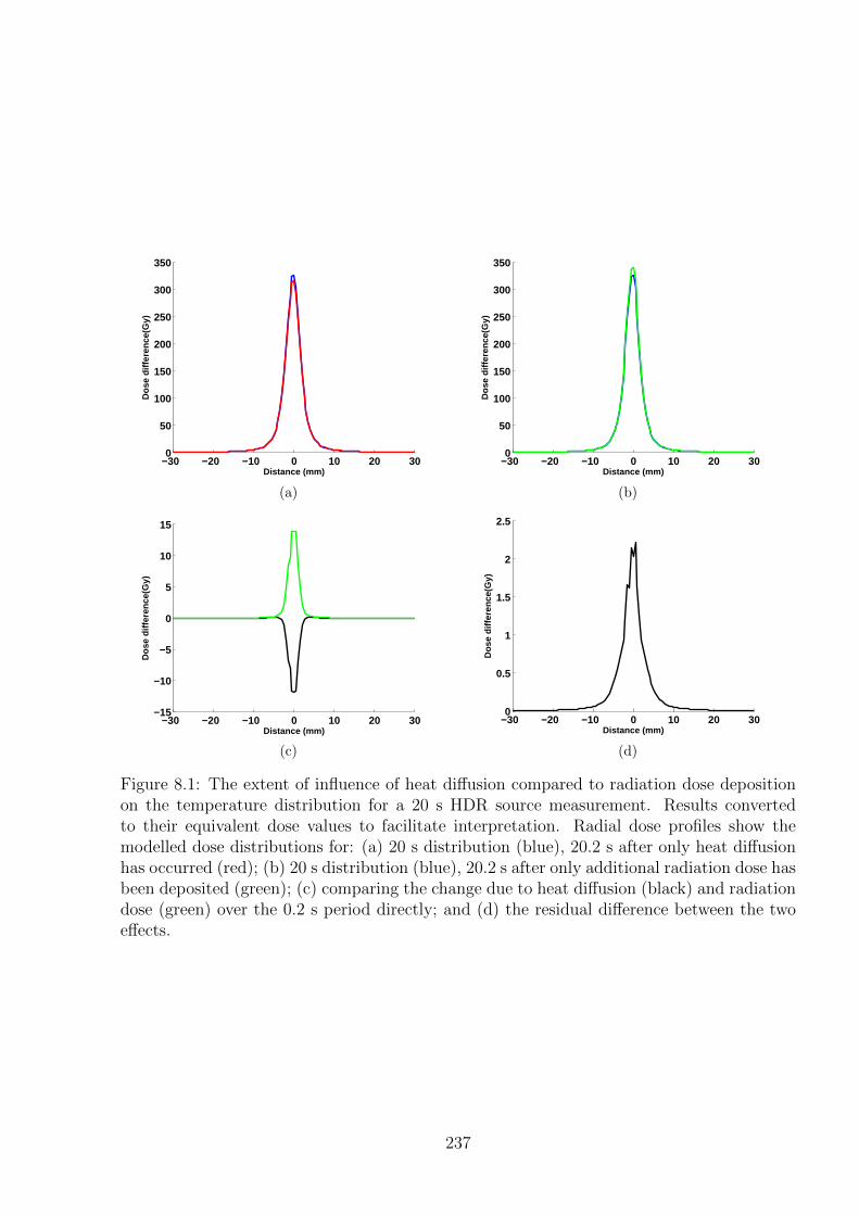
−30 −20 −10 0 10 20 300
50
100
150
200
250
300
350
Distance (mm)
Dos
e di
ffere
nce(
Gy)
(a)
−30 −20 −10 0 10 20 300
50
100
150
200
250
300
350
Distance (mm)D
ose
diffe
renc
e(G
y)(b)
−30 −20 −10 0 10 20 30−15
−10
−5
0
5
10
15
Distance (mm)
Dos
e di
ffere
nce(
Gy)
(c)
−30 −20 −10 0 10 20 300
0.5
1
1.5
2
2.5
Distance (mm)
Dos
e di
ffere
nce(
Gy)
(d)
Figure 8.1: The extent of influence of heat diffusion compared to radiation dose depositionon the temperature distribution for a 20 s HDR source measurement. Results convertedto their equivalent dose values to facilitate interpretation. Radial dose profiles show themodelled dose distributions for: (a) 20 s distribution (blue), 20.2 s after only heat diffusionhas occurred (red); (b) 20 s distribution (blue), 20.2 s after only additional radiation dose hasbeen deposited (green); (c) comparing the change due to heat diffusion (black) and radiationdose (green) over the 0.2 s period directly; and (d) the residual difference between the twoeffects.
237
entirely. The validity of many of the calculation parameters chosen was verified in Section
5.3.1 when the variation in the heat diffusion results under different calculation conditions
was determined. For instance for points 3 and 4, if the ratio of the irradiated volume to the
test cell volume is small, the boundary effects were shown to be negligible. As the ratio in-
creases, which may be required to increase the measurement sensitivity for some future DHI
applications, the boundary effects become superimposed on the radiation heating pattern,
resulting in distortions around the edges of the model, and errors of up to 50% exhibited in
preliminary calculations.
An unrelated area to consider is the radiation model that the heat diffusion was calcu-
lated on. In order to achieve accurate estimates of the expected heat distribution, it was
assumed that the radiation parameters were constant during the entire beam irradiation
period. Variation in for example, dose rate, beam symmetry or flatness, or instabilities in
the lateral dose distribution altered the reality compared to the generic model. For the HDR
source this assumption is reasonably valid, but for the proton beam this may be worth in-
vestigating further. Sarfehnia et al. found that a significant contribution to the uncertainty
in the heat transport models was due to the variation in irradiation times due to variations
in the accelerator output dose rate and, in the case of scanned beams, the required time to
change energy layers [96]. As the irradiation period increases the cumulative distribution
will approach the expected distribution of the model, however there will be subtle variations
in how the heat is deposited, resulting in small errors in the heat diffusion model. With
decreasing size of the radiation beam, instabilities in the beam have an increasing impact on
the uncertainties in the heat diffusion calculations [275].
Cell Wall Influence
The presence of the non-water cell wall was not accounted for in the heat diffusion calcu-
lations. According to Sarfehnia et al. this has the largest influence on calculation of the
kht factor [74, 96]. The deviation of kht from unity was found to increase with increasing
wall thickness, up to values of up to 4.7% for their irradiation conditions. However these
measurements were made using a glass vessel, with glass likely to have a more significant
impact than the Perspex used for the DHI dosimeter. Additionally, the substantially longer
measurement times would also increase the extent of the wall influence. Simulations by
Palmans et al. have shown that the impact of conduction from a glass vessel only appears
approximately three minutes following the end of a two minute irradiation, with negligible
238
effect within the two minute irradiation period [277]. For these reasons, the choice to not
include the wall effects in the present calculations is reasonable, and is unlikely to have
adversely impacted on the accuracy of the results. For future development of the system,
reduction of uncertainties wherever possible may be desirable, increasing the justification for
modelling of the influence of the wall effect on heat diffusion. This can be done by defining
the system with boundary conditions reflecting the impact of the cell wall material.
The additional effect which was not yet considered was the perturbation effects of the cell
wall on the radiation field, due to attenuation of the primary beam and variation in scatter
conditions. This effect is generally small, with various studies showing it to be less than 0.2%
for glass test cells [277]. The irradiation properties of Perspex/PMMA are more equivalent
to water than glass is, due to the average atomic number and density being more similar.
Two groups have shown that for proton beams irradiating a PMMA vessel with similar size
and wall thickness to the DHI test cell, the attenuation correction factor is equal to 1.000
±0.00012 [277]. The values for photon beams are very similar, with only small variations due
to differences in the relevant interaction cross sections, i.e. mass stopping powers for protons
and mass energy absorption coefficients for photons [17]. If required it would be possible
to include this influence into any Monte Carlo model of the radiation source, however those
results suggest this may not be necessary.
8.2.2 Consideration of Heat Convection
The pilot studies completed with the prototype DHI detector ignored the influence of heat
convection on the results when comparing the measured values to modelled values. This
assumption is likely to be valid for the time frames of the irradiations measured. Natural
convective motion occurs due to buoyancy forces created in a gravitational field by density
variations within a medium [218]. In water convection is generally said to occur when the
Rayleigh number exceeds 1000 [75]. The Rayleigh number is proportional to the thermal
expansion coefficient, and a function of the temperature gradient relative to the distance to
the medium barriers. In the context of DHI, the temperature gradients arising from irradi-
ation of water and source self-heating are small enough that there is some lag time before
the onset of convective effects. Additionally, if any convection does occur, the small size of
the test cell used means that the cell walls act as a convective barrier, which decreases the
effect of convective flow within the cell.
239
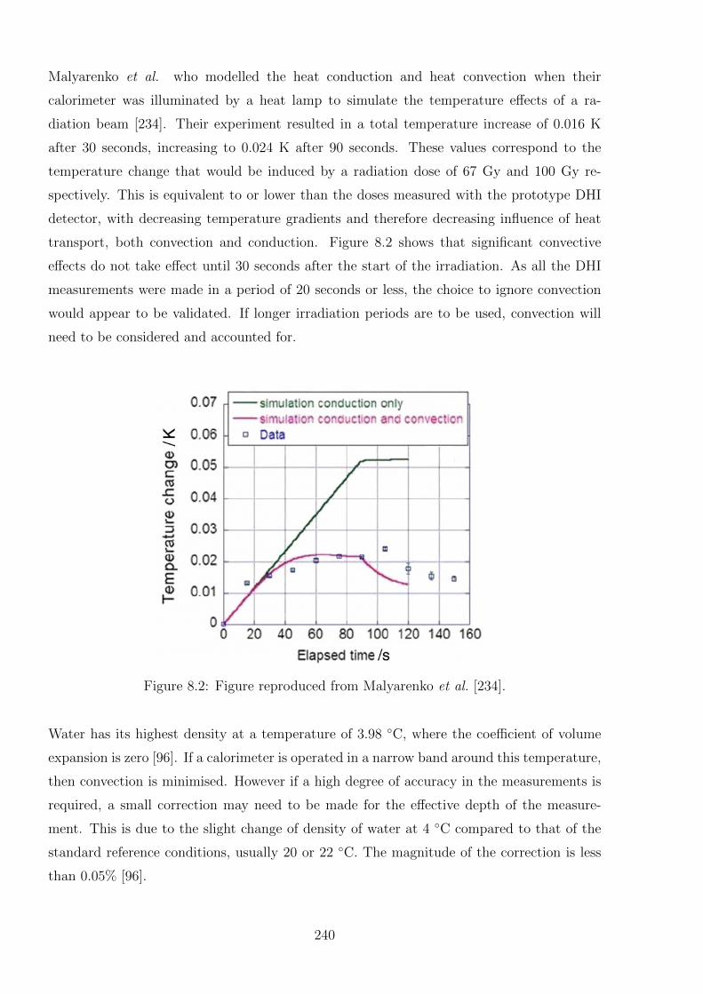
Malyarenko et al. who modelled the heat conduction and heat convection when their
calorimeter was illuminated by a heat lamp to simulate the temperature effects of a ra-
diation beam [234]. Their experiment resulted in a total temperature increase of 0.016 K
after 30 seconds, increasing to 0.024 K after 90 seconds. These values correspond to the
temperature change that would be induced by a radiation dose of 67 Gy and 100 Gy re-
spectively. This is equivalent to or lower than the doses measured with the prototype DHI
detector, with decreasing temperature gradients and therefore decreasing influence of heat
transport, both convection and conduction. Figure 8.2 shows that significant convective
effects do not take effect until 30 seconds after the start of the irradiation. As all the DHI
measurements were made in a period of 20 seconds or less, the choice to ignore convection
would appear to be validated. If longer irradiation periods are to be used, convection will
need to be considered and accounted for.
Figure 8.2: Figure reproduced from Malyarenko et al. [234].
Water has its highest density at a temperature of 3.98 ◦C, where the coefficient of volume
expansion is zero [96]. If a calorimeter is operated in a narrow band around this temperature,
then convection is minimised. However if a high degree of accuracy in the measurements is
required, a small correction may need to be made for the effective depth of the measure-
ment. This is due to the slight change of density of water at 4 ◦C compared to that of the
standard reference conditions, usually 20 or 22 ◦C. The magnitude of the correction is less
than 0.05% [96].
240

Another consideration for limiting the formation of convection currents is the direction of the
radiation induced temperature distribution. If the regions of higher temperature are located
above the regions of lower temperature, then there may be negligible buoyancy forces pro-
duced. If the irradiation equipment permits, the irradiation conditions should be arranged
to produce this effect as much as possible. For instance, external beam irradiation of a test
cell in a vertical rather than horizontal direction creates a situation where decrease in dose
with depth, outside of the initial build-up region, creates a vertically diminishing tempera-
ture profile. Measurement of a radiation source, as conducted in the early DHI HDR source
measurements produces the same effect, if the source is partially submerged from the top.
There are obviously situations where it is not possible to engineer this sort of dose distribu-
tion, for instance if the radiation gantry is only able to be horizontal, as is often the case for
proton beam or synchrotron radiation measurements. An additional limitation for a proton
beam even if a rotating gantry is used, is that the relatively long region of build-up dose
before the Bragg peak means that the buoyancy forces can still be created, and therefore
this approach cannot be used to reduce convective effects.
There may be situations for a given set of measurements where experimental limitation of
convection via a short irradiation period, small volume test cell, operation at 4 ◦C and ver-
tically decreasing and low temperature gradients, is not suitable. In these cases, then the
convection could be modelled using the incompressible Navies-Stokes equations [278]. This
approach has been used in other radiation calorimetry experiments [96, 234]. The result
from Malyarenko et al. shown in Figure 8.2 appears to show some agreement with measured
data in terms of the temperature at the sample point levelling off with time, but does not
completely characterise the trend after the source is turned off. Alternative calorimetry
approaches however are concerned with the dose at the point or points of measurement,
rather than the full two or three dimensional dose field of DHI. Thus the correction for
heat convection often consists of a single factor, which accounts for the cumulative effects of
heat motion around the measurement region. Any discrepancies in the exact shape of the
temperature map are likely to be averaged out. However the two or three dimensional DHI
results must be corrected at a much greater number and density of measurement points.
Therefore any discrepancies in the modelled convective currents, due to assumptions in the
model or incomplete knowledge of the initial conditions will be more visible in DHI. For this
reason it is anticipated to be difficult to conduct convection modelling to the extent neces-
sary to be able to remove its influence entirely from the DHI results. It may be possible to
optimise any model of the convective motion used for particular DHI irradiation conditions,
241
as described in the next section. However to achieve the highest degree of accuracy in the
results the methods introduced for limiting or circumventing convection should be applied
where possible.
8.2.3 Experimental Validation of Heat Transport Models
The multi-dimensional output of DHI is a key advantage over alternative point-based calorime-
try techniques, and allows for the potential use of DHI for a fundamental evaluation of the
accuracy of the heat transport models for radiation dosimetry. By recording DHI images
after the irradiation has ended, any evolution of the temperature distribution map is due
to heat transport effects. Taking the final irradiation frame as the initial conditions for the
various heat transport models, the efficacy of the models can be tested without the complica-
tion of additional heat being added from an external source. Alternative calorimetric studies
have reported similar measurements to validate their heat transport models, but the results
are fundamentally constrained by the limited number of measurement points [74, 82, 96].
This could be of particular use for validating models of heat convection, where the exact
temperature flow is much harder to predict than heat diffusion. By removing the modelled
effect of the heat diffusion, the resultant images will represent the heat convection alone.
This method can be used to quantify the extent of convection occurring, determine any pre-
dictability in the flow and optimise models if they are shown to be required. This would only
be able to be achieved for systems where the heat transport results in temperature gradients
which are of greater magnitude than the noise in the system. Validation of this sort could
also potentially help to reduce the uncertainties introduced by the heat transport correction
factors required in alternative calorimetric dosimetry systems.
8.3 Analysis of Uncertainty Budget and Evaluation Met-
rics
The method used for DHI dosimetry has many areas where uncertainty is introduced into the
system. Some of the uncertainties are inherent to the DHI method, such as the noise in the
system and the uncertainty in converting measured phases to absorbed dose. Other uncer-
tainties are specific for the radiation type under measurement, and the measurement process
required. These types include dose temporal and positional uncertainty, the influence of
the heat defect, and the potential need for scatter and attenuation corrections. Uncertainty
242
analysis can be divided into two different types, known as Type A and Type B [279]. A
combination of these approaches was used to determine the uncertainty estimates presented
in Chapters 4-7.
Type A uncertainty estimates are represented by a statistically estimated standard deviation.
The metric is based on deviation from the true value being due to random errors, with the
measurement reproducibility acting as an indication of the uncertainty. The determination
of phase by DHI was considered to be associated with Type A uncertainties. This analysis
incorporates the uncertainties due to noise in the measurement system, beam output varia-
tions and some variation in ambient conditions. The extent of these uncertainties were well
characterised in Chapter 6.
Type B uncertainties are based on scientific judgement of the possibility of error in specific
measurement parameters, and represent possible systematic uncertainties in a measurement
dataset. The anticipated range of possible values is considered, and bounds placed on the
extent of certainty which can be achieved in a result. For the DHI analysis, these sorts of un-
certainties included positioning errors, possible errors in the radiation model or subsequent
heat diffusion model, and uncertainties in the conversion factors used to quantify absorbed
dose from the measurement of the light phase variation.
The overall uncertainty budgets that were calculated for the HDR source and proton beam
measurements. The gamma index analysis conducted on the HDR results in Chapter 6 was
a first order check of these, by setting the dose tolerance to the level of the relative un-
certainty on each point of measured and modelled data. Excluding the random distortions
attributed to variations in air flows and external temperature effects, the results showed
that the uncertainties were not underestimated. It is probable that there are redundancies
in the way uncertainties were calculated, for example incorporating the dosimetric impact
of a positioning error may mean that the uncertainty on dose was overestimated and can be
reduced. Future investigation of this for the next iteration of the DHI detector will allow for
accurate comparison of detector advantages and disadvantages.
An alternative way to check some of the assumptions inherent in estimating uncertainties,
would be to devise a controlled test that can accurately produce temperature variations on
the same order as those induced by absorbed doses. Due to the very small temperature
variations involved, this is not a trivial matter. A possibility would be the use of incandes-
243
cent lamps, collimated and attenuated to produce small temperature changes in water, as
used by Malyarenko et al.. However the crude estimates of the spectral composition is still
a limiting factor on the accuracy, and they only showed measurements to a sensitivity of
approximately 100 µK s−1, which may not be enough to provide useful analysis of some of
the system uncertainties.
Most of the sources of uncertainty in the DHI system are covered in other sections through-
out this discussion chapter, when some key considerations and suggested improvements for
the different aspects of the measurements are discussed. The following sections include men-
tion only of those sources of uncertainty which have been accounted for in the uncertainty
calculations but may require further consideration, and have not been discussed elsewhere.
Many of the uncertainties in the measurements can be divided into two categories: positional
uncertainties and dosimetric uncertainties.
8.3.1 Positional Uncertainty
Positional uncertainties arise where the positioning of the measured sensitive region with
respect to the water surface and the radiation is not accurately known. This geometric error
effectively results in the dose to specific locations being misrepresented in the results. These
uncertainties were less significant for the HDR source measurements as the applicator was
clearly visible on the measurement image; although due to the small size of the measurement
region, only a small section of the applicator was visualisable, resulting in some uncertainty.
Additionally, the excess internal space within the applicator and the potential asymmetry
in source position could be a contributing factor. Both of these could be overcome by larger
field of view measurements, so the entire applicator could be located, and the symmetry
of the measured dose distribution around it calculated. For the external beam measure-
ments, there were more potential errors introduced in the positioning. The template around
the region of interest helped to reduce these, and the addition of a micrometre controlled
translation stage to hold the test cell, and more accurate measuring equipment to locate it
relative to the gantry would reduce these further. For this reason the positional uncertainty
is considered to be a relatively trivial problem that in the future could be experimentally
reduced to negligible levels.
An additional consideration in terms of positional uncertainty is the relative resolution of
the DHI measurements, as opposed to any model or alternative measurements that it may
244
be compared to. For lower resolution comparison data, error in the positioning can be more
readily introduced. Additionally, signal averaging in higher dose gradient regions may oc-
cur, which will also impact on the comparative doses. If this is of concern, then a higher
resolution model should be used, which is easily achievable with Monte Carlo approaches.
It is however also potentially useful to compare the DHI results with the output from a
treatment planning system in clinical use, which is likely to achieve lower resolutions. In
this case, the introduced positioning uncertainty due to resolution is unavoidable, and will
need to be incorporated in the uncertainties.
8.3.2 Dosimetric Uncertainty
Uncertainties in dosimetry can be divided into two types: those which affect the relative
dose, and those which affect the absolute benchmarking of that relative dose. Some of the
dosimetric uncertainties contribute to both categories, while some are specific to one cate-
gory. The contribution to dosimetric uncertainty from the relative shift will not be relevant
if the stability and consistency of the measured results is improved in future versions of the
detector, so that cumulative absolute dose values can be used. Additionally, a notable source
of uncertainty in the current results is the fact that all data is compared back to a single
reference image. With the current distortions visible in some of the measurements, careful
selection of a reference image is important, to avoid propagating a single discrepancy through
the entire image set. The selection of the reference image should be made by analysis of the
image series acquired prior to irradiation starting, and selecting high quality images, with
limited distortion, and phase values representative of the image series. It is also possible
to average some of the image series, to reduce the influence of random fluctuations. Care
should be taken not to introduce a systematic shift in the dosimetry values by averaging
images that display some kind of artificial trend.
A different aspect of the dosimetric uncertainty which has not yet been considered is the
small size of the test cell that was used. This means that the absorbed dose is measured in a
volume which is not necessarily representative of full scatter conditions, especially for higher
radiation energies. This may result in a somewhat lower dose than expected, however the
effect is likely to be small for the limited field sizes in the present measurements, but would
be worth considering if broad beam type geometries are studied in the future, or higher
energy radiation. The exact extent of these irradiation conditions can be easily investigated
with the use of a Monte Carlo model with active volumes of varying sizes.
245
With the present levels of noise in the measurement system, the choice of mathematical
filter makes some difference to the measured doses. The filter smooths out noise, but po-
tentially contributes to discrepancies in the shape of the measured dose distribution from
what it should be. The use of Type A uncertainties based on the standard deviation of null
images should account for these effects, but correct selection of a filter should prevent loss
of information, the overestimation of the level of uncertainty required, or the recording of
apparent signals which are actually artificially features of the noise. The choice of filter will
therefore be dependent on the structure of the radiation, and the sensitivity of the system.
As for the HDR source measurements presented in Chapter 6, multiple different filters can
be used within an image in order to optimise the situation. Whilst the largest uncertainty
in dose arising from the standard deviation of pixel values from the mean was used, further
refinement of the uncertainty analysis may allow for a tightened uncertainty budget in some
regions, depending on the filtration level required.
Temporal uncertainties are also another key component of the overall dosimetric uncertainty.
Accurate timing systems should be developed, in order to allow effective time stamping
relative to both the time of the reference image and the irradiation period. The current
results approximated these time periods, and checked the validity of the results by confirming
the number of images collected with the expected number. However this system could be
improved upon, as suggested in Section 8.4.
Calculation Parameters
There are several calculation parameters used when converting from the measured phase
change of the laser to the absorbed dose. These include the variation in refractive index
with temperature and the specific heat capacity. Also for the heat diffusion modelling to
be valid, there is a condition that the specific heat capacity and the thermal conductivity
coefficient be independent of both pressure and temperature.
The first step when calculating dose is to convert between the refractive index variation
in the water, as measured from the phase change, and the temperature change. This pro-
cess was conducted using a sixth order polynomial fit to data reported by Bashkatov and
Genina [243], as was shown in Figure 4.8. In order to estimate the accuracy of the fit, for
the temperature region of interest for DHI dosimetry, a sixth order polynomial was also
fitted to the inverse of the data. By converting from refractive index to temperature and
246
back again, it is possible to estimate the induced uncertainty as half of the variation in the
value of the refractive index. Thus with the current data and fit used, an uncertainty of
0.5% should be added to this parameter. This value is only required for any future absolute
dosimetry measurements, where an absolute temperature or dose measurement is required.
For the relative dosimetry measurements, i.e. the spatially varying dose differences at each
point in time, the error is negligible. This is because for the relative measurements, the dose
difference between points is small enough that the uncertainty in the refractive index to tem-
perature variation is very similar at each point, so therefore cancels out in the dose difference.
The next step is the conversion of temperature change to absorbed dose. It is assumed for
the calculation of absorbed dose and for the heat diffusion model, that the specific heat
capacity of water is constant with temperature. Over the temperature ranges of interest this
holds true. As shown in Figure 4.8, a trend line was fitted to the plot of the temperature
versus specific heat data from reported values [244]. From this it was determined that for
a 0.001 K temperature variation, which encompasses the range of measurements used, the
value of the specific heat capacity of water varies by less than 1.2×10⁻⁵% [244]. If the am-
bient temperature in the water cell is incorrectly measured, the impact is also negligible.
Variation by 1 K introduces only an 0.01% error into the value of the specific heat capacity.
Controlling the temperature of the water and measurement of the water temperature is easily
achievable to better than 1 K, so this error is effectively negligible, provided accurate source
data is used for the specific heat values. This agrees with the analysis by Karger et al. and
Medin et al. that the relative standard uncertainty for the water specific heat capacity used
in the uncertainty budget for their calorimetric measurements be set at 0.05%, after they
experimentally validated the heat capacity measurements [17, 111].
In calculating the heat diffusion the value of thermal conductivity is assumed to be constant
with respect to temperature. In reality, according to the data of thermal conductivity versus
temperature obtained from The Handbook of Chemistry and Physics [244], in the range of
normal room temperatures (20-25 ◦C), there is a 1.1% difference per degree in the calculated
thermal conductivity value. The impact of this on the calculated heat diffused temperature
distribution was quantified in Section 5.3.1, where the mean deviation for a typical proton
measurement was found to be 0.28%.
247
Heat Defect
The heat defect is a key consideration in all calorimetric dosimetry measurements, as de-
scribed in Section 2.2. No experimental efforts were made to reduce the heat defect for the
initial proof-of-principle DHI measurements, as the influence is negligible compared to the
other uncertainties in the system. However as the DHI detector is refined, reducing noise to
gain increasing sensitivity, it will become increasingly important to limit or account for the
heat defect.
The contributing mechanisms for heat defect depend on the impurities in the water and the
LET of the radiation source. There is no inherent difference between DHI and alternative
calorimetry systems in this respect, so the choice of a suitable medium can be considered
by reviewing work in this field. The presence of oxygen gas in water has been shown to
cause a strong transient exothermic effect when irradiated, of up to 10% [96]. Sarfehnia
et al. used high purity water saturated with hydrogen gas for their proton measurements,
and noted that any notable delay between measurements resulted in trace oxygen leakage
into the system, and observable heat defect [96]. Sassowsky et al. have also reported a
heat defect of effectively zero, to an uncertainty of ±0.3%, once hydrogen gas was used to
remove all traces of oxygen from the system and following pre-irradiation until a steady
state was reached [117]. These experimental results are in agreement with various numerical
simulations of heat defect for proton beams [105, 106, 111, 116, 117, 277]. There are also a
considerable number of studies investigating and accounting for the heat defect for low-LET
beams, such as photon or electron beams, and similar results have been found regarding
saturation of the system with hydrogen, nitrogen or argon gas [36,245].
For DHI dosimetry therefore, experimental reduction of the heat defect should be achieved
using hydrogen saturated water in a sealed test cell. This will require some modification of
the current test cell as an open-topped design is currently used, and glass may be a more
effective material to use to ensure the system is air tight. For measurements such as the
HDR source, a complicating factor is the need to introduce a physical applicator into the
test cell to house the source. It may be possible to incorporate an applicator through a
small port, with air tight seals around it. If the DHI detector achieves sufficiently sensitive
measurements then it should be possible to prove that this approach limits the influence of
the heat defect to be negligible.
248
8.3.3 Use of the Abel Transform
Implementation of the Abel transform to estimate the three dimensional dose distribution
overcomes a major limitation of the current DHI approach, which produces information on
the dose distribution as integrated across the test cell. This means that it is in a format
that physicists are inherently less familiar with, which can limit the understanding of the
results, and potential utilisation of the method. Additionally, the unmodified DHI results
have limited comparability with non-three dimensional point dose or planar detectors, except
via a three dimensional model. In irradiation conditions with cylindrical symmetry, the use
of the Abel transform overcomes these limitations, allowing a visualisation of any plane and
therefore any point within the test cell. Provided the Abel transform results are interpreted
with understanding of the regions where there are increased errors in the determined dose
values, and used in conjunction with the original integrated dose results, this approach can
add utility to the results of the DHI detector.
The mathematical solution to the Abel transform that was presented in this work was based
on that proposed by Pretzler [261, 262]. This is a numerical solution based on the prin-
ciple of Fourier-analysis, where the unknown radial distribution is expanded in a series of
cosine functions, and the amplitudes then calculated by a least-squares fitting of the Abel
transformed series to the measured data. In contrast, the conventional approach to the Abel
transform determines the radial distribution iteratively in increments from the edges into the
centre. The advantage of the Pretzler approach, and the reason it was selected for the initial
implementation in this work is that it is known to be relatively insensitive to noise and errors
in the determination of the location of the centre of the object. MATLAB code implement-
ing this function was available from www.mathworks.com, the MATLAB file exchange [263].
An implementation of the basic algorithm was programmed in MATLAB for comparison
purposes, and it was confirmed that the Pretzler code was superior at reconstructing radial
dose functions with a higher level of agreement to the expected values, especially for noisy
data and areas of sharply changing gradients.
The key limitations with the use of the Abel transform for this purpose is that there is a
fundamental loss of information when the algorithm is applied to the measured data. Despite
the improvements of the Pretzler algorithm on earlier methods, there is still loss of signal
when the dose gradient varies, with the exact radial dose function unable to be precisely
reproduced. Additionally, the presence of noise in the data can result in extreme oscillations
within the result of the transform. Both of these situations occur in the HDR measurements,
249
the noise being inherent, and a very sharp change in phase occurring between the high doses
adjacent to the applicator compared to the region where the sensor is physically shadowed
by the applicator. Thus comparison of measured results to a model by means of radial dose
function is inherently unreliable in the region immediately adjacent to the applicator. This
may be of less concern for alternative radiation therapy modalities which do not experience
such a sharp phase variation. Additionally, the assumption of cylindrical symmetry of the
dose distribution risks losing any information garnered from measurement about any asym-
metries in source positioning or beam flatness which may be detected from the measured
results.
The Pretzler code was also utilised for the initial development of the second approach to heat
diffusion that is described in Section 5.4. For this method the limitations of the code were
more evident. This is because of the cumulative effect of the errors in the Abel transform,
resulting in the final errors being proportionately higher than the signal being measured. As
described in that section, in order for that approach to be implemented alternative improved
versions of the Abel transform would be required. There are multiple groups in the field
of mathematics working on this problem, with a variety of approaches reporting promising
results for noisy data which look like they may be of use for these DHI results [280–282].
For example, Dribinski et al. report an Abel transform approach based on a variation of the
basis-set expansion approach used by Pretzler which improves the accuracy in particular in
the region close to the symmetry axis [280]. Gonzalez-Ramirez et al. and Dixit et al. have
developed approaches which achieve stable numerical inversion of experimental intensities
distorted by noise, using a Kalman filter approach and a direct operational matrix of in-
tegration approach respectively [281, 282]. Further study is required into these algorithms
to understand the benefits and limitations of the different approaches, implement them in
MATLAB and conduct a comparison study as to which will provide the most advantages for
the specific requirements of DHI, in particular for the Method 2 heat diffusion calculations.
The Abel transform could also be potentially useful if a tomographic approach to DHI is de-
veloped (this is described in Section 8.5). A tomographic DHI with sufficient beam angles to
allow for a full tomographic reconstruction would inherently determine a three dimensional
dose distribution. This may not be possible to achieve however, in which case the most
successful approach may prove to be a limited projection approach such as for tomosyn-
thesis. This would involve a refined estimate of the three dimensional image reconstructed
from projections at a finite number of angles, likely to be limited to two or three. In this
250
situation, the use of the Abel transform of each of the images could provide a comparison to
estimate the accuracy of the reconstruction algorithm. Additionally, multiple measurement
angles could be used to prove the cylindrical symmetry of the radiation, in which case a
limited projection tomographic reconstruction may actually provide less information than
just using the Abel transform directly on one or all of the images.
Radial Dose Function as an Evaluation Metric
The radial dose function is used for cylindrically symmetric geometries, and is a measure of
the dose along any given profile in a radial direction from the longitudinal axis of the dose
distribution. For HDR source dosimetry, it is a key parameter in the TG-43 algorithm, and
for proton dosimetry it is a useful parameter for comparison of measurements from different
dosimetric approaches. The radial dose function can be calculated from the current DHI
results by means of the Abel transform [260].
The radial dose function was calculated for a subset of the HDR prototype measurements.
Reductions in noise of the measurements would allow for improvements in the accuracy of
this function. The extent of the noise in the images for the HDR results determined the
distance from the applicator that was affected by the wild oscillations in the Abel transform
result, as was shown in Figure 6.22(a). For datasets with increased standard deviation of
the noise, the radial position to which the Abel radius was approximately accurate was fur-
ther from the central axis. An exact correlation for the extent of this effect was not able
to be determined from the limited datasets, because the extent of the noise had a limited
range across all the measurements. Future measurements could consider investigating this
effect further in order to provide an estimate on the limits of accuracy of the Abel transform.
Improvements in the Abel transform implementation, as described above, as well as experi-
mental improvement of the signal to noise ratio should improve the applicability of the radial
dose function as an evaluation metric. It may become possible to use DHI to validate some
aspects of the TG-43 protocol.
8.3.4 Gamma Index as an Evaluation Metric
The gamma index is commonly used in radiotherapy dosimetry as an evaluation metric for
considering the agreement between two or three dimensional dose distributions [267]. The
251
metric was developed as a means of overcoming the limitations inherent in using dose differ-
ence or distance-to-agreement comparisons, which were prone to failure in low dose and high
dose gradient regions respectively. Understanding of the areas of limitation of the metric are
important when interpreting the results of a gamma test. As the gamma index is likely to
be a very useful tool in evaluating results of future DHI measurements, an introduction to
these uncertainties is given here.
The gamma index is a more useful metric for the comparison of three dimensional dose
distributions than two dimensional distributions, because for a two dimensional dose distri-
bution the degree of agreement with the two datasets can be more easily visualised without
additional calculational methods. However a gamma test is still of value, as it provides
a quantitative result, which is comparable between multiple dose distribution comparisons.
The output of a gamma index test is a numeric indicating the percentage of points within the
test region or volume which passed the gamma criteria (e.g. had a gamma value of less than
one). Results should be interpreted with caution however, because in the presence of exces-
sive dose differences in the high dose gradient region and/or large DTA discrepancies in low
dose gradient regions, the result could still be a high value, as the test does not distinguish
between those datasets that failed grossly on a large number of points, from those which are
close to passing. The test is generally more prone to failure in low dose regions compared
to any other region, but the failure is more likely to be of less significance in terms of ab-
solute dose, so these regions should often be ignored using a low dose threshold. Grouped
failures in high dose or high dose gradient regions are more likely to be of significance. Thus
examination of a sole gamma index value is not sufficient for fully determining the degree
of agreement between datasets. Studies on the use of the gamma index for use in QA of
IMRT treatment plans have suggested that simple pass/fail use of the gamma test may not
be the best way to determine the quality of the agreement of the measured dose distribution
with the model [283]. Alternative suggestions include the use of further parameters based
on the gamma test, including maximum gamma index value, average gamma index value
and connected area of evaluated points with gamma index >1 [284–286]. These methods
may also be of use if a gamma test is used to quantify the agreement of DHI measured dose
distributions with the expected values.
An additional consideration is that the gamma test is also highly dependent on the normal-
isation method used [285]. The choice of normalisation position (e.g. maximum dose, dose
to a local point, surface dose etc.) is important, because the percentage value used for the
252
uncertainty will result in quite different absolute dose differences which are being compared,
depending on the dose value of the normalisation point.
The degree of noise in the two comparison datasets is also of importance [287]. The im-
pact is asymmetric, with the levels of noise in the reference data versus the evaluated data
having differing effects on the gamma test pass rate. When the gamma test is conducted,
each point within the evaluated data is considered in turn, and the surrounding points in
the reference image are searched to determine the closest match. As would be expected
intuitively, the presence of noise in the reference data makes this search more likely to find
a good match for each point, so the gamma index becomes lower and the test pass rates
increase. Alternatively, noise in the evaluated image moves the values at each point away
from the reference, decreasing the likelihood of locating a good match, so the gamma test
pass rate decreases. With increasing standard deviation of the noise the trends in both cases
are exacerbated, with higher impact from random noise than from spatially correlated noise.
For this reason, it is important to consider the relative noise in the datasets when selecting
the reference data compared to the evaluated data. In the case of the DHI results, gener-
ally the calculated model results will have lower noise than the experimental results, so this
should be used as the reference dataset in the gamma comparison. If two empirical datasets
are compared, which are both affected by noise, then the gamma index could be calculated
twice with switched roles for the reference and evaluated images, to determine a composite
result. An additional important consideration is the impact of the image resolution on the
noise. A decreased image resolution results in lower noise, which will affect the gamma pass
rate. For this reason the standard deviation of image noise should be stated when reporting a
gamma index, as it can give an idea of the uncertainty inherent in the gamma test evaluation.
The approach taken when analysing the HDR results (Section 6.2.6), in determining the
points where the two dose distributions agree to within experimental uncertainty is a use-
ful concept for analysing the results of the DHI measurements in terms of the validity of
the uncertainty estimates for both dosimetric and positioning error. If sufficient magnitude
uncertainty is included then the gamma test should show a 100% pass rate when the total
uncertainty values are used as the threshold criteria. This is complicated by the fact that
the dose deviation parameter is global, i.e. proportionate to the signal, as the gamma test
uses a single threshold value across the whole region based on a percentage of the maximum
dose. It would be possible to implement the test with variable threshold values across the
dataset, which would allow this to be accounted for. This may be an area of interest to
253
achieve a simple three dimensional evaluation of measurement accuracy and estimation of
experimental uncertainties, which could be used for future development of the DHI detector,
or any other multidimensional dosimetry approach.
8.4 Recommendations for Experimental Improvements
Based on the preliminary testing of the detector on the proton beam and HDR source, a
range of possibilities for improving the detector have been determined. The improvements
which apply specifically to the proton measurements have been described in Chapter 7. This
section will describe more general improvements to the system, and summarise the specific
improvements. The extent of the gains achievable by implementing these modifications are
estimated where possible, based on the understanding of the abilities of the current system,
and by comparison to literature results of DHI measurements of temperature distributions
in alternative industries.
There are various types of modifications which could induce notable improvements in the
current results: from the precise configuration of the interferometer, hardware choices, and
measurement conditions, to improvements and extension to the experimental process. These
aspects are combined to achieve some of the aims described in the sections below.
8.4.1 Independence from Ambient Conditions
From analysis of the initial pilot study results on the HDR source and the proton beam,
it is evident that considerable improvements to the reliability and usability of the results
could be achieved by better isolation of the detector from variations in the ambient condi-
tions. Ambient temperature and pressure fluctuations, and the resulting air flows vary the
conditions experienced by the laser beam. The major cause of noise and extraneous signal
is the temperature and pressure variations in the air portion of the laser path. A less sig-
nificant cause is temperature induced expansion or contraction of the optical components.
These effects alter the phase of the laser light, creating a signal which is conflicting with
the phase variations due to the radiation induced temperature increase in the test cell. The
phase of the laser light varies throughout the interferometer, with the signal measured being
the difference in phase, and therefore optical path length, between the reference and object
254
beams of the laser. The only part of the system which is producing the signal of interest is
the variation in phase of the water contained within the test cell. The inherent assumption
when interpreting the results is that the phase change of the entire reference beam, and the
object beam everywhere except the test cell, is temporally constant. This was shown in the
pilot study measurements to not be the case however. This is consistent with results from
other calorimetric based studies, where thermal drift in the laboratory is detected in base-
line measurements, even for systems with good experimental isolation [111, 116, 234]. For
measurements at a single point of reference, this can often be approximated as a linear back-
ground drift, and subtracted out to obtain accurate radiation induced temperature increases.
Unfortunately for the two dimensional nature of the DHI images, the variations have been
demonstrated to be not easily predictable, and can vary quasi-randomly both spatially and
temporally. This problem is exacerbated because the magnitude of the changes required to
noticeably interfere with the results is relatively low.
There are two different approaches for dealing with this problem. The first is to correct for
aspects of this issue with the use of careful control measurements. The second approach is to
attempt to reduce or eliminate the external influences. The second approach is fundamen-
tally a better approach, however may be technically difficult to realise in practice. Methods
to undertake each approach are proposed in the next sections, along with a discussion of the
advantages and limitations of each.
Simultaneous Control Measurements
The first approach to reducing the influence of variations in the environmental conditions
is by the use of simultaneous control measurements. This concept is similar to the use
of a reference ion chamber to correct for beam output variations during linear accelerator
water tank measurements. For DHI, the principle is based on the theory that two laser
beams, if they are sufficiently close together and pass through as many of the same optical
components as possible, will experience the same change in phase. So the proposal is to
build an interferometer configuration, with an inbuilt second interferometer which closely
mimics the path of the first, except the object beam will not pass through the test cell. A
proposed design is suggested in Figure 8.3.
The inclusion of multiple extra optical components for the control interferometer, and the
need for larger mirrors and space for the beam path would probably require a larger bread-
board. More efficient clamps and holders for some of the optical components could allow
255
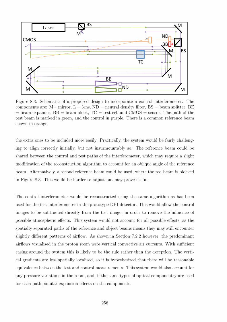
Laser M BS
BS
M
M
M
M
M BB ND
ND
BE
TC
L M Laser
CMOS
Figure 8.3: Schematic of a proposed design to incorporate a control interferometer. Thecomponents are: M= mirror, L = lens, ND = neutral density filter, BS = beam splitter, BE= beam expander, BB = beam block, TC = test cell and CMOS = sensor. The path of thetest beam is marked in green, and the control in purple. There is a common reference beamshown in orange.
the extra ones to be included more easily. Practically, the system would be fairly challeng-
ing to align correctly initially, but not insurmountably so. The reference beam could be
shared between the control and test paths of the interferometer, which may require a slight
modification of the reconstruction algorithm to account for an oblique angle of the reference
beam. Alternatively, a second reference beam could be used, where the red beam is blocked
in Figure 8.3. This would be harder to adjust but may prove useful.
The control interferometer would be reconstructed using the same algorithm as has been
used for the test interferometer in the prototype DHI detector. This would allow the control
images to be subtracted directly from the test image, in order to remove the influence of
possible atmospheric effects. This system would not account for all possible effects, as the
spatially separated paths of the reference and object beams means they may still encounter
slightly different patterns of airflow. As shown in Section 7.2.2 however, the predominant
airflows visualised in the proton room were vertical convective air currents. With sufficient
casing around the system this is likely to be the rule rather than the exception. The verti-
cal gradients are less spatially localised, so it is hypothesized that there will be reasonable
equivalence between the test and control measurements. This system would also account for
any pressure variations in the room, and, if the same types of optical componentry are used
for each path, similar expansion effects on the components.
256
The space constraints of this design may complicate the application of the further suggestions
made in the remainder of Section 8.4, however with careful implementation this is believed
to be a valid approach to accounting for the impact of ambient condition variation on the
results. If successful, this benchmarking of the phase change allows for the phase variation
in the test cell to be successfully isolated. This would allow the system to achieve absolute
dosimetric measurements, where the cumulative dose over the measurement period could be
accurately determined. This concept is discussed further in Section 8.4.3.
Isolation from Air Flow and Temperature Variation
The second approach to reducing the influence of variations in the ambient conditions is
more direct, and involves isolation of the system as much as possible from the surrounding
environment. This requires the use of an improved housing system for the optical system.
There must be an external window to the system for the radiation beam to enter. This has
the negative impact of introducing an additional attenuating object in the beam, however if
a suitable material and thickness is chosen this could be acceptable. Additionally, the laser
and the camera sensor should probably also be located outside of the temperature controlled
housing, so that the heat generated while they are running does not impact on the controlled
temperature. The windows for these may distort the results slightly, although this is unlikely
to have a significant effect.
It may be useful for the housing system to be temperature controlled. A key advantage of
this would be the ability to control the temperature down to a level of 4 ◦C, which is the
recommended temperature for calorimetric radiation measurements [35,36,276].This temper-
ature is when the density of water is maximal, and measuring here optimises the reliability of
the value of the specific heat of water [116]. Operating the system at this temperature would
increase the sensitivity, and lower the uncertainties achievable by the system, compared to
operating it at room temperature. The use of controlled temperatures may also allow for
the finite size of the test cell to be incorporated more accurately into the heat diffusion
calculations, as the extent of the heat diffusion through the walls of the test cell would be
more consistent and predictable.
There are several considerations with regards to the design of temperature controlled hous-
ing. The temperature must not be maintained by pumping air through the housing, as this
would introduce air flows of varying temperatures. The design of the temperature controlled
system which was utilised by Seuntjens et al. for their calorimetry measurements of an HDR
257
source is a good model to base the design for DHI housing on [116]. Their portable water
calorimeter was built in-house, and utilizes active cooling by controlling the temperature of
a copper shroud using a Neslab RTE-7 refrigerated bath/circulator, rather than through air
circulation. The casing consists of two 5 cm Styrofoam slabs, separated by a 5 mm copper
plate, with the entire system encased in a 1 cm thick plywood box. The temperature of
the copper plate can be easily and accurately adjusted to counter for variations in internal
temperature as measured by temperature probes in the internal cavity and in the copper.
The Styrofoam has insulating properties to reduce the rate of any heat transmission from
varying external conditions. The entire system can be controlled to a temperature of 4 ◦C.
The lack of airflow within the system means that slight variations in temperature which are
not detectable by the independent temperature probe will not be of impact on the qualitative
images of the dose distribution.
Improving the detector housing would be key in limiting the influence of air movement and
temperature variations on the DHI measurements. The housing would however increase the
weight and complexity of the system which would limit the portability, which is a key require-
ment of the DHI detector. It would also not isolate from any ambient pressure variations,
however as the pressure is generally relatively stable in the absence of changing weather
conditions, this is believed to be a much less significant effect.
An alternative approach which may be easier to implement, but has certain downsides, would
be to utilise a fibre-optic-type system, like that described in Section 4.4.4. This would re-
duce the impact of temperature flows and slow changing temperature gradients, however the
system would still be subject to these in some sections of the system, and the impact of
vibrations would significantly increase, due to vibrations of the optical fibres. Section 4.4.4
described some of the key advantages and limitations of this approach, which will not be
repeated here. The limitations in terms of environmental influences are that there would still
be potential for expansion of the components and optical fibres, and pressure fluctuations
would not be accounted for. However, the conversion would be relatively straightforward
and not encounter the space constraints of the control interferometer approach, or the bulk
of the temperature controlled housing.
258
8.4.2 Sensitivity Improvements
Improving the sensitivity of the DHI detector is key to increasing its accuracy and potential
for application to lower dose rate measurements. There are two approaches to improving
the effective sensitivity of a measurement: decrease the experimental noise, or increase the
signal. Noise in the system includes the impact of vibrations and any inherent defects in
the image quality, as well as the influence of ambient conditions described in the previous
section. Brief suggestions of methods to reduce the vibrational noise and improve image
quality are introduced below, as well as considerations for means to increase the signal.
Consideration of Vibration-Induced Noise
The influence of vibrations on the results is a key source of noise, reducing the sensitivity
of the measurements. In order to reduce the impact of vibrational noise, it is necessary to
identify the sources of the vibrations, and take steps to mitigate them where possible. There
are several different types of vibration which are relevant to the DHI detector, including seis-
mic vibrations, acoustic vibrations, and forces on the working surface. Seismic vibrations
occur when the floor under the experimental set-up is caused to vibrate, which is transmitted
to the working surface. The sources of these include wind on the building, people moving
around, nearby traffic, and building ventilation. Many common seismic sources also generate
sound, or acoustic vibrations, which are detected as local air pressure variations within the
experiment, although these are generally of less significance than mechanical motions. Forces
on the working surface are generated by any vibration sources which are directly coupled to
the experimental set-up, such as fans within equipment or moving translation stages. For
instance the slight movement caused by the HDR brachytherapy source as it extends from
the afterloader may be a source of this type of vibration. Vibration types can be further
classified as periodic or random. Periodic vibrations occur at a given frequency, for instance
a vacuum pump. Random vibrations are from unpredictable sources, such as wind, traffic
and people.
In any given clinical situation the types of vibrations present will be specific to the surround-
ings. There is often an ambient noise spectrum due to structural and acoustic vibrations. It
may be possible to isolate the source of a vibration based on the measured characteristics
of amplitude and frequency of the spectral components. Typical frequencies in a laboratory
situation are between 4 - 100 Hz [288].
Whilst it is a good general principle for interferometric experiments to limit the contributing
259
sources of vibration as much as possible, due to the need for transportability and ease of
use of the DHI detector in a clinical setting it is not necessarily feasible to incorporate a
high quality vibration isolated table into the transportable DHI set-up. If it is possible to
incorporate a vibration isolated table, it should be selected to have suitable damping char-
acteristics for the magnitude and frequency of the vibrations present. The present prototype
DHI detector did incorporate half tennis balls under the breadboard to reduce the trans-
mittance of mechanical vibrations, with a measurable reduction, however the influence of
vibrational noise cannot wholly be eliminated by this method. Therefore as far as possible
the contributing sources of vibrations should be limited at their source.
Air conditioning systems are a key factor in the ambient noise spectrum, producing peri-
odic vibrations as the fans rotate. The reduction of influence from ambient conditions was
discussed in the previous section, however if possible the air conditioning should be turned
off entirely during the measurement times. This is often not possible due to the location
of the clinical room within the facility’s wider air-conditioning network, in which case if
possible the outlets should hermetically sealed for the duration of the measurements. Other
vibration sources such as random noise due to nearby people, traffic, and machinery may
be reduced by conducting measurements out of normal hours. However it should be noted
that experiments have found that the local phase can fluctuate by several tenths of a radian
over measurements even for measurements performed at night, in an empty building with
ventilation turned off, and a vibration insulated table [289]. This is due to local eddies
and air disturbances. For instance any power source such as for the laser or computer may
produce small temperature differences which moderate the refractive index of air on a small
scale. The impact of this can be minimised with effective housing of the interferometer as
described in Section 8.4.1.
Improvement of Image Quality
All of the reconstructed images from the prototype DHI detector showed some degree of
inherent defects in the images due to scattered light. The interference patterns formed over-
laid on the main image, resulting in the so-called null images not being completely uniform.
Various methods are suggested to overcome this issue in future iterations of the detector,
including the use of higher quality optical components, the use of tubing surrounding the
paths of the laser light to prevent dust and extraneous reflections from impinging on any of
the mirrors, and a reconfiguration of the detector to avoid creating the unwanted reflections
260
and scattered light in the first place. All of these approaches should help to reduce the
measurement noise, thereby improving the sensitivity of the detector. Alternatively, pulsed
low coherence light sources have been shown to be efficient at taking away disturbances from
other scattering surfaces during speckle interferometry, so this is an avenue which could be
explored for DHI [289]. The use of a low-coherence source effectively defines the volume in
space in which the information detected is isolated, and effectively filters out information
outside this volume.
Interferometer Configuration
A fundamental method to increase the measured signal strength from the radiation induced
temperature change is to sample it multiple times. This can be achieved with the use of a
double pass interferometer configuration, where the object beam of the laser passes through
the test cell, and then doubles back directly on itself before impinging on the sensor. This
approach would inherently increase the signal strength by a factor of two. The noise in the
system is unlikely to increase to the same extent, resulting in an improvement in the signal
to noise ratio, and thus a more sensitive detector.
There are various ways in which a double pass interferometer can be configured, including
the basic Michelson Interferometer described in Chapter 3, and pictured in Figure 3.1. Care
must be taken that the selected configuration results in the path of the laser in each direction
through the test cell being exactly coincident upon itself, otherwise the spatial resolution of
the system is reduced. Additionally, the laser cannot pass more than twice through the test
cell, or there will be multi-order interference patterns produced, which will make the de-
termination of phase extremely complex. These requirements limit the interferometer types
which can be developed to include a double pass probe. For instance, an extension arm
on the LFTDH would be possible, however the test cell must then be located a significant
distance from the rest of the detector, in order to constrain the angle between the two test
cell paths. This would have some advantage in terms of locating the optoelectronic compo-
nents away from the region where they are likely to undergo radiation induced damage. It
would also reduce any impact of scatter from the high density components in the interfer-
ometer. However physical separation of some optical components from the remainder of the
interferometer may result in the varied influence of vibrations upon different parts of the
system, and more influence from ambient environmental conditions. This would result in
comparatively more noise in the images, however this may be of less extent than the increase
261
in the signal due to the double pass geometry, meaning this may still be a viable option.
Choice of Sensing Medium and Laser Wavelength
Water is the medium of choice for dosimetric measurements, as the absorbed dose to water is
the operative quantity used in all modern radiation dose prescriptions, as a representative of
tissue dose. For this reason, most dosimetric techniques go to some lengths to convert dose
in a non-water medium to dose to water, introducing a level of uncertainty via the correction
factors used. Therefore for DHI dosimetry water is the obvious choice for use as the sensi-
tive medium. Conveniently, water has a sufficiently well characterised relationship between
refractive index and temperature, as well as between absorbed dose and temperature. The
exact conditions in which the water should be used in order to reduce the impact of any heat
defect are described in Section 8.3.2. However in the context of increasing the sensitivity
of the detector it is possible that other mediums may have a more favourable relationship
between these physical parameters.
In the original holographic interferometry dosimetry experiments by Hussmann and Miller
[24, 26], the use of an alternative medium with a lower specific heat value or higher ratio of
refractive index to temperature was proposed to improve the sensitivity. Miller also made
measurements in isopropyl alcohol, glycerine and an unspecified high atomic number solu-
tion, to compare the relative depth dose curves achieved. No account was given of how they
calibrated the system to correct for the variation in refractive index with temperature, or
any heat defect, if indeed they did so at all.
Ideally any medium would have a higher refractive index to temperature ratio as well as
a lower thermal conductivity, k. This would both increase the sensitivity and decrease the
uncertainty arising due to the influence of heat diffusion. This combination of parameters
tends to occur more in non-polar substances. Table 8.1 shows values for some commonly
available liquids [290].
An alternative approach which has been considered is the use of DNA based solutions. This
is based on the principle that alterations to the DNA can cause a variation in the refractive
index. This phenomenon has been used by many groups for studying processes associated
with DNA, such as by Sun et al. who looked at DNA hybridization [291]. The theory is
that the primary mode of lethal radiation damage to cells is due to irreversible damage to
262
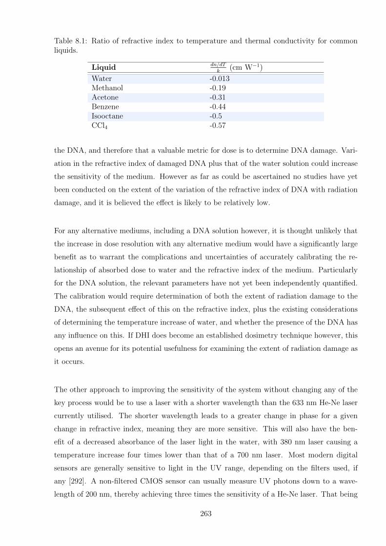
Table 8.1: Ratio of refractive index to temperature and thermal conductivity for commonliquids.
Liquid dn/dTk
(cm W−1)
Water -0.013Methanol -0.19Acetone -0.31Benzene -0.44Isooctane -0.5CCl4 -0.57
the DNA, and therefore that a valuable metric for dose is to determine DNA damage. Vari-
ation in the refractive index of damaged DNA plus that of the water solution could increase
the sensitivity of the medium. However as far as could be ascertained no studies have yet
been conducted on the extent of the variation of the refractive index of DNA with radiation
damage, and it is believed the effect is likely to be relatively low.
For any alternative mediums, including a DNA solution however, it is thought unlikely that
the increase in dose resolution with any alternative medium would have a significantly large
benefit as to warrant the complications and uncertainties of accurately calibrating the re-
lationship of absorbed dose to water and the refractive index of the medium. Particularly
for the DNA solution, the relevant parameters have not yet been independently quantified.
The calibration would require determination of both the extent of radiation damage to the
DNA, the subsequent effect of this on the refractive index, plus the existing considerations
of determining the temperature increase of water, and whether the presence of the DNA has
any influence on this. If DHI does become an established dosimetry technique however, this
opens an avenue for its potential usefulness for examining the extent of radiation damage as
it occurs.
The other approach to improving the sensitivity of the system without changing any of the
key process would be to use a laser with a shorter wavelength than the 633 nm He-Ne laser
currently utilised. The shorter wavelength leads to a greater change in phase for a given
change in refractive index, meaning they are more sensitive. This will also have the ben-
efit of a decreased absorbance of the laser light in the water, with 380 nm laser causing a
temperature increase four times lower than that of a 700 nm laser. Most modern digital
sensors are generally sensitive to light in the UV range, depending on the filters used, if
any [292]. A non-filtered CMOS sensor can usually measure UV photons down to a wave-
length of 200 nm, thereby achieving three times the sensitivity of a He-Ne laser. That being
263
said, it is the signal to noise ratio which is the current limit on resolvability of the measured
doses, and the more sensitive laser would also be proportionately more prone to noise, so no
experimental gain is to be achieved by this until the noise is reduced. The lower limit on sen-
sitivity with the current wavelength light should be reasonable for most dosimetric purposes.
Image quality and sensitivity can also be artificially improved by post-processing the images,
in a mathematical equivalent to measurement procedures such as phase shifting, as described
in Section 3.3.3. An example is the work by Demoli et al. who propose a pointwise operation
which can achieve a manifold increase in apparent sensitivity, limited only by the noise in
the system [293].
Irradiation Configuration
One means to increase the sensitivity of the DHI detector is to configure the irradiation of the
test cell such that the only variation in dose is effectively limited to one or two dimensions,
rather than three. If broad beam geometry is able to be used for the irradiation, whereby
the test cell is fully contained within the range of the flat part of the radiation beam with no
penumbra, then the only significant variation in absorbed dose is with depth. This means
that the signal is effectively not averaged across the width of the test cell in the direction
of the laser beam. Whilst this does not actually impact on the signal to noise ratio, it does
mean that the measured values will be able to be recorded as the actual dose values, and
not the projected dose values. Additionally, in one direction on the recorded DHI images
the dose profiles should be constant, allowing for signal averaging. This results in a depth
dose curve that has an improved signal to noise ratio due to any random noise across the
image being decreased, and increasing the statistical significance of the measured dose.
The limitations of this approach are the reduction of the acquired dose information to one
dimension, which reduces one of the advantages of DHI over the point or volume integrated
doses acquired in conventional calorimetry. Additionally, it is not always feasible to apply
this approach, depending on the radiation modality. For instance measurement of an HDR
source would not be able to exploit this technique. The measurement of other radiation
systems is also generally limited by the collimation systems that are available.
264
8.4.3 Absolute Dosimetry
The output of the prototype DHI detector is currently the measurement of relative dose
distributions, rather than absolute or total absorbed dose in the medium. The result is a
series of dose difference maps showing the variation in dose across the field of view at each
time instance. Due to the lack of temporal stability in the phase values of the images, an
absolute dose value is not able to be determined to benchmark the dose differences against to
determine total dose. This limits the measurements to those where the dose modulation in
at least one dimension is high enough to be detected. Any dose that is applied evenly across
the whole field of view is not measurable. The ability to measure relative dose distributions
means that DHI could be a useful tool for many highly modulated radiation types, however
with some improvements the system has the inherent potential to do absolute dose mea-
surements, which would greatly expand its usefulness. Accurate absolute dosimetry would
allow for the investigation of the use of DHI for reference dosimetry for a range of radiation
types, as well as measurement of radiation that has only low dose gradients across the field
of view. It would also allow for validation of the methods to account for heat diffusion, as de-
scribed in Section 8.2.3. This would be required for any potential use for reference dosimetry.
In principle the dose measured at each point in a DHI image should be able to be compared
directly back to the reference image to determine the total dose represented by each pixel,
according to the measured phase difference. If there is sufficient dose to cause a phase change
of greater than 2π this phase jump could be determined by visualising the series of images. It
would also be possible to compare each image to the previous image rather than an original
reference image, and obtain the total dose by the accumulation of the series, which should
give the same result. This approach relies on their being no extraneous influences causing
the phase to vary independently of any radiation dose. If the suggested modifications to
the DHI detector which were described in Section 8.4.1 are implemented, this may allow for
the stabilisation of the phase sufficiently to allow for absolute dosimetry to become possible.
The degree of accuracy achievable would be the same as for the relative dose distribution
measurements, limited only by the extent to which the phase stability is achieved. The
accuracy may in fact improve, as there would no longer be uncertainty introduced by the
difference normalisation process, which was described in Section 7.1.2.
In order to achieve accurate temporal resolution for the DHI results, a high quality three di-
mensional phase unwrapper may be required. Three dimensional phase unwrapping is more
complex than the two dimensional problem with the complications being due to excess noise
265
in the measurement system. If there is no noise in the system, three dimensional unwrap-
ping is straightforward. However with increasing levels of noise, pixels which appeared to
be correctly dealt with in one plane may cause discrepancies in other planes. So in order for
successful absolute dosimetry to occur, a suitably robust phase unwrapper should be chosen,
and the noise of the images, both within each image and between images, should be reduced
as much as possible.
An additional step to improve the accuracy of the results in order to enable absolute dosime-
try, could be to encase the test cell within a larger block of water equivalent material in order
to create full scatter conditions. Appropriate paths for the reference and object beams would
need to be drilled through, and alignment could be more complicated, however this approach
would provide a more clinically relevant result.
8.4.4 Spatial Resolution and Sensitive Region Size
Modifications to the system to potentially increase the size of the sensitive region were cov-
ered in Section 7.3.4, and will not be re-described here. Improvements in the size of the
sensitive region would be of benefit to measurement of all types of radiation, especially if the
spatial resolution is not significantly decreased. In fact in some cases it would be desirable
to increase the spatial resolution, even if this comes at the expense of a decreased sensitive
region. The discussion in Section 7.3.4 did not mention this concept, but all of the techniques
which were described can also be used to increase the spatial resolution. A camera sensor
with higher inherent resolution would be the primary means to achieve this. An alternative
approach is to expand the reference and object beams after they are recombined, and project
the expanded version on to the original resolution sensor. This increases the measurable res-
olution within the image features, although reduces the measurement size. Theoretically the
only inherent limits in the extent that the resolution can be increased to are the random
noise in the system, the need to retain a usable measurement region, and the power of the
laser beam that is used. So overall, the spatial resolution and sensitive region size can be
tweaked depending on the particular experimental requirements of any given dosimetric aims.
8.4.5 Experimental Process
A further improvement to the experimental process of acquiring a DHI measurement would
be the use of a micrometre controlled three dimensional translation stage for accurate po-
266
sitioning of the test cell. This would reduce the uncertainty in dose measurement and heat
diffusion calculation introduced by uncertainties in the exact localisation of the sensitive
region relative to the radiation beam, as quantified in Chapter 5. This would also allow for
improved consistency in positioning of subsequent datasets, which effectively increases the
sensitive region of the detector by being able to “stitch” together data acquired in different
irradiations. This process would then allow for a more accurate normalisation of the data,
which would be particularly useful for comparing to model datasets or measurements by
other detector types. Accurate positioning would also allow for the more precise under-
standing of the true dose values by allowing for the integration of dose across the test cell
to be calculated to a much smaller region by ensuring the beam is centrally located.
Another consideration for the experimental process is the timing accuracy of the measure-
ments compared to the irradiation time. The current method introduces a significant amount
of uncertainty into the system. Incorporation of a trigger system whereby the time-stamps of
the camera recording are accurately benchmarked against the radiation would be extremely
beneficial. The exact means for achieving this depends entirely on the control system of each
radiation source and whether it is possible to link external devices to this. For this reason
no specific method has been proposed here, and the possibilities should be discussed with
the control room scientists when specific measurements are planned.
8.5 Considerations for Extension to Tomographic Ac-
quisition
A key limitation of the basic DHI dosimeter is that the dose information is obtained from
the phase change occurring along the projection of the laser path across the test cell. This
integrated dose measurement means that at this stage the DHI detector cannot be used to
find dose at a point, or true relative doses between points in a three dimensional volume,
unless the dose distribution is cylindrically symmetric or effectively two dimensional. This
limits the applicability of the method, and validation of the DHI detector requires the use
of a three dimensional model of the dose distribution which can be compared to the DHI
results by integrated over the same volume. The ability to obtain three dimensional or quasi-
three dimensional dose distributions by expansion of the DHI technique to a tomographic
approach would increase the usability of the measurements. The optical mechanics behind
implementing this technique are achievable, but the process would not be without difficul-
ties, particularly for the measurement of time-variant irradiation processes.
267
There are many studies reporting the use of tomographic reconstructions to achieve three di-
mensional temperature distribution measurements by means of interferometry [201,220,294].
Tomography is the process of collating image data taken from projections taken at varying
angles through a sample, mathematically reconstructing the three dimensional properties.
The mathematical reconstruction is an inverse problem, obtained by considering the inte-
grated effect of the variable along lines in different directions through the medium. The
most fundamental method of tomography is filtered back projection using the Radon Trans-
form [295], but more modern approaches are based on iterative reconstruction [296].
The quality of the calculated three dimensional dose distribution is increased as the number
of projections included in the reconstruction increases. For a DHI set-up, there are two ap-
proaches for achieving multiple measurement angles for use in the reconstruction: 1) separate
interferometric measurements at a range of set angles, and 2) continuous image acquisition
with rotation of the interferometer about the sample. Both approaches have specific advan-
tages and limitations concerning the spatial resolution, temporal resolution and dosimetric
accuracy.
Discussion of each of these approaches for DHI dosimetry is compared to the tomographic
ultrasound thermometry system developed by Malyarenko et al. [234] which has a distinctly
different approach to tomography than possible with the current type of DHI detector, but
was chosen for comparison as the approach is also a calorimetric dosimetry method using
a remote temperature probing technique, and as such has encountered many of the same
considerations. Their approach was based on the use of a circular array of 128 ultrasound
transmitters and receivers, which probe a single plane of the irradiated volume, based on a
fan-beam geometry data acquisition technique. The approach could be extended to three
dimensions with the use of multiple rows of ultrasound transducers, in the same fashion as
a cone beam CT. The average temperature along each ultrasound path is determined by
each receiver in turn, and then the results tomographically reconstructed. The sensitivity
in temperature measurements achieved for a single ultrasound line results achieved for a
single ultrasound probe were temperature measurements as small as 3.2 µK along each
ultrasound line, sufficiently sensitive for therapy level radiation doses [234]. This value
was somewhat reduced under the tomographic acquisition conditions, however temperatures
on the order of mK were still resolvable. The nominal spatial resolution achieved at the
centre of the reconstruction volume was on the order of half the transducer spacing, or 4.4
268
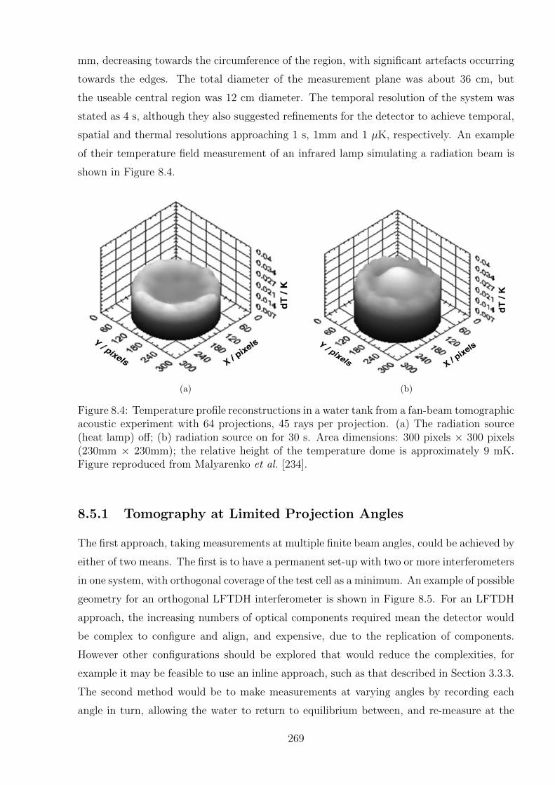
mm, decreasing towards the circumference of the region, with significant artefacts occurring
towards the edges. The total diameter of the measurement plane was about 36 cm, but
the useable central region was 12 cm diameter. The temporal resolution of the system was
stated as 4 s, although they also suggested refinements for the detector to achieve temporal,
spatial and thermal resolutions approaching 1 s, 1mm and 1 µK, respectively. An example
of their temperature field measurement of an infrared lamp simulating a radiation beam is
shown in Figure 8.4.
(a) (b)
Figure 8.4: Temperature profile reconstructions in a water tank from a fan-beam tomographicacoustic experiment with 64 projections, 45 rays per projection. (a) The radiation source(heat lamp) off; (b) radiation source on for 30 s. Area dimensions: 300 pixels × 300 pixels(230mm × 230mm); the relative height of the temperature dome is approximately 9 mK.Figure reproduced from Malyarenko et al. [234].
8.5.1 Tomography at Limited Projection Angles
The first approach, taking measurements at multiple finite beam angles, could be achieved by
either of two means. The first is to have a permanent set-up with two or more interferometers
in one system, with orthogonal coverage of the test cell as a minimum. An example of possible
geometry for an orthogonal LFTDH interferometer is shown in Figure 8.5. For an LFTDH
approach, the increasing numbers of optical components required mean the detector would
be complex to configure and align, and expensive, due to the replication of components.
However other configurations should be explored that would reduce the complexities, for
example it may be feasible to use an inline approach, such as that described in Section 3.3.3.
The second method would be to make measurements at varying angles by recording each
angle in turn, allowing the water to return to equilibrium between, and re-measure at the
269
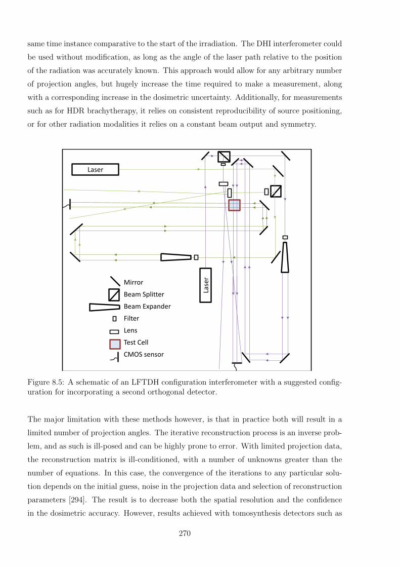
same time instance comparative to the start of the irradiation. The DHI interferometer could
be used without modification, as long as the angle of the laser path relative to the position
of the radiation was accurately known. This approach would allow for any arbitrary number
of projection angles, but hugely increase the time required to make a measurement, along
with a corresponding increase in the dosimetric uncertainty. Additionally, for measurements
such as for HDR brachytherapy, it relies on consistent reproducibility of source positioning,
or for other radiation modalities it relies on a constant beam output and symmetry.
Lase
r
Laser
Mirror
Beam Splitter
Beam Expander
Filter
Lens
Test Cell
CMOS sensor
Figure 8.5: A schematic of an LFTDH configuration interferometer with a suggested config-uration for incorporating a second orthogonal detector.
The major limitation with these methods however, is that in practice both will result in a
limited number of projection angles. The iterative reconstruction process is an inverse prob-
lem, and as such is ill-posed and can be highly prone to error. With limited projection data,
the reconstruction matrix is ill-conditioned, with a number of unknowns greater than the
number of equations. In this case, the convergence of the iterations to any particular solu-
tion depends on the initial guess, noise in the projection data and selection of reconstruction
parameters [294]. The result is to decrease both the spatial resolution and the confidence
in the dosimetric accuracy. However, results achieved with tomosynthesis detectors such as
270
used for breast cancer screening, using expectation maximisation reconstruction algorithms,
have been shown to have a high degree of accuracy, and the same principles are applicable
to the DHI results [297].
The advantage of this limited angle method over an approach like the Malyarenko system
however is that the measurements at each of the projections could be made at the same
relative time instance compared to the start of irradiation. Whether that be a simultane-
ous measurement, or a series of repeated measurements, the consequence is that the time
resolution would be accurate to a high degree. This means that measurements of radiation
distributions with high dose gradients could be measured and the impact of heat diffusion
could be accounted for in the same fashion as the current two dimensional DHI results.
Because the measurements at each time instance would be resolved in three dimensions,
with careful selection of the measurement intervals, it would be possible to directly account
for the heat diffusion in the results without the limitations encountered by the inaccuracies
introduced by the Abel transform.
The main difficulty would be achieving sufficient spatial resolution in each direction. As the
entire test cell volume would be probed by each projection, there would not be the limitation
experienced by the Malyarenko fan beam approach whereby the periphery regions of the test
area experienced lower spatial resolution. Additionally, with the size of the pixels in the DHI
detector vastly exceeding the spatial resolution of the ultrasound transceivers, the potential
spatial resolution achievable would be orders of magnitude less than the approximately 5
mm they achieved. Optical CT scanners used for gel dosimetry have reported resolution on
the scale of 1 mm3 [61, 173], with sensors with pixel sizes similar to that used for the DHI
detector. Resolutions this fine would not be achievable with limited projection angles how-
ever, as this results in a reconstruction process where the measured distributions are smeared
out over a volume which is inversely proportional to the number of projections. Addition-
ally, the reconstruction process and dosimetric uncertainty would be negatively impacted by
the magnitude of the noise in the recorded images, the impact of which is reduced by the
increasing redundancy in the reconstruction achieved by having a greater number of projec-
tion angles [294]. Implementation of a basic reconstruction algorithm for the DHI results at
various numbers and angles of projections would allow for an estimate of the potential three
dimensional resolution that could be achieved with each given experimental set-up, but this
remains an area of further work.
271
If this limited angle approach were to be implemented, the number of angles used would be
determined from the balance of multiple factors, including the cost of the system components,
the space and configuration constraints on the optical system, the finite apertures of the test
cell, the transportability of the set-up, the increase in experimental time required, and the
resolution achievable.
8.5.2 Tomography by Interferometer Rotation
The second approach to DHI tomography, rotating the interferometer, means that depending
on the speed of rotation and the acquisition rate of the camera, an unlimited number of pro-
jection angles can be achieved. This will allow for a three dimensional reconstruction with
high spatial resolution and accuracy. However, this approach means that the measurements
used are acquired over some time period, rather than instantaneously. For measurements of
transient phenomena, such as the temperature distribution introduced by radiation absorbed
dose this complicates the reconstruction immensely, and introduces a much higher level of
uncertainty, dependent on the rate of image acquisition. Note that the test cell must be
independent of the rotating detector, to avoid the introduction of undesired body forces in
the fluid medium which would affect the temperature distribution.
The Malyarenko approach effectively used this approach, as the ultrasound transducers were
measured consecutively around the circular array, with a total acquisition time of 4 s for the
entire dataset. They overcame the limitations associated with variation of the heat diffusion
by measuring a temperature source with a relatively low rate of temperature increase, and
no steep gradients. They also had a relatively low spatial resolution of approximately 5 mm.
Thus the resultant degradation of the signal due to heat transport over the 4 s measurement
acquisition time resulted in an effect smaller than the spatial resolution. Thus the measure-
ment acquisition time was not a limiting factor in the approach.
For the DHI detector, similar measurements could be made, which, if the sensitivity of the
detector could be increased and noise reduced sufficiently, would allow for the measurement
of clinically relevant dose distributions such as those used for IMRT [234]. However if to-
mographic measurements of radiation modalities such as HDR or proton beams are to be
made, the relatively high dose rates and dose gradients relative to the achievable resolution
will complicate this somewhat. The resolution achievable by this approach is limited only
by the noise in the images, rather than an inherent limit on projection angles. Thus to
achieve measurements where the signal degradation due to heat transport is less than the
272
ability to spatially resolve the beam, a very fast measurement acquisition time should be
used. This will be limited by the maximum camera frame rate and speed of rotation of
the system. With the camera used in the present DHI prototype, frame rates of up to 30
Hz are achievable, however scientific cameras with frame rates of several hundred Hz are
commercially available, although the corresponding reduction in the signal to noise ratio is
a consideration. Assuming the system can be accurately rotated at rates of up to 2 Hz,
it would be possible to achieve a similar number of reconstructions as the Malyarenko ap-
proach, with a measurement acquisition time on the order of 0.5-4 seconds. This is still a
considerable time, and depending on the radiation source will impose an inherent limitation
on the temperature/dose resolution achievable at a given spatial resolution.
It is possible that a modelling approach could be used to account for the variation in dose
deposition and heat transfer which occur with the varying time instances of each projection
image. This process would be complex and require an iterative reconstruction method to
be used which optimises the volumetric dose distribution based on a cost function which
incorporates the models for heat conduction and convection. If this could be successfully
implemented and validated against alternative three dimensional dosimetry approaches, then
it would vastly increase the usability of the DHI system.
It should be noted that when the interferometer is rotated this must occur about an axis of
rotation coincident with the centre of the test cell, but that the test cell must not rotate.
This is so that the alignment of the temperature distribution map remains correlated to the
direction of the radiation dose distribution, and so there is no additional blurring from the
water getting dragged around by the walls of the cell. Additional error can also be intro-
duced if there is some deviation between the centre of rotation of the interferometer and the
test cell, causing the projection data to be collected at angles different to those assumed for
the calculations.
8.5.3 Additional Considerations
A consideration with the use of tomography during holographic interferometry measurements
is the shape of the test cell. Unless a limited projection approach is used with projections
only at two cardinal angles, then a cubic test cell will result in the occurrence of artefacts
due to the edges of the test cell being thicker and less transparent than the bulk of the walls
of the cell. Additionally, the temperature/dose determined at each point in the projection
273
across the cell will be affected by different averaging effects depending on the radial location
of the point of interest. This will complicate both the interpretation of the DHI temperature
maps, and any tomographic reconstruction. This could be reduced by the use of a cylindrical
test cell which impacts the phase of the light to the same extent regardless of the direction
of the projection. This will cause added complexities in reconstructing the holograms to
determine the DHI temperature maps, due to uneven refraction of the light as it traverses
the cell walls. The extent of this effect should be investigated, and it should be ascertained
whether successful reconstructions can be performed, prior to the use of a cylindrical test
cell in any tomographic measurements.
Another practical consideration with tomographic DHI for radiation dosimetry is that it
would be extremely difficult to make a tomographic detector for a beam delivered horizon-
tally, such as the proton beam or a synchrotron beam, because the rotational axis for the
projection angles is coincident with the central axis of the radiation beam. This would re-
quire rotation of a breadboard or similar with all the optical components attached, however
in order to achieve rotation about the test cell there would not be a single axis of rotation
for the breadboard, instead it must traverse a circle about the measured point, similar to
the operation of a computed tomography (CT) machine. This would be difficult to achieve
mechanically to a high level of accuracy, as well as present many difficulties in the process
of shielding the system from ambient conditions. In particular if a temperature controlled
environment for the detector is required, as recommended for absolute dose measurements,
the size of the container would be prohibitive and render the detector difficult to transport.
This could still be feasible in the context of a standards laboratory, however reduces the use
of the approach for many applications.
8.6 Considerations for DHI Application to MRT Dosime-
try
The initial motivator behind the development of a DHI detector was the need for improved
detectors for synchrotron generated microbeam radiation therapy (MRT), as described in
Section 2.3.3. The initial development of the detector and proof-of-principle measurements
were first required to prove the potential viability of the method to build a solid justification
to apply for scarce beam time on a medical beamline. Based on the results achieved to date
for the HDR source and proton beam measurements, and the anticipated future improve-
ments to the system, this section is intended to give an estimate of the possible utility of
274
this method for MRT.
The key parameters to consider when discussing the theoretical potential of DHI for MRT
are the spatial resolution and the dynamic range - i.e. the ability to accurately resolve the
dose in both the peaks and the valleys of the highly modulated microbeams. The funda-
mental independence of DHI to beam energy means that the beam spectrum does not need
to be considered.
The present detector achieved spatial resolutions on the order of 25 µm. This would be not
quite sufficient to accurately spatially resolve the peak sizes used in MRT, as there would
only be approximately one pixel per peak, resulting in a high uncertainty in the peak lo-
calisation. However the resolution could be readily improved, by the means discussed in
Section 7.3.4, to the extent that spatial resolution is not the limiting factor in the possible
application of DHI to MRT.
In order for DHI to be used with the current detector design (and all anticipated future
designs), the MRT collimator must be horizontal. This is due to the horizontal orientation
of the object beam of the DHI detector which probes the water sample. If the collimator is
vertical then all the details of the peaks will be obscured. Details of the orientation of the
collimator at all synchrotron medical beamline facilities are not known, although it is noted
that the collimator in use at the Australian Synchrotron is horizontal. The angle of the DHI
detector must be carefully aligned with the collimator, otherwise dose averaging will occur
due to partial occlusion of the dose distribution.
The key limiting factor to consider will be the presence of heat diffusion. Although the dose
deposition rates are extremely high by conventional radiotherapy standards, the high dose
modulation means that the heating pattern quickly dissipates. This means that the rate of
image acquisition must be high compared to the time scale of the irradiation.
A basic heat diffusion calculation on a simulated MRT beam was modelled in MATLAB in
order to investigate the measurement parameters required. A typical MRT beam consists of
25 µm wide peaks, with a 200 µm peak separation [175]. This was approximated by sharp
peaks at this spacing, convolved with a Gaussian function, as a first approximation for the
expected blurring due to collimator scatter and scatter within the test cell at the measure-
ment depths. The dose was normalised to correspond to a dose delivery rate of 2000 Gy/s
275
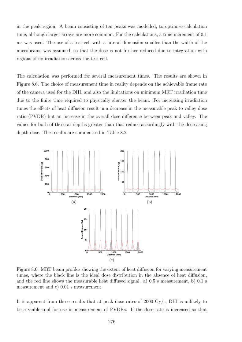
in the peak region. A beam consisting of ten peaks was modelled, to optimise calculation
time, although larger arrays are more common. For the calculations, a time increment of 0.1
ms was used. The use of a test cell with a lateral dimension smaller than the width of the
microbeams was assumed, so that the dose is not further reduced due to integration with
regions of no irradiation across the test cell.
The calculation was performed for several measurement times. The results are shown in
Figure 8.6. The choice of measurement time in reality depends on the achievable frame rate
of the camera used for the DHI, and also the limitations on minimum MRT irradiation time
due to the finite time required to physically shutter the beam. For increasing irradiation
times the effects of heat diffusion result in a decrease in the measurable peak to valley dose
ratio (PVDR) but an increase in the overall dose difference between peak and valley. The
values for both of these at depths greater than that reduce accordingly with the decreasing
depth dose. The results are summarised in Table 8.2.
0 500 1000 1500 20000
200
400
600
800
1000
Distance (mm)
Do
se d
iffe
ren
ce(G
y)
(a)
0 500 1000 1500 20000
50
100
150
200
Distance (mm)
Do
se d
iffe
ren
ce(G
y)
(b)
0 500 1000 1500 20000
5
10
15
20
Distance (mm)
Do
se d
iffe
ren
ce(G
y)
(c)
Figure 8.6: MRT beam profiles showing the extent of heat diffusion for varying measurementtimes, where the black line is the ideal dose distribution in the absence of heat diffusion,and the red line shows the measurable heat diffused signal. a) 0.5 s measurement, b) 0.1 smeasurement and c) 0.01 s measurement.
It is apparent from these results that at peak dose rates of 2000 Gy/s, DHI is unlikely to
be a viable tool for use in measurement of PVDRs. If the dose rate is increased so that
276
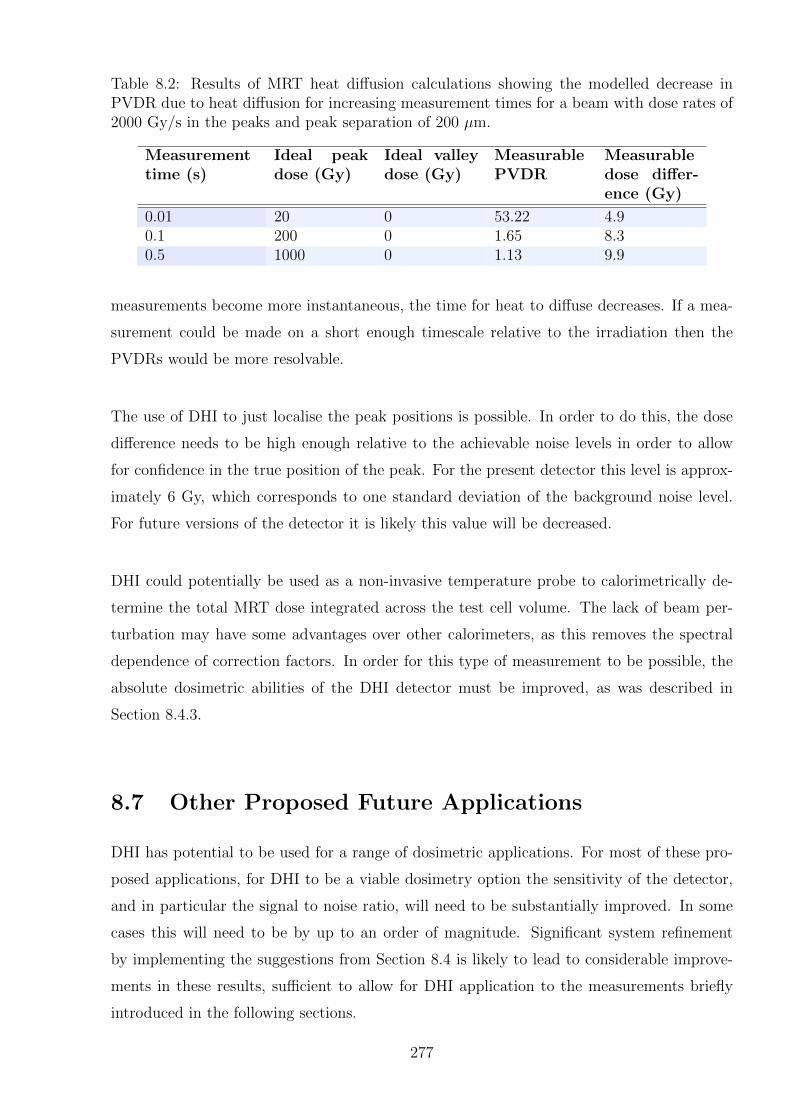
Table 8.2: Results of MRT heat diffusion calculations showing the modelled decrease inPVDR due to heat diffusion for increasing measurement times for a beam with dose rates of2000 Gy/s in the peaks and peak separation of 200 µm.
Measurementtime (s)
Ideal peakdose (Gy)
Ideal valleydose (Gy)
MeasurablePVDR
Measurabledose differ-ence (Gy)
0.01 20 0 53.22 4.90.1 200 0 1.65 8.30.5 1000 0 1.13 9.9
measurements become more instantaneous, the time for heat to diffuse decreases. If a mea-
surement could be made on a short enough timescale relative to the irradiation then the
PVDRs would be more resolvable.
The use of DHI to just localise the peak positions is possible. In order to do this, the dose
difference needs to be high enough relative to the achievable noise levels in order to allow
for confidence in the true position of the peak. For the present detector this level is approx-
imately 6 Gy, which corresponds to one standard deviation of the background noise level.
For future versions of the detector it is likely this value will be decreased.
DHI could potentially be used as a non-invasive temperature probe to calorimetrically de-
termine the total MRT dose integrated across the test cell volume. The lack of beam per-
turbation may have some advantages over other calorimeters, as this removes the spectral
dependence of correction factors. In order for this type of measurement to be possible, the
absolute dosimetric abilities of the DHI detector must be improved, as was described in
Section 8.4.3.
8.7 Other Proposed Future Applications
DHI has potential to be used for a range of dosimetric applications. For most of these pro-
posed applications, for DHI to be a viable dosimetry option the sensitivity of the detector,
and in particular the signal to noise ratio, will need to be substantially improved. In some
cases this will need to be by up to an order of magnitude. Significant system refinement
by implementing the suggestions from Section 8.4 is likely to lead to considerable improve-
ments in these results, sufficient to allow for DHI application to the measurements briefly
introduced in the following sections.
277
Small Field Measurements
For external beam radiation therapy, there is an increasing trend towards treatments con-
sisting of a larger number of smaller, more highly modulated treatment fields than those
used for conventional conformal radiotherapy. Treatment techniques such as intensity mod-
ulated radiation therapy (IMRT ), volumetric modulated arc therapy (VMAT), and various
stereotactic radiotherapy treatments (such as SABR and SBRT), allow the dose distribution
to conform better to the target volume, which allows for dose escalation to the tumour. The
fields can be sub-centimetre in size, considerably smaller than the traditional radiotherapy
fields of greater than approximately 4 × 4 cm in size. Clinical dosimetric uncertainty is
amplified by both cumulative errors from the increased number of fields, and the challenges
inherent in accurate measurement of smaller field sizes. Whilst there are recommendations
from organisations regarding appropriate dosimetry tools for this situation, improving the
accuracy of small field measurements further is an area of very active research.
The dosimetry of small fields is challenging due to the non-equilibrium conditions created as
a consequence of the secondary electron track lengths compared to the field width resulting
in a lack of charged particle equilibrium. This limits the use of ionisation chambers, which
are affected by the lack of lateral scatter. There are also prolonged electron tracks in the
presence of low density inhomogeneities. Radiation detectors introduced into the field per-
turb this disequilibrium, in a fashion that is harder to quantify in a reliable way [21, 22].
Additionally for a small field, partial blocking of the beam source by the collimating sys-
tem results in pronounced and overlapping penumbra. Many detectors have less accurate
measurements in penumbral regions due to the dose gradient, and traditional definition of
the field size by the full width at half maximum will not be accurate. Detectors must have
a resolution which is considerably smaller than the magnitude of the small field they are
measuring, as well as not be affected by the variations in the electron spectrum inducing
changes in the stopping power ratios. The choice of a suitable detector from amongst the
commercially available options is challenging, with various guidelines and recommendations
suggested in the literature [21, 22]. Each detector type has different perturbations and cor-
rections which may become relevant at different sizes. Thorough consideration of these is
required in order to have full confidence in their dosimetric accuracy.
Das et al. and others have stated the requirement for new detector types, with the state-
278
ment “Small volume detectors ion chambers, diodes, and others will be developed that have
minimum perturbations due to its presence and composition. Also, such detectors will have
minimum energy, dose, and dose rate dependence” [21]. DHI appears to have the potential
to achieve many of these, provided a sufficient level of sensitivity could be achieved.
DHI has the potential to be a useful contributor to the problems of small-field dosimetry.
Malyarenko et al. from NIST proposed the use of their ultrasound tomographic detector
to assess the absorbed dose in IMRT-type beam conditions [234]. The logic applied is also
relevant to a DHI detector. In order to achieve sufficiently accurate measurements, the tem-
perature resolution needs to be sufficient to resolve the small dose gradients that occur in
this sort of treatment. Their premise for this approach is that calorimetric standards for
primary reference dose are the most suitable for time-resolved spatial distribution measure-
ments because they are “constructed of a uniform, extended medium that could contain and
faithfully register the spatial features of the beam over time.” The influence of heat diffusion
is an obvious caveat to this assumption, although for the small dose gradients present for
IMRT this will have a much lower impact than the high dose gradients measured in other
applications. In order to achieve measurements of these kinds with a DHI detector, the
sensitivity of the detector will need to be improved by at least an order of magnitude.
Investigation of the Impacts of Tissue Inhomogeneities and Boundary InterfaceDosimetry
Some of the original interferometric dosimetry measurements by Miller in 1979 began to use
the technique to investigate the effect of various beam perturbations on the absorbed dose
distribution [26]. The work included a range of initial studies designed to help investigate
different aspects of beam perturbation, in order to help increase the accuracy of treatment
plans. For instance he measured the change in depth dose curves with varying backscat-
ter materials and thicknesses, at various penetration depths of the electron beam. This is
valuable for increasing understanding of the dose in the region prior to different density ma-
terials, for instance the higher density of bones. Another measurement actually visualised
the distortion in the isodose lines caused by a solid object intruding into the field, again a
useful simulacrum of a bone.
Measurement immediately adjacent to solid objects is possible for DHI (or the earlier film-
based systems) to an extent not possible for most alternative dosimetry systems. Achieving
two or three dimensional distributions concurrently would be a key advantage of DHI for
279
this purpose. The inherent energy independence of DHI is another key advantage, as the
variations in scatter from solid objects alters the energy spectrum of the radiation at each
point. For detectors that require various beam quality-based correction factors or calibra-
tions, this introduces potential errors in the result, which would be circumvented by the use
of DHI.
Future improved versions of the DHI detector could be used to extend the measurements
begun by Miller. Results achieved with sufficient accuracy could be used to validate the
output of treatment planning system dose distributions around regions of varying density
in transparent phantoms, for various algorithms. A very exciting possibility is the potential
for the use of DHI to quantify the extent of the beam perturbation around other detector
types. For instance the dose distribution around an ionisation chamber could be measured,
which may be useful to help experimentally verify correction factors and reduce uncertain-
ties associated with the parameters for TRS-398 reference dose measurements. Such factors
could include stopping power ratios and the beam perturbation factors for specific chamber
types which are incorporated in the beam quality correction factor kQ,Qo . This would be
particularly of use for more complex systems, such as scanning proton beam dosimetry [96],
where these parameters are more difficult to accurately calculate. Measurement of other
detectors such as in-vivo diodes also has an obvious benefit of quantifying the extent of the
influence on the dose distribution from in-vivo measurements. The potential beam perturba-
tions are an area of concern when conducting in-vivo dosimetry measurements, especially for
patients with short treatment courses of five or less fractions. Accurate measurement of the
resultant beam perturbations could allow for a greater measure of confidence in the patient
treatments in these cases, and potentially allow for safer extension of in-vivo measurements
to every fraction.
Surface Dosimetry
Conventionally, dosimetric measurements in the regions close to the surface are difficult to
measure. This is due to various complications including, amongst others, the partial volume
averaging effect, detector build-up requirements, rapid variation in beam spectra for electron
beams, and different scatter properties. Current methods for accurate measurement of sur-
face doses in linear accelerator beams include extrapolation chambers for low energy photon
beams, and parallel plate or extrapolation chambers for higher energy beams. Improving the
flexibility of surface dosimetric measurements would be particularly beneficial for treatment
techniques where fields are matched adjacent to each other, either to extend the treatment
280
region, or match different radiation types or energies. There are currently considerable un-
certainties in the surface dose for such techniques, which can have considerable effects on
the efficacy or risks of the treatment. The DHI detector, after further development, has the
potential to contribute to this type of problem.
8.8 Concluding Remarks
This chapter covered points of possible uncertainty and potential improvement across the
whole range of the DHI system, from the optical set-up, to the irradiation and image acquisi-
tion, to the image reconstruction and analysis. The intention was to provide a comprehensive
discussion of all aspects of the measurements, in order to fully investigate the potential of
the DHI detector for radiation dosimetry. Whilst the initial proof-of-principle results using
the prototype detector were positive, there are a range of areas where future iterations of the
system could be improved upon in order to fully realise the potential of the approach. The
limitations of the system were discussed, with suggestions for how improvements could be
implemented. Sources of uncertainty were analysed, and aspects of the uncertainty budget
which were not fully covered in earlier Chapters were described. Key sources of uncertainty
are the noise in the system, and the calculation of the impact of heat transport on the re-
sults, including the use of the Abel Transform. A comprehensive range of recommendations
were made, to improve all aspects of the detector performance. Considerations regarding
the possible extension to tomographic image acquisition were fully discussed. Other possi-
ble applications which would benefit from the possibilities presented by the features of DHI
dosimetry were introduced, with a brief description of the possibilities.
281

282
Chapter 9
Conclusions
This work aimed to develop a novel DHI detector capable of measuring small temperature
changes in water and apply the system to radiation applications as proof-of-principle of DHI
as a dosimetry tool. A full framework was established for the process of acquiring a DHI
measurement, including:
� Interferometer configuration and alignment of optical components
� Detector transport and re-building for in situ radiation measurements
� Optimising the region of interest localisation and the irradiation conditions
� Control and recording of influence factors
� Mathematical image reconstruction and subsequent absorbed dose determination
� Dose distribution analysis by comparison to model results
� Methods for accounting for heat diffusion of the measured temperature field
� Analysis of uncertainties of the system and methods to mitigate or quantify these
� Itemization and discussion of areas that should be considered for accurate and useful
dosimetric measurements
The pilot study measurements on an HDR source and a small field proton beam success-
fully demonstrated all of the above processes. The results of the HDR source measurements
proved that the DHI system was capable of resolving the small temperature gradients result-
ing from radiation absorbed dose to water. The proton beam measurements were useful for
consideration of the ability of the prototype detector, with the results used to inform a com-
prehensive set of recommendations for future experimental improvements of the detector.
The potential of the system for application to alternative radiation types was conjectured
283
based on the results of these measurements and the anticipated improvements.
9.1 Review of Research Questions
The initial work set out to answer four research questions which were posed in order to
focus the direction of the investigation into DHI as a potential dosimetry tool. The results
achieved by the DHI detector, that were fully described in the remainder of this work, will
therefore be summarised in the following sections by answering the research questions.
9.1.1 Research Question One
Can the optical technique of digital holographic interferometry be successfully
applied to radiation dosimetry?
The DHI measurements of the HDR source have experimentally demonstrated that the pro-
totype detector is capable of measuring radiation dose distributions. The results which were
achieved in the initial field testing predominantly agreed to within experimental uncertain-
ties when compared with an independent source model. The measured results achieved
dosimetric accuracy on the order of 4-6 Gy. This value consists of a combination of the
standard deviation of the noise, and the additional systematic dosimetric uncertainties in
the measurement.
The prototype detector was constructed using available materials as a proof-of-principle sys-
tem for the pilot studies. The successful results are therefore very promising for the future
development of the detector now that the initial achievements justify the investment of time
and financial resources into improving the system. The limited areas of deviation from com-
plete agreement between the expected and measured dose distributions will be able to be
mitigated by developments such as improving the detector housing, and the quality of the
optical components.
9.1.2 Research Question Two
Is it possible to develop a digital dosimeter based on the fundamental principles
of calorimetry that is capable of measuring dose with high two dimensional spa-
284
tial resolution?
The development of the DHI dosimeter has successfully resulted in a non-invasive optical
method of probing the radiation-induced temperature variation of a water sample. This
overcomes the two key limitations of most calorimetric dosimetry systems; those being the
perturbation of the beam by the temperature probe, and the lack of spatial resolution due
to the very limited number of measurement points. DHI also achieves the same main ad-
vantage of other calorimetric systems, which is the direct measurement of the fundamental
quantity of thermal energy transfer as a measure of absorbed radiation dose. Whilst in all
systems there are inevitably correction factors and parameters contributing uncertainties to
the result, calorimetric measurements are intrinsically suited for radiation dosimetry, and
preferable to all other dosimetry options in certain circumstances. To expand the benefits
of calorimetric measurement to include determination of the dose distribution in two dimen-
sions, as DHI has achieved, has the potential to be very useful. The further extension of the
two dimensional projections of the dose in the test cell to a three dimensional system would
require considerable development of the experimental set-up.
The resolution achieved by the protoype DHI detector was on the order of 0.025 mm/pixel,
over a sensitive region of approximately 7.5 mm by 6 mm. Compared to other dosimetry
options, this resolution is only surpassed by film. Additionally, there is the possibility to
further improve the resolution of the system for future versions of the detector. The fact that
the prototype DHI detector was able to calorimetrically measure dose to a very high spatial
resolution is a major advantage of this approach, and justifies the further development of
the system.
9.1.3 Research Question Three
Will the application of modern digital technology allow for dosimetric results
which advance the early achievements of Hussmann and Miller?
The novel DHI dosimetry work has advanced the results of the early interferometric dosime-
try measurements by Hussmann, Miller and McLaughlin by availing the key fundamental
concept of all the advantages of modern digital sensors and the associated computational
power [24–27]. It is difficult to directly compare the results, as the available radiation sources
were quite different. Their initial measurements using analogue detection systems were in
the range of 6000-22000 Gy, delivered almost instantaneously in 20 - 40 ns [24,27], although
285
later measurements were of relatively lower doses of between 100 - 1500 Gy [26]. The stated
dose resolution for the later work was 3.5 Gy, with an uncertainty of 20%. These kind of
dose rates were unfortunately not available for the DHI measurements, as they are optimal
conditions for accurate DHI measurements as well as the film based systems. The dosimetric
accuracy achieved by the DHI system appears comparable with this result, given favourable
measurement conditions.
Some of the original measurements presented by the early pioneers of this work were based
on single point measurements using a photodiode as the sensor of the interferometric fringes
[26, 27]. There were also some film measurements presented with a two dimensional dose
distribution measuring isodose lines and depth dose curves. The spatial resolution of the
film measurement was demonstrated by other cited authors of the period to be about 1 µm.
In contrast to this, the DHI results spatial resolution was lower than the film measurements,
but patently better than single point photodiode measurements. The size of the film sen-
stivie region was also larger than that of the current DHI prototype, however theoretically
the DHI size can be expanded indefinitely, with the use of sufficient magnification, so this
comparison is negligible.
The key advantage demonstrated by the digital approach over the earlier film method is
the ease of data collection, reconstruction and analysis. Multiple images can be recorded at
high frequency to allow for analysis of the data at any point in time before, during or after
an irradiation. This allows for the progression of the dose deposition to be directly viewed,
and avoids the introduction of excessive uncertainties due to timing errors triggering the
single shutter of a film image acquisition with the irradiation time. Additionally, the DHI
measurements at multiple close time increments means that the data can be used to help
account for heat diffusion. Interferometric film measurements are by nature limited to single
shot images. This is particularly important for most of the radiation techniques which are
relevant to modern radiation therapy. The increasing dose modulation, temporal variation
and dose rates used in many techniques mean that the capabilities of DHI are better suited
to the needs of modern radiation dosimetry technology. Additionally, with DHI there is also
no need for an expensive and time consuming film processing service which was an additional
requirement of the film interferometry methods used by Hussmann et al. All of the other
possible sources of uncertainty remain fairly consistent between film and digital systems.
The additional advantages of DHI of being readily able to digitally process the images, have
286
direct access to the phase values at any point, and use high power computing to evaluate
compare measured and modelled data. All of these features mean that the development of
the early interferometric measurements to a modern digital system is a demonstrable im-
provement on the earlier measurements. With developments applied to increase the DHI
spatial resolution and measurement sensitive region, as suggested in Chapters 7 and 8, DHI
will undisputably be an improvement to build on the early results using film interferometry.
9.1.4 Research Question Four
Is there a justification for further work to explore the potential for such a detec-
tor to be used to overcome the dosimetric problems associated with emerging
radiation therapy techniques?
According to Karger et al., regarding ion beam dosimetry: ”Although methods for ion beam
dosimetry have been established, there is still room for developments. This includes im-
provement of the dosimetric accuracy as well as development of more efcient measurement
techniques.” This principle also applies to most other emerging radiation therapy techniques
and some aspects of many other established techniques. For instance development of an
absolute dose standard for brachytherapy Ir-192 sources, accurate quantification of proton
beam Bragg peak, accurate penumbral measurements in small field dosimetry applications,
and surface dosimetry and beam perturbation measurements for a range of radiation types.
In some cases the lack of suitable dosimetry options is the limiting factor in the therapeu-
tic advancement of the technique. Additionally, the development of novel systems based
on fundamental principles of radiation dose measurement allows for potential contribution
to validation of “gold standard” Monte Carlo dose distribution models and measurement
correction factors. The application of the detector to MRT beams could allow for macro
measurements of the microbeam array, but considerable improvements in measurement tem-
poral resolution and accuracy would be required to overcome heat diffusion limitations on
resolving the individual microbeams and measuring PVDRs.
Based on the results from the initial field testing on an HDR brachytherapy source, com-
bined with the theoretical understanding of the system potential gained from implementing
the DHI detector measurement and analysis system suggest that DHI is also a promising
technique to approach some of these dosimetric challenges. There is a clear justification that
it would be worthwhile to implement the modifications recommended to improve the system
287
which were described in Chapter 8.
Many of the key advantages of a DHI system which make it potentially suitable for many
different applications were realised with the protoype detector. The measurements were
achieved to a high degree of temporal and spatial resolution, without pertubing the radi-
ation beam by insertion of a physical probe. Additionally the calorimetric nature of the
measurements means that the measurements are fundamentally independent of radiation
type, energy and dose rate (excluding the influence that the dose rate has on the extent of
the heat diffusion occurring). The direct determination of absorbed dose to water, the key
measurement quantity for radiation therapy purposes, and the possibility of absolute dose
measurements, are also key attributes.
The initial HDR brachytherapy results indicate a mandate to investigate the use of DHI
as an absolute dosimetry system for Ir-192 sources. The sensitivity of the current proto-
type detector limited the system to high dose rate radiation measurements, meaning that
the initial field testing on the proton beam did not successfully resolve the radiation dose
distributions. However the theoretical potential of the method warrants focus on improving
the sensitivity by increasing the signal to noise ratio, and further development of the heat
diffusion corrections.
Further work based on the framework described in this thesis for measurement, analysis and
future development of the DHI dosimeter, has the potential to contribute to the dosimetric
toolbox for a range of radiation applications. At this stage it appears unlikely that the ap-
proach would be of use to routine clinical measurement of small field photon beams such as
those used for IMRT. In principle it would be possible to measure these, avoiding some of the
pitfalls of current detectors which perturb the beams significantly, and do not always respond
well in regions of no lateral electronic equilibrium. However the lower limit on measurable
doses by the current system was on the order of 4-6 Gy, for projection doses of 20 Gy. For
a typical small field of treatment, the doses would be as much as 100 times less. Therefore
the sensitivity of the detector would need to be improved by at least an order of magnitude.
Doses considerably higher than those used clinically could be delivered, however this would
avoid the reduction in the heat diffusion issue which small fields generally produce. At this
stage the idea that DHI could contribute in this area of relatively low dose measurements
would be speculation.
288

Bibliography
[1] United States Institute for Health Metrics and Evaluation. New Zealand Global Burden
of Disease Study 2010. Seattle, WA, USA, 2013.
[2] New Zealand Ministry of Health. Cancer: New registrations and deaths 2010. Welling-
ton, New Zealand, 2013.
[3] New Zealand Ministry of Health. Cancer Projections: Incidence 2004 to 2014. Welling-
ton, New Zealand, 2010.
[4] New Zealand Ministry of Health. Cancer Patient Survival Covering the Period 1994
to 2009. Wellington, New Zealand, 2012.
[5] New Zealand Ministry of Health. Targeting Shorter Waits for Cancer Treatments.
Wellington, New Zealand, 2012.
[6] American Cancer Society. Cancer Treatment & Survivorship Facts & Figures 2012-
2013. Atlanta, GA, USA, 2012.
[7] David Hui, Ahmed Elsayem, Maxine de la Cruz, Ann Berger, Donna S. Zhuvosky,
Shana Palla, Avery Evans, Nada Fadul, J. Lynn Palmer, and Eduardo Brurera. Avail-
ability and Integration of Palliative Care at US Cancer Centers. Journal of the Amer-
ican Medical Association, 303(11):1054–1061, 2010.
[8] Lawrence B. Marks, Randall K. Ten Haken, and et al. Mary K. Martel. Quantitative
Analyses of Normal Tissue Effects in the Clinic. International Journal of Radiation
Oncology, Biology, Physics, 78(5):1285–1610, 2010.
[9] E. B. Podgorsak, editor. Radiation Oncology Physics: A Handbook for Teachers and
Students. International Atomic Energy Agency, Vienna, Austria, 2005.
[10] Michael Joiner and Albert van der Kogel, editors. Basic Clinical Radiobiology. Hodder
Education, London, UK, 4th edition, 2009.
289
[11] IAEA-TECDOC-896: Radiation dose in radiotherapy from prescription to delivery.
International Atomic Energy Agency, Vienna, Austria, 2008.
[12] A. L. Boyer, E. B. Butler, T. A. DiPetrillo, M. J. Engler, B. Fraas, W. Grant, C. C.
Ling, D. A. Low, T. R Mackie, R. Mohan, J. A. Purdy, M. Roach, J. G. Rosenman,
L. J. Verhey, J. W. Wong, R. L. Cumberlin, H. Stone, and J. R. Palta. Intensity-
modulated radiotherapy: Current status and issues of interest. International Journal
of Radiation Oncology, Biology, Physics, 51(4):880–914, 2001.
[13] Cedric X. Yu and Grace Tang. Intensity-modulated arc therapy: principles, technolo-
gies and clinical implementation. Physics in Medicine and Biology, 56:31–54, 2011.
[14] M. Teoh, C. H. Clark, K. Wood, S. Whitaker, and A. Nisbet. Volumetric modulated
arc therapy: a review of current literature and clinical use in practice. The British
Journal of Radiology, 84:967–996, 2011.
[15] R. D. Timmerman, B. D. Kavanagh, L. C. Cho, L. Papiez, and L. Xing. Stereotactic
body radiation therapy in multiple organ sites. Journal of Clinical Oncology, 25(8):947–
952, 2008.
[16] IAEA-TRS398: Absorbed Dose Determination in External Beam Radiotherapy. Inter-
national Atomic Energy Agency, Vienna, Austria, 2000.
[17] Christian P. Karger, Oliver Jakel, Hugo Palmans, and Tatsuaki Kanai. Dosimetry for
ion beam radiotherapy. Physics in Medicine and Biology, 55:193–234, 2010.
[18] S. M. Vatnitsky, D. W. Miller, M. F. Moyers, R. P. Levy, R. W. Schulte, J. D. Slater,
and J. M. Slater. Dosimetry techniques for narrow proton beam radiosurgery. Physics
in Medicine and Biology, 44:2789–2801, 1999.
[19] P. Suortti and W. Thomlinson. Medical applications of synchrotron radiation. Physics
in Medicine and Biology, 48(13), 2003.
[20] M. Torikoshi, Y. Ohno, N. Yagi, K. Umetani, and Y. Furusawa. Dosimetry for a
microbeam array generated by synchrotron radiation at SPring-8. European Journal
of Radiology, 68S:114–117, 2008.
[21] Indra J. Das, George X. Ding, and Anders Ahnesj. Small fields: Nonequilibrium
radiation dosimetry. Medical Physics, 35(1):206–215, 2008.
290
[22] Madelaine Tyler, Paul Z. Y. Liu, Kin Wa Chan, Anna Ralston, David R. McKenzie,
Simon Downes, and Natalka Suchowerska. Characterization of small-field stereotactic
radiosurgery beams with modern detectors. Physics in Medicine and Biology, 58:7595–
7608, 2013.
[23] Michael L. Taylor, Tomas Kron, and Rick D. Franich. A contemporary review of stereo-
tactic radiotherapy: Inherent dosimetric complexities and the potential for detriment.
Acta Oncologica, 50:483–508, 2011.
[24] E. K. Hussman. A holographic interferometer for measuring radiation energy deposi-
tion profiles in transparent liquids. Applied Optics, 10(1):182–186, 1971.
[25] E. K. Hussmann and W. L. McLaughlin. Dose-distribution measurement of high in-
tensity pulsed radiation by means of holographic interferometry. Radiation Research,
47:1–14, 1971.
[26] A. Miller. Holography and interferometry in dosimetry. Nukleonika, 24(9):907–924,
1979.
[27] A. Miller, E. K. Hussmann, and W. L. McLaughlin. Interferometer for measuring
fast changes of refractive index and temperature in transparent liquids. Reviews of
Scientific Instrumentation, 46(12):1635–1638, 1975.
[28] J. C. Crosbie, I. Svalbe, S. M. Midgley, N. Yagi, A. W. Rogers, and R. A. Lewis. A
method of dosimetry for synchrotron microbeam radiation therapy using radiochromic
films of differing sensitivity. Physics in Medicine and Biology, 53:6861–6877, 2008.
[29] J. W. Boag. The time scale in radiobiology. 12th Failla memorial lecture. Proceedings
of the 5th International Congress of Radiation Research, 1:9–29, 1975.
[30] IAEA-TECDOC-1585: Measurement Uncertainty, a practical guide for secondary
standards dosimetry laboratories. International Atomic Energy Agency, Vienna, Aus-
tria, 1996.
[31] David Thwaites. Accuracy required and achievable in radiotherapy dosimetry: have
modern technology and techniques changed our views? Journal of Physics: Converence
Series, 444, 2013.
[32] Pablo Castro, Feliciano Garcia-Vicente, Christina Minguez, Alejandro Floriano, David
Sevillano, Leopoldo Perez, and Juan J. Torres. Study of the uncertainty in the deter-
mination of the absorbed dose to water during external beam radiotherapy calibration.
Journal of Applied Clinical Medical Physics, 9(1):70–86, 2008.
291
[33] Peter R. Almond, Peter J. Biggs, B. M. Coursey, W. F. Hanson, M. Saiful Huq,
Ravinder Nath, and D. W. O. Rogers. AAPMs TG-51 protocol for clinical reference
dosimetry of high-energy photon and electron beams. Medical Physics, 26(9):1847–
1870, 1999.
[34] Steve R. Domen. An Absorbed Dose Water Calorimeter: Theory, Design, and Per-
formance. Journal of Research of the National Bureau of Standards, 87(3):211–235,
1982.
[35] C. K. Ross and N. V. Klassen. Water calorimetry for radiation dosimetry. Physics in
Medicine and Biology, 41(1), 1996.
[36] N. V. Klassen and C. K. Ross. Water Calorimetry: The heat defect. Journal of
Research of the National Institute of Standards and Technology, 2(1):63–74, 1997.
[37] Mahdi Sadeghi, Pooneh Saidi, and Claudio Tenreiro. Dosimetric Characteristics of the
Brachytherapy Sources Based on Monte Carlo Method, Applications of Monte Carlo
Methods in Biology, Medicine and Other Fields of Science. InTech Europe, Rijeka,
Croatia, 2011.
[38] Regina Maria Godoy Lopes, Laura Natal Rodrigues, and Heloisa de Andrade Carvalho.
High dose-rate endobronchial brachytherapy: a dosimetric sudy. Radiologia Brasileira,
43(1):1–6.
[39] Mark J. Rivard, Bert M. Coursey, Larry A. DeWerd, William F. Hanson, M. Saiful Huq,
Geoffrey S. Ibbott, Michael G. Mitch, Ravinder Nath, and Jeffrey F. Williamson. Up-
date of AAPM Task Group No. 43 Report: A revised AAPM protocol for brachyther-
apy dose calculations. Medical Physics, 31(3):633–674, 2004.
[40] H. A. Gay, R. R. Allison, G. H. Downie, H. C. Mota, C. Austerlitz, T. Jenkins, and
C. H. Sibata. Toward endobronchial Ir-192 high-dose-rate brachytherapy therapeutic
optimization. Physics in Medicine and Biology, 52:2987–2999, 2007.
[41] Walter A. Wohlgemuth, Giesbert Leissner, Hermann Wengenmair, Klaus Bohndorf,
and Klaus Kirchof. Endovascular Brachytherapy in the Femoropopliteal Segment Using
192-Ir and 188-Re. Cardiovasular Interventional Radiology, 31:698–708, 2008.
[42] R. Nath, H. Amols, C. Coffey, D. Duggan, S. Jani, Z. Li, M. Schell, C. Soares, J. Whit-
ing, P. E. Cole, I. Crocker, and R. Schwartz. Intravascular brachytherapy physics:
Report of the AAPM Radiation Therapy Committee Task Group No. 60. Medical
Physics, 26:119–151, 1999.
292
[43] David Odgers and Mamoon Haque. Near-catheter dosimetry of a HDR brachyther-
apy source using Gafchromic film. Australasian Physical & Engineering Sciences in
Medicine, 36(2):159–166, 2013.
[44] Rakesh M. Chandola, Samit Tiwari, Manoj K. Kowar, and Vivek Choudhary. Monte
Carlo and experimental dosimetric study of the mHDR-v2 brachytherapy source. Jour-
nal of Cancer Research and Therapeutics, 6(4):421–426, 2010.
[45] S. Agostinelli et al. GEANT4a simulation toolkit. Nuclear Instruments and Methods
in Physics Research A, 506:250–303, 2003.
[46] A. Angelopoulos, P. Baras, L. Sakelliou, and P. Karaikos. Monte Carlo dosimetry of a
new 192Ir high dose rate brachytherapy source. Medical Physics, 27:2521–2527, 2000.
[47] P. Karaikos, A. Angelopoulos, L. Sakelliou, P. Sandilos, C. Antypas, and L. Vlachos.
Monte Carlo and TLD dosimetry of an 192Ir high dose rate brachytherapy source.
Medical Physics, 25:1975–1984, 2000.
[48] S. Kirov, J. F. Williamson, A. Meigooni, S. Meigooni, and Y. Zhu. TLD diode and
Monte Carlo dosimetry of an 192Ir source for high dose rate brachytherapy. Physics
in Medicine and Biology, 40:2015–2036, 1995.
[49] Arman Sarfehnia, Iwan Kawakrow, and Jan Seuntjens. Direct measurement of ab-
sorbed dose to water in HDR 192-Ir brachytherapy: Water calorimetry, ionization
chamber, Gafchromic film, and TG-43. Medical Physics, 37(4):1924–1932, 2010.
[50] Slobodan Devic, N. Tomic, and F. DeBlois. Brachytherapy TPS QA using EBT model
Gafchromic film. Medical Physics, 36:2528, 2009.
[51] S. Chiu-Tsao, J. Hanley, J. Napoli, S. Davis, T. Pike, and L. DeWerd. Determina-
tion of TG43 parameters for Cs-131 model CS-1R2 seed using radiochromic EBT film
dosimetry. Medical Physics, 34:2434–2435, 2007.
[52] Y. Le, E. Armour, and J. Wong. Evaluation of heterogeneity effect in intra-operative
HDR (IOHDR) brachytherapy dose calculation using Monte Carlo simulation and
Gafchromic EBT film measurement. Medical Physics, 34:2450, 2007.
[53] A. S. Meigooni, M. F. Sanders, G.S. Ibbott, and S.R. Szeglin. Dosimetric characteristics
of an improved radiochromic film. Medical Physics, 23(11):1883–1888, 1996.
293
[54] Y. Zhu, A.S. Kirov, V. Mishra, A.S. Meigooni, and J.F. Williamson. Quantitative eval-
uation of radiochromic film response for two dimensional dosimetry. Medical Physics,
24(2):223–221, 1997.
[55] M. J. Butson, P.K. Yu, T. Cheung, and P. Metcalfe. High sensitivity radiochromic
film dose comparisons. Physics in Medicine and Biology, 47(22):291–295, 2002.
[56] S. T. Chiu-Tsao, T. Duckworth, C. Zhang, N. S. Patel, C. Y. Hsiung, L. Wang, J. A.
Shih, and L. B. Harrison. Dose response characteristics of new models of Gafchromic
films: dependence on densitometer light source and radiation energy. Medical Physics,
31(9):2501–2508, 2004.
[57] A. Rink, I. A. Vitkin, and D. A. Jaffray. Energy dependence (75 kVp18 MV) of
radiochromic films assessed using a realtime optical dosimeter. Medical Physics,
34(2):458–463, 2007.
[58] M. W. Skwarchuk, T. G. Ochran, R. Komaki, J. Cundiff, and E. L. Travis. The
use of radiochromic film to measure dose distributions resulting from high dose rate
192Iridium single catheter treatments. International Journal of Radiation Oncology,
Biology, Physics, 34(1):173–181, 1996.
[59] Fatma Issa, Richard P. Hugtenburg, Andrew Nisbet, and David A. Bradley. Novel
high resolution 125-I brachytherapy source dosimetry using Ge-doped optical fibres.
Radiation Physics and Chemistry, 92:48–53, 2013.
[60] C. Baldock, Y. De Deene, S. Doran, G. Ibbott, A. Jirasek, M. Lepage, K. B. McAuley,
M. Oldham, and L. J. Schreiner. Polymer gel dosimetry. Physics in Medicine and
Biology, 55:1–63, 2010.
[61] C-S. Wuu, P. Schiff, M. J. Maryanski, T. Liu, S. Borzillary, and J. Weinberger. Dosime-
try study of Re-188 liquid balloon for intravascular brachytherapy using polymer gel
dosimeters and laser-beam optical-CT scanner. Medical Physics, 30:132–137, 2003.
[62] P. Papagiannis, E. Pappas, P. Kipouros, A A.ngelopoulos, L. Sakelliou, P. Baras,
P. Karaiskos, I. Seimenis, P. Sandilos, and D. Baltas. Dosimetry close to an 192-
Ir HDR source using N-vinylpyrrolidone based polymer gels and magnetic resonance
imaging. Medical Physics, 28(7):1416–1426, 2001.
[63] J. G. Massillon, R. Minniti, M. G. Mitch, and C. G. Soares. Measurement of the
absorbed dose distribution near an 192Ir intravascular brachytherapy seed using a high-
294
spatial-resolution gel dosimetry system. Physics in Medicine and Biology, 57(11):3407–
3418, 2012.
[64] J. G. Massillon, R. Minniti, M. G. Mitch, C. G. Soares, and R. A. Hearn. High-
resolution 3D dose distribution measured for two low-energy X-ray brachytherapy
seeds: 125I and 103Pd. Physics in Medicine and Biology, 46(2):238–243, 2009.
[65] M. N. Amin, M. A. Horsfield, D. E. Bonnett, M. J. Dunn, M. Poulton, and P. F.
Harding. A comparison of polyacrylamide gels and radiochromic film for source mea-
surements in intravascular brachytherapy. British Journal of Radiology, 76:824–831,
2003.
[66] M. McJury, M. Oldham, V. P. Cosgrove, P. S. Murphy, S. Doran, M. O. Leach, and
S. Webb. Radiation dosimetry using polymer gels: methods and applications. British
Journal of Radiology, 73:919–929, 2000.
[67] C. Hurley, C. McLucas, G. Pedrazzini, and C. Baldock. High-resolution gel dosimetry
of a HDR brachytherapy source using normoxic polymer gel dosimeters: preliminary
study. Nuclear Instruments and Methods in Physics Research, 565:801–811, 2006.
[68] A. R. Farajollahi, D. E. Bonnett, A. J. Ratcliffe, R. J. Aukett, and J. Mills. An
investigation into the use of polymer gel dosimetry in low dose rate brachytherapy.
British Journal of Radiology, 72:1085–1092, 1999.
[69] Y. De Deene, N. Reynaert, and C. De Wagter. On the accuracy of monomer/polymer
gel dosimetry in the proximity of a high-dose-rate 192Ir source. Physics in Medicine
and Biology, 46:2801–2825, 2001.
[70] Alex Rijnders. Calibration of photon sources for brachytherapy. In Y. Lemoigne and
A. Caner, editors, Radiotherapy and Brachytherapy. Springer Science and Business
Media, New York, 2009.
[71] C. M. Ma and A. E Nahum. Bragg-Gray theory and ion chamber dosimetry for photon
beams. Physics in Medicine and Biology, 36(4):413–428, 1991.
[72] HDR 1000 Plus Well Chamber. http://www.standardimaging.com/brachytherapy/
hdr-1000-plus-well-chamber/, 2012. Accessed February 2014.
[73] Faiz M. Khan. The Physics of Radiation Therapy. Lippincott, Williams and Wilkins,
Philadelphia, USA, 3rd edition edition, 2003.
295
[74] Arman Sarfehnia and Jan Sauntjens. Development of a water calorimetry-based stan-
dard for absorbed dose to water in HDR 192 Ir brachytherapy. Medical Physics,
37(4):1914–1923, 2010.
[75] Arman Sarfehnia, Kristin Stewart, and Jan Sauntjens. An absorbed dose to water
standard for HDR 192-Ir brachytherapy sources based on water calorimetry: Numerical
and experimental proof-of-principle. Medical Physics, 34(12):4957–4961, 2007.
[76] J. Borg, I. Kawrakow, D. W. Rogers, and J. P. Seuntjens. Monte Carlo study of
correction factors for Spencer-Attix cavity theory at photon energies at or above 100
keV. Medical Physics, 27:1804–1813, 2000.
[77] E. Mainegra-Hing and D. W. Rogers. On the accuracy of techniques for obtaining
the calibration coefficient N(K) of 192Ir HDR brachytherapy sources. Medical Physics,
33:33403347, 2006.
[78] E. van Dijk, I. K. Kolkman-Deurloo, and P. M. Damen. Determination of the reference
air kerma rate for 192Ir brachytherapy sources and the related uncertainty. Medical
Physics, 31:2826–2833, 2004.
[79] J. Lambert, T. Nakano, S. Law, J. Elsey, D. R. McKenzie, and N. Suchowerska. In vivo
dosimeters for HDR brachytherapy: a comparison of a diamond detector, MOSFET,
TLD, and scintillation detector. Medical Physics, 34(5):1759–1765, 2007.
[80] International Atomic Energy Agency. IAEA TECDOC-1274 Calibration of photon
and beta ray sources used in brachytherapy. Guidelines on standardized procedures at
Secondary Standard Dosimetry Laboratories (SSDLs) and Hospitals. Vienna, 2002.
[81] M. Bambynek, A. Krauss, and H. J. Selbach. Calorimetric Determination of Ab-
sorbed Dose to Water for an 192Ir HDR Brachytherapy Source in Near-Field Geometry.
IFMBE Proceedings, 25(1):89–92, 2009.
[82] Eugene V. Malyarenko, Joseph S. Heyman, H. Heather Chen-Mayer, and Ronald E.
Tosh. High-resolution ultrasonic thermometer for radiation dosimetry. Journal of the
Accoustical Society of America, 124(6):3481–3490, 2008.
[83] Ronald E. Tosh. Interferometry for Detection of Temperature Rise in a Water Phan-
tom. Presented at the 55th American Association of Medical Physicists Annual Meet-
ing, Indianapolis, USA, 2013.
[84] Robert. R. Wilson. Radiological use of fast protons. Radiology, 47:487, 1946.
296
[85] Alfred R. Smith. Protontherapy. Physics in Medicine and Biology, 51:491–504, 2006.
[86] CSIntell. Proton therapy: The up-and-coming market. http://www.csintell.com/
attachments/File/Proton_Therapy_MarketR_TOC.pdf, 2012. Accessed February 2014.
[87] D. Jette and W. Chen. Creating a spread-out Bragg peak in proton beams. Physics
in Medicine and Biology, 56(11):131–138, 2011.
[88] A. Wambersie, J. H. Hendry, P. Andreo, P. M. DeLuca, R. Gahbauer, H. Menzel, and
G. Whitmore. The RBE issues in ion-beam therapy: conclusions of a joint IAEA/I-
CRU working group regarding quantities and units. Radiation Protection Dosimetry,
122:463–470, 2006.
[89] International Commision on Radiation Units and Measurements. ICRU Report 24:
Dermination of Absorbed Dose in a Patient Irradiated by Beams of X or Gamma rays
in Radiotherapy Procedures. 1976.
[90] H. Paganetti, A. Niemierko, M. Ancukiewicz, L. E. Gerweck, M. Goitein, J. S. Loeffler,
and H. D. Suit. Relative biological effectiveness (RBE) values for proton beam therapy.
International Journal of Radiation Oncology, Biology, Physics, 53:407–421, 2002.
[91] American Association of Physicists in Medicine Task Group 20. AAPM Report 16:
Protocol for heavy charged-particle therapy beam dosimetry. 1986.
[92] S. Vynckier, D. E. Bonnett, and D. T. Jones. Code of practice for clinical proton
dosimetry. Radiotherapy and Oncology, 23:53–63, 1991.
[93] S. Vynckier, D. E. Bonnett, and D. T. Jones. Supplement to the code of practice for
clinical proton dosimetry. Radiotherapy and Oncology, 32:174–179, 1994.
[94] International Commision on Radiation Units and Measurements. ICRU Report 59
Clinical Proton Dosimetry: Part I. Beam Production, Beam Delivery and Measurement
of Absorbed Dose. 1998.
[95] International Commision on Radiation Units and Measurements. ICRU Report 78
Prescribing, Recording, and Reporting Proton-Beam Therapy. 2008.
[96] A. Sarfehnia, B. Clasie, E. Chung, and J. Seuntjens. Direct absorbed dose to water
determination based on water calorimetry in scanning proton beam delivery. Medical
Physics, 37(7):3541–3550, 2010.
297
[97] Sandeep Dhanesar, Narayan Sahoo, Matthew Kerr, M. Brad Taylor, Paige Summers,
X. Ronald Zhu, Falk Poenisch, and Michael Gillin. Quality assurance of proton beams
using a multilayer ionization chamber system. Medical Physics, 40(9):092102, 2013.
[98] S. M. Vatnitsky, I. Ermakov, A. Chervjakov, and D. Karlin. Diamond detectors for the
dosimetry of narrow proton and photon beams. In International Workshop on Proton
and Narrow Photon Beam Therapy, pages 116–123, 1989.
[99] M. Heydarian, P. W. Hoban, and A. H. Beddoe. A comparison of dosimetry techniques
in stereotactic radiosurgery. Physics in Medicine and Biology, 41:93–110, 1996.
[100] U. Linz and J. Alonso. What will it take for laser driven proton accelerators to be
applied to tumor therapy? Physics Review Special Topics - Accelerators and Beams,
10:1–8, 2007.
[101] O. Zlobinskaya, C. Siebenwirth, C. Greubel, V. Hable, R. Hertenberger, N. Humble,
S. Reinhardt, D. Michalski, B. Roper, G. Multhoff, G. Dollinger, J. J. Wilkens, and
T. E. Schmid. The effects of Ultra-High Dose Rate Proton Irradiation on growth
delay in the treatment of human tumor xenografts in nude mice. Radiation Research,
181:177–183, 2014.
[102] Jianhui Bin, Klaus Allinger, Walter Assmann, Gunther Dollinger, Guido A. Drexler,
Anna A. Friedl, Dieter Habs, Peter Hilz, Rainer Hoerlein, Nicole Humble, Ste-
fan Karsch, Konstantin Khrennikov, Daniel Kiefer, Ferenc Krausz, Wenjun Ma,
Drte Michalski, Michael Molls, Sebastian Raith, Sabine Reinhardt, Barbara Rper,
Thomas E. Schmid, Toshiki Tajima, Johannes Wenz, Olga Zlobinskaya, Joerg
Schreiber, and Jan J. Wilkens. A laser-driven nanosecond proton source for radio-
biological studies. Applied Physics Letters, 101:243701, 2012.
[103] D. Doria, K. F. Kakolee, S. Kar, S. K. Litt, F. Fiorini, H. Ahmed, S. Green, J. C. G.
Jeynes, J. Kavanagh, D. Kirby, K. J. Kirkby, C. L. Lewis, M. J. Merchant, G. Ner-
sisyan, R. Prasad, K. M. Prise, G. Schettino, M. Zepf, and M. Borghesi. Biological
effectiveness on live cells of laser driven protons at dose rates exceeding 109 Gy/s. AIP
Advances, 2:11209, 2012.
[104] T. Esirkepov, M. Borghesi, S. V. Bulanov, G. Mourou, and T. Tajima. Highly effi-
cient relatavistic-ion generation in the laser-piston regime. Physical Review Letters,
92(17):175003, 2004.
298
[105] H. J. Brede, O. Hecker, and R. Hollnagel. Measurement of the heat defect in water and
A-150 plastic for high-energy protons, deuterons and -particles. Radiation Protection
Dosimetry, 70:505–508, 1997.
[106] H. J. Brede, K. D. Greif, O. Hecker, P. Heeg, J. Heese, D. T. Jones, H. Kluge, and
D. Schardt. Absorbed dose to water determination with ionization chamber dosimetry
and calorimetry in restricted neutron, photon, proton and heavy-ion radiation fields.
Physics in Medicine and Biology, 51:3667–3682, 2006.
[107] J. Medin, C. K. Ross, N. V. Klassen, H. Palmans, E. Grusell, and J. E. Grindborg.
Experimental determination of beam quality factors, kQ, for two types of Farmer
chamber in a 10 MV photon and a 175 MeV proton beam. Physics in Medicine and
Biology, 51:1503–1521, 2006.
[108] H. Palmans, J. Seuntjens, F. Verhaegen, J. M. Denis, S. Vynckier, and H. Thierens.
Water calorimetry and ionization chamber dosimetry in an 85-MeV clinical proton
beam. Medical Physics, 23:643–650, 1996.
[109] R. J. Schulz, L. J. Verhey, M. S. Huq, and N. Venkataramanan. Water calorimeter
dosimetry for 160 MeV protons. Physics in Medicine and Biology, 37:947–953, 1992.
[110] S. Gagnebin, D. Twerenbold, E. Pedroni, D. Meer, S. Zenklusen, and C. Bula. Direct
absorbed dose to water determination based on water calorimetry in scanning proton
beam delivery. Nuclear Instruments and Methods in Physics B, 268:524–528, 2010.
[111] J. Medin. Implementation of water calorimetry in a 180 MeV scanned pulsed proton
beam including an experimental determination of kQ for a Farmer Chamber. Physics
in Medicine and Biology, 55:3287–3298, 2010.
[112] M. Anton, K. Derrikum, R-P. Kapsch, H-M. Kramer, A. Krauss, and H-J. Selbach.
Progress report department ‘Dosimetry for Radiation Therapy’. In Bureau Interna-
tional des Poids et Measures Report CCRI(I)/07-23 BIPM, 2007.
[113] G. Stucki, S. Gagnebin, D. Twerenbold, and S. Voros. Recent activities in measurement
standards and dosimetry at METAS, 20052007. In Bureau International des Poids et
Measures Report CCRI(I)/07-10 BIPM, 2007.
[114] E. van Dijk. Progress report on radiation dosimetry standards, facilities and re-
lated topics at VSL, 20072009. In Bureau International des Poids et Measures Report
CCRI(I)/09-27 BIPM, 2009.
299
[115] H. Palmans, M. Bailey, S. Duane, D. Shipley, and R. Thomas. Development of a pri-
mary standard level proton calorimeter at NPL. Radiotherapy and Oncology, 84(1):135,
2007.
[116] J. Seuntjens, H. Palmans, F. Verhaegen, J-M. Denis, S. Vynckier, and H. Thierens.
Water calorimetry for clinical proton beams. In Proceedings of a Calorimetry Work-
shop, 1994.
[117] M. Sassowsky and E. Pedroni. On the feasibility of water calorimetry with scanned
proton radiation. Physics in Medicine and Biology, 50:5381–5400, 2005.
[118] H. Palmans and S. Vynckier. Reference dosimetry for clinical proton beams. In J. P. Se-
untjens and P. N. Mobit, editors, Recent Developments in Accurate Radiation Dosime-
try, pages 157–194. Medical Physics Publishing, Madison, WI, 2002.
[119] S. Delacroix, A. Bridier, A. Mazal, J. Daures, A. Ostrowsky, C. Nauraye, A. Kacperek,
S. Vynkier, N. Brassard, and J. L. Habrand. Proton dosimetry comparison involving
ionometry and calorimetry. International Journal of Radiation Oncology, Biology,
Physics, 37:711–718, 1997.
[120] H. Palmans, R. Thomas, M. Simon, S. Duane, A. Kacperek, A. Dusautoy, and F. Ver-
haegen. A small-body portable graphite calorimeter for dosimetry in low-energy clinical
proton beams. Physics in Medicine and Biology, 49:3737–3749, 2004.
[121] Jan Seuntjens and Simon Duane. Photon absorbed dose standards. Metrologia, (46):39–
58, 2009.
[122] M. T. Gillin, N. Sahoo, M. Bues, G. Ciangaru, G. Sawakuchi, F. Poenisch, B. Arjo-
mandy, C. Martin, U. Titt, K. Suzuki, A. R. Smith, and X. R. Zhu. Commissioning
of the discrete spot scanning proton beam delivery system at the University of Texas
M D Anderson Cancer Center, Proton Therapy Center, Houston. Medical Physics,
37:154–163, 2010.
[123] S. Lin, T. Boehringer, A. Coray, M. Grossmann, and E. Pedroni. More than 10 years
experience of beam monitoring with the Gantry 1 spot scanning proton therapy facility
at PSI. Medical Physics, 36:5331–5340, 2009.
[124] M. Torikoshi, S. Minohara, N. Kanematsu, M. Komori, M. Kanazawa, K. Noda,
N. Miyahara, H. Itoh, M. Endo, and T. Kanai. Irradiation system for HIMAC. Journal
of Radiation Research, 48A:15–25, 2007.
300
[125] C. Brusasco, B. Voss, D. Schardt, M. Kramer, and G. Kraft. A dosimetry system
for fast measurement of 3D depthdose profiles in charged-particle tumor therapy with
scanning techniques. Nuclear Instruments and Methods in Physics B, 168:578–592,
2000.
[126] D. Nichiporov, K. Solberg, W. Hsi, M. Wolanski, A. Mascia, J. Farr, and A. Schreuder.
Multichannel detectors for profile measurements in clinical proton fields. Medical
Physics, 34:2683–2690, 2007.
[127] K. Yajima, T. Kanai, Y. Kusano, and T. Shimojyu. Development of a multi-layer ion-
ization chamber for heavy-ion radiotherapy. Physics in Medicine and Biology, 54:107–
114, 2009.
[128] B. Arjomandy, N. Sahoo, X. Ding, and M. Gillin. Use of a two-dimensional ionization
chamber array for proton therapy beam quality assurance. Medical Physics, 35:3889–
3894, 2008.
[129] E. Spezi, A. L. Angelini, F. Romani, and A. Ferri. Characterization of a 2D ion
chamber array for the verification of radiotherapy treatments. Physics in Medicine
and Biology, 50:3361–3373, 2005.
[130] R. Cirio, E. Garelli, R. Schulte, S. Amerio, A. Boriano, F. Bourhaleb, G. Coutrakon,
M. Donetti, S. Giordanengo, P. Koss, E. Madon, F. Marchetto, U. Nastasi, C. Peroni,
D. Santuari, A. Sardo, G. Scielzo, M. Stasi, and E. Trevisiol. Two-dimensional and
quasi-three-dimensional dosimetry of hadron and photon beams with the magic cube
and the pixel ionization chambe. Physics in Medicine and Biology, 49:3713–3724, 2004.
[131] A. Z. Jones, C. D. Bloch, E. R. Hall, R. Hashemian, S. B. Klein, B. von Przewoski,
K. M. Murray, and C. C. Foster. Comparison of Indiana University Cyclotron Facility
Faraday cup proton dosimetry with radiochromic films, a calorimeter, and a calibrated
ion chamber. IEEE Transactions on Nuclear Science, 46:1762–1765, 1999.
[132] R. Cambria, J. Herault, N. Brassart, M. Silari, and P. Chauvel. Proton beam dosime-
try: a comparison between the Faraday cup and an ionization chamber. Physics in
Medicine and Biology, 42:1185–1196, 1997.
[133] E. Grusell, U. Isacsson, A. Montelius, and J. Medin. Faraday cup dosimetry in a proton
therapy beam without collimation. Physics in Medicine and Biology, 40:1831–1840,
1995.
301
[134] E. Pedroni, S. Scheib, T. Bohringer, A. Coray, M. Grossmann, S. Lin, and A. Lo-
max. Experimental characterization and physical modelling of the dose distribution of
scanned proton pencil beams. Physics in Medicine and Biology, 50:541–561, 2005.
[135] Helmut Paul, Oksana Geithner, and Oliver Jakel. The influence of stopping pow-
ers upon dosimetry for radiation therapy with energetic ions. Advances in Quantum
Chemistry, 52:289–306, 2007.
[136] I. Daftari, C. Castenadas, P. L. Petti, R. P. Singh, and L. J. Verhey. An application
of Gafchromic MD-55 film for 67.5 MeV clinical proton beam dosimetry. Physics in
Medicine and Biology, 44:2735–2745, 1999.
[137] D. Kirby, S. Green, H. Palmans, R. Hugtenburg, C. Wojnecki, and D. Parker. LET
dependence of Gafchromic films and an ion chamber in low-energy proton dosimetry.
Physics in Medicine and Biology, 55:417–433, 2010.
[138] S. M. Vatnitsky. Radiochromic film dosimetry for clinical proton beams. Applied
Radiation and Isotopes, 48:643–651, 1997.
[139] Martin J. Butson, Peter K. N. Yu, Tsang Cheung, and Peter Metcalfe. Radiochromic
film for medical radiation dosimetry. Materials Science and Engineering, 41:61–120,
2003.
[140] B. Spielberger, M. Scholz, M. Kramer, and G. Kraft. Calculation of the X-ray film re-
sponse to heavy charged particle irradiation. Physics in Medicine and Biology, 47:4107–
4120, 2002.
[141] T. Tessonnier, A. Mairani, F. Cappucci, A. Mirandola, G. Vilches Freixas, S. Molinelli,
M. Donetti, and M.Ciocca. Development and application of tools for Monte Carlo based
simulations in a particle beam radiotherapy facility. Applied Radiation and Isotopes,
83:155–158, 2014.
[142] Harald Paganetti. Range uncertainties in proton therapy and the role of Monte Carlo
simulations. Physics in Medicine and Biology, 57:99–117, 2012.
[143] G. Ottaviano, L. Picardi, M. Pillon, C. Ronsivalle, and S. Sandri. The radiation fields
around a proton therapy facility: A comparison of Monte Carlo simulations. Radiation
Physics and Chemistry, 95:236–239, 2014.
[144] A. Ferrari, P. R. Sala, A. Fasso, and J. Ranft. FLUKA: A Multi-Particle Transport
Code. CERN-2005-10 INFN TC-05/11,, pages SLAC–R–773, 2005.
302
[145] H. G. Hughes, R. E. Prael, and R. C. Little. MCNPXThe LAHET/MCNPCode
Merger. Los Alamos National Laboratory: X-DivisionResearchNote, pages XTM–
RN(U)97–012,LA–UR–97–4891, 1997.
[146] S. D. Randeniya, P. J. Taddei, W. D. Newhauser, and P. Yepes. Intercomparison of
Monte Carlo radiation transport codes MCNPX GEANT4 and FLUKA for simulating
proton radiation therapy of the eye. Nuclear Technology, 168:810–814, 2009.
[147] H. Paganetti, H. Jiang, K. Parodi, R. Slopsema, and M. Engelsman. Clinical imple-
mentation of full Monte Carlo dose calculation in proton beam therapy. Physics in
Medicine and Biology, 53:4825–4853, 2008.
[148] M. Soukup and M. Alber. Influence of dose engine accuracy on the optimum dose dis-
tribution in intensity modulated proton therapy treatment plans. Physics in Medicine
and Biology, 52:725–740, 2007.
[149] M. Soukup, M. Fippel, and M. Alber. A pencil beam algorithm for intensity modu-
lated proton therapy derived from Monte Carlo simulations. Physics in Medicine and
Biology, 50:5089–5104, 2005.
[150] H. Szymanowski and U. Oelfke. Two-dimensional pencil beam scaling: an improved
proton dose algorithm for heterogeneous media. Physics in Medicine and Biology,
47:3313–3330, 2002.
[151] A. Tourovsky, A. J. Lomax, U. Schneider, and E. Pedroni. Monte Carlo dose calcula-
tions for spot scanned proton therapy. Physics in Medicine and Biology, 50:971–981,
2005.
[152] U. Titt, N. Sahoo, X. Ding, Y. Zheng, W. D. Newhauser, X. R. Zhu, J. C. Polf, M. C.
Gillin, and R. Mohan. Assessment of the accuracy of an MCNPX-based Monte Carlo
simulation model for predicting three-dimensional absorbed dose distributions. Physics
in Medicine and Biology, 53:4455–4470, 2008.
[153] E. A. Siegbahn, E. Brauer-Krisch, J. Stepanek, H. Blattman, J. A. Laissue, and
A. Bravin. Dosimetric studies of microbeam radiation therapy (MRT) with Monte
Carlo simulations. Nuclear Instruments and Methods in Physics Research A, 548:54–
58, 2005.
[154] J. Spiga, E. A. Siegbahn, E. Brauer-Krisch, P. Randaccio, and A. Bravin. The GEANT-
4 toolkit for microdosimetry calculation: Application to microbeam radiation therapy
(MRT). Medical Physics, 34(11), 2007.
303
[155] M. Testa, J. Schmann, H-M. Lu, J. Shin, B. Faddegon, J. Perl, and H. Paganetti.
Experimental validation of the TOPAS Monte Carlo system for passive scattering
proton therapy. Medical Physics, 40:121719, 2013.
[156] A. Carnicer, G. Angellier, A. Grard, N. Garnier, C. Dubois, R. Amblard, and J. Hrault.
Development and validation of radiochromic film dosimetry and Monte Carlo simula-
tion tools for acquisition of absolute, high-spatial resolution longitudinal dose distri-
butions in ocular proton therapy. Radiation Measurements, 59:225–232, 2013.
[157] F-J. Kaiser, N. Bassler, and O. Jakel. COTS silicon diodes as radiation detectors
in proton and heavy charged particle radiotherapy. Radiation and Environmental
Biophysics, 49:365–371, 2010.
[158] M. Rodriguez-Ponce O. A. Garcia-Garduno J. M. Larraga-Gutierrez, P. Ballesteros-
Zebadua and O. O. Galvan de la Cruz. Properties of a commercial PTW-60019 syn-
thetic diamond detector for the dosimetry of small radiotherapy beams. Pysics in
Medicine and Biology, 60:905–924, 2015.
[159] S. M. Vatnitsky, D. Miller, J. Siebers, and M. Moyers. Application of solid state
detectors for dosimetry of therapeutic proton beams. Medical Physics, 22:469–473,
1995.
[160] A. K. Mandapaka, A. Ghebremedhin, B. Patyal, Marco Marinelli, G. Prestopino,
C. Verona, and G. Verona-Rinati. Evaluation of the dosimetric properties of a syn-
thetic single crystal diamond detector in high energy clinical proton beams. Medical
Physics, 40:121702, 2013.
[161] J. Besserer, P. Bilski, J. de Boer, T. Kwiecien, M. Moosburge, P. Olko P, and
P. Quicken. Dosimetry of low-energy protons and light ions. Physics in Medicine
and Biology, 46:473–485, 2001.
[162] O. Avila, I. Gamboa-deBuen, and M. E. Brandan. Study of the energy deposition in
LiF by heavy charged particle irradiation and its relation to the thermoluminescent
efficiency of the material. Journal of Physics D: Applied Physics, 32:1175–1181, 1999.
[163] T. Loncol, M. Hamal, J. M. Denis, S. Vynckier, A. Wambersie, and P. Scalliet. Re-
sponse analysis of TLD-300 dosimeters in heavy-particle beams. Physics in Medicine
and Biology, 41:1665–1678, 1996.
[164] T. Loncol, S. Vynckier, and A. Wambersie. Thermoluminescence in proton and fast
neutron therapy beams. Radiation Protection Dosimetry, 66:299–304, 1996.
304
[165] C. E. Andersen, J. M. Edmund, J. Medin, E. Grusell, M. Jain, and S. Mattsson. Medi-
cal proton dosimetry using radioluminescence from aluminium oxide crystals attached
to optical-fiber cables. Nuclear Instruments and Methods A, 580:466–468, 2007.
[166] S. N. Boon, P. van Luijk, T. Bohringer, A. Coray, A. Lomax, E. Pedroni, B. Schaffner,
and J. M. Schippers. Performance of a fluorescent screen and CCD camera as a two-
dimensional dosimetry system for dynamic treatment techniques. Medical Physics,
27:2198–2208, 2000.
[167] A. R. Smith. Vision 20/20: proton therapy. Medical Physics, 36:556–568, 2009.
[168] S. A. Johansson, P. Magnusson, A. Fransson, L. E. Olsson, J. O. Christoffersson,
A. Montelius, and S. Mattsson. Dosimeter gel and MR imaging for verification of
calculated dose distributions in clinical radiation therapy. Acta Oncologica, 36:283–
290, 1997.
[169] S. A. Back, J. Medin, P. Magnusson, P. Olsson, E. Grusell, and L. E. Olsson. Ferrous
sulphate gel dosimetry and MRI for proton beam dose measurements. Physics in
Medicine and Biology, 44:1983–1996, 1999.
[170] O. Lopatiuk-Tirpak, K. Langen, S. Meeks, P. Kupelian, M. Maryanski, W. Hsi,
J. Palta, and O. Zeidan. Evaluation of a novel 3-D polymer gel dosimetry system
for proton radiotherapy. Medical Physics, 35:2787, 2008.
[171] P. Guo, J. Adamovics, and M. Oldham. A practical three-dimensional dosimetry
system for radiation therapy. Medical Physics, 33:3962–3972, 2006.
[172] S. Brown, A. Venning, Y. De Deene, P. Vial, L. Oliver, J. Adamovics, and C. Baldock.
Radiological properties of the PRESAGE and PAGAT polymer dosimeters. Applied
Radiation and Isotopes, 66:1970–1974, 2008.
[173] S. Al-Nowais, S. Doran, A. Kacperek, N. Krstajic, J. Adamovics, and D. Bradley.
A preliminary analysis of LET effects in the dosimetry of proton beams using PRE-
SAGETM and optical CT. Applied Radiation and Isotopes, 67:415–418, 2009.
[174] D. Nichiporov. Verification of absolute ionization chamber dosimetry in a proton beam
using carbon activation measurements. Medical Physics, 30:972–978, 2003.
[175] J. C. Crosbie, R. L. Anderson, K. Rothkamm, C. M. Restall, L. Cann, S. Ruwanpura,
S. Meacham, N. Yagi, I. Svalbe, R. A. Lewis, B. R. Williams, and P. A. Rogers. Tumor
cell response to synchrotron microbeam radiation therapy differs markedly from cells
305
in normal tissues. International Journal of Radiation Oncology, Biology, Physics,
77(3):886–894, 2010.
[176] Michael Payne. Australian Synchrotron Diagram. https://www.synchrotron.org.au/.
Accessed October 2013.
[177] E. Brauer-Krisch, A. Bravin, L. Zhang, E. Siegbahn, J. Stepanek, H. Blattman, D. N.
Slatkin, J. O. Gebbers, M. Jasmin, and J. A. Laissue. Characterization of a tungsten/-
gas multislit collimator for microbeam radiation therapy at the European Synchrotron
Radiation Facility. Review of Scientific Instruments, 76(6), 2005.
[178] F. A. Dilmanian, G. M. Morris, Nan Zhong, T. Bacariana, James F. Hainfeld, J. Kalef-
Ezrad, L. J. Brewingtone, Jennifer Tammam, and E. M. Rosen. Murine EMT-6 Car-
cinoma: High Therapeutic Efficacy of Microbeam Radiation Therapy. Radiation Re-
search, 159(5):632–641, 2003.
[179] H. Blattman, J. O. Gebbers, E. Brauer-Krisch, A. Bravin, G. Le Duc, W. Burkard,
M. Di Michiel, V. Djonov, D. N. Slatkin, J. Stepanek, and J. A. Laissue. Applications
of synchrotron X-rays to radiotherapy. Nuclear Instruments and Methods in Physics
Research, 548:17–22, 2005.
[180] F. A. Dilmanian, Z. Zhong, T. Bacarian, H. Benveniste P. Romanelli, R Wang, J. Wel-
wart, T. Yuasa, E M. Rosen, and D. J. Anschelaf. Interlaced X-ray microplanar beams:
A radiosurgery approach with clinical potential. Proceedings of the National Academy
of Sciences of the United States of America, 103(25):9709–9714, 2006.
[181] A. J. Walker. Techniques for radiation measurements: microdosimetry and dosimetry.
Radiation Protection Dosimetry, 122(1-4):369–373, 2007.
[182] J. Spiga, E. A. Siegbahn, E. Brauer-Krisch, P. Randaccio, and A. Bravin. Geant-
4 simulations for microbeam radiation therapy (MRT) dosimetry. In IEEE Nuclear
Science Symposium Conference RecordProceedings of the COMSOL Conference, Han-
nover, pages 2571–2576, 2007.
[183] E. Brauer-Krisch, A. Bravin, M. L. Lerch, A. Rosenfeld, J. Stepanek, M. Di Michiel,
and J. A. Laissue. MOSFET dosimetry for microbeam radiation therapy at the Euro-
pean Synchrotron Radiation Facility. Medical Physics, 30(4), 2003.
[184] J. C. Crosbie, P. A. Rogers, A. W. Stevenson, C. J. Hall, J. E. Lye, T. Nordstrom, S. M.
Midgley, and R. A. Lewis. Reference dosimetry at the Australian Synchrotron’s imag-
306
ing and medical beamline using free-air ionization chamber measurements and theoret-
ical predictions of air kerma rate and half value layer. Medical Physics, 40(6):062103,
2013.
[185] P. D. Harty, J. E. Lye, G. Ramanathan, D. J. Butler, C. J. Hall, A. W. Stevenson, and
P. N. Johnston. Absolute x-ray dosimetry on a synchrotron medical beam line with a
graphite calorimeter. Medical Physics, 41(5):052101, 2014.
[186] M. Plaszkiewicz, E. Brauer-Krisch, M. Klosowski, L. Czopyk, and P. Olko. TLD
dosimetry for microbeam radiation therapy at the European Synchrotron Radiation
Facility. Radiation Measurements, 43:990–993, 2005.
[187] M. L. F. Lerch, M. Petasecca, A. Cullen, A. Hamad, H. Requardt, E. Brauer-Krisch,
A. Bravin, V. L. Perevertaylo, and A. B. Rosenfeld. Dosimetry of intensive synchrotron
microbeams. Radiation Measurements, 46(12), 2011.
[188] Albert Michelson and Edward Morley. On the Relative Motion of the Earth and the
Luminiferous Ether. American Journal of Science, 34(203):333–334, 1887.
[189] Ludwig Mach. Ueber einen Interferenzrefraktor. Zeitschrift fur Instrumentenkunde,
12:89–93, 1892.
[190] Ludwig Zehnder. Ein neuer Interferenzrefraktor. Zeitschrift fur Instrumentenkunde,
11:275–285, 1891.
[191] L. Bergmann and C. Schaefer. Optics of Waves and Particles. Walter de Gruyter Co.,
Berlin, 1999.
[192] G. Cavaccini, A. Ciliberto, L. DAntonio, P. Ferraro, A. Ortona, and C. Sabatino. Holo-
graphic interferometry used for structural analysis of bonded structures in aerospace
industry. In K. Stetson and R. Pryputniewicz, editors, Industrial Optoelectronic Mea-
surement Systems using Coherent Light, pages 379–384. International Conference on
Hologram Interferometry and Speckle Metrology, 1990.
[193] J. Gryzagoridis. Holographic non-destructive testing of composites. Optics and Laser
Technology, 21(2):113–116, 1989.
[194] G. M. Brown. Computer automated holometry for automotive applications. In W. F.
Fagan, editor, Industrial Optoelectronic Measurement Systems using Coherent Light,
volume 863, pages 213–222. Proceedings of the Society of Photo-optical Instrumenta-
tion, 2002.
307
[195] M. J. Ehrlich and J. W. Wagner. Investigation of transient acoustic wave and shock
wave propagation in bulk materials using high speed pulsed holographic interferometry
and computer assisted optical tomography. In International Conference on Hologram
Interferometry and Speckle Metrology, pages 422–428, 1990.
[196] A. Abe M. Watanabe, R. T. Casey, and K. Takayama. Holographic interferometric
observation of shock wave phenomena. Proceedings of the Society of Photo-optical
Instrumentation, 1553:418–426, 1991.
[197] J. S. Steckenrider, M. J. Ehrlich, and J. W. Wagner. Pulsed holographic recording of
very high speed transient events. Proceedings of the Society of Photo-optical Instru-
mentation, 1554:106–112, 1991.
[198] D. W. Watt and C. M. Vest. Digital interferometry for flow visualization. Experiments
in Fluids, 5:401–406, 1987.
[199] W. Merzkirch. Calculation of fluid density from holographic interferograms. In
P. Smigielski, editor, Deuxieme Colloque Franco-Allemand sur les Applications de
lHolographie, pages 195–207, 1989.
[200] T. Kreis. Handbook of Holographic Interferometry: Optical and Digital Methods. Wiley-
VCH Verlag Gmb H and Co., Weinham, 2005.
[201] D. Naylor. Recent developments in measurement of convective heat transfer rates by
laser interferometry. International Journal of Heat and Fluid Flow, 24:345–355, 2003.
[202] Z. Y. Guo, Y. Z. Song, and Z. X. Li. Laser speckle photography in heat transfer
studies. Experimental Thermal and Fluid Science, 10(1):1–16, 1995.
[203] Jianming Wen, Yong Zhang, and Min Xiao. The Talbot effect: recent advances in clas-
sical optics, nonlinear optics, and quantum optics. Advances in Optics and Photonics,
5(1):83–130, 2013.
[204] Michael J. Hargather and Gary S. Settles. A comparison of three quantitative schlieren
techniques. Optics and Lasers in Engineering, 50:8–17, 2012.
[205] U. Schnars and W. P. O. Juptner. Digital recording and reconstruction of holograms in
hologram interferometry and shearography. Applied Optics, 33(20):4373–4374, 1994.
[206] J. Colombani and J. Bert. Holographic interferometry for the study of liquids. Journal
of Molecular Liquids, 134:8–14, 2007.
308
[207] M. M. Hossain, D. S. Mehta, and C. Shakher. Refractive index determination: an
application of lensless Fourier digital holography. Optical Engineering, 45(10), 2006.
[208] C. Wagner, S. Seebacher, W. Osten, and W. Juptner. Digital recording and reconstruc-
tion of lensless Fourier holograms in optical metrology. Applied Optics, 38(22):4812–
4820, 1999.
[209] T. Kreiss. Digital holographic interference phase measurement using the Fourier trans-
form method. Journal of the Optical Society of America A, 3(6):847–855, 1986.
[210] E. A. Mnatsakanyan and S. V. Nefyodov. Skeletonizing of interferometric images for
finding maximum and minimum centres of fringes. In K. Stetson and R. Pryputniewicz,
editors, International Conference on Hologram Interferometry and Speckle Metrology,
pages 351–355, 1990.
[211] J. Budzinski. SNOP: a method for skeletonization of a fringe pattern along a fringe
direction. Applied Optics, 31(16):3109–3113, 1992.
[212] U. Schnars and W. Juptner. Direct recording of holograms by a CCD target and
numerical reconstruction. Applied Optics, 33(2):179–182, 1994.
[213] Harry Nyquist. Certain topics in telegraph transmission theory. Transactions of the
American Institute of Electrical Engineers, 47:617–644, 1928.
[214] Ulf Schnars and Werner P. O. Juptner. Digital recording and numerical reconstruction
of holograms. Measurement Science and Technology, 13:85–101, 2002.
[215] E. P. Goodwin and J. C. Wyant. Field Guide to Interferometric Optical Testing. SPIE
Press, Bellingham, WA, 2006.
[216] Vit Ledl, Tomas Vit, Roman Dolocek, and Pavel Psota. Digital holografic interferom-
etry used for identification of 2D temperature field. European Physical Journal Web
of Conferences, 25:02014, 2012.
[217] Qian Wang, Jianlin Zhao, Xiangyang Jiao, Jianglei Di, and Hongzhen Jiang. Visual
and quantitative measurement of the temperature distribution of heat conduction pro-
cess in glass based on digital holographic interferometry. Journal of Applied Physics,
111:093111, year = 2012.
[218] M. Hossain and C. Shakher. Temperature measurement in laminar free convective flow
using digital holography. Applied Optics, 48(10), 2009.
309
[219] D. Yan and S. S. Cha. Practical common-path interferometry for real-time ther-
mal/fluid flow measurements. International Communications in Heat and Mass Trans-
fer, 25(1):1–8, 1998.
[220] D. Mishra, J. P. Longtin, R. P. Singh, and V. Prasad. Coherent gradient scanning
interferometry: application in convective fluid medium for tomographic measurements.
Experiments in fluids, 38:59–69, 2005.
[221] M. Born and E. Wolf. Principles of Optics. Pergamon, New York, 5th edition, 1975.
[222] H. V. Tippur, S. Krishnaswamy, and A. J. Rosakis. A coherent gradient sensor for
crack tip deformation measurements: analysis and experimental results. International
Journal of Fracture, 48:193–204, 1991.
[223] O. Dupont, J. L. Dewandel, and J. C. Legros. Use of electronic speckle pattern inter-
feometry for temperature distribution measurements through liquids. Optics Letters,
20(17), 1995.
[224] Dario Ambrosinia, Domenica Paolettia, Antonio Ponticielloa, and Giuseppe Schirripa-
Spagnolob. Speckle decorrelation study of liquid diusion. Optics and Lasers in Engi-
neering, 37:341–353, 2002.
[225] Domenica Paolettia and Giuseppe Schirripa-Spagnolob. Temperature dependence of
uid mixtures diusivity by ESPI endoscopy. Optics and Lasers in Engineering, 26:301–
312, 1997.
[226] Daniel Malacara, Horst Schreiber, and John H. Bruning. Phase Shifting Interferometry.
In Optical Shop Testing, 2006.
[227] I. Yamaguchi and T. Zhang. Phase-shifting digital holography. Optics Letters, 22:1268–
1270, 1997.
[228] U. Schnars. Direct phase determination in hologram interferometry with use of digitally
recorded holograms. Journal of the Optical Society of America A, 11(7):2011–2016,
1994.
[229] S. Nicolau, D. Sporea, and V. I. R Niculescu. Holographic interferometry in radiation
dosimetry, microprocessor assisted. Proceedings of the SPIE, 3745:393–399, 1999.
[230] T. Ackerly, J. C. Crosbie, A. Fouras, G. J. Sheard, S. Higgins, and R.A. Lewis. High
resolution optical calorimetry for synchrotron microbeam radiation therapy. Journal
of Instrumentation, 6, 2011.
310
[231] A. Fouras, K. Hourigan, M. Kawahashi, and H. Hirahara. An improved, free surface,
topographic technique. Journal of Visualisation, 9:49–55, 2006.
[232] A. Fouras, D. Lo Jacono, G.J. Sheard, and K. Hourigan. Measurement of instantaneous
velocity and surface topography in the wake of a cylinder at low Reynolds number.
Journal of Fluid Structures, 24:1271–1278, 2008.
[233] R. J. Adrian. Twenty years of particle image velocimetry. Experiments in Fluids,
39:159, 2002.
[234] Eugene V. Malyarenko, Joseph S. Heyman, H. Heather Chen-Mayer, and Ronald E.
Tosh. Time-resolved radiation beam profiles in water obtained by ultrasonic tomogra-
phy. Metrologia, 47:208–218, 2010.
[235] R. M. Pope and E. S. Fry. Absorption spectrum (380-700 nm) of pure water. II.
Integrating cavity measurements. Applied Optics, 36:8710–8723, 1997.
[236] Dave Litwiller. CCD vs. CMOS: Maturing Technologies, Maturing Markets. Photonics
Spectra, 2005.
[237] U. Schnars. Direct phase determination in hologram interferometry with use of digitally
recorded holograms. Journal of the Optical Society of America A, 11(7):2011–2015,
1994.
[238] J. Fourier. The Analytical Theory of Heat. Dover Publications, New York, USA, 1955.
[239] J. M. Huntley. Noise-immune phase unwrapping algorithm. Applied Optics, 28:3268–
3270, 1989.
[240] D. C. Ghiglia and L. A. Romero. Robust two-dimensional weighted and unweighted
phase unwrapping that uses fast transforms and iterative methods. Journal of the
Optical Society of America A, 11:107–117, 1994.
[241] M. A. Herraez, D. R. Burton, M. J. Lalor, and M. A Gdeisat. Fast two-dimensional
phase-unwrapping algorithm based on sorting by reliability following a noncontinuous
path. Applied Optics, 41(35):7437–7445, 2002.
[242] Hussein Abdul Rahman. Three-Dimensional Fourier Fringe Analysis and Phase Un-
wrapping. PhD thesis, General Engineering Research Institute (GERI), Liverpool John
Moores University, 2007.
311
[243] A. N. Bashkatov and E. A. Genina. Water refractive index in dependence on temper-
ature and wavelength: A simple approximation. In Proceedings of the SPIE, volume
5068, pages 393–396, 2003.
[244] D. R. Lide, editor. CRC Handbook of Chemistry and Physics. CRC Press, Florida,
USA, 82nd edition, 2002.
[245] J. Seuntjens, A. Van der Plaetsen, K. Van Laere, and H. Thierens. Study of the relative
heat defect and correction factors of a water calorimetric determination of absorbed
dose to water in high-energy photon beams. Proc. Symp. on Measurement Assurance
in Dosimetry, IAEA-SM-330/6:45–59, 1993.
[246] A. K. Aggarwal, S. K. Kaura, D. P. Chhachhia, and A. K. Sherma. Holographic
optics-based interferometer for real-time testing of phase objects. Optics and Laser
Technology, 36:545–549, 2004.
[247] X. Xiao and I. K. Puri. Digital recording and numerical reconstruction of holograms
- an optical diagnostic for combustion. Applied Optics, 41(19):3890–3900, 2002.
[248] Kaidi Liang. Fibre Optics Approach to Dosimetry. Master’s thesis, University of
Canterbury, Christchurch, New Zealand, 2012.
[249] John H. Lienhard, IV and John H. Lienhard, V. A heat transfer textbook. Philogiston
Press, Massachusetts, USA, 4th edition, 2012.
[250] Yunus A. Cengel. Heat & Mass Transfer: A Practical Approach. McGraw-Hill Educa-
tion Pvt Limited, India, 3rd edition, 2007.
[251] R. K. M. Thambynayagam. The Diffusion Handbook: Applied Solutions for Engineers.
McGraw-Hill Professional, New York, USA, 2011.
[252] Howard Anton, Irl Bivens, and Stephen Davis. Calculus: Early Transcendentals Single
and Multivariable. Wiley, New York, USA, 8th edition, 2005.
[253] C. R. Gane and P. L. Stephenson. An explicit numerical method for solving tran-
sient combined heat conduction and convection problems. International Journal for
Numerical Methods in Engineering, 14(8), 1979.
[254] J. Crank and P. Nicholson. A Practical Method for Numerical Evaluation of Solutions
of Partial Differential Equations of the Heat-Conduction Type. Proceedings of the
Cambridge Philosophical Society, 43:50–67, 1947.
312
[255] Feng Kang. Finite element method and natural boundary reduction. Proceedings of
the International Congress of Mathematicians, pages 1439–1453, 1983.
[256] A. Hrennikoff. Solution of Problems of Elasticity by the Frame-Work Method. Journal
of Applied Mechanics, 8:A619–A715, 1941.
[257] J. Chaskalovic. Finite Elements Methods for Engineering Sciences. Springer Verlag,
2008.
[258] Thomas Blomberg. Heat conduction in two and three dimensions: Computer modelling
of building physics applications. Master’s thesis, Lund University, Sweden, 1996.
[259] M. Narayanan, C. Mochizuki, R. Stewart, G. Sandison, and E. Ford. Monte carlo
simulation of a precision proton radiotherapy platform designed for small-animal ex-
periments. In American Association of Physicists in Medicine 55th Annual Meeting,
pages SU–D–144–5, 2013.
[260] N. H. Abel. Resolution dun probleme de mechanique. Journal fur die reine und
angewandte Mathematik, 1:153–157, 1826.
[261] G. Pretzler. A new method for numerical Abel inversion. Zeitschrift fur Naturforschung
A: Journal of Physical Sciences, 46(7):639–641, 1991.
[262] G. Pretzler, H. Jager, T. Neger, H.Philipp, and J.Woisetschlager. Comparison of
Different Methods of Abel Inversion Using Computer Simulated and Experimental
Side-On Data. Zeitschrift fur Naturforschung A: Journal of Physical Sciences, 47:955–
970, 1992.
[263] C. Killer. Implementation of the Pretzler method for numerical Abel inversion. http://
www.mathworks.com/matlabcentral/fileexchange/43639-abel-inversion-algorithm,
2012. Accessed December 2013.
[264] M. Lamba A. Amoush, M. Luckstead and H. Elson. A Comparison of HDR Near
Source Dosimetry Using a Treatment Planning System, Monte Carlo Simulation, and
Radiochromic Film. Medical Physics, 40(6), 2013.
[265] David Freedman and Persi Draconis. On the histogram as a density estimator: L2
theory, volume 57. 1981.
[266] K. Zourari, E. Pantelis, A. Moutsatsos, L. Petrokokkinos, P. Karaiskos, L. Sakelliou,
E. Georgiou, and P. Papagiannis. Dosimetric accuracy of a deterministic radiation
313
transport based Ir 192 brachytherapy treatment planning system. Part I: Single sources
and bounded homogeneous geometries. Medical Physics, 37(2):649–661, 2010.
[267] D. A. Low, W. B. Harms, S. Mutic, and J. A. Purdy. A technique for the quantitative
evaluation of dose distributions. Medical Physics, 25:656, 1998.
[268] Inhwan Jason Yeo and Jong Oh Kim. A Procedural Guide to Film Dosimetry. Medical
Physics Publishing Corporation, 2004.
[269] J. Van Dyk, R. B. Barnett, J. E. Cygler, and P. C. Shragge. Commissioning and quality
assurance of treatment planning computers. Medical Physics, 26:261–273, 1993.
[270] Alan C. Hartford, James M. Galvin, David C. Beyer, Thomas J. Eichler, Geoffrey S.
Ibbott, Brian Kavanagh, Christopher J. Schultz, and Seth A. Rosenthal. American
College of Radiology and American Society for Radiation Oncology Practice Guideline
for Intensity-modulated Radiation Therapy. American Journal of Clinical Oncology,
35(6):612–617, 2012.
[271] G. Sandison. A small animal proton IGRT facility for comparative studies of tumor and
normal tissue responses. Presented at the First Symposium on Precision Image-Guided
Small Animal Radiotherapy, Maastricht, The Netherlands, 2013.
[272] A. H. Lettington and Q. H. Hong. An objective MRTD for discrete infrared imaging
systems. Measurement Science and Technology, 4:1106–1110, 1993.
[273] A. Cavan and J. Meyer. Digital holographic interferometry: A novel optical calorimetry
technique for radiation dosimetry. Medical Physics, 41(2), 2014.
[274] Ronald E. Tosh and Heather Chen-Mayer. Use of Simulation in the Development of
Next-generation Measurement Standards for Radiation Dosimetry. Proceedings of the
COMSOL Conference, 2013.
[275] A. Krauss. Heat conduction effects during the calorimetric determination of absorbed
dose to water in radiotherapy beams. Thermochimica Acta, 445(2):126–132, 2006.
[276] Wojciech Zielenkiewicz and Eugeniusz Margas. Theory of Calorimetry: Hot Topics in
Thermal Analysis and Calorimetry, volume 2. Springer, The Netherlands, 2002.
[277] H. Palmans, M. Defloor, S. Benmokhtar, I. Stoker, and K. Rosser. Scatter and
Heat Conduction Correction Factors for Two Glass Vessel Geometries in Sealed Water
Calorimeters. http://www.arpansa.gov.au/pubs/absdos/palmans.pdf, 2002. Accessed
November 2014.
314
[278] R. Temam. Navier-Stokes Equations: Theory and Numerical Analysis. North-Holland
Publishing Company, Oxford, 1977.
[279] K. Gregory, G. Bibbo, and J. E. Pattison. A standard approach to measurement
uncertainties for scientists and engineers in medicine. Australasian Physical Sciences
and Engineering in Medicince, 28(2):131–139, 2005.
[280] Vladimir Dribinski, Alexei Ossadtchi, Vladimir A. Mandelshtam, and Hanna Reislera.
Reconstruction of Abel-transformable images: The Gaussian basis-set expansion Abel
transform method. Review of Scientific Instruments, 73(7):2634–2642, 2002.
[281] E. Gonzalez-Ramirez, E. D. Miranda, J. G. Arceo-Olague, J. J. Villa-Hernandez, I. D.
Vargas, T. S. Anaya, L. R. Berriel-Valdos, and M. A. A. Esquivel. Abel Transform
Inversion using Kalman Filter. Proceedings of the SPIE, 8785, 2013.
[282] Sandeep Dixit, Om P. Singh, and Sunil Kumar. A stable numerical inversion of gener-
alized Abel’s integral equation. Applied Numerical Mathematics, 62(5):567–579, 2012.
[283] Niklas Olofsson. Evaluation of IMRT beam complexity metrics to be used in the IMRT
QA process. PhD thesis, Department of Medical Radiation Physics, University of
Gothenburg, 2012.
[284] M. van Zijtveld, M. H. Dirkx, H. C. de Boer, and B. J. Heijmen. Dosimetric pre-
treatment verification of IMRT using an EPID; clinical experience. Radiotherapy and
Oncology, 81, 2006.
[285] R. M. Howell, I. P. N. Smith, and C. S. Jarrio. Establishing action levels for EPID-
based QA for IMRT. Journal of Applied Clinical Medical Physics, 9(3), 2008.
[286] S. Both, I. M. Alecu, A. R. Stan, M. Alecu, A. Ciura, J. M. Hansen, and R. Alecu.
A study to establish reasonable action limits for patient-specific quality assurance in
intensity-modulated radiation therapy. Journal of Applied Clinical Medical Physics,
8(2), 2007.
[287] M. Chen, X. Mo, D. Parnell, G. Olivera, D. Galmarini, and W. Lu. Impact of Image
Noise on Gamma Index Calculation. XVII International Conference on the Use of
Computers in Radiation Therapy, 489, 2014.
[288] Thorlabs. Sources of Vibration. https://www.thorlabs.de/tutorials/tables2.cfm,
2014. Accessed October 2014.
315
[289] H. Lycksam, P. Gren, and M. Sjodahl. Digital Holographic Interferometry in a dis-
turbed environment. Proceedings of the SPIE, 6341(11), 2006.
[290] D.P. Almond and Pravin Patel. Photothermal Science and Techniques. Springer Science
and Business Media, 1996.
[291] D. Sun, T. Guo, Y. Ran, Y. Huang, and B. O. Guan. In-situ dna hybridization
detection with a reflective microfiber grating biosensor. Biosensors and Bioelectronics,
61:541–546, 2014.
[292] S. Nasuno, S. Kawada, Y. Koda, T. Nakazawa, K. Hanzawa, R. Kuroda, and S. Sug-
awa. A wide dynamic range CMOS image sensor with 200-1100 nm spectral sensitiv-
ity and high robustness to UV light exposure. Japanese Journal of Applied Physics,
53(6):069204, 2014.
[293] N. Demoli, M. Torcynski, and D. Vukicevic. Enhanced sensitivity digital holographic
interferometry. Optics Express, 15(17):560–572, 2007.
[294] D. W. Sweeney and C. M. Vest. Measurement of Three-Dimensional Temperature
Fields above Heated Surfaces by Holographic Interferometry. International Journal of
Heat and Mass Transfer, 17:1443–1454, 1974.
[295] J. Radon and P. C. Parks. On the determination of functions from their integral values
along certain manifolds. IEEE Transactions on Medical Imaging, 5(4):170–176, 1986.
[296] G. T. Herman. Fundamentals of computerized tomography: Image reconstruction from
projection. Springer, 2nd edition, 2009.
[297] Nehmat Houssamicorrespondenceemail, Petra Macaskill, Daniela Bernardi, Francesca
Caumo, Marco Pellegrini, Silvia Brunelli, Paola Tuttobene, Paola Bricolo, Carmine
Fanto, Marvi Valentini, and Stefano Ciatto. Breast screening using 2D-mammography
or integrating digital breast tomosynthesis (3D-mammography) for single-reading or
double-reading Evidence to guide future screening strategies. European Journal of
Cancer, 50(10):1799–1807, 2014.
316

Appendix A
List of Abbreviations
AAPM American Association of Physicists in Medicine
ADSL Asymmetric digital subscriber line
BE Beam expander
BS Beam splitter
C Corrected
CCD Charge coupled device
CDHB Canterbury District Health Board
CGS Coherent gradient sensing
CM Corner mirror
CMOS Complementary metal oxide semiconductor
CT Computed tomography
CVD Chemical vapour deposition
DAQ Data acquisition
DC Direct current
DD Dose difference
DHI Digital holographic interferometry
DNA Deoxyribose nucleic acid
DTA Distance-to-agreement
EBRT External beam radiation therapy
ECHED European Charged Heavy Particle Dosimetry
ESPI Electronic speckle pattern interferometry
ESRF European Synchrotron Radiation Facility
FPS Frames per second
GUI Graphical user interface
H&D Hurter and Driffield curve
HDR High dose rate
317
He-Ne Helium neon
IAEA International Atomic Energy Agency
ICRU International Commission on Radiation Units and Measurements
IMRT Intensity modulated radiation therapy
IQR Interquartile range
IS Iris shutter
L Lens
LDA Laser driven ion acceleration
LET Linear energy transfer
LFTDH Lensless Fourier transform digital holography
M Mirror
MC Monte Carlo
MCS Multiple Coulomb scattering
MOSFET Metal oxide semiconductor field effect transistor
MP Megapixel
MRI Magnetic resonance imaging
MRT Microbeam radiation therapy
ND Neutral density filter
NSLS National Synchrotron Light Source
OCT Optical coherence tomography
OEM Original equipment manufacturer
OPL Optical path length
OSL Optically stimulated luminescence
P Pinhole
PDD Percentage depth dose
PMMA Polymethylmethacrylate/Perspex
PSDL Primary standard dosimetry laboratory
PSRS Proton stereotactic radiosurgery
PTB Physikalisch-Technische Bundesanstalt (German standards laboratory)
PVDR Peak-valley dose ratio
RBE Relative biological effectiveness
RIT Reference image topography
ROI Region of interest
SABR Stereotactic ablative radiotherapy
SBRT Stereotactic body radiation therapy
SNR Signal-to-noise ratio
318
SOBP Spread out Bragg peak
SRT Stereotactic radiotherapy
SSDL Secondary standard dosimetry laboratory
T Temperature
TG Task group
TIFF Tagged image file format
TLD Thermoluminescent detector
TPS Treatment planning system
TRS Technical report series
UC Uncorrected
USB Universal serial bus
UWMC University of Washington Medical Center
VMAT Volumetric modulated arc therapy
319

320
Appendix B
MATLAB Code
There were many aspects of the DHI measurement and anaylsis process which used code
written in MATLAB. The key processes included the GUI created for the initial digital im-
age reconstruction and conversion to dose values, as well as the heat diffusion calculations,
and comparison of measured doses to modelled values. The fundamental code for the first
two of these processes is included here, with annotations where required for clarity, denoted
with a “%” sign.
For the analysis of the results, the scope of this appendix does not extend to the inclusion
of the ancillary coding required to adapt the basic process for the specific measurement,
model and analysis requirements of a given radiation application. This is because these can
vary considerably depending on the measurement conditions and available model parame-
ters. For instance there are considerations to do with: adjusting relative spatial resolutions
to allow direct comparisons, measurement geometry, lines and regions of interest, masking of
the measurement region for analysis and image filtration, type of filtration, and calculation
of noise and trends within and between images. For this reason, a specific example of the
code is not often directly applicable to other applications. These included tasks such as
masking of the measurement region, adjusting resolution of measured and modelled images
to facilitate comparison. Additional code developed when testing and characterising the
DHI system is also not included, but involved implementation of both the implicit and the
explicit method for solving heat diffusion equations, implementation of the heat diffusion
process (included in this Appendix) for Method 2 of accounting for heat diffusion, testing
different phase unwrappers and image filters, calculating radial dose functions and gamma
indices and calculating the extent of the uncertainty in interpolating data such as the refrac-
tive index to temperature conversion values. Additionally, code which was initially obtained
from external sources is not included, but links to sources of the code were referenced in the
321
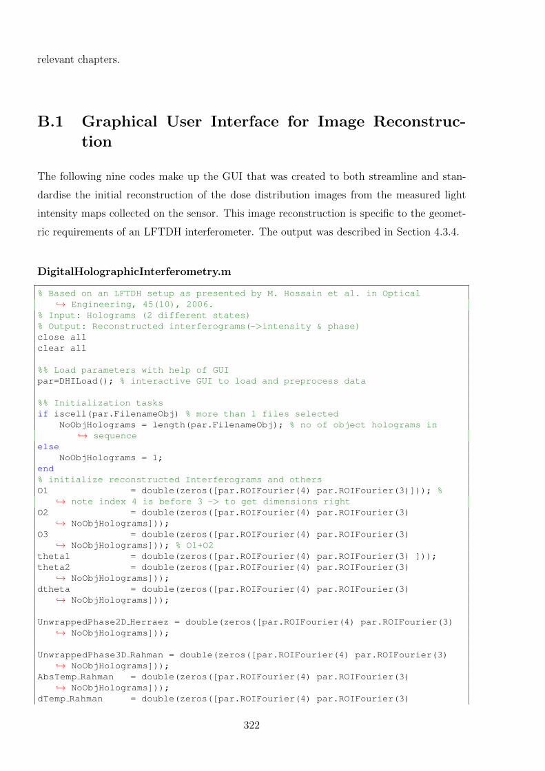
relevant chapters.
B.1 Graphical User Interface for Image Reconstruc-
tion
The following nine codes make up the GUI that was created to both streamline and stan-
dardise the initial reconstruction of the dose distribution images from the measured light
intensity maps collected on the sensor. This image reconstruction is specific to the geomet-
ric requirements of an LFTDH interferometer. The output was described in Section 4.3.4.
DigitalHolographicInterferometry.m
% Based on an LFTDH setup as presented by M. Hossain et al. in Optical↪→ Engineering, 45(10), 2006.
% Input: Holograms (2 different states)% Output: Reconstructed interferograms(->intensity & phase)close allclear all
%% Load parameters with help of GUIpar=DHILoad(); % interactive GUI to load and preprocess data
%% Initialization tasksif iscell(par.FilenameObj) % more than 1 files selected
NoObjHolograms = length(par.FilenameObj); % no of object holograms in↪→ sequence
elseNoObjHolograms = 1;
end% initialize reconstructed Interferograms and othersO1 = double(zeros([par.ROIFourier(4) par.ROIFourier(3)])); %
↪→ note index 4 is before 3 -> to get dimensions rightO2 = double(zeros([par.ROIFourier(4) par.ROIFourier(3)
↪→ NoObjHolograms]));O3 = double(zeros([par.ROIFourier(4) par.ROIFourier(3)
↪→ NoObjHolograms])); % O1+O2theta1 = double(zeros([par.ROIFourier(4) par.ROIFourier(3) ]));theta2 = double(zeros([par.ROIFourier(4) par.ROIFourier(3)
↪→ NoObjHolograms]));dtheta = double(zeros([par.ROIFourier(4) par.ROIFourier(3)
↪→ NoObjHolograms]));
UnwrappedPhase2D Herraez = double(zeros([par.ROIFourier(4) par.ROIFourier(3)↪→ NoObjHolograms]));
UnwrappedPhase3D Rahman = double(zeros([par.ROIFourier(4) par.ROIFourier(3)↪→ NoObjHolograms]));
AbsTemp Rahman = double(zeros([par.ROIFourier(4) par.ROIFourier(3)↪→ NoObjHolograms]));
dTemp Rahman = double(zeros([par.ROIFourier(4) par.ROIFourier(3)
322
↪→ NoObjHolograms]));cumul dTemp Rahman=double(zeros([par.ROIFourier(4) par.ROIFourier(3)
↪→ NoObjHolograms]));Dose Rahman = double(zeros([par.ROIFourier(4) par.ROIFourier(3)
↪→ NoObjHolograms]));
UnwrappedPhase3D JM = double(zeros([par.ROIFourier(4) par.ROIFourier(3)↪→ NoObjHolograms]));
AbsTemp JM = double(zeros([par.ROIFourier(4) par.ROIFourier(3)↪→ NoObjHolograms]));
dTemp JM = double(zeros([par.ROIFourier(4) par.ROIFourier(3)↪→ NoObjHolograms]));
cumul dTemp JM=double(zeros([par.ROIFourier(4) par.ROIFourier(3)↪→ NoObjHolograms]));
Dose JM = double(zeros([par.ROIFourier(4) par.ROIFourier(3)↪→ NoObjHolograms]));
TimeStamps = CreateTimestamp(par.ExposureTime, par.ResolutionHolograms(1),↪→ par.ResolutionHolograms(2), length(par.FilenameObj));
%% Reconstruct% Reference hologramdisp('Reconstructing O1...')O1 = SimplifiedFresnelReconstruction(...
par.HologRef,...par.LaserWavelength,...par.PixelSize,...par.ResolutionHolograms,...par.DistObjCamera,...par.ROIFourier); % optional parameter to crop ROI. Note that 'prime' is
↪→ required as dimensions are flipped
% Object hologramsdisp('Reconstructing O2...')ticfor holog i = 1:NoObjHolograms
O2(:,:,holog i)=SimplifiedFresnelReconstruction(...par.HologObj(:,:,holog i),...par.LaserWavelength,...par.PixelSize,...par.ResolutionHolograms,...par.DistObjCamera,...par.ROIFourier);
endtoc
% % % combined O3=O1+O2disp('Reconstructing O3...')ticfor holog i = 2:NoObjHolograms
O3(:,:,1) = O1(:,:);O3(:,:,holog i)= SimplifiedFresnelReconstruction(...
(par.HologRef + par.HologObj(:,:,holog i)),... %O ref + O2 1par.LaserWavelength,...par.PixelSize,...par.ResolutionHolograms,...par.DistObjCamera,...par.ROIFourier);
end
323
%Alternative code if you want to compare to the previous image each time%rather than the original one. Also need to change the sections where marked
↪→ below.% for holog i = 1:NoObjHolograms% if holog i == 1% O3(:,:,holog i)= SimplifiedFresnelReconstruction(...% (par.HologRef + par.HologObj(:,:,holog i)),... %O ref + O2 1% par.LaserWavelength,...% par.PixelSize,...% par.ResolutionHolograms,...% par.DistObjCamera,...% par.ROIFourier);% else% O3(:,:,holog i)= SimplifiedFresnelReconstruction(...% (par.HologObj(:,:,holog i-1) + par.HologObj(:,:,holog i)),... %
↪→ O2 -1 + O2 1% par.LaserWavelength,...% par.PixelSize,...% par.ResolutionHolograms,...% par.DistObjCamera,...% par.ROIFourier);% end% endtoc
%% Phase informationdisp('Extracting phase ...')tic% theta 1 (reference)theta1(:,:)=angle(O1(:,:)); %phase of reference.%theta1(:,:) = atan(imag(O1(:,:))./real(O1(:,:))); %%%%%%%%%%% Change here%to compare to previous imagefor holog i = 2:NoObjHolograms
% theta2theta2(:,:,holog i)=angle(O2(:,:,holog i));dtheta(:,:,holog i)= InterferencePhase(theta1(:,:,1),theta2(:,:,holog i));
%%%%%%%%%%%% Change here to compare to previous image%theta2(:,:,holog i)=atan(imag(O2(:,:,holog i))./real(O2(:,:,holog i)));
% if holog i == 1% dtheta(:,:,holog i) = InterferencePhase(theta1(:,:,1),theta2(:,:,
↪→ holog i));% else% dtheta(:,:,holog i) = InterferencePhase(theta2(:,:,holog i-1),theta2
↪→ (:,:,holog i));% end
% for holog i=2:NoObjHolograms% dtheta(:,:,holog i)=dtheta(:,:,holog i-1);% end
% Optional median filter applied here. Reccommend doing this in the data% analysis process instead so you can keep track of what you're doing% better.
%dtheta(:,:,holog i)= medfilt2(dtheta(:,:,holog i),[3,3],'symmetric');
324
end%disp('median filter applied to dtheta');toc
% OPTIONAL: Extract phase directly from O3 instead, for comparison purposes...%dtheta3=angle(fftshift(O3));%dtheta comp = dtheta-dtheta3;
% Unwrap in 2Dfor holog i=1:NoObjHolograms;UnwrappedPhase2D Herraez(:,:,holog i) = Herraez 2D unwrapper M(single(dtheta
↪→ (:,:,holog i)));%Herraez 2D unwrapper(single(dtheta(:,:,holog i))); %↪→ unwrap each image
end
% unwrap in 3d, two different methods.UnwrappedPhase3D Rahman = double(Rahman 3D unwrapper M(single(dtheta))); %
↪→ data needs to be of type single. Full 3d unwrapper. Not ideal for noisy↪→ data
UnwrappedPhase3D JM = JM 3D unwrapper(UnwrappedPhase2D Herraez); % unwrap↪→ third dimension only following previous 2D unwrap. ONLY suitable if↪→ looking at relative data at each time point only, NOT for cumulative/↪→ absolute doses.
% Convert to temperature/dose values. To map the refractive index n to the↪→ temperature and vice versa we use polynomials rather than an analytical↪→ solution.
RefInd ref = Temperature2RefractiveIndex(par.InitialCellTemp);%RefractiveIndex2Temperature(RefInd ref) %% Check
for holog i = 1:NoObjHolograms
% % % option 1: comparison of each image to the image before it to build up a↪→ cumulative dose. The plus pi is to account for the results being wrapped↪→ over - pi to pi and not zero to 2 pi.
% Rahman unwrapper:% AbsTemp Rahman(:,:,holog i) = RefractiveIndex2Temperature(
↪→ RefInd ref + ...% par.LaserWavelength.*(UnwrappedPhase3D Rahman(:,:,holog i)+pi)./(4*
↪→ piˆ2*par.PhysicalPathlength));% % if holog i ~= 1 % dtemp (:,:,1) and cumul temp(:,:,1) are zero
↪→ from initialization% dTemp Rahman(:,:,holog i) = AbsTemp Rahman(:,:,holog i) -
↪→ AbsTemp Rahman(:,:,holog i-1) ;% cumul dTemp Rahman(:,:,holog i) = cumul dTemp Rahman(:,:,holog i-1)
↪→ + dTemp Rahman(:,:,holog i);% end% Dose Rahman = dT2dose(cumul dTemp Rahman,par.InitialCellTemp);% JM unwrapper:%% AbsTemp JM(:,:,holog i) = RefractiveIndex2Temperature(RefInd ref
↪→ + ...% par.LaserWavelength.*(UnwrappedPhase3D JM(:,:,holog i)+pi)./(4*piˆ2*
↪→ par.PhysicalPathlength));%% if holog i ~= 1 % dtemp (:,:,1) and cumul temp(:,:,1) are zero from
↪→ initialization% dTemp JM(:,:,holog i) = AbsTemp JM(:,:,holog i) - AbsTemp JM(:,:,
↪→ holog i-1) ;
325
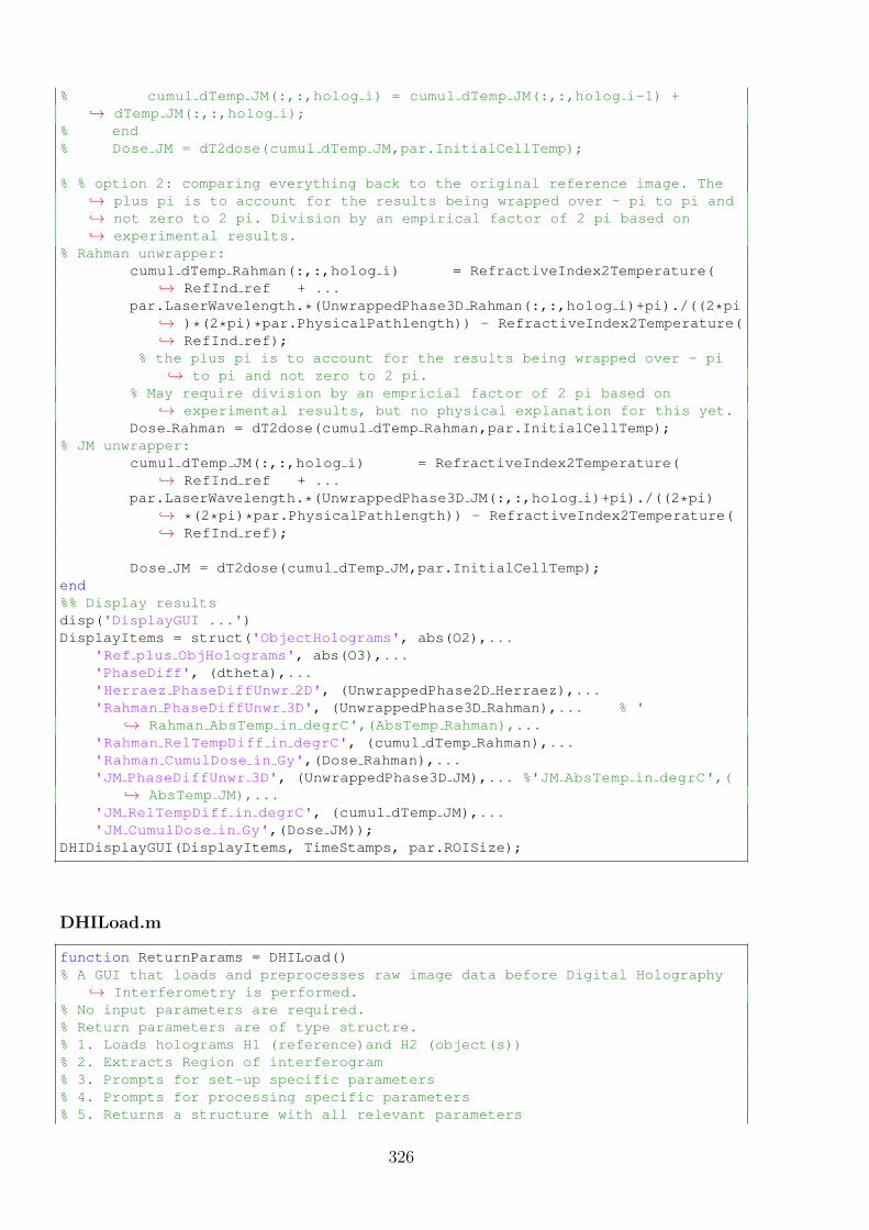
% cumul dTemp JM(:,:,holog i) = cumul dTemp JM(:,:,holog i-1) +↪→ dTemp JM(:,:,holog i);
% end% Dose JM = dT2dose(cumul dTemp JM,par.InitialCellTemp);
% % option 2: comparing everything back to the original reference image. The↪→ plus pi is to account for the results being wrapped over - pi to pi and↪→ not zero to 2 pi. Division by an empirical factor of 2 pi based on↪→ experimental results.
% Rahman unwrapper:cumul dTemp Rahman(:,:,holog i) = RefractiveIndex2Temperature(
↪→ RefInd ref + ...par.LaserWavelength.*(UnwrappedPhase3D Rahman(:,:,holog i)+pi)./((2*pi
↪→ )*(2*pi)*par.PhysicalPathlength)) - RefractiveIndex2Temperature(↪→ RefInd ref);
% the plus pi is to account for the results being wrapped over - pi↪→ to pi and not zero to 2 pi.
% May require division by an empricial factor of 2 pi based on↪→ experimental results, but no physical explanation for this yet.
Dose Rahman = dT2dose(cumul dTemp Rahman,par.InitialCellTemp);% JM unwrapper:
cumul dTemp JM(:,:,holog i) = RefractiveIndex2Temperature(↪→ RefInd ref + ...
par.LaserWavelength.*(UnwrappedPhase3D JM(:,:,holog i)+pi)./((2*pi)↪→ *(2*pi)*par.PhysicalPathlength)) - RefractiveIndex2Temperature(↪→ RefInd ref);
Dose JM = dT2dose(cumul dTemp JM,par.InitialCellTemp);end%% Display resultsdisp('DisplayGUI ...')DisplayItems = struct('ObjectHolograms', abs(O2),...
'Ref plus ObjHolograms', abs(O3),...'PhaseDiff', (dtheta),...'Herraez PhaseDiffUnwr 2D', (UnwrappedPhase2D Herraez),...'Rahman PhaseDiffUnwr 3D', (UnwrappedPhase3D Rahman),... % '
↪→ Rahman AbsTemp in degrC',(AbsTemp Rahman),...'Rahman RelTempDiff in degrC', (cumul dTemp Rahman),...'Rahman CumulDose in Gy',(Dose Rahman),...'JM PhaseDiffUnwr 3D', (UnwrappedPhase3D JM),... %'JM AbsTemp in degrC',(
↪→ AbsTemp JM),...'JM RelTempDiff in degrC', (cumul dTemp JM),...'JM CumulDose in Gy',(Dose JM));
DHIDisplayGUI(DisplayItems, TimeStamps, par.ROISize);
DHILoad.m
function ReturnParams = DHILoad()% A GUI that loads and preprocesses raw image data before Digital Holography
↪→ Interferometry is performed.% No input parameters are required.% Return parameters are of type structre.% 1. Loads holograms H1 (reference)and H2 (object(s))% 2. Extracts Region of interferogram% 3. Prompts for set-up specific parameters% 4. Prompts for processing specific parameters% 5. Returns a structure with all relevant parameters
326
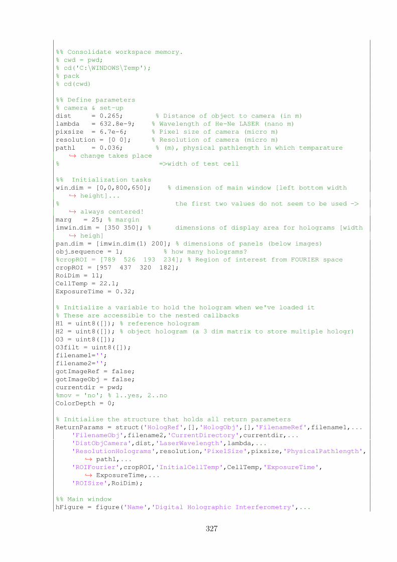
%% Consolidate workspace memory.% cwd = pwd;% cd('C:\WINDOWS\Temp');% pack% cd(cwd)
%% Define parameters% camera & set-updist = 0.265; % Distance of object to camera (in m)lambda = 632.8e-9; % Wavelength of He-Ne LASER (nano m)pixsize = 6.7e-6; % Pixel size of camera (micro m)resolution = [0 0]; % Resolution of camera (micro m)pathl = 0.036; % (m), physical pathlength in which temparature
↪→ change takes place% =>width of test cell
%% Initialization taskswin dim = [0,0,800,650]; % dimension of main window [left bottom width
↪→ height]...% the first two values do not seem to be used ->
↪→ always centered!marg = 25; % marginimwin dim = [350 350]; % dimensions of display area for holograms [width
↪→ heigh]pan dim = [imwin dim(1) 200]; % dimensions of panels (below images)obj sequence = 1; % how many holograms?%cropROI = [789 526 193 234]; % Region of interest from FOURIER spacecropROI = [957 437 320 182];RoiDim = 11;CellTemp = 22.1;ExposureTime = 0.32;
% Initialize a variable to hold the hologram when we've loaded it% These are accessible to the nested callbacksH1 = uint8([]); % reference hologramH2 = uint8([]); % object hologram (a 3 dim matrix to store multiple hologr)O3 = uint8([]);O3filt = uint8([]);filename1='';filename2='';gotImageRef = false;gotImageObj = false;currentdir = pwd;%mov = 'no'; % 1..yes, 2..noColorDepth = 0;
% Initialise the structure that holds all return parametersReturnParams = struct('HologRef',[],'HologObj',[],'FilenameRef',filename1,...
'FilenameObj',filename2,'CurrentDirectory',currentdir,...'DistObjCamera',dist,'LaserWavelength',lambda,...'ResolutionHolograms',resolution,'PixelSize',pixsize,'PhysicalPathlength',
↪→ pathl,...'ROIFourier',cropROI,'InitialCellTemp',CellTemp,'ExposureTime',
↪→ ExposureTime,...'ROISize',RoiDim);
%% Main windowhFigure = figure('Name','Digital Holographic Interferometry',...
327
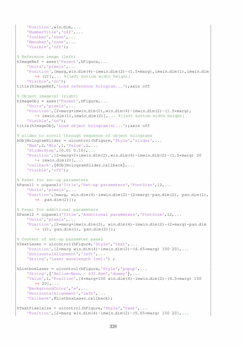
'Position',win dim,...'NumberTitle','off',...'Toolbar','none',...'Menubar','none',...'Visible','off');
% Reference image (left)hImageRef = axes('Parent',hFigure,...
'Units','pixels',...'Position',[marg,win dim(4)-imwin dim(2)-(1.5*marg),imwin dim(1),imwin dim
↪→ (2)],... %[left bottom width height]'Visible','on');
title(hImageRef,'Load reference hologram...');axis off
% Object image(s) (right)hImageObj = axes('Parent',hFigure,...
'Units','pixels',...'Position',[2*marg+imwin dim(2),win dim(4)-imwin dim(2)-(1.5*marg),
↪→ imwin dim(1),imwin dim(2)],... %[left bottom width height]'Visible','on');
title(hImageObj,'Load object hologram(s)...');axis off
% slider to scroll through sequence of object hologramshObjHologramSlider = uicontrol(hFigure,'Style','slider',...
'Max',2,'Min',1,'Value',1,...'SliderStep',[0.01 0.10],...'Position',[2*marg+2*imwin dim(2),win dim(4)-imwin dim(2)-(1.5*marg) 20
↪→ imwin dim(2)],...'callback',{@ObjHologramSlider callback},...'Visible','off');
% Panel for set-up parametershPanel1 = uipanel('Title','Set-up parameters','FontSize',12,...
'Units','pixels',...'Position',[marg, win dim(4)-imwin dim(2)-(2*marg)-pan dim(2), pan dim(1),
↪→ pan dim(2)]);
% Panel for additional parametershPanel2 = uipanel('Title','Additional parameters','FontSize',12,...
'Units','pixels',...'Position',[2*marg+imwin dim(2), win dim(4)-imwin dim(2)-(2*marg)-pan dim
↪→ (2), pan dim(1), pan dim(2)]);
% Content of set-up parameter panelhTextLaser = uicontrol(hFigure,'Style','text',...
'Position',[2*marg win dim(4)-imwin dim(2)-(4.65*marg) 150 20],...'HorizontalAlignment','left',...'String','Laser wavelength [nm]:') ;
hListboxLaser = uicontrol(hFigure,'Style','popup',...'String',{'Helium-Neon - 632.8nm','dummy'},...'Value',1,'Position',[4*marg+100 win dim(4)-imwin dim(2)-(4.5*marg) 150
↪→ 20],...'BackgroundColor','w',...'HorizontalAlignment','left',...'Callback',@ListboxLaser callback);
hTextPixelsize = uicontrol(hFigure,'Style','text',...'Position',[2*marg win dim(4)-imwin dim(2)-(5.65*marg) 150 20],...
328
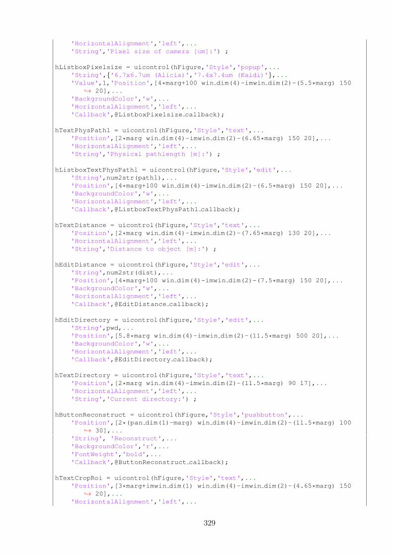
'HorizontalAlignment','left',...'String','Pixel size of camera [um]:') ;
hListboxPixelsize = uicontrol(hFigure,'Style','popup',...'String',{'6.7x6.7um (Alicia)','7.4x7.4um (Kaidi)'},...'Value',1,'Position',[4*marg+100 win dim(4)-imwin dim(2)-(5.5*marg) 150
↪→ 20],...'BackgroundColor','w',...'HorizontalAlignment','left',...'Callback',@ListboxPixelsize callback);
hTextPhysPathl = uicontrol(hFigure,'Style','text',...'Position',[2*marg win dim(4)-imwin dim(2)-(6.65*marg) 150 20],...'HorizontalAlignment','left',...'String','Physical pathlength [m]:') ;
hListboxTextPhysPathl = uicontrol(hFigure,'Style','edit',...'String',num2str(pathl),...'Position',[4*marg+100 win dim(4)-imwin dim(2)-(6.5*marg) 150 20],...'BackgroundColor','w',...'HorizontalAlignment','left',...'Callback',@ListboxTextPhysPathl callback);
hTextDistance = uicontrol(hFigure,'Style','text',...'Position',[2*marg win dim(4)-imwin dim(2)-(7.65*marg) 130 20],...'HorizontalAlignment','left',...'String','Distance to object [m]:') ;
hEditDistance = uicontrol(hFigure,'Style','edit',...'String',num2str(dist),...'Position',[4*marg+100 win dim(4)-imwin dim(2)-(7.5*marg) 150 20],...'BackgroundColor','w',...'HorizontalAlignment','left',...'Callback',@EditDistance callback);
hEditDirectory = uicontrol(hFigure,'Style','edit',...'String',pwd,...'Position',[5.8*marg win dim(4)-imwin dim(2)-(11.5*marg) 500 20],...'BackgroundColor','w',...'HorizontalAlignment','left',...'Callback',@EditDirectory callback);
hTextDirectory = uicontrol(hFigure,'Style','text',...'Position',[2*marg win dim(4)-imwin dim(2)-(11.5*marg) 90 17],...'HorizontalAlignment','left',...'String','Current directory:') ;
hButtonReconstruct = uicontrol(hFigure,'Style','pushbutton',...'Position',[2*(pan dim(1)-marg) win dim(4)-imwin dim(2)-(11.5*marg) 100
↪→ 30],...'String', 'Reconstruct',...'BackgroundColor','r',...'FontWeight','bold',...'Callback',@ButtonReconstruct callback);
hTextCropRoi = uicontrol(hFigure,'Style','text',...'Position',[3*marg+imwin dim(1) win dim(4)-imwin dim(2)-(4.65*marg) 150
↪→ 20],...'HorizontalAlignment','left',...
329
'String','Crop ROI pixels [x y w h]:') ;
hEditCropRoi = uicontrol(hFigure,'Style','edit',...'String',num2str(cropROI),...'Position',[4*marg+100+imwin dim(1)+30 win dim(4)-imwin dim(2)-(4.65*marg)
↪→ 120 20],...'BackgroundColor','w',...'HorizontalAlignment','left',...'Callback',@EditCropRoi callback);
hTextRoiDim = uicontrol(hFigure,'Style','text',...'Position',[3*marg+imwin dim(1) win dim(4)-imwin dim(2)-(5.65*marg) 150
↪→ 20],...'HorizontalAlignment','left',...'String','Square ROI size (pixel):') ;
hEditRoiDim = uicontrol(hFigure,'Style','edit',...'String',num2str(RoiDim),...'Position',[4*marg+100+imwin dim(1)+30 win dim(4)-imwin dim(2)-(5.65*marg)
↪→ 120 20],...'BackgroundColor','w',...'HorizontalAlignment','left',...'Callback',@EditRoiDim callback);
hTextCellTemp = uicontrol(hFigure,'Style','text',...'Position',[3*marg+imwin dim(1) win dim(4)-imwin dim(2)-(6.65*marg) 145
↪→ 20],...'HorizontalAlignment','left',...'String','Initial water temperature [ ]:') ;
hEditCellTemp = uicontrol(hFigure,'Style','edit',...'String',CellTemp,...'Position',[4*marg+100+imwin dim(1)+30 win dim(4)-imwin dim(2)-(6.65*marg)
↪→ 120 20],...'BackgroundColor','w',...'HorizontalAlignment','left',...'Callback',@EditCellTemp callback);
hButtonCropRoi = uicontrol(hFigure,'Style','pushbutton',...'Position',[2*(pan dim(1))+0.5*marg win dim(4)-imwin dim(2)-(4.65*marg) 20
↪→ 20],...'String', '...',...'Callback',@ButtonCropRoi callback);
htextExposureTime = uicontrol(hFigure,'Style','text',...'Position',[3*marg+imwin dim(1) win dim(4)-imwin dim(2)-(7.65*marg) 150
↪→ 20],...'String', 'Exposure time [ms]:',...'HorizontalAlignment','left');
hEditExposureTime= uicontrol(hFigure,'Style','edit',...'Position',[4*marg+100+imwin dim(1)+30 win dim(4)-imwin dim(2)-(7.65*marg)
↪→ 120 20],...'String', ExposureTime,...'HorizontalAlignment','left',...'BackgroundColor','w',...'Callback',@EditExposureTime callback);
hMenu = uimenu(hFigure,'Label','Load holograms');
330
hFileLoadReference = uimenu(hMenu,'Label','Open Reference Hologram',...'Callback',{@FileLoadReference callback});
hFileLoadObject = uimenu(hMenu,'Label','Open Object Hologram(s)',...'Callback',{@FileLoadObject callback});
% Initialization tasksset(hFigure,'Visible','on');
%while (reconstruct == false)
% Callbacks for dhi gui% Note that these functions are nested, so have access to variables from% the outer function
function FileLoadReference callback(hObject, eventdata) %#ok<*INUSD>[filename1, pathname1] = uigetfile({'*.tif';'*.jpg'},'Select reference
↪→ hologram');currentdir = pathname1;cd(currentdir)%H1 raw = double(imread(filename1));%H1 raw = medfilt2(imread(filename1));H1 raw = (imread(filename1));s=size(H1 raw);ImageDetails=imfinfo(filename1)if length(s) == 3
ColorDepth = 24; %-> convert bitdepthdisp(['Converting hologram (',filename1,') bitdepth...'])H1= (H1 raw(:,:,1)+H1 raw(:,:,2)+H1 raw(:,:,3))/3;
elseif ImageDetails.BitDepth == 16disp(['Converting (',filename1,') bitdepth...'])H1=uint8(H1 raw./256);
elseColorDepth = 8;H1=H1 raw;
end[resolution(2),resolution(1)]=size(H1);gotImageRef = true;updateDisplay;
end
function FileLoadObject callback(hObject, eventdata)[filename2, pathname2] = uigetfile( ...
{'*.tif';'*.jpg'}, ...'Select object hologram(s)',...'MultiSelect', 'on');
currentdir = pathname2;cd(currentdir)if iscell(filename2) % more than 1 files selected
disp(['Sequence of ',num2str(length(filename2)), ' holograms↪→ selected.'])
filename2=sort(filename2); % sort as uigetfile returns files in↪→ arbitrary order
obj sequence = length(filename2);h2 raw=(imread(char(filename2(1))));s=size(h2 raw);ImageDetails=imfinfo(char(filename2(1)));if length(s) == 3
ColorDepth = 24; %-> convert bitdepth
331
h2= (h2 raw(:,:,1)+h2 raw(:,:,2)+h2 raw(:,:,3))/3;disp(['Converting hologram (',char(filename2(1)),')
↪→ bitdepth...'])elseif ImageDetails.BitDepth == 16
ColorDepth = 8; % refers to color depth rather than bit depthdisp(['Converting hologram (',char(filename2(1)),')
↪→ bitdepth...'])h2=uint8(h2 raw./256);
elseColorDepth = 8;h2=h2 raw;
endH2=uint8(zeros(s(1),s(2),obj sequence));H2(:,:,1)=h2;for i = 2:obj sequence
if ColorDepth == 8if ImageDetails.BitDepth == 16
disp(['Converting hologram (',char(filename2(i)),')↪→ bitdepth...'])
H2(:,:,i) = uint8(imread(char(filename2(i)))/256); %↪→ hologram 2
elseH2(:,:,i) = (imread(char(filename2(i)))); % hologram 2
endelse
h2 raw = (imread(char(filename2(i)))); % hologram 2disp(['Converting hologram (',char(filename2(i)),')
↪→ bitdepth...'])h2i= (h2 raw(:,:,1)+h2 raw(:,:,2)+h2 raw(:,:,3))/3;H2(:,:,i)=h2i;
endend
% figure% a= H2(:,:,1);% b= medfilt2(H2(:,:,1));% plot(1:1024,a(:,500),'m.',1:1024,b(:,500),'r.-')% keyboard
set(hObjHologramSlider,'Visible','on','Value',1)set(hObjHologramSlider,'Max',obj sequence) % adjust slider to
↪→ number of obj hologramsset(hObjHologramSlider,'SliderStep',...
[1/(obj sequence-1) 3/(obj sequence-1)]) % adjust step size (↪→ minor 1 step, major 3 steps)
% if no reference hologram loaded, use first object holog in↪→ sequence
if gotImageRef == false;H1 = H2(:,:,1);gotImageRef = true;filename1 = char(filename2(1));[resolution(2),resolution(1)]=size(H1);
endelse
set(hObjHologramSlider,'Visible','off') % remove sliderobj sequence = 1;%H2 = double(imread(filename2));H2 = (imread(filename2));
endgotImageObj = true;
332
updateDisplay;end
function ObjHologramSlider callback(hObject, eventdata)updateDisplay;
end
function ListboxLaser callback(hObject, eventdata)switch get(hListboxLaser, 'Value')
case 1lambda = 632.8e-9;
case 2lambda = 0;
enddisp(['Laser wavelength has been changed to selection: ', num2str(get(
↪→ hListboxLaser, 'Value'))])end
function ListboxPixelsize callback(hObject, eventdata)switch get(hListboxPixelsize, 'Value')
case 1pixsize = 6.7e-6;
case 2pixsize = 7.4e-6;
enddisp(['Camera pixel size changed to selection: ', num2str(get(
↪→ hListboxPixelsize, 'Value'))])end
function ListboxTextPhysPathl callback(hObject, eventdata)pathl=str2num(get(hListboxTextPhysPathl, 'String'));disp(['Physical Pathlength changed to: : ', num2str(pathl),'m.'])
end
function EditDistance callback(hObject, eventdata)dist= str2num(get(hEditDistance, 'String'));disp(['Distance to object changed to ',num2str(dist) ,'m.'])
end
function EditDirectory callback(hObject, eventdata)disp(['Current directory changed to: ', get(hEditDirectory, 'String')
↪→ ])currentdir=get(hEditDirectory, 'String');cd(currentdir)updateDisplay
end
function EditCropRoi callback(hObject, eventdata)cropROI=str2num(get(hEditCropRoi, 'String')); %#ok<*ST2NM>disp(['CROP region: ', num2str(cropROI)])
end
% function EditTrackRoi callback(hObject, eventdata)% trackROI=str2num(get(hEditTrackRoi, 'String'));% disp(['Track region: ', num2str(trackROI)])% end
function EditCellTemp callback(hObject, eventdata)CellTemp=str2num(get(hEditCellTemp, 'String'));
333
disp(['Cell temperature : ', num2str(CellTemp)])end
function EditExposureTime callback(hObject, eventdata)ExposureTime = str2num(get(hEditExposureTime, 'String'));disp(['Exposure time is: ', num2str(ExposureTime)])
end
function EditRoiDim callback(hObject, eventdata)RoiDim = str2num(get(hEditRoiDim, 'String'));disp(['ROI dimensions: ', num2str(RoiDim)])
end
function ButtonCropRoi callback(hObject, eventdata)if (gotImageRef && gotImageObj)
O3 = SimplifiedFresnelReconstruction(H1+H2(:,:,1),lambda,pixsize,↪→ resolution,dist);
%cm=colormap;fr=figure;imagesc(log(abs(O3))); % log so ROI can be visualisedtitle('Reconstructed Interferogram. Select ROI. Double click to
↪→ close figure.')axis equal tightcolormap gray
% select Region of Interest (ROI)hrect1 = imrect(gca,cropROI);addNewPositionCallback(hrect1, @(p) set(hEditCropRoi, 'String',
↪→ num2str(round(p))));fcn = makeConstrainToRectFcn('imrect',get(gca,'XLim'),get(gca,'
↪→ YLim'));setPositionConstraintFcn(hrect1,fcn);wait(hrect1); % Interactively place a rectangle by clicking ...% and dragging. Use wait to block the MATLAB ...% command line. Double-click on the rectangle to% resume.%CROPcropROI=str2num(get(hEditCropRoi, 'String'));
O3filt = O3(cropROI(2):cropROI(2)+cropROI(4), cropROI(1):cropROI↪→ (1)+cropROI(3));
%colormap cmclose(fr) % close figure
%a=medfilt2(abs(O3filt));%figure%plot(1:163,a(:,80),'r.-',1:163,abs(O3filt(:,80)),'b.-')
elsemsgbox('Load holograms first!','Warning','warn')
endend
function ButtonReconstruct callback(hObject, eventdata)if (gotImageRef && gotImageObj)
% assign values to return structureReturnParams.HologRef=H1;ReturnParams.HologObj=H2;ReturnParams.FilenameRef=filename1;ReturnParams.FilenameObj=filename2;
334
ReturnParams.CurrentDirectory=currentdir;ReturnParams.DistObjCamera=dist;ReturnParams.LaserWavelength=lambda;ReturnParams.ResolutionHolograms=resolution;ReturnParams.PixelSize=pixsize;ReturnParams.PhysicalPathlength=pathl;ReturnParams.ROIFourier=cropROI;ReturnParams.InitialCellTemp=CellTemp;ReturnParams.ExposureTime=ExposureTime;ReturnParams.ROISize=RoiDim;close(hFigure) % This triggers a 'CloseRequestFct' -> close figure
↪→ and return arguments from functionelse
msgbox('Load holograms first!','Warning','warn')end
end
% Redrawfunction updateDisplay
set(hEditDirectory,'String',currentdir)
if gotImageRef == trueaxes(hImageRef)imagesc(H1);title(['Reference hologram: ',char(filename1)])axis equal tight off
end
if gotImageObj == trueif obj sequence == 1
axes(hImageObj)imagesc(H2(:,:,1));title(['Object hologram: ',char(filename2)])
elsecurrentObj=fix(get(hObjHologramSlider,'Value'));axes(hImageObj) %#ok<*MAXES>imagesc(H2(:,:,currentObj));title([num2str(currentObj),' of ',num2str(obj sequence),'
↪→ object holograms: ',char(filename2(currentObj))])endaxis equal tight off
end
if (gotImageRef && gotImageObj)set(hButtonReconstruct,'BackgroundColor','g')
elseset(hButtonReconstruct,'BackgroundColor','r')
endend
waitfor(hFigure,'CloseRequestFcn') % return when reconstruct button is pressedend
CreateTimestamp.m
function TimeStamps = CreateTimestamp(ExposureTime, ROIwidth, ROIheight,↪→ noImages)
% Calculates the 'Default USB2 frame rate' based on digital camera settings,
335
↪→ and then calculates time stamps for a series of images(noImages). Note↪→ that the actual frame rate can vary slightly.
% Based on PixeLINK PL-B740 Frame Rate Calculator (↪→ B740 series frame rate calc.xls).
% Input: Exposure time (in ms), no pixels in x & y, the number of images in↪→ the sequence
% Output: a vector with time stamps in seconds and short E notation% constantsTimeStamps = zeros(noImages,1);ClockPeriod = 1/40000000;BWDefaultUSB2 = 26214400;EffectiveColumns = ROIwidth;EffectiveRows = ROIheight;FrameBlanking = 15;LineBlanking = 10;LinePadding = 156;VFWidth = EffectiveColumns + LineBlanking;BytesPerPixel = 1;FrameSize = EffectiveRows*EffectiveColumns * BytesPerPixel +36;FrameTime = (VFWidth*ClockPeriod)* (EffectiveRows + FrameBlanking);DefaultUSBframeRate = min(1/(max(FrameTime,FrameSize/BWDefaultUSB2)...
+ExposureTime/1000),4000); % in frames/seconddisp(['Default USB 2.0 frame rate is ', num2str(DefaultUSBframeRate) ,' f/s.'
↪→ ])deltaTime = 1/DefaultUSBframeRate; % in sTimeStamps(1)=0.0;for i = 2:noImages
%TimeStamps(i)={num2str(deltaTime*(i-1),'%10.5e\n')}TimeStamps(i)=deltaTime*(i-1);
end
SimplifiedFresnelReconstruction.m
function O return = SimplifiedFresnelReconstruction(H,lambda,pixsize,res,dist↪→ ,cropROI)
%(the last argument is optional -> to crop ROI)k = 2*pi/lambda; % wave numberconst2 = 1; % constant 2 in Eq 3
% set o to centre of image[xi,yi] = meshgrid(-res(1)/2+1:res(1)/2,-res(2)/2+1:res(2)/2); % indicesX = xi.*pixsize; % convert to actual dimensionsY = yi.*pixsize;
% non fourier termnft = (exp(1i*k*dist)/(1i*lambda*dist))*exp(((-1i*k)/(2*dist))*(X.ˆ2+Y.ˆ2));
% Reconstruction (Eq 3): O(X,Y)%keyboardO = const2*nft.*fftshift(fft2(H));
if nargin == 5O return = O;
else if nargin == 6;O return = O(cropROI(2):cropROI(2)+cropROI(4)-1,cropROI(1):cropROI(1)+
↪→ cropROI(3)-1);end
336
endreturn
InterferencePhase.m
function dtheta = InterferencePhase(theta1, theta2)% calculate phase map dtheta on the range of pi to -pi instead.s=size(theta1);for m=1:s(1)
for n = 1:s(2)if theta2(m,n) - theta1(m,n) >= pi;
dtheta(m,n) = theta2(m,n) - theta1(m,n) - 2*pi;else
if theta2(m,n) - theta1(m,n) < -pi;dtheta(m,n) = theta2(m,n) - theta1(m,n) + 2*pi;
else dtheta(m,n) = theta2(m,n) - theta1(m,n);end
endend
endreturn
RefractiveIndex2Temperature.m
function Temperature = RefractiveIndex2Temperature(RefractiveIndex)polyn = [-306192022839.014
2025472069804.51-5359422226526.77090535267512.57
-4690394790752.351241078028359.92];
Temperature = polyval(polyn,double(RefractiveIndex));% Note: if double is removed the results are completely wrong instead of 20
↪→ degr it spits out a number several orders of magn bigger!!!!!!!!return
Temperature2RefractiveIndex.m
function RefractiveIndex = Temperature2RefractiveIndex(Temperature)polyn = [3.02416865046015e-018
-7.69286698973227e-0165.21449173722462e-009-1.93016045341355e-006-1.37327031294521e-0051.3322129684799];
RefractiveIndex = polyval(polyn,double(Temperature));return
dT2dose.m
337
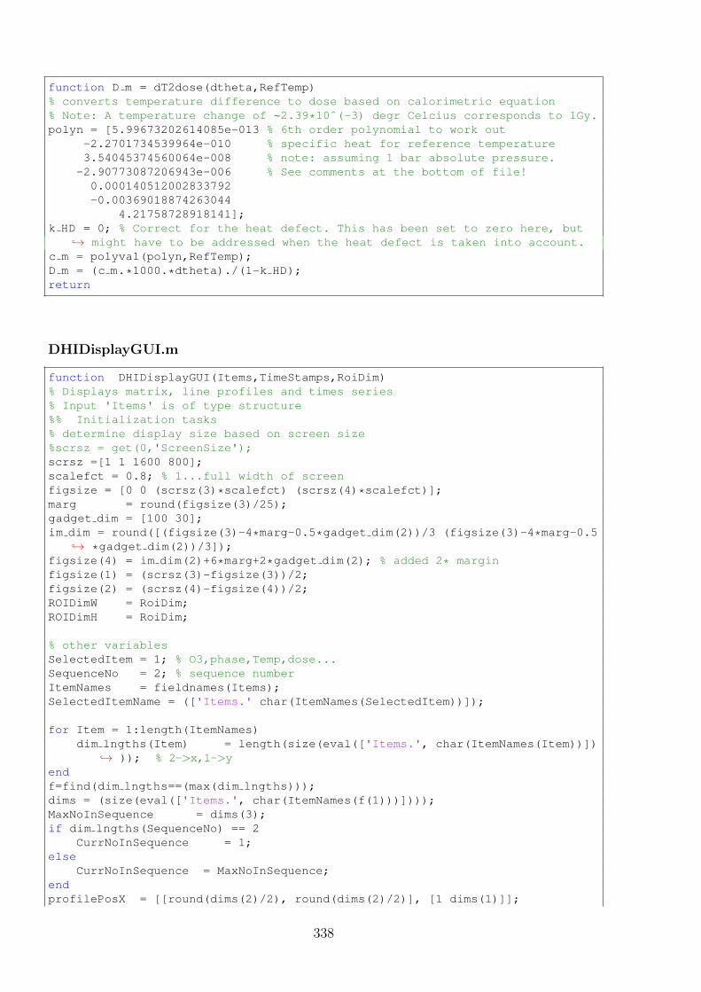
function D m = dT2dose(dtheta,RefTemp)% converts temperature difference to dose based on calorimetric equation% Note: A temperature change of ~2.39*10ˆ(-3) degr Celcius corresponds to 1Gy.polyn = [5.99673202614085e-013 % 6th order polynomial to work out
-2.2701734539964e-010 % specific heat for reference temperature3.54045374560064e-008 % note: assuming 1 bar absolute pressure.-2.90773087206943e-006 % See comments at the bottom of file!0.000140512002833792-0.00369018874263044
4.21758728918141];k HD = 0; % Correct for the heat defect. This has been set to zero here, but
↪→ might have to be addressed when the heat defect is taken into account.c m = polyval(polyn,RefTemp);D m = (c m.*1000.*dtheta)./(1-k HD);return
DHIDisplayGUI.m
function DHIDisplayGUI(Items,TimeStamps,RoiDim)% Displays matrix, line profiles and times series% Input 'Items' is of type structure%% Initialization tasks% determine display size based on screen size%scrsz = get(0,'ScreenSize');scrsz =[1 1 1600 800];scalefct = 0.8; % 1...full width of screenfigsize = [0 0 (scrsz(3)*scalefct) (scrsz(4)*scalefct)];marg = round(figsize(3)/25);gadget dim = [100 30];im dim = round([(figsize(3)-4*marg-0.5*gadget dim(2))/3 (figsize(3)-4*marg-0.5
↪→ *gadget dim(2))/3]);figsize(4) = im dim(2)+6*marg+2*gadget dim(2); % added 2* marginfigsize(1) = (scrsz(3)-figsize(3))/2;figsize(2) = (scrsz(4)-figsize(4))/2;ROIDimW = RoiDim;ROIDimH = RoiDim;
% other variablesSelectedItem = 1; % O3,phase,Temp,dose...SequenceNo = 2; % sequence numberItemNames = fieldnames(Items);SelectedItemName = (['Items.' char(ItemNames(SelectedItem))]);
for Item = 1:length(ItemNames)dim lngths(Item) = length(size(eval(['Items.', char(ItemNames(Item))])
↪→ )); % 2->x,1->yendf=find(dim lngths==(max(dim lngths)));dims = (size(eval(['Items.', char(ItemNames(f(1)))])));MaxNoInSequence = dims(3);if dim lngths(SequenceNo) == 2
CurrNoInSequence = 1;else
CurrNoInSequence = MaxNoInSequence;endprofilePosX = [[round(dims(2)/2), round(dims(2)/2)], [1 dims(1)]];
338
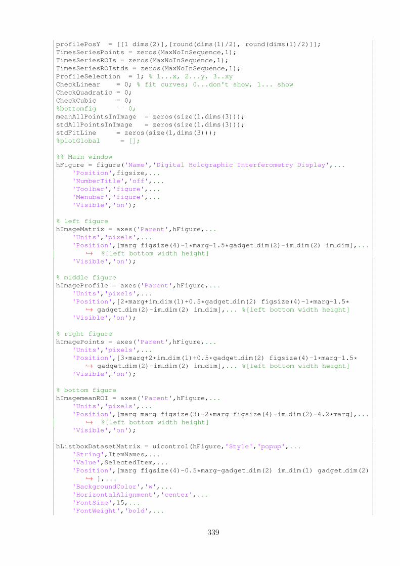
profilePosY = [[1 dims(2)],[round(dims(1)/2), round(dims(1)/2)]];TimesSeriesPoints = zeros(MaxNoInSequence,1);TimesSeriesROIs = zeros(MaxNoInSequence,1);TimesSeriesROIstds = zeros(MaxNoInSequence,1);ProfileSelection = 1; % 1...x, 2...y, 3..xyCheckLinear = 0; % fit curves; 0...don't show, 1... showCheckQuadratic = 0;CheckCubic = 0;%bottomfig = 0;meanAllPointsInImage = zeros(size(1,dims(3)));stdAllPointsInImage = zeros(size(1,dims(3)));stdFitLine = zeros(size(1,dims(3)));%plotGlobal = [];
%% Main windowhFigure = figure('Name','Digital Holographic Interferometry Display',...
'Position',figsize,...'NumberTitle','off',...'Toolbar','figure',...'Menubar','figure',...'Visible','on');
% left figurehImageMatrix = axes('Parent',hFigure,...
'Units','pixels',...'Position',[marg figsize(4)-1*marg-1.5*gadget dim(2)-im dim(2) im dim],...
↪→ %[left bottom width height]'Visible','on');
% middle figurehImageProfile = axes('Parent',hFigure,...
'Units','pixels',...'Position',[2*marg+im dim(1)+0.5*gadget dim(2) figsize(4)-1*marg-1.5*
↪→ gadget dim(2)-im dim(2) im dim],... %[left bottom width height]'Visible','on');
% right figurehImagePoints = axes('Parent',hFigure,...
'Units','pixels',...'Position',[3*marg+2*im dim(1)+0.5*gadget dim(2) figsize(4)-1*marg-1.5*
↪→ gadget dim(2)-im dim(2) im dim],... %[left bottom width height]'Visible','on');
% bottom figurehImagemeanROI = axes('Parent',hFigure,...
'Units','pixels',...'Position',[marg marg figsize(3)-2*marg figsize(4)-im dim(2)-4.2*marg],...
↪→ %[left bottom width height]'Visible','on');
hListboxDatasetMatrix = uicontrol(hFigure,'Style','popup',...'String',ItemNames,...'Value',SelectedItem,...'Position',[marg figsize(4)-0.5*marg-gadget dim(2) im dim(1) gadget dim(2)
↪→ ],...'BackgroundColor','w',...'HorizontalAlignment','center',...'FontSize',15,...'FontWeight','bold',...
339
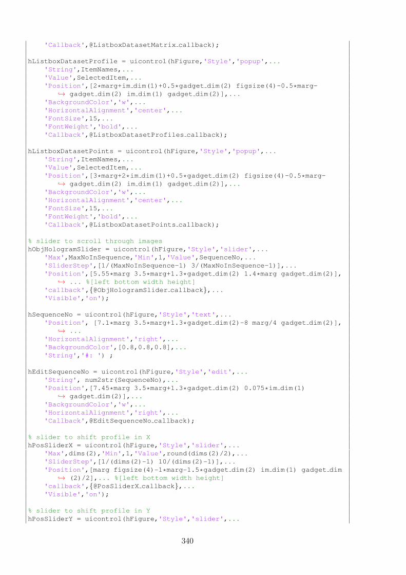
'Callback',@ListboxDatasetMatrix callback);
hListboxDatasetProfile = uicontrol(hFigure,'Style','popup',...'String',ItemNames,...'Value',SelectedItem,...'Position',[2*marg+im dim(1)+0.5*gadget dim(2) figsize(4)-0.5*marg-
↪→ gadget dim(2) im dim(1) gadget dim(2)],...'BackgroundColor','w',...'HorizontalAlignment','center',...'FontSize',15,...'FontWeight','bold',...'Callback',@ListboxDatasetProfiles callback);
hListboxDatasetPoints = uicontrol(hFigure,'Style','popup',...'String',ItemNames,...'Value',SelectedItem,...'Position',[3*marg+2*im dim(1)+0.5*gadget dim(2) figsize(4)-0.5*marg-
↪→ gadget dim(2) im dim(1) gadget dim(2)],...'BackgroundColor','w',...'HorizontalAlignment','center',...'FontSize',15,...'FontWeight','bold',...'Callback',@ListboxDatasetPoints callback);
% slider to scroll through imageshObjHologramSlider = uicontrol(hFigure,'Style','slider',...
'Max',MaxNoInSequence,'Min',1,'Value',SequenceNo,...'SliderStep',[1/(MaxNoInSequence-1) 3/(MaxNoInSequence-1)],...'Position',[5.55*marg 3.5*marg+1.3*gadget dim(2) 1.4*marg gadget dim(2)],
↪→ ... %[left bottom width height]'callback',{@ObjHologramSlider callback},...'Visible','on');
hSequenceNo = uicontrol(hFigure,'Style','text',...'Position', [7.1*marg 3.5*marg+1.3*gadget dim(2)-8 marg/4 gadget dim(2)],
↪→ ...'HorizontalAlignment','right',...'BackgroundColor',[0.8,0.8,0.8],...'String','#: ') ;
hEditSequenceNo = uicontrol(hFigure,'Style','edit',...'String', num2str(SequenceNo),...'Position',[7.45*marg 3.5*marg+1.3*gadget dim(2) 0.075*im dim(1)
↪→ gadget dim(2)],...'BackgroundColor','w',...'HorizontalAlignment','right',...'Callback',@EditSequenceNo callback);
% slider to shift profile in XhPosSliderX = uicontrol(hFigure,'Style','slider',...
'Max',dims(2),'Min',1,'Value',round(dims(2)/2),...'SliderStep',[1/(dims(2)-1) 10/(dims(2)-1)],...'Position',[marg figsize(4)-1*marg-1.5*gadget dim(2) im dim(1) gadget dim
↪→ (2)/2],... %[left bottom width height]'callback',{@PosSliderX callback},...'Visible','on');
% slider to shift profile in YhPosSliderY = uicontrol(hFigure,'Style','slider',...
340
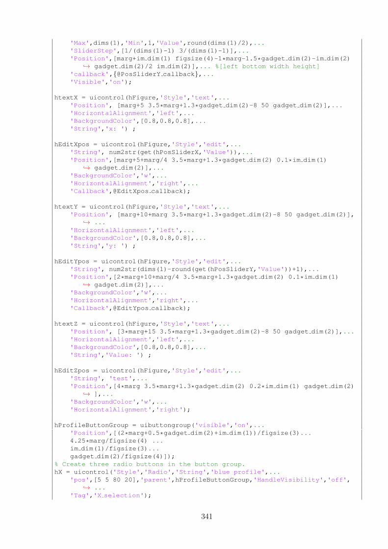
'Max',dims(1),'Min',1,'Value',round(dims(1)/2),...'SliderStep',[1/(dims(1)-1) 3/(dims(1)-1)],...'Position',[marg+im dim(1) figsize(4)-1*marg-1.5*gadget dim(2)-im dim(2)
↪→ gadget dim(2)/2 im dim(2)],... %[left bottom width height]'callback',{@PosSliderY callback},...'Visible','on');
htextX = uicontrol(hFigure,'Style','text',...'Position', [marg+5 3.5*marg+1.3*gadget dim(2)-8 50 gadget dim(2)],...'HorizontalAlignment','left',...'BackgroundColor',[0.8,0.8,0.8],...'String','x: ') ;
hEditXpos = uicontrol(hFigure,'Style','edit',...'String', num2str(get(hPosSliderX,'Value')),...'Position',[marg+5+marg/4 3.5*marg+1.3*gadget dim(2) 0.1*im dim(1)
↪→ gadget dim(2)],...'BackgroundColor','w',...'HorizontalAlignment','right',...'Callback',@EditXpos callback);
htextY = uicontrol(hFigure,'Style','text',...'Position', [marg+10+marg 3.5*marg+1.3*gadget dim(2)-8 50 gadget dim(2)],
↪→ ...'HorizontalAlignment','left',...'BackgroundColor',[0.8,0.8,0.8],...'String','y: ') ;
hEditYpos = uicontrol(hFigure,'Style','edit',...'String', num2str(dims(1)-round(get(hPosSliderY,'Value'))+1),...'Position',[2*marg+10+marg/4 3.5*marg+1.3*gadget dim(2) 0.1*im dim(1)
↪→ gadget dim(2)],...'BackgroundColor','w',...'HorizontalAlignment','right',...'Callback',@EditYpos callback);
htextZ = uicontrol(hFigure,'Style','text',...'Position', [3*marg+15 3.5*marg+1.3*gadget dim(2)-8 50 gadget dim(2)],...'HorizontalAlignment','left',...'BackgroundColor',[0.8,0.8,0.8],...'String','Value: ') ;
hEditZpos = uicontrol(hFigure,'Style','edit',...'String', 'test',...'Position',[4*marg 3.5*marg+1.3*gadget dim(2) 0.2*im dim(1) gadget dim(2)
↪→ ],...'BackgroundColor','w',...'HorizontalAlignment','right');
hProfileButtonGroup = uibuttongroup('visible','on',...'Position',[(2*marg+0.5*gadget dim(2)+im dim(1))/figsize(3)...4.25*marg/figsize(4) ...im dim(1)/figsize(3)...gadget dim(2)/figsize(4)]);
% Create three radio buttons in the button group.hX = uicontrol('Style','Radio','String','blue profile',...
'pos',[5 5 80 20],'parent',hProfileButtonGroup,'HandleVisibility','off',↪→ ...
'Tag','X selection');
341
hY = uicontrol('Style','Radio','String','black profile',...'pos',[0.25*im dim(1)+5 5 80 20],'parent',hProfileButtonGroup,'
↪→ HandleVisibility','off',...'Value',ProfileSelection, 'Tag','Y selection');
hXY = uicontrol('Style','Radio','String','3D profiles',...'pos',[0.5*im dim(1)+5 5 80 20],'parent',hProfileButtonGroup,'
↪→ HandleVisibility','off',...'Tag','XY selection');
hsurf = uicontrol('Style','Radio','String','surface',...'pos',[0.75*im dim(1)+5 5 80 20],'parent',hProfileButtonGroup,'
↪→ HandleVisibility','off',...'Tag','surf selection');
hCheckLinear = uicontrol('Style','CheckBox',...'pos',[4*marg+1.9*im dim(1)+0.5*gadget dim(2) figsize(4)-1.2*marg-
↪→ gadget dim(2) im dim(1)/4+10 gadget dim(2)],...'BackgroundColor',[0.8,0.8,0.8],...'ForegroundColor','m',...'String','Linear',...'Callback',@CheckLinear callback);
hCheckCubic = uicontrol('Style','CheckBox',...'pos',[4*marg+2.6*im dim(1)+0.5*gadget dim(2) figsize(4)-1.2*marg-
↪→ gadget dim(2) im dim(1)/4+10 gadget dim(2)],...'BackgroundColor',[0.8,0.8,0.8],...'ForegroundColor','y',...'String','Cubic',...'Callback',@CheckCubic callback);
hCheckQuadratic = uicontrol('Style','CheckBox',...'pos',[4*marg+2.25*im dim(1)+0.5*gadget dim(2) figsize(4)-1.2*marg-
↪→ gadget dim(2) im dim(1)/4+15 gadget dim(2)],...'BackgroundColor',[0.8,0.8,0.8],...'ForegroundColor','c',...'String','Quadratic',...'Callback',@CheckQuadratic callback);
% Initialize some button group properties.set(hProfileButtonGroup,'SelectionChangeFcn',@ProfileButtonGroup callback);set(hProfileButtonGroup,'Visible','on');
% DisplayupdateDisplay
%% Callback functionsfunction ObjHologramSlider callback(hObject, eventdata) %#ok<*INUSD>
SequenceNo = round(get(hObjHologramSlider,'Value'));updateDisplay;
end
function EditSequenceNo callback(hObject, eventdata)set(hObjHologramSlider,'Value',str2double((get(hEditSequenceNo,'String
↪→ '))))set(hEditZpos,'String',num2str((eval(char([SelectedItemName,'(
↪→ profilePosY(3),profilePosX(1),SequenceNo)'])))))ObjHologramSlider callback(hObject, eventdata)updateDisplay
end
342
function EditXpos callback(hObject, eventdata)set(hPosSliderX,'Value',str2num(get(hEditXpos,'String')))PosSliderX callback(hObject, eventdata)
end
function EditYpos callback(hObject, eventdata)set(hPosSliderY,'Value',dims(1)-round(str2num(get(hEditYpos,'String'))
↪→ )+1) %#ok<*ST2NM>PosSliderY callback(hObject, eventdata)
end
function PosSliderX callback(hObject, eventdata)CurrentSelectionX= round(get(hPosSliderX,'Value'));profilePosX = [CurrentSelectionX CurrentSelectionX 1 dims(1)];set(hEditXpos,'String',num2str(CurrentSelectionX))updateDisplay
end
function PosSliderY callback(hObject, eventdata)CurrentSelectionY= dims(1)-round(get(hPosSliderY,'Value'))+1;profilePosY = [1 dims(2) CurrentSelectionY CurrentSelectionY ];set(hEditYpos,'String',num2str(CurrentSelectionY))updateDisplay
end
function CheckLinear callback(hObject, eventdata)if (get(hObject,'Value') == get(hObject,'Max'))
% Checkbox is checked-take approriate actiondisp('Linear checked')CheckLinear = 1;updateDisplay
else% Checkbox is not checked-take approriate actiondisp('Linear unchecked')CheckLinear = 0;updateDisplay
endend
function CheckCubic callback(hObject, eventdata)if (get(hObject,'Value') == get(hObject,'Max'))
% Checkbox is checked-take approriate actiondisp('LinearMean checked')CheckCubic = 1;updateDisplay
else% Checkbox is not checked-take approriate actiondisp('Cubic unchecked')CheckCubic = 0;updateDisplay
endend
function CheckQuadratic callback(hObject, eventdata)if (get(hObject,'Value') == get(hObject,'Max'))
% Checkbox is checked-take approriate actiondisp('Quadratic checked')CheckQuadratic = 1;
343
updateDisplayelse
% Checkbox is not checked-take approriate actiondisp('Quadratic unchecked')CheckQuadratic = 0;updateDisplay
endend
function ProfileButtonGroup callback(hObject,eventdata)switch get(eventdata.NewValue,'Tag') % Get Tag of selected object.
case 'X selection'ProfileSelection=0;%disp(get(get(hObject,'SelectedObject'),'String'))
case 'Y selection'ProfileSelection=1;%disp(get(get(hObject,'SelectedObject'),'String'))
case 'XY selection'ProfileSelection=2;%disp(get(get(hObject,'SelectedObject'),'String'))
case 'surf selection'ProfileSelection=3;
endupdateDisplay
end
function ListboxDatasetMatrix callback(hObject,eventdata)SelectedItem=get(hListboxDatasetMatrix,'Value');SequenceNo=round(get(hObjHologramSlider,'Value'));SelectedItemName = (['Items.' char(ItemNames(SelectedItem))]);set(hListboxDatasetProfile,'Value',SelectedItem)set(hListboxDatasetPoints,'Value',SelectedItem)bottomfig = 0;%keyboardif length(size(eval(['Items.', char(ItemNames(SelectedItem))])))== 2;
CurrNoInSequence = 1;else
CurrNoInSequence = MaxNoInSequence;endif CurrNoInSequence == MaxNoInSequence
set(hEditZpos,'String',num2str((eval(char([SelectedItemName,'(↪→ profilePosY(3),profilePosX(1),SequenceNo)'])))))
elseset(hEditZpos,'String',num2str((eval(char([SelectedItemName,'(
↪→ profilePosY(3),profilePosX(1))'])))))end
updateDisplayend
%% Redrawfunction updateDisplay
set(hEditSequenceNo,'String', num2str(SequenceNo))%keyboardif CurrNoInSequence == 1
set(hObjHologramSlider,'Visible','off')set(hEditZpos,'String',num2str((eval(char([SelectedItemName,'(
↪→ profilePosY(3),profilePosX(1))'])))))else
344
set(hObjHologramSlider,'Visible','on')%keyboardset(hEditZpos,'String',num2str((eval(char([SelectedItemName,'(
↪→ profilePosY(3),profilePosX(1),SequenceNo)'])))))end
% left windowaxes(hImageMatrix) %#ok<*MAXES>
%keyboardif dim lngths(SelectedItem) == 2
eval(['imagesc((',SelectedItemName,'))']);else
eval(['imagesc(',SelectedItemName,'(:,:,',num2str(SequenceNo),'))'↪→ ]);
end
axis equal tighthold online(profilePosX(1:2),profilePosX(3:4),'LineWidth',2,'Color','b')line(profilePosY(1:2),profilePosY(3:4),'LineWidth',2,'Color','k')plot(hImageMatrix,profilePosX(1), profilePosY(3),'o',...
'MarkerEdgeColor','k',...'MarkerFaceColor','m',...'MarkerSize',7)
%colorbar('South')% w=25;% h=25;
ROIdims=[profilePosX(1)-floor(ROIDimW/2) profilePosY(3)-floor(ROIDimH↪→ /2) ROIDimW-1 ROIDimH-1];
ROIcoords=[ROIdims(2) ROIdims(2)+ROIDimH-1 ROIdims(1) ROIdims(1)+↪→ ROIDimW-1];
%check if inside imageif ROIcoords(1) <= 0
disp('ROI has hit top edge!')ROIcoords(1)= 1;
endif ROIcoords(2) > dims(1)
disp('ROI has hit bottom edge!')ROIcoords(2)= dims(1);
endif ROIcoords(3) <= 0
disp('ROI has hit left edge!')ROIcoords(3)= 1;
endif ROIcoords(4) > dims(2)
disp('ROI has hit right edge!')ROIcoords(4)= dims(2);
end
%ROIvals=eval([SelectedItemName,'(ROIcoords(1):ROIcoords(2),ROIcoords↪→ (3):ROIcoords(4),',num2str(SequenceNo),')']);
rectangle('Position',[ROIcoords(3) ROIcoords(1) ROIcoords(4)-↪→ ROIcoords(3) ROIcoords(2)-ROIcoords(1)],'LineStyle',':')
hold off
% middle windowaxes(hImageProfile)xPosX=1:dims(2);
345
yPosX=profilePosY(3)*ones(size(xPosX));xPosY=1:dims(1);yPosY=profilePosX(1)*ones(size(xPosY));
if CurrNoInSequence ~= 1zPosX=(eval(char([SelectedItemName,'(profilePosY(3),:,SequenceNo',
↪→ ')'])));zPosY=(eval(char([SelectedItemName,'(:,profilePosX(1),SequenceNo',
↪→ ')'''])));else
zPosX=(eval(char([SelectedItemName,'(profilePosY(3),:',')'])));zPosY=(eval(char([SelectedItemName,'(:,profilePosX(1)',')'''])));
end
switch ProfileSelectioncase 0 % X-profile
plot(hImageProfile,xPosY,zPosY,...'-b','LineWidth',0.5)
%xlabel('y-position')%ylabel('Intensity')axis tightgrid onhold onplot(hImageProfile,xPosY(profilePosY(3)),zPosY(profilePosY(3))
↪→ ,'o',...'MarkerEdgeColor','k',...'MarkerFaceColor','m',...'MarkerSize',7)
hold offcase 1 % Y-profile
plot(hImageProfile,xPosX,zPosX,...'-k','LineWidth',0.5);
%xlabel('x-position')%ylabel('Intensity')axis tightgrid onhold onplot(hImageProfile,xPosX(profilePosX(1)),zPosX(profilePosX(1))
↪→ ,'o',...'MarkerEdgeColor','k',...'MarkerFaceColor','m',...'MarkerSize',7)
hold offcase 2 % XY-profile
plot3(hImageProfile,yPosX,xPosX,zPosX,'k',xPosY,yPosY,zPosY,'b↪→ ')
hold onaxis tight
% if CurrNoInSequence == 1% (eval(char([SelectedItemName,'(
↪→ profilePosY(3),:',');'])));% else% (eval(char([SelectedItemName,'(
↪→ profilePosY(3),:,SequenceNo',');'])));% end%plot3(hImageProfile,profilePosY(3),profilePosX(1),(eval(char
↪→ ([SelectedItemName,'(profilePosY(3),profilePosX(1))'])))↪→ ,'o',...
346
plot3(hImageProfile,xPosY(profilePosY(3)),xPosX(profilePosX(1)↪→ ),zPosY(profilePosY(3)),'o',...'MarkerEdgeColor','k',...'MarkerFaceColor','m',...'MarkerSize',7)
%xlabel('y-pixels')%ylabel('x-pixels')%zlabel('Intensity')axis tightgrid onhold off
case 3 % surfaceif CurrNoInSequence == 1
surf(eval(char(['(',SelectedItemName,'(:,:))'])),'↪→ FaceColor','interp','FaceLighting','phong')
elsesurf(eval(char(['(',SelectedItemName,'(:,:,SequenceNo))'])
↪→ ),'FaceColor','interp','FaceLighting','phong')endhold onplot3(hImageProfile,xPosY(profilePosY(3)),xPosX(profilePosX(1)
↪→ ),zPosY(profilePosY(3)),'o',...'MarkerEdgeColor','k',...'MarkerFaceColor','m',...'MarkerSize',10)
camlight right%xlabel('y-pixels')%ylabel('x-pixels')zlabel('Intensity')axis tightgrid onhold off
end
%right windowaxes(hImagePoints)
% calculate on the flyif CurrNoInSequence ~= 1
for i = 1 : MaxNoInSequenceTimesSeriesPoints(i) = (eval(char([SelectedItemName,'(yPosX(1)
↪→ ,yPosY(1),',num2str(i),')'])));% for ROIs -> used in bottom figureTimesSeriesROIs(i) = mean2(eval([SelectedItemName,'(ROIcoords
↪→ (1):ROIcoords(2),ROIcoords(3):ROIcoords(4),',num2str(i),↪→ ')']));
TimesSeriesROIstds(i) = std2(eval([SelectedItemName,'(↪→ ROIcoords(1):ROIcoords(2),ROIcoords(3):ROIcoords(4),',↪→ num2str(i),')']));
endplot(hImagePoints,TimeStamps,TimesSeriesPoints,'r.-',TimeStamps(
↪→ SequenceNo),TimesSeriesPoints(SequenceNo),...'o',...'MarkerEdgeColor','k',...'MarkerFaceColor','m',...'MarkerSize',7)
xlabel('Time sequence [in s]')ylabel('Intensity')axis tight
347
grid on
if CheckLinear == 1%plot fit lineplotfit(hImagePoints, 1,'m')
else% delete fit lineplotfit(hImagePoints, 0,'m')
end
if CheckQuadratic == 1%plot fit lineplotfit(hImagePoints, 2,'c')
else% delete fit lineplotfit(hImagePoints, 0,'c')
end
if CheckCubic == 1%plot fit lineplotfit(hImagePoints, 3,'y')
else% delete fit lineplotfit(hImagePoints, 0,'y')
endhold off
elseTimesSeriesPoints = (eval(char([SelectedItemName,'(yPosX(1),yPosY
↪→ (1))'])));plot(hImagePoints,1:CurrNoInSequence,TimesSeriesPoints,'m.-',
↪→ SequenceNo,TimesSeriesPoints,...'o',...'MarkerEdgeColor','k',...'MarkerFaceColor','m',...'MarkerSize',7)
xlabel('Time sequence #')ylabel('Intensity')axis tightgrid on
end
%bottom windowaxes(hImagemeanROI)%cla % clear axis
polyn = polyfit(1:dims(3),TimesSeriesROIs',1); % linear fit to ROI↪→ mean
yi = polyval(polyn,1:dims(3));stdFitLine = std2(TimesSeriesROIs'-yi); % quick approximation...
plot(hImagemeanROI,1:dims(3), yi,'b','LineWidth',2)hold onerrorbar(hImagemeanROI,1:dims(3),TimesSeriesROIs,TimesSeriesROIstds,'
↪→ Color',[0.45 0.45 0.45])hold onplot(hImagemeanROI,SequenceNo,TimesSeriesPoints(SequenceNo),...
'o',...
348
'MarkerEdgeColor','k',...'MarkerFaceColor','m',...'MarkerSize',7);
hold onplot(hImagemeanROI,1:dims(3),TimesSeriesPoints,'m.')grid ongrid minora=axis;text(1,a(4)-((a(4)-a(3))/10),['Total change: ', num2str(yi(length(yi))
↪→ -yi(1)), ' +/-',num2str(stdFitLine)],...'Backgroundcolor',[1 1 1],'Edgecolor',[0 0 0])
xlabel('Image no')ylabel('Mean Pixel value')%legend('Linear fit ROI','Mean ROI & std','Current Point','Point
↪→ timeseries','FontSize',7,'Location','Bestoutside')hold off
endend
B.2 Heat Diffusion Calculations
The basic code for calculating heat diffusion of a three dimensional model is included here.
This process is common for both the Method 1 and Method 2 approaches of accounting for the
effects of heat diffusion on the measurement results. The code is presented in the context of
an example of the implementation of this code for Method 1, showing the differences required
for the proton versus the HDR source models.
newheatdiff3.m
%Based on an explicit approach to solving for heat diffusion in three↪→ dimensions.
close allradiation type = 'proton'; % 'proton' or 'HDR'
%%%%%%%%%%%%% For proton sourceif strcmp(radiation type,'proton')% Load the data to be heat diffused.
% This may be proton monte carlo data, brachyvision HDR data or a↪→ simulated shape.
load protonbeam3DMC.mat% If required Change the shape of the input data so the central axis is
↪→ the second dimension (Simplifies visualising the data).full3Ddata = permute(full3DMCdata,[1,3,2]);% crop if needed to run code faster.full3Ddata = full3Ddata(:,:,:); % larger option%full3Ddata = full3Ddata(134:169,65:100,134:169); %cropped option% Find location of maximum point in the data
[y, x, z] = size(full3Ddata);[num] = max(full3Ddata(:));[yy, xx, zz] = ind2sub(size(full3Ddata),find(full3Ddata==num));
% Enter the variables
349
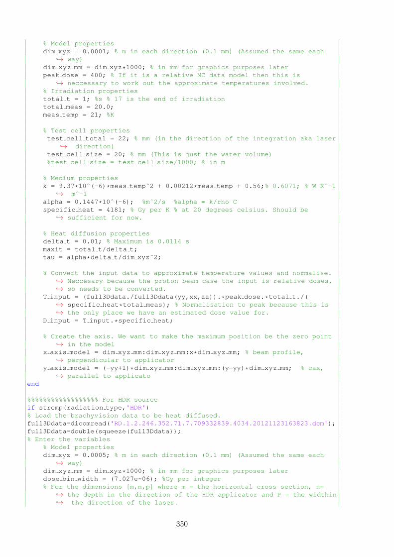
% Model propertiesdim xyz = 0.0001; % m in each direction (0.1 mm) (Assumed the same each
↪→ way)dim xyz mm = dim xyz*1000; % in mm for graphics purposes laterpeak dose = 400; % If it is a relative MC data model then this is
↪→ neccessary to work out the approximate temperatures involved.% Irradiation propertiestotal t = 1; %s % 17 is the end of irradiationtotal meas = 20.0;meas temp = 21; %K
% Test cell propertiestest cell total = 22; % mm (in the direction of the integration aka laser
↪→ direction)test cell size = 20; % mm (This is just the water volume)%test cell size = test cell size/1000; % in m
% Medium propertiesk = 9.37*10ˆ(-6)*meas tempˆ2 + 0.00212*meas temp + 0.56;% 0.6071; % W Kˆ-1
↪→ mˆ-1alpha = 0.1447*10ˆ(-6); %mˆ2/s %alpha = k/rho Cspecific heat = 4181; % Gy per K % at 20 degrees celsius. Should be
↪→ sufficient for now.
% Heat diffusion propertiesdelta t = 0.01; % Maximum is 0.0114 smaxit = total t/delta t;tau = alpha*delta t/dim xyzˆ2;
% Convert the input data to approximate temperature values and normalise.↪→ Neccesary because the proton beam case the input is relative doses,↪→ so needs to be converted.
T input = (full3Ddata./full3Ddata(yy,xx,zz)).*peak dose.*total t./(↪→ specific heat*total meas); % Normalisation to peak because this is↪→ the only place we have an estimated dose value for.
D input = T input.*specific heat;
% Create the axis. We want to make the maximum position be the zero point↪→ in the model
x axis model = dim xyz mm:dim xyz mm:x*dim xyz mm; % beam profile,↪→ perpendicular to applicator
y axis model = (-yy+1)*dim xyz mm:dim xyz mm:(y-yy)*dim xyz mm; % cax,↪→ parallel to applicato
end
%%%%%%%%%%%%%%%%%% For HDR sourceif strcmp(radiation type,'HDR')% Load the brachyvision data to be heat diffused.full3Ddata=dicomread('RD.1.2.246.352.71.7.709332839.4034.20121123163823.dcm');full3Ddata=double(squeeze(full3Ddata));% Enter the variables
% Model propertiesdim xyz = 0.0005; % m in each direction (0.1 mm) (Assumed the same each
↪→ way)dim xyz mm = dim xyz*1000; % in mm for graphics purposes laterdose bin width = (7.027e-06); %Gy per integer% For the dimensions [m,n,p] where m = the horizontal cross section, n=
↪→ the depth in the direction of the HDR applicator and P = the widthin↪→ the direction of the laser.
350
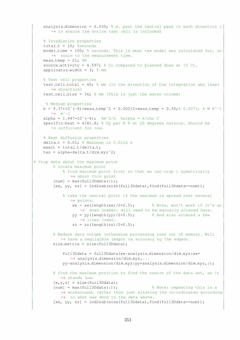
analysis dimension = 0.030; % m. past the central peak in each direction (↪→ to ensure the entire test cell is included)
% Irradiation propertiestotal t = 10; %secondsmodel time = 100; % seconds. This is what the model was calculated for, so
↪→ scale to the measurement time.meas temp = 21; %Ksource activity = 4.597; % Ci compared to planned dose at 10 Ci.applicator width = 3; % mm
% Test cell propertiestest cell total = 40; % mm (in the direction of the integration aka laser
↪→ direction)test cell size = 36; % mm (This is just the water volume)
% Medium propertiesk = 9.37*10ˆ(-6)*meas tempˆ2 + 0.00212*meas temp + 0.56;% 0.6071; % W Kˆ-1
↪→ mˆ-1alpha = 1.447*10ˆ(-6); %mˆ2/s %alpha = k/rho Cspecific heat = 4181.8; % Gy per K % at 20 degrees celsius. Should be
↪→ sufficient for now.
% Heat diffusion propertiesdelta t = 0.01; % Maximum is 0.0114 smaxit = total t/delta t;tau = alpha*delta t/dim xyzˆ2;
% Crop data about the maximum point% locate maximum point
% find maximum point first so that we can crop i symetrically↪→ about this point
[num] = max(full3Ddata(:));[xx, yy, zz] = ind2sub(size(full3Ddata),find(full3Ddata==num));
% take the central point if the maximum is spread over several↪→ points.xx = xx(length(xx)/2+0.5); % Note, won't work if it's an
↪→ even number, will need to be manually altered here.yy = yy(length(yy)/2+0.5); % And also altered a few
↪→ lines lower.zz = zz(length(zz)/2+0.5);
% Reduce data volume (otherwise processing runs out of memory. Will↪→ have a negligible imapct on accuracy by the edges).
size matrix = size(full3Ddata);
full3Ddata = full3Ddata(xx-analysis dimension/dim xyz:xx+↪→ analysis dimension/dim xyz,...
yy-analysis dimension/dim xyz:yy+analysis dimension/dim xyz,:);
% find the maximum position to find the centre of the data set, as it↪→ stands now.
[x,y,z] = size(full3Ddata);[num] = max(full3Ddata(:)); % Note: repeating this is a
↪→ workaround, rather than just altering the co-ordinates according↪→ to what was done to the data above.
[xx, yy, zz] = ind2sub(size(full3Ddata),find(full3Ddata==num));
351
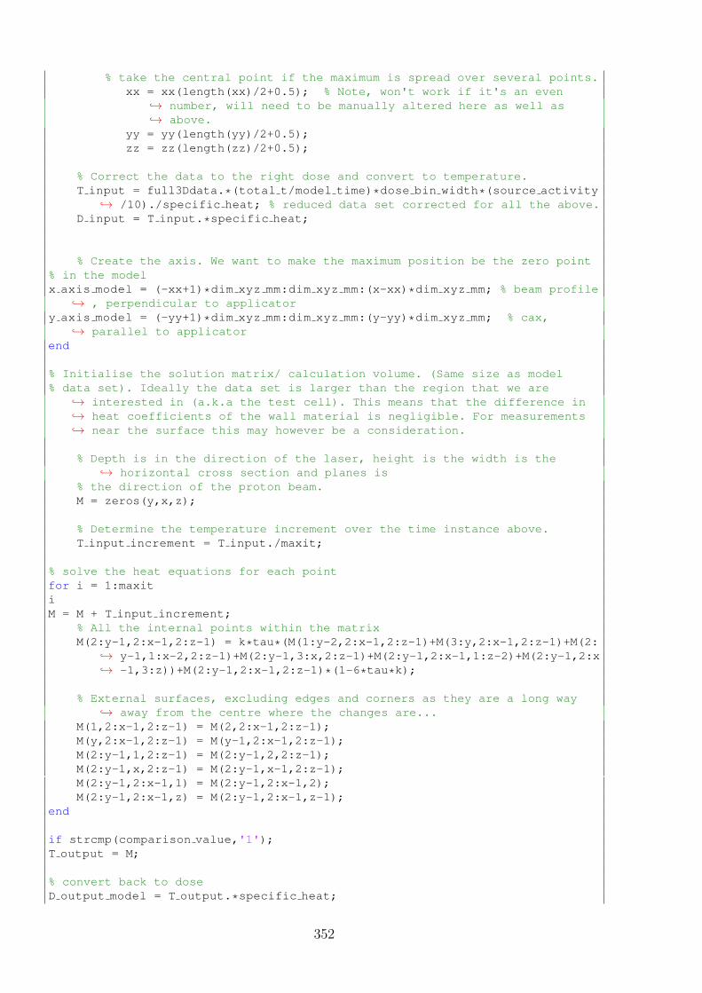
% take the central point if the maximum is spread over several points.xx = xx(length(xx)/2+0.5); % Note, won't work if it's an even
↪→ number, will need to be manually altered here as well as↪→ above.
yy = yy(length(yy)/2+0.5);zz = zz(length(zz)/2+0.5);
% Correct the data to the right dose and convert to temperature.T input = full3Ddata.*(total t/model time)*dose bin width*(source activity
↪→ /10)./specific heat; % reduced data set corrected for all the above.D input = T input.*specific heat;
% Create the axis. We want to make the maximum position be the zero point% in the modelx axis model = (-xx+1)*dim xyz mm:dim xyz mm:(x-xx)*dim xyz mm; % beam profile
↪→ , perpendicular to applicatory axis model = (-yy+1)*dim xyz mm:dim xyz mm:(y-yy)*dim xyz mm; % cax,
↪→ parallel to applicatorend
% Initialise the solution matrix/ calculation volume. (Same size as model% data set). Ideally the data set is larger than the region that we are
↪→ interested in (a.k.a the test cell). This means that the difference in↪→ heat coefficients of the wall material is negligible. For measurements↪→ near the surface this may however be a consideration.
% Depth is in the direction of the laser, height is the width is the↪→ horizontal cross section and planes is
% the direction of the proton beam.M = zeros(y,x,z);
% Determine the temperature increment over the time instance above.T input increment = T input./maxit;
% solve the heat equations for each pointfor i = 1:maxitiM = M + T input increment;
% All the internal points within the matrixM(2:y-1,2:x-1,2:z-1) = k*tau*(M(1:y-2,2:x-1,2:z-1)+M(3:y,2:x-1,2:z-1)+M(2:
↪→ y-1,1:x-2,2:z-1)+M(2:y-1,3:x,2:z-1)+M(2:y-1,2:x-1,1:z-2)+M(2:y-1,2:x↪→ -1,3:z))+M(2:y-1,2:x-1,2:z-1)*(1-6*tau*k);
% External surfaces, excluding edges and corners as they are a long way↪→ away from the centre where the changes are...
M(1,2:x-1,2:z-1) = M(2,2:x-1,2:z-1);M(y,2:x-1,2:z-1) = M(y-1,2:x-1,2:z-1);M(2:y-1,1,2:z-1) = M(2:y-1,2,2:z-1);M(2:y-1,x,2:z-1) = M(2:y-1,x-1,2:z-1);M(2:y-1,2:x-1,1) = M(2:y-1,2:x-1,2);M(2:y-1,2:x-1,z) = M(2:y-1,2:x-1,z-1);
end
if strcmp(comparison value,'1');T output = M;
% convert back to doseD output model = T output.*specific heat;
352

% Integrate across the width of the test cell to approximate the expected↪→ measurement result.
D output model integrated1 = sum(D output model(:,:,zz-test cell size/(2*↪→ dim xyz mm):zz+test cell size/(2*dim xyz mm)),3)./(test cell size/(↪→ dim xyz*1000))
353

354
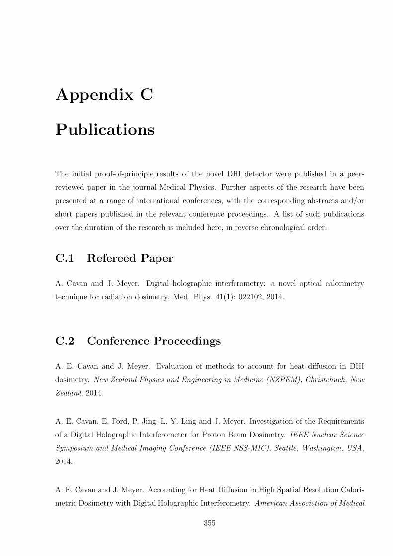
Appendix C
Publications
The initial proof-of-principle results of the novel DHI detector were published in a peer-
reviewed paper in the journal Medical Physics. Further aspects of the research have been
presented at a range of international conferences, with the corresponding abstracts and/or
short papers published in the relevant conference proceedings. A list of such publications
over the duration of the research is included here, in reverse chronological order.
C.1 Refereed Paper
A. Cavan and J. Meyer. Digital holographic interferometry: a novel optical calorimetry
technique for radiation dosimetry. Med. Phys. 41(1): 022102, 2014.
C.2 Conference Proceedings
A. E. Cavan and J. Meyer. Evaluation of methods to account for heat diffusion in DHI
dosimetry. New Zealand Physics and Engineering in Medicine (NZPEM), Christchuch, New
Zealand, 2014.
A. E. Cavan, E. Ford, P. Jing, L. Y. Ling and J. Meyer. Investigation of the Requirements
of a Digital Holographic Interferometer for Proton Beam Dosimetry. IEEE Nuclear Science
Symposium and Medical Imaging Conference (IEEE NSS-MIC), Seattle, Washington, USA,
2014.
A. E. Cavan and J. Meyer. Accounting for Heat Diffusion in High Spatial Resolution Calori-
metric Dosimetry with Digital Holographic Interferometry. American Association of Medical
355
Physics North West Branch Fall Meeting, Seattle, Washington, USA, 2014.
A. E. Cavan and J. Meyer. Digital Holographic Interferometry measurements of high dose
rate applications. American Association of Physicists in Medicine (AAPM) Annual Meet-
ing, Houston, Texas, USA, 2014.
A. E. Cavan and J. Meyer. A novel optical calorimeter applied to proton beam dosimetry.
American Association of Physicists in Medicine (AAPM) Annual Meeting, Indianapolis, In-
diana, USA, 2013.
A. E. Cavan and J. Meyer. A novel optical calorimetry dosimetry approach applied to
an HDR Brachytherapy source. 7th International Conference on 3D Radiation Dosimetry
(IC3DDose), Sydney, Australia, J. Phys.: Conf. Ser. 444:012069, 2013.
A. E. Cavan and J. Meyer. Evaluation of a novel digital holographic interferometer for
dosimetry of high dose rate brachytherapy sources. German Congress of Medical Physics
(DGMP), Cologne, Germany, 2013.
A. E. Cavan and J. Meyer. Digital Holographic Interferometry: Development of an op-
tical calorimetry technique for radiation dosimetry. Engineering and Physical Sciences in
Medicine (EPSM), Brisbane, Australia, 2012.
A. E. Cavan, R. Watts, and J. Meyer. Initial investigation of digital holographic interfer-
ometry as a pseudo-calorimetric dosimetry method for microbeam radiotherapy (MRT). NZ
Institute of Physics Conference, Wellington, New Zealand, 2011.
A. E. Cavan, A. Carlu, and J. Meyer. Pseudo-calorimetric dosimetry for Microbeam Radio-
therapy (MRT) based on optical interference. Engineering and Physical Sciences in Medicine
and the Australian Biomedical Engineering Conference (EPSM ABEC), Melbourne, Aus-
tralia, 2010.
356