an algorithm for detecting cycles in undirected graphs using cuda technology

An Algorithm for Detecting Cycles in Undirected Graphs using

CUDA Technology

Maytham Safar, Fahad Mahdi and Khaled Mahdi

Computer Engineering Department, Kuwait University, Kuwait

Research Administration, Kuwait University, Kuwait

Chemical Engineering Department, Kuwait University, Kuwait

[email protected],[email protected], [email protected]

ABSTRACT

Cycles count in a graph is an NP-complete

problem. This work minimizes the execution

time to solve the problem compared to the

other traditional serial, CPU based one. It

reduces the hardware resources needed to a

single commodity GPU. We developed an

algorithm to approximate counting the

number of cycles in an undirected graph, by

utilizing a modern parallel computing

paradigm called CUDA (Compute Unified

Device Architecture) from nVIDIA, using

the capabilities of the massively parallel

multi-threaded specialized processor called

Graphics Processing Unit (GPU). The

algorithm views the graph from

combinatorial perspective rather than the

traditional adjacency matrix/list view. The

design philosophy of the algorithm shows

that each thread will perform simple

computation procedures in finite loop

iterations to be executed in polynomial time.

The algorithm is divided into two stages, the

first stage is to extract a unique number of

vertices combinations for a given cycle

length using combinatorial formulas, and

then examine whether given combination

can for a cycle or not. The second stage is to

approximate the number of exchanges

(swaps) between vertices for each thread to

check the possibility of cycle existence. An

experiment was conducted to compare the

results between the proposed algorithm and

another distributed serial based algorithm

based on the Donald Johnson backtracking

algorithm.

KEYWORDS

Approximation algorithms, graph cycles,

GPU programming, CUDA parallel

algorithms, multi-threaded applications.

1 INTRODUCTION

Complex networks, such as social,

biochemical or genetic regulatory

networks[1-4] are structures made up of

individuals or organizations or

chemicals(reactants or products) also

referred to as "nodes", which are

connected by one or more types of

interdependency, such as friendship,

common interest, financial exchange or

chemical reaction. A known example of

a complex networks is a social network,

used as a model of a community. The

social network model helps predicting

community behavior; thus leveraging

social network to researchers demands.

[1-2] Numerous applications of complex

networks modeling are found in the

literature; when analyzed, complex

network is a graph composed of vertices

and edges.[4-5].

An essential characteristic of any

network is its resilience to failures or

attacks, or what is known as the

robustness of a network [6]. The

International Journal on New Computer Architectures and Their Applications (IJNCAA) 2(1): 193-212The Society of Digital Information and Wireless Communications, 2012 (ISSN: 2220-9085)

193

definition of a robust network is rather

debatable. One interpretation of a robust

network assumes that links connecting

people together can experience dynamic

changes, as is the case with many

friendship networks such as Facebook,

Hi5. Individuals can delete a friend or

add a new one without constraints. Other

networks have rigid links that are not

allowed to experience changes with time

such in strong family network. Entropy

of a network is proven to be a

quantitative measure of its robustness.

Therefore, the maximization of networks

entropy is equivalent to the optimization

of its robustness [6].

Network robustness is a vital property of

complex networks [6-8]. A dynamic

system is said to be robust if it is

resilient to attacks and random failures.

There are several types of threats that a

robust network must be secured from.

Random vertex removal, an intentional

attack to vertices, a network

fragmentation and any other event that

causes a reduction in the network

information-carrying ability can be

considered as a threat. In [9], they

experimentally found that a scale-free

network shows a good resilience to

random failures. The heterogeneity of

the network degree distribution dictates

the chance of randomly attacking a

crucial vertex. Depending on this

remark, criteria to characterize the

complex networks robustness by

measuring its heterogeneity were

suggested in [6]. They tried to use the

principle of entropy to calculate how

much the network degree distribution is

unbalanced and thus the network

heterogeneity. It was proven also that

unbalanced degree distribution causes in

contrast very low intentional attack

survivability [9].

The Entropy of a dynamic network is the

number of all configurations

(microstates) a network might acquire

constrained by its size, nodes and links

properties. Statistically describing a

network microstate requires defining a

microscopic (local) property of the

network such as the degree of a node,

clusters, cycles or any defined local

property. Based on a previous analysis,

[6-8] the robustness of a network is best

correlated to its ability to deal with

internal feedbacks within the network.

The more feedback loops (cycles) exist

in the network, the more robust the

network is. It follows that a fully

connected network should represent the

most robust networks. Among sets of

robust networks, the most stable robust

network is a network of size seven

because it has the highest cyclic entropy

among all sizes. Such interesting result

motivates us to explore and search other

network topology that has the maximum

cyclic entropy.

The topology of an undirected network

(graph) can be characterized in term of

feedback loops in the network. In other

words, an undirected link connecting

two nodes is a cycle of degree 2.

Extending the definition to three nodes

linked together, known as triad, we

obtain cycle of degree 3, such definition

is a coarse-grain of the former definition,

and lesser systems degree of freedom is

needed for system representation. The

total number of possible configuration

using cycle of degree 2 leads to degree

entropy. The total number of possible

configurations using triads’

representation should lead to triadic

entropy of the network. A more

generalized definition of network

topology is to consider all cycle’s size.

The motivation is the inclusion of all


194

possible feedbacks in the network. The

fact that the sums of all data bits in the

network are conserved can accurately be

represented in a set of cycles than in a

set of links or triads. The total number of

possible topologies using cycles’

representation leads to the introduction

of cyclic entropy, a property of a graph.

The problem of finding cycles in graphs

has been of interest to computer science

researchers lately due to its challenging

time/space complexity. Even though the

exhaustive enumeration technique, used

by smart algorithms proposed in earlier

researches, are restricted to small graphs

as the number of loops grows

exponentially with the size of the graph.

Therefore, it is believed that it is

unlikely to find an exact and efficient

algorithm for counting cycles. Counting

cycles in a graph is an NP-Complete

problem. Therefore, this paper will

present an approximated algorithm that

counts the number of cycles. Our

approximated approach is to design a

parallel algorithm utilizing GPU

capabilities using NVIDIA CUDA [14]

technology.

2 REALTED WORK

The proposed framework in modeling

virtual complex worlds in [21] is using

nodes degree level in the graph that

represent the virtual world, while the

network model was used for the online-

communities in video sharing in [28]

also using the same concept. Our

proposed method is different because we

are using the cycles in the network to

find out its resiliency.

Existing algorithms for counting the

number of cycles in a given graph, are

all utilizing the CPU approach. The

algorithm in [21] starts by running DFS

(Depth First Search) algorithm on a

randomly selected vertex in the graph.

During DFS, when discovering an

adjacent vertex to go deeper in the graph

if this adjacent vertex is gray colored

(i.e. visited before) then this means that

a cycle is discovered. The edge between

the current vertex (i) and the discovered

gray vertex (j) is called a back edge (i,j)

and stored in an array to be used later for

forming the discovered cycles. When

DFS is finished, the algorithm will

perform a loop on the array that stores

the discovered back edges to form the

unique cycles. The cycles will be formed

out of discovered back edges by adding

to the back edge all edges that form a

route from vertex (j) to vertex (i).

The algorithm in [28] is an

approximation algorithm that has proven

its efficiency in estimating large number

of cycles in polynomial time when

applied to real world networks. It is

based on transferring the cycle count

problem into statistical mechanics model

to perform the required calculation. The

algorithm counts the number of cycles in

random, sparse graphs as a function of

their length. Although the algorithm has

proven its efficiency when it comes to

real world networks, the result is not

guaranteed for generic graphs.

The algorithm in [21] is based on

backtracking with the look ahead

technique. It assumes that all vertices are

numbered and starts with vertex s. The

algorithm finds the elementary paths,

which start at s and contain vertices

greater than s. The algorithm repeats this

operation for all vertices in the graph.

The algorithm uses a stack in order to

track visited vertices. The advantage of

this algorithm is that it guarantees

finding an exact solution for the

problem. The time complexity of this


195

algorithm is measured as O

((V+E)(C+1)). Where, V is the number

of vertices, E is the number of edges and

C is the number of cycles. The time

bound of the algorithm depends on the

number of cycles, which grows

exponentially in real life networks.

The algorithm in [28] presented an

algorithm based on cycle vector space

methods. A vector space that contains all

cycles and union of disjoint cycles is

formed using the spanning of the graph.

Then, vector math operations are applied

to find all cycles. This algorithm is slow

since it investigates all vectors and only

a small portion of them could be cycles.

The algorithm in [21] is DFS-XOR

(exclusive OR)based on the fact that

small cycles can be joined together to

form bigger cycle DFS-XOR algorithm

has an advantage over the algorithm in

[28] in the sense that it guarantees the

correctness of the results for all graph

types. The advantage of the DFS-XOR

approximation algorithm over the

algorithm in [21] is that it is more time

efficient when it comes to real life

problems of counting cycles in a graph

because its complexity is not depending

on the factor of number of cycles.

3 GENERTAL OVERVIEW OF GPU

HARDWARE ARCHITECTURE

AND CUDA PARALLEL

PROGRAMMING MODEL

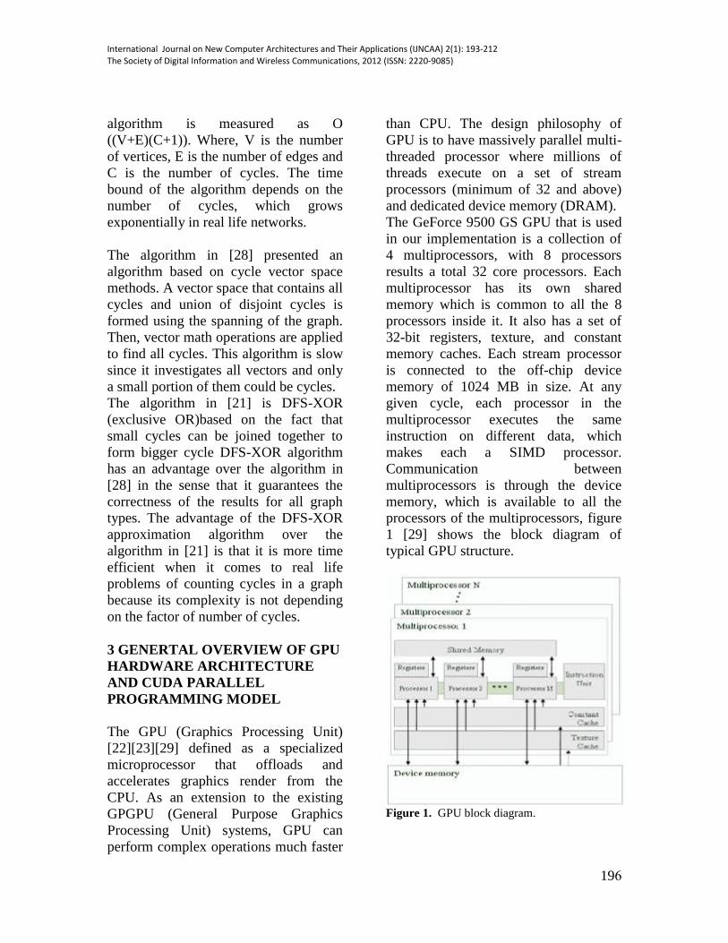
The GPU (Graphics Processing Unit)

[22][23][29] defined as a specialized

microprocessor that offloads and

accelerates graphics render from the

CPU. As an extension to the existing

GPGPU (General Purpose Graphics

Processing Unit) systems, GPU can

perform complex operations much faster

than CPU. The design philosophy of

GPU is to have massively parallel multi-

threaded processor where millions of

threads execute on a set of stream

processors (minimum of 32 and above)

and dedicated device memory (DRAM).

The GeForce 9500 GS GPU that is used

in our implementation is a collection of

4 multiprocessors, with 8 processors

results a total 32 core processors. Each

multiprocessor has its own shared

memory which is common to all the 8

processors inside it. It also has a set of

32-bit registers, texture, and constant

memory caches. Each stream processor

is connected to the off-chip device

memory of 1024 MB in size. At any

given cycle, each processor in the

multiprocessor executes the same

instruction on different data, which

makes each a SIMD processor.

Communication between

multiprocessors is through the device

memory, which is available to all the

processors of the multiprocessors, figure

1 [29] shows the block diagram of

typical GPU structure.

Figure 1. GPU block diagram.


196

CUDA [22][23][25] is an extension to C

based on a few easily-learned

abstractions for parallel programming,

coprocessor offload, and a few

corresponding additions to C syntax.

CUDA represents the coprocessor as a

device that can run a large number of

threads. The threads are managed by

representing parallel tasks as kernels (the

sequence of work to be done in each

thread) mapped over a domain (the set of

threads to be invoked). Kernels are

scalar and represent the work to be done

at a single point in the domain. The

kernel is then invoked as a thread at

every point in the domain. The parallel

threads share memory and synchronize

using barriers. Data is prepared for

processing on the GPU by copying it to

the graphics board's memory. Data

transfer is performed using DMA and

can take place concurrently with kernel

processing. Once written, data on the

GPU is persistent unless it is de-

allocated or overwritten, remaining

available for subsequent kernels.

CUDA [23][29]includes C/C++ software

development tools, function libraries,

and a hardware abstraction mechanism

that hides the GPU hardware from

developers. CUDA requires

programmers to write special code for

parallel processing; it doesn’t require

them to explicitly manage threads in the

conventional sense, which greatly

simplifies the programming model.

CUDA development tools work

alongside a conventional C/C++

compiler, so programmers can mix GPU

code with general-purpose code for the

host CPU. For now, CUDA aims at data-

intensive applications that need single-

precision floating-point math (mostly

scientific, engineering, and high-

performance computing, as well as

consumer photo and video editing).

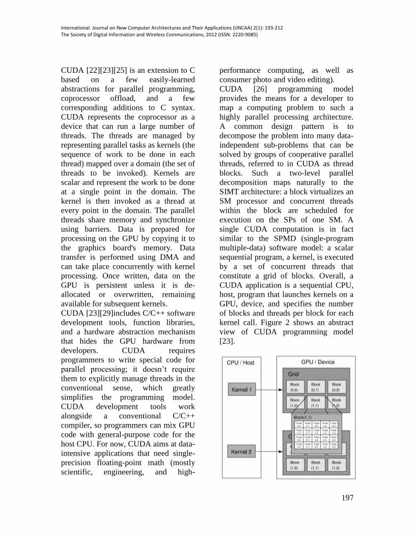
CUDA [26] programming model

provides the means for a developer to

map a computing problem to such a

highly parallel processing architecture.

A common design pattern is to

decompose the problem into many data-

independent sub-problems that can be

solved by groups of cooperative parallel

threads, referred to in CUDA as thread

blocks. Such a two-level parallel

decomposition maps naturally to the

SIMT architecture: a block virtualizes an

SM processor and concurrent threads

within the block are scheduled for

execution on the SPs of one SM. A

single CUDA computation is in fact

similar to the SPMD (single-program

multiple-data) software model: a scalar

sequential program, a kernel, is executed

by a set of concurrent threads that

constitute a grid of blocks. Overall, a

CUDA application is a sequential CPU,

host, program that launches kernels on a

GPU, device, and specifies the number

of blocks and threads per block for each

kernel call. Figure 2 shows an abstract

view of CUDA programming model

[23].


197

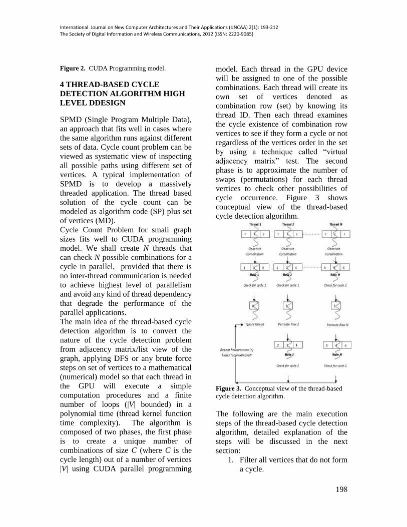
Figure 2. CUDA Programming model.

4 THREAD-BASED CYCLE

DETECTION ALGORITHM HIGH

LEVEL DDESIGN

SPMD (Single Program Multiple Data),

an approach that fits well in cases where

the same algorithm runs against different

sets of data. Cycle count problem can be

viewed as systematic view of inspecting

all possible paths using different set of

vertices. A typical implementation of

SPMD is to develop a massively

threaded application. The thread based

solution of the cycle count can be

modeled as algorithm code (SP) plus set

of vertices (MD).

Cycle Count Problem for small graph

sizes fits well to CUDA programming

model. We shall create N threads that

can check N possible combinations for a

cycle in parallel, provided that there is

no inter-thread communication is needed

to achieve highest level of parallelism

and avoid any kind of thread dependency

that degrade the performance of the

parallel applications.

The main idea of the thread-based cycle

detection algorithm is to convert the

nature of the cycle detection problem

from adjacency matrix/list view of the

graph, applying DFS or any brute force

steps on set of vertices to a mathematical

(numerical) model so that each thread in

the GPU will execute a simple

computation procedures and a finite

number of loops (|V| bounded) in a

polynomial time (thread kernel function

time complexity). The algorithm is

composed of two phases, the first phase

is to create a unique number of

combinations of size C (where C is the

cycle length) out of a number of vertices

|V| using CUDA parallel programming

model. Each thread in the GPU device

will be assigned to one of the possible

combinations. Each thread will create its

own set of vertices denoted as

combination row (set) by knowing its

thread ID. Then each thread examines

the cycle existence of combination row

vertices to see if they form a cycle or not

regardless of the vertices order in the set

by using a technique called “virtual

adjacency matrix” test. The second

phase is to approximate the number of

swaps (permutations) for each thread

vertices to check other possibilities of

cycle occurrence. Figure 3 shows

conceptual view of the thread-based

cycle detection algorithm.

Figure 3. Conceptual view of the thread-based

cycle detection algorithm.

The following are the main execution

steps of the thread-based cycle detection

algorithm, detailed explanation of the

steps will be discussed in the next

section:

1. Filter all vertices that do not form

a cycle.


198

2. Create a new set of vertex indices

in the array called V’.

3. For each cycle of length C,

generate unique combination in

parallel.

4. For each generated combination,

check cycle existence.

5. Compute the approximation

factor (n) to be the number of

swaps.

6. For each swapped combination,

check for cycle existence.

7. After each completion of cycle

existence check, decrement (n).

8. Send swapped combinations

from the GPU memory to CPU

memory.

9. Repeat steps (6, 7, 8), until

permutation factor (n) for all

threads equal to 0.

5 THREAD-BASED CYCLE

DETECTION ALGORITHM

DETALIED LEVEL DDESIGN

The following will go through a detailed

explanations of the steps listed in section

4. It gives the description of the

components that build up the entire

thread-based cycle detection algorithm.

5.1 Vertex Filtering

Each Element in the V’ array contains a

vertex that hasa degree greater than (2)

(excluding self loop edge). The major

advantage of filtering “pruning” is to

minimize the number of combinations

(threads) generated (i.e. combinations

that will never form a cycle). Since there

are some vertices that do not satisfy the

cycle existence, this will create wasteful

combinations. For example If |V| = 10,

looking for a cycle of length C=3, then

for all vertices the number of

combinations to be created without

pruning is 240. If we filter the vertices

having degree greater than (2);let us say

that 3 vertices have degree less than (2),

then |V`| = 7 (3 out of 10 vertices will be

eliminated from being used to generate

combinations), then we have to create 35

combinations, results of saving 205

unnecessary combinations.

5.2 Vertex Re-indexing

Vertices will be labeled by their index in

V’ array rather than their value in V, for

instance If V=2 It will be represented as

0 in V’.To retrieve the original set of

vertices if the set of combinations of V’

arrayforms a cycle,we do a simple re-

mapping procedure. For example, if the

combination (0, 1, 2, 0) forms a cycle in

V’ array, thenit will be resolved to (2, 3,

4, 2) in V array. The main reason for

vertex re-indexing is to allow each

thread to generate its own set of

combinations correctly, because the

combination generation mechanism is

relying on an ordered sequenced set of

numbers.

5.3 Parallel Combination Generator

Given |V|, where V is the graph size in

terms of the number of vertices, for

example if V = {1, 2, 3, 4… 10}, then |V|

=10. Given |Pos| where Pos is the index

of Vertex Position to be placed in the

cycle length, for a cycle of length C,

then |Pos| = C , we to have to place

vertices in the following order Pos(1),

Pos(2), Pos(3),….. Pos (C). For example

V={1,2,3,4,5,6}, take a cycle of length 4

(2-4-5-6) Then, at Pos(1) will have 2, at

Pos(2) will have 4, at Pos(3) will have 5

and at Pos(4) will have 6.


199

Knowing the first position vertex value

of the combination will allow us to know

the remaining positions,since the set of

vertices that form a given combination

are sorted, we can guarantee that at

position[i] the value must be at least

value of position [i-1] + 1. There is a

strong relationship between the row id of

the combination and the vertex value of

the first position.

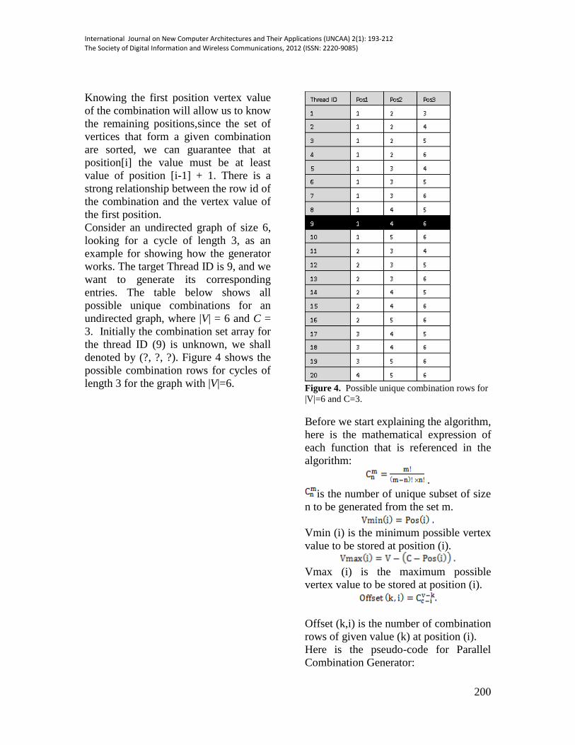
Consider an undirected graph of size 6,

looking for a cycle of length 3, as an

example for showing how the generator

works. The target Thread ID is 9, and we

want to generate its corresponding

entries. The table below shows all

possible unique combinations for an

undirected graph, where |V| = 6 and C =

3. Initially the combination set array for

the thread ID (9) is unknown, we shall

denoted by (?, ?, ?). Figure 4 shows the

possible combination rows for cycles of

length 3 for the graph with |V|=6.

Figure 4. Possible unique combination rows for

|V|=6 and C=3.

Before we start explaining the algorithm,

here is the mathematical expression of

each function that is referenced in the

algorithm:

.

is the number of unique subset of size

n to be generated from the set m.

Vmin (i) is the minimum possible vertex

value to be stored at position (i).

Vmax (i) is the maximum possible

vertex value to be stored at position (i).

Offset (k,i) is the number of combination

rows of given value (k) at position (i).

Here is the pseudo-code for Parallel

Combination Generator:


200

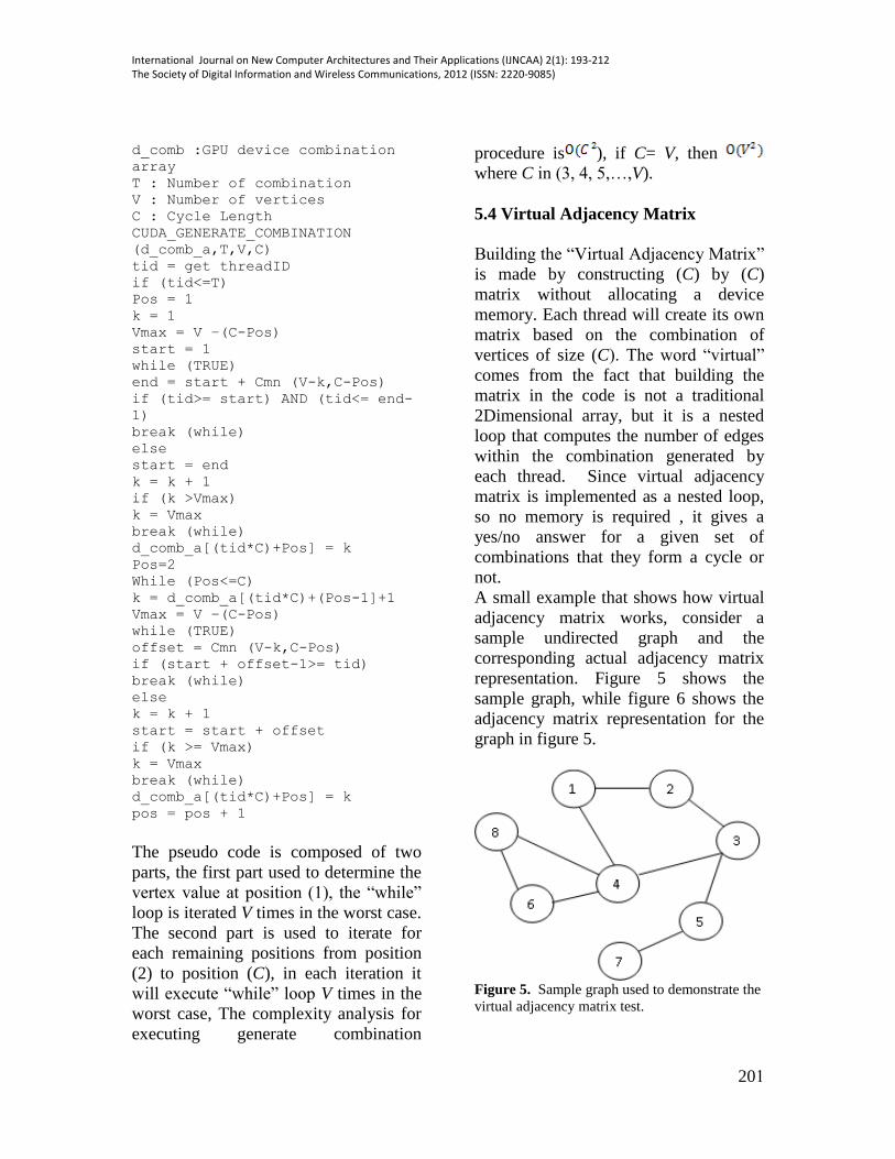
d_comb :GPU device combination

array

T : Number of combination

V : Number of vertices

C : Cycle Length

CUDA_GENERATE_COMBINATION

(d_comb_a,T,V,C)

tid = get threadID

if (tid<=T)

Pos = 1

k = 1

Vmax = V –(C-Pos)

start = 1

while (TRUE)

end = start + Cmn (V-k,C-Pos)

if (tid>= start) AND (tid<= end-

1)

break (while)

else

start = end

k = k + 1

if (k >Vmax)

k = Vmax

break (while)

d_comb_a[(tid*C)+Pos] = k

Pos=2

While (Pos<=C)

k = d_comb_a[(tid*C)+(Pos-1]+1

Vmax = V –(C-Pos)

while (TRUE)

offset = Cmn (V-k,C-Pos)

if (start + offset-1>= tid)

break (while)

else

k = k + 1

start = start + offset

if (k >= Vmax)

k = Vmax

break (while)

d_comb_a[(tid*C)+Pos] = k

pos = pos + 1

The pseudo code is composed of two

parts, the first part used to determine the

vertex value at position (1), the “while”

loop is iterated V times in the worst case.

The second part is used to iterate for

each remaining positions from position

(2) to position (C), in each iteration it

will execute “while” loop V times in the

worst case, The complexity analysis for

executing generate combination

procedure is ), if C= V, then

where C in (3, 4, 5,…,V).

5.4 Virtual Adjacency Matrix

Building the “Virtual Adjacency Matrix”

is made by constructing (C) by (C)

matrix without allocating a device

memory. Each thread will create its own

matrix based on the combination of

vertices of size (C). The word “virtual”

comes from the fact that building the

matrix in the code is not a traditional

2Dimensional array, but it is a nested

loop that computes the number of edges

within the combination generated by

each thread. Since virtual adjacency

matrix is implemented as a nested loop,

so no memory is required , it gives a

yes/no answer for a given set of

combinations that they form a cycle or

not.

A small example that shows how virtual

adjacency matrix works, consider a

sample undirected graph and the

corresponding actual adjacency matrix

representation. Figure 5 shows the

sample graph, while figure 6 shows the

adjacency matrix representation for the

graph in figure 5.

Figure 5. Sample graph used to demonstrate the

virtual adjacency matrix test.


201

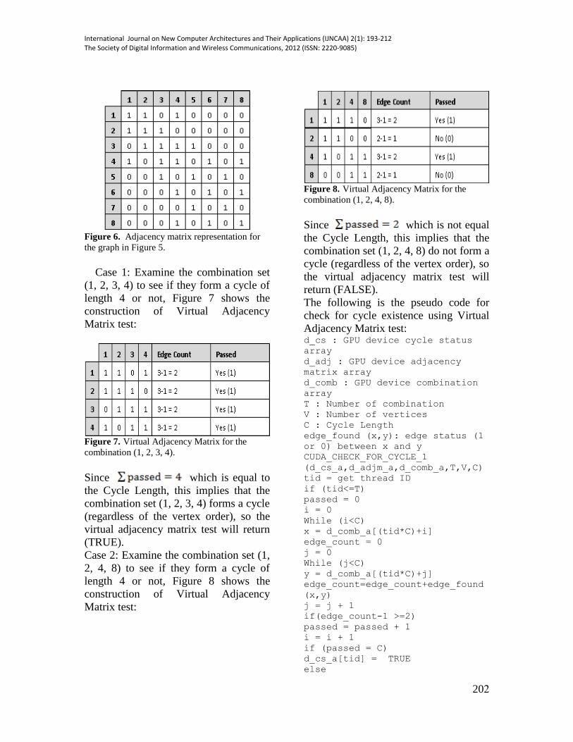
Figure 6. Adjacency matrix representation for

the graph in Figure 5.

Case 1: Examine the combination set

(1, 2, 3, 4) to see if they form a cycle of

length 4 or not, Figure 7 shows the

construction of Virtual Adjacency

Matrix test:

Figure 7. Virtual Adjacency Matrix for the

combination (1, 2, 3, 4).

Since which is equal to

the Cycle Length, this implies that the

combination set (1, 2, 3, 4) forms a cycle

(regardless of the vertex order), so the

virtual adjacency matrix test will return

(TRUE).

Case 2: Examine the combination set (1,

2, 4, 8) to see if they form a cycle of

length 4 or not, Figure 8 shows the

construction of Virtual Adjacency

Matrix test:

Figure 8. Virtual Adjacency Matrix for the

combination (1, 2, 4, 8).

Since which is not equal

the Cycle Length, this implies that the

combination set (1, 2, 4, 8) do not form a

cycle (regardless of the vertex order), so

the virtual adjacency matrix test will

return (FALSE).

The following is the pseudo code for

check for cycle existence using Virtual

Adjacency Matrix test: d_cs : GPU device cycle status

array

d_adj : GPU device adjacency

matrix array

d_comb : GPU device combination

array



C : Cycle Length

edge_found (x,y): edge status (1

or 0) between x and y

CUDA_CHECK_FOR_CYCLE_1

(d_cs_a,d_adjm_a,d_comb_a,T,V,C)

tid = get thread ID

if (tid<=T)

passed = 0

i = 0

While (i<C)

x = d_comb_a[(tid*C)+i]

edge_count = 0

j = 0

While (j<C)

y = d_comb_a[(tid*C)+j]

edge_count=edge_count+edge_found

(x,y)

j = j + 1

if(edge_count-1 >=2)

passed = passed + 1

i = i + 1

if (passed = C)

d_cs_a[tid] = TRUE

else


202

d_cs_a[tid] = FALSE

The time complexity analysis for

executing the virtual adjacency matrix

test operation is O ( ), if C= V, O ( )

then where C in (3, 4, 5…, V).

5.5 Check for Cycle Using Linear

Scan of Edge Count

Once each combination generated passed

the virtual adjacency test with (TRUE), a

second, detailed cycle detection

algorithm will be applied to check if the

ordered set of vertices can generate a

cycle or not. Because the virtual

adjacency matrix test will not tell us

what is the exact combination that

generates a cycle. The edge count

algorithm addresses this issue. The

algorithm does a simple nested linear

scan for the set of vertices. This

algorithm needs temporary array that is

assigned to each thread independently

called vertex cover of size (C). Initially a

vertex cover array is initialized to false.

A scan pointer starts from the vertex

indexed as current passed from the CPU,

current vertex will examine its nearest

neighborhood to check for an edge

connectivity provided that this neighbor

is not covered yet, if there is an edge,

then a counter called “edge counter” is

incremented and flag entry is set to

(TRUE) in the covered array for that

neighbor vertex is set to true, then

setting the newly connected vertex as

current. Restart from the first element in

the combination array and repeat the

procedure again. Keep scanning until the

end of the combination array. A cycle

exists for the set of vertices if the edge

counter is equal to the cycle length,

otherwise no cycle is formed.

The following is the pseudo code to

check for cycle existence using linear

scan of edge count:

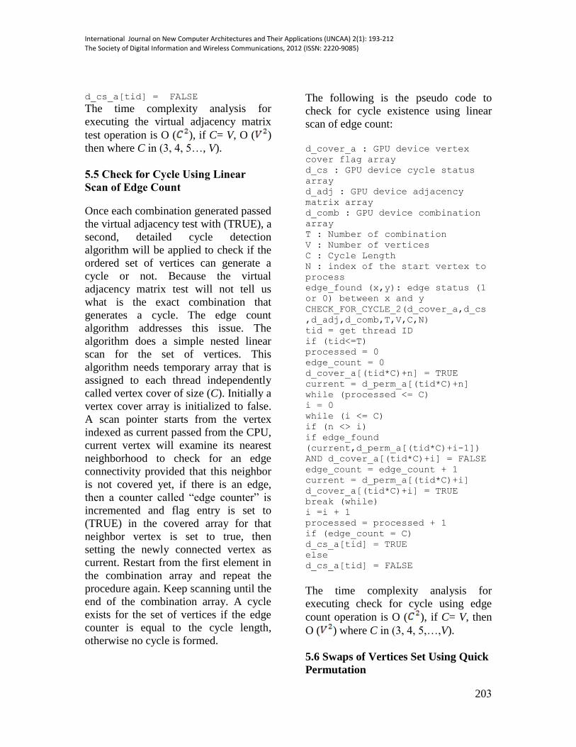
d_cover_a : GPU device vertex

cover flag array

d_cs : GPU device cycle status

array

d_adj : GPU device adjacency

matrix array

d_comb : GPU device combination

array



C : Cycle Length

N : index of the start vertex to

process

edge_found (x,y): edge status (1

or 0) between x and y

CHECK_FOR_CYCLE_2(d_cover_a,d_cs

,d_adj,d_comb,T,V,C,N)

tid = get thread ID

if (tid<=T)

processed = 0

edge_count = 0

d_cover_a[(tid*C)+n] = TRUE

current = d_perm_a[(tid*C)+n]

while (processed <= C)

i = 0

while (i <= C)

if (n <> i)

if edge_found

(current,d_perm_a[(tid*C)+i-1])

AND d_cover_a[(tid*C)+i] = FALSE

edge_count = edge_count + 1

current = d_perm_a[(tid*C)+i]

d_cover_a[(tid*C)+i] = TRUE

break (while)

i =i + 1

processed = processed + 1

if (edge_count = C)

d_cs_a[tid] = TRUE

else

d_cs_a[tid] = FALSE


executing check for cycle using edge

count operation is O ( ), if C= V, then

O ( ) where C in (3, 4, 5,…,V).

5.6 Swaps of Vertices Set Using Quick

Permutation


203

We have modified an existing

permutation of array algorithm called

“Quick Permutation reversals on the tail

of a linear array without using recursion”

[27]. The original algorithm works on

sequential behavior on the CPU; we

have adopted it to a parallel version that

can run on the GPU.

The following is the pseudo code for the

modified version of the quick

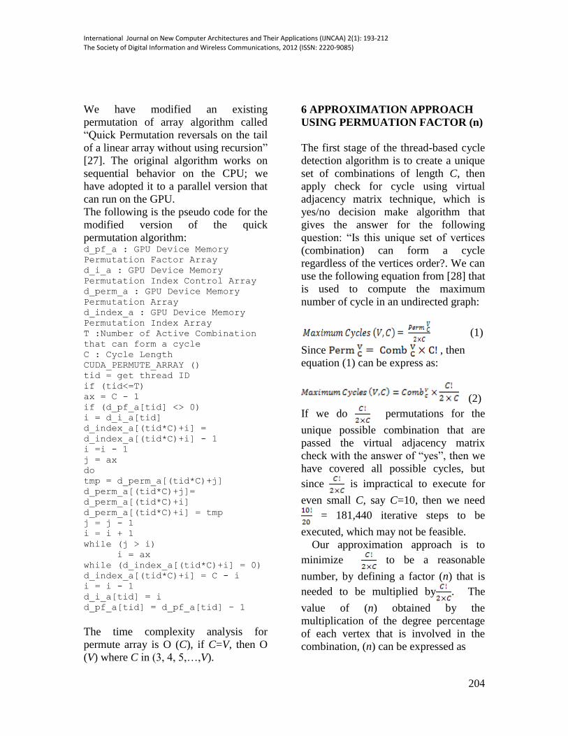
permutation algorithm: d_pf_a : GPU Device Memory

Permutation Factor Array

d_i_a : GPU Device Memory

Permutation Index Control Array

d_perm_a : GPU Device Memory

Permutation Array

d_index_a : GPU Device Memory

Permutation Index Array

T :Number of Active Combination

that can form a cycle

C : Cycle Length

CUDA_PERMUTE_ARRAY ()

tid = get thread ID

if (tid<=T)

ax = C - 1

if (d_pf_a[tid] <> 0)

i = d_i_a[tid]

d_index_a[(tid*C)+i] =

d_index_a[(tid*C)+i] - 1

i =i - 1

j = ax

do

tmp = d_perm_a[(tid*C)+j]

d_perm_a[(tid*C)+j]=

d_perm_a[(tid*C)+i]

d_perm_a[(tid*C)+i] = tmp

j = j - 1

i = i + 1

while (j > i)

i = ax

while (d_index_a[(tid*C)+i] = 0)

d_index_a[(tid*C)+i] = C - i

i = i - 1

d_i_a[tid] = i

d_pf_a[tid] = d_pf_a[tid] – 1


permute array is O (C), if C=V, then O

(V) where C in (3, 4, 5,…,V).

6 APPROXIMATION APPROACH

USING PERMUATION FACTOR (n)

The first stage of the thread-based cycle

detection algorithm is to create a unique

set of combinations of length C, then

apply check for cycle using virtual

adjacency matrix technique, which is

yes/no decision make algorithm that

gives the answer for the following

question: “Is this unique set of vertices

(combination) can form a cycle

regardless of the vertices order?. We can

use the following equation from [28] that

is used to compute the maximum

number of cycle in an undirected graph:

(1)

Since , then

equation (1) can be express as:

(2)

If we do permutations for the

unique possible combination that are

passed the virtual adjacency matrix

check with the answer of “yes”, then we

have covered all possible cycles, but

since is impractical to execute for

even small C, say C=10, then we need

= 181,440 iterative steps to be

executed, which may not be feasible.

Our approximation approach is to

minimize to be a reasonable

number, by defining a factor (n) that is

needed to be multiplied by . The

value of (n) obtained by the

multiplication of the degree percentage

of each vertex that is involved in the

combination, (n) can be expressed as


204

) (3)

The value of (n) will become very small

(close to zero) if the percentage degree

of each vertex is low, which means that

the set of vertices are poorly connected

and they have small chances to

constitute a cycle. For example if want

to do a permutation for a cycle of length

5 with a total degree of 40, the following

set of vertices (v1, v2, v3, v4, v5) have

the degrees (2, 2, 3, 3, 4), respectively. If

we use the equation in (3) then:

If we multiply 0.35 by will get n = 4,

rather than getting 12 (total

Permutations)

The value of n will become very large

(close to one) if the percentage degree of

each vertex is high, which means that the

set of vertices are strongly connected

and they have big chances to constitute a

cycle. For example if want to do a

permutation for a cycle of length 5 with

a total degree of 40, the following set of

vertices (v1, v2, v3, v4, v5) have the

degrees (9, 8, 7, 6, 6) respectively. If use

the equation in (3) then:

If we multiply 0.9 by will get n = 11,

rather than getting 12 (total

Permutations). As a result, based on the

connectivity behavior of the vertices

either strongly or poorly connected will

influence on value the permutation

factor (n).

Retrieving the value of (n) for each

possible cycle length, will create an

iteration control to determine when to

stop permuting.

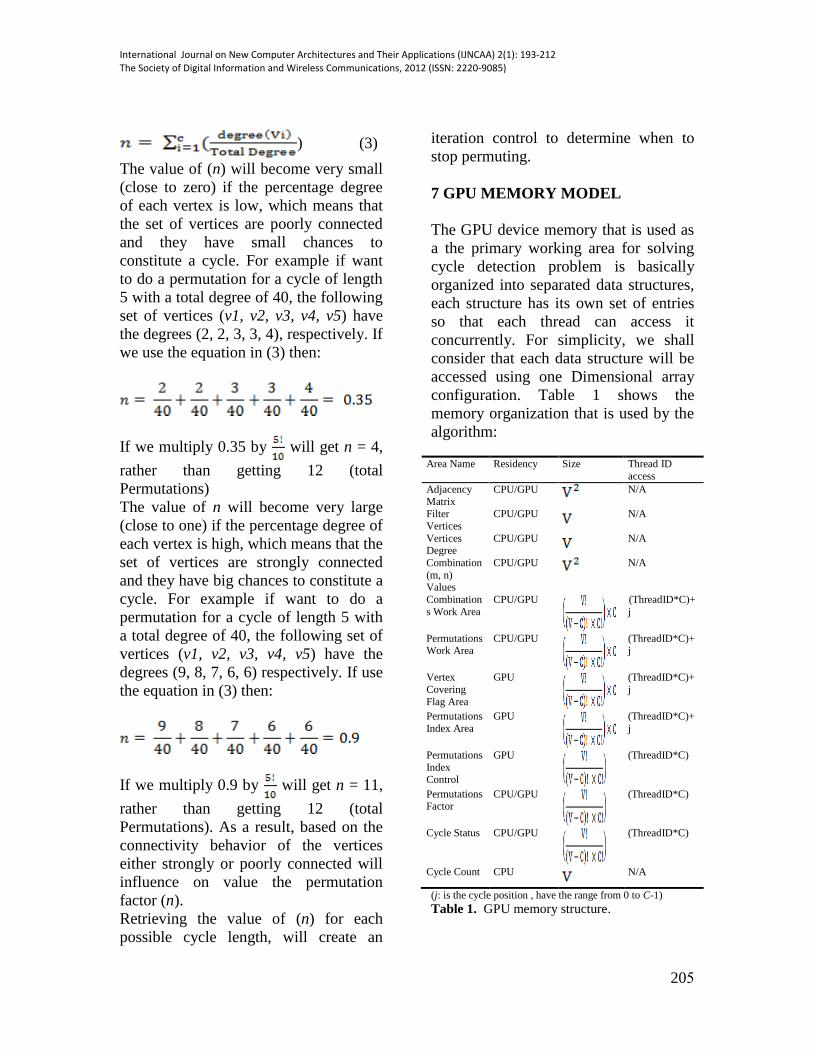
7 GPU MEMORY MODEL

The GPU device memory that is used as

a the primary working area for solving

cycle detection problem is basically

organized into separated data structures,

each structure has its own set of entries

so that each thread can access it

concurrently. For simplicity, we shall

consider that each data structure will be

accessed using one Dimensional array

configuration. Table 1 shows the

memory organization that is used by the

algorithm:

Area Name Residency Size Thread ID

access

Adjacency

Matrix

CPU/GPU

N/A

Filter

Vertices

CPU/GPU

N/A

Vertices Degree

CPU/GPU

N/A

Combination

(m, n) Values

CPU/GPU

N/A

Combination

s Work Area

CPU/GPU

(ThreadID*C)+

j

Permutations Work Area

CPU/GPU

(ThreadID*C)+ j

Vertex

Covering

Flag Area

GPU

(ThreadID*C)+

j

Permutations

Index Area

GPU

(ThreadID*C)+

j

Permutations

Index

Control

GPU

(ThreadID*C)

Permutations Factor

CPU/GPU

(ThreadID*C)

Cycle Status CPU/GPU

(ThreadID*C)

Cycle Count CPU

N/A

(j: is the cycle position , have the range from 0 to C-1)

Table 1. GPU memory structure.


205

Adjacency Matrix is used to store the

edge status between the vertices in

the graph; it is primarily used by the

function: edge_found.

Filter Vertices is an array of a size

less than or equal to the total vertices

count in the graph, the entries in this

array contains the vertices that have

degree of (2) and above.

Vertices Degree is an array used to

store the total degree value for each

vertex.

Combination (m, n) Values is an

array used to store the computed

value of the combination equation

rather than being computed every

time a thread needs to compute the

Combination of (m, n).

Combinations Work Area is the

primary array to be used to store the

generated combination by each

thread. Generate combination

procedure used this array for writing

generated vertices.

Permutations Work Area

Permutation work area is used to

hold temporary vertices values to be

used for generating the permutation

using the quick algorithm in

[27].Since the GPU programming

environment does not support

recursion, so we cannot use the

recursive version of any permutation

algorithm, and therefore we have to

replace it with the iterative counter-

part.

Permutations Index Control is

temporary array used by generate

permutation procedure.

Vertex Covering Flag Area is a

temporary array used by check for

cycle existence using linear scan.

Permutations Factor is a thread

based array used to store the

approximation factor (n) for each

thread.

Cycle Status is a thread based array

used to store the cycle existence

result for every thread that have

either combination or permutation

set of vertices.

Cycle Count is cycle length based

array used to accumulate the total

cycles detected by each thread.

Generally, the GPU memory accessed

either by each thread individually, where

the memory location element is the

thread ID this can be seen on Cycle

Status array (cs_a).The other way is to

indicate the vertex position in the

generated/permuted set of vertices, so

that the memory accessed is combined

between the thread ID and vertex

position index. This can be seen on

Combination Working Area array

(d_comb_a).

The total memory storage of all these

data structures should not exceed the

maximum memory amount the GPU

device can handle, for solving a specific

cycle length at a time. For example in a

graph size of length 10 we shall reuse

the device memory iteratively by

interchanging the memory allocation and

de-allocation for each cycle length, so

for a cycle of length 3 we shall allocated

the memory using the formulas above to

apply the algorithm, then for a length of

4, we de-allocate the previous memory

usage of the and reallocated again and

so. We use this technique for optimizing

the memory usages as the memory

device is fully dedicated to solve the

cycle detection of length C at a given

time.

8 CONIDERARTIONS RELATED

TO THE THREAD-BASED CYCLE


206

DETECTION ALGORTIHM

DESIGN

Since we are porting the parallelism of

the threads from the traditional CPU

programming to the GPU, there are

some important considerations that must

be reviewed first before starting the

implementation of the thread-based

cycle detection algorithm. These

considerations are related to the design

limitation of the GPU and the

mechanism that it works.

8.1 Maximum Numbers of

Combinations to Be Generated

Constraint

The maximum number of combinations

to be generated for a cycle of length C

should not exceed the maximum number

of threads supported by CUDA which is

according to nVIDIA specifications,

as far as the number of possible

combinations is less than we can

execute the combinations in parallel. But

once the numbers of combinations

exceed , then we need to breakdown

the combinations into batches of

combinations. In this case, every

combinations shall execute in a parallel,

passing the results of these combinations

to the CPU and start with the next

combinations and so on. For example, if

the possible combinations are

approximately , then we have execute

(=512) batches of

combinations by CPU iteratively. In our

experiment, the largest combinations

size was when C=13 for a graph of size

26, which is approximately equal to

, so we are in the safe margin. As long as

the number of combinations is less than

the maximum number of threads

supported by CUDA ( ) or the number

of combinations can be approximately

to be expressed as ( multiplied by a

factor (x), and that (x) can be a

reasonable number, then the approach to

solve the problem is still feasible,

otherwise it may be not.

8.2 Memory Storage Constraint

Since the thread-based cycle detection

algorithm needs a working area for

creating combinations and permutations,

it shows that the dominating factor for

memory consumption is function of (V!)

and (C!). These factors will play a

critical role in the memory usage as the

values of V and C increase. In our

experiment, |V| was 26 and peak cycle

length was 13, if we substitute the

entries in the memory organization table,

a total of 572033754memory locations

needed. If the unit of memory storage is

Byte, then = 546 MB is the total

memory used to solve the problem for

cycle length 13 for a graph of size 26, In

our experiments the GPU device

memory specification was 1024 MB.

Even though we reduce the time for

cycle detection using parallel computing

paradigm, the price to be paid is the

space complexity. It is extremely

difficult to develop an algorithm that can

be both time and space efficient.

8.3 CPU Based Export Procedure for

the Resulting Data to the Secondary

Storage

There is a major performance bottleneck

that appears when the GPU would send

the detected cycles to the storage. The

GPU cannot send directly its memory

content to the storage; it must be first

transferred to the CPU memory. Then a


207

sequential loop on the CPU context

based on the number of detected cycles

will dump the memory content to the

storage. If the detected cycles are large

(millions) then it will degrade the

performance of the entire application.

This is because the GPU will become

idle waiting for the loop to finish.

Because of the serial behavior of the

storage access this constraint cannot be

avoided.

8.4 The Value of Approximation

Factor (n)

The value of (n) plays an influence in the

execution time of the thread-based cycle

detection algorithm .Although the higher

(n) the more accurate results are

obtained, but a practical execution time

is an issue. A moderate value of (n) is an

alternative to be set in order to have a

reasonable execution time. Since the

goal of the thread-based cycle detection

algorithm is to accelerate the

computation procedure for the cycle

count, the accuracy must be traded off.

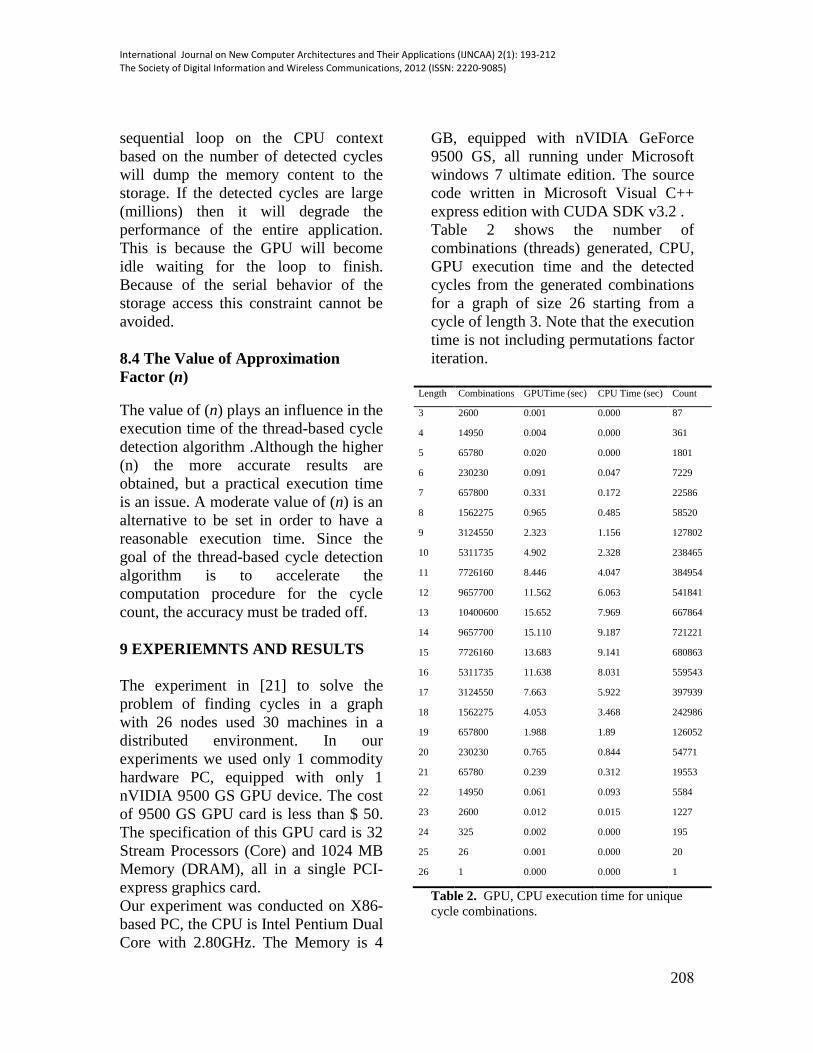
9 EXPERIEMNTS AND RESULTS

The experiment in [21] to solve the

problem of finding cycles in a graph

with 26 nodes used 30 machines in a

distributed environment. In our

experiments we used only 1 commodity

hardware PC, equipped with only 1

nVIDIA 9500 GS GPU device. The cost

of 9500 GS GPU card is less than $ 50.

The specification of this GPU card is 32

Stream Processors (Core) and 1024 MB

Memory (DRAM), all in a single PCI-

express graphics card.

Our experiment was conducted on X86-

based PC, the CPU is Intel Pentium Dual

Core with 2.80GHz. The Memory is 4

GB, equipped with nVIDIA GeForce

9500 GS, all running under Microsoft

windows 7 ultimate edition. The source

code written in Microsoft Visual C++

express edition with CUDA SDK v3.2 .

Table 2 shows the number of

combinations (threads) generated, CPU,

GPU execution time and the detected

cycles from the generated combinations

for a graph of size 26 starting from a

cycle of length 3. Note that the execution

time is not including permutations factor

iteration.

Length Combinations GPUTime (sec) CPU Time (sec) Count

3 2600 0.001 0.000 87

4 14950 0.004 0.000 361

5 65780 0.020 0.000 1801

6 230230 0.091 0.047 7229

7 657800 0.331 0.172 22586

8 1562275 0.965 0.485 58520

9 3124550 2.323 1.156 127802

10 5311735 4.902 2.328 238465

11 7726160 8.446 4.047 384954

12 9657700 11.562 6.063 541841

13 10400600 15.652 7.969 667864

14 9657700 15.110 9.187 721221

15 7726160 13.683 9.141 680863

16 5311735 11.638 8.031 559543

17 3124550 7.663 5.922 397939

18 1562275 4.053 3.468 242986

19 657800 1.988 1.89 126052

20 230230 0.765 0.844 54771

21 65780 0.239 0.312 19553

22 14950 0.061 0.093 5584

23 2600 0.012 0.015 1227

24 325 0.002 0.000 195

25 26 0.001 0.000 20

26 1 0.000 0.000 1

Table 2. GPU, CPU execution time for unique

cycle combinations.


208

The GPU time is the total execution time

to generate combinations kernel function

plus check for cycle existence using

virtual adjacency matrix.

The CPU time is the total execution time

for exporting generated combination

stored in GPU memory to the CPU

Memory and then dumps the memory

content to the secondary storage device.

The main reason behind milliseconds

execution time is that CUDA devices are

designed to work with massively parallel

thread , while in the Table 2 the

maximum execution time was for cycle

of length 13 (Peak Length), since there

around combinations generated for

this cycle length, which is far away than

the maximum number of possible

threads generated by the device.

The next phase of the experiment is to

include the permutation factor (n) for

each cycle length, and do a check for

cycle using edge count for each

generated permutation. For example if

the permutation factor for cycle of length

13 is n, we shall check (n )

possible permutations, where each of

(667,794) iterations are made in parallel.

We used same graph data in the

experiment in [21], and then apply our

experiment for a different set of fixed

approximation factor (n). Table 3 shows

the detected cycles and the

corresponding execution time for the

thread-based cycle detection algorithm.

Approximation Factor Cycles Detected Execution Time

2048 20830044 3.2 Hours

4096 39408671 7 Hours

8192 76635770 18 Hours

Table 3. Detected cycles and execution time for

the approximation solution.

The execution time is the total time used

to generate parallel swaps (permutations)

by a factor of (n) and then check the

cycle existence for each swap that is

executed at the GPU context plus the

total time needed to sum up the total

cycles detected at the CPU context.

The experiment in [21] to find the cycles

in a graph with 26 nodes takes around 16

days. In our experiment we have solved

all the unique possible combination of

each cycle length (this is the first phase

of the experiment) in less than 2 minutes

as show in table 2. Even though in the

approximation approach, where for each

possible combination that form a cycle

we have created (n) swaps (this is the

second phase of the experiment)it did

not last more than 3.2 hours when n =

2048. We can better approximate the

solution with more time needed, but still

less than the time in the original

experiment.

The way of viewing the cycle definition

plays an important decision making in

the solution feasibility. If the assumption

behind solving the problem stated that

any cyclic permutation of existing cycle

combination considered as one cycle (for

instance, cycle 1-2-3-4-1 is the same as -

1-3-2-4-1) then applying the first phase

of the thread-based cycle detection

algorithm (parallel combination

generator) will result a significant

improvement over existing algorithms.

This also achieves time breaker solution

compared with other algorithms. But, if

the assumption stated that cyclic

permutations are considered as

individual ones (for instance cycle 1-2-

3-4-1 is different as 1-3-2-4-1) then

applying approximation approach in the

thread-based cycle detection algorithms

has a time/resources advantage over

other approximation algorithms.


209

9.1 Approximation Accuracy of the

Thread-Based Cycle Detection

Algorithm

Table 4 shows the approximation

accuracy for the number of detected

cycles between the exact solution in the

algorithm specified in [21] and our

thread-based cycle detection algorithm

(approximated) alongside with the

results obtained from table 3 using the

three different approximation parameters

(n). Also within each run of the

approximation factor (n), we have

included the approximated entropy

calculations.

The approximation accuracy measured

using the following equation:

(4)

Approximation Factor Accuracy (%) Entropy

2048 0.147 2.407

4096 0.279 2.391

8192 0.542 2.355

Table 4. Approximation accuracy (%) of the

detected cycles and Entropy calculations for

running three different approximation factors (n)

of the experiment.

Although the approximation values are

quite small, but it can be increased as we

increase the permutation factor (n), since

our main concern in the thread-based

cycle detection algorithm design is

speeding up the computations.

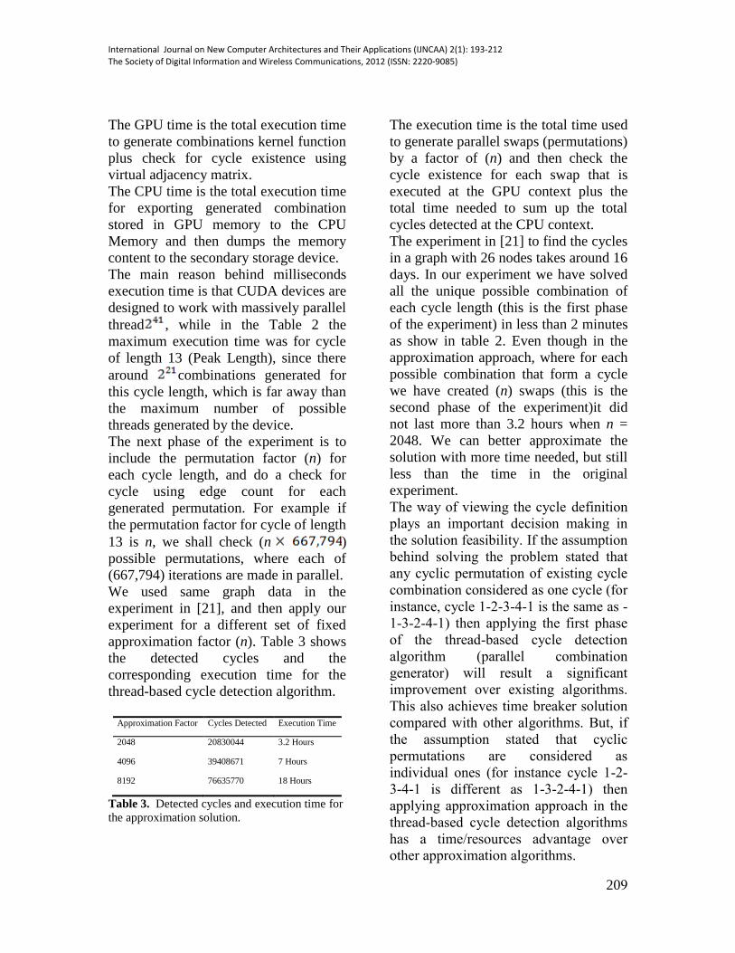
Figure 9 shows the normalized results

for the exact solution of the detected

cycle found in [21] and our

approximated solution using three

different values of the approximation

factor (n).

Figure 9. Normalized Results for the exact and

approximated solution.

10 CONCLUSIONS

Cycle count problem is still NP-

Complete, where no such polynomial

time solution has been found yet. We

have presented a GPU/CUDA thread-

based cycle detection algorithm as

alternative way to accelerate the

computations of the cycle detection.

Since other algorithms utilize the

traditional serial CPU based

implementation, we have utilized

GPU/CUDA computing model, because

it provides a cost effective system to

develop applications that are data-

intensive operations and needs high

degree of parallelism. This is obvious if

we look closely to the general solution

of problem from a systematic way of

exploring the possible occurrence of the

cycles by applying the same core

algorithm to a different set of vertices.

The thread-based cycle detection

algorithm have viewed the problem from

a mathematical perspective using the

equations of combinatorial theory, we

did not use classical graph operations


210

like DFS (Depth First Search) as other

algorithms do. GPU/CUDA fits well for

mathematical operations If we can do

more mathematical analysis of the

problem, we can get better results and

the solution will be more closely to the

actual one.

11 FUTURE WORKS

CUDA provides a lot of techniques and

best practices that can be applied on the

GPU applications to enhance the

performance of the execution time of the

code. Here we have selected two

techniques that are commonly used.

#pragma unroll [29] is a compiler

directive in the loop code. By default,

the compiler unrolls small loops with a

known trip count. The #pragma unroll

directive however can be used to control

unrolling of any given loop. It must be

placed immediately before the loop and

only applies to that loop.

Shared Memory [29], because it is on-

chip, the shared memory space is much

faster than the local and global memory

spaces. In fact, for all threads of a warp,

accessing the shared memory is as fast

as accessing a register as long as there

are no bank conflicts between the

threads.

Memory Coalescing [29] to maximize

global memory bandwidth using the

technique of memory coalesce which

minimizes the number of bus

transactions for memory accesses.

Coalescing provides memory

transactions are per half-warp (16

threads.) In best cases, one transaction

will be issued for a half warp.

Constant Memory [29] the constant

memory is a portion from the Device

global memory that allows read-only

access by the device and provides faster

and more parallel data access paths for

CUDA kernel execution than the global

memory. We can utilize the constant

memory by storing the vertex and edges

relations (adjacency matrix/list

representation of the graph).

Streams and Asynchronous API [29] the

default API behavior of CUDA

programming model that the Kernel

launches are asynchronous function with

CPU. CUDA calls block on GPU is

serialized by the driver. The introduction

of streams objects and asynchronous

functions provide asynchronous

execution with CPU to give the ability to

concurrently execute a kernel and the

function. Stream is sequence of

operations that execute in order on GPU.

Operations from different streams can be

interleaved. The kernel function and

asynchronous API function from

different streams can be overlapped.

Porting the application to 64 bit platform

to support wide range of integer numbers

since CUDA provides a 64-bit SDK

edition. Converting the idle threads the

do not form a cycle to an active threads

which form a cycle, by passing such

combinations to the idle threads in order

to increase the GPU efficiency and

utilization .Finding methods to do more

filtering procedures for vertices that may

not form a cycle, in the current

implementation only filter less than

degree 2 was used. Migrating the CPU

based cycle detect counter by thread

procedure to parallel GPU based count ,

since it creates a performance bottleneck

, especially for large number of cycles.

12 REFERENCES

1. S. A. J. Shirazi, “Social networking: Orkut,

facebook, and gather," Blogcritics, 2006.


211

2. M. Safar and H. B. Ghaith, “Friends network," in

IADIS International Conference WWW/Internet,

(Murcia, Spain), 2006. 3. A. P. Fiske, “Human sociality," International

Society for the Study of Personal Relationships

Bulletin, vol. 14, no. 2, pp. 4-9, 1998. 4. Wikipedia, “Social Networks”,2011. 5. Wikipedia, “Sociology”,2008. 6. B. Wang, H. Tang, C. Guo, and Z. Xiu, “Entropy

optimization of scale-free networks' robustness to

random failures," Physica A, vol. 363, no. 2, pp.

591-596, 2005. 7. L. d. F. Costa, F. A. Rodrigues, G. Travieso, and

P. R. Villas Boas, “Characterization of complex

networks: A survey of measurements," 2006.

8. R. Albert and A.-L. Barabasi, “Statistical

mechanics of complex networks," Reviews of

Modern Physics, vol. 74, 2002. 9. R. Albert, H. Jeong, and A.-L. Barabasi, "Error

and attack tolerance of complex networks,"

Nature, vol. 406, no. 6794, pp. 378-382, 2000.

10. Wikipedia, "Entropy," 2009. 11. K. Mahdi, M. Safar, and I. Sorkhoh, “Entropy of

robust social networks," in IADIS International

Conference e-Society, (Algarve, Portugal), 2008. 12. K. A. Mahdi, M. Safar, I. Sorkhoh, and A.

Kassem, “Cycle-based versus degree-based

classification of social networks," Journal of

Digital Information Management, vol. 7, no. 6,

2009. 13. J. Scott, Social Network Analysis: A Handbook.

Sage Publication Ltd, 2000. 14. Tom R. Halfhill, PARALLEL

PROCESSINGWITH CUDA Nvidia‟s High-

Performance Computing Platform Uses Massive

Multithreading ,Microprocessors Report,

www.MPROnline.com, Jan 2008.

15. Games, A.I. and Bauman, E.B. (2011) „Virtual

worlds: an environment for cultural sensitivity

education in the health sciences‟, Int. J. Web

Based Communities, Vol. 7, No. 2, pp.189–205. 16. Rotman, D. and Preece, J. (2010) „The „WeTube‟

in YouTube – creating an online community

through video sharing‟, Int. J. Web Based

Communities, Vol. 6, No. 3, pp.317–333.

17. K. Mahdi, H. Farahat, and M. Safar,

Temporal Evolution of Social Networks in

Paltalk .Proceedings of the 10th International

Conference on Information Integration and Web-

based Applications & Services (iiWAS), 2008. 18. E. Marinari, and G. Semerjian, On the number of

circuits in random graphs, Journal of Statistical

Mechanics: Theory and Experiment, 2006. 19. R. Tarjan, Enumaration of the Elementary

Circuits of a Directed Graph, Technical Report:

TR72-145, Cornell University Ithaca, NY, USA,

1972.

20. H. Liu, and J. Wang, A new way to enumerate

cycles in a graph , International Conference on

Internet and Web Applications and Services,

2006. 21. M. Safar, K. Alenzi, S. Albehairy, Counting

cycles in an undirected graph using DFS-XOR

algorithm, Network Digital Technologies, First

International Conference on, NDT 2009. 22. Shuai Che, Michael Boyer, JiayuanMeng, David

Tarjan, Jeremy W. Sheaffer, Kevin Skadron, A

Performance Study of General-Purpose

Applications on Graphics Processors Using

CUDA The Journal of Parallel and Distributed

Computing, Elsevier.

23. P.Harish and P.J. Narayann. Accelerating large

graph algorithms on GPU using CUDA. In

Proc14th Int‟l Conf. High Performance

Computing (HiPC‟07) , pages 197-208, Dec

2007. 24. JohnNickolls, and William J. Dally, THE GPU

COMPUTING ERA, the IEEE Computer Society

0272-1732/10, 2010. 25. M. Strengert, C. Müller, C. Dachsbacher, and T.

Ertl, CUDASA: Compute Unified Device and

Systems Architecture, Eurographics Symposium

on Parallel Graphics and Visualization, 2008. 26. Wen-Mei Hwu, Christopher Rodrigues, Shane

Ryoo, and John Stratton, Compute Unified

Device Architecture Application Suitability,

1521-9615/09, IEEE Co-published by the IEEE

CS and the AIP, 2009. 27. Phillip Paul Fuchs, (Countdown) Quick

Permutation Tail Reversals, 2008

http://www.oocities.com/permute_it/04example.h

tml. 28. M. Safar, K. Mahdi, and I. Sorkhoh, Maximum

entropy of fully connected social network. The

International Conference on Web Communities,

2008. 29. NVIDIA Corp, NVIDIA CUDA Programming

Guide version 3.0, 2010,

http://developer.download.nvidia.com/compute/c

uda/3_0/toolkit/docs/NVIDIA_CUDA_Program

mingGuide.pdf.


212

an algorithm for detecting cycles in undirected graphs using cuda technology

Documents