sickness absence and business cycles

Preliminary.

Please do not quote.

Sickness Absence and Business Cycles

By

Jan Erik Askildsen

Espen Bratberg

Øivind Anti Nilsen

Department of Economics, University of Bergen, Fosswinckelsgt. 6, N-5007 Bergen, Norway.

December 28, 1999

AbstractAbsenteeism is affected by the sickness benefit system. Countries with generous compensationduring sick leaves also experience high numbers of sick leave. Sick leaves may vary over thebusiness cycle due to unemployment disciplining effects or changes in labour forcecomposition. The latter hypothesis maintains that sickness may be pro-cyclical due toemployment of “marginal” workers with poorer health when demand increases. Usingindividual records of labour force participants in Norway, we investigate the explanatoryfactors behind differing spells of work absence at different stages of the business cycle. Wefind no indication that new entrants explain increases in absence, on the other hand workerswho stay in the labour force increase absences when the economy improves. Thus there issome evidence that unemployment has a disciplining effect..

JEL classification number: J22, J33, J38Keywords: Absenteeism, sickness benefits, unemployment

1

1. Introduction.

Expenditures associated with sickness absence have led to serious concerns in many

countries. In European welfare states, an increase in sick payments causes fiscal problems for

often highly indebted governments. Simultaneously, industry suffers losses when workers are

absent. This situation has triggered a debate about what are the causes of work absences, and

what measures that should be initiated to combat an alleged negative trend. Some countries,

like the Netherlands, Sweden, and Germany, have initiated changes in the sick payment

schemes, which reduce the economic compensation to be received during sick leaves. Most

economists will agree that this will reduce the incentives to stay away from work, at least to

the degree that some sick leaves are to be termed illegitimate. On the other hand, it is

interesting to observe that for most counties, irrespective of generosity of sick payment

systems, absenteeism seems to vary according to the same pattern over business cycles and

between sectors of the economy.

The overall work absence over the business cycle may be affected by the behaviour of

each worker and their characteristics. For instance, according to the efficiency wage theory,

Shapiro and Stiglitz (1984), shirking may be more frequent in booming periods since

workers’ fear of becoming unemployed due to both legitimate absences and illegitimate

shirking is low in such periods. This is confirmed in several studies for different countries, see

e.g. Allen (1981a), Kenyon and Dawkins (1989), Drago and Wooden (1992), Johansson and

Palme (1996) and Dyrstad (1997, 1999). On the other hand, higher demand is in itself likely

to affect the health status of the workers, and thereby increase legitimate sickness absenteeism

in booming periods. Another reason for variations in absenteeism over the business cycles,

can to be found from the changing composition of the labour force. As pointed out by Allen

(1981b) and Barmby and Treble (1991), employers may find it profitable to screen workers

and primarily offer contracts that are preferable for the healthiest workers. Then, when

economic conditions improve (worsen), the most sick and unhealthy workers, marginal

workers, are the last to get a job (the first to loose their jobs). Similarly, marginal workers

may serve as a reserve, to be called on when workers become scarce. This latter effect, often

termed composition effects or marginalisation of the labour force, will therefore lead to a

higher incidence of work absence in booming periods.

Empirical analyses of these competing hypotheses are important, because they may

give valuable information concerning the design of sick leave schemes. This design will again

affect the overall expenditure associated with work absenteeism. In this paper, we will use

2

sickness absence data from Norway to distinguish between these two competing hypotheses,

efficiency wage, and composition. Different from most other countries, Norway has a 100%

replacement ratio during absence caused by sickness. There is an income ceiling, at

approximately NOK 250 000, above which no additional benefit is paid. However, most

larger firms and the public sector will compensate the workers earning above the income

ceiling, so that the 100% replacement ratio is relevant for the bulk of the work force. Thus,

the Norwegian system is such that most workers will receive full wage for a sickness spell

lasting up to one year. This high replacement ratio may give incentives to stay away from

work even though it may not be strictly necessary, and to stay away for longer periods.

Expenditures associated with absenteeism are significant in Norway, and have

therefore led to serious concerns about the Norwegian sick leave scheme and its incentives.

According to the Norwegian Employers’ Association, Norway has more than 50% higher

work absenteeism than the other Scandinavian countries. The absence due to sickness was

calculated to cost NOK 28 billion in 1997 as measured by the amount received by workers

during work absences.1 This amounts to 2.6% of GDP. The payment of sickness benefits in

Norway is shared between the employer and the Social Insurance system. The employers pay

sickness benefits for the first 14 days, and Social Insurance covers sickness benefits

exceeding two weeks, and up to one year.2 Sickness benefits paid from the Social Insurance in

1997 amounted to NOK 15 billion. The remaining part, NOK 13 billion, was the employers’

share.

In Norway, both short run and long term sick leaves, together with sickness leave

payments, have increased considerably during the latter part of the nineties. This increase has

followed an increase in economic growth and reduction in unemployment. It is notable that

after surging in 1993, unemployment has decreased, while sickness absences did not start to

increase before 1995. There are also large variations according to occupational groups and

industries. Absenteeism is higher in the public sector, and in particular in occupations related

to health and education. All these observations are consistent with a theory stipulating that

costs of staying away from work are smaller when unemployment is low and job protection is

high. However, this pattern is also consistent with the alternative hypothesis that sicker and

more marginal workers are employed when economic conditions improve. A Norwegian

study (RTV (1998)) gives some evidence that at least marginal male workers have a higher

tendency for sick leaves than more established workers. A policy consequence of importance

1 NOK 12 ˜ £ 12 As of 1998, the employer’s period is increased to 16 days.

3

is thus whether the business cycle development indicates a cyclical demand for work related

health measures, or whether it is just shirking and a periodically more lenient behaviour that

account for the variation in number of work days lost.

The main question that we try to answer in this paper is: Are changes in sick leaves

explained by variation in behaviour, or is it the composition of the work force which is of

most importance? Furthermore, what drives the alleged business cycle dependence of sickness

absenteeism? Only sick leaves covered by the Social Insurance are considered, i.e. more long

term sick leaves exceeding two weeks. We compare two years at different stages in the

business cycle: 1992 when unemployment was high, and 1995, a year when unemployment

was clearly on its way down. The composition effects are isolated by comparing sickness

probabilities for workers with a low participation in the labour market (less than 500 hours) in

year t-2, t = (1992, 1995), to the rest of the workers. Workers who were under education, or

too young to participate in the labour force, are excluded from both these latter sub-samples.

We utilise the very rich KIRUT database, which contains detailed individual information for a

random 10% sample of the Norwegian population aged 16-67. From KIRUT we extracted

some 80 000 workers in 1992 and in 1995. The data set contains job-related information like

income and absenteeism above two weeks. There is also a lot of background information

about the participants, e.g. gender, age and former employment history, in addition to

information about the sector for which the individuals are working.

The paper is organised as follows. In the next section, we give a brief theoretical

background and overview over some literature of relevance for this study. In Section 3, we

give an institutional overview, with emphasis on the sickness benefit system and development

of unemployment and absenteeism during the nineties. Then in Section 4, we present the data

and how they are prepared for this particular purpose. The empirical specifications are

discussed in Section 5. In Section 6, we report the results, and some concluding remarks are

offered in the final section.

2. Theoretical background.

It is common in economics to consider the decision of being absent as resulting from utility

maximising. A worker maximises a utility function where consumption and leisure are

arguments. Each day a worker makes a decision whether to work or stay away from their job,

see e.g. Brown and Sessions (1996) and Johansson and Palme (1996). It is generally assumed

that leisure is a normal good. Therefore increased income will increase demand for leisure, or

4

in our framework the demand for absences. The wage rate works differently. Given the

replacement ratio, a higher wage rate makes absences more costly but simultaneously income

increases. The total effect is ambiguous. It is however common to make assumptions on the

utility function so that the wage rate effect is unambiguously negative on the demand for

absences.

The marginal rate of substitution between leisure and consumption depends on the

individual’s health state, see Barmby, Sessions and Treble (1994). In particular it is assumed

that leisure is relatively more valued when a person is sick. The individual or household

budget constraint is influenced by the compensation the person receives when sick. A 100%

replacement ratio gives an incentive for workers to stay away when sick, and also to be absent

for invalid reasons (‘shirking’), see Dunn and Youngblood (1986). This moral hazard problem

is well know within social insurance situations, Whinston (1983), since it is generally hard to

observe whether a person claiming that an insurance situation has arisen, really fulfils the

stated conditions. A strand of literature that explicitely addresses this issue is the ‘efficiency

wage theory’, Shapiro and Stiglitz (1984). The main point here is that a workers’ incentives to

shirk on the job depends on the relative wage received within the firm, and the firm’s

monitoring of its workers. Provided the latter is imperfect, a worker may shirk when wage

opportunities outside the firm improves, and when unemployment is reduced. Thus, with

(full) wage compensation during sickness, and assumedly imperfect monitoring, claimed

sickness benefits will follow the business cycle, and be negatively related to the wage.

Simultaneously, when economic conditions improve, it is reasonable that more

marginal workers are attracted to the labour force. The resulting changes in the composition

of the labour force over the business cycle can be explained by demand side behaviour in the

labour market, Barmby and Treble (1991). Firms may recruit people based on former sickness

records which are observable to the firms, experience rating. Thus, the firms will try primarily

to hire workers with few and short spells of absence. However, when activity in the economy

increases, together with firms’ demand for more workers, it may be hard to find the workers

with the best records. The firms will then have to recruit workers with a poorer experience in

absenteeism. These may be workers that are more prone to shirking but it is as likely that it is

workers with poorer health and thereby a higher probability of becoming sick and being

eligible for sickness benefits. Thus, if the firms are using an active policy of recruiting

workers depending on experience rating, there will be composition effects in observed

absenteeism, which also gives rise to a pro-cyclical development of absences. The pro-

cyclicality can also be explained by supply side factors. The last recruited workers are likely

5

to be those with the highest relative marginal valuation of leisure, indicating that a smaller

wage differential or lower rate of unemployment would give them incentives to absent from a

job, irrespective whether this is considered valid or invalid.

3. Institutional Background.

Sickness benefits in Norway is organised under the National Insurance Administration (NIA),

which also encompasses unemployment insurance, disability insurance, and old age pensions.

All employees who have been with the same employer for at least two weeks, are covered by

sickness insurance. Once this requirement is filled, coverage is 100 per cent from the first day.

There is an upper limit, but for typical employees there is little variation in replacement ratios.

The upper limit is 6G, where G is the basic unit used in the pension system, NOK 35 500 in

1992 and NOK 39 230 in 1995. The after tax replacement ratio is 100% for average wages in

manufacturing, and some 90% for wages 25% above that average (NOSOSCO (1992)). A

medical certificate is necessary for absences of more than three days. For sickness spells that last

for more than eight weeks the physician is obliged to provide a more detailed certificate to the

Social Insurance authorities, stating diagnosis and a prognosis assessment.

Sickness benefits are paid by the employer for the first two weeks, and then by the NIA

for a maximum of 50 weeks. If unable to return to work after one year, the options are to apply

for (permanent) disability benefits or for (temporary) rehabilitation benefits. These benefits are

comparable to old age pensions and considerably lower than sickness benefits. Being related to

earnings history, not only current wages, the replacement ratios will also vary more across

individuals. Payment of premia for sickness insurance is also part of the Social Insurance

system, based on a pay-as-you-go system. Workers pay a given share of income as a ‘sickness

insurance’ tax, and employers contribute through a payroll tax on total wage bill. There is no

experience rating, and firms are not allowed to use sickness as reasons for laying off some

employees.

NIA expenses are sizeable. In 1995, the last year covered in this analysis, NIA social

insurance payments totalled NOK 126.2 billion, about 13% of GDP. Sickness benefits

contributed 9% of NIA outlays. There has been an interesting development in sickness

absenteeism, i.e. paid sickness leave, during the nineties. In Figure 1, we see the average

number of sickness days per employee (the bold line and the right axis). The numbers are

calculated by counting the overall number of sickness days exceeding the first 14 days that the

6

employers have to pay, and divide this number by the number of employees. Note that this

figure does not give any information about the development of shorter sickness spells, only

those exceeding 14 days. Furthermore, state employees are excluded.

(Figure 1 in about here)

The yearly average number of sickness days, also reported in Figure 1, has its

minimum in 1994. However, if we hold this figure together with the unemployment rates,

given in Figure 2, we see that there is a lag between the average number of sickness days per

employee and the cyclical movements in the unemployment rates.

(Figure 2 in about here)

The unemployment rates start to decrease one year before the number of sickness days start to

rise. The lag seems to be even longer if we hold the unemployment rates and the duration of

the longer sickness spells together. The length of the spells decreased until its turning point in

1995. The significant lags between the unemployment rates and the sickness absence is

consistent with the hypothesis that increased absence is due to composition effects. In

addition, it is possible that the pattern comes from more stress and increased speed at the work

place. If on the other hand the shirking hypothesis dominates the composition effects, we

would expect unemployment and absenteeism to mirror each other more immediately. On the

other hand, it may be that workers are more careful during the early stage of an upturn.

4. Data

4.1 Data Sources

The analysis draws on data from the KIRUT database.3 The base contains detailed individual

information on socio-economic background, labour market participation, and social insurance

payments for a random 10% sample of the Norwegian population aged 16-67 (the total

sample exceeds 300 000 individuals).

Our sample includes a 50% selection of the individuals that occupy a job from

January 1, 1992 until December 31, 1992, and a 50% selection of the individuals that occupy

3 KIRUT is a Norwegian acronym that roughly translates into “Clients into, through and out of the SocialInsurance System”.

7

a job from January 1, 1995 until December 31, 1995.4 The drawings are done by selecting the

50% lowest identification-code of the individuals the relevant years. Note, however, that the

id-code is unrelated to any characteristics of the individuals. All state employees are excluded

from our sample since there is no information about sickness periods or payments for this

category of workers. After excluding individuals with missing variables and self-employed,

we end up with final samples of 82 349 individuals in 1992, and 88 354 individuals in 1995.

We construct several sub-samples. The first one covers those individuals that are included in

both the 1992 and 1995 yearly samples. We call this the common sample. This sample

consists of 69.131 individuals. Next we distinguish between what we term marginal workers

and non-marginal workers. Marginal workers are individuals who two years ahead of the year

of investigation, 1992 and 1995 respectively, had a loose relation to the labour force. The

requirement is that they did not work more than 500 hours. However, we are not interested in

those individuals who due to education or age could not be expected to work. Therefore we

exclude individuals with less than two years potential experience (age – years of education –

7). We also exclude workers with a seniority within a firm of more than two years, and those

who are younger than 18 years old in year t. The sub-sample of marginal workers covers 4028

individuals in 1992, and 4783 in 1995. This sample is compared to a sample of “non-

marginal”, the full sample except those with less than two years potential experience.

4.2 Variables

The number of days with sickness benefits paid by Social Insurance two years back,

ABSDYS_2, is used as a proxy for the health of the individuals. All the other explanatory

variables are measured the relevant year with the exception of income which is measured at year

t-1. The relevant family variables are: marital status, (UNMARR), divorced or widowed

(PRE_MARR), gender (WOMAN), and number of children less than 11 years old

(CHILDREN). Further background variables are origin of birth (NONSCAND = 1 if non-

Scandinavian), years of education (EDUCATIO), age (AGE) and age squared (AGE_SQR),

where the latter included to take potential non- linearities into consideration. EDUCATIO reflects

the worker’s education, and may also be interpreted as a skill variable. Since we do not have

access to hourly wage rates, EDUCATIO my serve as proxy for wage rates. In a utility

maximising framework EDUCATIO should therefore contribute negatively to absences,

assuming substitution effects dominate the income effects. There are other variables that also

4 This information is based on the registrations in the employers’ register. Employers are obliged to report to thisregister all new employees who are expected to stay in the job for at least three days.

8

may capture worker ability and wage rates. These are experience, seniority and whether an

individual works part time or full time. Experience (EXPERIEN) is measured as the number of

years with registered pension points (income above 1 G). Seniority (SENIORITY) is given by

the number of years a worker has been within a firm since the beginning of the running contract

period. PARTTIME indicates whether an individual works less than 20 hours a week. Income

previous year (INCOME) have several interpretations. The income variable gives information

about the individual’s income potential the current year, i.e. it is a proxy for expected income. To

account for non- linearities, we include squared income (INC_SQR). If absence is costly,

household wealth (WEALTH) and spouse’s income (SPOU_INC) should increase the propensity

of absence. Spouse’s income may also be given an alternative explanation in our model. So

called ‘assortative mating’ would indicate that those with a preference for working (low marginal

valuation of leisure) with find a spouse with similar property. If this is the case, spouse’s income

would affect absenteeism negatively. All income variables (spouse’s income, own income, and

wealth) are measured in NOK 10 000.

Finally, we control for the current labour market situation, location, and industry sectors.

We use unemployment (UNEMPERC) in the municipality where the individual lives. It

measures register unemployment as a percentage of the registered labour force (employed +

unemployed). The coefficient for UNEMPERC should be negative if efficiency wage

considerations play a role within a single year. Seven regional dummies represent places of

residence. The Oslo-area serves as the base case. We include six industry sector dummies, with

manufacturing industry serving as the base case. GOVER_HL is a dummy for the public

(municipal) sector excluding health services, while HEALTSEC is a dummy indicating that the

individual works in the health sector. For ease of exposition, we do not report the results for

these control variables in the regressions.

(Table 1 about here)

Summary statistics are presented in Table 1. We observe that for the total sample the

sickness probability is lower in 1995 than in 1992. This may seem surprising, since

unemployment is lower in 1995. It is first and foremost for the non-marginal workers and within

the private sector of the economy that absenteeism is reduced. For the common sample it has

increased. The other surprising result is that marginal workers for both years have a lower

absence probability than the non-marginal workers. We note that the sample of marginal workers

is younger than the non-marginal sample, and that they earn considerably less. We also note that

the marginal workers are slightly older in 1995 than in 1992. Furthermore, there are more non-

Scandinavians in this group but this share decreases from 1992 to 1995.

9

(Table 2 about here)

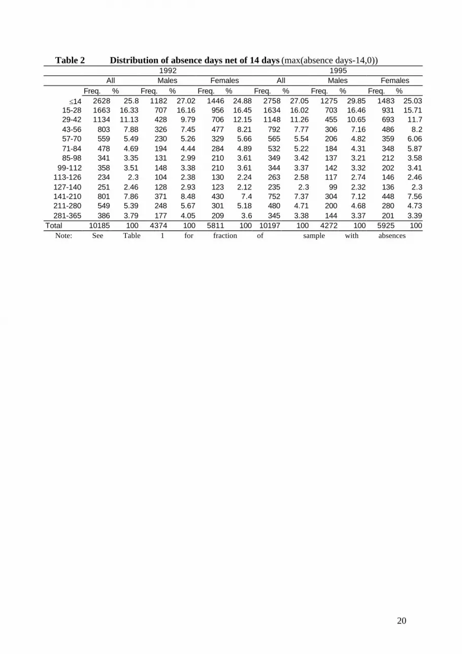
Table 2 shows the distributions of absence days (calendar days) for those who have any.

We remind the reader that our records only include absences lasting more than two weeks. When

that threshold is passed, roughly a quarter have less than 14 additional days of absence, and

about 50 % have less than 42 days.

5. Empirical specification

The number of absence days is an integer variable, suitable for count data modelling.

For each individual we have information on whether s/he had any sickness spells exceeding

two weeks (paid for by the NIA) in a given year, and the length of these spells, if any. This

introduces a censoring problem in our dependent variable, as a zero count may mean anything

between 0 and 14 days. We address the problem by using a two-part, or “hurdle” count model

(Mullahy 1986). The first part consists of a binary response model, and the second of a model

for the number of absence days once the hurdle has been passed. The hurdle model is a

generalisation of ordinary censoring models, where it is assumed that the same process

governs the probability of passing the threshold and the outcome conditional on having passed

it.

Consider first the Poisson regression model. Let Y denote a positive integer random

variable which follows the Poisson distribution, i.e.

(1)!

)exp()()Pr(

yyfyY

yλλ−=== .

Introducing covariates, zi, and coefficients, γ , and specifying ii z'γλln = , the Poisson

regression model is obtained. A restrictive property of the Poisson model is equidispersion,

i.e. the mean equals the variance: λ== )var()( YYE . The negative binomial (negbin) model

is a generalisation of the Poisson which allows the variance to exceed the mean. The

probability density function is

(2) .0,)()1(

)()(

11

1

1

11

>

+

+Γ+Γ

+Γ= α

µµ

µ αα

α

α

αα

y

y

yyf

10

For the limiting case α = 0, this reduces to the Poisson density. (2) may be derived from the

Poisson by letting ,vµλ = where v is a random variable. Assuming that v is gamma

distributed with mean 1 and variance α, it may be integrated out of the distribution of y and v,

and (2) results. This model has µ=)(YE and ).1()var( αµµ +=Y In the regression context,

,'lnlnln iiiii v εγµλ +=+= z where exp(ε i) = vi.5

Hurdle models allow for excess numbers of zeros (or values at some other truncation

point). It is assumed that the probability of having counts greater than zero results from one

process, and positive counts from another process. Consider a hurdle model where both parts

are negative binomial, but with different parameters. Let )(1 yf be the negbin density with

parameters ),( 11 αµ that governs the probability of having a zero count, Pr(y = 0). Using (2),

we have that

(3)

.)1(1)0(1)1Pr(

)1()0()0Pr(

1

1

111

1

1

1

111

111

1

1

1

α

α

α

µα

µαµα

α

−

−

+−=−=≥

+=

+===

fY

fY

Furthermore, let )(2 yf be the density function of the second process, which is also a negative

binomial model with parameters ),( 22 αµ . We obtain Pr(Y = y|Y ≥ 1) by conditioning on

21

)1(1)0(1 222αµα

−+−=− f , yielding the truncated negbin model:

(4) ( )( )11)()1(

)()1|(

1

11

1

−+

+Γ+Γ+Γ

=≥ ααµµ

µ

αα

α

y

yy

yyf .

The hurdle model may be estimated by maximum likelihood. Because ),( 11 αµ and

),( 22 αµ are independent by assumption, the ML estimates may be obtained by estimating

each part of the model separately. If we impose the restriction 11 =α , equation (3) reduces to

the logit model. That is the approach taken here: First we estimate Pr(Yi – 14 > 0) with a logit

model, and then we use the zero-truncated negative binomial model to estimate Pr(Yi –14 = yi

– 14 | yi – 14 > 0).

5 See Cameron and Trivedi (1998) for a comprehensive review of count data models.

11

Note that both parts of the hurdle model may be given a behavioural interpretation: in

the first part a latent variable measures the utility of having at least one long term absence.

What is observed is the binary outcome. In the second part an other latent variable measures

the utility of an additional absence day. Each time a threshold is passed, a new day is added to

the number of absence days.

As a shorthand, let us formulate the expected outcome of each part of the process as

(5) ( )β,)( XFyE = ,

where E(y) is either the probability of absence (logit) or the expected number of absence days

(negative binomial), and X and β denote vectors of variables and coefficients. The s−β

measure how individuals behave or respond when their characteristics vary, while the X

vector represents the individual characteristics. Consider two individuals indexed 0 and 1,

who differ in characteristics as well as response. The difference in outcome is

(6) ).,(),()()( 110010 ββ XFXFyEyE −=−=∆

For a linear model, i.e. E(y) = βX, (6) may be decomposed as

(7) )()( 1001011100 βββββ −+−=−=∆ XXXXX .

This decomposition, well known from the wage discrimination literature (Blinder 1973,

Oaxaca 1973), has an interesting interpretation: the first part on the r.h.s. expression is the part

of the difference which is caused by difference in characteristics, whereas the second part is

due to difference in behaviour, or response to the characteristics. By estimating the model

separately for “0-type” and “1-type” individuals, (7) may be evaluated at the sample means.

Equation (7) does not hold for the non-linear models used in this paper. However, we

shall perform decompositions as follows,

(8) )}.,(),({)},(),({),(),( 100011101100 ββββββ XFXFXFXFXFXF −+−=−=∆

12

We interpret these expressions as outlined above. (8) is evaluated by computing the necessary

components for each individual and then averaging.

At the outset we estimate the logit model for the full 1992 and 1995 samples, and

compare the estimated parameter-vectors and the predictions for the two sub-samples.

However, from the benchmark model it may be difficult to discriminate between the

hypothesis that it is the characteristics of the sub-samples that vary, or whether it is the

response to these characteristics that causes differences. Therefore we decompose the changes

in absence probabilities as described, deriving how much of the change that is due to

composition effects, and how much is due to efficiency wage effects. We estimate the model

for the 1992 and the 1995 sample. The hypothesis that TT9592 ββ = (T denoting “total sample”)

may be tested by a likelihood ratio test. Moreover, even if a likelihood ratio test rejects the

null hypothesis of no behavioural change, this change alone may not be responsible for the

full change in average outcome. The decomposition in (8) allows us to appreciate how much

of ∆ can be attributed to behaviour and characteristics, respectively.

We perform the same exercise for the sub-sample of those individuals that are present

both in the 1992-sample and in the 1995-sample, denoted the common sample. The common

sample is probably more interesting, since it will indicate a possible change of behaviour for

the same workers when conditions change. If the hypothesis that the coefficients are equal

(and the response effect in the decomposition is zero) is rejected, we may conclude that the

behaviour of the individuals has changed over time. Such a result would support an efficiency

wage explanation for absenteeism. We also report how much of the changes that are due to

behaviour and characteristics respectively.

We next compare the ‘marginal workers’ to the ‘non-marginal workers’ both in 1992

and 1995. Again, we can test if mnt

mt

−= ββ , with m denoting “marginal” and n-m ‘non-

marginal’. If the null hypothesis is not rejected, we may conclude that differences in the work

absence for the two samples are due to differences in characteristics, and not due to different

behaviour of the two samples. If we do reject the null hypothesis, we can use (8) to

decompose ∆ and appreciate the importance of composition effects for explaining differences

in the work absence pattern over the business cycle. Note that we evaluate the difference due

to characteristics at the coefficient vector of the non-marginal workers, and the difference due

to behaviour at the characteristics of the marginal workers.

13

The discussion has focused on the logit part of the model. Obviously, the same

exercises may be performed for the truncated negative binomial part. ∆ then refers to the

difference in expected absence days, conditional on the truncation point.

6. Results

The results from the hurdle regressions on the different samples are reported in Tables 3-5.

We have also run the regressions by gender and report those results in Table 3a and so forth.

However, we focus on the regressions in Table 3-5 in the discussion. In Table 6 we show

decompositions as explained in the previous section.

Table 3 contains estimates of absenteeism for the full samples in 1992 and 1995. As

was seen from summary statistics and in accordance with aggregate numbers of absences, the

predicted absence probability decreases from 1992 to 1995. Since unemployment is lower in

1995 than in 1992 the result is contrary to what is expected from theory. It may be due to a

delay in reaction to changes in economic conditions, or the reason may be that long term

sickness absences are not explained by the efficiency wage hypothesis. Looking at the

coefficients for the logit part, we see that there are small differences between the two years.

The coefficient for local unemployment, UNEMPERC, changes sign but it is not significant.

Thus, the cross section results are in general not strongly supportive of an efficiency wage

explanation, contrary to what is found e.g. for Sweden by Johansson and Palme (1996).

Former sickness, ABSDYS_2, explains absences as expected, with coefficients of 0.0046 in

1992 and 0.0044 in 1995. The income coefficient, INCOME, is positive and significant.

Interestingly, the effect on the number of absence days once absent (Part 2 of the model) is

negative. An explanation for this may be that the percentage of full time workers increase by

income, thus increasing exposure. Once sick, the effect is opposite because high income

workers are more prone to earning efficiency wages. Spouse’s income and wealth have

opposite signs to own income but the coefficients are smaller. The proxies for ability and

wages, EDUCATIO, EXPERIEN, SENIORITY and PARTTIME have negative signs, except

from experience, which is positive and significant in 1992, Part 1 of the model. This confirms

a conjecture that increased wage rates will reduce demand for absences, i.e. the substitution

effect dominates. The coefficient for number of children, CHILDREN, is positive as was

expected. More children induce more long term absences. However, when considering males

and females separately, we found that the coefficient was actually negative and significant for

14

men in 1992 (Part 1), and insignificant in 1995. With the exception of income, the results for

Part 2 are similar for the significant coefficients.

In Table 6 we find that when we decompose the changes from 1992 to 1995 in Part 1

into a composition (characteristics) effect and a behaviour effect, approximately 60% of the

change is due to changes in characteristics.

To investigate the decomposition further, we turn to the common sample, Table 4.

The results are very similar to what we found using the total samples for each year, so that the

coefficient estimates should need no further comments. However, the likelihood ratio tests

show that the coefficients for the 1995 sample are significantly different from the coefficients

in 1992 (both parts). Of most interest are the overall sickness probabilities, which are 0.111 in

1992 and 0.122 in 1995. For this sub-sample of workers who participate both in 1992 and

1995, we find that their sickness probability has increased. These results are as expected when

economic conditions improve. Are the changes due to different behaviour or differences in the

individuals’ background characteristics? Behaviour, i.e. disciplining effects, does matter.

From Table 6 we see that more than 70% of the change in absence probability (0.0082 out of

0.0109) is due to changes in the workers’ behaviour. This is even more pronounced for Part 2.

We find that once sick, the mean number of sickness days increase by 12.1. 11.2 (91%) are

due to changes in behaviour. Thus, a significant share of the increase in sickness absence from

1992 to 1995 for established workers can be explained by an efficiency wage effect, which is

the interpretation of a change in behaviour. The well established workers tend to be more sick

and absent from work when the economy is booming compared to a situation with high

unemployment.

We now turn to the so-called marginal workers, and compare them to the non-

marginal workers. The marginal workers are those who had a loose connection to the labour

market two years back. They were either working very few hours, were unemployed, or were

outside of the work force but not under education. Contrary to the composition effects

argument, we find that this group has a lower probability of being absent than the reference

group. The coefficients are significantly different (Part 1). When decomposing, we find that

different characteristics explain some 110% (1992) and 165% (1995) of the probability

difference. In other words, given the characteristics of the non-marginal workers, the marginal

workers would have more absence than them: the difference due to behaviour is positive.

There is, though, a tendency for the males entering the labour market in 1995, when

unemployment is on its way down, to increase absence probability (Tables 5a and 6). For the

number of sickness days, the picture is less clear. In 1992, marginal workers have less

15

absence days than the non-marginal, but there is no difference in 1995. The likelihood ratio

tests do not reject the null hypotheses of equal behaviour between marginal and non-marginal

workers. Comparing marginal workers in 1992 and 1995 in Table 5 (Part 2), we find an

increase in absence days from 1992 to 1995 for marginal workers, from 64.2 days to 68.5

days, contrary to what is found for non-marginal workers. The decompositions in Table 6

indicates that the relative change between the two groups over time can be ascribed to the

marginal workers changing their behaviour in the direction of longer absences, given their

characteristics. A disciplining effect seems to be working also for the marginal workers: they

are more prone to long absences in boom periods.

7. Concluding remarks.

We have investigated factors which explain sickness absence in Norway. The study is limited

to sickness spells lasting more than two weeks, i.e. spells that are paid for by the Social

Insurance. The data, drawn from the KIRUT database, include extensive individual

background information, so we can control for individual characteristics when analysing

sickness absence.

A prime objective was to investigate whether sickness absence is explained primarily

by the disciplinary effects of unemployment, or by composition effects within the labour

force. The disciplinary effects of unemployment are analysed by comparing sickness absences

in 1992 and 1995. Unemployment was high in the first of these years, lower and on its way

down during the latter. Sickness absence was slightly lower in 1995 than in 1992, but

increasing. The behaviour of the workers who participated in both 1992 and 1995 changed,

and such that they for given characteristics have more absences in 1995. The same seems to

hold true for male marginal workers. This gives some support to the hypothesis that

unemployment plays a disciplinary role. The composition effects are analysed by comparing

absenteeism between workers with a longer lasting attachment to the labour force, with

marginal workers. We find that the marginal workers actually have the lowest absence

probability. In aggregate, therefore, our analysis gives no support to the claim that cyclical

variations in sickness absence may be explained by composition effects, or “marginalised”

workers entering the labour force during an economic upturn. To the contrary, we find that the

“stable” workers – those who were in the labour force in both periods under study, are the

ones who change behaviour and increase absence. Thus our results provide some support for

the hypothesis that unemployment has a disciplining effect on sickness absence behaviour.

16

References.

Allen, S.G., 1981a, “An Empirical Model of Work Attendance”, Review of Economics andStatistics 63, 77-87

Allen, S.G., 1981b, “Compensation, Safety and Absenteeism: Evidence from the Paperindustry”, Industrial and Labor Relations Review 34, 207-18.

Barmby, T.A., and J.G. Treble, 1991, “Absenteeism in a Medium Sized ManufacturingPlant”, Applied Economics 23, 161-6.

Barmby T, J.G. Sessions, and J.G. Treble, 1994, “Absenteeism, Efficiency Wages andShirking”, Scandinavian Journal of Economics 96, 561-566.

Blinder, A.S. 1973, “Wage Discrimination: Reduced Form and Structural Estimates,” Journalof Human Resources 18, 436-455.

Brown S, and J.G. Sessions (1996), “The Economics of Absence: Theory and Evidence”,Journal of Economic Surveys 10, 23-53.

Cameron, C.A., and P.K. Trivedi, 1998, Regression Analysis of Count Data, Cambridge,Cambridge University Press.

Chaudhury, M., and I. Ng, 1992, “Absenteeism Predictors: Leas Squares, Rank Regression,and Model Selection Results”, Canadian Journal of Economics 3, 615-34.

Drago, R. And M Wooden, 1992, “The Determinants of Labour Absence: Economic Factorsand Workgroup Norms Across Countries”, Industrial and Labor Relations Review45, 764-78

Dunn, L.F., and S.A. Youngblood, 1986, “Absenteeism as a Mechanism for Approaching anOptimal Labor Market Equilibrium: An Empirical Study”, Review of Economics andStatistics 68, 668-674.

Dyrstad, J.M., 1997, “Absence: Discipline versus Composition Effects”, mimeo, Departmentof Economics, Norwegian University of Science and Technology, Trondheim,Norway.

Dyrstad, J.M., 1999, “Sick Pay Scheme Changes and Sickness Absenteeism: EmpiricalEvidence from Norway”, mimeo, Department of Economics, Norwegian Universityof Science and Technology, Trondheim, Norway.

Johansson, P. and M. Palme, 1996, “Do Economic Incentives Affect Work Absence?Empirical Evidence Using Swedish Micro Data”, Journal of Public Economics 59,195-218.

Kenyon, P. and P. Dawkins, 1989, “A Time Series Analysis of Labour Absence in Australia”,Review of Economics and Statistics 71, 232-39.

17

Mullahy, J., 1986, “Specification and Testing of Some Modified Count Data Models,”Journal of Econometrics 33, 341-365.

NOSOSCO, 1992, Statistical Reports of the Nordic Countries no. 58, Oslo, Norway.

Oaxaca, R., 1973, “Male Female Wage Differentials in Urban Labor Markets,” InternationalEconomic Review 14, 693-709.

Riphahn, R.T., and A. Thalmaier, 1999, “Absenteeism and Employment Probation”, mimeo,The Institute for the Study of Labor (IZA), Bonn.

RTV, 1998, “Basisrapport 1997: Sammendrag (Basis Report 1998: Summary)”, RTV(‘Rikstrygdeverket’ – National Insurance Administration) Report 04/98.

Shapiro, C. and J.E. Stiglitz, 1984, “Equilibrium Unemployment as a Worker DisciplineDevice”, American Economic Review 74, 433-444.

Whinston, M.D., 1983, ”Moral hazard, Adverse Selection, and the Optimal Provision ofSocial Insurance”, Journal of Public Economics 22, 49-71.

18

Figure 1. Sickness: Duration and Number of Days per Employee

Figure 2. Unemployment and GDP-growth

5 . 0

6 . 0

7 . 0

8 . 0

9 . 0

1 0 . 0

1 1 . 0

1 2 . 0

1 3 . 0

1 4 . 0

1 5 . 0

1 9 9 0 1 9 9 2 1 9 9 4 1 9 9 6 1 9 9 8

Nu

mb

er o

f d

ays

4 5 . 0

4 6 . 0

4 7 . 0

4 8 . 0

4 9 . 0

5 0 . 0

5 1 . 0

5 2 . 0

5 3 . 0

5 4 . 0

5 5 . 0

Du

rati

on

of

spel

ls

N b r . o f d a y sD u r a t i o n

-1.0

0.0

1.0

2.0

3.0

4.0

5.0

6.0

7.0

1990 1991 1992 1993 1994 1995 1996 1997 1998

Unemp loymen t

GDP-private

GDP-publ ic

19

Table 1 Sample means

Full Males Females Common Marginal Non-marginal1992 1995 1992 1995 1992 1995 1992 1995 1992 1995 1992 1995

absdys_2 6.61 5.59 5.43 4.50 7.86 6.74 5.98 6.27 2.23 1.77 7.15 6.07married 0.56 0.53 0.56 0.52 0.56 0.54 0.56 0.58 0.41 0.37 0.61 0.57pre_marr 0.11 0.12 0.09 0.10 0.13 0.14 0.11 0.13 0.09 0.09 0.12 0.13woman 0.49 0.49 0.49 0.49 0.58 0.53 0.48 0.48age 38.08 38.24 38.06 38.12 38.09 38.37 37.38 40.38 31.21 31.72 39.82 39.91children 0.39 0.41 0.36 0.36 0.42 0.46 0.41 0.41 0.48 0.46 0.41 0.43educatio 11.39 11.66 11.58 11.80 11.19 11.52 11.47 11.64 11.50 11.68 11.33 11.60nonScand 0.02 0.02 0.02 0.02 0.01 0.01 0.01 0.01 0.04 0.03 0.02 0.01income 16.88 17.11 20.78 20.72 12.77 13.28 17.32 18.90 10.83 11.77 18.13 18.32spou_inc 8.86 8.94 5.95 6.02 11.93 12.04 9.16 9.85 7.39 6.97 9.56 9.66wealth 14.60 16.21 14.00 15.36 15.24 17.12 12.92 17.85 8.23 7.86 15.88 17.70experien 13.86 14.89 15.71 16.54 11.93 13.14 13.85 16.73 8.36 9.25 15.10 16.19senority 5.66 6.01 6.12 6.38 5.16 5.62 5.66 7.23 1.10 1.02 6.32 6.73parttime 0.16 0.16 0.07 0.07 0.25 0.25 0.15 0.13 0.31 0.29 0.13 0.13unemperc 6.36 5.49 6.36 5.50 6.36 5.48 6.36 5.48 6.43 5.55 6.37 5.49agrifish1 0.02 0.02 0.02 0.02 0.01 0.01 0.01 0.01 0.02 0.02 0.01 0.01salhottr1 0.26 0.25 0.26 0.25 0.26 0.24 0.25 0.24 0.27 0.24 0.25 0.24dwelfina1 0.08 0.08 0.08 0.08 0.08 0.07 0.08 0.08 0.07 0.08 0.08 0.08gover_hl1 0.21 0.21 0.19 0.19 0.23 0.23 0.21 0.22 0.22 0.20 0.21 0.22healtsoc1 0.13 0.14 0.04 0.04 0.23 0.25 0.13 0.14 0.20 0.20 0.13 0.14norway_a1 0.08 0.08 0.08 0.08 0.08 0.08 0.08 0.08 0.08 0.08 0.08 0.08norway_e1 0.15 0.15 0.16 0.16 0.15 0.15 0.15 0.16 0.14 0.15 0.16 0.15norway_s1 0.09 0.09 0.09 0.09 0.09 0.09 0.09 0.09 0.10 0.09 0.09 0.09norway_w1 0.20 0.21 0.21 0.21 0.20 0.20 0.21 0.20 0.22 0.20 0.20 0.20norway_m1 0.14 0.14 0.14 0.14 0.14 0.14 0.14 0.14 0.13 0.13 0.14 0.14norway_n1 0.10 0.10 0.10 0.10 0.10 0.10 0.10 0.10 0.11 0.11 0.10 0.10≥1 absence 0.12 0.12 0.10 0.09 0.14 0.14 0.11 0.12 0.11 0.11 0.13 0.12absencedays 10.6 9.6 9.1 7.6 12.2 11.6 8.0 10.3 8.6 9.0 11.4 10.1absencedays if ≥1absence 85.4 82.2 87.2 80.3 84.0 83.6 71.2 83.3 78.3 82.2 86.0 82.7N 82349 88354 42234 45456 40115 42898 69131 69131 4028 4783 72966 78169

1Dummy variables used in the regressions but not reported

20

Table 2 Distribution of absence days net of 14 days (max(absence days-14,0))1992 1995

All Males Females All Males FemalesFreq. % Freq. % Freq. % Freq. % Freq. % Freq. %

≤14 2628 25.8 1182 27.02 1446 24.88 2758 27.05 1275 29.85 1483 25.0315-28 1663 16.33 707 16.16 956 16.45 1634 16.02 703 16.46 931 15.7129-42 1134 11.13 428 9.79 706 12.15 1148 11.26 455 10.65 693 11.743-56 803 7.88 326 7.45 477 8.21 792 7.77 306 7.16 486 8.257-70 559 5.49 230 5.26 329 5.66 565 5.54 206 4.82 359 6.0671-84 478 4.69 194 4.44 284 4.89 532 5.22 184 4.31 348 5.8785-98 341 3.35 131 2.99 210 3.61 349 3.42 137 3.21 212 3.58

99-112 358 3.51 148 3.38 210 3.61 344 3.37 142 3.32 202 3.41113-126 234 2.3 104 2.38 130 2.24 263 2.58 117 2.74 146 2.46127-140 251 2.46 128 2.93 123 2.12 235 2.3 99 2.32 136 2.3141-210 801 7.86 371 8.48 430 7.4 752 7.37 304 7.12 448 7.56211-280 549 5.39 248 5.67 301 5.18 480 4.71 200 4.68 280 4.73281-365 386 3.79 177 4.05 209 3.6 345 3.38 144 3.37 201 3.39

Total 10185 100 4374 100 5811 100 10197 100 4272 100 5925 100Note: See Table 1 for fraction of sample with absences

21

Table 3 Hurdle regressions for 1992 and 1995 (full samples)1992 1995

Part 1: Pr(Y>0) (Logit)Coef. z-value Coef. z-value

absdys_2 0.0077 27.049 0.0074 25.342married 0.2221 5.310 0.1152 2.817pre_marr 0.3584 8.682 0.2901 7.338woman 0.4600 16.161 0.4668 16.863age 0.0129 7.736 0.0152 8.285children 0.0481 2.816 0.0987 6.139educatio -0.1327 -25.179 -0.1170 -22.783nonScand 0.2036 2.342 0.1588 1.770income 0.0503 11.668 0.0827 18.125inc_sqr -0.0010 -10.546 -0.0018 -16.665spou_inc -0.0071 -5.117 -0.0066 -4.928wealth -0.0017 -4.112 -0.0041 -9.387experien 0.0028 1.079 -0.0028 -1.120senority -0.0125 -5.643 -0.0047 -2.234parttime -0.2378 -6.574 -0.1700 -4.879unemperc 0.0065 0.941 -0.0093 -1.192Constant -1.7636 -17.891 -2.1352 -21.670Loglikelihood -28820.3 -29595.7N 82349 88354Mean predicted 0.1189 0.1154

Part 2: E(Y|Y≥1) (Negative binomial)Coef. z-value Coef. z-value

absdys_2 0.0023 7.640 0.0026 8.218married 0.0437 0.978 0.0116 0.266pre_marr 0.0264 0.613 0.0270 0.648woman -0.0746 -2.366 0.0099 0.320age 0.0196 11.023 0.0182 9.115children 0.0246 1.311 0.0457 2.521educatio -0.0241 -4.263 -0.0150 -2.634nonScand 0.1152 1.217 -0.0854 -0.863income -0.0118 -4.201 -0.0105 -2.780inc_sqr 0.0001 2.031 0.0001 1.276spou_inc -0.0050 -3.323 -0.0031 -2.244wealth 0.0000 -0.011 0.0004 0.821experien -0.0076 -2.587 -0.0066 -2.317senority -0.0001 -0.021 -0.0024 -1.038parttime -0.0177 -0.466 0.0076 0.201unemperc -0.0048 -0.638 -0.0111 -1.253Constant 3.9755 39.803 3.8314 37.641alpha 1.409 1.446Loglikelihood -52972.16 -52612.9N 10185 10197Mean predicted 69.5 68.2Note: Location and sector dummies are used in the regressions but not reportedLR tests β92 = β95: Part 1: 71.56 (DF=28) Part 2: 35.22 (DF=29)

22

Table 4 Hurdle regressions for common sample1992 1995

Part 1: Pr(Y>0) (Logit)abs15yr1 Coef. z-value Coef. z-valueabsdys_2 0.0087 25.493 0.0075 23.767married 0.2372 4.917 0.1581 3.518pre_marr 0.3861 8.181 0.2872 6.623woman 0.4958 15.156 0.4822 15.500age 0.0074 3.584 0.0137 6.795children 0.0378 1.962 0.0857 4.747educatio -0.1314 -21.723 -0.1146 -20.366nonScand 0.1359 1.286 0.3018 2.818income 0.0464 9.212 0.0739 13.360inc_sqr -0.0009 -8.403 -0.0016 -13.224spou_inc -0.0068 -4.245 -0.0076 -5.210wealth -0.0017 -3.364 -0.0041 -8.691experien 0.0058 1.869 -0.0027 -0.954senority -0.0121 -4.583 -0.0034 -1.505parttime -0.2302 -5.497 -0.1236 -3.109unemperc 0.0083 1.048 -0.0088 -1.015Constant -1.7083 -14.989 -2.0583 -17.821Loglikelihood -22657.8 -24129.8N 69131 69131Mean predicted 0.1113 0.1223


0.0025 6.979 0.0027 8.086married 0.0531 1.026 0.0344 0.719pre_marr 0.0658 1.319 0.0562 1.222woman -0.0135 -0.366 0.0150 0.435age 0.0118 5.209 0.0179 8.249children 0.0314 1.461 0.0402 1.992educatio -0.0190 -2.910 -0.0105 -1.691nonScand 0.1511 1.293 -0.0974 -0.836income -0.0066 -2.120 -0.0146 -2.558inc_sqr 0.0000 1.458 0.0001 1.029spou_inc -0.0045 -2.543 -0.0038 -2.605wealth -0.0003 -0.890 0.0004 0.847experien -0.0035 -1.037 -0.0071 -2.241senority -0.0009 -0.303 -0.0032 -1.300parttime -0.0913 -2.051 0.0037 0.086unemperc -0.0060 -0.679 -0.0132 -1.360Constant 3.9048 33.892 3.8633 31.939alpha 1.4258 1.4433Loglikelihood -38455.3 -43740.3N 7697 8452Mean predicted 57.3 69.4Note: Location and sector dummies are used in the regressions but not reportedLR tests β92 = β95: Part 1: 64.27 (DF=28) Part 2: 103.93 (DF=29)

23

Table 5 Hurdle regressions for marginal and non-marginal samples

1992 1995Non-marginal Marginal Non-marginal Marginal

Part 1: Pr(Y>0) (Logit)Coef. z-value Coef. z-value Coef. z-value Coef. z-value

absdys_2 0.0076 26.079 0.0170 4.793 0.0073 24.414 0.0209 5.660married 0.2064 4.838 0.3892 1.970 0.0914 2.178 0.5241 2.923pre_marr 0.3204 7.612 0.6544 3.348 0.2569 6.341 0.6448 3.720woman 0.4410 14.914 0.4450 3.240 0.4717 16.306 0.3114 2.562age 0.0105 6.117 0.0100 1.116 0.0143 7.553 -0.0081 -0.849children 0.0115 0.643 0.1123 1.602 0.0816 4.836 0.0259 0.385educatio -0.1259 -23.156 -0.1285 -4.921 -0.1109 -20.857 -0.1133 -4.794nonScand 0.1965 2.143 -0.0399 -0.132 0.1940 2.071 -0.4249 -1.215income 0.0333 7.498 0.1357 5.413 0.0759 15.372 0.0219 2.224inc_sqr -0.0007 -7.461 -0.0035 -4.424 -0.0017 -14.917 -0.0001 -0.743spou_inc -0.0083 -5.799 -0.0022 -0.340 -0.0071 -5.148 -0.0080 -1.219wealth -0.0014 -3.602 -0.0099 -2.809 -0.0040 -8.976 -0.0081 -2.641experien 0.0037 1.377 0.0026 0.200 -0.0025 -0.947 0.0146 1.209senority -0.0121 -5.400 0.0424 0.545 -0.0041 -1.922 0.2366 3.304parttime -0.2062 -5.346 -0.2979 -2.231 -0.1517 -4.067 -0.3063 -2.447unemperc 0.0054 0.748 -0.0197 -0.632 -0.0119 -1.459 -0.0021 -0.063Constant -1.5055 -14.451 -2.0704 -4.398 -2.0521 -19.525 -1.3641 -3.182Loglikelihood -26747.8 -1284.1 -27221.6 -1549.6N 72966 4028 78169 4783Mean predicted 0.1312 0.1095 0.1213 0.1089

Part 2: E(Y|Y≥1) (Negative binomial)Coef. z-value Coef. z-value Coef. z-value Coef. z-value

absdys_2 0.0024 7.692 -0.0029 -0.920 0.0026 7.994 0.0022 0.619married 0.0397 0.857 0.0450 0.238 0.0041 0.092 0.2329 1.140pre_marr 0.0210 0.475 0.1364 0.638 0.0231 0.535 0.1592 0.878woman -0.0826 -2.532 0.1079 0.670 0.0063 0.196 -0.0507 -0.361age 0.0203 11.156 -0.0038 -0.407 0.0179 8.730 0.0136 1.166children 0.0244 1.245 -0.0340 -0.440 0.0432 2.294 0.0169 0.203educatio -0.0227 -3.902 -0.0310 -1.046 -0.0124 -2.114 -0.0378 -1.293nonScand 0.1027 1.034 0.2749 0.814 -0.0400 -0.388 -0.8970 -2.181income -0.0134 -4.432 -0.0212 -0.698 -0.0145 -2.881 0.0047 0.364inc_sqr 0.0001 2.132 0.0005 0.532 0.0001 1.249 0.0000 -0.029spou_inc -0.0051 -3.257 -0.0043 -0.804 -0.0031 -2.212 -0.0088 -1.047wealth 0.0000 -0.113 0.0007 0.371 0.0005 0.974 -0.0001 -0.049experien -0.0083 -2.755 0.0292 2.047 -0.0062 -2.090 -0.0163 -1.119senority -0.0003 -0.114 0.0814 0.862 -0.0020 -0.852 0.1147 1.368parttime -0.0236 -0.587 0.0559 0.366 -0.0042 -0.105 0.0529 0.382unemperc -0.0065 -0.824 0.0236 0.700 -0.0127 -1.392 0.0284 0.671Constant 3.9882 38.349 4.1648 7.843 3.8845 35.084 3.9269 8.259alpha 1.4031 1.3236 1.4444 1.3495Loglikelihood -49861.0 -2242.7 -49004.8 -2690.5N 9570 441 9485 521Mean predicted 72.1 64.2 68.7 68.5Note: Location and sector dummies are used in the regressions but not reportedLR tests βnon-marg= βmarg : Part 1, 1992: 67.00 (DF=28) Part 2, 1992: 30.22 (DF=29)

Part 1, 1995: 78.53 (DF=28) Part 2, 1995: 27.65 (DF=29)

24

Table 3a Hurdle regressions for 1992 and 1995 Males (full sample)1992 1995


absdys_2 0.0085 19.011 0.0077 16.806married 0.2440 3.772 0.0885 1.356pre_marr 0.3428 5.219 0.2674 4.231age 0.0186 6.196 0.0165 4.742children -0.0871 -3.047 0.0161 0.583educatio -0.1385 -17.552 -0.1277 -16.080nonScand 0.2896 2.450 0.1223 0.954income 0.0181 3.226 0.0526 8.496inc_sqr -0.0004 -3.958 -0.0012 -9.263spou_inc -0.0107 -3.629 -0.0117 -3.895wealth -0.0020 -3.105 -0.0028 -4.286experien 0.0015 0.293 -0.0002 -0.032senority -0.0157 -5.161 -0.0078 -2.678parttime -0.5429 -5.741 -0.3008 -3.538unemperc 0.0170 1.613 0.0100 0.830Constant -1.5268 -10.729 -1.7338 -11.752Loglikelihood -13091.1 -13289.0N 42234 45456Mean predicted 0.1036 0.0940


absdys_2 0.0023 4.954 0.0025 4.760married 0.1161 1.637 0.0921 1.254pre_marr 0.1017 1.446 0.1408 2.007age 0.0260 8.048 0.0277 7.016children -0.0390 -1.252 0.0107 0.337educatio -0.0194 -2.178 -0.0132 -1.402nonScand -0.0865 -0.651 -0.3199 -2.176income -0.0116 -3.199 -0.0145 -2.595inc_sqr 0.0001 1.893 0.0001 1.625spou_inc -0.0087 -2.593 -0.0078 -2.295wealth 0.0000 -0.070 0.0014 1.948experien -0.0133 -2.328 -0.0158 -2.749senority -0.0043 -1.318 -0.0077 -2.328parttime 0.0071 0.068 0.0828 0.853unemperc -0.0057 -0.473 -0.0242 -1.728Constant 3.7682 25.624 3.7585 23.723alpha 1.4581 1.5379Loglikelihood -22801.0 -21828.6N 4374 4272Mean predicted 73.3 66.4Note: Location and sector dummies are used in the regressions but not reportedLR tests β92 = β95: Part 1: 34.73 (DF=27) Part 2: 29.23 (DF=28)

25

Table 3b Hurdle regressions for 1992 and 1995 Females (full sample)1992 1995


absdys_2 0.0070 18.853 0.0071 18.691married 0.3232 5.604 0.2500 4.501pre_marr 0.4193 7.740 0.3421 6.658age 0.0121 5.744 0.0166 7.326children 0.1534 6.881 0.1667 8.078educatio -0.1218 -16.559 -0.1037 -14.858nonScand 0.0718 0.540 0.1537 1.193income 0.1165 13.708 0.1359 16.297inc_sqr -0.0029 -10.480 -0.0034 -12.673spou_inc -0.0089 -5.248 -0.0084 -5.142wealth -0.0015 -2.929 -0.0052 -8.761experien -0.0071 -2.118 -0.0106 -3.307senority -0.0060 -1.831 0.0012 0.383parttime -0.1272 -3.182 -0.1153 -2.983unemperc -0.0030 -0.321 -0.0250 -2.404Constant -1.8379 -13.040 -2.2849 -16.492Loglikelihood -15626.2 -16204.7N 40115 42898Mean predicted 0.1449 0.1381


absdys_2 0.0023 5.983 0.0026 6.510married 0.0342 0.567 -0.0196 -0.348pre_marr 0.0150 0.269 -0.0254 -0.481age 0.0160 7.174 0.0157 6.560children 0.0520 2.168 0.0544 2.417educatio -0.0332 -4.411 -0.0188 -2.546nonScand 0.2817 2.006 0.0265 0.195income -0.0149 -2.270 0.0066 0.946inc_sqr 0.0002 1.387 -0.0004 -2.162spou_inc -0.0046 -2.588 -0.0021 -1.311wealth 0.0001 0.151 -0.0003 -0.489experien -0.0088 -2.461 -0.0086 -2.480senority 0.0060 1.662 0.0036 1.116parttime -0.0208 -0.493 0.0178 0.430unemperc -0.0038 -0.398 -0.0025 -0.223Constant 4.1158 29.431 3.7715 26.915alpha 1.3596 1.3689Loglikelihood -30145.9 -30752.1N 5811 5925Mean predicted 70.0 69.6Note: Location and sector dummies are used in the regressions but not reportedLR tests β92 = β95: Part 1: 44.98 (DF=27) Part 2: 26.35 (DF=28)

26

Table 4a Hurdle regressions for common sample (males)1992 1995


absdys_2 0.0096 17.574 0.0080 15.750married 0.2736 3.647 0.2106 2.918pre_marr 0.3462 4.533 0.3223 4.568age 0.0064 1.583 0.0161 4.129children -0.0712 -2.236 -0.0192 -0.628educatio -0.1422 -15.187 -0.1247 -14.216nonScand 0.2110 1.450 0.2059 1.340income 0.0023 0.386 0.0524 6.586inc_sqr -0.0001 -1.423 -0.0012 -7.764spou_inc -0.0110 -3.208 -0.0138 -4.286wealth -0.0013 -1.567 -0.0028 -3.886experien 0.0134 2.107 -0.0040 -0.687senority -0.0122 -3.332 -0.0053 -1.690parttime -0.4924 -4.408 -0.1508 -1.428unemperc 0.0246 2.020 0.0138 1.016Constant -1.2265 -7.369 -1.7735 -10.074Loglikelihood -10119.0 -10591.2N 35473 35473Mean predicted 0.0907 0.0967


absdys_2 0.0029 4.879 0.0028 4.757married 0.1245 1.481 0.0983 1.191pre_marr 0.1236 1.490 0.1872 2.368age 0.0121 2.677 0.0290 6.584children -0.0361 -1.032 0.0285 0.806educatio -0.0039 -0.363 -0.0107 -1.029nonScand 0.1810 1.059 -0.3603 -2.069income -0.0094 -2.185 -0.0243 -2.576inc_sqr 0.0001 1.672 0.0002 1.577spou_inc -0.0092 -2.308 -0.0079 -2.188wealth -0.0001 -0.167 0.0018 2.138experien 0.0005 0.070 -0.0181 -2.701senority -0.0079 -1.884 -0.0060 -1.656parttime 0.0032 0.026 0.1120 0.924unemperc -0.0057 -0.400 -0.0292 -1.831Constant 3.7194 21.253 3.8333 19.597alpha 1.5011 1.5418Loglikelihood -16062.9 -17511.0N 3218 3429Mean predicted 57.7 67.0Note: Location and sector dummies are used in the regressions but not reportedLR tests β92 = β95: Part 1: 54.13 (DF=27) Part 2: 43.59 (DF=28)

27

Table 4b Hurdle regressions for common sample (females)1992 1995


absdys_2 0.0078 17.954 0.0071 17.714married 0.3111 4.694 0.2368 3.902pre_marr 0.4389 7.167 0.3099 5.549age 0.0105 4.083 0.0159 6.444children 0.1328 5.256 0.1687 7.208educatio -0.1125 -13.577 -0.1050 -13.803nonScand 0.0497 0.315 0.3365 2.197income 0.1351 13.044 0.1143 11.699inc_sqr -0.0035 -10.387 -0.0028 -9.417spou_inc -0.0081 -4.071 -0.0082 -4.677wealth -0.0020 -3.144 -0.0051 -8.118experien -0.0070 -1.835 -0.0099 -2.838senority -0.0088 -2.316 0.0006 0.175parttime -0.1081 -2.347 -0.0948 -2.187unemperc -0.0046 -0.437 -0.0271 -2.376Constant -2.0470 -12.569 -2.0742 -12.960Loglikelihood -12444.4 -13468.5N 33658 33658Mean predicted 0.1331 0.1492


absdys_2 0.0021 4.866 0.0026 6.380married 0.0250 0.362 0.0113 0.185pre_marr 0.0314 0.490 0.0032 0.055age 0.0115 4.199 0.0149 5.786children 0.0806 2.878 0.0362 1.432educatio -0.0319 -3.764 -0.0144 -1.797nonScand 0.1391 0.832 0.0140 0.088income 0.0059 0.563 -0.0014 -0.164inc_sqr -0.0002 -0.644 -0.0002 -0.948spou_inc -0.0037 -1.780 -0.0029 -1.746wealth -0.0006 -0.866 -0.0004 -0.658experien -0.0081 -1.967 -0.0085 -2.276senority 0.0070 1.661 0.0002 0.073parttime -0.0884 -1.763 0.0159 0.342unemperc -0.0083 -0.744 -0.0033 -0.267_cons 3.9501 23.811 3.8667 24.164alpha 1.3617 1.3633Loglikelihood -22374.2 -26197.5N 4479 5023Mean predicted 57.0 71.3Note: Location and sector dummies are used in the regressions but not reportedLR tests β92 = β95: Part 1: 52.26 (DF=27) Part 2: 92.08 (DF=28)

28

Table 5a Hurdle regressions for marginal and non-marginal samples (males)1992 1995

Non-marginal Marginal Non-marginal MarginalPart 1: Pr(Y>0) (Logit)

Coef. z-value Coef. z-value Coef. z-value Coef. z-valueabsdys_2 0.0083 18.226 0.0179 2.794 0.0076 16.329 0.0237 4.209married 0.2540 3.882 0.5350 1.388 0.0914 1.366 0.2099 0.691pre_marr 0.3409 5.121 0.4512 1.275 0.2611 4.017 0.3854 1.420age 0.0184 6.054 -0.0025 -0.116 0.0158 4.424 0.0121 0.635children -0.1041 -3.564 -0.0719 -0.452 0.0086 0.302 0.0082 0.057educatio -0.1350 -16.758 -0.1309 -2.841 -0.1212 -14.827 -0.1671 -4.288nonScand 0.2343 1.897 0.2514 0.517 0.1461 1.098 -0.5794 -1.034income 0.0057 1.029 0.1064 2.669 0.0491 7.217 0.0255 2.018inc_sqr -0.0002 -2.217 -0.0030 -2.712 -0.0012 -8.517 -0.0001 -0.726spou_inc -0.0111 -3.735 -0.0031 -0.166 -0.0117 -3.853 -0.0121 -0.709wealth -0.0017 -2.703 -0.0309 -2.862 -0.0026 -4.008 -0.0057 -1.230experien -0.0024 -0.459 0.0437 1.451 -0.0004 -0.071 -0.0045 -0.188senority -0.0148 -4.843 0.0220 0.165 -0.0065 -2.194 0.1881 1.684parttime -0.3810 -3.663 -0.3908 -1.243 -0.2421 -2.518 -0.3362 -1.384unemperc 0.0165 1.519 -0.0238 -0.447 0.0064 0.513 0.0133 0.257Constant -1.3078 -8.849 -1.9597 -2.367 -1.6947 -10.781 -1.0049 -1.479Loglikelihood -12314.7 -456.2 -12238.5 -673.2N 38154 1708 40685 2254Mean predicted 0.1090 0.0872 0.0974 0.0998

Part 2: E(Y|Y≥1) (Negative binomial)Coef. z-value Coef. z-value Coef. z-value Coef. z-value

absdys_2 0.0025 5.252 -0.0048 -0.712 0.0025 4.662 0.0063 1.209married 0.1038 1.432 0.3892 0.961 0.0600 0.781 0.6197 1.937pre_marr 0.1022 1.427 -0.0984 -0.243 0.1242 1.699 0.2269 0.791age 0.0266 8.166 -0.0122 -0.706 0.0284 7.055 -0.0194 -0.820children -0.0409 -1.287 -0.0299 -0.168 0.0209 0.642 -0.3628 -2.017educatio -0.0171 -1.893 -0.0929 -1.417 -0.0122 -1.262 0.0567 1.112nonScand -0.0688 -0.499 -0.3137 -0.483 -0.2781 -1.823 -1.0666 -1.652income -0.0131 -3.460 0.0014 0.029 -0.0211 -2.679 -0.0303 -1.643inc_sqr 0.0001 2.012 0.0000 0.001 0.0002 1.661 0.0003 1.667spou_inc -0.0087 -2.587 -0.0299 -1.188 -0.0079 -2.260 0.0088 0.512wealth 0.0000 0.020 -0.0222 -2.058 0.0015 2.091 -0.0012 -0.264experien -0.0133 -2.268 0.0454 1.671 -0.0161 -2.708 0.0179 0.588senority -0.0044 -1.333 0.2112 1.255 -0.0070 -2.085 0.0285 0.230parttime -0.0016 -0.014 -0.0646 -0.163 0.0721 0.655 0.2433 0.876unemperc -0.0076 -0.615 0.0577 0.902 -0.0232 -1.590 -0.0085 -0.128Constant 3.7624 24.885 4.4086 4.364 3.8233 21.931 4.3003 5.446alpha 1.4508 1.1535 1.5417 1.2362Loglikelihood -21694.7 -753.3 -20278.4 -1155.8N 4157 149 3964 225Mean predicted 73.9 66.6 66.9 68.6

Note: Location and sector dummies are used in the regressions but not reportedLR tests βnon-marg= βmarg : Part 1, 1992: 43.85 (DF=27) Part 2, 1992: 31.90 (DF=28)

Part 1, 1995: 52.79 (DF=27) Part 2, 1995: 24.65 (DF=28)

29

Table 5b Hurdle regressions for marginal and non-marginal samples (females)1992 1995

Non-marginal Marginal Non-marginal MarginalPart 1: Pr(Y>0) (Logit)

z-value Coef. z-value Coef. z-value Coef. z-value zabsdys_2 0.0069 18.349 0.0176 3.991 0.0069 17.987 0.0183 3.687married 0.2914 4.901 0.2914 1.183 0.1887 3.303 0.9557 3.857pre_marr 0.3756 6.757 0.6299 2.605 0.2926 5.556 0.9080 3.942age 0.0097 4.457 0.0153 1.493 0.0162 6.905 -0.0055 -0.472children 0.1130 4.727 0.1741 2.147 0.1464 6.654 0.0306 0.384educatio -0.1163 -15.210 -0.1217 -3.706 -0.1001 -13.832 -0.0575 -1.821nonScand 0.0659 0.464 -0.1193 -0.292 0.1983 1.463 -0.4303 -0.936income 0.0932 10.389 0.1696 4.252 0.1226 13.803 0.1469 3.701inc_sqr -0.0023 -8.142 -0.0047 -2.927 -0.0030 -10.986 -0.0050 -3.157spou_inc -0.0095 -5.440 -0.0008 -0.110 -0.0080 -4.808 -0.0164 -1.966wealth -0.0013 -2.561 -0.0060 -1.773 -0.0050 -8.430 -0.0088 -2.173experien -0.0054 -1.602 -0.0256 -1.584 -0.0106 -3.213 0.0064 0.395senority -0.0063 -1.907 0.0690 0.706 0.0008 0.259 0.2111 2.209parttime -0.1116 -2.628 -0.2543 -1.687 -0.1069 -2.608 -0.2194 -1.461unemperc -0.0041 -0.424 -0.0216 -0.557 -0.0269 -2.498 -0.0098 -0.210Constant -1.5761 -10.444 -1.8177 -2.973 -2.1361 -14.452 -2.6486 -4.148Loglikelihood -14347.6 -815.1 -14903.8 -855.0N 34812 2320 37484 2529Mean predicted 0.1555 0.1259 0.1473 0.1170

Part 2: E(Y|Y≥1) (Negative binomial)Coef. z Coef. z Coef. z Coef. z

absdys_2 0.0023 5.766 -0.0007 -0.178 0.0025 6.313 0.0004 0.078married 0.0385 0.606 0.0028 0.012 -0.0078 -0.134 -0.1430 -0.474pre_marr 0.0030 0.051 0.3099 1.199 -0.0166 -0.304 -0.1188 -0.480age 0.0164 7.124 -0.0024 -0.221 0.0147 5.998 0.0210 1.475children 0.0544 2.133 -0.0697 -0.797 0.0470 1.984 0.1328 1.423educatio -0.0329 -4.209 0.0104 0.288 -0.0153 -2.018 -0.0924 -2.427nonScand 0.2614 1.750 0.7257 1.605 0.0675 0.475 -0.6590 -1.249income -0.0179 -2.487 -0.0008 -0.016 0.0013 0.165 0.0314 0.756inc_sqr 0.0003 1.619 -0.0007 -0.388 -0.0003 -1.589 -0.0005 -0.342spou_inc -0.0051 -2.703 -0.0024 -0.386 -0.0022 -1.396 -0.0072 -0.660wealth 0.0000 -0.105 0.0009 0.439 -0.0003 -0.482 0.0014 0.401experien -0.0097 -2.652 0.0283 1.533 -0.0075 -2.123 -0.0282 -1.524senority 0.0060 1.640 0.0922 0.743 0.0037 1.135 0.2141 1.862parttime -0.0265 -0.597 0.1608 0.938 0.0087 0.198 -0.0697 -0.401unemperc -0.0057 -0.564 0.0008 0.021 -0.0063 -0.537 0.0211 0.393Constant 4.1548 28.149 3.9548 5.796 3.8453 26.012 3.9699 5.485alpha 1.3516 1.2909 1.3639 1.2847Loglikelihood -28138.7 -1477.2 -28695.5 -1519.8N 5413 292 5521 296Mean predicted 70.8 63.4 70.0 69.1Note: Location and sector dummies are used in the regressions but not reportedLR tests βnon-marg= βmarg : Part 1, 1992: 39.34 (DF=27) Part 2, 1992: 26.72 (DF=28)

Part 1, 1995: 43.25 (DF=27) Part 2, 1995: 29.64 (DF=28)

30

Table 6 Decompositions of mean differences in outcomesAll Males Females

Total Charac-teristics

Behavi-our


Behavi-our


Behavi-our

Fullsample 95vs. 92,Part 1

-0.0083 -0.0053 -0.0030 -0.0096 -0-0096 (-) -0.0067 -0.0041 -0.0027

Fullsample 95vs. 92,Part 2

-3.2 -3.2 (-) -6.9 -6.9 (-) -0.5 -0.5 (-)

Commonsample 95vs. 92,Part 1

0.0109 0.0028 0.0082 0.0059 0.0002 0.0058 0.0162 0.0058 0.0104

Commonsample 95vs. 92,Part 2

12.1 0.9 11.2 9.0 1.0 8.0 14.3 1.3 12.0

Marg. vs.non-marg,92, Part 1

-0.0217 -0.0240 0.0023 -0.0217 -0.0192 -0.0025 -0.0296 -0.0296 (-)


-7.9 -7.9 (-) -7.3 -7.3 (-) -7.4 -7.4 (-)


-0.0124 -0.0205 0.0081 0.0024 -0.0109 0.0133 -0.0302 -0.0328 0.0025


-0.2 -0.2 (-) 1.6 1.6 (-) -1.0 -1.0 (-)

Notes: Part 1: Pr(Y>0) Part 2: E(Y|Y>0)Non-rejection of 10 ββ = is interpreted as Total difference = Difference due to characteristics

31

Table A1 LR test for equal coefficients males and femalesPart 1 (logit) Part 2 (negbin)

Full sample 1992 206.0 50.6 1995 205.4 64.4Common sample 1992 188.8 26.4 1995 140.2 63.6Non-marginal 1992 171.0 55.2 1995 25.6 24.4Marginal 1992 158.6 61.8 1995 42.8 29.0DF= 27 for part 1, 28 for part 2 with critical values 40.1 and 41.3 (5%)

sickness absence and business cycles

Documents