all optical multicasting in wavelength routing mesh networks with power considerations: design and...
TRANSCRIPT
Iowa State UniversityDigital Repository @ Iowa State University
Graduate Theses and Dissertations Graduate College
2008
All optical multicasting in wavelength routing meshnetworks with power considerations: design andoperationAshraf M. HamadIowa State University
Follow this and additional works at: http://lib.dr.iastate.edu/etd
Part of the Electrical and Computer Engineering Commons
This Dissertation is brought to you for free and open access by the Graduate College at Digital Repository @ Iowa State University. It has been acceptedfor inclusion in Graduate Theses and Dissertations by an authorized administrator of Digital Repository @ Iowa State University. For moreinformation, please contact [email protected].
Recommended CitationHamad, Ashraf M., "All optical multicasting in wavelength routing mesh networks with power considerations: design and operation"(2008). Graduate Theses and Dissertations. Paper 10940.

All optical multicasting in wavelength routing mesh networks with power
considerations: design and operation
by
Ashraf Hamad
A dissertation submitted to the graduate faculty
in partial fulfillment of the requirements for the degree of
DOCTOR OF PHILOSOPHY
Major: Computer Engineering
Program of Study Committee:Ahmed Kamal, Major Professor
Arun SomaniManimaran Govindarasu
Robert WeberSigurdur Olafsson
Iowa State University
Ames, Iowa
2008
Copyright c© Ashraf Hamad, 2008. All rights reserved.

ii
DEDICATION
I affectionately dedicate this thesis to my parents, Mohammad and Sara, to my wife, Ala’a,
and to my daughters, Sarah and Noor, for their continuous love, encouragement, and support.
iii
TABLE OF CONTENTS
LIST OF TABLES . . . . . . . . . . . . . . . . . . . . . . . . . . . . . . . . . . . vii
LIST OF FIGURES . . . . . . . . . . . . . . . . . . . . . . . . . . . . . . . . . . ix
ACKNOWLEDGEMENTS . . . . . . . . . . . . . . . . . . . . . . . . . . . . . . xii
ABSTRACT . . . . . . . . . . . . . . . . . . . . . . . . . . . . . . . . . . . . . . . xiv
CHAPTER 1. Introduction . . . . . . . . . . . . . . . . . . . . . . . . . . . . . 1
1.1 Optical Networks Evolution . . . . . . . . . . . . . . . . . . . . . . . . . . . . . 3
1.2 Network Lifetime and Stages . . . . . . . . . . . . . . . . . . . . . . . . . . . . 7
1.2.1 Network Provisioning Phase . . . . . . . . . . . . . . . . . . . . . . . . . 8
1.2.2 Network Dimensioning Phase . . . . . . . . . . . . . . . . . . . . . . . . 9
1.2.3 Connection Provisioning Phase . . . . . . . . . . . . . . . . . . . . . . . 10
1.3 All Optical Multicasting (AOM) . . . . . . . . . . . . . . . . . . . . . . . . . . 11
1.4 Challenges of Supporting AOM Service in Wavelength Routing Networks . . . 18
1.4.1 Challenges Due to High-Transmission Rates . . . . . . . . . . . . . . . . 19
1.4.2 Challenges Due to the Characteristics of the Wavelength-Routing Networks 19
1.4.3 Challenges Due to Routing and Wavelength Assignment . . . . . . . . . 28
1.4.4 Challenges Due to the All-Optical-Multicasting (AOM) Characteristics . 30
1.5 Methodology and Contributions of the Thesis . . . . . . . . . . . . . . . . . . . 31
1.6 Preliminaries . . . . . . . . . . . . . . . . . . . . . . . . . . . . . . . . . . . . . 33
1.6.1 Power Constraints and Optical Amplifier Model . . . . . . . . . . . . . 33
1.6.2 System Model . . . . . . . . . . . . . . . . . . . . . . . . . . . . . . . . . 34
1.6.3 Experimental Setup . . . . . . . . . . . . . . . . . . . . . . . . . . . . . 36
iv
1.7 Thesis Outline . . . . . . . . . . . . . . . . . . . . . . . . . . . . . . . . . . . . 37
CHAPTER 2. Literature Review . . . . . . . . . . . . . . . . . . . . . . . . . . 38
2.1 Network Design Schemes . . . . . . . . . . . . . . . . . . . . . . . . . . . . . . . 38
2.2 Network Operation Schemes . . . . . . . . . . . . . . . . . . . . . . . . . . . . . 41
2.2.1 All-Optical-Multicasting Routing (AOM-R) Problem . . . . . . . . . . . 42
2.2.2 All-Optical-Multicasting Wavelength Assignment (AOM-WA) Techniques 62
2.3 Chapter Summary . . . . . . . . . . . . . . . . . . . . . . . . . . . . . . . . . . 64
CHAPTER 3. Power-Aware Design of All-Optical Multicasting in Wave-
length Routed Networks . . . . . . . . . . . . . . . . . . . . . . . . . . . . . 66
3.1 Introduction . . . . . . . . . . . . . . . . . . . . . . . . . . . . . . . . . . . . . . 66
3.2 Additional System Model Parameters . . . . . . . . . . . . . . . . . . . . . . . 69
3.3 MILP parameters and variables . . . . . . . . . . . . . . . . . . . . . . . . . . . 69
3.3.1 Network Parameters . . . . . . . . . . . . . . . . . . . . . . . . . . . . . 70
3.3.2 MILP Variables . . . . . . . . . . . . . . . . . . . . . . . . . . . . . . . . 71
CHAPTER 4. Optical Amplifiers Placement Problem: Asymmetric Power
Case . . . . . . . . . . . . . . . . . . . . . . . . . . . . . . . . . . . . . . . . . . 73
4.1 MILP Formulation . . . . . . . . . . . . . . . . . . . . . . . . . . . . . . . . . . 74
4.1.1 Routing and Wavelength Assignment Constraints: . . . . . . . . . . . . 75
4.1.2 Loop-Avoidance Constraints: . . . . . . . . . . . . . . . . . . . . . . . . 78
4.1.3 Power Constraints: . . . . . . . . . . . . . . . . . . . . . . . . . . . . . . 79
4.2 OA Placement Procedure . . . . . . . . . . . . . . . . . . . . . . . . . . . . . . 83
4.3 Numerical Results . . . . . . . . . . . . . . . . . . . . . . . . . . . . . . . . . . 84
4.3.1 Solution Validation . . . . . . . . . . . . . . . . . . . . . . . . . . . . . . 84
4.3.2 MILP Results . . . . . . . . . . . . . . . . . . . . . . . . . . . . . . . . . 86
4.4 Chapter Summary . . . . . . . . . . . . . . . . . . . . . . . . . . . . . . . . . . 87
CHAPTER 5. Optical Amplifiers Placement Problem: Symmetric Power
Case . . . . . . . . . . . . . . . . . . . . . . . . . . . . . . . . . . . . . . . . . . 89
5.1 Addition System Model Assumptions . . . . . . . . . . . . . . . . . . . . . . . . 90
v
5.2 Impact of Power Symmetry on Number of Optical Amplifiers: An Example . . 91
5.3 MILP Formulation . . . . . . . . . . . . . . . . . . . . . . . . . . . . . . . . . . 93
5.3.1 Routing and Wavelength Assignment Constraints: . . . . . . . . . . . . 93
5.3.2 Loop Avoidance Constraints: . . . . . . . . . . . . . . . . . . . . . . . . 93
5.3.3 Power Constraints: . . . . . . . . . . . . . . . . . . . . . . . . . . . . . . 94
5.4 The Heuristic Algorithm . . . . . . . . . . . . . . . . . . . . . . . . . . . . . . . 96
5.4.1 Greedy Algorithm Motivation and Main Characteristics . . . . . . . . . 96
5.4.2 Cost Functions Definitions . . . . . . . . . . . . . . . . . . . . . . . . . . 98
5.4.3 OP Algorithm Details . . . . . . . . . . . . . . . . . . . . . . . . . . . . 99
5.4.4 Light-Forest Construction Module . . . . . . . . . . . . . . . . . . . . . 101
5.4.5 Light-Forest Placement Module . . . . . . . . . . . . . . . . . . . . . . . 105
5.5 Numerical Results . . . . . . . . . . . . . . . . . . . . . . . . . . . . . . . . . . 106
5.5.1 Comparative Results Between the Optimal and Heuristic Numerical Re-
sults . . . . . . . . . . . . . . . . . . . . . . . . . . . . . . . . . . . . . . 107
5.5.2 OP Heuristic Results . . . . . . . . . . . . . . . . . . . . . . . . . . . . . 113
5.6 Chapter Summary . . . . . . . . . . . . . . . . . . . . . . . . . . . . . . . . . . 120
CHAPTER 6. Power Aware Multicasting (PAM) in Wavelength Routing
Networks . . . . . . . . . . . . . . . . . . . . . . . . . . . . . . . . . . . . . . . 123
6.1 Introduction . . . . . . . . . . . . . . . . . . . . . . . . . . . . . . . . . . . . . . 123
6.2 Additional System Model Assumptions . . . . . . . . . . . . . . . . . . . . . . . 127
6.3 MILP Problem Formulation . . . . . . . . . . . . . . . . . . . . . . . . . . . . . 127
6.3.1 Network Parameters . . . . . . . . . . . . . . . . . . . . . . . . . . . . . 128
6.3.2 MILP Variables . . . . . . . . . . . . . . . . . . . . . . . . . . . . . . . . 129
6.3.3 MILP Formulation . . . . . . . . . . . . . . . . . . . . . . . . . . . . . . 130
6.3.4 Routing and Wavelength Assignment Constraints . . . . . . . . . . . . . 131
6.3.5 Loop-Avoidance Constraints . . . . . . . . . . . . . . . . . . . . . . . . 133
6.3.6 Power Constraints: . . . . . . . . . . . . . . . . . . . . . . . . . . . . . . 133
6.4 The Heuristic Algorithm . . . . . . . . . . . . . . . . . . . . . . . . . . . . . . . 140
vi
6.4.1 Motivation of the PAM Algorithm and Main Characteristics . . . . . . . 140
6.4.2 Link Cost Function . . . . . . . . . . . . . . . . . . . . . . . . . . . . . . 142
6.4.3 The PAM Algorithm Details . . . . . . . . . . . . . . . . . . . . . . . . 143
6.4.4 Power Assignment Algorithm . . . . . . . . . . . . . . . . . . . . . . . . 147
6.5 Numerical Results . . . . . . . . . . . . . . . . . . . . . . . . . . . . . . . . . . 150
6.5.1 Solution quality of the PAM algorithm results . . . . . . . . . . . . . . . 151
6.5.2 PAM Heuristic Results . . . . . . . . . . . . . . . . . . . . . . . . . . . . 153
6.6 Chapter Summary . . . . . . . . . . . . . . . . . . . . . . . . . . . . . . . . . . 158
CHAPTER 7. Thesis Conclusions and Future Work . . . . . . . . . . . . . . 160
7.1 Summary . . . . . . . . . . . . . . . . . . . . . . . . . . . . . . . . . . . . . . . 160
7.2 Future Work . . . . . . . . . . . . . . . . . . . . . . . . . . . . . . . . . . . . . 162
BIBLIOGRAPHY . . . . . . . . . . . . . . . . . . . . . . . . . . . . . . . . . . . 165
vii
LIST OF TABLES
Table 1.1 Typical values for the system parameters that are used in the experiments 36
Table 2.1 Comparison between multicasting techniques in wavelength-routing net-
works in terms of: system model, multicast delivery structure (Struc-
ture), membership policy (Membership), destinations blocking policy
(Policy) and power-budget awareness (pow.) . . . . . . . . . . . . . . . 65
Table 4.1 Summary of the results obtained for the different number of sessions,
K, in the 6 node mesh sample network when |Λ| = 2. . . . . . . . . . 86
Table 5.1 Comparison of OAs numbers obtained by CPLEX (|OA|C) and OP
heuristic (|OA|i; where i = 1, 2, 3, 4 represents the number of alternate
paths) for the 6-mesh network. K and Λ represent number of sessions
and available lambda, respectively. . . . . . . . . . . . . . . . . . . . . 109
Table 5.2 Comparison of used network resources for the 6-mesh network. ψC (ÃLC)
and ψi (ÃLi) represent the maximum number of wavelengths (number of
links) used by CPLEX, and the OP heuristic, respectively. i = 1, 2, 3, 4
represents the number of alternate paths, while K and Λ represent
number of sessions and available lambda, respectively. . . . . . . . . . 110
Table 5.3 The relative performance of using Adaptive method alone with respect
to alternate routing at different traffic load. . . . . . . . . . . . . . . . 116

viii
Table 6.1 The relative performance of the rerouting scheme compared to the Fixed
scheme in terms of the number of accepted sessions when K = 10
and 20. The symbols F and R refer to Fixed and Rerouting schemes,
respectively. . . . . . . . . . . . . . . . . . . . . . . . . . . . . . . . . . 155
Table 6.2 The relative performance of the rerouting scheme compared to the Fixed
scheme in terms of the consumed network resources when K = 10 and
20 and number of alternate path is 1. The symbols F and R refer to
Fixed and Rerouting schemes, respectively. . . . . . . . . . . . . . . . . 156
ix
LIST OF FIGURES
Figure 1.1 Optical Networks Generations . . . . . . . . . . . . . . . . . . . . . . . 4
Figure 1.2 Optical Network Planning Stages under Multicast Communication . . 7
Figure 1.3 Splitter-and-Delivery (SaD) OXC. . . . . . . . . . . . . . . . . . . . . . 13
Figure 1.4 Multicast-only Splitter-and-Delivery (MOSaD) OXC. . . . . . . . . . . 14
Figure 1.5 An example of Multicast Capable Switch with Wavelength Conversion
reported in [1]. . . . . . . . . . . . . . . . . . . . . . . . . . . . . . . . 15
Figure 1.6 An example of Multicast Capable Switch with Wavelength Conversion
reported in [2]. . . . . . . . . . . . . . . . . . . . . . . . . . . . . . . . 16
Figure 1.7 Splitter converter sharing switch reported in [3]. . . . . . . . . . . . . . 17
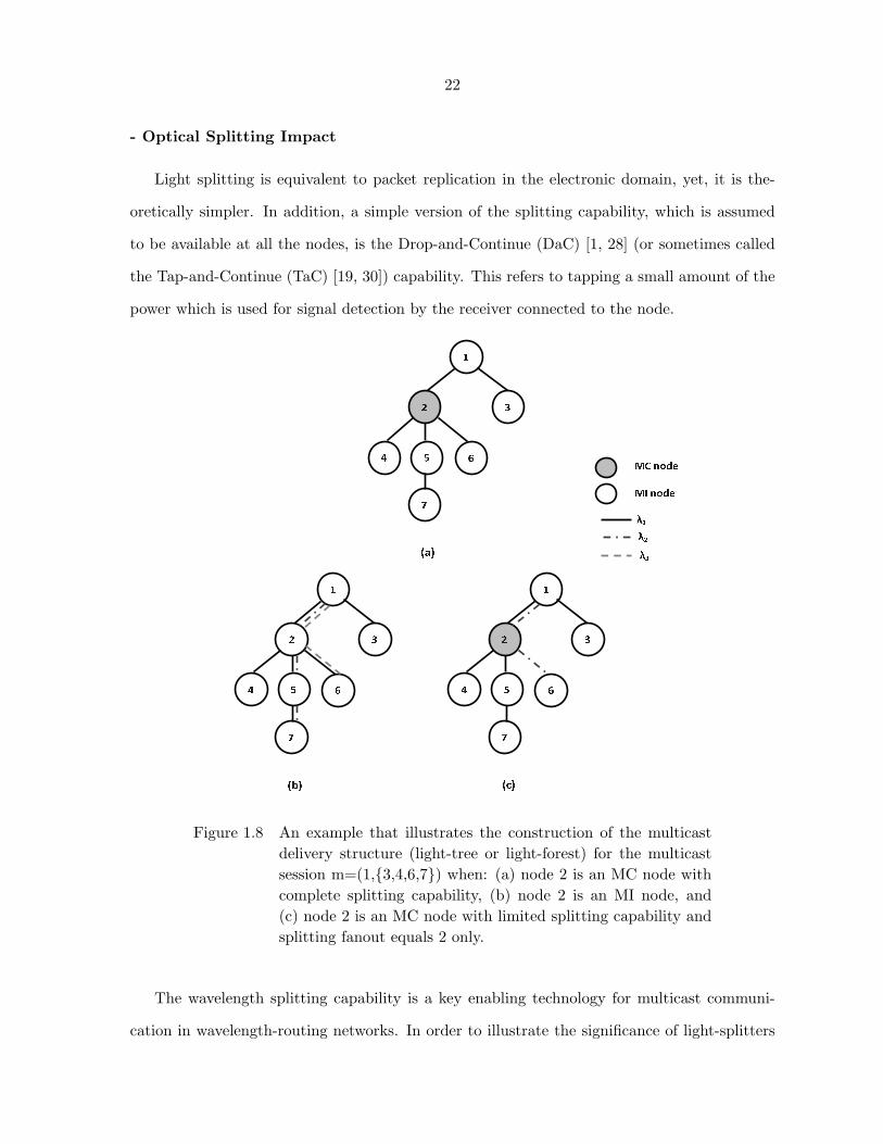
Figure 1.8 An example that illustrates the construction of the multicast delivery
structure (light-tree or light-forest) for the multicast session m=(1,3,4,6,7)when: (a) node 2 is an MC node with complete splitting capability, (b)
node 2 is an MI node, and (c) node 2 is an MC node with limited
splitting capability and splitting fanout equals 2 only. . . . . . . . . . . 22
Figure 1.9 Splitter-converter relative locality in the switch (a) Pre-Conversion Scheme,
and (b) Post-Conversion Scheme. . . . . . . . . . . . . . . . . . . . . . 26
Figure 1.10 Splitter-Amplifier relative locality in the switch (a) Pre-Amplification
Scheme, and (b) Post-Amplification Scheme. . . . . . . . . . . . . . . . 27
Figure 1.11 OA model in Equation (1.1) . . . . . . . . . . . . . . . . . . . . . . . . 34
Figure 1.12 OA model in Equation (1.2) . . . . . . . . . . . . . . . . . . . . . . . . 34
Figure 1.13 Six Nodes Mesh Network. . . . . . . . . . . . . . . . . . . . . . . . . . 36
Figure 1.14 NSFNET. . . . . . . . . . . . . . . . . . . . . . . . . . . . . . . . . . . 36
x
Figure 2.1 Classification Map for Multicast Routing Algorithms in Wavelength-
Routing Networks. . . . . . . . . . . . . . . . . . . . . . . . . . . . . . 43
Figure 4.1 Solution Steps for the OAP-Asymmetric Problem. . . . . . . . . . . . . 74
Figure 4.2 An illustrative example for the light-forest of the multicast session
(Src, 2, 3, 4, 5). . . . . . . . . . . . . . . . . . . . . . . . . . . . . . . 76
Figure 4.3 Sample output for connections x0 and x1 only when |Λ| = 2. (a)
RWA and power values, (b) Detailed solution per fiber link. . . . . . . 85
Figure 5.1 An example that shows the impact of using symmetric power values on
saving the number of OAs over link e(1, 2), whose length is 150 km,
when ALAP OA placement policy is used. (a) 4 OAs are needed for
the OAP-Asymmetric scenario, (b) 2 OAs are needed for the OAP-
Symmetric scenario. . . . . . . . . . . . . . . . . . . . . . . . . . . . . . 92
Figure 5.2 Basic Operation of the OP Algorithm. . . . . . . . . . . . . . . . . . . 100
Figure 5.3 Tree Construction Module. . . . . . . . . . . . . . . . . . . . . . . . . . 102
Figure 5.4 Tree Placement Module. . . . . . . . . . . . . . . . . . . . . . . . . . . 106
Figure 5.5 Impact of Using Alternate Routing on |OA| for the Fixed Scheme at
Different Traffic Loads. The notation T − i(F ) indicates that traffic
load (T ) is i sessions for the Fixed (F ) scheme. . . . . . . . . . . . . . 114
Figure 5.6 Impact of Using Alternate Routing on |OA| for the Adaptive Scheme
at Different Traffic Loads. The notation T − i(R) indicates that traffic
load (T ) is i sessions for the Adaptive (or Rerouting, R) scheme. . . . 115
Figure 5.7 Maximum number of used channels (ψ) at different traffic loads for the
Fixed and Adaptive schemes when number of alternate paths is 1. . . 117
Figure 5.8 Number of used links (ÃL) at different traffic loads for the Fixed and
Adaptive schemes when number of alternate paths is 1. . . . . . . . . . 118
xi
Figure 5.9 Network Bandwidth Utilization (NBU) achieved at various traffic loads
by the Fixed Scheme and Adaptive Scheme when one Alternate path is
used. . . . . . . . . . . . . . . . . . . . . . . . . . . . . . . . . . . . . . 119
Figure 5.10 Comparison of the Network Bandwidth Utilization (NBU) achieved
with different alternate paths When Fixed Scheme is used at various
traffic loads. . . . . . . . . . . . . . . . . . . . . . . . . . . . . . . . . . 120
Figure 5.11 Comparison of the Network Bandwidth Utilization (NBU) achieved
with different alternate paths When Adaptive Scheme is used at various
traffic loads. . . . . . . . . . . . . . . . . . . . . . . . . . . . . . . . . . 121
Figure 6.1 An illustration of the approximate linear conversion approach between
power levels in dBm and mW . . . . . . . . . . . . . . . . . . . . . . . . 136
Figure 6.2 An illustration of the approximate linear conversion approach between
total input power of OA in mW and the OA gain in dB. . . . . . . . . 138
Figure 6.3 Flow chart of the PAM Algorithm Operation. . . . . . . . . . . . . . . 144
Figure 6.4 Flow chart of the operation of Power Assignment Module. . . . . . . . 146
Figure 6.5 The greedy heuristic results with respect to the MILP for the 6 nodes
mesh network, when Λ = 4 and for different values of K. . . . . . . . . 151
Figure 6.6 Impact of the PAM algorithm on the number of accepted sessions when
the Fixed scheme is used and the number of available channels is 10.
Min-P determines the case when Min Power scheme is used with one
alternate path, while RP-P(i) indicates the case when the Rand Power
Scheme is used with ith alternate path. . . . . . . . . . . . . . . . . . . 154
Figure 6.7 System behavior with the existence of power constraints in the 6 nodes
network for 30 connections. . . . . . . . . . . . . . . . . . . . . . . . . 157
Figure 6.8 System behavior with the existence of power constraints in the NSFNET
for 20 connections. . . . . . . . . . . . . . . . . . . . . . . . . . . . . . 158

xii
ACKNOWLEDGEMENTS
First, I thank God, for all of His blessings and mercy in my life.
My deep gratitude and sincere thanks are due to my advisor, Dr. Ahmed Kamal, for
his constant guidance, support and encouragement. Dr. Kamal has a great influence on my
career and life. In my career, Dr. Kamal’s vision, research methodologies and standard,
shaped my thoughts and skills on conducting research and seeking knowledge. His insightful
comments and invaluable reviews were of great benefits to my learning experience, in general,
and to this research, in particular. I have learned greatly from him and he was always there
for his students with an endless dedication. In my life, Dr. Kamal’s achievements, sincere
commitments toward his work and students, and his dedication and love for what he is doing,
are always great sources of inspiration for me. It has been a great enlightening experience for
me to do my PhD research work under his extraordinary supervision.
I would also like to take this opportunity to express my thanks to my committee members,
Dr. Arun Somani, Dr. Manimaran Govindarasu, Dr. Robert Weber and Dr. Olafsson Sigurdur
for their valuable comments, discussions and feedback during conducting this research. I
would like to thank Dr. Arun Somani for his continuous encouragement and for many useful
discussions we had. Working closely with him during the early stage of my PhD gave me an
opportunity to benefit from his knowledge. I am also grateful to Dr. Manimaran Govindarasu
for his valuable feedback, especially during my preliminary and final oral examinations. I am
always amazed by his attention to the details and his enthusiasm to research. I would also like
to thank Dr. Robert Weber for his insightful comments and suggestions during conducting this
research. I am also thankful to Dr. Olafsson Sigurdur for his valuable feedback and references,
especially in the optimization field.

xiii
I cannot find any word to describe my deep appreciation and love toward my family; the
main reason for all the success in my life. I have been blessed with two wonderful parents
who taught me the value of education and responsibility. Without their unlimited love and
unwavering support, I will not be where I am today. I also would like to thank my wife, Ala’a
Nofal, for her patience, understanding and support during my PhD study. I cannot see how I
could manage at several critical times and situations without her unconditional love, and her
wonderful work in taking care of my little daughters, Sarah and Noor. My thanks also extend
to all my brothers and sisters, my extended family, and friends for being there for me with
their wishes and support.
I also cannot forget the great impact of many people I interacted with in the last few years
on my academic life. I would like to thank my colleague and friend, Raza Ul-Mustafa, for
all his sincere encouragement and useful discussions we have in our research, career and life.
His determination and enthusiasm are always inspiration for me from the first day we met in
Kuwait University. I am also greatly indebted to my friend Abd-Elhamid Taha for all the great
technical and emotional support. He is a real friend and we always had great times sharing our
thoughts and ideas about a wide range of topics and I learned a lot from him. I also would like
to thank my friends, Haider Qleibo, Bashar Gharaibeh, Osameh Al-Kofahi, Hisham Almasaeid
and Mohammad Al-Shayaa for their friendship, advice and help in preparing this thesis.
Finally, I would like to thank the ECpE Department, NSF agency, and Ames Laboratory
for the financial support I received to complete this work. Working with Dr. Dave turner,
Dr. Robert McQueeney, and Dr. Srinivas Aluru was great experience to me that helped me
pursuing my PhD and career.
xiv
ABSTRACT
Wavelength routing Wavelength Division Multiplexing (WDM) are optical networks that
support all-optical services. They have become the most appealing candidate for wide area
backbone networks. Their huge available bandwidth provides the solution for the exponential
growth in traffic demands that is due to the increase in the number of users and the surge
of more bandwidth intensive network applications and services. A sizable fraction of these
applications and services are of multi-point nature. Therefore, supporting multicast service in
this network environment is very critical and unique. The all-optical support of various services
has advantages, which includes achieving the signal transparency to its content. Nevertheless,
the all-optical operational support comes with an associated cost and new issues that make
this problem very challenging.
In this thesis, we investigate the power-related issues for supporting multicast service in the
optical domain, referred to as All-Optical Multicasting (AOM). Our study treats these issues
from two networking contexts, namely, Network Provisioning and Connection Provisioning.
We propose a number of optimal and heuristic solutions with a unique objective function for
each context. In this regard, the objective function for the network provisioning problem is
to reduce the network cost, while the solutions for the connection provisioning problem aim
to reduce the connection blocking ratio. The optimal formulations are inherently non-linear.
However, we introduce novel methods for linearizing them and formulate the problems as Mixed
Integer Linear Programs. Also, the design of the heuristic solutions takes into account various
optimization factors which results in efficient heuristics that can produce fast solutions that
are relatively close to their optimal counterparts, as shown in the numerical results we present.
1
CHAPTER 1. Introduction
Wavelength Division Multiplexing (WDM) is a technology that concurrently multiplexes
many optical wavelengths over a single optical fiber. Since its introduction as a new fiber-
optic communication technology in the 1970s, WDM has been a great drive for research in
different areas. These areas include, but are not limited to, advancements in optical devices
and switches, development of new protocols, and the introduction of new applications.
The development in hardware was realized by enhancing the optical layer condition via
improving the status of the various optical devices and components of the WDM ecosystem
[4, 5, 6, 7]. These efforts resulted in increasing the effective useful capacity of the fiber optic,
which could be achieved by:
1. Increasing the number of available wavelengths from 2 wavelengths in the first WDM
system built in the laboratory in 1978 to hundreds of channels in current commercial
systems. This number is in terms of thousands of channels per fiber in the research
laboratories.
2. Operating each of these channels at a high transmission speed. The current available
systems operate at 10 and 40 Gb/s; however, speeds of 80 to 120 Gb/s are achievable in
research laboratories using more sophisticated techniques, such as Optical Time-Division
Multiple-Access (OTDMA).
On the protocol side, accelerated research efforts have been made in the literature to
define, formulate and solve many challenging problems in order to support the various traffic
types and services in WDM based networks. These problems are specific to this networking
environment as they result from the unique characteristics and requirements of the WDM
2
technology. Among these classical problems is the Routing and Wavelength Assignment (RWA)
problem. This is an important problem that has been studied extensively in the literature under
different traffic types [8, 9]. Solving this problem is fundamental to supporting a number of
design and operational issues in mesh WDM networks, including the virtual topologies problem,
the traffic grooming problem and the optical amplifiers placement problems.
These problems were investigated under different types of networks, namely, opaque, translu-
cent and transparent. This classification is based on the impact of the transmission system on
the signal’s transparency level. In the opaque scheme, the signal is regenerated electronically
at every node while the translucent scheme allows the signal to travel in the network as much
as it can before it gets regenerated [10]. The transparent communication, also referred to as
all-optical communication, relies on keeping the signal in the optical domain all the time and
does not allow conversion between the optical and electronic domains except at end points.
While still impractical, the deployment of the all-optical communication scheme is the ultimate
goal of researchers and network operators; hence, tremendous efforts have been made toward
achieving this goal.
Finally, on the application side, we witness a surge in the number and volume of invest-
ments that are made by various vendors and providers to present new bandwidth-extensive
applications to their customers. This interest has intensified recently, especially after delivering
optical fibers to homes and businesses as a last mile network solution becomes commercially
available with competitive prices. One class of applications, which can capitalize on these
advances in networks, is the class of multicast or multi-point service. Multicasting refers to
the simultaneous delivery of information from a single point (called, the source) to a group
of subscribers (called, the destinations). The set of multicast-based applications includes, but
is not limited to: TV and video distribution, online gaming, database replication and search
queries, storage area networks updates and backups, multi-party video-conferences, computer-
supported collaborative work, etc.
This thesis studies the multicasting service mode in all-optical networks under realistic con-
ditions, and in particular the presence of optical power impairments. We conduct this study
3
in the context of two main networking problems, namely, the network design and network op-
eration. In this chapter, we start our thesis by presenting an overview of the main components
of the problems at hand. The rest of this chapter covers the following topics:
• A brief background about the optical networks.
• The various lifetime stages of the optical networks.
• All Optical Multicasting (AOM) support in wavelength routing networks.
• The challenges of supporting AOM.
• The methodology we employ in developing our solutions and the contribution of this
thesis.
• Some introductory information about the system and the assumptions we employ in this
thesis.
• The thesis organization.
1.1 Optical Networks Evolution
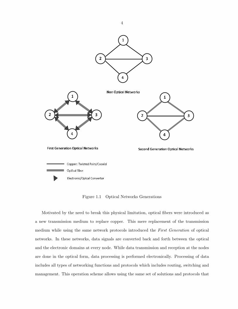
Optical networks have gone through two generations of development. These generations
are depicted in Figure 1.1 with respect to the non-optical networks. While this classification is
of no timing significance as many networks that are widely used today belong to these different
categories, it is mainly based on the degree of usage of the optical components and related
protocols.
Prior to using fiber optics as their transmission medium, communication networks that are
based on copper (e.g., twisted pairs and coaxial cables) and air were widely deployed. In order
to efficiently operate them, great investments were made in these networking technologies,
either in the form of network elements or protocols. As a result, most of these conventional
networks are still in use. However, these networks are not scalable to meet the rapid increase
in bandwidth demands since their transmission rates are upper bounded by their maximum
theoretical capacity according to Shannon-Hartley Theorem.
4 Non Optical Networks 2 4 1 3
Second Generation Optical Networks 2 4 1 3 First Generation Optical Networks 2 4 1 3 Copper: Twisted Pairs/Coaxial Optical fiber Electronic/Opical Convertor
Figure 1.1 Optical Networks Generations
Motivated by the need to break this physical limitation, optical fibers were introduced as
a new transmission medium to replace copper. This mere replacement of the transmission
medium while using the same network protocols introduced the First Generation of optical
networks. In these networks, data signals are converted back and forth between the optical
and the electronic domains at every node. While data transmission and reception at the nodes
are done in the optical form, data processing is performed electronically. Processing of data
includes all types of networking functions and protocols which includes routing, switching and
management. This operation scheme allows using the same set of solutions and protocols that
5
were used with the conventional non-optical networks, yet at faster speed and with better
performance. Hence, these networks are characterized as being the high-speed version of the
traditional networks. Examples of the first generation optical networks include the Synchronous
Optical Networks (SONET) and Synchronous Digital Hierarchy (SDH) networks, Enterprise
Serial Connection (ESCON), High-Performance Parallel Interface (HIPPI), Fiber Distributed
Data Interface (FDDI) and gigabit Ethernet.
Despite the enhancement in the network speed and performance, the effective capacity
achieved by the first generation optical networks is in terms of few Gigabits per second only
which is still much below the available capacity provided by the fiber (which is in terms of tens
of Terahertz). This transmission bottleneck is limited by the maximum electronic processing
speed at each node which allows converting the signals between the electrical and optical
domains at a maximum speed of few Gigabits per second.
On the other hand, the Second Generation of optical networks consist of several optical
solutions. However, these solutions are based on one common operational technology, called
the Wavelength Division Multiplexing (WDM) technology. WDM is proposed to overcome the
electronic bottleneck of the first generation networks by partitioning the optical spectrum into
independent non-overlapping channels. In order to support simultaneous transmissions, each
channel is centered at a specific frequency and assigned a certain bandwidth which allows them
to operate individually at the peak electronic speed using state-of-the-art technology.
Based on their architecture, WDM networks can be classified as Broadcast and Select
Networks and Wavelength Routing Networks. The operation of the first type is based on two
elements, namely, the broadcasting capability of the transmission medium and the tuning
capabilities of the nodes (if such capabilities exist). Due to the first element, no routing
is needed in the broadcast and select networks. Nevertheless, sharing the same transmission
medium requires the use of special medium access control (MAC) schemes in order to arbitrate
the usage of this medium. On the other hand, the second element has direct impact on the
design of these MAC techniques since it determines when and which channel each node can
transmit and receive its packets.
6
Two topologies are used in the broadcast and select networks, namely, the star and the
linear bus topologies. The star topology is based on the use of a special device, called the
Passive Start Coupler (PSC), whose job is to deliver the transmitted signal launched by each
node to all other nodes. This is achieved by internally combining the incoming signals from
the various nodes and splitting their power into multiple output copies that are delivered in-
dividually to every node. However, only those nodes that listen to the correct channel and are
destinations of the specific session are able to process the received data. On the other hand, the
bus topology is based on using a single bus by all the nodes such that transmitting/receiving
the data from/to the bus is done through separate power couplers. Due to the power limitation
imposed from using the power couplers, and because simultaneous usage of the same channel
by multiple transmissions is not allowed, WDM networks based on the broadcast-and-select
architecture are suitable for the use by the local and metropolitan area networks only and sev-
eral protocols were developed for packet switching on such networks using single and multihop
delivery strategies [11, 12].
Unlike the broadcast-and-select WDM architecture, the wavelength routing architecture is
more sophisticated as the network nodes have more networking functionalities (e.g., routing,
switching, wavelength conversion and multicasting capability). Under this architecture, the
network consists of a collection of Optical Cross Connects (OXCs) that are connected by fiber
links in an arbitrary mesh topology. Therefore, this architecture is widely deployed in wide
area networks. The OXCs are capable of routing different wavelengths at an input port to
different output ports which allows different nodes to use the same wavelength on different
fibers in the network using the spatial diversity property.
Depending on the traffic type and the employed protocol, the communication in wavelength
routing networks is carried over clear all-optical delivery structures that are constructed be-
tween the communicating nodes. The signal is transmitted in these structures in the optical
domain and is not converted back to the electronic domain until it reaches its destination
node(s). These delivery structures take the form of a light-path [13], light-tree [2] or light-forest
[14], which are the generalized form of the regular path, tree and forest used in conventional
7
NodalConnectivity
NetworkProvisioning start
Constraints
Network Dimensioning
QoS Constraints
DemandsLogical−circuit
No
SolutionSatistactory
?
OperationalUpgrade?
Yes
No
Actual
Provisioning CircuitsPhysical
Network Operation StageNetwork Design Stage
Existing
Traffic RoutingEstimatedEstimated
Traffic Demands
Yes
QoS Constriants
Connection
/Splitting/λ
Traffic Demands
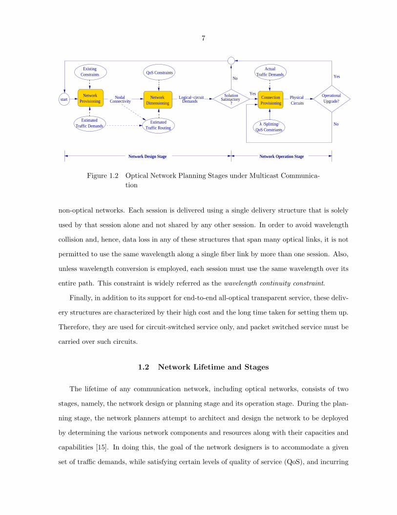
Figure 1.2 Optical Network Planning Stages under Multicast Communica-tion
non-optical networks. Each session is delivered using a single delivery structure that is solely
used by that session alone and not shared by any other session. In order to avoid wavelength
collision and, hence, data loss in any of these structures that span many optical links, it is not
permitted to use the same wavelength along a single fiber link by more than one session. Also,
unless wavelength conversion is employed, each session must use the same wavelength over its
entire path. This constraint is widely referred as the wavelength continuity constraint.
Finally, in addition to its support for end-to-end all-optical transparent service, these deliv-
ery structures are characterized by their high cost and the long time taken for setting them up.
Therefore, they are used for circuit-switched service only, and packet switched service must be
carried over such circuits.
1.2 Network Lifetime and Stages
The lifetime of any communication network, including optical networks, consists of two
stages, namely, the network design or planning stage and its operation stage. During the plan-
ning stage, the network planners attempt to architect and design the network to be deployed
by determining the various network components and resources along with their capacities and
capabilities [15]. In doing this, the goal of the network designers is to accommodate a given
set of traffic demands, while satisfying certain levels of quality of service (QoS), and incurring
8
minimal cost. Network planning is a very complex, and imprecise process. On the one hand,
the optimal allocation and determination of network resources is usually an NP-hard problem.
On the other hand, determining the exact volume, characteristics and requirements for future
traffic demands is an impossible task as these traffic properties are subject to change. There-
fore, coming up with a design that takes care of such imprecise determination of conditions is
a very challenging problem.
The network operation stage deals with a different set of challenges and problems. During
this stage, the network is already provisioned and up and running. Network operators need to
efficiently allocate the existing resources to the actual traffic demands present in the network.
As these demands can be totally different from the ones used during the network design stage,
the objective of the network operators during the network operation stage is to utilize the
available network resources efficiently in order to minimize the loss in the QoS and/or the loss
in the carried traffic. While the first objective is translated to minimizing the degradation
in the provided service quality, the latter objective is viewed as minimizing the number of
dropped sessions.
Based on the type of problems tackled, the network lifetime can be divided into three
conceptual phases, namely, Network Provisioning, Network Dimensioning, and Connection
Provisioning phases. These phases are executed iteratively. The relation, and interaction
between the three phases is shown in Figure 1.2 and are explained in the following subsections.
As shown in Figure 1.2, the Network Provisioning and Network Dimensioning phases are
performed during the network design and are closely related, while the Connection Provisioning
phase is performed during the network operation.
1.2.1 Network Provisioning Phase
Network Provisioning is the first task faced by the network designer. The purpose of this
phase is to determine the network topology, which includes determining:
• The locations and the quantities of the various network resources, such as the: optical
fibers, OXCs, optical amplifiers, wavelength converters, and light splitters.
9
• The virtual topology to be used to provision the estimated traffic demands given the
network resources. This entails computing the light-paths, light-trees and light-forests
for these traffic demands
The traffic demands used in this phase form a challenging problem for the network planner.
The traffic information consists of both the current and the projected traffic demands and it
describes the traffic volumes, characteristics, duration, and QoS. Usually, such traffic demands
are overestimated in order to extend the lifetime of the network.
The problems tackled in this phase are also subject to a number of existing constraints.
These constraints include, for example, the peer-nodes connectivity constraints, the geograph-
ical distribution of the nodes, and the existence of other networks that can be used to deliver
part of the traffic, or at least participate in switching it.
These problems are usually formulated as optimization problems, (e.g., a constrained re-
source allocation problem), whose solutions are obtained using conventional optimization tech-
niques. The objective function of these problems takes the form of minimizing a cost function
of the optical components used in the network.
The output of the Network Provisioning phase takes the form of a connectivity matrix that
specifies the connection pattern between the various network components along with their
optimal (or near optimal) physical locations in the network. This output in conjunction with
the estimated traffic demands and their QoS requirements form the input to the next phase of
the network design stage, namely, the Network Dimensioning phase.
1.2.2 Network Dimensioning Phase
The second phase of the network design stage is the Network Dimensioning phase. Its
goal is to determine the optimal dimension (i.e., size) of the various network resources such
that the QoS requirements are met. The input parameters to this phase include the projected
traffic demands, a specific routing strategy, and the network resources determined during the
Network Provisioning phase. The output results of this phase include determining:
• The link capacity in terms of the number of fibers per link,
10
• The fiber capacity in terms of the number of wavelength channels per fiber, and
• The channel capacity in terms of the transmission rate.
Up to this point, the network design in terms of its topology and resources capacities is
complete. Validating such a design is needed to examine its effectiveness before the physical
deployment of the network. A Design Effectiveness Metric (DEM) [15] is used for this purpose,
and it can be defined in a number of ways. The most widely used definition for the DEM is
the ratio of the number of accommodated (accepted) calls to the total cost of the designed
network. This metric is also referred to as calls per dollar. If the DEM of a certain solution
for the network design stage fails to satisfy a specific threshold measure, the network design is
revised in an iterative manner until the most appropriate network design candidate is found.
1.2.3 Connection Provisioning Phase
The network realization is the process of putting the network into operation and it com-
prehends the actual construction of the network from the design-blueprints and setting up the
protocol stacks. Once the network is launched, the network operators become in charge and
the network lifetime enters its operation stage.
As the projected traffic used to design the network is no more than an assessment of the
actual traffic, the traffic demands during network operation may, or may not, meet these
assessments. The difference in these traffic values may result in not accommodating all the
sessions in the network. This requires operating the network with its current provisioned
resources in a manner that maximizes the effective network utilization while guaranteeing the
different connections QoS requirements. This directly translates into greater revenue to the
network operator. Network utilization can be maximized by maximizing the ratio of the actual
accepted calls with respect to the total number of arriving calls which is referred to as the calls
acceptance probability.
This problem is known as the Connection Provisioning problem. In optical networks, the
Connection Provisioning problem is responsible for all of the following tasks:
11
1. Route determination,
2. Wavelength assignment and resource allocation along the computed routes,
3. Power allocation.
4. Call establishment,
5. Error recovery due to nodes and/or links failures,
6. Traffic rerouting and wavelength reassignment in order to accommodate more traffic
sessions (especially in the case of dynamic routing and wavelength assignment), and
7. Call termination and the deallocation of their associated network resources1.
As such, the Connection Provisioning problem lasts for the duration of the network op-
eration as it is exercised before call establishment, during the lifetime of calls, and after the
termination of calls.
1.3 All Optical Multicasting (AOM)
Traditionally, multicast communication refers to transmitting the information (data, audio
or video) from one source node to multiple receipts which helps reducing the amount of required
bandwidth. In the literature, it is also referred to as multipoint and 1-to-many communication.
Being a fundamental communication type in many networks, supporting multicast-based traffic
and services had been investigated in almost every networking environment and wavelength-
routing optical networks is not an exception. Nevertheless, what makes multicast support in
this environment more interesting is its capability to support a special form of multicasting,
called the All Optical Multicasting (AOM).
While supporting the same operational goal (i.e., 1-to-many data delivery), the main dif-
ference between the AOM and the conventional multicasting is in their operation layer. In
a nutshell, AOM operates in the lowest optical networking layer, namely, the optical layer,1Please note that the wavelength assignment and power allocation requirements are optical network specific
while the other tasks are common among the different types of networks.
12
while the conventional multicasting protocols reside at higher layers2. Consequently, AOM
eliminates any conversion of the transport signal between the electronic and optical domains
at the intermediate nodes and data duplication is achieved using passive power splitters as was
introduced in [2]. This operation scheme has the following advantages:
1. Removing the dependencies on the signal type, modulation, coding, bit rates and proto-
col. This provides signal transparency which has the advantage of enabling the optical
layer to support different networking layers at the same time (e.g., IP or ATM data).
Also, it contributes to reducing the nodes complexity and cost.
2. Since signal transparency is already achieved in unicast traffic by using light-paths, sup-
porting multicast traffic all-optically presents another huge step toward achieving the
all-optical service delivery as a unified delivery mechanism for the various traffic types in
the wavelength routing networks. Such unified transmission scheme provides consistency
in the network services which can reflect positively towards simplifying its design and
operation,
3. Using power splitters to duplicate multicast data in the optical domain is much simpler
than packet duplication used by the conventional multicasting. On one hand, these
devices are passive, namely, no power is needed to operate them; therefore, its operation
is more cost effective. On the other hand, this operation does not require the use of any
buffer for data duplication as it is the case with higher layer multicasting. With high
speed networks, this buffer can be so huge and consume a significant percentage of the
node power and processing capacity.
4. Simplifying the logical network stack structure by increasing the number and complexity
of the functions to be handled optically in the optical layer. Also, it enhances the quality
of the produced solution and improves response time to any changes in the optical layer.2For example, IP multicasting is implemented at the IP layer while Ethernet multicast addressing and ATM
point-to-multipoint Virtual Circuits (VCs) are at the data link layer.
13
5. Reducing the OXCs cost by eliminating the need for using the signal converters to trans-
form the signal between the optical and electronic domains.
6. As a result of eliminating the signal conversion and packet duplication using buffers,
the delay encountered by AOM at each OXC is much less than that of the conventional
multicasting. This has a positive impact on meeting the QoS requirements, especially
the delay and the delay jitter, of the received signals at all the destinations.
1
Outputs
Inputs . . .
. . . . . . . . . . . . . . . . . . . . . . . . . . . . . . . . .
2 P
1 2 P . . .
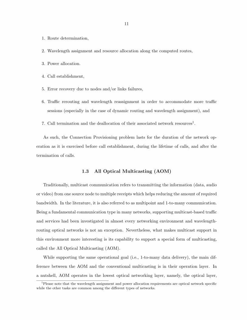
Splitter Gate 2 x 1 Switch Figure 1.3 Splitter-and-Delivery (SaD) OXC.
In order to support the AOM service in wavelength-routing networks, it is necessary to
integrate the splitting capability into the OXC architecture. OXCs that are equipped with
14
the splitting functionality are called the Multicast-Capable (MC) switches while those with no
splitting capability are referred to as the Multicast-Incapable (MI) switches [16].
Several MC nodal architectures have been proposed in the literature. For example, the
Splitter-and-Delivery (SaD) switch was introduced in [17] and it is depicted in Figure 1.3. The
design of the SaD switch consists of two stages. In the first stage, each input signal is initially
split into a number of sub-signals that equals the nodal degree. In the second stage, the split
signals are then switched to the appropriate output port using a combination of 1×2 switches.
This design of the SaD switches has the advantage of providing a non-blocking service, namely,
no call is dropped due to lack of the splitting or switching resources. However, it is a very
complicated design which does not distinguish between the different traffic types. Therefore,
the unicast traffic undergoes unnecessary power loss.
Po
we
rS
plitte
r
2x1 SE
Multicast 100%
Unicast
1
2
N
To Local Switch
Split−Switch Bank
λ 1 λ Μ
λ 1 λ Μ
λ 1 λ Μ
λ 1 λ Μ
λ 1 λ Μ
λ 1 λ Μ
2
Ν
1
2
Ν
1
λ Μ
SSB
λ 1 λ Μλ 1 λ Μ
λ 1
SSB
MuxDemux SwitchSpace Switch
Tx RxLocal Station
Split−Switch Bank
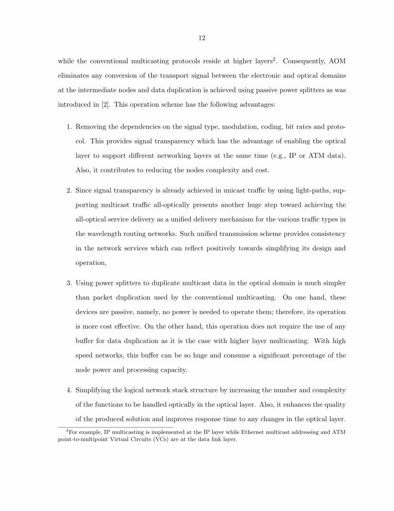
Figure 1.4 Multicast-only Splitter-and-Delivery (MOSaD) OXC.
To address the limitations of the SaD switch, the Multicast-Only Splitter-and-Delivery
(MOSaD) switch was proposed in [18]. First, it reduces the complexity of the switch by
15
sharing the splitters by a group of multicast sessions which reduces the number of used splitters.
Second, signal splitting is performed only for the multicast traffic. Figure 1.4 shows the basic
structure of the MOSaD OXC. As shown in the figure, the wavelengths are first optically
demultiplexed on all the input fibers and the signals of the same frequency are directed to the
corresponding space switch. Each space switch in turn switches the input signal to either a
corresponding output link if it is of unicast type or to a special component called Split-Switch
Bank (SSB) if it is of multicast type. Only one SSB is attached to each space switch and
its purpose is to split the incoming multicast signal and then switch it to the corresponding
output link. This contributes to reducing the structure complexity; yet, at most one multicast
session over each channel can be provisioned at the same time while others will be blocked.
1:M
Splitter
Nx1
SD Switch
λ 2
λ 1
λ Μ
12
Μ
12
Μ
12
Μ
λ 2
λ 1
λ Μ
λ 2
λ 1
λ Μ
λ 2
λ 1
λ Μ
λ 2
λ 1
λ Μ
λ 2
λ 1
λ Μ
λ 1 λ Μ
λ 1 λ Μ
λ 1 λ Μ
λ 1 λ Μ
λ 1 λ Μ
λ 1 λ Μ
2
Ν
1
2
Ν
1
TF WCMuxDeMux
Figure 1.5 An example of Multicast Capable Switch with Wavelength Con-version reported in [1].
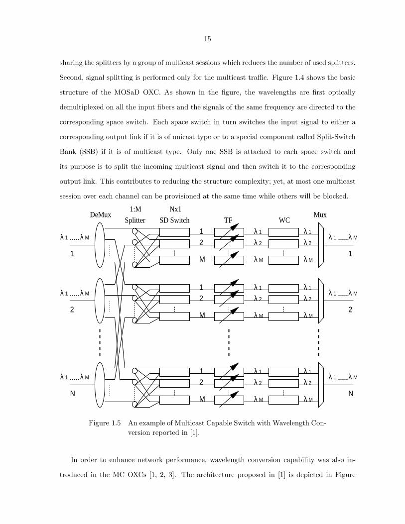
In order to enhance network performance, wavelength conversion capability was also in-
troduced in the MC OXCs [1, 2, 3]. The architecture proposed in [1] is depicted in Figure
16
1.5. First, the signals are split. The split signals then pass through a space-division (SD)
switch which can then be converted into different wavelengths by using wavelength converters.
Finally, the signals are then multiplexed on an output port fiber.
OSW
OSW
λa
λb
MuxDemux
Regeneration bank
Converter bank
Amplifier bank
Power splitter
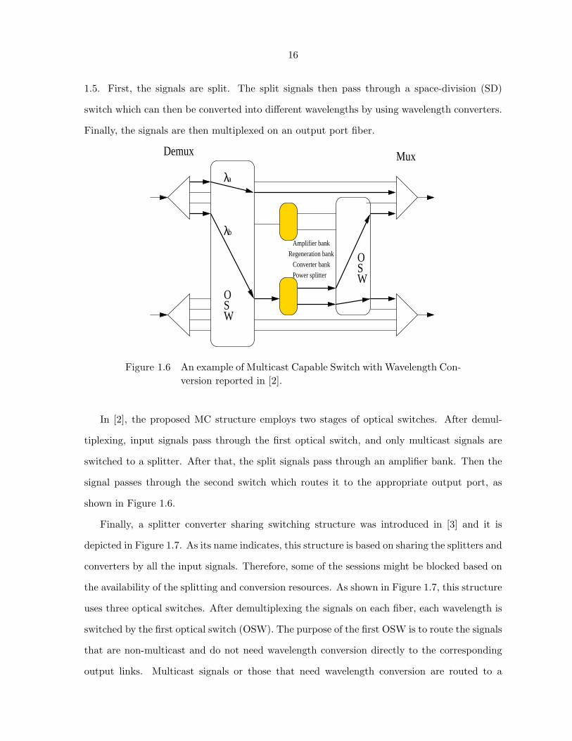
Figure 1.6 An example of Multicast Capable Switch with Wavelength Con-version reported in [2].
In [2], the proposed MC structure employs two stages of optical switches. After demul-
tiplexing, input signals pass through the first optical switch, and only multicast signals are
switched to a splitter. After that, the split signals pass through an amplifier bank. Then the
signal passes through the second switch which routes it to the appropriate output port, as
shown in Figure 1.6.
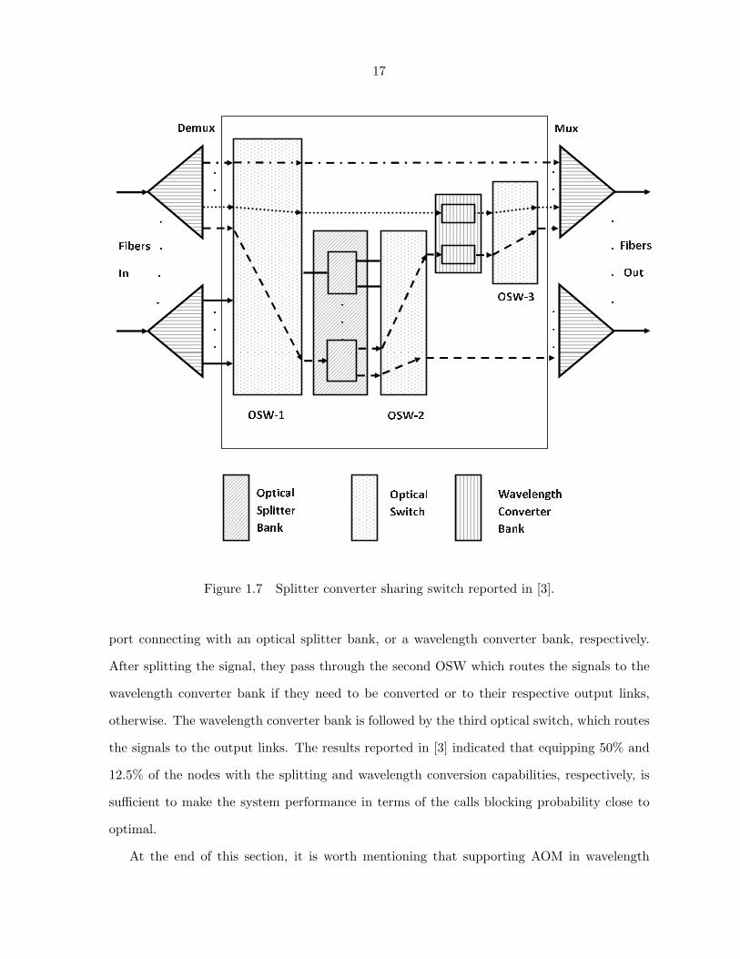
Finally, a splitter converter sharing switching structure was introduced in [3] and it is
depicted in Figure 1.7. As its name indicates, this structure is based on sharing the splitters and
converters by all the input signals. Therefore, some of the sessions might be blocked based on
the availability of the splitting and conversion resources. As shown in Figure 1.7, this structure
uses three optical switches. After demultiplexing the signals on each fiber, each wavelength is
switched by the first optical switch (OSW). The purpose of the first OSW is to route the signals
that are non-multicast and do not need wavelength conversion directly to the corresponding
output links. Multicast signals or those that need wavelength conversion are routed to a
17 . . Fibers . Out . . Fibers . In . . . . .
. . OSW-1 OSW-2
OSW-3 Mux Demux . . . . .
. . . Optical Switch Wavelength Converter Bank Optical Splitter Bank
Figure 1.7 Splitter converter sharing switch reported in [3].
port connecting with an optical splitter bank, or a wavelength converter bank, respectively.
After splitting the signal, they pass through the second OSW which routes the signals to the
wavelength converter bank if they need to be converted or to their respective output links,
otherwise. The wavelength converter bank is followed by the third optical switch, which routes
the signals to the output links. The results reported in [3] indicated that equipping 50% and
12.5% of the nodes with the splitting and wavelength conversion capabilities, respectively, is
sufficient to make the system performance in terms of the calls blocking probability close to
optimal.
At the end of this section, it is worth mentioning that supporting AOM in wavelength
18
routing networks can be achieved even without the use of optical splitters. In order to do
so, a new architecture, called the Tap-and-Continue (TaC) OXC was proposed in [19]. The
basic structure of the TaC OXC is similar to that of the MOSaD OXC [18]. However, the
SSB modules used in the MOSaD OXC are replaced by a new module called the TaC modules
(TCM) in the TaC OXC. In the TCM, instead of using splitters to split the signals, power
taps are used. When a multicast signal passes through a TCM, only a small fraction of this
signal is tapped and forwarded to the local station, while the remaining power is switched to
an output port. Special routing schemes are needed in TaC-based networks as the routing
problem is more difficult and involved.
1.4 Challenges of Supporting AOM Service in Wavelength Routing
Networks
Supporting multicast communication in single channel networks (e.g., IP networks) presents
a number of challenges, and has thus been the subject of extensive research [20, 21, 22, 23,
24]. These challenges become even more critical in multi-channel wavelength-routing networks
which also introduce their own set of unique problems that prevent having an easy application
of the traditional multicast solutions on wavelength routing networks.
The uniqueness of these problems stems from the distinctive characteristics of the wavelength-
routing networks. Among these characteristics is the operation mode of these networks. As
shown earlier in Subsection 1.2.3, the connection provisioning phase of the network operation
includes two operations which are unique to optical networks, namely wavelength assignment
and power allocation tasks. Therefore, any traditional multicast protocol that operates on
a non-optical network cannot perform well in its wavelength-routing counterpart due to lack
of consideration of these additional operations. Another unique source of challenges comes
from the optical hardware components of the networks. The impact of each optical component
on the signal quality and the degree of deployment of these elements in the network are two
fundamental factors in determining the success of any optical multicasting scheme.
However, other challenges and limitations also exist. To resolve all of these limitations
19
and to achieve an efficient use of the various network resources, the AOM protocols should
be carefully designed. In the following subsections, we will address these different challenges
individually, and we will discuss how they impact the implementation of AOM in wavelength-
routing networks.
1.4.1 Challenges Due to High-Transmission Rates
With the use of WDM technology, the transmission rate of the individual channels is on
the order of 10 Gb/s to 40 Gb/s. Therefore, the delay-bandwidth product3 in WDM networks
is very large, and it increases with the increase in the network diameter. As a result, network
operation that depends on the feedback from the network is adversely impacted and might
not be a good choice. For example, on-demand routing strategies which probe the network
resources when a connection is to be established will result in bandwidth wastage and increased
connection latency.
In addition, optimal provisioning, which requires increased computation, and node coor-
dination, can also result in far from optimal resource utilization. Therefore, it is essential to
design lightweight protocols that are efficient, but simple enough so that it can be executed fast
enough and don’t form a bottleneck to the network. However, the simplicity and the efficiency
of the protocols seem to be two conflicting goals.
1.4.2 Challenges Due to the Characteristics of the Wavelength-Routing Networks
Wavelength-routing networks are unique environment and they have a number of special
characteristics that affect its support for AOM service. These characteristics include the use
of multiple channels, the circuit-switched connection mode and the employment of the various
optical components. We will briefly describe each of these characteristics and the limitations
they impose in the following subsections:3The delay-bandwidth product is the ratio of the propagation delay to the packet transmission time. This
metric provides an indication of the number of data packets in the transmission pipe.
20
1.4.2.1 Multi-Channels Environment Limitations
Although WDM networks consist of multiple independent channels over any link, the usage
of these channels is not totally independent of each other, either on the same link or on
different links. Such channels dependency precludes the use of several conventional multicasting
techniques (e.g., IP multicasting) in the wavelength-routing networks as such techniques treat
these channels independently.
For example, different channels must be used by different sessions over the same link in
order to prevent data corruption. Also, in the case of no, or limited, wavelength conversion
in the network, maintaining the wavelength continuity constraint is required for the success of
any multicast session. Wavelength continuity constraint must be satisfied both in depth due
to signal propagation, and in breadth, due to multicasting and signal branching.
Finally, the availability of transceivers (i.e., transmitters and receivers) at the end points
of the trees (i.e., source and destination nodes, respectively) is necessary to ensure correct
operation of the network. These transceivers can be either fixed or tunable. To guarantee the
correct delivery of the data, the source’s transmitter and the destinations’ receivers should be
available and tuned to the same transmission channel.
1.4.2.2 Circuit-Switched Communications Limitations
Circuit-switching is the main communication mode employed in wavelength routing net-
works. Circuit-switching has the following characteristics [15]:
• Resource reservation is performed along each determined route,
• Setup time for each session route is long,
• Any connection request can be blocked due to lack of resources, and
• The connections are static and have long-duration.
These characteristics can be addressed in AOM at different contexts. First, the performance
metrics for multicasting must be chosen carefully. For example, since blocking can occur due
21
to lack of resources, the call acceptance probability can be defined differently. In this context,
data delivery to a subset of the multicast group is allowed instead of delivering it to all the
members of the group as was proposed in [25, 26]. Other performance metrics also include:
reducing the connection setup time [27], reducing the propagation delay per receiver [1] and
reducing the total multicast tree cost [1, 28, 29, 30].
Second, this operation mode affects the choice of applications to be supported in the net-
work. The circuit-switching nature best suits those applications that are of high utilization,
require low delay and are not affected by the high setup time of the connections. Such ap-
plications include for example the uncompressed audio and video and the various multimedia
applications. However, the real-time applications, especially those that require stringent con-
strains in terms of setup time, cannot directly fit into such network and they require special
treatment.
Third, these features do not only affect network operation, but also the network provisioning
and dimensioning, as they impact the cost of the network, and its ability to handle the projected
traffic.
1.4.2.3 Optical Hardware Limitations
The limitations of the state-of-the-art of optical components, and the high cost associated
with their usage preclude full deployment of such components at all nodes of the network.
This results in deploying different OXC structures in the network. For example, some nodes
may be MC nodes while others are MI. Also, only subset of the nodes (can be MC nodes
themselves) may be equipped with wavelength conversion capability. Moreover, the splitting
and conversion capabilities, if they exist, may be incomplete. In this context, the fanout of the
splitters can be less than the nodal degree while wavelength conversion can be done between
specific regions of the optical spectrum only. This asymmetric deployment has a significant
effect on the multicast routing and tree maintenance. In the following, we will describe the
impact of the various optical components on AOM.
22
- Optical Splitting Impact
Light splitting is equivalent to packet replication in the electronic domain, yet, it is the-
oretically simpler. In addition, a simple version of the splitting capability, which is assumed
to be available at all the nodes, is the Drop-and-Continue (DaC) [1, 28] (or sometimes called
the Tap-and-Continue (TaC) [19, 30]) capability. This refers to tapping a small amount of the
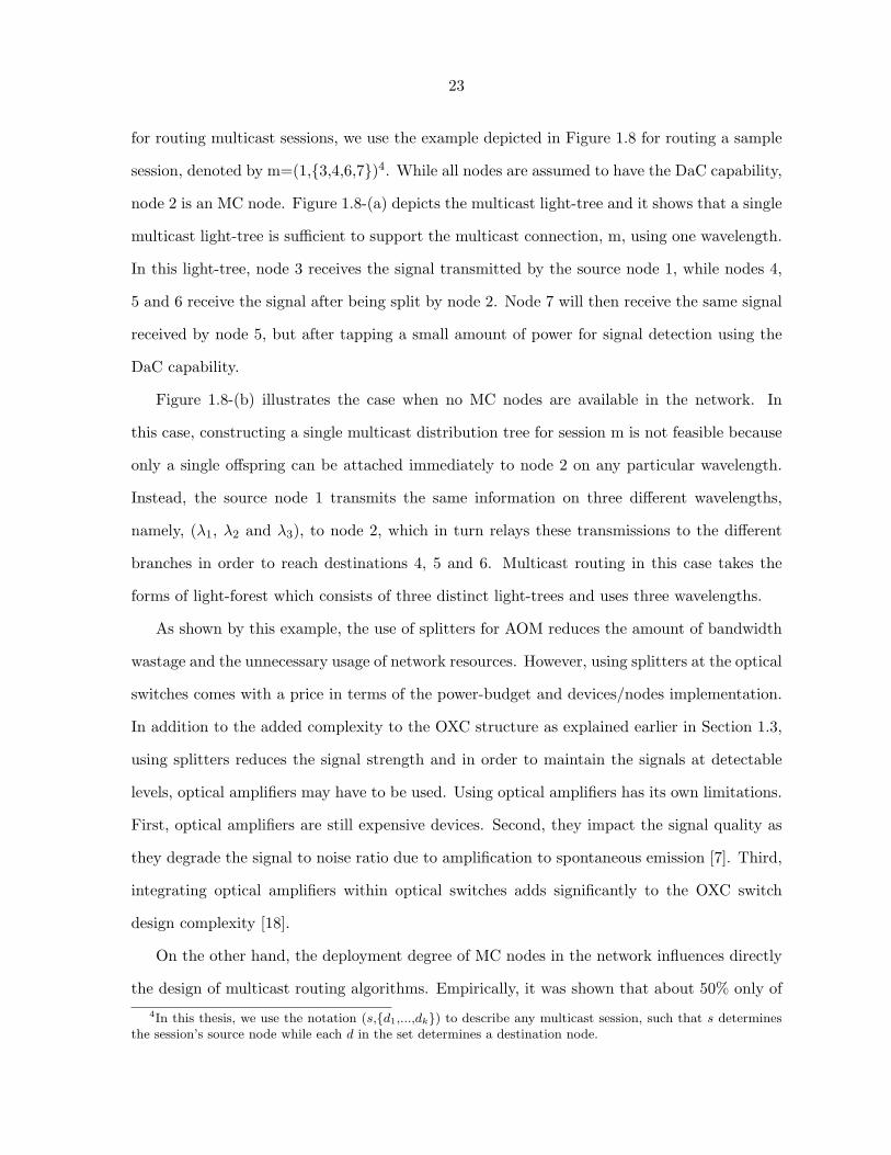
power which is used for signal detection by the receiver connected to the node. 4 7
1 6 3 5 2
(a) 2 λ3 MI node λ2 λ1 MC node
(b) 7 4 6 3 5 1
(c) 3 7 2 1
4 6 5 Figure 1.8 An example that illustrates the construction of the multicast
delivery structure (light-tree or light-forest) for the multicastsession m=(1,3,4,6,7) when: (a) node 2 is an MC node withcomplete splitting capability, (b) node 2 is an MI node, and(c) node 2 is an MC node with limited splitting capability andsplitting fanout equals 2 only.
The wavelength splitting capability is a key enabling technology for multicast communi-
cation in wavelength-routing networks. In order to illustrate the significance of light-splitters
23
for routing multicast sessions, we use the example depicted in Figure 1.8 for routing a sample
session, denoted by m=(1,3,4,6,7)4. While all nodes are assumed to have the DaC capability,
node 2 is an MC node. Figure 1.8-(a) depicts the multicast light-tree and it shows that a single
multicast light-tree is sufficient to support the multicast connection, m, using one wavelength.
In this light-tree, node 3 receives the signal transmitted by the source node 1, while nodes 4,
5 and 6 receive the signal after being split by node 2. Node 7 will then receive the same signal
received by node 5, but after tapping a small amount of power for signal detection using the
DaC capability.
Figure 1.8-(b) illustrates the case when no MC nodes are available in the network. In
this case, constructing a single multicast distribution tree for session m is not feasible because
only a single offspring can be attached immediately to node 2 on any particular wavelength.
Instead, the source node 1 transmits the same information on three different wavelengths,
namely, (λ1, λ2 and λ3), to node 2, which in turn relays these transmissions to the different
branches in order to reach destinations 4, 5 and 6. Multicast routing in this case takes the
forms of light-forest which consists of three distinct light-trees and uses three wavelengths.
As shown by this example, the use of splitters for AOM reduces the amount of bandwidth
wastage and the unnecessary usage of network resources. However, using splitters at the optical
switches comes with a price in terms of the power-budget and devices/nodes implementation.
In addition to the added complexity to the OXC structure as explained earlier in Section 1.3,
using splitters reduces the signal strength and in order to maintain the signals at detectable
levels, optical amplifiers may have to be used. Using optical amplifiers has its own limitations.
First, optical amplifiers are still expensive devices. Second, they impact the signal quality as
they degrade the signal to noise ratio due to amplification to spontaneous emission [7]. Third,
integrating optical amplifiers within optical switches adds significantly to the OXC switch
design complexity [18].
On the other hand, the deployment degree of MC nodes in the network influences directly
the design of multicast routing algorithms. Empirically, it was shown that about 50% only of4In this thesis, we use the notation (s,d1,...,dk) to describe any multicast session, such that s determines
the session’s source node while each d in the set determines a destination node.
24
the nodes in the networks need to be MC nodes in order to achieve good performance level [31,
32]. Networks in which both MC and MI nodes coexist are known in the literature as networks
with sparse-splitting [31] and they are known to implement Partial Packet Replication (PPR)
[33]. Many schemes were introduced to deal with sparse-splitting situation as in [1, 29, 30, 28].
In addition, two extreme strategies for MC node deployment were investigated in the literature
in which all the nodes are either MI nodes, e.g., [19], or MC nodes, e.g., [25, 2, 26]. These
strategies are called, no-splitting (or No Packet Replication-NPR), and full -splitting (or Full
Packet Replication-FPR), respectively.
Moreover, multicast support in wavelength-routing networks is also influenced by the split-
ting fanout, which is the maximum number of multicast tree branches supported per node.
The fanout of an MC node is denoted by f, where 1 ≤ f ≤ d -1 and d is the nodal degree.
When f equals d -1, the switch is said to have a complete splitting capability; otherwise, the
splitting capability of the node is limited since only a selected subset of the node’s neighbors
can receive the split signal. The splitting fanout is an important parameter in the design of
multicast trees and it also impacts the choice of the number of amplifiers, their placement, and
signal-to-noise ratio.
In order to illustrate the importance of the splitting degree on the resultant multicast
delivery structure, consider the same example and system setup depicted in Figure 1.8-(a)
but with the assumption that the f factor for node 2 is 2. This example is shown in Figure
1.8-(c). With this configuration, the branching node 2 can forward the signal to only two of
its offsprings, say nodes 4 and 5. In order to deliver the data to the remaining node, namely
node 6, a new light-tree connection from the source node 1 must be established via node 2
using a new wavelength (λ2). As a result, the multicast delivery structure is a light-forest that
consists of 2 light-trees that are carried on two different wavelengths.
Finally, the splitting ratio also influences the multicast tree construction. Signal splitting
ratio can be either fixed or adjustable. With fixed splitting, the light-splitter ideally divides the
input signal equally into f output signals (assuming no other loss is encountered), where f is
the fanout factor. This splitter type is a passive one, which is simple and inexpensive. However,
25
it can be power inefficient, especially when the multicast tree is unbalanced. In this case, some
signal power is wasted and the multicast tree size is affected. On the other hand, splitters
with adjustable splitting ratios can significantly reduce the power wastage which may lead to
increasing the multicast group size5. It is also worth mentioning that the use of splitters with
adjustable splitting ratios becomes imperative in the context of dynamic multicasting where
the multicast tree structure dynamically changes. However, splitters with adjustable-ratio are
active devices that are more expensive than their fixed-ratio counterparts, may be unstable
and may not be noise-immune.
- Wavelength Conversion Effect
Wavelength-converters are active optical devices which shift the optical signal from one
optical frequency to another. The employment of wavelength converters provides flexibility
in the network operation and enhances its performance. Using wavelength converters elimi-
nates the wavelength continuity constraint which results in simplifying the multicast routing
computation.
All-optical wavelength converters [34, 35], however, are still very expensive and immature.
Also, equipping the switch with wavelength converters complicates the switch design and in-
creases its cost, which hinders the full deployment of wavelength converters in the network.
Instead, the no- and sparse- wavelength conversion options are more practical options. The
full (no) wavelength conversion capability is the most (least) flexible and provides the best
(worst) blocking probabilities for the calls; however it is the most (least) expensive. The
sparse-wavelength conversion option, on the other hand, refers to the situation in which only
a subset of the nodes are equipped with converters. It can achieve a balance between the cost
and the network performance, and thus, it seems to be the most practical option.
On the other hand, wavelength conversion capability can be limited. Limited conversion
means that conversion from a certain wavelength is limited to only a sub-band of the optical
spectrum. Sparse-, no- and limited-conversion configurations requires some degree of wave-5Please refer to [9] for a detailed analysis of this issue
26
length continuity, which restricts the multicast tree construction.
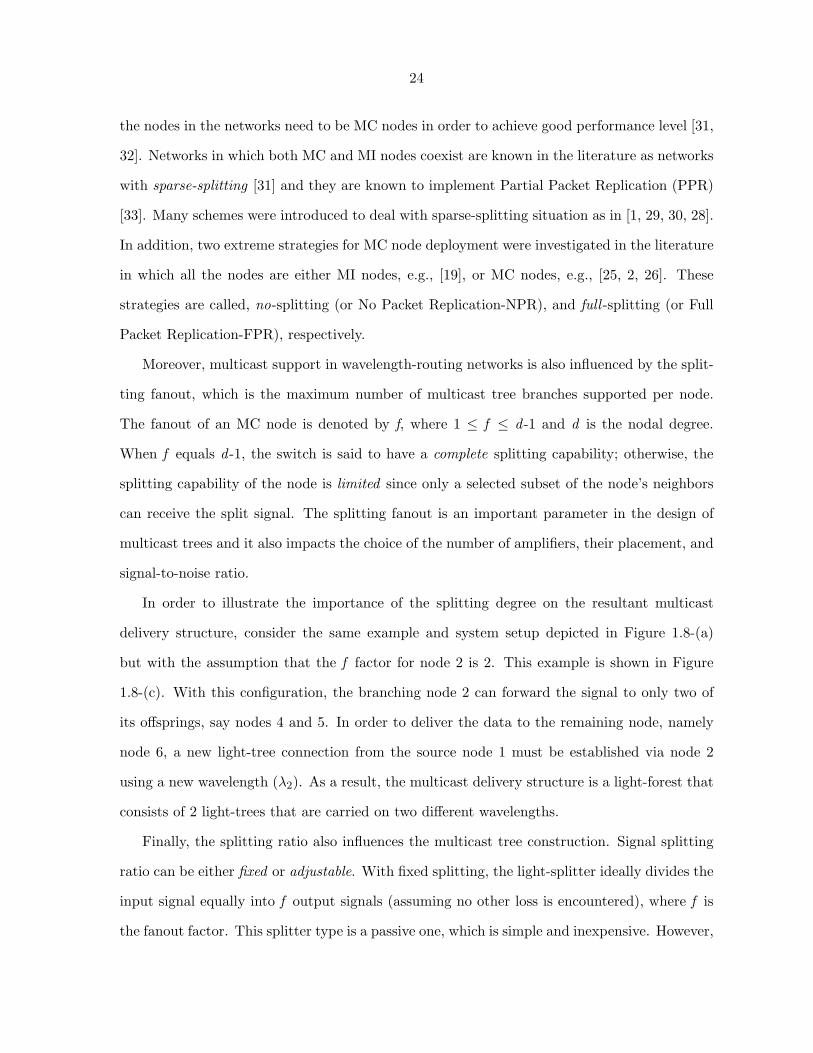
Moreover, integrating wavelength converters with splitters can take two forms, namely,
Pre-Conversion or Post-Conversion. As shown in Figure 1.9, these schemes correspond to
placing the converters before or after the light splitter, respectively6. Since a single converter
is needed, the cost associated with the Pre-Conversion scheme is much less than that of the
Post-Conversion scheme. Both schemes provide the same degree of flexibility if converters
always convert from λi to λj . Otherwise, the Post-Conversion scheme in general exhibits more
flexibility and results in higher system performance.
λ i
λ j
λ kλ i
λ i
(b) (a)
λ j
λ j
λ j
iλ
Light−Splitter
Wavelength−Converter
Figure 1.9 Splitter-converter relative locality in the switch (a) Pre-Conver-sion Scheme, and (b) Post-Conversion Scheme.
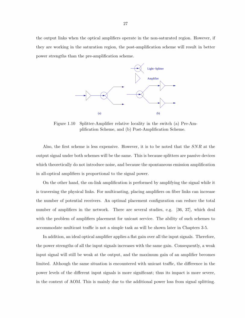
- Optical Amplification Impact
The final hardware-related challenge is the amplifier placement problem. In multicast
communication, power loss can be due to fiber attenuation and splitter loss, if any. One of two
techniques for signal amplification may be used, namely, on-site and on-link amplifications.
With the on-site amplification, the amplification is performed inside the switching node itself.
There are two methods to integrate the amplifier and the splitter within the node. In the first
one, called the Pre-Amplification technique, the amplifier is placed before the splitter, while in
the other case, called the Post-Amplification technique, it is placed after the splitter, as shown
in Figure 1.10. Both configurations exhibit the same performance in terms of power values at6Because each wavelength requires a separate converter, Figure 1.9 depicts the requirements for a single
input-output channel pair (i.e., λi and λj , or λk), regardless of the range of the wavelengths at their input andoutput.
27
the output links when the optical amplifiers operate in the non-saturated region. However, if
they are working in the saturation region, the post-amplification scheme will result in better
power strengths than the pre-amplification scheme.
Amplifier
Light−Splitter
(a) (b)
Figure 1.10 Splitter-Amplifier relative locality in the switch (a) Pre-Am-plification Scheme, and (b) Post-Amplification Scheme.
Also, the first scheme is less expensive. However, it is to be noted that the SNR at the
output signal under both schemes will be the same. This is because splitters are passive devices
which theoretically do not introduce noise, and because the spontaneous emission amplification
in all-optical amplifiers is proportional to the signal power.
On the other hand, the on-link amplification is performed by amplifying the signal while it
is traversing the physical links. For multicasting, placing amplifiers on fiber links can increase
the number of potential receivers. An optimal placement configuration can reduce the total
number of amplifiers in the network. There are several studies, e.g. [36, 37], which deal
with the problem of amplifiers placement for unicast service. The ability of such schemes to
accommodate multicast traffic is not a simple task as will be shown later in Chapters 3-5.
In addition, an ideal optical amplifier applies a flat gain over all the input signals. Therefore,
the power strengths of all the input signals increases with the same gain. Consequently, a weak
input signal will still be weak at the output, and the maximum gain of an amplifier becomes
limited. Although the same situation is encountered with unicast traffic, the difference in the
power levels of the different input signals is more significant; thus its impact is more severe,
in the context of AOM. This is mainly due to the additional power loss from signal splitting.
28
This implies that a multicast signal may not obtain enough power if it is accompanied by other
stronger signals.
Moreover, to find an optimal amplifier placement for a multicast tree, at least two parame-
ters, namely, signal power and source-destination distance, should be given. However, dynamic
multicasting and the use of adjustable splitting coefficient aggravate the problem since the for-
mer results in changing the communication diameter, while the latter changes the signal power.
This problem can be solved by using the splitter with Post-Amplifier configuration shown in
Figure 1.10-(b) or by introducing equalization at each amplifier stage [7].
Finally, using optical amplifiers impacts the SNR. All-optical amplifiers, e.g., Erbium-
Doped Fiber Amplifiers (EDFA), amplify noise due to spontaneous emission [7], which impacts
the signal quality levels and imposes an upper bound on the number of optical amplifiers the
signal can traverse before getting regenerated. Therefore, this contribution of the optical
amplifiers in the noise level has a direct influence on the network design and operation.
1.4.3 Challenges Due to Routing and Wavelength Assignment
In this subsection, we focus on two basic functions in wavelength-routing networks, namely,
Routing (R) and Wavelength Assignment (WA), from the multicasting viewpoint. R and WA
problems have been extensively studied under unicast communication [7]. Solving the com-
bined R and WA problems (conventionally referred to as RWA problem) produces the optimal
solutions. However, due to the difficulty of the RWA problem, the R and WA subproblems are
treated separately. The multicast extension of the conventional RWA problem is referred to as
MCRWA [25] or MC-RWA [26].
MCRWA problem is mainly concerned with establishing the multicast route in the net-
work, and determining the appropriate wavelength to be assigned to it. It has the objective of
minimizing the required network resources, especially the number of wavelengths, or maximiz-
ing the number of accepted calls. The combined problem has been proven to be NP-Complete
[25, 38] since it involves finding an optimal multicast tree which is the well-known NP-Complete
Steiner Minimum Tree (SMT) problem [39]. Hence, it is solved using heuristics. The com-
29
bined MCRWA can also be characterized as a wavelength-aware approach because computing
the multicast delivery structure is directly influenced by the status of the wavelengths in the
network and the cost associated with their use.
Similar to the traditional RWA in unicast networks, the MCRWA can be solved as two sepa-
rate problems, namely, the multicast tree is first determined, followed by appropriately selecting
wavelength(s) on this route. Therefore, the uncoupled version of MCRWA is a wavelength-
unaware approach. The routing part of the problem is still NP-Complete since it involves the
construction of the SMT, but the wavelength assignment part can be solved in polynomial time
for some special cases, e.g. [38, 40]. Decoupling the routing and wavelength assignment prob-
lems simplifies the problem slightly, and also provides flexibility in enhancing routing protocol
designs and integrating extra operations and features, such as QoS guarantees, fault-tolerance,
and security.
Furthermore, different operational modes for the R and WA operations were proposed
in the literature. Each mode has its own performance degrees and associated costs. The
performance-cost trade-off of these operation modes must be considered in the protocol design
process. In this context, and at the routing side of the problem, the routing schemes have been
traditionally characterized as either: (1) fixed : in which a fixed route per call is established, (2)
alternate: a set of paths are assigned for each call which are searched sequentially in a specific
order in order to pick the route, and (3) adaptive, in which the route is found dynamically
based on the network status. The flexibility of these schemes increases from the fixed to the
adaptive, but at the cost of increased overhead and complexity.
Similarly, many schemes have been proposed in the literature for WA. However, four of
these schemes were inherited from unicast communication, namely: (1)random, in which wave-
length selection is performed randomly from the set of available wavelengths, (2) first-fit, which
chooses the first available wavelength, (3) least-used, and (4) most-used, in which the wave-
length to be chosen is based on the degree of its usage. In general, the complexity of the
wavelength assignment problem is a design factor that must be considered.
Finally, the routing and wavelength assignment in optical network can be performed in two
30
computational modes: on-line and off-line. The on-line mode allows requests to be processed
as they arrive to the system, i.e., it does not assume prior knowledge of the traffic in the
network, and the admission decision of the connection is based on the instantaneous network
state. If the connection request is admitted, its route and the assigned wavelengths are usually
not changed during the lifetime of the connection. Otherwise, and because of the no waiting
feature of circuit-switched service, the connection is blocked. The off-line mode, on the other
hand, assumes prior knowledge of all the connection requests which makes it possible to obtain
an optimal allocation for the routes and the wavelengths. The first computation mode is more
practical, but optimal operation is more difficult, while the opposite is true for the second
computation mode.
1.4.4 Challenges Due to the All-Optical-Multicasting (AOM) Characteristics
All-Optical Multicasting (AOM) inherits all the problems of conventional multicasting. For
example, the ideal operation of the multicast session entails hiding the information about the
various receivers from the source node, and vice versa. This information includes the nodes’
addresses, locations and their total number. A dedicated address is assigned to the multicast
session, which is globally known. This requirement is still not yet fully achieved in most routing
and wavelength assignment techniques of AOM, which are based on a key assumption of global
(or partial) knowledge about the network topology, and the nodes membership. However, [27]
appears as an exception in which the source node needs not to know about the destination
nodes and their locations.
In addition, different attributes of the multicast session may necessitate the use of routing
strategies, which may look suboptimal, but are necessary because of the all-optical nature of
the session. For example, consider the case when the multicast session has a short duration,
and its member group size is small and are geographically far away from each other. Under
such scenario, the designers might find it more efficient to use separate unicast connections,
one for each destination, instead of attempting to construct a single optimal tree that joins
all the nodes. Such a solution may be even critical if free wavelengths exist, but wavelength
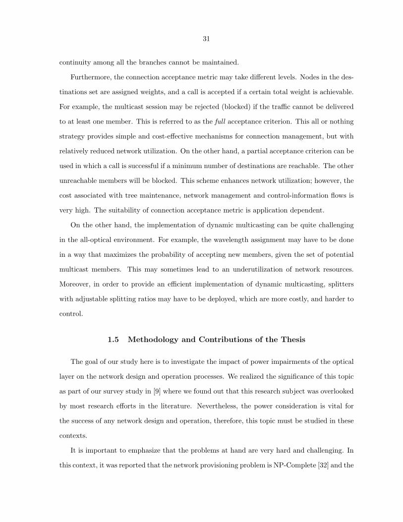
31
continuity among all the branches cannot be maintained.
Furthermore, the connection acceptance metric may take different levels. Nodes in the des-
tinations set are assigned weights, and a call is accepted if a certain total weight is achievable.
For example, the multicast session may be rejected (blocked) if the traffic cannot be delivered
to at least one member. This is referred to as the full acceptance criterion. This all or nothing
strategy provides simple and cost-effective mechanisms for connection management, but with
relatively reduced network utilization. On the other hand, a partial acceptance criterion can be
used in which a call is successful if a minimum number of destinations are reachable. The other
unreachable members will be blocked. This scheme enhances network utilization; however, the
cost associated with tree maintenance, network management and control-information flows is
very high. The suitability of connection acceptance metric is application dependent.
On the other hand, the implementation of dynamic multicasting can be quite challenging
in the all-optical environment. For example, the wavelength assignment may have to be done
in a way that maximizes the probability of accepting new members, given the set of potential
multicast members. This may sometimes lead to an underutilization of network resources.
Moreover, in order to provide an efficient implementation of dynamic multicasting, splitters
with adjustable splitting ratios may have to be deployed, which are more costly, and harder to
control.
1.5 Methodology and Contributions of the Thesis
The goal of our study here is to investigate the impact of power impairments of the optical
layer on the network design and operation processes. We realized the significance of this topic
as part of our survey study in [9] where we found out that this research subject was overlooked
by most research efforts in the literature. Nevertheless, the power consideration is vital for
the success of any network design and operation, therefore, this topic must be studied in these
contexts.
It is important to emphasize that the problems at hand are very hard and challenging. In
this context, it was reported that the network provisioning problem is NP-Complete [32] and the
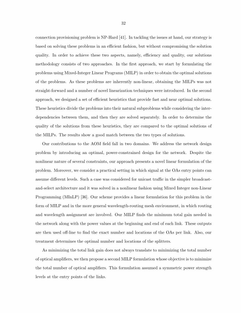
32
connection provisioning problem is NP-Hard [41]. In tackling the issues at hand, our strategy is
based on solving these problems in an efficient fashion, but without compromising the solution
quality. In order to achieve these two aspects, namely, efficiency and quality, our solutions
methodology consists of two approaches. In the first approach, we start by formulating the
problems using Mixed-Integer Linear Programs (MILP) in order to obtain the optimal solutions
of the problems. As these problems are inherently non-linear, obtaining the MILPs was not
straight-forward and a number of novel linearization techniques were introduced. In the second
approach, we designed a set of efficient heuristics that provide fast and near optimal solutions.
These heuristics divide the problems into their natural subproblems while considering the inter-
dependencies between them, and then they are solved separately. In order to determine the
quality of the solutions from these heuristics, they are compared to the optimal solutions of
the MILPs. The results show a good match between the two types of solutions.
Our contributions to the AOM field fall in two domains. We address the network design
problem by introducing an optimal, power-constrained design for the network. Despite the
nonlinear nature of several constraints, our approach presents a novel linear formulation of the
problem. Moreover, we consider a practical setting in which signal at the OAs entry points can
assume different levels. Such a case was considered for unicast traffic in the simpler broadcast-
and-select architecture and it was solved in a nonlinear fashion using Mixed Integer non-Linear
Programming (MInLP) [36]. Our scheme provides a linear formulation for this problem in the
form of MILP and in the more general wavelength-routing mesh environment, in which routing
and wavelength assignment are involved. Our MILP finds the minimum total gain needed in
the network along with the power values at the beginning and end of each link. These outputs
are then used off-line to find the exact number and locations of the OAs per link. Also, our
treatment determines the optimal number and locations of the splitters.
As minimizing the total link gain does not always translate to minimizing the total number
of optical amplifiers, we then propose a second MILP formulation whose objective is to minimize
the total number of optical amplifiers. This formulation assumed a symmetric power strength
levels at the entry points of the links.
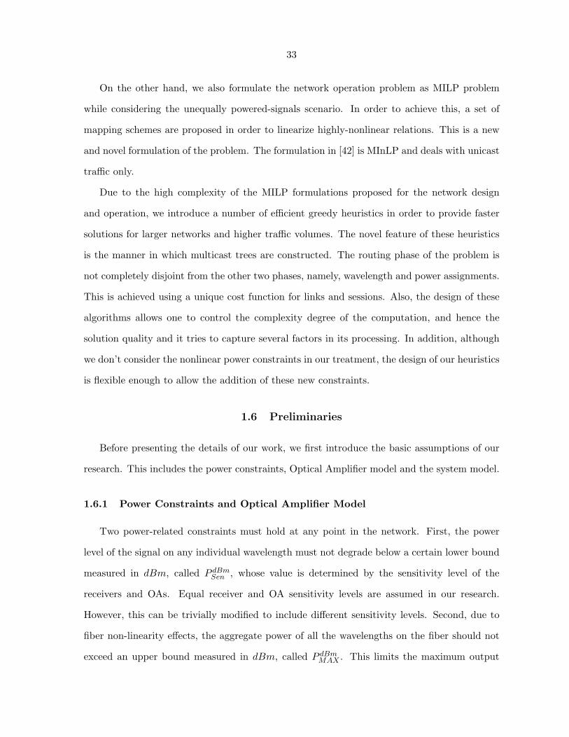
33
On the other hand, we also formulate the network operation problem as MILP problem
while considering the unequally powered-signals scenario. In order to achieve this, a set of
mapping schemes are proposed in order to linearize highly-nonlinear relations. This is a new
and novel formulation of the problem. The formulation in [42] is MInLP and deals with unicast
traffic only.
Due to the high complexity of the MILP formulations proposed for the network design
and operation, we introduce a number of efficient greedy heuristics in order to provide faster
solutions for larger networks and higher traffic volumes. The novel feature of these heuristics
is the manner in which multicast trees are constructed. The routing phase of the problem is
not completely disjoint from the other two phases, namely, wavelength and power assignments.
This is achieved using a unique cost function for links and sessions. Also, the design of these
algorithms allows one to control the complexity degree of the computation, and hence the
solution quality and it tries to capture several factors in its processing. In addition, although
we don’t consider the nonlinear power constraints in our treatment, the design of our heuristics
is flexible enough to allow the addition of these new constraints.
1.6 Preliminaries
Before presenting the details of our work, we first introduce the basic assumptions of our
research. This includes the power constraints, Optical Amplifier model and the system model.
1.6.1 Power Constraints and Optical Amplifier Model
Two power-related constraints must hold at any point in the network. First, the power
level of the signal on any individual wavelength must not degrade below a certain lower bound
measured in dBm, called P dBmSen , whose value is determined by the sensitivity level of the
receivers and OAs. Equal receiver and OA sensitivity levels are assumed in our research.
However, this can be trivially modified to include different sensitivity levels. Second, due to
fiber non-linearity effects, the aggregate power of all the wavelengths on the fiber should not
exceed an upper bound measured in dBm, called P dBmMAX . This limits the maximum output
34
Optical Amplifier Model
0
5
10
15
20
25
-30 -25 -20 -15 -10 -5 0
Total Power (dB)
Gai
n (d
B)
Gain (dB)
Max. OA Output
Optical Amplifier Model
0
5
10
15
20
25
-30 -25 -20 -15 -10 -5 0
Total Power (dB)
Gai
n (d
B)
Gain (dB)
Max. OA Output
Figure 1.11 OA model in Equation (1.1)
Simple OA Model
0
5
10
15
20
25
-30 -25 -20 -15 -10 -5 0
Total input Power in dBm
OA gain in dB
OA Gainin dB
Figure 1.12 OA model in Equation (1.2)
power of the OAs and the transmitters.
On the other hand, the gain of an OA is a non-linear function of the input signal power,
and it can be approximated using the following functional equation:
Pin
Psat=
1G− 1
lnG0
G(1.1)
where Pin and Psat represent the aggregate power of the input signal, and the internal sat-
uration power, respectively (both in mW ). Also, G and G0 are the actual gain, and the
small-signal gain, respectively (both in absolute scale). The gain is shown in Figure 1.11.
Another simple model for the OA gain is shown in Figure 1.12 and it is determined by:
G(10× log10(Pin)) = MING0, (P dBmMAX − (10× log10Pin) (1.2)
The amplifier gain applies to all input wavelengths (assuming a flat gain over all chan-
nels) and it drops when the total input power exceeds certain threshold and the OA becomes
saturated.
1.6.2 System Model
The main components of the system model used in our solutions is described in this sub-
section. Any additional system assumptions that are specific to any problem will be presented
in the corresponding chapter.
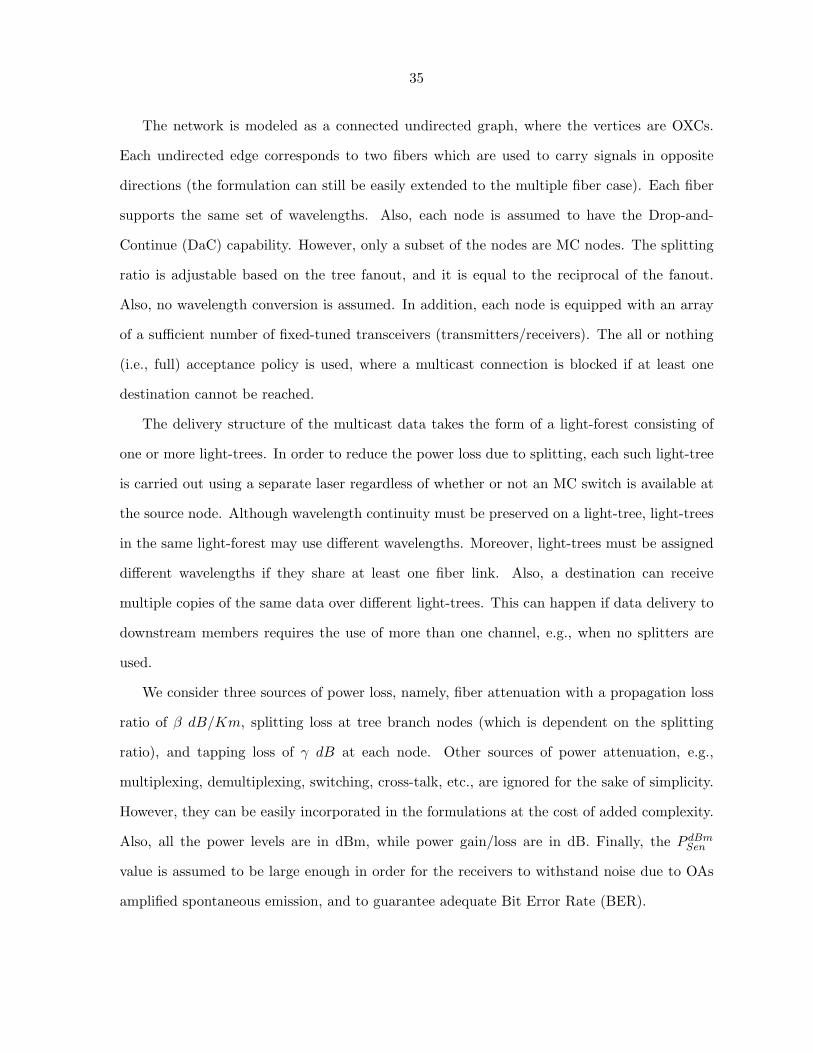
35
The network is modeled as a connected undirected graph, where the vertices are OXCs.
Each undirected edge corresponds to two fibers which are used to carry signals in opposite
directions (the formulation can still be easily extended to the multiple fiber case). Each fiber
supports the same set of wavelengths. Also, each node is assumed to have the Drop-and-
Continue (DaC) capability. However, only a subset of the nodes are MC nodes. The splitting
ratio is adjustable based on the tree fanout, and it is equal to the reciprocal of the fanout.
Also, no wavelength conversion is assumed. In addition, each node is equipped with an array
of a sufficient number of fixed-tuned transceivers (transmitters/receivers). The all or nothing
(i.e., full) acceptance policy is used, where a multicast connection is blocked if at least one
destination cannot be reached.
The delivery structure of the multicast data takes the form of a light-forest consisting of
one or more light-trees. In order to reduce the power loss due to splitting, each such light-tree
is carried out using a separate laser regardless of whether or not an MC switch is available at
the source node. Although wavelength continuity must be preserved on a light-tree, light-trees
in the same light-forest may use different wavelengths. Moreover, light-trees must be assigned
different wavelengths if they share at least one fiber link. Also, a destination can receive
multiple copies of the same data over different light-trees. This can happen if data delivery to
downstream members requires the use of more than one channel, e.g., when no splitters are
used.
We consider three sources of power loss, namely, fiber attenuation with a propagation loss
ratio of β dB/Km, splitting loss at tree branch nodes (which is dependent on the splitting
ratio), and tapping loss of γ dB at each node. Other sources of power attenuation, e.g.,
multiplexing, demultiplexing, switching, cross-talk, etc., are ignored for the sake of simplicity.
However, they can be easily incorporated in the formulations at the cost of added complexity.
Also, all the power levels are in dBm, while power gain/loss are in dB. Finally, the P dBmSen
value is assumed to be large enough in order for the receivers to withstand noise due to OAs
amplified spontaneous emission, and to guarantee adequate Bit Error Rate (BER).
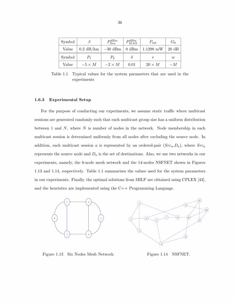
36
Symbol β P dBmSen P dBm
MAX Psat G0
Value 0.2 dB/km −30 dBm 0 dBm 1.1298 mW 20 dB
Symbol P1 P2 δ v w
Value −5×M −2×M 0.01 20×M −M
Table 1.1 Typical values for the system parameters that are used in theexperiments
1.6.3 Experimental Setup
For the purpose of conducting our experiments, we assume static traffic where multicast
sessions are generated randomly such that each multicast group size has a uniform distribution
between 1 and N , where N is number of nodes in the network. Node membership in each
multicast session is determined uniformly from all nodes after excluding the source node. In
addition, each multicast session a is represented by an ordered-pair (Srca,Da), where Srca
represents the source node and Da is the set of destinations. Also, we use two networks in our
experiments, namely, the 6-node mesh network and the 14-nodes NSFNET shown in Figures
1.13 and 1.14, respectively. Table 1.1 summarizes the values used for the system parameters
in our experiments. Finally, the optimal solutions from MILP are obtained using CPLEX [43],
and the heuristics are implemented using the C++ Programming Language.
0
4
1
2
3
5
Figure 1.13 Six Nodes Mesh Network.
1
2
3
4 5
6
7 8
9
10
11
12
13
14
Figure 1.14 NSFNET.
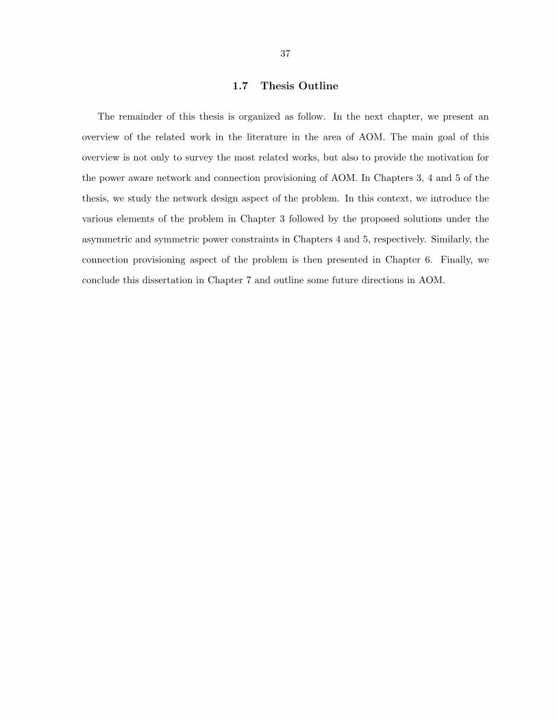
37
1.7 Thesis Outline
The remainder of this thesis is organized as follow. In the next chapter, we present an
overview of the related work in the literature in the area of AOM. The main goal of this
overview is not only to survey the most related works, but also to provide the motivation for
the power aware network and connection provisioning of AOM. In Chapters 3, 4 and 5 of the
thesis, we study the network design aspect of the problem. In this context, we introduce the
various elements of the problem in Chapter 3 followed by the proposed solutions under the
asymmetric and symmetric power constraints in Chapters 4 and 5, respectively. Similarly, the
connection provisioning aspect of the problem is then presented in Chapter 6. Finally, we
conclude this dissertation in Chapter 7 and outline some future directions in AOM.
38
CHAPTER 2. Literature Review
Different aspects of AOM have been addressed in the literature under different system
configurations and assumptions. We provide a review for these research efforts in this chapter.
For a detailed treatment of these various research efforts, the reader is referred to [9]. Our
review of the literature will first present those schemes that target network design in Section
2.1, followed by contributions to network operation in Section 2.2. The goal of this chapter is
not just to set up the background to the AOM field, but to also motivate our research.
2.1 Network Design Schemes
Several network design related issues of AOM were investigated in the literature. These
issues are either network provisioning-related or network dimensioning-related problems. In the
context of network provisioning, two main problems were studied, namely, MC nodes allocation
and optical amplifiers placement problems. Allocating the MC nodes entails determining
their number and locations. This problem was proven to be NP-Complete in [32], even with
the existence of the routing and wavelength assignment (RWA) of the multicast sessions. In
addition, the simulation results reported in [31] showed that:
1. Full light splitting capability can reduce the bandwidth consumed by an average of 8%−18% only
2. By equipping 50% of the network nodes with splitting capability, the network can obtain
around 80%− 90% of the benefit of full light splitting capability.
3. No more than 70% of the network nodes need to be equipped with light splitting capability
to obtain almost the same benefit as full light splitting capability.
39
The optimal placement of splitters was investigated in [14], in which an MILP formulation
is proposed for the RWA of the light-trees which is then extended to design logical topologies
for multicast streams. In [44], an iterative heuristic is proposed to optimize the placement of
a given number of splitters with an objective of minimizing the blocking probability of the
given multicast sessions whose routing trees are pre-computed. This algorithm proceeds for
k iterations to place a total of k splitting nodes in the whole network. In each iteration, all
the nodes without multicast capability are chosen one at a time to explore the possibility of
being equipped with a splitter. The traffic blocking probability is computed and the node
with minimum blocking probability is chosen as a new splitting node in the network. After k
iterations, the allocation assignment is returned as the best configuration of the sparse splitting
nodes placement.
The optical amplifier placement problem under multicast traffic is another open and chal-
lenging network provisioning problem. An optical amplifier gain model was developed in [36]
that considered fiber attenuation, amplifier saturation, sensitivity of detectors, as well as the
maximum power of transmitting light sources in fiber. The authors proposed a scheme that
minimizes the number of amplifiers for the LAN/MAN passive-star-based optical networks
without the restriction that wavelengths in the same fiber must be at the same power level.
This is a reasonable assumption due to the near-far phenomenon in which signals on different
wavelengths can originate from different locations in the network, and when they arrive at
an amplifier, their power levels can be different due to the propagation attenuation in fibers.
The difference in power levels of the input wavelengths can significantly limit the amount of
amplification available to lower powered wavelength because the higher powered wavelengths
could saturate the amplifier.
The authors formulated this problem as a Mixed Integer non-Linear Program (MInLP)
with the objective of minimizing the number of optical amplifiers in the network. The output
of the MInLP is used to allocate the determined number of optical amplifiers off-line. Two
placement policies were introduced in [36], namely, As Soon As Possible (ASAP) and As Late
As Possible (ALAP) methods. For each link, the ASAP places the optical amplifiers (except
40
the last one) on the link as soon as the total input power is low enough to allow the maximum
gain, while the last amplifier is placed such that the input power is low enough to allow it to
generate the remaining required gain. The ALAP method operates in a similar fashion, except
that it places the amplifiers such that the total input power is at its minimum detectable level
(i.e., the power of one or more of the individual input channels is at Psen) which results in
placing the amplifiers closer to the destination side of the link.
However, the equally powered version of the problem defined in [36] was also studied in [45]
where the signals over each link are assumed to be equal. This symmetric assumption helped
formulate the same problem using Mixed Integer Linear Program (MILP).
On the other hand, two new methods were proposed in [46], namely, Genetic Algorithm
implementation for amplifiers placement (GA2), and Smallest Gain First (SGF) algorithm. The
GA2 algorithm started with a set of placement topologies of amplifiers sorted with transmitting
power on the link. The two placement topologies with lowest powers are then selected as the
parents, and genetic functions are used to combine parents with a structured, but randomized
information exchange to form a child, and the child is then inserted in the whole set. The SGF
attempts to find a better amplifier placement by assigning the minimum transmission power to
every light-path, then it would add all the light-paths of the chosen permutation link by link
according to their length (longest one first). According to the simulations results presented in
[46], GA2 performs better than SGF with lower transmission powers for all light-paths.
The influence of amplifier noise power on the transmission signal is considered in [47].
However, it only considered the effect of the noise in saturating the amplifier, without using
the SNR concept. Such problem can be possibly solved by increasing the receiver sensitivity,
which is not the case if SNR is very low.
With multicast service, the amplifier placement problem must consider the power loss due
to light splitting or the use of DaC devices. Signal power decreases dramatically when it passes
through these devices. For example, the power loss is 3dB after passing through a splitter.
This requires adding new set of constraints to the optical amplifier placement formulation to
take care of these new requirements. Therefore, the demand for optical amplifiers (OAs) can be
41
more critical with multicast traffic than with its unicast counterpart. Since OAs are expensive
devices, every effort must be made to minimize their number in the network. Moreover, because
of the requirement of SNR, the total number of amplifiers on a link should also be considered
in the amplifier placement problem.
Finally, several efforts were reported in the literature in the network dimensioning field in
order to minimize the number of consumed network resources. Due to the space constraints
here, and since the design problems we address in this thesis are network provisioning problems,
the reader is referred to [9] for a brief description of some of these efforts.
2.2 Network Operation Schemes
Supporting AOM during the network operation stage is achieved by designing a set of
protocols and solutions for delivering the multicast traffic while maximizing the utilization of
the available network resources and/or minimizing the number of dropped calls. Like the case
of unicast traffic, the support of AOM in wavelength-routing networks is treated as a Routing
and Wavelength Assignment (RWA) problem. Solving the RWA problem is NP-Hard; thus, it
is commonly treated as two problems, namely, routing (denoted as AOM-R) and wavelength
assignment (denoted as AOM-WA). The techniques that address the AOM-R problem are
presented in the following subsection while those that are related to the AOM-WA problem
are demonstrated in Subsection 2.2.2.
Nevertheless, some efforts that tackled the RWA as a joint problem were also reported in
the literature. For example, the work in [48] investigated the RWA problem of the AOM under
the loss-balance constraint with sparse splitting and wavelength-conversion deployment. In this
context, loss-balanced light-forests are composed of a set of light-trees that are bounded in size
(number of destinations per multicast tree), in size variation (difference in the number of des-
tinations among different multicast trees), and in dimension (maximum source-to-destination
distance on each multicast tree). These bounds are used to ensure that the different desti-
nations in a multicast session can receive the optical signal with relatively equivalent signal
quality. This problem is formulated as an Integer Linear Program (ILP).
42
2.2.1 All-Optical-Multicasting Routing (AOM-R) Problem
Figure 2.1 depicts the classification framework we will follow in representing the multicast
routing algorithms in wavelength-routing networks. Based on the degree of coordination be-
tween the WDM and IP layers, these AOM solutions have been developed in two environments,
namely, Pure WDM-Layer and IP Multicasting Over WDM schemes. In the first approach, all
the necessary functionalities are solely handled by the WDM layer, which eliminates any role
for the IP layer. However, in the second approach, both layers coexist and cooperate. The
main focus of this thesis is on the first type of AOM and they are treated here. IP Multicast-
ing Over WDM is outside the scope of this thesis and due to space constraints, the reader is
encouraged to refer to [9] for a brief discussion of these schemes.
As indicated in Figure 2.1, the AOM-R techniques are divided into three different categories
based on the degree of deployment of the MC nodes in the network. Such deployment has
direct impact on the protocol design and, therefore, on the type of the delivery structure. In
this context, these algorithms are targeted for the networks with full, sparse and no splitting
capabilities. Under full splitting configuration, the conventional multicast routing protocols
can be used to construct a single light-tree as any node in the network can be a branching
node. Although these networks provide the highest flexibility, the cost of the full deployment
of MC nodes is too high, especially for large networks. On the other extreme, namely, for
networks that are not equipped with any splitting capability, building a distribution tree for
routing the multicast session is not possible due to the lack of branching capabilities. Therefore,
other routing structures need to be used like establishing a separate unicast session to each
destination node [49], or relying on the DaC functionality of the nodes to construct a trail [18].
Finally, the cost and flexibility of the networks with sparse splitting are in between these two
extreme configurations. In this case, constructing a single multicast tree may not always be
feasible to include all the destination nodes, and light-forests are more commonplace.
In the following subsections, we will present the various AOM-R techniques based on the
network splitting capability. In our treatment, we propose a novel simple notation to describe
the system model used by each of these techniques. Using this notation scheme provides a
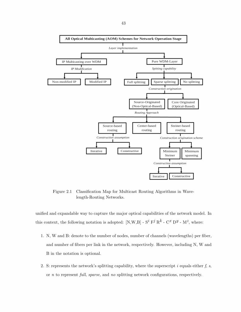
43 Construction assumption
Source-based routing
Center-based routing
Steiner-based routing
Construction origination scheme
Core Originated (Optical-Based)
Source-Originated (Non-Optical-Based)
Routing Approach
Construction origination scheme
Full splitting Sparse splitting No splitting Modified IP Non-modified IP
Layer implementation
All Optical Multicasting (AOM) Schemes for Network Operation Stage
IP Multicasting over WDM Pure WDM-Layer
Spitting capability IP Modification
Minimum spanning
Minimum Steiner
Iterative Constructive
Construction assumption
Iterative Constructive
Figure 2.1 Classification Map for Multicast Routing Algorithms in Wave-length-Routing Networks.
unified and expandable way to capture the major optical capabilities of the network model. In
this context, the following notation is adopted: [N,W,B] - Si Fj Rk - Cx Dy - Mz, where:
1. N, W and B: denote to the number of nodes, number of channels (wavelengths) per fiber,
and number of fibers per link in the network, respectively. However, including N, W and
B in the notation is optional.
2. S: represents the network’s splitting capability, where the superscript i equals either f, s,
or n to represent full, sparse, and no splitting network configurations, respectively.
44
3. F: represents the fan-out of the splitting nodes, where the superscript j is either c for
splitters with complete fan-out, or l for splitters with limited fan-out. It may also use
the symbol m for a mixed situation in which complete and limited splitters coexist.
4. R: which indicates whether the splitting ratio of the splitting node is either fixed (with
the superscript k equals x ) or adjustable (with k equals a).
5. C: represents the conversion capability in the network, such that the superscript x is
either f, s, or n to indicate that the network has full, sparse or no wavelength conversion
capability, respectively.
6. D: indicates the conversion degree, where that the superscript y can be either c, l or m
to represent complete, limited or mixed situations, respectively.
7. M: represents the on-site amplification, and has the following cases: full, sparse or no,
and they are represented by letting superscript z equal f, s or n, respectively.
Although the above notation can be extended to include other capabilities if needed, it is
also intended to keep it as compact as possible by omitting the Fj and Rk parts if the network
has no splitting capability, and Dy if no conversion is employed.
2.2.1.1 AOM-R in Networks with No Splitting Capabilities
The system model of the routing algorithm proposed in [18] is [N,W,B] - Sn - Cn - Mn.
The algorithm assumes that all the nodes are equipped with the Tap-and-Continue (TaC)
capability. The routing problem is solved by constructing an optimal trail which originates
from the multicast source node and spans all the destination nodes in the multicast group such
that these nodes are traversed no more than two times.
The problem is formulated with the objective of minimizing the number of traversed di-
rected edges and it is referred to as the problem of Multiple-Destination Minimum-Cost Trail
or MDMCT. The MDMCT was proven to be an NP-Complete problem that always has a
solution if the network is strongly connected. The authors proposed a heuristic of polynomial
time complexity in order to find a feasible trail and it works in two steps.
45
The first step assumes that all nodes are MC nodes and constructs a Steiner tree for the
multicast session using the Minimum Cost Path Heuristic (MCPH) proposed in [50]. Based
on the computed Steiner tree, the multiple-destination trail is then computed accordingly by
re-routing around the nodes in the Steiner tree which have an out-degree that is greater than
one. The algorithm for finding the trail starts from the Steiner Tree root, i.e., multicast source,
and recursively repeats at each node in the tree, referred to as the Current node, if this node
is not a leaf node. In the downstream direction, the algorithm attempts to include all the
downstream links between the Current node and all its children destinations. Backtracking is
required when a leaf node is reached and there are still some destination nodes which have not
been visited. In this case, backtracking is performed to the nearest branching node which has
some outgoing branches that have not been visited yet. Because of backtracking, and in order
to traverse as few edges as possible, the sub-trees rooted at each node are traversed according
to their depths, and in ascending order.
The advantage of this method is that it eliminates the high cost of having splitting nodes.
However, it traverses more link, and requires a longer set up time and the delay encountered
by the connection becomes higher.
2.2.1.2 AOM-R in Networks with Full Splitting Capabilities
Reference [25] studies the RWA problem of the AOM when all the nodes in the network
have complete, and fixed ratio splitting capability. However, various wavelength conversion
capabilities were investigated, i.e., no/full and complete/limited. Constructing the multicast
tree is done using the Minimum Cost Path Heuristic (MCPH) [50] under two traffic models,
namely, static and dynamic models. Under the static traffic model, a set of routing trees, ti,
are pre-calculated for each multicast session, i. Selecting a single tree from set ti for routing the
multicast session can be done in a fixed or alternate fashion. With the fixed fashion, only one
tree is used to route the multicast session. However, the alternate scheme computes multiple
tree per session, and the search for an available tree in ti is performed in a certain order.
Two criteria for multicast call acceptance were defined in [25]. With the first policy, called
46
the Full Destination Blocking Policy (FDBP), a multicast session is established only when all
the destinations are reachable using a distribution tree from set ti. The performance of this
policy is measured by the session blocking probability metric. The second policy is the Partial
Destination Blocking Policy (PDBP) and is based on launching the multicast connection even
if some of its destinations are not reachable by the multicast tree. Adopting any of these
policies is application dependent. The FDBP policy is appropriate for those applications that
have collaborative nature and require the simultaneous availability of the member nodes (e.g.,
teleconferencing, distributed databases and distributed computing). On the other hand, the
PDBP can be used with those applications that do not require all the destinations to be
connected to the multicast tree (e.g., Video-on-Demand and newsgroups).
The simulation results reported in [25] show that the dynamic scheme outperforms both
static schemes (fixed and alternate) with FDBP for single fiber and the performance of using
multiple unicast connections is the worst. Also, using PDBP enhances the system performance
significantly and it is the best under the static fixed scheme. Moreover, the results showed
that using wavelength-conversion improves the system performance, especially in the dynamic
case and most of this improvement is obtainable with a small conversion degree.
In addition, the concept of light-trees was first introduced in [2] as a generalization form
of the light-paths. As such, the light-tree operates as a point-to-multipoint all-optical channel
that provides a logical single-hop optical communication between the source node and the
destination node(s). However, the light-tree may traverse multiple links in the network. As
it is the case with light-paths, light-trees are subject to the wavelength-continuity constraint
in the absence of wavelength-conversion capability. However, the treatment in [2] assumes full
wavelength conversion; thus, the system model is denoted as [N,W,B] - Sf Fc Rx - Cf Dc - Mf.
The light-tree idea discussed in [2] makes use of a single tree to deliver one or more traffic
demand to a set of destinations. Each traffic demand is assumed to be a fraction of the total
channel capacity. These traffic instances originate from the source node and can be of any
type (e.g., unicast, multicast, or broadcast). Also, each destination node can be a member of
one or more of these sessions, but not necessarily all. Although the primary focus in [2] was
47
to provide a better solution to support the unicast traffic streams whose traffic demands are
much less than the wavelength capacity, the light-tree idea can be extended naturally for the
multicast traffic case with full wavelength capacity requirements.
The problem of light-tree virtual topology design was formulated as a Mixed Integer Linear
Program (MILP) and was solved for the unicast and broadcast traffic types only. The results
showed that light-trees are better than light-paths since they require fewer transceivers for
both traffic types and less number of hops for the unicast communication.
Finally, the work done in [26] is another example of multicast routing in wavelength-routing
networks with full splitting capability. With the Sf Fc Rx- Cn - Mf system model, the RWA
problem of AOM was studied in [26] with the objective of maximizing the total number of
served users using the PDBP described earlier by accommodating partial trees. The multicast
tree for each session is pre-computed by any conventional algorithm. Then, a Non-linear Integer
Program (NIP) was formulated for the general AOM-RWA case where the multicast sessions
in the network have different sources. Due to the difficulty of solving the NIP, two heuristics
were proposed to support multicast with PDBP in single-source systems, which is a special
case in which all the multicast sessions belong to a single source.
The first heuristic employs a two-step linear program (LP) based algorithm that consists
of two Integer Linear Programs (ILPs). The first ILP is responsible for accommodating the
completely served multicast sessions and then assigning the appropriate wavelength to each
tree. The link capacities are updated and the network topology is modified in order to exclude
any link with no available wavelength. The second ILP is then iteratively executed in order to
include as many users as possible from the remaining unserved multicast sessions.
The second heuristic is called the MAX-FIRST (MAX-1st) algorithm. It is an iterative
simple approach which accommodates the multicast sessions according to the number of their
users that can be served using an available wavelength. At each iteration, the multicast session
with the maximum number of serveable users is assigned an available wavelength, then the link
capacities and the network topology are updated accordingly. Based on the new system status,
the new multicast session with the maximum serveable users is identified, and the procedure
48
continues until no more users can be served.
Both heuristics are extended to allow re-routing. Rerouting is achieved by constructing
new trees on the available wavelengths for the remaining unprovisioned sessions. This step
allows accommodating more users that could not be reached according to the computed fixed
trees and the wavelength availability.
The user blocking probability is used in [26] as a performance metric in the simulation
experiments. These results show that both LP-Based and MAX-1st heuristics have compar-
atively similar performance with an advantage of simplicity for the MAX-1st algorithm. The
results also show that allowing re-routing decreases the user blocking probability significantly,
and 10%-20% performance improvement is achieved when PDBP is employed over the FDBP.
2.2.1.3 AOM-R in Networks with Sparse Splitting Capabilities
Multicast routing algorithms that have been proposed under the sparse splitting configu-
ration can be classified into two basic groups based on their originating scheme, namely, from
where the light-tree/light-forest construction originates. The first group is referred to as the
Source-Originated scheme because building the multicast distribution medium is initiated by
the source node itself regardless of its optical capabilities1. Therefore, this group can also
be called the Non-Optical-Capabilities-Based, or simply Non-Optical-Based, multicasting tech-
niques. On the other hand, constructing the multicast delivery medium can also originate from
an assisting node or a set of assisting nodes that have special optical capabilities and form a
special optical structure. This structure is referred to as the core structure and is employed
as an original structure in the final distribution structure of the multicast session. Hence, this
approach is called the Core-Originated, or Optical-Based, approach.
While Optical-Based schemes are unique for AOM, the Non-Optical-Based strategies exist
in non-optical networks too. Traditionally, the Source-Originated routing algorithms is further
divided into three main categories according to their routing approach, namely, Source-Based
Routing, Steiner-Based Routing and Center-Based Routing [51]. Essentially, the Source-Based1These optical capabilities are expressed in terms of splitting, wavelength conversion and/or amplification.
49
Routing approach constructs the multicast distribution medium by connecting the multicast
source node to each receiver individually using the appropriate least cost path. Therefore, this
approach aims to minimize the per source-receiver path cost.
Instead of minimizing the cost of each source-receiver pair path, the objective function of
the Steiner-Based Routing schemes is to minimize the overall cost of the multicast distribution
medium. This cost is defined as the total cost of all its links and these schemes are known to
be NP-Complete. Considering the membership requirement of the nodes, the algorithms under
this category can be furthermore subdivided into Minimum Spanning and Minimum Steiner
techniques. With the first approach, all the nodes in the routing structure are member nodes
only, while the second approach eliminates this restriction [20].
On the other hand, the objective of Center-Based Routing schemes is to provide a single
shared delivery medium that supports many-to-many communication. The heart of this ap-
proach is the choice of a certain center node to serve as the root for the multicast medium that
spans all the member nodes. All communication must take place through the selected center
node and from which it is directed to the destinations.
To the best of our knowledge, none of the currently proposed AOM-R techniques is a
Minimum-Spanning Steiner-Based or a Center-Based scheme. However, the map shown in
Figure 2.1 includes these categories for the sake of completeness. The various techniques that
are designed for sparse splitting deployment are presented in the following subsections.
A. Source Originated Techniques: Source-Based Routing
Two schemes were employed for constructing the multicast delivery medium in a form
of a light-forest in the source-based routing schemes. The first scheme adopts the iterative
(i.e., improvement) approach in which the routing medium is initially constructed as a single
tree with the assumption that all the nodes in the network are equipped with splitters. The
medium is then iteratively modified if any of the branching nodes happens to be an MI node.
The forest modification entails keeping one of the MI’s node children only, and attempt to
reconnect all the remaining ones through some other node. Alternatively, the second approach
50
is constructive in nature since it forms the routing medium from scratch and by checking the
splitting capability of nodes during the construction stage. The Re-Route-to-Source (RR2S)
and the Re-Route-to-Any (RR2A) algorithms [1] are iterative source-based routing algorithms
while Member-First (M1st) algorithm [1] is an example for the constructive approach.
Both the Re-Route-to-Source (RR2S) and the Re-Route-to-Any (RR2A) algorithms [1]
assume the following system model: [N,W,B] - Ss Fc Rx - Cs - Dc - Ms. Both algorithms
start by computing a minimum spanning tree that starts from the source node and spans all
the nodes. A single multicast tree is obtained by pruning those links that do not lead to
member nodes in the minimum spanning tree. Then the splitting capability of each node in
the multicast tree is checked in breadth-first or depth-first orders to check if the output degree
of any MI is greater than 1. Both algorithms operation terminate when all these nodes are
checked. However, the algorithms operation differ in the way the initial tree is reconstructed.
As such, each algorithm defines its own criterion in choosing the set of candidate nodes through
which the disconnected nodes rejoin the multicast structure.
Basically, the RR2S defines the set of candidate nodes that are used to rejoin any dis-
connected node to be all the nodes that are located along the reverse tree path from the
disconnected node to the source node and are equipped with both splitting and complete
conversion capabilities. However, if no such nodes are available, then the disconnected node
rejoins the multicast delivery structure directly at the source node. The availability of a wave-
length converter at the MC node is essential for the success of the algorithm operation. This
wavelength converter is used to ensure that all the disconnected children from the MI node are
carried over different channels on the same links that constitute the reverse path to the source
node. Although this re-joining strategy guarantees the use of shortest paths for the cutoff
members, it results in concentrating the traffic on certain links which results in exhausting the
wavelengths along them rapidly.
In an attempt to achieve load balancing in wavelength usage, the Re-Route-to-Any (RR2A)
algorithm eliminates the requirement proposed in RR2S of using the same backward shortest
path on T by all the disconnected children of a branching MI node. Instead, the RR2A permits
51
each of the disconnected nodes to choose its own path to reconnect itself to the multicast
delivery structure through the nearest node that is: (1) already part of the multicast delivery
structure, and (2) it is an MC, a source node or a leaf node.
Unlike the RR2S and RR2A algorithms, the Member-First (M1st) algorithm [1] takes the
splitting capability of the nodes into account while constructing the light-forests. The M1st
algorithm is designed to work with the [N,W,B] - Ss Fc Rx - Cn - Ms system model. It
constructs one light-tree of the light-forest at a time such that each light-tree is assembled on
a link by link basis through a special Priority Queue structure, called the Fringe Link List.
This list consists of a set of links, referred to as fringe links, which are to be included in the
light-tree. The Fringe Link List is updated whenever a node is to be included in the light-tree
and the link of the least shortest path distance to the source node has the highest priority.
The tree expansion starts by adding the source node to the light-forest and then the Fringe
Link List is updated by including all its outgoing links. For each subsequent tree expansion, the
fringe link with the highest priority in the list, denoted by (v, u), is selected. In this context,
node v of the link is a tree node, while node u is a new node to be added to the tree. The
algorithm distinguishes between the two cases where node u is a member node or not. In the
latter case, node u is attached to the current light-tree using the highest priority link and the
list is updated with its links. However, if node u is a member node in the multicast session,
the optical-multicasting capabilities of the tree node v is then examined.
A direct connection is established from node u to node v if the latter is an MC node.
Otherwise, the backward shortest path on the current tree that connects node v to the source
node is traced one node at a time in order to find the first MC node. If such a node is
found, node u is then connected to it; otherwise, a new separate connection to the source
node is established. At the same time, each MI node along this path undergoes additional two
operations, referred to as the cut and remove operations to process their links. In this case,
the algorithm cuts all the links in the current tree that originate from the MI nodes, except
the one that leads to node u. The cut process is also performed over all the fringe links that
originate from the MI nodes. Then, each of the cut links are examined to check whether it is
52
part of the current tree. If so, the remove operation is applied to all the links in the sub-tree
that expand the cut link as well as the corresponding fringe links. While the removed links are
allowed to participate in any future expansion for the current light-tree, the cut links are not.
More light-trees are necessary if the Fringe Links list becomes empty while some of the
members are not yet included in the light-forest. In such a case, all the links (either removed,
cut or are already part of the existing light-trees) are restored and can be used for the new
light-tree construction. Finally, the final light-forest becomes ready after pruning all the links
that do not lead to member nodes.
B. Source Originated Techniques: Steiner-Based Routing
Similar to the Source-Based Routing schemes of the previous subsection, the Minimum
Steiner-Based schemes can be described as being either constructive, e.g., Member-Only [1],
and Virtual-Source Capacity-Priority algorithm [28], or iterative, e.g., Centralized Splitting
algorithm [29], and Tabu-Search Based AOM [30].
The first Steiner-based source-originated routing scheme to be presented is the Member-
Only (M-Only) algorithm [1]. Like M1st algorithm, the M-Only algorithm is proposed for
the [N,W,B] - Ss Fc Rx - Cn - Ms, system model. Unlike the M1st algorithm, the M-Only
algorithm uses the member nodes only to expand each light-tree, such that a single member is
added at each iteration. Hence, no pruning is required.
The algorithm starts by including the source node to the current light-tree. It proceeds
in iterations such that at each algorithmic iteration, the light-tree grows by including one
destination node. Tree expansion is done through a set of expandable nodes that are updated
at the end of each iteration and by using the path with the least cost from among all the
candidate paths. The set of expandable nodes includes the source nodes, all the MC nodes in
the current tree and all the leaf nodes. The algorithm attempts to include as many member
nodes as possible, and it terminates only when all member nodes are included. If this is not the
case and it happened that no more qualified paths exist for expanding the current light-tree,
a new light-tree is needed and the same procedure is repeated.
53
The simulation results reported in [1] reveal that the M-Only algorithm requires the least
number of branches per forest (bandwidth) with respect to RR2S, RR2A and M1st. Both M1st
and M-Only result in the smallest number of channels per link, while the RR2S requires the
largest number of channels per link, as well as the highest bandwidth requirement. On the
other hand, RR2S achieves the shortest delay while M-Only exhibits the longest delay.
In addition, the Virtual-Source Capacity-Priority (VS-PC) algorithm proposed in [28] is an-
other Steiner-based source-originated technique. Its system model is characterized as [N,W,B]
- Ss Fc Rx - Cs Dc - Ms. In this work, the authors introduced the concept of a Virtual Source
(VS), which is an MC node that is equipped with wavelength conversion capability. VS-CP
algorithm is an enhancement to the M-Only algorithm [1] described earlier. The enhancement
is based on two key observations that lead to more savings in the network resources, especially,
the number of wavelength channels per forest (i.e., the number of the links in the forest) and
the required wavelengths (i.e., maximum number of wavelengths) per link.
The first observation is about the selection of the tree node from which the light-tree
is to be expanded when several qualified shortest paths of the same length exist. Because
such selection is performed without considering the optical capabilities of the various nodes to
which the connection is to be made, it may happen that an MI node is chosen while MC or
VS alternatives are available. This exhausts the expansion capability of the MI node and may
force the remaining unprovisioned members to search for longer qualified paths; hence, more
links are used. This may also necessitate the construction of a new light-tree(s) if no qualified
shortest path is available; thus, more wavelengths per link are required. Therefore, the authors
in [28] propose assigning different priorities to the nodes based on their optical capabilities.
The highest-priority is assigned to the VS nodes, followed by the MC nodes, the MI nodes
with wavelength conversion capability (referred to as wavelength converter, or WC, nodes),
and finally the MI nodes with no wavelength conversion capability with the lowest priority.
This priority scheme reflects the flexibility of each node in expanding the light-tree. The
higher the priority of the node, the more is its flexibility. Therefore, the priorities assigned to
the VS and MC nodes are higher than the MI-nodes. However, the significance of VS over the
54
regular MC node stems from its ability to support more than one connection (the split signals)
over the same link using different wavelengths; hence, it is assigned higher priority. Moreover,
the WC-MI nodes provide more flexibility than the non-WC MI nodes in terms of their ability
to carry the connection over any wavelength although they both have the same expansion
capability. The priorities of the nodes are then used in the routing algorithm such that the
node with the highest priority is selected in order to expand the light-tree. This postpones the
use of the various MI nodes, and may give more chance to utilize their expansion capability
more efficiently. This scheme is called the Capability-Based-Priority Heuristic.
The other observation is related to the mechanism of constructing the new light-trees. In
this context, the M-Only algorithm starts the construction of the new tree from scratch and
tries to connect the new node(s) to the source node itself. Instead, connecting these new
node(s) to a VS node that is closer than the source node can result in using less network
resources. This approach is called the spawn-from-VS Heuristic, and it gets its name from the
fact that the VS behaves like a source from which a sub light-tree is spawned.
Like the M-Only algorithm, the VS-CP algorithm attempts to include as many destinations
as possible in each light-tree and it deals with the member nodes only; thus, it is a prune-free
procedure. The VS-CP algorithm proceeds like the M-Only algorithm; however, unlike the
M-Only algorithm, the Capacity-Based Heuristic is invoked to break the tie between those
paths of the same smallest length that connect between the member nodes and the expandable
nodes such that the link that leads to the highest priority node is chosen. Once this node is
determined, the algorithm investigates the possibility of connecting the destination node to
this expandable node if and only if the length of this path is less than or equal to its distance
from the source node. If this is the case, the algorithm expands the current light-tree by
connecting the member node to the selected expandable node. Otherwise, if the path between
the new member node and the source node is shorter than that between the member node
and the expandable node, or even when there is no qualified expandable node exist, then the
Spawn-From-VS Heuristic is invoked. In this case, the member node is connected to the closest
VS tree node provided the distance from the member node to the selected VS node is less than
55
its distance to the source node itself.
When any of the destinations cannot be included in the current light-tree, the algorithm
repeats for a new tree construction and it terminates when no more destinations are to be
added to the light-forest. Comparing the performance of the VS-CP algorithm with that of
the M-Only algorithm, the simulation results in [28] show a considerable saving in the network
resources, in terms of number of wavelengths per link and the number of links per light forest,
especially with large group sizes.
On the other hand, the Centralized Splitting Algorithm (CSA) proposed in [29] is a Steiner-
based source-originated routing scheme that it designed to work in [N,W,B] - Ss Fc Rx - Cs
Dc - Ms system model. CSA takes care of the power-budget requirements when constructing
the multicast delivery structure. It aims to construct a minimum Steiner tree that achieves
an efficient utilization of the network resources and a reasonable delay while achieving small
power loss in order to maintain the delivered optical signal above the sensitivity threshold.
An adaptive strategy is presented in [29] where an initial light-forest is constructed using
the M-Only algorithm [1] and without considering the power-level requirements. If this light-
forest, denoted by FM Only, does not satisfy the receiver sensitivity requirements, it is adjusted
by following certain set of rules that aim to minimize the maximum power loss. The rules for
reconstructing FM Only are based on the following two main observations.
The first observation is related to the effect of signal splitting dimension (i.e., performing
splitting in-depth, or in-breadth) on the signal power loss. While it is true that power loss
is multiplicative when the splitting nodes are concatenated in a particular (sub) light-tree,
such an effect diminishes when the splitting capability of a single node is increased, and fewer
splitters are concatenated. For example, assume nodes x and y are two splitting nodes with
splitting fan-outs A and B, respectively, and that node x is the parent for node y in the
light-tree, either directly, or through some other non-splitting node(s). Neglecting the signal
attenuation due to light propagation in the fiber, the power at the output of node y is 1A.B
of the total power inserted at node x. On the other hand, and without loss of generality, if
the fan-out for node x is increased from A to A+1, then the growth in the power loss due
56
to splitting, i.e. ( 1A+1 - 1
A) of the input power, becomes small as A increases. These two
observations suggest that increasing the number of branches spawned by an MC-node in the
light-tree is more preferable from the point of view of power loss than concatenating various
MC nodes to each other. Therefore, the authors were motivated to propose the concept of the
Centralized Splitting Node, in which a splitting node is chosen (based on a certain criterion) to
replace a set of concatenated splitting nodes.
The second observation is related to the splitter location with respect to the root of the
light-tree. Although signal distribution can be more balanced if light-splitting occurs near the
root, this strategy has a side-effect of exposing more member nodes to this power reduction,
which can make them unable to detect the signal. Hence, placing the splitters as far away as
possible from the source node can achieve better power reception.
Modifying FM Only is performed on each of its light-trees that has concatenated splitting
nodes. The modification begins by determining a centralized splitting node, denoted as node
h. Node h is chosen such that it is any MC-node in the network that has the smallest average
distance to the member nodes in the current light-tree. In order to find h, a path structure,
denoted as the Main Path (P), is determined as the shortest path between the source node and
the nearest splitting node. Also, a special set of nodes, G′, is computed such that it consists
of all the nodes in the light-tree after excluding those non-member nodes that lie on P. The
average distance between all the nodes in the network and each node in G′ are computed and
node h is chosen as the MC node with the smallest computed average distance.
After determining node h, the next step modifies the light-tree such that: (1) light-splitting
at the nearest splitting node to the source node is removed and is pushed away from the root
to node h, and (2) node h represents a new branching node in the modified tree where all the
remaining members are reconnected to. The first requirement is achieved by extending the
main path P to include node h using the shortest path from the nearest splitting node. The
second requirement is fulfilled through establishing shortest paths connections from node h to
each member such that no nodes on the extended P are included in these new connections. If
this restriction is not satisfied, the member node is added to a special list, called the DropList.
57
After handling each light-tree in FM Only, CSA attempts to reconnect those member nodes in
the DropList (if any), such that each member node is reconnected to any established light-tree
using the shortest path to the nearest MC-node, MI-leaf node, or the source node.
The simulation experiments in [29] compared the CSA with the M-Only algorithm [1] using
the NSFNET. The results show that the CSA can achieve bandwidth utilization similar to that
achieved by the M-Only, while it can reduce the power loss by 17% when the multicast traffic
generation rate is high and group size is large.
Incorporating the power issues during the AOM-R was also considered by the authors in [52]
who introduced the concept of balanced tree. Using balanced trees in AOM-R is motivated by
the need to achieve two objectives. First, guaranteeing a certain level of quality for the signal
received by the destination nodes. Second, fulfilling fairness between these destinations. These
objectives are achieved by defining a set of constraints on the end-to-end paths to account for
the power losses at the optical layer. Both fiber attenuation and splitting loss are considered
in this treatment. The set of Source-Originated routing algorithms in [52] run in an iterative
manner. In this context, an initial tree first computed without any power considered. This
initial tree is then modified by identifying the node that suffers from the maximum total power
loss and move it closer to the source node in the logical light-tree.
Moreover, another Steiner-based source-originated routing algorithm was proposed in [30]
and its objective is to minimize the number of used links. It is based on the Tabu-Search
scheme and its system model is described as Ss Fc Rx - Cn - Ms. The TS-AOM heuristic [30]
considers the light-tree computed at each iteration as a solution. Two solutions are computed
using the MCPH and a modified version of the M-Only algorithm, and the better one is chosen
as the initial solution. During each iteration, the neighborhood of the current solution is
defined with the assistance of two operations, i.e., Insertion, and Deletion, that are performed
over all the nodes, except the source and the destinations.
The Insertion operation is carried out if the node under consideration is not part of the
current solution, and is done as follows. A path is established between the new node and the
only node in the current solution. This path is called the disjoint path. Connecting to an MC
58
or a leaf node in the current solution is given a higher priority, otherwise, the connection is
made to an MI node. Once the disjoint path is established, the connections from the new node
to the remaining nodes in the current solution is done (if possible) one at a time and starting
with the nearest. With each added node, its path in the current solution is pruned in order to
maintain the tree structure.
On the other hand, the Delete operation is performed on each node that is part of the
current solution. When a node is to be deleted, the pruning operation is performed to delete
its path that leads to the source node and all its outgoing links in the current solution. The
cut children are then reconnected to the source node.
An ILP was developed in [30] for the sake of comparison with the TS-AOM heuristic.
Simulation results show that the TS-AOM heuristic is able to determine a solution that is
within 10% of the optimal solution almost all the time, and within 5% in about half the time.
C. Core-Originated Techniques
The set of routing algorithms that belong to this category is based on employing a special
core structure in constructing the multicast delivery tree. The core structure, denoted by CS,
connects a subset of nodes, called core nodes, who have special optical capabilities in terms of
light-splitting and wavelength conversion. The multicast session is then established with the
assistance of the CS. Although the connection is still rooted at the source node, the process
of establishing the multicast delivery structure does not originate from it, and instead it orig-
inates from the CS. Currently, two different approaches belong to this category of algorithms,
namely, [27] and [33]. However, the CS-based routing algorithms can be characterized by their
implementation of the CS concept. Such distinction can take several forms which include, but
not limited to: (1) the nature of the intra-CS connections (namely, the type of connections
established between the various core nodes which can take the form of a tree, or a collection of
interconnected unicast connections, etc), (2) the membership requirements of the core nodes,
and (3) the setup time needed for establishing the CS.
The combined optical capabilities of light-splitting and wavelength conversion in VS nodes
59
are exploited again in the Virtual Source Based (VS-Based) algorithm proposed in [27]. The
system model proposed in [27] is attributed as [N,W,B] - Ss Fc Rx - Cs Dc - Ms. A single
CS that is shared among all the active multicast sessions is pre-established before starting any
multicast session. The CS connects all the VS nodes whether they are source or member nodes
in any active multicast session or not. Such CS may include some non-VS nodes that lie on
the established connections between each pair of VS nodes. These connections in the CS are
carried out over unicast connections using a dedicated wavelength for each VS-to-VS light-path;
thus, two distinct wavelengths are required to establish the bidirectional connection between
each pair of VS nodes. The basic operation of the VS-Based algorithm is then to extend these
light-paths to form a single light-tree for each connection.
The VS-Based algorithm runs in two stages. The first stage is of long term significance
and it consists of allocating the VS nodes, connecting them, and then clustering the network
according to VS nodes locality. Each cluster forms a sub-tree with the VS as the root, and the
nearest non-VS nodes as its children. The VS nodes are selected such that its nodal degree is
high, so that it can be connected to a large number of nodes, and the average distance from
the VS node to its cluster-nodes is nearly the same for all clusters2.
The second stage is the tree generation stage and it exploits the pre-established CS, and the
virtual node-clustering organization resulting from the first stage for setting up the multicast
tree. This stage is repeated for each new multicast session. For a successful establishment
for the multicast session, two conditions must be satisfied. The first one is related to the
VS-availability while the second one is concerned about wavelength-availability.
Each multicast session must be established through a freeVS node, i.e., through a VS node
that is not associated with any other multicast session. The VS nodes are checked in sequence
according to the source node distance from them, and the first free VS, called the Primary VS
(PVS), is chosen. Since wavelength conversion is available in the CS only, the same wavelength
should be available over all the links from the source node to the selected VS; otherwise, the
connection cannot be established and the next nearest VS is examined. The connection is2Although the CS is physically established, the clustering is performed virtually and will be employed when
the connection for multicast session is actually taking place.
60
blocked if no VS node is free and/or no single wavelength is available over the links of the
shortest path to a free VS. This mechanism relieves the source node from determining the
routes to destinations which achieves good scalability for the proposed algorithm.
On the receiver(s) side, each member node establishes a connection to its cluster VS, called
the Secondary VS (SVS), using a unicast connection over a single wavelength. The destination
is blocked only if no single wavelength is available over all the links between the destination
node to its SVS. This scheme allows the VS-Based algorithm to support dynamic multicasting
since it provides an easy means for the receivers to join/leave the multicast session at anytime
during the session lifetime.
In addition, establishing the connections from the member nodes to their SVS is done in
parallel which reduces the required setup time for the multicast session. This reduction in
the setup time is a direct result of the pre-establishment of the CS. However, reserving two
wavelengths per VS-VS connection pair to maintain the CS forms a bottleneck on the system
performance in terms of the number of multicast sessions that can be supported by the system,
which is equal to the number of VS nodes in the network. Therefore, the cost of increasing
the number of multicast sessions in the system is very high and is determined by the cost
of increasing the number of VS nodes in the network. Alternatively, more wavelengths can
be reserved for maintaining the CS (which increases the possibility of the inefficient usage of
the network resources), or an efficient time division multiplexing scheme over the wavelength
channel may be employed. However, it is worth noting that this bottleneck affects only the
number of outgoing multicast sessions that a single VS can support, i.e., as a PVS, but not
the number of incoming multicast sessions, i.e., as a SVS.
Similar to the VS-Based algorithm, the Partial Packet Replication All-Optical Multicast
Heuristic (PPR-AOMH) proposed in [33] uses the CS concept to construct the multicast dis-
tribution trees. However, the PPR-AOMH differs from the VS-Based algorithm in many ways.
First, the CS implementation in the PPR-AOMH takes the form of a tree that connects the
MC nodes instead of the interconnected unicast paths. Second, the core nodes are basically
MC nodes that are members in the multicast session, but they may also include some assist-
61
ing non-member MC nodes besides some MI nodes. Third, a single CS is constructed per
multicast session at the time of connection establishment. In addition, the AOMH takes into
consideration the fan-out constraint while constructing the multicast trees.
The PPR-AOMH is designed to support multicast traffic in Ss Fc Rx - Cf Dc - Ms, or Ss Fc
Rx - Cs Dc - Ms, where wavelength conversion can be deployed fully or sparsely, respectively.
However, the MC nodes are the only nodes which have the DaC capability while the MI
nodes can support the Drop-Only (DO) or Continue-Only (CO) capabilities using Add-Drop
Multiplexer (ADM)3. Due to this hardware limitation, each of the destination nodes that are
MI must be connected to an MC destination through a dedicated unicast connection. Hence,
the MI nodes will be leaf nodes in the constructed tree.
The construction of the multicast tree is triggered by a new connection request, and employs
three phases. The first phase is the Preparation Stage. In this stage, the algorithm divides the
member nodes, D, into two disjoint sets, i.e., Multicast Capable Group (MCG) and Multicast
Incapable Group (MIG), based on their splitting capability. Since each connection to an MI
node is established using a dedicated channel, the number of these connections will be limited
by: (1) the potential splitting capability over the path to the destination nodes, which is
referred to as the fan-out constraint f = W∑
δi> D where δi determines the nodal degree
of the i’s MC destination and W is the number of channels per link, and (2) the number of
available wavelengths on the links, i.e. link capacity constraint. If the MCG is empty or the
fan-out constraint is not satisfied, then the MCG is expanded to include some assistant MC
nodes, called Proxy MC (PMC) nodes, until such constraint is satisfied.
Then, the second stage starts to construct the CS. The CS, or the MCG-tree, is constructed
to include all the nodes in the MCG, and assumes that all the nodes in the network have the
splitting capability. Any source-based, shared-tree or Steiner-based tree construction algorithm
can be used to construct the MCG-Tree. Then, the branching nodes in the MCG-Tree are
examined one by one to check if they are MC nodes, and are hence capable of supporting
splitting in the tree. If a fork node happens to be an MI node, the algorithm pushes light3Although the ADMs are one possible hardware implementation at the MI nodes, other implementations
that achieve the DaC capability in an all-optical fashion are possible too.
62
splitting to the nearest ancestor MC node along the shortest path from this node to the source
node. In the worst case, if no MC nodes are encountered, then data duplication takes place at
the source node using multiple wavelengths. Finally, the third stage connects each remaining
MI node to the nearest MC node in the CS using a dedicated unicast connection, even though
if more than one MI destination lie on the same shortest path to the nearest MC core node
because of the limitation in the optical-capabilities explained earlier. This results in different
MIG sub-trees than the ones produced by the VS-Based algorithms. Moreover, the direction
of each connection is determined by whether the MI node is the source node or not. If the MI
node is the source node itself, then the connection will be directed towards the core MC node;
otherwise, the direction is reversed. The resulting sub-trees are called MIG-Trees.
Two deployment strategies for the MC nodes were proposed in [33]. The first one deploys
the MC nodes randomly in the network, hence the name RAND. The second one, called
PRIOR, makes use of the nodal degree and deploys the nodes semi-randomly such that a node
with a higher degree is chosen to be an MC node with higher priority. Simulation results
show that the number and the deployment strategy of the MC nodes have direct impact on
the system performance. The PPR-AOMH exhibits good performance when 20% of the nodes
in the network are MC nodes and they are deployed using the PRIOR scheme. However, the
PPR-AOMH may result in high delay.
2.2.2 All-Optical-Multicasting Wavelength Assignment (AOM-WA) Techniques
The AOM-WA has been investigated in the literature in two main directions. In the first
direction, researchers determine the wavelength requirements for supporting multicast in the
network. For example, in [53] some properties from expander graphs were exploited to derive
an asymptotic upper bound on the number of wavelengths needed to support AOM. According
to [53], such bound is impractical; however, it still can be used as a bound on the rate of growth
of the number of wavelengths. In [54], the authors derived bounds on the minimum number
of required wavelengths in some regular network topologies, which include linear arrays, rings,
hypercubes and meshes. Also, in [55] the author considers power limitation constraints and
63
assumes that a multicast message can be dropped or split only at a limited number of nodes
along a light-path or a light-tree. Based on this, the upper and lower bounds on wavelength
requirements for establishing a multicast connection in different topologies, such as mesh torus,
mesh, hypercube, and general topologies, are proposed and proved. Similar to [55], the work
in [56] computes the wavelength requirements of multicast communication when a limited
number of light-dropping or tapping is allowed in a multi-hop fashion. The author proved that
determining the minimum wavelength requirements in an arbitrary network is NP-Complete;
however, a solution for such a problem can be found in polynomial time in some regular
topologies, such as rings, tori and hypercubes.
In the other direction, several techniques were developed to assign wavelengths to multicast
sessions such that the number of wavelengths is minimized. These techniques were either
formulated as an optimization problem (e.g, [18]) or solved using heuristics. The wavelength
assignment optimization problem in [57] was studied in the context of several Quality of Service
(QoS) requests. Initial multicast trees along with their wavelength assignments are computed.
Then, minimizing the number of required wavelengths in the network can be solved by rerouting
the multicast trees that either contain the links of the maximum load, or are initially assigned
the least used wavelengths. Simulation results in [57] showed that the second approach performs
better than the first one. On the other hand, the AOM-WA is solved in [28] using a simple
heuristic in which the light-forest is divided into segments, each of which is a sequence of links
such that a wavelength converter resides at one end of each segment, or both. Then all the
links that constitute the segment are assigned one wavelength.
References [38, 58] proposed two different heuristics for the wavelength assignment problem.
The work in [38] aims to minimize the number of wavelength conversion occurrences in the
multicast tree. The nodes on the computed light-tree are processed using bottom-up approach,
namely, computing the wavelength conversion cost starts from the leaf nodes first. Each leaf
node selects a wavelength with minimum wavelength conversion cost compared to the incoming
wavelength from its parent node. The algorithm continues with the next node up the tree
such that each node adds its child nodes’ conversion cost, and includes its own wavelength
64
conversion, if any. The authors of [38] proved that such selected wavelength set is optimal.
The authors in [59] extended the work in [38] by allowing multiple available wavelengths
in a link to carry the multicast signal from the source node instead of one wavelength. In
this scenario, each wavelength is launched from the source node as a separate light-tree and
it can share some links with other light-trees. This scheme proved to significantly reduce the
wavelength conversion cost since instead of converting the signal at a node, a separate signal
from the source is used. This approach is employed with the assumption that the wavelength
conversion cost is much higher than the wavelength and splitting costs.
On the other hand, the objective function of the work in [58] is to minimize the number of
used wavelengths. The scheme is based on using an auxiliary bipartite graph whose vertex-sets
correspond to the set of wavelengths, and the set of nodes in the original network. An edge
between a wavelength and a node exists if and only if this wavelength can cover that node.
The wavelength assignment problem is then transformed to choosing the minimum wavelength
set that covers all nodes in the auxiliary bipartite graph. At each iteration, the wavelength
that covers the maximum number of nodes is selected. The auxiliary graph is then updated
by removing the covered nodes and the used wavelength. The algorithm is repeated until all
the nodes are removed.
2.3 Chapter Summary
In this chapter, we provided a literature review of the field of AOM in wavelength routing
networks. In this review, we addressed some design and operation aspects of the AOM. We
also introduced a detailed classification framework for the various AOM-R techniques and
a new notation for describing the system models of these techniques. The significance of
this framework and notation stems from the fact that they provide a clean and compact,
yet comprehensive, way to study the various aspects of AOM-R. These concepts can be easily
extended to include new concepts or components in the future. Table 2.1 summarizes the basic
features of these schemes. One of the key issues that can be concluded from this table is the
absence of support of the various power impairments issues of the optical layer in most of these

65
Tech. Ref. System Model Structure Membership Policy Pow.
MDMCT [18] Sn-Cn-Mn Trail Static FDBP No
RWA/WANs [25] SfFcRx-Cf/nDc/l-Mf Tree Static/Dynamic
FDBP/PDBP
No
Light-Tree [2] Sf FcRx-Cf Dc-Mf Tree Static FDBP NoRWA/SS [26] SfFcRx-Cn-Mf Tree/
ForestStatic/Dynamic
PDBP No
RR2S [1] SsFcRx-Cs-Dc-Ms Forest Static FDBP NoRR2A [1] SsFcRx-Cs-Dc-Ms Forest Static FDBP NoM1st [1] SsFcRx-Cn-Ms Forest Static FDBP No
M-Only [1] SsFcRx-Cn-Ms Forest Static FDBP NoVS-CP [28] SsFcRx-CsDc-Ms Forest Static FDBP NoCSA [29] SsFcRx-CsDc-Ms Forest Static FDBP Yes
TS-AOM [30] SsFcRx-Cn-Ms Tree Static FDBP NoVS-Based [27] SsFcRx-CsDc-Ms Tree Dynamic FDBP No
PPR-AOMH [33] SsFcRx-Cf/sDc-Ms Tree Static FDBP Nological-Network [14] SsFcRx-CsDc-Ms Forest Static FDBP No
Table 2.1 Comparison between multicasting techniques in wavelength--routing networks in terms of: system model, multicast deliverystructure (Structure), membership policy (Membership), des-tinations blocking policy (Policy) and power-budget awareness(pow.) .
routing schemes. This motivates us to explore this subject in this thesis, and to investigate the
impact of power issues on AOM. Our treatment includes both the design aspects of networks
for AOM support, as well as the operation of such networks.
66
CHAPTER 3. Power-Aware Design of All-Optical Multicasting in
Wavelength Routed Networks
3.1 Introduction
The quality of the optical signal traveling through the network links and nodes is directly
affected by the various impairments of the optical layer. This impact is accumulative and it
is described by the degradation in the Signal to Noise (SNR) ratio. This degradation in the
signal quality can render it undetectable at the receivers. Such degradation can take two forms,
namely, a decrease in the signal strength and/or an increase in the noise associated with the
signal. Both factors can happen simultaneously and the various optical components in the
network contribute differently toward these factors.
The focus of our study in this thesis is to investigate the impact of the first factor only,
namely, the power loss, on the signal quality. Therefore, we ignore any noise-related issues.
In addition, since power loss impairment results in a number of design-related and operation-
related issues, we investigate these issues separately. The design-related issues are formulated
as network provisioning problems and are handled in Chapters 4 and 5, while the operation-
related matters are formulated as connection provisioning problems in Chapter 6.
In the following two chapters, we study the impact of the power loss under the context of
AOM on one of the most prominent problems in all-optical networking, namely, the Optical
Amplifiers Placement (OAP) problem. Optical Amplifiers (OAs) are optical devices that are
used to restore the strength of the passing optical signals without the need to convert them to
the electronic domain. Using OAs in the network is very essential in order to keep the optical
signals at detectable levels. However, the operation of OAs has high associated cost. This cost
is not expressed in terms of its capital and maintenance cost only, but also by its impact on
67
the signal quality due to the noise it introduces to the signal. Therefore, finding the optimal
number and location of the OAs in the network becomes a challenging problem under regular
unicast traffic. Nevertheless, the introduction of AOM operation makes the OAP problem even
more profound and challenging. This is mainly because of the additional power loss the signals
encounter at the branching nodes due to signal splitting. In addition, the OAP problem was
addressed at different network topologies, including the point-to-point [60] and ring networks
[61]. However, the problem becomes more complicated in wavelength-routing mesh network as
it involves three integrated subproblems, namely, Routing (R), Wavelength Assignment (WA)
and Power Assignment (PA) subproblems.
In our treatment, we consider two system configurations. In the first configuration, called
the asymmetric configuration, the power strengths of the optical signals are not assumed to be
equal at the entry points of the links and OAs. However, these input signals are assumed to
be equal in the second configuration, referred to as the symmetric configuration. In order to
distinguish between these two cases, we refer to the OAP problem under the asymmetric and
symmetric system configurations as the OAP-Asymmetric and OAP-Symmetric, respectively.
For each system configuration, we introduce an optimal power-aware design of the wavelength-
routed optical networks. The network design problem is formulated using Mixed-Integer Linear
Programming (MILP) technique. While the objective of the MILP-based solution of the OAP-
Asymmetric problem is to minimize the total required gain in the network, the MILP solution
of the OAP-Symmetric problem aims to minimize the actual number of OAs. Also, both
MILPs find the optimal number and placement of the splitters. We used the CPLEX linear
optimization package in order to solve the MILPs formulation. Then, the number and location
of the optical amplifiers per link is computed off-line.
On the other hand, an efficient heuristic solution is then proposed for the symmetric case.
The solution is based on dividing the problem into subproblems and solving them separately
while taking the interdependency between these subproblems into consideration. By comparing
the results obtained from the heuristic solution to the optimal counterparts, we find out that
our heuristic scheme succeed to provide fast solutions that are near-optimal.
68
The contribution of the work done in the following two chapters is summarized as follows:
• The MILP formulations are designed to solve the combined problems of determining the
best RWA, power assignments, number/locations of splitters. From these values, we can
determine the number and locations of OAs. To the best of our knowledge, this is the
first attempt to solve such a combined problem in wavelength-routing networks for AOM.
Other schemes solve one part of the problem only with no consideration to the impact
of power issues or the other subproblems on their solutions. In this context, we find
that the optimal placement of the splitters was investigated in [14], in which an MILP
formulation is proposed for the RWA of the light-trees which is then extended to design
logical topologies for multicast streams. In [44], an iterative heuristic is proposed to
optimize the placement of a given number of splitters with the objective of minimizing the
blocking probability of the given multicast sessions whose routing trees are precomputed.
However, none of these design schemes considered the power issue.
• The combined problem we are investigating is nonlinear in nature. However, we are able
to formulate the problem as a linear problem in the form of MILP by using a set of
linearization mapping techniques. These techniques are used to convert the nonlinear
constraints of the formulation into their equivalent linear counterparts. The significance
of this effort can be clear when compared with the existing similar efforts in the literature.
In this context, the OAP-Asymmetric problem was addressed in [36] for the unicast traffic
in the simpler broadcast-and-select architecture (where no routing is involved) and it was
solved using MInLP. Our scheme provides the linear solution for this problem and in the
more general wavelength-routing mesh environment where RWA subproblem is involved.
On the other hand, OAP-Symmetric case was considered in [45] which solved the equal
powered-signals instance of the problem proposed in [36] using MILP. Hence, our solution
for the OAP-Symmetric problem is designed to solve the more complicated problem.
• The MILP formulations determine the optimal number and locations of the splitters.
This is in contrast to all previous studies which considered the number of splitters as a
69
predetermined input parameter.
• We present a set of heuristic solutions for the OAP-Symmetric problem that are able to
provide fast, but, near optimal solutions for large problem instances. These algorithms
implement a set of optimization schemes that help in achieving their goal and they are
based on the use of novel set of cost routing functions for the network links and trees.
3.2 Additional System Model Parameters
In addition to the system model parameters defined in Subsection 1.6.2, the following
system parameters are assumed by our formulations in Chapters 4 and 5. First, the splitters
have complete splitting capability (i.e., the splitting fanout of the node equals, at least, its
out-degree) with fixed splitting ratio (i.e., each copy of the signal acquires the same fraction of
the total signal power). Second, the network does not support wavelength conversion; hence,
wavelength continuity constraint should be maintained. Third, OAs can be placed either on-
site or on-link. The on-site placement is sparse and it can be at the node’s input (called
Pre-Amplification), or node’s output (called Post-Amplification). Accordingly, and based on
the notation introduced in 2.2.1, our system model is characterized as SsF cRx-Cn-M s.
In addition, in order to maintain the aggregate power levels over the links below PMax, the
power over the individual wavelengths is assumed to be upper-bounded by PMax−10∗ log10|Λ|,where |Λ| is the number of wavelengths. We make this assumption for the sake of simplifying the
formulation of both MILPs in Chapters 4 and 5. The greedy heuristic for the OAP-Symmetric
approach does not impose such assumption. Finally, the solution for the OAP-Asymmetric
problem uses the nonlinear OA gain model described by equation (1.1), while the solution
for the OAP-Asymmetric problem uses the simple piece-wise OA gain model determined by
equation (1.2)
3.3 MILP parameters and variables
In this section, we introduce the notations used by the MILP formulations that are defined
in Chapters 4 and 5. The notations consist of two parts, namely, the network parameter and
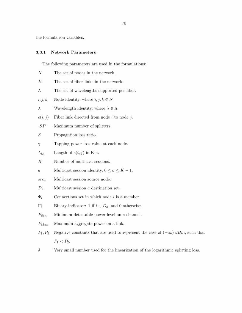
70
the formulation variables.
3.3.1 Network Parameters
The following parameters are used in the formulations:
N The set of nodes in the network.
E The set of fiber links in the network.
Λ The set of wavelengths supported per fiber.
i, j, k Node identity, where i, j, k ∈ N
λ Wavelength identity, where λ ∈ Λ
e(i, j) Fiber link directed from node i to node j.
SP Maximum number of splitters.
β Propagation loss ratio.
γ Tapping power loss value at each node.
Li,j Length of e(i, j) in Km.
K Number of multicast sessions.
a Multicast session identity, 0 ≤ a ≤ K − 1.
srca Multicast session source node.
Da Multicast session a destination set.
Φi Connections set in which node i is a member.
Γai Binary-indicator: 1 if i ∈ Da, and 0 otherwise.
PSen Minimum detectable power level on a channel.
PMax Maximum aggregate power on a link.
P1, P2 Negative constants that are used to represent the case of (−∞) dBm, such that
P1 < P2.
δ Very small number used for the linearization of the logarithmic splitting loss.

71
v, w Integer constants, such that v > w.
LGMaxi,j Auxiliary constant that determines maximum total gain on e(i, j).
Oi Degree of node i.
OMaxi Maximum node degree in the network.
M Very large numberIn our implementation, the value of M is chosen such that:
M ≥ max|E|, |Λ|, LGMaxi,j
K ∗ |Λ| , 10 ∗ log(OMaxi − 1) (3.1)
3.3.2 MILP Variables
The following variables are used in the MILP formulations:
LGi,j Total amplification gain needed over e(i, j).
ni,j Number of OAs on e(i, j).
T a,λi,j Tree link binary-indicator: 1 if e(i, j) is used by session a over λ; and
0 otherwise.
=a,λi Binary-indicator: 1 if λ is used by session a on any output (outgoing) tree link
from node i; and 0 otherwise.
Υai Binary-indicator: 1 if session a uses at least one output (outgoing) tree link from
node i.
Ra,hi,j Binary-indicator: 1 if h hops are needed to reach node j from node i for session a;
and 0 otherwise.
Ha,λi Number of hops between srca and node i over λ.
SLa,λi Splitting loss on channel λ at node i for session a.
f Tree fanout, i.e., number of outgoing tree links.

72
Aif Binary-indicator that is used for the linearization process of power splitting. It is
equal 1 if the value f is less than or equal the actual computed tree fanout; 0
otherwise.
Ω Power inspection site on a link, such that Ω ∈ beg,end.PΩ,a,λ
i,j Power level (in dBm) measured at the beginning (when Ω = beg) or end (when
Ω = end) of e(i, j) for wavelength λ that is used by session a.
αi Binary-indicator of node i’s splitting capability: 1 if it is an MC node; and 0
otherwise.
73
CHAPTER 4. Optical Amplifiers Placement Problem: Asymmetric Power
Case
In this chapter, we solve the asymmetric case of the OAP problem. Our solution is based on
the system model and notation defined earlier in Chapter 3. The OAP-Asymmetric problem is
formulated as a MILP with the objective of minimizing the total needed gain in the network.
The total network gain is defined as the summation of the gain required over all the links. Each
link gain is an abstraction of the accumulative gain achieved by a number of physical OAs1
whose number and location are computed off-line based on the power values at the beginning
of the links. For example, consider the case when the total gain over a link equals 53 dB and
assuming that the power strengths of the input signals allow the OAs to work in the non-
saturated region; hence produces the maximum gain. In this case, three OAs will be needed to
achieve this total gain value such that two OAs will provide the maximum gain value, i.e., 20
dB, and the third one operates in the saturated region and provides the remaining 13 dB gain.
If all the OAs operate in the saturated region, the number of OAs might increase and this
depends mainly on the variation (i.e., the degree of symmetry) of the input signals strengths.
The MILP solution provides the optimal solution for the OAP-Asymmetric problem by
solving all the constituent subproblems jointly. The OAP-Asymmetric problem we are trying
to solve here is formally defined as follows:
OAP-Asymmetric Problem Definition: ”Given the network topology, the maximum num-
ber of wavelengths and splitters, the traffic matrix, and assuming asymmetric power scenario,
the OAP-Asymmetric Problem attempts to find a feasible allocation of the OAs and splitters
(namely, their number and locations) such that all the traffic demands are satisfied and de-1In order to accommodate for any on-site amplification, the link gain includes any post-amplification at the
beginning of the link and any pre-amplification at end of the link, if available.
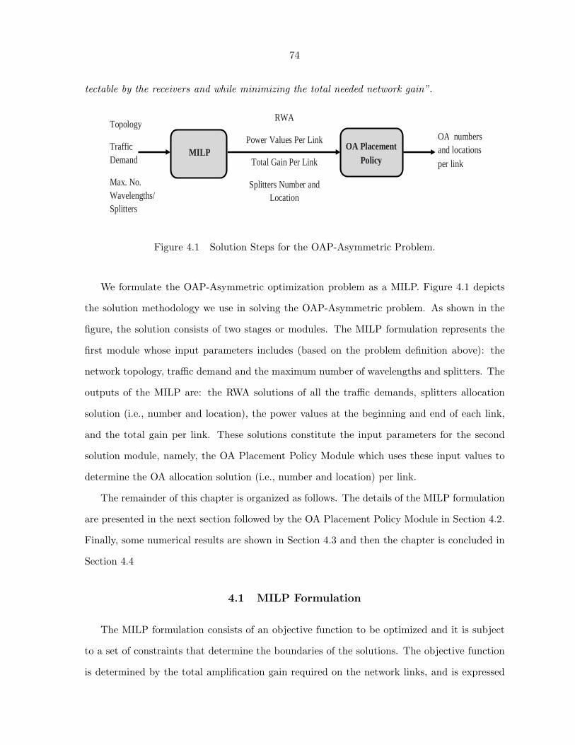
74
tectable by the receivers and while minimizing the total needed network gain”. Topology
Traffic Demand
Max. No. Wavelengths/Splitters
RWA
Power Values Per Link
Total Gain Per Link
Splitters Number and Location
MILP OA Placement
Policy
OA numbers and locations per link
Figure 4.1 Solution Steps for the OAP-Asymmetric Problem.
We formulate the OAP-Asymmetric optimization problem as a MILP. Figure 4.1 depicts
the solution methodology we use in solving the OAP-Asymmetric problem. As shown in the
figure, the solution consists of two stages or modules. The MILP formulation represents the
first module whose input parameters includes (based on the problem definition above): the
network topology, traffic demand and the maximum number of wavelengths and splitters. The
outputs of the MILP are: the RWA solutions of all the traffic demands, splitters allocation
solution (i.e., number and location), the power values at the beginning and end of each link,
and the total gain per link. These solutions constitute the input parameters for the second
solution module, namely, the OA Placement Policy Module which uses these input values to
determine the OA allocation solution (i.e., number and location) per link.
The remainder of this chapter is organized as follows. The details of the MILP formulation
are presented in the next section followed by the OA Placement Policy Module in Section 4.2.
Finally, some numerical results are shown in Section 4.3 and then the chapter is concluded in
Section 4.4
4.1 MILP Formulation
The MILP formulation consists of an objective function to be optimized and it is subject
to a set of constraints that determine the boundaries of the solutions. The objective function
is determined by the total amplification gain required on the network links, and is expressed
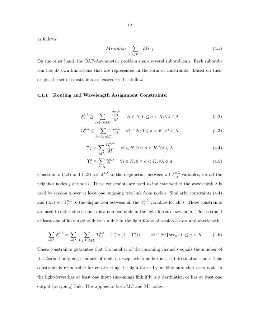
75
as follows:
Minimize∑
e(i,j)∈E
LGi,j (4.1)
On the other hand, the OAP-Asymmetric problem spans several subproblems. Each subprob-
lem has its own limitations that are represented in the form of constraints. Based on their
origin, the set of constraints are categorized as follows:
4.1.1 Routing and Wavelength Assignment Constraints:
=a,λi ≥
∑
j,e(i,j)∈E
T a,λi,j
M∀i ∈ N ; 0 ≤ a < K;∀λ ∈ Λ (4.2)
=a,λi ≤
∑
j,e(i,j)∈E
T a,λi,j ∀i ∈ N ; 0 ≤ a < K; ∀λ ∈ Λ (4.3)
Υai ≥
∑
λ∈Λ
=a,λi
M∀i ∈ N ; 0 ≤ a < K; ∀λ ∈ Λ (4.4)
Υai ≤
∑
λ∈Λ
=a,λi ∀i ∈ N ; 0 ≤ a < K; ∀λ ∈ Λ (4.5)
Constraints (4.2) and (4.3) set =a,λi to the disjunction between all T a,λ
i,j variables, for all the
neighbor nodes j of node i. These constraints are used to indicate wether the wavelength λ is
used by session a over at least one outgoing tree link from node i. Similarly, constraints (4.4)
and (4.5) set Υa,λi to the disjunction between all the =a,λ
i variables for all λ. These constraints
are used to determine if node i is a non-leaf node in the light-forest of session a. This is true if
at least one of its outgoing links is a link in the light-forest of session a over any wavelength.
∑
λ∈Λ
=a,λi =
∑
λ∈Λ
∑
k,e(k,i)∈E
T a,λk,i − Γa
i ∗ (1−Υai ) ∀i ∈ N/srca; 0 ≤ a < K (4.6)
These constraints guarantee that the number of the incoming channels equals the number of
the distinct outgoing channels of node i, except when node i is a leaf destination node. This
constraint is responsible for constructing the light-forest by making sure that each node in
the light-forest has at least one input (incoming) link if it is a destination or has at least one
output (outgoing) link. This applies to both MC and MI nodes.
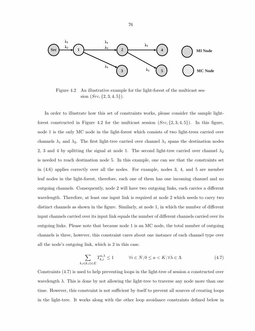
76 λ1 λ2
λ1 λ1 λ2
λ1 λ2
Src MI Node
MC Node
1 2
3
4
5
Figure 4.2 An illustrative example for the light-forest of the multicast ses-sion (Src, 2, 3, 4, 5).
In order to illustrate how this set of constraints works, please consider the sample light-
forest constructed in Figure 4.2 for the multicast session (Src, 2, 3, 4, 5). In this figure,
node 1 is the only MC node in the light-forest which consists of two light-trees carried over
channels λ1 and λ2. The first light-tree carried over channel λ1 spans the destination nodes
2, 3 and 4 by splitting the signal at node 1. The second light-tree carried over channel λ2
is needed to reach destination node 5. In this example, one can see that the constraints set
in (4.6) applies correctly over all the nodes. For example, nodes 3, 4, and 5 are member
leaf nodes in the light-forest, therefore, each one of them has one incoming channel and no
outgoing channels. Consequently, node 2 will have two outgoing links, each carries a different
wavelength. Therefore, at least one input link is required at node 2 which needs to carry two
distinct channels as shown in the figure. Similarly, at node 1, in which the number of different
input channels carried over its input link equals the number of different channels carried over its
outgoing links. Please note that because node 1 is an MC node, the total number of outgoing
channels is three, however, this constraint cares about one instance of each channel type over
all the node’s outgoing link, which is 2 in this case.
∑
k,e(k,i)∈E
T a,λk,i ≤ 1 ∀i ∈ N ; 0 ≤ a < K;∀λ ∈ Λ (4.7)
Constraints (4.7) is used to help preventing loops in the light-tree of session a constructed over
wavelength λ. This is done by not allowing the light-tree to traverse any node more than one
time. However, this constraint is not sufficient by itself to prevent all sources of creating loops
in the light-tree. It works along with the other loop avoidance constraints defined below in
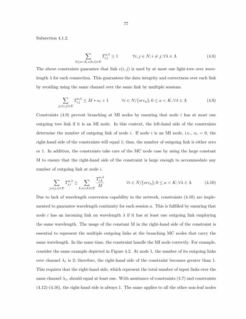
77
Subsection 4.1.2.
∑
0≤a<K,e(k,i)∈E
T a,λi,j ≤ 1 ∀i, j ∈ N ; i 6= j;∀λ ∈ Λ (4.8)
The above constraints guarantee that link e(i, j) is used by at most one light-tree over wave-
length λ for each connection. This guarantees the data integrity and correctness over each link
by avoiding using the same channel over the same link by multiple sessions.
∑
j,e(i,j)∈E
T a,λi,j ≤ M ∗ αi + 1 ∀i ∈ N/srca; 0 ≤ a < K; ∀λ ∈ Λ (4.9)
Constraints (4.9) prevent branching at MI nodes by ensuring that node i has at most one
outgoing tree link if it is an MI node. In this context, the left-hand side of the constraints
determine the number of outgoing link of node i. If node i is an MI node, i.e., αi = 0, the
right-hand side of the constraints will equal 1; thus, the number of outgoing link is either zero
or 1. In addition, the constraints take care of the MC node case by using the large constant
M to ensure that the right-hand side of the constraint is large enough to accommodate any
number of outgoing link at node i.
∑
j,e(j,i)∈E
T a,λj,i ≥
∑
k,e(i,k)∈E
T a,λi,k
M∀i ∈ N/srca; 0 ≤ a < K; ∀λ ∈ Λ (4.10)
Due to lack of wavelength conversion capability in the network, constraints (4.10) are imple-
mented to guarantee wavelength continuity for each session a. This is fulfilled by ensuring that
node i has an incoming link on wavelength λ if it has at least one outgoing link employing
the same wavelength. The usage of the constant M in the right-hand side of the constraint is
essential to represent the multiple outgoing links at the branching MC nodes that carry the
same wavelength. In the same time, the constraint handle the MI node correctly. For example,
consider the same example depicted in Figure 4.2. At node 1, the number of its outgoing links
over channel λ1 is 2; therefore, the right-hand side of the constraint becomes greater than 1.
This requires that the right-hand side, which represent the total number of input links over the
same channel λ1, should equal at least one. With assistance of constraints (4.7) and constraints
(4.12)-(4.16), the right-hand side is always 1. The same applies to all the other non-leaf nodes
78
in the light-forest.∑
i
αi ≤ SP ∀i ∈ N (4.11)
Constraint (4.11) ensures that the number of used splitters does not exceed the maximum
number of splitter, SP .
4.1.2 Loop-Avoidance Constraints:
The following set of constraints are used to guarantee that each light-tree of the light-
forest is loop free. These constraints are based on determining wether each destination node
is reachable from the source node through a number of hops that does not exceed N -1, where
N is the number of nodes in the network.
Ra,1i,j ≥
∑
λ
T a,λi,j
M∀e(i, j) ∈ E; 0 ≤ a < K (4.12)
Ra,1i,j ≤
∑
λ
T a,λi,j ∀e(i, j) ∈ E; 0 ≤ a < K (4.13)
Ra,1i,j = 0 ∀i, j ∈ N ; ∀e(i, j) /∈ E; 0 ≤ a < K (4.14)
Constraints (4.12) and (4.13) determine that, for session a, node j is reachable from node i by
one hop if link e(i, j) exists and is used by the light-tree at any wavelength. This is done by
setting the variable Ra,1i,j to the disjunction between all the T a,λ
i,j variables for all the channels.
On the other hand, constraints (4.14) ensure that Ra,1i,j is zero if the link e(i, j) does not exist
in the network.
Ra,hi,j =
∨
k
Ra,h−1i,k ∧Ra,1
k,j 0 ≤ a < K; ∀i, j ∈ N ; i 6= j; k 6= i; k 6= j; 1 < h < N (4.15)
Constraint (4.15) represents the general rule for determining the reachability of node j from
node i using h hops, where h is more than 1. This is a recursive equation which states that
node j is reachable over exactly h hops from the source node if there exist at least one path
that satisfies the following two conditions simultaneously:
1. Node j is reachable from an intermediate node, k, by one hop.
2. The intermediate node, k, is reachable from the source node by exactly h− 1 hops.
79
For example, consider the case for node 4 in the sample example depicted in Figure 4.2. At
this case, node 4 is reachable from the Src node through node 2 over 3 hops; thus, Ra,34,Src =1,
Ra,14,2 =1 and Ra,2
2,Src =1. The variable Ra,22,Src equals 1 since node 2 is reachable by the source
node via node 1 using 2 hops because both Ra,12,1 and Ra,1
1,Src equal 1 based on constraints (4.12)
and (4.13).
Please note that the expression c = a∧b, which is the conjunction operation, is represented
by the following set of constraints: c ≤ a+b2 and c ≥ a+ b− 1. Similarly, c = a∨ b, which is the
disjunction operation, can be represented by: c ≥ a+b2 and c ≤ a + b. In both cases, c ∈ 0, 1.
Γadst ≤
N−1∑
h=1
Ra,hsrca,dst 0 ≤ a < K; ∀dst ∈ Φa (4.16)
Constraints (4.16) ensure that any destination node is reached from its source node by no
more than N − 1 distinct hops. Since the left-hand side of the constraint is always 1, then, the
right-hand side must equal at least one, which means that each destination of the multicast
session much be reachable from the source node over at least one path who does not exceed
N-1 hops.
It is worth mentioning here that other schemes for loop avoidance are possible too. For
example, the loop avoidance scheme that was proposed in [14] relies on the use of the session
propagation delay bound in ensuring loop free construction of the light-forests. We also imple-
ment another simpler set of constraints for loop avoidance for the second MILP formulation.
These constraints will be presented in the next chapter.
4.1.3 Power Constraints:
The following constraints address the power constraints and the OA gain model issues. In
order to ensure that the total power constraint is met, we assume that the power value of each
wavelength cannot exceed PMax|Λ| , where |Λ| is the number of wavelengths. Although this can
result in using more OAs per link than needed (as more power can be used to reach longer
distance over links with more free channels), this helps in simplifying the MILP formulation
significantly.
PΩ,a,λi,j ≥ PSen∗T a,λ
i,j +P1∗(1−T a,λi,j ) ∀e(i, j) ∈ E; Ω ∈ beg, end; 0 ≤ a < K;∀λ ∈ Λ (4.17)
80
PΩ,a,λi,j ≤ (PMax − 10 ∗ log10|Λ|) ∗ T a,λ
i,j + P2 ∗ (1− T a,λi,j )
∀e(i, j) ∈ E; Ω ∈ beg, end; 0 ≤ a < K;∀λ ∈ Λ (4.18)
Constraints (4.17) and (4.18) ensure that each power level at the beginning and the end of
e(i, j) is within the valid ranges based on whether the light-forest uses e(i, j) over wavelength
λ or not. In the former case, T a,λi,j will equal 1; hence, constraints (4.17) ensure that the
power value is greater than PSen and constraints (4.18) ensure that the power value is less
than PMax|Λ| . In the case when link e(i, j) is not used by the light-forest, this value should be
equal to, theoretically, −∞ dBm (i.e., 0 mW). This case is represented by the constraints by
ensuring that the power value is a very small negative number that lies between two large
negative constants, namely, P1 and P2. The values of P1 and P2 are chosen to be (−5) ∗M
and (−2) ∗ M , respectively. The calculation of the value of P beg,a,λi,j is done before on-site
Post-Amplification, while P end,a,λi,j is measured after on-site Pre-Amplification, if any.
(1− T a,λi,j ) ∗M + P end,a,λ
i,j = (1− T a,λi,j ) ∗ (−M) + P beg,a,λ
i,j + LGi,j − β ∗ Li,j
∀e(i, j) ∈ E; 0 ≤ a < K;∀λ ∈ Λ (4.19)
Equation (4.19) is used on link e(i, j) to express the power on wavelength λ at the end point
of the link in terms of the power at the beginning of the link and the gain and loss due to
amplification and attenuation, respectively. It should be noted that when the link is not part
of the light-forest, i.e., the corresponding T a,λi,j equals 0, the power value at the end of the link
is guaranteed to be between P1 and P2.
(1− T a,λi,j ) ∗ v + P end,a,λ
i,j − SLa,λj − γ ≥ (1− T a,λ
j,k ) ∗ w + P beg,a,λj,k
∀e(i, j), e(j, k) ∈ E; 0 ≤ a < K; ∀λ ∈ Λ (4.20)
(1− T a,λi,j ) ∗ w + P end,a,λ
i,j − SLa,λj − γ ≤ (1− T a,λ
j,k ) ∗ v + P beg,a,λj,k
∀e(i, j), e(j, k) ∈ E; 0 ≤ a < K; ∀λ ∈ Λ (4.21)
Constraints (4.20) and (4.21) are used to relate the values of the power levels between the
end of an edge, say e(i, j) and the beginning of the following hop, say e(j, k), if any. In order
81
to maintain consistency with equations (4.17)-(4.19), and to be able to handle all the four
cases of the usage of the links e(i, j) and e(j, k), the values of v and w are chosen such that
v ≥ |P1| + M , and w < 0. The rationale of choosing these values is demonstrated with the
help of an example. Consider the case when both T a,λi,j and T a,λ
j,k equal 0. Recall that equations
(4.17) and (4.18) ensure that P beg,a,λi,j and P beg,a,λ
j,k are between P1 and P2. The value of v is
chosen to be (6∗M) in order to guarantee that left hand side of inequality (4.20) is still greater
than the right hand side even when both power values equal P1. The same holds for the left
hand side of inequality (4.20). Choosing the value of w to be negative helps in ensuring this
too. Proving that this criterion for choosing v and w hold for all the other cases of links usage
is straightforward.SLa,λ
i
M≤ αi ∀i ∈ N ; 0 ≤ a < K;∀λ ∈ Λ (4.22)
Constraints (4.22) ensure that the splitting loss value at an MI node is 0 dB for any connection
carried at any channel. In the case when node i is an MI node, the right-hand side of the
constraint is zero, which forces the left-hand side to be zero too; hence the splitting loss (SL)
at this node is zero over all channels. However, when αi is 1, the splitting loss can be more
than zero. In this case, the value of the splitting loss at the MC node is determined in dB by
this relation:
SLa,λi = 10 ∗ log10 f ∀i ∈ N ; 0 ≤ a < K;∀λ ∈ Λ (4.23)
Since the splitting degree, f , is a variable that is computed as part of the MILP solution,
incorporating this loss directly in the formulation will make it non-linear. Here, we introduce
an elegant way to find SLa,λi at MC nodes using a set of linear equations that are equivalent
to the non-linear one define by equation (4.23).∑
j,j 6=srca,e(i,j)∈E T a,λi,j − f + δ
M≤ Ai
f ∀i ∈ N ; 0 ≤ a < K;∀λ ∈ Λ; 2 ≤ f < Oi (4.24)
Aif ∗ 10 ∗ log10 f ≤ SLa,λ
i ∀i ∈ N ; 0 ≤ a < K; ∀λ ∈ Λ; 2 ≤ f < Oi (4.25)
SLa,λi ≥ 0 ∀i ∈ N ; 0 ≤ a < K;∀λ ∈ Λ (4.26)
In this context, we use the binary variable Aif to determine the actual tree fanout at the
specified node, i, that is computed by the formulation. Constraints (4.24) ensure that the
82
value of Aif is 1 for all the values of f that are less than or equal the actual computed tree
fanout at node i. Otherwise the value of Aif is either 0 or 1. This can be illustrated by the
following example. Assume that the actual fanout value at node i computed by the formulation
is 3. This value is represented in constraint (4.24) by the term∑
j,j 6=srca,e(i,j)∈E T a,λi,j . When
f= 2 and 3, we find out that the left-hand side of constraints (4.24) is always a positive real
number that is less than 1. Therefore, in order to satisfy this constraint, the value of Aif should
equal 1. Similarly, if we check for any value of f that is greater than 3 (the actual fanout of
the node), we find out that the left-hand side of the constraint is always negative; hence, the
constraint is satisfied whether Aif is 0 or 1.
Then, we use the value obtained for Aif from constraints (4.24) in conjunction with the
constraints in (4.25) in order to determine the exact splitting loss at node i over channel λ.
Two important things must be considered here with regards to the constraints defined in (4.25),
namely:
1. They are linear constraints since the log function is applied to a constance value, i.e., f .
2. The log function is an increasing function, namely, as the value of f increases, the splitting
loss increases.
Because the value of Aif is 1 as long as f equals the actual tree fanout, the splitting node
at node i should equal at least the amount of splitting loss corresponding to the actual f . For
example, when the actual fanout is 3, constraints (4.25) are satisfied for both f = 2 and 3 since
Ai2 and Ai
2 equal 1. But, since the splitting loss for the case of f=3 is greater than the case
when f=2, the actual SL value cannot be less than that of f=3. This draw a lower bound on
this value. Yet, no upper bound can be established using these constraints alone since they can
be still satisfied for the case when f is greater than the actual fanout (3, in our example). In
this case, the value of the splitting loss can grow indefinitely with no bound wether the value
of Ai2 is 0 or 1.
Luckily, this upper limit is implicity defined with the assistance of the objective function.
Since the objective function minimizes the total amplification gain, it indirectly attempts to
83
minimize all sources of power loss in the network including minimizing the fanout of the nodes.
Consequently, any unnecessary splitting loss value is eliminated from the computation which
forms the upper bound limit for the SLa,λi that is set to 0 for any f that is greater than the
actual fanout. Therefore, in order to satisfy the constraints in (4.25), the value of Aif in this
case will be set to 0 and the splitting loss is the actual splitting loss value of the node. Finally,
constraints (4.26) ensure that the splitting loss is always a non-negative value.
At the end of this section, we find out that this formulation has the following basic variables:
T a,λi,j , P beg,a,λ
srca,j , and LGi,j . The remaining variables are either topology-related variables, or can
be determined from the basic variables. Also, the number of variables and constraints used in
the formulation are found to be O(k ∗ |N |4) and O(k ∗ |N |3), respectively.
4.2 OA Placement Procedure
The second module of our solution is the OA Placement Policy Module. Many OA place-
ment policies are proposed in the literature. Our MILP formulation is generic and does not
assume any particular placement policy. Therefore, any OA placement policy can be used
in our implementation. We adopt the As Soon As Possible (ASAP) scheme [36] to find the
number and locations of the OAs per link. The policy is applied at each link and it uses the
power levels computed by the MILP formulation at the beginning and end of the link as well
as the total gain per link. The following steps are performed at each link and it repeats over
all the links in the network:
1. Initialize the remaining total amplification gain of the link (RLG) with the total ampli-
fication gain (LG) obtained from the formulation.
2. Traverse the link in the downstream direction and place an OA on the link if any of the
following conditions is satisfied:
(a) The total power over the link drops to a level that allows the OA to provide the
maximum gain, provided all power constraints are satisfied.
(b) The least-powered signal dropped to the minimum detectable level, namely, PSen.
84
(c) The distance of the segment traversed in the link is less than the remaining untra-
versed segment of the link.
3. RLG is then updated by subtracting the gain obtained by placing the OA from its current
value.
4. Steps 2 and 3 are repeated until RLG is zero or condition 2.b is not satisfied. In the
latter case, this means that the last OA should is placed before the end of the link and
its location is determined by the value of RLG. This is achieved by determining the total
input power that satisfy RLG and then compute the distance to which this total power
is obtained.
4.3 Numerical Results
In this section, some numerical results for the optimal solutions obtained using CPLEX [43]
are presented for the sample 6-nodes mesh network that is shown in Figure 1.13. We use the
experimental assumptions presented earlier in Subsection 1.6.3. Six connections are used in the
experiments and are denoted by: x0 = (0, 1, 2, 3, 4, 5), x1 = (1, 0, 2, 4), x2 = (5, 0, 1, 3, 4),x3 = (1, 5), and x4 = (1, 3, 5), and x5 = (2, 0, 1, 3, 4, 5). The results presented in this
section serve two purposes. First, they validate the correctness of the proposed solution,
and this done in the following subsection. Second, they present some numerical values of
the network resources computed by the MILP formulation. These results are provided in
Subsection 4.3.2.
4.3.1 Solution Validation
In order to validate the correctness of our solutions, Figure 4.3 depicts an example of the
optimal solutions obtained for the multicast sessions x0 and x1 when |Λ| = 2. The solutions
from the MILP formulation is shown in Figure 4.3-(a). The solutions include both the RWA
along with the power values measured at the beginning and the end of the tree links. Also,
the optimal number of splitters is found to be 1 and it is located at node 4. In addition, the
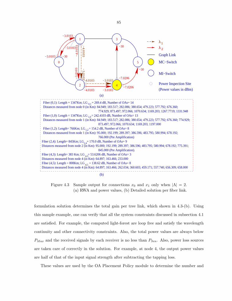
85
Fiber (4,5): Length = 808Km; LG4,5 = 138.62 dB, Number of OAs= 8Distances measured from node 4 (in Km): 64.897; 163.466; 262.034; 360.603; 459.171; 557.740; 656.309; 658.000
Distances measured from node 4 (in Km): 64.897; 163.466; 233.000Fiber (4,3): Length= 383 Km; LG4,3= 53.6206 dB, Number of OAs= 3
λ 1λ 2
0
4
1
2
3
5
−4.0103
−3
.01
03
−3.0103
−4
.01
03
MI−Switch
MC−Switch
Power Inspection Site
(Power values in dBm)
Graph Link
−4
.01
03
−3
.01
03
−30−3.0103
−3.0103
−30
−7.0206
−30
−7.0206−3.0103
−3.0103−4.0103
(a)
(b)
Fiber (0,1): Length = 1347Km; LG = 269.4 dB, Number of OAs= 140,1Distances measured from node 0 (in Km): 84.949; 183.517; 282.086; 380.654; 479.223; 577.792; 676.360;
Distances measured from node 1 (in Km): 84.949; 183.517; 282.086; 380.654; 479.223; 577.792; 676.360; 774.929; 1,0= 242.4103 dB, Number of OAs= 13Fiber (1,0): Length = 1347Km; LG
Fiber (1,2): Length= 766Km; LG1,2= 154.2 dB, Number of OAs= 8Distances measured from node 1 (in Km): 95.000; 192.199; 289.397; 386.596; 483.795; 580.994; 678.192;
Fiber (2,4): Length= 845Km; LG2,4= 170.0 dB, Number of OAs= 9Distances measured from node 2 (in Km): 95.000; 192.199; 289.397; 386.596; 483.795; 580.994; 678.192; 775.391;
845.000 (Pre Amplification).
774.929; 873.497; 972.066; 1070.634; 1169.203; 1267.7719; 1331.948
873.497; 972.066; 1070.634; 1169.203; 1197.000
766.000 (Pre Amplification)
Figure 4.3 Sample output for connections x0 and x1 only when |Λ| = 2.(a) RWA and power values, (b) Detailed solution per fiber link.
formulation solution determines the total gain per tree link, which shown in 4.3-(b). Using
this sample example, one can verify that all the system constraints discussed in subsection 4.1
are satisfied. For example, the computed light-forest are loop free and satisfy the wavelength
continuity and other connectivity constraints. Also, the total power values are always below
PMax and the received signals by each receiver is no less than PSen. Also, power loss sources
are taken care of correctly in the solution. For example, at node 4, the output power values
are half of that of the input signal strength after subtracting the tapping loss.
These values are used by the OA Placement Policy module to determine the number and
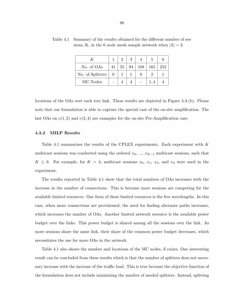
86
Table 4.1 Summary of the results obtained for the different number of ses-sions, K, in the 6 node mesh sample network when |Λ| = 2.
K 1 2 3 4 5 6
No. of OAs 41 55 94 108 165 252
No. of Splitters 0 1 1 0 2 1
MC Nodes - 4 4 - 1, 4 4
locations of the OAs over each tree link. These results are depicted in Figure 4.3-(b). Please
note that our formulation is able to capture the special case of the on-site amplification. The
last OAs on e(1, 2) and e(2, 4) are examples for the on-site Pre-Amplification case.
4.3.2 MILP Results
Table 4.1 summarizes the results of the CPLEX experiments. Each experiment with K
multicast sessions was conducted using the ordered x0, ..., xK−1 multicast sessions, such that
K ≤ 6. For example, for K = 4, multicast sessions x0, x1, x2, and x3 were used in the
experiment.
The results reported in Table 4.1 show that the total numbers of OAs increases with the
increase in the number of connections. This is because more sessions are competing for the
available limited resources. One form of these limited resources is the free wavelengths. In this
case, when more connections are provisioned, the need for finding alternate paths increases,
which increases the number of OAs. Another limited network resource is the available power
budget over the links. This power budget is shared among all the sessions over the link. As
more sessions share the same link, their share of the common power budget decreases, which
necessitates the use for more OAs in the network.
Table 4.1 also shows the number and locations of the MC nodes, if exists. One interesting
result can be concluded from these results which is that the number of splitters does not neces-
sary increase with the increase of the traffic load. This is true because the objective function of
the formulation does not include minimizing the number of needed splitters. Instead, splitting
87
should be used if this helps reducing the total amplification gain in the network. Another case
when splitting is used is when there is a shortage in the wavelengths. In this case, splitting can
help accommodating more sessions in the network. For example, one splitter is needed when
K = 3, while no splitter is needed when K = 4. This is due to the fact that by adding the
fourth connection to the network, a new situation is encountered in which different links are
used than those in the case of K = 3 and it is more beneficial in terms of total gain not to use
splitters.
4.4 Chapter Summary
In this chapter, we consider the OAP-Asymmetric problem under AOM in wavelength rout-
ing networks. Despite its nonlinearity, we successfully formulate the problem as a MILP with
the objective of minimizing the total required gain in the network. The following conclusions
can be drawn from this chapter:
1. Due to the complexity of the proposed MILP formulation, this solution is not scalable
for problems with bigger network size and higher traffic load. Therefore, efficient power-
aware heuristics are needed and this proposed MILP can act as a baseline against which
the accuracy of such heuristics can be assessed.
2. The objective function represented in (4.1) helps simplifying the formulation significantly.
Unfortunately, this objective function is not always a true representation of the actual
physical cost of the network which is represented by the number of OAs. The difference
in the power strengths of the different input signal at the entry point of the OAs is of
great importance too. For example, a link gain of 100 dB can be achieved using 5, 10
or 20 OAs each of which operates with a gain of 20, 10, or 5 dB, respectively, based on
their input powers.
Therefore, ensuring the symmetric of the input signals can play a significant role in saving
the number of OAs. Also, this formulation is considered as a basis for a more involved
formulation that takes care of the relationship between the link gain and the number of

88
OAs.
These two conclusions can be considered as the motivation of the work presented in the
next chapter which handles the OAP-Symmetric version of the problem. In this context, we
make use of the symmetric property to ensure good allocation of the OAs. Also, we devise a
new MILP formulation that takes care of the relation between the number of OAs and the link
gain in order to provide more accurate presentation of the network cost. Finally, we develop
a set of fast algorithms that provide near-optimal solutions for the large problem instances of
the OAP-Symmetric problem.
89
CHAPTER 5. Optical Amplifiers Placement Problem: Symmetric Power
Case
Motivated by the findings and remarks reported earlier in Section 4.4, we investigate the
OAP problem in this chapter under the symmetric power assumption. In order to address
these issues, our study here takes two directions. In the first direction, we formulate the OAP
problem as MILP with the objective of minimizing the total number of OAs needed in the
network. This new objective function provides the exact representation of the network cost
as it relates this network cost to the actual (or physical) presence of the OAs in the network
instead of relying on their collective effect. The latter case was used in Chapter 4 and it
was represented by the total amplification gain. Using this new objective function requires
modifying the MILP formulation introduced in Section 4.1 by including new set of constraints
that ensure the correct computation of the total number of OAs while maintaining the linearity
of the formulation.
In this chapter, we use the same two stages solution methodology depicted in Figure 4.1 to
solve the OAP-Symmetric Problem. The formal definition of the OAP-Symmetric Problem is
similar to that of the OAP-Asymmetric Problem presented earlier in Chapter 4 with respect to
their input parameters. However, they differ in their objective function as well as their power
symmetry assumption. The OAP-Symmetric Problem is formally defined as follows:
OAP-Symmetric Problem Definition: ”Given the network topology, the maximum number
of wavelengths and splitters, the traffic matrix, and assuming symmetric power scenario, the
OAP-Symmetric Problem is a network provisioning problem that aims to find a feasible allo-
cation of the OAs and splitters (namely, their number and locations) such that all the traffic
demands are satisfied and detectable by the receivers and while minimizing the total number of
90
optical amplifiers in the network”.
The solution from the proposed MILP formulation provides the optimal solution for the
OAP problem by solving all the constituent subproblems jointly. However, the MILP formula-
tion cannot provide fast solution for large instances of the problem. Therefore, in the second
direction of our study, we solve the problem using a greedy heuristic that provides faster,
yet near optimal solutions for the OAP problem. The operation of the heuristic approach is
based on solving the subproblems of the OAP problem separately, but without ignoring their
impact on each there. This could be achieved using novel set of routing cost functions for the
links, paths, and sessions that are represented in terms of the needed optical amplifiers. Using
these cost functions make it possible for the algorithm to make routing decisions that reduce
the required number of optical amplifiers; thus, minimize the network cost. In addition, the
heuristic solution is designed to provide a balance between the computation complexity and
the solution quality. This is achieved by defining two modes of operations, namely fixed and
adaptive, each of which can use fixed or alternate routing.
Our treatment of the OAP-Symmetric problem in this chapter is organized as follows.
Section 5.1 presents some additional system assumptions that we use in this chapter. This is
followed by an example that aims to present the significance of power symmetry in reducing
the number of OAs, and consequently the network cost, in Section 5.2. The details of the MILP
formulation and the heuristic algorithms are introduced in Sections 5.3 and 5.4, respectively.
Comprehensive set of results that report several system performance results are then introduced
in Section 5.5, and finally, we conclude this chapter in Section 5.6.
5.1 Addition System Model Assumptions
In addition to the two power constraints defined earlier in Subsection 1.6.1, our treatment
for the OAP-Symmetric problem requires the consideration of one additional power constraint
in our model, namely, the power symmetry over each link. In this context, all the channels
over any link must be of equal strength. Power Symmetry constraint is achieved by equipping
each output port of every OXC in the network with an optical power equalizer [7].
91
Moreover, the set of results reported in this chapter are obtained by using the As Late As
Possible (ALAP) OA placement policy [45, 36]. However, choosing any other policy does not
affect the main objective of this work, namely, determining the cost of the network in terms
of the number of OAs. It will only change the locations of these OAs.
5.2 Impact of Power Symmetry on Number of Optical Amplifiers: An
Example
The significance of the power symmetry constraint stems from the fact that it does not only
simplify the OAP solution, but it also ensures fair utilization of the deployed OAs. Ideally,
this can reduce the number of OAs by avoiding situations where the difference in strengths
between the input power signals is large enough to cause the OAs to be saturated by high-
powered input signal(s). This situation results in small OA gain and consequently small span
between the optical amplifiers.
In order to illustrate the significance of power symmetry constrain in reducing the number
of needed OAs over a link, let us consider the following example depicted in Figure 5.1 for link
e(1, 2) of length 150 km when the input power values over channels λ1 and λ2 equal −25 dBm
and −5 dBm, respectively. In this example, we use the ALAP OA placement policy. Figure
5.1-(a) shows the solution for the OAP-Asymmetric scenario where the number of needed OAs
equals 4 OAs. In this case, the first OA is placed 25 km away from node 1 since the strength
of the power signal over λ1 reached PSen, i.e., −30 dBm. At this location, the strength of the
other signal over λ2 is −10 dBm. Therefore, the difference between the two power strengths is
-20 dBm (0.01 mW), and the total input power to the first OA is −9.957 dBm (0.101 mW ).
Based on the simple OA model described by equation (1.2), the OA operates in the saturation
region. Therefore, its gain value equals 9.957 dB and the strengths of its output signals over
λ1 and λ2 increased to −20.043 dBm and −0.043 dBm, respectively. Similarly, the remaining
OAs are placed on the link such that the distance of the span between each consecutive OAs
equals 49.783 km. Finally, the length of the remaining link span between the last OA and
node 2 equals 25.43 km.
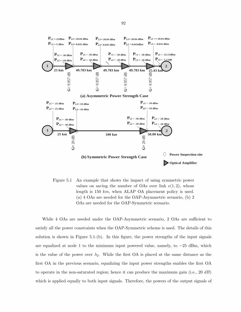
92 (a) Asymmetric Power Strength Case
(b) Symmetric Power Strength Case
Pλ1 = -30 dBm
Pλ2 = -10 dBm
Pλ1=-20.04 dBm
Pλ2=-0.043 dBm
Pλ1 = -30 dBm
Pλ2 = -10 dBm
Pλ1=-20.04 dBm
Pλ2 =-0.043dBm
Pλ1 =-25dBm
Pλ2 =-5 dBm
1 25 km 49.783 km 49.783 km
Pλ1 ==-20.04 dBm
Pλ2 = -0.043 dBm
Pλ1 = -10 dBm
Pλ2 = -10 dBm
Pλ1 = -30 dBm
Pλ2 = -30 dBm
Pλ1 = -25 dBm
Pλ2 = -25 dBm
1 100 km 50.00 km
Pλ1 = -20 dBm
Pλ2 = -20 dBm
G=
9.95
7 dB
2
2
G=
20 d
B
G=
9.95
7 dB
Pλ1=-20.04 dBm
Pλ2=-0.043 dBm
Pλ1 = -30 dBm
Pλ2 = -10 dBm
Pλ1 = -30 dBm
Pλ2 = -10 dBm
Pλ1 = -25.13dBm
Pλ2 = -5.13dB
49.783 km 25.43 km
G=
9.95
7 dB
G=
9.95
7 dB
Power Inspection site
Optical Amplifier
Pλ1=-10 dBm
Pλ2=-10 dBm
Pλ1 = -30 dBm
Pλ2 = -30 dBm 25 km
G=
20 d
B
Figure 5.1 An example that shows the impact of using symmetric powervalues on saving the number of OAs over link e(1, 2), whoselength is 150 km, when ALAP OA placement policy is used.(a) 4 OAs are needed for the OAP-Asymmetric scenario, (b) 2OAs are needed for the OAP-Symmetric scenario.
While 4 OAs are needed under the OAP-Asymmetric scenario, 2 OAs are sufficient to
satisfy all the power constraints when the OAP-Symmetric scheme is used. The details of this
solution is shown in Figure 5.1-(b). In this figure, the power strengths of the input signals
are equalized at node 1 to the minimum input powered value, namely, to −25 dBm, which
is the value of the power over λ2. While the first OA is placed at the same distance as the
first OA in the previous scenario, equalizing the input power strengths enables the first OA
to operate in the non-saturated region; hence it can produce the maximum gain (i.e., 20 dB)
which is applied equally to both input signals. Therefore, the powers of the output signals of
93
the first OA are still symmetric and higher than the output power signals produced from the
OAP-Asymmetric case. Using this hight powered strength, the signals can then reach further
away in the link (100 km in this case) without the need to amplify them.
5.3 MILP Formulation
In this section, we introduce the details of the proposed MILP formulation for solving
the OAP-Symmetric problem. The objective function of this formulation is to minimize the
network cost that is defined as the total number of OAs needed in the network to satisfy all
the required constraints. This objective function is expressed as follows:
Minimize∑
e(i,j)∈E
ni,j (5.1)
where ni,j is the number of OAs over each link.
The following subsections present the set of constraints we use in this formulation. However,
the MILP formulation we propose here to the solve the OAP-Symmetric problem shares some of
the constraints that were employed by the MILP formulation of the OAP-Asymmetric problem
in Chapter 4. For the sake of simplicity and due to the space constraints, the reader is referred
to these common constraints, whenever applicable.
5.3.1 Routing and Wavelength Assignment Constraints:
We use the same set of the Routing and Wavelength Assignments constraints defined earlier
in subsection 4.1.1 by constraints (4.2)-(4.11).
5.3.2 Loop Avoidance Constraints:
In this subsection, we define a new set of constraints that are used to ensure that the
constructed light-trees for each session do not include any loop. These sets of constraints rely
on computing the number of hops from the source node to each destination node and they
ensure that these number of hops do not exceed N − 1.
Ha,λsrca
= 0 0 ≤ a < K;∀λ ∈ Λ (5.2)
94
1− T a,λi,j − Ha,λ
i + 1−Ha,λj
M≥ 0 ∀e(i, j) ∈ E; 0 ≤ a < K; ∀λ ∈ Λ (5.3)
Γai +
Ha,λi − (|N | − 1)
M≤ 1 ∀e(i, j) ∈ E; 0 ≤ a < K;∀λ ∈ Λ (5.4)
By definition, the number of hops from the source node of any session to itself over any λ
is zero. Therefore, constraints (5.2) are used to ensure that this is true for each session under
investigation. In addition, constraints (5.3) ensure that if the link e(i, j) is used by session a
over a particular channel (i.e., T a,λi,j = 1), then node j is exactly one more hop away from the
session’s source node than node i over the light-tree carried by that channel. In this case, the
term (1 − T a,λi,j ) of the left-hand side of constraints (5.3) is zero, and for these constraints to
hold correctly, the fraction (Ha,λ
i +1−Ha,λj
M ) must be a non-positive quantity (i.e., either zero or
negative). This implies that Ha,λi + 1 ≤ Ha,λ
j is correct too. Since the formulation tries to
minimize the total number of OAs, it indirectly tries to minimize the total number of hops.
This results in forcing an upper bound on the number of hops, and the previous inequality
indicates that the difference in number of hops between any consecutive nodes connected by
a tree link is exactly 1. Please note than when (T a,λi,j = 0), constraints (5.3) is always true due
to the use of the large constant, M , which makes the fraction in the third term a very small
number that is less than 1.
Finally, constraints (5.4) ensure that a tree structure is generated with no loop by ensuring
that the number of hops from the source node to each destination node is no more than |N |−1
hops. In this context, if a node i is a destination node of session a, i.e., Γai = 1, the fraction in
the second term of constraints (5.4) must be a non-positive value in order for these constraints
to become true; which implies that Ha,λi ≤ (|N | − 1). On the other hand, when Γa
i = 0, the
left hand side of these constraints is always less than 1 because the use of the large constant,
M, in the second term makes it very small fraction that is much smaller than 1.
5.3.3 Power Constraints:
We use the same set of power constraints that were defined in Subsection 4.1.3 by constraints
(4.17) - (4.26). Nevertheless, in order to take care of the new objective function and the power
95
symmetric constraint, we define the following additional constraints:
P beg,a,λ1i,j − P beg,b,λ2
i,j = 3×M × (T a,λ1i,j − T b,λ2
i,j )
∀e(i, j); 0 ≤ a, b < K; ∀λ1, λ2,∈ Λ, λ1 6= λ2 (5.5)
Constraints (5.5) are used to enforce the power symmetric constraint by ensuring that all the
active signals at the beginning of each link have the same power strength. As the propagation
loss and power gain are both linear, enforcing these constraints at the beginning of the link is
sufficient to ensure that all the power signals over the whole link are symmetric. Please note
that when light-forest links (of the same connection or different connections) use link e(i, j),
the right hand side of constraints (5.5) becomes zero and both power values at the beginning
of the link should be equal. The same occurs in the case when both light-forest links do not
use the same link. However, when only one of them exist over the link, the difference in their
power values is guaranteed to be in the range between |P1| and |P2|, which is in compliance
with constraints (4.17) and (4.18).
LGi,j ≤ gmax × ni,j ∀e(i, j) (5.6)
LGi,j > gmax × (ni,j − 1) ∀e(i, j) (5.7)
These constraints determine the relation between the total gain and the needed number of OAs
per link such that the minimum number of OAs are used. Similar constraints were used in [45]
where gmax determined the maximum gain available at any amplifier which occurs when all the
input signals are at PSen. However, as the number of occupied channels per link is determined
by the MILP solution, we use an approximate approach to compute gmax in which we assume
that all the channels over all the network links are occupied. This assumption enables us to
pre-compute gmax using the OA model define in (1.1) such that the total input power (Pin)
is calculated as 10× log10(Λ× 10PSen
10 ). This approximation provides an exact value for gmax
when Λ is small, which is the case with our numerical results.
96
5.4 The Heuristic Algorithm
The OAP problem consists of three main subproblems. These subproblems are: Routing
(R), Wavelength Assignment (WA), and Power Assignment/Amplifiers Placement (PAAP)
subproblems. The solution of one subproblem impacts the solutions of the other subproblems.
Hence, the MILP formulation presented above solves the problem optimally by solving these
subproblems jointly. Despite its optimality, the MILP formulation is not scalable as it cannot
solve big-sized problem instances in a time efficient manner due to its high complexity. Such
complexity is represented in terms of the numbers of constraints and variables which are on
the order of O(|N |4 × |C| × |Λ|) and O(|N |2 × |C| × |Λ|), respectively.
Therefore, there is a need for a heuristic approach that produces fast solutions with high
quality degree. Such heuristic must be able to capture the main characteristics of the problem
under investigation. In this section, we present a heuristic solution, referred to as Optical-
amplifiers Placement (OP) algorithm.
5.4.1 Greedy Algorithm Motivation and Main Characteristics
The main goal of the OP algorithm is to achieve the balance between the produced solution
quality and the computation time. In order to achieve this goal, the operation of the OP
algorithm relies on the Divide-and-Conquer concept by dividing the problem into its natural
subproblems that are solved separately. However, the impact between these modules are taken
into account by employing a special set of cost functions for the links, network and sessions.
The significance of these cost functions stems from the fact that they are defined in terms of
optical amplifiers numbers. As these cost functions are used for the light-forest construction
and session routing, this allows us to capture the influence between R and PAAP subproblems
and results in efficient solutions.
Moreover, the design of the OP algorithm realizes the influence of the Power Sharing
concept. We introduced the Power Sharing concept in [62] as a means to capture the impact
of the various power issues on the network during the various stages of its lifetime. This
concept represents the result of sharing the available power by wavelengths at the entry point
97
of the links and OAs. Such influence is translated as connection blocking (called Power Sharing
Blocking) [62] during network operation phase. As a design problem, the power sharing concept
still holds, but it has different influence as all the connections must be accommodated (i.e., no
connection drops are allowed). In this context, the power sharing concept results in changing
the Network Power Status (NPS), which defines the network condition in terms of its
power values at the beginning of each link1, as well as the number, locations and gain values
of the OAs. The change in the NPS is a result of any of following behaviors:
1. As optical signal traverses from one link to another, its power strength may decay below
PSen anywhere in the light-forest, even with the use of the source node’s maximum
available power. This can result in adding more in-line, pre-amplification and/or post-
amplification OAs, which increases the network cost. We refer to this behavior as Power
Shortage Behavior.
2. Routing a new connection that shares links with some already provisioned connections
in the network can change the NPS by either:
(a) Dropping the gain of at least one OA to a level that causes a service disruption for at
least one session. Such service disruption occurs if the gain drop yields to changing
the strengths of its passing signals. As these signals traverse in the network, a
sequence of changes in the signals strength and other OAs gains can occur, which
might result in violating any of the power constraints. We refer to this behavior as
Gain Dropping Behavior.
(b) Changing the power values assigned to an already provisioned light-forest(s) in order
to maintain the power symmetry and maximum total power constraints defined by
constraints (4.18) and (5.5), respectively. Therefore, we call this behavior, the Power
Adjustment behavior.
The NPS is highly dynamic and sensitive to any change introduced to the NPS from these1Knowing the power values at the beginning of each link is merely sufficient to determine the power values
everywhere in the network.
98
behaviors. This is because any adjustment made to the network condition at one point in the
network may propagate to other network locations and can affect multiple connections. This
can create a complicated power management issue, especially if a large number of connections
are involved. Nevertheless, the OP algorithm is designed to tackle this dynamic nature by
allowing changes to occur to the NPS while ensuring that their impacts are handled in an
efficient manner.
Finally, the OP algorithm is designed to optimize the solutions at two levels. At the lowest
level, namely, the light-forest construction level, it allows the destinations to be attached to
the sub-forest using multiple alternate paths, instead of a single path. Using alternate routing
in this manner allows the OP algorithm to explore a bigger solution space and the light-forest
can expand to new destinations using the path of the minimum (present) path. In addition,
the OP algorithm allows constructing more than one light-forest per session. The one with the
least cost is then chosen to be placed in the network. At the light-forest placement level, the
algorithm defines two operation modes, namely, Fixed and Adaptive Modes. In the Fixed mode,
light-forests are constructed based on the initial NPS and then they are placed in the network
according to their costs. With the Adaptive mode, however, placing each light-forest in the
network is followed by reconstructing the remaining light-forests that are not yet provisioned
based on the most recent NPS. Rerouting the remaining sessions allows the OP algorithm to
account for the impact of light-forests on each other which improves the solution accuracy, yet,
at the cost of extra computation.
5.4.2 Cost Functions Definitions
The following set of cost definitions are employed by the OP algorithm:
• The current cost of link e(i, j) is defined as the current number of OAs needed over the
link, namely ce(i,j) = |ni,j |. This includes any Post-Amplification at node i, and any
Pre-Amplification at node j.
• The current network cost is computed as the total number of OAs over all the links in
the network. In other words, C =∑
e(i,j) ce(i,j)
99
• The cost of the path that connects a destination to the subtree-forest is defined as the
change in the network cost that results if such a path is used for expanding the subtree-
forest to that destination.
• The session cost is also calculated as the change in the network cost if its light-forest is
placed in the network.
Using these cost functions has the following advantages:
1. It is possible to base the routing decisions of the light-forests on the system power budget.
This establishes a connection between the R and PAAP subproblems and can result in
better solutions.
2. These cost functions are dynamic as their definition is based on the the most recent NPS.
This is important to ensure the correctness and goodness of the produced solutions.
3. Using the definitions of the path and session costs is effective in relating the routing
and placement decisions to its future consequences. This post-influence scheme help in
capturing the influence between the connections.
4. Finally, the link cost function is a positive increasing function. Therefore, link costs
increases as more of its channels become occupied with routed sessions. This is useful in
balancing the load in the entire network
5.4.3 OP Algorithm Details
We present the details of the OP algorithm in this subsection. The OP algorithm is
designed as an iterative algorithm such that the final solution is the result of a set of optimized
sub-solutions. Figure 5.2 depicts the basic operation of the algorithm which consists of three
main stages. These stages are: the Light-Forests Construction (LFC) Stage, the Light-Forests
Placement (LFP) Stage and the Light-Forest Reconstruction (LFR) Stage. The core operation
of the LFC and LFR stages is the Light-Forest Construction Module which is depicted in
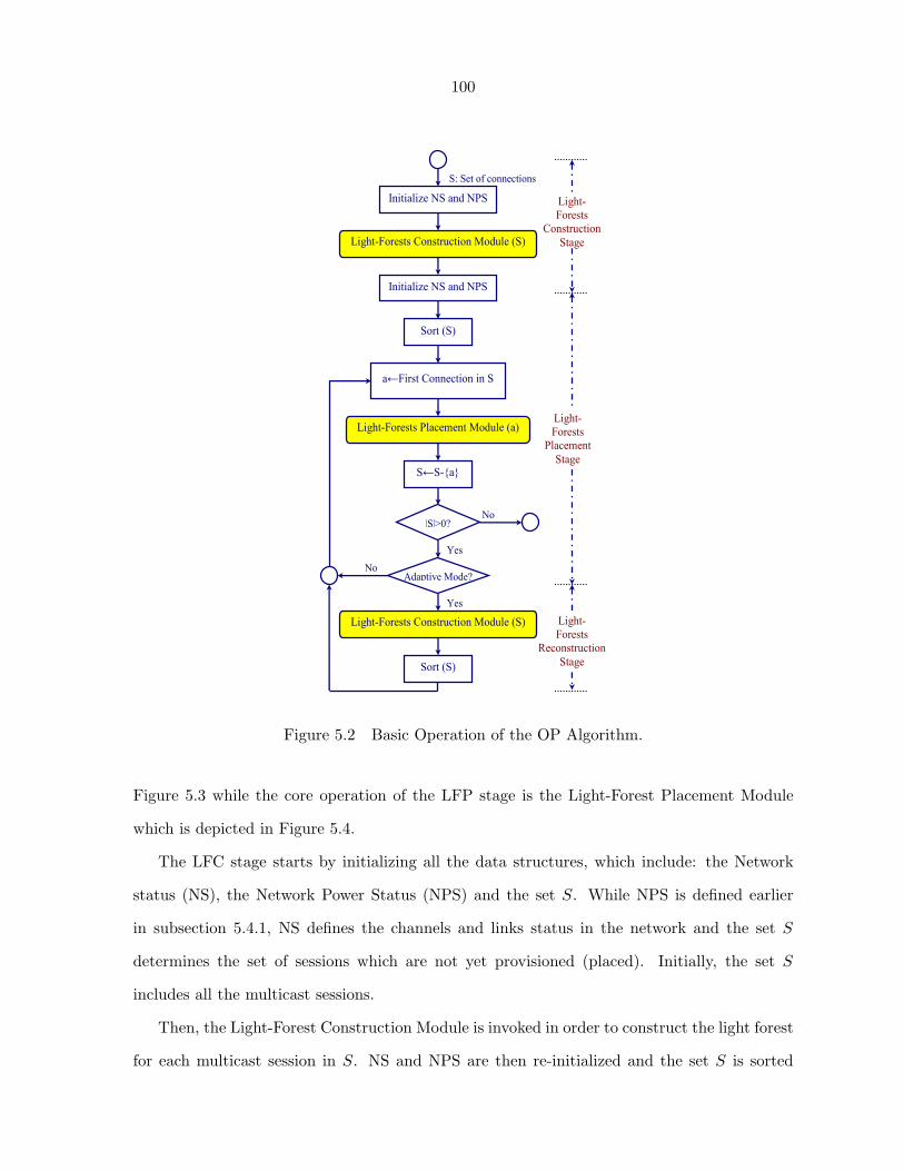
100
S: Set of connections
Initialize NS and NPS
Light-Forests Construction Module (S)
Sort (S)
Yes
No
a←First Connection in S
Light-Forests Placement Module (a)
|S|>0?
S←S-a
Adaptive Mode? No
Light-Forests Construction Module (S)
Yes
Sort (S)
Initialize NS and NPS
Light-
Forests
Reconstruction
Stage
Light-
Forests
Placement
Stage
Light-
Forests
Construction
Stage
Figure 5.2 Basic Operation of the OP Algorithm.
Figure 5.3 while the core operation of the LFP stage is the Light-Forest Placement Module
which is depicted in Figure 5.4.
The LFC stage starts by initializing all the data structures, which include: the Network
status (NS), the Network Power Status (NPS) and the set S. While NPS is defined earlier
in subsection 5.4.1, NS defines the channels and links status in the network and the set S
determines the set of sessions which are not yet provisioned (placed). Initially, the set S
includes all the multicast sessions.
Then, the Light-Forest Construction Module is invoked in order to construct the light forest
for each multicast session in S. NS and NPS are then re-initialized and the set S is sorted
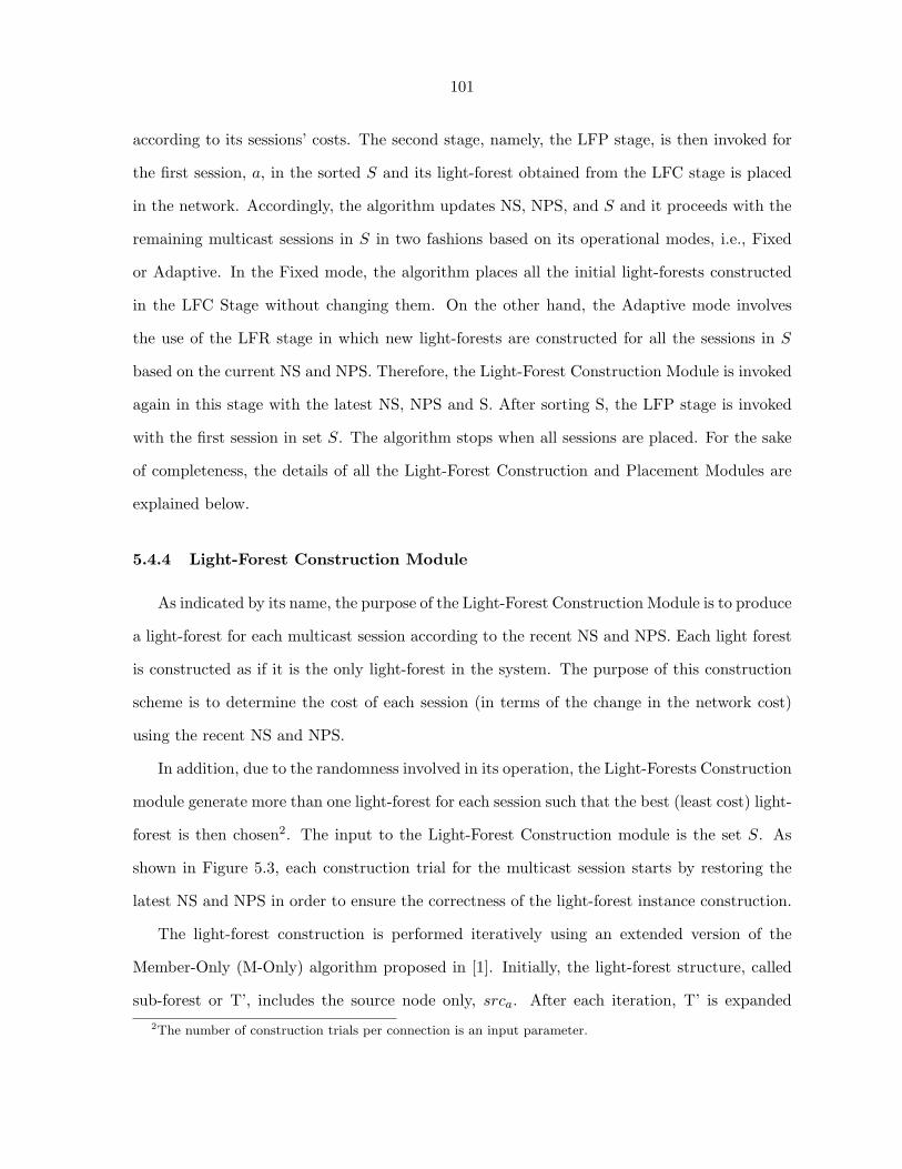
101
according to its sessions’ costs. The second stage, namely, the LFP stage, is then invoked for
the first session, a, in the sorted S and its light-forest obtained from the LFC stage is placed
in the network. Accordingly, the algorithm updates NS, NPS, and S and it proceeds with the
remaining multicast sessions in S in two fashions based on its operational modes, i.e., Fixed
or Adaptive. In the Fixed mode, the algorithm places all the initial light-forests constructed
in the LFC Stage without changing them. On the other hand, the Adaptive mode involves
the use of the LFR stage in which new light-forests are constructed for all the sessions in S
based on the current NS and NPS. Therefore, the Light-Forest Construction Module is invoked
again in this stage with the latest NS, NPS and S. After sorting S, the LFP stage is invoked
with the first session in set S. The algorithm stops when all sessions are placed. For the sake
of completeness, the details of all the Light-Forest Construction and Placement Modules are
explained below.
5.4.4 Light-Forest Construction Module
As indicated by its name, the purpose of the Light-Forest Construction Module is to produce
a light-forest for each multicast session according to the recent NS and NPS. Each light forest
is constructed as if it is the only light-forest in the system. The purpose of this construction
scheme is to determine the cost of each session (in terms of the change in the network cost)
using the recent NS and NPS.
In addition, due to the randomness involved in its operation, the Light-Forests Construction
module generate more than one light-forest for each session such that the best (least cost) light-
forest is then chosen2. The input to the Light-Forest Construction module is the set S. As
shown in Figure 5.3, each construction trial for the multicast session starts by restoring the
latest NS and NPS in order to ensure the correctness of the light-forest instance construction.
The light-forest construction is performed iteratively using an extended version of the
Member-Only (M-Only) algorithm proposed in [1]. Initially, the light-forest structure, called
sub-forest or T’, includes the source node only, srca. After each iteration, T’ is expanded2The number of construction trials per connection is an input parameter.
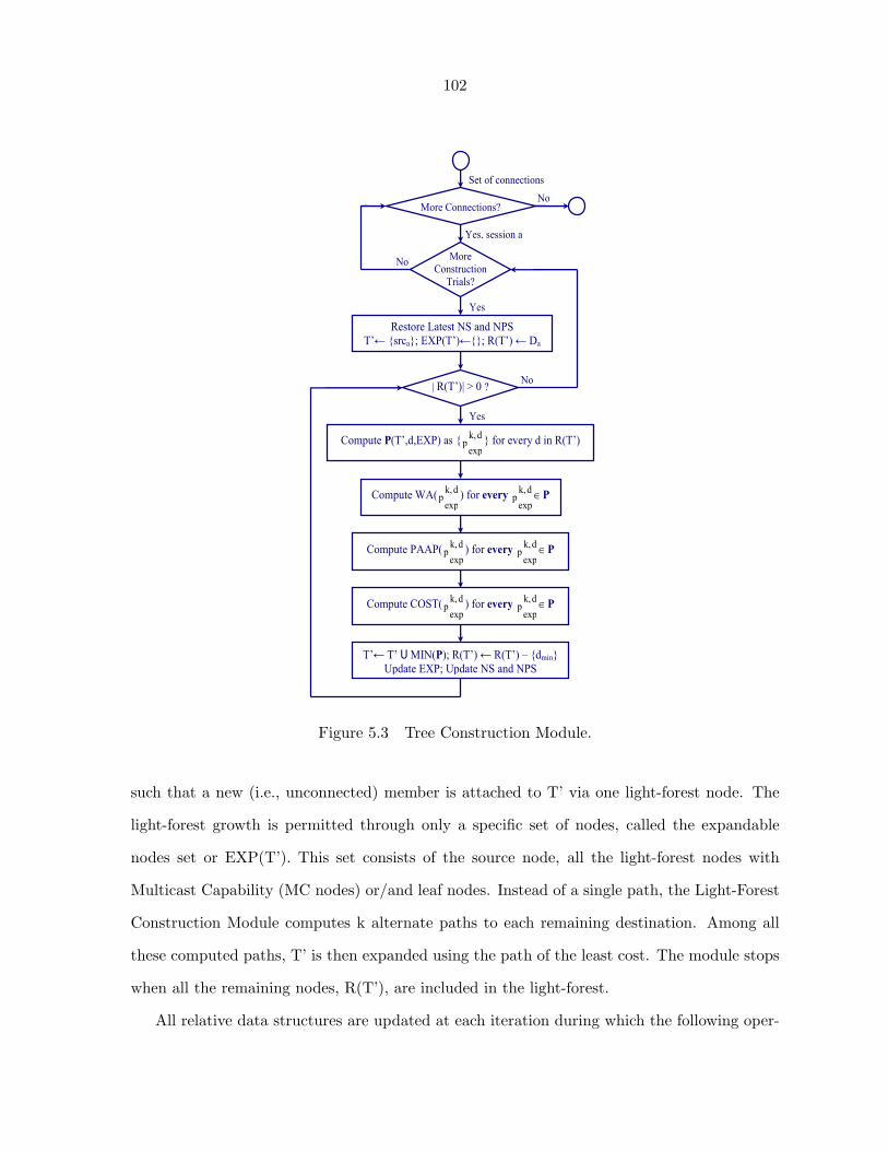
102
Set of connections
More Connections?
Yes, session a
More
Construction
Trials?
Yes
Restore Latest NS and NPS
T’← srca; EXP(T’)←; R(T’) ← Da
No
No
| R(T’)| > 0 ?
Yes
Compute P(T’,d,EXP) as exp
dk,p for every d in R(T’)
Compute WA(exp
dk,p ) for every
exp
dk,p ∈P
Compute PAAP(exp
dk,p ) for every
exp
dk,p ∈P
Compute COST(exp
dk,p ) for every
exp
dk,p ∈P
T’← T’ U MIN(P); R(T’) ← R(T’) – dmin
Update EXP; Update NS and NPS
No
Figure 5.3 Tree Construction Module.
such that a new (i.e., unconnected) member is attached to T’ via one light-forest node. The
light-forest growth is permitted through only a specific set of nodes, called the expandable
nodes set or EXP(T’). This set consists of the source node, all the light-forest nodes with
Multicast Capability (MC nodes) or/and leaf nodes. Instead of a single path, the Light-Forest
Construction Module computes k alternate paths to each remaining destination. Among all
these computed paths, T’ is then expanded using the path of the least cost. The module stops
when all the remaining nodes, R(T’), are included in the light-forest.
All relative data structures are updated at each iteration during which the following oper-
103
ations are performed:
1- Path Computation (PC):
In this step, a set of k-shortest alternative paths from each unconnected destination, d,
to each expandable node in T’, EXP(T’), is computed. Please note that the shortest path
does not always translate to the least costly path (in terms of the increase in the number of
OAs). Using k alternate paths increases the chance for the member node to join the sub-forest
structure, T’, using the least-cost shortest path. Nevertheless, it should be clear that this step
still requires checking and removing any overlapping or looping in the resultant sub-forest.
This step is necessary since the selected path may share some nodes and links with T’.
2- Path Wavelength Assignment (PWA):
The PWA step is performed for each computed path from step 1. Depending on the
expandable node, two scenarios are possible in this operation. On one hand, we employ the
First-Fit scheme (in which the first available common wavelength over all links in the path is
chosen) if the path under investigation connects the destination node to the source node itself
(i.e., new forest branch is created). On the other hand, if the attaching node is not the source
node, the new forest segment from the expandable node to the destination should continue using
the same channel (if available) used over the forest segment connecting the source node to the
expandable node. If such a wavelength is not available, the previous wavelength assignment is
ignored and a new wavelength is computed using the First-Fit scheme over the new path from
the source node to the connecting destination node via the expandable node.
3- Path Power Assignment/Amplifiers Placement (P-PAAP):
For each path instance passed the PWA step, the P-PAAP operation is responsible for
determining the power values and the OAs placement over each of its links. The P-PAAP
module relies on using a queue structure, called Q, which consists of unique entities of the link
identities and aims to separate the links identities from their power values.
The P-PAAP operation starts by marking the session under investigation as affected and
adding the first link of the path to Q. Then P-PAAP runs iteratively such that at each iteration,
104
the link at Q’s head is processed by performing the following operations:
• Initial Power Determination Operation.
This operation is responsible for determining the power values at the beginning of the
head link in Q such that no power constraint is violated and that the power symmetry
constraint is maintained. Two factors determine these power values, namely, whether
the head link is connected from the source and/or it has more than one channel. For
instance, if the link is launched from the session’s source node and it is the only channel
on the link, the maximum power value can be assigned to the channel. Otherwise, if the
head link is not launched from the session’s source, this step adjusts these power values
according to the power and symmetry constraints.
• OA Placement Operation.
Using the power values at the beginning of the head link, the OAs are placed over the
link based on the ALAP policy3. In order to accommodate for the change in NPS, this
step may involve changing the OAs locations (hence, their total number) over the head
link which were computed from the previous algorithm iteration.
Allowing such modification to happen by the OP algorithm is essential to provide accu-
racy to our solution and allows the system to adapt to any changes. However, this will
be done with the minimum maintenance overhead with the help of the Q structure and
its rules of addition/deletion of links to/from it, as will be shown below.
• Update Q Operation.
Q is then updated by adding more links, if any. The set of potential links to be added
to Q are chosen from the set of outgoing links, <, launched from the sink node of the
current link at Q’s head. In order to prevent Q from being unnecessarily modified, Q is
updated with those outgoing links that satisfy the following conditions:3Please note that we assume the As Late As Possible (ALAP) OA placement policy; yet, any other policy
can be used in our algorithm.
105
– They are part of the light-forest of the current session under investigation. This
should guarantee the continuation of power investigation for the current sub-forest.
– They are part of the light-forest of all the other sessions over the link, provided
that a new power value is observed at the end of the head link which is different
from the one computed from the previous iteration. Such change in power values
from iteration to iteration indicates a change in the system status that needs to be
propagated. Hence, we use Q to trace such a change in the NPS.
Once processed fully, the link at the Q’s head is removed and the P-PAAP operation
continues with the next link in Q and it stops when Q becomes empty. Please note here that
a link can be revisited more than once during the iteration lifetime4. This occurs because the
same link can be at different depth of the various light-forests. During each link traversal, more
power values over the link become available. P-PAAP deals with those power values that are
currently available which enables it to work even with partial knowledge of the power values.
However, allowing several traversals of the links ensures the complete availability of the power
values at the link.
4- Compute Path Cost:
Finally, the cost of all the computed paths is evaluated as explained in Subsection 5.4.2, and
T’ is then expanded using the path of the least cost. The Light-Forest Construction module
then stops when all the remaining nodes, denoted by R(T), are included in the light-forest.
5.4.5 Light-Forest Placement Module
This module is responsible for placing the light-forest constructed in the Light-Forest Con-
struction module in the network and then change the NS and NPS accordingly, as shown in
Figure 5.4. Therefore, there is no routing in this module and it focuses on solving the WA and
PAAP subproblems at the forest level. These two operations are similar to the corresponding
ones introduced in the Light-Forest Construction Module. However, the delivery structure4Although multiple traversals of the link is permitted during the P-PAAP, Q contains at most one instance
of the link at each algorithm step. Preventing multiple copies of the same link in Q eliminates any unnecessarycalculations since power values are separate from the link identities.
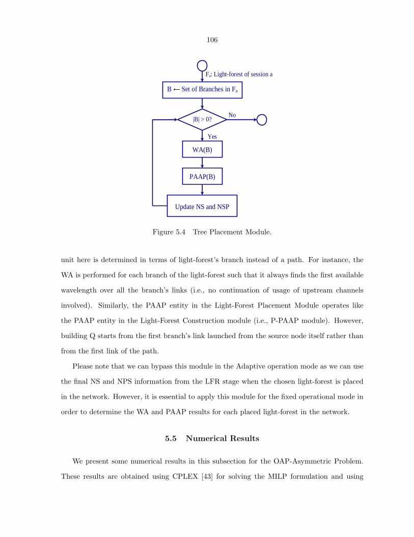
106
Fa: Light-forest of session a
|B| > 0?
Yes
WA(B)
No
B Set of Branches in Fa
PAAP(B)
Update NS and NSP
Figure 5.4 Tree Placement Module.
unit here is determined in terms of light-forest’s branch instead of a path. For instance, the
WA is performed for each branch of the light-forest such that it always finds the first available
wavelength over all the branch’s links (i.e., no continuation of usage of upstream channels
involved). Similarly, the PAAP entity in the Light-Forest Placement Module operates like
the PAAP entity in the Light-Forest Construction module (i.e., P-PAAP module). However,
building Q starts from the first branch’s link launched from the source node itself rather than
from the first link of the path.
Please note that we can bypass this module in the Adaptive operation mode as we can use
the final NS and NPS information from the LFR stage when the chosen light-forest is placed
in the network. However, it is essential to apply this module for the fixed operational mode in
order to determine the WA and PAAP results for each placed light-forest in the network.
5.5 Numerical Results
We present some numerical results in this subsection for the OAP-Asymmetric Problem.
These results are obtained using CPLEX [43] for solving the MILP formulation and using
107
the C++ Programming Language for implementing the OP algorithm. We first examine the
quality of the solutions produced by the OP algorithm by comparing them with the optimal
solutions of the MILP formulation using the 6-nodes mesh network shown in Figure 1.13. After
establishing such quantitative comparison, we present various results that illustrate different
aspects of the proposed OP algorithm using the 14-nodes NSFNET shown in Figure 1.14.
In addition to the experiments parameters and assumptions defined in Subsections 1.6.3
and 5.1, these results are obtained under the following assumptions:
1. Descending-order policy is used by the OP algorithm for sorting the set of connections
constructed in the LFC stage.
2. The OP algorithm runs for at least 10 times per problem instance and the best solution
that produces the minimum number of OAs is chosen.
5.5.1 Comparative Results Between the Optimal and Heuristic Numerical Re-
sults
Tables 5.1 and 5.2 compare the results obtained from CPLEX to their counterparts obtained
from the OP heuristic for the 6-nodes mesh network. It is important to note that the MILP
formulation aims to solve the OA Placement (OAP) problem with more restrictive constraints
than the OP heuristic. In this context, the optimal solutions from CPLEX are obtained not
only for the number of OAs, but also for the number of splitters and their locations. Also,
CPLEX experiments are conducted with limited number of available channels in the network.
These constraints are relaxed in the OP heuristic solutions as the number/location of the
splitters is predetermined and no upper bound is imposed on the number of available channels.
Therefore, in order to make a meaningful comparison between these results, the following
three actions are taken into account:
1. The OP heuristic experiments are carried out with the same number/location of splitters
obtained from CPLEX for the same problem instance.
108
2. The quality of the solutions obtained from the OP heuristic with respect to the optimal
solutions will be determined by two factors. First, the difference in the number of OAs
(i.e., the objective function) obtained from both solutions. Second, how much extra
network resources (if any) are needed by the OP algorithm.
3. Due to Constraints (4.18), we also make sure that the individual signal strength produced
by OP algorithm does not exceed PMaxΛ dBm 5.
4. The operation of the OP algorithm initializes the number of OAs per link e(i, j) with the
least number of OAs needed over the link, denoted by |OA|mini,j . The value of |OA|min
i,j
is computed as if PMax is used over the link e(i, j) to deliver the signal from node i to
node j only. Effectively, each link, e(i, j), will have at least |OA|mini,j , whether or not it
is used by any session in the network. The current MILP formulation reports that the
number of needed OAs is zero when link e(i, j) is not used in the network. Therefore,
we modify the OA Placement Policy Module to include the computation of |OA|mini,j in
the reported results.
Table 5.1 determines the number of OAs obtained from CPLEX (|OA|C) compared to
those obtained from the OP heuristic (|OA|i). The index i determines the number of alternate
paths used in constructing the light-forest in LFC stage. Each |OA|i solution takes the (x/y)
format to determine the |OA| when the Fixed and Adaptive schemes are employed, respectively.
The same symbolic notation and (x/y) format is used in Table 5.2 to determine the network
resources consumed by the produced solutions.
Basically, there are two network resources that are of interest to us and which are computed
at the network-wide scale. These resources are:
1. The maximum number of distinct channels used over any link; this is referred to as ψ.
2. The number of links used in constructing all the light-forests (i.e., links with at least one
used channel); this referred to as ÃL.5As this action is taken for comparison purposes only, we do not take this limitation into account for all the
results presented in Subsection 5.5.2.
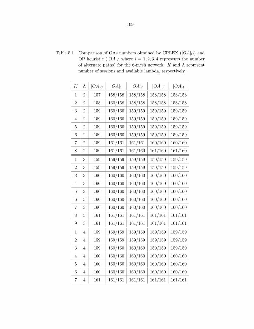
109
Table 5.1 Comparison of OAs numbers obtained by CPLEX (|OA|C) andOP heuristic (|OA|i; where i = 1, 2, 3, 4 represents the numberof alternate paths) for the 6-mesh network. K and Λ representnumber of sessions and available lambda, respectively.
K Λ |OA|C |OA|1 |OA|2 |OA|3 |OA|41 2 157 158/158 158/158 158/158 158/158
2 2 158 160/158 158/158 158/158 158/158
3 2 159 160/160 159/159 159/159 159/159
4 2 159 160/160 159/159 159/159 159/159
5 2 159 160/160 159/159 159/159 159/159
6 2 159 160/160 159/159 159/159 159/159
7 2 159 161/161 161/161 160/160 160/160
8 2 159 161/161 161/160 161/160 161/160
1 3 159 159/159 159/159 159/159 159/159
2 3 159 159/159 159/159 159/159 159/159
3 3 160 160/160 160/160 160/160 160/160
4 3 160 160/160 160/160 160/160 160/160
5 3 160 160/160 160/160 160/160 160/160
6 3 160 160/160 160/160 160/160 160/160
7 3 160 160/160 160/160 160/160 160/160
8 3 161 161/161 161/161 161/161 161/161
9 3 161 161/161 161/161 161/161 161/161
1 4 159 159/159 159/159 159/159 159/159
2 4 159 159/159 159/159 159/159 159/159
3 4 159 160/160 160/160 159/159 159/159
4 4 160 160/160 160/160 160/160 160/160
5 4 160 160/160 160/160 160/160 160/160
6 4 160 160/160 160/160 160/160 160/160
7 4 161 161/161 161/161 161/161 161/161
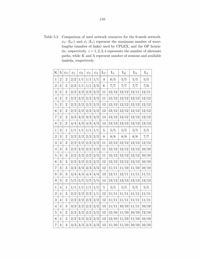
110
Table 5.2 Comparison of used network resources for the 6-mesh network.ψC (ÃLC) and ψi (ÃLi) represent the maximum number of wave-lengths (number of links) used by CPLEX, and the OP heuris-tic, respectively. i = 1, 2, 3, 4 represents the number of alternatepaths, while K and Λ represent number of sessions and availablelambda, respectively.
K Λ ψC ψ1 ψ2 ψ3 ψ4 ÃLC ÃL1 ÃL2 ÃL3 ÃL4
1 2 2 2/2 1/1 1/1 1/1 4 6/5 5/5 5/5 5/5
2 2 2 2/2 1/1 1/1 2/2 6 7/7 7/7 7/7 7/6
3 2 2 2/2 2/2 2/2 2/2 11 12/12 12/12 12/11 12/11
4 2 2 2/2 2/2 2/2 2/2 11 12/12 12/12 12/12 12/12
5 2 2 2/2 2/2 2/2 2/2 12 12/12 12/12 12/12 12/12
6 2 2 2/2 2/2 2/2 2/2 12 13/12 12/12 12/12 12/12
7 2 2 3/3 3/2 3/2 3/2 14 13/12 13/12 12/12 12/12
8 2 2 4/4 4/3 4/3 4/3 14 13/13 13/13 13/13 13/13
1 3 1 1/1 1/1 1/1 1/1 5 5/5 5/5 5/5 5/5
2 3 2 2/2 2/2 2/2 2/2 8 8/8 8/8 8/8 7/7
3 3 3 2/2 2/2 2/2 2/2 11 12/12 12/12 12/12 12/12
4 3 3 2/2 2/2 2/2 2/2 11 12/12 12/12 12/12 10/10
5 3 3 2/2 2/2 2/2 2/2 11 12/12 12/12 12/12 10/10
6 3 3 2/2 2/2 2/2 2/2 12 12/12 12/12 12/12 10/10
7 3 3 3/3 3/3 3/3 3/3 12 11/11 11/10 11/10 10/10
8 3 3 4/4 4/4 4/4 4/4 13 12/11 12/11 11/11 11/11
9 3 3 5/5 5/5 5/5 5/5 14 13/13 13/13 13/13 13/13
1 4 1 1/1 1/1 1/1 1/1 5 5/5 5/5 5/5 5/5
2 4 3 2/2 2/2 2/2 1/1 12 11/11 11/11 11/11 11/11
3 4 2 2/2 2/2 2/2 2/2 12 11/11 11/11 11/11 11/11
4 4 3 3/2 2/2 2/2 2/2 13 11/11 10/10 11/11 10/10
5 4 2 2/2 2/2 2/2 2/2 13 12/10 11/10 10/10 12/10
6 4 2 2/2 2/2 2/2 2/2 13 12/10 11/10 11/10 10/10
7 4 3 3/3 3/3 3/3 3/3 13 11/10 11/10 10/10 10/10
111
From the results in Table 5.1, it is clear that the quality of the solutions produced by
the OP heuristic is determined by its computation complexity. Two factors contribute to this
complexity, namely, the number of alternate paths used for constructing each light-forest, and
whether or not rerouting is performed to reconstruct the remaining unplaced light-forests. The
OP heuristic permits the use of any combination of these factors such that the computation
complexity ranges from minimum computation (namely, Fixed scheme with one alternate
path for routing) to maximum computation (namely, Adaptive scheme with maximum
number of alternate paths for routing).
The following conclusions can be drawn from the results in Tables 5.1:
• The OP heuristic remarkably succeeds to obtain the optimal solution in most cases, even
with the use of the minimum computation effort (For example, check the results for
all the cases when Λ=3 and 4). For the other cases, on the other hand, the mismatch
between the optimal solutions and the OP heuristics solution is 1 or 2 OAs only. This is
relatively too small difference, especially for Wide Area Networks which is the focus of
this study.
• Better solutions with lower mismatch are produced in most cases by increasing the com-
putation complexity of the OP heuristic. For instance, the optimal solution for the case
when Λ=2 and K=7 is 159 while the OP heuristic solutions improved from 161 to 160
when more alternate paths and Adaptive schemes are used. However, there is a trivial
trade-off between the computation time/resources and the solution quality.
• Using more alternate paths alone (i.e., Fixed mode with multiple paths routing) or al-
lowing rerouting scheme alone (i.e., Adaptive mode with single path routing) proves to
provide good solution, especially when the system traffic is lightly loaded. For example,
for the case when Λ = 2 and K = 5, using the Fixed mode with multiple paths routing
improves the solution from 160 to 159 OAs (which is the optimal solution) starting from
using two alternate paths and without the need for applying the Adaptive mode. On the
other hand, for the case of Λ = 2 and K = 2, using the Adaptive mode with single path
112
routing produces 158 OAs which is the optimal solution.
• The results also illustrate the fact that using alternate routing and allowing light-forest re-
construction do not conflict with each other when both are employed by the OP heuristic.
On the contrary, they improve the performance of each other which results in a greater
saving of OAs, especially when the system traffic load is high. For example, when Λ = 2
and K = 8, the |OA|2 equals 160 OAs when the Adaptive mode is employed, which is
an improvement from the 161 OAs solution achieved when i = 1 (for both Fixed and
Adaptive schemes) and when i = 2 (for the Fixed scheme). This means that using more
alternate paths alone did not help improve the solution quality in this case until it was
accompanied by using the Adaptive mode.
However, please note that the nature of the 6-node network as being a small network
with limited number of links and nodal degrees, makes it hard to distinguish between
the individual impact of each of these improvement schemes on the quality of the final
solution. Such a distinction will be addressed in Subsection 5.5.2 when the results from
NSFNET are presented.
• Finally, it is worth noting that because of Constraints (4.18), the (|OA|C) can increase
for the same number of sessions, K, when more number of channels becomes available in
the system as the maximum power of each channel will decrease. For instance, |OA|C =
159, 160, and 161 for K = 7, while Λ = 2, 3, and 4, respectively.
In order to complete our comparative investigation, we focus on Table 5.2 to determine the
amount of resources used by the OP heuristic compared to those consumed by CPLEX. With
respect to ψ, we note that the OP heuristic succeeded to use the same maximum number of
wavelengths over any link in most cases (e.g., for all the cases when Λ = 2 and K = 3 to 6)
which gives more credibility to these solutions as they are produced with similar experimental
conditions as CPLEX. Interestingly, the value of ψi can be even less than ψC which is absolutely
fine as it is not the objective of the MILP formulation to reduce ψ. This can happen especially
when the number of available channels, Λ, is high enough with respect to the traffic load as it
113
is the case when Λ = 3 and K = 2 to K = 6.
On the other hand, especially when the traffic load is high with respect to the number of
available wavelengths, we note that the OP heuristic tends to use more wavelength channels
per link than CPLEX. This is true for example when Λ = 2 and K = 8 and when Λ = 3
and K = 8 and 9. However, these extra resources are still within acceptable ranges (i.e., 1
or 2 extra wavelengths only) especially in Wide Area Network environments where the cost of
adding extra channels to the system is comparatively much less than adding extra OAs.
With respect to ÃL, we note that there is no direct relation between the CPLEX solutions
and the OP heuristic solutions as the problem is not formulated to take this parameter into
consideration. Generally, the results indicate that ÃL used in both methods are comparable.
Moreover, it is important to note that ψi and ÃLi decrease when more computation power
is added to the OP heuristic. This is very significant result and will be addressed further in
Subsection 5.5.2.
5.5.2 OP Heuristic Results
In this subsection, we use the NSFNET shown in Figure 1.14 to report various numerical
results for the OP heuristic. In these experiments, we use two splitters placed at nodes 5 and
8, and we assume that there is no upper limit on the number of available system channels.
These results address the following issues:
5.5.2.1 Impact of OP Heuristic on the Number of OAs
Figures 5.5 and 5.6 depict the impact of the OP heuristic on the number of OAs for
the Fixed and Adaptive operation modes, respectively, at different traffic loads. From these
figures, we find that the number of needed OAs, |OA|, increases as the traffic load increases.
However, for each traffic load, |OA| improves (i.e., decreases) as more computation power is
employed. In this context, and in agreement with the results in Subsection 5.5.1, we notice that
both solution improvement schemes (namely, using alternate routing and allowing light-forest
reconstruction) contribute to this solution improvement in a constructive manner by joining
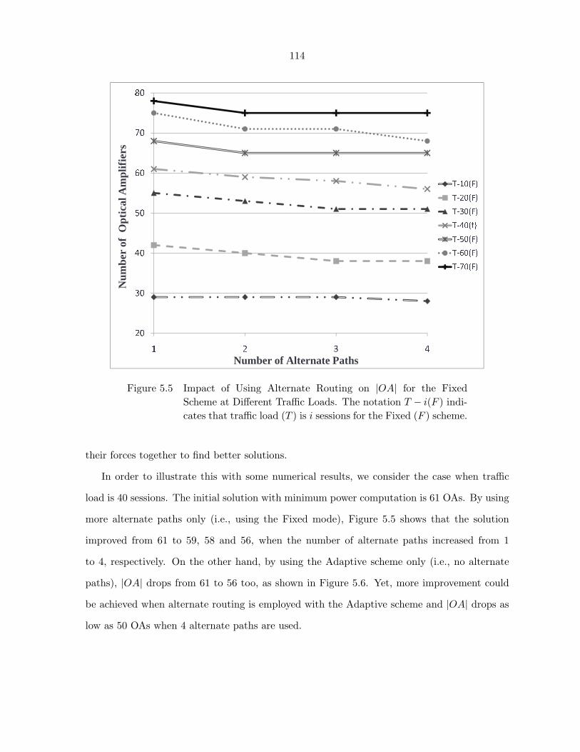
114
20304050607080
1 2 3 4
T-10(F)T-20(F)T-30(F)T-40(f)T-50(F)T-60(F)T-70(F)Number of Alternate Paths
Num
ber
of O
ptic
al A
mpl
ifie
rs
Figure 5.5 Impact of Using Alternate Routing on |OA| for the FixedScheme at Different Traffic Loads. The notation T − i(F ) indi-cates that traffic load (T ) is i sessions for the Fixed (F ) scheme.
their forces together to find better solutions.
In order to illustrate this with some numerical results, we consider the case when traffic
load is 40 sessions. The initial solution with minimum power computation is 61 OAs. By using
more alternate paths only (i.e., using the Fixed mode), Figure 5.5 shows that the solution
improved from 61 to 59, 58 and 56, when the number of alternate paths increased from 1
to 4, respectively. On the other hand, by using the Adaptive scheme only (i.e., no alternate
paths), |OA| drops from 61 to 56 too, as shown in Figure 5.6. Yet, more improvement could
be achieved when alternate routing is employed with the Adaptive scheme and |OA| drops as
low as 50 OAs when 4 alternate paths are used.
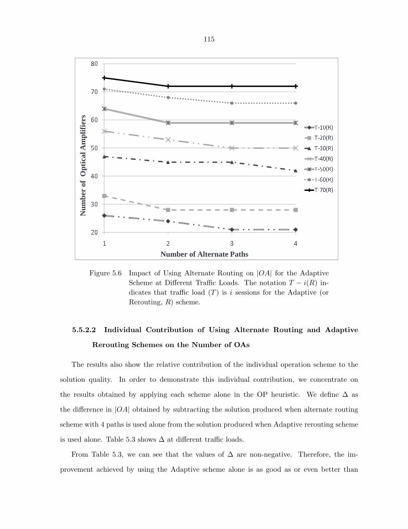
115
20304050607080
1 2 3 4
T-10(R)T-20(R)T-30(R)T-40(R)T-50(R)T-60(R)T-70(R)
Num
ber
of O
ptic
al A
mpl
ifie
rs
Number of Alternate Paths
Figure 5.6 Impact of Using Alternate Routing on |OA| for the AdaptiveScheme at Different Traffic Loads. The notation T − i(R) in-dicates that traffic load (T ) is i sessions for the Adaptive (orRerouting, R) scheme.
5.5.2.2 Individual Contribution of Using Alternate Routing and Adaptive
Rerouting Schemes on the Number of OAs
The results also show the relative contribution of the individual operation scheme to the
solution quality. In order to demonstrate this individual contribution, we concentrate on
the results obtained by applying each scheme alone in the OP heuristic. We define ∆ as
the difference in |OA| obtained by subtracting the solution produced when alternate routing
scheme with 4 paths is used alone from the solution produced when Adaptive rerouting scheme
is used alone. Table 5.3 shows ∆ at different traffic loads.
From Table 5.3, we can see that the values of ∆ are non-negative. Therefore, the im-
provement achieved by using the Adaptive scheme alone is as good as or even better than
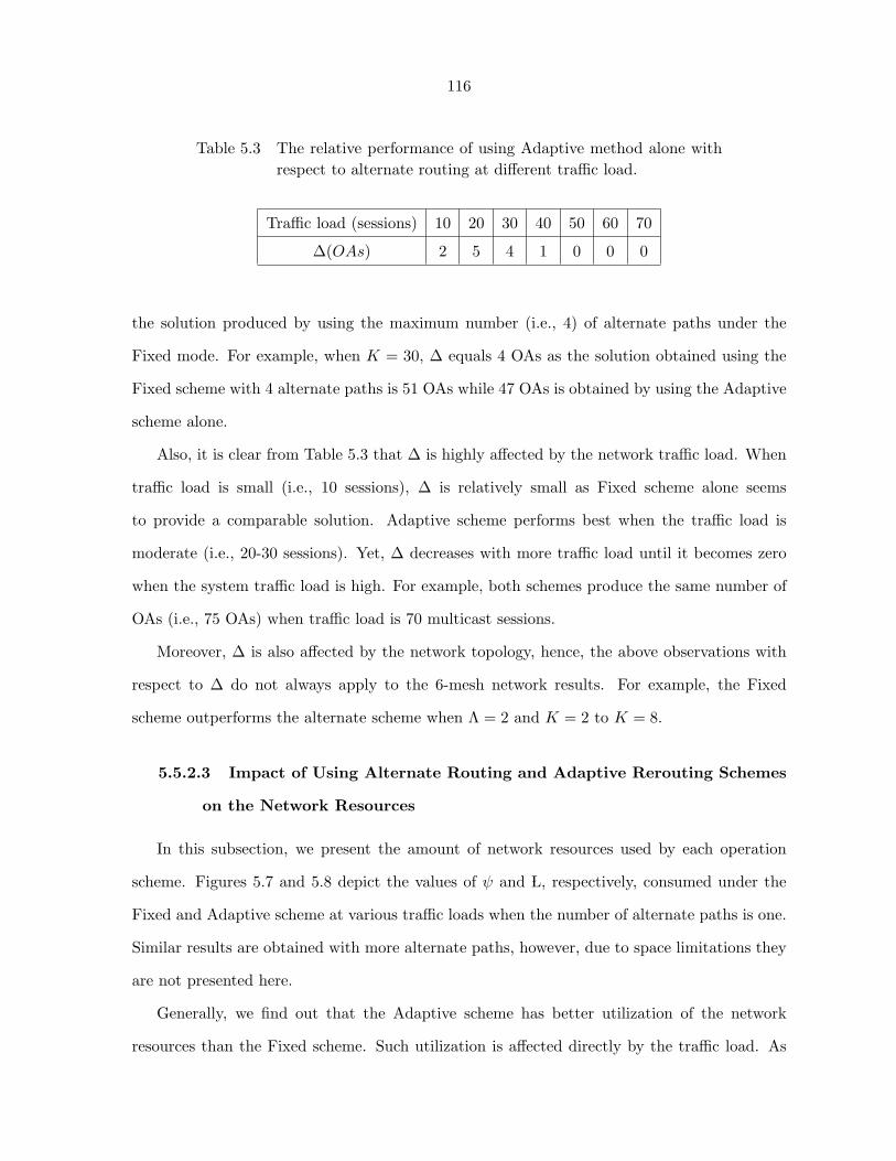
116
Table 5.3 The relative performance of using Adaptive method alone withrespect to alternate routing at different traffic load.
Traffic load (sessions) 10 20 30 40 50 60 70
∆(OAs) 2 5 4 1 0 0 0
the solution produced by using the maximum number (i.e., 4) of alternate paths under the
Fixed mode. For example, when K = 30, ∆ equals 4 OAs as the solution obtained using the
Fixed scheme with 4 alternate paths is 51 OAs while 47 OAs is obtained by using the Adaptive
scheme alone.
Also, it is clear from Table 5.3 that ∆ is highly affected by the network traffic load. When
traffic load is small (i.e., 10 sessions), ∆ is relatively small as Fixed scheme alone seems
to provide a comparable solution. Adaptive scheme performs best when the traffic load is
moderate (i.e., 20-30 sessions). Yet, ∆ decreases with more traffic load until it becomes zero
when the system traffic load is high. For example, both schemes produce the same number of
OAs (i.e., 75 OAs) when traffic load is 70 multicast sessions.
Moreover, ∆ is also affected by the network topology, hence, the above observations with
respect to ∆ do not always apply to the 6-mesh network results. For example, the Fixed
scheme outperforms the alternate scheme when Λ = 2 and K = 2 to K = 8.
5.5.2.3 Impact of Using Alternate Routing and Adaptive Rerouting Schemes
on the Network Resources
In this subsection, we present the amount of network resources used by each operation
scheme. Figures 5.7 and 5.8 depict the values of ψ and ÃL, respectively, consumed under the
Fixed and Adaptive scheme at various traffic loads when the number of alternate paths is one.
Similar results are obtained with more alternate paths, however, due to space limitations they
are not presented here.
Generally, we find out that the Adaptive scheme has better utilization of the network
resources than the Fixed scheme. Such utilization is affected directly by the traffic load. As
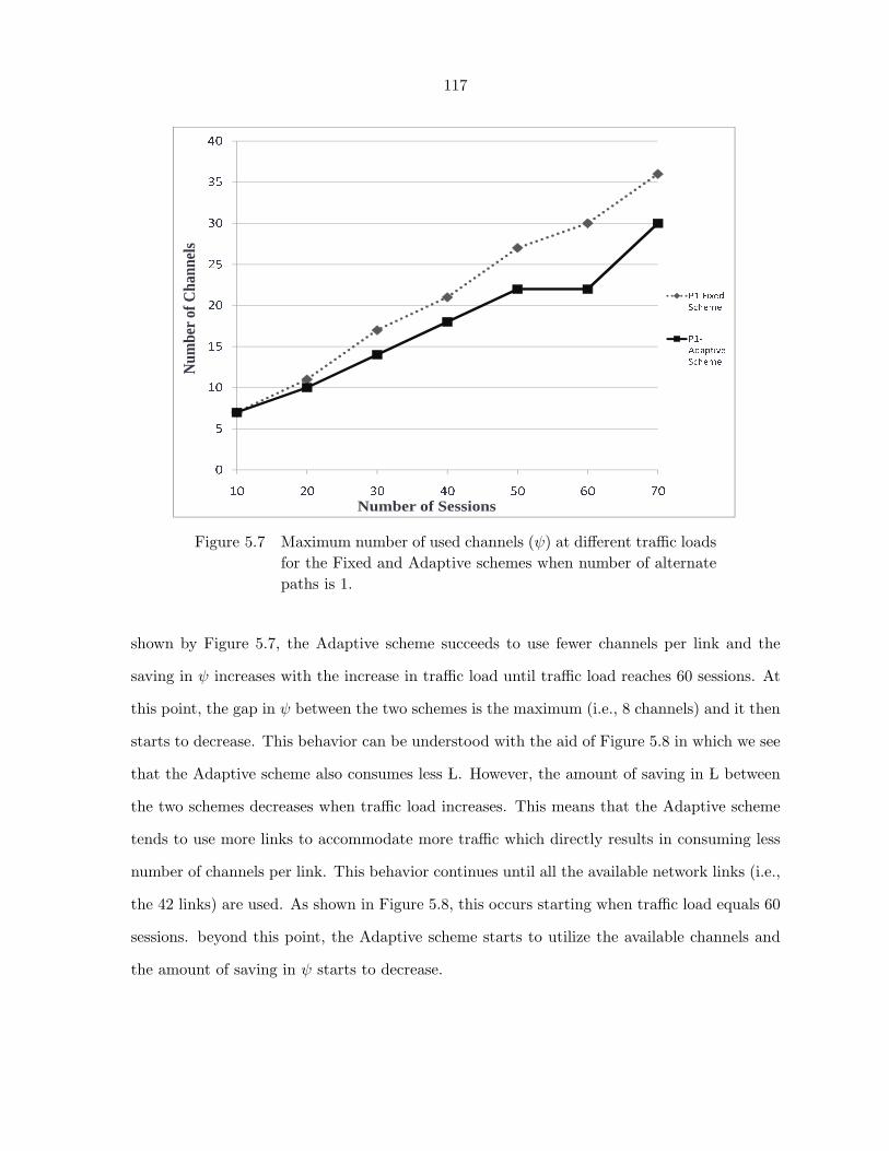
117
0510152025303540
10 20 30 40 50 60 70P1-Fixed SchemeP1-Adaptive Scheme
Num
ber
of C
hann
els
Number of Sessions
Figure 5.7 Maximum number of used channels (ψ) at different traffic loadsfor the Fixed and Adaptive schemes when number of alternatepaths is 1.
shown by Figure 5.7, the Adaptive scheme succeeds to use fewer channels per link and the
saving in ψ increases with the increase in traffic load until traffic load reaches 60 sessions. At
this point, the gap in ψ between the two schemes is the maximum (i.e., 8 channels) and it then
starts to decrease. This behavior can be understood with the aid of Figure 5.8 in which we see
that the Adaptive scheme also consumes less ÃL. However, the amount of saving in ÃL between
the two schemes decreases when traffic load increases. This means that the Adaptive scheme
tends to use more links to accommodate more traffic which directly results in consuming less
number of channels per link. This behavior continues until all the available network links (i.e.,
the 42 links) are used. As shown in Figure 5.8, this occurs starting when traffic load equals 60
sessions. beyond this point, the Adaptive scheme starts to utilize the available channels and
the amount of saving in ψ starts to decrease.
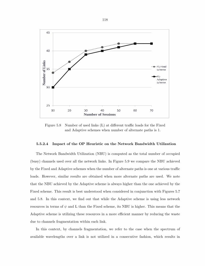
118
2530354045
10 20 30 40 50 60 70P1-Fixed SchemeP1-Adaptive Scheme
Number of Sessions
Num
ber
of L
inks
Figure 5.8 Number of used links (ÃL) at different traffic loads for the Fixedand Adaptive schemes when number of alternate paths is 1.
5.5.2.4 Impact of the OP Heuristic on the Network Bandwidth Utilization
The Network Bandwidth Utilization (NBU) is computed as the total number of occupied
(busy) channels used over all the network links. In Figure 5.9 we compare the NBU achieved
by the Fixed and Adaptive schemes when the number of alternate paths is one at various traffic
loads. However, similar results are obtained when more alternate paths are used. We note
that the NBU achieved by the Adaptive scheme is always higher than the one achieved by the
Fixed scheme. This result is best understood when considered in conjunction with Figures 5.7
and 5.8. In this context, we find out that while the Adaptive scheme is using less network
resources in terms of ψ and ÃL than the Fixed scheme, its NBU is higher. This means that the
Adaptive scheme is utilizing these resources in a more efficient manner by reducing the waste
due to channels fragmentation within each link.
In this context, by channels fragmentation, we refer to the case when the spectrum of
available wavelengths over a link is not utilized in a consecutive fashion, which results in
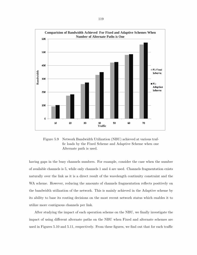
119
10 20 30 40 50 60 700100200300400500600P1-Fixed SchemeP1-Adaptive Scheme
Comparision of Bandwidth Achieved For Fixed and Adaptive Schemes When Number of Alternate Paths is One
Traffic
Ban
dw
idth
Figure 5.9 Network Bandwidth Utilization (NBU) achieved at various traf-fic loads by the Fixed Scheme and Adaptive Scheme when oneAlternate path is used.
having gaps in the busy channels numbers. For example, consider the case when the number
of available channels is 5, while only channels 1 and 4 are used. Channels fragmentation exists
naturally over the link as it is a direct result of the wavelength continuity constraint and the
WA scheme. However, reducing the amounts of channels fragmentation reflects positively on
the bandwidth utilization of the network. This is mainly achieved in the Adaptive scheme by
its ability to base its routing decisions on the most recent network status which enables it to
utilize more contiguous channels per link.
After studying the impact of each operation scheme on the NBU, we finally investigate the
impact of using different alternate paths on the NBU when Fixed and alternate schemes are
used in Figures 5.10 and 5.11, respectively. From these figures, we find out that for each traffic
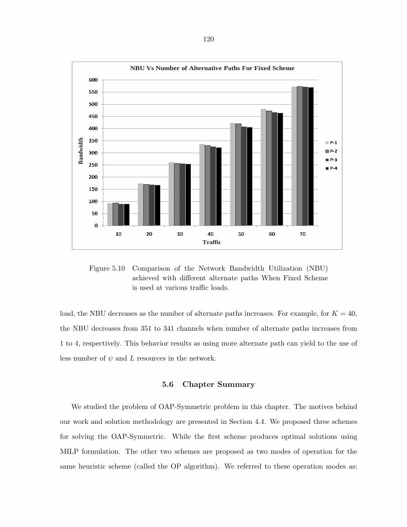
120
050100150200250300350400450500550600
10 20 30 40 50 60 70P-1P-2P-3P-4
NBU Vs Number of Alternative Paths For Fixed Scheme
Ban
dwid
th
Traffic
Figure 5.10 Comparison of the Network Bandwidth Utilization (NBU)achieved with different alternate paths When Fixed Schemeis used at various traffic loads.
load, the NBU decreases as the number of alternate paths increases. For example, for K = 40,
the NBU decreases from 351 to 341 channels when number of alternate paths increases from
1 to 4, respectively. This behavior results as using more alternate path can yield to the use of
less number of ψ and L resources in the network.
5.6 Chapter Summary
We studied the problem of OAP-Symmetric problem in this chapter. The motives behind
our work and solution methodology are presented in Section 4.4. We proposed three schemes
for solving the OAP-Symmetric. While the first scheme produces optimal solutions using
MILP formulation. The other two schemes are proposed as two modes of operation for the
same heuristic scheme (called the OP algorithm). We referred to these operation modes as:
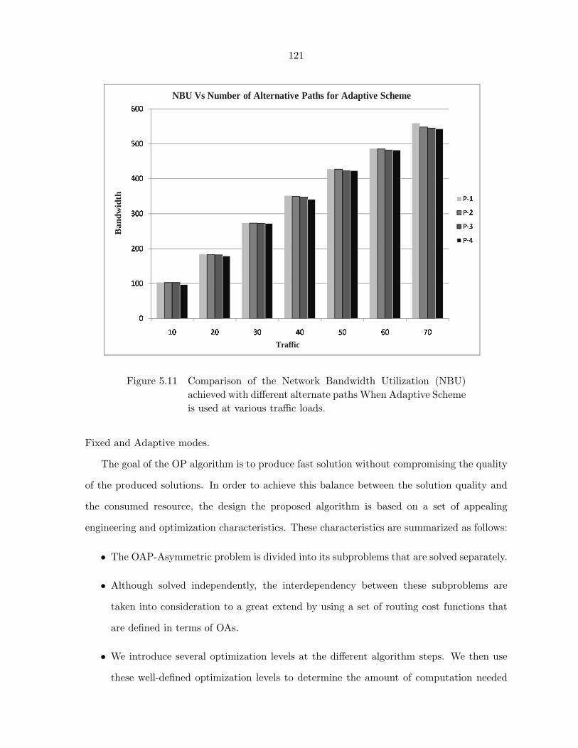
121
0100200300400500600
10 20 30 40 50 60 70P-1P-2P-3P-4
Traffic
Ban
dwid
th
NBU Vs Number of Alternative Paths for Adaptive Scheme
Figure 5.11 Comparison of the Network Bandwidth Utilization (NBU)achieved with different alternate paths When Adaptive Schemeis used at various traffic loads.
Fixed and Adaptive modes.
The goal of the OP algorithm is to produce fast solution without compromising the quality
of the produced solutions. In order to achieve this balance between the solution quality and
the consumed resource, the design the proposed algorithm is based on a set of appealing
engineering and optimization characteristics. These characteristics are summarized as follows:
• The OAP-Asymmetric problem is divided into its subproblems that are solved separately.
• Although solved independently, the interdependency between these subproblems are
taken into consideration to a great extend by using a set of routing cost functions that
are defined in terms of OAs.
• We introduce several optimization levels at the different algorithm steps. We then use
these well-defined optimization levels to determine the amount of computation needed

122
to find the corresponding solution. This provides us a handy mechanism to study the
impact of the OP algorithm at the various computation levels.
• The OP algorithm proves to be efficient in handling the management issues of the NS and
NPS with minimal overhead. This is achieved by using special set of data structures,
including the queue Q, that takes care of representing the network status in a very
effective manner.
The results reported in this chapter is comprehensive and cover a wide range of system
performance metrics. Generally speaking, these results show that the Adaptive scheme out-
performs the Fixed scheme, in terms of both the number of OAs and the network resources,
and it achieves better utilization of the network resources. However, this performance comes
at the cost of extra computations. Such extra computation can be tolerated, especially that
the problem at hand is a design problem, and taking more time to find a solution is mostly
fine if it will result in saving more OAs, hence more money for the designers.
123
CHAPTER 6. Power Aware Multicasting (PAM) in Wavelength Routing
Networks
6.1 Introduction
We focus in this chapter on the impact of power loss on the network operation under AOM
traffic. We identify and formulate this problem as a connection provisioning problem, which is
an optimization problem to find the best network operational strategy. In our study here, the
performance of the network operation is measured by the ability of the proposed solution to
minimize the number of dropped (blocked) sessions.
Like the OAP problem discussed in Chapters 3-4, the classical problem of Routing and
Wavelength Assignment (RWA) [8] has a fundamental role in the network operation. However,
due to its lack of consideration for any practical issues that are related to all-optical services,
not all the solutions produced from the classical RWA are feasible in practice. Therefore, in
our study here, the RWA is extended to include more realistic constraints which make it more
complicated. One of these constraints is the power impairments, which include the: Optical
Amplifiers (OAs) gain model, power loss and noise. In order to reduce the complexity of our
study, we focus in this chapter on the impact of OA gain model and power loss only without
considering the noise issues. This extension introduces a new dimension to the classical RWA
problem, namely, the power dimension. We refer to this problem extension as Power-Aware
RWA (PA-RWA) problem and we formally define it as follows:
PA-RWA Problem Definition: ”Given the network topology, the static multicast traffic
demand matrix, the number and locations of the splitters and OAs, number of wavelengths, the
Power-Aware Routing and Wavelength Assignment (PA-RWA) problem under AOM is defined
124
as a connection provisioning problem that aims to find a feasible route (in the form of a light-
forest) and a wavelength assignment for the maximum number of multicast sessions in order
to minimize the connection blocking rate.”.
There are many of similarities between the OAP and the PA-RWA problems. First, the
PA-RWA problem can be investigated in two system configurations based on the power sym-
metry assumption, namely, under equal and unequal power constraints. In our study here, we
assume the asymmetric system configuration only where the symmetric system configuration
needs separate investigation. Second, these problems share the same set of RWA and power
constraints. Hence, some of these constraints are reused in our solutions here in this chapter.
However, unlike the OAP problem, the PA-RWA has its own aspects and challenges that
distinguishes it from the OAP problem. This distinction is due to the fact that the PA-RWA
problem is a network operation problem while the OAP is a design problem. Therefore, the
PA-RWA problem has to deal with an existing network that is already provisioned and it is
unlikely to be upgraded or modified. This situation forces the network operator to handle the
RWA and power aspects differently than the network designer. These differences include, but
not limited to, the following situations:
• The solution to the PA-RWA problem has to deal with a set of traffic that is (most likely)
different than the one used to design the network. This mismatch in traffic demands can
result in not satisfying all the constraints used in provisioning the network and might
result in dropping some of these traffic demands.
• The objective function of the PA-RWA problem is different than that of the OAP problem
as the goal of the network operator is to best utilize this network by dropping the least
possible number of connections.
• Under OAP problem, the OA placement policy does not play a decisive factor in speci-
fying the number of OAs over the link. This number is determined mainly by the total
gain needed over the link and the input power values to the link. Therefore, the same
number of OAs over a link can be placed differently using different OA placement poli-
125
cies. However, this policy becomes an important factor in determining the feasibility of
the solutions for the PA-RWA problem as it determines the location of the OAs over
the links, which in turn determines whether or not the power constraints are met. For
example, using the ALAP placement policy might place the first OA further away from
the beginning of the link compared to the ASAP policy. Therefore, if the input power to
the link is weak, it has better chance to reach the first OA to get amplified if the ASAP
policy is used, assuming all other power constraints are met.
• The OAP problem is solved without allowing any kind of connection blocking as the
network is required to be provisioned for certain set of traffic demands. On the other
hand, the PA-RWA problem has to deal with different types and sources of connection
blocking. Some of these blocking sources are related to the shortage of network resources,
while others are related to the power constraints. In our treatment, we tackle all the
potential blocking sources and we investigate how these blocking sources impact the
system performance.
In this chapter, we follow the same solution strategy we adopted in tackling the OAP prob-
lem. We first formulate the PA-RWA problem as a MILP with the objective of minimizing the
total number of blocked sessions. While producing the optimal solutions, the MILP solutions
are not fast and not scalable for large instances of the problem. Therefore, a greedy heuristic
that provides fast and near optimal solutions for the PA-RWA problem is then introduced. The
algorithm operation is based on creating a connection between the tree construction and power
assignment. This connection is achieved using a special set of power-related cost functions for
the links and sessions that are used for make the appropriate routing decisions.
The contribution of the work done in this chapter is summarized as follows1:
• The MILP formulation solves the combined subproblems of the PA-RWA problem in a
jointly manner. These subproblems are the: Routing (R), Wavelength Assignment (WA)1Although we are handling two different problems, some of these contributions presented here are similar to
the ones presented in Chapter 3 for the OAP problem. This similarity in contributions is basically due to thefact that we are following the same methodology strategy in these works, namely, finding practical solutionsthat are fast without compromising the solution quality.
126
and Power Assignment (PA) subproblems. To the best of our knowledge, this is the first
attempt to solve the power extension of the RWA problem using MILP scheme. Other
MILP formulations reported in the literature are investigating the RWA problem under
unicast traffic and without considering the power constraints. Please refer to [8] for more
details on this subject. On the other hand, the PA-RWA problem was also formulated
in the context of unicast traffic in [42] using the more complicated MInLP formulation.
• Like the OAP problem, the PA-RWA problem is nonlinear. The main source of the
nonlinearity of the problem is the computations of the splitting power loss, OA gain,
and the total power over the link. Nevertheless, we provide a linear formulation of the
problem using a special set of mapping techniques to convert the nonlinear constraints
into linear counterparts. In this context, we use the same mapping scheme we used
earlier in Chapters 4 and 5 for computing the splitting power loss. However, in order to
determine the gain of an OA and the total power over a link, we propose a novel set of
mapping techniques that will be explained in the sequel.
• The set of heuristic solutions we present in solving the PA-RWA problem proves to
provide fast solutions that are of good quality when compared to the optimal solutions.
The operation of these heuristics is based on using a set of cost functions for the links and
sessions that are able to capture the dependencies between the different subproblems.
This allows the algorithm to work efficiently by solving these subproblems separately
while taking the impact of each subproblem on the others.
• We incorporate the impact of the OA gain model in determining the gain of the individual
OA in our MILP and heuristic solutions. Such consideration was either ignored [29] or
abstracted with very constrained conditions [52] in most of the other efforts reported in
the literature that handle the PA-RWA problem. In this context, an iterative heuristic
was proposed in [29] in which an initial tree is constructed without taking any power
constraint into consideration. This tree is then modified by replacing a set of adjacent
splitters by a single splitting node, called the Centralized Splitting Node, in order to
127
reduce the total amount of power loss. On the other hand, the heuristic algorithm
that is proposed in [52] is based on constructing balanced light-trees in order to ensure
a minimum signal quality and fairness among all destinations. An exception of this
situation is the scheme proposed in [42] in which a two-phase hybrid solution employing
a greedy heuristic and Genetic Algorithm for session establishment and power assignment
was introduced.
• The results reported in this chapter provide a comprehensive coverage of the various
system performance aspects under different experimental conditions. In addition, they
provide good guidelines for the network operators, as well as designers, in determining
the best choices for network upgrades.
The remainder of this chapter is organized as follows. The next section introduces the
system model and assumptions which is followed by the MILP formulation details in Section
6.3. The details of the proposed heuristic are then presented in Section 6.4. The numerical
results are reported in Section 6.5 and we finally conclude the chapter in Section 6.6.
6.2 Additional System Model Assumptions
In this chapter, we use the same system model described in Section 1.6. However, we use the
piece-wise model for the OA gain which is determined by equation 1.2. Moreover, the network
is pre-provisioned; therefore, the number and placement of the OAs is pre-determined and
known. Also, using the notation introduced in Section 2.2.1, our system model is characterized
as SsF cRx-Cn. Also, our study does not consider partial destination delivery of the multicast
session. Therefore, a session is accepted if and only if all members in its destination set are
reached by the light-forest.
6.3 MILP Problem Formulation
In this section, we present the MILP formulation for the PA-RWA problem. We intro-
duce the network parameters and the formulation variables, in subsections 6.3.1 and 6.3.2,
128
respectively. The objective function and formulation constraints are then presented in sub-
section 6.3.3. Although some of these variables and constraints are shared with the previous
formulation, we present them here for the sake of completeness and ease reference.
6.3.1 Network Parameters
The following network parameters are used in the MILP formulation:
N The set of nodes in the network.
E The set of fiber links in the network.
Λ The set of wavelengths supported per fiber.
i, j, k Node identity, where i, j, k ∈ N .
λ Wavelength identity, where λ ∈ Λ.
e(i, j) Fiber link directed from node i to node j.
OAi,j The set of optical amplifies on fiber e(i, j).
NOAi,j Binary indicator: 1 if |OAi,j | > 0; 0 otherwise.
o OA identity on e(i, j);1 ≤ o ≤ |OAi,j |.x, y Optical component identity on e(i, j);0 ≤ x ≤ |OAi,j | and 1 ≤ y ≤ |OAi,j |+ 1.
x = 0 and y = |OAi,j |+ 1 are source(i) and sink(j) nodes.
SP The set of splitters.
SPi Binary indicator: 1 if node i is a splitter.
β Propagation loss ratio.
γ Tapping power loss value at each node.
Li,j Length (Km) of fiber e(i, j).
Lx,yi,j Length (Km) between x and y of e(i, j).
K Number of multicast sessions.
a Multicast session identity; 0 ≤ a ≤ K − 1.
129
srca Multicast session source node.
Da Multicast session destination set.
Φi Set of sessions in which node i is a destination.
Γai Binary indicator: 1 if i ∈ Da; 0 otherwise.
P dBmSen Minimum detectable power (dBm) level on a channel by a receiver or an OA.
P dBmMAX Maximum power (dBm).
PmWMax Maximum aggregate power (mW) on a link.
PmWMin Minimum power (mW).
P1, P2 Two negative constants that are used to represent the case of (−∞) dBm, such
that P1 < P2.
δ Very small number used for mapping purposes.
v, w Integer constants, such that v > w.
Outi Out degree of node i.
M Very large number.
6.3.2 MILP Variables
The following variables are used in the MILP formulation:
R Auxiliary terms used in the objective function.
W1,W2 Weights of objective function terms; W1 À W2.
T a,λi,j Binary indicator: 1 if e(i, j) is used by session a over λ; 0 otherwise.
ϕa Binary indicator: 1 if session a is carried out in the network; 0 otherwise.
ϑai Binary indicator: 1 if node i is included in the light-tree of session a; 0 otherwise.
=ai,j Binary indicator: 1 if e(i, j) is used by session a over any wavelength; 0 otherwise.
130
Υi,j Binary indicator: 1 if e(i, j) is used by any session over any wavelength; 0 otherwise.
Goi,j Value of the amplification gain required from the oth optical amplifier on fiber e(i, j).
Ha,λi Number of hops of the path between the source node of session a and node i over
channel λ.
SLa,λi Splitting loss on channel λ at node i for a.
Ω Power inspection site; Ω ∈ beg, end.PΩ,a,λ
i,j,dBm Power level (dBm) at beginning (Ω = beg)/end (Ω = end) of e(i, j) for λ used by
session a.
P beg,a,λ,oi,j,mW Power level (mW) at beginning of oth OA on e(i, j) for wavelength λ used by
session a.
TP begi,j,mW Total power (mW) at beginning of e(i, j).
TP beg,oi,j,mW Total power (mW) at entry of oth OA on e(i, j).
f Tree fanout; number of outgoing tree links.
Af Binary indicator for power splitting linearization.
AP oi,j Binary indicator for OA gain linearization.
y A linear equation instance.
Y Set of linear equations that are selected for unit conversion between mW and
dBm/dB.
6.3.3 MILP Formulation
The objective function is to minimize the number of blocked sessions in the network, and
is expressed as follows:
Minimize : −W1
∑a
ϕa + W2R (6.1)
where:
R =∑
e(i,j)∈E
∑
o∈OAi,j
K−1∑
a=0
∑
λ∈Λ
TP beg,a,λ,oi,j,mW +
∑
e(i,j)∈E
∑
o∈OAi,j
Goi,j (6.2)
The rationale behind computing the auxiliary variable, R, in the objective function is to
simplify the determination of the correct values of the total power per link and the OA gain
131
variables, as will be shown below. The weight constant W2 is chosen such that its value is
much less than W1. This is essential in order to ensure that the contribution of R to the value
of objective function is much less than that of the number of admitted sessions.
Like the OAP problem, the objective function for the PA-RWA is subject to a set of
constraints, which are discussed below:
6.3.4 Routing and Wavelength Assignment Constraints
The construction of the light-forest and its wavelength(s) assignment are determined by
the following constraints:
ϕa ≤∑
i,i∈Da
ϑai
|Da| 0 ≤ a < K (6.3)
ϕa ≥∑
i,i∈Da
ϑai − (|Da| − 1) 0 ≤ a < K (6.4)
The above constraints compute ϕa as the conjunction between all ϑai variables of session a’s
destination nodes. They guarantee that the session, a, is accepted if all its destinations are
part of the session’s light-forest.
ϑai ≥
∑
j,j 6=i,e(j,i)∈E
∑
λ∈Λ
T a,λj,i
M∀i ∈ N ; 0 ≤ a < K (6.5)
ϑai ≤
∑
j,j 6=i,e(j,i)∈E
∑
λ∈Λ
T a,λj,i ∀i ∈ N ; 0 ≤ a < K (6.6)
Constraints (6.5) and (6.6) set ϑai to the disjunction between all T a,λ
j,i variables, for all incoming
links from the neighbor nodes j of node i over all wavelengths. They indicate that node i is
part of sessions a’s light-forest if it is part of at least one of its light-trees variables.
=ai,j ≥
∑
λ∈Λ
T a,λi,j
M∀i, j ∈ N ; 0 ≤ a < K (6.7)
=ai,j ≤
∑
λ∈Λ
T a,λi,j ∀i, j ∈ N ; 0 ≤ a < K (6.8)
Constraints (6.7) and (6.8) are used to determine if link e(i, j) is used by session a by setting
=a,i,j to 1 if at least one of its tree link is used over e(i, j) using any wavelength. This is achieved
by computing =a,i,j as the disjunction between all the tree links variables of session a that uses
132
link e(i, j) (i.e., T a,λi,j ) over all the wavelengths.
Υi,j ≥K−1∑
a=0
=ai,j
M∀e(i, j) ∈ E (6.9)
Υi,j ≤K−1∑
a=0
=ai,j ∀e(i, j) ∈ E (6.10)
Similar to Constraints (6.7) and (6.8), constraints (6.9) and (6.10) set Υi,j to the disjunction
between all =ai,j variables, for all the sessions. They ensure that link e(i, j) is used if it is used
by at least one session.
Γai +
∑λ∈Λ
∑k,k 6=i,e(i,k)∈E T a,λ
i,k
M≤
∑
k,k 6=i,e(k,i)∈E
T a,λk,i + (1− ϕa)×M
∀i ∈ N/srca; 0 ≤ a < K (6.11)
The above constraints are used to create the light-forest per session by ensuring the connectivity
of each of its destination. In a nutshell, this is achieved by guaranteeing that there should be
at least one incoming link to node i if it is a destination or it has one outgoing link. This
condition is fulfilled only when session a is accepted, i.e., ϕa = 1. For example, if node i is
a destination and/or it has multiple outgoing links, then the left-hand side of the constraints
becomes positive. Due to the use of the large constant, M, the left hand side is a positive
fraction that is less than 1. In order for the constraints to be satisfied, the right hand side of
the constraints, namely, the number of incoming links should be at least 1, if ϕa = 1.
Please note that these constraints have the same goal as the constraints defined by equation
(4.6). However, the constraints defined in (4.6) cannot be used here as they do not consider
the situation when the session is blocked.
∑
k,k 6=i,e(k,i)∈E
T a,λk,i ≤ 1 ∀i ∈ N/srca; 0 ≤ a < K;∀λ ∈ Λ (6.12)
Constraints (6.12) help preventing loops on the light-forest of session a on wavelength λ by
preventing traversing any node more than once. These constraints are similar to the ones
defined in (4.7).∑
0≤a<K,e(k,i)∈E
T a,λi,j ≤ 1 ∀i, j ∈ N ; i 6= j; ∀λ ∈ Λ (6.13)
133
These constraints guarantee that e(i, j) is used by at most one light-tree over wavelength λ
for each session. This guarantees the data integrity and correctness over each link by avoiding
using the same channel over the same link by multiple sessions. These constraints are similar
to the ones defined in (4.8).
∑
j,i6=j,e(i,j)∈E
T a,λi,j ≤ 1 ∀i ∈ N/srca; i /∈ SP ; 0 ≤ a < K; ∀λ ∈ Λ (6.14)
Constraints (6.14) prevent branching at MI nodes by ensuring that any MI node, say i, has at
most one outgoing tree link over a particular wavelength.
∑
j,j 6=i,e(j,i)∈E
T a,λj,i ≥
∑
k,k 6=i,e(i,k)∈E
T a,λi,k
M∀i ∈ N/srca; 0 ≤ a < K (6.15)
Constraints (6.15) are similar to the constraints defined in (4.10) and are used to guarantee
the wavelength continuity for each session. This achieved by ensuring node i should have an
incoming tree link over wavelength λ if node i has at least one outgoing link employing the
same wavelength.
6.3.5 Loop-Avoidance Constraints
We use the same hop counting scheme we introduced earlier in Subsection 5.3.2 to prevent
any loop in the constructed light-forests. Please refer to that subsection for the full details of
the following constraints:
Ha,λsrca
= 0 0 ≤ a < K;∀λ ∈ Λ (6.16)
1−=ai,j −
Ha,λi + 1−Ha,λ
j
M≥ 0 ∀e(i, j) ∈ E; 0 ≤ a < K (6.17)
Γai +
Ha,λi − (|N | − 1)
M≤ 1 ∀e(i, j) ∈ E; 0 ≤ a < K (6.18)
6.3.6 Power Constraints:
The following constraints we present here in this subsection address the power constraints
and OA gain model:
P beg,a,λ,oi,j,dBm ≥ P dBm
Sen ×T a,λi,j +P1×(1−T a,λ
i,j ) ∀e(i, j) ∈ E; 0 ≤ a < K;∀λ ∈ Λ;∀o ∈ OAi,j (6.19)
134
P end,a,λi,j,dBm ≥ P dBm
Sen × T a,λi,j + P1 × (1− T a,λ
i,j ) ∀e(i, j) ∈ E; 0 ≤ a < K;∀λ ∈ Λ (6.20)
These constraints ensure that the power level at specific power inspection sites is above P dBmSen
if the link is used by the light-forest. These inspection sites include: the beginning of each
OA, as well as the end of each optical fiber. Maintaining this condition at these sites is
sufficient to ensure that this lower bound is met everywhere in the network. This can help in
reducing the formulation complexity by avoiding unnecessary calculations. Please note that
these constraints also ensure that these power values are greater than P1 if the link is not used
by the light-forest. The significant of these conditions will be clear when they are used along
with constraints (6.21) below.
P beg,a,λi,j,dBm ≤ P2 × (1− T a,λ
i,j ) ∀e(i, j) ∈ E; 0 ≤ a < K; ∀λ ∈ Λ (6.21)
Constraints (6.21) ensure that the power level at the beginning of each link is less than P2 if
the fiber is not used as a tree link. In order to understand the important of these constraints,
please note that the values of P2 and P1 are chosen to be much less than any power loss in the
network such that P2 > P1. Therefore, these constraints are used along with constraints (6.19)
and (6.20) to guarantee that the power values are very small (as it typically lies between P1
and P2) everywhere in the unused channels of each fiber.
TP begi,j,mW ≤ PmW
MAX ×Υi,j + PmWMIN ∗ (1−Υi,j) ∀e(i, j) ∈ E; 0 ≤ a < K; ∀e(i, j) ∈ E (6.22)
The above constraints are used to ensure that the aggregate power level at the beginning of
each fiber is below the PmWMAX threshold if the link is used by any session; and PmW
MIN otherwise.
Since PmWMIN is zero, we can remove the second term in the right-hand side of the inequality.
Also, there is no need to extend this constraint to every OA since ensuring this upper bound at
the beginning of the link guarantees that the total input power at the first OA cannot exceed
PmWMAX . The OA gain model expressed by equation (1.2) guarantees that the output power
from the OA does not exceed this upper bound too.
Please note that the aggregate power values at the beginning of the links are expressed in
mW while the individual channel powers are expressed in dBm. In order to convert between
135
these two units, the following relation needs to be implemented in the formulation:
P beg,a,λ,oi,j,mW = 10
Pbeg,a,λ,oi,j,dBm
10 ∀e(i, j) ∈ E; ∀λ ∈ Λ; 0 ≤ a < K; ∀o ∈ OAi,j (6.23)
Unfortunately, this relation is non-linear. Therefore, we design a special set of linear constraints
that are equivalent to (6.23). These constraints take the following format:
P beg,a,λ,oi,j,mW ≥ AyP
beg,a,λ,oi,j,dBm +By ∀e(i, j) ∈ E; ∀λ ∈ Λ; 0 ≤ a < K; ∀y ∈ Y ; ∀o ∈ OAi,j (6.24)
The idea is to define a set, called Y , of piece-wise linear segments such that each segment is
represented by a linear equation, called y, whose value is greater than the non-linear curve of
the relation defined in (6.23) over a specific period denoted by Zy = [αy, βy]. Zy determines the
mathematical domain over which y is defined. In order to guarantee the correct representation
of these segments, the following conditions must be satisfied:
1. Z =⋃
y∈Y Zy = [P dBmSen , P dBm
MAX ]
2. αy = βy−1 ∀y ∈ Y, αy 6= P dBmSen
3. βy = αy+1 ∀y ∈ Y, βy 6= P dBmMAX
The first condition states that the union of the domains of the individual segments should
equal the total domain over which relation (6.23) is defined (namely, [P dBmSen , P dBm
MAX ]). The
second condition states that the first value in function y’s domain equals to the last value in
the previous function’s domain except for the first segment since its value should equal P dBmSen .
Similarly, the third condition ensure the last value in function y’s domain equals to the first
value in the next function’s domain except for the last segment since its value should equal
P dBmMAX . The last two conditions ensure that the total domain is represented in full by the
individual segments.
As long as these conditions are satisfied, any set Y can be defined over any sub-domains.
Trivially, the number of individual segment, i.e. |Y |, determines the accuracy of this approxi-
mation and can reflect on the formulation complexity. To help understanding the idea behind
this approximation, please refer to Figure 6.1 which depicts an example of this setting such
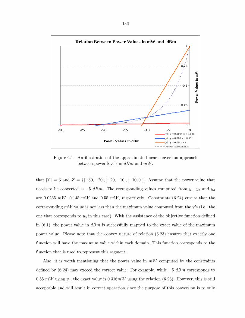
136
Relation Between Power Values in mW and dBm
0
0.25
0.5
0.75
1
-30 -25 -20 -15 -10 -5 0
Power Values in dBm
Pow
er V
alue
s in
mW
y1: y = 0.0009 x + 0.028
y2: y = 0.009 x + 0.19
y3: y = 0.09 x + 1
Power Values in mW
Figure 6.1 An illustration of the approximate linear conversion approachbetween power levels in dBm and mW .
that |Y | = 3 and Z = [−30,−20], [−20,−10], [−10, 0]. Assume that the power value that
needs to be converted is −5 dBm. The corresponding values computed from y1, y2 and y3
are 0.0235 mW , 0.145 mW and 0.55 mW , respectively. Constraints (6.24) ensure that the
corresponding mW value is not less than the maximum value computed from the y’s (i.e., the
one that corresponds to y3 in this case). With the assistance of the objective function defined
in (6.1), the power value in dBm is successfully mapped to the exact value of the maximum
power value. Please note that the convex nature of relation (6.23) ensures that exactly one
function will have the maximum value within each domain. This function corresponds to the
function that is used to represent this segment.
Also, it is worth mentioning that the power value in mW computed by the constraints
defined by (6.24) may exceed the correct value. For example, while −5 dBm corresponds to
0.55 mW using y3, the exact value is 0.316mW using the relation (6.23). However, this is still
acceptable and will result in correct operation since the purpose of this conversion is to only
137
ensure that the total power on the fiber is not exceeded, as shown below.
TP begi,j,mW =
∑
λ∈Λ
a=K−1∑
a=0
P beg,a,λi,j,mW ∀e(i, j) ∈ E (6.25)
TP beg,oi,j,mW =
∑
λ∈Λ
a=K−1∑
a=0
P beg,a,λ,oi,j,mW
∀e(i, j) ∈ E; ∀o ∈ OAi,j (6.26)
Constraints (6.25) and (6.26) calculate the total power in mW at the beginning of every fiber
and OA, respectively, as the sum of the power values in mW of the individual channels.
P beg,a,λ,1i,j,dBm = P beg,a,λ
i,j,dBm − β × L0,1i,j ∀e(i, j) ∈ E; ∀o ∈ OAi,j ; 0 ≤ a < K; ∀λ ∈ Λ (6.27)
P end,a,λi,j,dBm = [(1−NOAi,j)× (P beg,a,λ
i,j,dBm − β × Li,j)]+
[NOAi,j × (P beg,a,λ,|OAi,j |i,j,dBm +
Goi,j − β × L
|OAi,j |,|OAi,j |+1i,j )]
∀e(i, j) ∈ E; ∀o ∈ OAi,j ; 0 ≤ a < K; ∀λ ∈ Λ (6.28)
P beg,a,λ,o+1i,j,dBm = P beg,a,λ,o
i,j,dBm +Goi,j−β×Lo,o+1
i,j ∀e(i, j) ∈ E;∀o ∈ OAi,j ; 0 ≤ a < K;∀λ ∈ Λ (6.29)
The set of constraints (6.27 - 6.29) determine the power relation between the various optical
components over each link. The constraints in (6.27) find the relation between the power at
the beginning of the first OA and the beginning of the fiber link where the power decays due to
propagation loss only. Equations (6.28) are used on link e(i, j) to express the power strength
on wavelength λ at the end point of the link in terms of the power strength at the beginning of
the link and the loss due to attenuation in the whole fiber length when |OAi,j | = 0. However, if
|OAi,j | > 0, the power level at the link end is computed in terms of the power at the beginning
of the last OA, its gain and the loss due to attenuation in the last fiber segment. Finally, the
set of constraints (6.29) find the relation between the power at the beginning of an OA and
the beginning of the previous one on the same fiber link in terms of its gain and the power
attenuation in the fiber segment between the two consecutive OAs.
(1− T a,λi,j )× v + P end,a,λ
i,j − SLa,λj − γ ≥ (1− T a,λ
j,k )× w + P beg,a,λj,k
∀e(i, j), e(j, k) ∈ E; 0 ≤ a < K; ∀λ ∈ Λ (6.30)
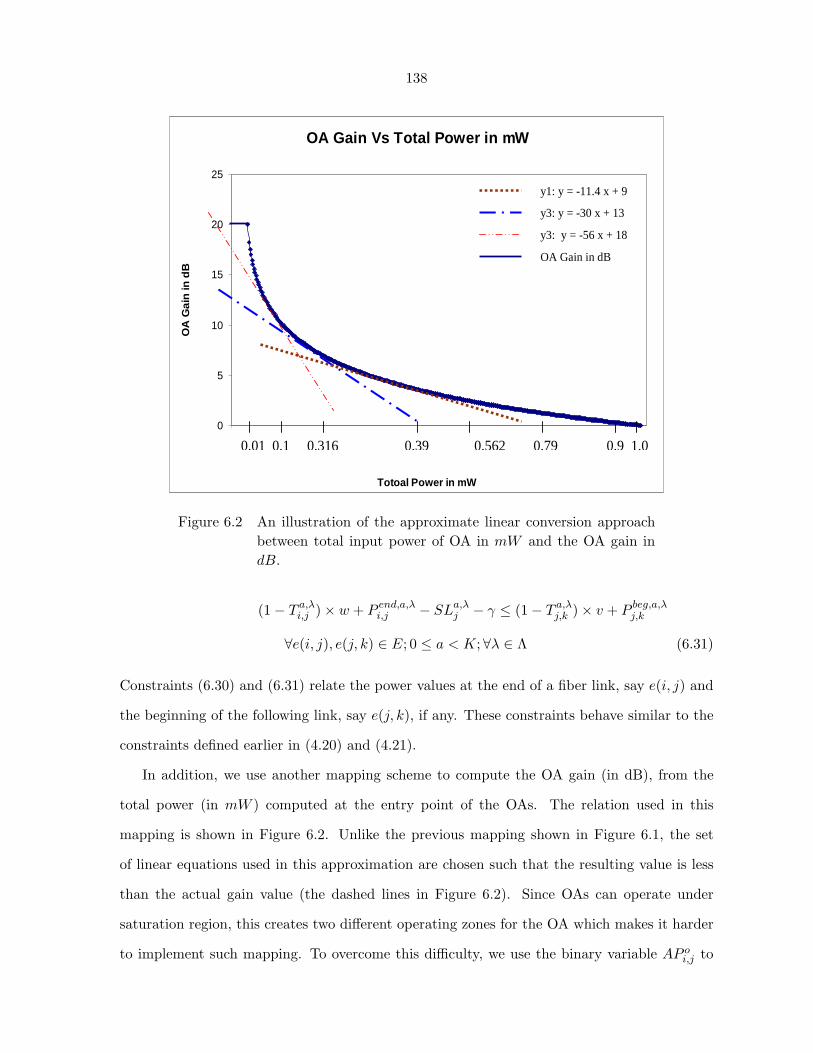
138
OA Gain Vs Total Power in mW
0
5
10
15
20
25
1.75
Totoal Power in mW
OA
Gai
n in
dB
0.01 0.1 0.316 0.39 0.562 0.79 0.9 1.0
OA Gain in dB
y1: y = -11.4 x + 9
y3: y = -30 x + 13 y3: y = -56 x + 18
Figure 6.2 An illustration of the approximate linear conversion approachbetween total input power of OA in mW and the OA gain indB.
(1− T a,λi,j )× w + P end,a,λ
i,j − SLa,λj − γ ≤ (1− T a,λ
j,k )× v + P beg,a,λj,k
∀e(i, j), e(j, k) ∈ E; 0 ≤ a < K; ∀λ ∈ Λ (6.31)
Constraints (6.30) and (6.31) relate the power values at the end of a fiber link, say e(i, j) and
the beginning of the following link, say e(j, k), if any. These constraints behave similar to the
constraints defined earlier in (4.20) and (4.21).
In addition, we use another mapping scheme to compute the OA gain (in dB), from the
total power (in mW ) computed at the entry point of the OAs. The relation used in this
mapping is shown in Figure 6.2. Unlike the previous mapping shown in Figure 6.1, the set
of linear equations used in this approximation are chosen such that the resulting value is less
than the actual gain value (the dashed lines in Figure 6.2). Since OAs can operate under
saturation region, this creates two different operating zones for the OA which makes it harder
to implement such mapping. To overcome this difficulty, we use the binary variable AP oi,j to
139
determine whether the oth OA operates in the saturation region or not. AP oi,j is ensured to be
1 if the total input power in mW is less than 0.01 mW (i.e., the cut off value of the total power
which determines the saturation region of the OA), and zero otherwise, using the following set
of constraints:
(0.01− TP beg,oi,j,mW ) + δ ≤ AP o
i,j ∀e(i, j) ∈ E;∀o ∈ OAi,j (6.32)
In this context, please note that when the total power is less than or equal the cut off value,
the left hand is a positive fraction that is less than 1. Therefore, constraint (6.32) is satisfied
only when the right hand side is 1. If the total power is greater than the cut off value, the
left hand side is negative, and AP oi,j can be either 0 or 1. Since the objective function tries to
minimize the total power in the R component of the objective function, this indirectly helps
in setting AP oi,j to zero. AP o
i,j is then used in constraints (6.33) and (6.34) to convert between
TP beg,oi,j,mW and Go
i,j .
(1−AP oi,j) +
Goi,j − 20M
≥ 0 ∀e(i, j) ∈ E; ∀o ∈ OAi,j (6.33)
AP oi,j +
Goi,j − (Ay × TP beg,o
i,j,mW + By)M
≥ 0 ∀e(i, j) ∈ E;∀o ∈ OAi,j (6.34)
Constraint (6.33) handles the maximum gain region, i.e., when AP oi,j = 1. In this case, Go
i,j
should equal 20 in order for the constraint to be satisfied. On the other hand, constraint (6.34)
handles the linear mapping for the saturation region in a fashion similar to the one proposed
in (6.24). In this case, AP oi,j = 0 and Go
i,j is represented by the set of linear mapping equations
Ay × TP beg,oi,j,mW + By.
SLa,λi
M≤ SPi ∀i ∈ N ; 0 ≤ a < K;∀λ ∈ Λ (6.35)
Constraint (6.35) ensures that the splitting loss value at an MI node is 0 dB for any connection
carried at any channel. However, splitting at MC nodes is determined in dB by this relation:
SLa,λi = 10 ∗ log10 f (6.36)
This relation is non-linear since the splitting degree, f , is a variable. Hence, we use the same
set of constraints we defined earlier in constraints (4.24 - 4.26).
140
6.4 The Heuristic Algorithm
The MILP formulation presented in the previous section provides the optimal solution
of the PA-RWA problem. However, the complexity of this formulation is of the order of
2 ×N2 ×K × |Λ| × |OA| for both the number of variables and constraints. Due to this high
complexity, obtaining the optimal solutions using MILP formulation is not practical or scalable
for big problem instances that involve both larger network and traffic sizes. Hence, there is a
need for a heuristic algorithm that can provide faster and efficient solutions.
In this section, we present a heuristic based approach for the PA-RWA problem under
AOM service. We refer to this approach as Power-Aware Multicasting (PAM) Algorithm. Our
scheme decomposes the PA-RWA into three subproblems, namely, Routing (R), Wavelength
Assignment (WA) and Power Assignment (PA) subproblems. Although solved separately, the
PAM heuristic considers the impact of these subproblems on each other by using a special set
of cost functions for the links, network and sessions.
6.4.1 Motivation of the PAM Algorithm and Main Characteristics
Call blocking can be due to many sources, some of which can be related to power issues.
The lack of availability of a continuous wavelengths on the light-trees is considered the main
source of non-power related source of call blocking. We refer to this type of call blocking as
Wavelength-Shortage Blocking and it occurs when the RWA algorithm cannot find a feasible
light-forest that has a single common wavelength among its links. On the other hand, power-
related sources of call blocking occur when the source nodes fail to launch their light-trees with
the appropriate power levels without violating any of the power constraints described in Sub-
section 1.6.1. This can happen even with the presence of network resources and wavelengths.
The reason of this blocking type is mainly due to sharing of the available power by wavelengths
at the links and OAs entry points. Hence, this blocking type is called Power-Sharing Blocking
and it takes three formats:
1. Power-Shortage Blocking, which occurs if the power strength of the signal drops below
PSen anywhere in the light-tree, even with the use of the source node’s maximum available
141
power. This drop results in the loss of ability to detect the optical signals at the receivers
and OAs.
2. Service-Disruption Blocking, which results when a new session is routed over links that
are shared with some already provisioned sessions in the network. Assigning a power
value to the new session can result in dropping the gain of at least one OA to a level
which can result in a service disruption of one or more already established sessions even
with the use of the minimum allowed power at the source node. Service disruption occurs
when gain drop yields a sequence of changes in the optical signals strength and other
OAs gains which results in violating the power constraints. In this case, the newly routed
sessions are blocked.
3. Non-linear Impact Blocking, which is a direct result of violating the maximum total power
constraint. This blocking can easily occur, even with the use of the minimum allowed at
the source node. For example, the routed signal can enter the next hop link with a high
power value that increases the total power over the link over PMAX . Allowing this to
happen causes the system to operate in the undesirable nonlinear region of the fiber2.
In order to achieve good near-optimal solution for the PA-RWA problem, the design of
the PAM algorithm is based on capturing the impact of the Power-Sharing Blocking. This is
achieved in part by using a novel cost function for the network links that reflects this nature.
Also, the operation of the PAM algorithm has two characteristics. First, the algorithm deals
with the sessions in a parallel (or grouping) fashion, rather than sequentially (or individually).
In this context, all, or a subset of, the sessions are treated together at the same algorithmic
iteration. This grouping mechanism provides a flexibility for the algorithm to take their impact
on each other which can result in reducing blocking due to service disruption. Second, inspired
by the fact that assigning the minimum power to each light-tree does not always give the best
solution, the power module of the proposed algorithm adopts a semi-random scheme, that is
closely controlled by a set of probabilities that are used to determine the best combination2Although this blocking behavior can be prevented with the use of equalizers, like in [63][64], our system
model does not assume the use of equalizers.
142
of power levels at the various source nodes. This semi-random power assignment scheme
accompanied with the grouping consideration of the sessions, proves to provide better solution
over the minimum power assignment and sequential treatment counterparts.
6.4.2 Link Cost Function
We need to define the following set of parameters first in order to define the link cost
function. P λ,MINi,j,mW is defined as the minimum power (in mW ) for channel λ that is needed to
be observed at the beginning of link e(i, j) in order for it to reach the first OA (if |OAi,j | > 0)
or the end of the link (if |OAi,j | = 0) with a power that is equal to PSen exactly. We also
extend this definition to each fiber segment that is defined between the oth and (o + 1)th OAs.
P λ,o,MINi,j,mW specifies the minimum power (in mW ) that is needed at the output of the oth OA
in order to reach the input of the (o + 1)th OA, or the end of the link if the oth OA is the last
OA on the link, with PSen.
The maximum number of wavelengths that e(i, j) can support, |ΛMAXi,j | , is then calculated
using this relation:
|ΛMAXi,j | = MIN(|Λ|, PmW
Max
P λ,MINi,j,mW
) (6.37)
According to equation (6.37), |ΛMAXi,j | is determined, not only by the wavelengths availability,
but also by the signals ability to reach the first OA, if any, and still be detectable3.
Also, we define |ΛAddi,j | as the current number of wavelengths that link e(i, j) can additionally
support, given the current supported wavelengths and their power assignments at the beginning
of the link. |ΛAddi,j | is computed as the:
MIN(bPmW
MAX −∑λ∈|ΛBusy
i,j | Pbeg,a,λi,j,mW
P λ,MINi,j,mW
c, |ΛFreei,j |) (6.38)
where, |ΛBusyi,j | and |ΛFree
i,j | represent number of used and unused channels over e(i, j), respec-
tively. From (6.37) and (6.38), it is clear that |Λ| ≤ |ΛMAXi,j | ≤ |ΛBusy
i,j |+ |ΛFreei,j |. The current
cost of e(i, j), ce(i,j), is then defined as the ratio of the maximum number of wavelengths
3This equation is based on the assumption that only one-hop sessions exist in the system (therefore, minimumallowed power values can be used) and it ignores the impact of the spans between subsequent OAs on the links.Hence, it is not a tight upper-bound, however, it is sufficient for the purpose of our algorithm design here.
143
supported over e(i, j) and the current potential available wavelengths, namely,
ce(i,j) =|ΛMAX
i,j ||ΛAdd
i,j | (6.39)
Equation (6.39) has the following significant properties:
• It intelligently incorporates the useful concepts of power sharing and wavelength avail-
ability into the link cost, which is used in the R phase. This is important in relating
the PA subproblems with the R subproblem and makes it possible to take the impact
of these subproblems on each other.
• It is a dynamic function, i.e., link costs change with the accumulated power values.
Hence, routing decisions are directly dependent on the changing network status.
• It is a positive increasing function, i.e., link costs increase with the increase in the link
usage. This results in balancing the load in the entire network.
In addition, we define the network cost as the summation of the costs of the individual
links. In order to take the impact of placing a light-forest on the remaining unplaced ones, the
cost of each light-forest is calculated as the increase in the network cost. Selecting sessions for
placement is performed using a certain order policy according to their cost. Any order policy
can be used in our scheme. The simulation experiments in this chapter are conducted using
the increasing ordering policy.
6.4.3 The PAM Algorithm Details
In this subsection, we present the details of the PAM heuristic whose basic operation is
depicted in Figure 6.3. The output of the PAM algorithm is the number of admitted sessions,
and their corresponding RWA and power values (or RWA-P).
As shown in Figure 6.3, the core operation of the PAM algorithm is the RWA-PAM Stage.
The input to the RWA-PAM stage is the set of sessions to be constructed, the sharing de-
gree and the construction mode. The sharing degree represents the number of sessions to be
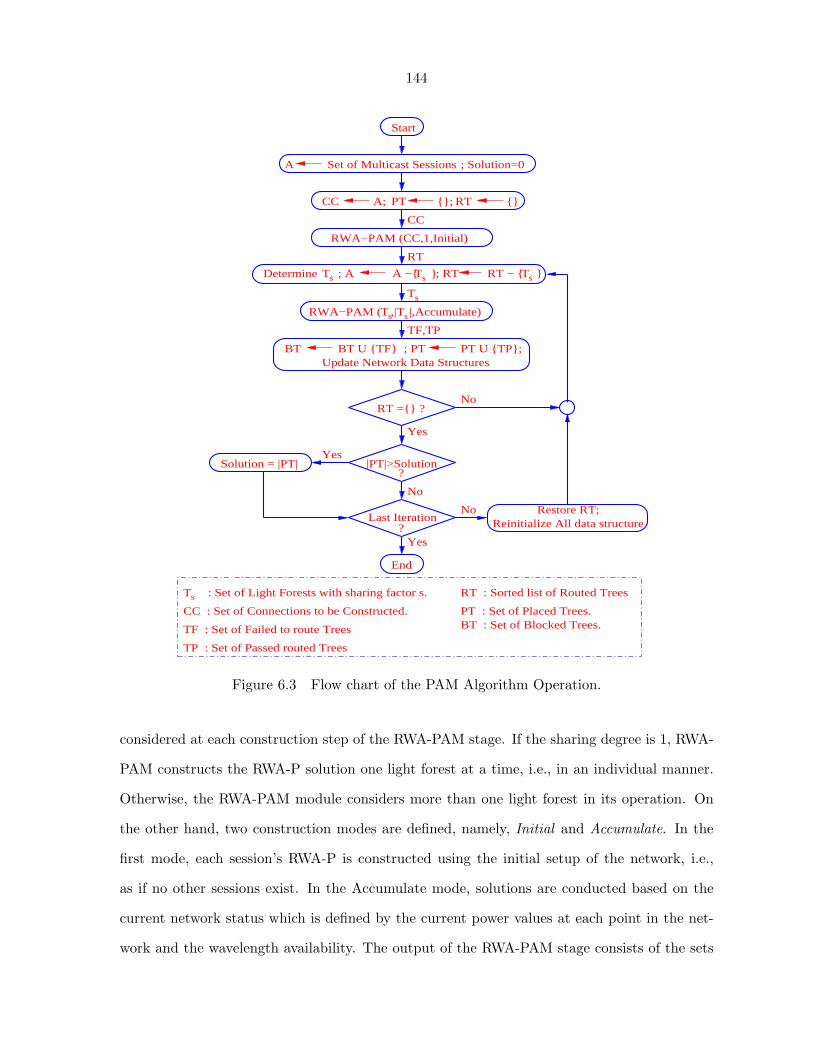
144
Start
Ts
A Set of Multicast Sessions
Solution = |PT|
Restore RT; Reinitialize All data structure
Ts
Ts TsDetermine Ts ; RT; A A − RT −
CC : Set of Connections to be Constructed.
RT : Sorted list of Routed Trees
PT : Set of Placed Trees.BT : Set of Blocked Trees.
RT
CC
RWA−PAM (CC,1,Initial)
; Solution=0
|PT|>Solution?
No
No
Yes?
Last Iteration
End
Yes
Update Network Data Structures
CC A; PT ; RT
NoRT = ?
Yes
BT BT U TF ; PT PT U TP;
TF,TP
TsRWA−PAM ( ,| |,Accumulate)
Ts : Set of Light Forests with sharing factor s.
TF : Set of Failed to route Trees
TP : Set of Passed routed Trees
Figure 6.3 Flow chart of the PAM Algorithm Operation.
considered at each construction step of the RWA-PAM stage. If the sharing degree is 1, RWA-
PAM constructs the RWA-P solution one light forest at a time, i.e., in an individual manner.
Otherwise, the RWA-PAM module considers more than one light forest in its operation. On
the other hand, two construction modes are defined, namely, Initial and Accumulate. In the
first mode, each session’s RWA-P is constructed using the initial setup of the network, i.e.,
as if no other sessions exist. In the Accumulate mode, solutions are conducted based on the
current network status which is defined by the current power values at each point in the net-
work and the wavelength availability. The output of the RWA-PAM stage consists of the sets
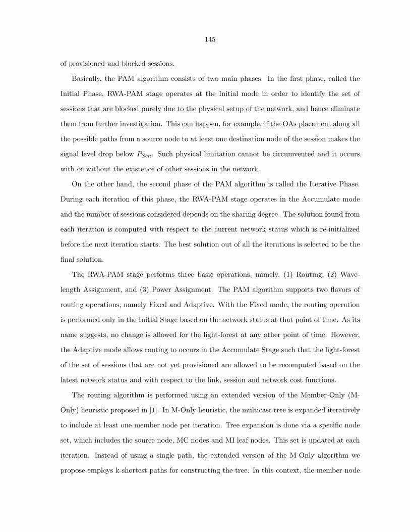
145
of provisioned and blocked sessions.
Basically, the PAM algorithm consists of two main phases. In the first phase, called the
Initial Phase, RWA-PAM stage operates at the Initial mode in order to identify the set of
sessions that are blocked purely due to the physical setup of the network, and hence eliminate
them from further investigation. This can happen, for example, if the OAs placement along all
the possible paths from a source node to at least one destination node of the session makes the
signal level drop below PSen. Such physical limitation cannot be circumvented and it occurs
with or without the existence of other sessions in the network.
On the other hand, the second phase of the PAM algorithm is called the Iterative Phase.
During each iteration of this phase, the RWA-PAM stage operates in the Accumulate mode
and the number of sessions considered depends on the sharing degree. The solution found from
each iteration is computed with respect to the current network status which is re-initialized
before the next iteration starts. The best solution out of all the iterations is selected to be the
final solution.
The RWA-PAM stage performs three basic operations, namely, (1) Routing, (2) Wave-
length Assignment, and (3) Power Assignment. The PAM algorithm supports two flavors of
routing operations, namely Fixed and Adaptive. With the Fixed mode, the routing operation
is performed only in the Initial Stage based on the network status at that point of time. As its
name suggests, no change is allowed for the light-forest at any other point of time. However,
the Adaptive mode allows routing to occurs in the Accumulate Stage such that the light-forest
of the set of sessions that are not yet provisioned are allowed to be recomputed based on the
latest network status and with respect to the link, session and network cost functions.
The routing algorithm is performed using an extended version of the Member-Only (M-
Only) heuristic proposed in [1]. In M-Only heuristic, the multicast tree is expanded iteratively
to include at least one member node per iteration. Tree expansion is done via a specific node
set, which includes the source node, MC nodes and MI leaf nodes. This set is updated at each
iteration. Instead of using a single path, the extended version of the M-Only algorithm we
propose employs k-shortest paths for constructing the tree. In this context, the member node
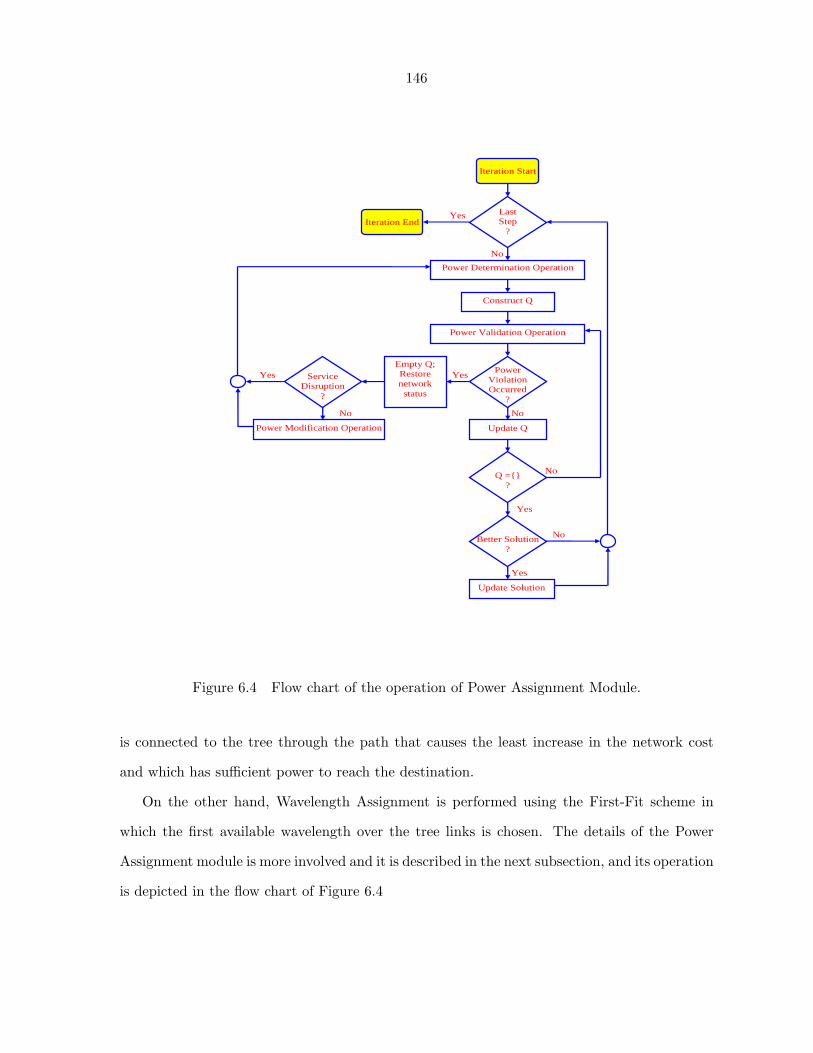
146
Yes
Empty Q; Restore network status
Last Step
?
Power Determination Operation
No
Iteration Start
Construct Q
Iteration End
Power Validation Operation
Update Q
Power Violation Occurred
?
No
Yes
No
Yes
Q =
?
Update Solution
Better Solution
?
Yes
No
Service Disruption
?
Yes
Power Modification Operation
No
Figure 6.4 Flow chart of the operation of Power Assignment Module.
is connected to the tree through the path that causes the least increase in the network cost
and which has sufficient power to reach the destination.
On the other hand, Wavelength Assignment is performed using the First-Fit scheme in
which the first available wavelength over the tree links is chosen. The details of the Power
Assignment module is more involved and it is described in the next subsection, and its operation
is depicted in the flow chart of Figure 6.4
147
6.4.4 Power Assignment Algorithm
The design of the Power Assignment (PA) Module relies on three observations.
1. Service disruption can be minimized, if not avoided, by grouping the sessions and treating
them together in each iteration in order to take their impact on each other.
2. The use of the minimum power at the source node is not always the best solution as it
does not guarantee connection acceptance.
3. The impact of power change is not localized within the network due to overlapping
between the sessions and the OAs operation that relies on the power sharing of the input
signals. Therefore, allowing power and gain values to change at one network link may
result in changing them at subsequent network links too. The situation becomes even
worse if such chain of power/gain changes propagates back to the initial affected link.
Note that not allowing these values to change is not an option since this results in poor
algorithm results.
The design of PA module makes use of two important elements in order to tackle these
observations with minimal overhead. First, it separates the link identities from their power
values by using the queue structure, called Q, that we employed in Chapter 5. The queue
consists of unique entities of the links identity. A link becomes part of the queue if it is part
of the current light-forests under investigating and/or it is part of the affected links. Although
multiple traversals of the link is permitted in the algorithm, Q contains at most one instance
of the link at each algorithm step. The link at Q’s head is examined and then is removed
from Q. The second design element is the power assignment mechanism. In this context, we
adopt a semi-random iterative scheme for determining the power values at the source nodes.
This scheme is based on a set of probabilities that determine the update action as well as the
amount of power change4. The details of these two elements are presented below.4We describe this scheme as semi-random because the values of these probabilities are selectively chosen to
reflect the source of power violations.
148
Basically, the Power Assignment scheme runs for a certain number of iterations and it
consists of three main operations:
1. Power Determination Operation,
2. Power Validation Operation, and
3. Power Modification Operation.
Given the power values of the already provisioned sessions, these three steps work together
during each iteration in order to determine the best power value to be launched at the source
nodes of the sessions under investigation. The first step determines the power values set (called
Power Vector) at the source nodes. The second operation determines if this Power Vector is
valid over the link, i.e., it does not result in any power constraint violation, while the last
operation is needed only to determine if a gain drop can be tolerated in the network. In this
sense, a session service is considered disrupted only if it was already provisioned in an earlier
algorithm step.
In the first iteration of the Power Assignment module, the Power Vector is initialized with
the minimum power values at the source nodes. Q is then populated with all the outgoing
links from the source nodes of the current sessions under investigation. The order of adding
these links is immaterial. The module proceeds on a link by link basis, starting from the link
at the queue head and it checks if power levels are valid on every points on this link. If so,
the link is removed from Q while its outgoing links are added to Q, if (1) they are not there
currently, and (2) they are part of the current sessions light-trees. At each algorithm step, Q
contains one instance of the link, even it is shared by more than one light-tree.
The PA algorithm continues with the next link in Q and it stops when Q becomes empty.
A link can be revisited more than once during the iteration lifetime. This occurs because the
same link can be at different depth of the various light-trees. With each link traversal, more
power values over the link become available. The algorithm deals with those power values that
are currently available; thus, the algorithm works even with partial knowledge of the power
values. However, allowing several traversals of the links ensures the complete availability of
149
the power values at the link. Having said that, it is important to note that prevent having
multiple copies of the same link in Q eliminates any unneeded calculations since power values
are separate from the link identities.
If the Power Validation Operation indicates that a gain drop occurs, but no service disrup-
tion is encountered, then the Power Modification Operation is invoked. In this operation, the
algorithm identifies the set of all sessions on the link where a gain reduction took place, and
we refer to them as the affected sessions set. These sessions include the old placed sessions
as well as the new ones. It then continues its normal operation. However, queue Q is now
populated with links from the affected sessions set.
If power violation is encountered at any point in the network, Q is emptied, the network
status is restored, and the Power Determination Operation is called in order to determine the
new Power Vector. In this operation, the power violation type is identified, and the set of
sessions that are involved in this power violation is determined to be the new sessions on the
link where the violation occurs. From these sessions, the operation then determines, randomly,
the sessions to be blocked from participating in the next iteration of the PA module. For
each remaining session, the module determines whether these sessions can reuse their power
value, or not. If the power value is to be changed, the algorithm then determines, randomly,
whether to increase or decrease the current power based on the power violation type. This
randomness is governed by certain probabilities that are carefully chosen to reflect the method
used to resolve this power violation type. For instance, if power violation is due to power drop
below PSen, then it is more probable that increasing the power value might solve the problem.
Therefore, increasing power value is given high probability in this case. On the other hand,
power violation due to service disruption is not necessarily always due to high-power input. For
example, in a cascade of OAs, decreasing the source node power might increase the gain of one
OA, which increases its output power. This results in more input power in the following OA,
which might decrease its gain and service disruption persists. Therefore, we assign moderate
values to the probabilities of increasing the power in the case of Service disruption. Finally,
this probability is low in the case of total power exceeding PMax.
150
Moreover, the amount of power change is determined randomly too. Changing the source
power values is performed on the current sessions under investigation while those sessions
which have already being provisioned are not changed. It is worth mentioning that we only
change the power values associated with already provisioned sessions on the links, if a gain
drop occurs, but not the source power itself. Due to the random nature of this solution, the
PA module runs for a number of steps (or if the solution does not improve within some limits)
and the maximum number of admitted sessions over all of these steps is chosen as the PA
module solution.
6.5 Numerical Results
In order to validate our solutions and to understand their main characteristics, we present
some numerical results in this section using the setup settings defined in Section 1.6.3. In
addition, the following assumptions were used for the experiments:
1. We employ the increasing order policy of the corresponding light-forests costs in deter-
mining the set of sessions to be provisioned in the network.
2. We run the PAM algorithm at least 5 times per problem instance. The solution of the
maximum number of accepted sessions is then chosen as the representative solution.
The results in this section are presented in two main parts. In the first part, we establish
the quality of the solution produced by the PAM algorithm. This is done by comparing these
results with the optimal counterparts collected from CPLEX while using the same network
settings in the 6-node network. In this part, we also demonstrate the significance of two
design elements of the PAM algorithm, namely, the concepts of sessions grouping (or sharing)
and the semi-random power assignment scheme. In the second part, we quantify some basic
characteristics of the PAM algorithm using the simulations results on the NSFNET. In this
part, we also demonstrate the characteristics of the other two algorithm design elements,
namely, using alternate routing and rerouting.
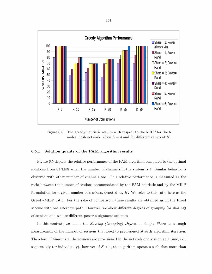
151
Greedy Algorithm Performance
0102030405060708090
100
K=5 K=10 K=15 K=20 K=25 K=30
Number of Connections
Gre
ed
y-M
ILP
%
Share = 1; Power=Always MinShare = 1; Power=RandShare = 2; Power=RandShare = 3; Power=RandShare = 4; Power=RandShare = 5; Power=RandShare = 6; Power=Rand
Figure 6.5 The greedy heuristic results with respect to the MILP for the 6nodes mesh network, when Λ = 4 and for different values of K.
6.5.1 Solution quality of the PAM algorithm results
Figure 6.5 depicts the relative performance of the PAM algorithm compared to the optimal
solutions from CPLEX when the number of channels in the system is 4. Similar behavior is
observed with other number of channels too. This relative performance is measured as the
ratio between the number of sessions accommodated by the PAM heuristic and by the MILP
formulation for a given number of sessions, denoted as, K. We refer to this ratio here as the
Greedy-MILP ratio. For the sake of comparison, these results are obtained using the Fixed
scheme with one alternate path. However, we allow different degrees of grouping (or sharing)
of sessions and we use different power assignment schemes.
In this context, we define the Sharing (Grouping) Degree, or simply Share as a rough
measurement of the number of sessions that need to provisioned at each algorithm iteration.
Therefore, if Share is 1, the sessions are provisioned in the network one session at a time, i.e.,
sequentially (or individually). however, if S > 1, the algorithm operates such that more than
152
one session are considered at a time.
Choosing the value for Share has a direct impact on the solution accuracy and the algorithm
performance and it can be a research topic by itself. However, it is important to note that
this value is used to capture the interdependency between the sessions that share the same
links in the network. Hence, it is essential to capture this sharing concept while constructing
the groups of sessions. The details of grouping these sessions is implementation-dependent
really. In our implementation, we simply relate the Share value with the number of sessions
to share at least one link by a certain percentage, called the Sharing Percentage (SP). In this
sense, whenever possible, the size of each group must be equal at least the Share value 5. More
sessions will be added to the group if the number of sessions that share at least one link is less
than SP × Share.
On the other hand, for the sake of reference, we refer to the semi-random power assignment
method proposed in Section 6.4 as the Rand method. In Figure 6.5, we compare the Rand
method with another deterministic scheme, referred to as the Min method. The Min method
operates by always choosing the minimum possible power value.
As shown in Figure 6.5, the performance ratio of the PAM algorithm with respect to the
optimal solutions is represented by a set of bars at each traffic load, K. Each bar represents
the experiment settings of the simulation at that traffic load. The results represented by the
first left bar for each K (i.e., when S = 1 and Min Power Assignment scheme is used) serves as
a benchmark to measure the usefulness of the Share and Rand aspects of the PAM algorithm.
The following important conclusions can be drawn from this figure:
1. The PAM algorithm performs very well with respect to the corresponding optimal solu-
tions. Not only it provided near optimal solutions, it sometimes was even able to get the
optimal solution. For example, the PAM algorithm produces the optimal solution (hence
the Greedy-MILP ratio equals 100%) when K = 30 and Share = 2 to 6.
2. Applying the Rand power scheme results in a huge performance improvement compared5An exception of this is when the number of remaining unprovisioned sessions is less than the value of the
Share.

153
to the Min Method. This improvement is measured as the increase in the value of the
Greedy-MILP ratio. The maximum performance improvement occurs when the value
of Share equals 1 and it ranges from 8% for K = 15 and K = 25, and 23% for K =
20. However, the incremental improvement decreases as the sharing degree increases.
This indicates that small sharing degrees are sufficient to reach an acceptable system
performance that is close to the optimal solution. This has the advantage of reducing
the system complexity since a fewer number of sessions per group can be considered at
each algorithm iteration.
6.5.2 PAM Heuristic Results
After establishing the solution quality of the PAM algorithm in the previous subsection,
this subsection is devoted to address the following characteristics of the PAM algorithm:
6.5.2.1 PAM Algorithm’s Impact on the Objective Function
The impact of the PAM algorithm on the number of accepted sessions is depicted in Figure
6.6 at different traffic loads using the Fixed scheme and when the number of available channels
is 10. Similar behavior is observed with the Adaptive scheme too. The results are collected at
different computation power, determined both by the employed power assignment scheme and
the number of alternate path. In this context, the least computational power configuration is
the Min-P where the Min power assignment scheme is used with single alternate path. The
maximum computational power configuration, on the other hand, is the one that involves Rand
power assignment with 3 alternate path routing, referred to as RP-P3.
Naturally, the number of accepted sessions increases as the traffic load increases. However,
It is obvious from this figure that for each traffic load, the objective function improves (i.e.,
increases) as more computation power is employed. For example, for K = 40, the number of
accepted sessions increases gradually from 14 to 24 when the algorithm mode increases from
Min-P to RP-P3.
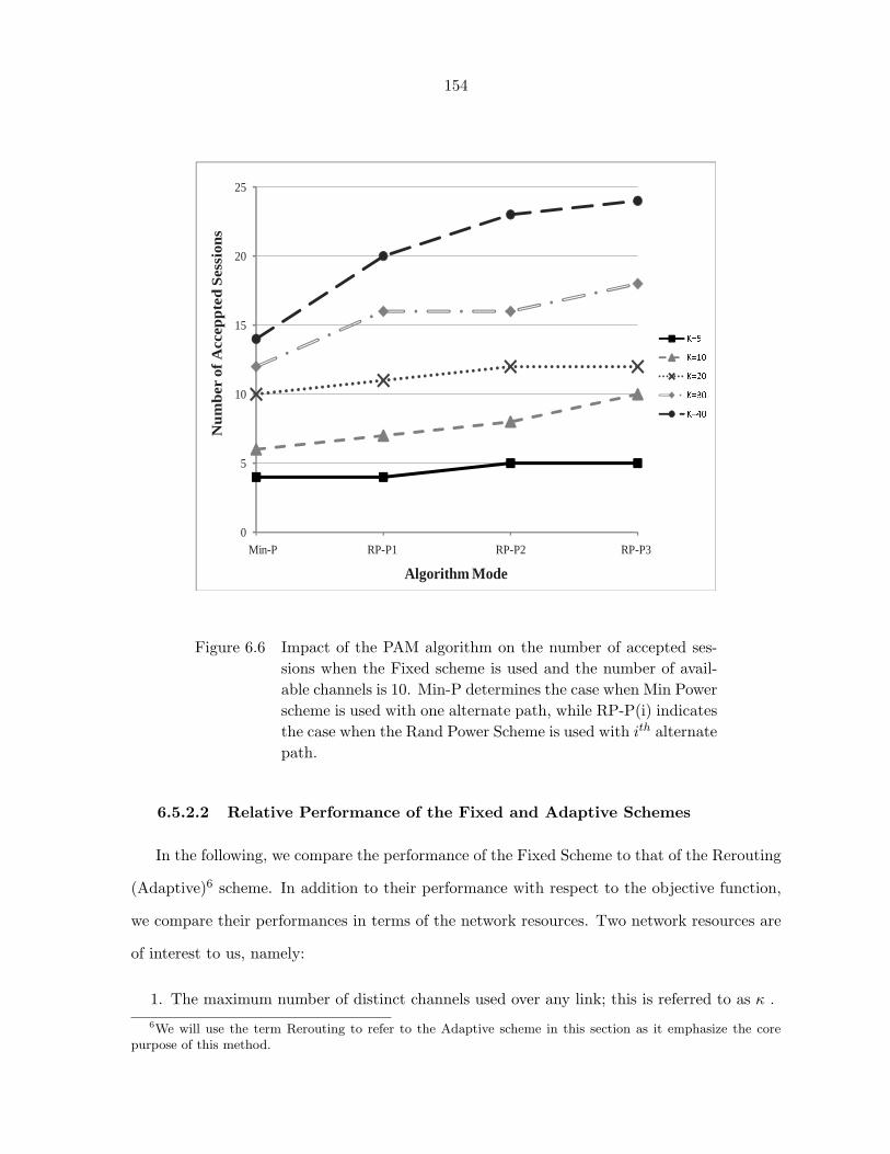
154
0
5
10
15
20
25
1 2 3 4K=5K=10K=20K=30K=40
Nu
mb
er o
f A
ccep
pte
dS
essi
ons
Algorithm Mode
Min-P RP-P1 RP-P2 RP-P3
Figure 6.6 Impact of the PAM algorithm on the number of accepted ses-sions when the Fixed scheme is used and the number of avail-able channels is 10. Min-P determines the case when Min Powerscheme is used with one alternate path, while RP-P(i) indicatesthe case when the Rand Power Scheme is used with ith alternatepath.
6.5.2.2 Relative Performance of the Fixed and Adaptive Schemes
In the following, we compare the performance of the Fixed Scheme to that of the Rerouting
(Adaptive)6 scheme. In addition to their performance with respect to the objective function,
we compare their performances in terms of the network resources. Two network resources are
of interest to us, namely:
1. The maximum number of distinct channels used over any link; this is referred to as κ .6We will use the term Rerouting to refer to the Adaptive scheme in this section as it emphasize the core
purpose of this method.
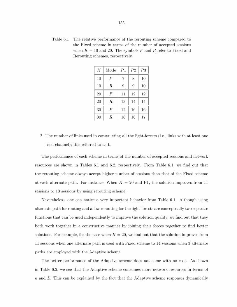
155
Table 6.1 The relative performance of the rerouting scheme compared tothe Fixed scheme in terms of the number of accepted sessionswhen K = 10 and 20. The symbols F and R refer to Fixed andRerouting schemes, respectively.
K Mode P1 P2 P3
10 F 7 8 10
10 R 9 9 10
20 F 11 12 12
20 R 13 14 14
30 F 12 16 16
30 R 16 16 17
2. The number of links used in constructing all the light-forests (i.e., links with at least one
used channel); this referred to as ÃL.
The performance of each scheme in terms of the number of accepted sessions and network
resources are shown in Tables 6.1 and 6.2, respectively. From Table 6.1, we find out that
the rerouting scheme always accept higher number of sessions than that of the Fixed scheme
at each alternate path. For instance, When K = 20 and P1, the solution improves from 11
sessions to 13 sessions by using rerouting scheme.
Nevertheless, one can notice a very important behavior from Table 6.1. Although using
alternate path for routing and allow rerouting for the light-forests are conceptually two separate
functions that can be used independently to improve the solution quality, we find out that they
both work together in a constructive manner by joining their forces together to find better
solutions. For example, for the case when K = 20, we find out that the solution improves from
11 sessions when one alternate path is used with Fixed scheme to 14 sessions when 3 alternate
paths are employed with the Adaptive scheme.
The better performance of the Adaptive scheme does not come with no cost. As shown
in Table 6.2, we see that the Adaptive scheme consumes more network resources in terms of
κ and L. This can be explained by the fact that the Adaptive scheme responses dynamically
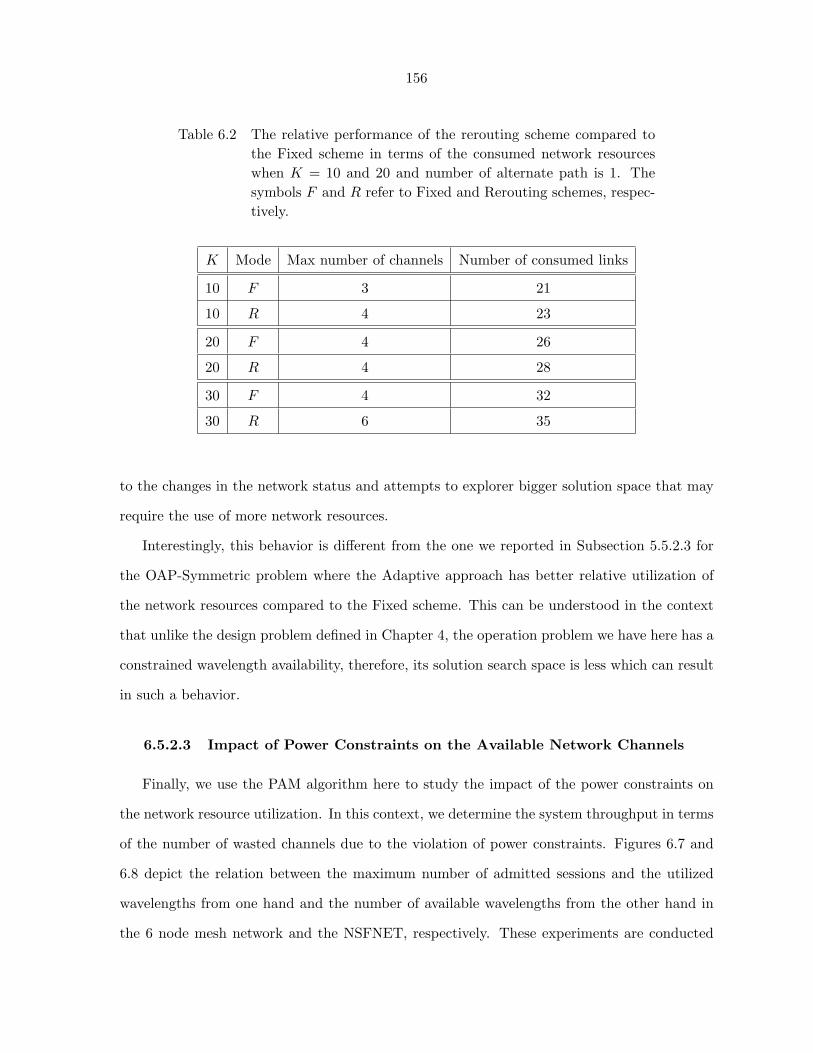
156
Table 6.2 The relative performance of the rerouting scheme compared tothe Fixed scheme in terms of the consumed network resourceswhen K = 10 and 20 and number of alternate path is 1. Thesymbols F and R refer to Fixed and Rerouting schemes, respec-tively.
K Mode Max number of channels Number of consumed links
10 F 3 21
10 R 4 23
20 F 4 26
20 R 4 28
30 F 4 32
30 R 6 35
to the changes in the network status and attempts to explorer bigger solution space that may
require the use of more network resources.
Interestingly, this behavior is different from the one we reported in Subsection 5.5.2.3 for
the OAP-Symmetric problem where the Adaptive approach has better relative utilization of
the network resources compared to the Fixed scheme. This can be understood in the context
that unlike the design problem defined in Chapter 4, the operation problem we have here has a
constrained wavelength availability, therefore, its solution search space is less which can result
in such a behavior.
6.5.2.3 Impact of Power Constraints on the Available Network Channels
Finally, we use the PAM algorithm here to study the impact of the power constraints on
the network resource utilization. In this context, we determine the system throughput in terms
of the number of wasted channels due to the violation of power constraints. Figures 6.7 and
6.8 depict the relation between the maximum number of admitted sessions and the utilized
wavelengths from one hand and the number of available wavelengths from the other hand in
the 6 node mesh network and the NSFNET, respectively. These experiments are conducted
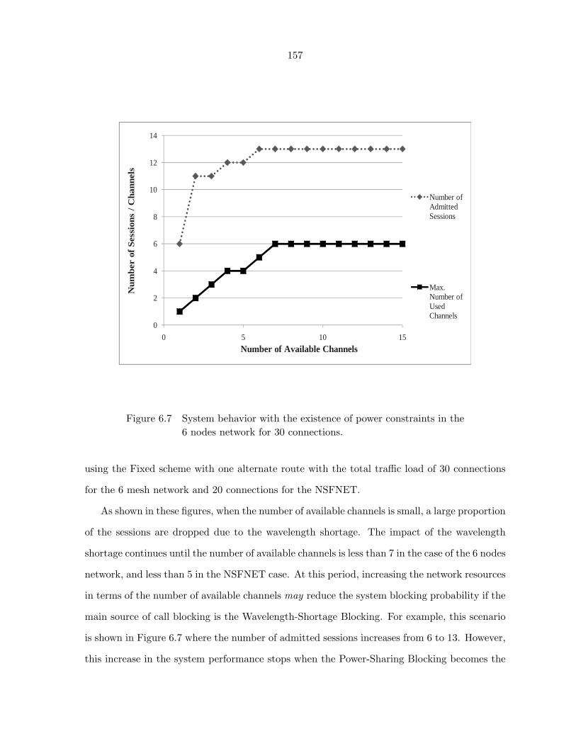
157
0
2
4
6
8
10
12
14
0 5 10 15
Number of Admitted Sessions
Max. Number of Used Channels
Number of Available Channels
Nu
mb
erof
Ses
sion
s /
Ch
ann
els
Figure 6.7 System behavior with the existence of power constraints in the6 nodes network for 30 connections.
using the Fixed scheme with one alternate route with the total traffic load of 30 connections
for the 6 mesh network and 20 connections for the NSFNET.
As shown in these figures, when the number of available channels is small, a large proportion
of the sessions are dropped due to the wavelength shortage. The impact of the wavelength
shortage continues until the number of available channels is less than 7 in the case of the 6 nodes
network, and less than 5 in the NSFNET case. At this period, increasing the network resources
in terms of the number of available channels may reduce the system blocking probability if the
main source of call blocking is the Wavelength-Shortage Blocking. For example, this scenario
is shown in Figure 6.7 where the number of admitted sessions increases from 6 to 13. However,
this increase in the system performance stops when the Power-Sharing Blocking becomes the
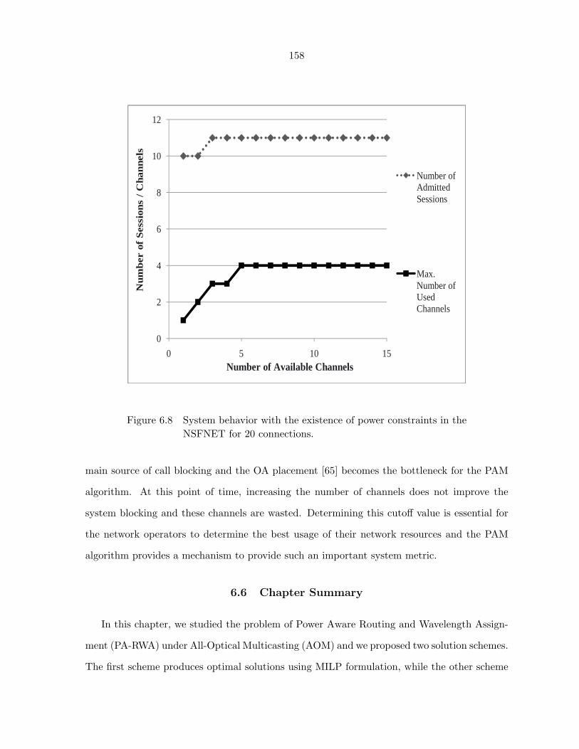
158
0
2
4
6
8
10
12
0 5 10 15
Number of Admitted Sessions
Max. Number of Used Channels
Number of Available Channels
Nu
mb
erof
Ses
sion
s /
Ch
ann
els
Figure 6.8 System behavior with the existence of power constraints in theNSFNET for 20 connections.
main source of call blocking and the OA placement [65] becomes the bottleneck for the PAM
algorithm. At this point of time, increasing the number of channels does not improve the
system blocking and these channels are wasted. Determining this cutoff value is essential for
the network operators to determine the best usage of their network resources and the PAM
algorithm provides a mechanism to provide such an important system metric.
6.6 Chapter Summary
In this chapter, we studied the problem of Power Aware Routing and Wavelength Assign-
ment (PA-RWA) under All-Optical Multicasting (AOM) and we proposed two solution schemes.
The first scheme produces optimal solutions using MILP formulation, while the other scheme
159
proposed a heuristic scheme, called Power Aware Multicasting (PAM) algorithm. The design
of the PAM heuristic consists of several optimization elements that make it able to produce
near optimal solutions in an efficient manner.
On the other hand, the results show that the PAM algorithm performs well in comparison
with the optimal solutions. It also provides a good understanding for the system performance.
One of the main advantages of the proposed PAM Algorithm is its ability to determine the
operation region for the network where adding more channels can benefit the overall system
performance which is of great advantage for the network operators.
160
CHAPTER 7. Thesis Conclusions and Future Work
7.1 Summary
In this thesis, we study the impact of optical power loss on the design and operation
of WDM networks under All Optical Multicasting (AOM). This impact was formulated as
network provisioning and connection provisioning problems. The objective function for the
network provisioning problem is to minimize the network cost in term of number of optical
amplifiers. On the other hand, the objective function for the connection provisioning problem
is to minimize the number of blocked sessions. The thesis introduces optimal solutions for
both problems. While the optimal solutions are exact, they can only be used to solve small
instances. Therefore, we also developed heuristic solutions, which are fast, and were found to
yield near optimal results.
In Chapter 1, we provide introductory information about the main components of the
problems we discuss in this thesis. This introduction covers background on optical networks,
its lifetime, and the concept of AOM. We then cover the challenges and problems encountered
when supporting AOM. These challenges are presented based on their sources. Also, we present
the solution strategy we adopt in our study, along with the main contributions of this thesis.
Finally, we determine the basic common information about the system and the assumptions
we use in our study.
We then provide a review of the research efforts that addressed the network design and
operation for AOM support in Chapter 2. This chapter serves two goals. First, it surveys the
most related work in AOM in order to establish a clear and solid background in this field. In this
context, we introduce a detailed classification framework for the various routing techniques and
a new notation for describing their system models. Introducing this classification and notation
161
provides a compact, yet comprehensive, way to present these schemes and help identifying
their basic characteristics. Second, it motivates the power aware network and connection
provisioning of AOM. From this chapter, we find out that the various power-related issues
were ignored by most of these efforts.
Our treatment of the power-aware network design issues takes the form of solving the
Optical Amplifiers Placement (OAP) problem which is tackled in Chapters 3, 4 and 5. Chapter
3 introduces the problem, and the motivation to study it under AOM. It then presents the two
flavors of this problem, namely, OAP-Asymmetric and OAP-Symmetric, in which the power
strengths are assumed to be unequal and equal per link, respectively. Our contributions in
solving this problem as well as the system model and formulation notations are then provided.
We solve the OAP-Asymmetric problem in Chapter 4 using MILP. In this formulation, we
introduce novel mapping techniques in order to find the equivalent linear constraints for some
of the nonlinear power constraints. The objective of the formulation is to minimize the total
amplification gain needed in the network. The formulation find the RWA solutions, the total
link amplifications, the power values at beginning and end of each links, as well as the number
and location of the splitters. These solutions from the MILP formulation are then used to find
the number and location of the OAs using any optical amplifiers placement policy.
In Chapter 5, we solve the symmetric version of the OAP problem using MILP and heuristic
approaches. The proposed MILP minimizes the number of OAs, instead of the total gain as
it is the case in Chapter 4. The heuristic approach simplifies the solution of the combined
problem by solving each of its subproblems separately. However, we use a special set of
cost functions (that are represented in terms of the number of optical amplifiers) in order to
compute the costs of the links and sessions. Using these cost functions for making routing
decisions establishes a connection between the routing and power assignment subproblems,
which contributes significantly to the solution quality. In addition, the algorithm operates at
different computation levels, which are determined mainly by: (1) the number of alternate
paths used in routing, and (2) the operation mode, namely, Fixed or Adaptive. The results
show that the Adaptive scheme outperforms the Fixed scheme due to the extra computations
162
involved, which might be acceptable in this problem where network design is done off-line.
Finally, the network operation aspect of the power-aware AOM is addressed in Chapter 6.
The problem is investigated as an extension of the classical RWA problem. This extension,
referred to as the power extension, takes care of the power loss impact on the RWA problem
under asymmetric power configuration. The problem is first solved using MILP whose objective
is to minimize the number of dropped sessions. The formulation incorporates several new
linearization mapping techniques. Beside the optimal approach, we also provide a heuristic
scheme using similar design guidelines that are used for the heuristic scheme in Chapter 5. As
a result, the solutions obtained from the greedy algorithm proved to achieve good performance
when compared to the optimal solutions. Also, the obtained results help understanding the
impact of the proposed heuristic on the system performance at various system conditions. In
particular, the proposed algorithm is able to determine when adding more channels to the
network can help enhancing the system performance.
7.2 Future Work
This thesis covers many important and practical power issues while solving the OAP and
RWA problems. Including more practical issues contributes more toward the solution correct-
ness, however, it increases its complexity significantly. The major source of complexity for
adding these additional constraints is due to their nonlinearity. Incorporating these additional
constraints in the proposed solutions makes the OAP and RWA problems nonlinear; thus,
more difficult to solve. Although some of these issues have been handled in the literature,
several issues have still not been resolved, and they require further research. The following list
identifies some of these topics and open issues in the field of power aware AOM:
1. Our investigation in this thesis limits the causes for power loss to three major sources
only, namely, propagation loss, splitting loss and tapping loss. Practically, other sources
for power loss exist, which include, but are not limited to, multiplexing/demultiplexing
loss, switching loss, etc. Our proposed MILP and heuristic solutions are generic enough to
163
include these losses, provided that they are representable by linear constraints, especially
in the MILP formulation.
2. The thesis concentrates only on the power loss impairments of the optical layer and it
ignores the noise issues caused by many optical components in the system, especially
the optical amplifiers. The main source of noise in optical amplifiers is the Amplified
Spontaneous Emission (ASE) which is added to the optical signal when amplified. ASE
accumulates in each optical amplifier, which imposes an upper limit on the number of
optical amplifiers the signal can traverse before being regenerated. Using regenerators in
the network compromises the signal transparency and increases the network cost due to
the need to include more hardware. Some efforts which take these constraints and other
power issues into account were reported in the literature, e.g., [66, 67, 68, 69].
In this field, the following future research works are identified. First, we were able to
extend our formulations to include the ASE noise issues, however, these formulations
become nonlinear. These formulations need to be solved using nonlinear solvers. Alter-
natively, new sets of mapping schemes need to be developed to linearize these constraints.
Moreover, the heuristic solutions needs to be extended to take the noise issues into con-
sideration. In particular, new cost functions might be needed to represent the ASE
impact.
3. The issue of power aware AOM in reconfigurable multicast topology did not receive much
attention from the research community yet. Topology reconfigurability can be achieved
under AOM by using power splitters of adjustable fanout outputs. Using such devices
produces more efficient management for splitting power loss which can result in increasing
the tree dimension and group size. Please refer to reference [9] for more details on this
subject. However, using such devices is not cheap, neither in terms of their cost, nor
in terms of the added complexity of the optimal formulation. It turns out that adding
such constraint to the formulation makes it nonlinear, as was demonstrated in reference
[63]. More investigation is needed to develop new mapping schemes for linearizing these

164
constraints and to include these constraints in the proposed heuristics.
4. In real life, placing the optical amplifiers at certain sites is not feasible or might entail
additional costs. Incorporating the cost associated with the optical amplifier location
can be of great impact on the solution credibility. More investigation is needed to study
this dependency, especially on the network operation as the optical locations has direct
impact on the computed gain.
5. Our work here assumes static traffic model where the demands are known beforehand
and assumed to last for long period of time. Considering the case of dynamic traffic
model can produce very challenging problems since the dynamic nature of the traffic
forces a special treatment for the power aware AOM, either during the network design
or operation. Nevertheless, some of the findings in this thesis can be of great help in
exploring this field.
165
BIBLIOGRAPHY
[1] X. Zhang, J. Y. Wei, and C. Qiao, “Constrained multicast routing in wdm networks with
sparse light splitting,” J. Lightw. Technol., vol. 18, no. 12, pp. 1917–1927, 2000.
[2] L. Sahasrabuddhe and B. Mukherjee, “Light trees: optical multicasting for improved
performance in wavelength routed networks,” IEEE Commun. Mag., vol. 37, no. 2, pp.
67–73, 1999.
[3] P. Jia, Y. Liang, S. Huang, J. Zhang, and W. Gu, “Multicast with a new switching
structure in optical networks,” Journal Photonic Network Communications, vol. 15, no. 1,
pp. 83–89, Feb. 2008.
[4] M. P. Barham Jalali and G. Reed, “Silicon photonic,” IEEE Microwave Magazine, vol. 7,
no. 3, pp. 58–68, 2006.
[5] M. S. Borella, J. P. Banerjee, B. Ramamurthy, and B. Mukherjee, “Optical components
for wdm lightwave networks,” Proceedings of the IEEE, vol. 85, no. 8, pp. 1274–1307,
1997.
[6] J. Elmirghani and H. Mouftah, “Technologies and architectures for scalable dynamic dense
wdm networks,” IEEE Communications Magazine, vol. 38, no. 2, pp. 58–66, 2000.
[7] R. Ramaswami and K. Sivarajan, Optical Networks: A Practical Perspective, 2nd ed.
Morgan Kaufmann, 2002.
[8] H. Zang, J. Jue, and B. Mukherjee, “A review of routing and wavelength assignment ap-
proaches for wavelength-routed optical wdm networks,” SPIE Optical Networks Magazine,
vol. 1, no. 1, 2000.
166
[9] A. Hamad, T. Wu, A. Kamal, and A. Somani, “On multicasting in wavelength-routing
mesh networks,” Computer Networks, vol. 50, no. 16, pp. 3105–3164, 2006.
[10] B. Ramamurthy, H. Feng, D. Datta, J. Heritage, and B. Mukherjee, “Transparent vs.
opaque vs. translucent wavelength-routed optical networks,” Optical Fiber Communica-
tion Conference and the International Conference on Integrated Optics and Optical Fiber
Communication, vol. 1, pp. 59–61, 1999.
[11] B. Mukherjee, “Wdm-based local lightwave networks-part i: Single-hop systems,” IEEE
Network Magazine, vol. 6, no. 3, pp. 12–27, 1992.
[12] ——, “Wdm-based local lightwave networks-part ii: Multihop systems,” IEEE Network
Magazine, vol. 6, no. 4, pp. 20–32, 1992.
[13] I. Chlamtac, A. Ganz, and G. Karmi, “Lightpath communications: An approach to high
bandwidth optical wans,” IEEE Trans. Commun., vol. 40, pp. 1171–1182, 1992.
[14] D. Yang and W. Liao, “Design of light-tree based logical topologies for multicast streams
in wavelength routed optical networks,” in IEEE INFOCOM 03, vol. 1, 2003, pp. 32–41.
[15] A. Girard, Routing and Dimensioning in Circuit-Switched Networks. Addison-Wesley,
1990.
[16] X. Zhang, J. Wei, and C. Qiao, “On fundamental issues in ip over wdm multicast,” IEEE
IC3N ’99, 1999.
[17] W. S. Hu and Q. J. Zeng, “Multicasting optical cross connects employing splitter-and-
delivery switch,” IEEE Photonics Technology Letters, vol. 10, pp. 970–972, 1998.
[18] M. Ali and J. Deogun, “Cost-effective implementation of multicasting in wavelength-
routed networks,” J. Lightw. Technol., vol. 18, no. 12, pp. 1628–1638, 2000.
[19] ——, “Power-effective design of multicast wavelength-routed networks,” IEEE Journal of
Selected Areas of Communications, vol. 18, no. 10, pp. 1852–1862, 2000.
167
[20] S. Paul, Multicasting on the Internet and Its Applications. Kluewer Academic Publishers,
1988.
[21] ——, Multicast Communication: Protocols, Programming, and Applications. Morgan
Kaufmann, 2000.
[22] C. Diot, B. N. Levine, B. Lyles, H. Kassem, and D. Balensiefen, “Deployment issues
for the ip multicast service and architecture,” IEEE Network, vol. 14, no. 1, pp. 78–88,
Jan.-Feb. 2000.
[23] J. Lin and R.-S. Chang, “A comparison of the internet multicast routing protocols,”
Computer Communications, vol. 22, no. 2, pp. 144–155, Jan. 1999.
[24] C. K. Yeo, B. S. Lee, and M. H. Er, “A survey of application level multicast techniques,”
Computer Communications, vol. 27, no. 15, pp. 1547–1568, Sep. 2004.
[25] G. Sahin and M. Azizoglu, “Routing and wavelength assignment in all-optical networks
with multicast traffic,” European Transactions on Telecommunications, vol. 11, no. 1, pp.
55–62, 2000.
[26] J. He, S. H. G. Chan, and D. Tsang, “Routing and wavelength assignment for wdm
multicast networks,” IEEE GLOBECOM ’01, vol. 3, pp. 1536–1540, 2001.
[27] N. Sreenath, N. K. M. Reddy, G. Mohan, and C. S. R. Murthy, “Virtual source based
multicast routing in wdm networks with sparse light splitting,” IEEE Workshop on High
Performance Switching and Routing, pp. 141–145, 2001.
[28] N. Sreenath, C. S. R. Murthy, and G. Mohan, “Virtual source based multicast routing in
wdm optical networks,” Photonic Network Communications, vol. 3, no. 3, pp. 213–226,
2001.
[29] J. W. K. Wu and C. Yang, “Multicast routing with power consideration in sparse splitting
wdm networks,” in IEEE ICC 01, vol. 2, 2001, pp. 513–517.
168
[30] S. Yan, M. Ali, and J. Deogun, “Route optimization of multicast sessions in sparse light-
splitting optical networks,” IEEE GLOBECOM ’01, vol. 4, pp. 2134–2138, 2001.
[31] R. Malli, X. Zhang, and C. Qiao, “Benefit of multicasting in all-optical networks,” SPIE
proceedings of Conf. All-optical Networking, vol. 3531, pp. 209–220, 1998.
[32] M. Ali and J. S. Deogun, “Allocation of multicast nodes in wavelength-routed networks,”
in IEEE ICC ’01, 2001, pp. 614–61.
[33] W. Tseng and S. Kuo, “All-optical multicasting on wavelength-routed wdm networks
with partial replication,” 15th International Conference on Information Networking, pp.
813–818, 2001.
[34] J. Elmirghani and H. Mouftah, “All-optical wavelength conversion: Technologies and
applications in dwdm networks,” IEEE Communications Magazine, vol. 38, no. 3, pp.
86–92, 2000.
[35] D. Wolfson, T. Fjelde, and A. Kloch, “Technologies for all-optical wavelength conversion in
dwdm networks,” 4th Pacific Rim Conference on Lasers and Electro-Optics, pp. 574–575,
2001.
[36] B. Ramamurthy, J. Iness, and B. Mukherjee, “Optimizing amplifier placements in a mul-
tiwavelength optical lan/man: the unequally powered wavelengths case,” IEEE/ACM
Trans. Netw., vol. 6, no. 6, pp. 755–767, 1998.
[37] L. Zhong and B. Ramamurthy, “Optimization of amplifier placements in switch-based
optical networks,” IEEE ICC ’01, vol. 1, pp. 224–228, 2001.
[38] B. Chen and J. Wang, “Efficient routing and wavelength assignment for multicast in wdm
networks,” IEEE Journal of Selected Areas of Communications, vol. 20, no. 1, pp. 97–109,
2002.
[39] F. K. Hwang and D. S. Richards, “Steiner tree problems,” Networks, vol. 22, no. 1, pp.
55–89, 1992.
169
[40] R. Libeskind-Hadas and R. Melhem, “Multicast routing and wavelength assignment in
multihop optical networks,” IEEE/ACM Transactions on Networking, vol. 10, no. 5, pp.
621–629, 2002.
[41] J. Wang, B. Chen, and R. Uma, “Dynamic wavelength assignment for multicast in all-
optical wdm networks to maximize the network capacity,” IEEE J. Sel. Areas Commun.,
vol. 21, no. 8, pp. 1274 – 1284, Oct. 2003.
[42] M. Ali, B. Ramamurthy, and J. Deogun, “Routing and wavelength assignment with power
considerations in optical networks,” Computer Networks and ISDN Systems, vol. 32, no. 5,
pp. 539–555, 2000.
[43] Http://www.ilog.com/products/cplex/.
[44] M. Ali, “Optimization of splitting node placement in wavelength-routed optical networks,”
IEEE J. Sel. Areas Commun., vol. 20, no. 1-2, pp. 1571–1579, Oct 2002.
[45] B. Ramamurthy, J. Iness, and B. Mukherjee, “Optimizing amplifier placements in a multi-
wavelength optical lan/man: the equally powered-wavelengths case,” J. Lightw. Technol.,
vol. 16, no. 9, pp. 1560–1569, 1998.
[46] L. Zhong and B. Ramamurthy, “Optimization of amplifier placements in switch-based
optical networks,” in IEEE ICC ’01, 2001, pp. 224–228.
[47] C. Li, F. F. Tong, C. J. Georgiou, and M. Chen, “Gain equalization in metropolitan and
wide area optical networks using optical mplifiers,” in IEEE INFOCOM’94, vol. 1, 1994,
pp. 130–137.
[48] Y. Cao and O. Yu, “Optimization of loss-balanced multicast in all-optical wdm networks,”
Journal of Combinatorial Optimization, vol. 12, no. 1-2, pp. 71–82, Sep 2006.
[49] Y. Sun, J. Gu, and D. H. K. Tsang, “Multicast routing in all-optical wavelength-routed
networks,” Optical Networks Magazine, vol. 2, no. 4, pp. 101–109, Jul/Aug 2001.
170
[50] H. Takahashi and A. Matsuyama, “An approximate solution for the steiner problem in
graphs,” Math. Japonica, vol. 24, no. 6, pp. 573–577, 1980.
[51] C. S. R. Murthy and G. Manimaran, Resource Management in Real-Time Systems and
Networks. MIT Press, 2001.
[52] X. Yufeng and G. Rouskas, “Multicast routing under optical layer constraints,” in IEEE
INFOCOM 04, 2004.
[53] R. K. Pankaj, “Wavelength requirements for multicasting in all-optical networks,”
IEEE/ACM Transactions on Networking, vol. 7, no. 3, pp. 414–424, Jun 1999.
[54] Y. Wang and Y. Yang, “Multicasting in a class of multicast-capable wdm networks,”
IEEE/OSA Journal of Lightwave Technology, vol. 20, no. 3, pp. 350–359, Mar 2002.
[55] S. Gao, X. Jia, X. Hu, and D. Li, “Wavelength requirements and routing for multicast
connections in lightpath and light-tree models of wdm networks with limited drops,” in
IEE Communications Proceeding, vol. 148, no. 6, Dec 2001, pp. 363–367.
[56] R. Libeskind-Hadas, “Efficient collective communication in wdm networks with a power
budget,” in IEEE IC3N’02, 2000, pp. 612–616.
[57] X. Jia, D. Du, X. Hu, M. Lee, and J. Gu, “Optimization of wavelength assignment for
qos multicast in wdm networks,” IEEE Transactions on Communications, vol. 49, no. 2,
pp. 341–350, Feb 2001.
[58] D. Li, X. Du, X. Hu, L. Ruan, and X. Jia, “Minimizing number of wavelengths in multicast
routing trees in wdm networks,” Networks, vol. 35, no. 4, pp. 260–265, Jul 2000.
[59] Y. Zhou and G. Poo, “A new multi-wavelength multicast wavelength assignment (mmwa)
algorithm in wavelength-routed wdm networks,” in IEEE ICC’04, ser. 1, vol. 27, 2004,
pp. 1786–1790.
171
[60] M. Dallaali, M. Premaratne, and A. Lowery, “Cost optimal strategies for placement of
amplifiers in a point to point optical link,” in Internation Conf. on Numerical Simulation
of Semiconductor Optoelectronic Devices, 2006, pp. 69–70.
[61] A. Tran, R. Tucker, and N. Boland, “Amplifier placement methods for metropolitan wdm
ring networks,” in J. Lightw. Technol., vol. 22, no. 11, 2004, pp. 2509–2522.
[62] A. Hamad and A. Kamal, “Routing and wavelength assignment with power aware multi-
casting in wdm networks,” in IEEE Broadnets 05, vol. 1, 2005, pp. 31–40.
[63] ——, “Optical amplifier placement in wdm mesh networks for optical multicasting service
support,” to appear in the Dec. issue for IEEE JSAC.
[64] ——, “Efficient power-aware network provisioning for all-optical multicasting in wdm
mesh networks,” to appear in IEEE Globecom ’08.
[65] ——, “Optimal power-aware design of all-optical multicasting in wavelength routed net-
works,” in IEEE ICC ’04, vol. 3, 2004, pp. 1796–1800.
[66] T. Deng and S. Subramaniam, “Source power management in transparent wavelength-
routed mesh networks,” in IEEE ICC ’04, vol. 3, 2004, pp. 1664–1668.
[67] ——, “Virtual loop effects in dwdm networks with dynamic power equalization,” in Con-
ference on Optical Network Design and Modeling (ONDM), 2005, pp. 439–445.
[68] ——, “Crosstalk-aware wavelength assignment in dynamic wavelength-routed optical net-
works,” in IEEE Broadnets 04, vol. 1, 2004, pp. 140–149.
[69] ——, “Adaptive qos routing in dynamic wavelength-routed optical networks,” in IEEE
Broadnets 05, vol. 1, 2005, pp. 184–193.