AEROELASTIC SYSTEM IDENTIFICATION USING TRANSONICCFD DATA FOR A 3D WING

G.A. Vio, J.E. Cooper, G. DimitriadisSchool of Mechanical, Aerospace and Civil Engineering, The University ofManchester, Manchester M13 9PL, UK. Email: gareth.a.vio@manchester.ac.uk

K. Badcock, M. Woodgate, A. RampurawalaCFD Laboratory, FST Group, Department of Engineering, Liverpool UniversityLiverpool L69 3GH, UK. Email: k.j.badcock@liverpool.ac.uk

INTRODUCTION

The influence of nonlinearities on modern aircraft and the requirement for more accurate toolsfor the prediction of their influence is becoming increasingly important. These nonlinearitiesmay occur due to structural (such as freeplay, hysteresis, cubic stiffness), and from aerodynamic(transonic effects) or control system (time delays, control laws, control surface deflection andrate limits) phenomena. Of particular interest is the prediction of certain Limit Cycle Oscilla-tions (LCO) which cannot be found from a linear structural and/or aerodynamic model is usedfor analysis.

Although not destructive in the same sense as flutter, LCO can lead to fatigue and pilot controlproblems. A further difficulty is the case of an unpredicted LCO occurring during the flight flut-ter test programme, as the question then arises as to whether the vibration is flutter or LCO [1].A significant amount of expensive testing is currently required to resolve this type of problem.

There has been much work given to determining the effects of structural non-linearities onlow order simulated aeroelastic systems [2, 3] and also some experimental studies as in ref-erence [4]. Recent studies have investigated the use of mathematical techniques to predict theamplitude of the LCO without recourse to numerical integration e.g. using Normal Form [5] orHigher Order Harmonic Balance [6].

A substantial amount of research has been directed recently towards modelling the effect ofnon-linear aerodynamics on aeroelastic systems in the transonic regime. Such coupled Com-putational Fluid Dynamics/Finite Element (CFD/FE) calculations are expensive and thereforethere is a need to produce Reduced Order Models (ROM) of aeroelastic systems that can be usedto determine and characterise the subcritical behaviour and stability boundaries. The CFD/FEcan then be directed towards the most critical flight regions of interest.

A key element of Reduced Order Modelling is the curve-fitting of data obtained from coupledCFD/FE models. Recent work in this area has included the use of higher order spectral meth-

ods [7] and Volterra Series [8]. One advantage for the analysis of aeroelastic systems containingconcentrated structural non-linearities [3] is that these non-linearities are always present and arerelated to a certain point of the structure. However aerodynamic non-linearities arising in thetransonic regime are not related to specific parts of the lifting surfaces as the shocks move abouton the structure.

This paper is part of a study investigating the prediction of aeroelastic behaviour subjected tonon-linear aerodynamic forces. Of interest here is whether the sub-critical vibration behaviourof the aeroelastic model gives any information about the onset of the LCO. It would be useful tobe able to use system identification methods to estimate aeroelastic models that characterise theLCO. Such a methodology would be very useful, not only for analysis with coupled CFD/FEmodels, but also during flight flutter testing.

In this paper, the responses to initial inputs on the Goland Wing [9] CFD/FE model at differentflight speeds are analysed to determine the extent of the non-linearity below the critical onset ofLCO. Analysis is also performed using a linear identification model.

AERODYNAMIC AND STRUCTURAL MODELLING

Aerodynamics

The three-dimensional Euler equations can be written in conservative form and Cartesian coor-dinates as

∂wf

∂t+

∂Fi

∂x+

∂Gi

∂y+

∂Hi

∂z= 0 (1)

where wf = (ρ; ρu; ρv; ρw; ρE)T denotes the vector of conserved variables. The flux vectorsFi, Gi and Hi are

Fi =

ρU∗

ρuU∗ + pρvU∗

ρwU∗

U∗(ρE + p) + x

Gi =

ρV ∗

ρuV ∗

ρvV ∗ + pρwV ∗

V ∗(ρE + p) + y

Hi =

ρW ∗

ρuW ∗

ρvW ∗ + pρwW ∗ + p

W ∗(ρE + p) + z

(2)

where ρ, u, v, w, p and E denote the density, the three Cartesian components of the velocity,the pressure and the specific total energy respectively, and U∗, V ∗, W ∗ the three Cartesian

components of the velocity relative to the moving coordinate system which has local velocitycomponents x, y and z i.e.

U∗ = u− x (3)V ∗ = v − y (4)W ∗ = w − z (5)

The flow solution in the current work is obtained using the PMB (Parallel Multi-Block) code,and a summary of some applications examined using the code can be found in reference [10].

A fully implicit steady solution of the Euler equations is obtained by advancing the solutionforward in time by solving the discrete non-linear system of equations

wn+1f −wn

f

∆t= Rf

(wn+1

f

)(6)

The term on the right hand side, called the residual, is the discretisation of the convective terms,given here by Oshers approximate Riemann solver [11], MUSCL (Monitone Upwind Schemefor Conservation Laws) interpolation [12] and Van Albadas limiter. The sign of the definition ofthe residual is opposite to convention in CFD but this is to provide a set of ordinary differentialequations which follows the convention of dynamical systems theory, as will be discussed in thenext section. Equation 6 is a non-linear system of algebraic equations. These are solved by animplicit method [13], the main features of which are an approximate linearisation to reduce thesize and condition number of the linear system, and the use of a preconditioned Krylov subspacemethod to calculate the updates. The steady state solver is applied to unsteady problems withina pseudo time stepping iteration [14].

Structural Dynamics, Inter-grid Transformation and Mesh Movement

The wing deflections δxs are defined at a set of points xs by

δxs =∑

αiφi (7)

where φi are the mode shapes calculated from a full finite element model of the structure andαi are the generalised coordinates. By projecting the finite element equations onto the modeshapes, the scalar equations

d2αi

dt2+ ω2

i αi = µφTi fs (8)

are obtained where fs is the vector of aerodynamic forces at the structural grid points and µ

is a coefficient related to the fluid freestream dynamic pressure which redimensionalises theaerodynamic forces. These equations are rewritten as a system in the form

dws

dt= Rs (9)

with ws = (. . . , αi, αi, . . .)T and Rs = (. . . , αi, µφT

i fs − ω2αi, . . .)T

The aerodynamic forces are calculated at cell centres on the aerodynamic surface grid. Theproblem of communicating these forces to the structural grid is complicated in the commonsituation where these grids not only do not match, but also are not defined on the same surface.This problem, and the influence it can have on the aeroelastic response, was considered in [15],where a method was developed called the constant volume tetrahedron (CVT) transformation.This method uses a combination of projection of fluid points onto the structural grid, transfor-mation of the projected point and recovery of the out-of-plane component to obtain a cheap,but effective, relation between deformations on the structural grid and those on the fluid grid.Denoting the fluid grid locations and aerodynamic forces as xa and fa, then

δxa = S(xa,xs, δxs) (10)

where S denotes the relationship defined by CVT. In practice this equation is linearised to give

δxa = S(xa,xs)δxs (11)

and then by the principle of virtual work fs = ST fa

The grid point velocity on the wing surface are also needed and these are approximated directlyfrom the linearised transformation as

δxa = S(xa,xs)δxs (12)

where the structural grid speeds are given by

δxs =∑

αiφi (13)

The geometries of interest deform during the motion. This means, unlike the rigid aerofoilproblem, that the aerodynamic mesh must be deformed rather than rigidly translated and ro-tated. This is achieved using transfinite interpolation of displacements (TFI) as described inreference [16]. The grid point velocity are also interpolated from known boundary velocity. Inthis way the grid locations depend on αi and the speeds on αi.

Time Domain Solver

For coupled CFD/FE calculations the aerodynamic and structural solutions must be sequenced.For steady solutions, taking one step of the CFD solver followed by one step of the structuralsolver will result in the correct equilibrium. However, for time accurate calculations more caremust be taken to avoid introducing additional errors. The exact formulation used to avoid thisis discussed in reference [17].

AEROELASTIC MODEL

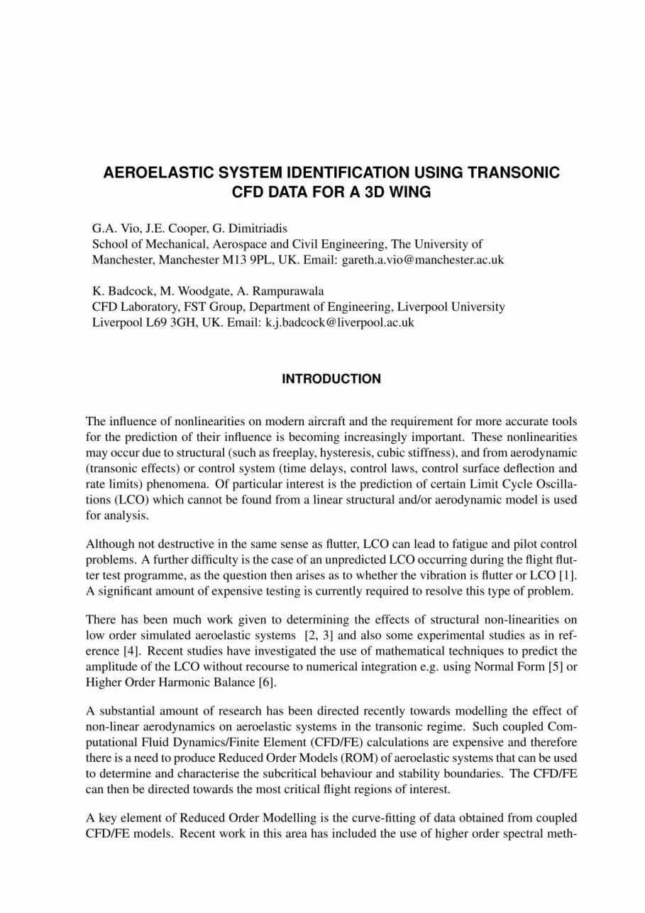
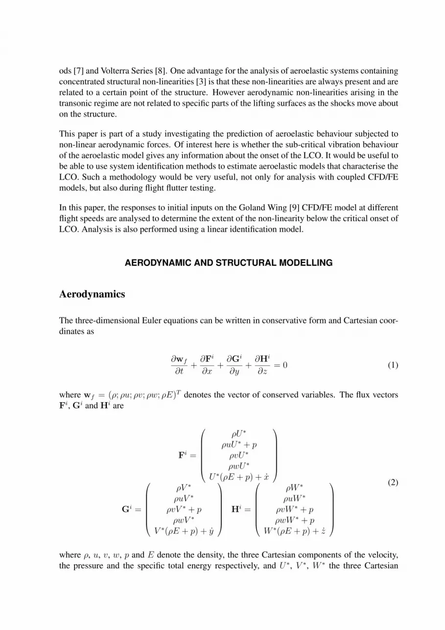
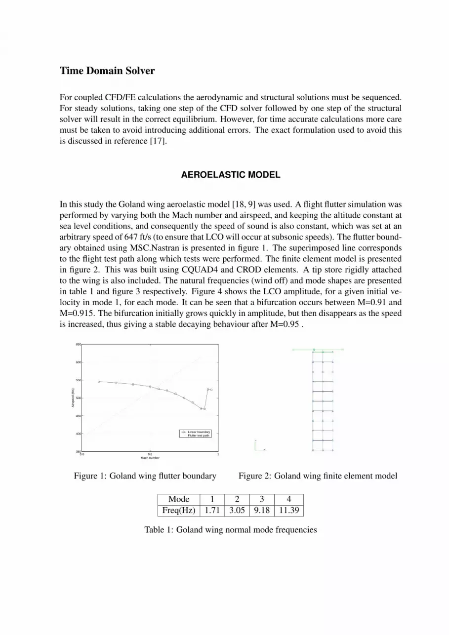
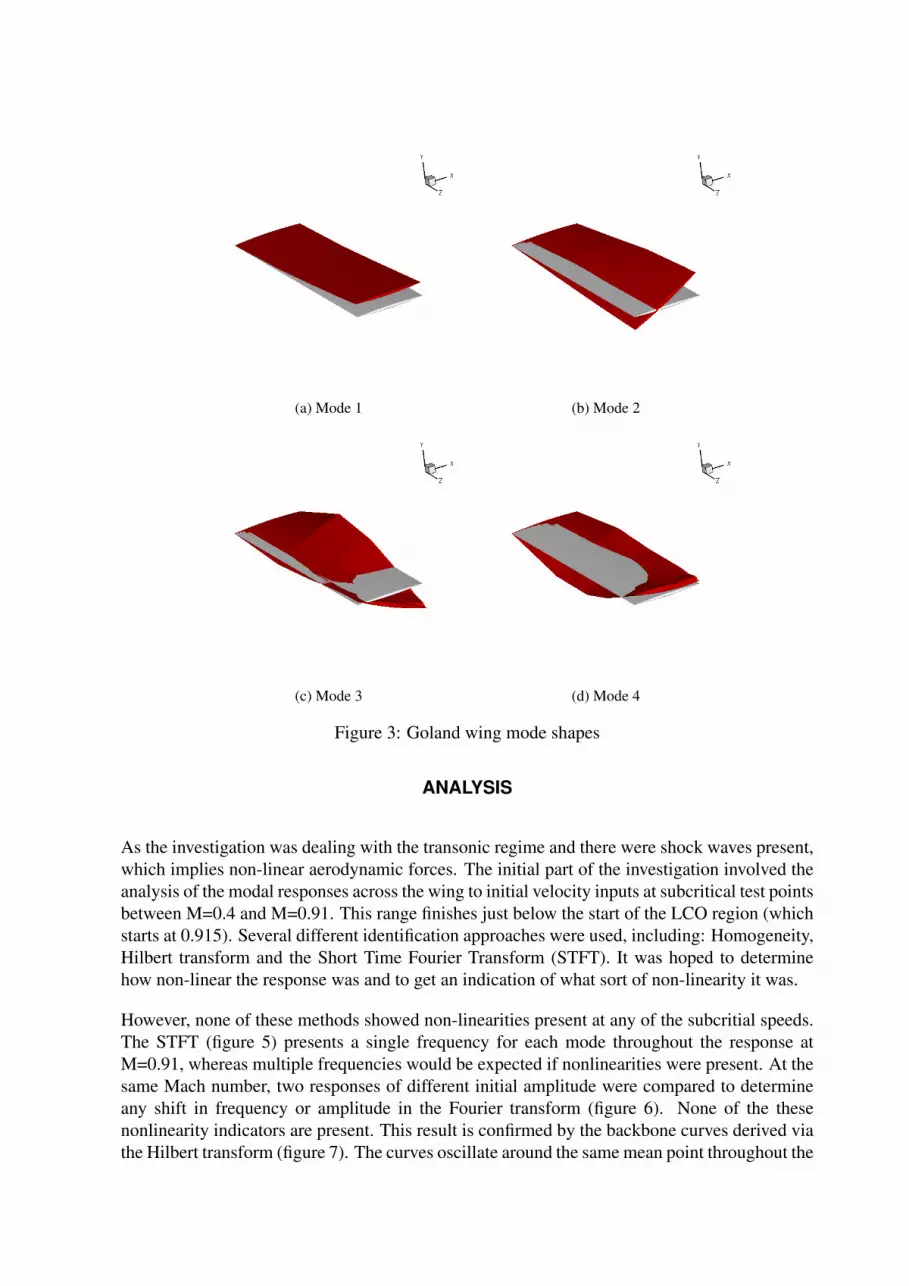
In this study the Goland wing aeroelastic model [18, 9] was used. A flight flutter simulation wasperformed by varying both the Mach number and airspeed, and keeping the altitude constant atsea level conditions, and consequently the speed of sound is also constant, which was set at anarbitrary speed of 647 ft/s (to ensure that LCO will occur at subsonic speeds). The flutter bound-ary obtained using MSC.Nastran is presented in figure 1. The superimposed line correspondsto the flight test path along which tests were performed. The finite element model is presentedin figure 2. This was built using CQUAD4 and CROD elements. A tip store rigidly attachedto the wing is also included. The natural frequencies (wind off) and mode shapes are presentedin table 1 and figure 3 respectively. Figure 4 shows the LCO amplitude, for a given initial ve-locity in mode 1, for each mode. It can be seen that a bifurcation occurs between M=0.91 andM=0.915. The bifurcation initially grows quickly in amplitude, but then disappears as the speedis increased, thus giving a stable decaying behaviour after M=0.95 .

0.6 0.8 1350

400

450

500

550

600

650

Mach number

Airs

peed

(ft/

s)

Linear boundaryFlutter test path

Figure 1: Goland wing flutter boundary Figure 2: Goland wing finite element model

Mode 1 2 3 4Freq(Hz) 1.71 3.05 9.18 11.39

Table 1: Goland wing normal mode frequencies

(a) Mode 1 (b) Mode 2

(c) Mode 3 (d) Mode 4

Figure 3: Goland wing mode shapes

ANALYSIS

As the investigation was dealing with the transonic regime and there were shock waves present,which implies non-linear aerodynamic forces. The initial part of the investigation involved theanalysis of the modal responses across the wing to initial velocity inputs at subcritical test pointsbetween M=0.4 and M=0.91. This range finishes just below the start of the LCO region (whichstarts at 0.915). Several different identification approaches were used, including: Homogeneity,Hilbert transform and the Short Time Fourier Transform (STFT). It was hoped to determinehow non-linear the response was and to get an indication of what sort of non-linearity it was.

However, none of these methods showed non-linearities present at any of the subcritial speeds.The STFT (figure 5) presents a single frequency for each mode throughout the response atM=0.91, whereas multiple frequencies would be expected if nonlinearities were present. At thesame Mach number, two responses of different initial amplitude were compared to determineany shift in frequency or amplitude in the Fourier transform (figure 6). None of the thesenonlinearity indicators are present. This result is confirmed by the backbone curves derived viathe Hilbert transform (figure 7). The curves oscillate around the same mean point throughout the

0.4 0.5 0.6 0.7 0.8 0.9 1−4

−3

−2

−1

0

1

2

3

4

Mach number

Mod

e 1

ampl

itude

(a) Mode 1

0.4 0.5 0.6 0.7 0.8 0.9 1−2.5

−2

−1.5

−1

−0.5

0

0.5

1

1.5

2

2.5

Mach number

Mod

e 2

ampl

itude

(b) Mode 2

0.4 0.5 0.6 0.7 0.8 0.9 1−0.3

−0.2

−0.1

0

0.1

0.2

0.3

0.4

Mach number

Mod

e 3

ampl

itude

(c) Mode 3

0.4 0.5 0.6 0.7 0.8 0.9 1−0.3

−0.2

−0.1

0

0.1

0.2

0.3

0.4

Mach number

Mod

e 3

ampl

itude

(d) Mode 4

Figure 4: Goland wing bifurcation plots

displacement, indicating linearity. The oscillation present arise from from leakage problems, asthe response has not fully decayed when the simulation was stopped. These results confirm thatnon-linear effect are not present at all transonic speeds.

As the responses were linear at all points below the LCO onset, it was thought that the aero-dynamic nonlinearities manifest themselves via changes in the speed between each test point,however, the aerodynamics behave in a linear manner at each flight condition. Such an effecthas been suggested elsewhere [19]. To verify this conjecture, the Nissim-Gilyard identificationmethod [20] was used to obtain the linear aerodynamic matrices using every consecutive pairof test points for the identification. Points between Mach number of 0.40 and 0.98 where used.Taking the standard linear aeroelastic equation of motion as

Ay + (ρUB + D)y + (ρU2C + E)y = 0 (14)

where A, B, C, D, E are respectively the mass, aerodynamic damping, aerodynamic stiffness,structural damping and structural stiffness, U is the airspeed and ρ is the density. The frequency-damping plot for the system is presented in figure 8, where the linear damping and frequencyestimates are obtained via the Eigenvalue Realisation Algorithm (ERA) method [21]. With theNissim-Gilyard method the A−1B, A−1D, A−1C, A−1E matrices can be identified. If thesystem was linear, the same matrices should have been identified at each point in the flutter

test. In figure 9 the behaviour for the A−1B matrix is displayed for each term. The Machnumbers used in the identification are in table 2. The identification shows that the terms arefairly constant until M=0.87 and M=0.88 (case 15) are used, where they start to deviate slightly.This deviation becomes considerable when M=0.905 and M=0.91 are used (case 18). The samepattern is found in all the other identified matrices. By the time the identification reaches case26 (M=0.945 and M=0.95) the terms in the identified matrices have returned to their linearidentified behaviour prior to M=0.87. As the bifurcation starts at M=0.91, a window of 25 ft/s,is available in which it should be possible to predict the start of the bifurcation. However, asthis bifurcation is within 4% of the flutter speed, this approach would not be acceptible in a realflight flutter test as an indicator of imminent LCO.

If a linear system is assumed, then the structural and aerodynamic matrices identified using theNissim-Gilyard method result in a predicted flutter speed of around 0.90, which is just belowthe LCO onset speed. If one of the speeds used in the identification was in the non-linear region,i.e. from M=0.86 onwards, no flutter speed is then detected.

LCO in the transonic region are caused by movement of the shock waves interacting with theflexible structure. It could be suggested that in this case, the position of the aerodynamic centrewould vary. A simple investigation to examine the influence of changing the position of aero-dynamic centre was carried out using a three degree-of-freedom aeroelastic model [22] withmodified quasi-steady aerodynamics. By changing the eccentricity, i.e. the distance betweenlift and flexural axis, the position of the aerodynamic centre was moved, mimicking the effectof moving the shocks along the wing in a transonic flow with different speeds. The eccentricitywas moved from the leading edge up to the half chord. Figure 10 shows the changes in thesystem matrices identified using the Nissim and Gilyard method. It can be seen that a similarbehaviour to the findings from the CFD/FE model with different terms being identified for theA−1B matrix as the aerodynamic centre is moved towards the half-chord.

Case M(1) M(2) Case M(1) M(2) Case M(1) M(2)1 0.400 0.450 11 0.800 0.825 21 0.920 0.9252 0.450 0.500 12 0.825 0.850 22 0.925 0.9303 0.500 0.550 13 0.850 0.860 23 0.930 0.9354 0.550 0.600 14 0.860 0.870 24 0.935 0.9405 0.600 0.650 15 0.870 0.880 25 0.940 0.9456 0.650 0.700 16 0.880 0.900 26 0.945 0.9507 0.700 0.725 17 0.900 0.905 27 0.950 0.9558 0.725 0.750 18 0.905 0.910 28 0.955 0.9609 0.750 0.775 19 0.910 0.915 29 0.960 0.965

10 0.775 0.800 20 0.915 0.920 30 0.965 0.970

Table 2: Nissim-Gilyard test cases

0 100 200 300 400 500 600 700 8000

0.1

0.2

0.3

0.4

0.5

0.6

0.7

0.8

0.9

1

Time

Fre

quen

cy

Figure 5: Short Time Fourier Transform atM=0.91

0 0.01 0.02 0.03 0.04 0.05 0.06 0.07 0.08 0.09 0.10

0.1

0.2

0.3

0.4

0.5

0.6

0.7

0.8

0.9

1

Frequency

FT

am

plitu

de

A=0.1A=1.0

Figure 6: Fourier Transform at M=0.91

0.1 0.105 0.11 0.115 0.12 0.1250

0.1

0.2

0.3

0.4

0.5

0.6

0.7

0.8

0.9

Frequency

Dis

plac

emen

t

−0.02 −0.01 0 0.010

0.1

0.2

0.3

0.4

0.5

0.6

0.7

0.8

0.9

Damping

Dis

plac

emen

t

Figure 7: Hilbert Transform at M=0.91

0.4 0.5 0.6 0.7 0.8 0.9 10

0.2

0.4

0.6

0.8

Mach number

Fre

quen

cy

0.4 0.5 0.6 0.7 0.8 0.9 1−0.1

0

0.1

0.2

0.3

0.4

Mach number

% D

ampi

ng

Figure 8: Frequency-damping plot

DISCUSSION OF RESULTS

The results show that for an aeroelastic wing in the transonic regime, it is possible for limit cycleoscillations to occur due to the presence of shock waves. However, it was shown that there isno indication of the non-linearity at sub-critical speeds until just before the LCO onset. At eachtest point the aerodynamics behaves in a linear manner, but the variation between test points isnon-linear. The linear identification using the Nissim / Gilyard approach backs this finding up,and comparison with the results obtained by moving the position of the aerodynamic centre ona simple aeroelastic model indicates that the changes in the aerodynamic centre position mayproduce this effect.

If these results are general, then this indicates that the production of reduced order models foraeroelastic systems with non-linear aerodynamics will need to include information about theflight regime at different test points. They also imply that sub-critical flight flutter test data mayremain linear even though a non-linear phenomenon such as LCO is about to occur. Furtherwork is ongoing to resolve some of these issues.

0 20 40−5

0

5x 10

−4

(1,1

)

0 20 40−0.01

0

0.01

(1,2

)

0 20 40−0.02

0

0.02

(1,3

)

0 20 40−0.05

0

0.05

(1,4

)

0 20 40−10

−5

0

5x 10

−4

(2,1

)

0 20 40−0.01

0

0.01

(2,2

)

0 20 40−0.05

0

0.05

(2,3

)

0 20 40−0.1

0

0.1

(2,4

)

0 20 40−5

0

5x 10

−4

(3,1

)

0 20 40−0.01

0

0.01

(3,2

)

0 20 40−0.01

0

0.01

(3,3

)

0 20 40−0.05

0

0.05

(3,4

)0 20 40

−5

0

5x 10

−4

(4,1

)

0 20 40−0.01

0

0.01

(4,2

)

0 20 40−0.02

0

0.02

(4,3

)

0 20 40−0.04

−0.02

0

0.02

(4,4

)

Figure 9: Identified matrix M−1B for Golandmodel

0 20 40 60−1

0

1

2

(1,1

)

0 20 40 60−0.1

−0.05

0

0.05

0.1

(1,2

)

0 20 40 60−1.2622

−1.2622

−1.2622

−1.2622

−1.2622x 10

−3

(1,3

)

0 20 40 60−50

0

50

100

150

(2,1

)

0 20 40 60−10

−5

0

5

(2,2

)

0 20 40 60−0.0292

−0.0292

−0.0292

−0.0292

−0.0292

(2,3

)

0 20 40 60−600

−400

−200

0

200

(3,1

)

0 20 40 60−10

0

10

20

30

(3,2

)

0 20 40 600.2805

0.2805

0.2805

(3,3

)

Figure 10: Identified matrix M−1B for 3DOFmodel

CONCLUSIONS

In this paper a number of system identification methods were applied to responses for theGoland aeroelastic model in the transonic flight regime. It was found that the model displayslinear behaviour at all subcritical speeds. The Nissim-Gilyard method was used to show that,by using linear identification, the identified structural and aerodynamic matrices of the aeroe-lastic model varied in their behaviour as the LCO region was approached. The same pattern ofbehaviour was found to occur on a simple aeroelastic model with varying aerodynamic centreposition.

ACKNOWLEDGEMENTS

The authors would like to acknowledge the support received by the Engineering and PhysicalSciences Research Council, BAE Systems, DTI and MOD through the PUMA DARP project.

REFERENCES

[1] Dunn, S. A., Farrell, P. A., Budd, P. J., Arms, P. B., Hardie, C. A., and Rendo, C. J.F/A-18A flight flutter testing-limit cycle oscillation or flutter? In International Forum onAeroelasticity and Structural Dynamics, Madrid, Spain, June 2001.

[2] Price, S. J., Alighambari, H., and Lee, B. H. K., The aeroelastic response of a two-dimensional airfoil with bilinear and cubic structural nonlinearities, Journal of Fluids andStructures, 1995, 9, 175–193.

[3] Lee, B. H. K., Price, S. J., and Wong, Y. S., Nonlinear aeroelastic analysis of airfoils:bifurcation and chaos, Progress in Aerospace Sciences, 1999, 35, 205–334.

[4] Conner, M. D., Tang, D. M., Dowell, E. H., and Virgin, L. N., Nonlinear behavior of atypical airfoil section with control surface freeplay: a numerical and experimental study,Journal of Fluids and Structures, 1997, 11, 89–109.

[5] Vio, G. A. and Cooper, J. E., Limit cycle oscillation prediction for aeroelastic systems withdiscrete bilinear stiffness, International Journal of Applied Mathematics and Mechanics,2005, 3, 100–119.

[6] Liu, L. and Dowell, E. H., Harmonic balance approach for an airfoil with a freeplay controlsurface, AIAA Journal, 2005, 43, 802–815.

[7] Silva, W. A., Strganac, T. W., and Hajj, M. R. Higher-order spectral analysis of a nonlinearpitch and plunge apparatus. In Structures, Structural Dynamics and Materials Conference,Austin, Texas, USA, April 2005.

[8] Gaitonde, A. L. and Jones, D. P., Reduced order state-space models from the pulse re-sponses of a linearized CFD scheme, International Journal for Numerical Methods inFluids, 2004, 42, 581–606.

[9] Beran, P. S., Khot, N. S., Eastep, F. E., Snyder, R. D., and Zweber, J. V., Numericalanalysis of store-induced limit-cycle oscillation, Journal of Aircraft, 2004, 41, 1315–1326.

[10] Badcock, K. J., Richards, B. E., and Woodgate, M. A., Elements of computational fluiddynamics on block structured grids using implicit solvers, Progress in Aerospace Sciences,2000, 36, 351–392.

[11] Osher, S. and Chakravarthy, S., Upwind schemes and boundary conditions with applica-tions to euler equations in general geometries, Journal of Computational Physics, 1983,50, 447–481.

[12] Leer, B. V., Towards the ultimate conservative conservative difference scheme II: Mono-tonicity and conservation combined in a second order scheme, Journal of ComputationalPhysics, 1974, 14, 361–374.

[13] Cantaritti, F., Dubuc, L., Gribben, B., Woodgate, M., Badcock, K., and Richards, B. Ap-proximate Jacobian for the solution of the Euler and Navier-Stokes equations. Aerospaceengineering report, University of Glasgow, 1997.

[14] Jameson, A. Time dependant calculations using multigrid, with applications to unsteadyflows past airfoils and wings. Technical Report 91-1596, AIAA, 1991.

[15] Goura, G. S. L., Badcock, K. J., Woodgate, M. A., and Richards, B. E., Extrapolationeffects on coupled CFD-CSD simulations, AIAA Journal, 2003, 41, 312–314.

[16] Gordon, W. J. and Hall, C. A., Construction of curvilinear coordinate systems and appli-cations to mesh generation, International Journal of Numerical Methods in Engineering,1973, 7, 461–477.

[17] Goura, G. S. L., Badcock, K. J., Woodgate, M. A., and Richards, B. E., Implicit methodfor the time marching analysis of flutter, Aeronautical Journal, 2001, 105, 119–214.

[18] Goland, M., The flutter of a uniform cantilever wing, Journal of Applied Mechanics, 1945,12, 197–208.

[19] Lisandrin, P., Carpentieri, G., and van Tooren, M. Open issues in system identification ofCFD based aerodynamic models for aeroelastic applications. In International Forum onAeroelasticity and Structural Dynamics, Munich, Germany, June 2005.

[20] Nissim, E. and Gilyard, G. B., Method for experimental identification of flutter speed byparameter identification, Report AIAA-89-1324, 1989.

[21] Juang, J. N. Applied System Identification. Prentice-Hall, Englewood Cliffs, New Jersey,1994.

[22] Dimitriadis, G. and Cooper, J. E., A time frequency technique for the stability analysisimpulse response from non-linear aeroelastic systems, Journal of Fluids and Structures,2003, 17, 1181–1201.