a tool for managing complexity in logistic systems under mass customization

A tool for managing complexity in logistic systems under mass customization

Carlo Rafele, Anna Corinna Cagliano

Abstract The logistic process of a manufacturing company can be regarded as a complex system since it involves many and different actors interconnected by a high number of non linear relationships. More precisely, a logistic process constitutes a Complex Adaptive System. Complexity is a particularly important feature of logistic systems in companies pursuing mass customization strategies. As a matter of fact, mass customization triggers considerable complexity owing to different and constantly varying products, markets, processes, customers and customers’ requirements. Traditional logistic management approaches are based on Newtonian and mechanistic principles, such as perfect rationality, determinism and linear causality. However, global competition and changing demands make markets more and more turbulent and nowadays logistic systems are characterized by uncertainty, non linearity and heterogeneity. Therefore, there is a need for managerial models able to capture and understand these drivers of complexity in logistic processes. The paper suggests the integration between performance measurement and Systems Dynamics to control complexity of logistic systems under mass customization conditions. A case study from the automotive industry is detailed. The authors are currently refining the model presented in this paper and trying to extend the approach to study the complexity of a supply chain as a system.

Keywords Complex Systems, Logistics, Mass Customization, Performance Measurement, System Dynamics

1 Introduction

The increasing competition in globally interconnected markets makes classical strategies of differentiation able to improve the operating results of a company only marginally. New drivers of value creation need to be found and customer satisfaction plays a leading role in this context. In particular, establishing enduring relationships with each customer is one of the main ways to achieve strategic advantages in today’s competitive environment (Schenk & Seelmann – Eggebert, 2004). The idea of mass customization originates in the late 1980’s and combines the benefits of mass and serial production with those of craft production, aiming at fulfilling the needs of single customers with relatively low costs and high responsiveness and performance. As pointed out by Da Silveira, Borenstein and Fogliatto (2001), mass customization provides many companies with a good alternative to differentiate themselves in strongly segmented markets. This is the reason why, starting from manufacturing settings, the concept has become popular also in service ones in the last few years. Focusing on the manufacturing sector, logistics is extremely important in mass customization. As a matter of fact, the great number of different products and the high degree of delivery service demanded by customers require efficient and timely logistic operations. Moreover, logistic processes have to manage effectively high part and subassembly variety, supplier variety and production planning and scheduling issues (Blecker, Friedrich, Kaluza, Abdelkafi & Kreutler, 2005, chap. 9). The complexity triggered by mass customization adds to the inherent complexity of logistic systems. This may lead for example to higher inventories and longer delivery times. Therefore, it is necessary to define models and methods to assess and control the degree of complexity, trying to reduce the problems caused by product proliferation. This work suggests a tool integrating performance measurement and System Dynamics methodology to understand complexity and monitor its effects on the behaviour of logistic processes in manufacturing companies pursuing mass customization strategies. Furthermore, with the future aim of extending this approach to supply chains, relationships between the operational performance of a focus company and that of its first tier suppliers are also studied. The reminder of the paper is organized as follows. Section 2 discusses logistic complexity and the need of new managerial approaches for dealing with it, whereas section 3 highlights the impacts of mass customization on the complexity of logistic processes. The proposed tool is detailed in section 4 and is applied to a case study in section 5. Finally, conclusions and future research aims are presented in section 6.

2 Complexity of logistic systems

2.1 Logistic systems are Complex Adaptive Systems

The notion of logistics as being complex traces back to the end of the 1970’s when Manheim observed that logistic systems consist of complex processes (as cited in Nilsson & Waidringer, 2002). Nowadays, several circumstances contribute to raise the level of logistic complexity (Lumsden, Hulten & Waidringer, 1998). Manufacturing and logistic systems are becoming more and more sensitive to disturbances, also because of short product lifecycles which create demands on quick changes in production, inducing to minimize the amount of manufactured products. Companies are able to choose to manufacture parts of a same product at different

locations, where it is most cost effective. Therefore, the internal material flow is extended to include external transports between firms. Another factor of complexity is outsourcing: the use of multiple subcontractors makes flows and relationships more complex and creates sensitive systems. Finally, individual adaptation of products, in order to confront current greater customer demand and increased competition, complicates the internal material flow. It may be argued that logistic systems are Complex Adaptive Systems (CASs). According to Gandolfi (1999), a CAS may be defined as an open system compounded by numerous elements interacting in a non linear way and forming a single, organized and dynamic entity, able to evolve and adapt itself to the environment. First of all, a logistic system is open since it communicates with the external environment, such as the other departments of a company, suppliers or customers, mainly by means of flows of materials and information. Moreover, a logistic system is constituted by a large number of different elements: parts, means of transport, equipment supporting logistic activities, managers, employees, logistic providers and so on. All of them are usually linked by non linear relationships. A sort of cohesion among components also exists and this makes logistic systems unitary entities. Since they coordinate human, material and financial resources towards a specific goal, moving parts through a value chain, it can be concluded that they are organized systems. A logistic process is characterized by dynamic variables and is able to evolve and adapt itself to changes in the environment. As a matter of fact, it has to be extremely flexible to satisfy the ever new requirements of both customers and manufacturing systems. Two meaningful examples can be mentioned. First, in today’s marketplaces the value is shifting towards adding service dimensions to product features (Nilsson & Waidringer, 2005) and firms are modifying their logistic operations to pursue differentiation strategies. Second, Just in Time philosophy recommends to produce only what is necessary and when it is necessary, reducing waste and consequently the level of stock. Thus, logistic departments have been obliged to increase their mix and volume flexibility to achieve small batch sizes and therefore fast throughput and short delivery lead times (Slack, Chambers & Johnston, 2001).

2.2 Managing complex logistic systems According to the conceptual framework proposed by Waidringer (2001), three properties have a significant impact on the management of logistic activities:

− structure property: it is related to physical as well as informational and communicational structures;

− dynamic property: it concerns the flows of goods, money and information within structures;

− adaptation property: it refers to the management and control of structures and dynamics in order to satisfy customer demand effectively.

Since the major benefits provided by logistics are time and place utility of products, traditional management approaches are founded on Newtonian and mechanistic principles and address the properties of structure and dynamics. They are built on a set of hypotheses including perfect rationality of behaviour, determinism and linear cause and effect relationships. Moreover, a central assumption is that logistic managers play a role of observers, putting themselves outside the controlled system. As a consequence, logistic activities are handled in a top – down fashion. Managers plan and decide actions “from above”, basing on the observation of global logistic phenomena, and these actions are then assigned to resources able to perform them. However, all

logistic processes in supply networks are heterogeneous, uncertain, non linear and increasingly complex. As a matter of fact, marketplaces are getting more and more turbulent making firms operate in a landscape which is not static. Logistic practice is to a great extent characterized by last minute changes and rearrangements, due for example to accidents, changes in customer demand, machine and computer breakdowns or mistakes. In addition, people, business functions and processes involved in logistic operations lack perfect information and often have different and conflicting goals (Nilsson & Waidringer, 2005). Furthermore, the common approach to handle logistic complexity is breaking down problems into separate parts easy to analyze and solve. But, since a complex whole may exhibit properties that cannot be understood by simply studying its single components, bottom up phenomena, formed from local interactions among individuals and parts, are not captured. In this context, logistic management models have to overcome the mechanistic view taking into account non linearity, heterogeneity, subjective and bounded rationality, self – organization and emergence. It is also necessary to take a bottom up perspective on the individual level at which activities are performed and affected by autonomous agents. This will provide insights and increased understanding about phenomena emerging from every day interactions and also about the causes of the observed global behaviour. Finally, logistic research and practice should pay more attention to the adaptation property of Waidringer’s framework, usually neglected by current theories.

3 The complexity of mass customization and its impact on logistic processes A mass customizing system cannot be a simple one owing to the complexity of the environment inside which it acts. More precisely, mass customization triggers high complexity mainly because of various products, markets, processes, customers, customer requirements and steadily changing circumstances. This induces production planning, manufacturing and product configuration complexity (Blecker, et al., 2005, chap. 3, p. 45, 46). Besides these aspects, mass customization heavily influences also the supply and distribution networks of a manufacturing company and hence its logistic processes. For instance, product modularity eases the outsourcing of production activities, so that internal manufacturing operations may be reduced, or gives the possibility to postpone some product customization tasks downstream in the distribution network (Salvador, Rungtusanatham & Forza, 2004). The degree of complexity added by mass customization to a logistic system depends on the practical methods to implement this concept. In particular, the use of common components for various items (part and procurement standardization) decreases the complexity of inbound logistics because of the small number and variety of material and informational flows coming from suppliers. In this situation complexity will affect chiefly internal and/or outbound logistics. Since different items follow similar manufacturing paths, process standardization simplifies internal logistic flows reducing the related complexity. In some cases, it may also lower the complexity of inbound logistics, especially when it is combined with part standardization. Generally speaking, in process standardization the customization is delayed as late in the process as possible and so logistic complexity moves downward in the value chain, towards customers. When adopting product standardization, companies stock only a few of the sold items (standardized items); if an unstocked product is demanded, the firm will produce it after receiving the order. The level of inbound, internal and outbound logistic complexity depends on the number and features of standardized products. Sometimes, when a lot of unstocked items are requested, it may increase.

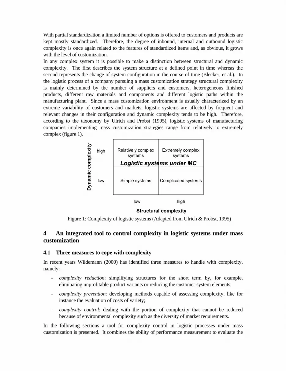
With partial standardization a limited number of options is offered to customers and products are kept mostly standardized. Therefore, the degree of inbound, internal and outbound logistic complexity is once again related to the features of standardized items and, as obvious, it grows with the level of customization. In any complex system it is possible to make a distinction between structural and dynamic complexity. The first describes the system structure at a defined point in time whereas the second represents the change of system configuration in the course of time (Blecker, et al.). In the logistic process of a company pursuing a mass customization strategy structural complexity is mainly determined by the number of suppliers and customers, heterogeneous finished products, different raw materials and components and different logistic paths within the manufacturing plant. Since a mass customization environment is usually characterized by an extreme variability of customers and markets, logistic systems are affected by frequent and relevant changes in their configuration and dynamic complexity tends to be high. Therefore, according to the taxonomy by Ulrich and Probst (1995), logistic systems of manufacturing companies implementing mass customization strategies range from relatively to extremely complex (figure 1).

Figure 1: Complexity of logistic systems (Adapted from Ulrich & Probst, 1995)

4 An integrated tool to control complexity in logistic systems under mass customization

4.1 Three measures to cope with complexity In recent years Wildemann (2000) has identified three measures to handle with complexity, namely:

- complexity reduction: simplifying structures for the short term by, for example, eliminating unprofitable product variants or reducing the customer system elements;

- complexity prevention: developing methods capable of assessing complexity, like for instance the evaluation of costs of variety;

- complexity control: dealing with the portion of complexity that cannot be reduced because of environmental complexity such as the diversity of market requirements.

In the following sections a tool for complexity control in logistic processes under mass customization is presented. It combines the ability of performance measurement to evaluate the

Dyn

amic

com

plex

ity

effects of complexity on the behaviour of a system with the power of System Dynamics approach to trace at the root the causes of these effects.

4.2 A model for logistic performance measurement: LOGISTIQUAL Constantly monitoring logistic service quality is essential for a company since it is a main driver of customer satisfaction. LOGISTIQUAL model helps achieve this purpose. The starting point in the development of the framework is SERVQUAL (Parasuraman, Zeithaml & Berry, 1985, 1988), a widely applied model for quality evaluation of a generic service. According to it, five dimensions characterize the quality of every kind of service: Tangibles, Reliability, Responsiveness, Assurance and Empathy (figure 2). Adapting SERVQUAL to the particular case of logistic service and analyzing real business settings, a classification of the main factors of logistic performance has been developed (Rafele, 2004; Grimaldi & Rafele, 2007) (figure 2). Let us notice that Tangible Components macro – class corresponds to SERVQUAL dimension Tangibles, whereas Way of Fulfilment to Reliability and Responsiveness and Informative Actions to Empathy and Assurance. LOGISTIQUAL aims at providing a company with a logical structure inside which operational performance indicators can be defined, according to the specific logistic process under study. In order to extend the model beyond the boundaries of a single organization, two frameworks of application have been derived. With the first, named Source – LOGISTIQUAL, a company evaluates the logistic performance carried out by its upstream suppliers. Whereas with the second, named Self – LOGISTIQUAL, a company assesses its internal logistic performance and the service carried out for downstream customers. LOGISTIQUAL is a well consolidated model since it has been extensively validated both in manufacturing and in service sector (Grimaldi & Rafele, 2007).

Figure 2: From SERVQUAL structure to LOGISTIQUAL structure

TANGIBLE COMPONENTS

WAYS OF FULFILMENT

INFORMATIVE ACTIONS

Internal assets

External assets

Personnel

Inventory/Availability

Flexibility

Service care

Supply conditions

Lead time

Marketing

Order managing

After sales

E-information

Forecasting

Internal communication

Perceived service

Supplied service

SERVQUAL

LOGISTIQUAL

TANGIBLE COMPONENTS

WAYS OF FULFILMENT

INFORMATIVE ACTIONS

Internal assets

External assets

Personnel

Inventory/Availability

Flexibility

Service care

Supply conditions

Lead time

Marketing

Order managing

After sales

E-information

Forecasting

Internal communication

Perceived service

Supplied service

SERVQUAL

LOGISTIQUAL

4.3 Studying the behaviour of logistic systems: System Dynamics approach First introduced by Forrester (1961) at MIT and later developed by Sterman (2000), System Dynamics (SD) is a methodology for analyzing the behaviour of complex, dynamic social, technological, economic and political systems, representing them by means of stocks, flows and interacting feedback loops. The main goal of SD is to understand, through the use of qualitative and quantitative models, how structure produces system behaviour and to use the resulting knowledge to predict the consequences over time of changes in policies ruling the system. SD approach bases heavily on the description of cause and effect relationships between variables since it is through their interactions that system behaviour emerges. As regards complexity management, it is interesting to notice that SD may help both in complexity reduction, to study a complex system in order to detect where it can be simplified, and in complexity prevention, for the purpose of evaluating complexity indicators, and in complexity control, to understand a complex system, control it and analyze the consequences of certain strategies. There are several reasons for adopting SD to understand how a logistic process works. First, this last involves changes over time and the transmission and receipt of information (feedbacks), the two major features SD is devoted to analyze. A logistic system is characterized by stock and flow structures for the acquisition, storage and delivery of products. Consequently, many logistic quantities are determined by flows exchanged between actors. Moreover, especially in a mass customization environment, the components of logistic processes often interact one another, both directly and indirectly, causing dependence relationships among variables. Finally, some logistic operations may imply time delays, like for example receiving materials or transferring information to other company’s departments, suppliers or customers. SD is particularly suitable to study how delays and phase lags determine oscillations in a system. In recent literature some authors have applied this methodology to study logistic aspects in supply chains (Sterman, 2000; Schieritz & Gröβler, 2003; Rafele & Cagliano, 2006 a, 2006 b).

4.4 The proposed integrated tool Metrics belonging to the classes of LOGISTIQUAL are able to assess how elementary logistic activities are performed, giving managers the bottom up perspective that is often lacking. However, performance measures only provide a number that synthesizes the impacts of phenomena related to complexity, such as self – organization or interactions among people and/or parts in the logistic system, on for instance timeliness, flexibility or inventory availability. Using System Dynamics methodology, Causal Loop Diagrams (CLDs) are sketched in order to identify system components affecting the values of selected performance indicators together with the cause and effect connections among these elements, between them and the metrics and also among metrics themselves. From qualitative CLDs, Stock and Flow Diagrams and the mathematical equations defining the model can be derived. After validation, simulation will give time evolutions of the quantities and relationships under consideration. System Dynamics makes possible to analyze in depth how complexity arises. As a matter of fact, CLDs and the related equations describe the non linear relationships and the feedback loops among the elements of a logistic process which determine its complexity. Operational performance indicators evaluated by LOGISTIQUAL are defined by system variables and thus the links among these quantities and metrics also allow to assess how complexity impacts on the behaviour of the process. The proposed tool particularly focuses on one main aspect of logistic complexity in mass customization environments: the variety of parts existing in at least one process stage. These

parts influence one another because their logistic paths intersect. The combined use of LOGISTIQUAL and System Dynamics provides companies with a scientific methodology to understand how the performance of each part is affected by the performance of the others. The evaluation of performance indicators, together with the study of the structure on which their mutual connections are based, allows to assess and analyze the level of complexity in a logistic system given by the coexistence of multiple parts. Moreover, possible strategies to try to reduce complexity or, at least, limit its negative effects may be found out and compared. It is also worth remarking that monitoring operational performance contributes to ensure efficiency, which is essential in a manufacturing – logistic system operating according to mass customization principles. Furthermore, the issues introduced by a large variety of raw materials, components and finished products may be overcome if the entire supply chain is coordinated in an optimal way (Blecker, et al., 2005, chap. 9, p. 213). With the aim of stimulating this coordination, the proposed approach could be extended to assess the mutual impacts of performance metrics evaluated in different supply chain echelons. In the next section a case study shows the practical implementation of the integrated tool.

5 A case study from the automotive industry

5.1 The company and the focus of the study The present case study focuses on a medium – sized Italian company producing injection moulded plastic parts for cars (belt carters, door panels, front/central/ rear panels for interior trim, etc.). This is a first equipment supplier of automotive manufacturers such as FIAT or OPEL and all of its products are made exactly to customers’ specifications, which depend on the different car models. In order to understand the interactions among raw materials, works in process and finished products in the logistic system of this company and the related performance, two representative types of products have been considered. These are a Belt Carter and Central and Rear Panels for interior trim (right and left item) for a same car model. Their product trees are represented in figures 3, 4, 5 together with the codes and usage per unit of product (UpU) of all their constituents. Works in process A1, A5, A6, A7 and the finished product BC are manufactured by the company’s moulding department using a same press that will be called Press 1. Component A3 is produced by the moulding department too, but with a different press, whereas components A2 and A4 are purchased from supplier S1. Plastic materials B1 and B3 are purchased from supplier S2 and B2 from supplier S3. Finally, finished products RCP, LCP, RRP and LRP are made by the internal assembling department. Both Central and Rear Panels are ordered and shipped to the customer in pairs, right and left item. Part standardization can be noticed in the finished products under study: as a matter of fact, their product trees have some common elements.

Figure 3: Belt Carter product tree

Figure 4: Right / Left Central Panel product tree

Figure 5: Right / Left Rear Panel product tree

5.2 Identifying logistic performance indicators and defining the SD model The first step in this analysis is defining the performance indicators used to study interactions among parts. In collaboration with management and adopting LOGISTIQUAL model as a reference framework, the key metrics for the focus company’s logistic process have been identified. They are all evaluated weekly and may be defined as follows:

- Inventory Availability (IA): the ratio between the inventory level of a raw material, component, work in process or finished product during a period and the required quantity of that item in the same period (LOGISTIQUAL Tangible Components, Inventory/Availability).

- Order Fulfilment Efficiency (OFE): the quantity of a finished product delivered in a period over the quantity of that item on order in the same period (LOGISTIQUAL Ways of Fulfilment, Service Care).

- Return Percentage (RP) (of raw materials and components purchased from suppliers): the quantity of an item returned to its supplier in a period over the quantity received in the same period (LOGISTIQUAL Informative Actions, After Sales).

- Defectiveness Percentage (DP) (of parts manufactured by the focus company): the ratio between the quantity discarded in a certain period and the quantity produced in that period (LOGISTIQUAL Tangible Components, Internal Assets).

Interviews to managers and employees from Logistics, Manufacturing, Quality Assurance and other departments were performed, a business process analysis by means of flow charts was

RCP / LCP – RIGHT / LEFT CENTRAL PANEL ASSEMBLED

A1/A5 – RIGHT / LEFT CENTRAL

PANEL MOULDEDUpU A1/A5

A2 - FIXING CLIP

UpU A2 for RCP/LCP

A3 – BRACKETFOR WIRING

UpU A3 for RCP/LCP

A4 – SEAT BELT UPPER FIXING

UpU A4 for RCP/LCP

B1 – PLASTICMATERIAL

UpU B1 for A1/A5

B2 – PLASTICMATERIAL

UpU B2

carried out and previous SD models about manufacturing settings (Sterman, 2000; Schieritz & Gröβler, 2003) were also reviewed. On this basis, in collaboration with the focus company’s managers and employees, the most important factors influencing the selected indicators, with reference to the studied finished products, were identified together with the relationships among them. These were first formalized sketching some Causal Loop Diagrams (some of them are reported in figures 6, 7, 8, 9, 10, 11, 12, 13) basically showing inventory management, order management and production planning for all the parts constituting a Belt Carter or a Panel. As an example of how CLDs should be read, let’s consider figure 6. Graph nodes represent the main quantities in managing both RCP and LCP inventory whereas arches the relationships among them. Plus and minus signs on arches indicate whether each relationship is positive or negative. For instance, there is a positive relationship between RCP/LCP Production Rate and RCP/LCP Inventory: an increase in the production rate causes an increase in the level of inventory. On the other hand, there is a negative link between RCP/LCP Scrap Rate and RCP/LCP Inventory because when the scrap rate increases more poor – quality items will be discarded making the level of inventory decrease. It is important to notice that in a CLD it is sufficient to define the existence of relationships and their nature, positive or negative. Only in the subsequent development of the SD model appropriate mathematical formulas have to be found in order to describe each arch. In the case study, after identifying the key quantities and their connections, stock variables were distinguished from flow ones and the mathematical equations characterizing the model were defined. The week was chosen as the time bucket of the model. The analysis of the SD model revealed important links among the considered performance metrics and also some connections between the focus company’s performance and its suppliers’. The following section presents the findings of the case study. As an example of the reasoning that has been used, the procedure followed to determine the interaction between two indicators is detailed.

5.3 Interactions between performance indicators First of all, an interaction between OFE of Panels and IA of the first level element in their product tree with the smallest production potential can be found. Let us consider RCP and LCP. As far as RCP is concerned, Ai Inventory Availability is defined as follows (∀i =1,2,3,4) (figures 7, 9, 10, 11):

BucketTime*RateUsageADesired

InventoryAIAi

iAi = (5.3.1)

where Desired Ai Usage Rate is the rate at which Ai should be used basing on the production planning. More precisely, Desired Ai Usage Rate = ∑ = LRP)RRP,LCP,RCP,(j i jforRateUsageADesired ∀i = 2, 3 and Desired A4 Usage Rate = (Desired

A4 Usage Rate for RCP + Desired A4 Usage Rate for LCP).

Again from figures 7, 9, 10, 11 it can be stated that the rate at which Ai may be used basing on its inventory availability is a fraction of the Desired Ai Usage Rate (∀i = 1, 2, 3, 4):

Available Ai Usage Rate (for j) = Desired Ai Usage Rate (for j) * Ai Usage Ratio (for j) (5.3.2)

where the relation holds ∀j = RCP, LCP, RRP, LRP if i = 2, 3 and ∀j = RCP, LCP if i = 4.

In the focus company’s production system RCP Production Rate is the minimum value between Desired RCP Production Rate, determined by the quantity of RCP on order in a week and the

current inventory level (figure 6), and Admissible RCP Production Rate, defined by the quantities of components / works in process available for usage. The production capacity of the assembling department is usually sufficient to fulfill production orders. More precisely,

⎭⎬⎫

⎩⎨⎧

=

RCPofUnitperUsageARCPforRateUsageAAvailable;

RCPofUnitperUsageARCPforRateUsageAAvailable

;RCPofUnitperUsageA

RCPforRateUsageAAvailable;UnitperUsageA

RateUsageAAvailableminRateProductionRCPAdmissible

4

4

3

3

2

2

1

1

(5.3.3)

As shown in (5.3.2), the rate of Ai (∀i = 1,2,3,4) available for usage is a percentage (Usage Ratio) of Desired Ai Usage Rate (for RCP) and this last is determined by the product between Desired RCP Production Rate and Ai Usage per Unit (of RCP) (figures 7, 9, 10, 11). Therefore, it can be deduced that Admissible RCP Production Rate ≤ Desired RCP Production Rate and that RCP Production Rate = Admissible RCP Production Rate. In order to focus the reasoning, let us consider for instance that A1 is the element of RCP with the smallest production potential, that is:

UnitperUsageARateUsageAAvailable

RateProductionRCPAdmissibleRateProductionRCP1

1== (5.3.4)

From figure 6, it follows that the level of RCP Inventory may be expressed as a function of RCP Production Rate. As a matter of fact, RCP Inventory = INTEGRAL [RCP Production Rate – RCP Shipment Rate – RCP Scrap Rate; RCP Inventory t0] = f1(RCP Production Rate). Moreover, also from figure 6:

TimeProcessingOrderPanelMinimum

InventoryRCPRateUsageRCPMaximum = (5.3.5)

⎥⎦

⎤⎢⎣

⎡=

RateShipmentRCPDesiredRateUsageRCPMaximumRatioUsageRCP 2f

Thus, substituting (5.3.5) in the expression for RCP Usage Ratio, it can be stated that this last is a function of RCP Production Rate:

RCP Usage Ratio = f3 (RCP Production Rate) (5.3.6)

From figure 6 and equations (5.3.4) and (5.3.6), the rate at which RCP may be shipped to the customer, basing on its inventory availability and on the desired shipment rate given by its quantity on order (Desired RCP Shipment Rate), is:

Available RCP Shipment Rate = RCP Usage Ratio * Desired RCP Shipment Rate = f4 (Available A1 Usage Rate) (5.3.7)

From figure 7 it can be seen that the rate of A1 available for production (Available A1 Usage Rate) depends on A1 Usage Ratio, that is defined by the maximum rate at which A1 Inventory may be used (Maximum A1 Usage Rate) and by Desired A1 Usage Rate. From these relationships and substituting equation (5.3.1) into (5.3.2), it follows that:

BucketTime*IAInventoryA

TimeDelivery&nPreparatioAMin.BucketTime*IA


RateUsageADesired*TimeDelivery&nPreparatioAMin.InventoryA


RateUsageA DesiredRateUsageA Maximum

RateUsageAAvailable

1

1

1

1

A

1

1

A5

A

1

11

15

A

1

1

151

*f

*f

*f

⎥⎥⎦

⎤

⎢⎢⎣

⎡=

=⎥⎦

⎤⎢⎣

⎡=

=⎥⎦

⎤⎢⎣

⎡=

Thus, Available A1 Usage Rate is a function f6 of IAA1 and, from (5.3.7), Available RCP Shipment Rate is also a function of A1 Inventory Availability, Available RCP Shipment Rate = f7

(IAA1). Since pairs consisting of one RCP and one LCP item have to be delivered to the customer, in every week RCP Shipment Rate = LCP Shipment Rate = CP Shipment Rate = min {Available RCP Shipment Rate; Available LCP Shipment Rate}. Therefore, a reasoning similar to the one just detailed has to be applied to LCP too.

LCP Production Rate = Admissible LCP Production Rate =

⎭⎬⎫

⎩⎨⎧

=

LCPofUnitperUsageALCPforRateUsageAAvailable

;LCPofUnitperUsageA

LCPforRateUsageAAvailable ;LCPofUnitperUsageA

LCPforRateUsageAAvailable;UnitperUsageA

RateUsageAAvailablemin

4

4

3

3

2

2

5

5

(5.3.8)

Here it is supposed that:

LCP)forRateUsageA(AvailableLCPofUnitperUsageA

LCPforRateUsageAAvailableRateProductionLCP 22

28f== (5.3.9)

In the same way as for RCP, from figure 6 it follows that LCP Inventory = INTEGRAL [LCP Production Rate – LCP Shipment Rate – LCP Scrap Rate; LCP Inventory t0] = f9(LCP Production Rate). Similarly to (5.3.5) and (5.3.6):

⎥⎦

⎤⎢⎣

⎡=

RateShipmentLCPDesiredRateUsageLCPMaximumRatioUsageLCP 10f = f11 (LCP Production Rate) (5.3.10)

From figure 9, A2 Usage Ratio for LCP may be defined as Maximum A2 Usage Rate divided by Desired A2 Usage Rate for LCP and by a function of the desired usage rate of A2 for other panel items. Maximum A2 Usage Rate is in turn the ratio between A2 Inventory and the minimum time to prepare and send this component from the warehouse to the manufacturing department. Thus, obtaining A2 Inventory from (5.3.1), it can be stated that:

A2 Usage Ratio for LCP =

=⎥⎥⎥

⎦

⎤

⎢⎢⎢

⎣

⎡

=∀

∑ =

LRP)RRP,LCP,RCP,jj,forRateUsageADesired (*TimeDelivery&nPreparatioAMin

BucketTime*jforRateUsageADesired *IA

22

LRP)RRP,LCP,RCP,(j 2A2

1312 f

f (5.3.11)

From (5.3.1), (5.3.2) and (5.3.11), Available A2 Usage Rate for LCP may be expressed as a function f14 of IAA2 and, from (5.3.9) and (5.3.10), LCP Usage Ratio = f15(IAA2). Thus, Available LCP Shipment Rate = LCP Usage Ratio * Desired LCP Shipment Rate = f16(IAA2).

Let us suppose that CP Shipment Rate = Available RCP Shipment Rate = f7 (IAA1). If the customer orders pairs of Central Panels, in each period Quantity of RCP on Order must equal Quantity of LCP on Order and Order Fulfilment Efficiency is defined as:

OrderonCPofQuantityBucketTime*)(IA

OrderonCPofQuantityBucketTime*RateShipmentCP

OrderonLCPofQuantityBucketTime*RateShipmentLCP

OrderonRCPofQuantityBucketTime*RateShipmentRCPOFEOFE

A17

LCPRCP

f==

==== (5.3.12)

A same procedure may be applied to RRP and LRP. Therefore, there is a link between OFERCP = OFELCP, or OFERRP = OFELRP, and the Inventory Availability of the first level element, in the

product tree of the panel item with the smallest Available Shipment Rate, having the smallest production potential. This is an example of interaction between works in process/components and end items.

Figure 6: RCP/LCP Inventory Management Figure 7: A1 Inventory Management

Figure 8: A5 Inventory Management Figure 9: A2 Inventory Management

Figure 10: A3 Inventory Management Figure 11: A4 Inventory Management

A3 Inventory

A3 ProductionRate

A3 Scrap Rate

Actual A3 Usage Ratefor j (for all j)

-j Production Rate

(for all j) +

Desired A3 UsageRate for j (for all j)

Desired j ProductionRate (for all j)

+

A3 Usage per Unitof j (for all j)

+

Desired A3Usage Rate

+

Desired A3Inventory

+

A3 Usage Time

+A3 Safety Stock

+

A3 Stock Factor

+

+

+

Adjustment for A3Inventory

+-

Desired A3Production Rate

+

Desired A3 InventoryAdjustment Time

-

Maximum A3Usage Rate+

Minimum A3Preparation andDelivery Time

-

A3 Usage Ratio forj (for all j)

+

Desired A3 Usage Rate forw (for all w different from j)

-

Available A3 UsageRate for j (for all j)

++

-

+

+-

j,w = RCP, LCP,RRP, LRP

A2 Inventory

A2 InventoryEntry Rate

A2 Arrival Rate

A2 Scrap Rate

+

-

+

Actual A2 Usage Ratefor j (for all j)

-j Production Rate

(for all j) +

Desired A2 UsageRate for j (for all j)

Desired j ProductionRate (for all j)

+

A2 Usage per Unitof j (for all j)

+


+

Desired A2Inventory

+

A2 Usage Time

+A2 Safety Stock

+

A2 StockFactor

+

+

+


+-

Desired A2Delivery Rate

+

Desired A2Inventory

Adjustment Time

-

Maximum A2Usage Rate+


-

A2 Usage Ratio forj (for all j)

+

Desired A2 UsageRate for w (for allw different from j)

-

Available A2Usage Rate for j

(for all j)

++

-

+j,w = RCP, LCP,

RRP, LRP

Quantity of j onOrder

j Order Rate

Desired jShipment Rate

++

j Safety Stock+

Customer OrderTime

+

CP StockFactor

+

Desired jInventory

+

Adjustment for jInventory

+

Desired j InventoryAdjustment Time

Desired jProduction Rate

+-

j Inventory

j ProductionRate

+j Scrap Rate--

+j Shipment Rate

CP ShipmentRate

+

-

-

Maximum jUsage RateMinimum Panel

Order ProcessingTime

-

j Usage Ratio+

Available jShipment Rate

+

+

-

Target j DeliveryTime-

+

j = RCP, LCP

A1 Scrap Rate

RCP ProductionRate

A1 Usage per Unit


+

Desired RCP ProductionRate (see fig. 6)

+

Desired A1Inventory

+

A1 Usage Time

+

A1 Safety Stock

+

+

A1 Stock Factor

+


+


A1 Inventory

A1 ProductionRate

+

Actual A1 UsageRate

-

++

-

-

+


-

+

Maximum A1Usage Rate

+


- A1 Usage Ratio+

-

Available A1Usage Rate

+

+

A5 Scrap Rate

LCP ProductionRate

A5 Usage per Unit


+

Desired LCP ProductionRate (see fig. 6)

+

Desired A5Inventory

+

A5 Usage Time

+

A5 Safety Stock

+

+

A5 Stock Factor

+


+


A5 Inventory

A5 ProductionRate

+

Actual A5 UsageRate

-

++

-

-

+


-

+

Maximum A5Usage Rate

+


- A5 Usage Ratio+

-

Available A5Usage Rate

+

+

A4 Usage perUnit of RCP

Desired A4Usage Rate for

RCP

Desired RCPProduction Rate

(see fig. 6)

Desired A4 UsageRate for LCP

Production Rate(see fig. 6)

A4 Usage perUnit of LCP

+

+

+ +


++

Desired A4Inventory

A4 Usage Time

+ +A4 Safety Stock

++

+

A4 StockFactor

+


+

A4 Inventory-

Desired A4Delivery Rate

+

Desired A4Inventory

Adjustment Time

-

A4 InventoryEntry Rate

A4 Arrival Rate

+

A4 Scrap Rate

-

+ Maximum A4Usage Rate

+


-

A4 UsageRatio for LCP+

--

Available A4Usage Rate for

LCP

+

+

Available A4Usage Rate for

RCPA4 Usage Ratio

for RCP

+

+--

Actual A4 UsageRate for RCP

RCP ProductionRate

+

+

-

Actual A4 UsageRate for LCP

LCP ProductionRate

+

+

-

+

Figure 12: B1 Inventory Management Figure 13: B2 Inventory Management

Using procedures similar to the one detailed before, the following relationships were also found:

a) Either OFERCP = OFELCP or OFERRP = OFELRP is linked to the OFE of the supplier of the first level element, in the product tree of the panel item with the smallest Available Shipment Rate, having the smallest production potential. This holds if the first level element is A2 or A4. Otherwise, if the first level element is A1, A3, A5, A6 or A7, either OFERCP = OFELCP or OFERRP = OFELRP is linked to the OFE of the supplier of the raw material from which the element is made.

b) For each raw material or component purchased from a supplier, its Inventory Availability is influenced by its Order Fulfilment Efficiency as it is determined by the supplier.

c) Let us consider Central / Rear Panels and suppose that Ai (i = 1,3,5,6,7) is the first level element, in the product tree of the panel item with the smallest Available Shipment Rate, having the smallest production potential. There is a link between DPAi and OFERCP = OFELCP / OFERRP = OFELRP.

d) For each raw material or component purchased from a supplier, its Inventory Availability is influenced by its Return Percentage. Therefore, when Inventory Availability of these raw materials/components influences the focus company’s OFE, there is also a link between the defectiveness of a supplier and the ability of the focus company to fulfill orders.

e) Since works in process A1, A5, A6, A7 and Belt Carters are all manufactured by Press 1, the production rate of each of them is reduced by the production rates of the others according to a specific mathematical equation.

This kind of analysis is yielding two main benefits to the focus company. First, traditionally performance metrics were evaluated without taking into account their connections. Managers were little aware of the fact that a portion of the performance of every item depends on the performance of the items intersecting its logistic path or of the raw materials or components it is made from. This is quite frequent in the mass customization environment under study, characterized by a large number of end items, some of them sharing common components. Through the development of the SD model, management explored the structure giving complexity to the logistic process, clarified the interactions between parts and consequently how

A3Production

Rate

B2 Usage per Unit

Desired B2Usage Rate

+

Planned A3Production Rate

+

Desired B2Inventory

+

B2 Usage Time

+

B2 Safety Stock

+

+

B2 Stock Factor

+

Adjustment for B2Inventory

+

Desired B2Delivery Rate

B2 Inventory

Actual B2 UsageRate

-

+

+

-

+

Desired B2 InventoryAdjustment Time

-

+

Maximum B2Usage Rate

+

Minimum B2Preparation andDelivery Time

- B2 UsageRatio

+-

Available B2Usage Rate

+

+

B2 InventoryEntry Rate

B2 Arrival Rate B2 Scrap Rate

+

+-

B1 Inventory

B1 InventoryEntry Rate

B1 Arrival Rate

B1 Scrap Rate

+

-

+

Actual B1 Usage Ratefor Ak (for all k)

-Ak ProductionRate (for all k) +

Desired B1Usage Rate forAk (for all k)

Planned AkProduction Rate (for

all k)+

B1 Usage per Unit ofAk (for all k)

+

Desired B1Usage Rate

+

Desired B1Inventory

+

B1 Usage Time

+B1 Safety Stock

+

B1 Stock Factor

+

+

+

Adjustment for B1Inventory

+-

Desired B1Delivery Rate

+

Desired B1 InventoryAdjustment Time

-

Maximum B1Usage Rate+

Minimum B1Preparation andDelivery Time

-

B1 Usage Ratio forAk (for all k)

+

Desired B1 Usage Rate forAt (for all t different from

k)

-

Available B1 UsageRate for Ak (for all k)

++

-

+

k,t = 1,5,6,7

these determine mutual influences among the values of monitored performance indicators. Second, the focus company paid little attention to its suppliers’ performance. The study is revealing that first tier suppliers may affect significantly not only internal logistic activities, but also those carried out for customers, thus impacting on the level of service perceived by them. The deep knowledge about relationships among various actors resulting from the analysis is also driving a reengineering of the company’s logistic and manufacturing processes. The authors are currently working with the focus company in order to refine the SD model presented in the paper, test and simulate it with quantitative data.

6. Conclusions Nowadays logistic systems are characterized by a growing complexity which implies turbulence, non linearity, uncertainty, heterogeneity, subjectivism and imperfect information. These phenomena become particularly evident in a mass customization environment, where the variability of customers and markets is high and non linear interactions among parts in the logistic process become more frequent. Traditional logistic management theories prove to be insufficient since they are founded on mechanistic principles of perfect rationality, linearity and determinism. Therefore, in order to cope with present features of logistic processes, new approaches are needed. In this paper a tool integrating performance measurement and System Dynamics methodology is proposed for monitoring complexity of logistic processes in manufacturing companies pursuing mass customization strategies. Evaluating the performances of single logistic activities helps managers assume a bottom up perspective, whereas SD allows to increase the knowledge about system structure clarifying the relationships between its elements. The tool makes possible to trace at the root the causes of phenomena emerging from everyday interaction between people and parts and to study how they impact on performance. Moreover, developing a SD model in close collaboration with people working in the logistic process takes account of heterogeneity and subjectivism. Finally, through computer simulation different policies to control complexity may be tested, studying their effects on system behaviour. Starting from the links between the focus company’s performance and its first tier suppliers’, the approach is being extended to connect indicators evaluated in multiple supply chain echelons. The aim is exploring the complexity of a supply chain as a system through the analysis of the interactions among the logistic processes of its partners.

References Blecker, Thorsten / Friedrich, Gerhard / Kaluza, Bernd / Abdelkafi, Nizar / Kreutler, Gerold

(2005): Information and management systems for product customization, Boston (MA): Springer’s Integrated Series in Information Systems, 2005.

Da Silveira, Giovani / Borenstein, Denis / Fogliatto, Flavio S. (2001): Mass customization: Literature review and research directions, Int. J. Production Economics, Vol. 72, No.1, pp. 1-13.

Forrester, Jay W. (1961): Industrial Dynamics, Cambridge / MA: The MIT Press, 1961. Gandolfi, Alberto (1999): Formicai, imperi, cervelli. Introduzione alla scienza della

complessità, Torino / Italy: Bollati Boringhieri Editore, 1999. Grimaldi, Sabrina / Rafele, Carlo (2007): Current applications of a reference framework for the

supply chain performance measurement, Int. J. of Business Performance Measurement, Vol. 9, No. 2, pp. 206 – 225.

Lumsden, Kenth / Hulten, Lars / Waidringer, Jonas (1998): Outline for a Conceptual Framework on Complexity in Logistic Systems, in: A. Bask, H.a.V. & A.P.J. (Ed.): Opening markets for Logistics, the Annual Conference for Nordic Researchers in Logistics – 10th NOFOMA 98, Helsinki / Finland: Finnish Association of Logistics, 1998.

Nilsson, Fredrik / Waidringer, Jonas (2002): Logistics Management from a Complexity Perspective, Proc. of MANAGING THE COMPLEX IV, Conference on Complex Systems and the Management of Organizations, Naples / Florida, December 7-10, 2002.

Nilsson, Fredrik / Waidringer, Jonas (2005): Toward Adaptive Logistics Management, Proc. of the 38th Hawaii International Conference on System Sciences.

Parasuraman, A./ Zeithaml, Valarie A. / Berry, Leonard L. (1985): A Conceptual Model of Service Quality and its Implications for Future Research, J. of Marketing, Vol. 49, pp. 41 – 50.

Parasuraman, A./ Zeithaml, Valarie A. / Berry, Leonard L. (1988): Servqual: A Multiple – Item Scale for Measuring Consumer Perceptions of Service Quality, J. of Retailing, Vol. 64, No.1, pp. 12 – 40.

Rafele, Carlo (2004): Logistic service measurement: a reference framework, J. of Manufacturing Technology Management, Vol. 15, No. 3, pp. 280 – 290.

Rafele, Carlo / Cagliano, Anna C. (2006 a): Performance measurement in supply chain supported by System Dynamics, in: Alexander Dolgui, Gerard Morel & Carlos E. Pereira (Ed.): Information Control Problems in Manufacturing 2006, Elsevier, 2006, vol. 2, pp. 559 – 564.

Rafele, Carlo / Cagliano, Anna C. (2006 b): Using System Dynamics to evaluate logistic performance, Proc. of RIRL 2006, Sixth International Congress of Logistics Research, Pontremoli / Italy, September 3-6, 2006, pp.445-457.

Salvador, Fabrizio / Rungtusanatham, Johnny M. / Forza, Cipriano (2004): Supply – chain configurations for mass customization, Production Planning & Control, Vol. 15, No. 4, pp. 381 – 397.

Schenk, Michael / Seelmann – Eggebert, Ralph (2004): Logistics Process Model for Mass Customization in the Footwear Industry, Proc. of the Fourth International ICSC Symposium on Engineering of Intelligent Systems, Island of Madeira / Portugal, February 29 – March 2, 2004.

Schieritz, Nadine / Gröβler, Andreas (2003): Emergent Structures in Supply Chains – A study Integrating Agent – Based and System Dynamics Modeling, Proc. of the 36th Hawaii International Conference on System Sciences.

Slack, Nigel / Chambers, Stuart / Johnston, Robert (2001): Operations Management, 3th Edition, Financial Times Prentice Hall, 2001.

Sterman, John D. (2000): Business Dynamics: systems thinking and modeling for a complex world, USA: Mc – Graw Hill, 2000.

Ulrich, Hans / Probst, Gilbert J. B. (1995): Anleitung zum ganzheitlichen Denken und Handeln, 4th Edition, Bern Stuttgart: Paul Haupt Verlag, 1995.

Waidringer, Jonas (2001): Complexity in transportation and logistics systems: an integrated approach to modelling and analysis, Doctoral thesis, Department of Transportation and Logistics, Chalmers University, Göteborg / Sweden.

Wildemann, Horst (2000): Komplexitaetsmanagement: Vertrieb, Produkte, Beschaffung, F&E, Produktion und Administration, Muenchen: TCW Transfer-Centrum, 2000.

a tool for managing complexity in logistic systems under mass customization

Documents