numerical integration in logistic-normal models

Computational Statistics & Data Analysis 51 (2006) 1535–1548www.elsevier.com/locate/csda

Numerical integration in logistic-normal models

Jorge Gonzáleza,∗, Francis Tuerlinckxa, Paul De Boecka, Ronald Coolsb

aDepartment of Psychology, K.U. Leuven, Tiensestraat 102, B-3000 Leuven, BelgiumbDepartment of Computer Science, K.U. Leuven, Celestijnenlaan 200A, B-3001 Heverlee, Belgium

Received 27 July 2005; received in revised form 5 May 2006; accepted 6 May 2006Available online 2 June 2006

Abstract

Marginal maximum likelihood estimation is commonly used to estimate logistic-normal models. In this approach, the contributionof random effects to the likelihood is represented as an intractable integral over their distribution. Thus, numerical methods such asGauss–Hermite quadrature (GH) are needed. However, as the dimensionality increases, the number of quadrature points becomesrapidly too high. A possible solution can be found among the Quasi-Monte Carlo (QMC) methods, because these techniques yieldquite good approximations for high-dimensional integrals with a much lower number of points, chosen for their optimal location.A comparison between three integration methods for logistic-normal models: GH, QMC, and full Monte Carlo integration (MC) ispresented. It turns out that, under certain conditions, the QMC and MC method perform better than the GH in terms of accuracy andcomputing time.© 2006 Elsevier B.V. All rights reserved.

Keywords: (Quasi-)Monte Carlo; Low discrepancy sequences; Gaussian quadrature; Multidimensional integrals

1. Introduction

In many different fields such as physics (e.g., Morokoff and Caflisch, 1995), geostatistics (e.g., Jank, 2005), psy-chometrics (e.g., Fischer and Molenaar, 1995; De Boeck and Wilson, 2004), biostatistics (e.g., Lesaffre and Spiessens,2001), and finance (e.g., Paskov, 1995) among others, the estimation process of the parameters of a model involvesthe calculation of an integral. In general, random parameters are included in a model to account for heterogeneity andrelated dependence between outcome variables. Although in principle these random parameters can follow any prob-ability distribution, the normal and multivariate normal distribution are typically assumed depending of whether oneor more random effects are included in the model. Unfortunately, the contribution of random effects to the likelihoodis represented as an integral over their distribution, and therefore it is necessary to use numerical methods to approxi-mate it. Well-known numerical methods are Gauss-Hermite quadrature (GH) and Monte Carlo (MC) integration. Bothmethods utilize the same kind of cubature formula in which the integral is approximated by a weighted sum of theintegrand evaluated in a set of points. The GH method makes use of a set of fixed (known) points and weights (availablefrom standard tables; Abramowitz and Stegun, 1972, p. 924). On the contrary, MC is based on a uniformly randomdistributed set of points (see e.g., Robert and Casella, 2004, p. 83).

∗ Corresponding author. Tel.: +32 16 325909; fax: +32 16 325916.E-mail address: [email protected] (J. González).

0167-9473/$ - see front matter © 2006 Elsevier B.V. All rights reserved.doi:10.1016/j.csda.2006.05.003

http://www.elsevier.com/locate/csda

mailto:[email protected]

1536 J. González et al. / Computational Statistics & Data Analysis 51 (2006) 1535–1548

A major disadvantage of the GH method is that the number of quadrature points increases as an exponential functionof the number of dimensions, so that the method rapidly becomes unfeasible. As an alternative, the MC method may beconsidered more suited for problems with high dimensionality. However, locating points at random does not guaranteean optimal distribution of the points (i.e., because of the sampling error, the points may not be distributed exactlyuniformly).

An alternative to both the GH and MC methods is the so-called Quasi-Monte Carlo (QMC) method (e.g., Niederreiter,1992; Judd, 1998; Caflisch, 1998). QMC works like the regular MC but instead of using an uniformly and randomlydistributed set of points, ‘uniformly distributed’ deterministic sequences, called low discrepancy sequences (LDS)(Niederreiter, 1992), are utilized. The strength of the QMC method is that the distribution of points is optimal indeed,following some criterion to be explained. For a recent survey of QMC aimed at a statistical readership, see Hickernellet al. (2005).

Applications of QMC in finance (Lemieux and L’Ecuyer, 2001) have shown that the method works remarkably wellin problems with integrals of very high dimensionality (see e.g., Paskov, 1995 where a 360-dimensional integral isevaluated). Jank (2005) implemented the MC EM algorithm based on QMC and applied it to a geostatistical problemin which an integral of dimensionality 16 had to be solved because the outcome covaries with 16 distinct geographicallocation variables.

The main aim of this paper is to compare the performance of three numerical integration methods: GH, MC and QMC,for the integrals appearing in the estimation process of logistic-normal models. Because QMC has been successfullyused in other fields, mainly in finance, we investigate its use for mixed logistic regression models because of itspromising performance for high-dimensional integration.

In this text, we will neither explain GH and related cubature (i.e. multivariate quadrature) methods, nor MC methodsin detail, as there are many good references (e.g., Stroud, 1971; Davis and Rabinowitz, 1984; Cools, 1997, 2002; Robertand Casella, 2004; Caflisch, 1998).

The paper is organized as follows. Section 2 explains how QMC methods work and briefly introduces two LDS,the Halton and Sobol’ sequences. Section 3 presents the logistic-normal model and motivates the problem of multi-dimensional integrals. In Section 4 we compare the three methods of integration: GH, QMC and MC for the simplecase of one integral over a logistic function, and next we report on a small case study with an integral over a productof logistic functions. Section 5 shows an application to a real data set about verbal aggression (De Boeck and Wilson,2004), comparing the three methods of integration in the complete optimization of the likelihood function. Finally, wediscuss the results and we draw some conclusions.

2. Quasi-Monte Carlo integration

Both MC and QMC methods approximate the integral of interest by means of an average in the following way:

∫�

f (x1, . . . , xd) dx1, . . . , dxd ≈ vol(�)

N

N∑i=1

f(xi

1, . . . , xid

). (1)

In the regular MC method the vector xi = (xi

1, . . . , xid

)follows a uniform distribution in �. Note that when the region

of integration is the unit hypercube, � = (0, 1)d , then vol(�) = 1 in (1). If an integration region not contained in theunit hypercube is considered, a suitable transformation of variables has to be applied. By the law of large numbers (seee.g., Shao, 2003) the average (1/N)

∑Ni=1f

(xi

)converges almost surely to the expected value E(f (x)), which is in

this case the integral we are interested in.Instead of using randomly distributed points, QMC uses deterministic points. So, in (1) the vector xi = (

xi1, . . . , x

id

)is not a random sample but a set of points deterministically chosen. These points are commonly known as LDS becausethey are a better approximation of uniformity (discrepancy is a measure of deviation from uniformity, for details seeNiederreiter, 1992). LDS provide better coverage of the unit hypercube than random points, because each new point ischosen in such a way that it is located in an area not covered by previous points.

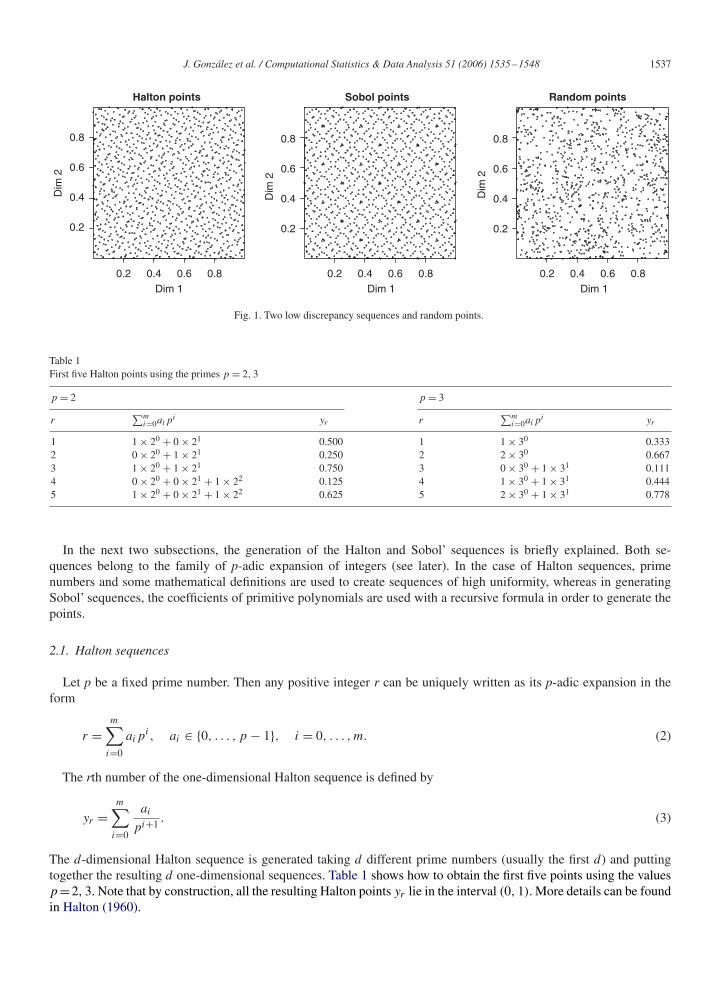
Although other LDS exist, in this paper we will use the Halton and Sobol’ sequences (e.g., Kocis and Whiten, 1997),because they are the most frequently used. Fig. 1 shows the improved uniformity, of Sobol’ and Halton points incomparison with random points, for the case of two dimensions and 1000 points.

J. González et al. / Computational Statistics & Data Analysis 51 (2006) 1535–1548 1537

0.2 0.4 0.6 0.8

0.2

0.4

0.6

0.8

Halton points

Dim

2

Dim 10.2 0.4 0.6 0.8

0.2

0.4

0.6

0.8

Sobol points

Dim

2

Dim 10.2 0.4 0.6 0.8

0.2

0.4

0.6

0.8

Random points

Dim

2

Dim 1

Fig. 1. Two low discrepancy sequences and random points.

Table 1First five Halton points using the primes p = 2, 3

p = 2 p = 3

r∑m

i=0aipi yr r

∑mi=0aip

i yr

1 1 × 20 + 0 × 21 0.500 1 1 × 30 0.3332 0 × 20 + 1 × 21 0.250 2 2 × 30 0.6673 1 × 20 + 1 × 21 0.750 3 0 × 30 + 1 × 31 0.1114 0 × 20 + 0 × 21 + 1 × 22 0.125 4 1 × 30 + 1 × 31 0.4445 1 × 20 + 0 × 21 + 1 × 22 0.625 5 2 × 30 + 1 × 31 0.778

In the next two subsections, the generation of the Halton and Sobol’ sequences is briefly explained. Both se-quences belong to the family of p-adic expansion of integers (see later). In the case of Halton sequences, primenumbers and some mathematical definitions are used to create sequences of high uniformity, whereas in generatingSobol’ sequences, the coefficients of primitive polynomials are used with a recursive formula in order to generate thepoints.

2.1. Halton sequences

Let p be a fixed prime number. Then any positive integer r can be uniquely written as its p-adic expansion in theform

r =m∑

i=0

aipi, ai ∈ {0, . . . , p − 1}, i = 0, . . . , m. (2)

The rth number of the one-dimensional Halton sequence is defined by

yr =m∑

i=0

ai

pi+1 . (3)

The d-dimensional Halton sequence is generated taking d different prime numbers (usually the first d) and puttingtogether the resulting d one-dimensional sequences. Table 1 shows how to obtain the first five points using the valuesp=2, 3. Note that by construction, all the resulting Halton points yr lie in the interval (0, 1). More details can be foundin Halton (1960).


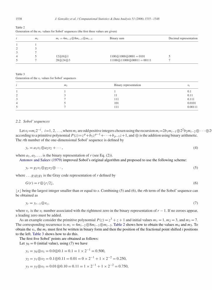
Table 2Generation of the mi values for Sobol’ sequences (the first three values are given)

i mi mi = 4mi−2�8mi−3�mi−3 Binary sum Decimal representation

1 12 33 74 5 12�8�1 1100�1000�0001 = 0101 55 7 28�24�3 11100�11000�00011 = 00111 7

Table 3Generation of the vi values for Sobol’ sequences

i mi Binary representation vi

1 1 1 0.12 3 11 0.113 7 111 0.1114 5 101 0.01015 7 111 0.00111

2.2. Sobol’ sequences

Letvi=mi2−i , i=1, 2, . . ., wheremi are odd positive integers chosen using the recursionmi=2b1mi−1�22b2mi−2� · · · �2p

according to a primitive polynomial P(z)=zp+b1zp−1+· · ·+bp−1z+1, and � is the addition using binary arithmetic.

The rth number of the one-dimensional Sobol’ sequence is defined by

yr = a1v1�a2v2 + · · · , (4)

where a1, a2, . . . is the binary representation of r (see Eq. (2)).Antonov and Saleev (1979) improved Sobol’s original algorithm and proposed to use the following scheme:

yr = g1v1�g2v2� · · · , (5)

where . . . g3g2g1 is the Gray code representation of r defined by

G(r) = r��r/2�, (6)

�x� being the largest integer smaller than or equal to x. Combining (5) and (6), the rth term of the Sobol’ sequence canbe obtained as

yr = yr−1�vc, (7)

where vc is the vi number associated with the rightmost zero in the binary representation of r − 1. If no zeroes appear,a leading zero must be added.

As an example consider the primitive polynomial P(z) = z3 + z + 1 and initial values m1 = 1, m2 = 3, and m3 = 7.The corresponding recurrence is mi = 4mi−2�8mi−3�mi−3. Table 2 shows how to obtain the values m4 and m5. Toobtain the vi , the mi must first be written in binary form and then the position of the fractional point shifted i positionsto the left. Table 3 shows how to do this.

The first five Sobol’ points are obtained as follows:Let y0 = 0 (initial value), using (7) we have

y1 = y0�v1 = 0.0�0.1 = 0.1 = 1 × 2−1 = 0.500,

y2 = y1�v2 = 0.1�0.11 = 0.01 = 0 × 2−1 + 1 × 2−2 = 0.250,

y3 = y2�v1 = 0.01�0.10 = 0.11 = 1 × 2−1 + 1 × 2−2 = 0.750,


y4 = y3�v3 = 0.11�0.111 = 0.001 = 0 × 2−1 + 0 × 2−2 + 1 × 2−3 = 0.125,

y5 = y4�v2 = 0.001�0.11 = 0.111 = 1 × 2−1 + 1 × 2−2 + 1 × 2−3 = 0.875.

In the first line we added v1 because the binary representation of r − 1 = 0 is 0, and the rightmost 0 is in the firstposition. In the second, we added v2 because 1 is 1 in binary representation, so we have to add a leading 0 which is inthe second position. In the third we added v1 because 2 in binary is 10 and then the rightmost 0 is in the first position,and so on.

The d-dimensional Sobol’ sequence is obtained considering d primitive polynomials and putting together the corre-sponding one-dimensional sequences generated with polynomial Pi , i=1, . . . , d. Note that like in the Halton sequence,all the values yr lie in the unit interval. More details and an implementation of a Sobol’sequence can be found in Bratleyand Fox (1988).

Codes for both the Sobol’ and Halton sequences have been implemented in some high-level software programs likethe library fOptions (Wuertz, 2005) of R (R Development Core Team, 2005), which was used in this paper.

3. The logistic-normal model

Often the integrand of interest appearing in the likelihood function to be maximized, is the product of a function f (t)

times the normal distribution. This kind of integral has been studied before for instance by Crouch and Spiegelman(1990) who compare their proposed method with GH. In this section, we discuss more in detail the logistic-normalmodel as it is common in biostatistics and psychometrics.

Let Yij be the binary outcome variable for observation j (j = 1, . . . , ki) in cluster i (i=1, . . . , c), � is a p-dimensionalvector of fixed effects with associated ki × p design matrix Xi , and �i is a d-dimensional vector of random effects forcluster i with associated ki ×d design matrix Zi (see Rijmen et al., 2003). The use of f (t)={1+exp(−t)}−1 is commonin this framework. The assumption that �i follows a multivariate normal distribution with 0 mean and covariance matrix

� =

⎛⎜⎜⎜⎝

�2�1

��1�2 · · · ��1�d

��2�1 �2�2

· · · ��2�d

......

. . ....

��d�1 · · · · · · �2�d

⎞⎟⎟⎟⎠ ,

leads to a logistic-normal model (Agresti, 2002, p. 496; Hosmer and Lemeshow, 2000, p. 310) of the form

Pr(Yij = 1 | Zi , Xi , �, �i

) = f(

z�ij�i + x�

ij�)

=exp

(z�ij�i + x�

ij�)

1 + exp(

z�ij�i + x�

ij�) . (8)

This models the probability of observation j in cluster i having a certain characteristic(Yij = 1

), with z�

ij and x�ij the jth

rows of the matrices Zi and Xi , respectively.Assuming that the observations regarding the same cluster are conditionally

independent given �i , the binary random variable Yij follows a Bernoulli distribution with parameter f(

z�ij�i + x�

ij�)

,

and the contribution of cluster i to the likelihood function is

Pr(Yi = yi | �, �

) =∫

Rd

ki∏j=1

exp{yij

(z�ij�i + x�

ij�)}

1 + exp{

z�ij�i + x�

ij�} g (�i; 0, �) d�i , (9)

where g (�i; 0, �) means that the vector �i follows a multivariate normal distribution with mean 0 and covariancematrix �. Assuming independence between clusters, the full log-likelihood function is

l(�, �) =c∑

i=1

log∫

Rd

ki∏j=1

exp{yij

(z�ij�i + x�

ij�)}

1 + exp{

z�ij�i + x�

ij�} g (�i; 0, �) d�i . (10)


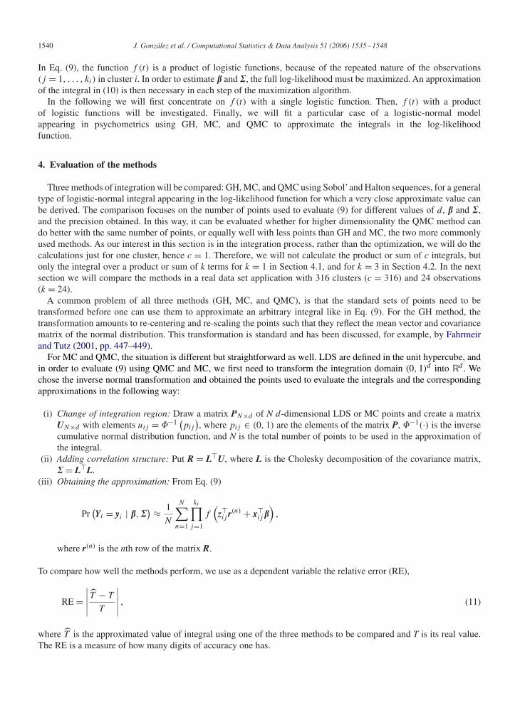
In Eq. (9), the function f (t) is a product of logistic functions, because of the repeated nature of the observations(j = 1, . . . , ki) in cluster i. In order to estimate � and �, the full log-likelihood must be maximized. An approximationof the integral in (10) is then necessary in each step of the maximization algorithm.

In the following we will first concentrate on f (t) with a single logistic function. Then, f (t) with a productof logistic functions will be investigated. Finally, we will fit a particular case of a logistic-normal modelappearing in psychometrics using GH, MC, and QMC to approximate the integrals in the log-likelihoodfunction.

4. Evaluation of the methods

Three methods of integration will be compared: GH, MC, and QMC using Sobol’and Halton sequences, for a generaltype of logistic-normal integral appearing in the log-likelihood function for which a very close approximate value canbe derived. The comparison focuses on the number of points used to evaluate (9) for different values of d, � and �,and the precision obtained. In this way, it can be evaluated whether for higher dimensionality the QMC method cando better with the same number of points, or equally well with less points than GH and MC, the two more commonlyused methods. As our interest in this section is in the integration process, rather than the optimization, we will do thecalculations just for one cluster, hence c = 1. Therefore, we will not calculate the product or sum of c integrals, butonly the integral over a product or sum of k terms for k = 1 in Section 4.1, and for k = 3 in Section 4.2. In the nextsection we will compare the methods in a real data set application with 316 clusters (c = 316) and 24 observations(k = 24).

A common problem of all three methods (GH, MC, and QMC), is that the standard sets of points need to betransformed before one can use them to approximate an arbitrary integral like in Eq. (9). For the GH method, thetransformation amounts to re-centering and re-scaling the points such that they reflect the mean vector and covariancematrix of the normal distribution. This transformation is standard and has been discussed, for example, by Fahrmeirand Tutz (2001, pp. 447–449).

For MC and QMC, the situation is different but straightforward as well. LDS are defined in the unit hypercube, andin order to evaluate (9) using QMC and MC, we first need to transform the integration domain (0, 1)d into Rd . Wechose the inverse normal transformation and obtained the points used to evaluate the integrals and the correspondingapproximations in the following way:

(i) Change of integration region: Draw a matrix PN×d of N d-dimensional LDS or MC points and create a matrixUN×d with elements uij = �−1

(pij

), where pij ∈ (0, 1) are the elements of the matrix P, �−1(·) is the inverse

cumulative normal distribution function, and N is the total number of points to be used in the approximation ofthe integral.

(ii) Adding correlation structure: Put R = L�U, where L is the Cholesky decomposition of the covariance matrix,� = L�L.

(iii) Obtaining the approximation: From Eq. (9)

Pr(Yi = yi | �, �

) ≈ 1

N

N∑n=1

ki∏j=1

f(

z�ij r(n) + x�

ij�)

,

where r(n) is the nth row of the matrix R.

To compare how well the methods perform, we use as a dependent variable the relative error (RE),

RE =∣∣∣∣∣ T̂ − T

T

∣∣∣∣∣ , (11)

where T̂ is the approximated value of integral using one of the three methods to be compared and T is its real value.The RE is a measure of how many digits of accuracy one has.


Table 4Values to form the � matrices used in Study 1

d �2�1

, . . . ,�2�d

3 (2.0, 1.5, 1.0)5 (2.0, 1.5, 1.0, 0.5, 0.3)7 (2.0, 1.5, 1.0, 0.5, 0.3, 0.6, 0.7)9 (2.0, 1.5, 1.0, 0.5, 0.3, 0.6, 0.7, 0.1, 0.25)

� 0.0, 0.3, 0.5, 0.7, 0.9

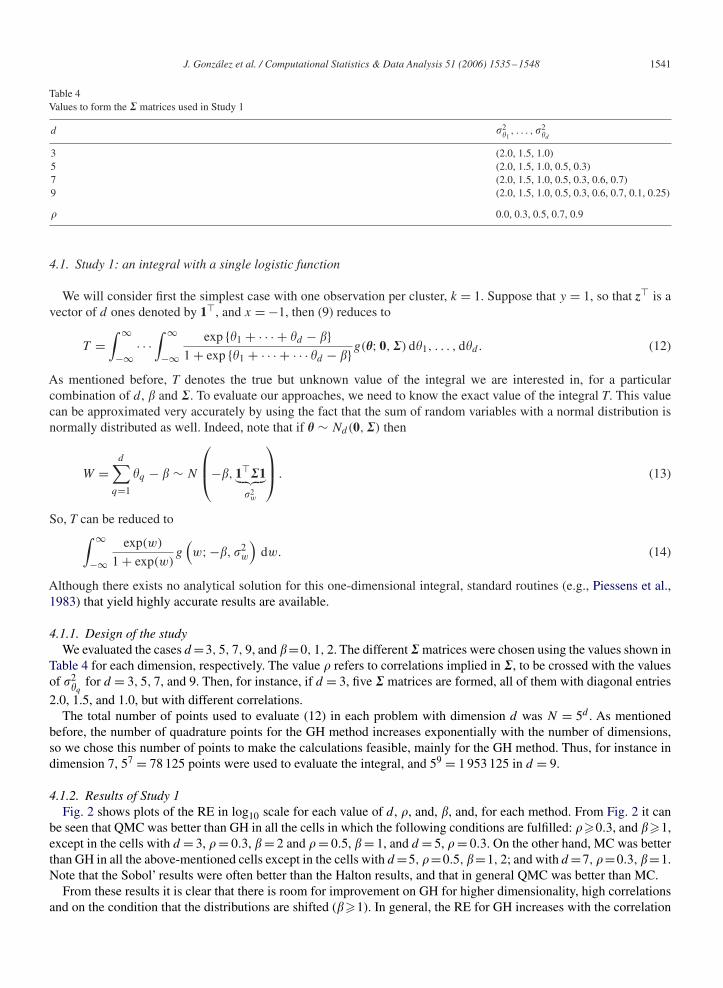
4.1. Study 1: an integral with a single logistic function

We will consider first the simplest case with one observation per cluster, k = 1. Suppose that y = 1, so that z� is avector of d ones denoted by 1�, and x = −1, then (9) reduces to

T =∫ ∞

−∞· · ·

∫ ∞

−∞exp {�1 + · · · + �d − �}

1 + exp {�1 + · · · + · · · �d − �}g(�; 0, �) d�1, . . . , d�d . (12)

As mentioned before, T denotes the true but unknown value of the integral we are interested in, for a particularcombination of d, � and �. To evaluate our approaches, we need to know the exact value of the integral T. This valuecan be approximated very accurately by using the fact that the sum of random variables with a normal distribution isnormally distributed as well. Indeed, note that if � ∼ Nd(0, �) then

W =d∑

q=1

�q − � ∼ N

⎛⎜⎝−�, 1��1︸︷︷︸

�2w

⎞⎟⎠ . (13)

So, T can be reduced to∫ ∞

−∞exp(w)

1 + exp(w)g

(w; −�, �2

w

)dw. (14)

Although there exists no analytical solution for this one-dimensional integral, standard routines (e.g., Piessens et al.,1983) that yield highly accurate results are available.

4.1.1. Design of the studyWe evaluated the cases d =3, 5, 7, 9, and �=0, 1, 2. The different � matrices were chosen using the values shown in

Table 4 for each dimension, respectively. The value � refers to correlations implied in �, to be crossed with the valuesof �2

�qfor d = 3, 5, 7, and 9. Then, for instance, if d = 3, five � matrices are formed, all of them with diagonal entries

2.0, 1.5, and 1.0, but with different correlations.The total number of points used to evaluate (12) in each problem with dimension d was N = 5d . As mentioned

before, the number of quadrature points for the GH method increases exponentially with the number of dimensions,so we chose this number of points to make the calculations feasible, mainly for the GH method. Thus, for instance indimension 7, 57 = 78 125 points were used to evaluate the integral, and 59 = 1 953 125 in d = 9.

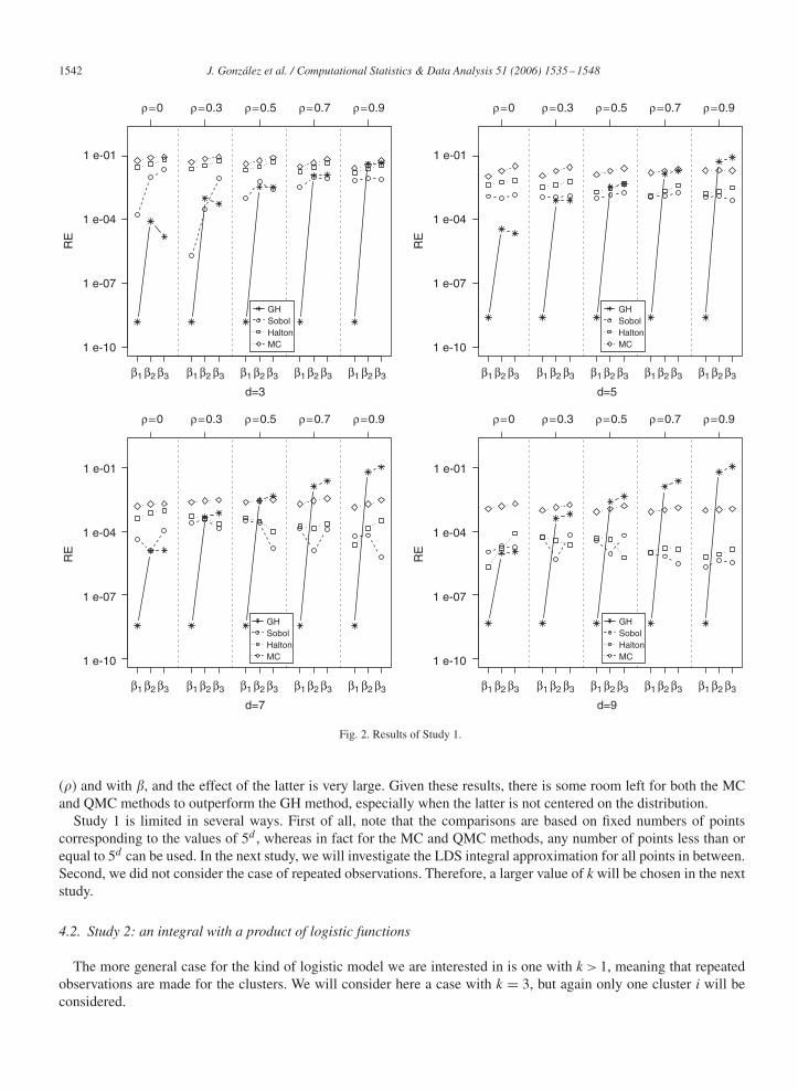
4.1.2. Results of Study 1Fig. 2 shows plots of the RE in log10 scale for each value of d, �, and, �, and, for each method. From Fig. 2 it can

be seen that QMC was better than GH in all the cells in which the following conditions are fulfilled: ��0.3, and ��1,except in the cells with d = 3, � = 0.3, � = 2 and � = 0.5, � = 1, and d = 5, � = 0.3. On the other hand, MC was betterthan GH in all the above-mentioned cells except in the cells with d =5, �=0.5, �=1, 2; and with d =7, �=0.3, �=1.Note that the Sobol’ results were often better than the Halton results, and that in general QMC was better than MC.

From these results it is clear that there is room for improvement on GH for higher dimensionality, high correlationsand on the condition that the distributions are shifted (��1). In general, the RE for GH increases with the correlation


d=3

RE

1 e-10

1 e-07

1 e-04

1 e-01

RE

1 e-10

1 e-07

1 e-04

1 e-01

RE

1 e-10

1 e-07

1 e-04

1 e-01

RE

1 e-10

1 e-07

1 e-04

1 e-01

β1 β2 β3 β1 β2 β3 β1 β2 β3 β1 β2 β3 β1 β2 β3 β1 β2 β3 β1 β2 β3 β1 β2 β3 β1 β2 β3 β1 β2 β3

d=5

d=7

β1 β2 β3 β1 β2 β3 β1 β2 β3 β1 β2 β3 β1 β2 β3 β1 β2 β3 β1 β2 β3 β1 β2 β3 β1 β2 β3 β1 β2 β3

d=9

ρ=0 ρ=0.3 ρ=0.5 ρ=0.7 ρ=0.9 ρ=0 ρ=0.3 ρ=0.5 ρ=0.7 ρ=0.9

ρ=0 ρ=0.3 ρ=0.5 ρ=0.7 ρ=0.9 ρ=0 ρ=0.3 ρ=0.5 ρ=0.7 ρ=0.9

GHSobolHaltonMC

GHSobolHaltonMC

GHSobolHaltonMC

GHSobolHaltonMC

Fig. 2. Results of Study 1.

(�) and with �, and the effect of the latter is very large. Given these results, there is some room left for both the MCand QMC methods to outperform the GH method, especially when the latter is not centered on the distribution.

Study 1 is limited in several ways. First of all, note that the comparisons are based on fixed numbers of pointscorresponding to the values of 5d , whereas in fact for the MC and QMC methods, any number of points less than orequal to 5d can be used. In the next study, we will investigate the LDS integral approximation for all points in between.Second, we did not consider the case of repeated observations. Therefore, a larger value of k will be chosen in the nextstudy.

4.2. Study 2: an integral with a product of logistic functions

The more general case for the kind of logistic model we are interested in is one with k > 1, meaning that repeatedobservations are made for the clusters. We will consider here a case with k = 3, but again only one cluster i will beconsidered.


10 50 100 500 5000

1 e-10

1 e-07

1 e-04

1 e-01

GHSobolHaltonMC

RE

1 e-10

1 e-07

1 e-04

1 e-01

RE

1 e-10

1 e-07

1 e-04

1 e-01

RE

1 e-10

1 e-07

1 e-04

1 e-01

RE

1 e-10

1 e-07

1 e-04

1 e-01

RE

Number of points

10 50 100 500 5000

Number of points

10 50 100 500 5000

Number of points

10 50 100 500 5000

Number of points

10 50 100 500 5000

Number of points

ρ=0 ρ=0.3 ρ=0.5

ρ=0.7 ρ=0.9

GHSobolHaltonMC

GHSobolHaltonMC

GHSobolHaltonMC

GHSobolHaltonMC

Fig. 3. Relative error versus number of points used to evaluate the test integral in Study 2, d = 3.

Suppose that z�j is a d-dimensional vector of ones and that for each of the three observations (k = 3), xj = −1,

j = 1, 2, 3. Assume that the observations y = (1, 1, 0), are made, then (9) reduces to the following integral:

T =∫

Rd

⎛⎝ exp

{∑dq=1�q − �1

}1 + exp

{∑dq=1�q − �1

}⎞⎠

⎛⎝ exp

{∑dq=1�q − �2

}1 + exp

{∑dq=1�q − �2

}⎞⎠

×⎛⎝ 1

1 + exp{∑d

q=1�q − �3

}⎞⎠ g(�; 0, �) d�. (15)

This integral can accurately be approximated using (13) and (14).

4.2.1. Design of the studyWe evaluated (15) for �= (0, 1, 2) and for the same values of d and � utilized in Study 1, see Table 4. In addition, we

varied the number of points used to evaluate (15) and computed the RE (11). The number of points will not be limitedto powers of quadrature points used per dimension. For the Sobol’ method all the numbers in between will be usedas well.

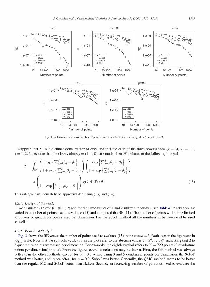
4.2.2. Results of Study 2Fig. 3 shows the RE versus the number of points used to evaluate (15) in the case d =3. Both axes in the figure are in

log10 scale. Note that the symbols ◦, �, ∗, in the plot refer to the abscissa values 2d , 3d , . . . , �d indicating that 2 to� quadrature points were used per dimension. For example, the eighth symbol refers to 93 = 729 points (9 quadraturepoints per dimension) in total. From the figure several conclusions may be drawn. First, the GH method was alwaysbetter than the other methods, except for � = 0.7 where using 3 and 5 quadrature points per dimension, the Sobol’method was better, and, more often, for � = 0.9, Sobol’ was better. Generally, the QMC method seems to be betterthan the regular MC and Sobol’ better than Halton. Second, an increasing number of points utilized to evaluate the


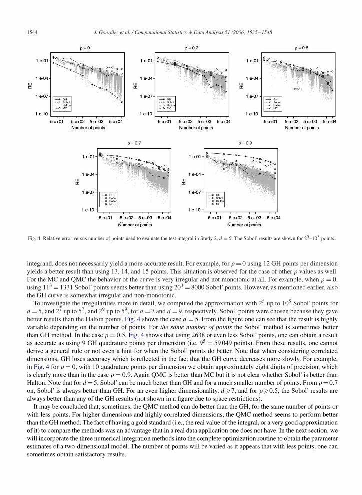
Fig. 4. Relative error versus number of points used to evaluate the test integral in Study 2, d = 5. The Sobol’ results are shown for 25.105 points.

integrand, does not necessarily yield a more accurate result. For example, for � = 0 using 12 GH points per dimensionyields a better result than using 13, 14, and 15 points. This situation is observed for the case of other � values as well.For the MC and QMC the behavior of the curve is very irregular and not monotonic at all. For example, when � = 0,using 113 = 1331 Sobol’ points seems better than using 203 = 8000 Sobol’ points. However, as mentioned earlier, alsothe GH curve is somewhat irregular and non-monotonic.

To investigate the irregularities more in detail, we computed the approximation with 25 up to 105 Sobol’ points ford = 5, and 27 up to 57, and 29 up to 59, for d = 7 and d = 9, respectively. Sobol’ points were chosen because they gavebetter results than the Halton points. Fig. 4 shows the case d = 5. From the figure one can see that the result is highlyvariable depending on the number of points. For the same number of points the Sobol’ method is sometimes betterthan GH method. In the case � = 0.5, Fig. 4 shows that using 2638 or even less Sobol’ points, one can obtain a resultas accurate as using 9 GH quadrature points per dimension (i.e. 95 = 59 049 points). From these results, one cannotderive a general rule or not even a hint for when the Sobol’ points do better. Note that when considering correlateddimensions, GH loses accuracy which is reflected in the fact that the GH curve decreases more slowly. For example,in Fig. 4 for � = 0, with 10 quadrature points per dimension we obtain approximately eight digits of precision, whichis clearly more than in the case � = 0.9. Again QMC is better than MC but it is not clear whether Sobol’ is better thanHalton. Note that for d = 5, Sobol’ can be much better than GH and for a much smaller number of points. From �= 0.7on, Sobol’ is always better than GH. For an even higher dimensionality, d �7, and for ��0.5, the Sobol’ results arealways better than any of the GH results (not shown in a figure due to space restrictions).

It may be concluded that, sometimes, the QMC method can do better than the GH, for the same number of points orwith less points. For higher dimensions and highly correlated dimensions, the QMC method seems to perform betterthan the GH method. The fact of having a gold standard (i.e., the real value of the integral, or a very good approximationof it) to compare the methods was an advantage that in a real data application one does not have. In the next section, wewill incorporate the three numerical integration methods into the complete optimization routine to obtain the parameterestimates of a two-dimensional model. The number of points will be varied as it appears that with less points, one cansometimes obtain satisfactory results.


-3 -2 -1 0

-3

QM

C-Q

N (

200

pts.

)

GH-QN (400 pts.)

Parameter estimates (QMC-Halton vs GH based)

Parameter estimates (MC vs GH based)

-1

0

1

2

3

1 2 3 -3 -2 -1 0

GH-QN (400 pts.)

1 2 3 -3 -2 -1 0

GH-QN (400 pts.)

1 2 3

Parameter estimates (QMC-Sobol vs GH based)

-2

-3Q

MC

-QN

(20

0 pt

s.)

-1

0

1

2

3

-2

-3

QM

C-Q

N (

200

pts.

)

-1

0

1

2

3

-2

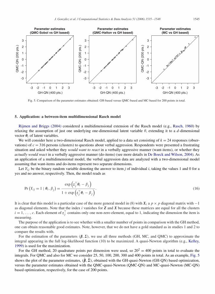
Fig. 5. Comparison of the parameter estimates obtained: GH-based versus QMC-based and MC-based for 200 points in total.

5. Application: a between-item multidimensional Rasch model

Rijmen and Briggs (2004) considered a multidimensional extension of the Rasch model (e.g., Rasch, 1960) byrelaxing the assumption of just one underlying one-dimensional latent variable �, extending it to a d-dimensionalvector �i of latent variables.

We will consider here a two-dimensional Rasch model, applied to a data set consisting of k = 24 responses (obser-vations) of c = 316 persons (clusters) to questions about verbal aggression. Respondents were presented a frustratingsituation and asked whether they would want to react in a verbally aggressive manner (want-items), or whether theyactually would react in a verbally aggressive manner (do-items) (see more details in De Boeck and Wilson, 2004). Asan application of a multidimensional model, the verbal aggression data are analyzed with a two-dimensional modelassuming that want-items and do-items represent two separate dimensions.

Let Yij be the binary random variable denoting the answer to item j of individual i, taking the values 1 and 0 for ayes and no answer, respectively. Then, the model reads as

Pr(Yij = 1 | �i , �j

) =exp

(z�j �i − �j

)1 + exp

(z�j �i − �j

) . (16)

It is clear that this model is a particular case of the more general model in (8) with Xi a p × p diagonal matrix with −1as diagonal elements. Note that the index i vanishes for Z and X because these matrices are equal for all the clustersi = 1, . . . , c. Each element of z�

j contains only one non-zero element, equal to 1, indicating the dimension the item ismeasuring.

The purpose of the application is to see whether with a smaller number of points in comparison with the GH method,one can obtain reasonable good estimates. Note, however, that we do not have a gold standard as in studies 1 and 2 tocompare the results with.

For the estimation of the parameters (�, �), we use all three methods (GH, MC, and QMC) to approximate theintegral appearing in the full log-likelihood function (10) to be maximized. A quasi-Newton algorithm (e.g., Kelley,1999) is used for the maximization.

For the GH method, 20 quadrature points per dimension were used, so 202 = 400 points in total to evaluate theintegrals. For QMC and also for MC we consider 25, 50, 100, 200, 300 and 400 points in total. As an example, Fig. 5shows the plot of the parameter estimates, (�̂, �̂), obtained with the GH-quasi-Newton (GH-QN) based optimization,versus the parameter estimates obtained with the QMC-quasi-Newton (QMC-QN) and MC-quasi-Newton (MC-QN)based optimization, respectively, for the case of 200 points.


1 e-05

1 e-03

1 e-01

Sobol 25Sobol 50Sobol 100Sobol 200Sobol 300Sobol 400

1 2 3 4 5 6 7 8 9 10 11 12 13 14 15 16 17 18 19 20 21 22 23 24 1 2 3 4 5 6 7 8 9 10 11 12 13 14 15 16 17 18 19 20 21 22 23 24 1 2 3 4 5 6 7 8 9 10 11 12 13 14 15 16 17 18 19 20 21 22 23 24

Item Item Item

Halton 25Halton 50Halton 100Halton 200Halton 300Halton 400

MC 25MC 50MC 100MC 200MC 300MC 400

|βj(Q

MC

) - β

j(GH

)|

1 e-05

1 e-03

1 e-01

|βj(Q

MC

) - β

j(GH

)|

1 e-05

1 e-03

1 e-01

|βj(Q

MC

) - β

j(GH

)|

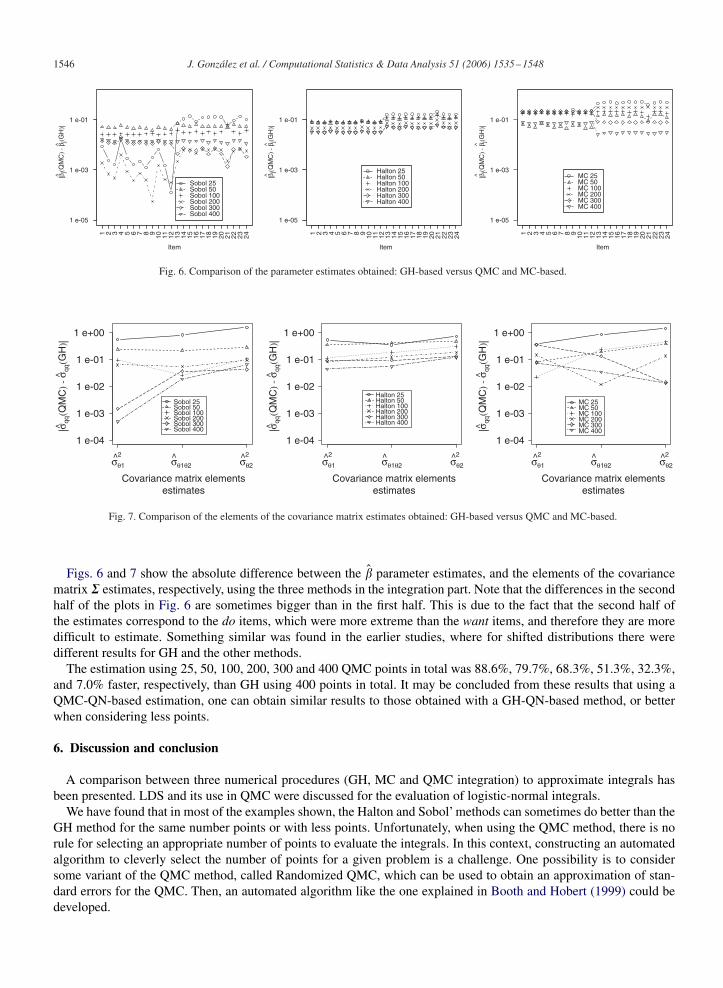
Fig. 6. Comparison of the parameter estimates obtained: GH-based versus QMC and MC-based.

1 e-04

1 e-03

1 e-02

1 e-01

1 e+00

Sobol 25Sobol 50Sobol 100Sobol 200Sobol 300Sobol 400

^2 ^2

Covariance matrix elementsestimates

Halton 25Halton 50Halton 100Halton 200Halton 300Halton 400

MC 25MC 50MC 100MC 200MC 300MC 400|σ

qq(Q

MC

) - σ

qq(G

H)|

1 e-04

1 e-03

1 e-02

1 e-01

1 e+00

1 e-04

1 e-03

1 e-02

1 e-01

1 e+00

σθ1 σ̂θ1θ2 σθ2^2 ^2


σθ1 σ̂θ1θ2 σθ2^2 ^2


σθ1 σ̂θ1θ2 σθ2

|σqq

(QM

C) -

σqq

(GH

)|

|σqq

(QM

C) -

σqq

(GH

)|

Fig. 7. Comparison of the elements of the covariance matrix estimates obtained: GH-based versus QMC and MC-based.

Figs. 6 and 7 show the absolute difference between the �̂ parameter estimates, and the elements of the covariancematrix � estimates, respectively, using the three methods in the integration part. Note that the differences in the secondhalf of the plots in Fig. 6 are sometimes bigger than in the first half. This is due to the fact that the second half ofthe estimates correspond to the do items, which were more extreme than the want items, and therefore they are moredifficult to estimate. Something similar was found in the earlier studies, where for shifted distributions there weredifferent results for GH and the other methods.

The estimation using 25, 50, 100, 200, 300 and 400 QMC points in total was 88.6%, 79.7%, 68.3%, 51.3%, 32.3%,and 7.0% faster, respectively, than GH using 400 points in total. It may be concluded from these results that using aQMC-QN-based estimation, one can obtain similar results to those obtained with a GH-QN-based method, or betterwhen considering less points.

6. Discussion and conclusion

A comparison between three numerical procedures (GH, MC and QMC integration) to approximate integrals hasbeen presented. LDS and its use in QMC were discussed for the evaluation of logistic-normal integrals.

We have found that in most of the examples shown, the Halton and Sobol’ methods can sometimes do better than theGH method for the same number points or with less points. Unfortunately, when using the QMC method, there is norule for selecting an appropriate number of points to evaluate the integrals. In this context, constructing an automatedalgorithm to cleverly select the number of points for a given problem is a challenge. One possibility is to considersome variant of the QMC method, called Randomized QMC, which can be used to obtain an approximation of stan-dard errors for the QMC. Then, an automated algorithm like the one explained in Booth and Hobert (1999) could bedeveloped.


Because of the non-monotonic relation between number of points and accuracy, it follows that a larger number ofquadrature points to approximate the integral, does not necessarily give more accurate results for the Sobol’ and Haltonsequences. Moreover and perhaps surprisingly, the same phenomenon also applies to the GH method when used forevaluating logistic-normal integrals.

An advantage of QMC or MC compared to GH in higher dimensions is that one can use any numbers of points whilethe GH method is restricted to the use of �d (� = 1, 2, 3, . . .) number of points. For instance using GH in dimension 5with 3 quadrature points per dimension (35 = 243 points in total) one cannot use 242, 241, 240, etc. points. For GH,there is no way of reducing the number of points by units.

Apart from this a priori advantage, it appears that the QMC and MC beat the GH method in higher dimensions whenthe distributions are shifted, and when also the dimensions are correlated. Not only do they have more precision, butthe same precision as that of the GH can be reached with less (and often much less) quadrature points. These resultsseem independent of the non-monotonic relation between number of points and accuracy.

For the optimization task, the QMC method seems to be a promising method to approximate the integral, in theprocess of maximizing the likelihood. Although without a gold standard to compare results, Section 5 showed that,one can obtain similar results as obtained with the GH method, and with less points. In this way the computationaleffort and time needed for the calculations can be reduced considerably. For practical purposes, a mixed method, GHcombined with QMC, may be useful, switching from GH to QMC, for the kind of problems where GH seems lessaccurate or needs too many points.

References

Abramowitz, M., Stegun, I. (Eds.), 1972. Handbook of Mathematical Functions. Dover Publications Inc., New York.Agresti, A., 2002. Categorical Data Analysis. second ed. Wiley, New York.Antonov, I., Saleev, V., 1979. An economic method of computing LP �-sequences. USSR Comput. Math. Math. Phys. 19, 252–256.Booth, J.G., Hobert, J.H., 1999. Maximizing generalized linear mixed model likelihoods with an automated Monte Carlo EM algorithm. J. Roy.

Statist. Soc. B 62, 265–285.Bratley, P., Fox, B.L., 1988. Algorithm 659 implementing Sobol’s quasirandom sequence generator. ACM Trans. Math. Software 14, 88–100.Caflisch, R., 1998. Monte Carlo and quasi-Monte Carlo methods. Acta Numer. 7, 1–49.Cools, R., 1997. Constructing cubature formulae: the science behind the art. Acta Numer. 6, 1–54.Cools, R., 2002. Advances in multidimensional integration. J. Comput. Appl. Math. 149, 1–12.

Crouch, A., Spiegelman, E., 1990. The evaluations of integrals of the form∫ ∞−∞ f (t) exp

(−t2

)dt : application to logistic-normal models. J. Amer.

Statist. Assoc. 85, 464–469.Davis, P., Rabinowitz, P., 1984. Methods of Numerical Integration. second ed. Academic Press, Orlando, FL.De Boeck, P., Wilson, M., 2004. Explanatory Item Response Models: A Generalized Linear and Nonlinear Approach. Springer-Verlag, New York.Fahrmeir, L., Tutz, G., 2001. Multivariate Statistical Modelling Based on Generalized Linear Models. second ed. Springer-Verlag, New York.Fischer, G., Molenaar, I. (Eds.), 1995. Rasch Models: Foundations and Recent Developments. Springer-Verlag, New York.Halton, J., 1960. On the efficiency of certain quasi-random sequences of points in evaluating multi-dimensional integrals. Numer. Math. 2, 84–90.Hickernell, F., Lemieux, C., Owen, A., 2005. Control variates for Quasi-Monte Carlo. Statist. Sci. 20, 1–31.Hosmer, D., Lemeshow, S., 2000. Applied Logistic Regression. second ed. Wiley, New York.Jank, W., 2005. Quasi-Monte Carlo sampling to improve the efficiency of Monte Carlo EM. Comput. Statist. Data Anal. 48, 685–701.Judd, K., 1998. Numerical Methods in Economics. MIT Press, Boston.Kelley, C.T., 1999. Iterative Methods for Optimization. SIAM, Philadelphia, PA.Kocis, L., Whiten, W., 1997. Computational investigations of low-discrepancy sequences. ACM Trans. Math. Software 23, 266–294.Lemieux, C., L’Ecuyer, P., 2001. On the use of quasi-Monte Carlo methods in computational finance. Available in 〈http://www.iro.umontreal.ca/∼

lecuyer/myftp/papers/iccs01.pdf〉.Lesaffre, E., Spiessens, B., 2001. On the effect of the number of quadrature points in a logistic random-effects model: an example. Appl. Statist. 50,

325–335.Morokoff, W., Caflisch, R., 1995. Quasi-Monte Carlo integration. J. Comput. Phys. 122, 218–230.Niederreiter, H., 1992. Random Number Generation and Quasi-Monte Carlo Methods (CBMS-NSF Regional Conference Series in Applied

Mathematics, No. 63).Paskov, S., 1995. Faster valuation of financial derivatives. J. Portfolio Management 22, 113–120.Piessens, R., de Doncker-Kapenga, E., Uberhuber, C., Kahaner, D., 1983. QUADPACK: A subroutine package for automatic integration. Springer-

Verlag, New York.R Development Core Team, 2005. R: A language and environment for statistical computing. R Foundation for Statistical Computing, Vienna, Austria.

ISBN 3-900051-07-0, URL 〈http://www.R-project.org〉.Rasch, G., 1960. Probabilistic Models for Some Intelligence and Attainment Test. Danish Institute for Educational Research, Copenhagen, Denmark.

http://www.iro.umontreal.ca/~lecuyer/myftp/papers/iccs01.pdf

http://www.R-project.org


Rijmen, F., Briggs, D., 2004. Multiple person dimensions and latent item predictors. In: De Boeck, P., Wilson, M. (Eds.), Explanatory Item ResponseModels: A Generalized Linear and Nonlinear Approach. Springer-Verlag, New York.

Rijmen, F., Tuerlinckx, F., De Boeck, P., Kuppens, P., 2003. A nonlinear mixed model framework for IRT models. Psychol. Methods 8, 185–205.Robert, C., Casella, G., 2004. Monte Carlo Statistical Methods. second ed. Springer-Verlag, New York.Shao, J., 2003. Mathematical Statistics. second ed. Springer-Verlag, New York.Stroud, A., 1971. Approximate Calculation of Multiple Integrals. Prentice-Hall, Englewood Cliffs, NJ.Wuertz, D., 2005. fOptions: Financial Software Collection—fOptions. R package version 220.10063. 〈http://www.rmetrics.org〉.

http://www.rmetrics.org

numerical integration in logistic-normal models

Documents