a strategic model for dynamic traffic assignment
TRANSCRIPT
Networks and Spatial Economics, 4: (2004) 291–315©C 2004 Kluwer Academic Publishers, Manufactured in the Netherlands.
A Strategic Model for Dynamic Traffic Assignment
YOUNES HAMDOUCHPATRICE MARCOTTE∗SANG NGUYENDIRO and CRT, C.P. 6128, succursale Centre-ville, Montreal, Canada H3C 3J7email: [email protected]
Abstract
In this paper, we propose a model of dynamic traffic assignment where strategic choices are an integral part of userbehaviour. The model is based on a discrete-time description of flow variation through a road network involvingarcs with rigid capacities. In such network, a driver’s strategy consists in a rule that assigns to each node of thenetwork a set of arcs in the forward star of that node, sorted according to some preference order. The main elementof the model is a ‘within-day’ submodel where strategic volumes are loaded onto the network in accordance withthe first-in first-out discipline and user preferences. An equilibrium assignment is achieved when expected delaysof active strategies are minimal, for every origin-destination pair. We prove the existence of such an assignmentand provide numerical results on test networks.
Keywords: Dynamic traffic assignment, strategy, hyperpath, capacities, variational inequalities
1. Introduction
Traffic assignment has been the topic of many studies in the last four decades, and it can besafely argued that the static case is settled by now. However, extending the results from astatic to a dynamic environment is far from trivial and, as no agreement on an ideal modelhas been reached within the scientific community, dynamic traffic assignment remains atopic of active research.
Macroscopic dynamic models belong to one of three classes: models using exit functions(Merchant and Nemhauser, 1978; Carey, 1992; Drissi-Kaıtouni and Gendreau, 1992), mod-els based on space-time networks (Drissi and Hamada-Benchekroun, 1992; Zawack andThompson, 1987) and models using arc travel delays (Friesz et al.,1993; Astarita, 1996). Inall these models, users travel along paths of the underlying network, which path cannot bemodified en route.
If congestion levels become very high, however, users may choose to switch path enroute rather than experience unduly delays on the path corresponding to their initial choice.Our proposal for dealing with this issue is to assume that users behave strategically andmodify their route choice according to congestion conditions. For instance, approaching ahighway, a user might base its decision of entering (or not) the highway on information aboutcongestion, either visual (viewing ramp congestion, variable message displays, on board
∗To whom all correspondence should be addressed.
292 HAMDOUCH, MARCOTTE AND NGUYEN
information systems) or auditive (traffic information from radio source). One of the aimsof this paper is to address this situation via a mathematical framework that takes explicitlyinto account the strategic behavior of the users. More precisely, a strategy associates witheach node of the network an ordered set of successor nodes, whose access is controlled bythree factors: the arrival time at the node, the capacity of the corresponding arc, the numberof users with overlapping strategies. This results in an extension of the strategic approach ofMarcotte et al. (2000) and Hamdouch et al. (2002) to a time-varying environment. Note that,in our model, randomness results from demand, i.e., the arrival process of users at nodes ofthe network. While there are obvious links with the notion of strategy used in transit models(see Nguyen and Pallottino, 1988 or Spiess and Florian, 1989), where randomness is drivenby supply (frequencies), there is a clear distinction.
Recently, Gao and Chabini (2003) proposed a very flexible framework for dynamictraffic assignment where user behavior is dictated by travel policies. At each node, a policyspecifies the next outgoing link, depending on the current state of the network; path choice,which is performed en route, is therefore stochastic. An equilibrium is achieved when theexpected delays of active policies are equal and less than those of inactive policies. Theirpolicy concept is closely related to that of strategy, with some key differences:
• nonlinearity is modelled through exogenous volume-delay functions; this is in contrastwith our approach where nonlinearities in travel delays, governed by link access proba-bilities, are endogenous;
• probability density functions describing the occurrence of incidents are assumed to beknown;
• the state of the network is flow-independent (this assumption could easily be lifted);• a single destination is considered.
As in most dynamic models, the main challenge faced by our model is to perform effi-ciently the ‘loading’ operation, whereby strategic volumes are converted into path and arcvolumes. It is a key feature of our approach that the loading preserves the order of arrivalof users at the nodes of the network, and thus automatically fulfills the FIFO (First In FirstOut) rule. While this makes for a complex loading process, this also results in a model withvery limited data requirements, as no calibration of nonlinear delay functions is required.Indeed nonlinearity, which is a consequence of the loading process, is endogenous to themodel.
The remainder of this paper is organized as follows. In the next section, we introduce thestrategic concepts underlying the dynamic assignment model and formulate the equilibriumproblem as a variational inequality. Based on these results, we develop an algorithmic frame-work and provide numerical results. Throughout the paper, we assume that time-dependentdemand and departure times are known, and that congestion is the sole consequence ofwaiting time at the tails of congested nodes.
2. A strategic dynamic assignment model
The notion of strategic behavior for transit users was first introduced by Chriqui andRobillard (1975) for dealing with the problem of assigning passengers to overlapping transit
A STRATEGIC MODEL FOR DYNAMIC TRAFFIC ASSIGNMENT 293
lines. The concept was next refined by Spiess and Florian (1989) and Nguyen and Pallottino(1988), who proposed elegant and efficient implementations that can easily deal with large-scale instances. The idea is simple. Let us consider a transit stop served by several transitlines. An optimal strategy consists in boarding a vehicle that minimizes total delay todestination (travel time plus waiting time). Whenever headways follow an exponential dis-tribution, an optimal strategy corresponds to a subset of available transit lines (the attractivelines), and can be computed by a dynamic procedure akin to the classical Ford-Bellman-Moore (1959) shortest path algorithm. The probability of boarding an attractive line issimply the ratio of its frequency over the combined frequency of all attractive lines. Inthis model, line capacities are neglected, and randomness arises from the vehicle arrivalprocess.
Alternatively, one can consider a model with fixed schedules and rigid capacities wherethe probability of accessing a given bus line is not related to the arrival process but to thequeueing process that takes place at boarding nodes. In this context, a strategy consists ofan ordered subset of available lines, and users board the first vehicle from that subset thathas an available seat. For a given user, the boarding probability clearly depends both on theresidual capacity and the position of the user within the queue. Such a model was proposedby Marcotte et al. (2000) and implemented in static priority networks by Hamdouch et al.(2002). In the current work, we adapt this concept to a time-varying and time-discretizedenvironment. This yields a dynamic traffic assignment model where users may adapt theirroute to current traffic conditions. We assumed that the capacities of the arc of the roadnetwork are fixed, and that access to a congested link can be achieved by waiting for somefreed capacity. Congestion is thus induced automatically from the queueing process. Wenow describe this process in a rigorous manner. For quick reference, a list of symbols isprovided in Appendix A.
Let G = (N , A) be a network with node set N , arc set A and time-varying demanddt
qr (t = 0, 1, . . . , T ′ ≤ T ), associated with users departing from origin node q at instantt and bound for destination node r . The objective of our research is to determine equi-librium strategic volumes and travel times over a fixed time interval T whose expecteddelays are consistent with constant, integer-valued travel delays ca and arc capacities ua .In the sequel, we assume that the time interval T is sufficiently large to allow all vehi-cles to reach their destination by T and that, whenever the number of drivers that wishto access an arc exceeds its capacity, a proportion of those commuters will either travelon an alternative (unsaturated) arc, or wait until an arc become available later in time.All operations take place on a time-space network R = (V, E) which is constructed asfollows:
– each node i ∈ N is expanded into T + 1 nodes it , t = 0, 1, . . . , T :
V = {it : i ∈ N , 0 ≤ t ≤ T }
– each link a ∈ A is expanded to T + 1 − ca links (it , jt+ca ) such that t + ca ≤ T ; we referto these links as travel links. The waiting time at the nodes is represented by means ofwaiting arcs of infinite capacity denoted (it , it+1) where t = 0, 1, . . . , T − 1.
294 HAMDOUCH, MARCOTTE AND NGUYEN
The set of arcs is partitioned into the set E1 of access arcs and its complement E2, the setof waiting arcs:
E1 = {(it , jt+ci j
): (i, j) ∈ A, 0 ≤ t ≤ T − ci j
}E2 = {(it , it+1) : i ∈ N , 0 ≤ t ≤ T − 1}E = E1 ∪ E2.
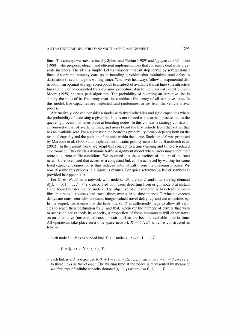
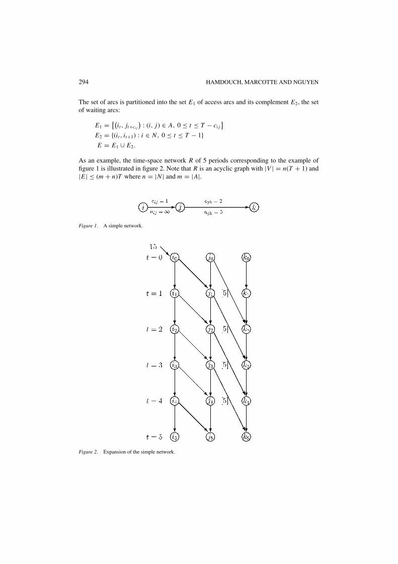
As an example, the time-space network R of 5 periods corresponding to the example offigure 1 is illustrated in figure 2. Note that R is an acyclic graph with |V | = n(T + 1) and|E | ≤ (m + n)T where n = |N | and m = |A|.
Figure 1. A simple network.
Figure 2. Expansion of the simple network.
A STRATEGIC MODEL FOR DYNAMIC TRAFFIC ASSIGNMENT 295
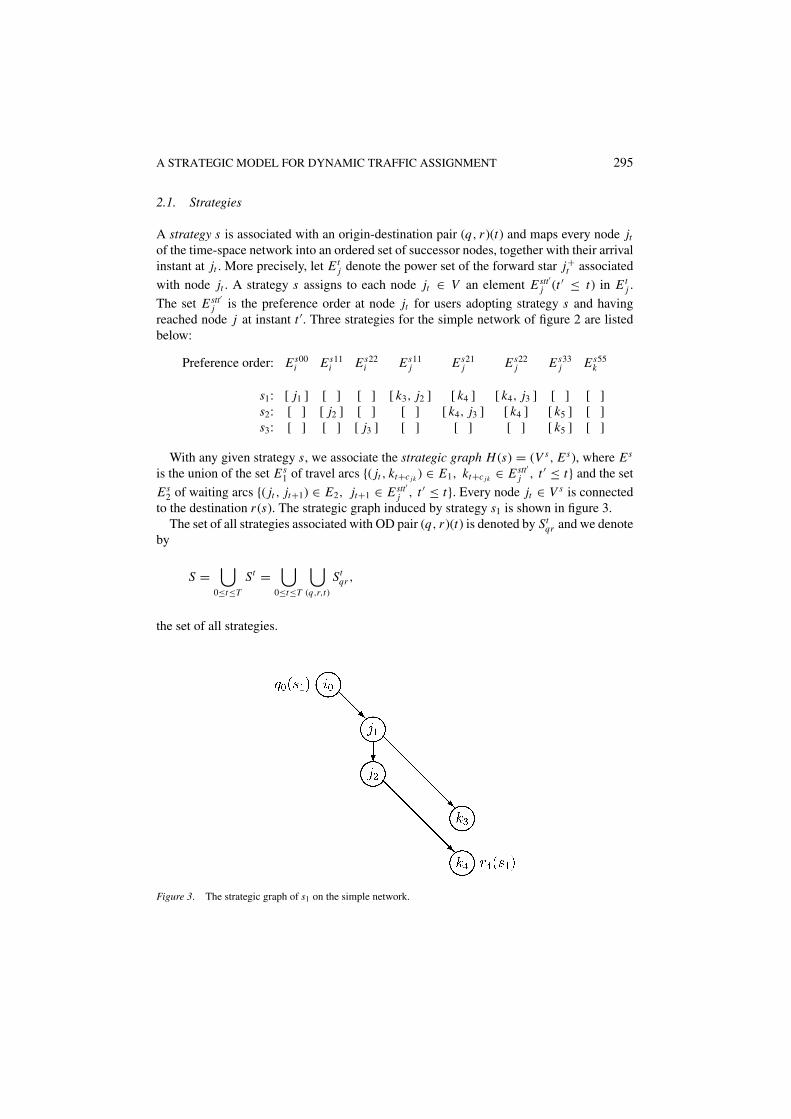
2.1. Strategies
A strategy s is associated with an origin-destination pair (q, r )(t) and maps every node jtof the time-space network into an ordered set of successor nodes, together with their arrivalinstant at jt . More precisely, let Et
j denote the power set of the forward star j+t associated
with node jt . A strategy s assigns to each node jt ∈ V an element Estt′j (t ′ ≤ t) in Et
j .
The set Estt′j is the preference order at node jt for users adopting strategy s and having
reached node j at instant t ′. Three strategies for the simple network of figure 2 are listedbelow:
Preference order: Es00i Es11
i Es22i Es11
j Es21j Es22
j Es33j Es55
k
s1: [ j1 ] [ ] [ ] [ k3, j2 ] [ k4 ] [ k4, j3 ] [ ] [ ]s2: [ ] [ j2 ] [ ] [ ] [ k4, j3 ] [ k4 ] [ k5 ] [ ]s3: [ ] [ ] [ j3 ] [ ] [ ] [ ] [ k5 ] [ ]
With any given strategy s, we associate the strategic graph H (s) = (V s, Es), where Es
is the union of the set Es1 of travel arcs {( jt , kt+c jk ) ∈ E1, kt+c jk ∈ Estt′
j , t ′ ≤ t} and the set
Es2 of waiting arcs {( jt , jt+1) ∈ E2, jt+1 ∈ Estt′
j , t ′ ≤ t}. Every node jt ∈ V s is connectedto the destination r (s). The strategic graph induced by strategy s1 is shown in figure 3.
The set of all strategies associated with OD pair (q, r )(t) is denoted by Stqr and we denote
by
S =⋃
0≤t≤T
St =⋃
0≤t≤T
⋃(q,r,t)
Stqr ,
the set of all strategies.
Figure 3. The strategic graph of s1 on the simple network.
296 HAMDOUCH, MARCOTTE AND NGUYEN
2.2. Strategic volumes and strategic delays
Let xts represent the number of drivers using strategy s and leaving their origin q(s) at
instant t . We denote by x = (xts)s∈S the vector of strategic volumes and by X the set of all
demand-feasible such vectors, i.e.,
X ={
x :∑s∈St
qr
x ts = dt
qr ∀(q, r ), ∀t ∈ T
}. (1)
The (expected) delay of strategy s depends directly on the arc access probabilities π st ′jk (x)
and π st ′j (x), the latter corresponding to a waiting arc; π st ′
jk (x) (respectively π st ′j (x)) is the
probability that drivers adopting strategy s access node kt ′+c jk (respectively jt ′+1) from nodejt ′ . These access probabilities are computed by a dynamic loading process that will be thefocus of Section 3. The arc access probabilities induce node access probabilities, computedrecursively as follows:
τ st ′j (x) =
0 if jt ′ /∈ V s
1 if jt ′ = qt (s)
τs(t ′−1)j π
s(t ′−1)j +
∑ktc ∈ j−
t ′
τstck π
stck j if jt ′ ∈ V s\{qt (s)},
(2)
where tc = t ′ − ck j is the instant when a user of strategy s leaves node k through arc (k, j).In a natural fashion, we define the strategic delay of a strategy s with departure time t
and destination q(s) as the weighted sum:
Cts(x) =
∑t ′≥t
{ ∑( jt ′ ,kt ′+c jk
)∈Es1
τ st ′j (x)π st ′
jk (x)c jk +∑
( jt ′ , jt ′+1)∈Es2
τ st ′j (x)π st ′
j (x)
}. (3)
The above definition implies that travel delays are link-additive and that the perception ofdelay is homogeneous across the population.
An equilibrium strategic flow x∗ is then readily characterized as a solution of the varia-tional inequality
〈C(x∗), x∗ − x〉 ≤ 0 ∀x ∈ X. (4)
If the cost function C were continuous, the existence of an equilibrium solution would fol-low directly from classical fixed point theorems, such as Brouwer’s or Kakutani’s. However,a technical difficulty arises in the degenerate situation where a null strategic volume wantsto access an arc with null residual capacity. This can be resolved exactly as in Hamdouchet al. (2002), i.e., by showing that setting the access probability to zero in the degeneratecase yields a lower semi-continuous cost mapping C . The proof will not be repeated here.
2.3. The FIFO rule and flow priority
A main feature of the model described by the variational inequality (4) is that the FIFO ruleis strictly enforced, which is not the case in several dynamic models. At a node jt ′ ∈ V ,
A STRATEGIC MODEL FOR DYNAMIC TRAFFIC ASSIGNMENT 297
FIFO is achieved by dividing each user group zst′j into subgroups according to their arrival
instant at node j . We denote by zst′t ′′j the strategic volume at node jt ′ adopting strategy s
and having reached node j at instant t ′′ ≤ t ′ and regroup all active strategies into a classSt ′t ′′
restricted to users having reached node j at instant t ′′:
St ′t ′′ = {s ∈ S : Est′t ′′j �= ∅, zst′t ′′
j > 0}. (5)
Based on the access probabilities π st′jk (x) and π st′
j (x), the volume zst′t ′′j is then computed
according to the recursion
zst′t ′′j =
0 if jt ′ /∈ V s
xts if jt ′ = qt (s) (t ′′ = t ′)
πs(t ′−1)j zs(t ′−1)t ′′
j if jt ′ ∈ V s\{qt (s)} and t ′′ ≤ t ′ − 1∑ktc ∈ j−
t ′
πstck j zstc
k if jt ′ ∈ V s\{qt (s)} and t ′′ = t ′ (tc = t ′ − c jk).
(6)
In order to control access priorities, we assign the highest priority to users of the first classSt ′0. The strategic volume of the remaining classes are then loaded in increasing orderaccording of their arrival instant at node j . This ordering is an integral part of the loadingprocess described in the next section.
3. The dynamic loading process
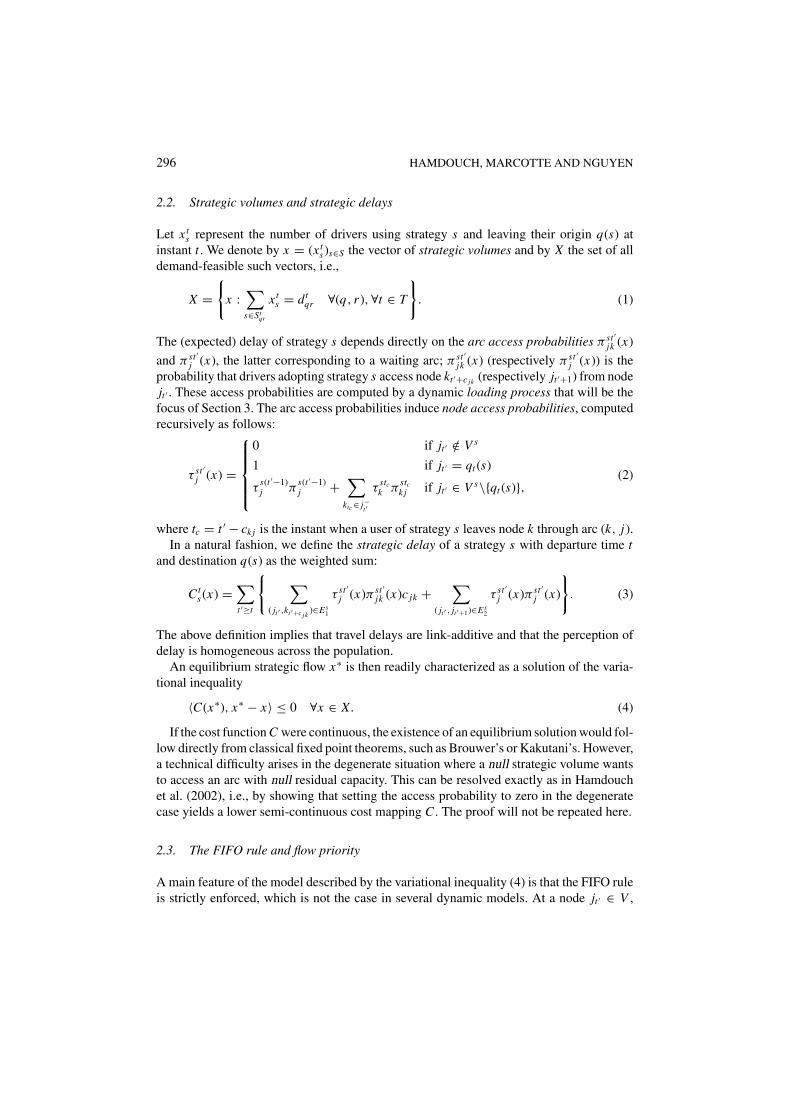
In standard static models, the arc-path incidence matrix is flow independent. As a conse-quence, link information can be readily recovered from path flow information. In dynamicmodels, the situation is different and calls for a mechanism that maps path (or strategic)flows into link flows. In our model, this operation is performed by a loading procedure thatassigns users to their preferred available arc, until their first choices becomes saturated.Saturated arcs are then removed from the preference sets and the procedure is iterated untilall users are assigned to an outgoing arc. Note that users arriving at a given node stand in acommon ‘vertical’ queue, irrespective of their destinations.
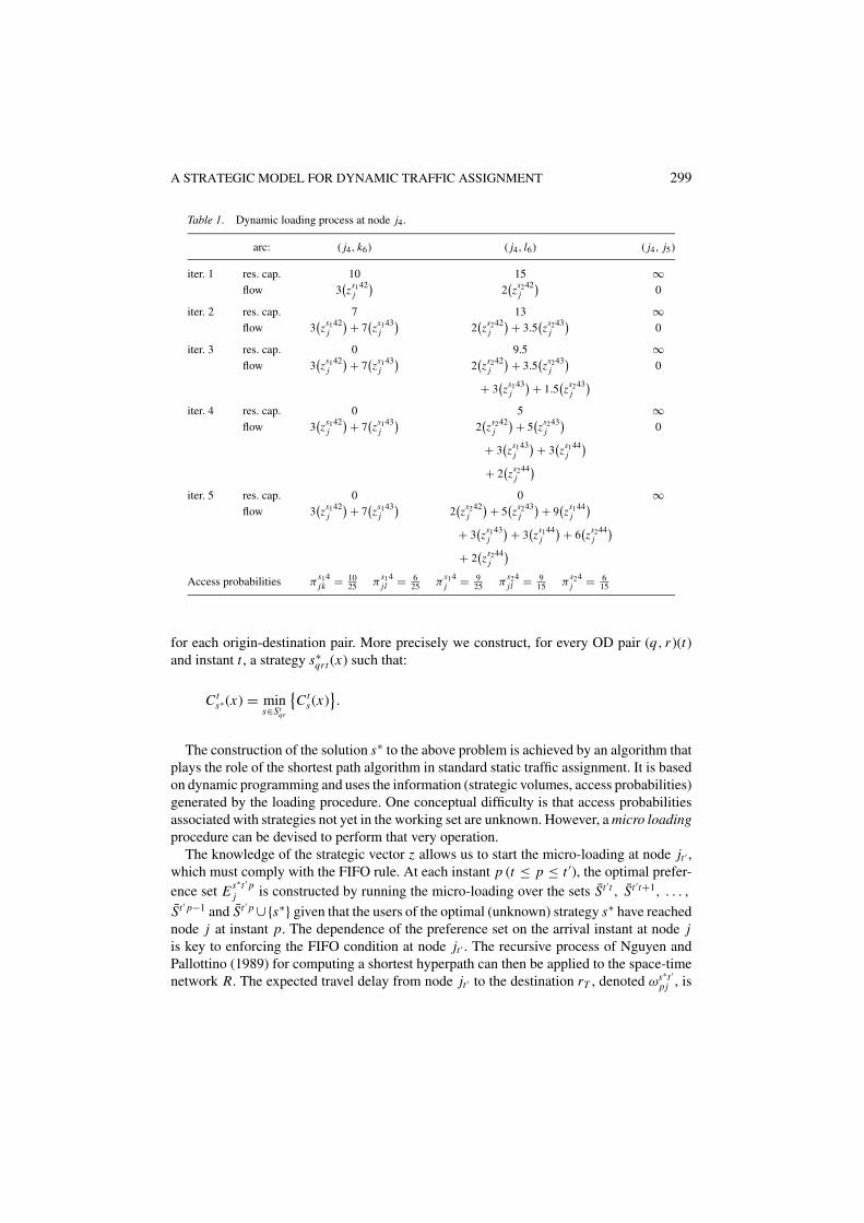
This procedure will be explained in detail on the example corresponding to figure 4,where capacities of the physical arcs ( j, k) and ( j, l) are set to 10 and 15, respectively. Wefocus on the loading process at node j4, i.e., the physical node j at instant 4. A total of 20users are already in the waiting queue at j ; among these, 15 users have been in the queue fortwo periods, and the remaining 5 for one period. They are joined in the queue by 20 usersthat access node j from node i . All users adopt one of either two strategies, s1 or s2, whichare specified by the preference sets Estt′
j displayed in the figure. Note that the preference setof a strategy can be time dependent, which it is in our example. Next to each arc is shownits volume, together with the repartition among the two classes.
We initiate the process by loading the strategic flow associated with class S42, i.e., flowthat arrived at node j at instant 2. Since capacity is not exceeded, 3 users from s1 and 2from s2 head for nodes k6 and l6, respectively. Next, residual capacities are updated and theloading ends for drivers of the first class. At the second iteration, strategic volumes zs143
j
298 HAMDOUCH, MARCOTTE AND NGUYEN
Figure 4. An example of strategic dynamic loading.
and zs243j of the second class S43 are assigned to their respective preferred node at a uniform
rate. Since the ratio 7/10 is less than 13/5, arc ( j4, k6) gets saturated first. At that instant, 710
of s1 and s2 flows are assigned, i.e., 7 users from s1 reach node k6 and 3.5 from s2 reach l6.At iteration 3, the saturation of ( j4, k6) forces users of strategy s1 to adopt their second bestchoice l6; 4.5 units of volume (3 from s1 and 1.5 from s2) vie for arc ( j4, l6) whose residualcapacity is 9.5. Since capacity exceeds demand, the loading of class S43 terminates. At thefourth iteration, 12 units of the strategic volume zs144
j and 8 of zs244j compete for the residual
capacity (5) of arc ( j4, l6). According to the ratio 1 to 4, 3 units from s1 and 2 from s2 reachnode l6. A fifth iteration is required to load the unassigned flow to the waiting arc ( j4, j5).The arc probabilities are then obtained by dividing the amount of strategic volume havingaccessed an arc by the total corresponding strategic volume. More details are provided inTable 1.
A pseudocode of the algorithm, which extends that presented in Hamdouch et al. (2002)for static networks with priority rules, is given in Appendix B. It provides a formal descrip-tion of the loading of a strategic flow vector x = (xt
s)s∈W t ⊂St , t≤T with respect to a subset ofstrategies W t , the working set. The working set includes at least one strategy for every ODpair (q, r )(t).
4. Computation of an optimal strategy
The algorithms that we implemented are extensions to the dynamic case of algorithmspresented in Hamdouch (2002). At each iteration, one moves from the current strategicvector toward another vector that incorporates a ‘best’ response to current traffic conditions,
A STRATEGIC MODEL FOR DYNAMIC TRAFFIC ASSIGNMENT 299
Table 1. Dynamic loading process at node j4.
arc: ( j4, k6) ( j4, l6) ( j4, j5)
iter. 1 res. cap. 10 15 ∞flow 3
(zs142
j
)2(zs242
j
)0
iter. 2 res. cap. 7 13 ∞flow 3
(zs142
j
) + 7(zs143
j
)2(zs242
j
) + 3.5(zs243
j
)0
iter. 3 res. cap. 0 9.5 ∞flow 3
(zs142
j
) + 7(zs143
j
)2(zs242
j
) + 3.5(zs243
j
)0
+ 3(zs143
j
) + 1.5(zs243
j
)iter. 4 res. cap. 0 5 ∞
flow 3(zs142
j
) + 7(zs143
j
)2(zs242
j
) + 5(zs243
j
)0
+ 3(zs143
j
) + 3(zs144
j
)+ 2
(zs244
j
)iter. 5 res. cap. 0 0 ∞
flow 3(zs142
j
) + 7(zs143
j
)2(zs242
j
) + 5(zs243
j
) + 9(zs144
j
)+ 3
(zs143
j
) + 3(zs144
j
) + 6(zs244
j
)+ 2
(zs244
j
)Access probabilities π
s14jk = 10
25 πs14jl = 6
25 πs14j = 9
25 πs24jl = 9
15 πs24j = 6
15
for each origin-destination pair. More precisely we construct, for every OD pair (q, r )(t)and instant t , a strategy s∗
qrt (x) such that:
Cts∗ (x) = min
s∈Stqr
{Ct
s(x)}.
The construction of the solution s∗ to the above problem is achieved by an algorithm thatplays the role of the shortest path algorithm in standard static traffic assignment. It is basedon dynamic programming and uses the information (strategic volumes, access probabilities)generated by the loading procedure. One conceptual difficulty is that access probabilitiesassociated with strategies not yet in the working set are unknown. However, a micro loadingprocedure can be devised to perform that very operation.
The knowledge of the strategic vector z allows us to start the micro-loading at node jt ′ ,which must comply with the FIFO rule. At each instant p (t ≤ p ≤ t ′), the optimal prefer-ence set Es∗t ′ p
j is constructed by running the micro-loading over the sets St ′t , St ′t+1, . . . ,
St ′ p−1 and St ′ p ∪{s∗} given that the users of the optimal (unknown) strategy s∗ have reachednode j at instant p. The dependence of the preference set on the arrival instant at node jis key to enforcing the FIFO condition at node jt ′ . The recursive process of Nguyen andPallottino (1989) for computing a shortest hyperpath can then be applied to the space-timenetwork R. The expected travel delay from node jt ′ to the destination rT , denoted ωs∗t ′
pj , is
300 HAMDOUCH, MARCOTTE AND NGUYEN
obtained from Bellman’s generalized recursion:
ωs∗t ′pj =
∞ if j �= r, t = T
0 if j = r∑kt ′′ ∈Es∗ t ′ p
j
π s∗t ′jk
(c jk + ωs∗t ′′
t ′′k) + π s∗t ′
j
(1 + ωs∗t ′+1
pj
)if j �= r, t < T,
(7)
where t ′′ = t ′ + c jk is the arrival instant at node k ∈ j−, and where the optimal preference
order Es∗t ′ pj is constructed efficiently by sorting the labels c jk + ωs∗t ′′
k in increasing order,with
ωs∗t ′′k =
{ωs∗t ′′
pk if kt ′′ = kt ′+c jk = jt ′+1
ωs∗t ′′t ′′k otherwise.
An optimal solution s∗, together with its cost vectorω∗, is then obtained by solving Bellman’sequations in reverse topological order, i.e., starting at instant T .
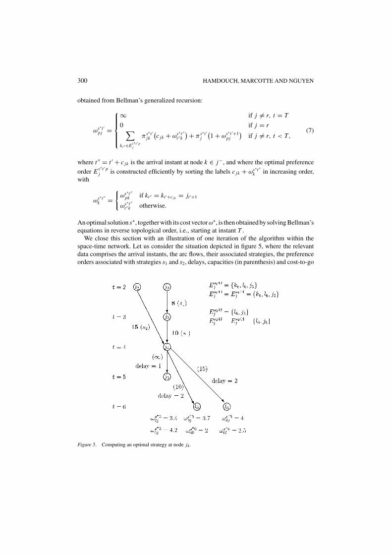
We close this section with an illustration of one iteration of the algorithm within thespace-time network. Let us consider the situation depicted in figure 5, where the relevantdata comprises the arrival instants, the arc flows, their associated strategies, the preferenceorders associated with strategies s1 and s2, delays, capacities (in parenthesis) and cost-to-go
Figure 5. Computing an optimal strategy at node j4.
A STRATEGIC MODEL FOR DYNAMIC TRAFFIC ASSIGNMENT 301
(bottom of picture) that are available at nodes j5, k6 and l6, since their topological index ishigher than that of node j . We compute the best strategic response, starting at the physicalnode j .
The optimal preference orders are obtained by minimizing the sum of arc delays and thecorresponding cost-to-go. Accordingly, the inequalities
c jk + ωs∗66k = 2 + 2 < 1 + ωs∗5
2 j = 1 + 3.4 < c jl + ωs∗66l = 2 + 2.5
yield Es∗42j = [k6, j5, l6]. In a similar fashion, we derive Es∗43
j = [k6, l6, j5] from
c jk + ωs∗66k = 4 < c jl + ωs∗6
6l = 4.5 < 1 + ωs∗53 j = 1 + 3.7
and Es∗44j = [k6, l6, j5] from the inequalities
4 < 4.5 < 1 + ωs∗54 j = 1 + 4.
The algorithm must now determine the values of ωs∗42 j , ωs∗4
3 j and ωs∗44 j at node j4. We start
with instant 2 and the strategy set S42 ∪{s∗} = {s1, s∗}. Since flow does not exceed availablecapacity, all users from s1 and s∗ head for node k6. This yields the access probabilitiesπ s∗4
jk = 1, π s∗4j = π s∗4
jl = 0 and the delay
ωs∗42 j = π s∗4
jk
(2 + ωs∗6
6k
) + π s∗4j
(1 + ωs∗6
2 j
) + π s∗4jl
(2 + ωs∗6
6l
)= 1(4) + 0(4.4) + 0(4.5) = 4.
We now repeat the loading operation for users that arrived at instant 3. We first performthe assignment of the 8 users that reached at instant 2 their preferred node k6. Next, theresidual capacity of arc ( j, k) is updated (it becomes 10 − 8 = 2) and the loading endsfor drivers of strategies S42. Next, the strategic volumes zs143
j and zs∗j associated with the
strategies in S43 are assigned to their respective preferred node at the uniform rate 2/10. Atthat instant, 1
5 of s1 and s∗ flows have reached node k6, and the arc ( j4, k6) is saturated. Thisforces users of strategy s1 and s∗ to adopt their second best choice l6; 8 units of volume froms1 and s∗ access arc ( j4, l6), whose residual capacity (15) exceeds demand (8). This yieldsthe access probabilities π s∗4
jk = 1/5, π s∗4jl = 4/5 and π s∗4
j = 0, from which we derive thecost-to-go
ωs∗43 j = π s∗4
jk
(2 + ωs∗6
6k
) + +π s∗4jl
(2 + ωs∗6
6l
) + π s∗4j
(1 + ωs∗6
3 j
)= 1
5(4) + 4
5(4.5) + 0(4.7) = 22
5= 4.4.
Then, we proceed with users that reached node j at instant 4. This involves loading theflows associated with strategy sets S42, S43 and S44 ∪ {s∗}. This yields (we skip details)π s∗4
jk = 0, π s∗4jl = 7/15, π s∗4
j = 8/15 and
ωs∗44 j = π s∗4
jk
(2 + ωs∗6
6k
) + +π s∗4jl
(2 + ωs∗6
6l
) + π s∗4j
(1 + ωs∗6
4 j
)= 7
15(4.5) + 8
15(5) = 71.5
15= 4.76.

302 HAMDOUCH, MARCOTTE AND NGUYEN
5. A solution algorithm and numerical results
Numerical results have been obtained using algorithm DSTRATEQ, which mimics themethod of successive averages for solving the variational inequality (4). Since the costmapping C may fail to be monotone,1 this method is heuristic in our context. AlgorithmDSTRATEQ generates a sequence of iterates by mixing the current strategic flow withthe flows corresponding to optimal strategies. Next, the dynamic loading procedure yieldsupdated link flows, access probabilities and expected cost vector C(xk+1), allowing thecontinuation of the process. In mathematical terms, this is expressed as
xk+1 = (1 − θ k)xk + θ k x(xk), k = 1, 2, . . .
where θ k ∈ (0, 1) and
x ts(xk) =
{dt
qr if s = s∗
0 otherwise, ∀(q, r ), ∀s ∈ W t
qr, ∀t ≤ T .
For improved convergence, the stepsize was chosen adaptively and independently for eachOD pair. More precisely:
θs = 1 − Cs∗
Cst
.
The algorithm was halted as soon as the relative gap function, a measure of disequilibriumdefined as
g(x) = maxy∈X 〈C(x), x − y〉〈C(x), x〉 , (8)
became smaller than some predetermined tolerance. We report numerical results on onesmall and one medium-sized network.
5.1. Small network
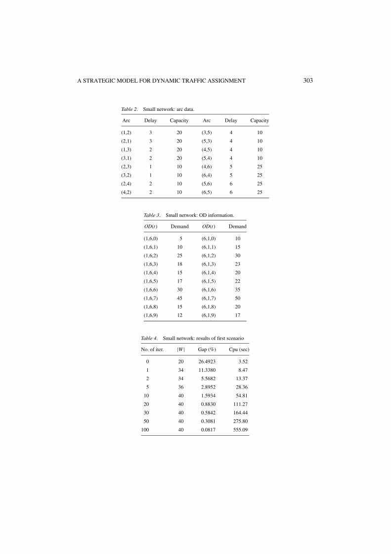
Our first test problem is based on the bidirectional network illustrated in figure 6. Thenumber of periods T is set to 65 and the latest departure instant T ′ is set to 9. Additional
Figure 6. Small network (T = 65).
A STRATEGIC MODEL FOR DYNAMIC TRAFFIC ASSIGNMENT 303
Table 2. Small network: arc data.
Arc Delay Capacity Arc Delay Capacity
(1,2) 3 20 (3,5) 4 10
(2,1) 3 20 (5,3) 4 10
(1,3) 2 20 (4,5) 4 10
(3,1) 2 20 (5,4) 4 10
(2,3) 1 10 (4,6) 5 25
(3,2) 1 10 (6,4) 5 25
(2,4) 2 10 (5,6) 6 25
(4,2) 2 10 (6,5) 6 25
Table 3. Small network: OD information.
OD(t) Demand OD(t) Demand
(1,6,0) 5 (6,1,0) 10
(1,6,1) 10 (6,1,1) 15
(1,6,2) 25 (6,1,2) 30
(1,6,3) 18 (6,1,3) 23
(1,6,4) 15 (6,1,4) 20
(1,6,5) 17 (6,1,5) 22
(1,6,6) 30 (6,1,6) 35
(1,6,7) 45 (6,1,7) 50
(1,6,8) 15 (6,1,8) 20
(1,6,9) 12 (6,1,9) 17
Table 4. Small network: results of first scenario
No. of iter. |W | Gap (%) Cpu (sec)
0 20 26.4923 3.52
1 34 11.3380 8.47
2 34 5.5682 13.37
5 36 2.8952 28.36
10 40 1.5934 54.81
20 40 0.8830 111.27
30 40 0.5842 164.44
50 40 0.3081 275.80
100 40 0.0817 555.09
304 HAMDOUCH, MARCOTTE AND NGUYEN
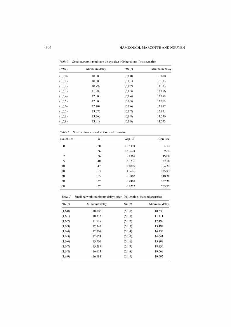
Table 5. Small network: minimum delays after 100 iterations (first scenario).
OD (t) Minimum delay OD (t) Minimum delay
(1,6,0) 10.000 (6,1,0) 10.000
(1,6,1) 10.000 (6,1,1) 10.333
(1,6,2) 10.799 (6,1,2) 11.333
(1,6,3) 11.888 (6,1,3) 12.156
(1,6,4) 12.000 (6,1,4) 12.189
(1,6,5) 12.000 (6,1,5) 12.263
(1,6,6) 12.209 (6,1,6) 12.617
(1,6,7) 13.075 (6,1,7) 13.831
(1,6,8) 13.360 (6,1,8) 14.536
(1,6,9) 13.018 (6,1,9) 14.555
Table 6. Small network: results of second scenario.
No. of iter. |W | Gap (%) Cpu (sec)
0 20 40.8394 4.12
1 36 13.3624 9.61
2 36 6.1367 15.00
5 40 3.8735 32.16
10 47 2.1099 64.32
20 53 1.0616 135.83
30 55 0.7803 210.38
50 57 0.4901 367.39
100 57 0.2222 765.75
Table 7. Small network: minimum delays after 100 iterations (second scenario).
OD (t) Minimum delay OD (t) Minimum delay
(1,6,0) 10.000 (6,1,0) 10.333
(1,6,1) 10.333 (6,1,1) 11.111
(1,6,2) 11.528 (6,1,2) 12.499
(1,6,3) 12.347 (6,1,3) 13.492
(1,6,4) 12.508 (6,1,4) 14.133
(1,6,5) 12.674 (6,1,5) 14.641
(1,6,6) 13.501 (6,1,6) 15.808
(1,6,7) 15.289 (6,1,7) 18.134
(1,6,8) 16.613 (6,1,8) 19.669
(1,6,9) 16.188 (6,1,9) 19.992
A STRATEGIC MODEL FOR DYNAMIC TRAFFIC ASSIGNMENT 305
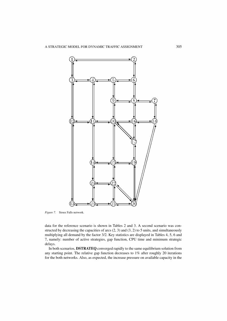
Figure 7. Sioux Falls network.
data for the reference scenario is shown in Tables 2 and 3. A second scenario was con-structed by decreasing the capacities of arcs (2, 3) and (3, 2) to 5 units, and simultaneouslymultiplying all demand by the factor 3/2. Key statistics are displayed in Tables 4, 5, 6 and7, namely: number of active strategies, gap function, CPU time and minimum strategicdelays.
In both scenarios, DSTRATEQ converged rapidly to the same equilibrium solution fromany starting point. The relative gap function decreases to 1% after roughly 20 iterationsfor the both networks. Also, as expected, the increase pressure on available capacity in the
306 HAMDOUCH, MARCOTTE AND NGUYEN
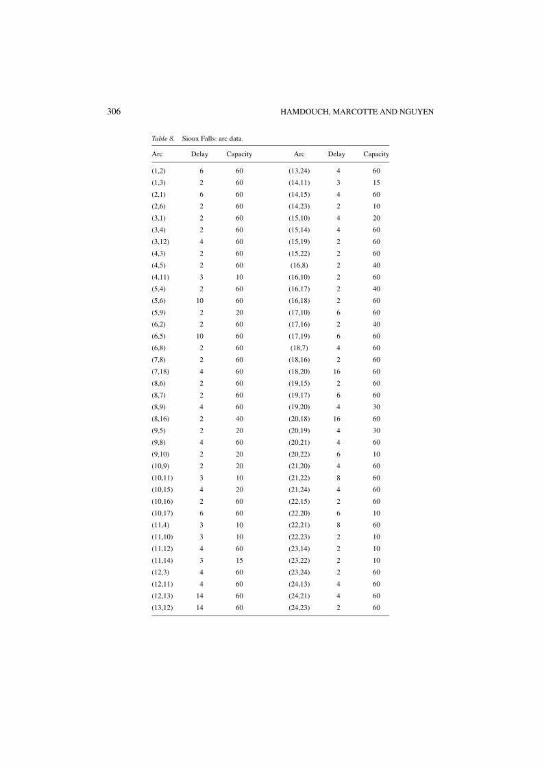
Table 8. Sioux Falls: arc data.
Arc Delay Capacity Arc Delay Capacity
(1,2) 6 60 (13,24) 4 60
(1,3) 2 60 (14,11) 3 15
(2,1) 6 60 (14,15) 4 60
(2,6) 2 60 (14,23) 2 10
(3,1) 2 60 (15,10) 4 20
(3,4) 2 60 (15,14) 4 60
(3,12) 4 60 (15,19) 2 60
(4,3) 2 60 (15,22) 2 60
(4,5) 2 60 (16,8) 2 40
(4,11) 3 10 (16,10) 2 60
(5,4) 2 60 (16,17) 2 40
(5,6) 10 60 (16,18) 2 60
(5,9) 2 20 (17,10) 6 60
(6,2) 2 60 (17,16) 2 40
(6,5) 10 60 (17,19) 6 60
(6,8) 2 60 (18,7) 4 60
(7,8) 2 60 (18,16) 2 60
(7,18) 4 60 (18,20) 16 60
(8,6) 2 60 (19,15) 2 60
(8,7) 2 60 (19,17) 6 60
(8,9) 4 60 (19,20) 4 30
(8,16) 2 40 (20,18) 16 60
(9,5) 2 20 (20,19) 4 30
(9,8) 4 60 (20,21) 4 60
(9,10) 2 20 (20,22) 6 10
(10,9) 2 20 (21,20) 4 60
(10,11) 3 10 (21,22) 8 60
(10,15) 4 20 (21,24) 4 60
(10,16) 2 60 (22,15) 2 60
(10,17) 6 60 (22,20) 6 10
(11,4) 3 10 (22,21) 8 60
(11,10) 3 10 (22,23) 2 10
(11,12) 4 60 (23,14) 2 10
(11,14) 3 15 (23,22) 2 10
(12,3) 4 60 (23,24) 2 60
(12,11) 4 60 (24,13) 4 60
(12,13) 14 60 (24,21) 4 60
(13,12) 14 60 (24,23) 2 60
A STRATEGIC MODEL FOR DYNAMIC TRAFFIC ASSIGNMENT 307
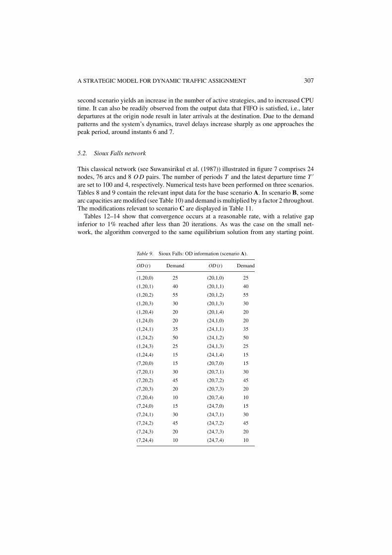
second scenario yields an increase in the number of active strategies, and to increased CPUtime. It can also be readily observed from the output data that FIFO is satisfied, i.e., laterdepartures at the origin node result in later arrivals at the destination. Due to the demandpatterns and the system’s dynamics, travel delays increase sharply as one approaches thepeak period, around instants 6 and 7.
5.2. Sioux Falls network
This classical network (see Suwansirikul et al. (1987)) illustrated in figure 7 comprises 24nodes, 76 arcs and 8 O D pairs. The number of periods T and the latest departure time T ′
are set to 100 and 4, respectively. Numerical tests have been performed on three scenarios.Tables 8 and 9 contain the relevant input data for the base scenario A. In scenario B, somearc capacities are modified (see Table 10) and demand is multiplied by a factor 2 throughout.The modifications relevant to scenario C are displayed in Table 11.
Tables 12–14 show that convergence occurs at a reasonable rate, with a relative gapinferior to 1% reached after less than 20 iterations. As was the case on the small net-work, the algorithm converged to the same equilibrium solution from any starting point.
Table 9. Sioux Falls: OD information (scenario A).
OD (t) Demand OD (t) Demand
(1,20,0) 25 (20,1,0) 25
(1,20,1) 40 (20,1,1) 40
(1,20,2) 55 (20,1,2) 55
(1,20,3) 30 (20,1,3) 30
(1,20,4) 20 (20,1,4) 20
(1,24,0) 20 (24,1,0) 20
(1,24,1) 35 (24,1,1) 35
(1,24,2) 50 (24,1,2) 50
(1,24,3) 25 (24,1,3) 25
(1,24,4) 15 (24,1,4) 15
(7,20,0) 15 (20,7,0) 15
(7,20,1) 30 (20,7,1) 30
(7,20,2) 45 (20,7,2) 45
(7,20,3) 20 (20,7,3) 20
(7,20,4) 10 (20,7,4) 10
(7,24,0) 15 (24,7,0) 15
(7,24,1) 30 (24,7,1) 30
(7,24,2) 45 (24,7,2) 45
(7,24,3) 20 (24,7,3) 20
(7,24,4) 10 (24,7,4) 10
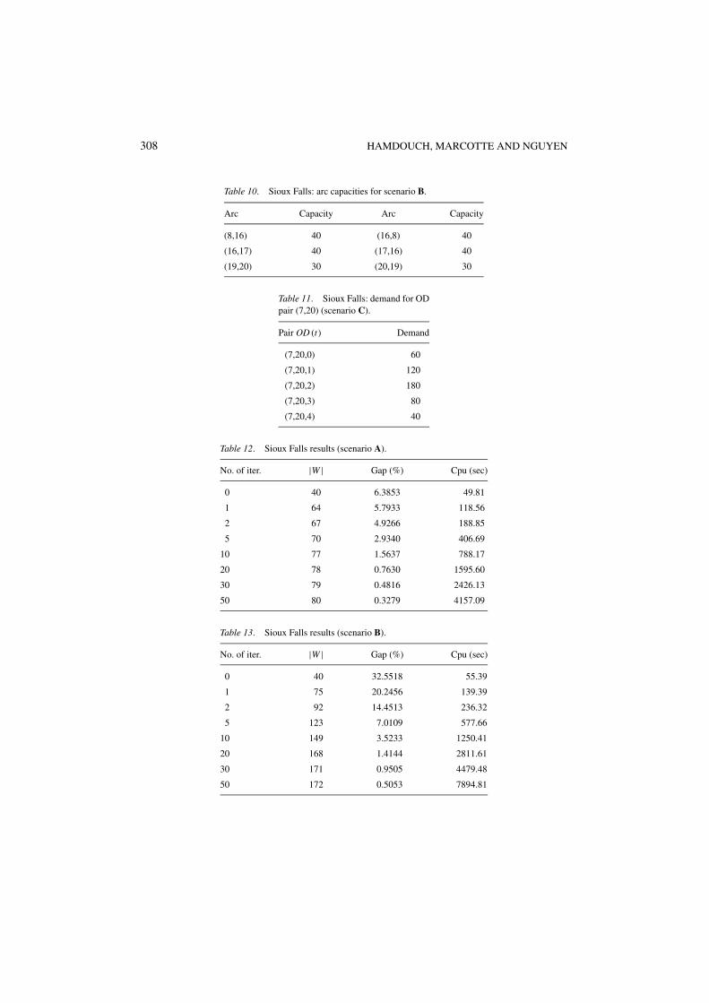
308 HAMDOUCH, MARCOTTE AND NGUYEN
Table 10. Sioux Falls: arc capacities for scenario B.
Arc Capacity Arc Capacity
(8,16) 40 (16,8) 40
(16,17) 40 (17,16) 40
(19,20) 30 (20,19) 30
Table 11. Sioux Falls: demand for ODpair (7,20) (scenario C).
Pair OD (t) Demand
(7,20,0) 60
(7,20,1) 120
(7,20,2) 180
(7,20,3) 80
(7,20,4) 40
Table 12. Sioux Falls results (scenario A).
No. of iter. |W | Gap (%) Cpu (sec)
0 40 6.3853 49.81
1 64 5.7933 118.56
2 67 4.9266 188.85
5 70 2.9340 406.69
10 77 1.5637 788.17
20 78 0.7630 1595.60
30 79 0.4816 2426.13
50 80 0.3279 4157.09
Table 13. Sioux Falls results (scenario B).
No. of iter. |W | Gap (%) Cpu (sec)
0 40 32.5518 55.39
1 75 20.2456 139.39
2 92 14.4513 236.32
5 123 7.0109 577.66
10 149 3.5233 1250.41
20 168 1.4144 2811.61
30 171 0.9505 4479.48
50 172 0.5053 7894.81
A STRATEGIC MODEL FOR DYNAMIC TRAFFIC ASSIGNMENT 309
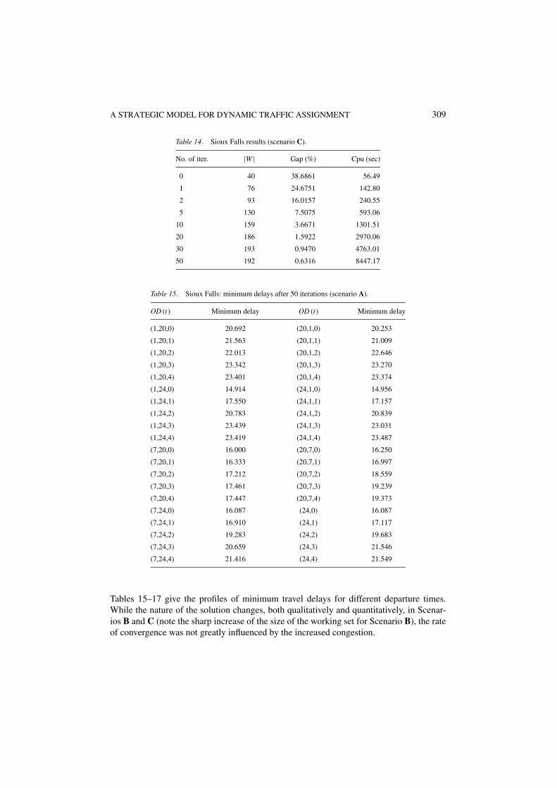
Table 14. Sioux Falls results (scenario C).
No. of iter. |W | Gap (%) Cpu (sec)
0 40 38.6861 56.49
1 76 24.6751 142.80
2 93 16.0157 240.55
5 130 7.5075 593.06
10 159 3.6671 1301.51
20 186 1.5922 2970.06
30 193 0.9470 4763.01
50 192 0.6316 8447.17
Table 15. Sioux Falls: minimum delays after 50 iterations (scenario A).
OD (t) Minimum delay OD (t) Minimum delay
(1,20,0) 20.692 (20,1,0) 20.253
(1,20,1) 21.563 (20,1,1) 21.009
(1,20,2) 22.013 (20,1,2) 22.646
(1,20,3) 23.342 (20,1,3) 23.270
(1,20,4) 23.401 (20,1,4) 23.374
(1,24,0) 14.914 (24,1,0) 14.956
(1,24,1) 17.550 (24,1,1) 17.157
(1,24,2) 20.783 (24,1,2) 20.839
(1,24,3) 23.439 (24,1,3) 23.031
(1,24,4) 23.419 (24,1,4) 23.487
(7,20,0) 16.000 (20,7,0) 16.250
(7,20,1) 16.333 (20,7,1) 16.997
(7,20,2) 17.212 (20,7,2) 18.559
(7,20,3) 17.461 (20,7,3) 19.239
(7,20,4) 17.447 (20,7,4) 19.373
(7,24,0) 16.087 (24,0) 16.087
(7,24,1) 16.910 (24,1) 17.117
(7,24,2) 19.283 (24,2) 19.683
(7,24,3) 20.659 (24,3) 21.546
(7,24,4) 21.416 (24,4) 21.549
Tables 15–17 give the profiles of minimum travel delays for different departure times.While the nature of the solution changes, both qualitatively and quantitatively, in Scenar-ios B and C (note the sharp increase of the size of the working set for Scenario B), the rateof convergence was not greatly influenced by the increased congestion.
310 HAMDOUCH, MARCOTTE AND NGUYEN
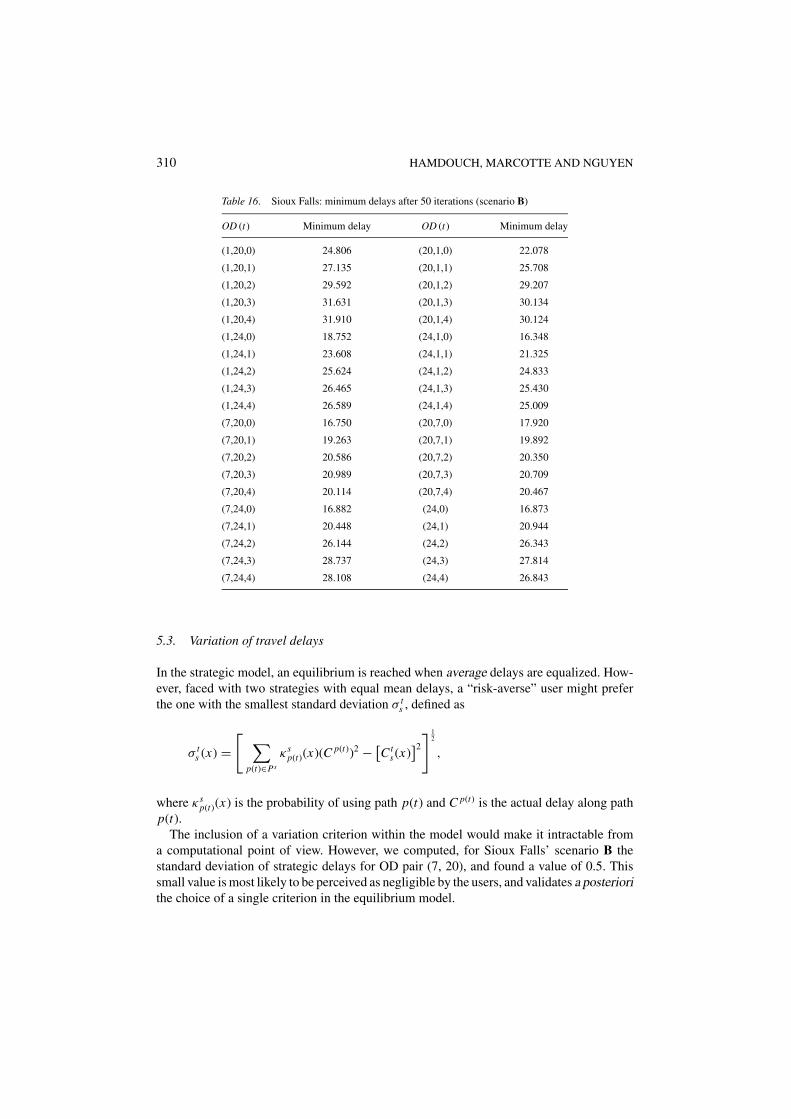
Table 16. Sioux Falls: minimum delays after 50 iterations (scenario B)
OD (t) Minimum delay OD (t) Minimum delay
(1,20,0) 24.806 (20,1,0) 22.078
(1,20,1) 27.135 (20,1,1) 25.708
(1,20,2) 29.592 (20,1,2) 29.207
(1,20,3) 31.631 (20,1,3) 30.134
(1,20,4) 31.910 (20,1,4) 30.124
(1,24,0) 18.752 (24,1,0) 16.348
(1,24,1) 23.608 (24,1,1) 21.325
(1,24,2) 25.624 (24,1,2) 24.833
(1,24,3) 26.465 (24,1,3) 25.430
(1,24,4) 26.589 (24,1,4) 25.009
(7,20,0) 16.750 (20,7,0) 17.920
(7,20,1) 19.263 (20,7,1) 19.892
(7,20,2) 20.586 (20,7,2) 20.350
(7,20,3) 20.989 (20,7,3) 20.709
(7,20,4) 20.114 (20,7,4) 20.467
(7,24,0) 16.882 (24,0) 16.873
(7,24,1) 20.448 (24,1) 20.944
(7,24,2) 26.144 (24,2) 26.343
(7,24,3) 28.737 (24,3) 27.814
(7,24,4) 28.108 (24,4) 26.843
5.3. Variation of travel delays
In the strategic model, an equilibrium is reached when average delays are equalized. How-ever, faced with two strategies with equal mean delays, a “risk-averse” user might preferthe one with the smallest standard deviation σ t
s , defined as
σ ts (x) =
[ ∑p(t)∈Ps
κsp(t)(x)(C p(t))2 − [
Cts(x)
]2
] 12
,
where κsp(t)(x) is the probability of using path p(t) and C p(t) is the actual delay along path
p(t).The inclusion of a variation criterion within the model would make it intractable from
a computational point of view. However, we computed, for Sioux Falls’ scenario B thestandard deviation of strategic delays for OD pair (7, 20), and found a value of 0.5. Thissmall value is most likely to be perceived as negligible by the users, and validates a posteriorithe choice of a single criterion in the equilibrium model.
A STRATEGIC MODEL FOR DYNAMIC TRAFFIC ASSIGNMENT 311
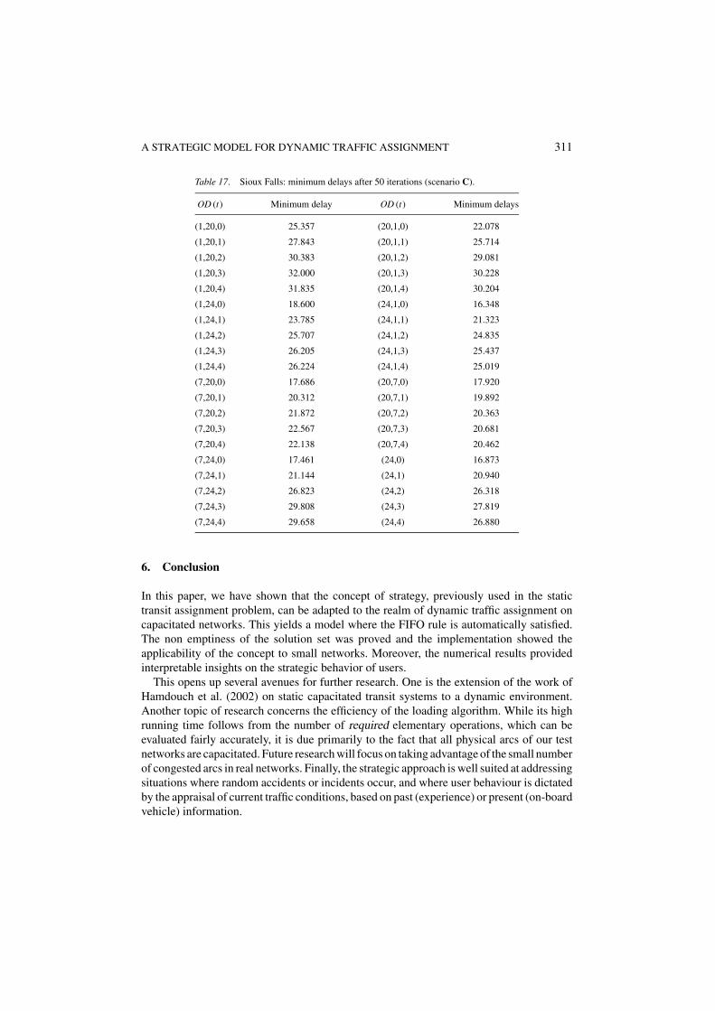
Table 17. Sioux Falls: minimum delays after 50 iterations (scenario C).
OD (t) Minimum delay OD (t) Minimum delays
(1,20,0) 25.357 (20,1,0) 22.078
(1,20,1) 27.843 (20,1,1) 25.714
(1,20,2) 30.383 (20,1,2) 29.081
(1,20,3) 32.000 (20,1,3) 30.228
(1,20,4) 31.835 (20,1,4) 30.204
(1,24,0) 18.600 (24,1,0) 16.348
(1,24,1) 23.785 (24,1,1) 21.323
(1,24,2) 25.707 (24,1,2) 24.835
(1,24,3) 26.205 (24,1,3) 25.437
(1,24,4) 26.224 (24,1,4) 25.019
(7,20,0) 17.686 (20,7,0) 17.920
(7,20,1) 20.312 (20,7,1) 19.892
(7,20,2) 21.872 (20,7,2) 20.363
(7,20,3) 22.567 (20,7,3) 20.681
(7,20,4) 22.138 (20,7,4) 20.462
(7,24,0) 17.461 (24,0) 16.873
(7,24,1) 21.144 (24,1) 20.940
(7,24,2) 26.823 (24,2) 26.318
(7,24,3) 29.808 (24,3) 27.819
(7,24,4) 29.658 (24,4) 26.880
6. Conclusion
In this paper, we have shown that the concept of strategy, previously used in the statictransit assignment problem, can be adapted to the realm of dynamic traffic assignment oncapacitated networks. This yields a model where the FIFO rule is automatically satisfied.The non emptiness of the solution set was proved and the implementation showed theapplicability of the concept to small networks. Moreover, the numerical results providedinterpretable insights on the strategic behavior of users.
This opens up several avenues for further research. One is the extension of the work ofHamdouch et al. (2002) on static capacitated transit systems to a dynamic environment.Another topic of research concerns the efficiency of the loading algorithm. While its highrunning time follows from the number of required elementary operations, which can beevaluated fairly accurately, it is due primarily to the fact that all physical arcs of our testnetworks are capacitated. Future research will focus on taking advantage of the small numberof congested arcs in real networks. Finally, the strategic approach is well suited at addressingsituations where random accidents or incidents occur, and where user behaviour is dictatedby the appraisal of current traffic conditions, based on past (experience) or present (on-boardvehicle) information.

312 HAMDOUCH, MARCOTTE AND NGUYEN
Appendix A: Notation
G = (N , A) network with node set N and arc set AT time intervalt (0 ≤ t ≤ T ) time instantdt
qr time-varying demand leaving origin q at instant t toward destination rc jk travel delay of arc ( j, k)u jk residual capacity of arc ( j, k)R = (V, E) space-time network with node set V and arc set EEstt′
j preference order at node jt for users adopting strategy sxt
s number of drivers using strategy s and leaving their origin at instant tx vector of strategic volumesX set of all demand-feasible strategic volumeszstt′
j strategic volume at node jt adopting strategy sand having reached j at instant t ′
π stjk probability of accessing node kt+c jk from node jt using strategy s
Cts(x) (expected) delay of strategy s with departure time t
C(x) vector of strategic costsW set of active strategies (working set)
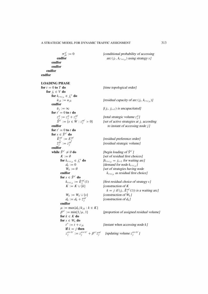
Appendix B: Dynamic loading procedure
ALGORITHM DCAPLOAD (x)
input: x = {xts}s∈W t ,t≤T [strategic volume vector]
output: {π stjk(x)}( j,k)∈A, s∈W t [conditional arc probabilities]
C = {Cts(x)}s∈W t ,t≤T [vector of strategic delays]
INITIALIZATIONfor t = 0 to T do
for s ∈ W t doCt
s := 0 [delay of strategy s]zstt
q(s) := xts [volume at origin node qt (s)]
τ stq(s) := 1 [probability of accessing qt (s)]
for t ′ = t to T dofor jt ′ ∈ V ( jt ′ �= qt (s)) do
for t ′′ = t to t ′ dozst′t ′′
j := 0 [strategic volume at node jt ′
endfor if j has been reached at instant t ′′]τ st′
j := 0 [conditional probability offor kt ′+c jk ∈ Est′
j do accessing node jt ′ using strategy s]vst′
jk := 0 [strategic volume on arc ( jt ′ , kt ′+c jk )]
A STRATEGIC MODEL FOR DYNAMIC TRAFFIC ASSIGNMENT 313
π st′jk := 0 [conditional probability of accessing
endfor arc ( jt ′ , kt ′+c jk ) using strategy s]endforendfor
endforendfor
LOADING PHASEfor t = 0 to T do [time topological order]
for jt ∈ V dofor kt+c jk ∈ j+
t dou jk := u jk [residual capacity of arc ( jt , kt+c jk )]
endforu j := ∞ [( jt , jt+1) is uncapacitated]
for t ′ = 0 to t dozst
j := zstj + zstt′
j [total strategic volume zstj ]
St t ′:= {s ∈ W : zstt′
j > 0} [set of active strategies at jt accordingendfor to instant of accessing node j]for t ′ = 0 to t dofor s ∈ St t ′
doE stt′
j := Estt′j [residual preference order]
zstt′j := zstt′
j [residual strategic volume]endforwhile St t ′ �= ∅ do [begin loading of St t ′
]K := ∅ [set of residual first choices]for kt+c jk ∈ j+
t do [kt+c jk = jt+1 for waiting arc]dk := 0 [demand for node kt+c jk ]Wk := ∅ [set of strategies having node
endfor kt+c jk as residual first choice]for s ∈ St t ′
dokt+c jk := E stt′
j (1) [first residual choice of strategy s]K := K ∪ {k} [construction of K
k = j if ( jt , E stt′j (1)) is a waiting arc]
Wk := Wk ∪ {s} [construction of Wk]dk := dk + zstt′
j [construction of dk]endforµ := max{dk/u jk : k ∈ K }β t t ′
:= min{1/µ, 1} [proportion of assigned residual volume]for k ∈ K dofor s ∈ Wk do
t ′′ := t + c jk [instant when accessing node k]if k = j thenzst+1t ′
j := zst+1t ′j + β t t ′
zstt′j [updating volume zst+1t ′
j ]
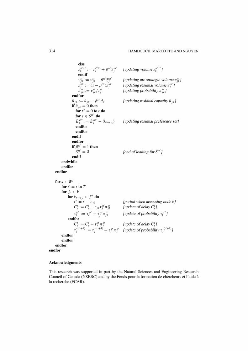
314 HAMDOUCH, MARCOTTE AND NGUYEN
elsezst′′t ′′
k := zst′′t ′′k + β t t ′
zstt′j [updating volume zst′′t ′′
k ]endifvst
jk := vstjk + β t t ′
zstt′j [updating arc strategic volume vst
jk]zstt′
j := (1 − β t t ′)zstt′
j [updating residual volume zstt′j ]
π stjk := vst
jk/zstj [updating probability π st
jk]endforu jk := u jk − β t t ′
dk [updating residual capacity u jk]if u jk = 0 then
for t ′′ = 0 to t dofor s ∈ St t ′′
doE stt′′
j := E stt′′j − {kt+c jk } [updating residual preference set]
endforendfor
endifendforif β t t ′ = 1 then
St t ′ = ∅ [end of loading for St t ′]
endifendwhileendfor
endfor
for s ∈ W t
for t ′ = t to Tfor jt ′ ∈ V
for kt ′+c jk ∈ j+t ′ do
t ′′ = t ′ + c jk [period when accessing node k]Ct
s := Cts + c jkτ
st′j π st′
jk [update of delay Cts]
τ st′′k := τ st′′
k + τ st′j π st′
jk [update of probability τ st′′k ]
endforCt
s := Cts + τ st′
j π st′j [update of delay Ct
s]
τs(t ′+1)j := τ
s(t ′+1)j + τ st′
j π st′j [update of probability τ
s(t ′+1)j ]
endforendfor
endforendfor
Acknowledgments
This research was supported in part by the Natural Sciences and Engineering ResearchCouncil of Canada (NSERC) and by the Fonds pour la formation de chercheurs et l’aide ala recherche (FCAR).
A STRATEGIC MODEL FOR DYNAMIC TRAFFIC ASSIGNMENT 315
Note
1. Marcotte et al. (2000) present an example where the set of equilibrium solutions is disconnected, even in thestatic case.
References
Astarita, V. (1996). “A Continuous Time Link Model for Dynamic Network Loading Based on Travel TimeFunction,” In J.B. Lesort (ed.), Proc. 13th International Symposium on Transportation and Traffic TheoryPergamon-Elsevier, pp. 79–102.
Carey, M. (1992). “Non Convexity of the Dynamic Traffic Assignment Problem.” Transportation Research B26,127–133.
Chriqui, C. and P. Robillard. (1975). “Common Bus Line.” Transportation Science 9, 115–121.Drissi-Kaıtouni, O. and A. Hamada-Benchekroun. (1992). “A Dynamic Traffic Assignment Model and a Solution
Algorithm.” Transportation Science 26, 119–128.Drissi-Kaitouni, O. and M. Gendreau. (1992). “A New Dynamic Traffic Assignment Model.” Publication CRT-854,
Centre de recherche sur les transports, Universite de Montreal.Friesz, T.L., D. Bernstein, T.E. Smith, R. Tobin, and B.W. Wie. (1993). “A Variational Inequality Formulation of
the Dynamic Network User Equilibrium Problem.” Operations Research 41, 179–191.Gao, S. and I. Chabini. (2003). “A Policy-Based Approach to Stochastic Dynamic Traffic Assignment.” Preprint,
Massachusetts Institute of Technology.Hamdouch, Y. (2002). Affectation Statique et Dynamique des Usagers Dans un Reseau de Transport Avec Capacites
Rigides, Ph.D dissertation, Departement d’informatique et de recherche operationnelle, Universite de Montreal.Hamdouch, Y., P. Marcotte, and S. Nguyen. (2002). “Capacitated Traffic Assignment with Priority Rules.” Report
CRT-2002-41, Centre de recherche sur les transports, Universite de Montreal.Marcotte, P. and S. Nguyen. (1998). “Hyperpath Formulations of Traffic Assignment Problems.” In P. Marcotte and
S. Nguyen (eds.), Equilibrium and Advanced Transportation Modelling Kluwer Academic Publisher, pp. 175–199.
Marcotte, P., S. Nguyen, and A. Schoeb. (2000). A Strategic Flow Model of Traffic Assignment in CapacitatedNetworks, Publication 2000-10, Centre de recherche sur les transports, Universite de Montreal.
Merchant, D. and G. Nemhauser. (1978). “A Model and an Algorithm for the Dynamic Traffic AssignmentProblems.” Transportation Science 12, 183–199.
Moore, E.F. (1959). “The Shortest Path Through a Maze.” In Proc. International Symposium on Theory of Switch-ing, Part 2, Harvard University Press, pp. 285–292.
Nguyen, S. and S. Pallottino. (1988). “Equilibrium Traffic Assignment for Large Scale Transit Networks.” Euro-pean Journal of Operational Research 37, 176–186.
Nguyen, S. and S. Pallottino. (1989). “Hyperpaths and Shortest Hyperpaths.” In B. Simeone (ed.), CombinatorialOptimization, vol. 1403 of Lecture Notes in Mathematics, Berlin: Springer-Verlag, pp. 258–271.
Spiess, H. et M. Florian. (1989). “Optimal Strategies: A New Assignment Model for Transit Networks.” Trans-portation Research B 23, 83–102.
Suwansirikul, C., T.L. Friesz, and R.L. Tobin. (1987). “Equilibrium Decomposition Optimization: A Heuristic forthe Continuous Equilibrium Network Design Problem.” Transportation Science 21, 254–263.
Wardrop, J.G. (1952). “Some Theoretical Aspects of Road Traffic Research.” In Proceedings of the Institution ofCivil Engineers, Part II, pp. 325–378.
Zawack, D. and G. Thompson. (1987). “A Dynamic Space-Time Network Flow Model for City Traffic Congestion.”Transportation Science 21, 153–162.