a singing drone choir - diva-portal
TRANSCRIPT

IN DEGREE PROJECT COMPUTER SCIENCE AND ENGINEERING,SECOND CYCLE, 30 CREDITS
, STOCKHOLM SWEDEN 2017
A Singing Drone Choir
VINCENT TRICHON
KTH ROYAL INSTITUTE OF TECHNOLOGYSCHOOL OF ELECTRICAL ENGINEERING AND COMPUTER SCIENCE
A Singing Drone Choir
VINCENT TRICHON
Master in Computer ScienceDate: 2017-09-20Supervisor: Hedvig KjellströmExaminer: Danica KragicSchool of Computer Science and Communication


Dedicated to my Mother and Julien.
Contents
1 Introduction 41.1 Motivation . . . . . . . . . . . . . . . . . . . . . . . . . . . . . . 41.2 Context . . . . . . . . . . . . . . . . . . . . . . . . . . . . . . . . 41.3 Contribution . . . . . . . . . . . . . . . . . . . . . . . . . . . . . 51.4 Limitations . . . . . . . . . . . . . . . . . . . . . . . . . . . . . . 61.5 Societal, ethical, and sustainability aspects . . . . . . . . . . . 61.6 Outline . . . . . . . . . . . . . . . . . . . . . . . . . . . . . . . . 7
2 Related Work 8
3 Background 113.1 Modelling the dynamics of a quadrotor X . . . . . . . . . . . . 11
3.1.1 The X design . . . . . . . . . . . . . . . . . . . . . . . . . 113.1.2 Reference frames . . . . . . . . . . . . . . . . . . . . . . 113.1.3 Rigid body dynamics . . . . . . . . . . . . . . . . . . . . 123.1.4 Action of one rotor . . . . . . . . . . . . . . . . . . . . . 123.1.5 Combined action of the rotors . . . . . . . . . . . . . . 13
3.2 Motion planning strategies . . . . . . . . . . . . . . . . . . . . 133.2.1 Implicit methods . . . . . . . . . . . . . . . . . . . . . . 143.2.2 Explicit methods . . . . . . . . . . . . . . . . . . . . . . 15
3.3 Discussion . . . . . . . . . . . . . . . . . . . . . . . . . . . . . . 16
4 Design and Building of the Quadrotors 184.1 Parts selection . . . . . . . . . . . . . . . . . . . . . . . . . . . . 18
4.1.1 The frame . . . . . . . . . . . . . . . . . . . . . . . . . . 184.1.2 The flight controller . . . . . . . . . . . . . . . . . . . . 204.1.3 The motors . . . . . . . . . . . . . . . . . . . . . . . . . 214.1.4 The propellers . . . . . . . . . . . . . . . . . . . . . . . . 244.1.5 The ESC . . . . . . . . . . . . . . . . . . . . . . . . . . . 244.1.6 The onboard computer . . . . . . . . . . . . . . . . . . 25
iv
4.1.7 The speaker . . . . . . . . . . . . . . . . . . . . . . . . . 254.1.8 The battery . . . . . . . . . . . . . . . . . . . . . . . . . 254.1.9 Miscellenous parts . . . . . . . . . . . . . . . . . . . . . 26
4.2 The design . . . . . . . . . . . . . . . . . . . . . . . . . . . . . . 274.3 Discussion . . . . . . . . . . . . . . . . . . . . . . . . . . . . . . 30
5 The Stage: Setting up the Flying Area 315.1 The location . . . . . . . . . . . . . . . . . . . . . . . . . . . . . 315.2 Hardware . . . . . . . . . . . . . . . . . . . . . . . . . . . . . . . 315.3 Software . . . . . . . . . . . . . . . . . . . . . . . . . . . . . . . 335.4 Safety measures . . . . . . . . . . . . . . . . . . . . . . . . . . . 345.5 Discussion . . . . . . . . . . . . . . . . . . . . . . . . . . . . . . 34
6 Control of the Quadrotors and Implementation 366.1 General control architecture . . . . . . . . . . . . . . . . . . . 366.2 Control by the PX4 flight controller . . . . . . . . . . . . . . . 386.3 Trajectory control: Using potentials . . . . . . . . . . . . . . . 38
6.3.1 Design of the potentials . . . . . . . . . . . . . . . . . . 396.3.2 Trajectory convergence . . . . . . . . . . . . . . . . . . 446.3.3 Prediction Step . . . . . . . . . . . . . . . . . . . . . . . 46
6.4 Implementation of the potentials . . . . . . . . . . . . . . . . 476.5 The motion library . . . . . . . . . . . . . . . . . . . . . . . . . 47
6.5.1 Hardcoded motions . . . . . . . . . . . . . . . . . . . . 486.5.2 Interactive motions . . . . . . . . . . . . . . . . . . . . . 486.5.3 Playback motions . . . . . . . . . . . . . . . . . . . . . . 48
6.6 The “Choreographer” . . . . . . . . . . . . . . . . . . . . . . . . 496.6.1 Description . . . . . . . . . . . . . . . . . . . . . . . . . 496.6.2 The syntax . . . . . . . . . . . . . . . . . . . . . . . . . . 49
7 Simulation and Visualization Tools 527.1 Quadrotor Simulation: PX4 SITL . . . . . . . . . . . . . . . . . 527.2 Simulation in ROS . . . . . . . . . . . . . . . . . . . . . . . . . 53
7.2.1 Implementation . . . . . . . . . . . . . . . . . . . . . . . 537.2.2 Hybrid simulation . . . . . . . . . . . . . . . . . . . . . 54
7.3 Web user interface . . . . . . . . . . . . . . . . . . . . . . . . . 547.3.1 Architecture . . . . . . . . . . . . . . . . . . . . . . . . . 567.3.2 Security . . . . . . . . . . . . . . . . . . . . . . . . . . . . 567.3.3 Use . . . . . . . . . . . . . . . . . . . . . . . . . . . . . . 567.3.4 Discussion . . . . . . . . . . . . . . . . . . . . . . . . . . 57
7.4 Visualization tools . . . . . . . . . . . . . . . . . . . . . . . . . 58
v
7.4.1 Automatic trajectory plotting . . . . . . . . . . . . . . . 597.4.2 Automatic potential visualization . . . . . . . . . . . . 59
8 Experiments and Results 618.1 Hardcoded motions . . . . . . . . . . . . . . . . . . . . . . . . 61
8.1.1 Experiment 1: Lines and Circle . . . . . . . . . . . . . . 618.1.2 Experiment 2: Drone Avoidance . . . . . . . . . . . . . 688.1.3 Experiment 3: Dancer Avoidance . . . . . . . . . . . . . 778.1.4 Experiment 4: Crash Test . . . . . . . . . . . . . . . . . 83
8.2 Interactive motions . . . . . . . . . . . . . . . . . . . . . . . . . 898.2.1 Experiment 1: Dancer Following . . . . . . . . . . . . . 898.2.2 Experiment 2: Dancer Interactions . . . . . . . . . . . . 968.2.3 Experiment 3: Hand Motions . . . . . . . . . . . . . . . 104
9 Conclusions and Future Work 1179.1 Conclusion . . . . . . . . . . . . . . . . . . . . . . . . . . . . . . 1179.2 Future work . . . . . . . . . . . . . . . . . . . . . . . . . . . . . 118
Bibliography 120
vi
Abstract
Drones have a new emerging use case: performing in shows and live events.This master thesis has been driven by an artistic project invited to takepart in a full-scale operatic performance in the Croatian National TheatreIvan Zajc in Rijeka, Croatia, in 2019. This project merges technological re-search with ancient theatrical and operatic traditions by using drones as anopera choir. After describing the process of designing and building a fleet ofquadrotors equipped with speakers, we present a reacting and interactingmotion planning strategy based on potential fields. We analyse and evalu-ate our drone design with its control strategy on simulation and on a realdrone.
1
Sammanfattning
Droner har ett nytt framväxande användarfall: att delta i show- och live-evenemang. Detta examensarbete har drivits av ett konstnärligt projektsom inbjudits att delta i ett fullskaligt opera-uppträdande i den kroatiskanationalteatern Ivan Zajc i Rijeka, Kroatien, 2019. Detta projekt förenarteknisk forskning med gamla teatraliska och opera-traditioner genom attanvända droner som en operakör. Efter att ha beskrivit processen att des-igna och bygga en flotta quadrotors utrustade med högtalare presenterar vien reagerande och interaktiv rörelseplaneringsstrategi baserad på poten-tiella fält. Vi analyserar och utvärderar vår drone-design med sin kontroll-strategi för simulering och på en riktig drone.
2

Acknowledgments
I would like to thank Hedvig Kjellström for proposing me and supervisingthis master thesis, Patric Jensfelt for his support along this project and Dan-ica Kragic Jensfelt for being my examiner. Åsa and Carl Unander-Scharinare at the origin of this project, and I am grateful for our collaboration. LeifHandberg opened us the doors of KTH R1 to setup a temporary flying areathere. Also, I would like to thank everyone involved in UAV activities at CASRPL, Antonio Adaldo for our discussions at the beginning of this projectand Kristina Höök for her support.
3
Chapter 1
Introduction
1.1 MotivationLet us imagine an opera singer dancing and singing with a flying choir, re-acting and interacting with each other through their movements accordingto the music. However, this is not your typical opera choir, it is formed ofcustom made quadrotors equipped with a speaker. For such robotic per-formance to come to light, having agile performers like the quadrotors isnot enough. Indeed, first it requires a flying area equipped with a local-ization system and appropriate security measures for the performance totake place. Then the drones need to have a motion planning strategy en-abling them to react and interact with a dynamical environment withoutcrashing into each other or into the dancer. And finally, the dancer needsto be empowered to interact with the drones and their singing so that thesynchronization of the music and the motions create an expressive chore-ography.
Although challenging, this is now possible to undertake, thanks to therecent developments in flying drone control. Initiated by composer
Carl Unander-Scharin and choreographer Åsa Unander-Scharin, whohave both internationally acclaimed robotic art-works behind them, thisrobotic choir is meant to merge technological research with ancient the-atrical and operatic traditions.
1.2 ContextDuring ancient times, the choir had the major function in the classicalGreek theatrical plays to comment on and interact with the main charac-
4
ters in the drama. Åsa Unander-Scharin and Carl Unander-Scharin aim tocreate a robotic choir, consisting of small flying drones equipped with asound mechanism so that they can react and interact with human singersthrough their motions and their singing as individual agents and as agroup. This project, ReCallas, has been invited to take part in a full-scaleoperatic performance in the Croatian National Theater Ivan Zajc in Rijeka,Croatia, in 2019.
1.3 ContributionThis master thesis is about the engineering part of the ReCallas project. Itdescribes the hardware, the software and the integration steps that makethis project possible. Specifically, there are four contributions:
1. We have designed and built a fleet of singing quadrotors. In Chap-ter 4, we provide a way to build custom drones with a speaker on-board connected to the onboard computer. These small quadrotorsweight less than 1200g, they can fly for 8-10min and are relativelyquiet allowing them to sing via their speaker while flying.
2. We have designed and implemented a motion planning solution en-abling the quadrotors to react and interact with the dancer and themusic as an opera choir. In Chapter 6, we implement and adapt a mo-tion planning strategy based on potential fields to meets our require-ments and constraints. It allows multiple quadrotors to fly accordinga choreography and at the same time interact with a dancer/singerthrough their motions.
3. We have created a scripting language to choreograph such perfor-mance. In the end of Chapter 6, we describe our solution to synchro-nize the movements of all the drones with those of the dancer andthe music.
4. We have integrated all the previous contributions into a flyingplatform/environment that will be used by Åsa Unander-Scharinand Carl Unander-Scharin for their project ReCallas. In fact, in thismaster thesis, we setup a mobile flying area (Chapter 5), we builtquadrotors (Chapter 4), we designed a control solution with itsvisualization tools and simulation environment (Chapter 6-7), wecreated a way to orchestrate complex and interactive choreographies(Chapter 6) and we integrated everything into a flying platform.
5
1.4 LimitationsThe project ReCallas will have many scientific contributions in terms of in-teractive design but they are not the focus of this master thesis. Also, we donot evaluate the expressiveness of the drone motions in this thesis.
1.5 Societal, ethical, and sustainability as-pects
Before discussing the sustainability aspects of this project, let us recall whatsustainability means. From the Latin sustinere (meaning ‘maintain’, ‘sup-port’) a broad definition would be the ability to continue a given behaviourindefinitely. In fact, the most accepted definition comes from the UN WorldCommission on Environment and Development report (Our Common Fu-ture, also known as the Brundtland Report) in 1987 [43] which defines sus-tainable development as “development that meets the needs of the presentwithout compromising the ability of future generations to meet their ownneeds.” This definition reveals two concepts: the concept of ‘needs’ andthe concepts of ‘limitations’ and ‘management’ particularly about the useand waste of natural resources. However, in our society, the sustainabil-ity problem is much broader, it encompasses environmental sustainabil-ity as well as economic sustainability and social sustainability (often calledthe three pillars of sustainability [42]). According to [41], economic sus-tainability refers to the ability of an economy to support a defined level ofeconomic production indefinitely; environmental sustainability is the abil-ity to maintain rates of renewable resource harvest, pollution creation, andnon-renewable resource consumption that can be continued indefinitely[8]; and social sustainability is the ability of a social system to function at adefined level of social well-being indefinitely.
This master thesis project is not designed for an economic purpose andits impact on the environment, apart from the unavoidable use of non-renewable resources for building the drones and the energy needed for run-ning them, is very limited and comparable to the impact of other devicesused for artistic performances such as lighting and sound systems. Indeed,we develop a reactive motion planning strategy to create interactive chore-ographies with a human dancer. Such motion control solution is not aimedto be optimal in terms of position accuracy, shortest path, trajectory dura-tion or energy efficiency and thus it is not meant to be used anywhere but
6
for research purposes and for its artistic values. This project due to its artis-tic and cultural value contributes to the social well-being of a society andthus is socially sustainable.
Linked to its social sustainability, the societal aspects of this project aremultiple. Through the exploration of the human-drone relationship, thisproject invites artists and roboticists to create and develop expressive per-formances. In particular, by merging technological research with ancienttheatrical and operatic traditions, it roots its innovative artistic value intoour cultural heritage. Moreover, by doing so, it takes part in popularizingdrone research and technology.
More generally, this project questions the place of robots in our society,as they are no longer used for productivity and efficiency purposes. In fact,it contributes to broaden the use of robots, their role and meaning for us,humans. Already omnipresent in our society by automating some of ourdaily tasks, by doing difficult or dangerous jobs for us and now by being asource and a vector of our creativity, it seems almost unimaginable to livein a world without them. Like the article [19] concluded “in the end, robotsmay expand what it means to be human. After all, they are machines, buthumans are the ones who built them.”
1.6 OutlineAfter presenting the related work (Chapter 2) and some background aboutmodelling the dynamics of a quadrotor and the different motion planningstrategies available (Chapter 3), we describe how we designed our drones(Chapter 4) and how we setup our flying area (Chapter 5). Then we ex-plain our motion planning and control strategy with its implementation(Chapter 6) and we discuss our simulation environment and the visualiza-tion tools used to test and diagnose our algorithms and their implementa-tion (Chapter 7). Finally, we analyse the results of our solution on a seriesof experiments (Chapter 8) before concluding and discussing future work(Chapter 9).
7
Chapter 2
Related Work
Robots and Arts have a long intertwined history [38]. It is not a coincidencethat the word ‘Robot’ was first introduced by the Czech playwright KarelCapek in his play ‘Rossumovi Univerzální Roboti’ (R.U.R) in 1920 [6]. Ety-mologically, it came from the Czech ‘robota’ which means forced manuallabour.
Since then, the exploration of the human-machine relationship has at-tracted many artists and roboticists. Artists — dancers, musicians, chore-ographers, composers — find in it a new form of expression and produc-tion. Roboticists consider it as a new dimension of robotics in terms ofcontrol, communication, interaction and collaboration. In fact, accordingto the preface of Control and Art [22], the research in control related to artscan be classified into three types: “research that (1) uses artistic ideas forthe purpose of control design and analysis, (2) uses control theoretic ideasto understand and analyze art, and (3) uses control theory as a generator ofartistic expressions”.
Among all the robotics platforms, drone shows are particularly inter-esting. Recently many collaborations between roboticists and artists haveemerged resulting in drone performances in shows or live events (a selec-tion is shown on Figure 2.0.1). Many of those collaborations have lead tothe creation of companies specialized in drone performances. For instance,Verity Studios [51] is a company emerged from Flying Machine Arena [12] atthe Swiss Federal Institute of Technology (ETH). It is responsible of manydrone performances [52, 7, 54, 53, 55]. The Flying Machine Arena is alsoactive in drone research related to art [35, 37, 2, 36].
In Japan the company Rhizomatiks [32], founded in 2006, is specializedin experimentation and research in art. It has collaborated with the dance
8
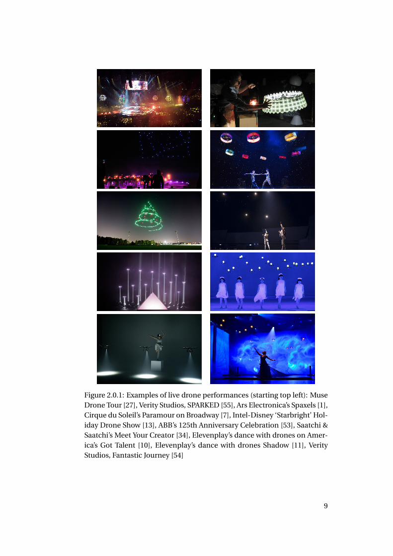
Figure 2.0.1: Examples of live drone performances (starting top left): MuseDrone Tour [27], Verity Studios, SPARKED [55], Ars Electronica’s Spaxels [1],Cirque du Soleil’s Paramour on Broadway [7], Intel-Disney ‘Starbright’ Hol-iday Drone Show [13], ABB’s 125th Anniversary Celebration [53], Saatchi &Saatchi’s Meet Your Creator [34], Elevenplay’s dance with drones on Amer-ica’s Got Talent [10], Elevenplay’s dance with drones Shadow [11], VerityStudios, Fantastic Journey [54]
9
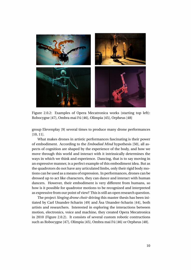
Figure 2.0.2: Examples of Opera Mecatronica works (starting top left):Robocygne [47], Ombra mai Fú [46], Olimpia [45], Orpheus [48]
group Elevenplay [9] several times to produce many drone performances[10, 11].
What makes drones in artistic performances fascinating is their powerof embodiment. According to the Embodied Mind hypothesis [50], all as-pects of cognition are shaped by the experience of the body, and how wemove through this world and interact with it intrinsically determines theways in which we think and experience. Dancing, that is to say moving inan expressive manner, is a perfect example of this embodiment idea. But asthe quadrotors do not have any articulated limbs, only their rigid body mo-tions can be used as a means of expression. In performances, drones can bedressed up to act like characters, they can dance and interact with humandancers. However, their embodiment is very different from humans, sohow is it possible for quadrotor motions to be recognized and interpretedas expressive from our point of view? This is still an open research question.
The project Singing drone choir driving this master thesis has been ini-tiated by Carl Unander-Scharin [49] and Åsa Unander-Scharin [44], bothartists and researchers. Interested in exploring the interactions betweenmotion, electronics, voice and machine, they created Opera Mecatronicain 2010 (Figure 2.0.2). It consists of several custom robotic contructionssuch as Robocygne [47], Olimpia [45], Ombra mai Fú [46] or Orpheus [48].
10
Chapter 3
Background
3.1 Modelling the dynamics of a quadrotor X
3.1.1 The X design
There are two main designs for quadrotors: “+” and “X”. In the literature,the dynamics is usually modelled for design “+”, with the four rotors in thefront, rear, left and right of the drone. The design we have chosen is “X”,with rotors positioned front left, front right, rear left, rear right. Of coursethe dynamics is the same, the only difference is a change of coordinates.
By construction, the center of mass G of the drone is at the same dis-tance ` (the arm length of the quadrotor) to each of the rotor axes. Therotors are numbered 1 to 4 according to the PX4 convention, with rotors 1and 2 turning counterclockwise and rotors 3 and 4 turning clockwise. Weset ε1 = ε2 = 1 and ε3 = ε4 =−1 to keep track of the rotation direction. Theangles between the forward axis and each arm
# »GRi (where Ri is the inter-
section of the axis of rotor i and the horizontal plane through G) are respec-tivelyΦ1 =−π/4,Φ2 = 3π/4,Φ3 =π/4, andΦ4 =−3π/4.
3.1.2 Reference frames
We shall use two reference frames. The first one, (A), is linked with thetheatre stage and is assumed to be an inertial frame. Its reference pointO is on the ground at the center of the stage, and axes are given by unitvectors #»a1 (pointing right when viewed from the audience), #»a2 (pointing tothe back), and #»a3 (pointing up). The second one, (B), is linked to the drone,centered on its center of mass G , and has unit vectors
#»
b1 (pointing forward),
11
#»
b2 (pointing left), and#»
b3 (pointing up).Note that this choice follows the usual conventions of ROS [31].
3.1.3 Rigid body dynamics
Let R be the rotation matrix that converts vector coordinates in (B) to co-ordinates in (A). The columns of (R) are the coordinates of the vectors
#»
b1,#»
b2,#»
b3 expressed in (A). The matrix R defines the attitude of the quadrotor,while its position is given by the vector ξ= # »
OG .The velocity of the quadrotor is described by its linear velocity v (in (A))
and its angular velocity Ω (in (B)), which is a vector pointing along the ro-tation axis. Angular velocity can also be represented by a skew-symmetricmatrixΩ× such thatΩ×u =Ω×u for any vector u.
The dynamics of the drone is then given by the equations:
ξ = v (3.1.1)
mv = −mg #»a3 +RF (3.1.2)
R = RΩ× (3.1.3)
I Ω = −Ω× IΩ+τ (3.1.4)
where m is the mass of the quadrotor and I its inertia matrix expressed in(B). The term −mg #»a3 is the gravitation force (pointing down). Finally, F isthe sum of all aerodynamic forces, and τ is the resulting torque.
3.1.4 Action of one rotor
The aerodynamics of rotors is rather complicated. But, for controlling adrone, an approximate model is sufficient. We will thus assume, for themoment, that the forces are independent of the relative motion of the airaround the drone: that is, we will assume that the drone is hovering. Also,we will neglect aerodynamic forces on the body of the drone. Then F and τare just the sum of the corresponding vectors for each rotor:
F =4∑
i=1Fi (3.1.5)
τ =4∑
i=1τi (3.1.6)
Aerodynamic forces on a single blade of a rotor can be decomposedas the sum of lift (vertical upwards, assuming the axis of the rotor is ver-tical) and drag (horizontal and opposed to motion), as with an airplane
12
wing. When the rotor is hovering, the lift on the blades sum up and pro-duce thrust Ti , while drag cancels but produces torque. So we have
Ti = cTω2i (3.1.7)
Qi = cQω2i (3.1.8)
where cQ and cT are constants that depend on rotor radius, rotor geometry,and air density, and are in practice determined by bench tests, while ωi isthe rotation speed of the rotor.
We then have
Fi = Ti#»
b3 (3.1.9)
τi = Ti# »GRi × #»
b3 −εi Qi#»
b3 (3.1.10)
3.1.5 Combined action of the rotors
Since# »GRi = `cosΦi
#»
b1 +`sinΦi#»
b2, we have:
τi = (`cT sinΦi#»
b1 −`cT cosΦi#»
b2 −εi cQ#»
b3)ω2i
For a quadrotor X, this is best expressed in matrix form :
(Tτ
)= Γ
ω2
1ω2
2ω2
3ω2
4
where Γ is the matrix
Γ=
cT cT cT cT
−CTp
2/2 cTp
2/2 cTp
2/2 −CTp
2/2−CT
p2/2 cT
p2/2 −CT
p2/2 cT
p2/2
−cQ −cQ cQ cQ
which is clearly invertible: given any desired vertical thrust and moment,the rotor speeds to achieve that effect can thus be computed.
3.2 Motion planning strategiesMotion planning is an essential problem in robotics and especially in robotautomation. From an initial configuration (position, orientation) to a final
13
configuration, its aims is to find a collision-free motion with its set of in-puts (forces, torques, etc.) in a specified environment. In other words, mo-tion planning is the process of selecting, among all possible motions andall their possible input sets, a motion with a corresponding set of inputsthat ensures that all constraints are satisfied. Therefore, it depends on themodel of the robot and its environment. The process to follow a plannedmotion is called control and it is not the focus of this section.
Several ways to classify motion planning strategies are proposed in theliterature. One way is to distinguish global methods from local ones. Globalstrategies ensure that if there exist collision-free trajectories between thecurrent robot configuration and its goal, the robot will try to follow onesuch trajectory. Usually, such strategies plan in advance the trajectory, andtry to make it optimal for some criterion (shortest distance, shortest time,least energy consumption, etc.). In contrast, local strategies aim to avoidunexpected obstacles (unmodelled or moving) by reacting to the robot en-vironment. However, we decide to follow another classification [18] thatdistinguishes implicit motion plans from explicit ones.
3.2.1 Implicit methods
Implicit motion strategies do not explicitly compute the trajectories beforethe motion starts. The motion is never pre-computed. Instead they definehow the robot interacts with its surroundings by specifying how it respondsto its sensory information.
Potential field. One such method is the potential field method [15, 16]. Inthis method an artificial potential is associated to all the obstacles and tothe goal, similar to the potential associated to conservative physical forcessuch as electrostatic forces. The robot has to follow the negative gradientof the potential until it reaches a local minimum, for instance by taking thenegative gradient as input for a velocity controller.
The potential function can be freely chosen and does not need to modelany existing physical force. However, it has to be smooth enough, minimalat the goal and maximal at the obstacles. Usually, this potential is chosenwith limited range so that the obstacle does not interfere with the motion ofthe robot when the robot is far from it. For instance, the following formula
14
is often used for the repulsive potential and the associated force:
V = β
(1
min(q,`)− 1
`
)2
(3.2.1)
#»F =
#»0 if q > `−2β
#»qq3
(1q − 1
`
)if q < ` (3.2.2)
where #»q is the vector from the obstacle to the robot, ` is the (constant)range of the force and β a coefficient.
This method has several advantages: it is computationally light, noprior processing is needed, it adapts well to unexpected environmentchanges. It has also several drawbacks [17]: the robot may not reach itsgoal when it is trapped in another local minimum, it may not find a passagebetween obstacles that are near each other, and it may oscillate when itis close to obstacles. The resulting trajectory can be very different fromtrajectories obtained by other algorithms and far from optimal for usualmeasures. It is difficult to integrate the kinematic and dynamic constraintsof the robot.
In order to avoid being trapped by local minima one can use harmonicpotentials (that have only one minimum) or a navigation function [33].
3.2.2 Explicit methods
Explicit motion planning strategies explicitly compute the complete trajec-tory by producing a set of sub-goals. They plan the trajectory from startto goal before the motion occurs. We can further divide explicit strategiesbetween the discrete ones and the continuous ones.
Discrete methods
Such methods discretize the configuration space and represent it with agraph. Motion planning is therefore reduced to a graph search problem.As the potential method, discrete explicit strategies do not accommodatefor kinematic and dynamic constraints of the robot. However a two-stepstrategy could be used: first find a suitable motion plan with the methodand then restrict it to make sure it meets all the constraints of the robot.Among these methods we find two types of algorithms: road map and celldecomposition.
15
Road map. Road map algorithms consist in constructing a set of curvesthat connect the space. Then finding a path between two points comesdown to connecting these two points to the connectivity graph. Methodssuch as visibility graph, Voronoi graph, etc. can then be used.
Cell decomposition. Cell decomposition algorithms subdivide the con-figuration space into non-overlapping cells and then construct a connec-tivity graph based on the neighbour relations of these cells. To find a path,we simply need to connect the cells from the start to the goal, using a short-est path algorithm.
Continuous methods
Continuous explicit methods are similar to open loop control laws. Thereare two types of continuous methods: specific methods for nonholonomicsystems (also called underactuated systems), and optimal methods.
Underactuated systems. The methods in this family, based on controlla-bility tests, provide ways to generate motion plans for nonholonomic sys-tems [23]. Also known as steering methods, they come from nonlinear con-trol [4, 39]. Some of these methods can be used for dynamic motion plan-ning [3, 28].
Optimal methods. Finding an optimal trajectory for a constrained robotis find a solution to a minimization problem (optimal control) [21]. Forsolving optimal control problems, we often need to use numerical meth-ods, such as the method of neighbouring extremals [5], conjugate gradientsalgorithms [14, 20, 25, 26], discretization [40, 30], or finite-elements tech-niques [56].
3.3 DiscussionIn our project, the drones live in a dynamic environment. Apart from thefixed restrictions of our flying area (ground, artificial walls and ceiling) thedrones have to avoid each other and the moving dancer. Also, unlike intypical motion planning problems, our drones do not require optimal mo-tions. Instead, we would like them to have natural and smooth motionssuitable to express emotions and intents. This is why we have decided to
16
use an implicit motion planning method, namely potential fields. More de-tails about our motion planning strategy can be found in Chapter 6.
17
Chapter 4
Design and Buildingof the Quadrotors
In this chapter we present the construction steps of our quadrotors. Afterstudying the market of the commercially available drones we concludedthat we had to build custom drones for the purpose of this project.
We have several constraints: it needs to carry a speaker, be connectablevia wifi, have a long flight time and be as silent as possible. Indeed, thedrones will fly during a singing performance. So we need to be able to hearthe sound coming from their respective speaker and also the singing of thesingers when they are surrounded by those flying drones. We had to domany trade-offs to meet all our constraints.
4.1 Parts selectionLet us look at all the component parts we need and what role they play. It isimportant to note that all the components have been selected so that theyare quickly available. Therefore we have prioritised components availablein Swedish stores.
4.1.1 The frame
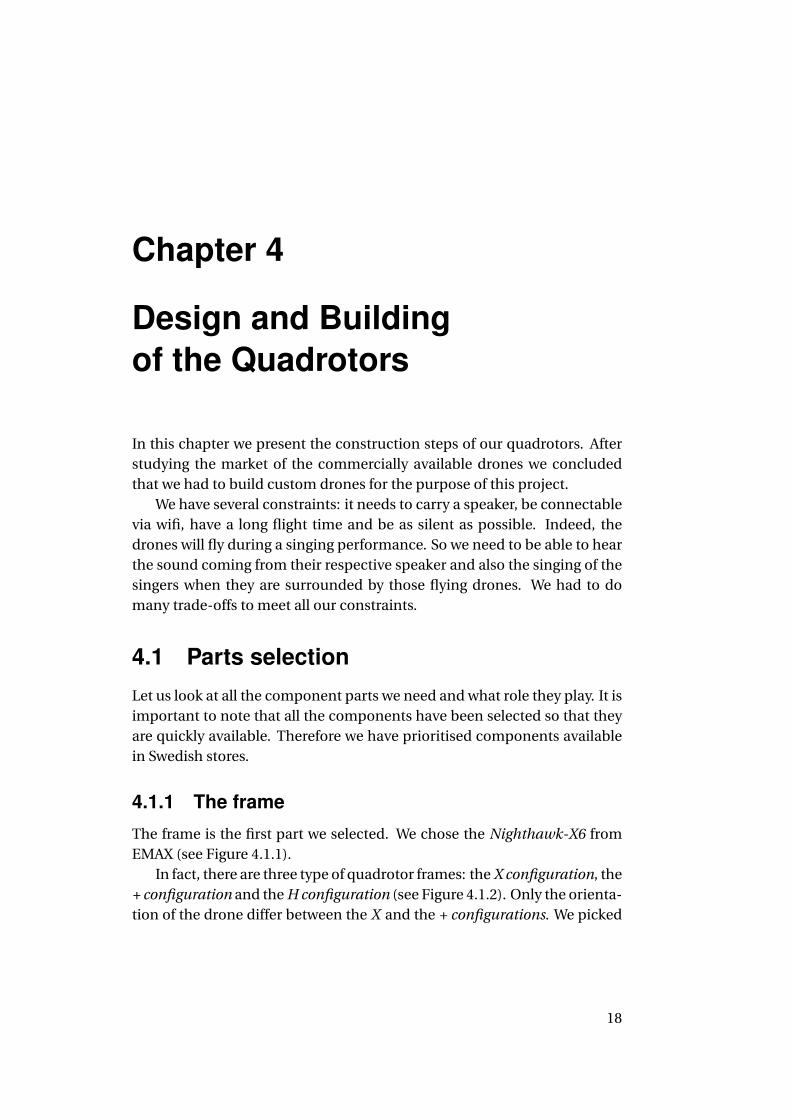
The frame is the first part we selected. We chose the Nighthawk-X6 fromEMAX (see Figure 4.1.1).
In fact, there are three type of quadrotor frames: the X configuration, the+ configuration and the H configuration (see Figure 4.1.2). Only the orienta-tion of the drone differ between the X and the + configurations. We picked
18
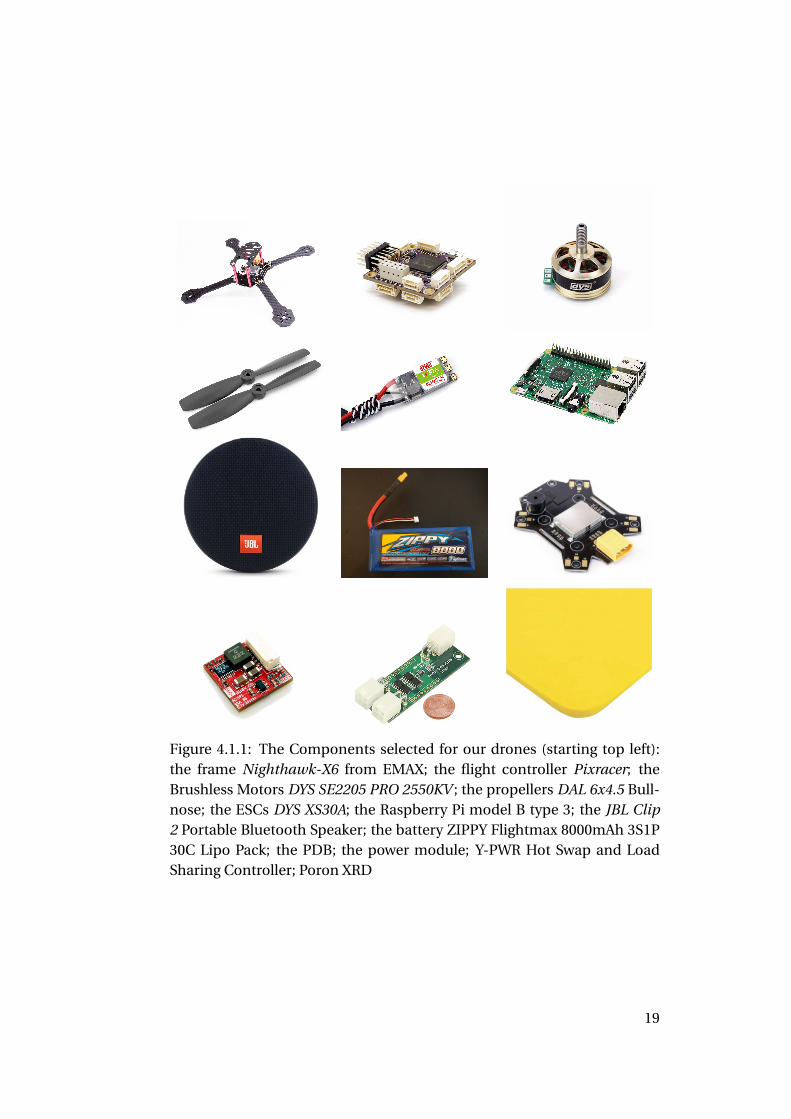
Figure 4.1.1: The Components selected for our drones (starting top left):the frame Nighthawk-X6 from EMAX; the flight controller Pixracer; theBrushless Motors DYS SE2205 PRO 2550KV ; the propellers DAL 6x4.5 Bull-nose; the ESCs DYS XS30A; the Raspberry Pi model B type 3; the JBL Clip2 Portable Bluetooth Speaker; the battery ZIPPY Flightmax 8000mAh 3S1P30C Lipo Pack; the PDB; the power module; Y-PWR Hot Swap and LoadSharing Controller; Poron XRD
19
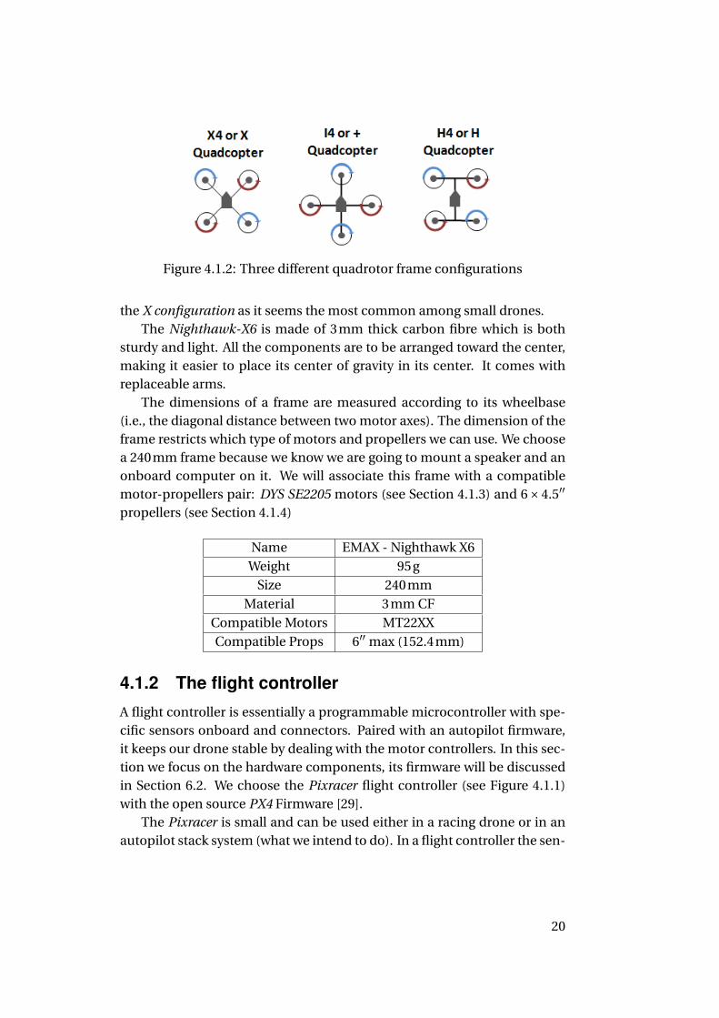
Figure 4.1.2: Three different quadrotor frame configurations
the X configuration as it seems the most common among small drones.The Nighthawk-X6 is made of 3mm thick carbon fibre which is both
sturdy and light. All the components are to be arranged toward the center,making it easier to place its center of gravity in its center. It comes withreplaceable arms.
The dimensions of a frame are measured according to its wheelbase(i.e., the diagonal distance between two motor axes). The dimension of theframe restricts which type of motors and propellers we can use. We choosea 240mm frame because we know we are going to mount a speaker and anonboard computer on it. We will associate this frame with a compatiblemotor-propellers pair: DYS SE2205 motors (see Section 4.1.3) and 6×4.5′′
propellers (see Section 4.1.4)
Name EMAX - Nighthawk X6Weight 95g
Size 240mmMaterial 3mm CF
Compatible Motors MT22XXCompatible Props 6′′ max (152.4mm)
4.1.2 The flight controller
A flight controller is essentially a programmable microcontroller with spe-cific sensors onboard and connectors. Paired with an autopilot firmware,it keeps our drone stable by dealing with the motor controllers. In this sec-tion we focus on the hardware components, its firmware will be discussedin Section 6.2. We choose the Pixracer flight controller (see Figure 4.1.1)with the open source PX4 Firmware [29].
The Pixracer is small and can be used either in a racing drone or in anautopilot stack system (what we intend to do). In a flight controller the sen-
20
Figure 4.1.3: Brushed DC motor vs brushless DC motor)
sors are the most important part since together with the firmware they per-form operations that keep the drone level and stable in the air. The Pixracerincludes:
• a ICM-20608-G 6-axis motion tracking device (3-axis accelerometer,3-axis gyroscope)
• a MPU-9250 9-axis motion tracking device (3-axis gyroscope, 3-axisaccelerometer, 3-axis magnetometer)
• a MEAS MS5611 barometer• a Honeywell HMC5983 magnetometer (temperature compensated)
As we will fly our drones indoors, we will only use the two motion track-ing devices with an external tracking system (see Chapter 5) to stabilize thedrones.
The flight controller connectors allows us to attach this control unit tothe motors, the battery, the RC controller and the onboard computer. Wediscuss the wiring of the Pixracer in Section 4.2.
The Pixracer also comes with a wifi module. It is meant to be used forwifi telemetry and firmware update and cannot be used for calibrating thesensors or receiving control commands. Because we will have an onboardcomputer, we decide to leave this component aside.
Name PixracerWeight 10.54g
Size 36×36mmSoftware PX4
4.1.3 The motors
The motors make the quadrotor fly by spinning the propellers. We chosethe DYS SE2205 PRO 2550KV Brushless Motors (see Figure 4.1.1). Two ofthem have to rotate clockwise and the other two counterclockwise. Fordrones, we use brushless motors instead of classic DC motors (see Fig-ure 4.1.3). In a brushless motor the permanent magnets are on the ro-
21
tor (rotating part of the motor) and the electromagnets are on the stator(immobile part). Then it requires an Electronic Speed Controller (ESC) totake care of switching the voltage of these electromagnets to make the ro-tor spin. Such motor has several advantages: no more brushes that canbe worn-out or need to be cleaned, no more frictions. A brushless motor ismore efficient and allows a more precise speed control than a regular brushmotor. Also the electromagnets on the stator are easy to cool. The motorsare characterized by their size, their speed of revolution, their efficiency.They are usually named according to their size which is given by the di-ameter of the stater and its length. For instance the motors SE2205 have astator with a 22mm diameter and it is 5mm tall. Next to their name comestheir speed given by the KV Rating coefficient. In fact, the speed is mea-sured by the number of revolution per minute (rpm) the motor will spin atfull throttle given a voltage. And specifically
Number of revolutions per minute = KV ×voltage
In our case at 11.1V, at full throttle our motors can speed at up to 28305 rev-olutions per minute (∼ 471 revolutions per second)! The thrust generatedby the motors depends on its KV Rating, the type of propeller it is associatedwith and the quantity of power it can instantaneously draw from the ESCand the battery. Indeed, an increase in the thrust implies a higher currentincoming from the battery. In physics we usually measure it in Newton (N,i.e. kg ·m · s−2) but in drone construction it is expressed in grammes (g). Ifour quadrotor weights 2kg (which is less than the final weight of our drone)then each motor need to produce 500g of thrust to make it takeoff. On thetechnical data sheet (Figure 4.1.4) we can see that with those motors, if ourdrone is less than 2kg, it will have no problem to takeoff.
Efficiency of the motor is measured by the power coming out dividedby the power coming in. Basically the efficiency measures the percentageof the incoming power transform into motion. The more efficient a motoris, the longer the drone will fly. And as a rule of thumb anything above7gW−1 is considered good.
Name DYS SE2205 PRO 2550KVWeight 29g
Motor dimensions 27.7×19.0mm (diameter × height)Stator Diameter 22mm
Stator Length 5mmKV 2550rpm/V
Max. Continuous Current (A) 27.8A
22
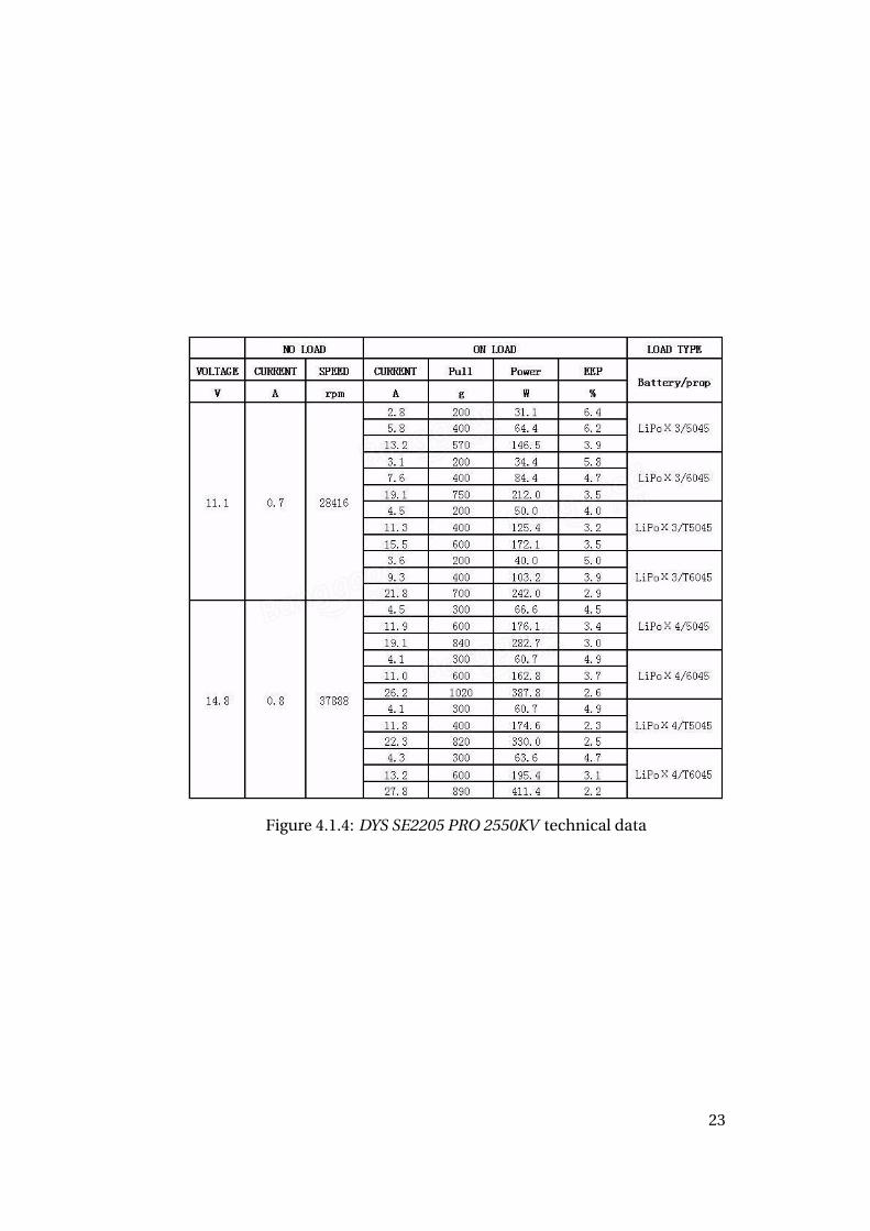
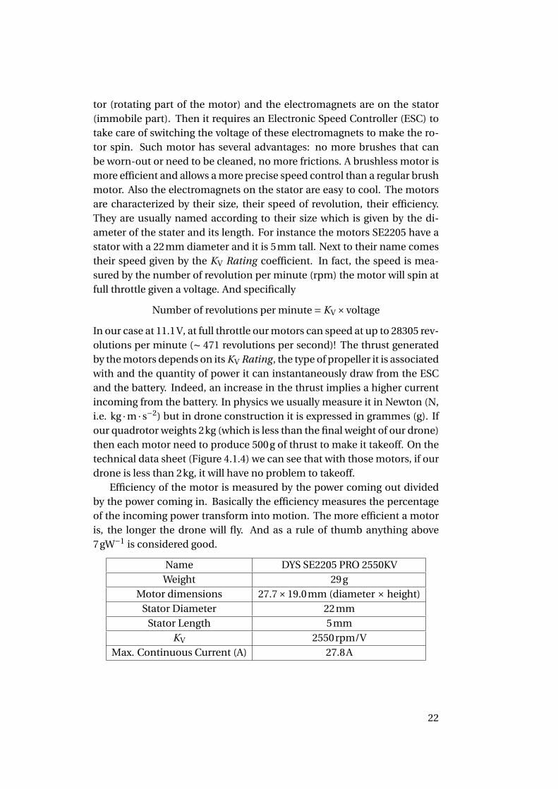
Figure 4.1.4: DYS SE2205 PRO 2550KV technical data
23
Figure 4.1.5: Electronic Speed Controller Schematic
4.1.4 The propellers
We choose the HQProp 6x4.5R propellers (see Figure 4.1.1). There are sev-eral types of propellers depending on their material, their dimensions, theirpitch, their number of blades and their shape.
The material used to make the props influences the flight characteris-tics but it will also influence its potential to hurt and wound a human op-erator. However, we should not forget about safety. That is why we chosethem to be in plastic instead of carbon fibre. The propellers are measuredby their diameters in inches. For instance, 6′′ prop (15.24cm) correspondto approximately 7.5cm blade. The pitch of a propeller is measured as adistance (usually in inches) instead of degree. It corresponds to the ver-tical distance a horizontal propeller would move after one revolution if itdidn’t slip. The difference between a two-blade propeller and a three-bladeone is in the thrust produced for a fix material, dimension and pitch. Thethree-blade propeller can reach higher thrust, but then they draw more cur-rent making the drone consume more power. Also, some propellers have ashape called “bullnose”. It means that the end of the blade is larger than thenormal ones.
Name DAL 6x4.5 Bullnose Propeller v2Weight 3.8g
Material PlasticNumber of blades 2
Shape BullnoseDiameter 6′′ (15.24cm)
Pitch 4.5′′
4.1.5 The ESC
We choose the DYS XS30A ESCs for our drone (see Figure 4.1.1).An ESC (Electronic Speed Controller) controls the speed of a brushless
motor. It has three sets of wires: one set to connect to the battery, one
24
to connect to the radio receiver or the flight controller and another one toconnect to the motor. It receives an input ppm signal (pulse position mod-ulation) from the receiver (or flight controller) which indicates how muchpower it should send to the motor. A brushless ESC has three wires to con-nect to the motor but only two are energized at any given time. The wirethat is not energized tells the ESC in which direction and how fast the motorspins by generating a small voltage proportional to the speed of the motor.That way the ESC knows how to adjust the charge of the electromagnetsto follow the speed instruction from the receiver or the flight controller.Also, the ESC must be able to handle the maximum current that the motorcan draw. That is why the ESCs are rated for a maximum current. In ourcase, the maximum continuous current that can be drawn from the motoris 27.8A, so no problem for our 30A ESCs.
Name DYS XS30A BLHeli_S Firmware 3-6S 8BB2 ESC for MulticopterWeight 8.6g
Size 45×16×6mmMax. Continuous Current 30A
Firmware BLHeli
4.1.6 The onboard computer
We choose the Raspberry Pi model B type 3 as our onboard computer (seeFigure 4.1.1). With its 1.2 GHz 64-bit quad-core ARM Cortex-A53 CPU andits 1GB SDRAM memory, it allows us to run our robotic software platformROS and to control the music playlist for each drone.
4.1.7 The speaker
Our sound system consists of a JBL Clip 2 speaker (see Figure 4.1.1). Withits small size 141×94×42mm and light weight 184g, this speaker can reachup to 3W of output power with up to 8 hours of play time.
4.1.8 The battery
We choose ZIPPY Flightmax 8000mAh 3S1P 30C Lipo battery (see Fig-ure 4.1.1). A lipo battery is characterized by its voltage (number of cells), itscapacity, its discharge rate, its weight and its size. A battery is constructedfrom rectangular cells which are connected together. Each cell holds a
25
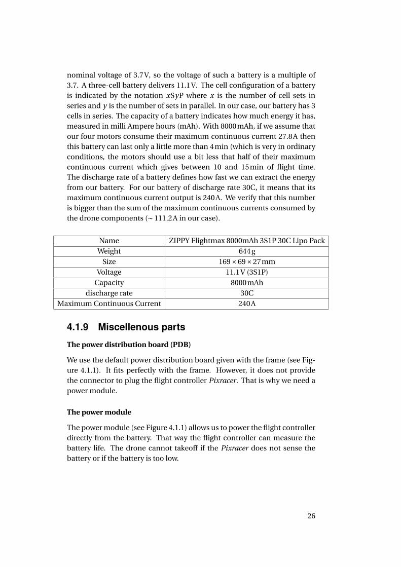
nominal voltage of 3.7V, so the voltage of such a battery is a multiple of3.7. A three-cell battery delivers 11.1V. The cell configuration of a batteryis indicated by the notation xSyP where x is the number of cell sets inseries and y is the number of sets in parallel. In our case, our battery has 3cells in series. The capacity of a battery indicates how much energy it has,measured in milli Ampere hours (mAh). With 8000mAh, if we assume thatour four motors consume their maximum continuous current 27.8A thenthis battery can last only a little more than 4min (which is very in ordinaryconditions, the motors should use a bit less that half of their maximumcontinuous current which gives between 10 and 15min of flight time.The discharge rate of a battery defines how fast we can extract the energyfrom our battery. For our battery of discharge rate 30C, it means that itsmaximum continuous current output is 240A. We verify that this numberis bigger than the sum of the maximum continuous currents consumed bythe drone components (∼ 111.2A in our case).
Name ZIPPY Flightmax 8000mAh 3S1P 30C Lipo PackWeight 644g
Size 169×69×27mmVoltage 11.1V (3S1P)
Capacity 8000mAhdischarge rate 30C
Maximum Continuous Current 240A
4.1.9 Miscellenous parts
The power distribution board (PDB)
We use the default power distribution board given with the frame (see Fig-ure 4.1.1). It fits perfectly with the frame. However, it does not providethe connector to plug the flight controller Pixracer. That is why we need apower module.
The power module
The power module (see Figure 4.1.1) allows us to power the flight controllerdirectly from the battery. That way the flight controller can measure thebattery life. The drone cannot takeoff if the Pixracer does not sense thebattery or if the battery is too low.
26
Hot Swap, Load Sharing Controller
The Y-PWR (see Figure 4.1.1) is used to perform a smooth transition be-tween AC/DC wall adapter and battery to power the onboard computer,the flight controller, and the RC receiver. Thanks to this component, wecan work on the onboard computer connected to the flight controller with-out powering the motors.
Poron XRD
Due to our design constraints we cannot put the pixracer on a traditionalanti vibration mount preventing the vibrations from the frame to interferewith the sensors of the autopilot. So we decided to use a small sheet (3mm)of poron XRD to isolate the flight controller (see Figure 4.1.1). Poron XRDwith its open-cell technology is often used as a cushioning and impact pro-tection solution (it is used in athletic shoes, etc.).
4.2 The designNow that all the parts have been selected, we create a CAD design to struc-ture our assembly process. In Figure 4.2.1, from bottom to top we have thebattery (in yellow), a level containing the Raspberry Pi (in black) with theHot Swap, Load Sharing Controller (in salmon), the main body of the frame(in grey), the Pixracer (in red) and on top the speaker (in black). The partsto expand the frame have been cut and drilled by ourselves.
As we can see in Figure 4.2.2, we have not yet mounted the speaker. Forthe moment the top of the drone is used to place the markers used for thelocalization.
The schematic representation in Figure 4.2.3 explains how the power isdistributed in the drone. There are two possible sources of power but onlythe battery can power the motors and therefore make the drone takeoff.The speaker is not linked with the other components in this representationbecause it has an independent battery: it does not use the power from thedrone battery. It is simply connected to the Raspberry Pi via the 3.5mmaudio jack.
27
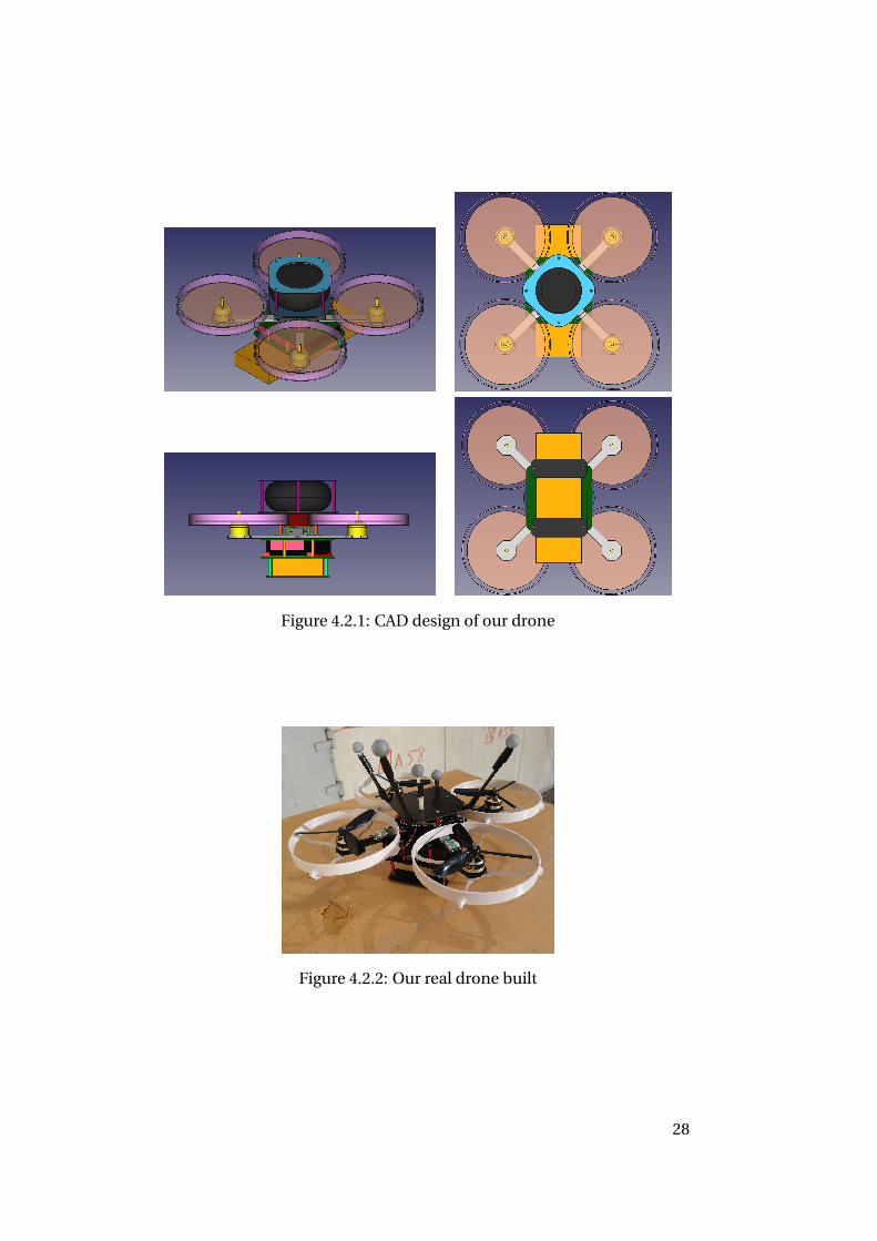
Figure 4.2.1: CAD design of our drone
Figure 4.2.2: Our real drone built
28
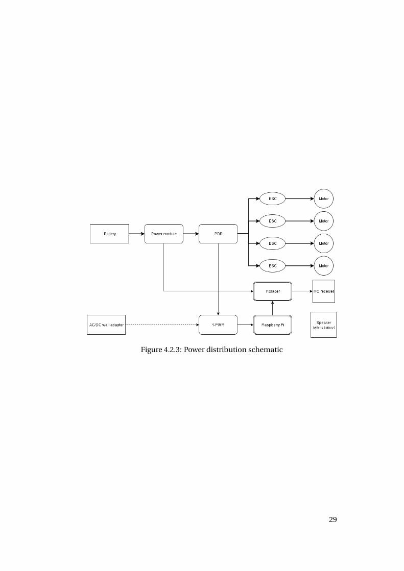
Figure 4.2.3: Power distribution schematic
29
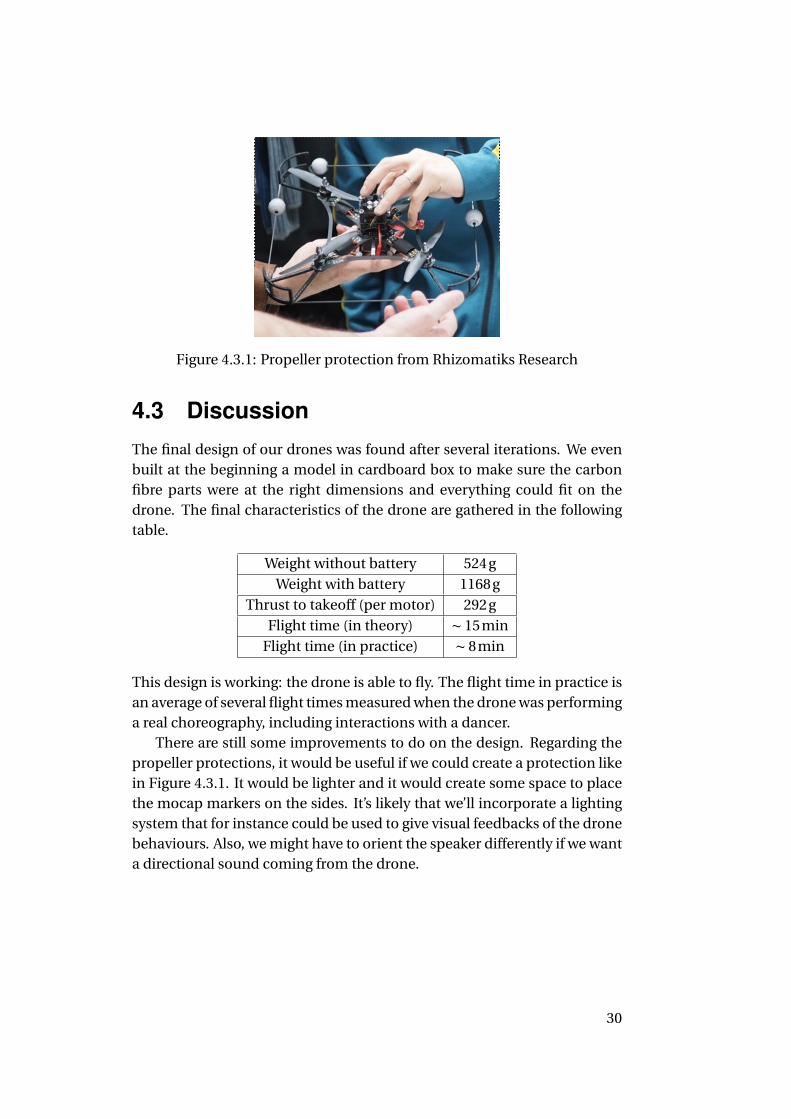
Figure 4.3.1: Propeller protection from Rhizomatiks Research
4.3 DiscussionThe final design of our drones was found after several iterations. We evenbuilt at the beginning a model in cardboard box to make sure the carbonfibre parts were at the right dimensions and everything could fit on thedrone. The final characteristics of the drone are gathered in the followingtable.
Weight without battery 524gWeight with battery 1168g
Thrust to takeoff (per motor) 292gFlight time (in theory) ∼ 15min
Flight time (in practice) ∼ 8min
This design is working: the drone is able to fly. The flight time in practice isan average of several flight times measured when the drone was performinga real choreography, including interactions with a dancer.
There are still some improvements to do on the design. Regarding thepropeller protections, it would be useful if we could create a protection likein Figure 4.3.1. It would be lighter and it would create some space to placethe mocap markers on the sides. It’s likely that we’ll incorporate a lightingsystem that for instance could be used to give visual feedbacks of the dronebehaviours. Also, we might have to orient the speaker differently if we wanta directional sound coming from the drone.
30
Chapter 5
The Stage:Setting up the Flying Area
In this section we present our flying area. First, we describe its current loca-tion, its position tracking system, its network/software setup and its safetymeasures. Second, we analyse and discuss its characterisitics.
5.1 The locationWhen the project started in September 2016, the RPL lab didn’t have a flyingarea for drones. And because the drone choir is meant to be performedindoors at different locations, we decided to setup an independent flyingarea for this project. This area had to be large enough to allow five dronesand one dancer to wander freely inside.
Thanks to the artistic value of this project, we settled down in KTH R1.R1 was Sweden’s first experimental nuclear reactor. It was in operation un-til 1970. After its dismantling around 1982 and its radioactive decontam-ination period, it became in 2007 part of KTH as a cultural experimentalcenter. Focused on the interconnection between science and art, a num-ber of different installations, performances and projects have been carriedout there.
5.2 HardwareTo track the position of the quadrotors we use an OptiTrack Motion Cap-ture System (MoCap). Currently it consists of 8 OptiTrack Flex 13 Cameras
31
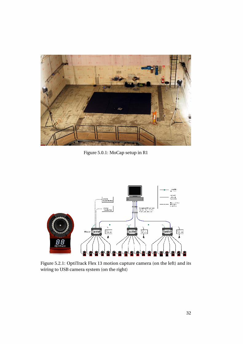
Figure 5.0.1: MoCap setup in R1
Figure 5.2.1: OptiTrack Flex 13 motion capture camera (on the left) and itswiring to USB camera system (on the right)
32
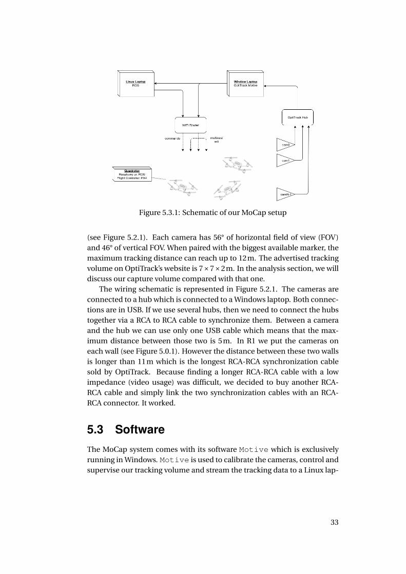
Figure 5.3.1: Schematic of our MoCap setup
(see Figure 5.2.1). Each camera has 56° of horizontal field of view (FOV)and 46° of vertical FOV. When paired with the biggest available marker, themaximum tracking distance can reach up to 12m. The advertised trackingvolume on OptiTrack’s website is 7×7×2m. In the analysis section, we willdiscuss our capture volume compared with that one.
The wiring schematic is represented in Figure 5.2.1. The cameras areconnected to a hub which is connected to a Windows laptop. Both connec-tions are in USB. If we use several hubs, then we need to connect the hubstogether via a RCA to RCA cable to synchronize them. Between a cameraand the hub we can use only one USB cable which means that the max-imum distance between those two is 5m. In R1 we put the cameras oneach wall (see Figure 5.0.1). However the distance between these two wallsis longer than 11m which is the longest RCA-RCA synchronization cablesold by OptiTrack. Because finding a longer RCA-RCA cable with a lowimpedance (video usage) was difficult, we decided to buy another RCA-RCA cable and simply link the two synchronization cables with an RCA-RCA connector. It worked.
5.3 SoftwareThe MoCap system comes with its software Motive which is exclusivelyrunning in Windows. Motive is used to calibrate the cameras, control andsupervise our tracking volume and stream the tracking data to a Linux lap-
33
top (Debian Jessie) via an Ethernet cable (see Figure 5.3.1). Motive usesthe NatNet streaming protocol to stream the tracking data.
We use the ROS package mocap_optitrack to parse the incomingstreaming data from Motive into tf transforms and poses usable in theROS environment.
We setup a local network which is not connected to the Internet insideR1, so that the Linux laptop can communicate with the drones via wifi. Be-cause each drone has an onboard computer also running ROS, the com-munication between the Linux laptop and the drones consists of ROS in-ternal messages. And the onboard computer will translate the flight in-structions to the flight controller via the MAVLink protocol thanks to thepackage mavros.
5.4 Safety measuresIn the flying area, safety measures are important not only to protect thesurrounding humans from hazardous drone behaviours but also to preventthe drones from destructing themselves when they crash.
On the ground we put six foam mattresses (210×182×35mm) to coveran area of 22m2. We restrict the flying area to the surface covered by thosemats so that it now measures 4.20× 5.46m. To protect the mats we hadplanned to put a plastic cover over them. However it turned out that theplastic was interfering with the tracking system and had to be removed.Instead we use simple black bed sheets. They provide protection for themats against dust, add more resistivity for the drone landings/crashes, andallow a better control of the tracking area regarding unwanted reflections.
It was not possible to put nets around the flying area. So we decided toattach each drone to a weight via a fishing wire. The wire is light enoughto not disturb the drone flight and rigid enough to prevent it from goingbeyond the flying area borders.
5.5 DiscussionIn our current setup the disposition of the cameras is not optimal. Thevolume covered by a MoCap depends heavily on how the cameras are po-sitioned, which depends on where we setup our flying area. In R1, to max-imize the stage area, we needed to put the cameras on the walls. However,by doing so, the mattress area which is half of the maximum advertised cov-
34
ered area is at the border of our tracked volume. Also, by having the cam-eras that far from the center of the stage (11m), it makes it hard to trackthe drone for two reasons: first, it is difficult to place the markers on thedrone so that the MoCap software does not consider two different markersas one due to the camera angle views. Second, as soon as a dancer stepsinto the flying area, he or she interferes with the tracking volume: in somepositions the dancer can prevent the MoCap from tracking the drone po-sition. We are conscious that our security measures are really rudimentary(no net). In fact, the main part of our safety measures relies on our controlbased on potential fields. Attaching the drone to a weight with a wire is onlyused for testing experimental features and making sure that our potentialscan keep the drone and the dancer safe.
35
Chapter 6
Control of the Quadrotorsand Implementation
In this chapter we present our motion planning and control strategy. Wedo not aim toward an accurate control of the trajectory with an optimizedpath planning. Our goal is to come up with a simple strategy preventingcollisions suitable for creating an expressive choreography.
We choose to use ROS Kinetic Kame as our robotics software plat-form. And all our implementation is done in C++. In ROS [31], a processperforming a computation is called a node. Several nodes can communi-cate with each other via streaming topics, RPC services, and the ParameterServer. In this chaper and the following we will refer to our code and ourimplementation in those terms.
First, we give an overview of our control architecture when we have onedrone and multiple drones. Then we dive in each control level, detailing itstheory and its implementation.
6.1 General control architectureWe have divided our control architecture into three levels: a low, a middleand high level (see Figure 6.1.1).
At the highest level, we have implemented a choreography controllerthat orchestrates and synchronizes the motions of all the drones with thedancer and the music. This node runs on the Linux laptop, receives thechoreography and the music playback instructions for all drones and allof the tracked positions coming from the MoCap. Then it distributes thatinformation to the drones.
36
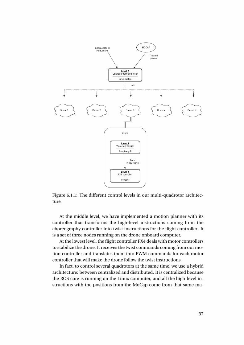
Figure 6.1.1: The different control levels in our multi-quadrotor architec-ture
At the middle level, we have implemented a motion planner with itscontroller that transforms the high-level instructions coming from thechoreography controller into twist instructions for the flight controller. Itis a set of three nodes running on the drone onboard computer.
At the lowest level, the flight controller PX4 deals with motor controllersto stabilize the drone. It receives the twist commands coming from our mo-tion controller and translates them into PWM commands for each motorcontroller that will make the drone follow the twist instructions.
In fact, to control several quadrotors at the same time, we use a hybridarchitecture: between centralized and distributed. It is centralized becausethe ROS core is running on the Linux computer, and all the high-level in-structions with the positions from the MoCap come from that same ma-
37
chine. However, our system is distributed in the sense that all the com-putations relative to a given drone are done inside this drone. Also, eachdrone can deduce its position thanks to its onboard sensors so that it canmove based on that position estimate only.
6.2 Control by the PX4 flight controllerThe PX4 is an open source autopilot software. Flashed on the flight con-troller component of our drone (Pixracer), it uses onboard sensors and tele-operation inputs to fly and stabilize the quadrotor. In fact, it has severalways (flight modes) to do that. In our case we will use only its Offboardmode and Land mode. In Offboard mode, a position, velocity or atti-tude set point is provided by an onboard computer connected via serialcable and MAVLink (Mavros package in ROS). Then it uses that input tocontrol the speed of the motors to make the drone follow that input.
In our case we use velocity set points, that are sent to Mavros via theROS topic /mavros/setpoint_velocity/cmd. Also, in order to en-ter this mode, the publishing rate of the set points must be faster than 2Hz, otherwise the quadrotor will fall back to the last mode the vehicle wasin before entering Offboard mode. In Land mode, the drone lands on theground from its current position. But the drone can drift a bit during thismode.
6.3 Trajectory control: Using potentialsWe control the movements of the drones using artificial potential fields (seethe discussion of different motion planning strategies in Section 3.2). Thisallows to direct the drones toward the desired points while avoiding colli-sions.
At each cycle, the controller of each drone computes the gradient ofthe potential, to obtain a force that is the sum of the attraction of the goaland the repulsion of the obstacles. Non-conservative forces are added: airresistance, to cause some damping, and optionally a rotational force thatwill force the drone to move in circles around its goal instead of remain-ing static. Then we integrate this force to control the speed of the drones.Specifically, for a drone at the nth iteration, we have:
# »Fn = −#»∇(Vrep,n +Vatt,n) (6.3.1)
# »sn+1 = #»sn (1−λ)+ # »Fnτ (6.3.2)
38
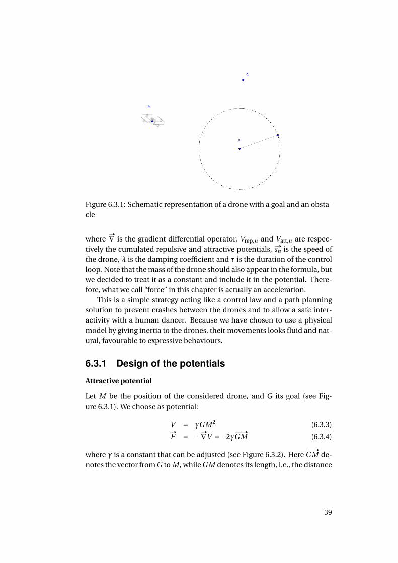
Figure 6.3.1: Schematic representation of a drone with a goal and an obsta-cle
where#»∇ is the gradient differential operator, Vrep,n and Vatt,n are respec-
tively the cumulated repulsive and attractive potentials, #»sn is the speed ofthe drone, λ is the damping coefficient and τ is the duration of the controlloop. Note that the mass of the drone should also appear in the formula, butwe decided to treat it as a constant and include it in the potential. There-fore, what we call “force” in this chapter is actually an acceleration.
This is a simple strategy acting like a control law and a path planningsolution to prevent crashes between the drones and to allow a safe inter-activity with a human dancer. Because we have chosen to use a physicalmodel by giving inertia to the drones, their movements looks fluid and nat-ural, favourable to expressive behaviours.
6.3.1 Design of the potentials
Attractive potential
Let M be the position of the considered drone, and G its goal (see Fig-ure 6.3.1). We choose as potential:
V = γGM 2 (6.3.3)#»F = −#»∇V =−2γ
# »GM (6.3.4)
where γ is a constant that can be adjusted (see Figure 6.3.2). Here# »GM de-
notes the vector from G to M , while GM denotes its length, i.e., the distance
39
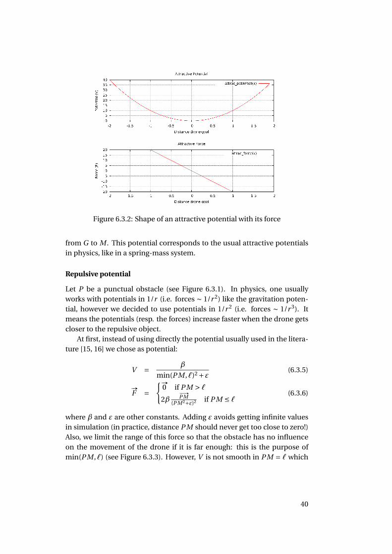
Figure 6.3.2: Shape of an attractive potential with its force
from G to M . This potential corresponds to the usual attractive potentialsin physics, like in a spring-mass system.
Repulsive potential
Let P be a punctual obstacle (see Figure 6.3.1). In physics, one usuallyworks with potentials in 1/r (i.e. forces ∼ 1/r 2) like the gravitation poten-tial, however we decided to use potentials in 1/r 2 (i.e. forces ∼ 1/r 3). Itmeans the potentials (resp. the forces) increase faster when the drone getscloser to the repulsive object.
At first, instead of using directly the potential usually used in the litera-ture [15, 16] we chose as potential:
V = β
min(P M ,`)2 +ε (6.3.5)
#»F =
#»0 if P M > `2β
# »P M
(P M 2+ε)2 if P M ≤ ` (6.3.6)
where β and ε are other constants. Adding ε avoids getting infinite valuesin simulation (in practice, distance P M should never get too close to zero!)Also, we limit the range of this force so that the obstacle has no influenceon the movement of the drone if it is far enough: this is the purpose ofmin(P M ,`) (see Figure 6.3.3). However, V is not smooth in P M = ` which
40
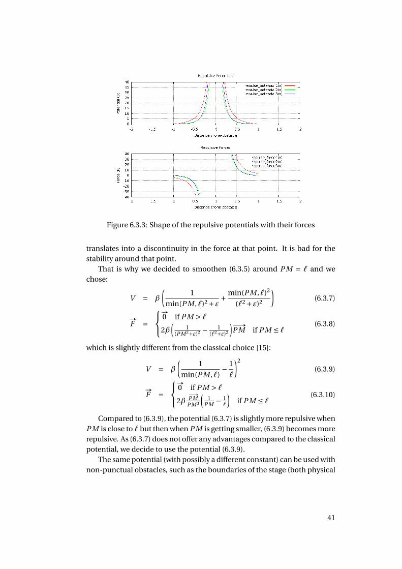
Figure 6.3.3: Shape of the repulsive potentials with their forces
translates into a discontinuity in the force at that point. It is bad for thestability around that point.
That is why we decided to smoothen (6.3.5) around P M = ` and wechose:
V = β
(1
min(P M ,`)2 +ε +min(P M ,`)2
(`2 +ε)2
)(6.3.7)
#»F =
#»0 if P M > `2β
(1
(P M 2+ε)2 − 1(`2+ε)2
)# »P M if P M ≤ ` (6.3.8)
which is slightly different from the classical choice [15]:
V = β
(1
min(P M ,`)− 1
`
)2
(6.3.9)
#»F =
#»0 if P M > `2β
# »P M
P M 3
(1
P M − 1`
)if P M ≤ ` (6.3.10)
Compared to (6.3.9), the potential (6.3.7) is slightly more repulsive whenP M is close to ` but then when P M is getting smaller, (6.3.9) becomes morerepulsive. As (6.3.7) does not offer any advantages compared to the classicalpotential, we decide to use the potential (6.3.9).
The same potential (with possibly a different constant) can be used withnon-punctual obstacles, such as the boundaries of the stage (both physical
41
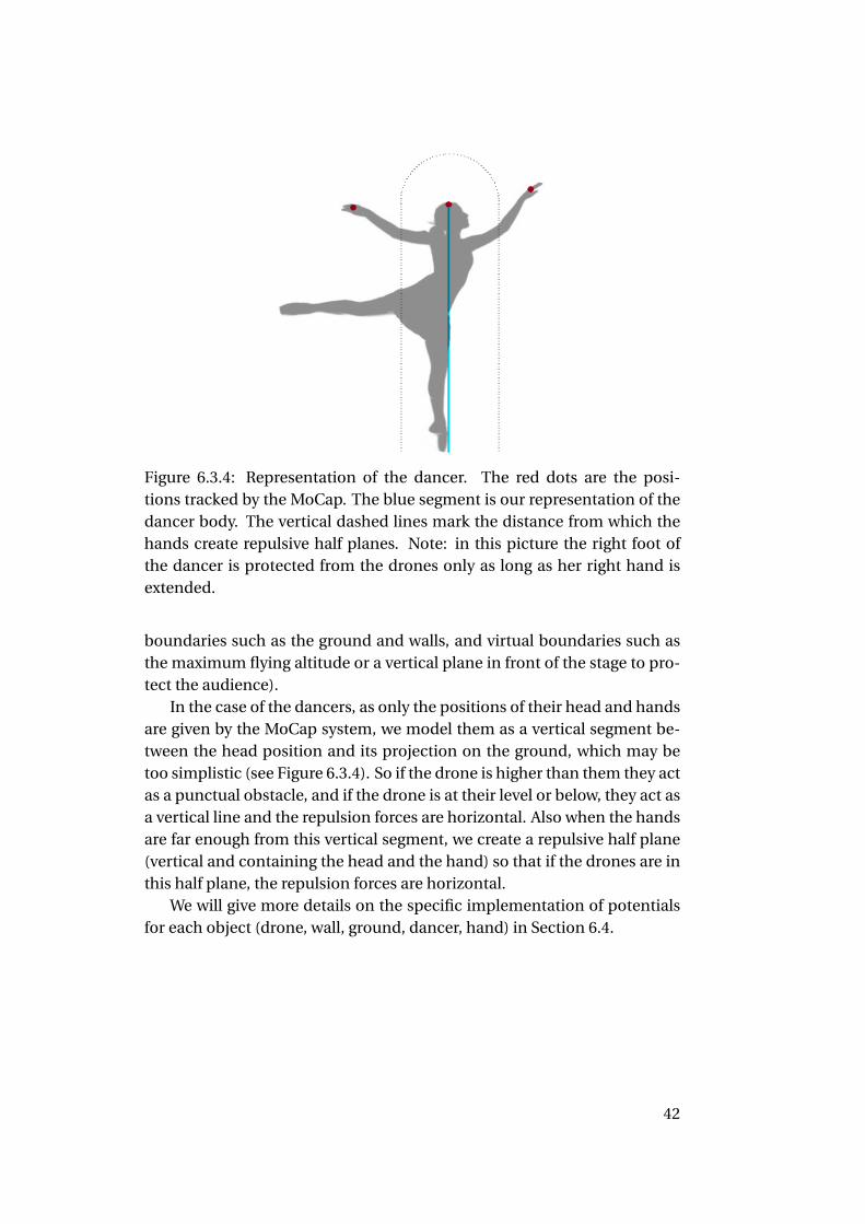
Figure 6.3.4: Representation of the dancer. The red dots are the posi-tions tracked by the MoCap. The blue segment is our representation of thedancer body. The vertical dashed lines mark the distance from which thehands create repulsive half planes. Note: in this picture the right foot ofthe dancer is protected from the drones only as long as her right hand isextended.
boundaries such as the ground and walls, and virtual boundaries such asthe maximum flying altitude or a vertical plane in front of the stage to pro-tect the audience).
In the case of the dancers, as only the positions of their head and handsare given by the MoCap system, we model them as a vertical segment be-tween the head position and its projection on the ground, which may betoo simplistic (see Figure 6.3.4). So if the drone is higher than them they actas a punctual obstacle, and if the drone is at their level or below, they act asa vertical line and the repulsion forces are horizontal. Also when the handsare far enough from this vertical segment, we create a repulsive half plane(vertical and containing the head and the hand) so that if the drones are inthis half plane, the repulsion forces are horizontal.
We will give more details on the specific implementation of potentialsfor each object (drone, wall, ground, dancer, hand) in Section 6.4.
42

Figure 6.3.5: Shape of a mixed potential with its force
Mixed potential
If we instruct the drone to go to a point which is also an obstacle (G = P ),the potential will be the sum of an attractive and a repulsive potential:
V = γP M 2 +β(
1
min(P M ,`)− 1
`
)2
(6.3.11)
#»F =
−2γ# »P M if P M > `
−2γ# »P M +2β
# »P M
P M 3
(1
P M − 1`
)if P M ≤ ` (6.3.12)
This will result in a minimum at a certain distance, where the drone willsettle (Figure 6.3.5).
When several drones are given the same goal (which may itself be anobstacle or not), they will take positions on a sphere centered around thatgoal, the radius of which depends on the number of drones due to the re-pulsion between drones. For instance, if the dancer becomes a goal thenthe drones will place themselves above her head. Because our attractivepotential is only punctual (on the head tracked by the MoCap), the dronescannot stay around her body as they will be attracted to go up toward thehead.
43
6.3.2 Trajectory convergence
In our model, we need to add a damping force to make the drone move-ments converge. Indeed, if we look at it with a physical point of view, with-out a damping, our system is conservative meaning its total energy is con-stant. When the drone gets closer to its goal, the potential energy of thesystem decreases while its kinetic energy increases. In that situation thedrone will never stop at its goal.
In this part we do a theoretical study of our system to find out its optimaldamping. We restrict our study to the unidimensional case.
Let us go back to our movement equation (6.3.2):
sn+1 = sn (1−λ)+Fnτ (6.3.13)
If λ = 1 then the speed of the drone becomes proportional to the force F .It removes the integration of the speed and thus the inertia. The dronesbecome more reactive but lose the smoothness of their movements. If λ=0, as we said earlier we don’t have any energy loss and the drone trajectoriescannot converge. The optimal λ is thus strictly between 0 and 1.
In this simple analysis we assume that the drones react immediately(i.e. with no latency) and faithfully to the speed command. The position ofthe drone then satisfies the following relation:
xn+1 = xn + snτ (6.3.14)
Case 1: attractive force
We study the case when there is only one attractive point at x = 0. Thesystem is then governed by equations 6.3.14 and 6.3.13 where:
Fn =−2γxn (6.3.15)
Setting Un =[
xn
sn
]we get Un+1 = AUn with
A =[
1 τ
−2γτ 1−λ]
(6.3.16)
The characteristic polynomial is X 2 − (2−λ)X + (1−λ+2γτ2) and its dis-criminant is ∆=λ2 −8γτ2. We notice that ∆<λ2.
When ∆> 0 the system has two real eigenvalues in the interval (0,1). Soit converges slowly without any overshoot.
44
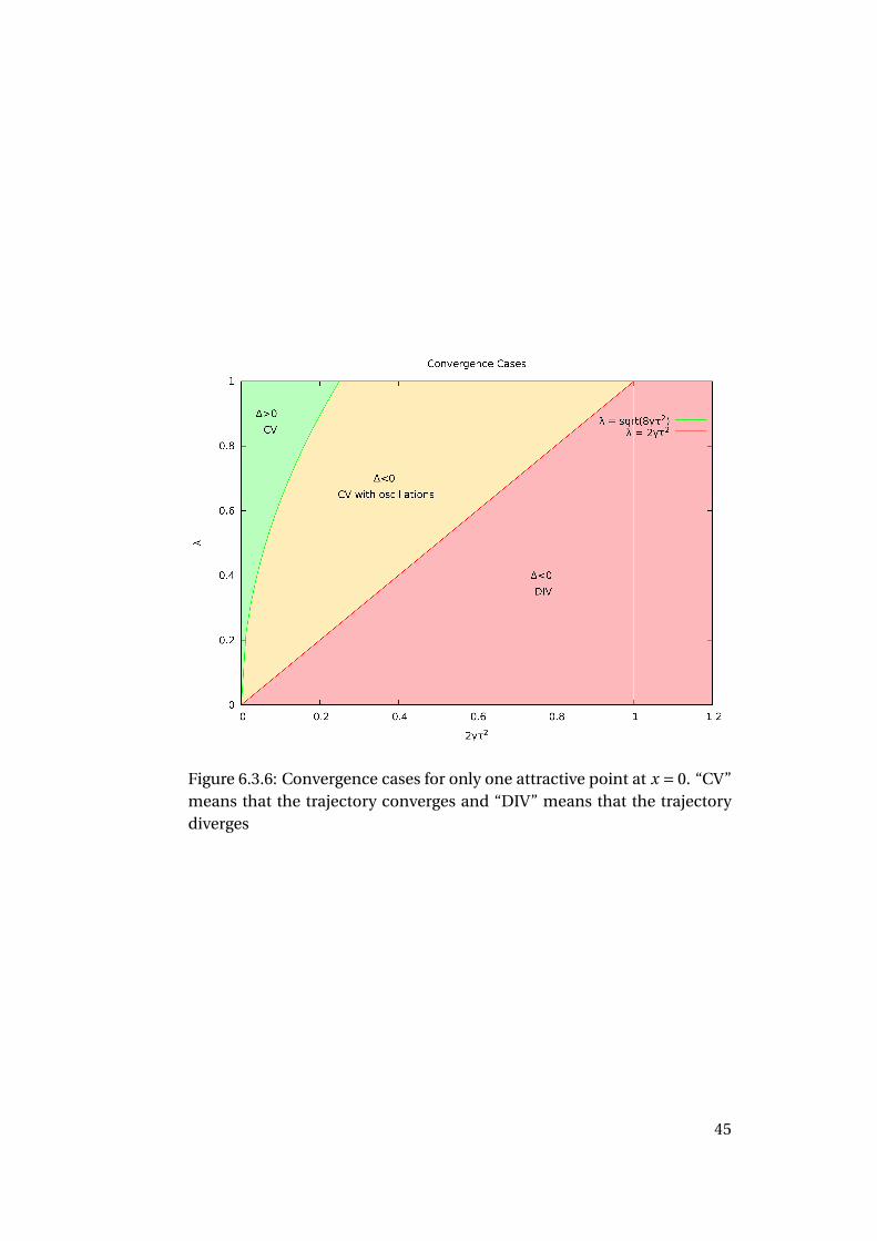
Figure 6.3.6: Convergence cases for only one attractive point at x = 0. “CV”means that the trajectory converges and “DIV” means that the trajectorydiverges
45
When ∆ < 0 the system has two conjugate complex eigenvalues withmodulus
√1−λ+2γτ2. Therefore if λ ≤ 2γτ2 the system diverges. And if
λ> 2γτ2 it converges with oscillations.Finally, when ∆ = 0 the system has one double eigenvalue 1−λ/2 and
converges quickly. This is the fastest convergence rate for fixed λ.If 2γτ2 ≥ 1 then no choice of λ can ensure convergence (see Fig-
ure 6.3.6).If 1/4 ≤ 2γτ2 < 1, then λ > 2γτ2 ensures the best convergence but we
cannot avoid oscillations (see Figure 6.3.6).If 0 < 2γτ2 < 1/4, then we can take λ=√
8γτ2 to get a fast convergencewithout oscillations (see Figure 6.3.6).
Case 2: mixed force
Now, we assume that there is an obstacle between the drone and the attrac-tive point. Assume all objects are on the x axis, with the obstacle at position0, the goal at position g < 0 and the drone at position x > 0.
For 0 < x ≤ `, the force is:
F =−2γ (x − g )+ 2β
x2
( 1
x− 1
`
)(6.3.17)
It is a decreasing function of x, with F →+∞ when x → 0 and F < 0 whenx = `. Therefore there is a unique equilibrium point x0 in (0,`). We do afirst order estimation of F around x0:
F =−2γ(x −x0)+O((x −x0)2) (6.3.18)
where γ= γ+β(
3x4
0− 2
x30`
). Then we see that the behaviour will be the same
as in the attractive case with γ replaced with γ. Since x0 < ` we have γ >γ+ β
`4 .If λ has been tuned to have ∆ = 0 in case 1, then we get oscillation
(or even divergence) in case 2. Therefore it may be necessary to choosea higher λ.
6.3.3 Prediction Step
In our system we have some latency to take into account. Indeed, betweenthe time the position of the drone is measured by the MoCap and the timethe drone executes our control command there is a delay.
46
For the moment, because we did not create a model of our drone, weuse a simple linear extrapolation for a fixed delay by using the previous po-sition of the drone. More complex and accurate predictions can be imple-mented. One such method is described in [24], where they are also usingthe list of commands sent to the flight controller.
A similar prediction step is also needed for other moving objects (thedancer and other drones). In this case we have no other information thanthe past positions.
6.4 Implementation of the potentialsTo implement the potential field motion strategy, we only use the gradientof the potential formula. Also, because in the repulsive potential there is asingularity (the potential tends toward infinity in 0) we are very careful inthe implementation when the distance between the drone and an obstacledecreases. First, to avoid huge forces when that distance is small we thresh-old the repulsive force. Second when we are too close to 0 we decide to donothing as it is not sure which side the drone is.
Since we have thresholded the repulsive potential, we need to do it forthe attractive potential too. Otherwise it could happen that the distancebetween the drone and its goal be such that the attractive force would bestronger than the repulsive force of the dancer, and the drone would thentry to pass through her.
6.5 The motion libraryThe expressiveness of a multi-quadrotor flight performance relies exclu-sively in their motions and their synchronization with the music and thehuman dancer. The PX4 flight controller has already two preprogrammedmotions: Takeoff and Land. In addition to these preprogrammedmotions we have developed three different kinds of motions: hardcodedmotions, motions relative to and interactive with the dancer and play-back motions. All these motions can be mixed in a same choreography.Crashes are prevented thanks to our reactive path planning. The nodeapply_motion contains our motion library.
47
6.5.1 Hardcoded motions
Hardcoded motions are motions that can be defined by a mathematical ex-pression. We have implemented two motions:
• Point: The quadrotor is attracted by a given point. It goes therevia the shortest path allowed by our path planning. If there are noobstacles, it will follow a straight line.
• Circle: The quadrotor is attracted by a moving point describinga circle. Due to our control with potentials, the quadrotor does notfollow exactly a circle trajectory. Instead it is trying to catch up thepoint it is following creating a more or less elliptical motion.
Other hardcoded motions could be easily added to the library if they areneeded.
6.5.2 Interactive motions
Interactive motions are of two different kinds. First, using the commandDancer, the drone can be instructed to follow the dancer position. Itsgoal is set to be the exact dancer position, but the repulsive potential of thedancer will cause the drone to remain at a fixed distance from the dancer.
Second, other motions of the drones result from the influence of themovements of the dancer. If the dancer approaches the drone, then it willgive way. If the dancer advances further, the drone will fly around her toresume its original position. With her hands the dancer can also interactwith the drones that are not close to her: when the hand is extended awayfrom the body it creates a repulsive half plane (vertical and containing thehead and the hand). This allows the dancer to push the drones in the direc-tion of her choice. This effect is activated only when the distance from thebody of the dancer to her hand is above a certain threshold, and its inten-sity increases when the hand moves further away. Both hands can be usedindependently.
Other parameters of the dancer movement could be used to create newinteractions. For instance, the height of her hands could control the alti-tude of the drones.
6.5.3 Playback motions
All the trajectories can be recorded: the trajectories of the drones as wellas those of the dancer head or hands. Recorded trajectories can then be
48
played back by a drone using thePlay command. It is for instance possibleto design a complex choreography, to have the dancer execute it, and thento use the recorded trajectory as the path for the drone so that it reproducesthe choreography.
Moreover, we have designed some operators to apply transformationsto recorded trajectories. They are automatically translated to start at thecurrent position of the drone. They can be scaled, rotated, reflected us-ing the commands SpaceMod, Rotation, Reflection. If needed anarbitrary matrix transformation can be given with Custom. They can beslowed down or sped up using TimeMod. When a transformation is set upit remains in effect for all the subsequent playbacks, until Reset is used.
6.6 The “Choreographer”
6.6.1 Description
In order to architect a complex choreography, we have implemented thenode choreographer that calls and synchronizes the movements of thedrones with those of the dancer and the music. All the choreography in-structions are chronologically written into a single text file. There are fourdifferent kinds of instructions: drone instructions (flight mode and move-ment commands), dancer simulation instructions, temporal instructions(sleep and repeat) and music playback instructions.
6.6.2 The syntax
The syntax of choreography text file is very simple. Each line corresponds toonly one command, and all the lines are read and executed chronologically.
Drone instructions
Drone instructions are structured as follows:UAV number commandThere are two flight mode commands implemented. They are directly in-terpreted by PX4:
• Offboard: The drone goes into mode OFFBOARD and flies towardits goal. For this instruction to be successful the drone has to have apredefined goal. That is why this command has to follow a movementcommand concerning the same drone to be effective.
49
• Land: The drone lands from its current position.The other commands are movements instructions. The two hardcoded
motions are called by:• Point x y z duration: We set a goal at position (x, y, z) (all coordi-
nates are in metres) and a duration to reach it (in seconds).• Circle x y duration: We move a goal along a circle, at a speed such
that a complete revolution is done in the specified duration.The interactive movement command:
• Dancer: The goal is the dancer. The drone will follow the dancer.Playback movements:
• Play trajectory_file: The drone replays a recorded trajectory.• Custom a11 a12 a13 a21 a22 a23 a31 a32 a33: Before it replays the tra-
jectory, we can modify this trajectory. With this command, we canapply a custom transformation, given as a matrix, to the trajectory.
• Reflection axis: Transform the recorded trajectory via a reflectionabout axis, which must be one of x, y, and z.
• Rotation axis angle: Transform the recorded trajectory via a rota-tion.
• TimeMod time_factor: We can slow down the trajectory thanks to thetime_factor.
• SpaceMod space_factor: We can transform via a homothety.• Reset: We reset the transformations on the recorded trajectory.
Special motion function:• Home: The drone goes to its ‘home’ position and then lands.
Music function:• Music n: The drone plays the nth song in the current playlist. If n = 0
then it stops playing.
Dancer simulation instructions
We can simulate the dancer motions. In the choreographer script, thoseinstructions are structured as follows:Dancer commandThe dancer has the same movement commands as the drones (see 6.6.2).Also, her hands can be moved thanks to the following commands (wherecoordinates are relative to the dancer’s head):
• Right_hand x y z duration• Left_hand x y z duration
50
Temporal instructions
To control the execution time of each instruction, we have implemented aSleep duration command. Like its name suggests, it pauses the executionof the script as long as its argument duration indicates. It allows the droneand the dancer to apply their corresponding instructions.
The command Repeat n followed by a series of instructions and end-ing with End repeats those instructions n times. If n = 0 then the instruc-tions are repeated indefinitely. That last option is handy for testing andtuning the control parameters.
51
Chapter 7
Simulationand Visualization Tools
To implement, design and test our control algorithms we use a simulationenvironment. Also, because our security measures depend heavily on theimplemented potential fields, it is important to have a simulation as real-istic as possible. For the development of this project, we have decided toalways test new features via the simulation before testing them in our fly-ing area.
We use ROS with the robotic simulator Gazebo as our simulation en-vironnemt. Gazebo consists of a server gzserver (headless) that simu-lates the world using its physics and sensor engine, and a graphical clientgzclient that connects to a running gzserver and visualizes the ele-ments. So it enables us to simulate a 3D model of our drones in a artificiallyrealistic environment.
7.1 Quadrotor Simulation: PX4 SITLIn this section, we describe the quadrotor simulation model that we used,PX4 SITL.
PX4 is the open-source autopilot system used in our drones (see Chap-ter 4.1.2). It supports two types of simulation: software-in-the-loop (SITL)simulation, where the autopilot firmware runs on computer and hardware-in-the-loop (HITL) simulation using a simulation firmware on a real flightcontroller board. While both of these two types of simulation are interest-ing, we focused on the SITL simulation.
Coupled with the PX4 SITL simulation we use the Gazebo simulator
52
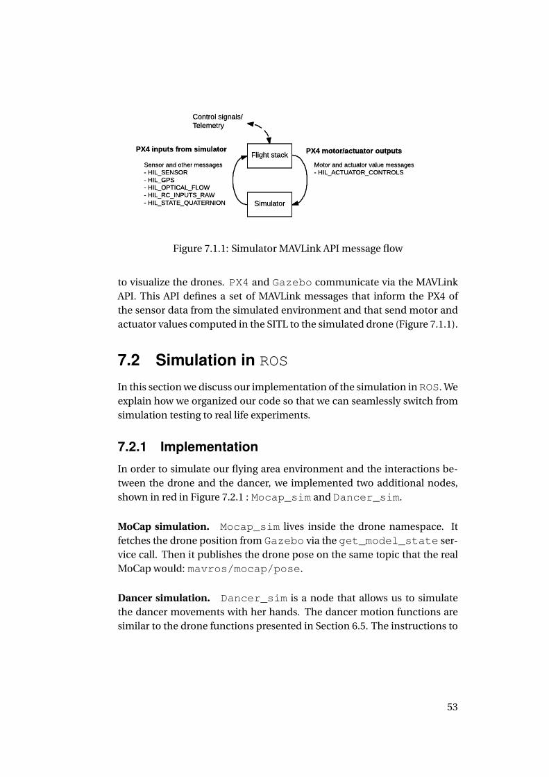
Figure 7.1.1: Simulator MAVLink API message flow
to visualize the drones. PX4 and Gazebo communicate via the MAVLinkAPI. This API defines a set of MAVLink messages that inform the PX4 ofthe sensor data from the simulated environment and that send motor andactuator values computed in the SITL to the simulated drone (Figure 7.1.1).
7.2 Simulation in ROS
In this section we discuss our implementation of the simulation inROS. Weexplain how we organized our code so that we can seamlessly switch fromsimulation testing to real life experiments.
7.2.1 Implementation
In order to simulate our flying area environment and the interactions be-tween the drone and the dancer, we implemented two additional nodes,shown in red in Figure 7.2.1 : Mocap_sim and Dancer_sim.
MoCap simulation. Mocap_sim lives inside the drone namespace. Itfetches the drone position from Gazebo via the get_model_state ser-vice call. Then it publishes the drone pose on the same topic that the realMoCap would: mavros/mocap/pose.
Dancer simulation. Dancer_sim is a node that allows us to simulatethe dancer movements with her hands. The dancer motion functions aresimilar to the drone functions presented in Section 6.5. The instructions to
53
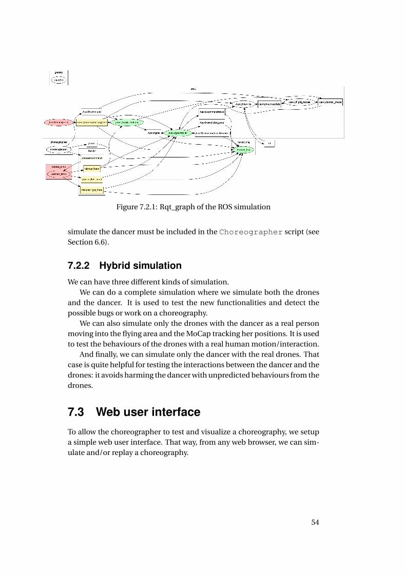
Figure 7.2.1: Rqt_graph of the ROS simulation
simulate the dancer must be included in the Choreographer script (seeSection 6.6).
7.2.2 Hybrid simulation
We can have three different kinds of simulation.We can do a complete simulation where we simulate both the drones
and the dancer. It is used to test the new functionalities and detect thepossible bugs or work on a choreography.
We can also simulate only the drones with the dancer as a real personmoving into the flying area and the MoCap tracking her positions. It is usedto test the behaviours of the drones with a real human motion/interaction.
And finally, we can simulate only the dancer with the real drones. Thatcase is quite helpful for testing the interactions between the dancer and thedrones: it avoids harming the dancer with unpredicted behaviours from thedrones.
7.3 Web user interfaceTo allow the choreographer to test and visualize a choreography, we setupa simple web user interface. That way, from any web browser, we can sim-ulate and/or replay a choreography.
54
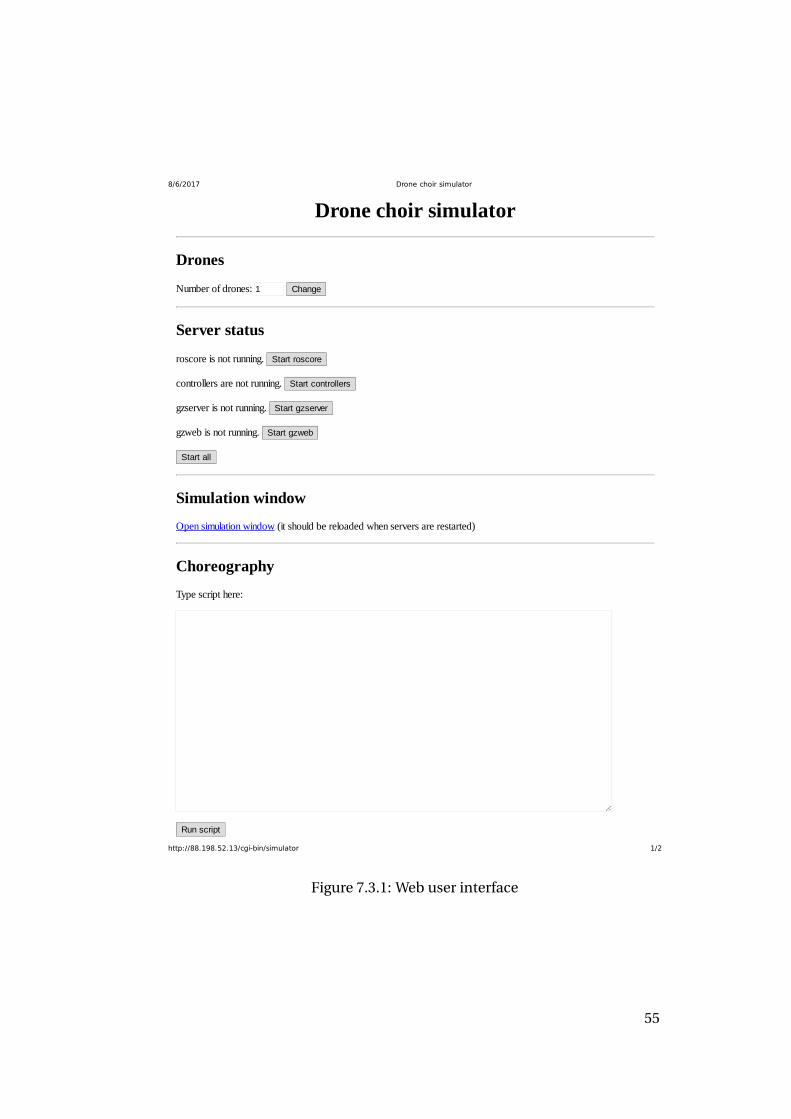
8/6/2017 Drone choir simulator
http://88.198.52.13/cgi-bin/simulator 1/2
Drone choir simulator
Drones
Number of drones: 1 Change
Server status
roscore is not running. Start roscore
controllers are not running. Start controllers
gzserver is not running. Start gzserver
gzweb is not running. Start gzweb
Start all
Simulation window
Open simulation window (it should be reloaded when servers are restarted)
Choreography
Type script here:
Run script
Figure 7.3.1: Web user interface
55
7.3.1 Architecture
The server is hosted on a remote Linux server running Debian Jessie. We in-stalled three kinds of software: simulation software, visualization softwareand a web server.
Simulation software. We installedROSKinetik, Gazebo, and thePX4firmware. We cloned our github repository to get the up to date version ofour code from our local simulation.
Visualization software. We installed on the server the WebGL client forGazebo, gzweb, and Xvfbwhich is a virtual display server. We found outthat Xvfb is needed on a headless host because gzweb needs a display forrendering the simulated objects.
Web server. We setup an Apache HTTP Server which is a free and open-source cross-platform web server software. On Apache, we run the CGI(Common Gateway Interface) script responsible of the User Interface. Infact, the CGI script simulator launches the different programs at theright moment and with the right environment. Also, we added a few auxil-iary shell scripts to make everything work.
7.3.2 Security
Currently the application is not particularly security critical. There are fourknown potential risks. First, a bug in the CGI script could allow an attackerto modify some files on the server host. Second, as we know simulations arecomputationally intensive, it is likely that our implementation is wastingresources on the server. Third, it is not protected against denial-of-serviceattack (DoS attack) which would render the application unaccessible. Andfinally, at the moment, a very basic password protocol is used to preventunauthorized uses of the CGI script. As the password is send in clear text,this is quite weak, and would not resist a serious attacker. The last pointshould definitely be improved if we ever decide to use this web user inter-face on a regular basis.
7.3.3 Use
First, we connect to http://88.198.52.13/cgi-bin/simulator.Then we enter the password to unlock the control panel of the script. The
56
control panel has several sections.
Drone parameters. Currently in contains only one parameter, the num-ber of drones. It has to be set before starting the server because some ROSnodes need it. In a future implementation, it would be more convenient tostart the simulation in an empty world, then spawn the drones when theyare needed, and possibly spawn new ones or un-spawn some of them later.Other parameters could also be included in that section, e.g. the initial po-sition of the drones, their physical properties, etc. However it would bemore convenient if this could be included in the scripts instead.
Status of the servers. Several servers have to work simultaneously andneed to be started in a given order. The status section allows to see thestatus of each individual server and start and stop them individually, butnormally only the Start all and Stop all button should be used.
Simulation window. Once the servers are started, we can click on theOpen simulation window link. Depending on the browser configu-ration, it opens a new window or a new tab, with the gzweb interface toGazebo in it. It can be used to watch the simulation, check the exact posi-tion of the drones, etc. The requested number of drones should be visible,initially immobile at their starting position.
Choreography. This is where the actual choreography is defined. It mustbe entered as a succession of commands in the text box in the same for-mat as the choreographer scripts. Then the button Run script getsthe drones moving, following the instructions. Other functionalities canbe added in this section, such as loading a choreography from a collectionof demos stored on the server or saving the current choreography on theserver.
7.3.4 Discussion
The collaboration with the choreographer, Åsa Unander-Scharin, has notreally started yet. We have implemented this web user interface as a possi-ble tool to use for this collaboration. At the moment, even if the basic func-tionalities are working, some improvements are needed to make it more
57
reliable and productive. For instance, we do not have solutions for pro-ducing sound, nor for using a gamepad to manually direct the drones or adancer that the drones should follow and/or avoid.
7.4 Visualization toolsIn order to design our potentials and tune our control parameters, havinggood plotting and visualization tools is essential. ROS provides packageslike Rviz and rqt_plot but they are not suited for potential field repre-sentation and are focused on live visualization instead of a posteriori analy-sis. That is why we decided to implement a nodeRecorderwhich recordsall the useful data during the flight time (either in simulation or in reality)into files that can be used later for plotting. We implemented two visualiza-tion tools: one that plots the trajectories as a function of time and anotherthat represents the potential fields as heat plots and vector fields. The plotsare done by gnuplotwhich is a freely distributed portable command-linedriven graphing utility.
In fact, each time we run the simulation or make the drones fly, werecord in a folder uniquely named by the date and time of the recordingthe following data:
• for each drone (numbered i ):– its positions from the MoCap (or MoCap simulation) in the fileuavi
– its goals in the file goali– its acceleration (as computed from the potential field) in the fileaccli
– its twist (as sent to the PX4, with damping applied) in the filetwisti
– its predicted position in the file predicti• the position of the dancer (dancer_head)• the position of the dancer hands (right_hand, left_hand)• the control parameters in params• the choreography played (list of timestamped instructions the drones
were supposed to follow) in the file eventThen, a Perl script goes through those files and computes a program that isgiven as input to gnuplot.
58
7.4.1 Automatic trajectory plotting
This tool plots two types of figures: a global view of the trajectories (e.g.Figure 8.2.2) and a view restricted to the x, y and z axis (e.g. Figure 8.2.3).The time interval for plotting is by default restricted to the interval betweenthe first and the last events in the choreographer script. However, it ispossible to manually specify a time interval for more accurate plotting.
The global view. In this representation, the 3D trajectories of all the ele-ments (drones, dancer, etc.) present during the recording are plotted. Also,every 0.5s we plot the computed speed vector on the drone trajectories. Itallows to correlate the real trajectories with our control input and thus de-tect and analyse any anomalies or suspicious behaviours.
The coordinate view. For each drone, we plot according to the x, y andz axis, its position given by the MoCap, its predicted position, its goals.Also, we add the positions of the walls/ceiling and of the dancer, and wemark with a vertical segment the timestamp of each new instruction in thechoreographer script. It allows us to visualize the overshoot or/and os-cillation with respect to each axis in the drone trajectories. Also it helps usevaluate and possibly re-design our position prediction procedure.
7.4.2 Automatic potential visualization
This tool aims to represent the potential fields. It plots two types of figures:heat maps, representing the potential itself (e.g. Figure 8.2.21), and vectorfields, representing the resulting forces (e.g. Figure 8.2.12). It does this foreach drone, as each drone has its own potential field, and at each new eventin the choreography. It is also possible to specify additional times for whicha plot should be made.
Since the potential is defined in three-dimensional space, it is not pos-sible to represent it directly (a 3D representation of the vector field is pos-sible, but not very legible). Therefore we have two make cuts. In order tocapture relevant features of the potential, we chose two variable cut planes:first, the horizontal plane at the altitude of the considered drone; second,the vertical plane containing both the drone and its goal, or a frontal planeif there is no goal or if the drone is too close to the goal. This second figureuses a horizontal coordinate system centered on the drone, and has vari-able width.
59
Each figure indicates the cut plane of the other figure, as well as theprojected position of other drones and of the dancer.
A difficulty arose in the representation of the potential. The repulsivepotentials, as designed in Section 6.3.1, tend to infinity when approachingthe repulsive point. But in our implementation, we decided to truncatethe forces so that the acceleration of the drone remains reasonable, andthis amounts to modify the potential field. However, to control the dronewe did not need to actually compute this modified potential, as we insteadcompute directly its gradient. So we had to compute the modified potentialspecifically for visualization. It is not possible to determine algebraicallyat which position the gradient reaches its maximum, so for this we haveto numerically solve an equation. This is done in the Perl script, then thevalue is plugged into the equation that is passed to gnuplot.
60
Chapter 8
Experiments and Results
In this chapter, we present several experiments that illustrate the differ-ent types of motions that we have defined (see Section 6.5). In each case,we first present the choreographer script, then the trajectory graphs ob-tained from both the simulation and the physical experiment (when onlyone drone is required) using the tools presented in Section 7.4, and finallywe discuss how these trajectories fit with the intended behaviour and howclose simulation is from reality.
As currently only one drone has been constructed, for the experimentswith several drones we have simulation results only. In a later stage we planto run the same scripts with the real drones and a real dancer and comparethe results of the physical experiments with those of simulation.
8.1 Hardcoded motions
8.1.1 Experiment 1: Lines and Circle
Description
Our first experiment demonstrates the two hardcoded motions, withoutany interaction with the environment: moving in a straight line to a spec-ified goal, and moving in a circle around a specified vertical axis and at aspecified speed. The corresponding choreographer script is given in Fig-ure 8.1.1. First this script instructs the drone to move along a horizontalsquare pattern, then it makes the drone go to points at different altitudesand finally it tells the drone to move in a counterclockwise circle aroundthe center of the stage.
61
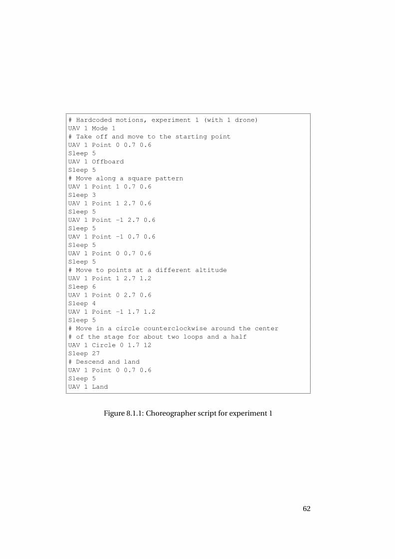
# Hardcoded motions, experiment 1 (with 1 drone)UAV 1 Mode 1# Take off and move to the starting pointUAV 1 Point 0 0.7 0.6Sleep 5UAV 1 OffboardSleep 5# Move along a square patternUAV 1 Point 1 0.7 0.6Sleep 3UAV 1 Point 1 2.7 0.6Sleep 5UAV 1 Point -1 2.7 0.6Sleep 5UAV 1 Point -1 0.7 0.6Sleep 5UAV 1 Point 0 0.7 0.6Sleep 5# Move to points at a different altitudeUAV 1 Point 1 2.7 1.2Sleep 6UAV 1 Point 0 2.7 0.6Sleep 4UAV 1 Point -1 1.7 1.2Sleep 5# Move in a circle counterclockwise around the center# of the stage for about two loops and a halfUAV 1 Circle 0 1.7 12Sleep 27# Descend and landUAV 1 Point 0 0.7 0.6Sleep 5UAV 1 Land
Figure 8.1.1: Choreographer script for experiment 1
62
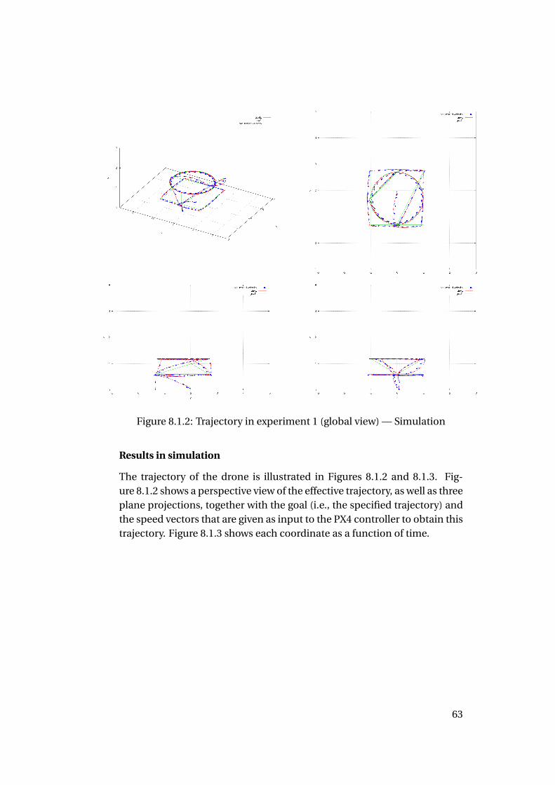
Figure 8.1.2: Trajectory in experiment 1 (global view) — Simulation
Results in simulation
The trajectory of the drone is illustrated in Figures 8.1.2 and 8.1.3. Fig-ure 8.1.2 shows a perspective view of the effective trajectory, as well as threeplane projections, together with the goal (i.e., the specified trajectory) andthe speed vectors that are given as input to the PX4 controller to obtain thistrajectory. Figure 8.1.3 shows each coordinate as a function of time.
63
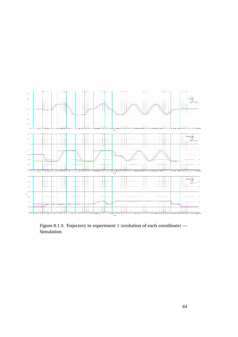
Figure 8.1.3: Trajectory in experiment 1 (evolution of each coordinate) —Simulation
64
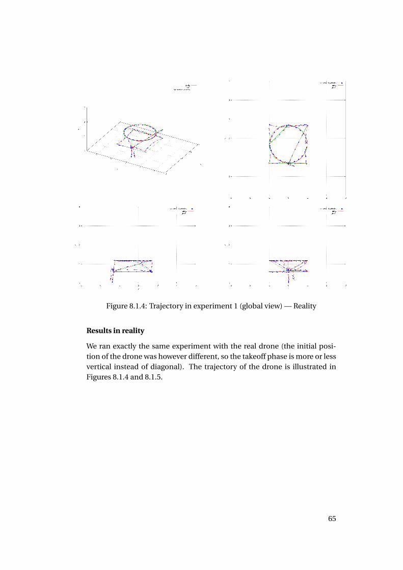
Figure 8.1.4: Trajectory in experiment 1 (global view) — Reality
Results in reality
We ran exactly the same experiment with the real drone (the initial posi-tion of the drone was however different, so the takeoff phase is more or lessvertical instead of diagonal). The trajectory of the drone is illustrated inFigures 8.1.4 and 8.1.5.
65
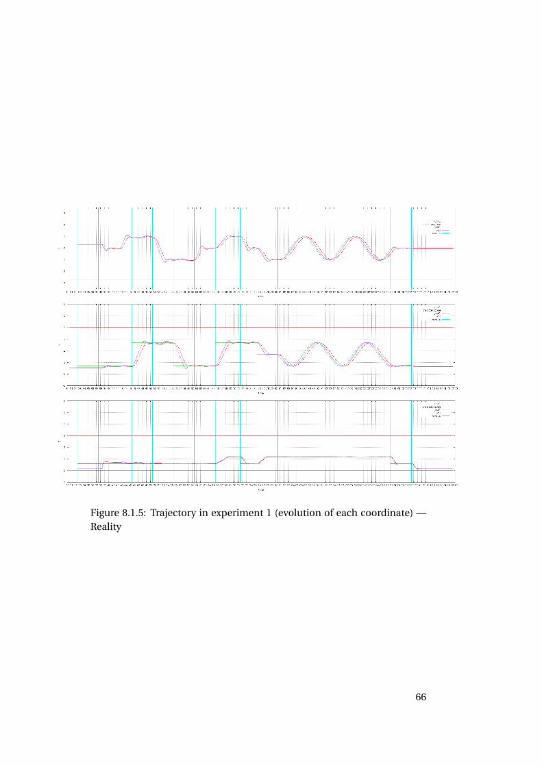
Figure 8.1.5: Trajectory in experiment 1 (evolution of each coordinate) —Reality
66
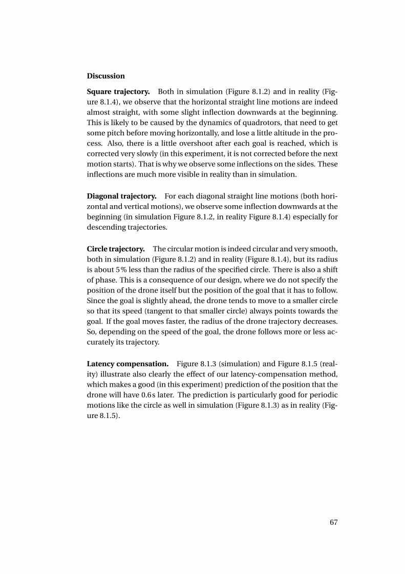
Discussion
Square trajectory. Both in simulation (Figure 8.1.2) and in reality (Fig-ure 8.1.4), we observe that the horizontal straight line motions are indeedalmost straight, with some slight inflection downwards at the beginning.This is likely to be caused by the dynamics of quadrotors, that need to getsome pitch before moving horizontally, and lose a little altitude in the pro-cess. Also, there is a little overshoot after each goal is reached, which iscorrected very slowly (in this experiment, it is not corrected before the nextmotion starts). That is why we observe some inflections on the sides. Theseinflections are much more visible in reality than in simulation.
Diagonal trajectory. For each diagonal straight line motions (both hori-zontal and vertical motions), we observe some inflection downwards at thebeginning (in simulation Figure 8.1.2, in reality Figure 8.1.4) especially fordescending trajectories.
Circle trajectory. The circular motion is indeed circular and very smooth,both in simulation (Figure 8.1.2) and in reality (Figure 8.1.4), but its radiusis about 5% less than the radius of the specified circle. There is also a shiftof phase. This is a consequence of our design, where we do not specify theposition of the drone itself but the position of the goal that it has to follow.Since the goal is slightly ahead, the drone tends to move to a smaller circleso that its speed (tangent to that smaller circle) always points towards thegoal. If the goal moves faster, the radius of the drone trajectory decreases.So, depending on the speed of the goal, the drone follows more or less ac-curately its trajectory.
Latency compensation. Figure 8.1.3 (simulation) and Figure 8.1.5 (real-ity) illustrate also clearly the effect of our latency-compensation method,which makes a good (in this experiment) prediction of the position that thedrone will have 0.6s later. The prediction is particularly good for periodicmotions like the circle as well in simulation (Figure 8.1.3) as in reality (Fig-ure 8.1.5).
67
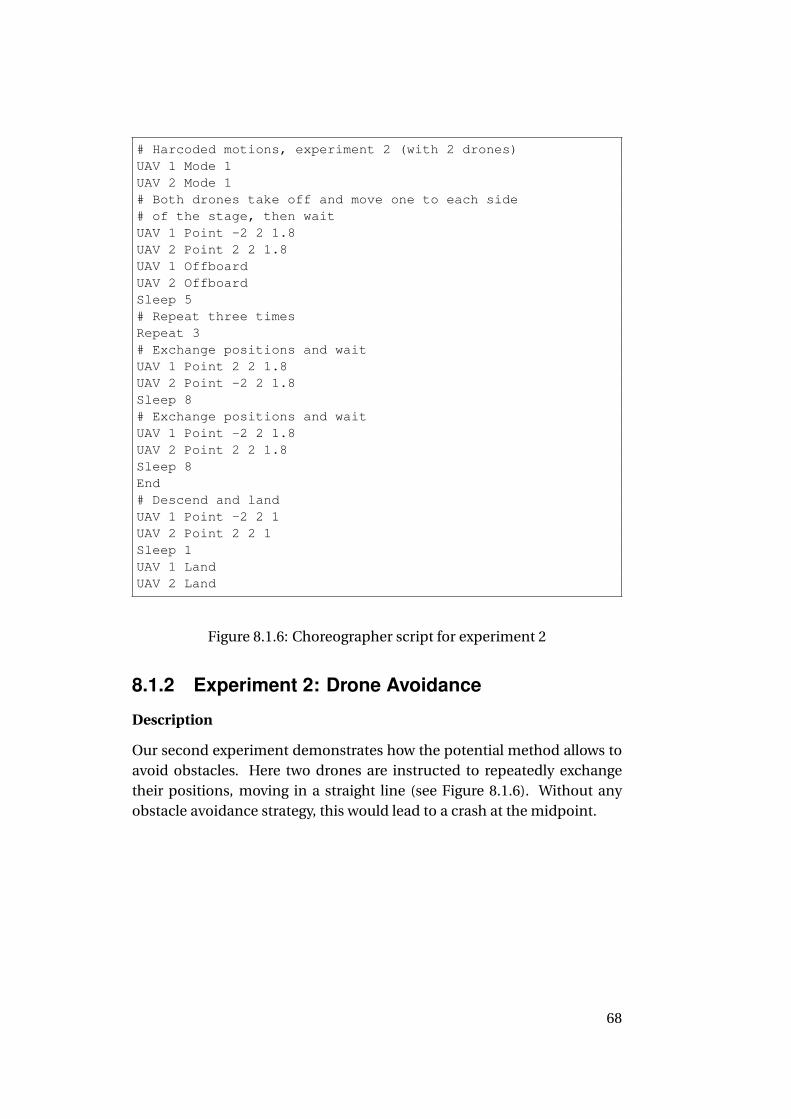
# Harcoded motions, experiment 2 (with 2 drones)UAV 1 Mode 1UAV 2 Mode 1# Both drones take off and move one to each side# of the stage, then waitUAV 1 Point -2 2 1.8UAV 2 Point 2 2 1.8UAV 1 OffboardUAV 2 OffboardSleep 5# Repeat three timesRepeat 3# Exchange positions and waitUAV 1 Point 2 2 1.8UAV 2 Point -2 2 1.8Sleep 8# Exchange positions and waitUAV 1 Point -2 2 1.8UAV 2 Point 2 2 1.8Sleep 8End# Descend and landUAV 1 Point -2 2 1UAV 2 Point 2 2 1Sleep 1UAV 1 LandUAV 2 Land
Figure 8.1.6: Choreographer script for experiment 2
8.1.2 Experiment 2: Drone Avoidance
Description
Our second experiment demonstrates how the potential method allows toavoid obstacles. Here two drones are instructed to repeatedly exchangetheir positions, moving in a straight line (see Figure 8.1.6). Without anyobstacle avoidance strategy, this would lead to a crash at the midpoint.
68
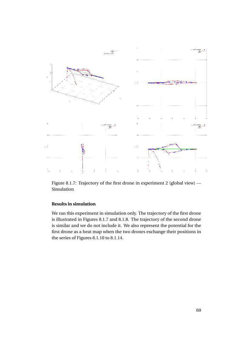
Figure 8.1.7: Trajectory of the first drone in experiment 2 (global view) —Simulation
Results in simulation
We ran this experiment in simulation only. The trajectory of the first droneis illustrated in Figures 8.1.7 and 8.1.8. The trajectory of the second droneis similar and we do not include it. We also represent the potential for thefirst drone as a heat map when the two drones exchange their positions inthe series of Figures 8.1.10 to 8.1.14.
69
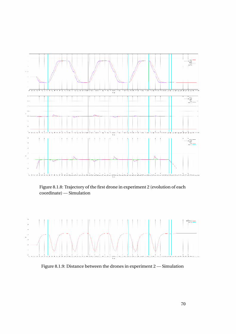
Figure 8.1.8: Trajectory of the first drone in experiment 2 (evolution of eachcoordinate) — Simulation
Figure 8.1.9: Distance between the drones in experiment 2 — Simulation
70
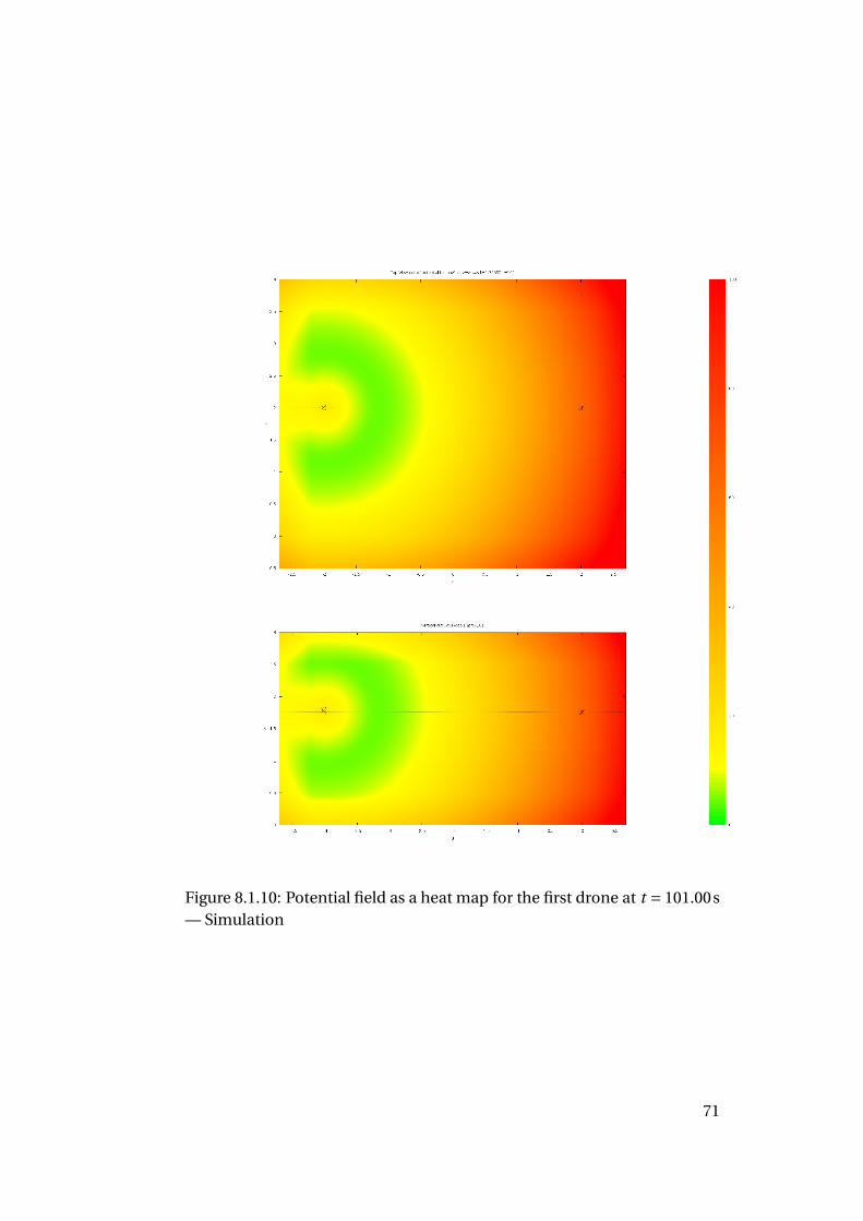
Figure 8.1.10: Potential field as a heat map for the first drone at t = 101.00s— Simulation
71
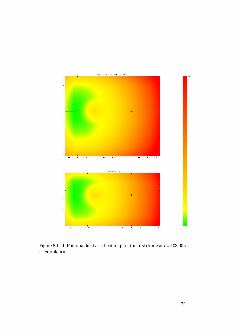
Figure 8.1.11: Potential field as a heat map for the first drone at t = 102.00s— Simulation
72
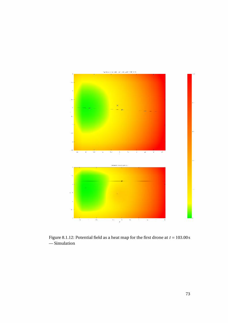
Figure 8.1.12: Potential field as a heat map for the first drone at t = 103.00s— Simulation
73
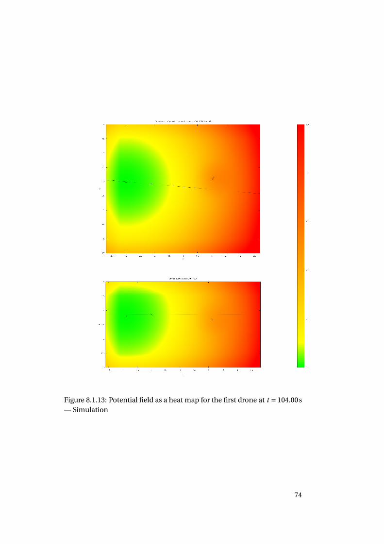
Figure 8.1.13: Potential field as a heat map for the first drone at t = 104.00s— Simulation
74
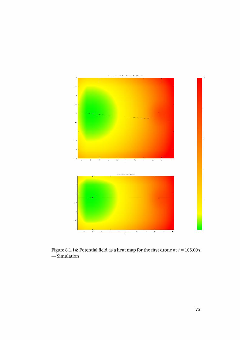
Figure 8.1.14: Potential field as a heat map for the first drone at t = 105.00s— Simulation
75
Discussion
The drones correctly avoid each other. Their mutual distance (see Fig-ure 8.1.9) always remains above 73cm. There is no visible oscillation, andthe x component of the speed is only slightly affected.
The situation has a rotational symmetry around the horizontal line be-tween the two extreme positions of the drones, so in principle only fluctu-ations should decide to what side one drone chooses to move to avoid theother one. However, we observe that almost the same pattern repeats ateach of the six crossings: the drone coming from the left moves down andto the back of the stage (increasing x and y , decreasing z) while the dronecoming from the right moves the opposite way. The horizontal component(y) tends to decrease, and is reversed for the last crossing. Maybe the factthat the drones prefer to use the vertical direction is due to the differentnature of vertical and horizontal propulsion of the quadrotors. We cannotexplain why they always make the same choice, but it is likely to be just anartifact of the simulation.
76
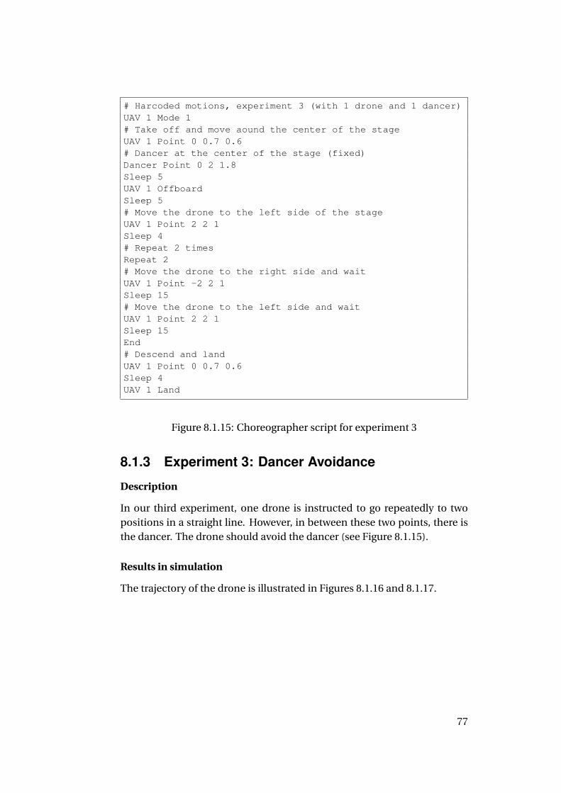
# Harcoded motions, experiment 3 (with 1 drone and 1 dancer)UAV 1 Mode 1# Take off and move aound the center of the stageUAV 1 Point 0 0.7 0.6# Dancer at the center of the stage (fixed)Dancer Point 0 2 1.8Sleep 5UAV 1 OffboardSleep 5# Move the drone to the left side of the stageUAV 1 Point 2 2 1Sleep 4# Repeat 2 timesRepeat 2# Move the drone to the right side and waitUAV 1 Point -2 2 1Sleep 15# Move the drone to the left side and waitUAV 1 Point 2 2 1Sleep 15End# Descend and landUAV 1 Point 0 0.7 0.6Sleep 4UAV 1 Land
Figure 8.1.15: Choreographer script for experiment 3
8.1.3 Experiment 3: Dancer Avoidance
Description
In our third experiment, one drone is instructed to go repeatedly to twopositions in a straight line. However, in between these two points, there isthe dancer. The drone should avoid the dancer (see Figure 8.1.15).
Results in simulation
The trajectory of the drone is illustrated in Figures 8.1.16 and 8.1.17.
77
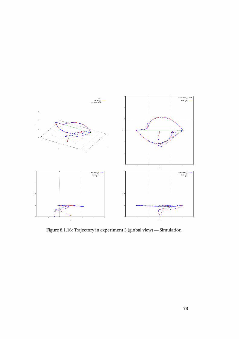
Figure 8.1.16: Trajectory in experiment 3 (global view) — Simulation
78
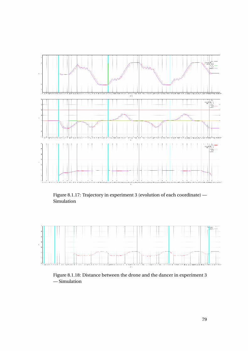
Figure 8.1.17: Trajectory in experiment 3 (evolution of each coordinate) —Simulation
Figure 8.1.18: Distance between the drone and the dancer in experiment 3— Simulation
79
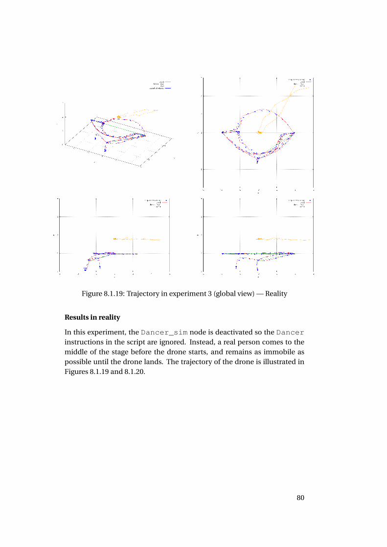
Figure 8.1.19: Trajectory in experiment 3 (global view) — Reality
Results in reality
In this experiment, the Dancer_sim node is deactivated so the Dancerinstructions in the script are ignored. Instead, a real person comes to themiddle of the stage before the drone starts, and remains as immobile aspossible until the drone lands. The trajectory of the drone is illustrated inFigures 8.1.19 and 8.1.20.
80
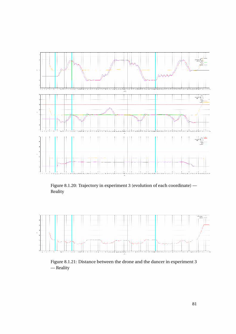
Figure 8.1.20: Trajectory in experiment 3 (evolution of each coordinate) —Reality
Figure 8.1.21: Distance between the drone and the dancer in experiment 3— Reality
81
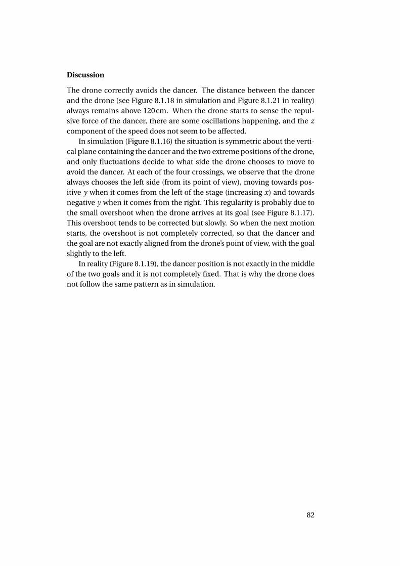
Discussion
The drone correctly avoids the dancer. The distance between the dancerand the drone (see Figure 8.1.18 in simulation and Figure 8.1.21 in reality)always remains above 120cm. When the drone starts to sense the repul-sive force of the dancer, there are some oscillations happening, and the zcomponent of the speed does not seem to be affected.
In simulation (Figure 8.1.16) the situation is symmetric about the verti-cal plane containing the dancer and the two extreme positions of the drone,and only fluctuations decide to what side the drone chooses to move toavoid the dancer. At each of the four crossings, we observe that the dronealways chooses the left side (from its point of view), moving towards pos-itive y when it comes from the left of the stage (increasing x) and towardsnegative y when it comes from the right. This regularity is probably due tothe small overshoot when the drone arrives at its goal (see Figure 8.1.17).This overshoot tends to be corrected but slowly. So when the next motionstarts, the overshoot is not completely corrected, so that the dancer andthe goal are not exactly aligned from the drone’s point of view, with the goalslightly to the left.
In reality (Figure 8.1.19), the dancer position is not exactly in the middleof the two goals and it is not completely fixed. That is why the drone doesnot follow the same pattern as in simulation.
82
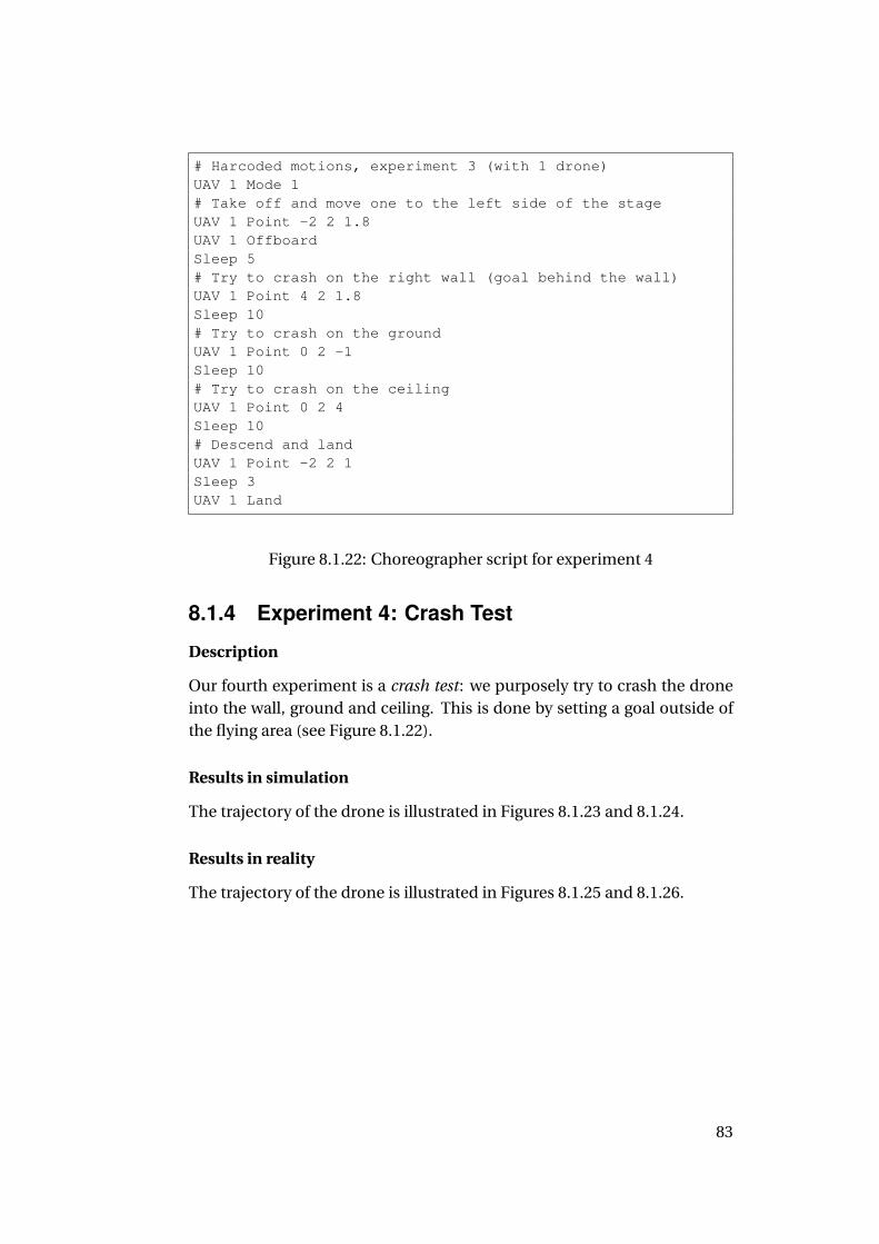
# Harcoded motions, experiment 3 (with 1 drone)UAV 1 Mode 1# Take off and move one to the left side of the stageUAV 1 Point -2 2 1.8UAV 1 OffboardSleep 5# Try to crash on the right wall (goal behind the wall)UAV 1 Point 4 2 1.8Sleep 10# Try to crash on the groundUAV 1 Point 0 2 -1Sleep 10# Try to crash on the ceilingUAV 1 Point 0 2 4Sleep 10# Descend and landUAV 1 Point -2 2 1Sleep 3UAV 1 Land
Figure 8.1.22: Choreographer script for experiment 4
8.1.4 Experiment 4: Crash Test
Description
Our fourth experiment is a crash test: we purposely try to crash the droneinto the wall, ground and ceiling. This is done by setting a goal outside ofthe flying area (see Figure 8.1.22).
Results in simulation
The trajectory of the drone is illustrated in Figures 8.1.23 and 8.1.24.
Results in reality
The trajectory of the drone is illustrated in Figures 8.1.25 and 8.1.26.
83
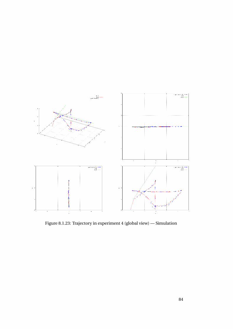
Figure 8.1.23: Trajectory in experiment 4 (global view) — Simulation
84
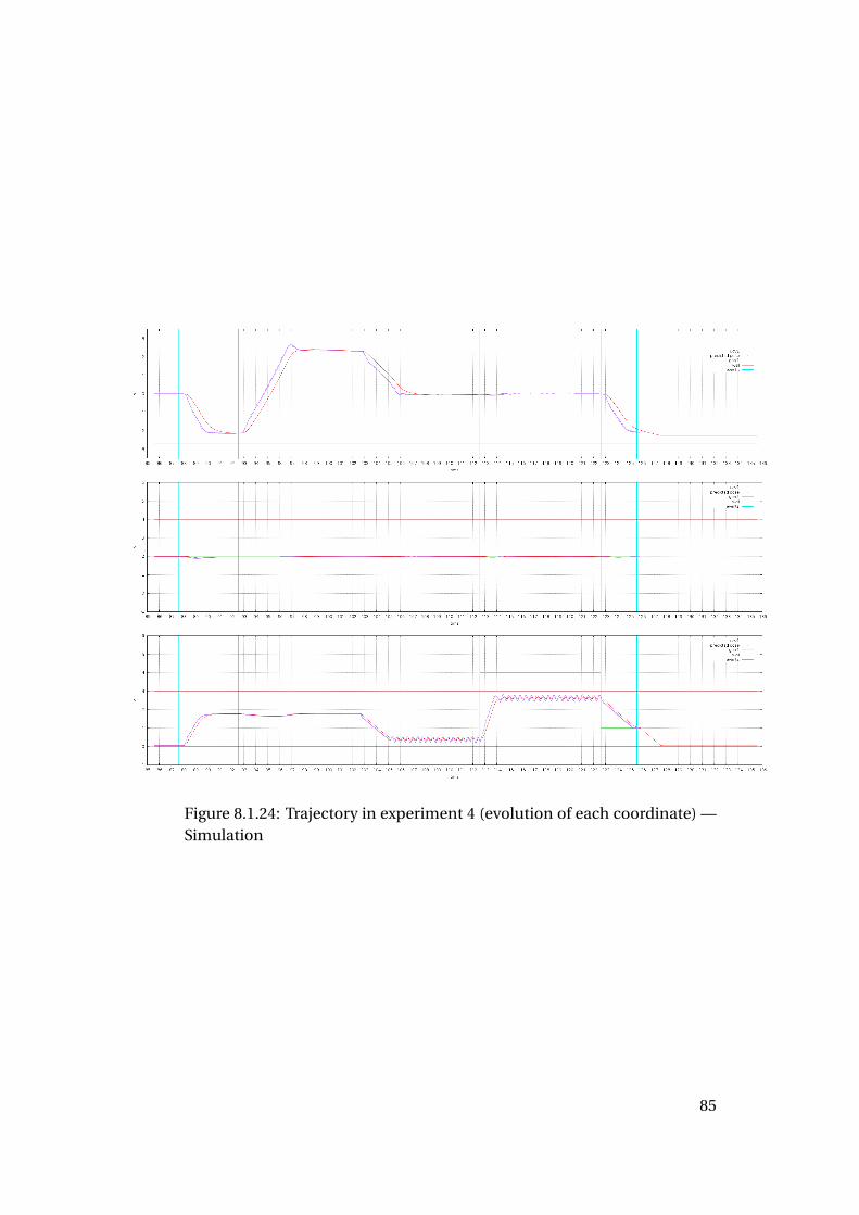
Figure 8.1.24: Trajectory in experiment 4 (evolution of each coordinate) —Simulation
85
Figure 8.1.25: Trajectory in experiment 4 (global view) — Reality
86
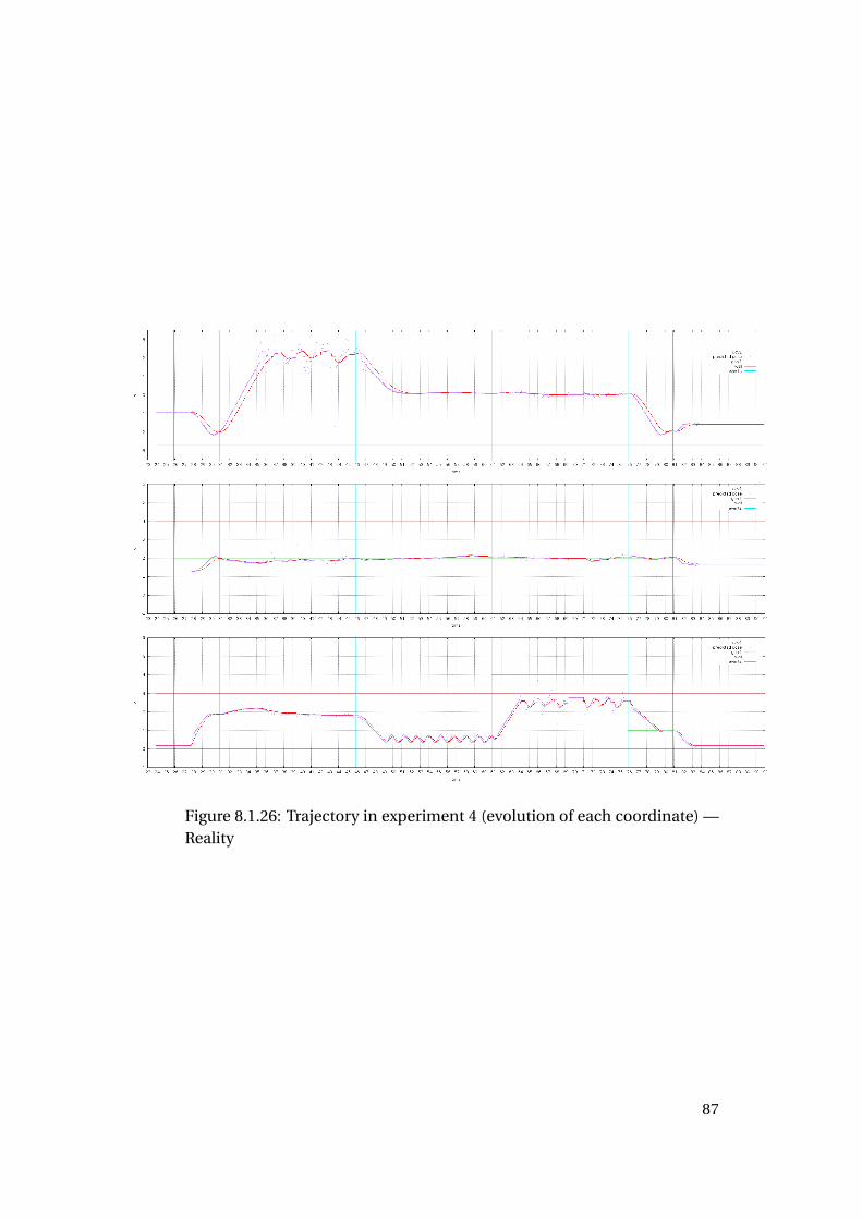
Figure 8.1.26: Trajectory in experiment 4 (evolution of each coordinate) —Reality
87
Discussion
Simulation. The first crash test, against a wall, is rather satisfactory. Thedrone stops neatly 30cm from the wall (the closest point is reached at t =99.3s) then settles about 38cm from it.
The other two tests are also successful, but they are much less stable asthe drone exhibits vertical oscillation, with a frequency slightly above 2Hz:between 33cm and 49cm from the ground, and between 31cm and 43cmfrom the ceiling. With a real drone this could result in a crash.
Reality. The crash test was successful, in the sense that the drone did notcrash and landed safely at the end. However, there is a lot of oscillation, in-cluding in the first test, and this needs to be improved. It may be necessaryto redesign the potentials for this.
Oscillations are slower than in simulation (around 0.4Hz for the wall,0.7Hz for the ground). In the case of the wall and ceiling, they are also moreirregular, almost chaotic. On Figure 8.1.26, one sees that the drone positionremains constant during small intervals (for instance around t = 37.5s forthe wall, and between t = 69.4s and t = 71.0s for the ceiling). This meansthat the MoCap did not report any position during those intervals, becausethe drone was not seen by enough cameras. During the longest such blindinterval, we observed that the drone actually flew above the virtual ceil-ing. This does not happen for the crash test on the ground, as it takesplace in a well-covered area in the middle of the stage. We can draw twoconsequences of this: first, we need additional cameras so that the flyingvolume is adequately covered; second, our controller should not rely onthe MoCap alone to estimate its position, and use the internal estimatorof the PX4 (which fuses the MoCap information with measurements fromthe IMU and other sensors), at least as a fallback when MoCap is lost. Ourdelay compensation procedure should also be improved in order to betterhandle such situations.
88
8.2 Interactive motions
8.2.1 Experiment 1: Dancer Following
Description
We now turn to interactive motions. Our first experiment has the dronefollow the dancer, who dances first along a rectangle, then along a circle.The choreographer script is given in Figure 8.2.1.
Results in simulation
The trajectories of the dancer and the drone are illustrated in Figures 8.2.2and 8.2.3.
Results in reality
In this experiment, the dancer is still simulated while the drone is real. Also,the drone is instructed to follow the dancer at 3/4 of her height, not at headlevel: this changes the z coordinate, but does not affect the trajectory oth-erwise. Finally, the dancer trajectory was slightly modified. The trajectoriesof the dancer and the drone are illustrated in Figures 8.2.5 and 8.2.6.
89
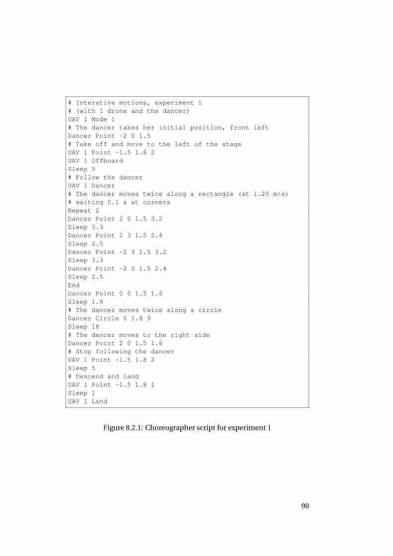
# Interative motions, experiment 1# (with 1 drone and the dancer)UAV 1 Mode 1# The dancer takes her initial position, front leftDancer Point -2 0 1.5# Take off and move to the left of the stageUAV 1 Point -1.5 1.8 2UAV 1 OffboardSleep 5# Follow the dancerUAV 1 Dancer# The dancer moves twice along a rectangle (at 1.25 m/s)# waiting 0.1 s at cornersRepeat 2Dancer Point 2 0 1.5 3.2Sleep 3.3Dancer Point 2 3 1.5 2.4Sleep 2.5Dancer Point -2 3 1.5 3.2Sleep 3.3Dancer Point -2 0 1.5 2.4Sleep 2.5EndDancer Point 0 0 1.5 1.6Sleep 1.6# The dancer moves twice along a circleDancer Circle 0 1.8 9Sleep 18# The dancer moves to the right sideDancer Point 2 0 1.5 1.6# Stop following the dancerUAV 1 Point -1.5 1.8 2Sleep 5# Descend and landUAV 1 Point -1.5 1.8 1Sleep 1UAV 1 Land
Figure 8.2.1: Choreographer script for experiment 1
90
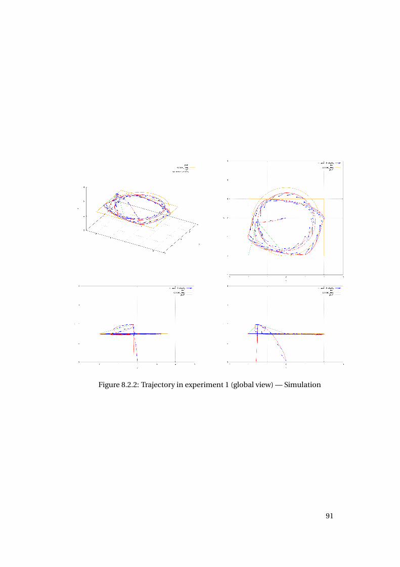
Figure 8.2.2: Trajectory in experiment 1 (global view) — Simulation
91
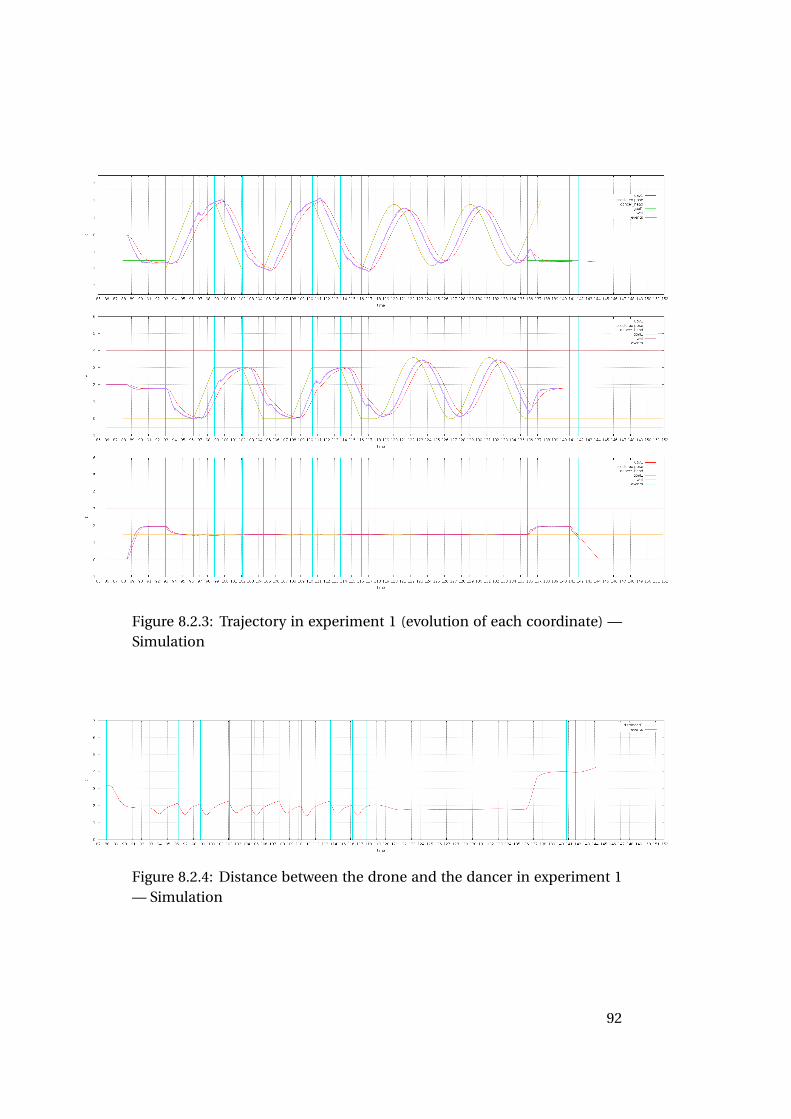
Figure 8.2.3: Trajectory in experiment 1 (evolution of each coordinate) —Simulation
Figure 8.2.4: Distance between the drone and the dancer in experiment 1— Simulation
92
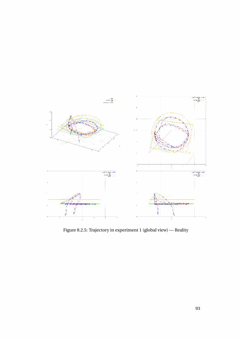
Figure 8.2.5: Trajectory in experiment 1 (global view) — Reality
93
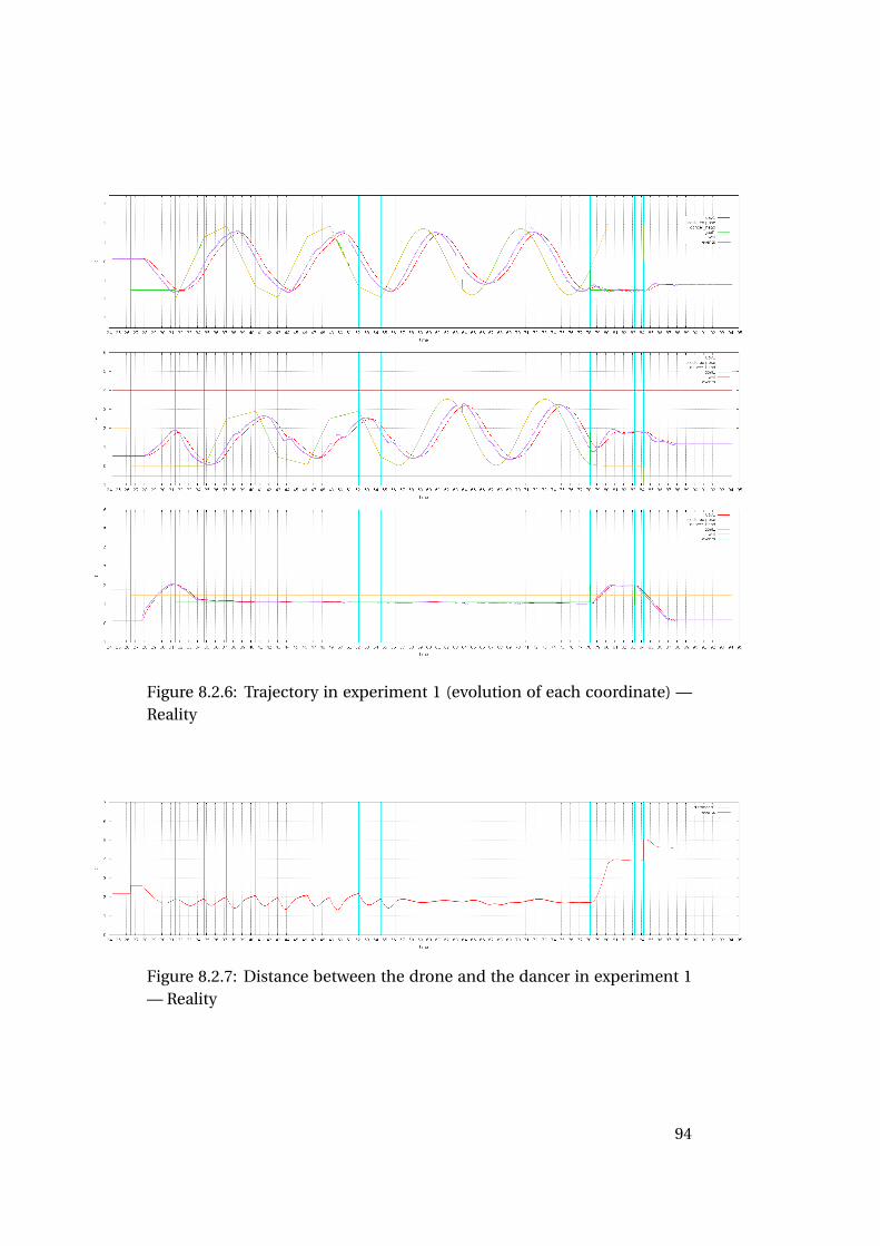
Figure 8.2.6: Trajectory in experiment 1 (evolution of each coordinate) —Reality
Figure 8.2.7: Distance between the drone and the dancer in experiment 1— Reality
94
Discussion
As can be seen on Figures 8.2.4 and 8.2.7, the drone remains at a good dis-tance behind the dancer: in simulation, between 1.40m and 2.28m duringthe rectangle part, and between 1.75m and 1.82,m during the circle part; inreality, between 1.33m and 2.20m during the rectangle part, and between1.59m and 1.85,m during the circle part. There is no oscillation, both insimulation and reality, except a little “hesitation” of the drone when thedancer reaches the end of the smaller sides of the rectangle.
When the dancer makes a rectangle, the drone makes a more or lessrectangular shape, slightly rotated. When the dancer makes a circle, thedrone makes a circle of smaller radius, as in the first experiment with hard-coded motions (see Section 8.1.1), for the same reason (the drone is follow-ing a moving goal) and also because of the repulsive potential of the dancerthat prevents the drone from approaching her too closely.
95
8.2.2 Experiment 2: Dancer Interactions
Description
The second kind of interactive motion is the motion caused by variationsof the potential when the dancer moves close to the drones. In this exper-iment, we have four drones flying in a square formation, and the dancerpasses back and forth between them (see Figure 8.2.8.
Results in simulation
The trajectory of the dancer and first drone are illustrated in Figures 8.2.9and 8.2.10. The trajectories of the other drones are similar and we do not in-clude them. The force field for the first drone is illustrated in Figures 8.2.12to 8.2.15.
Discussion
When the dancer approaches, the drones move away to a safe distance, al-ways above 1.06m (see Figure 8.2.11). Also the distance between dronesremains above 1.23m. When the dancer moves away, the drones resumetheir nominal position.
This experiment shows that the dancer can evolve in the middle of thedrones in good safety conditions. Moreover, it is visually pleasing and canpossibly be turned into interesting artistic effects.
96
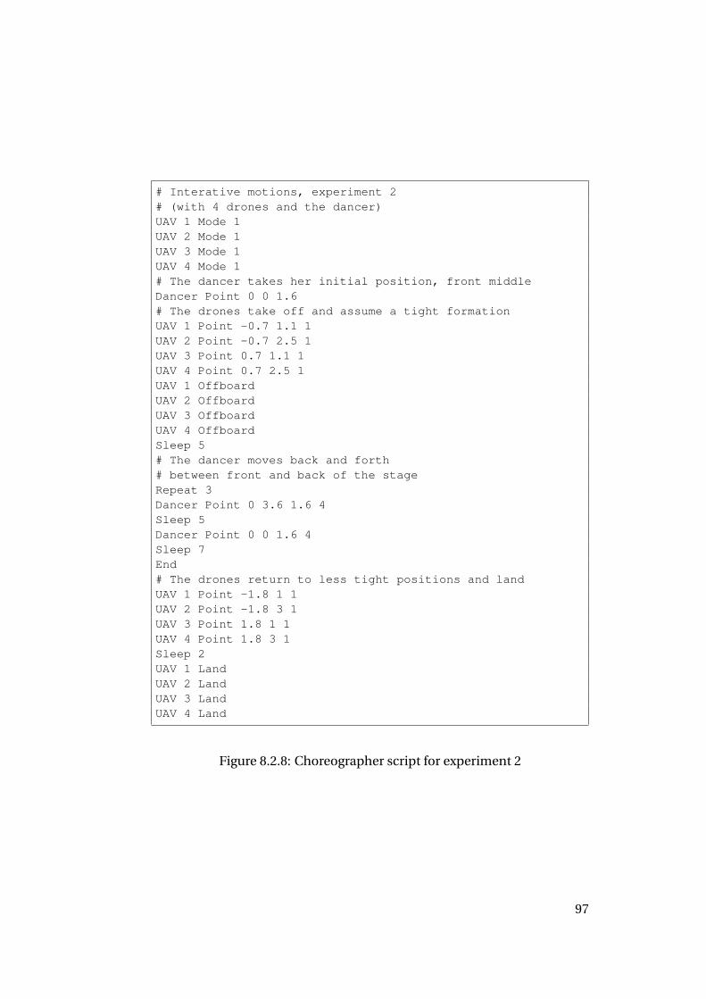
# Interative motions, experiment 2# (with 4 drones and the dancer)UAV 1 Mode 1UAV 2 Mode 1UAV 3 Mode 1UAV 4 Mode 1# The dancer takes her initial position, front middleDancer Point 0 0 1.6# The drones take off and assume a tight formationUAV 1 Point -0.7 1.1 1UAV 2 Point -0.7 2.5 1UAV 3 Point 0.7 1.1 1UAV 4 Point 0.7 2.5 1UAV 1 OffboardUAV 2 OffboardUAV 3 OffboardUAV 4 OffboardSleep 5# The dancer moves back and forth# between front and back of the stageRepeat 3Dancer Point 0 3.6 1.6 4Sleep 5Dancer Point 0 0 1.6 4Sleep 7End# The drones return to less tight positions and landUAV 1 Point -1.8 1 1UAV 2 Point -1.8 3 1UAV 3 Point 1.8 1 1UAV 4 Point 1.8 3 1Sleep 2UAV 1 LandUAV 2 LandUAV 3 LandUAV 4 Land
Figure 8.2.8: Choreographer script for experiment 2
97
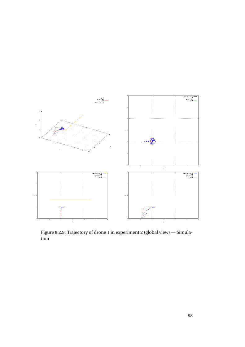
Figure 8.2.9: Trajectory of drone 1 in experiment 2 (global view) — Simula-tion
98
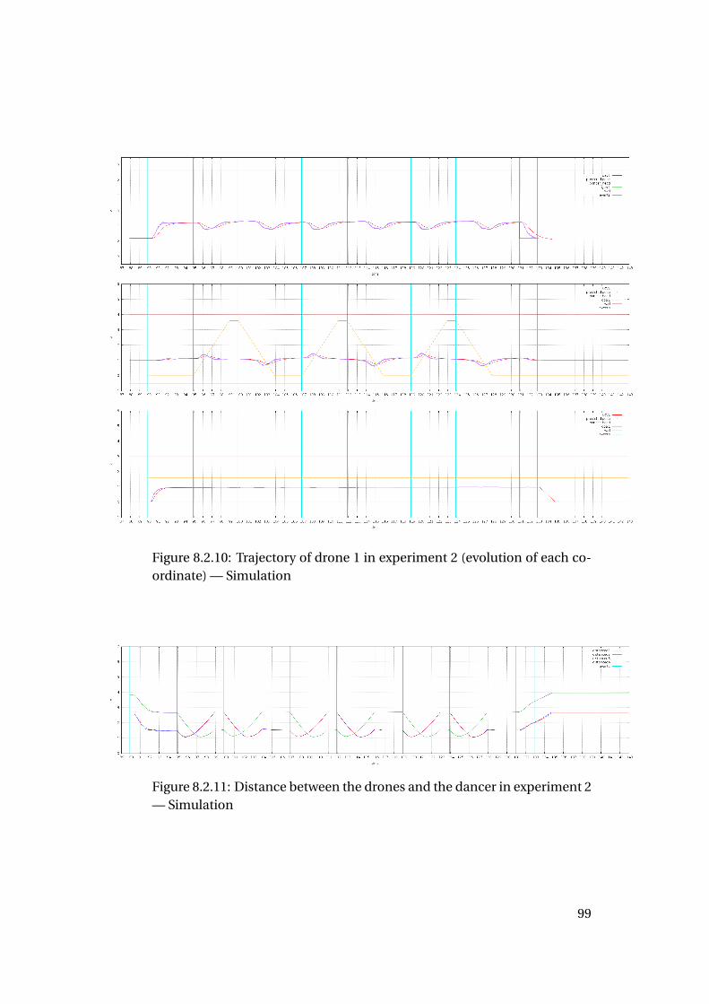
Figure 8.2.10: Trajectory of drone 1 in experiment 2 (evolution of each co-ordinate) — Simulation
Figure 8.2.11: Distance between the drones and the dancer in experiment 2— Simulation
99
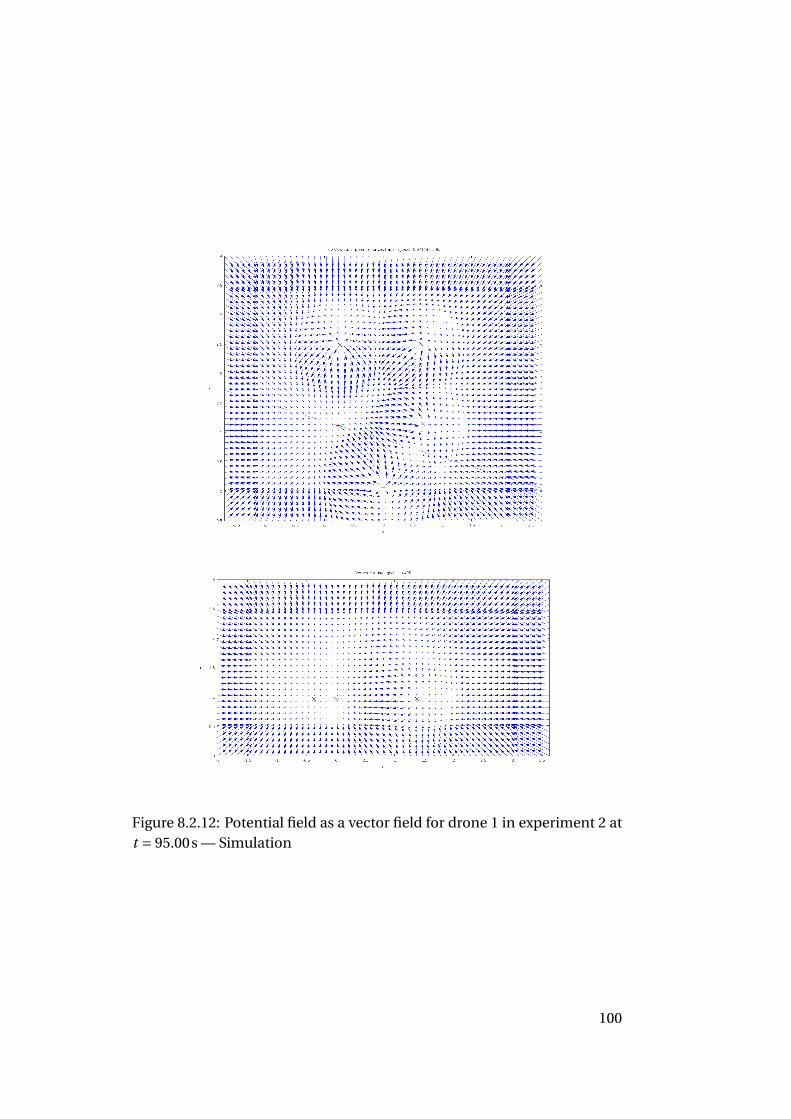
Figure 8.2.12: Potential field as a vector field for drone 1 in experiment 2 att = 95.00s — Simulation
100
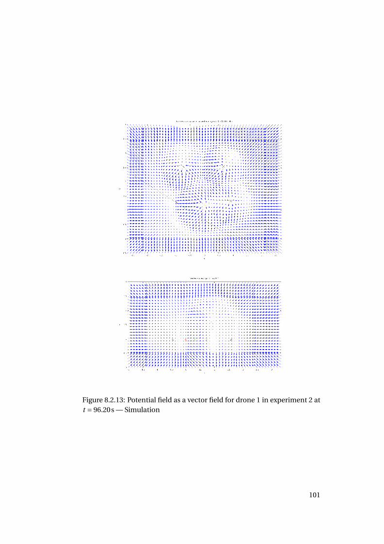
Figure 8.2.13: Potential field as a vector field for drone 1 in experiment 2 att = 96.20s — Simulation
101
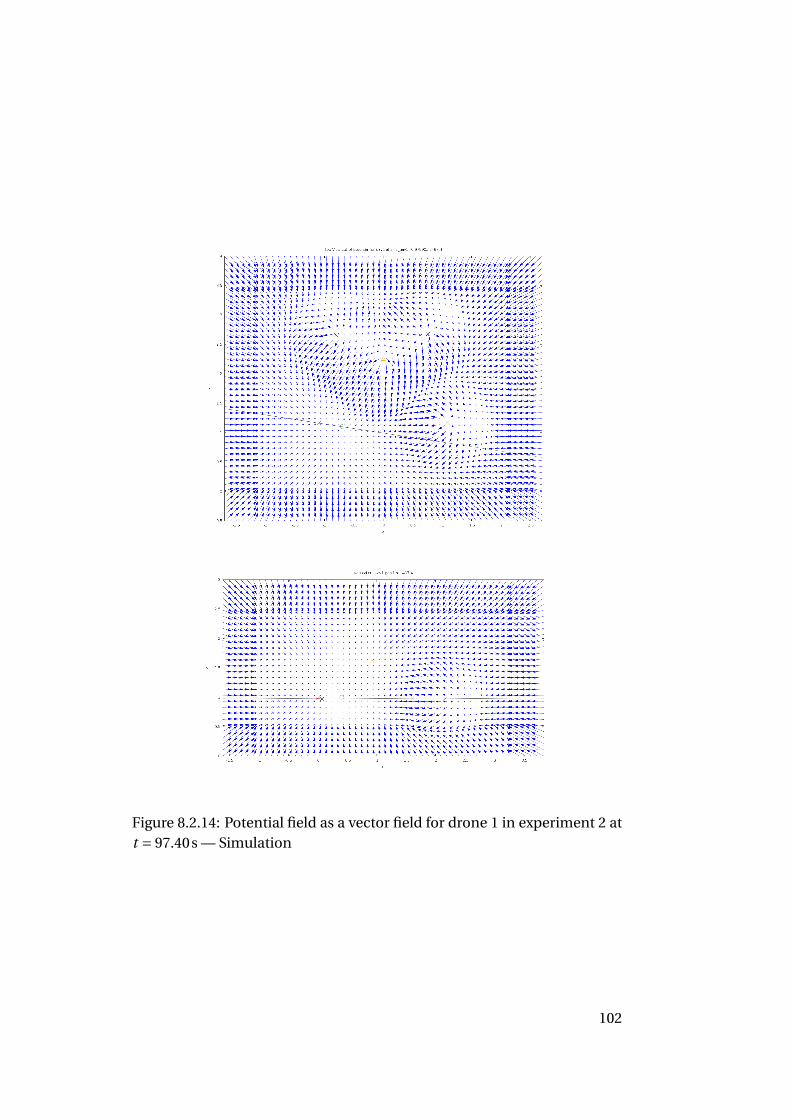
Figure 8.2.14: Potential field as a vector field for drone 1 in experiment 2 att = 97.40s — Simulation
102
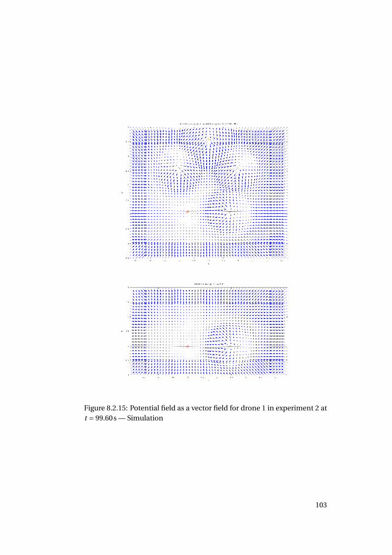
Figure 8.2.15: Potential field as a vector field for drone 1 in experiment 2 att = 99.60s — Simulation
103
8.2.3 Experiment 3: Hand Motions
Description
The third kind of interactive motion is prompted by hand movements ofthe dancer. In this experiment, again with four drones in a square, thedancer does not move her body, but extends both arms in the directionof the drones, splitting the group in two, then moves them further apart byopening her arms a little (see Figure 8.2.16). Note that the hands producean effect only when they are at least 50cm away from the body in horizontalprojection. Therefore, in the first five seconds of the experiment, the dronesgo to their nominal position unaffected by the hand movement (drones 1and 3 are slightly affected by the dancer herself).
Results in simulation
The trajectory of the drones 1 and 2 are illustrated in Figures 8.2.17 to 8.2.20.The trajectories of the other two drones are similar and we do not includethem. We also represent the potential for the first drone as a heat mapwhen the two drones exchange their positions in the series of Figures 8.2.21to 8.2.26.
104
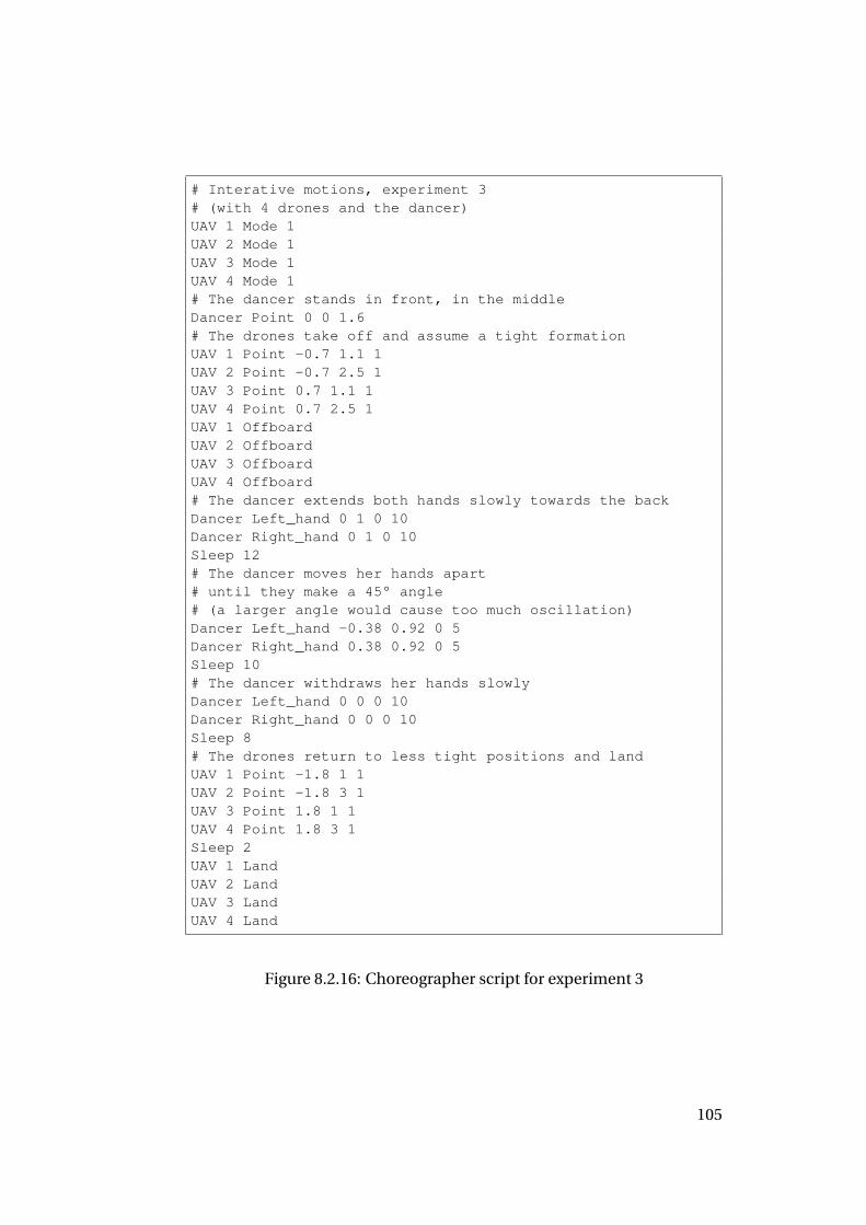
# Interative motions, experiment 3# (with 4 drones and the dancer)UAV 1 Mode 1UAV 2 Mode 1UAV 3 Mode 1UAV 4 Mode 1# The dancer stands in front, in the middleDancer Point 0 0 1.6# The drones take off and assume a tight formationUAV 1 Point -0.7 1.1 1UAV 2 Point -0.7 2.5 1UAV 3 Point 0.7 1.1 1UAV 4 Point 0.7 2.5 1UAV 1 OffboardUAV 2 OffboardUAV 3 OffboardUAV 4 Offboard# The dancer extends both hands slowly towards the backDancer Left_hand 0 1 0 10Dancer Right_hand 0 1 0 10Sleep 12# The dancer moves her hands apart# until they make a 45° angle# (a larger angle would cause too much oscillation)Dancer Left_hand -0.38 0.92 0 5Dancer Right_hand 0.38 0.92 0 5Sleep 10# The dancer withdraws her hands slowlyDancer Left_hand 0 0 0 10Dancer Right_hand 0 0 0 10Sleep 8# The drones return to less tight positions and landUAV 1 Point -1.8 1 1UAV 2 Point -1.8 3 1UAV 3 Point 1.8 1 1UAV 4 Point 1.8 3 1Sleep 2UAV 1 LandUAV 2 LandUAV 3 LandUAV 4 Land
Figure 8.2.16: Choreographer script for experiment 3
105
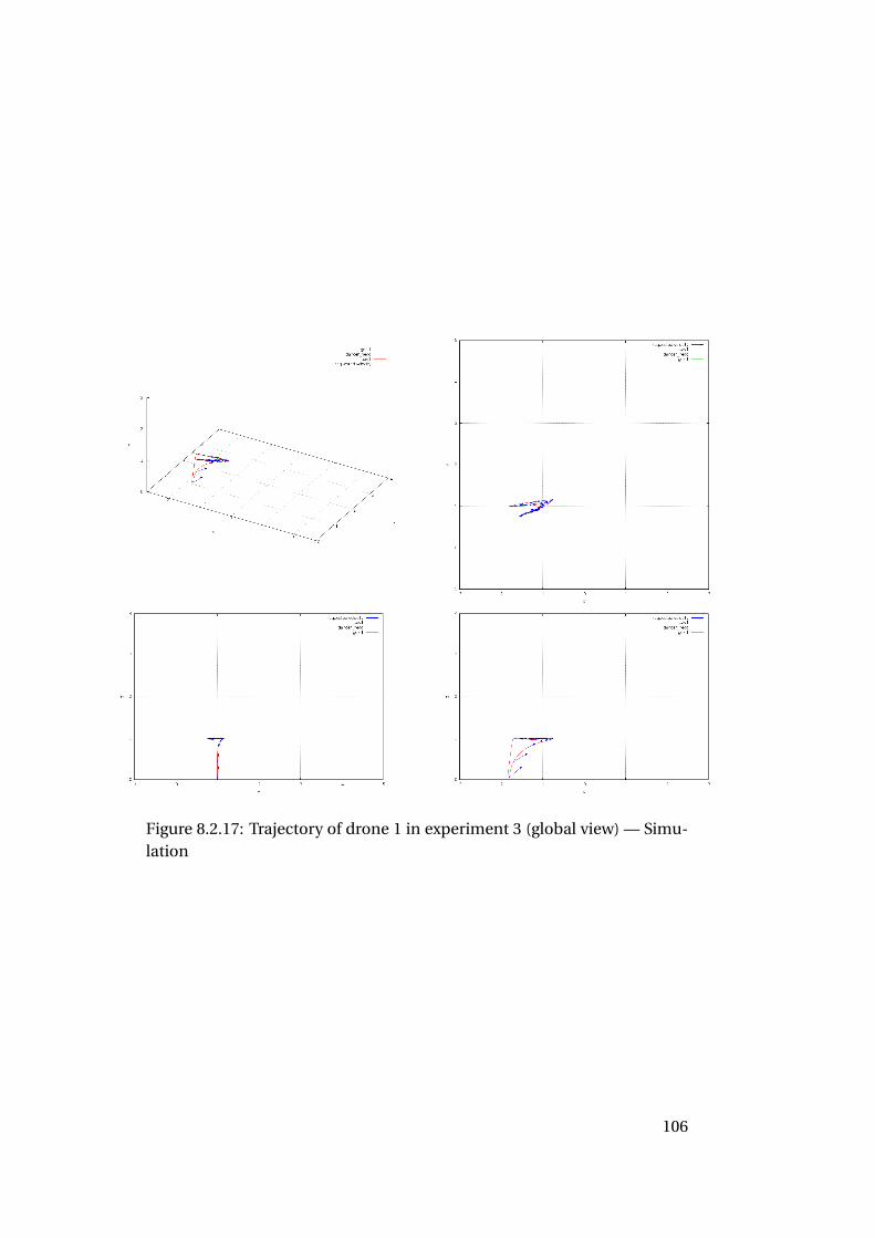
Figure 8.2.17: Trajectory of drone 1 in experiment 3 (global view) — Simu-lation
106
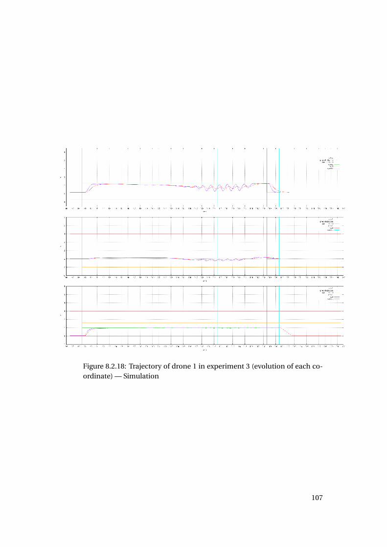
Figure 8.2.18: Trajectory of drone 1 in experiment 3 (evolution of each co-ordinate) — Simulation
107
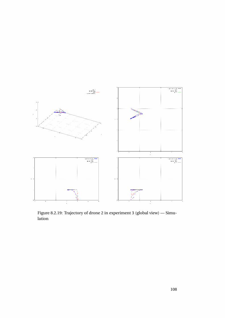
Figure 8.2.19: Trajectory of drone 2 in experiment 3 (global view) — Simu-lation
108
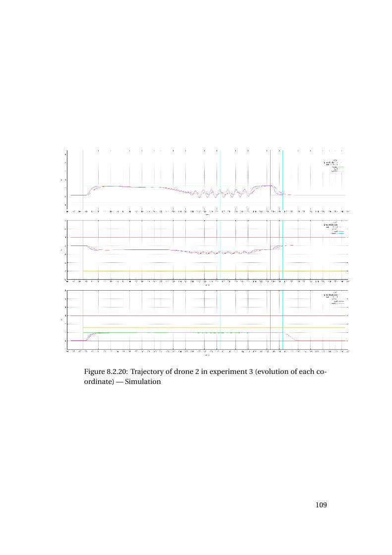
Figure 8.2.20: Trajectory of drone 2 in experiment 3 (evolution of each co-ordinate) — Simulation
109
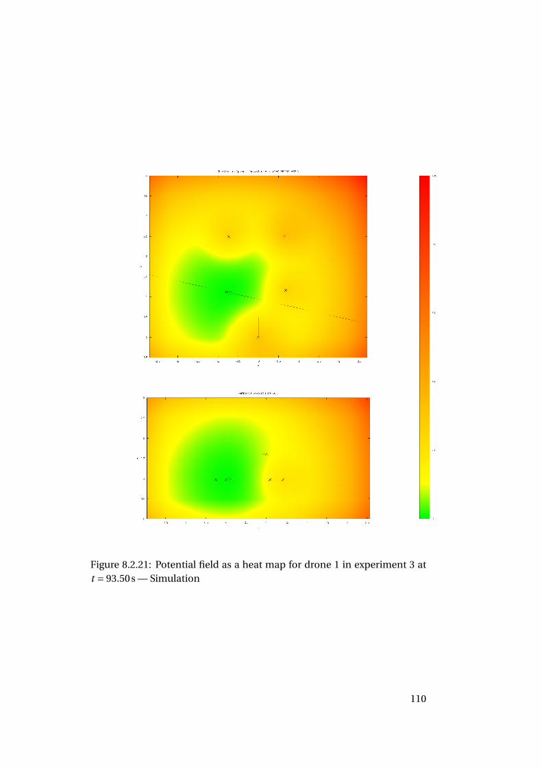
Figure 8.2.21: Potential field as a heat map for drone 1 in experiment 3 att = 93.50s — Simulation
110
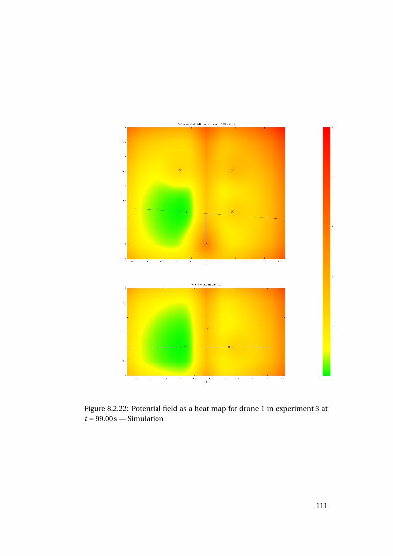
Figure 8.2.22: Potential field as a heat map for drone 1 in experiment 3 att = 99.00s — Simulation
111
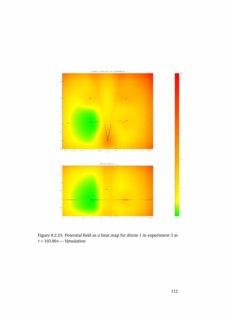
Figure 8.2.23: Potential field as a heat map for drone 1 in experiment 3 att = 103.00s — Simulation
112
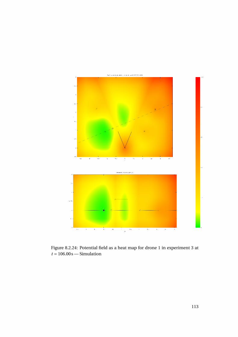
Figure 8.2.24: Potential field as a heat map for drone 1 in experiment 3 att = 106.00s — Simulation
113
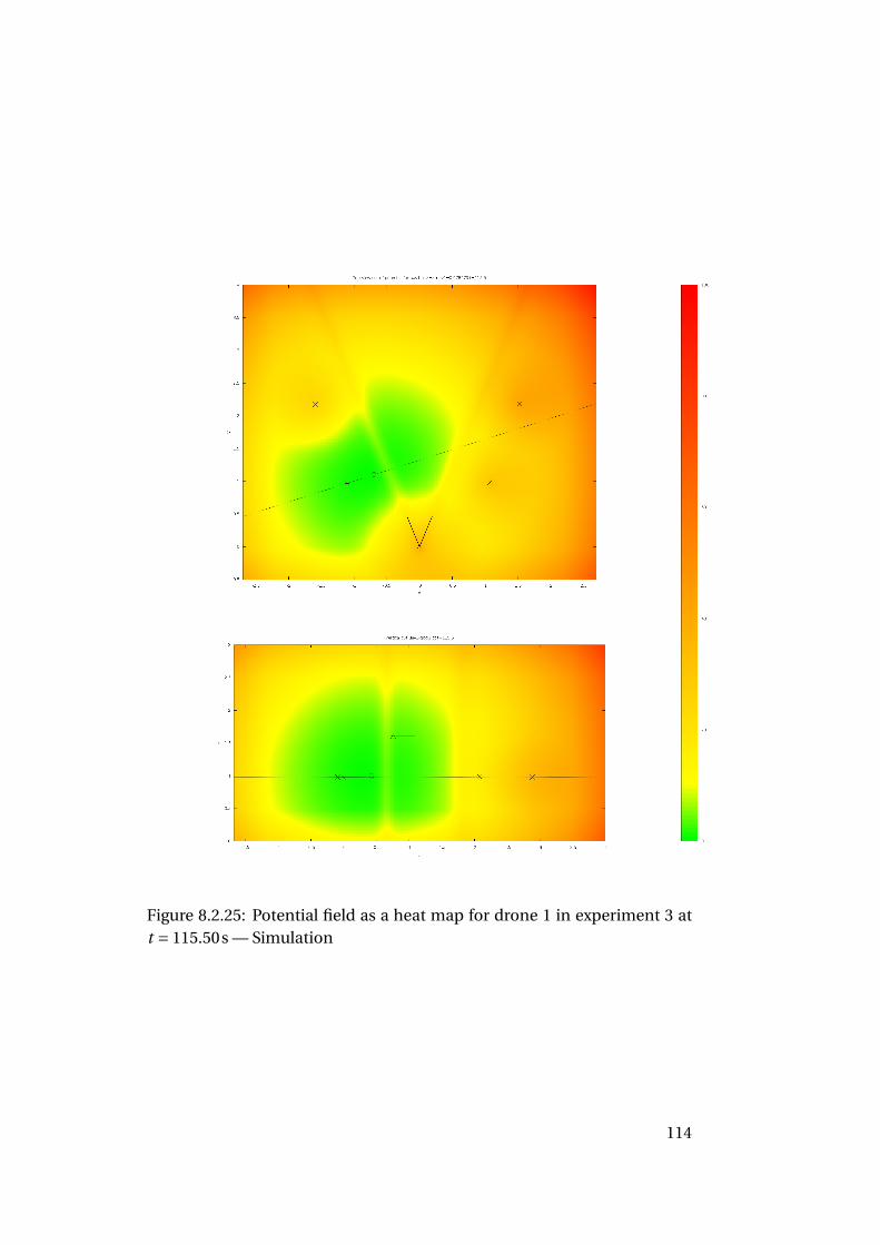
Figure 8.2.25: Potential field as a heat map for drone 1 in experiment 3 att = 115.50s — Simulation
114
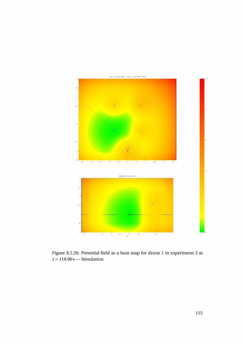
Figure 8.2.26: Potential field as a heat map for drone 1 in experiment 3 att = 118.00s — Simulation
115
Discussion
The first phase when the hands start having an effect is between t = 93.6sand t = 98.6s. It increases linearly, and the drones move from their nominalposition by about 18cm. This is a limited effect, not as spectacular as wewould have expected.
In the next two seconds, the dancer does not move and the positionof the drones stabilize. Then the dancer starts opening her arms and thedrones move further apart. Logically, drones 2 and 4 are more affectedsince the half-planes defined by the hands move faster at their level. Duringfive seconds the movement of the drones is regular enough. At t = 105.6s,drone 1 has moved by 44cm and drone 2 by 80cm. At this point oscillationsstart, and get quite bad (more than can be seen from the graphs, becausethe orientation of the drones also oscillates a lot). When the dancer’s handsretract, oscillations decrease and the drones return to their nominal posi-tions.
To eliminate oscillations, two directions can be explored. One optionis to put an upper bound on the attractive force of the goals, making thedrones more docile. Another is to implement an additional mode wherethere is no attractive force and the drone idle where they are in the absenceof obstacle. In the latter case, the drones would remain where they arewhen the dancer’s hands retract, allowing the dancer to move them aroundfreely.
116
Chapter 9
Conclusions and Future Work
9.1 ConclusionIn this Master thesis we explored most of the different steps of quadrotordesign, from the research and the purchase of the different components, tothe modeling and assembling of the drone; from the installation of a Mo-Cap system, to making the drone fly; from implementing a reactive motionplanning strategy to simulating several motion primitives ready to be partof a complex choreography. We have developed an environment to create,simulate, test and analyse a multi-quadrotor choreography.
For the moment, only the experiments involving one drone have beentested in reality. The results, gathered in Chapter 8, show us that our motionplanning strategy based on potential fields does provide safe and interac-tive drone trajectories. However, they also underline drawbacks linked tothis motion planning solution and to practical position tracking constraints(see Section 9.2). In overall, these first results are promising and pave thepath for future improvements.
117
9.2 Future workThe end goal of the extended version of this project, the opera performanceReCallas, will take place in September 2018. Therefore future work startswith everything that has to be done so that the flying opera choir is ready forthe performance. But future work also includes making our work reusablebeyond the performance, as well as more theoretical aspects.
Before the performance, many aspects of our platform should be im-proved. First, the design of the drone. Better and safer propeller protec-tions should be designed. Moreover, for stage effect purposes and human-drone interactions, we should think to incorporate a lighting system. Lightsignals could be used to visually communicate some information on thedrone internal state such as its behaviour mode, as well as some warningslike a low battery level, a component failure, or a software failure (for in-stance a ROS node not responding). Other light signals and effects could beused to add dramatic effects during the performance. Second, the speakersystem needs to be tested and analysed more thoroughly and it needs tosatisfy the composer constraints. Third, we have to build the other dronesand test the multi-drone system. Fourth, we should improve the safetymeasures, especially the drone response when a component fails. Indeed,we need to work on avoiding failures but also make sure that even if they dohappen the drone behaves safely. For instance, in our experiments we haveobserved that sometimes the MoCap system confused the drone markerpattern with the dancer marker pattern on her/his head. Fifth, in the ex-periments (Chapter 8), we observed that oscillations can occur around re-pulsive objects. These oscillations do not cause the immediate crash of thedrone but still represent a hinder to its stability. That is why we should workon reducing unwanted oscillations by improving the prediction step andby adapting the maximum speed of the drone to its environment. Sixth,we also should improve the flexibility of the choreographer script language.Especially, we would like to allow it to modify parameters and accept event-driven instructions. Seventh, to help or improve the collaboration with theartists, maybe we should develop the server interface and functionalities.And finally, the current motion primitives are meant to be completed bymotions imagined by the choreographer.
On a more theoretical level, it could be worth investigating how it is pos-sible for quadrotor motions to be recognized and interpreted as expressivefrom our point of view in term of individual motions and in term of group(multi-drones) motions. Indeed, we could look into the expressiveness of
118
a single drone’s motions and of the motions of a group of drones thanks totheir formations and their motions relative to each others. In addition onworking on making the drone motions expressive, we could also researchhow to make them understand or interpret emotions from the dancer mo-tions. This way we could start a real gestural communication between thedancer and the drones. Methods like deep learning could be employed toachieve such results.
119
Bibliography
[1] Ars Electronica. Spaxels. 2016. URL: http://www.spaxels.at/.
[2] F. Augugliaro, A. P. Schoellig, and R. D’Andrea. “Dance of the Fly-ing Machines: Methods for Designing and Executing an Aerial DanceChoreography”. In: IEEE Robotics Automation Magazine 20.4 (2013),pp. 96–104. DOI: 10.1109/MRA.2013.2275693.
[3] Anthony M. Bloch et al. “Nonholonomic mechanical systems withsymmetry”. In: Archive for Rational Mechanics and Analysis 136.1(1996), pp. 21–99. DOI: 10.1007/BF02199365.
[4] R. W. Brockett. “Control Theory and Singular Riemannian Geome-try”. In: New Directions in Applied Mathematics. Ed. by Peter J. Hiltonand Gail S. Young. New York, NY: Springer New York, 1982, pp. 11–27.DOI: 10.1007/978-1-4612-5651-9_2.
[5] A. E. Bryson and Y.-C. Ho. Applied Optimal Control. 481 p. New York,NY: Hemisphere, 1975.
[6] K. Capek. Rossumovi Univerzálnı Roboti (R.U.R.) 1920.
[7] Cirque du Soleil. PARAMOUR. Flying machine design and choreog-raphy by Verity Studios. 2016. URL: http://veritystudios.com/aboutus/.
[8] Herman E. Daly. Beyond Growth: The Economics of Sustainable De-velopment. Boston, MA: Beacon Press, 2014. ISBN: 978-080704709-5.
[9] Elevenplay. Accessed: 2017-08-05. URL: http://elevenplay.net/.
[10] Elevenplay. America’s Got Talent. 2016. URL: https : / / www .youtube.com/watch?v=1CjX1r-gh8U.
[11] Elevenplay. Shadow. 2016. URL: https : / / youtu . be /hX2TneyE41Q.
120
[12] ETH Zurich Institute for Dynamic Systems and Control. Flying Ma-chine Arena. 2016. URL: http://flyingmachinearena.org/.
[13] Intel Newsroom. Starbright. Intel, Disney light up the sky over WaltDisney World resort with new Starbright Holidays drone show. 2016.URL: https://newsroom.intel.com/news-releases/intel-disney-starbright-holidays-drone-show/.
[14] D. Jacobson. “Differential dynamic programming methods for solv-ing bang-bang control problems”. In: IEEE Transactions on Auto-matic Control 13.6 (1968), pp. 661–675. DOI:10.1109/TAC.1968.1099026.
[15] O. Khatib. “Commande Dynamique dans l’Espace Opérationnel desRobots Manipulateurs en Présence d’Obstacles”. in French. ThesisDissertation. École Nationale Supérieure de l’Aéronautique et del’Espace, Toulouse, 1980.
[16] O. Khatib. “Real-Time Obstacle Avoidance for Manipulators and Mo-bile Robots”. In: International Journal of Robotics Research 5.1 (1986),pp. 90–98.
[17] Y. Koren and J. Borenstein. “Potential field methods and their inher-ent limitations for mobile robot navigation”. In: Proceedings. 1991IEEE International Conference on Robotics and Automation. vol. 2.1991, pp. 1398–1404. DOI: 10.1109/ROBOT.1991.131810.
[18] Vijay Kumar, Miloš Žefran, and James P. Ostrowski. “Chapter 15. Mo-tion Planning and Control of Robots”. In: Handbook of IndustrialRobotics. John Wiley & Sons, Inc., 2007, pp. 295–315. DOI: 10.1002/9780470172506.ch15.
[19] Adrienne Lafrance. “What is a robot?” In: The Atlantic (2016). Ac-cessed: 2017-08-27. URL: https://www.theatlantic.com/technology/archive/2016/03/what- is- a- human/473166/.
[20] L. Lasdon, S. Mitter, and A. Waren. “The conjugate gradient methodfor optimal control problems”. In: IEEE Transactions on AutomaticControl 12.2 (1967), pp. 132–138. DOI: 10 . 1109 / TAC . 1967 .1098538.
[21] J. P. Laumond et al. “A motion planner for nonholonomic mobilerobots”. In: IEEE Transactions on Robotics and Automation 10.5(1994), pp. 577–593. DOI: 10.1109/70.326564.
121
[22] A. Laviers and M. Egerstedt. Controls and Art: Inquiries at the Inter-section of the Subjective and the Objective. 235 pages. Springer, 2014.DOI: 10.1007/978-3-319-03904-6.
[23] Zexiang Li and J. F. Canny, eds. Nonholonomic Motion Planning.Kluwer Academic Publishers, 1992. ISBN: 978-0-7923-9275-0.
[24] S. Lupashin et al. “A platform for aerial robotics research and demon-stration: The Flying Machine Arena”. In: Mechatronics 24.1 (2014),pp. 41–54. DOI: 10.1016/j.mechatronics.2013.11.006.
[25] Baoming Ma and W. S. Levine. “An algorithm for solving control con-strained optimal control problems”. In: Proceedings of 32nd IEEEConference on Decision and Control, vol. 4. 1993, pp. 3784–3790. DOI:10.1109/CDC.1993.325926.
[26] D. Mayne and E. Polak. “An exact penalty function algorithm for con-trol problems with state and control constraints”. In: IEEE Transac-tions on Automatic Control 32.5 (1987), pp. 380–387. DOI: 10.1109/TAC.1987.1104615.
[27] Oli Metcalfe Design. MUSE drones tour. 2016. URL: https://www.youtube.com/watch?v=LnfSL2ca3ag.
[28] J. P. Ostrowski. “The Mechanics and Control of Undulatory Loco-motion”. PhD thesis. California Institute of Technology, 1995. URL:http://thesis.library.caltech.edu/4194/.
[29] Linux Foundation DroneCode project. PX4: The Professional Autopi-lot. Accessed: 2017-08-05. URL: http://px4.io/.
[30] R. Pytlak and R. B. Vinter. “Second-order method for optimal controlproblems with state constraints and piecewise-constant controls”.In: Proceedings of 1995 34th IEEE Conference on Decision and Con-trol, vol. 1. Vol. 1. 1995, pp. 625–630. DOI: 10.1109/CDC.1995.478982.
[31] M. Quigley et al. “ROS: an open-source Robot Operating System”. In:ICRA Workshop on Open Source Software. 2009. URL: http://www.willowgarage.com/sites/default/files/icraoss09-ROS.pdf.
[32] Rhizomatiks. Accessed: 2017-08-05. URL: https://research.rhizomatiks.com/.
122
[33] E. Rimon and D. E. Koditschek. “Exact robot navigation using artifi-cial potential functions”. In: IEEE Transactions on Robotics and Au-tomation 8.5 (1992), pp. 501–518. DOI: 10.1109/70.163777.
[34] Saatchi & Saatchi. Meet Your Creator. 2012. URL: http : / /saatchi.com/en-us/news/saatchi__saatchi_new_directors_showcase_2012.
[35] A. Schöllig, F. Augugliaro, and R. D’Andrea. “A platform for danceperformances with multiple quadrocopters”. In: Proceedings of theIEEE/RSJ International Conference on Intelligent Robots and Systems(IROS)-Workshop on Robots and Musical Expressions. 2010, pp. 1–8.
[36] A. Schöllig et al. “Feasibility of motion primitives for choreographedquadrocopter flight”. In: American Control Conference (ACC), 2011.2011, pp. 3843–3849.
[37] A. Schöllig et al. “Synchronizing the motion of a quadrocopter tomusic”. In: Robotics and Automation (ICRA), 2010 IEEE InternationalConference. IEEE. 2010, pp. 3355–3360.
[38] E. Stephens and T. Heffernan. “We Have Always Been Robots: TheHistory of Robots and Art”. In: Robots and Art, Exploring an UnlikelySymbiosis. Ed. by D. Herath, C. Kroos, and Stelarc. Springer, 2016,pp. 29–45. DOI: 10.1007/978-981-10-0321-9_3.
[39] H. J. Sussmann. “Lie Brackets, Real Analyticity and Geometric Con-trol”. In: Differential Geometric Control Theory. Ed. by R. Millman,R. W. Brockett, and H. J. Sussmann. Boston, MA: Birkhäuser, 1983,pp. 1–116.
[40] K. L. Teo, C. J. Goh, and K. H. Wong. A Unified Computational Ap-proach to Optimal Control Problems. Burnt Mill, Harlow: LongmanScientific & Technical, 1991.
[41] Thwink.org, Inc. Sustainability. Accessed: 2017-08-27. URL:http : / / www . thwink . org / sustain / glossary /Sustainability.htm.
[42] UN General Assembly. 2005 World Summit Outcome : resolutionadopted by the General Assembly, 24 October 2005, A/RES/60/1. Ac-cessed: 2017-08-27. URL:http://www.refworld.org/docid/44168a910.html.
123
[43] UN World Commission on Environment and Development.Our Common Future. Oxford New York: Oxford Univer-sity Press, 1987. ISBN: 978-0-19-282080-8. URL: https : / /sustainabledevelopment.un.org/milestones/wced.
[44] Åsa Unander-Scharin. “Mänsklig mekanik och besjälade maskiner(Human Mechanics and Soulful Machines)”. Thesis Dissertation.Luleå Univ. of Technology, 2008.
[45] Åsa Unander-Scharin and Carl Unander-Scharin. Olimpia. 2010.URL: http://www.operamecatronica.com/node/1168.
[46] Åsa Unander-Scharin and Carl Unander-Scharin. Ombra mai fú.2010. URL: http : / / www . operamecatronica . com /ombramaifu.
[47] Åsa Unander-Scharin and Carl Unander-Scharin. Robotcygne. 2010.URL: http://www.operamecatronica.com/robocygne.
[48] Åsa Unander-Scharin and Carl Unander-Scharin. The Lamentationsof Orpheus. 2010. URL: http : / / www . operamecatronica .com/node/1171.
[49] C. Unander-Scharin. “Extending Opera - Artist-led Explorations inOperatic Practice through Interactivity and Electronics”. Thesis Dis-sertation. KTH Stockholm, 2015.
[50] Francisco J. Varela, Eleanor Rosch, and Evan Thompson. The Embod-ied Mind: Cognitive Science and Human Experience. Cambridge: MITPress, 1992.
[51] Verity Studios. Accessed: 2017-08-05. URL: http : / /veritystudios.com/.
[52] Verity Studios. 2047 Apologue. 2016. URL: http : / /veritystudios.com/.
[53] Verity Studios. ABB 125 Anniversary VIP Gala. 2016. URL: http://www.veritystudios.com/.
[54] Verity Studios. Fantastic Journey. 2016. URL: http : / / www .veritystudios.com/.
[55] Verity Studios, ETH Zurich, and Cirque du Soleil. SPARKED. 2014.URL: https : / / www . youtube . com / watch ? v =6C8OJsHfmpI&t=4s.
124
[56] Miloš Žefran. “Continuous methods for motion planning”. PhD the-sis. University of Pennsylvania, 1996. URL: http://repository.upenn.edu/dissertations/AAI9713033/.
125
www.kth.se