a simplified cacl –ca(oh) equilibration method to determine

J. Indian Soc. Coastal agric. Res. 32(2): 1-10 (2014)

A Simplified CaCl2–Ca(OH)

2 Equilibration Method to Determine

the Lime Requirement of Acid Soils of Odisha

P.K.DAS, A. SAMANTA and G.H. SANTRA

Department of Soil Science and Agricultural Chemistry

Orissa University of Agriculture & Technology, Bhubaneswar - 751 003, Odisha

Received: 19.11.2014 Accepted: 16.12.2014

Lime requirements (LR) of some acid soils of Odisha belonging to Alfisols, Inceptisols andEntisols were evaluated by Ca(OH)2 equilibration, CaCl2–Ca(OH)2 equilibration and modifiedWoodruff buffer (mod. WB) methods. Lime requirement of the soils increased in the order of LRdetermined by Ca(OH)2 equilibration method< LR determined by CaCl2–Ca(OH)2 equilibrationmethod< LR determined by mod. WB method. A linear relationship existed between the OH-

added and increase in pH in Ca(OH)2 and CaCl2–Ca(OH)2 equilibrations. On the basis of thislinearity a simple and rapid method was tried to develop to determine LR of the soils by addingCa(OH)2 solutions of selected concentrations instead of adding Ca(OH)2 solutions of severalconcentrations. It was observed that LR determined by adding saturated Ca(OH)2 solutions of 0& 4 mL in Ca(OH)2 equilibration method and 0 & 8 mL in CaCl2–Ca(OH)2 equilibration methodwere close to the LR determined from the full equilibration study i.e. after adding Ca(OH)2

solutions of several concentrations. These two methods were referred to as simplified Ca(OH)2

equilibration and simplified CaCl2–Ca(OH)2 equilibration methods, respectively. Laboratoryincubation and pot culture experiment showed that the simplified Ca(OH)2 equilibration methodunderestimated, whereas simplified CaCl2–Ca(OH)2 equilibration and mod. WB methodsoverestimated LR of the soils to the desired pH 6.5 measured after 15 days of liming. Soil pH inthe laboratory incubation study increased between 6.0 and 6.5 in different soils when lime wasapplied @ 0.5 LR as per simplified CaCl2–Ca(OH)2 equilibration method. It increased between6.3 and 6.8 when lime was applied at the same rate as per mod. WB method. In the pot cultureexperiment, the change in soil pH at 15 days of liming showed that application of lime @ 0.5 LRby simplified. CaCl2–Ca(OH)2 equilibration and mod. WB methods slightly overestimated theLR to the desired pH 6.5. Liming the soil at 0.3 LR as per the simplified CaCl2–Ca(OH)2

equilibration method slightly underestimated the desired pH 6.5. Liming the soil as per thesimplified CaCl2–Ca(OH)2 equilibration method was significantly superior to liming as persimplified Ca(OH)2 equilibration method but equivalent to liming as per mod. WB method inproducing the dry matter yield of maize. Increasing the lime level from 0.3 to 1.0 LR had nosignificant effect in increasing the dry matter yield of maize.

(Key words: Acid soils, Lime requirement, Modified Woodruff Buffer method, Simplified Ca(OH)2and CaCl2–Ca(OH)2 Equilibration methods)

Several buffer-pH methods have been developed

to determine the lime requirement of acid soils

(Woodruff, 1948, Shoemaker et al., 1961, Yuan,

1974, McLean et al., 1978, Fox, 1980, Tran and Van

Lierop, 1981). These methods are based on the

relationships of the decrease in pH of the soil buffer

suspension below the buffer pH and neutralizable

soil acidity to attain the desired pH which is not

exact but based on some approximations. Buffer

pH method, therefore, either overestimates or

underestimates the LR of soils in many cases. These

methods are also expensive requiring a number of

chemicals including toxic compounds l ike

p-nitrophenol (Min Liu et al., 2004) and K2CrO

4

(Pagani and Mallarino, 2011). Lime requirement by

incubation method although provides more accurate

information but is time consuming for routine analysis.

Dunn (1943) determined lime requirement of

soils by direct titration with Ca(OH)2. Lime

requirement by this method was calculated from the

full titration curve which is also time consuming.

This was simplified by M in Liu et al., (2004) on the

basis of the linear relationship between increase in

pH and Ca(OH)2 added. These authors calculated

the lime requirement from a titration curve of soil

pH against three additions of saturated Ca(OH)2

solutions in equal volumes to 1:1 soil water

suspension maintaining a time interval of 30

minutes between two successive additions. This

method was still time consuming for routine

analysis. Besides the concentration of Ca2+ in the

saturated Ca(OH)2 solution is too low to replace

exchangeable Al3+ for neutralization. This method,

therefore, has the possibility to underestimate the

*Corresponding author : E-mail:[email protected]

LR of the soils containing appreciable amount of

exchangeable Al3+.

Acid soils in Odisha constitute more than 70%

of the cultivated area (Panda and Nanda, 1985).

These soils are mostly light textured with low organic

matter content and are dominated by low active

clays. The modified Woodruff buffer method (Brown

and Cisco, 1984) is commonly followed in the soil

testing laboratories of Odisha and many parts of

India to determine the LR of the soils. This method

is expensive requiring a number of chemicals

including a toxic compound like p-nitrophenol.

Besides this method consists of adding a 0.01 M

CaCl2 which is too low to replace exchangeable Al3+

for neutralization. Considering all these problems

an attempt was made in the present investigation

to find out a simple, rapid and inexpensive method

to determine LR with greater accuracy through

CaCl2-Ca(OH)

2 equilibration method using 0.5 M

CaCl2

to replace exchangeable Al3+ completely for

neutralization. This method was compared with

simplified Ca(OH)2 equilibration method and mod.

WB methods through laboratory incubation and pot

culture studies.

MATERIALS AND METHODS

Surface soil samples (0-15 cm) were collected

from twenty one representative acid soil areas

belonging to eighteen districts of Odisha (Table 1).

Some important physical and chemical properties

of the soils were determined by standard

procedures. Exchange acidity and potential acidity

to pH 8.0 ± 0.02 were determined as per Black, 1965.

The pH-dependent acidity at pH 8± 0.02 was

calculated from the difference between potential

acidity and exchange acidity.

Lime requirement of the soil to pH 6.5 was

determined by mod. WB method as follows.

LR to pH 6.5 = LR to pH 7.0 x (6.5-pHS)/ (7.0-pHs)

where LR = cmole Ca(OH)2 kg-1

pHs = salt pH with 0.01 M CaCl2

LR(CaCO3 kg ha-1)=LR [cmole Ca(OH)

2 kg-1] x 2000

Determination of LR by Ca(OH)2 equilibrationmethod

Five gram of Ca(OH)2 was dissolved in 1 liter of

distilled water for 5 days and filtered. The filtrate

was saturated Ca(OH)2 solution which is 0.022 M

at 25oC. The strength of the saturated Ca(OH)2

Table 1. Selected areas for collection of soil samples

Sl. No. Location Districts Soil classification

1 Kashipur Rayagada Rhodic Paleustalfs

2 Ainginia Khurda Typic Haplustalfs

3 Jajpur Jajpur Aeric Fluvaquents

4 Phulbani Phulbani Typic Rhodustalfs

5 Mahishapat Dhenkanal Oxic Haplustalfs

6 Nawarangapur Nawarangapur Aeric Haplustalfs

7 Koraput Koraput Kandic Paleustalfs

8 Chandaka Khurda Typic Haplustalfs

9 Baripada Mayurbhanj Aeric Ochraqualfs

10 Keonjhar Keonjhar Typic Ustochrepts

11 Sundargarh Sundargarh Aeric Haplaquepts

12 Belapada Bolangir Typic Haplustalfs

13 Rayagada Rayagada Typic Propaquepts

14 Nuagada Gajapati Typic Rhodustalfs

15 Nayagarh Nayagarh Rhodic Paleustalfs

16 Bhanjanagar Ganjam Typic Ustochrepts

17 Semiliguda Koraput Typic Haplustalfs

18 Athagarh Cuttack Typic Ustochrepts

19 Sonepur Sonepur Typic Haplustalfs

20 Jashipur Mayurbhanj Typic Rhodustalfs

21 Angul Angul Typic Ustochrepts

2 Das et al. 32(2)

solution was determined by titrating against

standard 0.02 N HCl using methyl red indicator.

Saturated Ca(OH)2 solutions of 0,.0.5,1,2,3,4,

5,6,7,8,9 and 10 mL were diluted to 25 mL in a

series of 25 mL volumetric flasks. To 10 g of soils,

25 mL of the Ca(OH)2 solutions of different

concentrations, as prepared above, were added and

pH was measured after 30 minutes of equilibration.

Preliminary study on soil pH till 24 hours of

equilibration period showed an insignificant change

in pH after 30 minutes.

Lime requirement to pH 6.5 by Ca(OH)2

equilibration method was calculated as follows.

LR to pH 6.5 [cmole Ca(OH)2 kg-1] =[{ (mb-ma)/(pH

b-

pHa)} x (6.5-pH

a)+ma]x10

where m = molarity of the saturated Ca(OH)2

solution

‘a’ and ‘b’ were the volumes (mL) of saturated

Ca(OH)2 solutions added increasing the pH of the

soil suspensions to pHa and pH

b, respectively. pH

a

was just below 6.5, whereas pHb was just above 6.5

in the equilibration study for the particular soil.

(mb-ma)/(pHb-pH

a) is the mmole of Ca(OH)

2 required

to raise the pH by one unit between pHa and pH

b for

10 g soil.

[{(mb-ma)/ (pHb-pH

a)}] x (6.5-pH

a) is the mmole of

Ca(OH)2 required to increase the pH from pH

a to

6.5 for 10 g soil.

mmole of Ca(OH)2 required to raise the initial soil

pH to pHa for 10 g soils = ma.

Initial soil pH is the pH when zero mL of saturated

Ca(OH)2 solution is added.

Calculating the LR from this formula is more

appropriate than calculating the LR from the

regression equation of the increase in the pH with

Ca(OH)2 added.

Determinat ion of LR by CaCl2–Ca(OH)2

equilibration method

To 10 g of soils 25 mL of 0.5 M CaCl2 containing

different concentrations of Ca(OH)2 were added . The

solutions were prepared by adding 0,2,4,6,8,10,12,

and 14 mL of saturated Ca(OH)2 solutions to 10 mL

of 1.25 M CaCl2 in a series of 25 mL volumetric

flasks and finally diluted to 25 mL. The pH of the

soil suspensions were measured after 30 minutes.

Lime requirement to pH 6.5 by CaCl2–Ca(OH)

2

equilibration method was calculated by using the

same formula for determining LR by Ca(OH)2

equilibration method.

Development of simplified Ca(OH)2 and CaCl

2 –

Ca(OH)2

equilibration methods to determine LR

A high degree of linearity existed between OH-

added and the increase in pH in both the

equilibration methods with ‘r’ values varying from

0.951 to 0.994 in Ca(OH)2 equilibration method and

0.958 to 0.997 in CaCl2 –Ca(OH)

2 equilibration

method (Table 4). Similar observation had also been

reported by Magdoff and Bartlett (1985), Min Liu

et al. (2004) and Weaver et al. (2004). On this basis

of linearity LR was calculated by adding only two or

three different volumes of saturated Ca(OH)2

solutions instead of adding several volumes of

saturated Ca(OH)2 solutions. For Ca(OH)

2

equilibration method LR was calculated by adding

0&2; 0&3; 0&4; 0,1&3; 0,1&4 and 0,2&4 mL of

saturated Ca(OH)2

solutions. For CaCl2–Ca(OH)

2

Table 2. Some important physical and chemical properties and forms of acidity in the soils

Properties Range Mean Remarks

Texture sl to cl – sl=15, scl=3, cl=1,c=1

Clay (%) 12.6 to 35.4 17.5 –

pHw (1:2.5) 4.2 to 5.7 5.0 –

pHs with 0.5 M CaCl2 (1:2.5) 3.5 to 4.3 3.8 –

Organic carbon (kg-1) 1.8 to 8.6 4.7 Low=15, Med.=1, High=4

Forms of acidity [cmole (p+) kg-1 ] –

Exchange acidity 0.12 to 2.32 0.78 –

Exchangeable H+ 0.04 to 0.52 0.20 –

Exchangeable Al3+ ND to 2.20 0.58 ND=6

pH-dependent acidity 3.6 to 11.6 5.92 –

Potential acidity 4.1 to 12.1 6.70 –

NB: Figures in the remarks column indicate the number of soils.

ND = Not detectable

32(2) Lime requirement determination 3

Laboratory incubation study

Laboratory incubation study was carried out

with the soil samples collected from Angul,

Athagarh, Belapada, Jajpur, Jashipur, Keonjhar,

Koraput, Nayagarh, Rayagada and Sijua. Required

quantities of pure CaCO3 at 0.5 and 1.0 LR levels

calculated according to the above three methods

were added to 100 g soils and incubated for 15 days

maintaining the moisture content at field capacity.

After 15 days soil pH and exchange acidity were

determined.

Pot culture study

The pot culture experiment was conducted with

the surface soil (0-15 cm) samples collected from

Sijua, Bhubaneswar (Odisha). The soil was sandy

loam having 13.6% clay and organic carbon content

of 2g kg-1. Soil pHw was 5.4 and pH

s with 0.5 M

CaCl2

was 3.8. Exchangeable Ca2+ and Mg2+ were

1.3 and 1.1 cmole(p+) kg-1, respectively. Exchange

acidity, exchangeable H+, exchangeable Al3+,

potential acidity and pH-dependent acidity were

0.288, 0.156, 0.132, 4.08 and 3.79 cmole(p+) kg-1,

respectively. Available N (Alkaline KMnO4), available

P (Bray’s I), available K (Neutral normal NH4OAc

extract) and available S (0.15%, CaCl2.2H2O extract)

were 60, 14, 54 and 5 mg kg-1 in soil, respectively.

Lime requirement of the soil to pH 6.5 was 362,

1250 and 1421 mg CaCO3

kg-1 as determined by

simplified Ca(OH)2 equilibration, simplified CaCl

2–

Ca(OH)2 equilibration and mod. WB methods,

respectively.

Table 3. Lime requirement of the soils to pH 6.5 determined by Ca(OH)2,

CaCl2–Ca(OH)2 equilibration methods and mod. WB method

Methods LR to pH 6.5 [cmole Ca(OH)2 kg-1 ]

Range Mean

Ca(OH)2 equilibration 0.095 to 1.148 0.534

CaCl2–Ca(OH)2 equilibration 0.590 to 2.263 1.374

mod. WB 0.704 to 3.074 1.722

Table 4. Regression equations and correlation coefficient values between OH- added

and increase in soil pH in Ca(OH)2 and CaCl2–Ca(OH)2 equilibration methods

Method r r2 Y= a+bx

a b

Ca(OH)2 equilibration method 0.951**-0.994** 0.904-0.988 4.307-6.524 0.760-1.428

CaCl2–Ca(OH)2 equilibration method 0.958**-0.997** 0.917-0.995 3.373-5.007 0.564-1.098

* y = pH and x = OH- added [cmole (e-) kg-1]

equilibration method, LR was calculated by adding

0&2; 0&4; 0&6; 0&8; 0,2&4; 0,2&6 ; 0,2&8; 0,4&6;

0,4&8 and 0,6&8 mL of saturated Ca(OH)2 solutions.

Soil pH was measured in the same procedure as

described earlier.

Lime requirements to pH 6.5 for both the

equilibration methods were calculated as follows

when three different volumes of saturated Ca(OH)2

solutions including zero mL were added

LR = my-mx

(6.5-pH0) x 10

pHy-pHx

pH0,

pHx and pH

y were the pH of the soil suspensions

when 0, x and y mL of saturated Ca (OH)2 solutions

were added (y>x). When two different volumes of

saturated Ca(OH)2 solutions were added of which

one was zero mL this equation changed to

LR = mz

(6.5-pH0) x 10

pHz-pH0

Where, pHz was the pH of the soil suspension when

‘z’ mL of saturated Ca(OH)2 solution was added.

It was observed that LR calculated from the pH

values of the soils after adding saturated Ca(OH)2

solutions of 0&4 mL in Ca(OH)2 equilibration method

and 0&8 mL in CaCl2–Ca(OH)

2 equilibration method

were closest to the LR calculated from the full

equilibration studies as indicated by the lowest

(L2- L

1)2, lowest Sd and nonsignificant ‘t’ values

(Table 5). These two simple methods to determine

LR were evaluated through laboratory incubation

and pot culture studies along with the mod. WB

method.

4 Das et al. 32(2)

Five kg of air- dried and sieved (2mm) soils,

after being thoroughly mixed with the required

quantities of pure CaCO3 (LR grade) were taken in

earthen pots. There were ten treatments (Table 10)

replicated thrice in factorial randomized design. The

test crop grown was Zea mays cv Platinum. N, P2O

5,

K2O and S were added @ 150-75-75-20 kg ha-1 as

chemical grades (LR) of urea, KH2PO

4, KCl and

(NH4)2

SO4, respectively in solution forms. Twenty

five % of N, full dose of P2

O5

, 25% of K2O and full

dose of S were applied after germination of the seeds.

Another 50% N and 50% K2O were applied after 15

days of application of first dose of fertilizers and

the rest 25% N and 25% K2O were applied after 15

days of the application of second dose of fertilizers.

The N content in (NH4)2SO

4 was considered while

calculating the amount of urea to be applied in the

first dose. Soil samples were collected at 15, 30, 45

and 60 days of liming and analyzed for pH and

exchange acidity. Soil samples collected after

Table 5. Comparison of LR to pH 6.5 (L2) calculated from the pH values after adding 2 or 3 different

volumes of saturated Ca(OH)2 solution with the LR to pH 6.5 obtained from full

equilibration study (L1) in Ca(OH)2 and CaCl2–Ca(OH)2 equilibration methods

Volumes of saturated Ca(OH)2 Σ (L2-L1)2 Standard deviation (Sd) Cal. ‘t’ value

solutions added (ml) [cmole Ca(OH)2 kg-1 ]2

Ca(OH)2 equilibration method

0 & 2 0.514 0.149 2.042

0 & 3 0.411 0.131 2.210*

0 & 4 0.279 0.106 2.013

0, 1 & 3 0.735 0.173 2.320*

0, 1 & 4 0.616 0.152 2.760*

0, 2 & 4 0.632 0.161 2.300*

CaCl2–Ca(OH)


0 & 2 10.008 0.704 1.080

0 & 4 3.865 0.444 0.738

0 & 6 0.672 0.187 1.790

0 & 8 0.497 0.151 1.620

0, 2 & 4 4.034 0.448 1.040

0, 2 & 6 1.236 0.254 0.194

0, 2 & 8 1.907 0.291 1.850

0, 4 & 6 5.722 0.533 1.030

0, 4 & 8 6.320 0.577 2.270*

0, 6 & 8 28.916 1.00 3.110**

*Significant at 5% level ** Significant at 1% level

Table 6. Change in soil pH and exchange acidity with liming after 15 days of incubation in different soils

Sl.No Treatments CaCO3 added Soil pH Exchange acidity Exchangeable Al3+

([cmole kg-1 ]) [cmole(p+) kg-1] [cmole(p+) kg-1]

Range

1 0LR 0 4.5-5.6 0.180-1.980 0.022-1.672

2 1.0 LR by M1

0.262-1.510 5.2-6.4 0.036-0.360 ND-0.220

3 0.5 LR by M2

0.540-1.100 6.0-6.5 0.036-0.144 ND

4 0.5 LR by M3 0.683-1.537 6.3-6.8 0.036-0.072 ND

5 1.0 LR by M2 1.080-2.200 6.8-7.5 ND-0.036 ND

6 1.0 LR by M3 1.367-3.074 7.0-7.9 ND-0.036 ND

Initial – 4.3-5.4 0.164-2.324 ND-2.200

Figures in parentheses indicate exchangeable Al3+ [cmole (p+) kg-1]. ND= Not detectable

M1= Simplified Ca(OH)2 equilibration method, M2= Simplified CaCl2–Ca(OH)2 equilibration method, M3= mod. WB method


harvesting of the crop i.e. at 60 days of liming were

analyzed for potential acidity, pH-dependent acidity

and exchangeable Ca2+ and Mg2+ also. Dry matter

yields of the harvested plants were recorded after initial

sun-drying and then oven-drying at 60oC for 7 days.

RESULTS AND DISCUSSION

Most of the soils were sandy loam with low

organic matter content (Table 2). The soils were

moderately to strongly acidic. Positive difference

between pHw and pH

s indicated that the soils were

net negatively charged. Of the potential acidity, 88

to 96% was formed by pH-dependent acidity and

the rest by exchange acidity. Exchangeable Al3+ was

detected below pH 5.4. Both potential and pH-

dependent acidities were positively correlated with

clay (r=0.62** and 0.57**, respectively) and organic

carbon (r=0.57** and 0.68**, respectively).

Lime requirement of the soils

Lime requirement of the soils decreased in the

order of LR determined by Ca(OH)2 equilibration

method < by CaCl2–Ca(OH)

2 equilibration method <

by mod. WB method (Table 3). In the determination

of LR by Ca(OH)2 equilibration, the concentration

of Ca2+ in the Ca(OH)2 solution added is too low to

replace the exchangeable H+ and Al3+ completely to

the soil solution, whereas in CaCl2–Ca(OH)

2

equilibration a 0.5 M CaCl2 is used, which is

sufficient to replace all the exchangeable H+ and

Al3+ to the soil solution. Besides the excess of Ca2+

in the soil solution suppress the hydrolysis of Ca-

clay to prevent the rise in pH. More Ca(OH)2 is,

therefore, needed to raise the pH to 6.5 in CaCl2–

Ca(OH)2 equilibration than in Ca(OH)

2 equilibration.

The LR determined by CaCl2–Ca(OH)

2 equilibration

method is, therefore, greater than the LR determined

by Ca(OH)2 equilibration method. In mod. WB

method a 0.01 M CaCl2

is added to the soil. The

concentration of Ca2+ in this solution is also too

low to replace exchangeable Al3+ for neutralization.

The CaCl2–Ca(OH)

2 equilibration method is,

therefore, expected to estimate higher LR than mod.

WB method but the opposite was found in this

study. This showed that the basis of LR calculation

in mod. WB method that for each one unit decrease

in pH of the soil buffer suspension below 7.0, 10

meq of acidity is to be neutralized per 100 g soil

might be an overestimation. Over estimation of LR

by mod. WB method has also been reported by

Panda and Nanda (1985) and Das et al., (2006). The

r2 values between the OH- added and increase in

pH indicated 90.4 to 99.8% of linearity between pH

and OH- added in Ca(OH)2 equilibration method and

91.7 to 99.5% of linearity between these two

variables in CaCl2–Ca(OH)


(Table 4). The intercept and slope values of the

regression equations were higher in Ca(OH)2

equilibration method than in CaCl2–Ca(OH)

2

equilibration method.

Lime requirement determined by Ca(OH)2

equilibration was negatively correlated with pHw

(r = - 0.81**) and positively correlated with exchange

acidity (r = 0.70**). Lime requirement determined

by CaCl2–Ca(OH)

2 equilibration was negatively

correlated with pHw (r = - 0.48*) and was positively

correlated with clay (r = 0.50*) and exchange acidity

(r = 0.68**). Lime requirement determined by mod.

WB method was positively correlated with clay (r =

0.73**) and exchange acidity (r = 0.51*). Lime

requirement determined by all the three methods

showed significant positive correlation with

exchange acidity but a nonsignificant relationship

with potential and pH-dependent acidities. Lime

requirement calculated to attain the desired pH 6.5

includes neutralization of exchange acidity and pH-

dependent acidity at pH 6.5. But the potential acidity

determined includes exchange acidity and pH-

dependent acidity at pH 8.0. This difference in pH-

dependent acidities might be the reason of the

nonsignificant relationship of LR with potential and

pH-dependent acidities. Interrelationships existed

among the LR values determined by the three

methods (Table 5). Lime requirement determined by

Ca(OH)2 equilibration method was positively

correlated with that determined by CaCl2–Ca(OH)

2

equilibration method and mod. WB method (r =

0.65** and 0.56**, respectively). The LR values

calculated by CaCl2–Ca(OH)

2 equilibration and mod.

WB methods, on the other hands, were positively

correlated with each other (r = 0.84**). Buffering

capacity of the soils determined from the reciprocal

of the slopes of the regression equations of the

increase in pH with OH- added varied from 0.700 to

1.316 and 0.911 to 1.773 cmole(p+) kg-1 in Ca(OH)2

equilibration and CaCl2–Ca(OH)

2 equilibration

methods, respectively. Buffering capacity

determined by CaCl2–Ca(OH)


was positively correlated with clay (r = 0.77**) and

organic carbon (r = 0.53*). Lime requirement

determined by the simplified Ca(OH)2 equilibration

and simplified CaCl2–Ca(OH)

2 equilibration methods

varied from 0.247 to 1.510 and 0.828 to 2.200 cmole

Ca(OH)2 kg-1, respectively.

6 Das et al. 32(2)

Laboratory incubation studies on the change insoil pH and forms of acidity after liming accordingto different methods of LR determination

Soil pH after 15 days of incubation was the

lowest in zero lime treatment varying from 4.5 to

5.6 in different soils (Table 6). Soil pH varied from

5.2 to 6.4, 6.8 to 7.5 and 7.0 to 7.9 when lime was

added @1.0 LR as per simplif ied Ca(OH)2

equilibration, simplified CaCl2–Ca(OH)

2 equilibration

and mod. WB methods, respectively. This showed

that the simplified Ca(OH)2 equilibration method

underestimated the LR of the soils, whereas the

simplified CaCl2–Ca(OH)

2 equilibration and mod. WB

methods overestimated the LR of the soils. The

extent of overestimation was more in the mod. WB

method than in the simplified CaCl2–Ca(OH)

2

equilibration method. At 0.5 LR level, soil pH varied

from 6.0 to 6.5 and 6.3 to 6.8 when lime was added

as per simplified CaCl2–Ca(OH)

2 equilibration and

mod. WB methods, respectively.

Exchange acidity was the highest in zero lime

treatment. Exchangeable Al3+ was detected in zero

lime treatments varying from 0.02 to 1.672

cmole(p+) kg-1. In lime treatments, exchangeable Al3+

was detected only in Rayagada soil [0.220 cmole(p+)

kg-1] when lime was added @ 1.0 LR as per simplified

Ca(OH)2 equilibration method. Soil pH in this

treatment was 5.2.

Pot culture experiment

A high degree of linearity existed between the

increase in pH and OH- added in Ca(OH)2 and CaCl

2–

Ca(OH)2 equilibration methods in the Sijua soil used

for the pot culture study (Fig. 1).

Change in soil pH

Soil pH at different time intervals was the lowest

(5.3 to 5.5) in zero lime treatment (Table 7). It varied

from 5.6 to 7.4 at 15 days in different treatments

and either remained same or increased slightly at

30 days. It decreased to 5.5 to 7.5 at 45 days with

further reduction of 5.3 to 6.5 at 60 days in different

treatments. The decrease in pH at 45 days and

further decrease at 60 days might be due to loss of

Ca2+ from the exchange sites. At a given LR level,

soil pH at different time intervals increased in the

order of lime applied as per simplified Ca(OH)2

equilibration method < lime applied as per simplified

CaCl2–Ca(OH)

2 equilibration method < lime applied

as per mod. WB method.

Soil pH at 15 days of liming increased to 6.3,

7.1 and 7.4 when lime was added @ 1.0 LR as per

simplified Ca(OH)2 equilibration, simplified CaCl

2–

Ca(OH)2 equilibration and mod. WB methods,

respectively. This showed that the simplified Ca(OH)2

equilibration method slightly underestimated,

whereas the simplified CaCl2–Ca(OH)

2 equilibration

method and the mod. WB method overestimated the

Table 7. Soil pH at different time intervals in the pot study

Sl. No. Treatments Soil pH at different days of liming

15 30 45 60

1 CaCO3 @ 0LR 5.5 5.5 5.5 5.3

2 CaCO3 @ 0.3 LR by M1 5.6 5.8 5.5 5.3

3 CaCO3 @ 0.3 LR by M2 6.3 6.5 6.2 5.7

4 CaCO3 @ 0.3 LR by M3 6.5 6.6 6.3 6.1

5 CaCO3

@ 0.5 LR by M1

6.1 6.0 5.8 5.6

6 CaCO3

@ 0.5 LR by M2

6.7 6.7 6.5 6.2

7 CaCO3

@ 0.5 LR by M3

6.9 7.0 6.5 6.2

8 CaCO3

@ 1.0 LR by M1

6.3 6.3 6.0 5.8

9 CaCO3 @ 1.0 LR by M2 7.1 7.2 7.1 6.4

10 CaCO3 @ 1.0 LR by M3 7.4 7.6 7.5 6.5

NB: M1

, M2

& M3 are as in table 6

Fig. 1. Soil pH at different amounts of OH added in Ca(OH)2

and CalCl-Ca(OH)2 equilibration methods in Sijua soil


Table 9. Potential acidity, pH-dependent acidity, exchangeable Ca2+

and exchangeable Mg2+ contents at harvesting

Sl. No. Treatments Potential pH-dependant Exchangeable Exchangeable

acidity acidity Ca2+ Mg2+

[cmole (p+) kg-1]

1 CaCO3 @ 0LR 4.12 3.88 1.2 0.9

2 CaCO3 @ 0.3 LR by M1 4.03 3.79 1.2 0.7

3 CaCO3

@ 0.3 LR by M2

3.55 3.31 1.4 0.8

4 CaCO3

@ 0.3 LR by M3

3.44 3.20 1.7 1.0

5 CaCO3

@ 0.5 LR by M1

3.94 3.70 1.2 0.7

6 CaCO3

@ 0.5 LR by M2

3.45 3.21 1.8 1.2

7 CaCO3 @ 0.5 LR by M3 3.25 3.01 1.8 1.3

8 CaCO3 @ 1.0 LR by M1 3.55 3.31 1.4 1.1

9 CaCO3 @ 1.0 LR by M2 2.04 1.80 1.8 0.6

10 CaCO3 @ 1.0 LR by M3 1.76 1.52 2.0 1.2

Table 8. Exchange acidity at different time intervals in the pot study

Sl.No Treatments Exchange acidity at different days of liming

[cmole(p+) kg-1]

15 30 45 60

1 CaCO3 @ 0LR 0.132 0.144 0.182 0.244 (0.132)*

2 CaCO3

@ 0.3 LR by M1

0.108 0.072 0.072 0.180 (0.130)

3 CaCO3

@ 0.3 LR by M2

0.036 0.036 0.036 0.072

4 CaCO3

@ 0.3 LR by M3

0.036 0.036 0.036 0.036

5 CaCO3 @ 0.5 LR by M1 0.072 0.072 0.072 0.108

6 CaCO3 @ 0.5 LR by M2 0.036 0.036 0.036 0.036

7 CaCO3 @ 0.5 LR by M3 0.036 ND 0.036 0.036

8 CaCO3 @ 1.0 LR by M1 0.036 0.036 0.036 0.072

9 CaCO3

@ 1.0 LR by M2

ND ND ND 0.036

10 CaCO3

@ 1.0 LR by M3

ND ND ND 0.036

Figures in parentheses indicate exchangeable Al3+ [cmole (p+) kg-1]

NB: Exchangeable Al3+ was not detected in all other cases

LR of the soils to the target pH of 6.5. This

overestimation was more in case of mod. WB method

than in the simplified CaCl2–Ca(OH)

2 equilibration

method. At 0.5 LR level soil pH at 15 days was

slightly higher than 6.5 by CaCl2–Ca(OH)

2

equilibration and mod. WB methods. At 0.3 LR level,

soil pH at 15 days was 6.3 and 6.5 when lime was

added as per simplified CaCl2–Ca(OH)

2 and mod.

WB methods, respectively.

Change in exchange acidity

Exchange acidity was the highest in zero lime

treatment and was nondetectable when soil pH

increased to 7.0 and above with liming. (Table 8).

There was almost an increase in exchange acidity

in different treatments at 60 days of liming which

might be due to decrease in pH. Exchangeable Al3+

was detected at 60 days in zero lime treatment and

the treatment receiving 0.3 LR as per simplified

Ca(OH)2 equilibration method. Soil pH was 5.3 in

these treatments at this period. Soil pH in all other

cases was 5.5 and more and exchangeable Al3+ was

nondetectable.

Change in potential acidity, pH-dependent acidityand exchangeable Ca2+ and Mg2+ after harvestingof the crop

The highest values of potential and pH

dependent acidities were obtained in zero lime

treatments (Table 9). These values decreased after

liming. At a given LR level, potential as well as pH-

dependent acidities decreased in the order of lime

applied as per simplified Ca(OH)2 equilibration

method > lime applied as per the simplified CaCl2–

8 Das et al. 32(2)

Table 10. Effect of different LR methods and levels of lime added on the dry matter yield of maize

Methods Dry matter yield (g/pot)

Levels of lime applied

0 LR 0.3 LR 0.5 LR 1.0 LR Mean

Simplified Ca(OH)2 equilibration – 26.21 28.56 29.90 28.22

Simplified CaCl2-Ca(OH)2 equilibration – 32.48 35.02 35.27 34.26

Mod. WB – 33.11 34.01 30.94 32.69

Mean *23.1 30.60 32.52 32.04 –

CD at 5% Lime level Method Lime x method Control vs rest

6.007 4.017 10.295 7.756

*Mean value of dry matter yield of the three replications of control i.e. maize grown without liming

Ca(OH)2 equilibration method > lime applied as per

mod. WB method. This trend was opposite for the

change in exchangeable Ca2+ content at a given level

of LR applied. No definite trend of the change in

exchangeable Mg2+ content was noticed.

Effect of different LR methods and levels of limeadded on the dry matter yield of maize

Dry matter yield was the lowest in the control

i.e zero lime treatment (Table 10). It increased with

liming. The increase in yield over control at different

levels of lime added as per the simplified Ca(OH)2

equilibration method was not significant but there

was significant increase in yield over control at all

the three levels of lime added as per the simplified

CaCl2–Ca(OH)

2 equilibration and mod. WB methods.

Increasing the levels of lime from 0.3 to 1.0 LR had

no significant effect on the dry matter yield of maize.

Application of lime as per the simplified CaCl2-

Ca(OH)2 equilibration and mod. WB methods were

significantly superior to the application of lime as

per the simplified Ca(OH)2 equilibration method in

producing the dry matter yield of maize. The former

two methods, on the other hand, were statistically

at par with each other in producing the dry matter

yield of maize.

Results of the pot experiment revealed that

application of lime at 0.3 LR level was sufficient for

plant growth since a higher level of LR had no

significant effect on the dry matter yield of maize.

This showed that increasing the pH above 6.5 had

no significant effect on crop yield. With rise in pH

the concentration of different micronutrients in the

soil solutions decreases which might be the cause

of a nonsignificant increase in yield with increasing

levels of lime added beyond 0.3 LR. Kanwar and

Randhawa (1974) reported negative relationship

between pH and metallic micronutrients that cause

depression of the yield of maize, wheat, barley and

legume crops. Sahu and Pal (1987) reported similar

results in green gram, pigeon pea and groundnut.

Application of lime as per simplified Ca(OH)2

equilibration method is not effective for a satisfactory

increase in yield. The simplified CaCl2–Ca(OH)

2

equilibration method was equivalent to the mod. WB

method in producing the dry matter yield of maize.

REFERENCES

Black, C. A. (1965). Methods of Soil Analysis Part-

2, American Society of Agronomy, Madison,

Wisconsin, USA.

Brown, J. and Cisco, J. R. (1984). An improved

Woodruff buffer for estimation of l ime

requirements. Soil Science Society of America

Journal 48:587-592.

Das, P. K., Sahu, S. K. and Sarangi, D. (2006). Effect

of pH and lime on sulphate adsorption in some

Alfisols of Orissa. Journal of the Indian Society

of Soil Science 54: 283-289.

Dunn, L. E. (1943). Lime requirement estimation of

soils by means of titration curves. Soil Science

56: 341-351.

Fox, R. H. (1980). Comparison of several lime

requirement methods for agricultural soils in

Pennsylvania. Communication Soil Science Plant

Analysis 11:57-79.

Kanwar, J. S. and Randhwa, N. S. (1974).

Micronutrient Research in Soils and Plants in

India. ICAR Publication, New Delhi.

Magdoff, F. R. and Bartlett, R. J. (1985). Soil pH

buffering revisited. Soil Science Society of

America Proceedings 49:145-148.

McLean, E. O., Eckert, G. Y., Reddy, G. Y. and

Trierweiler, J. F. (1978). An improved SMP soil

lime requirement method incorporating double

buffer and quick-test features. Soil Science

Society of America Journal 42: 311-316.


Min Liu, Kissel, D. E., Vendrell, P. F. and Cabrera,

M. L. (2004). Soil lime requirement by direct

titration with Calcium Hydroxide. Soil Science

Society of America Journal 68:1228-1233.

Pagani, A. and Mallarino Antonio, P. (2011).

Comparison of methods to determine crop lime

requirement under field conditions. Soil Science

Society of America Journal : 1855-1866.

Panda, N. and Nanda, S. S. K. (1985). Soils of Orissa

and their Management. Published by the Fertilizer

Association of India. New Delhi. pp 284-386.

Sahu, S. K. and Pal, S. S. (1987). Direct and residual

effect of paper mill sludge and lime stone on

crop yield under three crop rotations in an acid

red soil. Journal of the Indian Society of Soil

Science 35:146-168.

Shoemaker, H. E., McLean, E. O. and Pratt, P. F.

(1961). Buffer methods for determination of lime

requirements of soils with appreciable amounts

of exchangeable aluminium. Soil Science Society

of America Proceedings 25: 274-277.

Tran, T. S. and Lierop, W. Van. (1981). Evaluation

and improvement of buffer-pH lime requirement

methods. Soil Science 131: 178-188.

Woodruff, C. M. (1948). Testing soils for lime

requirement by means of a buffered solutions

and glass electrode. Soil Science 65: 55-63.

Weaver, A. R., Kissel, D. E., Chen, F., West, L. T.,

Adkins, W., Rickman, D. and Luvall, J. C.

(2004). Mapping Soil pH buffering capacity of

selected fields in the coastal plain. Soil Science

Society of America Journal 68: 662-668.

Yuan, T. L. (1974). A double buffer method for the

determination of lime requirement of acid soils.

Soil Science Society of America Journal 38:

437-440.

10 Das et al. 32(2)


Restoration of Degraded Coastal Agroecosystems

through Phytoremediation

K.C. MANORAMA THAMPATTI* and V.I. BEENA

College of Agriculture, Kerala Agricultural University, Vellayani

Thiruvananthapuram, 695 522, Kerala

Received: 28.11.2014 Accepted:16.12.2014

The potential of phytoremediation for decontamination and restoration of an acid sulphate wetlandagroecosystem was evaluated by taking Kari lands of Kuttanad, Kerala as the test site. Soil/sedimentand water samples from rice fields and canals/waterways surrounding the rice fields were collectedduring summer season and analysed for different chemical parameters. The aquatic macrophytesfrom the same sites were also collected and analysed for elemental composition. Data on elementalstatus of soil indicated that the soil contains toxic levels of Fe, Al, S and contaminated with heavymetals like Cd, Zn, Cu and Pb. With regard to water quality, it was found that the water has beencontaminated with NO3-N, S, Fe, Mn and Al. Chemical analysis of native aquatic macrophytes revealedtheir ability for phytoextraction of elements from soil and their accumulation in plant parts.Bioconcentration factors were calculated for toxic elements and phytoextractors for differentelements were identified. Hydrilla verticilata was the best phytoextractor for Fe, Zn, Cu and Al followedby Eichhornia crassipes. Cyperus species was a good phytoextractor for Mn and Eichhornia crassipes

was the best phytoextractor for Cd and Pb.

(Key words: Phytoremediation, Decontamination, Restoration, Heavy metals and Phytoextractors)

*Corresponding author : E-mail: [email protected]

Coastal agroecosystem is one of largest

agroecosystem in India which is playing a major role

in rice cultivation and aquaculture. It is comprised

mainly of wetlands and water bodies with fringes of

coastal shore, positioned at or even below mean sea

level (MSL). This peculiar position make wetlands

an ideal sink for waste materials and pollutants.

These pollutants adversely affect the life of aquatic

organisms as well as the human li fe. The

agricultural produces from such tracts bear the

signature of the contaminants present in each zone

and interrupt the food chain with toxic materials.

Therefore, the coastal agroecosystems have to be

decontaminated and restored in an ecofriendly

manner. Phytoremediation is an ideal technology

for wetland restoration. The plants growing in the

tract will absorb the elements from soil/sediment/

water by roots. The absorbed elements travel from

the root, through the cell sap and finally get

precipitated in vacuole or cell membrane, thereby

reduces the level of contaminants in soil/water

(Chaney et al., 1995; Cunningham et al., 1995). The

present paper attempts an evaluation on the extent

of contamination in an acid sulphate rice based

wetland agroecosystem viz., Kari lands of Kuttanad

and how the native aquatic macrophytes can be

employed for the decontamination and restoration of

the above wetland through phytoremediation.


Kuttanad, the rice bowl of Kerala has been

recently acronymed as the “poison bowl or weeping

rice bowl of Kerala” because of the ensuing pollution

in the tract. The paddy fields, waterways, canals,

backwaters, soil , sediment, vegetation etc.

experience different levels of contamination. The

tract has been exposed to monsoon floods during

rainy seasons and tidal flushing during summer,

which facil itated a natural clean up of the

ecosystem. But developmental measures taken for

controlling the floods and saline water entry during

the period of rice cultivation had aggravated the

aquatic pollution in the tract by restricting the water

flow. The soil, water and sediment of Kuttanad have

been polluted with fertilizer residues/agrochemicals

and other effluents discharged to the system

(Thampatti and Jose,1998; Thampatti et al., 2006).

The Kari wetlands of Kuttanad region covers

an area of 14277 ha, lying 0.5 to 2.0 m below MSL

and characterized by the presence of acid sulphate

soils. The tract is highly acidic with a pH below 4.0,

moderately saline and possesses toxic quantities of

Fe, Al and S, which are mainly geogenic in origin.

Apart from the above, the tract has been subjected

to organic and inorganic contamination due to

anthropogenic activities. To assess the extent of

pollution, soil and water samples from rice fields,

and sediment and water from canals/waterways

surrounding the rice field were collected from 20

locations and analysed for different quality

parameters. The profusely growing natural flora

were collected from canals, cultivated rice fields and

abandoned rice fields from the above locations of

the study area. The chemical characteristics of soil

and sediment were analysed as per procedures

described by Page (1982) and that of water as

described by Guptha (1999). The chemical

composition of aquatic macrophytes was estimated

as per standard procedures described by Jackson

(1973).


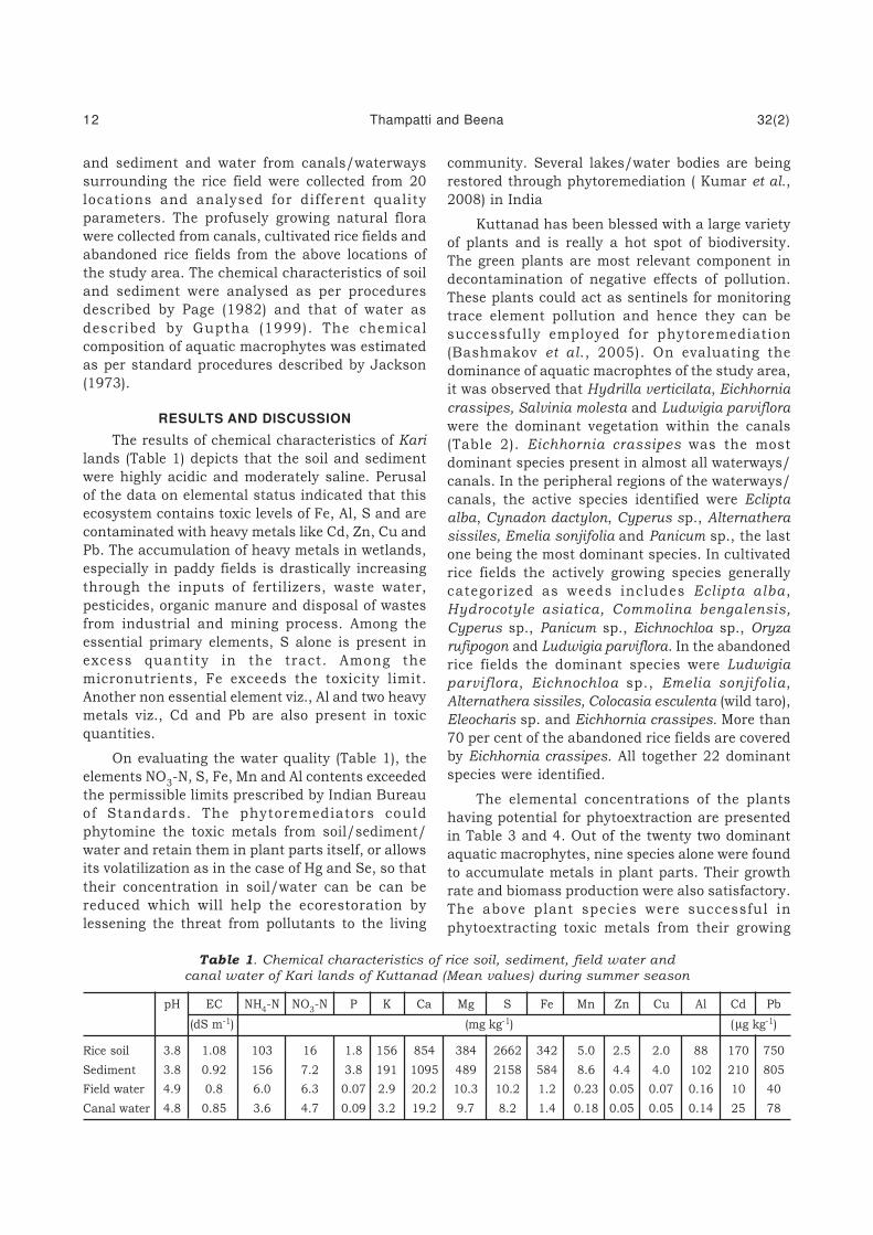
The results of chemical characteristics of Kari

lands (Table 1) depicts that the soil and sediment

were highly acidic and moderately saline. Perusal

of the data on elemental status indicated that this

ecosystem contains toxic levels of Fe, Al, S and are

contaminated with heavy metals like Cd, Zn, Cu and

Pb. The accumulation of heavy metals in wetlands,

especially in paddy fields is drastically increasing

through the inputs of fertilizers, waste water,

pesticides, organic manure and disposal of wastes

from industrial and mining process. Among the

essential primary elements, S alone is present in

excess quantity in the tract. Among the

micronutrients, Fe exceeds the toxicity limit.

Another non essential element viz., Al and two heavy

metals viz., Cd and Pb are also present in toxic

quantities.

On evaluating the water quality (Table 1), the

elements NO3-N, S, Fe, Mn and Al contents exceeded

the permissible limits prescribed by Indian Bureau

of Standards. The phytoremediators could

phytomine the toxic metals from soil/sediment/

water and retain them in plant parts itself, or allows

its volatilization as in the case of Hg and Se, so that

their concentration in soil/water can be can be

reduced which will help the ecorestoration by

lessening the threat from pollutants to the living

community. Several lakes/water bodies are being

restored through phytoremediation ( Kumar et al.,

2008) in India

Kuttanad has been blessed with a large variety

of plants and is really a hot spot of biodiversity.

The green plants are most relevant component in

decontamination of negative effects of pollution.

These plants could act as sentinels for monitoring

trace element pollution and hence they can be

successfully employed for phytoremediation

(Bashmakov et al., 2005). On evaluating the

dominance of aquatic macrophtes of the study area,

it was observed that Hydrilla verticilata, Eichhornia

crassipes, Salvinia molesta and Ludwigia parviflora

were the dominant vegetation within the canals

(Table 2). Eichhornia crassipes was the most

dominant species present in almost all waterways/

canals. In the peripheral regions of the waterways/

canals, the active species identified were Eclipta

alba, Cynadon dactylon, Cyperus sp., Alternathera

sissiles, Emelia sonjifolia and Panicum sp., the last

one being the most dominant species. In cultivated

rice fields the actively growing species generally

categorized as weeds includes Eclipta alba ,

Hydrocotyle asiatica, Commolina bengalensis,

Cyperus sp., Panicum sp., Eichnochloa sp., Oryza

rufipogon and Ludwigia parviflora. In the abandoned

rice fields the dominant species were Ludwigia

parviflora, Eichnochloa sp., Emelia sonjifolia,

Alternathera sissiles, Colocasia esculenta (wild taro),

Eleocharis sp. and Eichhornia crassipes. More than

70 per cent of the abandoned rice fields are covered

by Eichhornia crassipes. All together 22 dominant

species were identified.

The elemental concentrations of the plants

having potential for phytoextraction are presented

in Table 3 and 4. Out of the twenty two dominant

aquatic macrophytes, nine species alone were found

to accumulate metals in plant parts. Their growth

rate and biomass production were also satisfactory.

The above plant species were successful in

phytoextracting toxic metals from their growing

Table 1. Chemical characteristics of rice soil, sediment, field water and

canal water of Kari lands of Kuttanad (Mean values) during summer season

pH EC NH4-N NO

3-N P K Ca Mg S Fe Mn Zn Cu Al Cd Pb

(dS m-1) (mg kg-1) (µg kg-1)

Rice soil 3.8 1.08 103 16 1.8 156 854 384 2662 342 5.0 2.5 2.0 88 170 750

Sediment 3.8 0.92 156 7.2 3.8 191 1095 489 2158 584 8.6 4.4 4.0 102 210 805

Field water 4.9 0.8 6.0 6.3 0.07 2.9 20.2 10.3 10.2 1.2 0.23 0.05 0.07 0.16 10 40

Canal water 4.8 0.85 3.6 4.7 0.09 3.2 19.2 9.7 8.2 1.4 0.18 0.05 0.05 0.14 25 78

12 Thampatti and Beena 32(2)

Table 2. Dominant aquatic macrophytes found in Kari lands of Kuttanad and their distribution

Sl.No Aquatic macrophytes (I) No. of sites at which the plant were observed and

(II) their intensity ( %)

Canal/ waterways Cultivated rice fields Abandoned rice fields

Within Periphery

I II I II I II I II

1 Eclipta alba – – – – 14 5 2 10

2 Hydrocotyle asiatica – – 12 50 14 10 7 15

3 Bacopa monnieria – – 11 45 11 10 4 20

4 Hydrilla verticilata 15 55 11 40 – – – –

5 Commolina bengalensis – – – – 12 12 – –

6 Marselia quadrifolia 6 20 9 32 – – 4 20

7 Eichhornia crassipes 18 65 – – 2 5 17 85

8 Cynadon dactylon – – – – 11 5 11 15

9 Cyperus sp. 10 35 13 55 12 15 11 35

10 Eleocharis sp. – – 13 45 4 15 7 30

11 Colocasia esculenta (Wild taro) 6 25 6 20 – – 16 25

12 Alternanthera sissiles 6 15 11 25 5 5 13 30

13 Hydrophila auriculata 10 25 14 25 – – 3 15

14 Salvinia molesta 13 50 – – 4 8 8 30

15 Panicum sp. 11 35 – – 12 10 13 28

16 Borreria stricta – – 18 30 – – – –

17 Eemelia sonjifolia – – 5 15 11 5 12 5

18 Pistia striata – – 8 55 – – – –

19 Eichnochloa sp. – – 10 35 16 18 13 25

20 Oryza rufipogon – – – – 18 20 12 15

21 Monochoria vaginalis – – – – – – – –

22 Ludwigia parviflora 13 20 12 30 16 5 8 15

media and accumulate them in above ground plant

parts as evidenced by a bioconcentration factor

(BCF) for shoot, greater than one (Table 5).

Among the identified phytoextractors, Hydrilla

verticilata recorded the highest concentration for Fe,

Zn, Cu and Al in shoot and Fe and Zn in root

followed by Eichhornia crassipes. This has clearly

indicated that Hydrilla verticilata and Eichhornia

crassipes were capable of removing the above

elements from the soil/water and lessens the extent

Table 3. Chemical composition of aquatic macrophytes (shoot) of Kuttanad - Kari lands

Sl. Species P K Ca Mg S Fe Mn Zn Cu Al Cd Pb

No. (mg kg-1) (%) (mg kg-1) (µg kg-1)

1 H. asiatica 2625 7250 3.76 0.76 0.13 1295 25 80 17 1867 359 921

2 B monnieria 3200 18500 3.44 2.20 0.17 2375 20 34 19 1798 508 935

3 C. bengalensis 3287 18500 2.64 0.52 0.170 2185 5 66 20 1982 156 788

4 E. crassipes 0.41 2.15 3.75 1.68 0.45 22865 120 125 95 1728 2200 6163

5 C. dactylon 3666 43000 4.96 1.62 0.22 7480 175 112 41 1420 1612 658

6 Cyperus sp. 361 31000 4.46 2.30 0.28 5780 205 76 28 969 808 968

7 Eleocharis sp. 6102 45000 3.05 0.70 0.31 10051 178 64 22 1529 811 853

8 S. molesta 4105 21500 3.75 1.68 0.45 11460 62 71 95 1115 869 1130

9 H. verticilata 2000 5500 4.00 0.60 0.32 24251 53 211 198 2526 390 566

32(2) Restoration of degraded land 13

of pollution. Cyperus species was found to

accumulate highest quantity of Mn in both shoot

and root. Eichhornia crassipes recorded the highest

concentration of Cd and Pb in both shoot and root.

The highest bioconcentration factor (BCF) was

recorded by the same plants for the respective

metals, except for Fe, Zn and Cu which were present

in highest quantity in Hydrilla verticilata while the

BCF was highest for Eichhornia crassipes. This was

mainly because of the higher concentration of Fe,

Zn and Cu in the sediment compared to rice soil.

Since Hydrilla verticilata was present mainly in

waterways/canals the amount of the above elements

present in sediment sample was used for calculation

of BCF. Though the above three macrophytes had

recorded the highest content of toxic elements, the

other plants also possess fare hyperaccumulation

ability, since all of them have a BCF greater than

one, which is an essential criterion for the selection

of hyperaccumulators/phytoextractors.

The presence of aquatic macrophytes with good

phytoextracting ability in waterways/canals could

remove substantial quantities of contaminants from

water/soil/sediment and make the wetland

ecosystem safer for aquatic organisms. Similarly the

technology can be successfully utilized for purifying

metal loaded effluents discharged from factories by

growing them in constructed lagoons containing the

effluent. Thus, the aquatic macrophytes viz., Hydrilla

verticilata, Eichhornia crassipes and Cyperus sp. can

be utilized for improving water quality and safe

guarding the water bodies/rice fields from metal

contamination by removing an appreciable quantity

of toxic metals from soil/water and make the

ecosystem more healthy and sustainable.

REFERENCES

Bashmakov, D. I., Lukatkin, A. S. and Prasad, M.

N. V. (2005). Temperate weeds in Russia:

Sentinels for monitoring trace element pollution

and possible application in phyteremediation.

Table 4. Chemical composition of natural flora (root) of Kari lands

Sl. Species P K Ca Mg S Fe Mn Zn Cu Al Cd Pb

No. (mg kg-1) (%) (mg kg-1) (µg kg-1)

1 H. asiatica 0.21 0.90 1.6 1.2 0.22 1640 20 58 46 759 202 745

2 B monnieria 0.19 1.72 4.5 1.2 0.21 3735 25 26 15 1967 315 613

3 C. bengalensis 0.27 1.95 0.96 0.57 0.26 2750 10 46 15 1669 322 419

4 E. crassipes 0.30 1.2 3.75 1.20 0.32 8405 74 105 90 2300 1065 9114

5 C. dactylon 0.15 2.60 4.52 2.68 0.55 4200 100 40 22 1039 710 744

6 Cyperus sp. 0.48 1.55 3.92 1.39 0.19 6140 125 56 38 1563 916 880

7 Eleocharis sp. 0.51 2.25 2.95 1.10 0.27 8427 94 59 43 1425 714 1102

8 S. molesta 0.31 1.36 2.74 0.89 0.44 8245 96 105 21 1250 845 878

9 H. verticilata 0.20 0.60 2.8 0.61 0.16 10620 58 196 49 1238 324 658

Table 5. Bioconcentration factors for various toxic elements showed by

aquatic macrophytes (shoot) of paddy fields of Kari lands

Species Fe Mn Zn Cu Al Cd Pb

H. asiatica 3.78 5.00 32.0 3.00 21.2 2.11 1.23

B monnieria 6.94 4.00 17.0 7.50 20.4 2.98 1.25

C. bengalensis 6.38 0.58 33.0 7.50 22.5 0.917 1.05

E. crassipes 66.9 24.0 62.5 45.0 19.6 12.94 8.22

Cynadon dactylon 21.9 35.0 56.0 11.0 16.1 9.48 0.87

Cyperus sp. 16.9 41.0 38.0 19.0 11.1 4.75 1.29

Eleocharis sp. 29.4 35.6 32.0 21.5 17.3 4.77 1.14

S. molesta 33.6 24.0 62.5 11.5 12.6 5.11 1.51

H. verticilata* 41.5 6.30 47.9 12.5 24.6 1.86 0.70

*BCF calculated based on elemental content of sediment

14 Thampatti and Beena 32(2)

In: Trace Elements in the Environment –

Biogeochemistry, Biotechnology and

Bioremediation, M.N.V. Prasad, K.S. Sajwan and

Ravi Naidu (eds.) CRC Press, USA.

Chaney, R. L., Brown, S. L., Li, Y. M, Angle, J. S.,

Homer, F. A. and Green, C. E.(1995). Potential

use of metal hyperaccumulators. Mining

Environment Management 3(3): 9-11.

Cunningham, S. D., Shann, J. R., Crowley, D. E.

and Anderson, T. A. (1997). Phytoremediation

of contaminated water and soil . In:

Phytoremediation of Soil and Water

Contaminants, Kruger, E. L., Anderson, T. A and

Coats, J. R. (eds.), American Chemical Society,

Washington, D.C. pp 133-151.

Gupta, P. K. (1999). Soil, Plant, Water and Fertiliser

Analysis. Agrobios (India), Jodhpur. 438p.

Jackson , M. L. (1973). Soil Chemical Analysis.

Prentice hall of India Pvt. Ltd, New Delhi. 474p.

Kumar, J, N. I, Soni, H., Kumar, R. N. and Bhatt, I.

(2008). Macrophytes in phytoremediation of

heavy metal contaminated water and sediments

in Pariyej Community Reserve, Gujarat, India.

Turkish Journal of Fisheries and Aquatic

Sciences 8: 193-200.

Page A. L (1982). Methods of Soil Analysis.Part 2.

Second edition, American Society of Agronomy

Inc., Madison, Wisconsin, USA.

Thampatti, K. C. M. and Jose, A. I. (1998). Evaluation

of accumulation of pesticide residues in an acid

sulphate wetland agrosystem of South India.

Journal of Indian Society of Coastal Agricultural

Research 16(2): 85-88.

Thampatti, K. C. M., Varghese, S. S. and Jose, A. I.

(2006). Contamination by fertilizer residues in

wetland rice ecosystems of Kuttanad, Kerala.

Journal of Indian Society of Coastal Agricultural

Research 24: 30-33.

32(2) Restoration of degraded land 15


Evaluation of Soil Nutrient Balance with

Varying Organics and Doses of Inorganics under

Double Sucker System of Planting Banana

VANDANA VENUGOPAL and K.R. SHEELA

Department of Agronomy, College of Agriculture, Vellayani, Thiruvananthapuram,

Kerala Agricultural University - 695 522, Kerala


Banana is an exhaustive feeder of nutrients due to its rapid and vigorous growth and highproductivity. Competition for nutrients is one of the factors which result in reduced bunchweight under high density planting of banana. This necessitates the need for augmenting andoptimizing the nutritional requirement of banana under double sucker planting. An integratednutrient management practice combining organic and inorganic nutrient sources has to beadopted for better results. Different levels of inorganic nutrients and organic sources on doublesucker planting were studied. The treatments constituted three levels of nutrients viz.,recommended dose of nutrients, 133 per cent of recommended dose of nutrients and 167 percent of recommended dose of nutrients as well as three sources of organic manure viz., farmyardmanure, banana residue in fresh state and vermicomposted. Balance sheet of soil nutrientswere worked out utilizing the nutrient gains and losses recorded in the experiment. Soil nutrientstatus improved after two years of experimentation in all the treatments.

(Key words: Banana, Double sucker planting, Inorganic nutrients, Organic source, Soil nutrient

balance sheet)


Banana is an important fruit crop having great

socio-economic significance in India. It supports the

livelihood of millions of people. It is interwoven with

national heritage and due to its multi-faceted uses

it is referred to as ‘Kalpatharu’ (Plant of Virtues)

meaning ‘herb with all imaginable uses’. It can grow

well under a wide range of agro climatic situations,

ecological conditions and various systems of

production. Commercial banana cultivation is taken

up by small and marginal farmers on a large scale

as an answer to low returns from agriculture.

Increasing agricultural production by increasing

area is no longer possible as cultivable land left over

is only marginal. Hence, self sufficiency can be

attained by increasing the yield per unit area per

unit time through adoption of modern agricultural

technology and crop intensification is perhaps the

only possible solution for the same. Being adapted

to grow under low light intensities, banana plants

can withstand shade and hence are highly suitable

for high density planting. Adopting high density with

more number of suckers per pit in single row

planting with wider spacing provides more space

for intercropping. It also helps to reduce labour cost

and increase the efficiency of input utilization.

Banana being a heavy remover of nutrients,

high yields of quality bananas can only be sustained

through the application of optimal doses of nutrients

in balanced proportion. Nutrient application

throughout the growth stages is important in

realizing the economic yield in Nendran banana.

Competition for nutrients is one of the factors which

result in reduced bunch weight under high density

planting of banana. This necessitates the need for

augmenting and optimizing the nutrit ional

requirement of banana under high density planting.

An integrated nutrient management practice

combining organic and inorganic nutrient sources

has to be adopted for better results. Existing

technologies of nutrient supply are to be refined for

judicious use to enhance the profitability under

double sucker planting as increased manurial dose

may not be required for increased number of suckers

per pit. The socio-economic conditions of farming

community and prevalent local edaphic factors

should also be taken into account before nutrient

recommendations are advocated. Traditional

manuring system utilizing FYM is already under

pressure due to non availability, high cost and

drudgery in transporting and spreading the same.

Hence, the possibility of including alternative

organic sources in the nutrient package by recycling

banana residues as such or as vermicompost has

to be assessed. Though banana pseudostem is a

rich source of plant nutrients, its disposal after

harvest creates great problem. The efficacy of

incorporation of fresh crop residue (pseudostem) as

such or as vermicompost needs to be evaluated. This

practice helps to meet the organic manure

requirement of the crop and also ensures

sustainability by recycling of crop waste.


The investigation on nutrient management was

conducted in two consecutive cropping seasons at

the Instructional Farm attached to College of

Agriculture, Vellayani, Kerala Agricultural

University. Different levels of inorganic nutrients

and organic sources on double sucker system of

planting were studied. The treatments constituted

three levels of nutrients viz., recommended dose of

nutrients (RDN-300: 119 : 450 g NPK pit-1), 133 per

cent of RDN and 167 per cent of RDN as well as

three sources of organic manure viz., (FYM) @ 15

kg pit-1, banana residue in fresh state (BR) @20 kg

pit-1and vermicomposted (VC) @ 5 kg pit-1. The

experiment was in factorial randomized block design

with three replications. The plot size used was 6 m x

4 m. Pits of 50 cm x 50 cm x 50 cm were dug to

accommodate two suckers as per the treatment

schedule. In double sucker planting two suckers were

planted with 3 m x 2 m spacing towards the sides of

the pit at a spacing of 30 cm between plants.

The treatment combinations are detailed below

T1 – f

1o

1 – RDN + FYM @ 10 kg pit-1

T2 – f

1o

2 – RDN + VC @ 5 kg pit-1

T3 – f

1o

3 – RDN + BR @ 20 kg pit-1

T4 – f

2o

1 – 133 per cent of RDN + FYM @ 10 kg pit-1

T5 – f

2o

2 – 133 per cent of RDN + VC @ 5 kg pit-1

T6 – f

2o

3 – 133 per cent of RDN + BR @ 20 kg pit-1

T7 – f

3o

1 – 167 per cent of RDN + FYM @ 10 kg pit-1

T8 – f

3o

2 – 167 per cent of RDN + VC @ 5 kg pit-1

T9 – f

3o

3 – 167 per cent of RDN + BR @ 20 kg pit-1

To ensure maximum homogeneity in physiological

maturity, tissue cultured plantlets of two and a half

to three months old were used for planting the first

crop. Selected suckers of first crop having uniform

size and age were used for planting the second crop.

As per the POP Recommendations of Kerala

Agricultural University (2002) the fertilizers were

applied in splits. Nitrogen and potassium were given

in 6 splits (1, 2, 3, 4, 5 months after planting and at

bunch emergence) and phosphorus in two splits

(1 and 3 months after planting).In situ green manuring

of banana with cowpea was followed uniformly for all

the treatments.

The plant was separated into rhizome,

pseudostem, leaves and fruits at harvest and was

analyzed for nitrogen, phosphorus and potassium

content. Uptake of nutrients by each plant part at

harvest was calculated from the values of dry matter

production and per cent nutrient content of each

plant part and expressed in kg ha-1. Soil samples

were collected from the experimental area before

and after the investigation and analyzed for nitrogen,

phosphorus and potassium. Balance sheet of soil

nutrients were worked out utilizing the nutrient gains

and losses recorded in the experiment.

RESULTS AND DISCUSSIONS

Balance sheet of soil nutrients worked out in

the experiment was furnished in Table 1. Levels of

nutrients, organic sources and their interactions

caused variation on available nitrogen, phosphorus

and potassium status of the soil. In general there

was a buildup of soil nutrients after the experiment.

The computed values were more than the actual

values obtained by the direct analysis of the soil.

Available soil nitrogen recorded high values with f2

which might be due to decreased losses of the

nutrient in the treatment (Fig. 1). Inorganic nitrogen

added to all experimental plots might have enhanced

the nitrate nitrogen content of the soil, possibly due

to conversion of applied mineral nitrogen through

nitrification process (Krishnan, 1986).

Fig. 1. Soil nutrient balance sheet of available nitrogen as

influenced by nutrient levels and organic sources

Higher status of available P in the soil after

harvest was noticed as the phosphatic fertilizers

which are highly reactive might got fixed in the soil

and released phosphorus slowly to the available pool.

Maximum value of available soil phosphorus with

vermicompost addition could be attributed to the

formation of phospho - humic complexes (Fig. 2).

32(2) Soil nutrient balance in Banana plantation 17

Table 1. Balance sheet of the soil nutrients (kg ha-1)

Treatments Initial status Quantity added as fertilizer

N P K N P K

f1o1 103.49 7.2 82.4 1000 384 1500

f1o2 103.49 7.2 82.4 1000 384 1500

f1o3 103.49 7.2 82.4 1000 384 1500

f2o1 103.49 7.2 82.4 1332 510 2000

f2o2 103.49 7.2 82.4 1332 510 2000

f2o3 103.49 7.2 82.4 1332 510 2000

f3o1 103.49 7.2 82.4 1666 638 2500

f3o2 103.49 7.2 82.4 1666 638 2500

f3o3 103.49 7.2 82.4 1666 638 2500

Treatments Quantity added as organic manure Quantity added as green manure

N P K N P K

f1o

144.8 25 25 71.64 42.98 57.31

f1o

216.8 6.6 30 71.64 42.98 57.31

f1o3 4.2 1 23.2 71.64 42.98 57.31

f2o1 44.8 25 25 71.64 42.98 57.31

f2o2 16.8 6.6 30 71.64 42.98 57.31

f2o3 4.2 1 23.2 71.64 42.98 57.31

f3o1 44.8 25 25 71.64 42.98 57.31

f3o2 16.8 6.6 30 71.64 42.98 57.31

f3o3 4.2 1 23.2 71.64 42.98 57.31

Treatments Total quantity added Quantity removed

N P K N P K

f1o

11219.93 555.47 1685.8 399.3 82.5 1304.8

f1o

21191.93 537.07 1690.8 469.1 91 1281.4

f1o

31179.33 531.47 1684 355.7 90.2 1167.6

f2o

11551.93 681.47 2185.8 456.1 95.3 1299.1

f2o

21523.93 663.07 2190.8 486.1 98.3 1207.9

f2o

31511.33 657.47 2184 435.2 94.3 1187.6

f3o

11885.93 809.47 2685.8 468.5 81.7 1015.7

f3o

21857.93 791.07 2690.8 479.5 87 1429.3

f3o3 1845.33 785.47 2684 394.5 77.4 1497.6

Treatments Soil status after the experiment

Computed Actual

N P K N P K

f1o

1820.63 473 381 109.8 9.44 239.53

f1o

2722.83 446.1 409.4 130.7 11.64 463.83

f1o

3823.63 441.3 516.4 112.9 11.33 626.01

f2o

11095.8 586.2 886.7 119.2 12.58 499.97

f2o2 1037.8 564.8 982.9 112.9 14.26 306.13

f2o3 1076.1 563.2 996.4 182.3 9.65 489.51

f3o1 1417.4 727.8 1670.1 75.26 7.66 725.46

f3o2 1378.4 704.1 1261.5 138 11.12 575.83

f3o3 1450.8 708.1 1186.4 142.2 16.46 565.38

18 Venugopal and Sheela 32(2)

Improvement in soil potassium at f3 level could

be related to the higher dose of potassium added

(Fig. 3). Available N, P and K in soil were more with

incorporation of fresh banana pseudostem, could

be attributed to low uptake values of nitrogen,

phosphorus and potassium noticed in the treatment.

In addition, crop residues add to slow and passive

recalcitrant pools of soil organic matter. Their

nitrogen release potential is rather low due to higher

C : N ratio and consequent slow rate of

mineralization. Under adequate supply of N and P

when crop residues are returned to the soil, the

added nutrients might be immobilized in fairly stable

organic carbon compounds (Tisdale et al., 1995).

Less loss could be noticed due to slow

mineralization. Application of banana stems may

significantly increase soil potassium (Lassoudiere

and Godefroy, 1971) also supports the result.

Both the actual and computed values of soil

nutrients in the balance sheet are on positive side

indicating good nutrient management in all

treatment combinations. The variation in the

Table 2. Effect of nutrient levels and sources of organic manure on the yield of banana

Treatments Yield (t ha-1) Net income (Rs ha-1)

Season I Season II Pooled Season I Season II Pooled

f1o1 35.89 34.44 35.16 399115 380326 389721

f1o2 36.22 38.55 37.38 396697 400049 384874

f1o3 33.55 33.33 33.44 375034 372146 373590

f2o1 35.33 41.11 38.21 386393 461536 423965

f2o

236.88 32.77 34.82 372863 319409 346136

f2o

334.00 36.22 35.10 375312 404172 389742

f3o

130.11 38.33 34.22 313466 420351 366909

f3o

237.88 38.11 37.99 380817 383697 382258

f3o3 34.55 39.22 36.88 377488 438127 407808

F4,16 0.26ns 5.23** 3.41* 1.45ns 5.23** 3.41*

SEm± 2.601 1.479 1.170 23906.6 19233.9 15197.0

CD – 4.436 3.350 – 57665.9 43563.9

Fig. 2. Soil nutrient balance sheet of available phosphorus as

influenced by nutrient levels and organic sourcesFig. 3. Soil nutrient balance sheet of available potassium as

influenced by nutrient levels and organic sources

computed values and actual values for nitrogen

might be due to low nitrogen use efficiency and

different types of losses like leaching, surface runoff

and immobilization by microbes. The actual

phosphorus was very low compared to computed

value since the soil in experimental field belongs to

the order oxisol which is characterized by high P

fixation due to increased weathering and increased

clay fraction dominated by hydrous oxides, iron and

aluminium. In general not much variation in K

status between actual and computed values except

at highest dose of nutrients applied. This can be

attributed to interaction of potassium with other

cations, leaching losses and luxury consumption.

From the present study we can recommend

farmyard manure and fresh banana pseudostem

with 133 per cent of RDN and vermicompost with

RDN which recorded maximum yield per hectare

(Table 2) as economically viable and sustainable

practice for banana var. Nendran under paired


system of planting. However, soil nutrients in the

balance sheet are on positive side indicating good

nutrient management in all treatment combinations.

REFERENCES

KAU (2002). Package of Practices Recommendations:

Crops. Twelfth edition. Kerala Agricultural

University, Thrissur. 278 p.

Krishnan, P. K. (1986). Integrated use of organic

wastes and fertilizers nitrogen. M.Sc. (Ag.)

Thesis, Tamil Nadu Agricultural University,

Coimbatore, Tamil Nadu, India.

Lassoudiere, A. and Godefroy, J. (1971). Internet

de e’ utilization of bananeraie des e carts de

conditionnement des regimes de bananas.

Fruits 26: 255-262 (French).

Tisdale, S. L., Nelson, W. L., Beaton, J. D. and

Havelin, J. L. (1995). Soil Ferti l i ty and

Fertilizers. Prentice Hall of India Pvt. Ltd., New

Delhi. 634p.



Length of Growing Period and Water Productivity of Important

Crops and Cropping Systems for Coastal Areas of

Haldia, Paradip and Visakhapatnam

SUKANTA K. SARANGI, K. K. MAHANTA, S. MANDAL, B. MAJI and D. K. SHARMA

ICAR-Central Soil Salinity Research Institute, Regionla Research Station

Canning Town, South 24 Parganas, West Bengal - 743 329

Received : 25.08.2014 Accepted : 18.09.2014

Scarcity of water is going to be more acute under changing climate in the coastal areas of Indiadue to uncertainity in rainfall amount and distribution. Analysis of rainfall data from 1990-2011at three sites viz. Visakhapatnam, Paradip and Haldia in Andhra Pradesh, Odisha and WestBengal respectively revealed that the co-efficient of variation of annual rainfall was the highestfor Visakhapatnam (26.4), followed by Paradip (22.7) and Haldia (21.5). The trend analysis oflong-term rainfall data revealed that the average annual rainfall declined by 6.3% at Haldia,increased by 8.5% at Paradip and declined by 14.3% at Visakhapatnam during 2001-2010 fromthat of 1991-2000. The crop evapotranspiration (ETcrop) computed by modified Penman methodrevealed that during dry season highest ETcrop was observed in case of boro rice (604.8 mm) atHaldia, for brinjal (507.2 mm) at Paradip and for sugarcane (1178.9 mm) at Visakhapatnam,whereas water productivity (WP) on the basis of economic yield was highest in case of potatoat Haldia (7.2 kg m-3) and Paradip (6.6 kg m-3) and sugarcane at Visakhapatnam (6.7 kg m-3).Suitable cropping systems like rice-potato, rice-sunflower for Haldia, rice-tomato, Rice-potatoand rice-brinjal for Paradip and rice-chilli for Visakhapatnam may be followed to get higher WP

on net return basis. Irrespective of location, the WP on net return basis was more than j- 20 m-3 in

case of rice-tomato, rice-potato, rice-brinjal, rice-onion, rice-sunflower and rice-chilli. Underchanging climatic conditions, increasing degradation as well as limited availability of naturalresources in coastal areas suitable cropping systems should be identified and followed forbetter water productivity as well as profitability.

(Key words: Crop coefficient, Cropping system, Evapotranspiration, Growing period)

The coastal region of India is traditionally

disadvantaged and backward with low livelihood

security of the farmers. The ecology of the coastal

region is also highly fragile and vulnerable to further

degradation due to anthropogenic activities. The

farming communities of the coastal region are

dominated by backward classes of people who are

the poorest of the poor in the country. Low

agricultural productivity and high unemployment

among the rural people is the characteristic feature

of the area. The degraded soil and water quality,

together with climatic adversities contribute to low

cropping intensity and agricultural productivity.

The constraints like, waterlogging, drainage

congestion, lack of irrigation water, salinity of soil

and underground water, etc. have turned almost

the entire coastal region of the country as mono-

cropped area growing traditional rice varieties with

very poor yield in monsoon season. Most of the lands

remain fallow during the rest period of the year.

Due to heavy concentrated rainfall in a short span

of a few monsoon months (June-September), flat

topography, low infiltration rate, presence of ground

water at the surface and lack of proper drainage

facility most of the cultivated fields are deeply

waterlogged during Kharif season (June –

November). Due to presence of brackish water table

at a shallow depth there is always an increase in

soil and water salinity in dry months. However, the

region is endowed with bounty of natural resources

like high precipitation, diverse and fertile soils rich

in phosphorus and potassium, flat topography and

crop and varietal biodiversity. In spite of the vast

resource potentials in the coastal region, the

enhancement of the agricultural productivity of

coastal lands has been slow and much below the

potential. The coastal areas are much lagging behind

many inland areas in terms of agricultural

productivity and livelihood security of the farmers.

Low land productivity and consequently, poor

socio-economic condition of coastal region in India,

is one of the key problems in the overall development

of the country in spite of spectacular progress in

the field of agriculture in other regions. The demand


for food, fodder and fibre are increasing in this

fragile ecosystem. Soil salinity and water scarcity

of different degrees and duration occur in these

areas and reduce the choice of crop/variety and

yield. Sen et al., (2009) reported that the rice yield

during the wet season is as low as 1.0 to 1.5 t ha-1

in the coastal saline areas of eastern India due to

erratic rainfall, abiotic stresses viz. salinity,

drought, submergence and natural calamities

(storms and cyclones). Average land holding of most

farmers (more than 80%) in the coastal area is

marginal (<1 ha), land is fragmented in to multiple

parts and in majority cases the holding size is even

below 0.5 ha. Hence to raise the income of the

farming community, it looks imperative to diversify

the mono cropping of rice with other farming options

(Sarangi et al., 2014a). The coastal saline soil in

eastern India is concentrated mainly in three states

like West Bengal, Odisha and Andhra Pradesh, with

about 1.5 mha area out of total coastal saline area

of 3.09 mha (Yadav et al., 1983). The cropping

intensities in the east and west coasts of India are

only 134 and 125%, respectively. The major parts

of the coastal tracts of West Bengal, Odisha and

southern Andhra Pradesh – comprising nearly 50%

of the cultivated coastal saline areas where rice

largely grown under rainfed conditions – constitute

the low-productivity rice belt in India. To increase

cropping intensity and ensure food and economic

security in the coastal saline areas, efforts must be

focussed on developing diversified rice-based

integrated farming systems by including low water-

requiring, salt-tolerant non-rice crops (Mahata et al.,

2009). Appropriate technologies and cropping

pattern with respect to the extent of salinity and

available resources is needed to overcome the

problems in these areas. One of the major

impediments to cropping system intensification in

coastal areas of India is lack of availability of good

quality irrigation water during dry season. Avenues

to improve crop production include, adopting

cropping systems which make maximum use of

available water, increasing the length of the growing

season by advancing planting dates, adopting

cropping systems which avoid mid- or end-season

droughts and adopting improved agronomic

practices such as crop rotation and moderate inputs

(Virmani, 1987). For almost similar agroclimatic

conditions in coastal Bangladesh, Mainuddin et al.,

2014 contemplated strategies for cropping system

intensification with emphasis on knowledge-driven

water harvesting, management, conjunctive use of

surface and ground water, careful planning of crop

calendar, eff icient and timely agronomic

management practices of crops and benchmarking

them with their suitability to different saline zones

to provide farmers with the choice to fit appropriate

crops into their appropriate niche. To fit the suitable

crop to a particular region, ensuring availability of

irrigation water for that crop is essential. The

average per capita water availability, estimated at

1600 m3 year-1 is expected to fall around 1000 in

2050 based on current projected population. Again,

the effect of climate change will increase frequency

of extreme events like flood and droughts and this

makes future water availability and resources

uncertain (Biswal et al., 2014). With growth of other

sectors of economy, there will be cross-sectoral

competition for access to and control over water,

which will aggravate the situation of water scarcity

in agriculture sector, as a result the poor

smallholder farming communities inhabiting in

coastal areas would face extreme difficulties in

getting sufficient irrigation water for dry season

cropping. In view of this the present study was

undertaken to address such problems. Growing of

non-rice crops during dry season by conserving the

excess rainwater of wet season in on-farm reservoirs

is possible in the coastal areas. Shift from rice to

non-rice crops could also help enhance land and

water productivity, crop diversification and farmer’s

income and reduce the risk of yield losses due to

shortage of irrigation water during the grain filling

of rice (Singh et al., 2010). Irrigation water during

dry season being limited in availability, choice of

crops should be on water productivity basis.

Producing more food for each drop of water will be

a crucial strategy to address twin challenges of water

stress and food insecurity (Molden, 2007).


Experimental site

The study area covers Haldia, Paradip and

Visakhapatnam areas of West Bengal, Odisha and

Andhra Pradesh respectively in the eastern coast of

India within 50 km from the Bay of Bengal (Fig.1).

The basic soil characteristics of the study sites are

given in Table 1.

Haldia soil is mostly heavy textured, low saline

with acidic to neutral pH, medium in phosphorus

(P) and potassium (K), at Paradip the soils are sandy

to sandy clay loam, low to moderate saline with

acidic pH, medium in P and K, at Visakhapatnam,

the soils were sandy to sandy clay in texture with

neutral pH, low in P and high in K. The soils

22 Sarangi et al. 32(2)

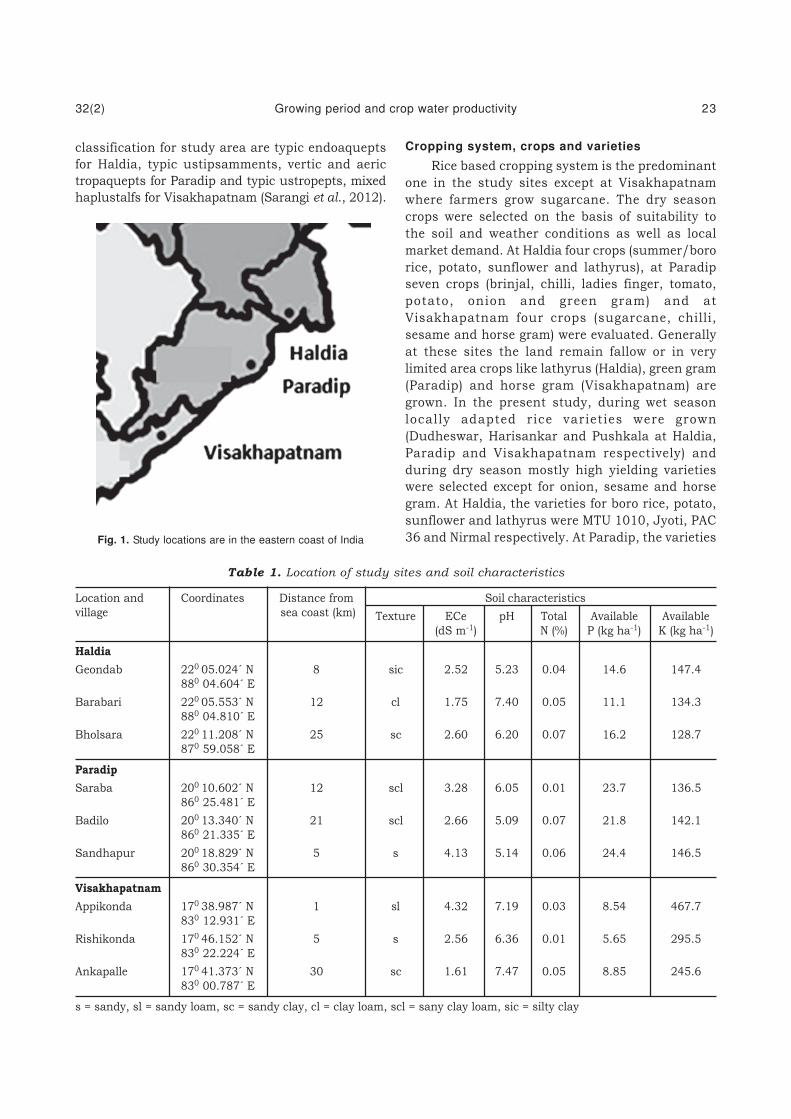
classification for study area are typic endoaquepts

for Haldia, typic ustipsamments, vertic and aeric

tropaquepts for Paradip and typic ustropepts, mixed

haplustalfs for Visakhapatnam (Sarangi et al., 2012).

Cropping system, crops and varieties

Rice based cropping system is the predominant

one in the study sites except at Visakhapatnam

where farmers grow sugarcane. The dry season

crops were selected on the basis of suitability to

the soil and weather conditions as well as local

market demand. At Haldia four crops (summer/boro

rice, potato, sunflower and lathyrus), at Paradip

seven crops (brinjal, chilli, ladies finger, tomato,

potato, onion and green gram) and at

Visakhapatnam four crops (sugarcane, chilli,

sesame and horse gram) were evaluated. Generally

at these sites the land remain fallow or in very

limited area crops like lathyrus (Haldia), green gram

(Paradip) and horse gram (Visakhapatnam) are

grown. In the present study, during wet season

locally adapted rice varieties were grown

(Dudheswar, Harisankar and Pushkala at Haldia,

Paradip and Visakhapatnam respectively) and

during dry season mostly high yielding varieties

were selected except for onion, sesame and horse

gram. At Haldia, the varieties for boro rice, potato,

sunflower and lathyrus were MTU 1010, Jyoti, PAC

36 and Nirmal respectively. At Paradip, the varieties

Table 1. Location of study sites and soil characteristics

Location and Coordinates Distance from Soil characteristics

village sea coast (km) Texture ECe pH Total Available Available

(dS m-1) N (%) P (kg ha-1) K (kg ha-1)

Haldia

Geondab 220 05.024´ N 8 sic 2.52 5.23 0.04 14.6 147.4

880 04.604´ E

Barabari 220 05.553´ N 12 cl 1.75 7.40 0.05 11.1 134.3

880 04.810´ E

Bholsara 220 11.208´ N 25 sc 2.60 6.20 0.07 16.2 128.7

870 59.058´ E

Paradip

Saraba 200 10.602´ N 12 scl 3.28 6.05 0.01 23.7 136.5

860 25.481´ E

Badilo 200 13.340´ N 21 scl 2.66 5.09 0.07 21.8 142.1

860 21.335´ E

Sandhapur 200 18.829´ N 5 s 4.13 5.14 0.06 24.4 146.5

860 30.354´ E

Visakhapatnam

Appikonda 170 38.987´ N 1 sl 4.32 7.19 0.03 8.54 467.7

830 12.931´ E

Rishikonda 170 46.152´ N 5 s 2.56 6.36 0.01 5.65 295.5

830 22.224´ E

Ankapalle 170 41.373´ N 30 sc 1.61 7.47 0.05 8.85 245.6

830 00.787´ E

s = sandy, sl = sandy loam, sc = sandy clay, cl = clay loam, scl = sany clay loam, sic = silty clay

Fig. 1. Study locations are in the eastern coast of India

32(2) Growing period and crop water productivity 23

for brinjal, chilli, ladies finger, tomato, potato and

green gram were BB44, Utkal Rashmi, Utkal Gaurav,

BT -1, Jyoti and Durga respectively. The sugarcane

and chilli varieties were Co 6907 and Bhagya

lakshmi (G-4) respectively at Visakhapatnam.

Data collection and statistical analyses

Rainfall and evaporation data from 1990-2011

were collected from these three sites and analyzed

for standard deviation (SD), co-efficient of variation

(CV), potential evapotranspiration (PET), length of

growing period (LGP) distribution pattern. For

computation of reference evapotranspiration (ET0)

four empirical methods (Blaney-Criddle, Radiation,

Modified Penman and Pan evaporation) were used

(Table 2). The data obtained from Modified Penman

method was used for calculation of crop

evapotranspiration (ETcrop), which was again used

for computation of water productivity.

= adjustment factor which depends on mean humidity

and daytime wind conditions from Fig. 2.

3. Modified Penman Method: ET0 = c[W.Rn +

(1-W).f(u).(ea-ed)] mm day-1

Where: ET0 = reference crop evapo-transpiration in

mm day-1 for the month considered, W =

temperature related weighting factor from Table 8,

Rn = net radiation in equivalent evaporation in mm

day-1, f(u) = wind related function = 0.27(1+U/100),

U = 24-hr wind run in km day-1 at 2 m height, ea-ed

= difference between the saturation vapour pressure

at mean air temperature and the mean actual vapour

pressure of the air, both in mbar from Table 5 & 6,

c = adjustment factor to compensate for the effect

of day and night weather conditions from Table 16.

Modified Penman Method is a fairly accurate method

for estimation of reference evapotranspiration as it

utilizes almost all the meteorological parameters

responsible for the process of evapotranspiration.

4. Pan Evaporation Method: ET0 = Kp.Epan

Where Kp = pan coefficient, Epan = measured pan

evaporation data, Values for Kp were obtained from

Table 18 for the Class A pan and in Table 19 for the

sunken Colorado pan for different humidity and

wind conditions and pan environment.

The four methods described above, predict the

effect of climate on ET0. To account for the effect of

the crop characteristics on crop water requirements,

crop coefficients (kc) are required to relate ET0 to

ETcrop

. The kc value relates to evapotranspiration

of a disease-free crop grown in large fields under

optimum soil water and fertility conditions and

achieving full production potential under the given

growing environment. ETcrop can be found by:

ETcrop

= ET0×kc

Based on the procedure suggested by

Doorenbos and Pruitt (1977), kc values were found

out (Table 3) for different crops at different locations

taking into account crop characteristics, time of

sowing, stages of crop development and general

climatic conditions.

The crop yield data of various crops were

collected from field experiments conducted during

2010-11 and 2011-12 in randomized block design

(RBD) at these sites in the farmer’s fields (3 farmers

at each site). There were three replications in each

farmer field, the mean data of each farmer was

considered as one replication for analysis of data.

At harvest, grain yield was recorded from a net area

of 30 m2 (6 m x 5 m) marked at the middle of each

Table 2. Different methods and parameters used

in the estimation of ET0 at the study sites

Method T H W S R E En

Blaney-Criddle * 0 0 0 0

Radiation * 0 0 * (*) 0

Modified Penman * * * * (*) 0

Pan evaporation 0 0 * *

T: Temperature, H: Humidity, W: Wind, S: Sunshine, R:

Radiation, E: Evaporation, En: Environment, * Measured data;

0 estimated data; (*) if available, but not essential

The empirical formulae of different methods are

given below. Tables and figures refereed in the

following four methods are from FAO Irrigation and

Drainage Paper 24 (Doorenbos and Pruitt, 1977).

1. Blaney-Criddle Method: ET0 = c[p(0.46T + 8] mm day-1


mm day-1 for the month considered, T = mean daily

temperature in oC over the month considered, p =

mean daily percentage of total annual daytime hours

obtained from Table 1 for a given month and

latitude, c = adjustment factor which depends on

minimum relative humidity, sunshine hours and

daytime wind estimates.

2. Radiation Method: ET0 = c(W.Rs) mm day-1


mm day-1 for the month considered, Rs = solar

radiation in equivalent evaporation in mm day-1,

Rs = (0.25+ 0.50 n/N)Ra, Ra = Extra Terrestrial

Radiation (Ra) expressed in equivalent evaporation in

mm day-1 from Table 2, W = weighting factor which

depends on temperature and altitude from Table 4, c


plot and converted into t ha-1 by multiplying suitable

conversion factor. Water Productivity (WP) of each

crop and cropping system was calculated by using

the following formula.

WP (kg m-3) on produce basis = Grain Yield (kg)/

Amount of water used through evapotranspiraiton

(m3), WP ( m-3) on return basis = Return (j-)/Amount

of water used through evapotranspiraiton (m3)

The benefit cost ratio (BCR) was calculated as

gross return accrued divided by total variable cost.

Total variable cost was calculated by taking into

account the costs of inputs (seed, fertilizer, and

pesticides), costs of human labour for land

preparation, irrigation, fertilizer, and pesticide

application, bunding, harvesting and threshing; and

costs of hiring power tillers for land preparation and

an irrigation pump. Gross return was calculated by

multiplying the amount of produce by its

corresponding market price at harvest. Net return

was the gross return minus total variable costs. The

economic analyses were conducted by taking into

account the prevailing market prices of inputs,

labour, and produce during the year 2011-12. The

data were subjected to analyses by STAR (Statistical

Tool for Agricultural Research) package developed

by International Rice Research Institute, Philippines

(IRRI). Treatment means were compared using the

least significant difference (LSD) tests and compared

at p=0.05 level of significance (Gomez and Gomez,

1984). Since the interaction between year and

different characters studied in this experiment were

non-significant, hence mean data are presented.


Rainfall, evaporation and evapo-transpiration

The analyzed rainfall data from 1990-2011 for

study sites are given in Table 4. The annual mean

rainfall is highest (1784.2 mm) for Haldia followed by

Paradip (1635.9 mm) and Visakhapatnam (1175.5 mm).

The co-efficient of variation of annual rainfall was

highest for Visakhapatnam (26.4) followed by Paradip

(22.7) and Haldia (21.5). The trend analysis of long-

term rainfall data revealed that the average annual

rainfall declined by 6.3% at Haldia, increased by 8.5%

at Paradip and declined by 14.3% at Visakhapatnam

during 2001-2010 from that of 1991-2000.

The rainfall pattern at Haldia, Paradip and

Visakhapatnam of West Bengal, Odisha and Andhra

Pradesh during 2009, 2010 and 2011 reveal that rainiest

months were August, July and September for Haldia,

Paradip and Visakhapatnam respectively (Fig. 2).

Table 3. Crop coefficient (kc) values used for estimation of crop water requirements (ETcrop)

Crops at different Jan Feb Mar Apr May Jun Jul Aug Sep Oct Nov Dec

locations

Haldia

Kharif rice *1.15 1.05 1.1 0.95 1.0

Boro rice 1.2 1.4 1.3 1.0

Potato 1.05 0.7 *0.7

Sunflower 0.6 1.2 0.8

Lathyrus 0.3 *0.5 1.05

Paradip

Brinjal *0.35 0.6 0.8 0.95 0.8

Chilli 0.8 *0.6 0.95 0.9

Ladies finger *0.5 0.95 0.9 0.8

Tomato 0.6 *0.4 0.6 1.05

Potato 0.6 1.05 0.7 *0.4

Onion 0.55 0.95 0.75 *0.35

Green gram 1.05 0.3 *0.4

Visakhapatnam

Sugarcane *0.4 0.5 0.6 0.7 1.0 1.0 1.3 1.3 1.3 0.7 0.8

Chilli 0.95 0.8 0.5 *0.3 0.5 0.7

Sesame *0.8 1.05 0.25

Horse gram 1.05 0.3 *0.8

*Initial crop period


computed by the modified Blaney-Criddle, radiation,

modified Penman and Pan evaporation methods. The

ET0

was highest for Radiation method for all the

locations and the total annual ET0

were 2112.6,

2032.5 and 2075.5 mm for Haldia, Paradip and

Visakhapatnam respectively (Table 5). The estimates

by modified Penman and Blaney-Criddle were found

be moderate among all the methods. Pan

evaporation method underestimated the ET0 when

compared with the actual pan evaporation data

(Epan).

The distribution of rainfall over pre-monsoon

(April-May), monsoon (June-October) and post

monsoon (November –March) was studied and it was

found that though the annual rainfall was lowest at

Visakhapatnam the distribution was more uniform

i.e. 14.7, 63.1 and 22.2% during the pre-monsoon,

monsoon and post monsoon period respectively

(Table 6).

Length of Growing Period (LGP)

The length of the “growing season” or “growing

period” (LGS or LGP), as defined by the Agro-

Ecological Zones project (FAO, 1978-81) is the period

(in days) during a year when precipitation (P)

exceeds half the potential evapotranspiration (PET).

On this basis the LGP was 150 (last week of May to

last week of October), 170 (first week of May to third

week of October) and 165 (first week of July to last

week of December) days for Haldia, Paradip and

Visakhapatnam respectively (Fig. 3).

Water Productivity (WP)

The crop evapotranspiration (ETcrop

) was

computed for potential crops at Haldia, Paradip and

Visakhapatam, taking into consideration the ET0

values obtained by Modified Penman method (Table 7).

Highest ETcrop

was observed in case of boro rice

(604.8 mm) at Haldia, for Brinjal (507.2 mm) at

Paradip and for Sugarcane (1178.9 mm) at

Visakhapatnam. The economic yield was highest for

potato at Haldia (14.5 t ha-1) and Paradip (19.0 t ha-1)

and for sugarcane (69.5 t ha-1) at Visakhapatnam,

similarly WP on the basis of economic yield was

highest in case of potato at Haldia (7.2 kg m-3) and

Paradip (6.6 kg m-3) and sugarcane at

Table 4. Rainfall parameters for Haldia, Paradip

and Visakhapatnam (1990-2011)

Parameters Haldia Paradip Visakhapatnam

Mean (mm) 1784.2 1635.9 1175.5

Range (mm) 1053-2581 793-2272 732-1763

SD (mm) 383.72 370.90 310.12

CV (%) 21.5 22.7 26.4

Fig. 2. Monthly rainfall distribution at (a) Haldia, (b) Paradip

and (c) Visakhapatnam of West Bengal, Odisha and Andhra

Pradesh respectively (mean data of 2009-2011)

Table 5. Annual ET0 (mm) in the coastal areas of West Bengal, Odisha and Andhra Pradesh

Location Blaney-Criddle Radiation Modified Penman Pan evaporation Epan

Haldia 1523.2 2112.6 1467.3 830.0 1081.9

Paradip 1496.4 2032.5 1476.3 1167.4 1572.9

Visakhapatnam 1396.2 2075.5 1427.5 1240.8 1155.7

A study of annual rainfall and evaporation

reveal that annual evaporation exceeded rainfall by

79 and 347 mm at Paradip and Visakhapatnam

respectively, whereas at Haldia the annual rainfall

exceeds evaporation by 270 mm. The reference

evapotranspiration (ET0) for the three locations were


Visakhapatnam (5.9 kg m-3). Brauman et al., 2013

reported that water consumption by crops varies

substantially, reflecting differences in cropping

density, crop choice, soil characteristics, irrigation

availability and agricultural management as well as

climatic drivers of evapotranspiration. The choice

of suitable crop likely to contribute substantially

towards water saving without affecting food

production, where water resources are scarce. Singh

et al., 2010 reported that across seasons and

salinity levels in coastal saline soils of the Mahanadi

delta, India, dry season crops like watermelon, chilli,

pumpkin and sunflower were the best performers

based on rice yield equivalent, net return, benefit-

cost ratio and water productivity, with sunflower

and chilli giving consistent yield. Studies at West

Bengal, India also suggests farmers particularly with

small and marginal holding size (< 1 ha) are

interested for crop diversification towards vegetable

crops and are interested to invest on water and

inputs to achieve greater returns from crops other

than rice (Chatterjee et al., 2013). Since, irrigation

water is a precondition for successful cropping

during dry season in coastal areas, every drop of

precious water could be used effectively by choosing

water productive crops and cropping patterns, which

not only increase production but also reduce the

pressure on natural resources. However, suitable

crops and varieties should be integrated with

eff icient irrigation methods and moisture

conservation practices (e.g. mulching).

In order to find out suitable cropping systems

for the study areas the water productivity was

calculated for potential cropping systems on the

basis of gross as well as net return basis (Table 8).

The economic water productivity though blurred by

fluctuations in market prices, still preferable and

is more appropriate for comparing different crops

(Droogers et al., 2003). In the coastal areas of

eastern India, rice-vegetable and rice-oilseeds were

found to be remunerative cropping systems for

getting higher WP. At Haldia highest WP on gross

return basis was observed in Rice-potato (j- 76 m-3),

followed by Rice-sunflower (j- 36 m-3), at Paradip

Rice-tomato (j- 102 m-3) and Rice-potato (j- 70 m-3)

Table 6. Distribution of rainfall (R), evaporation (E) and evapo-transpiration (ET)

in selected coastal areas of eastern India

Location April-May June-October November-March Total

Haldia R = 183.2 (13.5%) R = 1142.6 (84.4%) R = 27.9 (2.1%) R = 1353.7

E = 299.3 E = 423.9 E = 360.9 E = 1084.1

ET = 355.4 ET = 620.2 ET = 491.7 ET = 1467.3

Paradip R = 188.8 (12.7%) R = 1235.3 (82.9%) R = 65.7 (4.4%) R = 1489.8

E = 323.3 E = 648.9 E = 596.8 E =1569.0

ET = 349.8 ET = 621.9 ET = 504.6 ET =1476.3

Visakhapatnam R = 169.5 (14.7%) R = 728.9 (63.1%) R = 257.3 (22.2%) R = 1155.7

E = 370.5 E = 552.3 E = 580.2 E = 1503.0

ET = 313.8 ET = 591.0 ET = 522.7 ET = 1427.5

( c )

Fig. 3. Length of growing period (LGP) at (a) Haldia,

(b) Paradip and (c) Visakhapatam


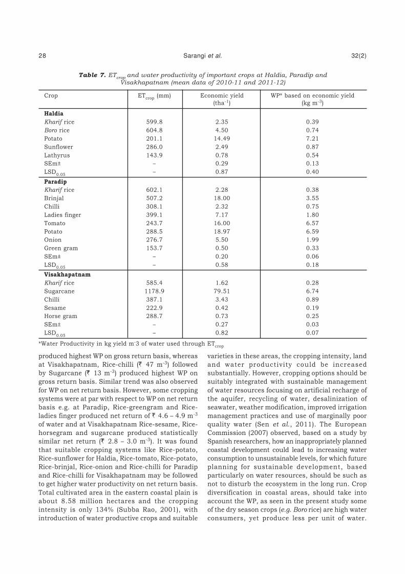
Table 7. ETcrop and water productivity of important crops at Haldia, Paradip and

Visakhapatnam (mean data of 2010-11 and 2011-12)

Crop ETcrop (mm) Economic yield WP* based on economic yield

(tha-1) (kg m-3)

Haldia

Kharif rice 599.8 2.35 0.39

Boro rice 604.8 4.50 0.74

Potato 201.1 14.49 7.21

Sunflower 286.0 2.49 0.87

Lathyrus 143.9 0.78 0.54

SEm± – 0.29 0.13

LSD0.05

– 0.87 0.40

Paradip

Kharif rice 602.1 2.28 0.38

Brinjal 507.2 18.00 3.55

Chilli 308.1 2.32 0.75

Ladies finger 399.1 7.17 1.80

Tomato 243.7 16.00 6.57

Potato 288.5 18.97 6.59

Onion 276.7 5.50 1.99

Green gram 153.7 0.50 0.33

SEm± – 0.20 0.06

LSD0.05 – 0.58 0.18

Visakhapatnam

Kharif rice 585.4 1.62 0.28

Sugarcane 1178.9 79.51 6.74

Chilli 387.1 3.43 0.89

Sesame 222.9 0.42 0.19

Horse gram 288.7 0.73 0.25

SEm± – 0.27 0.03

LSD0.05

– 0.82 0.07

*Water Productivity in kg yield m-3 of water used through ETcrop

produced highest WP on gross return basis, whereas

at Visakhapatnam, Rice-chilli (j- 47 m-3) followed

by Sugarcane (j- 13 m-3) produced highest WP on

gross return basis. Similar trend was also observed

for WP on net return basis. However, some cropping

systems were at par with respect to WP on net return

basis e.g. at Paradip, Rice-greengram and Rice-

ladies finger produced net return of j- 4.6 – 4.9 m-3

of water and at Visakhapatnam Rice-sesame, Rice-

horsegram and sugarcane produced statistically

similar net return (j- 2.8 – 3.0 m-3). It was found

that suitable cropping systems like Rice-potato,

Rice-sunflower for Haldia, Rice-tomato, Rice-potato,

Rice-brinjal, Rice-onion and Rice-chilli for Paradip

and Rice-chilli for Visakhapatnam may be followed

to get higher water productivity on net return basis.

Total cultivated area in the eastern coastal plain is

about 8.58 million hectares and the cropping

intensity is only 134% (Subba Rao, 2001), with

introduction of water productive crops and suitable

varieties in these areas, the cropping intensity, land

and water productivity could be increased

substantially. However, cropping options should be

suitably integrated with sustainable management

of water resources focusing on artificial recharge of

the aquifer, recycling of water, desalinization of

seawater, weather modification, improved irrigation

management practices and use of marginally poor

quality water (Sen et al., 2011). The European

Commission (2007) observed, based on a study by

Spanish researchers, how an inappropriately planned

coastal development could lead to increasing water

consumption to unsustainable levels, for which future

planning for sustainable development, based

particularly on water resources, should be such as

not to disturb the ecosystem in the long run. Crop

diversification in coastal areas, should take into

account the WP, as seen in the present study some

of the dry season crops (e.g. Boro rice) are high water

consumers, yet produce less per unit of water.


Table 8. Economic water productivity of different cropping systems for Haldia, Paradip and

Visakhapatnam (mean data of 2010-11 and 2011-12)

Cropping system at WP* on gross return Cost of cultivation* WP on net return

study sites basis (j- m-3) (j- m-3) basis (j- m-3)

Haldia

Rice-potato 77.00 44.13 32.87

Rice-sunflower 37.13 12.04 25.09

Rice-rice 14.13 10.39 3.74

Rice-lathyrus 20.00 12.12 7.88

SEm± 0.20 0.11 0.28

LSD0.05

0.59 0.33 0.84

Paradip

Rice-tomato 83.50 28.41 55.09

Rice-potato 70.50 36.31 34.19

Rice-brinjal 40.25 13.24 27.01

Rice-green gram 16.13 10.23 5.90

Rice-chilli 42.38 18.31 24.07

Rice-onion 44.50 18.57 25.93

Rice-ladies finger 19.13 13.55 5.58

SEm± 0.30 0.12 0.31

LSD0.05 0.88 0.35 0.91

Visakhapatnam

Rice-chilli 47.75 20.28 27.47

Rice-horse gram 9.88 6.27 3.61

Rice-sesame 11.50 7.72 3.78

Sugarcane 14.88 8.93 5.95

SEm± 0.24 0.06 0.27

LSD0.05

0.71 0.19 0.81

*Water Productivity and cost of cultivation in j- m-3 water used through ETcrop

However, productivity of boro rice is much higher in

comparision to kharif rice mainly due to favorable

weather conditions also when combined with better

management practices (Sarangi et al., 2014b)

Diversification of crops should be for higher profits to

farmers, sustainability of resources as well as for

mitigating risks (Singh et al., 2006).

CONCLUSION

Good quality irrigation water scarcity is the

major constraint for dry season cropping in the

coastal areas of eastern India, therefore selection

of crops on the basis of water productivity, fitting

these crops to the appropriate growing period are

essential for efficient use of limited quantity of

irrigation water. Choice of crops particularly during

dry season varied across locations, however growing

of vegetable crops like tomato, potato, brinjal, onion

and chilli in the rice fallows in the eastern coast of

India produced higher net income per unit of water

used for evapo-transpiration. Among field crops,

sunflower, green gram, horse gram and oilseed crop

like sesame may be selected depending upon

location. Diversification of dry season rice with water

efficient crops not only save precious water

resources, but also help increase the cropping

intensity by growing water efficient crops through

the saved water. However, besides choosing water

efficient crops, water efficient varieties also be

adopted wherever genetic diversity exists along with

other resource conservation and management

practices in a holistic manner for sustainability of

rice based cropping systems in the eastern coast of

India. Our study will help in judicious use of good

quality irrigation water as well as in designing

irrigation reservoirs in the coastal areas of India

based on targeted crops as well as adopting

conservation measures to achieve higher efficiency.


ACKNOWLEDGEMENTS

Authors greatly acknowledge the encouragement

and support provided by the Director, ICAR - Central

Soil Salinity Research Institute, Karnal, Haryana to

conduct this research work. The help rendered by

the Farm Science Centers, Regional Research

Stations and Government Agriculture Department

of respective states in the study areas to reach the

farmers and conduct field trials are also duly

recognized.

REFERENCES

Biswal, S., Behera, P. K., Nayak, L. and Sharma, P.

(2014). Food security, small farmers and water

concerns. In: Souvenir (Barik, T., Rath, B.S.,

Paikaray, R.K., Patra, A.K. and Dash R. eds),

National symposium on “Management options

for enhancing farm productivity and livelihood

security under changing climate”, organized by

Odisha chapter, Indian Society of Agronomy at

Orissa University of Agriculture and

Technology, Bhubaneswar, Odisha, India

during 29-30 October, 2014, pp 107-111.

Brauman, K. A., Siebert, S. and Foley, J. A. (2013).

Improvements in crop water productivity

increase water sustainability and food security

– a global analysis. Environmental Research

Letters 8: 024030 (doi: 10.1088/1748-9326/8/

2/024030).

Chatterjee, S., Ray, M., Halder, P. and Goswami, R.

(2013). Economic characterization of

predominant farming systems in West Bengal,

India. American Journal of Agriculture and

Forestry 1 (3): 40-47. doi: 10.11648/

j.ajaf.20130103.11

Doorenbos. J. and Pruitt, W.O. (1977). Guidelines

for predicting crop water requirements, FAO

Irrigation and Drainage Paper 24, Food and

Agriculture Organization of the United Nations,

Rome. 144p.

Droogers, P., Malik, R. S., Kroes, J. G.,

Bastiaanssen, W. G. M. and Dam, Van, J. C.

(2003). Future water management in Sirsa

district: options to improve water productivity.

In: Water productivity of irrigated crop in Sirsa

district, India – Integration of remote sensing,

crop and soil models and geographical

information system, J.C. van Dam and R.S.

Malik (eds). WATPRO final report, including CD-

ROM, ISBN 90-6464-864-6. 173 pp.

European Commission (2007). Sustainable use of

water resources in coastal areas (http://

ec.europa.eu/environment/integrat ion/

research/newsalert/pdf/61na2.pdf).

FAO, (1978–81). Report on the Agro-ecological Zones

Project. Vol.1, Methodology and results for

Africa; Vol.2, Results for Southwest Asia; Vol.3,

Methodology and results for South and Central

America; Vol.4, Results for Southeast

Asia. [FAO] World Soil Resources Report 48: (1-4).

Gomez, K. A., and Gomez, A. A. (1984). Statistical

procedures for agricultural research. John

Wiley and Sons, New York.

Mahata, K. R., Singh, D. P. and Ismail, A. M. (2009).

Crop and natural resource management for high

and stable productivity in coastal saline areas.

In: Natural resource management for poverty

reduction and environmental sustainability in

fragile rice-based systems, Haefele, S.M. and

Ismail, A.M. (eds.), Limited Proceedings No. 15,

International Rice Research Institute, Los

Banos, Philippines. pp 122-133.

Mainuddin, M., Ali, R., Shah-Newaz, S. M. and Roth,

C. H. (2014). Water resources in the coastal

zone of Bangladesh: Constraints or

opportunities for cropping intensification.

Abstracts, Revitalizing the Ganges coastal zone

conference organized by CGIAR Challenge

Program on Water and Food held at Dhaka,

Bangladesh during 21-23 October 2014, p.19.

Molden, D. (2007). Water for food, water for life: A

comprehensive assessment of water

management in agriculture (London:

Earthscan/James & James).

Sarangi, S. K., Mahanta, K. K., Mandal, S. and Maji,

B. (2012). Characterization of soils and cropping

pattern of coastal areas of Haldia, Paradip and

Visakhapatnam ports. Journal of Indian Society

of Coastal Agricultural Research 30(2): 12-18.

Sarangi, S. K., Maji, B. and Garnayak, L. M. (2014).

Approaches towards sustainable farming in

coastal salt-affected areas of India under

changing climate. In: Souvenir (Barik, T., Rath,

B. S., Paikaray, R. K., Patra, A. K. and Dash R.

(eds.), National symposium on “Management

options for enhancing farm productivity and

livelihood security under changing climate”,

organized by Odisha chapter, Indian Society of

Agronomy at Orissa University of Agriculture

and Technology, October, 29-30, 2014,

Bhubaneswar, Odisha, India. pp 102-106.


Sarangi, S. K., Maji, B., Singh, S., Sharma, D. K.,

Burman, D., Mandal, S., Ismail, A. M. and

Haefele, S. M. (2014b). Crop establishment and

nutrient management for dry season (Boro) rice

in coastal areas. Agronomy Journal, 106(6):

2013-2023.

Sen, P., Mahata, K. R. and Singh, D. P. (2009).

Development and Evaluation of Salt Tolerant

Rice Genotypes for Coastal Saline Areas of

Eastern, India. Journal of Indian Society of

Coastal Agricultural Research 27(1): 38-40.

Sen, H. S., Sahoo, N., Sinhababu, D. P., Saha, S.

and Behera, K. S. (2011). Improving agricultural

productivity through diversified farming and

enhancing livelihood security in coastal

ecosystem with special reference to India. Oryza

48(1): 1-21.

Singh, D. P., Mahata, K. R., Saha, S., and Ismail, A.

M. (2010). Crop diversification for improving water

productivity and rural livelihoods in coastal saline

soils of the Mahanadi Delta, India. In: Tropical

Deltas and Coastal Zones – Food production,

communities and environment at the land-water

interface, Chu T. Hoanh, Brian W. Szuster, Kam

Suan-Pheng, Abdelbagi M. Ismail and Andrew D.

Noble (eds.), CAB International Wellingford,

Oxfordshire, UK. pp 249-263.

Singh, N. P., Kumar, R. and Singh, R. P. (2006).

Diversification of Indian agriculture: composition,

determinants and trade implications. Agricultural

Economics Research Review 19: 23-36.

Subba Rao, I.V. (2001). Eco-friendly integration of

the natural resources – the best long term

strategy for higher sustainable production in

the coastal ecosystem. Journal of Indian Society

of Coastal Agricultural Research 19: 333-341.

Virmani, S. M. (1987). Climatic analyses and

cropping systems in the semiarid tropics. In:

Weather and Rice, Proceedings International

Workshop on Impact of weather parameters on

growth and yield of rice, 7-10 April, 1986,

International Rice Research Institute, Los

Banos, Laguna, Phillipines. pp 215-220.

Yadav, J. S. P., Bandyopadhyay, A. K., Bandyopadhyay,

B. K. (1983). Extent of coastal saline soils in

India. Journal of the Indian Society of Coastal

Agricultural Research 1: 1-6.



Influence of Organics on Phosphorus Fractions under Sweet

Corn in Coastal Region of Guntur District, Andhra Pradesh

C. H. SUJALA*, P. PRASUNA RANI AND P. R. K. PRASAD

Department of Soil Science and Agricultural Chemistry, Agricultural College,

Bapatla, Andhra Pradesh - 522 101


A field experiment was conducted during Kharif, 2013 at Agricultural College Farm, Bapatla,Guntur district to study the influence of farm yard manure (FYM) and poultry manure (PM) aloneand in combination with fertilizers on different P fractions viz., saloid-P, Al-P, Fe-P, Ca-P andtotal P in soil at different stages of sweet corn. Among various P fractions saloid-P wassignificantly influenced by application of organics over sole fertilizer treatment at all stages.The treatment supplied with 50 % of N through PM and 50% through inorganics registered 71%increase in saloid -P over 100% N through fertilizers at knee-high stage, while the per centincrease was only 20 % at harvest. The remaining P fractions viz., Fe-P, Al-P, Ca-P and total-Pwere not markedly influenced by the application of organics at any stage of crop growth. Al -Pranged from 25.67 to 32.40, 27.97 to 42.73 and 31.00 to 42.83 mg kg-1 at knee high, tasselingand harvest stages, respectively. Highest Fe-P was recorded in treatment with 100 % N throughPM at all stages whereas, the lowest Fe-P was observed in no nitrogen treatment. Maximum Ca-P values of 171 and 207 mg kg-1 at knee high and tasseling stages, respectively were registeredin the treatment supplied with 100% N through PM while, 185 mg kg-1 was observed at harvest in the50% N-PM+50% N- Fertilizer treatment. Regarding total-P, treatment supplied with 100 % N throughpoultry manure recorded maximum values at all stages of crop growth. All the inorganic fractions ofphosphorus exhibited a significantly positive correlation with organic carbon.

(Key words: Saloid-P, Iron-P, Aluminium-P, Calcium-P, Poultry manure, Farm yard manure)


Phosphorus, an essential plant nutrient being a

constituent of the energy currency adenosine

triphosphate (ATP), plays a vital role in all biochemical

process involving energy transfer. Phosphorus is

important for cell elongation, respiration, root growth,

early plant maturity, stalk strength and also imparts

resistance to stress conditions. Despite wide

distribution of phosphorus in nature, it is often a

limited source for crop production. About 80 to 90%

of the soils are deficient in plant available phosphorus.

The P problem in soils is attributed to various

adsorption and precipitation reactions of both the

applied as well as indigenous soil P with Ca and/or

Fe and Al compounds (Reddy et al., 2005). This

demands application of large quantities of inorganic

P fertilizers, which are expensive inputs across the

globe for successful crop production putting extra

economic burden on resource poor farmers of the

developing countries like India.

It is thus, imperative to develop some

practicable and cost effective P management

strategies in order to increase P use efficiency and

maintain soil fertility using the existing natural

resources. Organic manures are rich source of

nutrients and are known to enhance efficient use

of applied fertilizer. Wang et al., (2008) reported that

organic amendments consisting a mixture of humic

acids and fulvic acids increased recovery of applied

P due to decreases in the rate of precipitation in to

poorly soluble Ca phosphates. The farm yard

manure (FYM) and poultry manure (PM) are the two

commonly available bulky organic manures, which

influence the chemical and biotic processes, and

can affect the availability of applied and native soil

P. Keeping this in view, the present study was

carried out to investigate the effects of FYM and PM

on distribution of soil P into different forms viz.,

Saloid-P, Al-P, Fe-P, Ca-P and total P.

MATERIAL AND METHODS

A field experiment was carried out during

Kharif, 2013 at Agricultural College Farm, Bapatla.

The experimental field was a slightly alkaline, non

saline clay loam soil with medium organic carbon

(0.51%), low available nitrogen (198 kg ha-1),

medium available phosphorus (32.98 kg ha-1) and

high potassium (821 kg ha1). The experiment

consisted of eight treatments laid out in a

randomized block design replicated thrice. The

treatment combinations imposed were : T1 - Control,

T2 - 100% N - Fertilizers, T3 - 100% N - FYM, T4 - 100%

N - PM, T5

- 75% N- FYM + 25% N - Fertilizers , T6

-

75% N - PM + 25% N - Fertilizers, T7

- 50% N- FYM +

50% N - Fertilizers , T8

- 50% N - PM + 50% N -

Fertilizers. Necessary quantities of well decomposed

FYM and dried poultry manure were applied 15 days

before sowing. Nitrogen was applied in three splits

as per the treatments in the form of urea.

Phosphorus and potassium were applied in the form

of SSP and muriate of potash, respectively

considering their contents in organics. The P

fractions in the soil samples were sequentially

extracted following the procedure outlined by Hedley

et al., (1982) and the P in the extract was estimated

colorimetrically by ascorbic acid method using

spectrophotometer at 660 nm (Murphy and Riley,

1962). The Olsen P was extracted with 0.5M NaHCO3

and estimated colorimetrically using

spectrophotometer at 660nm (Watanabe and Olsen,

1954). The total P was estimated in diacid extract

following the method suggested by Jackson (1967).

The correlations between different P forms and soil

properties at harvest stage were worked out as per

Panse and Sukhatame (1978).


Saloid-P

Data presented in table 1 indicated a significant

influence of treatments on the saloid -P at all stages

of crop growth while, Fe-P was not influenced. At

knee high stage application of entire nitrogen

through fertilizer was superior to control but inferior

to organic treatments in different combinations.

Among organic treatments nitrogen application in

equal doses from organic and inorganic sources (T8

and T7) and 75 % N - PM + 25 % N- Fertilizers (T

6)

recorded higher saloid -P over the other treatments.

Treatment T8 recorded 70% increase in saloid P over

sole fertilizer application. The higher performance

of integrated treatments could be due to the

retention of applied P by organics. At tasseling, the

highest saloid - P was recorded in 100 % N through

poultry manure (T4), which was on par with all

organic and inorganic treatments. At harvest the

sole organic treatments recorded higher saloid -P

values which were comparable with other organic

combinations and statistically superior over sole

inorganics. Though application of 100 % N - through

fertilizers recorded 37 per cent higher saloid-P and

it was comparable with control. At various stages

of plant growth release of chelating agents obtained

from decomposition of manures capable of forming

complexes with calcium, manganese, iron and

aluminium salts of phosphates might have

enhanced the solubilisation of phosphorus leading

to more saloid -P. At harvest the significant influence

of sole organics could be due to the slow and steady

release of available forms over a long period. The

findings are in agreement with Subbiah et al., (2013).

Iron-P (Fe-P)

At knee high stage the values ranged from a

minimum of 42.87 mg kg-1 in control to a maximum

of 69.67 mg kg-1 with application of 100 % N through

fertilizer. The high amount of Fe-P in inorganic

treatments and all the integrated treatments except

T5 (75 % N - FYM + 25 % N - Fertilizer) in the initial

stages might be due to the rapid conversion of

applied P in to Fe-P compared to sole organics. At

tasseling, values of Fe-P ranged from 65.83 to 45.23

mg kg-1 with highest and lowest recorded in T2 (100

% N - Fertilizers ) and T1 (control), respectively. At

harvest the highest (55.53 mg kg-1) and the lowest

(40.08 mg kg-1 ) were recorded in the treatments

which received complete nitrogen through fertilizers

(T2) and no nitrogen (T

1), respectively (Table 1). The

decrease in Fe- P at later stages in the treatments

supplied with nitrogen irrespective of source could

be due to its conversion in to more available forms

with enhanced root exudates or in to less available

forms as in case of control where crop performance

was poor. The decomposition of manure might have

also produced organic compounds capable of

chelating iron and organic acids which affected the

dissolution of Fe-P (Bahl and Singh, 1997).

Aluminium-P (Al-P)

Data from table 2 revealed the occurrence of

lower values of Al - P at knee high stage compared

to tasseling and harvest. At knee high the values

ranged from 25.67 mg kg-1 in control (T1) to 32.40

mg kg-1 in 75 % N - PM + 25 % N - Fertilizers (T6).

Relatively higher values were recorded in integrated

treatments. At tasseling, the values ranged from

27.97 to 42.73 mg kg-1 with the highest and lowest

recorded in T4

(100 % N -PM ) and T1

(control),

respectively. Comparatively higher values were

recorded in complete organic treatments. At harvest

stage the maximum Al- P was recorded in the

treatment T5 (42.83 mg kg-1) and the minimum in T

1

(31.0 mg kg-1). It did not follow any particular trend.

Calcium -P (Ca-P)

Significant difference was not observed in Ca -

P at all the stages of crop growth by the imposed

treatments (Table 2). At knee high stage, Ca -P was

maximum (171 mg kg-1) in the treatment which

received nitrogen completely through poultry manure

(T4) and minimum (112 mg kg-1) in the treatment with

32(2) Influence of organics on P fractions 33

no nitrogen (T1). At tasseling, the values ranged from

115 mg kg-1 in control (T1) to 207 mg kg-1 in treatment

with 100 % N - PM (T4). Relatively higher values were

recorded in treatments supplied with organics. At

harvest the values ranged from 98 to 185 mg kg-1 with

the lowest recorded in T1

(control) and the highest in

T8 (50 % N -PM + 50 % N- Fertilizers).

Among different fractions of phosphorus,

contribution of Ca-P towards total P was highest

when compared to Fe-P, Al-P and saloid -P in all

the treatments at all the stages of the crop indicating

the cumulative accumulation of phosphorus mostly

in to Ca-P. It may be due to the slightly alkaline soil

reaction (pH 7.7) under which, calcium system is

more stable, irrespective of the nature and kind of

fertilizer. Similar observations were made by

Abolfazli et al., (2012).

Olsen P

The Olsen P was not significantly influenced

by imposed treatments at knee high and tasseling

stages of the crop (Table 3). However, at harvest

application of dif ferent sources of nitrogen

significantly influenced the available phosphorus

content of the soil. At knee high stage and tasseling

Table 2. Influence of organics on Al-P and Ca-P fractions (mg kg-1) in soils

Treatments Al-P Ca-P

Knee high Tasseling Harvest Knee high Tasseling Harvest

T1

- Control (No nitrogen) 25.67 27.97 31.00 112 115 98

T2 - 100% N- Fertilizers 29.23 37.76 39.58 147 153 168

T3 - 100% N - FYM 29.55 41.21 39.07 158 184 178

T4 - 100% N - PM 28.60 42.73 36.56 171 207 158

T5 - 75% N - FYM + 25% 30.23 35.55 42.83 147 203 159

N - Fertilizers

T6 - 75% N - PM + 25% 32.40 39.26 35.73 159 193 183

N - Fertilizers

T7

- 50% N - FYM + 50% 30.23 30.49 41.06 161 188 171

N - Fertilizers

T8

- 50% N - PM + 50% 31.80 38.23 39.79 169 190 185

N - Fertilizers

SEm± 3.53 2.97 3.66 15 16 19

CD (0.05%) NS NS NS NS NS NS

CV (%) 18.26 12.94 16.28 17.08 15.57 17.19

Table 1. Influence of organics on saloid-P and Fe-P fractions (mg kg-1) in soils

Treatments Saloid -P Fe -P


T1 - Control (No nitrogen) 5.53 6.92 6.33 5.53 6.92 6.33

T2 - 100% N- Fertilizers 7.46 8.87 8.69 7.46 8.87 8.69

T3 - 100% N - FYM 9.43 9.92 11.87 9.43 9.92 11.87

T4 - 100% N - PM 9.70 10.26 12.22 9.70 10.26 12.22

T5

- 75% N - FYM + 25% 9.33 9.75 10.97 9.33 9.75 10.97

N - Fertilizers

T6 -75% N - PM + 25% 11.38 9.83 11.08 11.38 9.83 11.08

N - Fertilizers

T7

- 50% N - FYM + 50% 12.39 9.20 9.67 12.39 9.20 9.67

N - Fertilizers

T8

- 50% N - PM + 50% 12.75 10.17 10.50 12.75 10.17 10.50

N - Fertilizers

SEm± 0.50 0.58 1.02 0.50 0.58 1.02

CD (0.05%) 1.50 1.78 2.56 1.50 1.78 2.56

CV (%) 8.81 10.72 14.39 8.81 10.72 14.39

34 Sujala et al. 32(2)

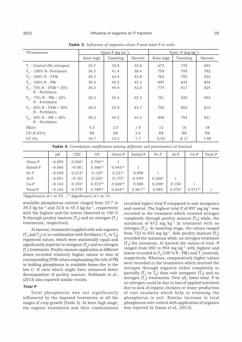
available phosphorus content ranged from 33.7 to

39.3 kg ha-1 and 32.6 to 45.5 kg ha-1, respectively

with the highest and the lowest observed in 100 %

N through poultry manure (T4) and no nitrogen (T

1)

treatments, respectively.

At harvest, treatments supplied with sole organics

(T3 and T

4) or in combination with fertilizers ( T

5 to T

8)

registered values, which were statistically equal and

significantly superior to inorganic (T2) and no nitrogen

(T1) treatments. Poultry manure application at different

doses recorded relatively higher values to that of

corresponding FYM values emphasizing the role of PM

in holding phosphorus in available forms due to the

low C: N ratio which might have enhanced faster

decomposition of poultry manure. Subbaiah et al.,

(2013) also reported similar results

Total P

Total phosphorus was not signif icantly

influenced by the imposed treatments at all the

stages of crop growth (Table 3). At knee high stage,

the organic treatments and their combinations

Table 4. Correlation coefficients among different soil parameters at harvest

pH CEC OC Olsen P Saloid-P Fe-P Al-P Ca-P Total-P

Olsen P –0.095 0.240* 0.790** 1

Saloid-P –0.060 –0.081 0.566** 0.545** 1

Fe-P –0.049 0.212* 0.135* 0.221* 0.098 1

Al-P –0.041 –0.181 0.220* 0.175* 0.449* 0.266* 1

Ca-P –0.163 0.193* 0.572** 0.626** 0.088 0.298* 0.150 1

Total-P –0.162 0.279* 0.788** 0.644** 0.561** 0.085 0.375* 0.571** 1

*Significance of r at 5% , ** Significance of r at 1%

recorded higher total P compared to sole inorganics

and control. The highest total P of 897 mg kg-1 was

recorded in the treatment which received nitrogen

completely through poultry manure (T4) while, the

minimum of 672 mg kg-1 in treatment with no

nitrogen (T1). At tasseling stage, the values ranged

from 722 to 835 mg kg-1. Sole poultry manure (T4)

recorded the maximum while, no nitrogen treatment

(T1) the minimum. At harvest the values of total -P

ranged from 692 to 854 mg kg-1 with highest and

lowest recorded in T4 (100 % N - PM ) and T

1 (control),

respectively. Whereas, comparatively higher values

were recorded in the treatments which received the

nitrogen through organics either completely or

partially (T3 to T8) than sole inorganic (T2) and no

nitrogen (T1) treatments. Over all, lower total -P in

no nitrogen could be due to loss of applied nutrients

due to lack of organic chelates or lesser production

of root exudates which help in retaining the

phosphorus in soil. Similar increase in total

phosphorus over control with application of organics

was reported by Ganai et al., (2013).

Table 3. Influence of organics olsen P and total P in soils

TTreatments Olsen P (kg ha-1) Total -P (mg kg-1)


T1 - Control (No nitrogen) 33.7 32.6 32.6 672 722 692

T2 - 100% N- Fertilizers 36.5 41.4 38.4 709 789 782

T3 - 100% N - FYM 38.5 43.4 43.8 762 793 832

T4 - 100% N - PM 39.3 45.5 45.3 897 835 854

T5

- 75% N - FYM + 25% 36.3 44.9 42.0 774 817 824

N - Fertilizers

T6 - 75% N - PM + 25% 38.5 45.3 45.3 781 830 853

N - Fertilizers

T7

- 50% N - FYM + 50% 38.0 43.8 43.7 792 802 819

N - Fertilizers

T8

- 50% N - PM + 50% 38.2 44.2 44.5 849 794 821

N - Fertilizers

SEm± 4.2 2.5 1.9 12 16 18

CD (0.05%) NS NS 5.6 NS NS NS

CV (%) 18.7 10.3 7.7 6.93 8.17 7.89

32(2) Influence of organics on P fractions 35

Pearson correlation coefficients

Data in table 3 revealed that all the P fractions

showed positive correlation among one another. The

Olsen P had a significant positive correlation with

the saloid-P (r=0.545**) which indicated that saloid-

P is the most readily available form of phosphorus

to the plant. The Ca-P and total-P were also

significantly positively related with Olsen extractable

P (r=0.626** and r=0.644**, respectively) indicating

their favourable contribution towards available P

pool. All the inorganic fractions of phosphorus were

negatively correlated with pH while, the organic

carbon showed a significant positive correlation with

all the inorganic P fractions and total P. Results

indicated that total P showed a highly significant

positive correlation with the saloid-P (r=0.561**) and

Ca-P (r=0.571**).

REFERENCE

Abolfazli, F., A Forghani and Norozoui M. (2012).

Effects of phosphorus and organic fertilizers on

phosphorus fractions in submerged soil.

Journal of Soil Science and Plant nutrition 12(2):

349-362.

Bahl, G. S., Vig, A.C., Yash pal and Singh A. (1997).

Effect of green manure and cropping on P

sorption in some soils of Punjab and Himachal

Pradesh. Journal of the Indian Society of Soil

Science 46(4): 574-579.

Ganai, A. Q., Singh, J. P. and Antil, R. S. ( 2013).

Long term effects of continuous cropping and

differential nutrient management practices on

P and K dynamics under rice- wheat cropping

sysem. Indian Journal of Fertilizers 8: 29-32.

Hedley, M. J., J. W. B. Stewart and Chauhan, B. S.

(1982). Changes in inorganic and organic soil

phosphorus fractions induced by cultivation

practices and by laboratory incubations. Soil

Science Society of American Journal 46 :

970-976.

Jackson, M. L. (1967). Soil chemical analysis.

Prenties Hall Publication Pvt. Ltd., New Delhi,

India.

Murphy, J and Riley, J. P. (1962). A modified single

solution method for the determination of

phosphate in natural waters. Analytical Chimica

Acta 27: 31-36.

Panse, V. G. and Sukhatme, P. V. (1978). Statistical

methods for agricultural workers. ICAR. New

Delhi. pp 199-211.

Reddy, D. D., S. A. Rao and Singh, M. (2005).

Changes in P fractions and sorption in Alfisol

following crop residues application. Journal of

Plant nutrition and Soil Science 168: 241-247.

Subbaiah, P. V., Sairam, A., Rao, P. C, and Naidu,

M. V. S. (2013). Effect of integrated use of

organic and inorganic sources of nutrients and

biofertilizers on soil available nutrients in

maize- onion cropping system. The Andhra

Agricultural Journal 60(2): 337-341.

Wang, G. P., Z. L. Zhai, J. S, Liu and Wang, J. D.

(2008). Forms and profile distribution of soil

phosphorus in four wet lands across gradients

of sand desertification in Northeast China.

Geoderma, 145: 59-74.

Watanabe, F. S and Olsen, S. R. (1965). Test for

ascorbic acid method for determining

phosphorus in water and sodium bicarbonate

extracts of soil. Soil Science Society of American

Journal 29: 677-678.

36 Sujala et al. 32(2)


Performance of Heliconia-An Exotic Cut Flower Crop as Intercrop

in Coconut under Coastal Climatic Conditions of Goa

M. THANGAM*, SAFEENA SA, S. PRIYA DEVI and N. P. SINGH

ICAR Research Complex for Goa, Old Goa - 403 402, Goa


A study on the performance of twenty three heliconia types/varieties was under taken undertwenty year old coconut plantation as intercrop under coastal humid conditions of Goa forthree years during 2010-2013. Suckers of different varieties/types of heliconia were planted at1.5x1.5m spacing so as to accommodate twenty five plants in four coconut trees. Analysis ofvariance indicated that all the traits observed differed significantly. The earliest flowering wasnoticed in heliconia type Choconiana (124 days) and Sexy Pink took 445 days for first flowering.Number of flowering suckers per clump was highest in Bihai (15) followed by Lobster Claw Two(13). Spike length was highest in Sexy Pink (108.15 cm) indicating its potential as cut flowerfollowed by Kenya Red (67.83 cm) and St. Vincent Red (66.41 cm). It is concluded from thestudy that intercropping heliconia in coconut plantation can give an additional income in therange of Rs. 32,160 in H-4 (Rostrata type) to Rs. 1, 37,200 in H-6 (Hybrid type). The heliconia typesGolden Torch (H-2), Hybrid type (H-6), Sexy Pink (H-8) and Wagneriana (H-9) recorded a total incomeof more than one lakh rupees by sale of flower and suckers from an area of one hectare undercoconut plantation and recommended as suitable intercrop in coconut.

(Key words: Heliconia, Intercrop, Coconut, Coastal Area)

Heliconias, which are native to South and

Central America, are popular as ornamental plants

and cut flowers because of their brilliant colours

and exotic appearance. Their enhancing beauty had

made them, a best landscape and as a potential cut

flower (Janakiram and Pavan Kumar, 2011). The

heliconias exhibit a wide array of colours led by red,

pink, orange, yellow, green combined with different

sizes and shapes (Goel, 2004). Due to its exotic

appearance and brilliant colours, it fetches premium

price in the market. Leaves of some varieties of

heliconia are also sold as cut leaves for flower

decoration. The genus Heliconia (Heliconiaceae)

includes a number of species showing potential as

commercial cut flower crops. H. psittacorum and

some of its hybrids ( i.e. ‘Golden Torch’) are

particularly promising because of their attractive

flowers, long straight clean peduncles, prolific year

round flower production, excellent post harvest

characteristics, and few pest problems. The

inflorescences can be used in a manner similar to

those of bird of paradise, but they are less massive

and are therefore, easily incorporated into smaller

floral arrangements.

Coconut is an important plantation crop in Goa

next only to Cashew. It is cultivated in an area of

25,730 ha with an average yield of 5014 kg ha-1


translating to only 32 nuts per tree per year. In

general, coconut is planted at a spacing of 8 x 8m

and interspaces in majority of the coconut farms is

either unutilized or underutilized. Generally various

intercrops are advocated to enhance the profitability

of coconut in Goa. Heliconia- an exotic introduced

flower crop performs extremely well under partial

shade in coastal humid conditions of Goa. Hence, a

study was planned to evaluate the performance of

23 varieties/types of heliconia under coconut as an

intercrop for vegetative and flower characteristics.


The present study was undertaken in the 20

year old coconut plantation (Cv. Benaulim) in ICAR

Research Complex for Goa, Old Goa for three years.

Only the heliconia cultivars that have eye appeal,

productivity, robust and healthy growth, long vase

life and suitable size and shape for packing can be

commercialized (Criley and Broschat, 1992). Though

institute germplasm bank has got several types and

varieties of heliconia, only those suitable for

commercialization were selected for this particular

study. The flowers of selected types were supplied

to market to document the feedback from the market

so as to short list the most promising heliconia types

with high floral value. The study included 23

varieties (Fig. 1) of heliconias planted as intercrop

in the existing coconut plantations. The study was

conducted from 2010-2013 for different purpose like

cut flower production, cut leaves production,

suckering habit, vase life studies etc. The coconut

spacing was 8x8m, where in 25 heliconia plants

were accommodated in the interspaces of four.

Initially, suckers were planted in a pit where in 250g

each of NPK was thoroughly mixed in soil .

Immediately after planting, the plants are watered

thoroughly for better establishment. Generally, it

takes about 30-45 days for the sucker to establish.

Hence periodic watering is important. Various

vegetative traits viz., number of suckers per clump,

flowering suckers per clump, leaf traits and several

floral characters which are important for cut flower

purpose were recorded six months and twelve

months after planting and the same is presented in

table 1 and 2.


Vegetative characters

The data pertaining to different morphological

traits are presented in Table 1. The productivity of

any heliconia type depends on important characters

like days to flowering, suckering habit and number

of flowering suckers per clump in a year. The data

indicated that the heliconia type Choconiana took

only 123.50 days for flower initiation followed by

commercial heliconia type Golden Torch (136.00

days). The most popular and costly heliconia type

Sexy Pink took the maximum (444.50) days for flower

initiation. Majority of the heliconia types recorded

first flowering within 300 days of planting from

sucker under coastal condition of Goa as intercrop

in coconut. Wider variability was reported for

vegetative and floral traits by Pavan Kumar et al.,

(2011) in different heliconia types.

The suckering habit of any heliconia type

decides its commercial viability as cut flower crop.

The cost of planting material accounts for 50 per

cent of the total cost of production. Therefore

profuse suckering habit is a desirable trait in

commercial cultivation of heliconia. The data for

three years indicated that there was wide variation

in sucker production among the heliconia types

evaluated. The highest number of suckers per clump

(41.09) was recorded in heliconia type Golden Torch

followed by heliconia type Lady Di (37.08). Other

popular heliconia types viz., Tagami, Latispatha and

Pedro Ortiz recorded only 6.25, 6.25 and 6.75

suckers per clump respectively. Important cut flower

type heliconias viz., Sexy Pink, Temptress,

Wagneriana etc. also recorded medium to high

sucker production per clump. Ramachandrudu and

Thangam (2012) also reported high sucker

production in heliconia types viz., Golden Torch,

Lady Di and Choconiana under coconut plantation.

Fig. 1. Glimpse of heliconia types used in the study

38 Thangam et al. 32(2)

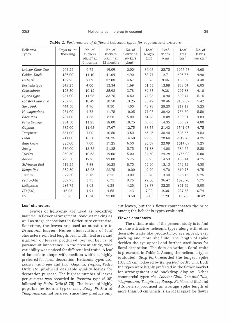
Leaf characters

Leaves of heliconia are used as backdrop

material in flower arrangement, bouquet making as

well as stage decorations in floriculture enterprise.

Sometime, the leaves are used as substitute to

Dracaena leaves. Hence observation of leaf

characters viz., leaf length, leaf width, leaf area and

number of leaves produced per sucker is of

paramount importance. In the present study, wide

variability was noticed for different leaf traits. A leaf

of lanceolate shape with medium width is highly

preferred for floral decoration. Heliconia types viz.,

Lobster claw one and two, Guyana, Tropics, Pedro

Ortiz etc. produced desirable quality leaves for

decoration purpose. The highest number of leaves

per suckers was recorded in Rostrata type (6.05)

followed by Pedro Ortiz (5.75). The leaves of highly

popular heliconia types viz., Sexy Pink and

Temptress cannot be used since they produce only

cut leaves, but their flower compensates the price

among the heliconia types evaluated.

Flower characters

The ultimate aim of the present study is to find

out the attractive heliconia types along with other

desirable traits like productivity, eye appeal, easy

packing and more shelf life. The length of spike

decides the eye appeal and further usefulness for

floral decoration. The data on various floral traits

is presented in Table 2. Among the heliconia types

evaluated, Sexy Pink recorded the longest spike

(108.15 cm) followed by Kenya Red (67.83 cm). Both

the types were highly preferred in the flower market

for arrangement and backdrop display. Other

commercial types viz., Lobster Claw One and Two,

Wagneriana, Temptress, Sassy, St. Vincent Red and

Adrian also produced an average spike length of

more than 50 cm which is an ideal spike for flower

Table 1. Performance of different heliconia types for vegetative characters

Heliconia Days to 1st No. of No. of No. of Leaf Leaf Leaf No. of

Types flowering suckers suckers flowering length width area leaves

plant-1 at plant-1 at suckers (cm) (cm) (cm 2) sucker-1

6 months 12 months plant-1

Lobster Claw One 264.25 6.75 19.09 2.00 84.03 25.75 1953.57 4.60

Golden Torch 136.00 11.10 41.09 4.90 53.77 12.71 605.86 4.90

Lady Di 152.25 7.09 37.08 4.67 38.28 9.46 460.09 4.40

Rostrata type 248.25 4.00 13.34 1.69 61.53 13.88 738.64 6.05

Choconiana 123.50 10.12 35.92 3.78 89.35 9.38 297.88 4.10

Hybrid type 234.00 11.25 33.75 6.50 74.03 10.90 600.74 5.15

Lobster Claw Two 257.75 10.49 18.50 13.25 85.47 30.46 2189.57 5.42

Sexy Pink 444.50 4.76 9.50 4.00 42.79 28.20 717.13 5.25

H. wagneriana 254.00 4.75 11.75 10.25 77.05 38.42 756.60 5.58

Eden Pink 237.00 4.38 8.50 5.00 61.48 10.08 490.91 4.83

Petra Orange 284.50 11.25 18.00 10.75 50.05 14.35 565.87 4.00

Guyana 382.00 11.63 17.67 12.75 88.73 21.43 1541.07 4.75

Temptress 381.00 7.00 10.50 3.50 65.46 30.40 803.85 4.83

Bihai 411.00 13.50 20.25 14.50 99.65 28.64 2319.45 4.25

Alan Carle 385.00 9.00 17.25 6.50 86.69 22.09 1614.09 5.25

Sassy 376.00 13.75 21.25 5.75 51.88 14.08 584.55 5.50

Tropics 360.50 10.63 19.00 5.00 84.60 24.28 1756.93 5.00

Adrian 293.50 12.75 22.00 5.75 38.95 14.53 488.14 4.75

St.Vincent Red 319.25 7.88 16.25 8.75 52.90 13.13 542.72 4.50

Kenya Red 352.50 13.25 22.75 10.00 49.20 14.70 610.75 4.75

Tagami 372.50 3.13 6.25 3.00 33.20 13.40 396.16 5.25

Pedro Ortiz 309.75 3.75 6.75 3.75 79.60 36.47 1595.70 5.75

Latispatha 284.75 3.63 6.25 4.25 68.77 32.28 851.52 5.00

CD (5%) 16.05 1.91 4.65 1.43 7.92 2.36 227.53 0.74

CV 3.36 15.70 22.00 13.50 8.48 7.29 15.26 10.42

32(2) Heliconia as intercrop in coconut 39

Table 2. Performance of different heliconia types for floral characters

Heliconia Types Stalk length Spike length No. of bracts Bract length No. of flowers

(cm) (cm) spike-1 (cm) bract-1

Lobster Claw One 87.10 51.99 10.53 20.86 8.21

Golden Torch 66.96 18.44 5.95 17.39 22.00

Lady Di 83.28 16.01 5.80 13.21 13.80

Rostrata type 67.79 49.13 16.55 8.62 11.45

Choconiana 86.09 13.25 4.00 12.83 10.38

Hybrid type 74.46 43.01 6.13 15.09 10.25

Lobster Claw Two 85.87 60.46 10.55 12.45 10.07

Sexy Pink 153.18 108.15 14.92 23.56 10.92

H. wagneriana 69.10 44.98 8.25 19.08 15.78

Eden Pink 60.51 37.72 5.51 16.86 7.92

Petra Orange 40.44 29.98 4.13 14.54 8.86

Guyana 77.59 49.51 4.88 14.44 12.25

Temptress 80.95 55.37 11.63 17.29 9.50

Bihai 47.15 37.88 8.38 24.33 13.65

Alan Carle 64.64 48.07 7.75 18.31 18.36

Sassy 83.60 63.53 3.88 14.69 10.24

Tropics 79.54 49.84 5.22 15.62 9.64

Adrian 79.79 56.53 5.10 15.58 10.71

St.Vincent Red 90.78 66.41 4.88 12.65 9.31

Kenya Red 96.90 67.83 6.25 17.80 18.13

Tagami 48.52 34.06 4.50 11.74 9.79

Pedro Ortiz 61.62 32.40 8.00 8.85 11.63

Latispatha 53.46 27.98 7.50 11.55 7.88

CD (5%) 9.82 7.73 0.80 2.52 1.81

CV 9.22 10.62 7.92 11.18 11.14

decoration. Varying spike length for different

heliconia types was earlier reported by Sheela

et al., (2007).

Economics of heliconia production under coconutplantation

The economics of heliconia production was

worked out for ten promising heliconia types for two

years. A total of 600-700 heliconia plants can be

accommodated in an area of one hectare as inter

crop. The economics of flower production was

calculated by taking in to account of total number

of flowers produced in a year and the cost of flower

at farm. Among the heliconia types evaluated for

flower sales, Wagneriana (H-9), Sexy Pink (H-8),

Hybrid type (H-6) and Golden Torch (H-2) produced

more number of flowers per hectare and fetched

premium price in the market (Fig. 2). The highest

income (Rs. 93, 824) per hectare was recorded in

H-9 followed by H-8 (Rs. 89, 600). The heliconia

type Rostrata recorded the lowest income due to less

number of flowers and priced low among the types

evaluated in the market.

Fig. 2. Income (Rs. ha-1) from heliconia

cut flower sales per hectare

Fig. 3. Income (Rs. ha-1) from sale

of heliconia sucker per hectare

40 Thangam et al. 32(2)

But in case of sucker production, the heliconia

types viz., Golden Torch (H-2), Lady Di (H-3),

Choconiana (H-5) and Eden Pink (H-6) produced

more numbers of suckers per hectare due to their

high suckering ability (Fig. 3). The highest income

through the sale of suckers was recorded in Golden

Torch (Rs.65, 744) followed by Lady Di (Rs.59, 328)

and other types viz., Sexy Pink (H-8), H-9

(Wagneriana) and H-10 (Eden Pink) recorded the

lowest income from sucker due to their low

suckering habit under coconut plantation.

The heliconia types Golden Torch (H-2), Hybrid

type (H-6), Sexy Pink (H-8) and Wagneriana (H-9)

recorded a total income of more than one lakh

rupees by sale of flower and suckers from an area

of one hectare under coconut plantation. Hence it

is recommended to grow these heliconia types for

increasing the income from coconut plantation.

REFERENCES

Criley, R. A. and Broschat, T. K. (1992). Heliconia:

Botany and Horticulture of a New Floral

Crop.In: Horticultural Reviews, J. Janik (ed.),

Wiley, New York. Vol. 14, pp 1-55.

Goel, A. K. (2004). Heliconias: nature wonders from

neotropical regions. Indian Horticulture April-

June, 20-21. ICAR, New Delhi.

Janakiram, T. and Pavan Kumar, P. (2011).

Enhancing flower potential of Heliconia. Indian

Horticulture January-February, 22-24. ICAR,

New Delhi.

Pavan Kumar, P., Janakiram, T and Venugopalan,

R. (2011). Genetic variability studies in

Heliconia cultivars. Journal of Ornamental

Horticulture 14(3&4): 10-13.

Ramachandrudu, K. and Thangam, M. (2012).

Performance of heliconia under coconut garden

and open field conditions. Indian Journal of

Horticulture 69(3): 450-453.

Sheela, V. L., Sabina George, T., Rakhi, R. and

Geetha Lekshmi, P. R. (2007). Variability

studies in cut flower varieties of Heliconias.

Indian Journal of Horticulture 64(1): 109-111.

32(2) Heliconia as intercrop in coconut 41


Yield Gap Analysis of Rice through Front Line

Demonstrations in Tropical Andaman Islands

S.K. ZAMIR AHMED, P.K. SINGH, R.K. GAUTAM* and S DAM ROY

ICAR-Central Island Agricultural Research Institute, Port Blair - 744 101

Andaman and Nicobar Islands


The present study aimed to know the gaps for yield performance between potential and actualyield of rice through 137 Front Line Demonstrations (FLD) conducted across 3 years in theAndaman Islands. Improved rice varieties with recommended package of practices could giveon an average yield of 4.72 t ha-1 to 5.78 t ha-1 as compared to local varieties yielding 3.21 t ha-

1 to3.69 t ha-1 under rainfed conditions of Andaman and Nicobar Islands. The extension gapranged between 1.22 to 1.70 t ha-1 in improved varieties as compared to 1.55 to 2.70 t ha-1 underhybrid varieties. The trend of technology gap ranged from 0.15 to0.30 t ha-1 in hybrid varietiescompared to 0.18– 0.35 t ha-1 in case of pure line varieties. The technology index showed thefeasibility of realising the performance of evolved technology at the farmer’s fields. The valuetechnology index showed wide range of 3.60 to 15.80 for HYVs and 2.50 to 5.00 in hybrid varieties.The benefit cost ratio was slightly high in hybrids than pure line varieties. The yield of ricecould be increased from 36% to 54% by high yielding varieties and from 37% to 86 % by ricehybrids complimented by improved seed and appropriate crop management technologies.Availability of improved seed of high yielding rice varieties and required inputs along withtimely extension interventions can greatly narrow the gap between potential yield and actualyield to reap high rice productivity in Andaman and Nicobar Islands.

(Key words: Rice, FLD, Technological gap, Extension gap, Technological index)

National food security bill envisages availability

of food for all. In this respect, productivity potential

especially of disadvantaged and less explored areas

has to be assessed and accordingly production

strategies to be followed. Rice is the main cereal

crop cultivated in Andaman and Nicobar Islands.

The climatic conditions including more than 3180

mm rainfall annual also favours rice cultivation.

Rice crop is annually grown on about 8,100 hectares

of cultivated land producing over 23976 tons of

paddy, with productivity of about 2.96 t ha-1

(Anonymous 2012) against the annual rice demand

of 60,000 tons for the islands. The substantial gap

between annual demand and production is bridged

by shipment of rice from mainland, India and thus

causing transport price rise and subsidy costs to

the government exchequre.

The main reason for large gaps between

production and demand is low productivity of rice

varieties (photosensitive, tall, very late, low yielding

and susceptible to biotic and abiotic stresses) which

grown on about 50 percent of paddy area. Other

major reasons for low productivity which are include

imbalanced and inadequate use of fertilizer, non-

availability of improved seed of HYVs, heavy and

prolonged rain up to December month, constant

warm temperature and high humidity favouring pest

and disease incidence. About 3000 ha area of rice

is also affected by costal salinity especially in the

aftermath of tsunami of 2004.

In view of high demand of rice and existing

climatic conditions of Bay Islands the rice varieties

should preferably possess long duration, high yield

ability, fertilizer responsiveness, semi-tall stature,

good grain and straw quality, resistance/tolerance

to biotic and abiotic stresses especially salinity and

submergence. Productivity can be increased to

about 4.5 to 5.0 t ha-1 through appropriate varieties

and other crop management and protection

technologies (Gautam et al., 2013). The available

agricultural technology does not serve the very

purpose until it uniformly reaches and adopted by

its ultimate users the farmers. Technology transfer

refers to the spread of new ideas from originating

sources to ultimate users (Prasad et al., 1987). It is

also important to ensure uniform adoption of

recommended package of practice through

understanding the extent of gaps between actual

and potential yield for introducing the urgency and

extent of technology interventions. Conducting of


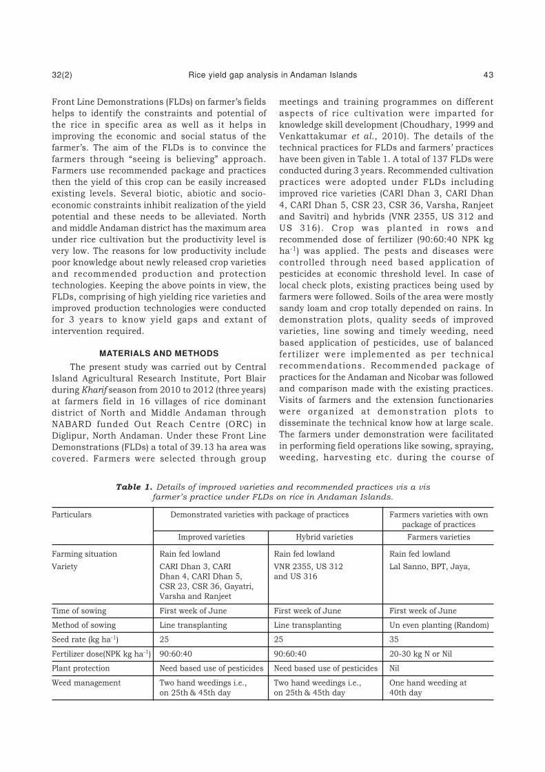
Front Line Demonstrations (FLDs) on farmer’s fields

helps to identify the constraints and potential of

the rice in specific area as well as it helps in

improving the economic and social status of the

farmer’s. The aim of the FLDs is to convince the

farmers through “seeing is believing” approach.

Farmers use recommended package and practices

then the yield of this crop can be easily increased

existing levels. Several biotic, abiotic and socio-

economic constraints inhibit realization of the yield

potential and these needs to be alleviated. North

and middle Andaman district has the maximum area

under rice cultivation but the productivity level is

very low. The reasons for low productivity include

poor knowledge about newly released crop varieties

and recommended production and protection

technologies. Keeping the above points in view, the

FLDs, comprising of high yielding rice varieties and

improved production technologies were conducted

for 3 years to know yield gaps and extant of

intervention required.


The present study was carried out by Central

Island Agricultural Research Institute, Port Blair

during Kharif season from 2010 to 2012 (three years)

at farmers field in 16 villages of rice dominant

district of North and Middle Andaman through

NABARD funded Out Reach Centre (ORC) in

Diglipur, North Andaman. Under these Front Line

Demonstrations (FLDs) a total of 39.13 ha area was

covered. Farmers were selected through group

meetings and training programmes on different

aspects of rice cultivation were imparted for

knowledge skill development (Choudhary, 1999 and

Venkattakumar et al., 2010). The details of the

technical practices for FLDs and farmers’ practices

have been given in Table 1. A total of 137 FLDs were

conducted during 3 years. Recommended cultivation

practices were adopted under FLDs including

improved rice varieties (CARI Dhan 3, CARI Dhan

4, CARI Dhan 5, CSR 23, CSR 36, Varsha, Ranjeet

and Savitri) and hybrids (VNR 2355, US 312 and

US 316). Crop was planted in rows and

recommended dose of fertilizer (90:60:40 NPK kg

ha-1) was applied. The pests and diseases were

controlled through need based application of

pesticides at economic threshold level. In case of

local check plots, existing practices being used by

farmers were followed. Soils of the area were mostly

sandy loam and crop totally depended on rains. In

demonstration plots, quality seeds of improved

varieties, line sowing and timely weeding, need

based application of pesticides, use of balanced

fertilizer were implemented as per technical

recommendations. Recommended package of

practices for the Andaman and Nicobar was followed

and comparison made with the existing practices.

Visits of farmers and the extension functionaries

were organized at demonstration plots to

disseminate the technical know how at large scale.

The farmers under demonstration were facilitated

in performing field operations like sowing, spraying,

weeding, harvesting etc. during the course of

Table 1. Details of improved varieties and recommended practices vis a vis

farmer’s practice under FLDs on rice in Andaman Islands.

Particulars Demonstrated varieties with package of practices Farmers varieties with own

package of practices

Improved varieties Hybrid varieties Farmers varieties

Farming situation Rain fed lowland Rain fed lowland Rain fed lowland

Variety CARI Dhan 3, CARI VNR 2355, US 312 Lal Sanno, BPT, Jaya,

Dhan 4, CARI Dhan 5, and US 316

CSR 23, CSR 36, Gayatri,

Varsha and Ranjeet

Time of sowing First week of June First week of June First week of June

Method of sowing Line transplanting Line transplanting Un even planting (Random)

Seed rate (kg ha-1) 25 25 35

Fertilizer dose(NPK kg ha-1) 90:60:40 90:60:40 20-30 kg N or Nil

Plant protection Need based use of pesticides Need based use of pesticides Nil

Weed management Two hand weedings i.e., Two hand weedings i.e., One hand weeding at

on 25th & 45th day on 25th & 45th day 40th day

32(2) Rice yield gap analysis in Andaman Islands 43

across three years. It is also pertinent to mention

that the yield of farmers varieties varied from 3.08

to 3.43 t ha-1 and 3.15 to 4.15 t ha-1 in case of

FLDs on HYVs and hybrids, respectively.

The percentage increase in yield over the local

varieties ranged from 36% to 55% and 37% to 86%

across years in HYVs and hybrids, respectively.

Tiwari et al., (2014) have also performed yield gap

analysis in chickpea through FLDs. The results

indicated that the Front Line Demonstrations have

given a good impact on the farming community of

this district as they were motivated by the improved

rice varieties and agricultural technologies used in

the Front Line Demonstrations. The results clearly

indicated the positive effects of improved rice varieties

over the existing rice varieties towards doubling the

rice productivity in Diglipur area, North Andaman.

Benefit-Cost ratio was also recorded higher

under demonstration plots against control plots in

all the years of study. The findings revealed that a

gap exists between the actual farmer’s yield and

realizable yield potential of the varieties. Use of

improved varieties has the potential to enhance the

present level of rice productivity which is not

percolating down at desired pace due to

communication gap and lack of confidence among

the farmers. Hence, to exploit the potential of

improved rice varieties coupled with production and

Table 3. Productivity, technology gaps, extension gaps, technology index and cost benefit

ratio of promising rice hybrids under FLD’s in North Andaman district.

Years Area Grain yield (t ha-1) % Technology Extension Technology B : C ratio

(ha) Potential FLD’s Control increase gap gap index FLD’s Controlover (t ha-1) (t ha-1) (%)

control

2010 6.30 6.00 5.80 3.78 53 0.20 2.02 3.33 3.31 2.39

2011 2.60 6.00 5.85 3.15 86 0.15 2.70 2.50 3.34 1.99

2012 1.60 6.00 5.7 4.15 37 0.30 1.55 5.00 3.26 2.62

Average 3.5 6.00 5.78 3.69 59 0.22 2.09 3.61 3.30 2.33

Table 2. Productivity, technology gaps, extension gaps, technology index and cost benefit

ratio of high yielding varieties under FLD’s of rice in North Andaman district

Years Area Grain yield (t ha-1) % Technology Extension Technology B : C ratio

(ha) Potential FLD’s Control increase gap gap index FLD’s Controlover (t ha-1) (t ha-1) (%)

control

2010 13.30 5.00 4.70 3.08 53 0.30 1.62 6.00 2.97 1.95

2011 2.25 5.00 4.65 3.43 36 0.35 1.22 7.00 2.94 2.17

2012 14.69 5.00 4.82 3.12 54 0.18 1.70 3.60 3.04 1.97

Average 10.08 5.00 4.72 3.21 48 0.28 1.51 5.53 2.98 2.03

trainings and field visits. The selection of sites and

farmers and layout of demonstration were followed

as suggested by Choudhary (1999). The traditional

practices followed by farmers were maintained in

case of local checks.

The data outputs were collected from both FLD

plots as well as control plots (farmer’s practices)

and finally the extension gap, technology gap,

technology index and benefit cost ratio were worked

out as per Samui et al., (2000) as given below:

Technology gap = Potential yield – Demonstration yield

Extension gap = Demonstration yield – Farmers yield

Technology index = (Potential yield – Demonstration yield)

x 100

Potential yield


The results of FLDs of HYVs and promising

hybrids conducted during 3 years (2010, 2011 and

20112) in North Andaman are presented in Table 2

and Table 3 respectively. FLDs on HYVs (4.72 t ha-1)

showed on an average 47.55% more yield of rice as

compared to local varieties (3.21 t ha-1) as shown

in Table 2. Similarly hybrids gave an average yield

of 5.78 t ha-1 which is 58.83% more compared to

local varieties 3.69 t ha-1 (Table 3). The data of

Tables 2 and 3 revealed that the yield of rice varied

from 4.65 to 4.82 t ha-1 in pure line varieties

whereas from 5.70 to 5.85 t ha-1 in case of hybrids

44 Ahmed et al. 32(2)

protection technologies, efforts through FLDs have

to be increased among the farmers. The extension

gap was found to range from 1.22 to 1.70 t ha-1 in

HYVs and from 1.55 to 2.70 t ha-1 in case of hybrids

during the study period. This highlights the need

to educate the farmers through various means for

adoption of improved varieties and agricultural

production technologies to achieve higher rice

productivity in the islands.

The technology gap ranged from 0.18 to 0.35

t ha-1 and from 0.15 to 0.30 t ha-1 in HYVs and

hybrid FLDs, respectively. This reflects farmer’s

cooperation in carrying out such demonstrations

with encouraging results in subsequent years. The

varying technology gaps might have arisen due to

the dissimilarity in soil fertility status and weather

conditions. Mukharjee (2003) stated that depending

on identification and use of farming situation,

specific interventions may have greater implications

in enhancing system productivity. Similar findings

were also recorded by Mitra and Sanajdar (2010)

and Katare et al ., 2011. The magnitudes of

technology index showed the technical feasibility

of the evolved technology at the farmer’s fields. The

lower the value of technology index, the more is the

feasibility of technology implementation. Over here

the technology index ranged from 3.60 to 7.00% in

improved varieties and from 2.50 to 5.00% in

hybrids during the study period. This implies that

the technology (rice varieties recommended) in field

conditions is very much accepted by the farmers

and varietal approach is practically feasible and

implementable. The lateral spread of the variety

technology is found to be remarkably acceptable

which is evidenced by the large scale cultivation of

CIARI recommended varieties especially in the North

and Middle Andaman district. The component of

benefit cost ratio of front line demonstrations has

clearly showed higher BC ratio of FLDs than control

plots i.e. farmers practice in all the years of study.

The benefit cost ratio of improved varieties FLDs in

demonstrated vis a vis control plots were 2.97 and

1.95, 2.94 and 2.17, 3.04 and 1.97 and in case of

hybrid varieties, benefit cost ratios were 3.31 and

2.39, 3.43 and 1.99, 3.26 and 2.62 during 2010,

2011 and 2012, respectively. Hence, technology

index and favourable benefit cost ratios proved the

technical and economic viability respectively of the

interventions and convinced the farmers on the utility

of these simple, economical and ecologically safe

interventions. Similar findings were also reported by

Sharma et al., (2003) in moth bean and Gurumukhi

et al., (2003) in sorghum and Mitra and Samajdar

(2010) in rapeseed mustard.

CONCLUSION

The results of rice front line demonstrations

convincingly brought out that the yield of rice could

be increased by 36% to 54% by improved varieties

and 37 – 86 % by adaptation of hybrids in

conjunction with their improved seed with balanced

fertilizer application and disease management in the

Andaman and Nicobar Islands. From the above

findings, it can also be concluded that use of

scientific methods of rice cultivation can reduce the

technology gap to a considerable extent thus leading

to increase in rice productivity in these Islands.

Moreover, extension agencies in the Islands need

to provide proper and timely technical support to

the farmers through different educational and

extension methods to reduce the extension gap for

achieving higher rice production and productivity.

Favourable benefit cost ratio of these interventions

indicates economic viability and convinced the farmers

for adoption of interventions towards high productivity

and better livelihood of the Islands farmers.

REFERENCES

Anonymous (2012). Economic survey of Andaman

and Nicobar Islands. Directorate of Economics

and Statistics Andaman and Administration.

42p.

Choudhary, B. N. (1999). Krishi Vigyan Kendra- A

guide for KVK managers. Division of

Agricultural Extension, ICAR, India. pp 73-78.

Gautam, R. ., Singh, P. K., Birah Ajanta, Kumar,

K., Singh, A. K., Kumar, Naresh, Zamir Ahmed,

S. K., Singh, Ajmer, Ravisankar, N., Devakumar,

K. and Dam Roy, S. (2013). Agro-technology for

high rice productivity in Andaman and Nicobar

Islands, Central Island Agricultural Research

Institute, Port Blair. pp1-42.

Gurumukhi, D. R. and Mishra, S. (2003). Sorghum

front line demonstration- A success story.

Agricultural Extension Review 15: 22-23.

Mitra, B. and Samajdar, T. (2010). Yield gap analysis

of rapeseed-mustard through Front Line

Demonstration. Agricultural Extension Review

22: 16-17.

Katare, S., Pandey, S. K. and Mustafa Mohd. (2011).

Yield gap analysis of Rapeseed-mustardthrough

front line demonstrations. Agricultural Update

6: 5-7.

32(2) Rice yield gap analysis in Andaman Islands 45

Mukharjee, N. (2003). Participatory Learning and

Action. Concept Publishing Company, New

Delhi, India. pp 63-65.

Prasad, C., Chaudhary, B. N. and Nayar, B. B.

(1987). First Line Transfer of Technology

Project, ICAR, New Delhi, India. pp 87

Samui, S. K, Maitra, S., Roy, D. K., Mandal, A. K.

and Saha, D. (2000). Evaluation of front line

demonstration on groundnut. Journal of Indian

Society of Coastal Agricultural Research 18:

180-183.

Sharma, O. P. (2003). Moth bean yield improvement

through Front Line Demonstrations.

Agricultural Extension Review 15: 11-13.

Tiwari, B. K. and Tripathi, P. N. (2014). Yield gap

analysis of chickpea (Cicer arietinum) through front

line demonstration on farmer’s field. The Journal

of Rural and Agricultural Research 14(1) 5-8.

Venkattakumar, R., Ramana, Rao S.V., Padmaiah,

M. and Madhuri, P. (2010). Production

constraintsand information needs of growers in

Andhra Pradesh. Agricultural Extension Review

(April-June): 21-24.

46 Ahmed et al. 32(2)


Studies on Performance of Some Elite Traditional Varieties of

Rice of West Bengal with Popular HYVs during Wet Season

SUSHIL KUMAR PANDEY, AWANEET KUMAR and BIJAN ADHIKARI

Rice Research Station, Chinsurah, West Bengal


Ten elite germplasm of traditional rice varieties of West Bengal along with two HYVs (IET 5656and MTU 7029), used as checks were grown at Rice Research Station (RRS), Chinsurah, Hooghly,West Bengal as replicated yield trial during Kharif 2011. These traditional varieties have beenchosen on the basis of their high yield potential and popularity among the farmers. Observationswere taken on agromorphic traits ( yield, days to 50% flowering, no. of panicles m-2, no. of filledgrains panicle-1, test weight, sterility%, etc.), physical grain quality parameters (grain length,grain breadth, grain L/B ratio, kernel length, kernel breadth, kernel L/B ratio etc), milling qualitytraits (hulling%, milling% and head rice recovery%), and some cooking and eating qualityparameters (volume expansion, elongation ratio, alkali spreading value, gel consistency andamylose content). Genetic analysis was conducted for all the parameters biometrically. Genotypicco-efficient of variation (GCV) and phenotypic co-efficient of variation (PCV), were found to bemaximum for cooking quality trait and alkali spreading value, followed by number of filledgrains panicle-1, panicle weight, amylose content, test weight and kernel breadth, respectively.Heritability ranged from 20.33% (Elongation ratio) to 96.93% (Alkali spreading) and highheritability was found in filled grains panicle-1, test weight, alkali spreading value, amylosecontent, grain breadth, grain L/B, kernel breadth, kernel L/B, kernel length, panicle weight,yield, plant height and gel consistency. Alkali spreading value, no of filled grains panicle-1, testweight, amylose content, kernel breadth, kernel L/B, panicle weight, plant height, gel consistencyand yield showed high heritability with high GCV which indicates the effectiveness of selectionbased on these traits. Filled grain panicle-1, test weight, plant height, yield, gel consistencyand amylose content showed high heritability coupled with high GCV and high GA indicatingthat these characters are mostly governed by additive gene action and hence, can be consideredas the basis of selection for varietal improvement. Out of 10 traditional rice varieties, five viz.Jamainadu, Talmari, Kerala Sundari, Jugal and Binni gave at par yield with high yielding checksIET 5656 and MTU 7029. Dudheswar, Binni, Jamainadu and Sarunagra were found to have bettercooking and eating quality than both the high yielding checks while Kerala Sundari, Jugal andDudheswar had better milling quality over the checks.

(Key words: Traditional rice varieties, HYVs, GCV, PCV, GA, Kernel length, Kernel breadth)

Rice, the most important food crop of the

developing world, feeds more than two billion people

as a staple food worldwide and is the number one

staple food in Asia, where it provides 40-70% of the

total food calories consumed. Rice is also used for

animal feed and provides the major source of income

for rural people. Due to the Green Revolution, a

quantum leap in rice yield took place over the past

three decades, although increased food production

did not eliminate poverty and hunger. Rice yield has

been stagnant for the last three decades, despite

the improved varieties and technologies in place.

All over the world, every night at least two billion

people go to sleep hungry and in India, the number

is miserably 320 millions.

Due to introduction of high-yielding varieties

(HYVs), presently only a few of traditional varieties

(TRVs) exist in farmers’ fields. Despite increase in

cost of production, aromatic rice Gobindobhog,

Badsabhog, Radhatilak, Kalonunia, Tulaipanji etc

and fine rice like Dudheswar, Seetasail etc still

fetches good price. The chemical intensive

agriculture of Green Revolution has not only

expunged the local crop genetic diversities but also

their wild relatives that are the only source of unique

of genes for disease and pest resistance. Farmers

were impressed by the initial high yields of these

so-called ‘miracle’ seeds and ignored the associated

costs of external inputs, subsequent loss of non-

grain bio-mass, loss of desirable traits (like tolerance

to diseases and pests, drought, floods, etc.), and

the extensive deterioration of the environment,

including soil and water. Over the years, the average

grain yield of ‘popular’ modern variety (HYV) MTU-

7029 of West Bengal has plummeted to the tune of

3.75 t ha-1 from 5 t ha-1 in most of the farmers’ fields.

These HYV cannot give substantial yield advantage

in the marginal lands like drought prone, saline

track and in deep water situation.

A World Wildlife Fund (WWF)- India survey,

conducted in 1994 in six districts of southern West

Bengal, recorded 137 traditional rice varieties still

surviving in marginal farms (Deb, 1995). An

investigation into the reasons for the continuation

of their cultivation highlighted the following factors:

l The small and marginal farmers who grow the

TRVs were too impoverished to buy the costly

inputs for growing HYVs.

l The HYVs failed to grow in dry uplands and wet

lowlands, where only a few specially adapted

local varieties could grow.

l Many native varieties were grown for their

special aroma and flavour, which were distinctly

lacking in the HYVs.

l A small number of native varieties fetched

higher market prices than the HYVs.

There are many varieties which are drought

tolerant, flood-tolerant and amenable to ill-drained and

lowland cultivation. A large number of varieties possess

the characteristics of disease and pest-resistance. Some

of them have the unique characteristics of tolerance to

salinity, alkalinity and being able to grow in ‘deep-water’

inland areas. In this perspective a study had been

undertaken to evaluate the performance of some

traditional rice varieties in comparison to popular HYVs

along with genetic analysis.


The experimental materials consisted of 10

traditional varieties viz. jugal, jamainadu, patnai 23,

kerala sundari, binni, latisail, dudheswar, talmari,

saru nagra and kalma 222 along with two high

yielding varieties viz. IET 5656 and MTU 7029 which

were used as checks. The crops were grown during

kharif 2011, in Randomized Block Design in 4

replication, in plot size of 6m x 2m, in 20cm x 15cm

spacing, at Rice Research Station, Chinsurah,

located at New Alluvial Zone of West Bengal at

(22052’N latitude and 88024’E longitude and at an

elevation of 8.62 meter from Mean Sea Level). The

soil of this location is texturally, sandy clay and is

mainly characterized by neutral reactions (pH 6.5-

7.8) and normal EC (less than 1 dSm-1). The nutrient

status of the soil is low to medium N, medium to

high P2O

5 and medium of high K

2O. Normal

agronomic practices were done in raising the crops.

The observations were taken on 8 agromorphic

characters viz. date of 50% flowering, plant height,

panicle length, panicle weight, no. of filled grain per

panicle, sterility percentage, test weight and yield;

5 cooking qualities viz. elongation ratio, volume

expansion, alkali spreading value, amylose content

and gel consistency and 9 physical and milling

characteristics viz. grain length, grain breadth, grain

L/B ratio, kernel length, kernel breadth, kernel L/

B ratio, hulling percentage, milling percentage and

head rice recovery.


The ANOVA of the various grain characters was

shown in the Table 1. It was found that all the grain

characters had significant differences which indicate

presence of wide variability among genotypes.

Agromorphic characters

Mean value, range, CD, CV and standard error of

agromorphic, characters were presented in Table 2.

Days to 50% flowering ranged from 105 days (Kerala

Sundari) to 120 days (IET 5656) with mean 115 days.

Plant height recorded from field ranged from 122.00

cm (IET 5656) to 174.67 cm (Kalma 222) with the

mean 147.47 cm. The number of panicle m-2 ranged

from 331(Kalma 222) to 488 (Jamainadu) with the

mean 409. Panicle length of experimental materials

varied from 21.28 cm (Binni) to 25.51 cm (Talmari)

with the mean 23.76 cm. Panicle weight is maximum

in Jamainadu (3.84 g) and minimum in Binni (1.97

g) and the mean is (3.09 g) Number of filled grains

per panicle varied from 74 (Binni) to 167 (Kerala

Sundari) with the mean of 127. Sterility percentage

was least in Kerala Sundari (14.76) and highest in

Kalma 222 was (22.45) with mean 18.51%. The test

weight i.e. the 1000 grain weight varied from 16.49

gm (Dudheswar) to 29.11 g (Patnai 23) with the mean

value 22.83g. The yield varied from 3.28 t ha-1

(Latisail) to 4.55 t ha-1 in Jamainadu which was

higher than both the high yielding check varieties.

The mean value was found to be 4.08 t ha-1.

Cooking Qualities

Mean value, range, CD, CV and standard error

of cooking quality were presented in Table 3. Kernel

elongation ratio ranged from 1.43 (Binni) to 1.69

(Dudheswar) with the mean of 1.54. Volume

expansion vareed from 3.78 (Kalma 222) to 5.17

(Sarunagra) with the mean 4.44. Alkali spreading

value recorded from 1.35 (Dudheswar) to 6.15

(Kerala Sundari) with mean 3.71. The value showed

that all the varieties were ranged from high-

intermediate gelatinization temperature to

intermediate gelatinization temperature. Amylose

content was lowest (19.70%) in Binni and highest

(33.13%) Kalma 222, with mean value of 25.46%.

According to the standard analytical methods for

48 Pandey et al. 32(2)

estimating amylose content (Juliano, 1971) low

amylase content belonged to a single variety Binni

and highest to Talmari, Sarunagra, Kalma 222 and

high yielding check variety IET 5656. Remaining all

belonged to intermediate amylase content. Gel

consistency value ranged from 64.00 mm (Talmari)

to 89.67 mm (Sarunagra) for different varieties

indicating significant variation for this trait with the

mean value of 77.28 mm. According to classification

of Cagampang et al., 1973, out of 12 varieties, all

the varieties showed soft gel consistency.

Physical & Milling Characteristics

Mean value, range, CD, CV and standard error

of physical and milling characters are presented in

Table 4. Grain length was observed lowest in Kerala

Sundari (7.57 mm) and highest in Patnai 23 (10.61

mm) with the mean 8.63 mm. The grain breadth

varied from 2.45 mm (Binni) to 3.02 mm (Latisail)

with the mean value 2.74 mm. Grain L/B ratio varied

from 2.80 (MTU 7029) to 3.68 (Patnai 23). The mean

value was 3.16. Kernel length was found to be lowest

in Jugal (5.5 mm) and highest in Patnai 23 (7.61 mm)

with the mean of 6.78 mm. The Kernel breadth varied

from 1.76 mm (Jugal) to 2.75 mm (Latisail) with the

mean value 2.35 mm. Kernel L/B ratio varied from

2.25 (Kerala Sundari) to 3.7 (Sarunagra) with the mean

value of 2.93. Hulling percentage varied from 77.33

(Jamainadu) to 83.50 (Jugal) with the mean of 79.21.

Milling percentage ranged from 65.83 (Jamainadu) to

73.5 (Jugal) and the mean value was 68.51. Head rice

recovery had the highest value of 65.00 (Kerala

Sundari) and lowest value of 55.83 (Patnai 23) with

the mean value of 61.82%.

Genotypic and phenotypic variance

Genotypic and phenotypic variances of

agromorphic, cooking quality and physical

characters are presented in Table 5. Genotypic

variance was highest in yield (166172.22) whereas

it is least in case of elongation ratio (0.01). The

genotypic variance is also low in case of milling

percentage (2.90), kernel length (0.37) and grain

breadth (0.04). Similarly the phenotypic variance

was highest in yield (220656.31) and lowest in

elongation ratio (0.02).

Table 1. Analysis of variance (ANOVA) of various grain characters (mean sum of square)

Sl. No. Characters Source of variance

Replication (2) Variety (11) Error (22)

1. 50 % flowering 5.36 40.03 28.13

2. Filled grain/panicle 21 2869.28 54.454

3. Panicle length 2.44 5.16 2.292

4. Panicle weight 0.002925 0.91 0.086

5. Plant height 415.19 971.79 109.39

6. Sterility % 2.95 20.24 3.45

7. Test weight 4.85 35.04 0.93

8. Panicle/ m2 1924 6515.30 1157.03

9. Yield 10508.33 553000 54484.09

10. Alkali spreading 0.014 5.28 0.0522

11. Amylose content 1.76 46.40 3.375

12. Elongation ratio 0.0432 0.0197 0.0111

13. Gel consistency 34.194 264.72 32.043

14. Volume expansion 0.098 0.43 0.056

15. Grain breadth 0.05 0.111 0.0028

16. Grain length 1.88 2.19 0.394

17. Grain L/B 0.027 0.296 0.021

18. Kernel breadth 0.0015 0.347 0.004

19. Kernel length 0.220 1.218 0.111

20. Kernel L/B 0.036 0.577 0.025

21. Hulling % 2.521 12.987 6.468

22. Milling % 6.861 14.507 5.816

23. Head rice recovery 10.361 28.461 4.058

32(2) Performance of traditional rice varieties 49

Table 2. Mean values of agromorphic traits of 10 traditional rice genotypes with 2 high yielding checks

Sl. Name of Days to Plant No. of Panicle Panicle No. of Sterility Test Yield

No. Variety 50% height panicle/ length weight filled % weight (t ha-1)

flowering (cm) m2 (cm) (g) grains/ (g)

panicle

1. Jugal 116 153.33 430.00 23.18 3.46 132.78 20.26 23.35 4.27

2. Jamainadu 114 156.67 488.33 25.47 3.84 143.11 20.67 24.71 4.55

3. Patnai 23 114 165.00 403.33 23.95 3.32 114.00 15.07 29.11 3.88

4. Kerala Sundari 105 135.00 429.00 25.11 3.61 167.00 14.76 20.79 4.41

5. Binni 113 150.00 429.33 21.28 1.97 74.33 15.05 21.29 4.16

6. Latisail 118 127.67 371.33 23.18 2.51 85.67 20.70 25.57 3.28

7. Dudheswar 112 159.00 388.00 24.63 2.54 146.89 16.29 16.49 3.44

8. Talmari 117 163.00 399.33 25.51 3.51 136.78 19.74 23.00 4.44

9. Sarunagra 116 144.33 484.67 23.25 3.08 135.89 18.36 21.29 3.91

10. Kalma 222 115 174.67 331.00 24.31 2.69 82.00 22.45 25.78 3.71

11. IET 5656 120 122.00 389.00 22.96 3.26 151.44 19.00 24.00 4.51

12. MTU 7029 115 119.00 362.67 22.26 3.34 155.00 19.77 18.53 4.38

Range 105-120 122- 331- 21.28- 1.97- 74.33- 14.76- 16.49- 3.28

174.67 488.33 25.51 3.84 167 22.45 29.11 4.55

Mean 115 147.47 409 23.76 3.09 127.1 18.51 22.83 4.08

CV 4.114 7.092 8.32 6.37 9.45 5.81 10.04 4.234 5.72

SEm± 3.85 8.54 27.77 1.236 0.239 6.03 1.52 0.789 0.19

CD(0.05)

7.61 16.91 54.991 2.45 0.473 11.93 3.0037 1.562 0.38

Table 3. Mean values of cooking quality of 10 traditional rice genotypes & 2 high yielding checks

Sl. No. Name of Variety Elongation Volume Alkali s Amylose Gel

ratio expansion ratio preading value content (%) consistency

1. Jugal 1.66 4.27 4.17 24.07 79.33

2 Jamainadu 1.57 4.86 2.67 23.93 87.67

3 Patnai 23 1.51 4.48 5.86 29.53 87.67

4 Kerala Sundari 1.55 4.31 6.15 24.47 67.00

5 Binni 1.43 4.33 3.18 19.70 75.00

6 Latisail 1.60 4.05 3.17 23.67 70.33

7 Dudheswar 1.69 4.84 1.35 20.70 81.67

8 Talmari 1.49 4.29 3.83 25.93 64.00

9 Sarunagra 1.60 5.17 3.57 25.33 89.67

10 Kalma 222 1.45 3.78 4.41 33.13 66.67

11 IET 5656 1.50 4.33 2.97 30.80 71.33

12 MTU 7029 1.49 4.60 3.22 24.20 87.00

Range 1.43-1.69 3.78-5.17 1.35-6.15 19.7-33.13 64-89.67

Mean 1.54 4.44 3.71 25.46 77.28

CV (%) 6.84 5.34 6.33 7.217 7.325

SEm± 0.086 0.194 0.192 1.5 4.623

CD(0.05) 0.17 0.383 0.38 2.97 9.15

Genotypic, phenotypic coefficient of variation,heritability and genetic advance

The genotypic and phenotypic coefficient of

variation, heritability (%) and genetic advance at 5%

Selection Intensity (SI) of agromorphic, cooking

quality and physical characters are presented in

Table 6. The magnitude of PCV was higher than the

corresponding GCV for all the characters and their


differences were low indicated that these traits have

less environmental influence. The GCV (35.55) and

the PCV (36.11) both were found to be highest for

the trait Alkali spreading value. High estimates of

GCV and PCV were recorded for filled grain/panicle,

test weight, panicle weight, amylose content, kernel

breadth and kernel L/B ratio. Sawant et al., (1994)

reported high GCV and PCV for grains/panicle, plant

height, 1000 grain weight and grain yield per plant;

Singh and Choudhary (1996) for number of panicle

per plant, number of grains per panicle, grain yield

per plant and 1000 grain weight; Nayak et al., (2002)

for number of panicle per plant, number of spikelet

per panicle, number of grains per panicle and grain

yield per plant; Sarkar et al., (2005) for number of

panicle per plant, number of tiller per plant and

grain yield per plant; Panwar et al., (1989) for straw

yield per plant, grain yield per plant, total biological

yield per plant, number of fertile floret per plant

and number of branches per panicle; Raut et al.,

(2009) for seed yield per plant, 1000 grain weight,

grains per panicle and effective tiller per plant;

Karthikeyan et al., (2009) for straw yield per plant,

total biological yield per plant, number of fertile

florets per panicle and number of branches per

panicle and Anjaneyulu et al., (2010) for number of

grain per panicle, fertility % and grain yield per

plant.

The range of heritability varied from 20.33%

(Elongation ratio) to 96.93% (Alkali spreading value).

High heritability was observed for filled grains

panicle-1, test weight, alkali spreading, amylose

content, grain breadth, grain L/B ratio, kernel

breadth, kernel L/B ratio and yield. These findings

were earlier corroborated by Yadav et al., (1995) for

plant height, yield per plant, sterility, harvest index,

days to 50 % flowering and days to maturity; Bihari

et al., (2004) for days to 50 % flowering and test

weight; Panwar et al., (1989) for days to 50 %

flowering, days to maturity and 1000 grain weight

and Karthikeyan et al., (2009) for days to 50 %

flowering, days to maturity and 1000 grain weight.

Yield had highest GA followed by panicle m-2

and plant height. These findings were in agreement

with that of Kumar and Ramesh (2008) for plant

height and Vishwakarma et al., (1989) for grain per

panicle.

All the characters except filled grains panicle-1,

test weight, alkali spreading, amylase content, grain

breadth, grain L/B ratio, kernel breadth, kernel

L/B ratio showed high heritability with low GA value

indicated that the traits were under the influence

of non additive genetic component in their

expression. High heritability coupled with GA was

obtained for yield, panicle m-2, plant height and filled

grain per panicle. these findings were earlier

Table 4. Mean of Physical and Milling Traits of 10 traditional Rice Genotypes with 2 High Yielding Check

Sl. Name of Grain Grain Grain Kernel Kernel Kernel Hulling Milling Head

No. Variety length breadth L/B length breadth L/B % % rice

(mm) (mm) ratio (mm) (mm) ratio recovery

%

1. Jugal 7.92 2.46 3.22 5.50 1.76 3.12 83.50 73.50 60.83

2 Jamainadu 8.26 2.86 2.89 6.76 2.13 3.17 75.50 65.50 58.67

3 Patnai 23 10.61 2.90 3.68 7.61 2.68 2.85 78.67 68.50 55.83

4 Kerala Sundari 7.57 2.63 2.87 6.11 2.71 2.25 79.33 68.33 65.00

5 Binni 8.11 2.45 3.30 6.98 2.15 3.25 77.67 66.17 62.50

6 Latisail 8.55 3.02 2.83 6.91 2.75 2.51 78.67 65.83 56.83

7 Dudheswar 8.92 2.65 3.39 6.59 2.06 3.20 82.00 70.00 63.50

8 Talmari 9.45 2.88 3.25 7.48 2.45 3.06 78.83 68.00 63.17

9 Sarunagra 9.33 2.63 3.51 7.10 1.92 3.70 77.33 68.50 64.33

10 Kalma 222 8.77 2.61 3.45 7.59 2.36 3.21 79.33 68.50 64.17

11 IET 5656 8.24 2.97 2.81 6.49 2.62 2.48 80.17 70.50 63.67

12 MTU 7029 7.83 2.83 2.80 6.26 2.65 2.37 79.50 68.83 63.33

Range 7.57- 2.45- 2.80- 5.5- 1.76- 2.25- 77.33- 65.83- 55.83-

10.61 3.02 3.68 7.61 2.75 3.7 83.5 73.5 65

Mean 8.63 2.74 3.16 6.78 2.35 2.93 79.21 68.51 61.82

CV 7.276 1.916 4.569 4.916 2.7 5.393 3.21 3.52 3.259

SEm± 0.513 0.043 0.118 0.272 0.052 0.129 2.077 1.969 1.645

CD(0.05) 1.015 0.085 0.234 0.539 0.103 0.256 4.11 3.899 3.257


corroboratd by Singh et al., (2005) for plant height;

Sanker et al., (2006) for days to 50 % flowering,

plant height, productive tiller per plant, panicle

length, grain per panicle, 1000 seed weight and

single plant yield.

In case of filled grain/panicle, plant height,

panicle weight, amylose content, gel consistency and

yield, the high heritability% combined with high GA

and high GCV which indicated that the character

was mostly governed by the additive gene action.

These characters can be considered as the basis of

selection for varietal improvement.

Selection of best traditional varieties on the basisof agromorphic traits

Days to 50% flowering are a parameter to decide

the duration of a crop like short, medium or long

duration. Kerala sundari was found to be the

shortest days to 50% flowering (105 days), five other

traditional varieties Dudheswar (112), Jamainadu

(113), Patnai 23 (113), Binni (113) and Kalma 222

(115) also had shorter days to 50% flowering than

that of two high yielding check varieties. It showed

that these traditional varieties were even better in

total time (as sown late) required for the crop than

the two HYV checks used. Almost all traditional

varieties had higher no. of panicle/m2 than the

check varieties. Only Kalma 222 (331 panicle/ m2)

have less no. of panicle m-2 than that of the two

checks Filled grains panicle-1 of Kerala Sundari (167

filled grains panicle-1) had a better count than the

two high yielding checks IET 5656 (151) & MTU 7029

(155) while Dudheswar (148) and Jamainadu (143)

also had at par count on this yield attribute. So

these traditional varieties can be preferred over the

two high yielding checks under selection program.

Test weight of Patnai 23 (29.11 g), Latisail (25.57 g)

and Kalma 222 (25.78 g) showed better result than

that of the two HYV checks IET 5656 (24 g) and

MTU 7029 (18.53 g). So, for this particular yield

attribute under a breeding program Patnai 23,

Latisail and Kalma 222 can be preferred over IET

5656 and MTU 7029. Kerala Sundari (sterility

14.76%) along with Patnai 23, Binni, Dudheswar

and Sarunagra showed a lower degree of grain

sterility than two high yielding checks, IET 5656

(19%) and MTU 7029 (19.77%). It meant these

traditional varieties have a higher degree of grain

filling than the HYV checks used, which was also a

desirable parameter under any breeding program.

The yield of varieties Jamainadu (4.55 t ha-1),

Talmari (4.43 t ha-1), Kerala Sundari (4.41 t ha-1),

Jugal (4.27 t ha-1) and Binni (4.18 t ha-1) gave at

par yield with the two HYV checks IET5656 (4.51

t ha-1) and MTU7029 (4.38 t ha-1) which suggested

that these traditional varieties can be recommended

for cultivation to the resource poor farmers in West

Bengal and also can be used under the most desired

breeding objective of a rice breeding program, the

yield, as a donor.

Selection of best traditional varieties on the basisof physical grain quality

All the traditional varieties had a grain L/B ratio

greater than the two high yielding check varieties,

IET 5656 (2.81) and MTU 7029 (2.80). It suggested

that the high effectiveness of selection based on

these traits. Except for the Kerala sundari (2.25),

all the traditional varieties show a greater Kernel

L/B ratio than high yielding check varieties,

IET5656 (2.52) and MTU7029 (2.24).

Selection of best traditional varieties on the basisof cooking and eating traits

Six traditional varieties out of ten, Jugal,

Jamainadu, Patnai 23, Kerala Sundari, Latisail and

Table 5. Genotypic and phenotypic variances of

agromorphic, cooking quality and physical characters

Sl. Characters Phenotypic Genotypic

No. variance variance

1. 50 % flowering 28.13 5.95

2. Filled grains panicle-1 992.73 938.28

3. Panicle length 3.25 0.96

4. Panicle weight 0.36 0.27

5. Plant height 396.87 287.46

6. Sterility % 9.05 5.59

7. Test weight 12.30 11.37

8. Panicles m-2 2943.12 1786.09

9. Yield 220656.31 166172.22

10. Alkali spreading 1.80 1.74

11. Amylose content 17.72 14.34

12. Elongation ratio 0.02 0.01

13. Gel consistency 109.60 77.56

14. Volume Expansion 0.18 0.12

15. Grain breadth 0.04 0.04

16. Grain length 0.99 0.60

17. Grain L/B 0.11 0.09

18. Kernel breadth 0.12 0.11

19. Kernel length 0.48 0.37

20. Kernel L/B 0.21 0.18

21. Hulling % 8.64 2.17

22. Milling % 8.71 2.90

23. Head rice recovery 12.19 8.13


Sarunagra had greater ratio of elongation than the

two high yielding checks IET 5656 (1.50) and MTU

7029 (1.49). So, these traditional varieties could be

considered over the two high yielding checks. Four

of the ten traditional varieties, Sarunagra being

maximum (5.17), Jamainadu (4.86), Patnai 23 (4.48)

and Dudheswar (4.87), showed volume expansion

ratio more than that of the two high yielding checks

IET 5656 (4.33) & MTU 7029 (4.60). Gel consistency

for all the varieties including all ten traditional

varieties and two high yielding checks falls under

the single category i.e. soft. Amylose content is high

in IET5656 (30.8%) and intermediate in MTU7029

(24.2%), while four traditional varieties show high

level of amylose content (25-32%). Binni (19.7%) and

Dudheswar (20.7%) having intermediate amount of

amylose were the best. In alkali spreading, both the

high yielding checks fall in the category of low

intermediate rating and high intermediate

gelatinization temperature while traditional varieties

range from low intermediate to high rating and from

high intermediate to low gelatinization temperature;

so there is scope of selection in the traditional

varieties for the alkali spreading.

Selection of best traditional varieties on the basisof milling qualities

Jugal and Dudheswar showed higher hulling%

as well as milling% than the two high yielding checks

IET5656 and MTU7029. The head rice recovery%

for the traditional variety Kerala sundari (65.00) is

better over the two high yielding checks, IET 5656

(63.57) & MTU 7029 (63.33). This indicates that in

the similar conditions some of the traditional

varieties gives a better milling results well over and

above the two high yielding check varieties used.

It can be concluded from the above discussion

that the traditional varieties Jamainadu, Talmari,

Kerala Sundari, Jugal & Binni gave at par yield with

two high yielding checks IET 5656 & MTU 7029.

Dudheswar, Binni, Jamainadu & Saru Nagra found

better in cooking and eating quality than both the

high yielding checks while Kerala Sundari, Jugal

and Dudheswar had better milling quality over the

checks. Therefore, the above mentioned traditional

rice varieties having high yield potentiality & good

quality may be recommended for widespread

cultivation in West Bengal, especially in resource

poor districts as they can successfully be grown with

low input management practices.

Table 6. Genotypic and Phenotypic coefficient of variation, Heritability and Genetic Advance at 5% Selection intensity

Sl. No. Characters GCV PCV Heritability (%) GA

1. 50 % flowering 2.13 4.63 21.15 1.063

2. Filled grains panicle-1 24.11 24.79 94.51 59.64

3. Panicle length 4.12 7.59 29.43 0.593

4. Panicle weight 16.94 19.40 76.25 0.823

5. Plant height 11.50 13.51 72.43 25.298

6. Sterility % 12.78 16.25 61.84 3.013

7. Test weight 14.47 15.37 92.41 6.418

8. Panicle m-2 10.34 13.27 60.69 52.834

9. Yield 9.99 11.52 75.31 632.40

10. Alkali spreading 35.55 36.11 96.93 2.635

11. Amylose content 14.88 16.53 80.95 6.315

12. Elongation ratio 3.46 7.66 20.33 0.0224

13. Gel consistency 11.40 13.55 70.76 12.738

14. Volume expansion 7.95 9.58 68.96 0.502

15. Grain breadth 6.94 7.20 92.91 0.364

16. Grain length 8.96 15.55 60.29 0.961

17. Grain L/B 9.56 10.60 81.41 0.508

18. Kernel breadth 14.38 14.63 96.59 0.673

19. Kernel length 8.96 10.22 76.85 0.962

20. Kernel L/B 14.64 15.60 88.05 0.7783

21. Hulling % 1.86 3.71 25.15 0.764

22. Milling % 2.48 4.31 33.25 1.166

23. Head rice recovery 4.61 5.65 66.72 3.92


REFERENCES

Anjaneyulu, M., Reddy, D. R. and Reddy, K. H. P.

(2010). Genetic variability, heritability and

genetic advance in rice (Oryza sativa L.).

Research on Crops 11(2): 415-416.

Bihari, P. K., Richaria, A. K. and Sahu, R. S. (2004).

Genetic advance for yield attributes in aromatic

rice. Journal of Applied Biology, 14(2): 1-5.

Cagampany, G. B. Perez, C. M., Juliano, B. O.

(1973). A gel consistency test for the eating

quality of rice. J. Sci. Food Agric. 24: 1589-1594.

Deb, D. (1995). Sustainable agriculture and folk rice

varieties: ecological, economic and cultural

aspects. Mimeo. WWF India Eastern Region,

Calcutta.

Juliano, B. O. (1971). A simplified assay for milled

rice amylose. Cereal Science Today, 16: 334-338.

Karthikeyan, P., Anbuselvam, Y., Elangaimannan,

R. and Venkatesan. M. (2009). Variability and

heritability studies in rice (Oryza sativa L.)

under coastal salinity. Electronic Journal of Plant

Breeding 1(2): 196-198.

Kumar, P. and Ramesh, B. (2008). Genetic variability

and character association in rice. Progressive

Agriculture 8(2): 260-262.

Nayak, A. R., Chaudhury, D. and Reddy, J. N.

(2002). Geenetic variability, heritability and

genetic advance in scented rice. Indian

Agriculturist 46(1/2): 45-47.

Panwar, D. V. S., Bansal, M. P. and Naidu, M. R.

(1989). Correlation and path-coeff icient

analysis in advanced breeding lines of rice.

Oryza 26(4): 396-398.

Raut, K.R., Harer, P. N. and Yadav, P. S. (2009).

Genetic variability and character association in

rice (Oryza sativa L.). Journal of Maharashtra

Agricultural Universities 34(2): 174-178.

Sankar, P. D., Sheeba, A. and Anbumalarmathi. J.

(2006). Variability and character association

studies in rice (Oryza sativa L.). Agricultural

Science Digest 26(3): 182-184.

Sarkar, K. K., Bhutia, K. S., Senapati, B. K., Roy,

S. K., Panda, S. and Mondal, A. B. (2005).

Genetic variability and relationship between

grain yield and its component traits in rice

(Oryza sativa L.). Environment and Ecology 23S

(Special 4): 702-706.

Sawant, D. S., Patil, S. L. and Bhave, S. G. (1994).

Variability, heritability and genetic advance in

pure lines of lowland rice. Annals of Agricultural

Research 15(1): 27-30.

Singh, S. and Choudhary, B. S. (1996). Variability,

heritability and genetic advance in cultivars of

rice (Oryza sativa L.). Crop Research Hisar

12(2): 165-167.

Singh, S. P., Singhara, G. S., Parray, G. A. and Bhat,

G. N. (2005). Genetic variability and heritability

in rice (Oryza sativa L.). Environment and

Ecology 23(Special 3): 549-551.

Vishwakarma, D., Lalji, N., Maurya, D. M. and

Maurya, K. N. (1989). Heritability and genetic

advance for yield and its components in rice

(Oryza sativa L.). Narendra Deva Journal of

Agricultural Research 4(1): 37-39.

Yadav, R. B., Dubey, R. K., Shrivastava, M. K. and

Sharma, K. K. (1995). Path coefficient analysis

under three densities in rice. Journal of Soils

and Crops 5(1): 43-45.



Evaluation of F1 Hybrids of Cucumber (Cucumis sativus L.)

under Naturally Ventilated Polyhouse

V.G. LAJURKAR*, P.C. MALI, P.C. HALDAVANEKAR, Y.R. PARULEKAR

V. G. MAGARAND and N.R. PHUTANKAR

Department of Horticulture, College of Agriculture, Dr. Balasaheb Sawant Konkan

Krishi Vidyapeeth, Dapoli, District- Ratnagiri, Maharashtra - 415 712, India


Seventeen cucumber hybrids were evaluated for growth, yield and yield attributing charactersunder naturally ventilated polyhouse in Konkan agroclimatic condition. The study revealed thatthe hybrid US-800 recorded highest main vine length (7.30 m), hybrid Malini recorded highestnumber of branches per vine (14), hybrid Daynasty recorded lowest days to appearance of firstmale flower (35 days), hybrid Swati recorded lowest days to appearance of first female flower(36 days), hybrid NCH-160 recorded lowest nodal position of first male flower (1.1 node), hybridSahyadri recorded lowest nodal position of first female flower (3.80 node), hybrid Shighrarecorded lowest days to first harvest (51.10 days), hybrid Malini recorded highest days to lastharvest (87.80 days), hybrid Shighra recorded highest harvest span (35.90 days), hybrid Daynastyrecorded highest number of harvesting (14.40 days), hybrid Mahabharat recorded highest lengthof fruit (19.10 cm), hybrid Malini recorded highest diameter of fruit (4.36 cm), highest fruitweight (241.18 g), highest number of fruit per vine (23.70), highest fruit yield per vine (4.92 kg)and highest yield per hectare (716.46 qt). Hybrid Sahyadri recorded highest leaf area (422.00cm2). Hybrid Malini was found superior based on the overall performance of different cucumberhybrids for growth, yield and yield attributing character for cultivation of cucumber undernaturally ventilated polyhouse.

(Key words: Cucumber, F1 hybrids evaluation, Polyhouse)

Cucumber (Cucumis sativus L.) is one of the

most popular vegetable of the family Cucurbitaceae

with a chromosome number 2n=14. Cucumber is

originated in India. It is an ideal summer vegetable

crop chiefly grown for its edible tender fruits,

preferred as salad, pickles, and desert fruit and as

a cooked vegetable. Cucumber is mainly cultivated

in the belts of the Konkan region of the Maharashtra.

Though, it is common and popular crop in growers

as a sole crop, it is also planted in kitchen garden

or an inter crop in mango, arecanut, coconut,

cashew plantation, near fencing, near some trees

and even on the thatches of the dwelling, particularly

during Kharif season. Farmers use their own seed or

available seed on large scale hence, the yields are low.

Now-a-days trend of growing F1

hybrids is increasing

among the farmers of Konkan region due to its high

yield potential over local and improved varieties.

Similarly, due to their easy availability and uniform

crop stand. Protected cultivation has higher water and

nutrient use efficiencies.

Both of these factors are of vital importance

for healthy and luxuriant growth of crop plants

Information about the evaluation of cucumber

hybrids under naturally ventilated polyhouse in the

Konkan is not available; hence, the study of

selection of proper hybrids which will grow

successfully,especially for off season cultivation

under naturally ventilated polyhouse is necessary.


The present investigation was carried out in a

polyhouse Department of Horticulture, College of

Agriculture, Dapoli, Dist. Ratnagiri (Maharashtra)

during the year 2012-13. The experiment was

carried out with 17 hybrids of Cucumber viz Swati,

Victoria, Ankur, Mahabharat, Nirmal 434,

Cucumber NS-46, Nirmal 388 and NCH- 160.All the

hybrids were sown on 7th December 2013 on raised

bed method with spacing 1m x 0.45 m between rows

and plants within row, respectively. Adopting the

recommended cultivation practices for raising a

healthy crop and used the trellis system for vines

climbing. The experiment was laid out in

Randomized Block Design with two replications.

Observations on various characters namely, main

vine length (m), number of branches per vine, days

to appearance of first male and female flower, nodal


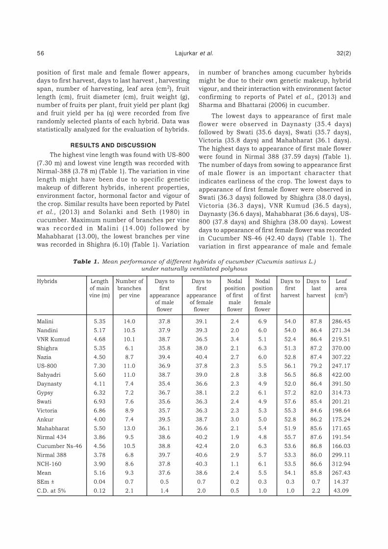
position of first male and female flower appears,

days to first harvest, days to last harvest , harvesting

span, number of harvesting, leaf area (cm2), fruit

length (cm), fruit diameter (cm), fruit weight (g),

number of fruits per plant, fruit yield per plant (kg)

and fruit yield per ha (q) were recorded from five

randomly selected plants of each hybrid. Data was

statistically analyzed for the evaluation of hybrids.


The highest vine length was found with US-800

(7.30 m) and lowest vine length was recorded with

Nirmal-388 (3.78 m) (Table 1). The variation in vine

length might have been due to specific genetic

makeup of different hybrids, inherent properties,

environment factor, hormonal factor and vigour of

the crop. Similar results have been reported by Patel

et al., (2013) and Solanki and Seth (1980) in

cucumber. Maximum number of branches per vine

was recorded in Malini (14.00) fol lowed by

Mahabharat (13.00), the lowest branches per vine

was recorded in Shighra (6.10) (Table 1). Variation

in number of branches among cucumber hybrids

might be due to their own genetic makeup, hybrid

vigour, and their interaction with environment factor

confirming to reports of Patel et al., (2013) and

Sharma and Bhattarai (2006) in cucumber.

The lowest days to appearance of first male

flower were observed in Daynasty (35.4 days)

followed by Swati (35.6 days), Swati (35.7 days),

Victoria (35.8 days) and Mahabharat (36.1 days).

The highest days to appearance of first male flower

were found in Nirmal 388 (37.59 days) (Table 1).

The number of days from sowing to appearance first

of male flower is an important character that

indicates earliness of the crop. The lowest days to

appearance of first female flower were observed in

Swati (36.3 days) followed by Shighra (38.0 days),

Victoria (36.3 days), VNR Kumud (36.5 days),

Daynasty (36.6 days), Mahabharat (36.6 days), US-

800 (37.8 days) and Shighra (38.00 days). Lowest

days to appearance of first female flower was recorded

in Cucumber NS-46 (42.40 days) (Table 1). The

variation in first appearance of male and female

Table 1. Mean performance of different hybrids of cucumber (Cucumis sativus L.)

under naturally ventilated polyhous

Hybrids Length Number of Days to Days to Nodal Nodal Days to Days to Leaf

of main branches first first position position first last area

vine (m) per vine appearance appearance of first of first harvest harvest (cm2)

of male of female male female

flower flower flower flower

Malini 5.35 14.0 37.8 39.1 2.4 6.9 54.0 87.8 286.45

Nandini 5.17 10.5 37.9 39.3 2.0 6.0 54.0 86.4 271.34

VNR Kumud 4.68 10.1 38.7 36.5 3.4 5.1 52.4 86.4 219.51

Shighra 5.35 6.1 35.8 38.0 2.1 6.3 51.3 87.2 370.00

Nazia 4.50 8.7 39.4 40.4 2.7 6.0 52.8 87.4 307.22

US-800 7.30 11.0 36.9 37.8 2.3 5.5 56.1 79.2 247.17

Sahyadri 5.60 11.0 38.7 39.0 2.8 3.8 56.5 86.8 422.00

Daynasty 4.11 7.4 35.4 36.6 2.3 4.9 52.0 86.4 391.50

Gypsy 6.32 7.2 36.7 38.1 2.2 6.1 57.2 82.0 314.73

Swati 6.93 7.6 35.6 36.3 2.4 4.9 57.6 85.4 201.21

Victoria 6.86 8.9 35.7 36.3 2.3 5.3 55.3 84.6 198.64

Ankur 4.00 7.4 39.5 38.7 3.0 5.0 52.8 86.2 175.24

Mahabharat 5.50 13.0 36.1 36.6 2.1 5.4 51.9 85.6 171.65

Nirmal 434 3.86 9.5 38.6 40.2 1.9 4.8 55.7 87.6 191.54

Cucumber Ns-46 4.56 10.5 38.8 42.4 2.0 6.3 53.6 86.8 166.03

Nirmal 388 3.78 6.8 39.7 40.6 2.9 5.7 53.3 86.0 299.11

NCH-160 3.90 8.6 37.8 40.3 1.1 6.1 53.5 86.6 312.94

Mean 5.16 9.3 37.6 38.6 2.4 5.5 54.1 85.8 267.43

SEm ± 0.04 0.7 0.5 0.7 0.2 0.3 0.3 0.7 14.37

C.D. at 5% 0.12 2.1 1.4 2.0 0.5 1.0 1.0 2.2 43.09

56 Lajurkar et al. 32(2)

flower might have been due to internodal length,

number of internodes, genetic makeup and vigour

of the crop. This result is inconformity with Sahni

et al.,(1987) in ridge gourd, Badgujar and More

(2004), Bairagi et al.,(2005) and Patel et al., (2013)

in cucumber.

The lowest nodal position of first male flower

was recorded in NCH-160 (1.1 node) and highest

nodal position of first male flower was noticed in

VNR Kumud (3.4 node) (Table 1). Lowest nodal

position of first female flower was recorded in

Sahyadri (3.8 node) followed by 434 (4.8 node).

Highest nodal position of first female flower was

noticed in Malini (6.9 node) (Table 1). Similar finding

were reported by Sharma and Bhattarai (2006), Patel

et al., (2013) in cucumber.

The lowest days to first harvest was recorded

in the Shighra (51.10 days) followed by Mahabharat

(51.9 days) and Daynasty (52.0 days). Highest days

to first harvest was noticed in Swati (54.12 days)

(Table 1). The highest days to last harvest was

recorded in the Malini (87.8 days) followed by Nirmal

434 (87.6 days), Nazia (87.4 days), Shighra (87.2

days), Cucumber Ns-46 (86.8 days), Sahyadri (86.8

days), NCH-160 (86.6 days), Daynasty (86.4 days),

VNR Kumud (86.4 days), Nandini (86.4 days), Ankur

(86.2 days), Nirmal 388 (86 days), Mahabharat

(33.70 days). Lowest days to last harvest was

recorded in US-800 (79.2 days) (Table 1). The

variation in days to first and last harvest might be

due to genetic factor, hormonal factor and vigour of

crop. Similar result have also been reported by

Sharma and Bhattarai (2006) in cucumber.The

highest harvest span was recorded in the Shighra

(35.9 days) followed by Nazia (34.6 days), Daynasty

(34.4 days), VNR Kumud (34.0 days), Malini (33.8

days) and Mahabharat (33.7 days). Lowest days for

harvesting span was noticed in US-800 (23.1 days)

(Table 1). The highest number of harvesting was

recorded in Daynasty (14.4) followed by Shighra

(13.8). Lowest number of harvesting was noticed in

Cucumber NS-46 (3.9). The variation in harvesting

span and number of harvesting in different

cucumber hybrid have might be due to appearance

of first female flower, genetic and varietal factor.

Comparable result have been reported by Sharma

and Bhattarai (2006) in cucumber.

The highest leaf area was recorded in the F1

hybrid Sahyadri (422.00 cm2) followed by Daynasty

(391.50 cm2) and the lowest leaf area was noticed

Table 2. Mean performance of different hybrids of cucumber (Cucumis sativus L.)

under naturally ventilated polyhouse.

Hybrids Length of Diameter of Fruit Number of fruits Fruit yield Yield per ha

fruit (cm) fruit (cm) weight (g) per vine per vine (kg) (qt)

Malini 18.81 4.36 241.18 23.7 4.92 716.46

Nandini 16.96 4.05 200.08 19.7 3.92 571.00

VNR Kumud 15.99 3.80 172.79 20.1 3.47 505.27

Shighra 18.36 3.73 171.25 19.4 3.32 483.67

Nazia 16.05 3.96 205.22 18.4 3.77 549.45

US-800 17.57 3.91 197.71 10.0 1.98 287.95

Sahyadri 17.93 3.94 195.27 13.6 2.63 382.88

Daynasty 18.94 3.88 189.63 21.2 3.97 578.05

Gypsy 18.82 3.92 197.78 13.8 3.26 474.76

Swati 14.59 3.43 136.29 7.5 1.06 153.97

Victoria 15.72 3.86 183.43 12.8 2.34 341.43

Ankur 12.82 4.03 167.84 18.2 3.12 454.95

Mahabharat 19.10 3.96 218.19 11.8 2.60 378.92

Nirmal 434 14.70 4.12 189.42 12.1 2.24 326.94

Cucumber Ns-46 18.34 3.65 163.38 6.7 1.10 160.40

Nirmal 388 17.23 3.89 179.83 16.1 2.89 420.77

NCH-160 14.25 4.05 161.76 16.0 2.60 378.96

Mean 16.83 3.91 186.53 15.4 2.89 421.52

SEm ± 0.20 0.06 8.02 0.3 0.23 33.12

C.D. at 5% 0.60 0.17 24.03 0.8 0.68 99.29

32(2) F1 hybrids of cucumber in polyhouse 57

in Cucumber NS-46 (166.03 cm2) (Table 1). These

findings were supported by Patel et al., (2013) and

Sharma et al., (2010). Data presented in Table 2

revealed that the highest length of fruit was recorded

in the Mahabharat (19.10 cm) followed by Daynasty

(18.94 cm), Gypsy (18.82 cm) and Malini (18.81 cm).

The lowest length of fruit was noticed in Ankur

(12.82 cm). Fruit yield is also depend on fruit length,

increasing fruit length will increase the fruit yield.

The variation in fruit length might be due to genetic

nature and vigor of crop. Similar results have also

been reported by Patel et al., (2013) and Sharma

et al., (2010) in cucumber. The highest diameter of

fruit was recorded in the Malini (4.36 cm) and lowest

diameter of fruit was noticed in Ankur (3.43 cm)

(Table 2). Increase in fruit yield is mostly influenced

by fruit diameter. When fruit diameter was high then

automatically fruit yield was also high. The variation

in fruit diameter might have been due to genetic

factor and vigour of the crop. Similar results have

also been reported by Patel et al., (2013) and Sharma

et al., (2010) in cucumber.

The highest fruit weight was recorded in Malini

(241.18 g) and the lowest fruit weight was noticed

in Swati (136.29 g) (Table 2). The highest fruit weight

in Malini may be due to its hybrid vigour, similar

result have been reported by Patel et al., (2013) and

Sharma et al., (2010) in cucumber.

The highest number of fruit per vine was

recorded in Malini (23.70) and the lowest number

of fruit per vine was noticed in Cucumber NS-46

(6.70) (Table 2). The variation in fruit per vine might

have been due to sex ratio, fruit set percentage,

genetic nature of hybrids. Similar result have been

reported by Patel et al., (2013) and Sharma et al.,

(2010) in cucumber.The highest fruit yield per vine

was recorded in Malini (4.92 kg) and the lowest fruit

yield per vine was noticed in Swati (1.06 kg) (Table 2).

The significant variation in yield per vine might have

been due to fruit set percentage, fruit length,

number of fruit per vine, fruit weight, fruit width,

genetic nature and vigour of crop. These findings

were supported by Patel et al., (2013), Sharma

et al., (2010) and Sharma and Bhattarai (2006) in

cucumber.

The highest yield per ha was recorded in Malini

(716.46 qt) and the lowest yield per ha was noticed

in Swati (153.97 qt) (Table 2). The significant

variation in yield per ha might have been due to

number of vines per ha, number of fruit per vines,

yield per vines and yield per plot. This investigation

was also supported by Patel et al., (2013) and

Sharma and Bhattarai (2006) in cucumber.

CONCLUSION

From the present findings, it could be concluded

that the cucumber hybrid Malini had shown better

performance with regards to the highest fruit weight

(241.18 g), number of fruit per vine (23.70) as well as

the highest marketable fruit yield per vine (4.92 kg)

and yield per ha (716.46 qt) in naturally ventilated

polyhouse under Konkan agroclimatic condition.

REFRENCES

Badgujar, C. D. and More, T. A. (2004). Off season

performance of selected tropical gynoecious

cucumber hybrids grown under different

regimes. South Indian Horticulture 52: 97-103.

Bairagi, S. K., Ram, H. H., Singh, D. K. and Maurya,

S. K. (2005). Exploitation of hybrid vigour for

yield and attributing traits in cucumber. Indian

Journal Horticulture 62: 41-45.

Patel, J. K., Bahadur, V., Singh, D., Prasad, V. M.

and Rangare, S. B. (2013). Performance of

cucumber (Cucumis sativus L.) hybrids in agro-

climatic conditions of Allahabad. Horticulture

Flora Research Spectrum 2(1): 50-55.

Sahni, G. P., Singh, R. K. and Saha, B. C. (1987).

Genotypic and phenotypic variability in ridge

gourd (Luffaacutangula Roxb.). Indian Journal

of Agriculture Science 57: 666-688.

Sharma, A., Kaushik, R. A., Sarolia, D. K. and

Sharma, R. P. (2010). Response of cultivars,

plant geometry and methods of fertilizer

application on parthenocarpic cucumber

(Cucumis sativus L.) under zero energy

polyhouse condition during rainy season.

Vegetable Science 37(2): 184-186.

Sharma, M. D. and Bhattarai, S. P. (2006).

Performance of cucumber cultivars at low hill

during summer-rainy seasons. Journal Institute

Agriculture Animal Science 27: l69-171.

Solanki, S. S. and Seth, J. N. (1980). Correlation

studies in cucumber (Cucumis sativus L.)

Vegetable Science 1: 94-101.

58 Lajurkar et al. 32(2)


Standardization of Callus derived in vitro Screening

Technique for Salt Tolerance in Rice (Oryza sativa L.)

S. R. KAMBLE, S. V. SAWARDEKAR*, N. B. GOKHALE, S. S. SAWANT and A. H. BANKAR

Plant Biotechnology Centre, College of Agriculture

Dr. B. S. Kokan Krishi Vidyapeeth, Dapoli, 415 712, Maharashtra


In-vitro studies on salt tolerance were carried out with callus of three indica varieties, Karjat-5(salt susceptible), Panvel-3 and FL-478 (salt tolerant). The study was conducted to obtain highersalt tolerant genotypes with variable characters of local rice varieties through somaclonalvariat ions. Various concentrat ion and combinations of plant growth regulators weresupplemented with MS medium to develop friable callus and plantlet regeneration ability ofmature embryo of rice. The calli were transferred to the proliferation medium of differentconcentration of NaCl to check the inherent capacity of calli to proliferate on medium undersalt stress condition. Maximum percentage of callus induction observed in MS mediumsupplemented with 2.5 mg L-1 2,4-D along with 0.5 mg L -1 BAP and 0.1 mg L-1 NAA in all threevarieties. Calli derived from the different concentration of 2, 4-D and other plant growthregulators were transferred on MS medium supplemented with various concentrations of BAP,Kinetin, NAA and IAA for plantlet regeneration. The weight of callus was decreased with increasedin salt concentration. The variety FL-478 showed proliferation of the callus upto 10 dS m-1

salinity followed by Panvel-3 (upto 8 dS m-1 salinity) whereas the callus of Karjat-5 was survivedonly up to 4 dS m-1 salinity. It indicates that variety FL-478 and Panvel-3 are potential varietyfor development of novel somaclones for salinity tolerance as compared to Karjat-5. It wasalso observed that MS medium supplemented with 4 mg L-1 BAP and 1 mg L-1 IAA producedhighest of plantlets for variety FL-478 (77.50) followed by Karjat-5 (69.17) and Panvel-3 (53.33).

(Key words: Callus, In vitro Screening, Salt tolerance, Rice)

Salinity is widespread soil problem in rice

growing countries. Rice production has mostly been

observed to be affected by soil salinity. In India,

saline soil covers nearly 4 million ha of land under

rice production (Paul and Ghosh, 1986). In

Maharashtra the total area occupied by this crop

was about 14.87 lakh hectares with annual

production of 26.01 lakh tones and productivity was

about 1.74 t ha-1 (Anonymous, 2012). Rice is rated

as an especially salt-sensitive crop (Shannon et al.,

1998). Apart from a delayed germination, salinity

was found to reduce the germination percentage

(Akbar and Yabuno, 1974). Early seedling stage of

rice was found to be highly sensitive to salinity

(Kaddah and Fakhrys, 1961).

An improvement of salt tolerance in rice is well

documented (Flower and Yeo, 1995). Tissue culture

approach might have proven effective in gaining

phenotypic variation in regenerated plants. An

implication of somaclonal variation in breeding is

that, novel variation can arise and these can be of

agronomic use. The plants generated from callus

cultures show heritable variation in both qualitative

and quantitative traits. It also act as a continuous

reservoir of genetic variability in crop production,

thereby making selection in the population easier

for further improvement. Keeping this in view

present investigation was carried out to obtain

somaclonal variants of rice for higher salt tolerance

and desirable character.


MS medium supplemented with 2, 4-D, NAA,

BAP, Kinetin and IBA in different combinations and

concentrations were included in the study. For

preparation of explants the excised seed were

washed in Ethyl alcohol (70 %) followed by washing

with double distilled water for 3-4 times. The

explants were dipped in HgCl2 solution of different

concentrations (0.1%, 0.5% and 1.0%) for varied

time period and then washed with double distilled

water for several times. Then seeds were soaked for

12-14 hours in distilled water. Treated seeds were

inoculated on callus induction media. Observations

were recorded on callus induction response (%),

days to initiation of callus, weight of callus after 4

weeks. After that six-week-old callus was divided

into pieces of 100 mg. These pieces were transferred

to the same medium those were used for callus

induction, supplemented with different NaCl


concentrations for salt stress responses. To prepare

media of different salt concentration of salt was

added per lit by using following formula.

1000 EC units = 1000 ìS cm–1 = 1.0 mS cm–1 = 1.0 dS

m-1 = 640 Mg L-1 TDS = 640 ppm TDS. i.e. 640 Mg L-

1 (Salinity measuring units, NSW Environment and

Heritage ) to prepare media of 1 dS m-1 and subsequent

salty media were prepared. At the end of the four-

week period, the callus was taken for growth analysis.

Observations were recorded weight of callus increased,

regeneration response (%), days to shooting, number

of shoots per explant and days to rooting.

Hardening and establishment of rooted plants

Plantlets with healthy root systems were

washed (especially the root portions) by double

distilled water to clear off the entire residual agar

medium so as to check the chances of fungal

contamination in soil. The root portions were then

dipped for about 5-10 minutes in an antifungal

solution 0.1% (w/v) Bavistin. The plantlets were then

transplanted in small (5 cm diameter) plastic tea cups

containing pre-soaked sterilized vermiculite medium

and kept in growth chamber. For the initial 10-15 days

high humidity was main tented and was gradually

reduced to the ambient level over a period of 2 weeks.

The potting mixture containing soil, sand, and

vermiculite (1:1:1) was used for transplantation of the

plants. Factorial Completely Randomized Design

(FCRD) was employed for the present study. The pooled

data was analyzed in SASs (Statistical Analysis System

software V. 9.1). The observations of callus response

and shoot response expressed in terms of percentage

were transformed into arcsine value.


Effect of media combination on callus induction

MS medium supplemented with different

concentration of 2, 4-dhormone were employed for

callus induction. Callus induction was stated at

12th to 24th days after transferring the caryopsis

to culture tube and there incubation (Table 1). The

final data on callus induction was recorded after

four weeks of inoculation.

Table 1. Callus induction frequency (%) and days to callus induction

Sr. Treatment details Karjat-5 Panvel-3 Fl-478 Days to callus induction Nature of

No. (%) (%) (%) Karjat-5 Panvel-3 FL-478 callus

T1

M.S. medium (control) 0.00 0.00 0.00 0.000 0.000 0.000 No callus

(0.00) (0.00) (0.00)

T2

M.S.+ 1.5 mg/l 2,4-D + 9.17 7.50 7.50 14.00 20.33 22.50 Yellowish-white,

0.5 mg/l KIN (17.5) (15.75) (15.75) compact

T3

M.S.+ 2.0mg/l 2,4-D + 14.17 15.00 14.17 15.25 20.08 17.33 Copious,

0.5 mg/l KIN (22.09) (22.79) (22.09) compact

T4 M.S. + 2.5 mg/l 2.4-D + 16.67 1500 17.50 20.75 15.50 16.41 Soft, friable

0.5 mg/l KIN (24.08) (22.74) (24.73)

T5 M.S. + 1.5 mg/l 2.4-D + 23.33 25.83 25.83 14.00 13.66 24.33 Soft, friable

0.5 mg/l BAP (28.88) (30.54) (30.54)

T6 M.S.+ 2.0mg/l 2,4-D + 32.50 26.67 30.83 15.25 20.41 19.75 White, Soft,

0.5 mg/l BAP (34.75) (31.07) (33.73) friable

T7 M.S. + 1.0 mg/l 2.4-D + 41.67 37.50 39.17 15.33 15.50 22.25 Yellowish-white,

0.5 mg/l BAP +0.1 mg/l NAA (40.20) (37.75) (38.74) compact

T8

M.S. + 1.5 mg/l 2.4-D + 68.33 64.17 63.33 15.08 12.41 19.83 Copious,


T9

M.S. + 2.0 mg/l 2.4-D + 72.50 76.67 76.67 22.50 13.83 17.16 Yellowish-white,


T10

M.S. + 2.5 mg/l 2.4-D + 83.33 85.00 81.67 23.25 12.91 20.91 Soft, friable

0.5 mg/l BAP +0.1 mg/l NAA (65.92) (67.26) (64.66)

T11

M.S. + 2.0 mg/l 2.4-D + 94.17 93.33 90.83 19.91 15.25 17.25 Yellowish-white,

0.5 mg/l KIN +0.1 mg/l NAA (76.09) (75.10) (73.43) compact

SEm ± 0.71 1.37 1.65 0.642 1.077 3.037

CD at 1% 2.81 5.46 6.56 0.308 0.516 1.455

C.V. 3.17 6.24 7.51 2.365 4.348 9.913

(*Figures in parenthesis are arcsine values)

60 Kamble et al. 32(2)

It was noticed that MS medium supplemented

with 2.0 mg L-1 2,4-D along with 0.5 mg L-1 kinetin

and 0.1 mg L -1 NAA (T11) produced higher

percentage of callus, 94.17% in karjat-5 followed

by 93.33% in Panvel-3 and 90.83% in FL-478. On

the other hand T2 treatment produced the lowest

percentage of callus, 9.17 %, 7.50% and 7.50% in

Karjat-5, Panvel-3 and FL-478, respectively.

Nature of callus

A reasonable callus formed after about four

weeks of culture. Callus formed on different media

combinations observed dif ferent in nature.

Embryogenic calli were found to be yellow to white,

dry, compact and nodular. On the other hand, non-

embryogenic calli appeared to be watery, light yellow

to tan and non-nodular. Further a soft, friable and

non-organogenic callus formation occurred in rice

cuticular rice embryo when the medium contained

M.S. + 1.5 mg L-1 2.4-D and 0.5 mg L-1 BAP. Soft

and friable callus was recorded on media

supplemented with 2.5 mg L-1 2.4-D + 0.5 mg L-1

KIN and 2.5 mg L-1 2.4-D + 0.5 mg L-1 BAP + 0.1

mg L-1 NAA. (Table 1).

Effect of salinity on callus proliferation

In Panvel-3 weight of callus was increased by

121 mg on media treatment T1, which was

significantly superior over all other treatments.

Callus growth was rapidly reduced with relative

increase of NaCl concentration in callus proliferation

media. These results are in accordance with

Senadhra (1987). Weight of callus decreased up to

78 mg on media having salt concentration of 4 dS

m-1. Callus was not proliferated on T4 i.e. salt

concentration of 10 dS m-1. Blackening and drying

Table 2. Weight of callus per 100 mg in MS media supplemented with various concentration of NaCl

Sr.No Treatment Karjat-5 (mg) Panvel-3 (mg) FL-478 (mg)

1 MS+ 2.0mg/l 2,4-D+0.5mg/l KIN 152 121 153

2 MS+ 2.0mg/l 2,4-D+0.5mg/l KIN+4 dS/m NaCl 99 78 89

3 MS+ 2.0mg/l 2,4-D+0.5mg/l KIN+6 dS/m NaCl 0.000 51 65

4 MS+ 2.0mg/l 2,4-D+0.5mg/l KIN+8 dS/m NaCl 0.000 89 64

5 MS+ 2.0mg/l 2,4-D+0.5mg/l KIN+10 dS/m NaCl 0.000 0.000 46

6 MS+ 0.5mg/l 2,4-D+0.5mg/l KIN+ 12 dS/m NaCl 0.000 0.000 0.000

SEm ± 0.005 0.078 0.005

CD at 1% 0.002 0.036 0.002

C.V. 7.080 7.697 4.014

Table 3. Frequency of callus regeneration and days required

for shoot induction in various media combination

Sr. Treatment details Callus regeneration frequency Days to shoot induction

No. Karjat-5 Panvel-3 FL-478 Karjat-5 Panvel-3 FL-478

(%) (%) (%) (%) (%) (%)

T1 MS medium(control) 0.00(0.00) 0.00(0.00) 0.00(0.00) – – –

T2 MS+0.5 mg/l BAP+0.2 mg/l IAA 0.00(0.00) 0.00(0.00) 0.00(0.00) – – –




T6 MS+1.5 mg/l BAP+1.0 mg/l IAA 61.67(51.81) 60.83(51.46) 64.17(53.23) 29.25 29.33 29.08






SEm ± 1.75 1.71 1.60 0.659 0.420 0.659

CD at 1% 6.99 6.83 6.38 0.316 0.201 0.316

C.V. 6.85 6.40 5.80 3.242 1.884 3.106

32(2) in vitro screening technique in rice 61

of callus was observed on this combination. Decrease

in weight was observed in variety FL- 478 as the

concentration of NaCl was increased. The 100 mg of

callus proliferated and increased its weight when it

put on media combination of T1 which was free from

NaCl. It was also observed that the callus of FL-478

was survived up to the 10 dS m-1 of NaCl

concentration. This showed that NaCl had an

inhibitory effect on the growth of callus with increasing

NaCl concentration inducing the inability of plant cell

and tissue to adjust with incremental increase of salt

over sufficient time period might be due to osmotic or

ionic shock (Shanti et al., (2010). Among all these three

varieties, the callus of FL-478 survived at higher salt

concentration (10 dS m-1) followed by Panvel-3 (8 dS

m-1) and Karjat-5 (4 dS m-1) (Table 2).

Frequency of callus regeneration in various mediacombination

Callus of all three varieties not regenerated on

media combination treatment T1 to T

6. Maximum

regeneration frequency recorded on MS media

supplemented with 3.5 mg L-1 BAP +1.0 mg L-1 IAA

(T10

) in Panvel-3 (80.00%) followed by FL-478

(70.83%) and Karjat-5 (65.83%) irrespective of media

combination. (Table 3). Variety Karjat-5 and FL-478

recorded early shoot initiation (13.08 days and 13.75

Table 4. Root induction frequency and days required for root induction

Sr. No. Treatment Regeneration frequency Days to induction

Karjat-5 Panvel-3 FL-478 Karjat-5 Panvel-3 FL-478

1 MS medium (control) 0.00(0.00) 0.00(0.00) 0.00(0.00) 0.000 0.000 0.000

2 MS+ 0.5 mg/l NAA 0.00(0.00) 0.00(0.00) 0.00(0.00) 0.000 0.000 0.000

3 MS+ 1.0 mg/l NAA 0.00(0.00) 0.00(0.00) 0.00(0.00) 0.000 0.000 0.000

4 MS+ 1.5 mg/l NAA 0.00(0.00) 0.00(0.00) 0.00(0.00) 0.000 0.000 0.000

5 MS+ 2.0 mg/l NAA 15.00 15.00 18.33 15.33 15.25 17.91

(22.74) (22.74) (25.34)

6 MS+ 3.0 mg/l 15.00 15.83 13.33 12.583 12.66 15.33

(22.66) (23.35) (21.40)

7 MS +1.0 mg/l NAA + 15.00 15.83 12.50 14.00 15.66 14.16

2.0mg/l BAP (22.79) (23.39) (20.64)

8 1/2 MS+ 0.2 mg/l IBA+ 15.83 16.67 57.50 5.08 15.75 5.83

0.1mg/l BAP (23.43) (24.08) (49.31)

9 1/2 MS+ 0.2 mg/l IBA+ 49.17 47.63 45.00 4.33 5.08 4.50

0.2mg/l BAP (44.52) (45.48) (42.13)

10 1/2 MS+ 0.5 mg/l IBA+ 50.83 49.83 45.83 4.16 5.00 4.66

0.1mg/l BAP (45.48) (45.48) (42.61)

11 1/2 MS+ 0.5 mg/l IBA+ 51.67 50.83 49.17 4.917 5.16 4.91

0.2mg/l BAP (45.96) (45.48) (44.52)

SEm ± 0.94 0.88 0.57 0.603 1.261 1.120

CD at 1% 3.74 3.52 2.27 0.289 0.604 0.537

C.V. 7.87 7.31 4.42 6.437 10.911 10.735

days, respectively.) whereas Panvel-3 showed late

shoot initiation (16.08 days). In Karjat-5, minimum

number of days to shoot initiation was recorded in

treatment T10

(13.08) which were significantly superior

over all other treatments. The maximum shoot

induction was recorded in treatment containing

highest concentration of BAP (T10

containing 3.5 Mg

L-1 BAP) for the varieties Karjat-5 and FL-478 i.e., 7.17

and 7.27, respectively. While higher shoot

multiplication in Panvel-3 recorded on MS

supplemented with 3.0 mg L-1 BAP +1.0 mg L-1 IAA.

Effect of media on root induction

It was observed that, the maximum days to

rooting ranged between 04 to 18 days. Among all

three varieties Karjat-5 and FL-478 showed early

root induction as compared to Panvel-3. In Karjat-

5, minimum number of days to root initiation were

recorded in treatment T10

(4.16).In Panvel-3, half

MS supplemented with 0.5 mg L-1 IBA+ 0.1 mg L-1

BAP showed minimum number of days to root

initiation (5.0). In FL-478, minimum number of days

to root initiation were recorded in treatment T9 (4.5).

The per cent of root induction was observed from

0.00 to 51.67. In all three varieties, no root induction

observed on treatment T1 i.e. control and T

2 to T

4.

The root induction frequency observed maximum

in Karjat-5 on media combination T11

(51.67%)


In Panvel-3, the root induction frequency

observed maximum on media combination T11

(50.83%).The root induction frequency was observed

maximum in FL-478 on media combination T8

(57.50%), followed by T11

(49.17%) (Table 4).

Hardening and establishment

Rooted plants were transferred to the potting

mixture of soil, sand and vermiculite (1:1:1).The

average lower percentage of survival was recorded

23.33 while average maximum survival recorded

74.17. The study concluded that for callus induction

M.S. + 2.0 mg L-1 2.4-D + 0.5 mg L-1 KIN +0.1 mg L-

1 NAA proved to be the best media combination for

callus induction. Better callus proliferation up to

level of 10 dS m-1 was observed in FL-478, followed

by Panvel-3 which showed better callus proliferation

up to 8 dS m-1. Karjat-5 callus was not survived on

6 dS m-1. MS+ 3 mg L-1 BAP proved to be the best

media combination for shoot induction.

REFERENCES

Akbar, M. and Yabuno, T. (1974). Breeding for

saline-resistant varieties of rice II comparative

performance of some rice varieties to salinity

during early developmental stages. Japanees L

Breeding 24:174-176.

Anonymous (2012) www.agritech.tanu.ac.in

Bano, S., Jabeen, M., Rahim, F. and Ilahi, I. (2005).

Callus induction and regeneration in seed

explants of rice (Oryza sativa Cv. Swat-ii). pak.

Journal of Botany 37(3): 829-836.

Flowers , T. J. and Yeo, A. R. (1995). Breeding for

salinity resistance in crop plants. Australian

.Journal of Plant Physiology 22: 875-884.

Kaddah, M. T. and Fakhrys, S. J (1961). Tolerance

of Egyptian rice to salt, I. Salinity effects when

applied continuously and intermittently at

different stages of growth after transplanting.

Soil Science 91: 113-120.

NSW Environment and heritage http://

www.environment. nsw.gov.au/salinity/basics/

units.html

Paul, N. K. and Ghosh, P. D. (1986). In Vitro selection

of NaCl tolerant cell cultures in rice. (Oryza

saliva L). Current Science 55: 568-569.

Shannon, M. C., Rhoades, J. D., Draper J. H.,

Scardaci, S. C. and Spyres, M. D. (1998).

Assessment of salt tolerance in rice cultivars

in response to salinity problems in California.

Crop Science 38(2): 394-39.

Senadhira, D. (1987). Salinity as a concept to

increasing rice production in Asia. In: Proc.

Regional Workshop in Maintaince of Life

Support Species in Asia Pacific Region, 4-7

April, 1987. NBPGR, New Delhi, India.

Shanthi, P., Jebaraj, S. and Geetha, S. (2010). In

vitro screening for salt tolerance in Rice (Oryza

sativa L). Electronic Journal of Plant Breeding

1(4): 1208-1212.

Yeo. A. R., Yeo, M. E., Flowers, S. A and Flowers, T.

J. (1990). Screening of rice genotypes for

physiological characters contributing to salinity

resistance and their relationship to overall

performance (Oryza sativa L.). Theory of

Approval Genetic 79: 377- 384.

32(2) in vitro screening technique in rice 63


Exploration of Artificial Groundwater

Recharge in Coastal West Bengal

K.K. MAHANTA1,*, S.K. KAMRA2, D. BURMAN1 and S. KUMAR2

1Central Soil Salinity Research Institute

RRS, Canning Town, South 24 Parganas, West Bengal 743329

2Central Soil Salinity Research Institute

Karnal, Haryana 132001

Fresh water scarcity is the main problem for growing crops in the coastal West Bengal beyondthe rainy season. To alleviate the water scarcity during the non-monsoon period, augmentationof capacity of ground water through artificial recharge during the rainy season was experimentedat ICAR-CSSRI, RRS, Canning Town farm. A recharge tube well of 12.7 cm diameter and 40.5 mdepth was installed in the year 2011. As the water table came up very close to the surface (< 1m bgl) during the rainy season, an experiment was carried out for lowering the water table bypumping during summer and artificial recharge of runoff water during the rainy season. Forpumping out the ground water, 1 HP electrical pump with discharge of 0.64 lps was used. Inspite of 30 days (6 hours per day) of pumping in the summer season, the pumping water levelwas not lowered below 6 m depth. There was depletion of the water table due to pumping till27th week from January, 2012. Later the water table moved up due to recharge in the monsoonperiod. The rising of water table near to the surface was similar to previous year when tubewell was installed during July/August, 2011 and there was no artificial recharge. Therefore, thepresent situations are not conducive for artificial recharge in the Canning area. However, if atany location the water table in post monsoon season depletes regularly beyond 3m bgl, thereartificial recharge may be done.

(Key words: Artificial recharge, Ground water, Aquifer, Coastal, Water table)

Despite of high rainfall (average annual rainfall:

1768 mm) in coastal West Bengal, fresh water

scarcity is felt in the non-monsoon period. More

than 80 % of the annual rainfall occurs only in the

few months of monsoon (June-Sept.). The lands are

flat or having little slope, remain inundated during

the rainy season and mostly mono-cropped with

paddy. The water sources in this area as tidal rivers

and rivulets are not utilizable because of the high

salinity. These sources of water also influence the

soil and water salinity in the inlands by intrusion

as surface/ground water. The ground water

available at shallow depths is also saline and not

usable for agriculture. The water quality of deeper

aquifers may be fresh or saline depending upon the

location specific geo-hydrological conditions.

The farmers of the Sundarbans region have

been exploiting the ground water since a few years

back through shallow tube wells for cropping in

post-kharif and summer period. According to the

farmers, the capacities of the tube wells are

decreasing time to time and the quality of ground

water is deteriorating. Overexploitation of

groundwater (Custodio, 2002) through shallow tube

wells may lead to decline in water quality as well as

water table, consequently resulting in failure of the

shallow tube wells. Under such circumstances,

besides augmenting groundwater resources,

recharge can help improvement of groundwater

quality (Kamra, 2010). Gupta and Paudwal (1988)

developed a technique to estimate recharge from

rainfall and to estimate aquifer parameters using

ground water level records and available

climatological data. The methodology combines a

hydro-meteorological model which links rainfall and

evaporation to the effective ground water recharge

and a geo-hydrological model which links the

recharge to the water level in the aquifer. Well

injection technique can be adopted to reduce decline

in water table and to improve the ground water

quality (Kumar et al., 2010). Akther et al. (2009)

observed that compared to the exploitation of

groundwater, the recharge to aquifer in Dhaka was

very negligible.

As per the findings of Central Ground Water

Board (2000) in the state of West Bengal, the

formation in coastal areas: North 24 Parganas,

South 24 Parganas, Medinipur, Haora are

unconsolidated recent alluvium. Fresh ground water

bearing aquifers occur in varying depth ranges


within 180-360 mbgl (within the depth of 600 mbgl).

The fresh water aquifers are sandwiched between

saline/brackish aquifers. The top saline/brackish

aquifer lies within the depth span of 20~180 m with

maximum depth of 320 mbgl in the extreme south.

Suitably constructed tubewell tapping 35 m

cumulative thickness can yield 100~150 m3/hr.

Shallow fresh water aquifers occur in present day

dunes in Digha-Ramnagar area of Medinipur (East)

dist. down to the depth of 9 mbgl & in levee deposit

within 50 mbgl in Baruipur-Sonarpur-Bhangar-

Canning tract in South 24 Parganas.

Artificial groundwater recharge began early in

last century in the Europe. First infiltration basis

for recharging the groundwater was constructed at

Goteborg, Sweden in 1897 and subsequently several

basins were developed. Infiltration rates ranging

from 2.1 to 15.6 m/day was reported for these

basins (Jansa, 1952). In Spain, groundwater

recharge was started in 1953 in Besos are with a

special well, surrounded by a crown of 16 small

diameter tube-wells, in order to accomplish an

intense back washing of coarse and gravel confined

aquifer was done by treated river water in excess of

city distribution using tubewells since 1969. During

the period of shortage of water, the injected water

was abstracted by other wells (Custodio et al., 1979).

Johansson (1987) applied two methods for

estimation of ground water recharge both based on

groundwater level fluctuations. These methods were

applied in a marine area in South Eastern Sweden.

The first method utilized a one dimensional model

which was tested against observed ground water

level. The boundary conditions were defined by

using meteorological data and sub-models for

precipitation, snow dynamics interception,

evapotranspiration and horizontal ground water

outflow. The second method directly transformed

groundwater level fluctuations to equivalent amount

of water from a constructed recession curve and

the specific yield concept. Recharge to underground

formations is possible depending upon natural geo-

hydrological conditions. Sophocealous and Perry

(1985) stated that antecedent moisture condition,

thickness and nature of the unsaturated zone were

found as major factors affecting recharge.

There is little information available about the

water table situations and need of artificial recharge

in the coastal region. Hence, artificial recharge in

the rainy season was experimented at the institute

farm.


An artificial recharge tube well was designed

and installed at the ICAR- Central Soil Salinity

Research Institute, Canning Town farm. The location

was previously the bed of tidal river Matla a few

decades back. The highly saline sea water swells in

this river during the high tide. The present river

course is almost 1 km away shifted by sedimentation

and other anthropogenic activities. The drilling was

carried out manually near a drain where runoff

water is collected during the rainy season by reverse

circular rotary drilling method up to depth of 45 m.

The drilling was made first by 12.7 cm diameter

and later 20.32 cm diameter. The soil and water

samples were collected at every 3m interval. The

recharge tube well installed was of 12.7 cm diameter

and 40.5 m depth with the strainer placed at

28.5~36 m depth during the year 2011. The water

table was monitored throughout the year. As the

water table came very close to the surface (<1 m)

during the rainy season, pumping during the

summer for lowering the water table and recharging

the aquifer with runoff water during the rainy season

was experimented.


While drilling manually by reverse circular

rotary drilling method, the soil and water samples

were collected at every 3 m depth. The soil texture

analyzed for different depth intervals and are

presented in Table 1. Sandy soil was found at depth

Table 1. Litholog of the drilling site

at CSSRI, RRS, Canning farm

Depth (m) Soil type

0~3 Silty clay

3~6 Silty clay

6~9 Sticky clay

9~12 Fine sand

12~15 Fine sand

15~18 Fine sand

18~21 Fine sand

21~24 Fine sand

24~27 Fine to medium sand

27~30 Fine to medium sand

30~33 Fine+Medium+Coarse sand

33~36 Fine+Medium+Coarse sand

36~39 Clay+Fine sand



32(1) Artificial groundwater recharge 65

12 m onwards till 36 m. As the aquifer was better

in the 24 m~36 m range, the strainer was placed at

28.5~36 m bgl.

The water quality parameters (EC and pH) of

samples collected depth-wise are presented in

Table 2. The data in Table 2 represents the mixed

water of ingoing surface fresh water and existing

ground water. The mixing was taken place while

drilling manually.

The water table is the primary indicator of

ground water status. So, the water table was

monitored periodically and observed that it is

coming very near to the surface (< 1 m) during the

monsoon period. Apprehending that the aquifer may

not receive much in this high water table condition,

it was perceived to pump out the saline water during

summer as much as possible, and recharge the fresh

water in the rainy season when plenty of runoff is

available through the heavy rainfall. A 1 HP

motorized electrical pump with discharge of 0.64

lps was used for pumping out ground water from

the aquifer during summer. The pumping was

carried out (Fig. 1) for 30 days (6 hours per day)

and the water table was recorded by the water level

indicator. It was observed that the pumping water

level was not lowered below 6 m depth during the

summer season.

Artificial Recharge of Ground water

The monsoon rainfall was insufficient at the

beginning to produce effective rainfall. The rainfall

data collected is presented in Fig. 2 in weekly basis

starting from the month of June, 2012. The effective

rainfalls which produced runoff in different times

of the monsoon period are presented in Fig. 2.

The runoff water collected in the nearby water

channel was diverted to the recharge structure

Table 2. Depth-wise water quality while drilling

for installation of recharge tubewell

Depth (m) EC(dS/m) pH

0~3 4.5 6.8

3~6 9.8 7.1

6~9 6.0 7.2

9~12 5.4 7.0

12~15 3.6 7.3

15~18 4.1 6.8

18~21 3.1 6.8

21~24 3.1 7.1

24~27 3.3 6.7

27~30 3.3 6.9

30~33 3.7 7.2

33~36 3.6 7.3

36~39 5.4 7.0

39~42 4.0 6.9

42~45 4.8 7.0

Table 3. The recharge amounts in different weeks

Week Total head Av. Head H5/2 Rate of Recharge Amount of

(cm) (cm) (lps) Recharge (l)

July 5-11 16.9 2.414 9.056 0.125 75589.68

July 19-25 19.4 2.771 12.786 0.176 106721.1

July 28-Aug.3 20.6 2.942 14.856 0.205 123997.8

Aug.5-11 18.9 2.700 11.978 0.165 99977.04

Aug.13-19 23.6 3.371 20.870 0.288 174191

Aug.20-27 24.6 3.514 23.152 0.319 193234

Aug.29-Sept.3 23.8 3.400 21.315 0.294 177905

Sept.6-12 17.9 2.557 10.456 0.144 87272.69

Oct. 10-16 16.4 2.343 8.401 0.116 70122.18

Total 1109010

Fig. 1. The withdrawal of ground water during

the summer season

66 Mahanta et al. 32(1)

Fig. 2. The weekly rainfall in different weeks

during monsoon (June, 2012 onwards)

Fig. 3. The hydraulic head of the recharged water

in the 90o V-notch during the effective rainfall

through a 900 V-notch for quantifying the recharge

amount. Four readings of the hydraulic head were

taken in the V-notch daily and the average was noted

(Fig. 3). As seen in figure the highest hydraulic head

was observed during August, 2012 (Fig. 3).

The corresponding discharge can be computed

by the equation: Q=0.0138 H5/2 where Q= discharge

(lps), H= head (cm). The recharge amount in different

weeks of effective rainfall are presented in Table 3.

Due to recharge, the water table was observed

closest to the ground surface during the months

Fig. 4. The water table in the recharge tubewell in different

weeks (Starting from January, 2012)

September/October, 2012 at about 0.75 m below

ground level (Fig. 4). In figure 4, it is seen that there

is depletion of the water table due to pumping till the

27 weeks. Later there is rise of the water table due to

recharge of the runoff water in the monsoon period.

CONCLUSIONS

The rising of water table to the shallow depth

below the ground surface during the rainy season

is at par as the previous year when tube well was

installed but artificial recharge was not carried out.

The frequent pumping during the summer was also

insufficient to create desired space in the fresh water

aquifer for recharge. The water table was rising very

near to the surface as usual. Therefore, it may be

concluded that the present conditions are inconvenient

for artificial recharge in the Canning area.

REFERENCES

Akther, H, Ahmed, M. S. and Rashed, K. B. S. (2009).

Spatial and temporal analysis of ground water

level fluctuation in Dhaka city, Bangladesh,

Asian J. of Earth Sciences:1-9.

Central Ground Water Board. (2000). Guide on

artificial recharge to groundwater. Ministry of

water resources, New Delhi.

Custodio, E., Isamat, F. J. and Miralles, J. M. (1979).

Twenty five years of groundwater recharge in

Barcelona (Spain). Intern. Symp. on Artificial

Groundwater Recharge, Dortmund. DVWK Bull

11, 171-192, Hamburg-Berlin: Verlag Paul Parey.

Custodio, E. (2002). Aquifer overexploitation, what

does it mean? Hydrogeology Journal 10(2):

254–277.

Gupta, A. D. and Paudwal, G. N. (1988). Estimating

aquifer recharge and parameters from water

level observation, J. of Hydrology 99:103-116.

Jansa, O. V. (1952). Artificial replenishment of

underground water. Pro. International Water

Supply Association, 2nd Congress, Paris,105.

Johansson, P. O.(1987). Methods for estimation of

direct natural groundwater recharge in humid

climates - with examples from sandy till aquifers

in southeastern Sweden, Royal Institute of

Technology, Dept, of land improvement and

drainage. Diss. Stockholm.

Kumar, S., Nehra, K. S., Tomar, V., Sharma, J. P. and

Kamra, S. K. (2010). Small structures for

recharging and improving groundwater. Abstract,

National Seminar on Soil salinity and Water

Quality, Jan.19-21,2010, Indian Society of Soil

Salinity and Water Quality, CSSRI, Karnal, 58.

32(1) Artificial groundwater recharge 67

Kamra, S. K. (2010). Skimming and recharge

technologies for augmentation and quality

improvement of ground water, Abstract, National

Seminar on Soil salinity and Water Quality,

Jan.19-21, Indian Society of Soil Salinity and

Water Quality, CSSRI, Karnal, 83.

Sophocleous, M. and Perry, C. A. (1985).

Experimental studies in natural groundwater

recharge dynamics, J. of Hydrology 81 :

297-332.

68 Mahanta et al. 32(1)


Knowledge and Adoption of Improved Practices by Trawl Net

Operators of Ratnagiri Coast of Maharashtra State

U. SURYAVANSHI, K. CHAUDHARI, M. SHIRDHANKAR, H. SINGH and P. SHINGARE

College of Fisheries, Dr. B. S. Konkan Krishi Vidyapeeth

Shirgaon, Ratnagiri, Maharashtra


Trawl net operators of Ratnagiri coast were selected for assessing knowledge and adoption ofimproved practices. Formulated interview schedule was used as method of collecting data inface-to-face situation. Thirty-three recommended practices regarding vessel construction,engine, gear, depth of operation accessories, fish handling, preservation, disinfectant, fishhold, marine fishing regulation act, day night signal, navigational equipments and instrumentsfor safety were analysed. Trawler owner’s knowledge on group of improved practices with regardto engine, gear, fish handling and preservation, marine fishing regulation act and day nightsignal was comparable with adoption. Knowledge with regard to improved practices such asvessel construction, accessories, fish hold and instrument for navigation and safety was moreas compared to adoption. The average knowledge quotient was found to be 74.19. Knowledgelevels of trawler owners were slightly high, moderately high and high than the expected number.The coefficient of skewness for the knowledge quotient (0.032) and value of kurtosis (3.22)showed positively skewed leptokurtic distribution pattern. The average adoption quotient wasfound to be 66.44. However, least trawler owners were observed in the lower adoption category.The positive skewness value of 0.085 and kurtosis 2.31 clearly showed a normal destitutionpattern. It is interesting to note that trawler owners had no knowledge and therefore, adoptionwith respective disinfection practices was nil.

(Key words: Adoption quotient, fishermen, knowledge quotient)

*Corresponding author : E-mail: [email protected] and [email protected]

Marine fisheries sector of India has undergone

rapid change during last three decades. The

introduction of synthetic nets coupled with high

export demand for shrimp has intensif ied

mechanised fishing along the coastal waters

(Sathiadhas et al., 1989). The lucrative external

market for shrimp and constant rise in the

mechanised trawl fishing fleets not only enhanced

the marine fish production of our country but also

showed the way for the growth of an organised sea

food export industry and increase in the employment

opportunities in the subsidiary sector. Although

with the development of designs of several

generations of mechanised boats, investigations on

fishing gear have been carried out on the net and

accessories. Since trawl fishing continued to be a

predominant method, investigations are more on

this gear than the others.

Maharashtra is an important maritime state

with respect to marine fish production, where both

mechanised and non-mechanised vessels operate

along the coast. It contributed 4,30,231 metric tonne

(MT) of fish production. The total fish production of

Ratnagiri district was 1,05,069 mt while total fish

production of Ratnagiri block was 13,244 MT.

Contribution of trawlers in marine fish production of

Maharashtra state was 1,85,837 MT and that of

Ratnagiri district was 70,641 MT while contribution

of trawlers in marine fish production of Ratnagiri block

was 10,443 MT. Considering the economic importance

of trawling, the extent of knowledge and adoption of

improved scientific technology by trawl net operators

were studied.


The state of Maharashtra has five coastal districts.

Trawl net operators of Ratnagiri coast were selected

for the present study. Formulated interview schedule

was used as method of collecting data in face-to-face

situation. Descriptive score sheet for each of the

recommended practices was constructed as per Das

et al., (1988). The knowledge of fishermen was studied

as per knowledge test used by Haque (1981)

The formula used to estimate knowledge

quotient is as follows.

Knowledge quotient = Total score obtained by fishermen

x 100 Maximum score

Knowledge with regard to improved practices such

as vessel construction, accessories, fish hold and

instrument for navigation and safety was more as

compared to adoption. It is interesting to note that

trawler owners had no knowledge and therefore did

not adopt practice of disinfecting vessel.

The relationship between knowledge quotient

and adoption quotient (r = 0.6465) indicated a

positive significant relationship (P<0.05). The

equation of relationship observed between adoption

quotient and knowledge quotient is as follows:

Y = 19.8526 + 0.6279 X

The coefficient of determination (r2) was 0.4129.

The regression coefficient was estimated as 0.6279

inferring that increase in knowledge quotient by one

increases the adoption quotient by 0.6279.

Several improved technologies have been

developed for the increasing production of fish from

marine sector along with the safety and maintenance

of fishing vessel. In order to have sustainable

development in capture fishery, ultimate follow up

of recommended improved practices will play and

imperative role.

Traditionally, majority of the trawler owners use

either wooden or metallic fasteners as they are

available at comparatively cheaper rate than the

recommended brass fasteners. It is therefore, the

adoption of use of brass fasteners was found to be

less. Vasanthakumar and Sundarvardarajan (1990)

studied adoption of scientific technology by trawler

owners of Tamil Nadu and found that the practice of

using correct type of fasteners or tacks for sheathing

was cent percent adopted by trawler owners because

respondents normally leave the job of boat building

to contractors. Balasubramaniam and Kaul (1984) in

Kerala also found that cent percent trawler owners

used of correct type of fasteners/tacks for sheathing.

Majority of the trawler owners adopted improved

practice of net preservation and cent percent

fishermen adopted nylon as a netting material. The

The formula for the adoption quotient used was

as given by Sengupta (1967)

Adoption quotient = Total score obtained by fishermens

x 100 Maximum score

Thirty-three recommended practices regarding

vessel construction, engine, gear, depth of

operation, preservative technique, accessories, fish

handling & preservation, disinfectant, fish hold,

marine fishing regulation act, day night signal,

navigational equipments and instruments for safety

were analysed by using above formula.


Relationship of socio-personal variables withadoption quotient

In view to study relationship between the socio-

personal variables with adoption quotient,

correlation analysis was performed and results are

given in table 1. Results revealed that education is

positively and significantly correlated with the

adoption of improved practices by trawler owners

of Ratnagiri coast, Maharashtra.

Knowledge and Adoption

Knowledge level of trawler owner was found

reasonably high indicating 95.40% trawler owner

in the higher knowledge category, followed by 4.60%

in medium knowledge category (Table 6). Regarding

adoption of improved practices by trawler owners,

it was observed that 43.67% trawler owners were

in medium adoption category whereas, 56.33% were

in high adoption category. None of the trawler

owners were found in low knowledge and low

adoption category.

The results of the study on knowledge and

adoption of group of improved practices by trawl

net owners of Ratnagiri are presented in Table 7.

Trawler owner’s knowledge of group of improved

practices with regard to engine, gear, fish handling

and preservation, marine fishing regulation act and

day night signal was comparable with adoption.

Table 1. Mean, Standard deviation and correlation coefficient of personal variables with

adoption of improved practices by trawler owner fishermen

Sl. No Particulars Mean SD r

1 Age (Years) 42.58 10.94 -0.05

2 Education 8.06 2.83 0.28*

3 Experience (Years) 16.22 10.01 -0.14

4 Number of fishing days per year 133.67 98.39 -0.10

5 Income (Rs) 6047 1875 -0.04

(*Significant at 5 per cent level ( P < 0.05 )

70 Suryavanshi et al. 32(1)

trawler owner used nylon as netting material

because of the awareness about the advantages of

nylon netting material. As per the Maharashtra

Marine Fishing Regulation Act, 1981 trawlers should

be operated beyond 10 fathom depth. Both these

conditions were followed by cent percent of trawler

owners in present study area. Maximum trawler

owners followed the provisions of the Maharashtra

Marine Fishing Regulation Act, 1981, such as no

fishing during the monsoon season, obtaining

license for fishing, insurance of the crewmembers

and registration of fishing vessel. Majority of the

trawler owners used wood for vessel construction.

Maximum numbers of trawler owner used teak wood

for vessel construction, since it has long life and

comparatively less troublesome during the

construction of vessel. However, some trawler

owners did not adopt teak wood as a material for

vessel construction due to high cost and

alternatively they adopted the other woods such as

Ain, Mango etc.

Maximum number of trawler owners adopted

the use of antifouling paints to protect the vessel

from fouling agents. However, some time they used

traditional antifouling preparations to protect the

vessel from fouling organisms. Similarly, cent

percent trawler owners adopted recommendations

of antifouling painting schedule (Vasanthakumar

and Sundarvardarajan, 1990; Balasubramaniam

and Kaul, 1984). Preference of some fishermen for

traditional antifouling preparations may be due to

high cost of commercial antifouling paints.

Majority of trawler owners used only one trawl

net at a time during fishing operations. Trawler

owners resisted the use of more than one net on

single vessel at a time during fishing operation

because such multi-gear operation require engine

of more horsepower to drag the net by single vessel.

Similarly, the cost of operation also increases

whenever more than one net operated from the

single vessel. Kandoran et al., (1996) in Kerala found

that use of more number of fishing net require more

dissemination of information and supply of inputs

to improve their extent of adoption. Vasanthakumar

and Sundarvardarajan (1990) in Tamil Nadu

observed that very few respondents adopts multi-

gear operations.

Maximum trawler owners used rectangular flat

otter boards for keeping the net mouth open during

the fishing operations. It was observed that the mini

trawl nets used the conventional flat rectangular

otter board for bottom trawling.

Adoption of recommended standard mesh size

for fish, shrimp and cod end of the trawl net is very

important from the point of view of the management

of fisheries resources. More number of trawler

owners adopted the recommended standard mesh

size for fish, shrimp and cod end of trawl net.

Majority of the trawler owners adopted the

recommendations regarding use of lead material for

sinkers and brass for propeller. Majority of them

used HDPE plastic material as floats though the

recommended material is aluminium since HDPE

plastic floats were cheaper than aluminium. None

of the author studied adoption of these aspects.

In the case of fish handling and preservation,

majority of the trawler owner fishermen adopted the

use of proper fish and ice ratio (i.e. 1:1), because

the proper use of ice increases the shelf life and

quality of fish, which in turn gives better price to

the produce. In all 59.77 per cent trawler owners

used proper ice ratio for fish preservation. The use

of recommended ‘flake ice’ on vessel is not possible

to trawler owners since recommended ‘flake ice’ was

not available near landing and berthing centre.

Trawler owner of Mirkarwada had the facility of

crushed ice near the landing and berthing station

and therefore, majority of them used crushed ice

for preservation of fish on vessel. Mohan et al.,

(1995) studied the technological gap in the adoption

of post-harvest technology from Ernakulam district

of Kerala and results revealed that in all 67.50 per

cent adopted the use of proper ice and fish ratio in

view to maintain longer keeping quality of fish.

However, the results of the present study are similar

with the Vasanthakumar and Sundarvardarajan,

1990, Balasubramaniam and Kaul, 1984.

Adoption of the good fish handling practices

targeted at prevention of contamination is necessary

as most of the quality fishes are the items of export.

Now a days most of the fish importing countries

emphasises on the quality of the product starting it

from the point of origin and handling onboard.

Table 2. Classification of trawler owners

according to level of knowledge and adoption of

recommended improved practices

Sl. No. Category Knowledge Adoption

1 Low 0(00) 0(00)

2 Medium 4 (4.60) 38 (43.67)

3 High 83 (95.40) 49 (56.33)

(Figures in parenthesis indicates percentage value)

32(1) Adoption of improved practices by Trawl net operators 71

Table 3. Knowledge quotient and adoption quotient as per the individual practices

Sl. No. Improved practices Quotient

Knowledge Adoption

1 Vessel construction

1.1Material for vessel construction 71.83 50

1.2 Type of wood 91.95 77.58

1.3 Fasters 100 100

If metal 75.28 59.77

1.4 Type of net used from vessel 73.56 50.57

1.5 Mouth opening of net 85.63 50

1.6 Antifouling paint 78.16 77.01

2 Engine

2.1Appropriate Horse power engine 88.50 88.50

2.2 Engine cylinder 100 100

2.3Engine maintenance 95.97 95.87

3 Gear

3.1 Netting material 100 100

3.2 Net mesh size for shrimp 83.33 83.33

3.3 Net mesh size for fish 86.78 86.78

3.4 Cod end mesh size 66.09 65.51

4 Depth of operation 100 100

5 Preservative techniques for net 99.42 98.85

6 Accessories

6.1 Floats 77.01 54.02

6.2 Sinkers 99.42 98.85

6.3 Propeller 89.08 85.05

7 Fish handling and preservation

7.1 Fish: Ice ratio 79.88 79.88

7.2 Type of ice 50.57 50.57

8 Disinfectant

8.1 Use of chlorine for washing equipment 00 00

8.2 Use of chlorine for washing fish hold 00 00

9 Fish hold

9.1 Type of box 94.82 83.33

9.2 Types of crates 97.70 97.12

10 Marine Fishing Regulation Act 83.33 79.88

11 Day Night Signal

11.1 Night signal 100 100

11.2 Day signal 1.14 1.14

12 Navigational equipment

12.1 Equipment for direction 97.70 94.25

12.2 Equipments for communication 90.22 50

12.3 Equipments for fish finding 25.86 5.74

13 Instrument for safety

13.1 Fire fighting 4.59 1.14

13.2 Life saving 60.91 28.16

However, awareness about this important aspect is

not observed along the Ratnagiri coast and cent

percent non-adoption was observed in practices

such as use of chlorine for washing equipments and

fish hold.

Maximum trawler owners adopted the

recommendation of use of plastic crates to store the

fish on board. This may be due to increased

awareness regarding the perishable aspect of the

fish, which resulted in the low price for the produce,

72 Suryavanshi et al. 32(1)

if not dealt carefully. Similarly majority of trawler

owners used recommended thermal insulated boxes

to store fish after segregation of catch.

The use of navigational equipment such as use

of equipment for direction like magnetic compass,

etc were adopted by majority of trawler owner

fishermen. However, adoption of electronic

instruments such as equipment for communications

and fish finding were very less. Similarly, in case of

life saving devices more trawler owners were

observed to be non-adopters. Balasubramaniam and

Kaul (1984) in their studies of adoption of improved

practices by fish trawler owners in Kerala also

observed that none of the trawler owners used

electrical instruments and they concluded that

adoption of electrical and electronic equipments

warrants financial assistance from nationalised

banks along with offer of training in operating skill.

Improved practices such as fasteners, engine

cylinder, netting material, depth of operation and use

of night signals were found under high knowledge and

high adoption category. None of the trawler owner

fishermen were observed in low knowledge and low

adoption category. Use of chlorine for washing

equipments, use of chlorine for washing fish hold, use

of day signals and use of instruments for safety, fire

fighting were not adopted or rarely adopted by trawler

owner fishermen. These improved practices needs to

be adopted for safety of food and crew members.

Positive and significant relationship was observed

between knowledge and adoption, indicating 0.6279

increases in adoption quotient with corresponding

increase in knowledge quotient.

REFERENCES

Balasubramaniam, S. and Kaul, P. N. (1984).

Adoption of improved practices by fish trawler

owners in Kerala. Indian Journal of Extension

Education 20(3 & 4): 35-42.

Das, P., Bhaumik, U., Pandit, P. K., Roy, B.,

Banerjee, B. K and Mondal, S. K. (1988). Some

variables contributing to the adoption of

composite fish culture innovations. In: The first

Indian fisheries forum, M. Mohan Joseph (ed.),

Asian Fisheries Society, Indian Branch,

Mangalore. pp 467-470.

Haque, M. A. (1981). Adoption of recommended species

of fish in composite fish culture. In: Studies in

Agricultural Extension and Management,

Proceedings, G. L. Raym (ed.), pp 99-130.

Sathiadas, R., Panikkar K. K. P. and Kanakkan, A.

(1989). Costs and earnings of trawl operations

along Nagapattinam coast of Tamil Nadu.

Marine Fisheries Information Service 118: 4-11.

Sengupta, T. (1967). A simple adoption scale for

farmers for high yielding verities of paddy.

Indian journal of extension education 3:107-115.

Srinath, K. (1996). Adoption of shrimp culture

practices by farmers. Seafood Export Journal

10: 9-12.

Vasanthakumar, J. and Sundaravaradarajan, K. R.

(1990). Adoption of scientific technology by

trawler operators of Tamil Nadu. In: The Second

Indian Fisheries Forum, Proceedings, M. Mohan

Joseph (ed.), Asian Fisheries Society, Indian

Branch, Mangalore: pp 361-363.

32(1) Adoption of improved practices by Trawl net operators 73


Economic Efficiency of Purse-Seine Fishing Operation

along Ratnagiri Coast of Maharashtra State

S. KAMBLE, K. CHAUDHARI, M. SHIRDHANKAR, S. BARVE, P. SHINGARE and H. SINGH

College of Fisheries, Dr. B. S. Konkan Krishi Vidyapeeth

Shirgaon, Ratnagiri, Maharashtra

Received:25.02.2013 Accepted:26.08.2014

Purse-seining is one of the most advanced and efficient fishing methods. Considering the purse-

seine fishing as an important pelagic fishing activity along the West coast of India, study was

carried out to analyze its costs and earning as well as its economic efficiency. Purse-seine

vessels operated along the Ratnagiri coast during 16th August 2008 to 31st May 2009 (fishing

period of year) were considered for collection of primary data related to costs and earning. In

catch composition, Indian oil sardine (28.58%) and cat fish (24.30%) contributed more in the

fish catches of purse-seine operated from Mirkarwada fish landing centre. Though the major

species caught were not high priced, the quantity of catch was enough to earn adequate revenue

and to make purse-seine operation profitable. Capital turnover ratio was estimated at 2.15 which

measure the efficiency of purse-seine owner in managing and utilizing fixed assets. Operating

cost fixed and variable cost ratios were 0.63, 0.45 and 0.17 respectively. The ratio of annual net

profit to the capital investment was estimated at 0.80 which indicated the efficient financial

performance of purse-seine fishing vessels. Payback period for capital investment was 1.09

years. All these efficiency ratios showed that the purse-seine fishing along Ratnagiri coast was

highly profitable and economically viable business during the fishing season.

(Keywords: Economics, Purse-seine fishing, Payback period)

Purse-seine fishing method accounts for 25 to

30 per cent to the total world marine catch.

Considering the purse-seine fishing as an important

pelagic fishing activity along the West coast of India,

economic viability needs to be explored. This

information would provide a basis to the planner

for proper planning and implementation of fisheries

development as well as management programmes

for the region. The factor determining the items of

cost and net profit would help to reduce the costs

in order to increase profit in mechanized fishing.

Moreover, the economic analysis of purse-seine

operations would help the financial institutions to

take a decision on providing credit to the fishermen.

This study would provide entrepreneurs necessary

information to invest in purse-seine fishing related

with initial investment for the purse-seine fishing,

variable cost and other daily expenses.

Entrepreneurs will get detailed information, so that

they will invest their money efficiently. Such an

efficient gear is a boon to the fishing sector, provided

the resources are judiciously exploited. Certain

review needs to be done to justify the present work.


Maharashtra, a coastal state having 720 km

long coastline comprising Thane (112 km), Mumbai

(80 km), Raigad (240 km), Ratnagiri (167 km) and

Sindhudurg (121 km) districts engaged in marine

fishing with various types of gears like trawl net,

gill net and purse-seine net. Purse-seine net was

selected for the study area. Purse-seines operated

along Maharashtra coast were 288 in number and

out of which 167 were operated from Mirkarwada

fishing harbour of Ratnagiri district (Anon, 2008).

Almost all purse-seiners operating along Ratnagiri

district landed their catch at Mirkarwada fishing

harbour. Therefore, Mirkarwada, a minor fishing

harbour situated in Ratnagiri district 2 km away

from Ratnagiri at 17o 00’ 00’’ North and 73o 16’ 23’’

East was selected as sampling area for economic

analysis of purse-seine fishing along Ratnagiri coast.

Fishing season considered for the data

collection was from 16th August to 31st May as

fishing was closed from 1st Jun to the 15th August,

considering the peak spawning season of many fish

species and rough conditions of sea. Information

related to initial investment in business was

*Corresponding author : E-mail: [email protected] and [email protected]

collected from randomly sampled 50 fishermen

operating purse-seine. Data regarding fishing

operation, day-to-day expenses on purse-seine

fishing as well as details of catch and revenue

earned in single trip of fishing was collected from

randomly selected five vessels in a week throughout

the fishing season. This information about quantity

of catch and value was gathered by inquiry and by

actual observations at landing centre.Different cost-

benefit ratios like payback period (Bensam, 1999),

capital turn over ratio, rate of return to loan amount,

expense-income ratios (Salim and Biradar, 2001)

were estimated to examine economic efficiency of

purse-seine operation.


Capital cost

Average expenditure on capital cost for

acquiring assets for operation of purse-seine was

estimated at Rs. 33,55,318. The major components

were the vessel cost Rs. 12,68,200 (38%), for purse-

seine net Rs. 13,16,000 (39%) and engine with

propeller and shaft Rs. 4,69,40 (14%). These three

components together contributed 91.00 per cent of

average total capital investment. Other than this,

average expenditure on cost of Dingi, purse-line

hauler and purse-line was observed as Rs. 47,280,

Rs. 48,060, and Rs. 42,122 respectively.

Remaining 4.90 per cent of capital cost included

fish finder of Rs. 48,960, navigational equipments

like GPS (Global Positioning System) costing

Rs. 21,420, magnetic compass of Rs. 3,000,

communication devices like VHF (Very High

Frequency) costing Rs. 16,860 and mobile phone of

Rs. 2,856. The average expenditure on the cost of

two batteries was Rs. 19,880, while cost of anchors

(two numbers) and purse-seine drum was Rs. 9,412

and Rs. 19,520 respectively. Average expenditure

towards the cost of other accessories like water

pump, water storage tank, brail, cans, crates, used

vehicle tyres were estimated as Rs. 3,104, Rs. 1,964,

Rs. 3,148, Rs. 3,510, Rs. 7,459 and Rs. 574

respectively (Table 1 and Fig. 1).

Table 1. Average per vessel expenditure (Rs) on the Capital cost items for purse-seiners

Sr. No. Particulars Amount (Rs.) %

1. Vessel 12,68,200 37.80

2. Dingi 47,280 1.41

3. Electric fitting 2,750 0.08

4. Engine 4,37,500 13.04

5. Propeller, shaft 31,740 0.95

6. Water pump 3,104 0.09

7. Battery @ Rs. 9,940 per battery and for 2 batteries 19,880 0.59

8. Hauler 48,060 1.43

9. Purse drum 19,520 0.58

10. Purse line 42,122 1.26

11. Anchor @ Rs. 4,706 per anchor and for 2 anchors 9,412 0.28

12. Nets @ Rs. 6,58,000 per net and for 2 nets 13,16,000 39.22

13. Fish finder 48,960 1.46

14. GPS 21,420 0.64

15. Compass 3,000 0.09

16. VHF 16,860 0.50

17. Mobile phone 2,856 0.09

18. Brail @ Rs. 1,574 and for 2 brail nets 3,148 0.09

19. Cans @ Rs. 140 and for 25 cans 3,510 0.10

20. Crates @ Rs. 265 per crate and for 25 crates 7,459 0.22

21. Water tank 1,964 0.06

22. Tyres @ Rs. 48 per tyre and for 12 tyres 574 0.02

Total 33,55,318 100

32(1) Purse-Seine Fishing Operation along Ratnagiri Coast 75

Variable cost

The major items in the variable cost of purse-

seine fishing were cost of salary of crew, diesel

expenses, cost of ice, expenditure on grocery and

maintenance of net, boat and engine. Average per

vessel expenditure on the items of variable cost was

Rs. 32,85,916. It was observed that average per

vessel expenses on diesel and crew salary were

contributing 40 and 34 per cent respectively.

Average per vessel expenditure towards ice was

estimated at Rs. 3,57,000 contributing 11 per cent,

while grocery shared 6 per cent of the total variable

cost.

Share of average expenditure on purse-seine

net maintenance was Rs. 1,37,500 (4%) while for

vessel, engine and equipments maintenance it was

Rs. 60,400 (2%), Rs. 21,100 (0.6%) and Rs. 11,050

(0.3%) respectively. Remaining 2.2 per cent included

expenditure on oil (Rs. 19,791), drinking water (Rs.

22,015), material transportation (Rs. 18,540),

bottom paint (Rs. 10,780) and baskets (Rs. 1,782)

(Table 2 and Fig. 2).

Fixed cost

The main elements of the fixed cost associated

were depreciation on the items of capital assets,

interest paid on the loan amount and the insurance.

The total fixed cost estimated was Rs. 12,64,703,

out of that total estimated expenditure on

depreciation was Rs. 3,88,348 (31%) of total fixed

cost whereas, expenditure on interest payment on

project cost was Rs. 6,90,688 accounting 55 per

cent of total fixed cost. Expenditure on insurance

was estimated at Rs. 1,80,000 (15%). Remaining

0.13 per cent in the fixed cost included registration

fees of vessel, fishing license fees and port duty

(Table 3 and Fig. 3).

Table 2. Average per vessel expenditure (in Rs) on the Variable cost items for purse-seiners


1. Diesel @ 325.6 litre per trip and for 119 trips @ Rs. 34 per litre 13,20,900 40.20

2. Oil 19,791 0.60

3. Salary 11,09,160 33.75

4. Ice @ 4 tone per trip and for 119 trips @ Rs. 750 per tonne 3,57,000 10.86

5. Drinking water @ Rs. 185 per trip and for 119 trips 22,015 0.67

6. Grocery @ Rs. 4,778 per week and for 41 weeks 1,95,898 5.96

7. Bottom paint 10,780 0.33

8. Material transportation 18,540 0.56

9. Vessel maintenance 60,400 1.84

10. Engine maintenance 21,100 0.64

11. Net maintenance 1,37,500 4.18

12. Equipment maintenance 11,050 0.34

13. Basket 1,782 0.05

Total 32,85,916 100

Fig. 1. Average per vessel expenditure on capital cost items

for purse-seiner operated along Ratnagiri coast

Fig. 2. Average per vessel expenditure on variable cost items

for purse-seiner operated along Ratnagiri coast


Table 3. Average per vessel expenditure (in Rs) on the Fixed cost items for purse-seiners


1. Vessel depreciation @ 4% 50,728 4.01

2. Engine depreciation @ 10% 46,924 3.71

3. Net depreciation @ 20% 2,63,200 20.81

4. Equipments depreciation @ 10% 9,310 0.74

5. Accessories depreciation @ 10% 18,187 1.44

6. Insurance 1,84,000 14.55

7. Interest @ 13% 6,90,688 54.61

8. Registration fees 500 0.04

9. Fishing License fee 167 0.01

10. Custom 1,000 0.08

Total 12,64,703 100

Total cost

The total cost, which was derived after

summation of variable cost and fixed cost, for the

purse-seine operations along the Ratnagiri coast

was estimated at Rs. 45,50,619.

Average gross revenue

After analysis of data, per week revenue was

Rs. 1,76,267 and for the entire fishing season

(annual) it was Rs. 72,26,940. Annual per vessel

revenue was estimated for 41 weeks (Fig. 4). The

major contributors to revenue of purse-seine fishing

were Indian mackerel (30%), cat fishes (22%), Indian

oil sardine (14%) horse mackerel (10%), tuna (8%),

seer fish (8%), lesser sardines (6%) and Croaker

(1%). Other species individually contributed less

than one per cent of total revenue generated

throughout the total fishing period.

Economic efficiency measures

Estimated aggregate measures (Table 4) and

economic efficiency measures (Table 5) showed

higher returns as compared to returns observed in

earlier studies. Capital turn over ratio indicated the

Fig. 3. Average per vessel expenditure on fixed cost items for

purse-seiner operated along Ratnagiri coast

Table 4. Aggregate measures of purse-seine fishing

Particular Quantity

Total number of fishing days 238

Number of fishing trips 119

Time for single fishing trip 45.55

Number of crew per trip 24

Total capital cost 33,55,318

Total variable cost 32,85,916

Total project cost 66,41,234

Total loan amount 53,12,987

Total fixed cost 12,64,703

Total cost 45,50,619

Annual catch 2,74,591

Annual revenue 72,26,940

Net annual profit 26,76,321

Income over variable cost 39,41,024

Quantity of fuel 41,174

Cost of fuel 13,20,900

Fig. 4. Average species-wise revenue for purse-seiners

operated along Ratnagiri coast during 2008-09

proportion of revenue with respect to the capital

investment in fixed assets and it was estimated at

2.15. It measures the efficiency of purse-seine owner


in managing and utilizing fixed assets. The rate of

return to loan amount was higher in purse-seiners

(63%). Gross ratio was estimated at 0.63 by taking

ratio of total cost and total revenue of entire fishing

season. Operating cost ratio and fixed cost ratio was

estimated by dividing the total annual revenue to

respective operating cost and fixed cost and the

values of ratio were 0.45 and 0.17 respectively. Ratio

of total cost to net annual profit, ratio of operating

cost to net profit, ratio of net profit to gross revenue

and ratio of operating profit to operating cost were

also estimated as 1.70, 1.25, 0.37 and 1.20

respectively. The ratio of annual net profit to the

capital investment was estimated as 0.80, which

indicated the financial performance of purse-seine

fishing vessels. Payback period for capital

investment was 1.09 (Table 6). According to Lery

et al., (1999) capital turnover ratio was 0.75 and

gross ratio was 1.30 whereas, Tietze et al., (2001)

found capital turnover ratio as 0.67 and gross ratio

as 0.97 for the purse-seiners operating along the

Kerala coast of India. Panikkar et al., (1993) found

capital turnover ratio and gross ratio 0.95 and 0.81

Table 6. Efficiency ratios

Turnover ratio 2.15

Gross ratio 0.63

Operating cost ratio 0.45

Fixed cost ratio 0.17

Ratio of total cost to net profit 1.70

Ratio of operating cost to net profit 1.25

Ratio of Net profit to gross revenue 0.37

Ratio of operating profit to operating cost 1.20

Rate of return to loan 63.37

Payback period 1.09

NCF/TE 0.37

ROI 0.80

Table 5. Economic efficiency measures for purse-seiners operating from Mirkarwada

fishing harbour during fishing season 2008-09

Economic efficiency measures Per fishing trip Per day Per kg of fish Per litre of

production fuel

Catch (kg) 2,307 1,154 6.67

Revenue (Rs) 60,731 30,365 26.32 175.52

Variable cost (Rs) 27,613 13,806 11.97 –

Income over variable cost (Rs) 33,118 16,559 14.35 95.72

Net profit (Rs) 22,490 11,245 9.75 65.00

Diesel per trip (litre) 346 173 – –

Cost of fuel (Rs) 11,100 5,550 4.81 –

respectively, therefore, it can be concluded that

purse-seine fishing along Ratnagiri coast was more

efficient than the results obtained by earlier

workers.

According to Panikkar et al., (1993), ratio of

net profit to annual gross revenue and rate of return

on investment (ROI) of purse-seine operated along

Kerala coast of India were 19 and 33 per cent. Lery

et al., (1999) estimated ratio of net profit to annual

gross revenue for purse-seiners of India, was 0.22

whereas, rate of return on investment (ROI) was 16

per cent. Tietze et al., (2001) stated that purse-

seiners operating along the Kerala coast were in loss

because of over-exploitation of target species but

then also they managed to recover their cost of

operation. In that case ratio of net profit to annual

gross revenue and rate of return on investment (ROI)

was 0.03 and 0.02 respectively. Panikkar et al.

(1993) given the per day details of purse-seiner

operating along Kerala coast. Per day average catch

recorded was 2,500 kg and earned Rs. 8,500 as a

revenue for a day by expending Rs. 4,387 on items

of operating cost, while generated profit of Rs. 1,609

per day of fishing. They reported diesel consumption

for single fishing trip of vessel as 220 litres with

the cost was of Rs. 1,320.

CONCLUSION

The purse-seine fishing along Ratnagiri coast

was highly profitable and economically viable

business during the fishing season August 2008 to

May 2009. Cost of fuel and labour charges

contributed more as compared to other components

of variable cost. Though the major species caught

were not highly priced, the quantity of catch was

enough to earn adequate revenue and to make

purse-seine operation a profitable venture.


REFERENCES

Anon, (2008). Fish production report, Government

of Maharashtra.

Bensam, P. (1999). Development of marine fisheries

science in India. Daya Publishing House, Delhi.

pp 211-213.

Lery, J. M., Prado, J. and Tietze, U. (1999).

Economic viability of marine capture fisheries.

Findings of global study and an interregional

workshop. FAO Fisheries Technical paper, 377.

Rome, FAO. 130p.

Tietze, U., Prado, J., Lery, J. M. and Lasch, R.

(2001). Techno-economic performance of

marine capture f isheries. FAO Fisheries

Technical paper, 421. Rome, FAO. 79p.

Panikkar, K. K. P., Sathiadhas, R. and Kanakkan,

A. (1993). A study of economics of different

fishing techniques along Kerala coast with

special reference to fuel eff iciency. In:

Proceedings of the national workshop on low

energy fishing, V. C. George, V. Vijayan, M. D.

Varghese, K. Radhalakshmi, S. N. Thomas and

J. Joseph (eds.) , Society of Fisheries

Technologists (India), Matsyapuri, Cochin. pp

265-271.

Salim, S. S. and Biradar, R. S. (2001). Fisheries

project formulation and management. Practical

manual published by Central Institute of

Fisheries Education, Deemed University,

ICAR. 91p.



Determinants to Climate Change Adaptation among the

Livestock-Rearers of Eastern Coastal Region of India

SANJIT MAITI, SUJEET KUMAR JHA, SANCHITA GARAI, ARINDAM NAG,

R. CHAKRAVARTY, K. S. KADIAN, K. K. DATTA and S. MANDAL

National Dairy Research Institute, Karnal - 132 001, Haryana


Adaptation to climate change and variability has recently become a subject of increasingimportance in climate change research with an objective to reduce the vulnerability of climatesensitive people. The present study was designed to identify the determinants of differentialadoption of adaptation strategies by the livestock rearers of eastern coastal region of India.Total 480 livestock rearers were selected randomly from the four coastal districts of the Odishaand West Bengal. ORDINAL LOGIT model was used to assess the determinants of differentiallevel of adoption of adaptation strategies among the livestock rearers of eastern coastal region.It was found that ‘extension contact’ and ‘farmer to farmer extension’ showed significant positiveeffect whereas ‘numbers of extreme climatic events experienced’ and ‘proportion income fromlivestock’ showed significant negative effect on adoption of adaptation strategies among thelivestock rearers of eastern coastal region.

(Key words: Adaptation, Climate change, Coastal area, Livestock-rearer)

Climate change induced sea level rise is likely

to result in loss of land due to submergence of

coastal areas, inland extension of saline intrusion

and ground water contamination may have wide

economic, cultural and ecological repercussions.

Observations suggest that the sea level has risen at

a rate of 2.5 mm per year along the Indian coastline

since 1950s. A mean sea level rise of between 15

and 38 cm is projected by the mid 21st century along

India’s coast. It has been estimated that 1 meter

rise in sea-level could displace nearly 7 million

people from their homes in India (IPCC 2001). Added

to this, a 15% projected increase in intensity of

tropical cyclones would significantly enhance the

vulnerability of populations living in cyclone prone

coastal regions of India.

Length of coastline of India including the

coastlines of Andaman and Nicobar Islands in the

Bay of Bengal and Lakshadweep Islands in the

Arabian Sea is 7517 km. Length of coastline of

Indian mainland is 6100 km. and divided into east

coast and west coast. Eastern Coastal region lies

between Eastern Ghats and Bay of Bengal,

stretching from Tamil Nadu in the south to West

Bengal in the east. Patnaik and Narayanan (2005)

reported that eastern coast is more vulnerable than

the west coast with respect to the frequency of

occurrence extreme climatic events. East coast of

India is the house of several livestock breed like

Chilka buffalo; Ganjam, Dalua, Garole breed of

sheep; Ganjam, Black Bengal, Dalua breed of goat

etc. Therefore, coastal region is as productive in

livestock as good in crop production and fisheries.

The phenomenon of global climate change occurring

due to GHG emissions has also been directly

affecting the livestock production system world over.

The studies have shown milk yield of crossbred cows

(e.g., Karan Fries, Karan Swiss and other Holstein

and Jersy crosses), Haryana cows, Sahiwal cows

and buffalo to be negatively correlated with

temperature humidity index (Kaur and Arora 1982;

Lal et al., 1987; Shinde et al., 1990, Kulkarni et al.,

1998, Mandal et al., 2002, Tailor and Nagda 2005).

The direct heat stress on lactating cows and

buffaloes causes a production loss of more than 1.8

million tones of milk. The increase in thermal stress

days due to temperature rise has been estimated to

cause an additional loss in milk production of 1.6

million tonnes in 2020 accounting about 2365.8 crores

INR at current price rate (Upadhyay et al., 2009).

More recently, adaptation to climate change and

variability has also come to be considered an

important response option worthy of research and

assessment, not simply in order to guide the

selection of the best mitigation policies, but rather

to reduce the vulnerability of groups of people to

the impacts of climate change, and hence minimize

the costs associated with the inevitable (Kane and


Shogren, 2000; Pielke, 1998; Smit and Pilifosova,

2001). Adaptation refers to adjustment in ecological,

social or economic systems in response to actual or

expected climate stimuli and effects or impacts. It

is often heard about different adaptation strategies

like micro-environment modification like shelter

management, ventilation in shelter, heat alleviation

by water cooling or sprinkler system; strategic

nutrient supplementation etc. But, not to forget the

ground reality that out of 529.7 million livestock,

440 mill ion livestock reared by 100 mill ion

household with/without any housing system and

by crop residue. But, livestock rearers modify

themselves in this changing climatic scenario for

sustainable productivity of their livestock. There are

several factors lying behind skilful implementation

of these adaptation strategies helps to reduce

vulnerability to prosper their ‘socio-economic status’

and overall ‘quality of life’. Therefore, a comprehensive

study on the determinants of differential adoption of

adaptation strategies by the livestock rearers of

eastern coastal region was conceptualized.


Sampling plan

Eastern Coastal region lies between Eastern

Ghats and Bay of Bengal, stretching from Tamil

Nadu in the south to West Bengal in the east. There

are four states in eastern coastal region of India

namely West Bengal, Odisha, Andhra Pradesh and

Tamil Nadu. Among these four states, two states

i.e. Odisha and West Bengal were selected randomly.

There are 6 districts in coastal Odisha namely

Balasore, Bhadrak, Kendrapara, Jagatsighpur, Puri

and Ganjam. In West Bengal, three districts namely

South 24 Parganas, North 24 Parganas and Purba

Medinipur lies in its coastal region. Two districts

i.e. Ganjam and Bhadrak were selected randomly

among six coastal districts of Odisha. From West

Bengal, Purba Medinipur and South 24 Parganas

were selected randomly. Thus, total 4 districts were

selected randomly for the present study.

Three blocks namely Rangeilunda, Ganjam, and

Chhtrapur were selected randomly from the coastal

blocks of Ganjam district of Odisha. Basudevpur,

Tihidi, and Chandbali block were selected randomly

from the coastal blocks of Bhadrak districts of

Odisha. Deshapran (Contai-II), Ramnagar-I and

Ramnagar-II blocks of Purba Medinipur district of

West Bengal were selected randomly from its coastal

blocks. In South 24 Parganas, three blocks i.e. Gosaba,

Basanti and Namkhana were selected randomly from

its coastal blocks. Thus, the present study was

confined in 12 blocks of 4 selected coastal districts.

A block wise list of villages, where few numbers

of livestock depended households were existing, were

prepared in consultation with the block level veterinary

officers. Subsequently, total 24 villages were selected

randomly by selecting 2 villages from each selected

block. A livestock-rearer who has more than 30 years

of experience in livestock rearing of at least one species

among cattle, buffalo, goat, sheep and pig; and having

main income from livestock was considered as

respondents for the present study. Village wise lists

of livestock depended households were prepared with

the help of livestock enumerator of that respective

villages. Household head was considered as

respondents for the present study. Subsequently, 20

(twenty) respondents from each village were selected

randomly. Thus, a total sample size of the present

study was 480.

Differential level of adoption among the sampledhouseholds

Climate change in Intergovernmental Panel on

Climate Change (IPCC) usage refers to a change in

the state of the climate that can be identified (e.g.

using statistical tests) by changes in the mean and

/or the variability of its properties, and that persists

for an extended period, typically decades or longer.

It refers to any changes in climate over time, whether

due to natural variability or as a result of human

activity. At first, the respondents was directly asked

Box – I. Adaptation strategies followed by the

livestock-rearers of eastern coastal region

1. Extra concentrate to livestock

2. Providing minerals supplementation and feedadditives

3. Use of more amount of crop residue and hay

4. Change in feeding schedule

5. Change in grazing time

6. Providing frequent clean and fresh drinking water

7. Extra bathing of cattle and buffaloes

8. Reduction in herd size

9. Change in micro-climate in cattle shed/grazingarea/stall

10. Shifting to small ruminant from large ruminant

11. Keeping/promoting/interested in local breed

12. Providing more healthcare practices to the livestock

13. Using mosquito net to protect from mosquito

14. Selling of few animals from the stock

15. Livestock insurance

16. Social migration

17. Search of alternate sources of income

32(1) Determinants to climate change adaptation 81

with zero mean and unit variance. Y* is unobserved;

what we do observe is:

Y =1, if y* d” µ2

Y = 2, if µ2 < y* d” µ3

Y = 3, if µ3 d” y*

The µ- values (µ2, µ3), referred to as cut-off

points, are unknown parameters to be estimated

along with β. A positive coefficient indicates an

increased chance that a respondent with higher

score on the independent variable will be observed

in a higher level of adoption. A negative coefficient

indicates the chances that a respondent with higher

score on the independent variables will be observed

in a lower level of adoption. The explanatory

variables included in the empirical model on the

basis of theoretical logic are given in Table 1 meant

for independent variable. The estimated coefficients

of the ordinal logit model provide only the direction

of the effect of the independent variables on the

dependent variables; they do not represent actual

magnitude of change or probabilities. Thus, the

marginal effect from the ordinal logit, which

measure the expected change in probability of a

particular choice being made with respect to a unit

change in an independent variable, are reported and

discussed.


Climate change adaptation among the livestockrearers of eastern coastal region who recognisedchanging climatic scenario

Table 2 depicts that 92 percent of the livestock

rearers of eastern coastal region recognised the

changing climatic scenario. Again these 92 percent

of livestock were asked if they had adopted any

adaptation strategies to reduce the negative impacts

of climate change and 81 percent of them expressed

that they adopted at least one adaptation strategies

to cope up with negative impacts of climate change.

It was also found that 19 percent of the livestock

rearers of coastal region did not adopt anything.

Dif ferent ia l leve l o f adopt ion of adaptat ionstrategies among the l ivestock rearers whoadopted in eastern coastal region

All the sampled households of eastern coastal

region who recognised the changing climatic

scenario and adopted at least one adaptation

strategy were categorised into three differential level

#Proportional odds assumption was satisfied (Chi-Square value for the test of proportional Odds Assumption was 21.451 with p

value 0.1230) in ordinal logit by using SAS 9.2 analytical software.

whether they feel any change in climate over the

past 30 years on the binary response ‘YES’ or ‘NO’.

livestock rearers who recognised the changing

climatic scenario during last 30 years were again

directly asked whether they adopt any measure to

cope up with the negative impact of climate change

on the binary response ‘YES’ or ‘NO’. Those who

responded ‘YES’, again they were requested to put

their response on a three point continuum viz.

continued the adoption, discontinued the adoption

and never followed/adopted with the score of 2,1,

and 0 on a prelisted adaptation strategies (Box-I)

for both the region.

Adaptation strategies was operationalized as the

measures adopted and/or followed by the livestock

rearers of coastal region to cope up with the adverse

impact of climate change on livestock rearing and/

or their l ivelihood for sustainable l ivestock

productivity and/or sustainable livelihood security.

Therefore, in order to quantify the adaptation

strategies, an exclusive ‘Climate Change Adaptation

Index (CCAI)’ was developed by using the following

formula:

Climae Change = Obtained Score

x 100Adaptation Index Maximum Obtainable Score

(CCAI)

All the sampled household were categorised into

three differential level of adoption of adaptation

strategies on the basis of obtained index score by

the respective households. Cumulative square root

frequency method was used to categories

households into three categories i.e. lower level of

adoption, medium level of adoption and higher level

of adoption.

Determinants of differential level of adaptationamong the livestock rearers

To trace out the determinants of differential

level of adoption of adaptation strategies among the

livestock-rearers, the ordinal logit# model was used

as the outcome variable, the level of adoption, was

categorised on an ordinal scale and ordered as: 1

for lower level of adoption, 2 for medium level of

adoption and 3 for higher level of adoption. The

following Greene (1993), the reduced form of ordinal

logit model is as given below:

Y* = β’ Z + ε (I)

Where y* is the given level of adoption, Z is the

set of explanatory variables, β’ is the vector of

coefficient to be determined and å is a random error

82 Maiti et al. 32(1)

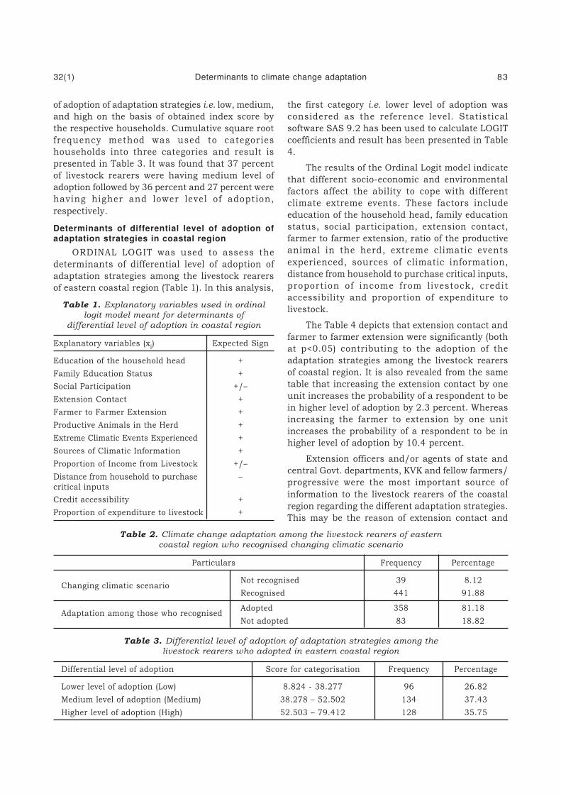
of adoption of adaptation strategies i.e. low, medium,

and high on the basis of obtained index score by

the respective households. Cumulative square root

frequency method was used to categories

households into three categories and result is

presented in Table 3. It was found that 37 percent

of livestock rearers were having medium level of

adoption followed by 36 percent and 27 percent were

having higher and lower level of adoption,

respectively.

Determinants of differential level of adoption ofadaptation strategies in coastal region

ORDINAL LOGIT was used to assess the

determinants of differential level of adoption of

adaptation strategies among the livestock rearers

of eastern coastal region (Table 1). In this analysis,

the first category i.e. lower level of adoption was

considered as the reference level. Statistical

software SAS 9.2 has been used to calculate LOGIT

coefficients and result has been presented in Table

4.

The results of the Ordinal Logit model indicate

that different socio-economic and environmental

factors affect the ability to cope with different

climate extreme events. These factors include

education of the household head, family education

status, social participation, extension contact,

farmer to farmer extension, ratio of the productive

animal in the herd, extreme climatic events

experienced, sources of climatic information,

distance from household to purchase critical inputs,

proportion of income from livestock, credit

accessibility and proportion of expenditure to

livestock.

The Table 4 depicts that extension contact and

farmer to farmer extension were significantly (both

at p<0.05) contributing to the adoption of the

adaptation strategies among the livestock rearers

of coastal region. It is also revealed from the same

table that increasing the extension contact by one

unit increases the probability of a respondent to be

in higher level of adoption by 2.3 percent. Whereas

increasing the farmer to extension by one unit

increases the probability of a respondent to be in

higher level of adoption by 10.4 percent.

Extension officers and/or agents of state and

central Govt. departments, KVK and fellow farmers/

progressive were the most important source of

information to the livestock rearers of the coastal

region regarding the different adaptation strategies.

This may be the reason of extension contact and

Table 1. Explanatory variables used in ordinal

logit model meant for determinants of

differential level of adoption in coastal region

Explanatory variables (xi) Expected Sign

Education of the household head +

Family Education Status +

Social Participation +/–

Extension Contact +

Farmer to Farmer Extension +

Productive Animals in the Herd +

Extreme Climatic Events Experienced +

Sources of Climatic Information +

Proportion of Income from Livestock +/–

Distance from household to purchase –critical inputs

Credit accessibility +

Proportion of expenditure to livestock +

Table 2. Climate change adaptation among the livestock rearers of eastern

coastal region who recognised changing climatic scenario

Particulars Frequency Percentage

Changing climatic scenarioNot recognised 39 8.12

Recognised 441 91.88

Adaptation among those who recognisedAdopted 358 81.18

Not adopted 83 18.82

Table 3. Differential level of adoption of adaptation strategies among the

livestock rearers who adopted in eastern coastal region

Differential level of adoption Score for categorisation Frequency Percentage

Lower level of adoption (Low) 8.824 - 38.277 96 26.82

Medium level of adoption (Medium) 38.278 – 52.502 134 37.43

Higher level of adoption (High) 52.503 – 79.412 128 35.75


Table 4. Estimated ORDINAL LOGIT Coefficients of factors determining level of adoption of

adaptation strategies among the livestock-rearers of eastern coastal region

Dependent Variable: Y (Y= Level of Adoption; Ordered variable: 1= Lower level, 2 = Medium level, 3 = Higher level of adoption)

Odds Ratio

Explanatory Variables (Xi) Estimated Standard P > 95% Confidence Limit Predicted

Coefficient Error o Chisq Point Lower Upper Marginalo Estimate Limit Limit Effect

(dP/dx)

Education of the household head: Primary 0.445 0.309 0.151 1.56 0.851 2.859 0.106

Education of the household head: Secondary 0.683* 0.366 0.062 1.98 0.966 4.059 0.152

Education of the household head: Higher Secondary 0.386 0.486 0.427 1.471 0.568 3.813 0.093

Education of the household head: Graduate and Above 1.072* 0.644 0.096 2.922 0.827 10.326 0.204

Family Education Status -0.004 0.047 0.937 0.996 0.908 1.093 -0.001

Social Participation -0.073 0.060 0.228 0.93 0.826 1.047 -0.018

Extension Contact 0.091** 0.043 0.034 1.095 1.007 1.191 0.023

Farmer to Farmer Extension 0.438** 0.176 0.013 1.549 1.097 2.188 0.104

Productive Animals in the Herd 0.021 0.017 0.213 1.021 0.988 1.054 0.005

Extreme Climatic Events Experienced -0.101** 0.046 0.028 0.904 0.827 0.989 -0.025

Sources of Climatic Information 0.097 0.084 0.249 1.102 0.935 1.299 0.024

Distance from household to purchase critical inputs -0.063 0.047 0.180 0.939 0.855 1.030 -0.016

Proportion of Income from Livestock -0.023** 0.010 0.014 0.977 0.959 0.995 -0.006

Credit Accessibility 0.054 0.232 0.817 1.055 0.669 1.664 0.013

Proportion of expenditure to livestock 0.007 0.024 0.780 1.007 0.96 1.056 0.002

-2 Loglikelihood 751.593

McFadden R-squared 0.073

LR statistic (15 df) 26.068**

Probability (LR stat) 0.037

Observations 358

Score test for Proportional Odd Assumption 21.451 (p > 0.1230)

**Indicates significant at 5 % level of significance, in a two tail test *Indicates significant at 10 % level of significance, in a two tail test

84

Ma

iti et a

l.3

2(1

)

farmer to farmer extension to be the significant

determinants of differential level of adoption. From

this result we may conclude that having extension

services and strong bonding among the livestock

rearers increased the likelihood of livestock rearers’

adaptation to climate change.

Deressa et al., (2011), Mandleni (2011), Dhaka

et al. (2010), Hassan & Nhemachena (2008) and

Nhemachena & Hassan (2007) also reported that

access to extension service was one of the important

determinants of farm level adaptation. Deressa et

al., (2011) also reported that farmer to farmer

extension was the important determinant of

adaptation strategies.

The same table also stated that number of

extreme climatic events experienced and proportion

of income from livestock were negatively

significantly (both at p<0.05) contributing to the

adoption of adaptation strategies among the

livestock rearers of coastal region. The same table

depicts that increasing one unit of extreme climatic

events experienced by one unit of decrease the

probability of a respondent to be in higher level of

adaptation. Tropical cyclone, heavy rainfall, flood

etc are the major extreme climatic events

experienced by the livestock rearers of coastal

region. For example livestock rearers of Coastal

South 24 Paragans experienced one cyclone every

year namely Aila, Laila, Mahasen etc during last 3-

4 years. With these events, other related events like

floods, inundation, salinization etc. also experienced

by them. Therefore, they discontinued adaptation

strategies. This may the reason of negative influence

of extreme climatic events to the adoption of

adaptation strategies.

The commercial livestock rearers followed the

scientific packages of practices for their livestock.

Therefore, their animals were not susceptible to the

negative impact of climate change. Hence, adoption

level of afore said adaptation strategies were too low

among them. This may be the reason of negative

influence of proportion of income from livestock to

the adoption of adaptation strategies.

CONCLUSION

Livestock rearers of eastern coastal region

recognised changing climatic scenario and adopted

several adaptation strategies mechanism to cope up

with its negative impact of climate change. It is

found that extension contact is one of the most

important determinants of differential level of

adoption of adaptation strategies. Therefore, a

dedicated team of veterinary /livestock extensionist

must be trained or promoted to teach livestock

rearers in different aspects of climate change

including scientific adaptation strategies. Other

important determinants like farmer to farmer

extension showed significant positive effect whereas

numbers of extreme climatic events experienced and

proportion income from livestock showed significant

negative effect on adoption of adaptation strategies

among the livestock rearers of eastern coastal region.

REFERENCES

Dhaka, B. L., Chayal, K. and Poonia, M. K. (2010).

Analysis of farmers’ perception and adaptation

strategies to climate change. Libyan Agriculture

Research Centre Journal International 1(6):

388-390.

Deressa, T. T., Hassan, R. M. and Ringler, C. (2011).

Perception and adaptation to climate change by

farmers in the Nile basin of Ethiopia. Journal

of Agricultural Science 149(1): 23-31.

Greene, W. H. (1993). Econometrics analysis,

Second edition, Macmillan, New York.

Hassan, R. and Nhemachena, C. (2008).

Determinants of climatic adaptation strategies

of African farmers: multinomial choice analysis.

African journal of Agricultural and Resource

Economics 2: 83-104.

Intergovernmental Panel on Climate Change (IPCC),

(2001). Climate Change. In: Impacts,

Adaptation, and Vulnerability, J. McCarthy, O.

Canziani, N. Leary, D. Dokken and K. White

(eds.), Cambridge University Press, Cambridge.

Kane, S. M. and Shogren, J. F. (2000). Linking

adaptation and mitigation in climate change

policy. Climatic Change 45 (1): 75–102.

Kaur, H. and Arora, S. P. (1982). Influence of level

of nutrition and season on the oestrus cycle

rhythm and on fertility in buffaloes. Tropical

Agriculture 59(4): 274–278.

Kulkarni, A. A., Pingle, S. S., Atakare, V. G. and

Deshmukh, A. B. (1998). Effect of climatic

factors on milk production in crossbred cows.

Indian Veterinary Journal 75(9):846–847.

Lal, S. N., Verma, D. N. and Husain, K. Q. (1987).

Effect of air temperature and humidity on the

feed consumption, cardio respiratory response

and milk production in Haryana cows. Indian

Veterinary Journal 64(2): 115–121


Mandal, D. K., Rao, A. V. M. S., Singh, K. and Singh,

S. P. (2002). Effects of macroclimatic factors

on milk production in a Frieswal herd. Indian

Journal of Dairy Science 55(3): 166–170

Mandleni, B. (2011). Impact of climate change and

adaptation on cattle and sheep farming in the

Eastern Cape province of South Africa.

Unpublished PhD Thesis. University of South Africa.

Nhemachena, C., and Hassan, R. (2007). Micro-level

analysis of farmers’ adaptation to climate change

in Southern Africa. IFPRI Discussion Paper No.

00714. International Food Policy Research

Institute, Washington, D.C.

Patnaik, U. and Narayanan, K. (2005). Vulnerability

and Climate Change: An analysis of the Eastern

coastal districts of India. Published in

International workshop on “Human security

and climate change” at Holmen Fjord Hotel,

Asker, near Oslo, 21–23 June 2005 organised

by Centre for the Study of Civi l War,

International Peace Research Institute, Oslo

(PRIO) , Centre for International Environmental

and Climate Research at the University of Oslo

(CICERO) and the Global Environmental

Change and Human Security Program (GECHS).

Pielke, R. A. (1998). Rethinking the role of

adaptation in cl imate policy. Global

Environmental Change 8 (2): 159–170.

Shinde, S., Taneja, V. K. and Singh, A. (1990).

Association of climatic variables and production

and reproduction traits in crossbreds. Indian

Journal of Animal Science 60(1): 81–85.

Smit, B. and Pilifosova, O. (2001). Adaptation to

climate change in the context of sustainable

development and equity. In: Climate Change

2001:Impacts, Adaptation and Vulnerability,

McCar thy, J.J., Canziani, O.F., Leary, N.A.,

Dokken, D.J., White, K.S. (eds.), Cambridge

University Press, Cambridge. pp 877–912.

Tailor, S. P. and Nagada, R. K. (2005). Conception

rate in buffaloes maintained under subhumid

climate of Rajasthan. Indian Journal of Dairy

Science 58(1): 69-70.

Upadhyay, R. C., Ashutosh, Raina, V. S. and Singh

S.V. (2009). Impact of climate change on

reproduction functions of cattle and buffaloes.

In: Global cl imate change and Indian

Agriculture, P.K. Aggarwal (ed.), ICAR, New

Delhi. pp 107-110.

86 Maiti et al. 32(1)

J. Indian Soc. Coastal agric. Res. 32(2): 87-91 (2014) Short communication

Impact of Soil and Water Conservation Measures on Productivity

and Groundwater Recharge in a Micro-watershed in

Coastal Zones of Odisha


There is a need to precisely monitor and to

evaluate the impact of soil and water conservation

measures/projects that are multi-sectoral in

essence from various angles to achieve the

objectives of sustainable development. The National

Watershed Development Programme is a single

window delivery system, in which, participatory,

integrated and sustainable development of

watershed is achieved. The literature related to

various studies and researches on impact of soil

and water conservation measures in micro-

watersheds are readily available. Prasad, 1999

studied the impact of watershed management on

runoff, water resource activity and productivity of

arable lands in Chhaljawa watershed of Baran

district in Eastern Rajasthan and results indicated

that integrated watershed development treatment

such as graded bunds, gulley control structures etc.

halted the process of land degradation and improved

the ground water recharge which could be

successfully exploited for increasing the productivity

of arable land. The investment made recovered in

four years indicating that the programme was

economically viable. Panda (2009) in his case study

on “Economics of watershed treatments in Odisha”,

two stage stratified random sampling techniques

was used for the study. He concluded that the

beneficiary village recorded 36% to 114% higher

productivity of crops in comparison to non-

beneficiary village. The production of paddy,

sesamum and groundnut in watershed area was

198%, 152% and 173%, respectively higher than

that of the non-beneficiary village. The productivity

of paddy and groundnut was 114% and 105% higher

in watershed area respectively in comparison to non-

beneficiary village. Black gram also registered 75%

higher productivity. Cattle per household of the

beneficiary village were 3.5 against 1.36 of non-

beneficiary vi l lage. Various soil and water

conservation, water harvesting and vegetal cover

improvement viz. bunding, staggered trenching,

loose boulder checks and vegetative barriers,

earthen embankment and ponds, pasture and

plantation etc. were taken up. After 4 years they

surveyed and concluded that the area under paddy,

sorghum, wheat, gram, mustard and linseed

increased by 60, 102, 179 and 83 % respectively.

Before implementation of watershed works, the

irrigated area was 34.7 ha through one earthen

embankment, one pond and one natural stream.

After execution of soil conservation works and

construction of earthen embankments across

natural stream and ponds, the irrigated area was

increased by 2.53 times i.e. 87.8 ha in 4 yrs. Yield

of paddy, sorghum, wheat, barley, pigeon pea, gram

and mustard had increased by 51, 22, 65, 43, 25,

57 and 70% ,respectively. Sharda et al., (2005)

studied the participatory watershed management

programmes for sustainable development and the

research area located in diverse ecological region

of the country, namely Eastern Ghats, Western

Ghats (Nilgiris), Shiwaliks (Himalayan foot hills),

Bundelkhand region, western coast Gujarat plains

and Chambal ravines. They concluded that the

various agronomical interventions improved the

yield of traditional crops. The overall crop

productivity of watersheds measured in terms of

crop productivity index (CPI) increased by 12 to 45%

and considering 5 watersheds together, CPI

improved from 0.50 in pre-project to 0.64 after

project implementation. The crop diversification

index considering all watersheds together improved

from 0.67 in pre project period to 0.82 after

implementation of the project. Also they concluded

that the overall cultivable land utilization showed

that CLUI had increased from 0.26 in pre-project

period to 0.33 in post-project period. Mondal et al.,

(2006) studied the impact evaluation of watershed

development works on socio-economic indicators in

Andhra Pradesh. The results showed that the total

cultivable area was 4677 ha which constituted

93.5% of the total geographical area of watershed

before implementation of the project. During the

project period an additional area of 14 ha (out of 17

ha of cultivable waste) and 9 ha of endowment land

which was also not under cultivation were converted

in to cultivated land and 3 ha degraded land was

brought under social forestry which resulted in an

increase of 47% in cultivated area. Introduction of

soil and water conservation programme improved

cropping intensity from 97% during pre- project

period to 114% during post- project period.

Increased ground water availability and improved

packages of practices for crops in study area brought

67.9 ha area under double cropping. They also

concluded that the adoption of package of practices

and land treatment increased the level of production

and productivity. Goel et al., (2007) studied the

performance evaluation of some soil and water

conservation measures in hot arid zone of India.

During 1993-2004 the soil and water conservation

measures adopted in Jhanwar watershed located

in Rajasthan. They revealed that the natural

resource base in arid region can be substantially

improved and the agricultural productivity could be

sustained even in extreme arid condition through

watershed approach. Introduction of improved crop

varieties and other dryland framing techniques has

resulted in substantial improvement in productivity

of various dryland crops viz. pearl-millet (52 %),

mung bean (177 %), moth bean (394 %) and cluster

bean (547 %). Similarly adoption of alternate land

use system like agriculture with ber (agri-horti),

agro-forestry with Prosopis Cineraria and farm

forestry with Acacia tortilis resulted in production

of various products and byproducts like fruit, fuel,

fodder, pods, top feed grains etc. resulting in better

sustainability of farmers of the project area. Naik

(2009) studied the impact of the National Watershed

Development Programme for Rainfed Areas and the

programme was implemented in Sukli watershed

which is situated near to Nagpur- Hyderabad

highway, Maharashtra. He concluded that the post

project cropped area was increased by 32 ha but

gross cropped area was increased by 175 ha with a

significant increase in the area under horticulture

(139.5 ha) and flower cultivation (3.5 ha) With

adoption of integrated watershed management the

productivity of major Kharif crops increased by 25%

to 37% and figure for Rabi crops was 33% to 44%.

Training of primary stakeholders, field demonstration

on crops, agro-forestry and improved composting

had created mass awareness on soil and water

conservation in the area and expected to yield good

results in long run. Panda (2000) observed the water

table level in wells during study period of both

watershed and non- watershed vil lages and

concluded that the average annual water table depth

in non -watershed area was 5.2 m. The watershed

area was found with average ground water table of

9.1 m, which was 3.9 m higher than that of the

non- watershed area in the state of Odisha.

Gitte and Pendke (2002) reported that the water

table in all the wells started rising since mid of June

and attended its peak in September. There was

steady decline in water table since September to

December and then that water table was maintained

a constant level up to March in almost all wells.

The water conservation measures were found to be

effective for increasing water table in observation

wells located in middle and lower reaches of

watershed. Generally, it was seen that there was

overall build up in water levels in entire watershed

area due to impoundment of water in water

harvesting structures. Naik (2009) studied that rise

in the water table was found to be in order of 0.30

to 0.45 m adjoining to the structures. In Rabi season

water pumping was increased for 2-3 hrs and in

summer for 1.0-1.5 hrs. Hence farmers were

encouraged to construct more number of wells which

was evidenced from the pre-project figure of 124 to

post project figure of 141. Number of bore wells was

also increased from 3 to 8 during this period.

The present study area Barapita-Nalla Micro-

Watershed comes under agro-climatic zone of south-

eastern coastal plain (Code No.-078) of the state of

Odisha. The project is coming under the range of

Chandaka P.S. of Bhubaneswar Block in Khurda

District, at a distance of 15 to 18 km from

Bhubaneswar. The project area is located in between

20o17’ to 20o20’ N latitude and 85o40’ to 85o44’ E

longitude. It comprises of three villages such as (1)

Giringaput, (2) Bhagabatipur and (3) Barapita with

a total geographical area of 1442.71 ha. The

watershed is generally f lat with undulating

topography. Physiographically the zone is located

in the coastal belt and has an altitude ranging from

40 to 70 m from mean sea level. The area is a

sedentary landscape with two distinct phases, such

as, erosion phase which includes the ridge and up

land and depositional phase which includes medium

and low land. There is a small fringe of level on

both sides of the stream. Detailed soil survey of the

area revealed that the soil is mostly sandy loam to

sandy clay loam and depth of soil is about 90 cm

(d5 class). The details of soil mapping units are given

in Table 2. Basically it is a fan shaped watershed.

Water from entire project area drained by a number

of small channels into the Gangua watershed of

Chilika catchment. Morphological characteristics of

the watershed are given in Table No. 1.

88 Behera et al. 32(1)

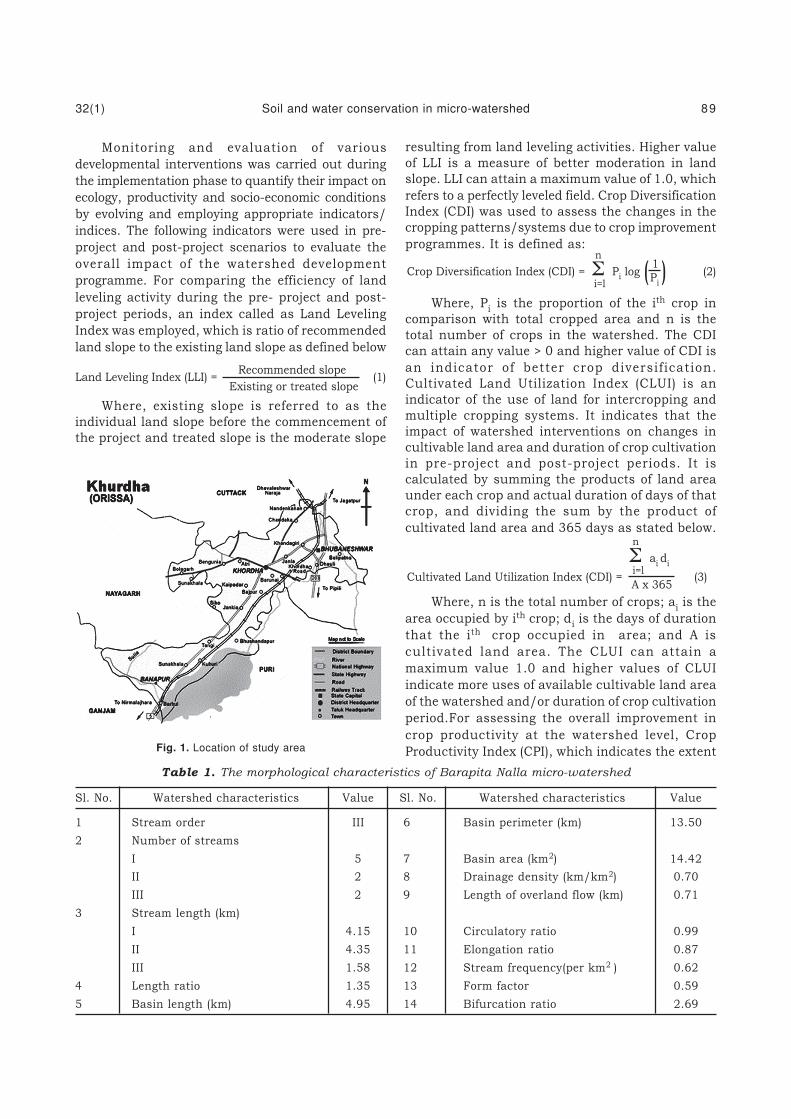
Table 1. The morphological characteristics of Barapita Nalla micro-watershed

Sl. No. Watershed characteristics Value Sl. No. Watershed characteristics Value

1 Stream order III 6 Basin perimeter (km) 13.50

2 Number of streams

I 5 7 Basin area (km2) 14.42

II 2 8 Drainage density (km/km2) 0.70

III 2 9 Length of overland flow (km) 0.71

3 Stream length (km)

I 4.15 10 Circulatory ratio 0.99

II 4.35 11 Elongation ratio 0.87

III 1.58 12 Stream frequency(per km2 ) 0.62

4 Length ratio 1.35 13 Form factor 0.59

5 Basin length (km) 4.95 14 Bifurcation ratio 2.69

Fig. 1. Location of study area

resulting from land leveling activities. Higher value

of LLI is a measure of better moderation in land

slope. LLI can attain a maximum value of 1.0, which

refers to a perfectly leveled field. Crop Diversification

Index (CDI) was used to assess the changes in the

cropping patterns/systems due to crop improvement

programmes. It is defined as:

Crop Diversification Index (CDI) = Σn

Pi log ( 1 ) (2)

i=l P

i

Cultivated Land Utilization Index (CDI) =

Σn

ai d

i

(3) i=l

A x 365

Monitoring and evaluation of various

developmental interventions was carried out during

the implementation phase to quantify their impact on

ecology, productivity and socio-economic conditions

by evolving and employing appropriate indicators/

indices. The following indicators were used in pre-

project and post-project scenarios to evaluate the

overall impact of the watershed development

programme. For comparing the efficiency of land

leveling activity during the pre- project and post-

project periods, an index called as Land Leveling

Index was employed, which is ratio of recommended

land slope to the existing land slope as defined below

Land Leveling Index (LLI) = Recommended slope

(1) Existing or treated slope

Where, existing slope is referred to as the

individual land slope before the commencement of

the project and treated slope is the moderate slope

Where, Pi is the proportion of the ith crop in

comparison with total cropped area and n is the

total number of crops in the watershed. The CDI

can attain any value > 0 and higher value of CDI is

an indicator of better crop diversif ication.

Cultivated Land Utilization Index (CLUI) is an

indicator of the use of land for intercropping and

multiple cropping systems. It indicates that the

impact of watershed interventions on changes in

cultivable land area and duration of crop cultivation

in pre-project and post-project periods. It is

calculated by summing the products of land area

under each crop and actual duration of days of that

crop, and dividing the sum by the product of

cultivated land area and 365 days as stated below.

Where, n is the total number of crops; ai is the

area occupied by ith crop; di is the days of duration

that the ith crop occupied in area; and A is

cultivated land area. The CLUI can attain a

maximum value 1.0 and higher values of CLUI

indicate more uses of available cultivable land area

of the watershed and/or duration of crop cultivation

period.For assessing the overall improvement in

crop productivity at the watershed level, Crop

Productivity Index (CPI), which indicates the extent

32(1) Soil and water conservation in micro-watershed 89

of crop productivity level in comparison to the

normal yield of crops before and after the project,

is calculated by dividing the crop yield obtained in

the watershed by the yield obtained under

recommended package of practices.

Crop Productivity Index was increased from 0.49 to

0.52. The concept of mono-cropping system waschanged and farmers were taking interest in

cultivating vegetable crops and floriculture onexperimental basis in Rabi season. Community

cashew nut plantation was adopted and was fruitful.

This resulted in increase in Crop DiversificationIndex from 0.301 to 0.775. Near about 25, 27,720

litres of water was stored throughout the year in 6ponds located in the village. As a result of this

harvested water, the irrigation intensity was

increased from 143% to 187% and cropping intensitywas increased from 114% to 186%. It was observed

that Cultivable Land Utilization Index was increasedfrom 0.103 to 0.670. During the period under study,

considerable development in water resources suchas construction of tube wells, wells and installation

of hand pumps were increased from 5 to 13, 10 to

12 and Nil to 7, respectively in the study village.

From the study it was concluded that totalincome of households generated from agriculture,

off-farm activities and minor forest activities. The

income contributions from all these three activitieswere changed from 41% to 85%, 35% to 8%, and

23% to 7%. in case of agriculture, forest, and offfarm activities, respectively. It was observed that

the income contribution from forest activities was

considerably reduced which ultimately helped inpreservation and conservation of forest resources.

It was also observed that the contribution throughoff-farm activities was decreased considerably;

which indicated reduction in migration of people tonear-by city/town area as most of the people were

engaged in farm activities.

Table 2. Details of soil mapping unit with present land use

Mapping unit no Soil Mapping Unit Area in ha Capability Physiographic

classification classification

1 SCL-d5/C-e2 16.50 IV e Up existing cashew pl.

2 SCL- d5/C-e2 36.40 III e Up C1

3 SCL- d5/B-e

213.10 II e Medium C

1

4 SCL- d5/C-e

29.80 IV e Up existing misc. Pl.

5 SCL- d5/C-e

258.53 IV es Up gochar

6 SCL- d5/C-e

2105.50 IV es Up F

0

7 SCL- d5/C-e2 19.14 III e Up C1

8 SCL- d5/B-e2 11.10 II e Medium C1

9 SCL- d5/B-e2 25.28 II e Low C1

10 SCL- d5/C-e2 29.12 II e Medium C1

Total 324.47

Homestead 7.17

Others 21.65

Grand Total 353.29

Crop Productivity Index (CDI) = 1

Σn

( yi) (4)

n

i=l

Yi

Where, n is the total number of crops in

watershed, is the average yield of ith crop cultivated

in watershed, and is the yield of ith crop with

standard package of practices. The CPI can attain

any value in a given location. Higher value of CPI

is an indicator of crops’ yield closer to the maximum

attainable yield under standard package of

practices. Major utilization of harvested water is for

irrigation of crops to ensure sustainable agricultural

production in the watershed. Irrigability Index (II)

is a ratio of additional gross irrigated area and net

incremental irrigated area. Gross irrigated may be

estimated by adding the net incremental irrigated

area as many times as it was irrigated. The index

can attain any value more than 0, and a higher value

will indicate successful utilization of harvested water

in watershed management project. Productivity of

paddy crop increased by 19% in Kharif and 26% in

Rabi. Productivity of vegetable crops increased by

25% in Kharif and in Rabi it gave production equal

to 42 q ha-1. A land of 6.4 ha. was under cashew

nut plantation ,from which, 12 q ha-1 production

was obtained. One of the beneficiaries produced

17,000 numbers of rose flower per ha. With

reference to all these outputs it was found that the

90 Behera et al. 32(1)

REFERENCES

Gitte, A.V. and Pendke, M. S. (2002). Effect of water

conservation practices on hydrological behaviour,

water table fluctuation and ground water recharge

in watershed, Journal of Maharashtra

Agricultural University 27(3): 290-292.

Goel, R. K., Bhati, T. K. and Ojasvi, P. R. (2007).

Performance evaluation of some soil and water

conservation measures in hot arid zone of India.

Indian Journal of Soil Conservation 35(1): 58-63.

Mondal B., Loganandhan, N. and Reddy, K. K.

(2006). Impact evaluation of watershed

development project on socio-economic

indicators- A case study, Central Soil and Water

Conservation Research and Training Institute,

Research Centre, Bellary, Karnataka. Indian

Journal of Soil Conservation 34(1): 69-74.

Naik, P. K. (2009). Impact of the National Watershed

Development Programme for Rainfed

Agriculture- A case study, Central Ground

Department of Soil & Water Conservation Engineering B.P. BEHERA, N. SAHOO,

College of Agricultural Engineering and Technology B. PANIGRAHI and G.A. EKNATH

OUAT, Bhubaneswar-751 003, Odisha

E mail: [email protected]

Water Board, Nagpur. Indian Journal of Soil

Conservation 37(3): 230-235

Prasad, S. N. (1999). Impact of watershed

management on runoff and productivity of land

in south eastern Rajasthan. Indian Journal of

Soil Conservation 25(1): 69-72.

Panda, D. K. (2009). Economics of watershed

treatment in Odisha – A case study. Watershed

development mission, Odisha

Sharda, V. N., Samra, J. S. and Dogra, P. (2005).

Participatory watershed management

programmes for sustainable development:

Experiences from IWDP. Indian Journal of Soil

Conservation 33(2): 93-103.

Sharda, V. N., Dogra P. and Dhyani, B. L. (2012).

Indicators for assessing the impact of watershed

development programmes in different regions

of India. Indian Journal of Soil Conservation

40(1): 1-12.

32(1) Soil and water conservation in micro-watershed 91


An Analysis of Marketing of Mat in Paschim Medinipur

District of West Bengal


Mat is an interior decorative of house, made of

synthetic fiber, cotton, bamboo and mat-stick

(Cyperus tegetum) etc. The demand of hand- made

mat is declining in this day due to increased

globalization. Our indigenous products are

becoming more and more commoditized and artisans

find their products competing with goods from open

economy. Thus it is not possible for our artisan to

overlook their product from the present market

situation. But this type of cottage industry has

capacity to absorbed surplus labour of our country

(Joy and Kani, 2013). The handicraft has a

significance role to Indian economy, which lies in

its employment potential as well as export earnings.

But this industry has not received much attention

due to lack of financial and marketing support

(Dash, 2011). The artisan habitually depends on

market intermediaries for their produce (Dash,

2011). Mat-stick made handicraft has an important

role in livelihood of rural economy of West Bengal.

Mat-stick is a wetland weed; it is economically grown

in some rainfed area of West Bengal. Paschim

Medinipur, North 24 Parganas and Nadia are major

district of this state, where growing and weaving of

mat are observed. Mat weaving is an indigenous and

ancestral practice of some community in Paschim

Medinipur. Finished weaved mats are also exported

to various countries. It is opined to be a good source

of income and provides gainful employment to family

member who otherwise have remained idle (Maiti

and Das, 2012). Beside cultivator and weavers, a

good number of people earned their livelihood from

mat marketing. The marketing of mat is unorganized

but mainly centered in Barabazer market of West

Bengal. Considering its importance in providing

employment and being a source of income, the

present work intends to examine the price spread

of marketing of mat and efficiency of existing

marketing system of mat weaved in Paschim

Medinipur district. Though mat-stick cultivated in

North 24 Parganas and other districts, but mat-stick

and mat weaved in Paschim Medinipur district is

well known for its quality and concentration of

cultivators and weavers. Hence, the present study

is restricted to Paschim Medinipur district only. The

field survey has been under taken for the agriculture

year 2011-12. Three primary wholesale markets viz.

Sabong, Temathani and Dashagram bazaar of

Paschim Medinipur are selected purposively as the

bulk of mat weaved in the district are marketed

through these markets. One secondary wholesale

market viz. Barabazar market of Kolkata is selected

purposively because of most of mat is transacted

through this market. Beside, 10 retail markets are

also selected randomly. From the existing marketing

channels 10 secondary wholesaler, 20 primary

wholesaler, 20 commission agent, 20 paikers and

40 retailers are selected for the present study.

Market informations are collected with the help of

pre-tested survey schedule by interviewing

personally.

Average cost per mat is calculated by

considering the total mat-stick produced per hectare

and number of mats presumably prepared by that

amount of mat-stick and adding to it the expenses

incurred for processing mat from mat stick.

Producer’s price, producer’s share in consumer’s

Rupee, marketing margin of middleman, cost of

marketing, price spread for each market are

analyzed by using conventional formulae and index

of marketing efficiency is worked out by Shepherd’s

method. The price spread in agriculture is assessed

by estimating price received by the farmers

expressed as a percentage of the retail price (i.e.

the price paid by the consumer). If it is the retail

price, the weaver share in the consumer’s rupee (Ws)

is expressed as follows.

Ws = Net price received by the producer

x 100 Price paid by the consumer

2011-12. Mat is noted to passing through four

stages of marketing namely, weaver, primary

wholesaler, secondary wholesaler and retailer. The

maximum cost of marketing is found at secondary

wholesaler level and least at retailer level. At each

level, this cost has increase with the increase in

size of mat. Octroi is observed only at weaver’s level.

Transportation is noted to consume maximum cost

in total cost of marketing. The increase in marketing

cost is mainly due to transportation cost.

Table 2 depicts the price spread of mat at

Sabong, Temathani and Dashagram primary

wholesale market of the district. It is clear from the

table that weaver’s share in consumer’s rupee,

marketing cost, and middleman profit has increased

with increase in size of mat. According to percent

share of weaver in price paid by consumer, it is

The efficiency measurement methods used in

the study are presented as follows:

Shepherd’s method:

ME = RP

= RP

MC + MM GMM

Where,

ME: Marketing efficiency

MME: Modified measure of marketing efficiency

MC: Total marketing costs

MM: Total net marketing margin

GMM: Gross marketing margin

RP: Retailer’s price or Price paid by the consumer

Table 1 represents the marketing cost of mat

from Sabong market of the district during the year

Table 1. Marketing cost of mat from Sabong market of Paschim Medinipur district

(Rs./ Pair of Mat)

Sl. No. Item Size of Mat

Small Medium Large

a) Cost incurred by the weaver

Transport 0.46 0.51 0.63

Octoroon 1.03 1.25 1.48

Misc. 0.40 0.46 0.63

Sub total 1.88 2.22 2.74

b) Cost incurred by Primary wholesaler

Transport 0.51 0.68 0.80

Packaging 0.57 0.74 0.91

Loading &unloading 0.34 0.40 0.51

Storage 0.30 0.40 0.40

Misc. 0.21 0.29 0.34

Sub total 1.93 2.51 2.96

c) Cost incurred by Secondary wholesaler

Transport 2.62 3.19 3.59

Packaging 0.32 0.34 0.51

Loading &unloading 0.41 0.51 0.57

Storage 0.29 0.34 0.34

Market fees 0.23 0.34 0.57

Misc. 0.40 0.57 0.86

Sub total 4.26 5.30 6.44

d) Cost incurred by Retailer

Transport 0.51 0.74 0.80

Loading & unloading 0.14 0.29 0.40

Storage 0.40 0.63 0.57

Market fees 0.29 0.34 0.57

Misc. 0.23 0.29 0.34

Sub total 1.56 2.28 2.68

32(1) Marketing of mat in West Bengal 93

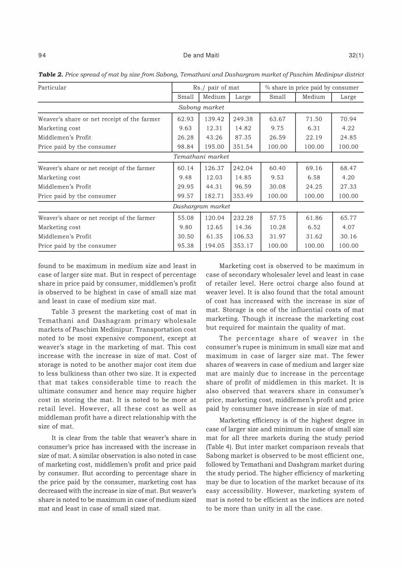
found to be maximum in medium size and least in

case of larger size mat. But in respect of percentage

share in price paid by consumer, middlemen’s profit

is observed to be highest in case of small size mat

and least in case of medium size mat.

Table 3 present the marketing cost of mat in

Temathani and Dashagram primary wholesale

markets of Paschim Medinipur. Transportation cost

noted to be most expensive component, except at

weaver’s stage in the marketing of mat. This cost

increase with the increase in size of mat. Cost of

storage is noted to be another major cost item due

to less bulkiness than other two size. It is expected

that mat takes considerable time to reach the

ultimate consumer and hence may require higher

cost in storing the mat. It is noted to be more at

retail level. However, all these cost as well as

middleman profit have a direct relationship with the

size of mat.

It is clear from the table that weaver’s share in

consumer’s price has increased with the increase in

size of mat. A similar observation is also noted in case

of marketing cost, middlemen’s profit and price paid

by consumer. But according to percentage share in

the price paid by the consumer, marketing cost has

decreased with the increase in size of mat. But weaver’s

share is noted to be maximum in case of medium sized

mat and least in case of small sized mat.

Marketing cost is observed to be maximum in

case of secondary wholesaler level and least in case

of retailer level. Here octroi charge also found at

weaver level. It is also found that the total amount

of cost has increased with the increase in size of

mat. Storage is one of the influential costs of mat

marketing. Though it increase the marketing cost

but required for maintain the quality of mat.

The percentage share of weaver in the

consumer’s rupee is minimum in small size mat and

maximum in case of larger size mat. The fewer

shares of weavers in case of medium and larger size

mat are mainly due to increase in the percentage

share of profit of middlemen in this market. It is

also observed that weavers share in consumer’s

price, marketing cost, middlemen’s profit and price

paid by consumer have increase in size of mat.

Marketing efficiency is of the highest degree in

case of larger size and minimum in case of small size

mat for all three markets during the study period

(Table 4). But inter market comparison reveals that

Sabong market is observed to be most efficient one,

followed by Temathani and Dashgram market during

the study period. The higher efficiency of marketing

may be due to location of the market because of its

easy accessibility. However, marketing system of

mat is noted to be efficient as the indices are noted

to be more than unity in all the case.

Dashargram market

Weaver’s share or net receipt of the farmer 55.08 120.04 232.28 57.75 61.86 65.77

Marketing cost 9.80 12.65 14.36 10.28 6.52 4.07

Middlemen’s Profit 30.50 61.35 106.53 31.97 31.62 30.16

Price paid by the consumer 95.38 194.05 353.17 100.00 100.00 100.00

Temathani market


Marketing cost 9.48 12.03 14.85 9.53 6.58 4.20



Table 2. Price spread of mat by size from Sabong, Temathani and Dashargram market of Paschim Medinipur district

Particular Rs./ pair of mat % share in price paid by consumer

Small Medium Large Small Medium Large

Sabong market


Marketing cost 9.63 12.31 14.82 9.75 6.31 4.22



94 De and Maiti 32(1)

Table 3. Marketing cost of mat from Temathani market of Paschim Medinipur district

(Rs./ Pair of Mat)

Sl. No. Item Size of Mat

Temathani Market Dasharam Market

Small Medium Large Small Medium Large

a) Cost incurred by the weaver

Transport 0.46 0.63 0.74 0.68 0.74 0.91

Octoroon 0.91 1.25 1.48 0.97 1.25 1.48

Misc. 0.23 0.34 0.46 0.29 0.34 0.46

Sub total 1.60 2.22 2.68 1.94 2.34 2.85

b) Cost incurred by Primary wholesaler

Transport 0.97 0.74 0.91 0.86 0.91 0.11

Packaging 0.46 0.57 0.68 0.40 0.57 0.68

Loading &unloading 0.40 0.40 0.51 0.29 0.40 0.51

Storage 0.29 0.34 0.34 0.23 0.29 0.40

Misc. 0.17 0.29 0.32 0.29 0.40 0.57

Sub total 2.28 2.34 2.77 2.05 2.57 2.28

c) Cost incurred by Secondary wholesaler

Transport 2.57 3.42 3.88 0.29 0.34 3.99

Packaging 0.34 0.40 0.40 0.29 0.51 0.63


Storage 0.23 0.29 0.40 0.40 0.57 0.34

Market fees 0.29 0.34 0.51 0.23 0.34 0.46

Misc. 0.29 0.34 0.34 0.23 0.46 0.34

Sub total 4.05 5.19 5.99 1.77 2.79 6.27

d) Cost incurred by Primary wholesaler

Transport 0.57 0.63 0.80 0.46 0.513 0.627


Storage 0.34 0.63 0.74 0.40 0.46 0.57

Market fees 0.23 0.34 0.46 0.17 0.29 0.46

Misc. 0.29 0.34 0.57 0.29 0.40 0.34

Sub total 1.56 2.22 3.02 1.48 1.88 2.28

The study represents the marketing of mat

marketed through different primary wholesale

market of Paschim Medinipur of during 2011-12.

In general three size mat are found to exist in the

market. The price of these mats has been observed

Table 4. Market wise and mat size wise marketing

efficiency of mat in Paschim Medinipur district

during 2011-12

Name of market Size of Mat

Small Medium Large

Sabong 1.75 2.51 2.44

Temathani 1.52 2.24 2.17

Dashagram 1.37 2.62 2.92

to increase with increase in size of mat. The total

cost components and amount of cost is observed to

be maximum in case of secondary wholesaler level.

The transportation cost is most expensive cost in

the marketing of mat. It is also found that that the

percentage share of weaver in price paid by the

consumer has direct relation with size of mat

whereas marketing cost is inversely related with the

size of mat. According to marketing efficiency

Sabong market is the most efficient market

irrespective of size of mat. The higher efficiency of

marketing may be due to location of market because

of its easy accessibility. However, marketing of mat

is found to be efficient one as the indices are noted

to be more than unity.

32(1) Marketing of mat in West Bengal 95

REFERENCES

Banerjee, A., Das, A. and Anu, M. P. (2014). In vitro

antidiabetic activity of Cyperus tegetum Roxb.

root extract, European Journal of Experimental

Biology 4(2): 250-253.

Das, P. K. and Mondal, A. K. (2012). The dye yielding

plants used in traditional art of ‘Patachitra’ in

Pingla and mat crafts in Sabang with prospecting

proper medical value in the Paschim Medinipur

district, West Bengal, India. Intitution Journal of

Life Science Bt & Pharm. Research 1(2).

Dash, M. (2011). Marketing of Orissa Handicrafts:

A Study on Challenges & Opportunity EXCEL.

International Journal of Multidisciplinary

Management Studies 1(2): 47-63.

Directorate of Industries, Govt. of West Bengal 1967.

Contemporary Crafts in West Bengal, Calcutta.

Ghosh, T. P. (1987). Krishi Hisab Byabastha,

Calcutta.

Handbook of Statistics and Indian Economy, Reserve

Bank of India, Bombay, 2006. pp 131- 132.

Hu-MF and Liu-Sy (1988). The production and

cultivation techniques for mat rush in Taiwan.

Taiwan Agricultural Bimonthly 24(3): 89-96.

Jana, K. and Puste, A. M. (2012). Effect of irrigation

schedule along with paddy straw mulching on

growth character of mat sedges (Cyperus

tegetum Roxb.) under old alluvial zone of West

Bengal. Journal of Progressive Agriculture 3(2):

99-105.

Joy, M. T. and Kani, R. M. (2013). Emerging

Opportunities and Challenges for Cottage

Industries in India, International Journal of

Scientific and Research Publications 3(3): 1-4.

Khanka, S. S. (1998). Development of small scale

industries in Assam, Yojana 42(9): 41-45.

Malabika, B. (2010). Human wetland dependency and

socio-economic evaluation of wetland functions

through participatory approach in rural India.

Water Science and Engineering 3(4): 467-479.

Maiti, A. K., Mukerjee, A. K. and Banerjee, B. N. (1986).

Economics of production and marketing of Mat in

West Bengal-A case study. Journal of Agricultural

Marketing, July-Sept. 1986; pp 28-32.

Maiti, B. K. and Das, C. (2012). Cost-Benefit

Analysis of Mat Industry (A case Study on

Weavers’ Households in Sabang Block of West

Bengal). Paripex- Indian Journal of Research

1(9): 43-44.

Maity, M. (1996). Economics of Mat Industry: A

study of P.S. Sabang, District Midnapore, West

Bengal. Finance India 10(3): 709-716.

Mondal, B. K., Choudhury, P. P. and Chatterjee, P.

(1990). Cultivating mat-making shrubs for high

profits. Indian Farming 40(4): 16-18.

Puste, A. M. (2012). Importance of aqua-terrestrial

ecosystem and development of an IFS modle in

water monitoring, productivity and

sustainability. ARPN Journal of Science and

Technology 2(Spl. ICESR): 31-47.

Sabir, A. M. (1998). “Participation of rural women

in socio economics development-A scenario”

Kurukshetra 47(33): 25-28

Singh, C. B., Dhaka, J. P and Sharma S. P. (1981).

Labour absorption and factor influencing levels

of employment in crop, dairy and poultry

enterprises, Indian journal of Agricultural

Economics 36(4): 14-20.

Research Scholar Deptt. Agril. Economics SEKHAR DE and ASIT KUMAR MAITI

Bidhan Chandra Krii Viswavidyalaya

Mohanpur - 741 252, Nadia, West Bengal

96 De and Maiti 32(1)


Special Features and Characterization of Rice Land Races of

Karen Community in Andaman and Nicobar Islands, India


Rice is the most important and traditional food

crop of Andaman and Nicobar Islands. The crop has

wide spectrum of genetic variability owing to ethnic

diversity of the settlers’ population thus more than

50% of rice area in the islands is still under

traditional land races. Many years ago these ethnic

land races were brought by different settlers from

different states of mainland India and even

neighbouring countries. Karen community who

originally came from Burma now called Myanmar

settled quite long back in North and Middle

Andaman and brought ethnic rice cultures like

Khushbaya, Black Burma, White Burma, Mushley

and Yaeon etc which suit to their likings and

requirements. These land races are still popular with

the community and Karens are thus indirectly

playing a vital role in conservation and cultivation

of these rice cultures. Through social surveys and

interviews, the special features of these rice

landraces were elicited. These cultures have also

been characterized in a systematic and scientific

manner to establish their unique identity and

morphological descriptors in the light of IPR

scenario.

Andaman and Nicobar group of islands located

in the Bay of Bengal is about 1200 km distant from

mainland India. The International Union for

Conservation of Nature has recently declared 19

“hope spots” in 2013 including A&N Islands, India

(Anonymous, 2013). The hope spot refers to an area

of ocean which deserves special protection because

of wild life & significant wild life habitats. Rice is

the mainstay cereal crop of the Andaman and

Nicobar Islands and supports the lifeline of the

islanders. Rice is cultivated in an area of about 8390

ha with a total production of 23,916 t resulting in

productivity of 2.85 t ha-1 (Gautam et al., 2013).

Rice cultivation started during post- independence

era with the settlement of various communities in

the Islands. More than 50% rice area is under

traditional land races in the islands (Mandal et al.,

2004). The availability of fertilizer is also a major

constraint and hence the adoption of high yielding,

fertilizer responsive varieties is quite less. Though

several efforts have been made to replace these old

land races with new high yielding varieties, the

farmers of these Islands are not ready to give up

these landraces due to their unique characteristics

including better response to low management

conditions, tolerance to adverse weather conditions

and better grain quality liked by the diverse ethnic

groups.

Karen community who originally came from

Burma (now Myanmar) settled quite long back in

North & Middle Andaman and brought rice cultures

of their taste and other special features. Initially,

12 Karen families from Burma came to Andaman

after persuasion by Beroti officer Dr. H. I. Marshall

in 1925 for clearing jungles for making settlements

(Mary Pee, 2013). The word “Karen” was coined by

British, whereas Burmese called them as “Kaylin”

meaning “polite and good hearted” The present

population of Karens in the Andaman Islands is

about 2000 and are mostly protestant Christian.

They are by nature artistic and love music, dance,

diving, singing and trekking. Predominantly they are

agriculturist and earn their livelihood by rice

farming, making mats, baskets, grain storing bins

etc. The senior citizens of Karens mostly lived longer

and some even up to 105 years. Their longevity is

ascribed to their love for nature, plants, herbs and

hard work. They practiced the concept of early to

bed and early to rise and had only two meals in a

day i.e. early brunch and supper.

The f ield exploration and surveys were

conducted from 2011 to 2013 in the Karen villages

in Middle Andaman. The location of the study areas

is shown in Figure 1. The interaction interviews were

done with key informants having the knowledge of

the history of introduction and cultivation of ethnic

land races of rice. The President, Karen Welfare

Association, Webygram facilitated the collection of

the information from the custodian farmers of Karen

rice land races through prior informed consent

(Singh et al., 2013). The seeds of their traditional

rice cultures like Khushbaya, Black Burma, White

Burma, Mushley, Yaeon etc. were collected,

evaluated and characterized during Kharif 2013 at

CIARI, Bloomsdale Farm, Port Blair.

The crop was transplanted following row and

plant spacing of 20 and 15 cm, respectively. The

recommended package of agronomic practices was

followed for raising the crop. Their detailed

characterization for the DUS (Distinctness,

Uniformity and Stability) traits as recommended by

Protection of Plant Varieties and Farmers’ Rights

Authority for rice crop was done at different growth

stages to know their minute phenotypic details.

A field survey and interaction interview with the

respondents revealed that they still cultivate old rice

cultures like Khushbaya (Choi-chi-mannai), Black

Burma, White Burma, Mushley, Yaeon etc due to

their special features. These rice land races were

originally brought by their forefathers somewhere

around 1925 from Burma to suit to their taste and

other growing requirements. These rice types are

anciently and deeply ingrained in the livelihood and

culture of Karen people. As per information derived

from the interviews with key informants, some

special features of these varieties which are

mentioned in Table1.

The population of Karen settlers is about 2000

who are residing in Webygram, Karmatang, Lataw,

Burmadera, Basecamp, Borang and Chipo villages.

The ethnic affinity towards the rice landraces could

be adjudged from the respondents that once

originally pure Burmeese “Karen race” has become

impure due to inter-marrying with other population,

but the rice land races preserved and grown by them

are pure. Though some of the Karen rice germplasm

has already been characterized including the Black

Burma and White Burma (Elanchezhiyan and

Mandal, 2001), yet the significant differences have

been revealed for some DUS traits as per the current

study. These changes may be due to inherent

variability present in each landrace due to the forces

of evolution, or selection cycles by different

custodians themselves.

Though there seems to be some variation

persistent within the land races making each

landrace a subgroup of diverse genotypes, however,

the current study aimed at the detailed

characterization as mentioned in Table 2 which is

expected to keep genetic identity of selected

landraces in present situation documented and

preserved. These traditional landraces are not only

important from social and cultural points of view

but are valuable genetic resources to meet the needs

and challenges of the future too. Earlier researchers

indicated that Khushbaya rice can act as donor for

quality traits, Black Burma can be used as source

for abiotic stress tolerance particularly for salt and

aluminium toxicities (Mandal et al., 2004). White

Burma was reported to be bearing good

carbohydrate balance as preferred for breakfast

dish, Mushley is useful germplasm for adaptability

traits.

The Bay Islands are home to several unique rice

land races patronised by dif ferent settlers

communities. These land races reveal their

historical and cultural identities and preferences.

In view of their economic, genetic and cultural

importance, prominent Karen rice types have been

characterized in details as per standard system and

custodian farmers’ interviews. This information is

Table 1. The special features of rice landraces still grown by Karen community in Andaman

Land race Origin When brought Salient features

Khushbaya Burma 1925 Also called as “Choi-chi-manai which in Burmese means it can

grow without manure. It is nutritive, gives high yield and used

for lunch.

White Burma Burma 1925 Sticky when cooked and used for Lassa/breakfast and gives

energy for long time.

Black Burma Burma 1925 It is sticky when cooked and ‘halwa’ is prepared from its flour

which is better than ‘maida’ and used for breakfast. It has low

grain yield.

Mushley Burma 1925 It is used for both lunch and dinner. It has high yield, small

grains and good taste.

Yaeon Burma 1925 It is best in terms of taste, quality and soft like basmati rice. It is

used for both lunch and dinner preparation but has low yield.

98 Gautam et al. 32(1)

Table 2. Characterization of popular Karen rice varieties performed by CIARI, Port Blair

Variety Characteristics Khusbaya Red White Black Musley Yaeon

Burma Burma Burma

Coleoptile colour Green Green Green Purple Green Green

Basal leaf Sheath colour Green Green Green Light purple Green Green

Leaf: intensity of green colour Light Medium Medium Dark Dark Light

Leaf: anthocyanin colouration Absent Absent Present Present Absent Absent

Leaf: distribution of anthocyanin Uniform Uniform Uniform On tips only Uniform Uniformcolouration

Leaf sheath: anthocyanin Absent Absent Absent Present Absent Absentcolouration

Leaf sheath: intensity of Very weak Very weak Very weak Weak Very weak Very weak

anthocyanin colouration

Leaf: pubescence of blade surface Absent Weak Strong Strong Weak Weak

Leaf: Auricles Present Present Present Present Present Present

Leaf: anthocyanin colouration Colourless Colourless Colourless purple purple purpleof auricles

Leaf: Collar Present Present Present Present Present Present

Leaf: anthocyanin colouration Present Present Present Present Present Present

of collar

Leaf: ligule Present Present Present Present Present Present

Leaf: shape of ligule Split Split Truncate Split Split Acute

Leaf: colour of ligule White White purple White White White

Leaf: length of blade Long Long Long Long Long Long

Leaf: width of blade Medium Medium Medium Medium Medium Medium

Days to 50 % heading 91 91 91 107 107 91

Flag leaf: attitude of blade Erect Erect Erect Erect Erect Erect

Spikelet: density of pubescence Strong Medium Medium Medium Strong Strongof lemma

Male sterility Absent Absent Absent Absent Absent Absent

Lemma: anthocyanin colouration Absent Absent Absent Absent Absent Absent

of area below keel

Lemma: anthocyanin colouration Absent Medium Medium Medium Absent Absent

of area below apex

Spikelet: colour of stigma Light green Light purple Light purple Light purple Light green Light green

Stem: thickness Thick Thick Thick Thick Thick Thin

Stem: length (excluding panicle; Long Short Short Short Short Short

excluding floating rice)

Stem: anthocyanin colouration Absent Absent Absent Absent Absent Absent

of nodes

Stem: intensity anthocyanin Absent Absent Absent Weak Absent Absent

colouration of nodes

Stem: anthocyanin colouration Absent Absent Absent Present Absent Absent

of internodes

Panicle: length of main axis Very long Medium Medium Medium Very long Very long

Flag leaf: attitude of blade Semi-erect Horizontal Horizontal Horizontal Erect Semi-erect(late observation)

Panicle: curvature of main axis Droopy Semi- Semi- Semi- Droopy Semi-straight straight straight straight

Panicle: number per plant Few Few Few Few Few Few

Contd.

32(1) Characteristics of rice land races of Karen community 99

being used for documenting the DUS traits and

registration of these important rice land races with

Protection of plant varieties and Famers’ Right Act (PPV

Spikelet: colour of tip of lemma White Purple Purple Purple White White

Lemma and Palea: colour Straw Reddish Reddish Brown Reddish Reddish

to light to light furrows to light to light

purple purple on straw purple purple

Panicle: awns Absent Absent Absent Absent Absent Absent

Panicle: secondary branching Clustered Weak Weak Strong Weak Weak

Panicle: attitude of branches Semi Semi Semi Semi Semi Semi

erected erected erected erected erected erected

Panicle: exsertion Partly Mostly Well Well Well Well

exserted exserted exserted exserted exserted exserted

Time maturity (days) 117 117 117 125 125 117

Leaf: senescence Medium Medium Medium Medium Medium Medium

Sterile lemma: colour Absent Absent Absent Absent Absent Absent

Plant height (cm) 140 158 140 174 132 –

Grain : weight of 1000 fully 23.5 23.3 30.0 24.1 27.1 –

developed grains (g)

Grain : length (L) in mm 8.73 9.78 10.75 9.7 8.75 –

Grain: breadth (B) in mm 3.48 3.83 3.95 3.85 3.25 –

Grain : L/B ratio 2.51 2.53 2.72 2.52 2.69 –

Gelatinization temperature Medium Low Low Low Medium –

Amylose content High Very high High High Low –

Yield (t/ha) 2.5 1.5 2.4 2.1 2.5 2.1

VarietyCharacteristics Khusbaya Red White Black Musley Yaeon

Burma Burma Burma

& FRA), a sui-genris system to enable the Karen

community to have exclusive rights for utilization and

get benefits for society foreseeing the IPR regime.

REFERENCES

Anonymous (2013). Preserving the ‘hope spot’, The

Daily Telegram, Nov. 25, 2013, Port Blair, India.

Gautam, R. K., Singh, P. K., Birah, A, Kumar, K.,

Singh, A., K., Kumar, N., Swain, S., SK, Z. A.,

Singh, A., Ravisankar, N., Devakumar, K., Dam

and Roy, S. (2013). Agro-technology for higher

rice productivity in Andaman & Nicobar Islands.

Technical Bulletin, CARI, Port Blair.

Mandal A. B., Elanchezhiyan, R. and Majumdar, N.

D. (2004). Genetic management for increased

productivity of rice in Andaman and Nicobar

Islands. CARI publication Port Blair. 196p.

Mary Pee (2013). The saga of Karen community of

the Andaman Islands, The Daily Telegrams, Port

Blair, December 1 and 8 : 3-4.

Singh, R. K. Singh, K. P. and Turner, N. J. (2013).

A special note on Prior Informed Consent (PIC)

Why are you asking our gyan (knowledge) and

padhati (practice)? Ethics and prior informed

consent for research on traditional knowledge

systems. Indian Journal of Traditional

Knowledge 12(3): 547-562

Elanchezhiyan, R. and Mandal, A. B. (2001). Rice

genetic resources indigenous to bay islands- a

profile, Tropical Agricultural Research and

Extension 4(2): 61-67.

ICAR- Central Island Agricultural Research Institute R.K. GAUTAM, P.K. SINGH

(CIARI), Port Blair -744101, Andaman & Nicobar Islands S.K. ZAMIR AHMED, A.K. SINGH

E-mail: [email protected] NARESH KUMAR, SAW SAYTHA

and S. DAM ROY

100 Gautam et al. 32(1)

a simplified cacl –ca(oh) equilibration method to determine

Documents