This content has been downloaded from IOPscience. Please scroll down to see the full text.

Download details:

IP Address: 62.201.220.78

This content was downloaded on 14/10/2013 at 05:57

Please note that terms and conditions apply.

Equilibration by quantum observation

View the table of contents for this issue, or go to the journal homepage for more

2010 New J. Phys. 12 053033

(http://iopscience.iop.org/1367-2630/12/5/053033)

Home Search Collections Journals About Contact us My IOPscience

T h e o p e n – a c c e s s j o u r n a l f o r p h y s i c s

New Journal of Physics

Equilibration by quantum observation

Goren Gordon1, D D Bhaktavatsala Rao and Gershon KurizkiDepartment of Chemical Physics, Weizmann Institute of Science,Rehovot 76100, IsraelE-mail: mail@gorengordon.com

New Journal of Physics 12 (2010) 053033 (18pp)Received 15 December 2009Published 21 May 2010Online at http://www.njp.org/doi:10.1088/1367-2630/12/5/053033

Abstract. We consider an unexplored regime of open quantum systems thatrelax via coupling to a bath while being monitored by an energy meter. Weshow that any such system inevitably reaches an equilibrium (quasi-steady)state controllable by the effective rate of monitoring. In the non-Markovianregime, this approach suggests the possible ‘freezing’ of states, by choosingmonitoring rates that set a non-thermal equilibrium state to be the desired one.For measurement rates high enough to cause the quantum Zeno effect, the onlysteady state is the fully mixed state, due to the breakdown of the rotating waveapproximation. Regardless of the monitoring rate, all the quasi-steady states ofan observed open quantum system live only as long as the Born approximationholds, namely the bath entropy does not change. Otherwise, both the system andthe bath converge to their fully mixed states.

1 Author to whom any correspondence should be addressed.

New Journal of Physics 12 (2010) 0530331367-2630/10/053033+18$30.00 © IOP Publishing Ltd and Deutsche Physikalische Gesellschaft

2

Contents

1. Introduction and background 21.1. Model . . . . . . . . . . . . . . . . . . . . . . . . . . . . . . . . . . . . . . . 31.2. Thermal equilibration . . . . . . . . . . . . . . . . . . . . . . . . . . . . . . . 4

2. Convergence to a steady state by monitoring 43. Steady states 6

3.1. Beyond Markov . . . . . . . . . . . . . . . . . . . . . . . . . . . . . . . . . . 63.2. Beyond RWA . . . . . . . . . . . . . . . . . . . . . . . . . . . . . . . . . . . 6

4. Beyond Born 75. Freezing states by observations 86. Discussion 11Acknowledgments 12Appendix A. Driven MLS dynamics 12Appendix B. Extensions to continuous measurements 14Appendix C. RWA and its breakdown 16References 18

1. Introduction and background

The quantum Zeno effect (QZE), namely evolution slowdown of unstable quantum systemsby frequent quantum measurements, has long been held to be a basic universal consequenceof quantum mechanics for either isolated (‘closed’) [1]–[4] or ‘open’ quantum systems,i.e. systems coupled to their environment (a ‘bath’) [5]–[13]. Although for less frequentmeasurements there can be a reversal of the QZE, known as the anti-Zeno effect (AZE) [9]–[12],the universal onset of QZE under sufficiently frequent measurements is still unchallenged.

Here we show that a basic aspect of the dynamics of frequently measured (monitored)open quantum systems has been overlooked, namely their inevitable convergence to a steadystate (equilibrium) that is determined by the measurement rate. We raise the questions:What is the essential difference between monitored closed systems, whose dynamics is wellunderstood [14, 15], and their open-system counterparts? More specifically: How does the open-system convergence toward a steady state depend on the measurement rate? What role, if any,does the bath play in this convergence? How do the QZE and the AZE fit into this open-systemdynamics?

In order to answer these fundamental questions, we conduct a thorough analysis of themonitoring dynamics (section 2) caused by repeated non-selective measurements of both openand closed systems. Indeed, in some respects measurements act on an open system as if theywere caused by an additional bath. However, the crux of our analysis is the need to turn themon and off at specific time intervals in order to steer the equilibrium state in the desired manner.Such intermittent operations do not represent the action of a natural bath but rather man-madeinterventions to which we refer as non-selective measurements.

We find that it is essential to transgress three basic approximations commonly used foropen systems (figure 1), namely the Markov approximation (section 1.2) [8], whereby the bathhas no memory; the rotating wave approximation (RWA) (section 3.2) [16]–[18], whereby only

New Journal of Physics 12 (2010) 053033 (http://www.njp.org/)

3

10−2

10−1

100

101

1020

0.1

0.2

0.3

0.4

0.5

ωaτ

χ(τ) Markov

RWA

10−2

100

102

0

0.05

0.1

ωaτ

γ(τ)

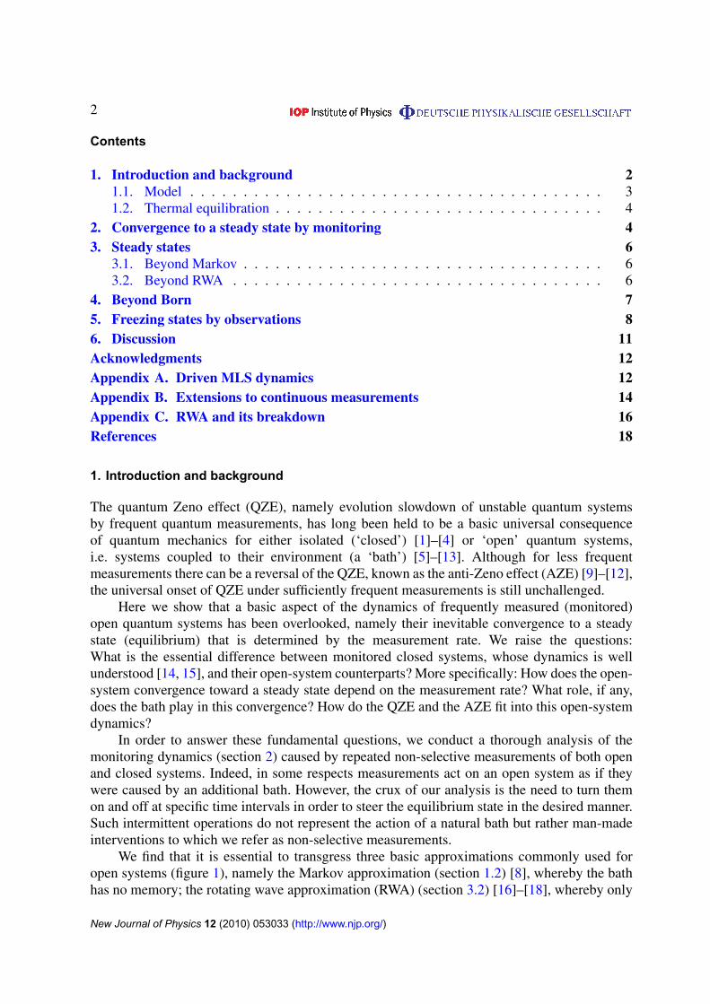
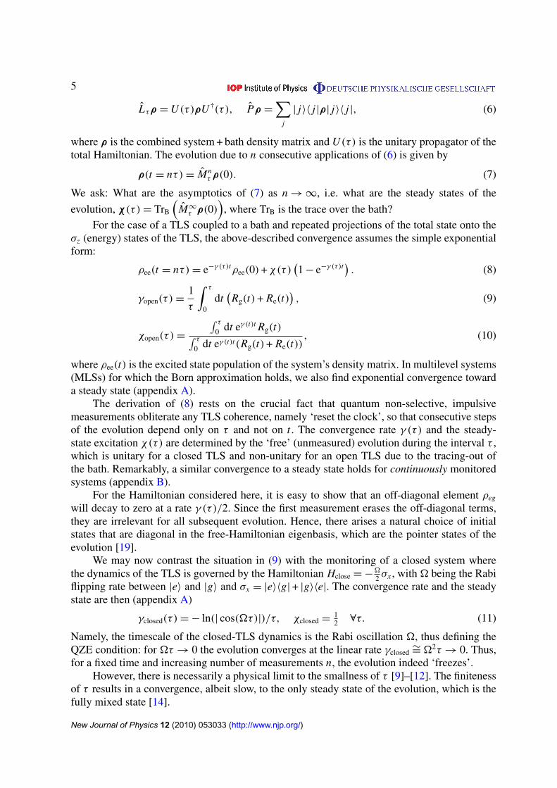
Figure 1. Steady states of the monitored open TLS as a function of τ for frequent(solid) and continuous (dotted) measurements under the complete Hamiltonian(without RWA) compared to their counterparts with RWA (dashed). A singleperiod (vertical dashed green line) delineates the transition to the RWA regime.The bath memory (correlation) time, tc (vertical dotted black line), delineatesthe transition to the Markov regime. The no-measurement limit (thermalequilibrium) is the saturation value in the Markovian time domain. Inset: thecorresponding rates of convergence γ (τ) for the three respective cases. The opensystem is a TLS with resonant frequency, ωa, coupled to an oscillator bath withthe Lorentzian coupling spectrum G0(ω) = (κ/ωa)(ω/(1 + (ω − ω0)

2t2c )), with

the following parameters: scaled coupling strength κ/ωa = 0.01, scaled inversetemperature βωa = 2, scaled correlation time ωatc = 10 and maximal couplingfrequency ω0 = 2ωa.

secular (near-resonant) energy exchange between the system and the bath affects the dynamics;and the Born approximation [8], whereby the bath state remains constant (section 6). We showthat deviations from these approximations have a dramatic influence on the convergence rate andsteady state of a monitored open system. An important corollary of the analysis is the possible‘freezing’ of states by choosing monitoring rates that set the equilibrium state to be the desiredone (section 5). The findings are then summarized and connected to existing results [19]–[23](section 6), particularly concerning pointer states and steady-state engineering.

1.1. Model

To answer the above questions, we first consider the well-studied model of a two-level system(TLS) coupled to a bath. With the free Hamiltonian H0 = ωaσz, the TLS is weakly coupledto a bath via Hopen = −gB(t)σx , with B(t) being an arbitrary bath operator in the interactionpicture.

New Journal of Physics 12 (2010) 053033 (http://www.njp.org/)

4

The reduced dynamics of the system is obtained to second order by a time-local non-Markovian master equation [17]. An initial state of the TLS that is diagonal in the H0 basisremains diagonal for all later times t . The coupling in Hopen is off-diagonal (σx ) to allowrelaxation of the level populations. These evolve according to the equation [17]

∂ρee(t)

∂t= −Re(t)ρee(t) + Rg(t)ρgg(t), (1)

where ρee(t) and ρgg(t) are the excited and ground state populations at time t satisfyingthe normalization condition ρee(t) + ρgg(t) = 1, with Re(t) and Rg(t) being their respectivetransition rates.

Under the weak coupling assumption (the Born approximation), these rates are givenas [17]

Re(g)(t) = 2t∫

∞

−∞

dωGT(ω)sinc[(ω ∓ ωa)t] . (2)

Here GT(ω), the Fourier transform of the bath correlation (response) function 〈B(0)B(t)〉T, isthe temperature-dependent coupling spectrum of the bath. The sinc function signifies the time-dependent uncertainty of the TLS level splitting centered at +ωa or −ωa.

1.2. Thermal equilibration

The longest timescale of relevance is the bath memory (correlation) time, tc, defined as theinverse width of GT(ω), which marks the transition from the non-Markovian to the Markovianmonitoring regime. In the Markovian regime, t � tc, the sinc function is much narrower than thecoupling spectrum GT(ω) and can be approximated by a delta function in frequency, resultingin

ρee(t � tc) = ρee(0)e−γ t + (ρee)Eq (1 − e−γ t), (3)

where the Markovian decay rate is given by

γ ≡1

t[Re + Rg](t � tc) = 2πGT(ωa). (4)

(ρee)Eq = e−βωa/2 cosh βωa is the temperature-dependent, bath-induced, equilibrium excitation.Equation (3) shows the convergence is at the Golden-Rule rate γ , to the steady state, which isthe thermal equilibrium state.

To examine whether the thermal equilibrium remains in the steady state under repeatedmeasurements, we study below the dynamics of a monitored (measured) TLS in the presence ofa bath.

2. Convergence to a steady state by monitoring

The problem at hand leads us to define the monitoring superoperator Mτ composed of a unitarypropagator over time τ , U (τ ), followed by a projector P corresponding to a non-selective,impulsive measurement in the basis of the system energy states | j〉 (of the free HamiltonianH0):

Mτρ = P Lτρ, (5)

New Journal of Physics 12 (2010) 053033 (http://www.njp.org/)

5

Lτρ = U (τ )ρU †(τ ), Pρ =

∑j

| j〉〈 j |ρ| j〉〈 j |, (6)

where ρ is the combined system + bath density matrix and U (τ ) is the unitary propagator of thetotal Hamiltonian. The evolution due to n consecutive applications of (6) is given by

ρ(t = nτ) = Mnτ ρ(0). (7)

We ask: What are the asymptotics of (7) as n → ∞, i.e. what are the steady states of the

evolution, χ(τ ) = TrB

(M∞

τ ρ(0))

, where TrB is the trace over the bath?

For the case of a TLS coupled to a bath and repeated projections of the total state onto theσz (energy) states of the TLS, the above-described convergence assumes the simple exponentialform:

ρee(t = nτ) = e−γ (τ)tρee(0) + χ(τ)(1 − e−γ (τ)t

). (8)

γopen(τ ) =1

τ

∫ τ

0dt(Rg(t) + Re(t)

), (9)

χopen(τ ) =

∫ τ

0 dt eγ (t)t Rg(t)∫ τ

0 dt eγ (t)t(Rg(t) + Re(t)), (10)

where ρee(t) is the excited state population of the system’s density matrix. In multilevel systems(MLSs) for which the Born approximation holds, we also find exponential convergence towarda steady state (appendix A).

The derivation of (8) rests on the crucial fact that quantum non-selective, impulsivemeasurements obliterate any TLS coherence, namely ‘reset the clock’, so that consecutive stepsof the evolution depend only on τ and not on t . The convergence rate γ (τ) and the steady-state excitation χ(τ) are determined by the ‘free’ (unmeasured) evolution during the interval τ ,which is unitary for a closed TLS and non-unitary for an open TLS due to the tracing-out ofthe bath. Remarkably, a similar convergence to a steady state holds for continuously monitoredsystems (appendix B).

For the Hamiltonian considered here, it is easy to show that an off-diagonal element ρeg

will decay to zero at a rate γ (τ)/2. Since the first measurement erases the off-diagonal terms,they are irrelevant for all subsequent evolution. Hence, there arises a natural choice of initialstates that are diagonal in the free-Hamiltonian eigenbasis, which are the pointer states of theevolution [19].

We may now contrast the situation in (9) with the monitoring of a closed system wherethe dynamics of the TLS is governed by the Hamiltonian Hclose = −

�

2 σx , with � being the Rabiflipping rate between |e〉 and |g〉 and σx = |e〉〈g| + |g〉〈e|. The convergence rate and the steadystate are then (appendix A)

γclosed(τ ) = − ln(| cos(�τ)|)/τ, χclosed =12 ∀τ. (11)

Namely, the timescale of the closed-TLS dynamics is the Rabi oscillation �, thus defining theQZE condition: for �τ → 0 the evolution converges at the linear rate γclosed

∼= �2τ → 0. Thus,for a fixed time and increasing number of measurements n, the evolution indeed ‘freezes’.

However, there is necessarily a physical limit to the smallness of τ [9]–[12]. The finitenessof τ results in a convergence, albeit slow, to the only steady state of the evolution, which is thefully mixed state [14].

New Journal of Physics 12 (2010) 053033 (http://www.njp.org/)

6

3. Steady states

The full landscape of measurement-induced steady states shown in figure 1 relies on twofeatures: (i) the interval between measurements is in the non-Markovian time domain; and (ii)the counter-rotating (CR) terms affect the system–bath interaction. The role played by eachfeature is detailed below.

3.1. Beyond Markov

In the non-Markovian regime, namely for τ 6 tc, the sinc function, representing energyuncertainty, and GT(ω) have comparable widths. This regime results in an oscillatory, non-monotonic dependence of the convergence rate on τ for a given coupling spectrum. As τ varies,γ (τ) alternates between speedup, as expected from the AZE [9]–[12], and slowdown. Likewise,the steady state of the evolution has a non-monotonic dependence on τ in this regime (figure 1).One can then reach a steady state that has higher or lower entropy than the thermal equilibrium,i.e. mix or purify the state upon choosing the appropriate measurement interval [17].

3.2. Beyond RWA

The shortest timescale of relevance is the natural oscillation period of the system, 1/ωa. Morefrequent measurements, τ � 1/ωa � tc, reveal another striking behavior:

γopen(τ � 1/ωa) = 40τ, χopen(τ � 1/ωa) ≈12 , (12)

where 0 =∫

∞

−∞dωGT(ω) is the total system–bath coupling strength. This timescale reveals

the closest analogue to the closed-system QZE, equation (11), in that the convergence rate islinear in τ and the steady state of the evolution is the fully mixed state. This shows that themanifestation of the QZE in open quantum systems paradoxically results in a fully mixed steadystate and not in ‘freezing’ the evolution.

On this timescale the energy spread 1/τ exceeds ωa; hence |e〉 and |g〉 becomeindiscriminate, so that the TLS may then absorb or emit quanta irrespective of the bath, atthe expense of the system–bath interaction energy. Remarkably, the QZE and the ensuing fullymixed steady state require monitoring on such a short timescale, as follows from (12). Thistimescale entails the breakdown of the RWA [17]. This means that the non-Markovian dynamicsby itself or, equivalently, the condition τ � tc does not suffice to ensure the QZE in opensystems, contrary to the prevailing view [5]–[12].

Why is the RWA breakdown mandatory for the QZE? A combined system–bathHamiltonian can always be decomposed into secular or rotating-wave (RW) and non-secularor CR parts (appendix C). The RWA neglects the CR terms since they are significant only atvery short times, i.e. ωat � 1. Yet, the QZE, whose signature is linear dependence of γ (τ) onτ , requires, according to (12), such ultrashort measurement intervals and thus must account forthe CR terms. Disregarding this fact and taking the RWA in the QZE regime, ωaτ � 1, yieldsa convergence ∝ τ , which has only half the magnitude of the convergence rate obtained fromthe complete Hamiltonian (appendix C). More importantly, the steady state under the RWA iswrong for such short τ : it strongly depends on the bath coupling spectrum, GT(ω), contraryto the steady state of the complete Hamiltonian that is the fully mixed state for the same τ

(appendix C) (figure 1).

New Journal of Physics 12 (2010) 053033 (http://www.njp.org/)

7

We can understand these novel results regarding the convergence to the steady state byconsidering the two competing aspects of open-system monitoring. The projective measure-ments of σz have quantum non-demolition (QND) effects on the system and hence preserve itsentropy, whereas the bath-induced evolution can either increase or decrease it, depending on thebath coupling spectrum, the evolution interval τ and the state of the system at that time. In thisrespect, the difference between the RW and CR dynamics is crucial. The RW terms preservethe combined system + bath state within the same energy subspaces, thus acting as if these weremany closed systems. The coupling strength and measurement interval determine the relativeweights of these subspaces. Hence, the RWA entails a strong dependence on the couplingspectrum and measurement interval, even in the QZE regime. By contrast, the CR terms mixthe energy subspaces, thereby turning the entire system–bath state into that of a single closedsystem, which should thus conform to (11). The shorter the measurement time interval, thelarger the contribution of the CR terms, resulting in an increasing entropy of the steady state.

4. Beyond Born

The major approximation in the above analysis is the Born approximation, under which the bathdoes not change from measurement to measurement and does not accumulate these changes inentropy. Thus, after each measurement, the relative contributions of the RW and CR terms aremaintained, allowing a wide range of steady states, as discussed above. Yet, these are strictlyspeaking quasi-steady states if the Born approximation is not exact: since the bath changes arecomparatively slower than the system dynamics, there could exist a timescale after which thecorrections in the bath state and the quasi-steady states of the system are no longer negligible.This introduces another timescale, namely the Born time tB, which depends on the bath size in amodel-specific fashion: whereas for t � tB the Born approximation holds and the convergenceto (9) applies, for t > tB the approximation breaks down and the accumulated bath changes startto influence the system dynamics (figures 2(a) and (b)).

The monitored (system + bath) dynamic equations (5)–(7) still hold without the Bornapproximation, but do they yield convergence to a steady state that depends on τ? RepeatedQND measurements of the system erase the system–bath coherences, thereby increasing thetotal entropy of the combined (system + bath) state. On the other hand, the free evolutionbetween measurements is unitary in the combined system + bath Hilbert space and thuspreserves the entropy. Where does this interplay lead to?

To answer this question, let us examine the structure of the combined density matrix, ρtot,of the system plus N -mode bath in two scenarios: (i) If the RWA applies (i.e. τ is not soshort that (12) holds), then ρtot is block-diagonal in N × N subspaces, with total energy En,n = 0 . . . ∞. The system + bath energy subspaces remain closed, and accumulate the entropyincrease resulting from the measurements (figure 3(b)). The steady state of each such subspaceconforms to closed-system dynamics (appendix A) i.e. is the fully mixed state, regardless ofτ (figure 2, main panel). The overall steady state in this scenario depends on the relativecontributions of the En-subspaces, which in turn depend solely on the bath coupling spectrum.Hence, only GT(ω) (cf (2)) determines the steady state.

(ii) In the other scenario where the RWA does not apply, the CR terms mix all thesubspaces and effectively render the combined system + bath state that of a single closed system(figure 3(b)). The steady state of such an effectively closed system, subject to entropy-increasingmeasurements and entropy-preserving evolution, can only be the fully mixed state. Hence, under

New Journal of Physics 12 (2010) 053033 (http://www.njp.org/)

8

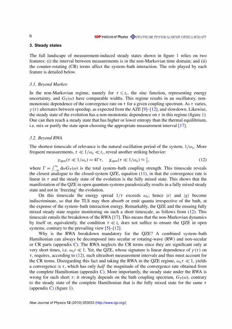
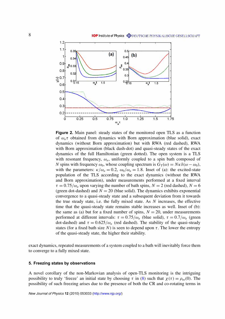
Figure 2. Main panel: steady states of the monitored open TLS as a functionof ωaτ obtained from dynamics with Born approximation (blue solid), exactdynamics (without Born approximation) but with RWA (red dashed), RWAwith Born approximation (black dash-dot) and quasi-steady states of the exactdynamics of the full Hamiltonian (green dotted). The open system is a TLSwith resonant frequency, ωa, uniformly coupled to a spin bath composed ofN spins with frequency ω0, whose coupling spectrum is GT(ω) = Nκδ(ω − ω0),with the parameters: κ/ωa = 0.2, ω0/ωa = 1.8. Inset of (a): the excited-statepopulation of the TLS according to the exact dynamics (without the RWAand Born approximation), under measurements performed at a fixed intervalτ = 0.75/ωa upon varying the number of bath spins, N = 2 (red dashed), N = 6(green dot-dashed) and N = 20 (blue solid). The dynamics exhibits exponentialconvergence to a quasi-steady state and a subsequent deviation from it towardsthe true steady state, i.e. the fully mixed state. As N increases, the effectivetime that the quasi-steady state remains stable increases as well. Inset of (b):the same as (a) but for a fixed number of spins, N = 20, under measurementsperformed at different intervals: τ = 0.75/ωa (blue solid), τ = 0.7/ωa (greendot-dashed) and τ = 0.625/ωa (red dashed). The stability of the quasi-steadystates (for a fixed bath size N ) is seen to depend upon τ . The lower the entropyof the quasi-steady state, the higher their stability.

exact dynamics, repeated measurements of a system coupled to a bath will inevitably force themto converge to a fully mixed state.

5. Freezing states by observations

A novel corollary of the non-Markovian analysis of open-TLS monitoring is the intriguingpossibility to truly ‘freeze’ an initial state by choosing τ in (8) such that χ(τ) = ρee(0). Thepossibility of such freezing arises due to the presence of both the CR and co-rotating terms in

New Journal of Physics 12 (2010) 053033 (http://www.njp.org/)

9

ClosedBornNo RWA

No BornRWA

No BornNo RWA

RW CR

(a) (b)

0.5No RWA RWA No RWA

1

2

E

E

RW CRCR

IndependentdependentTG

d d

2

RW

CR

0.0dependent

nEtotal

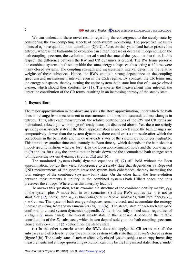
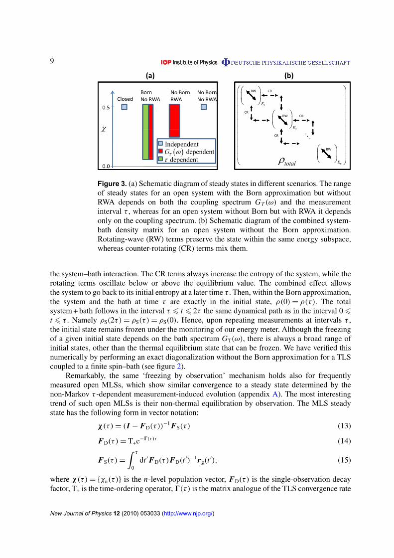
Figure 3. (a) Schematic diagram of steady states in different scenarios. The rangeof steady states for an open system with the Born approximation but withoutRWA depends on both the coupling spectrum GT (ω) and the measurementinterval τ , whereas for an open system without Born but with RWA it dependsonly on the coupling spectrum. (b) Schematic diagram of the combined system-bath density matrix for an open system without the Born approximation.Rotating-wave (RW) terms preserve the state within the same energy subspace,whereas counter-rotating (CR) terms mix them.

the system–bath interaction. The CR terms always increase the entropy of the system, while therotating terms oscillate below or above the equilibrium value. The combined effect allowsthe system to go back to its initial entropy at a later time τ . Then, within the Born approximation,the system and the bath at time τ are exactly in the initial state, ρ(0) = ρ(τ). The totalsystem + bath follows in the interval τ 6 t 6 2τ the same dynamical path as in the interval 06t 6 τ . Namely ρS(2τ) = ρS(τ ) = ρS(0). Hence, upon repeating measurements at intervals τ ,the initial state remains frozen under the monitoring of our energy meter. Although the freezingof a given initial state depends on the bath spectrum GT(ω), there is always a broad range ofinitial states, other than the thermal equilibrium state that can be frozen. We have verified thisnumerically by performing an exact diagonalization without the Born approximation for a TLScoupled to a finite spin–bath (see figure 2).

Remarkably, the same ‘freezing by observation’ mechanism holds also for frequentlymeasured open MLSs, which show similar convergence to a steady state determined by thenon-Markov τ -dependent measurement-induced evolution (appendix A). The most interestingtrend of such open MLSs is their non-thermal equilibration by observation. The MLS steadystate has the following form in vector notation:

χ(τ ) = (I − FD(τ ))−1 FS(τ ) (13)

FD(τ ) = T+e−0(τ )τ (14)

FS(τ ) =

∫ τ

0dt ′ FD(τ )FD(t ′)−1rg(t

′), (15)

where χ(τ ) = {χn(τ )} is the n-level population vector, FD(τ ) is the single-observation decayfactor, T+ is the time-ordering operator, 0(τ ) is the matrix analogue of the TLS convergence rate

New Journal of Physics 12 (2010) 053033 (http://www.njp.org/)

10

10−1

100

101

1020

0.05

0.1

0.15

0.2

0.25

0.3

ωaτ

χ n(τ)

MarkovRWA

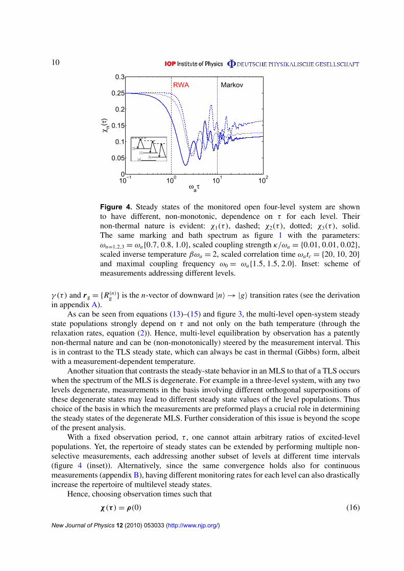
Figure 4. Steady states of the monitored open four-level system are shownto have different, non-monotonic, dependence on τ for each level. Theirnon-thermal nature is evident: χ1(τ ), dashed; χ2(τ ), dotted; χ3(τ ), solid.The same marking and bath spectrum as figure 1 with the parameters:ωn=1,2,3 = ωa{0.7, 0.8, 1.0}, scaled coupling strength κ/ωa = {0.01, 0.01, 0.02},scaled inverse temperature βωa = 2, scaled correlation time ωatc = {20, 10, 20}

and maximal coupling frequency ω0 = ωa{1.5, 1.5, 2.0}. Inset: scheme ofmeasurements addressing different levels.

γ (τ) and rg = {R(n)g } is the n-vector of downward |n〉 → |g〉 transition rates (see the derivation

in appendix A).As can be seen from equations (13)–(15) and figure 3, the multi-level open-system steady

state populations strongly depend on τ and not only on the bath temperature (through therelaxation rates, equation (2)). Hence, multi-level equilibration by observation has a patentlynon-thermal nature and can be (non-monotonically) steered by the measurement interval. Thisis in contrast to the TLS steady state, which can always be cast in thermal (Gibbs) form, albeitwith a measurement-dependent temperature.

Another situation that contrasts the steady-state behavior in an MLS to that of a TLS occurswhen the spectrum of the MLS is degenerate. For example in a three-level system, with any twolevels degenerate, measurements in the basis involving different orthogonal superpositions ofthese degenerate states may lead to different steady state values of the level populations. Thuschoice of the basis in which the measurements are preformed plays a crucial role in determiningthe steady states of the degenerate MLS. Further consideration of this issue is beyond the scopeof the present analysis.

With a fixed observation period, τ , one cannot attain arbitrary ratios of excited-levelpopulations. Yet, the repertoire of steady states can be extended by performing multiple non-selective measurements, each addressing another subset of levels at different time intervals(figure 4 (inset)). Alternatively, since the same convergence holds also for continuousmeasurements (appendix B), having different monitoring rates for each level can also drasticallyincrease the repertoire of multilevel steady states.

Hence, choosing observation times such that

χ(τ ) = ρ(0) (16)

New Journal of Physics 12 (2010) 053033 (http://www.njp.org/)

11

results in ‘freezing’ of the initial state for any number of measurements, even for non-thermalstates. This ‘freezing’ is not related to the one associated with the QZE, since it does not requirean extremely short measurement interval. On the contrary, this non-Markovian freezing appliesonly for a specific value of τ and for any number of measurements, constituting a more robustand lasting state-shelving mechanism than the QZE.

6. Discussion

Our analysis has revealed a cohesive picture of hitherto unnoticed, general anomalies offrequently probed quantum systems coupled to arbitrary (e.g. oscillator or spin) baths: (i)Whereas bath-induced inter-level transition rates in open systems exhibit slowdown underenergy measurements that are frequent enough to conform to the QZE, the system does notretain its state as the measurements accumulate, but rather exhibits measurement-inducedconvergence toward an asymptotic steady state (equations (8)–(10)). (ii) In the QZE regime, themore frequent the measurements, the higher the asymptotic excitation and entropy. This reflectsthe remarkable fact that the QZE dynamics does not conform to the RWA and must accountfor CR terms in the system–bath interaction Hamiltonian (equations (8) and (10), (appendix C).(iii) Convergence to a maximal-entropy steady state may be avoided, within a limited range ofinitial excitations, by choosing the measurement rate capable of ‘freezing’ the initial state. (iv)Finally, at times beyond the Born time tB (figure 2(a)), the steady state of a frequently measuredopen system no longer depends on the measurement interval. Rather, under the RWA, it dependssolely on the bath coupling spectrum, whereas without the RWA, it can be the fully mixed state(figure 2(b)).

We stress that our findings can be tested in a variety of quantum systems coupled to bathswhose non-Markovian timescales are experimentally accessible, e.g. ultracold atoms coupledto phonon baths [20], electron spins coupled to nuclear spins [21] or emitters with microwavetransitions coupled to a cavity mode [22].

It is instructive to contrast the present findings with previous approaches to asymptoticsteady states: (i) Since in our monitoring dynamics, any off-diagonal elements present in theinitial state eventually decay to zero, one can identify the energy eigenstates of the systemwith the pointer basis [19]. However, our non-Markov treatment allows us to go a step furtherand show how one can choose specific pointer states that are maximally stable, for a givenobservation rate. (ii) Another approach [23] has been to engineer the quantum jump operatorsthrough which the system couples to the bath, so as to achieve the desired end state of thesystem evolution. Whereas this end state is reached via Markovian dynamics, our treatmentdraws on the richness of non-Markovian dynamics to achieve diverse steady states. Furthermore,manipulating the jump operators is equivalent to an external control over the system–bathinteraction, assuming that the required control is at our disposal. In our approach, such controlis not required: instead, manipulations are effected by the detector, which couples to the systemalone and does not directly act on the system–bath coupling.

To conclude, the present findings shed new light on a fundamental issue at the interfaceof quantum measurement theory and the quantum dynamics of open systems: the interplaybetween measurement-induced and bath-induced rotating and counter-rotating non-Markoviandynamics. In particular, they essentially revise the notion of evolution freezing that has longbeen associated with the QZE.

New Journal of Physics 12 (2010) 053033 (http://www.njp.org/)

12

Acknowledgments

The support of the EC (MIDAS STREP), the DIP and the ISF is acknowledged. GK is supportedby the Meitner-Humboldt Prize.

Appendix A. Driven MLS dynamics

A.1. Closed MLS

Consider a driven, closed MLS with a ground state and N excited states, |g〉 and |n〉,respectively, with n = 1, . . . , N and energy separations hωn. Each excited level is drivenby a resonant field, with a constant Rabi frequency �n. The corresponding Hamiltonian is(henceforth we take h = 1):

Hclose =

N∑n=1

ωn|n〉〈n| +N∑

n=1

(�n|n〉〈g| + h.c.) . (A.1)

The resulting rate equations are given by:

ρgg = iN∑

n=1

�n(ρng − ρgn), (A.2)

ρnn′ = i�nρgn′ − i�n′ρng, (A.3)

ρgn = iN∑

n=1

�n′ρn′n − i�nρgg. (A.4)

Since the Rabi frequencies are time independent, the dynamics can be solved bydiagonalizing an (N + 1)2

× (N + 1)2 matrix. The matrix eigenvalues are the oscillationfrequencies of the system. The eigenvectors whose eigenvalues are equal to zero are thestationary states of the system.

We now show that for a three-level system, N = 2, the only diagonal linear combinationof eigenstates with zero eigenvalue is the fully mixed state. The matrix eigenvalues are

{0, ±√

�(1) ±√

�(2), ±√

�21 + �2

2}, where �(1)= 2�2

1 + �1�2 + 2�22 and �(2)

= 4�21 + �1�2 +

4�22. The three eigenstates with eigenvalue 0 are

ρa = {0, 1, 1, 1, 0, 0, 1, 0, 0}, (A.5)

ρb = {�1/�2, 0, 0, 0, (−�22 + �2

1)/�1/�2, 1, 0, 1, 0}, (A.6)

ρc = {1, 0, 0, 0, 1, 0, 0, 0, 1}, (A.7)

where ρ = {ρgg, ρ1g, ρ2g, ρg1, ρ11, ρ21, ρg2, ρ12, ρ22}. One can see that ρc is the identity, i.e.the fully mixed state, and is the only steady state of the closed MLS, since no other linearcombination of ρa and ρb can give a diagonal density matrix.

As a simple example, we consider a TLS. The closed σx -driven TLS dynamics is describedby Bloch equations, and in the absence of measurements it yields the Rabi oscillation

〈σz(τ )〉 = 〈σz(0)〉 cos(�τ) + 〈σy(0)〉 sin(�τ). (A.8)

New Journal of Physics 12 (2010) 053033 (http://www.njp.org/)

13

The impulsive, non-selective measurements of σz eliminate the off-diagonal terms, resulting in〈σy(0)〉 = 0 after every measurement. We then obtain

ρ(m+1)ee (τ ) = cos(�τ)ρ(m)

ee + 12 (1 − cos(�τ)) . (A.9)

We can cast this recursion relation in the form of exponential convergence, equation (8), withconvergence rate and steady state given by equation (11).

A.2. Open MLS

Consider an open (N + 1)-level MLS that is weakly coupled to a thermal bath with modeenergies hωλ. The coupling to the finite-temperature bath may differ from one excited stateto another. The total Hamiltonian is given by

Hopen = HS + HB + HSB HB =

∑λ

ωλa†λaλ, (A.10)

HS =

N∑n=1

ωn|n〉〈n|, (A.11)

HSB =

N∑n=1

σx,n Bn =

N∑n=1

∑λ

σx,n(κλ,naλ + κ∗

λ,na†λ), (A.12)

where σx,n = |n〉〈g| + |g〉〈n| is the nth X-Pauli matrix and κλ,n is the coupling coefficient of leveln to the bath mode λ. Note that we do not invoke the RWA.

Henceforth we shall adopt the Born approximation [8], whereby the bath remains constantthroughout the evolution.

Using Zwanzig’s projection-operator technique to trace out the bath in the Liouvilleequation of motion [17, 24] and then transferring to the interaction picture, where ρ(t) =

eiHStρ(t)e−iHSt , we have derived, to second order in the system–bath coupling, the non-Markovian master equation:

˙ρ =

N∑n,n′=1

∫ t

0dτ{8T,nn′(t − τ)

[Sn′(τ )ρ, Sn(t)

]+ h.c.

}, (A.13)

where 8T,nn′(t − t ′) = 〈Bn(t)Bn′(t ′)〉 is the finite-temperature system–bath correlation functionfor levels n, n′, and Sn(t) = eiωn t

|n〉〈g| + h.c.One can write the density matrix in the following form:

ρ = ρgg|g〉〈g| +N∑

n,n′=1

ρnn′|n〉〈n′| +∑n=1

(ρgn|g〉〈n| + ρng|n〉〈g|), (A.14)

where we have deliberately separated the ρgn terms from the ρnn′ terms. The equations forρgn are independent of the other terms in the density matrix. Hence, once they are set to zeroby a measurement, they remain so (do not evolve) after the measurement and are henceforthdisregarded.

For the vector defined as ρD= {ρnn}

T, n = 1, . . . , N , the evolution between consecutivemeasurements of the energy separated by τ can then be solved, to second order in thesystem–bath coupling, in the matrix form

ρD(τ ) = FD(τ )ρD(0) + FS(τ ), (A.15)

New Journal of Physics 12 (2010) 053033 (http://www.njp.org/)

14

where FD(τ ) and FS(τ ) are given in equations (14) and (15), respectively. The elements of thematrix analogue of the TLS convergence rate are given by

0nn′(t) =1

τ

∫ t

0dt ′

[δnn′(Rn(t

′) + R(n)g (t ′)) + R(n)

g (t ′)(1 − δnn′)], (A.16)

where δnn′ is Kronecker’s delta. The transition rates Rn(t) from |n〉 to |g〉 and Rg(t) from |g〉 to|n〉 are explicitly analyzed in [17].

Taking into account that a QND measurement of the MLS energy levels at t = 0 eliminatesall off-diagonal terms in the density matrix, i.e. ρnn′(0) = 0 for n 6= n′, we can integrate theequations of motion. The resulting ρnn′(t) are of fourth order in the system–bath coupling.Hence, we can neglect the off-diagonal elements in the dynamics of the diagonal elements.

Consecutive impulsive measurements of the energy levels n, separated by τ , yield, usingequations (13)–(A.16):

ρD(t = nτ) = FnD(τ )ρD(0) + (I − FD(τ ))−1

(I − Fn

D(τ ))

FS(τ ). (A.17)

By virtue of (14) and 0(τ ) being a real and positive definite matrix, FnD(τ ) → 0 as n → ∞. The

state ρD therefore converges to a steady state

χ(τ ) = (I − FD(τ ))−1 FS(τ ). (A.18)

Hence, equations (A.13)–(A.17) show that an MLS weakly coupled to a bath always exponen-tially converges to a steady state, χ(τ ), as the number of energy measurements increases.

Appendix B. Extensions to continuous measurements

B.1. Closed TLS

The continuous measurement of σz in a σx -driven closed TLS close system is described by thefollowing ME, to second order in the coupling to the measuring device [8]

ρ(t) =i�

2[σx , ρ(t)] −

1

2τ[σz, [σz, ρ(t)]], (B.1)

where τ expresses the inverse of the measurement strength or, equivalently, the effectivemeasurement interval. The solution after total monitoring time T conforms to equation (8)with

e−γclosed(τ )T=

µ2e−µ1T− µ1e−µ2T

µ2 − µ1, (B.2)

µ1,2 =1

τ

(1 ±

√1 − (�τ)2

), (B.3)

χclosed =12 . (B.4)

The real parts of the exponents in (B.2) are positive: µ1,2 > 0.We thus see that the monitoring dynamics is similar for impulsive frequent measurements

and continuous measurements.

B.2. Open TLS

Continuous measurements of an open quantum system may be described as stationary randomdephasing, at a rate 1/τ [13, 25]. The Hamiltonian then has a randomly fluctuating energy (σz)

New Journal of Physics 12 (2010) 053033 (http://www.njp.org/)

15

term in addition to the term of σx coupling to the bath:

Hopen = δr(t)σz − gB(t)σx . (B.5)

The corresponding ME, to second order in the system–bath coupling, assuming an initialproduct state of the form ρS(t) ⊗ ρB , can then be written as

ρ(t) =

∫ t

0dt ′

{8(t − t ′)[S(t), [S(t ′), ρ(t)]] + h.c.

}(B.6)

S(t) = e−iωa t−i∫ t

0 dt ′δr (t ′)σ+ + h.c., (B.7)

where the overbar denotes the ensemble average and 8T(t − t ′) = 〈B(t)B(t ′)〉 is the bathcorrelation (response) function.

The Bloch equations derived from (B.6) have the form

ρee(t) = −ρgg(t) = −Re(t)ρee(t) + Rg(t)ρgg(t). (B.8)

After time t � τ , i.e. monitoring over time that is equivalent to several measurements,the transition rates can be shown to be time independent and acquire the following spectralform [13, 25]:

Re(g)(τ ) = 2π

∫∞

−∞

dωGT(ω)Fτ (ω ∓ ωa), (B.9)

Fτ (ω) = π−1Re∫

∞

0dt′ei

∫ t ′

0 dt ′′δr (t ′′)eiωt ′ . (B.10)

In the limit of a broad spectrum, i.e. white noise, the ensemble average causes the stochastic

dephasing of the phase factor associated with δr(t): ei∫ t

t ′ dt ′′δr (t ′′) = e−(t−t ′)/τ , resulting in

Fτ (ω) =τ

π

1

1 + (ωτ)2. (B.11)

Thus, continuous measurements, modeled by a stochastic dephasing process with correlationtime τ , are described by Fτ (ω) being a Lorentzian of width 1/τ .

The exact solution to equation (B.8) is

ρee(T ) = e−γ (τ)T ρee(0) +∫ T

0dt ′e−γ (τ)(T −t ′) Rg(τ ), (B.12)

γ (t) = Rg(τ ) + Re(τ ). (B.13)

The exponential decay of the first term in (B.12) implies convergence to the steady state, whichconform to equations (8)–(10), with

χopen(τ ) =Rg(τ )

γ (τ ). (B.14)

B.3. Open MLSs

Similarly to the TLS scenario, continuous measurements of MLSs may be described as randomdephasing [13, 25]. In the multilevel case, each level may experience different dephasing rate

New Journal of Physics 12 (2010) 053033 (http://www.njp.org/)

16

1/τn, expressed as an additional factor in equation (A.11):

HS =

N∑n=1

(ωn + δr,n(t))|n〉〈n| (B.15)

Sn(t) = e−iωn t−i∫ t

0 dt ′δr,n(t ′)|n〉〈g| + h.c. (B.16)

Furthermore, the continuous measurement-induced dephasing of each level is uncorrelated to

the other levels’ dephasing, resulting in Sn(t)Sn′(t ′) = 0, ∀n 6= n′. This results in the diagonalvector dynamics:

ρD(t) = FD(t)ρD(0) + FS(t), (B.17)

with FD(t) and FS(t) given in equations (14), (15) and (A.16), with the transition rates Rn(t)and Rg(t) given by

Rn(t) = 2π

∫∞

−∞

dωGT(ω)Ft,n(ω − ωn), (B.18)

Rg(t) = 2π

∫∞

−∞

dωGT(ω)Ft,n(ω + ωn), (B.19)

Ft,n(ω) =τn

π

1

1 + (ωτn)2. (B.20)

Appendix C. RWA and its breakdown

C.1. σx -coupling to a thermal bath in the RWA

For a TLS coupled to a thermal bath with mode energies hωλ, the RWA Hamiltonian has theform

HS = ωa|e〉〈e|, HB =

∑λ

ωλa†λaλ, HI = B−σ+ + B+σ−, (C.1)

B− =

(∑λ

κλaλ

), B+ =

(∑λ

κ∗

λa†λ

), (C.2)

σ+ = |e〉〈g|, σ− = |g〉〈e| and aλ(a†λ) are the annihilation (creation) operators of mode λ of the

bath.Using the same procedure as in [13, 17, 24, 26], one arrives at the following transition

rates, RRWAe (|e〉 → |g〉) and RRWA

g (|g〉 → |e〉):

RRWAe(g) (t) = 2π t

∫∞

0dωGRWA

T ±(ω)sinc [(ω ∓ ωa)t] , (C.3)

where

GRWAT + (ω) = (nT (ω) + 1) G0(ω), (C.4)

GRWAT −

(ω) = nT (−ω)G0(−ω), (C.5)

New Journal of Physics 12 (2010) 053033 (http://www.njp.org/)

17

G0(ω) = |κλ|2δ(ω − ωλ), (C.6)

nT (ω) =(eβω

− 1)−1

, (C.7)

where β = 1/kBT is the inverse temperature of the bath.Thus, the |e〉 → |g〉 rate in the RWA is the overlap of GT and the sinc over positive

frequencies. At zero temperature, it survives due to the vacuum contribution (spontaneousdecay rate). The |g〉 → |e〉 rate in the RWA is the overlap of GT and the sinc over the negativefrequencies. It vanishes at zero temperature since it does not have the vacuum contribution.Clearly, the two transition rates are influenced by different coupling spectra, GRWA

T + and GRWAT −

inthe RWA.

C.2. σx -coupling to a thermal bath without RWA

Without RWA,

HI = σx B, B =

∑λ

(κλaλ + κ∗

λa†λ

), (C.8)

where σx = |e〉〈g| + |g〉〈e|. This HI can be decomposed into secular (RW) and non-secular (CR)parts:

HI = (B−σ+ + B+σ−)︸ ︷︷ ︸RW

+ (B+σ+ + B−σ−)︸ ︷︷ ︸CR

. (C.9)

Now, the |e〉 → |g〉 and |g〉 → |e〉 transition rates are given by

Re(g)(t) = 2π t∫

∞

−∞

dωGT(ω)sinc [(ω ∓ ωa)t], (C.10)

GT(ω) = (nT(ω) + 1) G0(ω) + nT(−ω)G0(−ω). (C.11)

Hence, both transition rates are given by the overlap over the entire range of frequencies(positive and negative) and therefore are influenced by the same coupling spectra.

C.3. Comparison of RWA and non-RWA decoherence rates

We compare the resulting transition rates with and without the RWA in two limits: (i) theMarkovian long time limit, where sinc[(ω ± ωa)t] ≈ δ(ω ± ωa)/t , and (ii) the QZE ultrashorttime limit, where sinc[(ω ± ωa)t] ≈ 1.

(i) The Markovian limit. In the Markovian long-time regime, one has the following results:

RRWAe = Re = 2π(nT(ωa) + 1)G0(ωa), (C.12)

RRWAg = Rg = 2πnT(ωa)G0(ωa), (C.13)

Re

Rg= eβωa . (C.14)

One can draw two conclusions: (a) The rates obtained with and without the RWA are the same inthe Markovian long-time regime. (b) The ratio of these rates conforms to the thermal equilibrium(Gibbs) state of the system.

New Journal of Physics 12 (2010) 053033 (http://www.njp.org/)

18

(ii) The QZE limit. In the ultrashort time limit, one obtains the following results:

RRWAe = 2π t

∫∞

−∞

dω(nT(ω) + 1)G0(ω), (C.15)

RRWAg = 2π t

∫∞

−∞

dωnT(ω)G0(ω) (C.16)

RRWAe

RRWAg

= eβRWAωa , Re = Rg = RRWAe + RRWA

g ,Re

Rg= 1. (C.17)

One can draw the following conclusions: (a) The RWA changes the results drastically in thislimit, indicating that the RWA does not hold there. (b) The RWA effective temperature is finiteand depends on the characteristics of the bath, whereas the non-RWA effective temperature isinfinite and does not depend on the bath. These features can be explained by the fact that atultrashort times after a measurement, the energy uncertainty is so large that the TLS couples toall modes of the bath, at both positive and negative energies, and therefore there is no distinctionbetween the ground and excited states as regards their coupling to the bath. By contrast, the RWAincreasingly distinguishes between the two as t decreases.

References

[1] Khalfin L A 1968 JETP Lett. 8 65–8[2] Fonda L, Ghirardi G, Rimini A and Weber T 1973 Nuouo Cimento A 15 689[3] Misra B and Sudarshan E C G 1977 J. Math. Phys. 18 756–63[4] Itano W M, Heinzen D J, Bollinger J J and Wineland D J 1990 Phys. Rev. A 41 2295–300[5] Kofman A G and Kurizki G 1996 Phys. Rev. A 54 R3750–3[6] Plenio M B, Knight P L P and Thompson R C 1996 Opt. Commum. 123 278[7] Mihokova E, Pascazio S and Schulman L S 1997 Phys. Rev. A 56 25–32[8] Breuer H P and Petruccione F 2002 The Theory of Open Quantum Systems (Oxford: Oxford University Press)[9] Kofman A G and Kurizki G 2000 Nature 405 546–50

[10] Fischer M C, Gutierrez-Medina B and Raizen M G 2001 Phys. Rev. Lett. 87 040402[11] Lane A M 1983 Phys. Lett. A 99 359–60[12] Facchi P and Pascazio S 2001 Prog. Opt. 42 147[13] Gordon G 2009 J. Phys. B: At. Mol. Opt. Phys. 42 223001[14] Milburn G J 1988 J. Opt. Soc. Am. B 5 1318[15] Mozyrsky D and Martin I 2002 Phys. Rev. Lett. 89 018301[16] Cohen-Tannoudji C, Dupont-Roc J and Grynberg G 1992 Atom–Photon Interactions (New York: Wiley)[17] Kofman A G and Kurizki G 2004 Phys. Rev. Lett. 93 130406[18] Zheng H, Zhu S Y and Zubairy M S 2008 Phys. Rev. Lett. 101 200404[19] Paz J P and Zurek W H 1999 Phys. Rev. Lett. 82 5181–5[20] Recati A, Fedichev P O, Zwerger W, von Delft J and Zoller P 2005 Phys. Rev. Lett. 94 040404[21] Hanson R, Dobrovitski V V, Feiguin A E, Gywat O and Awschalom D D 2008 Science 320 352–5[22] Guerlin C, Bernu J, Deleglise S, Sayrin C, Gleyzes S, Kuhr S, Brune M, Raimond J M and Haroche S 2007

Nature 448 889–93[23] Diehl S, Micheli A, Kantian A, Kraus B, Bchler H P and Zoller P 2008 Nature Phys. 4 878–83[24] Kofman A G and Kurizki G 2005 Trans IEEE. Nanotechnol. 4 116[25] Gordon G, Kurizki G, Mancini S, Vitali D and Tombesi P 2007 J. Phys. B: At. Mol. Opt. Phys. 40 S61[26] Gordon G 2008 Eur. Phys. Lett. 83 30009

New Journal of Physics 12 (2010) 053033 (http://www.njp.org/)