arX

iv:1

112.

3829

v2 [

quan

t-ph

] 4

Feb

201

2

Quantum Zeno effect: Quantum shuffling and Markovianity

A. S. Sanz∗, C. Sanz-Sanz, T. Gonzalez-Lezana, O. Roncero, S. Miret-Artes

Instituto de Fısica Fundamental (IFF–CSIC), Serrano 123, 28006 Madrid, Spain

Abstract

The behavior displayed by a quantum system when it is perturbed by a series of von Neumann measurementsalong time is analyzed. Because of the similarity between this general process with giving a deck of playingcards a shuffle, here it is referred to as quantum shuffling, showing that the quantum Zeno and anti-Zenoeffects emerge naturally as two time limits. Within this framework, a connection between the gradualtransition from anti-Zeno to Zeno behavior and the appearance of an underlying Markovian dynamics isfound. Accordingly, although a priori it might result counterintuitive, the quantum Zeno effect correspondsto a dynamical regime where any trace of knowledge on how the unperturbed system should evolve initiallyis wiped out (very rapid shuffling). This would explain why the system apparently does not evolve or decayfor a relatively long time, although it eventually undergoes an exponential decay. By means of a simpleworking model, conditions characterizing the shuffling dynamics have been determined, which can be ofhelp to understand and to devise quantum control mechanisms in a number of processes from the atomic,molecular and optical physics.

Key words: Quantum shuffling, Quantum Zeno effect, Anti-Zeno effect, Measurement theory,von Neumann measurement, Markov chain

1. Introduction

The legacy of Zeno of Elea becomes very apparent through calculus, the pillar of physics. It is not difficultto find manifestations of his famous paradoxes throughout the subtleties of any of our physical theories [1].In quantum mechanics, for example, Zeno’s paradox of the arrow is of particular interest, for it has givenrise to what is now known as quantum Zeno effect (QZE), which constitutes an active field of research [2].As conjectured by Misra and Sudarshan [3], this effect essentially consists of inhibiting the evolution of anunstable quantum system by a succession of shortly-spaced measurements —a classical analog of this effectis the watched-pot paradox: a watched pot never boils [4]—, although, generally speaking, it could also bea system acted by some environment or even the bare evolution of the system if the latter is not describedby a stationary state. The inhibition of the evolution of a quantum system, though, was already noted byvon Neumann [5] and others —an excellent account on the historical perspective of the QZE can be foundin [2]. From an experimental viewpoint, this effect was formerly detected by Itano et al. [6] considering theoscillations of a two-level system, a modification suggested by Cook [7] of the original theoretical proposal.Nonetheless, the first experimental evidences with unstable systems, as originally considered by Misra andSudarshan, were observed later on by Raizen’s group [8, 9]. Indeed, in the second experiment reported bythis group in this regard [9], it was also shown the possibility to enhance the system decay by consideringmeasurements more spaced in time. This is the so-called (quantum) anti-Zeno effect (AZE) [10–12].

In the literature, it is common to introduce the QZE and the AZE as antagonist, competing effects. Inthis work, however, we study their manifestation within a unifying framework, where they constitute the

∗Corresponding authorEmail address: asanz@iff.csic.es (A. S. Sanz)

Preprint submitted to Annals of Physics February 7, 2012

two limiting cases of a more general process that we shall refer to as quantum shuffling. To understandthis concept, consider a series of von Neumann measurements is performed on a quantum system, i.e.,measurements such that the outcome has a strong correlation with the measured quantity, thus implyinga high degree of certainty on the post-measured system state. This type of measurements provoke thesystem to collapse into any of the pointer states of the measuring device, breaking the time coherencethat characterizes its unitary time-evolution. In other words, the continuity in time between the pre andpost-measurement states of the system is irreversibly lost. This loss takes place even when the distance(in time) between the two states is so close that, in modulus, they look pretty much the same, due to thecorresponding loss of the phase accumulated with time (which is a signature of the unitary time-evolutionand therefore of the possibility to revert the process in time). Thus, consider the system is not stationary(regardless of the nature of the source that leads to such non-stationarity), decaying monotonically in timeat a certain rate. A series of measurements on this system will act similarly to giving a deck of orderedcards a shuffle —hence the name of quantum shuffling—, affecting directly its coherence and modifying itsnatural (unperturbed) decay time-scale. As it is shown here, depending on the relative ratio between thenatural time-scale and the shufflingly-modified one, the system decay can be either delayed or enhanced. Ifthe shuffling frequency (i.e., the amount of measurements per time unit) is relatively low with respect to thesystem natural decay rate, the pre and post-measurement system states will be very different. This turns intoa very fast decay due to the important lack of correlation between both states. Within the standard Zenoscenario, this enhancement of the decay corresponds to AZE. On the contrary, if the shuffling is relativelyfast, the pre and post-measurement states will be rather similar, for the system did not have time enoughto evolve importantly. The decay is then slower, giving rise to QZE. Now, as it is also shown, this inhibitionof the system decay is only apparent: the fast shuffling gives rise to an overall exponential decay law at longtimes that makes the QZE to be sensitive to the total time along which the system is monitored. Thus, inthe long term, one just finds out that the system evolution displays features typical of Markovian processes[13], such as exponential decays (with relatively long characteristic times) and time correlation functionswith the form of a Markov chain [14]. As a consequence, if the natural system relaxation goes as a decreasingpower series with time (e.g., in systems with a regular system dynamics), in the QZE regime it is foundthat the perturbed system undergoes decays that fall below the natural decay after some time due to theexponential decay induced by the short-spaced measurement process. This unexpected behavior is usuallymissed and therefore unexplored, since in QZE scenarios it is more common to consider the mathematicallimit rather than the physical one.

In order to demonstrate the assertions mentioned above as clearly as possible, here we have considered asa working model the free evolution of a Gaussian wave packet. When it is not perturbed by any measurement,this non-stationary system undergoes a natural decay. That is, this decay is not bound to effects linked tothe action of external potentials or surrounding environments, but only to the bare wave-packet spreadingas time proceeds. From a time-independent perspective, this spreading is explained by the continuum offrequencies or energies (plane waves) that contribute coherently to the wave packet, which give rise to anon-stationary evolution with time; from a time-dependent view, it is just a diffraction effect associated withthe initial localization (spatial finiteness) of the wave packet. In either case, this property together withthe analyticity and ubiquity of the model (it is a prototypical wave function describing the initial state ofatomic, molecular and optical systems) make of the free Gaussian wave packet an ideal candidate to explorethe Zeno dynamics. As it is shown, specific conditions for the occurrence of both QZE and AZE are thusobtained in relation to the two mechanisms involved in its dynamics: its translational motion and its intrinsicspreading, which have been shown to rule the dynamics of quantum phenomena, such as interference [15] ortunneling [16]. More specifically, in order to detect QZE and AZE, the overlapping of the wave function attwo different times must be non-vanishing. In this regard, therefore, if translation dominates the evolution,the correlation function will decay relatively fast and none of them will be observable. The analytical resultshere obtained, properly adapted to other contexts, may provide the physical insight necessary to understandmore complex processes described by the presence of external interaction potentials or coupled environments[17, 18]. It is also worth stressing that, to some extent, the Zeno regimes found keep a certain closeness withthe three-time domain scenario considered by Chiu, Sudarshan and Misra [19].

The work is organized as follows. The dynamics of a free wave packet is introduced in Section 2, in2

particular, the (analytical) behavior of its associated time-dependent correlation function. This will provideus with the basic elements to later on establish the conditions leading to QZE or AZE once the shufflingprocess induced by the succession of measurements will be introduced. In particular, the quantum shufflingeffect is analyzed in Section 3 assuming the wave packet is acted by a series of von Neumann measurements.These measurements will be assumed to occur at equally spaced intervals of time and their action on thesystem will be such that the post-measurement state will always be equal to the initial one. This couldbe the case, for example, when considering projections (diffractions) through identical slits [20]. Finally, inSection 4 we summarize the main conclusions extracted from this work.

2. Dynamics of a free wave packet

2.1. Characteristic time scales

Consider the initial state of a quantum system is described in configuration space by the Gaussian wavepacket

Ψ0(x) = A0e−(x−x0)

2/4σ2

0+ip0(x−x0)/~, (1)

where A0 = (2πσ20)

−1/4 is the normalization constant, x0 and p0 are, respectively, the position and transla-tional (or propagation) momentum of its centroid, and σ0 is its initial spatial spreading. The time-evolutionof this wave function in free space (V (x) = 0) is given [15] by

Ψt(x) = Ate−(x−xt)

2/4σ0σt+i p0(x−xt)/~+iE0t/~. (2)

Here, At = (2πσ2t )

−1/4 is the time-dependent normalization factor; xt = x0 + v0t is the time-dependentposition of the wave packet centroid, with v0 = p0/m being its speed; E0 = p20/2m is the average translationalenergy, responsible for the time-dependent phase developed by the wave packet as time proceeds; andσt = σ0

[

1 + (i~t/2mσ20)]

, with σt = |σt| = σ0

√

1 + (~t/2mσ20)

2 being the time-dependent spreading of thewave packet. This spreading arises [15] from a type of internal or intrinsic kinetic energy, which can besomehow quantified in terms of the so-called spreading momentum, ps = ~/2σ0, an indicator of how fastthe wave packet will spread out. This additional kinetic contribution becomes apparent when analyzing theexpectation value of the energy or average energy for the wave packet,

〈H〉 = p202m

+p2s2m

, (3)

as well as in the variance,

∆E ≡√

〈H2〉 − 〈H〉2 =

√

2p2sm

√

p202m

+p2s4m

. (4)

(These two quantities are time-independent because of the commutation between Hamiltonian operator, H ,

and the time-evolution operator, U = eitH/~.) From a dynamical point of view, the implications of this termin (3) are better understood through the real phase of (2),

S(x, t) = p0(x− xt) +~t

8mσ20σ

2t

(x− xt)2 + E0t−

~

2(tan)−1

(

~t

2mσ20

)

. (5)

Putting aside the third and fourth terms in these expressions —two space-independent phases related tothe propagation and normalization in time, respectively—, we observe that the first term is a classical-likephase associated with the propagation itself of the wave packet, while the second one is a purely quantum-mechanical phase associated with its spreading motion. Correspondingly, each one of these two motionsleads to the two energy contributions that we find in (3).

By inspecting the functional dependence of σt on time, a characteristic time scale can be defined, namelyτ ≡ 2mσ2

0/~. This time scale is associated with the relative spreading of the wave packet, allowing us todistinguish three dynamical regimes in its evolution depending on the ratio between t and τ [21]:

3

(i) The very-short-time or Ehrenfest-Huygens regime, t ≪< τ , where the wave packet remains almostspreadless: σt ≈ σ0.

(ii) The short-time or Fresnel regime, t ≪ τ , where the spreading increases nearly quadratically with time:σt ≈ σ0 + (~2/8m2σ3

0)t2.

(iii) The long-time or Fraunhofer regime, t ≫ τ , where the Gaussian wave packet spreads linearly withtime: σt ≈ (~/2mσ0)t.

By means of τ we can thus characterize the dynamics of the Gaussian wave packet, although similar timescales could also be found in the case of more general wave packets provided that we have at hand theirtime-dependent trend —this is in correspondence with the time-domains determined by Chiu, Sudarshanand Misra for unstable systems [19]. Keeping this in mind, consider the probability density associated with(2),

|Ψt(x)|2 =1

√

2πσ2t

e−(x−xt)2/2σ2

t . (6)

Case (i) is not interesting, because it essentially implies no evolution in time. So, let us focus directly oncase (ii), for which (6) reads as

|Ψt(x)|2 ≈ 1√

2πσ20

[

1−(

~2

8m2σ40

)

t2]

e−(x−xt)2/2σ2

0 , (7)

where the time-dependent factor in the argument of the exponential can be neglected without loss of general-ity (the exponential of such an argument is nearly one). According to (7), the initial falloff of the probabilitydensity is parabolic and therefore susceptible to display QZE if a series of measurement is carried out atregular intervals of time [22, 23] provided that these time intervals are, at least, ∆t . τ (later on, in Sec-tion 3, another characteristic time scale, namely the Zeno time, will also be introduced). For longer timescales (case (iii)),

|Ψt(x)|2 ≈√

2m2σ20

π~2t2e−(2m2σ2

0/~2)(x−xt)

2/t2 =1

√

2πσ20

τ

te−(τ/t)2(x−xt)

2/2σ2

0 . (8)

Accordingly, for distances such that the ratio (x − xt)/t remains constant with time (remember that thespreading is now linear with time), the probability density will decay like t−1, leading to observe AZE insteadof QZE. As it will be shown below in more detail, note that the effect of introducing N measurements isequivalent (regardless of constants) to having t−N , which goes rapidly to zero.

2.2. Correlation functions and survival probabilities

Now we shall focus on the quantity central to the discussion in this work: quantum correlation functionat two different times. Thus, let us consider |Ψt1〉 generically denotes the state of a quantum system at atime t1. The unitary time-evolution of this state from t1 to t2 (with t2 > t1) is accounted for the formalsolution of the time-dependent Schrodinger equation

|Ψt2〉 = U(t2, t1)|Ψt1〉 = e−iH(t2−t1)/~|Ψt1〉. (9)

The quantum time-correlation function is defined as

C(t2, t1) ≡ 〈Ψt1 |Ψt2〉, (10)

measuring the correlation existing between the system states at t2 and t1, or, equivalently, after a timet = t2 − t1 has elapsed (since t1). This second notion also allows us to rewrite (10) as the correlationfunction between the wave function at a time t = t2 − t1 and the initial wave function (t = 0), as it followsfrom

C(t2, t1) = 〈Ψt1 |Ψt2〉 = 〈Ψ0|U+(t1)U(t2)|Ψ0〉 = 〈Ψ0|U(t2 − t1)|Ψ0〉 = 〈Ψ0|Ψt〉 = C(t). (11)

4

Another related quantity of interest here is the survival probability,

P (t2, t1) ≡ |〈Ψt1 |Ψt2〉|2 = |〈Ψ0|Ψt〉|2 = P (t). (12)

This quantity indicates how much of the wave function at t1 still survives at t2 (in both norm and phase)or, equivalently, how much of the initial wave function (also, in norm and phase) survives at a later timet = t2−t1. From now on, concerning the Zeno scenario, we are going to work assuming the second approach,although it can be shown that both are equivalent (see Appendix A). Taking this into account together withthe general solution (9), the short-time behavior of P (t) can be readily found,

P (t) ≈ |〈Ψ0|(

1− iHt

~− H2t2

2~2

)

|Ψ0〉|2 = 1− (∆E)2t2

~2, (13)

after considering a series expansion up to the second order in t as well as the normalization of Ψ0.In our case, in particular, the fact that the wave packet spreads along time indicates that the quantum

system becomes more delocalized, this making the corresponding correlation function to decay. This can beformally seen by computing the correlation function associated with (2), which reads as

C(t) =

√

2σ0

σ0 + σte−E0t

2/2mσ0(σ0+σt)−iEt/~ =

[

1 +

(

t

2τ

)2]

−1/4

e−E0t2/4mσ2

0[1+(t/2τ)2]+iδt , (14)

with

δt =1

1 + (t/2τ)2E0t

~− 1

2(tan)−1

(

t

2τ

)

. (15)

The exponential in (14) only depends on the initial momentum associated with the wave packet centroid,but not on its initial position. This is a key point, for the loss of correlation in a wave function displaying atranslation faster than its spreading rate will mainly arise from the lack of spacial overlapping between itsvalues at t1 and t2 (or, equivalently, at t0 and t), rather than to the distortion of its shape (and accumulationof phase). However, a relatively slow translational motion will imply that the loss of correlation is mainlydue to the wave-packet spreading. In this regard, note how the spreading acts as a sort of intrinsic instability,which is not related at all with the action of an external potential or a coupling to a surrounding environment,but that only comes from the fact that the state describing the system is not stationary (i.e., an energyeigenstate of the Hamiltonian, as it would be the case of a plane wave).

Two scenarios can be thus envisaged to elucidate the mechanisms leading to the natural loss of correlationin a quantum system (at this stage, no measurement is assumed). First, consider p0 = 0, i.e., the wavepacket only spreads with time, first quadratically and then linearly after the boosting phase [24], as seen inSection 2.1. In this case the correlation function (14) reads as

C(t) =[

1 + (t/2τ)2]−1/4

eiϕt , (16)

with

ϕt = −1

2(tan)−1

(

t

2τ

)

, (17)

and the corresponding survival probability (12) as

P (t) =1

√

1 + (t/2τ)2. (18)

For short times (case (ii) above), (18) becomes

P (t) ≈ 1− t2

8τ2. (19)

5

The functional form displayed by (19) is the typical quadratic-like decay expected for any general quantumstate, as it can easily be seen by substituting (4) into the right-hand side of the second equality of (13) withp0 = 0. Conversely, at very long times,

P (t) ≈ 2τ

t, (20)

i.e., the survival probability decreases monotonically as t−1, in correspondence with the result found abovefor the asymptotic behavior of the probability density. As time evolves, the global phase of the correlationfunction goes from a linear dependence with time (ϕt ≈ −t/4τ) to an asymptotic constant value, ϕ∞ = −π/4.Its value thus remains bound at any time between 0 and ϕ∞.

In the more general case of nonzero translational motion for the wave packet (p0 6= 0), the survivalprobability is given by

P (t) =1

√

1 + (t/2τ)2e−E0t

2/2mσ2

0[1+(t/2τ)2]. (21)

In the short-time limit, this expression reads as

P (t) ≈(

1− t2

8τ2

)

e−E0t2/2mσ2

0 . (22)

which remarkably stresses the two aforementioned mechanisms competing for the loss of the system corre-lation: the spreading of the wave packet and its translational motion. This means that if the translationalmotion is faster than the spreading rate, the wave functions at t0 and t will not overlap, and P (t) will vanishvery fast. On the contrary, if the translational motion is relatively slow, the overlapping will be relevant andthe decay of P (t) will go quadratically with time. In order to express the relationship between spreadingand translation more explicitly, (22) can be expressed in terms of p0 and ps, i.e.,

P (t) ≈(

1− t2

8τ2

)

e−2(p0/ps)2(t2/8τ2). (23)

Thus, if the translational and spreading motions are such that

p0ps

≪ 2τ

t(24)

(actually, it is enough that p0/ps . 1/√2, since t2/8τ2 is already relatively small), then

P (t) ≈ 1−[

1 + 2

(

p0ps

)2]

t2

8τ2, (25)

which again decays quadratically with time. Otherwise, the decrease of P (t) will be too fast to observeeither QZE or AZE (see below). Regarding the long-time regime, we find

P (t) ≈ 2τ

te−2Eτ2/mσ2

0 =2τ

te−(p0/ps)

2

, (26)

which displays the same decay law (t−1) as in the case p0 = 0, since the argument of the exponentialfunction becomes constant. Regarding the phase δt, it should be mentioned that at short times it dependslinearly with time, increasing or decreasing depending on which mechanism (translation or spreading) isstronger. However, at longer times it approaches asymptotically (also like t−1) the value ϕ∞ regardless ofwhich mechanism is the dominant one.

6

3. Quantum Zeno effect and projection operations

In the standard QZE scenario, a series of von Neumann measurements are performed on the system atregular intervals of time ∆t. Between two any consecutive measurements the system follows a unitary time-evolution according to (9), while each time a measurement takes place (at times t = n∆t, with n = 1, 2, . . .)the unitarity of the process breaks down and the system quantum state “collapses” into one of the pointerstates of the measuring device. With this scheme in mind, consider the pointer states are equal to the systeminitial state —in the case we are analyzing here, this type of measurements could consist, for example, ofa series of diffractions produced by slits with similar transmission properties to the one that generated theinitial wave function [20]. Thus, after the first measurement the system state will be

|Ψt=∆t〉 = |Ψ0〉〈Ψ0|Ψ∆t〉, (27)

which coincides with the initial state, although its amplitude is decreased by a factor 〈Ψ0|Ψ∆t〉. Each newmeasurement will therefore add a multiplying factor |〈Ψ0|Ψ∆t〉|2 in the survival probability, which impliesthat it will read as

Pn(t) =[

P(0)∆t

]n

|〈Ψ0|Ψt−n∆t〉|2 (28)

after n measurements, where P(0)∆t ≡ |〈Ψ0|Ψ∆t〉|2. For ∆t sufficiently small, P(0)

∆t acquires the form of (13),

P(0)∆t ≈ 1− (∆E)2(∆t)2

~2, (29)

from which another characteristic time arises, namely the Zeno time [2], defined as

τZ ≡ ~

∆E. (30)

In Section 2.1, different stages in the natural evolution of the quantum system were distinguished giventhe ratio between t and the time scale τ . The new time scale provided by τZ also allows us to distinguishbetween two types of dynamical behavior. For measurements performed at intervals such that ∆t ≪ τZ , (29)holds and the decay of the perturbed correlation function will be relatively slow with respect to the totaltime the system is monitored. Traditionally, this defines the Zeno regime, where the decay of the correlationfunction is said to be inhibited due to the measurements performed on the system. On the contrary, as ∆tbecomes closer to τZ , (29) does not hold anymore and the decay of the correlation function becomes fasterthan the unperturbed one for finite t.

In the case of a free Gaussian wave packet with p0 = 0 (the system dynamics is only ruled by the wavepacket spreading), substituting (4) into (30) the Zeno time can be expressed as

τZ = 2√2 τ, (31)

which is nearly three times larger than τ . According to the standard scenario, provided that ∆t is smallerthan τZ , one should observe QZE. However, the characteristic time τ also plays a key role: as shown below,QZE is observable provided that measurements are performed at time intervals much shorter than the timescales ruling the wave-packet linear spreading regime. Otherwise, only AZE will be observed. If now weconsider the more general case, where the free wave packet has an initial momentum (p0 6= 0), a morestringent condition is obtained. According to (25) —or, equivalently, substituting (4) into definition (30)—,we find

τZ =2√2 τ

√

1 + 2(p0/ps)2, (32)

which implies that, in order to observe QZE, the time intervals ∆t between two consecutive measurementshave to be even shorter (apart from the fact that the condition p0/ps . 1/

√2 should also be satisfied). This

condition ensures that the wave function at t still has an important overlap with its value at t0.

7

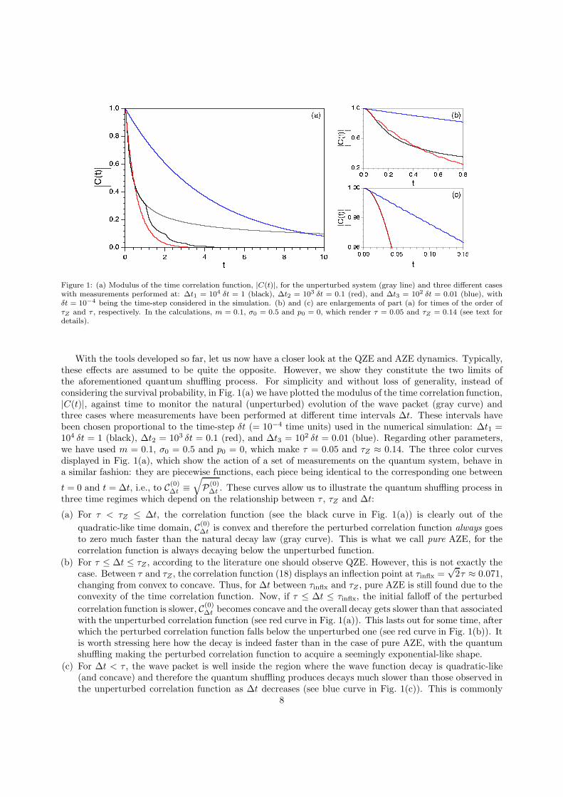
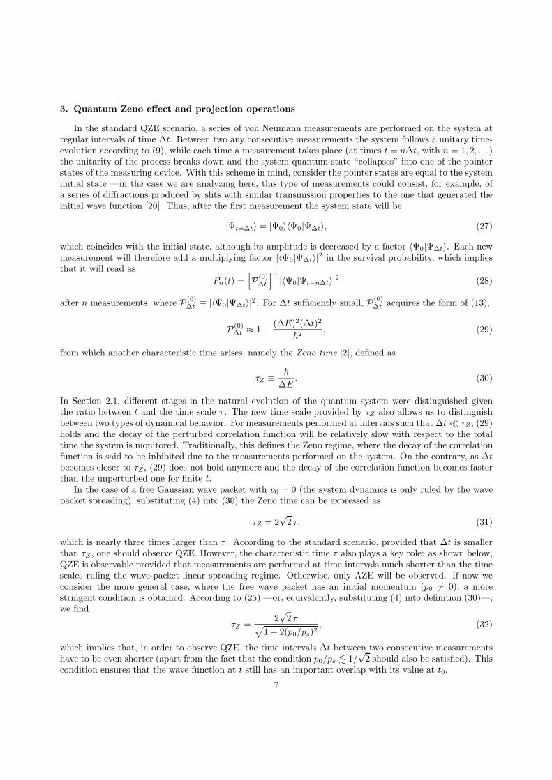
Figure 1: (a) Modulus of the time correlation function, |C(t)|, for the unperturbed system (gray line) and three different caseswith measurements performed at: ∆t1 = 104 δt = 1 (black), ∆t2 = 103 δt = 0.1 (red), and ∆t3 = 102 δt = 0.01 (blue), withδt = 10−4 being the time-step considered in the simulation. (b) and (c) are enlargements of part (a) for times of the order ofτZ and τ , respectively. In the calculations, m = 0.1, σ0 = 0.5 and p0 = 0, which render τ = 0.05 and τZ = 0.14 (see text fordetails).

With the tools developed so far, let us now have a closer look at the QZE and AZE dynamics. Typically,these effects are assumed to be quite the opposite. However, we show they constitute the two limits ofthe aforementioned quantum shuffling process. For simplicity and without loss of generality, instead ofconsidering the survival probability, in Fig. 1(a) we have plotted the modulus of the time correlation function,|C(t)|, against time to monitor the natural (unperturbed) evolution of the wave packet (gray curve) andthree cases where measurements have been performed at different time intervals ∆t. These intervals havebeen chosen proportional to the time-step δt (= 10−4 time units) used in the numerical simulation: ∆t1 =104 δt = 1 (black), ∆t2 = 103 δt = 0.1 (red), and ∆t3 = 102 δt = 0.01 (blue). Regarding other parameters,we have used m = 0.1, σ0 = 0.5 and p0 = 0, which make τ = 0.05 and τZ ≈ 0.14. The three color curvesdisplayed in Fig. 1(a), which show the action of a set of measurements on the quantum system, behave ina similar fashion: they are piecewise functions, each piece being identical to the corresponding one between

t = 0 and t = ∆t, i.e., to C(0)∆t ≡

√

P(0)∆t . These curves allow us to illustrate the quantum shuffling process in

three time regimes which depend on the relationship between τ , τZ and ∆t:

(a) For τ < τZ ≤ ∆t, the correlation function (see the black curve in Fig. 1(a)) is clearly out of the

quadratic-like time domain, C(0)∆t is convex and therefore the perturbed correlation function always goes

to zero much faster than the natural decay law (gray curve). This is what we call pure AZE, for thecorrelation function is always decaying below the unperturbed function.

(b) For τ ≤ ∆t ≤ τZ , according to the literature one should observe QZE. However, this is not exactly thecase. Between τ and τZ , the correlation function (18) displays an inflection point at τinflx =

√2τ ≈ 0.071,

changing from convex to concave. Thus, for ∆t between τinflx and τZ , pure AZE is still found due to theconvexity of the time correlation function. Now, if τ ≤ ∆t ≤ τinflx, the initial falloff of the perturbed

correlation function is slower, C(0)∆t becomes concave and the overall decay gets slower than that associated

with the unperturbed correlation function (see red curve in Fig. 1(a)). This lasts out for some time, afterwhich the perturbed correlation function falls below the unperturbed one (see red curve in Fig. 1(b)). Itis worth stressing here how the decay is indeed faster than in the case of pure AZE, with the quantumshuffling making the perturbed correlation function to acquire a seemingly exponential-like shape.

(c) For ∆t < τ , the wave packet is well inside the region where the wave function decay is quadratic-like(and concave) and therefore the quantum shuffling produces decays much slower than those observed inthe unperturbed correlation function as ∆t decreases (see blue curve in Fig. 1(c)). This is commonly

8

Figure 2: (a) Same as Fig. 1(a), but showing the envelope (36) superimposed to the corresponding perturbed decay functions:∆t1 = 1 (black), ∆t2 = 0.1 (red) and ∆t3 = 0.01 (blue). In the figure, the different types of line denote the modulus ofthe time correlation function, |C(t)|, obtained from: the simulation (dotted), the theoretical estimation (36) (solid), and thefitting to a pure exponential function (dashed); to compare with, the unperturbed correlation function is also displayed withgray line in panel (a). The decay rates arising from the theoretical estimation are γ′

1,est = 25 (black), γ′

2,est = 2.5 (red) and

γ′

3,est = 0.25 (blue), while those obtained from the fitting are γ′

1,fit= 1.224 (black), γ′

2,fit= 1.734 (red) and γ′

3,fit= 0.249

(blue). (b) Enlargement of part (a) in the time interval between t = 0 and t = 1. (c) Plot of the difference ∆(t) between theestimated envelope, C∆t(t), and the fitted envelope, in part (a).

known as QZE. Now, this inhibition of the decay is only apparent; if one considers longer times (seeblue curve in Fig. 1(a)), the correlation function is essentially a decreasing exponential, which eventuallyleads the (perturbed) system to decay to zero earlier than its unperturbed counterpart. As it will beshown below, these exponential decays can be justified in terms of a sort of Markovianity induced bythe shuffling process on the system evolution.

In order to better understand the subtleties behind the quantum shuffling dynamics (and therefore theQZE and the AZE), let us focus only on the overall prefactor that appears in (28), which in the short-timeregime can be written as

P(n)∆t ≡

[

P(0)∆t

]n

≈[

1− (∆t)2

τ2Z

]n

. (33)

This is a discrete function of n, the number of measurements performed up to tn ≡ n∆t, the time at whichthe n-th measurement is carried out. In the limit n → ∞, (33) becomes

P(∞)∆t (tn) ≈ e−γ∆ttn , (34)

with the decay rate being

γ∆t ≡∆t

τ2Z, (35)

as also noted in [2]. This rate defines another characteristic time, τ∆t ≡ γ−1∆t , associated with the falloff of

the continuous form of (34),P∆t(t) = e−γ∆tt (36)

(note that this function passes through all the points tn upon which (34) is evaluated). In Fig. 2 we showa comparative analysis between the correlation functions |C(t)| displayed in Fig. 1 and their respectiveenvelopes, given by C∆t(t) ≡

√

P∆t(t); the former are denoted with dotted line and the latter with solidline of the same color (again, the gray solid line represents the unperturbed correlation function). The

9

values for the estimated decay rates, given by γ′

∆t = γ∆t/2 for the curves represented, are: γ′

1 = 25 (black),γ′

2 = 2.5 (red) and γ′

3 = 0.25 (blue). As it can be seen, the agreement between the correlation functionand its envelope C∆t(t) becomes better as ∆t decreases (see Figs. 2(a) and (b)), which is in virtue of theapproximation considered in (33) —as ∆t increases the behavior of the envelope (36) will diverge moreremarkably with respect to the trend displayed by Pn(t), whereas both will converge as ∆t becomes smaller.Thus, while for long intervals ∆t between consecutive measurements the envelope deviates importantlyfrom the associated correlation function (see black dotted and solid lines), as ∆t becomes smaller thedifference between both curves reduces importantly and the relaxation takes longer times (of the order ofτ∆t). Nevertheless, for larger values of ∆t one can still perform a fitting of the correlation function to a

decaying exponential function, C(∞)∆t,fit(t) = e−γ′

fitt, which renders a qualitatively good overall agreement, as

can be seen from the corresponding dashed lines in Fig. 2(a). Note that the decay rates obtained fromthis fitting are closer to the falloff observed for the corresponding correlations functions (γ′

1,fit = 1.224,γ′

2,fit = 1.734, and γ′

3,fit = 0.249), converging to the estimated value γ′ as ∆t decreases (γ′

3,fit ≈ γ′

3).From the previous discussion, the idea of a series of sequential measurement acting as a shuffling process,

wiping out any memory of the system past history, arises in a natural way. Hence, as ∆t becomes smaller,|C(t)| becomes closer to its envelope C∆t(t) and therefore to an exponential decay law. Conversely, for largervalues of ∆t, the system keeps memory of its past evolution for relatively longer periods of time (between twoconsecutive measures), this leading to larger discrepancies between the correlation function and (36). Takinginto account this point of view and getting back to (28), one can notice a remarkable resemblance betweenthis expression and a Markov chain of independent processes [14] (which is also inferred from (34)): thestate after one measurement only depends on the state before it, but not on the previous history or sequenceuntil this state is reached. That is, between any two consecutive measurements we have a precise knowledgeof the probability to find the system in a certain time-dependent state, while, after a measurement, we looseany memory on that. Thus, as ∆t becomes smaller, the process becomes fully Markovian, with the timecorrelation function approaching the typical exponential-like decreasing behavior characteristic of this typeof processes. On the contrary, as ∆t increases, the memory on the past history is kept for longer times, thisturning the system evolution into non-Markovian, which loses gradually the smooth exponential-like decaybehavior. Only when a measurement is carried out such memory is suddenly removed, which is the causeof the faster (sudden) decays observed in black curve of Fig. 1(a).

The transition from the non-Markovian to the Markovian regime can be somehow quantified by moni-toring along time the distance between the estimated envelope, C∆t(t), and the fitted envelope, C∆t,fit(t),

∆(t) ≡ C∆t(t)− C∆t,fit(t), (37)

which is plotted in Fig. 2(c) for the three cases of ∆t considered. Thus, as ∆t becomes smaller, we approachan exponential decay law and ∆(t) goes to zero for any time (see blue curve in the figure), this beingthe signature of Markovianity. On the contrary, if the time evolution is not Markovian, as time increasesand the system keeps memory for longer times, the value of ∆(t) displays important deviations from zero(see black and red curves in the figure). These deviations mainly concentrate on the short and mediumterm dynamics, where values are relatively large to be remarkable. Nonetheless, analogously, one couldalso display the relative ratio between the two correlation functions, which would indicate or not the trendtoward Markovianity in the long-time (asymptotic) regime.

4. Conclusions

By assuming that the QZE inhibits the evolution of an unstable quantum system, one might also betempted to think that its coherence is also preserved, while the AZE would lead to the opposite effect in itsway through faster system decays. In order to better understand these effects, here we have focused directlyon the bare system, i.e., no external potentials or surrounding environments acting on the quantum systemhave been assumed. This has allowed us to elucidate the conditions under which such effects take place inrelation to the intrinsic time-scales characterizing the isolated system, which have been shown to play animportant role. Furthermore, by means of this analysis, we have also shown that both QZE and AZE are

10

indeed two instances of a more general effect, namely a quantum shuffling process, which eventually leads thesystem to display a Markovian-like evolution and its correlation function to follow an exponential decay lawas the interval between measurements decreases. Within this scenario, the QZE dynamics can be regardedas a regime where any trace of knowledge on the initial system state is lost due to a rapid shuffling, whilein the long-time regime the correlation function would fall to zero faster than the unperturbed one. Theapparent contradiction with the traditional no-evolution scenario can be explained very easily: Since oneoften cares only about the short-time dynamics, the long-time dynamics is usually completely neglected.In other words, the time during which the system dynamics is usually studied is relatively small comparedto the Markovian time-scale induced by the continuous measurement process and, therefore, one assumesnearly stationary dynamics.

Acknowledgements

The support from the Ministerio de Ciencia e Innovacion (Spain) through Projects FIS2010-18132,FIS2010-22082, CSD2009-00038; from Comunidad Autonoma de Madrid through Grant No. S-2009/MAT/1467;and from the COST Action MP1006 (Fundamental Problems in Quantum Physics) is acknowledged. A. S.Sanz also thanks the Ministerio de Ciencia e Innovacion for a “Ramon y Cajal” Research Fellowship.

A. Alternative Zeno scenario

In the Zeno scenario considered above, establishing a direct analogy with Zeno’s arrow, the wave packetplays the role of a quantum arrow, but with the particularity that this arrow slows down until its evolutionis frozen by means of a series of measurements. This is the scenario traditionally considered [2]. However,a more direct analogy with Zeno’s arrow paradox can be established if it is assumed that the wave packetis always in motion and the measurements are just like photographs indicating the particular instant fromwhich the correlation has to be computed [18]. Because of the actions on the wave packet in relation towhat a measurement is considered in each, we can call these two situations as:

(a) The stopping-arrow scenario, where the wave packet is “collapsed” or “stopped” after each measurement.(b) The steady-arrow scenario, where the wave packet time-evolution never stops, but the computation of

the correlation function is reset after each (photograph-like) measurement —like in a stop-motion orstop-action movie.

It can be shown that both scenarios are equivalent with the exception of a lost time-dependent phasein the latter. In order to prove this statement, let us start by considering the wave function is now left tofreely evolve in time. Following the idea behind this scenario, the survival probability is monitored in timeby computing the overlapping of the wave function at a time t with its value at successive times t0, t1, t2,with tn = n∆t, i.e.,

〈Ψtn−1|Ψt〉, (38)

where tn−1 ≤ t < tn. Note here the direct analogy with Zeno’s arrow, where at each instant we are observingthe arrow steady at a different space position, but without freezing its motion. Taking this into account, for0 ≤ t < t1, we have

P (t) = |〈Ψ0|Ψt〉|2. (39)

Now, if t1 ≤ t < t2,P (t) = α1|〈Ψt1 |Ψt〉|2, (40)

while the wave function for the same interval will be

|Ψt〉 =√α1|Ψt〉, (41)

i.e., the evolved wave function, but with a prefactor which ensures the matching of the different of P (t)before and after t = t1. Following the same argumentation, after the n− 1 measurement,

P (t) =(

Πn−1k=1αk

)

|〈Ψtn−1|Ψt〉|2, (42)

11

with tn−1 ≤ t ≤ tn.As it can be seen, by means of this procedure the wave function is never altered (which always keeps

evolving according to the Schrodinger equation), but only its relative amplitude. So, the key issue here isthe attenuation factor α, which can be evaluated as follows. For tn−1 ≤ t < tn, we note that

〈Ψtn−1|Ψt〉 = 〈Ψ0|eiH(n−1)∆t/~e−iHt/~|Ψ0〉 = 〈Ψ0|eiH[t−(n−1)∆t]/~|Ψ0〉. (43)

Therefore, the attenuation factor for the interval tn−1 ≤ t ≤ tn should come from the overlapping of thewave function at the times when the two previous measurements were performed, i.e.,

αn−1 = |〈Ψtn−2|Ψtn−1

〉|2 = |〈Ψ0|eiH∆t/~|Ψ0〉|2. (44)

This expression can be Taylor expanded to second order in ∆t (assuming ∆t is small enough) taking intoaccount that

〈Ψ0|Ψ∆t〉 ≈ 1− iτZ~

〈Ψ0|H|Ψ0〉+τ2Z2~2

〈Ψ0|H2|Ψ0〉, (45)

where we have assumed the wave function is initially normalized. This renders

αn = |〈Ψ0|Ψt1〉|2 ≈ 1− (∆t)2

~2

(

〈Ψ0|H2|Ψ0〉 − 〈Ψ0|H |Ψ0〉2)

= 1− (∆t)2

~2(∆H)2, (46)

which is valid for any n, since it does not depend explicitly on the particular time at which the measurementis made. Therefore, (42) can be expressed as

P (t) = αn−11 |〈Ψtn−1

|Ψt〉|2, (47)

which is formally equivalent to (28) after performing n measurements, although it describes a completelydifferent physics [18].

References

[1] J. Mazur, Zeno’s Paradox: Unraveling the Ancient Mystery behind the Science of Space and Time, Plume, New York,2007.

[2] P. Facchi, S. Pascazio, J. Phys. A: Math. Theor. 41 (2008) 493001.[3] B. Misra, E. C. G. Sudarshan, J. Math. Phys. 18 (1977) 756.[4] A. Peres, Am. J. Phys. 48 (1980) 931.[5] J. von Neumann, Die Mathematische Grundlagen der Quantenmechanik, Springer Verlag, Berlin, 1932.[6] W. M. Itano, D. J. Heinzen, J. J. Bollinger, D. J. Wineland, Phys. Rev. A 41 (1990) 2295.[7] R. J. Cook, Phys. Scr. T21 (1988) 49.[8] S. R. Wilkinson, C. F. Bharucha, M. C. Fischer, K. W. Madison, P. R. Morrow, Q. Niu, B. Sundaram, M. G. Raizen,

Nature 387 (1997) 575.[9] M. C. Fischer, B. Gutierrez-Medina, M. G. Raizen, Phys. Rev. Lett. 87 (2001) 040402.

[10] B. Kaulakys, V. Gontis, Phys. Rev. A 56 (1997) 1131.[11] A. Luis, L. Sanchez-Soto, Phys. Rev. A 57 (1998) 781.[12] A. G. Kofman, G. Kurizki, Nature 405 (2000) 546.[13] H.-P. Breuer, F. Petruccione, The Theory of Open Quantum Systems, Oxford University Press, Oxford, 2002.[14] P. E. Kloeden, E. Platen, Numerical Solution of Stochastic Differential Equations, Springer, Berlin, 1992.[15] A. S. Sanz, S. Miret-Artes, J. Phys. A: Math. Theor. 41 (2008) 435303.[16] A. S. Sanz, S. Miret-Artes, J. Phys. A: Math. Theor. 44 (2011) 485301.[17] C. Sanz-Sanz, A. S. Sanz, T. Gonzalez-Lezana, O. Roncero, S. Miret-Artes, (submitted for publication, 2011); eprint

arXiv:1106.4143.[18] C. Sanz-Sanz, A. S. Sanz, T. Gonzalez-Lezana, O. Roncero, S. Miret-Artes, (submitted for publication, 2011); eprint

arXiv:1111.1520.[19] C. B. Chiu, E. C. G. Sudarshan, B. Misra, Phys. Rev. D 16 (1977) 520.[20] M. A. Porras, A. Luis, I. Gonzalo, A. S. Sanz, Phys. Rev. A 84 (2011) 052109.[21] A. S. Sanz, S. Miret-Artes, Am. J. Phys. (at press, 2011); eprint arXiv:1104.1296.[22] E. Donkor, A. R. Pirich, H. E. Brandt (Eds.), Quantum Zeno and anti-Zeno effects: An exact model, in: Society

of Photo-Optical Instrumentation Engineers (SPIE) Conference Series, vol. 5436, SPIE, Bellingham, WA, 2004; eprintarXiv:quant-ph/0501098.

[23] H. C. Penate-Rodrıguez, R. Martınez-Casado, G. Rojas-Lorenzo, A. S. Sanz, S. Miret-Artes, J. Phys.: Condens. Matter(at press, 2011); eprint arXiv:1104.1294.

[24] A. S. Sanz, S. Miret-Artes, Chem. Phys. Lett. 445 (2007) 350.

12