arX

iv:q

uant

-ph/

0012

130v

2 2

2 Fe

b 20

01

Quantum Zeno and anti-Zeno effects in the Friedrichs model

I. Antoniou1, E. Karpov1, G. Pronko1,2, and E. Yarevsky1,3

1 International Solvay Institutes for Physics and Chemistry, C.P. 231, Campus Plaine ULB, Bd. du Triomphe, Brussels

1050, Belgium2 Institute for High Energy Physics, Protvino, Moscow region 142284, Russia

3 Laboratory of Complex Systems Theory, Institute for Physics, St.Petersburg State University, Uljanovskaya 1, St.Petersburg

198904, Russia

We analyze the short-time behavior of the survival probability in the frame of the Friedrichsmodel for different formfactors. We have shown that this probability is not necessary analytic at thetime origin. The time when the quantum Zeno effect could be observed is found to be much smallerthan usually estimated. We have also studied the anti-Zeno era and have estimated its duration.

I. INTRODUCTION

Since the very beginning of the quantum mechanics, the measurement process has been a most fundamental is-sue. The main characteristic feature of the quantum measurement is that the measurement changes the dynamicalevolution. This is the main difference of the quantum measurement compared to its classical analogue. On thisframework, Misra and Sudarshan pointed out [1] that repeated measurements can prevent an unstable system fromdecaying. Indeed, as the survival probability is in most cases proportional to the square of the time for short times(see, however, the discussion below), the measurement effectively projects the evolved state back to the initial statewith such a high probability that the sequence of the measurements “freezes” the initial state. Led by analogy withthe Zeno paradox, this effect has been called the quantum Zeno effect (QZE).

Cook [2] suggested an experiment on the QZE which was realized by Itano et al. [3]. In this experiment, the Rabioscillations have been used in order to demonstrate that the repeated observations slow down the transition process.However, the detailed analysis [4–6] has shown that the results of this experiment could equally well be understoodusing a density matrix approach for the whole system. Recently, an experiment similar to [3] has been performedby Balzer et al. [7] on a single trapped ion. This experiment has removed some drawbacks usually associated withthe experiment of Itano et al. [3], for example, dephasing system’s wave function caused by a large ensemble andnon-recording of the results of the intermediate measurements pulses. We refer to recent reviews [8,9] for detaileddiscussions of these and related questions.

Both experiments [3,7] demonstrate the perturbed evolution of a coherent dynamics, as opposed to spontaneousdecay. So the demonstration of the QZE for an unstable system with exponential decay, as originally proposed in [1],is still an open question. The main problem in such an experimental observation of the Zeno effect is the very shorttime when the quadratic behavior of the transition amplitude is valid [10,11]. On the other hand, the Zeno-typeexperiment could also reveal deviations from the exponential decay law and the magnitude of these deviations.

The QZE has been discussed for many physical systems including atomic physics [10–13], radioactive decay [14],mesoscopic physics [15–18], and has been even proposed as a way to control decoherence for effective quantumcomputations [19]. Recently, however, a quantum anti-Zeno effect has been found [20,21]. Under some conditionsthe repeated observations could speed up the decay of the quantum system. The anti-Zeno effect has been furtheranalyzed in [18,22–25].

We carefully analyze here the short-time behavior of the survival probability in the frame of the Friedrichs model [26].We have shown that this probability is not necessary analytic at zero time. Furthermore, the probability may not evenbe quadratic for the short times while the QZE still exists in such a case [20,27]. We have shown (see also Kofman andKurizki [24]) that the time period within which the QZE could be observed is much smaller than previously believed.Hence we conclude that the experimental observation/realization of the QZE is quite challenging.

We have also analyzed the anti-Zeno era. While it seems that most decaying systems exhibit anti-Zeno behavior,our examples contradict the estimations of Lewenstein and Rzazewski [22]. We have studied the duration of theanti-Zeno era and have estimated this duration when possible.

1

II. MODEL AND EXACT SOLUTION

The Hamiltonian of the second quantised formulation of the Friedrichs model [26] is

H = H0 + λV, (1)

where the unperturbed Hamiltonian is defined as

H0 = ω1a†a +

∫ ∞

0

dω ω b†ωbω,

and the interaction is

V =

∫ ∞

0

dωf(ω)(

ab†ω + a†bω

)

. (2)

Here a†, a are creation and annihilation boson operators of the atom excitation, b†ω, bω are creation and annihilationboson operators of the photon with frequency ω, f(ω) is the formfactor, λ is the coupling parameter, and the vacuumenergy is chosen to be zero. The creation and annihilation operators satisfy the following commutation relations:

[a, a†] = 1, [bω, b†ω′ ] = δ(ω − ω′). (3)

All other commutators vanish.The Hamiltonian H0 has continuous spectrum [0,∞) of uniform multiplicity, and the discrete spectrum nω1 (with

integer n) is embedded in the continuum. The space of the wave functions is the direct sum of the Hilbert space ofthe oscillator and the Fock space of the field.

For ω1 > 0 the oscillator excitations are unstable due to the resonance between the oscillator energy levels and theenergy of a photon. Therefore, the total evolution leads to the decay of a wave packet corresponding to the bare atom|1〉. Decay is described by the survival probability p(t) to find, after time t, the bare atom evolving according to theevolution exp(−iHt) in its excited state [11]:

p(t) ≡ |〈1|e−iHt|1〉|2. (4)

The survival probability can be easily calculated in the second quantized representation:

p(t) = |〈0|a(0)e−iHta†(0)|0〉|2 = |〈0|e−iHteiHta(0)e−iHta†(0)|0〉|2 = |〈0|a(t)a†(0)|0〉|2,

where a†(0) = a†. The time evolution of a(t) in the Heisenberg representation is presented in Appendix A. Using(A12) we obtain

p(t) = |A(t)|2,

where the survival amplitude A(t) is given by (A14).Due to the dimension argument, we can write the formfactor f(ω) in the form

f2(ω) = Λϕ(ω

Λ

)

,

where ϕ(x) is a dimensionless function. Here Λ is a parameter with the dimension of ω. The survival amplitude A(t)in the dimensionless representation is

A(t) =1

2πi

∞∫

−∞

dyeiyΛt

η−Λ (y)

, (5)

where

η−Λ (z) = ωΛ − z − λ2

∞∫

0

dxϕ(x)

x − z + i0, (6)

and ωΛ = ω1/Λ.

2

III. SHORT-TIME BEHAVIOR AND THE ZENO REGION

The short time evolution of the model (1) depends essentially on the formfactor. In order to illustrate differenttypes of the evolution, we shall consider two formfactors, namely:

f21 (ω) = Λ

√

ωΛ

1 + ωΛ

, ϕ1(x) =

√x

1 + x, (7)

and

f22 (ω) = Λ

ωΛ

(

1 +(

ωΛ

)2)2 , ϕ2(x) =

x

(1 + x2)2. (8)

The formfactor f1 permits exact calculations [28,29]. It turns out that the short-time behavior is not quadratic [20,27]as anticipated by [22]. We shall also use for comparison the results presented in [10,11] for the formfactor ϕ3(x) =

x(1+x2)4 [30]. To get a first impression about the time scales, we associate with each formfactor a physical system: the

photodetachement process for ϕ1(x) [22,28,31], the quantum dot for ϕ2(x) [32], and the hydrogen atom for ϕ3(x) [10].The corresponding numerical values of the parameters Λ, ω1, and λ2 are listed in Table 1. We would like to emphasizethat these values (as well as the model itself) are approximate estimations of the corresponding effects.

Let us discuss the short-time behavior of the survival probability p(t). We shall assume here the existence of allnecessary matrix elements, and denote 〈·〉 = 〈1| · |1〉.

p(t) = 〈e−iHt〉 = 〈1 − iHt − 1

2H2t2 +

i

6H3t3 +

1

24H4t4 + O(t5)〉 =

(

1 − t2

2〈H2〉 +

t4

24〈H4〉

)2

+

(

t〈H〉 − t3

6〈H3〉

)2

+ O(t6) =

1 − t2(

〈H2〉 − 〈H〉2)

+ t4(

1

4〈H2〉2 +

1

12〈H4〉 − 1

3〈H〉〈H3〉

)

+ O(t6) =

1 − t2

t2a+

t4

t4b+ O(t6). (9)

In order to calculate the parameters ta and tb, we need to calculate the averages of the powers of H = H0 + λV :

〈H〉 = ω1,

〈H2〉 = ω21 + λ2〈V 2〉,

〈H3〉 = ω31 + 2λ2ω1〈V 2〉 + λ2〈V H0V 〉, (10)

〈H4〉 = ω41 + λ2

(

3ω21〈V 2〉 + 2ω1〈V H0V 〉 + 〈V H2

0V 〉)

+ λ4〈V 4〉.

These expressions are valid in our model because of the special structure of the potential V (2). Now we can find:

1

t2a= λ2〈V 2〉 = λ2Λ2I0,

1

t4b= λ2

(

ω21

12Λ2I0 −

ω1

6Λ3I1 +

Λ4

12I2

)

+ λ4Λ4

(

I20

4+

∫∞0 ϕ2(x)dx

12

)

, (11)

where

Ik =

∫ ∞

0

xkϕ(x)dx.

In the weak coupling models the following inequalities are satisfied (see Table 1):

λ2 ≪ 1 and Λ ≫ ω1. (12)

In this approximation we can simplify the expression for tb:

3

1

t4b≈ λ2Λ4

12I2. (13)

The parameter ta has been called Zeno time [10,11] because it has been conjectured to be related to the Zenoregion, i.e. the region where the decay is slower than the exponential one and the Zeno effect can manifest. On theother hand, a more precise estimation reveals that the Zeno region is in fact orders of magnitude shorter than ta.We illustrate this in Fig. 1 where the survival probabilities for the formfactors ϕ1(x) and ϕ2(x) are plotted. Thecorresponding analytical expressions and the numerical values for different time scales are presented in Table 1. Wesee that p(t) is not convex already at times much shorter than the time ta.

In view of this fact, we propose another definition for the Zeno time. As one refers in discussions about the Zenoeffect on the expansion of survival probability for small times, and specifically on the second term, we shall define theZeno time tZ as corresponding to the region where the second term dominates. Hence the introduced time tZ is anatural boundary where the second and third terms have the same amplitude:

t2Zt2a

=t4Zt4b

, so tZ = t2b/ta. (14)

In the weak coupling models,

tZ =1

Λ

√

12I0

I2,

that agrees with the estimation in [24]. This time is much shorter than ta ∼ 1λΛ and agrees much better with the

numerical estimations. For example, for the interaction ϕ3(x) we find tZ = 2√

6Λ ≈ 5.8 · 10−19 s while ta =

√6

λΛ ≈3.6 · 10−16 s [10].

Our conclusions are in fact valid for a rather wide class of interactions. Namely, they are valid if the matrixelements (10) exist and conditions (12) are satisfied. For example, any bounded locally integrable interaction ϕ(x)decreasing as ϕ(x) ∼ C

x1.5+ǫ , ǫ > 0 at x → ∞, gives finite matrix elements (10). Furthermore, we show below that therelation tR ≪ tZ may be valid even when the matrix elements (10) do not exist.

For the formfactor ϕ1, already the matrix element 〈V 2〉 does not exist, and the short time expansion is written,Appendix B, as

p(t) = 1 −(

t

ta

)1.5

+

(

t

tb

)2

+ O(t5/2),

where ta = (3/(4√

2π))2/3/(λ4/3Λ), and tb = 1/(√

πλΛ). In fact, from the representation (10) one can easily deducethat for any formfactor decreasing according to the power law when x → ∞, p(t) is not analytic at t = 0. Specifically,if the formfactor decreases as ϕ(x) ∼ xα when x → ∞, only the Taylor coefficients up to tn with n < 1 + |α| can bedefined.

Following the previous discussion, for the formfactor ϕ1(x) the Zeno time tZ can be estimated by the condition

(

tZta

)1.5

=

(

tZtb

)2

, so tZ =32

9πΛ.

For this case, one can see that the time ta has scaling properties which differ from (11) while the Zeno time tZ has avalue similar to (14).

For ϕ2, the matrix element 〈V 2〉 exists so the usual time ta can be introduced: ta =√

2λΛ . However, 〈V H2

0V 〉 doesnot exist and the asymptotic behavior of p(t) is (see Appendix C)

p(t) = 1 −(

t

ta

)2

− λ2

12log (2ω1t)Λ

4t4 + O(t4).

Repeating the arguments concerning the Zeno region, we find tZ =√

6

Λ

√

| log (2√

6ω1Λ

)|. In this case one can see again

that the Zeno time tZ has a value similar to (14), and the inequality tZ ≪ ta is satisfied.

4

IV. ZENO AND ANTI-ZENO EFFECTS

The probability that the state |1〉 after N equally spaced measurements during the time interval [0, T ] has notdecayed, is given by [1]

pN (T ) = 〈1|(

|1〉〈1|e−iHT/N)N

|1〉 = pN(T/N)〈1|1〉 = pN(T/N). (15)

Expression (15) is only correct for the ideal von Neumann measurements [1]. We are interested in the behavior ofpN (T ) as N → ∞ or, equally, when the time interval between the measurements τ = T/N goes to zero:

limτ→0

pN(T ) = limτ→0

p(τ)T/τ =

limτ→0

(

1 −1−p(τ)

τ1τ

)1τ

T

=

0, when p′(0) = −∞,e−cT , when p′(0) = −c,1, when p′(0) = 0.

(16)

Hence for the case p(t) = 1− ctα one has the Zeno effect for all α > 1 [20,27]. We should notice that in case of thelinear asymptotics of p(t) at short times (in particular, for the purely exponential decay) there is no Zeno effect, andthe probability to find the system in the initial state |1〉 decreases exponentially with the time of observation. Theresults (16) are found in case of continuously ongoing measurements during the entire time interval [0, T ]. Obviously,this is an idealization. In practice we have a manifestation of the Zeno effect, if the probability (15) increases asthe time interval τ between measurements decreases. Formula (16) may be accepted as an approximation for a veryshort time interval τ ≪ tZ . For longer times we cannot use the Taylor expansion, therefore Eq. (16) is not valid. Itappears that in order to analyze longer time behavior, the long time asymptotics of the p(t) are more convenient.These asymptotics can be summarized as follows (see Appendicies B, C):

p(t) ≈ |A1|2e−4γ√

ω1Λt +πλ4Λ

4ω41t

3h2

1(t) −√

πλ2Λ1/2

ω21t

3/2|A1|h1(t)e

−2γ√

ω1Λt cos (ω1t − π/4) (17)

when t ≫ 24/ω1 for the ϕ1(x), and

p(t) ≈ |A2|2e−γ1Λt +λ4

ω41t

4h2

2(t) −2λ2e−γ1Λt/2

ω21t

2|A2|h2(t) cos (ω1t) (18)

when t ≫ 4/ω1 for the ϕ2(x). Here the constants A1, A2 satisfy the inequality |1−|Ak|2| ≪ 1, k = 1, 2. The functionsh1, h2 have the following asymptotic properties:

limt→∞

h1(t) = 1; limt→0

h1(t)

t3/2= const; lim

t→∞h2(t) = 1; lim

t→0

h2(t)

t2= const.

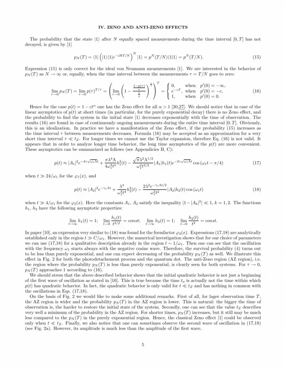
In paper [10], an expression very similar to (18) was found for the formfactor ϕ3(x). Expressions (17,18) are analyticallyestablished only in the region t ≫ C/ω1. However, the numerical investigation shows that for our choice of parameterswe can use (17,18) for a qualitative description already in the region t ∼ 1/ω1. Then one can see that the oscillationwith the frequency ω1 starts always with the negative cosine wave. Therefore, the survival probability (4) turns outto be less than purely exponential, and one can expect decreasing of the probability pN (T ) as well. We illustrate thiseffect in Fig. 2 for both the photodetachement process and the quantum dot. The anti-Zeno region (AZ region), i.e.the region where the probability pN(T ) is less than purely exponential, is clearly seen for both systems. For τ → 0,pN (T ) approaches 1 according to (16).

We should stress that the above described behavior shows that the initial quadratic behavior is not just a beginningof the first wave of oscillation as stated in [10]. This is true because the time ta is actually not the time within whichp(t) has quadratic behavior. In fact, the quadratic behavior is only valid for t ≪ tZ and has nothing in common withthe oscillations in Eqs. (17,18).

On the basis of Fig. 2 we would like to make some additional remarks. First of all, for lager observation time T ,the AZ region is wider and the probability pN (T ) in the AZ region is lower. This is natural: the bigger the time ofobservation is, the harder to restore the initial state of the system. Secondly, one can see that the value tZ describesvery well a minimum of the probability in the AZ region. For shorter times, pN(T ) increases, but it still may be muchless compared to the pN (T ) in the purely exponential region. Hence, the classical Zeno effect [1] could be observedonly when t ≪ tZ . Finally, we also notice that one can sometimes observe the second wave of oscillation in (17,18)(see Fig. 2a). However, its amplitude is much less than the amplitude of the first wave.

5

A general consideration of the AZ region is presented in [22]. The authors conclude that the AZ region exists forall generic weakly coupled decaying systems. Under some assumptions, they have found that

|Ak|2 < 1, (19)

and use this condition for the explanation of the existence of the AZ region. However, some assumptions madein [22] for the derivation of (19) are not always valid. For example, for the model ϕ1(x) (the formfactor usedin [22]) one calculates |A1|2 ≈ 1 + 1.1 10−6 > 1 for our choice of the parameters. For the model ϕ2(x) we have|A2|2 ≈ 1 + λ2(3 + 2 logωΛ) < 1, but this effect is of the second order in the coupling while in [22] the fourth orderwas found. Hence the above mentioned results can not be considered as a proof of the existence of the AZ region.

Indeed, our results show that there exist two different types of the AZ region. The first case takes place as theamplitude of oscillations in (17,18) is less than |1 − |A|2|, and |A|2 < 1. This corresponds to the arguments of [22].In this situation, the survival probability is always less than the “ideal” one corresponding to the pure exponentialdecay (except for the very short times t ≪ tZ). The second case arises when the amplitude of oscillations in (17,18)is bigger than |1− |A|2| (for any |A2|), or when |A2| > 1. In this case the survival probability may be lower or higherthan the “ideal” one, that may result in oscillations of the probability pN (T ). This is exactly the situation in Fig. 2a.

It would be very interesting to find an estimation for the duration of the AZ region. We have found that theminimum of the pN(T ) is reached at tZ , however the whole region is much wider. Unfortunately, we can present thisestimation only for the second type of the AZ region. In order to illustrate this, we plot in Fig. 3 the value

Nε(T ) : pNε(T )(T ) = (1 − ε)p1(T ). (20)

This value gives the maximum number of repeated observation such that the probability pN(T ) would not be lessthan p(T ) with accuracy ε. The difference between two types of the AZ region is very pronounced. For the first type(ϕ2(x) interaction) Nε(T ) ∼ Cε and is almost independent of the time T of observation. It means that the anti-Zenoregion tAZ should be described as tAZ ∼ cT/ε. So the duration depends critically on the time of observation and theaccuracy, and cannot be attributed to the properties of the system itself.

For the second type (ϕ1(x) interaction) Nε(T ) ∼ CT and is almost independent of the accuracy ε. This means thattAZ is independent of the time of the observation and the accuracy, so it can be correctly introduced. In fact, in thiscase tAZ is defined by the oscillations of the survival probability and can be estimated as 1/ω1.

The estimation tAZ ≪ 1/ω1 was given by Kofman and Kurizki [24]. While this estimation obviously holds, itis necessary to establish more precise boundaries for tAZ . We have found the boundary tAZ ∼ 1/ω1 for the ϕ1(x)interaction. However, from the results presented in Fig. 3, one can see that for the interactions ϕ2(x) and ϕ3(x) theestimation 1/ω1 can hardly be used, contrary to the results of [24].

We would like to mention that the estimation tDC = 1/ω1 has been obtained by Petrosky and Barsegov [33] asan upper boundary of the decoherence time marking the onset of the exponential era. As the Zeno effect cannot berealized for times lager than tDC , Petrosky and Barsegov called tDC the Zeno time. In fact this is a rough estimationof the real Zeno time tZ .

V. CONCLUSIONS

Let us summarize the short-time behavior of the survival probability. We introduce two regions: the very short Zenoregion tZ with the scale 1/Λ and the much longer anti-Zeno region tAZ . If one performs a Zeno-type experiment, andthe time between measurements is much shorter than tZ , then the Zeno effect – increasing of the survival probability– can be observed. In the time range between tZ and tAZ , the anti Zeno effect exists, i.e. decay is accelerated byrepeated measurements. That is why the Zeno time cannot be longer than tZ . The previous estimations of the Zenotime ta [10,11] and tDC [33] are much longer than our estimation tZ for physically relevant systems (12).

While the acceleration of decay is clearly seen in all cases, it is not always possible to introduce the value tAZ . Thereason is the possible dependence of tAZ on the moment of the observation and on the accuracy of the observation.When this dependence is absent, one finds tAZ ∼ 1/ω1. Hence the anti-Zeno region is, for typical values of parameters,a few orders of magnitude longer than the Zeno region. It would be very important from the experimental point ofview, to find an estimation for the anti-Zeno region in terms of the initial parameters without any reference to theconstant Ak.

It is possible in principle that the oscillations in (17,18) may give a few successive Zeno and anti-Zeno regions.However, as the amplitude of the oscillations decreases exponentially with time, these regions are hardly visible. Afterthe anti-Zeno region, the system decays exponentially up to the time tep when the long-tail asymptotics substitutesthe exponential decay.

6

In accordance with this picture, the experimental observation of the Zeno effect is very difficult. Indeed, the Zenoregion appears to be considerably shorter than previously belived. The acceleration of the decay should be observedbefore the deceleration will be possible. In this connection, the proposals for using the Zeno effect for increasing of thedecoherence time [19] should be critically analyzed. We conclude that the Zeno effect may not be very appropriatefor decoherence control desired for quantum computations.

There seems to be no place for the usual estimations of the Zeno time by ta. There are no physical effects whichcan be associated with this time scale. In our opinion, the widespread expectation that the time ta describes theZeno region, is based on a naive perturbation theory. One could assume that p(t) = 1 −∑∞

k=2 ck(λt)k, where ck aredefined in terms of the matrix elements of the interactions and are independent of λ. In this case all terms in theseries for p(t) have the same order at ta. However, this assumption is not true as H0 and V do not commute hence〈1|e−iHt|1〉 6= 〈1|e−iλV t|1〉.

We would like to mention a few interesting problems related to the Zeno effect. 1) A better characterization ofthe anti-Zeno region. This problem is relevant to the experimental demonstration of the (anti-) Zeno behavior of thesurvival probability. 2) How the non-ideal measurements influence the Zeno effect? 3) Is the asymptotic quantumZeno dynamics lim

N→∞pN (T ) governed by a unitary group or a semigroup of isometries or contractions [34]? This

question defines if the quantum Zeno dynamics introduces irreversibility in the evolution of a system.

ACKNOWLEDGMENTS

We would like to thank Profs. Ilya Prigogine, Tomio Petrosky and Saverio Pascazio for helpful discussions. Wewould also like to acknowledge the remarks of Profs. Kofman and Kurizki. This work enjoyed the financial supportof the European Commission Project No. IST-1999-11311 (SQID).

APPENDIX A: TIME EVOLUTION IN THE HEISENBERG REPRESENTATION

The second quantised form of the well-known Friedrichs model [26] is given by the Hamiltonian (1). For ω1 > 0the oscillator excitations are unstable due to the resonance between the oscillator energy levels and the energy of aphoton. Strong interaction however may lead to the emergence of a bound state. In weak coupling cases discussedhere bound states do not arise (see (A5)) below).

The solution of the eigenvalue problem

[H, B†ω] = ωB†

ω and [H, Bω] = −ωBω, (A1)

obtained with the usual procedure of the Bogolubov transformation [35,36] is

(B†ω) in

out= b†ω +

λf(ω)

η±(ω)

∫ ∞

0

dω′λf(ω′)

(

b†ω′

ω′ − ω ∓ i0− a†

)

, (A2)

(Bω) in

out= bω +

λf(ω)

η∓(ω)

∫ ∞

0

dω′λf(ω′)

(

bω′

ω′ − ω ± i0− a

)

. (A3)

In (A2), (A3) we used the notation 1/η±(ω) ≡ 1/η(ω ± i0) where the function η(z) of the complex argument z is

η(z) = ω1 − z −∫ ∞

0

dωλ2f2(ω)

ω − z. (A4)

The following condition on the formfactor f(ω)

ω1 −∫ ∞

0

dωλ2f2(ω)

ω> 0 (A5)

guarantees that the function 1/η(z) is analytic everywhere on the first sheet of the Riemann manifold except for thecut [0,∞). Therefore the total Hamiltonian H has no discrete spectrum and there are no bound states.

The incoming and outgoing operators (B†ω) in

out, (Bω) in

outsatisfy the following commutation relation

[

(Bω) in

out, (B+

ω′) in

out

]

= δ(ω − ω′). (A6)

7

The other commutators vanish. The bare vacuum state |0〉 satisfying

a1|0〉 = bω|0〉 = 0,

is also the vacuum state for the new operators:

(Bω) in

out|0〉 = 0.

Therefore, the new operators diagonalise the total Hamiltonian (1) as

H =

∫ ∞

0

dω ω (B†ω) in

out(Bω) in

out. (A7)

Using the inverse relations

b†ω = (B†ω)in − λf(ω)

∫ ∞

0

dω′ λf(ω′)

η−(ω′)

(B†ω′)in

ω′ − ω − i0, (A8)

bω = (Bω)in − λf(ω)

∫ ∞

0

dω′ λf(ω′)

η+(ω′)

(Bω′)inω′ − ω + i0

, (A9)

a† = −∫ ∞

0

dωλf(ω)

η−(ω)(B†

ω)in, (A10)

a = −∫ ∞

0

dωλf(ω)

η+(ω)(Bω)in, (A11)

we obtain the time evolution of the bare creation and annihilation operators in the Heisenberg representation:

b†ω(t) = b†ωeiωt + λf(ω)

{∫ ∞

0

dω′ λf(ω′)g(ω′, t) − g(ω, t)

ω′ − ωb†ω′ − g(ω, t)a†

}

,

bω(t) = bωe−iωt + λf(ω)

{∫ ∞

0

dω′ λf(ω′)g∗(ω′, t) − g∗(ω, t)

ω′ − ωbω′ − g∗(ω, t)a

}

,

a†(t) =

∫ ∞

0

dω λf(ω)g(ω′, t)b†ω′ + A(t)a†,

a(t) =

∫ ∞

0

dω λf(ω)g∗(ω′, t)bω′ + A∗(t)a. (A12)

Except for the oscillating exponent, all time dependence of the field operators is described by the functions g(ω, t)and A(t):

g(ω, t) = − 1

2πi

∫ ∞

−∞dω′ 1

η−(ω′)

eiω′t

ω′ − ω − i0, (A13)

A(t) =

(

i∂

∂t+ ω

)

g(ω, t) =1

2πi

∫ ∞

−∞dω′ eiω′t

η−(ω′). (A14)

APPENDIX B: TYPE 1 FORMFACTOR

For the formfactor ϕ1(x) =√

x1+x we have:

ηΛ(z) = ωΛ − z − πλ2

1 − i√

z, (B1)

8

where the first sheet of the complex z plane corresponds to the upper half of the complex√

z plane. The exactexpression for the survival amplitude is known [28,29,37]:

A(t) =iγ +

√ω̃Λ

2γ√

ω̃Λ

πλ2

z3 − z2eiz2Λt + πe

iπ4 λ2

3∑

k=1

3∏

m=1

m 6=k

1

zk − zm

√izkeizkΛt

(

−1 + erf(√

izkΛt))

. (B2)

Here zk are the roots of ηΛ(z) on the second sheet of z-plane, and ω̃Λ, γ are expressed in terms of zk. If conditions (12)are satisfied, we have the following approximate expressions:

γ ≈ π

2λ2, ω̃Λ ≈ ωΛ. (B3)

In order to analyze the survival probability for large times, we need the asymptotics of the A(t) as t → ∞:

A(t) =2it−3/2

z1z2z3

(

1 − 12

t

3∑

k=1

1

izk+ O(1/t2)

)

.

In the last expression, we can use the first term only when t ≫ 12∣

∣

∣

∑3k=1

1izk

∣

∣

∣ ≈ 24ω1

. We have in fact checked

numerically, that this is valid even on shorter times.Using (B3), we can now calculate the survival probability:

p(t) ≈ e−4γt√

ω1Λ +πλ4Λ

4ω41t

3−

√πλ2Λ1/2

ω21t

3/2e−2γt

√ω1Λ cos (ω1t − π/4) when t ≫ 24

ω1. (B4)

One can see that the survival probability decays exponentially for intermediate times, while for large times there is apower law. We can calculate the transition time tep when the exponential decay is replaced by the power law. Thishappens when these two terms in the expression for p(t) are equal. This condition leads to a transcendental equationwhich can be approximately solved

tep ≈ −5 log

(

(2π4)0.4λ4 Λω1

)

4πλ2√

Λω1

.

We should notice that in the vicinity of tep the survival probability oscillates with the frequency ω1.Let us now discuss the asymptotics of the (B2) for small times t ∼ 0. From the definition of the survival probability

p(t) we know that |A(0)| = 1. As the evolution is unitary, we know that a linear term in the expansion of p(t) vanishesin the vicinity of t = 0. Expanding (B2) at small times, we find for the survival probability

p(t) = 1 −(

t

ta

)1.5

+

(

t

tb

)2

+ O(t5/2). (B5)

where ta = (3/(4√

2π))2/3/(λ4/3Λ), and tb = 1/(√

πλΛ).

APPENDIX C: TYPE 2 FORMFACTOR

For the formfactor ϕ2(x) = x(1+x2)2 the dimensionless function ηΛ(z) is

ηΛ(z) = ωΛ − z − λ2 π − 2z

4(1 + z2)+ λ2 πz2 + 2z(log z − iπ)

2(1 + z2)2(C1)

This function has no roots on the first Riemann sheet. The roots on the second sheet are defined by the equation

ηΛ(z) +2πizλ2

(1 + z2)2= 0. (C2)

9

Inserting (C1) into (5), we can see that the integrand vanishes at infinity at the upper half of the complex z planeand we can change the contour of the integration as it is shown in Fig. 4. Hence only two roots of (C2) contribute toA(t):

z1 = ω1 + iγ1

2≈ ωΛ + iπλ2ωΛ,

z2 ≈√

π

2λ + i.

It is interesting to notice that the root z2 does not approach the continuous spectrum when λ → 0. Instead, z2

“annihilates” with the root z3 ≈ −√

π2 λ + i, which however does not contribute to the survival amplitude.

Combining the pole contributions with the background integral, we have for the survival amplitude

A(t) =2∑

k=1

R(zk)eizkΛt + λ2

∞∫

0

dxx(1 − x2)2e−xΛt

(Q(x) + 12λ2πx)(Q(x) − 3

2λ2πx)=

2∑

k=1

R(zk)eizkΛt + λ2I(t), (C3)

where

Q(x) = (ωΛ − ix)(1 − x2)2 − λ2

4(π − 2ix)(1 − x2) − λ2

2(πx2 − 2ix logx),

and

R(z) = −[

1 − λ2

2

(

3 − z2 + 2πz

(1 + z2)2+

1 − 3z2

(1 + z2)3(πz + 2 log z + 2iπ)

)]−1

.

It is worth noticing that we have two exponential terms in representation (C3). The first corresponds to the usualexponential decay of the system. The second decays very fast, with the time constant 1/2Λ. However, this term isvery important for description of the survival amplitude at times t ∼ 1/Λ. As shown in Section 4, in this regionthe Taylor expansion at t = 0 already cannot be used, hence the representation (C3) is the only way to get results.We would like to notice that for the interaction ϕ(x) = x

(1+x2)4 there are three roots contributing to the survival

amplitude: z1 ≈ ωΛ + iπλ2ωΛ, z2 ≈ i(1 −√

λ 4√

π8 eπi/8), and z3 ≈ i(1 −

√λ 4√

π8 e5πi/8). Hence, the expressions for

the survival amplitude previously obtained [10,11] cannot be used for arbitrary time t and should be corrected fort ∼ 1/Λ with adding two additional exponential terms.

Let us calculate first the long-time asymptotics. For the integral term in the A(t) we have

I(t) =1

Q2(0)Λ2t2

(

1 +4i

tΛQ(0)+ O(1/(Λt)2)

)

.

As in Appendix B, we can use only one term of the asymptotics when t ≫ 4/ω1. In this region, the survival probabilitycan be written as

p(t) ≈ e−γ1Λt +λ4

Q4(0)Λ4t4− 2λ2e−γ1Λt/2

Q2(0)Λ2t2cos (ω1t). (C4)

Here again we can see two regions: intermediate with exponential behaviour and long tail with the power law decay.The transition time tep can also be calculated:

tep = − 4

γ1log

λγ1

Q(0)Λ.

In order to calculate the short-time asymptotics we expand I(t) into the series at t = 0:

I(t) ≈ C0 + C1t + C2t2 + C3t

3 +

∞∫

0

dxx(−xΛ)4(1 − x2)2e−xΛt

(Q(x) − 12λ2πx)(Q(x) + 3

2λ2πx), (C5)

where Ci are constants. The asymptotics of the integral term in the last expression can be easily found [38]:

I(4)(t) ≈ −Λ4

∞∫

0

dxe−xΛt

x + 2iωΛ= Λ4 log (2iωΛt) + O(1).

10

Combining these results with Eq. (9), we get

p(t) = 1 −(

t

ta

)2

− λ2

12log (2ω1t)Λ

4t4 + O(t4), (C6)

where ta =√

2λΛ .

[1] B. Misra and E. C. G. Sudarshan, J. Math Phys. 18, 756 (1977).[2] R. Cook, Phys. Scr. T21, 49 (1988).[3] W. M. Itano, D. J. Heinzen, J. J. Bollinger, and D. J. Wineland, Phys. Rev. A 41, 2295 (1990).[4] T. Petrosky, S. Tasaki, and I. Prigogine, Phys. Lett. A 151, 109 (1990); T. Petrosky, S. Tasaki, and I. Prigogine, Physica

A 170, 306 (1991).[5] V. Frerichs and A. Schenzle, Phys. Rev. A 44, 1962 (1991).[6] E. Block and P. R. Berman, Phys. Rev. A 44, 1466 (1991).[7] Chr. Balzer, R. Huesmann, W. Neuhauser, and P. E. Toschek, Opt. Communic. 180, 115 (2000).[8] D. Home and M. A. B. Whitaker, Ann. Phys. N.Y. 258, 237 (1997).[9] P. E. Toschek and C. Wunderlich, LANL e-print quant-ph/0009021 (2000).

[10] P. Facchi and S. Pascazio, Phys. Lett. A 241, 139 (1998).[11] P. Facchi and S. Pascazio, Physica A 271, 133 (1999).[12] A. Beige and G. C. Hegerfeldt, J. Phys. A 30, 1323 (1997).[13] W. L. Power and P. L. Knight, Phys. Rev. A 53, 1052 (1996).[14] A. D. Panov, Ann. Phys. (N.Y.) 249, 1 (1996).[15] G. Hackenbroich, B. Rosenow, and H. A. Weidenmller, Phys. Rev. Lett. 81, 5896 (1998).[16] B. Elattari and S. A. Gurvitz, Phys. Rev. Lett. 84, 2047 (2000).[17] S. A. Gurvitz, Phys. Rev. B 56, 15215 (1997).[18] B. Elattari and S. A. Gurvitz, Phys. Rev. A 62, 032102 (2000).[19] L. Vaidman, L. Goldenberg, and S. Wiesner, Phys. Rev. A 54, R1745 (1996).[20] A. G. Kofman and G. Kurizki, Phys. Rev. A 54, R3750 (1996).[21] B. Kaulakys and V. Gontis, Phys. Rev. A 56, 1131 (1997).[22] M. Lewenstein and K. Rzazewski, Phys. Rev. A 61, 022105 (2000).[23] A. Marchewka and Z. Schuss, Phys. Rev. A 61, 052107 (2000).[24] A. G. Kofman and G. Kurizki, Nature 405, 546 (2000).[25] P. Facchi, H. Nakazato, and S. Pascazio, LANL e-print quant-ph/0006094 (2000).[26] K. Friedrichs, Comm. Pure Appl. Math. 1, 361 (1948).[27] C. B. Chiu, E. C. G. Sudarshan, and B. Misra, Phys. Rev. D 16, 520 (1977).[28] K. Rzazewski, M. Lewenstein, and J. H. Eberly, J. Phys. B 15, L661 (1982).[29] A. G. Kofman, G. Kurizki, and B. Sherman, J. Mod. Opt. 41, 353 (1994).[30] H. E. Moses, Lett. Nuovo Cimento 4, 51 (1972); Phys. Rev. A 8, 1710 (1973); J. Seke, Physica A 203, 269; 284 (1994).[31] S. L. Haan and J. Cooper, J. Phys. B 17, 3481 (1984).[32] L. Jacak, P. Hawrylak, A. Wojs, “Quantum Dots” (Springer, Berlin, 1998); D. Steinbach et al., Phys. Rev. B 60, 12079

(1999).[33] T. Petrosky and V. Barsegov, in “The chaotic Universe”, Proc. of the Second ICRA Network Workshop, Rome, Pescara,

Italy 1-5 February 1999, Eds. V .G. Gurzadyan and R. Ruffini (World Scientific, Singapore), p. 143.[34] P. Facchi, V. Gorini, G. Marmo, S. Pascazio, and E. C. G. Sudarshan, Phys. Lett. A 275, 12 (2000).[35] I. Antoniou, M. Gadella, I. Prigogine, and G. Pronko, J. Math. Phys. 39, 2995 (1998).[36] E. Karpov, I. Prigogine, T. Petrosky, and G. Pronko, J. Math. Phys. 41, 118 (2000).[37] A. Likhoded and G. Pronko, Int. Jour. Theor. Phys. 36, 2335 (1997).[38] I. S. Gradshteyn and I. M. Ryzhik, Table of Integrals, Series, and Products (Academic Press, Inc., London, 1980).

11

Figure captions

Fig. 1. The survival probability p(t) for the photodetachement model (ϕ1(x) =√

x1+x , the dashed line), and for the

quantum dot model (ϕ2(x) = x(1+x2)2 , the solid line). The Zeno time tZ is indicated. Time is in units of the decay

time td.Fig. 2. The probability pN(T ) (Eq. (15)) as a function of the duration τ between measurements. From above, the

curves correspond to the time of observation T = 10−4, 10−3, 10−2, and 10−1, respectively. T and τ are in units of the

decay time td. The photodetachement model (ϕ1(x) =√

x1+x ) (Fig. 2a) and the quantum dot model (ϕ2(x) = x

(1+x2)2 )

(Fig. 2b) are presented.Fig. 3. The value Nε(T ) (Eq. (20)) as a function of observation time T . From above, the curves correspond to the

accuracy ε = 10−2, 3 10−3, and 10−3, respectively. The solid lines are for the photodetachement model (ϕ1(x) =√

x1+x ),

and the dashed lines are for the quantum dot model (ϕ2(x) = x(1+x2)2 ). T is in units of the decay time td.

Fig. 4. The contour of integration.

12

Table 1. The Zeno time tZ , the time ta, the decay time td, and the time tep of the transition from the exponentialto power law decay for different model of interactions and for different physical systems. Numerical values are givenin seconds and in units of td.

formfactor ϕ(x)√

x1+x

x(1+x2)2

x(1+x2)4

tZ329π

1Λ

√6

Λ

√

| log (2√

6ω1Λ

)|2√

6Λ

ta( 3

4√

2π)2/3

λ4/3Λ

√2

λΛ

√6

λΛ

td1

πλ2√

Λω̃1

12πλ2ω1

12πλ2ω1

tep − 5 log(λ4 Λω̃1

)

4πλ2√

Λω̃1− 2 log (2πλ3)

πλ2ω1− 2 log (2πλ3)

πλ2ω1

system photodetachement quantum dot hydrogen atomΛ, s−1 1.0 1010 1.67 1016 8.498 1018

ω1, s−1 2.0 104 7.25 1012 1.55 1016

λ2 3.18 10−7 3.58 10−6 6.43 10−9

tZ , s (td) 1.1 10−10 (1.1 10−9) 5.9 10−17 (9.7 10−9) 5.76 10−19 (3.6 10−10)ta, s (td) 9.6 10−7 (9.6 10−6) 4.5 10−14 (7.4 10−6) 3.59 10−15 (2.2 10−6)td, s (td) 0.1 (1) 6.1 10−9 (1) 1.60 10−9 (1)tep, s (td) 1.7 (17) 4.2 10−7 (69) 1.69 10−7 (110)

13

0 2 10-8 4 10-8 6 10-8 8 10-8 1 10-7

0.999984

0.999988

0.999992

0.999996

1

p(t)

tZ

tZ

t (units of td)

10-11 10-10 10-9 10-8 10-7 10-6 10-5 10-4 10-3 10-2 10-1

0

0.2

0.4

0.6

0.8

1

p N(T

)

(a) τ (units of td)

10-10 10-9 10-8 10-7 10-6 10-5 10-4 10-3 10-2 10-1

0

0.2

0.4

0.6

0.8

1

p N(T

)

(b) τ (units of td)

0.0001 0.001 0.01 0.1 1T (units of td)

0

100

200

300

400

500

Nε(

T)

�Z2

C

0