THE OH MEGAMASER LUMINOSITY FUNCTION

Jeremy Darling and Riccardo Giovanelli

Department of Astronomy andNational Astronomy and Ionosphere Center, Cornell University, Ithaca, NY 14853;darling@astro.cornell.edu, riccardo@astro.cornell.eduReceived 2002 January 22; accepted 2002 February 21

ABSTRACT

We present the 1667 MHz OH megamaser luminosity function derived from a single flux-limited survey.The Arecibo Observatory OH megamaser (OHM) survey has doubled the number of known OH megamas-ers, and we list the complete catalog of OHMs detected by the survey here, including three redetections ofknown OHMs. OHMs are produced in major galaxy mergers that are (ultra)luminous in the far-infrared.The OH luminosity function follows a power law in integrated line luminosity, � / L�0:64

OH Mpc�3 dex�1, andis well sampled for 102.2 L� < LOH < 103:8 L�. The OH luminosity function is incorporated into predictionsof the detectability and areal density of OHMs in high-redshift OH surveys for a variety of current andplanned telescopes and merging evolution scenarios parameterized by ð1þ zÞm in the merger rate rangingfromm ¼ 0 (no evolution) tom ¼ 8 (extreme evolution). Up to dozens of OHMs may be detected per squaredegree per 50 MHz by a survey reaching an rms noise of 100 lJy per 0.1 MHz channel. An adequately sensi-tive ‘‘ OH Deep Field ’’ would significantly constrain the evolution exponent m even if no detections aremade. In addition to serving as luminous tracers of massive mergers, OHMs may trace highly obscurednuclear starburst activity and the formation of binary supermassive black holes.

Subject headings: galaxies: evolution — galaxies: interactions —galaxies: luminosity function, mass function — galaxies: starburst — masers —radio lines: galaxies

1. INTRODUCTION

OH megamasers (OHMs) are luminous masing lines at1667 and 1665 MHz that are at least a million times moreluminous than typical OH masers associated with compactH ii regions. OH megamasers are produced in (ultra)lumi-nous infrared galaxies ([U]LIRGs), major galaxy mergersundergoing extreme bursts of circumnuclear star formation.OH megamasers are especially promising as tracers of dust-obscured star formation and merging galaxies because theycan potentially be observed at high redshifts with modernradio telescopes in reasonable integration times, they favorregions of high dust opacity where ultraviolet, optical, andeven near-IR emission can be extremely difficult to detect,and their detection automatically provides an accurate red-shift measurement. The Arecibo Observatory1 OH mega-maser survey is a flux-limited survey designed to quantifythe relationships between merging galaxies and the OHMsthat they produce with the goal of using OHMs as luminoustracers of mergers at high redshifts (Darling & Giovanelli2000, 2001, 2002; hereafter Papers I, II, III). Central to theapplication of OHMs as tracers of merging galaxies at vari-ous redshifts is a measurement of the low-redshift OH lumi-nosity function (LF).

The Arecibo OH megamaser survey is the first surveywith adequate statistics to construct an OH luminosity func-tion from a flux-limited sample. Baan (1991) computed anOH luminosity function from the 48 OHMs that wereknown at the time under the assumption that they consti-tuted a flux-limited sample and that the fraction of LIRGsshowing detectable OHMs is constant. Baan’s OH LF hasa Schecter-type profile that is slowly falling from

LOH ¼ 100 102 L�, has a knee at roughly 102.5 L�, and hasa steep falloff out to 104 L�. We are now in a position torecompute the OH LF from a single complete survey withwell-defined selection criteria extracted from the PointSource Catalog Redshift Survey (PSCz), a flux-limited cata-log that also has well-defined selection criteria (Saunders etal. 2000). An OH LF will be a useful guide for deep surveysfor OHMs that can be related to the merging history of gal-axies, the dust-obscured star formation history of the uni-verse, and the production of some portions of the low-frequency gravitational-wave background.

This paper presents an overview of the Arecibo OHmega-maser survey, focusing on the issues pertinent to construct-ing an OH luminosity function from the survey results.Selection methods and the complete catalog of detectedOHMs are presented in x 2. Section 3 discusses the methodsused to compute the OH luminosity function, presents theOH LF, and compares it to previous results for OHMs andULIRGs. The OH LF is then applied to the problem ofdetecting OHMs at high redshift in x 4, and some discussionis made of the utility of OHMs as tracers of galaxy evolu-tion, including merging, dust-obscured nuclear starbursts,and the formation of binary supermassive black holes.

Note that Papers I–III assume a cosmology withH0 ¼ 75km s�1 Mpc�1, q0 ¼ 0, and �� ¼ 0 for ease of comparisonwith previous (U)LIRG surveys such as Kim & Sanders(1998). This analysis, however, assumes a more likely cos-mology that is flat but accelerating: �M ¼ 0:3 and�� ¼ 0:7. All of the OHM data presented here have beenconverted to this cosmology.

2. THE ARECIBO OH MEGAMASER SURVEY

Papers I–III present a survey for OHMs conducted at theArecibo Observatory covering one-quarter of the sky to a

1 The Arecibo Observatory is part of the National Astronomy and Iono-sphere Center, which is operated by Cornell University under a cooperativeagreement with the National Science Foundation.

The Astrophysical Journal, 572:810–822, 2002 June 20

# 2002. The American Astronomical Society. All rights reserved. Printed in U.S.A.

810

depth of roughly 1 Gpc. The survey doubles the number ofknown OH megamasers and quantifies the relationshipbetween luminous infrared galaxies and OH megamasers.The survey builds the foundation required to employ OHmegamasers as tracers of major galaxy mergers, dust-obscured star formation, and the formation of binary super-massive black holes spanning the epoch of galaxy evolutionto the present. Here we present details of the survey relevantto constructing an OH LF: the candidate selection criteriaand the complete catalog of detected OHMs with propertiesconverted to a flat�� ¼ 0:7 cosmology.

2.1. Candidate Selection

For the Arecibo OH megamaser survey, candidates wereselected from the PSCz (Saunders et al. 2000), supplementedby the NASA/IPAC Extragalactic Database.2 The PSCzcatalog is a flux-limited (IRAS f60 lm > 0:6 Jy) redshift sur-vey of 15,000 IRAS galaxies over 84% of the sky (see Saun-ders et al. 2000). We select IRAS sources that are in theArecibo sky (0� < � < 37�), were detected at 60 lm, andhave 0:1 � z � 0:45. The lower redshift bound is set toavoid local radio frequency interference (RFI), while theupper bound is set by the bandpass of the wide L-bandreceiver at Arecibo, although an effective upper bound isimposed around z ¼ 0:23 by the RFI environment, as dis-cussed in x 3.3. No constraints are placed on far-infrared(FIR) colors or luminosity. The redshift requirement limitsthe number of candidates in the Arecibo sky to 311. Thecondition that candidates have z > 0:1 automatically selects(U)LIRGs if they are included in the PSCz. The strong influ-ence of LFIR on OHM fraction in LIRGs (see Paper III) isthe primary reason for our high detection rate compared toprevious surveys (e.g., Staveley-Smith et al. 1992; Baan,Haschick, &Henkel 1992).

2.2. OHMegamaser Detections

Tables 1 and 2 list respectively the optical/FIR and radioproperties of the 50 new OHM detections and three redetec-tions. Note that OHM IRAS F11180+1623 is not in thePSCz sample but was observed along with other OHM can-didates not found in the PSCz sample to fill in telescope timewhen local sidereal time coverage of the official sample wassparse. This detection is not included in any of the surveystatistics or interpretation, including the OH LF. Spectra ofthe 53 OHMs appear in Papers I, II, and III. Table 1 lists theoptical redshifts and FIR properties of the nondetections inthe following format:

Column (1).—IRAS Faint Source Catalog (FSC) name.Columns (2) and (3).—Source coordinates (epoch

B1950.0) from the FSC, or the Point Source Catalog (PSC)if unavailable in the FSC.

Columns (4), (5), and (6).—Heliocentric optical red-shift, reference, and corresponding velocity. Uncertaintiesin velocities are listed whenever they are available.

Column (7).—Cosmic microwave background rest-framevelocity. This is computed from the heliocentric velocityusing the solar motion with respect to the CMB measuredby Lineweaver et al. (1996): cz� ¼ 368:7� 2:5 km s�1

toward ðl; bÞ ¼ ð264=31� 0=16; 48=05� 0=09Þ.

Column (8).—Luminosity distance computed from zCMB

via

DL ¼ ð1þ zCMBÞc

H0

Z zCMB

0

½ð1þ z0Þ3�M þ ����1=2dz0 ; ð1Þ

assuming�M ¼ 0:3 and�� ¼ 0:7.Columns (9) and (10).—IRAS 60 and 100 lm flux den-

sities in janskys. FSC flux densities are listed whenever theyare available. Otherwise, PSC flux densities are used. Uncer-tainties refer to the last digits of each measure, and upperlimits on 100 lm flux densities are indicated by a ‘‘ lessthan ’’ symbol.

Column (11).—The logarithm of the far-infrared lumi-nosity in units of h�2

75 L�. LFIR is computed following theprescription of Fullmer & Lonsdale (1989): LFIR ¼ 3:96�105D2

Lð2:58f60 þ f100Þ, where f60 and f100 are the 60 and 100lm flux densities expressed in janskys, DL is in h�1

75 Mpc,and LFIR is in units of h�2

75 L�. If f100 is only available as anupper limit, the permitted range of LFIR is listed. The lowerbound on LFIR is computed for f100 ¼ 0 Jy, and the upperbound is computed with f100 set equal to its upper limit. Theuncertainties in DL and in the IRAS flux densities typicallyproduce an uncertainty in logLFIR of 0.03.

Table 2 lists the OH emission properties and 1.4 GHz fluxdensity of the OH detections in the following format:

Column (1).—IRAS FSC name.Column (2).—Measured heliocentric velocity of the

1667.359 MHz line, defined by the center of the FWHM ofthe line. The uncertainty in the velocity of the line center isestimated assuming an uncertainty of �1 channel (�49kHz) on each side of the line. Although one can generallydetermine emission-line centers with much higher precisionwhen the shapes of lines are known, OHM line profiles areasymmetric, multicomponent, and non-Gaussian (seePapers I–III). They defy simple shape descriptions, so weuse this conservative and basic prescription to quantify theuncertainty in the line centers.

Column (3).—Peak flux density of the 1667MHzOH linein millijanskys.

Column (4).—Equivalent width–like measure in mega-hertz.W1667 is the ratio of the integrated 1667MHz line fluxto its peak flux. Ranges are listed for W1667 in cases wherethe identification of the 1665 MHz line is unclear, but inmany cases the entire emission structure is included inW1667

as indicated in the discussion of each source in Papers I–III.Column (5).—Observed FWHM of the 1667 MHz OH

line in megahertz.Column (6).—Rest-frame FWHM of the 1667 MHz OH

line in km s�1. The rest-frame width was calculated from theobserved width as Dvrest ¼ cð1þ zÞðD�obs=�0Þ.

Column (7).—Hyperfine ratio, defined by RH ¼F1667=F1665, where F� is the integrated flux density across theemission line centered on �. RH ¼ 1:8 in thermodynamicequilibrium. In many cases, the 1665 MHz OH line is notapparent or is blended into the 1667 MHz OH line, and agood measure of RH becomes difficult without a model forthe line profile. It is also not clear that the two lines shouldhave similar profiles, particularly if the lines are aggregatesof many emission regions in different saturation states.Some spectra allow a lower limit to be placed on RH , indi-cated by a ‘‘ greater than ’’ symbol. Blended or noisy lineshave uncertain values ofRH and are indicated by a tilde, butin some cases, separation of the two OH lines is impossibleand no value is listed forRH .

2 The NASA/IPAC Extragalactic Database (NED) is operated by theJet Propulsion Laboratory, California Institute of Technology, under con-tract with the National Aeronautics and Space Administration.

OH MEGAMASER LUMINOSITY FUNCTION 811

TABLE 1

Arecibo Survey OHMegamasers: Optical Redshifts and FIR Properties

IRASName (FSC)

(1)

�

(B1950.0)

(2)

�

(B1950.0)

(3)

z�(4)

zRef.

(5)

cz�(km s�1)

(6)

czCMB

(km s�1)

(7)

DL

(h�175 Mpc)

(8)

f60 lm(Jy)

(9)

f100 lm(Jy)

(10)

logLFIR

(h�275 L�)

(11)

01562+2528 ............ 01 56 12.0 +25 27 59 0.1658 1 49707(505) 49441(506) 739(8) 0.809(57) 1.62(24) 11.90

02524+2046 ............ 02 52 26.8 +20 46 54 0.1815 1 54421(125) 54213(129) 788(2) 0.958(77) <4.79 11.81–12.28

03521+0028 ............ 03 52 08.5 +00 28 21 0.1522 2 45622(138) 45501(142) 674(2) 2.638(237) 3.83(34) 12.28

03566+1647 ............ 03 56 37.8 +16 47 57 0.1335 1 40033(54) 39911(65) 585(1) 0.730(66) <2.37 11.40–11.75

04121+0223 ............ 04 12 10.5 +02 23 12 0.1216 3 36454(250) 36362(253) 529(4) 0.889(62) <2.15 11.40–11.69

06487+2208 ............ 06 48 45.1 +22 08 06 0.1437 4 43080(300) 43206(302) 637(5) 2.070(166) 2.36(26) 12.10

07163+0817 ............ 07 16 23.7 +08 17 34 0.1107 1 33183(110) 33367(115) 482(2) 0.891(89) 1.37(11) 11.53

07572+0533 ............ 07 57 17.9 +05 33 16 0.1894 1 56783(122) 57022(126) 865(2) 0.955(76) 1.30(20) 12.04

08201+2801 ............ 08 20 10.1 +28 01 19 0.1680 5 50365(70) 50583(77) 757(1) 1.171(70) 1.43(16) 12.00

08279+0956 ............ 08 27 56.1 +09 56 41 0.2085 1 62521(107) 62788(110) 963(2) 0.586(64) <1.26 11.75–12.01

08449+2332 ............ 08 44 55.6 +23 32 12 0.1510 1 45277(102) 45530(106) 675(2) 0.867(69) 1.20(17) 11.79

08474+1813 ............ 08 47 28.3 +18 13 14 0.1450 5 43470(70) 43739(75) 646(1) 1.279(115) 1.54(18) 11.91

09039+0503 ............ 09 03 56.4 +05 03 28 0.1250 5 37474(70) 37781(73) 551(1) 1.484(89) 2.06(21) 11.86

09531+1430 ............ 09 53 08.3 +14 30 22 0.2151 1 64494(148) 64818(149) 998(2) 0.777(62) 1.04(14) 12.08

09539+0857 ............ 09 53 54.9 +08 57 23 0.1290 5 38673(70) 39008(72) 570(1) 1.438(101) 1.04(18) 11.79

10035+2740 ............ 10 03 36.7 +27 40 19 0.1662 1 49826(300) 50116(301) 750(5) 1.144(126) 1.63(161) 12.01

10339+1548 ............ 10 33 58.1 +15 48 11 0.1965 1 58906(122) 59242(123) 903(2) 0.977(59) 1.35(16) 12.09

10378+1108a ........... 10 37 49.1 +11 09 08 0.1362 2 40843(61) 41190(62) 605(1) 2.281(137) 1.82(18) 12.05

11028+3130 ............ 11 02 54.0 +31 30 40 0.1990 5 59659(70) 59948(73) 915(1) 1.021(72) 1.44(16) 12.13

11180+1623b........... 11 18 06.7 +16 23 16 0.1660 5 49766(70) 50104(71) 749(1) 1.189(95) 1.60(18) 12.02

11524+1058 ............ 11 52 29.6 +10 58 22 0.1784 1 53479(134) 53823(135) 811(2) 0.821(66) 1.17(15) 11.93

12005+0009 ............ 12 00 30.2 +00 09 24 0.1226 1 36759(177) 37116(177) 540(3) 0.736(88) 0.98(15) 11.52

12018+1941a ........... 12 01 51.8 +19 41 46 0.1686 6 50559(65) 50880(67) 762(1) 1.761(123) 1.78(23) 12.16

12032+1707 ............ 12 03 14.9 +17 07 48 0.2170 5 65055(70) 65382(72) 1008(1) 1.358(95) 1.54(19) 12.31

12162+1047 ............ 12 16 13.9 +10 47 58 0.1465 1 43931(149) 44267(150) 654(2) 0.725(58) <0.95 11.50–11.68

12549+2403 ............ 12 54 53.4 +24 03 57 0.1317 1 39491(145) 39772(147) 582(2) 0.739(66) 1.03(13) 11.60

13218+0552 ............ 13 21 48.4 +05 52 40 0.2051 6 61488(58) 61788(62) 946(1) 1.174(82) 0.71(14) 12.13

14043+0624 ............ 14 04 20.0 +06 24 48 0.1135 1 34025(114) 34283(117) 496(2) 0.795(64) 1.31(16) 11.51

14059+2000 ............ 14 05 56.4 +20 00 42 0.1237 1 37084(89) 37316(93) 543(1) 0.857(120) 1.88(32) 11.68

14070+0525a ........... 14 07 00.3 +05 25 40 0.2655 1 79591(400) 79847(401) 1264(7) 1.447(87) 1.82(18) 12.55

14553+1245 ............ 14 55 19.1 +12 45 21 0.1249 1 37449(133) 37636(136) 549(2) 0.888(53) 1.17(16) 11.62

14586+1432 ............ 14 58 41.6 +14 31 53 0.1477 1 44287(118) 44467(122) 658(2) 0.569(91) 1.07(17) 11.64

15224+1033 ............ 15 22 27.4 +10 33 17 0.1348 1 40405(155) 40559(158) 595(2) 0.737(74) 0.72(15) 11.57

15587+1609 ............ 15 58 45.5 +16 09 23 0.1375 1 41235(195) 41329(198) 607(3) 0.740(52) 0.82(21) 11.60

16100+2527 ............ 16 10 00.4 +25 28 02 0.1310 3 39272(250) 39338(252) 575(4) 0.715(50) <1.38 11.39–11.63

16255+2801 ............ 16 25 34.0 +28 01 32 0.1340 1 40186(122) 40226(127) 590(2) 0.885(88) 1.26(26) 11.69

16300+1558 ............ 16 30 05.6 +15 58 02 0.2417 6 72467(64) 72515(73) 1133(1) 1.483(134) 1.99(32) 12.47

17161+2006 ............ 17 16 05.8 +20 06 04 0.1098 1 32928(113) 32903(118) 475(2) 0.632(44) <1.37 11.16–11.43

17539+2935 ............ 17 54 00.1 +29 35 50 0.1085 6 32525(58) 32441(67) 467(1) 1.162(58) 1.36(19) 11.58

18368+3549 ............ 18 36 49.5 +35 49 36 0.1162 2 34825(40) 34688(51) 502(1) 2.233(134) 3.83(27) 11.98

18588+3517 ............ 18 58 52.4 +35 17 04 0.1067 6 31973(35) 31810(46) 458(1) 1.474(103) 1.75(33) 11.66

20248+1734 ............ 20 24 52.3 +17 34 24 0.1208 6 36219(87) 35943(90) 522(1) 0.743(82) 2.53(38) 11.68

20286+1846 ............ 20 28 39.9 +18 46 37 0.1347 1 40396(127) 40117(129) 588(2) 0.925(74) 2.25(16) 11.81

20450+2140 ............ 20 45 00.1 +21 40 03 0.1284 1 38480(111) 38189(113) 557(2) 0.725(51) 1.90(15) 11.67

21077+3358 ............ 21 07 45.9 +33 58 05 0.1764 1 52874(117) 52587(119) 791(2) 0.885(88) <1.55 11.75–11.98

21272+2514 ............ 21 27 15.1 +25 14 39 0.1508 1 45208(120) 44890(121) 664(2) 1.075(118) <1.63 11.69–11.89

22055+3024 ............ 22 05 33.6 +30 24 52 0.1269 1 38041(24) 37715(29) 550(0) 1.874(356) 2.32(23) 11.93

22116+0437 ............ 22 11 38.6 +04 37 29 0.1939 1 58144(118) 57787(118) 878(2) 0.916(73) <1.03 11.85–12.01

23019+3405 ............ 23 01 57.3 +34 05 27 0.1080 6 32389(28) 32061(32) 462(0) 1.417(99) 2.11(38) 11.69

23028+0725 ............ 23 02 49.2 +07 25 35 0.1496 1 44845(198) 44476(198) 658(3) 0.914(100) <1.37 11.61–11.81

23129+2548 ............ 23 12 54.4 +25 48 13 0.1790 5 53663(70) 53314(71) 803(1) 1.811(145) 1.64(44) 12.21

23199+0123 ............ 23 19 57.7 +01 22 57 0.1367 3 40981(250) 40614(250) 596(4) 0.627(63) 1.03(16) 11.58

23234+0946 ............ 23 23 23.6 +09 46 15 0.1279 6 38356(24) 37988(24) 554(0) 1.561(94) 2.11(30) 11.88

a A knownOHM included in the survey sample.b IRAS 11180+1623 is not in the PSCz catalog (excluded by the PSCzmask; Saunders et al. 2000). It is in the 1 Jy survey (Kim& Sanders 1998).References.—Redshifts were obtained from (1) Saunders et al. 2000; (2) Strauss et al. 1992; (3) Lawrence et al. 1999; (4) Lu & Freudling 1995; (5) Kim &

Sanders 1998; (6) Fisher et al. 1995.

812

TABLE 2

Arecibo Survey OHMegamasers: OH-Line and 1.4 GHz Continuum Properties

IRASName (FSC)

(1)

cz1667;�(km s�1)

(2)

f1667(mJy)

(3)

W1667

(MHz)

(4)

D�1667a

(MHz)

(5)

Dv1667b

(km s�1)

(6)

RH

(7)

logLFIR

(h�275 L�)

(8)

logLOH

(h�275 L�)

(9)

f1:4GHzc

(mJy)

(10)

01562+2528 ............ 49814(15) 6.95 1.29 1.04 218 5.9 11.90 3.25 6.3(0.5)

02524+2046 ............ 54162(15) 39.82 0.50 0.36 76 3.2 11.81–12.28 3.74 2.9(0.6)

03521+0028 ............ 45512(14) 2.77 0.61 0.29 59 5.8 12.28 2.44 6.7(0.6)

03566+1647 ............ 39865(14) 1.96 0.98 0.23 48 e9.6 11.40–11.75 2.32 3.5(0.5)

04121+0223 ............ 36590(14) 2.52 0.76 1.04 209 2.9 11.40–11.69 2.32 3.1(0.5)

06487+2208 ............ 42972(14) 6.98 0.66 0.37 76 8.0 12.10 2.82 10.8(0.6)

07163+0817 ............ 33150(14) 4.00 0.69 0.12 24 �5.5 11.53 2.37 3.5(0.5)

07572+0533 ............ 56845(15) 2.26 1.03 0.73 156 10.4 12.04 2.74 <5.0

08201+2801 ............ 50325(15) 14.67 0.97–1.19 0.98 205 8.2 12.00 3.45 16.7(0.7)

08279+0956 ............ 62422(15) 4.79 1.02 0.95 207 5.9 11.75–12.01 3.23 4.4(0.8)

08449+2332 ............ 45424(14) 2.49 1.09 0.47 97 11.0 11.79 2.59 6.1(0.5)

08474+1813 ............ 43750(14) 2.20 1.29–1.70 1.98 409 3.0 11.91 2.70 4.2(0.5)

09039+0503 ............ 37720(14) 5.17 1.23 1.05 212 8.5 11.86 2.83 6.6(0.5)

09531+1430 ............ 64434(15) 3.98 1.03 1.17 256 �3.4 12.08 3.42 3.0(0.5)

09539+0857 ............ 38455(14) 14.32 1.47 1.56 317 2.5 11.79 3.48 9.5(1.2)

10035+2740 ............ 50065(14) 2.29 0.74 0.31 65 �15.4 12.01 2.50 6.3(0.5)

10339+1548 ............ 58983(15) 6.26 0.28 0.19 40 e14.5 12.09 2.65 5.1(0.5)

10378+1108d........... 40811(14) 19.70 1.50 0.87 177 . . . 12.05 3.54 8.9(0.6)

11028+3130 ............ 59619(15) 4.27 0.72 0.41 89 5.5 12.13 2.97 <5.0

11180+1623e ........... 49783(14) 1.82 0.42 0.61 127 5.1 12.02 2.34 4.2(0.5)

11524+1058 ............ 53404(15) 3.17 1.21 1.32 279 �4.9 11.93 2.98 <5.0

12005+0009 ............ 36472(14) 3.51 0.71 0.41 82 �2.0 11.52 2.62 5.4(0.6)

12018+1941d........... 50317(15) 2.63 0.81 0.86 181 5.6 12.16 2.59 6.5(0.5)

12032+1707 ............ 64920(15) 16.27 2.69 3.90 853 . . . 12.31 4.15 28.7(1.0)

12162+1047 ............ 43757(14) 2.07 0.64 0.51 105 11.1 11.50–11.68 2.25 6.8(1.6)

12549+2403 ............ 39603(14) 1.79 0.89 0.50 102 �2.6 11.60 2.37 3.7(0.5)

13218+0552 ............ 61268(15) 4.01 2.49 1.45 314 . . . 12.13 3.45 5.3(0.5)

14043+0624 ............ 33912(14) 2.75 0.33 0.27 54 1.4 11.51 2.10 15.6(1.0)

14059+2000 ............ 37246(14) 15.20 1.10 0.80 161 5.3 11.68 3.34 7.5(0.5)

14070+0525d........... 79929(16) 8.37 3.21 2.62 596 . . . 12.55 4.13 4.0(0.6)

14553+1245 ............ 37462(14) 2.93 0.39 0.38 77 14.5 11.62 2.27 3.8(0.5)

14586+1432 ............ 44380(14) 7.11 �2.67 1.79 369 . . . 11.64 3.41 11.1(0.6)

15224+1033 ............ 40290(14) 12.27 0.73–0.80 0.15 31 9.5 11.57 3.04 3.6(0.5)

15587+1609 ............ 40938(14) 13.91 0.99 0.86 176 6.9 11.60 3.26 <5.0

16100+2527 ............ 40040(14) 2.37 0.60 0.23 46 3.2 11.39–11.63 2.29 <5.0

16255+2801 ............ 40076(14) 7.02 0.45 0.39 79 13.7 11.69 2.57 <5.0

16300+1558 ............ 72528(15) 3.12 0.56 0.59 131 . . . 12.47 2.85 7.9(0.5)

17161+2006 ............ 32762(14) 4.84 0.62 0.38 76 �6.2 11.16–11.43 2.39 7.3(0.6)

17539+2935 ............ 32522(14) 0.76 0.72 0.81 161 2.9 11.58 1.76 4.0(0.6)

18368+3549 ............ 34832(14) 4.58 1.79 2.10 421 �9.5 11.98 2.85 21.0(0.8)

18588+3517 ............ 31686(14) 7.37 0.56 0.32 64 5.1 11.66 2.52 5.9(0.5)

20248+1734 ............ 36538(14) 2.61 1.36 0.88 177 �6.8 11.68 2.53 <5.0

20286+1846 ............ 40471(14) 15.58 1.51 1.10 224 4.4 11.81 3.41 <5.0

20450+2140 ............ 38398(14) 2.27 0.67 0.71 144 6.2 11.67 2.24 5.0(0.5)

21077+3358 ............ 52987(15) 5.04 1.86 1.15 243 7.4 11.75–11.98 3.26 9.4(1.0)

21272+2514 ............ 45032(14) 16.33 1.87 1.27 263 13.7 11.69–11.89 3.66 4.4(0.5)

22055+3024 ............ 37965(14) 6.35 0.77 0.46 92 6.2 11.93 2.73 6.4(0.5)

22116+0437 ............ 58180(15) 1.76 1.16 0.56 121 �5.2 11.85–12.01 2.77 8.4(0.6)

23019+3405 ............ 32294(14) 3.58 0.52 0.28 57 15.6 11.69 2.12 7.7(0.5)

23028+0725 ............ 44529(14) 8.69 1.09 1.06 219 1.9 11.61–11.81 3.29 19.5(1.1)

23129+2548 ............ 53394(15) 4.59 2.0 1.78 376 . . . 12.21 3.27 4.7(0.5)

23199+0123 ............ 40680(14) 1.80 0.82 0.68 139 �2.3 11.58 2.38 3.0(0.5)

23234+0946 ............ 38240(14) 3.32 1.23 1.32 266 2.4 11.88 2.75 11.6(1.0)

a The frequency widthD�1667 is the observedFWHM.b The velocity widthDv1667 is the rest-frameFWHM. The rest-frame and observed widths are related byDvrest ¼ cð1þ zÞðD�obs=�0Þ.c The 1.4 GHz continuum fluxes are courtesy of the NRAOVLA Sky Survey (Condon et al. 1998).d Redetection of a knownOHM included in the survey sample.e IRAS 11180+1623 is not in the PSCz catalog (excluded by the PSCz mask; Saunders et al. 2000). It is in the 1 Jy survey (Kim & Sanders

1998).

813

Column (8).—Logarithm of the FIR luminosity, as inTable 1.

Column (9).—Logarithm of the measured isotropic OH-line luminosity, which includes the integrated flux density ofboth the 1667.359 and the 1665.4018MHz lines.

Column (10).—The 1.4 GHz continuum fluxes from theNRAOVLA Sky Survey. If no continuum source lies within3000 of the IRAS coordinates, an upper limit of 5.0 mJy islisted.

3. THE OH LUMINOSITY FUNCTION

3.1. Computing a Spectral-Line Luminosity Function

The luminosity function �ðLÞ is the number density ofobjects with luminosity L per (logarithmic) interval in L. Anunbiased direct measurement of �ðLÞ would require that allobjects with a given luminosity be detected within the surveyvolume, which is generally not possible in a flux-limited sur-vey. Instead, each object in a survey has an effective volumein which it could have been detected by the survey, and thesum of detections weighted by their available volumes Va

determines the luminosity function. The most generalunbiased maximum likelihood computation of a luminosityfunction is computed from Va following the prescription(Page & Carrera 2000)

�ðLÞ ¼ 1

D logL

X 1

VaðLÞ; ð2Þ

where the sum is over the detected objects in the luminositybin D logL centered on L and redshift bin Dz centered on z.The uncertainty in the luminosity function is

�� ¼ 1

D logL

X 1

V2a

� �1=2

: ð3Þ

Computation of the volume available to each detectiondepends on the areal coverage of the survey � and the maxi-mum detectable distance of each object detected (DL;max orzmax). The relationship between physical comoving volumeand luminosity distance is given by

V ¼ �

3

DL

1þ z

� �3

ð4Þ

only when �k ¼ 0, where �k ¼ 1� �M � �� (Weinberg1972). From the definition of luminosity distance,

DL L

4�S

� �1=2

ð5Þ

for�k ¼ 0, where L is the integrated line luminosity and S isthe integrated line flux. Detection of spectral lines dependson the peak line flux density rather than the integrated lineflux. The luminosity distance of equation (5) must be modi-fied by a factor 1þ z in order to change to rest-frame lumi-nosity density and flux density:

DL ¼ L�0

4�S�

� �1=2

ð1þ zÞ1=2 : ð6Þ

For a survey with sensitivity limit n��, where �� is the rmsnoise flux density at frequency �, and assuming that thisnoise is independent of frequency, L�0 is an invariant quan-tity that relates the observed luminosity distance and peak

flux density S� to the maximum detectable distance and thesensitivity limit n��. We thus obtain an expression for themaximum detectable distance, DL;max, which depends onitself through zmax,

DL;max ¼ DLS�

n��

� �1=2 1þ zmax

1þ z

� �1=2

; ð7Þ

and must be solved such that DL;max can be related toobserved quantities only. Equation (1) has no simple ana-lytic solution for �� 6¼ 0 and must be solved numerically.Inserting this solution into equation (7), we obtain a relationin zmax:Z zmax

0

½ð1þ z0Þ3�M þ ����1=2dz0

¼ H0DL

cffiffiffiffiffiffiffiffiffiffiffi1þ z

p S�

n��

� �1=2

ð1þ zmaxÞ�1=2 ; ð8Þ

which has no analytical solution. The numerical solutionfor zmax (and the equivalent DL;max) can be inserted into anexpression for Vmax obtained from equation (4). Finally, weobtain the volume available to a given emission-line sourcein the survey in the case where there is a minimum surveyredshift zmin:

Va ¼Vmax � Vmin

¼ �

3

DL;max

1þ zmax

� �3

� DL;min

1þ zmin

� �3" #

: ð9Þ

Note that if zmax is greater than the upper bound in redshiftof the survey, then we set zmax equal to this upper bound.

3.2. Computing a Continuum Luminosity Function

The procedure for computing a continuum luminosityfunction closely follows the steps for the emission-line com-putation. The detection threshold is determined in the samemanner, from a flux density sensitivity rather than an inte-grated flux. Unlike spectral-line surveys, however, contin-uum surveys do not usually tune the bandpass to theredshift of each observed object. This introduces an error incomputing the invariant luminosity from the measured fluxbecause a different portion of the rest-frame spectral energydistribution is sampled for each object because of the red-shift. A k-correction must be applied to the measured fluxdensity to obtain the correct luminosity and hence to com-pute the maximum detectable distance for each source. Thenet k-correction between z and zmax will modify equation (7)slightly,

DL;max ¼ DLS��

n��

� �1=2 1þ zmax

1þ z

� �1=2

; ð10Þ

but will add another wrinkle to the derivation of Vmax inx 3.1 because the k-correction will itself depend on DL. Wewill approximate the k-correction to be constant at first,determineDL;max, recompute the k-correction, and then cor-rect DL;max if necessary. The k-correction is a weak functionof DL �DL;max, and this single-iteration approach to com-putingDL;max is adequate.

3.3. TheOHMegamaser Luminosity Function

The Arecibo OH megamaser survey is a flux-limited sur-vey for OH emission lines, but has three additional con-

814 DARLING & GIOVANELLI Vol. 572

straints: (1) objects observed in the survey are selected froma flux-limited 60 lm catalog (the PSCz; Saunders et al.2000), (2) the survey has low- and high-redshift cutoffs atz ¼ 0:1 and z ¼ 0:23, and (3) the survey cannot includeobjects close to z ¼ 0:174 where the OH lines are redshiftedinto the strong Galactic H i emission. The redshift cutoffsare imposed by RFI encountered at Arecibo above 1510MHz and below 1355 MHz. The typical rms flux density fora 12 minute integration is 0.65 mJy, and detections are gen-erally made at the 3 � level or greater, which is 2 mJy. Theseconstraints are well illustrated by Figure 1, which showsredshift cutoffs, the observable candidates, and the sensitiv-ity limits in both OH-line luminosity and FIR flux.

Ignoring constraint 1 for now, computation of the OHLF can follow the prescription outlined in x 3.1 by settingthe redshift bin Dz to span z ¼ 0:1 to z ¼ 0:23, with zmin ¼0:1.We use n�� ¼ 2:0mJy and can effectively ignore the thin

shell of space centered on z ¼ 0:174 since its contribution tothe total volume is negligible. The survey solid angle spans0� < � < 37� such that� ¼ 3:78 sr (30% of the sky).

Now fold in the PSCz selection criteria. First, the PSCzdoes not completely cover the 0� < � < 37� band. Itexcludes the Galactic plane and areas with inadequate orconfused IRAS coverage (Saunders et al. 2000). The PSCzmask excludes 18% of the Arecibo coverage, reducing thesurvey solid angle to� ¼ 3:21 sr (25.5% of the sky). The sur-vey volume from z ¼ 0:1 to z ¼ 0:23 is thus 0.63 Gpc3.

Second, the PSCz has a 60 lm flux density limit of 0.6 Jy.Hence, the volume available to each object in the survey canpotentially be limited by this cutoff rather than the OH-linedetectability. The true volume available to a given object inthe survey is now

Va ¼ min VOHa ;V 60 lm

a

� �: ð11Þ

Fig. 1.—The Arecibo OHmegamaser survey sample, observable candidates, and detected OHMegamasers. Shown are the 60 lm luminosities and the red-shifts of the complete sample of OHM candidates extracted from the PSCz (top panel), the observable subset of these candidates that have unambiguous OH-line properties (middle panel), and the OH-line luminosities of the detected OHMs vs. redshift (bottom panel). The dotted vertical lines indicate the z ¼ 0:1 cut-off, and the solid lines indicate the flux density limits of the PSCz and the OHM survey.

No. 2, 2002 OH MEGAMASER LUMINOSITY FUNCTION 815

Computation of V 60 lma follows the continuum prescription

outlined in x 3.2, and the calculation of the LF uses thismore restrictive definition of Va. The luminosity binsD logL refer to the integrated OH-line luminosities of theOHMs. Hence, the details of detecting OHMs from bothsurveys are folded into Va, and the luminosity intervalsin the LF incorporate the information about the OH-lineluminosities.

Third, the IRAS 60 lm flux measurements require net k-corrections from DL to DL;max. The k-corrections them-selves are derived from spectral energy distribution modelsfor star-forming galaxies developed by Dale et al. (2001).The models depend on the rest-frame FIR colorlogðf60 lm=f100 lmÞ, which is corrected from the observedcolor to the rest-frame color using values tabulated by D.Dale (2001, private communication). The typical color cor-rection from z ¼ 0:15 to z ¼ 0 for the OHM host sample is0.05–0.10 (colors get ‘‘ warmer ’’). The net k-correction foran OHM detected at z ¼ 0:15 that is detectable to z ¼ 0:20with rest-frame FIR color of �0.10 is � ¼ 0:98. Althoughthe OHM sample spans a wide range of FIR colors, the netk-corrections vary little from source to source in the rangez ¼ 0:1–0.23. Objects with no 100 lm detection generallyhave a range of possible net k-corrections centered on unity,which is adopted for lack of better information.

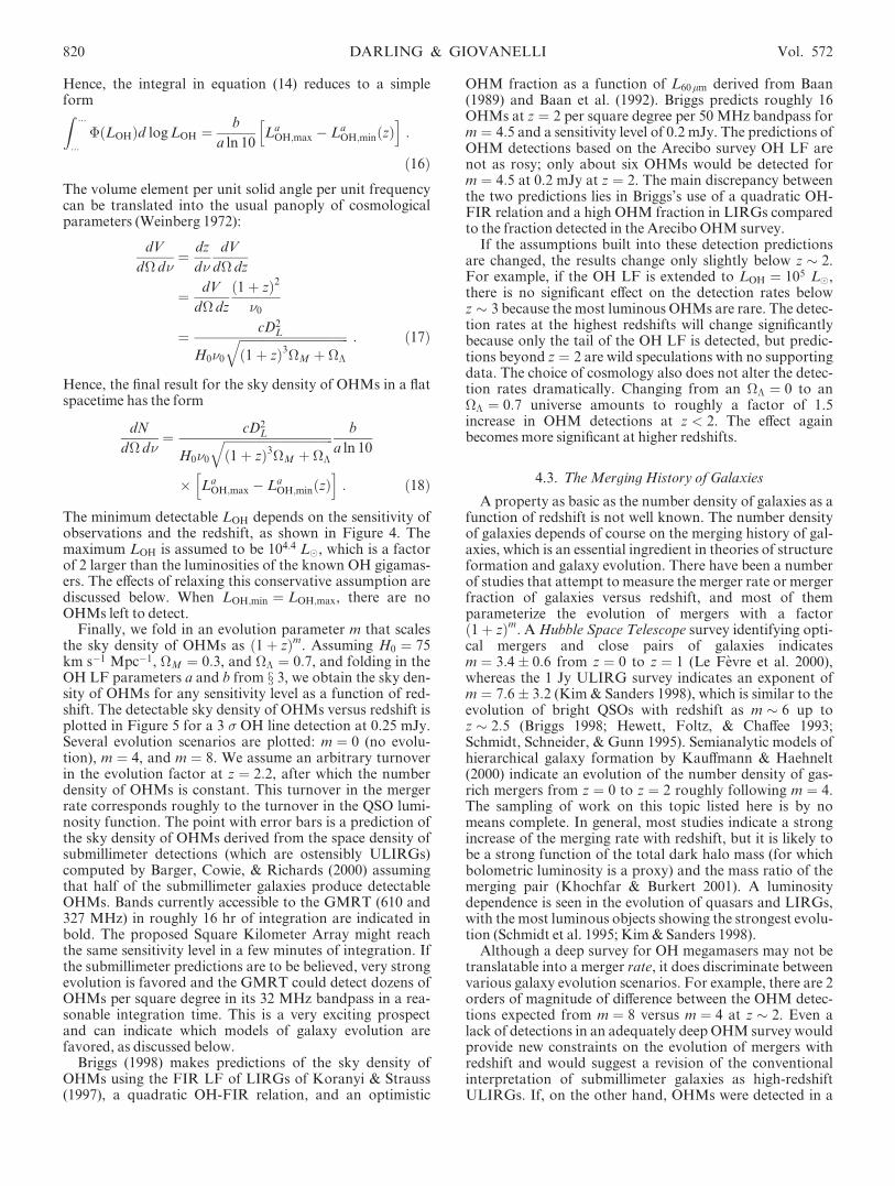
Figure 2 shows the OH luminosity, FIR luminosity, andredshift distributions of the OHM sample. Also shown arethe maximum detectable redshift distributions computedfrom the OH detections, the 60 lm detections, and the avail-able redshift distribution za. Note that the za distribution isquite flat but that the maximum detectable redshift distribu-tion for OH indicates two populations of OHMs: a popula-tion that is just detected by the survey and indicates a largepopulation of OHMs that would be detected by a deepersurvey, and a population of ‘‘ overluminous ’’ OHMs thatcan be detected in short integration times out to z ’ 1, simi-lar to QSOs or radio galaxies. Nearly half of the OHM sam-ple falls into this interesting latter category. These are theobjects that are useful for studies of galaxy evolution out tolarge redshifts. There is a hint of this population dichotomyin the plots of LOH versus LFIR analyzed in Paper III.

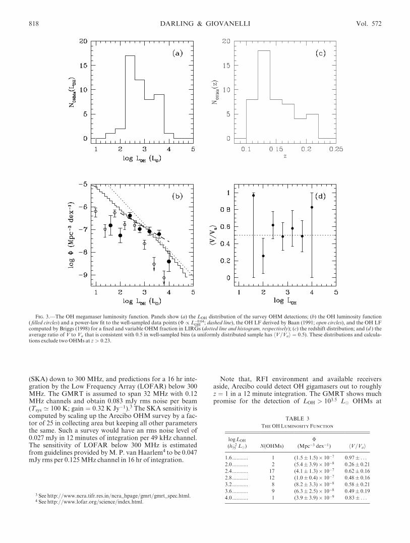
We combine all of the survey constraints and compute anOH LF, which is presented in Figure 3. A power-law fit tothe well-sampled OHLF points gives

� ¼ 9:8þ31:9�7:5 � 10�6

� �L�0:64�0:21OH Mpc�3 dex�1 ; ð12Þ

whereLOH is expressed in solar luminosities. The uniformityof the sampling in space is checked with the hV=Vai test(Schmidt 1968). A uniformly distributed sample between 0and 1 has mean 0.5. Hence, the hV=Vai values consistentwith 0.5 in well-sampled LOH bins shown in Figure 3 indi-cate a uniformly distributed sample of OH megamasers.Both the OH LF and hV=Vai are tabulated in Table 3,which includes the number of OHMs available in each LOH

bin.OH LFs previously computed by Baan (1991) and Briggs

(1998) show similar properties to the Arecibo OHM surveyLF, as indicated in Figure 3. Baan’s OH LF samples a largerrange of LOH, showing a knee at roughly 102.5 L�. The num-ber of OHMs in the Arecibo sample contributing to the OHLF below LOH ¼ 102:2 L� is inadequate to confirm thisturnover in the LF. The survey sensitivity cutoff at these lowline luminosities is severe, as seen in Figures 1 and 3. Also

noteworthy is the higher OHM density found in the AreciboLF versus Baan’s 1991 result for LOH > 103 L�. Briggs(1998) derived an OH LF from a quadratic OH-FIR rela-tion combined with a 60 lm luminosity function derived byKoranyi & Strauss (1997). Briggs computes the OH LF ana-lytically assuming an OHM fraction of unity in LIRGs forall L60 lm (Fig. 3b, dotted line) and numerically for anincreasing OHM fraction versus L60 lm (Fig. 3b, histogram).Although a quadratic OH-FIR relation is not supported bythe known OHMs (Paper III), Briggs’ OH LF follows theArecibo OH LF data points remarkably closely aboveLOH ¼ 102 L�. Briggs obtains a rough power-law slope of�1.15, which is inconsistent with the Arecibo result of�0:64� 0:2 (eq. [12]). The inconsistency can be attributedto the steep slope at the high-luminosity end of the 60 lmLF of Koranyi & Strauss (1997) compared to the shallowerslope obtained by Yun, Reddy, & Condon (2001) and Kim& Sanders (1998). When translated into an OH LF, thesteep 60 lm slope is significantly lessened by Briggs’s use ofa quadratic OH-FIR relation. The Arecibo power-law slopefor OHMs is consistent with the power-law LF Kim &Sanders (1998) determined for ULIRGs. They found� / L�2:35�0:3

IR Mpc�3 mag�1 over LIR ¼ 1012–1013 L� (theexponent becomes �0:94� 0:12 when � is expressed inMpc�3 dex�1).

A well-determined OH luminosity function forms thefoundation of any galaxy evolution study that uses OHmegamasers as luminous radio tracers of mergers, dust-enshrouded star formation, or supermassive black holebinaries. We now use this new OH LF to predict the detect-ability and abundance of OHMs available to deep radiosurveys.

4. DETECTING OH MEGAMASERS ATHIGH REDSHIFT

OH megamasers are excellent luminous tracers of merg-ing galaxies. They may become a tool for measuring themerging history of galaxies across much of cosmic time anddetermine the contribution of merging supermassive blackholes to the low-frequency gravitational-wave backgroundand to low-frequency gravitational-wave bursts. They alsoprovide an extinction-free tracer of bursts of highlyobscured star formation and may provide an independentmeasure of the star formation history of the universe. Appli-cation of OH megamasers to these topics requires (1) thatthey be detectable at moderate to high redshifts and (2) thattheir sky surface density be high enough for radio telescopesto detect at least a few per pointing.

4.1. Detectability with Current and Planned Facilities

The detectability of any given OHmegamaser at high red-shift depends on the strength of the OHM, the sensitivity ofthe instrumentation, and cosmology. Moving beyondz ’ 0:2 requires a careful treatment of cosmology becausethe differences between luminosity distances and volumesamong the manifold of possible cosmologies become signifi-cant. We assume for this analysis that H0 ¼ 75 km s�1

Mpc�1,�M ¼ 0:3, and�� ¼ 0:7.Assumptions are also required to translate the observed

quantity, flux density, to a line luminosity. We assume thatthe integrated flux density can be approximated by theproduct of the peak flux density and an average rest-frame

816 DARLING & GIOVANELLI Vol. 572

width, narrowed by the redshift:

FOH ¼ fOHD�01þ z

¼ fOH�0Dv0cð1þ zÞ ; ð13Þ

where the assumed rest-frame width is Dv0 ¼ 150 km s�1.

Figure 4 plots sensitivity thresholds for a 3 � detection ofan OHMwith luminosity LOH at redshift z. Included are theArecibo OHM survey detections and sensitivity limit, pre-dictions for a 16 hr integration by the Giant MetrewaveRadio Telescope (GMRT) at 610 and 327MHz, predictionsfor a 12 minute integration by the Square Kilometer Array

Fig. 2.—The OHmegamaser sample: LOH, L60 lm, redshift, and maximum detectable redshift distributions. Panels show (a) the LOH distribution of the sur-vey OHM detections, (b) the L60 lm distribution, (c) the redshift distribution, (d ) the maximum detectable redshift distribution calculated from the OH emis-sion line, (e) the maximum detectable redshift distribution calculated from the 60 lm flux density, and ( f ) the available redshift distribution computed fromminfzOH

max; z60 lmmax g. These distributions exclude twoOHMs at z > 0:23.

No. 2, 2002 OH MEGAMASER LUMINOSITY FUNCTION 817

(SKA) down to 300 MHz, and predictions for a 16 hr inte-gration by the Low Frequency Array (LOFAR) below 300MHz. The GMRT is assumed to span 32 MHz with 0.12MHz channels and obtain 0.083 mJy rms noise per beam(Tsys ’ 100 K; gain ¼ 0:32 K Jy�1).3 The SKA sensitivity iscomputed by scaling up the Arecibo OHM survey by a fac-tor of 25 in collecting area but keeping all other parametersthe same. Such a survey would have an rms noise level of0.027 mJy in 12 minutes of integration per 49 kHz channel.The sensitivity of LOFAR below 300 MHz is estimatedfrom guidelines provided byM. P. van Haarlem4 to be 0.047mJy rms per 0.125MHz channel in 16 hr of integration.

Note that, RFI environment and available receiversaside, Arecibo could detect OH gigamasers out to roughlyz ¼ 1 in a 12 minute integration. The GMRT shows muchpromise for the detection of LOH > 103:5 L� OHMs at

4 See http://www.lofar.org/science/index.html.

Fig. 3.—The OH megamaser luminosity function. Panels show (a) the LOH distribution of the survey OHM detections; (b) the OH luminosity function( filled circles) and a power-law fit to the well-sampled data points (� / L�0:64

OH ; dashed line), the OH LF derived by Baan (1991; open circles), and the OH LFcomputed by Briggs (1998) for a fixed and variable OHM fraction in LIRGs (dotted line and histogram, respectively); (c) the redshift distribution; and (d ) theaverage ratio of V to Va that is consistent with 0.5 in well-sampled bins (a uniformly distributed sample has hV=Vai ¼ 0:5). These distributions and calcula-tions exclude twoOHMs at z > 0:23.

TABLE 3

The OH Luminosity Function

logLOH

(h�275 L�) N(OHMs)

�

(Mpc�3 dex�1) hV=Vai

1.6........... 1 (1.5� 1.5)� 10�7 0.97� . . .

2.0........... 2 (5.4� 3.9)� 10�8 0.26� 0.21

2.4........... 17 (4.1� 1.3)� 10�7 0.62� 0.16

2.8........... 12 (1.0� 0.4)� 10�7 0.48� 0.16

3.2........... 8 (8.2� 3.3)� 10�8 0.58� 0.21

3.6........... 9 (6.3� 2.5)� 10�8 0.49� 0.19

4.0........... 1 (3.9� 3.9)� 10�9 0.83� . . .3 See http://www.ncra.tifr.res.in/ncra_hpage/gmrt/gmrt_spec.html.

818 DARLING & GIOVANELLI Vol. 572

z ¼ 1:7 in an integration of 16 hr. In integration times of lessthan an hour, a SKAwould be able to detect a large fractionof the OHM population out to medium redshifts and all OHgigamasers down to its lowest proposed operating fre-quency near 300MHz. LOFARwould be able to detect OHgigamasers in roughly 32 hr of integration from z ’ 4:5back to the reionization epoch if they exist. Clearly, OHmegamasers are detectable at moderate redshifts with cur-rent facilities and at high redshifts with future arrays, buthow abundant might they be?

4.2. The Sky Density ofOHMegamasers

The OH megamaser luminosity function derived in x 3can predict the sky density of detectable OHMs as a func-tion of instrument sensitivity, bandpass, and redshift. A use-ful function in terms of observational parameters would be

the number of OHMs detected per square degree on the skyper megahertz bandpass searched. This can be expressed asan integral of the OHLF over the range of detectable LOH:

dN

d� d�¼

Z logLOH;max

logLOH;minðzÞ

dN

d� d� d logLOHd logLOH

¼Z ...

...

dN

dV d logLOH

dV

d� d�d logLOH

¼ dV

d� d�

Z ...

...

�ðLOHÞd logLOH : ð14Þ

Recall that the OH LF is the number of OHMs with lumi-nosity LOH per cubic megaparsec per logarithmic interval inLOH, expressed as

�ðLOHÞ ¼ bLaOH : ð15Þ

Fig. 4.—Detectability of OH megamasers. Contours show the sensitivity required to detect an OHM with luminosity LOH at redshift z. Included are theresults and sensitivity of the Arecibo OHM survey and predictions for the GMRT, SKA, and LOFAR.

No. 2, 2002 OH MEGAMASER LUMINOSITY FUNCTION 819

Hence, the integral in equation (14) reduces to a simpleformZ ...

...

�ðLOHÞd logLOH ¼ b

a ln 10LaOH;max � La

OH;minðzÞh i

:

ð16Þ

The volume element per unit solid angle per unit frequencycan be translated into the usual panoply of cosmologicalparameters (Weinberg 1972):

dV

d� d�¼ dz

d�

dV

d� dz

¼ dV

d� dz

ð1þ zÞ2

�0

¼ cD2L

H0�0

ffiffiffiffiffiffiffiffiffiffiffiffiffiffiffiffiffiffiffiffiffiffiffiffiffiffiffiffiffiffiffiffiffiffiffiffið1þ zÞ3�M þ ��

q : ð17Þ

Hence, the final result for the sky density of OHMs in a flatspacetime has the form

dN

d� d�¼ cD2

L

H0�0

ffiffiffiffiffiffiffiffiffiffiffiffiffiffiffiffiffiffiffiffiffiffiffiffiffiffiffiffiffiffiffiffiffiffiffiffið1þ zÞ3�M þ ��

q b

a ln 10

� LaOH;max � La

OH;minðzÞh i

: ð18Þ

The minimum detectable LOH depends on the sensitivity ofobservations and the redshift, as shown in Figure 4. Themaximum LOH is assumed to be 104.4 L�, which is a factorof 2 larger than the luminosities of the known OH gigamas-ers. The effects of relaxing this conservative assumption arediscussed below. When LOH;min ¼ LOH;max, there are noOHMs left to detect.

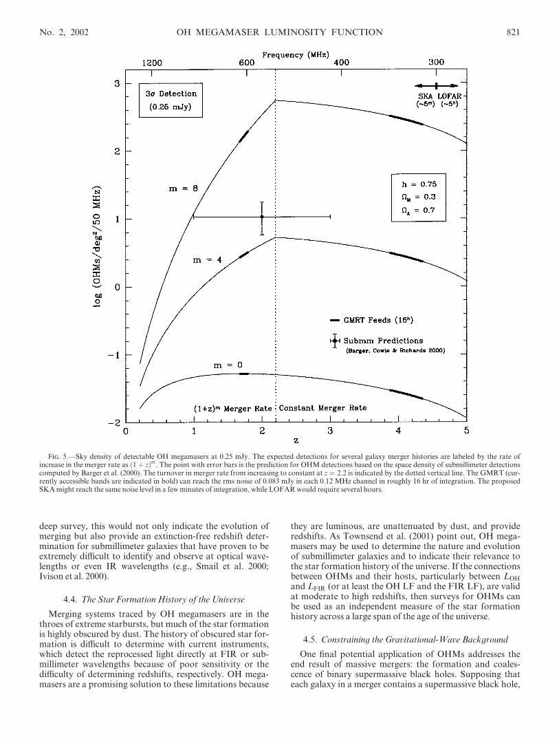
Finally, we fold in an evolution parameter m that scalesthe sky density of OHMs as ð1þ zÞm. Assuming H0 ¼ 75km s�1 Mpc�1, �M ¼ 0:3, and �� ¼ 0:7, and folding in theOH LF parameters a and b from x 3, we obtain the sky den-sity of OHMs for any sensitivity level as a function of red-shift. The detectable sky density of OHMs versus redshift isplotted in Figure 5 for a 3 � OH line detection at 0.25 mJy.Several evolution scenarios are plotted: m ¼ 0 (no evolu-tion), m ¼ 4, and m ¼ 8. We assume an arbitrary turnoverin the evolution factor at z ¼ 2:2, after which the numberdensity of OHMs is constant. This turnover in the mergerrate corresponds roughly to the turnover in the QSO lumi-nosity function. The point with error bars is a prediction ofthe sky density of OHMs derived from the space density ofsubmillimeter detections (which are ostensibly ULIRGs)computed by Barger, Cowie, & Richards (2000) assumingthat half of the submillimeter galaxies produce detectableOHMs. Bands currently accessible to the GMRT (610 and327 MHz) in roughly 16 hr of integration are indicated inbold. The proposed Square Kilometer Array might reachthe same sensitivity level in a few minutes of integration. Ifthe submillimeter predictions are to be believed, very strongevolution is favored and the GMRT could detect dozens ofOHMs per square degree in its 32 MHz bandpass in a rea-sonable integration time. This is a very exciting prospectand can indicate which models of galaxy evolution arefavored, as discussed below.

Briggs (1998) makes predictions of the sky density ofOHMs using the FIR LF of LIRGs of Koranyi & Strauss(1997), a quadratic OH-FIR relation, and an optimistic

OHM fraction as a function of L60 lm derived from Baan(1989) and Baan et al. (1992). Briggs predicts roughly 16OHMs at z ¼ 2 per square degree per 50 MHz bandpass form ¼ 4:5 and a sensitivity level of 0.2 mJy. The predictions ofOHM detections based on the Arecibo survey OH LF arenot as rosy; only about six OHMs would be detected form ¼ 4:5 at 0.2 mJy at z ¼ 2. The main discrepancy betweenthe two predictions lies in Briggs’s use of a quadratic OH-FIR relation and a high OHM fraction in LIRGs comparedto the fraction detected in the Arecibo OHM survey.

If the assumptions built into these detection predictionsare changed, the results change only slightly below z � 2.For example, if the OH LF is extended to LOH ¼ 105 L�,there is no significant effect on the detection rates belowz � 3 because the most luminous OHMs are rare. The detec-tion rates at the highest redshifts will change significantlybecause only the tail of the OH LF is detected, but predic-tions beyond z ¼ 2 are wild speculations with no supportingdata. The choice of cosmology also does not alter the detec-tion rates dramatically. Changing from an �� ¼ 0 to an�� ¼ 0:7 universe amounts to roughly a factor of 1.5increase in OHM detections at z < 2. The effect againbecomes more significant at higher redshifts.

4.3. TheMerging History of Galaxies

A property as basic as the number density of galaxies as afunction of redshift is not well known. The number densityof galaxies depends of course on the merging history of gal-axies, which is an essential ingredient in theories of structureformation and galaxy evolution. There have been a numberof studies that attempt to measure the merger rate or mergerfraction of galaxies versus redshift, and most of themparameterize the evolution of mergers with a factorð1þ zÞm. AHubble Space Telescope survey identifying opti-cal mergers and close pairs of galaxies indicatesm ¼ 3:4� 0:6 from z ¼ 0 to z ¼ 1 (Le Fevre et al. 2000),whereas the 1 Jy ULIRG survey indicates an exponent ofm ¼ 7:6� 3:2 (Kim & Sanders 1998), which is similar to theevolution of bright QSOs with redshift as m � 6 up toz � 2:5 (Briggs 1998; Hewett, Foltz, & Chaffee 1993;Schmidt, Schneider, & Gunn 1995). Semianalytic models ofhierarchical galaxy formation by Kauffmann & Haehnelt(2000) indicate an evolution of the number density of gas-rich mergers from z ¼ 0 to z ¼ 2 roughly following m ¼ 4.The sampling of work on this topic listed here is by nomeans complete. In general, most studies indicate a strongincrease of the merging rate with redshift, but it is likely tobe a strong function of the total dark halo mass (for whichbolometric luminosity is a proxy) and the mass ratio of themerging pair (Khochfar & Burkert 2001). A luminositydependence is seen in the evolution of quasars and LIRGs,with the most luminous objects showing the strongest evolu-tion (Schmidt et al. 1995; Kim& Sanders 1998).

Although a deep survey for OH megamasers may not betranslatable into a merger rate, it does discriminate betweenvarious galaxy evolution scenarios. For example, there are 2orders of magnitude of difference between the OHM detec-tions expected from m ¼ 8 versus m ¼ 4 at z � 2. Even alack of detections in an adequately deep OHM survey wouldprovide new constraints on the evolution of mergers withredshift and would suggest a revision of the conventionalinterpretation of submillimeter galaxies as high-redshiftULIRGs. If, on the other hand, OHMs were detected in a

820 DARLING & GIOVANELLI Vol. 572

deep survey, this would not only indicate the evolution ofmerging but also provide an extinction-free redshift deter-mination for submillimeter galaxies that have proven to beextremely difficult to identify and observe at optical wave-lengths or even IR wavelengths (e.g., Smail et al. 2000;Ivison et al. 2000).

4.4. The Star Formation History of the Universe

Merging systems traced by OH megamasers are in thethroes of extreme starbursts, but much of the star formationis highly obscured by dust. The history of obscured star for-mation is difficult to determine with current instruments,which detect the reprocessed light directly at FIR or sub-millimeter wavelengths because of poor sensitivity or thedifficulty of determining redshifts, respectively. OH mega-masers are a promising solution to these limitations because

they are luminous, are unattenuated by dust, and provideredshifts. As Townsend et al. (2001) point out, OH mega-masers may be used to determine the nature and evolutionof submillimeter galaxies and to indicate their relevance tothe star formation history of the universe. If the connectionsbetween OHMs and their hosts, particularly between LOH

and LFIR (or at least the OH LF and the FIR LF), are validat moderate to high redshifts, then surveys for OHMs canbe used as an independent measure of the star formationhistory across a large span of the age of the universe.

4.5. Constraining the Gravitational-Wave Background

One final potential application of OHMs addresses theend result of massive mergers: the formation and coales-cence of binary supermassive black holes. Supposing thateach galaxy in a merger contains a supermassive black hole,

Fig. 5.—Sky density of detectable OH megamasers at 0.25 mJy. The expected detections for several galaxy merger histories are labeled by the rate ofincrease in the merger rate as ð1þ zÞm. The point with error bars is the prediction for OHM detections based on the space density of submillimeter detectionscomputed by Barger et al. (2000). The turnover in merger rate from increasing to constant at z ¼ 2:2 is indicated by the dotted vertical line. The GMRT (cur-rently accessible bands are indicated in bold) can reach the rms noise of 0.083 mJy in each 0.12 MHz channel in roughly 16 hr of integration. The proposedSKAmight reach the same noise level in a fewminutes of integration, while LOFARwould require several hours.

No. 2, 2002 OH MEGAMASER LUMINOSITY FUNCTION 821

the rapid coalescence of nuclei due to dynamical friction willproduce a binary supermassive black hole that will continueto decay until a final coalescence event that will produce(among other things) a burst of gravitational waves. Burstsfrom supermassive black holes are likely to be the majorsource of 10�5 to 100 Hz gravitational waves (Haehnelt1994), which may someday be detectable by the Laser Inter-ferometer Space Antenna (LISA) or long-duration pulsartiming. The merging rate of galaxies, as well as the masses ofthe black holes involved, determine the event rate detectableby LISA. The integrated merging history of galaxies deter-mine the noise levels produced in pulsar timing and wouldprovide a ‘‘ foreground ’’ to any cosmological backgroundof gravitational waves produced during the inflationaryepoch (D. Backer 2001, private communication). Clearly,getting some handle on the event rate of supermassive blackhole mergers would provide much needed constraints andthresholds for the difficult work of detecting gravitationalwaves.

5. SUMMARY

The OH luminosity function constructed from a sampleof 50 OH megamasers detected by the Arecibo OH mega-maser survey indicates a power-law falloff with increasing

OH luminosity

� ¼ 9:8þ31:9�7:5 � 10�6

� �L�0:64�0:21OH Mpc�3 dex�1

valid for 2:2 < logLOH < 3:8 (expressed in L�) and0:1 < z < 0:23. The OH LF is used to predict the areal den-sity of detectable OHMs at arbitrary redshift for a manifoldof galaxy merger evolution scenarios parameterized byð1þ zÞm, where m 2 ½0; 8�. For reasonable choices of m, an‘‘ OH Deep Field ’’ obtained with the Giant MetrewaveRadio Telescope at 610 MHz (z ¼ 1:73) may detect dozensof OHMs per square degree in a reasonable integrationtime. A lack of detections in a sufficiently deep field wouldalso significantly constrain the evolution of merging andexclude the most extreme evolution scenarios.

The authors are very grateful to Will Saunders for accessto the PSCz catalog and to the excellent staff of NAIC forobserving assistance and support. We thank the anonymousreferee for thoughtful comments and suggestions. Thisresearch was supported by Space Science Institute archivalgrant 8373 and NSF grant AST 00-98526 and made use ofthe NASA/IPAC Extragalactic Database (NED), which isoperated by the Jet Propulsion Laboratory, California Insti-tute of Technology, under contract with the National Aero-nautics and Space Administration.

REFERENCES

Baan,W. A. 1989, ApJ, 338, 804———. 1991, in ASP Conf. Ser. 16, Atoms, Ions, & Molecules: NewResults in Spectral Line Astrophysics, ed. A. D. Haschick & P. T. P. Ho(San Francisco: ASP), 45

Baan,W. A., Haschick, A., &Henkel, C. 1992, AJ, 103, 728Barger, A. J., Cowie, L. L., & Richards, E. A. 2000, AJ, 119, 2092Briggs, F. H. 1998, A&A, 336, 815Condon, J. J., Cotton, W. D., Greisen, E. W., Yin, Q. F., Perley, R. A.,Taylor, G. B., & Broderick, J. J. 1998, AJ, 115, 1693

Dale, D. A., Helou, G., Contursi, A., Silbermann, N. A., & Kolhatkar, S.2001, ApJ, 549, 215

Darling, J., &Giovanelli, R. 2000, AJ, 119, 3003 (Paper I)———. 2001, AJ, 121, 1278 (Paper II)———. 2002, AJ, press (Paper III)Fisher, K. B., Huchra, J. P., Strauss, M. A., Davis, M., Yahil, A., &Schlegel, D. 1995, ApJS, 100, 69

Fullmer, L., & Lonsdale, C. 1989, Catalogued Galaxies and QuasarsObserved in the IRAS Survey (Version 2; Pasadena: JPL)

Haehnelt, M. G. 1994,MNRAS, 269, 199Hewett, P. C., Foltz, C. B., & Chaffee, F. H. 1993, ApJ, 406, L43Ivison, R. J., Smail, I., Barger, A. J., Kneib, J.-P., Blain, A. W., Owen,F. N., Kerr, T. H., & Cowie, L. L. 2000,MNRAS, 315, 209

Kauffmann, G., &Haehnelt, M. 2000,MNRAS, 311, 576

Khochfar, S., & Burkert, A. 2001, ApJ, 561, 517Kim, D.-C., & Sanders, D. B. 1998, ApJS, 119, 41Koranyi, D.M., & Strauss,M. A. 1997, ApJ, 477, 36Lawrence, A., et al. 1999,MNRAS, 308, 897Le Fevre, O., et al. 2000,MNRAS, 311, 565Lineweaver, C. H., Tenorio, L., Smoot, G. F., Keegstra, P., Banday, A. J.,& Lubin, P. 1996, ApJ, 470, 38

Lu, N. Y., & Freudling,W. 1995, ApJ, 449, 527Page,M. J., & Carrera, F. J. 2000,MNRAS, 311, 433Saunders,W., et al. 2000,MNRAS, 317, 55Schmidt, M. 1968, ApJ, 151, 393Schmidt, M., Schneider, D. P., &Gunn, J. E. 1995, AJ, 110, 68Smail, I., Ivison, R. J., Owen, F. N., Blain, A. W., & Kneib, J.-P. 2000,ApJ, 528, 612

Staveley-Smith, L., Norris, R. P., Chapman, J. M., Allen, D. A., Whiteoak,J. B., &Roy, A. L. 1992,MNRAS, 258, 725

Strauss, M. A., Huchra, J. P., Davis, M., Yahil, A., Fisher, K. B., & Tonry,J. 1992, ApJS, 83, 29

Townsend, R. H. D., Ivison, R. J., Smail, I., Blain, A. W., & Frayer, D. T.2001,MNRAS, 328, L17

Weinberg, S. 1972, Gravitation and Cosmology (NewYork:Wiley)Yun,M. S., Reddy, N. A., & Condon, J. J. 2001, ApJ, 554, 803

822 DARLING & GIOVANELLI