a real-time hurricane surface wind forecasting model: formulation and verification

A Real-Time Hurricane Surface Wind Forecasting Model: Formulationand Verification

LIAN XIE AND SHAOWU BAO

Department of Marine, Earth and Atmospheric Sciences, North Carolina State University, Raleigh, North Carolina

LEONARD J. PIETRAFESA

College of Physical and Mathematical Sciences, North Carolina State University, Raleigh, North Carolina

KRISTEN FOLEY AND MONTSERRAT FUENTES

Department of Statistics, North Carolina State University, Raleigh, North Carolina

(Manuscript received 19 January 2005, in final form 13 August 2005)

ABSTRACT

A real-time hurricane wind forecast model is developed by 1) incorporating an asymmetric effect into theHolland hurricane wind model; 2) using the National Oceanic and Atmospheric Administration (NOAA)/National Hurricane Center’s (NHC) hurricane forecast guidance for prognostic modeling; and 3) assimi-lating the National Data Buoy Center (NDBC) real-time buoy data into the model’s initial wind field. Themethod is validated using all 2003 and 2004 Atlantic and Gulf of Mexico hurricanes. The results show that6- and 12-h forecast winds using the asymmetric hurricane wind model are statistically more accurate thanusing a symmetric wind model. Detailed case studies were conducted for four historical hurricanes, namely,Floyd (1999), Gordon (2000), Lily (2002), and Isabel (2003). Although the asymmetric model performedgenerally better than the symmetric model, the improvement in hurricane wind forecasts produced by theasymmetric model varied significantly for different storms. In some cases, optimizing the symmetric modelusing observations available at initial time and forecast mean radius of maximum wind can produce com-parable wind accuracy measured in terms of rms error of wind speed. However, in order to describe theasymmetric structure of hurricane winds, an asymmetric model is needed.

1. Introduction

Hurricane-induced storm surge and flooding remaina severe threat to coastal communities despite progressmade over the past several decades on improved hur-ricane track and intensity forecasts. The accuracy of astorm surge forecast depends not only on the track andintensity, but also on the distribution of the forecastwind field. A variety of numerical and statistical modelshave been developed for forecasting (e.g., Holland1980; Jelesnianski et al. 1992) and hindcasting hurricanewind fields (e.g., Powell and Houston 1998; Houston etal. 1999). The extensive resources needed in the use offull physics mesoscale models have kept them from be-ing adopted in routine operational forecasts of hurri-

cane winds. Instead, simple parameterized models arewidely used in the simulations of hurricane wind fieldsand for providing hurricane forcing for storm surgeforecasting. Early studies (Depperman 1947; Hughes1952; Riehl 1954, chapter 11) used a modified Rankinevortex to approximate the structure of a generic tropi-cal cyclone (TC). The deficiency of the modified Ran-kine vortex model is that it requires accurate measure-ments of the radius of maximum winds, and the vortexis axisymmetric. Schleomer (1954) suggested a para-metric model that relates the wind field to the pressurefield. However, Schleomer’s model markedly underes-timates the radial extent of hurricane winds. Holland(1980) suggested further modifications to Schleomer’s(1954) formulation, using U.S. Army Corps of Engi-neers data in the Florida area. Holland’s model as-sumes that for a generic TC, the surface pressure fieldfollows a modified rectangular hyperbola, as a functionof radius, to give

Corresponding author address: Lian Xie, Department of Ma-rine, Earth and Atmospheric Sciences, North Carolina State Uni-versity, Box 8208, Raleigh, NC 27695-8208.E-mail: [email protected]

MAY 2006 X I E E T A L . 1355

© 2006 American Meteorological Society

MWR3126

P�r� � Pc � �Pn � Pc� exp��Rmax�r�B, �1�

and the tangential wind field is given by the pressurefield via cyclostrophic balance,

V�r� � �B

�a�Rmax

r �B

�Pn � Pc� exp��Rmax�r�B

� �rf

2 �2�1�2

�rf

2, �2�

where P(r) is the surface pressure at a distance of rfrom the hurricane center, Pn the ambient surface pres-sure, Pc the hurricane central surface pressure, Rmax theradius of maximum wind (RMW), B a hurricane-shapeparameter, f the Coriolis parameter, and V(r) the ve-locity at a distance r from the hurricane center. Forhurricanes at low latitudes, the terms associated withthe Coriolis parameter, f, are neglected.

In Holland’s model, there is no need to know theRMW in order to compute the maximum wind becauseof the cyclostrophic balance. However, in order to de-scribe the structure of the wind field, RMW must beknown. The parameter B (ranging from 1 to 2.5), whichrepresents the vortex’s shape and size, must be speci-fied. When the parameter B is poorly specified, theerrors of the calculated wind field can be significant.One way to estimate B is to develop a statistical rela-tionship between B and the hurricane center pressuredrop in a specific region (Jakobsen and Madsen 2004).Such an approach is useful for modeling historical hur-ricanes, but offers only limited improvement over theoriginal Holland model.

The Holland model is an axisymmetric model, mean-ing that the asymmetric structure of a hurricane cannotbe represented by the model no matter how B is deter-mined. On the other hand, it is well known that anactual hurricane is rarely axisymmetric. Within thesame hurricane, the differences in wind speeds at dif-ferent azimuthal directions can be substantial. Highlyasymmetric structures in a landfalling hurricane oftenlead to large errors in storm surge forecasting (Houstonet al. 1999).

Georgiou (1985) introduced a more sophisticatedmodel to overcome some of these limitations:

V � Vholland � 0.5Vt Sin��, �3�

where Vt is the hurricane translation speed and � is theangle from the direction of the hurricane movement. Inaddition to the cyclone movement included in Eq. (3),various other factors can contribute to the asymmetricstructure of a hurricane, such as friction (Shapiro 1983),vertical shear, and environmental conditions (Wangand Holland 1996), the near discontinuity of the surface

friction and the latent heat flux (Chen and Yau 2003),and the � effect (Ross and Kurihara 1992). There is noconsensus on how these factors should be incorporatedinto parametric hurricane models.

On the other hand, in recent years other resourceshave been made available in the public domain such asthe TC forecast guidance issued by the National Hur-ricane Center (NHC) of the National Oceanic and At-mospheric Administration (NOAA), observations frombuoy stations, and the near–real time hurricane surfacewind analysis provided by Atlantic Oceanographic andMeteorological Laboratory/Hurricane Research Divi-sion (HRD; referred to as the HRD winds, hereafter)that may be used to initialize hurricane winds and vali-date wind forecasts.

The NHC issues 120-h TC track and intensity fore-casts (the wind structure forecasts are limited to 72 h)four times a day for all storms in the North Atlantic andthe North Pacific east of 140°W (http://www.nhc.noaa.gov). The track forecasts include the latitude and lon-gitude (to the nearest tenth of a degree) of the stormcenter, and the intensity forecasts include the maximumsustained (1-min average) surface wind (to the nearest5 kt) at 12, 24, 36, 48, and 72 h. The storm structure isdepicted by the radial extent of the 34-, 50-, and 64-ktwinds in four quadrants (northeast, southeast, south-west, and northwest). These radii represent the maxi-mum radial extent of winds of a given threshold in eachof the four quadrants surrounding the storm. Forecastsof these wind radii are issued four times a day out to 36h. The 50-kt wind radii are also forecast at 48 and 72 h.The TC intensity models used by the NHC include theStatistical Hurricane Intensity Forecast (SHIFOR)(Jarvinen and Neumann 1979), the Statistical Hurri-cane Intensity Prediction Scheme (SHIPS) (DeMariaand Kaplan 1994), and the Geophysical Fluid DynamicsLaboratory (GFDL) hurricane model. The NHC fore-cast guidance is useful in hurricane warning and evacu-ation processes. However, the NHC forecast guidancehas not been effectively utilized for storm surge fore-casting because of a number of limiting factors, such asthe still relatively large mean track error and the lack ofa convenient method to incorporate the NHC forecastguidance into gridded hurricane wind forecasts.

In this study, an algorithm to produce near–real timeforecasts of hurricane wind fields is developed by usingthe NHC hurricane forecast guidance and real-timebuoy observations. Near–real time HRD surface windanalysis and buoy wind observations are used to vali-date model forecasts. The method is described in sec-tion 2. A statistical analysis of the model error relativeto the traditional Holland model was carried out for all2003 and 2004 hurricanes. Case studies were also car-

1356 M O N T H L Y W E A T H E R R E V I E W VOLUME 134

ried out for four recent hurricanes, namely, Floyd(1999), Gordon (2000), Lily (2002), and Isabel (2003).In the case study, the wind fields computed with thenew asymmetric wind model (AWM) were comparedwith those produced by the Holland model (HM), op-timized Holland model (OHM), buoy observations, andHRD wind analyses. The results and discussions arepresented in section 3. A case study of how to quantifyuncertainty in the simulated wind field is explained insection 4. A summary of the conclusions is provided insection 5.

2. Method

The objective of this study is to develop a near–realtime hurricane wind forecast system by incorporatingthe asymmetric representation of a hurricane wind fieldinto the well-known and very utilitarian HM, based onavailable real-time observations and analyses as well asthe NHC hurricane forecast guidance, to provide opti-mized asymmetric hurricane wind forecasts.

The National Data Buoy Center (NDBC) maintainsautomated reporting stations in the Gulf of Mexico, incoastal areas, in portions of the Atlantic and PacificOceans, and in the Great Lakes. These data acquisitionsystems collect real-time meteorological and oceano-graphic measurements for operations and for researchpurposes. Moored buoy and Coastal-Marine Auto-mated Network (C-MAN) stations routinely acquire,store, and transmit data every hour. Data obtained op-erationally include sea level pressure, wind speed anddirection, peak wind, and air temperature. Sea surfacetemperature and wave spectra data are measured by allmoored buoys and a limited number of C-MAN sta-tions. Relative humidity is measured at several stations.Ocean currents and salinity are measured at a fewcoastal stations. The buoy stations whose data are usedin this study are listed in the appendix.

The HRD wind analysis uses virtually all availablesurface weather observations (e.g., ships, buoys, coastalplatforms, surface aviation reports, reconnaissance air-craft data adjusted to the surface). Observational dataare downloaded on a regular schedule and then pro-cessed to fit the analysis framework. This includes thedata sent by NOAA P3 and G4 research aircraft duringthe HRD hurricane field program, the Step FrequencyMicrowave Radiometer measurements of surfacewinds, as well as U.S. Air Force Reserves (AFRES)C-130 reconnaissance aircraft, remotely sensed windsfrom the polar-orbiting Special Sensor Microwave Im-ager (SSM/I) and European Remote Sensing Satellite(ERS), the Quick Scatterometer (QuikSCAT) platformand Tropical Rainfall Measuring Mission (TRMM) Mi-

crowave Imager satellites, and Geostationary Opera-tional Environmental Satellite (GOES) cloud driftwinds derived from tracking low-level near-infraredcloud imagery from these geostationary satellites.Available data are composited relative to the stormover a 4–6-h period. All data are quality controlled andprocessed to conform to a common framework forheight (10 m or 33 ft), exposure (marine or open terrainover land), and averaging period (maximum sustained1-min wind speed) using accepted methods from mi-crometeorology and wind engineering (Powell et al.1996; Powell and Houston 1996). Note that the HRDwind analyses are highly variable in accuracy, depend-ing on the quality and quantity of the observationsused, and on the appropriateness of the underlying as-sumptions used to manipulate the observations. In par-ticular, analyses conducted without the benefit of SteppedFrequency Microwave Radiometer data may be in er-ror locally by 10–15 m s�1 or more. Despite these de-ficiencies, they remain the best available near–real timegridded hurricane wind analyses (J. L. Franklin 2003,personal communication).

We use the forecasting of the Hurricane Isabel (2003)wind field at 0000 UTC 18 September as an example toillustrate the asymmetric hurricane wind forecastingsystem. First, NHC hurricane forecast guidance issuedat 1500 UTC 17 September 2003 (as listed below) isretrieved from the NHC:

FORECAST VALID 18/0000UTC 31.4N 73.5W.MAX WIND 95 KT . . . GUSTS 115 KT.64 KT . . . 100NE 80SE 60SW 90NW.50 KT . . . 125NE 100SE 80SW 125NW.34 KT . . . 275NE 250SE 150SW 200NW.

The forecast is effective at 0000 UTC 18 September.The forecast storm center is at 31.4°N, 73.5°W. The1-min average maximum sustained surface wind is 95 ktwith gusts up to 115 kt. The storm structure is charac-terized by the radial extent of the 34-, 50-, and 64-ktwind in four quadrants (northeast, southeast, south-west, and northwest) relative to the storm center.

To incorporate the NHC forecast guidance into theHolland model, Rmax in Eq. (2) is modified to becomea function of the azimuthal angle (�):

Rmax�� P1�n�1 � P2�n�2 � · · · � Pn�1� � Pn,

�4�

P�r, �� Pc � �Pn � Pc� exp��Rmax��rB, �5�

VAholland � �B

�a�Rmax��

r �B

�Pn � Pc� exp��Rmax��rB

� �rf

2 �2�1�2

�rf

2, �6�

MAY 2006 X I E E T A L . 1357

where P is the atmospheric pressure, Pc the hurricanecenter pressure, Pn the environmental pressure, VAholland

the wind speed, a the air density, and f the Coriolisparameter.

From Eq. (2) we can determine the initial values of Busing Vmax, Pn, and Pc at the initial time (1500 UTC 17September 2003):

B0 �Vmax

2 �ae

Pn � Pc, �7�

where Vmax is hurricane maximum wind speed, and e �2.7183. Then, the NHC forecast guidance is used tocurve fit the polynomial [Eq. (4)] to obtain Rmax as afunction of �. Note that in Eq. (2), when values of V(r)and r are given, Rmax has two solutions in each of thefour quadrants. For example, in the NHC forecast for0000 UTC 18 September listed above, in the southeastquadrant, the radius of the 64-kt wind is 80 n mi. Equa-tion (2) can be solved based upon this information andthe two corresponding Rmax solutions are 23.7 and 176.2n mi, respectively (Fig. 1). However, only the smallervalue is the physical solution since the NHC forecastindicates that 64-kt winds occur within 80 n mi of thestorm center in the southeast quadrant. The Rmax val-ues computed for the four quadrants for the 0000 UTC18 September forecast are 29.62, 23.70, 18.96, and 29.62n mi for the northeast, southeast, southwest, and north-

west quadrants, respectively. Next, the coefficients ofthe fourth-order polynomial [Eq. (4)] are obtained by apolynomial curve fitting of the Rmax values. For theHurricane Isabel case, the coefficients at 0000 UTC 18September are estimated as follows:

n � 5,

P1 � �2.56�10�8�,

P2 � 2.17�10�5�,

P3 � �5.70�10�3�,

P4 � 4.83�10�1�,

P5 � 17.6.

The same procedure is used to compute P1 to P5 atthe initial time (1500 UTC 17 September 2003). Sec-ondary optimization of the initial wind field using theNDBC buoy winds is performed whenever there arefunctioning buoys within the analysis domain. The op-timal values of the parameters (B and Pi, i � 1–5) forthe initial wind field are those that minimize the fol-lowing root-mean-square (rms) error function:

��n�1

N

�V�B, P1�5� � Vbuoy2, �8�

FIG. 1. Hurricane Isabel wind profiles (kt) in the southeast quadrant: (a) curve is for Rmax

� 23.70 n mi; (b) curve is for Rmax � 176.20 n mi.


where N is the number of functioning buoy stationswithin the analysis domain. If there is no working buoywithin the analysis domain, secondary optimization ofthe initial wind field is not performed. Finally, the hur-ricane wind field at time T between the initial time T0

(in this case 1500 UTC 17 September) and NHC fore-cast guidance valid for T1 (in this case, 0000 UTC 18September) is linearly interpolated. Similarly, hurri-cane wind fields at T2 can be computed using NHCforecast guidance valid for T2, and the wind fields atany time between T1 and T2 are linearly interpolated.This forecast process can continue until the end of theNHC forecast guidance period. Note that, since buoyobservations are used to optimize the initial wind field,in the event that no operational buoy falls within theanalysis domain, the model-simulated initial windasymmetry only reflects the contribution from the NHCinitial estimation of the wind radii in each quadrant.The number of buoy observations or the lack of themmay affect the accuracy of the initial wind analysis andthe interpolated wind between the initial time (T0) andthe nearest NHC forecast time (T1). However whetheror not buoy observations are available at the initial timedoes not affect the wind forecast at or beyond T1 sinceonly the parameters in the NHC forecast guidance areused in the computation of the forecast wind field at orbeyond T1, which does not rely on the initial wind field.This is because parametric hurricane wind models suchthe Holland model are essentially balanced models thatdo not involve tendency (d/dt) calculation.

The NHC forecast guidance provides the radius ofthe 34-, 50-, and 64-kt winds in four quadrants. It doesnot provide information on the wind distribution in re-gions where the wind speed is greater than 64 kt. How-ever, because severe storm surge and flooding damagesare often associated with peak winds, the parametersobtained with the method described above may some-times still underestimate the effects of the wind asym-metries near the radius of maximum winds. To improvethe wind forecast in the vicinity of Rmax, we introducethe following formula:

V � A��Vholland�B, Rmax�, �9�

where B is the same as in that in Eq. (6), Rmax is theaverage of Rmax(�)in Eq. (6), A(�) � [Rmax(�)/Rmax]�,and � � B/2. By using Eq. (9), the asymmetric windstructure represented by Rmax(�)is translated into coef-ficient A(�), which reproduces not only the asymmetricshape but also the asymmetric distribution of the maxi-mum wind speed.

The pressure profile used by the original Holland(1980) model does not describe the surface (10 m) windbut may be used to estimate a gradient or cyclostrophic

wind. The wind fields obtained directly from the Hol-land model apply at the top of the surface layer. Theo-retically, surface friction in marine waters must be in-cluded when converting Holland winds to surfacewinds. However, in practice the Holland model is onlyneeded for mapping wind distribution. The actual mag-nitude of the wind speed is usually determined empiri-cally by fitting the radial profile of hurricane windspeed using observed surface (10 m) maximum sus-tained wind speed. Thus, the effect of surface friction isimplicitly included during the optimization processes[Eq. (9)].

3. Results and discussions

In this section, we present the results for model vali-dation. We begin with an extensive statistical validationby conducting 144 hurricane wind hindcasts for all 2003and 2004 Atlantic and Gulf of Mexico hurricanes ex-cept those whose buoy observations or HRD surfacewind analysis were incomplete (for validation pur-poses), or whose NHC forecast guidance were too fewto produce valid Rmax in all four quadrants. For allcases, 6- and 12-h wind forecasts are made. A 6-h (12 h)wind forecast utilizes NHC storm track and intensityforecast guidance that is validated 6 (12 h) from thetime when the wind forecast is made. Note that, al-though NHC forecast guidance contains hurricanetrack and intensity information at 12-h intervals, theforecast is updated at least four times a day. Thus, theNHC hurricane forecast guidance is available at 6-hintervals. For example, let t � 0 represent the currenttime, then a 12-h forecast guidance issued t � �6 hprovides information at t � 6 h, a 12-h forecast guid-ance issued at t � 0 gives information at t � 12 h, etc.

In the following, both 6- and 12-h forecast results arepresented. The forecast results using the AWM, HM,and OHM models are compared against the buoy dataas well as HRD surface wind analyses. The average rmserrors estimated by using the buoy data are 4.4, 4.4, 7.9,and 4.9 m s�1 for the AWM 6-h, AWM 12-h, HM 6-h,and OHM 6-h forecasts, respectively. The average rmserrors estimated by using the HRD wind analyses are3.4, 3.3, 9.9, and 4.8 m s�1 for the AWM 6-h, AWM12-h, HM 6-h, and OHM 6-h forecasts, respectively.Thus, both AWM 6- and 12-h forecasts are generally incloser agreement with buoy observations and HRD sur-face wind analyses than the 6-h forecasts computed bythe HM and the OHM.

Next, consider the forecast error in more detail forfour historical hurricanes, namely, Floyd (1999), Gor-don (2000), Lily (2002), and Isabel (2003). These fourcases are chosen because there are more complete buoy

MAY 2006 X I E E T A L . 1359

observations and HRD surface wind analysis availablefor these cases (for validation purposes). Forecastswere made for these four historical hurricanes using theasymmetric hurricane wind model described in section2. Comparisons of the difference in the hurricane maxi-mum wind speed between the buoy measurements andforecasts using different hurricane wind models areshown in Table 1. When the hurricane center is faraway from a buoy station, the winds measured by thebuoy reflect primarily the ambient winds. To focus onthe validation of hurricane wind fields, only the differ-ence between the buoy measurements and the forecastsvalid for local peak winds are presented. Note that boththe 6- and 12-h forecasts are updated hourly. The ad-vantage of the asymmetric model is clearly demon-strated. As shown in Table 1, the overall rms error for(a) 6-h and (b) 12-h forecasts using the asymmetricmodel was 2.26 and 2.33 m s�1, respectively, consider-ably smaller than that of the 6-h forecast using the (c)Holland model (6.93 m s�1) and the (d) optimized Hol-land model (5.18 m s�1).

Forecasts for Hurricane Floyd were made from 2100UTC 7 September to 0900 UTC 17 September, a 228-hperiod. Figure 2 shows the time series of Floyd’s windsat buoy stations FPSN7, CLKN7, VENF1, and 44014.For each panel, five time series are shown: 1) buoy data;2) the HM-derived wind; 3) the OHM-derived wind; 4)the new AWM 6-h; and 5) the AWM 12-h forecast

results. The wind speed at each hour is the forecastresult using the NHC forecast guidance available 6 and12 h prior to the forecast time. The buoy data are ad-justed to a standard 10-m height based on Large andPond (1981).

The hurricane tracks, hurricane center minimumpressures, and the maximum wind speed used in theaxisymmetric HM runs were the same as those used inthe AWM. In the axisymmetric HM runs without opti-mization, B was set to 1.0, as in the Sea, Lake, andOverland Surges from Hurricanes model (Jelesnianskiet al. 1992), and Rmax was specified based on climato-logical values suggested by Hsu and Yan (1998) and theNHC forecast guidance available 6 h before the fore-cast validation time. For the OHM runs, the parametersB and Rmax were optimized using the NHC forecastguidance available 6 h before the forecast validationtime.

Figure 2 shows that wind forecasts from the AWMshowed better agreement with buoy measurementsthan those forecast from the HM. As shown in Figs.2a–c, the HM overestimated the maximum wind speed,while in Fig. 2d, it underestimated the maximum windspeed. The rms error for the 6- and 12-h forecasts usingthe AWM are 3.07 and 4.19 m s�1, respectively,whereas the rms for the Holland model reached 10.14m s�1 (without optimization) and 8.22 m s�1 (with op-timization; Table 1). For all buoy stations, the Hollandmodel tended to overestimate the wind speed beforethe peak wind. Compared to the HM, the OHM im-proved the forecast overall. Thus, although optimiza-tion can lead to some improvement in hurricane windforecasts using the axisymmetric Holland model, theoptimization using the asymmetric model provided thebest hurricane wind forecasts.

Figure 3 shows the two-dimensional wind fields ofFloyd at 1300 UTC 11 September. The five panels ofthe figure are, respectively, (a) the wind field of HRDsurface wind analysis; (b) the AWM 6-h forecast; (c)the AWM 12-h forecast; (d) the HM 6-h forecast; and(e) the OHM 6-h forecast. It is shown that the AWM 6-and 12-h forecasts were able to capture the main char-acteristics of the asymmetric structure and the intensityof the hurricane winds. Stronger winds appear in thenortheast quadrant, consistent with the HRD hurricanewind analyses. The average rms error from the HRDsurface wind analysis is 4.18 and 5.45 m s�1 for theasymmetric model’s 6- and 12-h forecasts, and 8.29 and6.77 m s�1 for the HM 6-h and OHM 6-h forecasts,respectively (Table 2). The HM described neither themagnitude nor the asymmetric structure of the HRDdata correctly. The OHM depicted hurricane windstrength better than the HM, but because it cannot de-

TABLE 1. Comparison of the maximum wind speed differences(m s�1) from buoy station measurements using different models:(a) AWM 6-h prediction; (b) AWM 12-h prediction; (c) HM 6-hprediction; and (d) OHM 6-h prediction.

Storm/buoy (a) (b) (c) (d)

Floyd/44014 �2.57 �1.79 �3.62 �6.83Floyd/FPSN7 �1.22 0.77 5.21 5.83Floyd/BUZM3 3.70 2.13 �7.18 �10.44Floyd/CLKN7 0.22 �5.43 1.43 �2.95Floyd/VENF1 4.00 5.70 17.82 8.57Gordon/DPIA1 �0.01 �0.59 0.11 �2.13Gordon/SANF1 �1.79 �1.29 4.39 3.26Gordon/42041 �0.97 �0.38 3.89 2.60Gordon/LONF1 �0.71 �0.58 5.73 4.56Gordon/SPGF1 1.83 1.81 8.15 6.93Isabel/44014 4.52 2.36 3.85 2.18Isabel/44025 �1.04 �1.21 1.34 �1.94Isabel/CHLV2 0.61 0.14 0.89 �0.07Isabel/41001 0.37 1.63 2.80 �0.55Isabel/DUCN7 4.42 2.46 1.70 1.82Lily/DRYF1 �1.73 �1.73 8.15 5.65Lily/LONF1 �0.33 �0.60 8.40 5.52Lily/SANF1 �1.54 �2.02 7.44 4.67Lily/SMKF1 �1.00 �1.31 7.89 4.95Lily/BURL1 1.94 1.60 9.27 5.77Mean rms error 2.26 2.33 6.93 5.18


scribe the hurricane asymmetric wind structure, its rmserror is larger than those of the AWM 6- and 12-hforecasts.

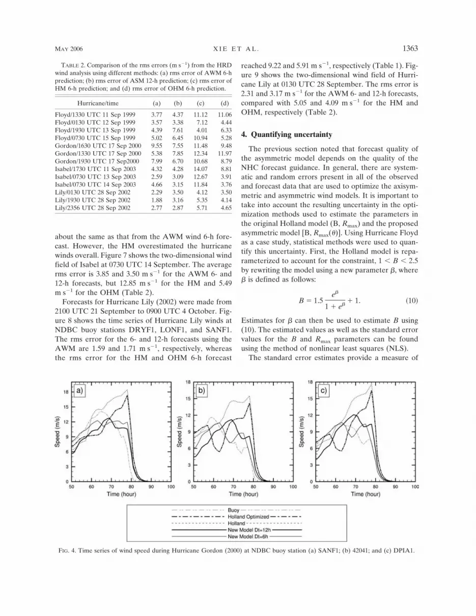
For the Floyd case the optimization on the axisym-metric Holland model had mixed effects (Tables 1 and2). For the other three hurricanes simulated in thisstudy, the performances of the AWM are similar to thatof Floyd, except that in all three cases, the OHM pro-duced better results than those of the axisymmetricHM. As an example, forecasts for Gordon (2000) weremade from 1500 UTC 14 September to 1500 UTC 18September. Figure 4 shows the time series of the fore-cast and buoy winds for Hurricane Gordon at buoystations SANF1, 42041, and 42041. The rms error forthe 6- and 12-h forecasts using the AWM are 1.41 and1.20 m s�1, respectively, whereas the rms error for the

HM and OHM reached 5.78 and 4.72 m s�1, respec-tively (Table 1). Figure 5 shows the two-dimensionalwind field of Gordon at 1330 UTC 17 September. Theaverage rms difference from the HRD surface windanalysis is 7.64 and 7.36 m s�1 for the AWM 6- and 12-hforecasts, but 11.50 and 10.07 m s�1 for the HM andOHM, respectively (Table 2).

Forecasts for Isabel (2003) were made from 1300UTC 6 September to 1500 UTC 19 September. Figure6 shows the time series of Hurricane Isabel winds atNDBC buoy stations 44025, 44014, CHLV2, and 41001.The rms error for the 6- and 12-h forecasts using theAWM are 3.22 and 1.98 m s�1, respectively, whereasthe rms error for the HM and OHM reached 2.65 and1.70 m s�1, respectively (Table 1). In this case, the HMand OHM results for the maximum wind speed were

FIG. 2. Time series of wind speed during Hurricane Floyd (1999) at NDBC buoy station (a) FPSN7;(b) CLKN7; (c) VENF1; and (d) 44014.

MAY 2006 X I E E T A L . 1361

FIG

.3.T

wo-

dim

ensi

onal

win

dst

ruct

ures

ofF

loyd

(199

9)at

1330

UT

C11

Sep:

(a)

HR

Dw

ind

anal

ysis

;(b)

new

asym

met

ric

mod

elfo

reca

st(

t�

6h)

;(c)

new

asym

met

ric

mod

elfo

reca

st(

t�

12h)

;(d)

nono

ptim

ized

Hol

land

mod

el;a

nd(e

)op

tim

ized

Hol

land

mod

el.


about the same as that from the AWM wind 6-h fore-cast. However, the HM overestimated the hurricanewinds overall. Figure 7 shows the two-dimensional windfield of Isabel at 0730 UTC 14 September. The averagerms error is 3.85 and 3.50 m s�1 for the AWM 6- and12-h forecasts, but 12.85 m s�1 for the HM and 5.49m s�1 for the OHM (Table 2).

Forecasts for Hurricane Lily (2002) were made from2100 UTC 21 September to 0900 UTC 4 October. Fig-ure 8 shows the time series of Hurricane Lily winds atNDBC buoy stations DRYF1, LONF1, and SANF1.The rms error for the 6- and 12-h forecasts using theAWM are 1.59 and 1.71 m s�1, respectively, whereasthe rms error for the HM and OHM 6-h forecast

reached 9.22 and 5.91 m s�1, respectively (Table 1). Fig-ure 9 shows the two-dimensional wind field of Hurri-cane Lily at 0130 UTC 28 September. The rms error is2.31 and 3.17 m s�1 for the AWM 6- and 12-h forecasts,compared with 5.05 and 4.09 m s�1 for the HM andOHM, respectively (Table 2).

4. Quantifying uncertainty

The previous section noted that forecast quality ofthe asymmetric model depends on the quality of theNHC forecast guidance. In general, there are system-atic and random errors present in all of the observedand forecast data that are used to optimize the axisym-metric and asymmetric wind models. It is important totake into account the resulting uncertainty in the opti-mization methods used to estimate the parameters inthe original Holland model (B, Rmax) and the proposedasymmetric model [B, Rmax(�)]. Using Hurricane Floydas a case study, statistical methods were used to quan-tify this uncertainty. First, the Holland model is repa-rameterized to account for the constraint, 1 � B � 2.5by rewriting the model using a new parameter �, where� is defined as follows:

B � 1.5e�

1 � e�� 1. �10�

Estimates for � can then be used to estimate B using(10). The estimated values as well as the standard errorvalues for the B and Rmax parameters can be foundusing the method of nonlinear least squares (NLS).

The standard error estimates provide a measure of

FIG. 4. Time series of wind speed during Hurricane Gordon (2000) at NDBC buoy station (a) SANF1; (b) 42041; and (c) DPIA1.

TABLE 2. Comparison of the rms errors (m s�1) from the HRDwind analysis using different methods: (a) rms error of AWM 6-hprediction; (b) rms error of ASM 12-h prediction; (c) rms error ofHM 6-h prediction; and (d) rms error of OHM 6-h prediction.

Hurricane/time (a) (b) (c) (d)

Floyd/1330 UTC 11 Sep 1999 3.77 4.37 11.12 11.06Floyd/0130 UTC 12 Sep 1999 3.57 3.38 7.12 4.44Floyd/1930 UTC 13 Sep 1999 4.39 7.61 4.01 6.33Floyd/0730 UTC 15 Sep 1999 5.02 6.45 10.94 5.28Gordon/1630 UTC 17 Sep 2000 9.55 7.55 11.48 9.48Gordon/1330 UTC 17 Sep 2000 5.38 7.85 12.34 11.97Gordon/1930 UTC 17 Sep2000 7.99 6.70 10.68 8.79Isabel/1730 UTC 11 Sep 2003 4.32 4.28 14.07 8.81Isabel/0730 UTC 13 Sep 2003 2.59 3.09 12.67 3.91Isabel/0730 UTC 14 Sep 2003 4.66 3.15 11.84 3.76Lily/0130 UTC 28 Sep 2002 2.29 3.50 4.12 3.50Lily/1930 UTC 28 Sep 2002 1.88 3.16 5.35 4.14Lily/2356 UTC 28 Sep 2002 2.77 2.87 5.71 4.65

MAY 2006 X I E E T A L . 1363

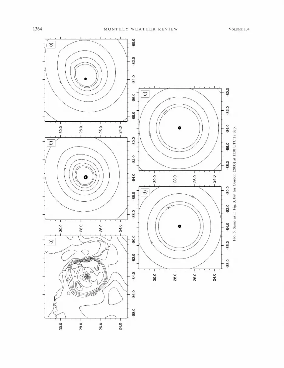
FIG

.5.S

ame

asin

Fig

.3,b

utfo

rG

ordo

n(2

000)

at13

30U

TC

17Se

p.


uncertainty associated with the estimated values foreach parameter. For example, for the axisymmetricmodel the Rmax estimates based on the NHC data atseven different time periods from 0130 UTC 14 Sep-tember to 0700 UTC 16 September ranged from 12.5 to16.25 n mi with standard errors ranging from 2.6 to 3.6n mi. In contrast, the estimates of Rmax in the fourquadrants (northeast, northwest, southwest, and south-east) used to construct the asymmetric model rangedfrom 11.5 to 41.5 n mi across the four quadrants withstandard errors ranging from 0.5 to 8.1 n mi. The esti-mates for the two parameters of the axisymmetric Hol-land model are based on the NHC reported maximumradial extent for sustained winds of 34-, 50-, and 64-ktwinds in each quadrant surrounding the storm as well as

additional buoy observations. Essentially the NHC dataare information about three locations within each quad-rant. The standard errors for the parameter estimatesquantify how well the model was able to fit these datapoints. As a result, the extra parameters of the asym-metric model within each quadrant are estimated usingfewer observations, and this additional uncertainty inthe estimates is reflected in the larger standard errorvalues. Thus, if only a small number of observationaldata points (such as in the case of buoy observations)are available, dividing these data points into four dif-ferent quadrants actually increases the uncertainty inthe error estimates.

Monitoring the standard errors of each estimate forRmax can help in a real-time situation when we may

FIG. 6. Time series of wind speed during Hurricane Isabel (2003) at NDBC buoy station (a) 44025;(b) 44014; (c) CHLV2; and (d) 41001.

MAY 2006 X I E E T A L . 1365

FIG

.7.S

ame

asin

Fig

.3,b

utfo

rIs

abel

at07

30U

TC

14Se

p20

03.


wish to decide if the axisymmetric or the asymmetricHolland model is more appropriate. As an example,Table 3 shows the nonlinear least square estimates andstandard errors for the Rmax parameter in the fourquadrants of Hurricane Floyd for 0600 UTC 14 Sep-tember and 1200 UTC 16 September. The HRD windfields on 14 September show Hurricane Floyd had notyet made landfall along the U.S. coast and was stillfairly organized with some evidence of stronger windsin the northeast and southeast quadrants. On 16 Sep-tember Floyd had made landfall and had begun toweaken and the structure of the storm was much lessorganized. Thus it is expected that the differences in theestimates for Rmax in the four quadrants will be morepronounced during this later time period. From Table3, we see that for 14 September there is not a significantdifference between the estimates for Rmax in the differ-ent quadrants when the standard errors, which are rela-tively large, are considered. However for 16 Septemberthe standard errors are smaller, suggesting the newasymmetric model is more appropriate to account forthese differences in the four quadrants.

The standard errors from the nonlinear least squareestimation are based on the assumption that the residu-als, or observed values minus fitted values, are inde-pendent and have homogeneous variance. For futureanalysis the estimation methods described here couldbe improved by taking into account the spatial correla-tion in the wind field. A generalized nonlinear leastsquares approach would account for errors that are cor-related and/or have unequal variance but would also bemore computationally demanding.

Another source of uncertainty in the analysis is the

use of the HRD winds to evaluate the Holland modeland new asymmetric model. Since the HRD winds arenot direct measurements of the wind but rather a re-analysis of several different observation sources thereare measurement errors as well as additional biases inthis data. However the HRD winds incorporate obser-vations from aircraft and so can give a better sense ofthe asymmetry of the storm than the buoys, which arescattered along the coast and can provide only limitedinformation about the spatial features of the hurricane.

As a final comparison, data from Hurricane Floydwere used to compare the HRD data to the observedbuoy winds to get a sense of the magnitude of the dif-ference in the wind speed values from these twosources. To compare the buoy and HRD observationsthe buoy data are first adjusted to 10-m height and theninterpolated in time and space. The buoy observationsare hourly and the HRD winds were reported every 3 h.The buoy observations were interpolated temporally tothe reporting time for the HRD winds. Additionally thebuoy locations were interpolated in space to the closestHRD grid point. This was only done for buoy locationsthat fell within the HRD domain for any given timesince the HRD reports a wind field only for a regionaround the center of the storm. This interpolation wasdone for 14 buoy locations during a period from 15 to16 September 1999 for Hurricane Floyd when the stormmoved up the eastern coast and eventually made land-fall.

Combining the data from all sites for all of the timeperiods, 95% of the differences between the buoy andHRD wind speed observations (buoy � HRD) fell be-tween �7.8 and 5.9 m s�1, and the average difference

FIG. 8. Time series of wind speed during Hurricane Lily (2002) at NDBC buoy station (a) DRYF1; (b) LONF1; and (c) SANF1.

MAY 2006 X I E E T A L . 1367

FIG

.9.S

ame

asin

Fig

.3,b

utfo

rL

ilyat

0130

UT

C28

Sep

2002

.


between the buoy and HRD wind speed observations(buoy � HRD) was �0.9 m s�1 with a standard devia-tion of 3.7 m s�1. The largest differences were approxi-mately �10 m s�1 when the HRD winds are larger thanthe buoy winds. Looking at these differences acrosstime the largest differences between the HRD andbuoy observations occurred when the hurricane madelandfall. At this point the HRD reported higher windspeeds at locations closest to the center of the storm.Also across all the time periods the difference in thetwo sources of data is largest for locations to the north-east of the storm center. Thus, despite the fact thatbuoy observations are included in HRD wind analysis,buoy observations and HRD winds still show large un-certainly. The uncertainty in observations presents achallenge in the validation of hurricane wind forecasts.

5. Conclusions

An asymmetric wind model is developed by incorpo-rating an asymmetry term into the Holland model. Thisnew asymmetric Holland model is further enhanced byusing various near–real time data that are available tooptimize the parameters in the model. Six- and twelve-hour forecasts of the wind fields for Hurricanes Floyd(1999), Gordon (2000), Lily (2002), and Isabel (2003)using this new model are compared against both theNDBC buoy data and HRD surface wind analysis, andthe results are quite promising. Furthermore, thescheme developed within may be used to forecast andhindcast hurricane wind fields. It can be applied in nu-merical simulations of storm surge and waves inducedby hurricanes. An automated real-time wind forecastsystem has been developed using this algorithm.

It should be noted that the accuracy of the forecastwind from the AWM strongly depends on the accuracyof the forecast (track and wind radii) guidance issuedby the NHC. The AWM model provides a method tomake use of the NHC forecast guidance, especially re-garding the wind structure. The AWM translates thetext of NHC forecast guidance of the four-quadrantradii of the 34-, 50-, and 64-kt wind speed and other

real-time surface wind data into gridded wind forecaststhat can be used by storm surge and wave modelers. Itshould be noted that real-time forecasting of hurricanewinds is not only a challenge in making the forecastsdue to errors and uncertainties in hurricane track andintensity forecasts, but also a challenge in quantifyingthe uncertainty in the forecasts due to uncertainties inhurricane wind analysis.

Acknowledgments. This study is jointly supported bythe Carolina Coastal Ocean Observation and Predic-tion System (Caro-Coops) project under NOAA GrantNA16RP2543 and the Coastal Ocean Research andMonitoring Program (CORMP) under NOAA GrantNA16RP2675, via the National Ocean Service, throughCharleston Coastal Services Center. Two anonymousreviewers provided insightful comments, which led tosignificant improvement of the paper.

APPENDIX

List of NDBC Buoy Stations Used for FourDifferent Hurricane Cases

a. Floyd (1999)

FPSN7 41001 41002 41004 41008 41009 41010 4203644004 44005 44007 44008 44009 44011 44013 4401444025 ABAN6 AL SN6 BUZM3 CDRF1 CHLV2CLKN7 DBLN6 DRYF1 DSLN7 DUCN7 FBIS1FWYF1 IOSN3 KTNF1 LKWF1 LONF1 MDRM1MISM1 MLRF1 SANF 1 SAUF1 SMKF1 SPGF1SUPN6 THIN6 TPLM2 VENF1

b. Gordon (2000)

41004 41008 41009 41010 42001 42003 42007 4203642039 42040 42041 42042 42054 BURL1 CDRF1CSBF1 DPIA1 DRYF1 FB IS1 FPSN7 FWYF1 GDIL1KTNF1 LKWF1 LONF1 MLRF1 SANF1 SAUF1SMKF1 SPGF1 VENF1

c. Lily (2002)

42001 42002 42003 42007 42019 42020 42035 4203642039 42040 42041 BURL1 CSBF1 DPIA1 DRYF1FWYF1 GDIL1 LONF1 ML RF1 PTAT2 SANF1SMKF1 SRST2 VENF1

d. Isabel (2003)

41001 41002 41008 41010 41025 44009 44014 4401744025 45002 45003 45005 45007 45008 45012 ABAN6ALSN6 CHLV2 CL KN7 DBLN6 DSLN7 DUCN7FBIS1 FPSN7 LSCM4 SBIO1 SUPN6 THIN6 TPLM2

TABLE 3. Estimates of the Rmax parameter (n mi) and standarderrors (SEs) obtained using nonlinear least squares.

0600 UTC 14 Sep 1200 UTC 16 Sep

Quadrant Rmax SE Quadrant Rmax SE

NE 26.6 6.0 NE 41.5 2.5NW 22.4 6.9 NW 10.7 1.4SW 13.6 3.2 SW 11.9 0.6SE 16.5 5.0 SE 32.8 1.5

MAY 2006 X I E E T A L . 1369

REFERENCES

Chen, Y., and M. K. Yau, 2003: Asymmetric structures in a simu-lated landfalling hurricane. J. Atmos. Sci., 60, 2294–2312.

DeMaria, M., and J. Kaplan, 1994: A Statistical Hurricane Inten-sity Prediction Scheme (SHIPS) for the Atlantic basin. Wea.Forecasting, 9, 209–220.

Depperman, R. C., 1947: Notes on the origin and structures ofPhilippine typhoons. Bull. Amer. Meteor. Soc., 28, 399–404.

Georgiou, P., 1985: Design wind speeds in tropical cyclone proneregions. Ph.D. thesis, University of Western Ontario, 295 pp.

Holland, G. J., 1980: An analytic model of the wind and pressureprofiles in hurricanes. Mon. Wea. Rev., 108, 1212–1218.

Houston, S. H., W. A. Shaffer, M. D. Powell, and J. Chen, 1999:Comparisons of HRD and SLOSH surface wind fields in hur-ricanes: Implications for storm surge modeling. Wea. Fore-casting, 14, 671–686.

Hsu, S. A., and Z. Yan, 1998: A note on the radius of maximumwind for hurricanes. J. Coastal Res., 14, 667–668.

Hughes, L. A., 1952: On the low-level wind structure of tropicalstorms. J. Meteor., 9, 422–428.

Jakobsen, F., and H. Madsen, 2004: Comparison and further de-velopment of parameteric tropical cyclone models for stormsurge modelling. J. Wind Eng. Ind. Aerodyn., 92, 375–391.

Jarvinen, B. R., and C. J. Neumann, 1979: Statistical forecasts oftropical cyclone intensity for the North Atlantic basin.NOAA Tech. Memo., NWS NHC-10, 22 pp.

Jelesnianski, C. P., J. Chen, and W. A. Shaffer, 1992: SLOSH: Sea,

lake and overland surges from hurricane. National WeatherService, Silver Spring, MD, 71 pp.

Large, W. G., and S. Pond, 1981: Open ocean momentum fluxmeasurements in moderate to strong winds. J. Phys. Ocean-ogr., 11, 324–336.

Powell, M. D., and S. H. Houston, 1996: Hurricane Andrew’slandfall in south Florida. Part II: Surface wind fields andpotential real-time applications. Wea. Forecasting, 11, 329–349.

——, and ——, 1998: Surface wind fields of 1995 Hurricanes Erin,Opal, Luis, Marilyn, and Roxanne at landfall. Mon. Wea.Rev., 126, 1259–1273.

——, ——, and T. A. Reinhold, 1996: Hurricane Andrew’s land-fall in south Florida. Part I: Standardizing measurements fordocumentation of surface wind fields. Wea. Forecasting, 11,304–328.

Riehl, H., 1954: Tropical Meteorology. McGraw-Hill, 392 pp.Ross, R. J., and Y. Kurihara, 1992: A simplified scheme to simu-

late asymmetries due to the beta effect in barotropic vortices.J. Atmos. Sci., 49, 1620–1628.

Schloemer, R. W., 1954: Analysis and synthesis of hurricane windpatterns over Lake Okeechobee. NOAA Hydromet Rep. 31,49 pp.

Shapiro, L., 1983: The asymmetric boundary layer flow under atranslating hurricane. J. Atmos. Sci., 40, 1984–1998.

Wang, Y., and G. J. Holland, 1996: Tropical cyclone motion andevolution in vertical shear. J. Atmos. Sci., 53, 3313–3332.


a real-time hurricane surface wind forecasting model: formulation and verification

Documents