a new riemann type hydrodynamical hierarchy and its integrability analysis
TRANSCRIPT

Available at: http://publications.ictp.it IC/2009/095
United Nations Educational, Scientific and Cultural Organizationand
International Atomic Energy Agency
THE ABDUS SALAM INTERNATIONAL CENTRE FOR THEORETICAL PHYSICS
A NEW RIEMANN TYPE HYDRODYNAMICAL HIERARCHY
AND ITS INTEGRABILITY ANALYSIS
Jolanta Jolanta Golenia1
The Department of Applied Mathematics, The AGH University of Science and Technology,Krakow 30059, Poland,
Nikolai N. Bogolubov (Jr.)2
The V.A. Steklov Mathematical Institute of RAN, Moscow, Russian Federationand
The Abdus Salam International Centre for Theoretical Physics, Trieste, Italy,in cooperation with
Ziemowit Popowicz3
The Institute of Theoretical Physics at the Physics Department of the University of Wroc law,Wroc law, Poland,
Maxim V. Pavlov4
The Department of Mathematical Physics, P.N. Lebedev Physical Institute of RAN,Moscow 119991, Russian Federation
andThe Department of Mathematical Sciences, Loughborough University, Loughborough,
LE11 3TU United Kingdom
and
Anatoliy K. Prykarpatsky5
The Department of Mining Geodesics at the AGH University of Science and Technology,Krakow 30059, Poland
andThe Ivan Franko State Pedagogical University, Drohobych, Lviv region, Ukraine.
MIRAMARE – TRIESTE
December 2009
[email protected] [email protected]@[email protected], [email protected]@ua.fm
Abstract
Short-wave perturbations in a relaxing medium, governed by a special reduction of the Ostro-
vsky evolution equation, and later derived by Whitham, are studied using the gradient-holonomic
integrability algorithm. The bi-Hamiltonicity and complete integrability of the corresponding dy-
namical system is stated and an infinite hierarchy of commuting to each other conservation laws
of dispersive type are found. The well defined regularization of the model is constructed and
its Lax type integrability is discussed. A generalized hydrodynamical Riemann type system is
considered, infinite hierarchies of conservation laws, related compatible co-symplectic structures
and Lax type representations for the special cases N = 2, 3 and N = 4 are constructed.
1

1. Introduction
Many important problems of propagating waves in nonlinear media with distributed param-
eters, for instance, invisible non-dissipative dark matter, playing a decisive role [1, 2] in the
formation of large scale structure in the Universe like galaxies, clusters of galaxies, super-clusters,
can be described by means of evolution differential equations of special type. In particular, if
the nonlinear medium is endowed with spatial memory properties, the propagation of the corre-
sponding waves can be modeled by means of the so-called generalized Ostrovsky-Hunter-Saxton
evolution equations [3, 11]. It is also well known [4, 14, 13, 8, 10] that shortwave perturbations in
a relaxing one dimensional medium can be described by means of some reduction of the Ostrovsky
equations, coinciding with the Whitham type evolution equation
(1.1) du/dt = 2uux +
∫
R
K(x, s)usds,
discussed first in [4]. Here the kernel K : R×R → R depends on the medium elasticity properties
with spatial memory and can, in general, be a function of the pressure gradient ux ∈ C∞(R; R),
evolving with respect to equation (1.1). In particular, if K(x, s) = 12 |x−s|, x, s ∈ R, then equation
(1.1) can be reduced to
(1.2) du/dt = 2uux + ∂−1u,
which was, in particular, studied before in [12, 13, 14, 4].
Since some media possess elasticity properties depending strongly on the spatial pressure gra-
dient ux, x ∈ R, the corresponding Whitham kernel looks like
(1.3) K(x, s) := −θ(x− s)us
for x, s ∈ R, naturally modeling the relaxing spatial memory effects. The resulting equation (1.1)
with the kernel (1.3) becomes
(1.4) du/dt = 2uux − ∂−1u2x := K[u],
which appears to possess very interesting mathematical properties. The latter will be the main
topic of the next sections below.
Owing to the results, obtained before in [20], the dynamical system (1.4) appeared to be
a Lax type integrable bi-Hamiltonian flow, but with ill posed temporal evolution. A suitable
finite-dimensional [15, 16] reduction scheme, if applied to the corresponding hierarchy of con-
servation laws, does not make it possible to construct, owing to the nonlocality, a wide class of
explicit solutions to the Ostrovsky-Whitham type nonlinear dynamical system (1.4) by means of
quadratures. Some of these integrability aspects were presented before in [8], where a suitable
regularization scheme for treating this nonlocality problem was proposed. Below the well posed
integrability problem for the Ostrovsky-Whitham type nonlinear and nonlocal dynamical system
(1.4) will be reanalyzed in detail making use of this regularization scheme.2

2. A regularization scheme and the geometric integrability problem
Define a smooth periodic function v ∈ C∞2π(R; R), such that
(2.1) v := ∂−1u2x
for any x, t ∈ R, where the function u ∈ C∞2π (R; R) solves equation (1.4). Then it is easy to state
that the following nonlinear dynamical system
(2.2)ut = 2uux − vvt = 2uvx
:= K[u, v]
of hydrodynamic type, being already well defined on the extended 2π-periodic functional space
M := C∞2π(R; R2), is completely equivalent to that given by expression (1.4). The system (2.2) is
equivalent to the following system
(2.3)ut = 2uux − v, vt = 2uvx
ux = w, vx = uxwwt = vx + 2uwx
:= K[u, v,w]
and further to the set of 2-forms
α := α(1) = du ∧ dx+ 2u du ∧ dt− v dx ∧ dt; α(2) = dv ∧ dx+ 2u dv ∧ dt;
α(3) = du∧ dt−w dx∧ dt; α(4) = dv ∧ dt−w du∧ dt; α(5) = dw ∧ dx+ dv ∧ dt+ 2u dw ∧ dt
This set of two-forms generates the closed ideal I(α), since
d α(1) = −α(2) ∧ dt; d α(2) = 2du ∧ α(4); d α(3) = −α(5) ∧ dt;
d α(4) = −dw ∧ α(3) − w dt ∧ α(5); d α(5) = −2dw ∧ α(3) − 2w dt ∧ α(5).
The integral submanifold M being defined by the condition I(α) = 0. Now making use of
the differential-geometric method devised in [15], we will look for a connection 1–form Γ reduced
upon the integral submanifold M, belonging to some not yet determined Lie algebra G. This
1-form can be represented as follows:
(2.4) Γ = A(u, v,w) dx+ B(u, v,w) dt,
where the elements A, B ∈ G satisfy determining equations
Ω =∂A∂u
du ∧ dx+∂A∂v
dv ∧ dx+∂A∂w
dw ∧ dx+∂B∂u
du ∧ dt+
(2.5)∂B∂v
dv ∧ dt+∂B∂w
dw ∧ dt+ [A,B]dx ∧ dt⇒
⇒ g1(du ∧ dx+ 2u du ∧ dt − v dx ∧ dt) + g2(dv ∧ dx+ 2u dv ∧ dt) +
+g3(du ∧ dt− w dx ∧ dt) + g4(dv ∧ dt− w du ∧ dt) +
+g5(dw ∧ dx+ 2u dw ∧ dt + dv ∧ dt) ∈ I(α) ⊗ G3
for some G-valued functions g1, ..., g5 ∈ G on M . From (2.5) one finds that
(2.6)∂A∂u
= g1,∂A∂v
= g2,∂A∂w
= g5,
∂B∂u
= 2u g1 + g3 − w g4,∂B∂v
= 2u g2 + g4 + g5,
∂B∂w
= 2u g5, [A,B] = −v g1 − w g3.
Thereby, from the obtained set of relationships (2.6) one can find that
B = 2uA + C(u, v), g4 =∂C∂v
− ∂A∂w
,
(2.7) g3 = 2A +∂C∂u
+ w∂C∂v
− w∂A∂w
,
[A, C] = −v∂A∂u
− 2wA− w∂C∂u
− w2 ∂C∂v
+ w2 ∂A∂w
,
being main algebraic relationships for final searching the connection (2.4), making use of the
differential-geometric scheme, based on analyzing the related holonomy Lie algebra, devised in
[15].
3. The bi-Hamiltonian structure and Lax-type representation
Consider the following polynomial expansion of the element A(u, v;w) ∈ G with respect to the
variable w :
(3.1) A = A0(u, v) + A1(u, v)w + A2(u, v)w2
and substitute it into the last equation of (2.6). As a result we obtain:
[A0, C] = −v∂A0
∂u, [A1, C] = −v∂A1
∂u− 2A0 −
∂C
∂u,(3.2)
[A2, C] = −v∂A2
∂u− ∂C
∂v−A1,
or
(3.3) A1 = [C,A2] − v∂A2
∂u− ∂C
∂v.
which can be substituted into the second equation of (3.2):
(3.4)[[C,A2], C] − 2v[∂A2
∂u , C] − [∂C∂v , C] = −v[∂C
∂u ,A2]−−v2 ∂2A2
∂u2 − v ∂2C∂u∂v − 2A0 − ∂C
∂u .4

Thus, recalling (3.2) and (3.3), we have that
2A0 = [C, [C,A2]] + 2v[∂A2
∂u,C] +(3.5)
+[∂C
∂v,C] − v[
∂C
∂u,A2] −
−v2∂2A2
∂u2− v
∂2C
∂u∂v− ∂C
∂u,
[A0, C] = −v∂A0
∂u, A1 = [C,A2] − v
∂A2
∂u− ∂C
∂v.
Now we will assume that the element C := C0 ∈ C is constant and the elements A0 and A2 are
linear with respect to variables u and v, that is
A0 = A(0)0 + A(1)
0 u+ A(2)0 v,(3.6)
A2 = A(0)2 + A(1)
2 u+ A(2)2 v.
Whence upon substituting in (3.5) one gets:
2A(0)0 = [C0, [C0,A(0)
2 ]], [A(1)0 , C0] = 0, [A(2)
0 , C0] = −A(1)0 ,(3.7)
2A(1)0 = [C0, [C0,A(1)
2 ]], 2A(2)0 = [C0, [C0,A(2)
2 ]] + 2[A(1)2 , C0].
To solve the closed system (3.7) we need to calculate the corresponding holonomy Lie algebra of
the connection (2.4). As a result of simple, but slightly cumbersome calculations, we derive that
elements A(j)2 , j = 0, 2, and C0 belong to the Lie algebra sl(2; C), whose basis L0, L+ and L− can
be taken to satisfy the following canonical commutation relations:
(3.8) [L0, L±] = ±L±, [L+, L−] = 2L0.
Thereby, making use of the standard determining expansions
A(j)2 =
∑
±
c(j)± L± + c
(j)0 L0,(3.9)
C0 =∑
±
k±L± + k0L0,
where j = 0, 2, and substituting (3.9) into (3.7), we obtain some relationships on values c(j)± , c
(j)0 ∈
C, j = 0, 2, and k±, k0 ∈ C. Resolving by means of simple but slightly cumbersome calculations
these relationships, depending on a spectral parameter λ ∈ C, we find the basic elements A and
B of the connection Γ, thereby giving rise to the corresponding Lax type commutative spectral
representation of dynamical system (2.2) in the following (2 × 2)−matrix form:
(3.10)
dfdx − ℓ[u, v;λ]f = 0, df
dt = p(ℓ)f, p(ℓ) := 2uℓ[u, v;λ] + q,
ℓ[u, v;λ] :=
(
−λux −vx
λ2 λux
)
, q :=
(
0 0λ 0
)
,
p(ℓ) =
(
−2λuxu −2vxuλ+ 2λ2u 2λuxu
)
,
defining the generalized time-independent spectrum Spec(ℓ) ⊂ C : λ ∈ Spec(ℓ), if the corre-
sponding solution f ∈ L∞(R; C2).5

The standard Riccati equation, derived from (3.10), allows to obtain right away an infinite
hierarchy of local conservation laws:
(3.11) γ−1 :=
∫ 2π
0
√
u2x − vxdx, γ0 :=
∫ 2π
0
(uxvxx − vxuxx)
2vx
√
u2x − vx
dx, ...,
and so on. All of the conservation laws (3.11) except γ−1, are singular at the Cauchy condition
(2.3). Thus, we need to construct other hierarchy of polynomial conservation laws which are
regular on the functional submanifold
(3.12) Mred := (u, v) ∈ M : u2x − vx = 0, x ∈ R/2πZ
for the Cauchy problem to become solvable. The latter exists owing to the results of [15, 5]. The
simplest way to search for them consists in determining the bi-hamiltonian structure of flow (2.2).
As it is easy to check, dynamical system (2.2) is canonically Hamiltonian, that is
(3.13)d
dt(u, v)⊺ := −ϑgrad Hϑ = K[u, v],
where the corresponding co-symplectic structure ϑ : T ∗(M) → T (M) is canonical, equals
(3.14) ϑ =
(
0 1−1 0
)
and satisfies the Noether equation
LK ϑ = 0 = dϑ/dt − ϑK ′,∗ − K ′ϑ.
To prove this, it is enough to find by means of the small parameter method, devised before in
[15] a non-symmetric (ϕ′ 6= ϕ′,∗) solution ϕ ∈ T (M) to the following Lie-Lax equation:
(3.15) dϕ/dt + K ′,∗ϕ = grad L
for some suitably chosen smooth functional L ∈ D(M). As a result of easy calculations one obtains
that
(3.16) ϕ = (−v, 0)⊺, L = −∫ 2π
0uvdx.
Making use of (3.16) and the classical Legendrian relationships for the corresponding symplectic
structure
(3.17) ϑ−1 := ϕ′ − ϕ′,∗ =
(
0 −11 0
)
and the Hamiltonian functional
(3.18) H := (ϕ, K) − L,
one obtains the implectic structure (3.14) and the corresponding non-singular Hamilton function
(3.19) Hϑ :=
∫ 2π
0(v2/2 + vxu
2)dx.
It is worth to mention here that the determining Lie-Lax equation (3.15) possesses still another
solution
(3.20) ϕ = (ux
2,− u2
x
2vx), L =
1
4
∫ 2π
0uvxdx,
6
giving rise, owing to formulas (3.17) and (3.18), to the new co-implectic (singular ”symplectic”)
structure
(3.21) η−1 := ϕ′ − ϕ′,∗ =
(
∂/2 −∂uxv−2x
−uxv−2x ∂ 1
2(u2xv
2x∂ + ∂u2
xv2x)
)
and the Hamiltonian functional
Hη :=1
2
∫ 2π
0(uvx − vux)dx.
The co-implectic structure (3.21) is, evidently, singular since ϑ−1s (ux, vx)⊺ = 0. The corresponding
implectic structure η : T ∗(M) → T ∗(M) satisfies the determining Noether equation
(3.22) LK η = 0 = dη/dt− ηK ′,∗ − K ′η
and whose solutions is exactly the operator η = ϑ−1. As a result, the second implectic operator
has the form
(3.23) η :=
(
2∂−1 4ux∂−1
4∂−1ux 4(vx∂−1 + ∂−1vx)
)
,
giving rise to a new infinite hierarchy of polynomial conservation laws
(3.24) γn :=
∫ 1
0dλ < (ϑ−1η)ngrad Hϑ[uλ, u >
for all n ∈ Z+.
Remark 3.1. It is worth to mention that the Lax pair (3.10), (2.4), obtained above for dynamical
system (2.2), was found first in the work [17]. It coincides with those found later in [5], making use
of a very special bi-Lagrangian representation of the dynamical system (2.2). But the existence
of the singular co-implectic structure (3.21) in these references was not stated. Concerning this
fact, it is also necessary to mention work [18], where the geometric aspects of the equation like
(1.1) were studied in detail.
In particular, one can easily observe that the following Hamiltonian representations
(3.25)d
dt(u, v)⊺ = −η grad Hη,
d
dx(u, v)⊺ = −ϑ grad Hη
hold, where
(3.26) Hη :=1
2
∫ 2π
0(uvx − vux)dx.
Now, making use of (3.24), one can apply the standard reduction procedure upon the correspond-
ing finite dimensional functional subspaces M2n ⊂ M, n ∈ Z+, and obtain a large set of exact
solutions to dynamical system (2.2) upon the functional submanifold Mred, if the Cauchy data
are taken to satisfy constraint (3.12).7

4. A Riemann type hydrodynamical generalization
Here it is interesting to mention (owing to an observation by D. Holm [6]) that the dynamical
system (2.2) can be equivalently rewritten up to the time rescaling as
(4.1) D2t u = 0, Dt := ∂/∂t + u∂,
under the flow velocity condition dx/dt := u, which is a partial case [7] of the generalized Riemann
type hydrodynamic system
(4.2) DNt u = 0
for any integer N ∈ Z+. If N = 3, one easily obtains the new dynamical system
(4.3)ut = v − uux
vt = z − uvx
zt = −uzx
:= K[u, v, z]
of hydrodynamical type, which also proves to possess infinite hierarchies of polynomial conserva-
tion laws.
Namely, the following polynomial functionals are conserved with respect to the flow (4.3):
H(1)n : =
∫ 2π
0dxzn(vux − vxu− n+ 2
n+ 1z),(4.4)
H(4) : =
∫ 2π
0dx[−7vxv
2u+ z(6zu+ 2vxu2 − 3v2 − 4vuux)],
H(5) : =
∫ 2π
0dx(z2ux − 2zvvx),H(6) :=
∫ 2π
0dx(zzv
3 + 3z2vxu+ z3),
H(7) : =
∫ 2π
0dx(zxv
3 + 3z2vux − 3z3),
H(8) : =
∫ 2π
0dxz(6z2u+ 3zvxu
2 − 3zv2 − 4zvux − 2vxv2u+ 2v3ux),
H(9) : =
∫ 2π
0dx[1001vxv
4u+ (1092z2u2 + 364zvxu3 −
−1092zv2u− 728zvuxu2 − 364vxv
2u2 + 273v4 + 728v3uxu]),
H(2)n : =
∫ 2π
0dxzxvz
n, H(3)n :=
∫ 2π
0dxzx(v2 − 2zu)n,
where n ∈ Z+. In particular, as n = 1, 2, ..., from (4.3) one obtains that
H(2)0 : =
∫ 2π
0dxzxv, H
(2)1 :=
∫ 2π
0dxzxzv, ...,(4.5)
H(3)1 : =
∫ 2π
0dxzx(v2 − 2uz),
H(3)2 : =
∫ 2π
0dxzx(v4 + 4z2u2 − 4zv2u), ...,
and so on. The problem which remains still open consists in proving the fact that the general-
ized hydrodynamical system (4.3) is a completely integrable bi-Hamiltonian flow on the periodic
functional manifold M := C(∞)(R/2π; R3), as was proved above for the system (4.2), if N = 2.
This problem will be analyzed in the section below.8

5. The Hamiltonian analysis
Consider the system (4.3) in the following more convenient analytical form:
(5.1)ut = v − uux
vt = z2/2 − uvx
zt = −uzx
:= K[u, v, z],
To tackle this problem, it is sufficient to construct [15] exact non-symmetric solutions to the
Lie-Lax equation
(5.2) dϕ/dt +K′,∗ϕ = grad L, ϕ
′ 6= ϕ′,∗,
for some functional L ∈ D(M), where ϕ ∈ T ∗(M) is, in general, a quasi-local vector, such that
the system (4.3) allows the following Hamiltonian representation:
(5.3)K[u, v, z] = −η grad H[u, v, z],
H = (ϕ,K) − L, η−1 = ϕ′ − ϕ′,∗.
As a test solution to (5.2) one can take the one
ϕ = (ux/2, 0,−z−1x u2
x/2 + z−1x vx)⊺, L =
1
2
∫ 2π
0(z2 + vux)dx,
which gives rise to the following co-implectic operator:
(5.4) η−1 := ϕ′ − ϕ′,∗ =
∂ 0 −∂uxz−1x
0 0 ∂zx
−uxz−1x ∂ zx∂
12(u2
xz−2x ∂ + ∂u2
xz−2x )−
−(vxz−2x ∂ + ∂vxz
−2x )
.
This expression is not strictly invertible, as its kernel possesses the translation vector field d/dx :
M → T (M) with components (ux, vx, zx)⊺ ∈ T (M), that is η−1(ux, vx, zx)⊺ = 0.
Nonetheless, upon formal inverting the operator expression (5.4), we obtain by means of simple
enough, but slightly cumbersome, direct calculations, that the Hamiltonian function equals
(5.5) H :=
∫ 2π
0dx(uxv − z2/2).
and the implectic η-operator looks as
(5.6) η :=
∂−1 ux∂−1 0
∂−1ux vx∂−1 + ∂−1vx ∂−1zx
0 zx∂−1 0
.
In the same way, representing the Hamiltonian function (5.5) in the scalar form
(5.7) H = (ψ, (ux, vx, zx)⊺), ψ =1
2(−v, u+ ...,− 1√
z∂−1√z)⊺,
9

one can construct a second implectic (co-symplectic) operator ϑ : T ∗(M) → T (M), looking up
to O(µ2) terms, as folows:
(5.8)
ϑ =
µ( (u(1))2
z(1) ∂ + ∂ (u(1))2
z(1) ) 1 + 2µ3 (u(1)v(1)
z(1) ∂ + 2∂ u(1)v(1)
z(1) ) 2µ3 (∂ (v(1))2
z(1) + ∂u(1))
−1 + 2µ3 (∂ u(1)v(1)
z(1) + 2u(1)v(1)
z(1) ∂)
2µ3 ( (v(1))2
z(1) ∂ + ∂ (v(1))2
z(1) )+
+2µ3 (u(1)∂ + ∂u(1))
2µ∂v(1)
2µ3 ( (v(1))2
z(1) ∂ + u(1)∂) 2µv(1)∂ µ(∂z(1) + z(1)∂)
+O(µ2),
where we put, by definition, ϑ−1 := (ψ′ − ψ′,∗), u := µu(1), v := µv(1), z := µz(1) as µ → 0,
and whose exact form needs some additional simple but cumbersome calculations, which will be
presented in a work under preparation.
The operator (5.8) satisfies the Hamiltonian vector field condition:
(5.9) (ux, vx, zx)⊺ = −ϑ grad H,
following easily from (5.7).
Now having applied to the pair of implectic operators the gradient-holonomic scheme [15, 21, 19]
of constructing a Lax type representation for the dynamical system (5.1) we obtain the following
compatible relationships:
(5.10)
fx = ℓ[u, v;λ]f, ft = p(ℓ)f, p(ℓ) := −uℓ[u, v;λ] + q(λ),
ℓ[u, v, z;λ =
λux −vx zx3λ2 −2λux λvx
λ2r[u, v, z] −3λ λux
, q(λ) :=
0 0 0λ 0 00 1 0
,
p(ℓ) =
−λuux uvx −uzx−3uλ2 + λ 2λuux −λuvx
−λ2r[u, v, z]u 1 + 3uλ −λuux
,
where f ∈ C∞(R; C3), λ ∈ C is an arbitrary spectral parameter and a smooth functional mapping
r : M → R satisfies the differential equation
(5.11) Dtr + uxr = 6.
The latter possesses a wide set R of different solutions amongst which there are the following:
r ∈ R := r(1)1 =vxv
3
z3− 3uxv
2
z2+u(uz − v2)zx
z3+
6v
z, r
(2)1 = [(6xv − 3u2)/z]x,(5.12)
r2 =6vx
zx− 3u2
x
zx, r3 = (
u3x
z2x
− 3uxvx
z2x
+9
2zx)/(
ux
zx− v2
x
2z2x
).
Note here that only the third element from the set (5.12) allows the reduction z = 0 to the case
N = 2. In Supplement 2 there is presented a method of solving equation (5.11) and related
differential-algebraic integrability of dynamical system (5.1). rintegrability10

6. The case N=4: the conservation laws, Hamiltonian structure and Lax type
representation
The Riemann type hydrodynamical equation (4.2) at N = 4 is equivalent to the nonlinear
dynamical system
(6.1)
ut = v − uux
vt = w − uvx
wt = z − uwx
zt = −uzx
:= K[u, v,w, z],
where K : M → T (M) is a suitable vector field on the smooth 2π-periodic functional manifold
M := C∞(R/2πZ; R4). To state its Hamiltonian structure, we need to find a functional solution
to the determining Lie-Lax equation (5.2):
(6.2) ψt +K′,∗
ψ = grad L
for some smooth functional L ∈ D(M), where
(6.3) K′
=
−∂u 1 0 0−vx −u∂ 1 0−wx 0 −u∂ 1−zx 0 0 −u∂
, K′,∗
=
u∂ −vx −wx −zx1 ∂u 0 00 1 ∂u 00 0 1 ∂u
are, respectively, the Frechet derivative of the mapping K : M → T (M) and its conjugate.
The small parameter method [15], applied to equation (6.2), gives rise to the following its exact
solution:
ψ = (−wx, vx/2, 0,−v2x
2zx+uxwx
zx)⊺,(6.4)
L =
∫ 2π
0(zux − vwx/2)dx.
As a result, we obtain right away from (6.2) that dynamical system (6.1) is a Hamiltonian system
on the functional manifold M, that is
(6.5) K = −ϑ grad H,
where the Hamiltonian functional equals
(6.6) H := (ψ,K) − L =
∫ 2π
0(uzx − vwx)dx
and the co-implectic operator equals
(6.7) ϑ−1 := ψ′ − ψ′,∗ =
0 0 −∂ ∂wx
zx
0 −u∂ 0 −∂ vx
zx
−∂ 0 0 ∂ ux
zx
wx
zx
∂ −vx
zx
∂ ux
zx
∂12 [z−2
x (v2x − 2uxwx)∂+
+∂(v2x − 2uxwx)z−2
x ]
.
The latter is degenerate: the relationship ϑ−1(ux, vx, wx, zx)⊺ = 0 exactly on the whole manifold
M, but the inverse to (6.7) exists and can be calculated analytically.11
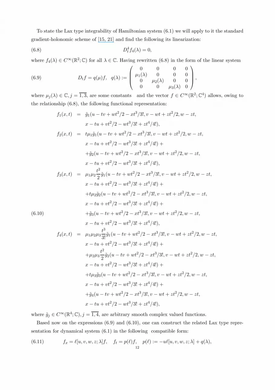
To state the Lax type integrability of Hamiltonian system (6.1) we will apply to it the standard
gradient-holonomic scheme of [15, 21] and find the following its linearization:
(6.8) D4t f4(λ) = 0,
where f4(λ) ∈ C∞(R2; C) for all λ ∈ C. Having rewritten (6.8) in the form of the linear system
(6.9) Dtf = q(µ)f, q(λ) :=
0 0 0 0µ1(λ) 0 0 0
0 µ2(λ) 0 00 0 µ3(λ) 0
,
where µj(λ) ∈ C, j = 1, 3, are some constants and the vector f ∈ C∞(R2; C4) allows, owing to
the relationship (6.8), the following functional representation:
f1(x, t) = g1(u− tv + wt2/2 − xt3/3!, v − wt + zt2/2, w − zt,
x− tu+ vt2/2 − wt3/3! + zt4/4!),
f2(x, t) = tµ1g1(u− tv + wt2/2 − xt3/3!, v − wt + zt2/2, w − zt,
x− tu+ vt2/2 − wt3/3! + zt4/4!) +
+g2(u− tv + wt2/2 − xt3/3!, v − wt+ zt2/2, w − zt,
x− tu+ vt2/2 − wt3/3! + zt4/4!),
f3(x, t) = µ1µ2t2
2g1(u− tv + wt2/2 − xt3/3!, v − wt+ zt2/2, w − zt,
x− tu+ vt2/2 − wt3/3! + zt4/4!) +
+tµ2g2(u− tv + wt2/2 − xt3/3!, v − wt+ zt2/2, w − zt,
x− tu+ vt2/2 − wt3/3! + zt4/4!) +
+g3(u− tv + wt2/2 − xt3/3!, v − wt+ zt2/2, w − zt,(6.10)
x− tu+ vt2/2 − wt3/3! + zt4/4!),
f4(x, t) = µ1µ2µ3t3
3!g1(u− tv + wt2/2 − xt3/3!, v − wt+ zt2/2, w − zt,
x− tu+ vt2/2 − wt3/3! + zt4/4!) +
+µ2µ3t2
2g2(u− tv + wt2/2 − xt3/3!, v − wt + zt2/2, w − zt,
x− tu+ vt2/2 − wt3/3! + zt4/4!) +
+tµ3g3(u− tv + wt2/2 − xt3/3!, v − wt+ zt2/2, w − zt,
x− tu+ vt2/2 − wt3/3! + zt4/4!) +
+g4(u− tv + wt2/2 − xt3/3!, v − wt+ zt2/2, w − zt,
x− tu+ vt2/2 − wt3/3! + zt4/4!),
where gj ∈ C∞(R4; C), j = 1, 4, are arbitrary smooth complex valued functions.
Based now on the expressions (6.9) and (6.10), one can construct the related Lax type repre-
sentation for dynamical system (6.1) in the following compatible form:
(6.11) fx = ℓ[u, v,w, z;λ]f, ft = p(ℓ)f, p(ℓ) := −uℓ[u, v,w, z;λ] + q(λ),12
where fx = ℓ[u, v,w, z;λ]f for f ∈ C∞(R2; C4) is a suitable matrix x-derivative representation,
wand whose exact form needs some simple but slightly cumbersome calculations. Owing to the
existence of the Lax type representation (6.11) and the related gradient like relationship [15, 21],
we can easily derive that the Hamiltonian system (6.1) is simultaneously also a bi-Hamiltonian
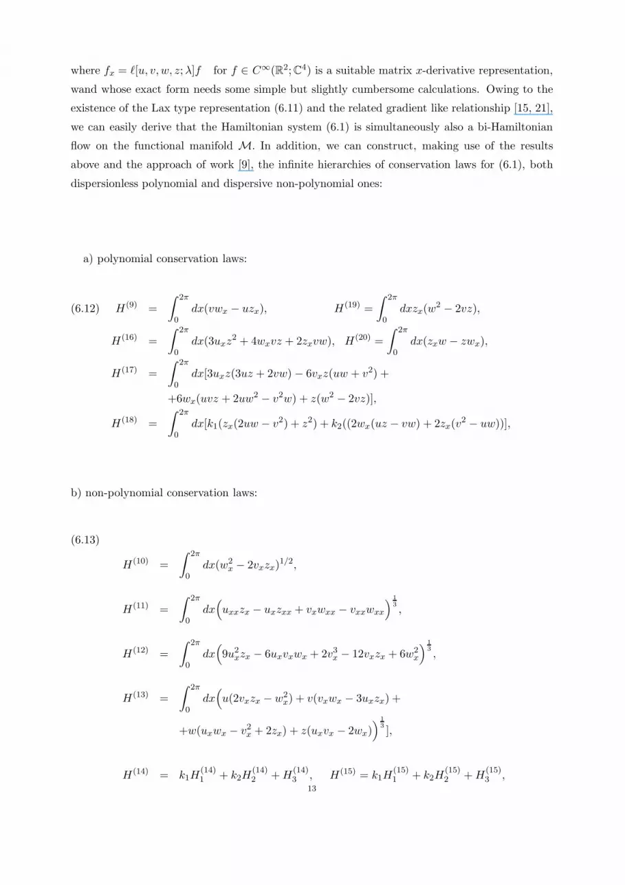
flow on the functional manifold M. In addition, we can construct, making use of the results
above and the approach of work [9], the infinite hierarchies of conservation laws for (6.1), both
dispersionless polynomial and dispersive non-polynomial ones:
a) polynomial conservation laws:
H(9) =
∫ 2π
0dx(vwx − uzx), H(19) =
∫ 2π
0dxzx(w2 − 2vz),(6.12)
H(16) =
∫ 2π
0dx(3uxz
2 + 4wxvz + 2zxvw), H(20) =
∫ 2π
0dx(zxw − zwx),
H(17) =
∫ 2π
0dx[3uxz(3uz + 2vw) − 6vxz(uw + v2) +
+6wx(uvz + 2uw2 − v2w) + z(w2 − 2vz)],
H(18) =
∫ 2π
0dx[k1(zx(2uw − v2) + z2) + k2((2wx(uz − vw) + 2zx(v2 − uw))],
b) non-polynomial conservation laws:
(6.13)
H(10) =
∫ 2π
0dx(w2
x − 2vxzx)1/2,
H(11) =
∫ 2π
0dx
(
uxxzx − uxzxx + vxwxx − vxxwxx
)13,
H(12) =
∫ 2π
0dx
(
9u2xzx − 6uxvxwx + 2v3
x − 12vxzx + 6w2x
)13,
H(13) =
∫ 2π
0dx
(
u(2vxzx − w2x) + v(vxwx − 3uxzx) +
+w(uxwx − v2x + 2zx) + z(uxvx − 2wx)
)13],
H(14) = k1H(14)1 + k2H
(14)2 +H
(14)3 , H(15) = k1H
(15)1 + k2H
(15)2 +H
(15)3 ,
13

where
H(14)1 =
∫ 2π
0
(
uxx(2vxzz − w2x
)
+ vxx
(
vxwx − 3uxzx)
+
+wxx
(
uxwx − v2x + 2zx
)
+ zxx
(
uxvx − 2wx
)
) 14,
H(14)2 =
∫ 2π
0dx
(
zxwxx − zxxwx
) 13,
H(14)3 =
∫ 2π
0dx[k1
(
v(2vxzx − w2x) + z(4zx − uxwx) + w(vxwx − 3uxzx)
)
+
+k2z(
2zx + v2x − uxwx
)
]12 ,
H(15)1 =
∫ 2π
0dx[uxxx(2vxzx − w2
x) + vxxx(vxww − 3uxzx) +
+zxxx(uxvx − 2wx) + wxxx(uxwx − v2x + 2zx) +
+3uxx(vxxzx − 3vxzxx + wxxwx) + 3vxx(2uxzxx −(6.14)
−vxxwx + vxwxx) − 3w2xxux]
15 ,
H(15)2 =
∫ 2π
0dx
(
4u2xw
2x − 4uxv
2xwx − 8uxzxwx + v4
x + +4v2xzx + 4z2
x
)14,
H(15)3 =
∫ 2π
0dx k3[u(zxwxx − zxxwx) +
+v(vxzxx − vxxzx) + zzxx +w(uxxzx − uxzxx)] +
+k4[z(uxxwx − uxwxx + 2zxx) + w(uxxzx − uxzxx − vxxwx + vxwxx)] +
+ k5zx(v2x − 2uxwx + 2zx)
13 ,
and kj ∈ R, j = 1, 5, are arbitrary constants. We observe also that the Hamiltonian functional
(6.6) coincides exactly up the sign with the polynomial conservation law H(9) ∈ D(M).
Concerning the general case N ∈ Z+, applying successively the method devised above and,
one can also obtain for the Riemann type hydrodynamical system (4.2) both infinite hierarchies
of dispersive and dispersionless conservation laws, their symplectic structures and the related
Lax type representations, which is a topic of the next work under preparation.
With the above results we present below in Supplement 1 the exact analytical integrability of
N = 2 and arbitrary N ∈ Z+ Riemann type dynamical system (4.2), making use of a slightly
generalized hodograph mapping, based on the special reciprocal transformation. These results
can serve as a firm background for the statement about the complete Lax type integrability of the
whole hierarchy (4.2) of the Riemann type hydrodynamical systems on the axis, analyzed above.14

7. Supplement 1. A general solution to the Gurevich-Zybin hydrodynamical
system of Riemann type
Let us introduce the auxiliary field variable ρ := zx. Then the second equation of (4.1) reduces
to the so-called continuity equation
(7.1) ρt + ∂x(ρu) = 0,
which can be utilized in the construction of a simple reciprocal transformation
(7.2) dz = ρdx− ρudt, dy = dt.
From (7.2) one easily obtains that ∂x = ρ∂z and ∂t = ∂y − ρu∂z. Thus, system (4.1) reduces to
the form
(7.3)
(
1
ρ
)
y
= uz, uy = z,
The second equation is integrated to
(7.4) u = yz + f(z),
where f : R → R is an arbitrary smooth function. Then, the first equation in (7.3) reduces to
the form(
1
ρ
)
y
= y + f ′(z),
which can easily be integrated as
(7.5)1
ρ= y2/2 + f ′(z)y + ϕ′(z),
where ϕ : R → R is another arbitrary smooth function. Taking into account (7.4) and (7.5),
an independent spatial variable x ∈ R can be found by means of integrating the inverse to (7.2)
reciprocal transformation
(7.6) dx =1
ρdz + udy, dt = dy.
Thus, the general solution to the dynamical system (4.1) is given implicitly in the following
parametric form:
(7.7) u = zt+ f(z), x =zt2
2+ f(z)t+ ϕ(z)
for all (x, t) ∈ R2 and any parameter z ∈ R.
7.1. An N-component generalized one-dimensional Riemann type hydrodynamical
equation and its integrability. The hydrodynamic type system (2.2) can be written, up to
its coefficients scaling, in the compact form (thanks to Darryl Holm for this observation)
(7.8) D2t u = 0,
where the flow operator Dt = ∂t +u∂x is well known in fluid dynamics [7]. Indeed, the aforemen-
tioned equation can be written as two related to-each-other equations of the first order
(7.9) Dtu = z, Dtz = 0,15

which is nothing else but exactly (2.2) up to its coefficients scaling. Thus, an obvious generaliza-
tion of (2.2) for an N−component case is written as
(7.10) DNt u = 0,
where N ∈ Z+ is arbitrary.
The important statement of this Supplement is the following.
Proposition 7.1. The generalized dynamical system (7.10) is also integrable by means of a
suitable reciprocal transformation (see (7.2)).
Indeed, let us write (7.10) as a N−component quasilinear system of the first order
(7.11) Dtu1 = u2, Dtu2 = u3, ..., DtuN−1 = uN , DtuN = 0,
where mappings u1 ≡ u, u2, u3, ..., uN−1, uN : R2 → R are the corresponding intermediate field
variables.
Let us introduce an auxiliary field variable ρ = zx, where z := uN . The hydrodynamic Riemann
type system (7.11), upon its rewriting as
(7.12) ∂tuN + u1∂xuN = 0, ..., ∂tuk + u1∂xuk = uk+1, ∂tu1 + u1∂xu1 = u1+1,
reduces by means of the reciprocal transformation (7.2), based on the continuity equation (7.1),
to the following form(
1
ρ
)
y
= ∂zu1, ∂yu1 = u2, ∂yu2 = u3, ..., ∂yuN−2 = uN−1, ∂yuN−1 = z,
which is, evidently, equivalent to a pair of the simple equations
(7.13)
(
1
ρ
)
y
= ∂zu, ∂N−1y u = z.
The last equation is easily integrated to
u =zyN−1
(N − 1)!+
N−2∑
n=0
fn+1(z)yn
n!,
where fn : R → R, n = 1, N − 1, are arbitrary smooth functions. Then the first equation reduces
to the form(
1
ρ
)
y
=yN−1
(N − 1)!+
N−2∑
n=0
f ′n+1(z)yn
n!
and also is easily integrated as
1
ρ=yN
N !+
N−2∑
n=0
f ′n+1(z)yn+1
(n + 1)!+ f ′0(z),
where f0 : R → R is an arbitrary smooth function. Thus, an independent spatial variable x ∈ R
can be found from the inverse reciprocal transformation (7.6) as
x =zyN
N !+
N−2∑
n=0
fn+1(z)yn+1
(n + 1)!+ f0(z).
16

As a result, a general solution to (7.10) is given implicitly by the parametric form
x =ztN
N !+
N−2∑
n=0
fn+1(z)tn+1
(n + 1)!+ f0(z),
u =ztN−1
(N − 1)!+
N−2∑
n=0
fn+1(z)tn
n!.
Remark 7.2. The hydrodynamic type system (7.12) with a common characteristic velocity
dx/dt = u1 := u can be generalized for the case of an arbitrary characteristic velocity
dx/dt = a(u1, u2, ..., uN ) := a(u), still preserving the reciprocal transformation integrability
described above. Indeed, such a hydrodynamic type system, looking as
∂tuN + a(u)∂xuN = 0, ..., ∂tuk + a(u)∂xuk = uk+1,
under the reciprocal transformation
dz = ρdx− ρa(u)dt, dy = dt,
reduces to the form(
1
ρ
)
y
= ∂za(u), uk =zyN−k
(N − k)!+
N−2∑
n=k−1
fn+1(z)yn+1−k
(n + 1 − k)!,
where k = 1, N − 1. Since all functions uk, k = 1, N − 1, are calculated above in terms of the
new independent variables z ∈ R and y ∈ R, the first equation can easily be integrated for any
functional dependence a : RN → R. Then the functional dependence x := x(z, y), (z, y) ∈ R
2,
can be also found in quadratures.
8. Supplement 2. The differential-algebraic description of the Lax type
integrability of the generalized Riemann type equation at N=3
8.1. The generalized Riemann type equation: the case N=3. We will begin with consid-
ering the differential ring R((x, t)) with two differentiations Dx and Dt : R((x, t)) → R((x, t)),
satisfying the following Lie-algebraic commutator relationship:
(8.1) [Dx,Dt] = uxDx,
where an element u ∈ R((x, t)) is fixed.
The generalized Riemann type equation under study at N = 3 reads as follows:
(8.2) D3t u = 0.
Subject to equation (8.2) we would like to describe the basic ideal R0((x, t)) ⊂ R((x, t)), realizing
the adjoint linear matrix representation of the differentiations Dx and Dt : Rp((x, t)) → R
p((x, t))
for some integer p ∈ Z+.
The following important lemma holds.17
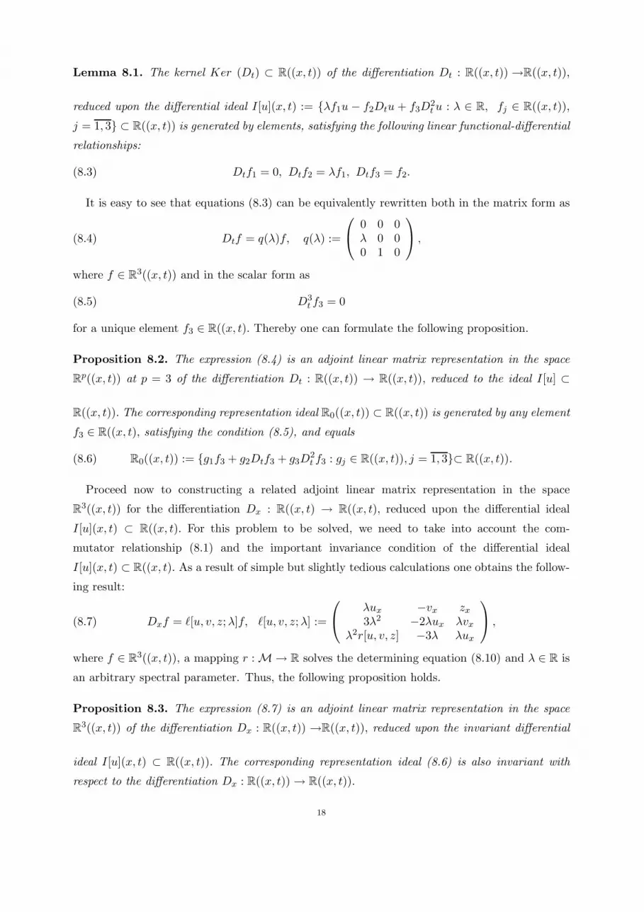
Lemma 8.1. The kernel Ker (Dt) ⊂ R((x, t)) of the differentiation Dt : R((x, t)) →R((x, t)),
reduced upon the differential ideal I[u](x, t) := λf1u − f2Dtu + f3D2t u : λ ∈ R, fj ∈ R((x, t)),
j = 1, 3 ⊂ R((x, t)) is generated by elements, satisfying the following linear functional-differential
relationships:
(8.3) Dtf1 = 0, Dtf2 = λf1, Dtf3 = f2.
It is easy to see that equations (8.3) can be equivalently rewritten both in the matrix form as
(8.4) Dtf = q(λ)f, q(λ) :=
0 0 0λ 0 00 1 0
,
where f ∈ R3((x, t)) and in the scalar form as
(8.5) D3t f3 = 0
for a unique element f3 ∈ R((x, t). Thereby one can formulate the following proposition.
Proposition 8.2. The expression (8.4) is an adjoint linear matrix representation in the space
Rp((x, t)) at p = 3 of the differentiation Dt : R((x, t)) → R((x, t)), reduced to the ideal I[u] ⊂
R((x, t)). The corresponding representation ideal R0((x, t)) ⊂ R((x, t)) is generated by any element
f3 ∈ R((x, t), satisfying the condition (8.5), and equals
(8.6) R0((x, t)) := g1f3 + g2Dtf3 + g3D2t f3 : gj ∈ R((x, t)), j = 1, 3⊂ R((x, t)).
Proceed now to constructing a related adjoint linear matrix representation in the space
R3((x, t)) for the differentiation Dx : R((x, t) → R((x, t), reduced upon the differential ideal
I[u](x, t) ⊂ R((x, t). For this problem to be solved, we need to take into account the com-
mutator relationship (8.1) and the important invariance condition of the differential ideal
I[u](x, t) ⊂ R((x, t). As a result of simple but slightly tedious calculations one obtains the follow-
ing result:
(8.7) Dxf = ℓ[u, v, z;λ]f, ℓ[u, v, z;λ] :=
λux −vx zx3λ2 −2λux λvx
λ2r[u, v, z] −3λ λux
,
where f ∈ R3((x, t)), a mapping r : M → R solves the determining equation (8.10) and λ ∈ R is
an arbitrary spectral parameter. Thus, the following proposition holds.
Proposition 8.3. The expression (8.7) is an adjoint linear matrix representation in the space
R3((x, t)) of the differentiation Dx : R((x, t)) →R((x, t)), reduced upon the invariant differential
ideal I[u](x, t) ⊂ R((x, t)). The corresponding representation ideal (8.6) is also invariant with
respect to the differentiation Dx : R((x, t)) → R((x, t)).
18

Remark 8.4. It is here necessary to mention that the representation (8.4) coincides completely
with that obtained before in the work [9] by means of completely different methods, based mainly
on the gradient-holonomic algorithm, devised in [15, 19, 21].
It is now worth to observe that the invariance condition for the differential ideal R0((x, t)) ⊂R((x, t)) with respect to the differentiations Dx,Dt : R((x, t)) → R((x, t)) is equivalent to the re-
lated Lax type representation for the generalized Riemann type dynamical system (8.8). Namely,
the following theorem holds.
Theorem 8.5. The linear matrix representations (8.4) and (8.7) in the space R3((x, t)) for
differentiations Dt : R((x, t)) →R((x, t)) and Dx : R((x, t)) → R((x, t)), respectively, provide us
with the standard Lax type representation for the generalized Riemann type dynamical system
(8.8), thereby stating its integrability.
The next problem of great interest is to construct, making use of the differential-algebraic
tools, the functional-differential solutions to the determining equation (8.10) as well as the local
densities of the related conservation laws, constructed before in [9].
8.2. The solution set analysis of the functional-differential equation Dtr + uxr = 6.
We consider the generalized Riemann type dynamical system on the functional manifold M =
C∞(R/2πZ; R3) at N = 3
(8.8)ut = v − uux
vt = z − uvx
zt = −uzx
:= K[u, v, z],
which, as is was shown before in [9], possesses the following Lax type representation:
(8.9)
fx = ℓ[u, v, z;λ]f, ft = p(ℓ)f, p(ℓ) := −uℓ[u, v, z;λ] + q(λ),
ℓ[u, v, z;λ] =
λux −vx zx3λ2 −2λux λvx
λ2r[u, v, z] −3λ λux
, q(λ) :=
0 0 0λ 0 00 1 0
,
p(ℓ) =
−λuux uvx −uzx−3uλ2 + λ 2λuux −λuvx
−λ2r[u, v, z]u 1 + 3uλ −λuux
,
,
where f ∈ L∞(R; E3), λ ∈ C is a spectral parameter and a function r : M → R satisfies the
following functional-differential equation:
(8.10) Dtr + uxrx = 6, Dt := ∂/∂t + u∂/∂x.
Below we will describe all functional solutions to equation (8.10), making use of the lemma,
following from the results of [9].19

Lemma 8.6. The following functions
(8.11) B0 = ξ(z), B1 = u− tv + zt2/2, B2 = v − zt, B3 = x− tu+ vt2/2 − zt3/6,
where ξ ∈ C(∞)(R; R) is an arbitrary smooth mapping, are the main invariants of the Riemann
type dynamical system (8.8), satisfying the determining condition
(8.12) DtB = 0.
As a simple inference of relationships (8.11) the next lemma holds.
Lemma 8.7. The local functionals
(8.13) b0 := ξ(z), b1 :=u
z− v2
2z2, b2 :=
ux
zx− v2
x
2z2x
, b3 := x− uv
z+
v3
3z2
and
b1 :=v
z, b2 :=
vx
zxon the manifold M are the basic functional solutions to the determining functional-differential
equations
(8.14) Dtb = 0
and
(8.15) Dtb = 1,
respectively.
Now one can formulate the following theorem about the general solution set to the functional-
differential equation (8.14).
Theorem 8.8. The following infinite hierarchies
(8.16) η(n)1,j := (α∂/∂x)nbj , η
(n)2,k := (α∂/∂x)n+1bk,
where α := 1/zx, j = 0, 3, k = 1, 2 and n ∈ Z+, are the basic functional solutions to the
functional-differential equation (8.14), that is
(8.17) Dtη(n)s,j = 0
for s = 1, 2, j = 0, 3 and all n ∈ Z+.
Proof. It is enough to observe that for any smooth solutions b and b : M → R to functional-
differential equations (8.14) and (8.15), respectively, the expressions (α∂/∂x)b and (α∂/∂x)b are
solutions to the determining functional-differential equation (8.14). Having iterated the operator
α∂/∂x, one obtains the theorem statement.
Proceed now to analyzing the solution set to functional-differential equation (8.10), making
use of the following transformation:
(8.18) r := 6a
αη,
20
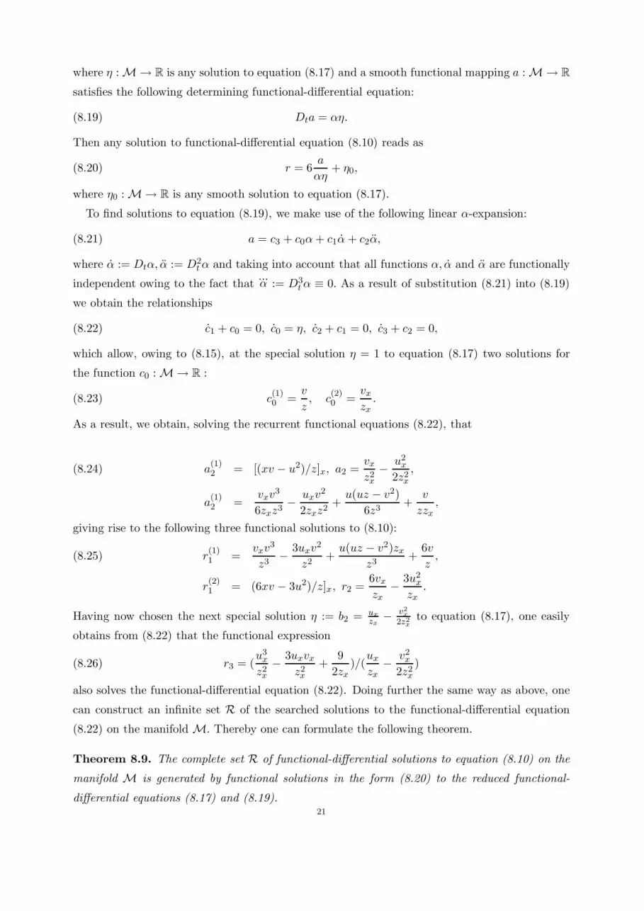
where η : M → R is any solution to equation (8.17) and a smooth functional mapping a : M → R
satisfies the following determining functional-differential equation:
(8.19) Dta = αη.
Then any solution to functional-differential equation (8.10) reads as
(8.20) r = 6a
αη+ η0,
where η0 : M → R is any smooth solution to equation (8.17).
To find solutions to equation (8.19), we make use of the following linear α-expansion:
(8.21) a = c3 + c0α+ c1α+ c2α,
where α := Dtα, α := D2tα and taking into account that all functions α, α and α are functionally
independent owing to the fact that...α := D3
tα ≡ 0. As a result of substitution (8.21) into (8.19)
we obtain the relationships
(8.22) c1 + c0 = 0, c0 = η, c2 + c1 = 0, c3 + c2 = 0,
which allow, owing to (8.15), at the special solution η = 1 to equation (8.17) two solutions for
the function c0 : M → R :
(8.23) c(1)0 =
v
z, c
(2)0 =
vx
zx.
As a result, we obtain, solving the recurrent functional equations (8.22), that
a(1)2 = [(xv − u2)/z]x, a2 =
vx
z2x
− u2x
2z2x
,(8.24)
a(1)2 =
vxv3
6zxz3− uxv
2
2zxz2+u(uz − v2)
6z3+
v
zzx,
giving rise to the following three functional solutions to (8.10):
r(1)1 =
vxv3
z3− 3uxv
2
z2+u(uz − v2)zx
z3+
6v
z,(8.25)
r(2)1 = (6xv − 3u2)/z]x, r2 =
6vx
zx− 3u2
x
zx.
Having now chosen the next special solution η := b2 = ux
zx− v2
x
2z2x
to equation (8.17), one easily
obtains from (8.22) that the functional expression
(8.26) r3 = (u3
x
z2x
− 3uxvx
z2x
+9
2zx)/(
ux
zx− v2
x
2z2x
)
also solves the functional-differential equation (8.22). Doing further the same way as above, one
can construct an infinite set R of the searched solutions to the functional-differential equation
(8.22) on the manifold M. Thereby one can formulate the following theorem.
Theorem 8.9. The complete set R of functional-differential solutions to equation (8.10) on the
manifold M is generated by functional solutions in the form (8.20) to the reduced functional-
differential equations (8.17) and (8.19).21

In particular, the subset
R = r(1)1 =vxv
3
z3− 3uxv
2
z2+u(uz − v2)zx
z3+
6v
z, r
(2)1 = [(6xv − 3u2)/z]x,(8.27)
r2 =6vx
zx− 3u2
x
zx, r3 = (
u3x
z2x
− 3uxvx
z2x
+9
2zx)/(
ux
zx− v2
x
2z2x
) ⊂ R
coincides exactly with (5.12) and constructed before in article [9].
9. Conclusion
As follows from the results obtained in this work, the generalized Riemann type hydrodynamical
system (4.2) at N = 2, 3 and N = 4 possesses many infinite hierarchies of conservation laws, both
dispersive non-polynomial and dispersionless polynomial ones. This fact can be easily explained
by the fact that the corresponding dynamical systems (4.3) and (6.1) possess many, plausibly,
infinite sets of algebraically independent compatible implectic structures, which generate via the
corresponding gradient like relationships [15, 21] the related infinite hierarchies of conservation
laws, and as a by-product, infinite hierarchies of the associated Lax type representations.
It is worth to mention here that the generalized Riemann type equation (4.2) is an example
of integrable dynamical systems belonging simultaneously to two different classes: C- and S-
integrable. Really, these systems ale linearizable and have exact general solutions though in the
unwieldy form. Thus, the Riemann type systems are from a C-integrable class. However, these
systems have also infinite sets of Hamiltonian structures and commuting flows. Thus, they belong
to the S- integrable class too. Such a situation within the theory of Lax type integrable nonlinear
dynamical systems is met, virtually, for the first time and may be appear to be interesting from
different point of view, as well as theoretical and practical. Keeping in mind these and some
other important aspects of the Riemann type hydrodynamical systems (4.2), we consider that
they deserve additional thorough investigation in the future.
Acknowledgments
Two of authors (A.P. and M.P.) are thankful to the Organizers of the NEEDS-2009 Conference
(15-23 May 2009), held in Isola Rossa of Sardinia, Italy, for the invitation to deliver reports,
and kind hospitality. M.P. is indebted to Professor Yavuz Nutku for his hospitality (1996) at
TUBITAK Marmara Research Centre and at the Feza Gursey Institute (Istanbul), for his helpful
explanation of the relationship between Monge-Ampere equation and its Hamiltonian structures.
He is also grateful to Professor Alexander Gurevich for his explanation of the physical nature
of these equations and to Professor Kirill Zybin for his remark that their system describing a
dynamics of dark matter in the Universe can be derived from the Vlasov kinetic equation (which
can be derived from the Liouville equation for the distribution function). He would also like to
thank Prof. Eugene Ferapontov and Prof. Gennady El for their interest and valuable discussions.22
M.P. is especially grateful to the Institute of Mathematics in Taipei (Taiwan) where a part of
this work has been done, and to Jen-Hsu Chang for hospitality at the National Defense University.
This research was, in part, supported by the Russian-Italian Research grant (RFBR grant).
The authors sincerely thank Profs. D.L. Blackmore, Z. Peradzynski, J. S lawianowski and M.
B laszak for useful discussions of the results obtained. They also wish to thank Mrs. Dilys Grilli
(Publications Office, ICTP) for the professional help in preparing the manuscript for publication.
References
[1] Gurevich A.V. and Zybin K.P. Nondissipative gravitational turbulence. Sov. Phys. JETP, 67 (1988), pp.1–12.[2] Gurevich A.V. and Zybin K.P. Large-scale structure of the Universe. Analytic theory Sov. Phys. Usp. 38
(1995), pp.687–722.[3] Ostrovsky L.A. Nonlinear internal waves in a rotating ocean., Oceanology, 18 (1978), pp.119-125.[4] Whitham G.B. Linear and Nonlinear Waves. Wiley-Interscience, New York, 1974, p.221.[5] Pavlov M. The Gurevich-Zybin system. J. Phys. A: Math. Gen. 38 (2005), pp.3823–3840.[6] Pavlov M. Private communication, June 2009.[7] Marsden J. and Chorin R. Mathematical theory of hydrodynammics.[8] Bogolubov N.(Jr.), Prykarpatsky A., Gucwa I. and Golenia J. Analytical properties of an Ostrovsky-Whitham
type dynamical system for a relaxing medium with spatial memory and its integrable regularization. PreprintICTP-IC/2007/109, Trieste, Italy. (available at: http://publications.ictp.it).
[9] Golenia J., Popowicz Z., Pavlov M. and Prykarapatsky A. On a nonlocal Ostrovsky-Whitham type dynamicalsystem, its Riemann type inhomogeneous regularizations and their integrability. SIGMA, 2010 (in press).
[10] Prykarpatsky A.K. and Prytula M.M. The gradient-holonomic integrability analysis of a Whitham-type non-linear dynamical model for a relaxing medium with spatial memory. Nonlinearity 19 (2006) pp.2115–2122.
[11] Hunter J.K., Saxton R., Dynamics of director fields. SIAM J. Appl. Math., 51 (1991), pp.1498–1521.[12] Parkes E.J. Explicit solutions of the reduced Ostrovsky equation. Chaos, Solitons and Fractals, 26, N.5 ( 2005),
pp.1309–1316.[13] Vakhnenko V.A. Solitons in a nonlinear model medium. J. Phys. A: Math. and Gen., 25 (1992), pp.4181–4187.[14] Morrison A.J., Parkes E.J. and Vakhnenko V.O. The N-loop soliton of the Vakhnenko equation., Nonlinearity,
12 (1999), pp.1427–1437.[15] Prykarpatsky A. and Mykytyuk I. Algebraic Integrability of nonlinear dynamical systems on manifolds: clas-
sical and quantum aspects. Kluwer Academic Publishers, the Netherlands, 1998, p.553.[16] Blaszak M. Multi-Hamiltonian theory of dynamical systems. Springer, Berlin, 1998.[17] Brunelli L. and Das A. J. Mathem. Phys. 2004, 45, p. 2633[18] Lenells J., The Hunter-Saxton equation: a geometric approach, SIAM J. Math. Anal. 40 (2008), pp.266–277.[19] Mitropolski Yu.A., Bogoliubov N.N. (Jr.), Prykarpatsky A.K., Samoilenko V.Hr. Integrable Dynamical Sys-
tems. Nauka dumka, Kiev, 1987 (in Russian).[20] Prykarpatsky A.K. and Prytula M.M. The gradient-holonomic integrability analysis of a Whitham type non-
linear dynamical model for a relaxing medium with spacial memory. Proceeding of the National Academy ofSciences of Ukraine, Math. Series, N.5, (2006), pp.13–18 (in Ukrainian).
[21] Hentosh O., Prytula M. and Prykarpatsky A. Differential-geometric and Lie-algebraic foundations of investi-gating nonlinear dynamical systems on functional manifolds. The Second edition. Lviv University Publ., 2006(in Ukrainian).
23