o

inry.

iouville

d by the

Differential Geometry and its Applications 22 (2005) 287–296www.elsevier.com/locate/difge

Analytic-non-integrability of an integrable analyticHamiltonian system✩

Gianluca Gornia,∗, Gaetano Zampierib

a Università di Udine, Dipartimento di Matematica e Informatica, via delle Scienze 208, I-33100 Udine UD, Italyb Università di Torino, Dipartimento di Matematica, via Carlo Alberto 10, I-10123 Torino TO, Italy

Received 31 December 2003; received in revised form 24 February 2004

Available online 12 February 2005

Communicated by T. Ratiu

Abstract

We introduce the polynomial HamiltonianH(q1, q2,p1,p2) := (q22 + (q2

1 + q22)2)p1 − q1q2p2 and we prove

that the associated Hamiltonian system is Liouville-C∞-integrable, but fails to be real-analytically integrableany neighbourhood of an equilibrium point. The proof only uses power series expansions, and is elementa 2005 Elsevier B.V. All rights reserved.

MSC:37J35; 37J30

Keywords:Liouville integrability; Real analytic non-integrability

1. The result

A Hamiltonian system inn degrees of freedom is called Liouville-integrable (see e.g.[1]) if there aren smooth first integrals which are in involution and independent on an open dense subset. A Lintegrable system is solvable by quadrature.

✩ This research was supported by the INdAM (Progetto GNFM-GNAMPA con responsabile il secondo autore), anMURST (Cofin con responsabile nazionale Fabio Zanolin).

* Corresponding author.

E-mail addresses:gorni@dimi.uniud.it(G. Gorni),gaetano.zampieri@unito.it(G. Zampieri).

0926-2245/$ – see front matter 2005 Elsevier B.V. All rights reserved.doi:10.1016/j.difgeo.2005.01.004

288 G. Gorni, G. Zampieri / Differential Geometry and its Applications 22 (2005) 287–296

t of,ntalozlov’s

c

tfical

yonian

meone

on theis

r’s

aroundgnificant

ult is the

Despite the fact that Liouville theorem only requiresCk smoothness in the first integrals, by far mosthe research in integrability and non-integrability has concentrated inanalyticintegrability. For exampleTaımanov proved in 1988 ([6], and the later[7]) that on analytic compact manifolds whose fundamegroup is not almost abelian there cannot be analytically integrable geodesic flows. See also Kpaper[5].

Taımanov’s result left open the question whether those manifolds could haveC∞-integrable geodesiflows. Leo Butler has addressed the problem in a series of papers[2–4].

In particular, with Butler’s systems we have a positive answer to the questionwhether there exisanalytic Hamiltonian systems that areC∞-integrable but not analytically integrable. However the prooof the non-analytic integrability part relies on Taımanov’s theorem, which uses advanced topologmethods.

The present paper answers the same question with a verysimpleexample, for which the proof is totallelementary, if perhaps a bit laborious. Our example is the following autonomous polynomial Hamiltin R

4:

(1)H(q1, q2,p1,p2) := (q2

2 + (q21 + q2

2)2)p1 − q1q2p2,

with its associated Hamiltonian system:

(2)

q1 = ∂H/(∂p1) = q22 + (q2

1 + q22)

2,

q2 = ∂H/(∂p2) = −q1q2,

p1 = −∂H/(∂q1) = p2q2 − 4q1(q21 + q2

2)p1,

p2 = −∂H/(∂q2) = p2q1 − (2q2 + 4q2(q21 + q2

2))p1.

Examples like this are so simple that they could have been produced a long time ago, if only sohad thought of looking for them.

Butler’s systems are on compact manifolds and enjoy rich ergodic properties. Our example isnoncompact setR4, and the Hamiltonian system(2) has non-globally defined solutions (an exampleq1(t) = −(3t)−1/3, q2 ≡ p1 ≡ p2 ≡ 0; Eq.(13) below gives a larger family). On the other hand, Butlesystems have no equilibria, while our system has. In fact, all the points(q1, q2,p1,p2) with q1 = q2 = 0are equilibria.

There are analytic non-integrability theorems in the literature that use power series techniquesan equilibrium point. Our example here suggests that those theorems may be somehow less sithan it was thought, if they do not rule out integrability in theC∞ sense too.

Our result can be divided into two statements:

Theorem 1 (C∞ integrability). The following function

(3)F(q1, q2,p1,p2) :={

q2 exp −12(q2

1+q22)

if (q1, q2) �= (0,0),

0 if (q1, q2) = (0,0)

is of classC∞ on R4 and it is a first integral of system(2). Moreover, the gradients ofF and ofH

are linearly independent on the dense open subspace{(q1, q2,p1,p2): q1 �= 0 or q2 �= 0}. Hence theHamiltonian system(2) is C∞-integrable in the Liouville sense.

The theorem above is a straightforward computation that we leave to the reader. The main resnext one:

G. Gorni, G. Zampieri / Differential Geometry and its Applications 22 (2005) 287–296 289

-

d of the

a

teresting

only at

ng

imple

Theorem 2 (Analytic non-integrability). Let g(q1, q2,p1,p2) be a first integral of the Hamiltonian system (2). Suppose thatg is analytic at the origin ofR4. Then there exists a one-variable functionϕ,analytic at0∈ R, such that

(4)g = ϕ ◦H.

As a consequence, the Hamiltonian system cannot be analytically integrable in any neighbourhooorigin, because all analytic first integrals are functionally dependent ofH.

In Section2 we provide some background on how we came up with the Hamiltonian of formul(1).Section3 contains the proof ofTheorem 2.

The referee of this paper has suggested that a Painlevé analysis of our system may be an indirection for future developments.

2. Origin of the example

We start by making up a smooth non-analytic two-variable function whose gradient vanishesthe origin. Our choice was

(5)F(q1, q2) :={

q2 exp −12(q2

1+q22)

if (q1, q2) �= (0,0),

0 if (q1, q2) = (0,0),

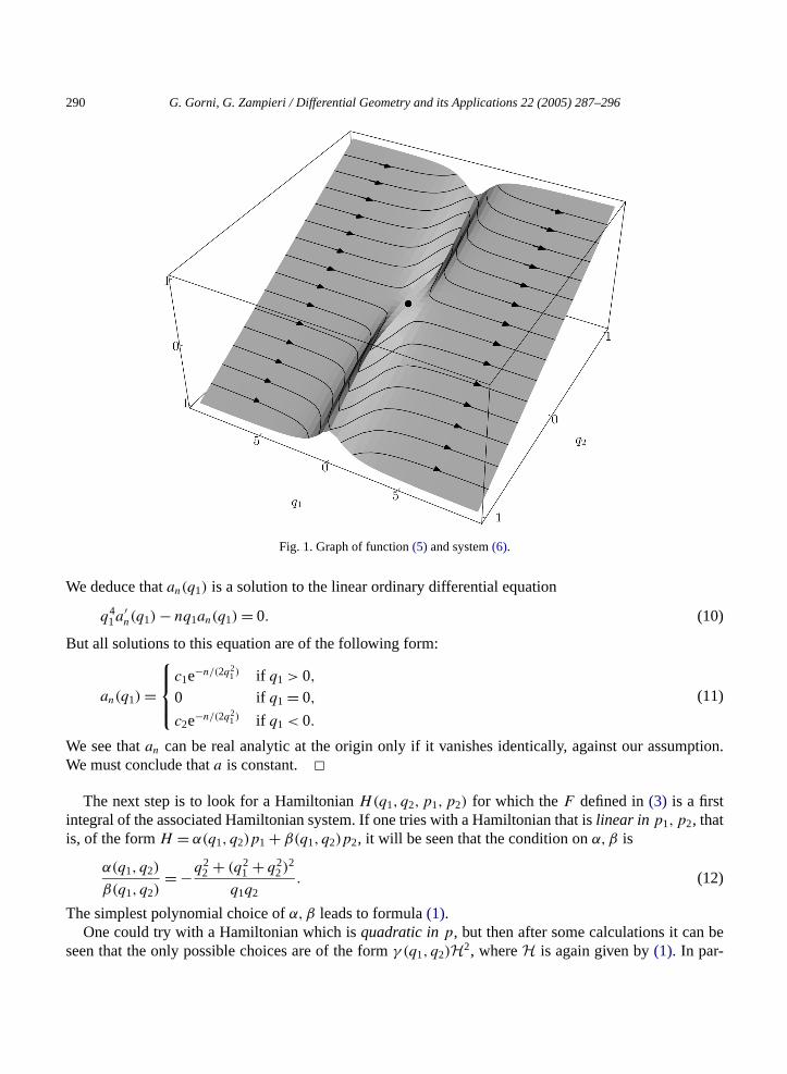
the progenitor of the functionF defined in(3). ThisF is a constant along the trajectories of the followisystem:

(6)

{q1 = q2

2 + (q21 + q2

2)2,

q2 = −q1q2.

Fig. 1superimposes a phase portrait of system(6) to a graph ofF .The following proposition will not be used later, but it is provided because its proof is a very s

illustration of the techniques that will be employed in proving the mainTheorem 2.

Proposition 3. The only first integrals of the two-dimensional system(6) that are real-analytic at theorigin are the constants.

Proof. Let a(q1, q2) be a first integral of system(6). The following relation holds:

(7)(q2

2 + (q21 + q2

2)2) ∂a

∂q1− q1q2

∂a

∂q2= 0.

Suppose thata is real-analytic and nonconstant around the origin. Then there exists an integern � 1 andanalytic functionsan(q1), an+1(q1, q2) such thatan is not identically 0 anda can be written as

(8)a(q1, q2) = a(0,0) + an(q1)qn2 + an+1(q1, q2)q

n+12 .

Replacing this expression ofa into (7) and collecting the powers ofq2 we get

(9)0 ≡ (q4

1a′n(q1) − nq1an(q1)

)qn

2 + higher order terms inq2.

290 G. Gorni, G. Zampieri / Differential Geometry and its Applications 22 (2005) 287–296

ption.

be

Fig. 1. Graph of function(5) and system(6).

We deduce thatan(q1) is a solution to the linear ordinary differential equation

(10)q41a

′n(q1) − nq1an(q1) = 0.

But all solutions to this equation are of the following form:

(11)an(q1) =

c1e−n/(2q21) if q1 > 0,

0 if q1 = 0,

c2e−n/(2q21) if q1 < 0.

We see thatan can be real analytic at the origin only if it vanishes identically, against our assumWe must conclude thata is constant. �

The next step is to look for a HamiltonianH(q1, q2,p1,p2) for which theF defined in(3) is a firstintegral of the associated Hamiltonian system. If one tries with a Hamiltonian that islinear in p1,p2, thatis, of the formH = α(q1, q2)p1 + β(q1, q2)p2, it will be seen that the condition onα,β is

(12)α(q1, q2)

β(q1, q2)= −q2

2 + (q21 + q2

2)2

q1q2.

The simplest polynomial choice ofα,β leads to formula(1).One could try with a Hamiltonian which isquadratic inp, but then after some calculations it can

seen that the only possible choices are of the formγ (q , q )H2, whereH is again given by(1). In par-

1 2

G. Gorni, G. Zampieri / Differential Geometry and its Applications 22 (2005) 287–296 291

e

-an

rplanesions ofplane.ential

rst

nnce

ticular, a Hamiltonian for whichF is a first integral and which is quadratic inp is always a semidefinitquadratic form, never definite.

3. Proof of Theorem 2

One key to our approach is the circumstance that the hyperplaneq2 = 0 in R4 is an invariant man

ifold for the Hamiltonian system(2). Moreover, the restriction of the system to this manifold hasadditional first integral(q1,p1,p2) �→ p2 exp 1

2q21

independent ofH(q1,0,p1,p2) = q41p1, and it can be

solved through elementary functions, namely:

(13)

q1(t) = q1(0)

(1−3q1(0)3t)1/3 ,

q2(t) = 0,

p1(t) = p1(0)(1− 3q1(0)3t)4/3,

p2(t) = p2(0)exp1−(1−3q1(0)3t)2/3

2q1(0).

Although we don’t use these solution formulas directly, they suggest that in that particular hypethings may somehow be much easier. We will attack the problem by making power series expanthe relevant functions with respect toq2 first, so as to reduce as soon as possible to that special hyperWe will then expand with respect to the other variables in turn, until we reach ordinary linear differequations whose power-series solutions can be computed easily.

The condition of being a first integral of(2) is equivalent to a partial differential equation of the fiorder. We can reformulateTheorem 2as follows.

Theorem 4. Letg(q1, q2,p1,p2) be a solution of the differential equation

0 = {H, g} = (p2q1 − p1

(2q2 + 4q2(q

21 + q2

2))) ∂g

∂p2+ (

p2q2 − 4p1q1(q21 + q2

2)) ∂g

∂p1

(14)− q1q2∂g

∂q2+ (

q22 + (q2

1 + q22)

2) ∂g

∂q1

and suppose thatg is analytic at the origin ofR4. Then there exists a one-variable functionϕ, analyticat 0∈ R, such that

(15)g = ϕ ◦H.

Proof. Let g0(q1,p1,p2) = g(q1,0,p1,p2). Thisg0 is an analytic solution of

(16)0 = p2q1∂g0

∂p2− 4p1q

31

∂g0

∂p1+ q4

1

∂g0

∂q1.

This equation is treated inProposition 5: the result is that there exists a one-variable functionϕ, analyticat the origin, such that

(17)g(q1,0,p1,p2) = g0(q1,p1,p2) = ϕ(p1q41) = ϕ

(H(q1,0,p1,p2)

).

The functionϕ ◦H is also a solution of the differential equation(14)(it is obviously a constant of motiofor the Hamiltonian system defined byH), and it is analytic at the origin too. Hence also the differe

292 G. Gorni, G. Zampieri / Differential Geometry and its Applications 22 (2005) 287–296

e

g := g − ϕ ◦ H is an analytic solution of Eq.(14). From(17) we see thatg(q1,0,p1,p2) ≡ 0. We aredone if we prove thatg vanishes identically.

Suppose the contrary. Expandg into powers ofy, and letn0 � 1 be the first exponent for which thcoefficient is not identically zero:

(18)g(q1, q2,p1,p2) =∑n�n0

hn(q1,p1,p2)qn2 , with gn0 /≡ 0.

Using Proposition 8with n = n0 and ϕn0−1 ≡ 0, we obtain that there exists an analyticϕn such thathn0(q1,p1,p2) ≡ ϕn(p1q

41)p

n02 . But then we can apply againProposition 8with n = n0 + 1, to get that

hn0 vanishes identically, against our assumption.�Proposition 5 (Base case). Letg0(q1,p1,p2) be a solution of the differential equation

(19)0 = p2q1∂g0

∂p2− 4p1q

31

∂g0

∂p1− q4

1

∂g0

∂q1,

and suppose thatg0 is analytic at the origin ofR3. Then there exists a one-variable functionϕ, analyticat 0∈ R, such that

(20)g0(q1,p1,p2) ≡ ϕ(p1q41).

Proof. Expandg0 into power series with respect top2, and letn be an exponent� 1 such that thecoefficient ofpk

2 vanishes identically for allk such that 1� k < n, so that we can write

(21)g0(q1,p1,p2) = g0,0(q1,p1) +∑k�n

g0,k(q1,p1)pk2.

Replace this expression into Eq.(19)and collect the powers ofp2. Equating to 0 the coefficient ofp02 we

get

(22)0 = −4p1q31

∂g0,0

∂p1+ q4

1

∂g0,0

∂q1.

This equation is studied inLemma 6: the only solutions analytic at the origin are of the form

(23)g0,0(q1,p1) = ϕ(p1q41),

whereϕ is analytic at 0∈ R. The coefficient ofpn2 leads to the equation

(24)0 = nq1g0,n − 4p1q31

∂g0,n

∂p1+ q4

1

∂g0,n

∂q1,

that has no solutions that are analytic at the origin, except for the null solution, as we see inLemma 7.We finally deduce by induction thatg0,k ≡ 0 for all k � 1. �Lemma 6. Letf (q1,p1) be a solution of the differential equation

(25)0 = −4p1q31

∂f

∂p1+ q4

1

∂f

∂q1,

and suppose thatf is analytic at the origin. Then there exists a one-variable functionϕ, analytic at theorigin, such thatf (q ,p ) ≡ ϕ(p q4).

1 1 1 1

G. Gorni, G. Zampieri / Differential Geometry and its Applications 22 (2005) 287–296 293

to

Proof. Expandf (q1,p1) into power series with respect top1:

(26)f (q1,p1) =∑m∈N

um(q1)pm1 ,

insert into Eq.(25), and collect the powers ofp1:

(27)0 =∑m∈N

(−4mq21um(q1) + q3

1u′m(q1)

)pm

1 .

The ordinary differential equation

(28)−4mq21um(q1) + q3

1u′m(q1) = 0

can be solved explicitly:

(29)um(q1) ={

cmq4m1 if q1 > 0,

c′mq4m

1 if q1 < 0.

Sinceum is analytic,c′m must be the same ascm. Hence

(30)f (q1,p1) =∑m∈N

(cmq4m1 )pm

1 = ϕ(p1q41), whereϕ(t) :=

∑m∈N

cmtm.

The series definingϕ has positive radius of convergence becausef is analytic at the origin. �Lemma 7. Let c �= 0 andf (q1,p1) be a solution of the differential equation

(31)0 = cf − 4p1q21

∂f

∂p1+ q3

1

∂f

∂q1

and suppose thatf is analytic at the origin ofR2. Thenf ≡ 0.

Proof. As in Lemma 6, expandf (q1,p1) into power series with respect top1:

(32)f (q1,p1) =∑m∈N

um(q1)pm1 ,

insert into Eq.(31), and collect the powers ofp1:

(33)0 =∑m∈N

((c − 4mq2

1)um(q1) + q31u

′m(q1)

)pm

1 .

The ordinary differential equation

(34)(c − 4mq21)um(q1) + q3

1u′m(q1) = 0

can be solved explicitly:

(35)um(q1) = αq4m1 exp

c

2q21

(α can depend on the sign ofq1). The only way for this solution to be analytic at the origin is for itvanish identically (α = 0). �

294 G. Gorni, G. Zampieri / Differential Geometry and its Applications 22 (2005) 287–296

Proposition 8 (Induction). Let g(q1, q2,p1,p2), be a solution of the differential equation(14), and sup-pose thatg is of the form

(36)g(q1, q2,p1,p2) = ϕn−1(p1q41)p

n−12 qn−1

2 + hn(q1,p1,p2)qn2 + hn+1(q1, q2,p1,p2)q

n+12 ,

wheren � 1 and the functionsϕn−1, hn, hn+1 are analytic at the origin in dimension1, 3, 4 respectively.Assume finally thatϕ0 ≡ 0. Thenϕn−1 ≡ 0 andhn(q1,p1,p2) is of the form

(37)hn(q1,p1,p2) = ϕn(p1q41)p

n2,

whereϕn is a one-variable function, analytic at the origin.

Proof. Replace formula(36) into Eq.(14)and collect the powers ofy. The coefficient ofqn2 is

−2(n − 1)p1pn−22 (1+ 2q2

1)ϕn−1(p1q41) − nxhn(q1,p1,p2)

(38)+ pn2q

41ϕ

′n−1(p1q

41) + p2q1

∂hn

∂p2− 4p1q

31

∂hn

∂p1+ q4

1

∂hn

∂q1.

This coefficient must be zero. Expandhn into power series with respect top2:

(39)hn(q1,p1,p2) =∑k∈N

fn,k(q1,p1)pk2,

insert the expansion into(38), and collect the powers ofp2. The coefficient ofpn−22 whenn � 2 is

(40)−2(n − 1)(1+ 2q21)ϕn−1(p1q

41)p1 − 2q1fn,n−2(q1,p1) − 4p1q

31

∂fn,n−2

∂p1+ q4

1

∂fn,n−2

∂q1,

the coefficient ofpn2 is

(41)q41ϕ

′n−1(p1q

41) − 4p1q

31

∂fn,n

∂p1+ q4

1

∂fn,n

∂q1,

and the generic coefficient ofpk2 for k ∈ N \ {n − 2, n} is

(42)(k − n)q1fn,k − 4p1q31

∂fn,k

∂p1+ q4

1

∂fn,k

∂q1.

Applying Lemma 9to formula(40)we get that whenn � 2 bothϕn−1 andfn,n−2 vanish identically. ThenLemma 6applied to(41) implies thatfn,n(q1,p1) = ϕn(p1q

41). Finally, from Lemma 7applied to(42)

we conclude thatfn,k ≡ 0 whenk is neithern norn − 2. �Lemma 9. Let ϕ(t), f (q1,p1) be functions that are analytic at the origin inR and R

2 respectively.Suppose thatf solves the differential equation

(43)0 = c(1+ 2q21)ϕ(p1q

41)p1 − 2q1f − 4p1q

31

∂f

∂p1+ q4

1

∂f

∂q1,

wherec �= 0. Then bothϕ(t) andf (q ,p ) vanish identically.

1 1

G. Gorni, G. Zampieri / Differential Geometry and its Applications 22 (2005) 287–296 295

d to

Proof. Expandϕ(t) andh into power series with respect tot andp1 respectively:

(44)ϕ(t) =∑m�0

rmtm, f (q1,p1) =∑m�0

um(q1)pm1 ,

replace into Eq.(43), and collect the powers ofp1:

0 = q41u

′0(q1) − 2q1u0(q1)

(45)+∑m�1

(cq

4(m−1)

1 (1+ 2q21)rm−1 − 2(q1 + 2mq3

1)um(q1) + q41u

′m(q1)

)pm

1 .

Equating to zero the coefficient ofp01 we get the differential equation

(46)q41u

′0(q1) − 2q1u0(q1) = 0

whose general solution isu0(q1) = λe−1/q21 , which is analytic at the origin only whenλ = 0. The coeffi-

cient ofpm1 for m � 1 is complicated enough to deserve its ownLemma 10. �

Lemma 10. Letu(q1) be a solution of the differential equation

(47)0 = cq4(m−1)1 (1+ 2q2

1) − 2(q1 + 2mq31)u(q1) + q4

1u′(q1),

wherec ∈ R, m ∈ N \ {0} are parameters. Ifu(q1) is analytic at the origin thenc = 0 andu ≡ 0.

Proof. Expandu(q1) into power series:

(48)u(q1) =∑k�0

akqk1,

replace in Eq.(47)and collect the powers ofq1:

(49)0 = −2a0q1 − 2a1q21 + cq4m−4

1 + 2cq4m−21 +

∑k�3

((k − 4m − 3)ak−3 − 2ak−1

)qk

1.

By equating most coefficients to 0 we obtain a recurrence formula:

(50)ak−1 = k − 4m − 3

2ak−3 for k � 3, k /∈ {4m − 4,4m − 2}.

The coefficient ofq11 is −2a0, which must vanish. From this and the recurrence formula applie

k = 3,5,7. . . in succession we see thata2, a4, a6 . . . are all zero.If m = 1 then the coefficients ofq0

1 andq21 are respectivelyc and 2(c − a1). Hencec anda1 must

vanish. The recurrence formula(50) implies then thatai = 0 for all odd i. Hencec = 0 andu ≡ 0 asdesired.

Suppose from now on thatm > 1. The coefficient ofq21 in (49)is −2a1. Hencea1 = 0. Again, ifm � 3,

the recurrence(50) written for k = 4,6, . . . ,4m − 6 implies thata3 = a5 = · · · = a4m−7 = 0. We deducethat allai = 0 for all i odd between 1 and 4m − 7 inclusive.

Let us prove thata4m−3 = 0. Consider the recurrence(50) for evenk � 4m. Sincek − 4m − 3 �= 0whenk is even, ifa were different from 0, then all coefficienta for odd i � 4m − 3 would be�= 0,

4m−3 i

296 G. Gorni, G. Zampieri / Differential Geometry and its Applications 22 (2005) 287–296

ion.

tempt

i. Soc.

(1979)

USSR

05 (6)

with an order of growth ask → +∞ more than exponential:

(51)limk→+∞k odd

ak−1

ak−3= lim

k→+∞k odd

k − 4m − 3

2= +∞.

The radius of convergence of the power series(48)would then be zero, against the analyticity assumptHenceai = 0 for all oddi � 4m − 3.

Only a4m−5 andc are left to decide. If we equate the coefficients of the remaining termsq4m−41 and

q4m−21 to zero we get the system of two equations

(52)

0= c + ((4m − 4) − 4m − 3)a(4m−4)−3 − 2a(4m−4)−1

= c − 7a4m−7 − 4a4m−5 = c − 4a4m−5,

0= 2c + ((4m − 2) − 4m − 3)a(4m−2)−3 − 2a(4m−2)−1

= 2c − 5a4m−5 − 2a4m−3 = 2c − 5a4m−5,

which is solved with respect toc anda4m−5 to give

(53)c = a4m−5 = 0.

We conclude thatc = 0 andu ≡ 0 also whenm � 2. �

Acknowledgements

We thank Prof. Massimo Villarini, with whom we had interesting discussions during an early atat the proof ofTheorem 2in a totally different direction.

References

[1] V.I. Arnol’d, Mathematical Methods of Classical Mechanics, second ed., Springer-Verlag, New York, 1989.[2] L.T. Butler, A new class of homogeneous manifolds with Liouville-integrable geodesic flows, C. R. Math. Acad. Sc

R. Can. 21 (4) (1999) 127–131.[3] L.T. Butler, New examples of integrable geodesic flows, Asian J. Math. 4 (3) (2000) 515–526.[4] L.T. Butler, Integrable geodesic flows onn-step nilmanifolds, J. Geom. Phys. 36 (3–4) (2000) 315–323.[5] V.V. Kozlov, Topological obstructions to the integrability of natural mechanical systems, Soviet Math. Dokl. 20 (6)

1413–1415.[6] I.A. Taımanov, Topological obstructions to integrability of geodesic flows on non-simply-connected manifolds, Math.

Izv. 30 (2) (1988) 403–409.[7] I.A. Taımanov, The topology of riemannian manifolds with integrable geodesic flows, Proc. Steklov Inst. Math. 2

(1995) 139–150.