On classification of integrableclasses of surfaces

Michal Marvan

Silesian University in Opava, Czech Republic

The talk will discuss integrable PDE related to immersed surfacesin R3. Cassification of such PDE is a joint project with HynekBaran.

Our expectations:

– obtaining lists of integrable classes of surfaces, as complete aspossible

– identifying old cases (including well-forgotten ones);

– discovering new integrable classes/new integrable PDE.

1

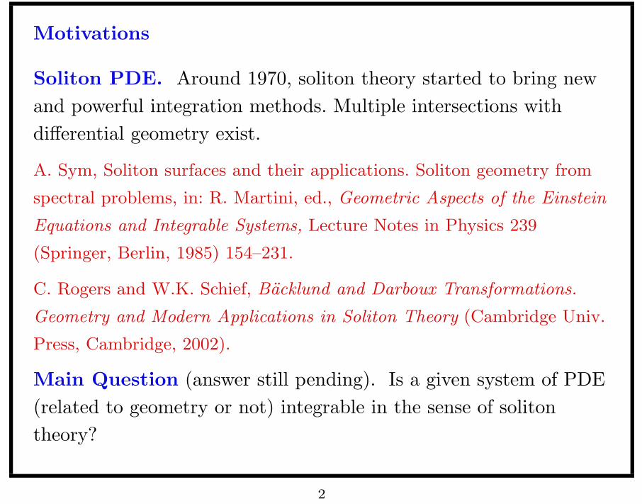
Motivations

Soliton PDE. Around 1970, soliton theory started to bring newand powerful integration methods. Multiple intersections withdi!erential geometry exist.

A. Sym, Soliton surfaces and their applications. Soliton geometry from

spectral problems, in: R. Martini, ed., Geometric Aspects of the Einstein

Equations and Integrable Systems, Lecture Notes in Physics 239

(Springer, Berlin, 1985) 154–231.

C. Rogers and W.K. Schief, Backlund and Darboux Transformations.

Geometry and Modern Applications in Soliton Theory (Cambridge Univ.

Press, Cambridge, 2002).

Main Question (answer still pending). Is a given system of PDE(related to geometry or not) integrable in the sense of solitontheory?

2

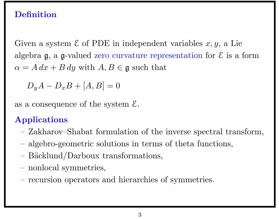
Definition

Given a system E of PDE in independent variables x, y, a Liealgebra g, a g-valued zero curvature representation for E is a form! = A dx + B dy with A, B ! g such that

DyA"DxB + [A, B] = 0

as a consequence of the system E.

Applications– Zakharov–Shabat formulation of the inverse spectral transform,– algebro-geometric solutions in terms of theta functions,– Backlund/Darboux transformations,– nonlocal symmetries,– recursion operators and hierarchies of symmetries.

3

Example

The mKdV equation ut + uxxx " 6u2ux = 0 has an sl2-valued zerocurvature representation A dx + B dt with

A =!

u "1 "u

",

B =!"uxx + 2u3 " 4"u 2"ux + 2"u2 " 4"2

"2ux + 2u2 " 4" uxx " 2u3 + 4"u

".

Indeed, Dt(A)"Dx(B) + [A, B] = (ut + uxxx " 6u2ux) · C, where

C =!

1 00 "1

".

Here " is a parameter (the spectral parameter).

Problem. How to tell whether a given nonlinear system has azero curvature representation?

4

The method

Resources:

M.M., A direct procedure to compute zero-curvature representations.

The case sl2, in: Secondary Calculus and Cohomological Physics, Proc.

Conf. Moscow, 1997 (ELibEMS, 1998) pp. 10.

Normal forms:

P. Sebestyen, Normal forms of irreducible sl3-valued zero curvature

representations, Rep. Math. Phys 55 (2005) No. 3, 435–445.

P. Sebestyen, On normal forms of irreducible sln-valued zero curvature

representations, Rep. Math. Phys 62 (2008) No. 1.

5

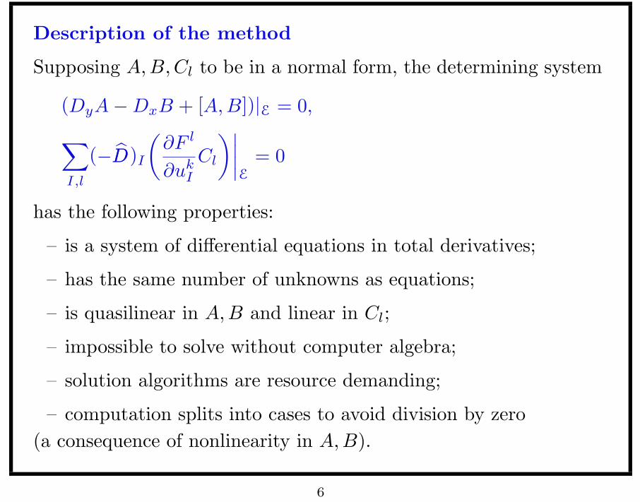
Description of the method

Supposing A, B, Cl to be in a normal form, the determining system

(DyA"DxB + [A, B])|E = 0,

#

I,l

(" $DD)I

!#F l

#ukI

Cl

"%%%%E

= 0

has the following properties:

– is a system of di!erential equations in total derivatives;

– has the same number of unknowns as equations;

– is quasilinear in A, B and linear in Cl;

– impossible to solve without computer algebra;

– solution algorithms are resource demanding;

– computation splits into cases to avoid division by zero(a consequence of nonlinearity in A, B).

6

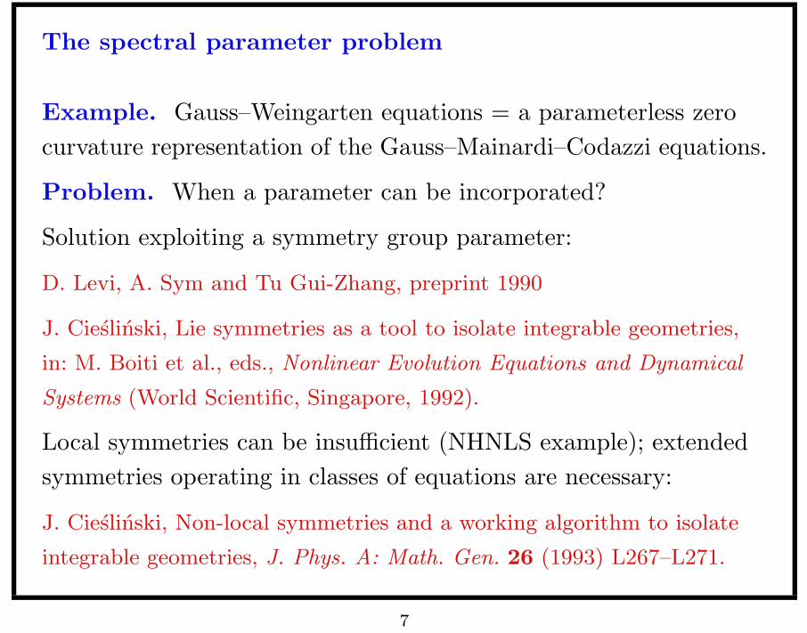
The spectral parameter problem

Example. Gauss–Weingarten equations = a parameterless zerocurvature representation of the Gauss–Mainardi–Codazzi equations.

Problem. When a parameter can be incorporated?

Solution exploiting a symmetry group parameter:

D. Levi, A. Sym and Tu Gui-Zhang, preprint 1990

J. Cieslinski, Lie symmetries as a tool to isolate integrable geometries,

in: M. Boiti et al., eds., Nonlinear Evolution Equations and Dynamical

Systems (World Scientific, Singapore, 1992).

Local symmetries can be insu"cient (NHNLS example); extendedsymmetries operating in classes of equations are necessary:

J. Cieslinski, Non-local symmetries and a working algorithm to isolate

integrable geometries, J. Phys. A: Math. Gen. 26 (1993) L267–L271.

7

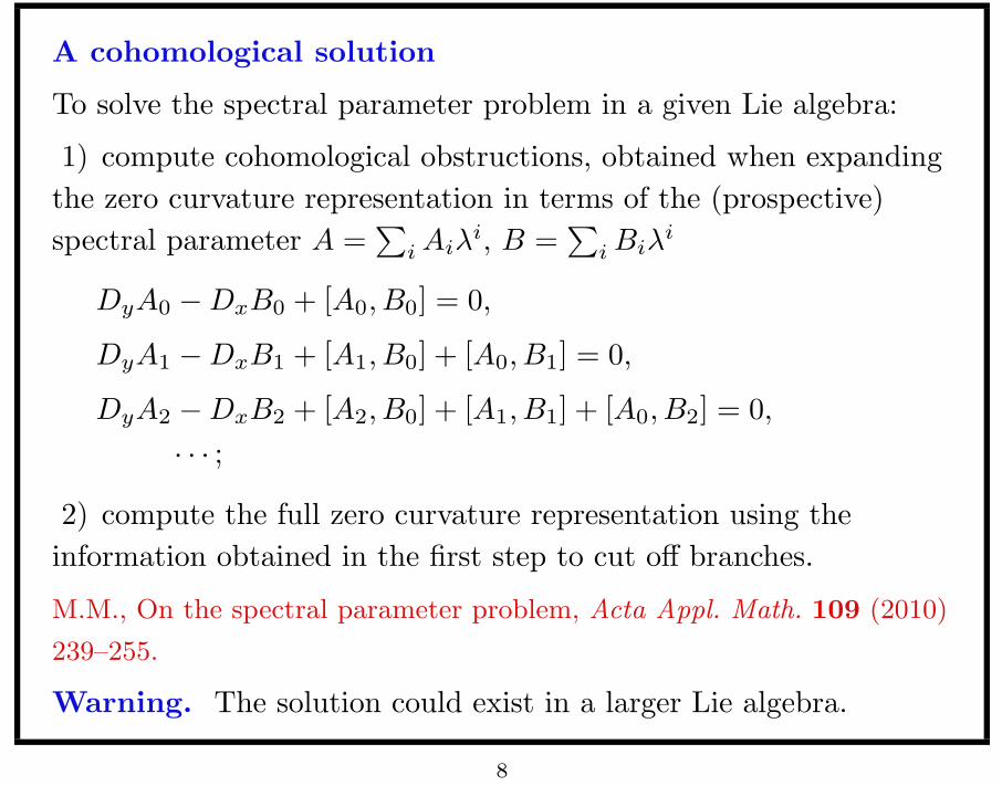
A cohomological solution

To solve the spectral parameter problem in a given Lie algebra:

1) compute cohomological obstructions, obtained when expandingthe zero curvature representation in terms of the (prospective)spectral parameter A =

&i Ai"i, B =

&i Bi"i

DyA0 "DxB0 + [A0, B0] = 0,

DyA1 "DxB1 + [A1, B0] + [A0, B1] = 0,

DyA2 "DxB2 + [A2, B0] + [A1, B1] + [A0, B2] = 0,

· · · ;

2) compute the full zero curvature representation using theinformation obtained in the first step to cut o! branches.

M.M., On the spectral parameter problem, Acta Appl. Math. 109 (2010)

239–255.

Warning. The solution could exist in a larger Lie algebra.

8

The classification project

We consider geometrically determined classes of surfaces, meaningclasses determined by a single condition

F (p1, . . . , pk) = 0,

where pi are di!erential invariants with respect toreparameterizations and euclidean motions (principal curvatures,their gradients, etc.).

We classify relations F = 0 such that

– the associated Gauss–Mainardi–Codazzi equations possess azero curvature representation depending on a nonremovable(spectral) parameter;

– the zero curvature representation has a prescribed order r andtakes values in a prescribed Lie algebra sl(n).

9

Weingarten surfaces

To start with, we focus on Weingarten surfaces, i.e., classes ofimmersed surfaces in E3 determined by a functional relationbetween the principal curvatures k1, k2.

Examples. All rotation surfaces; constant Gaussian curvaturesurfaces; constant mean curvature surfaces.

Classification Problem. Which functional relationsf(k1, k2) = 0 determine an integrable class of Weingarten surfaces?

Example. Bonnet surfaces are surfaces that admit a nontrivialisometry preserving both principal curvatures. Bonnet surfaces areintegrable, are Weingarten surfaces, but the functional relationf(k1, k2) = 0 is di!erent for di!erent Bonnet surfaces. Hence,Bonnet surfaces are not an integrable class of Weingarten surfaces.

10

The Finkel–Wu conjecture

Example. Any linear relation between the mean curvature12 (k1 + k2) and the Gauss curvature k1k2:

ak1k2 + b(k1 + k2) + c = 0

determines an integrable class (linear Weingarten surfaces).

Conjecture. The only class of integrable Weingarten surfaces arethe linear Weingarten surfaces.

Hongyou Wu, Weingarten surfaces and nonlinear partial di!erential

equations, Ann. Global Anal. Geom. 11 (1993) 49–64.

F. Finkel, On the integrability of Weingarten surfaces, in: A. Coley et al.,

ed., Backlund and Darboux Transformations. The Geometry of Solitons,

AARMS-CRM Workshop, June 4-9, 1999, Halifax, N.S., Canada, (Amer.

Math. Soc., Providence, 2001) 199–205.

11

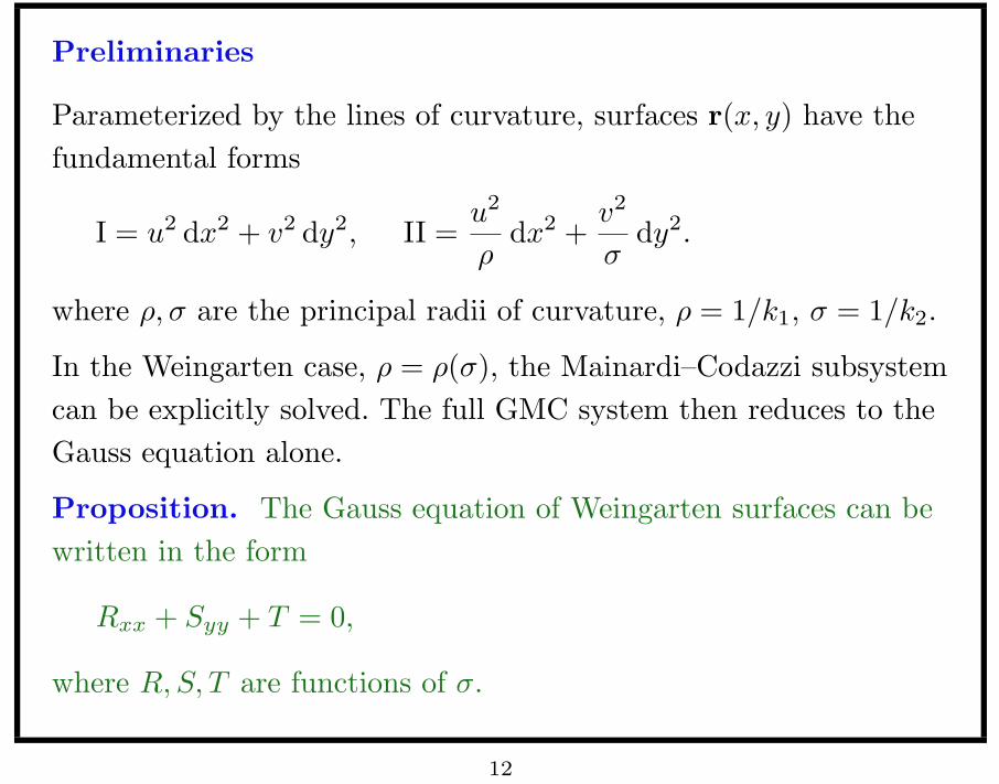
Preliminaries

Parameterized by the lines of curvature, surfaces r(x, y) have thefundamental forms

I = u2 dx2 + v2 dy2, II =u2

$dx2 +

v2

%dy2.

where $, % are the principal radii of curvature, $ = 1/k1, % = 1/k2.

In the Weingarten case, $ = $(%), the Mainardi–Codazzi subsystemcan be explicitly solved. The full GMC system then reduces to theGauss equation alone.

Proposition. The Gauss equation of Weingarten surfaces can bewritten in the form

Rxx + Syy + T = 0,

where R,S, T are functions of %.

12

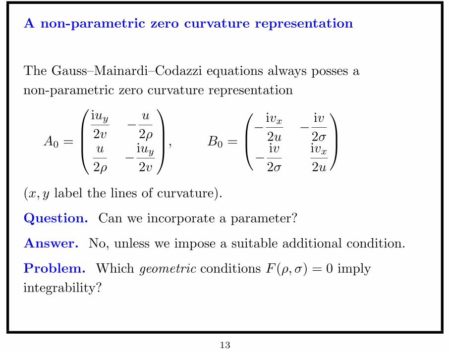
A non-parametric zero curvature representation

The Gauss–Mainardi–Codazzi equations always posses anon-parametric zero curvature representation

A0 =

'

(()

iuy

2v" u

2$u

2$" iuy

2v

*

++,, B0 =

'

()" ivx

2u" iv

2%

" iv2%

ivx

2u

*

+,

(x, y label the lines of curvature).

Question. Can we incorporate a parameter?

Answer. No, unless we impose a suitable additional condition.

Problem. Which geometric conditions F ($, %) = 0 implyintegrability?

13

Results of the computation

Weingarten surfaces determined by an explicit dependence $(%)possess a one-parametric zero curvature representation if and onlyif the determining equation

$!!! =3

2$!$!!2 +

$! " 1$" %

$!! + 2($! " 1)$!($! + 1)

($" %)2

holds (the prime denotes d/d%).

This equation has

– a general solution in terms of elliptic integrals;

– a number of special cases when the solution $(%) can beexpressed in terms of elementary functions.

Surprise. All the special cases were known in the XIX century.

Corollary. The Finkel–Wu conjecture is false.

14

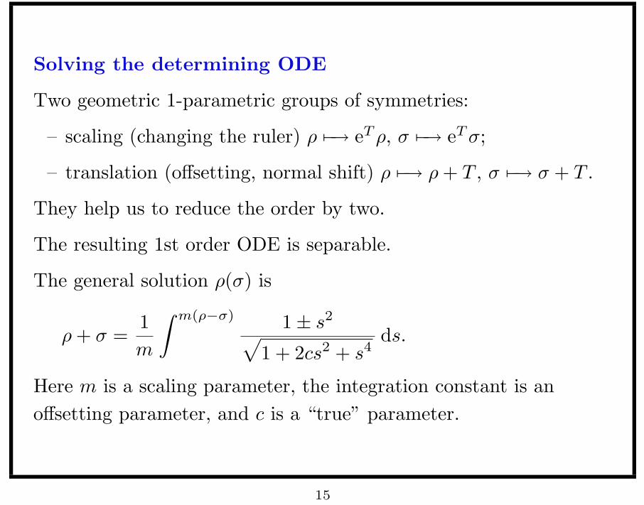
Solving the determining ODE

Two geometric 1-parametric groups of symmetries:

– scaling (changing the ruler) $ #"$ eT $, % #"$ eT %;

– translation (o!setting, normal shift) $ #"$ $ + T , % #"$ % + T .

They help us to reduce the order by two.

The resulting 1st order ODE is separable.

The general solution $(%) is

$ + % =1m

- m(!"") 1 ± s2

.1 + 2cs2 + s4

ds.

Here m is a scaling parameter, the integration constant is ano!setting parameter, and c is a “true” parameter.

15

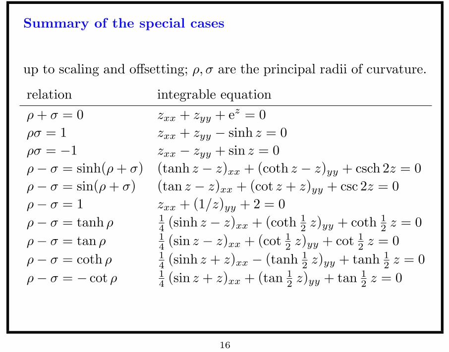
Summary of the special cases

up to scaling and o!setting; $, % are the principal radii of curvature.

relation integrable equation$ + % = 0 zxx + zyy + ez = 0$% = 1 zxx + zyy " sinh z = 0$% = "1 zxx " zyy + sin z = 0$" % = sinh($ + %) (tanh z " z)xx + (coth z " z)yy + csch 2z = 0$" % = sin($ + %) (tan z " z)xx + (cot z + z)yy + csc 2z = 0$" % = 1 zxx + (1/z)yy + 2 = 0$" % = tanh $ 1

4(sinh z " z)xx + (coth 1

2 z)yy + coth 12 z = 0

$" % = tan $ 14

(sin z " z)xx + (cot 12 z)yy + cot 1

2 z = 0$" % = coth $ 1

4(sinh z + z)xx " (tanh 1

2 z)yy + tanh 12 z = 0

$" % = " cot $ 14

(sin z + z)xx + (tan 12 z)yy + tan 1

2 z = 0

16

Surfaces of constant astigmatism

The relation $" % = const was among the special solutions.

H. Baran and M.M., On integrability of Weingarten surfaces: a forgotten

class, J. Phys. A: Math. Theor. 42 (2009) 404007.

Popular among nineteenth-century geometers:

A. Ribaucour, Note sur les developpees des surfaces, C. R. Acad. Sci.

Paris 74 (1872) 1399–1403.

A. Mannheim, Sur les surfaces dont les rayons de courbure principaux

sont fonctions l’un de l’autre, Bull. S.M.F. 5 (1877) 163–166.

R. Lipschitz, Zur Theorie der krummen Oberflachen, Acta Math. 10

(1887) 131–136.

R. von Lilienthal, Bemerkung uber diejenigen Flachen bei denen die

Di!erenz der Hauptkrummungsradien constant ist, Acta Math. 11 (1887)

391–394.

17

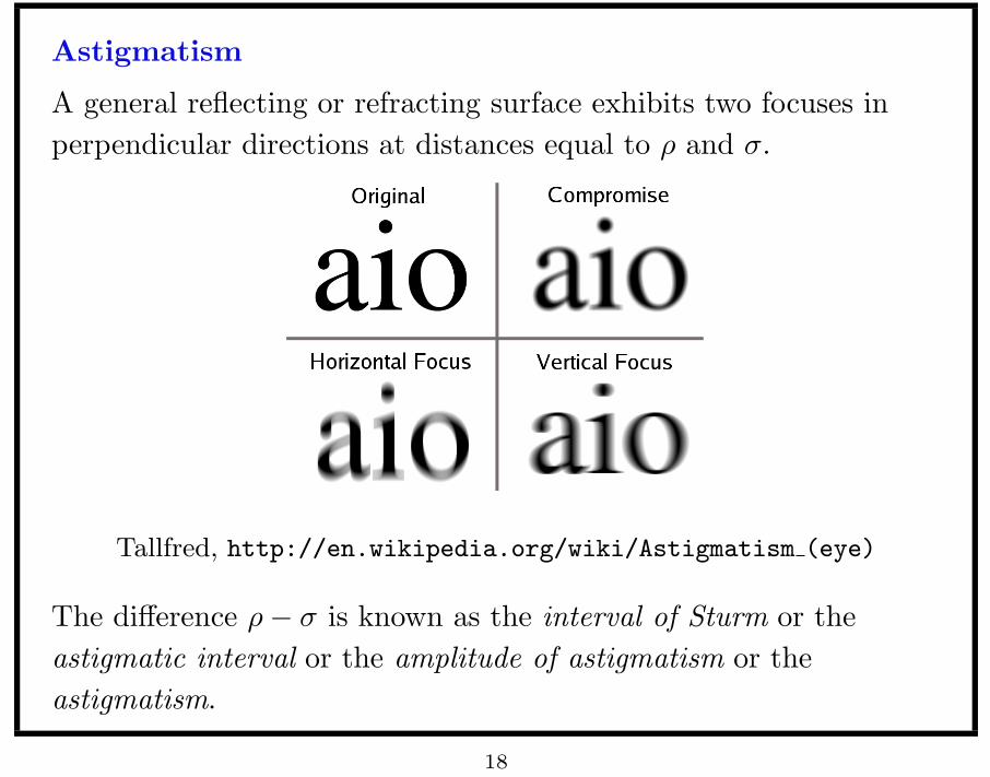
Astigmatism

A general reflecting or refracting surface exhibits two focuses inperpendicular directions at distances equal to $ and %.

Tallfred, http://en.wikipedia.org/wiki/Astigmatism (eye)

The di!erence $" % is known as the interval of Sturm or theastigmatic interval or the amplitude of astigmatism or theastigmatism.

18

The constant astigmatism equation

The constant $" % can be always reduced to 1 by rescaling theambient metric. Then the Gauss equation can be put in the form

zyy +!

1z

"

xx+ 2 = 0,

which we call the constant astigmatism equation.

The equation has obvious translational symmetries(reparameterization) #x, #y, the scaling symmetry

2z#

#z" x

#

#x+ y

#

#y,

which corresponds to o!setting, and a discrete symmetry

x "$ y, y "$ x, z "$ 1z,

which corresponds to swapping the orientation & taking theparallel surface at the unit distance.

19

Two third-order symmetries

One of them has the generator

z3

K3 (zxxx " zzxxy)

" 3K5 z3(zx " zzy)(zxx " zzxy)2 " 2

K5 z5(9zx " zzy)zxx

+1

2K5 z2(9z2x + 4zzxzy " z2z2

y)(zx " zzy)zxx

" 2K5 z3zx(zx " zzy)(4zx " zzy)zxy +

4K5 z6zxzxy

+3

K5 z4(5zx " zzy)z2x "

3K5 z(zx " zzy)z4

x,

where K =%

(zx " zzy)2 + 4z3 .

The other symmetry is obtained by conjugation with the discretesymmetry above.

20

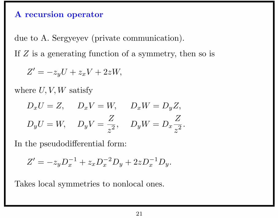
A recursion operator

due to A. Sergyeyev (private communication).

If Z is a generating function of a symmetry, then so is

Z ! = "zyU + zxV + 2zW,

where U, V, W satisfy

DxU = Z, DxV = W, DxW = DyZ,

DyU = W, DyV =Z

z2 , DyW = DxZ

z2 .

In the pseudodi!erential form:

Z ! = "zyD"1x + zxD"2

x Dy + 2zD"1x Dy.

Takes local symmetries to nonlocal ones.

21

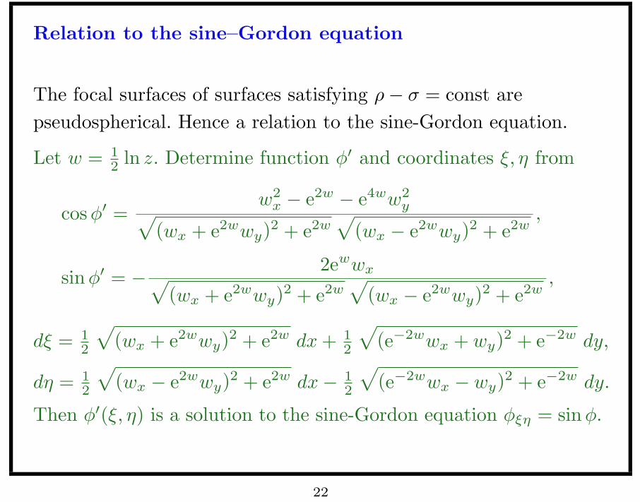
Relation to the sine–Gordon equation

The focal surfaces of surfaces satisfying $" % = const arepseudospherical. Hence a relation to the sine-Gordon equation.

Let w = 12 ln z. Determine function &! and coordinates ', ( from

cos &! =w2

x " e2w " e4ww2y.

(wx + e2wwy)2 + e2w.

(wx " e2wwy)2 + e2w,

sin &! = " 2ewwx.(wx + e2wwy)2 + e2w

.(wx " e2wwy)2 + e2w

,

d' = 12

.(wx + e2wwy)2 + e2w dx + 1

2

.(e"2wwx + wy)2 + e"2w dy,

d( = 12

.(wx " e2wwy)2 + e2w dx" 1

2

.(e"2wwx " wy)2 + e"2w dy.

Then &!(', () is a solution to the sine-Gordon equation &#$ = sin&.

22

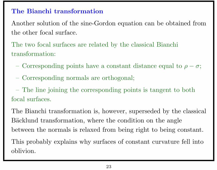
The Bianchi transformation

Another solution of the sine-Gordon equation can be obtained fromthe other focal surface.

The two focal surfaces are related by the classical Bianchitransformation:

– Corresponding points have a constant distance equal to $" %;

– Corresponding normals are orthogonal;

– The line joining the corresponding points is tangent to bothfocal surfaces.

The Bianchi transformation is, however, superseded by the classicalBacklund transformation, where the condition on the anglebetween the normals is relaxed from being right to being constant.

This probably explains why surfaces of constant curvature fell intooblivion.

23

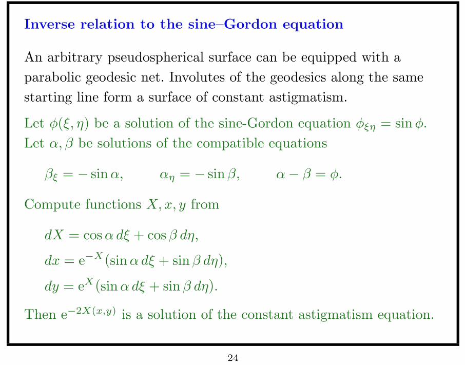
Inverse relation to the sine–Gordon equation

An arbitrary pseudospherical surface can be equipped with aparabolic geodesic net. Involutes of the geodesics along the samestarting line form a surface of constant astigmatism.

Let &(', () be a solution of the sine-Gordon equation &#$ = sin&.Let !,) be solutions of the compatible equations

)# = " sin !, !$ = " sin), !" ) = &.

Compute functions X, x, y from

dX = cos ! d' + cos ) d(,

dx = e"X(sin! d' + sin) d(),

dy = eX(sin ! d' + sin) d().

Then e"2X(x,y) is a solution of the constant astigmatism equation.

24

Von Lilienthal surfaces

R. von Lilienthal, Bemerkung uber diejenigen Flachen bei denen die

Di!erenz der Hauptkrummungsradien constant ist, Acta Math. 11 (1887)

391–394.

A special case of the Lipschitz solution

R. Lipschitz, Zur Theorie der krummen Oberflachen, Acta Math. 10

(1887) 131–136.

Von Lilienthal surfaces are (made of) involutes of meridians of thepseudosphere starting at the same ‘parallel’.

The pseudosphere itself is the involute of the catenoid.

All they are rotation surfaces:

– Catenoid = rotation of the catenary.

– Pseudosphere = rotation of the tractrix.

– Von Lilienthal surfaces = see the picture.

25

Weingarten’s ‘new class of surfaces’

Surfaces satisfying relation $" % = sin($ + %).

J. Weingarten, Uber die Oberflachen, fur welche einer der beiden

Hauptkrummungshalbmesser eine function des anderen ist, J. Reine

Angew. Math. 62 (1863) 160–173.

Covered in §§ 745, 746, 766, 769, 770 of

G. Darboux, “Lecons sur la theorie generale des surface et les

applications geometriques du calcul infinitesimal,” Vol. I–IV.

and §§ 135, 245, 246 of

L. Bianchi, “Lezioni di Geometria Di!erenziale,” Vol. I, II.

Darboux gave a general solution of the associated equation(tan z " z)xx + (cot z + z)yy + csc 2z = 0. He also gave a remarkablegeometric construction, further developed by Bianchi.

26

Darboux correspondence

Darboux discovered a relationship with translation surfaces, furtherdeveloped by Bianchi.

A translation surface is a surface that admits a parameterizationrr(', () such that

rr#$ = 0.

Equivalently, rr(', () = rr1(') + rr2((). The curves rr1(') and rr2(()are called the generating curves.

Otherwise said, a translation surface is obtained when translating acurve along another curve. Translation surfaces are manifestlyintegrable if the curves are given by integrable systems of ODE.

A middle evolute of a surface consists of mid-points between thetwo focal surfaces.

27

Darboux–Bianchi theorem I

Proposition. Let r satisfy

$" % = sin($ + %),

let ', ( be the common asymptotic coordinates of its focal surfaces.Then

(i) the coordinates ', ( render the middle evolute rr as atranslation surface, i.e., rr(', () = rr1(') + rr2(();

(ii) the generating curves rr1, rr2 have opposite nonzero constanttorsion;

(iii) the normal vector n to the surface r at a point belongs to theintersection of the osculating planes of the generating curvesrr1, rr2 through the corresponding point.

28

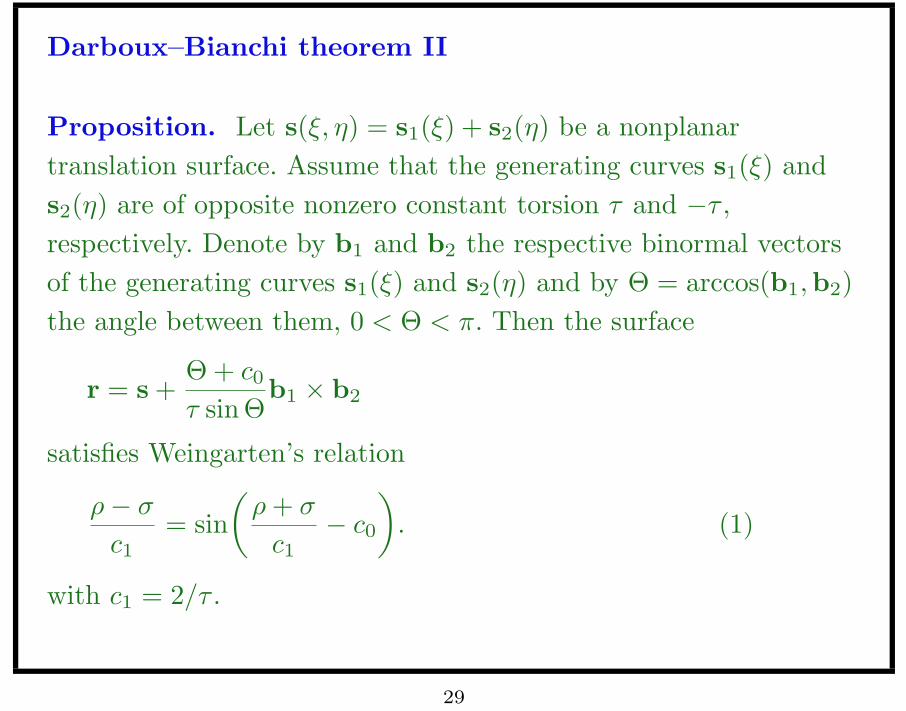
Darboux–Bianchi theorem II

Proposition. Let s(', () = s1(') + s2(() be a nonplanartranslation surface. Assume that the generating curves s1(') ands2(() are of opposite nonzero constant torsion * and "* ,respectively. Denote by b1 and b2 the respective binormal vectorsof the generating curves s1(') and s2(() and by # = arccos(b1,b2)the angle between them, 0 < # < +. Then the surface

r = s +# + c0

* sin #b1 & b2

satisfies Weingarten’s relation

$" %

c1= sin

!$ + %

c1" c0

". (1)

with c1 = 2/* .

29

Geometric characterization

The invertible o!setting transformation r #"$ r + Tn preservesintegrability in every reasonable sense of the word. Surfaces relatedby this transformation are said to be parallel. Either all areintegrable or none is.

Parallel surfaces = normal surfaces to the same line congruence.Consequently, integrability is a property of this congruence and,therefore, must have an expression in terms of congruenceinvariants.

Normal congruences of Weingarten surfaces are known asW -congruences.

Recall that a generic surface has two focal surfaces

r(1) = r + %n, r(2) = r + $n.

each of which is formed by the evolutes of one family of thecurvature lines.

30

Invariant characterization

The Gaussian curvatures are K(i) = det II(i)/det I(i), i = 1, 2. Wehave K(1) = "$!/($" %)2%!, K(2) = "%!/($" %)2$!.

It is convenient to choose

,(i) =1.

|K(i)|,

and

-(i) = 'grad(i) ,(i)'(i) =.

I(i)(grad(i) ,(i), grad(i) ,(i)) .

Proposition. Under the condition -(1) + -(2) (= 0, a Weingartensurface belongs to the integrable class i!

-(1)-(2) = const .

31